The Aquaculture Potential of Indigenous Catfish ( ) in the Lake Victoria Basin, Uganda.Clarias gariepinus

Thesis Submitted to the University of Stirling for the Degree of Doctor of Philosophy

by

Ajangale Nelly Isyagi,B. V. M.,

M.Sc. Aquaculture

Institute of AquacultureStirling, ScotlandUnited Kingdom

April, 2007

DECLARATION

I do hereby declare that this thesis has been achieved by myself and is the result of my own

investigations. It has neither been accepted nor is being submitted for any other degree or

qualification. All sources of information have been duly acknowledged.

Ajangale Nelly Isyagi

to my family,

especially mummy

ACKNOWLEGMENTS

I would like to express my gratitude to the Lake Victoria Management Project, Uganda for the

financial support and to my employers, the National Agricultural Research Organisation for

providing the facilities and time I required to accomplish my work.

I would also like to thank my supervisors Prof. J. F. r D. C. Little from Stirling

University for their guidance, help and support. Spec al thanks to my local supervisors Dr. P.

Ngategize, from the Ministry Of Finance And Economic Planning and Dr. F. W. Bugenyi from

Makerere University, for their support, advice, direction and encouragement during the difficult

times. I would also like to express my sincere thanks to Dr. M. C. M. Beveridge, who for the

first two years of my study was my main supervisor, and provided direction and advice right to

the end.

I appreciate the help and support of all my colleagues from the Aquaculture R arch and

Development Centre, Kajjansi. Most especially I would like to thank Fred Musimbi, Sulaiman

Kasibante, David Ddumba and John Walakira with whom I worked closely from the start both

on-station and in the field, patiently bearing with me during t long hours we had to work,

under the difficult conditions and including the days they should have been off. I truly am

grateful for all their help.

I would like to thank the district staff in the Lake Victoria basin for their co-operation. Special

thanks go to the Fisheries Officers in the sample dist icts - Moses Basana, Fred Kisubi, James

Emong, Eugene Egesa, Placcid Nyamutale, Richard Magenyi, R. S. Mugume, Albert Mugabe J.

Buherezo Kaazi, Rebecca Gimbo, Christine Sooka, Philemon Bwire, J. Ingom nd Michael

Luubulwa.

Special thanks too, to Mr. Bernand Tugumisirize of SunFish Farm Limited for all the

information I have used in the study of to assess the potential for bait production.

I would also like to thank Mr. J. Muhaise, for all the cow dung he gave me at no-charge to

cover all my requirements for all my experiments.

I would also like to thank the laboratory staff of Mak rere University Faculty of Veterinary

Medicine Nutrition Labs, Makerere University Faculty of Agriculture Soil Labs, Kawanda

Research Institute Soil Programme and Limnology Lab of The Fisheries Research Institute for

allowing me have samples analysed in their labs. I wo ke to thank the National

Biomass Study, John and Alfred Macapili for help on geographical information and mapping.

My sincere appreciation also goes to Dr. K. Veverica and Dr B. Daniels of Auburn University,

U.S.A. for their interest, time, and discussions durin he preliminary stages when I was

forming my ideas while they were in Kenya and Uganda r spectively. Particular thanks go to

Dr. Daniels for his continued interest and moral suppo t, including during the difficult time I

have been writing up. I would also like to show my appreciation to Dr. R. Muwazi for all his

help in the initial phases of my thesis investigating the reproductive aspects of indigenous

catfish. In addition I would like to thank all my fri nds and colleagues for their support –

moral, spiritual and professional: Julie Kaitu, Lucy Aliguma, Susan Tumwebaz , Justus

Rutaisire, Dr. S. Ossiya, Maureen Mayanja, Joseph Okor , Victoria Olok, Patricia Muhebwa,

Pamela Aporo, Agnes Atyang, Sema Yuksel, David Kabasa, Michael Ocaido, Ludwig Siefert,

C. gariepinus

Kobil Rugridev, Marie-Josée Mangen, Esther Aisu, Jackie Kigozi, Pat Okori and Stephen

Magero.

I would not in the end have been able to start, let alone accomplish, this commitment without

my family. Thank you Daddy, Mummy, Simon, Edward, Linda, Moses, Grace and Martin.

Thanks a lot for your understanding, patience, moral, spiritual and material support.

- i -

Local and international demand for Lake Victoria’s fish has begun to outstrip supply.

Production from the fishery has attained its sustainable limits, the diversity of catch has

declined and subsequently employment and levels of earnings among fishers have become less

secure. Under prevailing conditions, aquaculture offers the most immediate solution to

augmenting fish production and sustaining earnings from the sector. It may also provide an

avenue through which the diversity of aquatic resources can be increased through for example,

the culture of indigenous species; in this case the African catfish ( ),

particularly as a polyculture species with conventional tilapia ) culture..

To ensure that benefits be derived from the culture of , an assessment of its

potential as a candidate species and of appropriate production options was done within the

context of fish farmers’ local socio-economic, environmental and biotechnical constraints.

This was especially necessary because of the persistent poor performance of aquaculture as a

farm enterprise among Ugandan farmers and the need to improve their livelihoods. Hence also,

a systems approach was chosen as the basic research framework.

The study was conducted in 3 of the 5 agro-ecological zones in the Lake Victoria basin,

namely: the Banana Millet Cotton (BMC), Intensive Banana Coffee Lake Shore (IBC) and

Western Banana Coffee Cattle (WBC) farming systems. Rapid Rural Appraisals (RRAs) were

used to obtain data from a total of 104 fish farming units out of an estimated 212 in the study

area. The tools used included semi-structured interviews, ranks and scores, discussions with

key informants. Wealth rankings were conducted in 50 villages from which a total of 238 fish

farmers were ranked. Quantitative data on farmers’ man gement and production was obtained

Abstract

Clarias gariepinus

(Oreochromis

C. gariepinus

ii

from a subset of 54 fish farming units. 69 ponds were ampled. Data on the marketability of

for table fish was obtained from a total of 25 markets where 65 fish-sellers and 97

fish consumers were interviewed. Information on market potential of as bait was

obtained from 14 landing sites where 118 line fishermen and 38 dealers were interviewed.

The information obtained from the RRAs provided an insight into the social, financial and

human capital farmers had invested into aquaculture. t also provided information on the

environmental constraints in terms of the ability to generate natural ysical capital for

aquaculture. The effect of the interaction of these f ctors on farmer’s production was analysed

using Principal Component Analysis (PCA). Impact on yield was analysed with the PCA in

relation to state (inputs), rate (management) and intr nsic (farmers and farm characteristics plus

location) variables within the context of fish species currently farmed. The potential entry

points for were subsequently derived based on key constraints and marketability.

Poor performance of enterprises was noted by the fact that over 50% of farmers had had no

returns, either in cash or food from their ponds. In general, farmer’s management practices

were adaptive rather than strategic. Key variables causing greatest variance and unstable

production in current systems were found to be: (i) se d - notably stocking density, size at

stocking, stocking ratios and cost (ii) frequency and larity with which feed and fertiliser

were applied (iii) pond size (iv) location within the agro-ecological zones. .Though there was

variance between zones, maize bran and cow dung were t e most widely used feed and

fertiliser inputs in all zones respectively. It was also found that in a typical polyculture context,

was the most marketable fish

C.

gariepinus

C. gariepinus

C. gariepinus

O. niloticus

iii

Two experiments were designed to test comparative economic returns for monoculture and

polyculture based on the above findings (i) the effect of stocking density on pond yield and

economic returns of O fed maize bran in earthen ponds fertilised with cow d g (ii)

the effect of varying cow dung and maize bran input levels on pond yield and economic returns

in polyculture. The potential of farming as bait was

also assessed from secondary hatchery information. The financial returns were

assessed based on farmers’ actual local costs of production and prevailing local market prices.

Results indicated that (i) farming as either a table fish or bait resulted in higher

yields, better returns, improved productivity and utilisation of inputs, better technical and

economic efficiency compared to monoculture. (ii) in the farming

system has the potential to reduce the risk of aquaculture as a livelihood option. (iii) The

farming potential and constraints were significantly agro-ecological zone-specific and also

influenced by farmers’ profiles: therefore different options may be appropriate (iv) It is more

important for farmers if yields were defined in shillings based on local costs rather than tonnes,

as the units of exchange affecting investment and operating decisions were numbers and size.

. niloticus

O. niloticus – C. gariepinus C. gariepinus

C. gariepinus

C. gariepinus

O. niloticus C. gariepinus

iv

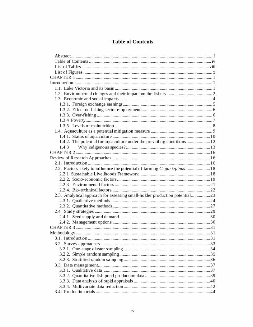
Abstract............................................................................................................................... iTable of Contents ............................................................................................................. ivList of Tables..................................................................................................................viiiList of Figures.................................................................................................................... x

CHAPTER 1 .......................................................................................................................... 1Introduction............................................................................................................................ 1

1.1. Lake Victoria and its basin ....................................................................................... 11.2. Environmental changes and their impact on the fishery......................................... 21.3. Economic and social impacts ................................................................................... 4

1.3.1. Foreign exchange earnings................................................................................ 51.3.2. Effect on fishing sector employment................................................................ 61.3.3. Over-fishing ....................................................................................................... 61.3.4 Poverty................................................................................................................. 71.3.5. Levels of malnutrition ....................................................................................... 8

1.4. Aquaculture as a potential mitigation measure ....................................................... 91.4.1. Status of aquaculture .......................................................................................101.4.2. The potential for aquaculture under the prevailing conditions .....................121.4.3 Why indigenous species?...........................................................................13

CHAPTER 2 ........................................................................................................................16Review of Research Approaches........................................................................................16

2.1. Introduction .............................................................................................................162.2. Factors likely to influence the potential of farming ......................18

2.2.1 Sustainable Livelihoods Framework ...............................................................182.2.2. Socio-economic factors...................................................................................192.2.3 Environmental factors .....................................................................................212.2.4. Bio-technical factors........................................................................................22

2.3. Analytical approach for assessing small-holder production potential.................232.3.1. Qualitative methods.........................................................................................242.3.2. Quantitative methods.......................................................................................27

2.4 Study strategies .......................................................................................................292.4.1. Seed supply and demand.................................................................................302.4.2. Management options........................................................................................30

CHAPTER 3 ........................................................................................................................31Methodology........................................................................................................................31

3.1. Introduction .............................................................................................................313.2. Survey approaches ..................................................................................................33

3.2.1. One-stage cluster sampling .............................................................................343.2.2. Simple random sampling .................................................................................353.2.3. Stratified random sampling .............................................................................36

3.3. Data management....................................................................................................373.3.1. Qualitative data ................................................................................................373.3.2. Quantitative fish pond production data ..........................................................393.3.3. Data analysis of rapid appraisals ....................................................................403.3.4. Multivariate data reduction .............................................................................42

3.4. Production trials ......................................................................................................44

Table of Contents

C. gariepinus

v

3.4.1. Introduction ......................................................................................................443.4.3. Pond management............................................................................................473.4.4. System data collection and analysis ...............................................................48

3.5. seed demand and supply .................................................................543.5.1. Introduction ......................................................................................................543.5.2. Demand.............................................................................................................543.5.3. Production and Supply ....................................................................................56

CHAPTER 4 ........................................................................................................................58Socio-economic factors affecting fish farming in the Lake Vi toria Basin.....................58

4.1. Introduction .............................................................................................................584.2. Farmers and Farm Profiles Characteristics of the Fish F rming Unit .............58

4.3. Socio-economic assets and aquaculture.................................................................634.3.1. Objectives for aquaculture ..............................................................................634.3.2. Species choice..................................................................................................634.3.3. Source of investment for aquaculture.............................................................644.3.4. Knowledge .......................................................................................................684.3.5. Security.............................................................................................................68

4.4. Market potential of table fish .................................................................................684.4.1. Market characteristics......................................................................................684.4.2. Source of fish ...................................................................................................694.4.3. Supply and demand..........................................................................................704.4.4. Marketability of Fish .......................................................................................724.4.5. Marketability of pond fish: case study ...........................................................81

4.5. Market potential of as bait ..............................................................834.5.1. Introduction ......................................................................................................834.5.2 Bait trade and supply potential.........................................................................854.5.3. The perspectives of fisheries officers.............................................................89

4.6. Concluding remarks................................................................................................89CHAPTER 5 ........................................................................................................................91Farming systems and their potential for fish farming .......................................................91

5.1. Introduction .............................................................................................................915.2 Major farm production characteristics....................................................................92

5.2.1. Crops and crop production practices by fish farmers....................................925.2.2. Livestock production practices .......................................................................945.2.3. Other activities .................................................................................................96

5.3. Potential Inputs for fish farming, source and use...................................................975.3.1. Introduction ......................................................................................................975.3.2. Feed materials ..................................................................................................975.3.3. Fertilisers........................................................................................................1045.3.4. Seed.................................................................................................................106

5.4. Water sources and site conditions.........................................................................1095.5. Concluding Remarks.............................................................................................111

CHAPTER 6 ......................................................................................................................113Fish farming production systems – current features .......................................................113

6.1. Introduction ...........................................................................................................1136.2. Pond systems and stocking...................................................................................113

6.2.1. Ponds ..............................................................................................................1136.2.2. Species farmed...............................................................................................114

6.3. Stocking practices .................................................................................................1156.3.1. Monoculture vs. polyculture .........................................................................115

C. gariepinus

C. gariepinus

vi

6.3.2. Stocking ratios ...............................................................................................1166.3.3. Stocking densities ..........................................................................................1176.3.4. Size at stocking ..............................................................................................1186.3.5. Time to stocking ............................................................................................119

6.4. Feeding ..................................................................................................................1206.4.1. Feed input levels ............................................................................................1206.4.2. Mixing of feedstuffs ......................................................................................1236.4.3. Feeding frequencies.......................................................................................1246.4.4. Role of feeding in the system........................................................................125

6.5. Fertilization............................................................................................................1266.5.1. Fertilizer input levels.....................................................................................1266.5.2. Mixing of fertilisers .......................................................................................1276.5.3. Fertilisation frequency...................................................................................1286.5.4. Importance of fertilisation in the system......................................................128

6.6. Production and yield .............................................................................................1296.6.1. Production cycles...........................................................................................1296.6.2. Yield ...............................................................................................................1296.6.3. Quality of yield ..............................................................................................131

6.7. Interactions and impacts on yield.........................................................................1316.7.1. Introduction ....................................................................................................1316.7.2. The effect of state variables on yield............................................................1316.7.3. Interactions between State, Rate Management and Intrinsic Variables on Yield ...........................................................................................................................134

6.8. Concluding Remarks.............................................................................................1396.8.1. Overview ........................................................................................................1396.8.2. Seed and Stocking..........................................................................................1406.8.3. Feed and fertiliser ..........................................................................................1426.8.4. Intrinsic factors ..............................................................................................145

CHAPTER 7 ......................................................................................................................147The potential of in current farming systems ............................................147

7.1. Introduction ...........................................................................................................1477.1.1. Objectives.......................................................................................................1477.1.2. Approaches adopted ......................................................................................1477.1.3. Experiments....................................................................................................148

7.2. Production..............................................................................................................1507.2.1. Experiment 1: Effect of stocking density on th nd economic returns of fed maize bran in earthen ponds fertilized with cow dung............1507.2.2. Experiment 2: Effect of varying cow dung and maize bran input levels on pond yield and returns in – Polyculture.......................1547.2.3. bait production........................................................................157

7.3. Economic Analysis ...............................................................................................1587.3.1. Returns............................................................................................................1587.3.2. Sensitivity Analysis .......................................................................................1627.3.3. Risk analysis...................................................................................................165

7.4. Concluding remarks..............................................................................................1677.4.1. Production ......................................................................................................1677.4.2. Efficiency of feed- fertiliser utilisation ........................................................1707.4.3. Economic returns...........................................................................................1717.4.4. Effect of unit of product sales.......................................................................1727.4.5. Returns to investment, farmers vs. economists view ..................................174

( )

C. gariepinus

O. niloticus

O. niloticus C. gariepinus C. gariepinus

vii

CHAPTER 8 Discussion and conclusions .......................................................................1768.1 Overview of results ................................................................................................176

8.1.1 Influence of socio-economic factors...............................................................1768.1.2 Influence of production factors......................................................................1798.1.3 Influence of bio-technical factors ...................................................................182

8.2 Sustainability and adoption ..............................................................................1848.2.1 Overview .........................................................................................................1848.2.2 Socio-economic factors ..................................................................................1858.2.3 Environmental factors......................................................................................1908.2.4 Bio-technical factors.......................................................................................191

8.3 Conclusions and recommendations .................................................................1968.3.1 Overview .........................................................................................................1968.3.2 Recommendations to farmers.........................................................................1978.3.3 Recommendations for research and development ........................................1978.3.4 Recommendations for policy .........................................................................199

References......................................................................................................................201Appendices.........................................................................................................................213

APPENDIX A: DESCRIPTION OF STUDY AREA ............................................213APPENDIX B: SAMPLING FRAME FOR DATA FROM FARMERS..............218APPENDIX C:QUALITATIVE DATA COLLECTION – PRETESTING TOOLS....................................................................................................................................220APPENDIX D: TOOLS USED FOR RAPID APPRAISALS...............................222APPENDIX E: PRODUCTION DATA – FARMERS..........................................228APPENDIX F: QUALITATIVE DATA ANALYSES ..........................................229APPENDIX G: MULTIVARIATE DATA REDUCTION ....................................230APPENDIX H: EXPERIMENTAL PONDS...........................................................233APPENDIX I: POND SAMPLING – EXPERIMENTS ........................................234APPENDIX J: SEED AND BAIT SUPPLY AND DEMAND......241APPENDIX K: CRITERIA USED BY FARMERS TO RANK WEALTH.........249APPENDIX L: SENSITIVITY ANALYSIS – EXPERIMENTS..........................251

C. gariepinus

viii

Table 3.1 Summary of Sampling Methods and Objectives ..............................................33Table 3.2 Variables used in Principle Component Analysis ...........................................43Table 3.3: Description Of Treatments In Experiment 2...................................................47Table 3.4 Methodology for Fortnightly Water Quality Analysis ...................................49Table 3.5 Considerations in Cost Allocation and Economic Analysis ............................52Table 3.6 Parameters and Economic Indicators used in Sensitivity Analysis................53Table 3.7 Values Kept Constant During Sensitivity Analysis of a Parameter ................54Table 3.8 Scenarios used in estimation of seed demand...........................55Table 4.1 Fish Farming Unit Size by Agro-Ecological Zones .........................................60Table 4.2. Percentage of units owned by women, by structure of unit a d AEZ...........60Table 4.3 Effects of Location, Farm Unit Structure, S and Age on Wealth Ranks....62Table 4.4 Farmers’ preferences for potential species for aquaculture .............................63Table 4.5 factors influencing amount farmers spent on labour for pond construction ...66Table 4.6 Effect of socio-economic factors on amount farmers spent on labour for pond management.........................................................................................................................67Table 4.7 Household monthly fish consumption rates by agro-ecological zone............69Table 4.8 Most marketable and preferred fish species.....................................................73Table 4.9 Proportion of fresh and preserved fish sold in Kampala, 2000. .....................75Table 4.10 Most Preferred Forms of Fish, as Scored by Fish sellers..............................76Table 4.11 Sizes of Fish Most Frequently Purchased by Consumers..............................77Table 4.12 Competitiveness of Animal Products..............................................................80Table 4.13 Fish prices for consumers................................................................................81Table 4.14 Comparison animal products market prices, Kasangati, Wakiso District....83Table 4.15 Bait used by fishermen, by fish species caught ..............................................84Table 4.16 Unit prices of bait ............................................................................................85Table 4.17 Sources of bait for bait traders.........................................................................85Table 4.18 Constraints faced in the bait trade ...................................................................87Table 4.19 Concerns of bait traders if they were to purchase bait from hatchery...........88Table 5.1 Crops grown by fish farmers overall and between zones................................92Table 5.2 Percentage of fish-farmers by AEZ using fertiliser for crop production .......94Table 5.3 Influence of Agro-Ecological Zone on numbers of livestock owned..............95Table 5.4 Management systems employed by fish farmers for livestock production.....96Table 5.5 Common items used as fish feed among farmers n the different zones.........97Table 5.6 Cost of inputs for farmers in each AEZ ..........................................................103Table 5.7 Comparative use of fertilisers by fish farmers................................................104Table 5.8 Major sources of seed for fish farming in different Agro-Ecological Zones108Table 5.9 Comparative seed costs ....................................................................................109Table 6.1 Pond sizes and depth in the different Agro-Ecological Zones......................114Table 6.2 Stocking ratios used by fish farmers................................................................117Table 6.3 The influence of Agro-Ecological Zone, fish farm unit structure, number of ponds a farmer has and species farmed on stocking densities........................................118Table 6.4 Stocking sizes by species farmed ...................................................................119Table 6.5 Time to stocking from completion of pond construction..............................120Table 6.6 Feed input levels by category of feedstuff and location...............................122Table 6.7 Feeding and fertilisation practices in zone for different species.................124

List of Tables

C. gariepinus

ix

Table 6.8 Factors influencing feeding frequencies..........................................................125Table 6.9 Fertilizer input levels by agro-ecological zone..............................................127Table 6.10 Factors influencing production cycles..........................................................129Table 6.11 Factors affecting yield ....................................................................................130Table 6.12 Overall farming system: effect of feed category on production..................132Table 6.13 farming system: effect of state variables on production.........133Table 6.14 Farming System: Influence of State Variables on Production.....................................................................................................................134Table 6.15: Overall Farming System : Effect of State, Rate and Int ic Variables on Production ..........................................................................................................................135Table 6.16 Farming System: Influence of State, Rate and Intrinsic Variables on Production....................................................................................................137Table 6.17 Mixed Farming System: Influence of State, Rate and Intrinsic Variables on Production..............................................................................138Table 7.1 Productivity of Experiments, Farmers’ Ponds and Bait Production ..........................................................................................................................153Table 7.2a Economic returns based on station costs for experiment I...........................159Table 7.2b Economic returns based on station costs for xperiment II .........................160Table 7.3 Cost return analysis of bait production per cycle ...........................................161Table 7.4 Partial budget analysis......................................................................................162Table 7.5 Variable cost structure of experiments...........................................................162Table 7.6 Cost structure of experiments as proportion of gross income (Receipts) ....163Table 7.7 Safety Margin (%) between Actual and Break-Even Production.................166Table 7.8 Safety margin (%) between market price and erimental break-even price............................................................................................................................................167Table 7.9 Comparative growth rates and feed conversion efficiencies ........................172

O. niloticusO. niloticus-C. gariepinus

O. niloticus

O. niloticus-C. gariepinus

C. gariepinus

x

Trend in Diversity of Fish Catch 3Methodological Framework 31Experimental Pond Layout 46

Potential Demand for as Seed and Bait. 86 Farm pasture and arable waste availability for fish g in the agro-ecological

zones99

Availability of farm cereal and grain residues for fish farming in the agroecological zones

102

Availability of farm manure for fish farming in the agroecological zones 107 monoculture: Treatment Net yields 151 monoculture: Average Fish Weight at Harvest 151 monoculture: Average Fish Total Length at Harvest 152 Polyculture: Treatment Net yields 154 Polyculture: Average Fish Weight at Harvest 155 Polyculture: Average Fish Total Length at Harvest 155

Description of Parameters used to Analyse Productivity and Economic Returns 51

List of Figures

Figure 1.1Figure 3.1 Figure 3.2 Figure 4.1Figure 5.1

Figure 5.2

Figure 5.3Figure 7.1Figure 7.2Figure 7.3Figure 7.4Figure 7.5Figure 7.6

Box 3.1

C. gariepinus

O. niloticusO. niloticusO. niloticusO. niloticus -C. gariepinus O. niloticus-C. gariepinus O. niloticus-C. gariepinus

Chapter 1

1

Lake Victoria is the second largest freshwater lake in the world. Its total water surface

area of 68,800 km2 is shared by Kenya (6%), Tanzania (49%) and Uganda (45%)

(Serruya and Pollingher, 1983). Its total catchment area is 184,000km2 and includes

Rwanda and Burundi. Lake Victoria and its basin support the livelihoods of a third of the

population of East Africa (Kenya, Tanzania and Uganda). The World Bank (1996)

estimated that 30 million people lived within the basin at income levels of US $ 90 - 172

per capita per annum. Estimates of the basin’s Gross Economic Product were US $ 3 to 4

billion per annum by 1996 (World Bank, 1996). The eco of the lake and its

catchment is derived from fisheries (10%), agriculture (35%), industries and mining

(15%) and the tertiary sector (40%) (World Bank, 1996; iba, 2003).

L. Victoria has the largest freshwater fishery in the world accounting for 25% of all

Africa’s inland fisheries yield (Pedini, 1991; Jansen, 2003), with fish exploited as the

main tradable commodity from as early as 1910 (Balarin, 1985). The combined export

earnings from the lake were estimated to be US$ 600 million annually (Ntiba, 2003). In

Uganda, fish from L. Victoria accounts for about 50% of the national catch (which is

estimated to be 227,000 mt) and 11% of the country’s export earnings (MFPED, 2000;

MAAIF, 1999), increasing by 14 times from US$ 5 million to US$ 76 million betwe n

1991 and 2001, making fish the country’s second most important export commodity after

coffee. Over 700,000 people in Uganda depend on the lake’s fishery directly or

indirectly for their livelihood (Kaelin and Cowx, 2002; Mutumba-Lule, 1999).

Other than for fish, the lake’s water resources are an important source of hydro-

electricity; transport; domestic, industrial and agricultural water. The basin’s soils and

CHAPTER 1

Introduction

1.1. Lake Victoria and its basin

Chapter 1

Lates niloticus Oreochromis niloticus

et al.

O. niloticus O. leucostictus

2

climatic conditions are also favourable for agricultur production, accounting for 59% of

Uganda’s coffee production (COMPETE and Gowa, 2001), and high capacity for

agricultural development (World Bank, 1996). There a e also mineral deposits in the

area in Kenya and Tanzania, while its scenery, wild life and varied cultures also make it a

prime tourist destination (The East African, 2002).

As a result of its economic potential, the L. Victoria Basin is among the most densely

populated areas in East Africa, with estimated growth ates of 3 to 6 % per annum

inclusive of immigration (Ntiba, 2003; Orach-Meza, 2000). According to Ntiba (2003),

the population in the basin may increase by 55% in the next d cade because of

urbanisation. All of Uganda’s major cities and industries are located withi the basin,

though most of the population is still rural based and depends on agriculture. During the

last fifty years increased human activity has had a great e ct on the natural resources of

the area., particularly from changes in land-use patterns (particularly of the wetlands and

forests), pollution, over-exploitation of natural resources, and introduction of non-

indigenous fish species (Leveque, 1997). This has had an effect not only on the status of

the fishery but also other sectors of agricultural pro ion.

The ecosystem of L. Victoria is in a state of flux. It has experienced major and

irreversible ecological transformation as a result of e introduction of the Nile perch

( ) and the Nile tilapia ( ) from Lake Albert in the late

1950’s to early 1960’s (Goudswaard , 2002; Goudswaard and Witte, 1997; Leveque,

1997; World Bank, 1996; Kudhongania and Chitamwebwa, 1 5; Ogutu-Ohwayo, 1990).

According to Ogutu-Ohwayo (1990) the Nile perch was introduced to convert the small

sized Haplochromines to a suitable sized table fish while and

1.2. Environmental changes and their impact on the fi hery

Chapter 1

Tilapia zillii

Rastrineobola argentea

3

were introduced possibly to supplement indigenous stock. on the other hand

was introduced to convert macrophytes into useful fish biomass. As a result, there has

been a five-fold increase in catch from the lake (World Bank, 1996), though at the

expense of notable loss in biodiversity.

Prior to these introductions, the fishery of L. Victoria comprised some 300 different fish

species (Leveque, 1997). Annual average production levels from 1961 to 1984 (with first

indications of Nile perch becoming established) were 26,000 t (MAAIF, 1999).

Population growth and the consequent market demands have since resulted in increased

fishing pressure. Earlier, impacts were more localised, mainly affecting species with low

reproductive potential and low resilience. However, since the 1980’s, biodiversity

declined tremendously and there are now only three major species in the catch: Nile

perch (63%), Nile tilapia (15%) and the indigenous (Ogutu-

Ohwayo, 1990; World Bank, 1996). Several indigenous sp that were previously

commercially important are now considered endangered (World Bank, 1996) (see figure

1.1).

(Unfortunately, only data on fish catches up to 1988 are disaggregated by species).

Lates Tilapia Bagrus Barbus Protopterus Clarias Haplochromines

T rend in D iversity of F ish C atch, Lake Victoria – U ganda. Adapted from MAAIF, 1999

0

10

20

30

40

50

60

70

80

90

100

1965196619671968196919701971 19721973197419751976 19771978197919801981 1982198319841985198619871988year

pro

po

rtio

n

of

tota

l ca

tch

(%

)

Figure 1.2.

Chapter 1

et al.

O. niloticus

O. variabilis O. esculentus

O. niloticus O. esculentus O. variabilis,

O. niloticus

O. niloticus

et al

et al.

O. niloticus

Bagrus dogmac

et al. et al.

4

Recent studies by Goudswaard (2002), however, indicate that the Nile perch is not

the sole cause of decline in species diversity. The authors found to be more

competitive than and for limited breeding and nursery space,

with higher reproductive success rates. Studies on genetics of L . Victoria tilapias also

show hybridisation between and or with later

generations tending to resemble . The degree to which this has occurred is

still unclear. is also a more opportunistic feeder and grows to a larger size.

Eutrophication associated with increased levels of pol s entering the lake has also

been cited as a major cause of L. Victoria’s decline in biodiversity (The East African,

2002; World Bank, 1996; Scheren , 2000). Poor municipal environmental waste

management, agricultural practices and land use patterns coupled with the encroachment

on wetlands have resulted in waste, silt and chemical pollution entering the lake (Scheren

2000) Water-borne diseases are reported to have increased as a result of declining

water quality, and changes have also resulted in algal blooms, causing transparency

values to fall from 5 m to less than 1 m from the 1930’s to date (World Bank, 1996).

There have been consequent shifts in plankton dynamics from predominantly large

filamentous diatoms to small colonial Cyanobacteria and green algae, further favouring

and also increasing benthic decompositon and the risk of major fish kills,

notably of Nile perch, the catfish (Forsskall) and deepwater

Haplochromines (Goudswaard , 2002; Scheren , 2000).

Before the Nile perch became established, the fishery esource was more or less open

access, and contributed greatly to rural employment, with small operators in local

communities involved in fishing, processing and marketing. A majority of processors and

1.3. Economic and social impacts

Chapter 1

5

traders were women and a significant proportion of payment for hired labour was in kind

as fish. Fishing was the main economic activity and in Uganda, fish was for a long time

regarded as the cheapest and most widely consumed source of animal protein

(NARO/MAAIF2, 2000; Owori-Wadunde, 2001; Balarin, 1985). However, since then, the

fishery has changed to one influenced by national and international markets, resulting in a

diversity of effects, both positive and negative, at individual, household, community,

national and international level (ACTS, 1999).

Although Uganda’s foreign exchange position is healthy, with an estimated surplus of

$179m in 2003/4, (MFPED, 2004), this is largely the re lt of aid flows. The balance of

trade deficit was estimated at US$712m for 2003/4, well over 10% of GDP. Fish remains

the second largest export commodity, after coffee , its export rising to $98.4m (31,000 mt

of fish), from $80m in 2001/2 (MFPED, 2004), some 11% of all exports of goods and

services, and 16% of all visible exports. This is probably an underestimate as it does not

include regional trade (e.g. exports to D. R. Congo). It is unsurprising that the

Government, through the Uganda Investment Authority, continues to encourage

investment in fish processing for export (UIA, 2005).

However, demand for fish, both for food and as a tradable commod ty, has begun to

outstrip supply (Kaelin and Cowx, 2002), Nile perch had become popular in the region

and indicated the existence of notable demand for a medium priced table fish (Jansen,

2003). However, local demand has been under pressure from the profitable export trade,

pushing up prices and/or reducing available quality on local markets across the region.

An illustration of this came when a ban on imports from Lake Victoria was instituted by

the European Union, and retail prices of fish in Kenya plummeted from US$1 to US$0.25

1.3.1. Foreign exchange earnings

Chapter 1

R. argentea

6

per kg. (Oduol, 2000). Increasingly too, tilapia is b filleted for export because export

demand is extremely high. has also been commercialised for animal feed

production (Jansen, 2003).

Fishing, handling and processing of fish have become increasingly technical and

commercialised. While this may have advantages, particularly in securing international

markets, artisanal fishermen, local processors and distributors are being driven out of

business because investment costs have increased. Those with little or no formal

education have been particularly affected (Jansen, 2003; Mugabe, 2003).

Consequently, the key actors, their roles and ownership patterns within the production

sector are changing. The chain is now increasingly comprised of absentee owners,

managers, operators and labourers (crew), the former of whom may have no prior

experience or link with the fisheries. More fishermen are becoming employees as crew

for larger businessmen. More also have contractual agreements with purchasing agents

of fish processing factories, who are increasingly dictating the terms of trade, paying

higher prices than the local fishmongers and market. They also dictate prices to

fishermen, especially in cases where there is vertical integration with processing plants.

Fishmongers, as well as local traders and processors, are consequently losing

employment. The number of people formally employed in the factories and processing

fish factory by-products for domestic consumption in the informal sect r is small

compared to those who have lost jobs in the traditional chain (Jansen, 2003).

The catching pressure on the lake has increased tremendously, driven by this demand and

1.3.2. Effect on fishing sector employment

1.3.3. Over-fishing

Chapter 1

7

the technical capacity to exploit and process fish has also increased. However, indications

are that these far outweigh supply. The exploitation rate of the Nile perch fishery (% of

mortality due to fishing) is estimated at 86%, and it would need to fall to 45% to achieve

optimal yields. The estimated Maximum Sustainable Yield (MSY) in Uganda’s share of

Lake Victoria is between 64–76,000 mt. In 2001 approximately 28,000t of finished ish

was exported from the lake, equivalent to 70,000 mt wet fish weight, with a total

estimated catch of 110,000 mt. excluding exports to local regional markets. Decreasing

stocks have combined with an increased number of fishermen, and as a result, the catch

has declined from about 80 kg/boat/day to 45 kg/boat/day (Kaelin and Cowx, 2002).

Establishing the percentage of people living in povert is not easy, both because

definitions of poverty are ultimately subjective and because data on income (and food

production) are hard to establish. The Government of Uganda estimates that 38% of the

population live in poverty, and average income is below 75c/person/day (given GDP of

$250 per capita, MFPED 2004). The other countries of the Lake Victoria Basin do not

fare differently: GNI per capita was estimated at $340 Kenya and $270 for Tanzania

(UNICEF, 2003).

Among fishers , reduced earnings are attributed both to increased competition for fish and

to the decline in catch as a result of over-exploitation pollution, and promotion of exports

(MFPED, 2002). They have been less able to take advantage of the expanded markets

because of the limitations they face in accessing financial and human assets such as

equipment and skills. The influence of the seasons on catch, lack of storage facilities that

leads to high post-harvest losses (estimated at 15-40% in Uganda) and the high

dependence on a single source of income have made it increasingly difficult for small-

1.3.4 Poverty

Chapter 1

R. argentea

8

scale fishers to earn a living from fishing (MFPED, 2002; Kaelin an Cowx, 2002; NRI

and IITA, 2002). More of the money earned is going to the larger businessmen, fish

processors and the state rather than directly to the local fishermen, fishmongers and

traditional fish processors. There is also very little re-investment at the local level by all

parties involved, particularly at sites not used by fish factories (The East African, 2002).

The factors discussed above have contributed to a decline in Uganda’s per capita food

production of 44% from 1970 to 1997 (Bahiigwa, 1999). Up to 95% of rural households

in Uganda depend on their own food production as a mai source of food. Rapid

population growth coupled with declining productivity s resulted in an increased need

for additional food sources (Hazell, 1998; MAAIF and MFPED, 2000; The East African,

2002). More households have therefore had to turn to he market as a source of food.

Low and declining rural incomes are therefore a concern for food security (Bahiigwa,

1999; MAAIF and MFPED, 2000).

Despite the local economic opportunities, being close to the lake has not necessarily

brought nutritional advantage. Even fishermen are now consuming less fish, which has

become too expensive. Studies conducted by the Kenya edical Research Institute

found 30-50% of children to be moderately to severely malnourished among the riparian

communities of L. Victoria in Kenya. Out of these, 60-70% of the malnutrition was

attributed to lack of zinc, iron and vitamin A that co be obtained from

(‘dagaa’/‘mukene’) (Mugabe, 2003). UNICEF (2003) figures indicated that the nati nal

incidence of chronic child malnutrition (stunting of under-fives) was 23% in Kenya, 29%

in Tanzania and 23% in Uganda. In Uganda as a whole, stimated per capita fish

consumption, based on national catch and fish export figures, has declined by 61 since

1.3.5. Levels of malnutrition

%

Chapter 1

9

1971 (Balarin, 1985; UBoS, 2002; MAAIF, 1999).

For the ordinary rural smallholder farmer in the basin, agricultural productivity has

declined despite potential. This is attributed to several compounding factors: the

extensive farming methods practised by the majority of farmers that are so vulnerable to

natural hazards; a long-term decline in terms of trade for agricultural produc making

investment less attractive; unequal gender relations; emographic pressures and

subsequent land shortage; limited options for rural non-farm income; and lack of energy

sources (MFPED, 2003). Levels and effects of poverty have been further aggrava ed by

HIV/AIDS (The East African, 2002). NEMA (1999) further links the increasing levels of

poverty among the rural farming population with the decline in national agri ural

yields and productivity and with increased environment degradation. Like the artisanal

fishers, small-scale farmers’ ability to derive benefits from economic growth programmes

focusing on the ability to exploit already existing capabilities has been constrained by

their limited assets (Okidi and Mugambe, 2002 and MFPED, 2002). Because of their

lack of financial and human assets, production options are limited to those that depend

heavily on climatic patterns. Consequently, they experience periods of relative

abundance and hardship in tune with the seasonal natur of primary production, income-

generation and expenditure. The nature of poverty amo small-scale farmers in the lake

basin (as elsewhere in Uganda) is therefore cyclical, seasonal and chronic, which makes it

difficult for them to invest in long-term sustainable management options (MFPED, 2002).

In order to mitigate the effects of 'seasonality' and he risks associated with changes in

climate, farmers have turned for survival to the use of marginal resources and

ecologically sensitive areas such as the fisheries, fo and wetlands (NEMA, 1999).

1.4. Aquaculture as a potential mitigation measure

Chapter 1

O. esculentus, O. variabilis, L. victorianus, B.

docmac Protopterus aethiopicus (

i)

10

Given the need to maintain exports and the simultaneou need to reduce poverty, it is

evident that the fisheries sector has to enlarge, but a manner that ensures local food

security and livelihoods and maintains the future yields of the fishery (Jansen, 2003;

Swick and Cremer, 2001; Kaelin and Cowx, 2002; Balarin, 1985; Rana, 1997, King,

2002). Food security will only be improved if additional ish produced is affordable for

the poor, which means expanding its supply (Tacon, 2001; Lem and Shehadeh, 1997).

Aquaculture offers a potentially non-exploitative option for expanding fish production

and sustaining the contribution of the fisheries to th national economy. It is for this

reason that the Lake Victoria Environment Management Project (LVEMP) opted for

aquaculture among its key interventions in fisheries. The LVEMP was set up to

rationalise natural resource use in the basin, with the of re-establishing ecosystem

integrity on a sustainable basis.

By targeting endangered indigenous species that are of high market value, it is hoped that

the loss of aquatic resources can be ameliorated through aquaculture. The species of

focus at the start of the project included

and World Bank, 1996).

Aquaculture is promising for many reasons (UNEP, 1990; Shang, 1990; Chopak and

Newman, 1998, Lightfoot et al, 1994; Goletti, 1999; Ta on, 2001), among which the key

arguments for Uganda are that it offers:

potential for low-risk agricultural diversification which is easily integrated into

many existing farms (where water is available).

mitigation against seasonality in both capture fisheri nd agriculture

to help meet demand beyond the natural sustainable capture fishery yield.

1.4.1. Status of aquaculture

ii)

iii)

.

Chapter 1

v)

vi)

et al.

11

to help foreign exchange revenues, by sustaining higher export levels.

significant potential as a much needed source of high-quality animal protein and

other essential nutrients.

an efficient way to recycle nutrients from the farm (into both protein and nutrient

rich pond mud), giving savings which have been valued at up to 40% of gross

farm income (Lightfoot et al., 1994).

Aquaculture in Uganda was started in 1931 and an experimental station set up in 1953 at

Kajjansi, now in Wakiso District which is within the L. Victoria Basin (Balarin, 1985).

According to a recent strategic assessment of aquaculture in Af a by Aguilar-Manjarrez

and Nath (1998) the potential within the basin is high for both small-scale and

commercial aquaculture. Similar conclusions have been drawn in a socio-economic

assessment by Nanyenya (1999) on technology adoption, the profitability and

competitiveness of aquaculture in Uganda.

However, aquaculture’s contribution to the agricultura sector has until now been

insignificant. National aquaculture production is est ed to have increased from 31 mt

to just 360 mt between 1985 to 1999, accounting for only 0.2% of national catch (Balarin,

1985; Kaelin and Cowx, 2002). Of this total, aquaculture in the L Victoria Basin

accounts for about 17%. According to Fisheries Depart ent estimates of 1997, there

were an estimated 1,085 ponds covering 21.3 ha in the basin (MAAIF, 1997).

The above estimates were however not based on actual d a from pond harvests, but on

calculations from theoretical yields. It was assumed at farmers should be getting 275-

300g/m² per year. Indications are that actual yields are much lower, from just 28 g to 138

g/m²/yr (KARDC, 2000), and so the actual total national harvest is probably only 50 to

150 mt per year. Even the theoretical figure of 360 t still leaves production much lower

than the estimated 11,000 t of the late 1960’s (Balarin, 1985). Persistently low yields and

poor yield quality have had a negative impact on profi bility, and consequently, there are

iv)

Chapter 1

12

many abandoned fish ponds. However, despite this, aquaculture offers the only option to

increase fish production from the basin. More importantly for the potential fish farmers

concerned, aquaculture continues to show significant p ential for helping farmers

increase their household income. Its history of failure has not been shown to be due to

inherent or insurmountable problems. The economic difficulties facing the population in

the area, including the problems with fishing in Lake ictoria already discussed, the

long-term collapse of the price of the main cash crop, coffee, and the difficulty in finding

alternative cash crops, mean that the search for profi nd sustainable aquaculture is a

worthwhile investment.

The natural resource potential for aquaculture in the ake Victoria basin is regarded as

favourable (Balarin, 1985; Anquila-Manjarezz and Nath, 1998). Economic potential is

higher than ever, as the value of fish rises, particularly for several highly prized

indigenous lake species. However, potential benefits can only be realised if systems are

appropriate and sustainably managed so that they have positive or at least neutral effect

on local natural resources and farmers’ livelihoods. appropriate system is one which

fits the farmer’s goals – their opportunities are financially determined, performance

linked, aimed at profits and at the enterprise’s resil ce (Muir and Young, 1998). Too

often, on the other hand, research takes a uni-dimensional perspective of maximising

yield in kilograms per unit area.

Farmers are not generally interested in ecological issues of increasing national harvest,

but only as a means to better income and food security. Aquaculture has to show that it

offers a competitive advantage compared to their other opportunities, d though this

might be the case (see below), it is a challenge to ma it work. This thesis is one

1.4.2. The potential for aquaculture under the prevailing conditions

Chapter 1

Cyprinus carpio

13

response to that challenge – a contribution to finding a production model that meets the

needs of farmers in the Lake Victoria basin.

Aquaculture in Uganda could in principle largely be revitalised through the introduction

of an exotic, high-performing species. Although this may not meet a conservation

objective of preserving endangered lake species, for aquaculture to thrive, it must meet

farmers’ objectives, not just those of the State. This thesis sets out to examine production

possibilities that meet farmers’ objectives and are appropriate for their assets and

livelihood possibilities: in that case, reasons for choosing to research an indigenous

species need to be justified.

The benefits of introducing exotic species should not be exaggerated, as their track record

shows that they rarely offer an advantage. In Asia, there have been 517 introduced

species, over 20% of the number of indigenous freshwat species (2,943). However,

exotics only contribute 5 % to total production (Brummett, 2000). In Africa, exotics have

resulted in a slightly higher level of 15 % of output, though 99% of this comes from one

species (common carp, ) in just two countries (Egypt and Madagascar).

The vast majority of introductions in Africa have failed to produce harvests of even 10 mt

a year.

The main reason for this is because the germplasm being cultivated has rarely been the

constraining factor. Some of the constraints in Uganda were discussed above (poor

policy, a research agenda that did not respond to farmers needs) and others will be

detailed later (e.g. inadequate inputs, shortage of seed, lack of research and extension to

give farmers viable management systems) (KARDC, 2000; Isyagi, 2001). Exotic species

tend to fare worse than indigenous species when it com to most of these constraints, in

1.4.3 Why indigenous species?

Chapter 1

14

particular for research and extension and for seed supply. Indigenous fish also end to

have market advantages, since most consumers are conservative and reluctant o buy

unfamiliar fish.

In Uganda, though there may be opportunities for larger scale production for domestic

and export markets, there is an important case for aquaculture research to prioritise the

needs of the small-holder sector – the vast majority of the rural population, many of

whom live below or close to the poverty line. Experience has shown how even larger

scale enterprises failed when support institutions collaps d during the years of Uganda’s

turmoil, and although social and political stability is somewhat improved, markets for

commercial production would need to be developed, and isks remain. Small-holders can

less afford dependency on inaccessible services, when he costs of their time and

transport to facilities for advice or for seed can out the potential profit from small

ponds. Hatcheries have had difficulties in maintainin rood fish for indigenous species,

though there are adequate stocks which can be found in the wild: if there are inadequate

reserves of exotic brood fish, there is a major danger of inbreeding (Brummett 2000).

It is recognised that small-holder farmers have to prioritise system resilience (i.e. low

risk) as highly as optimal profit potential. Risk comes from growing fish with an

uncertain market, growing species which may not prove o be well adapted to local

ecological conditions, and from production systems with expensive, inaccessible or

unfamiliar inputs. It is far easier to generate knowledge on production of indigenous fish

(diseases, feed, pond design, etc.) than for exotics. The more expensive the techniques

for producing seed (e.g. investment in new facilities), the higher the cost will be for

farmers. Since indigenous species are adapted to local conditions, they are more likely to

tolerate local variations in pond conditions. These are inevitable given the way farmers

inherently have to adapt any given technology because they are continually responding to

Chapter 1

ad hoc

C. gariepinus

15

circumstances rather than acting out a pre-planned management regime.

The choice to investigate an indigenous species is the efore not ideological, but because it

is more likely to have a market in rural areas, be easier for farmers to reproduce, be more

suitable for adaptation in management plans, to involve lower investment costs

and generally to be of lower risk. However, it not en gh to argue this on theoretical

grounds: any proposed production system must in the end be tested and prove itself on

exactly these criteria.

The African catfish ( ) is a promising candidate species: it is known to have

a good market, captive breeding technology is already available, and farming technology

is well established elsewhere at commercial level – both as small and large scale

enterprises. Nevertheless, the need for thorough preliminary research is clear.

Aquaculture in Uganda has consistently failed to perform, and it would be wrong to try

and introduce a new species into a context of chronic failure without fully understanding

the nature of the problems with the sector. If a goo diagnostic can be made which

explains why the progress of aquaculture has been so difficult, and if research can also

indicate which measures can be taken to ameliorate the problems, the there will be

reason to believe that a new technology may successfully be introduced. That is the

challenge of this thesis research.

Chapter 2

C. gariepinus

16

It has long been understood that diversity in small-holder production systems is not the

result of the execution of a theoretical plan, but a farmer’s effort to manage and react to

the complex interaction of biological, environmental a d socio-economic resources in

accordance with his/her preferences, capabilities and available technology (World Bank,

1991; Engel, 1995; Shehadeh and Pedini, 1999; Machena Moehl, 2001). Their

agricultural production systems are dynamic, complex a diverse because they

continuously evolve in response to local production constraints (Harrison, 1987;

Brummett, 1994).

Fish farmers in the country are characteristically rur smallholders for whom farming

fish is one of several farm enterprises (NARO/MAAIF2, 2000). It is necessary to take

into consideration many factors at the same time when eveloping appropriate

technological innovations for such farmers that they c n adopt (and adapt) (Doss, 2001).

The use of resources in such options should be commens rate with local resource

constraints and objectives. To assess the way in which aquaculture, or the production of

a particular species, may be incorporated into farming systems, it is necessary to identify

and consider the range of factors affecting potential ke, development of production,

and marginal risks and returns to the proposed developments. Identification of potential

entry points for the African catfish ( ), as any other fish, will consequently

be best assessed based on a sound understanding of current production systems and their

dynamics. An understanding of the full picture will h develop technologies with a

better fit to the complex livelihood strategies of the farmers. In this sense, it is preferable

to adopt a holistic analytical approach that puts emphasis on the comprehensiveness of

CHAPTER 2

Review of Research Approaches

2.1. Introduction

Chapter 2

et al

17

the system and analyses the object under investigation in view of its relationship with the

overall system.

In aquaculture, the systems approach has been identified as most suitable for identifying

key research issues, developing improved management alternatives including the

designing and testing of new systems among small-holder farms in developing countries

(World Bank, 1991; Tacon, 2001; Sorgeloos, 2001; Phill ps ., 2001). In this

approach, the farm or farming household economy as a whole (‘the system’) is analysed

as a single entity, rather than looking at one component (e.g. a fish pond) in iso lation.

The farm is seen to comprise multiple activities each of which affects the others, o one

set being understood without reference to the others. The ‘system’ as a whole determines

the investigations to be carried out, according to farmers’ overall livelihood goals –

which they try and achieve not through any one enterpr se on its own, but by balancing

various components of the system, which may sometimes compete and at other times

complement each other. This then requires a multi-disciplinary analytical framework.

Such a view cannot be obtained from a reductionist or disciplinary approach, which is

more relevant for longer-term research along innovative lines, or for following up

specific technical issues identified by the systems ap ach. This also necessitates

combining qualitative and quantitative approaches. It is first necessary to understand

which parameters in a system are important and need to be quantified, and this can only

realistically be handled using qualitative enquiry. The subsequent quantification of these

parameters will then enable objective hypothesis testing, because it can ensure a) that bias

is removed or accounted for and b) relationships that are not appar to system actors

can be revealed.

Chapter 2

C. gariepinus

et al.

18

Other than income, sustainability for such farmers implies that the capacity of the

technology to respond to and withstand local stressors is important. There is also a goal to

improve livelihoods. Such interventions might be achievable if based on an analysis of

stakeholders’ assets and the local characteristics of poverty. The possible effects of

interventions on local food supplies and markets also eed to be taken into account

(Berdegué and Escobar, 2002; Machena and Moehl, 2001). Hence the study used a

participatory approach to assess the effect and possibility of utilising farmers’ local socio-

economic, environmental and technological resource to roduce as a

potential sustainable livelihood option.

The starting point of the research was to come up with recommendations which would be

useful, contribute to poverty alleviation, and benefit poor farmers. The sustainable

livelihoods framework is a useful way of analysing livelihood options, and was therefore

used as an overall structure within which farming systems analysis was carried out. It has

already been introduced into forestry extension servic in Uganda with positive impact

(Goldman et al., 2001, Harrison , 2004).

The sustainable livelihoods framework makes personal, household or community assets

the centre of its analysis, rather than starting with rty or problems, as in a needs

based analysis (Dorward et al., 2001, Carney, 1998). Here it is appropriate to recognise

different kinds of capital or assets: human, natural, financial, social and physical.

However, rather than merely listing these assets, the ework is dynamic:

it allows the analysis to see interactions between dif erent kinds of capital and how

one kind of capital can be turned into another;

2.2. Factors likely to influence the potential of far ing

2.2.1 Sustainable Livelihoods Framework

C. gariepinus

Chapter 2

et al

19

it shows the different livelihood functions which assets can have for different people at

different times.

it can capture resource flows

Focusing on assets has two important consequences. First, it enables a technical

researcher to concentrate on people’s opportunities, rather than on their problems.

This creates a common language between the technical specialist and the rural

poor (and between the scientific researcher and the literature on poverty).

Secondly, it guides the research agenda and helps ensure that recommendations

are practical. A disciplinary scientist may look to maximise yield from a pond,

for example by increasing stocking densities. An economist may seek to increase

profitability by increasing the scale of the enterpris o improve economies of

scale. A livelihoods framework ensures that the farmer’s assets are considered:

do they have enough manure to follow the recommendations? What other

livelihood functions does the manure have? How do the resource flows of manure

vary with the seasons? Such questions must be the starting point for research, and

not problems to solve once the research is over.

Aquaculture in Uganda has not particularly thrived ove the past years. The reasons for

its mediocre performance have largely been socio-economic, at both the macro and micro

levels.

At the macro-level, weaknesses in Government policy have been cited the reason for

the poor performance and growth of fish farming across sub-Saharan Africa (Harrison,

1984; Pedini, 1997; Hecht, 2000; Brummett and Williams, 2000; Machena and Moehl,

2001; Phillips ., 2001). Historically, Government institutions determined farmers’

access to resources for production and to markets and edit. Aquaculture was often

regarded as a ‘novel’ venture, encouraged by institutions which relied he on external

support and direction. This resulted in a top-down approach to technology development

and transfer in which the farmer’s perspective was str kingly absent from consideration.

2.2.2. Socio-economic factors

Chapter 2

et al

20

As a result, production ventures were as unsustainable as the institutions which supported

them. In addition the public sector (and increasingly the voluntary sector) remained for a

long time the sole provider of technology, key technic inputs (notably seed and nets)

and services. Little was done to harness the potential of the private sector to provide

essential inputs and services.

This resulted in production options and Government sector objectives that failed to

develop in line with farmers’ changing conditions, and consequently became incongruent

with local needs and capabilities1 (Hecht, 2000). The fact that farmers were not equipp

with the skills to manage and adapt technology to suit their local needs also meant that

their production was vulnerable to operational and technical risks. These risks proved to

be high, given failures in the public system to deliver the necessary inputs and services.

This compromised the sustainable development and growth of aquaculture.

To address this, it is necessary to start by understanding the producer – their assets (or

‘capitals’) and their constraints (the level and natur of their poverty) (Berdegué and

Escobar, 2002; Machena and Moehl, 2001). The primary unit in a farming system is the

farming household, which decides the use of resources at its disposal according to its

economic aspirations, socio-cultural values and capabilities (World Bank, 1991). How

effectively resources are harnessed to achieve livelihood goals is influenced by the

household’s managerial ability. This is a function of its human assets such as the age of

the farmer(s), their level of knowledge and skills, labour availability and attitudes

(Panayotou ., 1982).

Where income is part of a farming household’s economic objective the role of the market

is important. Local markets influence the choice of species farmed, desired productivity

levels and affect investment and the diversification o agricultural activities (Balarin,

1 So for examp le for a long time, national development objectives centred on ho usehold food security defined narrowly as food production, when farmers’ objectives had shifted towards inco me.

Chapter 2

.

et al.

unpublished

et al

21

1985; Ruben and van Ruijven, 2001; Deininger and Okidi, 1999). Among farming

households where economic and social constraints are t access to finance for

purchase of inputs is constrained due to the high risks associated with rain-fed production

and the high cost of borrowing Risk minimisation, the resilience of an enterprise and

family persistence consequently become added concerns or poor rural households

(Hishamunda , 1998; World Bank, 1991; MFPED, 2001). It is also important that

new technologies have the capacity to reduce the margi al costs of production in view of

farmers’ constrained access to finance (Berdegué and Escobar, 2002).

Farmers’ ability to access and utilise resources from he environment for production is

determined by their human, financial and social assets and their alternative livelihood

options (Altieri and Nicholls, ). It is generally acknowledged that an

aquaculture site can only be managed with regard to th whole ecosystem (GAMBAS,

2002). Local ecosystem characteristics determine what natural assets are available to the

farm for production and, together with socio-economic characteristics, what technological

solutions are appropriate. In small-holder agriculture, agro-ecosystem and socio-

economic factors determine what technological solutions are appropriate rather than the

reverse , because they affect the dimensions of poverty and the supply of potential uts

(World Bank, 1991; Gomiero ., 1997; Ellis and Bahiigwa, 2003). The natural

resources accessible to the farmer therefore determine which species can be cultured, the

design and management options, and possible production and productivity levels.

Consequently where fish farming has been properly integrated with local natural resource

capacity it can have positive effects on the farm environment. Examples of

improvements in farm ecological integrity, productivit and incomes for small holders

2.2.3 Environmental factors

Chapter 2

et al.

et al. et al.

Protopterus aethiopicus

Bagrus docmac Oreochromis esculentus O. variabilis Mormyrus sp

O. niloticus Cyprinus carpio

22

include integrated pest management in rice-fish farming, watershed ponds in watershed

management and flood plain fish farming, credited with replenishing diminished wild fish

stocks in South East Asia (Barg and Phillips, 1997; Phillips , 2001).

The close relationship between aquaculture and the environment also makes it susceptible

to environmental degradation (Beveridge , 1997; Diana , 1997). Environmental

degradation caused by increased population pressure on forests has been cited as among

the major causes of the collapse of the traditional aq culture systems of Madagascar,

Côte d’Ivoire, Benin and Ghana. Likewise poorly established fish farms can have

negative impacts on the environment that may lead to p llution, habitat destruction and

outbreaks of fish disease (Swick and Cremer, 2001; Barg and Phillips, 1997).

The bio-technical aspects of aquaculture include the species cultured, th culture facility

and husbandry techniques (Brummett, 1996; Edwards, 1998). The biological attributes of

the species chosen for culture determine facility design, husbandry techniques and

production levels. Technical aspects determine the level of productivity of the resources

available to the system.

A total of 21 species have been investigated for aquac e in Uganda, of which only

five were indigenous fishes from Lake Victoria (Balarin, 1985), ,

, , and . However, only

two species, neither of which is indigenous ( and ), were

adopted in the 1960’s for culture because of the then echnological limitations in seed

production and management of other species. In addition the focus for aquaculture was

to provide supplementary protein to households, partic ly in areas far away from

natural waters. The amount and diversity of lake fish available in the local markets was

2.2.4. Bio-technical factors

Chapter 2

C. gariepinus

23

also considered adequate, so there was little comparat conomic advantage in farming

fish close to the lake. Low-input low-output technologies were therefore adopted, as

levels of production were aimed at meeting household demand.

Production incentives have since shifted towards the m and fish farming technology

the world over has become more developed. The diversit of species from the lakes

available to the market has also declined, and indigenous species now have greater

opportunity in aquaculture. However, production system may need to be more efficient

within the framework of local infrastructure, supplies and services to satisfy farmers’

objectives. Technical innovation in the transition fro ic to indigenous species, and

from subsistence to market oriented production would be best achieved by increasing

yields and income without threatening food security, raising debt and dependence of fish

farmers and/or exacerbating local environmental degrad tion (Tacon, 2001). So for

example, issues such as seed supply in relation to effects on wild stocks need be taken

into account. However native species have the potential to be a sustainable option: wild

stock is locally available for improving farmed stock, there are fewer negative impacts

associated with loss of species diversity in the wild and indigenous species are often more

suited to local environmental conditions (Brummett, 1994).

Nonetheless, whatever the technical suitability of , it must be able to

perform “socio-economically”, i.e. using technology commensurate to farmers resources

and in production systems which meet their objectives. Socio-economic factors, such as

incomes, markets, farmers’ skills, etc. therefore need to be considered.

To capture all the relevant parameters, the research used a variety of tools, both

quantitative and qualitative. These are discussed in this section.

2.3. Analytical approach for assessing small-holder production potential

Chapter 2

24

Several authors recommend participatory procedures as nostic techniques for

assessing opportunities and constraints among rural small-holder farmers within the

context of their local resource constraints (Chambers, 1989; Townsley, 1996; Machena

and Moehl, 2001). These have been derived from a range of anthropological methods

and rural development tools, notably Farming Systems Research (FSR), Agro-

Ecosystems Analysis (AEA) and Integrated Rural Development (IRD) (Pido, 1995).

They employ a bottom-up approach to research and development by facilitating a joint

multi-sectoral approach to analysis between beneficiaries, s akeholders and researchers

through all stages of the process. They acknowledge a build on the fact that farmers

are not just recipients or reproducers of knowledge but creative managers and integrators

of knowledge and information, pooled from many sources, including their own practical

experience. The significance of diversity of farmers, including gender and economic class

in resource allocation, utilisation and consumption is also fully considered.

Participatory tools are flexible in their approach, permitting the adaptat of procedures

during the research process to suit specific local situations (Sumberg and Okali, 1989;

Naegel, 1995; Pido, 1995). Adaptations can be made because the tools used for data

collection derive from a pool rather than a fixed set f recommended procedures. These

attributes are important, especially when dealing with farmers and environments with

diverse constraints. Furthermore they permit on-the-spot analysis of data during the

process, permitting early detection of limitations in selected tools, all wing for immediate

rectification or adaptation to improve the quality and relevance of data obtained. The

reliability of data is enhanced through triangulation, using different sets of tools to

2.3.1. Qualitative methods

Participatory assessments

Chapter 2

et al

25

generate comparable data. This helps reduce biases attributable to social and physical

factors that may impede information flow between the researcher and farmer/stakeholder.

These attributes make participatory tools very effective in assessing complex and diverse

production settings.

In this context Rapid Rural Appraisal (RRA) is designed to generate basic information for

planning, development and research (Pido, 1995; Townsley, 1996; University of Stirling,

1998). It is considered a rapid and cost effective way of learning about an area before

deciding which development interventions could be relevant or merit more in-depth

study. They may be exploratory or have a specific focus. In RRA, the level of

stakeholder participation is limited to information ge ation. Participatory Rural

Appraisal (PRA), set more broadly, has more social and political connotations, and is

designed to respond more to community, its needs and development. Its primary aim is to

stimulate local people’s own analysis, action and mobilization of local resources by

devolving management responsibilities to them. It is equently less defined than

RRA, which makes it more difficult for a researcher to achieve pre-set objectives, as the

community determines the research course. Unless very carefully set out, these

techniques can also become limited in their ability to account for stratification within

communities (Townsley, 1996).

RRA was considered to be more suitable here in view of the study objectives: to obtain

information from farmers on their aquaculture constraints that would be used to assess the

potential and design potential production systems. However, although methodologies

such as RRA, are considered to be rapid, cost efficient and effective, they have

limitations. While they may enable researchers to ask the right questions, some consider

them to be too ‘quick and dirty’ (Pido, 1995; Orr and Mwale, 2001; Gladwin .,

2002). Users of such tools may at times ‘ignore’ farmer variation and focus on

Chapter 2

26

similarities. They are also criticized as they have no inherent procedures to test

universality (White, 2002), compared with hypothesis t ng in basic science. However,

these shortfalls can be partly overcome by proper data handling, and by employing

statistical procedures so that hypotheses can be tested and/or derived..

Exploratory RRAs were therefore undertaken to obtain the following:

an understanding of the behaviour of, and interrelations betwee he different parts of

the farming systems;

knowledge of the basic objectives of the decision make naging the enterprise, and

factors likely to influence management decisions, and

an understanding of the system as a whole in its agro-eco-regional context.

Wealth plays an instrumental role as different forms o capital in the economic lives of

rural farmers (Berdegué and Escobar, 2002; Ellis and B 2003). It determines

their access to resources and the viability of their livelihood options especially in relation

to risk and choice (for example, when to sell or buy). Understanding farmers’ wealth is

more than a simple measure of their resources in the material sense, but needs to include

their own assessment of their livelihood opportunities (Bebbington, 1999).

In wealth ranking, wealth criteria are set by respondents, and data represented an

ordinal scale. These have an advantage over traditional surveys, because of their ability

to generate information on multiple dimensions of wealth. The complex context of rural

household wealth, its regional and ethnic variations c be inadequately represented by

the fixed sets of quantitative variables generated from traditional surveys. Data on

household consumption and expenditure may not always be reliable, as few rural

households keep records, and quantification in currency units removes the qualitative

contextual information necessary to verify and interpret it. Wealth ranking is therefore

Wealth rankings

Chapter 2

et al

et al

et al

27

very useful to complement survey and census data on household wealth where they exist,

and, in their absence, is a relevant, efficient and cost-effective alternative (Adams .,

1997; Takasaki ., 2000). It is able to capture a diversity of information because

respondents are allowed to incorporate a wide range of wealth measures, and value them

using their own defined local weights. Consequently it is possible to pick out differences

that appear small or irrelevant to outside observers but have profound influence on local

natural resource access and use, decision making and w fare outcomes.

However, their validity and reliability have sometimes been questioned, because when

respondents assign a ‘wealth rank’ to households, it can be difficult to verify how criteria

were applied. This potential quantitative unreliability is offset, though, by their ability to

overcome errors associated with respondents’ recall, a with sensitivities and

expectations common in traditional studies. Studies by Takasaki ., (2000) validated

wealth rankings against standard socio-economic indicators derived by questionnaire

survey. Their study indicated that local informants were able to differentiate households

accurately according to an array of culturally appropriate wealth criteria and to strat y

households sufficiently well into correct wealth group Errors in assessing asset

possession rates were low for productive capital but higher for consumer goods and

certain types of productive land. Errors were also found associated with under-ranking of

households and in differentiating bottom and middle groups, between which actual

differences tended to be small. The authors noted that weaknesses could be overcome by

not drawing inferences from wealth portfolios based on single household features.

The procedures described above often yield large sets of largely qualitative data. As

these data sets are complex, and subject to methodological limitations, a combination of

2.3.2. Quantitative methods

Chapter 2

p

et al

28

methods is recommended. This is known to yield greater insight in such situations han

the sum of the various approaches used independently (White, 2002). Qualitative and

quantitative methods used together provide a richer ba for analysis, opening up areas

for enquiry and facilitating interpretation of data (Adato and Meinzen-Dick, 2001).

Factor analysis is a set of techniques for analysing interrelationships among a large

number of variables and for explaining these variables in terms of common underlying

dimensions (factors). Unlike dependence methods (e.g. multiple regression and analysis

of variance), these look at interrelationships among variables, and no variable is

explained by (or predicted by) any other. When there are too many inter-acting variables

and it would be almost impossible to make sense of all the correlations, factor analysis

helps to look instead at the overall structure in the ata. They are therefore less suitable

for prediction (or hypothesis testing) because there is no -value; it is for the researcher to

interpret the output of the analysis to generate plausible assumptions and hypotheses

about how a system works (Cuenco, 1989).

Hence, they are exploratory techniques and seek to generate hypotheses rather than test

them (Chatfield, 1995) by picking up on key variables that n provide useful information

(Cacho, 1997; Phillips ., 2001). This makes it possible to derive a small and flexible

set of experiments or options that will be much less costly and potentially more useful

than a large set of experiments that will generate masses of data. Examples of

multivariate methods that have been used to this effect include principal components

analysis, cluster analysis and principal co-ordinates (Riley and Alexander, 1997).

Principal Component Analysis (PCA), one of the main forms of fa r analysis, was

chosen for this study, as it can combine highly heterogeneous groups of variables into

single components. It empirically assesses the structure of variables, from which it

creates composite measures (components) or selects subsets of representative variables

Chapter 2

et al

et al

C. gariepinus

29

that can be used for further analysis (Hair ., 1998). The limitation of PCA is that as a

linear technique it will not pick up non-linear correlations.

PCA’s ability to combine different kinds of data (quantitative, qualitative, etc.) is an

important attribute, as in most situations the weighting and quality of infor ation is not

as constant or uniform as in controlled experimental conditions In aquaculture, PCA has

been found useful in understanding production systems and identifying key constraints of

smallholder farmers in India (Veerina ., 1999). In Vietnam, a combination of

multivariate techniques, including PCA, common factor analysis and cluster analysis

were used to devise sustainable aquaculture systems in the Mekong delta that were

technically feasible, environmentally compatible and e onomically profitable (GAMBAS

2004).

Principal components comprise a set of variables which, when acting in combination,

have a strong influence on a certain parameter (e.g. y eld). The combination of variables

with the greatest effect are assigned numbers in decreasing numerical order, i.e. PC1,

PC2, etc. The variables are assigned positive or negative coefficients depending on what

trend their effect is on the given parameter. It beco possible to identify key variables

from large multivariate sets, allowing a researcher to ‘zero in’ on a few manageable

variables for further study, hypothesis elaboration and testing, or for experimentation. In

this study, PCA was used to: identify key production determinants/ constraints; examine

how these factors currently influence production; and identify production opportunities

for indigenous species in the system.

The study assesses the relevance of as an option for aquaculture. The

relevant factors were considered to be: the economic context (potential markets and

2.4 Study strategies

Chapter 2

et al

et al. et al.

et al

et al

30

price), the environmental context and farmers’ resource constraints (notably feed and

fertiliser inputs and access to seed). From these, different culture systems were chosen

for testing, with two key variables of seed input (species, quality) and pond management.

Among the major exogenous factors affecting the viability of a production system, is the

availability of seed. This is recognised as being among the major determinants affecting

farmers’ adoption rates and sustainability of producti n (Hoekstra, 1994; Little .,

1996). The lack of seed, in terms of physical access, q ality and price, has seriously

constricted aquaculture development in Uganda (as in much of sub-Saharan Africa)

(Machena and Moehl, 2001; KARDC, 2000).

The principles of pond farming focus on creating a suitable environment for fish growth

and increasing production and productivity by manipulating its environmental conditions.

Key inputs manipulated are the type, quantity and quali of fish seed, feed and fertiliser.

Water is sometimes quantitatively and qualitatively adjusted depending on the intensity

of farming (Nath , 1995; Diana , 1997). Appropriate management options are

based on the optimal use of scarce resources to achiev desired farm objectives. For

producers and extension personnel, the problem generally relates to the choice of optimal

management practices and outputs in the face of changi g exogenous forces associated

with environmental, bio-technical and socio-economic constraints (Weersink .,

2002). As discussed above, in their pursuit of higher and profits, farmers

commonly modify their practices by manipulating and substituting input combinations

(Veerina ., 1999).

2.4.1. Seed supply and demand

2.4.2. Management options

Chapter 3

31

The objective was to assess which aquaculture production options would be most

appropriate to farmers given their local constraints. A holistic approach was chosen,

using concepts of the sustainable livelihoods framework for analysis. This was further

linked with market and consumption data to determine viability and returns to farmers.

The detailed framework for data collection and analysis is shown in figure 3.1.

Results and Recommendations(potential production systems)

Human capitalFinancial capital

Social capital

Natural and physical capital

Dynamics, interactions, production risks, opportunities and constraints

CHAPTER 3

Methodology

3.1. Introduction

SOCIO-ECONOMIC FACTORS

ENVIRONMENTAL FACTORS

STAGE 1

STAGE 2

STAGE 3

STAGE 4

BIOTECHNICAL FACTORS

OPTIONS FOR C. gariepinus

Figure 3.1. Methodological Framework

Analysis of Prevailing Production Systems

Design and Analysis of Experiments

Chapter 3

C. gariepinus

C. gariepinus

32

Rapid rural appraisal techniques were used to generate primary data on farmer status,

current production practices and market options for in the basin.

Quantitative data to assess current or potential production was obtained through

estimating inputs and yield from sampled farmers’ ponds. On-station trials were used to

generate more quantitative data on production possibilities of . To assess

impact of location, sample sites were selected based on agro-ecological zones within the

Lake Victoria Basin. These were the Banana Millet Cotton (BMC), Intensive Banana

Coffee Lake Shore (IBC) and Western Banana Coffee Cattle (WBC) farming systems

(see appendix A).

RRA findings were augmented with quantitative production data from sub-set of

participant farmers. PCA was then used to identify key variables in the production

system, and to examine their inter-relationships and influence on current production

trends (figure 3.1). The following stages were employed.

Stage 1 Socio-economic data gathered from all fish-farmers in selected areas,

using rapid appraisal techniques. This covered human capital (labour availability, skills,

etc.), financial capital (ability to invest in aquacul economic goals), social capital

(how they worked together, access to markets, etc.) an natural and physical capital

(resources available from the natural environment, infrastructure, etc.). This was

supplemented with more detailed information on financial capital from wealth ranking

research, conducted on a sample of the farmers. Market surveys gave the necessary

information for economic analysis.

Stage 2 Analysis of this data revealed that the agro-ecological zone was a key

factor for all capitals. Quantitative data on pond production was therefore collected from

a sample of fish farmers in each of the 3 zones. This data was supplemented with

information from RRA with farmers (from stage 1) and from other key informants. Data

Chapter 3

C. gariepinus

33

was then analysed using PCA, with contextual information from stage 1 being the key to

interpreting the correlations.

Stage 3 Key correlations suggested the areas of most critical concern for further

research (seed, feed), and the most promising species for polyculture (tilapia/catfish).

On-station experiments were then designed and run.

Stage 4 Results of the experiments, together with the production data from stage 2,

were analysed for feasibility and profitability using the infor ation and analysis from

stage 1.

The basic techniques used for data collection were sample surveys incorporating a variety

of rapid appraisal tools and pond production trials. Sample surveys had different

objectives and varied in design and data collection te hnique, depending on the sample

frame and specific objectives (Table 3.1). This covered both producer and

market/consumption issues. Alterations were made to standard sampling techniques

where there were deficiencies in data on total target population sizes (Chatfield, 1995), to

improve sampling efficiency and reduce bias to reflect the actual fish farmer population.

fish farm unit

one-stage cluster design

RRAQualitative

household simple random wealth rankings

Resources for aquaculture, production and constraints

Quanti tativepond simple random Sampling ponds use of inputs for fish

production, production trends, costs of production

Qualitative

markets stratified simple random

RRA data and parameters for economic analysis

Qualitative & Quanti tative

landing site

simple random RRA demand for bait and options for production

3.2. Survey approaches

Table 3.1 Summary of Sampling Methods and Objectives

Source and Type of Data

Sample Unit

Sample Design Tools Use d Objective/Relevance to Study

Farme rs

Farme rs

Fishmongers and Consumers

Fishermen

Chapter 3

34

The sampling procedures used in the surveys were condu ted as described by Barnett

(2002). Sampling targets were based on proportions because there were no accurate

figures for the population size in most cases. A sampling intensity of 20% in this case

was considered sufficient.

This was used as the sampling framework for the RRAs targe ng fish farming units. A

cluster was defined by the sub-county, the main administrative unit within a District, with

a typical population of 4-5,000 households. Once 20% of the sub-counties in a District

were chosen by random sampling, all fish farmers in that sub-county were included in the

target population. This was used as fish farmers were spread non-uniformly in districts.

District fisheries staff also considered their records on fish farmer population as out-dated

and largely inaccurate. They commonly faced constraints in accessing their clients, and

so tended to visit or know only the farmers within easy access.

Consequently, upon selection of a sub-county, district records provided a guide to the

number and location of an initial set of fish farmers. These and other persons in their

villages were then asked if they knew of other fish farmers in their neighbourhood.

These farmers were also visited. Consequently in some a sampling intensity of

more than 20% of official records was obtained. The fact that this was higher than the

target was ignored because it was assumed that spatial and person biases associated with

district fish farmer records had been reduced in favour of increased sampling efficiency

within the cluster. A total of 104 fish farming units (i.e. fish farming households or

groups) were sampled out of an estimated 212 in the sample frame appendix B .

Other advantages offered by one-stage cluster sampling included administrative

convenience as each fisheries extension worker was responsible for specific sub-counties.

3.2.1. One-stage cluster sampling

( )

Chapter 3

35

It also eased sample specification, improved access to the population and reduced

sampling costs. Any loss in efficiency attributable t cluster sampling was assumed to be

outweighed by reduction in sampling costs and greater sampling facility (Barnett, 2002).

From within the population generated by the cluster sampling (of sub-counties, 3.2.1),

simple random sampling was used to develop two smaller sample sets, to generate data

on fish farmers’ relative wealth status and assess production levels. Sampling in both

cases was based on the total number fish farmers’ sampled in the RRA (see 3.2.1). In

each case a minimum target of 20% of the population wa set, in consideration of time

and resource limitations. Time limitations arose as a result of:

The distances between villages with fish ponds in some areas.

Time to complete the exercise particularly for wealth rankings in large villages and

where ponds were poorly constructed or unkempt.

The limited time available in a day for working with f rmers. It was not practically

possible to make appointments. During late mornings and afternoons, most

villagers would have gone off on their business and it ime to look for

participants. For wealth rankings and sampling of farmer’s ponds for production

data, their participation and help was also required.

Sampling for wealth ranking was done at village level Three persons

per village participated in the exercise, one of whom was a fish farmer. A total of 50

villages were sampled and 238 fish farmers ranked (appendix B). The number of fish

farmers was higher than the total sample population in above, as fish farming

groups were considered as a single unit, but members were ranked independently. The

number of persons ranked per village varied with village size and the number of

household heads participants could identify. In the latter case, some bias may have

resulted but useful comparative data were still obtained because of the independent

3.2.2. Simple random sampling

:

3.2.1,

Wealth rankings

Chapter 3

N,

36

participation of two other persons. (The extremely po , recent immigrants or landless

could have been excluded by participants.)

The sampling frame for production data was based on location rather

than wealth stratification because RRA information indicated tha the agro-ecological

zone was the key determinant variable of most other fa tors. Stratification could have

been done by wealth status, but results from the wealth rankings indicated that wealth

status was also significantly associated with location (Kruskal-Wallis Test: H = 45.7, DF

= 4, P = 0.00). A total of 54 fish farm units and 69 onds were sampled from the initial

sample (see appendix B).

This was used to obtain data from consumer fish markets. Markets in the ricts are

categorised administratively as major or minor. A total of 25 major and minor markets

were sampled (appendix B). The two categories were not distinguished in the analysis,

since the objective was just to establish basic information about fish marketing for w ich

no literature exists (sizes of fish sold, market prefe ences for size and species,

availability, prices, etc.). For the same reasons, the markets, rather than the population of

fishmongers in a district, were used as the sampling f ame. Formal market studies would

normally sample by reference to a frame of fish-sellers and consumers. However, no

records exist of the number of informal traders operating in rural areas (often without

stalls or any fixed place of work) and since the availability, prices and local preferences

for fish would depend upon a market rather than on an individual trader within a market,

there was no reason to spend time to independently est blish a sample frame of traders.

A total of 65 fish-sellers and 97 consumers were interviewed in the markets. Consumer

sample size was not pre-determined in relation to the total district population for the

Production data:

3.2.3. Stratified random sampling

Chapter 3

N,

37

reasons above. Consumers were interviewed within markets to verify information given

by fishmongers, and it was therefore considered sufficient to interview only the

consumers who came to purchase fish at the time of sampling. Results were not intended

to be statistically extrapolated to represent the views of the district population but only

to give an indication of what fish consumers preferred (appendix B).

A variety of Rapid Rural Appraisal tools were used to generate data, after pre-testing on a

randomly selected sample of 17 farmers from Kampala, Wakiso and Mpigi districts. A

range of RRA tools were employed, including semi-structured interviews with fish- and

non-fish-farmers, rankings, interviews with key informants, farm walks, discussion with

farmers and mapping of farms (see appendix C). Of these, three tools were selected and

refined for use in the rest of the study. These were selected on their ability to capture the

desired information as quickly and precisely as possible.

The objective was to enable the researcher

to generate information on local factors that affected farmers’ production at farm level.

This approach was opted for in recognition of the complexity of smallholder agriculture.

(Semi-structured interviews guide the farmer to certain topics, but leave him/her to raise

whichever issues are most appropriate: a closed questionnaire is useful for researching

complex systems only after the key issues have been identified in a ‘semi-structured’

enquiry). Information was collected on key factors affecting the ability of farmers to

engage in meaningful fish farming, as follows:

: farmers’ objectives, sources of investment for aquaculture,

knowledge and skills, species market potentials, costs of inputs.

3.3. Data management

3.3.1. Qualitative data

Semi-structured interviews and discussions:

Socio-economic issues

Chapter 3

38

: potential inputs locally available from farms or the natural

environment, levels of availability, water sources and supply.

: management practices, yields, quality of harvests, species

stocked, production constraints.

Semi-structured interviews were considered most appropriate as they ensured that

information covered the areas required, but without li iting dimensions of farmers’

responses. This made it possible to take each farmer’s case as important, appreciating the

uniqueness of each situation. The checklists used with farmers, extension workers,

district personnel and within the markets are included in appendix D.

Farmers, fishmongers and consumers were asked to rank or score

species preferences and key constraints and give reasons for their choices (see appendix

D for details). They had to prioritise only three or our choices. From the ranks and

scores, it was possible to identify limiting factors concerning their overall farm

management decisions regarding enterprise investment, availability and use, and

marketing issues concerning fish species, form and size.

Information was obtained from key informants through informal

discussions and interviews. They included district and national fisheries personnel,

managers of fish factories and NGO personnel in the ag icultural sector. They were used

to obtain information affecting fish farming off the farm, to verify farmers’ observations

(as a form of triangulation) and to obtain a broader view of production and its constraints

and potentials in the districts.

: Three informants were asked to describe the categor ation of

household wealth according to their own criteria. The names of all the household heads in

the village were then written on small cards, with fish farming households indicated by

the letter 'F', put in brackets beside the household h ’s name. Each participant was

then asked individually to group the cards according to their perceptions of the

Natural resource capacity

Bio-technical aspects

Ranks and scores:

Key informants:

Wealth rankings

Chapter 3

et al.

39

household’s wealth, and the score was recorded at the back. Scores were represented as

the percentage value of the ascribed wealth status from the total number of wealth groups

identified (for example, a household put in the second wealthiest of five wealth groups

was given a score of 0.4 or 40%). The average percentage of the three rankings was used

for analysis. Participants were also asked why and how they made these categories.

The objective of obtaining quantitative production dat was to augment and verify

inferences derived from the qualitative analysis. Thi data made it possible to translate

observations made in section 3.3.1. into actual produc ion and returns..

Quantitative data was obtained from a subset of farmers sampled as already described

(3.2). The selected farmers’ ponds were sampled for t quantity of input, yield,

production cycles and various pond characteristics (se endix E). Several difficulties

were encountered in giving values to these variables. None of the farmers sampled kept

any production records, or weighed their inputs. Characterising their management

practices was also difficult as these varied signif icantly during the production cycle.

Input quantities were therefore obtained by weighing the volumetric measures farmers

used (i.e. bunches, heaps, mugs, basins, wheelbarrows r sackfuls) as recommended by

Ashby (1986). Total net weights of inputs in kg/ha/yr e then derived from aggregate

figures as given by farmers, based on estimated monthly input (Lightfoot , 1994).

Items which farmers did not measure, such as household waste, were given a dummy

value of 1 if used as inputs and 0 if not. It was dif icult for farmers to estimate quantities

of household waste used as availability was highly variable.

It was not possible to quantify yields by asking farme s about actual harvests, because

many had never harvested and none kept any records of casional harvests. Fish yield

3.3.2. Quantitative fish pond production data

Chapter 3

40

was therefore estimated by sampling fish in the pond using a seine net and then

multiplying the average weights by the original number of fish that farmers had stocked.

It was not possible to obtain an accurate inventory of fish numbers in ponds, as this

would have entailed draining them. It was therefore not possible to quantify effects of

losses from predation and mortality or “gains” from reproduction or wild fish entering the

pond. Instead, where ponds exhibited signs of having eproduction, i.e. where there were

large numbers of small fish in the sample, it was assumed that their critical stocking

capacity (CSC) had been attained if production periods were coming to one year. This

was measured qualitatively with a dummy value.

Costs were also obtained for all inputs and in cases where farmers ad harvested and sold

some fish before, the estimated average weights and farm-gate price were obtained. Feed

and fertiliser inputs were analysed for dry matter, cr de protein and total nitrogen using

proximate analysis, in order that comparisons of yield in relation to total input could be

done between zones (Cacho, 1993; Ashby, 1986).

Only data from respondents with complete profiles was nalysed – 91 out the original

total of 104. Incomplete data profiles were obtained where:

the person(s) closely involved with the day-to-day pond management was not

available at the time of the visit.

the respondent was sensitive about giving information. Information which was

sensitive included earnings, livestock owned or the number of their children .

The ordinal data obtained from the rapid appraisals was coded and

analysed descriptively using cross-tabulation and the chi-square test of association with

the statistical package MINITAB release 13.1 by Minitab Inc. This made it possible to

examine relationships between two variables. The probability that there was an effect of

3.3.3. Data analysis of rapid appraisals

:Qualitative data

Chapter 3

41

one variable over another was considered significant at the level = 0.05. Ordinal data

was analysed using the Kruskal-Wallis Test in MINITAB release 13.1 (appendix F).

The availability of key inputs, fertiliser, pasture an arable wastes, cereal and grain

residues and seed variation was qualitatively determined based on scores. The criteria

used were:

seasonal influence

effect of the local farming system

market influences

competitive uses on farm

whether or not a farmer had to pay cash for the input.

An array of qualitative and quantitative information was derived, indicating

significant variation in availability of commonest pri ry fish farming inputs based on

agro-ecological zones. This information was mapped, using GIS techniques, with

ArcView 3.1 software (with positive scores for factors with a positive impact on

availability, and negative scores for a negative impact on availability). Primary inputs for

which maps were generated were: pasture and arable was e, cereal and grain residues,

fertiliser (cow dung). A catfish demand and supply map was also generated using

secondary data on pond sizes which gave farming intens ty, and hence potential supply

per study district, and the number of registered boats on the lake shore to estimate the

number of long line fishermen, and hence potential demand for bait..

Descriptive analyses were also done using MINITAB release 13.1 .

Ranges were considered more appropriate in the study b cause most figures obtained

were approximations. Furthermore quantities of some items such as livestock are never

constant in reality depending on reproduction, survival an onsumption.

α

•

•

•

•

•

Maps:

Quantitative data:

Chapter 3

42

For PCA, fish farming systems were categorised according to the pecies farmed.. The

description of variables was as follows (for details, table 3.2):

- direct physical inputs farmers put into their ponds su h as number of

fish stocked, and amount of feed and fertiliser input. Data was obtained from farmer

data, and pond sampling. Other than for seed, all measurements in the analysis were in

kg/ha/year.

were the regimes with which farmers applied their

inputs, the flow of materials to the system, in both quantitative and qualitative terms.

Where no records were available, qualitative values wer used, using dummy variables.

3.3.4. Multivariate data reduction

:

:

a) State Variables

b) Rate (management) Variables

Chapter 3

Fish inputsO. niloticus, or C. gariepinus: C. gariepinusO. niloticus and C. gariepinus: O. niloticus C. gariepinus

Feed/fertiliser inputs

posho

Galisoga pariflora kafumbe

43

Variable Units

Stocking density of either O niloticus or (no. ha-1)Stocking density of and (no. ha-1)

All fish types: Stocking density of all fish species farmed (no. ha-1)

cow dung, chicken dropping; goat droppings other animal manure

kg/ha/yr

compost maize bran rice bran wheat bran kg/ha/yrtermites fish meal fish intestines rumen content blood and abattoir waste

kg/ha/yr

cooked maize meal (“ ”) millet flour cassava weeds cassava leaves yam (taro) leaves (“grass”) sweet potato leaves

kg/ha/yr

household waste bread kg/ha/yrcotton seed cake sunflower seed cake kg/ha/yrorganic input kg/ha/yrprotein input kg/ha/yrnitrogen input kg/ha/yr

area of farm approx. ha?area of pond m2

depth of pond metreage of seed dummy (fingerlings = 1, young = 2, adult = 3)fertilisation frequency dummy (none = 0, weekly = 1, fortnightly = 2, several times a

week = 3, monthly = 4, irregularly = 5)fertilisation strategy dummy (single = 1, mixed = 2)feeding frequency dummy (none = 0, daily = 1, weekly = 2, fortnightly = 3, several

times a week = 4, monthly = 5, irregularly = 6)feeding strategy dummy (single = 1, mixed = 2)culture period months

age of farmer approx. yearsexperience as fish farmer approx. yearsage of pond approx. yearsagro-ecological zone dummy variable (BMC -FS = 1, MAIBC-FS = 2, WBC = 3)wealth ranking Scoresyield kg/ha/yr

These included farm area, pond area, depth, number of nds operated, size of seed

stocked, culture period, fertilisation and feeding strategy and frequency, CSC and number

of cohorts in pond.

factors that could not be changed or acquired at a gi n time by

farmers. These related to the farmer’s socio-economic profile and location, including

agro-ecological zone (AEZ), age of farmer, relative wealth tatus of farmer, category of

Table 3.2 Variables used in Principle Component Analysis

State Variables

Rate Variables

Intrinsic variables

:c) Intrinsic Variables

Chapter 3

et al

Socio-economic

Oreochromis

niloticus C. gariepinus

Environmental:

44

pond ownership (group or individual), farmer experienc , and age of ponds.

d) : in kg/ha/year

For each farming system there were two models. Model 1 comprised the state variable

only and Model 2 comprised the state, rate and intrinsic variables. Only variables with

correlation coefficients of 0.20 or above were taken as significant (Veerina ., 1999).

The choice of experiments for potential production sys ems was based on the conclusions

of the results of section 3.3. (discussed in Chapters to 6) in relation to the three primary

factors – socio-economic, environmental and bio-technical.

: The primary issue was the farmer’s main objective for aquaculture,

income. Hence factors affecting marketability, notably species, size and price were used

to assess potential returns. Farmers and consumers both ranked tilapia (

) as their preferred species. Among fish farmers was ranked

second, despite their knowing it had a higher market value and could attain a larger, more

marketable, size more quickly. In their view, tilapia was tastier and more popular, and so

more marketable. They also accounted for household preferences. Consideration was

also given to costs and availability of inputs for the rity of farmers, in choosing feed

and fertilizer inputs for the experiment.

Cow dung and maize bran were the most widely used and ailable

inputs in all zones. Maize bran was chosen as an input rather than pasture and arable

wastes as it was easier to obtain adequate amounts for on-station experiments. For most

farmers, local availability and accessibility of feed and fertilizer were also limited, and

Estimated yield

3.4. Production trials

3.4.1. Introduction

Chapter 3

Bio-technical

O. niloticus .

O. niloticus-C. gariepinus C.

gariepinus O. niloticus O niloticus

O. niloticus-C. gariepinus O.

niloticus

45

varied during the production cycle.

: Production was significantly limited by ponds attaining their critical

standing crop. Results showed that critical standing crop was the greatest limiting factor

influencing production The high number of cohorts also showed that this

was due to reproduction. Stocking rates were the second most important variable

affecting production levels and trends.

The effect of farmers’ management practices in response to production constraints was

also taken into account. Thus, polyculture rather than

monoculture was chosen, with the primary species, as

is the predominant species in aquaculture in the basin and the preferred market species.

Two experiments, one testing stocking densities and the other testing varying levels of

feed and fertilizer were conducted. Ideally a complete factorial design should have been

set up to test the effect of these variables with both and either species and at varied

stocking ratios. However, in view of resource limitations, two experiments were run,

based on most important constraints of stocking density and feed/fertilizer use. Figure 3.2

shows the pond layout, and the position of a dividing m, with potential effects (see

below).

Initially to be based on polyculture, this was run with only

. because of seed constraints. The trial was conducted in twelve 600 m2 earthen

ponds. Four treatments, I, II, III and IV, tested eff s of stocking density at 1, 2, 3 and 4

fish/m2 respectively. The experiment was run as a randomised ock design with six

ponds on either side of a stream. Consequently there ere three blocks each running a

replicate of the four treatments (figure 3.2). This enabled the detection of any effect of

Experiment 1: The effect of stocking density on yield and returns of fed maize bran in earthen ponds fertilised with cow dung

O. niloticus

Chapter 3

O. niloticus

.

ponds

Block 1

Block 2(stream effect)

Block 3

ponds

46

the stream on pond yields.

Ponds were stocked with fry averaging 1.00 g, over a period of four weeks

due to constraints of seed availability, each block stocked over one to three days. Fish

were fed maize bran at 5% of body weight per day except on the sampling day. All

ponds were fertilised with 10 kg cow dung/100 m2/week.

This also used sixteen 600 m2 earthen ponds in a randomised design. Six treatments

tested effects of varying cow dung and maize bran input (table 3.3). The cow dung was

substituted at a decreasing rate with maize bran. There were three replicates per treatment

for treatments I to V, but one replicate for treatment VI due to limitations in the number

of ponds. Hence the experimental design was unbalanced (Clarke, 1994).

stream

Experiment 2: The effect of varying cow dung and maize bran input levels on pond

yield and returns in polyculture

Figure 3.2: Experimental Pond Layout

O. niloticus – C. gariepinus

Chapter 3

O. niloticus C. gariepinus

O. niloticus C. gariepinus

O. niloticus

C. gariepinus

47

60 0 345 1 330 3 315 5 30 satiation 3

60 satiation 1

‘Satiation’ indicates that feed was given until the fish stopped feeding.

Ponds were stocked with and at the rate of 3 fish/m2 and at a

stocking ratio of 3 to 1 . Fry were stocked from a week after

filling ponds over a period of nine weeks, also due to seed supply limitations. One

replicate of every treatment was stocked at each time. The average weight of

at stocking was 1.5g and of 5.0g.

Prior to stocking, the ponds were cleared, drained, dredged and dried. Half the ponds had

been unused for several years prior to the experiment d were under bush. Pond

sediment was therefore sampled to a depth of 20cm prior to stocking, because previous

pond operations affect pond fertility and production (Boyd and Bowman, 1997). Samples

were analysed for pH, % organic matter, total N (%), total P (%), available P (mg/l), K

(mg/100g), Na (mg/100g), Ca (mg/100g), % sand, % clay, % silt by Makerere University,

Faculty of Agriculture and Kawanda Agricultural Research Institute soil laboratories.

The difference in values for all parameters between ponds was found to be small, so all

ponds received the same base treatment with slaked (builder’s) lime (Ca(OH)2) at the rate

of 0.08 kg/m2, and 10kg /100m2 of cow dung (appendix H).

In both experiments feed (maize bran) was broadcast. he daily feed requirement was

divided in half and fed at 10.00 and 16.00 hours. The maize bran was tested for % dry

Table 3.3: Description Of Treatments In Experiment 2

Treatment Fertilisation Rate(Kg Cow Dung /Pond/Week)

Feeding Rate(Maize Bran % Body Weight)

Numbe r Of Replicates

IIIIIIIVVVI

3.4.3. Pond management

Chapter 3

48

matter, % crude protein, and % crude fibre using proximate analyses (AOAC, 1990).

Samples were taken and analysed at the start, middle and end of each experiment by

Makerere University, Faculty of Veterinary Medicine, Nutrition laboratory.

Fresh cow dung was obtained from a zero-grazing unit once every 2 to 3 weeks. It was

stored outdoors in a heap both at source and on-station. Samples of cow dung were taken

and analysed at the start, middle and end of each expe for pH, total N (%), total P

(%) and dry matter by Makerere University, Faculty of iculture and Kawanda

Agricultural Research Institute soil laboratories. Bot laboratories used procedures

recommended by AOAC (1990).

Ponds were sampled for growth once every three weeks by seining. The sample size

from each pond was determined according to Knud-Hansen, (1997), (appendix I).

Parameters obtained were average batch weight (g) and i ividual total length (cm).

Weights were obtained to the nearest hundredth gram using an Adams balance, model

FEL 41005. Total lengths were obtained to the nearest mm with a standard 50 cm-ruler.

The amount of feed was calculated after each sampling eadjust to the desired level as

described for each experiment. Feed at each consequent feeding was measured to the

nearest gram with an Adams balance, model FEL 41005.

Water quality was analysed in order to ascertain its suitability for fish growth and to

explain variances in yield that may not be attributable to treatment. Ponds were sampled

every 10 days for pH, temperature, dissolved oxygen, and Secchi disc depth, as outlined

in table 3. In the first experiment a Wagtech portala model 5000 was used for water

3.4.4. System data collection and analysis

Fish performance

Environmental parameters

Chapter 3

49

quality analysis until the 5 th sampling point (14 weeks) when the apparatus became

faulty. In the second experiment these parameters were obtained as described in table

3.4. Water sampling was done between 7.30 hours and 9.00 hours at each sampling.

pH in situ pH Corning pH meter,

Temperature in situ OC Corning DO meter, model 9071

Oxygen in situ mg/l Corning DO meter, model 9071

Conductivity in situ Conductivity meter, Wagtech

Secchi depth in situ cm Secchi disc

Due to difficulties with field testing equipment, backup samples were also analysed

intermittently by an independent laboratory. These were obtained and sent for analyses

once during experiment 1 and three times during experi t 2 to the limnology

laboratory, Fisheries Research Institute. In experiment 2 this was one at the start,

middle and end of the experiment.

Other management and environmental factors could have affected the trials:.

Frequent leakage from a number of ponds resulted in loss of fish. This was accounted

for by use of dummy variables equalling the sum of lea oted between

sampling. Water depth was also taken in the morning and evening to assess the

level of leakage.

There were periods when manure and feed was not applied to the ponds.

Predation by birds and otters occurred in some of the ponds.

As far as possible, potential effects were noted, impa estimated, and considered in

subsequent analyses.

Table 3.4 Methodology for Fortnightly Water Quality Analysis

Parameter Measureme nt Units Method

Other issues

Chapter 3

50

Differences in levels of production between treatments was compared using analysis of

variance (ANOVA) followed Tukey’s means comparison tes using the statistical

package MINITAB release 13.1 by Minitab Inc. In Experiment 1, ANOVA was done

using the General Linear Model to assess the effect of reatment and blocks on yield. In

experiment 2, the General Linear Model was used instead of the two-way ANOVA to test

for treatment and species effect on production because the experimental design was

unbalanced. Means were considered significantly different at = 0.05. The effect of

environmental and management factors on production was analysed using factor analysis

(Milstein and Hulata, 1993; Milstein, 1993).

Parameters, adopted from Shang 1990 , to assess productivity of input use and economic

returns are detailed in Box 3.1. Initial investment costs, notably land and tools, were not

included as farmers converted, rather than purchased, land, and did not purchase tools

specifically for aquaculture. The only capital cost (as cash) most farmers had invested

was for pond construction, where opportunity costs were more relevant. ‘Returns to land’

were therefore viewed as construction costs and interest on construction cost.

In view of the cash flow structure of most rural farmers, their financial/capital capability

and their aquaculture production characteristics with espect to what are commonly

considered ‘variable costs’, were counted in analysing returns to investment.

Biological data analysis

Economic Analysis

α

( )

Experiments

Chapter 3

mareapondtotal

kgproducedfishamountmkglandoftyproductivi

mdusedlabouramount

kgproducedfishamountmdkglabouroftyproductivi

3.kguseddungcowamount

kgproducedfishamountkgkgfertiliseroftyproductivi

4. kgharvestedfishamount

kgfeedamountkgkgconversionfeed

tsloperationatotalincomegrossUShsprofit

6. tlabourtotaltsloperationatotalincomegross

UShstslabourofexclusiveprofit

UShstseedtotal

UShsprofitviewsfarmerinvestmenttoreturns

UShstcapitaltotaltloperationatotal

UShsprofit

viewseconomistinvestmenttoreturns

wdlabouramount

UShslabourttotalprofitwdUShslabourtoreturns

10.mareapondtotal

UShsonconstructierestonconstructitprofitmUShslandtoreturns

11. kgyieldtotal

UShstsloperationatotalkgUShsproducedfishoft

12.kgUShsfishoftunit

UShstsoperationtotalkgproductionevenbreak

13.tsoperatingtotal

profittoperatingtoprofitofratio

51

Parameters used to Analyse Productivity and Economic Returns

1. )(

)()/(

22

2. )(

)()/(

)()(

)/(

)()(

)/(

5. cos.)(

]coscos[

.)()cos(

7. )(cos

)()'(

8.

)(]coscos[)(

)'(

9. )(

)](cos[)/.(

)(

.)(]]int[cos[)/.

22

cos/cos

/.cos

.cos

cos

cos

According to Jolly and Clonts 1993 , the distinction between capital costs and total

variable costs is not always clear and application varies depending on the period of

production. Most farmers sampled had only had one cy le of production despite their

ponds having been in production for long periods. Thus, items such as seed or feed had

not yet become variable costs as no re-investment out of returns into another production

cycle had been done to ensure continuation of the enterprise. Furthermore, if one had

Box 3.1

Productivity of Inputs

Economic Indicators

=

=

=

=

−=

−−=

=

+

=

−=

( +−=

( ) ( )( )

=

( ) ( )( )

=−

=

( )

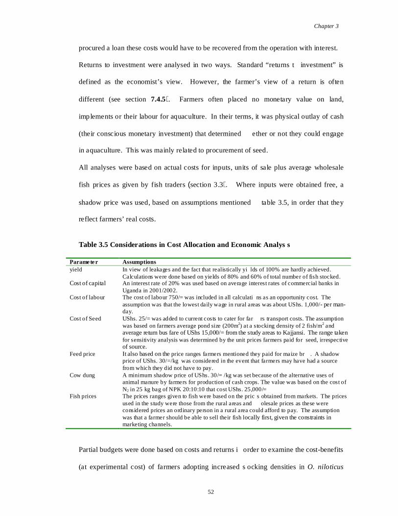
Chapter 3

O. niloticus

52

procured a loan these costs would have to be recovered from the operation with interest.

Returns to investment were analysed in two ways. Standard “returns t investment” is

defined as the economist’s view. However, the farmer’s view of a return is often

different (see section . Farmers often placed no monetary value on land,

implements or their labour for aquaculture. In their terms, it was physical outlay of cash

(their conscious monetary investment) that determined ether or not they could engage

in aquaculture. This was mainly related to procurement of seed.

All analyses were based on actual costs for inputs, units of sale plus average wholesale

fish prices as given by fish traders section 3.3 . Where inputs were obtained free, a

shadow price was used, based on assumptions mentioned table 3.5, in order that they

reflect farmers’ real costs.

yield In view of leakages and the fact that realistically yi lds of 100% are hardly achieved. Calculations were done based on yields of 80% and 60% of total number of fish stocked.

Cost of capital An interest rate of 20% was used based on average interest rates of commercial banks in Uganda in 2001/2002.

Cost of labour The cost of labour 750/= was included in all calculati ns as an opportunity cost. The assumption was that the lowest daily wage in rural areas was about UShs. 1,000/- per man-day.

Cost of Seed UShs. 25/= was added to current costs to cater for far rs transport costs. The assumption was based on farmers average pond size (200m2) at a stocking density of 2 fish/m2 and average return bus fare of UShs 15,000/= from the study areas to Kajjansi. The range taken for sensitivity analysis was determined by the unit prices farmers paid for seed, irrespective of source.

Feed price It also based on the price ranges farmers mentioned they paid for maize br . A shadow price of UShs. 30/=/kg was considered in the event that farmers may have had a source from which they did not have to pay.

Cow dung A minimum shadow price of UShs. 30/= /kg was set because of the alternative uses of animal manure by farmers for production of cash crops. The value was based on the cost of N2 in 25 kg bag of NPK 20:10:10 that cost UShs. 25,000/=

Fish prices The prices ranges given to fish were based on the pric s obtained from markets. The prices used in the study were those from the rural areas and olesale prices as these were considered prices an ordinary person in a rural area could afford to pay. The assumption was that a farmer should be able to sell their fish locally first, given the constraints in marketing channels.

Partial budgets were done based on costs and returns i order to examine the cost-benefits

(at experimental cost) of farmers adopting increased s ocking densities in

7.4.5

Table 3.5 Considerations in Cost Allocation and Economic Analys s

Parame te r Assumptions

)

( )

Chapter 3

O.

niloticus – C. gariepinus

et al

et al

53

mono-culture and an increase and/or reduction in fertiliser and feed i levels in

farming.

Sensitivity analysis was done to examine the cost and roduction limits within which

experimental production would be economically viable (Pannell, 1997; Herrero .,

1999). When analysing the effect of a selected paramet r on economic indicators, the

other parameters were kept constant table 3.7 (Petersen ., 2002). The parameters

were then discussed, based on their effects on the listed economic indicators.

profitpercent yield profit excluding labourpercent marketable size returns to investment, farmers

returns to investment, economistconstruction costs returns to labourcost maize bran returns to landcost cow dung break-even pricecost labour break-even productioncost capital net profit operating costprice fish receipts per fish receipt per kg

Sensitivity Analysis

( )

::

Table 3.6 Parameters and Economic Indicators used in Sensitivity Analysis

Parameter Used In Sensitivity Analysis

Economic Indicators Tested

Biological

Economic

Chapter 3

O. niloticus C. gariepinus

O. niloticus C. gariepinus

O. niloticus, C. gariepinus O. niloticus,

C. gariepinus

C. gariepinus

54

Marketable yield % 80Marketable size % 80Construction costs UShs/m2 250Cost of capital % 20Seed cost UShs/fish

75325

Feed cost UShs/kg 100Manure cost UShs/kg 30Price of fish, weight UShs/kg

1,2002,000

Price of fish, size UShs/fishsmall 300, small 1,000

medium 700 , medium 2,000

The initia l objective was to assess factors currently ffecting supply and demand.

However, in discussions with Fisheries Officers and traders, it became clear that there

was a demand for as bait. Demand was estimated using the

quantitative/survey techniques already described focus ng on fishermen/bait traders to

ascertain demand and possible opportunities for fish farming.

Potential demand for catfish seed by farmers was projected based on secondary data from

District Fisheries Offices (DFOs). Where not possible, records were consulted from the

Ministry of Agriculture on pond numbers and sizes within the basin, but unfortunately,

the most recent data available was for 1997. Rapid appraisals were used to augment the

data.

Table 3.7 Values Kept Constant During Sensitivity Analysis of a Parameter

Parameter Constant Value (UShs)

3.5. seed demand and supply

3.5.1. Introduction

3.5.2. Demand

Seed

( )( )

( )( )

( )

( )( )

( )

( )

C. gariepinus

Chapter 3

C. gariepinus

14.n

SDSRP

Sdemandseedpotentialannual

n

n

PSR O. niloticus C. gariepinusSDn

et alC. gariepinus

55

The average amount of seed required per annum was estimated from

scenarios described in table 3.8 below with respect to total pond area in the basin. It was

assumed that farmers had one production cycle per year.

9

1

][

)(.

Where, = total pond area in basin (m2) = stocking ratio ( : ) = stocking density (no. fish/m2)

= scenario

3a 13a 23a 35a 15a 25a 30b 10 b 20 b 3

a Adapted from de Graaf ., 1996.b Refers to monoculture.

Random sampling of bait usage was done as described in section 3.3. The sampling frame

was based on the number of landing sites on the shores of Lake Victoria in Busia, Bugiri

and Wakiso districts. Sampling intensity was 20% of the total number of landing sites

per district.

A total of 184 fishermen and 45 dealers in fish bait were interviewed. The number of

fishermen interviewed was determined by the number that came to the landing site that

day, irrespective of where they were normally based. Fishermen and traders were asked

to estimate demand and supply on a weekly basis. Aggregate figures were used because

∑

∑=

=

××

=

Table 3.8 Scenarios used in estimation of seed demand

ScenarioStocking

Ratio

Stocking density

(fish/m2)123456789

Bait

C. gariepinus

Chapter 3

C. gariepinus

15SM

bBdemandbaitannual

M

M

CS

AS

n

n .

bn

16. tS

Lbrequirmentmonthlytraders

C. gariepinus

C. gariepinus.

C. gariepinus

56

none of the fishermen sampled kept records (appendix J).

The annual demand for as bait was estimated using different scenarios

based on the sum of traders monthly requirement. It was calculated as described below

(see table 3.9).

4

1

12

1)(

Where: M = modelS = scenario

= traders monthly requirement = months of the year

)(

Where: L = number of registered long lines in Lake Victoria (MAAIF, 2000),S = scenariot = proportion of traders requiring a certain amount o ait (based on survey results)

Assumptions: Bait required per month based on weekly demand. However weekly d mand was not multiplied by four because medians/averages were used and it was assumed the variations were likely to be great either above or below the means as there were no accurate records.

.1 3 fishermen/trader2 8 fishermen/trader3 15 fishermen/trader4 Estimated no. traders

a Based on findings from survey.

The supply of was based on production records from Sunfish Farm Ltd., in

Kajjansi, the only commercial hatchery producing Data was also obtained

to assess the potential of farming as bait. It included

i. size and age of fry at stocking for growth to fingerlings in ponds

ii. feeding regimes

∑ ∑

∑ ∑ ∑=

=

=

=

=

=

=

∑×=

:

Table 3.9 Scenarios used to estimate annual bait demand

Modela ScenarioModel No

Characteristics A(10 lines/fisherman)

B(20 lines/fisherman)

C(30 lines/fisherman)

3.5.3. Production and Supply

C. gariepinus

Chapter 3

C. gariepinus

57

iii. time to minimum bait size recommended by fishermen and traders in fish bait

iv. stocking densities

v. costs of feed and manure

Economic analyses on potential of bait production as a farm enterprise were assessed

using hatchery costs of production as described in section 3.4 above.

Chapter 8 draws out the implications of these findings in as far as they affect the potential

of farming for smallholder farmers.

Chapter 4

N

58

This chapter analyses the potential for farming indigenous species based on a qualitative

analysis of farmers’ socio-economic conditions in relation to fish farming and lo al market

potential. Survey techniques are summarised in the previous chapter.

Structure and Size

Of the 91 fish farming units sampled, 67% were owned and managed by individual households

and 33% by fish farming groups. Households were regar ed as dependent family units living

within a homestead, and fish farming groups as a set o independent individuals or family units.

The proportion of households and groups varied between agro-ecological zones and districts

(Chi-Square P-Values 0.01 and 0.04 respectively). There were proportionately more groups (

= 30) in the IBC Farming System (57%) than within the BMC (30%) and WBC Farming

Systems (13%). The proportion of groups to households was higher at th level within

Bugiri (50%), Kampala (46%) and Wakiso (46%) districts.

Responses from key informants and farmers indicated that these differences were associated

with constraints farmers faced in accessing land, capital, labour, extension services and other

inputs for fish farming. Groups within the IBC Farming System were predominantly made up

of the wives of low-income earners who were often unemployed. Such groups within Kampa a

district had ‘urban welfare’ connotations because urban agricultural services were offered

CHAPTER 4

Socio-economic factors affecting fish farming in the Lake

Victoria Basin

4.1. Introduction

4.2. Farmers and Farm Profiles Characteristics of the Fish Farming Unit

Chapter 4

pers. comm

59

through the District’s welfare department, rather than the Agricultural department as in up-

country districts (Nyamutale .). Wives of low income earners were encouraged to

form groups through which they could pool resources to engage in income generating activities

to supplement household income (and the nutritional status of their children). Together, they

were able to acquire both inputs (notably feed, fertil ser and seed) and land for fish farming. As

groups, they were more likely to be allowed to use unused land for fish production, belonging

either to members of their communities (who often also became members) or to the local

authority. Forming groups also made it easier for such women to ain extension services or

financial support from NGOs or local government.

Within the BMC Farming System, farming groups were formed to improve ccess to extension

services or to obtain financial support from NGO or local government developmental

programmes. Within Bugiri district “groups” were often created only because access to services

was conditional upon being a “group”, though they were sometimes composed of “members”

who were actually all from the same family. Such “groups” were considered as household

units in this study. Fish farming groups in the zone were more commonly formed as a result of

services offered by neighbours or friends in cases where farmers were short of labour for pond

construction or inputs and the cash to obtain them. The neighbours and friends who helped

were offered a share in the proceeds.

Sizes of fish farming units were highly variable (see ble 4.1). Household sizes appeared to be

larger within the BMC Farming System than within the other two farming systems. Group sizes

on the other hand were generally larger within the IBC Farming System.

Chapter 4

Household

Group

N

60

BMC 13 17.2 6 14.0 42 10.1WBC 24 10.1 1 9.5 22 5.1IBC 15 11.1 5 10.0 20 5.1

Overall 52 12.3 1 10.0 19 7.3

BMC 8 27.6 10 19.0 60 21.0WBC 4 18.5 6 9.0 50 21.1IBC 12 28.3 10 22.5 58 17.1

Overall 25 18.4 6 18.4 60 18.4

It was difficult to get reliable information about hou ehold sizes in Wakiso District, as many

people, particularly older women, were cautious about giving details to strangers .

Difficulties in getting correct information about group size was attributable to the dynamic

nature of groups, and some respondents were not sure o the actual numbers of their members,

where new people had joined or old ones left. The sizes of families and groups where numbers

were regarded as probably being incorrect were not recorded in the study.

Heads of households

Most fish farming units sampled ( = 87) were headed by men (87%). However, the

proportion of male to female headed units depended on he structure of the farming unit and

their location within agro-ecological zones (Chi-Square P-Values 0.00 and 0.03 respectively),

as shown in Table 4.2 below.

0% 4% 14%20% 0% 45%

2

According to the 2002 census, the average househo ld si e is 5-6: this could ind icate that fish farming ho useholds have larger ho useho lds than average, e.g. because it is an activit o nly carried out by established families w ith many child ren, or because respondents are understanding the term househo ld in a slightly different way to UBoS.

Table 4.1 Fish Farming Unit Size by Agro-Ecological Zones

Fish Farming Unit

no. of re sponde nts (N)

Mean(no. of persons)

Minimum(no. of persons)

Median(no. of pe rsons)

Maximum(no. of pe rsons)

Standard Deviation (no. of persons)

2

Table 4.2. Percentage of units owned by women, by structure of unit and AEZ.

BMC WBC IBCHH units

Group units

Chapter 4

61

Women were far more likely to be the heads of fish-farming units (whether group or household

units) in the central IBC Farming System, and more likely to head group units than household

units in both the Eastern and Central zones. (There was only one female headed unit in the

WBC Farming System). The apparent absence of household fish farming units headed by

women in the Eastern BMC Farming System, may in part be because traditionally all farming

is run as a family enterprise in the East, where it is rare for women to have their own fields.

This does not necessarily indicate that women were not involved in managing any units.

However a full gender analysis of fish farming was beyond the s e of this study.

Respondents and key informants noted that there were p ortionately more female headed fish

farming units in the IBC Farming System because of its urban and peri-urban nature.

Consequently, there were more attractive economic oppo unities for men, and a greater

demand on them to work for immediate cash-income rather than engage in small-scale

agricultural groups. On the other hand in the BMC Farming System where the agricultural

sector was the major source of employment, fish farmer groups were mostly mixed sex

comprising young adults.

Wealth Status

Fish farmers were on the whole ranked among the wealthier members of their communities.

However, this masks a more complex picture, where the wealth status among fish farmers

varied according to their location within agro-ecological zones and districts, the sex of the

unit’s head and the structure of the farming unit (table 4.3). Fish farmers within the IBC

Farming System (notably Kampala district) were ranked among the poor as opposed to fish

farmers in the other zones. Women fish farmers were r ted as being poorer than their male

counterparts. Household heads who were members of a fish farming group were rated as being

poorer than those whose households farmed fish independently.

Chapter 4

Agro-ecological zone

District

Farm Unit Structure

Sex

Age Group

62

Various criteria were used by participants to assess wealth status. The main criteria used were

people’s additional sources of income; age and physica ability; ownership of livestock;

ownership of land; to what extent farmers engaged in cash cropping; the nature of housing;

education; and family size and structure (e.g. female headed households). These criteria were

not used uniformly across the different agro-ecological zones. The criteria used in different

farming systems are listed in full in appendix K.

BMC 34 41 46 16 88WBC 47 33 46 17 100IBC 158 67 66 15 100

Bugiri 13 37 36 16 56Busia 21 47 51 19 88Kampala 96 67 72 33 100Wakiso 62 60 56 15 100Ntungamo 47 33 46 17 100

Household 75 33 43 15 100Group 164 67 66 16 100

Male 75 50 57 17 100Female 65 67 72 33 100

up to 25 years 1 67 67 67 6726-35 years 2 70 70 39 10036-35 years 9 33 42 15 6746-55 years 8 34 39 16 80+56 years 11 33 40 20 80

The number of farmers from whom data was obtained and analysed in the respective categories

Table 4.3 Effects of Location, Farm Unit Structure, Sex and Age on Wealth Ranks

Categories used to Compare Ranks

among Fish Farme rsNa Me dian

Rank

Geome tric Average Wealth RankFish

farmer

Lowest Rank

(wealthiest)

Highest Rank

(poorest)

Kruskall-Wallis

Test, P-Value

0.00

0.00

0.00

0.40

a

Chapter 4

O. niloticus B. docmac C. gariepinus

C. gariepinusL. victorianusB. docmacC. carpioL. niloticus

N

63

The primary objectives that fish farming units had for aquaculture were income and household

consumption. Income was considered most important by 71% of 85 res ondents. Household

consumption was usually (65%) the second most important objective. However only 16% and

11% of units had the single objectives of income and hold food supply respectively,

while 62% cited both objectives. Fish farmers cited income and household consumption as

major objectives irrespective of their wealth ratings, location, age group or structure of fish

farming unit. Other multip le objectives included hous hold consumption and training by 2% of

units, and income and training by 9% of units. (This latter was cited by fish farming groups

rather than household units). In Ntungamo district (WBC Fish Farming System), fish farmers

who had no livestock hoped that through fish farming, they would eventually become cattle

owners .

Farmers were asked to list three species in order of p rence for aquaculture, irrespective of

whether they were currently farmed or only obtained fr he wild. The most preferred were

tilapias ( is the most preferred), and (see table 4.4).

Tilapia 40 45 1920 39 162 4 4

27 5 26 2 40 2 0

Any 2 6 56

Note: Not all farmers had a second or third choice of species, hence is not constant.

4.3. Socio-economic assets and aquaculture

4.3.1. Objectives for aquaculture

4.3.2. Species choice

Table 4.4 Farmers’ preferences for potential species for aquaculture

Fish SpeciesFarmers Rank 1

(%, = 68)Farmers Rank 2

(%, = 65)Farmers Rank 3

(%, = 57)N N N

Chapter 4

C. gariepinus B. docmac

C.

gariepinus

C. gariepinus

64

The reasons for species preferences in order of import ce were: family/local tastes; market

potential; familiarity of the species; ability to grow to large sizes and reproduce in ponds. The

potential growth rates and ability to attain preferred market size were important factors in the

choice of and . The fact that tilapia have a high reproductive rate was

not brought up as a major constraint in its choice. More farmers viewed this as positive, in that

they would have many fish and not need to buy new stock. Among the negative attributes of

mentioned was the fact that it burrowed. This was a major p of concern among

the farmers in Bugiri district whose fish ponds were a ong their rice paddies. However, its

size at harvest, growth rate and marketability appeared to outweigh this negative attribute in the

area, thus maintained its second place. There was no significan difference

between rankings and reasons for choice across agro-ecological zones.

The primary sources of investment capital for fish farming for 74% of fish farming units were

cash and non-cash capital from their farms. Only 21% of fish farmers sourced their investment

capital from off-farm earnings while 6% farmers used both on-farm and off-farm sources.

There was no significant association between a farmer’s investment sour or aquaculture and

the fish farm unit’s structure or location.

Most farmers (74%) did not consider financial capital s a major constraint. Among those who

did however, 67% were from within the IBC Farming System and 33% from the WBC Farming

System. None of the farmers within the BMC Farming system mentioned finance as among

their major constraints (Chi-Square P-Value = 0.00). This was associated with the fact that in

the IBC Farming System more hired labour was used for pond construction and ma agement

and proportionately more of the fish farmers purchased some inputs.

4.3.3. Source of investment for aquaculture

Chapter 4

65

Some farmers (21%) mentioned access to nets as a constraint. Of these, 89% were from the

IBC Farming System and 11% from the WBC Farming System (Chi-Square P-Value = 0.00).

In most districts, the District Fisheries Office was t source of seine nets. Farmers in the IBC

Farming System were also able to access nets from the uaculture station at Kajjansi because

of its proximity. In the BMC Farming System farmers also borrowed gill nets from fishermen.

A couple of farmers had improvised materials in the WBC Farming System for harvesting fish.

One farmer stitched up old gunny bags in the form of a seine net, made holes in it and used it to

fish his ponds. The other fed stock from a perforated tin that he would pull out when the family

wanted fish.

The family was the primary source of labour for most units, both for pond construction and

management. Labour availability for aquaculture was influenced by the structure of farming

unit, wealth status, location, age of farmer and the farmer’s alternative livelihood options.

Fifty percent of farming units had constructed their p th labour sourced from within the

unit and 42% with hired labour. Nine percent had used both hired and their own labour to

construct ponds. The source of labour for constructio aried significantly depending on

structure of fish farming unit at the 10% level (Chi-Square P-Value = 0.07). Among the

household units, 41% used family labour and 49% hired labour, the remainder using both.

However, 67% of fish farming groups had constructed ponds themselves compared to 27% that

had hired labour, and 7% that had used both. Although the difference is not significant at 5%

level, it makes sense that groups, who often come together because they lack labour on their

own, should use more of their own labour. Poorer fish farming households depended more on

family than hired labour for pond construction, 60% doing so, compared to 41% for the middle

group and 36% for the wealthiest, of whom 56% had hired labour to construct ponds.

Labour

Pond construction

Chapter 4

N

Agroecological zone

Farm unit

66

Costs of pond construction varied enormously. Forty-two of respondents ( = 64) had not

spent any cash on pond construction: 44% had spent up to UShs. 1,500/= per m2, 5% between

UShs. 1,500-3,000/= per m2 and 9% had spent above UShs. 3,000/= per m2. Table 4.5 shows

the characteristic cost ranges of pond construction costs as estimated by farmers.

BMC 15 8 802 200 4,037WBC 25 5 1,071 80 5,875IBC 24 14 1,141 29 4,100Overall 64 37 1,030 29 5,875

household 40 1,031 80 1,158group 24 1,017 29 1,224

Data from RRAs

Significantly more family labour was used for pond man nt than construction (Chi-Square

P-Value = 0.00). Most labour used was obtained from within the farming unit irrespective o

farmer’s location, age group and farm unit structure. Of the total number sampled (N = 90),

71% relied on family labour, 13% on hired labour and 16% on both hired and family labour.

While no signif icant P-Value was obtained, results indicated that the least amount of family

labour was used amongst the wealthiest farmers for pond management, which is as one would

expect.

Table 4.5 factors influencing amount farmers spent on labour for pond construction

Factor No. of Respondents

No. Responde nts

Mean (USh/m2)

Minimum (USh/m2)

Maximum (USh/m2)

Pond management

Chapter 4

Agroecological Zone

Farm unit

67

BMC 17 1 20,000 20,000 20,000WBC 26 3 29,667 5,000 54,000IBC 22 5 42,000 15,000 100,000Overall 65 9 35,444 5,000 100,000

household 42 5 40,800 5,000 100,000group 23 4 28,750 20,000 45,000Least wealthy 4 0 0 0 0

Data from RRAs

Forty-four percent (44%) of the wealthiest farming household units depended on family labour

compared to 71% of the households in the middle wealth group and all households in the least

wealthy group.

The view of most fish farmers (89%), irrespective of t ocation, wealth status, age group or

the structure of the fish farming unit, was that labour availabili a critical constraint.

However, some observations indicated that labour was i deed a constraint. For example, it took

more than a year to construct ponds, particularly for eholds depending on family labour.

Where households had older school going children, much of the construction was done during

dry-season school holidays. Consequently, some farmers would build and stock a series of

small ponds with the intention of merging them later, in order to derive output rather than

letting the land lie idle over long periods during which it might become overgrown. Among

groups, more of the women’s groups hired labour for construction, depending on how difficult

the site was. In mixed sex groups, men often did the heavy work. Also, it was observed that

during the rainy (growing) seasons ponds became less w managed among both households

and groups. This was because farmers diverted their attention to their fields and had less time

for fish farming. Indications were that the opportunity cost for labour was high.

Table 4.6 Effect of socio-economic factors on amount farmers spent on labour for pond management

Factor No. of Responde nts

No. of Respondents

Mean (Ush/month)

Minimum (Ush/month)

Maximum (Ush/month)

Chapter 4

O. niloticus C. gariepinus

N N

68

Fish farming experience among the units sampled varied m 3 months to 16 years, averaging

2.4 years. Twenty-five percent (25%) had farmed fish for less than one year, 56% for 1 to 3

years and 19% for more than 3 years. More of the new rmers were from the BMC and IBC

Farming Systems (Chi-Square P-Value = 0.00). In the WBC Farming System, more fish

farmers had farmed fish for at least 3 years.

Nevertheless, more farmers in the IBC Farming System considered their knowledge to be

adequate compared to the fish farmers in the other two zones (Chi-Square P-Value = 0.00).

This was attributed to the fact that the aquaculture s ation was within their zone. Station

records confirmed that most of the farmers who visited the quaculture station (individually or

as organised study groups with their local extension s aff or schools) were from the IBC

Farming System. A number of the farmers who had farmed fish for several years mentioned

they had learnt some things out of experience, notably what forage fish most preferred to eat.

Most fish farmers (91%) did not consider security a co traint. However, within the BMC

Farming System, after neighbours realised some farmers farming -

had good-sized fish, the incidence of theft from fish ponds increased. This issue came to light

after the study.

A wide range of persons bought fish. Most (89%) had come to purchase fish for household

consumption, 11% ( =96) had come to market to buy fish for restaurants. Almost all (99%,

4.3.4. Knowledge

4.3.5. Security

4.4. Market potential of table fish

4.4.1. Market characteristics

Chapter 4

B. docmac L. victorianus

C. gariepinus C. carsonii Protopterus

C. carsonii C. gariepinus

69

= 97) obtained fish from their local market and 57% felt they lived close to the markets. Some

of the purchasers had come to do other business rather than specifically to purchase fish.

According to respondents, some species were available markets. The commonest

species in all markets were tilapia and Nile perch. Fi hes like and

were available in only major markets. Forty-three percent, 60% and 40% of respondents who

sometimes consumed , and sp. respectively mentioned

that they had purchased it from other, more distant, markets..

Fifty percent of respondents consumed fish 1 – 5 times per month. Fish was most frequently

consumed in the East and least in the West. At each vi it most households bought 1 fish while

restaurants bought 1 to 4 large fish. The restaurants purchased fish almost daily depending on

local availability and customers demand. Fish was consumed more frequently in the BMC

Farming System and IBC Farming System.

BMC 35 20 43 9 14 6 11IBC 20 35 30 15 5 0 15WBC 41 73 12 7 5 0 2Total 96 46 26 9 8 2 8

Note: the information was gathered by interviewing consumers in the fish market, hence all respondents ate fish at least occasionally

The main source of fish to the markets sampled was Lak ictoria. In Ntungamo District fish

also came from wholesale fish markets in Mbarara district. In Kampala District, species of fish

were from lakes Albert and Kyoga. and were also caught from

Table 4.7 Household monthly fish consumption rates by agro-ecological zone

% of consumers eating fish at each monthly fre quencyLocation Consumers ( ) 1-5 6-10 11-15 16-20 21-25 26+

4.4.2. Source of fish

N

Chapter 4

Rastrineobola argentea “

(nkejje)

. carsonii C. gariepinus

R. argentea

R. argentea

70

swamps during the rainy season. No pond fish were available from local markets. Both

consumers and traders said this was because fish farmers sold all their fish by their ponds.

Fish supply was most abundant during the rainy seasons and on dark nights when catches were

at their peak. As a result of slight seasonal variatio in Busia district fish sellers considered the

supply of Nile perch as peaking from July to September and that of tilapia in April and

November. ( mukene”) supply was considered highest from October

to December. Supplies of both tilapia and Nile perch were observed by fish sellers to be at their

lowest from December to March. In Bugiri district on the other hand, fish sellers mentioned

April as the month when both tilapia and Nile perch were most abundant and November he

month when they were least abundant. The supply of Haplochromines in Bugiri

district was considered lowest during the months of April and August. Supply was also

affected by the lunar cycles.

In Ntungamo district, the seasonal supply of C and in Ntungamo was

most obvious. The fish were caught during the rainy season from the local swamps and Lake

Nyabihoko. Nile perch and tilapia from Lake Victoria w available throughout the year.

In Kampala and Wakiso districts, fish supply was also affected by the state of road networks

from the source. During the rainy season, supply sometimes dropped if rains were heavy and

roads bad, causing supply to be at its lowest during t e rainy month of September.

The supply of was considered highest in January. Fish sellers also noted that

supply of and Haplochromines dropped during rainy seasons because they were

difficult to sun dry, hence post-harvest losses were higher. The supply of Nile perch d tilapia

dropped during the months of July and August because o trong waves on Lake Victoria.

4.4.3. Supply and demand

Chapter 4

R. argentea,

71

Supply of Nile perch frames from the fish factories an Haplochromines was considered by fish

sellers as constant during the year. The quantity of fish into markets also depended on the

strictness of fisheries authorities that day.

All fish sellers interviewed considered local fish demand to be high. According to figures from

the district records, this translates to an estimated rate of 1.5 kg fish per person

per annum in Kampala when its day time population of 3,000,000 is used or 4.5 kg fish per

person per annum when resident population figures are sed (estimate 1,000,000). In either

case, consumption rates are extremely low given the re ed 12.5 kg fish per person per

annum by Balarin (1985). According to fishermen, demand for fish was further associated with

seasons, fruitfulness of the harvest and seasonal farm-gate prices of produce. In rural settings

where farming was the main occupation, demand peaked d ring the dry season when farmers

had no fresh vegetables or fresh beans on their farms. Demand also peaked at the end of

harvests especially of cash crops (notably maize and c e). The effect of growing seasons on

demand was less pronounced in urban Kampala and peri-urban areas of Wakiso districts. In

Kampala demand was influenced by how much money customers had - described by fish

sellers as being ‘as long as the fish was in the market and pr es were negotiable’. However,

fish sellers in Kampala observed that most fish was bought at the weekends, during public

holidays and, in the central wholesale market, on Tuesdays.

Demand in all districts was also affected by the schoo year and festive periods. More fish was

bought during the school holidays and festive seasons cept for Christmas and Easter when

other meats were preferred. Soon after Christmas and New Year and before the start of the new

school year, the cheaper fishes ( and Nile perch frames) were most marketable as

Chapter 4

N R. argentea B. docmac

C. gariepinus

R.

argentea C. gariepinus

72

farmers had less cash. Demand for haplochromines was relatively constant but peaked

depending on incidences of measles among children (see later)

Consumers also noted that fish was more expensive during the dry seasons because of

increased local demand (due to the lack of green veget les) and low supply from the lakes. It

was also more expensive during festive periods. Consumers from Ntungamo considered the

increase in fish prices during the dry season to be du also to the fact that there was more

money in circulation from coffee sales. In Kampala, consumers noted the fish prices were

progressively rising because of high demand in the city and probably because fish exports.

The marketability of the different fish was found to b related largely to their inherent

characteristics, size and form of processing.

The species ranked as most marketable by fish-sellers were tilapia and the Nile perch

(Kruskall-Wallis Test, adjusted for ties: P = 0.01). The specie consumed by most consumers

sampled ( = 97) were tilapia (93%), the Nile Perch (74%), (34%),

(27%) and (23%). Of the species available on the market, the most favoured

among consumers were tilapia and Nile perch (table 4.8 .

Kampala District records for the year 2000 showed that tilapia was the most sold fish. This

was largely because of consumer preferences and because most of the Nile perch caught from

the lake is exported. Of a total of 4,466 t of fish sold in Kampala district rkets, excluding

factory by-products, 56% of sales by weight comprised tilapia, 34% Nile perch and 1%

. The amount of sold through the registered markets was just 8.7 mt.

4.4.4. Marketability of Fish

Fish species

Chapter 4

BagrusClarias gariepinusClarias carsoniiLabeoR. argenteaProtopterusAlestesMormyrus

B. docmac, C. gariepinus, L. victorianus, Protopterus

Mormyrus

L. victorianus C. carsonii

Protopterus C. gariepinus

73

Tilapia 57 52 90 67Nile perch 43 39 72 17

sp. 3 3 26 81 1 22 24 4 9 0

sp. 1 1 5 04 4 33 0

sp. 1 1 8 1 sp. 1 1 1 0

sp. 1 1 1 0Haplochromines 2 2

Information from interviews with fish sellers and cons rs in markets.

Consumers’ species preferences were mostly associated with taste, cost and local availability.

The reasons for preferred choice were found not to be ignificantly associated with consumers’

primary occupation or location.

Tilapia and Nile Perch were ranked high by consumers because they were the most readily

available in both major and minor markets. They were also favoured as they were available in

various size ranges that were both affordable and pref rred. Tilapia was favoured over Nile

perch for its milder taste and smell. sp.

and sp. were preferred for their taste, but consumption was limited because of their

relatively high costs and low availability. and were also ranked low

because of their fine bones. Nile perch, and was preferred by

consumers with small children because they were fleshy and had fewer bones. It was also

mentioned that the preferences of the younger generation were based entirely on what they saw

in local markets, because their knowledge of alternative species was limited.

Table 4.8 Most marketable and preferred fish species

Trade rs ConsumersMost Preferred Species by Consumer

(Respondents = 97)total no. %

No. of consumers who consume species

No. of consumers for whom species was ranked first choice

Fish Species

Chapter 4

R. argentea

R. argentea

R. argentea

74

(“mukene”) and Haplochromines (“nkejje”) were purchased because they were

cheap and for their nutritive value. The latter was considered by most consumers to be part of

the ‘treatment’ regimen for young children with measle Both species were otherwise ranked

low because of their taste, strong smell, bones and th fact that they were often full of stones as

a result of poor handling during sun drying. Their small size was not considered a negative

factor. These species were bought by the poor.

Fish were presented to the consumer as fresh, sun drie , fried, salted or smoked. They were

also sold whole, in pieces/chunks or as “frames” (the bones and head of the fish, after the fillets

have been removed). There were greater variations in product form in Kampala and Wakiso

Districts than in the other districts. Fish sellers c ted whole fresh fish as the most marketable

form of fish for all species, except and the Haplochromines, that were always sold

sun dried table 4.9 and 4.10 . However, due to limitations in storage and handling both at

source and within the markets, fish of other species o en had to be smoked or fried to improve

shelf-life. Thus in areas far from the lake like Ntungamo, more than 80% of the fish sold was

not fresh. In both Kampala and Wakiso districts, the emand for fried Nile perch frames was

very high in the suburbs or minor markets mostly by youth and as a favourite accompaniment

for people having a drink in the evenings3. The fresh and smoked forms of Nile perch frames

tended to be purchased by families. There was a signif icant relationship between species a d

preference of the fish as fresh, smoked or sun dried by consumers. While most species other

than and Haplochromines were preferred fresh, in the WBC Farming System, more

consumers ranked smoked Nile perch higher than fresh Nile Perch. This was due to availability

and price.

3

In Wakiso district, the fisheries extensio n worker estimated that 4 mt o f N ile erch frames worth US h 2,000,000/= were so ld per

week in one sub-county, Busukuma w hich was co nsidered among the poores sub-county’s o f the district (Walak ira, per comm.).

Product forms

( )

Chapter 4

L. niloticus

C. gariepinus

75

1,499 55 45Tilapia 2,485 83 17

8 95 5TOTAL 4,466 72 28

Adapted from Kampala district fisheries records, 2000. Figures exclude fish factory by-products sold in markets.

Table 4.9 Proportion of fresh and preserved fish sold in Kampala, 2000.

Species

Total Sales

(mt/month)

Proportion Fish

Sold Fresh (%)

Proportion FishSold Preserve d

(%)

Chapter 4

B. docmac

C. gariepinus

C. carsonii

L. victorianus

R. argentea

P. aethiopicus

Alestes

76

Tilapia 128 68 80 74 77 63 35 3 2 3 2 3 4 4

Nile Perch 89 36 56 99 68 59 29 5 4 3 8 4

40 22 34 39 11 4 1 12 2

50 9 7 29 12 16

30 31 8 2

26 4 28 2

22 3 8 76 48

42 52

sp. 4

Table reflects most preferred processed form of each fish species in local markets. Total scores were used. Each fish sellers was asked to indicated

which was most marketable form of the different specie found in their local market. Data was obtained from the RRAs – markets.

Table 4.10 Most Preferred Forms of Fish, as Scored by Fish sellers

Fresh Smoked Sun dried Salted FriedFish Species

BMC WBC IBC BMC WBC IBC BMC WBC IBC BMC WBC IBC BMC WBC IBC

Chapter 4

B. docmacC. gariepinus

Small sized fish

R. argentea C. gariepinus

Medium Sized Fish

77

Consumers and traders were asked in what units they purchased and sold fish respectively. The

fish was purchased and sold based on number and size. Sizes were found to be relatively

standard in all markets, with fish classified as small, medium or large. Samples of these sizes

were measured, and the ranges are indicated in the table below.

Tilapia 68 18 21 16 46Nile Perch 59 3 17 7 42

24 0 42 13 4214 0 21 14 64

: The Kruskal-Wallis test indicated significant differences between species and

preferences for small sizes (Kruskal-Wallis Test, adjusted for ties: P-Value = 0.01). The most

marketable species as small sizes were the haplochromines, , , Nile

Perch and tilapia in decreasing order. There was also a significant variation between agro-

ecological zones and marketability of small sized fish (Kruskal-Wallis Test, adjusted for ties P-

Value = 0.00). Between zones, small sized fish were m st marketable in the WBC Farming

System.

: There was no significant difference between species d their

marketability when they were medium sized, though they were considered of higher

marketability in the BMC and IBC Farming Systems than the WBC Farming System. (Kruskal-

Wallis Test, adjusted for ties: P-Value = 0.00).

Fish sizes

Table 4.11 Sizes of Fish Most Frequently Purchased by Consumers

Fish Species N Respondents

Small fish (0-15 cm)

(% N)

Me dium fish (15-30 cm)

(% N)

Large fish (> 30 cm)

(% N)

Parts/pieces (% N)

Chapter 4

Large Sized Fish C. gariepinus

B. docmac C. gariepinus

Cost

R. argentea

78

: , Tilapia and Nile perch were more marketable when of large

size in the BMC Farming System and IBC Farming System than the WBC Farming System

(Kruskal-Wallis Test, adjusted for ties: P-Values 0.01 and 0.00 respectively).

Most consumers said their preferred sizes would be medium to large, but because of their

higher prices, they often could only afford small fish. Consequently it was those with higher

incomes or the restaurants who purchased larger fish. Consumers who run restaurants said they

earned more by buying and selling a large fish in piec s than serving whole small fish. Fish

such as Nile perch, and were sold in small pieces/parts, to be

affordable. This high demand for small fish has encouraged fishermen not to throw back small

(and immature) fish included in the catch, despite legislation forbidding sale of undersize fish.

Consumers ranked fish significantly higher than the ot animal products when asked which

of the products they would prefer to purchase when con trained by cash (Kruskal-Wallis Test:

P –Value 0.00). The factors that influenced the competitiveness of fish over other animal

products among consumers included the following:

: Fish was often the cheapest animal product. In Kampala and Wakiso, and in Busia milk

and eggs were considered expensive. The most expensive animal products in all areas were

goat and chicken. Although fresh fish is often an expensive form of animal protein, there are

cheaper forms such as and “frames”. Data from Kampala District markets showed

that of the animal products (per kg) fish was the third most expensive at UShs. 2,647/- per kg in

the year 2002. Chicken cost UShs. 4,196/- per kg, goat UShs. 2,388/- per kg, beef UShs.

2,115/- and milk UShs. 521/- per kg. In 2000, the average fish price per kg was UShs. 1,063/-.

Competitiveness of fish over other animal products

Chapter 4

pers. com.

Taste N

n n n

n

Family size

Culture/Religion

Availability N

79

In Bugiri district, the average prices of fish were US 1,600/- per kg, beef UShs. 2,200/- per

kg and chicken UShs. 2, 500/- (Fisheries Officer Bugiri district ).

: Of the consumers ( = 65) who cited fish as first choice when short of cash, 20%

favoured its taste. Animal products most preferred for their taste were (in order of decreasing

preference) beef, fish, milk, goat and eggs (see table 4.12). However, when short of cash

consumers would purchase animal products whose taste was preferred by the ntire family

rather than some members only. In such cases, eggs (2%, = 3), pork (5%, = 6), goat (2%,

= 2) and mutton (2%, = 2) would not be purchased.

: A number of consumers mentioned that they had large families when listing their

reasons for choice of animal product. Hence they preferred products that could be shared out

among the family, and fish and milk scored highest.

: Religion was the most important factor affecting choice, because Moslems

and Seventh Day Adventists did not consume pork. Two consumers considered pork a health

risk. For cultural reasons some consumers did not consume much goat and mutton. Fish was

acceptable to all.

: availability of the product in local markets was also importa ( = 42). Beef,

milk and fish were therefore more likely to be purchas than eggs and the other meats. There

was a significant association (Chi-square P-Value = 0.00) between the proportion of consumers

choosing animal products and local availability. Beef and milk were most readily available and

considered cheaper in the WBC Farming System. Fish was most readily available in the BMC

Chapter 4

Nutritive Value

Satisfaction

Ease of Cooking

R. argentea

B. docmac C. gariepinus

80

Farming System and IBC Farming System. Eggs were least available in local markets in the

WBC and BMC Farming Systems where there is less intensive production.

: The nutritional value of the animal product was also taken into consideration

by 28 of the consumers. Milk, f ish and eggs scored highest for this reason.

: The ability to satisfy a family was among the factors cited by consumers, for

which milk and eggs scored lower.

: Fish, milk and eggs were preferred because they wer easy and quick to cook

.

Another factor affecting purchase of fish was its quality. Consumers mentioned that they would

like smoked fish with no sign of deterioration. Sun dr ed often had many stones.

Cost 89 105 46 97 65 117 44 78 14Taste 86 60 72 42 50 60 42 56 42Family 51 69 18 6 18 30 15 0 0Religion 24 6 0 0 0 0 68 18 30Nutri tion 28 8 2 0 8 10 0 0 0Availability 42 15 38 2 2 18 4 4 22

Information from interviews with consumers in markets

Most fish sellers (73%) sold fish by size, rather than weight (6%). Some sold fish in pieces

(12%), mainly large species such as the Nile perch, , large tilapia and ,

to make them affordable. Prices, both at source in markets varied with the season (table 4.13)

Table 4.12 Competitiveness of Animal Products

ScoresCriteria

No. Respondents Fish Beef

Chicke n

Eggs Milk Pork Goat Mutton

Fish prices and units of trade

Chapter 4

B. docmacC. gariepinusC. carsonii

L. victorianusR. argenteaAlestes

O. niloticus C. gariepinus

C. gariepinus B. docmac

B. docmac

81

Tilapia 250 –800 500 – 1,400 1,000 – 2,500 1,000 – 1,500 800 – 1,800Nile Perch 500 – 800 500 – 1,500 800 – 1,800 2,200 800 – 1,500

- 1,300 – 5,500 5,000 – 6,000 1,200 – 5,000 1,200 – 3,000- 1,000 – 1,400 1,200 – 1,500 1,200 – 2,000 1,200 – 1,400

500 - -1,200 –1,500a -

- - - 2,000 – 2,500 -- - - 500 – 1,000 -

sp. - 1,000 – 2,500 - 1,000b -

a price per stick;b price per piece Data from fish markets

The case study was used to verify information gathered from other farmers on production and

the markets on marketability, i.e. as a form of triang ion. In this case, a female farmer had a

pond of 400m2 stocked with and in the ratio 3:1. Feeds used were

on-farm residues and occasional maize bran, fish meal and cotton seed cake. The growth

period was 8 months. Fertilisation was more regular than feeding and consisted of cow dung

and compost laid with in a crib in the pond. At harves the farmer sold about half of the fish,

consumed some and gave out the rest to friends and relatives.

The farmer found both species to be highly marketable. In the local market (about 1km from

the pond) major fish sold are tilapia (mainly smoked, some fresh) and Nile perch (fried and

smoked frames, fillet and smoked). Occasionally (only smoked) and

were sold . When available, was sold by auction at from UShs. 5,000/= to 10,000/=

or more per kg .

Table 4.13 Fish prices for consumers

Fish Species Small fish (0-15 cm)

(Ush.)

Me dium size d fish

(15-30 cm) (Ush.)

Large sized fish (> 30 cm)

(Ush.)

Parts/pieces (Ush/kg)

Amount Consumers

Spent at Each Visit

(Ush.)

4.4.5. Marketability of pond fish: case study

Chapter 4

C. gariepinus C.

gariepinus

C. gariepinus

C.

gariepinus

C. gariepinus

82

The farmer sold her tilapia table-sized (300g to 500g) at UShs. 500/= to 1,000/= depending on

the size of the fish and negotiating ability of the customer. In the market, the tilapia of the

similar sizes (small to medium) sold at UShs. 400/= to 1,000/=. In the dry season prices ranged

from UShs. 700/= to 1,600/=. The case study farmer noted that the major advantage she had

with respect to tilapia is that it was fresh. Consumers preferred fresh fish, which was not

always available except for short periods at certain times of the day. Furthermore, her quality

in terms of freshness was higher. To friends and poor farmers around she sold a small f ish

(about 200g) at about UShs. 300/=.

Local demand for in the area was high whether fresh or smoked. The

brought into the market was approximately 30cm long ( bout 1kg) and sold for

UShs. 2,500/=. The fish seller brought about 100 of this size range to the market

once every four days and sold them all, usually within a day. The farmer sold her fresh

at about UShs. 2,500/= to 3,000/= per kg on average, the same as the prevailing

market price. She sold a 5-kg fish at UShs. 15,000/= and was offered from up to UShs. 8,000/=

to 12,000/= for fish weighing 3.5 to 4kg. Her fish were similar sized to those in the market,

particularly since the size of brought for sale had dropped over the years. The

farmer was able to sell all her fish from the pond side even when she was completely draining

her pond for re-stocking, and did not have to take any to the market f ale. All she did was

inform her neighbours and friends that she would be harvesting her pond. Listed below (table

4.14) are the range of prices for animal products the rmer gave at the local market.

Chapter 4

C. gariepinus

C. gariepinusB. docmac

N C. gariepinus

P. aethiopicus.

n

83

Tilapia, smoked market 2,100Tilapia, fresh market 2,500

Tilapia, fresh pond 1,500

, smoked market 2,500

, fresh pond 2,000, smoked market 5,000

Nile perch frames, fried market 500

Beef market 2,200

Goat meat market 3,000

Offal (cattle) market 1,500

Chicken, broiler market 3,500 eachChicken, local cock market 5,500 eachChicken, local hen market 4,000 each

Eggs market 100/= each

As well as being marketed for human consumption, there is a sizeable, but often ignored,

demand for some fish species for use as fishing bait. Fishermen and bait traders were

interviewed to understand this market. (See appendix L for more details). Among fishermen

sampled ( = 184 , 64% caught Nile perch as their major fish, 27% tilapia, 19%

and 13% Forty-three percent of fishermen for whom Nile perch was the major

fish ( = 159 caught it with lines. The other species were not del rately targeted in large-

scale long line fishing. Tilapia was important among small-scale fishermen who angled from

shore. The choice of fishing method among fishermen was determined by the availability of

equipment (34%), cost of equipment (8%), catchability 21%), ease of use (33%), availability

of bait (2%), ease of maintenance (1%) and whether or a gear could easily be stolen (1%).

Ease of use was also related to the level of skill a f sherman had.

Table 4.14 Comparison animal products market prices, Kasangati, Wakiso District

Animal Product SourceAve rage Price

(UShs. / kg)

4.5. Market potential of as bait

4.5.1. Introduction

C. gariepinus

)

)

Chapter 4

Clarias R argentea

N

R. argentea

Synodontis sp.Mormyrus sp.

Labeo sp.

N

P. aethiopicus

P. aethiopicus

84

The bait used by fishermen for the different species o caught is listed in table 4.15. Of the

species used as bait for Nile perch, sp. and the haplochromines/ . were most

preferred by 42% and 50% of the fishermen ( = 67) respectively. The reasons given for

preferences were (in order) their availability, preference by the fish, ability to stay alive long

(thus attracting fish), and cost.

Haplochromines/ 48 0 28 34Small tilapia 11 0 15 21Earth worms 1 76 9 0Clarias sp. 32 4 19 40Crabs 1 0 0 0Nile perch 2 0 0 0

7 0 4 43 0 1 0

Termites 0 6 19 0Meat 0 0 1 0Spiders 0 0 1 0Maggots 0 4 0 0Maize meal 0 2 0 0Water insects 0 8 0 0

1 0 0 0

The estimated amount of bait a fisherman used per week for Nile perch ranged from 500 to

above 4,000 ( = 76). Where worms were used, a 0.5 litre tin of worms was used per week. At

peak fishing seasons the demand increased to 1,000 -10,000 bait per week. Among the

fishermen for whom was a major catch, the amount of bait required per we

ranged from 200–1,000 pieces at peak season. The peak fishing season for Nile perch and the

other species was during the rains, from April to August. During the dry months and full moon

demand for bait was lower. Small-scale fishermen spent on average UShs. 200/= to 2,700/ on

bait for and tilapia each week.

Table 4.15 Bait used by fishermen, by fish species caught

fishe rmen using each type of bait (of those catching each fish species)

Species Caught

Bait Nile perch Tilapia

%

C. gariepinus P. aethiopicus

Chapter 4

Clarias Synodontis

R. argentea

Clarias

Synodontis C. gariepinus

85

The major species of bait sold by traders was sp. 77 , sp. 18 and

Haplochromines/ 5 . Costs varied with the season and size of bait table 4.16 .

According to traders, marketable size for bait was from 2” to 4”. The price for this size range

was UShs. 30-50/= depending on season and availability.

Clarias sp. 20-150 40-200Synodontis sp. 20-80 40-100Haplochromines/R. argentea 50 20-100

Among traders interviewed, 14% were usually able to me t demand, 60% never to do so and

the rest met demand occasionally. Traders said they would require from 100 to 30,000

sp. per week (see appendix L). A third said their wee demand was above 5,000, but only

12% were able to get this amount. Only traders whose demand was estimated to be less than

5,000 per week were able to obtain their weekly demand. A similar trend was observed in

supply of sp. and Haplochromines. Estimated annual demand for as

bait is 4-24 million depending on the scenario i.e. number of clients, hooks per line .

Kenya 25a 69 0Local swamps and wetlands 47 0 0L. Victoria/rivers 5 31 100traders/suppliers 7 0 0

a sourced from both swamps and hatcheries.

( %) ( %)

( %) ( )

( )

Table 4.16 Unit prices of bait

Species Cost Price UShs. Retail Price UShs.

4.5.2 Bait trade and supply potential

Table 4.17 Sources of bait for bait traders

Source sp. (% responses,

= 59)

sp. (% responses,

= 13)

Haplochromines(% responses,

= 4)

( ) ( )

Clarias

n

Synodontis

n n

Chapter 4

MU KO N O

MB AR A R A

R AK AI

MP IG I

MA S AK A

MA Y U GE

JIN J AB U G IR I

B US IAWA K IS O

KA M P A LA

NT UG AMO

0 50 K ilom et ers

Lake Victoria

##

#

KajjansiAlupe

N

Number of long lines.0

up to 10,00010,000- 50,000 50,000 – 100,000

source of catfish seed

LEGEND

Fish farming intensity

up to 5 ha.above 5 ha

Fishing intensity:

Figure 4.1 Potential Demand for as Seed and Bait.C. gariepinus

Chapter 4

87

There were several constraints faced by traders and fishermen in accessing bait. The major

constraints were associated with irregularities in supply and distance to source. Bait traders

often could not get the desired amount of bait from a single sour particularly off-season.

Consequently, they had to travel far, sometimes across borders and spend several days (at times

weeks) in order to accumulate sufficient numbers to warrant the effort and cost. Trapping bait

in swamps was also time consuming and laborious (table 4.20).

availability 47variation in price 7consistency in supply 10distance to source 38legal issues 10wild animals 19survival of bait en-route 16health risks 9equipment 12few customers 2low profit 5alternatives 5labour 14theft of equipment and fish from traps 5non-payment by fishermen 2

Fishermen also raised issues pertaining to the ‘legality’ of using bait in long line fishing to

catch the prized Nile perch. Traders and fisheries of icers in the districts noted that the size of

fish caught as bait of all species were illegal. Use of beach seine nets in Uganda was also

illegal. Hence there was a paradox, since long line fishing was encouraged, as it yielded the

best quality of Nile perch for the processing plants, was more affordable and helped reduce

incidences of ‘illegal net sizes’. It also implied that most bait caught using seine nets came

from Kenya in the East, yet trade in fish across borde was also supposed to be illegal. Hence

traders in bait often got into trouble with the authorities, but had no other alternative.

Table 4.18 Constraints faced in the bait trade

Constraints Faced by Traders(n traders = 58)

Score

Chapter 4

C. gariepinus

88

Most bait was caught at night. This increased the likelihood of attack crocodiles and/or

snakes in shallow and swampy waters. Fishermen or tra collecting bait also got bitten by

leeches when catching bait in swamps and shallow water Other occupational health risks

mentioned included bilharzia and malaria. Furthermore, the stressful conditions under which

bait was caught, held for several days and transported resulted in low survival rates en route.

Some traders cited lack of access to appropriate facilities for packaging and transporting live

fish as a constraint. When the bait was got to the la sites, it was often fatigued. This

reduced marketability because fishermen preferred the bait alive and vigorous. Three percent

of the bait traders mentioned that the fact that they had no alternative sources as a nstraint.

cost 44location 68middle men 2supply to meet demand 10

Consequently, 83% of the traders said they would appreciate having a single and reliable

source of bait. Among fishermen, 70% mentioned they wo purchase bait if it

were available from a hatchery. In both cases, the conditions would be that the bait was of

good quality in terms of size, fish were alive, prices were fair, location was easily accessible

(distances of up to 1km from a landing site or major r ad network were considered accessible)

and supply was in concert with fluctuations in demand. Some said they would have to try it out

first before they made up their minds. Issues such as redit facilities or being able to purchase

some of the bait through bartering with fish were mentioned as factors that would enable them

access bait from such a would be supplier. Some of the traders (2%) noted that they would not

mind becoming middlemen and would be willing to transp rt the bait from more distant source

than mentioned above if supply was guaranteed and large enough.

Table 4.19 Concerns of bait traders if they were to purchase bait from hatchery

IssuesProportion of Traders

Concerns(% response = 63)n

Chapter 4

C. gariepinus

C. gariepinus

89

Discussions with fisheries extension staff from both in Kenya and Uganda also showed that

there was a large deficit in supply for both seed and bait to meet the potential

demand of the LVB. The estimated demand for bait in the basin based on the number of

registered fishermen with long lines as described in section 3.5.3. ranged from 4 – 24 million

per annum. Estimated annual hatchery production of in Uganda was of 930,000

(appendix 4), which production supplied both farmers and lake resto king programmes.

District fisheries staff in Bugiri observed that what limited fishermen’s use of long lines (for

Nile Perch), was the unreliable and low supply of bait. Much of the bait used in the district was

from Kenya, which was distant and expensive because of transport costs, particularly for

fishermen from the islands. The tightening of controls restricting cross-border sales of fish had

made it more difficult for fishermen to obtain bait from across the border. More fishermen had

therefore, resorted to the more expensive gill nets. At only one landing site in the district did

fishermen predominantly use gill or cast nets.

The socio-economic profiles of fish farmers show that access to land and labour for

constructing fish ponds have excluded certain of the poorest households, but that many could

own a pond by pooling resources through groups, which has been particularly important for

women. The failure of aquaculture to spread widely does not appear to be due to serious

constraints on pond establishment. Although farmers d d not believe labour was a limiting

factor, this seems to be partly due to their acceptanc of labour shortages as a constant, and

their ability to find ways around this. However, this also reflect the fact that they have

underestimated the importance of investing time in pon anagement during agricultural

seasons, which can have serious consequences for pond profitability (as will be discussed

later). Lack of feed and fertiliser for ponds is also widespread, though this may also be a

4.5.3. The perspectives of fisheries officers

4.6. Concluding remarks

Chapter 4

C. gariepinus

C. gariepinus

90

reflection of the low priority which is given to fish ponds compared to competing demands for

these resources. As will be discussed, this is also a reflection of the profitability of the ponds

under their current management regimes. From the supp y side, then, aquaculture spread has

been more limited by constraints in running ponds well (time, inputs) rather than in pond

establishment. This would fit well with the observed high number of abandoned and unused

fish ponds.

The results from the markets indicate that the local market potential for fish appears good and

at the national level, overall supply of fresh fish to consumers is currently stimated to be only

about 50% of demand, except in the central region of t e country (NARO/MAAIF, 20002).

Consumer preferences for species, for small to medium ized fish for affordability and their

preference for fresh whole fish all favour fish farmer . The high marketability for small fish

would benefit fish farmers because their capacity to produce fish beyond a certain size is

limited biologically and economically. Except in areas very close to markets, fish consumption

is limited by the costs (including time) of access to markets: this means that there is a large

potential market of currently un-met demand if fish are sold locally by ponds. The prices fish

farmers can get also compares favourably with market prices.

Though preferences for tilapia are high, has great market potential as a table fish,

since demand is limited by poor local availability. For farmers close to landing sites, there will

be greater competition for selling table fish. Here, emand for bait offers another opportunity

for fish farming for production. The risks incurred in obtaining bait from the wild

make it costly, hence it would be cheaper and easier t ain bait from a hatchery.

Chapter 5

91

This chapter looks at the resources locally available armers for aquaculture as natural and

physical assets, which a farmer is likely to draw on as productive capital. The data, much of it

qualitative, was generated using the Rapid Rural Appraisal tools described in chapter 3. The

availability of assets is discussed with a focus on th farm within the context of agro-ecological

zones. Seed and bait as key physical assets for produc ion are also discussed in this chapter.

Most fish-farmers sampled (75%) had mixed farms of crops, livestock and fish, 21% farmed

only crops and fish, 3% other enterprises and fish and 1% had crops, others and fish. Whether

or not farming units had multiple farm enterprises was significantly associated with a farmer’s

agro-ecological zone and structure of the fish farming unit (Chi-square P-Values 0.01 and 0.00

respectively). Relatively fewer farmers had multiple enterprises within the IBC Farming

System (70%) compared to 96% and 94% of farmers within the BMC and WBC Farming

Systems respectively.

Among fish farming units, none of the households had single enterprises while 52% of groups

did. (As individuals, members of fish farming groups grew crops and reared other livestock on

their personal farms and likewise ranked them first and second respectively.) It was largely

fish farming groups located within the IBC Farming System that farmed only fish as a joint

enterprise. No significant associations were found indicating an influence of wealth status, age

group, farm size or the sex of the head of the farming unit on the kinds of on-farm economic

activities.

CHAPTER 5

Farming systems and their potential for fish farming

5.1. Introduction

Chapter 5

92

Among farm enterprises, crops were considered as the most important of the farm enterprises

by 75% of farmers. Livestock were ranked second by 55% of respondents and fish third by

64%. Fish were ranked second by farmers who had no livestock. Crops were ranked highest

because they met farmers’ primary objectives, notably food and income.

The major crops grown by fish farmers in the study are listed below in table 5.1. In the BMC

Farming System, maize was the major cash crop. Fish farmers lso grew cassava, rice, some

coffee, vegetables and a few fruits as cash crops. In the Western-Banana-

banana 61 20 46 34 0.00cocoa 1 0 0 100 -vegetables 61 30 36 34 0.19beans 60 25 42 33 0.07fruits 58 26 40 35 0.22sweet potato 54 26 46 28 0.00maize 41 42 29 29 0.01coffee 39 15 60 27 0.00cassava 37 43 24 32 0.01millet 22 32 68 0 0.57sugarcane 18 17 33 50 0.00(“irish”) potato 9 0 29 0 0.00sorghum 9 67 33 0 0.00rice 5 100 0 0 0.00land fallow 39 26 36 39 0.93pasture 20 15 50 35 0.20leguminous trees 6 0 0 100 0.01trees 26 23 65 12 0.00groundnuts 13 15 15 69 0.08soya beans 4 50 25 25 0.51coco yams 27 15 22 63 0.02yams 1 0 0 3 -sisal 3 33 0 67 -cotton 1 100 0 0 -

5.2 Major farm production characteristics

5.2.1. Crops and crop production practices by fish farmers

Table 5.1 Crops grown by fish farmers overall and bet een zones

Crops Grown

Number of

Farmers (N)

BMC(% of N)

WBC(% of N)

IBC(% of N)

Chi-SquareP-Value

Chapter 5

93

Coffee-Cattle Farming System, the main cash crops grown were bananas followed by coffee.

In the IBC Farming System, coffee and vegetables were the major c rops. Fish farmers

also grew some bananas, cassava and sugarcane for sale.

Bananas and coffee were the principal cash crops within the WBC Farming System and IBC

Farming System. The banana was also the major food cr p in these zones. Cereals on the

other hand were mostly grown within the BMC Farming System as major commercial and

food crops. Most of the commercial vegetable production among fish farmers was done in the

WBC Farming System and IBC Farming System. The most important root crops were th

sweet potato and cassava, which were grown by relatively more farmers within the WBC and

BMC Farming Systems respectively. The scale of production root crops however was

highest within the BMC Farming System.

Where bananas, coffee and vegetables were major cash crops farmers fertilised them with

animal manures, compost and/or mulched them. Relatively more farmers fertilised their crops

within the WBC Farming System table 5.2 . Farmers and extension workers attributed this

partly to the effect of small-land sizes and intensified extension services in the d strict two

years previous to the study supported by the NGO CARE. Hardly any of the fish farmers

fertilised their cereal and root crops. Within the BMC Farming System hardly any farmers

fertilised their fields because they regarded their soils as fertile and had comparatively large

pieces of land under crop cultivation in relation to livestock numbers. Adequate fertilisation of

major crops was therefore impractical, and farmers foc d on fertilising vegetables that were

grown in smaller gardens.

( )

Chapter 5

94

Animal manure, banana 23 9 42 22 0.02

Animal manure banana-coffee mixed 26 0 52 27 0.00

Animal manure coffee 19 4 42 14 0.00

Animal manure, rice 1 4 0 0 -

Animal manure, vegetables 31 17 45 35 0.10

Mulch, banana 19 4 48 8 0.00

Mulch, banana-coffee mixed 11 4 23 8 0.08

Compost, banana 21 4 52 11 0.00

Compost, coffee 17 4 48 3 0.00

Compost, banana-coffee 8 4 16 5 0.20

Compost, vegetables 12 13 26 3 0.02

Artificial fertiliser, vegetables 5 9 3 5 -

Artificial fertiliser, maize 5 22 0 0 0.00

Artificial fertiliser, rice 3 13 0 0 -

= the total number of farmers from the sample population who used the production techn que.

The most commonly reared livestock were cattle, goats nd poultry. Proportionately more of

the fish farmers within the WBC Farming System reared livestock than in the other two zones

(see table 5.3). They also tended to have more livest

There was no significant variation between the species of livestock reared by fish farmers and

agro-ecological zones except that more of the fish farmers in the BMC Farming System and

WBC Farming System raised goats than in the Medium Altitude-Intensive-Banana-Coffee

Farming System (Chi-Square P-Value = 0.00).

Table 5.2 Percentage of fish-farmers by AEZ using fertiliser for crop production

Fe rtilisation of Major Crops

Numbe r of

farmers ( )

BMC(% of )

WBC(% of )

IBC(% of )

Chi-SquareP-Value

5.2.2. Livestock production practices

N

n n n

N

Chapter 5

Cattle

Goats

Sheep

Pigs

Rabbits

Chickens

Ducks

Turkeys

95

BMC 23 8 4.3 1 14WBC 31 15 8.3 1 25IBC 31 17 5.9 1 30Overall 85 40 6.5 1 30

BMC 23 11 6.4 1 18WBC 30 20 6.2 2 17IBC 31 5 5 3 5Overall 84 36 6.1 1 18

BMC 23 2 4.5 1 8WBC 30 5 3.8 2 7IBC 31 3 3 2 3Overall 84 10 4.3 1 8

BMC 23 2 5 4 6WBC 30 6 8 1 30IBC 30 7 4.6 2 12Overall 84 15 6 1 30

BMC 23 1 6 6 6WBC 30 6 12.3 4 30IBC 30 2 7 4 10Overall 83 9 10.4 4 30

BMC 23 12 15.7 2 46WBC 30 18 11.1 1 80IBC 30 16 130.8 2 540Overall 83 46 53.9 1 540

BMC 23 0 0.0 0 0WBC 30 2 1.5 1 2IBC 31 0 0.0 0 0Overall 84 2 1.5 1 2

BMC 23 1 7 7 7WBC 30 1 6 6 6IBC 30 0 0 0 0Overall 84 2 13.5 6 7.0

Information obtained from RRAs

Most fish farmers reared their livestock using extensive management systems (table 5.4).

Table 5.3 Influence of Agro-Ecological Zone on numbers of livestock owned.

Livestock Species and Zone

No. of responde nts

No. re spondents

with livestock

Mean herd size

(no.)

Minimum (no.)

Maximum (no.)

Chapter 5

96

Cattle 17.1 36.6 29.3 14.6 2.4Shoats 11.1 74.1 14.8 0.0 0.0Poultry 86.0 0.0 0.0 8.0 6.0Rabbits 0.0 0.0 0.0 100.0 0.0Pigs 7.7 38.5 0.0 53.8 0.0

Information from RRAs

More intensive methods of livestock production were employed by some farmers within the

WBC and IBC Farming Systems. Among the more intensive methods used for ruminants were

paddocking in the WBC Farming System and zero-grazing in the IBC Farming System.

Piggeries and deep-litter poultry production were done by some farmers within IBC Farming

System.

Activities undertaken around ponds included pasture, housing, brick making, paddocks, e

cultivation, trees, vegetables and sugarcane. In Kampala, housing and brick making were more

common; rice and food-crop gardens were common in the BMC Farming System; and trees,

vegetables, bees and paddocks in the WBC Farming System. In Wakiso, sugarcane, vegetables

and gardens were often found around ponds. In all farming systems, some farmers left bush

around their ponds. Most fish ponds were not close to homesteads, but located within the

valleys in wetlands, where water was more easily available in the volumes required for pond

production. Livestock and crops were kept closest to e. During the day larger livestock

depending on the farming system (penned or extensive) were taken down to the wetlands to

drink. Otherwise water was ferried to them.

Table 5.4 Management systems employed by fish farmers for livestock production

Management Syste m (% Farme rs)Livestock

species Free-range (%)

Te thered (%)

Paddocks (%)

Intensive (house d/zero graz ing)

(%)

Both free-range and

intensive (%)

5.2.3. Other activities

Chapter 5

Pasture and Arable Waste(Ipomea batatus)

Colocasia esculenta)

Galisoga pariflora and Oxalis latifolia

(Symphytum peregrinum)

Cassia

Cereal and Grain Residues

97

Most of the farmers’ inputs were obtained locally from within their farms or trading centres.

Farmers used a variety of feedstuffs and feedstuff combinations to feed fish (table 5.5). The

most commonly used were pasture/arable crop waste (65 ), cereal and grain residues (45%)

and kitchen/cooking waste (36%).

58 17.2 43.1 39.7 0.02Sweet potato leaves

29 20.7 34.5 44.8 0.76

Coco-yam (leaves

36 5.6 50.0 44.4 0.00

Vegetable waste 14 21.4 57.1 21.4 0.12Kafumbe grass 19 10.5 52.6 36.8 0.10

Russian comfrey 1 0.0 0.0 100.0 -

Milk leaf 2 100.0 0.0 0.0 -Cassava 4 50.0 0.0 50.0 0.28

sp. 1 0.0 100.0 0.0 -

41 41.5 7.3 51.2 0.00Maize bran 37 35.1 8.1 56.8 0.00Rice bran 8 87.5 0.0 12.5 0.00

Fish meal 14 14.3 0.0 58.7 0.00Terrestrial Invertebrates 4 75.0 0.0 25.0 0.06

Oil Seed Cakes 6 0.0 0.0 100.0 0.01Cotton seed cake 6 0.0 0.0 100.0 0.01Sunflower seed cake 1 0.0 0.0 100.0 -

Mill sweepings 8 25.0 62.5 12.5 0.15Kitchen Waste 33 21.2 42.4 36.6 0.44Rumen content 7 0.0 100.0 0.0 0.00Brewers waste 5 0.0 20.0 80.0 0.16Broilers mash 1 0.0 0.0 100.0 -Lake weeds 1 100.0 0.0 0.0 -

Information derived from RRAs. denotes the total number of farmers sampled in the appraisals . denotes the number of farmers sampled within the agro-ecological zones.

5.3. Potential Inputs for fish farming, source and use

5.3.1. Introduction

5.3.2. Feed materials

Table 5.5 Common items used as fish feed among farmers in the different zones

Feed Fed ( = 91) No. of farmers ( )

BMC(% of )

WBC (% of )

IBC (% of )

Chi-Square P-Value

Nn n n n

Nn

()

Chapter 5

Galisoga pariflora Oxalis latifolia)

98

The relative use of pasture and arable wastes as feed by farmers was significantly associated

with AEZ (figure 5.1). These were more available for aquaculture in the WBC and the IBC

Farming Systems. There was no significant association between the use of pasture and arable

wastes and wealth status, the structure of the fish farming unit or farm size. The most

commonly used arable wastes were coco-yam leaves (40%), sweet potato leaves (32 %), and

vegetables (15 %). Within all zones, farmers obtained pasture and arable wastes from their

farms. They were, with the exception of sweet potato ves, most abundant during the rainy

season. During the rainy season the high demand for sweet potato vines as planting material

reduced availability. There was also demand for pasture and arable wastes as animal feed.

Peelings and sweet-potato leaves were also fed to tethered cattle, goats nd pigs. Kafumbe

grass ( and , when available, was fed to rabbits. None of the

farmers fed their livestock with coco yam leaves. This may explain their greater availability for

fish production in the IBC Farming Systems and WBC where they were a common crop within

the wetlands. Pasture and arable wastes were obtained free.

Maize bran (69%) and rice bran (9%) were the most freq ntly fed cereal and grain residues.

They were more frequently used to feed fish in the BMC and IBC Farming Systems than the

WBC Farming System (figure 5.2). No significant association was found between the relative

use of either feedstuff among farmers and their wealth status, farm unit structure, farm size or

age group.

Maize bran (98%) and rice bran (91%) were chiefly purchased from nearby trading centres.

One of the farmers within the IBC Farming System obtained maize bran from her own mill at

no cost.

Pasture/arable crop wastes

Cereal and grain residues

Chapter 5

BUGIRIW AKISO

NTUNGAMO

BUSIAKAMPALA

Lake Victoria

LowMediumHigh

LEGEND

0 50 Kilometres

N

Figure 5.1 Farm pasture and arable waste availability for fish farming in the agro-ecological zones

Chapter 5

100

The availability of maize and rice bran for fish feed depended on the season and disposable

cash. Availability was higher at the end of the harvest and was lower, hence more costly, just

before and during the growing seasons. Market forces also influenced local pric s and

availability. Though maize and rice were grown on a much larger scale as commercial and

food crops within the BMC Farming System, trade meant that the price of maize bran was in

fact broadly similar in all the zones. Most maize produced in the BMC Farming System was

sold whole (unmilled) to major urban centres or export d to Kenya. Bran from locally milled

maize was also sold to Kenya for use in animal feed fa ories. Major urban centres were the

major destination for cereals and other agricultural produce. Rice on the other hand was hulled

within the BMC Farming System where it was grown and sold off as polished rice to other

areas. Demand for rice bran as an animal feed ingredient by commercial establishments was

also lower, and so it was cheaper and more available locally to farmers within the BMC

Farming System than maize bran.

There was no significant correlation between use of ki en/cooking waste as a fish feed and

the zone. This was also obtained from schools, and in the IBC Farming System was also

purchased from eating houses. Availability of kitchen waste was variable. Pigs, dogs and

poultry were also fed left over cooked food. Whether or not fish got any would depend on

which animals were the priority and what was considered utilisable.

Mill sweepings were used more frequently in the WBC Farming System. Their use was

statistically not associated with wealth, farm unit structure or farm size. Mill sweepings were

more accessible to farmers in the BMC Farming System and WBC Farming System because

there were a number of flour mills located locally within small trading centres/villages. In the

Kitchen waste

Mill sweepings

Chapter 5

101

IBC Farming System however, most flour was milled in larger establishments some of which

also made commercial animal feeds. Small-holder farmers who were able to obtain mill

sweepings in the zone did so for deep-litter poultry units. Mill sweepings were from millet,

cassava, sorghum and/or maize

Abattoir waste was predominantly used as feed in the WBC Farming System where it was

obtained free of charge from the local village butcher Within the IBC Farming System the

availability of abattoir waste for fish farmers was limited because of competitive demand for

commercial livestock feeds. In the IBC Farming System, livestock were slaughtered at

established abattoirs and slaughter slabs in and around Kampala, which meant that the waste

was not locally accessible in the villages. Where it was available, middlemen, and

consequently financial costs, were involved.

The principal sources of animal protein for fish feed re terrestrial invertebrates (termites)

and aquatic vertebrates (fish meal). Termites were largely used as fish feed in the BMC

Farming System where they were caught during the rainy season by farmers or by neighbours’

children at a cost (table 5.5). Fish meal was more frequently used in the IBC Farming System.

The use of fish meal showed no statistical association with wealth status or land size. It was

purchased from trading centres and was least available in shops during the rainy season. Use

depended on seasonal availability and disposable cash. Fish meal, brans and oil-cakes were fed

by preference first to dairy cattle, commercial poultry and pigs.

Abattoir waste

Terrestrial invertebrates and aquatic vertebrates

Chapter 5

Lake Victoria

BUGIRIWAKISO

NTUNGAMO

BUSIAKAMPALA High

Medium

Low

0 50 Kilometers

LEGEN D

N

Figure 5.2 Availability of farm cereal and grain residues for fish farming in the agroecological zones

Chapter 5

R.. argentea

103

Cotton and sunflower seed cake were fed to fish by 6 o e farmers sampled in the IBC

Farming System. They were purchased from trading cent es and their use was irregular

depending on cash at hand. Though none of these crops were grown within the zone, local

availability was influenced by the more intensive animal production practices. Supply was

lowest during the rainy season when prices were also at their peak.

Only five of the farmers sampled fed brewers waste. One was from the WBC Farming

System and four from the IBC Farming System. It was obtained from small-scale brewers

within local trading centres at a cost. Availability was constant year round.

cow dung 0-10 0-20 0.0goat dung 0.0 0.0 0.0chicken dung 0-5 0-25 0.0compost 0.0 0.0 0.0pig dung - 0.0 -maize bran 100-150 50-150 50-200

250-500 600-700 -sunflower - 300-500 -brewers waste - 0-20 -maize flower - 250-350 300-450kitchen waste 0.0 0-80 0-45cabbage - - 50.0rice bran 25.0 25.0 -blood meal - - 0cotton seed cake - 150-300 -yam leaves 0.0 0.0 0.0banana peels 0.0 0.0 0.0Kafumbe grass 0.0 0.0 0.0sweet potato leaves 0.0 0.0 0.0cassava peel 0.0 0.0 -pumpkin - - 0.0termites 0-500 - -

Data from RRAs ‘-’ indicates that the item was not used by farmers sampled in zone.

Oil seed residues

Brewers waste

Table 5.6 Cost of inputs for farmers in each AEZ

Max-Min Cost of Input in Agro-ecological Zones (UShs./kg)

Input

BMC IBC WBC

Chapter 5

104

Most farmers (61.5%) mentioned that they did not have enough material from their farms to

feed their fish. However, this was not considered a constraint by 52% of farmers in the IBC

Farming System, mainly for the groups. This was because group members collectively

contributed towards feeding in cash or kind (e.g. by bringing leaves and left-overs from their

homesteads). More household units in the zone could s mes afford to purchase feed

ingredients. Some farmers did not feed their fish eve ere they had possible access to

inputs from their farms or from the neighbourhood.

The commonest fertilisers used by fish farmers were co dung (66%), chicken dung (40%),

compost (mostly in cribs) 22% and goat dung 20%. The proportion of farmers using cow and

goat dung was significantly associated with agro-ecological zones. Cow dung was most

frequently used in the WBC Farming System. Chicken droppings were mostly used in BMC

Farming System and IBC Farming System. Fish farming groups in the IBC Farming System

used mainly chicken droppings. Goat droppings and compost were most often used by fish

farmers in the BMC Farming System (table 5.7).

Cow dung 60 25 47 46 0.00chicken droppings 36 36 14 50 0.00Compost 20 40 25 35 0.22Goat dung 18 67 28 6 0.00Sheep 1 100 0 0 -Rabbit droppings 4 25 75 0 -Pig manure 3 67 0 33 -Turkey 1 0 100 0 -Duck 1 100 0 0 -

Information derived from RRAs; denotes the total number of farmers sampled in the ap aisals. denotes the number of farmers sampled within the agro-ecological zones.

Most farmers obtained fertilisers from their farms. Others got it from neighbours, and

occasionally from the local butchers – but not in the IBC Farming System because of the

5.3.3. Fertilisers

Table 5.7 Comparative use of fertilisers by fish farmers

Fertilisers Used (N = 91)

No. of farme rs

( )

BMC(% of )

WBC (% of )

IBC (% of ) Chi-Square P-Value

nn n

n

Nn

Chapter 5

N

pers

comm

105

centralised abattoir system in Kampala. In either cas it was obtained at no cost. Manure

was sometimes paid for when obtained from sources off-farm

The majority of fish farmers considered the amount of fertilisers they generated from their

farms as inadequate for all their farm requirements. his was particularly so in the IBC

Farming System. Out of 91 fish farming units sampled, 0% of farmers had other uses for

the manure produced apart from fish farming. When the data was disaggregated by structure

of fish farming unit, 65% the households and 21% farmi groups had other uses for manure.

Where fertilizers were inadequate, 57% of respondents ( = 60) mentioned that they would

preferably fertilize their gardens while 43% would pre rably fertilize their ponds. Ponds

were consequently least fertilised during the planting season when whatever manure was

available was used for crop production. The crops that competed for animal manure most

were bananas, coffee and vegetables. Farmers who had cess to adequate quantities of

compost and mulch as supplements to animal manures for their banana and coffee gardens

were more likely to have a bit of manure to spare for their fish ponds. The availability of

material to make compost was limited, by the availability of material due to seasonal factors,

and the time needed to gather vegetative material.

Animal manure was least available in the BMC Farming System (figure 5.3). The low

availability of animal manure in the BMC Farming System was due to the fact that farmers

had fewer livestock that were mostly reared by grazing. A few farmers tethered their stock.

Furthermore, in the northern part of the district, a lot of livestock were lost due to an outbreak

of East Coast Fever complicated with chronic trypanosomiasis in 1999 (Wanyama,

.).. Thus availability even among neighbours was low. Despite the low availability,

72% of farmers in the BMC Farming System mentioned that they would prefer to fertilise

Chapter 5

N

N

O. niloticus C.

gariepinus

106

their ponds before their gardens. This was because they had large gardens, and so they

considered it more useful to fertilise a small pond properly rather than stretch what little

manure they had inadequately over large fields. Furthermore, the major cash and food crops

grown in the zone were not generally fertilised. Where maize and rice were fertilised,

artificial fertilisers were sometimes used.

Overall, a third of farmers considered access to fish seed a constraint, = 26 , 13%, 26%

and 41% of farmers in the BMC, WBC and IBC Farming Systems respectively. Farmers =

83 consequently obtained their seed from several sources namely, the wild 41 , hatcheries

37 or other farmers 17 . Six percent of fish farming units that constituted groups had

received seed through NGOs and did not know the origin source. The fish hatcheries from

which farmers obtained seed were Alupe Government Fish Station, Kenya and the

Aquaculture Research Centre or SunFish Limited both of which were at Kajjansi, Uganda.

All hatcheries sold . The hatcheries at Alupe and SunFish farm also produ d

seed.

5.3.4. Seed

( )

(

) ( %)

( %) ( %)

Chapter 5

Lake Victoria

BUG IRIWAKISO

NT UNGAMO

BUSIAKAMPALALEGEND

0 50 Kilometers

Low

MediumHigh

N

Figure 5.3 Availability of farm manure for fish farming in the agroecological zones

Chapter 5

N

108

The targeted market for Alupe were fish farmers and fishermen in the Lake Victoria Districts,

Kenya, but it was also used by farmers in the BMC Farming System in the east. The hatcheries

in Uganda in theory supplied the entire country. Until the change in economic to liberalisation

in the 1990s, the Government was supposed to be a supplier of seed for aquaculture. There

were several hatcheries around the country until the 1980’s. These all collapsed in th civil

wars and economic destruction of the 70s and 80s. The private sector is now supposed to meet

farmers’ demands, but this is a slow process. Only one signif private commercial hatchery

is functioning (as of 2004), SunFish Limited, which only began in the last few years. Supply

does not meet demand, hence the relatively high proportions of farmers who obtained seed

from the wild. In addition, access to seed for farmers was difficult because of the distances to

hatcheries. More fish farmers in the WBC Farming System therefore obtained seed from other

farmers and the wild than from hatcheries largely beca f the distance to source and the

subsequent high costs of transport farmers would have to incur table 5.8 . Seed costs were

subsequently affected by demand and supply factors table 5.9 . The total cost of seed for

farmers however was much higher. Quantitative data fr m the farmers sub-sampled who

incurred their own transport costs = 59 indicated that transport costs ranged from 30-300

of the seed purchase cost, depending on the quantities bought and the distance to the seed

source.

BMC 34 50 3 47IBC 30 40 3 57WBC 19 26 37 37

Information derived from RRAs. N denotes the total number of farmers sampled in the appraisals.n denotes the number of farmers who obtain seed from t is source.

( )

( )

( ) %

Table 5.8 Major sources of seed for fish farming in di gro-Ecological Zones

Source of seedAgro-

Ecological Zones = 83

Number of respondents Hatchery

Other Farmer

Wild( ) ( ) (% ) (%

)(% )N n n

nn

Chapter 5

. gariepinus

C.

gariepinus O. niloticus

Diplostomum

109

hatcheries Uganda 50 300hatcheries Kenya a 40 85farmer 100-120 -wild 100-2,000b 500

a cost based on exchange rate KShs.1 = UShs 21.00 in 1/02b At unit costs above UShs. 1,000/-, seed tended to be adult fish.Price excludes transport costs

Proximity to reliable sources of C has affected its adoption for aquaculture by

farmers.

The survival of stocking material was an issue among some farmers. Loss of fish due to

unexplained deaths soon after stocking was reported in the WBC Farming System by 13% of

the farmers, most of whom had obtained their seed from the wild or other farmers (Chi-Square

P-Value = 0.02). In the WBC Farming System, Lake Nyabihoko was an important source of

and tilapia seed. However fish from the lake were reported by

extension staff to have lesions during the dry seasons, the period most fish farmers were able to

stock their ponds. Only healthy looking fish were selected for stocking. Samples of affected

fish obtained during the course of the study were found by the author to be infected with

sp.

Wild seed was more expensive per unit, but when travel ts to hatcheries were included it

was often competitive. In any case, given the unreliab ity of hatchery supply/production, it was

often the farmers’ only option.

Most farmers (97%) had their fish ponds located in wetlands. The major sources of water for

ponds were underground sources – springs/wells (59%) and surface water – stream/river/

Table 5.9 Comparative seed costs

Unit Cost of Seed UShs.Source

5.4. Water sources and site conditions

( )O. niloticus C. gariepinus

( )( )

( )

Chapter 5

N

110

swamp (38%) or both underground and surface sources (2%). The majority of the farmers

considered their water to be of good quality, implying cleanliness at all times. Most farmers

were able to get enough water year round to meet their aquaculture needs. However, in the

WBC Farming System the prolonged drought experienced in the area in 1999 significantly

reduced water supply for aquaculture (Chi-Square P-Value = 0.00). Twenty-three percent

(23%) of the farmers’ ponds and water sources in this one dried up during that drought.

There were no reported water conflicts regarding access to water with other users except for

two cases within Kampala District. Where water sources to ponds were run-off points from

communal springs/wells, complaints were made associate h children playing in ponds, or

waste water from washing being poured into the pond . Only 3 farmers mentioned r gular

flooding as a constraint regarding their sites. All were from the BMC Farming System.

Sixty percent of fish farmers ( = 91) did not consider predators as a constraint to production.

However, there was a significant relationship between agro-ecological zones and whether or

not predators were a production constraint (Chi-Square P-Value = 0.00). Most of the farmers

who cited predators as a constraint were from the BMC Farming System (46%) and IBC

Farming System (43%). The prevalence of specific pred rs also varied with location.

Monitor lizards were the commonest predator for 52% of fish farmers sampled in the BMC

Farming System (Chi-Square P-Value = 0.00). Monitor lizards were not cited in the other two

zones. Birds on the other hand were a problem for 48% of farmers in the WBC and 13% of

farmers in the BMC Farming System (Chi-Square P-Value = 0.00). Otters were cited by 3

farmers. all from the WBC Farming System. Snakes were mentioned as a constraint by 8

farmers who were distributed in all zones. Some farmers planted plants such as tobacco to

keep off snakes.

Predators

Chapter 5

111

The results show that local supply and availability of feed and fertiliser for fish farming was

influenced not just by a farmer’s location in terms of the agro-ecological zone but also by

proximity to urban areas, climatic seasons, farming pr ctices, market factors affecting trade of

potential inputs or their by-products and availability of disposable cash to the farmer and

market factors. Most physical inputs were required as production inputs in farmers’ other farm

enterprises. Re-allocation of these resources depended on farmers’ ove l livelihood

objectives and their perception of the relative return on the inputs from the different enterprises.

Because most rural households in Uganda obtained food from their own farms, when

biophysical and socio-economic inputs were scarce, scarce resources were all cated to crop and

livestock production Bahiigwa, 1999; MFPED, 2002 . Consequently, even where farmers

obtained these inputs free from their farms or the neighbourhood, they had significant

opportunity costs.

The natural resource assets can be considered as gener lly being adequate. The major natural

resource that affects production is water, especially in densely populated areas. The Lake

Victoria basin has an estimated total wetland area of 7,448 km2 of which about 12% has been

converted for mainly agriculture and human settlement. Wetland degradation is increasing as

demand for land for agriculture, industry and housing reases. Most wetlands are open

access resources, except where there is commercial value. In Kampala because of the unclear

ownership and high population density, poorer sections of society move into such areas. Mos

of the fish farmers also depended on underground water as a water source for aquaculture.

Uganda lies on the basement complex of the pre-Cambrian rocks. Underground sources of

water are generally considered poor and occur in limited areas along fissure , cracks and joints

of the granite-gneiss formation at yields of 0.4-2.0 m3 per hour (NEMA, 2001). Day time

5.5. Concluding Remarks

( )

Chapter 5

C. gariepinus

112

ambient temperatures in the west were also prone to dr own to 15oC during the cold months

which may place limitations on production of (NEMA, 2001).

The importance of fish farming in the total resource f on farm was for most farmers small

or insignificant depending on the agro-ecological zone in which they were located. This was

not quantified in the study because of time constraints and because it was not central to the

objective of the study.

Chapter 6

C. gariepinus

see

113

Chapter 6 assesses and discusses how fish farmers combined their assets as capital to produce

fish. It also identifies and examines the effect of input-output inter-relationships on current

production. Consequently the opportunities and vulnerabilities in the system are identified, and

from this, the production systems for that may have the potential to improve

yields and returns in the current system. The results in this chapter were derived from the

quantitative sampling, PCA analysis and partly from the RRAs ( chapter 3).

Farmers’ pond sizes varied from 45m2 to 1,380m2 . The average was approximately 300m2 ,

though most ponds were approximately 200m2 see table 6.1 . The average pond depth was 47

cm and most had steep sides. Laboratory results indicated that pond bottom mud from sampled

ponds consisted on average of 30% silt. The RRAs showed that the factors that influenced a

farmer’s decisions on pond size were recommendations by extension staff, land size and

availability of labour for construction. Pond depth on the other hand was based on

recommendations by extension staff the majority of whom recommended a depth of 50 cm.

However, the depth was also eventually influenced by t e pond construction techniques

farmers used, i.e. dyke construction and levelling of excavated earth around the po d.

CHAPTER 6

Fish farming production systems – current features

6.1. Introduction

6.2. Pond systems and stocking

6.2.1. Ponds

( )

Chapter 6

Pond Sizes (m2)

Pond Depth (cm)

O. niloticus

O. niloticus, though it was

farmed

O. niloticus

O. niloticus

114

LocationN respondents

Mean Minimum Median MaximumStandard Deviation

BMC 26 369.2 74.2 209.4 1380.0 324.2WBC 23 251.6 45.0 209.0 1044.0 234.4IBC 19 314.1 60.0 250.0 1045.0 245.6Overall 68 314.0 45.0 215.0 1380.0 275.6

BMC 24 55.28 32.0 50.3 100.0 18.4WBC 20 46.40 20.0 46.3 75.5 10.9IBC 19 38.56 20.7 43.0 71.3 12.8Overall 63 47.42 20.0 46.3 100.0 16.06

Data on pond size and depth was obtained from both RRAs and quantitative sampling, during which actual measurements were taken while having discussions with farmers.

Several species were stocked in ponds. The commonest species farmed were tilapias, African

catfish and mirror carp.

Tilapia were farmed by 76% of farmers sampled in the R Significantly more farmers

farmed ‘tilapia’ in the WBC Farming System (94%) and BMC Farming System (83%) than in

the IBC Farming System (57%) (Chi-square P-Value 0.00). Proportionately more fish farming

households (85%) compared to groups (58%) farmed tilapia (Chi-square P-Value 0.00).

The commonest tilapia was , farmed by fifty-five percent of farmers. There was no

significant influence of zone on the number of farmers farming

by proportionately more households (63%) than groups (39%) (Chi-square P-Value

0.03). A farmer’s wealth status was also associated with the stocking of at the 10%

level. At this level of significance, tended to be farmed by relatively more of the

wealthiest farmers (62%) compared to farmers in the mi dle (32%) and least wealthy (9%)

categories (Chi-Square P-Value 0.09). This was because the wealthier farmers could afford to

Table 6.1 Pond sizes and depth in the different Agro-Ecological Zones

6.2.2. Species farmed

Tilapias

Chapter 6

O. niloticus

T. zillii . T. zillii

T. zillii

C. gariepinus

n

C.

gariepinus

Cyprinus carpio

C. carpio

B. docmac, Cynodontis . L. niloticus C. carsonii

N

115

buy seed of the more favoured from other farmers, hatcheries or from fishermen,

whereas poorer farmers would use whatever fry they cou d find free or very cheaply.

was farmed by 9% of fish farming units sampled Most farming was done in the

IBC Farming System (88%) (Chi-Square P-Value 0.02). There was no significant association

between the structure of the farming unit or wealth st and farming of .

The African catfish ( ) was farmed by 34 of farmers sampled in the RRAs. Most

of these farmers = 31 were from the BMC 42 and Medium-Altitude-Intensive-Banana-

coffee 42 Farming Systems (Chi-Square P-Value 0.01). There was no significant

association between the structure of the farming unit and wealth status with the farming of

.

The mirror carp ( ) was farmed by 13% of fish farmers, most of whom were

from the IBC Farming System. The farming of showed no significant correlation

with wealth status and structure of fish farming unit.

Other species farmed were sp and . was

sometimes stocked in ponds by some farmers. These species were also farmed at

experimental level by fish farmers.

Sixty percent (60%) of the farmers = 91 practiced mono-culture while 40 % practiced

mixed culture. Polyculture was practiced more frequently by farme s in the BMC Farming

African catfish

Mirror carp

6.3. Stocking practices

6.3.1. Monoculture vs. polyculture

%

( ) ( %)

( %)

( )

Chapter 6

O. niloticus - C. gariepinus T. zillii - C. gariepinus

T.

Zillii O. niloticus T. zillii C. carpio

116

System (61%) than in the IBC (43%) and the WBC (21%) Farming Systems (Chi-Square P-

Value 0.01). The number of species farmed in a pond ranged from 1 to 3, with an average of

1.4. The median and mean number species farmed per pond in the BMC Farming System were

2 and 1.7 respectively compared to a median of 1 and 1 2 in both the WBC and 1 and 1.5 in the

IBC Farming Systems. The structure of the fish farm unit had no significant influence on the

number of different species farmers stocked per pond.

The stocking ratios in and polyculture

varied among farmers and between zones (see table 6.2). The data on stocking ratios of

or were verified using both the RRA and quantitative data

sets because farmers raising the mentioned species did not have records of the exact numbers of

each species that they stocked.

6.3.2. Stocking ratios

: :

Chapter 6

O. niloticus: C. gariepinusa

T. zillii & C. gariepinusa

O. niloticus: C. carpiob

O. niloticus: T. zilliib

O. niloticus:C. carpio O. niloticus C Carpio.

O. niloticus C. gariepinus

117

BMC 11 3.0 0.2 2.9 9.4 2.4WBC 2 1.4 1.0 1.4 1.7 0.5IBC 9 8.7 1.5 3.4 27.8 9.2Overall 22 5.2 0.2 3.1 27.8 6.6

2 5.2 1.00 5.2 9.4 5.9

BMC 0WBC 1 5.0 5.0 5.0 5.0 0.0IBC 1 0.02 0.02 0.2 0.02 0.0Overall 2 2.5 0.02 2.5 5.0 3.5

BMC 1 1.0 1.0 1.0 1.0 0.0WBC 0IBC 2 1.0 1.0 1.0 1.0 0.0Overall 3 1.0 1.0 1.0 1.0 0.0

a data from farmers sampled in rapid rural appraisalsb data from farmers sub-sampled for quantitative dataRatios are given as the number of fish of the first species listed for each one fish of the econd , e.g.

of ratio 2.5 means 5 fish of to 2 fish of

Table 6.3 shows how stocking densities were affected b different factors. Average stocking

densities tended to be higher in the IBC and BMC Farming Systems, among groups and in

cases where was farmed alone or in combination with . This was

attributed to farmers proximity to seed sources, i.e. hatcheries. Farmers with more than 1 pond

growing tilapia tended to have lower stocking densities in their extra ponds. This was not

necessarily a management decision but due to the fact at a large proportion of farmers with

one pond had started production several years earlier when catfish seed was not av ilable, and

as was mentioned previously harvesting was not done by most. In more of the newer ponds

farmers had adopted newer technology

Table 6.2 Stocking ratios used by fish farmers

Polyculture and Zonefarmers

Mean Ratio

Minimum Ratio

Me dian Ratio

Maximum Ratio

SD

6.3.3. Stocking densities

N

Chapter 6

Agroecological Zonea

Fish Farm Unit Structurea

Pond Numbersa

O. niloticus & C. gariepinusO. niloticusT. zillii & C. gariepinusT. zillii & O. niloticus

118

BMC 20 1.4 0.3 1.4 2.5 0.7WBC 28 0.8 0.0 0.5 2.6 0.8IBC 32 2.1 0.2 1.6 7.9 1.5Overall 80 1.5 0.0 1.2 7.9 1.2

household 55 1.4 0.0 1.0 4.7 1.1group 25 1.6 0.1 1.4 7.9 1.5

Pond No. 1 63 1.5 0.0 1.3 7.9 1.3Pond No. 2 12 1.4 0.3 1.4 2.5 0.7Pond No. 3 4 0.8 0.1 0.6 1.8 0.8Pond No. 4 1 1.0 1.0 1.0 1.0 0.0

Species Farmedb

24 1.7 0.2 1.8 3.4 0.812 2.4 0.3 1.9 5.4 1.92 1.1 0.9 1.1 1.2 0.24 1.2 0.3 0.7 2.9 1.2

a data from farmers sampled in rapid rural appraisalsb data from farmers sampled for quantitative data

Most farmers (74%) mentioned that they had stocked the r ponds with fingerlings. Seventeen

percent had stocked what was described as ‘young fish’, 8% stocked adults and one farmer both

fingerlings and adults. Farmers described fingerlings as being approximately 5 – 10 cm long,

young fish from 7 – 15 cm long and adults above 15 cm long (all in total length). The majority

of farmers who had stocked fingerlings were from the BMC (49%) and IBC Farming Systems

(33%) while 18%, were from the WBC Farming System (Chi-Square P-Value 0.00). Seventy-

eight percent of farmers from the WBC Farming System mentioned that they had stocked

‘young fish’. ‘Young fish’, as described by fish farm were fish that looked small/young,

taken from other farmers, ponds or lakes. During the study, samples of ‘young fish’ from other

farmers’ ponds often showed signs of stunting. Such fish when actually measured were found

to 7-10 cm in total length. Depending on the source, finge ngs might have been ‘real’

Table 6.3 The influence of Agro-Ecological Zone, fish farm unit structure, number of ponds a farmer has and species farmed on stocking d ities

Factorfarmers

Mean (fish/m2)

Minimum (fish/m2)

Median (fish/m2)

Maximum (fish/m2)

Standard Deviation (fish/m2)

6.3.4. Size at stocking

N

Chapter 6

O. niloticus - C. gariepinusO. niloticus T. zillii - C. gariepinusT. zillii - O. niloticusC. gariepinusT. zillii - C. carpioC. carpio

119

fingerlings or ‘small’ fish. Farmers’ responses indic ted that most were aware that

‘fingerlings’ were the desired stocking material. The size of seed stocked also appeared to have

been associated with the species stocked (table 6.4).

27 85.2 14.817 70.6 29.42 50.0 50.04 25.0 75.01 0 1000 0 02 100 0

Data from RRA sampling

Time to stocking varied among farmers. Ponds were more often stocked over a period of

months (and in one case even eight years!) rather than fully at the start of the production cycle.

It generally took farmers longer in the WBC Farming System to stock their ponds table 6.5 .

Several of the farmers also mentioned that they had never fully stocked their ponds because of

issues pertaining to access, i.e. inadequate sources, distances to source and costs.

Table 6.4 Stocking sizes by species farmed

Species in PondNo. farme rs

farming species ( )

% farmers stocking with finge rlings (5-10 cm long)

Older Stock (> 10 cm long)

6.3.5. Time to stocking

N = 91

% farmers stocking with

( )

Chapter 6

Time to stocking

Time to stocking

Time to stocking

N

N

120

BMC 23 0.7 0 0 3.0 0.9WBC 35 0.9 0 0 8.0 1.7IBC 37 0.7 0 1.0 3.0 0.7Overall 95 0.8 0 0 8.0 1.2

household 27 0.8 0 0 8.0 1.4group 28 0.8 0 1.0 3.0 0.7

Pond No. 1 61 0.8 0 1.0 3.0 0.9Pond No. 2 25 0.9 0 0 8.0 0.9Pond No. 3 7 0.4 0 0 1.0 0.5Pond No. 4 2 0 0 0 0 0

Data obtained from RRAs and PCA. Information was collected in years, rather than months; hence 0 indicates stocking within a year rather and not no stocking.

Sixty-nine percent of farmers sampled in the RRAs ( = 91) fed their fish and 31% did not.

Thirty-six percent of those who were not feeding their fish a the time of the study ( = 28),

used to in the past. No significant association was found between whether or not a farmer fed

their fish and their location, wealth status or the st ure of a fish farming unit. Results in

table 6.6. show that the actual input levels of differ nt feedstuffs was influenced by the

farmer’s location (agro-ecological zone). Total input levels on average for p sture and arable

wastes plus cereal and grain residues were highest in the IBC Farming System and BMC

Farming System respectively. Overall, ponds in the IBC Farming System received a higher

feed input. Input levels were also found to vary during the production cycle depending on

local availability, farmer’s motivation and labour availability.

Table 6.6. indicates that input levels are extremely high, high enough in some cases to impede

production as a result of pollution/increased BOD. However, farmer’s inputs as feed are bulky,

Table 6.5 Time to stocking from completion of pond construction

Category

farmersMean

(years)Minimum

(years)Me dian (years)

Maximum (years)

Standard Deviation

(years)

6.4. Feeding

6.4.1. Feed input levels

N

Chapter 6

121

notably the leafy materials used which are freshly cut before application. Their rate of

degradation is low. In addition farmers tied up these leaves in bundles and attached them to

posts in the pond. Any left overs at the end of a day or two were removed and more fresh

leaves put into the ponds for fish to consume.

Chapter 6

Pasture and Arable Wastes

Cereal and Grain Residues

Mill Sweepings

Brewer by-Products

Household Waste

Abattoir Waste

Aquatic vertebrates

Oil Seed

Fruit Waste

Terrestrial Invertebrates

122

BMC 27 6 7,003 2,778 27,961IBC 19 7 264,928 142 1,262,000WBC 23 16 25,832 1,379 105,814Overall 69 29 79,649 142 1,262,000

BMC 27 10 607,001 4,812 102,857IBC 19 11 34,015 2,219 110,000WBC 23 4 10,374 1,984 19,200Overall 69 25 40,906 1,984 110,000

BMC 27 4 313 87 727IBC 19 2 11,652 6,977 16,327WBC 23 6 18,750 1,482 59,062Overall 69 12 11,424 87 59,062

BMC 27 0 0 0 0IBC 19 5 818,196 18,868 600,000WBC 23 4 1,377 179 3,273Overall 69 9 101,276 179 600,000

BMC 27 0 0 0 0IBC 19 5 6,660 20 16,326WBC 23 7 17,857 3,387 59,062Overall 69 12 13,034 20 59,062

BMC 27 0 0 0 0IBC 19 0 0 0 0WBC 23 1 5,626 - 5,626Overall 69 1 5,626 - 5,626

BMC 27 2 17,358 17,241 17,476IBC 19 6 118,832 142 608,442WBC 23 0 0 0 0Overall 69 8 93,464 142 608,442

BMC 27 0 0 0 0IBC 19 3 2,880 2,400 3,840WBC 23 0 0 0 0Overall 69 3 2,880 2,400 3,840

BMC 27 0 0 0 0IBC 19 0 0 0 0WBC 23 1 179 - 179.1Overall 69 0 0 - 179.1

BMC 27 0 0 0 0IBC 19 0 0 0 0WBC 23 1 491 - 491Overall 69 0 491 - 491

Table 6.6 Feed input levels by category of feedstuff and location

Type of Fe rtilizer/ ZoneNo. of

responde nts

No. of responde nts using input

Mean (kg/ha/yr)

Min.(kg/ha/yr)

Max.(kg/ha/yr)

Chapter 6

O. niloticus O. niloticus C. gariepinus

123

The data in the table above was obtained from the sample of farmers from whom quantitative

data was obtained, hence figures might not tally direc ly with the qualitative findings in

Chapter 5. The table reflects use among farmers. In evels appear high because they were

extrapolated linearly not taking into account application regimes as the data used was estimated

aggregate data. Farmers did not keep records.

Most farmers 63% tended to feed more than two feedstuffs simultaneously or concurrently

during the production cycle. The number of feedstuffs fed to fish at any one time depended on

availability as determined by farm factors see section 5.3.2 rather than strategy. The chi-

square test of association indicated no significant association between mixed feeding and

farmers’ location or wealth status. None of the farmers sampled had a fixed feeding strategy

because while most commonly used feedstuffs could be obtained from their farms, they were

often not able to generate sufficient quantities to su tain both fish and other livestock

production.

Table 6.7 shows how input levels of different feedstuf s varied as a proportion of total organic

input among farmers farming only and – . Factors behind

this were discussed in Chapter 5. The proportion of an item in the diet was influenced by local

availability on farm. Hence where bulky items such as pasture and arable wastes were most

available, organic input levels were high. The data f his table was obtained from the

quantitative data-set .

6.4.2. Mixing of feedstuffs

( )

( )

Chapter 6

O. niloticus

O. niloticus - C. gariepinus

N

Structure of fish farming unit

N

N

Wealth status

.

Agro-ecological zone

124

BMC 12.0 0.0 67.7 5.0 24.3 2.9WBC 3.5 49.9 0.0 0.5 44.6 4.9IBC 11.9 8.5 1.0 6.8 56.5 2.2

BMC 6.3 24.8 35.7 16.9 14.0 8.5WBC 5.9 54.7 16.2 1.4 27.0 0.7IBC 17.2 14.3 6.9 22.8 27.2 3.8

From the quantitative sub-sample, 22% of farmers ( = 69) did not feed at all, 46% fed daily,

10% fed once a week, 9% fed several times a week, 4% fed fortnightly, and 9% irregularly.

Feeding frequencies were found to be associated with s veral factors.

Relatively more households (23%) did not feed their fish at all

compared to groups (15%) (Chi-Square P-Value = 0.01). On the other hand, while more of the

groups may have fed their fish, they tended to fed less regularly than the household units that

did feed. Forty-six percent and 39% of groups ( = 13) fed weekly and less than once a week

respectively compared to 70% and 7% of households ( = 56) .

Though no statistically significant Chi-square P-Value was obtained, frequencies

indicated that the poorest and wealthiest farmers probably tended to fed their fish more

frequently than farmers in the middle wealth group

Significantly more farmers in the WBC and IBC Farming Systems fed

their fish weekly compared to those in the BMC Farming System table 6.8 .

Table 6.7 Feeding and fertilisation practices in zones for different species

Category of Input as Proportion of Total Organic Input

Spe cies Farme d and Farmers Location

total organic input

kg/m2/y

pasture and arable wastes (%)

cereal and grain

residues (%)

other food group (%)

cow dung (%)

other organic

fertilizers (%)

6.4.3. Feeding frequencies

:

:

:

( )

Chapter 6

Agro-ecological zone

Structure of Fish Farming Unit

Wealth Ratings

Feed type

N

N

125

0.02BMC 27 37.0 44.4 18.5IBC 19 21.1 63.2 15.8WBC 23 4.4 91.3 4.4overall 69 21.7 65.2 13.0

0.01Household 56 23.2 69.6 7.1Group 13 15.4 46.2 38.5

wealthiest 32 15.6 78.1 6.3middle 12 50.0 41.7 8.3poorest 9 22.2 66.7 11.1

Table links socioeconomic and environmental information to feeding practices (data from RRAs and quantitative data)

Feeding frequencies were on the whole found not to be significantly associated with

the type of feed fed to fish. However, whether or not a farmer fed cereal and grain residues

was found to be significantly associated with feeding frequency (Chi-Square P-Value = 0.00).

All the farmers sampled who fed fish cereal and grain s ( = 28), fed their fish on a

weekly basis. Among the farmers for whom cereal and g ain residues were not a feed input (

= 26), 65% fed their fish weekly and the rest did not.

The comparative importance of feed compared to fertiliser as an input showed significant

spatial variation associated with AEZ (Chi-Square P-Value = 0.02). More farmers from the

BMC Farming System (41%) fed so irregularly that they considered their feed input levels as

having no marked effect on yields compared to 21% and 4% of farmers in the IBC and WBC

Farming Systems respectively. Feed input was consider d more important than fertilization by

19%, 13% and 37% of farmers in the BMC, WBC and IBC farming systems respectively.

Feeding was secondary to fertilization among more of the farmers in the IBC Farming System

(37%) than among farmers from the BMC (7%) and WBC (18%) farming systems respectively.

Table 6.8 Factors influencing feeding frequencies

FactorNo

feedingWeekly feeding

Less than once a week

Chi-Square P-Value

6.4.4. Role of feeding in the system

N

:

Chapter 6

O. niloticus

126

Feeding was considered as important as fertilization by 33%, 26% and 65% f farmers in the

BMC, Medium-Altitude-Intensive-Banana-Coffee and WBC farming systems respectively.

Similar results were obtained in the PCA analysis of t e overall and production

systems (see section 6.7).

More farmers (80%) fertilised their ponds than fed their fish. The frequency of pond

fertilisation among farmers was not significantly infl enced by their location within agro-

ecological zones, wealth status or the structure of the farming unit. Only 20% of the 91 farmers

sampled did not fertilise their ponds.

The actual amounts of fertiliser used however, varied depending on the type of fertiliser used

and between zones. On average, ponds in the IBC and WBC farming systems received more

manure than ponds in the BMC farming system. Higher levels of goat droppings were used to

fertilise ponds in the WBC farming system and BMC farming system. Input levels for chicken

droppings were much higher in the IBC farming system than in the other farming systems

(table 6.9). The levels of fertilizer used by farmers varied during the cycle, depending on local

availability at any given time rather than according to any set management plan.

6.5. Fertilization

6.5.1. Fertilizer input levels

Chapter 6

Cow dung

Goat droppings

Chicken droppings

Compost

Pig dung

Rabbit Droppings

127

BMC 27 12 21,532 139 60,000IBC 19 15 66,683 142 310,651WBC 23 22 46,967 1,163 355,556overall 69 49 46,774 139 355,556

BMC 27 4 1,766 139 3,429IBC 19 0 0 0 0WBC 23 9 1,206 203 5,168overall 69 13 1,378 139 5,168

BMC 27 11 1,564 139 3,429IBC 19 6 138,838 349 402,516WBC 23 6 3,236 537 12,255overall 69 23 37,811 139 402,516

BMC 27 4 3,995 800 11,111IBC 19 1 480 480 480WBC 23 0 0 0 0overall 69 5 3,292 480 11,111

BMC 27 0 0 0 0IBC 19 1 8,805 - 8,805WBC 23 0 0 0 0overall 69 1 8,805 - 8,805

BMC 27 0 0 0 0IBC 19 0 0 0 0WBC 23 2 600 400 800overall 69 2 600 400 800

Information obtained from quantitative data.

Due to limitations in local supply, farmers used whatever ty e of manure they could get on

farm. Thus a fair proportion of farmers (42% of house and 63% of groups) used more

than one type of manure. Farmers used up to 4 different types of manure at a time(on average,

2.3, 1.5 and 1.1 types in the BMC, WBC and IBC farming systems respectively). In the IBC

Table 6.9 Fertilizer input levels by agro-ecological zone

ZoneNo. of

respondents

No. of responden

ts using input

Mean (kg/ha/yr)

Minimum input leve l (kg/ha/yr)

Maximum Input Level

(kg/ha/yr)

6.5.2. Mixing of fertilisers

Chapter 6

N

N

N

N

N

128

Farming System more farmers use a single type of manur because more intensive systems of

livestock management were practiced in the area.

The frequency with which farmers fertilized their pond red between agro-ecological

zones (Chi-Square P-Value 0.00). Farmers fertilized their ponds more frequently in the WBC

Farming System than in the BMC and IBC Farming Systems. Sixty-five percent and 68% of

farmers fertilized their ponds at least once every for night in the WBC ( = 23) and Medium-

Altitude-Intensive-Banana-Coffee ( = 19) farming system respectively. In the BMC Farming

System ( = 27) only 37% of fish farmers fertilized their ponds at least once every fortnight,

and 33% fertilized their ponds irregularly.

While fertilizer input levels and frequency varied dur he production cycle, there was less

variation in the type of manure farmers used during the production cycle.

The relative importance of fertilization compared to feeding varied between zones (Chi-Square

P-Value 0.00). Twenty-three percent (23%) of the farmers from whom quantitative data was

obtained did not fertilize or fertilized their ponds irregular and did not consider it worth it.

Seventy-five percent of these farmers were from the BMC Farming System. Thirty-seven

percent of farmers ( = 19) in the Medium-Altitude-Intensive-Banana-Coffee Fish Farming

System considered fertilization secondary to feeding. In the WBC Farming System on the other

hand, 65% of farmers ( =23), regarded fertilization as important as feeding. Fertilization was

the primary input for 4%, 16% and 22% of farmers in the BMC Farming System, WBC

Farming System and IBC Farming System respectively.

6.5.3. Fertilisation frequency

6.5.4. Importance of fertilisation in the system

Chapter 6

Agroecological Zone

O. niloticus & C. gariepinusO. niloticusT. zillii & C. gariepinusT. zillii & O. niloticusC. gariepinusT. zillii & C. carpioC. carpio

129

Table 6.10 shows how production cycles varied depending on agro-ecological zones and

species stocked. Irrespective of the duration of their production cycle, this had been the only

cycle for all the farmers sampled for quantitative dat . Cycles were longest in the West where

seed was less accessible and pasture and arable wastes were the major feed input.

BMC 19 14.4 2.0 13.0 36.0 8.8 WBC 4 10.8 8.0 10.8 18.0 4.9 IBCLC-FS 15 11.6 3.5 11.6 20.0 5.2 Overall 38 12.9 2.0 12.0 36.0 7.2

By species21 13.2 2.0 12.0 36.0 7.610 11.5 3.5 10.0 24.0 6.5

1 13 13 13 13 *3 16.7 8.0 18.0 24.0 8.1

nana2 16.5 13.0 16.5 20.0 5.0

Information in table is derived from qualitative RRAs and quantitative pond sampling surveys.

Out of the total number of farmers interviewed in the RRAs (N = 91) 51% had never sampled

or harvested their ponds. Table 6.11 shows how severa factors affected yield. The table links

socioeconomic findings, farmers spatial location and stocking practices to yield.

6.6. Production and yield

6.6.1. Production cycles

Table 6.10 Factors influencing production cycles

Factor NMean (months)

Minimum (months)

Median (months)

Maximum (months)

Standard Deviation (months)

6.6.2. Yield

Chapter 6

Agro-ecological Zone

O. niloticus & C. gariepinusO. niloticus T. zillii & C. gariepinusT. zillii & O. niloticus

Wealth Group

Structure of Farm Unit Characteristics

Number of Ponds

Farming Experience

Size at Stocking

N

130

BMC 13 2650 88 1570 11798 3091WBC 4 1075 111 2603 2267 1079IBC 13 3262 121 962 13749 4005Overall

Species 20 2946 104 2506 11798 2986

7 2705 88 888 13749 49121 814 814 814 814 *2 1241 214 1241 2267 1452

Wealthiest 9 1435 104 1521 2603 931middle 6 4639 214 3010 11798 4764Least wealthy 7 3365 121 1714 13749 4852

Family/Household 22 2454 88 2454 11798 2909Group 8 3396 121 3396 13749 4511

Pond 1 27 2329 88 2329 11798 2760Pond 2 3 6090 1521 6090 13749 6674

Up to 1 year 14 3514 88 2506 11798 3226Up to 3 years 10 2645 104 622 13749 4206Above 3 years 5 788 111 601 1709 696

Fingerlings 24 2099 88 1712 9197 1978Older than fingerling 6 5130 111 2454 13749 6184

Information in table is derived from socio-economic findings (analysis of qualitative RRAs data) nd quantitative pond sampling.

Of the total ponds sampled ( = 64), 68% appeared to have attained critical carrying capacity.

Results from the table suggest that farmers practicing African catfish and Nile tilapia

polyculture have better yields. Those with more than 1 pond appear to be better farmers

because in their newer ponds they some have different manageme t systems, notably catfish

and tilapia polyculture which they had copied from other farmers. The farmers who had

Table 6.11 Factors affecting yield

Factor NMean (kg/ha/yr)

Minimum (kg/ha/yr)

Median (kg/ha/yr)

Maximum (kg/ha/yr)

Standard Deviation (kg/ha/yr)

Chapter 6

O. niloticus

131

farmed fish longer, tended to have stocked only, which over the years had never

been harvested hence were overstocked with fish stunted as a result of reproduction.

There was significant variation between zones with respect to uniformity of fish size among

samples (Chi-Square P-Value = 0.03). Only 6 (13%) out of 46 farmers had uniform sizes, all of

whom used polyculture. Several ponds were found to ha e different cohorts and wild fish. The

number of different size groups from samples ranged fr 1 to 6, average being 2.3. Estimates

of numbers of cohorts in a sample may have been inaccurate, as stunted ish could easily have

been mistaken to be of a different cohort. At sampling, 61% of farmers were disappointed with

yields because of the size range of the sample. Only 30% of farmers who had harvested or

sampled their ponds had sold any fish – which is only 15% of all the fish-farmers sampled.

Results from above and the previous chapters derived fr the RRAs and quantitative

sampling showed that a large variety of variables influenced yield . Principle Component

analysis was used to identify the most important qualitative and q antitative variable(s)

affecting production and in what manner these variable acted or interacted to influence

production. For details on description and use of variables see chapter 3.

The factors, which were common to all combinations producing significantly higher yields,

were associated with seed, i.e. higher stocking density and choice of sp es (see tables 6.12 –

6.6.3. Quality of yield

6.7. Interactions and impacts on yield

6.7.1. Introduction

6.7.2. The effect of state variables on yield

Overall farming system

Chapter 6

O. niloticusC. gariepinus

O. niloticus

132

6.14). In all cases, the tables show that seed had significantly high loadings in the component

that causes greatest variation ‘PC1’. Feed and fertil ser on the other hand were secondary and

own their own appeared not to have significant impacts on production without the interaction of

seed. The species stocked and the number stocked matt red most in influencing production.

0.327 0.236 -0.4370.285 0.340 -0.424

Other tilapias -0.257pasture and arable waste 0.364 -0.282 -0.357 -0.338cereal and grain residues -0.383 -0.365mill sweepings 0.501household waste 0.468brewers waste 0.372 -0.389 -0.417oil seed residues -0.251aquatic vertebrates 0.273slaughter house wastefruit and pulp wasteterrestrial invertebratescow manure 0.276 -0.176 -0.172 0.200chicken droppings 0.357 0.510 0.200goat droppings -0.345 -0.371pig manure 0.300 0.553 0.281rabbit droppingscompost -0.417 -0.405yield 0.400 -0.027 0.154 -0.082 -0.027Eigenvalue 3.08 2.44 1.96 1.74 1.55Percentage variance (%) 18.1 14.3 11.5 10.2 9.1Cumulative variance (%) 18.1 32.4 44.0 54.2 63.3

* Only a correlation of >0.20 was considered significant

In the farming system, the PC1 – PC3 accounted for 74.9 of variability. In all

components, input levels of seed, feed and fertiliser simultaneously had a significant effect on

farmers’ yields. High stocking densities in combination with high input levels of pasture and

arable wastes, coupled with relatively low input levels of cereal and grain residues, household

waste and manure had a significant and positive effect n yield PC1 . However, where

stocking densities were low, despite farmers’ relatively high input levels of pasture and arable

Table 6.12 Overall farming system: effect of feed category on production.

Variable PC1 PC2 PC3 PC4 PC5

farming systemO. niloticus

%

( )

Chapter 6

O. niloticus

O. niloticus – C. gariepinus

O. niloticus

O. niloticus

C. gariepinus

C.

133

wastes, household waste and/or rabbit droppings, yields were low PC2 . PC3 however was

associated with increasing yields, despite including l w stocking densities: it also contained

low input levels of brewers waste, goat droppings and ompost, but its positive relation with

yield was probably the result of increased input levels of oil seed residues (table 6.13).

0.341 -0.279 -0.296pasture and arable waste 0.218 0.485cereal and grain residues -0.374mill sweepingshousehold waste -0.219 0.463brewers waste 0.325 -0.458oil seed residues 0.281aquatic vertebratesslaughter house wastefruit and pulp wasteterrestrial invertebratescow manure -0.386chicken droppings -0.427goat droppings -0.611pig manurerabbit droppings 0.557compost -0.336 -0.33yield 0.237 -0.235 0.205Eigenvalue 4.31 3.00 2.43Percentage variance (%) 33.1 23.1 18.7Cumulative variance (%) 33.1 56.2 74.9

The production trend among farmers who farmed was negative for

three out of four PCs (table 6.15). In this system, the interaction between feed and fertilisers

alone played a secondary role and had a positive effect on yiel s accounting for 17.9 of

variance PC2 . Levels of seed input were important. In PC1 that a counted for 20.7

variation in this system, negative trends in production were associated with low input levels of

, mill sweepings, household waste and cow manure; thou nput levels of brewers

waste and chicken dropping were relatively high. In PC3, low stocking densities of

and despite relatively high input levels of feed and variables and goat droppings

was insignif icantly related to production. In PC4, increasing stocking densities of

( )

%

( ) %

Table 6.13 farming system: effect of state variables on production

Variable PC1 PC2 PC3

farming system

O. niloticus

O. niloticus – C. gariepinus

Chapter 6

gariepinus

O. niloticusC. gariepinus

134

with low input levels of fertilisers as the only other significant input was

significantly associated with reduced yields.

-0.290 -0.246-0.462 0.243

pasture and arable waste -0.293 0.457cereal and grain residues 0.389 0.259mill sweepings -0.497household waste -0.464brewers waste 0.217 -0.313 0.388oil seed residues 0.211aquatic vertebratesslaughter house wastefruit and pulp wasteterrestrial invertebratescow manure -0.263 0.262chicken droppings 0.203 -0.272 -0.579goat droppings 0.434 0.255pig manure -0.222 -0.232 -0.601rabbit droppingscompost 0.490 -0.229yield -0.370 0.132 -0.010 -0.253Eigenvalue 3.11 2.68 1.98 1.84Percentage variance (%) 20.7 17.9 13.2 12.3Cumulative variance (%) 20.7 38.6 51.8 64.0

The previous results have indicated that input levels nd management are strongly influenced

by intrinsic factors such as their location. It is therefore important to understand more about

the influence of such factors.

Thirteen percent of variation in production in the ove l farming system was attributable to

farmers’ management practices and their intrinsic factors (table 6.16). In this system, relatively

high production levels were achieved by farmers who ha cking rates and had stocked

smaller seed fingerlings . While such farmers may have had low feed input levels, they fed

Table 6.14 Farming System: Influence of State Variables on Production

Variable PC1 PC2 PC3 PC4

6.7.3. Interactions between State, Rate Management and Intrinsic Variables on Yield

Overall Farming System

O. niloticus-C. gariepinus

( )

( )

Chapter 6

State Variables

Rate Variables

Intrinsic Variables

135

more frequently and the role of feed in their system was more important or as important as

fertilisation. Such farmers were likely: to come from the BMC or in some cases the IBC

farming systems; to have smaller farms and ponds; to be relatively new to fish farming; and to

manage their ponds as households PC1 . Poorer farmers on the other hand, for whom

fertilisers and feed were the more significant inputs nd farmed fish as groups, were less likely

to have significantly positive trends in production PC2 .

stocking density 0.295 0.220organic input -0.377 0.206protein input -0.189 -0.304nitrogen input 0.249 -0.377 0.212

farm area -0.301 0.273 0.324pond area -0.380pond depth -0.358number of ponds -0.333 -0.269size of seed -0.298 0.202culture period -0.285 0.345fertilisation strategy 0.517fertilisation frequency 0.221feeding strategy 0.296feeding frequency 0.224 0.246 0.335

AEZ -0.213 0.374age of farmer -0.251wealth status of farmer 0.284 -0.292category of pond ownership -0.213 0.226 -0.294experience of fish farmer -0.301 0.273age of ponds -0.216 -0.286

yield 0.416 -0.046 0.187 -0.055Eigenvalue 4.34 4.00 3.29 2.45Percentage variance (%) 20.7 19.0 15.7 11.7Cumulative variance (%) 20.7 39.7 55.4 67.1

When critical standing crop was included as a variable to refl t the state of the pond, it

accounted for 0.5 of variation the overall trend in production in the overall system. It was the

( )

( )

%

Table 6.15: Overall Farming System : Effect of State, Rate and Int insic Variables on Production

Variable PC1 PC2 PC3 PC4

Chapter 6

O. niloticus

136

most significant variable in where PC1 accounted for 20.8 of variability (appendix L).

Though yields in the overall farming system were all s gnificantly positive in the PC1, the

weighting of yield dropped when critical standing crop was included as a variable. This

showed that as a single variable, it had a large effect of current production trends within the

system. Hence the low weighting of yields in PCs wher culture period was a significant

variable interacting positively with other variables.

In the farming system 11% of variance in production was attributable to rate and

intrinsic variables (table 6.17). When rate and intrinsic variables were included in the analysis,

the major state variables PC1 influencing production were total organic input and ed input.

Rate and intrinsic variables played a primary role, the interactio of which however were

associated with insignificant and negative yields. Significant trends in production were

associated with the interaction between high stocking ensities, shallower ponds, smaller seed

sizes, shorter culture periods, increased fertilisation frequency, feeding as important as

fertilisation, lower feeding frequencies and fewer yea experience of fish farmer PC2 . The

role of fertilisation in the system was significant in PC3.

When critical standing crop4 and number of cohorts were included in the analysis, ly one PC

was obtained and yield coefficient indicated that production was significantly low. This

implied that production trends in the system are currently being limited primarily due to ponds

having achieved critical standing crop and the number of cohorts in ponds. Critical standing

crop and the number of cohorts in ponds accounted for 67 of variability.

4 The critical standing crop is the biomass in the pond at which growth starts reducing as a result of limits on the environment (in this case pond) to provide food In this case, ponds with several cohorts and fish showing signs of stunting were assumed to have attaine ir critical standing crop.

%

( )

( )

%

O. niloticus farming system

Chapter 6

State Variables

Rate Variables

Intrinsic Variables

O. niloticus – C. gariepinus

O. niloticus

137

stocking density 0.281organic input 0.355protein input 0.322 0.242nitrogen input -0.356

farm area 0.321 0.245pond area -0.261 0.202pond depth -0.395number of ponds 0.326 0.234size of seed -0.367culture period 0.242 -0.257fertilisation strategy 0.428fertilisation frequency 0.241feeding strategy 0.313feeding frequency -0.254 -0.239

AEZ -0.374age of farmer 0.282wealth status of farmer -0.456category of pond ownershipexperience of fish farmer -0.275 -0.225 0.197age of ponds -0.283 0.242

yield -0.047 0.412 0.087Eigenvalue 6.93 5.48 4.74Percentage variance (%) 34.6 27.4 23.7Cumulative variance (%) 34.6 62.0 85.7

In the farming system, 34.9 of variability in production was

attributable to rate and intrinsic variables (table 6.17). Indications were that where farmers

engaged in polyculture, the rate variables had greater influence in determining yields than was

the case the overall and monoculture system where reproduction hence critical

carrying capacity were key determinants. Seed size, pond depth, culture period, fertilisation and

feeding (PC1 in table 6.17 below) in combination infl enced production most highlighting the

Table 6.16 Farming System: Influence of State, Rate and Intrinsic

Variables on Production.

Variable PC1 PC2 PC3

farming system

O. niloticus

O. niloticus – C. gariepinus

%

Chapter 6

State Variables

Rate Variables

Intrinsic Variables

* O. niloticus : C. gariepinus

per se

O. niloticus – C. gariepinus

138

stocking density -0.343organic input 0.421protein input 0.279 0.226nitrogen input 0.396

farm area 0.315pond area 0.316pond depth 0.302 0.201number of ponds 0.283 0.212size of seed

stocking ratio* -0.208 0.362culture period -0.335fertilisation strategy -0.354fertilisation frequency -0.208feeding strategy -0.272feeding frequency 0.352

AEZ -0.313age of farmer 0.213 0.308wealth status of farmer -0.300category of pond ownership -0.313experience of fish farmer

age of ponds 0.253 0.252

yield 0.263 -0.155 -0.220Eigenvalue 7.79 7.31 3.98Percentage variance (%) 35.40 33.20 18.10Cumulative variance (%) 35.40 68.60 86.70

importance of managing input rather than quantity of i ut in determining yields.

Intrinsic variables were also primary and indicated th more of the

production occurred in the BMC Farming System among older farmers who tended to be

wealthier with several ponds and managed their ponds as households.

Table 6.17 Mixed Farming System: Influence of State,

Rate and Intrinsic Variables on Production

Variable PC1 PC2 PC3

O. niloticus-C. gariepinus

Chapter 6

et al

139

Results show how farmers combined their assets to produce fish and the effects of these

interactions on yield. While farmers primary inputs were similar, input levels and management

practices varied between farms and within the production cycle depending on the local

availability of resources. They also varied depending on the farmer’s location, wealth status

and depending on the structure of the fish farm unit. Similar findings have been observed by

Veerina . (1999), among smallholder farmers in India. However, while smallholder

farmers in India were more successful, farmers in the ake Victoria Basin failed to achieve

their expected yields and production levels were unpredictable.

The primary inputs that affected production were seed, fertiliser and feed. However, the

ability of farmers to access these inputs varied and consequently so did yields. Variation also

occurred between farmers, within farms and within the oduction cycle. The opportunities and

constraints identified affecting production in the current systems are discussed below.

The variation in stocking practices (stocking size, timing of stocking, densities, ratios and pond

size) may hint that farmers have little or no experien th fish farming. While this may be

true for some, the principle cause for this variation has been difficulties in accessing seed.

Availability of seed in the country has been a major problem for farmers (now being addressed

by encouraging the private sector become directly involved). Farmers’ yields have directly

suffered as a result (KARDC, 2000; Isyagi, 2001).

Total organic input levels were rather high. This was attributed to the bulky materials farmers

put into their ponds as feed and fertiliser, as explained above. In addition, data provided by

6.8. Concluding Remarks

6.8.1. Overview

Chapter 6

C. gariepinus

C. gariepinus

O. niloticus

C. gariepinus

O. niloticus

140

farmers was extrapolated linearly in order to have comparisons on a kg/ha/yr basis, in view of

farmers’ different size and production cycles. This may have distorted some figures.

Using PCA it was possible to identify the key loopholes in the current production systems and

potential points through which can be introduced in a manner that enhances

production and productivity within farmers local resource and management constraints.

The results showed that had the potential to improve yields in both the overall

farming system and production systems. The yields varied depending on th sizes

of seed and depending on what input levels and management strategy farmers used. In the case

of for example, farmers who stocked either smaller or larger sizes may have had

good or bad yields depending on what other input and m ent combinations they used. In

the case of though, poor yields were likely irrespective of the s ze of seed stocked

as long as they were reproducing. Likewise the effect on yield of stocking at higher rates and/or

ratios depended not only on the species but feed and fertiliser combinations used.

What species should a farmer farm? What should the sto size be? And what should the

stocking rates and ratios be for the available levels feed and fertiliser inputs? The following

analysis from a SWOT (strengths, weaknesses, opportuni nd threats) perspective

summarises the main findings from the study.

1. Currently, other than the mirror carp, all the species farmed are local species that are familiar and

acceptable to local communities.

6.8.2. Seed and Stocking

Strengths

Chapter 6

O. niloticus

O. niloticus

O. niloticus

O. niloticus – C. gariepinus

O. niloticus C. gariepinus

141

1. The magnitude of the effect of critical standing crop and several cohorts on

production trends in the overall and indicate that if production levels in

this system are to improve, the priority should be to rol reproduction in ponds.

In production, controlling reproduction is the most important facto if

yields are to improve.

2. Currently stocking rates are highly variable and undefined for farmers. The results

indicate the importance of stocking rates particularly in the overall and

farming systems. They show that if production in these systems is to be improved,

farmers current stocking rates should increase in light of the available feed and

fertiliser inputs. The sizes of seed stocked are curre y also variable in these

systems yet the stocking of smaller sizes of fish fingerlings shows greater potential

to improve production.

3. In the farming system, indications were that current

production trends can be improved by reducing the ratio ,

irrespective of the stocking density as long as feed input levels are appropriate. Low

stocking densities of either species in this case also resulted in insignificant yields.

1. Indications are that there is a good local market demand for fish and this includes

the species farmers are currently farming or attempting to farm.

2. In some cases, the interaction between small pond size high stocking densities and

small sizes of seed resulted in positive trends of pro uction for given management

regimes. This implies that a management system that o ses these variables,

while reducing the production cycle, would be beneficial to the overall system.

Weaknesses

Opportunities

( )

:

Chapter 6

C. gariepinus

O. niloticus

142

3. Increasing stocking densities of alone in the overall system showed

the potential to have a significant effect on yields i overall system even where

feed and fertiliser input levels were low.

1. The major threats likely to affect the sustainability of production in relation to seed

are low availability and accessibility of seed for far rs. Issues pertaining to supply

of seed have affected production negatively both quantitatively and qualitatively.

Consequently high levels of dissatisfaction with yields have arisen among farmers

after the given production periods. A continuation in this trend would result in more

farmers opting out of fish farming.

2. Lack of seed leads farmers to stock several different types of tilapias whose

production potential is known to be low.

The role of feed and fertiliser in the system affected yield in addition to input levels. Certain

input combinations and levels resulted in low yields whereas others demonstrated the potential

to improve yields for the given stock. For example, in table 6.14 of the system, a

combination where pasture and arable waste plus brewer aste were primary inputs combined

with low input levels of cereal and grain residues, household waste and fertilisation, the trend

in yield was significantly positive. Table 6.17 shows that frequency of feeding or fertilising, or

the feeding strategy can be associated positively with yields, even where the total input levels

are constant. This would indicate that it may be possible in some cases for farmers to maximise

the efficiency of their use of limited inputs and so i ove their yields by adjusting the feeding

or fertilisation strategy, where these can not be increased.

Threats

6.8.3. Feed and fertiliser

Chapter 6

G. pariflora

O. niloticus

143

1. Most of the feeds used are from local sources, except nd Kampala.

2. Fertiliser sources are available locally, and currently most organic fertilisers are

free-of-charge (i.e. do not need a cash outlay, even if there is an opportunity

cost).

1. In some cases, though feeding frequencies may have be n high, actual input

levels both quantitatively and/or qualitatively were low. The results indicate

that feeding regimes need to become congruent with production requirements,

with frequency of input matched to actual input levels. This applied in all

farming systems.

2. Marked seasonal availability of the most affordable an accessible feed inputs

for farmers.

3. High reliance on low quality inputs. Consequently in the overall system for

example, reliance on coco-yam leaves, and cabbage leaves as

primary feed inputs resulted had negative effects on production trends. In

addition such items were bulky hence apparent high organic input levels, the

quality of which for fish production as feed was poor.

4. Though fertiliser application may have been high in so e cases, quantitative

levels of input, were low by virtue of numbers of livestock, their management

levels and amount of manure that could be generated from each species.

1. Some ingredients such as oil seed cakes showed potenti o improve yields in the

system.

Strengths

Weaknesses

Opportunities

Chapter 6

O. niloticus – C. gariepinus

O. niloticus

144

2. Use of some combinations of feed inputs resulted in positive effects on production.

There may be opportunities for developments of low cost feedstuffs, since some

items can still be obtained on-farm and can be processed on-farm to improve

utilisation by fish.

3. Most farmers farmed tilapia, whose offspring would pro food for prey in

predator-prey culture.

4. Fertilisers showed potential to improve yield if input levels could be increased in all

systems.

1. Local supply in some cases was limited due to local agricultural production

systems, e.g. due to competitive demand by other livestock for feed, small

numbers of livestock owned, extensive livestock systems where manure was

mainly lost, etc.

2. Influence of market forces on local supply of inputs f fish farming

might fail to compete if it continues to be unprofitable.

3. The PCA suggests that in farming system, feed was

important to increase production. So, if feed input w mited for some

farmers, they were likely to have limited production p ential.

4. Amount of fertiliser (animal manure) generated on most farms was not adequate.

Even if general agricultural methods improve, supply is unlikely to be adequate

for fish ponds unless their contribution to household income makes it

worthwhile.

5. Poor farmers are more likely to have smaller animals a farm using more

extensive livestock production methods. Hence the quantity o re they

could produce is limited. In systems such as the farming system

Threats

Chapter 6

O. niloticus gariepinus

C. gariepinus

145

levels of fertilization were important, so production potential would be limited

for them.

Farm area affected access to inputs in as much as it i fluenced supply and competitive demand

for inputs. Farmers with more or larger ponds did not necessarily have higher yields depending

on whether or not their input levels were adequate. However, the number of ponds in some

cases influenced the adoption of -C. polyculture, a relatively new system

of fish production in the Lake Victoria Basin. Pond depth influenced production in relation to

total organic input and stocking densities.

Intrinsic factors also influenced production. The AEZs arming systems influenced the inputs

locally available for aquaculture production. Low input levels of chicken manure were likely

to be used, because, though poultry were largely available, they were raised free-range by most

farmers (except those around the city in the IBC Farming System). Farmers who relied

principally on goat droppings also face the constraint of inadequate supply, as well as the

problem of its high water stability, and so will be likely to face lower yields. Other than inputs,

location influenced production due to distances to reliable sources of seed.

Wealth as an intrinsic factor influenced production largely in terms of farmers access to

physical capital as inputs. The wealth status influenced yield in terms of number of ponds,

species farmed and their stocking densities, feed and quality of feed inputs. The wealthier

farmers were more likely to have higher stocking densities; to farm fish such as catfish whose

seed price was higher; and to have a higher total crude protein or feed input. The poorer

farmers on the other hand, depended more on fertilisers and farmed more ‘tilapia’, seed that

they could obtain easily and cheaply. tended to be farmed by farmers who were

6.8.4. Intrinsic factors

Chapter 6

O. niloticus

O. niloticus – C. gariepinus

146

more experienced, had more than one pond, and who were wealthier and better able to take the

initial risk of farming it. More catfish were farmed in the BMC and IBC Farming Systems than

the WBC Farming System .

The key question for farmers was ‘How best should I use the inputs at my disposal to ensure

the best possible yields?’. The experiments discussed in the next chapter are an attempt to find

some answers to this question. The findings suggest that to farm the key entry

point would be to control reproduction in ponds; whereas to farm

the key entry point would be to manage key inputs, i.e. feeding and fertilisation strategies and

frequencies of application in addition to the stocking ratio. Options with short production

cycles (rather than several years), stocking of smaller seed, i.e. fingerlings should also be

targeted. Indications are also that high production can be realised from small ponds.

Chapter 7

C. gariepinus

C. gariepinus

C. gariepinus O. niloticus

Socio-economic considerations

C. gariepinus

O. niloticus

147

If farming is to be sustainable it must be of benefit to the system and to farmers.

This section tries to identify what potential benefits are likely from farming given

the opportunities and constraints identified from chapters 4 to 6. Thus bo h grow-out and bait

production options for are assessed in relation to production, the

most commonly farmed species.

The choice of experiments was based on the conclusions of the previous chapters, and related

to three primary themes – socio-economic, environmental and bio-technical considerations.

: The primary socio-economic factor taken into account was the

farmer’s main objective for aquaculture, which is income. Hence factors that were found to

affect the marketability of fish notably species, size and price were assessed. Farmers and

consumers both ranked tilapia as their most preferred species for aquaculture. Among fish

farmers was ranked second as species of choice despite their appreciation of the

fact that it had a higher market value and ability to ttain a larger, more marketable, size within

a shorter period of time. In their view, tilapia was more tasty and more popul and so more

marketable. They also took into account household preferences. This is why a system where

was the primary species was considered most appropriate. Consideration was also

given to costs and availability of inputs for the majo y of farmers in choosing feed and

fertilizer inputs for the experiment.

CHAPTER 7

The potential of in current farming systems

7.1. Introduction

7.1.1. Objectives

7.1.2. Approaches adopted

C. gariepinus

Chapter 7

Environmental considerations:

Bio-technical considerations

O. niloticus .

O. niloticus-C. gariepinus C.

gariepinus O. niloticus

148

Cow dung and maize bran were the most widely used and

available inputs in all zones. Maize bran was opted for as a feed input rather than pasture d

arable wastes because it was easier to obtain adequate amounts of maize bran to run

experiments on-station as opposed to pasture and arable wastes. This highlights some of the

practical limitations of institutional research in relation to small farmers’ systems.

Consideration was also given to the fact that for most farmers, local availability and

accessibility of feed and fertilizer as inputs for far ng fish was limited and varied during the

production cycle simultaneously or concurrently. Hence the need to optimise feed and fertilizer

inputs in similar fashion during production.

: Production in the overall fish farming system was found to be

significantly limited by ponds having attained their critical standing crop. When data from the

overall system were analyzed as sub-models based on species farmed, the results showed that

critical standing crop was the greatest limiting factor influencing production The

high weighting of the number of cohorts in the production unit also revealed that this state of

affairs was due to fish reproduction. Stocking rates were found to be the second most

important variable affecting production levels and trends in the system. The effect of farmers’

management practices in response to their production c nstraints was also taken into account.

Results from chapter 6 showed how farmers tried to make the best use of resources at hand and

how the dynamic management patterns in turn influenced production trends. The effect of t e

role and frequency of feeding and fertilization, rearing period and pond size in the system were

taken into account.

In view of these considerations, polyculture rather than

monoculture was opted for, with as the primary species. Two

7.1.3. Experiments

Chapter 7

O. niloticus-C. gariepinus

O.

niloticus

O. niloticus

.

O. niloticus C. gariepinus

O. niloticus C. gariepinus

et al. vs

149

experiments, one testing stocking densities and the other testing varying levels of feed and

fertilizer were therefore conducted.

Experiment 1 on stocking density, was initially to have also been a

polyculture experiment, however, because of seed constraints, it was conducted as an

experiment The experiment comprised of four treatments, I to IV, that tested the

effect of stocking density at rates of 1 to 4 /m2 respectively (for details see 3.4.2).

Experiment 1 was conducted for 124 days, because of pond l ages.

In experiment 2, and were stocked in ponds at the rate of 3 fish/m2

and ratio of 3 to 1 . The experiment tested the effect on production

and returns of substituting fertilisers (cow dung) with feed (maize bran) at decreasing rates.

The effect of leakage, predation and inconsistencies in application of inputs as a result of

constraints in access during the course of the experiment resulted in inconsistencies in growth

trends, missing observations within replicates and outliers. The level to which they occurred

required that missing observations had to be estimated and outliers corrected in order that

statistical inferences could be made.

Estimates of missing observations and outliers were derived based on recommendations by

Pauly (1993) and Soderberg (1997). Weights were estimated using weight . time plots.

It was found that production trends from some replicat had a better exponential fit and others

a more linear fit. According to Soderberg (1997), the linear trends in the weight-length

relationship were probably due to the onset of gonadal evelopment that competed with

somatic growth. Lengths were then derived using the linearised version of equation 16.

Experiment 1: The effect of stocking density on the yield and returns of fed maize bran in earthen ponds fertilised with cow dung

Experiment 2: The effect of varying cow dung and maize bran input levels on pond yield and returns in polyculture

O. niloticus

O. niloticus – C. gariepinus

Chapter 7

vLmW

LmvW

WLv

m

C. gariepinus

.

150

16.

Hence,

17. logloglog

Where: = weight of fish = length of fish = intercept with ordinate

= exponent of the length-weight relationship (see appendix 7)

Bait production was considered a potential option for production in view of

findings from section 6.7.3 that suggested a positive luence on yield in combinations where

the following factors had high loadings; smaller pond izes, higher stocking densities, smaller

seed size and shorter production cycles. Market factors were also taken into consideration,

notably: accessibility of remote farmers to food markets, competition from lake catches where

fish farmers close to landing sites and the potential demand for bait.

By the end of harvest, due to leakages, treatment III 3 fish/m2) and treatment IV (4 fish/m2)

had one and two replicates respectively out of an init three . The highest net yield was

obtained from treatment IV at 4 fish/m2 (see figure7.1 below). However, ANOVA indicated

that there was no significant effect of treatment or b ock effect on total pond biomass. Fish

were observed to be larger in treatment I (1 fish/ m2).

⋅=

⋅+=

Production of as Bait

7.2. Production

7.2.1. Experiment 1: Effect of stocking density on the yield and economic returns of fed maize bran in earthen ponds fertilized with cow dung.

C. gariepinus

O niloticus

Chapter 7

151

Note: There are no standard error bars for Treatment III because by the end of the experiment, two of the replicates had been terminated prematurely due to leaking ponds and predation by birds.

There was a significant effect of treatment on average fish weight. Average fish weights were

significantly greater in treatment I compared to treat ents II, III and IV at P<0.04 (figure 7.2

below).

Note: There are no standard error bars for Treatment III because by the end of the experiment, two of the replicates had been terminated prematurely due to leaking ponds and predation by birds.Means with different letters in same figure were significantly different due to treatment effect at P= 0.05.

There was no significant difference in average fish weights as a result of the block effect. There

was no effect of between treatment on total length (figure 7.3 below).

0 .0

2 0 .0

4 0 .0

6 0 .0

8 0 .0

1 0 0 .0

1 2 0 .0

1 4 0 .0

1 6 0 .0

I I I I I I IV

0 .0

1 0 .0

2 0 .0

3 0 .0

4 0 .0

5 0 .0

6 0 .0

7 0 .0

8 0 .0

9 0 .0

I II I I I IV

a

bb

b

T r e a t m e n t

Net

Yie

ld (

kg)

T r e a t m e n t

Mea

n F

ish

Wei

gh

t (g

)

Figure 7.1 Monoculture – Net Yields

Figure 7.2 Monoculture – Mean Fish Weight at Harvest

O. niloticus

O. niloticus

Chapter 7

O. niloticus

152

Note: There are no standard error bars for Treatment III because by the end of the experiment, two of the replicates had been terminated prematurely due to leaking ponds and predation by birds.

In terms of efficiency of use of inputs, land and labour were used most productively in

treatment IV. While the highest amounts of feed/m2 were used in treatment IV compared to

treatment I, the productivity of feed was constant for all treatments because feed was given as a

percentage of total pond biomass (table 7.1 see following page). All treatments received the

same amount of fertilizer. The experimental ponds were more productive than farmers’ current

production.

FACTOR 1. 44.5% of variability was associated with production, duration in production, feed

and manure input and dissolved oxygen levels. Manure input interacted negatively with the

other variables. FACTOR 2. 16.8% of variability in production was found to be due to fish

stocking density. Feeding and fertilisation also positively influenced the biomass. FACTOR 3.

15.9% of variability was found to be associated with e fects on water quality on fish growth,

notably length (see appendix 7).

0 .0

2 .0

4 .0

6 .0

8 .0

1 0 .0

1 2 .0

1 4 .0

1 6 .0

1 8 .0

I II I I I IV

T r ea tm e n t

Mea

n F

ish

Len

gth

(cm

)

Figure 7.3 Monoculture – Mean Fish Length at Harvest

Effect of management factors

O. niloticus

Chapter 7

O. niloticus

O. niloticus -C. gariepinus

C. gariepinus

153

monocultureproductivity of landa (fish kg/m2/y) 0.21 0.26 0.40 0.48 - - 0.14 0.14 0.41productivity of labour (fish kg/wd) 3.50 4.42 6.83 8.08 - - - - -productivity of feedc (kg feed /fish kg) 5.01 4.82 5.05 4.93 - - 25.00 20.00 6.67productivity of fertiliser (fish kg/ kg fertiliser) 0.06 0.08 0.12 0.15 - - 0.10 0.02 0.05

productivity of landa (fish kg/m2/y) 0.21 0.26 0.40 0.48 0.48 0.48 0.32 0.01 0.29productivity of labour (fish kg/wd) 33.70 43.90 38.30 41.00 56.70 61.90productivity of feedc (kg feed /fish kg) * 0.45 2.10 2.70 1.71 2.63 7.69 381.65 50.00productivity of fertiliser (fish kg/ kg fertiliser) 0.26 0.39 0.39 1.14 ** 0.43 0.27 0.01 0.01

as Bait

Productivity of land (fish kg/m2/y)d 3.93 3.43 2.94 2.46Productivity of labour (fish kg/wd)e 6.54 5.71 4.91 4.10Feed conversion (feed kg/fish kg) 0.76 0.87 1.02 1.22Productivity of fertiliser (fish kg/fertiliser kg) 0.36 0.42 0.48 0.58

* Treatment I in experiment 2 had no feed input** No fertiliser input by farmers in WBC Productivity of land was based in production per year, in order to allow for comparisons with farmers’ current yields.

Farmers’ results based on averages by agro-ecological zone.c Farmers’ average total feed input included all categor es of feed farmers provided in each case.d Productivity per year, calculated based on 300 days i stead of 365 days in consideration of time required to drain and dry ponds before restocking.e Estimated labour was 42 work days, 1 each production day including time for harvesting.

Table 7.1 Productivity of Experiments, Farmers’ Ponds and Bait Production

Treatment Farmersb

Expe rimentI II III IV V VI BMC WBC IBC

Experime nt 1:

Experime nt 2:

80 70 60 50

C. gariepinus

Percent Yield

a

b

Chapter 7

O. niloticus C. gariepinus

154

Pond biomass increased as the level of feed input increased. Howev r, it was not significantly

affected by treatment (P>0.05) (see figure 7.4 below).

Note: There are no standard error bars for Treatment VI , there were no control replicates for the control. This was because there were no additional ponds on station.

It was noted, though, that in ponds receiving higher i ut levels of cow dung, average weights

of at harvest were higher. Conversely, average weights of were

higher in ponds that had higher input levels of maize bran (figure 7.5 below). There was a

significant treatment (P<0.05), species (P<0.05) and interaction of treatment and species (P<

0.05) effect on average weights.

7.2.2. Experiment 2: Effect of varying cow dung and bran input levels on pond yield and returns in – Polyculture.

Figure 7.4 Polyculture – Net Yield

O. niloticus C. gariepinus

O. niloticus – C. gariepinus

0

1 0 0

2 0 0

3 0 0

4 0 0

5 0 0

6 0 0

7 0 0

8 0 0

9 0 0

1 0 0 0

I I I I I I IV V V I

O v e r a l l

T r e a tm e n t

Net

Yie

ld (

kg)

O . n i l o t i c u s

C . g a r i e p in u s

Chapter 7

155

Note: There are no standard error bars for Treatment VI , there were no control replicates for the control. This was because there were no additional ponds on station.

Differences in lengths were due to species differences (P<0.05) rather than treatment effect

(P>0.05) (figure 7.6 below).

Note: There are no standard error bars for Treatment VI , there were no control replicates for the control. This was because there were no additional ponds on station.

0

1 00

2 00

3 00

4 00

5 00

6 00

7 00

8 00

9 00

I II I I I IV V V I

0

1 0

2 0

3 0

4 0

5 0

6 0

I II I I I IV V V I

T r ea tm e n t

Mea

n F

ish

Wei

gh

t (g

)

T re a tm en t

Mea

n F

ish

Len

gth

(c

m)

O . n i lo t ic u s

C . g a r ie p in u s

O . n i lo tic u s

C . g a r ie p in u s

Figure 7.5 Polyculture – Mean Fish Weight at Harvest

Figure 7.6 Polyculture – Mean Fish Length at Harvest

O. niloticus – C. gariepinus

O. niloticus – C. gariepinus

Chapter 7

O. niloticus

O.

niloticus-C. gariepinus

C. gariepinus

156

Treatments IV-VI were the most productive in terms of yield per unit area. Treatments V

and VI utilized labour most efficiently. Most fish was produced per unit of feed input from

treatment II. Fertilizer was used most efficiently in treatment IV. Maize bran yielded more

fish/kg in treatment II of the monoculture experiment. noculture experiment appeared

to have made more efficient use of the feed administer . The polyculture experiment appeared

to have resulted in more efficient use of fertilizer. Both experiments were more productive

than farmers’ current practices in terms of the utilization of feed and fertilizer (see table 7.1).

The tables shows that in the systems (monoculture), yields of farmers in the BMC

Farming System and WBC Farming Systems were 50% less than yields obtained from

treatment 1 (1 fish/m2). In addition the productivity of their feed and fertiliser inputs were up

to 80% and 40% less than were obtained from the same t eatment. Farmers’ production of

was as also less efficient than the experiments in terms of land, feed and

fertilizer utilization depending on the treatment.

FACTOR 1. 30.25% of variability was associated with f sh production, days in production,

feed and total rainfall. All variables had negative coefficients indicating a negative trend in the

parameters. This indicated the onset of the rainy season that started mid-experiment, when fish

were small and total feed input for all treatments as % body weight was low. FACTOR 2.

12.1% of variability was associated with treatment and fish growth rates. FACTOR 3. 11.3%

of variability was attributed to water quality. FACTOR 4. 7.7% of variability was due to the

effect of fertilization on water quality parameters, i icating the effect of primary production.

FACTOR 5. 5.6% of variability was attributable to pond leakage and its consequent effects on

growth and water temperature. It was only with FACTOR 3 that a positive

coefficient was associated with production as pond biomass. This was attributed to positive

Effect of management factors

Chapter 7

Xenopus Procambrus clarkii

O. niloticus

C. gariepinus

Productivity of labour O.

niloticus

157

changes in water quality as the effects of fertilisation. The factor was associated with no rainfall

and positive input of fertiliser.

Production was based on 12 nursery ponds each being about 500 m2. The stocking rate was

160 fish/m2. The production cycle was 7 weeks to attain fish of mini um 3 (7.5 cm). Fish

were fed a diet of 39% CP. Total feed and manure input over this period were 210 kg and 100

kg respectively. Harvest weight would be approximatel 344 kg fish average 4.5g/fish

depending on survival rates. Production was highly variable. To a large degree this was

because of predators, notably frogs ( sp.), birds and crayfish ( ).

Results indicate that bait production was more efficient than monoculture in terms

of the use land, labour, feed and fertiliser depending on the percent yields. The utilization of

fertilizer was found to be more comparable to experiment 2 (see table 7.1). However, the

quality of feed used by SunFish Farm Ltd for seed production was 39% CP

compared to 13% CP for maize bran.

: More kilograms of fish were produced per day from po yculture than

monoculture or bait production. Returns to labour were therefore potentially higher

from polyculture and bait production depending on the treatment and level of yield respectively

(i.e. also varied with different treatment levels). H ce where labour is a constraint, it would

be more worthwhile to engage in polyculture. In experiment 1, the productivity of labour was

so low that returns were negative where opportunity costs were included in economic analysis.

7.2.3. bait production C. gariepinus

″

( )

Chapter 7

158

Table 7.2 shows how returns differed between experiments. Whole fish were predominantly

sold in markets and by farmers based on number and size. Based on these criteria , when fish

were sold by kilogram, returns were lower. Experiment 1 was not profitable when returns were

based on fish sales by weight. However, when priced according to size and returns based on

number of fish, profits were positive for all treatments, up to 5 times as high as when fish was

priced per kilogram (table 7.2a). In experiment 2, production was profitable when yields were

priced based both on weight or number or size. Again, profits increased by up to 5 times when

fish were priced by number and size rather than by weight (table 7.2b). In the case of bait, there

was no change observed when fish were priced based on weight or number and size because

estimation of yield in weight was done by cross-multiplication, based on unit average weight of

fish at harvest (table 7.3).

5 Note: Calculating value of harvests depends on optima growing period for each stocking density. In experiments 1 and 2, the study could not go beyond 124 ays and 241 days respectively. (The latter is more likely to be optimal.) Different production cycles may have different optimal king densities. This in turn will affect profit sensitivity to price of seed (which is proportional to the stocking density).

7.3. Economic Analysis5

7.3.1. Returns

Chapter 7

O. niloticusC. gariepinus

O. niloticus C. gariepinus

O. niloticusC. gariepinus

O. niloticus C. gariepinus

O. niloticus C. gariepinus

O. niloticus O. niloticusC. gariepinus

159

(no.) 600 1200 1800 2400 (no.) 0 0 0 0

Feed (kg) 361 448 636 880 Fertiliser (kg) 660 660 660 660Estimated Labour (wd) 12 12 12 12

(UShs) 30,000 60,000 90,000 120,000 (UShs) 0 0 0 0

Feed (UShs) 36,100 44,800 63,600 88,000 Fertilizer (UShs) 0 0 0 0 Labour (UShs) 0 0 0 0

(kg) 42 53 82 97 (kg)

ECONOMIC RETURNS (by weight)

50,400 63,600 98,400 116,400

Profit, excluding labour costs (UShs.) -15,700 -41,200 -55,200 -91,600Returns to investment, farmers view -52% -69% -61% -76%Returns to investment, economists view -24% -39% -36% -44%Returns to labour (UShs.) -1,308 -3,433 -4,600 -7,633Returns to land (UShs.) -26 -69 -92 -153Break-even price (UShs./kg) 535 672 636 728Break-even production (kg) 55 87 128 173Ratio of profit to operating cost -0.2 -0.4 -0.4 -0.4

ECONOMIC RETURNS (numbers)a

144,000 288,000 432,000 576,0000 0 0 0

Profit, excluding labour costs (UShs.) 77,900 183,200 278,400 368,000Returns to investment, “farmer’s view” 260% 305% 309% 307%Returns to investment, “economists view” 118% 175% 181% 177%Returns to labour (UShs work-day) 6,492 15,267 23,200 30,667Returns to land (UShs. m2) 130 305 464 613Break-even price (UShs./kg) 138 109 107 108Break-even production (kg) 220 349 512 693Ratio of profit to operating cost 1.2 1.7 1.8 1.8

ratio receipts numbers/weight -5.0 -4.4 -5.0 -4.0a Value of Yield based on actual average size at harvest and numbers at 80% yield. In Experiment 1 valued at UShs 300/-. In Experiment 2, valued at UShs. 600/- and UShs. 1,800/-.

Table 7.2a Economic returns based on station costs for experiment IExperiment 1

InputsI II II IV

Value of Inputs

Total Variable Cost 66,100 104,800 153,600 208,000Ne t Yield

Pond Yield (kg) 42 53 82 97

Ne t Total Yield (kg/yr) 124 156 241 286

Value of Yield

Gross Income 50,400 63,600 98,400 116,400

Value of Yield

Gross Income 144,000 288,000 432,000 576,000

.//

Chapter 7

O. niloticusC. gariepinus

O. niloticusC. gariepinus

O. niloticusC. gariepinus

O. niloticusC. gariepinus

O. niloticusC. gariepinus

160

(no.) 1200 1200 1200 1200 1200 1200 (no.) 600 600 600 600 600 600

Feed (kg) 0 200 815 1122 978 1641Fertiliser (kg) 1440 1125 990 360 0 1440Estimated Labour (wd) 40 40 40 40 40 40

(UShs) 60,000 60,000 60,000 60,000 60,000 60,000 (UShs) 180,000 180,000 180,000 180,000 180,000 180,000

Feed (UShs) 0 20,011 81,500 112,195 97,783 164,100Fertilizer (UShs) 0 0 0 0 0 0Labour (UShs) 0 0 0 0 0 0

(kg) 207 219 165 170 185 274 (kg) 175 215 223 245 387 349

ECONOMIC RET URNS (by weight)

248,832 263,184 198,012 204,156 221,628 328,524262,950 323,145 333,960 367,290 580,035 419,088

Profit, excluding labour costs (UShs.) 271,782 326,318 210,472 219,251 463,880 343,512Returns to investment, farmers view 453% 544% 351% 365% 773% 573%Returns to investment, economists view

113% 126% 65% 62% 137% 85%

Returns to labour (UShs.) 6,795 8,158 5,262 5,481 11,597 8,588Returns to land (UShs.) 453 544 351 365 773 573Break-even price (UShs./kg) 414 395 548 560 390 428Break-even production (kg) 200 217 268 293 281 337Ratio of profit to operating cost 1.1 1.3 0.7 0.6 1.4 0.9

ECONOMIC RET URNS (numbers)a

576,000 576,000 576,000 576,000 576,000 576,000864,000 864,000 864,000 864,000 864,000 864,000

1,440,000 1,440,000 1,440,000 1,440,000 1,440,000 1,440,000

Profit, excluding labour costs (UShs.) 1,200,000 1,179,989 1,118,500 1,087,805 1,102,217 1,035,900Returns to investment, farmer’s view 2,000% 1,967% 1,864% 1,813% 1,837% 1,727%Returns to investment, economist’s view

500% 454% 348% 309% 326% 256%

Returns to labour (UShs work-day ) 30,000 29,500 27,963 27,195 27,555 25,898Returns to land (UShs. m2) 2,000 1,967 1,864 1,813 1,837 1,727Break-even price (UShs./kg) 250 271 335 367 352 421Break-even production (kg) 800 867 1072 1174 1126 1347Ratio of profit to operating cost 5.0 4.5 3.5 3.1 3.3 2.6

ratio receipts numbers/weight 4.4 3.6 5.3 5.0 2.4 3.0

Table 7.2b Economic returns based on station costs for experiment IIInputs Expe riment 2

I II II IV V VI

Value of Inputs

Total Variable Cost 240,000 260,011 321,500 352195 337,783 404,100Net Yield

Pond Yield (kg) 382 434 388 415 572 623

Net Total Yie ld (kg/yr) 580 658 587 629 865 944

Value of Yield

Gross Income 511,782 586,329 531,972 571,446 801,663 747,612

Value of Yield

Gross Income

.//

Chapter 7

Variable Costs

Fixed Costs

Investment Costs

161

Labour (UShs) 73,500 73,500 73,500 73,500 73,500Seed (UShs) 1,600,000 1,600,000 1,600,000 1,600,000 1,600,000Feed (UShs) 96,600 96,600 96,600 96,600 96,600Manure (UShs) 2,000 2,000 2,000 2,000 2,000

interest investment for construction (UShs)

85 85 85 85 85

pond construction (UShs) 125,000 125,000 125,000 125,000 125,000

Profit (UShs) 1,302,815 902,815 502,815 102,815 - 297,185profit (excluding labour costs) (UShs)

1,376,315 976,315 576,315 176,315 - 223,685

returns to investment, farmer’s view 81% 56% 31% 6% - 19%returns on total investment, economist’s view

69% 48% 27% 5% - 16%

returns to labour (UShs/wd) 28088 19925 11762 3598 - 4565returns to land (Ushs/m2) 1,302,564 902,564 502,564 102,564 297,436break-even price (Fish/fish) 28 32 37 44 55break-even production (no.) 35,444 35,444 35,444 35,444 35,444ratio of net profit to operating cost 0.74 0.51 0.28 0.06 - 0.17

FCR 0.8 0.9 1.0 1.2 1.5

Profit (UShs) 1,315,365 906,495 509,307 112,119 - 296,751profit (excluding labour costs) (UShs)

1,388,865 979,995 582,807 185,619 - 223,251

returns to investment, farmer’s view 82% 57% 32% 7% - 19%returns to investment, economist’s view

69% 48% 27% 6% - 16%

returns to labour (Wd/wd) 28,344 20,000 11,894 3,788 - 4556returns to land (UShs/ m2) 1,315,114 906,244 509,056 111,868 - 297,001break-even price (Kg/kg) 22 22 22 22 22break-even production (kg) 152 152 152 152 152ratio of net profit to operating cost 0.74 0.51 0.29 0.06 - 0.17

In experiment 1, proportionately fewer gains would be obtained from increasing stocking

density, even when fish were priced based on size. In experiment 2, it would be more

beneficial for a farmer using only fertilizer as an input (treatment I ) to adopt either treatment II

or V. However when fish are sold by number, farmers would get relatively more by adopting

treatment I (table7.4).

Table 7.3 Cost return analysis of bait production per cycle

Level of production80% 70% 60% 50% 40%

Total Operatio nal Costs 1,897,185 1,897,185 1,897,185 1,897,185 1,897,185Returns based on Fish numbers

Returns based on Fish Weight

Partial budget analysis

Chapter 7

O. niloticus

O. niloticus-C. gariepinus

see

162

III -52,843 71,925 49,009 -40,022III -30,214 63,792 -190,489 -92,184IV -20,203 58,571 -21,695 -61,489V - - 259,112 -32,665VI - - -81,317 -103,810

Seed accounted for 51-82% of total variable costs depending on the experimen and treatment.

It was the most costly of the operational inputs (table7.5). Seed costs in experiment 1 also

accounted for a larger proportion of gross income comp red to experiment 2 (table7.6).

% seed 58% 73% 79% 82% - -% feed 6% 4% 5% 5% - -% fertilizer 25% 16% 12% 9% - -% labour 12% 7% 5% 4% - -

% seed 84% 81% 70% 68% 72% 57%% feed 0% 6% 20% 27% 25% 33%% fertilizer 13% 10% 7% 3% 0% 9%% labour 4% 3% 3% 3% 3% 2%

Shadow prices included labour (UShs 750 per work day) and fertilizer (UShs.30/kg) ( Table 3.7).

Table 7.4 Partial budget analysis

Experime nt 1 Expe riment 2

Treatment Ne t Gains weight (UShs.)

Ne t Gains, numbers (UShs.)

Net Benefit Weights (UShs.)

Net Benefit Numbers (UShs.)

7.3.2. Sensitivity Analysis

Seed

Table 7.5 Variable cost structure of experiments

TreatmentInputs

I II III IV V VI

Chapter 7

see

O. niloticus

appendix L

O. niloticus and C. gariepinus

O. niloticus-C. gariepinus

C. gariepinus O. niloticus

163

Shadow prices included labour (UShs 750 per work day) and fertilizer (UShs.30/kg) ( Table 3.7).

In monoculture, a reduction in unit seed price of UShs. /- resulted in an increase

of 36 – 59% in operating profitability (farmers’ assessment of investment), when sales were

based on the number and size of fish sold (45 – 31% when produce was priced per kg) (see

). The effect of a unit fall in seed price was greater at the higher stocking densities

when product was valued per kilogram. In order to compensate for an increase in seed cost of

UShs. 25/-, production would have to increase by up to 58% to break-even, depending on the

treatment. Returns to investments, land and labour were more sensitive to changes in seed

price when product was valued by number and size rather than weight.

The effect of a unit change of UShs. 25/- and UShs. 65/-6 for

seed prices respectively resulted a change of 45 – 48% and 43 – 50% change in farmers’

returns to investment “farmers view” when sales were d ne by number and in kilograms

respectively in polyculture. The effect of change was from 9 – 17%

on profits. The magnitude of change in returns was least for the most pr ductive treatments (V

and VI). Farmers would need to have an increase in yield to break-even production of 14 –

6 marginal change o f seed price 20% of unit seed cost for and 30% of unit cost for

Experiment 1 Experiment 2

I II III IV I II III IV

Sales by Weight

% seed 60% 94% 91% 103% 12% 10% 11% 10% 7% 8%

% feed 72% 70% 65% 76% 0% 3% 15% 20% 12% 22%% fertilizer 39% 31% 20% 17% 8% 6% 6% 2% 0% 6%

% labour 18% 14% 9% 8% 6% 5% 6% 5% 4% 4%Sales by Number

% seed 21% 21% 21% 21% 4% 4% 4% 4% 4% 4%

% feed 25% 16% 15% 15% 0% 1% 6% 8% 7% 11%% fertilizer 14% 7% 5% 3% 3% 2% 2% 1% 0% 3%

% labour 6% 3% 2% 2% 2% 2% 2% 2% 2% 2%

Table 7.6 Cost structure of experiments as proportion of gross income (Receipts)

Inputs

V VI

Chapter 7

appendix L

164

24% to cover a UShs. 25/= increase in seed cost. UShs 25/= represented on average the

transport costs farmers incurred to purchase seed.

In the monoculture experiment, feed in all treatments was less than 10% of total variable costs.

When fish were sold by number, a change of UShs 25/- in feed prices resulted in a 2 – 11%

change in profits and returns to investment (both farm s and economists view). Production

would have to increase by not more than 2% to offset t ginal increase. Returns to

investment, land and labour were most affected in treatment II by increases in feed price. Fish

sales by weight were less sensitive to changes in feed price for all parameters following similar

trends when fish were valued by number and size.

A marginal change of UShs./kg 25/- of feed costs in the polyculture system resulted marginal

changes in profits of up to 117% (treatment II) when s les were per head or 279% (treatment

IV) by kilogram. The greatest effect on returns was from the treatments that had the highest

feed inputs and lowest feed productivity respectively. The corresponding change in break-even

production was similarly affected.

The monoculture experiment was only profitable when costs of labour, capital and land were

nil. The polyculture experiment however, registered positive returns when these were given

realistic prices or opportunity costs (see ).

Leakage and predators resulted in reduced marketable yields. A 20% decline in yield resulted

in a 15 – 88% and 5 – 6% decline in returns in the monoculture system when fish were sold per

Feed and fertiliser

Labour

Percent marketable yield

Chapter 7

165

head and kilogram respectively depending on the treatment. The marginal change in returns

declined more in treatments with higher stocking density.

In the polyculture system, a 20% decline in yield resu ted in a 48 – 78% and 47 – 110% decline

in returns when fish were sold per head and kilogram r pectively. Declines in fish yield had a

larger impact on returns to land of up to 100% or more depending on the productivity of the

treatment.

In both experiments, a marginal decline of 10% in interest rates resulted in not e than 1%

improvement on profits. In practice, the writing off ond construction costs is a difficult

issue, as in many respects it is considered by the far r as a ‘sunk cost’. However, if capital

has to be borrowed to develop the pond, and based on commercial interest rates of capital

(20%) on a loan, aquaculture is currently an unprofitable venture. Returns indicate that there is

a big difference between rehabilitating existing ponds and digging new ones even when capital

is repaid at 10% interest over 8 months.

A 10% decline in marketable size resulted in a 12 to 7 % decline in returns in the monoculture

system when fish were sold by number. In the polyculture experiment, the marginal decline in

returns was 14 – 17%.

The majority of small-holder rural farmers in the country are risk-averse and cannot afford to

make a loss on even one year. Hence this analysis based on one production cycle assuming that

one production cycle is achieved per year.

Cost of capital

Marketable size

7.3.3. Risk analysis

Chapter 7

Break-even production

O. niloticus

O. niloticus C.

gariepinus O. niloticus- C. gariepinus

O. niloticusO. niloticus-C. gariepinus

Break even yield as percent stocking density

O. niloticusO. niloticus- C. gariepinus

C. gariepinus

166

: Differences between actual yields and break-even production levels

were negative in experiment 1, indicating a high risk for unprofitability when fish were valued

by weight. In experiment 1, even when inputs and output were costed using on-station costs7,

production would have to increase by 371%, 202%, 418% d 134% in treatments I to IV

respectively in order to achieve the minimum acceptable ratio of profit (benefit: cost ratio 1.5)

to operating cost per cycle by small farmers,. This would be practically impossible with the

given the quality and levels of inputs used, even if there had been no leakages. There was

definitely less room for failure in monoculture (experiment 1) compared to

polyculture (experiment 2). However, when break-even production was assessed in terms of

number of fish (where sales would be by number and size), monoculture and

bait production offered wider safety margins than

polyculture (table 7.7)

Experiment 1: monoculture -62.8 -66.7 -64.5 -69.3 - -Experiment 2: polyculture

55.2 44.5 33.0 29.4 51.6 44.0

Experiment 1: monoculture 75.0 53.0 51.0 70.2 - -Experiment 2: polyculture

13.3 15.0 20.2 22.8 21.6 27.2

bait production 43.1 43.1 43.1 43.1 - -

Production by numbers was based on 80% percent yields.

Differences in break-even production were also affected by leakages, effects of application of

manure and seed: analysis of these was beyond the scope of the research.

7 On-station costs refer to costs at which inputs were purc ed for use in the experiments at the Aq uaculture Research and Development C entre, Kajjansi as opposed to the costs o hese inputs for farmers in the different AEZs.

Table 7.7 Safety Margin (%) between Actual and Break-Even Production

TreatmentExperime ntI II III IV V VI

Yield Value d by Weight

Yield Value d by Number And Size

Chapter 7

Break-even price

O. niloticusO. niloticus- C. gariepinus

O. niloticusO. niloticus- C. gariepinus

C. gariepinus

O. niloticus C. gariepinus O. niloticus

C. gariepinus

O. niloticus

C. gariepinus

167

: Farmers would be better off buying fish from the mar et than producing it

themselves in productions systems like experiment 1, if fish were valued by weight . At a

market price of UShs./kg 1,200/- on-station, their safety margin in case of price fluctuat s or

falls in production would be only 8%. Experiment 2 and bait production, had higher safety

margins for all treatments. Hence farmers had greater leeway for variations in market price and

fluctuations in production. They would even be able t give more fish away for free to meet

social obligations.

Experiment 1: monoculture 8.3 -2.4 4.3 -10.7 - -Experiment 2: polyculture a 69.9 69.5 54.9 52.7 68.1 56.8

Experiment 1: monoculture 5.3 33.3 35.7 34.3 - -Experiment 2: polycultureb 83.3 81.2 74.8 71.5 73.0 66.1

bait production 44.0 36.0 26.0 12.0 - -

a Unit weight of fish from experiment 2 based on proportion of total yield that was or and appropriate costs were attached (UShs./kg 1,200/- for and UShs./kg 1,500/-

for ).b Unit cost per fish in experiment 2 based on average of number and size of each of the species stocked, at original stocking density (UShs 1,000/-).

Total yields per cycle per year were lowest from monoculture compared to

polyculture (experiment 2) for all treatments. They were also lower than for bait

8 It should be noted that, ultimately, a complete factorial design needs to be conducted testing the variables (stocking density, feed, fertiliser) with both species. In view of the complexity of polyculture, more studies are required covering more permutations and factors, in order that more comprehensive recommendations can be made.

Table 7.8 Safety margin (%) between market price and xperimental break-even price

TreatmentExpe rimentI II III IV V VI

Yield Value d by Weight

Yield Value d by Number And Size

7.4. Concluding remarks8

7.4.1. Production

Experiment 1

Chapter 7

O.

niloticus

O. niloticus – C. gariepinus

O. niloticus et al

O. niloticus

O. niloticus – C. gariepinus et al

O.

168

production. Total net yields were lowest at 1 fish/m2, though fish were largest at this density.

Glasser and Oswald, (2001) in their studies on the effect of high stocking densities on

yield under extensive culture conditions in Côte d’Ivoire found similar results. By

simulating stocking density on net yield by successively imposing duration of rearing period

and fish market-size target as constraints they found that maximum yields were obtained when

organic input was fixed at 0.4 to 0.5 fish/m2. Yields at this stocking density were three times

higher than yields at 3 fish/m2 and more than 50% higher than yields obtained at 2 fi h/m2.

Based on results conducted both on-station and on-farm, they found that it was impossible to

obtain market-sized fish under low-input culture at 2 fish/m2, even after a 300d rearing period.

The authors explained the effect of stocking density o net yields to be due to increased

competition for food, especially protein, in ponds whose major input was organic matter. This

competition resulted in reduced growth and higher relative maintenance needs. They also

attributed this trend to Hepher’s hypothesis on the inverse relationship between increasing body

weight and relative maintenance needs which, according to formulae of maintenance rations

indicated that the carrying capacity for 400 g fish was, for example, 39% higher than that

formed by 200 g fish.

While rearing periods differed between experiments, findings by other r searchers confirmed

that polyculture resulted in increased production per unit area

under similar conditions to mixed sex monoculture (de Graaf ., 1996; Teichert-

Coddington, 1996; Fischer and Grant, 1994). In comparative studies between

mixed sex monoculture and polyculture, de Graaf ., (1996)

found that over a 200 day rearing period polyculture in experiments fed with wheat bran at

daily rates of 4-11 body weight, net yields (kg/ha) were not significantly different between

experiments. They obtained net yields of 3,380-4814 kg/ha and 3,891-4,953 kg/ha in

Experiment 2

%

Chapter 7

niloticus

O. niloticus

et al

O. niloticus

O. niloticus

et al

et al

et

al

O. niloticus

C. gariepinus

O. niloticus

169

monoculture and in polyculture experiments respectively with increased feed input,

depending on the size of the predator at stocking. In monoculture yields of 1,274-

2,929 kg/ha over a 145-day cycle in ponds receiving both feed and fertilizer were obtained by

Green . (2002). The authors found that yields were highest in ponds with organic fertiliser

and formulated feed and that in the case of monoculture, semi-intensive systems

had higher average returns per kg yield than extensive sy ems. In extensive systems, the

production potential of mixed-sex was limited because of excessive recruitment

that resulted in harvests where 28-70% of the total biomass consisted of low-value fingerlings

rather than that of stocked fish (de Graaf ., 1996). This results in reduced food availability

in ponds.

Average fish sizes and uniformity were higher in exper ment 2 than experiment 1. Several

authors have found that larger tilapia are obtained from predator-prey culture than monoculture

in tropical ponds using low quality inputs (de Graaf ., 1996; Fischer and Grant, 1994).

Growth rates of tilapia increase in the polyculture experiments because it eliminates the

negative effect of fingerling biomass on feed availability within the pond system. De Graaf

., (1996) noted that when the fingerling population constituted over 25% of pond biomass

(w/w) in an mixed sex system, production was interfered with because of

competition for feed. When a predator was added to th stem, fingerlings were converted to

an equal or higher biomass of and feed availability to the stocked fish was

increased. They concluded that stunting of fish in monoculture was primarily due

to husbandry practices and consequent limitations on s tem carrying capacity rather than the

species itself.

Chapter 7

O. niloticus

O. niloticus-C. gariepinus

et al. O. niloticus

C. gariepinus

O. niloticus

O. niloticus

O. niloticus

O. niloticus-C. gariepinus

O. niloticus

170

It should be noted though that fish growth rates in fa mers’ ponds (see table 7.9) were several

hundred times less than those achieved in the experimental ponds, even under

mono-culture. The use of one or two species is therefore not in itself the only remedy needed

for farmers’ management regimes.

In the experiments, the productivity of both feed and fertilizer was

improved. The improved level of efficiency can be att ibuted to the fact that in ponds with

heavy supplemental feeding, natural food organisms typically account for 30-50% of tilapia

growth, whereas only 5-10% of catfish growth is due to ingestion of natural food organisms

(Teichert-Coddington , 1997). Hence, performed better in treatments with

higher input levels of fertilizer and in treatments where feed input was high.

Feed utilization by in low input systems is often low because of the poor quality of

available feeds. Under such conditions tends to prefer phytoplankton, then detritus

which are products of fertilization to supplemental fe (Jamu and Piedrahita, 2002). Yields of

in fertilized ponds therefore correlate positively with net primary productivity (Yi,

1998).

The results showed that in culture, at different input levels of feed

and fertilizer, total pond production was better optimised which reduced the risk for farmers of

reduced yields and returns. This was important becaus dequate feed and fertilizer supply for

aquaculture were constraints for farmers. The farmers also indicated that by varying these

input levels, the production of either of the species could be enhanced depending on local

market preferences. Thus in Western Uganda where animal manure was more available and

local markets favoured tilapia, yields would have an advantage in the system. In

7.4.2. Efficiency of feed- fertiliser utilisation

Chapter 7

C. gariepinus C. gariepinus

O. niloticus

et al

, C. gariepinus

O. niloticus

171

the East of the country, where availability of cereal and grain residues was higher and that of

animal manure lower, yields of would be higher. was also found to

be culturally among the most preferred fish species in the East.

Higher economic returns from the polyculture experimen s can be attributed to effects on pond

carrying capacity as a result of reduced fingerling population and consequently increased food

availability for stocked fish. This resulted in comparatively higher overall growth rates (table

7.9). The loss in fish biomass by stocking fewer per unit area and through

predator control was economically compensated for by larger tilapia that fetched a higher price

(Glasser and Oswald, 2001; de Graaf ., 1996). In addition, fingerlings were in the latter

case converted to a more marketable product (Fischer and Grant, 1994). Since

fish are always marketed based on unit size, this is a important determinant for potential

returns. Production and returns were also affected by sp potential and prices of

each of the species. Higher profits, returns to investment, labour and land were consequently

obtained from polyculture (experiment 2) and bait prod ction than monoculture

(experiment 1).

7.4.3. Economic returns

Chapter 7

O. niloticus

O. niloticus - C. gariepinus

C. gariepinus

172

FarmersBMC 6.49 1.24 0.04 0.19 0.0005 830±574WBC 0.26 0.02 0.01 0.17 0.0005 68±97

MAIBC-FS 0.88 0.05 0.08 0.4 0.0011 59±87Experiments

I 0.19 0.02 0.04 0.21 0.33 0.56± 0.25II 0.23 0.03 0.04 0.24 0.41 0.78± 0.09III 0.36 0.05 0.04 0.38 0.64 0.58± -IV 0.52 0.07 0.04 0.46 0.76 0.61± 0.11

FarmersBMC 9.98 0.57 0.03 0.32 0.0009 651±1003WBC 1.84 0.14 0.02 0.001 0 880±1560

MAIBC-FS 8.59 0.24 0.11 0.26 0.0007 1979± -Experiments

I 0.00± 0.0 0.00± 0.0 0.00± 0.0 0.64 0.87 0.0 ± 0.0II 0.45 ±0.2 0.1 ±0.00 0.04 ±0.2 0.73 0.99 0.5 ± 0.2III 1.83 ±0.4 0.24± 0.1 0.03± 0.0 0.65 0.88 2.1 ± 0.5IV 2.52± 0.6 0.33± 0.1 0.01± 0.0 0.09 0.94 2.8 ± 0.5V 2.20± 0.5 0.29± 0.1 0.00± 0.0 1.12 1.33 1.6 ± 0.3VI 3.69± - 0.48 ±- 0.05± - 1.05 1.43 2.6 ± -

Bait (% yield)80% 2.53 0.98 0.02 2.3 3.270% 2.53 0.98 0.02 1.9 2.660% 2.53 0.98 0.02 1.4 250% 2.53 0.98 0.02 1 1.440% 2.53 0.98 0.02 0.5 0.7

The results indicated clear advantage when fish were p ed by size and number rather than unit

weight. This means consumers may be paying much highe prices for small fish, the reasons

for which were beyond the scope of the study to determined. They also indicated that

management factors for both experiments influenced individual sizes of fish more significantly

than they influenced pond biomass and hence the management factors were more important

determinants for profitability.

Table 7.9 Comparative growth rates and feed conversion efficiencies

Feed FertilizerSystem DM input

(kg/m2/y)CP Input(kg/m2/y)

% N Input

Net yield(kg/m2/y)

Growth Rate(g.d-1)

FCR

7.4.4. Effect of unit of product sales

Chapter 7

O. niloticus

173

This observations on the effect of fish size on profitability suggests experiments should be

aimed at optimising by number, not weight particularly for that for farmers targeting local

markets in the country. Scientific analysis by weight, but is therefore irrelevant to farmers

who only sell by number. The observations also highlight:

i. the difficulty of doing economic analysis in an economic environment when

marketing and prices are unstructured and variable

ii. that economic productivity can depend more upon how the farmer sells their fish

rather than how they grow them. Training on this must herefore be included in

extension.

The importance of understanding the actual possibilities open to farmers for formulating clear

recommendations is seen by the complex interplay of stocking densities, input man ement

regime and growing period: this interaction in turn needs interpreting in the light of actual

market options. So, for example, since price per unit weight can be higher where fish are priced

per fish (if they are of a small but favoured size, chapt ), sales by number and size can

favour the farmer as long as the percentage of marketable yield is high. The importance of good

management for quality yield becomes greater when stoc ng densities are increased. In the

case of monoculture, management of inputs is critical chieve high quality and this can be

beyond the capability of most farmers. In that case, could be advisable for them to stock at

lower densities. Faster growth rates (with low management) could still allow them more than

one crop a year, which would compensate for the lower stocking density. The experiment

showed that there may not have been be any effect on f sh size (the experiment showed no

statistical difference) if farmers increased inputs (maize bran, cow dung, and stocking rates) in

monoculture. In this case, it could be assumed that s long as the minimum

marketable sizes were obtained, at increased stocking ensities increased numbers might be

able to compensate for the lower prices received from smaller ish. Reaching this minimum

Chapter 7

O. niloticus .

174

marketable size however, may require longer production cycles, allowing only one crop a year.

In view of the discussion and management options identified above, this possibility was

limited. The findings also suggest the limitations of one-size-fits-all sets of recommendations

for monoculture

Returns to investment have been presented in what have loosely been called a “farmer’s view”

and “an economist’s view”. The economist’s view shows e profitability in purely financial

terms from a single “end view” perspective. However, f rmers are also influenced in their

analysis of investment by how and when investments are made. Farmers’ perceived returns to

investment seem to be based mainly on the price paid f r seed, their most significant capital

(cash) expenditure in fish farming. Small but regular inputs (including time for pond

management) which can be found from the farm/household do have a value (either pr ce or

opportunity cost), but farmers seem to be more prepare o make these investments since no

single large outlay is involved. In most cases, they constructed fish ponds on land they already

owned using family labour. (Where these factors were constraints, they often formed groups.

Farmers who hired labour to dig a pond would certainly have a different calculation on the

profitability of those ponds.) Again, although labour and land have a value, where there is no

single outlay of cash, a farmer may give a different economic value, or at least show behaviour

which expresses a different value given to such non-cash “ investment”. Farmers can therefore

sometimes be found behaving in ways which, from a purely economic perspective, could seem

“irrational”, and this may explain why fish farming has continued despite the fact that,

according to economists, it may be unprofitable. This analysis of “a farmer’s view” is

presented only as a rough attempt to analyse investments in another way, rather than to present

a definitive equation on how all farmers perceive investment and returns to investment. Since

investment decisions in fish farming systems are usual y farmers according to whether

7.4.5. Returns to investment, farmers vs. economists view

Chapter 7

C. gariepinus

O. niloticus

175

they “feel” profitable, rather than on book-keeping profit and loss accounts, research and

extension needs to understand how different regimes may be perceived. Further study and

analysis of farmers’ economic decision-making, which would be necessary to refine this

analysis, were beyond the scope of this research.

In conclusion, the results show that polyculture (experiment 2) is more productive both

biologically and economically. Production of as bait also presents a more

productive and profitable option than monoculture. However, the results also

highlight, by comparison, the very low growth rates th farmers are currently achieving, which

explains the fact that so few of them have ever bothered to harvest their ponds. Attention to the

factors outlines in this chapter, therefore, offer the potential for improvements in the efficiency

of pond culture on the scale of orders of magnitude.

Chapter 8

176

The results have shown how the interaction of factors endogenous and exogenous to the

farm, inter-dependently affected pond production and returns.

Fish farming was adopted by both rural and urban farme s in the Lake Victoria Basin,

largely for economic reasons. It was basically one among the several ro es through

which farmers put to use the productive assets they had access to in order to improve

their livelihoods and/or to trade up assets (Ellis and Bahiigwa, 2003). Hence, by farming

fish, farmers hoped they would have a cheaper and more easily accessible source of

animal protein, earn income and eventually acquire higher value livestock or even more

land. The relative importance of these objectives var ed, depending on the structure of

the fish farming unit, between units and on the assets possessed by the farmer.

Farmers in the area invested an array of resources in aquaculture, the levels and quality

of which varied, according to their personal capabilities. The levels and quality of

resources invested into aquaculture by farmers was found to be signif icantly influenced

by their location. Investment capital for farmers was in the form of cash and non-cash

capital obtained from their own savings, accruing to t ir other farm enterprises and off-

farm employment. The study showed that financial assets were not the most critical for

all aspects of investment, but finance for farmers was most critical for purchase of seed.

Pond construction depended more on the natural assets armers had (notably adequate

CHAPTER 8

Discussion and conclusions

8.1 Overview of results

8.1.1 Influence of socio-economic factors

Chapter 8

C. gariepinus

177

and suitable land), and their social and human assets (their ability to find labour). Pond

management depended more on the farming environment, a d on social and human

assets. Allocation of these resources for aquaculture depended on the farming units’

overall livelihood objectives.

According to Bebbington, (1999), where people’s liveli ods have shifted from being

directly based on natural resources to being based on range of other assets, income

sources and markets, it becomes important to have a wide concept of the resources that

they need to access in the process of ‘composing’ a li elihood. In this study, a range of

kinds of capital or assets needed for aquaculture were considered and how access to these

might affect the viability of the farming of for farmers.

Farmers gained access to labour by mobilising household labour, workgroups or hiring

labour. Hired labour was depended upon by fewer farme s and it was mainly hired for

pond construction. Most depended on household or group labour. Much of the labour

was therefore not costed by farmers in monetary terms. Such labour, however, did have

significant opportunity costs for farmers, because its availability was affected by local

labour markets and farmers’ alternative livelihood options. Consequent the

persistently poor returns to investment which farmers ere obtaining from aquaculture

resulted in human, physical and financial assets being reallocated to other enterprises.

This was obviously apparent where farmers utilised the land around their ponds for

vegetable, livestock (in paddocks), paddy rice, coco-yam and sugarcane production that

were more profitable. At peak demand for labour on-farm, fish ponds were consequently

also less well managed.

Labour and land

Chapter 8

C. gariepinus

C. gariepinus,

178

Despite the continued inability of aquaculture to meet farmers’ objectives, fish

farming in the Lake Victoria Basin has continued, with even new farmers picking it up.

It was practically impossible for disappointed farmers to get rid of an already excavated

pond. At the worst, they completely neglected their ponds and they let them become

overgrown with bush. However, many of the farmers had persisted in farming fish

because they still believed that local market potential was good and that aquaculture

could be a potentially profitable enterprise “if only y could just get it right”. The

results showed how farmers reached this conclusion bas d on their perception of financial

investment that was associated primarily with large cash outlays to procure seed and/or

construct ponds.

Some farmers had therefore out of their own accord, st rted to seek options that could

improve their production. Thus farmers for whom hatcheries were

accessible had already started to adopt polyculture before official guideline had been

released from the Aquaculture Research Station, Kajjansi. The research showed that such

farmers were often wealthier and hence could afford th risk of adopting

even without having examples of success. Some farmers had also started trying out other

species, the choice and pond management regimes of whi were sometimes influenced

by fishermen’s observations of these species in the wi A few farmers had also started

monitoring what their fish preferred to eat. Attempts were also made at improvising fish

harvesting gear. These attempts highlight the value o farmers’ human and social assets

in developing new knowledge to overcome their constrai ts. This again proves the point

(Sumberg and Okali, 1989) that research institutions a wrong to see farmers only as

consumers of ideas produced by scientists. Research n eds to harness this ingenuity.

Willingness to take risks

Chapter 8

et al

C. gariepinus

179

The importance of farmers’ human and social assets in nfluencing adoption, managerial

ability and agricultural productivity among rural farm s has been reiterated by several

authors (Panayatou ., 1982; Yang and An, 2002).

Agricultural markets also influenced the availability f inputs for aquaculture. The net

flow of agricultural produce to and from an area as a result local market transfers

affected local supply and costs of cereals, fish meal nd oil-seeds in particular.

Consequently, there was a greater variety of feed and fertiliser inputs locally available to

aquaculture and in more substantial amounts in Kampala and Wakiso Districts, as long as

farmers had disposable cash. The application of input farming in both the urban

and rural areas was subsequently influenced by competi demand for these inputs by

farmers’ other agricultural enterprises. Hence the po r performance of aquaculture

resulted in ponds receiving the least agriculturally competitive inputs.

The most critical limiting physical factor for farmers was access to seed. (It should be

remembered that this research had intended to conduct on-station polyculture

experiments, but had failed to find sufficient seed of . One would assume

that the difficulties facing farmers in accessing seed are even greater.) Low availability

and high cost has led farmers to obtain seed from vari us sources, and to stock seed of

different sizes and unknown quality. As a result far ers under-stocked their ponds

and/or stocked them over a period of time in an inconsistent fashion. This was found to

have had a profoundly negative effect on production and resulted in a high oportion of

unmarketable yield. Clearly because of constraints in access to seed, and the consequent

Markets

8.1.2 Influence of production factors

Seed

Chapter 8

180

inadequate stocking practices, the performance of fish ponds was compromised the

very start, both in terms of yield and returns. The r urns were affected not only by the

low yield and poor marketable quality. The relatively high allocation of financial

resources to seed compounded with the negative impact current seed utili ation practices

are having on yield shows how the lack of locally prod ced seed is resulting in enterprise

failure.

The demand for seed (as bait) not only affected fish f but also capture fisheries.

Indications were that fishermen might require anywhere between 4-24 million fish as bait

per year. The current demand is being obtained from the wild. From an ecological point

of view it would be not sustainable to continue obtaining such quantities from the natural

waters, particularly when the sustainability of fishery yields and diversity is being

questioned (World Bank, 1991; Kaelin and Cowx, 2002). demand for bait offers an

opportunity for farming which the study showed could be feasible. For farmers, the

potential benefits of farming bait would include increased productivity and profitability

of particularly small ponds. Taking into account trad ekly bait demand, bait would

more likely be purchased as a single crop (even in remote areas). Demand is year round,

though with some seasonal fluctuations.

The other primary inputs (feed and fertiliser, and lab used for fish farming were

derived from the farm or other agricultural by-products. Consequently the supply and

demand for these inputs was influenced by local farming systems, trade in agricultural

produce and local labour markets. The fact that agric e was exclusively rain-fed

resulted in the pronounced seasonal effect on local av ability, supply and cost of these

inputs. Similar findings have been found in studies a essing input use and rain-fed rural

Feed and fertiliser

Chapter 8

et al et al.

et al et al.

et al

181

agriculture (Alwang and Siegel, 1999; MFPED, 2000). eed and fertiliser management

subsequently varied in response to these factors depending on farmers’ priorities.

A great deal of literature exists showing the increase in productivity from fish ponds by

using different types of animal wastes as fertiliser (Athithan . 2001; Moav ,

1977; Prein 2002;, Gupta ., 1985; Banerjee , 1979; Fagbenro and Syndenham,

1988, Chellapa, 1996). Experiments conducted by Duan (1998) on carp-polyculture in

integrated fish farming indicated that 2 cows were required to adequately fertilise 0.13 ha

of fish pond stocked at 9,825-14,295 fingerlings/ha.; 8 pigs were needed for the same

area stocked at 13,500 fingerlings/ha, or 760 chickens at 14, 805 fingerlings/ha. Rahman

(1998), obtained favourable results with 500 broilers hectare of pond area stocked

with 6000 carp/ha.. Although many farmers do not have sufficient livestock, many

farmers in the study did have livestock in numbers which would provide

manure rates comparable to these. Extension in Uganda has therefore concentrated on

trying to persuade farmers to use this potential resource to improve pond productivity but,

as this study found, with little success. There are tw easons why even farmers who own

livestock use little manure on their ponds, as a farming systems perspective makes clear.

First, farmers in the Basin require their manure first for crops and only secondari for

pond production. This is based on a rational calculat of the comparative economic

returns per unit of manure from different uses. Retur from manuring ponds may be

worthwhile in experimental conditions, but have not been from farmers’ management

systems. Secondly, both livestock and fish management systems vary greatly. In the

Basin, most livestock are kept in extensive systems, r ging freely. This means that the

amount of manure which can actually be easily collected is low, and the quality of the

manure (in terms of % N) were lower than values found by other authors (e.g. Lin .,

in theory

Chapter 8

et al

182

1997), presumably because of nitrogen evaporation from poor managed manure. Just

as importantly, few of the fish ponds visited in this study were near the homesteads, but

were situated in the valleys in or near wetlands. Thi makes it difficult to physically

transport the manure to the ponds, and costly in terms of labour if this can be

accomplished. It is easier simply to use the manure on vegetables growing around the

house.

It was only in Kampala and parts of Wakiso District, where intensive livestock

production was more common and farmers had smaller are of land, that it would be

possible to generate the comparable amounts of manure at the recomme d frequencies

for fish farming throughout a production cycle. One response to this in Africa has been

to move towards lower grade inputs for which there is ess competition from other uses

(Chuikafumbwa ., 1993, Chuikafumbwa, 1996). Even here there may be

consideration of the labour input necessary. This is cially true where it has been

found, for example, that Napier grass needs to be chopped before it is applied

(Chuikafumbwa, 1996) in order for yields not be decreased.

Input and management practices varied between farmers. Few farmers were able to

provide the same level of management consistently during the production cycle, because

of the constraints they faced in accessing inputs. These constraints were linked to

aquaculture’s lower priority because of its failure to meet their material and economic

objectives. This further increased the likelihood of ntinued poor yields and low

reliability of production. Levels of feeding and fertilisation e based on input

availability at a particular time rather than on a planned strategy. As a result, feeding and

fertilisation application rates for most farmers were often sub-optimal.

8.1.3 Influence of bio-technical factors

Chapter 8

et al

et al et al et al et al

et al

C. gariepinus

183

Under ideal conditions, levels of supplementary feeding are based on the suitability of the

feed for the species stocked, stocking densities, age fish and physico-chemical pond

water characteristics (Jauncey, 2000). The commonest feed inputs used by farmers had

high crude fibre levels. High dietary fibre in a feedstuff (even where other nutrient

values are good) lowers feed utilisation for most fish s by diluting digestible nutrient

densities (Jauncey, 2000; Maina ., 2002; Rojas and Verreth, 2003). Fertilisation

levels should also be based on the nutritional requirements of species stocked, stocking

densities and on the type of fertiliser. Fertilisation is also supposed to be done in

consideration of local environmental factors (such as light intensity and duration, ambient

and/or water temperature, soil and water quality), pond depth and even the frequency of

its application, all of which are known to influence i efficacy (Garg and Bhatnagar,

2000; Soliman ., 2000; Lin ., 1997; El-Sayed, 1996; Yi ., 2003; Green .,

2002; Lin ., 1997). Inputs like rice bran, which are rich in phosphorus but whose

palatability for tilapia is low because of high crude e levels, have been shown to

improve yields as a result of a fertilisation effect, as phosphorous is commonly the

limiting factor of productivity in ponds (Glasser and ald, 2001; Rojas and Verreth,

2003). Hence, the question of efficacy of some farmers’ inputs as feed rather than to

supplement fertilisation may also be raised. Feeding and fertilisation need to be taken

considered together for successful pond management.

The commonest fish farmed in the Lake Victoria Basin was tilapia. Both survey and

experimental results indicated that tilapia yields were low, mainly as a result of

management factors (detailed above) rather than due to inherent species characteristics.

The introduction of into the system vastly improved yields, but the effect

Chapter 8

C. gariepinus

et al

184

on economic returns was even greater. This was due to three factors: the tilapia

production was improved, because more fish grew to mar able size, because of

population control; is a more valuable species because it tends to grow

much larger; and the polyculture combination improved the efficiency of input utilisation,

so that the combination was greater than either would ve been individually.

The above discussion shows how intertwined and varied e multiple factors

affecting production were. The results also highlighted the fact that farmers allocated

resources to specific enterprises in order to best meet their overall livelihood objectives

from their economic activities as a whole, rather than to optimise returns from specific

livelihood strategies. Similar observations have been made by Hishamunda . (1998)

among smallholder fish farmers in Rwanda. The authors noted that smallholder fish

farmers weighed economic benefits from their farm activities based on highest income

above cash expenses from the farm by value of the resources at hand. The apparent

under-utilisation of resources for aquaculture among farmers was in fact the reallocation

of scarce resources to farmers’ other livelihood activ ties that translated into positive net

benefits to overall livelihood objectives. Farmers, more often than not, had limited rather

than necessarily under-utilised or inefficiently utilised resources.

The limited access to resources for fish farmers was found in the study to be associated

with poor pond performance. Not all these limiting resources may hav been directly

required for aquaculture but their scarcity affected a culture production, in as far as

overall household objectives were affected. Limited a cess to resources by rural farmers

8.2 Sustainability and adoption

8.2.1 Overview

Chapter 8

185

is known to constrain greatly the viability of their economi activities (Bebbington,

1999). In addition, it should be appreciated that far ers relied heavily on their internally

available resources to improve productivity within the limits of their assets (Ruben and

van Ruijven, 2001). Consequently, in order to identify and develop the potentially most

useful technological options, it is important to have clear sense of the most important

assets for different people in different places, toget r with the factors governing the

access and use of these assets to build livelihoods (B 999; Allison and Ellis,

2001). The willingness of farmers to adopt and sustain alternative fish farming

techniques will be affected not only by their expectations for increased income or output,

but also on their resource constraints and the ability of the proposed technology to

alleviate prevailing production constraints (Doss, 200 ).

Gebremedhin and Swinton, (2003) in their study on rural farmers’ investment on soil

conservation technologies in Ethiopia, found that ther were different factors which

affected the probability of farmers adopting new practices from those which affected the

intensity with which they adopted them. These were two separate decisions, often made

at different times. Aquaculture research and extensio Uganda have not been based on

this kind of awareness. Whether farmers first experiment with aquaculture or a new

technology and what they then go on to do are two proc es, which need supporting in

different ways. An understanding of the decision making processes involved in both

processes is vital for sustainable improvements in the sector to be achieved.

Commodity prices, market development, labour markets, perceived risk and economic

returns to land and labour are among the major socio-economic factors that affect the

adoption and sustainability of agricultural technology (Green et al., 2002).

8.2.2 Socio-economic factors

Chapter 8

et al

et al

186

Markets and market transaction costs have far reaching implications on agricultural

production and productivity. They affect farmers’ choice of technology, investment

levels, and their access to, and use of, inputs (Deininger and Okidi, 2002; Alwang and

Siegel, 1999; Stifel ., 2003). The market dictates what commodity a farmer should

produce, how much of it should be produced and what th costs of production should be

if the farmer is to get reasonable profit (Shang, 1990 Hau and von Oppen (2002) noted

that, as a general rule, good market access leads farmers to produce high value

commodities for which they have comparative cost advantage. Low value and storable

commodities tended to be produced in more remote areas. According to Stifel .

(2003), in agriculture, the incidence of income poverty tends to increase with remoteness,

yields drop as one gets further away from major market , and the use of agricultural

inputs declines with isolation. Similar findings have been found in Uganda by Deininger

and Okidi (2002) in their study on capital market access, factor demand and agricultural

development in the rural areas of Uganda. In Uganda, 0% of producers still live at, or

close to, subsistence levels, because their remote loc tion means they have a limited

response to larger and more lucrative market signals. They thus tend to have a higher

proportion of their crop mix focused on non-tradables. This, according to the authors,

limits their scope for expansion and results in the relative stagnant state of rural

economies.

Producing fish as an alternative marketable product therefore offers oppor unities for

diversified farm income. However, in remote areas, while there may be a demand for

fish, the consumption capacity of rural markets is oft n limited (Glasser and Oswald,

2001). Thus production cycles may be longer, as farmers may not be able o sell all their

Markets

Chapter 8

C. gariepinus

187

stock within a short period. Farmers would be more likely to adopt less capital intensive

production strategies, as their costs of production would have to be

congruent with the purchasing power of local consumers. In more remote areas off major

road networks, if farmers want to obtain higher prices they would have to ferry their

produce to local major markets, rather than sell at the farm-gate. Such markets are often

not very accessible for farmers (taking into account available rural transport). Distances

to general markets are likely to be even greater for fish farmers, because ponds tend to be

located down in valleys close to wetlands or other wat r sources. Fish spoilage is

therefore a possible risk for fish farmers in remote locations intending to sell fresh fish to

general markets, especially when one remembers that 15-40% of fish harvested from the

lakes is lost due to spoilage along the marketing chain, even though major landings are

linked to better transport networks (NRI/IITA, 2002).

For remotely located farmers within easy reach of land ng sites, it might therefore be a

more appropriate response to opt for bait production (or better still, a system

incorporating both bait and food production to suit local m requirements) rather than

produce only food fish for the same market. Here they would have a greater comparative

advantage and it might be more profitable for them to ell bait and then purchase fish for

their household requirements.

The markets not only influence farmers’ income levels but also their access to inputs. As

has been cited earlier, the most limiting input to aqu ulture in the Lake Victoria Basin is

currently seed. There has long been a deficit in supply from traditional government

sources. Current government policy is to divest seed production and supply to the private

sector. However, this vacuum is yet to be filled by t private sector. This is may be

Chapter 8

et al

et al

et al

et al

188

partly due to limited skills among potential seed producers, but could also be due to real

fears about whether the sector – and hence their investment – will actually succeed

(Dorward ., 2004). Consequently, limited access and resulting gh costs have led to

stagnation of the sector and to lower, or haphazard, stocking rat Growth and the

partial intensification of fish farming, therefore, risks being an unsustainable rural

development strategy as long as there is inadequate in stment in seed and other inputs

(Reardon ., 1997; McMillan and Masters, 2003). Strengthening the human capital of

seed producers is important, as local availability of ffordable and good quality seed is

indeed a catalyst for developing sustainable fish farming (Boehringer and Ayuk, 2003;

Little ., 1996).

Economic considerations for selecting a farm enterprise include potential economic

returns, economic and resource use efficiency, and the farmer’s access to operating

capital (Green ., 2002). Access to capital, notably land, labour and finance, are

among the critical productive assets for rural farmers. According to Hoe tra, (1994), the

key endogenous factors that affect the economic viability of smallholder agriculture are

the management capability of farmers, labour costs (monetary/non-monetary) for

establishing and maintaining the system, and the cost seed. It is the opportunity costs

of land, labour and capital which are important for farmers. Where opportunity costs for

land are high, farmers are less willing to invest in enterprises of low productivity.

Likewise, if labour markets are not well developed and labour costs are low, farmers can

afford to use labour intensive technology. Intensity input use among smallholder

farmers is therefore influenced by the opportunity cost of land and/or labour on the one

hand, and the expected return from investment on the other (Gebremedhin and Swinton,

2003; Doss, 2001).

Capital

Chapter 8

O. niloticus

O. niloticus

O. niloticus C. gariepinus

C. gariepinus

189

Costs of establishment are influenced by the establishment method, choice of species and

management practices (Hoekstra, 1994). For example, findings from chapter 7 suggest

that unless fish farmers depend on social capital to procure labour for pond construction,

monoculture is not a viable option under prevailing c ditions. However if

rice farmers wanted to farm fish only for household consumption (i.e. small unmarketable

fish would be acceptable), adopting rice-fish culture would reduce their costs for pond

construction, improving the viability of monoculture. It may also be possible

to grow - in paddies with positive results (d’Oultremont and

Gutierrez, 2002). Where opportunity costs for land are high, farmers are less willing to

invest in enterprises with low productivity. Results owed that for pond systems in the

Lake Victoria Basin, adding to their fish production systems made fish

farming more competitive in terms of returns to labour and land.

Rural farmers’ earnings in the country are often unsta and unpredictable due to the

dependence on rain-fed production and the subsequent effects of climatic atterns on

production. Fluctuations in prices of agricultural pr e, particularly crops, are also

unpredictable (MFPED, 2000). Consequently, more farme are having to seek off-farm

income that is limited in the rural areas (MFPED, 20002; NEMA, 1999). Doss (2001)

estimated that 22-93% of total rural incomes across Africa are now from n-farm.

However, this study found that much of the investment aquaculture from the Lake

Victoria Basin was still associated with returns from gricultural production – directly

from farm sales or from rural employment in the sector. As long as cash flow structures

for rural smallholders remain precarious, enterprises ose budgets have a high cost ratio

will be unsustainable. This is heightened by the fact that production credit is at present

Chapter 8

et al

C. gariepinus

et al

et al

C. gariepinus

et

al

190

largely unavailable to fish farming, and the cost of c pital is high. The cost of capital in

Uganda for farmers from micro-finance institutions ranges from 4-7% per month, which

is equivalent to 60% to 125% APR (or at least 50-115% APR in real terms). The

minimisation of production risks and insecurity of income therefore has great

implications for farmers’ livelihoods. The economic role of a technology and assets in a

farmer’s overall livelihood strategy should therefore e appreciated. Recommendations

and evaluation of technologies should be based on unde tanding whether farmers’

investment objectives are risk-neutral and profit maximising, or risk-averse and utility

maximising (Peterson ., 2002; Goletti, 1999).

In view of farmers’ resource limitations and production constraints, if

production is to be sustainable, production practices and return hould place fish farming

in a competitive position in order to attract investment (Hishamunda ., 1998;

Machena and Moehl, 2001). In addition, production patt rns should be targeted at market

and economic variables that are most sensitive to profitability indices (Head ., 1996,

Setboonsarng and Edwards, 1998).

In view of the fact that most rural farmers may not afford technologies whose

cash outlays are large, appropriate technology demands variable cost-

structures with minimum cash outlays. Optimising on-farm resources as inputs for

farmers remains the most feasible option. It would en them to save, and offers a

cheaper source of investment capital. Saving on expenditure of inputs up to the tune of

40% of gross farm income has been found among small-scale Asian farmers (Lightfoot

., 1994). Hence, the agro-ecological zones, agricultural practices and productivity that

influence local agricultural potential are important a they determine the levels and

8.2.3 Environmental factors

Chapter 8

O. niloticus C. gariepinus

et al

191

quality of local inputs accessible to farmers (Soliman, 2000; Machena and Moehl, 2001).

Fish performance is strongly linked to environmental c aracteristics. Temperature, for

example is a major metabolic modifier for fish (Ross, 00). Consequently, altitude

influences the duration of production cycles, feed and manure input levels and efficiency

of utilisation in pond production systems (Balarin, 1985). In the higher altitude WBC

Farming System, growth rates are therefore likely to be slower. Optimal growth

temperatures are above 20oC for both and (Anquila-Majarezz

and Nath, 1998; Ross, 2000).

Thus the biological and socio-economic performance of aquaculture is limited by

physical determinants (Alwang and Siegel, 1999). As fish farming among the majority

of farmers is limited to extensive (and in the future, perhaps semi-intensive) production

technology should be designed based on local environme al factors in such a manner

that management of these resources is optimised (GAMBAS, 2000, Ramirez, 2002;

Haefele, 2003).

The economic and environmental conditions that affect riculture are not

constant (Petersen ., 2002). The stresses and uncertainty farmers face in accessing

resources and demands for sustainable incomes and food resources demands th

technical efficiency is improved. Neoclassical economic theory suggests that reduced

risk and longer planning horizons should enhance expec ed returns and encourage

investment (Gebremedhin and Swinton, 2003). If this is to be true for fish farming in he

basin, production efficiency needs to be high, and its risk needs to be lowered.

8.2.4 Bio-technical factors

Chapter 8

et al

O. niloticus C. gariepinus

O. niloticus

et al

et al.

C. gariepinus

192

The primary goal of rational pond management is to utilise existing conditions in ponds

to produce fish economically. Polyculture utilises the concept of complementary eding

habits and different ecological requirements to exploit resources. This results in

improved yields, productivity and returns for similar eed and manure inputs.

Experimental findings remain true, however only within the limits of the specified

stocking densities, food supply and pond environmental ions (Sharma ., 1999).

In order to ensure that positive returns are obtained der different conditions to suit

different resource constraints and production objectives, and/or

farming needs to be based on an understanding of the biology of species under local pond

conditions. In polyculture, simulating stocking densities, stocking ratios and t e time as

well as size at which the predator is stocked on the reproduction of would

help improve technical efficiency. Stocking ratios and size at which the predator and pre

should be introduced should be based on rates and leve s of fingerling recruitment rate, so

as to target predation efficiency (Fischer and Grant, 994; Teichert-Coddington, 1996;

Ludwig, 1996; de Graaf , 1996). Stocking densities and size at stocking affect

production levels and influence the survival of fish ( asser and Oswald, 2001,

Hengsawat , 1997). Stocking and harvesting recommendations should also be taken

into account, in view of farmers’ cash-flow constraints and demands of local consumer

markets. Hence multi-staged stocking and harvesting would be worth considering.

Species selection is important because it affects prod ction even with regard to the

performance of the predator.

The study showed that if farmers were to adopt either in polyculture or bait

production, total input costs were likely to rise, as has previously been indicated. Given

Chapter 8

et al

O. niloticus

C. gariepinus

et al

et al

et al.

193

farmers’ constraints in accessing resources, it is important to reduce risks of improved

input use (Reardon ., 1997). Higher safety margins mean that farmers are less

susceptible to yield-reducing factors (Haefele, 2003).

The findings of this study, when compared to experimen al results on

production by NARO/MAAIF (20001), show that the sub-optimal input use that currently

characterises fish farming in the country has resulted in significant differences between

farmers’ actual and potential yields. However, given e constraints farmers face in

accessing inputs, reducing this effect currently impli s improving the efficiency of use of

available inputs. in polyculture has demonstrated the ability to improve the

efficiency of feed and manure utilisation in ponds.

However, even if farmers adopt polyculture, gaps are still likely to occur between actual

and potential yields because, in practice, overcoming certain management constraints for

farmers is difficult (Michielsens ., 2002). In addition, imperfect technologies and the

difficulties inherent in managing complex culture syst ms may lead to substantial

differences between actual performance and theoretical potential in any type of

aquaculture system (Michielsens ., 2002). Rather than offering fish farmers fixed

technological packages, it is therefore more useful to provide them with flexible

production options, or to involve them in research for finalising the technologies, once

‘almost-ready’ technologies have been developed (Bentley , 2004).

Bearing in mind that farmers’ willingness to adopt a t chnology depends not only on their

expectations for increased income or output, but also the alleviation of production

constraints, the dynamics of resource accessibility sh also be integrated into

Chapter 8

O. niloticus

et al. et al et al.

C. gariepinus

194

management options (Doss, 2001). In the case of feed nd manure use for example,

seasonal factors should be considered when developing uction recommendations.

The competitive demand for both manure and labour for rop production is at a minimum

during the dry season. It would be therefore be more ragmatic if management regimes

were designed such that ponds were stocked in these months (time being particularly

crucial for finding seed), and such that the crucial t for fertilisation also coincided

with this time. Technically it may be feasible for both stocking and major fertilisation to

take place in the same dry season, because studies in Thailand have shown that it is most

economical to grow to 100-150 g for 3 months on fertiliser alone, before

beginning supplementary feeding (Little , 2004, Diana ., 1996, Green ,

2002). If stocking dates were correctly timed, the three month period of fertilisation

could bring farmers to the onset of the rains when the availability of pasture and arable

wastes on-farm is increased, and there is less competition from ivestock for food.

Feeding can then be intensified, coinciding with the time when fish are older, and their

nutritional requirements unlikely to be adequately met by fertilisation alone. In such a

system, scarce feed inputs will have been optimised, as will scarce natural fertiliser, since

the efficacy of fertilisation in still-ponds is known to be higher during the dry seasons

because temperatures are higher, there is less cloud cover, and no rain to dilute pond

water (Njoku, 1997; El-Sayed, 1996; Lin, 1997). The labour constraint in the rainy

season meant that farmers invest far less time in pond management than they do in the

dry season (see chapter 4). Stocking in the dry season would mean that the fish would

already be larger when pond management standards dropp and survival rates would

not be so critically affected. Further experimentation would be necessary to establish

whether these kinds of management regimes can be successful for . It is

noteworthy that neither the current aquaculture research agenda nor current aquaculture

Chapter 8

et al et al

et al.

et al.

et al

et al

et al.

195

extension advice have considered seasonality or tailoring manageme to meet such

constraints. There are other ways of improving the efficiency of scarce fertiliser inputs,

by changing the way in which they are applied (Azim ., 20021; Azim ., 20022).

It was not within the scope of this thesis to research diff rent application methods for

fertiliser or feed. However, it again needs to be stressed that a research agenda that was

guided by an socio-economic understanding of fish-farmers, rather than only a

technological understanding of fish farming, should begin to consider these ideas as

priorities.

Despite these possibilities, the extent to which farme can increase food production

using only low cost and locally available technologies and inputs needs to be realistically

assessed (Pretty , 2003). It is known that beyond extensive feed production, feed use

and management become more critical to higher producti (Iinuma , 1999). If

technology in seed production for seed producers was more efficient and costs fell,

farmers might find it profitable, and be better able t afford, more feed or even to top-up

with artificial fertilisers. Costs can be lowered by argeting production to profitability

indices, using locally prepared feed and vertically integrating hatchery and grow-out

operations (Head ., 1996). This is the kind of transformation which ha happened

over the last decade in the poultry industry in Uganda Reduction in production costs and

more efficient management are important for sustainable development, but the existence

and capacity of support services is also necessary (Shang ., 1998). A technology

package on its own will not be enough for small-holder farmers, without services such as

seed supply, cost-effective input supply, research and extension, financial services nd

infrastructure for markets (Dorward , 2004).

Chapter 8

C. gariepinus

O. niloticus

et al

C. gariepinus

C. gariepinus

C. gariepinus

196

The sustainability of production in the Lake Victoria Basin will ultimately

depend on whether production and productivity make the application of inputs

worthwhile for farmers (Ruben and van Ruijven, 2001). The greatest success for

improvement in rural agriculture has been found where technological alternatives have

optimised the use of scarce factors or have minimised he effects of factor scarcity. The

outline of a plan for matching C gariepinus and polyculture with seasonal

demands illustrates how this might work for aquaculture in Uganda. Developing these

technologies further demands that research builds on e isting practice, and exploits

farmers’ participation and knowledge to complement scientific input (Alwang and Siegel,

1999; Fagerström ., 2001; Chambers, 1989; Tacon, 2001; Allison and Ellis, 2001).

This implies that researchers have to integrate socio-economic and environmental factors

into the development of fish farming of indigenous spe , and have a more specific

focus on farmer and location characteristics. The profiles established in this research for

three agro-ecological zones were a first step in this direction.

Under the prevailing conditions there is potential for farming by fish

farmers in the Lake Victoria Basin. The potential exi ts if is farmed under

polyculture for table fish or monoculture for bait, depending on the location and

resources available to the farmer. Adding to the existing fish farming

systems can serve to intensify pond production with th limited available resources,

therefore increasing pond returns and/or food output.

However, this potential can only be sustainably realised under the following conditions:

8.3 Conclusions and recommendations

8.3.1 Overview

Chapter 8

O. niloticus-C. gariepinus O. niloticus

C. gariepinus

C. gariepinus

O. niloticus

O. niloticus

O. niloticus

197

Local availability of seed is improved and seed costs re reduced.

Technical efficiency improves to minimise farmers’ risks of production failure and loss.

Technologies are financially and ecologically viable, even for small-scale operations.

Based on the findings of the study, the following reco mendations can be made.

Opt for polyculture rather than monoculture,

irrespective of feed or fertiliser constraints.

In view of the market preferences, farmers in the East of the country should focus on

production of as both bait and for table fish by optimising feeding regimes.

Farmers in the West can use for population control of tilapia, and can

concentrate more on fertilising ponds for maximising tilapia yields.

In the event that only seed is available, and in conditions where feed and

fertiliser for aquaculture are limited, a stocking den of 1 fish/m2 would give a more

marketable product and highest economic returns within realistic time period. It is not

economically viable to begin monoculture if it is necessary to buy land or

hire labour to construct a pond. It could only be economically viable if a pond is already

available.

Current levels of production are unlikely to benefit large groups. Farming groups in the

city would rather engage in other ventures, unless ponds are linked with additional

enterprises, for example recreation or vegetable produ tion, in order to maximise returns.

Time invested in understanding production systems bett r in order to improve

management will bring significant returns from improved pond profitability.

The current emphasis on monoculture does not reflect the economic realities

8.3.2 Recommendations to farmers

8.3.3 Recommendations for research and development

Chapter 8

O. niloticus

C. gariepinus

C. gariepinus

198

of production under farmers’ conditions, and emphasis should be switched to

- polyculture.

It is preferable to develop dual-purpose systems of production for seed and

bait, because of the constraints rural farmers are likely to face in accessing inputs,

because of production and market risks. A dual purpose system reduces their risk

exposure by enabling them to switch production easily, according to prevailing local

demand.

Appropriate packages need to be developed for small and medium scale producers of

seed. These packages can use low-cost inputs, rather than, for example, expensive

imported tanks. Developing simple recommendations for improved transportation of

seed, and mechanisms for disseminating these recommendations, is also a priority for the

sector.

A new research agenda for aquaculture is needed. An integrated approach to research

and analysis should be adopted, which starts with an u erstanding of farmers’ local

ecosystems and socio-economic asset constraints. Research needs to find wa to

maximise efficiency of scarce resources.

Returns from aquaculture depend on the size and number of marketable fish. Therefore

production research should focus on increasing these, nd be evaluated based on survival

rates and proportion of marketable size in the yield rather than tonnes/unit area.

Management recommendations to farmers should be given terms of the proportion

(number of fish) of yield that will be of a particular size range (length and weight) and

their corresponding respective prices, including estimated duration of production for

different locations. This will make it possible for farmers to accurately gauge their

options. Assessment of economic viability should be o both net and returns to various

the limiting capitals farmers invest. For all product scenarios and local conditions

Chapter 8

O. niloticus-C. gariepinus

O. niloticus

C. gariepinus,

199

optimum production cycles need to be determined, targe ing different production

objectives and market requirements.

Extension information should include limitations of te under different situations

and enterprise budgets.

Aquaculture has suffered from the same vicious circle policy level as in farmers’

enterprises: poor performance of the sector resulted in poor investment in research and

extension hence the continued poor performance of, and rest in, the sector. The study

shows the sector has high potential, but structural pr at many levels means that

more attention is required at many levels simultaneously – research, extension, seed and

feed production, marketing and policy.

Extension messages should focus at promoting polyculture

rather than monoculture.

The capacity of the small- and medium private sector potential to produce seed i

currently impaired by technical constraints. This is a critical area that needs to be looked

into if local seed accessibility for farmers is to improve. Technical assistance would

better be provided to such farmers through attachments over a longer period rather than

the current one-two day training sessions they receive on-station. Site-specific

constraints would be tackled in this way.

Bait supply to fishermen should be given serious thoug in view of the current

productive status and economic value of the fisheries o the state. The current status quo

is unsustainable. More sustainable options, such as through farming of

should be sought. This would make it possible to stre ine policy and regulations on

the harvesting of young fish. Currently, while it is inst regulations, market forces that

have translated into foreign exchange are increasing p essure to harvest bait.

8.3.4 Recommendations for policy

Chapter 8

200

Current fish market studies are focussed on the export market. Information on local

markets and demand is equally important as its availability determines the production

techniques farmers are more likely to adopt and which research programs are appropriate.

This is particularly important given the current agricultural policy framework of PMA. It

is unlikely that there will be increased private sector investment in aquaculture, in

particular in seed or feed production, unless the mark potential for aquaculture products

is more clear, though informal indications are that lo al market potential is good.

Although investment is supposed to come from private sector, there is a chicken and egg

blockage – no seed, no farmers; no farmers no seed. Government an help break this

vicious circle, perhaps using the non-profit sector in short term, before privatising it.

There is a need to encourage investment in inputs for aquaculture.

There is a need to involve farmers more in setting the research agenda, and in

undertaking on-farm research.

The difficulties faced in undertaking this research, both in travelling to meet farmers and

in conducting on-station experiments, indicates clearly the need to improve research

capacity.

- 201 -

References

Adams, A.M., T. G. Evans, R. Mohammed, J. Farnsworth 1997. Socio-economic Stratification by Wealth Ranking: Is it Valid? 25, 1165-1172.

Adato M. and R. Meinzen-Dick, 200 . Assessing the Impact of Agricultural Research on Po erty Using the Sustainable Livelihoods Framework. Discussion Paper 128, Food Consumption and Nutrition Division, International Food Policy Research Institute, Washington D. C.

Aguilar-Manjarrez J. and S. S. Nath, 1998. A Strategic Reassessment of Fish Farming Potential in Africa. Committee for Inland Fisheries of Africa, (CIFA) Technical Paper No. 32, FAO, Rome.

Allison E.H. and F. Ellis, 2001. The Livelihoods Appr ch and Management of Small-Scale Fisheries. 25, 377-388.

Altieri M. A. and C. I. Nicholls, . The Third Way: Reaching Latin American Poor Farmers with Agroecological Approaches. Division of Insect Biology, Department of Environmental Science Policy and Management, University of California, Berkeley.

Alwang, J. and P. B. Siegel, 1999. Labour Shortages o Small Landholdings in Malawi: Implications for Policy Reforms. 27, 146-1475.

Ashby J. A., 1986. Methodology for the Participation of Small Farmers in the Design of On-Farm Trials. 22, 1-19.

Association of Official Analytical Chemists (AOAC), 1990. Official Methods of Analysis, 15th Edn. Association of Official Analytical Chemists. Washington, D.C.

Athithan, S., T . Francis, N. Ramanathan and V. Ramadhas. 2 01. Cattle Urine as a Befitting Source of Nutrients for Carp Production. 48 (2), 231-235.

Azim M. E., M. A. Wahab, A. A. van Dam, M. C. M. Beveridge, E. A. Huisman and M. C. J. Verdegem, 2001. Optimization of Stocking Ratios of Two Indian Major Carps, Rohu . and Catla

. In a Periphyton-Based Aquaculture System. 203, 33–49.

Azim M. E., M. C. J. Verdegem, M. M. Rahman, M. A. Wahab, A.A. van Dam and M.C.M. Beveridge , 20021. Evaluation of Polyculture of Indian major carps in periphyton-based ponds. 213, 131–149.

Azim M.E., M. C. J. Verdegem, H. Khatoon, M. A. Wahab, A. A. van Dam and M. C. M. Beveridge, 20022. A Comparison of Fertilization, Feeding and Three Periphyton Substrates for Increasing Fish Production in Freshwater Pond Aquaculture in Bangladesh. 212, 227–243.

Bahiigwa, G. B. A., 1999. Household Food Security in Uganda: An Empirical Analysis. unpublished , Economic Policy Research Centre, Kampala, Uganda.

Balarin, J. B. 1985. National Reviews for Aquaculture Development in Africa. 10. Uganda. FAO Fisheries Circular, No. 770.10.

Banerjee R. K., P. Ray, G. S. Sing, and B. R. Dutta, 1979; Poultry Droppings and Its Manurial Potentiality in Aquaculture. 2, 94-108

Barg U. and M. J. Phillips, 1997. Selected Developments and Trends. Environment and Sustainability. In: Review of the State of World Aquaculture. FAO Fisheries Circular No. 886 FIRI/C886 (Rev. 1), Rome, Italy. Online: http://www.fao.org/docrep/003/w7499e/w 9e14.htm

Barnett V., 2002. Sample Survey: Principles and Methods. 3rd Edn. Arnold, UK.

Bebbington A., 1999. Capitals and Capabilities: A Framework for Analysing Peasant Viability, Rural Livelihoods and Poverty. 27, 2021-2044.

, World Development

2

Marine Policy

unpublished

World Development

Agricultural Administration

Indian Journal of Fisheries

Labeo Rohita Ham Catla Catla Ham Aquaculture

Aquaculture

Aquaculture

Journal of the Inland Fisheries Society

World Development

202

Bentley, J., G. Thiele, R. Oros, C. Velasco, 2004. Cinderella’s Slipper: Sondeo Surveys and Technology Fairs for Gauging Demand. AgREN, Network Paper 138. ODI, UK.

Berdegué J. A. and G. Escobar, 2002. Rural Diversity, Agricult ral Innovation Policies and Poverty Reduction. AgREN, Network paper 122, ODI, UK.

Beveridge, M. C. M., M. J. Phillips and D. J. Macintosh. 1997. Aquaculture and the Environment: The Supply of and Demand for Environmental Goods and Services by Asian Aquaculture and the Implications for Sustainability. 28, 797-807.

Boehringer A. and E. T. Ayuk, 2003. Farmer Nurseries s a Catalyst for Developing sustainable Land Use Systems in Southern Africa. Part B: support Systems, Early Impact and Policy Issues.

77, 203-217.

Bonnard P., 1999. Increasing the Nutritional Impacts of Agricultural Interventions. Paper presented at the Greater Horn of Africa Regional Workshop: Agricultural Policy, Resource Access and Human Nutrition, Addis Ababa, Ethiopia. November, 1999 for F nd Nutritional Technical Assistance Project, Academy of Educational Development, USA.

Boyd C. E. and J. E. Bowman, 1997. Pond Bottom Soils. In: Egna, H. S. and C. E. Boyd, (Eds.) Dynamics of Pond Aquaculture, pp. 135-244. CRC Press, New York.

Brummett R. E., 1994. How Can Research Best Serve the Needs of Aquaculture in Sub-Saharan Africa?. , , 17(4), 15-17.

Brummett, R. E. 1996. Species selection for smallholder aquaculture NAGA. 19 (4), 19-22. Contribution No 1339.

Brummett R. E., 1999. A Farmer-Participatory Approach to Aquaculture Research and Technology Development and Dissemination. Paper Presented at the FAO Aquaculture Develo ment Study Group Workshop, Accra, Ghana.

Brummett, R.E. 2000. Indigenous Species for African Aquaculture Development. Paper presented to the World Aquaculture Society Annual Meeting, 1-5 May, Nice, France. Online: www.oceansatlas.com/world_fisheries_and_aquaculture/html/resources/aqua/introspec/exoticspecies.htm

Brummett R. E. and R. P. Noble, 1995. Farmer-Scientist Research Partnerships and Smallholder Integr ted Aquaculture in Malawi. In Seminar: The Management of Integrated Freshwater Agro-Piscicultural Ecosystems in Tropical Areas, pp 443-464. Eds. J. J. Symoens and J. C. Micha. Technical Centre for Agricultural and Rural Co-operation (CTA). Royal Academy of Overseas Sciences, B ussels.

Brummett R. E. and M. J. Williams, 2000. The Evolution of Aquaculture in African Rural and Economic Development. 33, 193-203.

Cacho O. J., 1993. Development and Implementation of Fish-Farm Bio-economic Model: A Three-Stage Approach. In: Models and Economics. Eds. Hatch U. and H. Kinnuc n pp 55-72. Westview Press Inc. USA. 288pp.

Cacho, O. J., 1997. Systems Modelling and Bioeconomic Modelling in Aquaculture. , 1(1), 45-64.

Carney, D., 1998. Sustainable Rural Livelihoods: What Contribution Can We Make? DFID, London. (Papers presented at International Development Advisers’ Conference July 1998).

Chambers, R., 1989. Introduction. In: Chambers R., R., A. Pacey and L. A. Thrupp (Eds). Farmer Innovation and Agricultural Research. pp 1-3. Intermediate Technology Publications, UK.

Chatfield C., 1995. Problems Solving. A Statistician's Guide. Second Edition. Chapman & Hall, UK.

Chellappa S., 1996. The Diet of Hybrid Red Tilapia (L.) x (Peters) Reared in the Freshwater Ponds of North-Eastern Brazil. 27, 945-952.

Aquaculture Research

Agricultural Systems

NAGA The ICLARM Quarterly

The ICLARM Quarterly

Ecological Economics

Aquaculture Economics and Management

Oreochromis niloticus Oreochromis mossambicusAquaculture Research

203

Chikafumbwa, F. J. K., 1996. The Use Of Napier Grass ( ) And Maize ( ) Bran As Low Cost Tilapia Aquaculture Inputs. 146, 101-107

Chikafumbwa, F. J. K., A. Costa-Pierce, D. M. Jamu and W. K. Kadongola. 1993. Investigations on the Use of On-Farm Resources as Pond Inputs for the Culture of nd n Small Holder Farms In Rural Malawi. 117, 261-271.

Chopak C. J. and J. R. Newman, 1998. The Status and P ntial of Michigan Aquaculture. Michigan State University Extension. Ag. Experiment Station Special orts-SR509201. Online: http://web1.msue.msu.edu/imp/modsr/sr509201.html

Clarke G.M., 1994 Statistics and Experimental Design. An Introduction for Biologists and Biochemists. John Wiley & Sons Inc., New York:

COMPETE and Gowa, 2001. The Path Forward in Uganda's Coffee Sector. Prepar for the Presidential Conference on Export Competitiveness, February. 2001. Ministry of Finance Planning and Economic Development, Kampala, Uganda.

Cuenco, M. L., 1989. Aquaculture Systems Modelling: An Intro tion with Emphasis on Warm Water Aquaculture. ICLARM Studies and Reviews 19, 46pp. International Centre for Living Aquatic Resources Management, Manila, Phillipines.

Deininger, K., and J. Okidi, 2002. Capital Market Access, Factor Demand, and Agricultural Development in Rural Areas of Developing Countries: the Case of Uganda. World Bank Economic and Policy Research Centre. http://www.eldis.org/fulltext/EPRC_Okidi3.pdf

Diana J. S.,1997. Feeding Strategies. In: Egna, H.S. and C. E. Boyd C.E., (eds.) Dynamics of Pond Aquaculture, pp. 245-262. CRC Press, New York. 437 pp.

Diana, J. S., D. D. Dettweiler, and C.K. Lin, 1991a. Effect of Nile Tilapia ( ) On The Ecosystem Of Aquaculture Ponds, and its Significance to the Trophic Cascade Hypothesis.

48,183-190.

Diana, J. S., C. K. Lin, and K. Jaiyen, 1994. Supplemental Feeding Of Tilapia In Fertilized Ponds. 25, 497-506.

Diana, J.S., C. K. Lin, and P.J. Schneeberger, 1991b. Relationships Among Nutrient Inputs, Water Nutrient Concentrations, Primary Production, and Yield of in ponds.

92, 323-341.

Diana, J. S., C. K. Lin, and Y. Yi, 1995. Stocking Density and Supplemental Feeding. In: H. Egna, B. Goetze, D. Burke, M. McNamara, and D. Clair, (Editors), Thirteenth Annual Technical Report. Pond Dynamics/Aquaculture CRSP, Office of International Research and Development, Oregon State University, Corvallis, OR, USA, pp. 117-125.

Diana, J. S., C. K. Lin, and Y. Yi, 1996. Timing of Supplemental Feeding for Tilapia Production. 27(4), 410-419.

Diana J. S., J. P. Szyper, T. Batterson, C. Boyd and R. Piedrahita (1997) Water Quality in Ponds. In: Egna, H.S.and C. E. Boyd (Eds.) Dynamics of Pond Aquaculture, pp. 53-72. CRC Press, New York. 437 pp.

Dorward, A. S. Anderson, S. Clark, B. Keane and J. Moguel , 2001. Asset Functions and Livelihood Strategies: A Framework for Pro-Poor Analysis, Policy and Practice. Contributed paper to EAAE seminar on Livelihoods and Rural Poverty, September 2001. European Association of Agricultural Economists, The Hague. Online: http://www.wye.imperial.ac.uk/AgEcon/ADU/CDPR/index.html

Dorward, A., S. Fan, J. Kydd, H. Lofgren, J. Morrison, C. Poulton, N. Rao, L. Smith, H. Tchale, S. Thorat and P. Wobst, 2004. Rethinking Agricultural Policies for Pro-poor Growth. , No. 94. ODI, London.

Doss C. R., 2001. Designing Agricultural Technology for Women Farmers: Lessons from 25 Years of Experience. 29, 2075-2092.

Pennisetum purpureum Zea maysAquaculture

Tilapia rendali a Oreochromis shiranus oAquaculture

Oreochromis niloticusCanadian

Journal of Fisheries and Aquatic Sciences

Journal of the World Aquaculture Society

Oreochromis niloticus Journal of theWorld Aquaculture Society

Journal of theWorld Aquaculture Society

Natural Resource Perspectives

World Development

204

Duan D., 1998. Fish Farming Integrated with Livestock and Poultry in China. In: Mathias, J.A., A. T . Charles and H. W. Baoteng, (Eds.) Integrated Fish Farming, pp. 73-82. CRC Press, New York.

The East African, 2002. Lake Victoria Basin: So Rich Yet So Poor. Features. Jan 14th, 2002., The Nation Group, Nairobi, Kenya.

Edwards P., 1998. A Systems Approach for the Promotion of Integrated Aquaculture. 2(1), 1-12.

El-Sayed A. F.M., 1996. Effects of Pond Depth and Water Temperature on the Growth, Mortality and Body Composition of Nile Tilapia, (L.). 27, 681-687.

Ellis F. and G. Bahiigwa, 2003. Livelihoods and Rural Poverty Reduction in Uganda. 31, 997-1013.

Engel P.G.H., 1995. Facilitating Innovation. An Action-Oriented Approach and Participatory Methodology to Improve Innovative Social Practice in Agriculture. Ph.D. Thesis. Wageningen Agricultural University, The Netherlands.

Fagbenro O. A. and D. H. J. Syndenham, 1988. Evaluation of (Sydenham) under semi-intensive management in ponds. 74, 287-291

Fagerstrom H. H., M. van Noordwijk. T . Phien and N. C. Vinh, 2001. Innovations within Upland Rice-Based Systems in Northern Vietnam with as Fallow Species, Hedgerow, or Mulch: Net Returns and Farmers' Response. , 86(1), 23-37.

Fischer G. W and W. E. Grant, 1994. Use of a Native Predator to Control Overcrowding in Warm-Water Polyculture Ponds: Simulation of a Tucunare ( ) - Tilapia ( ) system. 72, 205-227.

Garg, S. K. and A. Bhartnagar, 2000. Effect of Fertilisation Frequency on Pond Productivity and Fish Biomass in Still Water Ponds Stocked with (Ham 31, 409-414.

Gebremedhin, B.and S. M. Swinton, 2003. Investment in soil Conservation in Northern Ethiopia: The Role of Land Tenure Security and Public Programs. 29, 69-84.

Gladwin C., J. S. Peterson and A. C. Mwale, 2002. The Quality of Science in Participatory Research: A Case Study from Eastern Zambia. 30, 523-543.

Glasser F. and M. Oswald, 2001. High Stocking Densities Reduce Yield: Model Building to Aid the Optimisation of Production. 14, 319-326.

Göhl, B. 1981. Tropical feeds. FAO, Rome

Goldman I., M. Harrison, J. Carnegie and B. Ddungu 2001. Exploring Livelihoods and Identifying opportunities and Services for Livelihood Enhancement Through Forestry. Synthesis report from nine District surveys. Forestry Secretariat, Government of Uganda, Kampala.

Goletti F., 1999. Agricultural Diversification and Rural Industrialisation as a Strategy for Rural Income Growth and Poverty Reduction in Indochina and Myanmar. Paper he Symposium on ‘Food Policy in Indochina and Myanmar: The Effects of Globalisation’ by International Food Policy Research Institute and the Ministry of Agriculture and Rural Development, Hanoi.

Gomiero T., M. Giampietro, S. G. F. Bukkens, M. G. Paoletti 1997. Biodiversity use and Technical Performance of Freshwater Fish Aquaculture in different Socioeconomic Contexts: China and Italy.

62, 169-185.

Goudswaard, P. C. and F. Witte, 1997. The catfish fauna of Lake Victoria after the Nile perch upsurge. 49(1), 21-43.

Goudswaard P. C., F. Witte, E. F. B. Katunzi, 2002. The T ilapiine Fish Stock of Lake Victoria before and after the Nile Perch upsurge. 60, 838-856.

de Graaf, G F. Galemoni, and B. Banzoussi, 1996. Recruitment Control of Nile T ilapia,

Aquaculture Economicsand Management

Oreochromis niloticus Aquaculture Research

World Development

Clarias isheriensisAquaculture

Tephrosia candidaAgriculture, Ecosystems and Environment

Cichla monculus Oreochromis niloticusEcological Modelling

Cirrhinus mrigala .). Aquaculture Research

Agricultural Economics

World Development

Oreochromis niloticusAquatic Living Resources

Agriculture, Ecosystems and Environment

Environmental Fish Biology

Journal of Fish Biology

., Oreochromis

205

niloticus Clarias gariepinusOphicephalus obscuris Aquaculture

Aquaculture Research

Journal of the Inland Fisheries Society

.

Agricultural Systems

Multivariate Data Analysis

Journal of the World Aquaculture Society

World Aquaculture

Clarias gariepinus Aquaculture

Agricultural Systems

Aquaculture Economics and Management

Forest Ecology and Management

, by the African Catfish, (Burchell 1822), and the African Snakehead, . I. A Biological Analysis. 146, 85-100.

Green, B. W., Z. El Nagby and H. Hebicha, 2002. Evaluation of Nile T ilapia Pond Management Strategies in Egypt. 33, 1037-1048.

Gupta A., M. Biswanth and L. Uttam, 1985. Productive Potentiality and Economic Viability of Poultry manure Alone and in Combination with Pig Dung in Carp Culture. 20:3

Gwatkin D. R. and M. Guillot, 2000 The Burden of Disease among the Global Poor: Current Situation, Future Trends, and Implications for Strategy. World Bank, Washington DC.

Gwatkin D. R., S. Rustein, K. Johnson, R. Pande and A. Wagstaff, 2001. Socio-Economic Differences in Health, Nutrition and Population in Uganda. HNP/Povert Thematic Group of The World Bank.

Haefele, S. M., 2003. A Framework to Improve Fertilis Recommendations for Irrigated Rice in West Africa. 76, 313-335.

Hair J. Jr., R. E. Anderson, R. L. Tatham, and W. C. Black, 1998. , Prentice-Hall, Inc., USA.

Harrison P., 1987. The Greening of Africa: Breaking T ugh in the Battle for Land and Food. International Institute for Environment and Development – Earthscan. Paladin Grafton Books, UK.

Harrison E., 1994. Aquaculture in Africa: Socio-Economic Dimensions. In: Muir F. J. and R. J. Roberts (Eds). Recent Advances in Aquaculture V, pp. 240-229. Groom Helm, London.

Harrison M., R. Ssabaganzi, I. Goldman and J. Carnegie 2004. Reform of the Forestry Advisory Service: Learning from Practice in Uganda. Natural Resource Perspectives 93. ODI, London

Hau, A. and M. Von Oppen, 2002. Market Access and Agricultural Productivity in Doi Inthanon Villag s. International Symposium Sustaining Food Security and Managing Natural Resources in Southeast Asia -Challenges for the 21st Century- January 8-11. 2002 at Chiang Mai, Thailand.

Haylor G. and S. Bland, 2001. Integrating Aquaculture into rural Developme n Coastal and Inland Areas. In: Subasinghe R. P. P. Bueno, M. J. Phillips, C. Hough, S. E. McGladdery & J. R. Arthur., (eds.)Aquaculture in the Third Millennium. Technical Procee s of the Conference on Aquaculture in the Third Millennium, Bangkok, Thailand, 20-25 February 2000. pp. 7381. NACA, Bangkok and FAO, Rome.

Hazell P., 1998. Equity and Environmental "Modifiers" for rural Development Policies. In: Agriculture and the Environment. Perspectives on Sustainable Rural Development. Eds. Lutz E., H. P. Binswanger, P. Hazell and A. McCalla. The World Bank, Washington DC

Head W. D., A. Zerbi and W. O. Watanabe, 1996. Economic Evaluation of Commercial-Scale, Saltwater Pond Production of Florida Red T ilapia in Puerto Rico. 27, 275-289. (Abstract)

Hecht, T ., 2000. Considerations on African Aquaculture. 31(1), 12-15.

Hengsawat K., F. J. Ward and P. Jaruratjamorn, 1997. The Effect of Stocking Density on Yield, Growth and Mortality of African Catfish ( Burchell 1822) Cultured in Cages. 152, 67-76.

Herrero M., R. H. Fawcett and J. B. Dent 1999. Bio-economic Evaluation of Dairy Farm Management Scenarios using Integrated Simulation and Multiple-Criteria Models. 62, 169-188.

Hishamunda N., C. M. Jolly, R. Engle and R. Carole, 1998. Evaluating and Managing Risk in Small-Scale Fish Farming in a Developing Economy: An Application to Rwanda.

2, 31-39.

Hoekstra D. A., 1994. Factors Influencing the Economic Viability f Three Agroforestry Systems in Eastern and Southern Africa. 64, 265-276. (Abstract)

206

Iinuma, M , K. R. Sharma, P. Leung, 1999. Technical Efficiency of Carp Pond Culture in P ninsula Malaysia: An application of Stochastic Production Frontier and T al Inefficiency Model. 175, 199-213.

Isyagi, A. N., 2001 Aquaculture in Uganda. In: Agriculture in Uganda, Volume 4: Livestock and Fisheries. Chapter 13, pp 341-363. NARO. Fountain Publishers, Kampala. 380pp.

Jamu, D. M. and R. H. Piedrahita, 2002. An organic matter and nitrogen dynamics model for the ecological analysis of integrated aquaculture/agriculture systems: I. Model development and calibration.

17, 571-582.

Jansen E. J., 2003. Socio-Economics of the Nile Perch Fishery on Lake Victoria. h Fisheries - Poor Fisher folk. Some Preliminary Observations About the Effects of Trade and Aid in the Lake Victoria Fisheries. Online: http://www.iucn.org/places/earo/pubs/wetlands/ ICHPOOR.PDF

Jauncey K., 2000. Nutritional Requirements. In: Beveridge M. C. M. and B.J. McAndrew, (Eds.) Tilapias: Biology and Exploitation, pp. 327-376. Kluwer Academic Publishers, The Netherlands. 505pp.

Jolly, C. M. and H. A. Clonts, 1993. Economics of Aquaculture. The Howar ss, USA.

Kaelin and Cowx, 2002. Outline of the Path Forward In Uganda's Fisheries Sector. Online: http://www.foodnet.cgiar.org/market/Uganda/Reports/Fis .pdf

Kajjansi Aquaculture Research and Development Centre (KARDC), 2000. Aquaculture in Uganda. Results for the Baseline Survey, 1999- 2000. National Agricultural Research Organisation (NARO) and Ministry of Agriculture, Animal Industry and Fisheries (MAAIF), Uganda.

King A., 2002. Case Study: Livestock, Hides, Skins and Leather Products. Uganda. European Union.Online: http://www.foodnet.cgiar.org/market/Uganda/Reports/liv stocknnexes.pdf

Knud-Hansen C.F., 1997. Experimental Design and Analysis in Aquaculture. In: Egna, H. S. and C. E. Boyd, (eds.) Dynamics of Pond Aquaculture, pp. 325-376. CRC Press LLC, New York.

Kudhongania, A. W. and D. B. R Chitamwebwa, 1995. Impact of environmental change, species introductions and ecological interactions on the fish stocks of Lake Victoria. In Pitcher, T. J. and P. J. B Hart, (eds.)The Impact of Species Changes in African Lakes pp. 19-32. Fish and Fisheries Series 18, Chapman & Hall, London, UK.

Lem and Shehadeh,1997. ch 2.7 international trade in quaculture products,1997 International Trade in Aquaculture Products, in FAO Inland Water Resources and Aquaculture Service, Fishery Resources Division Review of the state of world aquaculture. FAO Fisheries Circular. No. 886, Rev.1. FAO,Rome.

Leveque C., 1997. Biodiversity Dynamics and Conservat The Freshwater Fish of Tropical Africa. Cambridge University Pres. ORSTOM

Lin C. K., Y. Yi, L.T. Luu and J. S. Diana, 2003. Asse ing Watershed Ponds for Aquaculture Development in Thai Nguyen, Vietnam. GIS Planning, Policy and Global Data Analysis Research 2 (10GISR2)/Study/Thailand and Vietnam. Pond Dynamics/Aquaculture Collaborative Research Support Program. Online: http://www.aqua.ait.ac.th/modules/library/singlefile.php?cid=1&lid=31

Lightfoot C., J. P. Dalsgaad and M. A. Bimbao, 1993. Farmer Participatory Procedure for Managing and Monitoring Sustainable Farming Systems. , 2:67-87

Lightfoot C., M. Prein and T. Lopez, 1994. Bioresource Flow Modelling with Farmers. ILEIA Newsletter, October Issue, 22-23.

Lin C K, D. R. Teichert-Coddington, B. W. Green and K. L. Veverica, 1997 Fertilization regimes. In: H.S. Egna and K.L. Boyd (Editors), Dynamic of pond aquaculture. CRC Press, New York. 437 pp.

Little, D.C. and P. Edwards, 2004. Impact of nutrition and season on pond culture performance of mono-sex and mixed-sex Nile tilapia ( ). 232, 279-292.

Little D. C., P. Surintaraseree, N. Innes-Taylor, 1996. Fish Culture in Rainfed Rice Fields of North East

.Aquaculture

Environmental Modelling & Software

Journal of Asian Farming System Assoc.

Oreochromis niloticus Aquaculture

207

Thailand. 140, 295-321.

Ludwig G. M., 1996. Comparison of Channel Catfish, , and Fathead Minnow, Production and Water Quality among a Polyculture and Two Monoculture Systems.

144, 177-187.

Machena C. and J. Moehl, 2001. African Aquaculture: A Regional Summary with Emphasis on Sub-Saharan Africa. In: Subasinghe R. P. , P. Bueno, M. J. Phillips, C. Hough, S. E. McGladdery and J. R. Arthur , (eds.) Aquaculture in the Third Millennium. Technical Proce dings of the Conference on Aquaculture in the Third Millennium, Bangkok, Thailand, 20-25 February 2000. NACA, Bangkok and FAO, Rome.

Maina J. G., R. M. Beames, D. Higgs, P. Mbugua, G. Iwama and S. Kisia, 2002. Digestibility and Feeding Value of some Feed Ingredients Fed to Tilapia (L.). 33, 853-862.

McMillan, M. S., and W. Masters. 2003. An African growth trap: Production technology and the time-consistency of agricultural taxation, R&D and investment. 7, 179-191.

Michielsens, C. G. J., K. Lorenzen, M. J. Phillips and R. Gauthier, 2002. Asian carp farming systems: Towards a typology and increased resource use efficiency. 33 (6), 403-413.

Milstein, A. 1993. Factor and Canonical Correlation Analyses: Basic concepts, Data Requirements and Recommended Procedures. p24-31. In: Prien M. G Hulata and D. Pauly , (Eds.) Multivariate Methods in Aquaculture Research: Case Studies of Tilapias in Experimental and Commercial Systems. ICLARM Study Review 20, 221pp. Philippines.

Milstein, A., A. Goldman, and G. Hulata. 1993. Multiple Regression Analysis Of Fish Yield And Profit In Commercial Fish Farms In Israel. pp161-177. In: M. Prein, G. Hulata and D. Pauly (eds.). Multivariate Methods In Aquaculture Research: Case Studies Of T ilap s In Experimental And Commercial Systems. ICLARM Studies and Reviews 20, 221pp. Philippines.

Milstein A. and G. Hulata 1993. Factor Analysis and Canonical Correlation Analysis of Fish Production in Commercial Farms in Israel. pp 119-160. In: M. Prien , G Hulata and D. Pauly., (Eds.) Multivariate Methods in Aquaculture Research: Case Studies of Tilapias in Experimental and Commercial Systems. ICLARM Study Review 20, 221pp. Philippines.

Ministry of Agriculture, Animal Industry and Fisheries (MAAIF), 1999. Fisheries Resources Department, Ministry of Agriculture, Animal Industry and Fisheries, Kampala, Uganda.

Ministry of Agriculture, Animal Industry and Fisheries (MAAIF), 2000. Statistical Unit,

Fisheries Resources Department. Ministry of Agriculture, Animal Industry and isheries, Kampala.

Ministry of Agriculture, Animal Industry and Fisheries and Ministry of Finance, Planning and Economic Development (MAAIF/MFPED), 2000.

. Government Strategy and Operational Framework. Ministry of Agriculture, Animal Industry and Fisheries, Kampala, Uganda.

Ministry of Finance, Planning and Economic Development (MFPED), 20001. . Kampala: Ministry of Finance, Planning and Economic Development, Kampala, Uganda.

Ministry of Finance, Planning and Economic Development (MFPED), 20002. . Kampala: Ministry of Finance, Planning and Economic

Development , Kampala, Uganda.

Ministry of Finance, Planning and Economic Development (MFPED), 2001. . Ministry of Finance, Planning and Economic

Development, Kampala, Uganda.

Ministry of Finance, Planning and Economic Development (MFPED), 20021. Ministry of Finance, Planning and Economic Development , Kampala, Uganda.

Ministry of Finance, Planning and Economic Development (MFPED), 20022. . Ministry of Finance, Planning and Economic Development ,

Aquaculture

Ictalurus punctatus Pimephales promelas,Aquaculture

Oreochromis niloticus Aquaculture Research

Review of Development Economics

Aquaculture Research

Fishery Statistics.

Report on Uganda Fisheries Frame Survey, Vol II. Report Summary of Landing Facilities, Fishing Crafts and Gears.

Plan for the Modernisation of Agriculture. Eradicating Poverty in Uganda

Poverty Eradication Action Plan

Learning from the Poor. Uganda Participatory Poverty Assessment Report

Uganda Poverty Status Report. Milestones in the Quest for Poverty Eradication

Summary of Background to the Budget 2001/02.

Uganda Poverty Reduction Strategy Paper. Progress Report 2002

208

Kampala, Uganda.

Ministry of Finance, Planning and Economic Development (MFPED), 20031. . Ministry of Finance, Planning and Economic Development , Kampala, Uganda.

Ministry of Finance, Planning and Economic Development (MFPED), 20032. . Ministry of Finance, Planning and

Economic Development , Kampala, Uganda.

Ministry of Finance, Planning and Economic Development (MFPED), 2004. . Ministry of Finance, Planning and Economic Development , Kampala,

Uganda.

Moav R., G. Wohlfarth, G. Schroeder, G. Hulata, 1977. sive Polyculture of Fish in Freshwater ponds. I. Substitution of expensive feeds by liquid cow manure. 10, 25-43

Mugabe, J. 2003. Biodiversity and sustainable development in Africa in J. Mugabe, and N. Clark, (Eds.), Managing Biodiversity. Nairobi, Kenya: African Centre for Technology Studies

Muir J. F and J. A. Young, 1998. Strategic Issues in w Species Development for Aquaculture. Paper: XXXIII International Symposium on New Species for Mediterranean Aquaculture. Alghero, April, 1998.

Mutumba-Lule, J., 1999. Confusion Over Fish Ban as City Council, Uganda Government Differ. In: The East African, May 5-12, 1999. Online: http://nationaudio.com/News?EastAfrican/030599/Regional/Regional14.html

Naegel L. C. A., 1995. Research with a Farming System Perspective needed for the Development of Small-Scale Aquaculture in Non-Industrialised Countries. 3, 227-291

Nanyenya W. , P. K. Ngategize, M. Kyangwa, and L. Aliguma, 1999. An Assessment of Technology Adoption, Profitability and Competitiveness of Aquaculture in Ug nda. Socio-Economics Programme. National Agricultural Research Organisation (NARO), Uganda.

NARO/MAAIF Fish Farming Project, 20001. On Farm Trials Programs 2000 (Preliminary Results) National Agricultural Research Organisation (NARO) and Ministry of Agriculture, Animal Industry and Fisheries (MAAIF), Uganda.

NARO/MAAIF Fish Farming Project, 20002, Baseline Survey. Regional Data Tables. Uganda: National Agricultural Research Organisation (NARO) and Ministry of Agriculture, Animal Industry and Fisheries (MAAIF), Uganda.

Nath S. S., J. P. Bolte and D. H. Ernst, 1995. Decision Support for Pond Aquaculture, Planning and Management. Paper presented at the Sustainable Aquaculture Conference held by PACON International, Hawai, 1995.

National Environment Management Authority (NEMA), 1999. State of the Environment Report for Uganda, 1998, National Environment Management Authority, Kampala, Uganda.

National Environment Management Authority (NEMA), 2001. State of Environment Report for Uganda 2000/2001, National Environment Management Authority, Kampala, Uganda.

Njoku D.C., 1997. Effects of Different Manure Levels on Fish Growth, Mortality and Yield in a Horizontally-Integrated Fish-Cum-Poultry Farming System in Nigeria. 28, 651-660.

NRI and IITA, 2002. Transaction Costs Analysis For Uga dan Crops. Final report for PMA. NRI/IITA

Ntiba M., 2003. Capacity Development in the Lake Victoria Basin, East frica. 14. MSW conference. 2003.

Nyamutale, . Organisation of Agricultural Services in Kampala Di ct. District Fisheries Officer, Kampala District.

Ogutu-Ohwayo R., 1990. The Decline of Native Fishes of Lakes Victoria and Kyoga (East Africa) and the Impact of Introduced Species, Especially the Nile Perch, , and the Nile Tilapia,

Summary of Background to the Budget 2002/03

Uganda Poverty Status Report, 2003. Achievements and Pointers for the PAEP Revision

Background To The Budget For Financial Year 2004/05

Aquaculture

Aquaculture International

Aquaculture Research

pers comm

Lates niloticus

209

Oreochromis niloticus Environmental Biology of Fishes

World Development

Ecological Modelling

Agricultural Economics

Agricultural Systems

Ocean & Coastal Management

Agricultural Systems

., ,Agriculture, Ecosystems and Environment

Food Policy

. Experimental

. 27, 81-96.

Okidi J. A. and G. K. Mugambe, 2002. An Overview of Chronic Poverty and Development Policy in Uganda. EPRC Working Paper 11. Economic Policy Research Centre Kampala, Uganda.

Orach-Meza F. L., 2000. The Rationale for the Lake Victoria Environment Management Project. LVEMP News Bulletin 1(1), 2.

Orr A. and B. Mwale (2001) Adapting to Adjustment: Smallholder Livelihood Strategies in Southern Malawi. 29, 1325-1343.

d'Oultremont, T. and A. Gutierrez. 2002. A multitrophic model of a rice-fish agroecosystem: II. Linking the flooded rice-fishpond system. 155, 159-176.

Owori-Wadunde A., 2001. Historical Perspectives of Aquacult evelopment in Uganda. Paper Presented at the National Aquaculture Information Workshop, Kampala, 15-16 February, 2001.

Panayotou T., S. Wattanutchariya, S. Isvilanonda and R. Tokrisna 1982. The Economics of Catfish Farming in Central Thailand. ICLARM Technical Reports 4, 60 pp. Kasetsart University and Development Institute, Bangkok, Thailand and International Centre for Living Aquatic Resources Management (ICLARM), Philippines

Pannell D. J., 1997. Sensitivity Analysis of Normative Economic M dels: Theoretical Framework and Practical Strategies. 16, 139-152.

Pauly D., M. Prein and K. D. Hopkins, 1993. Multiple Regression analysis of Aqua lture Experiments Based on the 'Extended Gulland-and Holt Plot': Model Derivation, Data Requirements and Recommended Procedures pp.13-23. In: M. Prein, G. Hulata and D. Pauly (eds). Multiv ate Mehtods in Aquaculture Research: Case Studies of Tilapias in Experimental and Commercial systems. ICLARM Stud Rev 20, 221 pp.

Pedini M., 1997. Regional Reviews: Sub-Saharan Africa. In: Review of the State of World Aquaculture. FAO Fisheries Circular No. 886 FIRI/C886(Rev.1) Italy www.fao./org/docrep

Petersen E. H., D. Pannell, T. L. Nordblom and F. Shomo, 2002. Potential Benefits from Alternative Areas of Agricultural Research for Dryland Farming in Northern Syria. 72, 93-108.

Phillips M.J., C. Boyd and P. Edwards, 2001. Systems Appro ch to Aquaculture Management. In R.P. Subasinghe, P. Bueno, M.J. Phillips, C. Hough, S.E. McGladdery & J.R. Arthur, eds. Aquaculture in the Third Millennium. Technical Proceedings of the Co ence on Aquaculture in the Third Millennium, Bangkok, Thailand, 20-25 February 2000. Pp.63-72. NACA, Bangkok and FAO, Rome

Pido M. D., 1995. The Application of Rapid Rural Appraisal Te hniques in Coastal Resources Planning: Experience in Malmpaya Sound, Philippines. 26, 57-72.

Prein, M. 2002. Integration of Aquaculture into crop-animal systems in Asia. 71, 127-146.

Pretty J. N J. Morison and R. Hine 2003. Reducing Food Poverty by Increasing Agricultur l Sustainability in Developing Countries. 95, 217-234.

Rahman M. A., 1998. Polyculture of Carps in Integrated Broiler-Cum-Fish Farming Systems. In: Mathias, J.A., A. T. Charles and H. Baoteng, (Eds.) Integrated Fish Farming, pp. 83-96. CRC Press, New York.

Ramirez, R., 2002., The Effectiveness of Small-Scale Agriculture Interventions on Household Food Security: A Review of the Literature (Phase 1, Part 2). The Canadian Foodgrains Bank.

Rana, K., 1997 Recent Trends in Global Aquaculture Production: 1984-1995, in FAO Aquaculture Newsletter (FAN) - No. 16, August 1997. FAO, Rome

Reardon T., V. Kelly, E. Crawford, B. Diagana, J. Dione, K. Savado o and D. Boughton 1997. Promoting sustainable Intensification and Productivity Growth in Sahel Agriculture after Macroeconomic Po icy Reform. 22 , 317-327.

Riley J. and C. J. Alexander, 1997. Statistical Literature for Participatory On-Farm Research

210

Agriculture

Oreochromis aureusAquaculture

Ecological Economics

.,Journal of

Environmental Management

Aquaculture Economics and Management

,Aquaculture

,Aquaculture

Aquaculture International

33, 73-82.

Rojas, U. J. B. and J. A. J. Verreth, 2003. Growth of Fed with Diets Containing Graded Levels of Coffee Pulp and Reared in Two Culture Systems. 217, 275-283.

Ross L. G., 2000. Environmental Physiology and Energetics. In: Beveridge, M. C. M. and B. J. McAndrew, (eds.) Tilapias: Biology and Exploitation, pp. 89-128. Kluwer Academic Publishers, The Netherlands. 505pp.

Ruben R. and A. van Ruijven, 2001. Technical Coeffici nts for Bio-Economic Farm Household Models: A Meta-Modelling approach with Applications for Southern Mali. 36, 427-441.

Scheren P. A. G. M H. A. Zanting and A. M. Lemmens, 2000. Estimation of Water Pollution Sources in Lake Victoria, East Africa: Application and Elaboration of the Rapid Assessment Methodology.

58, 235-248.

Setboonsarng, S. and P. Edwards, 1998. An Assessment of Alternative Strategies for the Integration of Pond Aquaculture into the Small-Scale Farming System of North-East Thailand.

2, 151-162.

Serruya, C., and U. Pollingher, 1983. Lakes of arm Belt. Cambridge University Press, New York.

Shang Y. C., 1990. Aquaculture Economic Analysis: Volume 2. The World Aquaculture Society, USA. 211 pp.

Shang Y. C., PingSun Leung and Bith-Hong Ling 1998. Comparative Economics of Shrimp Farming in Asia. 164, 183-200.

Sharma K. R., PingSun Leung, H. Chen 1999. Economic Efficiency and Optimum Stocking Densities in Fish Polyculture: an Application of Data Envelopment Analysis (DEA) to Chinese Fish Farms 180, 207-221.

Shehadeh Z. H. and M. Pedini, 1999. Issues and Chall n Review of the State of World Aquaculture Issues, FAO. http://www.fao.org/doc rep/003/w7499e/w7499e24.htm

Stifel D., B. Minten and P. Dorosh, 2003. Transaction Costs and Agricultural Productivity: Implications of Isolation for Rural Poverty in Madagascar. Markets and Structural Studies Division. International Food Policy Research Institute. USA.

Soderberg, R. W. 1997. Factors Affecting Fish Growth and Production. pp 199-213 in H. S. Egna and C. E. Boyd, (Eds.), Dynamics of Pond Fish Culture. CRC Press, New York. 437 pp.

Soliman A. K., 2000. Effects of Introducing Ducks into Fish Ponds on Water y, Natural Productivity and Fish Production together with the Economic Evaluation he Integrated and Non-Integrated Systems. 8, 315-326.

Sorgeloos P., 2001. Technologies for Sustainable Aquaculture Development. Plenary Lecture II. In: Subasinghe, P. Bueno, M. . Phillips, C. Hough, S. E. McGladdery and J. R. Arthur., (eds.)Aquaculture in the Third Millennium. Technical Procee s of the Conference on Aquaculture in the Third Millennium, Bangkok, Thailand, 20-25 February 2000. NACA, Bangkok and FAO, Rome.

Sumberg J and C. Okali, 1989. Farmers, On-Farm Research and New Technology. In: Farmer Innovation and Agricultural Research, pp. 109-114. Intermediate Technology Publications, UK.

Swick, R.A. and Cremer, M.C. 2001. Livestock Production: A model for Aquaculture?, Guest Lecture. In R. P. Subasinghe, P. Bueno, M. J. Phillips, C. Hough, S. E. McGladdery and J. R. Arthur, (eds.)Aquaculture in the Third Millennium. Technical Proceedings of the Conference on Aquaculture in the Third Millennium, Bangkok, Thailand, 20-25 February 2000. pp.49-60. NACA, Bangkok and FAO, Rome

Tacon A. G. J., 2001. Increasing the Contribution of Aquaculture for Food Security and Poverty Alleviation. In: R. P. Subasinghe, P. Bueno, M. J. Phillips, C. Hough, S. E. McGladdery and J.R. Arthur., Eds. Aquaculture in the Third Millennium. Technical Procee s of the Conference on Aquaculture in the Third Millennium, Bangkok, Thailand, 20-25 February 2000. NACA, Bangkok and FAO, Rome.

211

Takasaki Y., B. Barham, O. Coomes, 2000. Rapid Rural Appraisal in Humid Tropical Forests An Asset Possession-Based Approach and Validation Methods for Wealth Asses ent Among Forest Peasant Households. 28, 1961-1977.

Teichert-Coddington D. R., 1996. Effect of Stocking Ratio on Semi-Intensive Polyculture of and in Honduras, Central America. 143, 291-302.

Teichert-Coddington D. R., T. J. Popma, L. L. Lovshin, 1997. Attributes of Tropical Pond-cultured Fish, H. S. Egna and C. E. Boyd, Eds., Dynamics of Pond Fish Culture. CRC Press, New York. 437 pp.

Townsley, P., 1996. Rapid Rural Appraisal, Participatory Rural Appraisal and Aquaculture. FAO Fisheries Technical Paper No. 358. Rome, FAO. 109 pp

Uganda Bureau of Statistics (UBoS), 2000. Statistical Abstract, 2000. Uganda Bureau of Statistics, Ministry of Finance, Planning and Economic Development, Kampala, Uganda.

Uganda Bureau of Statistics (UBoS), unpublished. The Nutritional Status of Children in Uganda Now. A Brief Summary of Findings. January, 2001. Uganda National Household Survey (UNHS) Data Set. . Uganda Bureau of Statistics, Ministry of Finance, Planning and Economic Development, Kampala, Uganda.

Uganda Bureau of Statistics (UBoS) and ORC Macro, 2001. Uganda Demographic and Health Survey, 2000-2001. Claverton, Maryland, USA; Uganda Bureau of Statistics, Uganda and ORC Macro, USA.

Uganda Investment Authority (UIA), 2005. http://www.ugandainvest.com/fishing.pdf

UNICEF, 2003. State of the World’s Children, 2003. UNICEF, New York.

UNEP, 1990. Environmental Guidelines for Fish Farming. Environmental Guidelines, No. 19. United Nations Environment Programme, Kenya.

University of Stirling, 1998. Methods for Participatory Information Ga hering and Analysis. Working Paper No. 2. Aquaculture in Small-Scale Farmer-Managed Irrigation Systems. DFID Aquaculture Research Programme. Institute of Aquaculture, University of Stirling.

Ulloa, J.B.R. and J.A.J Verreth, 2002. Growth, Feed Utilisation and Nutrient Digestibility in Tilapia Fingerlings (O Steindachner) Fed Diets Containing Bacteria-Treated Coffee Pulp.

33, 189-195.

Veerina S.S., M. C. Nandeesha, S. De Silva and M. Ahmed. (1999) An Analysis of Pr duction Factors in Carp Farming in Andra Pradesh, India. 30, 805-814.

Walakira J., . Fisheries Officer, Wakiso District.

Wanyama J., . Veterinary Officer, Busia District.

Weersink, A., S. Jeffrey, and D. J. Pannell, 2002. Farm-Level Modelling for Bigger Issues. 24, 123-140.

White H., 2002. Combining Quantitative and Qualitative Approaches in Poverty Analysis. 30, 511-522.

World Bank, 1991. Tropical Aquaculture Development, Research Needs. World Bank Technical Paper No. 151, Fisheries Series. The World Bank/United Nations velopment Programme/Commission of the European Communities/Food and Agricultural Organisation.

World Bank, 1996. Staff Appraisal Report. The Republic of Kenya, United Republic of Tanzania and the Republic of Uganda for the Lake Victoria Environment Management Project. Report No. 15429-AFR, World Bank, Washington DC.

World Bank, 2003. Development Data. Country Profile Tables. World Bank, Washington DC.

Wortmann C. S. and C. A. Eledu, 1999. Agro-Ecological Zones of Uganda. A Guide for Planners and Policy Makers. CIAT, The Netherlands.

World Development

Colossoma macropomum Oreochromis niloticus Aquaculture

reochromis aureus Aquaculture Research

Aquaculture Research

pers comm

pers comm

Review of Agricultural Economics

World Development

212

Yang D.T. and M.Y. An, 2002. Human Capital, Entrepreneurship and Farm Household Earnings. 68, 65-88.

Yi Y., 1998. A Bioenergetics Growth Model for Nile Tilapia ( ) Based on Limiting Nutrients and Fish Standing Crop in Fertilised Ponds. 18, 157-173.

Yi Y., 1999. Modelling Growth of Nile Tilapia ( ) in a Cage-Cum-Pond Integrated Culture System. 21, 113-133.

Yi, Y., C. K. Lin and J. S. Diana, 1996. Influence Of Nile Tilapia ( ) Stocking Density In Cages On Their Growth And Yield In Cages And Ponds Containing The Cages. 146, 205-215.

Yi Y C. K. Lin and J. S. Diana 2003. Hybrid Catfish ( ) and Nile tilapia ( ) Culture in an Integrated Pen-Cum-Pond System: Growth Performance and Nutrient Budgets. 217, 395-408.

Journal of Development Economics

Oreochromis niloticusAquacultural Engineering

Oreochromis niloticusAquaculture Engineering

Oreochromis niloticusAquaculture

., , Clarias macrocephalus x C. gariepinusOreochromis niloticus

Aquaculture

- 213 -

The study was conducted in five of the Lake Victoria B sin districts of Uganda that were

randomly selected based on their location within the farming systems as described by NEMA

(1999) and Wortman and Eledu (1999) (see figures below . They were:

Ntungamo district in the Western Banana-Coffee-Cattle Farming System (WBC).

Kampala and Wakiso districts in the IBC Farming System (IBC).

Busia and Bugiri districts in the BMC Farming system (BMC).

The agroecological zones and farming systems were described based on the influence of local

environmental characteristics, land-use patterns, social history, and presence of tsetse fl on the

productivity and sustainability of agriculture. The farming systems are regarded as dynamic being

subject to changes in local socio-economic factors. Kampala District (the capital of Uganda) and

parts of Wakiso District were urban. Thus these two districts in addit ovided a contrast

between urban and rural settings.

Appendices

APPENDIX A: DESCRIPTION OF STUDY AREA

214

`

N

EW

SLAKE VICTORIA

LAKE

ALBERT

L. EDWARD

BUGIRIBUSIAIGANGAJINJAKAMPALAMASAKAMAYUNGEMBARARAMPIGIMUKONONTUNGAMORAKAIWAKISO

0 100 Kilometers

Districts within the Lake Victoria Basin – Uganda

215

Description of Agro-ecological Zones and Farming Systems

[ Wortman and Eledu,1999; and NEMA, 1999].

lies within the eastern section of Lake Victoria Cres nt. The area lies

on a plateau at about 1,174m asl, has average temperat re of more than 20oC and receives above

1,200 mm precipitation per year. The topography consists of less rolling hills with wide valleys.

The soils in the are considered less fertile than thos he western part of the same agro-

ecological zone. They are typically sandy loam with l w to medium fertility and often acidic

especially where K is often deficient. The profitabil ty of response to applied N and P in this area

varies and is lower than some other Agro-ecological zones. Soil erodibility is low and rainfall

erosivity moderate. 82% of the land in the area is farmed. Wetlands where used for agricultural

The BMC Farming System

Farming Systems, Uganda (Adapted from MFPED, 1998/99)

216

production are mostly used for rice cultivation. Population density is moderately high (about 280

persons per km2). Cropping systems are diverse. Cereal and grain legume crops are important as

cash crops. Other crops are beans, sweet potato, cassava, maize, rice, Robusta coffee (in parts of

Bugiri) and some bananas.

lies within the South-Western Grass-Farm Lands in the southern tip and

the Bushenyi-N. Rukungiri Farmlands towards the north. The former lies at 1,477m asl, has an

average annual temperature of <20oC and receives less than 1,000mm precipitation per yea as

bimodal rainfall. The soils are often moderately acidic clay loam and nutrient supply is considered

generally good. Soil is generally shallow on the ridges. Soil erodibility is generally low and

rainfall erosivity is low. Water deficits constrain land productivity, especially where soils are

shallow. This semi-arid area has roughly equal proportions of grass (Themeda-Chloris grass

savannah) and farmland. Population density is moderat (150 persons per km2). Cropping

systems: Banana is the major corp. This is a major ca tle-grazing area.

The Bushenyi-N. Rukungiri Farmlands on the other hand lie at 1,593m asl, have average

temperatures of less than or equal to 20oC and receive 1,000-1,200 mm bimodal rainfall per year.

The terrain is undulating with broad ridge tops and ge erally small valleys that may be steeply

sloping. There are extensive papyrus swamps. Soils are typically dark, deep and often acidic but

nutrient supply is generally good. They are ferralitic clay loams Soil erodibility is low and rainfall

erosivity is moderate. This sub-humid highland area is intensively farmed, with some woodland

and less grassland interspersed. Population density is moderately high (248 persons per km2).

Temperatures are lower than in the mid-altitude areas of the country. June and July are the driest

and coolest months. Rainfall is reliable during the second season. Banana is the major food and

market crop. Tea and coffee are important cash crops. Cattle and goat numbers are high. Dairy

farming on fenced farms are integrated and cattle feed on crop residues providing some manure in

The WBC Farming System

217

return. Deforestation on steep slopes has resulted in soil erosion and silting of water bodies. Also

grown are vegetables, cassava, sweet potatoes, beans.

also lies within the Lake Victoria Crescent, west of he Nile. As above

the area is about 1174m asl, has average temperature of more that 20oC and receives above 1,200

mm precipitation per year. The landscape in this area comprises an old land surface marked by

ridges or laterite-capped hills, long slopes and wide, often papyrus swamp valleys. The soils are

variable but often have a high clay loam texture in some places which may interfere with rooting

depth. Soils are often ferralitic, acidic and low in K, but with moderate levels of organic matter.

Crop production takes place primarily on the slopes where the soil is generally deep. Murram may

limit rooting depth in the places on the lower slopes; ridge tops and land fringing swamps are

generally not suitable for crop production. 82% of th and is farmed. Soils are degraded because

of continuous cropping of small plots in the absence of restorative measures t minimise

degradation, especially under the ‘mailo ’ land tenure system. The soils are generally leached.

Wetlands are important for plant products, environment l protection and vegetable production.

Banana is an important crop but has switched to vegeta owing, poultry and dairying. Bean,

sweet potato, cassava and maize are grown as food crop . Robusta coffee is the major cash crop

and is still inter-cropped with bananas. Dairy farming on fenced farms and under zero-grazing are

integrated and cattle feed on crop residues, providing some manure in return.

9 ‘mailo’ tenure is a relic of colonial days, and is a freehold, but often with absentee landlords where the long-term occupants of the land are not the owners.

The IBC Farming System

9

218

DistrictNo. of Fish

Farmers ( )*

No. of Fish Farming units

Sampled

No. of Checklists Analysed ( )

Busia 35 13 13Bugiri 6 11 10Kampala 15 12 11Wakiso 82 37 26Ntungamo 74 31 31TOTAL 212 104 91

Figures as given by district fisheries records 1999.

District Number of Villages

No. of Individual Fish Farmers

Ranked

No. of Fish Farmers in Groups Ranked

NUMBER OF FISH FARM

UNITSBugiri 6 8 5 7Busia 6 9 12 8Kampala 7 4 92 10Wakiso 14 25 37 30Ntungamo 17 29 18 31TOTAL 50 75 164 86

District Number of FishFarming Units

Total Number of Ponds Sampled

Bugiri 13 14Busia 8 13

Kampala 7 10Wakiso 7 9

Ntungamo 19 23TOTAL 54 69

District No. of Major

Markets

No. of Minor

Markets

Total Markets

No. of Markets Sampled

No. of Consumers

No. of Fish Sellers

Busia 2 2 6 2 9 19Bugiri 2 2 6 3 25 25Kampala 9 12 27 4 22 30Wakiso 2 5 13 2 2 11Ntungamo 3 0 3 1 39 6TOTAL 18 21 53 12 97 91

APPENDIX B: SAMPLING FRAME FOR DATA FROM FARMERS

Number of Fish Farming Units Sampled

*

Description of Participants in Wealth Rankings

Number of Fish Farming Units Sampled for Quantitative Production Data

Number of Registered Markets Sampled

Nn

c.f.

219

District Total No. Landing Beaches

in District

No. of Landing Beaches Sampled

Number of Fishermen Sampled

Number of Traders in Bait Sampled

Bugiri 74 5 20 10Busia 4 4 20Kampala 3 2 58Wakiso 57 3 20 28Ntungamo 0 0 0TOTAL 138 14 118 38

Sample Sizes of Landing Sites and Fishermen to Assess it Demand and Supply

220

CHECKLIST

DISTRICT: No:DATE:RESPONDANT:ADDRESS:/COUNTY:/SUB-COUNTY:/PARISH:/VILLAGE:FARM FAMILY:/SIZE:/HEAD:/EDUCATION LEVEL:/AGE:

SOURCES OF INCOME:Rank source of income in order of importance to family

LAND:/SIZE:/TENURE:/DESCRIPTION OF LAND:/LAND-USE ( ) - Indicating area covered (approx.), location on farm, import food/ h crop/animal, income form items if available.

crops, animals, trees, etc/ overall farm and for

individual enterprise

INPUTS:FERTILISERS:/What fertilisers are used, their source, availability and cost/What are the

fertilisers used for on farm, amount used per item if available/What would you fertilise first and why/Which are the preferred fertilisers, why?/

Are fertiliser requirements constant year roundFEEDS/What do you feed/What kind of feed is provided/S rces, availability, costs of feed/feed ingredients/Of the animals on farm which would you rather fe d first, why /Are the same feed provided for the various animals

WATER/Sources of water for the various activities on f rm/Reliability/availability of water supply for the various activities + water quality/Water use conflicts

LABOUR/Sources of labour/Whose engaged in the various activities/Distribution of labour over the various farm activities with time (daily, seasonal)

SEED/Sources of seed, cost and availability/Factors influencing selection of seed, why(management)/For each activity what, why, source of information,

practices, who does it, Seed selection/Planting/Spacing/Weeding/Pruning/Soil f tility –fertilising + liming/Pest

control/disease/Watering Culling /House management/construction/Site selection/Pasture/pond water/Harvesting

CAPITAL/Investment/Sources

OUTPUT/Amount harvested, regularity/Benefits accruing from enterprise

APPENDIX C:QUALITATIVE DATA COLLECTION – PRETESTING TOOLS

FARM ENTERPRISES: OBJECTIVES:

KNOWLEDGE

maps

221

CONSTRAINTS

1 Time Charts

Item/Activity Long Rainy Season (Mar -June)

Dry Season (July-Aug)

Short Rainy Season (Sept -Nov)

Dry Season (Dec - Feb)

Major Activities

2 Resource Flows

3 Transects

Natural resources

Upland Upland Mid-land Lowland

Soil TypeWater Source

Group Discussions with farmers

222

District:No:DATE:RESPONDENT:

ADDRESS: county, sub-county, parish, villageFARM FAMILY: Size, Name Household Head, Education level of household head,

Sex house hold head, Age house hold headSOURCES OF INCOME: Rank source of income

LAND: Size, tenure, description of land, land -use maps, indicate area covered by activity, important food/cash crop/animal, income from items if available

FARM ENTERPRISES:

AQUACULTURE:

Number of ponds, sizes, cost of construction, who did ruction.FERTILISERS:/What fertilisers are used, their source, availability and cost/What are

the fertilisers used for on farm, amount used per item if available/What would you fertilise first and why/Which are the preferred fertilisers, why?/Are fertiliser

requirements constant year roundFEEDS/What do you feed/What kind of feed is provided/S rces, availability, costs of feed/feed ingredients/Of the animals on farm which would you rather feed first, why/Are the same feed provided for the various animals

WATER/Sources of water for the various activities on f rm/Reliability/availability of water supply for the various activities + water quality/Water use conflicts

LABOUR/Sources of labour/Whose engaged in the various activities/Distribution of labour over the various farm activities with time (dai seasonal)

SEED/Sources of seed, cost and availability/Factors influencing selection of seed, why/Species/variety farmed

CAPITAL/Investment/Sources

OUTPUT/Amount harvested, regularity/Benefits accruing from enterprise/Are the fish of uniform at harvest/what sizes are marketableKNOWLEDGE/ Do you think the knowledge you have on aquaculture is adequate?

Objectives, feeds, seed, harvest, by-products and what they are used for.

Objective, feeds, yield, what the manure is used for.

APPENDIX D: TOOLS USED FOR RAPID APPRAISALS

Potential For Farming Indigenous Species, Description Fish Farming Systems, Identification Of Resources Available To Farmers

What crops do you grow?

What animals do you keep?

Objectives, Inputs

Constraints

223

Name of District:

Area of District: Number of counties in District: ……………………………………………………

What are the agro-ecological zones in your District? What are the farming systems in your district?What are the major agricultural activities in your district? Have you ever done any assessments of any of the agr cultural activities in your Districts? (What is your opinion of the results obtained from the methods you used?

What benefits are derived from aquaculture in your Distric ?Does it make a significant contribution to your distri t’s agricultural profile? (Please

rank in order of importance: crop/livestock/lake fisheries/aquaculture)Who are the main beneficiaries of aquaculture production?

Which NGOs or CBOs are involved in aquaculture and/or agriculture in your district? What is your district’s Policy towards aquaculture?

What is your personal opinion of aquaculture in your district? Are there specific issues related to gender and agriculture in your District?

DISTRICT EXTENSION CO-ORDINATOR

Agricultural Profile of District

If so, what were the reasons they were done? methods used?)

224

What is the relative contribution of the fisheries sector (both natural and aquaculture) to

your District?Of the contribution of the fisheries sector, how much does aquacultur contribute to the

fisheries sector?What is your perception of aquaculture’s contribution our district's economy?

(Significant/insignificant)

At what scale are fisheries and aquaculture practised in your district?

What physical resources are available that affect production of the fisheries?What factors affect the accessibility of fishermen to ese resources?

Is there seasonal variation in catch, composition of c tch and price of fish?/in which water bodies/trends in catch

What is the average price of fish in your district? Sp cies/unit costHow does it compare to other sources of animal protein? Type/unit cost/

Which is the most favoured/marketable of the species for human consumption? (If possible give reasons. Species/reasons for rating)

Which is the most favoured market size of fish in your district? (Species/minimum size accepted on market)Other uses of fish in your district?How much fish is consumed within your district and how much of it is exported?

Does your District import fish? If so how much and wh t for? (Species /quantity/purpose)

How many fish ponds are in your District? County/numbe f ponds/ Number of fish Farming Households or groupsWhat are the main reasons farmers adopt fish farming?How do most farmers come to learn about fish farming?

Who owns the fish ponds? Who runs/manages the fish ponds on a day –to-day basis?What resources do most farmers invest into aquaculture in your district?

What sort of fish farmers do you have (small scale, subsistence, etc.)What inputs are most readily available for aquaculture in your district? (source/ type/

availability/cost: rank in order of importance)What management practices (including harvesting) do the majority of fish farmers in your district undertake? why? (constraints? Yields?)Who are the major beneficiaries from fish farming in your District?

DISTRICT FISHERIES OFFICER

The general status of the fisheries sector in your dis rict

Fisheries

Markets and marketing

Aquaculture

225

What are your district’s policies towards fish farming?What is your personal assessment of fish farming your district?

What species of fish do you have in your district’s wa ers? Of these which species are harvested for market?

What is their trend in catches and yields?Have you realised a decline in fish diversity over the years? (details of species/year)

Of what significance is the fish or the change in fish biodiversity to (specify – income, adoption, etc.):-Which fish species are most preferred locally? And why?Have you observed an effect of trends in the fishery o aquaculture?

Biodiversity

226

Name of enumerator

Questionnaire Number (i.e. no. on questionnaire)

1. District, county, sub-county, parish, town

2. Name of market and location

3. What type of market is this? retail/wholesale/both

4. What type of goods are traded in this market? general merchandise/food only/fish only/other merchandise

5. Name/sex of consumer

6. What type of consumer are you? (Family/ taurant/institution)

7. How many are you in your establishment?

8. How old are you?

9. What level of education do you have?

10. What type of job do you have?

11. Do you live/work/is your institution/ is your restaurant near this market?

12. How much fish have you bought today?

13. How many fish do you normally buy each time?

14. How many times do you buy/consume fish in a month?

15. Which type of fish do you/your fa mily/customers like most? (Rank)

16. What are your reasons for the above choices?

17. How much does the fish cost?

18. At which season is the fish you prefer scarce or expensive?

19. Do you consider the fish you buy affordable?

20. Which fish do you consider the most valuable?

21. If you were short of cash, of the items listed which would you rather buy?

22. What are your reasons for purchasing the above items when you are short of cash?

23. What is the most important processed form in you prefe your fish?

24. Do you prefer your fish whole, filleted or both?

25. What sizes of fish do your customers prefer?

26. Where do you purchase most of your fish from?

FISH MARKETS - CONSUMERS

227

Name of enumerator

Questionnaire Serial Number

1 Location: district, county, sub-county, parish and town

2 Name and location of market

3 What type of market is this? (Retail/wholesal /both)

4 What types of goods are traded in this market?

5 What type of trader are you? (Retailer/wholesa er/both)

6 How do you measure the fish you trade in?

7 What fish do you trade in? (Rank most important)

8 What is the most important processed form in which you sell your fish?

9 In what form do you sell the fish you trade in?

10 With respect to the fish you trade in, which form do you sell most?

11 Why do you trade in these forms?

12 Where do you get the fish you sell in the market?

13 When are the periods when the supply of the fish you t s low at source?

14 What is the dry season cost price from your supplier?

15 What is the wet season cost price from your supplier?

16 What are the sizes of fish for which you have quoted the above prices?

17 When is the demand highest?

18 What sizes of fish do your customers prefer?

19 What category of customers prefers the sizes and types of fish you have mentioned?

20 What are the fluctuations in selling price?

21 When is the demand lowest?

FISH MARKETS - TRADERS

228

District/county/sub-county/parish/village1 Name/age/sex

2 Experience in fish farming (years)3 Total land area (acres)

4 Number of parcels of land/proximity to each other5 Ponds:

number/size/average depth/dykes

date constructed/age of pond (in years)date first stocked (in years)

source of water/pH/ iron (Fe) mg/l

6 Stocking:

species stockednumber stocked

date stocked

size at stocking

source of stock

total cost of stock7 Feeds Used by Farmers per Pond:

do you feed

feed typequantity

source of brewers waste usedcost of brewers waste

how frequently do you feed the brewers waste

8 Fertilisation:

do you fertilise ponds? (yes/no)

what do you use?unit of quantity

amount fertilised (e.g. 1 bundle, 1 kg, etc.)source cost how frequently do you use it?

9 Sampling/Harvest:

speciesnumber

total weightaverage weight

average lengthnumber of cohortsculture period (months)

10 Labour source:

estimate of a mount of labour used per month

estimate of cost of labour

APPENDIX E: PRODUCTION DATA – FARMERS

229

The null hypothesis there was no association between the expected frequencies for each observation in the table.

The expected frequency was calculated as:E = [(total of row ) * (total of column )] / total number of observations

The total 2 was calculated in the Minitab package by:(Oij - Eij)2

I j Eij

where O = observed frequency in cell ( ) and E = expected frequency for cell ( ).

The degrees of freedom associated with the contingency tables possessing r rows and c columns equalled

(r - 1)(c - 1). The contribution from each cell to the 2 statistic was:

observed count - expected countStandardised residual = expected count

The 2 contribution from each cell is used to analyse how different cells contribute to a judgement about the degree of association.

The Kruskal-Wallis test is a non-parameteric test used to analyse differences among populations medians.

The Kruskal-Wallis procedure tests:H: 1 = 2 = 3, versusH1: not all 's are equal, where the 's are the population means.

Minitab calculates the test statistic, H, by first ranking the c samples, with the smallest observation given rank 1, the second smallest 2, etc. If two or more observations are tied, the average rank is assigned to each before calculating the test statistic as:

1 2 ni[Ri – R]2

H =N(N + 1)

where, n i is the number of observations in group i, N is the total sample size, i is the average of the ranks in group i, and Ri is the average of all the ranks.

APPENDIX F: QUALITATIVE DATA ANALYSES

Cross-Tabulation and Chi-Square Test of Association

Kruskal-Wallis Test

:

χΣ Σ

χ

√

χ

Σ

ij i j

ij i, j ij i, j

h h hh h

230

is concerned with examining the interdependence of variables arising on an equal footing. The idea is to transform the p observed variables to p new, orthogonal variables, called principal components, which are linear combinations of the original variables ( = a ) and which are chosen in turn to explain as much of the variation as possible. Thus th st component is chosen to have maximum variance, subject to = 1, and is often some sort of average of the original variables Chatfield, (1995).

APPENDIX G: MULTIVARIATE DATA REDUCTION

Multivariate Analysis

Principle Component Analysis

aTXa1

TX a1

T a1

Σ iXi

231

Variable Units

Stocking density of (no. ha -1)Stocking density of (no. ha-1)

and Stocking density of and (no. ha-1)All fish types: Stocking density of all fish species farmed (no. ha -1)cow dung kg/ha/yrchicken dropping kg/ha/yrgoat droppings kg/ha/yrother animal manure kg/ha/yrcompost kg/ha/yrmaize bran kg/ha/yrrice bran kg/ha/yrwheat bran kg/ha/yrTermites kg/ha/yrfish meal kg/ha/yrfish intestines kg/ha/yrWeeds kg/ha/yrcooked maize meal (‘ ’) kg/ha/yrmillet flour kg/ha/yrCassava kg/ha/yrhousehold waste kg/ha/yrcassava leaves kg/ha/yryam (taro) leaves kg/ha/yr

(kafumbe grass) kg/ha/yrsweet potato leaves kg/ha/yrrumen content kg/ha/yrblood and abattoir waste kg/ha/yrcotton seed cake kg/ha/yrsunflower seed cake kg/ha/yrBread kg/ha/yrorganic input kg/ha/yrprotein input kg/ha/yrnitrogen input kg/ha/yr

area of farm approx. acresarea of pond m2

depth of pond Mage of seed dummy (fingerlings = 1, young = 2, adult = 3)fertilisation frequency dummy (none = 0, weekly = 1, fortnightly = 2, several a week = 3,

monthly = 4, irregularly = 5)Fertilisation strategy dummy (single = 1, mixed = 2)feeding frequency dummy (none = 0, daily = 1, weekly = 2, fortnightly = 3, several times a

week = 4, monthly = 5, irregularly = 6)feeding strategy dummy (single = 1, mixed = 2)culture period Months

age of farmer approx. yearsexperience as fish farmer approx. yearsage of pond approx. yearsAgro-ecological zone dummy variable (BMC -FS = 1, MAIBC-FS = 2, WBC = 3)wealth ranking Scores

Yield kg/ha/yr

Description of the Variables from Quantitative sub-Sample used in Principle Component Analysis

State Variables

Rate Variables

Intrinsic variables

O. niloticus: O. niloticusC. gariepinus: C. gariepinusO. niloticus C. gariepinus: O. niloticus C. gariepinus

posho

Galisoga pariflora

232

Feedstuff % CP % CFAnts/termites 36.04 1.08Cassava leaves 30.99 8.72Cotton seed cake 13.02 11.54

(Kafumbe grass) 22.43 14.90Maize bran 13.72 18.21Rice bran 10.12 18.32Sweet potato leaves 20.37 15.94Water plants 12.43 3.56Coco yam leaves 19.50 17.84Sunflower seed cake* 34.10 13.20Fish Meal 78.52 18.03Cassia sp. Leaves* 17.90 24.70Brewers waste* 27.80 12.60Russian comfrey* 19.00 14.00Sorghum flour 10.03 2.10Pumpkins 31.60 19.72Banana peelings (fresh) 7.91 7.72Cassava 25.82 15.24

* Values for feedstuffs with an asterix are estimates by Göhl, 1981.

Quality of Farmers Feedstuffs

G. pariflora

233

Pond Number

Treatment No. Block Bush pH

% Organic Matter

Total N (%)

Total P (%)

Available P (ppm)

K (mg/ 100g)

Na (mg/ 100g)

Ca (mg/ 100mg)

% Sand

% Clay

% Silt

F3 1 1 0 5.4 2.1 0.13 0.71 69.8 5.9 9.7 10 53.1 33.2 13.6

F4 2 1 0 4.5 0.9 0.08 0.31 27.9 2.4 6 3 53.1 25.2 21.6

F5 3 1 0 4.4 1 0.17 0.66 16.8 3.1 8.1 6 47.1 41.2 11.6

F8 4 1 0 4.5 1.8 0.13 0.57 40.9 2.8 6.9 2.8 73.1 21.2 5.6

F9 3 2 0 4.6 1.4 0.15 0.47 35.4 3.5 7.9 5 67.1 25.2 7.6

F10 4 2 0 4.5 2.7 0.3 0.45 29.8 4.2 11.6 4.8 69.1 27.2 3.6

F11 2 2 1 4.3 3.3 0.27 0.36 11.6 4.2 23.1 5.3 49.1 31.6 19.3

F12 1 2 1 4.5 3.5 0.17 0.36 12.1 4.7 14.8 7.3 37.1 35.6 27.3

F13 1 3 1 4.5 2.8 0.25 0.33 28.9 3.3 9 3.5 53.1 27.6 19.3

F17 2 3 1 4.5 3.7 0.17 0.52 30.7 4.5 11.3 5.8 49.1 31.6 19.3

F18 4 3 1 4.6 4.6 0.33 0.28 16.3 6.1 13.6 6.3 27.1 43.6 29.3

F19 3 3 1 4.5 2.9 0.18 0.26 34 4.2 16.2 4.8 61.1 27.6 11.3

APPENDIX H: EXPERIMENTAL PONDS

Pond Bottom Soil

234

: Effect of Stocking Density on Yield

Y-variable Variance between Blocksp-value

Variance between Sample Pointp-value

Variance between Treatmentp-value

Feed conversion 0.56 0.22 0.42Pond Biomass (kg) 0.64 0.00 0.00Average Weight (g) 0.21 0.00 0.00Average Length (cm) 0.01 0.00 0.21Average Body weight (g0 .8)

0.25 0.00 0.00

Growth in Length 0.10 0.06 0.74Growth in weight 0.39 0.00 0.29Growth Rate (g.d-1) 0.48 0.00 0.30Relative Growth Rate 0.24 0.00 0.91Specific Growth Rate 0.54 0.00 0.96

TreatmentParameterI II III IV

Stocking Density (fish/m2) 1 2 3 4 Total no. of fish/pond 600 1200 1800 2400 Mean weight (g/fish) 1.27 0.13 1.08 0.09 1.03 0.03 1.00 0.06 Total weight (kg) 0.76 0.07 1.30 0.11 1.87 0.05 2.41 0.14

Mean total length (cm/fish) 4.11 0.10 3.99 0.10 3.91 0.13 3.96 0.05Harvest Mean weight (g/fish) 70.59 10.71 44.31 11.11 45.41 - 49.54 9.13 Total weight (kg) 42.35 6.43 53.17 13.33 81.74 - 118.90

21.91 Mean total length (cm/fish) 15.52 0.64 13.12 1.16 13.44 - 13.90 0.70 FCR 1.23 0.28 1.35 0.03 1.06 - 1.04 0.35

Gains Mean weight gain (g/fish) 69.32 10.78 43.23 12.33 44.43 - 48.59 9.19 Daily weight gain (g/fish/day)

0.56 0.09 0.34 0.10 0.36 - 0.39 0.07

Mean total length gain (cm/fish)

11.41 0.61 8.13 2.08 9.79 - 9.95 0.64

Daily total length gain (cm/fish/d)

0.09 0.00 0.07 0.02 0.08 - 0.08 0.00

Total weight gain (kg) 41.49 6.47 50.37 14.64 79.97 - 116.60 22.04

Net yield (kg/m2) 0.07 0.01 0.08 0.02 0.13 - 0.19 0.03Net yield (t/ha/year) 2.04 .32 2.47 0.72 3.92 - 5.71 1.08Gross yield (kg/m2) 0.07 0.01 0.09 0.02 0.14 - 0.20 0.03Gross yield (t/ha/year) 1.85 0.28 2.32 0.58 3.57 - 5.20 0.96

APPENDIX I: POND SAMPLING – EXPERIMENTS

EXPERIMENT 1

Analysis of Variance (General Linear Model)

Yields after 124 Days Production

± ± ± ±± ± ± ±± ± ± ±

± ± ± ±± ± ± ±

± ± ± ±± ± ± ±

± ± ± ±± ± ± ±

± ± ± ±

± ± ± ±

± ± ± ±

± ± ± ±± ± ± ±± ± ± ±± ± ± ±

235

Principal Component Factor Analysis of the Correlation Matrix

Un-rotated Factor Loadings and Communalities

19 cases used 65 cases contain missing values

Sample P 0.912 -0.060 0.284 0.215 0.962block no 0.593 -0.346 -0.275 0.157 0.572treatment 0.012 0.886 -0.264 -0.205 0.897biomass 0.862 0.412 -0.131 -0.048 0.933gl 0.275 -0.156 0.462 -0.811 0.971gw 0.883 -0.220 -0.049 0.127 0.847total fe 0.762 0.498 -0.266 -0.138 0.919manure -0.719 0.410 0.141 0.458 0.915Oxygen m 0.743 0.111 0.459 0.406 0.941pH 0.111 -0.324 -0.911 -0.016 0.947

Variance 4.4456 1.6842 1.5906 1.1829 8.9033% Var 0.445 0.168 0.159 0.118 0.890

Sample P 0.205 -0.036 0.179 0.182block no 0.133 -0.205 -0.173 0.133treatment 0.003 0.526 -0.166 -0.173biomass 0.194 0.245 -0.082 -0.041gl 0.062 -0.093 0.290 -0.685gw 0.199 -0.131 -0.030 0.107total fe 0.171 0.296 -0.167 -0.116manure -0.162 0.244 0.089 0.388Oxygen m 0.167 0.066 0.289 0.343pH 0.025 -0.192 -0.573 -0.013

Factor Analysis, Experiment 1

Factor Score Coefficients

Variable Factor1 Factor2 Factor3 Factor4 Communality

Variable Factor1 Factor2 Factor3 Factor4

236

Analytical Procedure Used to Correct for Missing Variables and Outliers

Weight Time Relationships.

Treatment

y = 4.3891e0.01 75 x y = 0.5664x - 1.0309 y = 10.834e0.01 4 x y = 0.7817x - 3.3824R2 = 0.75 R2 = 0.66 R2 = 0.78 R2 = 0.68y = 3.6451e0.02 06 x y = 0.6835x - 0.7288 y = 6.4649e0.01 76x y = 1.2961x - 42.104

IIR2 = 0.78 R2 = 0.79 R2 = 0.92 R2 = 0.85y = 5.9419e0.01 59 x y = 0.5311x + 2.548 y = 7.6959e0.01 92x y = 1.8374x - 64.623

III R2 = 0.70 R2 = 0.72 R2 = 0.90 R2 = 0.84

y = 3.7467e0.01 89 x y = 0.6877x - 13.48 y = 12.303e0.01 51x y = 1.5024x - 47.935IV

R2 = 0.83 R2 = 0.93 R2 = 0.84 R2 = 0.61y = 2.9579e0.01 94 x y = 0.6849x - 20.169 y = 8.6642e0.01 91x y = 2.3868x - 98.431

V R2 = 0.85 R2 = 0.84 R2 = 0.85 R2 = 0.78y = 8.981e0.01 63 x y = 0.9757x - 6.2788 y = 10.852e0.02 x y = 2.6398x - 54.133

VI R2 = 0.76 R2 = 0.99 R2 = 0.84 R2 = 0.97

Treatmenty = 2.3886x - 0.9653 y = 2.804x - 1.8506IR2 = 0.91 R2 = 0.96y = 2.6096x - 1.1428 y = 2.6526x - 1.6428IIR2 = 0.94 R2 = 0.96y = 2.5355x - 1.1407 y = 2.6638x - 1.6491IIIR2 = 0.89 R2 = 0.95

y = 2.7353x - 1.3877 y = 2.7781x - 1.8101IVR2 = 0.94 R2 = 0.99y = 2.602x – 1.225 y = 2.7076x - 1.6675VR2 = 0.95 R2 = 0.95y = 2.6641x - 1.3204 y = 3.0018x - 2.1057VIR2 = 1.00 R2 = 0.99

PRODUCTION RESULTS EXPERIMENT 2: The Effect of Varying Cow Dung and Maize Bran Input Levels on Pond Yield and Returns in

Polyculture.

Equations Used To Estimate Above Weights for Treatment

Equations Used To Estimate Above Lengths for Treatment

O. niloticus-C. gariepinus

O. niloticus C. gariepinus

I

O. niloticus C. gariepinus

237

ParameterI II III IV V VI

StockingDensity (fish/m2) 2 2 2 2 2 2Total no. of fish 1200 1200 1200 1200 1200 1200Mean weight (g/fish) 1.64 0.16 1.48 0.00 1.48 0.00 1.36 0.12 1.48 0.00 1.48 -Total weight (kg) 1.96 0.19 1.78 0.00 1.78 0.00 1.63 0.14 1.78 0.00 1.78 -Total length (c m) 3.03 0.63 3.66 0.00 3.66 0.00 3.66 0.00 3.66 0.00 3.66 -

HarvestMean weight (g/fish) 172.80

49.98182.77 24.09

137.51 20.96

141.80 18.83

209.85 67.66

228 -

Total Weight (kg) 207.36 59.98

219.32 28.91

165.01 25.14

170.16 22.60

251.82 81.19

273.77 -

Total length (cm) 23.11 4.62 19.95 0.67 19.29 0.16 19.66 0.75 21.98 2.78 24.14 -

GainMean weight gain (g/fish)

171.16 49.83

181.29 24.09

136.03 20.96

140.44 18.81

208.37 67.66

226.66 -

Daily weight gain (g/fish/d)

0.71 0.21 0.75 0.10 0.56 0.09 0.58 0.08 0.86 0.28 0.94

Total weight gain (kg)

205.40 59.79

217.54 28.91

163.23 25.14

168.35 22.61

250.04 81.19

271.99 -

Net yield (kg/m2/crop)

0.34 0.10 0.36 0.05 0.27 0.04 0.28 0.03 0.30 0.03 0.45 -

Net yield (t/ha/year) 5.19 1.51 5.49 0.73 4.12 0.64 4.25 0.57 4.62 0.44 6.87 Gross yield (kg/m2/crop)

0.35 0.10 0.37 0.05 0.28 0.04 0.28 0.04 0.42 0.13 0.46 -

Gross yield (t/ha/year)

5.24 1.51 5.54 0.73 4.17 0.63 4.30 0.57 6.36 2.05 6.92 -

Mean length gain (cm/fish)

20.08 5.25 16.29 0.68 15.63 0.16 16.00 0.75 18.32 2.78 20.48 -

Growth Performance, O. niloticus

O. niloticus

± ± ± ± ± ±± ± ± ± ± ±± ± ± ± ± ±

± ± ± ± ± ±

± ± ± ± ± ±

± ± ± ± ± ±

± ± ± ± ± ±

± ± ± ± ± ±

± ± ± ± ± ±

± ± ± ± ± ±

± ± ± ± ± ±± ± ± ± ± ±

± ± ± ± ± ±

± ± ± ± ± ±

238

ParameterI II III IV V VI

StockingDensity (fish/m2) 1 1 1 1 1 1Total no. of fish 600 600 600 600 600 600Mean weight (g/fish) 5.14 0.01 4.22 0.74 4.37 0.76 6.28 1.15 5.00 0.13 3.31 -Total weight (kg) 3.09 0.00 2.48 0.55 2.62 0.46 3.77 0.69 3.00 0.08 1.99 -Total length (c m) 8.34 0.64 6.79 0.75 6.57 1.13 8.45 0.75 8.10 0.40 6.93 -

HarvestMean weight (g/fish) 292.17

52.91359.04 0.55 371.08

49.33408.10 121.12

729.41 73.86

582.06 -

Total Weight (kg) 175.30 31.75

215.42 41.78

222.65 29.60

244.86 72.68

437.64 44.32

349.24 -

Total length (c m) 32.87 3.43 38.36 1.37 38.04 0.98 37.99 4.51 46.70 4.26 42.17 -

GainMean weight gain (g/fish)

287.03 52.91

354.83 0.19 366.71 48.67

401.82 122.19

758.01 71.64

578.75 -

Daily weight gain (g/fish/d)

1.19 0.22 1.47 0.00 1.52 0.20 1.67 0.51 3.36 0.64 2.40 -

Total weight gain (kg) 172.22 31.75

212.90 0.11 220.03 29.20

241.10 73.31

434.64 44.25

347.25 -

Net yield (kg/m2/crop)

0.29 0.05 0.35 0.00 0.37 0.05 0.40 0.12 0.72 0.08 0.58 -

Net yield (t/ha/year) 4.35 0.80 5.38 0.00 5.56 0.74 6.09 1.85 10.98 1.12 8.77 -Gross yield (kg/m2/crop)

0.29 0.05 0.36 0.00 0.37 0.05 0.41 0.12 0.73 0.08 0.58 -

Gross yield (t/ha/year) 4.43 0.80 5.44 0.00 5.62 0.75 6.19 1.83 11.05 1.12 8.82 -Mean length gain (cm/fish)

24.53 3.41 30.83 1.24 31.47 1.28 29.54 5.25 38.59 4.55 35.24 -

Growth Performance, .C. gariepinus

C. gariepinus

± ± ± ± ± ±± ± ± ± ± ±± ± ± ± ± ±

± ± ± ± ± ±

± ± ± ± ± ±

± ± ± ± ± ±

± ± ± ± ± ±

± ± ± ± ± ±

± ± ± ± ± ±

± ± ± ± ± ±

± ± ± ± ± ±± ± ± ± ± ±

± ± ± ± ± ±± ± ± ± ± ±

239

OverallParameterI II III IV V VI

StockingDensity (fish/m2) 3 3 3 3 3 3Total no. of fish 1800 1800 1800 1800 1800 1800Mean weight (g/fish) 2.81 0.11 2.39 0.25 2.44 0.25 3.00 0.43 2.65 0.04 2.09 -Total weight (kg) 5.05 0.20 4.31 0.45 4.40 0.46 5.40 0.79 4.78 0.08 3.76 -

HarvestMean weight (g/fish) 212.59

39.98 241.52 15.88

215.36 2.75

230.57 47.70

323.08 19.41

346.11 -

Total Weight (kg) 382.66 71.96

434.74 28.57

387.65 4.95

415.02 85.86

740.41 173.30

623.0 -

FCR 0 0.47 0.13 2.13 0.31 2.87 0.32 1.71 0.16 2.65 -

GainMean weight gain (g/fish)

209.79 39.89

239.13 16.13

212.92 2.60

227.56 48.13

320.43 19.36

344.02 -

Daily weight gain (g/fish/d)

0.87 0.17 0.99 0.07 0.88 0.01 0.94 0.22 1.33 0.08 1.43 -

Total weight gain (kg) 251.74 47.86

286.96 19.35

255.51 3.13

273.03 57.76

441.00 33.99

412.83 -

Net yield (kg/m2/crop) 0.42 0.08 0.48 0.03 0.43 0.00 0.06 0.10 0.74 0.06 0.69 -Net yield (t/ha/year) 6.36 1.21 7.25 0.49 6.45 0.08 6.90 0.14 11.14 0.86 10.43 -Gross yield (kg/m2/crop)

0.64 0.12 0.72 0.05 0.65 0.00 0.69 0.14 0.97 0.06 1.04 -

Gross yield (t/ha/year) 9.67 1.82 10.98 0.72 9.79 0.13 10.48 2.17 14.69 0.88 15.74 -

Growth Performance, all species combined

± ± ± ± ± ±± ± ± ± ± ±

± ± ± ± ± ±

± ± ± ± ± ±

± ± ± ± ±

± ± ± ± ± ±

± ± ± ± ± ±

± ± ± ± ± ±

± ± ± ± ± ±± ± ± ± ± ±± ± ± ± ± ±

± ± ± ± ± ±

240

Principal Component Factor Analysis of the Correlation Matrix

Unrotated Factor Loadings and Communalities

123 cases used 72 cases contain missing values

days -0.864 -0.357 -0.134 -0.003 -0.070 0.897treatment -0.193 0.656 -0.357 0.444 0.261 0.861on weigh -0.881 -0.212 0.073 -0.159 0.038 0.852on grth -0.503 0.362 0.430 -0.373 0.164 0.734on grth 0.111 0.493 0.461 -0.228 0.295 0.608cg av. w -0.938 0.050 0.074 0.065 -0.063 0.897cg grth -0.634 0.455 0.369 -0.207 -0.193 0.824cg grth -0.137 0.572 0.391 -0.052 -0.368 0.636pond bio -0.966 -0.064 0.078 -0.031 -0.022 0.945feed (kg) -0.665 0.427 -0.019 0.133 0.186 0.677total ma 0.378 -0.371 0.330 -0.581 -0.061 0.731tot rain -0.641 -0.408 -0.150 0.067 -0.052 0.607amb temp 0.579 0.324 -0.092 -0.001 0.112 0.461leakage 0.192 -0.232 0.295 -0.163 0.647 0.624SD 0.546 -0.002 0.445 0.082 -0.256 0.569tot macr 0.202 -0.051 0.227 0.269 -0.044 0.169DO (mgl- -0.406 -0.124 -0.348 -0.393 0.168 0.484temp 0.099 0.358 -0.573 -0.373 -0.389 0.757condv 0.304 0.160 -0.408 -0.530 -0.013 0.565pH 0.020 0.286 -0.572 -0.207 0.200 0.492

Variance 6.0326 2.4168 2.2687 1.5463 1.1259 13.3903% Var 0.302 0.121 0.113 0.077 0.056 0.670

days -0.143 -0.148 -0.059 -0.002 -0.062treatment -0.032 0.272 -0.157 0.287 0.232on weigh -0.217 -0.100 0.047 -0.112 0.025on grth -0.083 0.150 0.189 -0.241 0.146on grth 0.018 0.204 0.203 -0.148 0.262cg av. w -0.253 0.004 0.054 0.029 -0.068cg grth -0.105 0.188 0.163 -0.134 -0.171cg grth -0.023 0.236 0.172 -0.034 -0.327pond bio -0.000 -0.000 0.000 -0.000 -0.000feed (kg -0.110 0.177 -0.009 0.086 0.165total ma 0.063 -0.154 0.145 -0.376 -0.054tot rain -0.106 -0.169 -0.066 0.043 -0.046amb temp 0.096 0.134 -0.041 -0.001 0.099leakage 0.032 -0.096 0.130 -0.106 0.575SD 0.091 -0.001 0.196 0.053 -0.227tot macr 0.034 -0.021 0.100 0.174 -0.039DO (mgl- -0.067 -0.051 -0.153 -0.254 0.150temp 0.016 0.148 -0.253 -0.241 -0.346condv 0.050 0.066 -0.180 -0.342 -0.011pH 0.003 0.118 -0.252 -0.134 0.178

Factor Analysis Experiment 2: days, treatment, weight, growth weight, growth length, av. weight

Factor Score Coefficients

O. niloticus O. niloticusO. niloticus C. gariepinus

Variable Factor1 Factor2 Factor3 Factor4 Factor5 Communality

Variable Factor1 Factor2 Factor3 Factor4 Factor5

241

ESTIMATED ANNUAL HATCHERY PRODUCTION

Estimated Monthly Production

January 100,000 February 100,000 March 100,000 April 100,000 May 100,000 June 10,000July 10,000 August 10,000 September 100,000 October 100,000 November 100,000 December 100,000

APPENDIX J: SEED AND BAIT SUPPLY AND DEMAND

Month No. Fingerlings

TOTAL 930,000

C. gariepinus

SENSITIVITY ANALYSIS ON POTENTIAL SUPPLY AND DEMAND FOR C. gari pinus SEED AND BAIT

C. gariepinus

POTENTIAL ANNUAL DEMAND FOR C. gariepinus AS SEED

District Number of Ponds

Pond Area (m2)

ON:CL = 3:1 SD = 1 fish/m2

ON:CL = 3:1 SD = 2 fish/m2

ON:CL = 3:1 SD = 3 fish/m2

CL only; SD = 1 fish/m2

CL only; SD = 2 fish/m2

CL only; SD = 2 fish/m2

ON:CL = 5:1 SD = 1 fish/m2

ON:CL = 5:1 SD = 2 fish/m2

ON:CL = 5:1 SD = 3 fish/m2

Average Demand

Assessed at one production cycle per year

Kalangala - - - - - - - - - - - -

Kampala 21 5,447 1,634 3,268 4,902 5,447 10,894 16,341 2,724 5,447 8,171 6,536

Masaka 83 18,260 5,478 10,956 16,434 18,260 36,520 54,780 9,130 18,260 27,390 21,912

Mpigi 88 19,360 5,808 11,616 17,424 19,360 38,720 58,080 9,680 19,360 29,040 23,232

Wakiso 108 65,167 19,550 39,100 58,650 65,167 130,334 195,501 32,584 65,167 97,751 78,200

Mukono 178 39,160 11,748 23,496 35,244 39,160 78,320 117,480 19,580 39,160 58,740 46,992

Rakai 8 1,760 528 1,056 1,584 1,760 3,520 5,280 880 1,760 2,640 2,112

Iganga 136 29,920 8,976 17,952 26,928 29,920 59,840 89,760 14,960 29,920 44,880 35,904

Jinja 96 21,120 6,336 12,672 19,008 21,120 42,240 63,360 10,560 21,120 31,680 25,344

Busia 35 10,325 3,098 6,195 9,293 10,325 20,650 30,975 5,163 10,325 15,488 12,390

Bugiri 26 10,130 3,039 6,078 9,117 10,130 20,260 30,390 5,065 10,130 15,195 12,156

Mbarara 212 80,400 24,120 48,240 72,360 80,400 160,800 241,200 40,200 80,400 120,600 96,480

Ntungamo 74 16,280 4,884 9,768 14,652 16,280 32,560 48,840 8,140 16,280 24,420 19,536

TOTAL 1,065 317,329 95,199 190,397 285,596 317,329 634,658 951,987 158,665 317,329 475,994 380,795

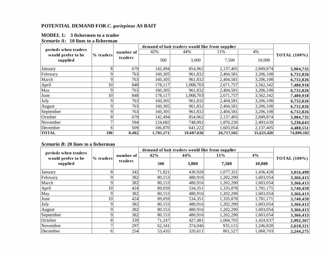
POTENTIAL DEMAND FOR AS BAIT

MODEL 1: 3 fishermen to a trader: 10 lines to a fisherman

demand of bait traders would like from supplier periods when traders

would prefer to be supplied

% traders number of

traders TOTAL (100%)

5,984,735 6,732,826 6,732,826 7,480,918 6,732,826 7,480,918 6,732,826 6,732,826 6,732,826 5,984,735 5,236,643 4,488,551

TOTAL 100 8,482 1,781,171 10,687,026 26,717,565 35,623,420 74,809,182

: 20 lines to a fisherman demand of bait traders would like from supplier

42% 44% 11% 4%periods when traders

would prefer to be supplied

% traders number of

traders 500 3,000 7,500 10,000

TOTAL (100%)

3,016,499 3,366,413 3,366,413 3,740,459 3,366,413 3,740,459 3,366,413 3,366,413 3,366,413 2,992,367 2,618,321 2,244,275

C. gariepinus

Scenario A

Scenario B

42% 44% 11% 4%

500 3,000 7,500 10,000

January 8 679 142,494 854,962 2,137,405 2,849,874 February 9 763 160,305 961,832 2,404,581 3,206,108 March 9 763 160,305 961,832 2,404,581 3,206,108 April 10 848 178,117 1,068,703 2,671,757 3,562,342 May 9 763 160,305 961,832 2,404,581 3,206,108 June 10 848 178,117 1,068,703 2,671,757 3,562,342 July 9 763 160,305 961,832 2,404,581 3,206,108 August 9 763 160,305 961,832 2,404,581 3,206,108 September 9 763 160,305 961,832 2,404,581 3,206,108 October 8 679 142,494 854,962 2,137,405 2,849,874 November 7 594 124,682 748,092 1,870,230 2,493,639 December 6 509 106,870 641,222 1,603,054 2,137,405

January 8 342 71,821 430,928 1,077,321 1,436,428 February 9 382 80,153 480,916 1,202,290 1,603,054 March 9 382 80,153 480,916 1,202,290 1,603,054 April 10 424 89,059 534,351 1,335,878 1,781,171 May 9 382 80,153 480,916 1,202,290 1,603,054 June 10 424 89,059 534,351 1,335,878 1,781,171 July 9 382 80,153 480,916 1,202,290 1,603,054 August 9 382 80,153 480,916 1,202,290 1,603,054 September 9 382 80,153 480,916 1,202,290 1,603,054 October 8 339 71,247 427,481 1,068,703 1,424,937 November 7 297 62,341 374,046 935,115 1,246,820 December 6 254 53,435 320,611 801,527 1,068,703

TOTAL 100 4,241 890,586 5,343,513 13,358,783 17,811,710 37,404,591

: 30 lines to a fisherman demand of bait traders would like from supplier

42% 44% 11% 4%periods when traders would prefer to be supplied

% traders number of

traders 500 3,000 7,500 10,000

TOTAL (100%)

2,011,000 2,244,275 2,244,275 2,493,639 2,244,275 2,493,639 2,244,275 2,244,275 2,244,275 748,092 1,745,548 1,496,184

TOTAL 100 2,827 593,724 3,562,342 8,905,855 11,874,473 24,936,394

MODEL 2: 8 fishermen to 1 trader: 10 lines to a fisherman

demand of bait traders would like from supplier 42% 44% 11% 4%periods when traders would

prefer to be supplied% traders

number of traders

500 3,000 7,500 10,000 TOTAL (100%)

2,244,275 2,524,810 2,524,810 2,805,344 2,524,810 2,805,344 2,524,810 2,524,810 2,524,810 2,244,275 1,963,741 1,683,207

Scenario C

Scenario A

January 8 228 47,881 287,286 718,214 957,619 February 9 254 53,435 320,611 801,527 1,068,703 March 9 254 53,435 320,611 801,527 1,068,703 April 10 283 59,372 356,234 890,586 1,187,447 May 9 254 53,435 320,611 801,527 1,068,703 June 10 283 59,372 356,234 890,586 1,187,447 July 9 254 53,435 320,611 801,527 1,068,703 August 9 254 53,435 320,611 801,527 1,068,703 September 9 254 53,435 320,611 801,527 1,068,703 October 8 85 17,812 106,870 267,176 356,234 November 7 198 41,561 249,364 623,410 831,213 December 6 170 35,623 213,741 534,351 712,468

Average annual demand, Model 1 = 45,716,722

January 8 254 53,435 320,611 801,527 1,068,703 February 9 286 60,115 360,687 901,718 1,202,290 March 9 286 60,115 360,687 901,718 1,202,290 April 10 318 66,794 400,763 1,001,909 1,335,878 May 9 286 60,115 360,687 901,718 1,202,290 June 10 318 66,794 400,763 1,001,909 1,335,878 July 9 286 60,115 360,687 901,718 1,202,290 August 9 286 60,115 360,687 901,718 1,202,290 September 9 286 60,115 360,687 901,718 1,202,290October 8 254 53,435 320,611 801,527 1,068,703 November 7 223 46,756 280,534 701,336 935,115 December 6 191 40,076 240,458 601,145 801,527

TOTAL 100 3,181 667,939 4,007,635 10,019,087 13,358,783 28,053,443

: 20 lines to a fisherman demand of bait traders would like from supplier

42% 44% 11% 4%periods when traders would prefer to be supplied

% traders number of

traders 500 3,000 7,500 10,000

TOTAL (100%)

1,131,187 1,262,405 1,262,405 1,402,672 1,262,405 1,402,672 1,262,405 1,262,405 1,262,405 1,122,138 981,871 841,603

TOTAL 100 1,590 333,970 2,003,817 5,009,543 6,679,391 14,026,722

: 30 lines to a fisherman demand of bait traders would like from supplier

42% 44% 11% 4%periods when traders would prefer to be supplied

% traders number of

traders 500 3,000 7,500 10,000

TOTAL (100%)

754,125 841,603 841,603 935,115 841,603 935,115 841,603 841,603 841,603 280,534 654,580 561,069

TOTAL 100 1,060 222,646 1,335,878 3,339,696 4,452,928 9,351,148

Scenario B

Scenario C

January 8 128 26,933 161,598 403,995 538,661 February 9 143 30,057 180,344 450,859 601,145 March 9 143 30,057 180,344 450,859 601,145 April 10 159 33,397 200,382 500,954 667,939 May 9 143 30,057 180,344 450,859 601,145 June 10 159 33,397 200,382 500,954 667,939 July 9 143 30,057 180,344 450,859 601,145 August 9 143 30,057 180,344 450,859 601,145 September 9 143 30,057 180,344 450,859 601,145 October 8 127 26,718 160,305 400,763 534,351 November 7 111 23,378 140,267 350,668 467,557 December 6 95 20,038 120,229 300,573 400,763

January 8 86 17,955 107,732 269,330 359,107 February 9 95 20,038 120,229 300,573 400,763 March 9 95 20,038 120,229 300,573 400,763 April 10 106 22,265 133,588 333,970 445,293 May 9 95 20,038 120,229 300,573 400,763 June 10 106 22,265 133,588 333,970 445,293 July 9 95 20,038 120,229 300,573 400,763 August 9 95 20,038 120,229 300,573 400,763 September 9 95 20,038 120,229 300,573 400,763 October 8 32 6,679 40,076 100,191 133,588 November 7 74 15,585 93,511 233,779 311,705 December 6 64 13,359 80,153 200,382 267,176

Average Annual Demand, Model 2 = 17,143,771

MODEL 3: 15 Fishermen to 1 trader: 10 lines to a fisherman

demand of bait traders would like from supplier 42% 44% 11% 4%periods when traders would

prefer to be supplied% traders

number of traders

500 3,000 7,500 10,000 TOTAL (100%)

1,196,947 1,346,565 1,346,565 1,496,184 1,346,565 1,496,184 1,346,565 1,346,565 1,346,565 1,196,947 1,047,329 897,710

TOTAL 100 1,696 356,234 2,137,405 5,343,513 7,124,684 14,961,836

Scenario B

demand of bait traders would like from supplier 42% 44% 11% 4%periods when traders would

prefer to be supplied% traders

number of traders

500 3,000 7,500 10,000 TOTAL (100%)

603,300 673,283 673,283 748,092 673,283 748,092 673,283 673,283 673,283 598,473 523,664 448,855

TOTAL 100 848 178,117 1,068,703 2,671,757 3,562,342 7,480,918

Scenario A

: 20 lines to a fisherman

January 8 136 28,499 170,992 427,481 569,975 February 9 153 32,061 192,366 480,916 641,222 March 9 153 32,061 192,366 480,916 641,222 April 10 170 35,623 213,741 534,351 712,468 May 9 153 32,061 192,366 480,916 641,222 June 10 170 35,623 213,741 534,351 712,468 July 9 153 32,061 192,366 480,916 641,222 August 9 153 32,061 192,366 480,916 641,222 September 9 153 32,061 192,366 480,916 641,222 October 8 136 28,499 170,992 427,481 569,975 November 7 119 24,936 149,618 374,046 498,728 December 6 102 21,374 128,244 320,611 427,481

January 8 68 14,364 86,186 215,464 287,286 February 9 76 16,031 96,183 240,458 320,611 March 9 76 16,031 96,183 240,458 320,611 April 10 85 17,812 106,870 267,176 356,234 May 9 76 16,031 96,183 240,458 320,611 June 10 85 17,812 106,870 267,176 356,234 July 9 76 16,031 96,183 240,458 320,611 August 9 76 16,031 96,183 240,458 320,611 September 9 76 16,031 96,183 240,458 320,611 October 8 68 14,249 85,496 213,741 284,987 November 7 59 12,468 74,809 187,023 249,364 December 6 51 10,687 64,122 160,305 213,741

Scenario C: 30 lines to a fisherman

demand of bait traders would like from supplier 42% 44% 11% 4%periods when traders would

prefer to be supplied% traders

number of traders

500 3,000 7,500 10,000 TOTAL (100%)

402,200 448,855 448,855 498,728 448,855 498,728 448,855 448,855 448,855 149,618 349,110 299,237

TOTAL 100 565 118,745 712,468 1,781,171 2,374,895 4,987,279

January 8 46 9,576 57,457 143,643 191,524 February 9 51 10,687 64,122 160,305 213,741 March 9 51 10,687 64,122 160,305 213,741 April 10 57 11,874 71,247 178,117 237,489 May 9 51 10,687 64,122 160,305 213,741 June 10 57 11,874 71,247 178,117 237,489 July 9 51 10,687 64,122 160,305 213,741 August 9 51 10,687 64,122 160,305 213,741 September 9 51 10,687 64,122 160,305 213,741 October 8 17 3,562 21,374 53,435 71,247 November 7 40 8,312 49,873 124,682 166,243 December 6 34 7,125 42,748 106,870 142,494

Average Annual Demand, Model 3 = 9,143,344

Average Supply and Demandsupply seed bait Balance

sum 930,000 320,546 25,144,192 (24,534,738)

930,000 320,546 4,987,279 (4,377,825)

248

up to 500 24500 - 1000 34

1000 - 1500 81500 - 2000 142000 - 3000 33000 - 4000 3above 4000 14

January 1February 1

March 4April 22May 14June 14July 15

August 20September 5

October 2November 1December 1

Fishermen’s Bait Demand to Catch Nile Perch

% response(n = 76)

Period of Peak Demand for Bait by Fishermen to Catch Nile Perch (month)

% response (n = 235)

- 249 -

Various criteria were used by participants to assess wealth status.

Additional job, nature of job, income levels and education

Wealth Category

BMC WBC IBC

Wealthiest Self-employed, business (commercial houses), civil servants, teachers, councillors, carpenters, clergy

Self-employed, traders, government jobs, business

Self employed, businesses (shops, housing, bakeries, etc), professionals (doctors)

Middle Small business, casual labourers, wives work

makers, sell buns, dealers in local chickens, brick layers, working class, brick layers, fishermen, brewer, teachers, motorbike-taxi drivers, buy and sell maize, make crates, fish mongers

No jobs, teachers, small business

Self employed, small-business (brewing, hair dressers), charcoal burners, casual labourers, firewood cutter/sellers, employees

Poorest Unemployed, fish mongers, casual workers, brewers

Seasonal workers, no permanent jobs, casual workers, no reliable income

Witch doctors, brick makers, casual labourers

Wealth Category

BMC WBC IBC

Wealthiest Some cattle (mostly local), goats, chickens

Cattle – cross breeds or exotics

Intensive poultry, piggeries, either several zero-grazers or several local cows

Middle Some cattle, chickens and goats

Small animals mostly goats, local chickens, rabbits, pigs. About 2 local cows

A zero grazer or two, tethered pigs, about two local cattle, tethered or free range.

Poorest Chickens and turkeys Small animals, some rabbits, a few but usually no cattle (local)

Tethered cattle, one or two, local birds

APPENDIX K: CRITERIA USED BY FARMERS TO RANK WEALTH

( = 73)

Local non-farm sources of income and their relationship to wealth ratings as viewed by participants.

Relationship between wealth ratings and species, breed and numbers of livestock

N

chapati

250

Wealth Category

BMC WBC IBC

Wealthiest Coffee (Bugiri district), cassava (Busia district), sugarcane plantations, early adopters, surplus to sell

Coffee and banana plantations, eucalyptus trees, commercial tomato or other vegetable gardens

Mainly livestock and jobs

Middle Small coffee gardens, supplemented with small business

Semi-subsistence farmers, small banana and coffee gardens, maize, sorghum and beans

Some gardens mostly for home consumption, sweet potatoes important followed by cassava among middle and poor. Depend on farming solely for survival

Poorest Subsistence farmers Subsistence farmers Tenants

Relationship between crop production practices and wea th ranking.

251

TreatmentParameter Unit ChangeI II III IV

% marketable yield 20%Profit -15% -33% -57% -88%profit (excluding labour costs) -16% -35% -61% -96%returns to investment, farmer’s view -15% -33% -57% -88%returns on total investment, economist’s view -15% -33% -57% -88%returns to labour -16% -35% -61% -96%returns to land -15% -33% -57% -88%cost of per fish produced/break-even price -33% -33% -33% -33%break-even production 0% 0% 0% 0%profit operations cost ratio -15% -33% -57% -88%

cost capital 10%profit -0.1% 0.4% 0.0% 0.0%profit (excluding labour costs) -0.1% 0.2% 0.0% 0.0%returns to investment, farmer’s view -0.1% 0.4% 0.0% 0.0%returns on total investment, economist’s view 0.0% 0.4% 0.1% 0.0%returns to labour -0.1% 0.2% 0.0% 0.0%returns to land -0.1% 0.4% 0.0% 0.0%cost of per fish produced/break-even price -0.1% 0.0% 0.0% 0.0%break-even production -0.1% 0.0% 0.0% 0.0%profit operations cost ratio 0.0% 0.5% 0.1% 0.0%

% marketable size 10%profit -12% -27% -46% -70%profit (excluding labour costs) -12% -28% -49% -77%returns to investment, farmer’s view -12% -27% -46% -70%returns on total investment, economist’s view -12% -27% -46% -70%returns to labour -12% -28% -49% -77%returns to land -12% -27% -45% -70%cost of per fish produced/break-even price 0% 0% 0% 0%break-even production 0% 0% 0% 0%profit operations cost ratio -12% -27% -46% -70%

fish prices UShs. 100/- 36% 114% 396% -1768%profit 39% 128% 526% -967%profit (excluding labour costs) 36% 114% 396% -1768%returns to investment, farmer’s view 36% 114% 396% -1768%returns on total investment, economist’s view 39% 128% 526% -967%returns to labour 36% 114% 393% -1810%returns to land 0% 0% 0% 0%cost of per fish produced/break-even price 33% 33% 33% 33%break-even production 36% 114% 396% -1768%profit operations cost ratio

APPENDIX L: SENSITIVITY ANALYSIS – EXPERIMENTS

Experiment 1, Numbers

252

feed prices UShs. 25/-profit -2% 11% 2% 2%profit (excluding labour costs) -2% 7% 2% 2%returns to investment, farmer’s view -2% 11% 2% 2%returns on total investment, economist’s view -1% 11% 3% 3%returns to labour -2% 7% 2% 2%returns to land -1% 11% 2% 2%cost of per fish produced/break-even price -2% -2% -2% -2%break-even production -2% -2% -2% -2%profit operations cost ratio 0% 12% 4% 3%

seed prices UShs. 25/-profit -27% 42% 23% 19%profit (excluding labour costs) -33% 37% 22% 18%returns to investment, farmer’s view 36% 71% 61% 59%returns on total investment, economist’s view -18% 49% 35% 34%returns to labour -33% 37% 22% 18%returns to land -27% 42% 23% 19%cost of per fish produced/break-even price -31% -45% -53% -58%break-even production -31% -45% -53% -58%profit operations cost ratio 3% 60% 50% 49%

253

TreatmentParameter Unit Change

I II III IV% marketable yield 20%profit -5% -5% -6% -6%profit (excluding labour costs) -5% -5% -6% -6%returns to investment, farmer’s view -5% -5% -6% -6%returns to investment, economist’s view

-5% -5% -6% -6%

returns to labour -5% -5% -6% -6%returns to land -5% -5% -6% -6%cost of per fish produced/break-even price 0% 0% 0% 0%break-even production 0% 0% 0% 0%profit operations cost ratio -5% -5% -6% -6%receipts per fish/receipts/kg 0% 0% 0% 0%

cost capital 10%profit 0.0% 0.0% 0.0% 0.0%profit (excluding labour costs) 0.0% 0.0% 0.0% 0.0%returns to investment, farmer’s view 0.0% 0.0% 0.0% 0.0%returns to investment, economist’s view 0.0% 0.0% 0.0% 0.0%returns to labour 0.0% 0.0% 0.0% 0.0%returns to land 0.0% 0.0% 0.0% 0.0%cost of per fish produced/break-even price -0.1% 0.0% 0.0% 0.0%break-even production -0.1% 0.0% 0.0% 0.0%profit operations cost ratio 0.0% 0.0% 0.0% 0.0%receipts per fish/receipts/kg 0% 0% 0% 0%

% marketable size 10%profit 0.0% 0.0% 0.0% 0.0%profit (excluding labour costs) 0.0% 0.0% 0.0% 0.0%returns to investment, farmer’s view 0.0% 0.0% 0.0% 0.0%returns to investment, economist’s view 0.0% 0.0% 0.0% 0.0%returns to labour 0.0% 0.0% 0.0% 0.0%returns to land 0.0% 0.0% 0.0% 0.0%cost of per fish produced/break-even price 0.0% 0.0% 0.0% 0.0%break-even production 0.0% 0.0% 0.0% 0.0%profit operations cost ratio 0.0% 0.0% 0.0% 0.0%receipts per fish/receipts/kg 20% 20% 20% 20%

fish prices per kg UShs. 250/-profit 4% 5% 7% 7%profit (excluding labour costs) 5% 5% 7% 7%returns to investment, farmer’s view 4% 5% 7% 7%returns to investment, economist’s view 4% 5% 7% 7%returns to labour 5% 5% 7% 7%returns to land 4% 5% 7% 7%cost of per fish produced/break-even price 0% 0% 0% 0%break-even production 17% 17% 17% 17%profit operations cost ratio 4% 5% 7% 7%receipts per fish/receipts/kg -25% -25% -25% -25%

Experiment 1, Weight

254

feed prices per kg UShs. 250/-profit -1% -1% -1% -1%profit (excluding labour costs) -1% -1% -1% -1%returns to investment, farmer’s view -1% -1% -1% -1%returns to investment, economist’s view 0% 0% 0% 0%returns to labour -1% -1% -1% -1%returns to land -1% -1% -1% -1%cost of per fish produced/break-even price -2% -2% -2% -2%break-even production -2% -2% -2% -2%profit operations cost ratio 1% 1% 0% 0%receipts per fish/receipts/kg 0% 0% 0% 0%

seed prices UShs. 25/-profit -10% -18% -30% -38%profit (excluding labour costs) -10% -19% -31% -41%returns to investment, farmer’s view 45% 41% 35% 31%returns to investment, economist’s view -2% -4% -9% -12%returns to labour -10% -19% -31% -41%returns to land -10% -18% -29% -38%cost of per fish produced/break-even price -31% -45% -53% -58%break-even production -31% -45% -53% -58%profit operations cost ratio 16% 19% 16% 12%receipts per fish/receipts/kg 0% 0% 0% 0%

255

TreatmentParameter Unit ChangeI II III IV V VI

% marketable yield 20%profit 70% 56% 77% 67% 54% 48%profit (excluding labour costs) 61% 51% 67% 60% 50% 45%returns to investment, farmer’s view

70% 56% 77% 67% 54% 48%

returns on total investment, economist’s view 70% 56% 77% 67% 54%returns to labour 61% 51% 67% 60% 50% 45%returns to land 289% 114% 287% 158% 92% 65%cost of per fish produced/break-even price

-33% -33% -33% -33% -33% -33%

break-even production 0% 0% 0% 0% 0% 0%profit operations cost ratio 70% 56% 77% 67% 54% 48%

cost capital 10%profit 0% 0% 0% 0% 0% 0%profit (excluding labour costs) 0% 0% 0% 0% 0% 0%returns to investment, farmer’s view

0% 0% 0% 0% 0% 0%

returns on total investment, economist’s view

0% 0% 0% 0% 0% 0%

returns to labour 0% 0% 0% 0% 0% 0%returns to land 0% -1% 0% 0% 1% 0%cost of per fish produced/break-even price

0% 0% 0% 0% 0% 0%

break-even production 0% 0% 0% 0% 0% 0%profit operations cost ratio 0% 0% 0% 0% 0% 0%

% marketable size 10%profit 14% 14% 15% 15% 15% 17%profit (excluding labour costs) 14% 14% 15% 15% 14% 17%returns to investment, farmer’s view

14% 14% 15% 15% 15% 17%

returns on total investment, economist’s view 14 15% 15 15 15 17returns to labour 14% 14% 15% 15% 14% 17%returns to land 17% 17% 19% 19% 18% 22%cost of per fish produced/break-even price

0% 0% 0% 0% 0% 0%

break-even production 0% 0% 0% 0% 0% 0%profit operations cost ratio 14% 14% 15% 15% 15% 17%

fish prices UShs. 100/-profit -80% -53% -91% -71% -46% -38%profit (excluding labour costs) -61% -45% -68% -57% -40% -35%returns to investment, farmer’s view

-80% -53% -91% -71% -46% -38%

returns on total investment, economist’s view 80 53 91 71 46 38returns to labour -61% -45% -68% -57% -40% -35%returns to land 154% -478% 125% 362% -169% -69%break-even price 0% 0% 0% 0% 0% 0%break-even production 0% 0% 0% 0% 0% 0%profit operations cost ratio -80% -53% -91% -71% -46% -38%

Experiment 2, numbers

256

feed prices UShs. 25/-profit 0% -5% -117% -50% -18% -15%profit (excluding labour costs) 0% -4% -43% -33% -15% -14%returns to investment, farmer’s view

0% -5% -117%

-50% -18% -15%

returns on total investment, economist’s view 0 6 125 57 23 22returns to labour 0% -4% -43% -33% -15% -14%returns to land 0% 10% 15% 30% 190% -35%break-even price 0% 1% 4% 6% 6% 7%break-even production 0% 1% 4% 6% 6% 7%profit operations cost ratio 0% -6% -128% -60% -25% -25%

seed prices UShs. 25/-; 67/-profit 17% 14% 17% 15% 12% 9%profit (excluding labour costs) 16% 13% 16% 14% 11% 8%returns to investment, farmer’s view

48% 45% 47% 46% 44% 42%

returns on total investment, economist’s view 31 27 28 26 24 19returns to labour 16% 13% 16% 14% 11% 8%returns to land 29% 20% 28% 23% 17% 11%break-even price -35% -33% -25% -24% -27% -18%break-even production 14% 15% 20% 20% 19% 24%profit operations cost ratio 39% 35% 34% 31% 31% 23%

257

TreatmentParameter Unit ChangeI II III IV V VI

% marketable yield 20%profit 79% 64% 101% 88% 47% 59%profit (excluding labour costs) 67% 57% 84% 75% 44% 55%returns to investment, farmer’s view 79% 64% 101% 88% 47% 59%returns on total investment, economist’s view 67 79% 64% 101% 88% 47%returns to labour 67% 57% 84% 75% 44% 55%returns to land 914% 173% -1305% 679% 69% 98%cost of per fish produced/break-even price -33% -33% -33% -33% -33% -33%break-even production 0% 0% 0% 0% 0% 0%profit operations cost ratio 79% 64% 101% 88% 47% 59%

cost capital 10%profit 0% 0% -5% 0% 0% 0%profit (excluding labour costs) 0% 0% 0% 0% 0% 0%returns to investment, farmer’s view 0% 0% -5% 0% 0% 0%returns on total investment, economist’s view 0% 0% -5% 1% 0% 0%returns to labour 0% 0% 0% 0% 0% 0%returns to land 0% 0% 0% 0% 0% 4%cost of per fish produced/break-even price 0% 0% 0% 0% 0% 0%break-even production 0% 0% 0% 0% 0% 0%profit operations cost ratio 0% 0% -5% 1% 0% 0%

% marketable size 10%profit 0% 0% 0% 0% 0% 0%profit (excluding labour costs) 0% 0% 0% 0% 0% 0%returns to investment, farmer’s view 0% 0% 0% 0% 0% 0%returns on total investment, economist’s view 0% 0% 0% 0% 0%returns to labour 0% 0% 0% 0% 0% 0%returns to land 0% 0% 0% 0% 0% 0%cost of per fish produced/break-even price -11% -11% -11% -11% -11% -11%break-even production 0% 0% 0% 0% 0% 0%profit operations cost ratio 0% 0% 0% 0% 0% 0%

fish prices UShs. 100/-profit -78% -52% -155% -105% -30% -48%profit (excluding labour costs) -56% -42% -86% -70% -27% -42%returns to investment, farmer’s view -78% -52% -155% -105% -30% -48%returns on total investment, economist’s view 78 52 155 105 30 48returns to labour -56% -42% -86% -70% -27% -42%returns to land 75% 269% 52% 69% -63% -214%cost of per fish produced/break-even price 0% 0% 0% 0% 0% 0%break-even production 0% 0% 0% 0% 0% 0%profit operations cost ratio -78% -52% -155% -105% -30% -48%

feed prices UShs. 25/-profit 0% -9% 64% 279% -11% -33%profit (excluding labour costs) 0% -6% 980% -141% -10% -27%returns to investment, farmer’s view 0% -9% 64% 279% -11% -33%returns on total investment, economist’s view 0 10 62 288 16 41returns to labour 0% -6% 980% -141% -10% -27%returns to land 0% 5% 11% 18% -36% 158%cost of per fish produced/break-even price 0% 1% 4% 6% 6% 7%break-even production 0% 1% 4% 6% 6% 7%profit operations cost ratio 0% -10% 62% 291% -18% -44%

seed prices UShs. 25/-; 67/-

Experiment 2, weight

258

profit 19% 16% 20% 19% 10% 12%profit (excluding labour costs) 17% 15% 19% 17% 10% 11%returns to investment, farmer’s view 49% 47% 50% 48% 43% 44%returns on total investment, economist’s view 32 29 31 29 23 22returns to labour 17% 15% 19% 17% 10% 11%returns to land 34% 25% 39% 33% 13% 16%cost of per fish produced/break-even price -35% -33% -25% -24% -27% -18%break-even production 14% 15% 20% 20% 19% 24%profit operations cost ratio 40% 36% 37% 34% 29% 25%

259

TreatmentParameter Unit Change80 70 60 50 40

manure UShs. 25/-profit 0% 0% -2% 1% 0%profit (excluding labour costs) 0% 0% -1% 1% 0%returns to investment, farmer’s view 0% 0% -2% 1% 0%returns on total investment, economist’s view 0% -1% -2% 1% 0%returns to labour 0% 0% -1% 1% 0%returns to land 0% 0% -2% 1% 0%cost of per fish produced/break-even price

0% 0% 0% 0% 0%

break-even production 0% 0% 0% 0% 0%ratio of net profit to operating costs 0% -1% -2% 1% 0%

% marketable size 10%profit 29% 50% 189% -108% -42%profit (excluding labour costs) 27% 44% 126% -153% -47%returns to investment, farmer’s view 61% 88% 261% -110% -28%returns on total investment, economist’s view 47 71 229 110 34returns to labour 27% 44% 126% -153% -47%returns to land 29% 50% 189% -108% -42%cost of per fish produced/break-even price

-19% -19% -19% -19% -19%

break-even production -19% -19% -19% -19% -19%profit operations cost ratio 59% 85% 256% -110% -29%

bait prices UShs. 5/-profit -96% -49% -29% -19% -12%profit (excluding labour costs) -123% -56% -32% -20% -13%returns to investment, farmer’s view -96% -49% -29% -19% -12%returns on total investment, economist’s view 96 49% 29% 19% 12%returns to labour -123% -56% -32% -20% -13%returns to land -96% -49% -29% -19% -12%break-even price 0% 0% 0% 0% 0%break-even production -14% -14% -14% -14% -14%profit operations cost ratio -96% -49% -29% -19% -12%

feed prices UShs. 50/-profit -31% -23% -17% -12% -9%profit (excluding labour costs) -34% -24% -18% -13% -9%returns to investment, farmer’s view -31% -23% -17% -12% -9%returns on total investment, economist’s view 31 23% 17% -12% -9%returns to labour -34% -24% -18% -13% -9%returns to land -31% -23% -17% -12% -9%break-even price 0% 0% 0% 0% 0%break-even production -17% -17% -17% -17% -17%profit operations cost ratio -31% -23% -17% -12% -9%

seed prices UShs. 5/-profit -23% -30% -42% -73% -273%profit (excluding labour costs) -22% -28% -39% -65% -182%returns to investment, farmer’s view -42% -47% -57% -80% -230%returns on total investment, economist’s view -40% -45% -55% -79%returns to labour -22% -28% -39% -65% -182%returns to land -23% -30% -42% -73% -274%cost of per fish produced/break-even price 30% 30% 30% 30% 30%break-even production 30% 30% 30% 30% 30%profit operations cost ratio -41% -46% -56% -79% -233%

C. gariepinus bait, numbers

260

TreatmentParameter Unit Change80 70 60 50 40

manure UShs. 25/-profit 0% 0% -2% 1% 0%profit (excluding labour costs) 0% 0% -1% 1% 0%returns to investment, farmer’s view 0% 0% -2% 1% 0%returns on total investment, economist’s view 0% -1% -2% 1% 0%returns to labour 0% 0% -1% 1% 0%returns to land 0% 0% -2% 1% 0%cost of per fish produced/break-even price 0% 0% 0% 0% 0%break-even production 0% 0% 0% 0% 0%profit operations cost ratio 0% -1% -2% 1% 0%

% marketable size 10%profit -31% -47% -182% 64% 20%profit (excluding labour costs) -29% -41% -111% 88% 22%returns to investment, farmer’s view -31% -47% -182% 64% 20%returns on total investment, economist’s view -31% -47% -182% 64%returns to labour -29% -41% -111% 88% 22%returns to land -31% -47% -182% 64% 20%cost of per fish produced/break-even price 25% 43% 67% 100% 150%break-even production 22900% 22900% 22900% 22900% 22900%profit operations cost ratio -31% -47% -182% 64% 20%

fish prices per kg UShs. 1,000/-profit -31% -23% -17% -12% -9%profit (excluding labour costs) -34% -24% -18% -13% -9%returns to investment, farmer’s view -31% -23% -17% -12% -9%returns on total investment, economist’s view -31% -23% -17% -12%returns to labour -34% -24% -18% -13% -9%returns to land -31% -23% -17% -12% -9%cost of per fish produced/break-even price 0% 0% 0% 0% 0%break-even production -17% -17% -17% -17% -17%profit operations cost ratio -31% -23% -17% -12% -9%

feed prices per kg UShs. 50/-profit -1.1% -2.0% -8.4% 4.0% 1.6%profit (excluding labour costs) -1.1% -1.8% -5.3% 5.5% 1.8%returns to investment, farmer’s view -1.1% -2.0% -8.4% 4.0% 1.6%returns on total investment, economist’s view -1.6% -2.5% -8.8% 3.5%returns to labour -1.1% -1.8% -5.3% 5.5% 1.8%returns to land -1.1% -2.0% -8.4% 3.9% 1.6%cost of per fish produced/break-even price 0.5% 0.5% 0.5% 0.5% 0.5%break-even production 0.5% 0.5% 0.5% 0.5% 0.5%profit operations cost ratio -1.6% -2.5% -8.8% 3.4% 1.1%

0.0% 0.0% 0.0% 0.0% 0.0%seed prices per fish UShs. 5/-profit -23% -31% -44% -76% -328%profit (excluding labour costs) -22% -29% -40% -67% -205%returns to investment, farmer’s view -43% -48% -58% -82% -271%returns on total investment, economist’s view -40% -46% -56% -81%returns to labour -22% -29% -40% -67% -205%returns to land -23% -31% -44% -76% -329%cost of per fish produced/break-even price 30% 30% 30% 30% 30%break-even production 30% 30% 30% 30% 30%profit operations cost ratio -41% -47% -57% -82% -275%

C. gariepinus bait, weight

261