Factors Affecting Technical Efficiency of Catfish Farms in Chicot County, Arkansas

ALOYCE R. KALIBA AND CAROLE R. ENGLE

Aquaculture/Fisheries Center, University of Arkansas at Pine Bluff, AR, USA

Abstract

Technical and scale efficiency measures of a sample of catfish farms in Chicot County, Arkansas

were estimated using a data envelopment analysis technique. A measure of technical efficiency under

variable returns-to-scale is used to determine operator characteristics, farm practices, and

institutional support services that are likely to lead to higher levels of efficiency. Results indicate that

live catfish production could increase by 67% using the same level of inputs if all farms could

produce along the estimated efficient frontier. Higher feeding rates and availability of extension

services were associated with increased technical efficiency. Higher stocking density affected

technical efficiency negatively. The marginal value of extension contacts in Chicot County was

estimated to be $2,988. These results suggest that higher catfish farm efficiency in Chicot County,

Arkansas, can be achieved by adjusting inputs used in production to optimal levels rather than by

adjusting the scale of operation.

Keywords: catfish, efficiency, and data envelopment analysis.

Correspondence Aloyce R. Kaliba or Carole R. Engle, Aquaculture/Fisheries Center, University of

Arkansas at Pine Bluff, 1200 North University Drive, Mail Slot 4912, Pine Bluff, AR 71603, USA.

Tel: (870) 575-8108 or (870) 575-8113 E-mail: akaliba@uaex.edu or cengle@uaex.edu

2

Introduction

Catfish is the leading sector of U.S. aquaculture industry. The national value of catfish sales

exceeded $425 million in 2003 with the four states of Mississippi, Arkansas, Alabama, and

Louisiana contributing 95% of the national total (NASS 2004). The water surface area under catfish

production totaled more than 75, 442 hectares (187,200 acres) in 2003. Catfish production in the four

major states is concentrated in the Mississippi Delta Region that is characterized by relatively high

poverty rates compared to other parts of the U.S. Industry growth is an important tool in stimulating

growth in other sectors of the economy in the delta region. Chicot County is located in the southeast

corner of Arkansas bordering Mississippi and Louisiana and represents a typical catfish production

area within the Delta Region.

The live catfish price fell from approximately $1.65/kg to about $1.25/kg in 2001 and

remained at an average of $1.28/kg in 2003 (NASS 2004). Among the factors that have influenced

this decline has been an increase in imports of frozen Pangasius Sp. fillets that have been sold at

lower prices (Quagrainie and Engle 2000). Given that the seafood market demand in the U.S. is

large, and the U.S. dollar is relatively strong, imports of aquaculture products are expected to grow.

In the long run, survival of catfish farms may depend on farmers' ability to produce live catfish

efficiently. Given the economic importance of the catfish industry in the Delta Region, this paper

examines levels of technical and scale efficiency and factors linked to higher technical efficiency

measures of catfish farms in Chicot County, Arkansas.

A study by Hanson, Dean, and Spurlock (2004) show that in 2001, the Mississippi catfish

industry created 10,760 jobs, generated $208.25 million in household income, and $342.33 in value

added. A study by Kaliba and Engle (2004) that analyzed the contribution of the catfish industry to

3

the economy of Chicot County, Arkansas, indicated that total employment created by the catfish

industry in that county was 2,665 jobs. This represented 48% of all employment in the county. Total

economic impact of the catfish industry in Chicot County was over $384 million. Contractions in

catfish acreage in Chicot County by 10% would cause unemployment rates to increase by 2%.

As study by Kaliba, Verkuijl, and Mwangi (2000) shows that variables that are linked to the

economics of farm enterprises can be divided into three groups: socioeconomic and demographic

characteristics of the farmers (e.g., age, gender, education and experience); farm practices (e.g., size

of farm, type of feeds); and institutional support (e.g., marketing and availability of extension

services). However, none of these studies has addressed the issue of efficiency of catfish farms in

the U.S. A study by Featherstone, Langemeier and Ismet (1997) that examined efficiency of Kansas

beef cow farms indicated that the size of operation represented by the number of beef cows was

important in explaining efficiency measures. These conform to the results obtained by Gillespie,

Schupp and Taylor (1997) for the ratite industry in Louisiana. A study by Morgan and Langemeier

(2002), on a sample of Kansas’s farms, indicated that higher scores of overall efficiency were

significantly concentrated on larger farms. Langemeier and DeLano (1999) used a sample of

Kansas’s farms to examine the relationship between overall efficiency and farm characteristics. They

concluded that overall efficiency was significantly related to operator’s age, farm size, and farm type.

In a study to identify factors affecting technical efficiency of Missouri hog producers, Ben-

Belhassen and Womack (2000) concluded that the type of technology used in production and

managerial skills were important in explaining the level of productive efficiency. In these studies age

was associated with experience or managerial skill of the farm operator. Farm size and farm type,

4

respectively, were used to capture the influence of economies of scale and specialization in

production.

Another variable of interest is the availability of extension services. The impact of

agricultural extension services on productive efficiency can be evaluated through its marginal

product, where extension is considered as a factor of production (Patrick and Kehrberg 1973), or as a

factor explaining individual technical efficiency measures (Dinar, Karagiannis and Tzouvelekas

2002). The relationship between availability of extension services and efficiency may be of interest

to the catfish industry. The catfish industry in Arkansas depends mostly on public extension services

for production and market information. Aquaculture extension services in Chicot County, Arkansas,

are provided through the University of Arkansas at Pine Bluff (UAPB). The Aquaculture/Fisheries

Center at UAPB provides bacteriological, parasitological, viral, histological, and water quality

diagnostics support for fish health problems and other services free of charge. The

Aquaculture/Fisheries Center specialist assigned to the Chicot County laboratory assists farmers by

providing research-based information related to management alternatives for catfish farms. The

educational and technology transfer programs facilitate selection of optimal input mixes and thus

affect farm efficiency given the existing set of technology and management alternatives. The paper is

organized as follows. A brief review of the data envelopment analysis (DEA) is presented and

focuses on calculation of technical and scale efficiency measures. Description and sources of data are

also presented along with the results of the study and the policy implications that arise are discussed.

Data and Methods

The measurement of a farm's technical efficiency is based on deviations of observed production from

the efficient frontier. The ratio of the potential production or minimum cost to actual production or

5

cost of production defines the level of efficiency of the individual farm. If a farm's actual production

is on the efficient frontier, it is considered to be perfectly efficient. If it is away from the frontier it is

considered to be inefficient. Approaches for estimating the efficient frontier can be classified into

parametric and non-parametric methods. The first approach involves the estimation of a stochastic

function, where output or cost of a farm is a function of a set of inputs, inefficiency, and random

errors (Aigner, Lovell, and Schmidt 1977). However, this method imposes an explicit functional

form and distribution assumption on the data. By contrast, a non-parametric method does not impose

any assumptions about functional form and therefore is not subject to the problems of assuming an

underlying distribution for the error term (Coelli 1995).

The data envelopment analysis technique is a non-parametric method that identifies the most

efficient farm within a sample (Farrell 1957). DEA calibrates the level of efficiency of each farm by

constructing an efficient frontier, which provides a yardstick for all farms within a sample. A farm

located on the frontier uses the lowest quantities of inputs such that farms using different

combinations of inputs to produce different combinations of outputs can coexist on the same frontier.

A farm on the efficient frontier is given a score of one. Farms that are not on the efficient frontier are

inefficient and are given a score between zero and one. DEA compares efficiency from two points of

view: output-expansion and input-contraction. The output-expansion model poses the question of

how much more output could be produced given different levels of inputs. In contrast, the input-

contraction model evaluates how much a farm could reduce inputs without lowering its output

(Coelli 1995). This study uses the input contraction model because farmers tend to have greater

control over inputs than over output.

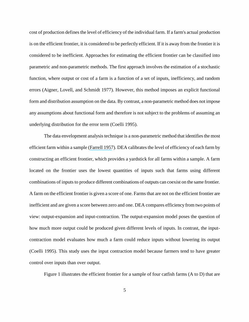
Figure 1 illustrates the efficient frontier for a sample of four catfish farms (A to D) that are

6

assumed to produce a quantity of live catfish (Y) using aggregated inputs (X). Joining A, B, and C

gives rise to the line segments AB and BC, which represent combinations of efficient farms. The

line segments form part of the efficient frontier or envelopment surface. Farms A, B and C make up

the frontier because a linear combination of adjacent pairs generates the highest output, given the

same levels of inputs. Farm D is inefficient because it uses more inputs than B to produce less

output. Note that farm D is compared with linear combinations of farms A and B (i.e., D's peer

group) at point DV because the ratio of output and input at points A, DV and B are similar. Farm C is

in a separate group as its output-input structure (i.e., the ratio of output and input) differs from A, DV

and B. As a result C is not used to evaluate D. The technical efficiency (TE) score of farm D that

measures the extent to which production can be affected by factors not related to the (dis)advantage

of farm size and other aspects of the farm's production process, is given by the ratio YDDV/YDD. That

is, the benchmark point DV uses only YD DV instead of YD D of inputs used by farm D to produce the

same level of output (YD). In other words, D could produce the same level of output using only

(YDDV/YDD) of the input used to produce YD by using the best production practices demonstrated by

farm A and B.

The overall technical efficiency (OE) score includes the combined influence of the technical

and scale effects. OE is a gross measure of relative productivity as it captures all sources of variation

in the ratio of output to input, including TE (Coelli 1995). On the other hand, the scale effect (SE)

measures the extent to which overall efficiency can be affected as the size of operation changes (i.e.,

SE = OE/TE). Under DEA, all catfish farms would be ranked in terms of their relative OE,

regardless of the potential effect of scale. In other words, each farm is compared with the most

efficient farm of a similar size in terms of input intensity and output mix, thereby taking into account

7

the potential effect of scale on the TE score.

Figure 1 also illustrates the decomposition of OE into SE and TE for a single input-output

case. The OE frontier is represented by line OX, which depicts the highest ratio of output to input

that was attained by farm B. The horizontal distance between the overall and technical efficiency

frontier captures the scale effect. The OE benchmark for farms A, C and D are points AC, CC and DC.

For example, the OE score for farm D is given by the ratio (YDDC/ YDD) and the SE is given by

YDDC/YDDV. Notice that the peer group for farm D is B for OE analysis and A and B for TE. In

addition, while farms A and C are technically efficient, the two farms are scale inefficient. Farm B is

efficient from both technically and scale perspectives (i.e., overall efficient). In addition, under input-

contraction, the level of the technical efficiency score is always greater than or equal to the overall

efficiency score. If the two scores are identical, OE efficiency is fully explained by TE. If TE is

higher than OE, overall efficiency is partly determined by the effect of scale. As demonstrated by

Coelli, Rao and Battese (1998), the OE frontier in Fig 1 represents TE under constant returns to scale

(CRS) and line ABC represents the TE frontier under variable returns to scale (VRS), which is

sometimes called the pure technical efficiency frontier.

To develop the DEA input-contraction model, let each farm (j) produce quantities of live

catfish (Yk,j) using multiple inputs (Xi,j) and each farm determines its own set of weights for both

inputs and outputs. In a linear programming framework, with the objective of maximizing efficiency

of a selected farm (j0) subject to the conditions that all efficiencies of other farms remain less than or

equal to one, the dual DEA model that represents the input-contraction approach can be stated as:

8

0

0 0

0

, ,

, ,

0.

joj

j k j k j

j

j i j j i j

j

j

Minimize z

subject to Y Y

X X

(1)

Equation (1) represents the Charnes, Cooper and Rhodes (CCR) model after the authors Charnes,

Cooper and Rhodes (1978) and stands for CRS technology. The score j0 is the measure of overall

technical efficiency of farm j0; λj are nonnegative weights.

According to Coelli, Rao and Battese (1998), the CRS model is only appropriate when the

farm is operating at an optimal scale. Some factors such as constraints to production resources may

cause the farm to operate at a size that is less than optimal. As shown by Banker, Charnes and

Cooper (1984), Equation (1) can be transformed to a VRS technology model by adding a restriction

that sums the weights to one (i.e., the constraint jj = 1 is added to Equation (1)). As stated earlier,

the scores from this model are due to pure technical efficiency because scale effects are eliminated

from the analysis. In the absence of scale effects, j0 represents a pure TE score of farm j0 under

VRS. Restricting the weights in Equation (1) to sum to one eliminates scale effects from the analysis.

Solving Equation (1) with the restriction that the weights must be equal to or less than one (jj ≤ 1),

show whether inefficiency occurs because a farm is using too many or too few inputs. The restriction

imposes non-increasing returns-to scale (NIRS). If the value of the objective function is unequal to

the value of the objective function under VRS technology, then increasing returns to scale exist for

that farm. If they are equal, then decreasing returns to scale apply (Coelli, Rao, and Battese 1998).

Dividing TE under CRS to TE under VRS estimates scale efficiency (SE) measures.

Data for this study were obtained from a survey of catfish farms in Chicot County, Arkansas.

9

A structured questionnaire was developed and used to collect 2001 input-output data from catfish

farms in the study area. Data collection included both mail surveys and personal interviews. While

some farms completed and returned the mailed questionnaire, some farms requested assistance and

personal interviews were conducted. Out of 85 farms in the county, 44 farms agreed to participate in

the study. Of these, 30 farms contributed complete datasets usable for this study. Five inputs were

used for the efficiency analysis: labor, energy cost, quantity of fingerlings/stockers, quantity of feed,

and other costs that included expenditures on telephone, pond repairs, interest payments, office

supplies and consumables, and land and farm equipment lease costs. The quantity of fish marketed in

2001 was used to measure output. Other data were collected on the size of operation, experience of

the operator and type of ownership.

Table 1 presents the summary statistics of variables used in the efficiency analysis on a per-

hectare basis. The sample farms included in the analysis employed about 15 people on average. The

minimum was three persons and the maximum was 62 persons. This included both hired and

household farm labor, and full-time and part-time farm workers. The type and number of workers

employed by the farms were largely related to farm size. Family members operated smaller farms

either on a part-time or full-time basis (<100 ha). Medium-sized farms (100-200 ha) tended to have

a family member working fulltime on the farm, who was assisted by a part-time employee. Farms

that operated more than 200 ha were more likely to hire full-time employees and a professional farm

manager. Energy cost included gas and diesel consumed by tractors, trucks, motors, and other

vehicles operated on the farm as well as electricity. Total energy consumption increased with the size

of operation, but on a per-ha basis decreased with farm size. Energy cost averaged $674/ha.

Fingerling stocking density averaged approximately 14,000 fish/ha, and farms used the

10

recommended stocking density of 12,000- 15,000 fish/ha (Engle and Killian 1996).

Feed was the largest single cost. The average feeding rate was 12 tons/ha/year. Feed cost

constituted 37% of the total average cost and 31% of the total production cost. The average annual

expenditure on other cost items was about $1,610/farm/ha. Payment on borrowed capital was the

largest expenditure in this cost item. Annual sales of live catfish averaged approximately 8,000 kg/ha

in 2001. The quantity of foodfish produced increased with farm size but on a per-ha basis, decreased

with farm sizes because stocking densities of smaller farms were relatively higher than those of

larger farms.

Three linear programs (i.e., Equation 1 under CRS, VRS, and NIR) were solved for each farm

in the sample using onFront software (Färe and Grosskopf 2000). SE was calculated residually.

During the analysis, the law of one price was assumed for energy and other inputs; all producers

were assumed to face the same relative prices for inputs (Chavas and Aliber 1993). In determining

the factors influencing technical efficiency measures, Tobit models have been used to determine

which factors influence technical efficiency, because the calculated economic efficiency measures

are bounded between zero and one or can be scaled to be between zero and 100% (Tobin 1958).

Moreover, the Tobit model calculates both the marginal effect of the explanatory variable on the

efficiency measure and the probability of improvement for inefficient farms (Greene 2000). The

Tobit model for this analysis was specified as follows:

0 0

1 1

0

0 .

N N

ij i i i i i i

i i

ij

S Z if Z

S if otherwise

(2)

In Equation (2), Sij is the measure of technical efficiency for farm j, Z's are explanatory variables that

11

influence economic efficiency of the farms, N is the number of explanatory variables, and and

are parameters of the model and a random error term, respectively.

Including an extension variable in the Z matrix of Equation (4) allows calculation of cost

savings associated with the use of extension services. McDonald and Moffitt (1982) show that,

when the variables included in Equation (2) are expressed as natural logarithms, the first partial

derivatives of Equation (2) are proportional to the estimated Zi coefficients. Thus, the most negative

coefficient is the most important factor in increasing farm inefficiency. DEA-calculated efficiency

levels do not identify the type of input that needs to be scaled down to increase efficiency

(Featherstone, Langemeier and M. Ismet 1997; Rowland et al 1998). Therefore, two Tobit models

were used to examine the relationship between economic efficiency measures and inputs used in

production and farm characteristics. The explanatory variables included in the first Tobit model were

the natural logarithm of the five inputs, i.e., labor, energy cost, stocking density, quantity of feed, and

cost of other miscellaneous inputs (Table 1). The second Tobit model was specified as:

* 2 2 2

0 1 1 12 1 2 2 22 2 3 3 32 3 4 4

*

**

2 22

2

, 2 .

ij i

ij T T

j i j ij i j

S z z z z z z z

Swhere CS w X S w X

z

(3)

The explanatory variables included in Equation (3) were: experience of the operator in years (z1),

availability of extension services (z2), size of the operation in ha (z3), and type of ownership (z4).

The square of each variable was included in the model to capture the decreasing marginal effect of

each variable.

The extension service variable was measured as the number of contacts between catfish farm

managers and extension personnel in Lake Village. This included the number of times the farm

12

manager sought laboratory services for both disease and water quality diagnoses and tests, and other

contacts in which an extension person was involved in advising or training the farmer on issues

related to catfish production. Ownership was represented as a dummy variable such that

ownership=1, if the operator owned the farm; ownership=0, otherwise. Also, in Equation (3), CSj is

the estimated cost savings by farm j associated with using extension services offered by UAPB's

aquaculture laboratory in Chicot County, δS*ij/δz2 is the partial derivative of S*

ij, with respect to the

extension services variable (z2), Φ(.) is the cumulative normal density function, and S**ij is the

estimated Tobit index for the economic efficiency measure, and other variables are explained in

Equation (2).

The summary statistics for variables used in Equation (3) are presented in Table 2. The

average farm size was 123 ha with a maximum and minimum of 543 and 16 ha, respectively. There

was a great deal of variation in farm size. These numbers show that while the size of operation was

highly variable, most farms were within a range of 75-90 ha (P<0.01). Approximately, 55% of the

farms were less than 100 ha in size. Only 9% of the farms were more than 360 ha.

For these 30 farms, operator experience in catfish production was about 8 years. Farm owners

with 5-10 years of experience relied more on professional farm managers to operate the farm. Farm

owners with more than ten years experience relied on full-time workers more than professional

managers to operate the farm. Experienced farm owners were more likely to manage farms

themselves and not hire professional farm managers. Extension contacts were about 33 contacts per

farm. There was no clear association between extension contacts and either farm size or between

extension contacts and experience of the operator.

13

Results and Discussion

Technical efficiency under VRS efficiency ranged from 0.01 to 1. The average was 0.33 ±

0.24 (Table 3). Thus, on average, live catfish production potentially could be increased by roughly

67% using the same level of inputs if each farm in the sample was overall efficient or if all farms had

the lowest per unit cost of production. Average cost efficiency under VRS or pure cost efficiency

was 0.45 with a standard deviation of 0.21. Thus, catfish farms in the sample could increase live

catfish production by an average of 55% using the same level of input if each farm was operating

along the efficient frontier. Scale efficiency was 0.73±0.32, on average. About 70% of the farms

were over 80% scale efficient. Individual analysis of the farms indicated that 10 of the farms had

decreasing returns to scale and 20 farms had increasing returns to scale. Only three farms were scale

efficient. In general, the estimated cost efficient scores were low meaning that there was great room

for improvement.

Table 4 represents results of the Tobit model on the relationship between technical efficiency

under VRS and inputs used in production, assuming that farmers have no control over the size of

operation (scale effect). The hypothesis that all variables included in the model have no influence on

pure cost efficiency was rejected at the 1% level of significance. Only the feeding rate variable was

found to have a positive and significant impact on technical efficiency under VRS. A 1% increase in

feeding will increase pure technical efficiency by 0.11 or about 11%, on average. Increase in

operating expenses (other cost) was associated with higher pure technical efficiency but was not

statistically significant. Stocking density and labor use were negatively related to technical efficiency

under VRS and significant at the 5% level. Thus, lower stocking rates and labor use were linked to

higher technical efficiency under VRS. Also, lower energy use was associated with higher technical

14

efficiency under VRS but was not statistically significant.

Under normal conditions, higher feeding rates should parallel higher stocking density and

energy use. Results of this study suggested otherwise. Feed is a major component of catfish farm

operation and management costs. Declining catfish prices after stocking ponds may have forced

some catfish farms to feed less than the recommended amount due to declining prices and increased

cash flow problems, thus decreasing total farm output and cost efficiency. Kouka and Engle (1998)

showed that catfish supply adjusted to changing market prices over a period of approximately 18

months. Higher variation in output and input costs (Table 1) is an indicative of heterogeneous

choices of input mixes by catfish farms in Chicot County, Arkansas. These results imply that

efficiency could be improved with selection of optimal stocking and feeding rates.

The importance of farmer characteristics, farm practices, and institutional support in

explaining technical efficiency under VRS is reported in Table 5. The likelihood ratio test statistics,

which tested the hypothesis that all variables included in the model were statistically insignificant,

was rejected at the 1% percent level. The positive or negative sign on the estimated coefficients

indicates that higher values of the variable should be associated with increased or decreased technical

efficiency under VRS. Except for farm size, all signs of estimated parameters are as expected.

Experience of the operator and extension contacts were significantly associated with increases in the

farm's technical efficiency under VRS but at a decreasing rate. Experienced operators were more

technically efficient than new operators. Extension contacts appeared to facilitate resource allocation

on catfish farms; farm managers who frequently used the extension services were likely to be more

technically efficient than those with less frequent use of extension services.

Farm size was associated significantly with catfish farm inefficiency. The signs on the farm

15

size (negative) and farm size squared (positive) indicate that farms that were too large were likely to

be cost inefficient. These results differ with other livestock studies in which larger farms were

associated with higher technical efficiencies due to economies of scale. These studies did not include

the square of the variable representing the size of operation to capture the decreasing marginal effects

of size of operation. Moreover, catfish production involves many interlinked production activities.

Farms that are too large to handle the complex decision making process involved in catfish farming

may not be able to take advantage of economies of scale. Type of farm ownership was not

statistically significant.

The estimated coefficients for the extension contacts and extension contacts squared variables

were used to calculate the cost savings associated with using the Lake Village, Chicot County

extension services. The marginal effects in Table 5 are partial derivatives of Equation (3) with

respect to the corresponding variables. The total marginal effect for the extension variable is about

0.013 (see Equation 3). The product of the total marginal effect and the total cost used in production

approximate the cost saved per unit use of extension services. From Table 3, total cost was $223,037,

on average. The marginal value of extension services in Chicot County is, therefore, $2,988 per

contact (i.e., on average, for every extension contact, the farm saved $2,988). In 2001, extension

personnel in Lake Village made 1,858 extension contacts with catfish farms in Chicot County.

Consequently, the catfish industry in Chicot County saved about $5.6 million through these services.

At the county level, this is a substantial amount, given the economic uncertainties facing the catfish

industry.

Summary and Conclusion

This study estimated technical efficiency under constant, variable, and non-increasing

16

returns-to-scales technologies and scale efficiency measures for a set of catfish farms in Chicot

County, Arkansas. The estimated technical efficiency scores under variable returns-to-scale were

then regressed on inputs used in production, and operator characteristics, farm practices, and

institutional support services that are likely to lead to higher levels of farm efficiency. Estimated

efficiency scores were relatively low and may indicate adjustments to the price downturn. About

70% of the farms were over 80% scale efficient. This shows that, while most of the catfish farms

were operationally inefficient, they were of optimal size. Most catfish farms could become more

efficient by adjusting input use rather than by adjusting the scale of operation. Experience of the

operators and extension contacts were important factors positively influencing farm efficiency but at

a decreasing rate. In 2001, extension services in Chicot County, saved the catfish industry about $5.6

million. Increased competition in the catfish industry requires catfish farms to be cost efficient for

their own survival. Cost efficiency analysis allows identification of efficiency levels, source of

inefficiency and ways of improvement. Farm level technical efficiency measures were relatively low,

likely reflecting the beginning of an adjustment period to lower production prices.

ACKNOWLEDGEMENT

The authors thank Drs Kwamena Quagrainie, Young-Suhk Wui, and Usman Adamu for helpful

comments and suggestion on this manuscript. This material is based upon work supported by the

Cooperative State Research, Education, and Extension Services, U.S. Department of Agriculture,

under agreement No. 2001-34454-10537. Options, findings, conclusions or recommendation

expressed in this paper are those of the authors and does not necessarily reflect the view of the U.S.

Department of Agriculture.

17

References

Aigner, D.J., Lovell, C.A.K. & Schmidt, P. (1977) Formulation and Estimation of Stochastic

Frontier Production Function Models. Journal of Econometrics, 6, 21-37.

Banker, R.D., Charnes, A. & Cooper, W.W. (1984) Some Models for Estimating Technical and

Scale Inefficiencies in Data Envelopment Analysis. Management Science, 30, 1078-92.

Ben-Belhassen, B., & Womack, A.B. (2000). Measurement and Explanation of Technical

Efficiency in Missouri Hog Production. Paper Presented at the American Agricultural

Economist Association, Tampa, FL.

Charnes, A., Cooper, W.W. & Rhodes, E. (1978) Measuring the Efficiency of Decision Making

Units. European Journal of Operation Research, 2, 429-444.

Chavas, J.P. & Aliber, M. (1993) An Analysis of Economic Efficiency in Agriculture: A

nonparametric approach. Journal of Agricultural and Resource Economics, 18, 1-16.

Coelli, T.J. (1995) Recent Development in Frontier Modeling and Efficiency Measurement.

Australian Journal of Agricultural Economics, 39, 219-245.

Coelli, T.J., Rao, D.S.P. & Battesse, G.E. (1998) An Introduction to Efficiency and Productivity

Analysis. Boston: Kluwer Publishing.

Dinar, A., Karagiannis, G. & Tzouvelekas, V. (2002) Evaluating the Impact of Public and Private

Agricultural Extension on Farms Performance: A Non-neutral Stochastic Frontier Approach.

Working Paper Series, Economics Department, School of Social Studies, University of Crete,

Greece.

Engle, C.R. & Killian, H.S. (1996) Costs of Producing Catfish Farms in Levee Ponds in

Arkansas. ETB252, Cooperative extension Program, University of Arkansas At Pine

18

Bluff, Arkansas.

Färe, R. & Grosskopf, S. (2000). OnFront Reference Guide. Economic Measurement and

Quality Corporation, Lund: Sweden.

Farrell, M.J. (1957) Measurement of Production Efficiency. Journal of Royal Statistical Society,

Series A General 125, 252 – 267.

Featherstone, A., Langermeir, M.R. & Ismet, M. (1997) A nonparametric Analysis of Efficiency for

a Sample of Kansas Beef Cow Farms. Journal of Agricultural and Applied Economics,

29, 175-184.

Gillespie, J., A. Schupp, A. & Taylor, G. (1997). Factors Affecting Production Efficiency in a New

Alternative Enterprise: The Case of Ratite Industry. Journal of Agricultural and Applied

Economics 29, 409-418

Greene, W.H. (2000) Econometric Analysis. 4th ed. Upper Saddle River, NJ: Prentice Hall.

Hanson,T.R, Dean, S.& Spurlock, S.R. (2004) Economic Impact of the Farm-Raised Catfish

Industry on the Mississippi State Economy. Journal of Applied Aquaculture, 15(1/2), 11-28.

Kaliba, A. R., Verkuijl, H.J.M. & Mwangi, W. (2000) Adoption of Maize Production

Technologies in the Intermediate and Lowlands of Tanzania. Journal of Agricultural and

Applied Economics, 32(1), 35-47.

Kaliba, A.R.& Engle, C.R. (2004) The Economic Impact of the Catfish, Ictalurus punctatus, Industry

on Chicot County, Arkansas. Journal of Applied Aquaculture, 15(1/2), 29-60.

Kouka, P.J. and C.R. Engle. 1998. An estimation of supply in the catfish industry. Journal

of Applied Aquaculture, 8(3), 1-15.

Langemeier, M.R. & DeLano, F.D (1999). Characteristics of Highly Efficient Farms. Paper

Presented at the Western Agricultural Economist Association, Fargo, ND.

McDonald, J.F. & Moffit, R.A. (1982) The Use of Tobit Analysis. Review of Economics and

19

Statistics, 62, 318-21.

Morgan, J.D. & Langemeier, M.R. (2002). Impact of Farm Size and Type on Competitive

Advantage. Paper presented at the Risk and Profit Conference, Manhattan, Kansas.

NASS (National Statistical Services). (2004) Catfish Production. US Department of Agriculture,

Washington, D.C.

Patric, G.F. & Kehrberge, E.W.(1973) Costs and Returns of Education in Five Agricultural Areas of

Eastern Brazil. American Journal of Agricultural Economics, 55, 145-154.

Quagrainie, K.K. & Engle, C.R. (2000) Analysis of Catfish Pricing and Market Dynamics. The

Role of Imported Catfish. Journal of the World Aquaculture Society, 33, 389-397.

Rowland, W.W., Langemeier, M.R., Schurle, B.W. & Featherstone, A.M. (1998) A nonparametric

Efficiency Analysis for a Sample of Kansas Swine Operations. Journal of Agricultural and

Applied Economics, 30, 189-199.

Tobin, J. (1958) Estimation of Relationships for Limited Dependent Variables. Econometrica,

31, 24 – 34.

20

Table 1 Summary statistics of variables used in the efficiency analysis

Variable Mean STD

Labor (number of workers/ha) 15.31 14.43

Cost of electricity ($/ha) 673.62 1,034.13

Stocking rate (number of fish/ha) 12,416.32 4,199.64

Feeding rate (tons/ha) 12.00 4.99

Overhead cost ($/ha) 1,610.65 2,498.62

Output (kg/ha) 8,074.06 5,043.40

21

Table 2 Summary statistics of variables used in the tobit model

Variable Mean STD

Size of operation (ha) 123.42 128.14

Experience of operator (years) 8.35 2.81

Extension services (number of contacts) 32.93 123.29

Land lessee in the sample (%) 16.13

22

Table 3 Results of cost efficiency analyses

Variable Mean STD

Minimum cost under CRS 128,144.46 116,103.96

Minimum cost under VRS 159,430.69 115,408.92

Minimum cost under NIRS 134,927.12 123,333.98

Total average cost of farms 223,037.39 317,332.37

Cost efficiency under CRS 0.33 0.24

Cost efficiency under VRS 0.45 0.21

Cost efficiency under NIRS 0.35 0.26

Scale efficiency 0.73 0.32

1 Costs are in $ and CRS, VRS, and NIRS represents constant, variable, and non-increasing returns-

to scales technologies. STD denotes standard deviation.

23

Table 4 Tobit model results on relationship among technical efficiency and input used

Variable Estimated

Parameters

Asymptotic

Errors

Marginal

Values

Constant 2.938 1.241

Log of labor (number of workers/ha) -0.064 0.036* -0.060

Log of cost of electricity ($/ha) -0.024 0.032 -0.225

Log of stocking rate (kg/ha) -0.304 0.115** -0.283

Log of feeding rate (tons/ha) 0.118 0.057** 0.109

Log of overhead cost ($/ha) 0.038 0.025 0.035

Likelihood ratio test statistics 12.214 **

1 Marginal effects of the expected value are computed at the mean of dependent variable.

Single (*) or double (**) denotes, respectively, significance at the 10% and 5% level.

24

Table 5 Influence of farm characteristics on technical efficiency

Variable Normalized Asymptotic Elasticity

Coefficients Errors of E(Y)

Constant 3.17920 0.98329

Type of farm ownership -1.08560 0.78752

Experience of the operator (years) 0.30802 0.12369** 0.84280

Extension contacts 0.00628 0.00290** 0.02270

Farm Size (ha) -0.02257 0.00756** -0.88490

Experience of the operator squared -0.01855 0.00711** -0.71670

Extension contacts squared -0.00019 0.00036 -0.02820

Farm size squared 0.00006 0.00002** 0.59950

Likelihood ratio statistics 14.35280 **