arX

iv:g

r-qc

/981

1078

v3 1

Mar

199

9

Imperial/TP/98–99/13.

The action operator for continuous-time histories

K. Savvidou1

Theoretical Physics Group

Blackett Laboratory

Imperial College of Science, Technology & Medicine

London SW7 2BZ, U.K.

November 1998

Abstract

We define the action operator for the consistent histories formal-ism, as the quantum analogue of the classical action functional, forthe simple harmonic oscillator case. We conclude that the action op-erator is the generator of time transformations, and is associated withthe two types of time-evolution of the standard quantum theory: thewave-packet reduction and the unitary time-evolution. We constructthe corresponding classical histories and demonstrate the relevancewith the quantum histories. Finally, we show the relation of the ac-tion operator to the decoherence functional.

1e-mail: k.savvidou@ic.ac.uk.

1 Introduction

One of the basic elements in the consistent histories formalism is the idea of a‘homogeneous history’. This is a time-ordered sequence of propositions aboutthe system and, in the original approaches to the formalism, is representedby a class operator C

C := U(t0, t1)αt1U(t1, t2)αt2 ...U(tn−1, tn)αtnU(tn, t0) (1.1)

where αti is a single-time projection operator representing a property of the

system at time ti, and U(t, t′) = e−ih

H(t−t′) is the unitary time evolutionoperator. [4, 5, 16, 17]

In the ‘History Projection Operator’ (HPO) approach developed by Ishamand collaborators [1, 2, 3, 14], a homogeneous history “αt1 is true at time t1and αt2 is true at time t2 ... and αtn is true at time tn” is represented by aprojection operator α, defined as the tensor product of projection operatorsα := αt1⊗αt2 ⊗ ...⊗αtn on the n-fold tensor product of copies of the standardHilbert space Vn := Ht1 ⊗Ht2 ⊗ ... ⊗Htn . This approach re-establishes thelogical nature of propositions about a physical system since these projectionoperators (and their disjunctions) represent a type of temporal quantum logic.

Most discussions of the consistent-histories formalism have involved his-tories defined at a finite set of time points. However, it is important toextend this to include a continuous time variable (especially for potentialapplications to quantum field theory), and in order to construct continuous-time histories on the continuous tensor product of copies of the Hilbert spaceVcts := ⊗Ht, Isham and Linden defined the History Group [2] as an analogueof the canonical group of normal quantum theory. This group plays a cru-cial role in the physical interpretation of the theory: the spectral projectorsof the generators of its Lie algebra represent history propositions about thesystem.

For the example of a non-relativistic point particle moving on a line, thehistory group was defined as a generalised Weyl group with Lie algebra

[ xt, xt′ ] = 0 (1.2)

[ pt, pt′ ] = 0 (1.3)

[ xt, pt′ ] = ihτδ(t− t′) (1.4)

where −∞ < t, t′ < +∞ and τ is a constant with dimensions of time. Itis important to emphasise that the generators of the history algebra xt and

1

pt, t ∈ R, are Schrodinger-picture operators. After being properly smeared,they correspond (actually, their spectral projectors), to propositions aboutthe time-averaged values of the position and the momentum of the systemrespectively. The evident resemblance of the history algebra to the algebra ofa quantum field theory meant that the one-dimensional quantum mechanicshistory theory could be treated mathematically in some respects as a 1 + 1dimension quantum field theory.

In a previous paper [1], the requirement of the existence of the Hamil-tonian operator H which represents propositions about the time-averagedvalues of the energy of the system—in particular, for the example of a simpleharmonic oscillator in one dimension—together with the explicit relation be-tween the Hamiltonian and the creation and annihilation operators, selecteduniquely a Fock space as the representation space of the history algebra [1.2-1.4] on the history space Vn. We shall return to this representation in moredetail shortly.

The history algebra generators xt and pt can be seen heuristically asoperators, (actually they are operator-valued distributions on Vn), that foreach time label t, are defined on the Hilbert space Ht. The question thenarises if, and how, these Schrodinger-picture objects with different time labelsare related: in particular, is there a transformation law ‘from one Hilbertspace to another’? One anticipates that the analogue of this question in thecontext of a histories treatment of a relativistic quantum field theory wouldbe crucial to showing the Poincare invariance of the system.

In the Hamilton-Jacobi formulation of Classical Mechanics, it is the action

functional that plays the role of the generator of a canonical transformation ofthe system from one time to another. Indeed, the Hamilton-Jacobi functionalS, evaluated for the realised path of the system—i.e., for a solution of theclassical equations of motion, under some initial conditions—is the generatingfunction of a canonical transformation, which transforms the system variablesposition x and momentum p from an initial time t = 0 to another time t. Itis therefore natural to investigate whether a quantum analogue of the actionfunctional exists for the HPO theory.

Indeed, in [1] where we explored the quantum field theory case for thecontinuous-time histories, we were not able to show the manifest covarianceof the theory under the ‘external’ Poincare group. However, we did notconsider the action as an operator; the main goal of the present paper isto enhance the theory in this direction so as to have a clearer view of thetime-transformation issue. This will ultimately allow us to re-address the

2

problem of the Poincare covariance of the quantum field theory [?]In what follows, we first prove the existence of the action operator Sκ,

using the same type of quantum field theory methods that were used toprove the existence of the Hamiltonian operator Hκ [1]. We will show that,constructed as a quantum analogue of the classical action functional, Sκ

does indeed act as a generator of time-transformations in the HPO theory.Furthermore—and more speculatively—this is arguably related to the twolaws of time-evolution in standard quantum theory: namely, wave-packetreduction and the unitary time-evolution between measurements.

A comparison with the classical theory case seems appropriate at thispoint, and thus, in Sections 3 and 4, we present a classical analogue of theHPO, where the continuous-time classical histories can be seen to be ananalogue of the continuous-time quantum histories.

In Section 5, we further exploit the classical analogy to discuss the ‘clas-sical’ behaviour of the history quantum scheme. In particular, we expectthe action operator to be involved in some way with the dynamics of thetheory. To this end, we show how it appears in the expression for the deco-herence functional expression, with operators acting on coherent states, asused earlier by Isham and Linden [2].

2 The action operator defined

In the generalised consistent histories theory by Gell-Mann and Hartle [4, 5]and others, a homogeneous history α is a time-ordered sequence of proposi-tions about the system, and is represented by a class operator C

C := U(t0, t1)αt1U(t1, t2)αt2 ...U(tn−1, tn)αtnU(tn, t0) (2.1)

where αti is a single-time projection operator representing a propositionabout the system at time ti. If a particular history α belongs to a consistentset, then the probability for the history to be realised is

Prob(α) = trHC†αρt0Cα (2.2)

where ρt0 is the density matrix of the initial state. Deciding whether or nota particular set of histories is consistent involves evaluating the decoherencefunctional

d(α, β) := trHC†αρt0Cβ (2.3)

3

which is a complex-valued function of a pair of histories α and β. In partic-ular, if α and β are disjoint propositions belonging to a consistent set, thenthey satisfy the ‘decoherence’ condition

d(α, β) = 0 (2.4)

We note that, as a product of projectors, the class operator Cα is generallynot itself a projector, and hence the temporal logic structure of quantummechanics is lost. This is remedied in the HPO theory, in which the historyproposition “αt1 is true at time t1 and αt2 is true at time t2 ... and αtn istrue at time tn” is represented by the tensor product α := αt1 ⊗αt2 ⊗ ...⊗αtn

[14]. This is a genuine projection operator on the n-fold tensor productVn := Ht1 ⊗ Ht2 ⊗ ... ⊗ Htn . Each constituent proposition αt, labelled bythe time parameter t, is defined on a copy of the standard quantum theoryHilbert space, with the same t-label Ht.

This is a straightforward idea for a discrete set of times (t1, t2, . . . , tn)but, for reasons given in the Introduction, it is important to extend theseideas to continuous-time histories which are to be defined on some sort ofcontinuous tensor product of copies of the Hilbert space Vcts := ⊗Ht.

A key technical tool is the history group, constructed as an analogue ofthe canonical group [16] of normal quantum theory. For a particle moving inone dimension, the standard canonical commutation relation

[ x, p ] = ih (2.5)

is replaced by the ‘history algebra’

[ xt, xt′ ] = 0 (2.6)

[ pt, pt′ ] = 0 (2.7)

[ xt, pt′ ] = ihτδ(t− t′) (2.8)

where −∞ < t, t′ < +∞. The constant τ has dimensions of time [15] and, inwhat follows, for convenience we shall choose units in which τ = 1 . Theseoperators are written in the Schrodinger picture: t labels the Hilbert space—it is not the time parameter that appears in the Heisenberg picture for normalquantum theory.

To be mathematically precise, the eqs. (2.6—2.7) must be smeared

[ xf , xg ] = 0 (2.9)

[ pf , pg ] = 0 (2.10)

[ xf , pg ] = ih∫ +∞

−∞f(t)g(t)dt (2.11)

4

where f and g belong to some appropriate subset of the space L2(R, dt) ofsquare integrable functions on R.

The evident resemblance of the above with the canonical commutationalgebra of a quantum field theory in 1+1 dimensions, leads to the treatmentof the history algebra using mathematical ideas drawn from the former. Inparticular, a unique representation of the history algebra can be selected bythe requirement that a representation of the (analogue of the) Hamiltonianoperator exists [13]: physically, this operator represents history propositionsabout the time-averaged values of the energy.

In previous work [1], we explored the familiar example of a simple har-monic oscillator in one dimension. In this case, the history algebra is ex-tended to include the commutators

[Hκ, xf ] = −ih

mpκf (2.12)

[Hκ, pf ] = ihω2xκf (2.13)

[Hκ, Hκ′ ] = 0 (2.14)

where Hκ is the time-averaged history energy operator Hκ :=∫∞−∞ κ(t)Htdt.

The smearing function κ(t) belongs to some subset of the space L2(R, dt), ingeneral not the same as the subset on which the test functions of the xt andpt are defined. The specific choice of test functions is partly determined bythe physical situations to which the formalism is to be applied.

The Fock representation of the history algebra, is based on the definitionof the ‘annihilation’ operator

bt :=

√

mω

2hxt + i

√

1

2mωhpt (2.15)

with commutation relations

[ bt, bt′ ] = 0 (2.16)

[ bt, b†t′ ] = δ(t− t′) (2.17)

and is uniquely selected by the requirement that the time-averaged Hamil-tonian operator exists in this representation; heuristically, Ht is connectedwith the operator b† by the expression Ht = hωb†tbt.

In the Hamiltonian formalism for a classical system, the action functionalis defined as

Scl :=∫ +∞

−∞(pq −H)dt (2.18)

5

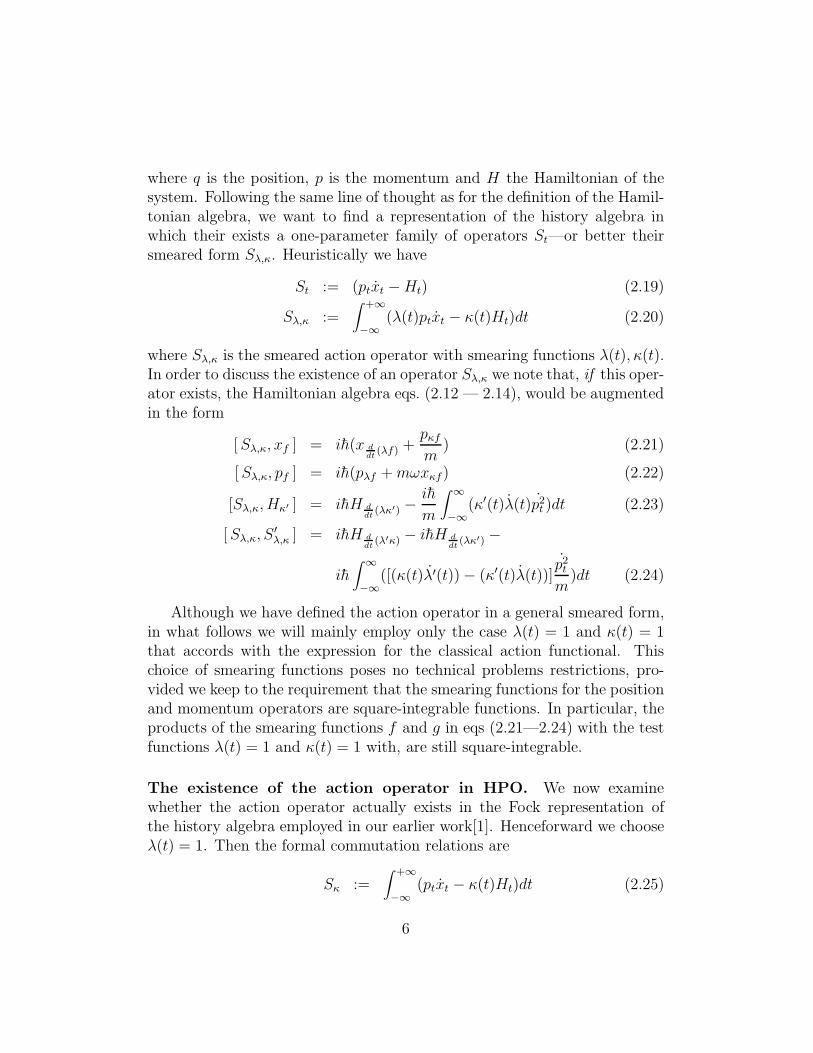
where q is the position, p is the momentum and H the Hamiltonian of thesystem. Following the same line of thought as for the definition of the Hamil-tonian algebra, we want to find a representation of the history algebra inwhich their exists a one-parameter family of operators St—or better theirsmeared form Sλ,κ. Heuristically we have

St := (ptxt −Ht) (2.19)

Sλ,κ :=∫ +∞

−∞(λ(t)ptxt − κ(t)Ht)dt (2.20)

where Sλ,κ is the smeared action operator with smearing functions λ(t), κ(t).In order to discuss the existence of an operator Sλ,κ we note that, if this oper-ator exists, the Hamiltonian algebra eqs. (2.12 — 2.14), would be augmentedin the form

[Sλ,κ, xf ] = ih(x ddt

(λf) +pκf

m) (2.21)

[Sλ,κ, pf ] = ih(pλf +mωxκf) (2.22)

[Sλ,κ, Hκ′ ] = ihH ddt

(λκ′) −ih

m

∫ ∞

−∞(κ′(t)λ(t)p2

t )dt (2.23)

[Sλ,κ, S′λ,κ ] = ihH d

dt(λ′κ) − ihH d

dt(λκ′) −

ih∫ ∞

−∞([(κ(t)λ′(t)) − (κ′(t)λ(t))]

p2t

m)dt (2.24)

Although we have defined the action operator in a general smeared form,in what follows we will mainly employ only the case λ(t) = 1 and κ(t) = 1that accords with the expression for the classical action functional. Thischoice of smearing functions poses no technical problems restrictions, pro-vided we keep to the requirement that the smearing functions for the positionand momentum operators are square-integrable functions. In particular, theproducts of the smearing functions f and g in eqs (2.21—2.24) with the testfunctions λ(t) = 1 and κ(t) = 1 with, are still square-integrable.

The existence of the action operator in HPO. We now examinewhether the action operator actually exists in the Fock representation ofthe history algebra employed in our earlier work[1]. Henceforward we chooseλ(t) = 1. Then the formal commutation relations are

Sκ :=∫ +∞

−∞(ptxt − κ(t)Ht)dt (2.25)

6

[Sκ, xf ] = ih(xf +pκf

m) (2.26)

[Sκ, pf ] = ih(pf +mωxκf) (2.27)

[Sκ, Hκ′ ] = ihHκ′ (2.28)

[Sκ, Sκ′ ] = ihHκ − ihHκ′ (2.29)

A key observation is that if the operators eih

Sκ existed they would producethe history algebra automorphism

eih

Sκbte− i

hSκ = e−iω

∫ t+s

tκ(t+s′)ds′+s d

dt bt (2.30)

or, in the more rigorous smeared form

eih

Sκbfe− i

hSκ = bΣsf (2.31)

where the unitary operator Σs is defined on L2(R) by

(Σsψ)(t) := e−iω∫ t+s

tκ(t+s′)ds′ψ(t+ s). (2.32)

However, an important property of the Fock construction states that whenthere exists a unitary operator eisA acting on L2(R), there exists a unitaryoperator Γ(eisA) that acts on the exponential Fock space2 F(L2(R)) in suchway that

Γ(eisA)b†fΓ(eisA)−1

= b†eisAf (2.33)

then the operator dΓ(A) on F(L2(R)) can also be defined as

Γ(eisA) = eisdΓ(A) (2.34)

in terms of A, a self-adjoint operator that acts on L2(R). In particular,it follows that the representation of the history algebra on the Fock spaceF(L2(R)) carries a (weakly continuous) representation of the one-parameter

family of unitary operators s 7→ eih

sSκ = Γ(Σs). Therefore, the generatorSκ also exists on F(L2(R)) and S = dΓ(−hσκ) where σκ is a self-adjointoperator that acts on L2(R) and is defined as

σκψ(t) :=

(

−ωκ(t) − id

dt

)

ψ(t). (2.35)

2A general expression for a Fock space is eH = ⊕∞

n=0(⊗nH)n where H is called the base

Hilbert space of the Fock space eH.

7

In what follows, we will restrict our attention to the particular case κ(t) =1 for the simple harmonic oscillator action operator S

S :=∫ +∞

−∞(ptxt −Ht)dt. (2.36)

The Liouville operator definition. The first term of the action operatoreq. (2.36) is identical to the kinematical part of the classical action functionaleq. ( 2.18 ). For reasons that will become apparent later, we write Sκ as thedifference between two operators: the Liouville operator and the Hamiltonianoperator. The Liouville operator is formally written as

V :=∫ ∞

−∞(ptqt)dt (2.37)

whereSκ = V −Hκ (2.38)

We prove the existence of V on F(L2(R)) using the same technique as before.Namely, we can see at once that the history algebra automorphism

eih

sV bfe− i

hsV = bBsf (2.39)

is unitarily implementable. Here, the unitary operator Bs, s ∈ R, acting onL2(R) is defined by

(Bsf)(t) := es ddtf(t) = eisDf(t) = f(t+ s) (2.40)

where D := −i ddt

. The Liouville operator V has some interesting commuta-tion relations with the generators of the history algebra:

[V, xf ] = −ihxf (2.41)

[V, pf ] = −ihpf (2.42)

[V,Hκ ] = −ihHκ (2.43)

[V, Sκ] = ihHκ (2.44)

[V,H ] = 0 (2.45)

[V, S ] = 0 (2.46)

where we have defined H :=∫∞−∞Htdt.

8

We notice that V transforms, for example, bt from one time t—that refersto the Hilbert space Ht—to another time t + s, that refers to Ht+s. Moreprecisely, V transforms the support of the operator-valued distribution btfrom t to t+ s:

eih

sV bfe− i

hsV = bfs

(2.47)

where fs(t) := f(s+ t). We shall return to the significance of this later.

The Fourier-transformed ‘n-particle’ history propositions. An in-teresting family of history propositions emerges from the representation spaceF [L2(R, dt)], acting on the δ-function normalised basis of states |0〉, |t1〉 :=b†t1 |0〉 , |t1, t2〉 := b†t1b

†t2 |0〉 etc; or, in smeared form, |φ〉 := b†φ|0〉 etc. The pro-

jection operator |t〉〈t| corresponds to the history proposition ‘there is a unitenergy hω concentrated at the time point t’. The physical interpretation forthis family of propositions, was deduced from the action of the Hamiltonianoperator on the family of |t〉 states:

Ht|0〉 = 0 (2.48)

Ht|t1〉 = hωδ(t− t1)|t1〉 (2.49)

Ht|t1, t2〉 = hω[δ(t− t1) + δ(t− t2)]|t1, t2〉 (2.50)...

To study the behaviour of the S operator, a particularly useful basis forF [L2(R, dt)] is the Fourier-transforms of the |t〉-states. Indeed, if we considerthe Fourier transformations

|ν〉 =∫ +∞

−∞eiνtb†t |0〉dt (2.51)

|ν1, ν2〉 =∫ +∞

−∞eiν1t1eiν2t2b†t1b

†t2 |0〉dt1dt2 (2.52)

bν =∫ +∞

−∞eiνtbtdt (2.53)

b†ν =∫ +∞

−∞e−iνtb†tdt (2.54)

the Fourier transformed |ν〉- states are defined by |ν〉 := b†ν |0〉, |ν1, ν2〉 :=b†ν1b†ν2

|0〉 etc. The eigenvectors of the operator S are calculated to be

S|0〉 = 0 (2.55)

9

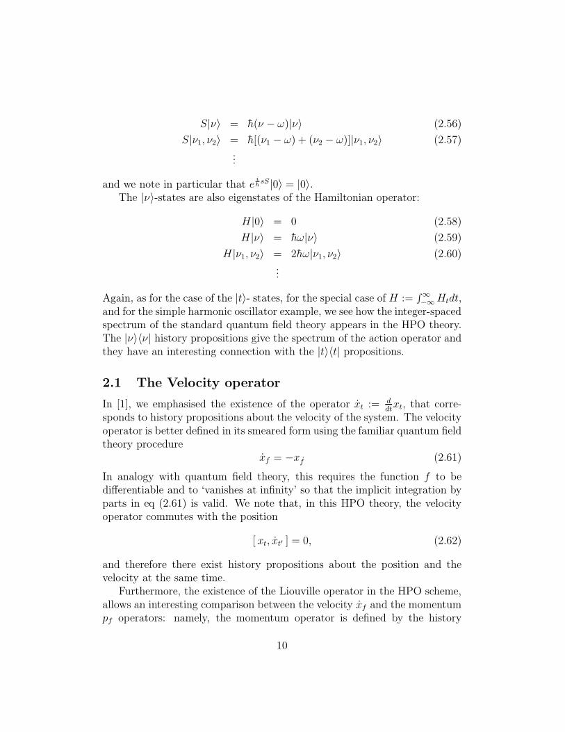
S|ν〉 = h(ν − ω)|ν〉 (2.56)

S|ν1, ν2〉 = h[(ν1 − ω) + (ν2 − ω)]|ν1, ν2〉 (2.57)...

and we note in particular that eih

sS|0〉 = |0〉.The |ν〉-states are also eigenstates of the Hamiltonian operator:

H|0〉 = 0 (2.58)

H|ν〉 = hω|ν〉 (2.59)

H|ν1, ν2〉 = 2hω|ν1, ν2〉 (2.60)...

Again, as for the case of the |t〉- states, for the special case of H :=∫∞−∞Htdt,

and for the simple harmonic oscillator example, we see how the integer-spacedspectrum of the standard quantum field theory appears in the HPO theory.The |ν〉〈ν| history propositions give the spectrum of the action operator andthey have an interesting connection with the |t〉〈t| propositions.

2.1 The Velocity operator

In [1], we emphasised the existence of the operator xt := ddtxt, that corre-

sponds to history propositions about the velocity of the system. The velocityoperator is better defined in its smeared form using the familiar quantum fieldtheory procedure

xf = −xf (2.61)

In analogy with quantum field theory, this requires the function f to bedifferentiable and to ‘vanishes at infinity’ so that the implicit integration byparts in eq (2.61) is valid. We note that, in this HPO theory, the velocityoperator commutes with the position

[ xt, xt′ ] = 0, (2.62)

and therefore there exist history propositions about the position and thevelocity at the same time.

Furthermore, the existence of the Liouville operator in the HPO scheme,allows an interesting comparison between the velocity xf and the momentumpf operators: namely, the momentum operator is defined by the history

10

commutation relation of the position with the Hamiltonian, while we candefine the velocity operator from the history commutation relation of theposition with the Liouville operator:

[ xf , H ] = ihpf

m(2.63)

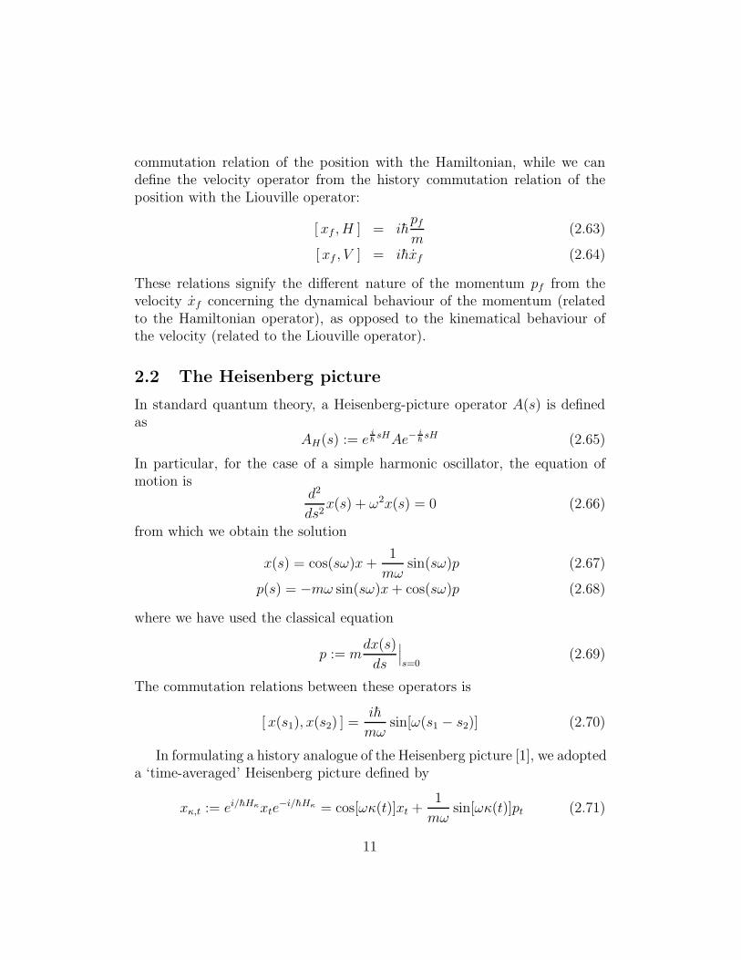
[ xf , V ] = ihxf (2.64)

These relations signify the different nature of the momentum pf from thevelocity xf concerning the dynamical behaviour of the momentum (relatedto the Hamiltonian operator), as opposed to the kinematical behaviour ofthe velocity (related to the Liouville operator).

2.2 The Heisenberg picture

In standard quantum theory, a Heisenberg-picture operator A(s) is definedas

AH(s) := eih

sHAe−ih

sH (2.65)

In particular, for the case of a simple harmonic oscillator, the equation ofmotion is

d2

ds2x(s) + ω2x(s) = 0 (2.66)

from which we obtain the solution

x(s) = cos(sω)x+1

mωsin(sω)p (2.67)

p(s) = −mω sin(sω)x+ cos(sω)p (2.68)

where we have used the classical equation

p := mdx(s)

ds

∣

∣

∣

s=0(2.69)

The commutation relations between these operators is

[ x(s1), x(s2) ] =ih

mωsin[ω(s1 − s2)] (2.70)

In formulating a history analogue of the Heisenberg picture [1], we adopteda ‘time-averaged’ Heisenberg picture defined by

xκ,t := ei/hHκxte−i/hHκ = cos[ωκ(t)]xt +

1

mωsin[ωκ(t)]pt (2.71)

11

for suitable test functions κ. The analogue of the equations of motion is thefunctional differential equation

δ2xκ,t

δκ(s1)δκ(s2)+ δ(t− s1)δ(t− s2)ω

2xκ,t = 0 (2.72)

and

δ(t− s)pt = mδxκ,t

δκ(s)

∣

∣

∣

κ=0(2.73)

is the history analogue of the classical equation p := mdx(s)ds

∣

∣

∣

s=0.

We noted then that the Heisenberg-picture in an HPO theory involvestwo time labels: an ‘external’ label t—that specifies the time the propositionis asserted—and an ‘internal’ label s that, for a fixed time t, is the timeparameter of the Heisenberg picture associated with the copy Ht of the stan-dard Hilbert space. Using our new results, the two labels appear naturallyin a new version of the Heisenberg picture: they are related to the groupsthat produce the two types of time transformations. In addition, the analogywith the classical expressions is regained.

To see this explicitly, we define a Heisenberg picture analogue of xt as

xκ,t,s : = eih

sHκxte− i

hsHκ (2.74)

= cos[ωsκ(t)]xt +1

mωsin[ωsκ(t)]pt

pκ,t,s : = eih

sHκpte− i

hsHκ (2.75)

= −mω sin[ωsκ(t)]xt + cos[ωsκ(t)]pt

The commutation relations for these operators are

[ xκ,t(s), xκ′,t′(s′) ] =

ih

mωsin[ωκ(s′ − s)]δ(t− t′) (2.76)

[xκ,t(s), Sκ′ ] = ih[

cos[sωκ(t)]xt +1

mωsin[sωκ(t)]pt −

κ′

mpκ,t,s

]

(2.77)

[ pκ,t(s), Sκ′ ] = ih[

cos[sωκ(t)]pt −mω sin[sωκ(t)]xt + κ′(t)xκ,t,s

]

(2.78)

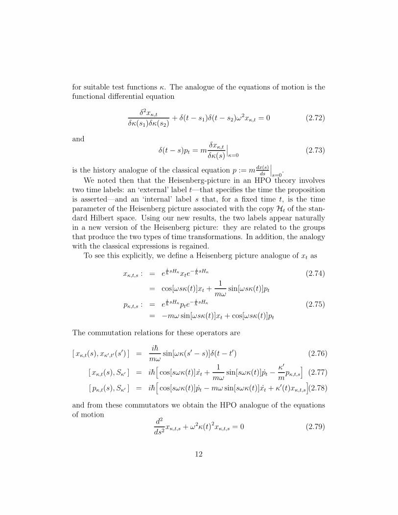
and from these commutators we obtain the HPO analogue of the equationsof motion

d2

ds2xκ,t,s + ω2κ(t)2xκ,t,s = 0 (2.79)

12

We notice the strong resemblance with standard quantum theory; for thecase κ(t) = 1, the classical expressions are fully recovered.

In the HPO formalism, the Heisenberg picture objects appear time av-eraged with respect to the ‘external’ time label t. On the other hand, the‘internal’ time label s is the time-evolution parameter of the standard Heisen-berg picture, as viewed in the Hilbert space Ht. In what follows, we will showhow the Heisenberg picture operators evolve in time under the action of thegroups of time transformations.

3 Time transformation in the HPO formal-

ism

In classical theory, the Hamiltonian H is the generator of time transforma-tions. In terms of Poisson brackets, the generalised equation of motion foran arbitrary function u is given by

du

dt= {u,H}+

∂u

∂t. (3.1)

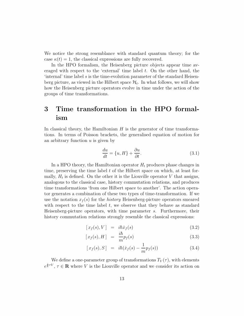
In a HPO theory, the Hamiltonian operator Ht produces phase changes intime, preserving the time label t of the Hilbert space on which, at least for-mally, Ht is defined. On the other it is the Liouville operator V that assigns,analogous to the classical case, history commutation relations, and producestime transformations ‘from one Hilbert space to another’. The action opera-tor generates a combination of these two types of time-transformation. If weuse the notation xf (s) for the history Heisenberg-picture operators smearedwith respect to the time label t, we observe that they behave as standardHeisenberg-picture operators, with time parameter s. Furthermore, theirhistory commutation relations strongly resemble the classical expressions:

[ xf(s), V ] = ihxf (s) (3.2)

[xf (s), H ] =ih

mpf(s) (3.3)

[ xf (s), S ] = ih(xf (s) −1

mpf(s)) (3.4)

We define a one-parameter group of transformations TV (τ), with elements

eih

τV , τ ∈ R where V is the Liouville operator and we consider its action on

13

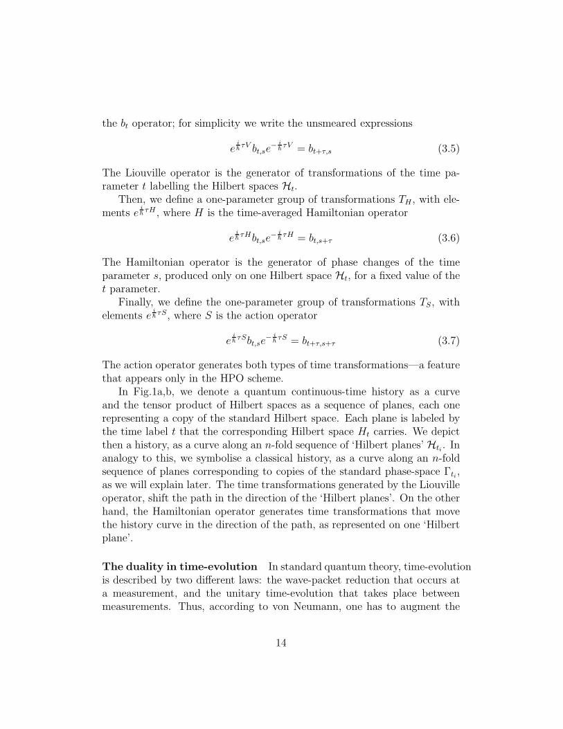
the bt operator; for simplicity we write the unsmeared expressions

eih

τV bt,se− i

hτV = bt+τ,s (3.5)

The Liouville operator is the generator of transformations of the time pa-rameter t labelling the Hilbert spaces Ht.

Then, we define a one-parameter group of transformations TH , with ele-ments e

ih

τH , where H is the time-averaged Hamiltonian operator

eih

τHbt,se− i

hτH = bt,s+τ (3.6)

The Hamiltonian operator is the generator of phase changes of the timeparameter s, produced only on one Hilbert space Ht, for a fixed value of thet parameter.

Finally, we define the one-parameter group of transformations TS, withelements e

ih

τS, where S is the action operator

eih

τSbt,se− i

hτS = bt+τ,s+τ (3.7)

The action operator generates both types of time transformations—a featurethat appears only in the HPO scheme.

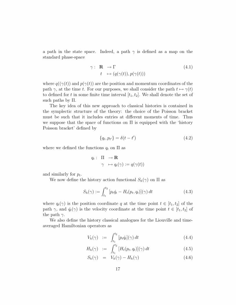
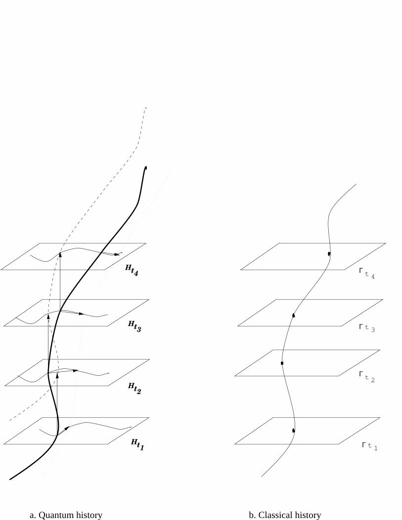
In Fig.1a,b, we denote a quantum continuous-time history as a curveand the tensor product of Hilbert spaces as a sequence of planes, each onerepresenting a copy of the standard Hilbert space. Each plane is labeled bythe time label t that the corresponding Hilbert space Ht carries. We depictthen a history, as a curve along an n-fold sequence of ‘Hilbert planes’ Hti . Inanalogy to this, we symbolise a classical history, as a curve along an n-foldsequence of planes corresponding to copies of the standard phase-space Γti ,as we will explain later. The time transformations generated by the Liouvilleoperator, shift the path in the direction of the ‘Hilbert planes’. On the otherhand, the Hamiltonian operator generates time transformations that movethe history curve in the direction of the path, as represented on one ‘Hilbertplane’.

The duality in time-evolution In standard quantum theory, time-evolutionis described by two different laws: the wave-packet reduction that occurs ata measurement, and the unitary time-evolution that takes place betweenmeasurements. Thus, according to von Neumann, one has to augment the

14

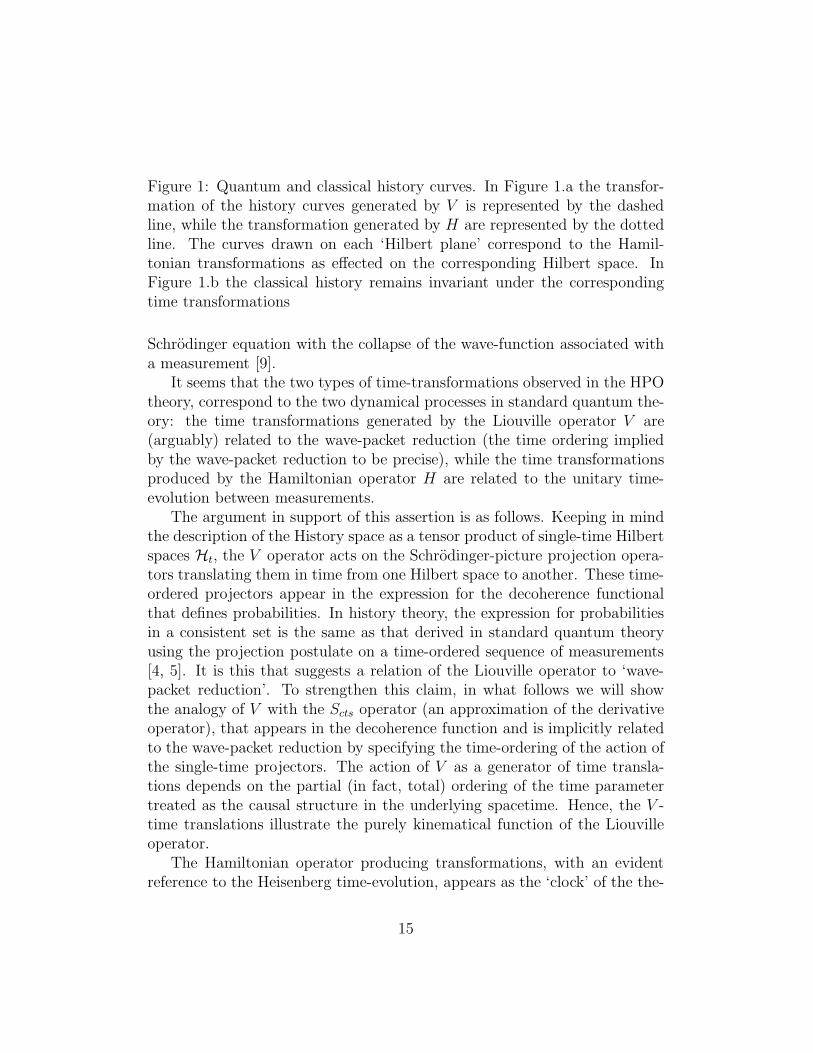
Figure 1: Quantum and classical history curves. In Figure 1.a the transfor-mation of the history curves generated by V is represented by the dashedline, while the transformation generated by H are represented by the dottedline. The curves drawn on each ‘Hilbert plane’ correspond to the Hamil-tonian transformations as effected on the corresponding Hilbert space. InFigure 1.b the classical history remains invariant under the correspondingtime transformations

Schrodinger equation with the collapse of the wave-function associated witha measurement [9].

It seems that the two types of time-transformations observed in the HPOtheory, correspond to the two dynamical processes in standard quantum the-ory: the time transformations generated by the Liouville operator V are(arguably) related to the wave-packet reduction (the time ordering impliedby the wave-packet reduction to be precise), while the time transformationsproduced by the Hamiltonian operator H are related to the unitary time-evolution between measurements.

The argument in support of this assertion is as follows. Keeping in mindthe description of the History space as a tensor product of single-time Hilbertspaces Ht, the V operator acts on the Schrodinger-picture projection opera-tors translating them in time from one Hilbert space to another. These time-ordered projectors appear in the expression for the decoherence functionalthat defines probabilities. In history theory, the expression for probabilitiesin a consistent set is the same as that derived in standard quantum theoryusing the projection postulate on a time-ordered sequence of measurements[4, 5]. It is this that suggests a relation of the Liouville operator to ‘wave-packet reduction’. To strengthen this claim, in what follows we will showthe analogy of V with the Scts operator (an approximation of the derivativeoperator), that appears in the decoherence function and is implicitly relatedto the wave-packet reduction by specifying the time-ordering of the action ofthe single-time projectors. The action of V as a generator of time transla-tions depends on the partial (in fact, total) ordering of the time parametertreated as the causal structure in the underlying spacetime. Hence, the V -time translations illustrate the purely kinematical function of the Liouvilleoperator.

The Hamiltonian operator producing transformations, with an evidentreference to the Heisenberg time-evolution, appears as the ‘clock’ of the the-

15

ory. As such, it depends on the particular physical system that the Hamil-tonian describes. Indeed, we would expect the definition of a ‘clock’ for theevolution in time of a physical system to be connected with the dynamicsof the system concerned. We note that the idea of reparametrizing time de-pends on the smearing function κ(t) used in the definition of the Hamiltonianoperator; κ(t) is kept fixed for a particular physical system.

The coexistence of the two types of time-evolution, as reflected in theaction operator identified as the generator of such time transformations, isa striking result. In particular, its definition is in accord with its classi-cal analogue, namely the Hamilton action functional. In classical theory, adistinction between a kinematical and a dynamical part of the action func-tional also arises in the sense that the first part corresponds to the symplecticstructure and the second to the Hamiltonian.

4 The classical signature of the HPO formal-

ism

Let us now consider more closely the relation of the classical and the quan-tum histories. We have shown above how the action operator generates timetranslations from one Hilbert space to another, through the Liouville opera-tor; and on each labeled Hilbert space Ht, through the Hamiltonian operator.We now wish to discuss in more detail the analogue of these transformationsin the classical case.

We recall that a history is a time-ordered sequence of propositions aboutthe system. The continuous-time quantum history in the HPO system, makesassertions about the values of the position or the momentum of the system,or a linear combination of them, at each moment of time, and is representedby a projection operator on the continuous tensor product of copies of thestandard Hilbert space.

One expects that a continuous-time classical history should reflect theunderlying temporal logic of the situation. Thus the assertions about theposition and the momentum of the system at each moment of time should berepresented on an analogous history space: this can be achieved by using theCartesian product of a continuous family (labelled by the time t) of copiesof the standard classical state space.

In classical mechanics, a (fine-grained) classical history is represented by

16

a path in the state space. Indeed, a path γ is defined as a map on thestandard phase-space

γ : R → Γ (4.1)

t 7→ (q(γ(t)), p(γ(t)))

where q((γ(t)) and p(γ(t)) are the position and momentum coordinates of thepath γ, at the time t. For our purposes, we shall consider the path t 7→ γ(t)to defined for t in some finite time interval [t1, t2]. We shall denote the set ofsuch paths by Π.

The key idea of this new approach to classical histories is contained inthe symplectic structure of the theory: the choice of the Poisson bracketmust be such that it includes entries at different moments of time. Thuswe suppose that the space of functions on Π is equipped with the ‘historyPoisson bracket’ defined by

{qt, pt′} = δ(t− t′) (4.2)

where we defined the functions qt on Π as

qt : Π → R

γ 7→ qt(γ) := q(γ(t))

and similarly for pt.We now define the history action functional Sh(γ) on Π as

Sh(γ) :=∫ t2

t1[ptqt −Ht(pt, qt)](γ) dt (4.3)

where qt(γ) is the position coordinate q at the time point t ∈ [t1, t2] of thepath γ, and qt(γ) is the velocity coordinate at the time point t ∈ [t1, t2] ofthe path γ.

We also define the history classical analogues for the Liouville and time-averaged Hamiltonian operators as

Vh(γ) :=∫ t2

t1[ptqt](γ) dt (4.4)

Hh(γ) :=∫ t2

t1[Ht(pt, qt)](γ) dt (4.5)

Sh(γ) = Vh(γ) −Hh(γ) (4.6)

17

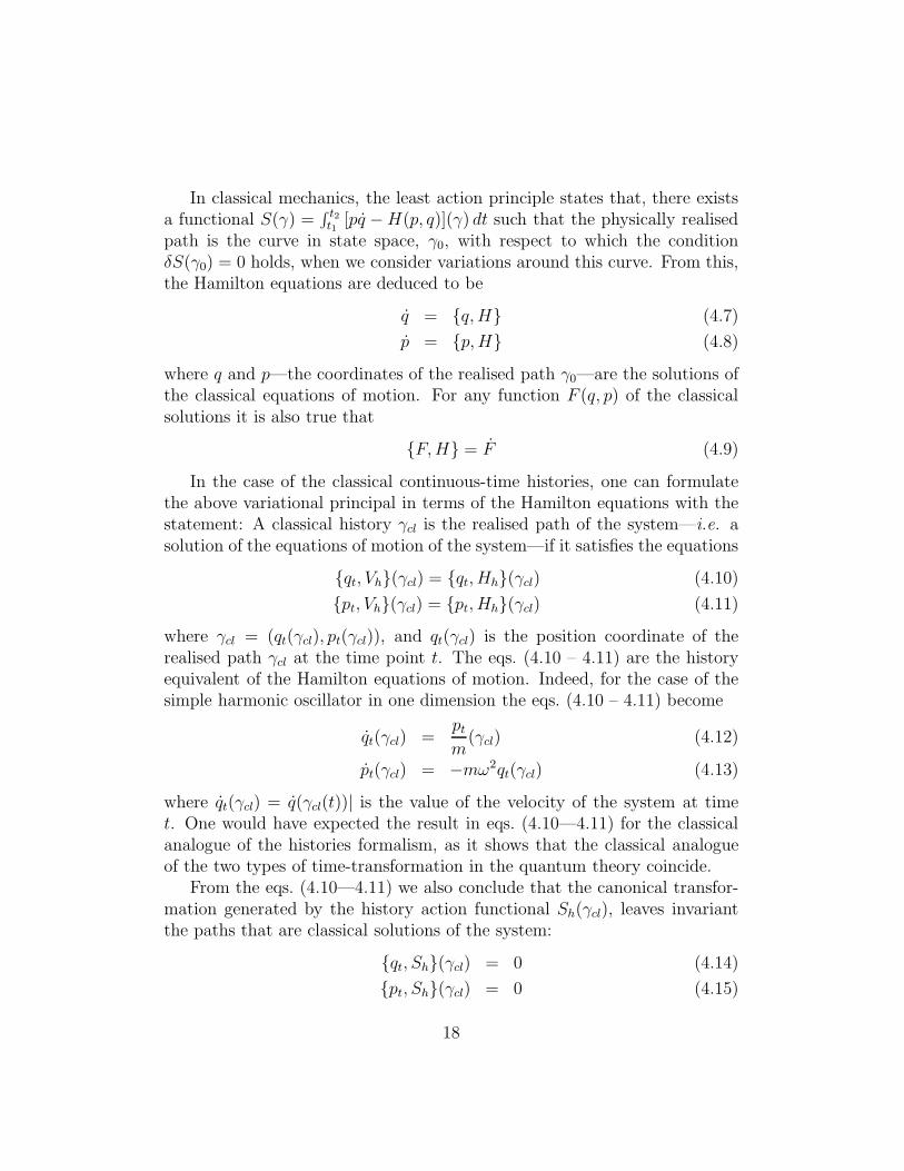
In classical mechanics, the least action principle states that, there existsa functional S(γ) =

∫ t2t1

[pq −H(p, q)](γ) dt such that the physically realisedpath is the curve in state space, γ0, with respect to which the conditionδS(γ0) = 0 holds, when we consider variations around this curve. From this,the Hamilton equations are deduced to be

q = {q,H} (4.7)

p = {p,H} (4.8)

where q and p—the coordinates of the realised path γ0—are the solutions ofthe classical equations of motion. For any function F (q, p) of the classicalsolutions it is also true that

{F,H} = F (4.9)

In the case of the classical continuous-time histories, one can formulatethe above variational principal in terms of the Hamilton equations with thestatement: A classical history γcl is the realised path of the system—i.e. asolution of the equations of motion of the system—if it satisfies the equations

{qt, Vh}(γcl) = {qt, Hh}(γcl) (4.10)

{pt, Vh}(γcl) = {pt, Hh}(γcl) (4.11)

where γcl = (qt(γcl), pt(γcl)), and qt(γcl) is the position coordinate of therealised path γcl at the time point t. The eqs. (4.10 – 4.11) are the historyequivalent of the Hamilton equations of motion. Indeed, for the case of thesimple harmonic oscillator in one dimension the eqs. (4.10 – 4.11) become

qt(γcl) =pt

m(γcl) (4.12)

pt(γcl) = −mω2qt(γcl) (4.13)

where qt(γcl) = q(γcl(t))| is the value of the velocity of the system at timet. One would have expected the result in eqs. (4.10—4.11) for the classicalanalogue of the histories formalism, as it shows that the classical analogueof the two types of time-transformation in the quantum theory coincide.

From the eqs. (4.10—4.11) we also conclude that the canonical transfor-mation generated by the history action functional Sh(γcl), leaves invariantthe paths that are classical solutions of the system:

{qt, Sh}(γcl) = 0 (4.14)

{pt, Sh}(γcl) = 0 (4.15)

18

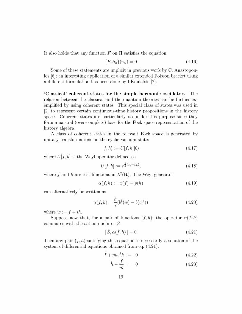
It also holds that any function F on Π satisfies the equation

{F, Sh}(γcl) = 0 (4.16)

Some of these statements are implicit in previous work by C. Anastopou-los [6]; an interesting application of a similar extended Poisson bracket usinga different formulation has been done by I.Kouletsis [7].

‘Classical’ coherent states for the simple harmonic oscillator. Therelation between the classical and the quantum theories can be further ex-emplified by using coherent states. This special class of states was used in[2] to represent certain continuous-time history propositions in the historyspace. Coherent states are particularly useful for this purpose since theyform a natural (over-complete) base for the Fock space representation of thehistory algebra.

A class of coherent states in the relevant Fock space is generated byunitary transformations on the cyclic vacuum state:

|f, h〉 := U [f, h]|0〉 (4.17)

where U [f, h] is the Weyl operator defined as

U [f, h] := eih(xf−ph), (4.18)

where f and h are test functions in L2(R). The Weyl generator

α(f, h) := x(f) − p(h) (4.19)

can alternatively be written as

α(f, h) =h

i(b†(w) − b(w∗)) (4.20)

where w := f + ih.Suppose now that, for a pair of functions (f, h), the operator α(f, h)

commutes with the action operator S

[S, α(f, h) ] = 0 (4.21)

Then any pair (f, h) satisfying this equation is necessarily a solution of thesystem of differential equations obtained from eq. (4.21):

f +mω2h = 0 (4.22)

h−f

m= 0 (4.23)

19

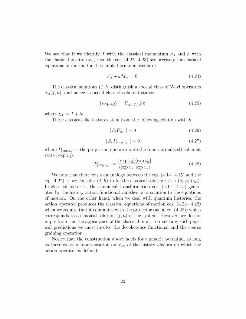
We see that if we identify f with the classical momentum pcl and h withthe classical position xcl, then the eqs. (4.22– 4.23) are precisely the classicalequations of motion for the simple harmonic oscillator:

xcl + ω2xcl = 0. (4.24)

The classical solutions (f, h) distinguish a special class of Weyl operatorsαcl(f, h), and hence a special class of coherent states:

| exp zcl〉 := Uαcl(f,h)|0〉 (4.25)

where zcl := f + ih.These classical-like features stem from the following relation with S

[S, Uαcl] = 0 (4.26)

[S, P| exp zcl〉 ] = 0 (4.27)

where P| exp zcl〉 is the projection operator onto the (non-normalised) coherentstate | exp zcl〉:

P| exp zcl〉 :=| exp zcl〉〈exp zcl|

〈exp zcl| exp zcl〉(4.28)

We note that there exists an analogy between the eqs. (4.14– 4.15) and theeq. (4.27), if we consider (f, h) to be the classical solution: t 7→ (qt, pt)(γcl).In classical histories, the canonical transformation eqs. (4.14– 4.15) gener-ated by the history action functional vanishes on a solution to the equationsof motion. On the other hand, when we deal with quantum histories, theaction operator produces the classical equations of motion eqs. (4.23– 4.22)when we require that it commutes with the projector (as in eq. (4.28)) whichcorresponds to a classical solution (f, h) of the system. However, we do notimply from this the appearance of the classical limit: to make any such phys-ical predictions we must involve the decoherence functional and the coarsegraining operation.

Notice that the construction above holds for a generic potential, as longas there exists a representation on Vcts of the history algebra on which theaction operator is defined.

20

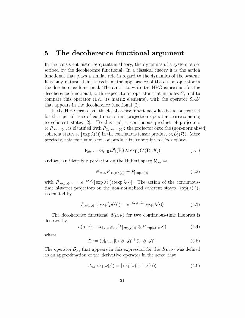
5 The decoherence functional argument

In the consistent histories quantum theory, the dynamics of a system is de-scribed by the decoherence functional. In a classical theory it is the actionfunctional that plays a similar role in regard to the dynamics of the system.It is only natural then, to seek for the appearance of the action operator inthe decoherence functional. The aim is to write the HPO expression for thedecoherence functional, with respect to an operator that includes S, and tocompare this operator (i.e., its matrix elements), with the operator SctsUthat appears in the decoherence functional [2].

In the HPO formalism, the decoherence functional d has been constructedfor the special case of continuous-time projection operators correspondingto coherent states [2]. To this end, a continuous product of projectors⊗tP| exp λ(t)〉 is identified with P⊗t| exp λ(·)〉: the projector onto the (non-normalised)coherent states ⊗t| expλ(t)〉 in the continuous tensor product ⊗tL

2t (R). More

precisely, this continuous tensor product is isomorphic to Fock space:

Vcts := ⊗t∈RL2t(R) ≈ exp(L2(R, dt)) (5.1)

and we can identify a projector on the Hilbert space Vcts as

⊗t∈RP| exp(λ(t)〉 = P| exp λ(·)〉 (5.2)

with P| exp λ(·)〉 = e−〈λ,λ〉| expλ(·)〉〈expλ(·)|. The action of the continuous-time histories projectors on the non-normalised coherent states | exp(λ(·))〉is denoted by

P| exp λ(·)〉| exp(µ(·))〉 = e−〈λ,µ−λ〉| expλ(·)〉 (5.3)

The decoherence functional d(µ, ν) for two continuous-time histories isdenoted by

d(µ, ν) = trVcts⊗Vcts(P| exp µ(·)〉 ⊗ P| exp(ν(·)〉X) (5.4)

whereX := 〈0|ρ−∞|0〉(SctsU)† ⊗ (SctsU). (5.5)

The operator Scts that appears in this expression for the d(µ, ν) was definedas an approximation of the derivative operator in the sense that

Scts| exp ν(·)〉 = | exp(ν(·) + ν(·))〉 (5.6)

21

while the dynamics was introduced by the operator U , defined in such waythat the notion of time evolution is encoded

e〈λ,λ〉eih

H[λ] = trVcts(SctsUP| exp λ(·)〉) (5.7)

We expect V andH to play a similar role to that of Scts and U respectively,inside an expression for the decoherence functional. To demonstrate this wewill use the type of Fock space construction given in eqs. (2.33—2.34). Inparticular, we use the property

Γ(A)| exp ν(·)〉 = | exp(Aν(·))〉 (5.8)

where A is an operator that acts on the elements ν(·) of the base Hilbertspace H, while the operator Γ(A), defined by eq. (2.33), acts on the coherentstates | exp ν(·)〉 of the Fock space eH.

We notice that U is related to the unitary time-evolution eq. (5.7) in asimilar way to that of the Hamiltonian operator H

eisH | exp ν(·)〉 = Γ(eisωI)| exp ν(·)〉 = | exp(eisων(·))〉 (5.9)

where I is the unit operator. We also notice that the action of the operatoreisH produces phase changes, as reflected in the right hand side of eq. (5.9)(which has been calculated for for the special case of the simple harmonicoscillator). Furthermore, when the operator Scts acts on a coherent state eq.(5.6), it transforms it to another coherent state which involves the additionto the defining function ν(·) in a way that involves the time derivative of ν;and it is noteworthy that the Liouville operator V acts in a similar way:

eisV | exp ν(·)〉 = Γ(eisD)| exp ν(·)〉 = | exp(eisDν(·))〉 (5.10)

where(eisDν)(t) = ν(t+ s) (5.11)

where D := −i ddt

. The operator eisD acts on the base Hilbert space, andcorresponds to the operator eisV under the Γ-construction on the Fock space;that is, it acts on the vector ν(t) and transforms it to another one ν(t + s),which, for each time t is translation by the time interval s.

This suggests that we define the operator As := eisS, where S :=∫+∞−∞ (ptxt−

Ht)dt is the action operator for the simple harmonic oscillator, which one ex-pects to be related to the operator SctsU . For this reason, we write the matrixelements of both operators and compare them.

22

The general formula for the matrix elements of an arbitrary operator Twith respect to the coherent states basis in the history space that was usedin [2] is

〈expµ(·)|T | exp ν(·)〉 = e(〈µ, δ

δλ〉+〈 δ

δλ,ν〉)〈expλ(·)|T | expλ(·)〉

∣

∣

∣

λ=λ=0(5.12)

hence we need only compare the diagonal matrix elements of the two opera-tors SctsU and As. Thus we have

〈exp(λ(·)|SctsU| exp(λ(·)〉 = e〈λ,λ+λ〉eih

H[λ] (5.13)

where H [λ] :=∫∞−∞H(λ(t))dt and H(λ) := H(λ, λ) = 〈λ|H|λ〉/〈λ|λ〉; and

〈expλ(·)|As| expλ(·)〉 = e〈λ,eis(ωI+D)λ〉 (5.14)

with(eis(ωI+D)λ)(t) = eisωλ(t+ s) (5.15)

We can also write both of the above operators on the history spaceF(L2(R)) using their corresponding operators on the Hilbert space L2(R).The Γ construction shows that

SctsU = Γ(1 + iσ) (5.16)

As = Γ(eisσ) = eisdΓ(σ) (5.17)

where σ = ωI + iD, and I is the unit operator. As expressions of thesame function σ, the operators SctsU and As commute. However, we cannotreadily compute their common spectrum because the operator SctsU is notself-adjoint.

We might speculate that the value of the decoherence functional is max-imised for a continuous-time projector that corresponds to a coarse grainingaround the classical path. Indeed, if we take such a generic projection oper-ator P , we expect that it should commute with the operator SctsU . In thiscontext, we noticed earlier that the projection operator which correspondsto a classical solution (f, h) commutes with the action operator

[SctsU , P(f,h)] = 0. (5.18)

Finally, this argument should be compared with the similar condition forclassical histories:

{Sh, FC}(γcl) = 0. (5.19)

23

Conclusions

We have examined the example of the simple harmonic oscillator, in one di-mension, within the History Projection Operator formulation of the consistent-histories scheme. We defined the action operator as the quantum analogueof the classical Hamilton action functional and we have proved its existenceby finding a representation on the F(L2(R)) space of the history algebra.We have shown that the action operator is the generator of two types of timetransformations: translations in time from one Hilbert space Ht, labeled bythe time parameter t, to another Hilbert space with a different label t, andphase changes in time with respect to the time parameter s of the stan-dard Heisenberg-time evolution that acts in each individual Hilbert spaceHt. We have expressed the action operator in terms of the Liouville andHamiltonian operators—which are the generators of the two types of timetransformation—and which correspond to the kinematics and the dynamicsof the theory respectively.

We have constructed continuous-time classical histories defined on thecontinuous Cartesian product of copies of the phase space and demonstratedan analogous expression to the classical Hamilton’s equations.

Finally we have shown that the action operator commutes with the defin-ing operator of the decoherence functional, thus appearing in the expressionfor the dynamics of the theory, as would have been expected.

One of the major reasons for undertaking this study was to provide newtools for tackling the recalcitrant problem of constructing a manifestly covari-ant quantum field theory in the consistent histories formalism. Work on thisproblem is now in progress with the expectation that the Hamiltonian andLiouville operators will play a central role in the proof of explicit Poincareinvariance of the theory.

Acknowledgements

I would like to thank Chris Isham for the help and support during this work. Iwould also like to thank Charis Anastopoulos and Nikos Plakitsis. I gratefullyacknowledge support from the NATO Research Fellowships department of theGreek Ministry of Economy.

24

References

[1] C. Isham, N. Linden, K. Savvidou and S. Schreckenberg. Continuoustime and consistent histories. J. Math. Phys. 37, 2261 (1998).

[2] C. Isham and N. Linden. Continuous histories and the history group ingeneralised quantum theory. J. Math. Phys. 36:5392-5408, (1995).

[3] C.J.Isham. Quantum logic and the histories approach to quantum the-ory. J. Math. Phys. 23, 2157 1994.

[4] J.Hartle. Spacetime quantum mechanics and the quantum mechanics ofspacetime. In Proceedings on the 1992 Les Houches School, Gravitation

and Quantisation. 1992.

[5] M.Gell-Mann and J.Hartle. Quantum mechanics in the light of quan-tum cosmology. In K.K.Phua and Y.Yamaguchi, editors, Proceedings of

the 25th International Conference on High Energy Physics, Singapore,

August, 2-8, 1990, Singapore, 1990. World Scientific.

[6] C.Anastopoulos, Int.Jour. Theor. Phys. 37, 2261 (1998).

[7] I. Kouletsis. A classical history theory: geometrodynamics and general

field dynamics regained gr-qc 9801019.

[8] P.A.M. Dirac. The Lagrangian in quantum mechanics. In Selected papers

on quantum electrodynamics, edited by J.Schwinger. Dover Publications,Inc. New York (1958).

[9] H.D.Zeh. The physical basis of the direction of time Springer-VerlagBerlin Heidelberg 1992.

[10] F.A.Berezin. The method of second quantization Academic Press NewYork and London 1966.

[11] H.Goldstein. Classical Mechanics Addison-Wesley Publishing Company1980.

[12] J.J.Halliwell Notes on quantum cosmology lectures Imperial College,M.Sc. course in quantum fields and fundamental forces 1995.

25

[13] H.Araki. Hamiltonian formalism and the canonical commutation rela-tions in quantum field theory. J.Math. Phys, 1:492-504 1960.

[14] C.J.Isham, N.Linden and S. Schreckenberg. The classification of deco-herence functionals: an analogue of Gleason’s theorem. J. Math. Phys.

35, 6360 1994.

[15] From a private communication of Prof. Tulsi Dass with Prof. ChrisIsham.

[16] R.B.Griffiths. Consistent histories and the interpretation of quantummechanics. J.Stat.Phys. 36:219-272, 1984.

[17] R.Omnes. Logical reformulation of quantum mechanics. I.Foundations.J.Stat.Phys., 53:893-932, 1988.

26

Ht1

Ht2

Ht3

Ht4

Γ

Γ

Γ

Γ

t 1

t 2

t 3

t 4

a. Quantum history b. Classical history