Tests for bounded rationality with a linear dynamic model distorted by heterogeneous expectations

Journal of Economic Dynamics & Control23 (1999) 1517}1543

Tests for bounded rationality with a lineardynamic model distorted by heterogeneous

expectations

Saang Joon Baak*Economic Survey and Forecasting Division, Korea Institute for Industrial Economics and Trade (KIET),

P.O. Box 205, Cheong-Ryang, Seoul, South Korea

Accepted 20 November 1998

Abstract

The purpose of this paper is to develop a methodology which will use economic data todetect the existence of boundedly rational economic agents. The bounded rationalitymodel presented in this paper generalizes a linear dynamic rational expectations modelby nesting two types of expectations. In this paper, it is claimed that the boundedrationality model as presented can be transformed into an optimal regulator problemwith distortions. As a result, the methodologies developed by the optimal control theorycan be used to solve the model. The likelihood function for the model is constructed bythe Kalman "ltering using the solution of the model. Maximum Likelihood Estimation(MLE) is performed to test for bounded rationality in the U.S. cattle market for the periodfrom 1900 to 1990. The empirical results indicate that some fraction of economic agents inthe market are boundedly rational. ( 1999 Elsevier Science B.V. All rights reserved.

JEL classixcation: C51; C61; C63; E32; E37

Keywords: Heterogeneous expectations; Bounded rationality; Optimal regulatorproblem with distortions; Kalman "ltering; Maximum likelihood estimation

1. Introduction

Rational expectations models, which have dominated the "eld of macroeco-nomics for the past few decades, are based on two assumptions. The "rst is the

*Now at International University of Japan, Yamato-machi, Minami Uonuma-gun, Niigata949}7277, Japan. E-mail: [email protected]

0165-1889/99/$ - see front matter ( 1999 Elsevier Science B.V. All rights reserved.PII: S 0 1 6 5 - 1 8 8 9 ( 9 8 ) 0 0 0 8 2 - 7

rationality of an economic agent, which posits that the expectations of aneconomic agent are equivalent to mathematical expectations which exploit allavailable information. The second is the homogeneity of expectations of alleconomic agents.1

Recently, a growing number of economists have questioned the validity ofthese two assumptions2 and have presented a variety of bounded rationalitymodels which, instead of modelling all agents as possessing rational expecta-tions, restrict the rationality of some or of all economic agents (known as`boundedly rationala economic agents). For example, Brock and LeBaron(1996), de Fontnouvelle (1994), Arthur et al. (1997a), and Arthur et al. (1997b)show that their models, which assume heterogeneity in expectations, producedynamics consistent with empirical facts observed in the U.S. stock market.Brock and Hommes (1997) analytically explore the evolutionary dynamics ofa cobweb model with rational and namKve expectations. Nerlove and Fornari(1998) present a quasi-rational expectations model in which all economic agentstreat an endogenous variable as exogenous. Their test results suggest that thefully rational expectations hypothesis should be rejected in favor of a quasi-rational one. Grandmont (1994) and Hommes and Sorger (1998) introducemodels with self-ful"lling mistakes, where agents do not know the marketequilibrium equations, but they formulate their expectations based on timeseries observations.

The issue of incorporating bounded rationality (or boundedly rational eco-nomic agents) in economic models is important to our understanding of theeconomy because it is related to the question of stability. Some boundedrationality models predict instability under much weaker conditions than ra-tional expectations models. For instance, Brock and Hommes (1997) showthat a simple dynamic model with linear demand and supply may producea complicated dynamics and even chaos when rational and boundedly rationalagents coexist.

As is well known, rational expectations models tend to ascribe the volatility ofthe economy to relatively large outside shocks, while bounded rationalitymodels attribute the volatility to the inherent instability of the economy and/orrelatively small outside shocks. Cobweb models show this contrast very clearly,demonstrating that price and quantity may #uctuate even without any outsideshocks. When boundedly rational suppliers are replaced with rational ones, theonly sources of #uctuation become outside shocks, which have smaller andshorter-lived e!ects under this scenario. Brock and Hommes (1995) mention this

1See Sargent (1993).

2 In fact, a considerable number of studies testing the rationality of individuals performed bypsychologists and experimental economists have often shown that subjects are not as rational as theconventional economic models have assumed. See Conlisk (1996).

1518 S.J. Baak / Journal of Economic Dynamics & Control 23 (1999) 1517}1543

point in their comparison of Rosen et al. (1994), (RMS hereafter) to Chavas andHolt (1993). In RMS's rational expectations model, outside shocks are the onlysources of the beef cattle market's instability. On the other hand, Chavas andHolt (1993), who adopt static expectations in their model, show that the dairycattle market is inherently unstable under some conditions. Grandmont (1994)and Hommes and Sorger (1998) also imply that our economy may be inherentlyunstable.

The purpose of this paper, motivated by the importance of the presence ofboundedly rational economic agents implied by the existing bounded rationalityliterature, is to develop a methodology which will use economic data to detectthe existence of boundedly rational economic agents.3

Speci"cally, we will develop a method which is capable of producing a pointestimate of the fraction of boundedly rational economic agents based on ananalytical model of bounded rationality. In addition, we will investigate whetherthe bounded rationality model has added empirical value to a fully rationalexpectations model in explaining the economic data.

The bounded rationality model presented in the present paper generalizesa linear-quadratic rational expectations model by nesting some fraction ofboundedly rational economic agents within the rational expectations model.Therefore, the bounded rationality model is a model with heterogeneous expec-tations like those presented by Brock and Hommes (1997) and Arthur et al.(1997a). Unlike their models, however, the fraction of boundedly rational agentsis assumed to be "xed for econometric tractability. Following Grandmont(1994), Hommes and Sorger (1998) and Nerlove and Fornari (1998), the bound-edly rational agents are assumed to form their expectations based on time seriesobservations. If the fraction of boundedly rational economic agents is zero, themodel collapses to a rational expectations model. Therefore, a linear-quadraticrational expectations model can be regarded as a special case of this type ofbounded rationality model.

In particular, we present a bounded rationality model that generalizes RMS'srational expectations model which aims to explain the U.S. beef cattle cycle.Accordingly, this paper investigates the presence of boundedly rational eco-nomic agents in the U.S. beef cattle market. As Nerlove et al. (1979) point out,the U.S. cattle industry is a good place for this kind of inquiry becausea relatively large amount of data and information about the production techno-logy are available. Diebold et al. (1995), Anderson et al. (1995), (AHMS here-after), and Nerlove and Fornari (1998) also utilize data from this industry toprovide a substantial illustration of their research. It should be noted that,

3As far as I know, Chavas (1995) is the only researcher attempting to estimate the fraction ofboundedly rational agents. The methodological di!erence between the work of Chavas (1995) andthe present study is explained in Section 3.

S.J. Baak / Journal of Economic Dynamics & Control 23 (1999) 1517}1543 1519

however, as is the case with the authors mentioned above, the methodologydeveloped in this paper is not restricted to the speci"c industry.

As shown in Hansen and Sargent (1996) and AHMS, a linear dynamicrational expectations model of a competitive market can be solved e$ciently byconverting the model into an optimal regulator problem. Hansen andSargent (1996) and AHMS illustrate the converting procedures with the modelof RMS. They transform the rational expectations model of RMS into a socialplanner's problem based on the "rst welfare theorem. The social planner'sproblem takes the form of a linear-quadratic dynamic optimization problemwhich can be then mapped into an optimal regulator problem. Once thetransformation is done, the model is easily solved by the well-establishedoptimal control theory.

The bounded rationality model presented in this paper cannot be solved bythe same procedures as outlined above. Since there are two types of agentswhose expectations are di!erent from each other in a competitive market, thebounded rationality model cannot be formed as a representative agent's prob-lem. Subsequently, it cannot be transformed into a social planner's problem. Infact, the model is distorted by the presence of boundedly rational economicagents. This paper, however, claims that in spite of the heterogeneity in expecta-tions, the bounded rationality model can be transformed into a "ctional socialplanner's problem with side constraints (i.e., side equilibrium conditions). There-fore, it can be reformatted as a linear-quadratic optimal regulator problem withdistortions. The methodology of solving a distorted optimal regulator problemillustrated by McGrattan (1994) is used to solve this model. If we assumethat the fraction of boundedly rational agents is zero, the side constraints ofthe "ctional social planner's problem are no longer binding. As a result,the distortions of the optimal regulator problem disappear. In this case, thebounded rationality model of this paper produces the same solution as therational expectations model of RMS and AHMS.

Once the solution is obtained, the fraction of boundedly rational agents alongwith other deep parameters of the model can be estimated by MLE. Themethods of state space representations and innovations representations usingthe Kalman "lter are useful in constructing the log-likelihood function.

Sections 2 and 3 present the rational expectations model and the boundedrationality model and then solve them. The rational expectations model ofRMS is presented "rst because the bounded rationality model of this paper isa generalized version of it. Both models are initially solved by lag operatormanipulations, and then by the optimal control theory. Solutions obtained bylag operator manipulations will be compared with those obtained by theoptimal control theory to check the validity of the latter. Some discussion isgiven to the stationarity of the two models. If the fraction of boundedly rationaleconomic agents exceeds a certain point, the bounded rationality model losesstationarity.


The empirical test results are shown in Section 4. The point estimate and thelikelihood ratio test signi"cantly indicate the presence of boundedly rationalagents in the U.S. cattle market. In addition, one-step ahead forecasting experi-ments by the bounded rationality model generate lower mean-squared errorsthan by the rational expectations model. Section 5 presents the conclusions.

2. The rational expectations model

Because the bounded rationality model is based on the rational expectationsmodel and extends it by assuming heterogeneity in beliefs (i.e., allowing forboundedly rational economic agents as well as rational agents), the rationalexpectations model employed by RMS and AHMS to explain the cattle cycle ispresented in this section, preceding the bounded rationality model of this paperin Section 3. The de"nitions and notations in this section will also be used inSection 3.

The models presented in this paper are based on the production technology ofthe beef cattle industry. The "nal output of the industry at the beginning of timet is the sum of surviving adult animals from the previous year and the two-yearold animals joining the adult stock.

yt"(1!d)k

t~1#gk

t~3(1)

where ytis the "nal output, k

t~1is the adult stock at time t!1, d is the natural

death rate, and g is the birth (fertility) rate per adult animal. The death rate isassumed to be non-negative and the birth rate, positive. Since all steers (youngmale cattle) are slaughtered at the age of two, the surviving adult stock arecomposed of females reserved for breeding. Therefore, k

t~1is also breeding

stock at time t!1. Breeding stock are regarded as capital in that they are beingused for production.

The last term in the production function (1), gkt~3

, represents calves conceiv-ed at time t!3 and born at the beginning of time t!2. Since g is the fertilityrate per adult animal and the gestation period is almost one year, the breedingstock at time t!3 give birth to gk

t~3calves at time t!2. The calves join the

adult stock at time t when they are two-years old. The "nal output is either soldfor consumption or held for breeding (that is, invested for future production). Inthis industry, the amount of capital (breeding) stock at time t is the same as theamount of investment at time t.

yt"i

t#c

t, (2)

kt"i

t, (3)

where itis investment, c

tconsumption (or sales), and k

tbreeding (capital) stock

at time t.


The goal of a producer (rancher) in this industry is assumed to be to maximizethe expected present discounted value of current and future pro"ts over anin"nite horizon of time.

In this section, we will examine the dynamic optimizing model of a representa-tive rational rancher in a competitive economy and the equilibrium solution ofthe model (Section 2.1). Following this, in Section 2.2 we will convert the modelinto a social planner's problem of the Hansen and Sargent (1996) type (HS typesocial planning problem, hereafter). In Section 2.3 the social planner's problemwill be reformatted as a discounted stochastic optimal regulator problem. AsAHMS show, these transformations enable us to solve the rational expectationsmodel more quickly and to perform MLE more e$ciently.

2.1. The rational expectations model in a competitive cattle market

The objective function of a rational rancher is the following:

maxit

E0G

=+t/1

btCptct!mtct!h

t(k

t#c

0gk

t~1#c

1gk

t~2)

!

tc

2c2t!

t0

2k2t!

t1

2k2t~1

!

t2

2k2t~2DH (4)

s.t. ct"(1!d)k

t~1#gk

t~3!i

t, (5a)

kt"i

t, (5b)

where ptis the market price of an adult animal, m

tis the marketing cost of

preparing an adult animal for slaughter, and ht, c

1ht, c

0htare the one-period

holding costs for a breeding animal, a yearling and a calf, respectively. Thediscount factor b is assumed to be positive, yet less than one. The parametersc0and c

1are assumed to be positive. Eqs. (1) and (1) generate the constraint (5a).

The quadratic terms (t0/2)k2

t, (t

1/2)k2

t~1and (t

2/2)k2

t~2capture the increas-

ing costs of holding adult animals, yearlings and calves, respectively, and(t

c/2)c2

tcaptures the increasing costs of preparing adult animals for slaughter.

These quadratic terms do not appear in the model of RMS. AHMS include thembecause the cost function should be quadratic to transform RMS's model intoan optimal regulator problem. To make their model as close to that of RMS aspossible, AHMS assume that the parameters of the quadratic cost terms areclose to zero. When dealing with competitive models in Sections 2 and 3, weshall assume that t

0"t

1"t

2"0 for simplicity. However, t

cis assumed to be

positive since one quadratic cost term, at the least, is needed to nest static priceexpectations. As RMS state, a model with a linear technology and linear costfunctions tends to generate corner solutions when combined with static expecta-tions. In addition, such a model cannot nest two types of expectations.


The costs Mht, m

tN=t/0

are exogenous state variables, while the price streamMp

tN=t/0

is determined by the competitive market equilibrium. Following RMS,the exogenous state variables are assumed to be AR(1) processes.

ht"(1!o

h)h*#o

hht~1

#pheht

where

h*50, 0(oh(1, eh

t&white noise, (6a)

mt"(1!o

m)m*#o

mm

t~1#p

memt

where

m*50, 0(om(1, em

t&white noise. (6b)

The supply of beef cattle is determined by the "rst-order condition of theobjective function (4). It is assumed that the ranchers are able to observe thecurrent values of endogenous and exogenous state variables before they makedecisions at each period. In the meantime, the demand for beef cattle is assumedto be a linear function of the market price.

ct"a

0!a

1pt#d

twhere a

0'0, a

1'0, (7a)

dt"p

dedt

where edt&white noise. (7b)

The "rst-order condition (that is, the Euler equation) of the dynamic optim-ization problem is:

EtC!p

t#m

t#t

cct!h

t#b(p

t`1(1!d)!m

t`1(1!d)!t

cct`1

(1!d)!ht`1

gc0)

#b2(!ht`2

gc1)#b3(p

t`3g!m

t`3g!t

cct`3

g) K ItD"0

(8)

where It

is the information set which contains all information available toa rancher at time t, such as the current and past values of endogenous andexogenous state variables. The constraints (5a) and (5b) imply

ct"(1!d)k

t~1#gk

t~3!k

t. (9)

From Eqs. (8) and (9), the following conditions are required for positive valuesof the endogenous state variables at the steady state

b3g#b(1!d)!1'0, (10)

g!d'0. (11)

After substituting demand equation (7a) and the law of motion of the endo-genous state variables (9) into the Euler equation (8), the market equilibriumsolution of the model is obtained by the lag operator manipulations illustratedin Sargent (1987) and Whiteman (1983). To obtain a non-explosive solution


(i.e., to satisfy the transversality condition), we must solve stable roots of theEuler equation backwards and unstable roots forwards. The market equilibriumsolution is:4

kt"(n

1#/

2#/

3)k

t~1!(n

1/

2#/

2/3#/

3n1)k

t~2

#n1/2/

3kt~3

!C1!D

1dt!M

1m

t!H

1ht,

where

C1"

n1/~11

(1!n~13

)(1!n~12

)(1!/~11

)C

0,

D1"

n1/~11

1#tca1

,

M1"

n1/~1

1(1!n~1

3om)(1!n~1

2om)(1!/~1

1om)M

0,

H1"

n1/~1

1(1!n~1

3oh)(1!n~1

2oh)(1!/~1

1oh)H

0,

M0"

!a1(1!(1!d)bo

m!b3go3

m)

1#tca1

,

C0"

a0(1!(1!d)b!b3g)

1#tca1

,

H0"

a1(1#bgc

0oh#b2gc

1o2h)

1#tca

,

/i's are the roots of the polynomial /3!(1!d)/2!g"0 and n

i's are the

roots of the polynomial b3gn3#(1!d)bn!1"0. By conditions (10) and (11),n1

is real and stable, n2

and n3

are imaginary and unstable, /1

is real andunstable, /

2and /

3are imaginary and stable. The dynamics for c

tand p

tare

computed using the solution and Eqs. (7a) and (9).This market equilibrium solution can be computed more e$ciently by a solu-

tion method known as the optimal control theory. In addition, it enables us tocompute the derivatives of the likelihood function. The following two sub-sections show how the dynamic optimization problem in a competitive market

4 In other words, the equilibrium solution ktshould satisfy the di!erence equation. Since we solve

stable roots backwards and unstable roots forwards, the characteristic roots of this di!erenceequation are all stable. For computational simplicity, I assume that h*"m*"0.


can be reformulated into an optimal regulator problem. The dynamic optimiza-tion problem is transformed into an HS type social planning problem inSection 2.2, and the social planning problem is represented by an optimalregulator problem in Section 2.3.

2.2. The social planner+s problem

Hansen and Sargent (1996) illustrate how to transform the competitiveequilibrium model of the cattle market into a social planning problem. Theobjective function of an HS type social planner is the following:

Maxit

EtA!

1

2G=+t/0

bt[(st!b

t)@(s

t!b

t)#u@

tut]HB (12)

s.t. /gut"!/

cct!/

iit#Ck

t~1#d

t,

kt"D

kkt~1

#Hkit,

ht"D

hht~1

#Hhct,

st"Kh

t~1#Pct,

where bt";

bzt, d

t";

dzt, z

t"[1, h

t, m

t, d

t]@, u

t"[g

1,t, g

2,t, g

3,t, g

4,t]@, and

kt~1

"[kt~1

, kt~2

, kt~3

]@. The vector of exogenous state variables ztis assumed

to have the following transition dynamics: zt`1

"A22

zt#C

2et`1

, where et`1

isa vector white noise.

The de"nitions of the parameters are illustrated in Appendix A. With thede"nitions of the variables and the parameters illustrated above and in Appen-dix A, objective function (12) generates the same "rst-order condition as Eq. (8)with p

treplaced by the market equilibrium condition (7a), the same law of

motion as Eq. (9), and the same processes for exogenous state variables asEqs. (6a), (6b) and (7b).

2.3. The optimal regulator problem

The social planning problem presented above can be reformatted into a dis-counted linear regulator problem of the following form:

Maxut

EtA!

=+t/0

bt[xt,u

t]C

R=

=@QDCxt

utDB

s.t. xt`1

"Axt#Bu

t#Ce

t`1, (13)


where xtis a vector of state variables, and u

tis a vector of control variables. The

de"nitions of the vectors and matrices in the optimal regulator problem (13) arepresented in Appendix B.5

The solution of the optimal regulator problem (13) is given by ut"!Fx

t,

where F"(Q#bB@PB)~1(bB@PA#=) and P"R#bA@P@A!(bA@PB#=@)(Q#bB@PB)~1(bB@PA#=). The equation in P is known as the algebraicmatrix Riccati equation. AHMS and Hansen et al. (1994) provide severalalgorithms to search for the value of P. Once the value of P is known, thesolution of the model can be obtained by computing F. The regularity condi-tions for a unique stationary solution is checked by examining the eigenvalues ofthe transition matrix of the state-costate evolution equation of the model.Provided just one half of the eigenvalues of the transition matrix are less thanunity in modulus, a unique stationary solution is obtained. If this condition isviolated, the algorithms, which search for the value of P, do not work, andsubsequently the computer programs which implement the algorithms yielderror messages. In practice, the conditions are checked during the computations.

The stationarity of the solution can be double-checked by the transitionmatrix of the state evolution equation, x

t`1"(A!BF)x

t. The transition matrix

(A!BF), should have stable eigenvalues. In Section 2.1, the stationarity of thesolution was obtained by solving the stable roots of the Euler equation back-wards and unstable roots forwards.

When we transform the competitive model in Section 2.1 into an optimalregulator problem in Section 2.3 and code computer programs to search for F,the validity of the reformation and the computer programs can be examined bycomparing !Fx

twith the solution obtained by the lag operator manipulations

in Section 2.1. They should produce the same results.AHMS's solution method, however, provides a much faster and more conve-

nient vehicle than lag operator manipulations, and also enables us to performMLE more e$ciently. Especially when a model has a high dimension of statevariables, using the optimal control solving method is desirable. In fact, thecurse of dimensionality sometimes makes it impossible to solve a dynamicproblem with a high dimension of state variables by lag operator manipula-tions.6 Therefore, the optimal control theory is preferred as a solution methodfor bounded rationality models, since a bounded rationality model tends to bemore complicated than a rational expectations model. The following sectionexplores how we can solve a bounded rationality model using optimal controltheory.

5Hansen and Sargent (1996) prove that the social planning problem (12) is equivalent to theoptimal regulator problem (13).

6 In Section 2.1, we made some simplifying assumptions to make lag operator manipulationspossible.


3. The bounded rationality model

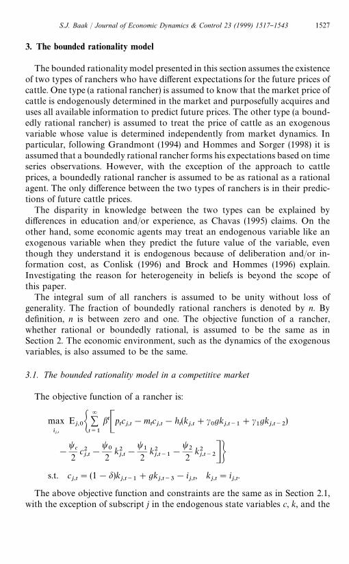
The bounded rationality model presented in this section assumes the existenceof two types of ranchers who have di!erent expectations for the future prices ofcattle. One type (a rational rancher) is assumed to know that the market price ofcattle is endogenously determined in the market and purposefully acquires anduses all available information to predict future prices. The other type (a bound-edly rational rancher) is assumed to treat the price of cattle as an exogenousvariable whose value is determined independently from market dynamics. Inparticular, following Grandmont (1994) and Hommes and Sorger (1998) it isassumed that a boundedly rational rancher forms his expectations based on timeseries observations. However, with the exception of the approach to cattleprices, a boundedly rational rancher is assumed to be as rational as a rationalagent. The only di!erence between the two types of ranchers is in their predic-tions of future cattle prices.

The disparity in knowledge between the two types can be explained bydi!erences in education and/or experience, as Chavas (1995) claims. On theother hand, some economic agents may treat an endogenous variable like anexogenous variable when they predict the future value of the variable, eventhough they understand it is endogenous because of deliberation and/or in-formation cost, as Conlisk (1996) and Brock and Hommes (1996) explain.Investigating the reason for heterogeneity in beliefs is beyond the scope ofthis paper.

The integral sum of all ranchers is assumed to be unity without loss ofgenerality. The fraction of boundedly rational ranchers is denoted by n. Byde"nition, n is between zero and one. The objective function of a rancher,whether rational or boundedly rational, is assumed to be the same as inSection 2. The economic environment, such as the dynamics of the exogenousvariables, is also assumed to be the same.

3.1. The bounded rationality model in a competitive market

The objective function of a rancher is:

maxij,t

Ej,0G

=+t/1

btCptcj,t!mtcj,t!h

t(k

j,t#c

0gk

j,t~1#c

1gk

j,t~2)

!

tc

2c2j,t!

t0

2k2j,t!

t1

2k2j,t~1

!

t2

2k2j,t~2DH

s.t. cj,t"(1!d)k

j,t~1#gk

j,t~3!i

j,t, k

j,t"i

j,t.

The above objective function and constraints are the same as in Section 2.1,with the exception of subscript j in the endogenous state variables c, k, and the


control variable i, which denotes that the variables are associated with a typej ( j"1 or 2) rancher. Hereafter, subscripts 1 and 2 represent rational andboundedly rational economic agents, respectively.

Even though these two types of ranchers have the same objective function,they have di!erent Euler equations because they predict future cattle pricesdi!erently. The Euler equation of a rational rancher is:7

EtC!p

t#m

t#t

cc1,t

!ht#b(p

t`1(1!d)!m

t`1(1!d)!t

cc1,t`1

(1!d)!ht`1

gc0)

#b2(!ht`2

gc1)#b3(p

t`3g!m

t`3g!t

cc1,t`3

g) D"0.

(14a)

Eq. (14a) is the same as Eq. (8) which was presented as the Euler equation ofa rational rancher in Section 2.8

On the other hand, the Euler equation of a boundedly rational rancher is:

EtC!p

t#m

t#t

cc2,t!h

t#b(!m

t`1(1!d)!t

cc2,t`1

(1!d)!ht`1

gc0)

#b2(!ht`2

gc1)#b3(!m

t`3g!t

cc2,t`3

g)#E2,t

(bpt`1

(1!d)#b3pt`3

g)D"0

(14b)

where E2,t

denotes the expectations operator of a boundedly rational agent. Forillustrative purposes, it is assumed that boundedly rational ranchers forecastfuture cattle prices from an AR(1) process.9 Therefore,

E2,t

(pt`1

)"a0#a

1pt. (15)

The aggregate (market) Euler equation (16) is obtained by the summation ofEqs. (14a) and (14b) after multiplying Eq. (14a) by the fraction of rationalranchers, (1!n), and multiplying Eq. (14b) by the fraction of boundedlyrational ranchers, n.

EtC!(1!n)p

t#m

t#t

cct!h

t#b((1!n)p

t`1(1!d)!m

t`1(1!d)!t

cct`1

(1!d)!ht`1

gc0)

#b2(!ht`2

gc1)#b3((1!n)p

t`3g!m

t`3g!t

cct`3

g)

!npt#nb(1!d)(a

0#a

1pt)#nb3g(b

0#a3

1pt) D"0

(16)where b

0"a

0(1#a

1(1#a

1)).

7 It is assumed that W+"0 for j"0, 1, 2 as in Section 2.1.

8They are the same because a rational rancher in Section 3, as in Section 2, is assumed to fullyunderstand the market dynamics, which also means he knows the existence of boundedly rationalranchers.

9Baak (1996) incorporated higher order AR processes as the prediction equation of the boundedlyrational ranchers. However, the empirical tests produced the best results when AR(1) process isassumed.


The same law of motion as in Eq. (9) is obtained by aggregating the con-straints of each type of rancher. From the Euler equation (16) and law of motion(9), the same conditions as in Eqs. (10) and (11) are required to assure positiveendogenous state variables at the steady state. In fact, the di!erence betweena rational and a boundedly rational rancher disappears at the steady state. Sincethe price is constant at the steady state, both ranchers have perfect foresight.

The market demand equation (7a) and the dynamics of exogenous statevariables (6a), (6b) and (7b) are still assumed. Now the market as a whole isdescribed by Euler equation (16), law of motion (9), demand equation (7a) anddynamic processes of the exogenous variables (6a), (6b) and (7b). As a matter offact, the bounded rationality model is di!erent from the rational expectationsmodel only with respect to the Euler equation.

The deep parameters of the model can be estimated with these six equationsusing GMM. Chavas (1995) adopts this methodology. In this paper, however,the deep parameters are estimated with the solutions of the model using MLEfollowing the line of AHMS. Among the merits of the AHMS methodology arethat it uses all the available cattle data sets whether or not they are shown in themodel, and that it does not require proxies for exogenous variables. In fact, threequantity data sets and one price data set are available in the U.S. beef cattlemarket and the empirical research in Section 4 uses all, and only, these four datasets. In addition, the methodology adopted in this paper automatically checksthe stationarity conditions of the model by examing the state-costate evolutionequation and the solution of the model. In the case of linear-quadratic models,the stationarity of the model should be carefully checked for the model to bemeaningful both theoretically and empirically.

The assumption of the lag of the prediction equation (15) is important becauseit in#uences the dimension of the state variables of the model. If we assume anAR(1) process for Eq. (15), the bounded rationality model has the same dimen-sion of the state variables as the rational expectations model. In contrast, if weassume a higher order of AR process, the dimension of state variables isextended. If we assume AR(2) process for Eq. (15), for example, the Eulerequation contains p

t~1term, and subsequently k

t~4and d

t~4are included as

state variables by Eqs. (7a) and (9).The market equilibrium solution is obtained by attacking the Euler equation

(16). Substituting Eqs. (6a), (7b) and (9) into the Euler equation yields

Et[(1!g~1

1¸~1)(1!g~1

2¸~1)(1!g~1

3¸~1)

](1!/1¸)(1!/

2¸)(1!/

3¸)k

t]"E

t[!C

0!M

0m

t!H

0ht!D

0dt]

where

C@0"i

2[(!i

1!(1!n)(1!d)b!(1!n)b3g)a

0

#(n(1!d)ba0#nb3gb

0)a

1],


M@0"!i

2a1(1!(1!d)bo

m!b3go3

m),

H@0"i

2a1(1#bgc

0oh#b2gc

1o2h),

D@0"!i

1i2, i

1"nb(1!d)a

1#nb3ga3

1!1, i

2"

1

tca1!i

1

,

and gi's are the roots of the polynomial equation

i2b3g(1#t

ca1!n)g3#i

2b(1!d)(1#t

ca1!n)g!1"0. (17)

The de"nitions of /i's are the same as in Section 2.1, and subsequently two

out of the three /i's are stable. As a result, to obtain a unique stationary

solution, just one out of the three g@is should be stable. If n"0, polynomial

equation (17) is the same as the characteristic equation for n@is whose values are

determined by the deep parameters of the model. In contrast, if n is a positivenumber, the roots of the polynomial equation (17) depend on the speci"cation ofthe price prediction equation (15) along with the parameter values of the modelincluding n. For example, if we assume that a

0"0 and a

1"1, then two roots of

Eq. (17), say g2

and g3, are always imaginary and always exceed unity in

modulus. For small positive values of n, the other root, g1, is real and less than

one in modulus. If n exceeds a certain positive point, n*(1, it turns out to beunstable.

The form of the prediction equation (15) will be speci"ed in Section 4.2. Untilthen, we will assume that g

1is stable and g

2and g

3are unstable. In this case, the

equilibrium solution of the model is

kt"(g

1#/

2#/

3)k

t~1!(g

1/2#/

2/

3#/

3g1)k

t~2

#g1/2/3kt~3

!C@1!D@

1dt!M@

1m

t!H@

1ht

where

C@1"

g1/~1

1(1!g~1

3)(1!g~1

2)(1!/~1

1)C@

0, D@

1"

g1/~11

1#tca1

D@0,

M@1"

g1/~1

1(1!g~1

3om)(1!g~1

2om)(1!/~1

1om)

M@0H@

1"

g1/~11

(1!g~13

oh)(1!g~1

2oh)(1!/~1

1oh)H@

0.

If we assume n"0, then the solution is the same as in Section 2.1. Since thevalue of g

1, which plays a role in the solution, is a!ected by the fraction of the

boundedly rational economic agents, the market dynamics of the model is alsoa!ected by the fraction. This issue will be revisited in Section 4.2 where theprediction equation (15) is speci"ed.


The following two sub-sections 3.2 and 3.3 illustrate how to solve thebounded rationality model using the optimal control theory.

3.2. The social planning problem with side constraints

The bounded rationality model presented in Section 3.1 cannot be repres-ented by a social planners problem because the model violates the "rst welfaretheorem by assuming heterogeneity in beliefs. In fact the model is distorted bythe presence of boundedly rational economic agents.

Competitive equilibrium models with some distortions such as externalitiesand taxes also violate the "rst welfare theorem. However, in the case of thosemodels, the dynamic optimization problem of a representative economic agentcan be replaced by a social planning problem with some side constraints (i.e.,side equilibrium conditions). That is, for those models, there can be a "ctionalsocial planning problem whose "rst-order conditions are the same as those ofthe competitive solution.10

If we examine the Euler equation (16), it looks like the Euler equation ofa representative economic agent who faces some distortions such as externalitiesor taxes. The "rst two lines of the Euler equation are the same as in the Eulerequation of a rational rancher if in the latter equation is replaced by (1!n)p

t.

The third line is an extra element in the Euler equation of a rational rancher, andit can be treated as being imposed by an equilibrium condition associated withdistortions. Speci"cally, if we include an extra term, q

tit, in the objective function

and if qtis equal to the third line of the Euler equation (16) in the equilibrium, the

aggregate Euler equation (16) can be regarded as the "rst-order condition ofa representative agent with p

treplaced by (1!n)p

t. The "ctional agent is

assumed to accept this side equilibrium condition as given, just like the demandequation. Therefore, when we solve the objective function, is treated as anexogenous variable. After obtaining the "rst-order condition of the objectivefunction, the equilibrium condition of q

tis plugged in. This is much like the &big'

Ktin the versions of Lucas and Prescott (1971) investment model analyzed by

Kydland and Prescott (1977) and Whiteman (1983).Based on this background, the bounded rationality model presented in

Section 3.1 can be transformed into a HS type social planning problem with sideconstraints. The dynamic optimization problem of the "ctional social planner is

Maxit

EtA!

1

2 G=+t/0

bt[(st!b

t)@(s

t!b

t)#u@

tut!2i

tqt]HB (18)

s.t. /gut"!/

cct!/

iit#Ck

t~1#d

t,

10For example, see Becker (1985) and McGrattan (1994).


kt"D

kkt~1

#Hkit,

ht"D

hht~1

#Hhct,

st"Kh

t~1#Pc

t,

where

P"

J1!n

Ja1

and

;b"C

a0J1!n

Ja1

0 0J1!n

Ja1D .

The other variables and parameters are de"ned in the same way as inSection 2.2.

The objective function (18) contains a new term, itqt, which was not a part of

the objective function (12) in the rational expectations model. The variableqtshould satisfy the following side constraint:

qt"B

0#B

1kt~1

#B3kt~3

#Bddt#B

iit

(19)

where

B0"A

0#

a0

a1

A1, B

1"!

1!da1

A1, B

3"!

g

a1

A1, B

d"B

i"

1

a1

A1,

A0"n(b(1!d)a

0#b

3gb

0) and A

1"n(b(1!d)a

1#b

3ga3

1!1).

The right-hand side of constraint (19) is the same as the third line of the Eulerequation (16). To make the third line serve as a function of state and controlvariables, demand equation (7a) and law of motion (9) were substituted forptand c

t.

In the following section, objective function (18) will be reformatted into anoptimal regulator problem with distortions (side equilibrium conditions).

3.3. The optimal regulator problem

The dynamic optimization problem of a "ctional social planner (18) can bemapped into the following discounted optimal linear regulator problem withside equilibrium conditions:

Maxut

EtA!

4+t/0

btA[xt,q

t]C

Q11

Q12

Q21

Q22D C

xt

qtD#u@

tRu

t#2[x

t,q

t] C=

1=

2DutBB

s.t. xt`1

"Axxt#A

qqt#Bu

t#Ce

t`1(20)


where Q11"Q, Q

12"[0,0,0,0,0,0,0,0]@, Q

21"Q@

12, Q

22"0, =

1"=,

=2"!1

2, A

x"A, A

z"0. The vectors and matrices (x

t, u

t, Q, R,=, A, B, C)

are de"ned in the same way as in Section 2.3. The side equilibrium condition (19)is imposed in the following form:

qt"Hx

t#Wu

t

where H"[0, B1, B

2, B

3, B

0, 0, 0, B

d] and W"B

i.

The dynamic optimization problem (20) includes a discount factor (b) andcross-product terms. McGrattan (1994) and AHMS suggest converting theproblem to one without cross-products and discounting to simplify the analysis.Let xI

t"bt@2x

t, qJ

t"bt@2q

t, uJ

t"bt@2u

t, eJ

t"bt@2e

t, QI

11"Q

11!=

1R~1=@

1,

QI12"Q

12!=

1R~1=@

2, QI

22"Q

22!=

2R~1=@

2, AI

x"Jb(A

x!BR~1=@

1),

AIq"Jb(A

q!BR~1=@

2), BI "JbB, HI "(I#WR~1=@

2)~1(H!WR~1=@

1),

and WI "(I#WR~1=@2)~1W.

With these de"nitions, we can restate the optimization problem as follows:

Maxut

EtA

=+t/0

[xJtqt] C

QI11

QI12

QI21

QI22D C

xJt

qtD#uJ @

tRuJ

tBs.t. xJ

t`1"AI

xxJt#AI

qqJt#BI uJ

t#CeJ

t`1.

Let AK "AIx#AI

qHI , QK "QI

11#QI

12HI , BK "BI #AI

qWI , and AI "AI

x!

BI R~1WI @QI @12

. The solution of the problem is given by uJt"!FI x

t, where

FI "(R#BI @PBK )~1BI @PAK , and P satis"es P"QK #AI @PAK !AI @PBK (R#B@PBK )~1

B@PAK . The solution of the original problem is given byF"(R#=@2W)~1

(RFI #=@1#=@

2H) and the equilibrium law of motion for x

tis x

t`1"A0x

t,

A0"Ax#A

qH!A

qWF!BF"b~1@2(AK !BK F).11

The computer programs capable of searching for the solution for the boundedrationality model (the optimal linear regulator problem with distortions) in thispaper were coded by modifying AHMSs computer programs which were usedfor solving their rational expectations model (the optimal linear regulatorproblem without distortions). The programs should generate the same solutionas in Section 3.1, when the same parameter values are assigned. Also, if weassume, they should generate the same solution as in Section 2. The validity ofthe computer programs that solve the bounded rationality model was checkedby these conditions. As in the case of the computer programs for the rationalexpectations model, the computer programs for the bounded rationality modelcheck the regulatory conditions for a unique stationary solution by investigatingthe eigenvalues of the transition matrix of the state}costate evolution equation.

11See Appendix B.3 in AHMS and Appendix B in Hansen et al. (1994).


The computer yields error messages if the regulatory conditions are violated. Ifthe conditions are satis"ed, one of the roots of characteristic equation (17) inSection 3.1, g

1, is stable and the other two roots, g

2and g

3, are unstable.

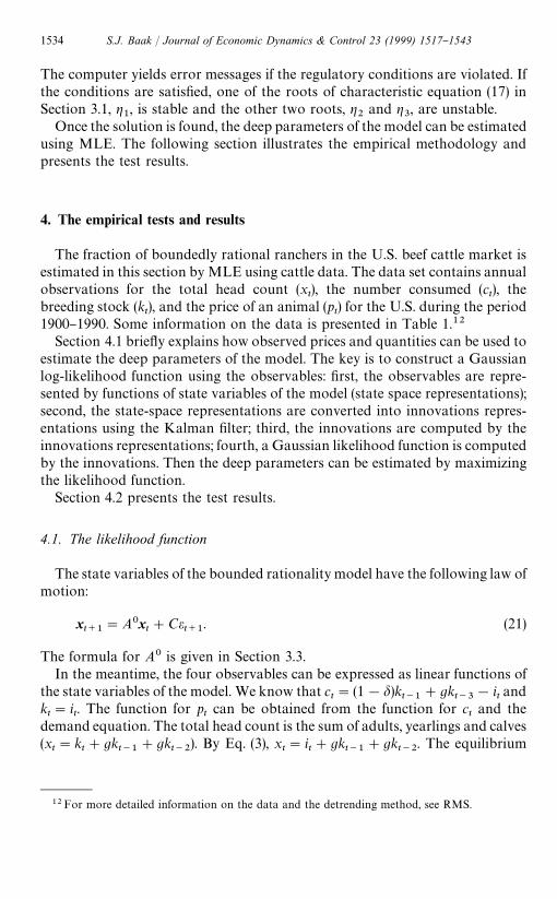
Once the solution is found, the deep parameters of the model can be estimatedusing MLE. The following section illustrates the empirical methodology andpresents the test results.

4. The empirical tests and results

The fraction of boundedly rational ranchers in the U.S. beef cattle market isestimated in this section by MLE using cattle data. The data set contains annualobservations for the total head count (x

t), the number consumed (c

t), the

breeding stock (kt), and the price of an animal (p

t) for the U.S. during the period

1900}1990. Some information on the data is presented in Table 1.12Section 4.1 brie#y explains how observed prices and quantities can be used to

estimate the deep parameters of the model. The key is to construct a Gaussianlog-likelihood function using the observables: "rst, the observables are repre-sented by functions of state variables of the model (state space representations);second, the state-space representations are converted into innovations repres-entations using the Kalman "lter; third, the innovations are computed by theinnovations representations; fourth, a Gaussian likelihood function is computedby the innovations. Then the deep parameters can be estimated by maximizingthe likelihood function.

Section 4.2 presents the test results.

4.1. The likelihood function

The state variables of the bounded rationality model have the following law ofmotion:

xt`1

"A0xt#Ce

t`1. (21)

The formula for A0 is given in Section 3.3.In the meantime, the four observables can be expressed as linear functions of

the state variables of the model. We know that ct"(1!d)k

t~1#gk

t~3!i

tand

kt"i

t. The function for p

tcan be obtained from the function for c

tand the

demand equation. The total head count is the sum of adults, yearlings and calves(x

t"k

t#gk

t~1#gk

t~2). By Eq. (3), x

t"i

t#gk

t~1#gk

t~2. The equilibrium

12For more detailed information on the data and the detrending method, see RMS.


Table 1Sample means and standard deviations

Variable Mean Std. Dev.

xt

44.253 9.273kt

16.636 4.041ct

14.604 3.123pt

13.382 6.494

solution is it"!Fx

t. If we add measurement errors to the observables, we can

obtain the following:

yt"Gx

t#v

t(22)

where yt"[x

t, k

t, c

t, p

t]@, v

tis a martingale di!erence sequence of measurement

errors that satis"es Evtv@t"R, Ee

t`1v@s"0 for all t#15s, and

G"C0 g g 0 0 0 0 0 0

0 0 0 0 0 0 0 0 0

0 (1!d) 0 g 0 0 0 0 0

0 ~(1~d)a1 0 ~g

a1 0 a0a1 0 0 1

a1

0

0

0

0D#C!FI

!FI

FI

!FI /a1D .

Eqs. (21) and (22) yield the following state space representation of the model:

xt`1

"A0xt#Ce

t`1, (23)

yt`1

"GA0xt#GCe

t`1#v

t`1.

Then, the time-invariant innovations representation for system (23) is

xLt`1

"A0xLt#Ka

t, (24)

yt`1

"GA0xLt#a

t,

where xLt"E) [x

tD y

t, y

t~1,2, y

0, xL

0], a

t"y

t`1!E) [y

t`1D y

t, y

t~1,2, y

0, xL

0],

K is the Kalman gain, and E) is the linear least squares projection operator.13The innovations to y

t(i.e., a

t) can be recursively computed by Eq. (24), if we

assume xL0"x

0where x

0is the initial value of x

t. That is, a

0"y

1!GA0xL

0,

xL1"A0xL

0#Ka

0, a

1"y

2!GA0xL

1and so on. Then, the log likelihood function

for MytN is:14

¸(h)"!

1

2

T+t/0

MlogDXtD#trace(X~1

tata@t)N

13See Hamilton (1995), (Chapter 5) and Hansen and Sargent (1996), (Chapter 8).

14See AHMS (Section 11).


where Xt

is the covariance matrix of at. AHMS shows that X

tequals

GA0R(GA0)@#R where R is the state covariance matrix associated with theKalman "lter. The Kalman gain and the state covariance matrix can be com-puted by a MATLAB function kfilter coded by Hansen and Sargent (1996).

AHMS illustrate the analytic derivatives of the log-likelihood function andthe formula for the standard errors in the Appendix and Section 11 of theirpaper, respectively.

4.2. The estimations and results

The computer programs used for the estimations in this paper are based onthe programs coded by AHMS.15 Since AHMS's codes are designed to estimatethe deep parameters of the rational expectations model, they deal with anoptimal control problem without distortions. We modi"ed these codes to solvean optimal control problem with distortions and estimate the parameters of thebounded rationality model of this paper. If we set n"0, the bounded rationalitymodel collapses to the rational expectations model. Therefore, the solutions, thelog-likelihood functions, and the derivatives of the functions of the two modelsshould be exactly the same if n"0. The modi"ed computer codes satisfy thiscondition.

In Section 3, we assumed that boundedly rational cattle producers believedthat the cattle price had an AR(1) process. Therefore, the "rst stage of theestimation requires that we determine the coe$cients of the AR(1) processgoverning the expectation scheme of the boundedly rational producers. Thecoe$cients in the AR(1) process are estimated by OLS using the annual timeseries of the cattle price. The estimates (with standard errors in parenthesis) ofthe coe$cients are shown in the following regression equation:

pt`1

"1.760#0.881 pt, R2"0.740.

(0.832) (0.056). (25)

Since the expectations of the boundedly rational agents are formulated froma time series model of the market price, it may be interpreted as a kind ofquasi-rational expectation suggested by Nerlove et al. (1979).

Bounded rationality models incorporating pure static expectations or AR(2)process for the prediction equation of boundedly rational agents were alsotested. Even if they produced lower likelihood values than the model incorporat-ing AR(1) process, they generated estimates similar to those reported in thispaper.

15Both are programmed by MATLAB. The codes of AHMS were kindly supplied by EllenMcGrattan.


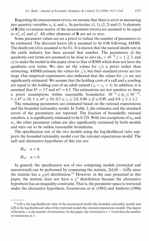
Regarding the measurement errors, we assume that there is error in measuringjust quantity variables x

t, k

tand c

t. In particular, (1, 1), (2, 2) and (3, 3) elements

of R (the covariance matrix of the measurement errors) are assumed to be equalto p2

x, p2

kand p2

c. All other elements of R are set to zero.

Some parameter values are set a priori to reduce the number of parameters tobe estimated. The discount factor (b) is assumed to be 0.96 following AHMS.The death rate (d) is assumed to be 0.1. It is known that the natural death rate inthe cattle industry has been around that number. The parameters of thequadratic cost terms are assumed to be close to zero (t

j"10~8, j"1, 2, 3, and

c), to make the model in this paper close to that of RMS which does not have thequadratic cost terms. We also set the values for c

j's a priori rather than

estimating. AHMS estimate the values for cj's, but their standard errors are too

large. Our empirical experiments also indicated that the values for cj's are not

signi"cantly estimated. We assume that the holding costs of a calf and a yearlingare equal to the holding cost of an adult animal (c

0"c

1"1). In addition, it is

assumed that h*"3.7 and m*"6.3. The estimations are not sensitive to thesea priori assumptions within reasonable boundaries: 10~64t

j410~10,

14h*410, 14m*410, 0.34cj42.0, 0.904b40.99, and 0.84d41.2.

The remaining parameters are estimated based on the rational expectationsand the bounded rationality model. In Table 2, the estimates and the standarderrors of the parameters are reported. The fraction of boundedly rationalranchers, n, is signi"cantly estimated to be 0.329. With two exceptions of p

mand

px, the other parameter values are also signi"cantly estimated by both models

and turn out to be within reasonable boundaries.The speci"cation test of the two models using the log-likelihood ratio sup-

ports the bounded rationality model over the rational expectations model. Thenull and alternative hypotheses of this test are:

H0: n"0,

HA: n'0.

In general, the speci"cation test of two competing models (restricted andunrestricted) can be performed by computing the statistic, 2(¸(hK )!¸(hI )), sincethe statistic has a s

2(r) distribution.16 However, in the case presented in this

paper, the statistic does not have a s2 distribution because the alternativehypothesis has an inequality constraint. That is, the parameter space is restrictedunder the alternative hypothesis. Gourieroux et al. (1982) and Andrews (1996)

16¸(hK ) is the log-likelihood value of the unrestricted model (the bounded rationality model) and¸(hI ) is the log-likelihood value of the restricted model (the rational expectations model). The degreeof freedom, r, is the number of restrictions. In this paper, the restriction is n"0 and thus the numberof restrictions is 1.


Table 2MLE test results of the two models

Parametersestimated

Theoreticalbenchmarks

Rational expectations model!(let n"0)

Bounded rationalitymodel

Estimates Std. Error Estimates Std. Error

n 04n41 n.a. n.a. 0.329 0.110a0

# 19.127 0.544 19.931 0.251a1

# 0.559 0.034 0.555 0.020g Around 0.85 0.861 0.014 0.835 0.002oh

0(o)(1 0.950 0.024 0.938 0.015

om

0(o.(1 0.774 0.199 0.663 0.116

ph

0.928 0.227 0.572 0.119pm

6.687 506.21 1.400 5.867pd

4.171 0.260 2.777 0.081px

# 0.033 0.0309 0.000 0.001pk

# 1.704 0.320 0.129 0.014pc

# 7.076 0.576 11.379 1.332

Log likelihood !487.16 !424.55

!The test results of this column are produced by the computer programs for the rational expectationsmodel. The computer programs for the bounded rationality model re-produce these results when weset n"0.

show that the critical point for the speci"cation test can be calculatedfrom a mixture of Chi-squared distributions. Speci"cally, under the null hypoth-esis, the critical value is obtained from 1

2s2(0)#1

2s2(1). The critical value at

the 5% signi"cance level is 2.71 and the likelihood ratio exceeds the criticalvalue with a large margin. Therefore, the null hypothesis of full rationality isrejected.

Table 3 shows the mean-squared errors of one-step ahead forecasts for eachof the four observables. The one-step ahead forecasts are computed by GA0xL

tusing the estimated parameter values of the two models. The bounded rational-ity model produces lower mean-squared errors for the three quantity variablesand a slightly higher mean-squared error for the price variable.17

In Section 3.1, we mentioned that the stationarity and the dynamics of thebounded rationality model depend on the fraction of the boundedly rational

17 It may be somewhat intriguing that the mean-squared errors only for the quantity variables,and not the price variable, are smaller for the bounded rationality model. However, there is notheoretical reason that the bounded rationality model should be better in forecasting just thequantities. Even if the bounded rationality model generates a slightly higher mean-squared error forthe price variable, it is notable that the bounded rationality model produces lower mean-squarederrors associated with three out of four observables.


Table 3Mean squared errors of one-step ahead forecasts

xt

kt

ct

pt

RE! 8.080 7.740 9.720 14.320BR" 7.331 7.438 7.335 14.532

!RE"rational expectations model."BR"bounded rationality model.

economic agents. If we compute the values of g@is using the estimated parameter

values and the coe$cients of the AR(1) prediction equation, we can con"rm thatg1

is stable and g2

and g3

are unstable when n"0.329. As mentioned inSection 3.3, this implies that the regularity conditions are satis"ed.

Regardless of the magnitude of n, g2

and are imaginary and exceed unity inmodulus. If n"0, g

1has the same value as u

1which is positive, real and less

than one in modulus. For small positive values of n (n(0.789"n*), g1

is stillpositive real and stable. Therefore, as far as n is less than n*, the boundedrationality model shows similar dynamics to the rational expectations model. Ifthe value of n exceeds n*, the value of g

1turns out to be negative and

subsequently the dynamics of the bounded rationality model becomes quitedi!erent from that of the rational expectations model. For example, simulationsfrom both of the rational expectations model and the bounded rationality modelwith n"0.329 revealed that the cattle market would have reached the steadystate within 20 periods from 1900, if there had not been any outside shocks. Incontrast, the bounded rationality model with n"0.8 required 3433 periodsto reach the steady state under the same conditions. If the fraction of theboundedly rational economic agents is higher than n**"0.907, g

1exceeds

unity in modulus and the bounded rationality model loses stationarity.These "ndings imply that the dynamics of a market is closely related with the

expectation formation of the market participants. Even if the market conditionsdo not change, the market dynamics can be altered if the fraction of boundedlyrational economic agents changes. This issue could be explored with a model inwhich the fraction of a type of market participants is endogenously determinedwithin the model, such as in Brock and Hommes (1996). However, in this paper,for econometric tractability, the fraction of boundedly rational economic agentsis assumed to be exogenous and constant over the whole period.

5. Summary and conclusions

In this paper, we present a methodology which uses economic data to detectthe existence of boundedly rational economic agents. By the methodology, we


test for bounded rationality in the U.S. beef cattle market based on a boundedrationality model which generalizes the rational expectations model of RMS byassuming heterogeneity in beliefs. If the fraction of boundedly rational ranchersis zero, the bounded rationality model collapses to the rational expectationsmodel.

The bounded rationality model is solved by the methodologies developedby the optimal control theory. In order to do so, the following proceduresare taken: "rst, the model is transformed into a social planning problemwith side equilibrium conditions; second, the social planning problem is refor-matted to an optimal regulator problem with distortions; third, the optimalregulator problem is solved by the methodologies developed by McGrattan(1994).

The fraction of boundedly rational economic agents is estimated basedon the solution of the model using the Kalman "lter and MLE. The observ-ables of cattle data are represented in the state space form using the solution ofthe model, and then the state space representations are used to generateinnovations representations. The innovations to the observed data are cal-culated by the innovations representations and used to construct the log-likelihood function of the model. Then the values of the deep parametersof the model are estimated by maximizing the value of the log-likelihoodfunction.

The empirical tests by MLE indicate that some positive fraction(about 33%) of the cattle market participants are boundedly rational. Thepoint estimate of the fraction of boundedly rational agents is positiveand signi"cant. Moreover, the log-likelihood ratio test implies that thebounded rationality model is better speci"ed than the rational expecta-tions model in which the fraction of boundedly rational agents is assumed to bezero.

In addition, the bounded rationality model produces lower mean squarederrors of one-step ahead forecasting experiments than the rational expectationsmodel.

Acknowledgements

I would like to thank two anonymous referees and the participants of the 1997SCE conference at Stanford for their helpful comments, and Jean-Paul Chavas,Dee Dechert and Blake LeBaron for their invaluable advice. I would especiallylike to thank William Brock for his guidance during the shaping of this paper.I also thank Ellen McGrattan for permitting me to use her computer codes andSherwin Rosen for providing me with the U.S. cattle data. Any errors, of course,remain my own.


Appendix A. The de5nitions of the parameters in Section 2.2

K"Dh"H

h"0, P"

1

Ja1

, ;b"C

a0

Ja1

, 0, 0,1

Ja1D,

/c"C

1

0

0

0

!f7D , /

i"C

1

!f5

0

0

0 D , /g"C

0 0 0 0

1 0 0 0

0 1 0 0

0 0 1 0

0 0 0 1D ,

C"C(1!d) 0 g

0 0 0

f1

0 0

0 f3

0

0 0 0D , ;d"C

0 0 0 0

0 f6

0 0

0 f2

0 0

0 f4

0 0

0 0 f8

0D ,

Dk"C

0 0 0

1 0 0

0 1 0D , Hk"C

1

0

0D ,

A22"C

1 0 0 0

(1!oh)h* o

h0 0

(1!om) m* 0 o

m0 0 0 0 D , C

2"C

0 0 0

ph

0 0

0 pm

0

0 0 pdD ,

f 21"t

0, f 2

3"t

1, f 2

5"t

2, f 2

7"t

c;

f1

f2"1, f

3f4"c

0g, f

5f6"c

1g, f

7f8"1.

Appendix B. The de5nitions of the parameters in Section 2.3

xt"[h@

t~1, k@

t~1, z@

t]@, z

t"[1, h

t, m

t, d

t]@, u

t"i

t,

A"CDhhh;

c[/

c, /

g]~1C h

h;

c[/

c, /

g]~1;

d0 D

k0

0 0 A22

D ,


B"C!h

h;

c[/

c, /

g]~1/

iH

k0 D , C"C

0

0

C2D ,

Hs"[K, P;

c[/

c, /

g]~1C, P;

c[/

c, /

g]~1;

d!;

b] ,

Hc"[!P;

c[/

c, /

g]~1/

i],

Gs"[0,;

g[/

c, /

g]~1C,;

g[/

c, /

g]~1;

d] , G

c"[!;

g[/

c, /

g]~1/

i]

;c"[1, 0, 0, 0, 0], ;

g"C

0 1 0 0 0

0 0 1 0 0

0 0 0 1 0

0 0 0 0 1D ,

R"!12

(H@sH

s#G@

sG

s), Q"!1

2(H@

cH

c#G@

cG

c),

="!12

(H@cH

s#G@

cG

s).

References

Anderson, E.W., Hansen, L.P., McGrattan, E.R., Sargent, T.J., 1995. Mechanics of forming andestimating dynamic linear economies. Mimeo, University of Chicago.

Andrews, D.W.K., 1996. Admissibility of the likelihood ratio test when the parameter space isrestricted under the alternative. Econometrica 64, 705}718.

Arthur, W.B., Holland, J., LeBaron, B., Palmer, R., Taylor, P., 1997a. Asset pricing under endogen-ous expectations in an arti"cial stock market. In: Arthur, W.B., Durlauf S., Lane, D., (Eds.), TheEconomy as an Evolving Complex System II. Addison-Wesley, Redwood City, pp. 15}44.

Arthur, W.B., LeBaron, B., Palmer, R., 1997b. Time series properties of an arti"cial stock market.SSRI Working paper 9725, University of Wisconsin-Madison.

Becker, R.A., 1985. Capital income taxation and perfect foresight. Journal of Public Economics 26,147}167.

Baak, S., 1996. Bounded rationality: an application to the U.S. cattle market. Technical Report,University of Wisconsin-Madison.

Brock, W., Hommes, C., 1995. Rational routes to randomness. SSRI Working paper 9506, Univer-sity of Wisconsin-Madison.

Brock, W., Hommes, C., 1996. Heterogeneous beliefs and routes to chaos in a simple asset pricingmodel. SSRI Working paper 9621, University of Wisconsin-Madison.

Brock, W., Hommes, C., 1997. A rational route to randomness. Econometrica 65, 1059}1095.Brock, W., LeBaron, B., 1996. A dynamic structural model for stock return volatility and trading

volume. Review of Economics and Statistics 78, 94}110.Chavas, J.P., 1995. On the economic rationality of market participants: the case of expectations in

the U.S. pork market. Mimeo, University of Wisconsin-Madison.Chavas, J.P., Holt, M., 1993. Market instability and nonlinear dynamics. American Journal of

Agricultural Economics 75, 113}120.


Conlisk, J., 1996. Why bounded rationality? Journal of Economic Literature 34, 669}700.Diebold, F.X., Ohanian L.E., J., Berkowitz, 1995. Dynamic equilibrium economies: a framework for

comparing models and data. Working paper, University of Pennsylvania.de Fontnouvelle, P., 1994. Stock returns and trading volume: a structural explanation of the

empirical regularities. Mimeo, University of Wisconsin-Madison.Gourieroux, C., Holly, A., Monfort, A., 1982. Likelihood ratio test, Wald test, and Kuhn-Tucker test

in linear models with inequality constraints on the regression parameters. Econometrica 50,63}80.

Grandmont, J.M., 1994. Expectations formation and stability in large socioeconomic systems.CEPREMAP Working paper 9424.

Hansen L.P., McGrattan E.R., Sargent, T.J., 1994. Mechanics of forming and estimating dynamiclinear economies, Research department sta! report 182, Federal Reserve Bank of Minneapolis.

Hansen, L., Sargent, T., 1996. Recursive linear models of dynamic economies. Manuscript, Univer-sity of Chicago.

Hommes, C.H., Sorger, G., 1998. Consistent expectations equilibria. Macroeconomic Dynamics 2,287}321.

Kydland, F.E., Prescott, E., 1977. Rules rather than discretion: the inconsistency of optimal plans.Journal of Political Economy 85, 473}491.

Lucas, R.E., Prescott, E.C., 1971. Investment under uncertainty. Econometrica 39, 659}681.McGrattan, E., 1994. A note on computing competitive equilibria in linear models. Journal of

Economics Dynamics and Control 18, 149}160.Nerlove, M., Grether, D., Carvalho, J.L., 1979. Analysis of Economic Time Series. Academic Press,

New York.Nerlove, M., Fornari, I., 1998. Quasi-rational expectations, an alternative to fully rational expecta-

tions: an application to US beef cattle supply. Journal of Econometrics 83, 129}161.Rosen, S., Murphy, K., Scheinkman, J., 1994. Cattle cycle. Journal of Political Economy 102,

468}492.Sargent, T., 1987. Macroeconomic Theory. 2nd ed., Academic Press, Orlando.Sargent, T., 1993. Bounded Rationality in Macroeconomics. Clarendon Press, Oxford.Whiteman, C., 1983. Linear Rational Expectations Models: A User's Guide. University of

Minnesota Press, Minneapolis.


Tests for bounded rationality with a linear dynamic model distorted by heterogeneous expectations

Documents

Transcript of Tests for bounded rationality with a linear dynamic model distorted by heterogeneous expectations