TES mapping of Mars' north seasonal cap
19
Icarus 154, 162–180 (2001) doi:10.1006/icar.2001.6670, available online at http://www.idealibrary.com on TES Mapping of Mars’ North Seasonal Cap Hugh H. Kieffer and Timothy N. Titus U.S. Geological Survey, Flagstaff, Arizona 86601 E-mail: [email protected] Received January 17, 2001; revised May 3, 2001 The Mars Global Surveyor thermal emission spectrometer has made observations of Mars’ north polar region for nearly a full martian year. Measurements of bolometric emission and reflectance, as well as brightness temperatures in specific bands synthesized from thermal radiance spectra, are used to track the behavior of sur- face and atmospheric temperatures, the distribution of condensed CO 2 and H 2 O, and the occurrence of dust storms. CO 2 grain size in the polar night is variable in space and time, and is influenced by at- mospheric conditions. Some specific locations display concentration of H 2 O frost and indicate the presence of long-term water-ice near the surface. Annual budgets of solid CO 2 range up to 1500 kg m −2 ; preliminary analysis suggests significant transport of energy into latitudes near 70 ◦ N during the polar night. c 2001 Elsevier Science Key Words: Mars; ices; infrared observations. 1. INTRODUCTION The seasonal polar caps are a major element of Mars’ cli- mate and circulation. Theoretical calculations (Leighton and Murray 1966, Forget et al. 1998) and surface pressure mea- surements (Tillman et al. 1993) indicate that about 1 4 of the CO 2 in the atmosphere condenses each year in the seasonal caps. The atmosphere above the north cap, but not the south, becomes nearly saturated with water vapor as the CO 2 disappears in late summer (Farmer et al. 1976, Jakosky and Haberle 1992). The importance of water to human interest in exploration of Mars makes its important to minimize any confusion between the oc- currence of CO 2 and H 2 O frost. The similarity in reflectance of fresh CO 2 and H 2 O snow makes them difficult to distinguish in monochrome or multiband reflectance imaging unless cover- age extends longward of about 1 µm. Because the condensation temperatures of CO 2 and H 2 O differ by about 50 K, with solid CO 2 not occurring on Mars above about 150 K, temperature measurements are generally unambiguous in determining the composition of transitory “white stuff.” Thermal infrared ob- servations have resolved the composition of the seasonal and permanent polar caps on Mars (Neugebauer et al. 1971, Hanel et al. 1972, Kieffer et al. 1976, Kieffer 1979). The dense cov- erage of the Mars polar regions by the thermal emission spec- trometer (TES) on the Mars Global Surveyor (MGS) space- craft provides the ability to monitor the seasonal variations of condensates. The Mars Global Surveyor spacecraft was inserted in orbit around Mars in September 1997, but did not attain its mapping orbit until March 1999 (Albee et al. 1998, Albee et al. 2001). This paper is intended as an overview of TES observations of the north polar region, especially the seasonal cap, for a martian year. It addresses the annual cycle and is a companion to the first analysis of MOC wide-angle observations acquired at the same time (James and Cantor 2001). The TES measures directly the total reflected and emitted ra- diation from the surface and atmosphere, which in turn allow measurement of the geographic variation of the net radiation balance and, through integration of the inferred condensation/ sublimation rates, the annual solid CO 2 budget; this is a useful constraint on global circulation models (GCMs). These obser- vations also address the nature of transient brightenings around the polar cap, and TES spectral capabilities will constrain, if not determine, the composition of the dark lanes interior to the permanent caps. TES observations of the south polar region during the aero- braking phase (southern summer) revealed an unexpected large range of CO 2 albedo (Kieffer et al. 2000) (termed herein Paper I) and observations of the northern winter cap showed that CO 2 condensation occurred in three forms, including a slab-ice form thought to be the cause of the low-albedo CO 2 deposits (Titus et al. 2001) (termed herein Paper II). The brightness variations of CO 2 and H 2 O seasonal frosts are a major aspect of this current paper. Although there are some gaps in seasonal coverage, spectral observations are used to help separate the properties of the at- mosphere, clouds, soil surface, and surface ices. An overview of seasonal events is provided by averaging over longitude to reveal the fundamental relations as a function of latitude and time. Lo- cal deviations from these zonal-average trends are identified, and most are probably associated with the spatially irregular abun- dance of H 2 O. Estimates of the heat budget associated with the condensation and sublimation of solid CO 2 leave major issues unanswered. This paper is intentionally largely descriptive. The numer- ous implications for the nature of the seasonal deposits and 162 0019-1035/01 $35.00 c 2001 Elsevier Science All rights reserved.
-
Upload
independent -
Category
Documents
-
view
4 -
download
0
Transcript of TES mapping of Mars' north seasonal cap

Icarus 154, 162–180 (2001)
doi:10.1006/icar.2001.6670, available online at http://www.idealibrary.com on
TES Mapping of Mars’ North Seasonal Cap
Hugh H. Kieffer and Timothy N. Titus
U.S. Geological Survey, Flagstaff, Arizona 86601E-mail: [email protected]
Received January 17, 2001; revised May 3, 2001
The Mars Global Surveyor thermal emission spectrometer hasmade observations of Mars’ north polar region for nearly a fullmartian year. Measurements of bolometric emission and reflectance,as well as brightness temperatures in specific bands synthesizedfrom thermal radiance spectra, are used to track the behavior of sur-face and atmospheric temperatures, the distribution of condensedCO2 and H2O, and the occurrence of dust storms. CO2 grain size inthe polar night is variable in space and time, and is influenced by at-mospheric conditions. Some specific locations display concentrationof H2O frost and indicate the presence of long-term water-ice nearthe surface. Annual budgets of solid CO2 range up to 1500 kg m−2;preliminary analysis suggests significant transport of energy intolatitudes near 70◦N during the polar night. c© 2001 Elsevier Science
Key Words: Mars; ices; infrared observations.
craft provides the ability to monitor the seasonal variations of
6
1. INTRODUCTION
The seasonal polar caps are a major element of Mars’ cli-mate and circulation. Theoretical calculations (Leighton andMurray 1966, Forget et al. 1998) and surface pressure mea-surements (Tillman et al. 1993) indicate that about 1
4 of the CO2
in the atmosphere condenses each year in the seasonal caps.The atmosphere above the north cap, but not the south, becomesnearly saturated with water vapor as the CO2 disappears in latesummer (Farmer et al. 1976, Jakosky and Haberle 1992). Theimportance of water to human interest in exploration of Marsmakes its important to minimize any confusion between the oc-currence of CO2 and H2O frost. The similarity in reflectance offresh CO2 and H2O snow makes them difficult to distinguishin monochrome or multiband reflectance imaging unless cover-age extends longward of about 1 µm. Because the condensationtemperatures of CO2 and H2O differ by about 50 K, with solidCO2 not occurring on Mars above about 150 K, temperaturemeasurements are generally unambiguous in determining thecomposition of transitory “white stuff.” Thermal infrared ob-servations have resolved the composition of the seasonal andpermanent polar caps on Mars (Neugebauer et al. 1971, Hanelet al. 1972, Kieffer et al. 1976, Kieffer 1979). The dense cov-erage of the Mars polar regions by the thermal emission spec-trometer (TES) on the Mars Global Surveyor (MGS) space-
1
0019-1035/01 $35.00c© 2001 Elsevier Science
All rights reserved.
condensates.The Mars Global Surveyor spacecraft was inserted in orbit
around Mars in September 1997, but did not attain its mappingorbit until March 1999 (Albee et al. 1998, Albee et al. 2001).This paper is intended as an overview of TES observations ofthe north polar region, especially the seasonal cap, for a martianyear. It addresses the annual cycle and is a companion to the firstanalysis of MOC wide-angle observations acquired at the sametime (James and Cantor 2001).
The TES measures directly the total reflected and emitted ra-diation from the surface and atmosphere, which in turn allowmeasurement of the geographic variation of the net radiationbalance and, through integration of the inferred condensation/sublimation rates, the annual solid CO2 budget; this is a usefulconstraint on global circulation models (GCMs). These obser-vations also address the nature of transient brightenings aroundthe polar cap, and TES spectral capabilities will constrain, ifnot determine, the composition of the dark lanes interior to thepermanent caps.
TES observations of the south polar region during the aero-braking phase (southern summer) revealed an unexpected largerange of CO2 albedo (Kieffer et al. 2000) (termed herein Paper I)and observations of the northern winter cap showed that CO2
condensation occurred in three forms, including a slab-ice formthought to be the cause of the low-albedo CO2 deposits (Tituset al. 2001) (termed herein Paper II). The brightness variationsof CO2 and H2O seasonal frosts are a major aspect of this currentpaper.
Although there are some gaps in seasonal coverage, spectralobservations are used to help separate the properties of the at-mosphere, clouds, soil surface, and surface ices. An overview ofseasonal events is provided by averaging over longitude to revealthe fundamental relations as a function of latitude and time. Lo-cal deviations from these zonal-average trends are identified, andmost are probably associated with the spatially irregular abun-dance of H2O. Estimates of the heat budget associated with thecondensation and sublimation of solid CO2 leave major issuesunanswered.
This paper is intentionally largely descriptive. The numer-ous implications for the nature of the seasonal deposits and
2

163

164 KIEFFER AND TITUS
FIG. 3. A mosaic showing areas of water-ice (purple), and bright (green) and dark (red) nonvolatile materials; orientation as in Fig. 1. The purple areas haveT25 less than 210 K. The green areas have T25 above 210 K and Lambert albedo brighter than 0.17. The red areas have T25 above 210 K and Lambert albedo darker
than 0.17. The data cover Ls = 137◦ to 146◦. Observations of cryptic-like material during the northern spring are only located where the underlying substrate was dark (red areas). Small yellow areas are transitional between dark and bright soilsunderlying material, and the nature of the seasonal and longerclimate cycles, are beyond the scope of this paper.
2. OBSERVATIONAL COVERAGE
The MGS spacecraft orbit has an inclination of 93◦, ascending(going north) on the nightside and going south (descending) onthe dayside with a 14-h Mars local time (H) equator crossing.For simplicity, we will refer to TES observations acquired on the
ascending leg as AM and those acquired on the descending legas PM. In normal mapping nadir-oriented mode, TES sweeps aMGS TES observed the north polar region during the first2 years of mapping, over Ls = 104◦–360◦–93◦. Bolometer data
FIG. 1. Thermal mosaic of the north polar region in mid-summer. T30 data for 18 days of TES observations from the north polar ring out to 70◦N latitude fromLs = 137◦ to 146◦. The data gaps near 85◦N are due to acquisition of emission phase function observations; the gaps near 79◦ and 72◦N are due to acquisition oflimb observations. The outline of the regions of interest are shown (see text and Table I). Latitudes 70◦ and 80◦N are shown as circles. Longitude 0◦is toward thebottom of the figure, and west longitudes run clockwise.
FIG. 2. A Lambert albedo mosaic showing the permanent polar cap; orientation as in Fig. 1. Only areas with T25 below 210 K are shown. The color scale
has a minimum threshold of 0.30 to demarcate the dark interior lanes. The datanorthern limit is the cold-and-bright anomaly.; blue areas are transitional between soil and ice.
9-km wide swath along the sub-spacecraft track, which is almostparallel to meridians except near the pole (Figs. 1 and 2). In thisobservation mode, the time between repeat coverage is highlydependent on latitude, ranging from only a few hours along the“polar rings” at ±87◦ latitude to several days at ±60◦. Thisallows detailed analysis of spatial and temporal changes nearthe polar caps. However, at more equatorial latitudes seasonalanalysis of specific locations is restricted due to the lengthyrepeat time, approaching hundreds of days near the equator.
cover the summer season from Ls = 137◦ to 146◦. The high-albedo spot at the
TES MAPPING OF MARS’
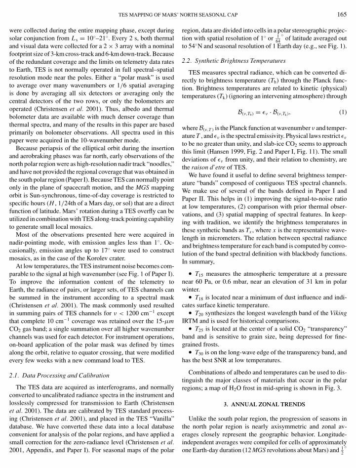
were collected during the entire mapping phase, except duringsolar conjunction from Ls = 10◦–21◦. Every 2 s, both thermaland visual data were collected for a 2 × 3 array with a nominalfootprint size of 3-km cross-track and 6-km down-track. Becauseof the redundant coverage and the limits on telemetry data ratesto Earth, TES is not normally operated in full spectral–spatialresolution mode near the poles. Either a “polar mask” is usedto average over many wavenumbers or 1/6 spatial averagingis done by averaging all six detectors or averaging only thecentral detectors of the two rows, or only the bolometers areoperated (Christensen et al. 2001). Thus, albedo and thermalbolometer data are available with much denser coverage thanthermal spectra, and many of the results in this paper are basedprimarily on bolometer observations. All spectra used in thispaper were acquired in the 10-wavenumber mode.
Because periapsis of the elliptical orbit during the insertionand aerobraking phases was far north, early observations of thenorth polar region were as high-resolution nadir track “noodles,”and have not provided the regional coverage that was obtained inthe south polar region (Paper I). Because TES can normally pointonly in the plane of spacecraft motion, and the MGS mappingorbit is Sun-synchronous, time-of-day coverage is restricted tospecific hours (H , 1/24th of a Mars day, or sol) that are a directfunction of latitude. Mars’ rotation during a TES overfly can beutilized in combination with TES along-track pointing capabilityto generate small local mosaics.
Most of the observations presented here were acquired innadir-pointing mode, with emission angles less than 1◦. Oc-casionally, emission angles up to 17◦ were used to constructmosaics, as in the case of the Korolev crater.
At low temperatures, the TES instrument noise becomes com-parable to the signal at high wavenumber (see Fig. 1 of Paper I).To improve the information content of the telemetry toEarth, the radiance of pairs, or larger sets, of TES channels canbe summed in the instrument according to a spectral mask(Christensen et al. 2001). The mask commonly used resultedin summing pairs of TES channels for ν < 1200 cm−1 exceptthat complete 10 cm−1 coverage was retained over the 15-µmCO2 gas band; a single summation over all higher wavenumberchannels was used for each detector. For instrument operations,on-board application of the polar mask was defined by timesalong the orbit, relative to equator crossing, that were modifiedevery few weeks with a new command load to TES.
2.1. Data Processing and Calibration
The TES data are acquired as interferograms, and normallyconverted to uncalibrated radiance spectra in the instrument andlosslessly compressed for transmission to Earth (Christensenet al. 2001). The data are calibrated by TES standard process-ing (Christensen et al. 2001), and placed in the TES “Vanilla”database. We have converted these data into a local databaseconvenient for analysis of the polar regions, and have applied a
small correction for the zero-radiance level (Christensen et al.2001, Appendix, and Paper I). For seasonal maps of the polarNORTH SEASONAL CAP 165
region, data are divided into cells in a polar stereographic projec-tion with spatial resolution of 1◦ or 1
64◦
of latitude averaged outto 54◦N and seasonal resolution of 1 Earth day (e.g., see Fig. 1).
2.2. Synthetic Brightness Temperatures
TES measures spectral radiance, which can be converted di-rectly to brightness temperature (Tb) through the Planck func-tion. Brightness temperatures are related to kinetic (physical)temperatures (Tk) (ignoring an intervening atmosphere) through
B(ν,Tb) = εν · B(ν,Tk), (1)
whereB(ν,T ) is the Planck function at wavenumber ν and temper-ature T , and εν is the spectral emissivity. Physical laws restrict εν
to be no greater than unity, and slab-ice CO2 seems to approachthis limit (Hansen 1999, Fig. 2 and Paper I, Fig. 11). The smalldeviations of εν from unity, and their relation to chemistry, arethe raison d’etre of TES.
We have found it useful to define several brightness temper-ature “bands” composed of contiguous TES spectral channels.We make use of several of the bands defined in Paper I andPaper II. This helps in (1) improving the signal-to-noise ratioat low temperatures, (2) comparison with prior thermal obser-vations, and (3) spatial mapping of spectral features. In keep-ing with tradition, we identify the brightness temperatures inthese synthetic bands as Tx , where x is the representative wave-length in micrometers. The relation between spectral radianceand brightness temperature for each band is computed by convo-lution of the band spectral definition with blackbody functions.In summary,
• T15 measures the atmospheric temperature at a pressurenear 60 Pa, or 0.6 mbar, near an elevation of 31 km in polarwinter.
• T18 is located near a minimum of dust influence and indi-cates surface kinetic temperature.
• T20 synthesizes the longest wavelength band of the VikingIRTM and is used for historical comparisons.
• T25 is located at the center of a solid CO2 “transparency”band and is sensitive to grain size, being depressed for fine-grained frosts.
• T30 is on the long-wave edge of the transparency band, andhas the best SNR at low temperatures.
Combinations of albedo and temperatures can be used to dis-tinguish the major classes of materials that occur in the polarregions; a map of H2O frost in mid-spring is shown in Fig. 3.
3. ANNUAL ZONAL TRENDS
Unlike the south polar region, the progression of seasons inthe north polar region is nearly axisymmetric and zonal av-erages closely represent the geographic behavior. Longitude-independent averages were compiled for cells of approximately
one Earth-day duration (12 MGS revolutions about Mars) and 12◦

166 KIEFFER A
of latitude. Ninety percent of the cells from 45◦ to 87◦N are filled.Images of these averages reveal the basic seasonal trends (Fig. 4).
We begin the description of the north seasonal cycle withthe beginning of the MGS mapping mode in late spring, atLs = 104◦, and continue through nearly a full martian year toLs = 093◦.
3.1. Derived Parameters
Simple derivations of TES observations can be used as surro-gates for several physical parameters. Although these relationsare approximate, their simplicity allows the discussion to be tiedclosely to the observations and they display the essence of themartian seasons. More complex processing of the data is notwarranted for this first presentation of results.
The bolometric albedo is derived from the TES measure-ment of the total reflected solar energy by the assumption thatMars scatters light according to the Lambert relation wherein thereflectance depends only on the incidence angle. This is knownto be an approximation, particularly for the seasonal frost (seePaper I, Section 6.3). However, the deviation of this assumptionfrom the true relation is probably not many times larger than thedeviation of far more complicated models. There is a significantvariation of soil Lambert albedo with latitude in the north polarregion (e.g., related to the dark circum-polar erg), as well aslarge seasonal changes associated with condensates (Fig. 4A).
The fundamental seasonal variation is exemplified by theaverage surface temperature, represented by the average of theTES AM and PM observations of T18, (T18). T18 generallyvaries smoothly with season, tracking or lagging the insolation(Fig. 4B).
The atmospheric temperature is represented by the averageof the AM and PM measurements of T15, T15 (Fig. 4C). The di-urnal variation of atmospheric temperature, represented by thedifference between AM and PM T15, or �T15, is taken as a directindication of the amount of dust in the atmosphere (Fig. 4D).Dust increases the coupling of the atmosphere to solar irradiance,and modest amounts of dust decrease the radiative time constantof the atmosphere. Although traveling wave structures can in-crease temperature oscillations in the atmosphere, TES observa-tions should catch such waves at random phase, and they wouldappear as scatter in T18 rather than as changes in the mean value.
The difference between the estimated surface kinetic temper-ature and the brightness temperature in the CO2 25-µm trans-parency band, T18–T25, effectively measures the emissivity at25 µm and is taken as an indicator of the grain size of CO2 frost(Fig. 4E) (see Papers I and II). This measure can be influencedby the presence of atmospheric dust; however that effect has notyet been quantified. Analysis of TES spectra during the northernwinter indicate that there is a wide range of CO2 condensate grainsize, reasonably represented by three endmembers, and that highT18–T25 is a good indication of fine-grained frost (Paper II).Equal-area weighted statistics for T18–T25 were computed whereand when the maximum T18 was less than 150 K, indicating CO2
ice; less than 2% of the values are negative and these occur nearthe edge of the seasonal cap and probably represent unresolved
ND TITUS
mixing of surface temperatures. Sixty-five percent of the valuesare <5 K, about 5% are >10 K, and less than 1
2 % are >15 K.In Paper II, T18–T25 > 15 K was defined as a “cold spot,” that
is, a region where brightness temperatures were significantly be-low the kinetic temperatures expected for Mars. Because bolo-metric temperature is less sensitive to the 25-µm CO2 band,and we are often dealing with longitude averages, in this paperwe also use the term “cold spot” to refer to conditions wherethe bolometric temperature is >5 K below the expected CO2
condensation temperature.
3.2. Seasonal Evolution
At the beginning of MGS mapping at Ls = 103.8, there wasno solid CO2 in the northern hemisphere. The albedo representssoil and residual H2O ice (Fig. 4A). Albedo averaged over alllongitudes and the first 120 days (to Ls = 163◦) is less than 0.22south of 80◦N, with a broad minimum of 0.16 at 58◦N and anarrow minimum of 0.16 at 77◦N caused by the circum-polarerg. Poleward of 80◦N, the albedo rises roughly linearly to 0.34at the polar ring.
At Ls = 122◦, average surface temperatures range from 226 Kat 45◦N to 205 K at 86◦N (Fig. 4B), and AM surface temperaturesexceed 195 K north of 70◦N. At this season, the atmospheric tem-perature is uniform over the polar region at 174 ± 3 K (Fig. 4C),and the diurnal variation of atmospheric temperature (�T15) isgenerally less than 3 K (Fig. 4D); �T15 is less than 5 K 74%of the time. The atmospheric opacity is thus low at the start ofMGS mapping, with a small dust storm indicated at Ls = 146◦
near 55◦N.There is some brief H2O cloudiness at Ls = 112◦, 74◦N.
These conditions continue with little change until Ls = 162◦
when cooling of the atmosphere north of 64◦N begins simul-taneously with an increase in apparent albedo, which indicatesformation of condensate clouds. Because atmospheric tempera-tures have a minimum of ∼153 K at the north limit of observa-tions, which is above CO2 condensation, these must be water-iceclouds. There is also a small decrease in �T15 that extends to45◦N.
From Ls = 164◦ to 184◦, in a band from 68◦ to 76◦N, the albe-dos become higher than that of the soil earlier, and T18 and T15
are both below 190 K, low enough for H2O to condense, so thatthese data cannot distinguish between surface and atmosphericcondensation. From Ls = 185◦ until Ls = 202◦, this band ofbrightness moves southward, suggesting that it may originate inthe atmosphere. During Ls = 205◦ to 234◦, there is an intriguingcorrelation between this transitory brightness increase and �T15,suggesting that the brightness is due to H2O particles seededon suspended dust. At Ls = 234◦, this consistent brightness in-crease ends. A “polar hood” has commonly been observed, par-ticularly prominant in blue or violet light, over the northern capin the winter, and these TES observations of transient high broad-band albedo probably correspond to the traditional polar hood.
CO2 condensation, indicated by afternoon T18 less than 150 K,
begins near Ls = 179◦, basically at polar sunset (Fig. 4B, whitecurve). Although the edge of the growing seasonal cap has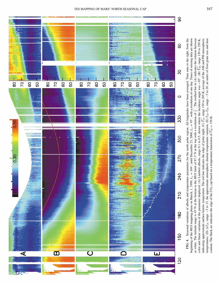
TES MAPPING OF MARS’ NORTH SEASONAL CAP 167
FIG
.4.
Seas
onal
vari
atio
nsof
albe
doan
dte
mpe
ratu
repa
ram
eter
sfo
rth
eno
rth
pola
rre
gion
.A
lllo
ngitu
des
have
been
aver
aged
.T
ime
runs
toth
eri
ght,
from
the
begi
nnin
gof
the
MG
Sm
appi
ngph
ase
onM
arch
,1,1
999,
Ls=
104◦
,unt
ilD
ecem
ber
23,2
000,
Ls=
93◦ ,
with
are
solu
tion
ofon
eda
y.T
imes
ofm
issi
ngda
taar
esh
own
asw
hite
.The
latit
ude
rang
eis
45◦ N
atth
ebo
ttom
toth
eM
GS
limit
of87
.3◦ N
atth
eto
pw
itha
reso
lutio
nof
1 2◦ .T
heto
othe
dba
rin
(A)
indi
cate
sth
ere
latio
nbe
twee
nco
lor
and
linea
rva
riat
ion
ofth
epa
ram
eter
disp
laye
d.(A
)L
ambe
rtal
bedo
,ran
ge0.
1to
0.5,
show
nw
here
the
inci
denc
ean
gle
was
<85
◦ .(B
)T 1
8,r
ange
130
to25
0K
,in
dica
ting
appr
oxim
ate
surf
ace
kine
ticte
mpe
ratu
re.T
here
dlin
ein
dica
tes
the
edge
ofpo
lar
nigh
t.(C
)T 1
5,r
ange
130
to20
5K
,ave
rage
ofth
eA
Man
dPM
atm
osph
eric
tem
pera
ture
s.(D
)�
T 15,r
ange
−5to
15,t
heap
prox
imat
eat
mos
pher
icdi
urna
lte
mpe
ratu
reva
riat
ion.
(E)
T 18–T
25,r
ange
−5to
20,a
nin
dex
offr
ost
grai
nsi
zean
ddu
stco
nten
t.T
hebl
ack
arc
indi
cate
sth
eed
geof
the
CO
2ca
pba
sed
ona
tem
pera
ture
tran
sist
ion
ofT 1
8=
156
K.
168 KIEFFER A
large grain size, indicated by the small T18–T25 (Fig. 4E), byLs = 202◦ cold spots begin to form near the pole, indicatingfine-grained frost there. Within the seasonal cap, the observeddiurnal surface temperature, �T18, is less than 1 K; of course,the hour difference between the AM and PM legs of the MGSorbit goes to 0 at the MGS nadir latitude limit. At the time of thestrongest dust storm, the boundary where T18–T25 > 6 K jumpedto 69◦N, where it remained until at least Ls = 318◦ (Fig. 4D).It is unknown why this grain-size boundary appears or why itpersists through much of the winter.
A small dust storm occurs at Ls = 211◦, 58◦N, which clearsin 8 days. A substantial increase in atmospheric dustiness occursat Ls = 226◦, with �T15 increasing within four days from an av-erage value of 4 K to as much as 22 K over 58◦ to 71◦N (Fig. 4C).The atmospheric heating associated with dust briefly penetratesall the way to the pole at Ls = 230◦. At this season (only) theT18–T25 index is significantly influenced by atmospheric dust.From Ls = 230◦ to Ls = 245◦, T15 is nearly constant between45◦N and 58◦N. With the appearance of this dust storm, thesouthern limit of cold spots (T18–T25 > 5 K, indicating fine-grained CO2 frost) jumps from 81◦N to near 70◦N, where itremains until Ls = 315◦. Although the opacity (indicated by�T15) is variable, and clears briefly near Ls = 270◦, the effectsof increased opacity are evident in �T15 until Ls = 335◦. Thesedust storms occurred in the season when Mars historically expe-
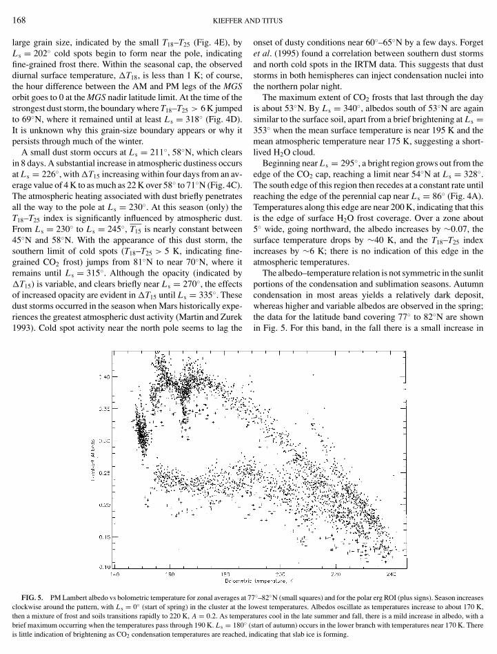
riences the greatest atmospheric dust activity (Martin and Zurek the data for the latitude band covering 77◦ to 82◦N are shown 1993). Cold spot activity near the north pole seems to lag theFIG. 5. PM Lambert albedo vs bolometric temperature for zonal averages at 77◦–82◦N (small squares) and for the polar erg ROI (plus signs). Season increasesclockwise around the pattern, with Ls = 0◦ (start of spring) in the cluster at the lowest temperatures. Albedos oscillate as temperatures increase to about 170 K,then a mixture of frost and soils transitions rapidly to 220 K, A = 0.2. As temperatures cool in the late summer and fall, there is a mild increase in albedo, with a
in Fig. 5. For this band, in the fall there is a small increase in
brief maximum occurring when the temperatures pass through 190 K. Ls = 180◦is little indication of brightening as CO2 condensation temperatures are reached,
ND TITUS
onset of dusty conditions near 60◦–65◦N by a few days. Forgetet al. (1995) found a correlation between southern dust stormsand north cold spots in the IRTM data. This suggests that duststorms in both hemispheres can inject condensation nuclei intothe northern polar night.
The maximum extent of CO2 frosts that last through the dayis about 53◦N. By Ls = 340◦, albedos south of 53◦N are againsimilar to the surface soil, apart from a brief brightening at Ls =353◦ when the mean surface temperature is near 195 K and themean atmospheric temperature near 175 K, suggesting a short-lived H2O cloud.
Beginning near Ls = 295◦, a bright region grows out from theedge of the CO2 cap, reaching a limit near 54◦N at Ls = 328◦.The south edge of this region then recedes at a constant rate untilreaching the edge of the perennial cap near Ls = 86◦ (Fig. 4A).Temperatures along this edge are near 200 K, indicating that thisis the edge of surface H2O frost coverage. Over a zone about5◦ wide, going northward, the albedo increases by ∼0.07, thesurface temperature drops by ∼40 K, and the T18–T25 indexincreases by ∼6 K; there is no indication of this edge in theatmospheric temperatures.
The albedo–temperature relation is not symmetric in the sunlitportions of the condensation and sublimation seasons. Autumncondensation in most areas yields a relatively dark deposit,whereas higher and variable albedos are observed in the spring;
(start of autumn) occurs in the lower branch with temperatures near 170 K. Thereindicating that slab ice is forming.

TES MAPPING OF MARS’
albedo as temperatures drop through 190 K (near Ls = 165◦);this is probably surface water frost, perhaps localized. The po-lar erg (at the same latitude) displays a similiar behavior, withadditional weak brightenings. In the spring, the surface emergesinto sunlight with an albedo near 0.33 for all longitudes. ByLs = 22◦, the zonal albedo has risen to 0.35 with the polar ergabout 0.01 darker. The zonal albedo rises to 0.40 at Ls = 35◦.The albedo of the polar erg generally tracks the variations of thezone, with the separation in albedo gradually increasing untilnear Ls = 70◦ when the zone albedo is 0.40 and the erg albedois 0.3 just before their rapid decrease in common. The corre-lation between T18–T25 and albedo through the spring indicatesthat these albedo variations are largely due to surface CO2 grain-size variations.
3.3. The Polar Ring
The term “polar ring” has been used within the MGS sci-ence teams to designate a narrow latitude range at the limit ofMGS nadir coverage that results from the inclination of the MGSorbit. Because the nadir track here becomes tangent to the par-allels of latitude, dense coverage in both longitude and seasonis possible. Data for the north polar ring (85◦ to 87.3◦N, thedefinition of the temperate-side edge is arbitrary), from both as-cending and descending legs of the MGS orbit, were averagedwith one-day temporal resolution; the annual mean of the stan-dard deviation over the five such 1
2◦
latitude strips was 1.2 to1.7 K for the surface bands, 0.6 K for T15, and 0.013 for albedo.These polar ring averages show a slow, nearly linear, rise insurface-sensing brightness temperatures from near Ls = 350◦
to Ls ∼ 73◦, when exposure of the perennial ice begins (Fig. 6,heavy lines). Note that Fig. 6 is basically a cross section throughFig. 4 along the polar ring latitude. Surface temperatures reach amaximum near 222 K at Ls = 105◦ (the peak may have occurredduring a data gap). Throughout the period of H2O ice exposure,the spectrum from 17 to 30 µm is flat, as indicated by smallT18–T25. CO2 condensation temperatures are attained again nearLs = 180◦, and T18–T25 begins to rise. “Cold-spot” conditions(T18–T25 > 5 K) are reached by Ls = 212◦. A brief rise in T15 atLs = 229◦ indicates increased dust in the atmosphere, and thecold-spot index rises 9 days later. From Ls = 245◦ to 300◦, con-ditions are steady with T18 = 146 K, and all the surface-sensingbands exhibit small, well-correlated variations in T ; this periodcorresponds to the minimum atmospheric temperatures. Thereis a second interval of cold spots near Ls = 320◦, which ends asT18 begins to rise.
3.4. Frost Mass Budget
The TES bolometer channels measure the total reflected sun-light and the total emitted energy (shortward of ∼100 µm).These observations supply a good estimate of the total radia-
tive energy balance for the planet (the vertical column from thesurface to the top of the atmosphere) at the instant and loca-NORTH SEASONAL CAP 169
tion of observations. Because diurnal variations are relativelysmall in the polar regions, an estimate of these variations al-lows a first-order estimate of the daily average planetary fluxbalance.
We use the ascending (nighttime) and descending (daytime)bolometric temperatures to estimate the mean effective bolomet-ric temperature by assuming that they sample the minimum andmaximum of a sinusoidal diurnal variation
T = T0 − δ cos2π H
24, (2)
where T0 = (Tpm + Tam)/2 and δ = (Tpm − Tam)/2.The average effective temperature is then approximately
T 4eff = T 4
0 + 3T 20 δ2 + 3
8δ4. (3)
The average net energy balance (into the surface) for a day is
〈F〉 = FU 2
1
2π
∫ 2π
0(1 − A) cos iθ dθ − σ T 4
eff, (4)
where F is the solar constant, U the heliocentric range in as-tronomical units, iθ the incidence angle as a function of theplanetary rotation θ though one day, and the cosine taken as 0when i > 90◦.
The solid CO2 budget is
M = 1
L
∫〈F〉 dt, (5)
where L is the latent heat of sublimation for CO2 (6.0 × 10⁵ Jkg−1 (James et al. 1992)) and the integration runs over the seasonwhen the surface temperature (roughly T0) drops below the CO2
condensation temperature.Missing data in the latitude/season cells were filled by linear
interpolation (or constant fill for gaps at the ends of mappingcoverage). Use of the bolometric temperature and the bolometricLambert albedo allow a first-order energy balance to be derivedfor each zone using Eq. (4). The largest errors probably resultfrom deviations of the bolometric albedo from Lambertian, andlateral heat transport in the atmosphere as either sensible heator the latent heat of sublimation of CO2. The specific heat atconstant presure of the Mars atmosphere is about 860 J K−1
kg−1, so that sublimation of 1 kg m−2 is equivalent to the heatrelease of cooling the entire atmospheric column by 4.6 K.
A date for beginning the integration was chosen as the first
time that the flux balance was negative and T0 < 155 K. Theenergy balance for each latitude is summed forward in time until
170 KIEFFER AND TITUS
FIG. 6. Seasonal variations for two latitude strips. The heavy lines are for the polar ring, latitudes 85◦–87◦N. The light lines are for latitudes 70◦–75◦N.(A) Lambert albedo observed in the PM. The wide data gaps centered on Ls = 270◦ are where the latitudes were in the dark of polar night. (B) Diurnally averagedbolometric brightness temperature. (C) Diurnally averaged atmospheric temperature, T15. The brief rises in temperature indicate dust stroms, the strongest beingat Ls = 229◦ when dust penetrated to the polar ring. (D) Diurnal variation of atmospheric temperature, �T15. The much smaller values for the polar ring are due
to the small variations of solar incidence angle through a day there. (E) CO2 grain size index, T18–T25. The values are near zero unless CO2 is present. (F) Diurnal surface temperature variation, �T18.T0 rises above 165 K; this temperature was chosen somewhatabove the CO2 frost point to account for the mix of surface
temperatures that occurs in a latitude strip in the spring. Themaximum frost budget from this estimate is shown in Fig. 7.The net energy budget at the end of this integration was notzero, but indicated that CO2 condensation occurred less than
predicted from the polar night observations; the discrepancywas small at the north and south extremes of the seasonal cap
TES MAPPING OF MARS’ NORTH SEASONAL CAP 171
FIG. 10. Detail of the normal cap (ROI 1) and a few north polar dark lanes. Colored squares are TES observation of T25; the squares are about half the size ofa TES pixel. The image is 168 km across, north is to the lower left, and the longitude line 240◦W is shown; the latitude limit of TES observations is just within the
b
image. Coverage was obtained over Ls = 137◦–146◦. The color bar indicates theas indicated by the grayscale bar.and largest (up to 500 kg m−2 equivalent, or 10 W m2 overthe frost season) near 71◦N. These discrepancies cannot be dueonly to albedo errors; at 68◦N, even if the springtime albedois assumed to be zero, the mass imbalance is still 100 kg m−2.More complete one-dimensional models, accounting for at leastthe radiative effects of dust and heat flow from the soil in the
winter, are required to usefully constrain the amount of lateralheat transport required.rightness temperature scale. The gray tones are MOLA elevations in kilometers,
4. MAPPING VARIATIONS WITH LONGITUDE
Analysis of longitudinally averaged latitude zones is a usefulway of gaining an understanding of the seasonal behavior ofthe seasonal cap. While the seasonal behavior of the north po-lar cap is generally symmetric, an examination of longitudinal
variations aids in identifying regional anomalies and indicatesthe limitations of zonal analysis.
172 KIEFFER AND TITUS
FIG. 12. TES observations strips across the Korolev crater during four seasons. The gray tones are MOLA elevations and the colors are TES bolometertemperatures. The orientation is that standard for north polar maps; north is toward 7 o’clock. The extended path is 3 km wide from a single TES detector; the
wider patch is a 5–angle look full-resolution TES mosaic. (upper left) L = 336.7◦, H = 12.55. (upper right) L = 350.8◦, H = 12.61. (lower left) L = 7.7◦, sH = 12.81. (lower right) Ls = 36.1◦, H = 13.14.
To account for the strong latitude dependence of TES ob-servation frequency, all observations were initially binned intocells approximately 60 km square for each Earth day of obser-vation. Many cells are unpopulated for latitudes south of 65◦N.For analysis of seasonal variation at specific locations, a convexpolygon “cell” was constructed to define a “region of interest”(ROI); see Fig. 1.
At the start of MGS mapping, the permanent H2O ice cap iscompletely exposed. Most of the perennial cap has an albedoof ∼0.30 with temperatures T30 ∼ 215 K. A cool-and-bright
anomaly (CABA) lies near 87◦N, 35◦W, and has AL = 0.5,T30 = 185 K (see Section 5.5). Other areas of the cap with albedos s
greater than 0.45 exist along the edges of the Chasma Borealeand smaller reentrants along the edge of the permanent cap (seeSection 5.3). Chasma Boreale itself is relatively dark, warm, andhence free of ice. The floors of several craters, including Korolevand Lomonosov, are bright and cold and presumed to be cov-ered with H2O frost (see Section 5.7). Of the many bright outliersthat develop as the edge of the seasonal cap recedes, none thatbecome significantly detached retain temperatures compatiblewith solid CO2.
The bare soil surrounding the permanent cap is bimodal with
albedos of ∼0.25 and ∼0.10 (Fig. 2). As the season progresses,the cool and bright anomaly continues to be the brightest part of
TES MAPPING OF MARS’ NORTH SEASONAL CAP 173
FIG. 7. CO2 frost mass budget. The lines are based upon the procedures discussed in Section 3.4 using zonally averaged observations of the bolometrictemperature and Lambert albedo. The solid line is the condensation budget, the dot-dashed line is the sublimation budget, and the dashed line is the differencebetween the estimated condensation and sublimation budgets. The dots are the sublimation budgets of individual 60 km square cells, which used the thermal
inflection date to indicate the end of the sublimation season; these sublimation budgets are higher than the zonal results because the latter used a temperature of 165 K as the termination of sublimation, earlier than the temperature inflection.the cap; the only brighter location is the Korolev crater. The polarerg is dark, except for some ice deposits around craters. Thistrend continues until Ls = 130◦ when the CABA and Korolevcrater start to darken slightly.
At the end of the period covered here, nearly a complete mar-tian year after the beginning of mapping, there are some differ-ences indicating interannual variations. The most significant arealbedo variations, with several areas that are cool and bright, notjust the area noted at the beginning of mapping (see Section 5.5).Whether they will persist through the martian northern summerof 2001 is unknown.
4.1. Springtime Temperature Rise and Crocus Dates
In Paper I (Section 7.1), the time of final CO2 disappearencewas defined as the “Crocus date,” and established fitting anarc-tangent function to the rapid rise of surface temperature inthe spring. The recession of the north seasonal cap is quanti-fied using the same techniques as were applied in Paper I toTES premapping data of the south polar cap. Afternoon tem-perature observations for each 60-km square cell are fitted intime with an arc-tangent function to establish the timing ofthe most rapid surface temperature rise. However, in the norththe observed springtime temperature rise is not as rapid as
in the south, probably due to both the higher thermal iner-tias of the surface in the north and the greater distance fromthe Sun. Thus, the time of most rapid temperature rise, takenas the inflection point in the arc-tangent temperature fit or the“thermal inflection date,” can significantly lag behind the sea-son when temperatures start to rise sharply, an event whichis commonly well defined in the north. For consistency withthe earlier work, we have calculated the “inflection date,” al-though it seems less closely related to the Crocus date than inthe south.
The thermal recession map for 2000 is basically axisymmetricaround the geographic pole; recession was slightly advancednear 270◦W at Ls = 0◦, and slightly delayed near 200◦W at Ls =40◦ (Fig. 8). By Ls = 80◦, the influence of the perennial cap isseen near 180◦W. The general relation between inflection dateand latitude was also derived by applying the same techniquesto zonal averages (Fig. 9). The dates derived by this techniquefall roughly 10◦ of Ls after the temperature rises through 165 Kand may be retarded from the true disappearence of solid CO2,the proper Crocus date. These data should be compared with therecession derived from MOC wide-angle imaging for the sameperiod (James and Cantor 2001).
4.2. Local CO2 Sublimation Budget
The annual budget of solid CO2 was mapped using the tech-
niques discussed in Section 3.4. However, the frequency ofTES coverage of any particular area is a function of latitude,
174 KIEFFER AND TITUS
FIG. 8. The 25-µm springtime thermal inflection dates. The retreat of the northern cap is shown as a function of season. The contours are spaced every 20◦
of Ls from Ls = 340◦ to 80◦. These dates probaly lag the date of CO2 disappearance by about 10◦ of Ls. The central circle marks the limit of observations. Gray tones are MOLA elevations.decreasing away from the polar ring; day- and nighttime tem-peratures are not collected on the same MGS revolution. In orderto estimate the day and night temperatures and the albedo, wesmooth the data and then interpolate to get data evenly spacedin time. This allows us to determine the season when the po-
lar cap transitions from condensation to sublimation. This date,combined with the inflection date, allows us to integrate 〈F〉over the sublimation season, thus calculating the total amountof solid CO2 that had been accumulated.
The data were smoothed in time using iterative convolutionwith a Gaussian filter and elimination of outliers (see Paper I,Fig. 5 caption). The net energy balance was then calculated usingequations of Section 3.4. Unlike the zonal budgets, the radiative
flux imbalance was integrated over only the sublimation season
TES MAPPING OF MARS’ NORTH SEASONAL CAP 175
FIG. 9. The 25-µm thermal inflection date vs latitude. The season of retreat ofe
inflection dates for individual cells. The solid line is the solution for the zonal avto estimate the amount of CO2 required to hold temperaturesdown from the time when 〈F〉 transitions from negative to posi-tive, to the surface temperature inflection date. The distributionof mass budgets with latitude in shown in Fig. 7. A map of themass budget shows that budgets are slightly higher in a quadrantcentered along 30◦W than at other longitudes.
These sublimation budget estimates are generally higher thanthose of the zonal analysis, due in part to a different definition ofwhen sublimation ends. However, even these sublimation bud-gets are lower than the zonal condensation budget over latitudesfrom 60◦ to 80◦N, and some additional undetermined source ofheat is required to explain the timing of solid CO2 disappearance.
4.3. Cryptic Region
TES observations of the southern spring revealed a regionin the polar cap with temperatures near the CO2 frost point (a
slight diurnal change was seen), but which was almost as darkas the underlying soil. The region has been referred to as thethe northern cap edge is shown as a function of latitude. The dots are the thermalrages, and the dashed line is the date when the zonal T18 rises through 165 K.
“cryptic” region and the seasonal material there as “cryptic”material. Cryptic material can easily be identified by its albedo–temperature relation, of having albedo less than 0.3 and temper-atures less than 170 K. An A–T plot for regions with seasonalfrost is shaped like a high-heeled shoe pointing toward hightemperatures with the cryptic material forming the heel. Fromits thermal spectrum, cryptic material is believed to be composedof solid CO2 with an effective grain size of several centimetersor larger, which we have called “slab ice.” Similar features areseen in the northern spring cap. A formation process of CO2 slabice has been suggested (Paper II), but is far from definite. It isknown that cryptic regions in the south repeat on an annual basis(Paper I).
Observations of the northern spring reveal similar behavior ofthe CO2 cap, where regions remain cold and dark while the rest ofthe cap brightens. In general, the northern cryptic region (NCR)is brighter than the southern cryptic region (SCR), having aminimum albedo of about 0.25 in comparison with a minimum in
the SCR of 0.20. The SCR does not tightly correlate to any known
temperatures of the three areas have merged with adjacent areas.
176 KIEFFER A
geological units (Kieffer et al. 2000), but the NCR correlates tothe polar erg, or dark sand seas. We do not know if the conditionsthat cause formation of cryptic material are the same in bothhemispheres.
The NCR first appears at A = 0.21, T = 152 K (Fig. 5) atLs = 357.5◦, at which time the cryptic material covers a largearea of the cap (correlating to the underlying polar erg). The NCRpersists until Ls = 35◦, where the region appears to brighten; thismay be due to atmospheric dust instead of surface changes. ByLs = 40◦, the cryptic region has darkened. The NCR begins toshrink and lose contrast starting at Ls = 50◦, and is gone byLs = 60◦.
The NCR occurs at similar latitudes and similar seasons asthe SCR. The SCR is the cause of the asymmetric recession ofthe southern cap. The NCR causes the dissection of the north-ern cap into two pieces, the main permanent cap and the largeoutlier. The fact that in the NCR the substrate is darker than theminimum CO2 albedo suggests that sunlight is not penetratingall the way through the slab ice, a point that was inconclusivein the SCR. Comparison with observations made a martian yearearlier, in the MGS aerobraking phase, indicates that the NCRrepeats annually.
5. SPECIFIC FEATURES
The general trends of the north seasonal cap are consider-ably more symmetric than the behavior of the south pole cap(Paper I); however, there are still features, or ROIs, where ther-mal and albedo properties and behaviors differ from their zonalmeans. Several areographic regions were selected on the basisof being either representative of a class of polar seasonal behav-ior or representing extreme behavior. These ROIs were definedby polygons in polar projections, and all data that fell in eachpolygon averaged with a time resolution of one Earth day. In thefollowing sections we discuss first an area representative of thepermanent ice cap, then three dark regions, and then three regionswhere seasonal H2O frost seems to play a major role. The poly-gons defining the ROIs are shown in Fig. 1; some are too smallto be seen. The central locations of each are listed in Table I.
TABLE ILocation of ROIs
Name Index Latitude (◦) Longitude (◦)
Nominal cap 1 87.0 247Polar ring 2 85.0–87.3 —Dark lane [a] 3a 87.0 206Dark lane [b] 3b 85.4 231Dark lane [c] 3c 86.8 59Chasma Boreale 4 83.5 36Polar erg 5 82.0 180CABA 6 86.9 36Frost outlier 7 75.8 204Korolev rim 8 72.8 196
Korolev floor 8 72.8 196ND TITUS
5.1. Representative Perennial Cap
At the beginning of mapping, Ls = 104◦, the temperature ofthe nominal location on the permanent cap is near its annual max-imum of 205 K and the albedo is 0.34 and slowly rising. The capbrightens to a local maximum of 0.38 at Ls = 142◦ while coolingsteadily. The last albedo measurement at Ls = 175◦, just beforeannual sunset, is 0.31. At Ls = 180◦ the temperature has reached150 K, and there is an abrupt decrease in the cooling rate markingthe beginning of CO2 condensation. The bolometric temperaturereaches a minimum of 138 K at Ls = 215◦, rises smoothly to145 K at Ls = 270◦, then decreases to 140 K at about Ls = 320◦;during this period there are erratic excursions of a few de-grees in the difference between AM and PM observations, as-sumed to be related to transient cold spots. Zonal observationsindicate that cold spots at this latitude occur primarily overLs = 205◦–260◦ and Ls = 306◦–320◦ (where a gap in coveragebegins).
At the first polar dawn observations at Ls = 6◦, the albedo is0.34 and the temperature 148 K. Whereas the bolometric tem-perature rises nearly linearly with Ls until reaching 162 K atLs = 78◦, the albedo rises rapidly to 0.44 at Ls = 40◦ then os-cillates toward 0.40 at Ls = 78◦. The abrupt increase in warmingrate at Ls = 78◦ indicates the final loss of solid CO2, althoughthe albedo decreases steadily through this transition to 0.38 atLs = 86◦ (when the temperature is 185 K), then drops abruptlyto 0.31. This period of rapid warming and slow darkening mustrepresent the final evolution of the H2O frost and dust that weredeposited in the winter.
5.2. Three Dark Lanes
Three small areas corresponding to dark lanes in the latesummer were selected as ROIs. The seasonal trends of theseregions are similar to each other and to the mean for all darkareas outside the perennial cap at similar latitudes. During thedark of winter and throughout the springtime loss of CO2
frost, these areas are indistinguishable thermally from adjacentareas.
Early after spring sunrise, the albedos of the dark lanes arepoorly distinguished from other areas at the same latitudes.Between Ls = 40◦ and Ls = 50◦, the lanes are occasionallybrighter than the rest of the polar cap. At Ls = 70◦, the CO2
sublimates and the temperatures rise quickly. At Ls = 85◦, thedark lanes reach minimum albedos of 0.20, 0.25, and 0.25 forROI a, b, and c, respectively, but then quickly rise to 0.27. Thereis no indication in the TES data of cloud activity off of the perma-nent polar cap at this time. Thus the primary candidate for thesesmall albedo changes is surface H2O frost, perhaps due to watervapor being released from the subsurface and recondensing onthe surface.
At the beginning of mapping, all three areas are warmer anddarker than the adjacent cap (Fig. 10). By Ls = 160◦–170◦, the
During this same period, the nominal cap darkens so that the

is a causal relation between summer cold-and-bright behavior
TES MAPPING OF MARS’
three dark lanes are the same albedo as the cap. During the winter,the dark lanes exhibit cold spot activity; however, comparisonwith the remainder of the cap at equivalent latitudes does notindicate an unusual level of activity.
The observed seasonal trends suggest that the dark lanes aresurface dust overlaid on ice. The dark lanes are topographictroughs, perhaps causing retention of a dust/soil layer that is thickenough to be a permanent feature, but generally thin enough toallow vertical diffusion of H2O on an annual basis, i.e., the scaleof the annual thermal wave, or on the order of a meter.
5.3. Chasma Boreale
At the beginning of mapping, Chasma Boreale has temper-atures in excess of 220 K, an albedo of less then 0.2 and isfree of ice. The temperatures of the Chasma decrease with sea-son until at Ls = 160◦ it has the same temperature as otherareas at the same latitude. As the temperature decreases, thealbedo increases, suggestive of small amounts of frost forma-tion. As the Sun sets into polar night (Ls = 185◦), the meanalbedo of the Chasma is 0.25. After Ls = 160◦, the tempera-ture continues to drop until CO2 solid forms at Ls = 190◦; thetransition in cooling rate is not abrupt as it is for the nominalcap location. During the condensation season, the mean temper-ature is generally a few degrees warmer than the zonal average,consistent with the difference in elevation between the ice capand the Chasma. The Chasma experiences a moderate amountof cold spot activity, with the most activity occurring betweenLs = 305◦ and 330◦. As the Sun rises, the initial albedo is 0.32,consistent with the zonal average. The bolometric temperaturescontinue to rise from a warming atmosphere until Ls = 70◦,when a sharp increase in temperature indicates the disappearanceof solid CO2. There is a 10◦ delay in Ls before the albedo drops,suggesting that there is a residue of water ice/frost that had beendeposited on the chasma floor prior to the onset of CO2 con-densation or incorporated with solid CO2 formation. At the endof mapping, Ls = 90◦, the chasma has darkened to an albedoof 0.15.
Both the polar erg and Chasma Boreale display similar albedoand thermal trends. High-resolution imaging of the Chasma floorshows dune forms, suggesting that the floor material may be sandseas similar/identical to those in the polar erg (Tanaka and Scott1987).
5.4. Representative Polar Erg
We selected a large region of the polar erg; this is withinthe north cryptic region. At the beginning of mapping, the ROIalbedo is 0.13, among the darkest locations in the polar regionand peak summer temperatures are near 240 K. The albedo/temperature relation for the polar is similar to that of corre-sponding zone although the erg is consistently darker than otherregions near this latitude (see Fig. 5). At Ls = 135◦, the albedobegins to rise, reaching ∼0.24 at sunset at Ls = 190◦, whereasthe albedo of the remainder of the zone is steady. CO forms at
2Ls = 198◦, consistent with other areas at the same latitude. The
NORTH SEASONAL CAP 177
temperatures remain constant throughout the winter, with littlecold spot activity. At sunrise at Ls = 350◦, the ROI has albedoof 0.32 and an bolometric temperature of 148 K. The albedopeaks briefly at 0.39 at Ls = 33◦, then continues at ∼0.35 untilLs = 70◦, when it begins a fall to 0.14 at Ls = 88◦. The tem-perature has risen to 165 K at Ls = 41◦, then holds steady untilLs = 60◦. CO2 is gone by about Ls = 70◦.
5.5. Bright–Cool Anomaly
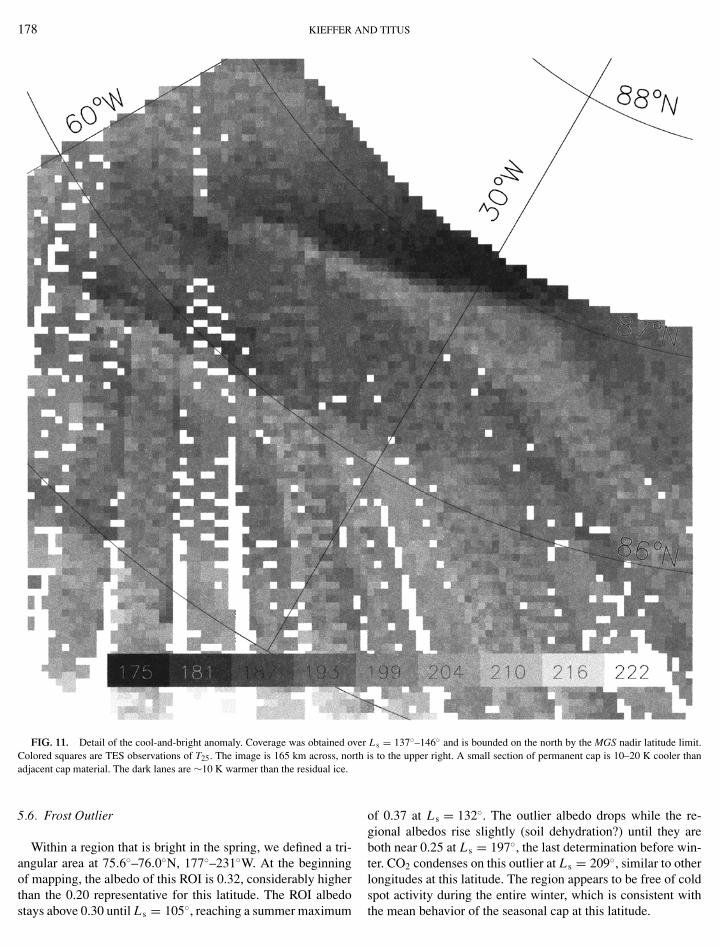
At the beginning of mapping, a small region near 87◦N, 30◦Wwas noted as being brighter and 5◦–15◦ cooler than other partsof the polar cap at the same latitude (Fig. 11). This area is at least900 km2 in extent; its northern boundary is beyond the range ofTES coverage. This area was first revealed at the beginning ofthe mapping phase, as the nearby dark lanes became distinct; werefer to this area as the cool-and-bright anomaly. This area ap-peared bright in many Mariner and Viking summertime images;see, for example, Fig. 7a in Bass et al. (2000), which indicatesthat TES may have covered about half of the bright area.
At Ls = 103.8◦ the CABA was the brightest region of thepolar cap. The mean albedo of this region varied between 0.40and 0.50, and temperatures were as much as 10◦ lower than thesurrounding region. Since the region is cooler than surroundingregions, we believe that the CABA is a cold trap for H2O vaporcoming from the adjacent perennial cap or possibly from thewarm dark areas at the edge of the cap; irregular water frostformation could account for the observed albedo variability.
The CABA remains clearly distinct until Ls = 147◦, whenthe albedo drops suddenly to 0.35 and temperatures rise a fewdegrees while the surrounding region is cooling. A second rapidchange at Ls = 162◦ brings temperature and albedo to the re-gional mean. At Ls = 181◦, CO2 starts to form at this latitude.During fall, the CABA has bolometric temperatures less than thelatitude average, indicating that the CABA is an area of cold spotformation. By Ls = 206◦, cold spot formation occurs regularlyat this latitude, with CABA consistently being colder. While coldspot occurrences decrease for the mean latitude by Ls = 242◦,the CABA continues to experience repeated cold spots. Coldspot activity ceases about Ls = 0◦. The first spring albedo mea-surements of the area, Ls = 9◦, show that the area has an albedohigher than that of other areas at the same latitude. The CABAalbedo varies rapidly and erratically through the summer. TheCABA follows the temperature trends of the mean latitude untilthe CO2 disappears at Ls = 73◦, but remains brighter than thesurrounding cap.
The CABA increases in temperature more slowly than otherareas at the same latitude and maintains a significantly brighteralbedo, resulting in a cold trap for water frost formation, a pro-cess of positive feedback. The CABA remains cool and bright,consistent with the beginning of mapping, one martian year later.However, unlike 1998, in late 2000 many more areas show be-havior similar to that of the CABA. We do not yet know if there
and enhanced winter cold spot activity.
178 KIEFFER AND TITUS
FIG. 11. Detail of the cool-and-bright anomaly. Coverage was obtained over Ls = 137◦–146◦ and is bounded on the north by the MGS nadir latitude limit.
Colored squares are TES observations of T25. The image is 165 km across, north is to the upper right. A small section of permanent cap is 10–20 K cooler than adjacent cap material. The dark lanes are ∼10 K warmer than the residual ice.5.6. Frost Outlier
Within a region that is bright in the spring, we defined a tri-angular area at 75.6◦–76.0◦N, 177◦–231◦W. At the beginningof mapping, the albedo of this ROI is 0.32, considerably higher
than the 0.20 representative for this latitude. The ROI albedostays above 0.30 until Ls = 105◦, reaching a summer maximumof 0.37 at Ls = 132◦. The outlier albedo drops while the re-gional albedos rise slightly (soil dehydration?) until they areboth near 0.25 at Ls = 197◦, the last determination before win-ter. CO2 condenses on this outlier at Ls = 209◦, similar to otherlongitudes at this latitude. The region appears to be free of cold
spot activity during the entire winter, which is consistent withthe mean behavior of the seasonal cap at this latitude.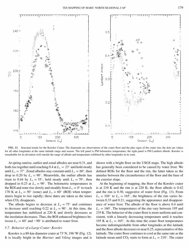
TES MAPPING OF MARS’ NORTH SEASONAL CAP 179
FIG. 13. Seasonal trends for the Korolev Crater. The diamonds are observations of the crater floor and the plus signs of the crater rim; the dots are values
PM bolometric temperature; the right panel is PM Lambert albedo. Korolev is for all other longitudes at the same latitude range and season. The left panel isremarkable for its deviation well outside the range of albedo and temperature exh
At spring sunrise, outlier and zonal albedos are near 0.31, andboth rise together until reaching 0.4 at Ls = 23◦ and hold steadyuntil Ls = 37◦. Zonal albedos stay constant until Ls = 60◦, thendrop to 0.20 by Ls = 90◦. Meanwhile, the outlier albedo hasrisen to 0.44 by Ls = 55◦, held steady until Ls = 70◦, thendropped to 0.23 at Ls = 90◦. The bolometric temperatures inthe ROI and zone rise slowly and steadily from Ls = 0◦ to reach170 K at Ls = 50◦ (zone) and Ls = 60◦ (ROI) when temper-atures begin to rise rapidly; these dates are taken as the timeswhen CO2 disappears.
The albedo begins to decrease at Ls = 75◦ and continuesto decrease until reaching 0.22 at Ls = 90◦. At this time, thetemperature has stabilized at 220 K and slowly decreases asthe insolation decreases. Thus, the ROI enhanced brightness be-tween Ls = 60◦ and ∼90◦ is attributed to water frost.
5.7. Behavior of a Large Crater: Korolev◦ ◦
Korolev is a 80-km diameter crater at 73 N, 196 W (Fig. 12).It is locally bright in the Mariner and Viking images and is
ibited by other longitudes in its zone.
shown with a bright floor on the USGS maps. The high albedohas generally been considered to be caused by water frost. Wedefined ROIs for the floor and the rim, the latter taken as theannulus between the circumference of the floor and the base ofthe exterior slope.
At the beginning of mapping, the floor of the Korolev crateris at 210 K and the rim is at 220 K; the floor albedo is 0.42and the rim is 0.30, suggestive of water frost (Fig. 13). FromLs = 104◦ to Ls = 165◦, the brightness of the rim varies be-tween 0.33 and 0.21, suggesting the appearance and disappear-ance of water frost. The albedo of the floor is above 0.4 untilLs = 160◦. The temperatures of the rim vary between 195 and235 K. The behavior of the crater floor is more uniform and con-sistent, with a linearly decreasing temperature until it reaches195 K at Ls = 165◦. At this time the crater floor temperaturesbecome indistinguishable from other longitudes at this latitudeand the floor albedo decreases to near 0.25, representative of thislatitude. The crater floor continues to cool at the same rate as the
latitude mean until CO2 starts to form at Ls = 210◦. The crater
N
180 KIEFFER Afloor has cold spot activity from Ls = 225◦ until 330◦, when thedominant CO2 endmember becomes coarse-grained or slab ice.At Ls = 335◦, when the sun has risen enough to allow albedo de-termination, the crater floor albedo is 0.46, significantly brighterthan the latitude mean of 0.30–0.38. The albedo of both the craterfloor and the mean latitude decrease to reach 0.33 at Ls = 360◦.This is evidence that fine-grained CO2 formed in the winter isbright, but quickly sinters into darker, coarser grain CO2. Mean-while, the crater rim albedo varies between 0.35 and 0.42. Asthe insolation increases, both the crater rim and floor increasein brightness to 0.40–0.45. At Ls = 50◦, the crater floor reachesmaximum brightness with an albedo of 0.47; soon thereafter thebolometric temperature rises from 175 to 193 K in only a fewdays. The Crocus date for the Korolev crater floor is Ls = 58◦.The temperature continues to increase, and the albedo to de-crease, until Ls = 90◦, when the temperature reaches 215 K andthe albedo is 0.27. Just as quickly as the albedo dropped, it in-creases again to 0.33 at Ls = 92◦.
The summertime temperatures and high albedos are consis-tent with the presence of water frost; there seems to be no otherexplanation except the similar, and less likely, formation of in-terior clouds. The closure of temperature and albedo betweenthe beginning of mapping and the end of the TES data stud-ied suggest a closely repeating cycle for the annual behavior ofKorolev.
The behavior of the dark lanes near summer solstice is similarto the behavior of the floor of the Korolev crater. The darkeningof the surface, followed by a quick rise in albedo, is suggestiveof an underlying permafrost. As soon as the surface ice subli-mates, a thermal pulse travels to the permafrost. The subsequentsubsurface sublimation then results in recondensation of froston the cooling visible surface.
6. SUMMARY
The TES observations and the brief analysis presented hereyield a picture of the north seasonal cap that is much moresymmetric than the southern seasonal cap, with the overall be-havior following that predicted for CO2 condensation bufferingsurface temperatures through the martian winter. However, thefirst-order estimates of condensation and sublimation do not bal-ance, especially over the intermediate latitudes covered by theseasonal cap. Varigated and oscillatory variations is brightnessgenerally occur when temperatures are near 190 K, suggestinga strong association with erratic motion of H2O. The richnessof these observations is just being uncovered, and the detailedobservations should be adquate to keep the surface geologistsand atmospheric modelers challenged for several years.
ACKNOWLEDGMENTS
The reviews by two anonymous referees were helpful and resulted in substan-
tial restructuring of the paper. We are especially grateful to Ken Herkenhoff foran extraordinarily extensive set of comments.D TITUS
REFERENCES
Albee, A. L., R. E. Arvidson, F. D. Palluconi, and T. Thorpe 2001. Overview ofthe Mars Global Surveyor mission. J. Geophys. Res. 106, 23291–23316.
Albee, A. L., F. D. Palluconi, and R. E. Arvidson 1998. Mars Global Surveyormission: Overview and status. Science 279, 1671–1672.
Bass, D. S., K. E. Herkenhoff, and D. A. Paige 2000. Variability of Mars’ northpolar water ice cap. I. Analysis of Mariner 9 and Viking Orbiter imaging data.Icarus 144, 382–396.
Christensen, P. R., and 19 colleagues 2001. Mars Global Surveyor Thermal Emis-sion Spectrometer experiment: Investigation description and surface scienceresults. J. Geophys. Rev. 106, 23823–23871.
Farmer, C. B., D. W. Davies, and D. D. LaPorte 1976. Mars: Northern summerice cap water vapor observations from Viking 2. Science 194, 1339–1341.
Forget, F., G. B. Hansen, and J. B. Pollack 1995. Low brightness temperaturesof the martian polar caps: CO2 clouds or low surface emissivity? J. Geophys.Res. 100, 21,219–21,234.
Forget, F., F. Hourdin, and O. Talagrand 1998. CO2 snowfall on Mars: Simulationwith a general circulation model. Icarus 131, 302–316.
Hanel, R., B. Conrath, W. Hovis, V. Kunde, P. Lowman, W. Maguire, J. Pearl,J. Pirraglia, C. Prabhakara, B. Schlachman, G. Levin, P. Straat, and T. Burke1972. Investigation of the martian environment by infrared spectroscopy onMariner 9. Icarus 17, 423–442.
Hansen, G. 1999. Control of the radiative behavior of the martian polar capsby surface CO2 ice: Evidence from Mars Global Surveyor measurements.J. Geophys. Res. 104, 16,471–16,486.
Jakosky, B. M., and R. M. Harberle 1992. The seasonal behaviour of wateron Mars In Mars (H. H. Kieffer, B. A. Jakosky, C. W. Snyder, and M. S.Matthews, Eds.), Chap. 28, pp. 969–1016. Univ. of Arizona Press, Tucson.
James, P. B., and B. A. Cantor 2001. Martian north polar cap recession: 2000Mars Orbiter Camera observations. Icarus 154, 130–144.
James, P. B., H. H. Kieffer, and D. A. Paige 1992. The seasonal cycle of carbondioxide on Mars. In Mars (H. H. Kieffer, B. A. Jakosky, C. W. Snyder, andM. S. Matthews, Eds.), Chap. 27, pp. 934–968. Univ. of Arizona Press, Tucson.
Kieffer, H. H. 1979. Mars south polar spring and summer temperatures: A resid-ual CO2 frost. J. Geophys. Res. 84, 8263–8288.
Kieffer, H. H., S. C. Chase Jr., T. Z. Martin, E. D. Miner, and F. D. Palluconi1976. Martian north pole summer temperatures: Dirty water ice. Science 194,1341–1344.
Kieffer, H. H., T. N. Titus, K. F. Mullins, and P. Christensen 2000. Mars southpolar spring and summer behavior observed by TES: Seasonal cap evolutioncontrolled by frost grain size. J. Geophys. Res. 105, 9653–9699.
Leighton, R. B., and B. C. Murray 1966. Behavior of carbon dioxide and othervolatiles on Mars. Science 153, 136–144.
Martin, L. J., and R. W. Zurek 1993. An analysis of the history of dust activityon Mars. J. Geophys. Res. 98, 3221–3246.
Neugebauer, G., G. Munch, H. H. Kieffer, S. C. Chase Jr., and E. D. Miner1971. Mariner 1969 infrared radiometer results: Temperatures and thermalproperties of the martian surface. Astron. J. 76, 719–749.
Tanaka, K. L. and D. H. Scott 1987. Geologic map of the polar regions of Mars,scale 1:15,000,000. U.S.G.S. Misc. Inv. Series Map, I-1802-C.
Tillman, J. E., N. C. Johnson, P. Gettorp, and D. B. Percival 1993. The mar-tian annual atmospheric pressure cycle: Years without great dust storms.J. Geophys. Res. 98, 10,963–10,971.
Titus, T. N., H. H. Kieffer, and K. F. Mullins 2001. Slab ice and snow flurries inthe martian polar night. J. Geophys. Res. 106, 23181–23196.
Zurek, R., J. R. Barnes, R. M. Haberle, J. B. Pollack, J. E. Tillman, and C. B.Leovy 1992. Dynamics of the atmosphere of Mars. In Mars (H. H. Kieffer,
B. M. Jakosky, C. W. Snyder, and M. S. Matthews, Eds.), pp. 835–933. Univ.of Arizona Press, Tucson.