Telecommunications System Bulletin TSB-84A Licensed PCS ...

Telecommunications System Bulletin

TSB-84A

Licensed PCS to PCS Interference

10th March, 2001

TIA/EIA TSB-84A

v2.0a

TIA/EIA TSB-84A

v2.0a

Table of Contents

0. Foreword . . . . . . . . . . . . . . . . . . . . . . . . . . . . . . . . . . . . . . . . . . . . . . . . . . . . . . 1

0.1 Revision History . . . . . . . . . . . . . . . . . . . . . . . . . . . . . . . . . . . . . . . . . . . . . . . 2

0.2 Document Organization . . . . . . . . . . . . . . . . . . . . . . . . . . . . . . . . . . . . . . . . . . . 2

0.3 Abbreviations, Acronyms And Symbols . . . . . . . . . . . . . . . . . . . . . . . . . . . . . . . . . . . 3

0.4 References . . . . . . . . . . . . . . . . . . . . . . . . . . . . . . . . . . . . . . . . . . . . . . . . . . 6

0.5 Scope . . . . . . . . . . . . . . . . . . . . . . . . . . . . . . . . . . . . . . . . . . . . . . . . . . . . 10

0.6 Definitions . . . . . . . . . . . . . . . . . . . . . . . . . . . . . . . . . . . . . . . . . . . . . . . . . . 11

1. Introduction. . . . . . . . . . . . . . . . . . . . . . . . . . . . . . . . . . . . . . . . . . . . . . . . . . . . 15

1.1 The Licensed PCS Bands . . . . . . . . . . . . . . . . . . . . . . . . . . . . . . . . . . . . . . . . . . 15

1.1.1 Spectrum Allocations . . . . . . . . . . . . . . . . . . . . . . . . . . . . . . . . . . . . . . . . . 15

1.1.2 Geographic Service Areas . . . . . . . . . . . . . . . . . . . . . . . . . . . . . . . . . . . . . . . 15

1.2 How Interference Can Occur . . . . . . . . . . . . . . . . . . . . . . . . . . . . . . . . . . . . . . . . 16

1.2.1 Operators Using the Same Frequency Block in Different Geographic Markets . . . . . . . . . . . 17

1.2.2 Operators Using Different Frequency Blocks Within the Same Geographic Market . . . . . . . . . 17

1.2.3 Single and Multiple Interferers . . . . . . . . . . . . . . . . . . . . . . . . . . . . . . . . . . . . 18

2. Recommendations . . . . . . . . . . . . . . . . . . . . . . . . . . . . . . . . . . . . . . . . . . . . . . . . 19

3. How To Use This Document . . . . . . . . . . . . . . . . . . . . . . . . . . . . . . . . . . . . . . . . . . . 21

3.1 Adaptability . . . . . . . . . . . . . . . . . . . . . . . . . . . . . . . . . . . . . . . . . . . . . . . . . 21

3.1.1 Desired Accuracy of Output . . . . . . . . . . . . . . . . . . . . . . . . . . . . . . . . . . . . . . 21

3.1.2 Available Input Data. . . . . . . . . . . . . . . . . . . . . . . . . . . . . . . . . . . . . . . . . . 21

3.1.3 Level of Resources Available . . . . . . . . . . . . . . . . . . . . . . . . . . . . . . . . . . . . . 22

3.2 Procedures . . . . . . . . . . . . . . . . . . . . . . . . . . . . . . . . . . . . . . . . . . . . . . . . . . 22

4. Interference Estimation Methodology . . . . . . . . . . . . . . . . . . . . . . . . . . . . . . . . . . . . . . 25

4.1 Simplified Methodology . . . . . . . . . . . . . . . . . . . . . . . . . . . . . . . . . . . . . . . . . . 25

4.2 Detailed Methodology. . . . . . . . . . . . . . . . . . . . . . . . . . . . . . . . . . . . . . . . . . . . 26

5. Performance Metrics . . . . . . . . . . . . . . . . . . . . . . . . . . . . . . . . . . . . . . . . . . . . . . . 31

5.1 Carrier to Noise plus Interference (C/(N+I)) Curves . . . . . . . . . . . . . . . . . . . . . . . . . . . . 31

5.1.1 Simulation of Carrier to Noise plus Interference Curves . . . . . . . . . . . . . . . . . . . . . . . 32

5.1.1.1 Simulation in the Absence of Noise: Carrier-to-Interference (C/I) Ratio . . . . . . . . . . . . 32

5.1.1.2 Simulation With Noise: Carrier to Noise plus Interference Ratio . . . . . . . . . . . . . . . 33

5.1.2 Measurement of Carrier/(Noise + Interference) Curves. . . . . . . . . . . . . . . . . . . . . . . . 36

5.1.2.1 Measurement Set-Up . . . . . . . . . . . . . . . . . . . . . . . . . . . . . . . . . . . . . . 36

5.1.2.2 Limitation of Measurements. . . . . . . . . . . . . . . . . . . . . . . . . . . . . . . . . . . 37

5.2 Receiver Sensitivity Degradation . . . . . . . . . . . . . . . . . . . . . . . . . . . . . . . . . . . . . . 38

5.3 Related Metrics . . . . . . . . . . . . . . . . . . . . . . . . . . . . . . . . . . . . . . . . . . . . . . . 39

5.3.1 Eb/No (Energy per bit per Hertz). . . . . . . . . . . . . . . . . . . . . . . . . . . . . . . . . . . . 39

5.3.2 BER . . . . . . . . . . . . . . . . . . . . . . . . . . . . . . . . . . . . . . . . . . . . . . . . . . 39

5.3.3 FER (Frame Error Rate) . . . . . . . . . . . . . . . . . . . . . . . . . . . . . . . . . . . . . . . . 41

5.4 Continuous vs Bursty Interference . . . . . . . . . . . . . . . . . . . . . . . . . . . . . . . . . . . . . 41

6. Receiver Characteristics . . . . . . . . . . . . . . . . . . . . . . . . . . . . . . . . . . . . . . . . . . . . . 43

6.1 Base Station Receiver . . . . . . . . . . . . . . . . . . . . . . . . . . . . . . . . . . . . . . . . . . . . 43

6.1.1 Characteristics . . . . . . . . . . . . . . . . . . . . . . . . . . . . . . . . . . . . . . . . . . . . . 43

6.1.1.1 Receiver Operating Theory and Some Typical Parameters . . . . . . . . . . . . . . . . . . . 43

6.1.1.2 Receiver Interference Rejection Characteristics. . . . . . . . . . . . . . . . . . . . . . . . . 45

6.1.1.2.1 Co-channel Interference . . . . . . . . . . . . . . . . . . . . . . . . . . . . . . . . . . 45

6.1.1.2.2 Off-channel Interference . . . . . . . . . . . . . . . . . . . . . . . . . . . . . . . . . . 46

6.1.1.2.2.1 An Example of Off-Channel Desensitization Definition and Measurements . . . . 47

i v2.0a

TIA/EIA TSB-84A

6.1.1.2.2.1.1 Definition. . . . . . . . . . . . . . . . . . . . . . . . . . . . . . . . . . . . 47

6.1.1.2.2.1.2 Method of Measurement . . . . . . . . . . . . . . . . . . . . . . . . . . . . 47

6.1.1.2.2.1.3 Minimum Standard. . . . . . . . . . . . . . . . . . . . . . . . . . . . . . . 48

6.1.1.2.2.2 Intermodulation Spurious Response Attenuation . . . . . . . . . . . . . . . . . . 48

6.1.1.2.2.2.1 Definition. . . . . . . . . . . . . . . . . . . . . . . . . . . . . . . . . . . . 48



6.1.1.2.2.3 Protection Against Spurious Response Interference . . . . . . . . . . . . . . . . . 48

6.1.1.2.2.3.1 Definition. . . . . . . . . . . . . . . . . . . . . . . . . . . . . . . . . . . . 48



6.1.1.3 Third-Order Intermodulation Tutorial . . . . . . . . . . . . . . . . . . . . . . . . . . . . . . 49

6.1.2 Base Station RF Filter Characteristics. . . . . . . . . . . . . . . . . . . . . . . . . . . . . . . . . 50

6.1.3 Base Station Front-End Low Noise Amplifier Characteristics . . . . . . . . . . . . . . . . . . . . 51

6.1.4 Out-of-Band Interference to Receiver Front Ends . . . . . . . . . . . . . . . . . . . . . . . . . . 52

6.2 Mobile Station Receiver. . . . . . . . . . . . . . . . . . . . . . . . . . . . . . . . . . . . . . . . . . . 53

6.2.1 Characteristics . . . . . . . . . . . . . . . . . . . . . . . . . . . . . . . . . . . . . . . . . . . . . 54

6.2.2 Receiver Operating Theory and Some Typical Parameters . . . . . . . . . . . . . . . . . . . . . . 54

6.2.2.1 Receiver Interference Rejection Characteristics. . . . . . . . . . . . . . . . . . . . . . . . . 57

7. Transmitter Characteristics . . . . . . . . . . . . . . . . . . . . . . . . . . . . . . . . . . . . . . . . . . . . 59

7.1 Base Station Transmitter . . . . . . . . . . . . . . . . . . . . . . . . . . . . . . . . . . . . . . . . . . 59

7.1.1 General Characteristics . . . . . . . . . . . . . . . . . . . . . . . . . . . . . . . . . . . . . . . . 59

7.1.2 Base Station Transmit Power . . . . . . . . . . . . . . . . . . . . . . . . . . . . . . . . . . . . . 60

7.1.3 External Losses and Gains. . . . . . . . . . . . . . . . . . . . . . . . . . . . . . . . . . . . . . . 61

7.1.4 Unwanted Emissions . . . . . . . . . . . . . . . . . . . . . . . . . . . . . . . . . . . . . . . . . 61

7.1.5 Channel Spacing vs. Bandwidth for PCS Emissions . . . . . . . . . . . . . . . . . . . . . . . . . 62

7.1.6 Frequency Hopping . . . . . . . . . . . . . . . . . . . . . . . . . . . . . . . . . . . . . . . . . . 62

7.1.7 Base Station Filters . . . . . . . . . . . . . . . . . . . . . . . . . . . . . . . . . . . . . . . . . . 62

7.2 Mobile Station Transmitters. . . . . . . . . . . . . . . . . . . . . . . . . . . . . . . . . . . . . . . . . 63


7.2.2 Mobile Station Transmit Power . . . . . . . . . . . . . . . . . . . . . . . . . . . . . . . . . . . . 63

7.2.3 Unwanted Emissions . . . . . . . . . . . . . . . . . . . . . . . . . . . . . . . . . . . . . . . . . 64

7.2.4 Channel Spacing vs. Bandwidth for PCS Emissions . . . . . . . . . . . . . . . . . . . . . . . . . 64

7.2.5 Mobile Station Transmitter Duty Cycle . . . . . . . . . . . . . . . . . . . . . . . . . . . . . . . . 65

8. Antennas . . . . . . . . . . . . . . . . . . . . . . . . . . . . . . . . . . . . . . . . . . . . . . . . . . . . . 67

8.1 Base Station Antennas. . . . . . . . . . . . . . . . . . . . . . . . . . . . . . . . . . . . . . . . . . . . 67


8.1.2 Isolation between Closely Spaced Antennas . . . . . . . . . . . . . . . . . . . . . . . . . . . . . 70

8.1.3 Antenna Downtilt . . . . . . . . . . . . . . . . . . . . . . . . . . . . . . . . . . . . . . . . . . . 71

8.2 Mobile Station Antennas . . . . . . . . . . . . . . . . . . . . . . . . . . . . . . . . . . . . . . . . . . 73

9. Geometry . . . . . . . . . . . . . . . . . . . . . . . . . . . . . . . . . . . . . . . . . . . . . . . . . . . . . 75

9.1 Symbols and Abbreviations . . . . . . . . . . . . . . . . . . . . . . . . . . . . . . . . . . . . . . . . . 75

9.2 Distance, Azimuth, and Mutual Horizon Distance between Radio Antennas on the Earth’s Surface . . . 75

9.3 Antenna Discrimination . . . . . . . . . . . . . . . . . . . . . . . . . . . . . . . . . . . . . . . . . . . 76

9.4 Near/Far Effect . . . . . . . . . . . . . . . . . . . . . . . . . . . . . . . . . . . . . . . . . . . . . . . 77

9.4.1 Example Using Out-of-Block Interference and COST 231 Propagation . . . . . . . . . . . . . . . 78

9.5 Spatial Aggregation Methods . . . . . . . . . . . . . . . . . . . . . . . . . . . . . . . . . . . . . . . . 78

10. Intermodulation . . . . . . . . . . . . . . . . . . . . . . . . . . . . . . . . . . . . . . . . . . . . . . . . . 81

10.1 Introduction to Intermodulation Product Frequencies and Power Levels . . . . . . . . . . . . . . . . . 81

10.2 Intermodulation Sources in PCS Networks . . . . . . . . . . . . . . . . . . . . . . . . . . . . . . . . 83

10.2.1 Transmitter Intermodulation . . . . . . . . . . . . . . . . . . . . . . . . . . . . . . . . . . . . . 84

10.2.1.1 Intermodulation from Single-carrier Transmitters . . . . . . . . . . . . . . . . . . . . . . . 84

v2.0a ii

TIA/EIA TSB-84A

10.2.1.2 Intermodulation from Multi-carrier Transmitters . . . . . . . . . . . . . . . . . . . . . . . 86

10.2.1.3 Intermodulation Products from Co-located Base Station Transmitters . . . . . . . . . . . . 86

10.2.1.3.1 Intermodulation due to Insufficient Isolation between PCS Base Station Transmitters . 87

10.2.1.3.2 Intermodulation due to Antenna Site Imperfections (Corroded Connections) . . . . . . 89

10.2.1.4 Intermodulation Products from Mobile Station Transmitters . . . . . . . . . . . . . . . . . 89

10.2.2 Receiver Intermodulation . . . . . . . . . . . . . . . . . . . . . . . . . . . . . . . . . . . . . . 89

10.3 Examples of Intermodulation Interference between Multiple PCS Networks . . . . . . . . . . . . . . . 91

10.3.1 Interference Example from a Single PCS Transmitter . . . . . . . . . . . . . . . . . . . . . . . . 91

10.3.2 Interference Example from Multiple PCS Transceivers . . . . . . . . . . . . . . . . . . . . . . . 92

11. Dynamic Responses . . . . . . . . . . . . . . . . . . . . . . . . . . . . . . . . . . . . . . . . . . . . . . . 95

11.1 Introduction to Dynamic Responses . . . . . . . . . . . . . . . . . . . . . . . . . . . . . . . . . . . . 95

11.1.1 Monitoring of Radio Link Quality (MRLQ) for IS-136 Systems . . . . . . . . . . . . . . . . . . 95

11.1.2 Monitoring of Radio Link Quality (MRLQ) for J-STD-007 PCS1900 TDMA Systems . . . . . . 96

11.1.3 Monitoring of Radio Link Quality (MRLQ) for IS-95 CDMA Systems . . . . . . . . . . . . . . 96

11.2 Power Control and Its Effect on Interference and Interference Estimation . . . . . . . . . . . . . . . . 96

11.2.1 IS-136 TDMA Systems . . . . . . . . . . . . . . . . . . . . . . . . . . . . . . . . . . . . . . . 96

11.2.2 J-STD-007 PCS1900 TDMA Systems . . . . . . . . . . . . . . . . . . . . . . . . . . . . . . . . 96

11.2.3 IS-95 CDMA Systems . . . . . . . . . . . . . . . . . . . . . . . . . . . . . . . . . . . . . . . . 97

11.2.4 IS-661 CCT. . . . . . . . . . . . . . . . . . . . . . . . . . . . . . . . . . . . . . . . . . . . . . 97

11.3 Handover and Diversity . . . . . . . . . . . . . . . . . . . . . . . . . . . . . . . . . . . . . . . . . . 98

11.3.1 IS-136 Handover . . . . . . . . . . . . . . . . . . . . . . . . . . . . . . . . . . . . . . . . . . . 98

11.3.2 PCS-1900 Handover . . . . . . . . . . . . . . . . . . . . . . . . . . . . . . . . . . . . . . . . . 98

11.3.3 IS-95 CDMA Handover . . . . . . . . . . . . . . . . . . . . . . . . . . . . . . . . . . . . . . . 98

12. Effect of Interference on System Capacity . . . . . . . . . . . . . . . . . . . . . . . . . . . . . . . . . . . 99

12.1 Effect of Interference on IS-95 CDMA Capacity and Coverage . . . . . . . . . . . . . . . . . . . . . 99

12.1.1 Introduction . . . . . . . . . . . . . . . . . . . . . . . . . . . . . . . . . . . . . . . . . . . . . 99

12.1.2 Factors Affecting IS-95 CDMA Capacity and Coverage . . . . . . . . . . . . . . . . . . . . . . 99

12.1.3 Reverse Link Capacity . . . . . . . . . . . . . . . . . . . . . . . . . . . . . . . . . . . . . . . . 99

12.1.4 Reverse Link Coverage . . . . . . . . . . . . . . . . . . . . . . . . . . . . . . . . . . . . . . . 104

12.1.5 Forward Link Capacity . . . . . . . . . . . . . . . . . . . . . . . . . . . . . . . . . . . . . . . 106

12.2 Effect of interference on TDMA Capacity . . . . . . . . . . . . . . . . . . . . . . . . . . . . . . . . 106

iii v2.0a

TIA/EIA TSB-84A

Annex A. Propagation Models. . . . . . . . . . . . . . . . . . . . . . . . . . . . . . . . . . . . . . . . . . . A-1

Annex A.1 Simple Propagation Formulae . . . . . . . . . . . . . . . . . . . . . . . . . . . . . . . . . . . A-1

Annex A.1.1 Free Space Model . . . . . . . . . . . . . . . . . . . . . . . . . . . . . . . . . . . . . . A-1

Annex A.1.2 Two-Slope Model . . . . . . . . . . . . . . . . . . . . . . . . . . . . . . . . . . . . . . A-1

Annex A.2 General Propagation Formulae . . . . . . . . . . . . . . . . . . . . . . . . . . . . . . . . . . A-1

Annex A.2.1 Physical Environments . . . . . . . . . . . . . . . . . . . . . . . . . . . . . . . . . . . A-2

Annex A.2.2 Indoor Model . . . . . . . . . . . . . . . . . . . . . . . . . . . . . . . . . . . . . . . . . . A-2

Annex A.2.3 General Outdoor Transmission Loss Model. . . . . . . . . . . . . . . . . . . . . . . . . A-2

Annex A.2.4 Transmission Loss for Base Station Antenna Heights at Rooftop Level . . . . . . . . . . A-3

Annex A.2.5 Transmission Loss for Base Station Antenna Height above Rooftop Level . . . . . . . . A-4

Annex A.2.6 Outdoor Transmission Loss for Base Station Antenna Height below Rooftop Level. . . . A-5

Annex A.3 Okumura Model and its Extensions . . . . . . . . . . . . . . . . . . . . . . . . . . . . . . . . A-6

Annex A.4 COST-231/Walfish/Ikegami Model . . . . . . . . . . . . . . . . . . . . . . . . . . . . . . . . A-7

Annex B. Transceiver Characteristics . . . . . . . . . . . . . . . . . . . . . . . . . . . . . . . . . . . . . . . B-1

Annex B.1 Transmitter Characteristics . . . . . . . . . . . . . . . . . . . . . . . . . . . . . . . . . . . . B-2

Annex B.1.1 IS-661 CCT . . . . . . . . . . . . . . . . . . . . . . . . . . . . . . . . . . . . . . . . . B-3

Annex B.1.1.1 Mobile Station (MS) . . . . . . . . . . . . . . . . . . . . . . . . . . . . . . . . . . B-3

Annex B.1.1.1.1 Mobile Station Average Power Output. . . . . . . . . . . . . . . . . . . . . . B-4

Annex B.1.1.1.2 Mobile Station Transmit Power Control by Base Station . . . . . . . . . . . . B-4

Annex B.1.1.2 Base Station (BS) . . . . . . . . . . . . . . . . . . . . . . . . . . . . . . . . . . . B-4

Annex B.1.1.3 Spectral Mask . . . . . . . . . . . . . . . . . . . . . . . . . . . . . . . . . . . . . B-4

Annex B.1.1.4 Base Spurious RF Emissions. . . . . . . . . . . . . . . . . . . . . . . . . . . . . . B-4

Annex B.1.1.4.1 Conducted Emissions. . . . . . . . . . . . . . . . . . . . . . . . . . . . . . . B-4

Annex B.1.1.4.2 Radiated Emissions. . . . . . . . . . . . . . . . . . . . . . . . . . . . . . . . B-4

Annex B.1.1.4.3 Total Spurious Emissions . . . . . . . . . . . . . . . . . . . . . . . . . . . . B-5

Annex B.1.1.5 Mobile Spurious Emissions . . . . . . . . . . . . . . . . . . . . . . . . . . . . . . B-5

Annex B.1.1.5.1 Conducted Emissions. . . . . . . . . . . . . . . . . . . . . . . . . . . . . . . B-5

Annex B.1.1.5.2 Radiated Emissions. . . . . . . . . . . . . . . . . . . . . . . . . . . . . . . . B-5

Annex B.1.1.5.3 Total Spurious Emissions . . . . . . . . . . . . . . . . . . . . . . . . . . . . B-5

Annex B.1.1.6 Transmitter Spectral Masks . . . . . . . . . . . . . . . . . . . . . . . . . . . . . . B-5

Annex B.1.1.7 Definition and Measurement of EIRP . . . . . . . . . . . . . . . . . . . . . . . . . B-6

Annex B.1.2 IS-95 CDMA. . . . . . . . . . . . . . . . . . . . . . . . . . . . . . . . . . . . . . . . . B-6

Annex B.1.2.1 Power Output Characteristics . . . . . . . . . . . . . . . . . . . . . . . . . . . . . B-6

Annex B.1.2.1.1 Mobile Station . . . . . . . . . . . . . . . . . . . . . . . . . . . . . . . . . . B-6

Annex B.1.2.1.2 Base Station . . . . . . . . . . . . . . . . . . . . . . . . . . . . . . . . . . . B-6

Annex B.1.2.2 Base Limitations on Emissions . . . . . . . . . . . . . . . . . . . . . . . . . . . . B-6

Annex B.1.2.2.1 Conducted Spurious Emissions . . . . . . . . . . . . . . . . . . . . . . . . . B-6

Annex B.1.2.2.2 Radiated Spurious Emissions . . . . . . . . . . . . . . . . . . . . . . . . . . B-7

Annex B.1.2.2.3 Intermodulation. . . . . . . . . . . . . . . . . . . . . . . . . . . . . . . . . . B-7

Annex B.1.2.3 Mobile Limitations on Emissions . . . . . . . . . . . . . . . . . . . . . . . . . . . B-7


Annex B.1.2.3.1.1 Definition . . . . . . . . . . . . . . . . . . . . . . . . . . . . . . . . . . B-7

Annex B.1.2.3.1.2 Minimum Standard . . . . . . . . . . . . . . . . . . . . . . . . . . . . . B-7


Annex B.1.2.3.2.1 Definition . . . . . . . . . . . . . . . . . . . . . . . . . . . . . . . . . . B-8

Annex B.1.2.3.2.2 Minimum Standard . . . . . . . . . . . . . . . . . . . . . . . . . . . . . B-8

Annex B.1.2.4 Transmitter Spectral Masks . . . . . . . . . . . . . . . . . . . . . . . . . . . . . . B-8

Annex B.1.2.5 Definition and Measurement of EIRP . . . . . . . . . . . . . . . . . . . . . . . . B-11

Annex B.1.3 J-STD-014 PACS . . . . . . . . . . . . . . . . . . . . . . . . . . . . . . . . . . . . . . B-11

Annex B.1.3.1 Power Output Characteristics . . . . . . . . . . . . . . . . . . . . . . . . . . . . . B-11

Annex B.1.3.1.1 RP (downlink) Transmit Power . . . . . . . . . . . . . . . . . . . . . . . . . B-11

Annex B.1.3.1.2 SU (uplink) Transmit Power . . . . . . . . . . . . . . . . . . . . . . . . . . B-11

Annex B.1.3.2 Out of Band Emissions . . . . . . . . . . . . . . . . . . . . . . . . . . . . . . . . B-11

Annex B.1.3.2.1 Adjacent channel protection . . . . . . . . . . . . . . . . . . . . . . . . . . B-11

v2.0a iv

TIA/EIA TSB-84A

Annex B.1.3.3 Spurious Emissions . . . . . . . . . . . . . . . . . . . . . . . . . . . . . . . . . . B-12

Annex B.1.3.4 Transmitter Spectral Masks. . . . . . . . . . . . . . . . . . . . . . . . . . . . . . B-12


Annex B.1.4 IS-136 TDMA . . . . . . . . . . . . . . . . . . . . . . . . . . . . . . . . . . . . . . . B-13

Annex B.1.4.1 Base Station Transmitter . . . . . . . . . . . . . . . . . . . . . . . . . . . . . . . B-13

Annex B.1.4.1.1 Base Station RF Power Output . . . . . . . . . . . . . . . . . . . . . . . . . B-13

Annex B.1.4.1.2 Spectrum Noise Suppression - Broadband . . . . . . . . . . . . . . . . . . . B-13

Annex B.1.4.1.3 Harmonic and Spurious Emissions (Conducted) . . . . . . . . . . . . . . . . B-14

Annex B.1.4.1.4 Harmonic and Spurious Emissions (Radiated) . . . . . . . . . . . . . . . . . B-14

Annex B.1.4.1.5 Transmitter Intermodulation Spurious Emissions . . . . . . . . . . . . . . . B-14

Annex B.1.4.2 Mobile RF Power Output . . . . . . . . . . . . . . . . . . . . . . . . . . . . . . . B-14

Annex B.1.4.2.1 Mobile Suppression inside Cellular/PCS Band . . . . . . . . . . . . . . . . . B-16

Annex B.1.4.2.2 Mobile Spectrum Noise Suppression - Broadband . . . . . . . . . . . . . . . B-16

Annex B.1.4.2.2.1 Adjacent and Alternate Channel Power Due to Modulation . . . . . . . B-16

Annex B.1.4.2.2.2 Out of Band Power Arising from Switching Transients . . . . . . . . . B-16

Annex B.1.4.2.3 Mobile Harmonic and Spurious Emissions (Conducted) - Discrete . . . . . . B-16

Annex B.1.3.2.4 Mobile Harmonic and Spurious Emissions (Radiated) - Discrete . . . . . . . B-16



Annex B.1.5 J-STD-007 PCS1900 . . . . . . . . . . . . . . . . . . . . . . . . . . . . . . . . . . . . B-18

Annex B.1.5.1 Mobile Station Maximum Rated Output Power . . . . . . . . . . . . . . . . . . . B-19

Annex B.1.5.2 Base Station Maximum Rated Output Power. . . . . . . . . . . . . . . . . . . . . B-19

Annex B.1.5.2.1 Static Power Levels . . . . . . . . . . . . . . . . . . . . . . . . . . . . . . . B-20

Annex B.1.5.2.2 Dynamic Power Levels . . . . . . . . . . . . . . . . . . . . . . . . . . . . . B-20

Annex B.1.5.3 Output RF Spectrum . . . . . . . . . . . . . . . . . . . . . . . . . . . . . . . . . B-20

Annex B.1.5.3.1 Spectrum Due to the Modulation and Wide Band Noise . . . . . . . . . . . . B-21

Annex B.1.5.4 Spurious Emissions . . . . . . . . . . . . . . . . . . . . . . . . . . . . . . . . . . B-24

Annex B.1.5.4.1 Principle of the Specification . . . . . . . . . . . . . . . . . . . . . . . . . . B-24

Annex B.1.5.4.2 Base Transceiver Station . . . . . . . . . . . . . . . . . . . . . . . . . . . . B-24

Annex B.1.5.4.3 Mobile Station . . . . . . . . . . . . . . . . . . . . . . . . . . . . . . . . . B-25



Annex B.1.6 J-STD-015 W-CDMA . . . . . . . . . . . . . . . . . . . . . . . . . . . . . . . . . . . B-26

Annex B.1.6.1 Maximum RF Output Power . . . . . . . . . . . . . . . . . . . . . . . . . . . . . B-26

Annex B.1.6.2 Limitations on Emissions . . . . . . . . . . . . . . . . . . . . . . . . . . . . . . . B-27


Annex B.1.6.2.1.1 Definition . . . . . . . . . . . . . . . . . . . . . . . . . . . . . . . . . B-27

Annex B.1.6.2.1.2 Minimum Standard . . . . . . . . . . . . . . . . . . . . . . . . . . . . B-27






Annex B.1.7 IS-713 Upbanded AMPS . . . . . . . . . . . . . . . . . . . . . . . . . . . . . . . . . . B-28

Annex B.1.7.1 Mobile Transmitter . . . . . . . . . . . . . . . . . . . . . . . . . . . . . . . . . . B-28

Annex B.1.7.1.1 Power output characteristics . . . . . . . . . . . . . . . . . . . . . . . . . . B-28

Annex B.1.7.1.1.1 Carrier on/off conditions . . . . . . . . . . . . . . . . . . . . . . . . . B-28

Annex B.1.7.1.1.2 Power output and power control . . . . . . . . . . . . . . . . . . . . . B-28

Annex B.1.7.2 Base Transmitter . . . . . . . . . . . . . . . . . . . . . . . . . . . . . . . . . . . B-29

Annex B.1.7.2.1 Power output characteristics . . . . . . . . . . . . . . . . . . . . . . . . . . B-29

Annex B.1.7.3 Residential Personal Power Output Characteristics . . . . . . . . . . . . . . . . . B-29


Annex B.1.8 SP-3614 PWT-E . . . . . . . . . . . . . . . . . . . . . . . . . . . . . . . . . . . . . . B-30

Annex B.1.8.1 Normal Transmitted Power (NTP) . . . . . . . . . . . . . . . . . . . . . . . . . . B-30

Annex B.1.8.2 Peak Power per Transceiver . . . . . . . . . . . . . . . . . . . . . . . . . . . . . B-30

v v2.0a

TIA/EIA TSB-84A

Annex B.1.8.3 Spectral Mask . . . . . . . . . . . . . . . . . . . . . . . . . . . . . . . . . . . . . B-31

Annex B.1.8.3.1 Emissions due to Modulation . . . . . . . . . . . . . . . . . . . . . . . . . . B-31

Annex B.1.8.3.2 Emissions due to Transmitter Transients . . . . . . . . . . . . . . . . . . . . B-31

Annex B.1.8.3.3 Emissions due to Intermodulation . . . . . . . . . . . . . . . . . . . . . . . B-31

Annex B.1.8.3.4 Emissions Outside the Assigned Operating Band . . . . . . . . . . . . . . . B-32



Annex B.2 Channel Plan . . . . . . . . . . . . . . . . . . . . . . . . . . . . . . . . . . . . . . . . . . . B-33

Annex B.2.1 IS-661 CCT . . . . . . . . . . . . . . . . . . . . . . . . . . . . . . . . . . . . . . . . . B-33

Annex B.2.2 IS-95 CDMA . . . . . . . . . . . . . . . . . . . . . . . . . . . . . . . . . . . . . . . . B-34

Annex B.2.2.1 Channel Spacing and Designation . . . . . . . . . . . . . . . . . . . . . . . . . . B-34

Annex B.2.2.2 Frequency Tolerance . . . . . . . . . . . . . . . . . . . . . . . . . . . . . . . . . B-36


Annex B.2.4 IS-136 TDMA . . . . . . . . . . . . . . . . . . . . . . . . . . . . . . . . . . . . . . . B-37

Annex B.2.5 J-STD-007 PCS1900 . . . . . . . . . . . . . . . . . . . . . . . . . . . . . . . . . . . . B-38



Annex B.2.7.1 Channel Spacing and Designation . . . . . . . . . . . . . . . . . . . . . . . . . . B-39

Annex B.2.7.1.1 Wide Analog Channels . . . . . . . . . . . . . . . . . . . . . . . . . . . . . B-40

Annex B.2.7.1.2 Narrow Analog Voice Channels . . . . . . . . . . . . . . . . . . . . . . . . B-40

Annex B.2.7.2 Residential Channel Spacing and Designation . . . . . . . . . . . . . . . . . . . . B-41

Annex B.2.8 SP-3614 PWT-E . . . . . . . . . . . . . . . . . . . . . . . . . . . . . . . . . . . . . . B-42

Annex B.2.8.1 RF Channels . . . . . . . . . . . . . . . . . . . . . . . . . . . . . . . . . . . . . B-42

Annex B.2.8.2 Dynamic Channel Allocation (DCA) . . . . . . . . . . . . . . . . . . . . . . . . . B-43

Annex B.2.8.3 Nominal Position of RF Carriers . . . . . . . . . . . . . . . . . . . . . . . . . . . B-44

Annex B.2.8.3.1 Unlicensed . . . . . . . . . . . . . . . . . . . . . . . . . . . . . . . . . . . B-44

Annex B.2.8.3.2 Licensed. . . . . . . . . . . . . . . . . . . . . . . . . . . . . . . . . . . . . B-44

Annex B.2.8.4 Accuracy and Stability of RF Carriers . . . . . . . . . . . . . . . . . . . . . . . . B-44

Annex B.3 Transmit/Receive Duty Cycle . . . . . . . . . . . . . . . . . . . . . . . . . . . . . . . . . . B-45

Annex B.3.1 IS-661 CCT . . . . . . . . . . . . . . . . . . . . . . . . . . . . . . . . . . . . . . . . . B-45

Annex B.3.1.1 TDMA Frame and Time Slot Structure. . . . . . . . . . . . . . . . . . . . . . . . B-45

Annex B.3.1.2 TDMA Channel (Time Slot) Assignment . . . . . . . . . . . . . . . . . . . . . . B-46

Annex B.3.1.2.1 Multiple TDMA Channels (Time Slots) per User . . . . . . . . . . . . . . . B-46

Annex B.3.1.2.2 Sub-Multiple TDMA Channels (Time Slots) per User . . . . . . . . . . . . . B-46

Annex B.3.2 IS-95 CDMA . . . . . . . . . . . . . . . . . . . . . . . . . . . . . . . . . . . . . . . . B-47

Annex B.3.2.1 Mobile Gated Output Power . . . . . . . . . . . . . . . . . . . . . . . . . . . . . B-47

Annex B.3.2.2 Mobile Data Rates . . . . . . . . . . . . . . . . . . . . . . . . . . . . . . . . . . B-47

Annex B.3.2.3 Mobile Code Symbol Repetition . . . . . . . . . . . . . . . . . . . . . . . . . . . B-47

Annex B.3.2.3.1 Mobile Rates and Gating . . . . . . . . . . . . . . . . . . . . . . . . . . . . B-48

Annex B.3.2.3.2 Mobile Data Burst Randomizing Algorithm . . . . . . . . . . . . . . . . . . B-48

Annex B.3.2.4 Base Data Rates. . . . . . . . . . . . . . . . . . . . . . . . . . . . . . . . . . . . B-50

Annex B.3.2.5 Base Code Symbol Repetition . . . . . . . . . . . . . . . . . . . . . . . . . . . . B-50

Annex B.3.2.6 Base Forward Traffic Channel Time Alignment and Modulation Rates . . . . . . . B-50


Annex B.3.3.1 SU Rampup and Rampdown . . . . . . . . . . . . . . . . . . . . . . . . . . . . . B-51

Annex B.3.3.2 TDM/TDMA Frame Structure . . . . . . . . . . . . . . . . . . . . . . . . . . . . B-51

Annex B.3.3.3 TDM/TDMA Burst Structure and Sequence . . . . . . . . . . . . . . . . . . . . . B-53

Annex B.3.4 IS-136 TDMA . . . . . . . . . . . . . . . . . . . . . . . . . . . . . . . . . . . . . . . B-53

Annex B.3.5 J-STD-007 PCS1900 . . . . . . . . . . . . . . . . . . . . . . . . . . . . . . . . . . . . B-54

Annex B.3.5.1 TDMA Frame Structure . . . . . . . . . . . . . . . . . . . . . . . . . . . . . . . B-54

Annex B.3.5.2 Output Level Dynamic Operation . . . . . . . . . . . . . . . . . . . . . . . . . . B-55

Annex B.3.5.2.1 Base Transceiver Station . . . . . . . . . . . . . . . . . . . . . . . . . . . . B-55

Annex B.3.5.2.2 Mobile Station . . . . . . . . . . . . . . . . . . . . . . . . . . . . . . . . . B-55


Annex B.3.6.1 Mobile DTX . . . . . . . . . . . . . . . . . . . . . . . . . . . . . . . . . . . . . B-56

v2.0a vi

TIA/EIA TSB-84A

Annex B.3.6.2 Base DTX . . . . . . . . . . . . . . . . . . . . . . . . . . . . . . . . . . . . . . . B-56


Annex B.3.8 SP-3614 PWT-E . . . . . . . . . . . . . . . . . . . . . . . . . . . . . . . . . . . . . . B-57

Annex B.3.8.1 Frame and Slot Structure . . . . . . . . . . . . . . . . . . . . . . . . . . . . . . . B-57

Annex B.3.8.2 Physical Packet Definition . . . . . . . . . . . . . . . . . . . . . . . . . . . . . . B-58

Annex B.3.8.3 Power Time Template . . . . . . . . . . . . . . . . . . . . . . . . . . . . . . . . B-59

Annex B.4 Receiver Characteristics . . . . . . . . . . . . . . . . . . . . . . . . . . . . . . . . . . . . . B-60

Annex B.4.1 IS-661 CCT . . . . . . . . . . . . . . . . . . . . . . . . . . . . . . . . . . . . . . . . . B-60

Annex B.4.1.1 Base Station . . . . . . . . . . . . . . . . . . . . . . . . . . . . . . . . . . . . . . B-60

Annex B.4.1.1.1 Sensitivity . . . . . . . . . . . . . . . . . . . . . . . . . . . . . . . . . . . . B-60

Annex B.4.1.1.2 Co-Channel Performance . . . . . . . . . . . . . . . . . . . . . . . . . . . . B-60

Annex B.4.1.1.2.1 Signals. . . . . . . . . . . . . . . . . . . . . . . . . . . . . . . . . . . B-60

Annex B.4.1.1.2.2 CW Signals . . . . . . . . . . . . . . . . . . . . . . . . . . . . . . . . B-60

Annex B.4.1.1.3 Multipath Performance . . . . . . . . . . . . . . . . . . . . . . . . . . . . . B-61

Annex B.4.1.1.4 Adjacent Channel Performance . . . . . . . . . . . . . . . . . . . . . . . . . B-61

Annex B.4.1.1.5 Intermodulation Performance . . . . . . . . . . . . . . . . . . . . . . . . . . B-61

Annex B.4.1.1.6 Spurious RF Emissions . . . . . . . . . . . . . . . . . . . . . . . . . . . . . B-61

Annex B.4.1.2 Mobile Station . . . . . . . . . . . . . . . . . . . . . . . . . . . . . . . . . . . . B-62

Annex B.4.1.2.1 Sensitivity . . . . . . . . . . . . . . . . . . . . . . . . . . . . . . . . . . . . B-62


Annex B.4.1.2.2.1 MCPS Signals . . . . . . . . . . . . . . . . . . . . . . . . . . . . . . . B-62

Annex B.4.1.2.2.2 CW Signals . . . . . . . . . . . . . . . . . . . . . . . . . . . . . . . . B-62

Annex B.4.1.2.3 Multipath Performance . . . . . . . . . . . . . . . . . . . . . . . . . . . . . B-62

Annex B.4.1.2.4 Adjacent Channel Performance . . . . . . . . . . . . . . . . . . . . . . . . . B-62

Annex B.4.1.2.5 Intermodulation Performance . . . . . . . . . . . . . . . . . . . . . . . . . . B-63

Annex B.4.1.3 Generic Mobile and Base Receiver Block Diagrams . . . . . . . . . . . . . . . . . B-63

Annex B.4.2 IS-95 CDMA . . . . . . . . . . . . . . . . . . . . . . . . . . . . . . . . . . . . . . . . B-64

Annex B.4.2.1 Mobile Receiver Limitations on Emissions . . . . . . . . . . . . . . . . . . . . . B-64


Annex B.4.2.1.1.1 Suppression Inside the PCS Band. . . . . . . . . . . . . . . . . . . . . B-64

Annex B.4.2.1.1.2 Suppression Outside the PCS Band . . . . . . . . . . . . . . . . . . . . B-64


Annex B.4.2.2 Mobile Receiver Performance Requirements. . . . . . . . . . . . . . . . . . . . . B-64

Annex B.4.2.3 Base Limitations on Emissions . . . . . . . . . . . . . . . . . . . . . . . . . . . . B-64

Annex B.4.2.4 Base Receiver Performance Requirements . . . . . . . . . . . . . . . . . . . . . . B-64



Annex B.4.3.1 Receiver Sensitivity. . . . . . . . . . . . . . . . . . . . . . . . . . . . . . . . . . B-66

Annex B.4.3.2 Receiver Selectivity. . . . . . . . . . . . . . . . . . . . . . . . . . . . . . . . . . B-66


Annex B.4.4 IS-136 TDMA . . . . . . . . . . . . . . . . . . . . . . . . . . . . . . . . . . . . . . . B-67

Annex B.4.4.1 Base Station Receiver Minimum Standards . . . . . . . . . . . . . . . . . . . . . B-67

Annex B.4.4.1.1 Conducted Spurious Emission . . . . . . . . . . . . . . . . . . . . . . . . . B-67

Annex B.4.4.1.2 Radiated Spurious Emission . . . . . . . . . . . . . . . . . . . . . . . . . . B-67

Annex B.4.4.2 Base Receiver Performance. . . . . . . . . . . . . . . . . . . . . . . . . . . . . . B-68

Annex B.4.4.2.1 RF Sensitivity Static and Faded. . . . . . . . . . . . . . . . . . . . . . . . . B-68

Annex B.4.4.2.2 Adjacent and Alternate Channel Desensitization . . . . . . . . . . . . . . . . B-68


Annex B.4.4.2.2.2 Method of Measurement . . . . . . . . . . . . . . . . . . . . . . . . . B-68


Annex B.4.4.2.3 Intermodulation Spurious Response Attenuation . . . . . . . . . . . . . . . . B-69




Annex B.4.4.2.4 Protection Against Spurious Response Interference . . . . . . . . . . . . . . B-69

vii v2.0a

TIA/EIA TSB-84A





Annex B.4.4.3 Mobile Receiver Performance . . . . . . . . . . . . . . . . . . . . . . . . . . . . B-70

Annex B.4.4.3.1 Static and Faded RF Sensitivity. . . . . . . . . . . . . . . . . . . . . . . . . B-70

Annex B.4.4.3.2 Adjacent and Alternate Channel Desensitization . . . . . . . . . . . . . . . . B-71




Annex B.4.4.3.3 Intermodulation Spurious Response Attenuation . . . . . . . . . . . . . . . . B-71




Annex B.4.4.3.4 Blocking and Spurious-Response Rejection . . . . . . . . . . . . . . . . . . B-72

Annex B.4.4.3.4.1 Definitions. . . . . . . . . . . . . . . . . . . . . . . . . . . . . . . . . B-72



Annex B.4.4.3.5 Mobile Assisted Handoff / Mobile Assisted Channel Allocation Bit Error RateB-73

Annex B.4.4.3.6 Co-channel Performance . . . . . . . . . . . . . . . . . . . . . . . . . . . . B-74

Annex B.4.4.4 Conducted Spurious Emissions . . . . . . . . . . . . . . . . . . . . . . . . . . . . B-75

Annex B.4.4.5 Radiated Spurious Emissions . . . . . . . . . . . . . . . . . . . . . . . . . . . . . B-75


Annex B.4.4.7 Mobile Station Receiver Parameters . . . . . . . . . . . . . . . . . . . . . . . . . B-77

Annex B.4.4.7.1 Summary . . . . . . . . . . . . . . . . . . . . . . . . . . . . . . . . . . . . B-78

Annex B.4.5 J-STD-007 PCS1900 . . . . . . . . . . . . . . . . . . . . . . . . . . . . . . . . . . . . B-79

Annex B.4.5.1 Receiver Characteristics . . . . . . . . . . . . . . . . . . . . . . . . . . . . . . . B-79

Annex B.4.5.1.1 Blocking Characteristics . . . . . . . . . . . . . . . . . . . . . . . . . . . . B-79

Annex B.4.5.1.2 Spurious Response Characteristics . . . . . . . . . . . . . . . . . . . . . . . B-80

Annex B.4.5.1.3 AM Suppression Characteristics . . . . . . . . . . . . . . . . . . . . . . . . B-80

Annex B.4.5.1.4 Intermodulation Characteristics. . . . . . . . . . . . . . . . . . . . . . . . . B-81

Annex B.4.5.1.5 Spurious Emissions . . . . . . . . . . . . . . . . . . . . . . . . . . . . . . . B-81

Annex B.4.5.2 Receiver Performance . . . . . . . . . . . . . . . . . . . . . . . . . . . . . . . . B-81

Annex B.4.5.2.1 Reference Sensitivity Level . . . . . . . . . . . . . . . . . . . . . . . . . . . B-81

Annex B.4.5.2.2 Reference Interference Ratio . . . . . . . . . . . . . . . . . . . . . . . . . . B-82

Annex B.4.5.2.3 Nominal Error Rates (NER) . . . . . . . . . . . . . . . . . . . . . . . . . . B-82

Annex B.4.5.2.4 Erroneous Frame Indication Performance . . . . . . . . . . . . . . . . . . . B-83

Annex B.4.5.2.4.1 Dedicated and Associated Control False Detection Rate . . . . . . . . . B-83

Annex B.4.5.2.4.2 Traffic Channel False Detection Rate. . . . . . . . . . . . . . . . . . . B-83

Annex B.4.5.2.4.3 Access Channel False Detection Rate. . . . . . . . . . . . . . . . . . . B-83



Annex B.4.6.1 Receiver Sensitivity and Dynamic Range . . . . . . . . . . . . . . . . . . . . . . B-85

Annex B.4.6.1.1 Definition . . . . . . . . . . . . . . . . . . . . . . . . . . . . . . . . . . . . B-85

Annex B.4.6.1.2 Minimum Standard . . . . . . . . . . . . . . . . . . . . . . . . . . . . . . . B-85

Annex B.4.6.2 Single Tone Desensitization . . . . . . . . . . . . . . . . . . . . . . . . . . . . . B-85



Annex B.4.6.3 Intermodulation Spurious Response Attenuation. . . . . . . . . . . . . . . . . . . B-86



Annex B.4.6.4 Conducted Spurious Emissions . . . . . . . . . . . . . . . . . . . . . . . . . . . . B-86



Annex B.4.6.5 Radiated Spurious Emissions . . . . . . . . . . . . . . . . . . . . . . . . . . . . . B-86

v2.0a viii

TIA/EIA TSB-84A





Annex B.4.7.1 Mobile Station Receiver . . . . . . . . . . . . . . . . . . . . . . . . . . . . . . . B-88

Annex B.4.7.1.1 Conducted Spurious Emissions inside PCS Band . . . . . . . . . . . . . . . B-88

Annex B.4.7.1.2 Conducted Spurious Emissions outside PCS Band . . . . . . . . . . . . . . . B-88


Annex B.4.7.2 Base Station Receiver. . . . . . . . . . . . . . . . . . . . . . . . . . . . . . . . . B-88

Annex B.4.8 SP-3614 PWT-E . . . . . . . . . . . . . . . . . . . . . . . . . . . . . . . . . . . . . . B-89

Annex B.4.8.1 Radio Receiver Sensitivity . . . . . . . . . . . . . . . . . . . . . . . . . . . . . . B-89

Annex B.4.8.2 Radio Receiver Reference Bit Error Rate . . . . . . . . . . . . . . . . . . . . . . B-89

Annex B.4.8.3 Radio Receiver Interference Performance . . . . . . . . . . . . . . . . . . . . . . B-89

Annex B.4.8.4 Radio Receiver Blocking . . . . . . . . . . . . . . . . . . . . . . . . . . . . . . . B-89

Annex B.4.8.4.1 Owing to Signals Occurring at the Same Time but on Other Frequencies . . . B-89

Annex B.4.8.4.2 Owing to Signals Occurring at a Different Time . . . . . . . . . . . . . . . . B-90

Annex B.4.8.5 Receiver Intermodulation Performance. . . . . . . . . . . . . . . . . . . . . . . . B-90

Annex B.4.8.6 Spurious Emissions when not Allocated a Transmit Channel . . . . . . . . . . . . B-90

Annex B.4.8.6.1 Out of Band . . . . . . . . . . . . . . . . . . . . . . . . . . . . . . . . . . . B-90

Annex B.4.8.6.2 In the PWT-E Band . . . . . . . . . . . . . . . . . . . . . . . . . . . . . . . B-90


Annex C. Methods for Measurement of Out-of-Band Emissions . . . . . . . . . . . . . . . . . . . . . . . . . C-1

Annex C.1 Methods of Measurement of Unwanted Emissions . . . . . . . . . . . . . . . . . . . . . . . . C-1

Annex C.1.1 Measuring Equipment . . . . . . . . . . . . . . . . . . . . . . . . . . . . . . . . . . . . C-1

Annex C.1.1.1 Selective Measuring Receiver . . . . . . . . . . . . . . . . . . . . . . . . . . . . . C-1

Annex C.1.1.1.1 Weighting Functions of Measurement Equipment . . . . . . . . . . . . . . . . C-1

Annex C.1.1.1.2 Recommended Resolution Bandwidths . . . . . . . . . . . . . . . . . . . . . C-1

Annex C.1.1.1.3 Video Bandwidth . . . . . . . . . . . . . . . . . . . . . . . . . . . . . . . . . C-1

Annex C.1.1.1.4 Measurement Receiver Filter Shape Factor . . . . . . . . . . . . . . . . . . . C-1

Annex C.1.1.2 Fundamental Rejection Filter . . . . . . . . . . . . . . . . . . . . . . . . . . . . . C-2

Annex C.1.1.3 Coupling Device . . . . . . . . . . . . . . . . . . . . . . . . . . . . . . . . . . . . C-2

Annex C.1.1.4 Terminal Load . . . . . . . . . . . . . . . . . . . . . . . . . . . . . . . . . . . . . C-2

Annex C.1.1.5 Measuring Antenna . . . . . . . . . . . . . . . . . . . . . . . . . . . . . . . . . . C-2

Annex C.1.1.6 Condition of Modulation . . . . . . . . . . . . . . . . . . . . . . . . . . . . . . . . C-2

Annex C.1.2 Measurement Limitations . . . . . . . . . . . . . . . . . . . . . . . . . . . . . . . . . . C-2

Annex C.1.2.1 Bandwidth Limitations . . . . . . . . . . . . . . . . . . . . . . . . . . . . . . . . . C-2

Annex C.1.2.2 Sensitivity Limitations . . . . . . . . . . . . . . . . . . . . . . . . . . . . . . . . . C-3

Annex C.1.2.3 Time Limitations . . . . . . . . . . . . . . . . . . . . . . . . . . . . . . . . . . . . C-3

Annex C.1.3 Methods of Measurement of Spurious Emissions . . . . . . . . . . . . . . . . . . . . . . C-3

Annex C.1.3.1 Introduction . . . . . . . . . . . . . . . . . . . . . . . . . . . . . . . . . . . . . . C-3

Annex C.1.3.2 Method 1 - Measurement of Spurious Emission Power Supplied to the Antenna Port C-3

Annex C.1.3.2.1 Direct Conducted Approach . . . . . . . . . . . . . . . . . . . . . . . . . . . C-4

Annex C.1.3.2.2 Substitution Approach . . . . . . . . . . . . . . . . . . . . . . . . . . . . . . C-5

Annex C.1.3.3 Method 2 - Measurement of Spurious EIRP . . . . . . . . . . . . . . . . . . . . . . C-5

Annex C.1.3.3.1 Measurement Site for Radiated Measurements . . . . . . . . . . . . . . . . . C-5

Annex C.1.3.3.2 Direct Approach . . . . . . . . . . . . . . . . . . . . . . . . . . . . . . . . . C-6

Annex C.1.3.3.3 Substitution Approach . . . . . . . . . . . . . . . . . . . . . . . . . . . . . . C-6

Annex C.1.3.4 Special Cabinet Radiation Measurement. . . . . . . . . . . . . . . . . . . . . . . . C-6

Annex C.2 Example Measurements . . . . . . . . . . . . . . . . . . . . . . . . . . . . . . . . . . . . . . C-7

Annex C.2.1 Measurement Techniques . . . . . . . . . . . . . . . . . . . . . . . . . . . . . . . . . . C-7

Annex C.2.1.1 Out-of-Block Measurements . . . . . . . . . . . . . . . . . . . . . . . . . . . . . . C-7

Annex C.2.1.2 In-Block Measurements . . . . . . . . . . . . . . . . . . . . . . . . . . . . . . . . C-8

Annex C.2.1.3 Correction and Normalization of PSD . . . . . . . . . . . . . . . . . . . . . . . . . C-8

Annex C.2.1.4 Measurement Summary . . . . . . . . . . . . . . . . . . . . . . . . . . . . . . . . C-9

ix v2.0a

TIA/EIA TSB-84A

Annex C.2.2 Analysis . . . . . . . . . . . . . . . . . . . . . . . . . . . . . . . . . . . . . . . . . . . C-9

Annex C.2.3 Results . . . . . . . . . . . . . . . . . . . . . . . . . . . . . . . . . . . . . . . . . . . . C-9

Annex C.2.3.1 Occupied and Emission Bandwidths . . . . . . . . . . . . . . . . . . . . . . . . . . C-9

Annex C.2.3.2 Out-of-Block Emissions . . . . . . . . . . . . . . . . . . . . . . . . . . . . . . . C-10

Annex D. Examples of Interference Analysis . . . . . . . . . . . . . . . . . . . . . . . . . . . . . . . . . . . D-1

Annex D.1 A C/I Coverage Hole Analysis of PCS to PCS Interference . . . . . . . . . . . . . . . . . . . D-1

Annex D.1.1 Canonical Model and Approach . . . . . . . . . . . . . . . . . . . . . . . . . . . . . . . D-1

Annex D.1.1.1 Canonical Model Description . . . . . . . . . . . . . . . . . . . . . . . . . . . . . D-1

Annex D.1.1.2 Propagation Model and Area Classifications . . . . . . . . . . . . . . . . . . . . . D-3

Annex D.1.1.3 Analysis . . . . . . . . . . . . . . . . . . . . . . . . . . . . . . . . . . . . . . . . D-3

Annex D.1.1.3.1 Compute Cell Size, Dcell . . . . . . . . . . . . . . . . . . . . . . . . . . . . . D-3

Annex D.1.1.3.2 Compute Carrier Power . . . . . . . . . . . . . . . . . . . . . . . . . . . . . D-4

Annex D.1.1.3.3 Internal Interference, Iint, and noise, N. . . . . . . . . . . . . . . . . . . . . . D-4

Annex D.1.1.3.4 External Interference, Iext. . . . . . . . . . . . . . . . . . . . . . . . . . . . . D-4

Annex D.1.1.3.5 Carrier to Total Interference Ratio . . . . . . . . . . . . . . . . . . . . . . . . D-5

Annex D.1.1.3.6 Coverage Holes . . . . . . . . . . . . . . . . . . . . . . . . . . . . . . . . . D-5

Annex D.1.2 IS-136 Interference into PCS-1900 . . . . . . . . . . . . . . . . . . . . . . . . . . . . . D-5

Annex D.1.2.1 IS-136 Interference . . . . . . . . . . . . . . . . . . . . . . . . . . . . . . . . . . D-5

Annex D.1.2.2 PCS-1900 System Performance Requirements . . . . . . . . . . . . . . . . . . . . D-6

Annex D.1.2.3 Results . . . . . . . . . . . . . . . . . . . . . . . . . . . . . . . . . . . . . . . . . D-6

Annex D.1.2.3.1 Position of Interfering Base Station and Coverage Hole Size . . . . . . . . . . D-6

Annex D.1.2.3.2 Interference Margin, Mi, and Coverage Hole Size. . . . . . . . . . . . . . . . D-8

Annex D.1.3 Conclusions. . . . . . . . . . . . . . . . . . . . . . . . . . . . . . . . . . . . . . . . . D-10

Annex D.1.4 Propagation Considerations Used in the C/I Coverage Hole Model . . . . . . . . . . . . D-11

Annex D.1.4.1 COST-231 Hata Model . . . . . . . . . . . . . . . . . . . . . . . . . . . . . . . . D-11

Annex D.1.4.2 COST-231 Walfish-Ikegami Model . . . . . . . . . . . . . . . . . . . . . . . . . D-12

Annex D.1.4.3 Combining the Two Models . . . . . . . . . . . . . . . . . . . . . . . . . . . . . D-13

Annex D.2 Receiver Sensitivity Degradation . . . . . . . . . . . . . . . . . . . . . . . . . . . . . . . . D-14

Annex D.2.1 Introduction. . . . . . . . . . . . . . . . . . . . . . . . . . . . . . . . . . . . . . . . . D-14

Annex D.2.2 Channel Frequency Separation . . . . . . . . . . . . . . . . . . . . . . . . . . . . . . . D-15

Annex D.2.3 System Impact Metric . . . . . . . . . . . . . . . . . . . . . . . . . . . . . . . . . . . D-15

Annex D.2.4 Propagation Formulas . . . . . . . . . . . . . . . . . . . . . . . . . . . . . . . . . . . D-16

Annex D.2.5 Calculation of Path Loss for a Given Receiver Desensitization . . . . . . . . . . . . . . D-16

Annex D.2.5.1 Definition of Parameters . . . . . . . . . . . . . . . . . . . . . . . . . . . . . . . D-16

Annex D.2.5.2 Desensitization of Systems Not Utilizing Power Control . . . . . . . . . . . . . . D-16

Annex D.2.5.3 Desensitization of Systems Utilizing Power Control. . . . . . . . . . . . . . . . . D-16

Annex D.2.5.4 Calculating the Path Loss. . . . . . . . . . . . . . . . . . . . . . . . . . . . . . . D-17

Annex D.2.6 Examples of Possible Scenarios . . . . . . . . . . . . . . . . . . . . . . . . . . . . . . D-17

Annex D.2.6.1 Calculated Scenarios . . . . . . . . . . . . . . . . . . . . . . . . . . . . . . . . . D-17

Annex D.2.6.1.1 Interference Between PCS 1900 and IS-136 . . . . . . . . . . . . . . . . . . D-17

Annex D.2.6.1.2 Interference Between PCS1900 and IS-95 . . . . . . . . . . . . . . . . . . . D-22

Annex D.2.6.2 Measured Scenarios . . . . . . . . . . . . . . . . . . . . . . . . . . . . . . . . . D-22

Annex D.3 Examples of Intermodulation between CDMA and TDMA Systems . . . . . . . . . . . . . . D-25

Annex D.3.1 Simulation of Receiver Intermodulation . . . . . . . . . . . . . . . . . . . . . . . . . . D-25

Annex D.3.2 Channel Allocation . . . . . . . . . . . . . . . . . . . . . . . . . . . . . . . . . . . . . D-26

Annex D.3.3 Simulation Algorithm . . . . . . . . . . . . . . . . . . . . . . . . . . . . . . . . . . . D-26

Annex D.3.4 Technologies Evaluated . . . . . . . . . . . . . . . . . . . . . . . . . . . . . . . . . . D-28

Annex D.3.5 Simulation Results Exploring Different Conditions . . . . . . . . . . . . . . . . . . . . D-28

Annex D.3.5.1 Example 1 - Highway, Rural and Airport . . . . . . . . . . . . . . . . . . . . . . D-28

Annex D.3.5.2 Example 2 - Selectivity of Preselect Filters . . . . . . . . . . . . . . . . . . . . . D-29

Annex D.3.5.3 Example 3 - Antenna Height . . . . . . . . . . . . . . . . . . . . . . . . . . . . . D-29

Annex D.3.5.4 Example 4 - LNA Linearity . . . . . . . . . . . . . . . . . . . . . . . . . . . . . D-30

Annex D.3.6 Investigation of Particular PCS Scenarios - 8-pole and 15-pole Filters . . . . . . . . . . D-30

Annex D.3.7 Conclusions. . . . . . . . . . . . . . . . . . . . . . . . . . . . . . . . . . . . . . . . . D-31

v2.0a x

TIA/EIA TSB-84A

Annex E. The Effect of Lognormal Shadowing and Traffic Load on IS-95 CDMA Cell Coverage . . . . . . . E-1

Annex E.1 Introduction . . . . . . . . . . . . . . . . . . . . . . . . . . . . . . . . . . . . . . . . . . . . E-1

Annex E.2 Assumptions . . . . . . . . . . . . . . . . . . . . . . . . . . . . . . . . . . . . . . . . . . . . E-1

Annex E.2.1 Voice Activity . . . . . . . . . . . . . . . . . . . . . . . . . . . . . . . . . . . . . . . . E-1

Annex E.2.2 Power Control . . . . . . . . . . . . . . . . . . . . . . . . . . . . . . . . . . . . . . . . E-1

Annex E.2.3 Propagation Model . . . . . . . . . . . . . . . . . . . . . . . . . . . . . . . . . . . . . . E-2

Annex E.3 Computation of Outage Probability . . . . . . . . . . . . . . . . . . . . . . . . . . . . . . . . E-2

Annex E.4 Numerical Results . . . . . . . . . . . . . . . . . . . . . . . . . . . . . . . . . . . . . . . . . E-4

Annex E.5 Application to Network Planning . . . . . . . . . . . . . . . . . . . . . . . . . . . . . . . . . E-5

xi v2.0a

TIA/EIA TSB-84A

0. Foreword

(This foreword is not part of the Telecommunications Systems Bulletin)

The intended purpose of this Telecommunications Systems Bulletin,TSB-84 Revision A, is to

provide the necessary information to perform either a simplified analysis or a detailed analysis of

adjacent frequency block and co-frequency block interference between similar and dissimilar air

interfaces for the standardized PCS technologies operated in the bands 1850 to 1910 and 1930 to

1990 MHz. The generalized analysis methodology, developed as part of Revision A, includes

issues related to multiple interferers, self interference, and antenna patterns. Revision A forms the

basis for the development of spectrum coordination rules necessary to reduce the adjacent

frequency block and co-frequency block interference.

This document contains significant portions of material originally submitted to the T1P1/TR46

Joint Technical Committee (JTC), TR45 and TR41. Annex B, Transceiver Characteristics, is a

compilation of interference-related data which has been extracted from the following PCS

standards: IS-95 (CDMA), IS-136 (TDMA), J-STD-007 (PCS1900), J-STD-015 (W-CDMA),

J-STD-014 (PACS), IS-661 (CCT), SP-3614 (PWT-E), and IS-713 (Upbanded AMPS ). Annex B

also includes: Base Station and Mobile Equipment receiver block diagram performance data,

Transmit Masks, and some interference analysis information for the standardized PCS

technologies, which have been derived from contributions. This document also contains extracts

from several T1 and TIA standards listed in “0.4 Related Standards”.

Throughout the development of TSB-84A, the Working Group (TR46.2.1) did not modify any

data which was extracted from the standards listed above. Judgments related to the accuracy of the

standards data were not addressed within the working group.

The TR46.2.1 Working Group of the TIA/EIA/TR46 Committee, which developed this document,

had the following members:

Mike Williams Chairman

John Gabor Vice-chairman

Muya Wachira Editor

Dick Blake Dennis Gross Jan Kransmo Jay Ramasastry

Dick Bobilin Rob Guennewig David Lee Richard Ross

Robert Boyle Mark Hosford Yee Chum Lee Walt Tamminen

Jean-Claude Brien James Hoffmeyer John Lemmon Siiva Veerepalli

Brian Buesking David Huo Jay Melvin Chris Wallace

Andrew Clegg Tom Inklebarger Linda Melvin Jian-Ren Wang

Asok Chatterjee Atlee Jacobson Graham Mostyn Kerry Weaver

Tony Chu Patrick Johnson Peter Murray Les Wilding

Nicolas Cotanis Gary Jones Donovan Nak Ray Young

Reed Fisher Patrick Kearns Richard Nelhams Yianni Zacharioudakis

Fred Fotouhi Ronald Ketchum Dan Prenatt Don Zelmer

John Gardner Christopher Kingdon Tim Riley Dawei Zhang

1 v2.0

TIA/EIA TSB-84A

0.1 Revision History

v1.0 8th October 1997 Text approved following default ballot

v1.1 30th March 1998 Rev A. Working Document

v1.2 1st April 1998 Rev A. Working Document

v1.3 16th April, 1998 Rev A. Working Document

v1.4 17th April, 1998 Rev A. Working Document

v1.5/v1.5.1 20th April, 1998/23rd April, 1998 Rev A. Working Document

v1.6 8th May, 1998 Rev A. Working Document

v1.7/v1.7.1/v1.7.28th June, 1998/

17th August,1998/15 Sept,1998Rev A. Working Document

v1.7.3 6th November, 1998 Rev A. Working Document

v1.8 2nd December, 1998 Rev A. Working Document

v1.9 19th January, 1999 Rev A. Working Document

v1.9.1 8th February, 1999 Rev A. Draft V&V Document

v1.9.2 23rd April, 1999 Rev A. Ballot Version

v2.0 9th July, 1999 Text approved following ballot for TSB-84A

v2.0a 10th March, 2001 Correction of missing characters, undetected errors

0.2 Document Organization

Chapter 1, Introduction, describes in general terms the basic interference problems facing PCS

operators. The problems are broken down into interference between providers at the edge of the

service area(s), and the interference between providers using different frequency blocks, but

located within the same service area. Chapter 1 also discusses briefly the issue of intermodulation.

Chapter 2, Recommendations, discusses some general recommendations related to interference

between PCS systems which, if followed, will help mitigate the severity of interference.

Chapter 3, How To Use This Document, is a simple guide on how to use this document. It

discusses the adaptability of the document depending on available input data, desired accuracy of

output and level of resources available.

Chapter 4, Interference Estimation Methodology, is a general overview of the steps required

for estimation of inter-PCS interference. It includes qualitative discussions of algorithms used in

the process of interference analysis, and provides some examples.

Chapter 5, Performance Metrics, provides the metrics that may be used to evaluate PCS

interference, including C/(N+I) curves, receiver sensitivity degradation, power spectral density,

BER, and frame error rate.

Chapters 6, Receiver Characteristics, and 7, Transmitter Characteristics, discuss the receiver

and transmitter characteristics respectively. The use of Base Station RF Filters to reduce unwanted

emissions from base station transmitters, and to reduce the response of base station receivers to

out-of-band signals is also described.

Chapter 8, Antennas, discusses general characteristics of PCS antennas, which affect

interference analysis.

Chapter 9, Geometry, describes considerations related to the geometry between victim and

interfering PCS systems.

v2.0a 2

TIA/EIA TSB-84A

Chapter 10, Intermodulation, discusses the issue of intermodulation in PCS systems.

Chapter 11, Dynamic Responses, provides a description of some of the interference mitigation

and avoidance mechanisms that are designed into PCS systems. Those mechanisms can include

events such as handoff, time-slot hopping, RF channel hopping, mobile station power control, etc.

Chapter 12, Effect of Interference on System Capacity, describes how various technologies

react to noise and interference, and compensate to maintain system capacity and coverage.

Annex A, Propagation Models, is included as part of TSB-84A. It is recognized that the annex

may not include all propagation formulae or address all propagation issues; however, it is useful to

include the most commonly used industry propagation models, for estimation of propagation.

Annex B, Transceiver Characteristics, describes the transmitter and receiver characteristics that

are relevant in PCS-to-PCS interference analysis for each PCS technology considered in this

document. The characteristics are from published standards, from T1/TIA Committees, or from

other appropriate sources. Some of this information is subject to update and improvements in

future releases of this document.

Annex C, Methods for Measurement of Out-of-Band Emissions, includes ITU

Recommendations and Practical Considerations for measurement of in-service transmitters,

methods for improving measurement accuracy, suggested parameters for collecting and presenting

measurements, and some example measurements.

Annex D, Examples Of Interference Analysis, includes examples using the preliminary

methodology from the first release of TSB-84, and includes an additional analysis based upon the

material described in Chapter 4.

Annex E, The Effect of Lognormal Shadowing and Traffic Load on IS-95 CDMA Cell

Coverage, is based on an unpublished document supporting the discussion of interference effects

on CDMA capacity in Section 12.1.

0.3 Abbreviations, Acronyms And Symbols

3IP Third-Order Intermodulation Product(s)

A/D Analog to Digital

ACRE Authorization and Call Routing Equipment

AGC Automatic Gain Control

AMPS Advanced Mobile Phone System

AWGN Additive White Gaussian Noise

BER Bit Error Ratio or Bit Error Rate

BPF Band Pass Filter

BS Base Station

BTA Basic Trading Area

BTS Base Transceiver Station

BW Bandwidth

3 v2.0a

TIA/EIA TSB-84A

CCH Control Channel

CCT Composite CDMA/TDMA PCS

CDF Cumulative Distribution Function

CFR Code of Federal Regulations

CDMA Code Division Multiple Access

CIC Intermodulation Isolation Conversion

CISPR Comite International Special Des Perturbation Radioelectrique (International Special

Committee on Radio Interference)

C/(N+I) Ratio of Carrier Power to Noise plus Interference Power

CPRU Customer Premises Radio Unit

CW Continuous Wave

D/A Digital to Analog

DAMPS Digital Advanced Mobile Phone System

DQPSK Differential Quadrature Phase Shift Keying

DTX Discontinuous Transmit Mode

dBi Decibels referenced to an isotropic (antenna gain) radiator

DCA Dynamic Channel Allocation

DR Dielectric Resonator

DTX Discontinuous Transmission

Eb/N0 Ratio of Energy per Bit to Thermal Noise Density

EIRP Effective Isotropically Radiated Power [TIA]

Equivalent Isotropically Radiated Power [FCC]

ERP Effective Radiated Power

EUT Equipment Under Test

FACCH Fast Associated Control Channel

FDD Frequency Division Duplexing

FDMA Frequency Division Multiple Access

FER Frame Erasure Rate or Frame Error Rate

GMSK Gaussian Minimum Shift Keying

GTEM Gigahertz Transverse Electromagnetic

HAAT Height Above Average Terrain

v2.0a 4

TIA/EIA TSB-84A

IIP3 Third-Order Input Intercept Point

IM Intermodulation

I/Q In-phase/Quadrature

ITU-R International Telecommunication Union - Radiocommunication Sector

ITU-T International Telecommunication Union - Standardization Sector (formerly CCITT)

JTC Joint T1P1/TR46 Technical Committee on Personal Communications

LNA Low Noise Amplifier

LO Local Oscillator

LPA Low Power Amplifier

LPCS Licensed Personal Communications Services

LPF Low Pass Filter

MACA Mobile Assisted Channel Allocation

MAHO Mobile Assisted Handoff

MCPS Megachips per Second

MS Mobile Station

MTA Major Trading Area

NER Nominal Error Rate

NSMA National Spectrum Managers Association

NTP Nominal Transmitted Power

OFS Operational Fixed Microwave Services

PA Power Amplifier

PACS Personal Access Communication System

PCS Personal Communications Services

PP Portable Part

PSD Power Spectral Density

QAM Quadrature Amplitude Modulation

QPSK Quadrature Phase Shift Keying

PWT-E Personal Wireless Telecommunications - Enhanced

RACH Random Access Channel

RBER Residual Bit Error Ratio

5 v2.0a

TIA/EIA TSB-84A

RBW Resolution Bandwidth

RF Radio Frequency

RFP Radio Fixed Part

RP Radio Port

RSSI Received Signal Strength Indicator

RX Receiver

SACCH Slow Associated Control Channel

SBN Sideband Noise

SDCCH Stand-alone Dedicated Control Channel

SINAD Ratio of Signal plus Noise plus Distortion to Noise and Distortion

SU Subscriber Unit

TCH Traffic Channel

TDD Time Division Duplexing

TDM Time Division Multiplexing

TDMA Time Division Multiple Access

TEM Transverse Electromagnetic

TSB Telecommunications Systems Bulletin

TVRO TV Receive Only

UPCS Unlicensed Personal Communications Services

W-CDMA Wideband CDMA

VAD Voice Activity Detection

0.4 References

The following references include standards. At the time of publication, the editions indicated were

valid. All standards are subject to revision, and parties to agreements based on this Standard are

encouraged to investigate the possibility of applying the most recent editions of the standards

indicated below. ANSI and TIA maintain registers of currently valid national standards published

by them. Informative references mentioned in the document are listed below:

[1] NSMA Document WG 20.97.048 Rev. 1.0 “Inter-PCS Co-block Coordination

Procedures”, Jan 1999

[2] Code of Federal Regulations, Title 47, Chapter I, Part 24 - Personal Communications

Services

[3] Ch 1, Subpart A, §2.1 of Title 47 of the Code of Federal Regulations, 10-1-95

Edition

v2.0a 6

TIA/EIA TSB-84A

[4] The Memorandum Opinion and Order FCC 94-144, June 13, 1994, which amends

Part 24.236 of Chapter I of Title 47 of the Code of Federal Regulations

[5] Third Memorandum Opinion and Order FCC 94-265, October 19, 1994, which

amends Part 24.238 of Chapter I of Title 47 of the Code of Federal Regulations

[6] Ferranto, J. G., “Interference Simulation for Personal Communications Services

Testing, Evaluation, and Modeling,” NTIA Report 97-338, July, 1997

[7] L.B. Milstein, D.L. Schilling, R.L. Pickholtz, V. Erceg, M. Kullback, E. Kanterakis,

D. Fishman, W.H. Biederman, and D. Salerno, “On the feasibility of a CDMA

overlay for personal communications networks,” (submitted for publication in the

IEEE Journal on Selected Areas in Communications)

[8] V. Kumar, “Applying 065 for air interface performance evaluation,”

JTC(AIR)/94/09/19-481-R2

[9] “Interference Criteria for Microwave Systems”, TIA TSB-10F, Annex F, 1994

[10] TIA/EIA, “Telecommunications Systems Bulletin, Wireless Communications

Systems - Performance in Noise and Interference-Limited Situations -

Recommended Methods for Technology-Independent Modeling, Simulation, and

Verification,” TSB-88, January, 1998

[11] Smith, David R., Digital Transmission Systems, Van Nostrand Reinhold, 1985, ISBN

0-534-03382-2

[12] CCITT Yellow Book, Vol. IV.4, Specifications of Measuring Equipment (Geneva:

ITU, 1981)

[13] CCITT Yellow Book, Vol. VIII.1, Data Communication Over the Telephone

Network (Geneva: ITU, 1981)

[14] Rollins, W. M., “Confidence Level in Bit Error Rate Measurement,”

Telecommunications 11(12)(December 1977), pp. 67-68

[15] Spread Spectrum Communications Handbook, McGraw Hill, 1994, part 4, p. 751

[16] W.C. Jakes, editor, Microwave Mobile Communications, John Wiley, 1974.

Diversity: pp. 309-544, noise p. 297

[17] Reference Data for Radio Engineers, Howard Sams, 7th edition, 1985, p. 34-9

[18] “TDMA Cellular/PCS - Radio Interface - Minimum Performance Standards for Base

Stations, Rev A”, TIA/EIA IS-138-A, July 1996

[19] FCC OET Bulletin 65, Evaluating Compliance with FCC Guidelines for Human

Exposure to Radiofrequency Electromagnetic Fields, Edition 97-01, August 1997

[20] Ross Ruthenberg, Motorola, PCIA, “PCS Transmitter Intermodulation (IM)

Specifications Requirements”, JTC(AIR)/95.04.17-126, 17 April 1995

[21] TIA/EIA IS-136-A TDMA Cellular/PCS – Radio Interface –Mobile Station - Base

Station Compatibility, Revision A, October 1996

[22] TIA/EIA/IS-136.1-1 Section 5.5 (Addendum No.1 to TIA/EIA/IS136-136.1)

7 v2.0a

TIA/EIA TSB-84A

[23] TIA/EIA-95-B “Mobile Station - Base Station Compatibility Standard for

Dual-Mode Wideband Spread Spectrum Cellular System”, Telecommunication

Industry Association, October 1998.

[24] R. Padovani, “Reverse Link Performance of IS-95 Based Cellular Systems”, IEEE

Personal Communications, 3rd quarter, 1994

[25] TIA/EIA/IS-95 “Mobile Station - Base Station Compatibility Standard for

Dual-Mode Wideband Spread Spectrum Cellular System”, Telecommunication

Industry Association, July 1993

[26] K.S. Gilhousen, et al., “On the Capacity of a Cellular CDMA System,” IEEE Trans.

Veh. Technol., Vol. 40, pp. 303-311, May 1991

[27] W.C.Y. Lee, “Overview of Cellular CDMA,” IEEE Trans. Veh. Technol., Vol. 40,

pp. 291-301, May 1992

[28] A.J. Viterbi, “The Orthogonal-Random Waveform Dichotomy for Digital Mobile

Personal Communications,” IEEE Personal Communications, Vol. 1, pp. 18-24, First

Quarter, 1994

[29] A.M. Viterbi and A.J. Viterbi, “Erlang Capacity of a Power Controlled CDMA

System,” IEEE Journ. on Sel. Areas of Commun., Vol. 11, pp. 892-890, Aug 1993

[30] A.J. Viterbi, A.M. Viterbi, and E. Zehavi, “Other-Cell Interference in Cellular

Power-Controlled CDMA,” IEEE Trans. on Commun., Vol. 42, No. 4, pp.

1501-1504, Apr 1994

[31] A.J. Viterbi, A.M. Viterbi, E. Zehavi, and K.S. Gilhousen, “Soft Handoff Extends

CDMA Cell Coverage and Increases Reverse Link Capacity,” IEEE JSAC, Special

Issue on Wireless Mobile High Speed Communications Networks, Oct.1994, Vol.

12, pp. 1281-8

[32] R. Vijayan, R. Padovani, and E. Zehavi, “The Effects of Lognormal Shadowing and

Traffic Load on CDMA Cell Coverage,” submitted for publications to IEEE Trans.

on Commun.

[33] Parsons, J. D., The Mobile Radio Propagation Channel, Pentech Press Ltd., 1992

[34] K. Low, “Comparison of Urban Propagation Models With CW Measurements,”

COST 231, TD (92) 44, Leeds, 1992.

[35] H.H.Xia, H.L. Bertoni, “Diffraction of Cylindrical and Plane Waves by an Array of

Absorbing Half Screens”, IEEE Trans., AP-40, No. 2, February 1992, pp. 170-177

[36] J.Walfisch, and H.L.Bertoni, “A Theoretical Model of UHF Propagation in Urban

Environments”, IEEE Trans., AP-36, 1988, pp. 1788-1796

[37] Y. Okumura, et al., “Field Strength and Its Variability in VHF and UHF

Land-Mobile Radio Service,” Review of the ECL 16, 1968, pp. 825-873.

[38] M.M. Hata , “Empirical Formula for Propagation Loss in Land Mobile Radio

Services,” IEEE Trans., VT-29. No. 3, 1980, pp. 317-325.

[39] COST. “Urban Transmission Loss Models for Mobile Radio in the 900 and 1800

MHz Bands.” COST 231, TD (91) 73, 1991.

v2.0a 8

TIA/EIA TSB-84A

[40] F. Ikegami, et al., “Propagation Factors Controlling Mean Field Strength on Urban

Streets”. IEEE Trans. AP-32, 1984. pp. 822-829

[41] R. Rathgeber, F. M.Landsdorfer, and R. W. Lorenz, “Extension of the DBP Field

Strength Prediction Programme to Cellular Mobile Radio”. IEE ICAP Conf Proc..

333, 1991. pp. 164-168

[42] CCIR Report 238-6, “Propagation Data and Prediction Methods Required for

Terrestrial Trans-horizon Systems, CCIR, Volume V, Annex A - Propagation in

Non-Ionized Media,” Dusseldorf, 1990.

[43] “Composite CDMA/TDMA/FDMA Air Interface”, IS-661, 2 July 1996

[44] “Personal Station-Base Station Compatibility Requirements for 1.8 to 2.0 GHz Code

Division Multiple Access (CDMA) Personal Communications Systems”, J-STD-008,

March 1995

[45] “Recommended Minimum Performance Requirements for 1.8 to 2.0 GHz Code

Division Multiple Access (CDMA) Personal Stations”, J-STD-018, September 1995

[46] “Recommended Minimum Performance Requirements for Base Stations Supporting

1.8 to 2.0 GHz Code Division Multiple Access (CDMA) Personal Stations”,

J-STD-019, September 1995

[47] “Personal Access Communications System Air Interface Standard”, J-STD-014, July

1995

[48] “TDMA Cellular/PCS - Radio Interface - Minimum Performance Standard for

Mobile Stations, Rev A”, TIA/EIA IS-137-A, July 1996

[49] “PCS1900 Air Interface Standard”, J-STD-007, February 1995

[50] “W-CDMA (Wideband Code Division Multiple Access) Air Interface Compatibility

Standard for 1.85 to 1.99 GHz PCS Applications”, IS-665/ J-STD-015, June 1995

[51] “Mobile Station-Base Station Compatibility Delta Document for 1900 MHz Analog

PCS”, IS-713

[52] “Mobile Station - Base Station Compatibility Standard for 800 MHz Analog

Cellular, Auxiliary, and Residential Services”, TIA/EIA IS-91-A, November 6, 1995

[53] “Personal Wireless Telecommunications Interoperability Standard (PWT)”,

ANSI/TIA/EIA 662-1998

[54] “Personal Wireless Telecommunications - Enhanced Interoperability Standard

(PWT-E)”, Standards Project: SP-3614, 1996

[55] Annex 2 of Draft Revision of Recommendation ITU-R SM.329-6 “Spurious

Emissions”, 30 October 1996

[56] R. Padovani, “The capacity of CDMA cellular: Reverse link field test results”, in

Mobile Communications: Advanced Systems and Components, (Proceedings of the

1994 International Zurich Seminar on Digital Communications), Christoph G.

Günther (Ed.), Springer-Verlag

9 v2.0a

TIA/EIA TSB-84A

0.5 Scope

This document, Telecommunications Systems Bulletin (TSB-84A), is a revision to the previous

document, Telecommunications Systems Bulletin (TSB-84). TSB-84A addresses issues related to

radio frequency interference between licensed-band PCS systems operating in the frequency

ranges of 1850 to 1910 and 1930 to 1990 MHz.

This revision considers all of the standardized PCS technologies intended for use in the Licensed

PCS Bands. The compilation of interference-related data in Annex B, was extracted from the

following PCS standards: IS-95 (Upbanded CDMA), IS-136 (Upbanded D-Amps), J-STD-007

(PCS1900), J-STD-015 (W-CDMA), J-STD-014 (PACS), IS-661 (CCT), SP-3614 (PWT-E), and

IS-713 (Upbanded AMPS). This document also contains significant portions of material originally

submitted to the T1P1/TR46 Joint Technical Committee (JTC), TR45 and TR41. Base station and

mobile station equipment receiver block diagrams, performance data, transmit masks, and some

interference analysis information for the standardized PCS technologies, have been derived from

contributions. This document also contains extracts from several T1 and TIA standards, FCC rules

and ITU recommendations. These extracts are listed in “0.4 References”. Updates to reflect the

latest revision of all referenced standards were performed through the assistance of liaisons to the

respective technical committees.

The purpose of this revision is to provide the necessary information and methodology to perform

either a simple analysis, or a more detailed analysis, of adjacent frequency block and co-frequency

block interference between neighboring PCS radio frequency systems. Interference may occur

to/from the same MTA/BTA or to/from other MTA/BTAs. By providing relevant standards data,

and by providing a generalized methodology for estimating and measuring interference, the TSB

is designed to facilitate minimizing this type of interference from neighboring PCS systems. In

this way, the TSB provides the basis for the development of spectrum coordination procedures

necessary to reduce the adjacent frequency block and co-frequency block interference between

PCS operators.

This document is not intended to provide the coordination procedures to minimize interference. It

does, however, provide the data and methodology necessary to perform an analysis of the

interference. The National Spectrum Managers Association (NSMA) has recommended

coordination procedures [1] that utilize the current version of TSB-84 to perform coordination

between PCS operators.

It is crucial that the parameters and methodologies for interference calculations are equitable for

each of the PCS technologies; therefore, it is necessary to define a normalized set of operational

parameters for interference calculations, such that all technologies are properly characterized.

A detailed list of assumptions and parameters used in the interference calculations is provided.

These assumptions and parameters are divided into two groups:

1) Common assumptions and parameters for all technologies (propagation, for example)

2) Unique assumptions and parameters for the specific technologies (transmitter emission

characteristics, for example)

The generalized methodology includes: self interference, other interference, channel plans, third

order intermodulation products, multiple interferers, the effects of transmit power, transmitter

spectrum masks, a uniform resolution bandwidth, the use of peak and average power values and

their definitions, the duration and frequency of burst transmissions, antenna height, feeder losses,

antenna patterns, antenna characteristics, propagation, receiver sensitivity, receiver performance,

and impact parameter metrics.

v2.0a 10

TIA/EIA TSB-84A

At a system level, the methodology considers the impact of dynamic responses of user access

control, including; power control, frequency changes, and handover. It does not consider the

probability of interference versus the severity of the interference.

This document is not intended to alter any existing TIA minimum performance standards.

TSB-84A should be considered a living document. Future revisions may address topics such as

Unlicensed PCS, and IMT-2000 technologies. The first priority of Revision A is licensed PCS

interference; however, during the course of the development of subsequent revisions, additional

considerations may be made to include other bands.

0.6 Definitions

Annex B was developed by extracting text (without technical modification) from other related

standards. It is thus possible that parts of Annex B use definitions different from this subsection.

For the purposes of this TSB, the following definitions apply.

BER The ratio of the errored bits to the total number of bits in a measured

sequence.

Block The PCS licensee frequency pairs designated A, D, B, E, F, or C as

defined by the FCC in 47CFR Part 24. A radio frequency block is

usually divided into a number of different radio frequency channels.

Figure 1.1.0-1 depicts the designated blocks and frequencies.

Co-block The term co-block refers to the complete block of radio frequencies

(Licenses A through F) that is shared in common between two

operators (For example: A block to A block, or D block to D block)

along geographic (MTA to MTA, or BTA to BTA) boundaries.

Emission Bandwidth The width of the signal between two points, one below the carrier

center frequency and one above the carrier center frequency, outside of

which all emissions are attenuated at least 26 dB below the transmitter

power [2].

Necessary Bandwidth For a given class of emission, the width of the frequency band which is

just sufficient to ensure the transmission of information at the rate and

with the quality required under specified conditions [3].

Noise Figure For a receiver, the noise figure is the ratio of the total noise power

available at the output of the receiver at room temperature to the noise

power that would be available if the receiver had no

internally-generated noise.

Occupied Bandwidth The width of a frequency band such that, below the lower and above

the upper frequency limits, the mean powers emitted are each equal to a

specified percentage �/2 of the total mean power of a given emission.

Note: Unless otherwise specified by the ITU-R for the appropriate class

of emission, the value of �/2 should be taken as 0.5% [3].

Out-of-band Emissions Emissions on a frequency or frequencies immediately outside the

necessary bandwidth which results from the modulation process, but

excluding spurious emissions [3].

Out-of-block Emissions Emissions outside an operator’s allocated frequency block.

11 v2.0a

TIA/EIA TSB-84A

Peak EIRP The equivalent isotropic radiated power measured over any interval of

continuous transmission, using instrumentation calibrated in terms of

an rms-equivalent voltage.

The measurement interval is technology specific, and measurements

should use worst-case modulating waveforms.

The measurement results shall be properly adjusted for any instrument

limitations, such as detector response times, limited resolution

bandwidth, sensitivity, etc., so as to obtain a true peak measurement for

the emission in question over the full bandwidth of the channel.

Peak transmit power The peak power output as measured over an interval of time equal to

the transmission burst duration of the device under all conditions of

modulation. [FCC 15.303(f)]

Power spectral density The average power per specified bandwidth. The units are

[power/bandwidth] – e.g. watts/Hz, dBW/Hz, dBm/4 kHz, dBW/MHz.

For example, if a spectrum analyzer measures 1 mW in a 3 kHz

resolution bandwidth, the power spectral density (PSD) is 0.33 �W/Hz

= �34.8 dBm/Hz = 0 dBm/3 kHz = �4.8 dBW/MHz.

Resolution Bandwidth The 3 dB bandwidth of the test equipment used to measure emissions.

Optionally a smaller measurement bandwidth can be used, as long as

the measurements are integrated over the required resolution

bandwidth.

SINAD For a baseband output signal, it is the ratio of the total output power to

the power of the noise plus distortion only. That is:

SINADsignal noise distortion

noise distortion�

� ��

Spurious Emissions (1) Emissions on a frequency or frequencies which are outside of the

necessary bandwidth, and the level of which may be reduced without

affecting the corresponding transmission of information. Spurious

emissions include harmonic emissions, parasitic emissions,

intermodulation products and frequency conversion products, but

exclude out-of-band emissions [3].

(2) Emissions on a frequency or frequencies immediately outside of the

necessary bandwidth which result from the modulation process and

including emissions whose level of which may be reduced without

affecting the corresponding transmission of information. Spurious

emissions include harmonic emissions, parasitic emissions,

intermodulation products and frequency conversion products and

include out-of-band emissions [TIA].

Thermal noise power The noise power N in a specified bandwidth B measured at a

temperature T (in Kelvin). The noise power is given by the formula

N = kTB, where k is Boltzmann’s constant. For N in mW, T in Kelvin,

and B in Hertz, k = 1.38 × 10-20 mJ/K. For example, common

engineering practice is to use a reference temperature of T = 290 K, in

which case N(mW) = 4 × 10 –18 × B, or N (dBm) = �174 + 10 log (B),

where B is in Hz.

v2.0a 12

TIA/EIA TSB-84A

Transmit power The total energy transmitted over a time interval of at most 30/B

(where B is the emission bandwidth of the signal), divided by the

interval duration. [ANSI C63 S/C 7].

Unwanted Emissions Consist of spurious emissions and out-of-band emissions [3].

13 v2.0a

TIA/EIA TSB-84A

1. Introduction

PCS operators are deploying wireless systems across North America, with a choice of

standardized technologies. An individual PCS operator is expected to deploy the same technology

throughout a given market area with minimal intra-system interference. However, with up to six

licensed operators in each service area in adjacent frequency bands and minimal coordination

(especially of the mobile station users) between them, interference between systems is likely to

occur in many cases. The use of different technologies may significantly complicate the issues.

Interference can arise between adjacent geographic areas, between adjacent frequency blocks, or

between both. In 1994, the FCC released Part 24.236 Rule [4], which limits the

out-of-geographic-territory limits, and Part 24.238 Rule [5], which provides the basic limits for

out-of-block spurious emissions.

1.1 The Licensed PCS Bands

In the United States, the FCC allocated 120 MHz of spectrum for licensed broadband PCS and

designated two different types of geographic service areas for PCS licenses in the United States.

1.1.1 Spectrum Allocations

The FCC allocated six blocks of spectrum for licensed broadband PCS from 1850 MHz to 1910

MHz and 1930 MHz to 1990 MHz. The spectrum allocation is divided into three 30 MHz blocks

(blocks A, B, and C) and three 10 MHz blocks (blocks D, E, and F) as shown in Figure 1-1 below.

A block of spectrum from 1910 MHz to 1930 MHz is allocated for unlicensed PCS (UPCS)

applications.

The FCC allows spectrum disaggregation, where PCS block licensees may resell portions of or

their entire spectrum to other PCS providers.

1.1.2 Geographic Service Areas

The FCC licenses PCS operators on a geographic basis — either Major Trading Areas (MTA) for

licenses “A” (1850-1865/1930-1945 MHz) and “B” (1870-1885/1950-1965 MHz) or Basic

Trading Areas (BTA) for licenses “C” (1895-1910/1975-1990 MHz), “D” (1865-1870/1945-1950

MHz), “E” (1885-1890/1965-1970 MHz) and “F” (1890-1895/1970-1975 MHz).

15 v2.0

TIA/EIA TSB-84A

A

15

MHz

D

5

MHz

B

15

MHz

E

5

MHz

F

5

MHz

C

15

MHz

Unlicensed

PCS

20 MHz

A

15

MHz

D

5

MHz

B

15

MHz

E

5

MHz

F

5

MHz

C

15

MHz

60 MHz 60 MHz

MOBILE STATION Transmit BASE STATION Transmit

1

8

5

0

1

8

6

5

1

8

7

0

1

8

8

5

1

8

9

0

1

8

9

5

1

9

1

0

1

9

3

0

1

9

4

5

1

9

5

0

1

9

6

5

1

9

7

0

1

9

7

5

1

9

9

0

Figure 1-1 U.S. PCS Bands (1850-1990 MHz)

The FCC allows geographic partitioning of licences, where PCS licensees may resell portions or

all of their geographic service area to other PCS providers.

1.2 How Interference Can Occur

The impact of interference will depend partly on physical separation between the interference

source, the victim receiver and the victim’s corresponding base or mobile station equipment.

Noise generated by the other operators will be added to the thermal noise, receiver noise figures,

and internal interference from the operator’s own system. Coverage-limited cells tend to be

limited by noise sources, while capacity-limited cells tend to be limited by interference sources.

External sources of interference are generated by systems outside of a given PCS system. These

include microwave links in the PCS frequency band, and other PCS systems sharing the

geographical area. Microwave link interference to PCS systems has been discounted by several

sources[6][7][8]; however, PCS systems may interfere with microwave links[6][9].

Using the block diagram of a typical PCS receiver as a generic model for a victim receiver, all

PCS technologies, and the potential interferers to that technology, may be treated as having

thermal noise added to the IF bandwidth of the receiver by the interferers; however, the impact

will occur typically at the detector stage (see Annex B.4). This technique will provide a first

estimate of the effects of interference due to dissimilar systems. These estimates can be improved

by more accurate modeling and actual test data on systems.

The number of possible cases that will be encountered in the actual deployments of PCS systems

is clearly a large number. The relevance of each of these cases will vary by the specific sites and

combinations of systems as they are deployed. There are some additional cases needing similar

consideration that will be illustrative of the procedures necessary to further understand the

magnitude of the interference environment. These cases will be useful in testing the ideas and

techniques for reducing the effects of this interference.

The notion of near/far, meaning the source of interference is relatively near to the victim receiver,

while the victim receiver is simultaneously far from its desired transmitted source, has been

described with simple propagation models (see Annex A). These models are useful for high cell

antenna deployments as a first approximation, but in reality, each base station site must be

considered individually with much greater care. It is important to recognize that near/far really

means the relative signal strengths of the two sources, which usually corresponds to their relative

distances to the receiver.

For example: consider a cell on top of a three story building in an urban setting, intended to

illuminate a small cell. A mobile station expects to receive this signal around a corner several

blocks away, while in direct line of sight with a potential interferer, and also near that interferer.

Clearly, a simple propagation model is not always appropriate to use to model the desired path.

However, it may be adequate to use a simple propagation model for the interferer (as in Annex A).

For systems that have a transmit or receive duty cycle, it is possible that the relative

synchronization between the victim and interference source may reduce interference.

Operators using the same frequency block in different geographic markets (co-block operators)

typically will affect only border cells. The deployment of adjacent frequency blocks (non-co-block

operators) may introduce significant interference anywhere within a service area.

v2.0a 16

TIA/EIA TSB-84A

1.2.1 Operators Using the Same Frequency Block in Different Geographic Markets

Operators on both sides at the geographic MTA or BTA boundaries will be trying to offer radio

coverage to the extreme edge of their respective service areas, causing accidental mutual channel

interference. Any interference from this cause typically will be limited to cells on geographic

boundaries, which facilitates the possibility for cooperation between the neighboring operators.

The interference is controlled partly by the FCC out-of-geographic territory limit [4]. In Part

24.236 [4], the FCC limits the field strength at the edge of the PCS service area to 47 dBµV/m,

unless the parties agree to a higher field strength.

Between like technologies, bilateral frequency coordination may be possible, although the precise

degree of coordination needed is still to be determined. With differing technologies, the precise

impact of interference is unclear and also may not be reciprocal, which complicates the

coordination process. Cell site locations, frequency coordination, power control and careful design

of the antenna coverage pattern may be used to minimize interference.

The coordination issue is further complicated at the Canadian and Mexican borders by

cross-border agreements and different national regulations. For example, the Canadian

government has used the same sub-band allocation, but only issued four licenses (“A”, “B, “D”

and “F”) on a national, rather than MTA/BTA basis. The other two licenses (“C” and “E”) are

being held in reserve.

1.2.2 Operators Using Different Frequency Blocks Within the Same Geographic Market

All radio transmitters emit low-level emissions outside of their intended channel. Within an

operator’s assigned frequency block, the impact of these “adjacent channel interference”

emissions is managed by system design; e.g., power control, spreading code or frequency reuse

pattern; however, outside of the operator’s assigned frequency block, these emissions cause

interference to operators in adjacent frequency blocks. This reduces channel performance in some

parts of a cell, or even disables the use of some channels in some locations, and causes gaps in

coverage due to the interference.

Typically, disturbing interference is likely to occur when a mobile station is near the edge of a cell

for its operator and also happens to be close to the base station of a second operator. In this case,

the mobile station is trying to receive a low-level signal from its distant home base station and

receiving relatively high-levels of undesired signals and interference from the nearby base station

of the second operator. Simultaneously, the mobile station is using maximum (or near maximum)

transmit power to reach its home base station, causing high interference to low-level signals being

received by the nearby second operator’s base station.

For systems using Frequency Division Duplexing (FDD), there is frequency separation between

upstream and downstream signals. During the T1P1/TR46 JTC deliberations, all FDD system

proponents agreed that all FDD mobile stations would transmit on the lower frequency band and

all FDD base stations on the upper frequency band. Thus, if intermodulation is not significant,

base stations typically interfere with mobile stations and NOT with other base stations and

similarly mobile stations interfere with base stations and NOT with other mobile stations.

For systems using Time Division Duplexing (TDD), every channel is used for both base station

and mobile station transmissions; therefore, base stations can interfere with both mobile stations

and other base stations and similarly mobile stations can interfere with both other mobile and base

stations. Within an operator’s allocation, system TDD synchronization minimizes

self-interference, and this could potentially be extended to other operators with compatible

equipment.

17 v2.0a

TIA/EIA TSB-84A

Where both FDD and TDD systems are deployed in the same area, interference issues become

more complex.

Part 24.232 [2] requires that power control must be incorporated into PCS systems such that they

use the minimum power necessary for successful communications. Where power control is

employed, uncoordinated interference may force the power control into non-optimal operation.

Interference may cause an operator to add a cell to maintain coverage. Adding a cell may solve the

operator’s local problem, but could trigger a new need for a similar cell by the adjacent operators

and so on, thus initiating an expensive and repetitive escalating process of further installations.

While the “geographic boundary” problem only affects a few border cells, this

“adjacent-frequency block near/far” problem could affect significant parts of every cell, and has

the potential of being more important. These considerations point out the need for cooperative

efforts between PCS operators to coordinate site locations and illustrate the resulting benefits to all

cooperating operators within a service area.

1.2.3 Single and Multiple Interferers

PCS operators often share common base station sites to reduce deployment costs, and to reduce

near/far interference; however, PCS operators sharing nearby cell sites must consider

intermodulation products. The FCC allows maximum base station power output up to 1640 watts

EIRP. The base station EIRP limit is reduced for antenna heights in excess of 300 m above terrain

(see 47 CFR 24.232).

Interference discussions often tend to focus on one-on-one interference; that is, one interferer

transmitting RF power, causing interference to one victim. Examples include: co-channel

interference, adjacent channel interference, and blocking desensitization. Interference that is

caused by more than one transmitter is referred to as many-on-one interference. One example of

this type of interference is intermodulation distortion, which is discussed further in chapter 10.

One case of many-on-one interference is multiple interfering signals reaching the low noise

amplifier of the victim base station receiver, where intermodulation products are generated on the

desired receive frequency.

Another case is that of multiple interfering signals reaching the power amplifier stage of a (usually

associated) transmitter, in which intermodulation products are generated and transmitted on the

wanted frequency to the victim base station receiver. Ferrite isolators, however, at the power

amplifier output are usually used to mitigate this situation.

v2.0a 18

TIA/EIA TSB-84A

2. Recommendations

Interference between PCS systems is a complicated issue; however, there are some general

recommendations which, from the outset, will help mitigate the interference severity.

• Cooperation between neighboring PCS operators is essential to minimize interference

problems. This reduces the deployment costs for neighboring PCS operators.

• Cooperation between neighboring PCS operators is essential to prevent the escalation of

unnecessary near/far interference between adjacent frequency block operators, which reduces

the deployment costs for neighboring PCS operators.

• Unwanted out-of-block and spurious emissions should be kept to a minimum. Little can be

done at the victim receiver for adjacent frequency block interference, when the out-of-block

and spurious emissions are on the receive frequency for the victim receiver. Operators can

improve their neighbors’ performance, resulting in better opportunities for base station site

sharing.

• When directional base station antennas are mounted above building level, their antenna patterns

should be kept only as wide as necessary to serve the intended service area. Directional

antennas provide additional attenuation due to off-beam antenna discrimination and will reduce

interference.

• In many instances, co-location of base stations belonging to different PCS providers will reduce

the near/far problem. Co-location of base stations using FDD technologies generally avoids the

worst effects of the near/far problem.

• For shared base station sites, it should be determined exactly how close the base station

transmitter antennas of one (or more) operators can be to the base station receiver antennas of

the victim system, without creating inter-band base station receiver desensitization due to

out-of-block emissions or intermodulation desensitization.

• For shared base station sites, it should be determined exactly how close a base station

transmitter antenna can be to the base station transmitter antenna of another operator, to

maintain an acceptable level of transmitter intermodulation.

19 v2.0a

TIA/EIA TSB-84A

3. How To Use This Document

3.1 Adaptability

This document can be used under a wide range of circumstances including: field engineering,

initial site planning and system engineering. This document is designed to make the process of

calculating the interference adaptable, depending upon the desired accuracy needed for the output,

the available input data, and the level of resources available at the time.

3.1.1 Desired Accuracy of Output

The desired level of accuracy may allow the use of simpler models to provide adequate estimates

of interference. In some cases the simpler models provide inadequate predictions or suggest that

more accurate modeling is required.

• First estimates

Before a project is undertaken, some first estimates are made to determine possible candidates

for more detailed analysis.

• Field estimates

After sufficient data has been established for typical system deployments and the resulting

interference environments, field estimates may become available, based upon limited variables.

These may provide field engineers with guides to aid in selection of site variables.

• System Planning

Detailed modeling based upon the agreed methodology will provide the system designer with a

guide to help plan the system deployment, coordinated with other PCS operators.

• Resolution of Interference

The complexity of the PCS RF environment does not lend itself to simple interference

environments. The result is that in spite of the best efforts to coordinate with other operators,

interference will occur. Once interference between PCS operators has been detected, it

becomes necessary to have a common framework for more accurately estimating interference,

one which allows PCS operators to communicate through a common set of guidelines for

describing the problem, and therefore assists them in being able to resolve the problem. It also

provides the framework to understand the root problem, and reduce the probability of

recurrence.

3.1.2 Available Input Data

The methodology is designed to be adaptable depending on available input data. A better estimate

of a specific interference case may be obtained by using measured data or manufacturer data. In

many cases it may be easier and sufficient to use the standards data for estimating interference.

• Standards data

Standards data for the technology standards is included in Annex B. This data is submitted as

contributions from the corresponding technical committees, or extracted directly from the

relevant PCS standards.

• Manufacturer’s data

Manufacturers may provide measured data or specifications specific to the equipment being

analyzed, which may exceed the minimum requirements for the listed standards.

21 v2.0a

TIA/EIA TSB-84A

• Measured data

Measured data may be obtained for the equipment being analyzed. Example measurement

techniques are described in Annex C.

3.1.3 Level of Resources Available

The level of resources available may dictate the degree of analysis. When there is not sufficient

time or resources available to perform a complete analysis, a lesser degree of analysis may be

sufficient or necessary.

• Desktop or laptop computers running simplified software

Complex interference analysis may be performed using specific field and equipment

parameters. This generally requires interactive inputs or prompts to perform a scenario

analysis. “What if” variables allow optimization of site and system variables.

• Workstation interference analysis software

More complex analysis can be performed using all parameters as possible inputs. Typically,

this analysis is confined to an office setting where a complete study of PCS systems and

trade-offs can be performed.

3.2 Procedures

Figure 3-1 schematically illustrates the general process in using this document to estimate PCS

interference.

The major steps are:

Step 1 Determine the desired accuracy;

Step 2 Determine the performance metric to use;

Step 3 Determine the available input data (standards, manufacturer’s, or measured data);

Step 4 Determine the level of resources available;

Step 5 Chose the interference estimation methodology to use (Simplified or Detailed);

Step 6 Perform the computation using the methodology selected;

Step 7 Check to verify if the results satisfy the desired accuracy. If they do, accept them; it

is the end of the process. If the desired accuracy is not achieved, go back to an

appropriate branch in Steps 1 to 6 and make other (better) selections.

v2.0a 22

TIA/EIA TSB-84A

23 v2.0

TIA/EIA TSB-84A

START

DesiredAccuracy of

Output?

DesiredPerformance

Metric?

AvailableInputData?

Level ofResourcesAvailable?

InterferenceEstimation

Methodology?

DesiredAccuracySatisfied?

ChooseBetter

SelectionsResults

FirstEstimates

Responses toInterference

(5.4)

StandardsData

WorkstationSoftware

GeneralMethod

(4.1)

DetailedMethod

(4.2)

Desktop/LaptopSoftware

Manufacturer’sData

MeasuredData

ReceiverDesensitivity

(5.2)

FieldEstimates

SystemPlanning

Resolution ofInterference

orCI

CN+I

(5.1)

YESNO

Figure 3-1 PCS Interference Estimation Procedure

4. Interference Estimation Methodology

This chapter is a general overview of the steps required for estimation of inter-PCS interference. It

includes qualitative discussions of algorithms used in the process of interference analysis.

Technical descriptions of the algorithms can be found as referenced in the text.

4.1 Simplified Methodology

Interference analysis starts with knowledge of the relative locations of the victim system and the

interference sources as well as the characteristics of the victim system and interference. The

generic interference estimation process is summarized in the Simplified Flowchart (Figure 4-1).

Victim Geometry specifies a wide variety of factors related to the physical layout of the victim

receiver. These factors include: location, terrain height, antenna center line height, antenna

pointing azimuth, antenna siting relative to obstructions (buildings, etc.) that may impact

interference analysis, and other geographic or geometric properties of the victim receiver, as

needed. Since the received strength of the desired signal is a necessary component in the analysis

of interference, geometric factors of the desired signal’s transmitter configuration are also needed,

including: location, terrain height, antenna center line height, antenna pointing azimuth, antenna

siting relative to obstructions, and other factors as needed.

Interferer Geometry includes the geographic and geometric factors for the interfering source, and

is represented in the simplified flowchart as a set of boxes, since there may be multiple interfering

sources affecting the victim receiver. Ultimately, the victim and interferer geometries are used to

25 v2.0a

TIA/EIA TSB-84A

InterfererGeometry

InterfererCharacteristics

VictimGeometry

VictimCharacteristics

DegradationMetric

CALCULATION

CN+ I�

Figure 4-1 A Simplified Representation of the Parameters and Process Needed to Perform an Interference

Estimation.

determine the total path loss (including propagation loss, antenna discrimination, and obstruction

losses) between victim and interfering sources.

Victim Characteristics is the set of factors related to the operation and performance of the victim

receiver that impacts its response to interfering sources. These factors include: antenna gain,

feeder line losses, receive frequency, receive filter characteristics, receiver noise threshold,

receiver performance characteristics [for example, BER vs. C/(N+I)], victim technology (CDMA,

etc.), and other properties as needed. Victim Characteristics also include parameters needed to

calculate the signal strength (C) from the victim’s desired (interfered-with) signal: desired signal

antenna gain, desired signal feeder losses, desired signal transmit power, desired signal duty cycle,

desired signal power spectral density (PSD), and other properties as needed.

Interferer Characteristics are the operating parameters for the interference source, including:

antenna gain; feeder line losses; transmit power; transmit duty cycle; transmit frequency; transmit

PSD, including intended and unwanted emissions; interferer technology; and other properties as

needed. Since multiple interfering sources may be present, multiple sets of interferer

characteristics may be required.

The Calculation process receives all relevant parameters from the victim/interferer geometry and

victim/interferer characteristics blocks, and uses them to determine the net values of: received

desired signal strength (C), receiver noise (N), and received interfering signal strength (I) (total

internal PCS interference and external PCS interference). These net values include all relevant

effects of transmit powers and PSDs, path losses, filtering, duty cycles, and summation over

multiple interferers.

Ultimately, a Degradation Metric is employed to determine how these net values will impact the

performance of the victim receiver, and whether this impact is acceptable or unacceptable. Metrics

employed in example sections of this document include C/I considerations and receiver noise floor

degradation considerations, but other metrics may be appropriate, depending on the situation.

4.2 Detailed Methodology

A detailed flowchart that expands upon the general process defined above is presented in Figure

4-2. It may be used to plan, on an algorithm-by-algorithm level, the estimation of interference

between PCS systems. With reference to Chapter 3 of this document, the blocks of the detailed

flowchart may be employed, not employed, expanded upon, or simplified, based upon data,

resources, and time available to the user, but with regard to good engineering practices.

The detailed flowchart schematically illustrates the need to consider: both downlink and uplink

processes in the interference equation; specific performance features that may impact interference

analysis, such as the dynamic responses; internal noise (generated within the victim’s own PCS

system); and other external noise sources (generated outside the victim’s own PCS system) other

than discrete interferer transmitters.

A qualitative description of each of the blocks in the detailed flowchart is provided here. These

descriptions are valid for both the downlink and uplink directions.

Transmitter Characteristics. Includes the operating characteristics of the victim (desired signal)

transmitter. The needed data include transmit power, transmit frequency, transmit duty cycle,

transmitted PSD, transmit technology, and other parameters as needed.

TX Antenna Characteristics. Includes the victim (desired signal) transmit antenna gain, feeder line

losses, and antenna pattern.

Geometry. Describes the geographic and geometric properties of the victim (desired signal)

transmit antenna and the victim’s receiver with sufficient detail to estimate the total path loss

v2.0a 26

TIA/EIA TSB-84A

between the victim transmitter and receiver. Includes the latitude and longitude of the antennas,

the terrain heights at the antenna sites, the antenna center line heights, the pointing azimuths of the

antennas, the location of discrete obstructions, and other factors as needed.

Path Loss Characteristics. Describes an algorithm by which the total path loss between a transmit

antenna and the victim’s receive antenna is computed. The algorithm should include the

determination of antenna gains along the propagation path from transmitter to receiver, the effect

of discrete obstructions such as buildings or tower support structures, and the use of a suitable

propagation model.

External PCS Interference. Includes those characteristics of the interfering signal or signals that

determines their signal strength at the victim receiver antenna and their ultimate impact on the

victim receiver. These parameters include interferer transmitter characteristics, interferer transmit

antenna characteristics, geometry between interferer and victim receiver, and path loss

characteristics between interferer and victim receiver. The sources of potential External PCS

Interference include: co-channel base/mobile stations from a PCS operator in the bordering MTA

or BTA license area, out-of-block emissions from other PCS operator’s base/mobile stations

within the same MTA or BTA license area, and transmitter signals as well as transmitter

intermodulation products from multiple co-located operators. Figure 4-3 schematically illustrates

the process of computing the aggregate interference level from external PCS systems.

Other External Noise. Includes all other noise sources outside of the victim and interferer PCS

systems. The sources of Other External Noise may include man-made noise (motors, computers,

etc.), cosmic and other naturally produced broadband noise, cellular systems, paging systems, and

point-to-point microwave transmissions.

27 v2.0a

TIA/EIA TSB-84A

External PCS

Interference

Receiver

Characteristics

Rx Antenna

Characteristics

Path Loss

Characteristics

Tx Antenna

Characteristics

Transmitter

Characteristics

UPLINK

Other External

Noise

Internal PCS

(Self) Interference

Transmitter

Characteristics

TX Antenna

Characteristics

Path Loss

Characteristics

RX Antenna

Characteristics

Receiver

Characteristics

Geometry

DOWNLINK

Dynamic

Responses

Detailed Flowchart

Performance

Metrics

Module

Performance

Metrics

Module

Dynamic

Responses

External PCS

Interference

Other External

Noise

Internal PCS

(Self) Interference

�

�

C

N + � �

Geometry

C

N + � �

Figure 4-2 Detailed Description of Process Used to Estimate Interference between PCS Systems.

Internal PCS (Self) Interference. Defines internal PCS interference, or self-interference, as the RF

noise and interference that is created by the PCS operator’s own PCS system and users. The

Internal PCS (Self) Interference module of the flowchart includes those characteristics of the

interfering signal or signals, from the victim’s own PCS system, that determines their signal

strength at the victim receiver antenna and their ultimate impact on the victim receiver. These

parameters include interferer transmitter characteristics, interferer transmit antenna characteristics,

geometry, and path loss characteristics between interferer and victim receiver. Typical sources of

potential internal PCS interference may include: co-channel base/mobile stations surrounding the

cell under study; co-channel subscriber units within the same cell (especially for CDMA systems);

and out-of-band emissions from nearby transmitters on other channels, especially co-located

transmitters. Figure 4-4 illustrates the process of estimating interference contributed from the

operator’s own PCS system.

RX Antenna Characteristics. Includes the victim receiver antenna gain, feeder line losses, and

antenna pattern.

Receiver Characteristics. Includes the operating characteristics of the victim receiver. The needed

data include: receive frequency, receive filter characteristics, receiver noise threshold, receiver

performance characteristics [for example, BER vs. C/(N+I)], victim technology (CDMA, etc.), and

other properties as needed.

v2.0a 28

TIA/EIA TSB-84A

Transmitter 3Characteristics

Transmitter NCharacteristics

TX Antenna 3Characteristics

TX Antenna NCharacteristics

Path Loss 3Characteristics

Path Loss NCharacteristics







Geometry 3

Geometry N

Geometry 2

Geometry 1

�

Interferer 1

Interferer 2

Interferer 3

Interferer N

External PCS Interference

Figure 4-3 Process of Computing Aggregate Level of Interference from External PCS Systems.

C N I/ ( ).�� This module computes the net values of desired signal strength C, external noise N,

and interference I, and appropriate ratios of these values, as needed.

Performance Metrics Module. Determines how the net values of C, N, and I will impact the

performance of the victim receiver, and whether this impact is acceptable or unacceptable. Metrics

employed in example sections of this document include C/I considerations and receiver noise floor

degradation considerations, but other metrics may be appropriate, depending on the situation.

Dynamic Responses. Accounts for specific, time-variable system characteristics that impact

interference estimation. Examples include dynamic power control capabilities built into CDMA,

PCS1900, and other technologies; handover; frequency changes; beam forming techniques used

on base station antennas; and spatial/polarization diversity receiving systems, as appropriate.

29 v2.0a

TIA/EIA TSB-84A


Transmitter NCharacteristics


TX Antenna NCharacteristics


Path Loss NCharacteristics







Geometry 3

Geometry N

Geometry 2

Geometry 1

�

Interferer 1

Interferer 2

Interferer 3

Interferer N

Internal PCS (Self) Interference

Figure 4-4 Process of Computing Aggregate Level of Interference from the Victim’s Own PCS System.

5. Performance Metrics

This chapter discusses some methods that are used to estimate how much interference a particular

communications system can withstand. Two general methods are presented:

• Carrier to Noise plus Interference Ratio (C/(N+I)): This method presumes that a

communications link will function at a specified performance level if, after receiver filtering,

the strength of the desired signal is greater, by a specified amount, than the combined strength

of the interfering signal (or signals) plus thermal noise.

• Receiver sensitivity degradation. The relevant metric is the increase in the receiver noise floor

due to interfering signals. The amount of allowable interference will depend upon the noise

floor degradation that a service provider is willing to accept.

Note that these methods are general techniques that have been used to estimate interference effects

on a variety of analog or digital communications systems. There is little empirical data regarding

the specific applicability of any of these techniques to the estimation of inter-PCS interference.

Several responses to interference are discussed. Eb/N0 presumes that the communications link will

function at a specified performance level if, after receiver filtering, the energy in each received

data bit exceeds the energy from the combined effect of interference and thermal noise (as

measured over the same time period as a single data bit) by a specified amount. BER is a measure

of the quality of the link and is used when the link can be removed from service and a test pattern

can be transmitted. If the link can not be removed from service, frame error rate can be used to

estimate the link quality.

Different types of interference have different effects on system performance. Continuous

interference will have a different effect on a system than bursty or intermittent interference.

Continuous interference can overwhelm most forward-error-correction schemes, but since there is

a higher possibility that the source of continuous interference can be detected, it can be eliminated

or mitigated through system redesign or relocation. The sources of intermittent interference are

much more difficult to identify but the effects can be reduced through error detection/correction

schemes and retransmission of data.

5.1 Carrier to Noise plus Interference (C/(N+I)) Curves

The discussion in this section is an example only. It does not necessarily represent the actual

performance of any system or technology.

In the following discussion, variables in upper-case letters (for example, C or I) represent

logarithmic quantities, such as dBm. Variables in lower-case letters (for example, n f ) represent

linear quantities, such as mW.

Note that the customary designation for C/(N+I) uses upper-case letters for linear quantities, even

though the ratio itself is customarily expressed in logarithmic units (dB). This customary

designation is not mathematically correct, and is therefore inconsistent with the nomenclature used

in this document.

31 v2.0a

TIA/EIA TSB-84A

5.1.1 Simulation of Carrier to Noise plus Interference Curves

5.1.1.1 Simulation in the Absence of Noise: Carrier-to-Interference (C/I) Ratio

In this section, it is assumed that there is no broadband thermal noise, so that the C/(N+I) ratio

reduces to a C/I ratio. The effect of broadband noise is included in the next section.

To simulate the C/I objective for interference between two PCS1900 systems, the PSD of the

interferer system is taken to be the PCS1900 data of Figure C-4 in Annex C. The victim receiver

filter shape is assumed to be identical to its PSD, an assumption used, for example, in reference

[9] when a microwave receiver filter response is unknown.

The fraction of the interfering signal power that is present after filtering by the victim receiver is

given by:

s f

psd f f h f df

psd f h f df

( )

( ) ( )

( ) ( )

�

�

��

�

��

�

�

�

(5-1)

where psd f( ) is the power spectral density of the interfering signal and h f( ) is the frequency

response of the victim receiver filter. The function s f( ) is the selectivity of the filter to the

interfering signal, as a function of the frequency offset f between the center of the interfering

signal and the center of the victim receive filter. The selectivity is the relative amount of power

from the interfering signal that is present at the output of the victim receive filter. Note that the

selectivity depends on both the frequency response of the filter and the shape of the interfering

PSD.

Figure 5-1 shows a computed selectivity for a victim PCS1900 system to a PCS1900 interfering

signal, under the assumptions mentioned above. The data of Figure C-4 in Annex C was

v2.0a 32

TIA/EIA TSB-84A

Relative Power into Victim PCS1900 System from PCS1900 Interferer

-70

-60

-50

-40

-30

-20

-10

0

-2.0 -1.5 -1.0 -0.5 0.0 0.5 1.0 1.5 2.0

Frequency Offset Between Victim and Interferer, f (MHz)

Se

lec

tiv

ity,

S(

f)(d

B)

Figure 5-1 Example selectivity for PCS1900-into-PCS1900 interference

extrapolated beyond 500kHz by assuming that the out-of-band emissions drop “linearly” (in the

log domain) to �90dBc at the PCS block edges ( 75. MHz), which is consistent with the

out-of-block emissions shown in Figure C-5 of Annex C. The interferer PSD was normalized to

unit area, and the receive filter response was normalized such that the minimum attenuation was 0

dB. The figure can then be used to directly determine the fraction of power that passes through the

receive filter. For example, if the victim and interferer systems are co-channel (f � 0 kHz), the

filter attenuates the incoming signal by approximately s( ) .0 24� dB. The first adjacent PCS1900

channel (f � 200kHz) is attenuated by approximately s( 200 kHz) = 20.7 dB. The second

adjacent PCS1900 channel (f � 400 kHz) is attenuated by approximately s( 400 kHz) =

55.3 dB.

If inter-PCS interference occurs when the filtered signal strength C f of the desired signal is less

than X dB above the filtered signal strength I f of the interfering signal (in logarithmic units), then

a C/I objective curve can be derived from the filter selectivity S f( ) (in dB) and the value of X

(the determination of the appropriate value of X is discussed in Section 5.1.3). Assuming that the

desired signal is always centered in the receiver passband, and the interfering signal is separated

by a frequency , then

C C Sf � � ( )0 (5-2)

I I S ff � � ( ) (5-3)

C I C I S S f Xf f� � � � � �( ) ( )0 (5-4)

where and are the unfiltered signal strengths of the desired and interfering signals, respectively,

and and are the corresponding signal strengths after filtering. Based on this relation, a minimum

unfiltered Carrier/Interference ratio ( ) minC I� can be defined as a function of frequency offset

between victim and interferer systems:

( ) ( ) ( ) ( )minC I f X S S f� � � � 0 (5-5)

If the victim and interferer use different technologies, then the notation is slightly different.

Assume the victim uses technology A, and the interferer uses technology B. Denote the selectivity

of the victim receiver (technology A) to a technology A interfering signal as S A A� , and the

selectivity of the victim receiver to a technology B signal as S B A� . Then

( ) ( ) ( ) ( ).min,C I f X S S fB A A A B A� � � �� 0 (5-6)

Figure 5-2 shows a plot of ( ) ( )minC I f� based upon the PCS1900-into-PCS1900 filter selectivity

in Figure 5-1, and assuming that X = 10 dB.

The interpretation of this curve is that if the victim and interferer signals are both at the same

frequency, the desired (victim) signal must be 10 dB stronger to meet the interference objective, as

measured at the input of the victim receiver. If the interfering signal is on the first adjacent

channel (200 kHz away), the interfering signal can be 8.3 dB stronger than the victim signal as

measured at the input of the victim receiver, because the interferer suffers 18.3 dB more

attenuation in the victim receiver filter stage. Similarly, an interfering signal two channels

(400 kHz) away can be 42.9 dB stronger than the victim system since it suffers 52.9 dB more

attenuation in the victim receiver filter.

5.1.1.2 Simulation With Noise: Carrier to Noise plus Interference Ratio

If broadband thermal noise is present along with an interfering signal, the Carrier/Interference

curve is changed. In that case, the relevant parameter X is the number of dB above the total

in-band (filtered) noise and interference ( )n if f� that the filtered desired signal c f must be in

order for the system to meet a set performance objective. Since the noise is broadband (uniform at

33 v2.0a

TIA/EIA TSB-84A

all frequencies), the selectivity of the victim system is different than in the case of the interfering

signal alone.

In this case, the amount of broadband noise passing through the victim filter is:

n n h f dff ��

�

� 0 ( )(5-7)

where n0 is the power spectral density of the broadband noise (units of power per unit bandwidth).

The quantity n f is the power due to broadband noise that is present at the output of the victim

filter. The total power due to noise and interference at the output of the filter is then

n i n i s ff f f� � � ( ) (5-8)

The amount of desired signal that is present at the output of the victim filter is

c c sf � ( )0 (5-9)

so that

� �c

n i

c s

n i s fx

f

f f f�

�

��

�

��

�

�( )

( ).

0

(5-10)

The equation can be re-written in several ways, including

� �c

x i s f n

s

f� �( )

( )

0

(5-11)

ic s

x s f

n

s f

f�

�( )

( ) ( )

0

(5-12)

v2.0a 34

TIA/EIA TSB-84A

Minimum Carrier-to-Interference Ratio to Meet Interference Objective

-60

-50

-40

-30

-20

-10

0

10

20

-2.0 -1.5 -1.0 -0.5 0.0 0.5 1.0 1.5 2.0


Ca

rrie

r/In

terf

ere

nc

eR

ati

o(d

B)

Figure 5-2 Example Carrier/Interference Objective Curve

The first expression gives the minimum desired signal level needed to provide the desired

performance level, as a function of the unfiltered interferer signal strength, the selectivity of the

victim filter, and the total level of broadband noise present at the output of the victim filter.

The second expression gives the maximum interferer signal strength at the input of the victim

receiver given the received desired signal strength (before the filter), the filter selectivity, and the

broadband noise present at the output of the victim filter.

Note that these equations are written in terms of linear (lower-case) units, as opposed to the

Equations 5-2 to 5-6, which are in logarithmic (upper-case) units.

Two examples are shown. In Figure 5-3, the bottom two curves (lines 1 and 2) show the desired

unfiltered signal strength needed to meet the interference objective, when the unfiltered strength of

the interfering signal is –70 dBm, and the filtered broadband noise level is –100 dBm. Line 1 is

with the noise included; for comparison, line 2 is not including the noise. The parameter X is set to

10 dB for this analysis. On the same figure, a different simulation is also shown: The top curve

shows the maximum allowable interferer signal strength, given a desired signal strength of

–70 dBm, and a filtered broadband noise power of –100 dBm. Because the broadband noise power

is much less than the desired signal strength, there is virtually no difference in this curve whether

the noise effect is included or not. Figure 5-4 shows an analysis similar to Figure 5-3 except with

lower noise and interference levels (interference signal strength = –90 dBm and filtered broadband

noise level = –113 dBm). Unlike the case shown in Figure 5-3, removing the broadband noise

(line 4) causes a significant difference in the allowable interferer power.

TIA/EIA TSB-84A

v2.0 35

Required C and I for PCS1900 System Interfered With by PCS1900 Interferer

-140

-120

-100

-80

-60

-40

-20

0

-2.0 -1.5 -1.0 -0.5 0.0 0.5 1.0 1.5 2.0


Po

we

rto

Me

et

Ob

jec

tiv

e(d

Bm

)

1

2

3

Figure 5-3 Sample analysis showing: (1) Required minimum desired signal level when the unfiltered

interferer signal strength is –70 dBm, and the filtered broadband noise level is –100 dBm; (2) same as 1 with

broadband noise removed; (3) maximum permissible unfiltered interferer signal strength when the desired

unfiltered signal strength is –70 dBm and the broadband noise level is –100 dBm. Because the desired signal

level is much stronger than the broadband noise, there is no significant difference in this last curve when the

noise contribution is not included.

5.1.2 Measurement of Carrier/(Noise + Interference) Curves

5.1.2.1 Measurement Set-Up

With proper equipment, PCS service providers may forego the simulation of Carrier/(Noise +

Interference) curves and instead perform actual measurements that more closely characterize the

actual performance of their equipment.

This section demonstrates the measurement of a Carrier/(Noise + Interference) objective for a

mobile station handset, using a technique that does not require complicated, circuit board-level

access to the handset electronics. This technique does, however, presume that the user has access

to a functioning base station or base station simulator, a handset, drive test equipment (equipment

that extracts received signal quality from the handset), a digital signal generator capable of

generating an interfering signal with the appropriate PSD, and a variety of circulators, attenuators,

dummy loads, and directional couplers.

Figure 5-5 shows the measurement set-up. The general idea is to mix a desired signal (from the

base station) with an interfering signal (from the digital signal generator), and to introduce the

combined signal into the handset. The drive test equipment is used to determine the quality of the

communications link, as a function of the relative strengths of the desired and undesired signals,

and as a function of the frequency offset between the two signals. The spectrum analyzer is used

to confirm the relative signal strengths and frequency offset, the attenuators simulate the loss due

to propagation, and the circulators are used to isolate various portions of the experiment.

v2.0a 36

TIA/EIA TSB-84A

Required C and I for PCS1900 System Interfered With by PCS1900 Interferer

-160

-140

-120

-100

-80

-60

-40

-2.0 -1.5 -1.0 -0.5 0.0 0.5 1.0 1.5 2.0


Po

we

rto

Me

et

Ob

jec

tiv

e(d

Bm

)

Figure 5-4 Similar analysis to Figure 5-3, showing: (1) Required minimum desired signal level when the

unfiltered interferer signal strength is –90 dBm, and the filtered broadband noise level is –113 dBm; (2) same

as 1 with broadband noise removed; (3) maximum permissible unfiltered interferer signal strength when the

desired unfiltered signal strength is –100 dBm and the broadband noise level is –113 dBm; (4) same as 3 with

broadband noise removed. In this case, since the noise power is not insignificant compared to the desired

signal, there is a difference in allowable interferer power with and without the broadband noise term

included.

If the user specifies a minimum level of received quality, this measurement set-up can be used to

derive a rudimentary C/(Noise + Interference) curve given the specified performance requirement.

5.1.2.2 Limitation of Measurements

There are several limitations to this technique, but the resulting curve may be a more accurate

representation of the system performance than the simulated Carrier/(Noise + Interference) curve

derived by the techniques of the previous section.

The limitations include the following:

• This technique simulates C/(N + I) performance in a static channel only. In practice, the base

station/mobile station link is through a faded channel. A channel simulator could be added to

the experiment to simulate the effects of fading.

• The drive test equipment typically returns only a coarse measurement of received signal

quality. For example, the PCS1900 specification for received signal quality (RXQUAL) only

delineates 8 levels of received signal quality.

• This test only generates a Carrier/(Noise + Interference) curve for base station-to-mobile station

or mobile station-to-mobile station interference. It does not measure the impact of interference

on base stations.

37 v2.0a

TIA/EIA TSB-84A

Downlink

Uplink

BTS(C)

60 dB

0 ~ 70 dB

DIGITALSIGNAL

GENERATOR(I)

+ SPLITTER

SPECTRUMANALYZER PCS

HAND-SET

0 ~ 70 dB

60 dB

PC

STATIC CHANNEL C/(N+I) TEST & MEASUREMENT SETUP

NOISEGENERATOR

Figure 5-5 C/(N+I) Curve Measurement Set-Up

5.2 Receiver Sensitivity Degradation

“Receiver Sensitivity” quantifies the ability of a receiver to respond to weak input signal levels. It

is defined as the minimum available RF signal power (normally expressed in dBm) required to

ensure a service quality (usually this corresponds to a specified error rate for a digital system, or a

specified demodulated SINAD for an analog system). The receiver sensitivity depends on such

factors as the type of modulation used, the bandwidth, the implementation margin and the receiver

noise. It is also sometimes specified in a static or fading environment.

For each air interface technology, the receiver sensitivity is discussed in Annex B. Table 5-1 gives

a cross-reference for receiver sensitivity for the various technology standards.

Table 5-1 Cross-reference for Minimum Receiver Sensitivity for each Standardized Air InterfaceTechnology (Annex B)

Air Interface Technology Base Station Mobile/Portable Station

IS-661 CCT B.4.1.1.1 B.4.1.2.1

IS-95 CDMA B.4.2.4 B.4.2.2

J-STD-014 PACS B.4.3.1 B.4.3.1

IS-136 TDMA B.4.4.2.1 B.4.4.3.1

J-STD-007 PCS-1900 B.4.5.2.1 B.4.5.2.1

J-STD-015 W-CDMA B.4.6.1

IS-713 Upbanded AMPS B.4.7 B.4.7

SP-3614 PWT-E B.4.8.1 B.4.8.1

If sufficient interference is simultaneously introduced, the error rate or SINAD degrades from the

specified amount. In order to maintain the specified error rate or SINAD, the input signal level

would have to be increased. The amount by which this minimum input signal power would have to

increase in order to maintain the original specified error rate or SINAD, is called the “Receiver

Sensitivity Degradation”. It is also known as the “Receiver Desensitization”. “Receiver Sensitivity

Degradation” is normally expressed in dB.

For the listed technology standards, Receiver Sensitivity Desensitization due to co-channel

interferers usually assumes co-channel interferers that are the same technology as the victim

receiver technology. The cross-reference for co-channel specifications for the technology

standards are listed in Table 5-2.

When the co-channel interferer is not of the same technology, it usually has a different channel

bandwidth and is not exactly the same as a simple co-channel interferer. For example, an IS-95

CDMA channel is 1.25 MHz, and an IS-136 channel is 30 kHz. Not all of the energy of an IS-95

transmitter will fall within the IS-136 receiver, and may not have the same center frequency.

Clearly, the IS-136 receiver receives less power in the channel than the total IS-95 power in the

whole IS-95 channel. In the reverse case, where the transmitter is an IS-136 transmitter and the

victim receiver is an IS-95 receiver, the receiver collects all the energy of the IS-136 transmitter. If

there are additional IS-136 transmitters transmitting on nearby transmit frequencies, such that they

fall within the receive bandwidth on the IS-95 system, then the power received from each

transmitter is additive to the total interference. This situation is not currently addressed in the

listed technology standards.

v2.0a 38

TIA/EIA TSB-84A

Table 5-2 Cross-reference for Co-Channel Degradation of Minimum Receiver Sensitivity for eachStandardized Air Interface Technology (Annex B)

Air Interface Technology Base Station Mobile/Portable Station

IS-661 CCT B.4.1.1.2 B.4.1.2.2

IS-95 CDMA B.4.2.4 B.4.2.2

J-STD-014 PACS

IS-136 TDMA B.4.4.2.5 B.4.4.3.6

J-STD-007 PCS-1900 B.4.5.2.2 B.4.5.2.2

J-STD-015 W-CDMA

IS-713 Upbanded AMPS B.4.7 B.4.7

SP-3614 PWT-E B.4.8.3 B.4.8.3

5.3 Related Metrics

5.3.1 Eb/No (Energy per bit per Hertz)

The efficiency of a communication system in the presence of wideband noise with a single-sided

noise spectral density of No is commonly measured by the received information bit

energy-to-noise ratio (Eb/No) required to achieve a specified BER. This ratio can be expressed in

terms of the received modulated signal power (P) by:

E

N

P

N R

b

bps0 0

� (5-13)

where Rbps is the information data rate in bits per second (bps).

The measurement of Eb/No versus BER for both faded and non-faded conditions is commonly

made. For conventional technology implementations, Eb/No for either condition can be converted

to static and faded C/N values with the following equation [10]:

C

N

E

N

R

ENBW HzPGb bps� �

�

��

�

��

0

10log( )

(5-14)

where ENBW is the Equivalent Noise Bandwidth and PG is the Processing Gain for CDMA

systems. PG = 0 for non-CDMA systems. The ENBW for a known receiver can be used, or a value

may be selected from standard receiver bandwidths, to determine faded C/N values for various

channel performance criteria.

5.3.2 BER

The most commonly used performance indicator in the testing of digital transmission systems is

BER [11]. Error performance can be expressed in many forms, such as errored seconds, errored

blocks, and average BER. Usually the error parameter used in measuring system performance is

selected to match the error parameter used in the system design process to allocate performance.

Whatever the error parameter, there are two general approaches to measurement: out-of-service

and in-service. In the case of out-of-service measurement, operational traffic is replaced by a

known test pattern on the desired radio frequency channel. The repetition period of the test pattern,

given by 2n-1 (for a shift register of n bits), is selected to provide a sufficiently smooth spectrum

for the system data rate. The most common patterns for standard data rates are shown in Table 5-3

[12][13]. Since out-of-service measurement eliminates traffic carrying capability, it is best suited

to production testing, installation testing, or experimental systems.

39 v2.0a

TIA/EIA TSB-84A

In-service error measurement is possible when the traffic has an inherent repetitive pattern, the

line format has inherent error detection, or the received signal is monitored for certain threshold

crossings. In-service techniques only estimate the error rate and do not yield a true measurement;

however, these techniques are useful as performance monitors during live system operation.

Table 5-3 Pseudo-random Binary Sequences Recommended by the ITU-R for the Measurement of Error Rate.

Applicable Bit Rate Pattern Length ITU-R Recommendation

up to 20 kb/s 29 - 1 V.52

20 to 72 kb/s 220 - 1 V.57

1.544 Mb/s 215 - 1 O.151

2.048 Mb/s 215 - 1 O.151

6.312 Mb/s 215 - 1 O.151

8.448 Mb/s 215 - 1 O.151

32.064 Mb/s 215 - 1 O.151

34.368 Mb/s 223 - 1 O.151

44.736 Mb/s 215 - 1 O.151

139.264 Mb/s 223 - 1 O.151

Measured bit error rates have greater significance when a confidence level (probability of

occurrence) is stated. For bit error rate measurements, the confidence level is defined as the

probability that the measured error rate is within an accuracy factor (�) of the true average BER. It

is assumed that the errors are independently distributed and that the number of measured bits is

large, so that the number of expected errors is large as well (>1). When k1 is the number of

observed errors, the probability that �k1 or fewer errors occur over the duration of the measured

period is defined as:

� �P errors k erfc k( ) ( )� � � �� 1 11 1 (5-15)

where erfc(x) is the complementary error function.

A plot of the confidence level versus the number of errors observed, for various values of � is

shown in Figure 5-6 [14].

Example:

Suppose that for acceptance of a 10 Mb/s system, the actual BER must be less than 10-9 with a

90% confidence. Assuming that the errors are independently distributed, what duration of test

would be required and how many errors would be allowable?

Solution:

From Figure 5-6, for seven measured errors there exists a 90% confidence that the actual BER is

less than 1.5 times the measured BER. Therefore, if we measure over

1.5 x 7 x 109 = 1.05 x 1010 bits,

we are 90% confident that the actual BER is less than 10-9 if seven or fewer errors are recorded

during a measurement period of:

1.05 x 1010 bits / 10 x 106 bits/second = 1050 seconds.

For ten measured errors there exists a 90% confidence that the actual BER is less than 1.4 times

the measured BER. Therefore, if we measure over

v2.0a 40

TIA/EIA TSB-84A

1.4 x 10 x 109 = 1.4 x 1010 bits,

we are 90% confident that the actual BER is less than 10-9 if ten or fewer errors are recorded

during a measurement period of:

1.4 x 1010 bits / 10 x 106 bits/second = 1400 seconds.

5.3.3 FER (Frame Error Rate)

Digital multiplexers contain a repetitive frame pattern used for synchronization. Since this pattern

is fixed and known, an estimate of BER can be obtained by measuring bit errors in each frame

while the circuit remains in-service. This estimate is only valid in the case of evenly distributed

errors. Errors in the framing pattern can sometimes result in the loss of the entire frame,

necessitating the re-transmission of the frame. An error in the data transmission can be corrected,

or in the case of voice transmission, ignored. If the circuit to be measured can not be taken out of

service and a test signal can not be used, FER can be used as a substitute for BER.

5.4 Continuous vs Bursty Interference

Up to this point, this document has characterized interference by its source. Internal and external

interference have different effects on a system due to different spectral distributions and the point

at which they enter the victim system. These different types of interference also have different

time characteristics. Interference should also be characterized by its distribution over time.

Continuous interference is defined as interference with a non-periodic duration that affects a

significant number of received frames. By definition, the duration of bursty or intermittent

interference is short, generally less than a potential victim received frame’s duration. The

interference repetition rate can be regular or random, depending on the source. Besides the

previously mentioned internal and external PCS interference, likely sources of continuous

interference can include power systems, medical equipment, other types of telecommunications

41 v2.0a

TIA/EIA TSB-84A

Co

nfi

den

cele

vel

(%)

Errors observed (k )1

100

90

80

70

60

501 10 100 1000

�=2.0

�=1.5

�=1.4

�=1.3

�=1.2

�=1.1

Figure 5-6 Confidence Level that Actual BER is Less Than �k1.

equipment, and electromechanical equipment, such as elevators. Sources of intermittent

interference include radar, electrostatic discharge, power arcing, etc.

Continuous interference will have a different effect on system performance than bursty or

intermittent interference. The solutions to counteract the two types of interference will differ.

Continuous interference must be dealt with before it enters the victim system, since it can

overwhelm most error-correction schemes. Due to its higher frequency of duration, there is a

greater possibility that the source of continuous interference can be detected. Consequently, it can

often be eliminated or mitigated either through system redesign, relocation or cooperation with the

source of the interference.

Due to its infrequent nature, the sources of intermittent interference are much more difficult to

identify. Depending on the nature of the information being transmitted, intermittent interference

may have little or no effect on the link quality; in the case of voice transmission, occasional errors

can be ignored. In those cases where error-free communication is required, the effects of

intermittent interference can be reduced through the use of error detection/correction schemes and

the retransmission of corrupted data frames.

v2.0a 42

TIA/EIA TSB-84A

6. Receiver Characteristics

This chapter describes basic receiver characteristics relevant to the performance of PCS systems in

interference environments. Since the architecture and interference considerations for base station

and mobile station equipment can be different, the chapter is divided into sections for the base

station and the mobile station receivers. Additional information relevant to the specific PCS air

interface technology is located in Annex B of this document.

6.1 Base Station Receiver

This section first presents a brief overview of base station receiver system design and some

operating characteristics. Receiver weaknesses, that may produce interference from non-desired

transmitters, are defined and discussed. Finally, typical methods of measurement are described

which quantify a receiver’s susceptibility to unwanted interference.

6.1.1 Characteristics

6.1.1.1 Receiver Operating Theory and Some Typical Parameters

A generic base station receiver block diagram is shown in Figure 6-1. A diversity system employs

at least two such receivers.

RF signals arriving at the antenna are sent through a coaxial transmission line to the pre-select

bandpass filter. This filter and associated low noise amplifier (LNA) may be located near the

antenna or at the base station location some distance away from the antenna. The pre-select filter

may pass all, or portions of, the assigned frequency block. It should reject the base station

transmitter frequencies, 80 MHz above the base station receiver frequencies, and other

out-of-block PCS base station and mobile station frequencies. Pre-select filter characteristics are

described in Section 6.1.2.

The in-block output signals from the pre-select filter enter the LNA which provides gain and is the

main determinant in the receiver noise figure. Some LNA characteristics are discussed in Section

6.1.3. For example, a typical LNA has gain (G) = 20 dB, noise figure (NF) = 3 dB, and a

third-order input intercept point (IIP3) = +10 dBm. IIP3 is a measured amplifier constant which

43 v2.0a

TIA/EIA TSB-84A

PreselectBPF

Antenna

LNA

Splitter

LO1

Mixer

IF BPFBPF IF Amp

AGC

Mixer

Mixer

BasebandLPF

A/D

A/D

I

Q

Demodulator

90°

LO2

Figure 6-1 Generic Base Station Receiver

predicts its resistance to producing third-order intermodulation products (3IP). The origin and

measurement of third-order intermodulation is discussed in Section 6.1.3 and Chapter 10. There is

a trade-off between LNA gain and IIP3. High gain is desired to minimize the receiver’s noise

figure. Unfortunately, high gain enhances intermodulation generation in the LNA and subsequent

mixer.

In multiple-carrier base stations, the signals leaving the LNA enter a 1 to N power splitter. This is

so that one antenna, filter and LNA can simultaneously feed N demodulators, thus reducing

system complexity and cost. N = 8 is not uncommon. Since splitter loss in dB = 10log N, care

must be taken to mitigate the increased system NF produced by the splitter loss.

A bandpass filter (BPF), commonly a second order filter, follows the splitter to reject LNA output

noise which falls into the image band of the mixer.

In single-carrier base stations using broadband CDMA, all mobile station signals are code

multiplexed into one RF channel, eliminating the need for a splitter.

Signals leaving the BPF enter the mixer where they are product modulated (mixed) with a strong

(+7 dBm) single frequency local oscillator (LO1 in Figure 6-1) which has a frequency stability that

is usually better than 1 part in 107. The LO1 signal is derived from a lower frequency (< 20 MHz)

quartz or atomic-beam source. The LO1 frequency may be fixed or programmable using a

frequency synthesizer. The mixer is usually the passive, balanced type with G = –7 dB, NF =

7 dB, and IIP3 = +20 dBm.

Frequency downconverted signals leaving the mixer enter the intermediate frequency bandpass

filter (IF BPF) where, in narrowband systems, the one desired signal is finally separated from the

many downconverted signals.

In narrowband TDMA systems, the filter’s 3 dB bandwidth (BW3) may be 28 kHz < BW3 <

220 kHz; in CDMA systems, 1.23 MHz � BW3 �5 MHz (or more). The filter’s center frequency is

usually between 70 and 150 MHz. The number of filter resonators (order) is usually between 8 and

16. The resonators are either discrete quartz or distributed surface acoustic wave (SAW) devices.

The split and filtered signal leaving the IF BPF enters the intermediate frequency amplifier (IF

AMP). This is usually a variable gain amplifier whose gain (G) can be varied over the range 0 dB

< G < +90 dB. Gain control is obtained via the automatic gain control (ACG) voltage derived in

the subsequent demodulator circuit.

Some base station receivers use a double conversion scheme, with a second IF, such as described

in Section 6.2.1.1 (Figure 6-7). The advantages and disadvantages of this design are discussed in

Section 6.2.1.1.

AGC is required to accommodate the system dynamic range which is defined by the strongest

expected signal (in dBm) minus the weakest expected signal (in dBm). In narrowband TDMA

systems, the strongest signal is approximately –30 dBm and the weakest signal, near the noise

floor, is about –120 dBm. Therefore, the system dynamic range is 90 dB. Broadband CDMA

systems employ sophisticated mobile station transmitter power control so that the system dynamic

range is considerably less, in the order of 30 dB.

The essentially constant power signal leaving the IF AMP enters the demodulator circuit which

converts the modulated IF signal to the final baseband TTL-level bit streams. A 4-phase I & Q

demodulator is shown in Figure 6-1. Systems employing constant envelope binary FM

modulation, such as J-STD-007 PCS-1900 and IS-713 Upbanded AMPS, may use a

limiter-discriminator circuit similar to that found in analog FM radios.

v2.0a 44

TIA/EIA TSB-84A

The filtered IF signal entering the demodulator drives two balanced mixers. The local oscillator1

LO2 drives both mixers, one mixer at a 0 degree phase angle and the other mixer at a 90 degree

phase angle. If LO2 is located at the correct frequency and phase, a baseband in-phase (I) bit

stream will appear at the I output and a baseband quadrature-phase (Q) bit stream will appear at

the Q output.

Keeping LO2 phase-locked is a formidable task especially in a low S/N environment. Proprietary

techniques are often used here, some based on the Costas loop [15]. One design lets LO2 “free

run”, then chases the bits as they alternatively appear at the I & Q ports.

The demodulated I & Q bit streams are passed through baseband lowpass filters (LPF) to remove

residual IF and LO2 frequencies and high frequency baseband noise.

In CDMA systems, many bit streams are demodulated simultaneously since each bit stream

represents a CDMA mobile station. The resulting multi-level I & Q outputs are fed to

analog-to-digital converters (A/D) for subsequent processing by the code channel separation logic

circuits. In TDMA systems, only one mobile station bit stream is received at a given time and the

A/D converters generally are not used.

It is important to maintain a constant level IF signal into the demodulator so that the mixers and

A/D converters will operate within their specified dynamic ranges. Therefore, the demodulator

generates a baseband AGC voltage which represents a weighted average value of the I & Q

baseband bit streams. As stated earlier, this AGC signal is fed back to control the gain of the IF

AMP. A good AGC system must follow the slow and rapid (100 Hz) fading encountered in a

1.9 GHz PCS system. In TDMA systems, the AGC also must track the incoming bursts from weak

and strong mobile stations.

If diversity reception is used, outputs from two (or more) receivers are combined in some manner.

In selection diversity [16], a logic circuit determines which receiver is receiving the stronger

signal, perhaps by a comparison of AGC voltages. The stronger bit stream is then switched in to

drive the bit processing system. One hundred switches per second may be encountered. Other

forms of diversity include switching, equal gain and maximal ratio combining. In co-phasing

diversity, such as equal gain and maximal ratio combining [16], the IF AMP outputs are co-phased

then combined to drive one demodulator.

6.1.1.2 Receiver Interference Rejection Characteristics

An idealized generic base station receiver is described in Section 6.1.1.1. The ideal receiver is a

linear frequency downconverter and filter system which should properly demodulate on-channel

signals within its dynamic range. Unfortunately, practical receivers may fall short of this goal for

several reasons.

There are two classes of interfering signals that degrade receiver performance: co-channel signals

and off-channel signals.

6.1.1.2.1 Co-channel Interference

Co-channel interference is produced by unwanted signals, which appear within the receiver

passband. Interference may come from PCS transmissions from nearby cells owned by the service

providers or competitors. Co-channel interference may be intentional since maximum system

capacity is achieved with a controlled amount of this interference. Intentional co-channel

interference is controlled by careful selection of base station sites during the system design phase.

45 v2.0a

TIA/EIA TSB-84A

1 Although a local oscillator is shown here, in most applications the LO2 signal is extracted from the incomingsignal using carrier recovery systems.

Non-intentional co-channel interference may come from non-PCS fixed-point microwave services

which still occupy the PCS band.

Co-channel interference also may arise from nearby white noise or pulse sources. References [16]

and [17] state that, at 1.9 GHz, urban man-made noise may be 20 dB above kT0B where k =

Boltzmann’s constant, T0 = 290 K and B = channel bandwidth. Suburban noise is usually near

kT0B.

Co-channel interference effectively increases the noise floor of the receivers. This increased noise

floor must be countered by increased transmission power to achieve the design BER (the

maximum error rate allowed by the system design).

6.1.1.2.2 Off-channel Interference

Off-channel interference is produced by strong signals located outside the receiver passband.

There are two classes of off-channel interference: single-signal and third-order intermodulation.

Single-signal receiver desensitization usually occurs from nearby strong signals which may “leak”

into the IF passband because of insufficient rejection by the IF BPF in Figure 6-1.

Single-signal desensitization may also arise from noise sidebands associated with LO1 of Figure

6-1. LO1 down converts all signals entering the first mixer to equivalent IF signals. The down

conversion formula is: fIF = fsig - flo where fsig are incoming signals near 1.9 GHz, flo is the single

frequency generated by LO1 near 1.8 GHz and fIF are output intermediate frequencies near 100

MHz. If flo has noise sidebands, then all downconverted IF output signals will have the same noise

sideband spectrum. Thus, the noise sidebands associated with a nearby off-channel signal may fall

into the passband of the desired channel and increase its noise floor. This phenomenon is known

as “reciprocal mixing”.

A third source of single-signal desensitization is receiver spurious responses. These responses may

arise from:

• Harmonics on LO1 and LO2

• Non-harmonic spurious outputs from a frequency-synthesized LO1

• Image responses of first and second mixers

The procedure for locating spurious responses is shown in Section 6.1.1.2.2.3.

The single-signal desensitization definition and measurement for a 30 kHz bandwidth TDMA

system are given in Section 6.1.1.2.2.1.

Another source of off-channel interference is intermodulation products generated when some

receiver components become nonlinear. Referring to Figure 6-1, the LNA and the LO1 mixer are

the most likely to be driven nonlinear by strong off-channel signals. These strong off-channel

signals can come from other intrasystem or intersystem transmitters in proximity to the victim

receiver.

In narrowband TDMA systems the pre-select BPF may pass all the assigned frequency block, e.g.

15 MHz block, but the IF BPF may be only 30 kHz wide. Thus, the LNA and mixer are exposed to

all frequencies within the block, even though the desired channel is only 30 kHz wide. The details

of receiver third-order intermodulation are discussed in Section 6.1.3 and Chapter 10. Third-order

intermodulation is produced by two strong off-channel signals that satisfy the relationship f0=2f2-f1

or f0=2f1-f2; where f0 is desired channel frequency, f1 and f2 are the frequencies of the interferers.

As an example, if the receiver is tuned to a weak mobile station at f0=1860 MHz and there are also

two strong mobile stations at f1=1861 MHz and f2=1862 MHz, then 2f1-f2=f0=1860 MHz and the

two off-channel mobile stations together have produced on-channel interference. Broadband

v2.0a 46

TIA/EIA TSB-84A

CDMA systems usually are more resistant to third-order intermodulation since the pre-select filter

and IF BPF may have nearly the same bandwidth.

Intermodulation interference due to intra-system mobile station transmitters may be mitigated by

mobile station transmitter power control within the system. The power control range must be such

that nearby intrasytem mobile stations transmit at low power to reduce the likelihood of

third-order intermodulation. A power control range of 30 dB is usually sufficient. Intermodulation

interference from intersystem sources can not be mitigated using this power control method,

unless the base stations are co-located.

CDMA systems are required to have sophisticated mobile station power control to maximize

system capacity. A common design goal is to require that all mobile station transmissions should

reach the base station at 10 log kTB + 7 dB, +/– 3 dB. T is the system noise temperature floor,

which includes man-made noise. The tight tolerance on power control requires that mobile station

transmit power be updated approximately 1000 times per second via a feedback technique. Thus,

intermodulation interference, from in-block mobile stations, is virtually non-existent in CDMA

systems.

Intermodulation spurious response attenuation definition and measurement for a 30 kHz TDMA

system are given in Section 6.1.1.2.2.2.

6.1.1.2.2.1 An Example of Off-Channel Desensitization Definition and Measurements

Narrowband TDMA and analog FM systems are generally most susceptible to off-channel

desensitization. Therefore, the following sections, extracted from TIA/EIA-IS-138-A[18], present

a condensed definition and measurement of off-channel desensitization for the IS-136 TDMA

system.

6.1.1.2.2.1.1 Definition

The adjacent channel selectivity and desensitization of a receiver is a measure of its ability to

receive a modulated input signal on its assigned channel frequency in the presence of a second

modulated input signal spaced either one channel (30 kHz) above or one channel (30 kHz) below

the assigned channel frequency.

The alternate channel selectivity and desensitization of a receiver is a measure of its ability to


modulated input frequency spaced either two channels (60 kHz) above or two channels (60 kHz)

below the assigned channel frequency.

BER on the Data Field bits shall be used to measure performance for each test.

6.1.1.2.2.1.2 Method of Measurement

Equally couple a /4 Shifted DQPSK test signal and an interfering RF generator to the mobile

station antenna terminal. Set the /4 Shifted DQPSK test signal to the assigned channel and set its

RF level at the receiver to �107 dBm. Transmitted Data Field bits shall consist of pseudo random

data. Set the interfering RF generator to 30 and 60 kHz above the frequency of the RF Test

Generator and modulate it with pseudo random /4 Shifted DQPSK data. Ensure that this

pseudo-random data is independent of the test signal pseudo-random data. Adjust the level of the

interfering RF generator to �94 dBm for the 30 kHz offset and �65 dBm for 60 kHz offset. The

Base Station shall provide a BER monitoring means for Data Field bits with no error correction.

Repeat the above procedure with the frequency of the interfering RF generator set to 30 and

60 kHz below the frequency of the Digital RF Test Generator.

47 v2.0a

TIA/EIA TSB-84A

6.1.1.2.2.1.3 Minimum Standard

The BER on the assigned channel shall be less than or equal to 3%.

6.1.1.2.2.2 Intermodulation Spurious Response Attenuation


The intermodulation spurious response attenuation of the receiver is the measure of its ability to

receive a modulated input RF signal frequency in the presence of two interfering signals, one

modulated and one unmodulated, so separated from the assigned input signal frequency and from

each other that the nth-order mixing of the two undesired signals can occur in the non-linear

elements of the receiver, producing a third signal whose frequency is equal to that of the assigned

input RF signal frequency. BER on the Data Field bits shall be used to measure performance for

each test.


Equally couple a /4 Shifted DQPSK test signal and two interfering RF signal generators to the

receiver input terminals. Set the /4 Shifted DQPSK test signal to the assigned channel and set its

RF level at the receiver to –107 dBm. Transmitted Data Field bits shall consist of pseudo random

data. Adjust the second RF generator to a frequency 120 kHz above the assigned input frequency,

and the third generator to a frequency 240 kHz above the assigned frequency. Adjust the level of

the second and third generators to –45 dBm and modulate the third generator with pseudo random

/4 Shifted DQPSK data. Ensure that this pseudo-random data is independent of the test signal

pseudo-random data. The base station shall provide a BER monitoring means for Data Field bits

with no error correction.

Repeat the above measurement with the second RF generator set to 120 kHz below and the third

generator to 240 kHz below the assigned input frequency.



6.1.1.2.2.3 Protection Against Spurious Response Interference


The receiver spurious-response attenuation is a measure of the receiver’s ability to discriminate

between the input signal at the assigned frequency and an undesired signal at any other frequency

to which it is responsive. BER on the Data Field bits shall be used to measure performance for

each test.


Connect a /4 Shifted DQPSK test signal and an RF signal generator to the base station under test

through an appropriate matching or combining network. Set the /4 Shifted DQPSK test signal to

the assigned channel and set its RF level at the receiver to –107 dBm. Transmitted Data Field bits

shall consist of pseudorandom data. Switch the other (undesired) input RF signal source on, and

set it to a high level (i.e., at least 57 dB above the level of the desired input RF signal source).

Modulate the undesired input RF signal source with pseudorandom /4 Shifted DQPSK data in the

band 1850-1910 MHz. Outside the band, the test signal shall be unmodulated. The base station

shall provide a BER monitoring means for Data Field bits with no correction.

The undesired input RF signal source shall be varied over a continuous frequency range from the

lowest intermediate frequency or lowest oscillator frequency used in the receiver, whichever is

v2.0a 48

TIA/EIA TSB-84A

lower, to at least 6000 MHz, and all responses shall be noted. At the frequency of each spurious

response, measure the BER.


The BER shall be less than or equal to 3% except within 90 kHz of the assigned channel.

6.1.1.3 Third-Order Intermodulation Tutorial

Overdriven amplifiers and mixers produce unwanted spurious output frequencies. The most

important of these spurious frequencies are the third-order intermodulation products (3IP). The

mathematical theory of third-order intermodulation generation is discussed in Section 10.1.

The third-order intermodulation characteristics of a practical amplifier or mixer is found by the

two-tone test. In this test, two equal-amplitude closely spaced frequencies (tones) are added, then

fed to the amplifier or mixer input. A spectrum analyzer examines the amplified (or

downconverted) tones emerging from the output. If more than two tones are seen on the spectrum

analyzer display the amplifier or mixer is not linear since it has added distortion. The amount of

non-linearity is determined by how far below, in dB, the spurious tones are from the desired two

tones.

Figure 6-2 shows the spectrum analyzer display of the output spectrum from a slightly overdriven

1.85 GHz LNA similar to that described in Section 6.1.1. The two desired output tones, are at f1 =

1861 MHz and f2 = 1862 MHz. The undesired third-order intermodulation tones, 30 dB lower than

the desired tones, are at

2f1-f2 = 1860 MHz and 2f2-f1=1863 MHz.

49 v2.0a

TIA/EIA TSB-84A

1860 1861 1862 1863

-10

-50

-40

-30

-20

0

+10

Ou

tpu

tp

ow

er(d

Bm

)

Frequency (MHz)

Figure 6-2 Two-Tone Intermodulation Test Display

Figure 6-3 shows the measured output power versus input power of this same LNA. Note that

when PIN= �30 dBm, Po! �12 dBm. Hence, the small signal gain G = Po� PIN = 18 dB. When PIN!�7 dBm, however, Po = +10 dBm and G = 17 dB which is 1 dB lower than the small signal value.

This is the 1 dB compression point which is sometimes specified by LNA vendors. At this point

each third-order intermodulation tone is 30 dB lower than Po and this appears on the spectrum

shown in Figure 6-2. When PIN exceeds –7 dBm Po flattens rapidly into saturation. Note that the

third-order intermodulation tones rise rapidly with a slope of 3IP/Po = 3 dB/1 dB. When the

desired output and third-order intermodulation curves are extrapolated, via the dashed lines, a

point is reached where the dashed lines intersect. This point is called the third-order intercept

point, which is most often specified by amplifier vendors. The input power value for this point is

referred to as third-order input intercept point (IIP3), while the output power value for the point is

referred to as third-order output intercept point (OIP3).

IIP3 allows a receiver system designer to estimate how hard a candidate LNA can be driven. The

3 dB/1 dB slope remains valid down to very small output signal levels. For example, if the

proposed system uses the LNA described above and it is desired to keep third-order

intermodulation products 60 dB below Po, then Po should not exceed 0 dBm.

6.1.2 Base Station RF Filter Characteristics

Required attributes of a preselect RF filter

To prevent unwanted interference sources from entering the base station receiver to degrade the

receiver sensitivity, a RF front-end filter is needed to reject or reduce such interference signals.

Such a filter is usually placed between the front-end low-noise amplifier (LNA) and the receiver

antenna. This filter is responsible for rejecting various out-of-band interference sources including

v2.0a 50

TIA/EIA TSB-84A

1 dB GainCompression

Third-order intercept point

Desired Output 3IP

LinearRegion

SaturationRegion

-30 -20 -10 0 +10-12

-10

0

+10

+20

+30

P=

Ou

tpu

tp

ow

erp

erto

ne

(dB

m)

O

1:1

3:1

OIP3

IIP3

P = Input power per tone (dBm)IN

Figure 6-3 LNA Output Power vs Input Power

transmission from adjacent band mobile stations, base station transmit leakage, and various other

interference sources outside the receiver passband.

A typical RF filter is constructed from a set of RF resonators that couple together through proper

structures. The filter passes signals that are inside the receiver frequency band with minimal loss

and rejects signals that are outside the receiver frequency band. The lower the passband loss

(referred as insertion loss of the filter), the lower the noise figure contribution of the filter to the

whole receiver system. The sharper the rejection skirts of the filter, the better this filter rejects

unwanted signals close to the edge of the receiver passband.

A good RF filter should have both low insertion loss and sharp skirt rejections; however, the

insertion loss of a filter and its rejection skirts are always being traded off in design, depending on

the system requirement on this filter.

The “quality” of a front-end RF receive filter is determined by two factors:

(1) The unloaded Q factor of resonators within the filter, and

(2) The order of the filter or the number of resonators within the filter.

Cavity, combline and dielectric resonator technology

Resonator unloaded Qs are responsible for the insertion loss of the filter. The higher the Q factors,

the lower the insertion loss. Depending on the resonator technologies used, unloaded Q usually

varies from a few thousand (metal cavity or combline filter technology) up to 25,000 at PCS

frequencies (dielectric resonator, DR, filter technology). The trade-off in choosing different filter

technologies determines the size and cost of the filter.

Filter order, or the number of resonators used in a filter, determines the filter skirt rejection at the

band edges. The higher the order, the sharper the filter. A front-end filter usually ranges from

4-pole (4 resonators per filter) to 8-pole. Further increase in the number of poles increases the

filter insertion loss, difficulty in realization and cost in today’s metal cavity or dielectric resonator

cavity technologies.

Various filter design techniques have been developed through the years to enhance the filter

performance. A quasi-elliptical design places transmission zeros at the edges of the filter passband

to enhance the near edge rejection characteristics by sacrificing the further edge rejections. A

dual-mode filter uses two modes within a single resonator cavity to achieve performance

comparable to two resonator cavities, which reduces size and cost.

Superconducting Technology

Superconducting RF filter technology is derived from the invention of the high-temperature

superconducting (HTS) materials. These materials (such as YBa2Cu3O7-" ceramics) exhibit

extremely low RF loss (about 1,000 times lower loss than copper) at liquid nitrogen temperature

(77 K). Using thin film microstrip technology made from these materials, very compact filters can

be made with greater number of poles. Unloaded Qs of over 70,000 have been demonstrated at

PCS frequencies. Such HTS thin film technology can provide filters with low insertion loss, sharp

skirts, and compact size.

Figure 6-4 shows the performance of typical state-of-the-art conventional filter technology and

high-temperature superconducting filter technology for cellular applications.

6.1.3 Base Station Front-End Low Noise Amplifier Characteristics

In base station receivers, the low noise amplifier (LNA) is another crucial component that sets the

performance of the whole receiver system. LNAs are usually placed after the front-end RF filter.

51 v2.0a

TIA/EIA TSB-84A

An LNA is required to have a low noise figure, reasonable gain, and a reasonably high third-order

input intercept point (IIP3).

The noise figure of the LNA directly affects the coverage of the base station. The lower the noise

figure, the greater the coverage area. Typical LNAs for base station receiver front ends have noise

figures from 1 dB to a few dB, depending on the cost and the system requirement. Sub 1 dB noise

figure LNAs are also available, but usually cost much more and have poorer linearity.

Front-end LNAs usually should have gains of 10 dB or more to minimize the noise contributions

from the later stage components (second stage LNAs, power splitters, mixers, etc.). Good input

return loss is also needed for the LNA to guarantee good matching to the front-end filter.

IIP3, or the third-order input intercept point, is another critical parameter for LNAs. Higher IIP3

means better linearity, or less susceptibility to out-of-band interference. Commercially available

front-end LNAs have input IIP3s ranging from –20 dBm to +10 dBm (see Annex B.4).

The cost of LNAs goes up significantly if all three parameters approach technology limits.

Cooling front-end LNAs reduces noise figure further.

6.1.4 Out-of-Band Interference to Receiver Front Ends

Because of the nonlinearity of the front-end LNA, and because of the limited rejection capabilities

of the front-end RF filters, out-of-band interference signals can still pass through the front-end

filters and produce intermodulation products within the LNA. Those intermodulation products add

interference (I) to in-band signals. This increase in the interference level within the receiver

passband degrades the receiver sensitivity. (see Annex D.3 for details).

Better (sharper skirt rejection) filters improve this intermodulation interference situation. By

increasing the number of poles in the front-end receive filters, the out-of-band interference signals

v2.0a 52

TIA/EIA TSB-84A

-100

-90

-80

-70

-60

-50

-40

-30

-20

-10

0

810 820 830 840 850 860 870

f(MHz)

Tra

ns

mis

sio

nL

os

s(d

B)

Typical combline bandpass filter

and dieletric resonator cavity notch

Typical superconducting microstrip

bandpass filter and notch

Figure 6-4 Filter Performance Comparison of the-State-of-the-art Conventional Filter Technology and

Superconducting Filter Technology for Cellular Applications.

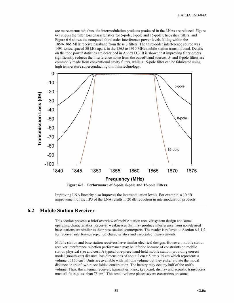
are more attenuated; thus, the intermodulation products produced in the LNAs are reduced. Figure

6-5 shows the filter loss characteristics for 5-pole, 8-pole and 15-pole Chebyshev filters, and

Figure 6-6 shows the computed third-order interference power levels falling within the

1850-1865 MHz receive passband from these 3 filters. The third-order interference source was

1491 tones, spaced 30 kHz apart, in the 1865 to 1910 MHz mobile station transmit band. Details

on the tone power statistics are described in Annex D.3. It is shown that improving filter orders

significantly reduces the interference noise from the out-of-band sources. 5- and 8-pole filters are

commonly made from conventional cavity filters, while a 15-pole filter can be fabricated using

high temperature superconducting thin film technology.

Improving LNA linearity also improves the intermodulation levels. For example, a 10 dB

improvement of the IIP3 of the LNA results in 20 dB reduction in intermodulation products.

6.2 Mobile Station Receiver

This section presents a brief overview of mobile station receiver system design and some

operating characteristics. Receiver weaknesses that may produce interference from non-desired

base stations are similar to their base station counterparts. The reader is referred to Section 6.1.1.2

for receiver interference rejection characteristics and associated measurements.

Mobile station and base station receivers have similar electrical designs. However, mobile station

receiver interference rejection performance may be inferior because of constraints on mobile

station physical size and cost. A typical one-piece hand-held mobile station, providing correct

modal (mouth-ear) distance, has dimensions of about 2 cm x 5 cm x 15 cm which represents a

volume of 150 cm3. Units are available with half this volume but they either violate the modal

distance or are of two-piece folded construction. The battery may occupy half of the unit’s

volume. Thus, the antenna, receiver, transmitter, logic, keyboard, display and acoustic transducers

must all fit into less than 75 cm3. This small volume places severe constraints on some

53 v2.0a

TIA/EIA TSB-84A

-100

-90

-80

-70

-60

-50

-40

-30

-20

-10

0

Frequency (MHz)

Tra

nsm

issio

nL

oss

(dB

)

1840 1845 1850 1855 1860 1865 1870 1875

5-pole

8-pole

15-pole

Figure 6-5 Performance of 5-pole, 8-pole and 15-pole Filters.

non-integrable components such as the antenna, and RF/IF bandpass filters. The result is that

antenna efficiency is reduced and filter passband loss is increased.

6.2.1 Characteristics

6.2.2 Receiver Operating Theory and Some Typical Parameters

Figure 6-7 shows a generic mobile station receiver block diagram. The antenna is usually a quarter

wave (4 cm) wire driven against the transmitter circuit board which serves as a “ground plane”.

The theoretical resonant driving point resistance of this radiating system is about 36 ohms which

nearly matches the duplexer 50 ohm input impedance. To radiate effectively, the quarter-wave

wire can not be parallel to, or within, the circuit board. Thus, the wire radiator is usually enclosed

within a flexible plastic cylinder which protrudes from the top of the mobile station housing. Some

designs use a sliding wire, which must be pulled out from the housing before call initiation. The

antenna gain is usually assumed to be 2 dBi. Some antenna gain and radiation pattern

characteristics are described in Section 8.2.

The duplexer is an RF filter structure which allows mobile station duplex, (simultaneous receive

and transmit) operation. Analog FM and non-packet CDMA systems operate in the duplex mode.

Some TDMA systems, which transmit and receive in different time slots, do not require a

duplexer. For these systems, a PIN diode transmit-receive switch sometimes replaces the duplexer.

Figure 6-7 shows that the duplexer consists of a transmit bandpass filter (T-BPF) and a receive

bandpass filter (R-BPF). These filters are usually separate units. The R-BPF may pass all, or

portion of, the assigned frequency block. The R-BPF must also reject the mobile station’s own

transmitter signal, which may be 140 dB stronger than the received signal. Transmitter signal

v2.0a 54

TIA/EIA TSB-84A

-200

-190

-180

-170

-160

-150

-140

-130

-120

-110

-100

-90

-80

1850 1855 1860 1865

Frequency (MHz)

Inte

rfe

ren

ce

Po

we

rL

ev

el

(dB

m)

5-pole

8-pole

15-pole

Figure 6-6 Example of Interference Power Resulting from Different Skirt Rejection Characteristics of

5-pole, 8-pole, and 15-pole Pre-select Filters.

rejection usually exceeds 60 dB, which requires at least a sixth-order (6 resonator) filter.

Quarter-wave coaxial resonators are used, each loaded with a temperature-compensated high

dielectric constant (k) barium titanate ceramic. If k ! 80, then the coaxial resonator length can be

reduced by a factor of 800.5 = 8.9. Thus, the loaded quarter wavelength is about 0.45 cm.

To minimize size and cost the resonators are fabricated together into a single metal plated block of

ceramic, which is soldered to the circuit board. The volume of a 6-resonator R-BPF may be less

than 1 cm3, which allows a comfortable fit upon the receiver’s printed circuit board. The penalty

paid for this small volume is high passband loss, which may reach 3 dB.

The purpose of the T-BPF is to reject transmitter wideband noise and spurious output signals

which fall into the receive frequency block. A fourth-order filter is usually sufficient and the

passband loss is usually kept below 2 dB.

The in-block signals from the R-BPF enter the low noise amplifier (LNA) which provides gain

and determines the receiver noise figure. Some LNA characteristics are described in Section 6.1.3.

A low-cost LNA has gain (G) <10 dB, noise figure (NF)> 4 dB and third-order input intercept

point (IIP3)< 0 dBm. There is a trade-off between LNA gain and third-order intermodulation

product generation. High gain is desired to minimize total receiver noise figure, but it also

enhances third-order intermodulation product generation in the LNA and mixer. The origin and

control of third-order intermodulation is found in Sections 6.1.1.3 and Chapter 10. Because of

increased loss caused by cost and size restrictions the receiver noise figure may reach 10 dB.

A bandpass filter (BPF), commonly a second order, follows the LNA to reject LNA output noise

which falls into the image band of the mixer.

Signals leaving the BPF enter MIXER1 where they are product modulated with a strong single

frequency local oscillator LO1 which has a frequency stability of a few parts in 106. The LO1

signal is frequency synthesized from a lower frequency (<20 MHz) temperature compensated

quartz oscillator. Some systems (e.g. CDMA) phase lock LO1 to the demodulated bit stream. The

LO1 frequency synthesizer can generate (one at a time) hundreds of digital programmable

frequencies. To minimize cost, the mixer is often a single bipolar transistor or FET with G =

+6 dB, NF = 7 dB and IIP3 < 0 dBm.

Frequency downconverted signals leaving MIXER1 enter the first intermediate frequency

bandpass filter (IF BPF) where the one desired channel is separated from the many downconverted

channels. In narrowband TDMA systems the filter’s 3 dB bandwidth (BW3) may be 28 kHz <

BW3 < 220 kHz; in CDMA systems 1.23 MHz � BW3 � 5 MHz (or more). The second- order

55 v2.0a

TIA/EIA TSB-84A

ReceiveBPF

TransmitBPF

Antenna

LNA

LO2

Mixer2

IF BPF2BPF IF Amp2

AGC

Mixer

Mixer

BasebandLPF

A/D

A/D

I

Q

Demodulator

Duplexer

90°

LO3

LO1

Mixer1

IF BPF1 IF Amp1

Transmitter

Figure 6-7 Generic Mobile Station Receiver

(2-resonator) filter’s center frequency is usually between 70 and 150 MHz. Quartz resonators are

most often used.

The filtered first IF signal leaving IF BPF, is amplified by the IF amplifier (IF AMP1) before it

enters MIXER2 where it is further downconverted to a second, much lower intermediate

frequency. LO2, driving MIXER2, is derived from the same frequency synthesizer which generates

LO1.

The downconverted signal leaving MIXER2 enters the second IF bandpass filter (IF BPF2). This,

often eighth-order, filter is constructed from inexpensive ceramic piezo-electric resonators similar

to those used in broadcast AM radios. IF BPF2 completes the channel filtering requirements.

The filtered signal leaving IF BPF2 enters the second IF amplifier (IF AMP2). The total gain (GT)

of IF AMP1 and IF AMP2 can be varied over a range of 0 dB < G < + 90 dB. Gain control is

obtained via the automatic gain control (AGC) voltage derived in the subsequent demodulator

circuit.

AGC is required to accommodate the system dynamic range which is defined by the strongest

expected signal (in dBm) minus the weakest expected signal (in dBm). In narrowband TDMA

systems, the strongest signal is approximately –30 dBm and the weakest signal, near the noise

floor is about –120 dBm. Therefore, the system dynamic range is 90 dB. Broadband CDMA

systems employ base station transmitter power control so that the system dynamic range is

considerably less, in the order of 30 dB.

The essentially constant power signal leaving IF AMP2 enters the demodulator circuit which

converts the modulated IF signal to the final baseband TTL-level bit streams. A 4-phase I &Q

demodulator is shown in Figure 6-7. Systems employing constant envelope FM modulation, such

as J-STD-007 PCS1900, and IS 713 Upbanded AMPS may use a limiter-discriminator circuit

similar to that found in analog FM radios.

The filtered IF signal drives two balanced mixers. The local oscillator LO2 drives both mixers, one

mixer at a 0 degree phase angle and the other at a 90 degree phase angle. If LO2 is located at the

correct frequency and phase, a baseband in-phase (I) bit stream will appear at the I output and a

baseband quadrature-phase (Q) bit stream will appear at the Q output.

The demodulated I & Q bit streams are passed through baseband lowpass filters (LPF) to remove

residual IF and LO2 frequencies and high frequency baseband noise.

In CDMA systems, many bit streams are demodulated simultaneously since each bit stream

represents a CDMA mobile station. The resulting multi-level I & Q outputs are fed to

analog-to-digital converters (A/D) for subsequent processing by the code channel separation logic

circuits. In TDMA systems, only one mobile station bit stream is received at a given time and

simple one-bit A/D converters may be used.

It is important to maintain a constant level IF signal into the demodulator so that the mixers and

A/D converters will operate within their specified dynamic ranges. Therefore, the demodulator

generates a baseband AGC voltage which represents a weighted average value if the I & Q

baseband bit streams. As stated earlier, this AGC signal is fed back to control the gain of the IF

amplifiers. A good AGC system must follow the slow and rapid (100 Hz) fading encountered in a

1.9 GHz PCS system.

There are several advantages to this double-conversion, two-IF receiver:

• Lower cost bandpass filters can be used since the expensive IF BPF1 is simple (second-order)

and the more complex ceramic resonator IF BPF2 is inexpensive.

• Since the second IF is below 1 MHz, the demodulator circuits can often be implemented within

a single, low-power integrated circuit.

v2.0a 56

TIA/EIA TSB-84A

• Most of the IF gain can be in IF AMP2. This sub MHz second IF lessens the tendency for gain

instability and self-oscillation of circuits upon the poorly shielded amplifier circuit board.

Some disadvantages of double-conversion are:

• Since there is more gain added ahead of the final channel filter, IF BPF2, there is likelihood of

third-order intermodulation products generation in IF AMP1 and MIXER2.

• MIXER2 increases the spurious responses of the receiver.

• A second local oscillator LO2, is required.

6.2.2.1 Receiver Interference Rejection Characteristics

Mobile station receiver interference rejection characteristics are similar to their base station

counterparts; therefore, refer to Section 6.1.1.2 for interference rejection theory, definitions and

typical measurements for an IS-136 TDMA system.

57 v2.0a

TIA/EIA TSB-84A

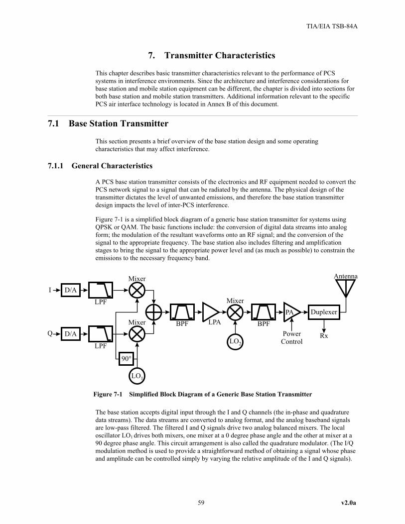
7. Transmitter Characteristics

This chapter describes basic transmitter characteristics relevant to the performance of PCS

systems in interference environments. Since the architecture and interference considerations for

base station and mobile station equipment can be different, the chapter is divided into sections for

both base station and mobile station transmitters. Additional information relevant to the specific

PCS air interface technology is located in Annex B of this document.

7.1 Base Station Transmitter

This section presents a brief overview of the base station design and some operating

characteristics that may affect interference.

7.1.1 General Characteristics

A PCS base station transmitter consists of the electronics and RF equipment needed to convert the

PCS network signal to a signal that can be radiated by the antenna. The physical design of the

transmitter dictates the level of unwanted emissions, and therefore the base station transmitter

design impacts the level of inter-PCS interference.

Figure 7-1 is a simplified block diagram of a generic base station transmitter for systems using

QPSK or QAM. The basic functions include: the conversion of digital data streams into analog

form; the modulation of the resultant waveforms onto an RF signal; and the conversion of the

signal to the appropriate frequency. The base station also includes filtering and amplification

stages to bring the signal to the appropriate power level and (as much as possible) to constrain the

emissions to the necessary frequency band.

The base station accepts digital input through the I and Q channels (the in-phase and quadrature

data streams). The data streams are converted to analog format, and the analog baseband signals

are low-pass filtered. The filtered I and Q signals drive two analog balanced mixers. The local

oscillator LO1 drives both mixers, one mixer at a 0 degree phase angle and the other at mixer at a

90 degree phase angle. This circuit arrangement is also called the quadrature modulator. (The I/Q

modulation method is used to provide a straightforward method of obtaining a signal whose phase

and amplitude can be controlled simply by varying the relative amplitude of the I and Q signals).

59 v2.0a

TIA/EIA TSB-84A

Antenna

LPA

LO2

Mixer

BPF

Rx

PA

BPF

LPF

LPF

D/A

D/A

I

Q

Mixer

Mixer

90°

LO1

Duplexer

PowerControl

Figure 7-1 Simplified Block Diagram of a Generic Base Station Transmitter

After summing the mixer outputs, the signal is bandpass filtered, amplified by the low power

amplifier (LPA), and subsequently upconverted to the final transmission frequency by mixing with

a local oscillator signal LO2 of the appropriate frequency. The upconverted signal is amplified to

the necessary power level by the power amplifiers. The power control input adjusts the level of the

signal transmitted by the base station. Power control is often a dynamic response and is described

in Chapter 11, Dynamic Responses, and in Annex B. The output of the power amplifier is fed to

the antenna duplexer, which isolates the antenna receive (incoming) and transmit (outgoing)

signals. The duplexer includes a transmit filter that attenuate unwanted emissions (emissions

outside of the licensed frequency block, or outside of the base station transmit band). Finally, the

RF signal is connected to a feeder line that is terminated with an antenna, which couples the RF

signal to free space.

The simplified block diagram is generally appropriate to a single RF carrier base station

transmission system. Additional components are needed when a single PCS provider transmits

multiple co-block RF carriers into one antenna, or when multiple PCS providers (using different

frequency blocks) share a single antenna. In the former case, a signal combiner (or combiners) is

added after each power amplifier, and the summed signal is fed through the duplexer to the

antenna. In the latter case, an antenna combiner is added at the output of the duplexer. The

combiner filters each PCS provider’s signals (keeping them isolated to their appropriate frequency

blocks), combines the signals, and feeds the total signal to the single antenna. An important factor

when using any type of combiner is to insure that the level of intermodulation products generated

by the combiner is kept as low as possible.

Most outdoor base station installations also include a lightning protection unit between the

transmitter and antenna. The function of the lightning protection unit is to safely discharge large

electrostatic charges that may be created by lightning strikes near the antenna system.

7.1.2 Base Station Transmit Power

Base station transmit power is constrained by standards and by FCC limits. The limits for each

technology (and the relevant section in this document) are summarized in Table 7-1:

Table 7-1 Summary of Maximum Base Station Transmitter Output Power. Where a specific limit is notgiven in the standard, the 100 W FCC maximum is listed. The powers in this table are maximum transmitter

output powers, not maximum EIRP.

TechnologySummary of Transmit Power Limit(see referenced section for details)

Referenced Section

IS-661 CCT 2 W B.1.1.2

IS-95 CDMA 100 W* B.1.2.1.2

J-STD-014 PACS 0.8 W B.1.3.1.1

IS-136 TDMA 100 W* B.1.4.1.1

J-STD-007 PCS1900 39.8 W B.1.5.2

J-STD-015 W-CDMA 100 W* —

IS-713 Upbanded AMPS 100 W* B.1.7.2.1

SP-3614 PWT-E 0.5 W B.1.8.1

* FCC limit

In addition to power limits specified in the relevant standards, the FCC provides for maximum

transmitter output power and EIRP. The transmitter power limit is always 100 W, and the EIRP

limit is 1640 W for antennas below 300 m HAAT. The EIRP limits are lower for higher antennas.

The FCC also specifies maximum received power levels at market boundaries, and with regard to

protection of incumbent microwave links. Further details on FCC power limits are in Section B.1.

v2.0a 60

TIA/EIA TSB-84A

Under certain circumstances, FCC-mandated RF exposure guidelines may limit emission levels

below the constraints provided in the technology standards and in the FCC power limits. Further

information on RF exposure guidelines is available in FCC OET Bulletin 65 [19].

7.1.3 External Losses and Gains

Passive components placed after the power amplifier will result in some loss of the transmission

power that is ultimately delivered to the antenna. The antenna duplexer, signal combiner(s),

lightning protection unit, connecting jumpers and antenna feeder lines may each contribute

between 1 and 3 dB of insertion loss. As a result, a transmitter that is specified to produce 40 W of

power at the output of the power amplifier may deliver less than 10 W to the input of the antenna.

When performing inter-PCS interference estimations, these losses must be included to accurately

model the signal level (EIRP) that is radiated from the antenna.

To counteract the power lost in the various external base station components, some PCS systems

employ external high power amplifiers that boost the power amplifier signal back up to its pre-loss

level. The linearity and intermodulation performance of external amplifiers must be good to avoid

producing high levels of unwanted emissions. Particular attention should be given to the

possibility of spectral regrowth, where high-order self-mixing products between the components

that comprise a single RF carrier produce broad, out-of-band emissions that surround the desired

carrier signal.

7.1.4 Unwanted Emissions

Base stations will radiate emissions outside of their intended RF channels, and outside of their

intended blocks. The term “unwanted emissions” refers to both out-of-band emissions and

spurious emissions, as defined in Section 0.6. The unwanted emissions from a base station that fall

outside the intended frequency block and within the base station transmit (mobile station receive)

frequencies of another system may interfere with nearby handsets of that other system. The

unwanted emissions from a base station that fall within the TDD base station receive (mobile

station transmit) frequencies may interfere with nearby TDD base stations.

The use of transmit filters is required to reduce the level of unwanted emissions to acceptable levels.

Section 7.1.7 below discusses transmit filter characteristics and their affect on unwanted emissions.

Technology standards and FCC rules constrain the allowed level of unwanted emissions. Table

7-2 indicates the reference section that contain the relevant standards limits:

Table 7-2 Allowable Level of Unwanted Emissions

Technology Referenced Section(s)

IS-661 CCT B.1.1.3 – B.1.1.4, B.1.1.6

IS-95 CDMA B.1.2.2, B.1.2.4

J-STD-014 PACS B.1.3.2 – B.1.3.4

IS-136 TDMA B.1.4.1.2 – B.1.4.1.5, B.1.4.3

J-STD-007 PCS1900 B.1.5.3 – B.1.5.5

J-STD-015 W-CDMA Figure B-15

IS-713 Upbanded AMPS —

SP-3614 PWT-E B.1.8.3 – B.1.8.4

The FCC rules on unwanted emissions are discussed in Section B.1. Methods of measuring

unwanted emissions are presented in Annex C.

61 v2.0a

TIA/EIA TSB-84A

7.1.5 Channel Spacing vs. Bandwidth for PCS Emissions

PCS emissions are channelized in the sense that their center frequencies are required by standards

to fall at specified increments. For example, PCS1900 channels fall at a frequency spacing of 200

kHz—as specified in the PCS1900 standard, 1956.4, 1956.6, and 1956.8 MHz are valid PCS1900

carrier frequencies, but 1956.5 MHz is not.

Despite the channelization of PCS emissions, it is important to recognize that the emissions are

generally not constrained to a bandwidth equal to the channel spacing. For example, even though

PCS1900 channels fall at 200 kHz spacings, the occupied bandwidth (Section 0.6) of a PCS1900

signal is over 250 kHz and the emission bandwidth (Section 0.6) exceeds 325 kHz (refer to Figure

C-4). The spillover of PCS emissions beyond their channel boundaries must be accounted for

when estimating interference effects between PCS transmissions on neighboring channels.

Table 7-3 summarizes the approximate occupied and emission bandwidths of various PCS

technologies. These values are based on measurements made with either an operating base station

for the specified technology or a digital signal generator capable of simulating the specified

technology’s signal.

Table 7-3 Approximate Occupied and Emission Bandwidths for Various PCS Technologies.

TechnologyChannel Spacing

(kHz)Occupied Bandwidth

(kHz)Emission Bandwidth

(kHz)

IS-661 CCT 1600 1600 1875

IS-95 CDMA 1250 1260 1420

J-STD-014 PACS 300

IS-136 TDMA 30 29 34

J-STD-007 PCS1900 200 253 328

J-STD-015 W-CDMA 2500

IS-713 Upbanded AMPS 30*

SP-3614 PWT-E 1000

*Narrow Analog Voice Channel spacing is 10 kHz. The measured bandwidths are for standard (30

kHz) voice channels.

7.1.6 Frequency Hopping

Some PCS technologies are capable of operating in a frequency hopping mode in which the carrier

frequency is changed rapidly (typically several times each second). The base and mobile stations

are synchronized so that each is on the proper frequency at the proper time. The purpose of

frequency hopping is to reduce the degradation of the transmitted signal due to frequency-selective

fading or from interference that may be more prevalent on one RF channel than the others.

7.1.7 Base Station Filters

Base stations employ filters of various forms to reduce the level of unwanted emissions. For

example, a filter in the duplexer stage may be a lumped-element or cavity filter that is resonant

over the appropriate band of frequencies. In contrast, filtering in the early stages of the transmitter

signal chain may take place in the time domain; for example, by bit shaping to reduce sudden

voltage transitions that would result in a large occupied bandwidth of the transmitted signal.

For the reduction of out-of-block emissions, the most important filters are generally those that

occur after the power amplifier stage. It is these filters that perform the last step of attenuation of

v2.0a 62

TIA/EIA TSB-84A

unwanted emissions before the signal is radiated by the antenna. Many FDD base stations employ

filtering that provides two levels of attenuation to unwanted signals. The first level is designed to

specifically attenuate out-of-block emissions, while the second stage further attenuates emissions

outside of the base station transmit portion of the PCS allocation (below 1930 MHz). The amount

of attenuation of out-of-block emissions depends on the specific filter implementation. Informal

measurements of various base station systems show attenuation levels of better than –90 dBc

within the FDD base station transmit band.

Good base station filtering is necessary to reduce the chance of interference with nearby systems,

since no level of filtering by the victim receiver can reduce the level of unwanted base station

emissions that are co-channel with the victim receiver. If needed, additional filters (to complement

filters already built into the base station) are readily available on the commercial market. These

external filters can produce better than 80 dB of additional out-of-block attenuation, have

relatively low insertion loss (less than approximately 1 dB), are compact in size, and cost a few

hundred dollars each.

7.2 Mobile Station Transmitters

This section presents a brief overview of the mobile station design and some operating

characteristics that may affect interference.


Mobile station transmitters are designed with three main objectives: low cost, small size, and low

power consumption. These considerations lead to a transmitter design that is necessarily less

complex than that employed in base stations.

A simplified block diagram of a mobile station transmitter is similar to Figure 7-1. Some TDMA

systems do not require a duplexer, since the mobile station is never receiving and transmitting

simultaneously.

Mobile stations must be frequency agile since the operating PCS block may change as the user

moves from one market to another. The out-of-block transmitter filtering is therefore not as

thorough as it is for base stations; however, the mobile stations are generally transmitting at

significantly lower power levels than the base station.

7.2.2 Mobile Station Transmit Power

Mobile station transmit power is constrained by standards and by FCC limits. The limits for each

technology (and the relevant section in this document) are summarized in Table 7-4:

63 v2.0a

TIA/EIA TSB-84A

Table 7-4 Summary of Maximum Mobile Station Transmitter Output Power.

TechnologySummary of Transmit Power Limit

†

(see referenced sections for details)Referenced Section

IS-661 CCT 1 W EIRP B.1.1.1

IS-95 CDMA 2 W EIRP B.1.2.1.1

J-STD-014 PACS 0.2 W B.1.3.1.2

IS-136 TDMA 1.6 W EIRP B.1.4.2

J-STD-007 PCS1900 2 W EIRP B.1.5.1

J-STD-015 W-CDMA 0.2 W EIRP B.1.6.1

IS-713 Upbanded AMPS 2 W EIRP* B.1.7.1.1.2

SP-3614 PWT-E 0.5 W B.1.8.1

* FCC limit

† Where a specific limit is not given in the standard, or the standard limit exceeds the FCC limit,

the 2 W EIRP FCC maximum is listed. The maximum power levels for J-STD-014 PACS and

SP-3614 PWT-E are listed as transmitter output power, but these technologies are still constrained

by the 2W EIRP FCC limit.

7.2.3 Unwanted Emissions

Mobile stations will radiate emissions outside of their intended RF channels, and outside of their

intended blocks. The unwanted emissions from a mobile station that fall outside the intended

frequency block and within the mobile station transmit (base station receive) frequencies of

another system may interfere with nearby base stations of that other system. The unwanted

emissions from a mobile station that fall within the TDD mobile station receive (base station

transmit) frequencies may interfere with nearby TDD mobile stations.

Technology standards and FCC rules constrain the allowed level of unwanted emissions.

Table 7-5 indicates the reference section that contain the relevant standards limits:

Table 7-5 Unwanted Emissions

Technology Referenced Section(s)

IS-661 CCT B.1.1.3, B.1.1.5 – B.1.1.6

IS-95 CDMA B.1.2.3 – B.1.2.4

J-STD-014 PACS B.1.3.2 – B.1.3.4

IS-136 TDMA B.1.4.2 – B.1.4.3

J-STD-007 PCS1900 B.1.5.3 – B.1.5.5

J-STD-015 W-CDMA B.1.6

IS-713 Upbanded AMPS —

SP-3614 PWT-E B.1.8.3 – B.1.8.4

The FCC rules on unwanted emissions are discussed in Section B.1. Methods of measuring

unwanted emissions are presented in Annex C.

7.2.4 Channel Spacing vs. Bandwidth for PCS Emissions

Refer to Section 7.1.5.

v2.0a 64

TIA/EIA TSB-84A

7.2.5 Mobile Station Transmitter Duty Cycle

In many PCS systems, mobile and portable stations have non-continuous transmit modes. The air

interfaces used for PCS often utilize discontinuous transmit modes which affect the duration and

timing of interference. These effects must be included in the interferer characteristics to properly

characterize the interference to a potential victim. These modes include the use of time division

multiple access (TDMA), voice activity detection (VAD), discontinuous transmit modes (DTX),

and frequency hopping (FH), or dynamic channel allocation (DCA). These modes must be

considered with respect to both the interferer transmit duration and timing, as well as the potential

victim receive duration and timing. All PCS systems are required to ensure a service quality

(usually this corresponds to a specified BER or FER for a digital system, or a specified

demodulated SINAD for an analog system). If sufficient interference is simultaneously introduced,

the BER, FER or SINAD degrades from the specified amount. In order to maintain the specified

BER, FER or SINAD, the desired input signal level would have to be increased. Table 7-6

provides the relevant reference for each standardized air interface technology.

Table 7-6 Locator for Relevant Reference for Each Standardized Air Interface Technology

Air Interface Technology TDMA VAD or DTX FH or DCA

IS-661 CCT B.3.1.1

IS-95 CDMA B.3.2

J-STD-014 PACS B.3.3.2

IS-136 TDMA B.3.4

J-STD-007 PCS-1900 B.3.5.1 B.4.2.5 B.4.5.2

J-STD-015 W-CDMA B.3.6

IS-713 Upbanded AMPS not applicable not applicable not applicable

SP-3614 PWT-E B.3.8.1 B.2.8.2

65 v2.0a

TIA/EIA TSB-84A

8. Antennas

Antennas used in the transmission and reception of PCS signals have gain and directivity, which

affect interference analysis. The purpose of this chapter is to provide general characteristics of

PCS antennas for the purpose of interference estimation.

8.1 Base Station Antennas


The physical construction of base station antennas is diverse, but most project a wide beam in the

horizontal plane, and a much narrower pattern in the vertical plane. Omnidirectional antennas

project a horizontal beam that is typically constant to within a dB or so at all azimuths. A standard

vertical stick or dipole antenna will produce such a pattern. Directional antennas, commonly

employed in sectored cell sites, focus more of their energy towards a particular azimuth. The

directional pattern is commonly achieved by using “panel” antennas, inside of which an array of

dipole antennas (as shown in Figure 8-1) provides the desired pattern through coherent phasing.

With a panel antenna, the width of the horizontal beam is controlled by the horizontal spacing

between the constituent antennas, and the width of the vertical beam is controlled by the number

of pairs of dipoles that are stacked vertically.

As the beamwidth is approximately inversely proportional to the physical dimension of the

radiating surfaces, taller PCS antennas (more pairs of dipoles) will generally produce narrower

beams in the vertical direction than similar antennas using fewer pairs of dipoles. Smaller

beamwidths produce larger antenna directivity; and, therefore, for antennas of similar

construction, those with larger gain can be assumed to have smaller beamwidths than those with

smaller gain.

Example radiation patterns for omnidirectional and directional antennas are shown in Figures. 8-2

through 8-5.

Base station antennas are generally vertically polarized, although many offer “dual-slant”

polarization with peak polarization at 45 degrees from vertical. The dual-slant antennas are used

in polarization diversity systems. Because PCS signals often suffer multiple reflections,

polarization characteristics beyond line-of-sight distances are difficult to predict.

67 v2.0a

TIA/EIA TSB-84A

Dipole Pair

Conducting Backplane

Figure 8-1 Simplified Example of a Six-Dipole PCS Panel Antenna.

v2.0 68

TIA/EIA TSB-84A

0

5

Gain (dBi)

90 deg

0 deg

180 deg

270 deg

1010

Figure 8-2 Horizontal Plane Pattern for a 10 dBi Omnidirectional Antenna.

-40

-30

-20

-10

0

10

Gain (dBi)

0 deg

+90 deg

-90 deg

180 deg

Figure 8-3 Vertical Plane Pattern for a 10 dBi Omnidirectional Antenna.

69 v2.0a

TIA/EIA TSB-84A

-20

-15

-10

-5

0

5

10

15

20

90 deg

0 deg

180 deg

270 deg

(dBi)Gain

Figure 8-4 Horizontal Plane Pattern for a 16 dBi Gain Directional Antenna.

-30

-20

-10

0

10

20

Gain (dBi)

0 deg

+90 deg

-90 deg

180 deg

Figure 8-5 Vertical Plane Pattern for a 16 dBi Gain Directional Antenna.

8.1.2 Isolation between Closely Spaced Antennas

Victim and interferer base station antennas sharing the same tower, rooftop, or other antenna site

will be separated by small distances. An important consideration is the degree of isolation that can

be achieved between the ports of the two antennas. Isolation will depend on many factors,

including: Physical separation distance; relative positions (i.e., horizontal and vertical spacings,

and whether one antenna is within the main beam of the other); the position and conducting

properties of the tower or other support structure; the beam pattern of the antennas; and the

physical construction of the antennas.

Due to the large number of factors affecting isolation, it is best determined through on-site

measurements; however, this is commonly impractical due to the nature of the antenna

installations and the fact that the antennas may belong to competing PCS providers. Barring such

measurements, operators may need to rely on measurements obtained through controlled tests of

standard antennas, and attempt to extend these data to their own situations.

The data in this section may prove helpful for obtaining a rough estimate of isolation between

co-located base station antennas. Figure 8-6 shows the isolation between the ports of two

vertically separated dipole antennas, as a function of distance between their centers. At PCS base

station transmit frequency, the vertical isolation can be approximated by1:

I dB yvert ( ) log( ),� �55 40 (8-1)

where y is the separation distance in meters. This formula has been shown to be a good

approximation for both omnidirectional and directional antennas under many circumstances.

v2.0a 70

TIA/EIA TSB-84A

40

50

60

70

80

90

100

110

120

0.0 5.0 10.0 15.0 20.0 25.0 30.0

VERTICAL SEPARATION (m)

ISO

LA

TIO

N(d

B)

Figure 8-6 Isolation between the Ports of Two Vertically-Separated Dipole Antennas as a Function of the

Distance between their Centers.

1 Johnson, R. C. (Ed.), Antenna Engineering Handbook (3rd Edition), (New York: McGraw Hill), 1993, page40-19.

Isolation between omnidirectional antennas that are horizontally offset can be estimated from:

I dB x K

K dbG G x m

x m

hor

A B

( ) . log( )

( ), .

( / . )

� � �

��

385 20

15

15 ( ), .

( ) min( , ),

G G x m

K dB K

A B� #$%&

�

15

10

(8-2)

where GA and GB are the maximum gains of the two antennas in dB, and x is their horizontal

separation in meters.

Isolation between omnidirectional antennas that are both horizontally and vertically offset (slant

offset) is approximated by2:

I dBI I I I I

Islant

vert hor hor vert hor( )( ) , ,�

��

��

2�

hor vert horI I#

$%'

&'

(8-3)

where � is the vertical angle from the center of the upper antenna to the center of the lower

antenna, in radians [� = tan-1(y/x)].

8.1.3 Antenna Downtilt

Downtilt is the pointing of the main lobe of the antenna in the downward direction. Base station

antennas are often downtilted to improve close-in coverage and to reduce interference to and from

distant sources. Downtilt can be accomplished either mechanically (for example, by pointing the

face of a directional antenna in the downward direction), or electrically (by phasing the antenna

components such that, when the antenna is installed in an upright position, the main lobe falls

below the horizontal plane). The amount of downtilt depends upon the situation, but typically

ranges between 0 and 10 degrees.

This section presents equations that can be used to estimate the gain of a PCS antenna in any

direction, given its nominal (non-downtilted) radiation patterns in the horizontal and vertical

planes. The concept of “nominal” requires explanation: For an antenna that has no built-in

electrical downtilt, the nominal horizontal plane pattern is the pattern measured in the horizontal

plane when no mechanical downtilt has been applied. This pattern will contain the main lobe of

the antenna. For an antenna that does have electrical downtilt built-in, the nominal horizontal

plane pattern is not measured in a plane per se, but is the pattern measured along a cone defined

by the degree of electrical downtilt. For example, if the antenna has a 3-degree electrical downtilt,

then the nominal horizontal plane pattern is that pattern measured in a cone surrounding the

antenna and 3 degrees below the horizontal plane. This nominal pattern will contain the main lobe

of the antenna.

In this section, the following definitions are used:

Horizon Plane The plane containing the center point of the antenna and parallel to the

surface of the Earth at the location of the antenna.

Horizontal Plane For antenna patterns, the “horizontal plane” pattern cut is the maximum

gain of the antenna as a function of azimuth. Note that for electrically

downtilted antennas, the “horizontal plane” is not a plane, but a cone

defined by the degree of electrical downtilt.

71 v2.0a

TIA/EIA TSB-84A

2 Johnson, R. C. (Ed.), Antenna Engineering Handbook (3rd Edition), (New York: McGraw Hill), 1993, page40-19.

( The azimuthal angle measured along the horizon plane, with the origin

being the point at which the vertical plane containing the main lobe

intersects the horizon plane. [In practical use, ( usually increases in a

clockwise direction as viewed from above the antenna, so that it agrees

with the sense in which directional azimuth (degrees east of north) is

defined.]

) The angle measured downward from the horizon plane.

�e The angle by which the antenna is electrically downtilted (positive

angle denotes downtilt; negative angle denotes uptilt).

�m The angle by which the antenna is mechanically downtilted (positive

angle denotes downtilt; negative angle denotes uptilt).

Gmax The maximum (main lobe) gain of the antenna.

G((,)) Gain of the antenna as a function of azimuth and elevation.

P((,)) The antenna pattern as a function of azimuth and elevation. P((,)) is

related to the gain G((,)) of the antenna by P((,)) = G((,)) � Gmax.

The horizon plane pattern is P((,0), and the vertical plane pattern is

P(0,)). Note: for electrically downtilted antennas, the nominal

horizontal plane pattern is equivalent to P((,�e).

Using these definitions, the gain of a downtilted antenna (where the downtilt can be any

combination of electrical and mechanical downtilt) at any arbitrary azimuth and elevation, is given

by:

G G P Pe( , ) ( , ) ( , ),max( ) ( � )� � * � *0 (8-4)

where

* � ��) � ) � ) (sin [cos sin sin cos cos ]1m m

(8-5)

and

* �

� ��

�� + +

� ��

�� # +

�

�(

tan , ,

tan , ,

t

1

1

0 0

0 0

N

DN D

N

DN D

an ,� ��

��

$

%

'''

&

'''

1 N

Dotherwise

(8-6)

where

N

D m m

,, �

cos sin ;

cos cos cos sin sin .

) (� ) ( � )

(8-7)

The equations in this section assume that the general shape (not amplitude) of the azimuthal-plane

patterns is independent of elevation angle. A limited number of full-pattern measurements of

directional PCS antennas indicate that this assumption is reasonable.

v2.0a 72

TIA/EIA TSB-84A

8.2 Mobile Station Antennas

The current generation of mobile station handset antennas are simple radiating elements. The

radiation patterns are generally omnidirectional, consistent with their application, in which the

user may orient the handset in any direction. In controlled environments, the stubs may provide up

to 2 dBi of gain in the broadside direction; but, in use, the radiation pattern will be modified by the

close proximity of the user’s body.

For interference calculation, it can be assumed that the handset antennas offer 2 dBi gain in all

directions when used outdoors. Although not physically valid for any one instant, this assumption

is a conservative estimate of the antenna’s directivity for the purpose of incoming and outgoing

interfering signals.

Assumptions regarding changes in effective mobile station antenna gain due to in-building or

in-vehicle use are available in Annex F of TSB 10F [9].

73 v2.0a

TIA/EIA TSB-84A

9. Geometry

This chapter describes considerations related to the geometry between victim and interfering PCS

systems.

9.1 Symbols and Abbreviations

In this chapter, the following symbols and abbreviations will be used:

� Longitude on the Earth’s surface, in radians. Positive is east of the prime meridian,

negative is west of the prime meridian. Longitudes are negative for all of North America.

If the longitude is given in dd mm ss.s format, the angle in radians is (dd + mm/60 +

ss.s/3600)/57.2958.

" Latitude on the Earth’s surface, in radians. Positive is north of the equator, negative is

south of the equator. All latitudes are positive in North America. If the latitude is given in

dd mm ss.s format, the angle in radians is (dd + mm/60 + ss.s/3600)/57.2958.

Re Radius of the Earth. For this chapter, the Earth is assumed to be spherical with a radius

Re =6367 km.

9.2 Distance, Azimuth, and Mutual Horizon Distance between Radio

Antennas on the Earth’s Surface

For a transmit antenna and a receive antenna located at points 1 and 2 on the Earth’s surface

respectively (see Figure 9-1), specified by the latitude (") and longitude (�- pairs ( , )" �1 1 and

( , )" �2 2 , the great circle distance between the points is:

D Re� � ��cos [sin sin cos cos cos( )].11 2 1 2 2 1" " " " � � (9-1)

The azimuth (angle in radians measured eastward from north) from Point 1 towards Point 2 is

calculated from:

AZ

D R

D R

e

e1 2

1 2 1

1�

�

�

��

��

�

�cos

sin sin cos( / )

cos sin( / )

" "" � � �

��

, sin( )

cossin sin cos( / )

cos sin

� �

" "

"

1 2

1 2 1

1

0

2D Re

( / ), sin( )

D Re

�

��

�

�� +

$

%''

&''

� �1 2 0

(9-2)

The corresponding azimuth from Point 2 towards Point 1 is obtained from Equation (9-2) by

simply interchanging the subscripts 1 and 2.

The azimuth in radians can be converted to degrees by multiplying by 57.2958 deg/rad.

75 v2.0

TIA/EIA TSB-84A

For two antennas located at the points ( , )" �1 1 and ( , )" �2 2 , and at heights above mean sea level

of h1 and h2 (in m), respectively, the horizon distance (in km) between the antennas is given by:

� �D h hh � �357 1 2. . (9-3)

If the antennas are separated by a distance less than Dh, then they will have a direct line of sight

between each other, assuming a smooth and spherical Earth and no refraction of the ray paths. If

the antennas are separated by more than Dh, then the line of sight between the antennas will be

obstructed by the curvature of the Earth (under the same assumptions).

9.3 Antenna Discrimination

Antenna discrimination must be taken into account when computing the total path loss from one

antenna to another. Discrimination is the difference between the maximum gains specified for the

antennas and their actual gains in the direction of the ray path between the two. For antennas in

close proximity (closer than 1 km, for example), and within direct line of sight of each other,

discrimination in the vertical plane must be considered in addition to the azimuthal plane

discrimination normally included in path loss calculations.

Characteristics of the transmit and receive antennas will be indicated by the subscripts t and r,

respectively. The main beams of the antennas are pointed towards azimuths AZt and AZr (an

azimuth of 0. means the antenna is pointed north, 90. denotes east, etc.). The azimuth from the

v2.0 76

TIA/EIA TSB-84A

1

2

NORTH

AZ1 2� D1 2�

Figure 9-1 Distance and Bearing from Point 1 to Point 2.

h1 h2Dh

Figure 9-2 Horizon Distance between Two Radio Towers.

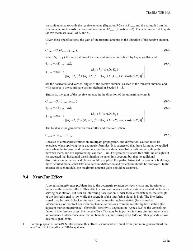
transmit antenna towards the receive antenna (Equation 9-2) is AZt r� , and the azimuth from the

receive antenna towards the transmit antenna is AZr t� (Equation 9-2). The antennas are at heights

(above mean sea level) of ht and hr.

Given these specifications, the gain of the transmit antenna in the direction of the receive antenna

is

G Gt r t t r t r� � �� ( , ),( ) (9-4)

where Gt ( , )( ) , the gain pattern of the transmit antenna, is defined by Equation 8-4, and

(

)

t r t r t

t re r e

e r

AZ AZ

R h D R

R h

� �

��

� �

��

� �cos

( )sin( / )

[( )

1

2 ( ) ( )( )cos( / )]R h R h R h D Re t e t e r e� � � �

$%'

&'

/0'

1'2 2

12

(9-5)

are the horizontal and vertical angles of the receive antenna, as seen at the transmit antenna, and

with respect to the coordinate system defined in Section 8.1.3.

Similarly, the gain of the receive antenna in the direction of the transmit antenna is

G Gr t r r t r t� � �� ( , )( ) (9-6)

(

)

r t r t r

r te t e

e t

AZ AZ

R h D R

R h

� �

��

� �

��

� �cos

( )sin( / )

[( )

1

2 ( ) ( )( )cos( / )]R h R h R h D Re r e r e t e� � � �

$%'

&'

/0'

1'2 2

12

(9-7)

The total antenna gain between transmitter and receiver is then

G G Gtotal t r r t� �� . (9-8)

Because of atmospheric refraction, multipath propagation, and diffraction, caution must be

exercised when applying these geometric formulas. It is suggested that these formulas be applied

only when the transmit and receive antennas have a direct (unobstructed) line of sight path

between them, and are separated by less than 1 km. For greater distances (but still line of sight), it

is suggested that horizontal discrimination be taken into account, but that no additional

discrimination in the vertical plane should be applied. For paths obstructed by terrain or buildings,

more detailed models that take into account diffraction and reflections should be employed. In the

absence of such models, the maximum antenna gains should be assumed.

9.4 Near/Far Effect

A potential interference problem due to the geometric relation between victim and interferer is

known as the near/far effect.1 This effect is produced when a mobile station is located far from its

serving base station, but near an interfering base station. Under these circumstances, the strength

of the desired signal is low while the strength of the interfering signal is high. The interfering

signal may be out-of-block emissions from the interfering base station (for co-market

interference), or co-block (or even co-channel) emissions from the interfering base station (for

adjacent market interference). Generally, sensitivity degradation (Annex D.1) is the controlling

factor in interference cases, but the near/far effect may be important in some circumstances, such

as co-channel interference near market boundaries, and during deep fades or other periods of low

desired signal levels.

77 v2.0a

TIA/EIA TSB-84A

1 For the purpose of inter-PCS interference, this effect is somewhat different from (and more general than) thenear/far effect that affects CDMA systems.

The effect of the near/far problem on the C/I ratio can be quantified as follows: Assume the

victim’s base station is transmitting with a power Pv into an antenna with a gain Gv in the direction

of the victim mobile station. The EIRP of the victim base station in the direction of the victim

mobile station is then EIRPv = Pv + Gv. At the same time, the interferer is transmitting with a

power Pi within the passband of the victim mobile station. This could be the result of either

adjacent channel or out-of-block emissions from the interferer, if it is operating in a different

channel or frequency block from the victim, or the result of co-channel emissions if the

interferer’s desired emissions overlap the victim’s operating channel. The power from the desired

and interfering signals, respectively, within the victim mobile station’s passband is then:

R EIRP PL D

R EIRP PL D

v v v m

i i i m

� ��

�

�

( )

( ),

(9-9)

where PL is the propagation loss over the distance between the victim’s base and mobile stations

( )Dv m� or between the interfering base station and the victim mobile station ( )Di m� .

Assuming that the victim mobile station requires a co-channel C/I of at least ( / ) minC I to operate,

interference will occur unless

PL D PL D C I EIRP EIRPi m v m i v( ) ( ) ( / ) .min� �� (9-10)

9.4.1 Example Using Out-of-Block Interference and COST 231 Propagation

The victim base station is PCS1900 technology using 20 W (43 dBm) transmit power and an

18 dBi antenna pointed slightly away from the mobile station, so that the gain in the direction of

the mobile station is 10 dBi. Then EIRPv = 53 dBm. The victim mobile station is located at a

height of 1.5 m and a distance of 8 km from its base station, which is operating at a height of 100

m in a rural (open-area) environment. Using the open-area COST 231 model (Annex A.4), the

path loss is PL Dv m( )� = 127 dB, and the received power from the base station (assuming 0 dBi

handset antenna gain) is �74 dBm.

The interferer is operating an unspecified technology in the adjacent PCS frequency block. The

interfering transmitter is operating at the FCC maximum for unwanted emissions, �13

dB(mW/MHz) = �20 dBm within the 200 kHz bandpass of the PCS1900 victim receiver, and is

using an 18 dBi antenna that is pointed toward the victim mobile station. Then EIRPi = �2 dBm.

Assuming a value of (C/I)min = 15 dB, Equation 9-10 results in

PL Di m( )� � 127 dB + 15 dB + (-2 dBm) - 53 dBm = 87 dB. (9-11)

Based upon this requirement, the distance between the interfering base station and the victim

mobile station handset must be greater than approximately 250 m, at which the free space loss

reaches a value of 87 dB.

9.5 Spatial Aggregation Methods

For the purpose of simplifying the process of interference estimation, the spatial aggregation of

several interfering sources into a single “equivalent” source may be desirable. This section adapts

the spatial aggregation methods of reference [9].

Center of Defined Area (CDA) based aggregation of interfering PCS transmitter powers is

permitted when the boundary of a region which encompasses the transmitters subtends an

transverse angle less than � degrees as viewed from the victim antenna, and when the distance

from the CDA to the boundary, along a line from the CDA to the victim antenna, does not exceed

25% of the distance from the boundary to the victim antenna. For angles greater than � degrees, or

v2.0a 78

TIA/EIA TSB-84A

for distances that do not meet the 25% criterion, the Defined Area may be further divided into a

number of sub-areas that meet the criteria.

The allowed transverse angle � is equal to the 3 dB beamwidth of the victim antenna:

79 v2.0a

TIA/EIA TSB-84A

POINTING AZIMUTHOF PCS ANTENNA

CENTER

VICTIM PCSANTENNA

(

�

DEFINED AREA(Encompasses interfering

PCS sites)Figure 9-3 Schematic of Spatial Aggregation Method

10. Intermodulation

This chapter describes Intermodulation and identifies the most likely elements requiring

consideration within and between PCS systems. Since intermodulation between PCS operators

employing dissimilar air interfaces is of particular interest, this subject is described separately

from Transmitter Characteristics and Receiver Characteristics.

10.1 Introduction to Intermodulation Product Frequencies and Power

Levels

Intermodulation products are produced whenever a non-linear device, such as a mixer, combiner,

or power amplifier processes two or more signals at the same time. The resulting outputs from this

process are the original signals, typically the linear output of the given device, and some undesired

signals, which include intermodulation products.

Consider the simple case where a signal, x(t), with two continuous wave (CW) components at

frequencies f1 and f2 drive a power amplifier with the following response

y t A x t A x t A x t( ) ( ) ( ) ( )� � �1 22

33 (10-1)

Note that in this case, the amplifier’s response consists of a linear term whose constant A1 is the

actual amplification or gain of the device. However, the amplifier’s response also consists of a

quadratic and a cubic term, both of which will cause undesired new products, at frequencies other

than the intended frequencies of f1 and f2. The constants A2 and A3 describe the relative amplitude

of these new frequency components. A2 and A3 are generally very small compared to A1 and are a

function of the amplifier drive level. When the input signal level is small, A2 and A3 are nearly

zero. This is called the linear region. When the input signal level is high, A2 and A3 are no longer

small enough to ignore. This is called the non-linear region and in this region, intermodulation

products may become significant.

The output of the amplifier in this case is the following

y t

A f t f t

Af

( )

[cos( ) cos( )]

{ [cos( (

�

�

� �

1 1 2

2 12 1

2 2

21 2 2

) ) cos( ( ) )] cos( ( ) ) cos( ( ) )t f t f f t f f t� � � � �2 2 2 22 1 2 1 2 }

[cos( ) cos( )]

[cos( ( ) ) co

� �

� �

5

42 2

42 3

31 2

31

Af t f t

Af t

s( ( ) )]

[cos( ( ) ) cos( ( )

2 3

3

42 2 2 2

2

31 2 1 2

f t

Af f t f f t� � � � ) cos( ( ) ) cos( ( ) )]� � � �

$

%

''''

&

'''' 2 2 2 21 2 1 2 f f t f f t

(10-2)

Note that the first term (row 1) consists of the two original signals. The second term (row 2)

consists of second-order harmonics (2f1 & 2f2) and second-order intermodulation products, which

occur at frequencies f1+f2 and f1-f2. The fourth and fifth terms (rows 4 and 5) consist of third-order

harmonics and third-order intermodulation products. These intermodulation products occur at the

following frequencies: 2f1+f2, f1+2f2, 2f1-f2, and f1-2f2.

This example shows three important facts about intermodulation products and the potential

interference that may result from these products:

First, intermodulation products occur at frequencies that are a linear combination of the input

frequencies. Therefore, if one knows the center frequency of each input signal, then one can

predict the output frequencies associated with each intermodulation component.

81 v2.0a

TIA/EIA TSB-84A

Suppose we wish to compute the frequencies of all Kth-order intermodulation products of two CW

signals with frequencies f1 and f2. Then a Kth-order intermodulation product will occur at each

frequency, f, as determined by the following equation

f K n f nf n K� � � # #( ) 1 2 0 (10-3)

This fact is important because it implies that one may predict and sometimes avoid cases of

potential intermodulation interference via a prudent selection of frequencies, by assuring that all

intermodulation products occur at frequencies that are not of concern.

Second, the amplitude associated with each intermodulation component decreases as the

intermodulation order increases. This implies that the major contributors of intermodulation

interference are intermodulation products of low order. Typically, RF engineers only concern

themselves with the effects of third-order and fifth-order intermodulation products since they are

the most significant products that can fall within the receiver’s passband. Some engineers also

address the effects of seventh-order intermodulation products. Very few ever address the effects of

higher-order intermodulation products.

A third important concept associated with intermodulation products is that of bandwidth

spreading. Consider two narrow-band signals

x t M t f t t1 1 1 12( ) ( )cos( ( ))� � ) (10-4)

x t M t f t t2 2 2 22( ) ( )cos( ( ))� � ) (10-5)

where the signals, x1(t) and x2(t) each have a rectangular spectrum with bandwidths of B1 and B2,

respectively, as shown in Figure 10-1.

It is well known that the multiplication of two signals results in the convolution of the spectrum

for each signal. Therefore, the spectrum associated with each second-order intermodulation

product, which is the product of x1(t) and x2(t), is shown in Figure 10-2. This spectrum is centered

upon the second-order intermodulation frequencies of f1+f2 and f1-f2, where f1 and f2 are the carrier

frequencies of x1(t) and x2(t), respectively, and f1 is assumed to be greater than f2. The shape of the

resulting spectrum is obtained by the convolution of the spectra of the two narrow-band signals.

v2.0a 82

TIA/EIA TSB-84A

-B /21 -B /22+B /21 +B /22

|X (f)|1 |X (f)|2

(a) (b)f f

Figure 10-1 The Spectrum of x1(t) and x2(t)

-(B +B )/21 2 +(B +B )/21 2

|X (f) * X (f)|1 2

f

Figure 10-2 The Spectrum of a Second-Order Intermodulation Product Involving x1(t) and x2(t).

Notice how the bandwidth of the resultant signal is equal to the sum of the bandwidths x1(t) and

x2(t). Hence, the bandwidth of each second-order intermodulation component consists of the sum

of the bandwidths of each signal involved in the generation of that component.

The spectrum associated with each third-order intermodulation product of x1(t) and x2(t) is shown

in Figure 10-3. The spectrum in Figure 10-3 (a) occurs when x1(t) mixes with itself and x2(t).

Similarly, the spectrum in Figure 10-3 (b) occurs when x2(t) mixes with itself and x1(t). Notice that

since the bandwidth of x2(t) (i.e., B2) is assumed to be greater than the bandwidth of x1(t) (i.e., B1),

the spectrum in Figure 10-3 (b) is wider than the spectrum in Figure 10-3 (a). The spectrum in

Figure 10-3 (a) has a bandwidth of 2B1+B2, and the spectrum in Figure 10-3 (b) has a bandwidth

of B1+2B2.

Note that in this case, the spectrum is even wider. In fact, some of the resulting intermodulation

products have a bandwidth equal to

B B BIM 3 1 22� � (10-6)

However, other intermodulation products have a bandwidth of

B B BIM 3 1 22� � (10-7)

These two examples show that the bandwidth of intermodulation products increases with

increasing order. However, these examples also show that one may readily predict the bandwidth

of each intermodulation product. For example, suppose we wish to determine the bandwidth of the

Kth-order intermodulation products of two signals, x1(t) and x2(t), with bandwidths of B1 and B2,

respectively. In particular, we wish to determine the bandwidth of that intermodulation

component, which is present at the carrier frequency, f, as determined by Equation (10-3).

Then that intermodulation component has a bandwidth that is equal to

B K n B nBIMK � � �( ) 1 2 (10-8)

10.2 Intermodulation Sources in PCS Networks

There are two general sources of intermodulation products found in PCS networks: transmitter

intermodulation products and receiver intermodulation products. These intermodulation products

often degrade the performance of the “victim receiver” system. Intermodulation products may be

either the result of non-linearities of one or more transmitters that occur when transmitters radiate

new intermodulation products due to the coupling of other transmitted signals, or they may be the

result of non-linearities in the victim receiver that occur when the victim receiver can not handle

large interfering signals without producing additional unwanted intermodulation products (a.k.a.

“frequency mixing products”).

83 v2.0a

TIA/EIA TSB-84A

- B +B )1 2½(2 +½(2B +B )1 2(a) - B +2B )1 2½( +½(B +2B )1 2(b)f f

Figure 10-3 Two Possible Spectra from a Third-order Intermodulation Product Involving x1(t) and x2(t).

10.2.1 Transmitter Intermodulation

The primary concern for transmitter intermodulation is generally related to third-order

intermodulation products (2f1 – f2 or 2f2 – f1) since these resulting intermodulation products are the

largest and sometimes fall on nearby frequencies of interest. Fifth-order (3f1 – 2f2 or 3f2-2f1) and

seventh-order (4f1 – 3f2 or 4f2-3f1) intermodulation products may also be of interest, but normally,

third-order products are the worst, system limiting products. Intermodulation products that fall

onto operational PCS frequencies can interfere with proper system operation on those frequencies.

In other words, if the resulting radiated intermodulation products are significant, they can interfere

with receivers of other PCS systems.

With proper consideration being provided by neighboring PCS transmitters, the level of this type

of interference is controllable. The victim receiver system has little opportunity to solve the

problem, except to move to another frequency channel, or to physically move away from the

interference. The frequencies degraded by this type of interference become less usable by the

victim system, and may result in smaller cells for the victim. If the victim cells become smaller as

a result of this type of interference, the need for contiguous coverage will then result in a need to

place the victim system’s next cell closer, resulting in the interfering systems needing to add more

fill-in cells, to reduce the resulting near/far interference from the victim system’s smaller cells. In

effect, the original interferers become the new victim systems. An escalation of adding fill-in cells

for all nearby PCS systems results.

10.2.1.1 Intermodulation from Single-carrier Transmitters

Consider the transmission system shown in Figure 10-4

Power amplifiers represent a major source of potential intermodulation interference in

transmitters. All power amplifiers eventually become non-linear amplifiers at sufficiently high

power levels, even amplifiers that are normally operated as linear power amplifiers. Spurious

emissions due to transmitter intermodulation products are produced whenever multiple radio

frequency signals “mix” in transmitters with non-linear RF stages. It is important to note that

transmitter final amplifier stages can become quite non-linear, even when designed to be linear for

their intended transmitter signals. The presence of at least one strong signal, the signal being

transmitted, f1, is guaranteed. High level transmitted signals from other nearby transmitters (f2,

etc.) may also be coupled into the PCS transmitter’s antenna by virtue of their locations. These

nearby transmitted signals are then inadvertently coupled into the transmitter’s final amplifier

stages. Non-linearities of the final amplifier stages sometimes cause subsequent re-transmission of

the resulting intermodulation products.

The main source of potential intermodulation products for the transmitter in Figure 10-4 is the RF

power amplifier. Intermodulation occurs when the transmitted signal s1(t) at frequency f1 mixes

with another transmitter signal sext(t) at frequency fext to create intermodulation products. If the

external transmitter signal is coupled into the antenna at a sufficiently high power level, the power

amplifier may become non-linear enough to generate intermodulation products. Two of these

v2.0a 84

TIA/EIA TSB-84A

Isolator Isolator

Antenna Antenna

PowerAmplifier

PowerAmplifier

S (t)1 S (t)extRF FilterBW = B

RF FilterBW = B

fext

Figure 10-4 Basic Block Diagram of a Single-Carrier Transmitter

intermodulation frequencies are third-order products separated from the carrier frequency by the

difference between the two original signals. One is above f1 and fext, and the other is below f1 and

fext. The other third-order products are out-of-band and not important to other PCS operators.

The largest and therefore the most important intermodulation product will normally be the one that

is on the opposite side of the intended transmitter frequency f1. That is, if the external transmitter

frequency is greater than the intended frequency f1, then the largest intermodulation product is

below f1 at 2f1-fext. Similarly, if the external transmitter frequency is less than f1, then the largest

intermodulation product will be at f1-2fext above f1 (note: negative frequency means positive

frequency with opposite phase). As the number of input signals increase, so does the likelihood

that an intermodulation signal will be created to pass through the RF amplifier, unfiltered, and be

radiated into the environment.

As an example, assume that two 20 watt (+43 dBm) base station transmitters are spaced 10 meters

apart, and that two 15 dBi gain antennas are pointed directly at one another. Using Equation A-1

in Annex A, the free space path loss, PL, between two isotropic antennas separated by 10 meters,

at 1960 MHz, is 58.3 dB.

To calculate the signal level from one transmitter into the output of the other:

Pexternal = Ptransmitter + Gantenna 1 + Gantenna 2 – PL (10-9)

Substituting for example values:

Pexternal = +43 dBm + 15 dBi + 15 dBi –58.3 dB = 14.7 dBm (10-10)

To calculate the resulting intermodulation level, it is necessary to know the intermodulation

isolation conversion, CIC, of the transmitter power amplifier, which is defined as the relative

power of the external signal into the amplifier’s output, to the resulting intermodulation product

output from the amplifier (this is also sometimes called intermodulation isolation).

Demonstrations in the past have shown that some class C type power amplifiers [20] measure

between +3 and –10 dB intermodulation isolation conversion. The type of amplifiers used for PCS

have improved intermodulation isolation. Assume that the example PCS amplifier has been

measured to have –40 dB intermodulation isolation conversion from the antenna port of the

amplifier.

To calculate the power level of the new intermodulation product:

PIM = Pexternal + CIC (10-11)


PIM = +14.7 dBm –40 dB = –25.3 dBm (10-12)

The power level of the transmitter is +43 dBm, and the new intermodulation product is

�25.3 dBm. This new emission is 68.3 dB below the intended carrier. While this power does not

exceed the allowable FCC out-of-block emission limits for PCS transmitters described in 47CFR

Part 24, it does represent a level of emission that could possibly interfere with a nearby user on an

adjacent frequency block.

For example, assume that a nearby PCS receiver also has 15 dBi antenna gain and is 10 meters

away, and that the antennas are pointed directly into one another. At 1960 MHz, the free space

path loss, PL, between two isotropic antennas is 58.3 dB.

To calculate the intermodulation signal level from one transmitter into the potential victim

receiver:

85 v2.0a

TIA/EIA TSB-84A

Preceived = PIM + Gantenna 1 + Gantenna 2 – PL (10-13)


Pexternal = –25.3 dBm + 15 dBi + 15 dBi – 58.3 dB = – 53.6 dBm (10-14)

Signals this large will incapacitate the victim receiver if it happens to be on an operating receive

frequency. If it is not on the receive frequency of the neighboring system, it becomes a new,

relatively large signal to add to the RF frequencies needing to be rejected by the receiver.

10.2.1.2 Intermodulation from Multi-carrier Transmitters

Many base stations employ multi-carrier transmission systems where two or more RF channels are

transmitted through a single antenna or antenna array. These base stations require combinations of

RF combiners and RF amplifiers. Power combiners are used to convert two or more input signals

into a single output signal, where the output is a sum of the inputs. RF amplifiers have non-linear

properties and the potential for generating intermodulation products. The intensity of these

products can be reduced through (1) the careful selection of components (i.e., choosing amplifiers

with high IIP3) and (2) the careful design of the combining/amplification subsystem.

RF engineers use a number of approaches when designing RF combining/amplification networks.

Here, we discuss two approaches. In the first approach (Figure 10-5), each RF signal is combined

and then delivered to the antenna via a multi-carrier amplifier. The relative scaling of each RF

channel, for power control purposes, is performed prior to the combiner. This

combine-then-amplify approach employs one large power amplifier to drive the antenna.

However, the combine-then-amplify approach also contains a potential source for intermodulation

products, namely the multi-carrier amplifier.

An alternative approach is the amplify-then-combine approach, depicted in Figure 10-6. In the

amplify-then-combine approach, each RF channel contains a dedicated power amplifier before the

combiner. This approach requires a greater number of power amplifiers than the

combine-then-amplify approach. Since each power amplifier only operates on one, single RF

channel signal (rather than a number of RF channels as a multi-carrier signal), the power amplifier

is less likely to be a major source for intermodulation products, especially if isolators are included

between the power amplifiers and the combiner.

10.2.1.3 Intermodulation Products from Co-located Base Station Transmitters

Emissions from co-located transmitters may interact to produce intermodulation interference. High

level transmitted signals from nearby transmitters may be coupled into a PCS receiver’s antenna

by virtue of being at nearby locations. These nearby transmitters may generate the intermodulation

products due to mixing in the power amplifiers of the transmitters, or may generate the

intermodulation products due to mixing in the victim receiver system. This interference could

v2.0a 86

TIA/EIA TSB-84A

Combiner

Multi-carrierAmplifier

S(t)

X (t)1

X (t)2

X (t)N

Figure 10-5 Simplified Block Diagram of a Multi-Carrier Base Station Transmission System Implemented

Using a Combine-then-Amplify Approach.

overlap the receive channel of a co-located receiver. Note in Figure 10-7, that base station

transmitters from licenses A through F potentially interfere with base station receivers of licenses

B, E, F and C. This reduces the ability for PCS operators to share base station sites unless

operators provide adequate isolation and filtering to prevent these products from degrading the

performance of their neighboring PCS operators. The potential for intermodulation interference is

a common threat to transceiver systems that operate in close proximity to one another, such as on

the same roof top or radio tower. Transceivers that operate on the same roof top or radio tower are

commonly referred to as co-located transceivers.

The generation of intermodulation products from co-located transmitters is not a new issue. Radio

engineers have addressed this problem for a number of decades ever since the deployment of the

first point-to-point microwave radio systems. As a consequence, many solutions for mitigating

interference from intermodulation products exist. The most common techniques for minimizing

the effects of intermodulation products involve:

• Vertical separation between antenna systems for RF isolation purposes

• The prudent selection of frequencies so that an intermodulation product is not generated at a

potentially sensitive frequency

• Careful site maintenance techniques to ensure that the site itself does not possess entities with

non-linear characteristics that could result in intermodulation products.

The following two sections discuss two common mechanisms for the generation of

intermodulation products from multiple PCS transmitters. The first mechanism occurs when a

signal, radiated from one transmitter, actually couples or leaks into a nearby or co-located second

transmitter at sufficiently high power levels, which results in a non-linear response and the

generation of intermodulation products that are radiated from the second transmitter. The second

common mechanism is a consequence of improper site maintenance, where corrosion is allowed to

form on the antenna, antenna connections, or supporting tower.

10.2.1.3.1 Intermodulation due to Insufficient Isolation between PCS Base Station Transmitters

Suppose two transceivers are co-located on a roof top or radio tower. In such situations,

insufficient isolation may exist between the two systems thereby allowing the emissions from one

transmitter to couple or inadvertently leak into the other transceiver. While the duplexer of

transceiver #2 will isolate the receiver section from the leakage coming via the antenna, the

leakage can still propagate into the output of the transmitter’s power amplifier or combiner. Recall

that power amplifiers have non-linear properties that are characterized by their IIP3 and

compression points. Therefore, interaction of the leaked RF signal with the other RF signals

intended to be processed by that device can result in a non-linear interaction. This non-linear

interaction will produce unexpected intermodulation products that sometimes fall on a frequency

that another base station receiver on the tower is using for reception. Note that in Figure 10-7, base

station transmitters from licenses A through F potentially interfere with base station receivers of

Licenses B, E, F, and C.

87 v2.0a

TIA/EIA TSB-84A

Combiner

Power Amp #N

Power Amp #1

Power Amp #2

S(t)

X (t)1

X (t)2

X (t)N

Figure 10-6 Simplified Block Diagram of a Multi-Carrier Base Station Transmission System that

Implements an Amplify-then-Combine Approach.

v2.0a 88

TIA/EIA TSB-84A

1850

1860

1870

1880

1990

1980

1970

1960

1950

1940

1930

1920

1910

1900

1890

A F FE ED D CBUNLICENSEDPCSCB A

BASE RECEIVE MOBILE RECEIVE

FREQUENCY (MHz)

PA

IRS

OF

PC

ST

RA

NS

MIT

BA

ND

S

A/C

A/F

D/F

D/E

D/D

A/E

A/B

A/A

A/D

B/C

B/F

B/E

B/B

B/D

E/F

C/C

E/E

F/F

C/F

C/E

C/D

Third-Order IM Productsdue to Mobile Transmitters

Third-Order IM Productsdue to Base Transmitters

Figure 10-7 Possible Third-Order Intermodulation Products due to Pairs of PCS Transmitters

Site engineers generally use two techniques to mitigate this phenomenon: antenna separation and

frequency selection. Clearly, greater separation distances between two antennas on a given tower

will reduce the coupling between the two antennas. Usually, vertical separation between two

antennas will result in more RF isolation than horizontal separation. This is due to the fact that

most PCS base station antenna systems are vertically polarized and that this is where the nulls are

generally found with most PCS antenna patterns.

By carefully selecting the operating frequencies of each base station transmitter, engineers can

often ensure that any incidental intermodulation products will not fall on a frequency of interest,

such as a co-located base station receiver frequency. One may determine both the center frequency

and bandwidth of all intermodulation products of a given order by the center frequencies and

bandwidths involved in the non-linear process. Therefore, if one knows the center frequencies and

bandwidths of all the signals radiated from all the transmitters using a particular base station site,

then using Equations 10-2, 10-6, and 10-7, one can predict the spectral location and bandwidths of

all of the third-order intermodulation products. Similarly, one can predict the fifth-order

intermodulation products. Reduction of harmful interference requires close cooperation between

the PCS systems sharing the site.

10.2.1.3.2 Intermodulation due to Antenna Site Imperfections (Corroded Connections)

Various imperfections such as corrosion on the antenna, antenna connections, or supporting tower

surfaces, are sometimes a major source of intermodulation products. It is well known that a

corroded connection can behave as a non-linear device, just like a diode. Therefore, when two or

more very strong signals impinge upon the corroded connection, the interaction of the connection

with the signals produces intermodulation products. This problem may not occur immediately

after the initial deployment of the antennas. Rather, the problem may occur some time later when

the connection begins to oxidize.

Clearly, engineers can mitigate this unexpected form of intermodulation products through the

proper design and maintenance of base station radio sites. The site owner should perform regular

maintenance checks to ensure that any oxidation is removed, and that the surfaces are protected

from oxidizing. This is a natural part of any site maintenance program.

10.2.1.4 Intermodulation Products from Mobile Station Transmitters

Interference due to mobile station transmitter intermodulation might be observed within a PCS

Base Station receiver system. High level transmitted intermodulation signals from nearby mobile

station transmitters can be coupled into a nearby PCS base station receiver antenna. mobile station

transmitters typically do not include filters to deselect other mobile station transmitter signals, and

are usually somewhat more vulnerable to transmitter intermodulation generation. Typically, these

mobile station transmitters will produce lower intermodulation products when their power output

and the power output of other nearby mobile stations are reduced due to power control. Mobile

station power control is exercised when the mobile stations are not forced to be transmitting at

higher power levels to overcome noise and interference at the base station receiver, especially

when they are close to their serving base stations. Note that in Figure 10-7, that mobile station

transmitters from licenses A through F potentially interfere with mobile station receivers of

licenses A, D, B and E. Although mobile station interference is transitory and intermittent, this

provides the A, D, B and E operators with sufficient motivation to share base station sites, to

reduce nearby mobile station transmitter power output and therefore nearby mobile station

transmitter intermodulation interference.

10.2.2 Receiver Intermodulation

Interference due to receiver intermodulation might be observed within one’s own PCS receiver

system or in a neighboring receiver system. High level transmitted signals from nearby

89 v2.0a

TIA/EIA TSB-84A

transmitters ( f1 , f2 , etc.) may be coupled into the PCS receiver’s antenna. These nearby

transmitted signals are coupled into the receiver’s low noise amplifier and mixer stages, with

non-linearities of these stages sometimes causing subsequent intermodulation products to be

generated.

The primary concern for these intermodulation products is generally related to third-order

intermodulation products 2f1 - f2 or 2f2 - f1, since these resulting intermodulation products

generally occur at the lowest interferer levels, and are often created from channel frequencies near

the desired channel frequency that are not filtered out by receiver front-end RF filters.

Intermodulation products that fall onto operational PCS frequencies can interfere with proper

system operation. This type of interference is usually controllable by the design of the victim PCS

receiver system.

Consider the following simplified block diagram for a typical single channel receiver.

For the receiver, the main source for intermodulation products is usually the mixer. The mechanisms

that generate these products are similar to those found on the transmitter. The non-linear combination

of an undesired received signal, sr(t), and the LO results in intermodulation products at the

frequencies fc+2flo, fc-2flo, 2fc+flo, and 2fc-2flo, where fc is the carrier frequency for sr(t) and flo is the

LO frequency. The non-linear combination of two or more undesired received signals, at carrier

frequencies fX and fY , results in intermodulation products, 2fX-fY and 2fY-fX. Some of these products

may fall on or near the desired receive frequency or IF frequency. If any of these intermodulation

products fall within the bandwidth of the IF filter, then the intermodulation products will propagate

down the IF chain and into the baseband detector. At the baseband detector, the intermodulation

product provides an unwanted signal (much like noise) that reduces the desired signal-to-interference

plus noise ratio (C/(N+I)) and, therefore, degrades the receiver BER performance.

The low noise amplifier, also referred to as the pre-amplifier, is also a potential source of

intermodulation products. For most mobile station receivers, the RF filter in Figure 10-8 has a 60

MHz bandwidth that spans from 1930 MHz to 1990 MHz. Therefore, the RF stage of every PCS

mobile station receiver receives every signal in the PCS band that is detectable at the given location.

One may view the received signals as a multi-carrier signal where sr(t) is just one component of that

signal. The amplifier, a device with a non-linear characteristic at large signal levels, not only

amplifies the entire received signal, but also generates intermodulation products, from every

combination of components from the multi-carrier signal. For base station receivers, the RF filter in

Figure 10-8 usually has a bandwidth of something less than the full 60 MHz base station receive

band that ranges from 1850 MHz to 1910 MHz. Base stations generally reduce the undesired signal

levels from potential external interference sources that reach the low noise amplifier and mixer by

using more selective RF filters that reject undesired portions of this band. This practice reduces the

number and levels of the consequent undesired receiver intermodulation products.

The number of possible frequency combinations producing intermodulation products is enormous.

For example, consider a mobile station that is operating in a region where all six PCS systems, one

per PCS block, are deployed and operating. Further, assume that exactly one signal from each PCS

v2.0a 90

TIA/EIA TSB-84A

Antenna

Mixer

To DetectorRF Filter

BW = 60 MHz

Amplifier

S (t)lo

S (t)r IF FilterBW = B

Figure 10-8 Basic Block Diagram of a Receiving System.

operator is incident upon the mobile station’s receiver1. Then, six signals are incident to the

receiver’s amplifier. The amplifier will amplify the six signals and may produce significant

intermodulation products. These intermodulation products will occur at 50 frequencies2. To

compound the matter, the mixer, another device with intentionally non-linear properties, must

process these amplified signals and may also produce greater levels of intermodulation products.

This discussion clearly illustrates the need for receiver components with very linear characteristics

in PCS receiver systems (both mobile and fixed). Furthermore, these devices should also possess

low noise characteristics. The linearity of amplifiers is generally expressed in terms of two

specified parameters, namely the third-order input intercept point (IIP3) and the 1 dB compression

point. The higher these parameters, the more linear the amplifier. Similarly, the measure of

linearity for mixers is expressed via the IIP3 point. Again, a higher IIP3 point implies a mixer with

a higher measure of linearity. The 1 dB compression points for mixers are usually not specified.

However, the acceptable ranges for RF input and LO input generally are specified.

10.3 Examples of Intermodulation Interference between Multiple PCS

Networks

The most common cases of intermodulation interference between PCS networks involve

co-located PCS transceivers. Therefore, this discussion focuses on intermodulation cases resulting

from emissions by a single base station transmitter and multiple, co-located base station

transceivers.

10.3.1 Interference Example from a Single PCS Transmitter

A single PCS transmitter, particularly a multi-channel transmitter can generate intermodulation

products from the non-linearities associated with the power amplifier. These transmitters can

generate intermodulation interference at frequencies that fall outside of the provider’s frequency

allocation. Further, this intermodulation interference can fall (or overlap) on a frequency that a

mobile station, which belongs to another provider in the same service area, is using for reception.

Consider the following example. Suppose a multi-carrier PCS base station transmitter, using

PCS-1900 technology, is operating on a tower using channels 613 and 685, which correspond to

frequencies of 1950.2 MHz and 1964.8 MHz, respectively3. Note that both channels reside in the

B block. This base station transmitter can generate intermodulation signals at frequencies of

1935.6 MHz and 1979.4 MHz, which reside in the A and C blocks, respectively, and since

PCS-1900 signals have a bandwidth of 200 kHz, these intermodulation signals will have a

bandwidth of 600 kHz.

Further, suppose that this base station is not co-located with an A block base station, using IS-136

technology, and a C-block base station, using PCS-1900 technology. Depending upon the

amplitude, the resulting intermodulation products will interfere with three mobile station receive

channels in the C block and as many as twenty mobile station receive channels in the A-block.

91 v2.0a

TIA/EIA TSB-84A

1 This assumption may be somewhat unrealistic. It implies that IS-136 systems and PCS-1900 systems areoperating with just one carrier per tower. These systems generally operate with multiple carriers per tower.Nevertheless, one may easily extend the discussion to include a multi-carrier case.

2 This computation is performed as follows. Suppose N tones are incident upon a non-linear device. Then thenumber of tones that are generated due to a third-order intermodulation is computed as follows:

NN

N N3 83

4 1��

��

�

�� ( ) where

N

k

N

N k kN k

N k

�

��

�

��

�

#

$%'

&'

!

( )! !0

3 Channel numbers are different for each technology and are explained in Annex B.2.

PCS-to-PCS interference to mobile station receivers can result here due to the near/far

phenomenon, which causes a coverage hole near the interfering base station. One may mitigate

this form of interference via a number of techniques. One technique is for the offending PCS

provider assign new frequencies to the multi-carrier transceiver so that any intermodulation

products do not fall out of the provider’s assigned frequency block. For a lightly loaded system,

providers may accomplish this by selecting frequencies toward the middle of their assigned

spectrum and using frequencies closer together.

For example, suppose the PCS provider used channels, 633 and 640, which corresponds to

frequencies of 1954.4 MHz and 1955.8 MHz, respectively. Then the intermodulation products will

occur at frequencies of 1953.0 MHz and 1957.2 MHz. Therefore, the intermodulation products

would remain in the B-block and not interfere with nearby PCS mobile stations operating in the

other PCS license blocks.

Another technique to reduce interference between operators involves the installation of block

filters at the transmitter output. This will attenuate any out-of-band signals, including

intermodulation products that may fall out of the provider’s assigned frequency allocation.

Clearly, this approach has the main disadvantage of increased costs for the purchase of such

filters.

Finally, co-location of the base stations shows great promise in mitigating the effects of

PCS-to-PCS interference due to the near/far phenomenon. Co-location of all PCS base stations for

a given cell, results in correlated path loss characteristics, which greatly reduces the risk of

near/far, PCS-to-PCS interference. That is, when path losses are low between one base station and

its mobile stations, the same is true for all systems. So when a mobile station is near the base

station where there are larger levels of interference, it is also near its own base and can therefore

overcome the interference. However, this strategy also increases the likelihood of PCS-to-PCS

interference due to the intermodulation products generated from the coupling of multiple base

station transceivers, which we discuss in the next section.

10.3.2 Interference Example from Multiple PCS Transceivers

Multiple PCS transceivers can generate intermodulation products through RF coupling (e.g.,

leakage from one transceiver into another) or by coupling with an external non-linear source, such

as corrosion on an antenna connection. These intermodulation products can fall on frequencies

used by nearby mobile stations for reception, or these products can also fall on received

frequencies of co-located base station receivers. Such interference could essentially render the

victim base station receiver useless at those frequencies if the intermodulation levels were high

enough.

Consider the following example. Suppose three base stations operate from the same radio tower.

One base station operates in the A block using IS-95 technology, while the second operates in the

C block using PCS-1900 technology. The third operates in the B block using IS-136 technology.

Further, suppose the CDMA base station uses channel 25 (1931.25 MHz), and the PCS-1900 base

station uses channel 810 (1989.8 MHz). The non-linear combination of these two signals (either

via transceiver leakage or a corroded antenna connection) will produce a third-order

intermodulation product at 1872.7 MHz. Furthermore, this intermodulation product will have a

bandwidth4 of 2.7 MHz. The resultant intermodulation interference will overlap ninety IS-136 RF

channels in the B block.

Clearly, one technique to minimize this phenomenon is to not co-locate transceivers. However,

this approach would result in an increased likelihood of interference due to the near/far

v2.0a 92

TIA/EIA TSB-84A

4 This is due to the double mixing of the 1931.25 MHz CDMA signal and the subsequent mixing of the 1989.8MHz PCS-1900 signal. Squaring the CDMA signal and then multiplying the resultant signal with thePCS-1900 signal produces this third order intermodulation product. Therefore, the bandwidth of the resultantintermodulation signal at that frequency is 2BCDMA+BPCS-1900.

phenomenon. Note that the technical decision to co-locate or not co-locate represents a tradeoff

between interference due to intermodulation products and interference due to the near/far

phenomenon.

PCS providers can effectively minimize this form of interference via prudent tower management

(or site management) procedures. This involves the careful placement of antennas to maximize

isolation, the careful selection of frequencies, and prudent tower maintenance practices. The

careful placement of antennas is necessary to ensure that the emissions from one transmitter does

not leak into or otherwise couple with another transceiver. As mentioned earlier, increased antenna

separation increases the RF isolation between antennas. Further, vertical separation and the

vertical alignment of antennas that belong to different providers will greatly increase the RF

isolation due to the nulls that are found in the poles of most PCS antennas.

The prudent selection of frequencies for each provider will greatly decrease the risk of interference

due to intermodulation products. Again, if one knows the frequencies and bandwidth of all signals

radiated from a given tower, one can then compute the frequencies and bandwidths of all resulting

intermodulation products. Therefore, provided that all co-located PCS providers work together,

and the system capacities are not near saturation, it should be possible find a set of transmit

frequencies that (1) meets the needs of each provider and (2) does not cause any harmful levels of

intermodulation products on the corresponding receive frequencies.

Finally, careful site maintenance practices will ensure that no intermodulation products arise due

to corrosion or other imperfections in the antenna system. Corrosion is often a major source of

intermodulation interference for older base station sites.

93 v2.0a

TIA/EIA TSB-84A

11. Dynamic Responses

This chapter describes Dynamic Responses within PCS systems and identifies the most likely

elements requiring consideration within and between PCS systems. Dynamic responses between

PCS operators employing dissimilar air interfaces are of particular interest. Complex system level

responses result from the interaction of normal system dynamics and external interference.

11.1 Introduction to Dynamic Responses

Dynamic responses are the automatic changes that a PCS system makes in response to the changes

(especially degradation) in the radio link or call quality at the base or mobile station. In PCS

systems, the radio link or call quality is constantly monitored by the base station, mobile station,

or both. Each deployment of a PCS system is unique in its responses to external interference. Each

PCS air interface technology varies in the precise approach to channel bandwidths, handover,

diversity, multiplex techniques, and power control. Since these dynamic responses are reactions to

continuously changing system conditions, it is necessary to understand how each potential victim

system monitors the radio link quality, performs handovers from cell to cell, and in this context,

how each surrounding transmitter system transmits, and especially how it adjusts transmitter

power.

11.1.1 Monitoring of Radio Link Quality (MRLQ) for IS-136 Systems

The following is taken from references [21],[22].

Measurement Procedure and Processing

In order to estimate the radio link quality, the mobile station shall measure the Word Errors based

on CRC check failure and update the MRLQ counter during the reading of one and only one slot

in each paging frame.

For MRLQ purposes only, a mobile station having an Assigned PFC (see Section 4.7 of

TIA/EIA/IS-136.1) higher than 1 may, whenever it deems appropriate, reduce the interval between

MLRQ Word Error measurements and remain at the reduced interval as long as necessary to

ascertain the quality of the radio link. However, the interval between MLRQ Word Error

measurements shall not be less than one hyperframe1.

The mobile station shall initialize the MRLQ counter to 10 upon entering the DCCH Camping

state (see Section 6.2.3 7 of TIA/EIA/IS-136.1). Each MRLQ updating shall increase the MRLQ

counter by 1 if the CRC check was successful. A CRC check failure shall decrease the MRLQ

counter by 1. The MRLQ counter shall be truncated to the value of 10, i.e., its value shall never

exceed 10.

Radio Link Failure Criteria

Whenever the MRLQ counter reaches 0, a Radio Link Failure is declared (see Section 6.3.3.4.1 of

TIA/EIA/IS-136.1 addendum No. 1). The mobile station shall then perform a Control Channel

Reselection (see Section 6.3.3 of TIA/EIA/IS-136.1 addendum No. 1).

95 v2.0a

TIA/EIA TSB-84A

1 From TIA/EIA/IS-136.1 Section 4.5, a superframe is 640mS, and from Section 4.6 a hyperframe consists oftwo superframes.

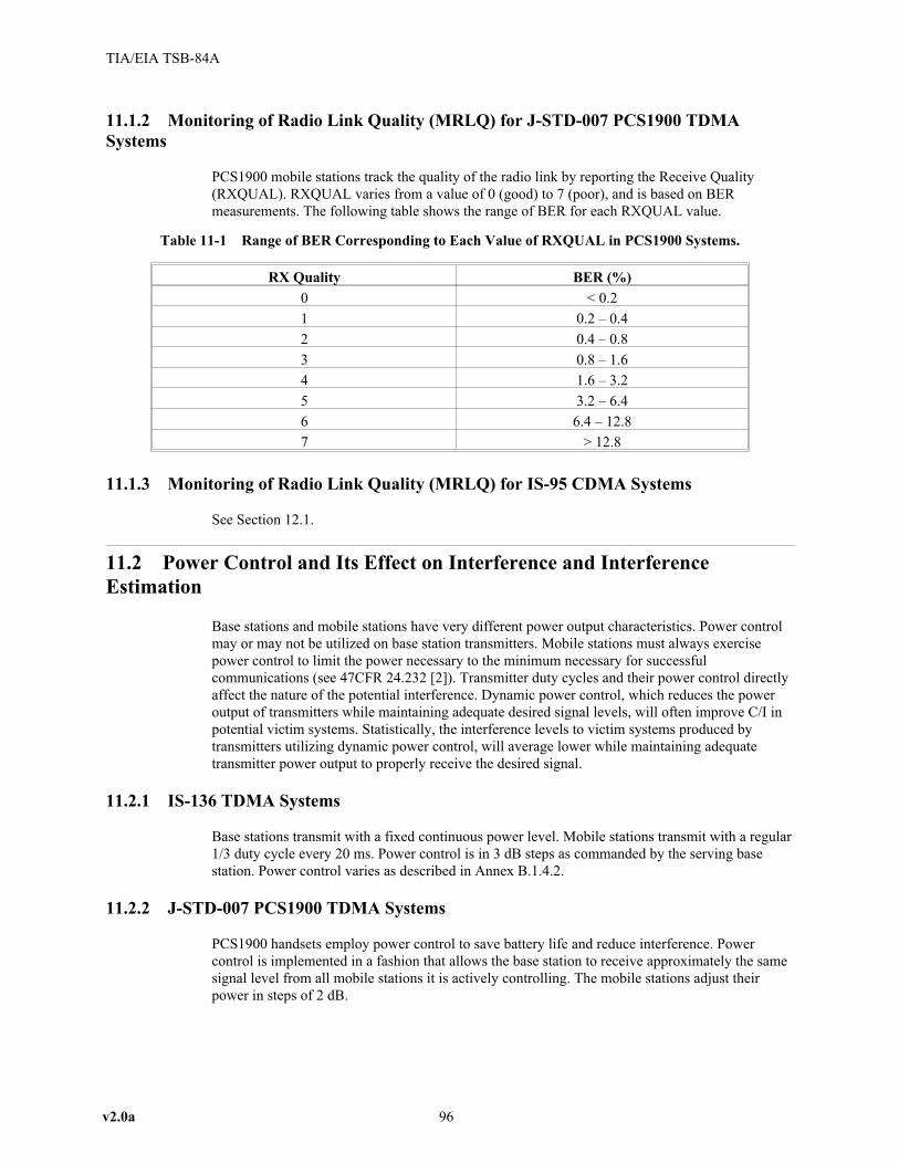
11.1.2 Monitoring of Radio Link Quality (MRLQ) for J-STD-007 PCS1900 TDMA

Systems

PCS1900 mobile stations track the quality of the radio link by reporting the Receive Quality

(RXQUAL). RXQUAL varies from a value of 0 (good) to 7 (poor), and is based on BER

measurements. The following table shows the range of BER for each RXQUAL value.

Table 11-1 Range of BER Corresponding to Each Value of RXQUAL in PCS1900 Systems.

RX Quality BER (%)

0 < 0.2

1 0.2 – 0.4

2 0.4 – 0.8

3 0.8 – 1.6

4 1.6 – 3.2

5 3.2 – 6.4

6 6.4 – 12.8

7 > 12.8

11.1.3 Monitoring of Radio Link Quality (MRLQ) for IS-95 CDMA Systems

See Section 12.1.

11.2 Power Control and Its Effect on Interference and Interference

Estimation

Base stations and mobile stations have very different power output characteristics. Power control

may or may not be utilized on base station transmitters. Mobile stations must always exercise

power control to limit the power necessary to the minimum necessary for successful

communications (see 47CFR 24.232 [2]). Transmitter duty cycles and their power control directly

affect the nature of the potential interference. Dynamic power control, which reduces the power

output of transmitters while maintaining adequate desired signal levels, will often improve C/I in

potential victim systems. Statistically, the interference levels to victim systems produced by

transmitters utilizing dynamic power control, will average lower while maintaining adequate

transmitter power output to properly receive the desired signal.

11.2.1 IS-136 TDMA Systems

Base stations transmit with a fixed continuous power level. Mobile stations transmit with a regular

1/3 duty cycle every 20 ms. Power control is in 3 dB steps as commanded by the serving base

station. Power control varies as described in Annex B.1.4.2.

11.2.2 J-STD-007 PCS1900 TDMA Systems

PCS1900 handsets employ power control to save battery life and reduce interference. Power

control is implemented in a fashion that allows the base station to receive approximately the same

signal level from all mobile stations it is actively controlling. The mobile stations adjust their

power in steps of 2 dB.

v2.0a 96

TIA/EIA TSB-84A

PCS1900 base stations may also adjust their power output, as a function of time slot, if one or

more mobile stations is reporting poor received signal strength. This capability is an option and is

not used by all PCS1900 base stations.

11.2.3 IS-95 CDMA Systems

Power control is a mechanism to ensure that mobile stations at the edge of a cell maintain

significantly enhanced forward link performance, while power to mobile stations close to the base

station is adequately reduced to conserve overall power (or increase system capacity).

Both the capacity and reliability of the forward link can be enhanced by dynamically adjusting the

baseband injection level of each traffic channel on the basis of the individual mobile station’s

needs. This dynamic adjustment can improve the survival of mobile stations in interference

situations or near the cell edge, while at the same time improving overall capacity to serve

additional mobile stations on the forward link by utilizing the unneeded traffic channel power by

mobile stations in favorable environments near the base station.

The mobile station reports its FER by means of Power Measurement Report Messages These

reports are used by forward link power control algorithms to trigger dynamic adjustment of the

traffic channel power. The base station continually reduces the strength of each mobile station’s

forward baseband chip stream. When a particular mobile station experiences errors on the forward

link, it requests more energy. The complaining mobile station’s chip stream gets a quick power

increase; after which the continual reduction by the base station resumes. This constant reduction

by the base station ensures that mobile stations always have just sufficient power to correctly

decode their signals and only mobiles actually experiencing problems get extra power.

For the reverse link, the system tries to have the signal from each mobile station reach the base

station at approximately the same level. Three methods of power control are usually used

simultaneously: reverse open loop control, reverse close loop control and reverse outer loop

control.

In the open loop control, the mobile station adjusts its power up or down depending on the

variation of the signal power received from the base station. This is a coarse control and

adjustments can be as much as 20 dB.

In the closed loop control, every 1.25 ms (800 times per second) the base station estimates the

received signal strength on the Reverse Traffic Channel of a particular mobile station, and uses

this estimation to decide whether that mobile station should increase or reduce its transmission

power. A one-bit command is sent by the base station to that mobile station 800 times a second on

the corresponding forward traffic channel for it to adjust the power by 1 dB – up (0) or down (1).

The Power Control Bits are sent at full power and are uncoded. This is referred to as the “Power

Control Subchannel” for that mobile station. At the rates of Set 1, these “Power Control Bits”

overwrite 2 out of every 24 modulation symbols. At the rates of Set 2, these “Power Control Bits”

overwrite 1 out of every 24 modulation symbols. See Annex B.3.2 and Section 6.1.2 of [23].

The outer loop control is a higher-level supervisory reaction control to the frame erasure rate for

the individual mobile station.

11.2.4 IS-661 CCT

See Annex B.1.1.1.2.

97 v2.0a

TIA/EIA TSB-84A

11.3 Handover and Diversity

Handover and receive diversity techniques affect the dynamic responses of PCS systems. [The

term handover is the same as the term handoff used in some documents.] There are different types

of handover available to PCS systems. Hard handover is defined here to mean when the radio

frequency channel is changed, or for TDMA systems, when the time slot or radio frequency

channel is changed. The initial radio frequency or time slot is left and no longer used by the radio

to communicate. Soft handover is defined here to mean when two or more receivers intended to

provide service in different areas (e.g. different sectors of one base station, or different base

stations) are simultaneously receiving a transmitted signal and combining the signal. The initial

radio frequency is not changed. It is important to note here that the use of receiver diversity within

a base station sector is usually called combining, and that receiver diversity from sector to sector

in CDMA systems is usually called micro-diversity, and that receiver diversity between two

geographically separated base stations is usually called macro-diversity. When a PCS system

determines the need to perform a hard handover, the dynamic response called hard handover is

attempted. Successful handovers have minimal or no call degradation. Unsuccessful handovers

result in dropped calls or degraded call quality. Each type of PCS air interface technology

responds differently to interference. In general, TDMA systems attempt to locate another available

frequency or timeslot to communicate. CDMA systems attempt to have another base station take

the call with soft handover, or perform a hard handover.

11.3.1 IS-136 Handover

To be added later.

11.3.2 PCS-1900 Handover

To be added later.

11.3.3 IS-95 CDMA Handover

In IS-95 CDMA, handover is done by means of pilots transmitted by the base station to the mobile

stations. A pilot search in the mobile station is always checking for available candidate pilots in

neighboring cells for potential useful signals it can request to use in soft handover. It does this by

measuring the pilot chip energy-to-total power spectral density ratio (Ec/I0). The mobile station

reports to the system the pilots it is receiving. The system will then assign a new sector for that

mobile station and starts transmitting to (and receiving from) it on that sector, in addition to the

current sector. The mobile station will then assign its correlators (“rake fingers”) accordingly.

While some systems can assign up to six sectors for each mobile station and receive from it

simultaneously on all six, the mobile station is capable of decoding only up to three sectors at a

time and chooses whichever signal it prefers.

v2.0a 98

TIA/EIA TSB-84A

12. Effect of Interference on System Capacity

12.1 Effect of Interference on IS-95 CDMA Capacity and Coverage

Based on [24]

12.1.1 Introduction

This section presents a description of the 850 MHz IS-95 CDMA [25] reverse link (mobile station

to base station link) characteristics and its performance in terms of both coverage and capacity.

Steps taken to control noise and interference result in a worthwhile increase of coverage and

capacity. The results of this analysis are scalable to the 1900 MHz PCS band EIA/TIA 95-B [23].

12.1.2 Factors Affecting IS-95 CDMA Capacity and Coverage

IS-95 CDMA systems attempt to maintain the FER constant. An FER around 1% is typically used.

Corresponding to this FER, the E Nb / 0 varies over a range which is typically 4 to 10 dB. The actual

E Nb / 0 depends on the base station design, soft handoff status, and the propagation. Figure 12-1 compares

the FER versus E Nb / 0 for two IS-95 CDMA architectures for 1, 2 and 4 independent Rayleigh paths.

12.1.3 Reverse Link Capacity

In the reverse link, one of the fundamental parameters to be analyzed and measured in determining

the capacity is the total power received at the base station antennas [26],[27]. With M active users

in one isolated sector, the total received power C can be expressed as

C N W Pi i

i

M

� ��0

1

2(12-1)

99 v2.0

TIA/EIA TSB-84A

1.00E+00

1.00E-01

Fra

me

Err

or

Rat

e

1.00E-02

1.00E-03

0 1 2 3 4 5 6 7 8 9 10 11 12 13 14 15

E /N per path [dB]b 0

(a)(b)

(a) (b)

(a)(b)

4 Paths2 Paths 1 Path

Figure 12-1 Comparison of FER versus E Nb / 0 for Two Architectures: (a) Sub-optimal Multipath

Diversity Receiver Architecture and (b) Optimal Multipath Diversity Receiver Architecture. Vehicle speed of

100 km/h at a carrier frequency equal to 850 MHz. Results are shown for 1, 2, and 4 independent Rayleigh

where N W0 represents the background noise power in the bandwidth W, 2 i represents voice

activity of the ith user, and Pi is the received power of the ith user. For IS-95 CDMA, W = 1.2288

MHz and E{ }2 is taken to be equal to 0.4 (during the 850 MHz field tests the precise average voice

activity of 40% was achieved by setting the mobile stations in test mode). Z is defined as the

received power relative to the background noise:

ZC

N W

P

N Wi

i

i

M

� � ��

0 01

1 2(12-2)

Furthermore, the signal-to-noise plus interference ratio for a given user is given by,

E

N I

W

R

P

N W

WNP

bi

i

j j

j

M0 0

0

0 1

1

11�

�

��

�

� 2

(12-3)

where R=9600 bps. Combining Eqs. (12-2) and (12-3) and approximating M–1 with M in (12-3),

we obtain

ZR

W

E

N I

Xi

bi

i

M3

��

��

��

1

1

1

1

0 01

2

(12-4)

where

XR

W

E

N Ii

bi

i

M

��

� 20 01

(12-5)

The signal-to-interference ratio is closely approximated by a lognormal distribution with mean �

dB and standard deviation � dB [28]. The voice activity � is a quaternary random variable with

mean E{ }2 . By central limit arguments, the variable X approaches a normal distribution1.

Therefore, with � = ln(10)/10, we obtain

E XR

WM E e{ } { } [( ) / ]� �2 �4 �52 2 (12-6)

Var XR

WM e E e E{ } [ { { } ]( ) ( )��

��

��

22 2 2 22 2�4 �5 �42 2

(12-7)

Expressing Z in dB, i.e. Z = –10 log (1–X), we can derive the distribution and density functions of

the rise in dB over background noise, namely

P z e dyzy

e E x

Var x

z

( ) /

( )

( )

� �

��

� ��

�1

2

2 2

1

� (12-8)

p zVar x

e ez

e E x

Var x z

z

( )( )

[ ( )]

( )��

�

�

1

2

1

2

2

�

�

�(12-9)

v2.0a 100

TIA/EIA TSB-84A

1 It should be clear that the approximation of Equation (12-4) holds only if the probability of X +1is small.

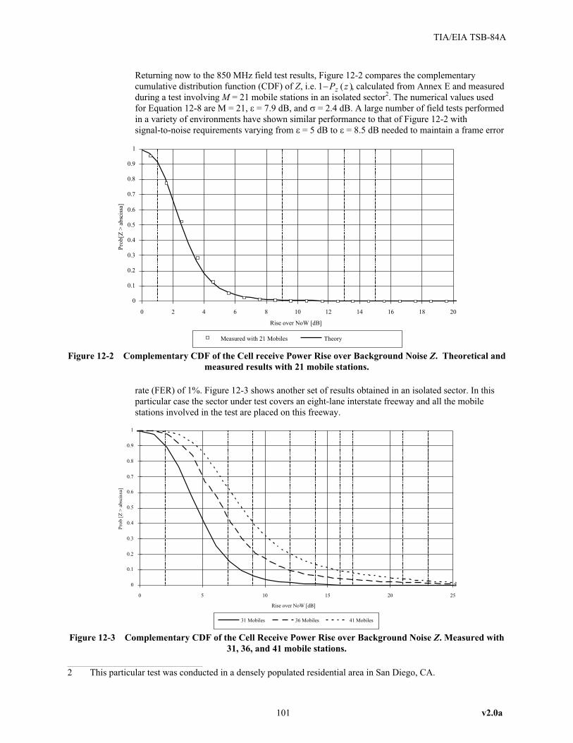
Returning now to the 850 MHz field test results, Figure 12-2 compares the complementary

cumulative distribution function (CDF) of Z, i.e. 1�P zz ( ), calculated from Annex E and measured

during a test involving M = 21 mobile stations in an isolated sector2. The numerical values used

for Equation 12-8 are M = 21, 5 = 7.9 dB, and 4 = 2.4 dB. A large number of field tests performed

in a variety of environments have shown similar performance to that of Figure 12-2 with

signal-to-noise requirements varying from 5 = 5 dB to 5 = 8.5 dB needed to maintain a frame error

rate (FER) of 1%. Figure 12-3 shows another set of results obtained in an isolated sector. In this

particular case the sector under test covers an eight-lane interstate freeway and all the mobile

stations involved in the test are placed on this freeway.

101 v2.0a

TIA/EIA TSB-84A

Rise over NoW [dB]

Pro

b[Z

>ab

scis

sa]

0

0.1

0.2

0.3

0.4

0.5

0.6

0.7

0.8

0.9

1

0 2 4 6 8 10 12 14 16 18 20

Measured with 21 Mobiles Theory

Figure 12-2 Complementary CDF of the Cell receive Power Rise over Background Noise Z. Theoretical and

measured results with 21 mobile stations.

Rise over NoW [dB]

Pro

b[Z

>ab

scis

sa]

0

0.1

0.2

0.3

0.4

0.5

0.6

0.7

0.8

0.9

1

0 5 10 15 20 25

31 Mobiles 36 Mobiles 41 Mobiles

Figure 12-3 Complementary CDF of the Cell Receive Power Rise over Background Noise Z. Measured with

31, 36, and 41 mobile stations.

2 This particular test was conducted in a densely populated residential area in San Diego, CA.

An improvement in the signal-to-noise ratio requirement is obtained from low mobility users, e.g.

pedestrian or in-building users, which are not experiencing the faster fading induced by a vehicle

motion. Figure 12-4 shows the E Nb / 0 required to achieve a 1% FER as a function of vehicle

speed in a 2 antenna system with one independent Rayleigh path per receive antenna.

The shape of the curve shown in Figure 12-4 is explained by the fact that at relatively low speeds

power control is more effective in counteracting the slow fades whereas at higher speeds, where

power control is not as effective in counteracting the fast fading, the effects of interleaving

become increasingly beneficial.

Since each user is accurately power-controlled to the minimum signal-to-noise value necessary to

achieve a given FER, low mobility users produce approximately one half the interference of high

mobility users (typical signal-to-noise requirements for low mobility users is 4 to 5 dB). This has

the effect of increasing the capacity of the reverse link when the user population is a mix of high

and low mobility users.

A complete analysis of the reverse link capacity must include the effects of interference from other

cells (other-cell interference) and a model for the traffic load [29],[30]. In the following analysis

example, the derivation assumes the following parameters:

(a) Median E N I dBb / ( ):0 0 7� �5

This assumption utilizes the values measured in the 850 MHz field tests for high mobility users

with the Optimal Multipath Diversity Receiver Architecture mentioned in Figure 12-1 [24].

(b) E N Ib / ( )0 0� standard deviation: 4 = 2.5 dB

This value, induced by the closed loop power control, has been consistently measured in the field

tests for high mobility users. Smaller values (4 = 1.5 dB) have been consistently measured in field

tests for low mobility users.

(c) Average voice activity: E Var{ } . , { } . .2 2� �04 015

(d) Other-cell interference fraction: f = 0.55.

v2.0a 102

TIA/EIA TSB-84A

Figure 12-4 TypicalPerformance vs Vehicle Speed for 850 MHz Links to Achieve an FER=1%.

Other-cell interference fraction is defined to be the ratio of other-cell interference to in-cell

interference generated in an equally loaded network. This example assumes a fourth power

propagation law with 8 dB lognormal shadowing. Higher propagation exponents will reduce the

factor f and lower exponents will increase it [30].

(e) Traffic model:

Assume Poisson arrival rate of calls with parameter 6 calls/sec and exponential service time with

parameter 1/µ sec/call. The probability that there are k active users per sector during an average

call duration of 1/µ seconds is

Pr(k active users/sector) =( / )

!

/6 � 6 �k

ke�

(12-10)

E k Var k{ } { }� �6�

6�

(12-11)

Given all the of the above assumptions, the rise over background noise, Z, can now be expressed

as

ZC

N W

P

N W

P

N Wi

i

i

k

ij i

j

i

k

j

j

� � � ��

0 01 01

1 2 2 ( )( )other cells

� ,(12-12)

where in the last term on the right hand of the equation, index j runs through all other cells and

index i runs through all kj users in the j-th cell.

The distribution of Z is then given by Equation (12-12) where the mean and variance of X are now

given by

E XR

WE e f{ } { } ( )( ) /� ��6

�2 �4 �52 2 1

(12-13)

and

Var XR

WE e f{ } { } ( )( )��

��

��

22 2 22

16�

2 �4 �5 (12-14)

From Equations (12-12), (12-13), and (12-14) it is straightforward to calculate the offered load in

Erlangs for a given blocking probability. The blocking probability is defined as the probability of

Z exceeding a given value z in dB [29]. Figure 12-5 shows the offered load per sector versus z for

1% and 2% blocking probabilities.

Operationally, values of z = 10 dB and 2% blocking probability are a compromise between offered

load and coverage. As seen in Figure 12-5, this corresponds to 19 Erlangs/sector or approximately

27 voice channels per sector. Notice that this result applies to a single IS-95 CDMA frequency

assignment, i.e. one 1.25 MHz block.

Finally, Table 12-1 summarizes the capacity results for 2% blocking probability.

103 v2.0a

TIA/EIA TSB-84A

Table 12-1 Reverse Link Capacity Summary

System Radio Capacity/Sector Erlang Capacity/Sector

IS-95 CDMA 2779 = 243 229

12.1.4 Reverse Link Coverage

In this section we present a simple link budget for an IS-95 CDMA based system. The link budget

is derived for a mobile station with an output power of 200 mW.

Figure 12-6 shows the complete reverse link processing for a mobile station in soft handoff. In

order to close the link, a mobile station at the edge of coverage and in soft handoff with two (or

multiple) base stations needs to transmit the minimum power required to achieve the desired SNR

to either of the two or more base stations.

The margin required to achieve a given probability of service Ps at the cell border, taking into

account the effects of lognormal shadowing and soft-handoff, is calculated in detail in [31].

Additionally, in [32] the effects of shadowing, soft-handoff, and offered traffic are combined to

obtain the final margin shown in Table 12-2. The margin required by a mobile station to overcome

independent lognormal shadowing (with 8 dB sigma) between two base stations equally loaded at

a level of 19 Erlangs is equal to 7.7 dB for a probability of service at the cell border equal to 90%.

With the above assumptions, the maximum isotropic path loss that a portable unit can sustain

equals 147.5 dB.

v2.0a 104

TIA/EIA TSB-84A

6

8

2

10

12

14

16

18

20E

rla

ng

s/se

cto

r/1

.25

Mh

z

3 4 5 6 7 8 9 10

z[dB]

11 12

Pr[Z>z]=0.02 Pr[Z>z]=0.01

Figure 12-5 Erlangs/sector/1.25 MHz with 1% and 2% Blocking Probabilities.

105 v2.0a

TIA/EIA TSB-84A

In soft-handoff the mobile transmits theminimum power required

to close the link with either Base Station

Combining and

Decoding

Select Best Frame

Speech Decoder

Combining and

Decoding

Figure 12-6 Reverse-link Processing for a Mobile Station in soft Handoff.

Table 12-2 IS-95 CDMA Reverse Link Budget

Parameter Symbol Value Value Value Units Equation

Chip Rate W 1.2288 1.2288 1.2288 Mcps

Data Rate R 9600 9600 9600 bps

Processing Gain Gp 21.1 21.1 21.1 dB = 10 log(W/R)

Mobile Station Peak Power PM 23 23 23 dBm

Mobile Antenna Gain GA,M 0 0 0 dBi

Mobile Peak EIRP EIRPM 23 23 23 dBm = PM + GA,M

Base station Antenna Gain GA,B 12 12 12 dBi

Base Station Losses LB –2 –2 –2 dB

Base station Receiver Noise Figure NFB 3 5 10 dB

Base station Receiver Noise Density NDB –171 –169 –164 dBm/Hz =10 log(kBT) + NFB

Base station Receiver Sensitivity SB –110.1 –108.1 –103.1 dBm = NDB + 10 log(W)

Required Eb/N0 Eb/N0 7 7 7 dB

Required Received Signal Strength PR –124.2 –122.2 –117.2 dBm = SB - Gp + Eb/N0

Maximum Path Loss(Single User, No Shadowing)

PLSU,NS –157.2 –155.2 –150.2 dB= PR - EIRPM - GA,B -

LB

Probability of Service at Cell Edge PS 90 90 90 %

Log Normal Shadowing Sigma �LNS 8 8 8 dB

Offered Load OL 19 19 19Erlangs/Se

ctor

Margin to Achieve Specifiedwith Soft-Handoff

MP 7.7 7.7 7.7 dB Ref. [31],[32]

Maximum Isotropic Path Loss PLmax –149.5 –147.5 –142.5 dB = PLSU,NS + MP

12.1.5 Forward Link Capacity

{Text to be added at a later revision}

12.2 Effect of interference on TDMA Capacity

{Text to be added at a later revision}

v2.0a 106

TIA/EIA TSB-84A

Annex A. Propagation Models

All the text in Annex A is informative text.

Several propagation models have been proposed and a selection is provided below. In some cases,

simple propagation loss formulas may be appropriate, whereas in other circumstances, more

complex models may be more appropriate.

Many of the propagation models available for use are a mixture of empiricism and the application

of analytical propagation theory [33]. More recently, comparison of some urban propagation

models with carrier-wave (CW) measurements have also been presented in the ETSI’s COST-231

program [34]. A comprehensive description of most of the available and relevant models and the

supporting theory is presented by Parsons [33]. As relevant examples for this Annex, the Okumura

model and its extensions, and the COST-231 model are presented as alternative propagation

models.

Annex A.1 Simple Propagation Formulae

Annex A.1.1 Free Space Model

Free space (r2) propagation models are appropriate for high antennas within line-of-sight of each

other.

Path Loss = ( / )4 2 6r (A-1)

Annex A.1.2 Two-Slope Model

It is often appropriate to use a simple two-slope formula like the one described below:

r h ht transmitter receiver� 4 / 6 (A-2)

Path Loss = ( / )4 2 6r r rt# (A-3)

Path Loss = ( / )4 2 6r r r rt t+ (A-4)

Annex A.2 General Propagation Formulae

The transmission loss modeling problem is divided into four groupings: Indoor, outdoor with base

station antenna height below rooftop level, outdoor with base station antenna height at rooftop

level, and outdoor with base station antenna height above rooftop level. This is in recognition of

the fact that there are generally three diffraction zones about most obstacles, the first being the

shadow region into which little energy is diffracted. For this zone the low antenna or microcell

model is used. A second diffraction region exists where the receiver is within the shadow of the

obstacle but into which some energy is diffracted. In this case the antenna at rooftop level model is

used. And finally there is the region that is within or very near line of sight of the source. The

antenna above mean roof level model is used in this case. In all of the following transmission loss

models a carrier frequency of 1900 MHz is assumed.

A-1 v2.0a

TIA/EIA TSB-84A

Annex A.2.1 Physical Environments

The addition of a “rural” category is necessary, since the physical environment differs for this

environment over the residential. Velocity of the mobile/portable station is unimportant for

transmission loss calculations.

Table A-1 Radio Environments for Transmission Loss Calculation.

Indoor

Residential

Office

Commercial

Outdoor

Urban High-Rise

Urban/Suburban Low-Rise

Residential

Rural

Annex A.2.2 Indoor Model

The use of this indoor transmission loss model assumes that the base station and the portable

station are located inside the same building. The model has the following form

L A BLog d L nTotal f� � �10 ( ) ( ), (A-5)

where: A is an environment dependent fixed loss factor (dB),

B is the distance dependent loss coefficient,

d is separation distance between the base station and portable, in meters,

L f is a floor penetration loss factor (dB), and

n is the number of floors between base and portable.

All parameters are given in the table below.

Table A-2 Model Parameters for Indoor Transmission Loss Calculation.

Environment Residential Office Commercial

A (dB) 38 38 38

B 28 30 22

L f (n) (dB) 4n 15 + 4(n-1) dB 6 + 3(n-1) dB

Log Normal Shadowing(Std. Dev. dB)

8 10 10

Annex A.2.3 General Outdoor Transmission Loss Model

In the general model for outdoor transmission loss, the total transmission loss L in decibels

between isotropic antennas is expressed as the sum of free space loss, L fs , the diffraction loss from

rooftop to the street, Lrts , and the reduction due to multiple screen diffraction past rows of

buildings, Lmsd . This model is based on the work done by Xia [35] and by Walfish and Bertoni

[36]. In this model, L fs and Lrts are independent of the base station antenna height, while Lmsd is

dependent upon whether the base station antenna is at, below or above building heights. In

general, the Xia model:

L d L L Lfs rts msd( ) � � � (A-6)

v2.0a A-2

TIA/EIA TSB-84A

Given a mobile-to-base separation d, the free space loss between them is given by:

L Logd

fs ��

��10

410

26

(A-7)

The diffraction from the rooftop down to the street level gives the excess loss to the mobile

station:

L Logr

rts � ��

��

��

�

��

�

��

102

1 1

210 2

26

( (

(A-8)

where:

( � �

��

�

��tan 1 h

x

m (A-9)

r h xm� �( ) 2 2 (A-10)

hm is the difference between the mean building height and the mobile antenna height;

x is the horizontal distance between the mobile station and the diffracting edges.

For all deployment scenarios the parameter x is given as one half the average building edge to

building edge street width, w.

xw�2

(A-11)

For the general Xia model, the multiple screen diffraction loss from the base antennas due to

propagation past rows of buildings is:

L Log Qmsd M10 102( ) (A-12)

where QM is a factor dependent on the relative height of the base station antenna as being either

at, below or above the mean building heights. The following sections define each case separately.

Annex A.2.4 Transmission Loss for Base Station Antenna Heights at Rooftop Level

This model is applicable for deployment scenarios where base station antenna heights are at or

very near average rooftop level. Table A-3 lists the bounds about mean rooftop level for which

this model applies.

Table A-3 Environment-specific Roof-top Boundary Parameters.

Environment Urban High-Rise Urban/Suburban Residential Rural

Distance within mean rooftoplevel for which the at/near rooftop

model applies.±2.5 meters ±1.5 meters ±1 meter ±1 meter

From Equation A-12, the multiple screen diffraction due to propagation past rows of buildings is:

L Log Qmsd M�10 102( ) (A-13)

For the case where the base station antenna height is at or near rooftop level,

A-3 v2.0a

TIA/EIA TSB-84A

Qb

dM � (A-14)

Where:

b is the average separation between rows of buildings.

For all deployment scenarios the parameter b is given as twice the average building edge to

building edge street width, w.

b w� 72

The total transmission loss for the at-rooftop case then becomes:

L d Logd

Logr

( ) � ��

��

��

��10

410

2

1 1

210

2

10 2

6

6

( � (

2

10

2

10�

��

�

��

��

��Log

b

d

(A-15)

Note: L d( ) shall, in no circumstances, be less than free space loss.

Table A-4 Environment-dependent Parameters.

Environment Urban High-Rise Urb/Suburb Low-Rise Residential Rural

Street Width w (m) 25 35 30 50

Building PenetrationLoss/Deviation (dB)

18/10 18/10 12/5.5 12/5.5

Log Normal ShadowingStandard Deviation (dB)

12 10 8 8

Annex A.2.5 Transmission Loss for Base Station Antenna Height above Rooftop Level

The following model is applicable in cases where the base station antenna height is above the

mean rooftop level. Distances from mean rooftop level are given in Table A-5 for each of the

identified environments. This type of model is referred to as a macrocell type model.

Table A-5 Environment-specific Rooftop Boundary Parameters.


Distance above mean rooftop level forwhich the macrocell model applies.

>2.5 meters >1.5 meters >1 meter >1 meter


L Log Qmsd M�10 102( ) (A-16)

For the case where the base station antenna height is above rooftop level,

Qh

d

bM

b��

��

�

��235

0 9

.

.

6

(A-17)

Where:

hb is the height difference between the base station antenna and the building rooftops.

The total transmission loss for the above rooftop case then becomes:

v2.0a A-4

TIA/EIA TSB-84A

L d Logd

Logr

( ) � ��

��

��

��10

410

2

1 1

210

2

10 2

6

6

( � (8 -

2

102

1 8

10 235�

��

�

��

�

��

�

��

�

�

��

�

�

��

Logh

d

bb.

.

6

(A-18)



Environment Urban High-Rise Urban/ Suburb Low-Rise Residential Rural


Bldg Penetration Loss (dB)/standard deviation (dB)

18/10 18/10 12/5.5 12/5.5

Log Normal Shadowing StandardDeviation (dB)

10 10 10 10

Annex A.2.6 Outdoor Transmission Loss for Base Station Antenna Height below Rooftop

Level

The following model is applicable in cases where the base station antenna is below mean rooftop

level. Distances from mean rooftop level is given in Table A-7 for each of the identified

environments. This type of model is referred to as a microcell type model.

Caution should be used when utilizing this model for actual system implementation. In certain

situations, the results obtained may be overly pessimistic.

Table A-7 Environment-specific Roof-top Boundary Parameters.


Distance, of base station antenna, below meanrooftop level for which the microcell model is

applicable.>2.5 meters >1.5 meters >1 meter >1 meter


L Log Qmsd M�10 102( ) (A-19)

For the case where the base station antenna height is below rooftop level,

Qb

dM � �

��

��

�

��2

1 1

2 69 : :

(A-20)

Where:

:� �

��

�

��tan 1 h

b

b (A-21)

9 � �( )h bb2 2 (A-22)

The total transmission loss for the below rooftop case then becomes:

A-5 v2.0a

TIA/EIA TSB-84A

L d Logd

Logr

( ) � ��

��

��

��10

410

2

1 1

210

2

10 2

6

6

( � (

2

10

2 2

102

1 1

2

�

��

�

��

� ��

��

�

��

�

��

�

��Log

b

d 69 : � :�

�

��

(A-23)



Environment Urban High-Rise Urban/Suburb Low-Rise Residential Rural


Bldg Penetration Loss (dB)/standard deviation (dB)

18/10 18/10 12/5.5 12/5.5

Log Normal ShadowingStandard Deviation (dB)

10 10 8 8

Annex A.3 Okumura Model and its Extensions

In the following, the symbols bm and dm are intended to be measured in meters, whereas the

symbols dkm is intended to be measured in kilometers.

The model has been developed from an extensive series of field trials under the following

conditions:

• frequencies from 100 MHz to 3000 MHz;

• distances from 1 km to 100 km;

• different terrain conditions: urban, suburban, rural, with varying degrees of undulation;

• effective base station antenna height from 1m to 1000 m;

• other factors such as blockage, land-water conditions;

The basis of the method is to determine the free-space path loss at a receiver located dkm from a

transmitter and then add that value to the median attenuation, Amu , in an urban area over

quasi-smooth terrain with a base station effective antenna height, hte , of 200 m and a mobile

antenna height, hre , of 3 m. We can determine Amu by using Figure 15 in Okumura [37]. The free

space path loss at a frequency, f MHz , can be determined using the following equation [33]:

L dB G G f df T R MHz km( ) log log log log� � � � �10 10 20 2010 10 10 10 32 44. (A-24)

where GT and GR are the gain of the transmitting and receiving antennas, respectively.

Different correction factors can then be introduced to account for:

• Transmitting and receiving antennas not at reference heights;

• Transmission over non quasi-urban areas: for example, suburban or rural;

• Orientation of streets;

• Presence of mixed land-sea paths.

Okumura produced different graphs that can be used to determine these correction factors. The

Okumura model is probably the most widely quoted of the available models. It has come to be

used as a standard by which to compare other models, since it is intended for use over a wide

range of radio paths encompassing not only urban areas, but also different types of terrain.

v2.0a A-6

TIA/EIA TSB-84A

In an attempt to make the Okumura model easy to apply, Hata [38] established empirical

mathematical relationships to describe the graphical information given by Okumura. Hata’s

formulation is limited to certain ranges of input parameters and is applicable over quasi-smooth

terrain. The mathematical expressions and their range of applicability are:

L f h a hhaUr MHz te m re. . .. . log . log (� � � �6955 2616 138210 10 m

te m kmh d

)

( . . log ) log.� �44 9 655 10 10

(A-25)

where

150 1500

1 20

30 200

1 10

� ��

� �

f

d

h

h

MHz

km

te m

re m

.

.

and a hre m( ). is the correction factor for mobile-antenna height and is computed for a small- or

medium-sized city and for a large city as

a h f h fre m MHz re m MHz( ) ( . log . ) . log .. .� � � �11 07 1 56 0810 10 ( )

( ). (log . )

..

small medium city�

� �a h

hre m

re m829 154102 11 200

32 1175 4 97 400102

.

. (log . ) ..

f MHz

h f MHzre m

��

$%'

&'( )large city

(A-26)

The path loss for suburban areas is given by1

L dB L dB fha Su haUr MHz. .( ) ( ) [log ( / )] .� � �2 28 54102 (A-27)

The path loss for open areas is given by

L dB L dB f fha Op haUr MHz. .( ) ( ) . (log ) . log� � �4 78 1833102

10 MHz �4094. (A-28)

Hata’s formulations, more commonly known as Hata’s model, have enhanced the practical value

of the Okumura model, since they are easily entered into a computer.

Annex A.4 COST-231/Walfish/Ikegami Model

In the following, the symbols bm and dm are intended to be measured in meters, whereas the

symbols dkm is intended to be measured in kilometers.

The European research committee COST-231 (evolution of land mobile radio) has created a

combination empirical and deterministic model for estimating the urban transmission loss in the

900- and 1800-MHz bands known as the COST-231/Walfish/Ikegami model [39]. The model

accounts for the free-space loss, the diffraction loss along the radio path, and the loss between the

rooftops of the surrounding buildings and the mobile. It is mainly based on the models of Walfish

and Bertoni [36] and Ikegami et al [40]. Additionally, empirical corrections [41] were introduced

in order to apply it to base stations and to match it to measurements considering street orientation

and frequency [34]. The COST-231 model can be applied to radio paths in urban areas within the

following ranges:

• Frequencies of 800 MHz to 2000 MHz;

• Distances of 200 m to 5000 m;

• Base station antenna heights of 4 m to 50 m;

• Mobile antenna heights of 1 m to 3 m.

A-7 v2.0a

TIA/EIA TSB-84A

1 For TSB-84A, the “small-medium city” value of the a hre m( ). correction factor should be used.

The COST-231 model is composed of three terms:

L dBL dB L dB L dB L dB L

COSTF rts rts

� ��

231 ( )( ) ( ) ( ) ( )mod mod

mod

( )

( ) ( ) ( )

dB

L dB L dB L dBF rts

+� �

$%&

0

0

(A-29)

where L dBF ( ) is the free-space loss, L dBrts ( ) is the rooftop-to-street diffraction and scatter loss,

and L dBmod ( ) is the multiscreen loss. L dBrts ( ) is based on Ikegami’s model [40]:

L dB w f hrts MHz mob m( ) . log log log .� � � � �169 10 10 2010 10 10 � L dBori ( ) (A-30)

where w is the street width and

h h hmob m roof m mob m. . .� � (A-31)

is the difference between the building height hroof m. and the mobile antenna height hmob m. .

L dBori ( ) is an empirical correction function that accounts for the street orientation and was

evaluated from earlier measurements undertaken in Mannheim [41].

L dBori ( )

.

. . (

.

��

� �10 0354

2 5 0075 35 5

4 0

: ; :#<=:�<=- : # =

� �

$

%'

&' 0114 55 9. (:�==- : # ;

(A-32)

where : is the angle of incidence in degrees relative to the direction of the street. L dBmod ( ) is

based on the Walfish and Bertoni model with some empirical corrections:

L dB L dB k k d k f bbsh a d m f MHzmod ( ) ( ) log log log� � � � �10 10 109 m (A-33)

where bm is the distance between the buildings along the path. The terms L dBbsh ( ) and ka do not

exist in the model of Walfish and Bertoni. They represent the increase of path loss due to reduced

base station antenna height hbase . The different terms introduced in the above equation are given

as follows:

L dBI h h h

hbshbase m base m roof m

base

( )log ( ). . .�

� � +18

0

10

. .m roof mh�$%&

k

h h

h h ha

base m roof m

base m base m roof m�+

� �54

54 08

. .

. . .. ; d

h d h h d

km

base m km base m roof m km

�� 7 � #

$

% 05

54 1 6 05

.

. ; .. . .

'

&'

k

h h

h

hh hd

base m roof m

base m

roof mbase m r

�+

� �

18

18 15

. .

.

..

oof m.

$

%'

&'

(A-34)

where

h h hbase m base m roof m. . .� �

The term k f is dependent on the transmission frequency and the degree of urbanization. For

medium-sized cities and suburban centers with moderate tree density, k f is given by

kf

fMHz� � � ��

��

�

��4 07

9251.

(A-35)

v2.0a A-8

TIA/EIA TSB-84A

For metropolitan centers, k f is

kf

fMHz� � � ��

��

�

��4 1 5

9251.

(A-36)

In the absence of detailed data about building structure, COST 231 recommends employing these

default values:

• bm = 20 m to 50 m

• w = b/2

• hroof m. = 3 (number of floors) + roof

• roof = 3 m for pitched; 0 m for flat

• := 90 degrees

The COST 231 model has been tested recently by Low [42]. A number of measurements were

undertaken in the cities of Mannheim, where the land cover can be characterized as homogeneous,

and in Darmstadt, a city with inhomogeneous built-up structures, irregular streets, and small

terrain undulations. Low reported that the comparison with measurements resulted in a good

path-loss estimation for base antennas installed above the rooftops of the adjacent buildings. The

mean error is within 3 dB and the standard deviation is within 5 to 7 dB.

A-9 v2.0a

TIA/EIA TSB-84A

Annex B. Transceiver Characteristics

This section provides transmitter and receiver characteristics for the following eight licensed PCS

technologies. The source of the data is either an approved standard or the consensus of a standards

body. Explicit references are attached. The following is intended to define a generic description of

the technologies considered in this document.

1. IS-661 CCT, a Combined CDMA TDMA technology [43]. It uses a

FDMA/CDMA/TDMA/TDD or FDMA/CDMA/TDMA/FDD implementation.

2. IS-95 CDMA, a CDMA technology based on the CDMA digital cellular standard

[44][45][46]. It uses a FDMA/CDMA/FDD implementation.

3. J-STD-014 PACS is a low power TDMA technology [47]. It uses a FDMA/TDMA/FDD

implementation.

4. IS-136 TDMA, a FDMA /TDMA/FDD implementation based on the TDMA digital

cellular standard utilizing a digital control channel [21][48][18].

5. J-STD-007 PCS1900, a TDMA technology [49] based on the GSM cellular standard. It

uses a FDMA/ TDMA/FDD implementation.

6. J-STD-015 W-CDMA, a wideband CDMA technology [50]. It uses a

FDMA/CDMA/FDD implementation.

7. IS-713 Upbanded AMPS, a version of cellular AMPS upbanded to 1900 MHz [51][52]. It

uses a FDMA/FDD implementation.

8. SP-3614 PWT-E, Personal Wireless Telecommunications - Enhanced [53][54]. It uses a

FDMA/TDMA/TDD implementation.

Although eight technologies have been identified, the IS-713 Upbanded AMPS technology cannot

be considered as part of the PCS to PCS interference analysis in this Revision since there has been

insufficient data submitted. The IS-713 Upbanded AMPS technology interference analysis will be

considered when data is available. All IS-713 Upbanded AMPS information contained herein

should be considered as informative text.

Typically, only those characteristics relevant to interference analysis are included. The data are

generally copied verbatim from standards documents. They are supplemented by spectrum masks

and other information which was supplied by appropriate sources, as referenced.

Information for each technology is provided in the following four subsections:

• Transmitter Characteristics, Annex B.1

• Channel Plan, Annex B.2

• Transmit/Receive Duty Cycle, Annex B.3

• Receiver Characteristics, Annex B.4

For the purposes of this TSB, radiated power measurements should be indicated in Peak EIRP as a

power (e.g., watts) and/or as an electric field strength (e.g., µV/m). In the case of E, the distance

from the antenna must be specified. Conversion between power and field strength (assuming

free-space propagation) can be done using the following equations:

PE d

Gi

�

( )

( )

2

30

(B-1)

B-1 v2.0a

TIA/EIA TSB-84A

EG P

d

i� 30 (B-2)

where P = transmit power (watts)

E = electric field strength (volts/meter)

d = distance from the transmitter (meters)

Gi =isotropic transmitter antenna gain (dimensionless linear quantity)

In the far-field, the conversion between power density and field strength at a given point is given

by:

pE

Z�

2

0

(B-3)

where p = power density (watts/m2)

E = electric field strength (volts/meter)

Z0 =free-space impedance = 377 ohms

Annex B.1 Transmitter Characteristics

This section summarizes the characteristics of the transmitter output (base and mobile) for the

various licensed PCS technologies. The characteristics are governed by the applicable standards

documents; however, all emissions must meet FCC requirements. Those requirements, at the time

of approval of this version of the document, consist of the following as copied the FCC Rules [2].

Extract from 47 CFR Part 24—Personal Communications Services:

47 CFR 24.232 Power and Antenna Height Limits

(a) (Base stations are limited to 1640 watts peak equivalent isotropically radiated power

(EIRP) with an antenna height of up to 300 meters HAAT. See 24.53 for HAAT

calculation method. Base station antenna heights may exceed 300 meters with a

corresponding reduction in power; see Table B-1 of this section. In no case may the peak

output power of a base station transmitter exceed 100 watts. The service area boundary

limit and microwave protection criteria specified in Section 24.236 and Section 24.237

shall apply.

Table B-1 Reduced Power for Base Station Antenna Heights Over 300 Meters

HAAT in meters Maximum EIRP†

(watts)

<=300 1,640

<=500 1,070

<=1,000 490

<=1,500 270

<=2,000 160

† Peak EIRP

(b) Mobile/portable stations are limited to two watts EIRP peak power and the equipment

must employ means to limit the power to the minimum necessary for successful

communications.

v2.0a B-2

TIA/EIA TSB-84A

(c) Peak transmit power must be measured over any interval of continuous transmission

using instrumentation calibrated in terms of an rms-equivalent voltage. The measurement

results shall be properly adjusted for any instrument limitations, such as detector response

times, limited resolution bandwidth, sensitivity, etc., so as to obtain a true peak

measurement for the emission in question over the full bandwidth of the channel.

47 CFR 24.235 Frequency Stability

The frequency stability shall be sufficient to ensure that the fundamental stays within the

authorized frequency block.

47 CFR 24.236 Field Strength Limits

The predicted or measured field strength at any location on the border of the PCS service area

shall not exceed 47 dBµV/m unless the parties agree to a higher field strength.

47 CFR 24.238 Emission Limits

(a) On any frequency outside a licensee’s frequency block, the power of any emission shall

be attenuated below the transmitter power (P) by at least 43 + 10log (P) dB.

(b) Compliance with these provisions is based on the use of measurement instrumentation

employing a resolution bandwidth1 of 1 MHz or greater. However, in the 1 MHz bands

immediately outside and adjacent to the frequency block a resolution bandwidth of at

least one percent of the emission bandwidth of the fundamental emission of the

transmitter may be employed. The emission bandwidth is defined as the width of the

signal between two points, one below the carrier center frequency and one above the

carrier center frequency, outside of which all emissions are attenuated at least 26 dB

below the transmitter power.

(c) When measuring the emission limits, the nominal carrier frequency shall be adjusted as

close to the licensee’s frequency block edges, both upper and lower, as the design

permits.

(d) The measurements of emission power can be expressed in peak or average values,

provided they are expressed in the same parameters as the transmitter power.

(e) When an emission outside of the authorized bandwidth causes harmful interference, the

Commission may, at its discretion, require greater attenuation than specified in this

section.

Annex B.1.1 IS-661 CCT

The following information was extracted from [43].

Annex B.1.1.1 Mobile Station (MS)

Although the FCC permits up to 2 watts Effective Isotropic Radiated Power (EIRP2) for the MS,

the peak EIRP of the MS is a nominal 1 watt. The average power delivered to the antenna is less

than 19 milliwatts for each 9.6 kbps time slot, permitting long duration between MS battery

recharges.

B-3 v2.0a

TIA/EIA TSB-84A

1 Section 0.6 defines resolution bandwidth as used in this TSB consistent with Part 27.53(a)(5) of the FCC Rules

2 Peak EIRP

Annex B.1.1.1.1 Mobile Station Average Power Output

The mobile station average power output shall be determined by the number of channels

aggregated to deliver the desired data rate. For example, each channel delivers a 9.6 kbps data rate

and transmits 18.6 mW (maximum). Since a 38.4 kbps user consumes 4 channels, it therefore

transmits 4 times the average power output of a 9.6 kbps user. Power control will reduce the

average power output as directed by the base station.

Annex B.1.1.1.2 Mobile Station Transmit Power Control by Base Station

Transmit Power Control shall be directed by the base station in 3 dB steps over a total range of

33 dB nominal. The 3 dB steps shall be accurate to within ±1 dB.

Annex B.1.1.2 Base Station (BS)

The FCC rules permit up to 1640 watts peak EIRP per RF channel for PCS base stations. Since the

BS peak power output to its antenna is 2 watts, the maximum permissible BS antenna gain

(ignoring feed losses) is therefore limited by the FCC rule to 29.15 dB.

Annex B.1.1.3 Spectral Mask

The spectral emission masks for CCT are given in Tables B-2 and B-3. Measurements are

referenced at the center frequency made in a 30 kHz measurement bandwidth.

Table B-2 CCT Base Station Mask

|f�fc| 0-900 kHz 900-1875 kHz 1875-2275 kHz 2275-6000 kHz >6000 kHz

Base StationPower = 33 dBm

+0.5 dB�26 dB linear

decrease to �42 dB�42 dB linear

decrease to �48 dB�48 dB �53 dB

Table B-3 CCT Mobile Station Mask

|f�fc| 0-900 kHz 900-1875 kHz 1875-3000 kHz >3000 kHz

Mobile StationPower = 28 dBm

+0.5 dB�21 dB linear

decrease to �33 dB�33 dB linear decrease

to �48 dB�48 dB

Annex B.1.1.4 Base Spurious RF Emissions

This technology uses the second definition for “Spurious Emissions” in Section 0.6.

Annex B.1.1.4.1 Conducted Emissions

Conducted emissions shall comply with FCC Part 24.238, “Emission Limits for the licensed PCS

bands”.

Annex B.1.1.4.2 Radiated Emissions

Radiated emissions shall comply with FCC Part 15 rules for incidental and intentional radiators.

The radiated emissions shall also comply with ANSI C95.1-1991.

v2.0a B-4

TIA/EIA TSB-84A

Annex B.1.1.4.3 Total Spurious Emissions

All spurious emissions and out of band emissions shall comply with FCC Part 24.238 Emission

Limits for the licensed PCS bands. All spurious emissions include: modulation spectral sidelobes,

transmitter harmonics, transmitter on-off switching transient emissions, power control transients,

or multiple co-sited transmitter intermodulation products.

Annex B.1.1.5 Mobile Spurious Emissions


Annex B.1.1.5.1 Conducted Emissions

Conducted emissions shall comply with FCC Part 24.238, “Emission Limits for the licensed PCS

bands”.

Annex B.1.1.5.2 Radiated Emissions

Radiated emissions shall comply with FCC Part 15 rules for incidental and intentional radiators.

The radiated emissions shall also comply with ANSI C95.1-1991.

Annex B.1.1.5.3 Total Spurious Emissions

All spurious emissions and out of band emissions shall comply with FCC Part 24.238, “Emission

Limits for the licensed PCS bands”.

All spurious emissions include: modulation spectral sidelobes, transmitter harmonics, transmitter

on-off switching transient emissions, power control transients, or multiple co-sited transmitter

intermodulation.

Annex B.1.1.6 Transmitter Spectral Masks

The transmit mask shown in Figure B-1 below is valid for both base and mobile station

transmitters. The mask information was obtained from Committee T1P1.6.

B-5 v2.0a

TIA/EIA TSB-84A

fc

f (MHz)

-{43+10log(P)}

-{26+10log(P)}

P = peak TX power

RBW > 16

kHz

RBW > 16

kHz

RBW > 1

MHz

RBW > 1

MHz

Ref: 47 CFR 24.238

fc-1.8 f

c-0.8 f

c+0.8 f

c+1.8

Figure B-1 IS-661 Generic Base and Mobile Station Transmit Mask

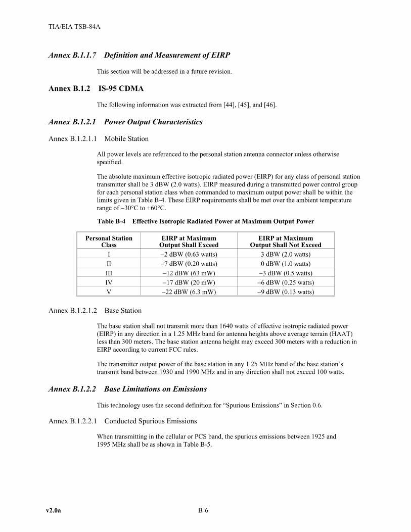
Annex B.1.1.7 Definition and Measurement of EIRP

This section will be addressed in a future revision.

Annex B.1.2 IS-95 CDMA

The following information was extracted from [44], [45], and [46].

Annex B.1.2.1 Power Output Characteristics

Annex B.1.2.1.1 Mobile Station

All power levels are referenced to the personal station antenna connector unless otherwise

specified.

The absolute maximum effective isotropic radiated power (EIRP) for any class of personal station

transmitter shall be 3 dBW (2.0 watts). EIRP measured during a transmitted power control group

for each personal station class when commanded to maximum output power shall be within the

limits given in Table B-4. These EIRP requirements shall be met over the ambient temperature

range of �30°C to +60°C.

Table B-4 Effective Isotropic Radiated Power at Maximum Output Power

Personal StationClass

EIRP at MaximumOutput Shall Exceed

EIRP at MaximumOutput Shall Not Exceed

I �2 dBW (0.63 watts) 3 dBW (2.0 watts)

II �7 dBW (0.20 watts) 0 dBW (1.0 watts)

III �12 dBW (63 mW) �3 dBW (0.5 watts)

IV �17 dBW (20 mW) �6 dBW (0.25 watts)

V �22 dBW (6.3 mW) �9 dBW (0.13 watts)

Annex B.1.2.1.2 Base Station

The base station shall not transmit more than 1640 watts of effective isotropic radiated power

(EIRP) in any direction in a 1.25 MHz band for antenna heights above average terrain (HAAT)

less than 300 meters. The base station antenna height may exceed 300 meters with a reduction in

EIRP according to current FCC rules.

The transmitter output power of the base station in any 1.25 MHz band of the base station’s

transmit band between 1930 and 1990 MHz and in any direction shall not exceed 100 watts.

Annex B.1.2.2 Base Limitations on Emissions


Annex B.1.2.2.1 Conducted Spurious Emissions

When transmitting in the cellular or PCS band, the spurious emissions between 1925 and

1995 MHz shall be as shown in Table B-5.

v2.0a B-6

TIA/EIA TSB-84A

Table B-5 Band Class 1 Transmitter Spurious Emission Limits

For |�f| Greater than Emission Limit

885 kHz �45 dBc / 30 kHz

1.98 MHz�55 dBc / 30 kHz; Pout � 33 dBm

�22 dBm / 30 kHz; 28 dBm � Pout < 33 dBm�50 dBc / 30 kHz; Pout < 28 dBm

2.25 MHz �13 dBm / 1 MHz

NOTE: All frequencies in the measurement bandwidth shall satisfy the restrictions

on |Df|, where Df = center frequency - closer measurement edge frequency and Pout is the

average transmitter power. The �13 dBm / 1 MHz emission limit is based on FCC rules

which are more stringent than ITU Category A emission limits.

Current FCC rules shall also apply.

Annex B.1.2.2.2 Radiated Spurious Emissions

Radiated spurious emissions (from sources other than the antenna connector) shall meet the levels

corresponding to the conducted spurious requirements listed in B.1.2.2.1.

Annex B.1.2.2.3 Intermodulation

Radiated products from co-located transmitters shall not exceed FCC spurious and harmonic level

requirements that would apply to any of the transmitters operated separately.

Annex B.1.2.3 Mobile Limitations on Emissions



Annex B.1.2.3.1.1 Definition

Conducted spurious emissions are emissions at frequencies that are outside the assigned CDMA

Channel, measured at the personal station antenna connector. This test measures the spurious

emissions during continuous transmission and gated transmission.

Annex B.1.2.3.1.2 Minimum Standard

When transmitting in the cellular or PCS band, the spurious emissions between 1845 and

1915 MHz shall be less than the limits specified in Table B-6.

Table B-6 Band Class 1 Transmitter Spurious Emission Limits

For |�f| Greater than Emission Limit

1.25 MHzless stringent of

�42 dBc / 30 kHz or �54 dBm / 1.23 MHz

1.98 MHzless stringent of

�50 dBc / 30 kHz or �54 dBm / 1.23 MHz

2.25 MHz �13 dBm / 1 MHz

NOTE: All frequencies in the measurement bandwidth shall satisfy the restrictions on |Df| where

Df = center frequency - closer measurement edge frequency. The �13 dBm / 1 MHz

B-7 v2.0a

TIA/EIA TSB-84A

emission limit is based on FCC rules which are more stringent than ITU Category A

emission limits.



Radiated spurious emissions are emissions generated or amplified by the personal station and

radiated by the housing and all power, control and audio leads normally connected to the personal

station, when connected to a non-radiating load, at frequencies that are outside the assigned

CDMA Channel.


Radiated spurious emissions shall be less than the levels specified for the conducted spurious

emissions in B.1.2.3.1.


The following MS and BTS transmit mask information was obtained from TR45.5.

For CDMA, it is difficult to show a single spectral mask for the mobile station and base station.

This is because the measurement bandwidths for spectral emissions are different, the specification

of some spurious emission requirements are in terms of relative power levels and some are in

terms of absolute emission levels, and the emission limits are different depending upon transmit

power. Thus, the following graphs are illustrative of the base station and mobile station emissions.

NOTE: The term “dB” in Figure B-2 refers to the spectral density relative to the nominal

�20.9 dBm/Hz inband spectral density. Conversions are given in Table B-7.

v2.0a B-8

TIA/EIA TSB-84A

-29 dB

-39 dB

-52 dB

1.5 dB

-1.5 dB

-29 dB

-39 dB

-52 dB

Notes:The mask assumes a 40dBm transmitter outputpower

The shows the basicspectral characteristic asset by the basebandtransmit filter

There is no emission limitspecification within 885kHz as the spectral maskis set by the basebandtransmit filter characteristics

0 dBm/Hz

f -2.25 MHzc

f -1.98 MHzcf -885 kHzc

f -740 kHzc

f -590 kHzc f +590 kHzc

f +740 kHzc

f +885 kHzcf +1.98 MHzc

f +2.25 MHzc

f -3 MHzcf -2 MHzc f -1 MHzc fc f +1 MHzc

f +2 MHzc f +3 MHzc

Figure B-2 Base Station Spectral Mask

Table B-7 Base Mask Conversions

dB (Spectral Density Relative to Passband)3

dBc/30kHz dBm/Hz

�29 �45 �50

�39 �55 �60

�52 �68 �73 (= -13 dBm/1 MHz)

NOTE: The term “dB” in Figure B-3 refers to the spectral density relative to the nominal

�37.9 dBm/Hz inband spectral density. Conversions are given in Table B-8.

Table B-8 Mobile Mask Conversions

dB (Spectral Density Relative to Passband)4

dBc/30kHz dBm/Hz

�26 �42 �64

�34 �50 �72

�35 �51 �73 (= -13 dBm/1 MHz)

The baseband filters shall have a frequency response S(f) that satisfies the limits given in

Figure B-4. Specifically, the normalized frequency response of the filter shall be contained within

±"1 in the passband 0 � f � fp and shall be less than or equal to �"2

in the stopband f � fs. The

numerical values for the parameters are "1 = 1.5 dB, "2= 40 dB, fp = 590 kHz, and fs = 740 kHz.

B-9 v2.0a

TIA/EIA TSB-84A

-26 dB

-26 dB

-34 dB -35 dB

1.5 dB

-1.5 dB

-26 dB

-34 dB-35 dB

Notes:The mask assumes a 23dBm transmitter outputpower

There is no emissionlimit specification within1.25 MHz as the spectralmask is set by thebaseband transmitfilter characteristics

0 dBm/Hz

The shows the basicspectral characteristic asset by the basebandtransmit filter

f -2.25 MHzc

f -1.98 MHzc

f -740 kHzc

f -590 kHzc f +590 kHzc

f +740 kHzc

f +1.98 MHzc

f +2.25 MHzc

f -3 MHzcf -2 MHzc f -1 MHzc

fc f +1 MHzcf +2 MHzc f +3 MHzc

f -1.25 MHzc f +1.25 MHzc

Figure B-3 Mobile Station Spectral Mask

3 also known as “Out-of-Band Spectral Density Relative to In-Band Spectral Density”

4 also known as “Out-of-Band Spectral Density Relative to In-Band Spectral Density”

Let s(t) be the impulse response of the baseband filter. Then s(t) should satisfy the following

equation:

[ ( ) ( )] . ,� >s kT h ks

k

� � ��

�

� 2

0

003(B-4)

where the constants � and > are used to minimize the mean squared error. The constant Ts is equal

to 203.451... ns, which equals one quarter of a PN chip. The values of the coefficients h(k), for k <

48, are given in Table B-9; h(k) = 0 for k �48. Note that h(k) equals h(47 � k).

Table B-9 Coefficients h(k)

k h(k)

0, 47 �0.025288315

1, 46 �0.034167931

2, 45 �0.035752323

3, 44 �0.016733702

4, 43 0.021602514

5, 42 0.064938487

6, 41 0.091002137

7, 40 0.081894974

8, 39 0.037071157

9, 38 �0.021998074

10, 37 �0.060716277

11, 36 �0.051178658

12, 35 0.007874526

13, 34 0.084368728

14, 33 0.126869306

15, 32 0.094528345

16, 31 �0.012839661

17, 30 �0.143477028

v2.0a B-10

TIA/EIA TSB-84A

20 log |S(f)|10

"1

"1

"2

0

0 fp fsf

Figure B-4 Baseband Filters Frequency Response Limits

k h(k)

18, 29 �0.211829088

19, 28 �0.140513128

20, 27 0.094601918

21, 26 0.441387140

22, 25 0.785875640

23, 24 1.0



Annex B.1.3 J-STD-014 PACS


Annex B.1.3.1 Power Output Characteristics

RPs and SUs have different transmitter power output characteristics as described in Sections

B.1.3.1.1 and B.1.3.1.2.

Annex B.1.3.1.1 RP (downlink) Transmit Power

Transmission on the downlink channels is continuous (TDM). The maximum allowable

transmitter output power as measured at the RP antenna connection is 800 mW. In the event that

an antenna connection is not available, the RP’s manufacturer shall supply a calibrated RF

coupling device at the time of test. Over time and temperature, this maximum power output is

allowed to increase as much as +20%.

Annex B.1.3.1.2 SU (uplink) Transmit Power

The SU transmits in bursts (TDMA) with a burst power level determined by the adaptive power

control process. The maximum allowable burst transmitter output power as measured at the SU

antenna connection is 200 mW. In the event that an antenna connection is not available, the SU’s

manufacturer shall supply a calibrated RF coupling device at the time of test. Over time and

temperature, this maximum power output is allowed to increase as much as +20%.

Annex B.1.3.2 Out of Band Emissions

Annex B.1.3.2.1 Adjacent channel protection

When the RP’s or SU’s carrier is modulated with random data, ninety-nine percent (99%) of the

total transmitted power must be contained in the occupied bandwidth of 288 kHz (carrier

frequency ±144 kHz).

Maximum transmitted power levels (in a measurement bandwidth of 192 kHz centered upon the

specified offset frequencies) are listed below:

• at offsets of ±600 kHz or greater from the center frequency, the RP’s transmitted power must

be less than 8 µW and the SU’s transmitted power must be less than 2 µW.

• at offsets of ±900 kHz or greater from the center frequency, the RP’s transmitted power must

be less than 2.5 µW and the SU’s transmitted power must be less than 0.625 µW.

B-11 v2.0a

TIA/EIA TSB-84A

The differences between the allowable limits for the RP and the SU are due to the differences in

maximum allowable transmitter power levels as described in Sections B.1.3.1.1 and B.1.3.1.2

(Refer to Figure B-5).

Annex B.1.3.3 Spurious Emissions


Spurious emissions on transmit bands outside the authorized band must be attenuated below

�13 dBm. Spurious emissions over receive bands must be attenuated below �85 dBm. The

emissions outside the licensed band must meet FCC requirements.


The worst case emissions for the Subscriber Unit (SU) and the Radio Port (RP) are given in

Figure B-5. The integrated transmit power for the SU is 200 mW (+23 dBm). The integrated

power for the RP is 800 mW (+29 dBm).

The SU and RP transmitter masks, as obtained from Figure B-5, are given in Table B-10 and

Figure B-6.

Table B-10 Transmitter Mask for SU and RP

Frequency Offset (kHz) SU (dB) RP (dB)

�804 �55 �55

�504 �50 �50

�144 0 0

144 0 0

504 �50 �50

804 �55 �55

v2.0a B-12

TIA/EIA TSB-84A

+900 kHz-900 kHz

+600 kHz-600 kHz

±96 kHz BW2 µW max. (SU)8 µW max. (RP)

±96 kHz BW2 µW max. (SU)8 µW max. (RP)

±96 kKHz BW0.625 µW max. (SU) 0.625 µW max. (SU)0.625 µW max. (SU)2.5 µW max. (RP)

±96 kHz BW

2.5 µW max. (RP)

±144 kHz99% Total

transmitted power

Carrier Frequency

Figure B-5 Off-channel emissions limits



Annex B.1.4 IS-136 TDMA

The following information was extracted from [21], [48], and [18].

Annex B.1.4.1 Base Station Transmitter


Annex B.1.4.1.1 Base Station RF Power Output

Maximum effective radiated power (ERP) and antenna height above average terrain (HAAT) must

be coordinated locally on an ongoing basis. For digital mode operation, the base station output

power shall be maintained at a constant level for the full duration of the frame if any slot is

occupied, unless the base station is operating as part of a low power in-building system, in which

case the base station may optionally discontinue transmissions for a maximum of one inactive slot

per frame for an RF channel bearing a DCCH. For this type of operation, the base station shall

continue transmissions during the inactive slot until after transmitting the synchronization word.

The base station operating in this manner shall employ a ramp down interval of 3 symbols in

duration (symbols 15, 16, and 17) after transmission of the synchronization word, and a ramp up

interval of 3 symbols in duration (symbols 160, 161, and 162) prior to beginning transmission in

the next slot.

Annex B.1.4.1.2 Spectrum Noise Suppression - Broadband

The emission power in either adjacent channel, centered ±30 kHz from the carrier frequency, shall

not exceed a level of 26 dB below the mean output power. The emission power in either alternate

channel, centered ±60 kHz from the carrier frequency, shall not exceed a level of 45 dB below the

mean output power. For output powers 50 W or less, the emission power in either second alternate

channel, centered ±90 kHz from the carrier frequency, shall not exceed a level of 45 dB below the

mean output power or �13 dBm, whichever is the lower power. For output powers greater than

B-13 v2.0a

TIA/EIA TSB-84A

0 dB

-50 dB

-55 dB

Rel

ativ

ePow

erD

ensi

ty(d

B)

Frequency Offset (kHz)

-804 -696 -504 -144 144 504 696 804

Figure B-6 Transmitted Mask for PACS

50 W, the emission power in either second alternate channel, centered ±90 kHz from the carrier

frequency, shall not exceed a level of 60 dB below the mean output power.

Annex B.1.4.1.3 Harmonic and Spurious Emissions (Conducted)

The peak power level of conducted spurious emissions shall not exceed a level of 80 dB below the

mean carrier output power or �13 dBm, whichever is higher, measured in a 1 MHz bandwidth. For

output powers 50 W or less, the peak power level of any emissions within the base station transmit

band between 1930 – 1990 MHz, measured using a 30 kHz bandwidth centered 120 kHz or more

from the carrier frequency, shall not exceed a level of 45 dB below the mean carrier output power

or �13 dBm, whichever is the lower power. For output powers greater than 50 W, the peak power

level of any emissions within the base station transmit band between 1930 - 1990 MHz, measured

using a 30 kHz bandwidth centered 120 kHz or more from the carrier frequency, shall not exceed

a level of 60 dB below the mean carrier output power. The peak power level of any emissions

within the base station receive band between 1850 - 1910 MHz, measured using a 30 kHz

bandwidth, shall not exceed �80 dBm.

Annex B.1.4.1.4 Harmonic and Spurious Emissions (Radiated)

The peak power level of radiated spurious emissions shall not exceed a level of 80 dB below the

mean carrier output power or �13 dBm, whichever is higher, measured in a 1 MHz bandwidth. For

output powers 50 W or less, the peak power level of any emissions within the base station transmit

band between 1930 - 1990 MHz, measured using a 30 kHz bandwidth centered 120 kHz or more

from the carrier frequency, shall not exceed a level of 45 dB below the mean carrier output power

or �13 dBm, whichever is the lower power. For output powers greater than 50 W, the peak power

level of any emissions within the base station transmit band between 1930 – 1990 MHz, measured

using a 30 kHz bandwidth centered 120 kHz or more from the carrier frequency, shall not exceed

a level of 60 dB below the mean carrier output power. The peak power level of any emissions

within the associated base station receive band between 1850 - 1910 MHz, measured using a

30 kHz bandwidth, shall not exceed �80 dBm.

Annex B.1.4.1.5 Transmitter Intermodulation Spurious Emissions

The transmitter intermodulation spurious emissions shall be attenuated at least 60 dB below the

power level of either transmitter when all transmitter combining and isolation equipment is

connected in its normal configuration.

A manufacturer of transmitters that are to be used with other manufacturers’ combining and

isolation equipment may choose to specify a different intermodulation performance for the

transmitter itself with the understanding that the overall goal of 60 dB attenuation is to be

achieved when all combining and isolation equipment is in place in a normal installation.

Annex B.1.4.2 Mobile RF Power Output


The mean effective radiated power (ERP) of the mobile station is shown in Table B-11. The

manufacturer should recommend the net power gain or loss of the antenna system to be installed

with the mobile station such that the power measured at the transmitter output terminals can be

directly related to the required ERP (typical antenna systems have 2.5 dB gain with respect to a

half-wave dipole and 1.5 dB cable loss). The station class indicated by the mobile station at the

beginning of any call will be assumed by the system to be maintained throughout that call.

v2.0a B-14

TIA/EIA TSB-84A

Table B-11 Mobile Station Nominal Power Levels

Mobile StationPower Level

(PL)

MobileAttenuation Code

(MAC)

Nominal ERP(dBW) forMobile Station Power Class

(see Note 4)

II III IV

0 0000 0.0 ? �2

1 0001 0.0 ? �2

2 0010 �2 ? �2

3 0011 �6 ? �6

4 0100 �10 ? �10

5 0101 �14 ? �14

6 0110 �18 ? �18

7 0111 �22 ? �22

8 1000 �28±4dB ? �28±4dB

9 1001 �33±5dB ? �33±5dB

10 1010 �38±6dB ? �38±6dB

NOTES

1 The three least significant bits of MAC are used in the VMAC field. All four bits of

MAC are used in the DMAC field.

2 The output powers shown above shall be maintained within the range of +2 dB, �4 dB of

nominal value for Power Levels 0 … 7, and within +2 dB, �6 dB of the nominal value for

Power Levels 8 … 10 (see Note 3).

3 The Nominal Output Power for levels 8, 9, and 10 are expressed as a range, rather than an

absolute value. When the mobile station changes to one of these power levels, it shall

insure that it stabilizes within the range centered around the target value for that level.

For example, the target value for power level 8 in the 1900 MHz operating band is

�28 dBW. The mobile station is considered to be within the requirement provided it

stabilizes within 4 dB of this target level. Once the mobile station has stabilized, the

operating tolerance is applied to the specific value within the nominal range on which the

mobile station stabilized.

4 Nominal ERP values in watts for power level 0 are 1 W for Class II and 0.6 W for Class

IV. Class III is reserved.

Table B-12 Relative Step Accuracy -Vs- Power Level on a Single Channel

Mobile Station Power Class IILevels (PL)

Mobile Station Power Class IVLevels (PL)

Step Between SuccessivePower Levels (dB)

0…7 2…7 4±1

- 7…10 4±2

NOTE 1: The Power Class IV and Step Between Successive Power Levels columns indicate

the dB reduction required when changing from the current power level to the next

higher power level. Thus, the change from level 6 to level 7 utilizes the top row

criteria, while the change from level 7 to level 8 uses the bottom row criteria.

When the mobile station changes from power level X to power level X+1, it shall satisfy the

requirements for the Nominal Output Power for that level (see Table B-11). Additionally, the

B-15 v2.0a

TIA/EIA TSB-84A

mobile station shall satisfy the requirements identified for the Relative Step Accuracy going into

the X+1 Power Level (see Table B-12). Thus, the mobile station shall reduce its power such that it

conforms to the Nominal level, with a reduction in power at least as great as the minimum

specified by the Relative Step requirement.

Annex B.1.4.2.1 Mobile Suppression inside Cellular/PCS Band

Any RF signals emitted in the mobile station’s receive band must not exceed –80 dBm, as

measured at the antenna connector. Additionally, signals in the mobile station’s transmit band

must not exceed –60 dBm, as measured at the antenna connector.

Annex B.1.4.2.2 Mobile Spectrum Noise Suppression - Broadband

Annex B.1.4.2.2.1 Adjacent and Alternate Channel Power Due to Modulation

The emission power in either adjacent channel, centered +30 kHz from the center frequency, shall

not exceed a level of 26 dB below the mean output power. The emission power in either alternate

channel, centered +60 kHz from the center frequency, shall not exceed a level of 45 dB below the

mean output power. The emission power in either second alternate channel centered +90 kHz from

the center frequency, shall not exceed a level of 45 dB below the mean output power or �13 dBm,

whichever is the lower power.

Annex B.1.4.2.2.2 Out of Band Power Arising from Switching Transients

The peak emission power in either adjacent channel, centered +30 kHz from the center frequency,

shall not exceed a level of 26 dB below the peak output power reference. The peak emission

power in either alternate channel, centered +60 kHz from the center frequency, shall not exceed a

level of 45 dB below the peak output power reference. The peak emission power in either second

alternate channel centered +90 kHz from the center frequency, shall not exceed a level of 45 dB

below the peak output power reference or �13 dBm, whichever is the lower power.

Annex B.1.4.2.3 Mobile Harmonic and Spurious Emissions (Conducted) - Discrete

The peak power level of conducted spurious emissions shall not exceed �13 dBm. The peak power

level of any emissions within the mobile transmit band using a 30 kHz bandwidth centered

120 kHz or more from the carrier frequency, shall not exceed 45 dB below the mean carrier output

power or �13 dBm, whichever is the lower power. The peak power level of any emissions within

the mobile’s operating receive band, measured using a 30 kHz bandwidth, shall not exceed

�80 dBm.

• 1900 MHz: operating receive band 1930-1990 MHz

Annex B.1.3.2.4 Mobile Harmonic and Spurious Emissions (Radiated) - Discrete

The peak power level of radiated spurious emissions shall not exceed �13 dBm. The peak power

level of any emissions within the mobile transmit band, measured using a 30 kHz bandwidth

centered 120 kHz or more from the carrier frequency, shall not exceed 45 dB below the mean

carrier output power or –13 dBm, whichever is the lower power. The peak power level of any

emissions within the mobile’s operating receive band, measured using a 30 kHz bandwidth, shall

not exceed �80 dBm.

• 1900 MHz: operating receive band 1930-1990 MHz

v2.0a B-16

TIA/EIA TSB-84A


The following MS and BTS transmit mask information provides the base station transmitter mask

at different power levels:

B-17 v2.0a

TIA/EIA TSB-84A

-48.23 dBm -48.23 dBm -48.23 dBm

-100 dBm

-45 dBc -45 dBc

-26 dBc -26 dBc

0 dBc

Base Station Transmit Maskfor mean output powers less than 32 dBm (1.58 Watts)

1850 MHz 1910 MHz

1929.975 MHz f -90c f -60c f -30c f +30c f +60c f +90cfc 1990.065 MHz

Resolution Bandwidth: 300 HzOffsets in kHz

Note: Assuming a flat spectrum, -48.23 dBm in a 300 Hz resolution bandwidth equates to -13 dBm in a 1 MHz bandwidth

Figure B-7 IS-136 Base Spectrum Mask

-48.23 dBm -48.23 dBm -48.23 dBm

-100 dBm

-45 dBc -45 dBc

-26 dBc -26 dBc

0 dBc

Base Station Transmit Maskfor mean output powers between 47 dBm (50 Watts) and 32 dBm (1.58 Watts)

1850 MHz 1910 MHz




-33 dBm -33 dBm


Figure B-10 provides the mobile station transmitter mask:



Annex B.1.5 J-STD-007 PCS1900


Requirements are given in terms of power levels at the antenna connector of the equipment, unless

otherwise stated. For equipment with integral antenna, a reference antenna with 0 dBi gain shall be

assumed unless otherwise specified by the manufacturer. For equipment that uses active antenna

arrays or multiple radiating elements, all active components between the BTS and the radiating

elements shall be considered as part of the equipment. A reference point shall be defined at which

v2.0a B-18

TIA/EIA TSB-84A

-48.23 dBm -48.23 dBm -48.23 dBm

-100 dBm

-45 dBc -45 dBc

-26 dBc -26 dBc

0 dBc

Base Station Transmit Maskfor mean output powers greater than 47 dBm (50 Watts)

1850 MHz 1910 MHz




-60 dBc -60 dBc


-48.23 dBm

-45 dBc -45 dBc

0 dBc

Mobile Station Transmit Mask


Resolution Bandwidth: 300 Hz Offsets in kHz


-26 dBc -26 dBc

-48.23 dBm -48.23 dBm

1930 MHz 1990 MHz

-100 dBm

Figure B-10 IS-136 Mobile Spectrum Mask

the active portion of the equipment begins and the passive portion of the antenna system ends.

Figure B-11 depicts this reference point.

In addition to the requirements in this section, the MS and BTS must comply with all applicable

FCC rules for wideband PCS services.

The terms power and output power refers to the measure of the power when averaged over the

useful part of the burst5 or the time period specified if different.

The terms peak power and peak hold refers to the maximum instantaneous power level over the

useful part of the burst or the time period specified if different.

Annex B.1.5.1 Mobile Station Maximum Rated Output Power

The mobile station maximum output power and lowest power control level shall be, according to

its power class, as defined in Table B-13:

Table B-13 MS Power Classes

Mobile Station Power Class Maximum Output Power Maximum Output Power Tolerance

11 watt

(+30 dBm)± 2 dB Normal

± 2.5 dB Extreme

20.25 watts(+24 dBm)

± 2 dB Normal± 2.5 dB Extreme

32 watts

(+33 dBm)± 2 dB Normal

± 2.5 dB Extreme

Note: The lowest power control level for MS power classes 1-3 is 15, with a nominal power level of 0 dBm.

The MS, including its actual antenna gain, shall not exceed a maximum of 2 watts (+33 dBm)

EIRP6 per the applicable FCC rules for wideband PCS services [5]. Power Class 37 is restricted to

transportable or vehicular mounted units.

Annex B.1.5.2 Base Station Maximum Rated Output Power

The BTS transmitter maximum rated output power per carrier, measured at the input of the

transmitter combiner, shall be, according to its TRX power class, as defined in Table B-15. The

base station output power may also be specified by the manufacturer or system operator at a

different reference point (e.g. after transmitter combining)8.

B-19 v2.0a

TIA/EIA TSB-84A

BTS

Active Elements of

Antenna System

(optional) A

Passive

Radiator(s)

Measurement

Reference

Point

Figure B-11 Logical Representation of BTS and Antenna System

5 This refers to the duration of one ACTIVE timeslot

6 Peak EIRP

7 Even under extreme conditions, Power Class 3 must not exceed the FCC 2 W EIRP limit.

8 For the purposes of this TSB, power should normally be measured at the input to the antenna

The maximum radiated power from the BTS, including its antenna system, shall not exceed a

maximum of 1640 watts EIRP, equivalent to 1000 watts ERP, per the applicable FCC rules for

wideband PCS services.

The tolerance of the specified maximum rated output power of the BTS9, shall be not greater than

± 2 dB under normal conditions and ± 2.5 dB under extreme conditions.

Table B-14 Standard BTS TRX Power Classes

TRX Power Class Maximum Output Power (watts) Maximum Output Power (dBm)

1 20 � Po < 40 43.0 � Po < 46.0

2 10 � Po < 20 40.0 � Po < 43.0

3 5 � Po < 10 37.0 � Po < 40.0

4 2 � Po < 5 34.0 � Po < 37.0

The micro-BTS maximum output power per carrier measured at the antenna connector after all

stages of combining shall be, according to its class, defined in Table B-15.

Table B-15 Micro BTS Power Classes

Micro BTS Power class Maximum output Power (watts) Maximum output Power (dBm)

M1 0.5 < Po � 1.6 27 < Po � 32 dBm

M2 0.16 < Po � 0.5 22 < Po � 27 dBm

M3 0.05 < Po � 0.16 17 < Po � 22 dBm

Annex B.1.5.2.1 Static Power Levels

The BTS must provide a static power control feature which allows the output power to be reduced

monotonically from its maximum rated output power in six steps with a nominal step size of 2 dB

and with a step size tolerance of not greater than ± 1 dB. The maximum rated output power shall

be defined as static power level 0. In addition, the actual absolute output power at each static RF

power level (N) shall be 2N dB below the absolute output power at static RF power level 0 with a

maximum tolerance of ± 3 dB under normal conditions and ± 4 dB under extreme conditions.

Annex B.1.5.2.2 Dynamic Power Levels

The BTS may provide up to 15 steps of dynamic downlink RF power control in addition to the

static power control requirements of Section B.1.5.2.1. The dynamic power control steps shall

form a monotonic sequence with a step size of nominally 2 dB and with a step size tolerance of

not greater than ± 1.5 dB. In addition, the actual absolute output power at each dynamic power

control level (N) shall be 2N dB below the absolute output power at dynamic power control level

0 with a tolerance of ± 3 dB under normal conditions and ± 4 dB under extreme conditions. The

dynamic power control level 0 shall be referenced to the set static power control level defined in

Section B.1.5.2.1.

Annex B.1.5.3 Output RF Spectrum

The specifications contained in this section apply to both BTS and MS, in frequency hopping as

well as in non frequency hopping mode unless otherwise specified. All requirements apply for the

case of a single active transmitter unless otherwise specified.

v2.0a B-20

TIA/EIA TSB-84A

9 Even under extreme conditions, the BTS must not exceed the FCC 1640 W EIRP limit.

Annex B.1.5.3.1 Spectrum Due to the Modulation and Wide Band Noise

The output RF modulation spectrum is specified in Table B-16. A mask representation of this

specification is shown in Figure B-12 for the MS and Figure B-13 for the BTS.

The specification applies to the entire relevant transmit band and up to 2 MHz either side.

The limits in Table B-16, at the listed frequency offsets from the carrier in kHz, are the maximum

level in dB relative to a reference measurement in a measurement bandwidth of 30 kHz centered

on the carrier frequency. For power levels that fall between those specified, a linear interpolation

will be used for the limits.

Table B-16 Modulation and Noise Spectrum Mask

TX PowerLevel(dBm)

Measurement Bandwidth at Specified Frequency Offset (kHz)

30 kHz 100 kHz

100 200 250 400600 to<1200

1200 to<1800

1800 to<6000

�6000

�4341393735�33

+0.5+0.5+0.5+0.5+0.5+0.5

-30-30-30-30-30-30

-33-33-33-33-33-33

-60-60-60-60-60-60

-70-68-66-64-62-60

-73-71-69-67-65-63

-75-73-71-69-67-65

-80-80-80-80-80-80

BTS

3332302826�24

+0.5+0.5+0.5+0.5+0.5+0.5

-30-30-30-30-30-30

-33-33-33-33-33-33

-60-60-60-60-60-60

-60-60-60-60-60-60

-60-60-60-60-60-60

-68-67-65-63-61-59

-76-75-73-71-69-67

MS

The following exceptions and minimum measurement levels shall apply; all absolute levels in

dBm shall be measured using the same bandwidth as that used in Table B-16:

i) in the combined range 600 kHz to 6 MHz above and below the carrier, in up to three

bands of 200 kHz width centered on a frequency which is an integer multiple of 200 kHz,

exceptions at up to �36 dBm are allowed.

ii) above 6 MHz offset from the carrier in up to 12 bands of 200 kHz width centered on a

frequency which is an integer multiple of 200 kHz, exceptions at up to �36 dBm are

allowed.

iii) For MS measured below 600 kHz from the carrier, if the limit according to the above

table is below �36 dBm, a value of �36 dBm shall be used instead. For 600 kHz up to

less than 1800 kHz this limit shall be �56 dBm. At 1800 kHz and beyond, this limit shall

be �51 dBm.

iv) For BTS, if the limit according to the above table is below L, a value L shall be used

instead, where L is L1 dB relative to the output power of the BTS at the lowest static

power level measured at 30 kHz, or L2 dBm, whichever is higher

For up to 1800 kHz from the carrier: L1 = � 88 dB

Beyond 1800 kHz: L1 = � 83 dB

For BTS: L2 = � 57 dBm

B-21 v2.0a

TIA/EIA TSB-84A

The micro-BTS spectrum due to modulation and noise at all frequency offsets greater than 1.8

MHz from carrier shall be �76 dB for all micro-BTS classes. These are average levels in a

measurement bandwidth of 100 kHz relative to a measurement in 30 kHz on carrier. The

measurement will be made in non-frequency hopping mode under the conditions specified for the

normal BTS.

For the micro-BTS, if the limit as specified above is below the values in Table B-17, then the

values in the table will be used instead.

TIA/EIA TSB-84A

B-22 v2.0

0

-10

-20

-30

-50

-40

-60

-70

-80

0 200 400 600 1200 1800 6000 Edge of TX

band + 2 MHz

measurement bandwidth 30 kHz measurement bandwidth

100kHz

Relative

Power

(dB)

Frequency Offset from the Carrier (KHz)

Limit depends upon

transmitter power level.

Figure B-12 MS Modulation and Noise Spectrum Mask

Table B-17 Micro BTS Modulation and Noise Exceptions

Microcell BTS PowerClass

Maximum spectrum due to modulation andnoise in 100 kHz (dBm)

M1 �57

M2 �62

M3 �67

B-23 v2.0a

TIA/EIA TSB-84A

0

-10

-20

-30

-50

-40

-60

-70

-80

0 200 400 600 1200 1800 6000 Edge of TX

band + 2 MHz

measurement bandwidth

100kHz

measurement bandwidth 30 kHz

Frequency Offset from the Carrier

Limit in shaded areas depends

upon transmitter power level.

Figure B-13 BTS Modulation and Noise Spectrum Mask

Annex B.1.5.4 Spurious Emissions

This technology uses the first definition for “Spurious Emissions” in Section 0.6.

In addition to the requirements of this section, the BTS and MS shall also comply with the

applicable limits for spurious emissions established by the FCC rules for wideband PCS services.

The limits specified in this section are based on a 5-pole synchronously tuned measurement filter.

Annex B.1.5.4.1 Principle of the Specification

The conditions are specified in Tables B-18 and B-19, a peak-hold measurement being assumed.

Table B-18 TX Band Spurious Emissions

Band Frequency Offset Measurement Bandwidth

Relevant TX band

(offset from carrier)

� 1.8 MHz

� 6 MHz

30 kHz

100 kHz

Table B-19 TX Out of Band Spurious Emissions

Band Frequency Offset Measurement Bandwidth

100 kHz - 50 MHz – 10 kHz

50 MHz – 500 MHz – 100 kHz

Above 500 MHz and outside the relevantTX band (offset from edge of relevant TX

band)

� 2 MHz 30 kHz

� 5 MHz 100 kHz

� 10 MHz 300 kHz

� 20 MHz 1 MHz

� 30 MHz 3 MHz

The limits in the following sections assume a resolution bandwidth of the measurement device

equal to the value of the measurement bandwidth in the table, and a video bandwidth

approximately three times the resolution bandwidth.

Annex B.1.5.4.2 Base Transceiver Station

The power measured under the conditions specified in Table B-18 shall be no more than �36 dBm.

The power measured under the conditions specified in Table B-19 shall be no more than:

• 250 nW (�36 dBm) in the frequency band 9 kHz – 1 GHz

• 1 mW (�30 dBm) in the frequency band 1 - 12.75 GHz

In the BTS receive band, the power measured using the conditions specified in B.1.5.3.1, with a

filter and video bandwidth of 100 kHz shall be no more than that specified in Table B-20.

v2.0a B-24

TIA/EIA TSB-84A

Table B-20 TX Emissions in RX Band

BTS Type Power in RX Band (dBm)

Normal BTS � 98

Micro BTS M1 � 96

Micro BTS M2 � 91

Micro BTS M3 � 86


The peak power measured in the conditions specified in Table B-18, for a MS when allocated a

channel, shall be no more than �36 dBm.

The peak power measured in the conditions specified in Table B-19 for a MS, when allocated a

channel, shall be no more than:

• �36 dBm in the frequency band 9 kHz – 1 GHz

• �30 dBm in all other frequency bands 1 - 12.75 GHz

The power emitted by the MS in a 100 kHz bandwidth using the measurement techniques for

modulation and wideband noise (Section B.1.5.4.1) shall not exceed:

• �71 dBm in the frequency band 1930 –1990 MHz


The following MS and BTS transmit mask information was obtained from T1P1.5.

The mobile and base transmitter masks have been extracted from J-STD-007 (and Figs B-12 and

B-13 of this document), and the power density data adjusted back to a 3 kHz measurement

bandwidth (nominal 1%). The results are shown in the masks below in Figure B-14 and Table

B-21. In addition, integration of the mask has produced a total “carrier reference power”

approximately 18.8 dB above the (3 kHz) nominal in-band carrier power density.

B-25 v2.0a

TIA/EIA TSB-84A

PCS1900 Spectrum Masks (3kHz Res)

-90.00

-80.00

-70.00

-60.00

-50.00

-40.00

-30.00

-20.00

-10.00

0.00

10.00

-10.00 -5.00 0.00 5.00 10.00

Frequency (MHz)

Po

we

r(d

B/3

kH

z)

BTS Power (dB)

MS Power(dB)

Figure B-14 Transmitter Mask

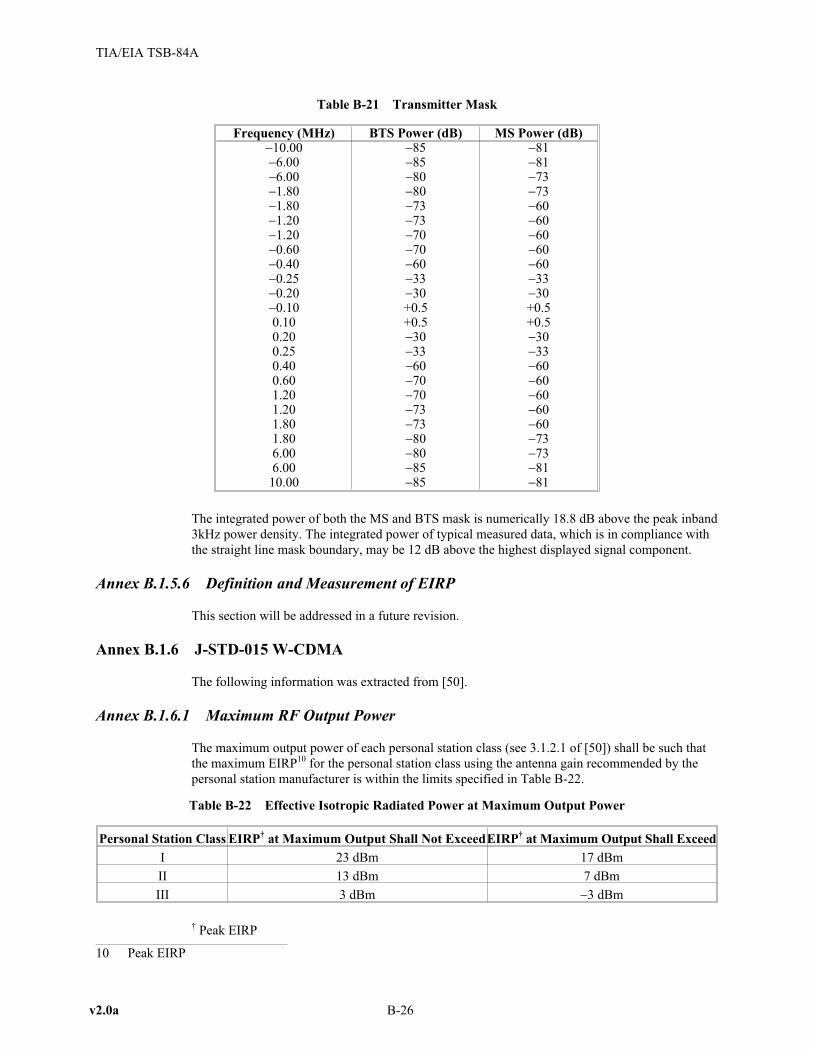
Table B-21 Transmitter Mask

Frequency (MHz) BTS Power (dB) MS Power (dB)�10.00 �85 �81�6.00 �85 �81�6.00 �80 �73�1.80 �80 �73�1.80 �73 �60�1.20 �73 �60�1.20 �70 �60�0.60 �70 �60�0.40 �60 �60�0.25 �33 �33�0.20 �30 �30�0.10 +0.5 +0.50.10 +0.5 +0.50.20 �30 �300.25 �33 �330.40 �60 �600.60 �70 �601.20 �70 �601.20 �73 �601.80 �73 �601.80 �80 �736.00 �80 �736.00 �85 �8110.00 �85 �81

The integrated power of both the MS and BTS mask is numerically 18.8 dB above the peak inband

3kHz power density. The integrated power of typical measured data, which is in compliance with

the straight line mask boundary, may be 12 dB above the highest displayed signal component.



Annex B.1.6 J-STD-015 W-CDMA


Annex B.1.6.1 Maximum RF Output Power

The maximum output power of each personal station class (see 3.1.2.1 of [50]) shall be such that

the maximum EIRP10 for the personal station class using the antenna gain recommended by the

personal station manufacturer is within the limits specified in Table B-22.

Table B-22 Effective Isotropic Radiated Power at Maximum Output Power

Personal Station Class EIRP†

at Maximum Output Shall Not ExceedEIRP†

at Maximum Output Shall Exceed

I 23 dBm 17 dBm

II 13 dBm 7 dBm

III 3 dBm �3 dBm

† Peak EIRP

v2.0a B-26

TIA/EIA TSB-84A

10 Peak EIRP

Annex B.1.6.2 Limitations on Emissions




Conducted spurious emissions are emissions at frequencies that are outside the assigned CDMA

Channel, measured at the personal station antenna connector. This test measures the spurious

emissions during continuous transmission and gated transmission.


The spurious emission level outside of the W-CDMA channel shall be attenuated below the

transmitter power (P) by at least 43+10 log (P) dB. The resolution bandwidth for measuring the

emissions shall be 1 MHz, except within the 1 MHz bandwidth immediately outside and adjacent

to the frequency block, where a resolution bandwidth of at least 1% of the emission bandwidth of

the fundamental emission of the transmitter may be employed. The emission bandwidth is defined

as the width of the signal between two points, one below the carrier center frequency and one

above the center frequency, outside of which all emissions are attenuated at least 26 dB, below the

transmitter power.



Radiated spurious emissions are emissions generated or amplified by the personal station and

radiated by the housing and all power, control and audio leads normally connected to the personal

station, when connected to a non-radiating load, at frequencies that are outside the assigned

CDMA Channel.


Radiated spurious emissions shall be less than the levels specified for the conducted spurious

emissions in B.1.6.2.1.2.


The following MS and BTS transmit mask information was obtained from subcommittee T1P1.7.

B-27 v2.0a

TIA/EIA TSB-84A

0 +2.05-2.05 +2.50-2.50 f MHz

dBm/50 kHz

+4

-31

Figure B-15 W-CDMA Base and Personal Station Transmitter Spectrum Mask (J-STD-015)



Annex B.1.7 IS-713 Upbanded AMPS

The information contained in this section is incomplete and as such the IS-713 Upbanded AMPS

technology cannot be considered as part of this Revision’s interference analysis. The IS-713

Upbanded AMPS technology information contained herein should be considered as informative

text pending receipt of additional information. The following information was extracted from [51]

and [52].

Annex B.1.7.1 Mobile Transmitter

Annex B.1.7.1.1 Power output characteristics

Annex B.1.7.1.1.1 Carrier on/off conditions

The carrier-off condition is defined as a power output at the transmitting antenna connector not

exceeding �60 dBm. When commanded to the carrier-on condition on a reverse control channel,

an MS transmitter shall come to within 3 dB of the specified output power and to within the

required stability within 2 ms. Conversely, when commanded to the carrier-off condition, the

transmit power shall fall to a level not exceeding �60 dBm within 2 ms. Whenever a transmitter is

more than 1 kHz from its initial or final value during channel switching, the transmitter carrier

shall be inhibited to a power output level not greater than �60 dBm.

Annex B.1.7.1.1.2 Power output and power control

The maximum effective radiated power with respect to a half-wave dipole (ERP) for any class MS

transmitter is 8 dBW (6.3 watts). An inoperative antenna assembly shall not degrade the spurious

emission levels. The maximum nominal ERP for each class of MS transmitter is shown in Table

B-23:

Table B-23 MS Maximum Nominal Power Levels

Class I 6 dBW (4.0 watts)

Class II 2 dBW (1.6 watts)

Class III �2 dBW (0.6 watts)

Class IV �2 dBW (0.6 watts)

Class V, Class VI, Class VII, and Class VIII are reserved for future definition. All MS transmitters

shall be capable of reducing power in steps of 4 dB on command from a BS specifying the power

level 0 to 7. Mobile stations in classes IV through VIII shall further be able to change power to

levels in the range of power levels 0 to 10 on command from a BS. The nominal levels are given

in Table B-24. Each power level in levels 0 to 7 shall be maintained within the range of +2 dB and

�4 dB of its nominal level over the ambient temperature range of �30 degrees Celsius to +60

degrees Celsius, and over the supply voltage range of ±10 percent from the nominal value,

accumulative.

For power levels 8 through 10, RF power emission shall be maintained within the range +2 dB/�6

dB of the specified power level over the same temperature and supply voltage conditions stated

above.

v2.0a B-28

TIA/EIA TSB-84A

Table B-24 MS Nominal Power Levels

MS PowerLevel (PL)

Mobile Attenuation Code(VMAC(3)) and VMAC (CMAC(3))

and CMAC Code (MAC)

Nominal ERP forMS Power Class (dBW)

I II III IV

0 (0)000 6 2 �2 �2

1 (0)001 2 2 � 2 �2

2 (0)010 �2 �2 �2 �2

3 (0)011 �6 �6 �6 �6

4 (0)100 �10 �10 �10 �10

5 (0)101 �14 �14 �14 �14

6 (0)110 �18 �18 �18 �18

7 (0)111 �22 �22 �22 �22

8 (1)000 �22 �22 �22 �26±3dB

9 (1)001 �22 �22 �22 �30±6dB

10 (1)010 �22 �22 �22 �34±9dB

Annex B.1.7.2 Base Transmitter

Annex B.1.7.2.1 Power output characteristics

Maximum effective radiated power (ERP) and antenna height above average terrain (HAAT) shall

be coordinated locally on an ongoing basis.

Annex B.1.7.3 Residential Personal Power Output Characteristics

The maximum effective radiated power with respect to a half-wave dipole (ERP) for the PB

transmitter is �20 dBW (10 mW). An inoperative antenna assembly shall not degrade the spurious

emission levels. The nominal ERP for PB transmitters is �22 dBW (6.3 mW). All PB transmitters

shall be capable of reducing power in steps of 4 dB on command from the ACRE specifying the

power level 7 to 10. Each power level shall be maintained within the range of +2 dB and –4 dB of

its nominal level, unless otherwise indicated, over the ambient temperature range of 0 degrees

Celsius to +50 degrees Celsius, and over the supply voltage range of ±10 percent from the nominal

value, accumulative.

For power levels 8 through 10, RF power emission shall be maintained within the range

+2 dB/�6 dB of the initial power level unless commanded to change by the ACRE, over the same

temperature and supply voltage conditions stated above.

The power level of the PB is controllable by the ACRE. Table B-25 contains these power levels.

Table B-25 Personal Base Nominal Power Levels

Value in MAX_PB_TX_LEVEL field Nominal ERP (dBW) for Personal Base transmitter

0 �22

1 �22

2 �22

3 �22

4 �22

5 �22

6 �22

B-29 v2.0a

TIA/EIA TSB-84A

Value in MAX_PB_TX_LEVEL field Nominal ERP (dBW) for Personal Base transmitter

7 �22

8 �26 ± 3 dB

9 �30 ± 6 dB

10 �34 ± 9 dB

11 �34 ± 9 dB

12 �34 ± 9 dB

13 �34 ± 9 dB

14 �34 ± 9 dB

15 �34 ± 9 dB



Annex B.1.8 SP-3614 PWT-E

The following information was extracted from [53] and[54].

Annex B.1.8.1 Normal Transmitted Power (NTP)

The normal transmitted power is the transmitted power averaged from the start of the physical

packet, to the end of the physical packet. The equivalent isotropically radiated NTP shall be less

than PNTP per simultaneously active transceiver at nominal conditions. Power levels are

referenced to the antenna connector. This definition applies to both the Portable Part (PP) and the

Radio Fixed Part (RFP).

The transmitter power PNTP is defined in Table B-26:

Table B-26 Power Levels

Power Level PNTP (mW)

Level 1 2

Level 2 90

Level 3 200

Level 4 500

Annex B.1.8.2 Peak Power per Transceiver

All equipment shall be capable of working at power level 2. The default power level for the PP

operating for carriers c � 20 shall be level 3, if capable of operation at this power level.

If the RFP is operating at a power level other than level 2, it shall indicate a recommended power

level for the PP by means of the PT MAC information message “recommended PP power mode”.

It is recommended that the RFP indicate a power level to match the RFP operation but no higher

than the maximum permitted level for the PP.

If the PP is capable of operating at levels other than level 2, then it shall be capable of interpreting

the PT MAC information message “recommended PP power mode” and shall operate at the

recommended power level if it is capable of doing so. Otherwise, the PP should operate at the

default power level.

v2.0a B-30

TIA/EIA TSB-84A

Annex B.1.8.3 Spectral Mask

This technology uses the second definition for “Spurious Emissions” in Section 0.6

Annex B.1.8.3.1 Emissions due to Modulation

With transmissions on a physical channel (defined as one time slot on one specific RF channel) in

successive frames, the power in physical channel shall be less than the values in the table below.

Table B-27 Adjacent Channel Power Levels due to Modulation

Emissions on RF Channel ‘Y’ Maximum Power Level

Y= First adjacent channel PNTP � 30 dB

Y= Second adjacent channel Greater of PNTP � 50 dB and 900 nW

Y = Any other allocated channel11 Greater of PNTP � 60 dB and 90 nW

The power in RF channel Y is defined by integration over a bandwidth of 600 kHz centered on the

nominal center frequency, Fy, averaged over at least 60 % but less than 80 % of the physical

packet, and starting before 25 % of the physical packet has been transmitted but after the

synchronization word.

Annex B.1.8.3.2 Emissions due to Transmitter Transients

The power level of all modulation products on channel ‘Y’ (including Amplitude Modulation

(AM) products due to the switching on or off of a modulated RF carrier) arising from a

transmission on RF channel M shall, when measured using a peak hold technique, be less than the

values given in the table below. The measurement bandwidth shall be 30 kHz and the peak power

over a 600 kHz bandwidth centered on the PWT-E frequency, Fy, shall be recorded.

Table B-28 Adjacent Channel Power Levels due to Transients

Emissions on RF Channel ‘Y’ Maximum Power Level

Y = First adjacent channel PNTP � 30 dB

Y= Second adjacent channel Greater of PNTP � 40 dB and 9 �W

Y = Any other allocated channel12 Greater of PNTP � 50 dB and 900 nW

Annex B.1.8.3.3 Emissions due to Intermodulation

The power level of intermodulation products that are on any PWT-E physical channel when any

combination of the transmitters at a radio endpoint are in calls on the same slot on different

frequencies shall be less than 500 nW. The power level is defined by integration over the 600 kHz

centered on the nominal center frequency of the afflicted channel and averaged over the time

period in Emissions due to modulation Section B.1.8.2.1.

B-31 v2.0a

TIA/EIA TSB-84A

11 For example, systems operating in the isochronous band the allocated channels are defined as channelnumbers c = 0-7, and as c = 10-17 for systems operating in the asynchronous band

12 For example, systems operating in the isochronous band the allocated channels are defined as channelnumbers c = 0-7, and as c = 10-17 for systems operating in the asynchronous band

Annex B.1.8.3.4 Emissions Outside the Assigned Operating Band

Emissions outside the PWT-E band must be below �13 dBm. The measurements at frequencies

within the first MHz outside the DCT-1900 band are made with 10 kHz resolution bandwidth, and

measurements at other frequencies are made with 1 MHz resolution bandwidth.


The PWT-E standard for emissions due to modulation is defined below:

Y = First Adjacent channel

Y = Second adjacent channel

Y = Any other allocated channel

(The power in RF Channel Y is defined by integration over a bandwidth of 600 kHz centered on

the nominal center frequency averaged over at least 60% but less than 80% of the physical packet,

and starting before 25% of the physical packet has been transmitted, but after the synchronization

word. The channel spacing is 1 MHz.)

The emission bandwidth as defined in Part 24.238 for the PWT-E transmitter is 814 kHz. The 1%

resolution bandwidth used for calculations is therefore 10 kHz (exact 1% value is 8.14 kHz with

10 kHz being the nearest standard setting for instrumentation). This results in a 0 dB carrier

reference power of �19.1 dB.

Related to a 0 dB reference power level at the center carrier frequency, the mask shall be

attenuated at least:

0 dB at 0.4 MHz offset from the center of the carrier frequency







v2.0a B-32

TIA/EIA TSB-84A

Rela

tive

Po

wer

(dB

/10kH

z)

-60

-50

-40

-30

-20

-10

0

10

-3 -2 -1 0 1 2 3Frequency Offset (MHz)

Figure B-16 Transmitter Spectral Mask

Limit values between the above points are located on the straight lines connecting nearby points in

an x/y diagram with linear power [dB] and frequency [MHz] scales.

The emission bandwidth as defined in 47CFR Part 24.238 for the PWT-E transmitter is 814 kHz.



Annex B.2 Channel Plan

In order to anticipate which frequency an interfering technology may be operating on, the

following lists of channel plans for the various technologies are presented. Note that these are

channel plans as suggested by the appropriate standards documents. The FCC itself does not

regulate channel assignments.


The system should utilize the following preferred RF channelization plan. There are channel

identifier numbers, currently omitted, that may be utilized in alternate channel plans. Table B-29

shows the channel identifiers for both TDD and FDD systems. In TDD systems, the mobile

stations, customer premises radio units (CPRUs) and base stations transmit on the same frequency.

In FDD systems, the mobile station or CPRU transmits in the lower frequency band (between

1850 and 1990 MHz), paired with a base station which transmits in the upper frequency band

(between 1930 and 1990 MHz) at a frequency exactly 80 MHz higher. In FDD systems, the

channel identifier is determined by the mobile station or CPRU transmit frequency.

The system cellular frequency plans within each of the licensed frequency blocks A through F will

normally use channels that are separated by 1.6 MHz. However, it is possible to use other

frequencies not listed in the table.

Table B-29 IS-661 CCT Channelization Plan

Channel Identifier(FDD & TDD)

Transmit Frequency(MHz)

Channel Identifier(FDD or TDD)


11 1851.1 11 or 811 1931.1

27 1852.7 27 or 827 1932.7

43 1854.3 43 or 843 1934.3

59 1855.9 59 or 859 1935.9

75 1857.5 75 or 875 1937.5

91 1859.1 91 or 891 1939.1

107 1860.7 107 or 907 1940.7

123 1862.3 123 or 923 1942.3

139 1863.9 139 or 939 1943.9

159 1865.9 159 or 959 1945.9

175 1867.5 175 or 975 1947.5

191 1869.1 191 or 991 1949.1

211 1871.1 211 or 1011 1951.1

227 1872.7 227 or 1027 1952.7

243 1874.3 243 or 1043 1954.3

259 1875.9 259 or 1059 1955.9

B-33 v2.0a

TIA/EIA TSB-84A

Channel Identifier(FDD & TDD)


Channel Identifier(FDD or TDD)


275 1877.5 275 or 1075 1957.5

291 1879.1 291 or 1091 1959.1

307 1880.7 307 or 1107 1960.7

323 1882.3 323 or 1123 1962.3

339 1883.9 339 or 1139 1963.9

359 1885.9 359 or 1159 1965.9

375 1887.5 375 or 1175 1967.5

391 1889.1 391 or 1191 1969.1

401 1890.1 401 or 1201 1970.1

425 1892.5 425 or 1225 1972.5

441 1894.1 441 or 1241 1974.1

461 1896.1 461 or 1261 1976.1

477 1897.7 477 or 1277 1977.7

493 1899.3 493 or 1293 1979.3

509 1900.9 509 or 1309 1080.9

525 1902.5 525 or 1325 1982.5

541 1904.1 541 or 1341 1984.1

557 1905.7 557 or 1357 1985.7

573 1907.3 573 or 1373 1987.3

589 1908.9 589 or 1389 1988.9


Annex B.2.2.1 Channel Spacing and Designation

The Band Class 1 block designators for the personal station and base station shall be as specified

in Table B-30.

The personal station and base station shall be capable of transmitting in Band Class 1. The channel

spacings, CDMA channel designations, and transmit center frequencies of Band Class 1 shall be

as specified in Table B-31. The personal station and base station shall support operations on

channel numbers 25 through 1175 as shown in Table B-32. Note that certain channel assignments

are not valid and others are conditionally valid. Transmission on conditionally valid channels is

permissible if the adjacent block is allocated to the licensee or if other valid authorization has been

obtained.

A preferred set of CDMA frequency assignments is given in Table B-33.

v2.0a B-34

TIA/EIA TSB-84A

Table B-30 Band Class 1 System Frequency Correspondence

BlockDesignator

Transmit Frequency Band (MHz)

Personal Station Base Station

A 1850–1865 1930–1945

D 1865–1870 1945–1950

B 1870–1885 1950–1965

E 1885–1890 1965–1970

F 1890–1895 1970–1975

C 1895–1910 1975–1990

Table B-31 CDMA Channel Number to CDMA Frequency Assignment Correspondence for Band Class 1

TransmitterCDMA Channel

NumberCenter Frequency of

CDMA Channel in MHz

Personal Station 0 � N � 1199 1850.000 + 0.050 N

Base Station 0 � N � 1199 1930.000 + 0.050 N

Table B-32 CDMA Channel Numbers and Corresponding Frequencies for Band Class 1

BlockDesignator

Valid CDMAFrequency

Assignments

CDMAChannelNumber



A(15 MHz)

Not ValidValid

Cond. Valid

0–2425–275

276–299

1850.000–1851.2001851.250–1863.7501863.800–1864.950

1930.000–1931.2001931.250–1943.7501943.800–1944.950

D(5 MHz)

Cond. ValidValid

Cond. Valid

300–324325–375376–399

1865.000–1866.2001866.250–1868.7501868.800–1869.950

1945.000–1946.2001946.250–1948.7501948.800–1949.950

B(15 MHz)

Cond. ValidValid

Cond. Valid

400–424425–675676–699

1870.000–1871.2001871.250–1883.7501883.800–1884.950

1950.000–1951.2001951.250–1963.7501963.800–1964.950

E(5 MHz)

Cond. ValidValid

Cond. Valid

700–724725–775776–799

1885.000–1886.2001886.250–1888.7501888.800–1889.950

1965.000–1966.2001966.250–1968.7501968.800–1969.950

F(5 MHz)

Cond. ValidValid

Cond. Valid

800–824825–875876–899

1890.000–1891.2001891.250–1893.7501893.800–1894.950

1970.000–1971.2001971.250–1973.7501973.800–1974.950

C(15 MHz)

Cond. ValidValid

Not Valid

900–924925–1175

1176–1199

1895.000–1896.2001896.250–1908.7501908.800–1909.950

1975.000–1976.2001976.250–1988.7501988.800–1989.950

Table B-33 CDMA Preferred Set of Frequency Assignments for Band Class 1

Block Designator Preferred Set Channel Numbers

A 25, 50, 75, 100, 125, 150, 175, 200, 225, 250, 275

D 325, 350, 375

B 425, 450, 475, 500, 525, 550, 575, 600, 625, 650, 675

E 725, 750, 775

F 825, 850, 875

C 925, 950, 975, 1000, 1025, 1050, 1075, 1100, 1125, 1150, 1175

B-35 v2.0a

TIA/EIA TSB-84A

Annex B.2.2.2 Frequency Tolerance

The base station transmit carrier frequency shall be maintained within ±5 ´ 10-8 of the CDMA

frequency assignment.

The personal station transmit carrier frequency shall be below the base station transmit frequency,

as measured at the personal station receiver, by 80 MHz ±150 Hz.


The downlink and uplink RF channels are spaced at 300 kHz intervals. The channel number and

center frequency for each channel in each block is given in Table B-34. Note that although the

required channel spacing is 300 kHz, channel numbers are assigned at 100 kHz intervals. This

channelization plan is designed to permit the system operator to select the amount of unused

spectrum allowed as guardband near band edges.

An operator licensed to use Band A may choose to allow 150 kHz of “guardband” by assigning

RPs to channels 3, 6, 9, 12 … 144, and 147. Though the choice of offset from the band edge is a

system configuration issue, all RPs within a given system must have their center frequencies set at

300 kHz intervals.

Table B-34 Channel Numbers and Frequencies

Channel BlockSU-TX Center Freq.

(MHz)RP-TX Center Freq.

(MHz)Channel Numbers (N)

Center Freq.(MHz)

A(30 MHz)

1850.1 1930.1 1

1850 + 0.1Nor

1930 + 0.1N

1850.2 1930.2 21850.3 1930.3 31850.4 1930.4 4

M M M1864.7 1944.7 1471864.8 1944.8 1481864.9 1944.9 149

D(10 MHz)

1865.0 1945.0 1501865.1 1945.1 1511865.2 1945.2 152

M M M1869.7 1949.7 1971869.8 1949.8 1981869.9 1949.9 199

B(30 MHz)

1870.0 1950.0 2001870.1 1950.1 2011870.2 1950.2 202

M M M1884.7 1964.7 3471884.8 1964.8 3481884.9 1964.9 349

E(10 MHz)

1885.0 1965.0 3501885.1 1965.1 3511885.2 1965.2 352

M M M1889.7 1969.7 3971889.8 1969.8 3981889.9 1969.9 399

v2.0a B-36

TIA/EIA TSB-84A

Channel BlockSU-TX Center Freq.

(MHz)RP-TX Center Freq.

(MHz)Channel Numbers (N)

Center Freq.(MHz)

F(10 MHz)

1890.0 1970.0 4001890.1 1970.1 4011890.2 1970.2 402

M M M1894.7 1974.7 4471894.8 1974.8 4481894.9 1974.9 449

C(30 MHz)

1895.0 1975.0 4501895.1 1975.1 4511895.2 1975.2 452

M M M1909.7 1989.7 5971909.8 1989.8 5981909.9 1989.9 599


Channel spacing shall be 30 kHz with the mobile station and corresponding base station transmit

channels as listed in Table B-35. The transmitter center frequency in MHz corresponding to the

channel number, N, is calculated as follows:


Transmitter Channel Number Center Frequency

Mobile 1 N 1999� � 1849.980 + 0.030N

Base 1 N 1999� � 1930.020 + 0.030N

Table B-36 defines the channel numbering scheme and identifies the center frequencies of

channels for 1900 MHz systems.


BandBandwidth

(MHz)Number ofChannels

BoundaryChannelNumbers

Transmitter Center Frequency (MHz)

Mobile Base

Not Used 1 1 1850.010 1930.050

A 15 4972

498

1850.040

1864.920

1930.080

1944.960

A,D (Note 1) 1 499 1864.950 1944.990

A,D (Note 1) 1 500 1864.980 1945.020

A,D (Note 1) 1 501 1865.010 1945.050

D 5 164502

665

1865.040

1869.930

1945.080

1949.970

D,B (Note 1) 1 666 1869.960 1950.000

D,B (Note 1) 1 667 1869.990 1950.030

B 15 498668

1165

1870.020

1884.930

1950.060

1964.970

B,E (Note 1) 1 1166 1884.960 1965.000

B,E (Note 1) 1 1167 1884.990 1965.030

E 5 1651168

1332

1885.020

1889.940

1965.060

1969.980

B-37 v2.0

TIA/EIA TSB-84A

BandBandwidth

(MHz)Number ofChannels

BoundaryChannelNumbers

Transmitter Center Frequency (MHz)

Mobile Base

E,F (Note 1) 1 1333 1889.970 1970.010

E,F (Note 1) 1 1334 1890.000 1970.040

F 5 1641335

1498

1890.030

1894.920

1970.070

1974.960

F,C (Note 1) 1 1499 1894.950 1974.990

F,C (Note 1) 1 1500 1894.980 1975.020

F,C (Note 1) 1 1501 1895.010 1975.050

C 15 4971502

1998

1895.040

1909.920

1975.080

1989.960

Not Used 1 1999 1909.950 1989.990

NOTE 1: This channel does not entirely fall into a single band (A,B,C,D,E, or F). A mobile

station capable of operating in any band (A, B, C, D, E or F or any combination of

these) shall also be able to operate on the associated border channel(s).


The carrier frequencies are defined by the ARFCN (Absolute Radio Frequency Channel Number)

according to Table B-37:

Table B-37 ARFCN Mapping

ARFCN Uplink Frequencies (MHz) Downlink Frequencies (MHz)

512 � N � 810 Ful(N) = 1850.2 + 0.2 * (N – 512) Fdl(N) = Ful(N) + 80

The MS must support the entire frequency range defined in Table B-37. The BTS may support any

subset of or the entire frequency range defined in Table B-37.


The channel bandwidths, channel designations, and transmit center frequencies shall be as

specified in Table B-38. The personal station shall support operations on channel numbers 1

through 23 as shown in Table B-39. Note that certain channel assignments are not valid and others

are conditionally valid. Transmission on conditionally valid channels is permissible, provided that

the adjacent block is allocated to the licensee or provided that other valid authorization has been

obtained.

The center frequency in MHz corresponding to the channel number (expressed as N) is calculated

as follows:

Table B-38 Channel Number to CDMA Frequency Assignment Correspondence

TransmitterChannelNumber

Center Frequency ofChannel in MHz

Personal Station 1 � N � 23 1850.000 + 2.5 N

Base Station 1 � N � 23 1930.000 + 2.5 N

v2.0 B-38

TIA/EIA TSB-84A

Table B-39 Channel Numbers and Corresponding Frequencies


BlockDesignator

Valid CDMAFrequency

Assignments

ChannelNumber


A(15 MHz)

Valid 1-5 1852.5-1862.5 1932.5-1942.5

D(5 MHz)

Cond. ValidValid

67

1865.01867.5

1945.01947.5

B(15 MHz)

Cond. ValidValid

89-13

1870.01872.5-1882.5

1950.01952.5-1962.5

E(5 MHz)

Cond. ValidValid

1415

1885.01887.5

1965.01967.5

F(5 MHz)

Cond. ValidValid

1617

1890.01892.5

1970.01972.5

C(15 MHz)

Cond. ValidValid

1819-23

1895.01897.5-1907.5

1975.01977.5-1987.5


Annex B.2.7.1 Channel Spacing and Designation

Spectrum used in analog PCS systems is according to Table B-40.

Table B-40 System Channel Allocations

SystemBand-widthMHz

Numberof

channels

Boundarychannelnumber

Low Set 1stDedicatedControlChannel

High Set 1stDedicatedControlChannel

Transmitter centerfrequency (MHz)

Mobile Land Station

A 15 499

1

499

25444

1850.030

1850.750

1863.320

1864.970

1930.030

1930.750

1943.320

1944.970

D 5 167

500

666

524611

1865.000

1865.720

1868.330

1869.980

1945.000

1945.720

1948.330

1949.980

B 15 499

667

1166

6911111

1870.010

1870.730

1883.330

1884.980

1950.010

1950.730

1963.330

1964.980

E 5 165

1167

1333

11911278

1885.010

1885.730

1888.340

1889.990

1965.010

1965.730

1968.340

1969.990

F 5 166

1334

1499

13581444

1890.020

1890.740

1893.320

1894.970

1970.020

1970.740

1973.320

1974.970

B-39 v2.0

TIA/EIA TSB-84A

SystemBand-widthMHz

Numberof

channels


Low Set 1stDedicatedControlChannel

High Set 1stDedicatedControlChannel

Transmitter centerfrequency (MHz)

Mobile Land Station

C 15 500

1500

1999

15241944

1895.000

1895.720

1908.320

1909.970

1975.000

1975.720

1988.320

1989.970

Channel numbering - Channels are numbered from 1 to 1999 consecutively in 30 kHz increments.

This maintains maximum commonality with 800 MHz operation. This numbering system utilizes

the same eleven address bits, along with C12 and C13 for narrow designation, as the 800 MHz

system, which is sufficient to address all channels within the 60 MHz PCS band.

In Table B-40, the center frequency in MHz corresponding to the channel number (expressed as

N) is calculated as shown in Table B-41 below:

Table B-41 Center Frequency Calculations

Transmitter Channel Number Center Frequency (MHz)

Mobile Station 1 � N � 1999 0.030 N + 1850.000

Land Station 1 � N � 1999 0.030 N + 1930.000

Annex B.2.7.1.1 Wide Analog Channels

Channel spacing shall be 30 kHz and the MS transmit channel at1850.030 MHz (and the

corresponding BS transmit channel at1930.030 MHz) shall be termed channel number 1. The 60

MHz range of channels 1 through 1999 as shown in Table B-40 for System A through F is basic.

The station class mark (SCM) shall be set appropriately.

Annex B.2.7.1.2 Narrow Analog Voice Channels

Channel spacing shall be 10 kHz and the MS transmit channel at 1850.030 MHz (and the

corresponding BS transmit channel at 1930.030 MHz) shall be termed channel number 1. The 60

MHz range of channels 1 through 1999 as shown in Table B-39 for System A through F is basic.

The station class mark (SCM) shall be set appropriately.

Additional narrow analog channels are located 10 kHz above and below the standard wide analog

channels. Mobile stations are directed to those voice channels with an order containing the channel

number (N) plus two additional fields C12 and C13 (Table B-42). C12 directs the mobile stations

to the narrow analog channel below the standard wide analog channel (N) sent and C13 directs the

mobile to the narrow analog channel above the standard wide analog channel (N).

v2.0 B-40

TIA/EIA TSB-84A

Table B-42 Narrow Analog Channel Numbers and Frequencies

C13 C12Narrow Analog

ChannelDescription

0 1 NL Channel 10 kHz below N

0 0 NM Channel centered on N

1 0 NU Channel 10 kHz above N

1 1 RESERVED

TransmitterChannelNumber

Narrow AnalogChannel Designator

Center Frequency (MHz)

MS 1 � N � 1999 NL 0.030 N +1850.000 - 0.010

NM 0.030 N + 1850.000

NU 0.030 N + 1850.000 + 0.010

BS 1 � N � 1999 NL 0.030 N + 1930.000 � 0.010

NM 0.030 N + 1930.000

NU 0.030N+ 1930.000 + 0.010

Annex B.2.7.2 Residential Channel Spacing and Designation

WRE communication utilizes narrow analog channels that have a spacing of 10 kHz. Channel

numbers are represented as 13-bit numbers. The least significant 11 bits of the channel number

contain the wide channel number. The wide channel number indicates a 30 kHz channel. The most

significant two bits of the channel number determine the 10 kHz channel within the three 10 kHz

channels of the wide channel.

The channel numbers and corresponding frequencies for the wide channels are depicted in Table

B-43.

The most significant two bits of the channel number are C13 and C12. C12 directs mobile stations

to the narrow analog channel below the middle channel. C13 directs mobile stations to the narrow

analog channel above the middle analog channel (See Table B-44).


SystemBandwidth

(MHz)Number ofchannels


Transmitter center frequency of themiddle channel (MHz)

MobileStation

PersonalBase

A 15 4991

4991850.0301864.970

1930.0301944.970

D 5 167500666

1865.0001869.98

1945.0001949.980

B 15 4996671166

1870.0101884.980

1950.0101964.980

E 5 16511671333

1885.0101889.990

1965.0101969.990

F 5 16613341499

1890.0201894.970

1970.0201974.970

C 15 50015001999

1895.0001909.970

1975.0001989.970

B-41 v2.0

TIA/EIA TSB-84A


C13 C12 Narrow Analog Channel Description

0 1 NL Channel 10 kHz below N

0 0 NM Channel centered on N

1 0 NU Channel 10 kHz above N

1 1 RESERVED

Transmitter Channel Number Narrow Analog Channel Designator Center Frequency (MHz)

MS 1� N � 1999 NL 0.030 N + 1850.000 � 0.010

NM 0.030 N +1850.000

NU 0.030 N + 1850.000 + 0.010

PB 1� N � 799 NL 0.030 N + 1930.000 � 0.010

NM 0.030 N + 1930.000

NU 0.030 N + 1930.000 + 0.010


Annex B.2.8.1 RF Channels

PWT-E operates in Time Division Duplex mode, TDD. PWT-E operates on 1 MHz spaced

carriers within the licensed bands A - F (referenced as carriers c � 20), and on 1.25 MHz spaced

carriers in the unlicensed 1910 - 1930 MHz band (referenced as carriers 0 � c � 17). A PWT-E PP

is capable of operating in the whole licensed and unlicensed band 1850 - 1930 MHz. A PWT-E

RFP operates in a specific part or parts of the licensed band (dependent on the carrier’s license)

and may operate in the unlicensed band.

A PWT-E physical channel is defined as a time slot window on a specific carrier. Therefore, a

channel plan for PWT-E in this context does not relate to notations of physical channels as defined

by PWT-E, but to notations of RF carrier numbers. Furthermore the carrier notations in the table

below relates to the notations used by the PWT-E base stations, RFPs, in the broadcast messages

to inform the PWT-E portables, PPs, which carriers are allocated to the specific PWT-E system.

This notation is a combination of an RF band number and a carrier number, c.

A PWT-E system is only able to operate on one set of carrier numbers 20 < c < 67 related to one

specific (logical) RF band number. Carrier numbers 0 - 19 relate to the unlicensed PCS band.

Carrier numbers 20 - 67 relate to the licensed PCS band and to the specific (logical) RF band

number. The definitions in Table B-45 below are not comprehensive, but are designed to cover

most operators needs. If an operator needs to operate on a set of carriers not covered by RF bands

1 - 13, then one of the reserved RF band numbers 14 - 31 shall be designated to define the required

set of carriers.

Table B-45 Carrier Number and Frequencies

FCC bandFrequency band (with nominal

carriers at nnnn.5 MHz centers)RF bandnumber

Carriernumber (c)

A30 carriers

1850 - 1855 MHz 5 carriers1930 - 1935 MHz 5 carriers1855 - 1860 MHz 5 carriers1935 - 1940 MHz 5 carriers1860 - 1865 MHz 5 carriers1940 - 1945 MHz 5 carriers

121211111010

24 - 2029 - 2524 - 2029 - 2524 - 2029 - 25

D10 carriers

1865 - 1870 MHz 5 carriers1945 - 1950 MHz 5 carriers

99

24 - 2029 - 25

v2.0a B-42

TIA/EIA TSB-84A

FCC bandFrequency band (with nominal

carriers at nnnn.5 MHz centers)RF bandnumber

Carriernumber (c)

B30 carriers


887766

24 - 2029 - 2524 - 2029 - 2524 - 2029 - 25

E10 carriers


55

24 - 2029 - 25

F10 carriers


44

24 - 2029 - 25

C

30 carriers


332211

24 - 2029 - 2524 - 2029 - 2524 - 2029 - 25

20 carriers 1880 - 1900 MHz 20 carriers 13 39 - 20

reserved for future standardization 14 - 31 20 - 42

Annex B.2.8.2 Dynamic Channel Allocation (DCA)

The physical channel is selected by the PP based upon a Dynamic Channel Allocation criterion in

order to achieve optimal performance, coexistence and interoperability. The outline below briefly

summarizes the selection criteria. The selection rules are defined in the PWT Interoperability

Specification, Part 3, Section 11.4 of [53].

Prior to the first transmission on any bearer, PWT-E RFPs and PPs have to select physical

channels. To find an appropriate channel the PP scans all available channels in the operating

environment and dynamically adapts a list of quiet and busy channels according to the measured

field strength. The receiver shall be able to measure the strength of signals on physical channels

that are received stronger than �95 dBm (i.e. 48 dBµV/m) and weaker than �40 dBm (i.e. 103

dBµV/m) with an accuracy of better than 6 dB. A PP shall be in a locked state before it may

start transmission on a physical channel. The initial set up should be performed so as to always

connect to the RFP with the strongest measured signal strength level.

The relevant physical channel refers to a TDD pair (i.e. two time slots using the same frequency,

and starting points of the time slots are separated by 0.5 frame). The received signal strength

indicator (RSSI) measurement in the relevant physical channel determines the selection

performance for one or both physical channels of a TDD pair. The choice of the relevant physical

channel of a TDD pair depends on the wanted bearer type as outlined in the Table B-46 below.

Table B-46 PWT-E Choice of Relevant Physical Channel

Wantedbearer type

Relevant Physical channel of the TDD pair

Selection by a PP Selection by an RFP

duplex channel in normal receiving TDD half frame channel in normal receiving TDD half frame

simplex channel in normal receiving TDD half frame channel with higher measured RSSI

doublesimplex

channel with higher measured RSSI channel with higher measured RSSI

The physical channel is selected by the PP and is only allowed to be changed if one of the

following conditions occurs: Detection of bad quality or interference on the physical channel in

B-43 v2.0a

TIA/EIA TSB-84A

use or detection of an RFP that is stronger than the currently selected RFP. When a change in

channel is required, the PP will select the quietest channel from its list.

Annex B.2.8.3 Nominal Position of RF Carriers

Annex B.2.8.3.1 Unlicensed

The radio frequency band allocated to PWT unlicensed PCS equipment (UPCS) is 1910 - 1930

MHz. Sixteen RF carriers shall be placed in this band with center frequencies Fc, given by:

Fc = F0 � c x 1.25 MHz c = 0, 1, ..., 713

Fc = F1 � c x 1.25 MHz c = 10, 11,..., 17

where F0 = 1 929.375 MHz

F1 = 1 931.875 MHz

For c = 0,1, ...,7 and c = 10, 11, ..., 17 the frequency band between Fc � 625 kHz and Fc + 625

kHz shall be designated RF channel c.

All PWT-E equipment shall be capable of working on all 8 PWT RF channels in the isochronous

band (0 < c < 7).

Annex B.2.8.3.2 Licensed

Equipment also capable of operation in any or all of the licensed bands A - F14 shall have center

frequencies given by:

Fc = F2 � 5 x (RF band number) � c x 1.0 MHz c = 20, 21,..., 24

Fc = F2 + 85 � 5 x (RF band number) � c x 1.0 MHz c = 25, 26,..., 29

where F2 = 1 934.5 MHz

Valid RF band numbers are 1 to 12. RF band numbers 13 to 29 are reserved for future

standardization, and numbers 30 and 31 are for proprietary escapes.

For c = 20, 21,..., 24 and c = 25, 26,..., 29 the frequency band between Fc � 500 kHz and Fc + 500

kHz shall be designated RF channel c.

Annex B.2.8.4 Accuracy and Stability of RF Carriers

At an RFP the transmitted RF carrier frequency corresponding to RF channel c shall be in the

range Fc ± 18 kHz at extreme conditions.

At a PP the center frequency accuracy shall be ± 18 kHz at extreme conditions either relative to an

absolute frequency reference or relative to the received carrier.

Note: Frequency stability compliance testing will be carried out over the temperature range �20 C

to +50 C. Although operation over this extended range is not demanded for PWT-E

interoperability, if the device does operate then the frequency stability requirement shall be 10

ppm.

v2.0a B-44

TIA/EIA TSB-84A

13 Values of c =8, 9, 18 and 19 are not used

14 Licensed bands A - F are covered by 12 RF bands, each having 5 MHz in the lower licensed band(c = 20 to 24) and 5 MHz in the upper licensed band (c = 25 to 29).

Annex B.3 Transmit/Receive Duty Cycle

Different technologies use different duty cycles. The duty cycle refers to that fraction of time that

a particular transmitter is on, during the course of a normal pseudo-continuous transmission. The

duty cycles as listed here are copied from the relevant standards. The FCC does not regulate duty

cycles.


Annex B.3.1.1 TDMA Frame and Time Slot Structure

The TDMA frame and time slot structure is based on a 20 millisecond frame (polling loop) for

user access to the RF link. See Figure B-17. Utilizing a TDD or FDD mode, the 20 ms frame is

equally divided between 16 full duplex channels within the frame. Each resulting time slot

(channel) is capable of supporting a 9.6 kbps full duplex user in a raw mode (i.e., without error

detection or correction).

At the Base Station, the first half of the TDMA time slot is allocated for the MS or CPRU transmit

function. During the second half, the BS transmits to the Mobile Station or CPRU assigned to that

particular time slot.

The BS receives during the first half of the time slot and transmits during the last half. After each

TDMA transmission from either the Base or Mobile or CPRU unit, a small portion of each time

slot (designated Guard Time) is allocated to allow the transmitted signal to propagate from a

mobile transmitter at the maximum specified distance from the Base Station (maximum cell

radius), and back again. In the TDD mode, this is necessary to prevent received and transmitted

signals from overlapping in time at the Base and Mobile or CPRU terminals.

The transmission received from the MS or CPRU serves as a channel sounding signal to determine

link propagation loss and to serve as a measurement of link quality for the CCT power control

subsystem. This is also used to determine which of the multiple antennas to use for the CCT

spatial diversity scheme and permits spatial diversity control to be updated during each TDMA

time slot period.

B-45 v2.0a

TIA/EIA TSB-84A

Figure B-17 TDMA Frame and TDMA Channel Time Slot Structure

Annex B.3.1.2 TDMA Channel (Time Slot) Assignment

Multiple or Sub-Multiple slots in the polling loop may be negotiated for and assigned to an

individual MS or CPRU. The negotiation may take place at any time via signaling traffic. The

slots, if available, are assigned by the BS to the MS or CPRU. Slot synchronization is maintained

for each assigned slot.

Annex B.3.1.2.1 Multiple TDMA Channels (Time Slots) per User

By assigning additional time slots per TDMA frame to one of the Mobile Stations or CPRUs

within a cell, the BS provides that MS or CPRU a circuit capable of communicating at a higher

data rate. For example, if 2 time slots per frame were allocated, the Mobile Station or CPRU

would have a 19.2 kbps data rate circuit, versus a 9.6 kbps channel when one time slot per frame is

allocated. The maximum data rate supported per Mobile Station or CPRU is 153.6 kbps full

duplex or 307.2 kbps half duplex. See Figure B-18.

Regardless of whether the circuit is carrying bearer or signaling information, the channels will be

treated as one circuit composed of sequential packets—two or more of which happen to occur in

the same frame—rather than as two or more parallel channels (each one slot per frame).

Annex B.3.1.2.2 Sub-Multiple TDMA Channels (Time Slots) per User

A mobile station or CPRU need not be granted a (time slot) in every frame. Slots may be granted

in frames separated by an integral number of intermediate frames to support user data rates of less

than 9.6 kbps. The maximum limit on the separation of slots allocated to a single MS or CPRU is

0.5 seconds. This equates to a per user data rate of 384 bits per second.

v2.0a B-46

TIA/EIA TSB-84A

MS1

MS1

20 msTDMAFrame

Figure B-18 Multiple TDMA Channel (Time Slots) per User

MS1/CPRU1 MS1/CPRU1

20mSFrame 1

20mSFrame 2

20mSFrame 3

Figure B-19 Sub-multiple TDMA Channels (Time Slots) per User


Annex B.3.2.1 Mobile Gated Output Power

When operating in the variable data rate transmission mode, the personal station transmits at

nominal controlled power levels only during gated-on periods, each defined as a power control

group. Given an ensemble of power control groups, all with the same mean output power, the time

response of the ensemble average shall be within the limits shown in Figure B-20. During

gated-off periods, between the transmissions of power control groups, the personal station shall

reduce its mean output power either by at least 20 dB with respect to the mean output power of the

most recent power control group, or to the transmitter noise floor, whichever is the greater power.

The transmitter noise floor should be less than �60 dBm/1.23 MHz and shall be less than �54

dBm/1.23 MHz.

Annex B.3.2.2 Mobile Data Rates

The Access Channel shall support fixed data rate operation at 4800 bps.

The Reverse Traffic Channels data rates are grouped into sets called rate sets. Rate Set 1 contains

four elements, specifically 9600, 4800, 2400, and 1200 bps. Rate Set 2 contains four elements,

specifically 14400, 7200, 3600, and 1800 bps.

Annex B.3.2.3 Mobile Code Symbol Repetition

Code symbols output from the convolutional encoder are repeated before being interleaved when

the data rate is lower than 9600 bps for Rate Set 1 and 14400 bps for Rate Set 2.

The code symbol repetition rate on the Reverse Traffic Channel varies with data rate. Code

symbols shall not be repeated for the 14400 and 9600 bps data rates. Each code symbol at the

7200 and 4800 bps data rates shall be repeated 1 time (each symbol occurs two consecutive times).

Each code symbol at the 3600 and 2400 bps data rates shall be repeated three times (each symbol

occurs four consecutive times). Each code symbol at the 1800 and 1200 bps data rates shall be

repeated seven times (each symbol occurs eight consecutive times). For all of the data rates, this

results in a constant repeated code symbol rate of 28800 code symbols per second. On the Reverse

B-47 v2.0a

TIA/EIA TSB-84A

Mean output power of theensemble average

(reference line)

Time response of theensemble average

(average power control group)

7 s� 7 s�

1.247 ms

20 dB orto noise floor 3 dB

Figure B-20 Transmission Envelope Mask (Average Gated-on Power Control Group)

Traffic Channel, these repeated code symbols shall not be transmitted multiple times. Rather, the

repeated code symbols shall be input to the block interleaver function, and all but one of the code

symbol repetitions shall be deleted prior to actual transmission due to the variable transmission

duty cycle.

Annex B.3.2.3.1 Mobile Rates and Gating

The Reverse Traffic Channel interleaver output stream is time gated to allow transmission of

certain interleaver output symbols and deletion of others. This process is illustrated in Figure

B-21. As shown in the figure, the duty cycle of the transmission gate varies with the transmit data

rate. When the transmit data rate is 9600 or 14400 bps, the transmission gate allows all interleaver

output symbols to be transmitted. When the transmit data rate is 4800 or 7200 bps, the

transmission gate allows one-half of the interleaver output symbols to be transmitted, and so forth.

The gating process operates by dividing the 20 ms frame into 16 equal length (i.e., 1.25 ms)

periods, called power control groups. Certain power control groups are gated-on (i.e., transmitted),

while other groups are gated-off (i.e., not transmitted).

Annex B.3.2.3.2 Mobile Data Burst Randomizing Algorithm

The data burst randomizer generates a masking pattern of ‘0’s and ‘1’s that randomly masks out

the redundant data generated by the code repetition. The masking pattern is determined by the data

rate of the frame and by a block of 14 bits taken from the long code. These 14 bits shall be the last

14 bits of the long code used for spreading in the previous to the last power control group of the

previous frame (see Figure B-21). In other words, these are the 14 bits which occur exactly one

power control group (1.25 ms) before each Reverse Traffic Channel frame boundary. These 14

bits are denoted as

b0 b1 b2 b3 b4 b5 b6 b7 b8 b9 b10 b11 b12 b13,

where b0 represents the oldest bit and b13 represents the latest bit.

Each 20 ms Reverse Traffic Channel frame shall be divided into 16 equal length (i.e., 1.25 ms)

power control groups numbered from 0 to 15 as shown in Figure B-21. The data burst randomizer

algorithm shall be as follows:

Data Rate Selected: 9600 or 14400 bps

Transmission shall occur on power control groups numbered:

0, 1, 2, 3, 4, 5, 6, 7, 8, 9, 10, 11, 12, 13, 14, 15.



b0, 2 + b1, 4 + b2, 6 + b3, 8 + b4, 10 + b5, 12 + b6, 14 + b7.



b0 if b8 = ‘0’, or 2 + b1 if b8 = ‘1’;

4 + b2 if b9 = ‘0’, or 6 + b3 if b9 = ‘1’;

8 + b4 if b10 = ‘0’, or 10 + b5 if b10 = ‘1’;

12 + b6 if b11 = ‘0’, or 14 + b7 if b11 = ‘1’.


v2.0a B-48

TIA/EIA TSB-84A


b0 if (b8, b12) = (‘0’, ‘0’), or

2 + b1 if (b8, b12) = (‘1’, ‘0’), or

4 + b2 if (b9, b12) = (‘0’, ‘1’), or

6 + b3 if (b9, b12) = (‘1’, ‘1’);

8 + b4 if (b10, b13) = (‘0’, ‘0’), or

10 + b5 if (b10, b13) = (‘1’, ‘0’), or

12 + b6 if (b11, b13) = (‘0’, ‘1’), or

14 + b7 if (b11, b13) = (‘1’, ‘1’).

B-49 v2.0a

TIA/EIA TSB-84A

Previous Frame

12 13 14 15 0 1 2 3 4 5 6 7 8 9 10 11 12 13 14 15

Previous Frame

12 13 14 15 0 1 2 3 4 5 6 7 8 9 10 11 12 13 14 15

Previous Frame

12 13 14 15 0 1 2 3 4 5 6 7 8 9 10 11 12 13 14 15

Previous Frame

12 13 14 15 0 1 2 3 4 5 6 7 8 9 10 11 12 13 14 15

Code Symbols Transmitted:1 33 65 97 ... 481 513 545 2 34 66 98 ... 482 514 546

1.25 ms = {36 code symbols = 6 modulation symbols =1 Power Control Group

20 ms = {576 repeated code symbols96 modulation symbols16 Power Control Groups

Power Control Group Number

9600 and14400 bpsframe







Sample masking streams shownare for the 14-bit PN sequence:

(b0, b1, ..., b13) = 0 0 1 0 1 1 0 1 1 0 0 1 0 0

PN bits usedfor streaming

PCG 15PCG 14

b0

b1

b2

b3

b4

b5

b6

b7

b8

b9

b10

b11

b12

b13

Figure B-21 Reverse CDMA Channel Variable Data Rate Transmission Example

Annex B.3.2.4 Base Data Rates

The Sync Channel shall operate at a fixed rate of 1200 bps. The Paging Channel shall support

fixed data rate operation at 9600 or 4800 bps.

The Forward Traffic Channels data rates are grouped into sets called Rate Sets. Rate Set 1

contains four elements, specifically 9600, 4800, 2400, and 1200 bps. Rate Set 2 contains four

elements, specifically 14400, 7200, 3600, and 1800 bps.

The base station shall support Rate Set 1 on the Forward Traffic Channel. The base station may

support Rate Set 2 on the Forward Traffic Channel. The base station shall support variable data

rate operation with all four elements of each supported rate set.

Annex B.3.2.5 Base Code Symbol Repetition

For the Sync Channel, each convolutionally encoded symbol shall be repeated 1 time (each

symbol occurs 2 consecutive times) prior to block interleaving.

For the Paging Channel, each convolutionally encoded symbol shall be repeated prior to block

interleaving whenever the information rate is lower than 9600 bps. Each code symbol at the 4800

bps rate shall be repeated 1 time (each symbol occurs 2 consecutive times).

The code symbol repetition rate on the Forward Traffic Channels varies with data rate. Code

symbols shall not be repeated for the 14400 and 9600 bps data rates. Each code symbol at the

7200 and 4800 bps data rates shall be repeated one time (each symbol occurs two consecutive

times). Each code symbol at the 3600 and 2400 bps data rates shall be repeated three times (each

symbol occurs four consecutive times). Each code symbol at the 1800 and 1200 bps data rates

shall be repeated seven times (each symbol occurs eight consecutive times).

Annex B.3.2.6 Base Forward Traffic Channel Time Alignment and Modulation Rates

The base station shall transmit information on the Forward Traffic Channel at variable data rates

of 9600, 4800, 2400, and 1200 bps for Rate Set 1. The base station may transmit information on

the Forward Traffic Channel at 14400, 7200, 3600, and 1800 bps for Rate Set 2. The Forward

Traffic Channel frame shall be 20 ms in duration. The data rate within a rate set shall be selected

on a frame-by-frame (i.e., 20 ms) basis. Although the data rate may vary on a frame-by-frame

basis, the modulation symbol rate is kept constant by code repetition at 19,200 symbols per second

(sps).

The modulation symbols that are transmitted at the lower data rates shall be transmitted using

lower energy. Specifically, the energy per modulation symbol (Es) for the supported data rates

should be as in Table B-47 where Eb is the energy per information bit. Note that all symbols in an

interleaver block are from the same frame. Thus, they are all transmitted at the same energy.

Table B-47 Transmitted Symbol Energy Versus Data Rate

Data Rate (bps) Energy per Modulation Symbol

9600 Es = Eb/2

4800 Es = Eb/4

2400 Es = Eb/8

1200 Es = Eb/16

14400 Es = 3Eb/4

7200 Es = 3Eb/8

v2.0a B-50

TIA/EIA TSB-84A

Data Rate (bps) Energy per Modulation Symbol

3600 Es = 3Eb/16

1800 Es = 3Eb/32


Annex B.3.3.1 SU Rampup and Rampdown

The rampup time for the power of the modulated carrier transmitted by the SU over the uplink RF

channel’s transmission must not exceed 13 µsec. Following the transmission of the final symbol in

the burst, the SU must rampdown over an interval less than 13 µsec. These intervals are shown in

Figure B-22.

Annex B.3.3.2 TDM/TDMA Frame Structure

A basic frame structure of 2.5 msec is employed in order to minimize speech transmission delay.

Each TDM frame is made up of eight (8) bursts. Use of the term “time slot” refers to use of an

ongoing sequence of bursts, whereas the term “burst” means specifically one (1) 312.5 µsec

segment.

Groups of eight (8) frames are referred to as a traffic superframe. The twenty (20) msec traffic

superframe structure provides for sub-rate channel multiplexing.

Figures B-23 and B-24 illustrate the TDM/TDMA frame structure. The downlink has the

following features:

• the frame period is 2.5 msec, corresponding to a frame rate of 400 frames per second;

• time division multiplexing (TDM) is used where each frame comprises 480 symbols (960 bits),

segmented into eight (8) bursts of sixty (60) symbols each;

B-51 v2.0a

TIA/EIA TSB-84A

Specification valueof average power

when carrier is OFF(80nW)

4dB

14dB*

13µs 13µs

108 bits

281.25 µs

Average powerwithin the burst

4dB

Lower limit of

instantaneous

power

* The upper and lower limits of instantaneous power are the ratio

of the max power and min power with respect to average power of /4 DQPSK(root roll off a=0.5) (+2.9 dB and -11 dB) plus margins (max +1.1 dB, min -3 dB).

Upper limit of

instantaneous power

Guard6 Symbols

DE1 Sym

SC5 Sym

FC + CRC + Reserved48 Symbols

Ramp Ramp

Figure B-22 Transmission envelope mask

• the aggregate bit rate of the downlink is 384 kbps.

The uplink has the following features:

• the base frame period is 2.5 msec corresponding to a frame rate of 400 frames per sec;

v2.0a B-52

TIA/EIA TSB-84A

Time2.5 msec frame

960 bits

Frame0 1 2 3

…DownlinkTDM

312.5 µsec burst120 bits

2.5 msec 960 bits

DownlinkTDM Frame

…

Time-slot0 1 2 3 4 5 6 7 0

Frame0 1 2

…UplinkTDMA

400 Frames/sec

nominaloffset (375 µs)

281 µsec108 bits

Note: Each time slot will only be "filled" on the uplinkif an SU is in fact transmitting on that slot.

UplinkTDMA Frame

…

Time-slot0 1 2 3 4 5 6 7

Figure B-23 TDM/TDMA frame structure

Time

281 µsec108 bits

Time-slot0 1 2 3 4 5 6 7 0

DownlinkTDM Frame

312.5 µsec120 bits

SyncChan

14 bits

CRC15 bits

PCC 1 bit

Fast Channel80 bits

SlowChan

10 bits

DownlinkBurst

Time-slot0 1 2 3 4 5 6 7 0

UplinkTDMA Frame

CRC15 bits

Diff. Encoding Reference Symbol2 bit interval

Guard Time12 bit

interval

SlowChan

10 bits

Fast Channel80 bits reserved 1 bit

UplinkBurst

Figure B-24 TDM/TDMA burst structure

• the uplink uses time division multiple access (TDMA), with information sent in bursts of

fifty-four (54) symbols, transmitted at the same symbol rate as the downlink.

An uplink burst is nominally 281.2 µsec in duration. The difference between the downlink’s 312.5

µsec burst and the uplink’s 281.2 µsec burst constitutes 31.3 µsec of guard time for variations in

propagation delay and turn-on and turn-off period of the SU’s transmitter.

The SU is not required to receive and transmit a burst at the same time.

The offset between the beginning of the receipt of the downlink burst and the beginning of the

transmission of the uplink burst is a nominal 375 µsec, as represented in Figure B-25. The SU

transmit timing variation “t” is defined as the departure from this nominal offset measured at the

SU’s antenna.

Long transmission paths add additional delay relative to the RP’s receiver. Therefore the RP must

be able to successfully decode uplink bursts with an offset between the beginning of the

transmission of the downlink burst and the beginning of the reception of the uplink burst,

measured at the RP’s antenna, in the range of 375 µsec, �1 symbol, +3 symbols.

Annex B.3.3.3 TDM/TDMA Burst Structure and Sequence

There are eight (8) bursts per frame, with a basic structure shown in Figures B-23 and B-24. The

downlink contains fourteen (14) bits of synchronizing information in the Sync Channel (SYC) to

facilitate synchronization by the SU. Due to its fixed offset from the downlink, uplink bursts need

no such synchronizing information, and instead use this period as a guard time (to avoid overlap of

adjacent bursts) and send a single symbol (two bits) as a start symbol to prime the differential

decoder of the RP.

Both downlink and uplink bursts carry a ten (10) bit Slow Channel (SC), an eighty (80) bit Fast

Channel (FC), and a fifteen (15) bit cyclic redundancy check (CRC). The final bit of the downlink

burst is the power control channel (PCC). The final bit of the uplink is reserved for future use.


The frame structure may be depicted as follows:

B-53 v2.0a

TIA/EIA TSB-84A

DownlinkFrame 2

UplinkFrame 1

TS 3 TS 4 TS 5 TS 6 TS 7

•••

TS 4

375.0 µsec + t i

TS 3 TS 5 TS 6TS 2

{

guard time

•••

343.25 µsec } precise conceptual burst offset

} measurable offset withtransmit timing variation

Figure B-25 Frame and burst offset as measured at the SU’s antenna

One Frame = 1944 bits (972 Symbols) = 40 ms. (25 frames per second)

Slot 1 Slot 2 Slot 3 Slot 4 Slot 5 Slot 6

One TDMA Block One Slot

Figure B-26 Frame Structure

A TDMA frame is 40 milliseconds long and consists of six equally sized time slots (1–6), each

162 symbols (324 bits) in length. A TDMA Block consists of half a TDMA frame (either slots 1 to

3 or slots 4 to 6).

The Bit Position (BP) of forward and reverse slots/bursts are numbered sequentially from 1 to 324.

In the forward direction, the first transmitted bit of the SYNC has BP = 1 and the last transmitted

bit of the RSVD field has BP = 324. In the reverse direction, the first transmitted bit of the Guard

has BP = 1. In the normal slot format, the last transmitted bit of the DATA field has BP = 324.

Interpretation of the fields is as follows:

DATA Coded Information Bits

G Guard Time

PREAM Preamble

R Ramp Time

SYNC Synchronization

SYNC+ Additional Synchronization

The base station output power shall be maintained at a constant level for the full duration of the

frame when any slot is occupied.

The output of the mobile transmitter will be on only during the time slots corresponding to the

Traffic Channel i.e. the paired slots (1,4), (2,5) or (3,6) for a Full Rate Traffic Channel or any time

slot for a Half Rate Traffic Channel.


Annex B.3.5.1 TDMA Frame Structure

The access scheme is Time Division Multiple Access (TDMA) with eight basic physical channels

(time slots) per RF carrier. A basic TDMA frame, comprising eight time slots has a duration of or

approximately 4.62 ms (60/13 ms). The basic radio resource is a time slot lasting approximately

576.9 ms (15/26 ms) and transmitting information at a modulation rate of approximately 270.833

kb/s (1625/6 kb/s). This means that the time slot duration, including guard time, is 156.25 bit

durations.

The 26-frame multiframe has a duration of 120 ms, comprising 26 TDMA frames. This

multiframe is used to carry the TCH, its SACCH and the FACCH.

The 51-frame multiframe with a duration of approximately 235.4 ms (3060/13 ms), comprising 51

TDMA frames. There are 26 of these multiframes per superframe. This multiframe is used to carry

BCCH, CCCH (AGCH, PCH and RACH) and the SDCCH and its SACCH.

The normal burst (156.25 bit durations) is used to carry information on traffic and control

channels, except for RACH. It contains 3 tail bits (preamble), 116 encrypted bits, 26 training

sequence bits, 3 tail bits (postamble) and a guard time of 8.25 bits.

v2.0a B-54

TIA/EIA TSB-84A

G R PREAM SYNC DATA SYNC+ DATA

6 6 16 28 122 24 122

Figure B-27 Normal Slot Format MS � BMI on DCCH

Annex B.3.5.2 Output Level Dynamic Operation

The term “any transmit band channel” is used here to mean any RF channel of 200 kHz bandwidth

centered on a multiple of 200 kHz which is within the relevant transmit band.

Annex B.3.5.2.1 Base Transceiver Station

The BTS shall be capable of not transmitting a burst in a time slot not used by a logical channel or

where DTX applies. The output power relative to time when sending a burst is shown in Figure

B-28. A measurement bandwidth of 300 kHz is assumed. In the case where the bursts in two or

more consecutive time slots are actually transmitted, at the same frequency, no requirements are

specified to the power ramping in the guard times between the active time slots, and the time mask

of Figure B-28 shall be met at the beginning and the end of the series of consecutive bursts. The

residual output power on the frequency channel in use, if a timeslot is not activated, shall be

attenuated to a level not higher than �30 dBc relative to the maximum rated output power of the

BTS, or to a level that does not exceed the minimum power level of the BTS inclusive of both

static and dynamic power control claimed by the manufacturer, whichever is the lower power

level.


The output power for dynamic power control is reduced by steps of 2 dB.

The transmitted power level relative to time when sending a normal burst is shown in Figure B-29.

A measurement bandwidth of 300 kHz is assumed. Between the active bursts, the residual output

power shall be maintained at, or below, the level of �48 dBc or �48 dBm, whichever is the greater

level on any transmit band channel.


Transmission is normally continuous, however during discontinuous transmission (DTX), burst

transmission is used.

B-55 v2.0a

TIA/EIA TSB-84A

dB

t ( s)�- 30

+4

8 10 10 87056/13 (542.8) 10

(*)

10

-1

+10

(147 bits)

(*) For BTS: -30 dBc referenced to dynamic power step 0See text in B.3.5.2.1 above for exceptions.

Dashed Lines indicate reference points only

Figure B-28 BTS Transmitter Time Mask

Annex B.3.6.1 Mobile DTX

The personal station shall follow the indication of DTX from the base station. When DTX is

enabled prior to transmission, the Reverse Information Channel interleaver output stream is gated

with a time filter with a unit of frame length.

When the frame is gated-off (i.e. not transmitted) according to the voice activity detection

indicator, the input data of the previous frame shall be encoded by “0". This is called the tail frame

and is used to provide tail bits to the convolutional code decoder in the base station.

When the personal station detects that the voice activity indication transitions from the OFF state

(i.e. not transmitted) to the ON state (i.e. transmitted), the convolutional encoder shall be set to the

all-zero state at the start of frame. This process is illustrated in Figure B-30.

Annex B.3.6.2 Base DTX

When DTX is enabled, prior to transmission, the Forward Traffic Channel is gated by a time filter

that allows transmission of certain punctured, multiplexed output symbols and deletion of others

according to the voice activity detection indication. The signaling and power control bits shall be

transmitted at all times. As shown in Figure B-31, the cycle of the signaling and power control bits

is gate-on (i.e., transmitted) for 46.875, 93.75 and 125 µs for transmission rates of 64000, 32000

v2.0a B-56

TIA/EIA TSB-84A

dB

-6

-30

+4

(*)

-1+1

(*) For MS: - 48 dBc or - 48 dBm, whichever is the higher.

(147 bits)

t ( s)�8 10 10 87056/13 (542.8) 1010

Figure B-29 MS Normal Burst Time Mask

VAD ON state

VAD OFF state

Tail frame

Frame

Reverse Information

Figure B-30 Discontinuous Transmission Example

and 16000 bps, respectively., and gate-off (i.e., not transmitted) for 453.125, 531.25 and 375 µs

for transmission rates of 64000, 32000 and 16000 bps. This cycle provides ten repetitions per each

frame.


The analog waveform is continuous.


Annex B.3.8.1 Frame and Slot Structure

In a PWT-E system, the radio medium is segmented in the frequency and time domain. To access

the medium in time, a time division multiple access (TDMA) structure is used. The TDMA

structure is broken into multiframes, frames and time slots.

One multiframe consists of 16 frames with a duration of 160 ms. The multiframe structure is for

the multiplexing of data that does not have to be transmitted each frame such as paging or system

information.

One frame consists of 24 slots. In a duplex connection, the first 12 slots are used for downlink

transmission ( from RFP to PP) and the other 12 slots are used for the uplink transmission (PP to

RFP). The duration of one frame is 10 ms. The data is transmitted at a bit rate of 1,152 kbit/s

resulting in a total frame length of 11,520 bits. A double slot has a length of two full slots, and

starts concurrently with an even numbered full slot. Since PWT-E is a Time Domain Duplex

(TDD) system the uplink and downlink are completed using the same RF channel.

There are four types of slots defined in the PWT-E system: short slot, half slot, full slot and double

slot. The duration of one time slot is 417 �s (480 bits). Full-slots are numbered from K = 0 to 23.

B-57 v2.0a

TIA/EIA TSB-84A

VAD ON state

VAD OFF state

Frame(5 msec)

Forward TrafficChannel

Pilot Code Period = 20 msec

Frame Offset (in the unit of 125 �sec)

Tail frame

453.125 �sec(64000 bps)406.25 �sec(32000 bps)375 �sec(16000 bps)

46.875 �sec(64000 bps)93.75 �sec(32000 bps)125 �sec(16000 bps)

Figure B-31 Discontinuous Transmission Example

Normally full-slots K = 0 to 11 are used in the RFP to PP direction, while full slots K = 12 to 23

are normally used in the PP to RFP direction. Bit intervals within a full-slot are denoted f0 to f479

where interval f0 occurs earlier than interval f1. Figure B-32 below summarizes these

associations:

In a normal operating environment the RFP will have at least one active physical channel in use at

all times. This will either be as an active call or a beacon. RFP are capable of operation on all 12

time slots simultaneously on any of the authorized channels for the particular system. PP will

transmit only during active calls and operate on only one physical channel at a time. An exception

to this is during a handover to a new physical channel or to a new RFP. At this time the PP will

operate on two physical channels simultaneously until the handover has been completed.

Annex B.3.8.2 Physical Packet Definition

Physical packets are the data units transmitted over the air interface. There are four types of

packets:

Packet P00: Short packet, transmitted in short slot (152 bits)

Packet P08j: Low Capacity packet, transmitted in half slot (240 bits)

Packet P32: Basic packet, transmitted in full slot (480 bits)

Packet P80: High capacity packet, transmitted in double slot (960 bits)

Each packet consists of the following fields:

Guard Space Duration of 56 bits with normal preamble and 32 bits with extended preamble.

Synchronization Duration of 32 bits with normal preamble and 48 bits with extended preamble.

Used for preamble detection and timing synchronization.

A-field Duration of 64 bits. Used for messaging and paging information.

B-field Duration of 0, 84, 324 or 804 bits depending on packet type.

v2.0a B-58

TIA/EIA TSB-84A

15210

Multiframe, 160 ms

0 11 12 23

Frame, 10 ms

RFP to PP (5 ms) PP to RFP (5 ms)

Slot (417 �s)

Guard

56

Sync

32

A-field

64

B-field

0 - 804

Z-field

4,0

Figure B-32 Frame Structures

Z-field Duration of 4 or 0 bits. Used to detect sliding interference from unsynchronized

systems.

Annex B.3.8.3 Power Time Template

The Power Time Template for the PWT-E transmitter is defined based upon the type of preamble

used, extended or normal. The extended preamble starts at bit s-12 while the normal preamble at s0.

The following definitions along with Figures B-33 and B-34 describe the template for both normal

and extended preamble, respectively.

For the extended preamble case the transmitter attack time is less than 5 �s and is defined as the

time taken for the transmitted power to increase from 20 nW to the time that the first symbol, s-12,

of the physical packet starts transmission. For the normal preamble case the attack time is less than

10 �s and is defined as the time taken for the transmitted power to increase from 5 �W to the time

that the first symbol of the physical packet, s0, starts transmission

For the extended preamble case the transmitter release time is less than 5 �s and is defined as the

time taken from the end of the physical packet for the transmitted power to decrease to 20 nW. For

the normal preamble case the release time is less than 10 �s and is defined as the time taken from

the end of the physical packet for the transmitted power to decrease to 5 �W.

From the first symbol of the packet, s-12 or s0, to the end of the physical packet, the instantaneous

transmitted power is greater than PNTP – 14 dB at extreme conditions.

From 5 µs before the start of symbol, s-12 or s0, to 5 µs after the end of the physical packet, the

instantaneous transmitted power is less than PNTP + 4 dB at extreme conditions.

For the time period starting 5 µs after the end of the physical packet and finishing 5 µs before the

next transmission of symbol s-12, the transmitter idle power is less than 20 nW, except when s0 of

the next transmitted packet occurs less than 54 µs after the end of the transmitted physical packet.

B-59 v2.0a

TIA/EIA TSB-84A

4 dB

14 dB

PNTP

5 W�

[20] nW4 dB

10 s� 10 s�

24 s� 24 s�

End of physical packetSymbol s0

Figure B-33 Physical Packet Power-Time Template for Slots with Normal Preamble

Annex B.4 Receiver Characteristics

This section summarizes receiver standards for the various technologies, as they apply to

PCS-to-PCS interference coordination. The FCC does not regulate receiver standards.


Annex B.4.1.1 Base Station

Annex B.4.1.1.1 Sensitivity

The minimum receive sensitivity shall be �104 dBm for a 10-3 BER.

Annex B.4.1.1.2 Co-Channel Performance

Annex B.4.1.1.2.1 Signals

The minimum co-channel interference (C/I) performance shall be 6 dB. An “On Channel” 2.5

CCT RF signal shall be adjusted to 20 dB above the measured receive sensitivity for a 10-3 BER.

A second “On Channel” signal using another DSSS code set shall be adjusted to within �6 dB of

the first RF signal. The BER shall not exceed 10-3.

Annex B.4.1.1.2.2 CW Signals

The minimum co-channel interference (C/I) performance shall be 4 dB for CW interferes. An “On

Channel” RF signal shall be adjusted to 20 dB above the measured received sensitivity for a 10-3

BER. A second “On Channel” CW signal shall be adjusted to within �4 dB of the signal. The BER

shall not exceed 10-3.

v2.0a B-60

TIA/EIA TSB-84A

4 dB

14 dB

PNTP

[20] nW

End of physical packetSymbol s-12

5 s� 5 s�

Figure B-34 Physical Packet Power-Time Template for Slots with Extended Preamble

Annex B.4.1.1.3 Multipath Performance

The receiver shall be able to maintain a BER of 10-3 minimum when receiving a signal with the

multipath conditions as shown in Table B-48:

Table B-48 Minimum Receiver Performance in Multipath

Tap Rel Delay (nSec) Avg. Power (dB)

1 0 0

2 0-6000 �3.0

Test Conditions: No fading, static multipath test

0 - 6 µs

0° phase

Radio test performed at Eb/No=20 dB

Annex B.4.1.1.4 Adjacent Channel Performance

The minimum adjacent channel receiver performance shall be determined by the ratio in dB of two

signals; where one signal (center frequency) is on the desired channel, the other signal (center

frequency) is on an adjacent channel, and the desired signal is communicating with the receiver at

a BER of 10-3. Minimum performance specifications are listed in the chart in Table B-49 below:

Table B-49 Minimum Adjacent Channel Performance

Adj. Chan Spacing Modulation Type On Chan Signal Power Min. Spec

1.6 MHz 2.5 MCPS + 2 dB above sens. �25 dB

3.2 MHz 2.5 MCPS + 2 dB above sens. �57 dB

1.6 MHz 2.5 MCPS +20 dB above sens. �28 dB

3.2 MHz 2.5 MCPS +20 dB above sens. �60 dB

1.6 MHz CW + 2 dB above sens. �30 dB

3.2 MHz CW + 2 dB above sens. �57 dB

1.6 MHz CW +20 dB above sens. �34 dB

3.2 MHz CW +20 dB above sens. �60 dB

Annex B.4.1.1.5 Intermodulation Performance

The minimum receiver intermodulation performance shall be determined by using three signal

sources. One signal source shall be an “On Channel 2.5 MCPS” signal source, and the other two

signal sources shall be CW sources located at 1.6 MHz and 3.2 MHz above the desired “On

Channel” frequency. The test shall be repeated with the two CW signal sources located at 1.6

MHz and 3.2 MHz below the desired “On Channel” receive frequency. The “On Channel” signal

shall be adjusted to 2 dB above the receiver sensitivity of the unit under test. (Receiver sensitivity

is defined in Annex B.4.1.1.) Both CW signals shall be adjusted together at the same power level

until the receiver BER is 10-3. The difference between the “On Channel” signal and the CW

signals shall be 51 dB minimum.

Annex B.4.1.1.6 Spurious RF Emissions

RF emissions from the base station receiver shall meet the FCC Part 15 incidental radiator rules.

B-61 v2.0a

TIA/EIA TSB-84A

Annex B.4.1.2 Mobile Station

Annex B.4.1.2.1 Sensitivity

The minimum receive sensitivity shall be �100 dBm for a 10-3 BER. The receiver sensitivity is

measured in AWGN.


Annex B.4.1.2.2.1 MCPS Signals

The minimum co-channel interference (C/I) performance shall be 6 dB. An “On Channel” RF

signal shall be adjusted to 20 dB above the measured receive sensitivity for a 10-3 BER. A second

“On Channel” signal using another DSSS code set shall be adjusted to within �6 dB of the first RF

signal. The BER shall not exceed 10-3.

Annex B.4.1.2.2.2 CW Signals

The minimum co-channel interference (C/I) performance shall be 2 dB for CW interferers. An

“On Channel” RF signal shall be adjusted to 20 dB above the measured receive sensitivity for a

10-3 BER. A second “On Channel” CW signal shall be adjusted to within �2 dB of the signal. The

BER shall not exceed 10-3.

Annex B.4.1.2.3 Multipath Performance

The receiver shall be able to maintain a maximum BER of 10-3 when receiving a signal with the

multipath conditions as shown in Table B-50 below:

Table B-50 Minimum Receiver Performance in Multipath

Tap Rel Delay (nSec) Avg. Power (dB)

1 0 0

2 0-6000 �3.0

Annex B.4.1.2.4 Adjacent Channel Performance

The minimum adjacent channel receiver performance shall be determined by the ratio in dB of two

signals; where one signal, C, (center frequency) is on the desired channel, the other signal, I,

(center frequency) is on an adjacent channel, and the desired signal is communicating with the

receiver at a BER of 10-3. Other test conditions are listed in Table B-51 below:

Table B-51 Adjacent Channel Performance

Adj. ChanSpacing (MHz)

ModulationType

On ChanSignal Power

Min. SpecC/I

1.6 2.5 MCPS + 2 dB above sens. �25 dB

3.2 2.5 MCPS + 2 dB above sens. �57 dB

1.6 2.5 MCPS +20 dB above sens. �28 dB

3.2 2.5 MCPS +20 dB above sens. �60 dB

1.6 CW + 2 dB above sens. �30 dB

3.2 CW + 2 dB above sens. �57 dB

1.6 CW +20 dB above sens. �34 dB

3.2 CW +20 dB above sens. �60 dB

v2.0a B-62

TIA/EIA TSB-84A

Annex B.4.1.2.5 Intermodulation Performance

The minimum receiver intermodulation performance shall be determined by using three signal

sources. One signal source shall be an “On Channel ”2.5 MCPS” signal source, and the other two

signal sources shall be CW sources located at 1.6 MHz and 3.2 MHz above the desired “On

Channel” frequency. The test shall be repeated with the two CW signal sources located at 1.6

MHz and 3.2 MHz below the desired “On Channel” receive frequency. The “On Channel” signal

shall be adjusted to 2 dB above the receiver sensitivity of the unit under test. (Receiver sensitivity

is defined in Annex B.4.1.1.1.) Both CW signals shall be adjusted together at the same power level

until the receiver BER is 10-3. The difference between the “On Channel” signal and the CW

signals shall be 53 dB minimum.

Annex B.4.1.3 Generic Mobile and Base Receiver Block Diagrams

B-63 v2.0a

TIA/EIA TSB-84A

LO

I & Q

Baseband

Processing

BPF

-1.5dB BW = 60MHz

-30dB BW = 100MHz

LNA

21dB

NF = 2dB

Band Pass Filter

-1.5dB BW = 60MHz

-30dB BW = 100MHz

T/R Switch

Loss = -0.5dB

Mixer

Loss = -10dB

NF = 10dB

IF Amplifier

Gain = 12dB

NF = 6.5dB

IF BPF

3dB BW = 1.5MHz

60dB BW = 3MHz

IF Processing

Receiver 3rd order input intercept point = -10dBm

Receiver noise figure = 6dB

Figure B-35 Generic Base Station Receiver

(numbers are representative, but may not be completely internally consistent)

LO

I & Q

Baseband

Processing

BPF

3dB BW = 60MHz

30dB BW = 100MHz

LNA

21dB

NF = 2dB

Band Pass Filter

3dB BW = 60MHz

30dB BW = 100MHz

T/R Switch

Loss = -0.8dB

Mixer

Loss = -10dB

NF = 10dB

IF Amplifier

Gain = 12dB

NF = 6.5dB

IF BPF

3dB BW = 1.5MHz

60dB BW = 3MHz

IF Processing

Receiver 3rd order input intercept point = -18dBm

Receiver noise figure = 7dB

Figure B-36 Generic Mobile Station Receiver



Annex B.4.2.1 Mobile Receiver Limitations on Emissions


Annex B.4.2.1.1.1 Suppression Inside the PCS Band

Total spurious emissions in each 1.23 MHz band located anywhere in the personal station receive

band, as given by the base station transmit frequency band in Table B-29, shall be less than �80

dBm. Total spurious emissions in each 1.23 MHz band located anywhere in the personal station’s

transmit band given in Table B-29 shall not exceed �60 dBm. These requirements shall apply to

measurements made at the personal station antenna connector with the transmitter disabled.

Annex B.4.2.1.1.2 Suppression Outside the PCS Band

Current FCC rules shall apply.



Annex B.4.2.2 Mobile Receiver Performance Requirements

System performance is predicated on receivers meeting the requirements set forth in

“Recommended Minimum Performance Requirements for 1.8 to 2.0 GHz Code Division Multiple

Access (CDMA) Personal Stations.” [45]

Annex B.4.2.3 Base Limitations on Emissions


Annex B.4.2.4 Base Receiver Performance Requirements

System performance is predicated on receivers meeting the requirements set forth in

“Recommended Minimum Performance Requirements for base stations Supporting 1.8 to 2.0 GHz

Code Division Multiple Access (CDMA) Personal Stations.” [46]

v2.0a B-64

TIA/EIA TSB-84A


B-65 v2.0a

TIA/EIA TSB-84A

90o

A/D

A/D

ToBaseband

IC

AGCControl

-50

dB

TX

Receiver Noise Figure10 dB

LNA

Low Noise AmplifierG=16 dB

NF=3.5 dBIIP3=-5 dBm

Band Pass Filter3 dB BW=70 MHz

G=-3 dB

MixerG=10 dB

NF=12 dBIIP3=+5dBm

BPF 1.25 MHzG(f )=-9 dB

G(f 0.625)=-9 dB

G(f ±1.25 MHz)=-42 dB

G(f ±2.05 MHz)=-42 dB

Attenuation is AbsoluteNF=9 dB

IF

IF

IF

IF

IF AmplifierG(max)=40 dBG(min)=-40 dB

IIP3(G )=-40 dB

IIP3(G )=0 dB

NF 5 dB

NF TBD

Dynamic Range = 80 dB

max

min

Gmax

Gmin

!!

Baseband MixerG=5 dB

NF=30 dBIIP3=0 dBm

Baseband FilterG(0)=0 dB

G(0.625 MHz)=0 dBG(1.25 MHz)=-40 dBG(2.05 MHz)=-40 dB

Baseband AmplifierG=35 dB

Generic Mobile Station Receiver

G GainNF Noise FigureIIP3 3rd Order Input Intercept Pointf Intermediate FrequencyIF

-55 dBm(nominal)

f -1.25c f +1.25cf +0.625cf -0.625c fc

-42

-9

0.625 1.25

-40

0

-4dB

-3dB

Receiver 3 Order Input Intercept Point-12 dBm

rd

Receiv

eP

athF

requen

cyR

espo

1910 206019901930

-35

-25

-4

nse

1780 2120 1910 386019901930

-25

-20

-3

f in MHz1500

Figure B-37 Generic Mobile Station Receiver


90o

A/D

A/D

ToBaseband

IC


LNA

Low Noise AmplifierG=18 dBNF=3 dB

Duplexer/Simplexer3 dB BW=70 MHz

MixerG=-7 dBNF=7 dB

BPF 1.25 MHzG(f )=-5 dB

G(f 0.625)=-5 dB

G(f ±1.25 MHz)=-80 dB

G(f ±2.05 MHz)=-80 dB

NF=5 dBAttenuation is Absolute

IF

IF

IF

IF

IF AmplifierG(max)=20 dB

NF=4 dBBaseband Filter

G(0)=-6 dBG(0.625 MHz)=-6 dBG(1.25 MHz)=-30 dBG(2.05 MHz)=-30 dB

Generic Base Station Receiver

G GainNF Noise FigureIIP3 3rd Order Input Intercept Pointf Intermediate FrequencyIF

f -1.25c f +1.25cf +0.625cf -0.625c fc

-80

-5

Receiver 3 Order Input Intercept Point-22 dBm

rd

SplitterG=-7 dBNF=7 dB

AGC

0.625 1.25

-30

-6

f in MHz

Figure B-38 Generic Base Station Receiver



Annex B.4.3.1 Receiver Sensitivity

The sensitivity of the SU and RP receivers under static conditions must be at least �101 dBm for a

word-error-rate (WER) of 0.03. The carrier-to-interference ratio to achieve a WER = 0.03 in the

presence of Rayleigh fading with a maximum rms delay spread of 0.5 microseconds must be less

than eighteen (18) dB. These specifications are applicable at 25 °C. Specifications of equipment

characteristics over an operating temperature range are not included in this document.

Annex B.4.3.2 Receiver Selectivity

SU and RP receiver selectivity is defined as the ratio of the receive sensitivity plus three (3) dB

and the unwanted digitally modulated de-tuned signal level at which the WER becomes 0.03.

Selectivity is specified as 0 dB for signals de-tuned by 300 kHz and 50 dB for signals de-tuned by

600 kHz. This specification is applicable at 25°C. Specification of equipment characteristics over

an operating temperature range is not included in this document.


v2.0a B-66

TIA/EIA TSB-84A

GNFIIP3fIF1fIF2

:Gain:Noise Figure:3rd Order Input Intercept Point:1st Intermediate Frequency:2nd Intermediate Frequency

Receiver 3rd OrderInput Intercept Point:-12dBm

Receiver Noise Figure:4dB

ANT1

ANT2

Band PassFilter

G=-1.0dB

ANT SWG=-0.8dB

Low NoiseAmplifierG=15dB

NF=1.8dBIIP3=-5dBm

LNA

Band PassFilter

G=-1.0dB

BPFG(fIF1)=-4dBG(fIF1±0.11)=-4dB

±0.5)=-25dB1)=-60dB

G(fIF1G(fIF1-2

Mixer1G=8dBNF=7dB

IIP3=0dBm

Mixer1G=8dBNF=7dB

IIP3=0dBm

Mixer2G=20dBNF=7dB

IIP3=-14dBm

BPFG(fIF2)=-4dBG(fIF2±0.11)=-4dB

±0.6)=-38dBG(fIF2

IF2 AmplifierG=60dB

To Demod

Frequency ResponseFrequency ResponseFrequency Response

(dB)

(MHz)

-4

-38

fIF2-0.6fIF2-0.11

fIF2fIF2+0.11

fIF2+0.6

-4

-25

(dB)-60

fIF1-0.5 fIF1(MHz)(MHz)

(dB)

-50

-30

-1

1500 1930 1990 3400 fIF1-21

fIF1-0.11 fIF1+0.11fIF1+0.5

Figure B-39 Generic PACS-SU Block Diagram



Annex B.4.4.1 Base Station Receiver Minimum Standards

Annex B.4.4.1.1 Conducted Spurious Emission

No spurious-output signals appearing at the antenna terminals shall exceed 1000 �V across 50 @(or equivalent output power of �47 dBm).

No spurious-output signals appearing at the antenna terminals and falling within the associated base

station receive band shall exceed 22.4 �V across 50 @ (or equivalent output power of �80 dBm).

No spurious-output signals appearing at the antenna terminals and falling within the base station

transmit band shall exceed 224 �V across 50 @ (or equivalent output power of �60 dBm).

Annex B.4.4.1.2 Radiated Spurious Emission

The radiated-spurious power levels from the receiver when measured using the procedure in

Section 5 of [18] shall not exceed the levels in Table B-52.

Table B-52 Maximum Allowable Radiated Spurious Emission

Frequency Range (MHz) Maximum Allowable EIRP†

(dBm)

25 –70 �45

70 –130 �41

130 –174 �41 to �32*

174 –260 �32

260 –470 �32 to �26*

470 –6000 �21

† Peak EIRP

*Interpolate linearly on log frequency scale.

B-67 v2.0a

TIA/EIA TSB-84A

LNA

Gain 21 dB

NF =1.8 dB

Duplexer

Loss 1 dB@20 MHz

-6 dB @ 45 MHz

-60 dB @160 MHz

Bandpass Filter

Loss 2 dB

-10 dB @ 120 MHz

Mixer

Loss 8 dB

NF = 8 dB

LNA

Gain 18 dB

NF= 2.5 dB

Bandpass Filter

Loss 11 dB

-6dB @ 500 kHz

-30 dB @ 900 kHz

Mixer

Gain 25 dB

NF = 4 dB

Bandpass Filter

Loss 12 dB

-3 db @ 240 kHz

-50 dB @ 600 kHz

Limiting

Amplifier

Cascade Noise Figure (NF) = 4 dB

Input 3rd Order Intercept Point = -5 dBm

Center Frequencies: 1860,1880,1900 MHz

Figure B-40 Generic PACS-RP Block Diagram


Annex B.4.4.2 Base Receiver Performance

Annex B.4.4.2.1 RF Sensitivity Static and Faded

The actual error rate performance for each test of the receiver shall not be greater than that listed

in Table B-53.

Table B-53 RF Sensitivity Error-Rate Performance

Channel Equivalent Vehicle Speed (km/h) RF Level (dBm) Error Rate (%)

DTCData Field

(BER)

Faded, 100 �103 3

Faded, 8 �103 3

Static �110 3

RACH(WER)

Faded, 100 �103 9

Faded, 8 �100 9

Static �111 9

Annex B.4.4.2.2 Adjacent and Alternate Channel Desensitization




modulated input frequency spaced either one channel (30 kHz) above or one channel (30 kHz)







Annex B.4.4.2.2.2 Method of Measurement

Equally couple a AB-DQPSK test signal and an interfering RF generator to the base station

antenna terminal through a suitable matching network. Set the AB-DQPSK test signal to the

assigned channel and set its RF level at the receiver to –107 dBm. Transmitted Data Field bits

shall consist of pseudorandom data. Set the interfering RF generator to 30 and 60 kHz above the

frequency of the RF Test Generator and modulate it with pseudorandom AB-DQPSK data. Adjust

the level of the interfering RF generator to �94 dBm for the 30 kHz offset and �65 dBm for 60

kHz offset. The base station shall provide a monitoring means for Data Field bits with no

correction. All tests shall be performed with the delay interval compensation operational.

Repeat the above procedure with the frequency of the interfering RF generator set to 30 and 60

kHz below the frequency of the Digital RF Test Generator.


The adjacent-channel BER shall be below 3%. The alternate-channel BER shall be below 3%.

v2.0a B-68

TIA/EIA TSB-84A

Annex B.4.4.2.3 Intermodulation Spurious Response Attenuation



receive a modulated input RF signal frequency in the presence of one modulated signal and one

unmodulated signal, so separated from the assigned input signal frequency and from each other

that the nth order mixing of the two undesired signals can occur in the non-linear elements of the

receiver, producing a third signal whose frequency is equal to that of the assigned input RF signal

frequency. BER on the Data Field bits shall be used to measure performance for each test.


Equally couple a AB-DQPSK test signal and two interfering RF signal generators to the base

station antenna terminal. Set the AB-DQPSK test signal to the assigned channel and set its RF

level at the receiver to �107 dBm. Transmitted Data Field bits shall consist of pseudorandom data.

Adjust the second RF generator to a frequency 120 kHz above the assigned input frequency, and

the third RF generator to a frequency 240 kHz above the assigned frequency. Adjust the level of

the second and third RF generators to �45 dBm and modulate the third generator with

pseudorandom AB-DQPSK data. The base station shall provide a monitoring means for Data Field

bits with no correction. All tests shall be performed with the delay interval compensation

operational.

Repeat the above procedure with the second RF generator set to 120 kHz below and the third



The BER shall be less than 3%.

Annex B.4.4.2.4 Protection Against Spurious Response Interference


The receiver spurious-response attenuation is a measure of the receiver’s ability to discriminate

between the input signal at the assigned and an undesired signal at any other frequency to which it

is responsive. BER on the Data Field bits shall be used to measure performance for each test.


Connect a AB-DQPSK test signal and an interfering RF signal generator to the base station under

test through an appropriate matching or combining network. Set the AB-DQPSK test signal to the

assigned channel and set its RF level at the receiver to �107 dBm. Transmitted Data Field bits

shall consist of pseudorandom data. Switch the other (undesired) input RF signal source ON, and

set it to a high level (i.e., at least 57 dB above the level of the desired input RF signal source).

Modulate the undesired input RF signal source with pseudorandom AB-DQPSK data in the band

1850-1910 MHz. Outside the band, the test signal shall be unmodulated. The base station shall

provide a monitoring means for Data Field bits with no corrections. All tests shall be performed

with the delay interval compensation operational.



lower, to at least 6000 MHz and all the response shall be noted.

At the frequency of each spurious response, measure the BER.

B-69 v2.0a

TIA/EIA TSB-84A


The BER shall be less than or equal to 3% except within 90 kHz of the assigned channel.


The error rate performance for each test of the receiver shall not be greater than that listed in Table

B-53 with the RF level of the co-channel interferer adjusted so that the ratio between the test

signal of �85 dBm and the interferer is as specified in Table B-54.

Table B-54 Co-Channel Rejection Error-Rate Performance

Channel Simulated Vehicle Speed (km/h) Error Rate (%) CIR (dB)

RACH(WER)

8 10.0 16

100 10.0 14

FACCH(WER)

8 7.3 14

100 3.3 12

SACCH(WER)

8 14.0 14

100 9.0 12

VSELP Class 1(WER)

8 7.1 17

100 1.4 17

EFR Class 1(WER)

8 7.8 17

100 1.7 17

DTCData Field

(BER)

8 3 17

50 3 17

100 3 17

Annex B.4.4.3 Mobile Receiver Performance

Annex B.4.4.3.1 Static and Faded RF Sensitivity

The actual error rate for each test of the receiver shall not be greater than that listed in Table B-55.

Table B-55 RF Sensitivity Error-Rate Performance

Channel Equivalent Vehicle Speed (km/h) RF Level (dBm) Error Rate (%)

DTCData Field

(BER)

Faded, 100 �103 3

Faded, 8 �103 3

Static �110 3

Static �25 3

BCCH(WER)

Faded, 100 �103 9

Faded, 8 �100 9

Static �111 9

Static �25 9

v2.0a B-70

TIA/EIA TSB-84A

Annex B.4.4.3.2 Adjacent and Alternate Channel Desensitization




modulated input frequency spaced either one channel (30 kHz) above or one channel (30 kHz)








Equally couple a AB-shifted DQPSK test signal and an interfering RF generator to the mobile

station antenna terminal through a suitable matching network. Set the AB-shifted DQPSK test

signal to the assigned channel and set its RF level at the receiver to �107 dBm. Transmitted Data

Field bits shall consist of pseudorandom data. Set the interfering RF generator to 30 and 60 kHz

above the frequency of the RF Test Generator and modulate it with pseudorandom AB-shifted

DQPSK data. Adjust the level of the interfering RF generator to �94 dBm for the 30 kHz offset

and �65 dBm for 60 kHz offset. The mobile station shall transpond the Data Field bits via

TDMAON command with ECHO=0. All tests shall be performed with the delay interval

compensation operational.

Repeat the above procedure with the frequency of the interfering RF generator set to 30 and 60

kHz below the frequency of the Digital RF Test Generator.



Annex B.4.4.3.3 Intermodulation Spurious Response Attenuation



receive a modulated input RF signal frequency in the presence of one modulated signal and one

unmodulated signal, so separated from the assigned input signal frequency and from each other

that the nth-order mixing of the two undesired signals can occur in the non-linear elements of the

receiver, producing a third signal whose frequency is equal to that of the assigned input RF signal

frequency. BER on the Data Field bits shall be used to measure performance for each test.


Equally couple a AB-shifted DQPSK test signal and two interfering RF signal generators to the

receiver input terminals. Set the AB-shifted DQPSK test signal to the assigned channel and set its

RF level at the receiver to �107 dBm. Transmitted Data Field bits shall consist of pseudorandom

data. Adjust the second RF generator to a frequency 240 kHz above the assigned input frequency,

and the third RF generator to a frequency 480 kHz above the assigned frequency. Adjust the level

of the second and third RF generators to �45 dBm and modulate the third generator with

pseudo-random AB-shifted DQPSK data. The mobile station shall transpond the Data Field bits

B-71 v2.0a

TIA/EIA TSB-84A

via TDMAON command with ECHO=0. All tests shall be performed with the delay interval

compensation operational.

Repeat the above procedure with the second RF generator set to 240 kHz below and the third



The BER shall be less than 3%.

Annex B.4.4.3.4 Blocking and Spurious-Response Rejection

Annex B.4.4.3.4.1 Definitions

Blocking

Blocking is defined as the de-sensitization of the receiver by a signal separated in frequency from

the wanted signal by at least three channels. The signal frequencies that may block the receiver

range from the lowest intermediate frequency of the receiver to at least three times the wanted

signal frequency (fc in Figure B-41 below) of the receiver.

Spurious Response

A spurious response is defined as the de-sensitization of the receiver by signals in a specific small

band of frequencies which has a bandwidth (bs in Figure B-41 below) of the same order as the

channel bandwidth. The frequencies of signals that may produce spurious responses are in the

same range as those that may cause blocking. The bandwidth, bs, of the spurious response is the

continuous range of frequencies in which a signal at the level of the blocking level limit causes the

error rate limit to be exceeded.


Connect a A4 DQPSK test signal and an RF signal generator to the receiver under test. Set the A4DQPSK test signal to the assigned channel and set its RF level at the receiver the specified desired

signal level. Transmitted Data Field bits shall consist of pseudo-random data.

v2.0a B-72

TIA/EIA TSB-84A

Level

freq

fc

Blocking

level limit

Spurious

level limit

SPURIOUS

RESPONSE

bs

MEASURED

BLOCKING LEVEL

(of blocking signal requiredto cause de-sentisation)

Figure B-41 Blocking and Spurious Response Limits

Switch the other (undesired) input RF signal source on, and set its level to the specified blocking

limit level. Modulate the undesired input RF signal source with pseudo-random A4 DQPSK data

within the operating band(s) and unmodulated elsewhere. The mobile station shall transpond the

Data Field bits via the TDMAON command with ECHO = 0. All tests shall be performed with the

delay interval compensation operational.



lower, to at least 6000 MHz, and all responses shall be noted.

The sweep rate, or frequency step size & step rate, of the generator providing the undesired signal

shall be slow enough to allow sufficient time for any responses to be detectable as a change in

error rate. This will require the time during which this generator dwells within a frequency range

equal to the receiver bandwidth to be greater than the measurement interval used for error rate

determinations. Special attention should be given to measurements around frequencies at which

spurious responses are more likely to occur; e.g. due to “image” & harmonically-related

frequencies.

For each spurious response, measure the bandwidth over which the spurious response occurs & the

minimum signal required to cause the spurious response.


Table B-56 Blocking and Spurious Response Rejection

Frequency BandDesired Signal(frequency f)

Blocking Signal(frequency fo)

SpuriousResponse limit(frequency fo)

ErrorRate(%)

|f�fo| > 3 MHz �102 dBm �30 dBm �45 dBm 3

3 MHz > |f�fo| > 90 kHz �102 dBm �45 dBm �45 dBm 3

Up to 12 in band and 24 out of band spurious responses are allowed.

The maximum bandwidth for any individual spurious response shall be 60 kHz up to the highest

frequency in the operating band. At higher frequencies, the maximum bandwidth of an individual

spurious response shall be 180 kHz. Responses having bandwidths greater than these limits shall

be treated as multiple responses for the purpose of accumulating the response limit numbers.

The unwanted signal level required to cause any spurious response shall not be lower than the

limit value.

Annex B.4.4.3.5 Mobile Assisted Handoff / Mobile Assisted Channel Allocation Bit Error Rate

The reported bit error rate pattern returned in the channel quality measurement shall be as

indicated in Figure B-42 for any induced transmitted bit error rate within the shaded regions of the

Figure for at least 8 out of 10 consecutive reporting periods of 25 frames each. For 0% induced

transmitted BER, the reported bit pattern shall be ‘000’ for at least 8 out of ten consecutive

reporting periods of 25 frames each.

Table B-57 AHO/MACA BER

Bit Pattern TX Induced BER (%) RX Reported BER Interval (%)

000 0 less than 0.01

001 0.013 to 0.08 0.01 to less than 0.1

010 0.133 to 0.4 0.1 to less than 0.5

B-73 v2.0a

TIA/EIA TSB-84A

Bit Pattern TX Induced BER (%) RX Reported BER Interval (%)

011 0.667 to 0.8 0.5 to less than 1.0

100 1.333 to 1.6 1.0 to less than 2.0

101 2.667 to 3.2 2.0 to less than 4.0

110 5.333 to 6.4 4.0 to less than 8.0

111 10.667 greater than 8.0

The shaded intervals indicate ranges for which the reported MAHO/MACA BER pattern must be

as shown.

Annex B.4.4.3.6 Co-channel Performance

The error rate for each test of the receiver shall not be greater than that listed in Table B-58 with

the RF level of the cochannel interferer adjusted so that the ratio between the test signal of �85

dBm and the interferer is specified in Table B-58.

Table B-58 Error Rates Vs C/I Ratio


BCCH(WER)

8 10 16

100 12.3 14

FACCH(WER)

8 7.3 14

100 3.3 12

SACCH(WER)

8 14.0 14

100 9.0 12

VSELP Class 1(WER)

8 7.1 17

100 1.4 17

IS-641 Class 1(WER)

8 7.8 17

100 1.7 17

v2.0a B-74

TIA/EIA TSB-84A

0 0.01 0.1 0.5 1.0 2.0 4.0 8.0000

001

010

011

100

101

110

111R

eport

edM

AH

OB

ER

Pat

tern

Induced Transmitted Bit Error Rate (in %)

.013 .08

.133 .4

.667 .8

1.333 1.6

2.667 3.2

5.333 6.4

>10.667

Figure B-42 Reported MAHO BER Patterns


DTCData Field

(BER)

8 3 17

50 3 17

100 3 17

Annex B.4.4.4 Conducted Spurious Emissions

No spurious-output signals appearing at the antenna terminals shall exceed 1000 µV across 50 @(or equivalent output power of �47 dBm).

No spurious-output signals appearing at the antenna terminals and falling within the mobile station

receive band shall exceed 22.4 µV across 50 @ (or equivalent output signals power of �80 dBm).

No spurious-output signals appearing at the antenna terminals and falling within the mobile station

transmit band shall exceed 224 µV across 50 @ (or equivalent output power of �60 dBm).

Annex B.4.4.5 Radiated Spurious Emissions

The radiated-spurious power levels from the receiver when measured using the procedure in

Section 5 of [48] shall not exceed the levels in Table B-59.

Table B-59 Maximum Allowable Radiated Spurious Emission

Frequency Range Maximum Allowable EIRP†

25 -70 MHz �45 dBm

70 -130 MHz �41 dBm

130 - 174 MHz �41 to �32 dBm*

174 - 260 MHz �32 dBm

260 - 470 MHz �32 to �26 dBm*

470 - 2000 MHz �21 dBm

† Peak EIRP

*Interpolate linearly on log frequency scale.

B-75 v2.0a

TIA/EIA TSB-84A


v2.0a B-76

TIA/EIA TSB-84A

Generic Base Station Receiver

Receiver 3 Order Input Intercept PointTBD

rd


Duplexer/Simplexer3 dB BW = 70 MHz

Low Noise AmplifierG = 19 dBNF = 6 dB Splitter

G = -7 dBNF = 7 dB

MixerG = -7 dBNF = 7 dB

BPF 30.0 kHzG(f ) = -5 dB

G(f ) = -5 dBG(f ) = -30 dBG(f ) = -30 dBG(f ) = -60 dBG(f ) = -60 dBG(f ) = -80 dB

NF = TBDAttenuation is Absolute

IF

IF

IF

IF

IF

IF

IF

±15 kHz±15 kHz±45 kHz±45 kHz±75 kHz±75 kHz

IF AmplifierG(max) = 20 dB

NF = 4 dB

AGC

90°

A/D

A/D

ToBaseband

IC

Baseband FilterG(0) = -6 dB

G(15.0 kHz) = -6 dBG(45.0 kHz) = -36 dBG(75.0 kHz) = -36 dB

GNFIIP3fIF

GainNoise Figure3rd Order Input Intercept PointIntermediate Frequency

LNA

dB

-5

-30

-60

-80

f -75c f -45c f -15c fc f +15cf +45c f +75c

f in kHz

dB

-6

-36

15 45f in kHz

Figure B-43 Generic BS Receiver Diagram

(numbers are representative, but may not be completely internally consistent; for illustrative purposes only)

Generic IS-136 Mobile Station Receiver

Receiver 3 Order Input Intercept PointTBD

rd


Low Noise AmplifierG = 16 dBNF = 6 dB

MixerG = -5 dB

NF = 12 dB

BPF 30.0 kHzG(f ) = -9 dB

G(f ±15.0 kHz) = -9 dB

G(f ±15.0 kHz) = -34 dB

G(f ±45.0 kHz) = -34 dB

G(f ±45.0 kHz) = -64 dB

G(f ±75.0 kHz) = -64 dB

G(f ±75.0 kHz) = -84 dB

Attenuation is AbsoluteNF = 9 dB

IF

IF

IF

IF

IF

IF

IF

AGC

GNFIIP3fIF

GainNoise Figure3rd Order Input Intercept PointIntermediate Frequency

LNA

TX

ToBaseband

IC

Baseband FilterG(0) = -10 dB

G(15 kHz) = -10 dBG(45 kHz) = -40 dBG(75 kHz) = -40 dB

A/D

A/D

90°

dB-9

-34

-64

-84

f -75c f -45c f -15cfc f +15c f +45c f +75c

f in kHz

dB

dB

-10

-3

-40

-20

15

1500

45f in kHz

f in MHz

Receiv

eP

athF

requen

cyR

esponse

Band Pass Filter3 dB BW = 70 MHz

G = -3 dB

-3dB

-4dB

-50

dB

dB

-4

-25

1780

MHz-35

1910 1930 1990 2060 2120

-25

1910 1930 1990 3860

Figure B-44 Generic MS Receiver Diagram

(numbers are representative, but may not be completely internally consistent; for illustrative purposes only)

An

nex

B.4

.4.7

Mobil

eS

tati

on

Rec

eive

rP

ara

met

ers

IS-1

37A

ref.

Tit

leE

xp

lan

ati

on

Pri

nci

pal

Req

uir

emen

ts(c

hec

kIS

-137A

for

det

ails

)Is

sues

Rel

evan

ce

2.3

.2.1

Rec

eiver

Sig

nal

Lev

elR

ange

Cap

abil

ity

Rep

lace

s&

exte

nds

Rec

eive

rSen

siti

vity

�110

to�2

5dB

mfo

r<

3%

BE

Runfa

ded

.

Rx

nois

efi

gure

.D

ynam

icra

nge

of

the

det

ecto

r&

pre

cedin

gst

ages

on

the

wan

ted

chan

nel

.A

GC

acti

on.

Imp

ort

an

tp

ara

met

er:

Inte

rfer

ing

signal

sm

ust

hav

eco

mbin

edpow

ersp

ectr

alden

sity

low

erth

aneq

uiv

alen

tth

erm

alnois

ein

torx

final

IF.

2.3

.2.2

Adja

cent

and

Alt

ernat

eC

han

nel

Des

ensi

tiza

tion

Rej

ecti

on

of

inte

rfer

ing

signal

sat

freq

uen

cies

close

toth

ew

ante

dfr

equen

cy.

Inte

rfer

ence

level

>�9

4dB

m@

f c±

30

kH

z;>�6

5dB

m@

f c±

60

kH

z;fo

r�3

%B

ER

,w

ante

dsi

gnal�1

07

dB

m.

Com

bin

edIF

filt

er(s

)off

-chan

nel

reje

ctio

n(c

lose

in)

Pro

bab

lynot

import

ant

asal

loth

ersy

stem

shav

ew

ider

emis

sion

ban

dw

idth

whic

hw

ill

smoth

erIS

-136

AC

Ref

fect

s.

2.3

.2.3

Inte

rmodula

tion

Spuri

ous

Res

ponse

Att

enuat

ion

Rej

ecti

on

of

inte

rfer

ence

due

toth

ird-o

rder

inte

rmodula

tion

pro

duct

sca

use

dby

two

equal

-lev

elin

terf

erin

gsi

gnal

ssp

aced

from

the

wan

ted

signal

by

n-

&2*n-t

imes

the

syst

emch

annel

spac

ing.

Eac

hin

terf

erer

�45

dB

m,±

(240

&480)

kH

z

for

3%

BE

R,

wan

ted

signal�1

07

dB

m.

Lin

eari

tyof

ampli

fier

s&

mix

ers

not

pre

ceded

by

filt

ers

nar

row

enough

tore

move

the

inte

rfer

ing

off

-chan

nel

signal

s.

Pro

bab

lynot

import

ant

asm

ost

oth

ersy

stem

shav

ew

ider

emis

sion

ban

dw

idth

whic

hw

ill

pro

bab

lysm

oth

erIS

-136

rxIM

effe

cts.

Iden

tica

lle

vel

tosi

ngle

-car

rier

blo

ckin

gli

mit

atth

ese

freq

uen

cyoff

sets

.

2.3

.2.4

Blo

ckin

gR

ejec

tion

Blo

ckin

g:

Abil

ity

tore

ject

single

or

mult

iple

non-h

arm

onic

ally

-rel

ated

signal

sw

idel

ysp

aced

from

the

wan

ted

freq

uen

cy.

Min

imum

signal

todes

ensi

tise

:

�45

dB

m,90

kH

z<|f�f

c|<

3M

Hz

�30

dB

m,

|f�f

c|>

3M

Hz

for

<3%

BE

R,

wan

ted

signal�1

07

dB

m.

Ult

imat

ebro

adban

dre

ject

ion

of

filt

ers

(RF

&IF

).D

ynam

icra

nge

of

earl

yac

tive

stag

es(b

efore

maj

or

filt

erin

g).

Loca

losc

illa

tor

phas

enois

e,&

reci

pro

cal

mix

ing.

Most

imp

ort

an

tp

ara

met

er:

Mea

sure

dusi

ng

nar

row

ban

dsi

gnal

.E

ffec

tof

non-I

S-1

36

inte

rfer

erw

ill

be

equal

toth

atof

nar

row

ban

dm

easu

rem

ent

signal

wit

hsa

me

tota

l(p

eak

envel

ope)

pow

er.

B-7

7v2.0

TIA

/EIA

TS

B-8

4A

IS-1

37A

ref.

Tit

leE

xp

lan

ati

on

Pri

nci

pal

Req

uir

emen

ts(c

hec

kIS

-137A

for

det

ails

)Is

sues

Rel

evan

ce

2.3

.2.4

Spuri

ous

Res

ponse

Rej

ecti

on

Spuri

ous

resp

onse

:E

xce

pti

ons

toth

egen

eral

blo

ckin

gli

mit

cause

dby

har

monic

ally

-rel

ated

signal

s(e

.g.im

age)

.

Spuri

ous

exce

pti

ons:

not

more

than

12

inban

d&

24

outb

and

at>�4

5dB

m,

max

imum

ban

dw

idth

/sp

uri

ous

60

kH

zup

tom

axim

um

oper

atin

gfr

equen

cy,180

kH

zab

ove,

wid

erre

sponse

sco

unt

asm

ult

iple

spuri

i.

Non-l

inea

rity

of

earl

yac

tive

stag

es(b

efore

maj

or

filt

erin

g).

Non-r

ejec

tion

of

conse

quen

tunw

ante

dm

ixin

gpro

duct

sby

poor

filt

erin

g.

Mea

sure

dusi

ng

nar

row

ban

dsi

gnal

.

Eff

ect

of

non-I

S-1

36

inte

rfer

erw

ill

be

equal

toth

atof

nar

row

ban

dm

easu

rem

ent

signal

wit

hsa

me

(pea

ken

vel

ope)

pow

eras

inte

rfer

erpro

vid

esin

the

ban

dw

idth

of

each

spuri

ous

resp

onse

.

2.3

.2.5

Mobil

eA

ssis

ted

Han

doff

/M

obil

eA

ssis

ted

Chan

nel

All

oca

tion

MS

mea

sure

s&

report

sR

SS

I&

ER

or

reques

ted

chan

nel

sto

BS

.

n/a

RS

SI

indic

ator

&si

gnal

ling

MS

toB

S.

Not

rele

van

tunle

ssR

SS

Ier

rors

cause

dby

oth

erre

ceiv

erfa

ilure

modes

(e.g

.blo

ckin

gre

duce

sle

vel

inIF

amps.

)or

exte

rnal

inte

rfer

ence

(e.g

.in

terf

erin

gpuls

ednois

esi

deb

ands

blo

cks

pro

duce

sfa

lse

mea

sure

men

t).

2.3

.2.6

Co-c

han

nel

Per

form

ance

Rej

ecti

on

of

unw

ante

dsi

gnal

son

the

wan

ted

signal

freq

uen

cy

Inte

rfer

er>

17

dB

bel

ow

wan

ted

signal

of�8

5dB

mfo

r<

3%

BE

Ron

DT

Cdat

abit

s

This

isa

fundam

enta

lpro

per

tyof

the

modula

tion

schem

ew

hic

hm

aybe

deg

raded

by

des

ign

of

the

det

ecto

r.

Pro

bab

lynot

rele

van

tfo

rP

CS

inte

rfer

ence

:�1

10

dB

mth

resh

old

sensi

tivit

ym

ust

be

use

dto

calc

ula

teon-c

han

nel

inte

rfer

ence

.

2.3

.2.7

Del

ayIn

terv

alR

emoval

of

radio

pat

hec

hoes

n/a

Rad

ioch

annel

equal

iser

Not

rele

van

tunle

sseq

ual

iser

mis

-ali

gns

due

tooth

erre

ceiv

erfa

ilure

mec

han

ism

sor

exte

rnal

inte

rfer

ence

(e.g

.in

terf

erin

gpuls

ednois

eblo

cks

trai

nin

gon

sync

word

s).

Annex

B.4

.4.7

.1S

um

mar

y

Rec

eiver

thre

shold

��

110

dB

m.

Off

set

(Hz)

30k

60k

90k-3

M240k

&480k

�3M

Min

imu

mL

evel

toD

esen

siti

ze(d

Bm

)�9

4�6

5�4

5�4

5�3

0

v2.0

B-7

8

TIA

/EIA

TS

B-8

4A


Annex B.4.5.1 Receiver Characteristics

In this section, the requirements are given in terms of power levels at the antenna connector of the

receiver. In the case of base transceiver stations the requirements apply for measurement at the

connection with the antenna feeder of the BTS for any supported configuration of the equipment

including any low noise receiver amplifiers or receiver multicouplers. For equipment using active

antenna arrays or multiple radiating elements, the reference measurement point shall be as shown

in Figure B-11.

Annex B.4.5.1.1 Blocking Characteristics

The blocking characteristics of the receiver are specified separately for in-band and out-of-band

performance as identified in Table B-60.

Table B-60 RX Blocking Mask

Frequency Band MS Freq. Range (MHz) BTS Freq. Range (MHz)

in band 1910 � f � 2010 1830 � f � 1930

out-of-band (i) 0.1 � f < 1830 0.1 � f < 1830

out-of-band (ii) 1830 � f < 1910 –

out-of-band (iii) 2010 < f � 2070 –

out-of-band (iv) 2070 < f � 12750 1930 < f � 12750

The static reference sensitivity performance as specified in Table B-67 shall be met when the

following signals are simultaneously input to the receiver:

• a desired, GMSK BT=0.3 modulated signal at frequency f0, 3 dB above the static reference

sensitivity level as specified in Section B.4.5.2.1;

• a continuous, unmodulated interfering signal at a level as in the table below and at a frequency

(f) which is an integer multiple of 200 kHz.

Table B-61 RX Blocking Limits

Frequency BandMS BTS

dB mV (emf) dBm dB mV (emf) dBm

|f – f0| = 600 kHz 70 � 43 78 � 35

800 kHz � |f – f0| < 1.6 MHz 70 � 43 88 � 25

1.6 MHz � |f – f0| < 3 MHz 80 � 33 88 � 25

3 MHz � |f – f0| 87 � 26 88 � 25

out of band

i 113 0 113 0

ii 101 � 12 – –

iii 101 � 12 – –

iv 113 0 113 0

The blocking characteristics of the micro-BTS receiver are specified for in-band performance

according to the following table. The out-of-band blocking remains the same as a normal BTS

defined above.

B-79 v2.0a

TIA/EIA TSB-84A

Table B-62 Micro BTS Blocking Limits

Frequency BandMicro BTS Power Class

M1 (dBm) M2 (dBm) M3 (dBm)

|f – f0| = 600 kHz �40 �35 �30

800 kHz � |f – f0| < 1.6 MHz �30 �25 �20

1.6 MHz � |f – f0| < 3 MHz �30 �25 �20

3 MHz � |f – f0| �30 �25 �20

A finite number of exceptions to the blocking requirements are permitted as specified in Section

B.4.5.1.2.

Annex B.4.5.1.2 Spurious Response Characteristics

Spurious responses frequencies are those frequencies at which the blocking requirements of

Section B.4.5.1.1 were not met. The maximum number of spurious response frequencies are

subjected to the following requirements:

a) No more than 12 spurious responses are allowed in-band

b) No more than 24 spurious responses are allowed out-of-band

For all spurious response frequencies, the static reference sensitivity performance specified in

Table B-67 shall be met when the following signals are input to the receiver:

• a desired, GMSK BT=0.3 modulated signal at frequency f0, 3 dB above the static reference


• a static, continuous, unmodulated interfering signal at a level of 70 dB mV (�43 dBm) and at a

frequency (f) which is an integer multiple of 200 kHz.

Annex B.4.5.1.3 AM Suppression Characteristics

The reference sensitivity performance as specified in Table B-67 shall be met when the following

signals are simultaneously input to the receiver:

• A useful signal to f0 , 3 dB above reference sensitivity level as specified in Section B.4.5.2.1.

• A single frequency (f), in the relevant receive band, Cf - f0C > 6 MHz, which is an integer

multiple of 200 kHz, a PCS1900 TDMA signal modulated by any 148-bit sequence of the

511-bit pseudo random bit sequence, defined in CCITT (now ITU-T) Recommendation O.153

fascicle IV.4, at a level as defined in the table below. The interferer shall have one timeslot

active and the frequency shall be at least 2 channels separated from any identified spurious

response. The transmitted bursts shall be synchronized to but delayed in time between 61 and

86 bit periods relative to the bursts of the wanted signal.

NOTE: When testing this requirement, a notch filter may be necessary to ensure that the

co-channel performance of the receiver is not compromised.

Table B-63 Test Signals

MS (dBm) BTS (dBm)Micro BTS Power Class

M1 (dBm) M2 (dBm) M3 (dBm)

PCS1900 -29 -35 -33 -28 -23

v2.0a B-80

TIA/EIA TSB-84A

Annex B.4.5.1.4 Intermodulation Characteristics

The reference sensitivity performance as specified in Table B-67 shall be met when the following

signals are simultaneously input to the receiver:

• a desired, GMSK BT=0.3 modulated signal at frequency f0, 3 dB above the reference


• a continuous, unmodulated interfering signal at frequency f1

and a level of 64 dBmV emf (-49

dBm)

• a continuous, GMSK BT=0.3 modulated interfering signal at frequency f2,

modulated by a

pseudo-random sequence, and a level of 64 dBmV emf (-49 dBm)

such that f0

= 2f1

- f2

and |f2

- f1| = 800 kHz.

NOTE: Instead of any 148-bit subsequence of the 511-bit pseudo-random sequence, defined in

CCITT Recommendation O.153 fascicle IV.4, it is also allowed to use a more random

pseudo-random sequence.

Annex B.4.5.1.5 Spurious Emissions

The spurious emissions from the BTS receiver shall be no more than:

• 2 nW (�57 dBm) in the frequency band 9 kHz – 1 GHz

• 20 nW (�47 dBm) in the frequency band 1 - 12.75 GHz

NOTE: For radiated spurious emissions for BTS, the specifications currently only apply to the

frequency band 30 MHz to 4 GHz. The specification and method of measurement outside

this band are under consideration.

Spurious emissions for the MS receiver are included in the requirements of Section B.1.5.4.3.

Annex B.4.5.2 Receiver Performance

The performance limits of this section apply at the receiver input antenna connector of the

equipment under test. In the case of base transceiver stations the performance limits apply for

measurement at the antenna connection of the BTS for any supported configuration of the

equipment including any receiver multicoupler or low noise receive amplifier. For equipment

using active antenna arrays or multiple radiating elements, the reference measurement point shall

be as shown in Figure B-11. If multi-branch receiver diversity is supported, the requirements of

this section shall be met independently for each of the individual receiver inputs. All the values

given are valid if any of the features, Discontinuous Transmission (DTX), Discontinuous

Reception (DRX), or Slow Frequency Hopping (SFH) are used or not. The received power levels

under multipath fading conditions given are the mean powers of the sum of the individual paths.

Annex B.4.5.2.1 Reference Sensitivity Level

The reference sensitivity performance in terms of frame erasure, bit error, and residual bit error

rates for each channel type and propagation condition is specified in Table B-67. The actual

sensitivity level is defined as the input level for which this performance is met. The actual

sensitivity level shall be less than a specified limit, called the reference sensitivity level. The

reference sensitivity level is defined in Table B-64.

B-81 v2.0a

TIA/EIA TSB-84A

Table B-64 Reference Sensitivity Levels

Station Type Reference Sensitivity (dBm)

MS � 102 dBm

standard BTS � 104 dBm

micro-BTS M1 � 102 dBm



The static reference sensitivity performance specifications for any timeslot must be met in the

presence of GMSK BT=0.3 modulated signals in each of the two adjacent timeslots at a level 50

dB above the signal on the desired timeslot for the BTS and 20 dB above the signal on the desired

timeslot for the MS.

Annex B.4.5.2.2 Reference Interference Ratio

The reference interference performance for co-channel, C/Ic, or adjacent channel, C/Ia in terms of

frame erasure, bit error and residual bit error rates is specified in Table B-68, according to the type

of channel and the propagation condition. The actual interference ratio is defined as the

interference ratio for which this performance is met. The actual interference ratio shall be less than

a specified limit, called the reference interference ratio. The reference interference ratio defined in

Table B-65 shall be met, for all classes of BTS and MS.

Table B-65 Reference Interference Ratios

Interferer Offset from Desired Signal C/I Definition C/I Requirement

0 kHz (co-channel) C/Ic 9 dB

± 200 kHz (adjacent channel 1) C/Ia1 � 9 dB

± 400 kHz (adjacent channel 2) C/Ia2 � 41 dB

These limits apply for a wanted signal input level of 20 dB above the reference sensitivity level,

and for a pseudo-random modulated, continuous, interfering signal. In case of frequency hopping,

the interference and the desired signals shall have the same frequency hopping sequence. The

desired and interfering signals shall be independently subjected to the same propagation profile

but with independent fading for each profile. The desired and interfering signals are then summed

with the appropriate weighting to achieve the desired C/I ratio and the combined signal is applied

to the input of the receiver.

Annex B.4.5.2.3 Nominal Error Rates (NER)

Under the relevant propagation conditions, without interference and with an input level at least 20

dB above the reference sensitivity level, the channel bit error rate, equivalent to the bit error rate

of the non-protected bits (TCH FS, Class II) or equivalently, the bit error rate prior to channel

decoding, shall not exceed the limits of Table B-66.

Table B-66 Maximum Channel BER

Propagation ConditionMaximum Channel BER up to

�40 dBmMaximum Channel BER up to

�23 dBm

static channel 10-4

10-3

EQ50 channel 3 % –

v2.0a B-82

TIA/EIA TSB-84A

Annex B.4.5.2.4 Erroneous Frame Indication Performance

This section defines the minimum performance requirements for erroneously detecting a speech or

control frame in the presence of a randomly modulated interfering signal. A randomly modulated

interfering signal is defined to be either a GMSK BT=0.3 modulated signal with a symbol rate of

270.8333 kb/s at a level up to 20 dB above reference sensitivity, or AWGN (Additive White

Gaussian Noise) at a level up to 20 dB above reference sensitivity.

Annex B.4.5.2.4.1 Dedicated and Associated Control False Detection Rate

On a full rate speech TCH (TCH/FS) or a SDCCH with a random RF input, of the frames believed

to be FACCH, SACCH, or SDCCH frames, the overall reception performance shall be such that

no more than 0.002% of the frames are assessed to be error free.

Annex B.4.5.2.4.2 Traffic Channel False Detection Rate

On a full rate speech TCH (TCH/FS) with a random RF input signal, the overall reception

performance shall be such that, on average, less than one undetected bad speech frame in 10

seconds will be measured.

Annex B.4.5.2.4.3 Access Channel False Detection Rate

For a BTS on a RACH with a random RF input, the overall reception performance shall be such

that less than 0.02 % of frames are assessed to be error free.

Table B-67 Reference Sensitivity Performance

Type of Channel

Propagation Conditions

staticTU50

(no FH)TU50

(ideal FH)RA130(no FH)

HT100(no FH)

FACCH/H (FER) 0.1 % 7.2 % 7.2 % 5.7 % 10.4 %

FACCH/F (FER) 0.1 % 3.9 % 3.9 % 3.4 % 7.4 %

SDCCH (FER) 0.1 % 9 % 9 % 8 % 13 %

RACH (FER) 0.5 % 13 % 13 % 12 % 13 %

SCH (FER) 1 % 19 % 19 % 15 % 25 %

TCH/F9.6 & H4.8 (BER) 10-5 0.4 % 0.4 % 0.1 % 0.7 %

TCH/F4.8 (BER) – 10-4 10-4 10-4 10-4

TCH/F2.4 (BER) – 10-4 10-5 10-5 10-5

TCH/H2.4 (BER) – 10-4 10-4 10-4 10-4

TCH/FS (FER) 0.1� % 4� % 3� % 2� % 7� %

class 1b (RBER) 0.4/� % 0.3/� % 0.3/� % 0.2/� % 0.5/� %

class 2 (RBER) 2 % 8 % 8.1 % 7 % 9 %

NOTES1 The specification for SDCCH applies also for BCCH, AGCH, PCH, SACCH.2 Definitions:

FER: Frame erasure rateBER: Bit error rateRBER: Residual bit error rate (defined as the ratio of the number of errors detected over the frames

defined as “good” to the number of transmitted bits in the “good” frames).3 1 � � �1.6. The value of � can be different for each channel condition but must remain the same for

FER and class Ib RBER measurements for the same channel condition.4 FER for CCH’s takes into account frames which are signaled as being erroneous (by the FIRE code,

parity bits, or other means) or where the stealing flags are wrongly interpreted.5 Ideal FH (Frequency Hopping) assumes perfect decorrelation between bursts.

B-83 v2.0a

TIA/EIA TSB-84A

Table B-68 Reference Interference Ratio Performance

Type of Channel

Propagation Conditions

TU 1.5(no FH)

TU 1.5(ideal FH)

TU50(no FH)

TU 50(ideal FH)

RA 130(no FH)

FACCH/H (FER) 22 % 6.7 % 6.9 % 6.9 % 5.7 %

FACCH/F (FER) 22 % 3.4 % 3.4 % 3.4 % 3.5 %

SDCCH (FER) 22 % 9 % 9 % 9 % 8 %

RACH (FER) 15 % 15 % 16 % 16 % 13 %

SCH (FER) 17 % 17 % 19 % 19 % 18 %

TCH/F9.6 & H4.8 (BER) 8 % 0.3 % 0.8 % 0.3 % 0.2 %

TCH/F4.8 (BER) 3 % 10-4 10-4 10-4 10-4

TCH/F2.4 (BER) 3 % 10-5 10-5 10-5 10-5

TCH/H2.4 (BER) 4 % 10-4 10-4 10-4 10-4

TCH/FS (FER) 21� % 3� % 3� % 3� % 3� %

class 1b (RBER) 2/� % 0.2/� % 0.25/� % 0.25/� % 0.2/� %

class 2 (RBER) 4 % 8 % 8.1 % 8.1 % 8 %

NOTES1 The specification for SDCCH applies also for BCCH, AGCH, PCH, SACCH.2 Definitions:

FER: Frame erasure rateBER: Bit error rateRBER: Residual bit error rate (defined as the ratio of the number of errors detected over the framesdefined as “good” to the number of transmitted bits in the “good” frames).

3 1 � � �1.6. The value of � can be different for each channel condition but must remain the same forFER and class Ib RBER measurements for the same channel condition.

4 FER for CCHs takes into account frames which are signaled as being erroneous (by the FIRE code,parity bits, or other means) or where the stealing flags are wrongly interpreted.

5 Ideal FH (Frequency Hopping) assumes perfect decorrelation between bursts.


The following diagram is not intended to represent any specific hardware implementation of a

PCS1900 MS receiver.

v2.0a B-84

TIA/EIA TSB-84A

Antenna

IdealDown-

converterLNA

G (dB)

f (MHz)ff-0.2f-0.4f-0.6 f+0.2 f+0.4 f+0.6

-50

-65

-20

0

NF = 0 dBIIP3 =

G = GainNF = Noise Figure

Overall Characteristics: NF = 10 dB IIP3 = -15 dBm

IIP3 = 3 Order Input Intercept Pointrd

Figure B-45 PCS1900 Generic Handset Receiver Block Diagram


The following diagram is not intended to represent any specific hardware implementation of a

PCS1900 BTS receiver.


Annex B.4.6.1 Receiver Sensitivity and Dynamic Range

Annex B.4.6.1.1 Definition

The RF sensitivity of the personal station receiver is the minimum available received power,

measured at the personal station antenna connector, at which the bit error rate (BER) does not

exceed a specified value. The receiver dynamic range is the available input power range at the

personal station antenna connector over which the BER does not exceed a specified value.

Annex B.4.6.1.2 Minimum Standard

With a traffic channel received power of �114 dBm, the BER shall not exceed 0.1% with 95%

confidence.

Annex B.4.6.2 Single Tone Desensitization


Single tone desensitization is a measure of a receiver’s ability to receive a CDMA signal at its

assigned channel frequency in the presence of a single tone spaced at a given frequency offset

from the center frequency of the assigned channel. The receiver desensitization performance is

measured by the bit error rate (BER).

B-85 v2.0a

TIA/EIA TSB-84A

Duplexer/Simplexer

3 dB BW = 70 MHz

Antenna

SplitterG = -7 dBNF = 7 dB


BPF200 KHz

NF = 9.7 dB

IF AmpG = 20 dBNF = 4 dB

DSP

Low Noise AmpG=18 dBNF=3 dB

G (dB)

f (MHz)

ff-0.2f-0.4f-0.8f-1.2 f+0.2 f+0.4 f+0.8 f+1.2

-50

-80

-88

-18

-30


Receiver IIP3 = -17 dBmReceiver NF = 8 dB

IIP3 = 3 Order Intercept PointIF = Intermediate Frequency

rd

Figure B-46 PCS1900 Generic BTS Receiver Block Diagram



With �30 dBm single tone offset at +5 MHz or �5 MHz from the desired channel, the BER shall

not exceed 0.1% with 95% confidence.

Annex B.4.6.3 Intermodulation Spurious Response Attenuation


The Intermodulation spurious response attenuation is a measure of a receiver’s ability to receive a

CDMA signal on its assigned channel frequency in the presence of two interfering CW tones.

These tones are separated from the assigned channel frequency and from each other such that the

third order mixing of the two interfering CW tones can occur in the non-linear elements of the

receiver, producing an interfering signal in the band of the desired CDMA signal. The receiver

performance is measured by the bit error rate (BER) degradation.


With two �43 dBm tones offset +5 MHz and +9 MHz (or �5 MHz and �9 MHz), the BER shall

not exceed 0.1% with 95% confidence.

Annex B.4.6.4 Conducted Spurious Emissions


Conducted spurious emissions are spurious emissions generated in a personal station receiver that

appear at the personal station antenna connector.


The conducted spurious emissions shall be:

1. Less than –81 dBm, measured in a 1 MHz resolution bandwidth at the personal station

antenna connector, for frequencies within the personal station receive band between 1930

and 1990 MHz.

2. Less than �61 dBm, measured in a 1 MHz resolution bandwidth at the personal station

antenna connector, for frequencies within the personal station transmit band between

1850 and 1910 MHz.

3. Less than �47 dBm, measured in a 30 kHz resolution bandwidth at the personal station

antenna connector, for all other frequencies.

Annex B.4.6.5 Radiated Spurious Emissions


Radiated spurious emissions are those spurious emissions generated or amplified in a receiver and

radiated by the antenna, housing and all power, control and audio leads normally connected to the

receiver.


The radiated spurious power levels from the receiver shall not exceed the levels specified in Table

B-69.

v2.0a B-86

TIA/EIA TSB-84A

Table B-69 Maximum Allowable Radiated Spurious Emissions

Frequency Range Maximum Allowable EIRP

25 to 70 MHz �45 dBm

70 to 130 MHz �41 dBm

130 to 174 MHz �41 to �32 dBm*

174 to 260 MHz �32 dBm

260 to 470 MHz �32 to �26 dBm*

470 to 2000 MHz �21 dBm

† Peak EIRP

*Interpolate linearly on a log frequency scale.


B-87 v2.0a

TIA/EIA TSB-84A

DuplexFilter

DuplexFilter

Antenna

LNA

Tx

LO1

MixerG = 10 dB

NF = 12 dBIP3= +5 dBm

Low Noise AmpG = 18 dBNF = 3 dB

IP3 = -5 dBm

5 MHzBandpass

Filter

BandpassFilter

IF AmpG(max) = 40 dBG(min) = -40 dBNF(min) = 5 dB

AGC

BasebandMixer

G = 5 dBNF = 30 dBIP3 = 0 dBm

BasebandAmplifierG = 35 dB

BasebandFilter

A/D

A/D

I

Q

Demodulator

90°

LO2

To Baseband IC

Receiver IP3 = -10 dBmReceiver NF = 8 dB

G (dB)

f (MHz)fiff -2.5iff -5if f +2.5if f +5if

-50

-5

G (dB)

f (MHz)193019001500 1990 2020

-40

-3

G (dB)

f (MHz)1930 199019101780 2060 2120

-35

-25

-4

G (dB)

f (MHz)10

-40

5

0G = GainNF = Noise Figure

IP3 = 3 Order Intercept PointIF = Intermediate Frequency

rd

Figure B-47 W-CDMA Personal Station Receiver (5 MHz System)



The information contained in this section is incomplete and as such the IS-713 Upbanded AMPS

technology cannot be considered as part of the initial interference analysis. The IS-713 Upbanded

AMPS technology information contained herein should be considered as informative text pending

receipt of additional information for Revision A.

Annex B.4.7.1 Mobile Station Receiver

Annex B.4.7.1.1 Conducted Spurious Emissions inside PCS Band

Any RF signals emitted by the receiver and falling within the MS receive band shall not exceed

�80 dBm, as measured at the antenna connector. Additionally, signals falling within the MS

transmit band shall not exceed �60 dBm, as measured at the antenna connector.

Annex B.4.7.1.2 Conducted Spurious Emissions outside PCS Band




Annex B.4.7.2 Base Station Receiver


v2.0a B-88

TIA/EIA TSB-84A

BandpassFilter

Antenna

LNA

SplitterG = -7 dBNF = 7 dB LO1


IP3 = +30 dBm

Low Noise AmpG = 18 dBNF = 3 dB

IP3 = +30 dBm

BandpassFilter

IF AmpG(max) = 20 dBNF(min) = 4 dB

AGC

Mixer

Mixer

BasebandFilter

A/D

A/D

I

Q

Demodulator

90°

LO2

To Baseband IC

Receiver IP3 = +20 dBmReceiver NF = 6 dB

G (dB)

f (MHz)fiff -2.5iff -5if f +2.5if f +5if

-60

-5

G (dB)

f (MHz)10

-30

5

-6


IP3 = 3 Order Intercept PointIF = Intermediate Frequency

rd

Figure B-48 W-CDMA Base Station Receiver (5 MHz System)



Annex B.4.8.1 Radio Receiver Sensitivity

The radio receiver sensitivity is defined as the power level at the receiver input at which the Bit

Error Rate (BER) is 0.001 in the D-field.

The radio receiver sensitivity shall be �90 dBm (i.e. 53 dBµV/m), or better for the PP and �92

dBm for the RFP. This limit shall be met for a PWT-E reference endpoint transmitted frequency

error of 18 kHz for PPs and RFPs.

Annex B.4.8.2 Radio Receiver Reference Bit Error Rate

The radio receiver reference bit error rate is the maximum allowed bit error rate for a power level

at the receiver input of �80 dBm or greater (i.e. 63 dBµV/m).

The reference bit error rate is 0.00001 in the D-field.

Annex B.4.8.3 Radio Receiver Interference Performance

With a received signal strength of �80 dBm (i.e. 63 dBµV/m) on RF channel M, the BER in the

D-field shall be maintained better than 0.001 when a modulated, reference PWT-E interferer of the

indicated strength is introduced on the PWT-E RF channels shown in Table B-70.

Table B-70 Receiver Interferer

Interferer on RF Channel ‘Y’Interferer Signal Strength

(dB�V / m) (dBm)

Y = Co-channel (50) �94 dBm

Y = 1st adjacent channel1.25 MHz Channel Spacing1.00 MHz Channel Spacing

(78)(75)

�65 dBm�68 dBm

Y = 2nd adjacent channel (98) �45 dBm

Y = Any other channel (103) �40 dBm

Note: The RF carriers “Y” shall include the three nominal PWT-E RF carrier positions immediately outside eachedge of the PWT-E band

Annex B.4.8.4 Radio Receiver Blocking

Annex B.4.8.4.1 Owing to Signals Occurring at the Same Time but on Other Frequencies

The receiver should work in the presence of strong signals on other frequencies. These interferers

may be modulated carriers or single frequency signals. The operation in the presence of PWT-E

modulated signals has been described in Annex B.4.8.4.

With the desired signal set at �80 dBm, the BER shall be maintained below 0.001 in the D-field in

the presence of any one of the signals shown in Table B-71.

B-89 v2.0a

TIA/EIA TSB-84A

Table B-71 Receiver Blocking

Frequency (f)Continuous sine wavecarrier level (dB�V/m)

25 MHz � f < 1320 MHz 120

1320 MHz � f < 1905 MHz 105

D f�fc D > 6 MHz 100

1935 MHz < f � 2000 MHz 105

2000 MHz < f � 12.75 GHz 120

Annex B.4.8.4.2 Owing to Signals Occurring at a Different Time

With a signal of strength �14 dBm (i.e. 129 dBµV/m) incident on the receiver in slot “N” on RF

carrier “M”, the receiver shall be able to receive at �90 dBm, and with the BER in the D-field

maintained better than 0.001, on slot (N + 2) modulo 24 on any PWT-E RF carrier.

Annex B.4.8.5 Receiver Intermodulation Performance

With a call set up on a particular physical channel, two interferers are introduced so that they can

produce an intermodulation product on the physical channel already in use.

If RF carrier number “d” is in use, a reference PWT-E interferer and a continuous wave interferer

are introduced on PWT-E carriers “e” and “f” to produce an intermodulation product on carrier

“d.” Neither ”e" nor “f” shall be adjacent to “d.”

With “e” and “f” being received 33 dB greater than “d”, and “d” being received at �87 dBm, the

receiver shall still operate with a BER of less than 0.001 in the D-field.

Annex B.4.8.6 Spurious Emissions when not Allocated a Transmit Channel

Annex B.4.8.6.1 Out of Band

Spurious emissions outside the PWT-E band must comply with national regulations defined in

Part 24.238 of the FCC Rules. Signals shall not exceed �13 dBm.

Annex B.4.8.6.2 In the PWT-E Band

The power level of any spurious emissions within the PWT-E band shall not exceed 2 nW

measured in a 1 MHz bandwidth. The following exceptions are allowed:

a) in one 1 MHz band, the maximum allowable Effective Radiated Power (ERP) shall be

less than 20 nW;

b) in up to two bands of 30 kHz, the maximum ERP shall be less than 250 nW.

v2.0a B-90

TIA/EIA TSB-84A


B-91 v2.0a

TIA/EIA TSB-84A

Mobile - Noise Figure=7 dB IP3=-10 dBmAntenna

T/R

G = -1 dB3dB BW = 140 MHz G = -1 dB

G = -1 dB

G(1400 MHz) = -50 dBG(2900 MHz) = -50 dB

Base - Noise Figure=7 dB IP3=-10 dBmAntenna

Antenna

T/R

G = -1 dB3 dB BW = 140 MHz

G = -1 dB

G(1400 MHz) = -50 dBG(2900 MHz) = -50 dBDiversity

Switch

LNA

G = 16 dBNF < 2.5

G=-1 dB3 dB BW=140 MHz

50 dB BW=2000 MHz

MixerG = 8 dB

NF = 9 dB

G = 8 dB3 dB BW=1 MHz

50 dB BW=5 MHz

G = -3 dB3 dB BW=1 MHz

20 dB BW=10 MHz

AMP

G = 19 dBNF = 4 dB

Mixer

G = 9 dBNF = 8 dB

Limit A/DA

ATO

ATO

Figure B-49 Generic Mobile and Base Receiver Diagram


Annex C. Methods for Measurement of Out-of-Band Emissions

Annex C.1 Methods of Measurement of Unwanted Emissions

The following information was based on [55], which covers the complete electromagnetic

spectrum, therefore some data may not be pertinent to PCS and some original text has been

deleted as it did not impact the 1850-1990 MHz band. FCC Part 15 & 24 Rules are essential

requirements for equipment in the U.S. and take precedence over any data in this section.

Annex C.1.1 Measuring Equipment

Annex C.1.1.1 Selective Measuring Receiver

Annex C.1.1.1.1 Weighting Functions of Measurement Equipment

Either a selective receiver or a spectrum analyzer may be used for the measurement of spurious

power supplied to the antenna and cabinet radiation. It is recommended that all measurement

receivers be procured with both the mean and peak weighting functions.

Annex C.1.1.1.2 Recommended Resolution Bandwidths

As a general rule, the resolution bandwidth (measured at the �3 dB points of the final IF filter) of

the measuring receiver should be equal to the reference bandwidth. To improve measurement

accuracy, sensitivity and efficiency, the resolution bandwidth can be different from the reference

bandwidth. When the resolution bandwidth is smaller than the reference bandwidth, the result

should be integrated over the reference bandwidth. When the resolution bandwidth is greater than

the reference bandwidth, the result for broadband spurious emissions should be normalized to the

bandwidth ratio. For discrete spurii, normalization is not applicable.

The resolution bandwidths should be close to the recommended values. A correction factor should

be introduced depending on the actual resolution bandwidth of the measuring receiver (e.g. -6 dB

resolution bandwidth) and on the nature of the measured spurious (e.g. pulsed signal or Gaussian

noise).

Annex C.1.1.1.3 Video Bandwidth

The video bandwidth must be at least as large as the resolution bandwidth, and preferably be three

times as large as the RBW.

Annex C.1.1.1.4 Measurement Receiver Filter Shape Factor

Shape factor is a selectivity parameter of a band-pass filter and is usually defined as the ratio of

the desired rejection bandwidth to the desired pass bandwidth. In an ideal filter this ratio would be

1. However, practical filters have attenuation roll-off far from this ideal. For example spectrum

analyzers, which approximate Gaussian filters by using multi-tuned filters to respond to signals

while in swept mode, typically define the ratio between the �60 dB bandwidth and the �3 dB

bandwidth ranging from 5:1 to 15:1.

C-1 v2.0a

TIA/EIA TSB-84A

Annex C.1.1.2 Fundamental Rejection Filter

The ratio of the power of the fundamental to the power of the spurious emissions may be of the

order of 70 dB or more. A ratio of this order may often result in an input at the fundamental

frequency of a sufficient level to generate non-linearities in the selective receiver. Hence, a

rejection filter to attenuate the fundamental frequency at the input of the measuring device is

usually required (if the spurious emission frequency is not too close to the fundamental

frequency). For frequency ranges well above the fundamental frequency (for harmonic frequencies

for example), it is also possible to use a band-pass or high-pass filter. The insertion loss of this

filter for spurious emission frequencies must not be too high. However, the frequency response of

the filter has to be very well characterized.

Annex C.1.1.3 Coupling Device

Measurements are made using a directional coupler capable of handling the power of the

fundamental emission. The impedance of this coupler must match the transmitter impedance at the

fundamental frequency.

Annex C.1.1.4 Terminal Load

To measure the power of spurious emissions, the transmitter shall be connected to a test load or

terminal load. The level of spurious emission depends on proper impedance matching between the

transmitter final stage, the transmission line and the test load.

Annex C.1.1.5 Measuring Antenna

Measurements are made with a tuned dipole antenna or a reference antenna with a known gain

referenced to an isotropic antenna.

Annex C.1.1.6 Condition of Modulation

Whenever it is possible, the measurements are made in the presence of the maximum rated

modulation under normal operating conditions. It may sometimes be useful to start the

measurements without applying the modulation, in order to detect some particular spurious

frequencies. In this case, it must be pointed out that all spurious emission frequencies may not be

detected and switching the modulation on may produce other spurious frequency components.

Annex C.1.2 Measurement Limitations

Annex C.1.2.1 Bandwidth Limitations

The limits of 250% of the necessary bandwidth established the start of the measurement

frequency band for spurious emissions. In some cases this is not possible because significant

measurement errors may result due to inclusions non-spurious emissions. In order to establish a

new boundary for the spurious measurement bandwidth, a new frequency separation other than

250% of the necessary bandwidth can be justified. Alternatively a smaller RBW may be used

with the 250% of the necessary bandwidth.

The new boundary and RBW are related by the following equation:

RBW 7 {(Shape Factor)-1} � 2 7 {(Out of Band Boundary) - (Necessary bandwidth)/2} (C-1)

From the above equation, it is clear that if the RBW cannot be changed, then a new out-of-band

boundary should be calculated. The opposite case is also true.

v2.0a C-2

TIA/EIA TSB-84A

Consider a signal with a 16 kHz necessary bandwidth, and a 250% out-of-band boundary (i.e.

40 kHz) which cannot be changed. If the measuring RBW filter has a shape factor of 15:1 and the

required rejection of the carrier in-band power is 60 dB then the RBW has to be approximately

4.5 kHz, from:

Required RBW � 2 7 {(Out of Band Boundary) - (Necessary BW)/2}/(shape factor - 1)

� 2 7 (40 - 16/2)/(15-1) � 4.5 kHz

(C-2)

On the other hand, given the same signal and measurement receiver parameters, if the RBW is

fixed at 100 kHz then a new out of band boundary is calculated by rearranging the above formula

and solving for the new out of band boundary. In this case, if the RBW is fixed at 100 kHz, then

the new boundary is 708 kHz.

Annex C.1.2.2 Sensitivity Limitations

Under certain conditions, the sensitivity of commercially available spectrum analyzers, together

with transition and cable losses might lead to insufficient measurement sensitivity. This may be

overcome by using a Low Noise Amplifier.

Annex C.1.2.3 Time Limitations

For any desired signal, where the output amplitude changes with time (e.g. non-constant envelope

modulation), ten or more averaged measurements may be used for consistency.

Annex C.1.3 Methods of Measurement of Spurious Emissions

Annex C.1.3.1 Introduction

There are two methods for measurement of spurious emissions described herein. Method 2 is

described in IEC/CISPR Publication 16. Care must be taken with Methods 1 and 2 that emissions

from the test do not cause interference to systems in the environment.

• Method 1 is the measurement of spurious emission power supplied to the antenna port of the

Equipment Under Test (EUT). This method should be used whenever it is practical and

appropriate.

• Method 2 is the measurement of the spurious Equivalent Isotropic Radiated Power (EIRP),

using a suitable test site. Systems using waveguides should use this approach, since terminating

waveguides in a transition device can cause many testing problems. If the antenna port is a

waveguide flange, distant spurious emissions might be greatly attenuated by the waveguide to

coaxial transition, unless specific tapered waveguide sections are placed in the measurement

line, so that method 1 may be utilized.

Annex C.1.3.2 Method 1 - Measurement of Spurious Emission Power Supplied to the Antenna Port

No particular test site or anechoic chamber is required and EMI should not affect the results of the

tests. Whenever it is possible, the measurement should include the feeder cable. This method does

not take into account attenuation due to antenna mismatch and radiation inefficiencies presented to

any spurii, or the active generation of spurii by the antenna itself. The block-diagram of the

measurement set-up for the spurious emission power to the antenna port is shown in Figure C-1.

C-3 v2.0a

TIA/EIA TSB-84A

Annex C.1.3.2.1 Direct Conducted Approach

In this approach, it is required to calibrate all the measuring components individually (filter(s),

coupler, cables), or to calibrate these connecting devices as a whole. Most accurate results can be

obtained by calibrating both. In either case, the calibration is performed by using a calibrated

adjustable level generator at the input of the measurement receiver. At each frequency, f, the

calibration factor is then determined as follows:

k I Of f f� � (C-3)

where :

k f : calibration factor (dB) at the frequency f ,

I f : input power (delivered by the calibrated generator) at the frequency f (dBW or dBm);

O f : output power (determined by the measurement receiver) at the frequency f (in the same

unit as I f ).

This calibration factor represents the total insertion loss of all the devices connected between the

generator and the measurement receiver.

If making individual device calibration measurements, calibration of the whole measurement

set-up is derived by using the following formula:

k kms f i f

i

, ,�� (C-4)

where :

kms f, : calibration factor of the measurement set-up at the frequency f (dB);

ki f, : individual calibration factor of each device in the measurement chain at the frequency f

(dB).

During measurement of actual spurious levels, Pr f, (dBW or dBm) is the power (read on the

measuring receiver) from the spurious emission at the frequency f , the spurious emission power

Ps f, (same unit as Pr f, ) at the frequency f is calculated by using the following formula:

P P ks f r f ms f, , ,� � (C-5)

v2.0a C-4

TIA/EIA TSB-84A

coupling

device

terminal

loadEUT

measuring

receiver

filter

rejection

fundamental

calibrated

generator

Figure C-1 Measurement Set-up for the Spurious Emission Power to the Antenna Port

Annex C.1.3.2.2 Substitution Approach

This method does not require calibration of all measuring components. Instead, the spurious

output power is recorded from the measuring device. Then this power level is matched by a signal

from a calibrated signal generator that is substituted for the EUT. The power supplied by the

generator is then equal to the power of the spurious emission.

Annex C.1.3.3 Method 2 - Measurement of Spurious EIRP

The block-diagram of the measuring set-up for the spurious emission EIRP is shown in Figure

C-2.

The measurements must be made in the far field, which is often difficult for very low frequencies

or for certain combinations of frequency and antenna size (e.g. transmissions at 14 GHz using a

1.2 meter dish requires about 140 meters to reach the far field). The measurements of the EIRP of

the spurious emissions in any direction, in several polarizations and for any frequency could be

very time consuming, although techniques to check compliance may reduce this workload.

Annex C.1.3.3.1 Measurement Site for Radiated Measurements

Test sites shall be validated by making site attenuation measurements for both horizontal and

vertical polarization fields. A measurement site shall be considered acceptable if the horizontal

and vertical site attenuation measurements are within 4 dB of the theoretical site attenuation.

The test site shall characteristically be flat, free of overhead wires and nearby reflecting structures,

sufficiently large to permit antenna placement at the specified distance and provide adequate

separation between antenna, EUT and reflecting structures. Reflecting structures are defined as

those whose construction material is primarily conductive. The test site shall be provided with a

horizontal metal ground-plane. The test site shall satisfy the site attenuation requirements of

IEC/CISPR Publication 16-1 for open-area test sites.

Tests may also be conducted in absorber lined shielded room. In that case, the walls of a shielded

room are covered with absorber materials that ensure no reflections of power. Validation

measurements of such anechoic chambers are very important to ensure that the site attenuation

measurements can be performed within the 4 dB criteria (see also IEC/CISPR Publication 22).

C-5 v2.0a

TIA/EIA TSB-84A

EUTfundamental

rejectionfilter

measuringreceiver

antenna

calibrated

measuring

calibrated

generator

calibrated

substitution

antenna

Figure C-2 Measuring Set-up for the Spurious Emission EIRP

A conducting ground-plane shall extend at least 1 m beyond the periphery of the EUT and the

largest measuring antenna, and cover the entire area between the EUT and the antenna. It should

be of metal with no holes or gaps, having dimensions larger than one tenth of the wavelength at

the highest frequency of measurement. A larger size conducting ground-plane may be required if

the site attenuation requirements of the test site are not satisfied. These requirements are also

applicable in the case of semi-anechoic chambers

Additional equipment is becoming available as the site for spurious emission measurements.

These are various chambers, such as stirred mode chambers (SMC), and TEM or GTEM systems.

The SMC is described in IEC/CISPR Publication 16 and it use in measuring TVRO equipment is

described in ETS 300 457 of November 1995. These relatively new measurement systems are not

universally accepted as yet by all standardization bodies. The techniques used with these systems

should be re-examined in the future, with a view towards incorporating details of their use.

Annex C.1.3.3.2 Direct Approach

In this approach, it is required to calibrate all the measuring components individually (filter(s),

cables), or to calibrate the whole measuring set. See the previous direct approach section for the

determination of the calibration factor of the measuring set at the frequency f .

The spurious emission EIRP power, Ps f, , at the frequency f , is given by the following formula:

P P k G f ds f r f ms f f, , , log log .� � � � � �20 20 276 (C-6)

where :

Pr f, : power of the spurious emission read on the measuring receiver at the frequency f (dBW

or dBm, same units as Ps f, )

kms f, : calibration factor of the measuring set-up at the frequency f (dB)

G f : gain of the calibrated measuring antenna at the frequency f (dBi)

f : frequency of the spurious emission (MHz)

d: distance between the transmitting antenna and the calibrated measuring antenna (m)

Annex C.1.3.3.3 Substitution Approach

In this approach, a calibrated substitution antenna and a calibrated generator are used, the test

source being adjusted for the same received spurious signal.

Annex C.1.3.4 Special Cabinet Radiation Measurement

To provide a means of measuring cabinet radiation, Method 2 can be used to measure transmitter

cabinet spurious radiation. This method requires replacing the EUT antenna with a calibrated

terminal load, and proceeding with the approaches listed above for method 2, to obtain case EIRP.

The terminating dummy load should be placed in a small, separate shielded enclosure so that

re-radiation from the load does not interfere with the measuring of radiation from the cabinet

under test. Additionally, connecting cables may radiate and adversely affect the measurements, so

care must be taken to prevent this by using double shielded cables or using the shielded enclosure

for the cables also.

v2.0a C-6

TIA/EIA TSB-84A

Annex C.2 Example Measurements

This section describes an example of measurements of the PSDs from a sample of in-service

PCS1900 base stations. The measurements have been used to estimate the occupied bandwidth,

emission bandwidth, and out-of-block emission levels from the base stations. While the results are

indicative of the particular sample of measured base stations, they should not be construed to

necessarily represent typical emission characteristics of PCS1900 systems.

Note that because the base stations were in commercial operation at the time of measurement, this

section balances accuracy of measurement with the practical aspects of measuring systems whose

operating parameters (frequency, power, etc.) could not be altered for purposes of testing.

Annex C.2.1 Measurement Techniques

PSD measurements were obtained with a swept-frequency spectrum analyzer. The analyzer was

connected to the PCS base station by way of a directional coupler installed immediately after the

duplexer and before the cable leading to the base antenna. The coupler produced a loss of

approximately 10 dB between the transmitter output and the spectrum analyzer input. Additional

attenuation was also used. The measurement setup is shown schematically in Figure C-3. Video

averaging was used to increase sensitivity to low-level emissions. The data were transferred to a

laptop computer for storage and additional analysis.

Relevant spectrum analyzer settings were: resolution bandwidth, 30 or 10 kHz; resolution/video

bandwidth ratio = 1; detection mode = sample; number of sweeps in video average = 100.

In-block and out-of-block measurement techniques are summarized in the next two sections. The

following nomenclature is used: When referring to power spectral density, lower-case letters

denote values in linear units (for example, mW/Hz), upper-case letters denote values in

logarithmic units (for example, dBm per Hz).

Annex C.2.1.1 Out-of-Block Measurements

The BTS signal outside of its intended PCS frequency block is broadband and weak. Measurement

accuracy was increased by obtaining two measurements. The first, m fon ( ), is the measured PSD

with the BTS signal connected to the analyzer, and contains contributions from the BTS signal

s f( ) and from noise internal to the analyzer, n fint ( ):

C-7 v2.0a

TIA/EIA TSB-84A

BTS

RF OUT

Directional Coupler

–10 dB

PCData Out SPECTRUM

ANALYZER

Attenuato

ror

Band

Sto

pF

ilter

Figure C-3 Measurement Setup

m f s f n fonA( ) ( ) ( ),/

int� ��10 10 (C-7)

where A is the signal attenuation between the BTS and the spectrum analyzer input, in dB. The

attenuation consists of the 10 dB loss in the directional coupler, and additional external attenuation

(typically 20�30 dB) inserted to prevent overload of the analyzer front end.

The second, m foff ( ), is the measured PSD with the BTS signal replaced by a 50 @ load, and

consists only of noise internal to the analyzer:

m f n foff ( ) ( ).int� (C-8)

The BTS signal is estimated from the difference spectrum:

s f m f m fon offA( ) [ ( ) ( )] ./� � 10 10 (C-9)

All out-of-block emissions were measured using a 30 kHz resolution bandwidth (Gaussian filter,

3 dB points).

Annex C.2.1.2 In-Block Measurements

The BTS emission inside the intended frequency block is dominated by a single strong signal (the

RF carrier). In this region, the PSD is approximated by

s f m fonA( ) ( ) ./� 10 10 (C-10)

Measurements were obtained across a 1 MHz bandwidth centered on the transmitter carrier center

frequency using a 10 kHz resolution bandwidth. The 10 kHz data were summed over three

measurement bins to create 30 kHz-equivalent measurement data. Approximately 60 dB of

external attenuation (A) was needed to reduce the levels of spurious signals generated within the

spectrum analyzer.

For the set of initial measurements described in this document, the in-block data are used only to

determine the occupied bandwidth and the emission bandwidth of the PCS1900 signal. These

bandwidths are needed to determine out-of-block emission mask requirements from the FCC rules

and from the PCS1900 standards, as these requirements are determined using measurement

bandwidths that are a specified fraction of the occupied or emission bandwidths. The bandwidths

are defined in Section 0.6.

Annex C.2.1.3 Correction and Normalization of PSD

The numerical value of the power spectral density returned by the spectrum analyzer assumes

measurement of a deterministic signal. Since the out-of-block emissions of the PCS base station

were close to the noise floor of the analyzer and the emissions themselves are presumed similar to

broadband noise in their statistics, a correction factor of c = 1.8 (C = 2.5 dB) was added to the

measured values.

To facilitate comparison of the results with measurements made by others using different

hardware, the data have been normalized to magnitudes (mW or dBm) realized in a 1 Hz

bandpass. The reference 1 Hz bandpass is taken to be rectangular in shape, and an additional

correction factor k = 1.1 (K = 0.41) has been employed to convert the response of the Gaussian

spectrum analyzer filter to a theoretical rectangular bandpass response. Note that the k-factor is

approximate and is spectrum analyzer-specific.

v2.0a C-8

TIA/EIA TSB-84A

The corrected and normalized spectra are:

* �

� 7

* � �

�s fc s f

k RBWs f

S f S f RB

( )( )

. ( );

( ) ( ) log(

55 10

10

5

W Hz C K S f dB/ ) ( ) . .1 426� � � �

(C-11)

Annex C.2.1.4 Measurement Summary

The following table summarizes the set of measurements that were made.

Table C-1 Summary of Measurements

FrequencySpan (MHz)

Res/VideoBW (kHz)

# SweepsAveraged

ExternalAtten (dB)

Notes

1850-1930 30 100 23 PCS low band; unlicensed band

1930-1950 30 100 23 A, D blocks

f0 05 . 10 100 50-62 Carrier Frequency

1965-1990 30 100 23 E, F, C blocks

The PCS center frequency f0 was always in the B-block between 1950 and 1965 MHz.

Annex C.2.2 Analysis

The measurement results are expressed in terms of average, average +1 standard deviation, and

average �1 standard deviation, from the sample of 18 measured BTS systems. All quantities are

computed in the linear domain.

In determining the mean and standard deviation, the two (minimum/maximum) outlying data

points were removed. That is, at each frequency, the data points that represented the minimum and

the maximum of the measured emissions at that frequency were not used in the computation of the

mean and standard deviation. This procedure was used because specific combinations of PCS

center frequency, spectrum analyzer center frequency, and external impulse-like noise gave rise to

local maxima and minima (spikes and nulls) in the measured spectrum which were not related to

the PCS emissions.

Annex C.2.3 Results

Annex C.2.3.1 Occupied and Emission Bandwidths

The in-block measurements have been used to determine the occupied and emission bandwidths of

the PCS1900 signal. Since the data were obtained with in-service transmitters, the signal

modulation could not be controlled. The data represent a “real world” example of modulation

conditions.

A 1 MHz sweep centered on the nominal carrier frequency is shown in Figure C-4. The solid line

is the average over the 18 measurements (excluding min/max data points). The dotted lines are the

average *14 . The vertical lines show the occupied bandwidth and the emission bandwidth. The

numerical values are occupied bandwidth = 252.5 kHz; emission bandwidth = 327.5 kHz.

C-9 v2.0

TIA/EIA TSB-84A

Annex C.2.3.2 Out-of-Block Emissions

Relative and absolute levels of out-of-block emissions are shown in Figures C-5 and C-6,

respectively.

In Figure C-5, the data are normalized relative to the power spectral density at the PCS carrier

frequency measured in a 30 kHz Gaussian bandpass and re-normalized to a 1 Hz rectangular

bandpass. The solid line is the average of 18 measurements (excluding min/max), and the dotted

lines are the average 1 standard deviation. The dashed line is the unwanted emissions limit as

specified in the PCS1900 standard.

In Figure C-6, the bold line shows the average measured power spectral density as a function of

frequency. The line has been box-car averaged over 11 data points to smooth noise-like

fluctuations. The spike near 1948 MHz is a spectrum analyzer mixer artifact. The bold line is

surrounded by lighter lines which are the average 1 standard deviation. The solid line near the

top of the plot is the FCC out-of-block emission limits.

v2.0 C-10

TIA/EIA TSB-84A

-70

-60

-50

-40

-30

-20

-10

0

10

-600.0 -400.0 -200.0 0.0 200.0 400.0 600.0

OFFSET FROM CARRIER FREQUENCY (kHz)

PS

DR

ELA

TIV

ET

OC

EN

TE

RF

RE

QU

EN

CY

AVERAGE

AVG - 1 SIGMA

AVG + 1 SIGMA

Occupied

Bandwidth

253 kHz

Emission

Bandwidth

328 kHz

Figure C-4 Measured PCS1900 Power Spectral Density

-115.0

-110.0

-105.0

-100.0

-95.0

-90.0

-85.0

-80.0

-75.0

-70.0

1850 1870 1890 1910 1930 1950 1970 1990

FREQUENCY (MHz)

Average, Average ± 1411 point smoothing

PCS1900 Standards Limit

PO

WE

RS

PE

CT

RA

LD

EN

SIT

YR

EL

AT

IVE

TO

CE

NT

ER

FR

EQ

UE

NC

Y(d

B)

Figure C-5 Out-of-Block Emissions 30 kHz RBW/VBW

C-11 v2.0a

TIA/EIA TSB-84A

-120

-115

-110

-105

-100

-95

-90

-85

-80

-75

-70

-65

-60

-55

-50

-45

-40

1850 1870 1890 1910 1930 1950 1970 1990

FREQUENCY (MHz)

PO

WE

RS

PE

CT

RA

LD

EN

SIT

Yd

B(m

W/H

z)

Average, Average ± 1411 point smoothing

FCC Limit

Figure C-6 Out-of-Block Emissions (Absolute Level) 30 kHz RBW/VBW

Annex D. Examples of Interference Analysis

The examples of interference analysis in this annex are presented to demonstrate basic interference

calculations. More accurate calculations must take complete system-specific parameters into

account.

Annex D.1 A C/I Coverage Hole Analysis of PCS to PCS Interference

This section presents a canonical model for analyzing the near/far effects of PCS-to-PCS

interference. This model allows one to analyze possible PCS-to-PCS interference for a variety of

deployment and technology combinations. Further, the model provides insights into the

relationships between the deployment of two or more PCS networks, and the design of these

networks (specifically their coverage design and frequency plan). This model only addresses

PCS-to-PCS interference in the base station to mobile station link.

We used this model to analyze the potential PCS-to-PCS interference, due to the near/far

phenomenon, between PCS-1900 and IS-136 systems. The near/far phenomenon occurs when the

victim mobile station receiver is far from its serving base station but very near an interfering base

station. In these situations the out-of-band emissions from the interfering base station may

overwhelm the mobile station receiver, thereby creating a coverage hole. Using this model, we

estimated the size of these coverage holes for a number of parameters that included terrain

classification, location of the interfering site relative to victim site, victim cell size, and system

coverage margins and carrier to interference margins (resulting from frequency planning). We

focus on the effects of IS-136 interference into PCS-1900 systems.

Annex D.1.1 Canonical Model and Approach

Annex D.1.1.1 Canonical Model Description

The canonical model is depicted in Figure D-1. PCS System A is the victim system and PCS

System B is the interfering system. System A has two base stations, each operating with a

transmitted power of PA. Both base stations have an antenna with a height of hb and a maximum

gain of GA. Note that pursuant to the FCC rules PAGA must not exceed 1640 watts or 62.15 dBm.

For simplicity in our canonical model, we assume that the maximum gain of the antenna is always

pointing in the direction of the mobile station. A more realistic model should incorporate the

affects of antenna patterns and near field transmission.

The cell boundary is located at x= Dcell. The coverage area for Base Station #1 (BS1) is from

x=[0,Dcell] and the coverage area for Base Station #2 (BS2) is from (Dcell,2Dcell]. In the context of

this paper, the coverage area of a given base station is defined as the region where the power

received by that base station exceeds the power received by all other base stations in the system.

The mobile station moves along the interval x=[0,2Dcell] and attempts to communicate with PCS

System A (i.e., either BS1 or BS2). This communication is possible, provided that the mobile

station receives a signal that exceeds its RF sensitivity, Cmin, and the received Carrier to

Interference (C/I) ratio exceeds the minimum acceptable C/I ratio, (C/I)min.

Note that the provider of PCS System A may design the system so that it has a margin in both

coverage and interference. This is a common practice among many service providers to account

for unanticipated phenomenon such as unexpected signal fades, unexpected interference events

(e.g., impulse noise), etc. We denote the coverage margin as MC and the interference margin as

MI. When the provider designs a coverage margin of MC into the system, the weakest signal power

received by the mobile station, which occurs in this model at x=Dcell, will be Cmin+MC, thereby

exceeding the mobile station’s RF sensitivity by MC at x=Dcell.

D-1 v2.0a

TIA/EIA TSB-84A

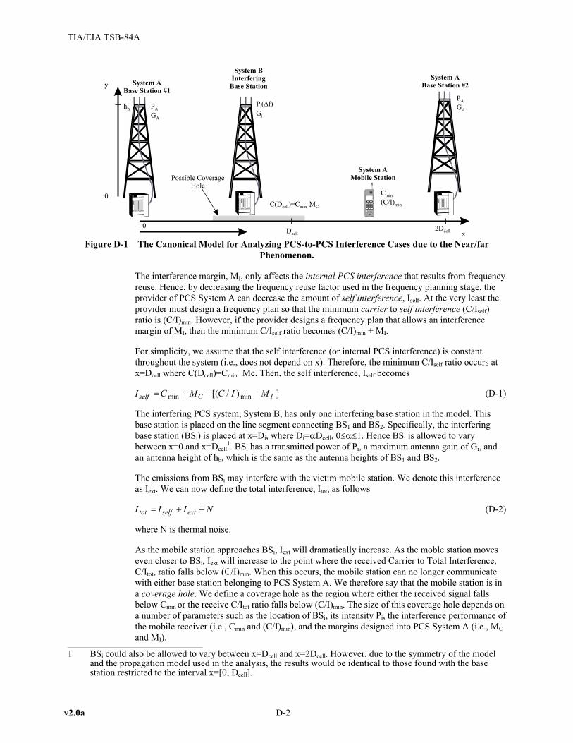
The interference margin, MI, only affects the internal PCS interference that results from frequency

reuse. Hence, by decreasing the frequency reuse factor used in the frequency planning stage, the

provider of PCS System A can decrease the amount of self interference, Iself. At the very least the

provider must design a frequency plan so that the minimum carrier to self interference (C/Iself)

ratio is (C/I)min. However, if the provider designs a frequency plan that allows an interference

margin of MI, then the minimum C/Iself ratio becomes (C/I)min + MI.

For simplicity, we assume that the self interference (or internal PCS interference) is constant

throughout the system (i.e., does not depend on x). Therefore, the minimum C/Iself ratio occurs at

x=Dcell where C(Dcell)=Cmin+Mc. Then, the self interference, Iself becomes

I C M C I Mself C I� � � �min min[( / ) ] (D-1)

The interfering PCS system, System B, has only one interfering base station in the model. This

base station is placed on the line segment connecting BS1 and BS2. Specifically, the interfering

base station (BSi) is placed at x=Di, where Di=�Dcell, 0��1. Hence BSi is allowed to vary

between x=0 and x=Dcell1. BSi has a transmitted power of Pi, a maximum antenna gain of Gi, and

an antenna height of hb, which is the same as the antenna heights of BS1 and BS2.

The emissions from BSi may interfere with the victim mobile station. We denote this interference

as Iext. We can now define the total interference, Itot, as follows

I I I Ntot self ext� � � (D-2)

where N is thermal noise.

As the mobile station approaches BSi, Iext will dramatically increase. As the moble station moves

even closer to BSi, Iext will increase to the point where the received Carrier to Total Interference,

C/Itot, ratio falls below (C/I)min. When this occurs, the mobile station can no longer communicate

with either base station belonging to PCS System A. We therefore say that the mobile station is in

a coverage hole. We define a coverage hole as the region where either the received signal falls

below Cmin or the receive C/Itot ratio falls below (C/I)min. The size of this coverage hole depends on

a number of parameters such as the location of BSi, its intensity Pi, the interference performance of

the mobile receiver (i.e., Cmin and (C/I)min), and the margins designed into PCS System A (i.e., MC

and MI).

v2.0a D-2

TIA/EIA TSB-84A

System ABase Station #1

System BInterfering

Base Station

System ABase Station #2

System AMobile Station

y

hb PA

GA

0

0

Possible CoverageHole

C(D )=C Mcell min + C

PA

GA

P ( f)i Gi

C

(C/I)min

min

Dcell2Dcell

x

Figure D-1 The Canonical Model for Analyzing PCS-to-PCS Interference Cases due to the Near/far

Phenomenon.

1 BSi could also be allowed to vary between x=Dcell and x=2Dcell. However, due to the symmetry of the modeland the propagation model used in the analysis, the results would be identical to those found with the basestation restricted to the interval x=[0, Dcell].

Annex D.1.1.2 Propagation Model and Area Classifications

Three propagation models are used in this analysis. Free Space Loss is used for distances less than

20 meters. The COST-231-Walfish-Ikegami Model [See Annex A.4] is used for cases where the

path length is between 20 meters and 1 kilometer. Finally, when the path length is between 1 and

100 kilometers, the COST-231-Hata model is used. Both the COST-231-Walfish-Ikegami and the

COST-231-Hata models are described at the end of Section D.1.

Although a detailed description of the COST-231-Walfish-Ikegami Model is given in Annex A.4,

it is necessary to describe its application to this model. The COST-231-Walfish-Ikegami model is

acceptable for path lengths between 20 meters and 1 kilometer. Furthermore, as the path length

approaches 20 meters, this model approaches the free space loss model. Hence, it provides for a

continuous propagation loss curve at 20 meters. Also, with a prudent selection of parameters, the

COST-231-Walfish-Ikegami Model approaches the COST-231-Hata model as the path length

approaches 1 kilometer. The specific procedure is described at the end of Section D.1. Therefore,

the use of the COST-231-Walfish-Ikegami Model as a bridge between the Free Space Loss Model

and the COST-231-Hata Model, results in a continuous propagation loss model for path lengths up

to 100 kilometers.

Three Area classes are described for this model: urban, suburban, and rural. Note that the

COST-231-Hata and the COST-231-Walfish-Ikegami Models have 6 and 2 Area Classes,

respectively. The mapping is displayed in the following table

Table D-1 Terrain Classifications and Mapping

Composite Model Hata Model Walfish-Ikegami Model

Area Classification Area Type City Size Area Type

Urban Urban Large Metropolitan Center

Suburban Suburban Small Suburban Center

Rural Open Small Suburban Center

Annex D.1.1.3 Analysis

Our objective is to (1) determine if the interference from BSi results in a coverage hole and, if so,

(2) compute the size of that hole. This is accomplished as via the following algorithm.

• Compute Cell Size, Dcell

• Compute the Carrier Power from BS1, C1(x)

• Compute the Carrier Power from BS2, C2(x)

• Compute C(x)=Max{C1(x),C2(x)}

• Compute Iext(x)

• Compute Iint and N

• Compute (C/Itotal)(x), where Itotal includes internal interference, external interference, and

thermal noise.

• Find the regions (values of x) where (C/Itot)(x)<(C/I)min. These regions are coverage holes

• Compute the size of the coverage holes.

The specific details of each step are described below as required.

Annex D.1.1.3.1 Compute Cell Size, Dcell

The inputs PA, GA, Cmin, and MC are used to compute cell size, Dcell. Recall, we wish to design the

system so that the received carrier power is not less than Cmin+MC. This implies that

D-3 v2.0a

TIA/EIA TSB-84A

C D C Mcell c1 ( ) min� � (D-3)

Given a radiated power of PA+GA, the required propagation loss is

L P G C Mreq A A c� � � �( ) ( )min (D-4)

Then Dcell is found by setting L(Dcell)=Lreq, and solving for Dcell.

Once Dcell is found, BS2 is placed at x=2Dcell. Then the carrier power from BS2 at x=Dcell is also

equal to Cmin+MC (i.e., C2(Dcell)=Cmin+MC).

Annex D.1.1.3.2 Compute Carrier Power

The carrier power for BS1, C1(x), is computed as follows

C x EIRP L xA1 ( ) ( )� � (D-5)

where L(x) is the propagation loss. The carrier power for BS2, C2(x), is computed as follows

C D x EIRP L xcell A2 2( ) ( )� � � (D-6)

Note that

C x C D xcell1 2 2( ) ( )� � (D-7)

We make the simplifying assumption that any MS will handoff whenever it receives a stronger

carrier from another source. Therefore the carrier power for 0�x�2Dcell is

C x C x C xC x x D

C x D x

cell

cell

( ) max{ ( ), ( )}( )

( )� �

� �# �1 2

1

2

0

2Dcell

$%&

(D-8)

Annex D.1.1.3.3 Internal Interference, Iint, and noise, N

Let iint and n be the self interference due to frequency reuse and thermal noise, respectively, in

milliwatts. Define a new parameter, Iint+N such that

I i nN selfint log( )� � �10 (D-9)

Since Iself is assumed to be constant, Iint+N is also a constant (i.e., it does not vary with x). Now

Iint+N can be expressed in terms of Cmin, MC and (C/I)min+Mi. Note that one may express

(C/I)min+Mi as follows

( / ) min min intC I M C M Ii C N� � � � � (D-10)

where Cmin is the minimum received carrier power expressed in dBm. Note the Iext is not included

simply because it is generally unknown in the PCS deployment phase. Iint,N is then computed as

follows

I C M C I MN C imin min min( ) [( / ) ]� ! � � � (D-11)

for cases where Iint is much larger than N, Iint,N!Iint.

Annex D.1.1.3.4 External Interference, Iext

The external interference is computed from Pi, Gi, and Di (=�Dcell) as follows

I x P G L D xext i i i( ) ( )� � � � (D-12)

v2.0a D-4

TIA/EIA TSB-84A

Annex D.1.1.3.5 Carrier to Total Interference Ratio

Given C(x), Iint,N, and Iext(x) for 0�x�2Dcell, the carrier to total interference ratio, (C/Itot)(x), is

computed as follows

( / )( ) log( )

( ) int

C I xc x

i x i ntot

ext

��

$%&

/01

10(D-13)

where

c x

C x

( )

( )

�10 10 and(D-14)

i n

I N

int

min,

� �10 10(D-15)

Annex D.1.1.3.6 Coverage Holes

Upon computing ( / )( )C I xtot , one may easily identify coverage holes by comparing this quantity

to the receiver’s minimum carrier to interference threshold ( / ) minC I . Coverage holes then occur

at all values of x such that ( / )( ) ( / ) minC I x C Itot # . Once the coverage holes are identified, one

may easily compute the number2 and size of these holes.

Annex D.1.2 IS-136 Interference into PCS-1900

Annex D.1.2.1 IS-136 Interference

The intensity of IS-136 interfering signals are derived from TIA/EIA IS-138 A [18], paragraphs

3.4.2.2.3.2 and 3.4.4.1.3. Three types of interfering signals are considered:

1. side band noise signals (due to noise in power amplifiers)

2. spurious signals (due to non-linearities in the transmitter-e.g., harmonics in local

oscillators followed by non-linear mixers)

3. transmitter inter-modulation signals (typically due to multi-carrier base stations).

The intensity of sideband noise signals and spurious signals is derived from paragraph 3.4.2.2.3.2

of [18]. Note that PCS System A and PCS System B operate in different PCS blocks. Therefore,

the frequency offset between their respective signals will always exceed 120 kHz. For this

particular case the aforementioned paragraph requires the peak level of any conducted emission to

not exceed peak power of -13 dBm when measured in a 1 MHz bandwidth3. The paragraph also

requires that the peak power of any transmission not exceed -13 dBm when measured in a 30 kHz

bandwidth.

Therefore, for the sideband noise case, we assume that the out of band emission is spread

uniformly across the 1 MHz spectrum. We also assume that the PCS-1900 receiver has an ideal

200 kHz brick wall filter. Therefore, for the sideband noise case, Pi,SBN = -19.99 dBm.

For the spurious response case, we assume that the out that the out-of-band emission (-13 dBm) is

concentrated in a 30 kHz spectrum, as allowed in paragraph 3.4.2.2.3.2 of IS-138A[18]. As a

D-5 v2.0a

TIA/EIA TSB-84A

2 For cases where MC=0 and Mi=0, two coverage holes are possible: one centered around Di and one centeredaround Dcell.

3 Even though the FCC allows a -13 dBm emission in a resolution bandwidth of 300 Hz when the emission iswithin 1 MHz of the block edge, the IS-136 specification (IS-138A) still requires a resolution of 1 MHz, evenin this range.

consequence there can be no other out of band emissions in any 1 MHz region of spectrum that (1)

is out of the PCS System B transmit block and (2) contains that 30 kHz emission. Therefore, for

the spurious response case, Pi,spur = -13 dBm.

The interference due to transmitter inter-modulation is derived from paragraph 3.4.4.1.3 of [18],

which simply states that any inter-modulation product should be attenuated at least 60 dB below

the power level of either transmitter. Since the maximum transmitted power is limited to 100 watts

(50 dBm), the maximum power of any transmitter inter-modulation product is -10 dBm.

Therefore, for the transmitter inter-modulation case, Pi,IM = -10 dBm.

The Pi’s for IS-136 interference into PCS-1900 receivers is summarized as follows

1. Side Band Noise Pi,SBN = -19.99 dBm

2. Spurious Signals Pi,spur = -13 dBm

3. Transmitter Intermodulation Pi,IM = -10 dBm

Annex D.1.2.2 PCS-1900 System Performance Requirements

J-STD-007 states that the RF sensitivity of a PCS-1900 Mobile Station (MS) must be less than

-102 dBm. J-STD-007 also states that the MS must perform (to a prescribed acceptable standard)

when the co-channel C/I = 9 dB and the desired signal power is no less than 20 dB above the RF

sensitivity (or -82 dBm for the worst case MS receiver). Therefore, based on J-STD-007, one

could set C min = -82 dBm and ( / ) minC I = 9 dB.

However, PCS-1900 service providers tend to use other values for C min and ( / ) minC I . Typical

values for C min and ( / ) minC I are -90 dBm and 12 dB, respectively. These values are used to

compute the results that follow.

Annex D.1.2.3 Results

Annex D.1.2.3.1 Position of Interfering Base Station and Coverage Hole Size

Figure D-2 presents the results for an urban environment for the three different interference levels.

As expected, the interference due to transmitter inter-modulation produces the largest coverage

hole of 443.4 meters. However, Figure D-2 shows that for Pi = -19.99 dBm, the coverage hole size

reaches a maximum at Di=0.92Dcell. One would expect that the coverage hole size would reach a

v2.0a D-6

TIA/EIA TSB-84A

0

50

100

150

200

250

300

350

400

450

500

0 0.1 0.2 0.3 0.4 0.5 0.6 0.7 0.8 0.9 1

Interferer Position (normalized to Dcell)

Co

vera

ge

Ho

leS

ize

(mete

rs)

Pi =-19.99 dBm Pi = -13 dBm Pi = -10 dBm

Figure D-2 Coverage Hole Size versus Position of BSi (normalized to Dcell) for Interference Levels of �19.99, �13,

and �13 dBm in an Urban Environment. PA=44 dBm, GA=18 dB, Dcell=2.90 km, Mi=3 dB, Mc=0 dB.

maximum at Di=Dcell, where C(x) is at a minimum. However, this does not occur. Rather, as Pi

decreases, the maximum approaches Dcell.

Figure D-3 compares the results for the three different environments for the cases of IS-136 side

band noise interference, Pi = -19.99 dBm, and for a fixed EIRPA of 62 dBm. Note that since the

EIRP is fixed, then Dcell must change so that the requirement,

C D C Mcell C( ) min� � (D-16)

is maintained. Therefore, due to the different propagation characteristics, the rural environment

yields larger values of Dcell that the suburban and urban environments. However, the different

propagation characteristics, also cause the coverage holes to be larger for the rural environment.

In Figure D-3, the coverage hole in the rural environment reaches as maximum of 1,768 meters as

compared to 531 meters and 247 meters for the suburban and urban environments, respectively.

We make another comparison between coverage hole and terrain classification in Figure D-4.

However, in this case, we fix Dcell to 2.90 km and vary PA so that the received power at the cell

D-7 v2.0a

TIA/EIA TSB-84A

0

200

400

600

800

1000

1200

1400

1600

1800

2000

0 0.1 0.2 0.3 0.4 0.5 0.6 0.7 0.8 0.9 1


Co

ve

rag

eH

ole

Siz

e(m

ete

rs)

Urban Environmnet Suburban Environment Rural Environment

Dcell=23.08 km

Dcell=6.08 km

Dcell=2.90 km

Figure D-3 Coverage Hole Size versus Position of BSi (normalized to Dcell) for the Three Different

Environment Classes. Pi = �19.99 dBm, Gi=18 dB, PA=44 dBm, GA=18 dB, Mi=3 dB, and MC=0dB.

Coverage Hole Size

0.00

200.00

400.00

600.00

800.00

1000.00

1200.00

1400.00

1600.00

0.00 0.10 0.20 0.30 0.40 0.50 0.60 0.70 0.80 0.90 1.00


Co

ver

ag

eH

ole

Siz

e(m

eter

s)

Urban Environmnet Suburban Environment Rural Environment

PA=11.64 dBm

PA=31.83dBm

PA=44.09dBm

Figure D-4 Coverage Hole Size versus Position of BSi (normalized to Dcell) for the Three Different

Environment Classes. Pi = �19.99 dBm, Gi=18 dB, GA=18 dB, Mi=3 dB, and MC=0dB. Dcell=2.9 km.

boundary (x=Dcell) equals Cmin+MC. Again note that the rural environment produces very large

coverage holes. In fact when Di=0.7Dcell, the radius of the coverage hole is 1.4 km, about half of

the cell radius! This large coverage hole is likely a direct consequence of the environment’s

propagation model. In rural environments, the propagation loss does not increase as dramatically

as in the suburban and urban models. As a result of this reduced propagation loss slope, the

isolation between base stations is reduced in rural and suburban environments. Accordingly, the

coverage holes in these environments are relatively larger than those in urban environments.

Figure D-5 compares results for four different interference design margins, Mi for the cases of

IS-136 sideband noise interference, Pi=�19.99 dBm. This figure shows that small increases in Mi

will dramatically reduce the coverage hole size. However, this improvement will diminish as Mi

increases. Note that as Mi is increased from 6 dB to 10 dB, the increase in coverage hole size is

negligible. Also note that as Mi increases from 0 dB the curve’s maximum moves from

DI = 0.9Dcell to Di = Dcell for the case where Mi = 10 dB.

Figure D-5 also shows that for cases where Mi is 3 dB or better and Di is less than Dcell/4, no

coverage holes exist. This result implies that in addition to co-siting, providers may eliminate

PCS-to-PCS interference cases, resulting from the near/far phenomenon, by placing antennas so

that they are within a circle of diameter of no less than Dcell/4. One may call this strategy,

near-siting. Near-siting has advantages over co-siting because it not only mitigates PCS-to-PCS

interference due to the near/far phenomenon, but it also mitigates the inter-modulation and

antenna separation issues associated with co-siting.

Annex D.1.2.3.2 Interference Margin, Mi, and Coverage Hole Size

The next figures illustrate the relationship between coverage hole size and interference margin.

Figure D-6 shows this relationship for various locations of BSi (i.e., various values of Di). Again,

Figure D-6 shows that when Mi is small, the larger coverage holes occur when Di!0.9Dcell.

However when Mi>0.3, the maximum coverage hole occurs at Di = Dcell, as typically expected. For

the case where BSi is collocated with BSA, a small coverage hole occurs when Mi = 0. However,

any increase in the interference margin, Mi, removes this coverage hole. This confirms the obvious

conjecture that, due to the correlated propagation loss profiles, PCS networks whose base stations

are collocated will not suffer from PCS-to-PCS interference due to the near/far phenomenon.

v2.0a D-8

TIA/EIA TSB-84A

0

50

100

150

200

250

300

350

400

450

500

0 0.1 0.2 0.3 0.4 0.5 0.6 0.7 0.8 0.9 1


Co

vera

ge

Ho

leS

ize

(mete

rs)

Mi=0dB Mi=3dB Mi=6dB Mi=10dB Dcell = 2.902 km

Figure D-5 Coverage Hole Size versus Position of BSi (normalized to Dcell) for Four Different Interference

Margins in an Urban Environment. Pi = �19.99 dBm, Gt = 18 dBi, PA=44 dBm, GA=18 dB, Mc=0 dB.

However, recall from the discussion in Figure D-5 that for Mi �3 dB, providers may mitigate this

interference by placing their base stations within Dcell/4 of each other4.

Figure D-6 also shows that for small values of Mi, the improvement in the coverage hole size is

dramatic. However, as Mi increases the improvement in coverage hole size becomes less dramatic

and appears to approach to a constant (e.g., for the Di = Dcell/2 case). In this region, the

propagation loss approaches the free space loss model. Accordingly, the propagation loss from the

nearby interfering base station, BSi is very small and the external interference Iext is the major

factor contributing to hole size. As Mi approaches � and Iself approaches 0, a coverage hole of

some size will always remain. The only way that PCS providers may avoid this problem is either

via co-siting, near-siting, or significantly reducing the out-of-band emissions of each base station

in the given area.

Figure D-7 plots the relationship between coverage hole size and interference margin, Mi, for the

three terrain classifications. Again, as in Figure D-7, we fixed the PA at 44 dBm, assumed an

D-9 v2.0a

TIA/EIA TSB-84A

-50

0

50

100

150

200

250

300

350

400

450

500

0 1 2 3 4 5 6 7 8 9 10

Interference Margin, Mi, in dB

Co

ve

rag

eH

ole

Siz

ein

me

ters

Di=0 Di=0.5Dcell Di=0.9Dcell Di=Dcell

Dcell = 2.902 km

Figure D-6 Coverage Hole Size versus Mi for Different Positions of BSi in an Urban Environment. Pi =

�19.99 dBm, Gi = 18 dBi, PA = 44 dBm, GA=18 dB, Mc = 0 dB

Coverage Hole Size

0

500

1000

1500

2000

2500

0 1 2 3 4 5 6 7 8 9 10

Interference Margin, Mi, in dB

Co

vera

ge

Ho

leS

ize

inm

ete

rs

Urban Environment Suburban Environment Rural Environment

Dcell = 2.902 km

Dcell=6.08 km

Dcell=23.08 km

Figure D-7 Coverage Hole Size versus Mi for the Three Different Environment Classes. PA=44 dBm, GA=18

dBi, Pi=�19,99 dBm, Gi=18 dBi, MC=0dB, Di=0.9Dcell.

4 Note that this solutions assumes that all involved providers design their systems to have the same cell radius,Dcell. In general cases where different providers will have different design strategies and performancerequires, the solution will be more involved.

18 dB antenna, and adjusted the cell size (Dcell) appropriately. This resulted in Dcell values of

2.90 km, 6.08 km, and 23.08 km for the urban, suburban, and rural terrain classes, respectively.

Figure D-7 again shows the same relationship between coverage hole size and interference margin

as does Figure D-6. Specifically as Mi increases, the coverage hole approaches a constant value.

Figure D-7 also shows the same relationship between coverage hole size and terrain classification

as does Figure D-3. Specifically, for the same set of parameters, the rural environment produces

the largest coverage holes. The suburban environment produces the next largest coverage holes.

Finally, the urban environment, which also has the largest propagation loss slope (with respect to

path length), produces the smallest coverage holes.

Annex D.1.3 Conclusions

We developed a simplified model to evaluate the near/far interference between two or more PCS

networks that operate in the same geographical area. We then applied this model to the case where

an IS-136 based PCS network and a PCS-1900 based PCS network operate in the same service

area via different PCS frequency blocks. In our analysis we only considered IS-136 interference

into a PCS-1900 based mobile station, which was being served by the PCS-1900 base PCS

network.

The analysis assumed three different forms of IS-136 interference: side band noise, spurious

interference, and inter-modulation interference. The specific interference values were derived from

IS-138A. One may expect that these emission values err on the high side. Initial studies indicate

that actual out-of-band emission levels are as much as 30 dB below what one may derive from the

applicable standards.

The analysis shows that coverage holes will exist whenever the interfering cell base station is

located on or near the cell boundary of a victim system. In terms of the canonical model, whenever

the interfering base station is placed at Di>Dcell/4, a coverage hole will exist.

The analysis also indicates that one may reduce coverage holes by reducing the amount of self

interference, Iself, or increasing the interference margin, Mi. One may accomplish this through

clever frequency planning techniques or by increasing the network’s frequency re-use factor.

Providers may also reduce Iself, by employing smart antennas and adaptive antennas that focus

beams toward the mobile station receivers and track their movements.

For cases where Mi is small, the maximum coverage hole size does not occur at the cell boundary

as one may expect. Rather it occurs when the interfering base station is near the boundary. In

Figure D-5 the maximum occurs when the interfering base station is placed at 0.9Dcell. Figure D-4

indicates that for rural environments, the maximum occurs at 0.68Dcell.

PCS providers may mitigate PCS-to-PCS interference, due to the near/far phenomenon, by either

co-siting or near-siting their respective base stations. If providers opt to co-site their base stations,

they must be prepared to address the antenna separation and inter-modulation issues associated

with any co-siting scenario. However, our results indicate that providers may mitigate

PCS-to-PCS interference, due to the near/far phenomenon, by placing their base stations within

Dcell/4 of base stations belonging to other networks that serve the same area. We call this

near-siting. Near-siting has an advantage over co-siting because it not only mitigates near/far,

PCS-to-PCS interference, but also provides sufficient separation between sites to mitigate any of

the issues associated with co-siting, provided that the base station antennas are sufficiently

separated.

Finally, one should understand that this analysis is using data that was derived from the relevant

standards, which is rather conservative. One may expect that the out-of-band emission

performance of actual transmitters may be significantly less than what the relevant standards call

for. Initial studies indicate that this may indeed be the case. Further, one may expect that the

v2.0a D-10

TIA/EIA TSB-84A

interference performance of mobile station receivers may exceed the required specifications as

stated in the relative standards. As of yet, we have no data that would support or refute this claim.

If this is the case, then the size of the coverage holes would be much less than indicated in this

rudimentary study. One would find it instructive to analyze this model using actual measured

performance parameters from real equipment.

Annex D.1.4 Propagation Considerations Used in the C/I Coverage Hole Model

Annex D.1.4.1 COST-231 Hata Model

For an urban area, the COST-231 Hata Model estimates the basic transmission loss as follows

L

f h

a hbu

b

m�

� �

� �

6955 2615 1382

44 9 655

. . log( ) . log( )

( )[ . . log( )][log( )]h df

b�

150 1500MHz MHz

46.3+ 33.9log(f) -1

# #

3.82log(h15000M

b )

( )[ . . log( )][log( )]� �a h h dm b44 9 655 �Hz < 2000MHz�

$

%''

&''

f

(D-17)

where

� ��

� � 7 � 7 ��

��

1 20

1 014 187 10 107 1020

4 3

d km

f hd

b( . . . ) log��

�

��

�

�� +

$%'

&'

0 8

20

.

d km

(D-18)

For medium and small cities, a(hm) is

a h f h fm m( ) [ . log( ) . ] . log( ) .� � � �11 07 156 08 (D-19)

For large cities, we have

a hh f

hm

m( ). [log( . )] .

. [log( .� � #829 154 11 400

32 1175

2 MHz

m f)] .2 4 97 400� �

$%'

&' MHz

(D-20)

For the urban area model

L Lhata bu� (D-21)

For the suburban area model

L Lf

hata bu� � ��

��

�

��

�

�� 2

2854

2

log .(D-22)

For the open area model

L L f fhata bu� � � �4 78 1833 40942. [log( )] . log( ) . (D-23)

where

f is frequency in MHz

hb is effective base station antenna height in meters

hm is effective mobile station antenna height in meters

d is distance in kilometers

D-11 v2.0a

TIA/EIA TSB-84A

Note that the COST 231 Hata model is a function of f, hm, hb, d, city-size model (small/medium or

large), area model (urban, suburban, or rural).

The model is valid for

150 MHz � f � 2000MHz

30 m � hb � 200 m

1m � hm � 10m

1 km � d � 100 km

Quasi-smooth terrain

Annex D.1.4.2 COST-231 Walfish-Ikegami Model

The COST-231 Walfish-Ikegami model is stated in Annex A but repeated here for convenience.

The model contains a free space loss term, L0, a roof-top-to-street diffraction and scatter loss, Lrts,

and a multi-screen loss, Lmsd.

One may compute L0 as follows

L d f0 324 20 20� � �. log( ) log( ) (D-24)

Lrts is computed as follows

L w f h Lrts mobile ori� � � � � �169 10 10 20. log( ) log( ) log( ) (D-25)

where

w b� / 2 (D-26)

Lori �� .

� .� .�

10 0354

25 0075 5

4 0

.

. . (

.

) ; ) #<=)�<=- <= ) # =

0114. ()�==- == ) E;.� � .

$

%'

&'

(D-27)

h h hmobile roof m� � (D-28)

h h hbase b roof� � (D-29)

Lmsd is then computed as follows

L L k k d k f bmsd bsh a d f� � � � �( ) ( ) ( ) ( )log( ) log( ) log( )1 1 1 1 9 (D-30)

where

Lh h h

h hbsh

base b roof

b roof

( )log( )

118 1

0�

� � +�

$%&

(D-31)

k

h h

h d km and h ha

b roof

base b roof( ) . .1

54

54 08 05

54 0

�+

� � �

�

8 -..

.805

05hd

d km and h hbase b roof��

�� # �

$

%

''

&

''

(D-32)

v2.0 D-12

TIA/EIA TSB-84A

k

h h

h

hh hd

b roof

base

roofb roof

( )1

18

18 15�

+

� �

$

%'

&'

(D-33)

k

f

f( )

.1 4

07925

1

� � ��

��

�� mediumsized cities and suburban centers

metropolitan centers15925

1.f��

��

��

$

%''

&''

(D-34)

The COST-231 Walfish-Ikegami loss is then computed as follows

LL L L L L

L L LWI

rts msd rts msd

rts msd

�� +

� �$%&

0

0

0

0

(D-35)

The COST-231 Walfish-Ikegami model is valid for

800 MHz � f � 2000 MHz

4 m � hb � 50 m

1 m � hm � 3 m

20 m � d � 5 km

The parameters necessary for the COST-231 Walfish-Ikegami model are

b = building separation in meters

hb = base station height in meters

hm = mobile station height in meters

hroof = roof height in meters

f = frequency in MHz

d = distance in kilometers

) = road orientation with respect to the direct radio path

Area model – either small/medium city or metropolitan center

Annex D.1.4.3 Combining the Two Models

The analysis of PCS-to-PCS interference via the canonical model requires a propagation model

that provides reasonable results for distances from less than 10 meters to greater than

10 kilometers. The COST-231 Hata model is only valid for distances that exceed one kilometer

(and is less than 100 km). Hence it is not useful for distances below one kilometer, which is the

range of interference for PCS-to-PCS cases due to the near/far phenomenon.

On the other hand, the COST-231 model is valid for distances less than one kilometer (provided

that the distance is greater than 20 meters). Further, as the distance approaches 20 meters the

model approaches the free space model, L0. Hence, the COST-231 model can effectively estimate

the propagation loss from the interfering base station, BSi, to the mobile station for cases where

the mobile station is in the coverage hole. However, this model cannot estimate the propagation

loss from the victim base station to the mobile station because the distance may exceed five

kilometers, especially in rural environments. In such a case, the COST-231 Hata model was more

appropriate.

Therefore, we decided to create a model by combining the COST-231 Hata model and the

COST-231 Walfish-Ikegami model. For cases where the path length was greater than one

kilometer, we used the COST-231 Hata model. For cases where the path length was less than or

equal to one kilometer we use the COST-231 Walfish-Ikegami model. This provided a model that

D-13 v2.0a

TIA/EIA TSB-84A

(1) was easy to implement and (2) approached the free space model as the path length became

small and (3) provided valid results for path lengths up to 100 kilometers.

The remaining issue was the continuity between the COST-231 Walfish-Ikegami model and the

COST-231 Hata model. We decided to adjust the COST-231 Walfish-Ikegami model parameters

so that the two models would be continuous at d = 1 km. This was accomplished as follows. Three

area models were defined: urban, suburban, and rural. The mapping between these area models

and area model used in the COST-231 Walfish-Ikegami and COST-231 Hata models are provided

in Table D-1. The remaining COST-231 Hata model parameters, hb, hm, & f were set as required

by the case under study. The COST-231 Hata model was then evaluated at d = 1km to obtain a

propagation loss estimate.

The parameters of the COST-231 Walfish-Ikegami model were then adjusted at d=1km so that the

model’s estimate equaled that of the COST-231 Hata model estimate. This is accomplished by

setting hb, hm, & f. Other parameters, such as the building separation, b, and the road orientation

with respect to the direct radio path, ), are set to 50 meters and 900, respectively. The remaining

parameter, the roof height, hroof, is then adjusted so that the COST-231 Walfish-Ikegami estimate

equals the COST-231 Hata estimate at d=1 km.

The following figure compares the propagation loss curves for the three area models: urban,

suburban, and rural.

Annex D.2 Receiver Sensitivity Degradation

Annex D.2.1 Introduction

The analysis of receiver desensitization includes the effects of transmitter power, antenna height,

feeder losses, third-order intermodulation products, multiple interferers, coherent interference, and

antenna radiation patterns. The equipment is assumed to be sufficiently well designed so that

self-interference (transmitter power falling within the same unit’s receive band) can be safely

ignored.

The basic methodology is to compute a worst case, one-on-one, simple path-loss calculation to

estimate at what transmitter/receiver separation the spurious emissions from a transmitter of one

v2.0a D-14

TIA/EIA TSB-84A

Combined COST-231 Hata/Walfish-Ikegami Model Results

40

60

80

100

120

140

160

180

200

0.001 0.01 0.1 1 10 100

Path Length (km)

Pro

pa

ga

tio

nL

oss

(dB

)

Rural Area Model Suburban Area Model Urban Area Model

Figure D-8 Propagation Loss Curves Using the Combined Model. hb=30 m, hm=1.5 m, f=1960 MHz.

technology (at maximum power, since the mobile station is assumed to be at a cell’s edge) would

impact a receiver of another technology.

Interference and consequent receiver desensitization between the following four or eight

transmitter/receiver pairs should be analyzed (see Figure D-9):

All systems:

• Technology X mobile station transmitter impacting a Technology Y base

• Technology X base transmitter impacting a Technology Y mobile station

• Technology Y mobile station transmitter impacting a Technology X base

• Technology Y base transmitter impacting a Technology X mobile station

If one or both systems are TDD systems:

• Technology X mobile station transmitter impacting a Technology Y mobile station

• Technology X base transmitter impacting a Technology Y base

• Technology Y mobile station transmitter impacting a Technology X mobile station

• Technology Y base transmitter impacting a Technology X base

NOTE: X and Y may be the same technology.

Annex D.2.2 Channel Frequency Separation

Determine the frequency separation between channels of the two systems. It is suggested that the

minimum frequency separations be used for one-on-one analysis, as these will typically be worst

cases. Note that the minimum frequency separation may be determined by agreement between

operators and/or may require reduced transmit power at the block edge to meet FCC requirements

for out-of-block emissions.

Annex D.2.3 System Impact Metric

The important metric is the degradation in receiver sensitivity called Receiver Desensitization, D.

When D exceeds the system impact threshold, x dB, an unacceptable degradation in system

performance occurs.

D-15 v2.0a

TIA/EIA TSB-84A

Technology XBase Station

Technology YBase Station

Technology YMobile Station

Technology XMobile Station

Interference

Interference

Inte

rfer

ence

Interferen

ce

Technology X Link Technology Y Link

All systems may create interferencebetween Base Stations and Mobile Stations

Figure D-9 Basic Interference Scenario

Annex D.2.4 Propagation Formulas

Commonly used propagation formulas are listed in Annex A. Selection of the proper propagation

formulas depends upon the circumstances of the RF paths under consideration.

The proper selection of propagation formulas is a matter of engineering judgement, and is

substantiated in the actual deployment.

Annex D.2.5 Calculation of Path Loss for a Given Receiver Desensitization

Annex D.2.5.1 Definition of Parameters

The following parameters are defined at the antenna port of the receiver module:

ni = self interference power spectral density (mW/Hz)

no = thermal noise power spectral density (mW/Hz)

ne = external interferer power spectral density (mW/Hz)

nt = total power spectral density = ne + ni + no (mW/Hz)

et = energy per bit (mJ)

NF = receiver noise figure (dB)

Ni = 10 log (ni) (dBm/Hz)

Ne = 10 log (ne) (dBm/Hz)

No = 10 log (no) (dBm/Hz)

= �174 (dBm/Hz) + NF

NOTE: When summing power spectral densities, mW/Hz must be used rather than dBm/Hz.

Annex D.2.5.2 Desensitization of Systems Not Utilizing Power Control

The following equations are used to calculate ne given the desensitization (D) for TDMA and

FDMA systems (e.g., PCS1900, IS-136 and AMPS):

D = 10 log [ ( ne + ni + no ) / ( ni + no ) ] (dB) (D-36)

ne = ( ni + no ) * 100.1*D � ( ni + no ) (W) (D-37)

Annex D.2.5.3 Desensitization of Systems Utilizing Power Control

The same method can be used to calculate ne given the desensitization (D) for CDMA systems

(e.g., IS-95). The following discussion applies to the CDMA reverse link:

Due to power control in IS-95, if there is any extra interference, all the mobile stations in the

cell/sector will raise their power to maintain the required et/nt, therefore, the desensitization also

will depend upon the number of active mobile stations. With few mobile stations, ni is

insignificant, however, for a large number of mobile stations, the combined ni will become

increasingly significant and affect the calculation. The following equation assumes that the system

is running at maximum power, and does not include the effects of power control. At less than

about six mobile stations, the desensitization is close to:

D = 10 log [ ( ne + no ) / no ] (dB) (D-38)

ne = no * 100.1*D � no (W) (D-39)

v2.0a D-16

TIA/EIA TSB-84A

Annex D.2.5.4 Calculating the Path Loss

The required Path Loss (PL) is the amount of attenuation necessary, such that the received

interference signal is equal to the level the receiver can withstand for a given desensitization D.

Step 1: Given the receiver desensitization (D in dB), calculate the corresponding ne from

Equation D-37 or D-39.

Step 2: With the calculated ne from Step 1, the required Path Loss (PL) can be obtained from the

following equation:

PL = PSDtx(f) + Gtx � Ltx + Grx � Lrx � Ne (dB) (D-40)

where:

PSDtx(f) = tx power per unit bandwidth (PSD) at a frequency offset f from the carrier

frequency (dBm/Hz)

Ltx = tx transmission loss (dB)

Gtx = tx antenna isotropic gain in the direction toward the interfered rx antenna (dB)

f = offset frequency between the tx carrier frequency and the rx bandpass center (Hz)

Grx = rx antenna isotropic gain in the direction toward the interfering tx antenna (dB)

Lrx = rx transmission loss (dB)

Annex D.2.6 Examples of Possible Scenarios

The scenarios and graphs in the following section, depict worst case one-on-one interference

calculations for the path loss, PL, required for a given desensitization, D. These calculations are

based upon the Receiver Sensitivity Degradation methodology described above. Most PCS

systems or users within the system, will not be operating at the sensitivity limits. However, this

illustrates the basic possibility for interference to occur between systems, identifying the need for

more detailed analysis and coordination between operators.

Annex D.2.6.1 Calculated Scenarios

Annex D.2.6.1.1 Interference Between PCS 1900 and IS-136

The following data includes a correction to the PCS1900 BTS data to comply with Part 24.238 and

uses the methodology described in Annex D.2. Since only FDD systems were studied, the

scenarios listed are impacts from base to mobile station or from mobile station to base. This

analysis assumed that the interferer transmit mask was flat over the resolution bandwidth and the

receiver function had a flat response inband with infinite attenuation at the channel edge and with

negligible adjacent channel interference. Emissions based strictly on existing standards will

typically be more pessimistic than reality.

For both technologies, a 3 dB impact of self-interference was chosen to represent the case of

interference-limited, large suburban cells, where the co-channel interference (Ni) is equal to the

noise floor (No). Clearly in tightly packed urban/suburban cells, the value of Ni may be different.

Mitigation techniques for either technology were not considered in the analysis. The following

analysis assumed that both technologies use the permissible frequencies closest to the other block

within their own block.

? PCS1900:

• emissions based on J-STD-007

D-17 v2.0a

TIA/EIA TSB-84A

• base station macrocell antenna with 17 dBi gain, 2.5 dB cable loss, 36.3 dBm transmitter power

(reduced from 40 dBm by compliance with Part 24.238) and 5 dB receiver noise figure

• mobile station antenna 0 dBi gain, 30 dBm transmitter power and 9 dB receiver noise figure

? IS-136:

• emissions based on IS-136A, IS-137A, IS138A

• base station macrocell antenna with 17 dBi gain, 2.5 dB cable loss, 40 dBm transmitter power

and 5 dB receiver noise figure

• mobile station antenna 0 dBi gain, 30 dBm transmitter power and 9 dB receiver noise figure.

Because of the apparent high impact of PCS1900 on IS-136, the above calculations were repeated

with an increase in separation of 90 kHz. This caused a major reduction in interference signifying

the possible power spillover into the first few IS-136 channels. Note also that “brick-wall” filters

were assumed, and that at 240 kHz separation real filters would probably allow some adjacent

carrier power to “bleed-in” to the other technology.

Clearly both technologies appear to suffer from significant interference - even with an increase in

separation by 90 kHz. Analysis of the above results is still continuing to evaluate what parameters

are more sensitive than others - from six graphs it is impossible to estimate which technology is

more or less tolerant of interference.

v2.0a D-18

TIA/EIA TSB-84A

D-19 v2.0a

TIA/EIA TSB-84A

IS-136 BTS (Interferer) to PCS1900 MS (Victim)

90

95

100

105

110

115

120

0 1 2 3 4 5 6 7 8 9 10

Receiver desensitization (dB)

Path Loss (dB) Band A to D (Spec)

Band A to B (Spec)

Figure D-10 IS-136 Base Impacts PCS1900 Mobile Station

Figure D-11 IS-136 Mobile Station Impacts PCS1900 Base

v2.0a D-20

TIA/EIA TSB-84A

PCS1900 BTS (Interferer) to IS-136 MS (Victim)

60

70

80

90

100

110

120

130

140

150

0 1 2 3 4 5 6 7 8 9 10


Path Loss (dB)Band D to A (Spec)

Band B to A (Spec)

Figure D-12 PCS1900 Base Impacts IS-136 Mobile Station

PCS1900 MS (Interferer) to IS-136 BTS (Victim)

60

70

80

90

100

110

120

130

140

0 1 2 3 4 5 6 7 8 9 10


Path Loss (dB)

Band D to A (Spec)

Band B to A (Spec)

Figure D-13 PCS1900 Mobile Station Impacts IS-136 Base

D-21 v2.0a

TIA/EIA TSB-84A

Figure D-14 PCS1900 Base Impacts IS-136 Mobile Station (90 kHz offset)

PCS1900 MS (Interferer) to IS-136 BTS (Victim)

70

75

80

85

90

95

100

105

110

115

120

0 2 4 6 8 10


Path Loss (dB)

Band D to A (Spec)

Band B to A (Spec)

Figure D-15 PCS1900 Mobile Station Impacts IS-136 Base (90 kHz offset)

Annex D.2.6.1.2 Interference Between PCS1900 and IS-95

The following data includes a correction to the PCS1900 BTS data to comply with Part 24.238 and

uses the methodology described in Annex D.2. This analysis assumed that the interferer transmit

mask was flat over the resolution bandwidth and the receiver function had a flat response inband

with � attenuation at the channel edge and with negligible adjacent channel interference.

Emissions based strictly on existing standards will typically be more pessimistic than reality.

Mitigation techniques for either technology were not considered in the analysis. The following

analysis assumed that both technologies use the permissible frequencies closest to the other block

within their own block e.g. PCS1900 on frequencies 1865.2/1945.2 (block D) and IS-95 on

1863.75/1943.75 (block A).

? PCS1900:

• emissions based on J-STD-007

• base station macrocell antenna with 17 dBi gain, 2.5 dB cable loss and 36.3 dBm transmitter

power (reduced from 40 dBm by compliance with CFR Part 24.238)

• mobile station antenna 0 dBi gain and 30 dBm transmitter power

• a 3 dB impact of self-interference was chosen to represent the case of interference-limited,

large suburban cells, where the co-channel interference (Ni) is equal to the noise floor (No).

Clearly in tightly packed urban/suburban cells, the value of Ni may be different.

? CDMA:

• emissions based on J-STD-019 & 018

• base station macrocell antenna with 17 dBi gain, 2.5 dB cable loss and 40 dBm transmitter

power

• mobile station antenna 0 dBi gain and 23 dBm transmitter power.

Clearly both technologies appear to suffer from significant interference. Analysis of the above

results is still continuing to evaluate what parameters are more sensitive than others - from four

graphs it is impossible to estimate which technology is more or less tolerant of interference.

Annex D.2.6.2 Measured Scenarios

(This section will be added in a later revision.)

v2.0a D-22

TIA/EIA TSB-84A

D-23 v2.0a

TIA/EIA TSB-84A

Figure D-16 IS-95 Base Impacts PCS1900 Mobile Station

Figure D-17 IS-95 Mobile Station Impacts PCS1900 Base

v2.0a D-24

TIA/EIA TSB-84A

PCS-1900 BTS (Interferer) to IS-95 MS (Victim)

60

65

70

75

80

85

90

95

100

105

110

0 1 2 3 4 5 6 7 8 9 10


Path Loss (dB)Band D to A (Spec)

Band B to A (Spec)

Figure D-18 PCS1900 Base Impacts IS-95 Mobile Station

PCS-1900 MS (Interferer) to IS-95 BTS (Victim)

60

65

70

75

80

85

90

95

100

105

110

0 2 4 6 8 10


Path Loss (dB)

Band D to A (Spec)

Band B to A (Spec)

Figure D-19 PCS1900 Mobile Station Impacts IS-95 Base

Annex D.3 Examples of Intermodulation between CDMA and TDMA Systems

This section presents an analysis of base station receiver sensitivity degradation due to

intermodulation resulting from nearby mobile stations. It discusses an example of “many-on-one”

interference - the case of multiple mobile stations near a second operator’s base station. With

attenuation depending upon the selectivity of the pre-select receive filter (before the first stage

LNA), signals from the multiple mobile stations will reach the first LNA and cause

intermodulation products in the passband (see Figure D-20).

Annex D.3.1 Simulation of Receiver Intermodulation

A simulation of this effect was performed by considering a number of mobile stations grouped

around a base station. The density of mobile stations followed three distinct models:

• A highway environment with a constant mobile station density in a corridor circling the base

station.

• A rural environment with a constant mobile station density in a torroidal plane

• A dense urban or airport environment with high mobile station density near the base station,

reducing further away.

The density, 9F and total number of mobile stations, N, for each case are defined by the equations

in Figure D-21.

D-25 v2.0a

TIA/EIA TSB-84A

PCS Receive

Pass Band

Interferers

Intermodulation

Products

Figure D-20 In-band Intermodulation Products due to Out-of-band Interferers

RR

R

Highway/uniformdensity

9 99

(r) = at r=R

(r) = density/unit length

N=2 R

0

•90

Rural/uniformdensity

9 99

9

(r) = at r<R

(r) = density/unit area

N= Rexp(2 )

1

1

Airport/Concentrationat center

9 99

9

(r) = /r at r<R

(r) = density/unit area

N=

2

2•2 R Figure D-21 Mobile Stations Distribution

Annex D.3.2 Channel Allocation

In this example, the mobile stations were operating on blocks D, B, E, F and C. The victim base

station was receiving on block A. This is illustrated in Figure D-22.

Annex D.3.3 Simulation Algorithm

The computer simulation assumes a base station antenna and RF front end with definable

characteristics. Inputs to the computer simulation are: antenna height, gain and pattern; RF

pre-select filter characteristics, LNA gain, noise figure and linearity.

A collection of mobile stations is presupposed, at distances from the base station in accordance

with the chosen scenario defining mobile station density. Input parameters are the mobile station

transmit power, antenna gain and height. Frequencies are then assigned randomly among the

mobile stations.

The path loss from each mobile station to the base station antenna is calculated using the urban

canyon COST231 Walfish model modified to include vertical antenna beam pattern (please refer

to Figure D-23 - additional description of various Walfish models are given in Annex A). The

simulation then computes and sums the power of all the inband intermodulation products,

resulting from the out of band mobile station signals received. Additional simulation runs are then

performed using new frequency assignments among mobile stations. The overall intermodulation

product noise floor to be expected is then obtained by averaging the results from all these runs.

v2.0a D-26

TIA/EIA TSB-84A

A D B E F C

Rx

PCS TDMA Mobile Transmit-600 mW

1850 1865 1870 1885 18901895 1910 1930

Intermods from LNAFigure D-22 Interference Sources

SIMULATION INPUT PARAMETERS

INTERFERENCE SOURCES MOBILE STATION: TX POWER, ANTENNA GAIN, HEIGHT

TRANSMISSION Mobile station placement and Path loss model

BASE STATION RECEIVER

Antenna gain, height & pattern

Antenna shadow effect

RF pre-select filter performance

LNA gain, noise figure, input IP3

SIMULATION OUTPUT PARAMETERS

Noise floor plotted as a function of one or more input variables

D-27 v2.0a

TIA/EIA TSB-84A

r

d

pathloss G GRx Tx

��

�

�

��

�

�

��

��

��

1

2

4

2

2

4 (( (

6

Gcos

sin tan

tan@

G

G

�

��

��

1

202

d

for d < 20m

for d > 20m

d

h

G

G

2

Rx

Tx

Figure D-23 COST231 Path Loss Model Modified to Include Vertical Antenna Beam Pattern

Annex D.3.4 Technologies Evaluated

In this section, we consider the effect of IS-136 mobile station transmitters interfering with IS-95

base station receivers. In all cases, unless otherwise stated, the LNA had an input IP3 of +10 dBm

and a 5-pole filter was used. The simulation analyzed third-order intermodulation products. Refer

to Figure D-24 for the performance of the group of filters used.

Annex D.3.5 Simulation Results Exploring Different Conditions

Annex D.3.5.1 Example 1 - Highway, Rural and Airport

Figure D-25 shows the simulation results of a few hundred mobile stations located in the vicinity

of a base station for the three environments. Note that the intermodulation products are clearly

higher when the mobile stations are concentrated in the highway and airport scenarios.

v2.0a D-28

TIA/EIA TSB-84A

-100

-90

-80

-70

-60

-50

-40

-30

-20

-10

0

1837.5 1842.5 1847.5 1852.5 1857.5 1862.5 1867.5 1872.5 1877.5

Freq.(MHz)

S2

1(d

B)

2-pole

5-pole

8-pole

Figure D-24 Comparisons of Rejection Performance of the Filters

-200

-180

-160

-140

-120

-100

-80

-60

-40

1850 1855 1860 1865

Frequency (MHz)

Inte

rfe

rence

Po

we

rL

eve

l(d

Bm

)

Highway

Airport

Rural

Highway

Airport

Rural

Figure D-25 Comparison of Intermodulation Products for Highway, Rural and Airport

Annex D.3.5.2 Example 2 - Selectivity of Preselect Filters

In Figure D-26, under the same conditions, the influence of different degrees of selectivity in the

RF pre-select filters is shown.

Annex D.3.5.3 Example 3 - Antenna Height

Particularly interesting is the variation of interference level as a function of antenna height. A low

antenna reduces the path loss to the nearest mobile station - significant in the case of

wall-mounted microcell base stations. See Figure D-27.

D-29 v2.0a

TIA/EIA TSB-84A

-200

-180

-160

-140

-120

-100

-80

-60

-40

1850 1855 1860 1865

Frequency (MHz)

Inte

rfe

rence

Po

we

rL

eve

l(d

Bm

)5-pole filter

2-pole filter

8-pole filter

2-pole

5-pole

8-pole

Figure D-26 Comparison of Intermodulation Products for Different RF Pre-select Filters

-200

-180

-160

-140

-120

-100

-80

-60

-40

1850 1855 1860 1865

Frequency (MHz)

Inte

rfe

rence

Po

we

rL

eve

l(d

Bm

)

50 feet, 8 dB antenna

125 ft, 6 dB antenna

50 feet

125 feet

Figure D-27 Comparison of Noise Floor as a Function of Antenna Height

Annex D.3.5.4 Example 4 - LNA Linearity

The plot in Figure D-28 shows the relation of interference level against LNA input IP3. As might

be anticipated, the noise floor is reduced by twice the amount of the increase in LNA intercept

point (dBm scale).

Annex D.3.6 Investigation of Particular PCS Scenarios - 8-pole and 15-pole Filters

In Figures D-30 to D-33, the interference levels from IS-136 adjacent block D-block to PCS

A-block are evaluated for specific highway and airport scenarios. The filters used for this

comparison were an 8-pole dielectric resonator (quasi-elliptical) and a 15-pole superconducting

thin-film device. Please refer to Figure D-29 for the response curves.

v2.0a D-30

TIA/EIA TSB-84A

-200

-180

-160

-140

-120

-100

-80

-60

-40

1850 1855 1860 1865

Frequency (MHz)

Inte

rfe

rence

Po

we

rL

eve

l(d

Bm

)IP3=20 dBm

IP3=10 dBm

Figure D-28 Comparison of Intermodulation Products against Linearity of LNA

-100

-90

-80

-70

-60

-50

-40

-30

-20

-10

0

1837.5 1842.5 1847.5 1852.5 1857.5 1862.5 1867.5 1872.5 1877.5

Freq. (MHz)

S21

(dB

) 8- pole (quasi-elliptic)

15-pole(superconducting)

Figure D-29 Comparisons of Rejection Performance of the Filters

Annex D.3.7 Conclusions

The IS-95 system channels are 1.25 MHz in width, and the thermal noise (kTB) corresponding to

this bandwidth is of order -115 dBm; assume that system capacity commences to suffer reduction

when the intermodulation product power in the channel bandwidth exceeds this amount.

Figures D-30 and D-31 show that intermodulation problems may occur when there is a high

concentration of IS-136 mobile stations transmitting simultaneously close to the base station

antenna. The graphs show this in the case of:

• A crowded highway, with 40 cars separated by 9 m each, transmitting at an average distance of

60 m from the base station. Antenna height < 25 m.

• An airport, where 40 mobile stations are used simultaneously within a radius of 60 m. Antenna

height < 40 m.

The results for a uniform density of interferers (the rural distribution) did not show

intermodulation products above -115 dBm, unless the mobile stations were constrained within 60

m radius, approximating the highway situation.

D-31 v2.0a

TIA/EIA TSB-84A

Antenna Height (ft)

0 50 100 150 200

-40

-50

-60

-70

-80

-90

-100

-110

-120

-130

-140

-150

-160

-170

-180

Inte

rfer

ence

No

ise

Po

wer

wit

hin

1st

CD

MA

Ch

ann

el(d

Bm

)

Antenna Beam = 60 deg

Rx antenna gain = 14.5 dB

Mobile power = 0.6 W

Mobile Tx gain = 2 dB

LNA gain = 10 dB

LNA IP3 = 15 dBm

No building

Highway r = 57.5 m 42 modules

Highway r = 115 m 84 modules



Figure D-30 Adjacent Block IS-136 to IS-95 Interference

(with 8-pole Dielectric Resonator Quasi-Elliptical Filter)

Figures D-32 and D-33 show that the influence of a more selective superconducting filter of

15-poles reduces intermodulation products to approximately 30-40 dB lower than for the 8-pole

filter. The figures show that a level of -115 dBm is exceeded only for antennas less than 12 m in

height (highway and airport cases), and clearly some mobile stations would then be in very close

proximity. Further details on the types and characteristics of available filters can be found in

Section 6.1.2 - Base Station filter characteristics. The large 30-40 dB differential indicates that a

more selective RF pre-select filter can materially reduce intermodulation products from strong

nearby mobile stations in adverse conditions when the density of interferers is particularly high.

v2.0a D-32

TIA/EIA TSB-84A

Antenna Height (ft)

0 50 100 150 200

-40

-50

-60

-70

-80

-90

-100

-110

-120

-130

-140

-150

-160

-170

-180

Inte

rfer

ence

Nois

eP

ow

erw

ithin

1st

CD

MA

Chan

nel

(dB

m)





LNA gain = 10 dB

LNA IP3 = 15 dBm

No building

Airport r = 57.5 m 42 modules

Airport r = 115 m 84 modules




(with 8-pole Dielectric Resonator Quasi-Elliptical Filter)

Antenna Height (ft)

0 50 100 150 200

-40

-50

-60

-70

-80

-90

-100

-110

-120

-130

-140

-150

-160

-170

-180

Inte

rfer

ence

Nois

eP

ow

erw

ithin

1st

CD

MA

Ch

ann

el(d

Bm

)





LNA gain = 10 dB

LNA IP3 = 15 dBm

No building

Highway r = 57.5 m 42 modules





(with 15-pole Superconducting Filter)

D-33 v2.0a

TIA/EIA TSB-84A

Antenna Height (ft)

0 50 100 150 200

-40

-50

-60

-70

-80

-90

-100

-110

-120

-130

-140

-150

-160

-170

-180

Inte

rfer

ence

No

ise

Po

wer

wit

hin

1st

CD

MA

Ch

ann

el(d

Bm

)Antenna Beam = 60 deg




LNA gain = 10 dB

LNA IP3 = 15 dBm

No building

Airport r = 57.5 m 42 modules





(with 15-pole Superconducting Filter)

Annex E. The Effect of Lognormal Shadowing and Traffic Load on

IS-95 CDMA Cell Coverage

Based on [41]

Annex E.1 Introduction

An important measure of cellular PCS system performance is the coverage level, i.e. the amount

of path loss that a phone with a given output power can handle. In the case of a CDMA cellular

PCS system, the cell coverage limit depends on the amount of shadowing experienced by the

phone, and also on the interference level at the base station. The shadowing is commonly assumed

to be a lognormally distributed random variable. In systems such as those based on the IS-95

standard, users transmit at variable rates to take advantage of the burstiness of speech. The phones

are also tightly power controlled to transmit only the amount of power required for satisfactory

link performance. Thus, the total interference power depends on the variability of each user’s

received power, and also on the voice activity level of the users.

In this annex, we describe a technique for evaluating the margin required to overcome the

combined effects of lognormal shadowing and variable traffic loading with a desired probability.

We first derive the outage probability for an isolated cell. We then consider the case of two

neighboring cells. In this case, the loading levels at the two base stations are correlated since there

are phones whose transmissions are picked up at both stations. For a phone that is at the boundary

of the two cells, an outage occurs only if both links are unusable, since it will be in soft handoff

with the two cells. The probability of such an outage is then calculated. These results are used to

evaluate the required margins for a variety of situations.

The margin required to overcome lognormal shadowing was calculated in [40]. Here, we extend

the analysis of [40] by also taking into account the variations in interference level due to traffic

load, voice activity, and power control.

Annex E.2 Assumptions

Annex E.2.1 Voice Activity

We assume that the voice activity of each user in the system (we only consider users with calls in

progress) at a given point in time is a binary random variable that has value 1 with probability pva

(corresponding to the user transmitting at R bits/second) and 0 with probability 1� pva

(corresponding to the user not transmitting). Based on numerous field trials, a commonly accepted

value for pva is 0.4.

Annex E.2.2 Power Control

A particular user’s link performance depends on his signal-to-noise ratio (SNR) defined as the

ratio between Eb , the received energy per bit, and I, the spectral density of the total interference,

i.e. the sum of thermal noise and other-user interference, which is modeled as a Gaussian random

process with a flat spectrum over the band of interest. Each user’s power is tightly controlled so

that he achieves the minimum signal-to-noise ratio required for satisfactory link performance. The

variability in received power is modeled by considering the SNR of each user to be lognormally

distributed; i.e. the SNR in dB is normally distributed with mean msnr and standard deviation 4snr .

Simulations and measurements from field tests have repeatedly validated this assumption. Typical

values for 4snr are 2.5 dB for high mobility users and 1.5 dB for low mobility users.

E-1 v2.0a

TIA/EIA TSB-84A

Annex E.2.3 Propagation Model

The attenuation on the link from cell i to the mobile station is proportional to ri

i� H10

10/, where ri is

the distance from the mobile station to the i th cell site and Hi is the lognormal shadowing in dB,

which is normally distributed. In order to account for the correlation between the losses to two or

more base stations, the shadowing is modeled [40] as H I �IJ� �a , where I I I, , ,0 1 �, are

independent N f( , )0 24 random variables, and a b2 2 1� � . Thus, a2 is the correlation coefficient

between the shadowing values to two cells.

In the sequel, we assume that the mobile station is at the boundaries of the cells under

consideration, so that ri ,1. Figure E-1 depicts a mobile station located at the corner of three cells

in an idealized hexagonal cell pattern. The mobile station will then be communicating with some

subset of these three cells.

Annex E.3 Computation of Outage Probability

Our aim is to compute the margin that must be added to the mean path loss to obtain reliable

coverage at the cell border. This margin is relative to the mean path loss that could be tolerated if

there were no shadowing and no cell loading, i.e., if the only channel impairment were thermal

noise. If a margin of K dB is added to the mean path loss, then the link with cell i becomes

unusable if 10 1010 10K H/ // i Zi# , where Zi is the total received power relative to the background

noise power at cell i. Zi is given by

ZP

N Wi j k

j ki

j

M

k I

k

i

� ��L��1

01

M ,,( ) (E-1)

where I i is the set of cells from which interfering signals are received at cell i, M k is the number

of active calls in cell k, M j k, is the random variable that represents the voice activity of the j th user

in the k th cell, Pj ki,( ) is the power received at cell i from the j th user in the k th cell, and N W0 is the

total background noise power in the bandwidth W. At cell i, the signal of the j th user in the k th

cell is received with SNR ej ki,

( ) given by

v2.0a E-2

TIA/EIA TSB-84A

Figure E-1 Mobile station located at the border of three cells in a hexagonal arrangement.

eP R

Z Nj ki j k

i

i,

( ) ,( ) /

�0

(E-2)

Substituting into Eq E-1, we get

Ze RZ N

N W ei j k

j ki

i

j

M

k I

j kj ki

k

i

� � �

��L��1

1

1

0

01

M

M

,,

( )

,,

( )

Kj

M

k I

k

i �L��

1

(E-3)

where K W R� / is the processing gain.

It has been shown in [42] that, using the central limit theorem and Eq E-3 Zi can be approximated

by 8 -Z Xi i� �1 1/ , where X i is an N mx x( , )42 random variable whose statistics depend on the

traffic density1. Since the total received power at a base station includes power received from

mobile stations in neighboring cells, the X i ‘s associated with neighboring cells will be correlated.

In order to account for this correlation, we represent the X i ‘s for a group of neighboring cells as

X m W Wi x i� � �� , where W W W, ,0 1�are independent N x( , )0 24 random variables, and

� �2 2 1� � .

We first consider the case where the mobile station is in contact with only one cell, say cell 0. The

outage probability is then given by

� �P X

Qm

out

x

uf

� � � #

��

�Pr( ) Pr

( )/

(

outage 1 10

1

2

1 10

0100H K

4

��

��

� �

�

��

�

�

��

K

4

)//

1022

x

ue du

(E-4)

We now consider the case where the mobile station is in soft handoff with two cells, say cells 0

and 1. At any instant, the switching center has the option of choosing between the packets

received from the mobile station at the two cell sites. Hence, an outage occurs only if both links

are unusable. For this case, the outage probability is given by

P X Xout � � � # � #� �Pr( ) Pr ,

( )/ ( )/outage 1 10 1 100

101

10 1H K H K� �00

1011 10 1 100� � � � # � � � #� � �

Pr ,( )/ (

m W W m W Wxa b

xa� � � �I I K I� �b

x f x f

w u

I K

4 4 4 4

1 10

2

2

2

2

1

2 2 2

�

� � ��

�

��

�

�

��

�

�

��

�

�

��

)/

exp Pr( | , )outage W w u dw du� ��

�

��

�

�� I

(E-5)

Since the Ii ‘s and Wi ‘s are independent, we have

� �Pr( | , ) Pr( )/

outage W w u m w Wxau b� � � � � � # � �I � � I K

1 10010

20 (E-6)

We define

� �G w u m w W

Qm w

xau b

x

( , ) Pr( )/� � � � #

��

� �1 10

1

2

1 1

0100� �

�

I K

010

2( )/

/au b y

x

yf

e dy

� ��

��

� �

�

��

�

�

��

4 K

�4

(E-7)

E-3 v2.0a

TIA/EIA TSB-84A

1 Note that, since Zi is a positive quantity, the Gaussian approximation is valid only if the loading levels aresuch that Pr[ ( , )]X i N 01 is negligible.

Substituting from Eq E-6 and Eq E-7 into Eq E-5, the outage probability is given by

8 -Pw u

G w u dw duout x f� � ��

��

�

��

�

��

�

��

��

1

2 2 2

2 22

4 4exp ,

�

��

�

��(E-8)

Annex E.4 Numerical Results

The outage probability was computed by numerical integration, and the margin required to

achieve Pout � 01. at the cell boundary was determined for various parameter values. It was shown

in [42] that for a loading of 19 Erlangs per sector with a frequency reuse factor of 1.55, the mean

and variance of X i are given by mx � 05484. and 4x � 01659. , respectively. Hence, these values

were used in the computations. The different propagation conditions considered were:

I. no shadowing

II. uncorrelated shadowing

III. shadowing with a correlation coefficient of 0.5.

Similarly, the different loading conditions considered were:

I. no loading

II. uncorrelated loading

III. loading with a correlation coefficient of 0.5.

Table E-1 summarizes the results for a mobile station in contact with one cell. We see that the

additional margin required to account for the loading variance is 2.7 dB in the absence of

shadowing and only 0.8 dB with shadowing. The results for a mobile station in soft handoff with

two cells are shown in Table E-2 . The margin required is significantly smaller than for the

one-cell case, the reduction varying from 6.7 dB with uncorrelated shadowing and loading to 4.3

dB for the correlated case. It is to be expected that any correlation between the links to with the

two cell sites increases the required margin, since correlation reduces the diversity gain of soft

handoff. However, we see that while correlated shadowing increases the required margin by about

2 dB, the effect of correlated loading is relatively insignificant. We also note that the variance of

the loading factor does not affect the margin by much. In the presence of shadowing, the

combined effect of load variations and correlated loading is only 0.6 dB.

Table E-1 Margin required to have Pout=0.1 at cell border for mobile station in contact with one cell

LoadingShadowing

4 f � 0 (No shadowing) 4 f dB� 8

None ( )X i , 0 0 dB 10.2 dB

Non-zero constant ( . , )mx x� �05484 04 3.5 dB 13.7 dB

Variable ( . , . )mx x� �05484 016594 6.2 dB 14.5 dB

v2.0a E-4

TIA/EIA TSB-84A

Table E-2 Margin required to have Pout=0.1 at cell border for mobile station in contact with two cells

Loading

Shadowing

None( )4 f � 0

Uncorrelated( , )� 4� �0 8f dB

Correlated( . , )� 4� �0 5 8f dB

None ( )X i , 0 0 dB 3.8 dB 6.2 dB

Non-zero constant ( . , )mx x� �05484 04 3.5 dB 7.3 dB 9.6 dB

Uncorrelated( , . , . )� 4� � �0 05484 01659mx x

4.3 dB 7.8 dB 10.0 dB

Correlated( . , . , . )� 4� � �05 05484 01659mx x

4.9 dB 7.9 dB 10.2 dB

Annex E.5 Application to Network Planning

Using this method to estimate the link margin required to account for the combined effects of

shadowing and load variations should be useful to CDMA network planners. For example, the

procedure can be used to trade coverage for capacity, always a topic of interest for CDMA

deployment. Table E-3 summarizes a particular situation by comparing the margins for single cell

vs. two-cell links, for both coverage limited and capacity limited (55% load) deployment.

Table E-3 Soft handoff gain under various conditions

Deployment Link type Margin Soft handoff gain

Coverage limited (No load)Single cell 10.2 dB

4.0 dBTwo cell soft handoff 6.2 dB

Capacity limited(55% load, � � 05. )

Single cell 14.5 dB4.3 dB

Two cell soft handoff 10.2 dB

E-5 v2.0a

TIA/EIA TSB-84A

Telecommunications System Bulletin TSB-84A Licensed PCS ...

Documents

Transcript of Telecommunications System Bulletin TSB-84A Licensed PCS ...