0

TABLE OF CONTENTS

Table of Contents .......................................................................................................................... i

Author responses to Reviewer #1’s comments ..........................................................................1

Author responses to Reviewer #2’s comments ..........................................................................7

i

Revised manuscript with tracked changes ...............................................................................16

1

Responses to Reviewer #1’s comments

We thank the reviewer for this interesting comment. The retrieval technique used in this manuscript does return the total column above the Table Mountain (2.25 km), no matter how small the tropospheric contribution is. The phrase in the original title, “diurnal variability of total column NO2”, has an important purpose, which is to inform the reader that our retrieval is limited to the total column NO2 only and that the diurnal variability is generally a sum of the tropospheric and stratospheric diurnal variability, regardless whether the atmosphere is clean or not. Given this limitation, a diagnostic tool, like the HYSPLIT model, needs to be employed to reveal the tropospheric contribution in some cases where high total column NO2 is observed, like the one we have in the manuscript on Oct 27 (see new Figure 3). In contrast, if we use the phrase “stratospheric diurnal variability”, we are afraid that the reader might have an impression that we had a retrieval technique that separate the stratospheric column from the total column.

Another suggestion made by the reviewer is to add in the title “and modelled” after “measured”. We are afraid that the suggested title may be a little inaccurate because the diurnal variability is not modelled “using direct solar and lunar spectra”. We thought of something like

“Diurnal variability of total column NO2 measured using direct solar and lunar spectra over Table Mountain, California (34.38°N) and modelled in a 1-D photochemical model”

but this title looks a bit long. We think that the original title contains the most important component of the research (retrieval based on direct solar/lunar spectra) and the reader will be able to learn about our modeling work from the abstract. We believe that the original title is a balance of multiple factors. We are happy to continue to consider further suggestions should the reviewer has other concerns about the original title.

Again, we greatly appreciate all suggestions made by the reviewer. We have considered these suggestions very seriously before we made our final decisions.

Box 1.1 For Table Mountain, a mostly NO2 free site, the diurnal variation is stratospheric, except for 1 day during the 1-week campaign. The title should say as much. “Stratospheric diurnal variability of NO2 measured and modelled using direct solar and lunar spectra over Table Mountain, California (34.38°N)”.

2

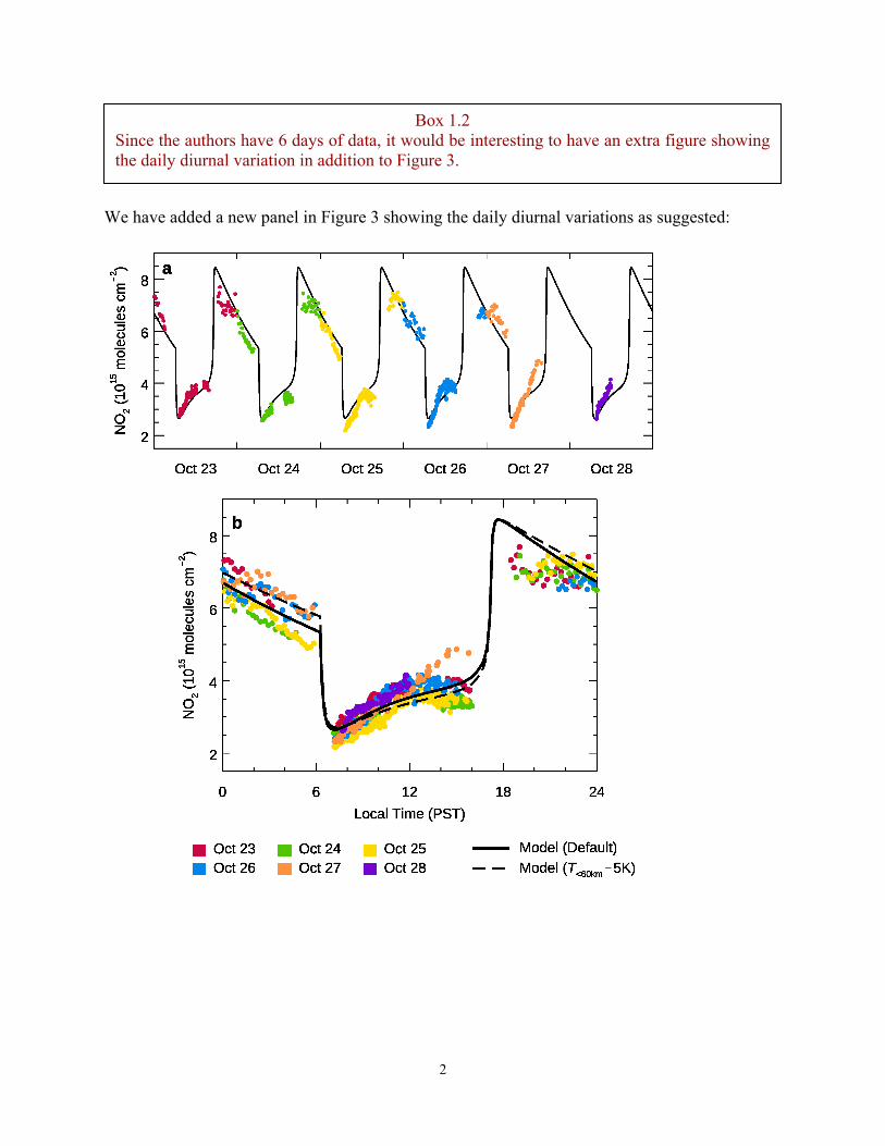
We have added a new panel in Figure 3 showing the daily diurnal variations as suggested:

Box 1.2 Since the authors have 6 days of data, it would be interesting to have an extra figure showing the daily diurnal variation in addition to Figure 3.

3

We thank the reviewer for this insightful comment. Although we did not say explicitly in the manuscript, the temperature sensitivity test (Section 3.3) was intended to explore one possible cause of the difference between the model and the observation during the nighttime. The modelled rate of decrease at night with the default temperature is greater than observed (the solid line in Figure 3). Lowering the temperature by 5 K reduces the modelled rate of decrease (the dashed line). Thus, the temperature profile could be a possible reason for the different shapes at night. However, a more definitive study would be needed in future publications to investigate this problem. In response to this comment, we have added a paragraph at the beginning of Section 3.4:

“While the 1-D model simulation captures most of the observed diurnal variability, the rate of decrease in the total NO2 column during nighttime is slightly overestimated in the model. Here we explore a possible uncertainty due to the prescribed temperature profile.”

and have revised the conclusion of the same section in Line 333 of the revised manuscript

“Thus, while the equinox temperature profile used in the baseline run is sufficient for the simulation of the diurnal cycle of the NO2 column, we do not exclude possible effects of temperature uncertainties on the nighttime simulation.”

We thank the reviewer for this insightful comment. The model results shown in Figure 4 were calculated assuming a plane-parallel atmosphere. We have conducted another calculation using the spherical geometry, where the sunrise and sunset times are dependent on altitude. We compare the resultant diurnal cycles with the one in the original manuscript below:

Box 1.3 The agreement with the model run is quite good except after sunset (Fig. 3) when the magnitude and shape are different. Is there an explanation?

Box 1.4 I know this is not a modelling paper, but the treatment of sunrise and sunset seems incomplete. There should be a time delay as a function of altitude with the sun reaching higher altitudes first. Since the authors are not showing data during sunrise and sunset, it does not matter much.

4

The above figure shows that the difference of the two diurnal cycles is much smaller than the spread of the data. Therefore, our conclusions remain unchanged when the spherical geometry is used.

In response to this comment, we added in the above figure in the new Appendix B.

The linear fit in Figure 6 is used to compare with an independent measurement over Germany that is discussed in Section 3.3 [Fig. 3a of Sussmann et al., Atmos. Chem. Phys., 5, 2657–2677, 2005, https://doi.org/10.5194/acp-5-2657-2005]. Sussmann et al. reported a linear increasing rate of daytime NO2 for the first time. To consistently compare with their analysis, we follow their definition of a linear fit through the daytime data. Our comparison with their value corroborates the findings over two different sites in mid-latitudes.

Our simulated total column NO2 also shows a regime change before and after noon, although the simulated regime change is not as strong as in the observation. Thus, based on our photochemical model, the two linear regimes are likely due to the conversion of the reservoir species N2O5. Apart from the continuous production of NO through the reaction between N2O and O(1D), the photolysis rate of N2O5 peaks at local noon, causing a quadratic time dependence during the daytime and hence an apparent change in the linear regime before and after local noon. Indeed, in the original manuscript, we pointed out the important role of the N2O5 conversion in Line 232:

“Figure 5 shows that the conversion between the reservoir and NO2 dominates between 18 km and 34 km, consistent with the NO2 diurnal cycles. Therefore, the secular NO2 changes during daytime and nighttime are dominated by N2O5 conversions.”

In response to this comment, we add the following in Line 308 of the revised manuscript:

“Figure 5 shows that the conversion between the reservoir and NO2 dominates between 18 and 34 km, consistent with the NO2 diurnal cycles. In particular, the quadratic decreasing trend of the daytime N2O5 is consistent with the quadratic increasing trend of the daytime NO2. Therefore, the secular NO2 changes during daytime and nighttime are dominated by N2O5 conversions.”

The stray light is typically of the order of 10−4–10−3, which is normally not high enough to affect the retrievals. In response to this comment, we added in Line 76:

“The stray light is typically of the order of 10−4−10−3.”

Box 1.5 The linear fit in Figure 6 does not mean much, other than as a baseline, as there are two linear regimes, one from 07:00 to 13:00 and from 13:00 to 16:00 hours. Is there an explanation for the two regimes?

Box 1.6 On the instrument: What is the stray light?

5

We have estimated the SNR at full moon transit to be ~2900 and the SNR at solar transit to be ~4900. The SNR is estimated by taking the standard deviation of the difference of two consecutive spectra as the noise and the signal being the average intensity. During the low Sun/Moon observations the SNR is more difficult to measure directly. However, the fitting residuals are consistent with these estimates.

In response to this statement, we have added at the end of Section 2.1 (Line 94):

“We estimate the signal-to-noise ratio (SNR) by assuming that the standard deviation of the difference of two consecutive spectra is close to the noise and that the average intensity of the two consecutive spectra is the signal. As a result, the SNR at full moon and solar transits are ~2900 and ~4900, respectively. During the low sun/moon observations the SNR is more difficult to measure directly. However, the fitting residuals are consistent with these estimates.”

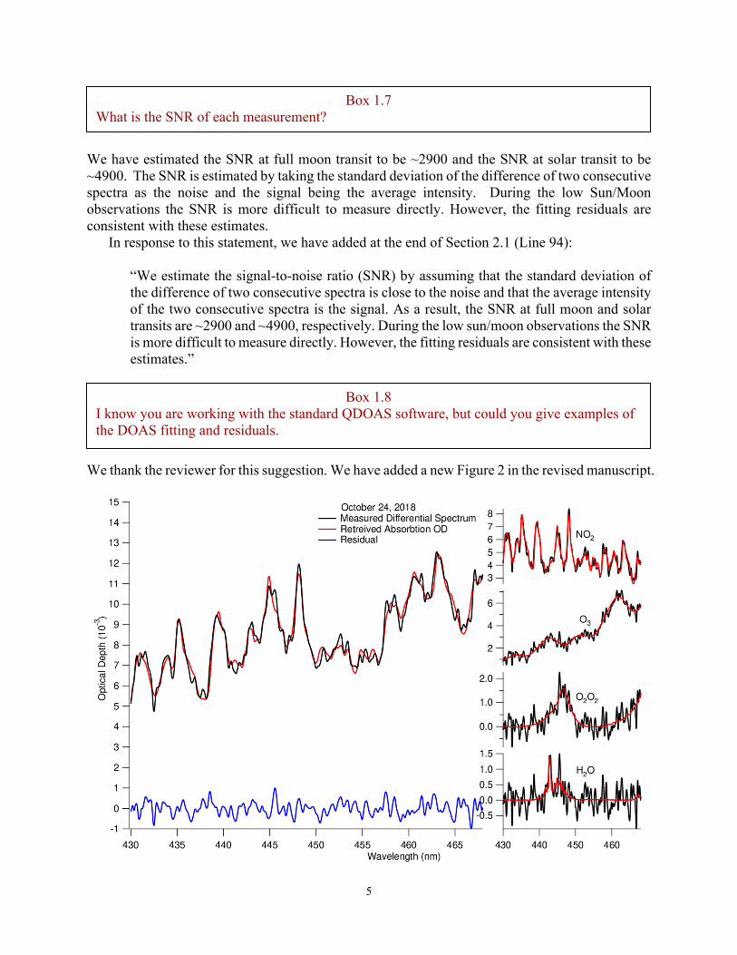
We thank the reviewer for this suggestion. We have added a new Figure 2 in the revised manuscript.

Box 1.7 What is the SNR of each measurement?

Box 1.8 I know you are working with the standard QDOAS software, but could you give examples of the DOAS fitting and residuals.

6

The measured spectrum is shown by the black curve on the left panel. The fitted spectrum (red) is overlaid, and the residual spectrum (blue) is shown at the bottom. Four species are considered in the spectral fit: NO2, O3, O4, and H2O. The spectral fits are performed simultaneously in QDOAS. The red lines on the right column are the fitted spectra of the corresponding species. To visualize the signal-to-noise ratios, we add the residual spectrum (blue on the left panel) to individual fitted spectra, which are shown as the black spectra in the subpanels on the right.

Once again, we thank the reviewer for his/her favour in our manuscript.

Box 1.9 The writing is clear with no significant errors. The figures are clear and easy to understand. The title should be revised. The paper should be published with only minor changes as described above.

7

Responses to Reviewer #2’s comments

We thank Reviewer #2 for his/her time and useful comments that have greatly improved our manuscript.

We thank the reviewer for this insightful comment. Since multiple instruments share the same dome at the TMF, the period we could run our instrument has been limited. Our preliminary measurements showed that 2 days away from the full moon would decrease the measured lunar intensity by ~20%, so we performed the measurement only when the moon was almost full to ensure a good signal-to-noise ratio (SNR). In addition to the full moon, we needed a non-cloudy atmosphere. The 6 consecutive days in October 2018 reported in this manuscript were the best period that satisfied these two conditions. It is our best interest to make more 24-hour measurements in the future.

While we agree with the reviewer that a low percentile gives a better representation of the background NO2 in a polluted site, the measurement over the TMF, as a clean site, may allow a higher percentile for an adequate estimation of the background on the TMF. As our back-trajectory analysis suggests, only one day out of six showed a sign of the urban source. Most vertical spread of the Langley plot is likely due to natural daily variability in the background. We therefore argue that the 20-percentile we used in the original manuscript still lies within the background variation. Nonetheless, we follow the reviewer’s suggestion and have performed another Langley extrapolation using the 5-percentile baseline. The resulting equation is

Box 2.0 King-Fai Li et al 2020 present direct sun and direct moon NO2 measurements over a high altitude mostly unpolluted site, JPL-TMF near Wrightwood, CA, during 6 days (around full moon) in October 2018. They proposed to combine two Langley-like techniques to estimate amount of NO2 atmospheric absorption during the reference spectrum measurement time. The proposed approach takes advantage of 1-D photochemical model to estimate diurnal variation in NO2 and minimum Langley extrapolation technique to reduce the effect of NO2 pollution. Modeling results are compared with the measurements. Chemical reactions for different processes are shown. Accurate measurements of diurnal NO2 variation are important and the topic fits into the scope of the “Atmospheric Measurement Techniques” journal.

Box 2.1 Not sufficient measurements (only 6 days) were presented in the paper to apply minimum Langley extrapolation technique (MLE). MLE is a statistical method and requires sufficient data to “accouter” conditions with “constant” vertical columns at each solar zenith angle. This threshold was not met during this study. MLE uses as low percentile for fitting as possible (within SNR) to capture background NO2. Increasing percentile used for Langley fitting does not simply improves the statistics, as stated in the paper, but can significantly alter the result. This can be easily remediated by including more measurements, especially at this mostly clean site.

8

𝑦 = (0.88 ± 0.08) 𝑚 𝑥 − (6.09 ± 0.65) × 10 (5-percentile).

The y-intercept is now 0.32×1015 more negative than the previous value obtained using the 20-th percentile in the original manuscript (which was 5.77±0.87×1015) but they are well within the 2-σ error. The new result is presented in Figure 3 of the revised manuscript:

We thank the reviewer for this insightful comment. The simulated diurnal cycle is used to remove the asymmetry about noon in the total column NO2. This asymmetry is natural, and it exists even under clean conditions and cannot be dealt with by the standard MLE (as explained in Section 2.3 of the original manuscript). To further illustrate the necessity of the removal of the diurnal asymmetry, we plot the observed total column NO2 on a single day (e.g. Oct 25, 2018) against the air mass factor (AMF = sec 𝜃) as in a standard MLE.

Box 2.2 While the idea of improving estimation of slant column density in the reference spectrum using a 1-D photochemical model is appealing, the authors have not demonstrated that it provides a better result than MLE itself. Looking at the data in Fig. 2 and 3, MLE will most likely result in lower amount in the reference spectrum, and the final vertical columns will agree significantly better with the model diurnal change than the retrieved columns (but will have an offset). Authors need to show that the results are better than the MLE by itself, and for that more measurements are required. Note, that to determine amount in the reference spectrum, full moon is not needed, since the analysis is done on the direct sun data. It is not clear from the presented results if the error in the model simulations actually is smaller than the uncertainty in MLE. This needs to be demonstrated.

9

Panel (a) plots the observations on October 25, 2018 against the air mass factor (AMF = sec 𝜃) as in a standard MLE. Based on our back-trajectory analysis, the atmosphere above TMF on October 25, 2018 should have little urban NO2 contamination. Both solar (pale orange dots) and lunar (pale blue dots) data exhibit a U shape that is due to the secular increase and decrease during the daytime and the nighttime, respectively. For the solar data, the AM data lies on the lower arm of the U shape and the PM data lies on the upper arm. For the lunar data, the reverse is true: data before sunrise lie on the upper arm of the U shape and data after sunset lie on the lower arm.

To perform a Langley extrapolation for the data shown in Panel (a), one needs to decide which of the four arms to be used for the linear regression model 𝑦 = 𝑎 AMF + 𝑏. The Principle of Minimum-amount suggests that we should start with the lowest arm, i.e. the daytime AM data. Note that in order to obtain the straight line passing through the 2-percentile baseline, we have ignored the points before noon (around 10 AM to 11:30 AM), i.e. points located around the bottom of the U-shape. If we use the observations between 6 AM and 10 AM, we obtain the purple line in Panel (a), which gives a y-intercept of (−4.12 ± 0.14) × 10 molecules cm−2.

10

The above Langley extrapolation, however, does not take any of the daytime PM and all lunar data into account. In particular, the daytime PM data should also be used to define a minimum-amount profile, given the fact that the atmosphere was mostly clean on that day. Suppose we perform another Langley extrapolation using the daytime PM data between 12 PM and 5 PM (rose line). The resultant y-intercept is (−5.25 ± 0.27) × 10 molecules cm−2 (2- 𝜎 ), which is statistically different from the value obtained using the daytime AM data. A reasonable estimate of the y-intercept is then the average of the two values, which is (−4.69 ± 0.21) × 10 molecules cm−2.

Finally, since the wind on the TMF is mostly downhill during autumn, the lunar data also correspond to a clean atmosphere and should also be used to derive the y-intercept. If we use all four arms in Panel (a), then the average value of the y-intercept is (−4.36 ± 0.25) × 10 molecules cm−2, where the uncertainty is the root-mean-squares of the uncertainties of the four values.

In the above calculation, the ignorance of the data points near the bottom of the “U”-shape has excluded a large number of observations near local solar/lunar noon and thus the resultant y-intercept is biased by high zenith angles. It is not clear how the data near the solar/lunar noon may be kept in the standard MLE due to the assumption of the linearity in AMF. As a result, a zenith angle-dependent Langley extrapolation model needs to be developed.

The above example shows that the determination of the y-intercept of the standard MLE is not straightforward when (i) the background NO2 has secular trends in daytime and nighttime and (ii) the daytime and nighttime abundances are different before and after the terminator. In contrast, the modified MLE (MMLE) approach we have developed in this work minimizes the background diurnal asymmetry, so that the “regularized” data points almost form a straight line (Panel b) when they are plotted against the modelled diurnal cycle. The linear regression model 𝑦 = 𝑎 𝑚 𝑥 + 𝑏, where 𝑚 𝑥 is the modelled slant column NO2, can be applied to all data points, regardless of the time of the day or whether the data point is a solar or lunar measurement. With this MMLE, the regressed y-intercept is (−5.22 ± 0.14) × 10 molecules cm−2, which is statistically different from the average of the values derived from the four arms in the standard MLE approach.

The issue with the standard MLE is exacerbated when observations on multiple days are plotted against the AMF. The U-shape may be smeared vertically into a continuum (Panel c). The smearing, in our case, are primarily due to natural variability of the background, except for October 27 when total column NO2 appears above the continuum of the daytime data due to the urban pollution. As a result, while we are still able to define the minimum-amount profile for the daytime AM data, the determination of the minimum-amount profiles of the daytime PM and the lunar data are difficult. This leaves us the daytime AM data alone for the Langley extrapolation (red line) but, as shown above, the resultant y-intercept [(−4.10 ± 0.46) × 10 molecules cm−2] may be biased.

In contrast, the observed data points still almost form a straight line in the MMLE approach when they are plotted against the modelled diurnal cycle (Panel d). This allows the determination of the minimum-amount profile using all solar and lunar measurements (raspberry line). The resultant y-intercept, (−6.09 ± 0.65) × 10 molecules cm−2, is again statistically different from the one obtained using the standard MLE approach.

As pointed out in Box 2.1 and Box 2.8, 2 days away from the full moon would decrease the lunar signal by 20%. We thus focused on full moon to ensure a high SNR for testing our instrument.

In response to this comment, we have put the above argument in a new Appendix A of the revised manuscript.

11

As explained in Box 2.3 (and Appendix A of the revised manuscript), the standard MLE may have a bias in the y-intercept because the total column NO2 has a natural diurnal asymmetry in the background, regardless of the pollution level. The removal of the natural diurnal asymmetry using the 1-D stratospheric model is thus necessary for NO2. The removal is also necessary to monitor the pollution level.

In addition, Table Mountain has been providing ground-based measurements for validating satellite retrievals because the site is away from the Los Angeles area and the tropospheric contribution to NO2 is generally low, even during summer daytime when upslope wind from the southwest (through LA downtown) is the strongest compared to other seasons, as discussed in one of our previous publications (Wang et al., JGR 2010, 10.1029/2009JD013503, cited in the original manuscript). We thus anticipate that pollution does not pose much of a problem in our MMLE. Furthermore, the more data we have in the future, the more accurate will be the minimum-amount baseline of the Langley plot, which can be directly compared with the 1-D stratospheric model. Indeed, in the original manuscript, we wrote (Line 136):

“When a large number of measured NO2 columns on clean and polluted days are plotted together against 𝑚 𝑥 (𝑚), the baseline of the scattered data may be considered as the background NO2 diurnal cycle in a clean atmosphere (Herman et al., 2009).”

In response to this comment, we clarify in the revised manuscript (Line 190):

“Our measurements made during October (a non-summer season) were mostly under unpolluted conditions. Thus, we applied the MMLE to derive a baseline for an estimation of the background NO2 diurnal cycle, which is then used in the regression with the modelled diurnal cycle.”

We use 3rd order polynomials for broadband and offset. The NO2 cross section is from Nizkorodov et al. (2004) for 215 K, 229 K, 249 K, 273 K, and 299 K, as discussed in the original manuscript. The O3 cross section is from Serdyuchenko et al. (2014) for 11 temperature references ranging from 193 K to 293 K. The O4 cross section is from Thalman and Volkamer 2013 at 273 K, and

Box 2.3 It is unclear what benefits this approach (1D stratospheric model) will have under the “persistent” pollution levels when the total NO2 abundance is dominated by anthropogenic emissions at all times.

Box 2.4 Description of the DOAS fitting settings is not sufficient. What are polynomial orders (e.g. broad band, offset, wavelength shift), what sources of other gases cross sections and at what temperatures were used in the analysis? Were NO2 cross sections at all five temperatures used in the retrieval? If yes, how they were fitted and combined? Why this fitting window was selected (430 and 468 nm)? How exactly air mass factor was calculated? What is the DOAS fitting quality of NO2 from direct sun and direct moon (residual OD)?

12

H2O cross section at 296 K is from HITRAN 2016. All five cross sections were used to create a single NO2 reference. The yearly average from the TMF temperature LIDAR are used to derive a reference for each altitude level by linear interpolation between each adjacent cross-section, which is also adjusted for pressure broadening using the results of Nizkorodov et al. (2004). Each level’s reference is then multiplied by a weight which is proportional to the standard atmosphere and then summed to obtain a single reference used in the fitting. A similar procedure was used for the O3 reference; for O4 and H2O only a single reference was used.

As shown in Figure 3 of Spinei et al. (2014), the 430−468 nm window has stronger NO2 absorptions relative to other wavelengths in the 411−475 nm range. In addition, this window also has less interfering absorption from other species. These two factors add up to increase the accuracy of the DOAS spectral fit.

The air mass is calculated using secant of the solar/lunar zenith angle, sec(VZA). Herman et al. (2009) considered an altitude correction in this equation. However, the correction is generally negligible except for VZA > 80° but we do not make measurements at those VZAs.

The new Figure 2 in the revised manuscript shows an example of the spectral fit. In response to this comment, we have added the above descriptions in the revised Section 2.2:

“The differential slant column NO2 is retrieved by fitting the ratioed spectrum in a

smaller window between 430 and 468 nm. This window has stronger NO2 absorptions relative to other wavelengths in the instrument range (411−475 nm); see Figure 3 of Spinei et al. (2014). In addition, this window also has less interfering absorption from species other than the O3, O4 (O2 dimer), and H2O (see below).

The spectral fitting is accomplished through the Marquardt-Levenberg minimization using QDOAS retrieval software (http://uv-vis.aeronomie.be/software/QDOAS/). The highly spectrally resolved NO2 absorption cross sections at 𝑇 = 215 K, 229 K, 249 K, 273 K, 298 K, and 299 K based on Nizkorodov et al. (2004) are convolved to the instrument resolution using the instrument line shape function and the Voigt line shape prior to its use in QDOAS. The yearly average from the TMF temperature LIDAR measurements are used to derive a reference for each altitude level by linear interpolation between each adjacent cross-section, which is also adjusted for pressure broadening using the results of Nizkorodov et al. (2004). We use 3rd order polynomials for broadband and offset. All five cross sections were used to create a single NO2 reference. Each level’s reference is then multiplied by a weight which is proportional to the standard atmosphere and then summed to obtain a single reference used in the fitting. In addition to NO2, other absorptions by O3, O4 (O2 dimer), and H2O in the same spectral window are simultaneously retrieved. The O3 cross section is from Serdyuchenko et al. (2014) for 11 temperature references ranging from 193 K to 293 K. Like NO2, all 11 cross-sections are used in the spectral fitting for O3. In contrast, for O4 and H2O, only a single temperature reference is used. The O4 cross section is from Thalman and Volkamer (2013) at 273 K. The H2O cross section at 296 K is from HITRAN 2016 (Gordon, 2017). Figure 2 shows an example of a fitted spectrum on October 24, 2018. The NO2 abundance retrieved from QDOAS is the desired differential slant column NO2 relative to our chosen reference spectrum.

The air mass factor is calculated using secant of the solar/lunar zenith angle. Herman et al. (2009) considered an altitude correction of the air mass factor. The altitude

13

correction is generally negligible except for zenith angles ≥ 80° but we do not make measurements at those zenith angles (see Section 2.1).”

We considered two major sources of error: the fitting residual of the DOAS spectral fit and the error of the y-intercept of the Langley extrapolation. The errors from the QDOAS fitting residual generally lies between than 0.1×1015 cm-2 and 0.6×1015 cm-2 (2-σ) for all zenith angles, which is now shown in an inset of Figure 3 of the revised manuscript:

The error of the y-intercept of the Langley extrapolation is ±0.65×1015 cm-2 (2-σ), which is also added in the revised Figure 3 (see the figure above). The root-mean-square of these two sources of error gives an estimate of a total error of ~0.9×1015 cm-2 (2-σ).

In response to this comment, we added in the revised manuscript in Line 143:

The 2-𝜎 uncertainty due to the spectral fitting residual lies between 0.1×1015 molecules cm–2 and 0.6×1015 molecules cm–2, with a mean of ~0.4×1015 molecules cm–2. The distribution of the retrieval uncertainty is shown in Figure 2 (inset).

and in Line 198:

“We estimate the total retrieval uncertainty to be the root-mean-square of the spectral fitting uncertainty and the uncertainty in 𝑦 , which is 0.8×1015 molecules cm–2 (2-𝜎).”

Box 2.5 No error budget is presented for the measured NO2 columns.

14

Thanks for this comment. Actually, Reviewer #1 has an opposite comment. The aim of this paper is to present a new instrument for measuring daytime and nighttime NO2 column. Perhaps the confusion may be due to the frequent appearances of models in the retrieval strategy and the back-trajectory calculations. However, the 1-D stratospheric model is mainly used to assist, not determine, the retrieval (by minimizing the diurnal asymmetry). The retrieval per se is still observation-based, in contrast to the common Bayesian-based approach where the statistics of the a priori model is also used to constrain the retrieved value.

In response to this comment, in the revised manuscript, we have removed the phrase “model-based” from the name of our method. Instead, our method is now called “the modified minimum-amount Langley extrapolation” or MMLE in short.

We thank the reviewer for mentioning these references. We are aware of them. Indeed, we have used NDACC NO2 data in our recent publication (Wang et al., Solar 11-Year Cycle Signal in Stratospheric Nitrogen Dioxide—Similarities and Discrepancies Between Model and NDACC Observations, Solar Phys., doi:10.1007/s11207-020-01685-1, 2020, cited in the revised manuscript). In addition, MF-DOAS and Pandora were used in our earlier publication (Wang et al., 2010, cited in the original manuscript.).

In response to this comment, we have added a number of references involved in NDACC and PGN. In particular, the statement in Line 24:

“NO2 column abundance has been measured using ground-based instruments since the mid-1970s [Network for the Detection of Atmospheric Composition Change (NDACC), http://www.ndacc.org] …”

has been revised as

“NO2 column abundance has been measured using ground-based instruments since the mid-1970s [Network for the Detection of Atmospheric Composition Change (NDACC), http://www.ndacc.org] (e.g., Hofmann et al., 1995; Piters et al., 2012; Roscoe et al., 1999; Roscoe et al., 2010; Vandaele et al., 2005; Kreher et al., 2020) …”

In addition, the statement in Line 59:

“Other techniques, such as balloon-based in situ measurements (May and Webster, 1990; Moreau et al., 2005), balloon-based solar occultations (Camy-Peyret, 1995) and ground-

Box 2.6 The paper in general reads more like a modeling paper then the measurement paper.

Box 2.7 There are routine NO2 stratospheric measurements conducted by the NDACC stations (zenith sky DOAS) and total column measurements of NO2 using direct sun and direct moon within Pandonia Global Network. They should be mentioned in the review of NO2 measurements. In general, citations tend to include mostly early works and not give current status.

15

based multi-axis DOAS (MAX-DOAS; Hönninger et al., 2004; Sanders et al., 1993) have also been employed to further characterize the vertical distributions of NO2.”

has been revised as

“Other techniques, such as balloon-based in situ measurements (May and Webster, 1990; Moreau et al., 2005), balloon-based solar occultations (Camy-Peyret, 1995), as well as ground-based multi-axis DOAS (MAX-DOAS; Hönninger et al., 2004; Sanders et al., 1993), multi-functional DOAS, and Pandora (Herman et al., 2009; Spinei et al., 2014) that have been actively involved in NDACC and the Pandonia Global Network (Kreher et al., 2020), have also been employed to further characterize the vertical distributions of NO2.”

We apologize for the confusion. For the sunlight measurement, we insert a diffuser plate to reduce the solar throughput by a factor of ~1.3×10−5 and protect the instrument. The diffuser plate is not used during the moonlight measurement. Since the sun is ~400,000 times the intensity of the full moon, the ratio between the light hitting our detector for solar noon (after inserting the diffuser and the filter) and lunar noon during the full moon is ~5. Thus, in order to maintain an approximately constant solar and lunar signal-to-noise ratio and fitting residuals, we need to vary slightly the exposure time during specific times of solar and lunar noon, typically around ~3 s for lunar noon and ~0.6 s for solar noon, giving a ratio of ~5 to balance out the photon counts mentioned above. In the original manuscript, we wrote the statement (Line 77)

“The exposure time was 4 s and 0.25 s during the lunar/solar noon observations, respectively.”

The 4 s and 0.25 s are the full range of exposure times between which we varied during that week of measurement in October 2018, but the writing of this statement may be confusing. The exposure times were not constant during the measurement.

In response to this comment, the above quoted statement has been revised to (Line 86)

“When direct moonlight is measured, the diffuser plates are removed. Since the sun is ~400,000 times the intensity of the full moon, the ratio between the light hitting our detector for solar noon (after inserting the diffuser plates) and lunar noon during the full moon is ~5. To maintain an approximately constant solar and lunar signal-to-noise ratio and fitting residuals, we vary the exposure time during specific times of solar and lunar noon, typically around ~3 s for lunar noon and ~0.6 s for solar noon, giving a ratio of ~5 to homogenize the solar and lunar photon counts mentioned above.”

Box 2.8 It is unclear how the lunar measurement where taken. Lunar irradiance is about 106 lower than solar irradiance. In this study, integration time for sun measurements is 16 times shorter than for moon. Difference in lunar vs solar measurements (diffusers, filters, etc), and what effect it has on spectrometer illumination should be presented. Target signal-to-noise ratio stated.

1

Diurnal variability of total column NO2 measured using direct solar and lunar spectra over Table Mountain, California (34.38°N) King-Fai Li1, Ryan Khoury1, Thomas J. Pongetti2, Stanley P. Sander2, Yuk L. Yung2,3 1Department of Environmental Science, University of California, Riverside, California, USA 2Jet Propulsion Laboratory, California Institute of Technology, Pasadena, California, USA 5 3Division of Geological and Planetary Sciences, California Institute of Technology, Pasadena, California, USA

Correspondence to: King-Fai Li (king-fai.li@ucr.edu)

Abstract. A full diurnal measurement of total column NO2 has been made over the Jet Propulsion Laboratory’s Table Mountain

Facility (TMF) located in the mountains above Los Angeles, California, USA (2.286 km above mean sea level, 34.38°N,

117.68°W). During a representative week in October 2018, a grating spectrometer measured the telluric NO2 absorptions in 10

direct solar and lunar spectra. The total column NO2 is retrieved using a modified minimum-amount Langley extrapolation,

which enables us to accurately treat the non-constant NO2 diurnal cycle abundance and the effects of pollution near the

measurement site. The measured 24-hour cycle of total column NO2 on clean days agrees with a 1-D photochemical model

calculation, including the monotonic changes during daytime and nighttime due to the exchange with the N2O5 reservoir and

the abrupt changes at sunrise and sunset due to the activation or deactivation of the NO2 photodissociation. The observed 15

daytime NO2 increasing rate is (1.31 ± 0.41) × 10 cm–2 h–1. The total column NO2 in one of the afternoons during the

measurement period was much higher than the model simulation, implying the influence of urban pollution from nearby

counties. A 24-hour back-trajectory analysis shows that the wind first came from inland in the northeast and reached the

southern Los Angeles before it turned northeast and finally arrived TMF, allowing it to pick up pollutants from Riverside

County, Orange County, and Downtown Los Angeles. 20

1 Introduction

Nitrogen dioxide (NO2) plays a dominant role in the ozone (O3)-destroying catalytic cycle (Crutzen, 1970). NO2

column abundance has been measured using ground-based instruments since the mid-1970s [Network for the Detection of

Atmospheric Composition Change (NDACC), http://www.ndacc.org] (e.g., Hofmann et al., 1995; Piters et al., 2012; Roscoe

et al., 1999; Roscoe et al., 2010; Vandaele et al., 2005; Kreher et al., 2020), which serve as the standards for validating satellite 25

measurements. Noxon (1975) and Noxon et al. (1979) retrieved the stratospheric NO2 column by differential optical absorption

spectroscopy (DOAS) in the visible spectral range using ratios of scattered sunlight from the sky and direct sun/moonlight at

low (noon/midnight) and high (twilight) air mass factors over Fritz Peak, Colorado (39.9°N). Since the optical path of

sun/moonlight at dawn or dusk (solar/lunar zenith angle ≈ 90°) is much longer than the optical path of the direct sunlight at

noon/midnight, the NO2 absorption in the noon/midnight spectrum can be assumed to be small and the NO2 absorption in the 30

Deleted: model-based

Deleted: 29Deleted: 30Deleted: cities

Deleted: (

Deleted: ,

2

twilight slant column could therefore be isolated effectively by ratioing the scattered twilight spectrum to the scattered noon

spectrum. This DOAS principle also applies to ratios of direct moonlight or sunlight at low and high air mass factors. Noxon

et al.’s (1979) measurements revealed sharp changes of the stratospheric NO2 column before and after sunsets and sunrises at

mid-latitudes. Similar DOAS measurements at high latitudes in the 1980s focused on the role of NOx in controlling O3 and 40

active halogen species in the polar stratosphere (Fiedler et al., 1993; Flaud et al., 1988; Keys and Johnston, 1986; Solomon,

1999). Johnston and McKenzie (1989) and Johnston et al. (1992) reported a reduction in the southern hemispheric NO2 over

Lauder, New Zealand (45.0°S), following the eruptions of El Chichón (in 1982) and Pinatubo (in 1991), respectively.

NO2 column abundance has also been measured using direct solar spectra acquired by Fourier-Transform infrared

(FTIR) spectrometers. Advantages of direct solar measurements are the lack of Raman scattering in the spectra, air mass 45

factors determined geometrically rather than through a radiative transfer code, and provision of NO2 column abundances at

most times during the day. Sussmann et al. (2005) retrieved the stratospheric NO2 column abundance over Zugspitze, Germany

(47°N) using the infrared absorption in the solar spectrum near 3.43 μm. The stratospheric NO2 column abundance was then

subtracted from the total column estimated from satellite measurements to obtain the tropospheric column. Wang et al. (2010)

demonstrated how high spectral resolution measurements using a Fourier transform spectrometer could perform absolute NO2 50

column abundance retrievals without the need for a solar reference spectrum. Because of the solar rotation, the Fraunhofer

features in the UV spectra acquired simultaneously from the east and west limbs of the solar disk are Doppler shifted while

the telluric NO2 absorptions are not shifted (Iwagami et al., 1995). Thus, the telluric NO2 absorptions can be identified by

correcting the Doppler shift without the need of an a priori solar spectrum. Other techniques, such as balloon-based in situ

measurements (May and Webster, 1990; Moreau et al., 2005), balloon-based solar occultations (Camy-Peyret, 1995), as well 55

as ground-based multi-axis DOAS (MAX-DOAS; Hönninger et al., 2004; Sanders et al., 1993), multi-functional DOAS, and

Pandora (Herman et al., 2009; Spinei et al., 2014) that have been actively involved in NDACC and the Pandonia Global

Network (Kreher et al., 2020), have also been employed to further characterize the vertical distributions of NO2.

Here we retrieve the total column NO2 over Table Mountain Facility (TMF) in Wrightwood, California, USA (2.286

km above mean sea level, 34.38°N, 117.68°W) using Langley extrapolation to determine the reference spectrum and 60

considering both daytime and night time chemistry. Daytime NO2 concentration remains significant, albeit small relative to

the night-time concentration, and varies from morning to afternoon. This daytime variation has been a source of error in

determination of the DOAS reference spectrum using Langley extrapolation. Comprehensive assessment of NO2 must include

both daytime and nighttime values. We therefore also retrieve daytime column NO2 by acquiring direct sun spectra throughout

the day. We will compare the daytime and nighttime total column NO2 with those simulated in a one-dimensional (1-D) 65

photochemical model. The effect of urban pollution on the measured total column NO2 can be deduced from this comparison.

Deleted: ) and

Deleted: traditionally

3

2 Data and Method

2.1 Instrumentation and measurement technique 70

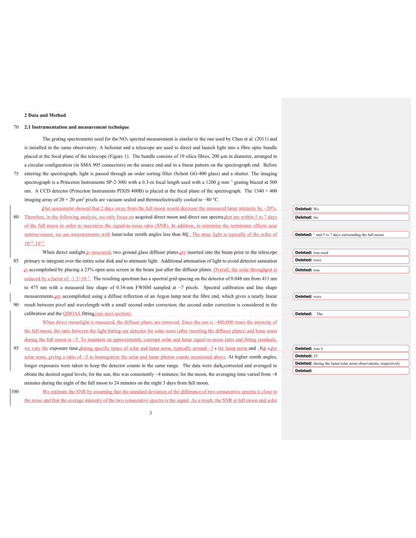
The grating spectrometer used for the NO2 spectral measurement is similar to the one used by Chen et al. (2011) and

is installed in the same observatory. A heliostat and a telescope are used to direct and launch light into a fibre optic bundle

placed at the focal plane of the telescope (Figure 1). The bundle consists of 19 silica fibres, 200 µm in diameter, arranged in

a circular configuration (in SMA 905 connectors) on the source end and in a linear pattern on the spectrograph end. Before

entering the spectrograph, light is passed through an order sorting filter (Schott GG-400 glass) and a shutter. The imaging 75

spectrograph is a Princeton Instruments SP-2-300i with a 0.3-m focal length used with a 1200 g mm−1 grating blazed at 500

nm. A CCD detector (Princeton Instruments PIXIS 400B) is placed at the focal plane of the spectrograph. The 1340 × 400

imaging array of 20 × 20 µm2 pixels are vacuum sealed and thermoelectrically cooled to −80 °C.

Our assessment showed that 2 days away from the full moon would decrease the measured lunar intensity by ~20%.

Therefore, in the following analysis, we only focus on acquired direct moon and direct sun spectra that are within 5 to 7 days 80

of the full moon in order to maximize the signal-to-noise ratio (SNR). In addition, to minimize the terminator effects near

sunrise/sunset, we use measurements with lunar/solar zenith angles less than 80°. The stray light is typically of the order of

10−4–10−3.

When direct sunlight is measured, two ground glass diffuser plates are inserted into the beam prior to the telescope

primary to integrate over the entire solar disk and to attenuate light. Additional attenuation of light to avoid detector saturation 85

is accomplished by placing a 23% open area screen in the beam just after the diffuser plates. Overall, the solar throughput is

reduced by a factor of ~1.3×10−5. The resulting spectrum has a spectral grid spacing on the detector of 0.048 nm from 411 nm

to 475 nm with a measured line shape of 0.34-nm FWHM sampled at ~7 pixels. Spectral calibration and line shape

measurements are accomplished using a diffuse reflection of an Argon lamp near the fibre end, which gives a nearly linear

result between pixel and wavelength with a small second order correction; the second order correction is considered in the 90

calibration and the QDOAS fitting (see next section).

When direct moonlight is measured, the diffuser plates are removed. Since the sun is ~400,000 times the intensity of

the full moon, the ratio between the light hitting our detector for solar noon (after inserting the diffuser plates) and lunar noon

during the full moon is ~5. To maintain an approximately constant solar and lunar signal-to-noise ratio and fitting residuals,

we vary the exposure time during specific times of solar and lunar noon, typically around ~3 s for lunar noon and ~0.6 s for 95

solar noon, giving a ratio of ~5 to homogenize the solar and lunar photon counts mentioned above. At higher zenith angles,

longer exposures were taken to keep the detector counts in the same range. The data were dark-corrected and averaged to

obtain the desired signal levels; for the sun, this was consistently ~4 minutes; for the moon, the averaging time varied from ~8

minutes during the night of the full moon to 24 minutes on the night 3 days from full moon.

We estimate the SNR by assuming that the standard deviation of the difference of two consecutive spectra is close to 100

the noise and that the average intensity of the two consecutive spectra is the signal. As a result, the SNR at full moon and solar

Deleted: We

Deleted: for

Deleted: ° and 5 to 7 days surrounding the full moon.

Deleted: was used

Deleted: were

Deleted: was

Deleted: were

Deleted: . The

Deleted: was 4

Deleted: 25

Deleted: during the lunar/solar noon observations, respectively

Deleted:

4

transits are ~2900 and ~4900, respectively. During the low sun/moon observations the SNR is more difficult to measure

directly. However, the fitting residuals are consistent with these estimates. 115

2.2 The DOAS retrieval

The DOAS technique is used to retrieve the NO2 slant column (Noxon, 1975; Noxon et al., 1979; Platt et al., 1979;

Stutz and Platt, 1996). A spectrum measured by the grating spectrometer at any time of the day is ratioed to a pre-selected

reference spectrum. From the ratioed spectrum, we retrieve the differential slant column NO2 relative to the column that is

represented by the reference spectrum. The total slant column is then the sum of the differential slant column and the reference 120

column.

Our reference spectrum is a solar spectrum measured at the TMF ground level at local noon (Chen et al., 2011). This

solar reference spectrum is used to ratio all other spectra collected, including those during the solar and lunar measurement

cycles. In principle, one can retrieve the reference NO2 column from the reference spectrum. However, this requires precise

knowledge of the solar spectrum at the top of the atmosphere in order to isolate the NO2 absorption. We will use a variant of 125

the Langley extrapolation to circumvent the need of the retrieval of the reference column (Lee et al., 1994; Herman et al.,

2009); see following section for details.

The differential slant column NO2 is retrieved by fitting the ratioed spectrum in a smaller window between 430 and

468 nm. This window has stronger NO2 absorptions relative to other wavelengths in the instrument range (411−475 nm); see

Figure 4 of Spinei et al. (2014). In addition, this window also has less interfering absorption from species other than the O3, 130

O4 (O2 dimer), and H2O (see below).

The spectral fitting is accomplished through the Marquardt-Levenberg minimization using QDOAS retrieval software

(http://uv-vis.aeronomie.be/software/QDOAS/). The high-resolution NO2 absorption cross-sections at 𝑇 = 215 K, 229 K,

249 K, 273 K, 298 K, and 299 K based on Nizkorodov et al. (2004) are convolved to the instrument resolution using the

instrument line shape function and the Voigt line shape prior to its use in QDOAS. The yearly average from the TMF 135

temperature LIDAR measurements are used to derive a reference for each altitude level by linear interpolation between each

adjacent cross-section, which is also adjusted for pressure broadening using the results of Nizkorodov et al. (2004). We use

3rd order polynomials for broadband and offset. All five cross-sections were used to create a single NO2 reference. Each

level’s reference is then multiplied by a weight which is proportional to the standard atmosphere and then summed to obtain a

single reference used in the fitting. In addition to NO2, other absorptions by O3, O4 (O2 dimer), and H2O in the same spectral 140

window are simultaneously retrieved. The O3 cross section is from Serdyuchenko et al. (2014) for 11 temperature references

ranging from 193 K to 293 K. Like NO2, all 11 cross-sections are used in the spectral fitting for O3. In contrast, for O4 and

H2O, only a single temperature reference is used. The O4 cross-sections are from Thalman and Volkamer (2013) at 273 K. The

H2O cross-sections at 296 K are from HITRAN 2016 (Gordon et al., 2017). Figure 2 shows an example of a fitted spectrum

on October 24, 2018. The NO2 abundance retrieved from QDOAS is the desired differential slant column NO2 relative to our 145

chosen reference spectrum.

Deleted: between 430 and 468 nm.

Deleted: highly spectrally resolved

Deleted:

Deleted: 215 K, 229 K, 249 K, 273 K, 298 K, and 299 KDeleted: The temperature profile for the calculation of the Voigt line shape is determined by the yearly average of the TMF temperature lidar measurements.

5

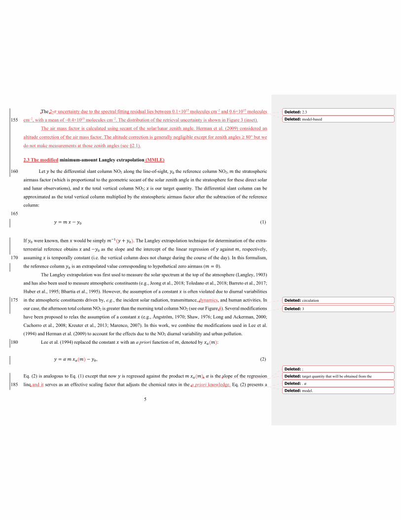
The 2-𝜎 uncertainty due to the spectral fitting residual lies between 0.1×1015 molecules cm–2 and 0.6×1015 molecules

cm–2, with a mean of ~0.4×1015 molecules cm–2. The distribution of the retrieval uncertainty is shown in Figure 3 (inset). 155

The air mass factor is calculated using secant of the solar/lunar zenith angle. Herman et al. (2009) considered an

altitude correction of the air mass factor. The altitude correction is generally negligible except for zenith angles ≥ 80° but we

do not make measurements at those zenith angles (see §2.1).

2.3 The modified minimum-amount Langley extrapolation (MMLE)

Let 𝑦 be the differential slant column NO2 along the line-of-sight, 𝑦 the reference column NO2, 𝑚 the stratospheric 160

airmass factor (which is proportional to the geometric secant of the solar zenith angle in the stratosphere for these direct solar

and lunar observations), and 𝑥 the total vertical column NO2; 𝑥 is our target quantity. The differential slant column can be

approximated as the total vertical column multiplied by the stratospheric airmass factor after the subtraction of the reference

column:

165 𝑦 = 𝑚 𝑥 − 𝑦 (1)

If 𝑦 were known, then 𝑥 would be simply 𝑚 (𝑦 + 𝑦 ). The Langley extrapolation technique for determination of the extra-

terrestrial reference obtains 𝑥 and −𝑦 as the slope and the intercept of the linear regression of 𝑦 against 𝑚, respectively,

assuming 𝑥 is temporally constant (i.e. the vertical column does not change during the course of the day). In this formulism, 170

the reference column 𝑦 is an extrapolated value corresponding to hypothetical zero airmass (𝑚 = 0).

The Langley extrapolation was first used to measure the solar spectrum at the top of the atmosphere (Langley, 1903)

and has also been used to measure atmospheric constituents (e.g., Jeong et al., 2018; Toledano et al., 2018; Barreto et al., 2017;

Huber et al., 1995; Bhartia et al., 1995). However, the assumption of a constant 𝑥 is often violated due to diurnal variabilities

in the atmospheric constituents driven by, e.g., the incident solar radiation, transmittance, dynamics, and human activities. In 175

our case, the afternoon total column NO2 is greater than the morning total column NO2 (see our Figure 4). Several modifications

have been proposed to relax the assumption of a constant 𝑥 (e.g., Ångström, 1970; Shaw, 1976; Long and Ackerman, 2000;

Cachorro et al., 2008; Kreuter et al., 2013; Marenco, 2007). In this work, we combine the modifications used in Lee et al.

(1994) and Herman et al. (2009) to account for the effects due to the NO2 diurnal variability and urban pollution.

Lee et al. (1994) replaced the constant 𝑥 with an a priori function of 𝑚, denoted by 𝑥 (𝑚): 180

𝑦 = 𝛼 𝑚 𝑥 (𝑚) − 𝑦 , (2)

Eq. (2) is analogous to Eq. (1) except that now 𝑦 is regressed against the product 𝑚 𝑥 (𝑚). 𝛼 is the slope of the regression

line and it serves as an effective scaling factor that adjusts the chemical rates in the a priori knowledge. Eq. (2) presents a 185

Deleted: 2.3

Deleted: model-based

Deleted: circulation

Deleted: 3

Deleted: ;Deleted: target quantity that will be obtained from the

Deleted: . 𝛼Deleted: model.

6

modified Langley extrapolation. The y-intercept, 𝑦 , obtained from the modified Langley extrapolation is then used to derived

the observed total vertical column through the transformation 𝑚 (𝑦 + 𝑦 ). Note that 𝛼 is not used in this transformation. 195

As in Lee et al. (1994), assuming the chemical processes of NO2 are much faster than the dynamical processes so that

the NO2 diurnal cycle is at photochemical equilibrium, we obtain 𝑥 (𝑚) from a 1-D photochemical model (to be described in

the next section). The 𝑥 (𝑚) we use corresponds to a clean atmosphere only. To perform the regression, we plot 𝑦 against the

product 𝑚 𝑥 (𝑚) (Figure 3, blue open circles). If all NO2 columns are measured on clean days, then they would ideally fall

on a straight line (which, apart from the natural variability in the background, holds true for Lee et al.’s (1994) measurements 200

over Antarctica). However, if there is a pollution source near a measurement site, like the TMF, then some of the measured

NO2 column may be significantly higher than 𝑥 (𝑚), leading to a large vertical spread in the scattered plot. The pollution-

induced deviation from 𝑥 (𝑚) may be highly variable, depending on the source types and the meteorology. When a large

number of measured NO2 columns on clean and polluted days are plotted together against 𝑚 𝑥 (𝑚), the baseline of the

scattered data may be considered as the background NO2 diurnal cycle in a clean atmosphere (Herman et al., 2009). Herman 205

et al. (2009) called their method the minimim-amount Langley extrapolation (MLE). Expanding on their terminology, we call

our method, which combines the MLE with Lee et al.s’ modification, the modified MLE, or MMLE. Note, however, that the

MMLE differs from the optimal estimation that is commonly used in satellite retrieval, where the statistics of priori knowledge

is used to constrain the retrieved value; no prior constraint is used in the MMLE.

Our measurements made during October (a non-summer season) were mostly under unpolluted conditions (see §3.5). 210

Thus, we applied the MMLE to derive a baseline for an estimation of the background NO2 diurnal cycle, which is then used

in the regression with the modelled diurnal cycle. On the Langley plot (Figure 3), we divide the range of 𝑚 𝑥 (𝑚) (from ~5 × 10 to 3 × 10 molecules cm–2 during our campaign) into 20 equal bins. We use the 5-percentile of the 𝑦 distribtion

in each bin to define a baseline (Figure 3, green dots). We then fit the 5-percentile baseline to Eq. (2) and obtain the values of 𝛼 and 𝑦 (Figure 3, red line). The fitted line in Figure 3 gives 𝛼 = 0.88 ± 0.04 and 𝑦 = (6.09 ± 0.65) × 10 molecules 215

cm–2 (at 2-𝜎 levels). This value of 𝑦 is our reference column used for both daytime and nighttime measurements. We estimate

the total retrieval uncertainty to be the root-mean-square of the spectral fitting uncertainty and the uncertainty in 𝑦 , which is

0.9×1015 molecules cm–2 (2-𝜎).

2.4 The photochemical model

Our 𝑥 (𝑚) is based on the Caltech/JPL 1-D photochemical model (Allen et al., 1984; Allen et al., 1981; Wang et al., 220

2020), shown as the black solid line in Figure 4. This photochemical model includes the stratospheric species that are important

for O3, odd-nitrogen (NOx = N + NO + NO2 + NO3 + 2N2O5) and odd-hydrogen (HOx = H + OH + HO2) chemistry, including

the reactions discussed in §3.1. Nitrous oxide (N2O) is the main parent molecule of NO2 in the lower stratosphere. The

concentration of N2O at the ground level of the model is fixed at 330 ppb

Deleted: model-based

Deleted: 2

Deleted: .

Deleted: Following

Deleted: ’sDeleted: terminology, we call our

Deleted: model-based

Deleted: .

Deleted: To obtain

Deleted: ,

Deleted: Herman et al. (2009) used

Deleted: 2Deleted: . To enhance the statistical robustness of the baseline, we use the 20-percentile instead (Figure 2

Deleted: 20

Deleted: 2Deleted: 2Deleted:

Deleted: = 5.77 × 10Deleted: .

Deleted: 3

Deleted: Section

7

(https://www.esrl.noaa.gov/gmd/hats/combined/N2O.html). The kinetic rate constants are obtained from the 2015 JPL

Evaluation (Burkholder et al., 2015).

The sunrise/sunset times and the solar noontime in the model are calculated using the ephemeris time. We use

Newcomb parameterizations of the perturbations due to the Sun, Mercury, Venus, Mars, Jupiter, and Saturn (Newcomb, 1898). 250

We also use Woolard parameterizations for the nutation angle and rate (Woolard, 1953). More modern calculation of the

ephemeris time may be used (e.g., Folkner et al., 2014) but the difference in the resulting ephemeris time is small (less than

0.1 s) and does not significantly impact our model simulation.

We progress the model in time until the diurnal cycle of the stratospheric NO2 becomes stationary. Throughout the

progression, the pressure and temperature profiles are fixed and do not vary with time. The model latitude is set at 34.38°N 255

and the model day is set as October 26. The total column NO2 is the vertical integral of the NO2 concentration. The simulation

represents the NO2 abundance in a clean atmosphere without tropospheric sources.

3 Results and Discussions

3.1 Diurnal variation in total column NO2

Figure 4 presents our preliminary observational data (colour dots) obtained during October 23–28, 2018. During the 260

measurements, the skies were mostly clear or only partly cloudy, so we were able to make continuous solar spectral

measurements throughout the whole period. During October, the local sunrise and sunset time were around 07:00 PST and

18:00 PST, respectively. At sunrise and sunset, the ambient twilight in the background of the moonlight occultation should be

accounted for in the NO2 retrieval, which is beyond the scope of this work. For this work, we exclude lunar total column NO2

data when the ambient scattered twilight, including those from civil sources, is significant, which typically occurs when the 265

lunar elevation angle is less than 6° above the horizon. Figure 4a shows the daily diurnal cycles during the week of

measurements and Figure 4b shows the aggregated diurnal cycle as a function of local time. The solid black line in both panels

is the simulated 24-hour cycle of the total column NO2 variability in the 1-D model. The dashed line in Figure 4b is a second

simulation with a slightly lower temperature (see §3.4). Overall, the baseline simulation captures the observed trends during

the daytime and the nighttime. The observations reveal day-to-day variability, but our back-trajectory analysis shows that the 270

day-to-day variations during October 23−26 and 28 are likely due to natural variability of the background in the north while

that on October 27 is likely due to urban sources from the Los Angeles basin in the south (see §3.5)

On most days, the total column NO2 over TMF increased from ~2 × 10 molecules cm–2 in the morning to ~3.5 × 10 molecules cm–2 in the evening. There are 3 main sources of NOx contributing to the daytime increase. The ultimate

source is the reaction of N2O with excited oxygen O(1D) resulting from the photolysis of O3 in the stratosphere between 20–275

60 km, which produces nitric oxide (NO) molecules and eventually NO2 through the NOx cycle aided by O3:

Deleted: 3

Deleted: The solid black line of Figure 3

Deleted: Section

Deleted: 3

8

N2O + O(1D) → NO + NO, (R1)

NO + O3 → NO2 + O2. (R2)

Another major source is the photolysis of the reservoir species, nitric acid (HNO3) and dinitrogen pentoxide (N2O5): 285

HNO3 + ℎ𝜈 → NO2 + OH, (R3)

N2O5 + ℎ𝜈 → NO2 + NO3. (R4)

There is also a small source due to the photolysis of NO3: 290

NO3 + ℎ𝜈 → NO2 + O, (R5)

but this source is not significant due to the low NO3 abundance during daytime. NO2 is converted back into NO through the

reaction with oxygen atom (O) in the upper stratosphere (above 40 km): 295

NO2 + O → NO + O2 (R6)

or via photolysis below 40 km:

300

NO2 + ℎ𝜈 → NO + O. (R7)

But since NO and NO2 are quickly interconverted within the NOx family, Reactions R6 and R7 do not contribute to a net loss

of NO2. The ultimate daytime loss of NO2 is the reaction with the hydroxyl radicals (OH) that forms HNO3, which may be

transported to the troposphere, followed by rainout: 305

NO2 + OH + M → HNO3 + M. (R8)

The significant deviation of daytime NO2 from the model simulation on October 27 was likely due to urban pollution (see

§3.5). 310

At sunset, the photolytic destruction (Reaction R7) in the upper stratosphere terminates while the conversion of NO

(Reaction R2) continues in the lower stratosphere. Meanwhile, the production of O is significantly reduced, which also reduces

the loss of NO2 via Reaction R6. As a result, the total column NO2 increases by a factor of ~3 at sunset.

Deleted: section

Deleted: 4

9

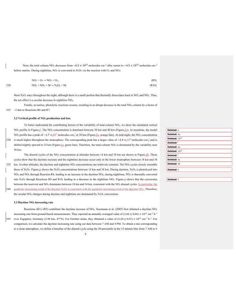
Next, the total column NO2 decreases from ~6.5 × 10 molecules cm–2 after sunset to ~4.5 × 10 molecules cm–2

before sunrise. During nighttime, NO2 is converted to N2O5 via the reaction with O3 and NO3:

NO2 + O3 → NO3 + O2, (R9)

NO2 + NO3 + M → N2O5 + M. (R10) 320

Most N2O5 stays throughout the night, although there is a small portion that thermally dissociates back to NO2 and NO3. Thus,

the net effect is a secular decrease in nighttime NO2.

Finally, at sunrise, photolytic reactions resume, resulting in an abrupt decrease in the total NO2 column by a factor of

~2 due to Reactions R6 and R7. 325

3.2 Vertical profile of NO2 production and loss

To better understand the contributing factors of the variability of total column NO2, we show the simulated vertical

NO2 profile in Figure 5. The NO2 concentration is dominant between 20 km and 40 km (Figure 5a). At noontime, the model

NO2 profile has a peak of ~1.7 × 10 molecules cm–3 at 30 km (Figure 5a, orange line). At mid-night, the NO2 concentration

is much higher throughout the stratosphere. The corresponding peak has a larger value of ~2.4 × 10 molecules cm–3 and is 330

shifted slightly upward to 32 km (Figure 5a, green line). Therefore, the total column NO2 is dominated by the variability near

30 km.

The diurnal cycles of the NO2 concentration at altitudes between 14 km and 38 km are shown in Figure 5b. These

cycles show that the daytime increase and the nighttime decrease occur only in the lower stratosphere between 18 km and 34

km. At other altitudes, the daytime and nighttime NO2 concentrations are relatively constant. The NO2 cycles closely resemble 335

those of N2O5. Figure 6 shows the N2O5 concentrations between 14 km and 34 km. During daytime, N2O5 is photolyzed into

NO2 and NO3 through Reaction R4, leading to an increase in the daytime NO2; during nighttime, NO2 is thermally converted

into N2O5 through Reactions R9 and R10, leading to a decrease in the nighttime NO2. Figure 6 shows that the conversion

between the reservoir and NO2 dominates between 18 km and 34 km, consistent with the NO2 diurnal cycles. In particular, the

quadratic decreasing trend of the daytime N2O5 is consistent with the quadratic increasing trend of the daytime NO2. Therefore, 340

the secular NO2 changes during daytime and nighttime are dominated by N2O5 conversions.

3.3 Daytime NO2 increasing rate

Reactions (R1)–(R5) contribute the daytime increase of NO2. Sussmann et al. (2005) first obtained a daytime NO2

increasing rate from ground-based measurements. They reported an annually averaged value of (1.02 ± 0.06) × 10 cm–2 h–1

over Zugspitze, Germany (2.96 km, 47°N). For October alone, they obtained a value of (1.20 ± 0.57) × 10 cm–2 h–1. For 345

comparison, we calculate the daytime increasing rate using our data between 7 AM and 4 PM. To obtain a rate corresponding

to a clean atmosphere, we define a baseline of the diurnal cycle using the 20-percentile in the 15-minute bins from 7 AM to 4

Deleted: 4Deleted: 4a

Deleted: 10Deleted: 2

Deleted: 4a

Deleted: 10Deleted: 2

Deleted: 4a

Deleted: 4b

Deleted: 5

Deleted: 5

10

PM (Figure 7). This results in a total of 37 bins, which is roughly the number of points in October shown in Figure 4a of

Sussmann et al. (2005). We then apply the linear regression to the baseline and obtain an increasing rate of 360 (1.31 ± 0.41) × 10 cm–2 h–1 in October over TMF (34.4°N). Thus our value is consistent with Sussmann et al.’s (2005) value.

3.4 Temperature sensitivity

While the 1-D model simulation captures most of the observed diurnal variability, the rate of decrease in the total

NO2 column during nighttime is slightly overestimated in the model. Here we explore a possible uncertainty due to the

prescribed temperature profile. 365

The chemical kinetic rates in the model are dependent on temperature. The temperature profile that has been used to

obtain the baseline diurnal cycle corresponds to a zonal mean temperature profile at the equinox and 30° latitude (Figure 8,

solid line). To test the sensitivity of the simulated 24-hour cycle of NO2 column, we reduce the input temperature below 60

km by 5 K (Figure 8, dashed line). Note that the 5 K reduction is much larger than the observed tidal variation in stratospheric

temperature below 50° latitude, which is ~0.1 K in the lower stratosphere and ~1 K in the middle stratosphere (Sakazaki et al., 370

2012). We choose this exaggerated reduction in order to clearly show the temperature effect on the NO2 chemistry.

Figure 4b (dash-dotted line) shows the simulated NO2 column using the reduced temperature profile. Because of the

reduction in temperature, the nighttime loss due to the reactions with O3 and NO3 through Reactions R9 and R10 is slower. As

a result, the simulated nighttime NO2 column is higher than the baseline simulation but the rate of decrease agrees better with

the observations. On the other hand, due to the less efficient reaction NO + O3, the simulated daytime NO2 column is slightly 375

lower than the baseline simulation but it still agrees with the daytime observation. Thus, while the equinox temperature profile

used in the baseline run is sufficient for the simulation of the diurnal cycle of the NO2 column, we do not exclude possible

effects of temperature uncertainties on the nighttime simulation.

3.5 Back-trajectories

Since the TMF is located at the top of a mountain in a remote area, high values of column NO2 measured on October 380

27, 2018, were likely due to atmospheric transport of urban pollutants from nearby cities, especially the Los Angeles megacity.

While chemical processes would quantitatively alter the amount of NO2 to be observed over TMF, a back-trajectory study

suffices to provide evidence on how the urban pollutants may be transported to TMF.

Figure 9 shows the 24-hour back-trajectories that eventually reached TMF (2.286 km above sea level) at 3 PM during

the observational period. These back-trajectories are calculated using the National Oceanic and Atmospheric Administration 385

(NOAA)’s Hybrid Single Particle Lagrangian Integrated Trajectory (HYSPLIT) model (Stein et al., 2015). We use wind fields

from the National Centres for Environmental Prediction (NCEP)’s North American Mesoscale (NAM) assimilation at a

horizontal resolution of 12 km. To illustrate the wind speed, we plot the 6-hour intervals using the black dots on the trajectories.

The trajectories on 4 of the 6 days (October 23–26) during the observational period converged towards TMF from

inland in the north and the east. These inland areas are behind the San Gabriel and San Bernardino Mountain Ranges and are 390

Deleted: 6Deleted: 3a

Deleted: 29Deleted: 30

Deleted: 7

Deleted: 7

Deleted: 3

Deleted: it still

Deleted: spread of the nighttime

Deleted: In addition

Deleted: Thus, given that the tidal temperature change in the middle atmosphere is much smaller than the change in the sensitivity test,…

Deleted: 8

11

shielded from the urbanized Los Angeles basin. Therefore, the total column NO2 measured over TMF on these days closely 405

follow the clean atmosphere simulated by the 1-D model. The trajectories on the other 2 days (October 27–28) converged

towards TMF from the Los Angeles basin in the southwest. But these 2 trajectories were very different. The back-trajectory

of October 27 (Figure 9, orange) started going southwestward from the Mojave Desert north of the San Bernardino Mountains

at the 24-hour point and passed across the Riverside Basin between the Santa Ana Mountains and San Jacinto Mountains at

18-hour point. The Riverside Basin is one of the most polluted areas in the United States. Then the trajectory continued 410

southwest to pass across the Orange County at the 12-hour point before it turned northwestward towards Downtown Los

Angeles at the 6-hour point. Finally, the trajectory turned northeastward and reached TMF. The wind speed over the Los

Angeles basin on October 27 was slower than those in other days, favouring more accumulation of pollutants over the Basin.

Thus, the 24-hour back-trajectory on October 27 transported the pollutants in the Riverside Basin and the Los Angeles basin,

resulting a significant surplus of NO2 in the TMF observation as seen in Figure 4. In contrast, the trajectory on October 28, 415

(Figure 9, purple) came directly from the Pacific Ocean at a relatively high speed, spending only ~4 hours in the Los Angeles

basin before reaching TMF. However, our measurement on October 28 stopped at noon due to a change in instruments and we

are unable to verify whether the urban source would elevate the total column NO2 in that evening.

4 Summary

We have presented the diurnal measurements of total column NO2 that has been made over the TMF located in 420

Wrightwood, California (2.286 km, 34.38°N, 117.68°W) from October 23 to October 28, 2018. The instrument measures the

differential slant column NO2 relative a reference spectrum at the noontime. To retrieve total column NO2 in the reference

spectrum, we applied a variant of the Langley extrapolation. The conventional Langley extrapolation assumes a constant

column throughout the day, which does not hold for NO2. To properly consider the time-dependency of column NO2, we

combine two methods independently developed by Lee et al. (1994) and Herman et al. (2009). The combined method, called 425

the modified minimum-amount Langley extrapolation (MMLE), first obtains a baseline of the observed diurnal cycle, which

is assumed to be the diurnal cycle in a clean atmosphere. Then the baseline is fitted against the modelled diurnal cycle in a 1-

D photochemical model so that the column NO2 in the reference spectrum is given by the y-intercept of the fitted line.

The measured 24-hour cycle of the TMF total column NO2 on clean days agrees well with a 1-D photochemical model

calculation. Our model simulation suggests that the observed monotonic increase of daytime NO2 column is primarily due to 430

the photodissociation of N2O5 in the reservoir. From our measurements, we obtained a daytime NO2 increasing rate of (1.31 ± 0.41) × 10 cm–2 h–1, which is consistent with the value observed by Sussmann et al. (2005), who reported a daytime

NO2 increasing rate of (1.20 ± 0.57) × 10 over Zugspitze, Germany (2.96 km, 47°N). Our model also suggests that during

nighttime, the monotonic decrease of NO2 is primarily due to the production of N2O5. Furthermore, the abrupt NO2 decrease

and increase at sunrise and subset, respectively, are due to the activation and deactivation of the NO2 photodissociation. 435

Deleted: Basin

Deleted: Basin

Deleted: On October 28, the trajectory (Figure 8, purple) came directly from the Pacific Ocean at a relatively high speed, spending only ~4 hours in the Los Angeles Basin before reaching TMF. This fast sea breeze helped reduce the level of accumulated pollutants over the Los Angeles Basin. As a result, the NO2 level measured at TMF on October 28 was also similar to a clean atmosphere. In contrast, the…

Deleted: 8

Deleted: Basin

Deleted: Basin

Deleted: 3

Deleted: model-based

Deleted: ,

Deleted: 29Deleted: 30

12

The total column NO2 in the afternoon on October 27, 2018 was much higher than the model simulation. We

conducted a 24-hour HYSPLIT back-trajectory analysis to study how urban pollutants were transported from the Los Angeles

basin. The back-trajectories in 4 of the 6 days during the measurement period went directly from inland desert areas to the 455

TMF. The back-trajectory in another day came from the southwest coastline, spending less than 6 hours over the Los Angeles

basin before reaching the TMF. Lastly, the 24-hour back-trajectory on October 27, 2018 was characterized by a unique slow

wind that came from inland in the northeast and spent more than 18 hours in the Los Angeles basin, picking up pollutants from

Riverside, Orange County, and finally Downtown Los Angeles before reaching TMF.

Appendix A. Comparison of the modified MLE (MMLE) with the standard MLE 460

The MMLE is used to account for the diurnal asymmetry of the stratospheric NO2 column before the Langley

extrapolation is applied. To illustrate the necessity of the removal of the diurnal asymmetry, consider a single day of observed

total column NO2. Figure A1a plots the observations on October 25, 2018 against the air mass factor (AMF = sec 𝜃) as in a

standard MLE. Based on our back-trajectory analysis, the atmosphere above TMF on October 25, 2018 should have little urban

NO2 contamination. Both solar (pale orange dots) and lunar (pale blue dots) data exhibit U-shapes that is due to the secular 465

increase and decrease during the daytime and the nighttime, respectively. For the solar data, the AM data lies on the lower arm

of the U-shape and the PM data lies on the upper arm. For the lunar data, the reverse is true: data before sunrise lie on the

upper arm of the U shape and data after sunset lie on the lower arm.

To perform a Langley extrapolation for the data shown in Figure A1a, one needs to decide which of the four arms to

be used for the linear regression model 𝑦 = 𝑎 AMF + 𝑏. The Principle of Minimum-amount suggests that we should start with 470

the lowest arm, i.e. the daytime AM data. Note that in order to obtain the straight line passing through the 2-percentile baseline,

we have ignored the points before noon (around 10 AM to 11:30 AM), i.e. points located around the bottom of the U-shape. If

we use the observations between 6 AM and 10 AM, we obtain the purple line in Figure A1a, which gives a y-intercept of (−4.12 ± 0.14) × 10 molecules cm−2.

The above Langley extrapolation, however, does not take any of the daytime PM and all lunar data into account. In 475

particular, the daytime PM data should also be used to define a minimum-amount profile, given the fact that the atmosphere

was mostly clean on that day. Suppose we perform another Langley extrapolation using the daytime PM data between 12 PM

and 5 PM (rose line). The resultant y-intercept is (−5.25 ± 0.27) × 10 molecules cm−2 (2-𝜎), which is statistically different

from the value obtained using the daytime AM data. A reasonable estimate of the y-intercept is then the average of the two

values, which is (−4.69 ± 0.21) × 10 molecules cm−2. 480

Finally, since the wind on the TMF is mostly downhill during autumn, the lunar data also correspond to a clean

atmosphere and should also be used to derive the y-intercept. If we use all four arms in Figure A1a, then the average value of

the y-intercept is (−4.36 ± 0.25) × 10 molecules cm−2, where the uncertainty is the root-mean-squares of the uncertainties

of the four values.

Deleted: Basin

Deleted: Basin

Deleted: Basin

13

In the above calculation, the ignorance of the data points near the bottom of the “U”-shape has excluded a large

number of observations near local solar/lunar noon and thus the resultant y-intercept is biased by high zenith angles. It is not

clear how the data near the solar/lunar noon may be kept in the standard MLE due to the assumption of the linearity in AMF. 490

As a result, a zenith angle-dependent Langley extrapolation model needs to be developed.

The above example shows that the determination of the y-intercept of the standard MLE is not straightforward when

(i) the background NO2 has secular trends in daytime and nighttime and (ii) the daytime and nighttime abundances are different

before and after the terminator. In contrast, the MMLE approach we have developed in this work minimizes the background

diurnal asymmetry, so that the “regularized” data points almost form a straight line (Figure A1b) when they are plotted against 495

the modelled diurnal cycle. The linear regression model 𝑦 = 𝑎 𝑚 𝑥 + 𝑏, where 𝑚 𝑥 is the modelled slant column NO2, can

be applied to all data points, regardless of the time of the day or whether the data point is a solar or lunar measurement. With

this modified MLE, the regressed y-intercept is (−5.22 ± 0.14) × 10 molecules cm−2, which is statistically different from

the average of the values derived from the four arms in the standard MLE approach.

The issue with the standard MLE is exacerbated when observations on multiple days are plotted against the AMF. 500

The U-shape may be smeared vertically into a continuum (Figure A1c). The smearing, in our case, are primarily due to natural

variability of the background, except for October 27 when total column NO2 appears above the continuum of the daytime data

due to the urban pollution. As a result, while we are still able to define the minimum-amount profile (5-percentile) for the

daytime AM data, the determination of the minimum-amount profiles of the daytime PM and the lunar data are difficult. This

leaves us the daytime AM data alone for the Langley extrapolation (red line) but, as shown above, the resultant y-intercept 505

[(−4.10 ± 0.46) × 10 molecules cm−2] may be biased.

In contrast, the observed data points still almost form a straight line in the MMLE approach when they are plotted

against the modelled diurnal cycle (Figure A1d). This allows the determination of the minimum-amount profile using all solar

and lunar measurements (raspberry line). The resultant y-intercept, (−6.09 ± 0.65) × 10 molecules cm−2, is again

statistically different from the one obtained using the standard MLE approach. 510

Appendix B. Effects of spherical geometry in the 1D model

The diurnal cycle simulated in the 1D model (Figure 3) is calculated assuming a plane-parallel atmosphere, where

the times of the sunrise and the sunset do not depend on altitude. For a more realistic simulation, we have conducted another

calculation using the spherical geometry, so that the terminator chemistry is dependent on altitude. Figure B1 compare the

simulated diurnal cycles in a plane-parallel atmosphere and in a spherical atmosphere. The difference between the two diurnal 515

cycles is the largest in the evening but it is much smaller than the spread of the observations due to the natural variability.

Therefore, the simulation with a plane-parallel atmosphere is adequate to provide a theoretical diurnal cycle for the modified

Langley extrapolation.

14

Acknowledgements. The assistance of George Mount (Washington State University) in Langley analysis is greatly 520

appreciated. KFL thanks Sally Newman and Tracy Xia (Bay Area Air Quality Management District) for their assistance in

setting up and executing the HYSPLIT model. RK was an undergraduate research assistant under the supervision of KFL. We

thank Ralf Sussmann for handling our manuscript and providing useful comments. Financial support. Support from the NASA SAGE-III/ISS Validation, Upper Atmosphere Research and Tropospheric 525

Composition Programs is gratefully acknowledged. YLY was supported in part by NASA grant P1847132 via UCLA. RK

thanks the generous supports from the AGU Student Travel Grant Award and the Marsh Environmental Sciences Travel Award

by the University of California, Riverside.

Data availability. The differential slant column NO2 used in this paper can be obtained from the supplement of this article. 530

Supplement. The supplement related to this article is available online.

Author contributions. KFL and TJP prepared the manuscript, with significant conceptual input from SPS and YLY, and

critical feedback from all the co-authors. SPS and TJP designed and operated the instrument at the Table Mountain. TJP 535

retrieved the slant column NO2 from the spectra and developed the Langley method. KFL and YLY performed the model

simulations. RK analysed some of the observational and model data. Competing interests. The authors declare that they have no conflict of interest.

References 540

Allen, M., Yung, Y. L., and Waters, J. W.: Vertical transport and photochemistry in the terrestrial mesosphere and lower

thermosphere (50–120 km), J. Geophys. Res., 86, 3617–3627, doi:10.1029/JA086iA05p03617, 1981.

Allen, M., Lunine, J. I., and Yung, Y. L.: The vertical-distribution of ozone in the mesosphere and lower thermosphere, J.

Geophys. Res., 89, 4841–4872, doi:10.1029/JD089iD03p04841, 1984.

Ångström, A.: Apparent solar constant variations and their relation to the variability of atmospheric transmission, Tellus, 22, 545

205–218, doi:10.3402/tellusa.v22i2.10215, 1970.

Barreto, A., Roman, R., Cuevas, E., Berjon, A. J., Almansa, A. F., Toledano, C., Gonzalez, R., Hernandez, Y., Blarel, L.,

Goloub, P., Guirado, C., and Yela, M.: Assessment of nocturnal aerosol optical depth from lunar photometry at the Izana

high mountain observatory, Atmos. Meas. Tech., 10, 3007–3019, doi:10.5194/amt-10-3007-2017, 2017.

Deleted: https://

Deleted: .org/

Deleted: https://

Deleted: .org/

Deleted: https://

Deleted: .org/

Deleted: ,Deleted: https://

Deleted: .org/

15

Bhartia, P. K., Taylor, S., McPeters, R. D., and Wellemeyer, C.: Application of the Langley plot method to the calibration of

the solar backscattered ultraviolet instrument on the Nimbus-7 satellite, J. Geophys. Res. Atmos., 100, 2997–3004, 560

doi:10.1029/94JD03072, 1995.

Burkholder, J. B., Sander, S. P., Abbatt, J., Barker, J. R., Huie, R. E., Kolb, C. E., Kurylo, M. J., Orkin, V. L., Wilmouth, D.

M., and Wine, P. H.: Chemical Kinetics and Photochemical Data for Use in Atmospheric Studies, Evaluation No. 18, JPL

Publication 15-10, Jet Propulsion Laboratory, Pasadena, 2015.

Cachorro, V. E., Toledano, C., Berjón, A., de Frutos, A. M., and Sorribas, M.: Comment on "On Langley plots in the presence 565

of a systematic diurnal aerosol cycle centered at noon: A comment on recently proposed methodologies'' by F. Marenco, J.

Geophys. Res. Atmos., 113, D11210, doi:10.1029/2007JD009137, 2008.

Camy-Peyret, C.: Balloon-borne infrared Fourier Transform spectroscopy for measurements of atmospheric trace species,

Spectrochim. Acta A, 51, 1143–1152, doi:10.1016/0584-8539(94)00145-2, 1995.

Chen, C. M., Cageao, R. P., Lawrence, L., Stutz, J., Salawitch, R. J., Jourdain, L., Li, Q., and Sander, S. P.: Diurnal variation 570

of midlatitudinal NO3 column abundance over table mountain facility, California, Atmos. Chem. Phys., 11, 963–978,

doi:10.5194/acp-11-963-2011, 2011.

Crutzen, P. J.: The influence of nitrogen oxides on atmospheric ozone content, Q. J. R. Meteorol. Soc., 96, 320–325,

doi:10.1002/qj.49709640815, 1970.

Fiedler, M., Frank, H., Gomer, T., Hausmann, M., Pfeilsticker, K., and Platt, U.: Ground-based spectroscopic measurements 575

of stratospheric NO2 and OClO in Arctic winter 1989/90, Geophys. Res. Lett., 20, 963–966, doi:10.1029/92GL00088,

1993.

Flaud, J. M., Camypeyret, C., Brault, J. W., Rinsland, C. P., and Cariolle, D.: Nighttime and daytime variation of atmospheric

NO2 from ground-based infrared measurements, Geophys. Res. Lett., 15, 261–264, doi:10.1029/GL015i003p00261, 1988.

Folkner, W. M., Williams, J. G., Boggs, D. H., Park, R. S., and Kuchynka, P.: The Planetary and Lunar Ephemerides DE430 580

and DE431, JPL Interplanetary Network Progress Report, accessible at http://ipnpr.jpl.nasa.gov/progress_report/42-

196/196C.pdf, 42-196, 2014.

Gordon, I. E., Rothman, L. S., Hill, C., Kochanov, R. V., Tan, Y., Bernath, P. F., Birk, M., Boudon, V., Campargue, A.,

Chance, K. V., Drouin, B. J., Flaud, J. M., Gamache, R. R., Hodges, J. T., Jacquemart, D., Perevalov, V. I., Perrin, A.,

Shine, K. P., Smith, M. A. H., Tennyson, J., Toon, G. C., Tran, H., Tyuterev, V. G., Barbe, A., Császár, A. G., Devi, V. 585

M., Furtenbacher, T., Harrison, J. J., Hartmann, J. M., Jolly, A., Johnson, T. J., Karman, T., Kleiner, I., Kyuberis, A. A.,

Loos, J., Lyulin, O. M., Massie, S. T., Mikhailenko, S. N., Moazzen-Ahmadi, N., Müller, H. S. P., Naumenko, O. V.,

Nikitin, A. V., Polyansky, O. L., Rey, M., Rotger, M., Sharpe, S. W., Sung, K., Starikova, E., Tashkun, S. A., Vander

Auwera, J., Wagner, G., Wilzewski, J., Wcislo, P., Yu, S., and Zak, E. J.: The HITRAN2016 molecular spectroscopic

database, J. Quant. Spectrosc. Radiat. Transfer, 203, 3−69, doi:10.1016/j.jqsrt.2017.06.038, 2017. 590

Deleted: https://

Deleted: .org/

Deleted: https://

Deleted: .org/

Deleted: https://

Deleted: .org/

Deleted: https://

Deleted: .org/

Deleted: https://

Deleted: .org/

Deleted: https://

Deleted: .org/

Deleted: https://

Deleted: .org/

16

Herman, J., Cede, A., Spinei, E., Mount, G., Tzortziou, M., and Abuhassan, N.: NO2 column amounts from ground-based 605

Pandora and MFDOAS spectrometers using the direct-sun DOAS technique: Intercomparisons and application to OMI

validation, J. Geophys. Res. Atmos., 114, D13307, doi:10.1029/2009JD011848, 2009.

Hofmann, D., Bonasoni, P., Demaziere, M., Evangelisti, F., Giovanelli, G., Goldman, A., Goutail, F., Harder, J., Jakoubek, R.,

Johnston, P., Kerr, J., Matthews, W. A., Mcelroy, T., Mckenzie, R., Mount, G., Platt, U., Stutz, J., Thomas, A.,

Vanroozendael, M., and Wu, E.: Intercomparison of UV/visible spectrometers for measurements of stratospheric NO2 for 610

the Network for the Detection of Stratospheric Change, J. Geophys. Res. Atmos., 100, 16765−16791,

doi:10.1029/95JD00620, 1995.

Hönninger, G., von Friedeburg, C., and Platt, U.: Multi axis differential optical absorption spectroscopy (MAX-DOAS),

Atmos. Chem. Phys., 4, 231–254, doi:10.5194/acp-4-231-2004, 2004.

Huber, M., Blumthaler, M., Ambach, W., and Staehelin, J.: Total atmospheric ozone determined from spectral measurements 615

of direct solar UV irradiance, Geophys. Res. Lett., 22, 53–56, doi:10.1029/94GL02836, 1995.

Iwagami, N., Inomata, S., Murata, I., and Ogawa, T.: Doppler detection of hydroxyl column abundance in the middle

atmosphere, J. Atmos. Chem., 20, 1–15, doi:10.1007/BF01099915, 1995.

Jeong, U., Tsay, S. C., Pantina, P., Butler, J. J., Loftus, A. M., Abuhassan, N., Herman, J. R., Dimov, A., Holben, B. N., and

Swap, R. J.: Langley Calibration Analysis of Solar Spectroradiometric Measurements: Spectral Aerosol Optical Thickness 620

Retrievals, J. Geophys. Res. Atmos., 123, 4221–4238, doi:10.1002/2017JD028262, 2018.

Johnston, P. V., and McKenzie, R. L.: NO2 observations at 45°S during the decreasing phase of Solar Cycle 21, from 1980 to

1987, J. Geophys. Res. Atmos., 94, 3473–3486, doi:10.1029/JD094iD03p03473, 1989.

Johnston, P. V., McKenzie, R. L., Keys, J. G., and Matthews, W. A.: Observations of depleted stratospheric NO2 following

the Pinatubo volcanic eruption, Geophys. Res. Lett., 19, 211–213, doi:10.1029/92GL00043, 1992. 625

Keys, J. G., and Johnston, P. V.: Stratospheric NO2 and O3 in Antarctica: Dynamic and chemically controlled variations,

Geophys. Res. Lett., 13, 1260–1263, doi:10.1029/GL013i012p01260, 1986.

Kreher, K., Van Roozendael, M., Hendrick, F., Apituley, A., Dimitropoulou, E., Frieß, U., Richter, A., Wagner, T., Lampel,

J., Abuhassan, N., Ang, L., Anguas, M., Bais, A., Benavent, N., Bösch, T., Bognar, K., Borovski, A., Bruchkouski, I., Cede,

A., Chan, K. L., Donner, S., Drosoglou, T., Fayt, C., Finkenzeller, H., Garcia-Nieto, D., Gielen, C., Gómez-Martín, L., 630

Hao, N., Henzing, B., Herman, J. R., Hermans, C., Hoque, S., Irie, H., Jin, J., Johnston, P., Butt, J. K., Khokhar, F., Koenig,

T. K., Kuhn, J., Kumar, V., Liu, C., Ma, J. Z., Merlaud, A., Mishra, A. K., Müller, M., Navarro-Comas, M., Ostendorf, M.,

Pazmino, A., Peters, E., Pinardi, G., Pinharanda, M., Piters, A., Platt, U., Postylyakov, O., Prados-Roman, C., Puentedura,

O., Querel, R., Saiz-Lopez, A., Schönhardt, A., Schreier, S. F., Seyler, A., Sinha, V., Spinei, E., Strong, K., Tack, F., Tian,

X., Tiefengraber, M., Tirpitz, J. L., van Gent, J., Volkamer, R., Vrekoussis, M., Wang, S., Wang, Z., Wenig, M., Wittrock, 635

F., Xie, P. H., Xu, J., Yela, M., Zhang, C., and Zhao, X. Y.: Intercomparison of NO2, O4, O3 and HCHO slant column

measurements by MAX-DOAS and zenith-sky UV-visible spectrometers during CINDI-2, Atmos. Meas. Tech., 13, 2169–

2208, doi:10.5194/amt-13-2169-2020, 2020.

Deleted: https://

Deleted: .org/

Deleted: https://

Deleted: .org/

Deleted: https://

Deleted: .org/

Deleted: https://

Deleted: .org/

Deleted: https://

Deleted: .org/

Deleted: https://

Deleted: .org/

Deleted: https://

Deleted: .org/

Deleted: https://

Deleted: .org/

17

Kreuter, A., Wuttke, S., and Blumthaler, M.: Improving Langley calibrations by reducing diurnal variations of aerosol 655

Ångström parameters, Atmos. Meas. Tech., 6, 99–103, doi:10.5194/amt-6-99-2013, 2013.

Langley, S. P.: The "solar constant" and related problems, Astrophys. J., 17, 89–99, doi:10.1086/140999, 1903.

Lee, A. M., Roscoe, H. K., Oldham, D. J., Squires, J. A. C., Sarkissian, A., Pommereau, J. P., and Gardiner, B. G.:

Improvements to the accuracy of measurements of NO2 by zenith-sky visible spectrometers, J. Quant. Spectrosc. Radiat.

Transfer, 52, 649–657, doi:10.1016/0022-4073(94)90031-0, 1994. 660

Long, C. N., and Ackerman, T. P.: Identification of clear skies from broadband pyranometer measurements and calculation of

downwelling shortwave cloud effects, J. Geophys. Res. Atmos., 105, 15609–15626, doi:10.1029/2000JD900077, 2000.

Marenco, F.: On Langley plots in the presence of a systematic diurnal aerosol cycle centered at noon: A comment on recently

proposed methodologies, J. Geophys. Res. Atmos., 112, D06205, doi:10.1029/2006JD007248, 2007.

May, R. D., and Webster, C. R.: Balloon-borne laser spectrometer measurements of NO2 with gas-absorption sensitivities 665

below 10-5, Appl. Optics, 29, 5042–5045, doi:10.1364/AO.29.005042, 1990.

Moreau, G., Robert, C., Catoire, V., Chartier, M., Camy-Peyret, C., Huret, N., Pirre, M., Pomathiod, L., and Chalumeau, G.:

SPIRALE: a multispecies in situ balloonborne instrument with six tunable diode laser spectrometers, Appl. Optics, 44,

5972–5989, doi:10.1364/AO.44.005972, 2005.

Newcomb, S.: Tables of the Sun, Astron. Pap. Amer. Ephem. VI, Part I, 7−170, 1898. 670

Nizkorodov, S. A., Sander, S. P., and Brown, L. R.: Temperature and pressure dependence of high-resolution air-broadened

absorption cross sections of NO2 (415–525 nm), J. Phys. Chem. A, 108, 4864–4872, doi:10.1021/jp049461n, 2004.

Noxon, J. F.: Nitrogen dioxide in stratosphere and troposphere measured by ground-based absorption spectroscopy, Science,

189, 547−549, doi:10.1126/science.189.4202.547, 1975.

Noxon, J. F., Whipple, E. C., and Hyde, R. S.: Stratospheric NO2. Part I. Observational method and behavior at mid-latitude, 675

J. Geophys. Res. Oceans, 84, 5047–5065, doi:10.1029/JC084iC08p05047, 1979.

Piters, A. J. M., Boersma, K. F., Kroon, M., Hains, J. C., Van Roozendael, M., Wittrock, F., Abuhassan, N., Adams, C.,

Akrami, M., Allaart, M. A. F., Apituley, A., Beirle, S., Bergwerff, J. B., Berkhout, A. J. C., Brunner, D., Cede, A., Chong,

J., Clemer, K., Fayt, C., Frieß, U., Gast, L. F. L., Gil-Ojeda, M., Goutail, F., Graves, R., Griesfeller, A., Großmann, K.,

Hemerijckx, G., Hendrick, F., Henzing, B., Herman, J., Hermans, C., Hoexum, M., van der Hoff, G. R., Irie, H., Johnston, 680

P. V., Kanaya, Y., Kim, Y. J., Baltink, H. K., Kreher, K., de Leeuw, G., Leigh, R., Merlaud, A., Moerman, M. M., Monks,

P. S., Mount, G. H., Navarro-Comas, M., Oetjen, H., Pazmino, A., Perez-Camacho, M., Peters, E., du Piesanie, A., Pinardi,

G., Puentedura, O., Richter, A., Roscoe, H. K., Schönhardt, A., Schwarzenbach, B., Shaiganfar, R., Sluis, W., Spinei, E.,

Stolk, A. P., Strong, K., Swart, D. P. J., Takashima, H., Vlemmix, T., Vrekoussis, M., Wagner, T., Whyte, C., Wilson, K.

M., Yela, M., Yilmaz, S., Zieger, P., and Zhou, Y.: The Cabauw Intercomparison campaign for Nitrogen Dioxide measuring 685

Instruments (CINDI): design, execution, and early results, Atmos. Meas. Tech., 5, 457–485, doi:10.5194/amt-5-457-2012,

2012.

Deleted: https://

Deleted: .org/

Deleted: https://

Deleted: .org/

Deleted: https://

Deleted: .org/

Deleted: https://

Deleted: .org/

Formatted: SuperscriptDeleted: https://

Deleted: .org/

Deleted: https://

Deleted: .org/

Deleted: https://

Deleted: .org/

Deleted: https://

Deleted: .org/

Formatted: SubscriptDeleted: https://

Deleted: .org/

18

Platt, U., Perner, D., and Patz, H. W.: Simultaneous measurement of atmospheric CH2O, O3, and NO2 by differential optical

absorption, J. Geophys. Res. Oceans Atmos., 84, 6329−6335, doi:10.1029/JC084iC10p06329, 1979.

Roscoe, H. K., Johnston, P. V., Van Roozendael, M., Richter, A., Sarkissian, A., Roscoe, J., Preston, K. E., Lambert, J. C.,

Hermans, C., Decuyper, W., Dzienus, S., Winterrath, T., Burrows, J., Goutail, F., Pommereau, J. P., D'Almeida, E., Hottier,

J., Coureul, C., Didier, R., Pundt, I., Bartlett, L. M., McElroy, C. T., Kerr, J. E., Elokhov, A., Giovanelli, G., Ravegnani, 710

F., Premuda, M., Kostadinov, I., Erle, F., Wagner, T., Pfeilsticker, K., Kenntner, M., Marquard, L. C., Gil, M., Puentedura,

O., Yela, M., Arlander, D. W., Hoiskar, B. A. K., Tellefsen, C. W., Tornkvist, K. K., Heese, B., Jones, R. L., Aliwell, S.

R., and Freshwater, R. A.: Slant column measurements of O3 and NO2 during the NDSC intercomparison of zenith-sky

UV-visible spectrometers in June 1996, J. Atmos. Chem., 32, 281–314, doi:10.1023/A:1006111216966, 1999.

Roscoe, H. K., Van Roozendael, M., Fayt, C., du Piesanie, A., Abuhassan, N., Adams, C., Akrami, M., Cede, A., Chong, J., 715

Clémer, K., Frieß, U., Ojeda, M. G., Goutail, F., Graves, R., Griesfeller, A., Grossmann, K., Hemerijckx, G., Hendrick, F.,

Herman, J., Hermans, C., Irie, H., Johnston, P. V., Kanaya, Y., Kreher, K., Leigh, R., Merlaud, A., Mount, G. H., Navarro,

M., Oetjen, H., Pazmino, A., Perez-Camacho, M., Peters, E., Pinardi, G., Puentedura, O., Richter, A., Schönhardt, A.,

Shaiganfar, R., Spinei, E., Strong, K., Takashima, H., Vlemmix, T., Vrekoussis, M., Wagner, T., Wittrock, F., Yela, M.,

Yilmaz, S., Boersma, F., Hains, J., Kroon, M., Piters, A., and Kim, Y. J.: Intercomparison of slant column measurements 720

of NO2 and O4 by MAX-DOAS and zenith-sky UV and visible spectrometers, Atmos. Meas. Tech., 3, 1629–1646,

doi:10.5194/amt-3-1629-2010, 2010.

Sakazaki, T., Fujiwara, M., Zhang, X., Hagan, M. E., and Forbes, J. M.: Diurnal tides from the troposphere to the lower

mesosphere as deduced from TIMED/SABER satellite data and six global reanalysis data sets, J. Geophys. Res. Atmos.,

117, D13108, doi:10.1029/2011JD017117, 2012. 725

Sanders, R. W., Solomon, S., Smith, J. P., Perliski, L., Miller, H. L., Mount, G. H., Keys, J. G., and Schmeltekopf, A. L.:

Visible and near-ultraviolet spectroscopy at McMurdo station, Antarctica. Part 9: Observations of OClO from April to

October 1991, J. Geophys. Res. Atmos., 98, 7219–7228, doi:10.1029/93JD00042, 1993.

Serdyuchenko, A., Gorshelev, V., Weber, M., Chehade, W., and Burrows, J. P.: High spectral resolution ozone absorption

cross-sections — Part 2: Temperature dependence, Atmos. Meas. Tech., 7, 625–636, doi:10.5194/amt-7-625-2014, 2014. 730

Shaw, G. E.: Error analysis of multi-wavelength sun photometry, Pure Appl. Geophys., 114, 1–14, doi:10.1007/BF00875487,

1976.

Solomon, S.: Stratospheric ozone depletion: A review of concepts and history, Rev. Geophys., 37, 275–316,

doi:10.1029/1999RG900008, 1999.

Spinei, E., Cede, A., Swartz, W. H., Herman, J., and Mount, G. H.: The use of NO2 absorption cross section temperature 735

sensitivity to derive NO2 profile temperature and stratospheric-tropospheric column partitioning from visible direct-sun

DOAS measurements, Atmos. Meas. Tech., 7, 4299–4316, doi:10.5194/amt-7-4299-2014, 2014.

Deleted: https://

Deleted: .org/

Deleted: https://

Deleted: .org/

Deleted: https://

Deleted: .org/

Deleted: https://

Deleted: .org/

Deleted: https://

Deleted: .org/

19

Stein, A. F., Draxler, R. R., Rolph, G. D., Stunder, B. J. B., Cohen, M. D., and Ngan, F.: NOAA's HYSPLIT atmospheric

transport and dispersion modeling system, Bull. Amer. Meteorol. Soc., 96, 2059–2077, doi:10.1175/BAMS-D-14-00110.1,

2015. 750

Stutz, J., and Platt, U.: Numerical analysis and estimation of the statistical error of differential optical absorption spectroscopy

measurements with least-squares methods, Appl. Optics, 35, 6041−6053, doi:10.1364/AO.35.006041, 1996.

Sussmann, R., Stremme, W., Burrows, J. P., Richter, A., Seiler, W., and Rettinger, M.: Stratospheric and tropospheric NO2

variability on the diurnal and annual scale: a combined retrieval from ENVISAT/SCIAMACHY and solar FTIR at the

Permanent Ground-Truthing Facility Zugspitze/Garmisch, Atmos. Chem. Phys., 5, 2657–2677, doi:10.5194/acp-5-2657-755

2005, 2005.

Thalman, R., and Volkamer, R.: Temperature dependent absorption cross-sections of O2–O2 collision pairs between 340 and

630 nm and at atmospherically relevant pressure, Phys. Chem. Chem. Phys., 15, 15371–15381, doi:10.1039/C3CP50968K,

2013.

Toledano, C., González, R., Fuertes, D., Cuevas, E., Eck, T. F., Kazadzis, S., Kouremeti, N., Gröbner, J., Goloub, P., Blarel, 760

L., Román, R., Barreto, Á., Berjón, A., Holben, B. N., and Cachorro, V. E.: Assessment of Sun photometer Langley

calibration at the high-elevation sites Mauna Loa and Izaña, Atmos. Chem. Phys., 18, 14555−14567, doi:10.5194/acp-18-

14555-2018, 2018.

Vandaele, A. C., Fayt, C., Hendrick, F., Hermans, C., Humbled, F., Van Roozendael, M., Gil, M., Navarro, M., Puentedura,

O., Yela, M., Braathen, G., Stebel, K., Tørnkvist, K., Johnston, P., Kreher, K., Goutail, F., Mieville, A., Pommereau, J. P., 765

Khaikine, S., Richter, A., Oetjen, H., Wittrock, F., Bugarski, S., Frieß, U., Pfeilsticker, K., Sinreich, R., Wagner, T., Corlett,

G., and Leigh, R.: An intercomparison campaign of ground-based UV-visible measurements of NO2, BrO, and OClO slant

columns: Methods of analysis and results for NO2, J. Geophys. Res. Atmos., 110, doi:10.1029/2004JD005423, 2005.

Wang, S., Pongetti, T. J., Sander, S. P., Spinei, E., Mount, G. H., Cede, A., and Herman, J.: Direct Sun measurements of NO2

column abundances from Table Mountain, California: Intercomparison of low- and high-resolution spectrometers, J. 770

Geophys. Res. Atmos., 115, D13305, doi:10.1029/2009JD013503, 2010.

Wang, S., Li, K.-F., Zhu, D., Sander, S. P., Yung, Y. L., Pazmino, A., and Querel, R.: Solar 11-Year cycle signal in

stratospheric nitrogen dioxide—Similarities and discrepancies between model and NDACC observations, Solar Phys., 295,

117, doi:10.1007/s11207-020-01685-1, 2020.

Woolard, E. W.: Theory of the rotation of the Earth around its center of mass, Astron. Pap. Amer. Ephem. XV, Part I, 1−165, 775

1953.

Deleted: NOAA’s

Deleted: https://

Deleted: .org/

Deleted: https://

Deleted: .org/

Deleted: https://

Deleted: .org/

Deleted: https://

Deleted: .org/

Deleted: https://

Deleted: .org/

20

Figure 1: Schematic of the instrument light path over the Table Mountain Facilities (TMF, 2.286 km above mean sea level, 34.38°N, 117.68°W), Wrightwood, California, USA. (a) Light is collected by the primary of the heliostat (tracker), reflected down to the telescope on the first floor which conditions it to a 7- cm diameter beam. (b) The light is then reflected to a condensing lens into a fibre optic bundle, past a shutter, order-sorting filter, and then into the spectrometer. The fibre bundle contains 19 fibres in a round pattern at the 795 entrance, and at the exit fibres are arranged in a line pattern that is set parallel to the spectrometer slit.

Deleted: Figure 2. The model-based minimum-amount Langley extrapolation.

21

Figure 2. An example of the QDOAS spectral fit on October 24, 2018. The measured spectrum is shown by the black curve on the left panel. The fitted spectrum (red) is overlaid and the residual spectrum (blue) is shown at the bottom. Four species are considered in the spectral fit: NO2, O3, O4, and H2O. The spectral fits are performed simultaneously in QDOAS. The red lines on the right column are the fitted spectra of the corresponding species. To visualize the signal-to-noise ratios, we add the residual spectrum (blue on the left panel) to 805 individual fitted spectra, which are shown as the black spectra in the subpanels on the right.

22

Figure 3. The modified minimum-amount Langley extrapolation (MMLE). The blue circles are the observed differential slant columns during our campaign over TMF from October 23 to October 28, 2018. Each observational value is plotted against the total slant column 810 modelled at the same time of the day (e.g. 11:05 AM PST). The green dots are the 5-percentile of 20 uniform bins on the 𝒙-axis. The red line is a linear regression of the green dots, which is taken as the background diurnal cycle in a clean atmosphere. The linear fit is 𝒚 =𝟎. 𝟖𝟖 𝒎 𝒙𝒂(𝒎) − 𝟔. 𝟎𝟗 × 𝟏𝟎𝟏𝟓 . The 2-𝝈 uncertainties of the slope and the intercept are 𝟎. 𝟎𝟒 and 𝟎. 𝟔𝟓 × 𝟏𝟎𝟏𝟓, respectively. The 𝒚-intercept thus gives a reference column, 𝒚𝟎 = 𝟔. 𝟎𝟗 × 𝟏𝟎𝟏𝟓 molecules cm–2. The inset shows the distribution of the 2-𝝈 uncertainty of the observed differential slant columns. 815

Deleted: 20

Deleted: 𝟓. 𝟕𝟕Deleted: the

Deleted: 𝟓. 𝟕𝟕

23

Figure 4: The total column NO2 abundance measured over TMF on October 23−28, 2018, represented by the color dots. The 1-D model simulation, with default input temperature and surface N2O being 330 ppb, representing October 26 is shown as the solid black line. (a) The total column NO2 measurements on individual dates. (b) The aggregated total column NO2 measurements as a function of local time. An additional 1-D model simulation with temperature below 60 km reduced by 5 K, is shown as the dashed line. 825

Deleted:

Deleted: 3

24

Figure 5: Simulated vertical NO2 concentration. (a) The simulated NO2 vertical concentration between 14−38 km at 00:00 PST (green) 830 and 12:00 PST (orange) corresponding to October 27 in the 1-D photochemical model. (b) Same as (a) except the simulated NO2 variation over the 24 hours at selected altitudes.

Deleted: 4

25

Figure 6. Same as Figure 5(b) except for N2O5. 835

Deleted: Figure 5.

Moved (insertion) [1]Deleted: 4

26

840

Figure 7. The daytime NO2 increase obtained from the baseline of the observed diurnal variability. The blue points are the same as the daytime data shown in Figure 4. The red points are the 20-percentile of the daytime data in 15-minute intervals between 7 AM to 4 PM, which form a baseline of the daytime variability. The daytime NO2 increase rate, obtained from the linear regression of the red points, is (𝟏. 𝟑𝟏 ± 𝟎. 𝟒𝟏) × 𝟏𝟎𝟏𝟒 cm–2 h–1.

845

Deleted:

Moved up [1]: Figure 6.

Deleted: 3

Deleted: 𝟐𝟗Deleted: 𝟑𝟎Formatted: Font: Not Bold

27

Figure 8: The temperature profiles used in the 1-D Caltech/JPL photochemical model: the baseline profile (solid line) based on the equinox zonal average at 30° latitude and the modified profile where the temperature below 60 km is reduced by 5 K (dash-dotted line). 855

Deleted: 7

28

Figure 9: The 24-hour back-trajectories of ambient air flow that reached TMF at 15:00 PST on each day from October 23 to October 28, 2018. The colour codes are the same as those used in Figure 4. The black dots represent the 6-hour intervals on the trajectories.

860

Deleted: 8Deleted: 3

29

Figure A1. Comparison of the standard MLE (a, c) and the modified MLE (MMLE) (b, d) introduced in this work for single-day (a, 865 b) and multiple-day data (c, d). Panel d is the same as Figure 3 except for the separation of the daytime and nighttime data.

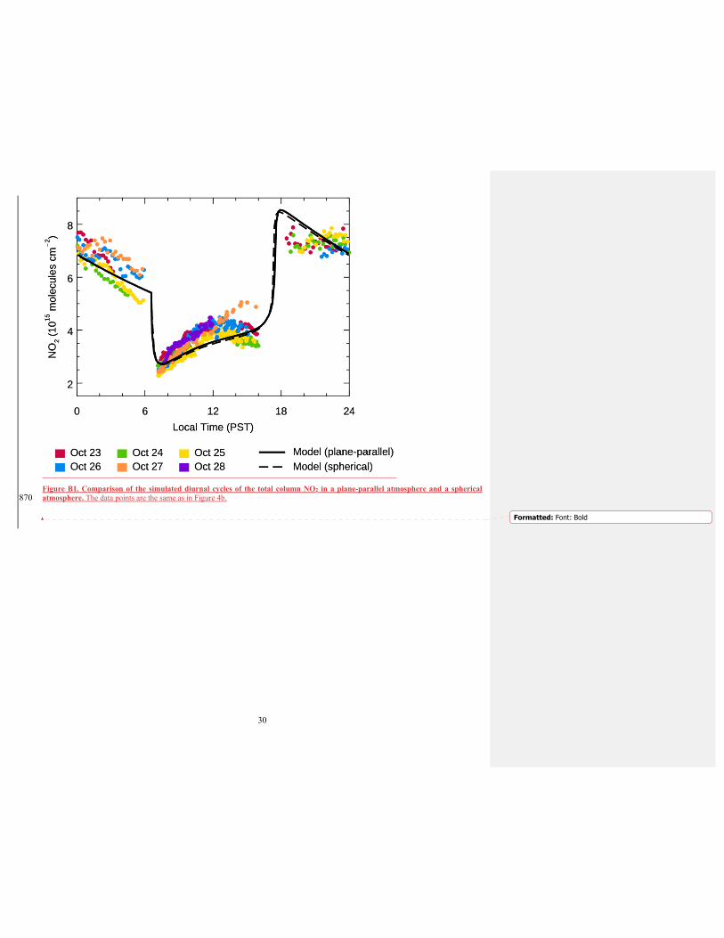
30

Figure B1. Comparison of the simulated diurnal cycles of the total column NO2 in a plane-parallel atmosphere and a spherical atmosphere. The data points are the same as in Figure 4b. 870

Formatted: Font: Bold