Table of Contents - Survey of India

1

Table of Contents

Topographical Hand Book – Digital Photogrammetry ................................................................................... 7

SECTION – 1 ........................................................................................................................................................... 7

1.1 Purpose ................................................................................................................................................. 7

1.2 Applicability .......................................................................................................................................... 7

1.3 Scope ..................................................................................................................................................... 7

1.4 References ............................................................................................................................................ 8

1.5 Trade Name Exclusions ....................................................................................................................... 8

1.6 Using the Chapter ................................................................................................................................ 8

SECTION – 2 .............................................................................................................................................................

Introduction to Digital Photogrammetry ....................................................................................................... 10

2.1 Definition ............................................................................................................................................ 10

2.2 Transition In Photogrammetry ........................................................................................................ 10

2.3 New Developments in Digital Photogrammetry ........................................................................... 11

2.4 Advantages of Digital Photogrammetry ........................................................................................ 12

2.5 Hardware and Software Configuration .......................................................................................... 13

2.6 Photogrammetric Software: ............................................................................................................ 14

2.7 Integration of Digital Photogrammetry and Gis ........................................................................... 15

2.8 Future Developments in Digital Photogrammetry ....................................................................... 15

2.9 Input in Digital (Softcopy) Photogrammetry: ................................................................................ 16

2.10 Specifications of a suitable hardware system for DPWS: ........................................................... 16

2.11 Few Standard Softwares: ................................................................................................................. 17

SECTION – 3 .............................................................................................................................................................

Principles of Digital Photogrammetry ............................................................................................................ 18

3.1 Coordinate Systems: ......................................................................................................................... 18

3.1.1 Pixel Coordinate System .................................................................................................................. 18

3.1.2 Image Coordinate System ................................................................................................................ 18

3.1.3 Image Space Coordinate System .................................................................................................... 19

3.1.4 Ground Coordinate System ............................................................................................................. 19

3.1.5 Geocentric and Topocentric Coordinate System .......................................................................... 20

3.2 Interior Orientation (IO) ................................................................................................................... 20

3.2.1 Principal Point and Focal Length ..................................................................................................... 20

3.2.2 Fiducial Marks.................................................................................................................................... 21

3.2.3 Lens Distortion .................................................................................................................................. 22

3.2.4 Theory of Interior Orientation ........................................................................................................ 23

3.2.5 Pixel to Fiducial co-ordinate Transformation: .............................................................................. 24

3.2.6 Refinement of Photo Co-ordinates: - ............................................................................................. 27

3.3 Exterior Orientation (EO): - .............................................................................................................. 28

3.4 Space Resection: ............................................................................................................................... 31

3.5 Block Triangulation: .......................................................................................................................... 33

3.5.1 Ground Control Points (GCPs): ........................................................................................................ 34

2

3.5.2 TIE Point: ............................................................................................................................................ 35

3.5.3 Image Matching Techniques ........................................................................................................... 36

3.5.4 Feature -based Matching: ................................................................................................................ 37

3.5.5 Relation based Matching: ................................................................................................................ 37

3.5.6 Formation of Simultaneous Equation: ........................................................................................... 37

3.5.7 Setting of Quality Indicators: ........................................................................................................... 39

3.6 Bundle Block Triangulation adjustment: ....................................................................................... 40

3.7 Principles of Satellite Photogrammetry ......................................................................................... 42

3.8 Collinearity Equations & Satellite Block Triangulation ................................................................ 47

3.9 Control for Satellite Block Triangulation ........................................................................................ 47

3.10 Introduction to Digital Orthophotography .................................................................................... 48

3.11 Orthorectification ............................................................................................................................. 49

3.12 Advantages of Digital Orthophotos ................................................................................................ 51

3.13 Other advantages/disadvantages of orthophotography: ........................................................... 51

3.14 Basic Components of an Orthoimage: ........................................................................................... 52

3.15 Digital Orthophoto Problems .......................................................................................................... 54

3.16 Conclusion: ......................................................................................................................................... 58

SECTION – 4 .............................................................................................................................................................

SCANNING ...............................................................................................................................................................

4.1 Introduction .................................................................................................................................... 60

4.2 Principles of Scanning .................................................................................................................... 60

4.3 Photogrammetric Scanners - Introduction ................................................................................. 66

4.3.1 Types of Photogrammetic Scanners ............................................................................................ 67

4.4 Scanning Resolution: ...................................................................................................................... 67

4.5 Scan process – Quality Assurance / Quality Control ................................................................. 69

SECTION – 5 .............................................................................................................................................................

DIGITAL TERRAIN MODEL ................................................................................................................................. 73

5.1 Introduction: ..................................................................................................................................... 73

5.3 Challenges in Generation of Accurate DEM/DTM ........................................................................ 73

5.4 DEM Acquisition Technologies ....................................................................................................... 74

5.4.1 Ground Surveying ............................................................................................................................. 74

5.4.2 Photogrammetry: .............................................................................................................................. 74

5.4.3 ALS or LIDAR: ..................................................................................................................................... 75

5.4.4 IFSAR .................................................................................................................................................. 76

5.4.5 Digitization of Topographic Maps ................................................................................................... 76

5.5 General Descriptions ........................................................................................................................ 77

5.5.1 Data Types ......................................................................................................................................... 77

5.5.1.1 System Data: ..................................................................................................................................... 77

5.5.1.2 Primary Data ..................................................................................................................................... 77

5.5.1.3 Derivative Data ................................................................................................................................. 77

5.6 Data Models ...................................................................................................................................... 77

5.6.1 Mass Points ....................................................................................................................................... 77

5.6.2 Breaklines .......................................................................................................................................... 77

3

5.6.3 Triangular Irregular Network (TIN) ................................................................................................. 78

5.6.4 Grids .................................................................................................................................................... 78

5.6.5 Contours ............................................................................................................................................. 78

5.6.6 Cross Sections .................................................................................................................................... 78

5.6.7 Other Product Types ......................................................................................................................... 79

5.7 Data Formats ...................................................................................................................................... 79

5.7.1 Digital Contour Lines and Breaklines .............................................................................................. 79

5.7.2 Mass Points and TINs ........................................................................................................................ 79

5.7.3 Common Lidar Data Exchange Format - .LAS ................................................................................ 79

5.7.4 Grid Elevations .................................................................................................................................. 79

5.8 PHASES OF DEM GENERATION IN DIGITAL PHOTOGRAMMETRY .............................................. 79

5.8.1 Data Collection .................................................................................................................................. 80

5.8.1.1 Sampling pattern ............................................................................................................................... 80

5.8.1.2 Sampling Density ............................................................................................................................... 80

5.8.1.3 Sampling Mode ................................................................................................................................. 80

5.8.1.4 Strings ................................................................................................................................................. 81

5.8.1.5 Breaklines ........................................................................................................................................... 81

5.8.1.6 Outlines .............................................................................................................................................. 81

5.9 Pre-Processing ................................................................................................................................... 81

5.10 Main Processing ................................................................................................................................ 81

5.11 Post-Processing ................................................................................................................................. 81

5.12 Horizontal and Vertical Data Standards ......................................................................................... 82

5.13 Testing and Reporting of Accuracy ................................................................................................. 83

5.13.1 Fundamental Accuracy ..................................................................................................................... 83

5.13.2 Supplemental and Consolidated Vertical Accuracies .................................................................. 83

5.13.3 95th Percentile .................................................................................................................................. 83

5.14 Reporting Vertical Accuracy of Untested Data ............................................................................. 85

5.15 Testing and Reporting Horizontal Accuracy .................................................................................. 85

5.16 Accuracy Assessment Summary ..................................................................................................... 85

5.17 Relative Vertical Accuracy ............................................................................................................... 86

5.18 Metadata Standards ......................................................................................................................... 86

5.19 Surface Treatment Factors .............................................................................................................. 86

5.19.1 Hydrography ...................................................................................................................................... 86

5.19.2 Man-made Structures ...................................................................................................................... 87

5.19.3 Special Earthen Features ................................................................................................................. 88

5.19.4 Artefacts ............................................................................................................................................. 88

5.19.5 Special Surfaces ................................................................................................................................. 88

5.20 Why DTMS are required? ................................................................................................................ 88

SECTION – 6 ......................................................................................................................................................... 91

LIDAR 91

6.1 Introduction .................................................................................................................................... 91

6.2 Laser ................................................................................................................................................... 91

6.3 Principle of LiDAR ............................................................................................................................. 92

4

6.4 Topographic LiDAR ......................................................................................................................... 92

6.5 Bathymetric LiDAR .......................................................................................................................... 94

6.6 Multiple return LiDAR .................................................................................................................... 95

6.7 Full waveform digitization ............................................................................................................. 96

6.8 Physical principle of LiDAR ............................................................................................................ 97

6.8.1 Continuous wave ranging .............................................................................................................. 97

6.8.2 Pulse ranging ................................................................................................................................... 98

6.8. 3 Laser pulse and nomenclature ..................................................................................................... 99

6.9 Time of Travel (ToT) measuring methods ................................................................................. 100

6.9.1 Constant fraction method ........................................................................................................... 100

6.9.2 Centroids of pulses ....................................................................................................................... 101

6.9.3 Correction using ratio of amplitudes ......................................................................................... 102

6.9.4 Correction using calibration ........................................................................................................ 102

6.10 Requirement of the laser for altimetric LiDAR ......................................................................... 103

6.11 LiDAR power and pulse firing rate ............................................................................................. 103

6.12 Geolocation of LiDAR footprint .................................................................................................. 103

6.13 Reference Systems ....................................................................................................................... 104

6.14 Process for geolocation ............................................................................................................... 104

6.15 LiDAR sensor and data characteristics....................................................................................... 106

6.15.1 Available sensors .......................................................................................................................... 106

6.15.2 LiDAR Scanning pattern ............................................................................................................... 106

6.15.4 Parallel line pattern ..................................................................................................................... 107

6.15.5 Elliptical pattern ........................................................................................................................... 107

6.15.6 Parallel lines-Toposys type ......................................................................................................... 108

6.15.7 Data density .................................................................................................................................. 108

6.16 Example LiDAR data ..................................................................................................................... 109

6.17 LiDAR error sources ...................................................................................................................... 110

6.18 Reporting LiDAR accuracy ........................................................................................................... 111

6.19 Application of airborne altimetric LiDAR .................................................................................. 111

6.19.1 Floods ............................................................................................................................................. 112

6.19.2 Coastal applications ..................................................................................................................... 112

6.19.3 Bathymetric applications ............................................................................................................ 112

6.19.4 Glacier and Avalanche ................................................................................................................. 112

6.19.5 Landslides ...................................................................................................................................... 112

6.19.6 Forest mapping ............................................................................................................................. 112

6.19.7 Urban applications ....................................................................................................................... 113

6.19.9 Mining ............................................................................................................................................ 114

6.19.10 Corridor mapping ......................................................................................................................... 114

6.19.11 Transmission line mapping ......................................................................................................... 114

6.20 Advantages of LiDAR technology .............................................................................................. 115

SECTION 7 117

Photogrammetric Accuracy Standards ......................................................................................................... 117

7.1 General ......................................................................................................................................... 117

5

7.2 Photogrammetric Mapping Standard ........................................................................................ 121

7.4 Aerotriangulation accuracy standards ....................................................................................... 124

7.5 Orthophoto and Orthophoto Map Accuracy Standards ......................................................... 124

SECTION – 8 ....................................................................................................................................................... 126

GUIDELINES FOR BEST PRACTICE AND QUALITY CONTROL/QUALITY ASSURANCE STANDARDS ...... 126

8.1 Requirement of quality Assurance ............................................................................................ 126

8.1.1 Quality Assurance ......................................................................................................................... 126

8.1. 2 Quality Control .............................................................................................................................. 126

8.1.3 Quality Audits................................................................................................................................ 126

8.1.4 Quality Control Records .............................................................................................................. 126

8.1.5 The key features of QCR: ............................................................................................................. 126

8.1.6 QA Phases ...................................................................................................................................... 127

8.1.7 Thresholds ..................................................................................................................................... 127

8.1.8 Air-Photo Orthocorrection QA.................................................................................................... 128

8.1.9 Input Data ...................................................................................................................................... 128

8.1.10 Digital frame instruments ........................................................................................................... 129

8.1.11 Geometric correction requirements .......................................................................................... 129

8.1.12 Documentation associated with ground reference data ........................................................ 131

8.1.13 Geometric Correction Process for Air-Photo orthocorrection ............................................... 132

8.1.14 QCRs and quality audits for air-photo orthocorrection .......................................................... 132

8.1.15 Updating of zones covered by existing orhophotos ................................................................ 133

8.2 Airborne digital image acquisition and correction QA ............................................................ 135

8.2.1 Scope .............................................................................................................................................. 135

8.2.2 Sensor calibration ......................................................................................................................... 135

8.2.3 Flight plan and execution ............................................................................................................ 135

8.2.4 Overlap Completeness map ........................................................................................................ 136

8.2.5 GCP report location ...................................................................................................................... 136

8.2.6 Image check................................................................................................................................... 136

8.2.7 Analogous sections from air-photo survey ............................................................................... 137

8.3 Satellite Image Correction QA .................................................................................................... 138

8.3.1 Introduction .................................................................................................................................. 138

8.3.2 Input data ...................................................................................................................................... 138

8.3.3 Ground control requirements .................................................................................................... 139

8.3.4 Geometric correction process .................................................................................................... 139

8.3.5 QCRs and quality audits for satellite image rectification ........................................................ 142

8.4 Method of External Quality Checks ........................................................................................... 144

8.4.1 Introduction .................................................................................................................................. 144

8.4.2 Digital image delivery (scanned aerial photographs and digital airborne imagery): .......... 144

8.4.3 Inputs to orthocorrection external quality check .................................................................... 144

8.4.4 Check point selection ................................................................................................................... 145

8.4.5 External quality checking method for image accuracy ........................................................... 145

8.4.6 Result calculation – within block ................................................................................................ 146

8.4.7 Result calculation – project level ............................................................................................... 146

6

SECTION- 9 ................................................................................................................................. 150

GLOSSARY

7

Topographical Hand Book – Digital Photogrammetry

SECTION – 1

1.1 Purpose

This chapter presents procedural guidance, technical specifications, and quality control (QC) criteria

for performing aerial photogrammetric mapping activities.

1.2 Applicability

The contents of this chapter will be used as a reference material for carrying out aerial photography

and photogrammetric activities in Survey of India both for departmental as well as extra

departmental jobs.

1.3 Scope

a. This chapter provides standard procedures, minimum accuracy requirements, instrumentation and

equipment requirements, product delivery requirements and QC criteria for photogrammetric

mapping. This includes aerial photography and standard line mapping (topographic or planimetric)

products, including digital spatial data for use in computer-aided design and drafting (CADD) systems

and Geographic Information Systems (GIS). The chapter is intended to be a primary reference

specification for contracted photogrammetric services. It should be used as a guide in planning

mapping requirements, developing contract specifications, and preparing cost estimates for all

phases of aerial photography and photogrammetric mapping.

b. This chapter is intended to cover primarily the large-scale photogrammetric mapping products.

c. Computer Automated Drafting and Design (CADD) vs. Geographic Information System (GIS).

Photogrammetric mapping data collection is generally a necessary but costly process. The decision

regarding final formats (CADD vs GIS) of spatial data is not always clear cut. Organization, storage,

manipulation, and updating of data in a CADD system are efficient and appropriate for many

engineering and mapping purposes. The decision to move from CADD to GIS stems from the

requirement or desire to spatially analyze the data. While analysis capabilities are becoming

increasingly more desirable, GIS databases can be more expensive to develop than CADD data. A

portion of the time and cost in photogrammetric map production is the final format of the data sets.

Factors that may affect the decision regarding CADD vs GIS include:

(1) Immediate and future uses of the spatial data sets collected.

8

(2) Immediate and future data analysis requirements for spatial data sets.

(3) Costs and time for each format requested.

(4) Project cost sharing and ownership.

However lot of work is being done to minimize the gap between CADD and GIS and lot of softwares

are currently available for creation of GIS ready data in the first instant itself.

d. Every attempt should be made to collect spatial data sets in the formats that will provide its most

use and utility. GIS formatting costs can be minimized if the Organization is aware of the request at

the time of initial data collection. Many engineering, planning, and environmental projects can make

use of and may require GIS capability in spatial data analysis. When planning a photogrammetric

mapping project, both CADD and GIS formats may be required. Collection of the spatial data in both

CADD and GIS will provide for the most utility of the spatial data sets and should be the first

recommendation.

1.4 References

The contents of different sections of the section have been compiled from various sources including

that of best practices being applied in this field in the department, study materials as available in

Indian Institute of Surveying & Mapping, Survey of India Hyderabad, Papers from various esteemed

authors, QC/QA standards set by U.S. Army corps of engineers, European union, American Society of

Photogrammetry & Remote Sensing and chapters of Leica Photogrammetry Suite Software and the

same is duly acknowledged.

1.5 Trade Name Exclusions

The citation in this chapter of trade names of commercial firms, commercially available mapping

products, or photogrammetric instruments does not constitute their official endorsement or

approval.

1.6 Using the Chapter

The contents of this section lay down basic theory, the best practices as being followed in the

Department to create the digital data from softcopy photogrammetry techniques and the quality

control/quality assurance standards as required to be applied for any photogrammetric product. The

intent of this section is not to educate the reader to the proficiency level of a photogrammetry

technician. Accordingly it will be desirable to seek technical assistance while carrying out any

designated photogrammetry project.

9

1.6.1 Section 2

This section discusses the whole evaluation of photogrammetry over a period of time alongwith input

data, hardware/software configuration for carrying out any softcopy photogrammetric project.

1.6.2 Section 3

This section presents some of the basic geometric principles of aerial photographs and satellite

imagery.

1. 6.3 Section 4

The procedure of scanning and other related topics have been described in this section.

1. 6.4 Section 5

The creation of Digital Terrain Model is a very essential item in the entire work flow for subsequent

extraction of features and orthophotos. This section outlines various theoretical and other associated

aspects of DEM.

1.6.5 Section 6

This section aims at describing the various aspects of the Lidar technology viz. principle, data

collection issues, data processing and applications.

1.6.6 Section 7

This section includes information regarding quality control for photogrammetric mapping and the

allowable accuracy standards for large-scale maps and orthophotos.

1.6.7 Section 8

Quality control/Quality assurance standards for various products of softcopy photogrammetry have

been discussed here.

1.6.8 Section 9

Photogrammetry terms and abbreviations used in the section are defined in the Glossary.

10

SECTION – 2

INTRODUCTION TO DIGITAL PHOTOGRAMMETRY

2.1 Definition

Photogrammetry is the "art, science and technology of obtaining reliable information about physical

objects and the environment through the process of recording, measuring and interpreting

photographic images and patterns of electromagnetic radiant imagery and other phenomena"

(ASP 1980).

Raw aerial photography and satellite imagery have large geometric distortion that is caused by

various systematic and non-systematic factors. Photogrammetric processes eliminate these errors

most efficiently, and provide the most reliable solution for collecting geographic information from raw

imagery. Photogrammetry is unique in terms of considering the image forming geometry, utilizing

information between overlapping images, and explicitly dealing with the third dimension i.e. elevation.

2.2 Transition In Photogrammetry

There have been very rapid technological changes in the field of photogrammetry mainly due to

tremendous advancement in information technology and the general development of science and

engineering. Looking back over the last few decades one can distinguish great developments in

several facets of photogrammetry. The general development, in particular electronics and computer

technology, undoubtedly has opened up new advances in photogrammetry in the areas of

instrumentation, methodology, and integration.

Photogrammetry was invented in 1851 by Laussedat, and has continued to develop over the last 149

years. Over time, the development of photogrammetry has passed through the following phases:

1. Stereo photogrammetry and analog stereo plotter

2. Analytical photogrammetry

3. Computer-assisted photogrammetry

4. Digital photogrammetry

Analog photogrammetry It lasted about 40 years. Aerial survey techniques became a

standard procedure in mapping. There was no automation involved in any modern sense.

Measurement and drafting were done manually. Classical analog stereo plotters have disappeared

from the market and are not being manufactured anymore.

Analytical Photogrammetry This second phase of development began in the 1950’s due to

the advent of computers. Many analytical techniques were developed and computer-aided-

photogrammetry and mapping were designed. The first operational photo triangulation program

became available in the late sixties (Ackermann, Brown, Schut, to name a few). Another area of

development in this period was the generation of DEM and manual feature extraction. These were

11

also the result of consistent application of computer technology. In these applications, the operator

handles the task of measurement with very few computer-assisted operations. It is the data

processing that has made photo triangulation, DEM generation, and feature extraction very efficient

and reliable techniques.

Perhaps the most important development in this period was the invention of the analytical stereo

plotter by Helava (1957). The analytical stereo plotter is essentially an instrument with a built-in

digital computer as its main component, which handles the physical and mathematical relationship

between object (ground) space and image space. The analytical plotters were introduced into the

market during 1976 International Society of Photogrammetry and Remote Sensing (ISPRS) Congress.

Intergraph’s InterMap Analytic (IMA), a flexible photogrammetric workstation that combines

interactive graphics and an advanced stereo plotter, was introduced in 1986.

Computer-assisted Photogrammetry The third phase of development, known as computer-

assisted photogrammetry, began in the early seventies when electronic plotting tables became

available. Computer-assisted photogrammetry has undergone great development by making use of

computer technology and graphical data processing. The early systems were mainframe based and

were created on mini computers characterized by unstructured formats and internal proprietary

formats. The next stage brought computer assisted design (CAD), workstation based systems. These

systems had graphic displays that provided on-line graphics for reviewing and editing digitized data.

Database technology began to emerge in digital mapping systems. Interactive graphical workstations

were the result of advances in this period which changed the process of map compilation drastically

in terms of flexibility and efficiency in the final output products.

Softcopy or digital photogrammetry The new phase of transition is known as “softcopy” or

digital photogrammetry. By digital photogrammetry, we mean input data are digital images or

scanned photographs. Digital photogrammetry has its root in the late sixties when Hobrough (1968)

began experimenting with correlation, even though the solutions were analog in nature. For almost

20 years, correlation techniques remained the only noticeable activity in digital photogrammetry.

Research efforts in digital photogrammetry have increased tremendously in recent years due to the

availability of digital cameras, satellite imagery, high quality scanners, increased computing power,

and image processing tools. A digital photogrammetric system should perform not only all the

functionalities that as analytical stereo plotter does, but should also automate some processes that

are usually performed by operators. Two digital photogrammetric workstations were introduced

during the XVI ISPRS Congress in Kyoto, 1988.

2.3 New Developments in Digital Photogrammetry

Some of the important factors that caused rapid development in digital photogrammetry (Dowman,

1991) may be summarized as:

• Availability of increasing quantities of digital images from satellite sensors, CCD cameras, and

scanners.

12

• Availability of fast and powerful workstations/computers with many innovative and reliable high-

tech peripherals, such as storage devices, true color monitors, fast data transfer, and

compression/decompression techniques.

• Integration of all types of data in a unified and comprehensive information system such as GIS.

• Real-time applications such a quality control and robotics.

• Computer-aided design (CAD) and industrial applications.

• Lack of trained and experienced photogrammetric operators and high cost of photogrammetric

instruments thereby imparting impetus to automation.

Because of these key technological advances and new areas of applications (GIS and CAD), digital

photogrammetric systems are being designed.

2.4 Advantages of Digital Photogrammetry 1. With the advent of computers, the digital maps are in demand in place of conventional paper

maps. Digital photogrammetry facilitates direct production of Digital maps.

2. The direct output DTDB (Digital Topographical Data Base) from DPWS has growing needs in

the society for GIS input.

3. The DPWS is a computer system together with other electronic peripherals, therefore cost

effective and its maintenance is easier compared to other two types of instruments, where optical-

mechanical components are involved.

4. Unlike other two types of instruments, it does not require any periodic maintenance.

5. It can handle inputs from other non-traditional sources such as

Digital camera output

Remote sensing stereo imagery

LIDAR imageries and other such imageries from active sensors.

Video camera output

Since digital photogrammetry accepts digital input and generates digital output, it is closely

integrated with Remote Sensing as well as Geographical Information System (GIS) Unlike Analog and

Analytical instruments the DPWS offers other photogrammetric products such as Orthophotos, Digital

Elevation Model (DEM) etc. Since computers carry out the photogrammetric operations in Digital

photogrammetry, many operations have been automated. Besides, there is continuous research

being conducted by photogrammetrist for further automations.

Feature collection is easy and quick. Photogrammetric techniques allow for the collection of the

following topographic data:

3D GIS vectors

DTMs, DSMs which include TINs, DEMs and Contours

Orthorectified images

13

In essence, photogrammetry produces accurate and precise topographic information from a wide

range of photographs and images. Any measurement taken on a photogrammetrically processed

photograph or image reflects a measurement taken on the ground. Rather than constantly going to

the field to measure distances, areas, angles and point positions on the earth‘s surface,

photogrammetric tools allow for accurate collection of information from imagery with higher accuracy.

INPUT DATA, HARDWARE / SOFTWARE 2.5 HARDWARE AND SOFTWARE CONFIGURATION An integrated digital photogrammetry system is defined as hardware/software configuration that

produces photogrammetric products from digital imagery using manual and automatic techniques.

The output for such systems may include three-dimensional object point coordinates, restructured

surfaces, extracted features, and orthophotos.

There are two major differences between a digital photogrammetry workstation (DPW) and an

analytical stereoplotter. The first and perhaps the most significant is input data. Most problems arise

due to the extremely large size of the digital images. The most efficient way to handle large image

files is through smart file formats and image compression techniques.

The second change brought on by the digital photogrammetry system is a potential for automatic

measurement and image matching that simply did not exist in the analytical stereoplotter

environment. The automatic measurement and image matching techniques are the great value-

added components that the new digital technologies bring to photogrammetry.

The advent of low cost symmetric multiprocessing computers and very high performance frame

buffers allowed a new solution to the DPW design. The new DPW should satisfy the photogrammetry

requirements. Furthermore, it should keep pace with the rate at which computer technology is

changing.

A DPW system consists of the following components:

• Stereo Workstation

• Stereo viewing Device

• Command Selection and XYZ Movement Controller Devices

There are several types of stereo workstations, most of them commercially available, based on

different data processing speed, data transfer rates, disk drive storage, graphics and color display

capabilities, and other auxiliary devices.

Stereo Viewing The display systems of these workstations are capable of switching from a 60-

hz planar mode to a 120-hz non-destructive stereo mode. The stereo effect may be achieved by an

interface to the workstation’s monitor by a special viewing device. There are a great variety of stereo

technologies to choose from. One of the very popular stereo technologies is to use a passive

polarization system. This system consists of a binocular eyepiece and an infrared emitter. The

14

eyepiece has liquid crystal (LC) shutters. A sensor on the eyepiece detects the infrared signals

broadcasted by the emitter to switch the LC shutters in exact synchronization with the image fields as

the monitor displays them. The active eyepiece is shuttered at 1/120 second providing stereo by

allowing the left eye to view the left image while the right eye is blocked and the right eye to view

the right image while the left eye is blocked. Thus each eye only sees its appropriate image.

Mouse, trackball, hand-held controller, or similar devices may be used as input devices for various

menu and function selections, such as window manipulation, zoom-in/zoom-out, image rotation,

mono/stereo point measurements, and three-dimensional feature extraction.

2.6 Photogrammetric Software:

Digital photogrammetry software configuration varies from one vendor to another and the system

provides the following capabilities:

• Enhanced images for brightness and contrast.

• Rotate, flip, and transpose imagery.

• Display overview, full resolution, and detail imagery.

• Measure fiducials, pass points, and control points; manually, semi-automatically, or automatically.

• Interior, relative, absolute, exterior orientation and bundle adjustment.

• Create epipolar stereo models (if necessary) and image pyramids.

• Display a digital stereo model for compilation, DEM generation, and three-dimensional feature

extraction.

• Automatic aerial triangulation, DEM collection and linear feature extraction

• Manual collection of breaklines and other map features

• Graphic updates, while reviewing, roaming, and editing

• Stereo superimposed points, lines, and other map features while roaming

• Several editing options for a quick model set-up

Automatic measurement of image coordinates of conjugate points for the computation of

object coordinates is another task of the digital photogrammetry. This task is referred to as “image

matching”. The image matching can be accomplished by gray-level correlation, feature-based

matching, or a combination of both.

Resampling is involved in all geometric manipulations of images, such as rectification,

rotation, zooming, and even positioning for subpixel measurements. Digital imagery can be rectified

and resampled to normalize images on the fly by using interior and exterior orientation parameters.

15

Different mathematical models, such as nearest-neighbour, bilinear, and cubic convolution are used

for resampling. The cubic convolution process provides the best image clarity. Nearest-neighbour and

bilinear interpolation can be performed when a quick solution is desired.

DEM extraction is one of the most time-consuming aspects of the map production process.

Automating this process can speed the overall map production process by a significant factor. Many

photogrammetric and mapping companies use automatic DEM collection software. Characteristic

features such as break lines, boundary areas, and abrupt changes still are digitized manually. In any

aerial triangulation process, the image coordinates of all tie, control, and check points appearing on

all photographs are measured and then a least squares bundle adjustment is performed. This process

ultimately provides exterior orientation parameters for all photographs and three-dimensional

coordinates for all measured object points. New advances in digital photogrammetry permit

automatic tie point extraction using image-matching techniques to automate the point transfer and

the point mensuration procedures. Automatic Aerial Triangulation (AAT) solution has reached the

accuracy level of a conventional aerial triangulation. It has been proven, that the AAT solution is

much more economical than a conventional one.

Automatic feature extraction is one of the most difficult tasks in digital photogrammetry. Artificial

intelligence and pattern recognition may provide some help to analyze this process. Extraction of

linear features and building extraction are somehow automated. An example of this approach might

be in the extraction of road networks.

2.7 Integration of Digital Photogrammetry and GIS

The GIS is a computer system designed to allow users to collect, manage, and analyze volumes of

spatially referenced and associated attribute data. There exists a tremendous amount of cartographic

and thematic information derived from a variety of sources. The GIS efficiently stores, retrieves,

manipulates, analyzes, and displays these data according to user-defined specifications.

Digital photogrammetry and remote sensing data also produce a tremendous amount of

information. While photogrammetry has proved to be an economical method for topographic

mapping, remote sensing has proved itself to be an effective tool for resource management.

Conventional frame aerial photography used in photogrammetry can be characterized as low

altitude, analog, and capable of providing stereoscopic viewing while satellite imagery is generally

very high altitude and digital such as IKONOS, Quick Bird, Cartosat, Digital Globe, Geo-Eye and SPOT.

However, photogrammetry and remote sensing are merging. As photogrammetry becomes more

digital and the resolution of satellite images improves, the tools developed in each respective

discipline can be applied to the other. Both technologies can be effective means to detect manmade

or natural changes on the ground on a cyclic basis for map revision.

2.8 Future Developments in Digital Photogrammetry

Recent experiences indicate that there is a great potential for the use of the digital photogrammetric

systems, particularly in the areas of automatic aerial triangulation, automatic DEM collection, feature

extraction, and orthophoto generation considering that computer technology is currently advancing

16

at an incredible pace in terms of higher performance and lower costs. In addition, the digital domain

is better suited to exploit the benefits of image data recorded digitally, such as images acquired from

satellites or airborne digital scanner devices. These types of data sources usually provide improved

spectral resolution over photographic images, thus providing more data to aid in the semantic

information extraction.

2.9 Input In Digital (Softcopy) Photogrammetry:

The following inputs can be used for a digital photogrammetric task.

Scanned aerial photographs.

Stereo imageries from various remote sensing platforms.

Multi sensor stereo imageries.

Output from Digital Aerial, video and terrestrial cameras .

For the input of first kind a Scanner is absolutely necessary. A Photogrammetric Scanner is of high

precision and resolution capable of providing high spatial resolution from 5-10 microns size of picture

elements (PIXELS) and excellent positional accuracy.

The required photogrammetric resolutions for various tasks are as follows.

1) Aerial Triangulation and feature extraction 10-15 microns.

2) Orthophoto collection (Panchromatic) 15-30 microns.

3) Orthophoto (Colour) 20-40 microns.

However the resolution is directly proportional to the output accuracy. Therefore optimum scanning

resolution may be decided depending upon the accuracy desired from the task to be performed.

An example showing the volumes of data those are to be manipulated during digital

photogrammetric tasks

Pixel size in microns Black and White Colour

12.5X 12.5 352 MB 1056 MB

20 X 20 137 MB 411 MB

25 X 25 88 MB 264 MB

50 X 50 22 MB 66 MB

100 X 100 5.5 MB 16.5 MB

2.10 Specifications of a Suitable Hardware System for DPWS:

Processor Intel Xeon 2.4 GHZ Dual Processor

Chip Set Intel E-7505 Chip Set

Cache Memory 512 KB Integrated full speed

17

Front side Bus 533 Mhz.

Memory 1GB (2X512MB) of PC 2100 ECC upgradable to 8 GB

SCSI Controller Ultra 320 SCSI controller

Network Integrated gigabit Ethernet controller

Operating system WIN –XP or WIN-2000

Monitor 21 inches colour monitor

2.11 Few Standard Softwares:

Leica Photogrammetric Suite (LPS) from Erdas Leica Geosystems

Stereo Softcopy kit (Professional) from Z/I Imaging

Atlas DSP -----

Geomatica from PCI Canada

Digital Videoplotter(DVP) from Leica

Socket Set from Leica Geosyst

Virtu oZo from SUPERSOFT Inc. China

18

SECTION – 3

PRINCIPLES OF DIGITAL PHOTOGRAMMETRY

The Photogrammetry involves establishing the relationship between the camera or sensor

used to capture the imagery, the imagery itself, and the ground. In order to define this relationship,

each of the three variables associated with it are required to be defined with respect to a coordinate

space and coordinate system.

3.1 Coordinate Systems:

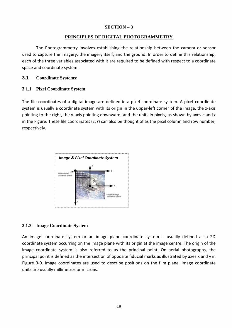
3.1.1 Pixel Coordinate System

The file coordinates of a digital image are defined in a pixel coordinate system. A pixel coordinate

system is usually a coordinate system with its origin in the upper-left corner of the image, the x-axis

pointing to the right, the y-axis pointing downward, and the units in pixels, as shown by axes c and r

in the Figure. These file coordinates (c, r) can also be thought of as the pixel column and row number,

respectively.

3.1.2 Image Coordinate System

An image coordinate system or an image plane coordinate system is usually defined as a 2D

coordinate system occurring on the image plane with its origin at the image centre. The origin of the

image coordinate system is also referred to as the principal point. On aerial photographs, the

principal point is defined as the intersection of opposite fiducial marks as illustrated by axes x and y in

Figure 3-9. Image coordinates are used to describe positions on the film plane. Image coordinate

units are usually millimetres or microns.

Image & Pixel Coordinate System

19

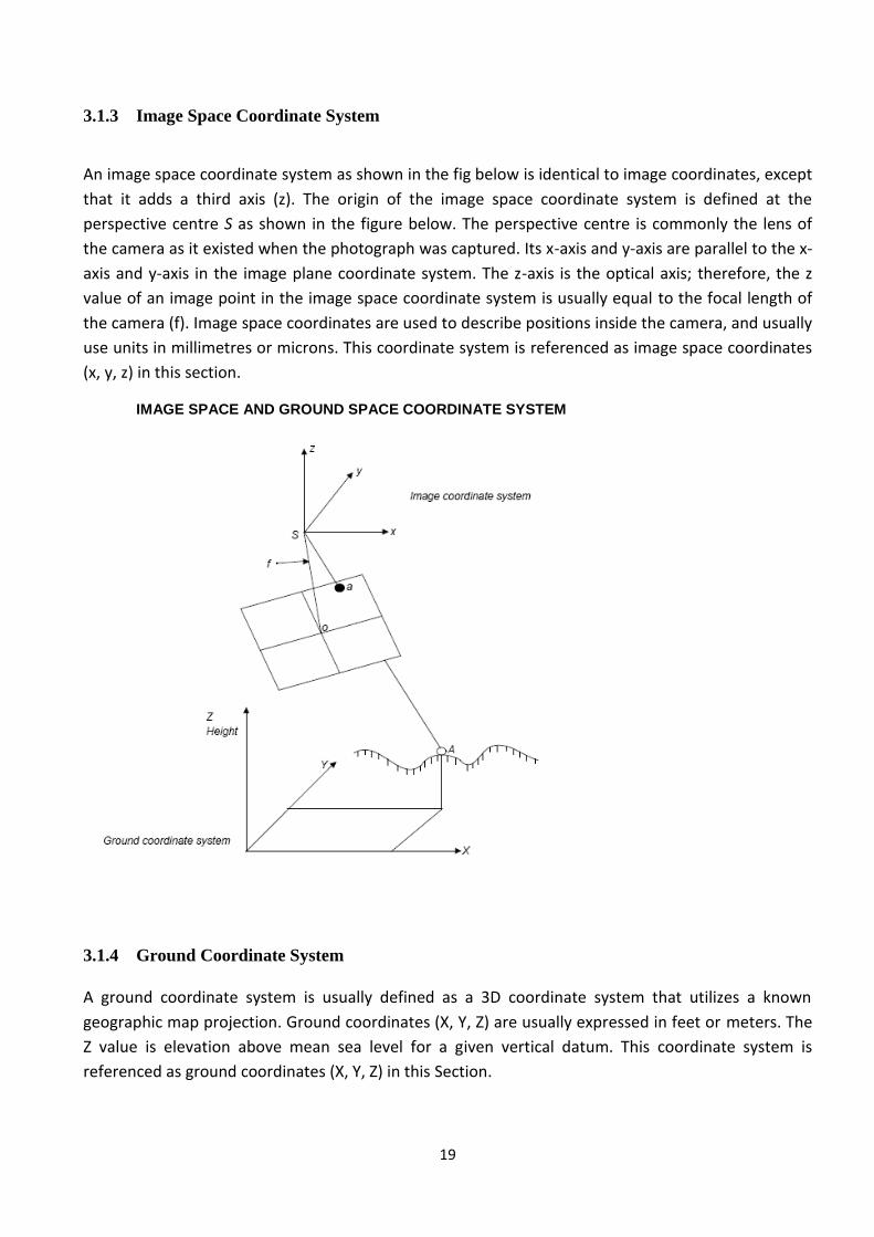
3.1.3 Image Space Coordinate System

An image space coordinate system as shown in the fig below is identical to image coordinates, except

that it adds a third axis (z). The origin of the image space coordinate system is defined at the

perspective centre S as shown in the figure below. The perspective centre is commonly the lens of

the camera as it existed when the photograph was captured. Its x-axis and y-axis are parallel to the x-

axis and y-axis in the image plane coordinate system. The z-axis is the optical axis; therefore, the z

value of an image point in the image space coordinate system is usually equal to the focal length of

the camera (f). Image space coordinates are used to describe positions inside the camera, and usually

use units in millimetres or microns. This coordinate system is referenced as image space coordinates

(x, y, z) in this section.

IMAGE SPACE AND GROUND SPACE COORDINATE SYSTEM

3.1.4 Ground Coordinate System

A ground coordinate system is usually defined as a 3D coordinate system that utilizes a known

geographic map projection. Ground coordinates (X, Y, Z) are usually expressed in feet or meters. The

Z value is elevation above mean sea level for a given vertical datum. This coordinate system is

referenced as ground coordinates (X, Y, Z) in this Section.

20

3.1.5 Geocentric and Topocentric Coordinate System

Most photogrammetric applications account for the Earth’s curvature in their calculations. This is

done by adding a correction value or by computing geometry in a coordinate system that includes

curvature. Two such systems are geocentric and topocentric coordinates.

A geocentric coordinate system has its origin at the centre of the Earth ellipsoid. The Z-axis equals the

rotational axis of the Earth, and the X-axis passes through the Greenwich meridian. The Y-axis is

perpendicular to both the Z-axis and X-axis, so as to create a three dimensional coordinate system

that follows the right hand rule.

A topocentric coordinate system has its origin at the centre of the image projected on the Earth

ellipsoid. The three perpendicular coordinate axes are defined on a tangential plane at this centre

point. The plane is called the reference plane or the local datum. The x-axis is oriented eastward, the

y-axis northward, and the z-axis is vertical to the reference plane (up).

3.2 Interior Orientation (IO)

The interior Orientation defines the internal geometry of a Camera or Sensor as it existed at

the time of image capture. The variables associated with

image space are defined during the process of defining

Interior orientation. This orientation is primarily used to

transform the image pixel coordinate system or other image

coordinate measurement systems to the image space

coordinate system. The discussions here are limited to Metric

Aerial Camera input. The variables associated with the

internal geometry of an Aerial Camera are:

1. Focal Length (f) 2. Principal point(PP) 3. Fiducial Marks (Xi Yi , 4 or 8 marks) 4. Lens Distortion Pattern (ri)

This information is available in Camera Calibration Certificate (CCC)

3.2.1 Principal Point and Focal Length

The principal point is mathematically defined as the intersection of the perpendicular line through

the perspective centre of the image plane. The length from the principal point to the perspective

centre is called the focal length (Wang 1990).

The image plane is commonly referred to as the focal plane. For wide-angle aerial cameras, the focal

length is pproximately 152 mm, or 6 inches. For some digital cameras, the focal length is 28 mm. Prior

to conducting photogrammetric projects, the focal length of a metric camera is accurately

determined or calibrated in a laboratory environment.

Internal Geometry

21

The optical definition of principal point is the image position where the optical axis intersects the

image plane. In the laboratory, this is calibrated in two forms: principal point of autocollimation and

principal point of symmetry, which can be seen from the camera calibration report. Most applications

prefer to use the principal point of symmetry since it can best compensate for any lens distortion.

3.2.2 Fiducial Marks

As stated previously, one of the steps associated with calculating interior orientation involves

determining the image position of the principal point for each image in the project. Therefore, the

image positions of the fiducial marks are measured on the image, and then compared to the

calibrated coordinates of each fiducial mark.

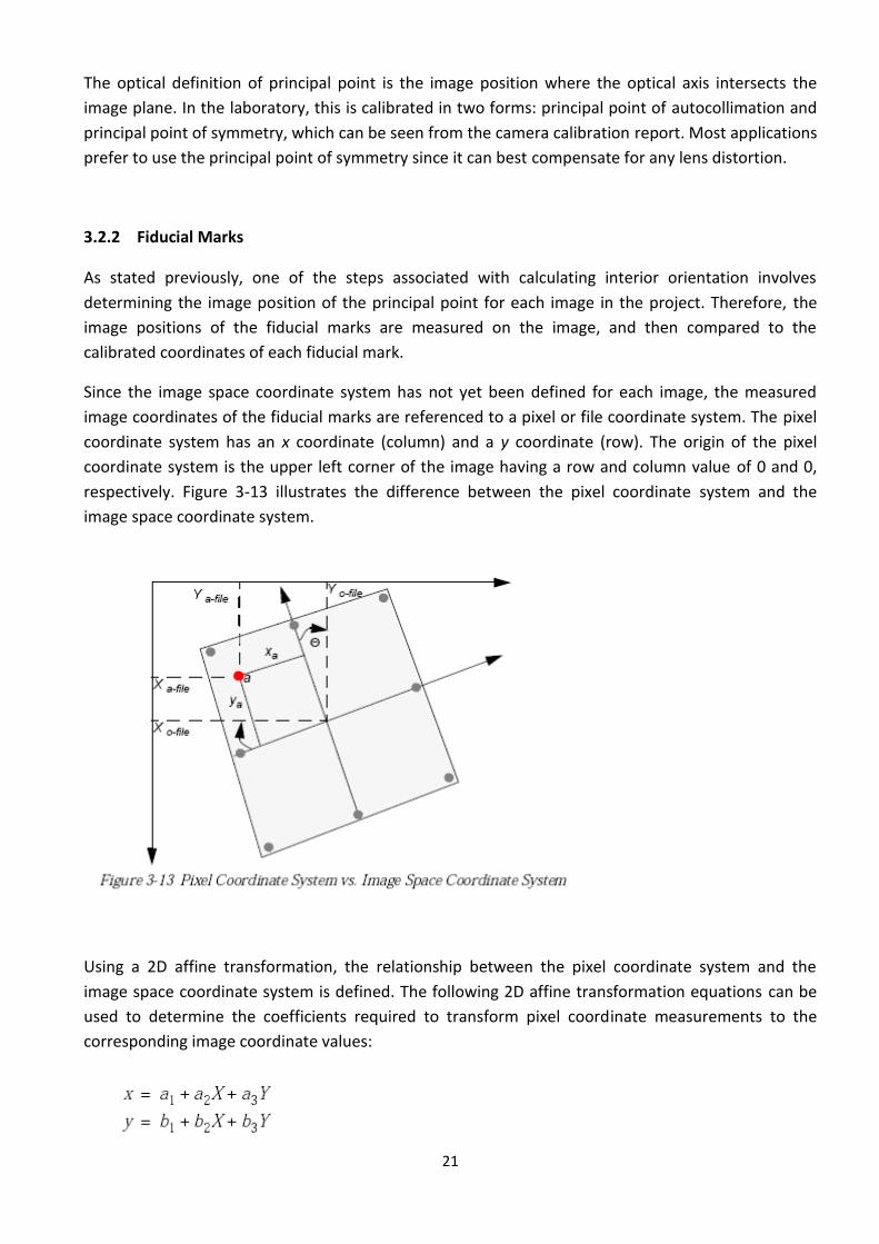
Since the image space coordinate system has not yet been defined for each image, the measured

image coordinates of the fiducial marks are referenced to a pixel or file coordinate system. The pixel

coordinate system has an x coordinate (column) and a y coordinate (row). The origin of the pixel

coordinate system is the upper left corner of the image having a row and column value of 0 and 0,

respectively. Figure 3-13 illustrates the difference between the pixel coordinate system and the

image space coordinate system.

Using a 2D affine transformation, the relationship between the pixel coordinate system and the

image space coordinate system is defined. The following 2D affine transformation equations can be

used to determine the coefficients required to transform pixel coordinate measurements to the

corresponding image coordinate values:

22

The x and y image coordinates associated with the calibrated fiducial marks and the X and Y pixel

coordinates of the measured fiducial marks are used to determine six affine transformation

coefficients. The resulting six coefficients can then be used to transform each set of row (y) and

column (x) pixel coordinates to image coordinates.

The quality of the 2D affine transformation is represented using a root mean square (RMS) error. The

RMS error represents the degree of correspondence between the calibrated fiducial mark

coordinates and their respective measured image coordinate values. Large RMS errors indicate poor

correspondence. This can be attributed to film deformation, poor scanning quality, out-of-date

calibration information, or image mismeasurement.

The affine transformation also defines the translation between the origin of the pixel coordinate

system and the image coordinate system (xo-file and yo-file). Additionally, the affine transformation

takes into consideration rotation of the image coordinate system by considering angle Θ. A scanned

image of an aerial photograph is normally rotated due to the scanning procedure.

The degree of variation between the x-axis and y-axis is referred to as nonorthogonality. The 2D

affine transformation also considers the extent of nonorthogonality. The scale difference between

the x-axis and the y-axis is also considered using the affine transformation.

3.2.3 Lens Distortion

Lens distortion deteriorates the positional accuracy of image points located on the image plane.

Two types of radial lens distortion exist: radial and tangential lens distortion. Lens distortion occurs

when light rays passing through the lens are bent, thereby changing directions and intersecting the

image plane at positions deviant from the norm. Figure 3-14 illustrates the difference between radial

and tangential lens distortion.

Radial lens distortion causes imaged points to be distorted along radial lines from the principal point

o. The effect of radial lens distortion is represented as Δr. Radial lens distortion is also commonly

referred to as symmetric lens distortion. Tangential lens distortion occurs at right angles to the radial

lines from the principal point. The effect of tangential lens distortion is represented as Δt. Because

tangential lens distortion is much smaller in magnitude than radial lens distortion, it is considered

23

negligible. The effects of lens distortion are commonly determined in a laboratory during the camera

calibration procedure.

The effects of radial lens distortion throughout an image can be approximated using a polynomial.

The following polynomial is used to determine coefficients associated with radial lens distortion:

represents the radial distortion along a radial distance r from the principal point (Wolf 1983). In most

camera calibration reports, the lens distortion value is provided as a function of radial distance from

the principal point or field angle. Three coefficients, k0, k1, and k2, are computed using statistical

techniques. Once the coefficients are computed, each measurement taken on an image is corrected

for radial lens distortion.

3.2.4 Theory of Interior Orientation

The Inner Orientation aims at Recreation of bundle of rays that existed inside the camera at the

instant of Exposure. This can be achieved analytically by defining the vector Oa Where ‘O’ is the

origin and ‘a’ is the end point. The coordinate system is defined with

Origin ‘O’ i.e. Exposure (0, 0, 0)

x-axis Flight direction & Parallel to image plane.

y-axis 90o to x-axis & parallel to image plane.

z-axis Optical axis of the camera towards Zenith.

The co-ordinate of image point ‘a’ (n Fig Image and Ground space coordinate system) is

necessary to define the required vector. Image point ‘a’ cannot be measured physically with respect

to Image Space Co-ordinate System as ‘O’ is not a physical point.

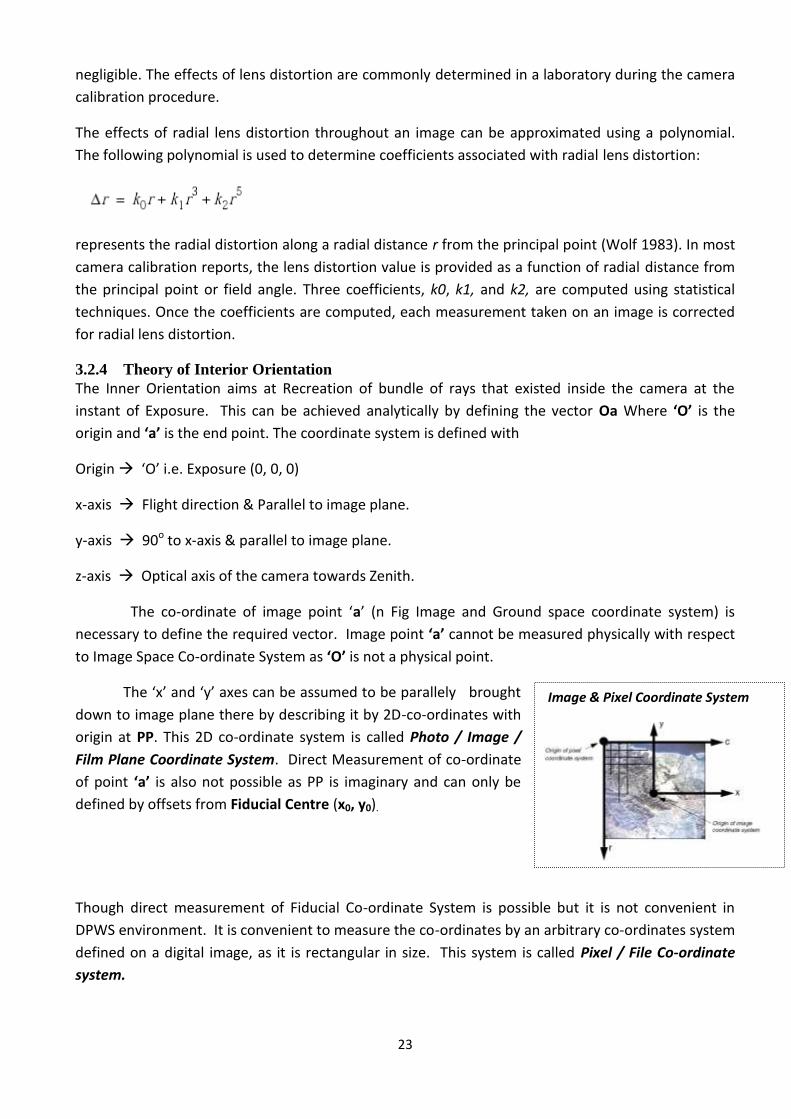
The ‘x’ and ‘y’ axes can be assumed to be parallely brought

down to image plane there by describing it by 2D-co-ordinates with

origin at PP. This 2D co-ordinate system is called Photo / Image /

Film Plane Coordinate System. Direct Measurement of co-ordinate

of point ‘a’ is also not possible as PP is imaginary and can only be

defined by offsets from Fiducial Centre (x0, y0).

Though direct measurement of Fiducial Co-ordinate System is possible but it is not convenient in

DPWS environment. It is convenient to measure the co-ordinates by an arbitrary co-ordinates system

defined on a digital image, as it is rectangular in size. This system is called Pixel / File Co-ordinate

system.

Image & Pixel Coordinate System

24

X3 Y3

x3 y3

X2Y2 x2 y2 x1 y1 X1 Y1

x4 y4

X4 Y4

x4 y4

X4 Y4

Direct measurement of pixel / file coordinates of image point ‘a’ is convenient and accurate

too. Therefore in DPWS all the primary measurements are done in Pixel / File coordinate system

only.

For constructing the vector Oa the coordinates of ‘a’ is necessary to be known in Image Space

co-ordinate system. Therefore, it is necessary to convert the primary co-ordinate measured in Pixel

system to be converted into Image Space coordinate system. This necessitates following one of the

coordinate transformation to be adopted.

3.2.5 Pixel to Fiducial co-ordinate Transformation:

Any transformation involves two coordinate systems as below

To perform transformation the followings are needed.

1. Some points co-ordinates known in both Input & Reference Systems. Such points are called Control Points.

2. Mathematical model involving the relation between the two involved systems.

In the case of transformation of Pixel Co-ordinates to Fiducial Co-ordinates, the former is the

Input system and Later the final system. The two requirements are met as below:

Control Points: - The fiducial marks on digital images are used as control points where co-ordinates

in Final system available in camera calibration certificate (CCC), and pixel coordinates are measured

by the operator either manually or by adopting automation (if the S/W allows).

Point No. Fiducial Co-ordinate Pixel Coordinate

1 X1 Y1 x1 y1

2 X2 Y2 x2 y2

3 X3 Y3 x3 y3

4 X4 Y4 x4 y4

Input System Reference/Final Systems Transformation

25

The equation establishing the relation between any two 2D Co-ordinate system depends on the following

parameters.

1) Translation (x0 y0)

2) Rotation ()

3) Scale Uniform in both axes ()

Non-uniform in axes (x y)

Varies points to points i.e.

Differential involved (cx, cy)

4) Skew ()

According to the combination of parameters involved the form of equation generated will differ and

accordingly there are `5’ types of 2D linear transformation possible as enumerated below.

Sl.No. Name of Transformation Parametres Innovation No. of Parameters

1 Projective Transformation x0, y0, , x, y cx, cy, 8

2 Affine transformation x0, y0, , x, y, 6

3 Conformal/Similarity transformation x0, y0, , 4

4 Identity Transformation x0, y0 2

In the case of pixel co-ordinate system (INPUT) and Fiducial co-ordinate system (REFERENCE), the

following parameters are included.

1. Translation (x0, y0,) - Evident from diagram

2. Rotation () - -do-

3. Scale () - If scanner accuracy is dependable

or

(x, y) - If scanner expected to have scale error different

(Most likely)

4. Skew () - As scanner is a Electro-mechanical device it may have

non-orthogonality of its axis system while scanning.

Accordingly the most suitable transformation to be chosen is `Affine’. However, if the scanner is

assured to be of absolute accuracy with respect to scale error and skew, then 4-parametre transformation can

also be chosen. Most of the photogrammetric application S/W prefers to use affine transformation to be in

the safer side and precise. The mathematical model for affine transformation is:

X = ax + by + c

Y = dx + ey + f ----------- ---------------------------------- (1)

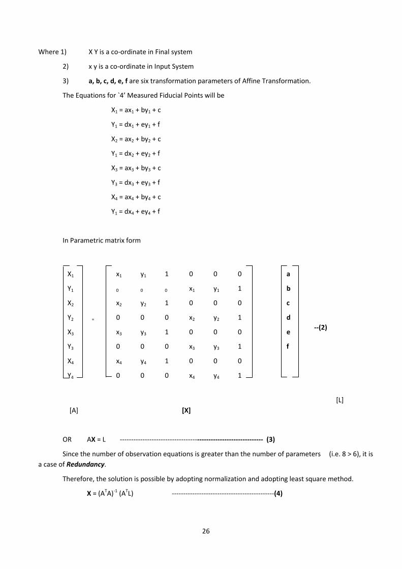
26

Where 1) X Y is a co-ordinate in Final system

2) x y is a co-ordinate in Input System

3) a, b, c, d, e, f are six transformation parameters of Affine Transformation.

The Equations for `4’ Measured Fiducial Points will be

X1 = ax1 + by1 + c

Y1 = dx1 + ey1 + f

X2 = ax2 + by2 + c

Y1 = dx2 + ey2 + f

X3 = ax3 + by3 + c

Y3 = dx3 + ey3 + f

X4 = ax4 + by4 + c

Y1 = dx4 + ey4 + f

In Parametric matrix form

--(2)

[L]

[A] [X]

OR AX = L --------------------------------------------------------------- (3)

Since the number of observation equations is greater than the number of parameters (i.e. 8 > 6), it is

a case of Redundancy.

Therefore, the solution is possible by adopting normalization and adopting least square method.

X = (ATA)-1 (ATL) ---------------------------------------------(4)

X1 x1 y1 1 0 0 0 a

Y1 0 0 0 x1 y1 1 b

X2 x2 y2 1 0 0 0 c

Y2 = 0 0 0 x2 y2 1 d

X3 x3 y3 1 0 0 0 e

Y3 0 0 0 x3 y3 1 f

X4 x4 y4 1 0 0 0

Y4 0 0 0 x4 y4 1

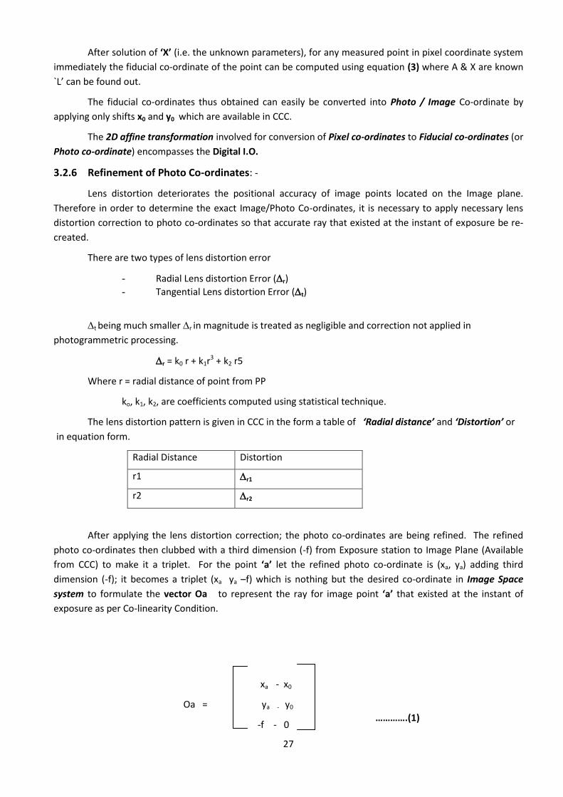
27

xa - x0

Oa = ya - y0

-f - 0

After solution of ‘X’ (i.e. the unknown parameters), for any measured point in pixel coordinate system

immediately the fiducial co-ordinate of the point can be computed using equation (3) where A & X are known

`L’ can be found out.

The fiducial co-ordinates thus obtained can easily be converted into Photo / Image Co-ordinate by

applying only shifts x0 and y0 which are available in CCC.

The 2D affine transformation involved for conversion of Pixel co-ordinates to Fiducial co-ordinates (or

Photo co-ordinate) encompasses the Digital I.O.

3.2.6 Refinement of Photo Co-ordinates: -

Lens distortion deteriorates the positional accuracy of image points located on the Image plane.

Therefore in order to determine the exact Image/Photo Co-ordinates, it is necessary to apply necessary lens

distortion correction to photo co-ordinates so that accurate ray that existed at the instant of exposure be re-

created.

There are two types of lens distortion error

- Radial Lens distortion Error (r)

- Tangential Lens distortion Error (t)

t being much smaller r in magnitude is treated as negligible and correction not applied in

photogrammetric processing.

r = k0 r + k1r3 + k2 r5

Where r = radial distance of point from PP

ko, k1, k2, are coefficients computed using statistical technique.

The lens distortion pattern is given in CCC in the form a table of ‘Radial distance’ and ‘Distortion’ or

in equation form.

Radial Distance Distortion

r1 r1

r2 r2

After applying the lens distortion correction; the photo co-ordinates are being refined. The refined

photo co-ordinates then clubbed with a third dimension (-f) from Exposure station to Image Plane (Available

from CCC) to make it a triplet. For the point ‘a’ let the refined photo co-ordinate is (xa, ya) adding third

dimension (-f); it becomes a triplet (xa ya –f) which is nothing but the desired co-ordinate in Image Space

system to formulate the vector Oa to represent the ray for image point ‘a’ that existed at the instant of

exposure as per Co-linearity Condition.

………….(1)

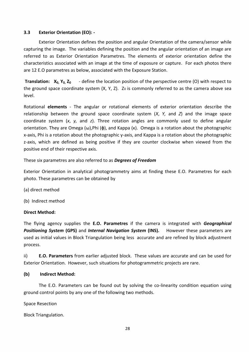
28

3.3 Exterior Orientation (EO): -

Exterior Orientation defines the position and angular Orientation of the camera/sensor while

capturing the image. The variables defining the position and the angular orientation of an image are

referred to as Exterior Orientation Parametres. The elements of exterior orientation define the

characteristics associated with an image at the time of exposure or capture. For each photos there

are 12 E.O parametres as below, associated with the Exposure Station.

Translation: X0, Y0, Z0 - define the location position of the perspective centre (O) with respect to

the ground space coordinate system (X, Y, Z). Z0 is commonly referred to as the camera above sea

level.

Rotational elements - The angular or rotational elements of exterior orientation describe the

relationship between the ground space coordinate system (X, Y, and Z) and the image space

coordinate system (x, y, and z). Three rotation angles are commonly used to define angular

orientation. They are Omega (ω),Phi (ϕ), and Kappa (κ). Omega is a rotation about the photographic

x-axis, Phi is a rotation about the photographic y-axis, and Kappa is a rotation about the photographic

z-axis, which are defined as being positive if they are counter clockwise when viewed from the

positive end of their respective axis.

These six parametres are also referred to as Degrees of Freedom

Exterior Orientation in analytical photogrammetry aims at finding these E.O. Parametres for each

photo. These parametres can be obtained by

(a) direct method

(b) Indirect method

Direct Method:

The flying agency supplies the E.O. Parametres if the camera is integrated with Geographical

Positioning System (GPS) and Internal Navigation System (INS). However these parameters are

used as initial values in Block Triangulation being less accurate and are refined by block adjustment

process.

ii) E.O. Parameters from earlier adjusted block. These values are accurate and can be used for

Exterior Orientation. However, such situations for photogrammetric projects are rare.

(b) Indirect Method:

The E.O. Parameters can be found out by solving the co-linearity condition equation using

ground control points by any one of the following two methods.

Space Resection

Block Triangulation.

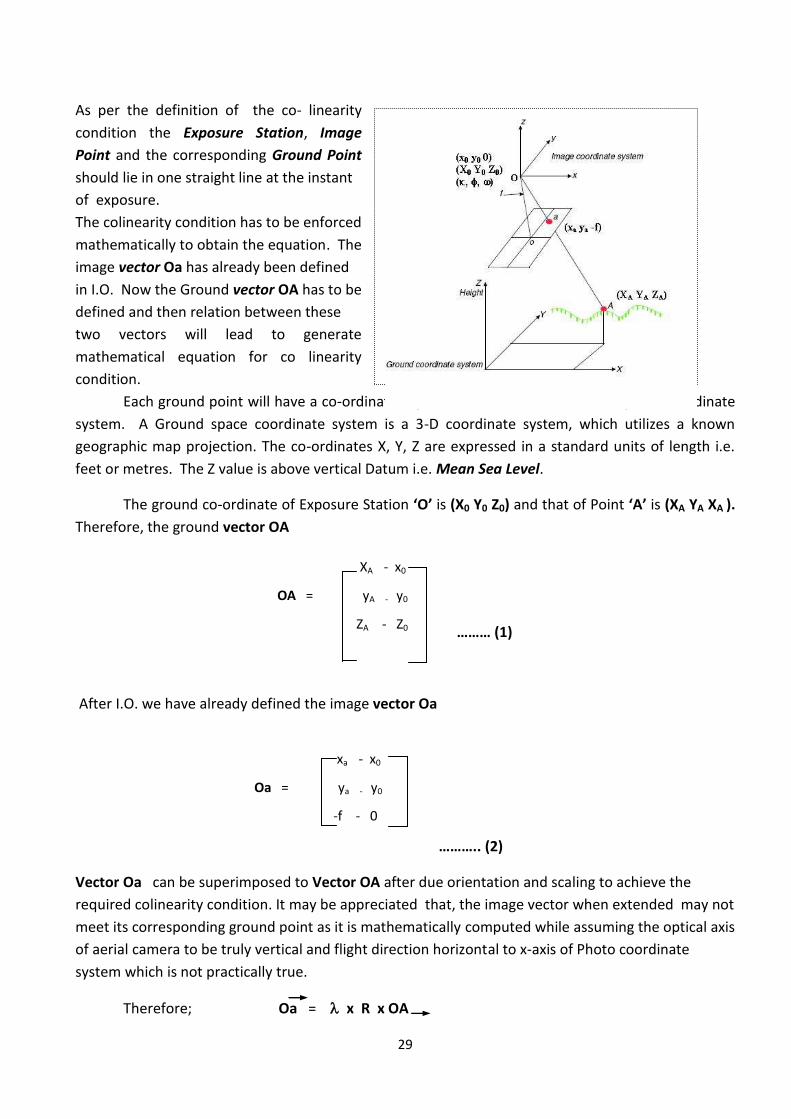
29

xa - x0

Oa = ya - y0

-f - 0

XA - x0

OA = yA - y0

ZA - Z0

As per the definition of the colinearity

condition the Exposure Station, Image

Point and the corresponding Ground Point

should lie in one straight line at the instant

of exposure.

The colinearity condition has to be enforced

mathematically to obtain the equation. The

image vector Oa has already been defined

in I.O. Now the Ground vector OA has to be

defined and then relation between these

two vectors will lead to generate

mathematical equation for co linearity

condition.

Each ground point will have a co-ordinate triplet with reference to Ground Space co-ordinate

system. A Ground space coordinate system is a 3-D coordinate system, which utilizes a known

geographic map projection. The co-ordinates X, Y, Z are expressed in a standard units of length i.e.

feet or metres. The Z value is above vertical Datum i.e. Mean Sea Level.

The ground co-ordinate of Exposure Station ‘O’ is (X0 Y0 Z0) and that of Point ‘A’ is (XA YA XA ).

Therefore, the ground vector OA

……… (1)

After I.O. we have already defined the image vector Oa

……….. (2)

Vector Oa can be superimposed to Vector OA after due orientation and scaling to achieve the

required colinearity condition. It may be appreciated that, the image vector when extended may not

meet its corresponding ground point as it is mathematically computed while assuming the optical axis

of aerial camera to be truly vertical and flight direction horizontal to x-axis of Photo coordinate

system which is not practically true.

Therefore; Oa = x R x OA

30

Where = Scale factor, R = Rotation matrix (3x3) =

Expanding we get

……(3)

Dividing the former two equations by the third and rearranging we have

-f [ r11(XA – Xo] + r12(Yn – Yo) + r13(ZA – Zo)]

xa – xo = ------------------------------------------------------------------------------

[ r31(XA – Xo] + r32(YA – Yo) + r33(ZA – Zo)]

…..(4)


Ya – Xo = ------------------------------------------------------------------------------


The above two Equations are

called “Co linearity Condition

Equations”. Thus one single observation

of Pixel Co-ordinates of an image Point

after I.O. can yield a pair of co linearity

equations.

xa – xo = [ r11(XA – Xo] + r12(Yn – Yo) + r13(ZA – Zo)]

ya – xo = [ r21(XA – Xo] + r22(Yn – Yo) + r23(ZA – Zo)]

-f = [ r31(XA – Xo] + r32(YA – Yo) + r33(ZA – Zo)]

O ( X0 Y0 Z0 )

(x0, y0 0)

c (xc yc -f)

a (xa ya -f)

b (xb yb -f)

C (XC YC ZC)

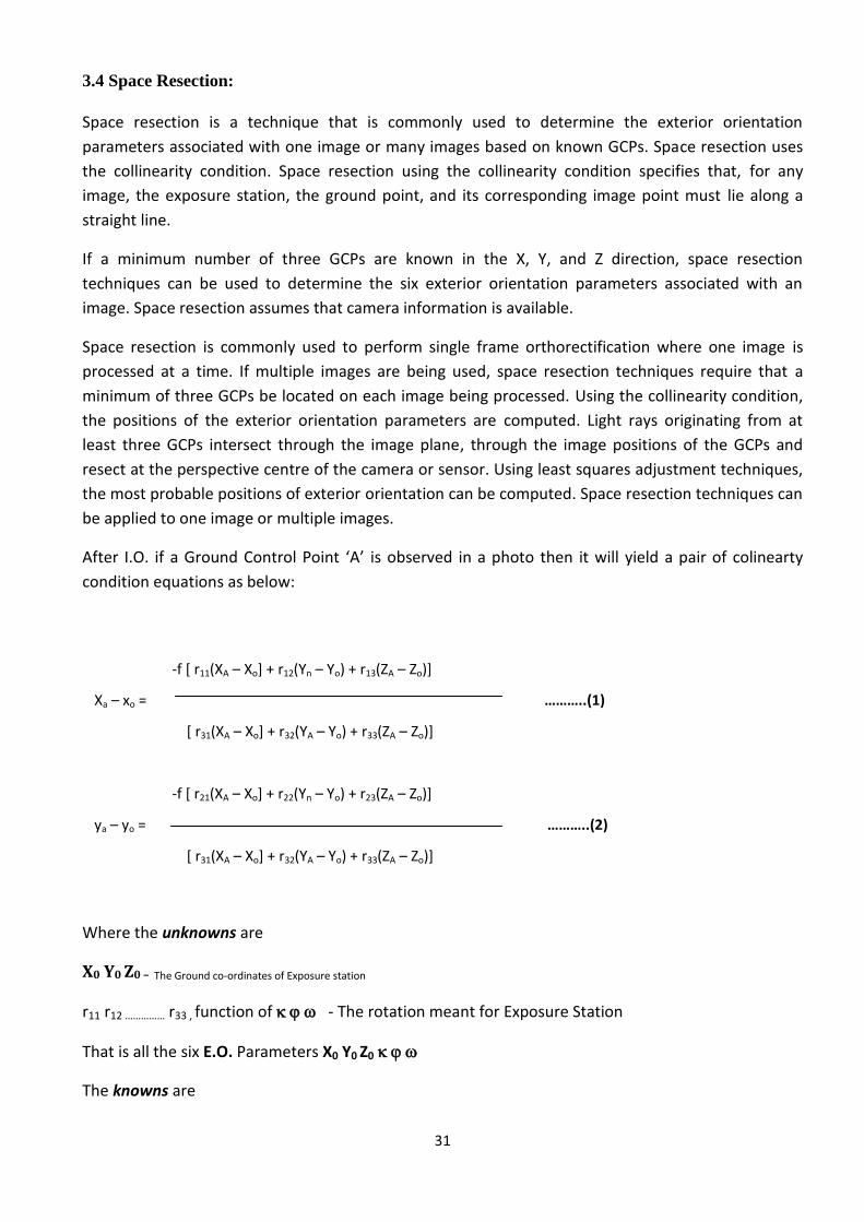
31


Xa – xo = ………..(1)



ya – yo = ………..(2)


3.4 Space Resection:

Space resection is a technique that is commonly used to determine the exterior orientation

parameters associated with one image or many images based on known GCPs. Space resection uses

the collinearity condition. Space resection using the collinearity condition specifies that, for any

image, the exposure station, the ground point, and its corresponding image point must lie along a

straight line.

If a minimum number of three GCPs are known in the X, Y, and Z direction, space resection

techniques can be used to determine the six exterior orientation parameters associated with an

image. Space resection assumes that camera information is available.

Space resection is commonly used to perform single frame orthorectification where one image is

processed at a time. If multiple images are being used, space resection techniques require that a

minimum of three GCPs be located on each image being processed. Using the collinearity condition,

the positions of the exterior orientation parameters are computed. Light rays originating from at

least three GCPs intersect through the image plane, through the image positions of the GCPs and

resect at the perspective centre of the camera or sensor. Using least squares adjustment techniques,

the most probable positions of exterior orientation can be computed. Space resection techniques can

be applied to one image or multiple images.

After I.O. if a Ground Control Point ‘A’ is observed in a photo then it will yield a pair of colinearty

condition equations as below:

Where the unknowns are

X0 Y0 Z0 – The Ground co-ordinates of Exposure station

r11 r12 …………… r33 , function of - The rotation meant for Exposure Station

That is all the six E.O. Parameters X0 Y0 Z0

The knowns are

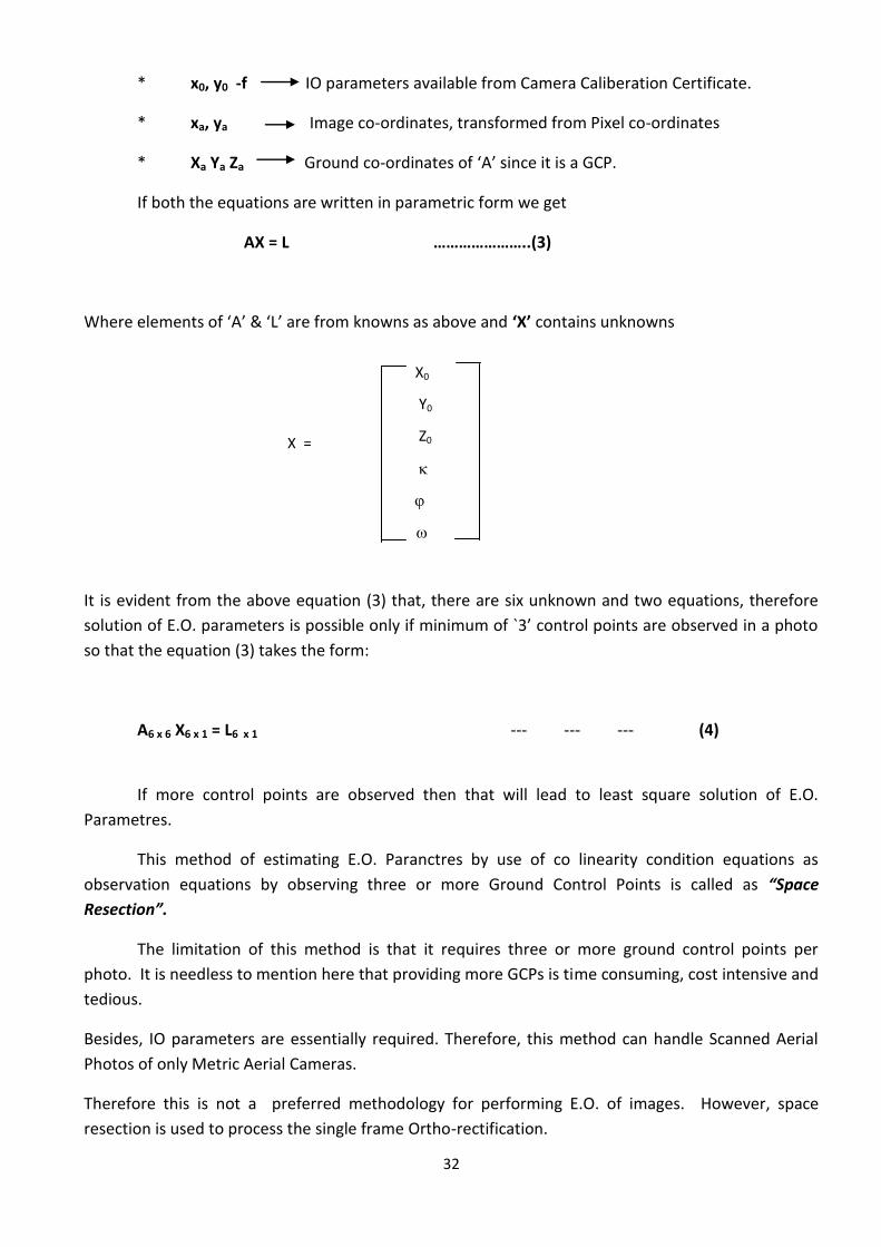
32

X0

Y0

Z0

X =

* x0, y0 -f IO parameters available from Camera Caliberation Certificate.

* xa, ya Image co-ordinates, transformed from Pixel co-ordinates

* Xa Ya Za Ground co-ordinates of ‘A’ since it is a GCP.

If both the equations are written in parametric form we get

AX = L …………………..(3)

Where elements of ‘A’ & ‘L’ are from knowns as above and ‘X’ contains unknowns

It is evident from the above equation (3) that, there are six unknown and two equations, therefore

solution of E.O. parameters is possible only if minimum of `3’ control points are observed in a photo

so that the equation (3) takes the form:

A6 x 6 X6 x 1 = L6 x 1 --- --- --- (4)

If more control points are observed then that will lead to least square solution of E.O.

Parametres.

This method of estimating E.O. Paranctres by use of co linearity condition equations as

observation equations by observing three or more Ground Control Points is called as “Space

Resection”.

The limitation of this method is that it requires three or more ground control points per

photo. It is needless to mention here that providing more GCPs is time consuming, cost intensive and

tedious.

Besides, IO parameters are essentially required. Therefore, this method can handle Scanned Aerial

Photos of only Metric Aerial Cameras.

Therefore this is not a preferred methodology for performing E.O. of images. However, space

resection is used to process the single frame Ortho-rectification.

33

3.5 Block Triangulation:

Block triangulation is the process of defining the mathematical relationship between the images

contained within a block, the camera or sensor model, and the ground. Once the relationship has

been defined, accurate imagery and geographic information concerning the Earth’s surface can be

created and collected in 3D.

A bundle block adjustment is best defined by examining the individual words in the term. A

bundled solution is computed including the exterior orientation parameters of each image in a block (

Two or more images involved in a photogrammetric project for mapping is referred to be a block) and the X,

Y, and Z coordinates of tie points and adjusted GCPs. A block of images contained in a project is

simultaneously processed in one solution. A statistical technique known as least squares adjustment

is used to estimate the bundled solution for the entire block while also minimizing and distributing

error.

When processing frame camera, digital camera, videography, and nonmetric camera imagery, block

triangulation is commonly referred to as aerial triangulation (AT). When processing imagery collected

with a pushbroom sensor, block triangulation is commonly referred to as triangulation.

In a block the coordinates of few GCPs and user defined points in specific standard positions

known as TIE points are taken as input and adjusted so as to get unknowns. Such adjustment is

called as Block Triangulation. If the images used are aerial photos then Block triangulation is called

as Aerial Triangulation.

Based on the type of input co-ordinates, the Block triangulation can be performed by

following three methods:

Name Input Required

Strip Block Triangulation Strip Coordinates

Model Block Triangulation Or Model Coordinates

Independent Model Triangulation (IMT)

Bundle Block Triangulation Photo Coordinates

As mentioned earlier in Digital Photogrammetry all primary measurements are done in pixel

coordinate terms and can be converted into refined photo co-ordinates once the I.O. has been done.

The strip Block Triangulation requires conversion of this photo co-ordinate to strip co-ordinate

through model co-ordinates. Similarly if the Model Block Triangulation is adopted then the photo co-

ordinates need to be converted into Model co-ordinates so as to use the same as input for

adjustment. As can be seen, the former requires two times co-ordinate transformation for making

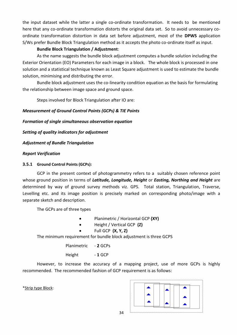
34

the input dataset while the latter a single co-ordinate transformation. It needs to be mentioned

here that any co-ordinate transformation distorts the original data set. So to avoid unnecessary co-

ordinate transformation distortion in data set before adjustment, most of the DPWS application

S/Ws prefer Bundle Block Triangulation method as it accepts the photo co-ordinate itself as input.

Bundle Block Triangulation / Adjustment:

As the name suggests the bundle block adjustment computes a bundle solution including the

Exterior Orientation (EO) Parameters for each image in a block. The whole block is processed in one

solution and a statistical technique known as Least Square adjustment is used to estimate the bundle

solution, minimising and distributing the error.

Bundle block adjustment uses the co-linearity condition equation as the basis for formulating

the relationship between image space and ground space.

Steps involved for Block Triangulation after IO are:

Measurement of Ground Control Points (GCPs) & TIE Points

Formation of single simultaneous observation equation

Setting of quality indicators for adjustment

Adjustment of Bundle Triangulation

Report Verification

3.5.1 Ground Control Points (GCPs):

GCP in the present context of photogrammetry refers to a suitably chosen reference point

whose ground position in terms of Latitude, Longitude, Height or Easting, Northing and Height are

determined by way of ground survey methods viz. GPS. Total station, Triangulation, Traverse,

Levelling etc. and its image position is precisely marked on corresponding photo/image with a

separate sketch and description.

The GCPs are of three types

Planimetric / Horizontal GCP (XY)

Height / Vertical GCP (Z)

Full GCP (X, Y, Z) The minimum requirement for bundle block adjustment is three GCPS

Planimetric - 2 GCPs

Height - 1 GCP

However, to increase the accuracy of a mapping project, use of more GCPs is highly

recommended. The recommended fashion of GCP requirement is as follows:

*Strip type Block:

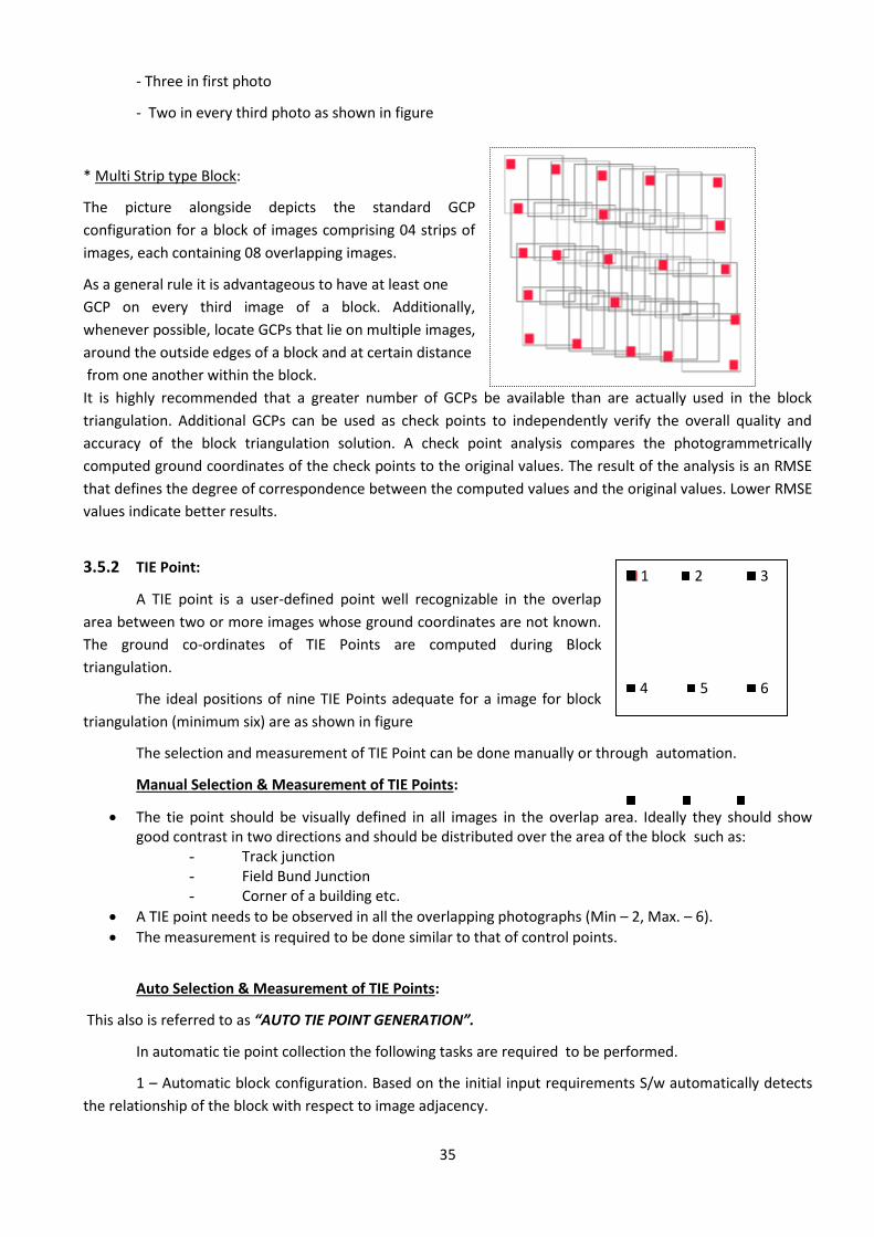
35

- Three in first photo

- Two in every third photo as shown in figure

* Multi Strip type Block:

The picture alongside depicts the standard GCP

configuration for a block of images comprising 04 strips of

images, each containing 08 overlapping images.

As a general rule it is advantageous to have at least one

GCP on every third image of a block. Additionally,

whenever possible, locate GCPs that lie on multiple images,

around the outside edges of a block and at certain distance

from one another within the block.

It is highly recommended that a greater number of GCPs be available than are actually used in the block

triangulation. Additional GCPs can be used as check points to independently verify the overall quality and

accuracy of the block triangulation solution. A check point analysis compares the photogrammetrically

computed ground coordinates of the check points to the original values. The result of the analysis is an RMSE

that defines the degree of correspondence between the computed values and the original values. Lower RMSE

values indicate better results.

3.5.2 TIE Point:

A TIE point is a user-defined point well recognizable in the overlap

area between two or more images whose ground coordinates are not known.

The ground co-ordinates of TIE Points are computed during Block

triangulation.

The ideal positions of nine TIE Points adequate for a image for block

triangulation (minimum six) are as shown in figure

The selection and measurement of TIE Point can be done manually or through automation.

Manual Selection & Measurement of TIE Points:

The tie point should be visually defined in all images in the overlap area. Ideally they should show good contrast in two directions and should be distributed over the area of the block such as:

- Track junction - Field Bund Junction - Corner of a building etc.

A TIE point needs to be observed in all the overlapping photographs (Min – 2, Max. – 6).

The measurement is required to be done similar to that of control points.

Auto Selection & Measurement of TIE Points:

This also is referred to as “AUTO TIE POINT GENERATION”.

In automatic tie point collection the following tasks are required to be performed.

1 – Automatic block configuration. Based on the initial input requirements S/w automatically detects

the relationship of the block with respect to image adjacency.

1 2 3

4 5 6

7 8 9

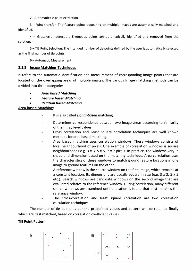
36

2 - Automatic tie point extraction

3 - Point transfer. The feature points appearing on multiple images are automatically matched and

identified.

4 – Gross-error detection. Erroneous points are automatically identified and removed from the

solution.

5 – TIE Point Selection. The intended number of tie points defined by the user is automatically selected

as the final number of tie points.

6 – Automatic Measurement.

3.5.3 Image Matching Techniques

It refers to the automatic identification and measurement of corresponding image points that are

located on the overlapping areas of multiple images. The various Image matching methods can be

divided into three categories.

Area based Matching

Feature based Matching

Relation based Matching Area-based Matching:

- It is also called signal-based matching.

- Determines correspondence between two image areas according to similarity of their gray level values.

- Cross correlation and Least Square correlation techniques are well known methods for area based matching.

- Area based matching uses correlation windows. These windows consists of local neighbourhood of pixels. One example of correlation windows is square neighbourhoods e.g. 3 x 3, 5 x 5, 7 x 7 pixels. In practice, the windows vary in shape and dimension based on the matching technique. Area correlation uses the characteristics of these windows to match ground feature locations in one image to ground features on the other.

- A reference window is the source window on the first image, which remains at a constant location. Its dimensions are usually square in size (e.g. 3 x 3, 5 x 5 etc.). Search windows are candidate windows on the second image that are evaluated relative to the reference window. During correlation, many different search windows are examined until a location is found that best matches the reference window.

- The cross-correlation and least square correlation are two correlation calculation techniques.

The number of tie points as per the predefined values and pattern will be retained finally

which are best matched, based on correlation coefficient values.

TIE Point Pattern:

i) ii)

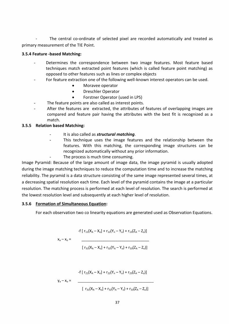
37


xa – xo = ________________________________



ya – xo = ____________________________________


- The central co-ordinate of selected pixel are recorded automatically and treated as

primary measurement of the TIE Point.

3.5.4 Feature -based Matching:

- Determines the correspondence between two image features. Most feature based techniques match extracted point features (which is called feature point matching) as opposed to other features such as lines or complex objects

- For feature extraction one of the following well-known interest operators can be used.

Moravee operator

Dreschler Operator

Forstner Operator (used in LPS) - The feature points are also called as interest points. - After the features are extracted, the attributes of features of overlapping images are

compared and feature pair having the attributes with the best fit is recognized as a match.

3.5.5 Relation based Matching:

- It is also called as structural matching. - This technique uses the image features and the relationship between the

features. With this matching, the corresponding image structures can be recognized automatically without any prior information.

- The process is much time consuming. Image Pyramid: Because of the large amount of image data, the image pyramid is usually adopted

during the image matching techniques to reduce the computation time and to increase the matching

reliability. The pyramid is a data structure consisting of the same image represented several times, at

a decreasing spatial resolution each time. Each level of the pyramid contains the image at a particular

resolution. The matching process is performed at each level of resolution. The search is performed at

the lowest resolution level and subsequently at each higher level of resolution.

3.5.6 Formation of Simultaneous Equation:

For each observation two co linearity equations are generated used as Observation Equations.

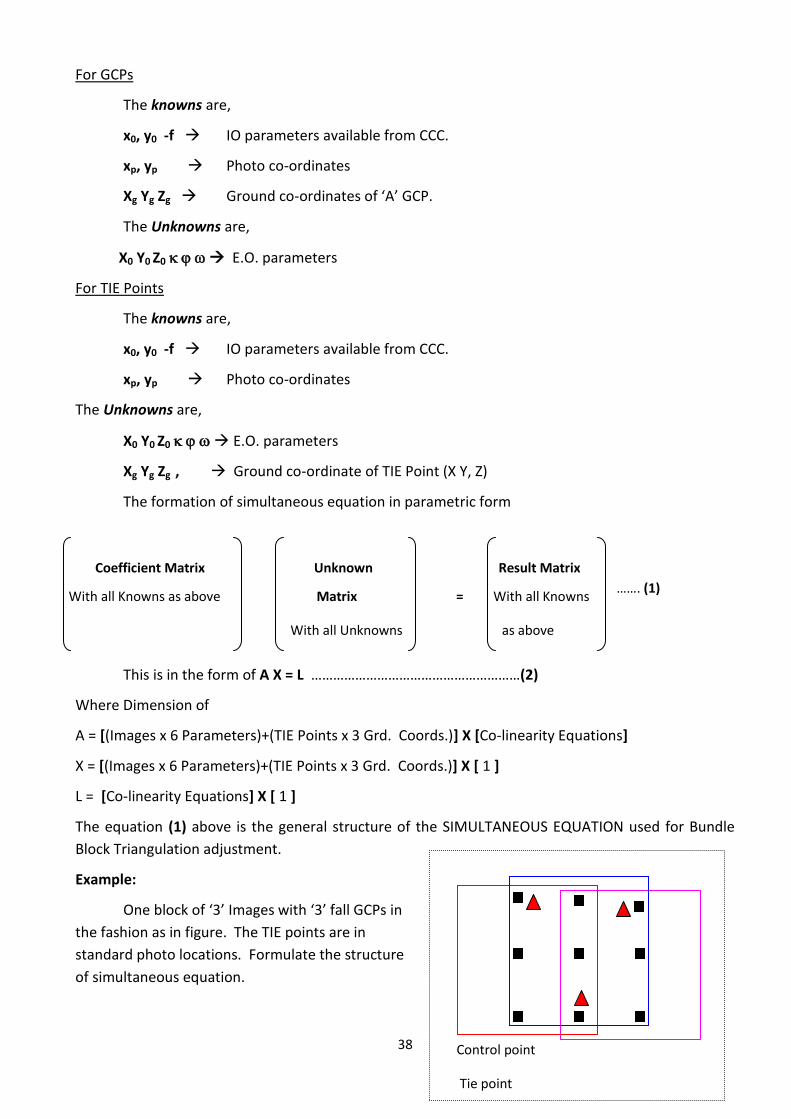
38

Control point

Tie point

For GCPs

The knowns are,

x0, y0 -f IO parameters available from CCC.

xp, yp Photo co-ordinates

Xg Yg Zg Ground co-ordinates of ‘A’ GCP.

The Unknowns are,

X0 Y0 Z0 E.O. parameters

For TIE Points

The knowns are,

x0, y0 -f IO parameters available from CCC.

xp, yp Photo co-ordinates

The Unknowns are,

X0 Y0 Z0 E.O. parameters

Xg Yg Zg , Ground co-ordinate of TIE Point (X Y, Z)

The formation of simultaneous equation in parametric form

……. (1)

This is in the form of A X = L …………………………………………………(2)

Where Dimension of

A = [(Images x 6 Parameters)+(TIE Points x 3 Grd. Coords.)] X [Co-linearity Equations]

X = [(Images x 6 Parameters)+(TIE Points x 3 Grd. Coords.)] X [ 1 ]

L = [Co-linearity Equations] X [ 1 ]

The equation (1) above is the general structure of the SIMULTANEOUS EQUATION used for Bundle

Block Triangulation adjustment.

Example:

One block of ‘3’ Images with ‘3’ fall GCPs in

the fashion as in figure. The TIE points are in

standard photo locations. Formulate the structure

of simultaneous equation.

Coefficient Matrix Unknown Result Matrix

With all Knowns as above Matrix = With all Knowns

With all Unknowns as above

39

Exposure Station

Image Point

Solution:

Number of equations generated.

GCPs:

2 tier point = 2, Hence Number of equations = 2 x 2 x 2 = 8

3 tier point = 1, Hence Number of equations = 3 x 1 x 2 = 6

----------------

Total 14

----------------

TIE Points:

2 Tier points = 6, Hence Number of equations = 2 x 6 x 2 = 24 3 Tier points = 3, Hence Number of equations = 3 x 3 x 2 = 18

Total 42

Total number of equations = 14 + 42 = 56

b Number of unknown involved:

1) E.O. parameters of 3 Images = 3 x 6 = 18 2) Ground Co-ordinates of 9 TIE points = 9 x 3 = 27

_________________________

Total number of unknowns = 42

The simultaneous equation

A56 X 45 X45X1 =L56X1 …. (1)

Number of observation equations > Number of unknowns hence a case of Redundancy.

Therefore, solution requires normalisation and least square technique.

Therefore: X = (ATA)-1 (ATL) … (2)

3.5.7 Setting of Quality Indicators:

There is every possibility of

cropping of error while doing

measurements. The control points are

obtained by field measurements and input

coordinates of GCPs as well as TIE points

are measured in DPWS and thus are prone

to inaccuracies. To check the propagation

of errors in least square adjustment

adopted for block triangulation it is

40

necessary to input the Quality Indicators / Estimates.

For GCPs Measurement:

- Standard deviations () with respect to X Y & Z coordinates i.e. plan and height both. - The reliability of points can be differentiated by concept of weights. (Higher the weight more

reliable and vice versa).

E.g.: Standard deviation of a point A (X Y Z) = 5m implies the true location of point A in motion 5

metres radius in plan & ± 5 metres in height.

For Image Point Measurements:

Standard deviation in (x, y) Planimetric only as the primary image measurement involved in

DPWS is in Pixel terms 2-D coordinate system.

E.g.: Standard deviation of image point = 0.33 pixel implies the true location is within a radius

of 0.33 of a pixel.

For Perspective Centre:

The quality estimate is also set for the Perspective Centre (Exposure Station) if initial values

are available in terms of standard deviations for all three x, y and z coordinates.

3.6 Bundle Block Triangulation adjustment:

Least squares adjustment:

It is statistical technique that is used to estimate the unknown parameters associated with a

solution while also minimizing error within the solution. With respect to block triangulation, least

squares adjustment techniques are used to:

Estimate or adjust the values associated with exterior orientation.

Estimates the X, Y, Z coordinates associated with the TIE Points.

Estimate or adjust the values associated with interior orientation.

Minimise and distribute data error through the network of observations. Data error is attributed to the inaccuracy associated with the input GCP coordinates,

measured tie point and GCP image positions, camera information, and systematic errors.

The least squares approach requires iterative processing until a solution is attained. A

solution is obtained when the residuals, or errors, associated with the input data are minimized.

A residual is the difference between the measured (i.e. the user input) and the computed

value for any particular measurement.

The simultaneous equation formulated is used as functional model for Least Squares

adjustment, which is in the form of

A X = L ….. ……(1)

In iterative process the residual error occurs in each iteration therefore the differentiation

yield least square condition which is given by

A X = L + V

41

Or V = A X – L ….. ……(2)

Where

V = The Matrix containing the image coordinate residuals.

A = Coefficient matrix containing the partial derivatives with respect to unknown

parameters, including exterior orientation, interior orientation, XYZ tie point

and GCP coordinates.

X = Unknown parameters correction matrix.

L = Matrix containing input observations.

(Initial – estimated values)

X = (ATPA)-1 (ATPL) ….. ……(3)

Where ‘P’ is the weight matrix.

Once the iteration is completed, the corrections to the unknown parameters are added to the

initial estimates. These values are then taken for 2nd iteration and so on. The iterative process of

least square adjustment continues until the corrections to unknown parameters are less than user

specified threshold commonly referred to as Convergence value.

The convergence is the difference of the residuals. At the end of every iteration the residuals

or `V’ matrix is computed. The new estimates based on ‘V’ are used as input for subsequent

iteration and again ‘V’ is computed. The difference of two successive ‘V’ matrices gives convergence

matrix. If each elements of convergence matrix is less than the threshold set by user then the

iteration stops and the residuals added to estimates for final adjusted values to the following results.

Final E.O. parameters of each image in block and their accuracy.

Final I.O. parameters of each image in block and their accuracy

X, Y, Z co-ordinates to each tie points and their accuracy.

Adjusted GCP co-ordinates and their residuals.

Image co-ordinate residuals. However, the Convergence may not be achieved in case of large error in data set. In such

event the iteration will never stop. To come out of iterative loop it is necessary to pre-define

maximum number of iterations after which the block bundle adjustment will break premature. The

adjustment has to be carried out after correcting the dataset.

This method of solving E.O. parameters is superior to all other methods as it not only

estimates accurate E.O. parameters by rigorous adjustment method but also has tremendous

capability to distribute the errors in measurements throughout the block.

The results from block triangulation are then used as the primary input for the following tasks:

Stereo pair creation

Feature Collection

Highly accurate Point determination

DEM extraction

Ortho rectification.

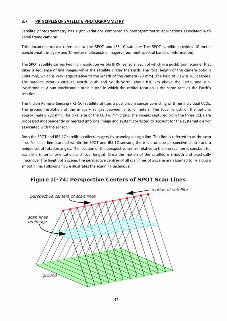
42

3.7 PRINCIPLES OF SATELLITE PHOTOGRAMMETRY

Satellite photogrammetry has slight variations compared to photogrammetric applications associated with

aerial frame cameras.

This document makes reference to the SPOT and IRS-1C satellites.The SPOT satellite provides 10-meter

panchromatic imagery and 20-meter multispectral imagery (four multispectral bands of information).

The SPOT satellite carries two high resolution visible (HRV) sensors, each of which is a pushbroom scanner that

takes a sequence of line images while the satellite circles the Earth. The focal length of the camera optic is

1084 mm, which is very large relative to the length of the camera (78 mm). The field of view is 4.1 degrees.

The satellite orbit is circular, North-South and South-North, about 830 km above the Earth, and sun-

synchronous. A sun-synchronous orbit is one in which the orbital rotation is the same rate as the Earth’s

rotation.

The Indian Remote Sensing (IRS-1C) satellite utilizes a pushbroom sensor consisting of three individual CCDs.

The ground resolution of the imagery ranges between 5 to 6 meters. The focal length of the optic is

approximately 982 mm. The pixel size of the CCD is 7 microns. The images captured from the three CCDs are

processed independently or merged into one image and system corrected to account for the systematic error

associated with the sensor.

Both the SPOT and IRS-1C satellites collect imagery by scanning along a line. This line is referred to as the scan

line. For each line scanned within the SPOT and IRS-1C sensors, there is a unique perspective centre and a

unique set of rotation angles. The location of the perspective centre relative to the line scanner is constant for

each line (interior orientation and focal length). Since the motion of the satellite is smooth and practically

linear over the length of a scene, the perspective centres of all scan lines of a scene are assumed to lie along a

smooth line. Following figure illustrates the scanning technique.

43

The satellite exposure station is defined as the perspective centre in ground coordinates for the

centre scan line. The image captured by the satellite is called a scene. For example, a SPOT Pan 1A

scene is composed of 6000 lines. For SPOT Pan 1A imagery, each of these lines consists of 6000 pixels.

Each line is exposed for 1.5 milliseconds, so it takes 9 seconds to scan the entire scene. (A scene from

SPOT XS 1A is composed of only 3000 lines and 3000 columns and has 20-meter pixels, while Pan has

10-meter pixels.)

NOTE: The following section addresses only the 10 meter SPOT Pan scenario. A pixel in the SPOT

image records the light detected by one of the 6000 light sensitive elements in the camera. Each pixel

is defined by file coordinates (column and row numbers). The physical dimension of a single, light-

sensitive element is 13 ×13 microns. This is the pixel size in image coordinates. The centre of the

scene is the centre pixel of the centre scan line. It is the origin of the image coordinate

system. Following figure depicts image coordinates in a satellite

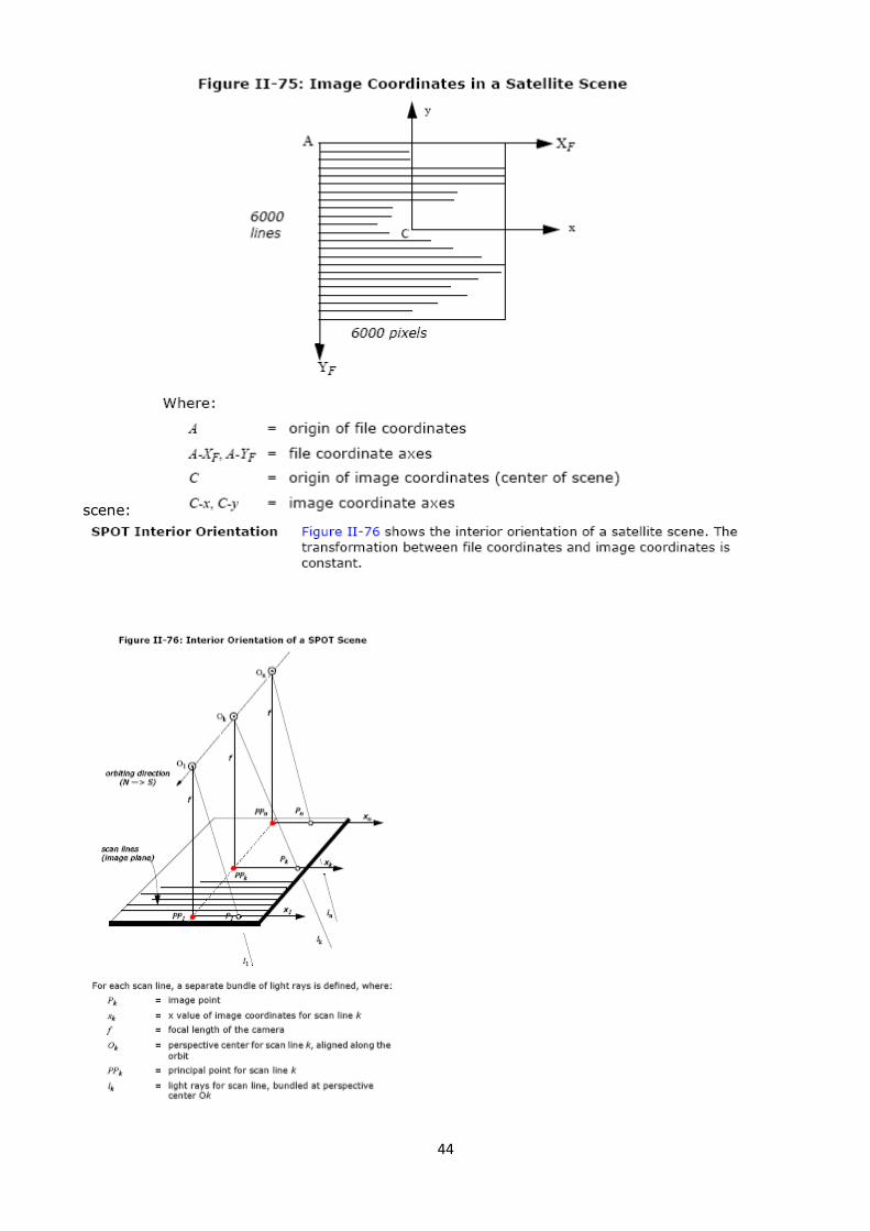
44

scene:

45

Ephemeris data for the orbit are available in the header file of SPOT scenes. They give the satellite’s

position in three-dimensional, geocentric coordinates at 60-second increments. The velocity vector

and some rotational velocities relating to the attitude of the camera are given, as well as the exact

time of the centre scan line of the scene. The header of the data file of a SPOT scene contains

ephemeris data, which provides information about the recording of the data and the satellite orbit.

Ephemeris data that can be used in satellite triangulation include:

• Position of the satellite in geocentric coordinates (with the origin

at the centre of the Earth) to the nearest second

• Velocity vector, which is the direction of the satellite’s travel

• Attitude changes of the camera

• Time of exposure (exact) of the centre scan line of the scene

The geocentric coordinates included with the ephemeris data are converted to a local ground system

for use in triangulation. The centre of a satellite scene is interpolated from the header data. Light rays

in a bundle defined by the SPOT sensor are almost parallel, lessening the importance of the satellite’s

position. Instead, the inclination angles (incidence angles) of the cameras on board the satellite

become the critical data.

The scanner can produce a nadir view. Nadir is the point directly below the camera. SPOT has off-

nadir viewing capability. Off-nadir refers to any point that is not directly beneath the satellite, but is

off to an angle (i.e., East or West of the nadir).

A stereo scene is achieved when two images of the same area are acquired on different days from

different orbits, one taken East of the other. For this to occur, there must be significant differences

in the inclination angles.

Inclination is the angle between a vertical on the ground at the centre of the scene and a light ray

from the exposure station. This angle defines the degree of off-nadir viewing when the scene was

recorded. The cameras can be tilted in increments of a minimum of 0.6 to a maximum of 27 degrees

to the East (negative inclination) or West (positive inclination). Following figure illustrates the

inclination.

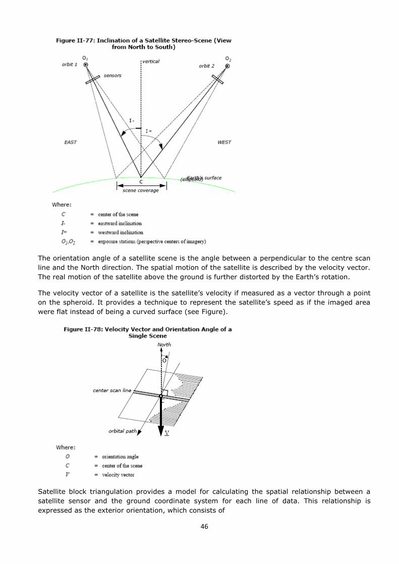
46

The orientation angle of a satellite scene is the angle between a perpendicular to the centre scan

line and the North direction. The spatial motion of the satellite is described by the velocity vector.

The real motion of the satellite above the ground is further distorted by the Earth’s rotation.

The velocity vector of a satellite is the satellite’s velocity if measured as a vector through a point

on the spheroid. It provides a technique to represent the satellite’s speed as if the imaged area

were flat instead of being a curved surface (see Figure).

Satellite block triangulation provides a model for calculating the spatial relationship between a

satellite sensor and the ground coordinate system for each line of data. This relationship is

expressed as the exterior orientation, which consists of

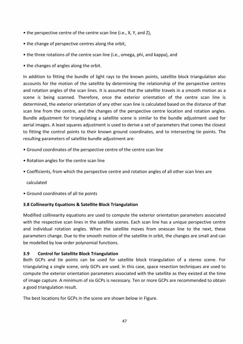
47

• the perspective centre of the centre scan line (i.e., X, Y, and Z),

• the change of perspective centres along the orbit,

• the three rotations of the centre scan line (i.e., omega, phi, and kappa), and

• the changes of angles along the orbit.

In addition to fitting the bundle of light rays to the known points, satellite block triangulation also

accounts for the motion of the satellite by determining the relationship of the perspective centres

and rotation angles of the scan lines. It is assumed that the satellite travels in a smooth motion as a

scene is being scanned. Therefore, once the exterior orientation of the centre scan line is

determined, the exterior orientation of any other scan line is calculated based on the distance of that

scan line from the centre, and the changes of the perspective centre location and rotation angles.

Bundle adjustment for triangulating a satellite scene is similar to the bundle adjustment used for

aerial images. A least squares adjustment is used to derive a set of parameters that comes the closest

to fitting the control points to their known ground coordinates, and to intersecting tie points. The

resulting parameters of satellite bundle adjustment are:

• Ground coordinates of the perspective centre of the centre scan line

• Rotation angles for the centre scan line

• Coefficients, from which the perspective centre and rotation angles of all other scan lines are

calculated

• Ground coordinates of all tie points

3.8 Collinearity Equations & Satellite Block Triangulation

Modified collinearity equations are used to compute the exterior orientation parameters associated

with the respective scan lines in the satellite scenes. Each scan line has a unique perspective centre

and individual rotation angles. When the satellite moves from onescan line to the next, these

parameters change. Due to the smooth motion of the satellite in orbit, the changes are small and can

be modelled by low order polynomial functions.

3.9 Control for Satellite Block Triangulation Both GCPs and tie points can be used for satellite block triangulation of a stereo scene. For

triangulating a single scene, only GCPs are used. In this case, space resection techniques are used to

compute the exterior orientation parameters associated with the satellite as they existed at the time

of image capture. A minimum of six GCPs is necessary. Ten or more GCPs are recommended to obtain

a good triangulation result.

The best locations for GCPs in the scene are shown below in Figure.

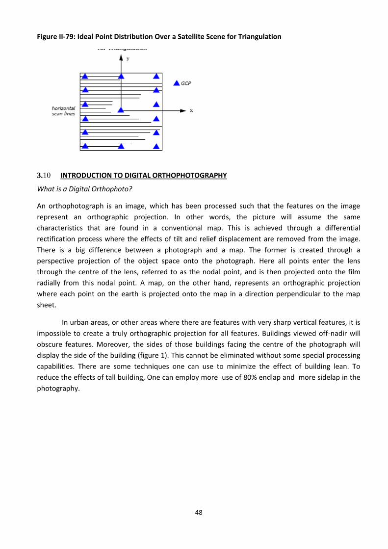
48

Figure II-79: Ideal Point Distribution Over a Satellite Scene for Triangulation

3.10 INTRODUCTION TO DIGITAL ORTHOPHOTOGRAPHY

What is a Digital Orthophoto?

An orthophotograph is an image, which has been processed such that the features on the image

represent an orthographic projection. In other words, the picture will assume the same

characteristics that are found in a conventional map. This is achieved through a differential

rectification process where the effects of tilt and relief displacement are removed from the image.

There is a big difference between a photograph and a map. The former is created through a

perspective projection of the object space onto the photograph. Here all points enter the lens

through the centre of the lens, referred to as the nodal point, and is then projected onto the film

radially from this nodal point. A map, on the other hand, represents an orthographic projection

where each point on the earth is projected onto the map in a direction perpendicular to the map

sheet.

In urban areas, or other areas where there are features with very sharp vertical features, it is

impossible to create a truly orthographic projection for all features. Buildings viewed off-nadir will

obscure features. Moreover, the sides of those buildings facing the centre of the photograph will

display the side of the building (figure 1). This cannot be eliminated without some special processing

capabilities. There are some techniques one can use to minimize the effect of building lean. To

reduce the effects of tall building, One can employ more use of 80% endlap and more sidelap in the

photography.

49

3.11 Orthorectification

Orthorectification is the process of removing geometric errors inherent within photography and

imagery. The variables contributing to geometric errors include, but are not limited to:

• Camera and sensor orientation

• Systematic error associated with the camera or sensor

• Topographic relief displacement

• Earth curvature

By performing block triangulation or single frame resection, the parameters associated with camera

and sensor orientation are defined. Utilizing least squares adjustment techniques during block

triangulation minimizes the errors associated with camera or sensor instability. Additionally, the use

of self-calibrating bundle adjustment (SCBA) techniques along with Additional Parameter (AP)

modeling accounts for the systematic errors associated with camera interior geometry. The effects of

the Earth’s curvature are significant if a large photo block or satellite imagery is involved. They are

accounted for during the block triangulation procedure by setting the relevant option. The effects of

topographic relief displacement are accounted for by utilizing a DEM during the orthorectification

procedure.

The orthorectification process takes the raw digital imagery and applies a DEM and triangulation

results to create an orthorectified image. Once an orthorectified image is created, each pixel within

the image possesses geometric fidelity. Thus, measurements taken off an orthorectified image

represent the corresponding measurements as if they were taken on the Earth’s surface (see Figure).

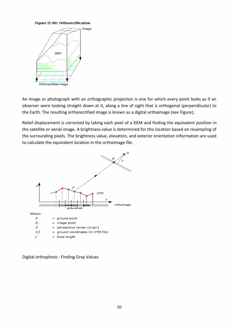
50

An image or photograph with an orthographic projection is one for which every point looks as if an

observer were looking straight down at it, along a line of sight that is orthogonal (perpendicular) to

the Earth. The resulting orthorectified image is known as a digital orthoimage (see Figure).

Relief displacement is corrected by taking each pixel of a DEM and finding the equivalent position in

the satellite or aerial image. A brightness value is determined for this location based on resampling of

the surrounding pixels. The brightness value, elevation, and exterior orientation information are used

to calculate the equivalent location in the orthoimage file.

Digital orthophoto : Finding Gray Values

51

In contrast to conventional rectification techniques, orthorectification relies on the digital elevation

data, unless the terrain is flat. Various sources of elevation data exist such as DEM automatically

created from stereo image pairs. For aerial photographs with a scale larger than 1:60000, elevation

data accurate to 1 meter is recommended. The 1 meter accuracy reflects the accuracy of the Z

coordinates in the DEM, not the DEM resolution or posting. Resampling methods used are nearest

neighbor, bilinear interpolation, and cubic convolution. Generally, when the cell sizes of orthoimage

pixels are selected, they should be similar or larger than the cell sizes of the original image. For

example, if the image was scanned at 25 microns (1016 dpi) producing an image of 9K × 9K pixels,

one pixel would represent 0.025 mm on the image. Assuming that the image scale of this photo is

1:40000, then the cell size on the ground is about 1 m. For the orthoimage, it is appropriate to choose

a pixel spacing of 1 m or larger. Choosing a smaller pixel size oversamples the original image. For

SPOT Pan images, a cell size of 10 meters is appropriate. Any further enlargement from the original

scene to the orthophoto does not improve the image detail. For IRS-1C images, a cell size of 6 meters

is appropriate.

3.12 Advantages of Digital Orthophotos

Despite these limitations, an orthophoto is a very useful mapping tool. It has the interpretative

qualities inherent in an image and the geometric properties of a map. This means that the features

on the image can be accurately measured, just like one might want to do with a conventional line

map. Because of this, orthophotographs form an excellent base or control layer for a GIS. It is also

relatively inexpensive, especially when one considers the costs incurred in conventional line mapping.

3.13 Other advantages/disadvantages of orthophotography:

The output image can be either a hard copy analog image or stored in digital form.

The orthophoto is an image therefore the viewer sees what is depicted on the image, whereas in a

conventional vector map the information is not complete because it conveys what the cartographer

felt the map should contain for its intended purpose. In other words, the map has undergone

generalization.

Digital orthophotos are GIS compatible since most software packages can incorporate the image into

their display. In fact, it has been the growth of GIS that has contributed significantly to the use of

digital orthophotography.

The image can be overlaid with existing vector data. This is particularly useful when performing

assessment of map accuracy.

The digital orthophoto is an excellent vehicle for assessing change in an area. New

imagery can be simply overlaid older orthophotography for analysis of the presence and extent of

change.

Orthophotos, being images, can use a wider spectrum of the electromagnetic spectrum for

specialized purposes. For example, infrared or filtered imagery could be used to emphasize features

on the ground.

The orthophoto is an excellent medium from which mapping can be done in inaccessible areas.

52

Although not frequently employed, stereomates could be created from an orthophoto for stereo

viewing of the area.

Disadvantages of Orthophotography

It is important for the user community to understand that orthophotography is just a tool and as such

is not applicable in all situations. Disadvantages include:

The data are an image that needs interpretation by the user. While features can be depicted on the

image, there is still a wealth of information missing such as feature classification and specific feature

identification. An example of the latter is that it may be impossible to differentiate between buildings

used for commercial or residential purposes. All the view sees is a building.

There are hidden areas where no data exist

Data shown on the image only represents that data above ground, and even this may sometimes be

hidden.

There are no spatial analysis capabilities. For example, a line could be identified within a vector map

and an attribute table can be displayed. But, clicking on that same feature on a rasterized image will

result in displaying pixel location.

3.14 Basic Components of an Orthoimage:

A digital orthophoto is nothing more than an orthoimage stored in digital form. The image consists of

an array of pixels that record the ground reflectance values for that pixel. The resolution of the image

is dictated, in part, by the size of the pixels and as we increase the resolution to finer levels, the size

of the image in the computer increases accordingly. There are basically four data sources needed to

create a digital orthophoto.

These are:

1. an unrectified raster image file acquired by either scanning an image or collected directly by a

digital sensor,

2. a digital elevation model (DEM) or digital terrain model (DTM) of the same area covered by the

imagery,

3. ground control

4. sensor calibration data.

The calibration data is required to compensate for the distortion characteristics that are inherent in

any measurement system. One set of calibration data is the interior orientation parameters that help

define the camera or sensor used to acquire the image. A second set of calibration values represent

the characterization of the sensor that may have been used to convert the analog picture into a

digital form. The ground control provides the absolute orientation of the image and allows us to

georeference each of the pixels within the image. The DEM/DTM is used to compensate for the

effects of relief displacement. This can be obtained from a number of different sources, but one must

be careful that the density of the ground sampling be consistent with the area being mapped.

53

Imagery used in the creation of a digital orthophoto can be of different types: black-andwhite (B/W),

color, color infrared (CIR), and other imagery captured in different regions of the electromagnetic

spectrum [URISA, 2001]. Black-and-white imagery consists of shades of gray extending from pure

white to pure black. It is very versatile and yields excellent resolution if properly exposed. B/W film

can accommodate large-scale enlargements. Additionally, it only requires about 1/3rd the storage

space of color. The disadvantage of B/W imagery is that it may not be as helpful for analysis such as

vegetation monitoring or when color or heat is important. If used for interpretation purposes, more

training of the analyst is usually required. Color film is often a medium that users prefer to work with

because it yields a picture that closely resembles how humans view the scene. It does not require as

much training for interpretation. Additionally, detail that may be lost in shadows in a black-and-white

film, particularly light shadows, may still be visible in color. It is more expensive than B/W film and

requires more storage space. Color infrared or false color film is similar to color film except that it is

sensitive to the green, red, and near-infrared regions of the electromagnetic spectrum. For example,

vegetation will appear as red in CIR film, although one can change the colors of the different bands

when the image is displayed in digital form. This type of film is particularly helpful in delineating

differences in vegetation since reflectance between vegetation features is markedly different in this

part of the electromagnetic spectrum. While color and black-and-white films are the most common

means of creating a digital orthophoto, other parts of the electromagnetic spectrum can also be use.

Radar, as an active sensor that is very useful in obtaining a digital elevation model of the earth's

surface. Moreover, it is helpful in obtaining an image of the surface under many different weather

conditions.

An important consideration when obtaining any kind of imagery is when should the imagery be

acquired. In other words, one must consider the season of the year. If terrain features are important

then leaf-off imagery should be collected. The best time to acquire the imagery is the spring because

snow has melted and the tall grasses that might be otherwise present are matted. If the purpose is to

analyze vegetation then leaf-on imagery will be desired. Imagery can be acquired in a number of

ways. Conventionally, an aerial camera is used to acquire the picture and then the processed

negative is scanned and converted to digital form. Imagery can also be obtained directly in digital

form using a digital camera. Currently there are four vendors providing digital cameras in a large

format and they are Leica Geosystems, Vexcel Imaging, Dimac Systems, and Z/I Imaging. These

cameras are much more expensive than their film counterparts.

If the pictures are film based then they need to be converted to digital form and this is done using a

scanner. There is a wide array of scanners available in the marketplace today, from less than $100 to

tens of thousands of dollars. For orthophotography, a high-end scanner should be used. This

equipment is more stable, has better geometric fidelity and yields a more robust digital orthophoto

product by incorporating scanner calibration values. Scanners come in different speeds. Normally, it

takes 10-15 minutes to scan a complete 9” square format image. They can also handle different types

of input media including cut film, glass diapositives, roll film, etc. Some scanners are highly

automated in that it will take a film roll and automatically scan each frame. In a similar vein, most

systems also provide different types of output formats. A TIFF file is the most common method of

showing the output data. This data represents the raw input data. While systems do allow for

compression of data, it is recommended that the data be stored in TIFF format and, if desired, a

54

working copy stored in the same compression format can be used if the user wants. It takes no more

time to scan the image so it is beneficial to store that raw data image

Two important aspects of scanners play critical roles in the geometric relationship of the scanned

image. First, the scanner calibration will define how the scanner behaves in its measurement process.

There are manufacturing/service producers who claim that they have “distortion free” optics, but this

is unrealistic. The second aspect is resolution. As it will be seen later, the selection of the scanner

resolution will have important repercussions upon the orthophoto products. Image data are

commonly stored in files called tiles. When the tiles are brought together they should form a

seamless map of the project area. For proper data management, an image catalog should be created

and provided to the user (this may be transparent to the user). Thecatalog locates all of the tiles of

orthophotography. Some systems use what is called an image pyramid. This consists of a series of

images sampled at different ground resolutions, such as 1’, 2’, 5’, and 10’. The idea is to provide rapid

image display by automatically loading only those images that are needed for the current views

extent with the appropriate pixel resolution.

3.15 Digital Orthophoto Problems

The creation of a digital orthophoto brings with it competing issues. These include accuracy, quality,

cost, and the hardware/software display and manipulation capabilities. Image quality is dependent

upon a number of production components such as

camera quality

diapositive/negative sharpness

photo to orthophoto map scale magnification

orthophoto diapositive density range or bits in the scanner scan pixel (radiometric

resolution)

sample scan rate in micrometers or dots per inch (dpi) and the photo scale

rectification procedures

final pixel size in ground units (pixel ground resolution)

electronic auto-dodging or radiometric image smoothing after the rectification process

selection of control points

DEM data density

Modulation Transfer Function

Pixel output being proportion to density or to the “transmissivity” of the medium

Assuming that the correct inputs are used, the accuracy that can be achieved in orthophotography is

comparable to that found in line maps. Accuracy of a digital orthophoto is a function of:

55

magnification

geometric accuracy of the scanner

quality of the DEM

control

focal length of the taking camera

One of the most abused aspects of digital data on the computer is the use of scale or magnification.

Computers have the ability to zoom in or out very simply. This may give the user a false sense of the

accuracy of the map product. As an example, field measurements may be taken of features with one

meter positioning capabilities, such as with “resource-grade” global positioning system (GPS)

receivers. But in the computer, these positions could be displayed at the millimeter level. Clearly,

displaying data at this range is inappropriate for data collected at the “coarse” meter range. The

same applies to orthophoto imagery. Remember that the farther the camera is away from the

ground, there is a loss of detail in the features imaged on the photo. For example, a manhole might

not be imaged on the photo because it is too small at the scale in which the photography was taken.

Therefore, the size of the smallest feature that needs to be depicted on the orthophoto will be a

major consideration when designing the scale of the photography. Magnification also affects the

image quality. The recommended magnification range is 8 or 9 times enlargement. Magnification of

ten times or more will degrade the image quality because the distance between the silver crystals on

the film become noticeable. Below five times enlargement does not noticeably improve the image

quality. Therefore, a range of 5-9 times enlargement is the optimum range, depending upon the area

being mapped. This means that if the desired final orthophoto scale is 1" = 100' then the photo scale

should not be less than 1" = 900'. Note that this would be for optimum terrain. Larger photo scales,

such as 1" = 700', may be required to meet the needs of the client. Radiometric resolution relates to

the ability to discern small changes in the tonal change within an image. The Content Standard

recommends that 8-bit binary data be used for black and white imagery and 24-bit, 3-byte data for

color imagery. This gives the user 256 gray levels over the image (0 – 255). The value zero represents

black and 255 is white. Radiometric corrections such as contrast stretching, analog dodging, noise

filtering, destriping, and edge matching are frequently applied to the data before it is given to the

user. The standard recommends that these processing techniques be used sparingly to minimize the

amount of data loss. Image quality is also affected by the resolution of the scanner.

The scanner and the scanning process have inherent errors associated with them. It is important that

high precision scanners be used in converting the image into a digital form. Additionally, it must be

calibrated to ensure that the performance of the equipment is within the minimum specifications for

the mapping. Many of the softcopy instruments used today have the capability of adding the scanner

calibration parameters into the program to correct for the distortion scanning introduces. It should

be evident that the coarser the resolution (larger the pixel size), the more “steplike” lines and

features become (recall that this is called pixelization). The important issue is the relationship

between the size of the scan pixel to the scale of the photography and the desired output orthophoto

scale. One suggestion is to scan the photo at about 240 dpi for each magnification range. This means

56

that if the desired photo to final orthophoto magnification range is 5 times, then the photo should

be scanned at 5 x 240 = 1200 dpi as a minimum

(micrometers) at the photo scale. Taking the magnification recommendation to its limit of 9 times

yields a sampling rate of 2160 dpi with a pixel size of roughly 12 micrometers. While a smaller pixel

size may yield better resolution, it does not necessarily mean higher accuracy since accuracy is

affected by a number of factors like the survey control, flying height, and focal length of the camera

along with pixel size. These results are consistent with other studies. For example, it has been

aerial film . Higher resolution does little to enhance interpretability of the image. In fact, 20 –

scan rates are commonly utilized in industry. These levels are both economical and meet the needs of

most mapping applications. Another issue affecting image quality is the pixel size expressed in ground

units. This is frequently performed by resampling the pixel values to create a smoother image in

terms of it tone. When this is done, the preference will be to sample to a coarser resolution, such as

sampling at half a foot and resample to the foot level. As a rule of thumb, a 1.2 times or larger factor

should be applied to the scanned pixel. For example, using this factor to a one-foot scan, the final

orthophoto would have at least a 1.2' pixel size. Subsampling should only be applied within the limits

defined ,which limits the resampling to a maximum of 2X. This limit is arrived at to avoid undesirable

aliasing.

The accuracy of the orthophoto is dependent upon two primary factors: control and DEM accuracy.

Survey control is required to fix the map to the ground. It is used to remove/reduce many of the

random errors associated with the imagery, such as terrain relief, platform position/orientation, and

faulty elevation data. Photogrammetrists often use aerotriangulation to provide control between the

primary ground control on a project. In some instances, control for the orthophoto is derived from

existing maps of the area. Significant errors can be introduced into the process thereby degrading the

orthophoto. For large-scale mapping, ground targets that will be imaged on the photo should be

used. The control needs to meet the specifications for the mapping. With the global positioning

system (GPS) and an inertial measurement unit (IMU), it is operationally feasible to perform the

mapping without control. The combined GPS/IMU allows for direct sensor orientation (DSO). Since

control is used to fix the exterior orientation, measurement of these parameters negates the

necessity to obtain control, although it is oftenprudent to obtain control for quality control/quality

assurance purposes and to make the photogrammetric solution more robust.

DEM accuracy is critical to the final quality of the orthophoto. The appropriate DEM must be selected

to match the scale of the orthophoto, terrain conditions, focal length of the camera used to acquire

the photography, and the magnification. The sampling interval for collecting the elevation data

depends upon the terrain conditions. Where the ground is relatively flat, a coarser DEM can be used.

On the other hand, if there is a lot of an elevation change (or surface roughness) in the area, a denser

sampling rate is required. It is generally acknowledged that the density and accuracy of the DEM for

orthophotography does not need to be as accurate as a DEM used for contouring or 3-D modeling.

For large-scale mapping, it is important to also include break lines in the data collection. A break line

is where the terrain changes direction in slope, such as the bottom or toe of a hill. These break lines

control the modeling of the characteristics of the surface and fixes the placement of contour lines on

the site. While density is important, the quality of the break lines is more significant. In fact,

57

experience indicates that the sample rate can be very course provided that sufficient break lines exist

in order to correctly capture the characteristics of the terrain surface DEM. Generally, the density of

the DEM needs to be denser with smaller magnification ratios. As a rule of thumb, if the

magnification is less than 3 times then the spacing for the DEM needs to be 4-8 mm at the final map

scale. If the magnification is 3-8 times, then the spacing at the final map scale should be 8-16 mm.

Over 8 times magnification allows a grid spacing of 12- 24 mm at the final map scale. The operator

needs to be aware that the density is greater when the terrain changes rapidly on the site and can be

relaxed or spread farther when the terrain is flat. DEM characteristics change with the terrain

therefore it is impossible to outline minimum criteria that would be applicable for all surfaces. It is

even possible to find a lot of variability within a single map sheet or tile. Because terrain variability

can exist within a project, the map itself may meet accuracy specifications but local anomalies can

exist where the map can fail stipulated testing. This is particularly true in areas where elevation

changes are abrupt or where bridges, elevated highways and the like are present Problems with

digital orthophotos that need to be looked at include:

Image Completeness - The image area is not adequately covered by a DEM resulting in an inaccurate

orthophoto. One of the biggest problems is cloud cover. Either the cloud itself or the shadow from a

cloud may obscure ground detail. It is the users responsibility to ensure that if the image contains

cloud cover that the percentage of obstruction is acceptable for the intended purpose.

Image Stretch (Blurring, also called image smear) - This is typically caused by anomalies within the

DEM data resulting in a spike or large error. Excessive relief on the edge of the photography can also

be the cause of this problem. The result is that ground image data is hidden from view. Smearing can

occur when an interpolation program is used to assign brightness values to the hidden area using the

surrounding visible image. There is no easy way of correcting for this problem except by using

subjective visible inspection. It is up to the user to determine whether the amount of these smear

artifacts affect the image data for their intended use.

Image Distortions – For large-scale orthophotos, local distortions can exist as was discussed

earlier. Figure 3a shows a distortion along a bridge deck due to reliance on a regular grid of

elevations. These distortions can be reduced, but not eliminated, by either collecting break line

information or densification of the DEM grid. Figure 3b shows how this distortion can be edited to

create a more faithful rendition of the terrain.

Double Image - This is when the adjacent orthophotos are compared and the same feature is

mapped on both photos when this should not occur. In other words, the maps should be mutually

exclusive. The problem may be either improper orientation in the control or less accuracy in the DEM

where ground elevations are given that are larger than the reality.

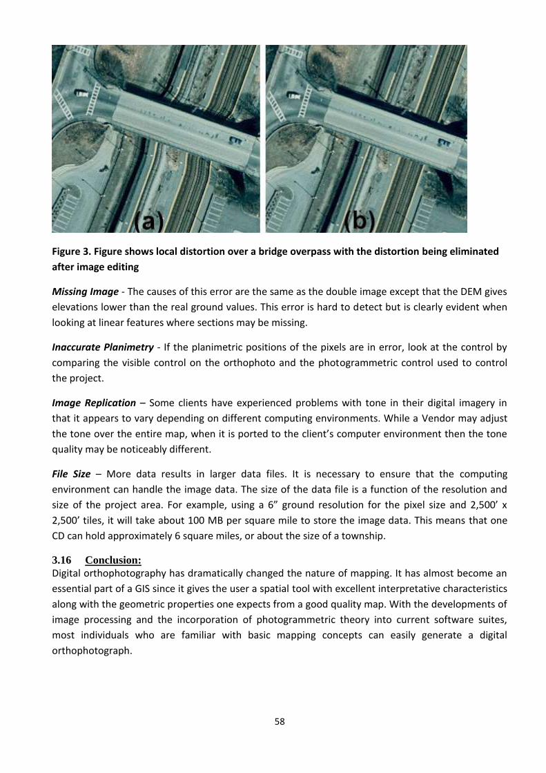
58

Figure 3. Figure shows local distortion over a bridge overpass with the distortion being eliminated

after image editing

Missing Image - The causes of this error are the same as the double image except that the DEM gives

elevations lower than the real ground values. This error is hard to detect but is clearly evident when

looking at linear features where sections may be missing.

Inaccurate Planimetry - If the planimetric positions of the pixels are in error, look at the control by

comparing the visible control on the orthophoto and the photogrammetric control used to control

the project.

Image Replication – Some clients have experienced problems with tone in their digital imagery in

that it appears to vary depending on different computing environments. While a Vendor may adjust

the tone over the entire map, when it is ported to the client’s computer environment then the tone

quality may be noticeably different.

File Size – More data results in larger data files. It is necessary to ensure that the computing

environment can handle the image data. The size of the data file is a function of the resolution and

size of the project area. For example, using a 6” ground resolution for the pixel size and 2,500’ x

2,500’ tiles, it will take about 100 MB per square mile to store the image data. This means that one

CD can hold approximately 6 square miles, or about the size of a township.

3.16 Conclusion:

Digital orthophotography has dramatically changed the nature of mapping. It has almost become an

essential part of a GIS since it gives the user a spatial tool with excellent interpretative characteristics

along with the geometric properties one expects from a good quality map. With the developments of

image processing and the incorporation of photogrammetric theory into current software suites,

most individuals who are familiar with basic mapping concepts can easily generate a digital

orthophotograph.

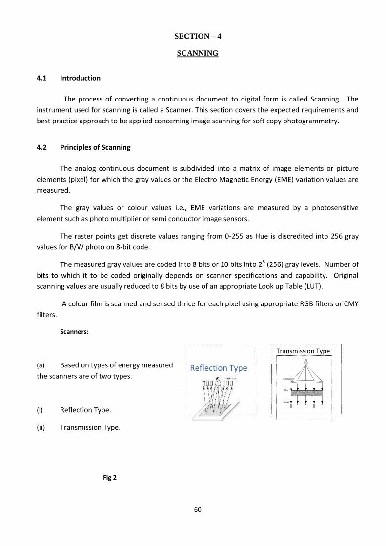
60

SECTION – 4

SCANNING

4.1 Introduction

The process of converting a continuous document to digital form is called Scanning. The

instrument used for scanning is called a Scanner. This section covers the expected requirements and

best practice approach to be applied concerning image scanning for soft copy photogrammetry.

4.2 Principles of Scanning

The analog continuous document is subdivided into a matrix of image elements or picture

elements (pixel) for which the gray values or the Electro Magnetic Energy (EME) variation values are

measured.

The gray values or colour values i.e., EME variations are measured by a photosensitive

element such as photo multiplier or semi conductor image sensors.

The raster points get discrete values ranging from 0-255 as Hue is discredited into 256 gray

values for B/W photo on 8-bit code.

The measured gray values are coded into 8 bits or 10 bits into 28 (256) gray levels. Number of

bits to which it to be coded originally depends on scanner specifications and capability. Original

scanning values are usually reduced to 8 bits by use of an appropriate Look up Table (LUT).

A colour film is scanned and sensed thrice for each pixel using appropriate RGB filters or CMY

filters.

Scanners:

(a) Based on types of energy measured

the scanners are of two types.

(i) Reflection Type.

(ii) Transmission Type.

Fig 2

Reflection Type

Transmission Type

Condenser

Film Sensor

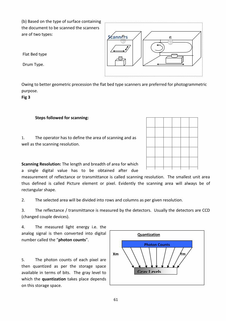
61

Scanners

(i) Flat Bed type. (ii) Drum Type.

Fig.3

(b) Based on the type of surface containing

the document to be scanned the scanners

are of two types:

Flat Bed type

Drum Type.

Owing to better geometric precession the flat bed type scanners are preferred for photogrammetric

purpose.

Fig 3

Steps followed for scanning:

1. The operator has to define the area of scanning and as

well as the scanning resolution.

Scanning Resolution: The length and breadth of area for which

a single digital value has to be obtained after due

measurement of reflectance or transmittance is called scanning resolution. The smallest unit area

thus defined is called Picture element or pixel. Evidently the scanning area will always be of

rectangular shape.

2. The selected area will be divided into rows and columns as per given resolution.

3. The reflectance / transmittance is measured by the detectors. Usually the detectors are CCD

(changed couple devices).

4. The measured light energy i.e. the

analog signal is then converted into digital

number called the “photon counts”.

5. The photon counts of each pixel are

then quantized as per the storage space

available in terms of bits. The gray level to

which the quantization takes place depends

on this storage space.

Fig 4

Quantization

Xm Ym

0 255

Fig.5

Photon Counts

Gray Levels

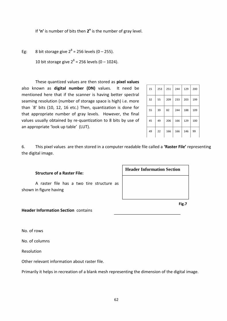
62

If ‘n’ is number of bits then 2n is the number of gray level.

Eg: 8 bit storage give 28 = 256 levels (0 – 255).

10 bit storage give 28 = 256 levels (0 – 1024).

These quantized values are then stored as pixel values

also known as digital number (DN) values. It need be

mentioned here that if the scanner is having better spectral

seaming resolution (number of storage space is high) i.e. more

than `8’ bits (10, 12, 16 etc.) Then, quantization is done for

that appropriate number of gray levels. However, the final

values usually obtained by re-quantization to 8 bits by use of

an appropriate ‘look up table’ (LUT).

6. This pixel values are then stored in a computer readable file called a ‘Raster File’ representing

the digital image.

Structure of a Raster File:

A raster file has a two tire structure as

shown in figure having

Header Information Section contains

No. of rows

No. of columns

Resolution

Other relevant information about raster file.

Primarily it helps in recreation of a blank mesh representing the dimension of the digital image.

15 253 251 244 129 200

32 55 209 233 203 199

55 39 82 244 188 109

45 49 206 166 129 100

49 22 166 166 146 99

34 44 104 199 100 66

Fig.6

Header Information Section

Actual Data Section

Fig.7

63

Actual data section contains the actual pixel values. The number of values contained = No. of rows x

No. of columns. This section helps in painting the relevant pixels in the blank mesh created with the

help of header section by the gray shade as per the D/N values. This enables creation of actual

digital image of scanned analog document. The values always remain between 0 – 255.

Types of Raster Files/Images:

There are three types of Raster files namely

Binary Raster

Continuous Tone Raster

Colour Raster.

The following prints are noteworthy in connection with Raster images.

The scanning is usually done for continuous tone file as narrated above i.e. the scanning process is

unique.

Other two types of files are derivative of the same scanned product.

Binary Raster File:

Defining a threshold value and re-

quantizing the pixel values of Continuous tone

Raster file can obtain the binary raster file. In a

binary raster file one bit is available for storage.

Therefore only ‘2’ gray levels (0 – 1) are

possible.

e.g. Let Threshold = 128

Quatization

0 255

0 1

Threshold =128

Gray Values

Fig 8

15 253 251 244 129 200

32 55 209 233 203 199

55 39 82 244 188 109

45 49 206 166 129 100

49 22 166 166 146 99

34 44 104 199 100 66

Continuous Tone Raster

0 1 1 1 1 1

0 0 1 1 1 1

0 0 0 1 1 0

0 0 1 1 1 0

0 0 1 1 1 0

0 0 0 1 0 0

Binary File

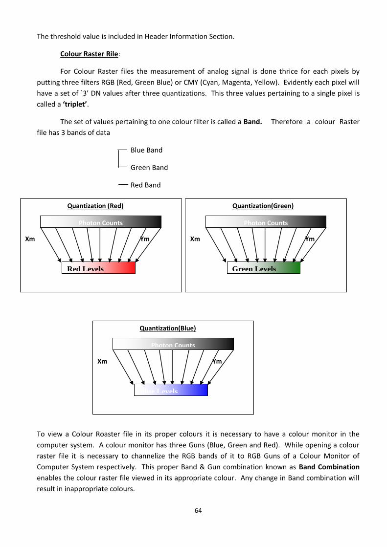
64

The threshold value is included in Header Information Section.

Colour Raster Rile:

For Colour Raster files the measurement of analog signal is done thrice for each pixels by

putting three filters RGB (Red, Green Blue) or CMY (Cyan, Magenta, Yellow). Evidently each pixel will

have a set of `3’ DN values after three quantizations. This three values pertaining to a single pixel is

called a ‘triplet’.

The set of values pertaining to one colour filter is called a Band. Therefore a colour Raster

file has 3 bands of data

Blue Band

Green Band

Red Band

To view a Colour Roaster file in its proper colours it is necessary to have a colour monitor in the

computer system. A colour monitor has three Guns (Blue, Green and Red). While opening a colour

raster file it is necessary to channelize the RGB bands of it to RGB Guns of a Colour Monitor of

Computer System respectively. This proper Band & Gun combination known as Band Combination

enables the colour raster file viewed in its appropriate colour. Any change in Band combination will

result in inappropriate colours.

Quantization (Red)

Xm Ym

0 255

Fig.5

Photon Counts

Red Levels

Quantization(Green)

Xm Ym

0 255

Photon Counts

Green Levels

Quantization(Blue)

Xm Ym

0 255

Photon Counts

Blue Levels

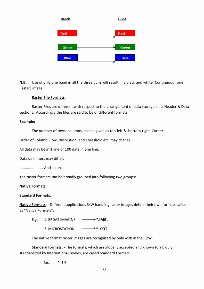
65

Bands Guns

N.B: Use of only one band in all the three guns will result in a black and white (Continuous Tone

Raster) image.

Raster File Formats:

Raster Files are different with respect to the arrangement of data storage in its Header & Data

sections. Accordingly the files are said to be of different formats.

Example: -

- The number of rows, columns, can be given as top-left & bottom-right Corner.

Order of Column, Row, Resolution, and Threshold etc. may change.

All data may be in 1 line or 100 data in one line.

Data delimiters may differ.

……………………. And so on.

The raster formats can be broadly grouped into following two groups:

Native Formats

Standard Formats.

Native Formats: - Different applications S/W handling raster images define their own formats called

as “Native Formats”.

E.g. 1. ERDAS IMAGINE *.IMG.

2. MICROSTATION *. COT

The native format raster images are recognized by only with in the S/W.

Standard formats: - The formats, which are globally accepted and known to all, duly

standardized by International Bodies, are called Standard Formats.

Eg.: *. TIF

Red Red

Green Green

Blue Blue

66

*. JPG

N.B: - i) Usually the raster data are transported from one S/w to other S/w by standard formats.

ii) Every S/W accepts standard format and facilitate Import & Export facilities.

4.3 Photogrammetric Scanners - Introduction

Photogrammetric scanners are special devices capable of high image quality and excellent positional

accuracy. Use of this type of scanner results in geometric accuracies similar to traditional analog and

analytical photogrammetric instruments. These scanners are necessary for digital photogrammetric

applications that have high accuracy requirements. These units usually scan only film because film is

superior to paper, both in terms of image detail and geometry. These units usually have a Root Mean

Square Error (RMSE) positional accuracy of 4 microns or less, and are capable of scanning at a

maximum resolution of 5 to 10 microns (5 microns is equivalent to approximately 5,000 dpi).

The original film (or alternatively the diapositive) should be scanned with a photogrammetric quality

scanner of the following general characteristics:-

Scan resolution of 20µm or better; typically, up to 12µm scan resolution will be applied.

Final radiometric resolution of atleast 8-bit per channel. However it is strongly advised that 11-or-

12bit scanning systems are used.

Geometric precision of scanner <5µm.

The required pixel resolution varies depending on the application. Aerial triangulation and feature

collection applications often scan in the 10- to 15-micron range. Orthophoto applications often use

15- to 30-micron pixels. Color film is less sharp than panchromatic, therefore, color ortho applications

often use 20- to 40-micron pixels. The optimum scanning resolution also depends on the desired

photogrammetric output accuracy. Scanning at higher resolutions provides data with higher accuracy.

The image correlation techniques that are necessary for automatic tie point collection and elevation

extraction are often sensitive to scan quality.

Desktop Scanners Desktop scanners are general purpose devices. They lack the image detail and

geometric accuracy of photogrammetric-quality units, but they are much less expensive. Desktop

scanners are appropriate for less rigorous uses, such as GIS or remote sensing applications.

Calibrating these units improves geometric accuracy, but the results are still inferior to

photogrammetric units and therefore not recommended for Digital Photogrammetry. Therefore,

errors attributable to scanning errors can be introduced into GIS data that is photogrammetrically

derived. One of the primary factors contributing to the overall accuracy of 3D feature collection is the

resolution of the imagery being used. Image resolution is commonly determined by the scanning

resolution (if film photography is being used), or by the pixel resolution of the sensor.

67

In order to optimize the attainable accuracy of GIS data collection, the scanning resolution must be

considered. The appropriate scanning resolution is determined by balancing the accuracy

requirements versus the size of the mapping project and the time required to process the project.

4.3.1 Types of Photogrammetic Scanners

Based on types of energy measured, the scanners are of two types.

Reflection Type.

Transmission Type.

Based on the type of surface containing the document to be scanned the scanners are of two types.

Flat Bed Type

Drum Type.

Owing to better geometric precession the flat bed type scanners are preferred for photogrammetric

purpose.

The photogrammetry scanners available in market are:

Wehrli & Associate Product

Z/I Imaging Product

Vexcel Imaging Austria

L.H. Systems.

4.4 Scanning Resolution:

The length and breadth of area for which a single digital value has to be obtained after due

measurement of reflectance or transmittance is called scanning resolution. The smallest unit area

thus defined is called Picture element or pixel. Evidently the scanning area will always be of

rectangular shape.

The selected area will be divided into rows and columns as per given resolution.

The reflectance / transmittance is measured by the detectors. Usually the detectors are CCD

(changed couple devices).

The measured light energy i.e., the analog signal is then converted into digital number called the

“Photon Counts”

The photon counts of each pixel are then quantized as per the storage space available in

terms of storage space available in terms of bits. The gray level to which the quantization takes place

depends on this storage space.

If ‘n’ is number of bits then 28 is the number of gray level.

Eg: 8 bit storage give 28 = 256 level (0-255)

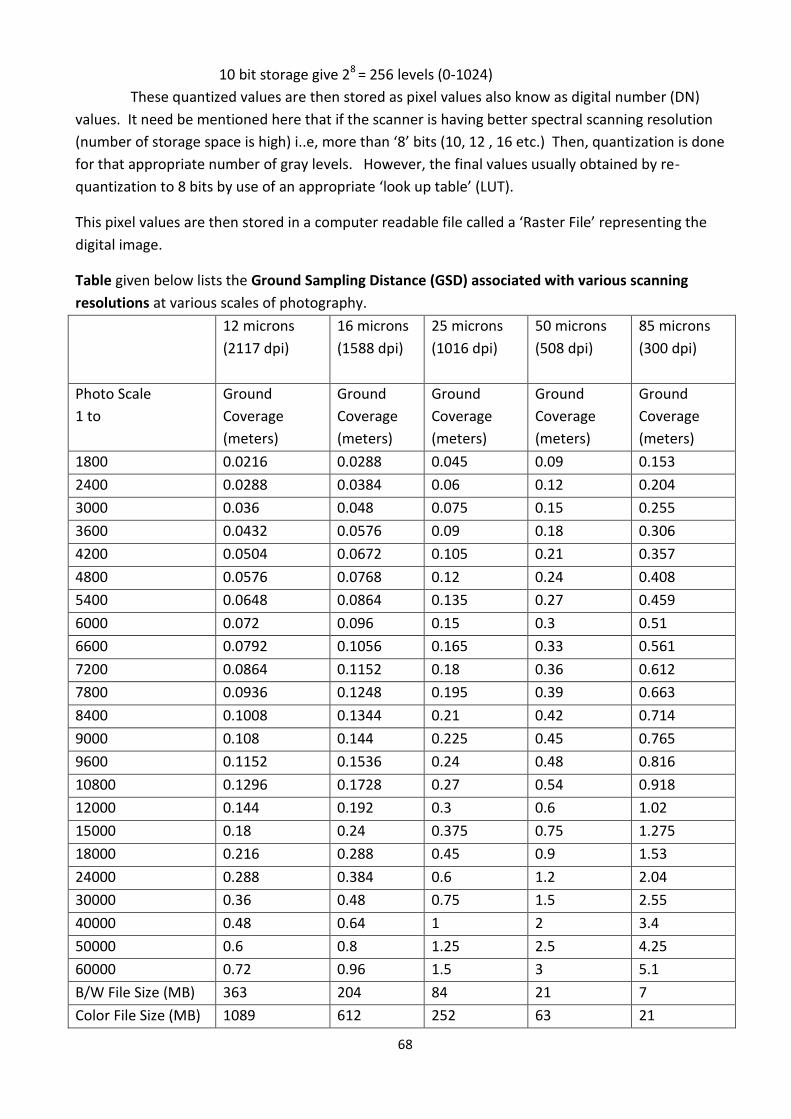
68

10 bit storage give 28 = 256 levels (0-1024)

These quantized values are then stored as pixel values also know as digital number (DN)

values. It need be mentioned here that if the scanner is having better spectral scanning resolution

(number of storage space is high) i..e, more than ‘8’ bits (10, 12 , 16 etc.) Then, quantization is done

for that appropriate number of gray levels. However, the final values usually obtained by re-

quantization to 8 bits by use of an appropriate ‘look up table’ (LUT).

This pixel values are then stored in a computer readable file called a ‘Raster File’ representing the

digital image.

Table given below lists the Ground Sampling Distance (GSD) associated with various scanning

resolutions at various scales of photography.

12 microns

(2117 dpi)

16 microns

(1588 dpi)

25 microns

(1016 dpi)

50 microns

(508 dpi)

85 microns

(300 dpi)

Photo Scale

1 to

Ground

Coverage

(meters)

Ground

Coverage

(meters)

Ground

Coverage

(meters)

Ground

Coverage

(meters)

Ground

Coverage

(meters)

1800 0.0216 0.0288 0.045 0.09 0.153

2400 0.0288 0.0384 0.06 0.12 0.204

3000 0.036 0.048 0.075 0.15 0.255

3600 0.0432 0.0576 0.09 0.18 0.306

4200 0.0504 0.0672 0.105 0.21 0.357

4800 0.0576 0.0768 0.12 0.24 0.408

5400 0.0648 0.0864 0.135 0.27 0.459

6000 0.072 0.096 0.15 0.3 0.51

6600 0.0792 0.1056 0.165 0.33 0.561

7200 0.0864 0.1152 0.18 0.36 0.612

7800 0.0936 0.1248 0.195 0.39 0.663

8400 0.1008 0.1344 0.21 0.42 0.714

9000 0.108 0.144 0.225 0.45 0.765

9600 0.1152 0.1536 0.24 0.48 0.816

10800 0.1296 0.1728 0.27 0.54 0.918

12000 0.144 0.192 0.3 0.6 1.02

15000 0.18 0.24 0.375 0.75 1.275

18000 0.216 0.288 0.45 0.9 1.53

24000 0.288 0.384 0.6 1.2 2.04

30000 0.36 0.48 0.75 1.5 2.55

40000 0.48 0.64 1 2 3.4

50000 0.6 0.8 1.25 2.5 4.25

60000 0.72 0.96 1.5 3 5.1

B/W File Size (MB) 363 204 84 21 7

Color File Size (MB) 1089 612 252 63 21

69

The ground coverage column refers to the ground coverage per pixel. Thus, a 1:40000 scale black and

white photograph scanned at 25 microns (1016 dpi) has ground coverage per pixel of 1 m × 1 m. The

resulting file size is approximately 85 MB, assuming a square 23 cm × 23 cm photograph.

4.5 Scan process – Quality Assurance / Quality Control

The scanning process should be checked frequently and a quality assurance report submitted at the

time of delivery of data. The quality control data (“scan file”) produced by the scanning software

would normally be a suitable information source to include. The quality assurance report should also

contain information on:

Frequency, execution and details on geometric quality control using e.g. a calibrated

photogrammetric grid performed before and during project.

Frequency, execution and details on radiometric quality control using e.g. photographic step tablet

performed before and during project.

Details on quality tests of the scanned photographs including the following checks:

Saturation should not exceed 0.5% at each tail of the histogram (e.g. the resulting 0 and 255 values

for an 8-bit image). For the full image. For colour/multispectral images, this assessment should be

made in the Luminosity histogram.

Effective use of the radiometric resolution - This should be determined by a check for grey-values

which contain no pixels in the output image.

Contrast: The coefficient of variation (Represented as standard Deviation of the DN values as a

percentage of the available grey levels) of the image DN values should be in the range of 10-20%.

Exception will, however, occur where the scene contains features like sun-glint on water bodies, etc.

Clear visibility of fiducial marks.

A table should be provided giving the meta-data characteristics of the files delivered (file name,

photo number, CD number, radiometric statistics, results of sample tests, date and time of scanning,

operator, etc.)

In addition, sufficient checks should be carried out to ensure that the following parameters are

respected:

Geometry: a photogrammetric interior orientation (affine transformation of the images will be

expected to produce and RMSE of <10µm (four corner fiducials), with no residual greater than 30µm.

In the case of use of eight fiducial marks, the RMSE can increase to <20 µm (although again, no

residual should exceed 30 µm).

Correct labeling of files: this should follow a standard window platform naming convention, without

spaces and with a name plus extension (file type) e.g. photo_nr.tif. The naming used should

correspond with that used in the meta-data table described above.

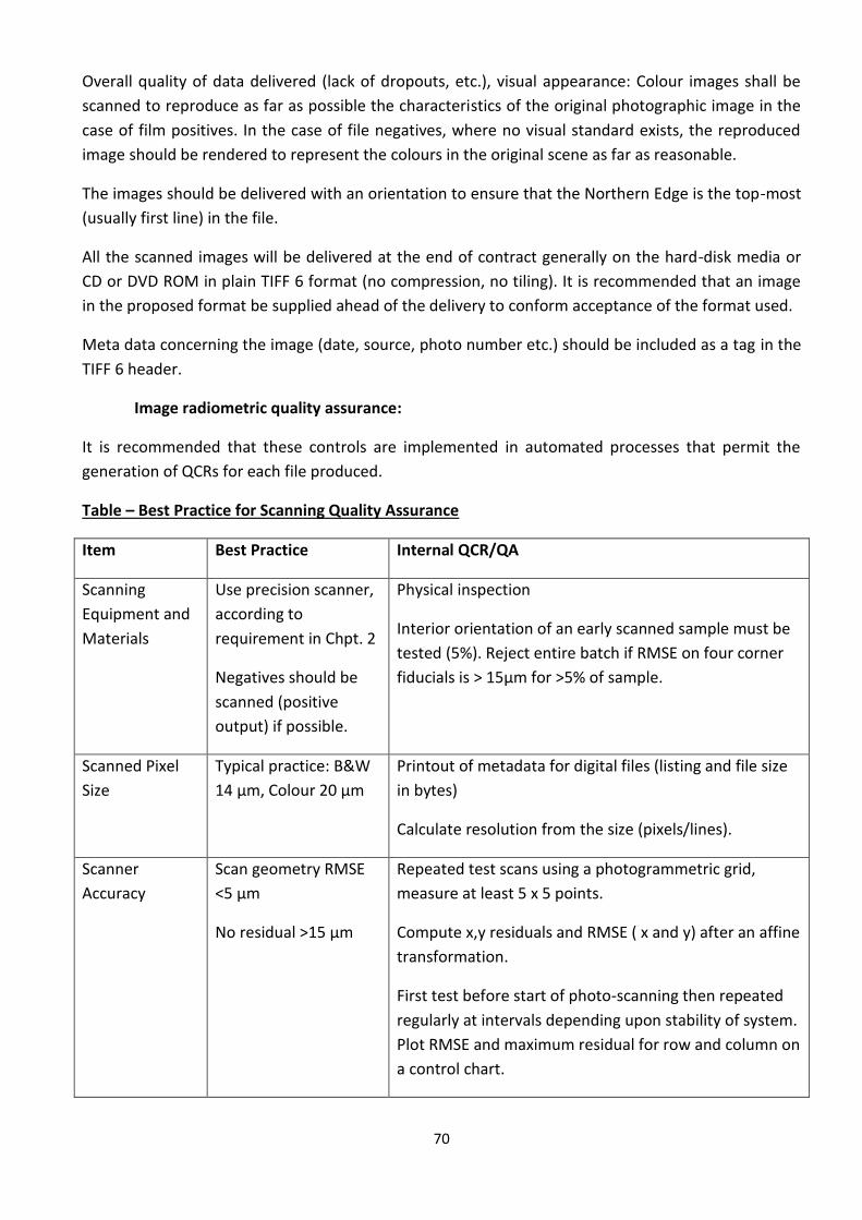
70

Overall quality of data delivered (lack of dropouts, etc.), visual appearance: Colour images shall be

scanned to reproduce as far as possible the characteristics of the original photographic image in the

case of film positives. In the case of file negatives, where no visual standard exists, the reproduced

image should be rendered to represent the colours in the original scene as far as reasonable.

The images should be delivered with an orientation to ensure that the Northern Edge is the top-most

(usually first line) in the file.

All the scanned images will be delivered at the end of contract generally on the hard-disk media or

CD or DVD ROM in plain TIFF 6 format (no compression, no tiling). It is recommended that an image

in the proposed format be supplied ahead of the delivery to conform acceptance of the format used.

Meta data concerning the image (date, source, photo number etc.) should be included as a tag in the

TIFF 6 header.

Image radiometric quality assurance:

It is recommended that these controls are implemented in automated processes that permit the

generation of QCRs for each file produced.

Table – Best Practice for Scanning Quality Assurance

Item Best Practice Internal QCR/QA

Scanning

Equipment and

Materials

Use precision scanner,

according to

requirement in Chpt. 2

Negatives should be

scanned (positive

output) if possible.

Physical inspection

Interior orientation of an early scanned sample must be

tested (5%). Reject entire batch if RMSE on four corner

fiducials is > 15µm for >5% of sample.

Scanned Pixel

Size

Typical practice: B&W

14 µm, Colour 20 µm

Printout of metadata for digital files (listing and file size

in bytes)

Calculate resolution from the size (pixels/lines).

Scanner

Accuracy

Scan geometry RMSE

<5 µm

No residual >15 µm

Repeated test scans using a photogrammetric grid,

measure at least 5 x 5 points.

Compute x,y residuals and RMSE ( x and y) after an affine

transformation.

First test before start of photo-scanning then repeated

regularly at intervals depending upon stability of system.

Plot RMSE and maximum residual for row and column on

a control chart.

73

SECTION – 5

DIGITAL TERRAIN MODEL

5.1 Introduction:

The concept of DTM is relatively straightforward, namely the provision of bare-earth elevations,

referenced to a vertical datum.

In some instances there are conflicts in definitions of key words like DEM, DTM and DSM. The most

commonly used definition, which has been adopted in this SECTION, are as follows:

The term Digital Elevation Model (DEM) is used to describe bare earth elevations within a grid at a

specified spacing.

A term that is often used synonymously with DEM is DTM or Digital Terrain Model. DTM often

implies that the elevation data is not gridded. Instead a DTM may incorporate breaklines that

describe discontinuities in the terrain (e.g. creeks or ridge lines) and mass points for characterising

topographic features. A DTM represents the elevation associated with the Earth's topography and

not necessarily the human-made (e.g., buildings) or natural (e.g., trees) features located on the

Earth’s surface.

A digital surface model (DSM) represents the elevation associated with the Earth's surface

including topography and all natural or human-made features located on the Earth’s surface. The

primary difference between a DSM and a DTM is that the DTM represents the Earth’s terrain

whereas a DSM represents the Earth's surface. The digital surface model (DSM) is a very useful

elevation data set in its own right.

5.2 Scope

Given that this SECTION deals with Digital Photogrammetry, although acknowledging other DEM

acquisition technologies, focuses on generation of DTM from aerial photography and satellite

imagery. Airborne Laser Scanning (ALS) or LIDAR and other technologies like IFSAR will be the subject

of a separate review, and may be incorporated into the SECTION in the near future, once these

technologies are adopted in the Department.

5.3 Challenges in Generation of Accurate DEM/DTM

Realisation of accurate DEM, however, is a complex proposition for a number of reasons, which

include the data acquisition technologies involved, issues with the definition of a uniform vertical

datum, the horizontal density and vertical resolutions involved, data quality and data formats.

Virtually all technologies for automatic acquisition of elevation data are based on remotely sensing

the terrain from above. As a consequence the surface modelled in the first instance is the DSM which

is the ‘reflective’ surface that comprises buildings and vegetation as well as the bare earth. The DTM

is generated through a post-processing of the DSM. The accurate and comprehensive removal of

74

‘above ground’ features or ‘artefacts’ remains one of the significant challenges in DTM/DEM

generation, especially in urban and heavily vegetated areas.

5.4 DEM Acquisition Technologies

Any new elevation data acquisition programs that are to be undertaken within the foreseeable future

for the purpose of generating DEM are going to involve one of a finite number of sensor

technologies. The purpose of the following discussion is to give an overview of the current

techniques for DEM data generation, primarily to illustrate their capabilities.

The technologies covered are

Ground Surveying

Photogrammetry

Airborne light detection and ranging (LIDAR), also termed airborne laser scanning (ALS)

Interferometric synthetic aperture radar (IFSAR)

Digitization of Topographic Maps

In the case of photogrammetry and IFSAR, the sensor platforms can be either airborne or

spaceborne. All technologies generate, in the first instance, DSMs though both LIDAR and multi-band

IFSAR have the potential of penetrating vegetation to provide bare-earth elevations.

5.4.1 Ground Surveying

Surveying levels, total stations and/or ground GPS units can be used for the measurement of 3D

information pertaining to the Earth's surface. Discrete points (i.e., spot heights) are surveyed and

recorded. Each recorded point has a 3D coordinate associated with it. All of the 3D points are used to

interpolate a 3D surface of the specific area of interest.

Generally field survey methods are used Its use in data collection is very much limited because of the

high cost of collection per point., where there is a considerable change in the relief and high accuracy

is required (mostly for large scale surveys).

This approach is highly accurate, but time-consuming. Its use in data collection is very much limited

because of the high cost of collection per point. Ground surveying techniques are commonly used for

civil engineering applications (e.g., road and bridge construction) and for survey of small areas, where

high accuracy is required.

5.4.2 Photogrammetry:

As a tool for topographic mapping, photogrammetry has a long history spanning more than 60 years

and has consistently delivered reliable results. The technology can use stereo frame or line scan data

from aerial or satellite sensors. Historically it was a manual process to observe elevation data but

with the advent of digital softcopy photogrammetric processes, automated DSM generation through

image matching technology became feasible. Today the generation of a DSM from digital aerial or

satellite imagery is almost a fully automatic batch process. Nevertheless, the cost of the DSM-to-

DEM conversion can be very significant, and can exceed the total cost of producing the DSM.

75

Broad area DTM/DEM generation via photogrammetry is presently not the preferred approach,

particularly over densely vegetated areas. It does however potentially provide advantages where

high accuracy DTM/DEMs of better than 10cm vertical resolution are required over sparse

vegetation, for applications such as 3D city modelling, or where the DTM/DEM is highly reliant on

breaklines.

High resolution satellite imaging systems have gained popularity for DSM generation at vertical

resolutions within the range of about 1m to 10m. For example, the recently launched World View 1

satellite has a 50cm GSD, which, although not verified, may support DSM extraction to around 1-1.5m

vertical accuracy; and stereo-imageries from Indian Satellites, with highly stable platform may

support DSM extraction to around 3-5m.

While aerial photogrammetry remains a flexible and accurate means of topographic mapping, it

tends not to be a preferred technology for stand-alone DEM generation over large project areas

where terrain models with vertical accuracies in the 10cm to 1m range are required.

5.4.3 ALS or LIDAR:

Airborne laser scanning or LIDAR has evolved over the last decade into the clear ‘technology of

choice’ for the generation of high-resolution elevation models, as characterised by vertical accuracies

of 10-50cm and horizontal post spacings of 1-3m. The advantages of LIDAR centre upon its relatively

high-accuracy of 10-15cm in height and 30cm to 60cm in the horizontal, and upon the very high mass

point density of at least 1 point/m2. This high point density greatly assists artefact removal in the

DSM-to-DEM conversion. Moreover, LIDAR has high productivity of around 300 km2 of coverage per

hour, and it can be operated ‘locally’, day or night. In practise, data acquisition is generally confined

to daylight hours since most LIDAR units nowadays come with dedicated digital cameras (usually

medium format), the resulting imagery being used both to assist in the artefact removal process and

for orthoimage production.

One of the most significant attributes of LIDAR is multi-pulse sensing, where the first returned pulse

indicates the highest point encountered and the last the lowest point. There may also be mid pulses.

As a consequence, LIDAR has the ability to ‘see through’ all but thick vegetation and it can be safely

assumed that a good number of the last returns will be from bare earth. This greatly simplifies the

DSM-to-DEM conversion process in vegetated areas.

The advantages of LIDAR over high-resolution photogrammetry in urban and city environments are

less pronounced since the reflections of surfaces such as the sides of buildings can complicate shape

definition and obscure breaklines. However, LIDAR is a near nadir sensing system, with its field of

view extending only about 200 each side of the vertical. This allows penetration into urban canyons.

As with the photogrammetric DSM-to-DEM conversion, considerable manual post processing of the

filtered and thinned out LIDAR DEM is required to ‘clean’ the bare-earth representation. The cost of

the manual post-processing stage has been reduced over recent years as software systems have

become more sophisticated. Although the manual intervention may account for 90% of the post-

processing budget, it is now down to something in the order of 20%-30% of the overall project

budget.

76

In many respects LIDAR data is similar to image acquisition from aerial photography: Flights are

carried out in strips, with a nominal side overlap of around 30%, depending upon terrain.

‘Accuracy’ is again a function of flying height, but in the case of LIDAR the height accuracy (i.e.

ranging accuracy) remains reasonably constant whereas the ground sampling density varies.

In general, LIDAR is less expensive than standard photogrammetry, with the cost advantages

becoming more pronounced as project areas become larger.

5.4.4 IFSAR

Interferometric Synthetic Aperture Radar (IFSAR) systems determine the relative heights of imaged

ground points as a function of the phase difference of the coherently combined signals received at

two antennas. At the present time there are basically two commercial providers of airborne IFSAR

DEMs, both being US-based. One is Intermap Technologies, who operate a number of X-band

sensors, and the other is Fugro EDI whose GeoSAR system employs X- and P-band sensors. In broad

terms, both commercial providers offer similar radar imaging and DEM generation services. Both

these systems can produce DSMs to around 1m vertical accuracy and with a post spacing of 5m. Also

the use of stereo radar imagery as a complement to the process allows a semi-automated DSM-to-

DEM conversion. Airborne IFSAR can record data at a very rapid rate, with swath widths exceeding

10km, and importantly, data collection is not impeded by clouds. As a tool for providing DEM data

within the NEDF, airborne IFSAR holds a lot of promise, but it is likely only to be cost effective at the

present time for large area DEMs with vertical accuracy of around 1m and horizontal resolutions

between 5m and 30m. The absence of any locally based Airborne IFSAR operator further escalates

the cost of using this technology. Based on these limitations and the limited number of IFSAR service

providers globally, it will not be further considered in this review, however it is recognised that IFSAR

offers potential and the use of this technology will need to considered in the future as the number of

service providers increases.

When compared to airborne IFSAR as a technology for DEM generation, LIDAR displays advantages

that go beyond its inherently higher accuracy. For a start, LIDAR is a near nadir sensing system, with

its field of view extending only about 200 each side of the vertical. This allows penetration into urban

canyons and enhanced prospects for penetration through vegetation. As will be discussed in the next

section, IFSAR is side-looking, which can leave shadowing and data voids in the oblique ranging data,

thus complicating somewhat DEM acquisition over urban areas. Over small areas LIDAR displays cost

advantages over airborne IFSAR, but when it comes to very large area coverage IFSAR is more cost

competitive.

5.4.5 Digitization of Topographic Maps

Existing topographic maps can be digitized to record spot heights and contour lines. The elevation

associated with the digitized spot heights and contour lines can be attributed. The resulting features

can be interpolated to create a 3D surface. This technique is however limited by the accuracy of the

original source map used.

77

5.5 GENERAL DESCRIPTIONS

5.5.1 Data Types

Elevation data can take many forms and include both ground and non-ground surface information.

However, when looking from an ‘acquisition’ through ‘user’ perspective, data can broadly be divided

into three types:

1) System Data,

2) Primary Data and

3) Derived Data

5.5.1.1 System Data:

System specific data sets are usually produced at the time of acquisition or during preliminary

processing stage prior to production of elevation data.

For Photogrammetry this may include negatives, image files, inertial navigation data, GPS data,

ground control, aero-triangulation data, etc.

5.5.1.2 Primary Data

For photogrammetry this would include elevation data consisting of random or regular spot heights

and sometimes breaklines. They may also include other data, for example polygons around areas of

dense vegetation where the elevation data is likely to be less reliable or nonexistent.

Primary data sets are generally mandatory and must form part of the deliverable to the end user.

5.5.1.3 Derivative Data

Derivative data sets are interpolated from the Primary data sets. These can include triangular

irregular networks (TINs), contours and regular grid (or DEM) files interpolated from the primary

(mass points and breaklines) data. Other examples include vegetation density, hill shading, slope and

aspect grids, overland flow paths, catchment or watershed boundaries, etc.

These data sets are optional and should be generated as per the requirement of end user.

5.6 Data Models

The data models for DEM are detailed below:

5.6.1 Mass Points

Mass points are irregularly spaced points, each with x/y location coordinates and z- values. When

generated manually, mass points are ideally chosen so that subtle terrain characteristics (i.e., gradual

variations in slope or aspect) are adequately represented in the data. A mass point file containing

ground only points is known as a Digital Terrain Model (DTM).

5.6.2 Breaklines

A breakline is used to represent a relatively abrupt linear change in the smoothness or continuity of

surface slope or aspect. Breaklines may appear within a DTM.

The two most common forms of breaklines are as follows:

78

A soft breakline ensures that known z-values along a linear feature are maintained (For example,

elevations along a pipeline, road centreline or drainage ditch, or gentle ridge), and ensures that linear

features and polygon edges are maintained in a TIN (triangulated irregular network) surface model,

by enforcing the breaklines as TIN edges. They are generally synonymous with 3-D breaklines

because they are depicted with series of x/y/z coordinates. Somewhat rounded ridges or the trough

of a drain may be collected using soft breaklines.

A hard breakline defines interruptions in surface smoothness, For example, to define streams,

shorelines, dams, ridges, building footprints, and other locations with abrupt surface changes.

Although hard breaklines are often depicted as 3-D breaklines, they can also be depicted as 2-D

breaklines because features such as shorelines and building footprints are normally depicted with

series of x/y coordinates only, often digitised from digital orthophotos that include no elevation data.

5.6.3 Triangular Irregular Network (TIN)

A fundamental data structure frequently used to model mass points from photogrammetry and

LIDAR collection is the TIN. A TIN is a set of adjacent, non-overlapping triangles computed from

irregularly spaced points with x/y coordinates and z- values. The TIN data structure is based on

irregularly spaced point, line, and polygon data interpreted as mass points and breaklines and stores

the topological relationship between triangles and their adjacent neighbours. The TIN structure is

often superior to other data models derived from mass points because it preserves the exact location

of each ground point sample.

5.6.4 Grids

Grids are the most common structures used for modelling terrain and bathymetric surfaces. There

are several advantages to grids over other types of elevation models. A regular spacing of elevations

requires that only one point be referenced to the ground. From this point, and using coordinate

referencing information supplied with the grid, the location of all other points can be determined.

This eliminates the need to explicitly define the horizontal coordinates of each elevation and

minimizes the file size. Grids are also efficient structures for data processing. A grid containing

ground only data is known as Digital Elevation Model (DEM)

5.6.5 Contours

Contours are lines of equal elevation on a surface. A contour is also defined as an imaginary line on

the ground, all points of which are at the same elevation above or below a specified reference

surface (vertical datum).

5.6.6 Cross Sections

Cross sections are a string of x/y/z coordinates along a designated line from point A (zero station) to

point B (terminal station). Cross section points may be surveyed conventionally on the ground, to

include subsurface terrain, or "cut" from 3-D surfaces such as mass points, TINs, and DEMs for above

or below water surfaces.

79

5.6.7 Other Product Types

It may be advantageous to acquire other types of products simultaneously during elevation data

capture. For example, recent ortho-imagery is useful during the edit and quality assurance phase of

LIDAR processing. These images assist the operator with identifying the causes of surface anomalies

and eliminating effects of surface cover during bare-earth processing. If recent images are not

available, it may be necessary to capture the data during LIDAR collection. Simultaneous digital

imagery capture by ALB systems is now routine for operations during daylight.

5.7 Data Formats

Some of the commonly used data formats in which the various models of DEM are produced and

archived are mentioned below:

5.7.1 Digital Contour Lines and Breaklines

Digital contours and breaklines are vector datasets that are typically produced in any of the following

file formats: .DGN, .DWG, .DXF, .E00, .MIF/.MID, .SHP. Other vector file formats may be specified if

required.

5.7.2 Mass Points and TINs

Mass points are typically produced as ASCII x/y/z files, ASCII files with additional attribute data, LAS,

or BIN format. They may be converted and stored in a TIN format, but TIN files are much larger than

the mass point files from which they are derived because the TIN structure has to accommodate the

topological data structure that exists between each TIN triangle and its adjoining neighbouring

triangles. For this reason, users often store the x/y/z point data files in ASCII format, and then

reconstruct TINs when needed.

5.7.3 Common Lidar Data Exchange Format - .LAS

The Common Lidar Data Exchange Format - .LAS is seeing greater use for the delivery, exchange,

analysis and manipulation of lidar data between data providers, data analysts and data users has

been identified as an area where substantial improvements could be made by the adoption of an

industry-wide binary data format. The .LAS format is now being offered by a large number of

commercial providers.

5.7.4 Grid Elevations

Grid elevations are typically produced in any of the following file formats: ASCII x/y/z, .BIL,.BIP, .DEM

(USGS standard), DTED (NGA standard), ESRI 3D Shapefiles, GeoTIFF, or .RLE. Other grid elevation

formats may be specified if required.

5.8 PHASES OF DEM GENERATION IN DIGITAL PHOTOGRAMMETRY

Data Collection

Pre-processing

Main processing

Post processing

80

5.8.1 Data Collection

The primary data to be collected for generation of DTM are mass points, breaklines and outlines . The

collection phase has the greatest influence on the economy and accuracy of DTM.

The following parameters are involved in the collection of mass points:

Sampling Pattern

Sampling density

Sampling mode – Manual, semi-automatic, automatic

5.8.1.1 Sampling pattern

The pattern of planimetric positions of points measured for relief representation form the sampling

pattern which could be regular grid or random. For accurate depiction of complexity of terrain, at

times contours are captured directly as primary data.

Each pattern type has specific characteristics. Regular grids have a low adaptability to terrain

variability but sampling is fast and objective since interpretation is not required.

Random points are adaptable to terrain relief variation but sampling is time consuming as intense

interpretation and subjectivity is required to depict the variations in terrain and changes in slope.

Though the adaptability to terrain relief is high when contours are captured as primary data, yet the

accuracy of derived DTM is low due to dynamic mode operation. Also, the accuracy along contour

lines is usually higher than across.

5.8.1.2 Sampling Density

Density of points during sampling depends upon the type of terrain, accuracy requirement and the

purpose of DTM. The point density can be increased by various interpolation methods during data

processing stage. However, it should be noted that no interpolation method could regain

information, which has been lost during sampling (i.e. due to scarce data). Therefore segments of

terrain surface between sampled points must show only negligible irregularities. The traditionally

applied standard is that segments between sampled points should approximate planes or hyperbolic

surfaces.

The sampling density can be selected at predetermined interval or can be continuously

adjusted, as per requirement of terrain

5.8.1.3 Sampling Mode

The sampling mode can be manual, semi-automatic or fully automatic. While regular grid pattern

allows full or part automation in collection of mass points, the same has to be done manually in

random sampling.

Digital photogrammetric work stations have achieved a high degree of reliability, accuracy and speed

in sampling of mass points by Automatic mode. However, this mode is not suitable for densely

vegetated or highly urbanized areas.

81

Semi automatic mode involves manual measurement of heights only, while positioning of cursor for

planimetry is automatic. This mode allows correction for bare earth elevations, during collection of

mass points even in thickly vegetated and highly urbanized areas, as the height measurements are

done manually.

Manual mode of sampling requires both planimetry and height measurements, which is time

consuming and subjective.

5.8.1.4 Strings

Breaklines and outlines of obscured areas fall under this category.

5.8.1.5 Breaklines

Breaklines represent terrain discontinuity/ change of slope eg. Ridge lines, top and bottom of hill

tops, roads, railway lines, cuttings, embankments, retaining walls, streams, canals, etc.. Higher

density of points is required along the breaklines to model the terrain more closely to reality. The

collection of breaklines requires huge manual effort as automation is not possible. Since high degree

of subjectivity and interpretation is involved, the operator needs to be highly trained.

5.8.1.6 Outlines

The relief representation should be discontinued at outlines of water-bodies like limits of lakes and

obscured areas due to cloud cover. Hence the boundary of such areas should form part of primary

data for DTM.

5.9 Pre-Processing

Aim of pre processing is to check or analyze input data from various sources, correct for any

deficiency or gross error, check the compatibility of data formats and prepare the data for storage

and conversion.

5.10 Main Processing

The aim of main processing is conversion of the pre-processed input data to the Regular grid or

Triangular Irregular Network (TIN) or any other required DTM Model. Random-to-Grid conversion

enables the arbitrary input point pattern into regular grid. The triangulation takes care to convert any

arbitrary input point pattern into TIN structure.

The program, to complete random-to-grid conversion, generates X, Y coordinates in pre-specified

grid positions,. For each XY position, an elevation is found by interpolation. Several methods of

interpolation like nearest neighbour, bi-linear interpolation, cubic convolution etc. are available for

this purpose.

5.11 Post-Processing

The purpose of post-processing is to improve the visual appearances of the derived products and to

condition data for further use.

Common operations in post processing are filtering or smoothing, aggregation, cartographic

generalization, symbolization, elimination and addition of information. Post processing might also

include extracting specific relief features (e.g. ridges, drainage lines, peaks) for specific applications.

82

5.12 HORIZONTAL AND VERTICAL DATA STANDARDS

Vertical Accuracy Requirements

Vertical accuracy is the principal criterion in specifying the quality of digital elevation data, and

vertical accuracy requirements depend upon the intended user applications. There are five principal

applications where high vertical accuracy is normally required of digital elevation datasets: (1) for

marine navigation and safety, (2) for storm water and floodplain management in flat terrain, (3) for

management of wetlands and other ecologically sensitive flat areas, (4) for infrastructure

management of dense urban areas where planimetric maps are typically required at scales of 1:1200

and larger scales, and (5) for special engineering applications where elevation data of the highest

accuracy are required. Whereas there is a tendency to specify the highest accuracy achievable for

many other applications, users must recognise that lesser standards may suffice, especially when

faced with the increased costs for higher accuracy elevation data.

Assessment of vertical accuracy requirements should be based on the potential harm that could

caused to the public health and safety in the event that the digital elevation data fail to satisfy the

specified vertical accuracy

It is important to specify the vertical accuracy expected for all final products being delivered. For

example, when contours or gridded DEMs are specified as deliverables from photogrammetric, a TIN

may first be produced from which a DEM or contours are derived. If done properly, error introduced

during the TIN to contour/DEM process should be minimal; however, some degree of error will be

introduced. Accuracy should not be specified and tested for the TIN with the expectation that

derivatives will meet the same accuracy. Derivatives may exhibit greater error, especially when

generalization or surface smoothing has been applied to the final product. Specifying accuracy of the

final product(s) requires the data producer to ensure that error is kept within necessary limits during

all production steps.

If specific accuracy is to be met within other ground cover categories, “supplemental” accuracies

should be stated for individual or multiple categories. It may be preferable to specify a different

vertical accuracy in forested areas, for example, than in tall grass. Supplemental accuracy

requirements should be explained in attached documentation.

Horizontal Accuracy Requirements

Horizontal accuracy is another important characteristic of elevation data; however, it is largely

controlled by the vertical accuracy requirement. If a very high vertical accuracy is required then it will

be essential for the data producer to maintain a very high horizontal accuracy. This is because

horizontal errors in elevation data normally (but not always) contribute significantly to the error

detected in vertical accuracy tests.

Horizontal error is more difficult than vertical error to assess in the final elevation product. This is

because the land surface often lacks distinct (well defined) topographic features necessary for such

tests or because the resolution of the elevation data is too coarse for precisely locating distinct

surface features

83

5.13 TESTING AND REPORTING OF ACCURACY The testing and reporting of Accuracy of DEM recommended below are based on the ICSM-

Guidelines Digital Elevation Data.

5.13.1 Fundamental Accuracy

The fundamental vertical accuracy of a dataset must be determined with check points located only in

open terrain, where there is a very high probability that the sensor will have detected the ground

surface. The fundamental accuracy is the value by which vertical accuracy can be equitably assessed

and compared among datasets. Fundamental accuracy is calculated at the 95-percent confidence

level as a function of vertical RMSE.

5.13.2 Supplemental and Consolidated Vertical Accuracies

In addition to the fundamental accuracy, supplemental or consolidated accuracy values may be

calculated for other ground cover categories or for combinations of ground cover categories.

Because elevation errors often vary with the height and density of ground cover, a normal

distribution of error cannot be assumed and, therefore, RMSE cannot be used to calculate the 95-

percent accuracy value. Consequently a nonparametric testing method (95th Percentile) is employed

for supplemental and consolidated accuracy tests.

5.13.3 95th Percentile

For supplemental and consolidated accuracy tests, the 95th percentile method shall be employed to

determine accuracy. The 95th percentile method may be used regardless of whether or not the

errors follow a normal distribution and whether or not errors qualify as outliers. Computed by a

simple spreadsheet command, a "percentile" is the interpolated absolute value in a dataset of errors

dividing the distribution of the individual errors in the dataset into one hundred groups of equal

frequency. The 95th percentile indicates that 95 percent of the errors in the dataset will have

absolute values of equal or lesser value and 5 percent of the errors will be of larger value. With this

method, Accuracy is directly equated to the 95th percentile, where 95 percent of the errors have

absolute values that are equal to or smaller than the specified amount.

Prior to calculating the data accuracy, these steps should be taken:

rrors and blunders

Once these steps are completed, the fundamental vertical accuracy must be calculated. If additional

land cover categories are to be tested, supplemental and/or consolidated accuracies may also be

computed.

Fundamental Vertical Accuracy Test

Using check points in open terrain only:

1) Compute the vertical RMSEz = sqrt[S(z data i – z check i )2 /n]

84

2) Compute Accuracyz = 1.9600 x RMSEz = vertical accuracy at 95 percent confidence level.

3) Report Accuracyz as “Tested ______(meters) fundamental vertical accuracy at 95 percent

confidence level in open terrain using RMSEz x 1.9600.”

The following accuracy statements are optional. When used they must be accompanied by a

fundamental vertical accuracy statement. The only possible exception to this rule is the rare

situation where accessible pockets of open terrain (road clearings, stream beds, meadows, or

isolated areas of exposed earth) do not exist in sufficient quantity for collecting the minimum test

points. Only in this instance may supplemental or consolidated accuracies be reported without an

accompanying fundamental accuracy. However, this situation must be explained in the metadata.

Most likely, when producing an elevation surface where little or no accessible open-terrain exists, the

data producer will employ a collection system that has been previously tested to meet certain

accuracies and a “compiled to meet” statement would be used in lieu of a “tested to” statement.

Supplemental Vertical Accuracy Tests

When testing ground cover categories or combinations of categories excluding open terrain:

1) Compute 95th percentile error (described above) for each category (or combination of categories).

2) Report ―Tested ______(meters) supplemental vertical accuracy at 95th percentile in (specify land

cover category or categories)‖

3) In the metadata, document the errors larger than the 95th percentile. For a small number of

errors above the 95th percentile, report x/y coordinates and z-error for each QC check point error

larger than the 95th percentile. For a large number of errors above the 95th percentile, report only the

quantity and range of values.

Consolidated Vertical Accuracy Tests

When 40 or more check points are consolidated for two or more of the major land cover categories,

representing both the open terrain and other land cover categories

(for example, forested), a consolidated vertical accuracy assessment may be reported as follows:

1) Compute 95th percentile error (described above) for open terrain and other categories combined.

2) Report ―Tested ______(meters) consolidated vertical accuracy at 95th percentile in: open terrain,

(specify all other categories tested)‖

3) In the metadata, document the errors larger than the 95th percentile. For a small number of

errors above the 95th percentile, report x/y coordinates and z-error for each QC check point error

larger than the 95th percentile. For a large number of errors above the 95th percentile, report only the

quantity and range of values.

If the fundamental accuracy test fails to meet the prescribed accuracy, there is a serious problem with

the control, collection system, or processing system or the achievable accuracy of the production

system has been overstated. If a systematic problem can be identified, it should be corrected, if

possible, and the data should be retested.

85

5.14 Reporting Vertical Accuracy of Untested Data Use the ‗compiled to meet‘ statement below when the above guidelines for testing by an independent

source of higher accuracy cannot be followed and an alternative means is used to evaluate accuracy.

Report accuracy at the 95 percent confidence level for data produced according to procedures that

have been demonstrated to produce data with particular vertical accuracy values as:

Compiled to meet ___ (meters) fundamental vertical accuracy at 95 percent confidence level in open

terrain

The following accuracy statements are optional. When used they must be accompanied by a

fundamental vertical accuracy statement.

For ground cover categories other than open terrain, report:

Compiled to meet ___ (meters) supplemental vertical accuracy at 95th percentile in

(specify land cover category or categories)

For all land cover categories combined, report:

Compiled to meet ___ (meters) consolidated vertical accuracy at 95th percentile in:

open terrain, (list all other relevant categories)

5.15 Testing and Reporting Horizontal Accuracy Independent testing of horizontal accuracy for elevation products is not required. When the lack of

distinct surface features makes horizontal accuracy testing of mass points, TINs, or DEMs difficult or

impossible, the data producer should specify horizontal accuracy using the following statement:

Compiled to meet ___ (meters) horizontal accuracy at 95 percent confidence level

The expected accuracy value used for this statement must be equivalent to the horizontal accuracy at

the 95 percent confidence level = Accuracyr = RMSEr x 1.7308. This accuracy statement would be

appropriate for the following situation.

5.16 Accuracy Assessment Summary Providers of digital elevation data use a variety of methods to control the accuracy of their products.

Photogrammetrists use survey control points and aerotriangulation to control and evaluate the

accuracy of their data. LIDAR and IFSAR providers may collect hundreds of static or kinematic

control points for internal quality control and to adjust their datasets to these control points. To the

degree that such control points are used in a fashion similar to control for aerotriangulation, for which

the LIDAR or IFSAR datasets are adjusted to better fit such control points, then the data providers

may use the "compiled to meet" accuracy statements listed above. With mature technologies such as

photogrammetry, users generally accept "compiled to meet" accuracy statements without

independent accuracy testing. However, with developing technologies such as LIDAR or IFSAR,

users often require independent accuracy tests for which accuracy reporting is more complex,

especially when errors include "outliers" or do not follow a normal distribution as required for the use

of RMSE in accuracy assessments. Because of these complexities, the NDEP mandates the"truth in

advertising" approach, described above, that reports vertical accuracies in open terrain separately

from other land cover categories, and that documents the size of the errors larger than the 95th

percentile in the metadata.

86

5.17 Relative Vertical Accuracy The accuracy measurement discussed above refers to absolute vertical accuracy, which accounts for

all effects of systematic and random errors. For some applications of digital elevation data, the point-

to-point (or relative) vertical accuracy is more important than the absolute vertical accuracy. Relative

vertical accuracy is controlled by the random errors in a dataset. The relative vertical accuracy of a

dataset is especially important for derivative products that make use of the local differences among

adjacent elevation values, such as slope and aspect calculations. Because relative vertical accuracy

may be difficult to measure unless a very dense set of reference points is available, this SECTION

does not prescribe an approach for its measurement. If a specific level of relative vertical accuracy is

a stringent requirement for a given project, then the plan for collection of reference points for

validation should account for that. Namely, reference points should be collected at the top and

bottom of uniform slopes. In this case, one method of measuring the relative vertical accuracy is to

compare the difference between the elevations at the top and bottom of the slope as represented in

the elevation model vs. the true surface (from the reference points). In many cases, the relative

vertical accuracy will be much better than the absolute vertical accuracy, thus the importance of

thoroughly measuring and reporting the absolute accuracy, as described above, so the data users

can have an idea of what relative accuracy to expect.

5.18 METADATA STANDARDS Metadata is structured information that describes information or services. The information in the

metadata enables people to find, manage, control, understand and preserve their data assets. A

metadata standard improves the discoverability, utility and management of resources by adopting

standard and structured descriptions, enabling organisations to improve the visibility and accessibility

of their resources.

A metadata conforming to NSDI standards should invariably be produced while generating DEM.

5.19 SURFACE TREATMENT FACTORS The surface types presented previously in section three, although useful for general discussion,

define only broad categorizations of elevation surface characteristics. Merely specifying a ―bare-

earth‖ or ―top surface‖ elevation model does not sufficiently define how all terrain features are to be

represented in the final surface. For example, specifying a bare- earth surface usually implies that

elevations on buildings and vegetation should be removed but it does not necessarily imply that

overpasses and bridges should be removed from the surface.

The intended application of an elevation model typically dictates the particular terrain features to be

represented and how those features are to be depicted. Conventions for depicting various features

have changed over time. Because of the increasing variety of applications for elevation models, the

trend is moving away from strict standardization of how features should be depicted and is moving

toward customisation for the primary data application.

The explicit instructions for representation of the features discussed below or any other terrain feature

that might require special treatment should be provided. Data producers should document special

feature treatments in the metadata.

5.19.1 Hydrography Hydro enforcement, performed to depict the flow of water in digital elevation models, is required

when capture man-made structures as well as natural irregularities in the terrain are captured by

photogrammetric or remote-sensing methods. There are different forms of hydro-enforcement that

may include any or all of the following: levelling of ponds, lakes and reservoirs that ought to be flat

instead of undulating; shorelines, rivers, streams and narrow drains that ought to depict the downward

flow of water instead of undulating up and down; manmade structures that actually impede the flow of

87

water (in the case of buildings) as opposed to other structures that only appear to impede the flow of

water (in the case of bridges and overpasses); and sinkholes and depressions that actually exist as

opposed to artificial puddles that fail to depict natural outlet drains or culverts. Each of these topics is

further explained in the following sections.

d that currents and

other physical forces do not significantly alter the water surface.

Oceans, bays, or estuaries at mean sea level were traditionally assigned an elevation value of zero,

although more recent datums properly account for the physical situation that mean sea level actually

equates to different elevations along different coastlines because of variations in ocean topography,

currents, and winds. Ponds, lakes and reservoirs are assigned their known or estimated elevations,

and their shorelines may be treated as breaklines with constant elevation.

the downward flow of water. These features are generally wide enough that both shorelines can be

represented in the elevation model. These shorelines are also treated as breaklines and serve as

checks for crossing of contours.

may be enforced by a single 3D breakline. Breakline enforcement in this situation ensures that no

false dams or puddles are represented in the model. Such erroneous features commonly occur in

elevation surfaces captured or represented by randomly or uniformly spaced discrete points. A

drainage breakline, captured as described under Rivers and Streams, may be used to represent the

actual drain channel in a TIN or may be used to assign a lowest local-area elevation to the nearest

point in an elevation grid.

5.19.2 Man-made Structures

trees) are removed, basements are neglected, and the terrain where the building exists is smoothed

and interpolated from ground elevations surrounding the buildings. However, for hydraulic modeling

of floodplains, elevations of buildings may be retained to show that buildings occupy spaces where

floodwaters flow and they also impede the natural flow of flood waters.

satellite sensors detect the first reflective surface, bridge

surfaces and supporting structures are represented in the original source data. When the surface is

intended primarily for road network modeling, such representation may be desirable. If so, the

desired bridge structure (for example, road surface without superstructure) should be specifically

requested for the elevation model. If, however, water modeling is the primary purpose for the data, it

may be preferable to request that elevations falling on bridge surfaces be edited out and replaced with

a logical stream-flow surface.

specifically documented.

ypically not depicted in elevation models. Whereas

bridges and large concrete box culverts are obvious on most images, metal pipe culverts are often

concealed, making it difficult for hydro-enforced DEMs to reflect all drainage features associated with

roads and railroads. For some large-scale drainage applications it may be desirable to model the

drainage surface of the culvert, but usually the cost of collecting necessary information on culverts

significantly outweighs the benefits of this type of hydrographic enforcement. Large concrete culverts

88

may be more easily identified from project photography allowing the underlying drain surface to be

affordably modeled.

5.19.3 Special Earthen Features Special earthen features are natural features of the earth that require special consideration. These

include:

elevation model.

model. When

water flow modeling is the primary application for an elevation surface, it may be preferable to treat

natural bridges similar to man-made bridges and depict the stream surface below the bridge.

5.19.4 Artefacts An important quality factor for a DEM is its "cleanness" from artefacts. Artefacts are detectable

surface remnants of buildings, trees, towers, telephone poles or other elevated features in a bare-

earth elevation model. They may also be detectable artificial anomalies that are introduced to a

surface model via system-specific collection or processing techniques.

The majority of artefacts are normally removed by automated post-processing. However, the final

cleaning of the last 10 percent of the artefacts may take 90 percent of the post- processing budget.

Because of costs, users sometimes accept a moderate amount of artefacts, whereas others find

artefacts totally unacceptable. Cleanness can be specified as a percentage of the total area.

However, quantifying and testing to an acceptable threshold of artefacts is a difficult, subjective, and

time-consuming process. Because artefacts are so difficult to quantify, it is best if the user discusses

with the data provider the types of artefacts, which artefacts are acceptable (if any), and which

artefacts are unacceptable and must be eliminated.

5.19.5 Special Surfaces -Data Areas: Specific information needs to be provided by the data producer that differentiates

whether the lack of data is intentional or unintentional. Some indication must be provided outside of

the data model (for example in the project metadata or as a polygon) that describes where these

areas are in the elevation deliverable.

Examples of intentional No-Data Areas would be areas outside the project area, large bodies of water

on DEM tiles that are deliberately not collected to lower production costs or areas of sensitive

information such as military bases. Unintentional No-Data Areas are those where high winds, pilot or

navigation errors cause gaps between adjoining strips. For both intentional and unintentional No-

Data Areas a unique value, such as –32768, may be used to flag the areas.

are areas where the producer questions whether the elevations compiled or sensed represent the

bare earth. Some indication must be provided outside of the data model (for example in the project

metadata or as a polygon) that describes where these areas are in the elevation deliverable.

5.20 Why DTMS are required? Topography governs many of the processes associated with the Earth and its geography. GIS

professionals involved with mapping and geographical modeling must be able to accurately represent

the Earth's surface. Inadequate and inaccurate representations can lead to poor decisions that can

negatively impact our environment and the associated human, cultural, and physical landscape.

DTMs are required as a necessary form of input for:

89

Determining the extent of a watershed. Combining DTMs over a large region, a DTM is used as a

primary source of input for determining the extent of a watershed.

Extracting a drainage network for a watershed. Many GIS packages automatically delineate a

drainage network using a DTM, primarily a DEM, as a primary source of input.

Determining the slope associated with a geographic region. Slope is required when designing road

networks, pipeline infrastructure, and various other forms of rural and urban infrastructure.

Determining the aspect associated with a geographic region. Aspect illustrates and displays the

direction of a slope. Aspect influences the growth of vegetation due to the availability of sunlight, the

location of real estate, and intervisibility studies.

Modeling and planning for telecommunications. A height model is required as a primary source of

input for planning the location of radio antennas and performing point-to-point analysis for wireless

communications.

Orthorectifying. The orthorectification process requires highly accurate DTMs for the creation of map-

accurate imagery for use in a GIS. Using DTMs lessens the effect of topographic relief displacement

on raw imagery.

Preparing 3D Simulations. DTMs are the fundamental data source required for preparing

3D perspectives and flight simulations. Without DTMs, 3D simulations cannot be created.

Analyzing Volumetric Change. Comparing DTMs of a region from different time periods allows for the

computation of volumetric change (e.g., cut and fill).

Estimating River Channel Change. Rates of river channel erosion and deposition can be estimated

using DTMs extracted from imagery collected at various time periods.

Creating Contour Maps. Contour maps can be derived from DTMs. Using a series of mass points,

contour lines for a given range in elevation can be automatically extracted.

In general, DTMs are a first generation data product derived from imagery using the principles of 3D

geographic imaging. Second generation data products such as slope and aspect images, contour

maps, and volumetric change analyses can be derived from DTMs for use in various GIS and

engineering applications.

91

SECTION – 6

LIDAR

6.1 Introduction

The recently emerged technique of airborne altimetric LiDAR (Light Detection and Ranging) provides

accurate topographic data at high speed. This technology offers several advantages over the

conventional methods of topographic data collection viz. higher density, higher accuracy, less time for

data collection and processing, mostly automatic system, weather and light independent, minimum

ground control required and data being available in digital format right at beginning. Due to these

characteristics, LiDAR is complementing conventional techniques in some applications while

completely replacing them in several others. Various applications where LiDAR data is being used

are flood hazard zoning, improved flood modelling, coastal erosion modelling and monitoring,

bathymetry, geomorphology, glacier and avalanche studies, forest biomass mapping and forest DEM

(Digital Elevation Model) generation, route/corridor mapping and monitoring, cellular network planning

etc. The typical characteristics of LiDAR have also resulted in several applications which were not

deemed feasible hitherto with the conventional techniques viz. mapping of transmission lines and

adjoining corridor, change detection to assess damages ( e.g. in buildings) after a disaster etc.

This SECTION aims at describing the various aspects of this technology, viz. principle, data

collection issues, data processing and applications.

6.2 Laser

Laser (Light Amplification by the Stimulated Emission of Radiation) is highly monochromatic,

coherent, directional, and can be sharply focused.

Simulated emission

When a photon of energy h√ (h is Plank’s constant and √ the frequency of radiation) interacts with an

atomic system ( Figure 1) which is in its upper state E2, the system is driven down to its lower state

E1 (h = E2 -E1) and two photons exit from the system. This process is called stimulated emission.

The emitted photon is in every way identical with the triggering or simulating photon. It has the same

energy, direction, phase, and state of polarisation. Furthermore, each of these photons can cause

another stimulated emission event and results in four photons emitted. Continuation of this process

leads to a chain reaction. All photons emitted in this way have identical energy, direction, phase, and

state of polarisation. This is how laser light acquires its characteristics.

The laser could be classified in many ways: pulsed and continuous; infrared, visible, and

ultraviolet; high-power and low-power; and so on. The most important classification is into solid-state,

gas, liquid, and semiconductor categories. For remote sensing purposes, Lasers capable of emitting

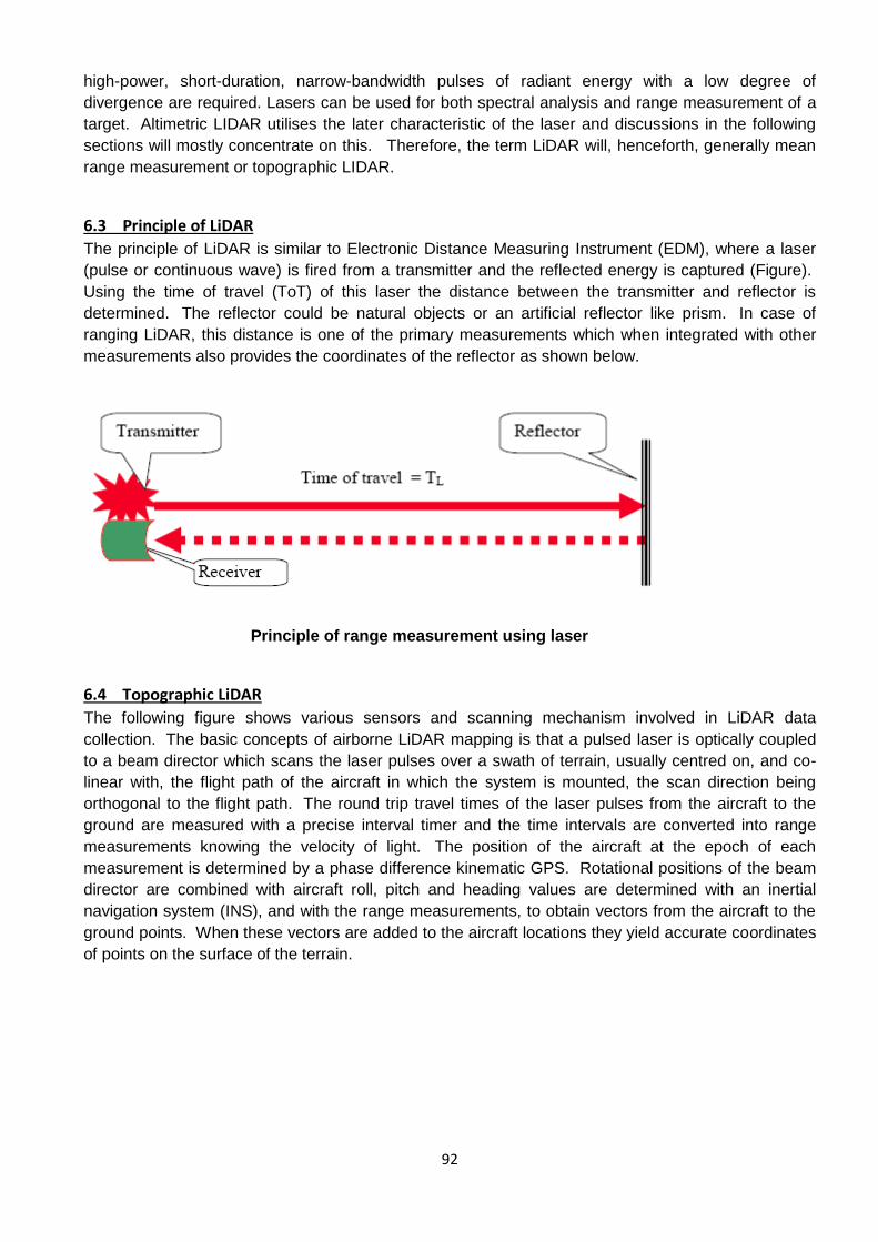
92

high-power, short-duration, narrow-bandwidth pulses of radiant energy with a low degree of

divergence are required. Lasers can be used for both spectral analysis and range measurement of a

target. Altimetric LIDAR utilises the later characteristic of the laser and discussions in the following

sections will mostly concentrate on this. Therefore, the term LiDAR will, henceforth, generally mean

range measurement or topographic LIDAR.

6.3 Principle of LiDAR

The principle of LiDAR is similar to Electronic Distance Measuring Instrument (EDM), where a laser

(pulse or continuous wave) is fired from a transmitter and the reflected energy is captured (Figure).

Using the time of travel (ToT) of this laser the distance between the transmitter and reflector is

determined. The reflector could be natural objects or an artificial reflector like prism. In case of

ranging LiDAR, this distance is one of the primary measurements which when integrated with other

measurements also provides the coordinates of the reflector as shown below.

Principle of range measurement using laser

6.4 Topographic LiDAR

The following figure shows various sensors and scanning mechanism involved in LiDAR data

collection. The basic concepts of airborne LiDAR mapping is that a pulsed laser is optically coupled

to a beam director which scans the laser pulses over a swath of terrain, usually centred on, and co-

linear with, the flight path of the aircraft in which the system is mounted, the scan direction being

orthogonal to the flight path. The round trip travel times of the laser pulses from the aircraft to the

ground are measured with a precise interval timer and the time intervals are converted into range

measurements knowing the velocity of light. The position of the aircraft at the epoch of each

measurement is determined by a phase difference kinematic GPS. Rotational positions of the beam

director are combined with aircraft roll, pitch and heading values are determined with an inertial

navigation system (INS), and with the range measurements, to obtain vectors from the aircraft to the

ground points. When these vectors are added to the aircraft locations they yield accurate coordinates

of points on the surface of the terrain.

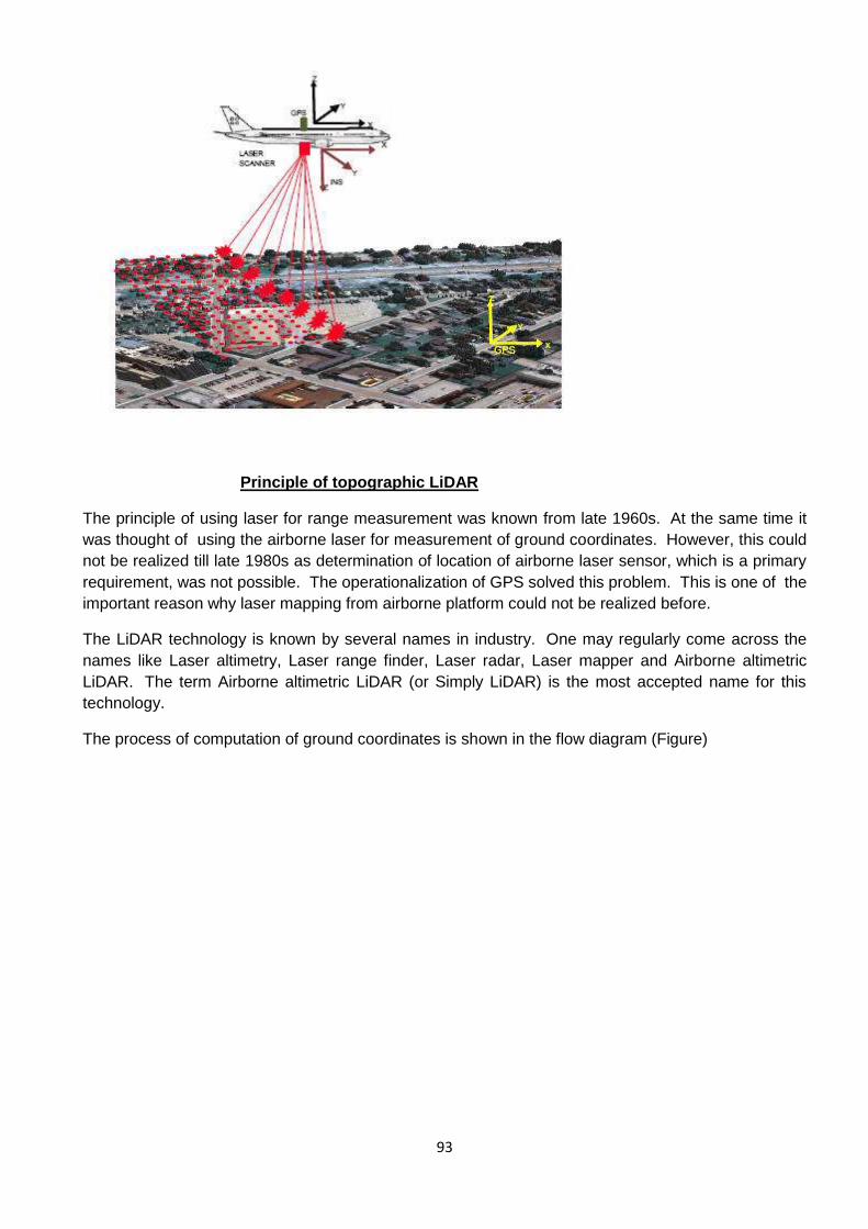
93

Principle of topographic LiDAR

The principle of using laser for range measurement was known from late 1960s. At the same time it

was thought of using the airborne laser for measurement of ground coordinates. However, this could

not be realized till late 1980s as determination of location of airborne laser sensor, which is a primary

requirement, was not possible. The operationalization of GPS solved this problem. This is one of the

important reason why laser mapping from airborne platform could not be realized before.

The LiDAR technology is known by several names in industry. One may regularly come across the

names like Laser altimetry, Laser range finder, Laser radar, Laser mapper and Airborne altimetric

LiDAR. The term Airborne altimetric LiDAR (or Simply LiDAR) is the most accepted name for this

technology.

The process of computation of ground coordinates is shown in the flow diagram (Figure)

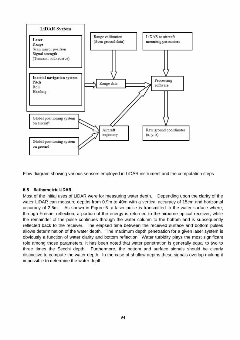
94

Flow diagram showing various sensors employed in LiDAR instrument and the computation steps

6.5 Bathymetric LiDAR

Most of the initial uses of LiDAR were for measuring water depth. Depending upon the clarity of the

water LiDAR can measure depths from 0.9m to 40m with a vertical accuracy of 15cm and horizontal

accuracy of 2.5m. As shown in Figure 5 a laser pulse is transmitted to the water surface where,

through Fresnel reflection, a portion of the energy is returned to the airborne optical receiver, while

the remainder of the pulse continues through the water column to the bottom and is subsequently

reflected back to the receiver. The elapsed time between the received surface and bottom pulses

allows determination of the water depth. The maximum depth penetration for a given laser system is

obviously a function of water clarity and bottom reflection. Water turbidity plays the most significant

role among those parameters. It has been noted that water penetration is generally equal to two to

three times the Secchi depth. Furthermore, the bottom and surface signals should be clearly

distinctive to compute the water depth. In the case of shallow depths these signals overlap making it

impossible to determine the water depth.

95

Principle of Bathymetric LiDAR

The wavelength used in this case is blue or green as these can transmit in the water body thus

maximizing the measurable depth by LiDAR.

A hybrid LiDAR system employs both infra-red and green laser (concentric). While the infra red

laser is reflected from land or from the water surface, the green wavelength proceeds to and gets

reflected from the bottom of water body. This makes it possible to capture both land topography and

water bed bathymetry simultaneously.

6.6 Multiple return LiDAR

A laser pulse has a finite diameter (~10 cm and larger). It is possible that only a part of the diameter

comes across an object. This part of pulse will reflect from there, while the rest of the pulse keeps

travelling till it encounters other objects which result in reflection of other parts of the pulse. On

receiving the reflected laser pulse, the detector triggers when the in-coming pulse reaches a set

threshold, thus measuring the time-of-flight. The sampling of the received laser pulse can be carried

out in different ways- sampling for the most significant return, sampling for the first and last significant

return, or sampling all returns which are above threshold at different stages of the reflected laser

waveform. Accordingly, the range is measured to each of those points wherefrom a return occurred to

yield their coordinates.

96

Example of multiple returns from a tree

In the figure shown above the first return is the most significant return. In case of capturing of only

most significant return the coordinate of the corresponding point (here the top of tree) only will be

computed. Capturing of first and last returns as shown above will result in determination of the height

of the tree. It is important to note that last return will not always be from the ground. In case of a

laser pulse hitting a thick branch on its way to ground, the pulse will not reach ground thus there will

be no last return from ground. The last return will be from the branch which reflected entire laser

pulse. Commercially available sensors at present support up to 4 returns from each fired laser pulse

and provide the option to choose among first, first and last and all 4 returns data.

6.7 Full waveform digitization

In this technique, the analogue echo signal is sampled at fine constant time intervals (black lines in

Figure). The digital conversion of signal results in a digital data stream. The full wave measurement

starts before the first detectable signal and lasts after the last detectable signal. The advantage of

unlimited number of returns per pulse is that the canopy and sub-canopy details are revealed. The

data can resolve surface roughness, slope and land cover within footprint. From full waveform the

first significant return, first and last returns or multiple returns can be obtained in laboratory by data

processing with more accuracy. The systems having this facility are RIEGL LMS-Q560, Litemapper

and ALTM3100.

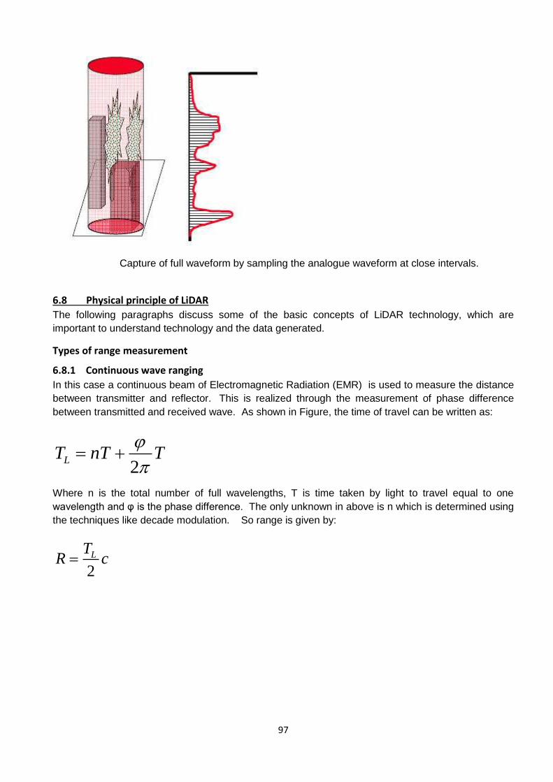
97

Capture of full waveform by sampling the analogue waveform at close intervals.

6.8 Physical principle of LiDAR

The following paragraphs discuss some of the basic concepts of LiDAR technology, which are

important to understand technology and the data generated.

Types of range measurement

6.8.1 Continuous wave ranging

In this case a continuous beam of Electromagnetic Radiation (EMR) is used to measure the distance

between transmitter and reflector. This is realized through the measurement of phase difference

between transmitted and received wave. As shown in Figure, the time of travel can be written as:

2LT nT T

Where n is the total number of full wavelengths, T is time taken by light to travel equal to one

wavelength and φ is the phase difference. The only unknown in above is n which is determined using

the techniques like decade modulation. So range is given by:

2

LTR c

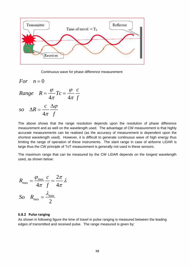
98

Continuous wave for phase difference measurement

0

4 4

4

For n

cRange R Tc

f

cso R

f

The above shows that the range resolution depends upon the resolution of phase difference

measurement and as well on the wavelength used. The advantage of CW measurement is that highly

accurate measurements can be realised (as the accuracy of measurement is dependent upon the

shortest wavelength used). However, it is difficult to generate continuous wave of high energy thus

limiting the range of operation of these instruments. The slant range in case of airborne LiDAR is

large thus the CW principle of ToT measurement is generally not used in these sensors.

The maximum range that can be measured by the CW LiDAR depends on the longest wavelength

used, as shown below:

maxmax

maxmax

2

4 4

2

cR

f

So R

6.8.2 Pulse ranging

As shown in following figure the time of travel in pulse ranging is measured between the leading

edges of transmitted and received pulse. The range measured is given by:

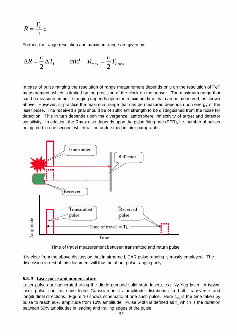
99

2

LTR c

Further, the range resolution and maximum range are given by:

max max2 2

L L

c cR T and R T

In case of pulse ranging the resolution of range measurement depends only on the resolution of ToT

measurement, which is limited by the precision of the clock on the sensor. The maximum range that

can be measured in pulse ranging depends upon the maximum time that can be measured, as shown

above. However, in practice the maximum range that can be measured depends upon energy of the

laser pulse. The received signal should be of sufficient strength to be distinguished from the noise for

detection. This in turn depends upon the divergence, atmosphere, reflectivity of target and detector

sensitivity. In addition, the Rmax also depends upon the pulse firing rate (PFR), i.e. number of pulses

being fired in one second, which will be understood in later paragraphs.

Time of travel measurement between transmitted and return pulse

It is clear from the above discussion that in airborne LiDAR pulse ranging is mostly employed. The

discussion in rest of this document will thus be about pulse ranging only.

6.8. 3 Laser pulse and nomenclature

Laser pulses are generated using the diode pumped solid state lasers, e.g. Ny-Yag laser. A typical

laser pulse can be considered Gaussian in its amplitude distribution in both transverse and

longitudinal directions. Figure 10 shows schematic of one such pulse. Here trise is the time taken by

pulse to reach 90% amplitude from 10% amplitude. Pulse width is defined as tp, which is the duration

between 50% amplitudes in leading and trailing edges of the pulse.

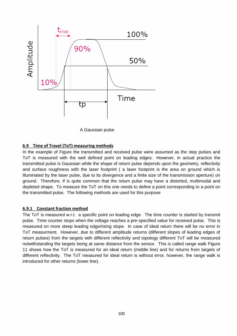
100

A Gaussian pulse

6.9 Time of Travel (ToT) measuring methods

In the example of Figure the transmitted and received pulse were assumed as the step pulses and

ToT is measured with the well defined point on leading edges. However, in actual practice the

transmitted pulse is Gaussian while the shape of return pulse depends upon the geometry, reflectivity

and surface roughness with the laser footprint ( a laser footprint is the area on ground which is

illuminated by the laser pulse, due to its divergence and a finite size of the transmission aperture) on

ground. Therefore, if is quite common that the return pulse may have a distorted, multimodal and

depleted shape. To measure the ToT on this one needs to define a point corresponding to a point on

the transmitted pulse. The following methods are used for this purpose

6.9.1 Constant fraction method

The ToT is measured w.r.t. a specific point on leading edge. The time counter is started by transmit

pulse. Time counter stops when the voltage reaches a pre-specified value for received pulse. This is

measured on more steep leading edge/rising slope. In case of ideal return there will be no error in

ToT measurment. However, due to different amplitude returns (different slopes of leading edges of

return pulses) from the targets with different reflectivity and topology different ToT will be measured

notwithstanding the targets being at same distance from the sensor. This is called range walk Figure

11 shows how the ToT is measured for an ideal return (middle line) and for returns from targets of

different reflectivity. The ToT measured for ideal return is without error, however, the range walk is

introduced for other returns (lower line).

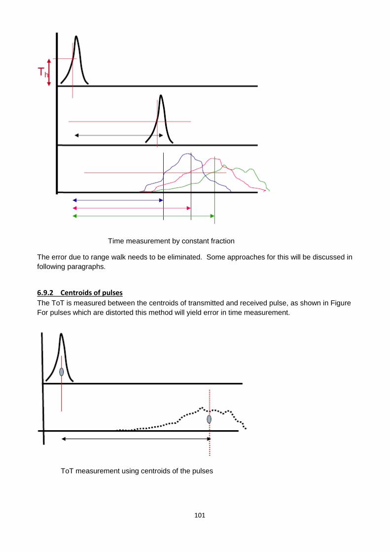
101

Time measurement by constant fraction

The error due to range walk needs to be eliminated. Some approaches for this will be discussed in

following paragraphs.

6.9.2 Centroids of pulses

The ToT is measured between the centroids of transmitted and received pulse, as shown in Figure

For pulses which are distorted this method will yield error in time measurement.

ToT measurement using centroids of the pulses

102

6.9.3 Correction using ratio of amplitudes

Correction to ToT using Ppeak

In this method correction to measured time is applied using the power of returned signal. The basic

idea is to bring the time of travel to the level of step pulse, i.e., where for step pulse is being

measured. The correction to be applied in measured time is given by tc as shown in Figure 13:

6.9.4 Correction using calibration

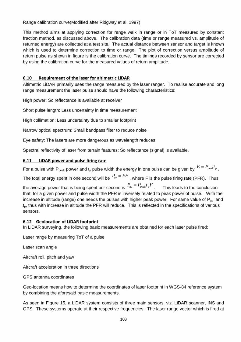
103

Range calibration curve(Modified after Ridgway et al, 1997)

This method aims at applying correction for range walk in range or in ToT measured by constant

fraction method, as discussed above. The calibration data (time or range measured vs. amplitude of

returned energy) are collected at a test site. The actual distance between sensor and target is known

which is used to determine correction to time or range. The plot of correction versus amplitude of

return pulse as shown in figure is the calibration curve. The timings recorded by sensor are corrected

by using the calibration curve for the measured values of return amplitude.

6.10 Requirement of the laser for altimetric LiDAR

Altimetric LiDAR primarily uses the range measured by the laser ranger. To realise accurate and long

range measurement the laser pulse should have the following characteristics:

High power: So reflectance is available at receiver

Short pulse length: Less uncertainty in time measurement

High collimation: Less uncertainty due to smaller footprint

Narrow optical spectrum: Small bandpass filter to reduce noise

Eye safety: The lasers are more dangerous as wavelength reduces

Spectral reflectivity of laser from terrain features: So reflectance (signal) is available.

6.11 LiDAR power and pulse firing rate

For a pulse with Ppeak power and tp pulse width the energy in one pulse can be given by peak pE P t.

The total energy spent in one second will be avP EF, where F is the pulse firing rate (PFR). Thus

the average power that is being spent per second is av peak pP P t F. This leads to the conclusion

that, for a given power and pulse width the PFR is inversely related to peak power of pulse. With the

increase in altitude (range) one needs the pulses with higher peak power. For same value of Pav and

tp, thus with increase in altitude the PFR will reduce. This is reflected in the specifications of various

sensors.

6.12 Geolocation of LiDAR footprint In LiDAR surveying, the following basic measurements are obtained for each laser pulse fired:

Laser range by measuring ToT of a pulse

Laser scan angle

Aircraft roll, pitch and yaw

Aircraft acceleration in three directions

GPS antenna coordinates

Geo-location means how to determine the coordinates of laser footprint in WGS-84 reference system

by combining the aforesaid basic measurements.

As seen in Figure 15, a LiDAR system consists of three main sensors, viz. LiDAR scanner, INS and

GPS. These systems operate at their respective frequencies. The laser range vector which is fired at

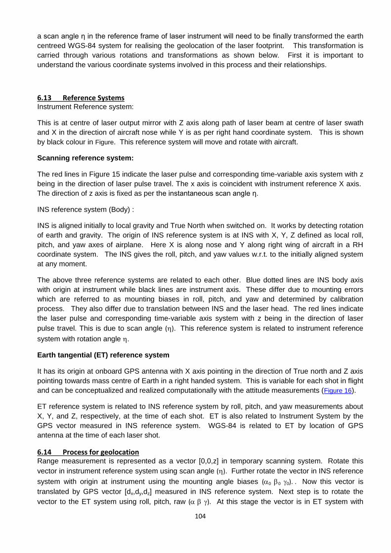
104

a scan angle η in the reference frame of laser instrument will need to be finally transformed the earth

centreed WGS-84 system for realising the geolocation of the laser footprint. This transformation is

carried through various rotations and transformations as shown below. First it is important to

understand the various coordinate systems involved in this process and their relationships.

6.13 Reference Systems Instrument Reference system:

This is at centre of laser output mirror with Z axis along path of laser beam at centre of laser swath

and X in the direction of aircraft nose while Y is as per right hand coordinate system. This is shown

by black colour in Figure. This reference system will move and rotate with aircraft.

Scanning reference system:

The red lines in Figure 15 indicate the laser pulse and corresponding time-variable axis system with z

being in the direction of laser pulse travel. The x axis is coincident with instrument reference X axis.

The direction of z axis is fixed as per the instantaneous scan angle η.

INS reference system (Body) :

INS is aligned initially to local gravity and True North when switched on. It works by detecting rotation

of earth and gravity. The origin of INS reference system is at INS with X, Y, Z defined as local roll,

pitch, and yaw axes of airplane. Here X is along nose and Y along right wing of aircraft in a RH

coordinate system. The INS gives the roll, pitch, and yaw values w.r.t. to the initially aligned system

at any moment.

The above three reference systems are related to each other. Blue dotted lines are INS body axis

with origin at instrument while black lines are instrument axis. These differ due to mounting errors

which are referred to as mounting biases in roll, pitch, and yaw and determined by calibration

process. They also differ due to translation between INS and the laser head. The red lines indicate

the laser pulse and corresponding time-variable axis system with z being in the direction of laser

pulse travel. This is due to scan angle (). This reference system is related to instrument reference

system with rotation angle .

Earth tangential (ET) reference system

It has its origin at onboard GPS antenna with X axis pointing in the direction of True north and Z axis

pointing towards mass centre of Earth in a right handed system. This is variable for each shot in flight

and can be conceptualized and realized computationally with the attitude measurements (Figure 16).

ET reference system is related to INS reference system by roll, pitch, and yaw measurements about

X, Y, and Z, respectively, at the time of each shot. ET is also related to Instrument System by the

GPS vector measured in INS reference system. WGS-84 is related to ET by location of GPS

antenna at the time of each laser shot.

6.14 Process for geolocation Range measurement is represented as a vector [0,0,z] in temporary scanning system. Rotate this

vector in instrument reference system using scan angle (). Further rotate the vector in INS reference

system with origin at instrument using the mounting angle biases (0 0 0). . Now this vector is

translated by GPS vector [dx,dy,dz] measured in INS reference system. Next step is to rotate the

vector to the ET system using roll, pitch, raw ( ). At this stage the vector is in ET system with

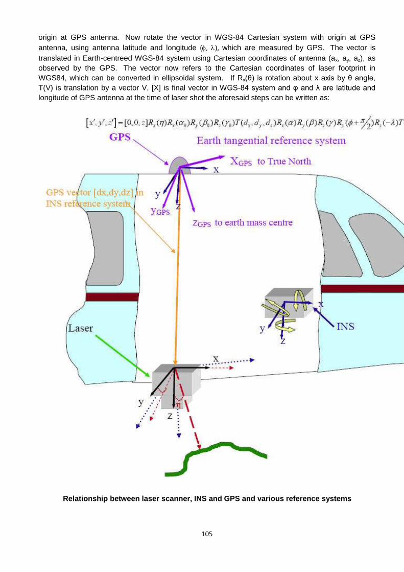
http://home.iitk.ac.in/~blohani/LiDAR_Tutorial/Process%20for%20geolocation.htm

105

origin at GPS antenna. Now rotate the vector in WGS-84 Cartesian system with origin at GPS

antenna, using antenna latitude and longitude (, ), which are measured by GPS. The vector is

translated in Earth-centreed WGS-84 system using Cartesian coordinates of antenna (ax, ay, az), as

observed by the GPS. The vector now refers to the Cartesian coordinates of laser footprint in

WGS84, which can be converted in ellipsoidal system. If Rx(θ) is rotation about x axis by θ angle,

T(V) is translation by a vector V, [X] is final vector in WGS-84 system and φ and λ are latitude and

longitude of GPS antenna at the time of laser shot the aforesaid steps can be written as:

Relationship between laser scanner, INS and GPS and various reference systems

106

Relationship between ET and WGS-84 system

6.15 LiDAR sensor and data characteristics 6.15.1 Available sensors An excellent comparison of various available LiDAR sensors can be found at (Lemmens, 2007) .

Sensors vary in their specifications and accordingly are suitable for collecting data with varied

characteristics, as required in different applications. Moreover, each sensor possesses a large range

of parameters in order to arrive at the required data specification. Some of the most commonly used

sensors are ALTM by Optech Canada, ALS by Leica Geosystems, Toposys by Toposys GmBH,

TopEye by Hansa Luftbild and RIEGL.

6.15.2 LiDAR Scanning pattern Scanning pattern on ground depends primarily on the LiDAR sensors which scan the ground in

different modes. The pattern also gets affected by the nature of terrain and the perturbations

(attitude and acceleration) in flight trajectory. A few common types are described below:

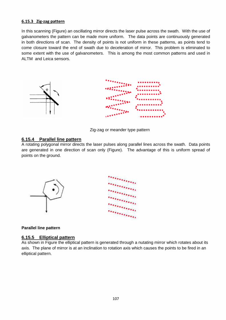
107

6.15.3 Zig-zag pattern

In this scanning (Figure) an oscillating mirror directs the laser pulse across the swath. With the use of

galvanometers the pattern can be made more uniform. The data points are continuously generated

in both directions of scan. The density of points is not uniform in these patterns, as points tend to

come closure toward the end of swath due to deceleration of mirror. This problem is eliminated to

some extent with the use of galvanometers. This is among the most common patterns and used in

ALTM and Leica sensors.

Zig-zag or meander type pattern

6.15.4 Parallel line pattern A rotating polygonal mirror directs the laser pulses along parallel lines across the swath. Data points

are generated in one direction of scan only (Figure). The advantage of this is uniform spread of

points on the ground.

Parallel line pattern

6.15.5 Elliptical pattern As shown in Figure the elliptical pattern is generated through a nutating mirror which rotates about its

axis. The plane of mirror is at an inclination to rotation axis which causes the points to be fired in an

elliptical pattern.

108

Elliptical pattern

6.15.6 Parallel lines-Toposys type This pattern is typical to the Toposys sensors. Laser pulses are fired through an array of optical fibres

and the return pulses are also collected through a similar system. The optical fibre array ensures that

the scan lines are parallel and uniformly spaced on the ground as shown in Figure.

Parallel line pattern (Courtesy Toposys)

6.15.7 Data density Data density is an important parameter in LiDAR survey. While a dense data captures the terrain

better and helps in information extraction the time and resource requirement is high. The data density

is decided depending the application for which the data is being collected. The data density mainly

depends upon the parameters of sensor and platform e.g., flying height, velocity, scan angle, scan

frequency, pulse firing rate, scanning pattern, acceleration and attitude variation of platform.

Additionally, it also depends upon the ground geometry and reflectivity.

Scan definitions

Depending the sensor a scan could be of any of the two types as shown in Figure 21.

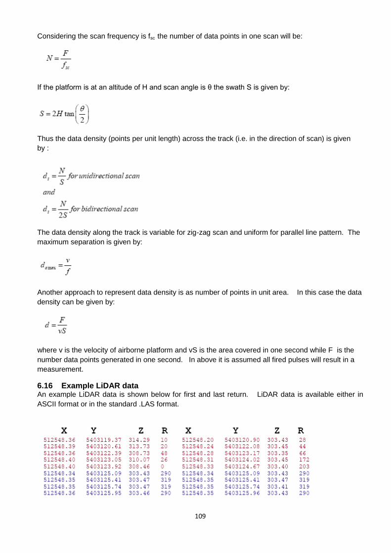
109

Considering the scan frequency is fsc the number of data points in one scan will be:

If the platform is at an altitude of H and scan angle is θ the swath S is given by:

Thus the data density (points per unit length) across the track (i.e. in the direction of scan) is given

by :

The data density along the track is variable for zig-zag scan and uniform for parallel line pattern. The

maximum separation is given by:

Another approach to represent data density is as number of points in unit area. In this case the data

density can be given by:

where v is the velocity of airborne platform and vS is the area covered in one second while F is the

number data points generated in one second. In above it is assumed all fired pulses will result in a

measurement.

6.16 Example LiDAR data An example LiDAR data is shown below for first and last return. LiDAR data is available either in

ASCII format or in the standard .LAS format.

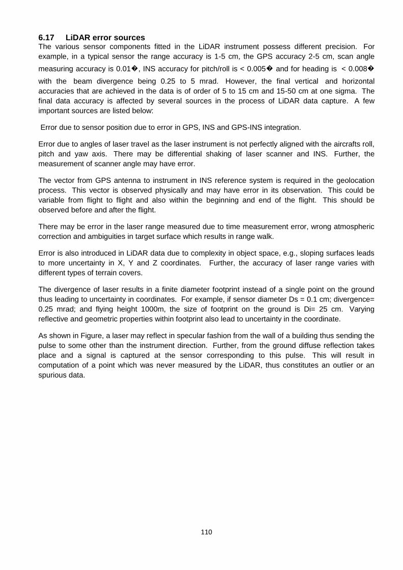
110

6.17 LiDAR error sources The various sensor components fitted in the LiDAR instrument possess different precision. For

example, in a typical sensor the range accuracy is 1-5 cm, the GPS accuracy 2-5 cm, scan angle

measuring accuracy is 0.01�, INS accuracy for pitch/roll is < 0.005� and for heading is < 0.008�

with the beam divergence being 0.25 to 5 mrad. However, the final vertical and horizontal

accuracies that are achieved in the data is of order of 5 to 15 cm and 15-50 cm at one sigma. The

final data accuracy is affected by several sources in the process of LiDAR data capture. A few

important sources are listed below:

Error due to sensor position due to error in GPS, INS and GPS-INS integration.

Error due to angles of laser travel as the laser instrument is not perfectly aligned with the aircrafts roll,

pitch and yaw axis. There may be differential shaking of laser scanner and INS. Further, the

measurement of scanner angle may have error.

The vector from GPS antenna to instrument in INS reference system is required in the geolocation

process. This vector is observed physically and may have error in its observation. This could be

variable from flight to flight and also within the beginning and end of the flight. This should be

observed before and after the flight.

There may be error in the laser range measured due to time measurement error, wrong atmospheric

correction and ambiguities in target surface which results in range walk.

Error is also introduced in LiDAR data due to complexity in object space, e.g., sloping surfaces leads

to more uncertainty in X, Y and Z coordinates. Further, the accuracy of laser range varies with

different types of terrain covers.

The divergence of laser results in a finite diameter footprint instead of a single point on the ground

thus leading to uncertainty in coordinates. For example, if sensor diameter Ds = 0.1 cm; divergence=

0.25 mrad; and flying height 1000m, the size of footprint on the ground is Di= 25 cm. Varying

reflective and geometric properties within footprint also lead to uncertainty in the coordinate.

As shown in Figure, a laser may reflect in specular fashion from the wall of a building thus sending the

pulse to some other than the instrument direction. Further, from the ground diffuse reflection takes

place and a signal is captured at the sensor corresponding to this pulse. This will result in

computation of a point which was never measured by the LiDAR, thus constitutes an outlier or an

spurious data.

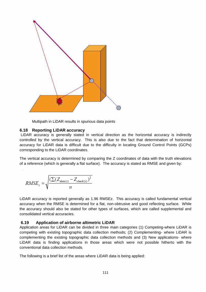
111

Multipath in LiDAR results in spurious data points

6.18 Reporting LiDAR accuracy LiDAR accuracy is generally stated in vertical direction as the horizontal accuracy is indirectly

controlled by the vertical accuracy. This is also due to the fact that determination of horizontal

accuracy for LiDAR data is difficult due to the difficulty in locating Ground Control Points (GCPs)

corresponding to the LiDAR coordinates.

The vertical accuracy is determined by comparing the Z coordinates of data with the truth elevations

of a reference (which is generally a flat surface). The accuracy is stated as RMSE and given by:

LiDAR accuracy is reported generally as 1.96 RMSEz. This accuracy is called fundamental vertical

accuracy when the RMSE is determined for a flat, non-obtrusive and good reflecting surface. While

the accuracy should also be stated for other types of surfaces, which are called supplemental and

consolidated vertical accuracies.

6.19 Application of airborne altimetric LiDAR Application areas for LiDAR can be divided in three main categories (1) Competing-where LiDAR is

competing with existing topographic data collection methods; (2) Complementing- where LiDAR is

complementing the existing topographic data collection methods and (3) New applications- where

LiDAR data is finding applications in those areas which were not possible hitherto with the

conventional data collection methods.

The following is a brief list of the areas where LiDAR data is being applied:

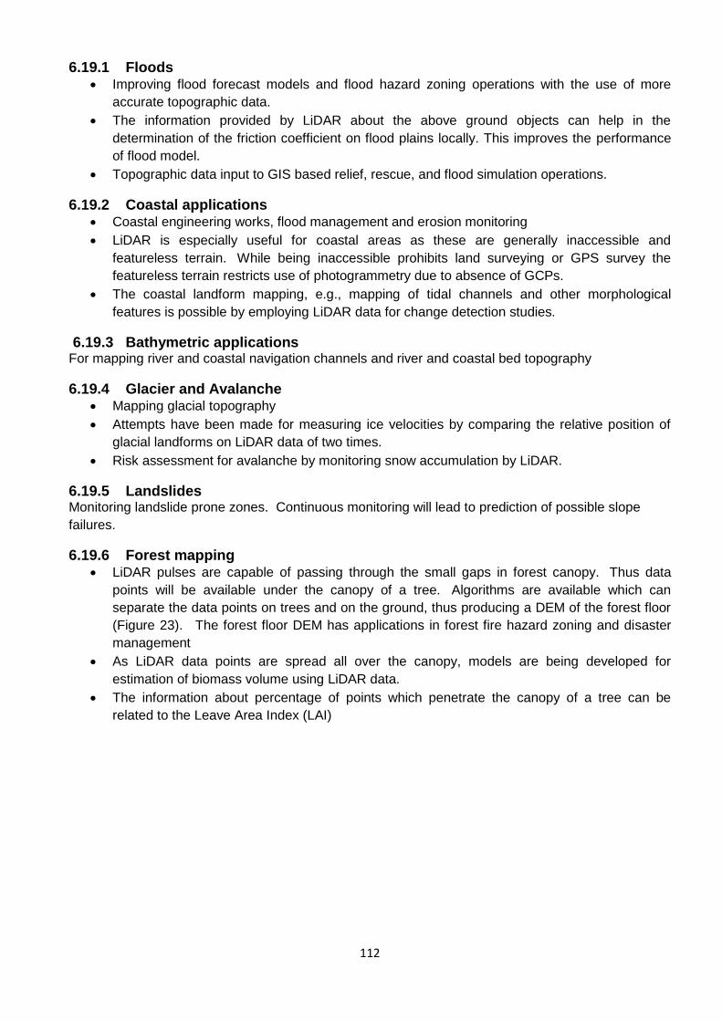
112

6.19.1 Floods Improving flood forecast models and flood hazard zoning operations with the use of more

accurate topographic data.

The information provided by LiDAR about the above ground objects can help in the

determination of the friction coefficient on flood plains locally. This improves the performance

of flood model.

Topographic data input to GIS based relief, rescue, and flood simulation operations.

6.19.2 Coastal applications Coastal engineering works, flood management and erosion monitoring

LiDAR is especially useful for coastal areas as these are generally inaccessible and

featureless terrain. While being inaccessible prohibits land surveying or GPS survey the

featureless terrain restricts use of photogrammetry due to absence of GCPs.

The coastal landform mapping, e.g., mapping of tidal channels and other morphological

features is possible by employing LiDAR data for change detection studies.

6.19.3 Bathymetric applications For mapping river and coastal navigation channels and river and coastal bed topography

6.19.4 Glacier and Avalanche Mapping glacial topography

Attempts have been made for measuring ice velocities by comparing the relative position of

glacial landforms on LiDAR data of two times.

Risk assessment for avalanche by monitoring snow accumulation by LiDAR.

6.19.5 Landslides Monitoring landslide prone zones. Continuous monitoring will lead to prediction of possible slope

failures.

6.19.6 Forest mapping LiDAR pulses are capable of passing through the small gaps in forest canopy. Thus data

points will be available under the canopy of a tree. Algorithms are available which can

separate the data points on trees and on the ground, thus producing a DEM of the forest floor

(Figure 23). The forest floor DEM has applications in forest fire hazard zoning and disaster

management

As LiDAR data points are spread all over the canopy, models are being developed for

estimation of biomass volume using LiDAR data.

The information about percentage of points which penetrate the canopy of a tree can be

related to the Leave Area Index (LAI)

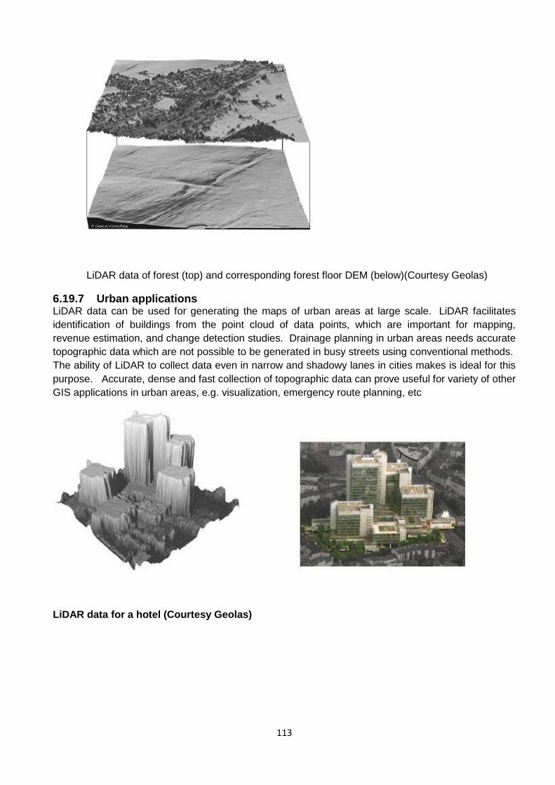
113

LiDAR data of forest (top) and corresponding forest floor DEM (below)(Courtesy Geolas)

6.19.7 Urban applications LiDAR data can be used for generating the maps of urban areas at large scale. LiDAR facilitates

identification of buildings from the point cloud of data points, which are important for mapping,

revenue estimation, and change detection studies. Drainage planning in urban areas needs accurate

topographic data which are not possible to be generated in busy streets using conventional methods.

The ability of LiDAR to collect data even in narrow and shadowy lanes in cities makes is ideal for this

purpose. Accurate, dense and fast collection of topographic data can prove useful for variety of other

GIS applications in urban areas, e.g. visualization, emergency route planning, etc

LiDAR data for a hotel (Courtesy Geolas)

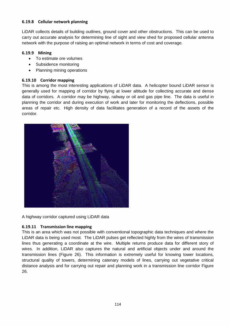
114

6.19.8 Cellular network planning

LiDAR collects details of building outlines, ground cover and other obstructions. This can be used to

carry out accurate analysis for determining line of sight and view shed for proposed cellular antenna

network with the purpose of raising an optimal network in terms of cost and coverage.

6.19.9 Mining To estimate ore volumes

Subsidence monitoring

Planning mining operations

6.19.10 Corridor mapping This is among the most interesting applications of LiDAR data. A helicopter bound LiDAR sensor is

generally used for mapping of corridor by flying at lower altitude for collecting accurate and dense

data of corridors. A corridor may be highway, railway or oil and gas pipe line. The data is useful in

planning the corridor and during execution of work and later for monitoring the deflections, possible

areas of repair etc. High density of data facilitates generation of a record of the assets of the

corridor.

A highway corridor captured using LiDAR data

6.19.11 Transmission line mapping This is an area which was not possible with conventional topographic data techniques and where the

LiDAR data is being used most. The LiDAR pulses get reflected highly from the wires of transmission

lines thus generating a coordinate at the wire. Multiple returns produce data for different story of

wires. In addition, LiDAR also captures the natural and artificial objects under and around the

transmission lines (Figure 26). This information is extremely useful for knowing tower locations,

structural quality of towers, determining catenary models of lines, carrying out vegetative critical

distance analysis and for carrying out repair and planning work in a transmission line corridor Figure

26.

115

Transverse section of a transmission line using LiDAR data (Courtesy Toposys)

There are many more application areas for LiDAR data e.g., Creating realistic 3D environment for

movies, games, and pilot training; Simulation of Hurricane movement and its effect; Simulation of Air

pollution due to an accident or a polluting source; Transport of vehicular pollution in urban

environment; etc. Basically, all those application areas where topographic data is fundamental can

benefit with LiDAR data. LiDAR instruments are also being used for extra-terrestrial mapping (e.g.

MOLA, LLRI)

6.20 Advantages of LiDAR technology The other methods of topographic data collection are land surveying, GPS, inteferrometry, and

photogrammetry. LiDAR technology has some advantages in comparison to these methods, which

are being listed below:

Higher accuracy

Vertical accuracy 5-

Horizontal accuracy 30-50 cm

Fast acquisition and processing

Acquisition of 1000 km2 in 12 hours.

DEM generation of 1000 km2 in 24 hours.

Minimum human dependence

As most of the processes are automatic unlike photogrammetry, GPS or land surveying.

Weather/Light independence

Data collection independent of sun inclination and at night and slightly bad weather.

Canopy penetration

LiDAR pulses can reach beneath the canopy thus generating measurements of points there unlike

photogrammetry.

Higher data density

Up to 167,000 pulses per second. More than 24 points per m2 can be measured.

Multiple returns to collect data in 3D.

GCP independence

116

Only a few GCPs are needed to keep reference receiver for the purpose of DGPS. There is not need

of GCPs otherwise.

This makes LiDAR ideal for mapping inaccessible and featureless areas.

Additional data

LiDAR also observes the amplitude of back scatter energy thus recording a reflectance value for each

data point. This data, though poor spectrally, can be used for classification, as at the wavelength

used some features may be discriminated accurately.

Cost

It has been found by comparative studies that LiDAR data is cheaper in many applications. This is

particularly considering the speed, accuracy and density of data.

117

SECTION 7

Photogrammetric Accuracy Standards

7.1 General

This section presents photogrammetric mapping standards to specify the quality of the spatial data

product (i.e., map) to be produced.

Minimum accuracy standards. This involves the accuracy standards to be used for

photogrammetrically derived maps and related spatial data products. Suggested requirements to

meet these accuracy standards are given for critical aspects of the photogrammetric mapping

processes such as maximum flight altitudes, maximum photo enlargement ratios and aero

triangulation adjustment criteria.

Map scales. Mapping accuracy standards are associated with the final development scale of the map

or compilation scale, both horizontal and vertical components. The use of CADD and GIS software

allows the separation of planimetric features and elevations to various layers along with depiction at

any scale. Problems arise when source scales are increased beyond their original values or when the

image is subjected to so-called “rubber sheeting.” It is therefore critical that these spatial data layers

contain descriptor information (Metadata) identifying the original source target scale and designed

accuracy.

CADD vs GIS. Photogrammetric mapping data collection is generally a necessary but costly process.

The decision regarding final formats (CADD vs GIS) of spatial data is not always clear cut. A portion of

the time and cost in photogrammetric map production is required for creating final format of the

data sets. Factors affecting the decision regarding CADD vs. GIS include:

(1) Immediate and future uses of the spatial data sets collected.

(2) Immediate and future data analysis requirements for spatial data sets.

(3) Costs and time for each format requested.

(4) Project cost sharing and ownership.

Every attempt should be made to collect spatial data sets in the formats that will provide the most

useful utility. GIS formatting costs can be minimized if the data producer is aware of the request at

the time of initial data collection. Many engineering, planning, and environmental projects can make

use of and may require GIS capability in spatial data analysis. When planning a photogrammetric

118

mapping project, both CADD and GIS formats may be required. However this aspect has been taken

care of in the presently available Softwares where format of the data serves both the purposes.

d. Mapping requirements. The specified accuracy of a geospatial data collection effort shall be

sufficient to ensure that the map can be reliably used for the purpose intended, whether this purpose

is an immediate or a future use. However, the accuracy of a map should not surpass that required for

its intended functional use. Specifying map accuracies in excess of those required is the general

tendency. This could result in increased costs and may delay project completion. It is absolutely

essential that mapping accuracy requirements originate from the functional and realistic accuracy

requirements of the project. Photogrammetric mapping design criteria such as flight altitude,

horizontal and vertical ground control required and its accuracy, types of features to be collected and

optimum scanning resolution are determined from the required map scale and contour interval.

These requirements should be part of project planning and cost estimates.

Table 2-1 depicts typical mapping parameters for various engineering, construction, and real estate

mapping applications. The table is intended to be a general guide in selecting a target scale for a

specific project while numerous other project-specific factors may dictate variations from these

general values. The table does not apply exclusively to photogrammetric mapping activities. Some of

the required surveying and mapping accuracies identified exceed those obtainable from

photogrammetry and may need to be obtained using conventional surveying techniques. Selection of

an appropriate CI is extremely site-dependent and will directly impact the mapping costs since the

photo negative scale (and resultant model coverage and ground survey control) is determined as a

function of this parameter. Table 2-1 may be used as general guidance in selecting a CI (or DTM

elevation accuracy, as applicable).

Table 7-1 Recommended Surveying and Mapping Specifications for Military Construction, Civil Works,

Operations, Maintenance, Real Estate, and other Projects

Project of Activity Equivalent

Target

(Plot) Map

Scale Sl

Ratio

Feature

Location

Tolerance

mm,

RMSE

Feature

Elevation

Tolerance

mm, RMSE

Typical

Contour

Interval mm

Design and Construction of New

Facilities: Site Plan Data for Direct

Input into CADD 2-D/3-D Design Files

General Construction Site Plan Feature

and Topo Detail

1:500 100mm 50mm 250mm

Surface/Subsurface Utility Detail 1:500 100mm 50mm N/A

Building or Structure Design 1:500 25mm 50mm 250mm

Airfield Pavement Design Detail 1:500 25mm 25mm 250mm

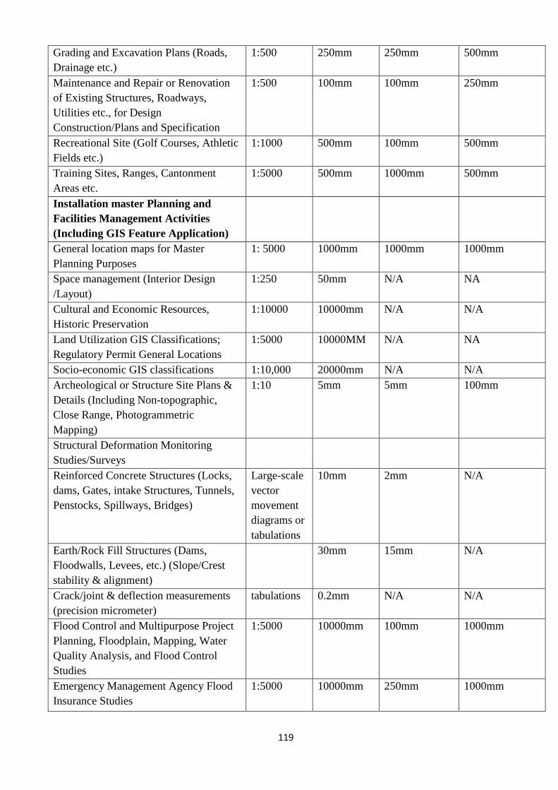
119

Grading and Excavation Plans (Roads,

Drainage etc.)

1:500 250mm 250mm 500mm

Maintenance and Repair or Renovation

of Existing Structures, Roadways,

Utilities etc., for Design

Construction/Plans and Specification

1:500 100mm 100mm 250mm

Recreational Site (Golf Courses, Athletic

Fields etc.)

1:1000 500mm 100mm 500mm

Training Sites, Ranges, Cantonment

Areas etc.

1:5000 500mm 1000mm 500mm

Installation master Planning and

Facilities Management Activities

(Including GIS Feature Application)

General location maps for Master

Planning Purposes

1: 5000 1000mm 1000mm 1000mm

Space management (Interior Design

/Layout)

1:250 50mm N/A NA

Cultural and Economic Resources,

Historic Preservation

1:10000 10000mm N/A N/A

Land Utilization GIS Classifications;

Regulatory Permit General Locations

1:5000 10000MM N/A NA

Socio-economic GIS classifications 1:10,000 20000mm N/A N/A

Archeological or Structure Site Plans &

Details (Including Non-topographic,

Close Range, Photogrammetric

Mapping)

1:10 5mm 5mm 100mm

Structural Deformation Monitoring

Studies/Surveys

Reinforced Concrete Structures (Locks,

dams, Gates, intake Structures, Tunnels,

Penstocks, Spillways, Bridges)

Large-scale

vector

movement

diagrams or

tabulations

10mm 2mm N/A

Earth/Rock Fill Structures (Dams,

Floodwalls, Levees, etc.) (Slope/Crest

stability & alignment)

30mm 15mm N/A

Crack/joint & deflection measurements

(precision micrometer)

tabulations 0.2mm N/A N/A

Flood Control and Multipurpose Project

Planning, Floodplain, Mapping, Water

Quality Analysis, and Flood Control

Studies

1:5000 10000mm 100mm 1000mm

Emergency Management Agency Flood

Insurance Studies

1:5000 10000mm 250mm 1000mm

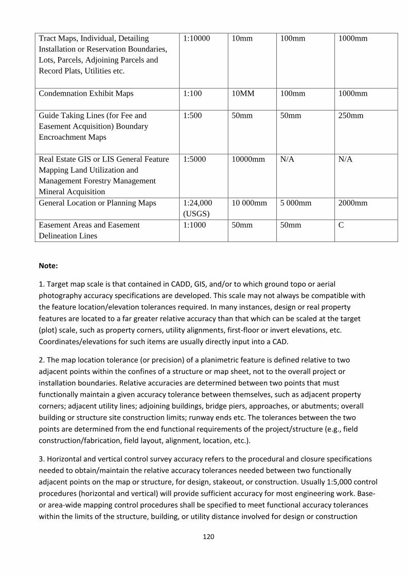
120

Tract Maps, Individual, Detailing

Installation or Reservation Boundaries,

Lots, Parcels, Adjoining Parcels and

Record Plats, Utilities etc.

1:10000 10mm 100mm 1000mm

Condemnation Exhibit Maps

1:100 10MM 100mm 1000mm

Guide Taking Lines (for Fee and

Easement Acquisition) Boundary

Encroachment Maps

1:500 50mm 50mm 250mm

Real Estate GIS or LIS General Feature

Mapping Land Utilization and

Management Forestry Management

Mineral Acquisition

1:5000 10000mm N/A N/A

General Location or Planning Maps 1:24,000

(USGS)

10 000mm 5 000mm 2000mm

Easement Areas and Easement

Delineation Lines

1:1000 50mm 50mm C

Note:

1. Target map scale is that contained in CADD, GIS, and/or to which ground topo or aerial

photography accuracy specifications are developed. This scale may not always be compatible with

the feature location/elevation tolerances required. In many instances, design or real property

features are located to a far greater relative accuracy than that which can be scaled at the target

(plot) scale, such as property corners, utility alignments, first-floor or invert elevations, etc.

Coordinates/elevations for such items are usually directly input into a CAD.

2. The map location tolerance (or precision) of a planimetric feature is defined relative to two

adjacent points within the confines of a structure or map sheet, not to the overall project or

installation boundaries. Relative accuracies are determined between two points that must

functionally maintain a given accuracy tolerance between themselves, such as adjacent property

corners; adjacent utility lines; adjoining buildings, bridge piers, approaches, or abutments; overall

building or structure site construction limits; runway ends etc. The tolerances between the two

points are determined from the end functional requirements of the project/structure (e.g., field

construction/fabrication, field layout, alignment, location, etc.).

3. Horizontal and vertical control survey accuracy refers to the procedural and closure specifications

needed to obtain/maintain the relative accuracy tolerances needed between two functionally

adjacent points on the map or structure, for design, stakeout, or construction. Usually 1:5,000 control

procedures (horizontal and vertical) will provide sufficient accuracy for most engineering work. Base-

or area-wide mapping control procedures shall be specified to meet functional accuracy tolerances

within the limits of the structure, building, or utility distance involved for design or construction

121

surveys. Higher order control surveys shall not be specified for area-wide mapping or GIS definition

unless a definitive functional requirement exists (e.g., military operational targeting or some low-

gradient flood controls projects).

4. (See note 2.) Some flood control projects may require better relative accuracy tolerances than

those shown.

Each of these standards has application to different types of functional products, ranging from wide-

area small-scale mapping to large-scale engineering design. Their resultant accuracy criteria (i.e.,

spatial errors in X-Y-Z), including QC compliance procedures, do not differ significantly from one

another. In general, use of any of these standards for a photogrammetric mapping contract will result

in a quality product.

7.2 Photogrammetric Mapping Standard

This standard is intended for site plan development work, involving mapping scales larger than

1:20,000. It also is applicable to conventional surveying topographic site development work. This

standard, like most other mapping standards, defines map accuracy by comparing the mapped

location of selected well defined points to their "true" location as determined by a more accurate,

independent field survey. When no independent check is feasible or practicable, a map's accuracy

may be estimated based on the accuracy of the technique used to locate mapped features (e.g., GPS,

total station, plane table, etc.).

Application of standards. The objective of these photogrammetric standards is twofold:

(1) To help ensure that the topographic map accuracy standards or geospatial database accuracy are

met during the production process.

(2) To help ensure that deliverables other than maps, such as aerial photographs, ground control,

etc., possess quality of the required degree.

b. Map accuracy sub classifications. This Standard classifies a map as statistically meeting a certain

level of accuracy. Its primary advantage is that it contains more definitive statistical map testing

criteria. Using guidance in Tables 2-2 and 2-3, specifications for site plans need only indicate the map

class, target scale (horizontal map scale), and contour interval.

c. Use of Standards for ground survey mapping. These Standards are also applicable to large-scale

site plan mapping performed by plane table or electronic total station techniques. This work may

either supplement the aerial mapping work (e.g., surface or subsurface utility details) or be of a scale

too large for aerial mapping.

122

Table 7-2

Planimetric Feature Coordinate Accuracy Requirement (Ground X or Y) for Well-Defined Points

Target Map Scale Limiting RMSE (Metres)

1:500 0.125

1:1000 0.25

1:2,000 0.50

1:2,500 0.63

1:3,000 0.75

1:4,000 1.0

1:5,000 1.25

1:8,000 2.0

1:9,000 2.25

1:10,000 2.5

1:16,000 4.0

1:20,000 5.0

Table 7-3

Topographic Elevation Accuracy Requirement for Well-Defined Points

Limiting RMSE in Meters

Target Contour Interval Topographic Feature

Points

Spot or DTM

elevation points

Meters

0.5 0.17 0.08

1 0.33 0.17

2 1.33 0.33

4 2.67 0.67

5 3.33 0.83

123

7.3 Accuracy Standards for Large-Scale Maps

Large scale standards define map accuracy by comparing the mapped location of selected well-

defined points to their actual location as determined by a more accurate, independent field survey. It

contains more definitive statistical map testing criteria, which, from a contract administration

standpoint, is desirable. These large scale standards are synopsized below.

a. Horizontal accuracy criteria. The planimetric standard makes use of the RMSE. The limiting

horizontal RMSEs shown in Table 2-2 are the maximum permissible RMSEs established by this

standard. These limits of accuracy apply to well-defined points only.

b. Vertical accuracy criteria. Vertical accuracy is defined relative to the required contour interval (CI)

for a map. In cases where only digital terrain models (DTM) or digital elevation models (DEM) are

being generated, an equivalent CI must be specified based on the required digital point (spot)

elevation accuracy. The contours themselves may be generated later using CADD software routines.

The vertical standards are also defined by RMSE but only for well-defined features between contours

containing interpretative elevations or spot elevation points. Contours in themselves are not

considered as well-defined feature points. Testing for vertical map compliance is also performed by

independent, higher accuracy ground survey methods, such as differential levelling. Table 2-3

summarizes the limiting vertical RMSEs for well-defined points as checked by independent surveys at

the full (ground) scale of the map.

Map accuracy testing. Map accuracy testing can be costly and time consuming. One or more sheets

(or segments of a design file) may be tested for compliance. The decision whether to check

photogrammetric mapping products rests with the Organization and is dependent on numerous

factors, such as intended design work, available personnel, known vendor capabilities and personnel

resources available for the test. Every attempt should be made to review and check major phases of

the mapping process (i.e., project planning, ground control, aerotriangulation, and compilation) as

they are completed. Additional ground survey checks of map feature accuracy should be limited and

in most cases eliminated. The Government should rely heavily on the Vendor's QC program and

procedures to check for and catch blunders. When it becomes necessary to perform independent

QA checks for map accuracy, the standards for map accuracy tests should be followed. Horizontal

and vertical accuracy is to be checked by comparing measured coordinates or elevations from the

map (at its intended target scale) with coordinates determined by a check survey of higher accuracy.

The check survey should be at least twice as accurate as the map feature tolerance given in the tables

above, with a minimum of 20 points tested. Maps and related geospatial databases complying with a

required standard shall have a statement indicating that standard. This accuracy statement

requirement is especially applicable to GIS databases that may be compiled from a variety of sources

containing known or unknown accuracy reliability.

(1) For horizontal points, the check survey should produce a standard deviation equal to or less than

one third of the limiting RMSE selected for the map. This means that the relative distance accuracy

ratio of the check survey must be less than one-third that of the limiting RMSE.

124

(2) For vertical points, the check survey (i.e., Global Positioning System (GPS), differential levelling, or

electronic total station trig elevations) should produce an RMSE not greater than 1/20th of CI,

expressed relative to the longest diagonal dimension of a standard drawing sheet. The map position

of the ground point may be shifted in any direction by an amount equal to twice the limiting RMSE in

horizontal position. Ground survey techniques considered acceptable for check surveys should

include GPS, differential levelling, or total station trig elevations. The RMSE requirement for the

check survey should direct the survey techniques utilized.

(3) The same survey datum must be used for both the mapping and check surveys.

d. Checkpoints. The checkpoints should be confined to well-defined features. Depending upon map

scale, certain features will be displaced for the sake of map clarity. These points should not be used

unless the rules for displacement are well known. Test points should be well distributed over the map

area. Any checkpoint whose discrepancy exceeds three times the limiting RMSE should be corrected

before the map is considered to meet the standard.

7.4 Aerotriangulation accuracy standards

Aerotriangulation shall be accomplished by softcopy workstation/scanning methods. The

requirement and criteria will be the horizontal and vertical accuracy achieved.

Table 7-4

Aerotriangulation Accuracy Criteria

7.5 Orthophoto and Orthophoto Map Accuracy Standards

This section sets forth the standards for orthophotos and orthophoto maps. Orthophoto production

is generally achieved by digital processes. High resolution scanning of diapositives or negative film

coupled with the merging of DEM or DTM data utilizing acceptable rectification algorithms are the

main processes involved in digital orthophoto production. Items that affect digital orthophoto

accuracy include: scanner quality and geometric accuracy, scanning pixel size, photography negative

scale, and DTM resolution and accuracy. Each orthophoto shall meet the quality and precision

specified in the contract. Survey of India standards for digital orthophoto mapping will conform to

the accuracy standards specified below.

a. Photographic detail. The ground surface, vegetation, culture, planimetry & all other details should

be clearly seen and accordingly the photography scale should be designed. The level of discernible

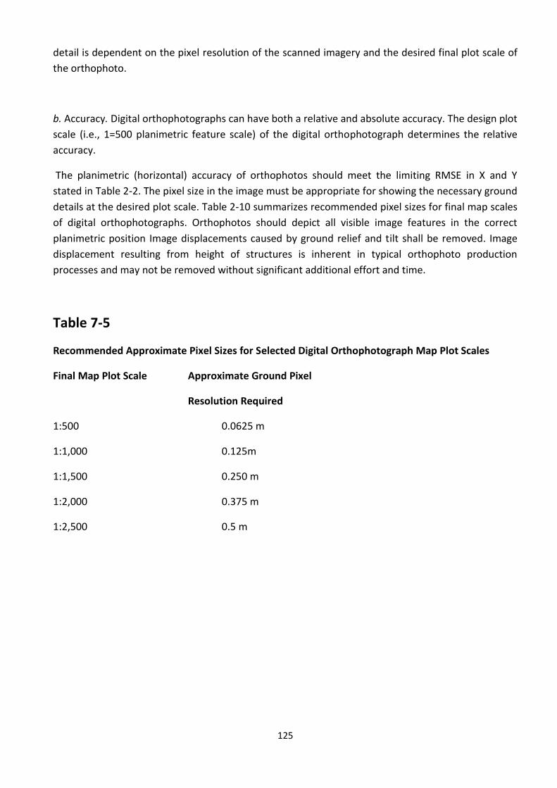
125

detail is dependent on the pixel resolution of the scanned imagery and the desired final plot scale of

the orthophoto.

b. Accuracy. Digital orthophotographs can have both a relative and absolute accuracy. The design plot

scale (i.e., 1=500 planimetric feature scale) of the digital orthophotograph determines the relative

accuracy.

The planimetric (horizontal) accuracy of orthophotos should meet the limiting RMSE in X and Y

stated in Table 2-2. The pixel size in the image must be appropriate for showing the necessary ground

details at the desired plot scale. Table 2-10 summarizes recommended pixel sizes for final map scales

of digital orthophotographs. Orthophotos should depict all visible image features in the correct

planimetric position Image displacements caused by ground relief and tilt shall be removed. Image

displacement resulting from height of structures is inherent in typical orthophoto production

processes and may not be removed without significant additional effort and time.

Table 7-5

Recommended Approximate Pixel Sizes for Selected Digital Orthophotograph Map Plot Scales

Final Map Plot Scale Approximate Ground Pixel

Resolution Required

1:500 0.0625 m

1:1,000 0.125m

1:1,500 0.250 m

1:2,000 0.375 m

1:2,500 0.5 m

126

SECTION – 8

GUIDELINES FOR BEST PRACTICE AND QUALITY CONTROL/QUALITY ASSURANCE STANDARDS

8.1 Requirement of quality Assurance

8.1.1 Quality Assurance

Quality assurance (QA) is a set of approaches which is consciously applied and, when taken together,

tends to lead to a satisfactory outcome for a particular process. A QA system based on these

guidelines will employ documented procedural rules, templates and closely managed processes into

which various checks are built. Quality controls (QC) and quality audits are important checks within a

QA system.

8.1. 2 Quality Control

A Quality control (or check) is clearly specified task that scrutinises all, or a sample, of the

items issuing during, or at the end of, the geometric correction process in order to ensure that the

final product is of satisfactory quality. The scrutiny involves review, inspection or quantitative

measurement, against well defined pass/fail criteria which are set out in these guidelines.

8.1.3 Quality Audits

A Quality audit is a qualitative quality control that covers an area of activity as a whole. The EC

will normally appoint an independent quality auditor to inspect geometric correction work in

progress at the Vendor’s site. Quality audits will be carried out by comparison of actual practice with

the applicable quality assurance procedures contained in these guidelines.

8.1.4 Quality Control Records

The information used in a Quality Audit will mainly be provided by quality control records

(QCRs) which are generated during the work, by the people doing the work. QCRs take a variety of

formats, such as paper forms completed manually, printouts or computer files recording the result of

a particular procedure, or just simply hand-written records in log books.

8.1.5 The key features of QCR:

Is marked with a date

Uniquely identifies the item, operation or product to which it relates.

Identifies the operator who generated the QCR.

May be countersigned by a supervisor or other independent inspector (only for the

most important records).

Is stored in a well defined and predictable location so that it can be found easily by

others.

These guidelines identify the essential (minimum) set of QCRs required for QA of geometric

correction.

127

8.1.6 QA Phases

Procurement of geometrically corrected images by the EC almost always occurs through a

process of competitive tendering. The technical execution of the work is therefore not directly under

the control of the EC so the QA process takes this into account. There is a sequence of three activities

which can be controlled by the EC and which affects the quality of the outcome.

ITT specification and tender evaluation

These guidelines distinguish between work components that are explicit requests in an ITT and those

that are looked for in the response.

Quality Control during the geometric correction work, including input data

The purpose of QC during the work is to identify potential early. Potential problems are defined as

those that could cause the geometric error in a product to exceed the specified tolerance.

Internal quality assurance will be the responsibility of the Vendor and will result in the production of

QCRs.

A representative of the EC who is independent of the Vendor will carry out external quality audits

(physical checks of conformity to specifications and scrutiny of ACRs produced by the internal QA)

and a limited amount of sample based QC.

Measurement of geometric error in the output images

An independent external quality control will be carried out by the EC on a sample of geometrically

corrected image products in order to establish an overall accuracy. The acceptance criterion for this

check is the tolerance stated in ITT.

8.1.7 Thresholds

In general, the orthoimage products (and associated DEMs) will be assessed from three

geometric perspectives:

RMSEx

RMSEy

For DEMs, RMSEz

Product deliveries determined to be outside this specification will be returned to the Vendor

for evaluation by the Vendor (internal QA) and redelivery, followed by further (possibly repeat)

checks (external QA).

Thresholds for scanning are described in §3.

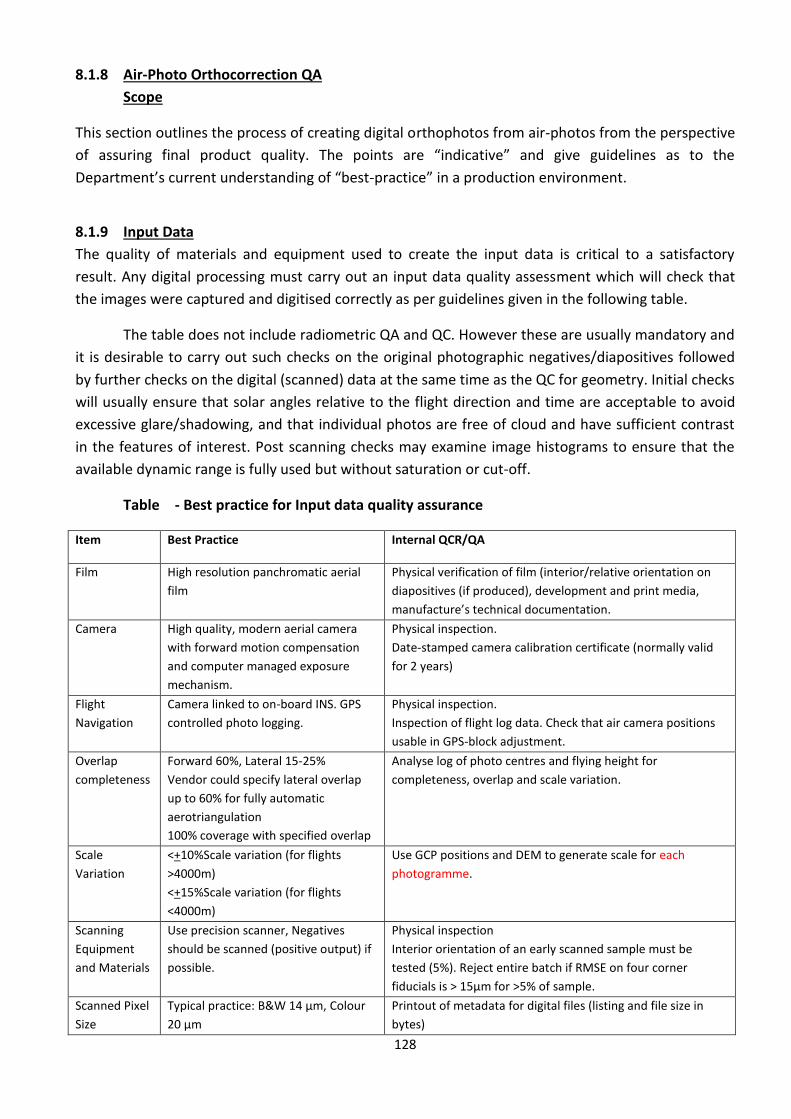
128

8.1.8 Air-Photo Orthocorrection QA

Scope

This section outlines the process of creating digital orthophotos from air-photos from the perspective

of assuring final product quality. The points are “indicative” and give guidelines as to the

Department’s current understanding of “best-practice” in a production environment.

8.1.9 Input Data

The quality of materials and equipment used to create the input data is critical to a satisfactory

result. Any digital processing must carry out an input data quality assessment which will check that

the images were captured and digitised correctly as per guidelines given in the following table.

The table does not include radiometric QA and QC. However these are usually mandatory and

it is desirable to carry out such checks on the original photographic negatives/diapositives followed

by further checks on the digital (scanned) data at the same time as the QC for geometry. Initial checks

will usually ensure that solar angles relative to the flight direction and time are acceptable to avoid

excessive glare/shadowing, and that individual photos are free of cloud and have sufficient contrast

in the features of interest. Post scanning checks may examine image histograms to ensure that the

available dynamic range is fully used but without saturation or cut-off.

Table - Best practice for Input data quality assurance

Item Best Practice Internal QCR/QA

Film High resolution panchromatic aerial

film

Physical verification of film (interior/relative orientation on

diapositives (if produced), development and print media,

manufacture’s technical documentation.

Camera High quality, modern aerial camera

with forward motion compensation

and computer managed exposure

mechanism.

Physical inspection.

Date-stamped camera calibration certificate (normally valid

for 2 years)

Flight

Navigation

Camera linked to on-board INS. GPS

controlled photo logging.

Physical inspection.

Inspection of flight log data. Check that air camera positions

usable in GPS-block adjustment.

Overlap

completeness

Forward 60%, Lateral 15-25%

Vendor could specify lateral overlap

up to 60% for fully automatic

aerotriangulation

100% coverage with specified overlap

Analyse log of photo centres and flying height for

completeness, overlap and scale variation.

Scale

Variation

<+10%Scale variation (for flights

>4000m)

<+15%Scale variation (for flights

<4000m)

Use GCP positions and DEM to generate scale for each

photogramme.

Scanning

Equipment

and Materials

Use precision scanner, Negatives

should be scanned (positive output) if

possible.

Physical inspection

Interior orientation of an early scanned sample must be

tested (5%). Reject entire batch if RMSE on four corner

fiducials is > 15µm for >5% of sample.

Scanned Pixel

Size

Typical practice: B&W 14 µm, Colour

20 µm

Printout of metadata for digital files (listing and file size in

bytes)

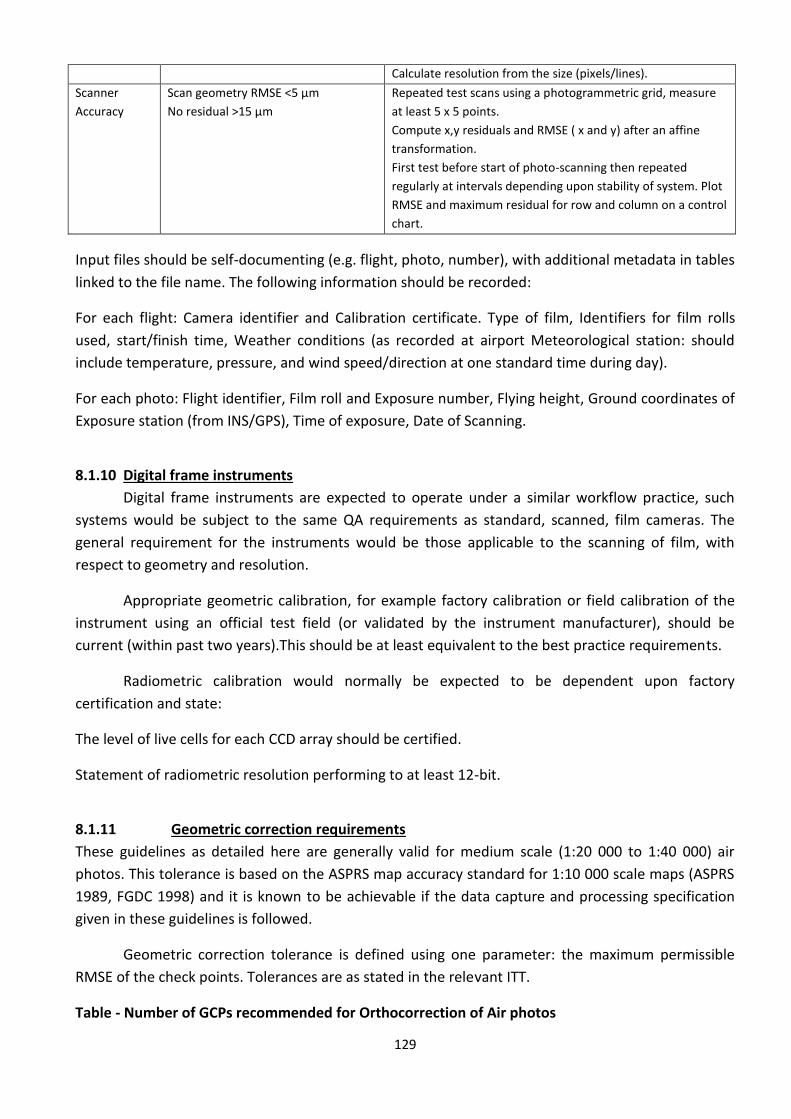
129

Calculate resolution from the size (pixels/lines).

Scanner

Accuracy

Scan geometry RMSE <5 µm

No residual >15 µm

Repeated test scans using a photogrammetric grid, measure

at least 5 x 5 points.

Compute x,y residuals and RMSE ( x and y) after an affine

transformation.

First test before start of photo-scanning then repeated

regularly at intervals depending upon stability of system. Plot

RMSE and maximum residual for row and column on a control

chart. T

Input files should be self-documenting (e.g. flight, photo, number), with additional metadata in tables

linked to the file name. The following information should be recorded:

For each flight: Camera identifier and Calibration certificate. Type of film, Identifiers for film rolls

used, start/finish time, Weather conditions (as recorded at airport Meteorological station: should

include temperature, pressure, and wind speed/direction at one standard time during day).

For each photo: Flight identifier, Film roll and Exposure number, Flying height, Ground coordinates of

Exposure station (from INS/GPS), Time of exposure, Date of Scanning.

8.1.10 Digital frame instruments

Digital frame instruments are expected to operate under a similar workflow practice, such

systems would be subject to the same QA requirements as standard, scanned, film cameras. The

general requirement for the instruments would be those applicable to the scanning of film, with

respect to geometry and resolution.

Appropriate geometric calibration, for example factory calibration or field calibration of the

instrument using an official test field (or validated by the instrument manufacturer), should be

current (within past two years).This should be at least equivalent to the best practice requirements.

Radiometric calibration would normally be expected to be dependent upon factory

certification and state:

The level of live cells for each CCD array should be certified.

Statement of radiometric resolution performing to at least 12-bit.

8.1.11 Geometric correction requirements

These guidelines as detailed here are generally valid for medium scale (1:20 000 to 1:40 000) air

photos. This tolerance is based on the ASPRS map accuracy standard for 1:10 000 scale maps (ASPRS

1989, FGDC 1998) and it is known to be achievable if the data capture and processing specification

given in these guidelines is followed.

Geometric correction tolerance is defined using one parameter: the maximum permissible

RMSE of the check points. Tolerances are as stated in the relevant ITT.

Table - Number of GCPs recommended for Orthocorrection of Air photos

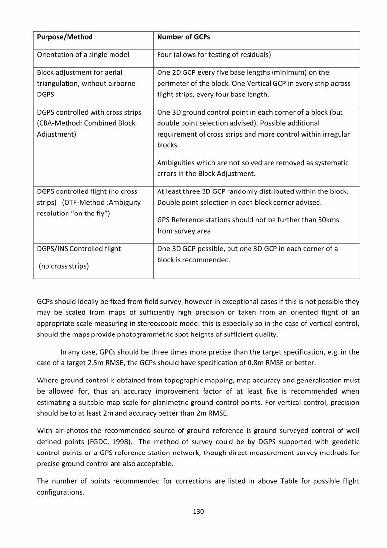
130

Purpose/Method Number of GCPs

Orientation of a single model Four (allows for testing of residuals)

Block adjustment for aerial

triangulation, without airborne

DGPS

One 2D GCP every five base lengths (minimum) on the

perimeter of the block. One Vertical GCP in every strip across

flight strips, every four base length.

DGPS controlled with cross strips

(CBA-Method: Combined Block

Adjustment)

One 3D ground control point in each corner of a block (but

double point selection advised). Possible additional

requirement of cross strips and more control within irregular

blocks.

Ambiguities which are not solved are removed as systematic

errors in the Block Adjustment.

DGPS controlled flight (no cross

strips) (OTF-Method :Ambiguity

resolution “on the fly”)

At least three 3D GCP randomly distributed within the block.

Double point selection in each block corner advised.

GPS Reference stations should not be further than 50kms

from survey area

DGPS/INS Controlled flight

(no cross strips)

One 3D GCP possible, but one 3D GCP in each corner of a

block is recommended.

GCPs should ideally be fixed from field survey, however in exceptional cases if this is not possible they

may be scaled from maps of sufficiently high precision or taken from an oriented flight of an

appropriate scale measuring in stereoscopic mode: this is especially so in the case of vertical control,

should the maps provide photogrammetric spot heights of sufficient quality.

In any case, GPCs should be three times more precise than the target specification, e.g. in the

case of a target 2.5m RMSE, the GCPs should have specification of 0.8m RMSE or better.

Where ground control is obtained from topographic mapping, map accuracy and generalisation must

be allowed for, thus an accuracy improvement factor of at least five is recommended when

estimating a suitable map scale for planimetric ground control points. For vertical control, precision

should be to at least 2m and accuracy better than 2m RMSE.

With air-photos the recommended source of ground reference is ground surveyed control of well

defined points (FGDC, 1998). The method of survey could be by DGPS supported with geodetic

control points or a GPS reference station network, though direct measurement survey methods for

precise ground control are also acceptable.

The number of points recommended for corrections are listed in above Table for possible flight

configurations.

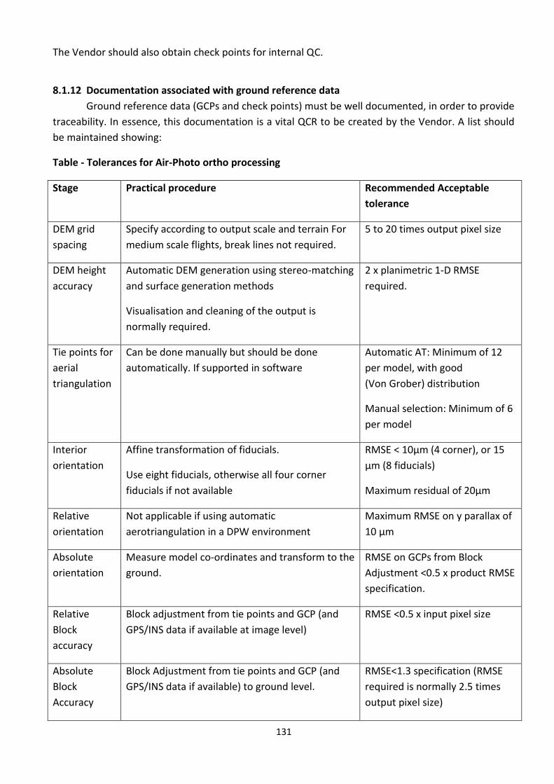
131

The Vendor should also obtain check points for internal QC.

8.1.12 Documentation associated with ground reference data

Ground reference data (GCPs and check points) must be well documented, in order to provide

traceability. In essence, this documentation is a vital QCR to be created by the Vendor. A list should

be maintained showing:

Table - Tolerances for Air-Photo ortho processing

Stage Practical procedure Recommended Acceptable

tolerance

DEM grid

spacing

Specify according to output scale and terrain For

medium scale flights, break lines not required.

5 to 20 times output pixel size

DEM height

accuracy

Automatic DEM generation using stereo-matching

and surface generation methods

Visualisation and cleaning of the output is

normally required.

2 x planimetric 1-D RMSE

required.

Tie points for

aerial

triangulation

Can be done manually but should be done

automatically. If supported in software

Automatic AT: Minimum of 12

per model, with good

(Von Grober) distribution

Manual selection: Minimum of 6

per model

Interior

orientation

Affine transformation of fiducials.

Use eight fiducials, otherwise all four corner

fiducials if not available

RMSE < 10µm (4 corner), or 15

µm (8 fiducials)

Maximum residual of 20µm

Relative

orientation

Not applicable if using automatic

aerotriangulation in a DPW environment

Maximum RMSE on y parallax of

10 µm

Absolute

orientation

Measure model co-ordinates and transform to the

ground.

RMSE on GCPs from Block

Adjustment <0.5 x product RMSE

specification.

Relative

Block

accuracy

Block adjustment from tie points and GCP (and

GPS/INS data if available at image level)

RMSE <0.5 x input pixel size

Absolute

Block

Accuracy

Block Adjustment from tie points and GCP (and

GPS/INS data if available) to ground level.

RMSE<1.3 specification (RMSE

required is normally 2.5 times

output pixel size)

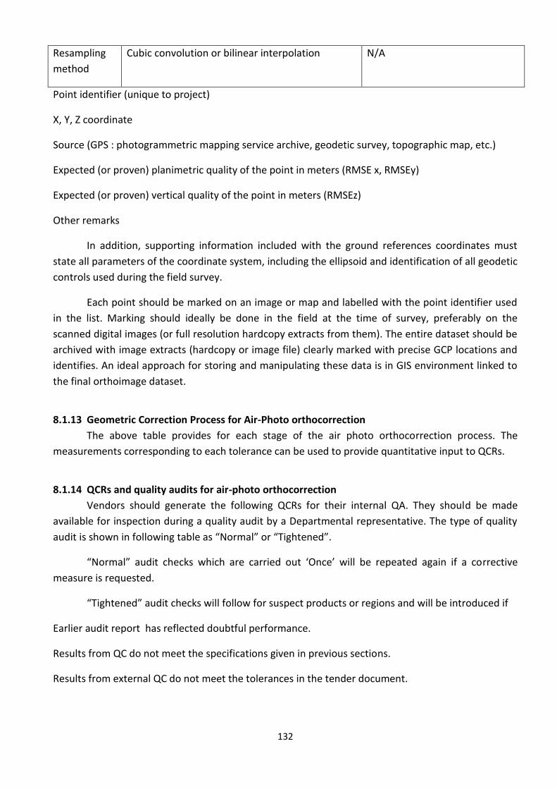
132

Resampling

method

Cubic convolution or bilinear interpolation N/A

Point identifier (unique to project)

X, Y, Z coordinate

Source (GPS : photogrammetric mapping service archive, geodetic survey, topographic map, etc.)

Expected (or proven) planimetric quality of the point in meters (RMSE x, RMSEy)

Expected (or proven) vertical quality of the point in meters (RMSEz)

Other remarks

In addition, supporting information included with the ground references coordinates must

state all parameters of the coordinate system, including the ellipsoid and identification of all geodetic

controls used during the field survey.

Each point should be marked on an image or map and labelled with the point identifier used

in the list. Marking should ideally be done in the field at the time of survey, preferably on the

scanned digital images (or full resolution hardcopy extracts from them). The entire dataset should be

archived with image extracts (hardcopy or image file) clearly marked with precise GCP locations and

identifies. An ideal approach for storing and manipulating these data is in GIS environment linked to

the final orthoimage dataset.

8.1.13 Geometric Correction Process for Air-Photo orthocorrection

The above table provides for each stage of the air photo orthocorrection process. The

measurements corresponding to each tolerance can be used to provide quantitative input to QCRs.

8.1.14 QCRs and quality audits for air-photo orthocorrection

Vendors should generate the following QCRs for their internal QA. They should be made

available for inspection during a quality audit by a Departmental representative. The type of quality

audit is shown in following table as “Normal” or “Tightened”.

“Normal” audit checks which are carried out ‘Once’ will be repeated again if a corrective

measure is requested.

“Tightened” audit checks will follow for suspect products or regions and will be introduced if

Earlier audit report has reflected doubtful performance.

Results from QC do not meet the specifications given in previous sections.

Results from external QC do not meet the tolerances in the tender document.

133

8.1.15 Updating of zones covered by existing orhophotos

Two strategies are considered applicable for the updating of zones with existing orthophotos: Use of GPS controlled flight: repeat of (automated) aerotriangulation. Model based approach, using ground and photo point data used in initial orthophoto creation. Both approaches make use of existing ground control and DTM/DEM data: neither approach

should require re-visits in the field, nor serious revisions of block adjustment data (GCP positioning

quality). Where the terrain has changed the DTM/DEM should be edited. Such areas may be detected

with correlation techniques from new flights and a comparison with the existing DEM/DTM.

Since many of the steps for production are the same as for the initial creation, these are not

re-specified here: reference is made to the preceding section. However, the revision flight should be

compatible with (although not necessarily identical to) the initial flight, hence a preference for GPS

controlled/pin point execution.

Furthermore, a technical preference based upon quality consideration reinforces the

application of a GPS based flight, with a full aerotriangulation and block adjustment, over the model-

based approach. Again, this introduces no new technical considerations not treated above, so no

further details are included here; internal quality assurance will be expected to comply as previously

described.

However, where a dense GCP network of sufficient quality already exists, and alternative

approach is to produce orientation parameters by model. Again, the above sections contain

guidelines as to the guidelines as to the quality of the various input data and the expected tolerances

for the results.

In all cases, final acceptance will be made by applying the external quality control guidelines

detailed in §7.

Table - QCR Production and Use for Aerial Ortho-images

QCR Format of QCR Vendor

Production Level

Department

Inspection level

(Sample)

Normal

Department

Audit Stage

Camera calibration

certificate

Paper 100% Normal (100%) Before flight

Flight data including

log of photo centres

and flying height

ASCII or GIS

files

100% Normal (100%) Before scanning

(or 10 days

after flight)

Control chart for the

scanner performance

( Geometric)

Paper/Graph Every 7 days, then

14 days if stable

Normal (Once) From start of

scanning

onwards

CV/training

certificate for DPWS

operators

Paper -- Normal (100%) Start of AT

134

Table of ground

reference data for

GCPs and check

points (used for

internal QC)

ASCII 100% Normal (100%) End of AT

Interior and exterior

orientation results

Paper or ASCII

files

100% Normal (first

few)

Tightened

End of AT

Number of items

rejected/reprocessed

at each stage of

internal QC

Progress report Complete list Normal

(Monthly)

N/A

Visualization of the

DEMs: Preferably

digital stereo image

with DEM data

overlaid

Paper or digital 100% Normal (Once)

Tightened (trail)

Start of

Orthocorrection

Comparison of DEMs

with vertical check

points (if available,

AT vertical points)

Paper/Graph Sample First DEM Start of

Orthocorrection

Residuals of block

adjustment on

control points

Paper or digital

software

reports

100% Normal (Once)

Tightened (trail)

Orthoimage

production

RMSE of finalised

block adjustment

using Vendor check

points including

individual residuals

Paper or digital

software

reports

100% Normal

(100% of

blocks)

Orthoimage

production

Ortho-image

metadata

Database 100% Normal (10%)

Tightened

(100%)

Start of

orthomosaic

production

Ortho images

(inspection result)

Paper or

metadata

100% Normal (10%) Orthoimage

production

135

8.2 Airborne digital image acquisition and correction QA

8.2.1 Scope

The scope of this section is limited to pushbroom airborne scanners since pushbroom scanners have

different geometric configuration, image characteristics and processing requirements. In particular,

since flight planning and execution present specific requirements, these are covered here in more

detail.

As in previous sections, the points below are “indicative” and give guidelines as to the

Department’s current understanding of “best-practice”. In this sense, they can be adopted as far as

the Vendor considers they are sensible and plausible in a production environment.

8.2.2 Sensor calibration

Appropriate geometric calibration, for example factory calibration or field calibration of the

instrument using an official test field (or validated by the instrument manufacturer), should be

current (within past two years).

Radiometric calibration would normally be expected to be dependent upon factory

certification and reflect

A level of 100% live cells for each CCD array should be certified.

Statement of radiometric resolution performing to at least 12-bit.

8.2.3 Flight plan and execution

The flight planning should ensure that issues related to sidelap, run length, height above

ground, traffic control clearance etc. are adequately addressed.

Sidelap: normally 15-25%, for specialist products this would increase to 80%.

Flight direction: alternate (e.g. W-E, E-W, W-E...) for inter-track redundancy.

Run length/duration:

< 15 minutes (to keep the highest achievable accuracy with IMU drift).

Alternatively typically less than 30 minutes of flying time (usually <80km) for medium scale (1m pixel

GSD) products.

Scale variation should remain less than =+10% for GSD of 0.4m to 1m. Ground sampling distance (or

final product pixel size) will be determined by:

Flight altitude: will determine the Ground Sampling Distance across-track.

136

Aircraft Speed: will determine the Ground Sampling Distance along track, together with the CCD

timecycle.

Sensor configuration:

Angle of CCD bands used for orthoimage product as close as possible to nadir.

RGB or CIR composite at same angle.

Use of staggered arrays for resolution enhancement is not currently considered to be appropriate for

best practice operations.

Need for forward and rearward stereo bands for DEM generation.

Due to the reliance upon DGPS processing, proximity to GPS base station(s) should be under

normal circumstances:

<20km for in flight alignment of IMU.

<50km for image acquisition.

Interval/frequency: every 1 to 10 second.

The specificity of such systems will require specialist/experienced instrument operators to

ensure that the above conditions are met.

8.2.4 Overlap Completeness map

This check should permit control in GIS that the full zone is covered with the prerequisite

number of overlapping images.

Attention should be paid to start and end of flight lines (forward/rearward viewing scanners).

8.2.5 GCP report location

Five well distributed 3D ground control points normally used per block (or flight session).

However double point selection is advised to guard against failure of point identification in the

image. Furthermore, for irregular blocks, this number should be doubled.

A check should be undertaken to permit the comparison of positions of ground control in

relation to the flight block.

8.2.6 Image check

An image check should be carried out before orthoprocessing; a QC report should be

available. Validation should be made of the rectification trajectory (over the raw image) using

GPS/INS data.

Cloud cover: A quick look should be provided as a QCR, either run by run or mosaicked.

137

Radiometry: Basic level check should be executed on image histogram, saturation.

A Flight and Geometry validation report should be made giving a clear diagram of the flight

plan. The flight report should include a 4-D (X, Y, Z, time) track of the flight and permit the

quantitative analysis of the flight characteristics.

Interval/frequency: every second

Ancillary data: uncertainly parameter (if applicable) of position.

8.2.7 Analogous sections from air-photo survey

In general, the sections covering documentation associated with ground reference data, QCRs

and quality audits for air photo orthocorrection and updating of zones covered by existing

orthophotos will also apply to digital scanner flights.

A QC report should be issued on the post-processing of GPS and IMU data, and on the

aerotriangulation results (residuals).

Assuming that the DEM is produced internally, the following QCRs should be provided

Meta data

Quality Report

QCR reporting listed in Table of QCR production and use for aerial ortho-images as above,

specifically 1,2,4,5,7,8,9,11,12, and 13 will in general be generated during the production process.

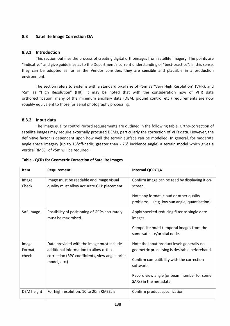
138

8.3 Satellite Image Correction QA

8.3.1 Introduction

This section outlines the process of creating digital orthoimages from satellite imagery. The points are

“indicative” and give guidelines as to the Department’s current understanding of “best-practice”. In this sense,

they can be adopted as far as the Vendor considers they are sensible and plausible in a production

environment.

The section refers to systems with a standard pixel size of <5m as “Very High Resolution” (VHR), and

>5m as “High Resolution” (HR). It may be noted that with the consideration now of VHR data

orthorectification, many of the minimum ancillary data (DEM, ground control etc.) requirements are now

roughly equivalent to those for aerial photography processing.

8.3.2 Input data

The image quality control record requirements are outlined in the following table. Ortho-correction of

satellite images may require externally procured DEMs, particularly the correction of VHR data. However, the

definitive factor is dependent upon how well the terrain surface can be modelled. In general, for moderate

angle space imagery (up to 15°off-nadir, greater than 75° incidence angle) a terrain model which gives a

vertical RMSEz of <5m will be required.

Table - QCRs for Geometric Correction of Satellite Images

Item Requirement Internal QCR/QA

Image

Check

Image must be readable and image visual

quality must allow accurate GCP placement.

Confirm image can be read by displaying it on-

screen.

Note any format, cloud or other quality

problems (e.g. low sun angle, quantisation).

SAR image Possibility of positioning of GCPs accurately

must be maximised.

Apply specked-reducing filter to single date

images.

Composite multi-temporal images from the

same satellite/orbital node.

Image

Format

check

Data provided with the image must include

additional information to allow ortho-

correction (RPC coefficients, view angle, orbit

model, etc.)

Note the input product level: generally no

geometric processing is desirable beforehand.

Confirm compatibility with the correction

software

Record view angle (or beam number for some

SARs) in the metadata.

DEM height For high resolution: 10 to 20m RMSEz is Confirm product specification

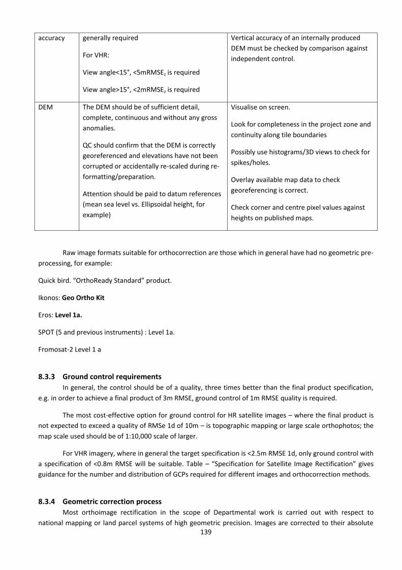
139

accuracy generally required

For VHR:

View angle<15°, <5mRMSEz is required

View angle>15°, <2mRMSEz is required

Vertical accuracy of an internally produced

DEM must be checked by comparison against

independent control.

DEM The DEM should be of sufficient detail,

complete, continuous and without any gross

anomalies.

QC should confirm that the DEM is correctly

georeferenced and elevations have not been

corrupted or accidentally re-scaled during re-

formatting/preparation.

Attention should be paid to datum references

(mean sea level vs. Ellipsoidal height, for

example)

Visualise on screen.

Look for completeness in the project zone and

continuity along tile boundaries

Possibly use histograms/3D views to check for

spikes/holes.

Overlay available map data to check

georeferencing is correct.

Check corner and centre pixel values against

heights on published maps.

Raw image formats suitable for orthocorrection are those which in general have had no geometric pre-

processing, for example:

Quick bird. “OrthoReady Standard” product.

Ikonos: Geo Ortho Kit

Eros: Level 1a.

SPOT (5 and previous instruments) : Level 1a.

Fromosat-2 Level 1 a

8.3.3 Ground control requirements

In general, the control should be of a quality, three times better than the final product specification,

e.g. in order to achieve a final product of 3m RMSE, ground control of 1m RMSE quality is required.

The most cost-effective option for ground control for HR satellite images – where the final product is

not expected to exceed a quality of RMSe 1d of 10m – is topographic mapping or large scale orthophotos; the

map scale used should be of 1:10,000 scale of larger.

For VHR imagery, where in general the target specification is <2.5m RMSE 1d, only ground control with

a specification of <0.8m RMSE will be suitable. Table – “Specification for Satellite Image Rectification” gives

guidance for the number and distribution of GCPs required for different images and orthocorrection methods.

8.3.4 Geometric correction process

Most orthoimage rectification in the scope of Departmental work is carried out with respect to

national mapping or land parcel systems of high geometric precision. Images are corrected to their absolute

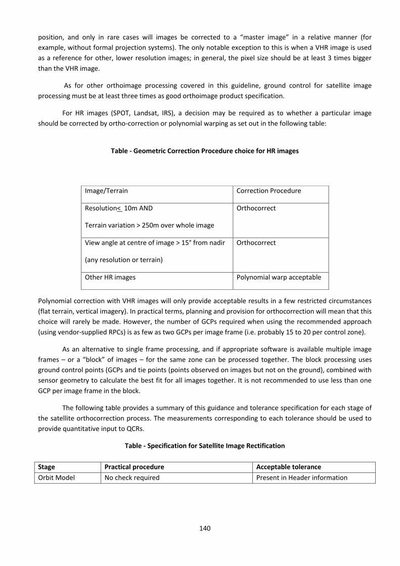
140

position, and only in rare cases will images be corrected to a “master image” in a relative manner (for

example, without formal projection systems). The only notable exception to this is when a VHR image is used

as a reference for other, lower resolution images; in general, the pixel size should be at least 3 times bigger

than the VHR image.

As for other orthoimage processing covered in this guideline, ground control for satellite image

processing must be at least three times as good orthoimage product specification.

For HR images (SPOT, Landsat, IRS), a decision may be required as to whether a particular image

should be corrected by ortho-correction or polynomial warping as set out in the following table:

Table - Geometric Correction Procedure choice for HR images

Polynomial correction with VHR images will only provide acceptable results in a few restricted circumstances

(flat terrain, vertical imagery). In practical terms, planning and provision for orthocorrection will mean that this

choice will rarely be made. However, the number of GCPs required when using the recommended approach

(using vendor-supplied RPCs) is as few as two GCPs per image frame (i.e. probably 15 to 20 per control zone).

As an alternative to single frame processing, and if appropriate software is available multiple image

frames – or a “block” of images – for the same zone can be processed together. The block processing uses

ground control points (GCPs and tie points (points observed on images but not on the ground), combined with

sensor geometry to calculate the best fit for all images together. It is not recommended to use less than one

GCP per image frame in the block.

The following table provides a summary of this guidance and tolerance specification for each stage of

the satellite orthocorrection process. The measurements corresponding to each tolerance should be used to

provide quantitative input to QCRs.

Table - Specification for Satellite Image Rectification

Stage Practical procedure Acceptable tolerance

Orbit Model No check required Present in Header information

Image/Terrain Correction Procedure

Resolution< 10m AND

Terrain variation > 250m over whole image

Orthocorrect

View angle at centre of image > 15° from nadir

(any resolution or terrain)

Orthocorrect

Other HR images Polynomial warp acceptable

141

GCP selection, HR

(SPOT, IRS,

Landsat)

GCPs should be well distributed- for example

one in each cell of a 4x4 grid dividing the image

with additional points as near as possible to

each corner/edge.

Polynomial warp (not for VHR)

Quantity >15 GCPS per image frame

or physical model orthorectification

(at least 9 GCPs per frame):

Record number in metadata/QCR

GCP selection, VHR

with vendor

supplied RPC

processing

Recommendation is to use supplied RPC data –

as few as two GCPs per image frame or 100-

200Km2 could be used. Although 4 points

located in the image corners should be the

preferred approach. For lKONOS strip scenes,

add minimum tow GCPs per extra 100Km2

Minimum 2-4 per image frame, plus 2

per additional 100Km2 of strip scene.

GCP distribution not critical, but well

distributed preferred.

Record number in metadata/QCR

For VHR block processing (multiple frames),

ground control may be reduced up to 1 GCP per

frame if sufficient good tie points available

between imagery

GCP can fall in overlap zones (image

corners) but not critical

GCP selection, VHR

with physical

model or RPC

generation from

ground control

For VHR orthorectification using a physical

sensor model, at least 9 GCPs will be required

usually per image (100Km2). For EROS vector

scenes, this number should be doubled.

RPC generation is GCP intensive: not

recommended

More than 9 GCPs (physical model) or

16 GCPs (RPC generation) required

per image frame. Distribution of GCPs

should cover full area of interest.

Record number in metadata/QCR.

GCP Blunder Check HR: Fit a first order polynomial to the GCPs

VHR: Residuals should be calculated when

redundancy available in GCPs; otherwise check

independent points

Maximum residual should not exceed

3x the target RMSE

Record result in metadata/QCR

Polynomial warp

(only)

Use a first or second order polynomial, third

order must not be used

Record the polynomial order in the

metadata/QCR

Rectification

results

Calculate RMSE discrepancy on 10 check points

(if available) OR

Record the prediction sum of squares (√PRESS)

– if available

Record the residuals for each GCP and their

RMSE compared to the fitted model.

Checkpoint RMSE < tolerance for

geometric accuracy

√PRESS<tolerance for geometric

accuracy

RMSE if calculated on residuals on

residuals should <0.5x tolerance for

geometric accuracy Save

GCPs/residuals to file

Record summary results in

metadata/QCR.

Resampling For imagery unlikely to be quantitatively

analysed/classified – particularly panchromatic

imagery or pan sharpened – bilinear

interpolation or Cubic convolution is

appropriate; output pixel size ≈ input pixel size

Nearest neighbour may be used if justified (e.g.

classification), but output pixel size should be

0.5x input pixel size

Record sampling method and output

pixel size

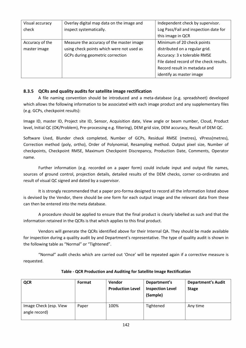
142

Visual accuracy

check

Overlay digital map data on the image and

inspect systematically.

Independent check by supervisor.

Log Pass/Fail and inspection date for

this image in QCR

Accuracy of the

master image

Measure the accuracy of the master image

using check points which were not used as

GCPs during geometric correction

Minimum of 20 check points

distributed on a regular grid.

Accuracy: 3 x tolerable RMSE

File dated record of the check results.

Record result in metadata and

identify as master image

8.3.5 QCRs and quality audits for satellite image rectification

A file naming convention should be introduced and a meta-database (e.g. spreadsheet) developed

which allows the following information to be associated with each image product and any supplementary files

(e.g. GCPs, checkpoint results):

Image ID, master ID, Project site ID, Sensor, Acquisition date, View angle or beam number, Cloud, Product

level, Initial QC (OK/Problem), Pre-processing e.g. filtering), DEM grid size, DEM accuracy, Result of DEM QC.

Software Used, Blunder check completed, Number of GCPs, Residual RMSE (metres), √Press(metres),

Correction method (poly, ortho), Order of Polynomial, Resampling method. Output pixel size, Number of

checkpoints, Checkpoint RMSE, Maximum Checkpoint Discrepancy, Production Date, Comments, Operator

name.

Further information (e.g. recorded on a paper form) could include input and output file names,

sources of ground control, projection details, detailed results of the DEM checks, corner co-ordinates and

result of visual QC signed and dated by a supervisor.

It is strongly recommended that a paper pro-forma designed to record all the information listed above

is devised by the Vendor, there should be one form for each output image and the relevant data from these

can then be entered into the meta database.

A procedure should be applied to ensure that the final product is clearly labelled as such and that the

information retained in the QCRs is that which applies to this final product.

Vendors will generate the QCRs identified above for their Internal QA. They should be made available

for inspection during a quality audit by and Department’s representative. The type of quality audit is shown in

the following table as “Normal” or “Tightened”.

“Normal” audit checks which are carried out ‘Once’ will be repeated again if a corrective measure is

requested.

Table - QCR Production and Auditing for Satellite Image Rectification

QCR Format Vendor

Production Level

Department’s

Inspection Level

(Sample)

Department’s Audit

Stage

Image Check (esp. View

angle record)

Paper 100% Tightened Any time

143

DEM (esp. anomalies and

height accuracy)


Ground reference Source 100% Tightened Any time

Software -- -- Normal (once) Before any correction

CV/Training certificate for

operators

Paper -- Tightened Any time

File of GCPs check points

and residuals (used for

Internal QC)


Adjustment/warp results Paper and

metadata

100% Normal (first few)

Tightened

Any time

Resampling Paper and

metadata

100% Tightened Any time

Visual accuracy Paper results

Or on-screen

100% Normal (once)

Tightened

Start of image-

correction

Accuracy of the master

image

Paper or

metadata

100% Normal (100%) Start of image

production on each

site

Image metadata Database 100% Normal (100%) Start and end of

image production

“Tightened” audit checks will follow an audit trail for suspect products and will be introduced if

Earlier audits result in doubts about performance.

Results from QC do not meet the specifications given in previous sections.

Results from External QC do not meet the tolerance in the tender document.

144

8.4 Method of External Quality Checks

8.4.1 Introduction

This section describes a method for independently checking the accuracy of geometrically

corrected images.

The check is intended to be carried out independently by the Department using a sample of

the final products.

8.4.2 Digital image delivery (scanned aerial photographs and digital airborne imagery):

The Department will check according to the criteria specified for scanning, at least a sample

(minimum 10%) of the image delivered. If on this sample test, more than 5% of the images tested fail

on one or more of the specifications marked above, the entire delivery may be returned to the

Vendor for quality checking a re-delivery. In other cases, imagery failing the specification on one or

more of the tests may be required to be re-scanned until the specification is met in full.

8.4.3 Inputs to orthocorrection external quality check

For the external checking of orthoimage accuracy the following information is required as

input.

Table - Inputs to External QC of airborne orthoimage (digital or photographic)

Item Specification Format

Ortho-

image

Selected extracted from the final products, georeferenced

to the (national) map projection

Digital format (as agreed

in specification)

GCPs Document listing the GCP id/description and coordinates:

short text explaining how the GCPs were collected

(equipment, vertical and horizontal control(s) used),

estimated precision and accuracy.

Image extracts (hardcopy or image file) clearly marked

with precise GCP locations and identifies.

Hardcopy and softcopy

(ASCII, Tab delimited) or

GIS layers.

Check

points

Check points (acquired by department), generally a

minimum of 25 per block/site

Document with image

extracts showing position

and coordinates.

The checkpoints should (ideally) be provided from a different source than the Vendor;

however, QCR information may permit use of Vendor data where these show that the data are

reliable.

145

For orthophotos, around 5-10% of orthoimage files will be checked externally. For satellite

image products, in general the whole set of data will be assessed. Product files will be selected on a

systematic basis to ensure that QC covers the entire block/site area. The results for separate photos

will be analysed together as a guard against systematic errors. Additional blocks/images will also be

selected, possibly on a random basis but also potentially to provide closer inspection in areas where

problems are anticipated (e.g. known quality problems with specific batches of original photos or

significant terrain variation, high view angles, etc.).

8.4.4 Check point selection

Conformance with tolerances will be assessed on a sample of images using independent

measurements of image accuracy (i.e. not the GCPs used for correction) using a checkpoint reference

which is at least three times more accurate that the product specification.

Each check point must be considered to be “well defined” (ASPRS 1989) in the context of the image

resolution, contrast and features that are present. A well-defined point represents a feature for

which the horizontal position is known to a high degree of accuracy and position with respect to the

geodetic datum. For the purpose of accuracy testing, well-defined pointes must be easily visible:

On the ground

On the product itself

The selected points will differ depending on the type of dataset and output scale of the

dataset. For orthoimagery with a 1m pixel sixe, suitable well-defined points may represent features

such as small isolated shrubs or bushes, road intersections (corners) in addition to right-angle

intersections of linear features. For lower resolution images, the same principles should apply,

although the features to be detected may be more often similar to cartographic representations.

Care will be taken not to choose features which are over-generalised on maps.

Buildings which represent vertical displacement (corners of buildings, telegraph poles) should

in all cases not be selected as checkpoints.

8.4.5 External quality checking method for image accuracy

The operator identifies the location of each checkpoint on the image and enters this and the

‘true’ co-ordinate in a table. A discrepancy is then calculated for each checkpoint together with an

overall RMSE. These calculated values are then compared to the project tolerances and a ‘Pass’ or

‘Fail’ status applied to the final result. The operator applies a ‘Fail’ to an image where the calculated

RMSE is greater than the tolerable RMSE entered. Normally the tolerable RMSE will be the same as

the tolerable RMSE specified in the tender document.

The concept of maximum tolerable discrepancy is defined as three times the calculated RMSE.

A point that exceeds the maximum tolerable discrepancy may be considered as blunder error if

further inspection of the point reveals that this decision is justified (type of point, uncertainty of

location, etc.). In addition, justification for the elimination of such a point must be documented

146

(equipment failure, change of feature between photography and survey, etc.). No point that is within

the maximum tolerance may be eliminated from the sample dataset.

The recommended output is a three-page report showing an analysis of the results. A text page

contains a table of check points with the individual discrepancy between the image and their ‘true’

location, together with the ‘Pass’ or ‘Fail’ status and summary statistics (mean error in x and y,

RMSEx, RMSEy, maximum discrepancy). A graphical report shows the position of each checkpoint

relative to the grid, together with the size and direction of the discrepancy.

8.4.6 Result calculation – within block

A block is normally considered to be a geometrically homogeneous group of image products

(orthoimage, DEM), such as a photogrammetric aerotriangulation block, or RS control site. However,

in the case of orthoimages created by space resection neither per image nor per photogramme), each

will be treated as a block.

The absolute RMSE of all check points in the block/site will be calculated: should this exceed

the project specification, all products associated with the block/site will be rejected. However,

further investigations may be necessary to increase confidence in the result should the final result be

marginal (just below or above the tolerance). These may involve the acquisition of further points, or

may involve the follow-up of specific production problems (tightened auditing checks).

The planimetric threshold will be applied independently in X, and Y. Failure to meet the

specification in either of these two dimensions (i.e. RSMEx or RMSEy) will reject the block.

Where the DEM is also a deliverable in the contract, the DEM will be checked using the Z

threshold tolerance. Again, Exceeding the RMSEz tolerance will reject all products for the block.

8.4.7 Result calculation – project level

At least 10% of the sites or photogrammetric blocks (or a minimum of one site) will be

independently checked following the method outlined above. All blocks that fail will be examined by

the Vendor, corrected and redelivered.

Should more than 5% of the blocks that are subjected to external QC fail, all products will be

returned to the Vendor for further QA. In effect, the Department will pass responsibility to the

Vendor to provide adequate and clear internal Quality Audits to identify the extent and cause of the

problems, and (where necessary to comply with the specification) make new products.

Redelivery of products will be followed by a further independent check on a new sample of the

products. This procedure will continue until the products are finally acceptable under the terms

above.

147

SECTION- 9

GLOSSARY

Within the separate literature on geometric correction of satellite images, map accuracy assessment

and photogrammetry, different terms are sometimes assigned the same meaning when they can

usefully be assigned more precise and distinct meanings (e.g. discrepancy and residual). The

following definitions apply to terms as used in this document and have been phrased, where possible,

to be applicable both to air-photo and satellite image correction. Cross references to other definitions

are indicated with italics.

Term Definition Adapted

from

2D Images or photos in X and Y coordinates only, there is no vertical element (Z) to 2D

images.

Viewed in mono, 2D images are good for qualitative analysis.

3D Images or photos in X, Y, and Z (vertical) coordinate. Viewed in stereo, 3D images

approximate true Earth features.

3D floating

cursor

The 3D floating cursor is apparent in a Digital Stereo Model (DSM) (i.e., two

images of approximately the same area) displayed in the Digital Stereoscope

Workspace.

The 3D floating cursor‘s position is determined by the amount of x-parallax evident

in the DSM, and its positioning on the ground or feature or interest.

3D

shapefile

A 3D shapefile is a standard shapefile with the added Z, or elevation dimension.

*.blk. The .blk extension stands for an IMAGINE OrthoBASE Block File containing one or

more images that can be viewed in stereo. One can use the Stereo Pair Chooser to

select a stereo-pair from an IMAGINE OrthoBASE Block File.

*.fpj The .fpj extension stands for feature project. In an .fpj project, one can collect

features in vector format from stereo imagery.

148

*.stp. The .stp extension stands for stereo pair. An .stp image is made of two

images.

κ. Kappa. An angle used to define angular orientation. κ is rotation about

the z-axis.

ω. Omega. An angle used to define angular orientation. ω is rotation about

the x-axis.

Ø Phi. An angle used to define angular orientation. Ø is rotation about the

y-axis.

Accuracy Accuracy is the relationship of a set of features to a defined reference

system and is expressed as a multiple (1 or more) of the rms error of a set

of derived points (if possible expressed as a ground distance in meters, but

sometimes given as pixel or microns).

Active tool. In ERDAS Stereo Analyst, the active tool is the one you are currently using

to collect or edit features in a Feature Project. Its active status is indicated

by its apparent depression in the ERDAS Stereo Analyst feature tool bar.

The active tool can be locked for repeated use using the Lock Tool.

Adjusted stereopair An adjusted stereopair is a pair of images displayed in a Digital

Stereoscope Workspace that has a map projection system associated with

it.

Aerial photographs Photographs taken from vertical or near vertical positions above the Earth

captured by aircraft or satellite. Photographs used for planimetric mapping

projects.

Aerial triangulation (AT) The process of establishing a mathematical relationship between

images, the camera or sensor model, and the ground. The information

derived is necessary for ortho-rectification, DEM generation, and stereopair

creation.

Aero-triangulation The process of aerial triangulation is the densification of geometric control

of the individual stereomodel level by the identification of ground co-

ordinates for tie points based on the network of known survey data. This

process computes a project-wide network of control and confirms the

integrity of the ground control points.

Wolf 1983

Affine

transformation

Defines the relationship between the pixel coordinate system and the

image space coordinate system using coefficients.

Air base The distance between the two image exposure stations.

Airborne GPS A technique used to provide initial approximations of exterior orientation,

which defines the position and orientation associated with each image as

they existed during image capture. See also Global positioning system.

Airborne INS INS stands for inertial navigation system. Airborne INS data is available for

each image, and defines the position and orientation associated with an

149

image as they existed during image capture.

Anaglyph An anaglyph is a 3D image composed of two oriented or non-oriented

stereo-pairs. To view an anaglyph, you require a pair of red/blue glasses.

These glasses isolate your vision into two distinct parts corresponding with

the left and right images of the stereo-pair. This produces a 3D effect with

vertical information.

Analog

photogrammetry.

Optical or mechanical instruments, such as analog plotters, used to

reconstruct 3D geometry from two overlapping photographs.

Analytical

photogrammetry.

The computer replaces some expensive optical and mechanical

components by substituting analog measurement and calculation with

mathematical computation.

Anti-aliasing In a DSM, anti-aliasing appears as shimmering effects visible in urban

areas due to limited texture mapping.

ASCII American Standard Code for Information Interchange—(ASCII) a ―basis

of character sets...to convey some control codes, space, numbers, most

basic punctuation, and unaccented letters a-z and A-Z‖ (Free On-Line

Dictionary of Computing 1999).

AT

see Aerial triangulation.

Attribute table An attribute table is automatically created when 3D features are digitized

and contains default information depending on the type of feature it

represents. For example, an attribute table detailing road features has a

length attribute.

Attribute. An attribute is a piece of information stored about a feature collected in the

Digital Stereoscope Workspace. For example, for a road feature attributes

associated with this will include the X, Y, and Z components of each vertex

making up the road. Attribute information also includes the total line length.

One can add additional attribute information to the feature, such as the

name of the road, if you wish.

Attribution Attribution is attribute data associated with a feature. See Attribute.

Base-height ratio The ratio between the average flying height of the camera and the distance

between exposure stations of overlapping images.

b/h. See Eye-base to height ratio.

Block triangulation. The process of establishing a mathematical relationship between images,

the camera or sensor model, and the ground. The information derived is

150

necessary for orthorectification, DEM generation, and stereo-pair creation.

Block, block

processing

Two or more image strips (or image frames) having a lateral overlap,

usually a set of aerial images or a set of VHR image frames.

Wolf 1983

Blunder See Error

Breakline. An elevation polyline in which each vertex has its own X, Y, Z value.

Bundle block

adjustment

A mathematical technique that determines the position and orientation of

each image as they existed at the time of image capture, determines the

ground coordinates measured on overlap areas of multiple images, and

minimizes the error associated with the imagery, image measurements,

and GCPs.

Cache .A temporary storage area for data that is currently in use. The cache

enables fast manipulation of the data. When data is no longer held by the

cache, it is returned to the permanent storage place for the data, such as

the hard drive.

CAD .see Computer-aided design.

Calibration

certificate/report

In aerial photography, the manufacturer of the camera specifies the interior

orientation in the form of a certificate or report.

Charge-coupled

device (CCD)

―A semiconductor technology used to build light-sensitive electronic

devices such as cameras and image scanners‖

Check point A well-defined ground reference point used for checking the accuracy of a

geometrically correct image or image mosaic. The location accuracy of the

check point must exceed the tolerable accuracy of the image by a factor of

at least three. Check points must not be the same as GCPs.

Wolf 1983

Collinearity

condition.

The condition that specifies that the exposure station, ground point, and its

corresponding image point location must all lie along a straight line.

Collinearity equations describe the relationship among image coordinates,

ground coordinates, and orientation parameters.

Computer-aided

design.

(CAD) Computer application used for design.

Control point

extension

This technique requires the manual measurement of ground points on

photos of overlapping areas. The ground coordinates associated with the

GCPs are then determined by using photogrammetric techniques of analog

or analytical stereo plotters.

Coordinate system A method of expressing location of any point. In 2D coordinate systems,

locations are expressed by a column and row, also called X and Y. In a 3D

151

coordinate system, the elevation value is added, called Z.

Coplanarity

condition

The coplanarity condition is used to calculate relative orientation. It uses an

iterative least squares adjustment to estimate five parameters (By, Bz,

Omega [ω], Phi [ϕ], and Kappa [κ]). The parameters explain the difference

in position and rotation between the two images making up the stereopair.

Correlate Matching regions of separate images for the purposes of tie point or GCP

collection, as well as elevation extraction

Datum Defines the height of the camera above sea level

Degrees of freedom Also known as redundancy. The number of unknowns is subtracted from

the number of knowns. The resulting number is the redundancy, or degree

of freedom in a solution.

Delta Difference, usually in elevation, slope, or degree.

Delta Z Difference in elevation between points.

Digital Elevation

Model (DEM)

A digital, raster representation of land surface elevation above sea level.

DEM is used in preference to digital terrain model (DTM) because the term

‗terrain‘ implies attributes of the landscape other than elevation.

Burrough

1986

Digital orthophoto An aerial photo or satellite scene that has been transformed by the

orthogonal projection, yielding a map that is free of most significant

geometric distortions.

Digital

photogrammetry

Photogrammetry as applied to digital images that are stored and

processed on a computer. Digital images can be scanned from

photographs or can be directly captured by digital cameras.

Digital stereo

model

(DSM) Stereo models that use imaging techniques of digital

photogrammetry that can be viewed on desktop applications.

Digital terrain

model

(DTM) A DTM is a discrete expression of topography in a data array,

consisting of a group of planimetric coordinates (X, Y) and the elevations

(Z) of the ground points and breaklines. See also Breakline.

Direction of flight Images in a strip are captured along the aircraft or satellite‘s direction of

flight. Images overlap in the same manner as the direction of flight.

Discrepancy A discrepancy is the linear distance between a point on the image and a

check point. A discrepancy is not the same as a residual, because a

discrepancy is an error at each point measured using a reference point

known to a higher order of accuracy.

Dynamically loaded

library

(DLL) A Dynamically Loaded Library is loaded by the application as they

are needed. DLLs provide added functionality such as stereo display and

import/export capabilities.

152

Elements of

exterior orientation

Variables that define the position and orientation of a sensor as it obtained

an image. It is the position of the perspective centre with respect to the

ground space coordinate system.

Ellipsoid For conversion to a flat surface (i.e. for mapping), a projection process is

applied to a world reference system (Geodetic Datum) with its associated

ellipsoid. Ellipsoidal models define an ellipsoid with an equatorial radius

and a polar radius. The best of these models can represent the shape of

the earth over the smoothed, averaged sea-surface to within about one-

hundred meters. WGS 84 is a standard for the whole world but may give

not an exact fit in a given area.

Dana,

1998

Ephemeris Data contained in the header of the data file of a scene, provides

information about the recording of the data and the satellite orbit.

Epipolar stereopair A stereopair without y-parallax.

Error Geometric error in an image which has been corrected to fit a map

projection. Three classes of error are commonly recognised:

A random error is not predictable at any given location but the population

of random geometric errors commonly follows a normal (Gaussian)

probability distribution. If random errors are normally distributed the mean

error is zero for a large sample of points.A systematic error is predictable

at any given location once it has been identified and its pattern of variation

is understood. For a large sample of points, a mean error that is not zero

can sometimes indicate presence of a systematic error.

A blunder is a (large) error at one location arising from a mistake or

equipment fault whilst marking the location or recording its coordinates. An

error at a single point that exceeds 3 x RMSE of a sample population is

usually due to a blunder.

Harley,

1975

Exposure station During image acquisition, each point in the flight path at which the camera

exposes the film. The 3D position of an aerial camera at the time of film

exposure, projected XYZ; typically given by GPS, or post-AT.

Exterior orientation All images of a block of aerial photographs in the ground coordinate system

are computed during photogrammetric triangulation, using limited number

of points with known coordinates. The exterior orientation of an image

consists of the exposure station and the camera attitude at the moment of

image capture. It establishes precise relationships between the focal plane

co-ordinates and a geographic reference system (map projection). It can

be achieved by relative and absolute orientation or can be carried out in a

single step.

153

Exterior

orientation

parameters

The perspective centre‘s ground coordinates in a specified map projection and

three rotation angles around the coordinate axes.

Eye-base to

height ratio

(b/h) The eyebase is the distance between a person‘s eyes. The height is the

distance between the eyes and the image datum. When two images of a

stereopair are adjusted in the X and Y direction, the b/h ratio is also changed. You

change the X and Y positions to compensate for parallax in the images.

Feature

collection.

The process of identifying, delineating, and labeling various types of natural and

human-made phenomena from remotely-sensed images.

Feature

extraction

The process of studying and locating areas and objects on the ground and

deriving useful information from images.

Feature ID(FID) Each feature in a feature project has its own ID number, which enables to identify

and select it individually.

Feature Project A Feature Project contains all the feature classes and their corresponding

attribute tables you need to create features in your stereo Viewers.

Fiducial centre The centre of an aerial photo.

Fiducial marks Four or eight reference markers fixed on the frame of an aerial metric camera and

visible in each exposure. Fiducials are used to compute the transformation from

data file to image coordinates.

Floating mark Two individual cursors, one for the right image of the stereopair and one for the

left image of the stereopair. When the stereopair is viewed in stereo, the two

floating marks display as one when x-parallax is reduced.

Focal length The distance between the optical centre of the lens and where the optical axis

intersects the image plane. Focal length of each camera is determined in a

laboratory environment.

Geocentric A coordinate system with its origin at the centre of the Earth ellipsoid. The Z-axis

equals the rotational axis of the Earth, the X-axis passes through the Greenwich

meridian, and the Y-axis is perpendicular to both the Z-axis and the X-axis so as

to create a 3D coordinate system that follows the right-hand rule.

Geocoding Synonym for orthorectification, but more commonly used when discussing SAR

data. Generally avoided here because the same word is also used for automated

postal address matching in GIS.

154

Geocorrect A method of establishing a geometric relationship between imagery and the

ground. Geocorrection does not use many GCPs, and is therefore not as accurate

as orthocorrection, or orthorectification.

Geodetic datum When an ellipsoid is fixed at a particular orientation and position with respect to

the Earth, it constitutes a so-called ‗Geodetic Datum‘. WGS 84 is one such

Geodetic Datum. An Ellipsoid itself is therefore insufficient to define a Geodetic

datum, the position and orientation of the ellipsoid to the Earth need to be defined

also.

Dana,

1998

Geolink A method of establishing a relationship between attribute data and the features

they pertain to.

Geometric

correction

Informal term for rectification.

Global

Positioning

System.

(GPS) ―A system for determining position on the Earth‘s surface by comparing

radio signals from satellites‖.

Ground control

point

(GCP) A specific pixel in image data for which the output map coordinates (or

other output coordinates) are known. GCPs are used for computing a

transformation matrix, for use in rectifying an image.

Ground control

point

A well-defined point used for orientation and rectification. The position of GCP is

known both in ground reference co-ordinates and in the co-ordinates of the image

to be corrected. If 2D(x,y) ground reference co-ordinates are given, it is a

horizontal or planimetric GCP; if the height (z co-ordinates) is known, the point is

a vertical GCP.

Ground

coordinate

space

A coordinate system used by oriented stereopairs. Ground coordinate space

relates directly to the Earth‘s surface. Measurements in ground coordinate space

are 3D, including length, width, and elevation values.

Ground

coordinate

system

A 3D coordinate system that utilizes a known map projection. Ground coordinates

(X, Y, and Z) are usually expressed in meters.

Ground

Reference

The source used to obtain ground reference coordinates for a ground control

point or check point. May be a topographic map, a field survey by triangulation, a

geodetic bench mark, a field survey by GPS, or a geocoded image.

Ground space Events and variables associated with the objects being photographed or imaged,

including the reference coordinate system.

Header file A portion of a sensor-derived image file that contains ephemeris data. The header

file contains all necessary information to determine the exterior orientation of the

sensor at the time of image acquisition.

Image A digital Earth observation picture in raster form, may be scanned from an aerial

photograph or produced directly from a satellite sensor.

Image

coordinate

The coordinate system used by non-oriented stereopairs. It is a 2D space where

155

space measurements are recorded in pixels.

Image Frame A unit of image acquisition with a single set of orientation parameters.

Image scale (SI) Expresses the ratio between a distance in the image and the same distance on

the ground.

Image space Events and variables associated with the camera or sensor as it acquired the

images. The area between perspective centre and the image.

Indian Remote

Sensing

Satellite.

(IRS) Satellites operated by Space Imaging, including IRS-1A, IRS-1B, IRS-1C,

IRS-1D and CARTOSAT series.

Inertial

navigation

system (INS)

A technique that provides initial approximations to exterior orientation.

Interior

orientation

Defines the geometry of an image‘s sensor. This information is defined in fiducial

marks in the case of cameras. Definition of the light rays passing from the

perspective centre through the image plane and onto the ground.

Interpolation Method used to estimate a pixel value for a corrected image grid, when re-

sampling from pixel values in the original grid. Common methods are nearest

neighbour, bilinear interpolation and cubic convolution.

ISPRS International Society of Photogrammetry and Remote Sensing.

Kappa (κ) A measurement used to define camera or sensor rotation in exterior orientation.

Kappa is rotation about the photographic z-axis.

Landsat A series of Earth-orbiting satellites that gather imagery. Operated by EOSAT.

Least squares

adjustment

A technique used to determine the most probable positions of exterior orientation.

The least squares adjustment technique reduces error.

Lens distortion Caused by the instability of the camera lens at the time of data capture. Lens

distortion makes the positional accuracy of the image points less reliable.

Line of sight Area that can be viewed along a straight line without obstructions.

Line segment The area between vertices of a polyline or polygon.

Linear

interpolation

―Data file values are plotted in a graph relative to their distances from one

another, creating a visual linear interpolation‖.

LOS Line of sight.

Map coordinate

system.

A map coordinate system that expresses locations on the Earth‘s surface using a

particular map projection such as Universal Transverse Mercator (UTM), State

Plane, or Polyconic.

156

Maximum Tolerable

Discrepancy

Defined as three times the RMSE of the check point sample : is used to

help determine if a point can be considered as a blunder error.

Metric

photogrammetry

The process of measuring information from photography and satellite

imagery.

Model Abbreviation of Steroscopic Model

Mono A mono view is that in which there is only one image. There are no two

consecutive overlapping images to create a stereopair.

Mosaicking. ―The process of piecing together images, side by side, to create a larger

image‖.

Multiple points Multiple points can be collected from a DSM to create a TIN or DEM.

Like a single point, multiple points have X, Y, and Z coordinate values.

Nadir The area on the ground directly beneath a scanner‘s detectors.

Nearest neighbor A resampling method in which the output data file value is equal to the

input pixel whose coordinates are closest to the retransformed

coordinates of the output pixel.

Nonoriented

stereopair

A non-oriented stereopair is made up of two overlapping photographs or

images that have not been photogrammetrically processed. Neither the

interior nor the exterior orientation, defining the internal geometry of the

camera of the sensor as well as its position during image capture, has

been defined. You can collect measurements from a nonoriented

stereopair; however, the measurements are in pixels and 2D.

Nonorthogonality The degree of variation between the x-axis and the y-axis.

Object space

coordinate system

The origin is defined by the projection, spheroid, and datum of the area

being imaged.

Oblique photographs Photographs captured by an aircraft or satellite deliberately offset at an

angle. Oblique photographs are usually used for reconnaissance and

corridor mapping applications.

Off-nadir Any point that is not directly beneath a scanner‘s detectors, but off to an

angle. The SPOT scanner allows off-nadir viewing.

Omega. (ω) A measurement used to define camera or sensor rotation in exterior

orientation. Omega is rotation about the photographic x-axis.

OpenGL. OpenGL is a development environment that allows stereopairs to be

displayed in a stereo Viewer in 3D space. For more information, visit the

web site www.opengl.org.

Orientation Orientation can have two or three stages.

Interior orientation establishes precise relationships between a real

image an the focal plane of a perfect imaging system.

Relative orientation establishes precise relationships between the focal

planes of perfect stereopair to establish a precise stereomodel.

157

Absolute orientation establishes a precise relationship between the

stereomodel a an geographic reference system (map projection).

Absolute orientation follows relative orientation.

Exterior orientation established precise relationships between the focal

plane co-ordinates and a geographic reference system (map projection).

I can be achieved by relative and absolute orientation or can be carried

out in a single step.

Orientation matrix A three-by-three matrix defining the relationship between two coordinate

systems (i.e., image space coordinate system and ground space

coordinate system).

Oriented stereopair An oriented stereopair has a known interior (camera or sensor internal

geometry) and exterior (camera or sensor position and orientation)

orientation. The y-parallax of an oriented stereopair has been improved.

Additionally, an oriented stereopair has geometric and geographic

information concerning the Earth‘s surface and a ground coordinate

system. Features and measurements taken from an oriented stereopair

have X, Y, and Z coordinates.

Orthorectification A photogrammetric technique used to eliminate errors in DSMs

efficiently, which allows accurate and reliable information. IMAGINE

OrthoBASE makes use of orthorectification to obtain a high degree of

accuracy.

Orthorectification

(orthorcorrection)

Rectification of an image (or image stereo pair) using 3D ground

reference and a DEM to position all image features in their true

orthographic locations. The process eliminates displacements due to

image geometry (especially tilt) and topographic relief, and results in an

image having the same geometric properties as a map projection.

Wolf 1983

Overlay 1. A function that creates a composite file containing either the minimum

or the maximum class values of the input files. Overlay sometimes refers

generically to a combination of layers. 2. The process of displaying a

classified file over the original image to inspect the classification.

Overview Viewer . In an Overview Viewer, you can see the entire DSM displayed in a

stereo Viewer. Overview Viewers can render DSMs in both mono and

stereo.

Paging When data is read from the hard disk into main memory, it is referred to

as paging. The term paging originated from blocks of disk data being

read into main memory in fixed sizes called pages. Dynamic paging

brings manageable subsets of a large data set into the main memory.

Parallactic angle The resulting angle made by eyes focusing on the same point in the

distance. The angle created by intersection.

Parallax Displacement of a ground point appearing in a stereopair as a function of

the position of the sensors at the time of image capture. You can adjust

parallax in both the X and the

Y direction so that the image point in both images appears in the same

image space.

Pass point A synonym of tie point

158

Perspective centre ―1. A point in the image coordinate system defined by the x and y

coordinates of the principal point and the focal length of the sensor. 2.

After triangulation, a point in the ground coordinate system that defines

the sensor‘s position relative to the ground‖ (ERDAS 2000).

Phi. (ϕ) A measurement used to define camera or sensor rotation in exterior

orientation. Phi is rotation about the photographic y-axis.

Photogrammetric

quality scanners.

Special devices capable of high image quality and excellent positional

accuracy. Use of this type of scanner results in geometric accuracy

similar to traditional analog and analytical photogrammetric instruments.

Photogrammetry. the ―art, science and technology of obtaining reliable information about

physical objects and the environment through the process of recording,

measuring, and interpreting photographic images and patterns of

electromagnetic radiant imagery and other phenomena‖ (ASP 1980).

Pixel Abbreviated from ―picture element;‖ the smallest part of a picture (image)

Pixel size Distance represented by each pixel in an image or DEM in x and y

components. Pixel size can be expressed as a distance on the ground or

a distance on scanned hardcopy (e.g. microns). It is not a measure of

resolution.

Point A point is a feature collected in ERDAS Stereo Analyst that has X, Y,

and Z coordinates.

A point can represent a feature such as a manhole cover, fire hydrant, or

telephone pole.

You can collect multiple points for the purposes of creating a TIN or

DEM.

Polygon A polygon is a set of closed line segments defining an area, and is

composed of multiple vertices. In ERDAS Stereo Analyst, polygons can

be used to represent many features, from a building to a field, to a

parking lot. Additionally, polygons can have an added elevation value.

Polyline A polyline is an open vector attribute made up of two or more vertices. In

a DSM, polylines have X, Y, and Z coordinates associated with them.

Polynomial

rectification (also

called Warping)

Rectification of an image to a ground reference using horizontal ground

control points. It assumes that the local distortion of the image is uniform

and continuous since it ignores effect of terrain.

Precision The precision of a GCP or check point is the standard deviation of its

position (in x, y and z) as determined from repeated trials under identical

conditions.

Precision indicates the internal consistency of a set of data and is

expressed as standard deviation.

Note: Data can be precise yet inaccurate; precision is not used when

comparing a set of date to and external reference, RMSE is used to

express this.

Press The cross validation estimate, also referred to as the Prediction Sum of

Squares (PRESS) statistic. In the statistic the bet-fit model is refitted ‗n‘

159

times. Each time it is fitted to a subset of the GCPs from which one point

has been removed. By using the best fit to all the other points, the

predicted location of the omitted point is computed and the difference

from its actual location is then obtained. The average of these squared

differences computed on the complete set of ‗n‘ differences is the

PRESS value and the square root provides a figure in the measurement

units of the residuals.

Principal point (Xp,

Yp).

The point in the image plane onto which the perspective centre is

projected, located directly beneath the interior orientation. The origin of

the coordinate system. Where the optical axis intersects the image

plane.

Pushbroom A scanner in which all scanning parts are fixed and scanning is

accomplished by the forward motion of the scanner, such as the SPOT

scanner.

Pyramid layer. A pyramid layer is an image layer that is successively reduced by the

power of 2 and resampled. Pyramid layers enable large images to be

displayed faster in the stereo Viewers at any resolution.

Radial lens distortion Imaged points are distorted along radial lines from the principal point.

Also referred to as symmetric lens distortion.

Raw stereopair A raw stereopair is a stereopair displayed in a stereo Viewer that does

not have a map projection system associated with it. However, because

the images are of the same relative area, they can be displayed in a

stereo Viewer.

Rectification The process of resampling pixels of an image into a new grid which is

referenced to a specific geographic projection, using a spatial

transformation (matrix). The resampling is achieved through

interpolation.

Reference coordinate

system

Defines the geometric characteristics associated with events occurring in

object space. Also referred to as the object space coordinate system

Registration Rectification of an image to conform to another image.

Rendering An image is rendered in the stereo Viewer when it is redrawn at the

scale indicated by the zoom in or out factor. Rendering is another term

for drawing the image in the stereo Viewer.

Residual A residual in the linear distance between a fixed reference point (ground

control point) and the position determined by the transformation applied

to the observed data to give a best fit to the reference points.

Note: This is not the same as discrepancy because the computed error

of a residual is based only on the internal (statistical) consistency of a

set of points and not on comparison to independent locations known to

higher accuracy.

Resolution

(resolving power)

The smallest visible separation between similar object that can be clearly

reproduced by a remote sensing system – usually expressed as the

maximum number of line pairs per unit length.

Light 1993

Right hand rule. ―A convention in 3D coordinate systems (X,Y,Z) that determines the

location of the positive Z-axis. If you place your right hand fingers on the

160

positive X-axis and curl your fingers toward the positive Y-axis, the

direction your thumb is pointing is the positive Z-axis direction‖ (ERDAS

1999).

RMS Error The square root of the average of the squared discrepancies or

residuals:

√1/n∑n

1 d2

n where d is the measured discrepancy or residual in x,y or z

For small samples (n<30) or if systematic error is present this is not the

same as the standard deviation of the discrepancy.

ASPRS

1989

RMSE (Absolute) RMSE based on check points obtained from a ground reference of

recognised higher accuracy.

Adapted

from EC

1997

RMSE (Relative) RMSE based on check points obtained from a ground reference of

recognised higher accuracy.

Adapted

from EC

1997

RMSE. See Root Mean Square Error.

Root Mean Square

Error

(RMSE) Used to measure how well a specific calculated solution fits the

original data. For each observation of a phenomena, a variation can be

computed between the actual observation and a calculated value. (The

method of obtaining a calculated value is application-specific.) Each

variation is then squared. The sum of these squared values is divided by

the number of observations and then the square root is taken This is the

RMSE value (ERDAS 1997).

Rubber sheeting. A 2D rectification technique (to correct nonlinear distortions), which

involves the application of a nonlinear rectification (2nd-order or higher)

(ERDAS 2000).

Scene In ERDAS Stereo Analyst, a scene is made up of the stereo Viewer and

the data layers, including any features, that are displayed in the stereo

Viewer. A scene can be in either mono or stereo. The four major

features of a scene are the stereo Viewer, a menu bar, a tool bar, and a

status message bar.

Screen digitizing The process of drawing vector graphics on the display screen with a

mouse.

Self-calibration A technique used in block bundle adjustment to determine internal

sensor model information.

Sensor A device that gathers energy, converts it to a digital value, and presents

it in a form suitable for obtaining information about the environment.

Shapefile A shapefile is an ESRI vector format that contains spatial data. This data

is recorded in ERDAS Stereo Analyst in the form of attributes in an

attribute table. These attributes include X and Y coordinates. Multiple

shapefiles can be saved in one ERDAS Stereo Analyst Feature Project.

See also Vector.

Single frame

orthorectification

Orthorectification of one image at a time using the space resection

technique. A minimum of 3 GCPs is required for each image.

Space intersection A technique used to determine the ground coordinates X, Y, and Z of

points that appear in the overlapping areas of two images, based on the

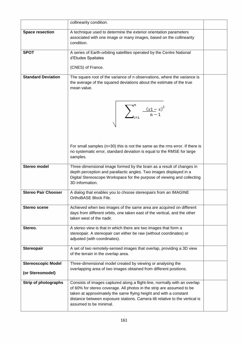
161

collinearity condition.

Space resection A technique used to determine the exterior orientation parameters

associated with one image or many images, based on the collinearity

condition.

SPOT A series of Earth-orbiting satellites operated by the Centre National

d‘Etudes Spatiales

(CNES) of France.

Standard Deviation The square root of the variance of n observations, where the variance is

the average of the squared deviations about the estimate of the true

mean value.

For small samples (n>30) this is not the same as the rms error. If there is

no systematic error, standard deviation is equal to the RMSE for large

samples.

Stereo model Three-dimensional image formed by the brain as a result of changes in

depth perception and parallactic angles. Two images displayed in a

Digital Stereoscope Workspace for the purpose of viewing and collecting

3D information.

Stereo Pair Chooser A dialog that enables you to choose stereopairs from an IMAGINE

OrthoBASE Block File.

Stereo scene Achieved when two images of the same area are acquired on different

days from different orbits, one taken east of the vertical, and the other

taken west of the nadir.

Stereo. A stereo view is that in which there are two images that form a

stereopair. A stereopair can either be raw (without coordinates) or

adjusted (with coordinates).

Stereopair A set of two remotely-sensed images that overlap, providing a 3D view

of the terrain in the overlap area.

Stereoscopic Model

(or Stereomodel)

Three-dimensional model created by viewing or analysing the

overlapping area of two images obtained from different positions.

Strip of photographs Consists of images captured along a flight-line, normally with an overlap

of 60% for stereo coverage. All photos in the strip are assumed to be

taken at approximately the same flying height and with a constant

distance between exposure stations. Camera tilt relative to the vertical is

assumed to be minimal.

162

Tangential lens

distortion

Distortion that occurs at right angles to the radial lines from the principal

point.

Terrestrial

photographs

Ground-based photographs and images taken with a camera stationed

on or near the Earth‘s surface. Photographs are usually used for

archeology, geomorphology, and civil engineering.

Texels. Texture pixels used to determine filtering and texturing. Screen pixels

per texture pixels.

Texture map A chunk of image data that can be warped and stretched in three

dimensions to fit a set of coordinates specified for the corners.

Theodolites. ―A surveyor‘s instrument for measuring horizontal and usually also

vertical angles‖ (Merriam-Webster OnLine Dictionary 2000).

Three-dimensional. See 3D.

Tie point A point whose ground coordinates are not known, but can be recognized

visually in the overlap or sidelap area between two images.

Tie points Points that appear on the overlap area of adjacent image. They are used

for orientation and aerotriangulationor block processing. The general are

not measured on the ground and only image coordinates are used.

TIN see Triangulated Irregular Network.

Tolerance The tolerance is the permissible degree of error in a geometrically

corrected image or mosaic as determined using a well distributed set of

check points. Tolerance is specified with one value: the maximum all

able RMS error of all check points.

Topocentric A coordinate system that has its origin at the centre of the image

projected on the Earth ellipsoid. The three perpendicular coordinate

axes are defined on a tangential plane at this centre point. The plane is

called the reference plane of the local datum. The x-axis is oriented

eastward, the y-axis northward, and the z-axis is vertical to the reference

plane (up).

Transparency Transparency is used in traditional photogrammetry techniques as a

method of collecting features. It is a clear cover placed over two images

which form a stereopair. Then, features are hand-drawn on the

transparency, and can then be transferred to digital format by scanning

or digitizing. A brand of transparency is Mylar®.

Triangulated Irregular

Network

(TIN) A TIN enables you to collect TIN points and create breaklines in

an image displayed in a stereo Viewer. A TIN is a type of DEM that,

unlike a raster grid-based model, allows you to place points at varying

intervals.

Triangulation. Establishes the geometry of the camera or sensor relative to objects on

the Earth‘s surface.

United States

Geological Survey

(USGS) An organization dealing with biology, geology, mapping, and

water. For more information, visit the web site www.usgs.gov.

USGS See United States Geological Survey.

163

Vector. A vector can be represented as a point, line, or polygon. A vector is a

one-dimensional matrix, having either one row (1 by j), or one column (i

by 1). Vectors typically represent objects such as road networks,

buildings, and geographic features such as contour lines.

Vertex A vertex is a component of a feature digitized in the Digital Stereoscope

Workspace. A vertex is made up of three axes: X, Y, and Z. The Z

component corresponds to the elevation of the vertex. A feature can be

composed of only one vertex (i.e., a point as in a TIN) or many vertices

(i.e., a polyline or polygon). You can adjust the X, Y, and Z components

of an existing vertex. See also Point, Polyline, and Polygon.

Vertical exaggeration The effect perceived when a DSM is created and viewed. Vertical

exaggeration is also referred to as relief exaggeration, and is the

evidence of height differences in a stereo model.

Vertices A polyline or polygon is composed of multiple vertices. These vertices,

like a single vertex, have X, Y, and Z components. You can adjust the X

and Y component of vertices of a polyline or polygon by using feature

editing tools such as Reshape. You can also add a vertex or vertices to

an existing feature. To edit the Z component, use the C key on the

keyboard. See also Vertex.

Warping Synonym for polynomial Rectification

Well-defined point A well-defined point represents a feature for which horizontal position is

known to high degree of accuracy and position in respect to the geodetic

datum. For the purpose of accuracy testing, well points must be easily

visible or recoverable on the ground, on the source of higher accuracy,

and on the product itself.

FGDC,

1998

Workspace An Digital Stereoscope Workspace is where you complete digital

mapping tasks. The Digital Stereoscope Workspace allows you to view

stereo imagery and collect 3D features from stereo imagery.

X-parallax The difference in position of a common ground point appearing on two

overlapping images, which is a function of elevation.

X-parallax is measured horizontally. Xparallax is required to measure

elevation, and cannot be completely removed from a stereopair.

Y-parallax The difference in position of a common ground point appearing on two

overlapping images, which is caused by differences in camera position

and rotation between two images.Y-parallax is measured vertically.

Z The vertical (height) component of a vertex, floating cursor, or feature.

165

SECTION-10

PROJECT MANAGEMENT & COST ESTIMATES

10-1. General

This section contains guidance for project engineers, project managers, or project engineering

technicians who are required to plan and develop cost estimates for negotiated qualification-based

Architect-

a. Section I provides guidance on the elements of project planning and estimating costs for all phases

of a photogrammetric mapping project.

b. Section II provides the elements of a general costing procedure.

c. Section III presents a sample scope of work and estimate for a typical project.

Section I

10-2. Photogrammetric Mapping Project Planning

a. In order to estimate photogrammetric mapping costs, it is necessary to visualize production

procedures that must be accomplished. The project manager should design a specific procedural

scheme before a Government cost estimate is formulated. With a logical project plan in mind, it is

possible to estimate man-hour and material needs and apply cost factors. Since labour rates,

equipment rental rates, overhead, and profit margins vary widely, it is necessary to estimate costs for

contract negotiations based on a specific production system.

b. Digital mapping projects require several basic operations:

(1) Aerial photography, which may or may not involve ABGPS, with appropriate film types.

(2) Field control surveys using conventional and/or GPS procedures.

(3) Aerotriangulation utilizing a workstation or an analytical stereoplotter.

(4) Collection and editing of digital planimetric and/or topographic data with an analytical

stereoplotter or a workstation.

(5) Orthophoto images generated with a workstation.

c. Some production items are rather straightforward to determine. For instance, once the relevant

photo scale is selected, it is relatively easy to calculate the number of photos, which is a determining

factor for a number of production parameters. Other costs may be rather difficult to determine and will

vary from one project site to another, depending on the ground conditions and product requirements

of the specific project. Many unit item timeframes can be estimated only with a fairly thorough

understanding of the equipment and production procedures, generally termed "experience."

Unfortunately, these difficult items usually form the bulk of the project costs. This is coupled with the

fact that most organizations cannot afford the time and money to train experienced photogrammetrists

to estimate mapping costs.

166

d. During the estimating process of a project, it is essential to include every item that could be

required. The estimator must include overhead expenses and, when working through a private

Vendor, a reasonable profit for the Vendor.

e. One of the principal objectives of planning is the assessment of risk that may be inherent in a

project. There are several types of risk: programmatic, technical, schedule, and cost. Risk should be

identified whenever possible, and the project plan should include actions to mitigate their possible

impact.

f. The relationship between the Depatmental project manager and the private Vendor should not be

adversarial. Rather, it must be a cooperative effort to produce a product of legitimate quality for a

reasonable price. Both the Depatmental representative and the private Vendor should cooperate

toward this end. Since digital mapping is a dynamic discipline, Depatmental cost estimators should

make a positive effort to visit the map production facilities of private Vendors in order to enhance

familiarity with state-of-the-art equipment and procedures. Private mapping Vendors are deservedly

proud to display their facilities and share their technical expertise, especially if it contributes to the

collective understanding of project requirements. It is recognized that the Depatmental project

manager and a private Vendor will not necessarily approach cost estimating from a singular

perspective. However, if both have a similar understanding of the specifications and a common

knowledge of production procedures, their independent cost estimates should provide a basis for

negotiating a reasonable fee that will provide a quality product.

g. Before specific cost estimating can be addressed, the project manager should study the

procedures to gain a technical knowledge with regard to issues of practical photogrammetric

production. The project manager and the Vendor may consider developing a production flow diagram

noting all major tasks and associated schedules.

10-3. Photo Scale, Contour Interval, and Target Map Scale Determination

Photo scale, contour interval (CI), and target mapping scale are integrally related and directly affect

the cost of a spatial data product.

a. Photo scale selection. Planimetric and topographic detailing are the two main factors that must be

considered in selecting a photo scale for digital mapping. Usually one or the other will govern the final

photo scale.

(1) Planimetric (cultural) features. On larger-scale mapping projects, a great deal of finite features

(poles,street signs, inlets, traffic signs, sidewalks, manholes, etc.) are drawn. As map scale gets

smaller, progressively more of this finite detail is omitted (by reason that it may not be visible and/or

identifiable on the photos or to reduce map clutter), and some features may be symbolized because

of minimum size limitations. This dictates that large-scale planimetric mapping requires large-scale

photos. In most cases, the enlargement factor from photo to map should not exceed the maximum

factors in Table 2-4 for determining maximum enlargement ratios for a specific map class. Tables in

SECTION 2 should be used as a guide for appropriate flight heights and photo negative scales

required to achieve specified map scales and accuracies.

(2) Topographic (terrain) features. Flight height determines the attainable accuracy of the vertical data

and also regulates photo scale. Tables in SECTION 2 should be used as a guide for appropriate flight

heights and photo negative scales for topographic feature detail required to achieve specified map

scales and accuracies.

10-4. Data Compatibility

167

There can be no doubt that the advent of digital databases has been a boon to mapping and

GIS/CADD applications; however, there are photogrammetric pitfalls. Perhaps the greatest hazard,

though seemingly an apparent strong suit, stems from the ability of a computer, driven by proper

software, to accept almost any block of X-Y-Z data and create a map to any scale or contour interval.

A primary advantage of automated information systems is not simply aggregating various themes to

draw a composite map. More important is the capability of the user to reach into the database, select

particular portions of information, and formulate reliable alternative solutions to given situations.

Automated information systems will generate hard copy maps, data tabulations, and reports.

a. Information from a multitude of diverse sources can be integrated into a single database, since

these systems are capable of comparing various blocks of dissimilar data and presenting the viewer

with a composite scenario based on given situation parameters. This allows the manager to

manipulate variable parameters to compare multiple solutions with limited expenditure of time.

b. Collected data for various themes are placed on specific data layers for convenience in accessing

the database. For this reason, individual layers must be georeferenced to a common ground

reference (State Plane, Universal Transverse Mercator, Latitude/Longitude) so that data from various

layers geographically match one another when composited. Digital data for many layers will have

been collected from various existing map and aerial photo sources. This implies that not all data is

compatible.

c. All features go into a database as a group of individual spatial coordinate points that are relational

to each other through a common geographic positioning grid. However, not all information is collected

to the same degree of accuracy! A map is as reliable only as its most inaccurate information layer.

Serious thought must be given to the compatibility of information that resides in an integrated

database.

d. As was stated previously, there are two accuracy factors to be considered, each as an autonomous

parameter. These factors are Horizontal scale and Topographic relief. A word to the wise. Do not ―mix

& match‖ data just because they are readily available and/or economical. All data layers must mesh

into the overall accuracy of the final product. Metadata must be developed for all data and be fully

compliant standards.

10-5. Project Design

Prior to cost estimating a mapping project, there must be a concept, mental or written, as to what is

required to complete that project. Writing the general job specifications and outlining the project

design can be helpful. The following factors must be considered in performing this effort.

a. Parameters.

(1) Project site. It is usually best to outline the site on a suitable map of the site.

(2) Contour interval. This must be upon the function for which mapping is intended. A general

consideration is that smaller contour intervals are for design purposes, while larger intervals are for

planning studies.

(3) Mapping scale. This is also dependent upon the user's functional requirements. It must be kept in

mind that after the information resides in the database, a map can be generated to any scale.

b. Aerial photography.

168

(1) Photo flight parameters. Determine photo scale, film type, flight altitude, number of flight lines, and

number of photographs based on the guidance in section 2 and other sections in this manual. It is

good practice, once these items are calculated, to make a preliminary photo mission flight map.

(2) Special considerations. Make some assumptions as to whether there may be any special

considerations to this flight. Is the project in an area where overflights will be restricted to specific time

slots? Are there any chronic adverse atmospheric (lingering haze, consistent cloud cover) or ground

(snow, vegetation) conditions that will interfere with or prolong the flight?

c. Field surveys.

(1) Travel time. Determine how far it is from surveyor's office to project site. This will influence labour

travel costs and per day expectations.

(2) Control reference. Collect information regarding nearest existing benchmarks and triangulation

stations that must be used as geographic reference ties. Ground control references to distant

established control is labour intensive and costly.

(3) Photo control density. Determine the pattern of horizontal and vertical field control points that will

be needed. If a project requires preflight ground targets, it is helpful to arrange the layout on a map.

Ground control point selection should be done with some thought toward amenable survey routing.

Final ground control plan should be planned and agreed upon with the mapping contractor prior to

implementation.

d. Aerotriangulation.

(1) Aerotriangulation is the control extension link between a limited amount of strategic field survey

points and the stringent pattern of photo passpoints that control the photos for mapping.

(2) Control extension can be accomplished with a a softcopy workstation which is a self contained

operation. Film or diapositive is scanned and loaded into the softcopy system.

(3) The photos to be used in mapping are to be employed in the control extension.

e. Digital mapping.

(1) Map detail density. The departmental officials must have perception of the density of cultural

features and terrain character of the site. This is normally a great variable between sites and often

even within a site. It is probably the biggest labour-intensive item in the whole project. It takes a much

longer time to digitize all of the congested cultural detail in an urban area than the few features in a

rural setting. It also takes a longer time to digitize DEM data in rough, steep hills than in a flat river

valley.

(2) Data edit. Once the data digitizing is complete, its editing must be performed.

(3) Data translation. After data is compiled and edited, it must be translated into whatever format is

compatible with the user's CADD system.

(4) Data plot. A line plot of the digital data should be generated to ensure that the data is complete

and valid.

f. Orthophoto images.

(1) GIS projects increasingly demand orthogonal pictorial images to merge as a background for other

data layers.

169

(2) Orthophotos are as accurate as line maps except in areas of sudden vertical change. It may be

necessary in these areas to patch images from other photos.

(3) Relevant DEM data is required to generate an orthophoto image.

(4) Scan resolution must be as finite as is required to maintain pixel integrity at the image enlarged

image scale.

g. Miscellaneous. Determine what other auxiliary items may be specifically required to complete this

project.

(1) Does the project require any accessory photo reproduction items (contact prints, indexes,

enlargements, mosaics)?

(2) Are there any supplementary field surveys required?

(3) Are there any supplementary digital mapping items required?

(4) What hidden utility data text attributes will the mapper be required to integrate into the mapping

database?

10-6. Photogrammetric Mapping Production Flow

In order to bring the various photogrammetric mapping procedures together in a logical sequence,

Figure 4-9, parts a and b, depict a typical photogrammetric mapping and orthophoto production flow,

respectively. Orthophoto production flow is generally a part of a photogrammetric mapping project and

utilizes much of the same information collected for photogrammetric mapping to include aerial

photography, ground control, aerotriangulation, and digital terrain model development. However,

when only orthophotos are required for a project the amount of digital elevation model collection can

be reduced as well as vertical ground control. The end user should be warned that a digital elevation

model developed ONLY for orthophoto production will not be suitable for contour generation. This

SECTION presents the project elements that must be addressed when planning, specifying, and

estimating costs for a digital mapping project.

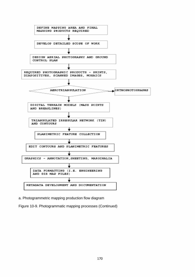
170

a. Photogrammetric mapping production flow diagram

Figure 10-9. Photogrammatic mapping processes (Continued)

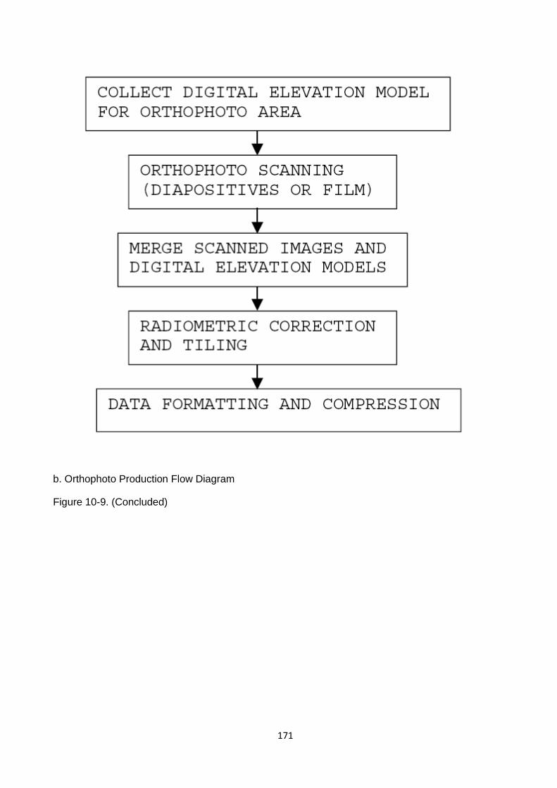
171

b. Orthophoto Production Flow Diagram

Figure 10-9. (Concluded)

172

Section II

10-7. Approach to Estimating Detailed Photogrammetric Mapping Project Costs

Detailed independent Government cost estimates are required for contract negotiation purposes and

must specifically account for all significant cost phases of a digital mapping operation. This is

necessary since these estimates (both the Government's and the Contractor's) may be subject to

subsequent field audits and/or other scrutiny. Also, contract modifications must relate to the original

estimate. Initially, it is important to specify which of the activities involved in making a map will be

completed by the Contractor and which may be done by the Government.

a. General estimating procedure. The cost estimating procedures presented here can be used to

estimate all or only certain parts of a mapping project. This approach allows each user to develop a

cost estimating method that incorporates information needed in a specific locale.

(1) Those using the following procedures should indicate which of these activities need to be

estimated. As stated earlier, those steps in a cost estimating procedure for mapping include aerial

photography, photo control surveying, aerotriangulation, map production, and orthophoto images. For

each of these activities, the cost estimates have been further stratified into production elements.

(2) Paragraphs 4-10 through 4-15 present the cost estimating procedure in its entirety. The procedure

provides the individual production elements which can be summed with overhead and profit to arrive

at estimated budgetary cost for a specific project.

b. Labour. One of the most significant production factors in a mapping project relates directly to hours

expended by highly qualified technicians. Amount of work that personnel will conduct is characterized

as Direct Labour. It is convenient to express work in hours because it provides a per unit cost basis

for estimating purposes.

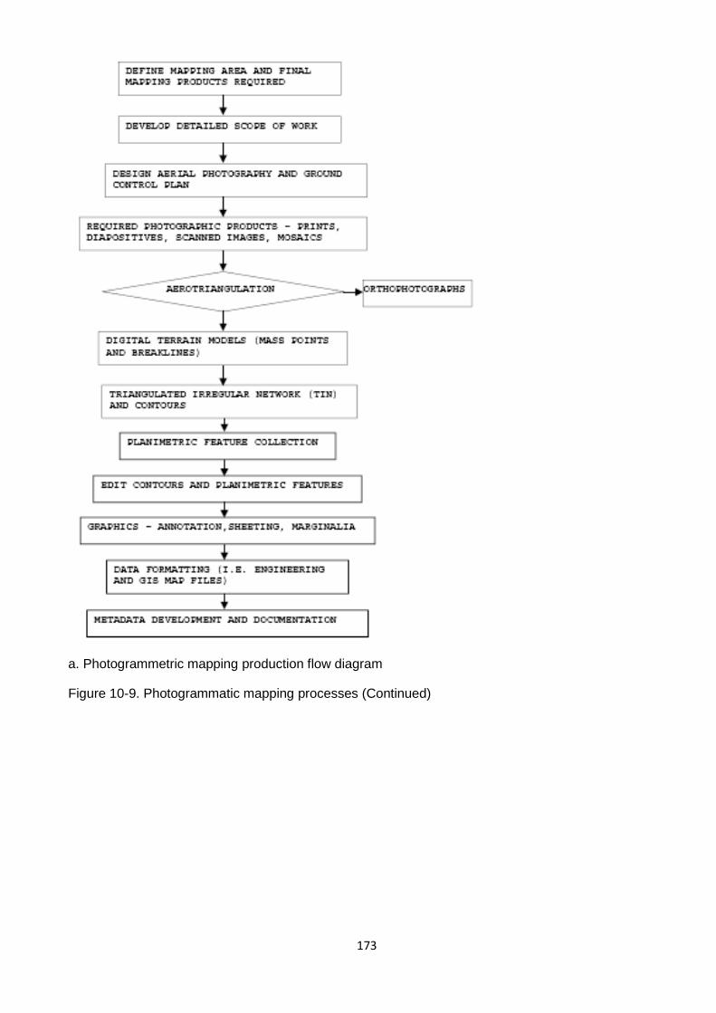
173

a. Photogrammetric mapping production flow diagram

Figure 10-9. Photogrammatic mapping processes (Continued)

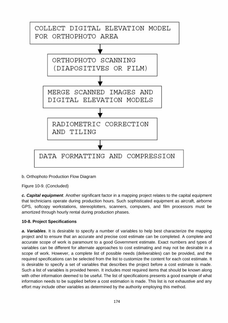
174

b. Orthophoto Production Flow Diagram

Figure 10-9. (Concluded)

c. Capital equipment. Another significant factor in a mapping project relates to the capital equipment

that technicians operate during production hours. Such sophisticated equipment as aircraft, airborne

GPS, softcopy workstations, stereoplotters, scanners, computers, and film processors must be

amortized through hourly rental during production phases.

10-8. Project Specifications

a. Variables. It is desirable to specify a number of variables to help best characterize the mapping

project and to ensure that an accurate and precise cost estimate can be completed. A complete and

accurate scope of work is paramount to a good Government estimate. Exact numbers and types of

variables can be different for alternate approaches to cost estimating and may not be desirable in a

scope of work. However, a complete list of possible needs (deliverables) can be provided, and the

required specifications can be selected from the list to customize the content for each cost estimate. It

is desirable to specify a set of variables that describes the project before a cost estimate is made.

Such a list of variables is provided herein. It includes most required items that should be known along

with other information deemed to be useful. The list of specifications presents a good example of what

information needs to be supplied before a cost estimation is made. This list is not exhaustive and any

effort may include other variables as determined by the authority employing this method.

175

b. Labour. Cost per hour of personnel can be obtained from regional wage rates or from negotiated

information supplied by the Contractor. These can be applied to the estimated production hours to

arrive at a project cost.

10-9. Contract Parameters

It is necessary to have information for the following items to best specify a project. Many of the items

listed below are inputs to the cost estimating procedure and are used in calculations of parameters.

a. Area to be mapped. It is desirable to provide a firm definition of the area to be mapped. This may

be delineated on large-scale topographic maps. Other descriptive and measurement information

should be provided if available. Information may include details from surveys, deeds, or whatever

other documents are available. Descriptions may also include gross north/south and east/west

dimensions of project.

b. Parameters. Other mapping parameters should include the following:

(1) Final map scale consistent with data usage.

(2) Contour interval consistent with data usage.

(3) Photo scale based on enlargement factor and C-Factor.

(4) Flight height above mean ground level calculated from photo scale.

(5) Film type pertinent to data usage.

(6) Calibrated focal length of camera.

(7) Assumed C-Factor.

(8) Enlargement factor.

(9) Nominal endlap, usually 60 percent but may differ for special usage.

(10) Nominal sidelap, usually 30 percent but may differ for special usage.

(11) Distance from aircraft base to project site measured on atlas.

(12) Number of flight lines based on calculations from project short dimension.

(13) Number of photos per flight line based on calculations from project long dimension.

(14) Distance from site to nearest established horizontal control reference measured from map.

(15) Distance from site to nearest established vertical control reference measured from map.

(16) Cruising speed of aircraft from equipment specifications.

(17) Terrain slope variability estimated from a map.

(18) Cultural development variability estimated from a map.

c. Deliverables. A list of delivery items should be supplied. This is necessary to clearly define the end

products, which should ensure an accurate estimate of cost. The list below consists of a number of

possible products that may be requested. Products should be specified in the contract. Also, the

number of copies or sets to be furnished must be stated.

176

(1) Contact prints.

(2) Hardcopy map sheets.

(3) Digital data in CADD or GIS/LIS format (planimetric features, DEM, DTM, TIN, Contours).

(4) Photo enlargements.

(5) Photo index.

(6) Photo mosaics.

(7) Field surveys.

(8) Orthophotos.

(9) Aerotriangulation report.

(10) Field survey report.

(11) Aerial camera current Calibration Report.

10-11. Photo Control Surveying Cost Items

Offsite information. The following items are to be specified to assist in the calculations of costs

associated with photo control surveying.

a. Distance from survey office to site.

b. Distance to horizontal reference.

c. Distance to vertical reference.

d. Time to complete horizontal photo control or number of points required.

e. Time to complete vertical photo control or number of points required.

No production estimating procedure is presented for ground surveys. This is best left to District survey

branches once they are apprized of the number and location of required ground targets.

10-13. Photogrammetric Compilation and Digital Mapping Cost Items

Site specific information. The following items are to be calculated, estimated, or measured to assist

in the computing costs associated with digital mapping.

a. Number of stereomodels to orient.

b. Number of acres and or stereomodels to map.

c. Complexity of terrain character.

d. Complexity of planimetric culture.

e. Format translations of digital data.

Digital data capture:

177

Planimetry (cultural features) - The project planning map used to outline the mapping area should

be overlain with a proposed flight line layout. The flight line layout should note the approximate

location of each photo stereopair. The planimetric feature detail in each of the models should be

assessed based on the amount of planimetric detail to be captured (full or partial stereomodel and the

final map scale) and the density of planimetry to be captured in each stereomodel. As an example:

Highly urban area stereomodels require more time to compile than rural area stereomodels.

Topography - The project planning map used to outline the mapping area should be overlain with a

proposed flight line layout. The flight line layout should note the approximate location of each photo

stereopair. The topographic feature detail in each of the models should be assessed based on the

amount of planimetric detail to be captured (full or partial stereomodel and the final map scale).

Topographic detail must consider the character of the land to be depicted. As an example: 1-mt

contour development in a relatively flat terrain requires much less time than collection of 1-mt

contours in very mountainous terrain.

10-14. Orthophoto Images

PRODUCTION HOURS FOR ORTHOPHOTOS

Current technology allows for total softcopy generation of orthophotos. If a Contractor has collected

the digital terrain model with an analytical stereoplotter and created diapositives then a clean set of

diapositives must be made and scanned for orthophoto generation. However, if the Contractor uses

softcopy stereo compilation for the elevation model collection then the same scanned images may be

used to generate the orthophotos. The Government must assume one method or the other in

developing a cost estimate. The difference in cost should be negligible.

10-15. Summary of Production Hours

A summary of the production hours itemized above is shown in the following list. Current Unit Costs

should be established for each task to be used in a project. The Unit Costs should include necessary

equipment as well as labour. These rates may be most accurately estimated by reviewing similar

current Government Contracts. Note that in addition to the total labour hours an appropriate overhead

should be established and applied to the total cost of labour. Also, an appropriate profit should be

established and applied to the total of labour and direct costs. Ground survey requirements

established by Government survey staff should be added to the total costs.

Table of Contents - Survey of India

Documents

Transcript of Table of Contents - Survey of India