
T34210.pdf - UNIVERSIDAD COMPLUTENSE DE MADRID
298
UNIVERSIDAD COMPLUTENSE DE MADRID FACULTAD DE CIENCIAS QUÍMICAS Departamento de Química Física I TESIS DOCTORAL Simulación del equilibrio de fases del agua: cristales plásticos, constantes dieléctricas y disoluciones MEMORIA PARA OPTAR AL GRADO DE DOCTOR PRESENTADA POR Juan Luis Aragonés Gómez Director Carlos Vega de las Heras Madrid, 2013 © Juan Luis Aragonés Gómez, 2012
-
Upload
khangminh22 -
Category
Documents
-
view
0 -
download
0
Transcript of T34210.pdf - UNIVERSIDAD COMPLUTENSE DE MADRID

UNIVERSIDAD COMPLUTENSE DE MADRID
FACULTAD DE CIENCIAS QUÍMICAS
Departamento de Química Física I
TESIS DOCTORAL
Simulación del equilibrio de fases del agua: cristales plásticos, constantes dieléctricas y disoluciones
MEMORIA PARA OPTAR AL GRADO DE DOCTOR
PRESENTADA POR
Juan Luis Aragonés Gómez
Director
Carlos Vega de las Heras
Madrid, 2013
© Juan Luis Aragonés Gómez, 2012

En esta memoria se presentan varios estudios de simulación por ordenador sobre las propiedades del agua. En particular, se ha investigado el comportamiento de diferentes fases en condi-ciones extremas: a 0K, a altas presiones y en presencia de un campo eléctrico. Finalmente, y puesto que se trata de una de las disoluciones más comunes en la tierra, se ha estudiado la solubi-lidad del cloruro sódico en agua, así como el punto de fusión de varios haluros alcalinos.
Simulación del equilibrio de fases del agua:cristales plásticos, constantes dieléctricas y disoluciones.
Juan Luis Aragonés Gómez
Simula
ción d
el eq
uilibr
io de
fase
s del
agua
: cris
tales
plás
ticos
, con
stante
s diel
éctri
cas y
dis
olucio
nes.
Juan
Luis
Arag
onés
Góm
ez
Madrid, 2012
“El éxito es aprender a ir de fracaso en fracaso sin desesperarse“
Winston Churchill

Universidad Complutense de MadridFacultad de Ciencias Químicas
Dpto. Química-Física I
Simulación del equilibrio de fases delagua:
cristales plásticos, constantesdieléctricas y disoluciones.
Memoria para optar al grado deDoctor en Ciencias Químicas
por
Juan Luis Aragonés Gómez
Director: Prof. Carlos Vega de las Heras
Madrid, 2012


A mi padre.
Muchas son las personas que me ha enseñado,pero es mi padre quién me ha dado la lección
más importate de todas: No rendirse nunca.


Agradecimientos
Esta página, la más difícil de escribir de toda la tesis, marca el final de un viaje alucinan-te que empezó cuando cursaba cuarto curso de la licenciatura. Recuerdo que los Miércolesa última hora teníamos clase de Química-Física avanzada, impartida por el profesor CarlosVega. Una de esas tardes, al finalizar la clase, me acerque a Carlos con una de mis infinitasdudas. Una vez resuelta, surgió otra, y luego otra. Carlos fue resolviendo una duda tras otra y,llevándome a la siguiente. En todos los ejemplos que utilizaba aparecía el agua, unas vecescomo molécula aislada, otras en “un vaso de agua". En algún momento de la conversaciónme dijo que fuésemos a su despacho, que me enseñaría una película en la que se podía vercomo cristalizaba el agua en contacto con un bloque de hielo. Sin saber muy bien de queiba todo esto, ahogado en curiosidad, le seguí hasta su despacho. Una vez allí, se colocóa los mandos de su ordenador y no paró de hablar sobre el agua y la “sociología de susmoléculas". Lo que más me impresiono, más incluso que todas esas moléculas moviéndosefrenéticamente sobre un fondo azul, fue la pasión con la que Carlos hablaba de todo esto.Así fue como Carlos me hizo morder el gusanillo de la ciencia. Hoy, mucho tiempo despuésde aquel Miércoles, sigo caminado detrás de Carlos exactamente igual que entonces: llenode curiosidad, hipnotizado por su pasión y divirtiéndome a cada paso. Además de habermeenseñado un oficio, me has enseñado a apasionarme por la ciencia. Por esto, tus consejos,tu apoyo y tu dedicación, muchas gracias. Espero poder corresponderte algún día.
El siguiente en la larga lista de personas que me han ayudado durante estos años esJosé Luis. Contigo también he disfrutado de la ciencia, e igual que Carlos, me has mostradotu pasión y dedicación. Nunca podré olvidar todos esos días en los que, a últimisima hora,discutíamos sobre alguna fascinante propiedad del agua frente a la pantalla de tu ordenador,que recordaba insistentemente que era hora de irse a casa. Son momentos como estos losque vienen a mi cabeza cuando todo se vuelve demasiado frustrante. Gracias por enseñar-me al jl científico y la excepcional persona que hay detrás. Otra persona fundamental parael desarrollo de esta tesis ha sido Luis. Tanto profesional como personalmente he podidodisfrutar de su compañía; brillante científico, mejor persona. Igual que Eva, que me aguantodurante los primeros años de tesis y con la que he compartido despacho, trabajo y grandesmomentos. Dejaste un gran vacío y se te ha echado mucho de menos. Agradecer también ami compañera Maria su apoyo incondicional, siempre dispuesta a echar una mano y mejorarla presentación de todos los trabajos. Todo mi agradecimiento para Carl, sin él los días detrabajo habrían sido mucho más duros. He descubierto un compañero inmejorable, del quehe aprendido valiosas lecciones.
Más recientemente se han sumado a la lista de agradecimientos Mac, Eduardo y Chan-tal. Gracias a Mac, que además de resolver mis dudas sobre Gromacs, me ha hecho pasarbuenos ratos y olvidar el trabajo en momentos de desesperación. La llegada de Eduardo yChantal ha hecho que este último año haya sido muy estimulante, tanto personal como cien-tíficamente. He podido conocer a dos personas geniales, con las que he tenido el placer decompartir algo más que trabajo. Agradecer en especial a Chantal toda su dedicación desin-teresada. He perdido la cuenta de las cervezas que te debo por todas las veces que me hasayudado y aconsejado, muchas gracias.
Gracias a todos los amigos que me habéis apoyado en los buenos y malos momentos. Es-pecialmente a los que lleváis acompañándome tantos años, ya lo sabéis, soy un incondicional

vuestro! Muchas gracias: Desio, Pol, Vence, Fer, Chencho, Putto, Lex, Txele, Ruben, Ñañe,Chule y muchos más, que espero disculpen el límite de espacio. Gracias a Emilio, todo hasido mucho más fácil gracias a ti. Gracias por alejarme de la realidad con tu: “Un PES.....?";el día mejoraba cuando oía esta semi-pregunta. Tu apoyo como amigo empequeñece toda laayuda que me has prestado con el trabajo, aguantando todas mis charlas y corrigiendo todosmis escritos. Creo que no vale con un muchas gracias, tendré que salvarte la vida en un parde ocasiones para compensar.
Entra aquí una nueva incorporación a mis páginas de agradecimiento. Gracias Lauri, poraguantarme a mi, mis ensayos y mis drafts, pero más importante, por darme ilusión y motiva-ción.
Para finalizar, y por eso más importante, todo mi agradecimiento a mi familia. Cuandopienso en la suerte que tengo de haber caído en esta familia me emociono. Son muchasvuestras virtudes, pero por lo que realmente os quiero es por vuestros “defectos", esperoque disculpéis los mios. Que estas lineas sirvan de disculpa/agradecimiento, porque soisvosotros los que más habéis sufrido este doctorado. Perdonar mis ausencias, tanto físicascomo mentales. Sois todos geniales. Abuelos, abuelas, tíos, tías, primos, primas....no puedonombrarlos a todos. Mi agradecimiento a mis primos, Juanan y Alberto, por su apoyo a todala familia cuando yo no pude estar.
Gracias a mi Madre, que con su ejemplo me ha enseñado a enfrentarme a la vida. Siem-pre he sabido que eres una madre excepcional, pero cuando he tenido conciencia del mundoy su asqueroso funcionamiento, he comprobado que además eres una persona excepcional,la mejor persona que conozco. Admiro tus ganas y forma de afrontar las adversidades, tueres la que nos mantiene en perpetuo movimiento. Gracias a mi Padre, al que dedico estatesis y echo de menos cada día. Todas las mañanas de estos últimos años atendistes misdudas, divagaciones e ilusiones, siempre me diste tu opinión y consejo, y lo hiciste sin deciruna sola palabra, gracias. Él, junto con mi madre, son mis referentes. Sólo aspiro a ser lamitad de bueno que ellos. Gracias también a mis dos hermanos, Nacho y Jesús, porque sinellos nada sería posible. Sois vosotros en los que me miro y busco consejo.
II

Resumen
El agua es una sustancia fascinante. En nuestro planeta es una de las moléculas másabundantes, y se presenta en varias de sus formas. La gran mayoría de las propiedadesdel agua suponen un comportamiento anómalo respecto al comportamiento general de otrassustancias formadas por moléculas de tamaño y características similares. La simulación porordenador es una herramienta tremendamente útil para comprender el comportamiento ma-croscópico de las sustancias a partir de parámetros moleculares. En esta tesis se han es-tudiado algunas de las propiedades del agua mediante simulación. Para ello es necesariodefinir los parámetros moleculares de la molécula de agua, y existen una gran variedad demodelos de potencial de agua. Cada uno de ellos presenta ventajas e inconvenientes. Si-guiendo los pasos de Whalley, propusimos un test para evaluar la calidad de los modelos deagua con unos rápidos y sencillos cálculos, el test de Whalley.
El agua en forma líquida interviene en una gran cantidad de procesos biológicos, geoló-gicos y atmosféricos. Lo que la convierte en la matriz de la vida. En fase sólida presenta unode los diagramas de fases más complejos, con al menos 16 estructuras cristalinas diferentes.En esta tesis se aborda el estudio de la región de altas presiones del diagrama de fases delagua. Durante este estudio se encontraron dos fases de cristal plástico a altas presiones, nodescritas hasta la fecha. Llevar a cabo medidas experimentales en esta región del diagramade fases es tremendamente complicado, por lo que existe cierto desacuerdo entre las medi-das de distintos grupos. Creemos que estas discrepancias pueden ser debidas a la existenciade una fase de cristal plástico.
También se ha llevado a cabo el estudio de las constantes dieléctricas de los hielos, ysobre el efecto que tiene la aplicación de un campo eléctrico sobre el diagrama de fases delagua. Para ello ha sido necesario incluir movimientos de rotación de anillos para muestrearcorrectamente el desorden de protón. Gracias a la correción de los resultados de simulacióncon el momento dipolar efectivo de la molécula de agua, para tener en cuenta la diferencia enla polarización de la molécula en función del entorno químico, se han realizado prediccionescuantitativas del efecto de un campo electrico sobre las transiciones de fase del agua.
Finalmente, y ya que la alta constante dieléctrica del agua la convierte en el disolventeuniversal, hemos estudiado la solubilidad del NaCl en agua. Los cálculos de solubilidad invo-lucran el cálculo del potencial químico del soluto sólido. De manera que para que un modelode potencial de NaCl sea capaz de reproducir la solubilidad en agua, debe ser capaz de pre-decir correctamente las propiedades de la sal pura. Por esta razón, también se han estudiadolas propiedades de coexistencia sólido–líquido para varios modelos de potencial de NaCl yotros haluros alcalinos monovalentes.
Palabras Claves: simulación, agua, hielo, constantes dieléctricas, campos eléctricos y disoluciones.


Índice general
1. Introducción 1
I TEORÍA Y SIMULACIÓN 19
2. Termodinámica estadística 21
3. Campos eléctricos: polarización y constante dieléctrica. 27
4. Simulación molecular 354.1. Condiciones de contorno periódicas . . . . . . . . . . . . . . . . . . . . . . . . 354.2. Potencial Lennard-Jones . . . . . . . . . . . . . . . . . . . . . . . . . . . . . . 364.3. Truncamiento del potencial . . . . . . . . . . . . . . . . . . . . . . . . . . . . . 374.4. Correcciones de largo alcance . . . . . . . . . . . . . . . . . . . . . . . . . . . 374.5. Sumas de Ewald . . . . . . . . . . . . . . . . . . . . . . . . . . . . . . . . . . 384.6. Método de Monte Carlo . . . . . . . . . . . . . . . . . . . . . . . . . . . . . . . 414.7. Dinámica Molecular . . . . . . . . . . . . . . . . . . . . . . . . . . . . . . . . . 444.8. Modelos de potencial de agua . . . . . . . . . . . . . . . . . . . . . . . . . . . 45
5. Metodología 495.1. Cálculos de energía libre . . . . . . . . . . . . . . . . . . . . . . . . . . . . . . 50
5.1.1. Integración termodinámica . . . . . . . . . . . . . . . . . . . . . . . . . 505.1.2. Integración termodinámica hamiltoniana . . . . . . . . . . . . . . . . . . 525.1.3. Energía libre de líquidos . . . . . . . . . . . . . . . . . . . . . . . . . . 535.1.4. Energía libre de sólidos . . . . . . . . . . . . . . . . . . . . . . . . . . . 545.1.5. Potencial químico de solutos . . . . . . . . . . . . . . . . . . . . . . . . 66
5.2. Simulaciones Gibbs-Duhem . . . . . . . . . . . . . . . . . . . . . . . . . . . . 685.2.1. Integración Gibbs-Duhem no hamiltoniana . . . . . . . . . . . . . . . . . 695.2.2. Integración Gibbs-Duhem hamiltoniana . . . . . . . . . . . . . . . . . . 69
5.3. Coexistencia directa . . . . . . . . . . . . . . . . . . . . . . . . . . . . . . . . . 715.4. Gibbs Ensemble . . . . . . . . . . . . . . . . . . . . . . . . . . . . . . . . . . . 735.5. Movimientos de rotación de anillos . . . . . . . . . . . . . . . . . . . . . . . . . 77
II RESULTADOS 81
6. Properties of ices at 0 K : a test of water modelsJournal of Chemical Physics, 127, 14518 (2007) 83
7. The phase diagram of water at high pressures as obtained by computer simula-tions of the TIP4P/2005 model: the appearance of a plastic crystal phasePhyscal Chemistry Chemical Physics, 11, 543-555 (2009) 99
8. Plastic crystal phases of simple water modelsJournal of Chemical Physics, 130, 244504 (2009) 119

Índice general
9. The dielectric constant of ices and water: a lesson about wa ter interactionsJournal of Physical Chemistry A, 115, 5745-5758 (2011) 143
10.The phase diagram of water under an applied electric fieldPhysical Review Letters, 107, 155702 (2011) 167
11.Solubility of NaCl in water by molecular simulation revisitedJournal of Chemical Physics, Aceptado, (2012) 173
12.Calculation of the melting point of alkali halides by means of computer simula-tionsJournal of Chemical Physics, Enviado, (2012) 203
III DISCUSIÓN DE RESULTADOS 219
13.Discusión integradora 221
14.Conclusiones 231
IV APÉNDICES 235
A. Colectivo microcanónico (N,V,E) 237
B. Colectivo canónico (NVT) 239
C. Teorema de divergencia 241
D. Transformación de la ecuación 3.5 243
E. Propiedades de la función Gaussiana 245
F. Cambio de variable en la integral de la ec. (4.5) 247
G. Función error 249
H. Vectores de espacio recíproco 251
I. Demostración del teorema 4.7 253
J. Función de partición del cristal de Einstein con el centro de masas fijo 255
K. Contribucion ideal al potencial quimico 259
VI

CAPÍTULO 1
Introducción
“The full area of ignorance is not mapped.We are at present only exploring the fringes."
John D. Bernal
El objetivo principal de esta tesis ha sido avanzar en el conocimiento de las propiedadesdel agua. Para ello hemos estudiado el equilibrio de fases del agua mediante simulación porordenador.
Los elementos más abundantes en el universo son hidrógeno, helio, oxígeno y carbono,en ese orden. Y el helio es un elemento inerte, así que desde el punto de vista de la compo-sición química, el agua no es nada especial. Pero siguiendo este mismo argumento, tampocolo sería la vida basada en el carbono (tal y como la concebimos), el elemento químicamen-te más versátil y cuarto más abundante. Pero lo cierto es que lo son, tanto la vida como elagua son algo especial. Tendemos a pensar que las cosas son especiales o únicas cuandono comprendemos su funcionamiento o comportamiento. ¿Es el agua una sustancia especialdebido a nuestra ignorancia o realmente tiene algo que la hace especial? Aunque en unaprimera impresión el agua no nos parezca algo muy llamativo; aparece en todos los lugares,en todo momento y en varias formas. Lo cierto es que es la sustancia mas increíble con quenos podemos encontrar. Y por suerte para nosotros, la encontramos en todos lados. Precisa-mente estos tres factores, su abundancia, recurrencia y nuestra falta de conocimiento, hacenque el agua este rodeada de un aura de misticismo. Transciende de lo químico o lo físico,se ha convertido en un símbolo de vida, pureza, fuerza, adaptación, maternal, desastre na-tural, etc... Muchas son las investigaciones que se han llevado a cabo sobre como el aguainterviene en procesos biológicos: plegamiento y estabilidad de proteínas [1, 2], interaccionesenzima-substrato [3], solvatación de iones, ciencia espacial [4] y un largo etcétera. Este papelfundamental en procesos biológicos es lo que nos ha llevado a tener una visión mística deesta molécula. Se la llama molécula de la vida, matriz de la vida [5, 6]... Pero entra en juegoen muchos más procesos. El agua hace posible la gran mayoría de procesos de transferenciade energía en nuestro planeta. Controla el tiempo en nuestro esférico hogar, moviliza enor-mes cantidades de energía gracias a las corrientes oceánicas. De esto he podido ser testigodurante mi estancia en la Universidad de Minnesota, en Minneapolis, donde los tornadosoriginados en el “Tornado Alley´´ (callejón de los tornados) eran semanales. También es elsoporte de transferencia de energía en sistema hidrodinámicos, y en química es el disolventeuniversal. Tiene un papel fundamental en infinidad de procesos geológicos y atmosféricos.A lo largo de este estudio vamos intentar restar algo del simbolismo que rodea al agua dela única forma posible, conociendo como es y como se comporta. En general, la descripcióncientífica de mitos y leyendas es decepcionante, pero como veremos, esto no ocurre con elagua, conocerla es todavía mas fascinante que cualquier mitificación posible.
Los intentos por conocer y entender el agua se remontan a los inicios de la ciencia, cuan-do el agua todavía era uno de los cuatro elementos –tierra, aire, fuego y agua–. Y han sidomuchas las teorías falsadas, en términos del filósofo de la ciencia Karl Popper [7]. Y es que

1. Introducción
según él mismo, esta es la única forma objetiva que tiene el conocimiento epistémico deavanzar, esquivando la subjetividad humana. Pero fueron Bernal y Fowler, cuya formaciónera en sólidos, los que hicieron la primera aproximación a la estructura del agua líquida co-mo la entendemos hoy día, con su magistral trabajo del 1933: A theory of water and IonicSolutions, with Particular Reference to Hydrogen and Hydroxyl Ions [8]. Se apartaron de lasideas de la época para las que el agua estaba formada por varias clases diferentes y dis-tintivas de agua. Adoptaron un modelo uniformista, centrándose en la estructura media delagua líquida. Basándose en resultados de difracción de rayos X, y tomando como punto departida el hielo, mostraron una imagen de la estructura del agua completamente diferente alas propuestas hasta el momento. El hielo Ih está formado por moléculas de agua en unadisposición tetraédrica formando enlaces de hidrógeno con sus cuatro moléculas vecinas, loque genera una estructura muy abierta. Bernal y Fowler propusieron que, de forma análogaal hielo Ih, el agua está formada por una red tetraédrica de moléculas de agua, pero en estecaso los tetraedros se van distorsionando al aumentar la temperatura (alejarse del hielo Ih),de manera que la estructura deja de ser tan abierta y la densidad aumenta. Esta distorsióndebilita los enlaces de hidrógeno, pero la estructura del agua de Bernal y Fowler no se basa-ba en la ruptura de los enlaces sino en la distorsión progresiva de los tetraedros al alejarnosdel hielo. Sin embargo, el modelo de Bernal y Fowler no es capaz de tener en cuenta todaslas medidas experimentales. Esto es debido a que se intenta dar una imagen estática de algoque está en continuo cambio. Si observásemos durante un tiempo, o tuviésemos varias ins-tantáneas, podríamos hacernos una idea de como es el proceso. Esto nos permite hacerlola simulación por ordenador. La imagen que se obtiene mediante simulación de la estructuradel agua líquida es: una red continua, irregular y dinámica de enlaces de hidrógeno, en lacual cada molécula enlaza a otras cuatro mediante enlaces de hidrógeno (raras veces a treso cinco), pero lo hace formando tetraedros distorsionados. Debido a esto, la red de enlacesde hidrógenos es mas débil e irregular, y las moléculas ocupan parcialmente los huecos quequedaban libres en la estructura del hielo Ih aumentando la densidad. Similar a la estructurade Bernal, pero con la novedad de una red de enlaces de hidrógeno dinámica, en continuocambio. La idea fundamental, y huella dactilar de la estructura del agua líquida, es que cadamolécula de agua forma un tetraedro más o menos distorsionado con las cuatro moléculasvecinas mediante enlaces de hidrógeno, en promedio.
La simulación por ordenador nace en Los Alamos durante el proyecto Manhattam. Peroes después del lanzamiento de la bomba atómica, en 1949, cuando se construye el primerordenador electrónico digital (MANIAC). De esta manera se abría un amplio abanico de posi-bilidades de investigación científica hasta ese momento inalcanzables. Metropolis desarrolló,junto a Teller, John von Neumann, Stanislaw Ulam, y Robert Richtmyer, los llamados métodosde Monte Carlo, basados en el muestreo de importancia, y conocidos como algoritmos de Me-tropolis [9]. A partir de este momento, y a través de los años, la simulación se ha convertidoen una herramienta fundamental en el estudio del comportamiento de sistemas molecula-res. La simulación permite estudiar propiedades macroscópicas de un sistema a partir de losparámetros moleculares del mismo. En función de estos parámetros se definen las interac-ciones ente las moléculas del sistema. No es posible conocer de manera exacta el potencialde interacción entre las moléculas, y la única “máquina´´ capaz de resolver de forma exactatodas las interacciones entre las mismas es la naturaleza. Así que, es conveniente saber quese está haciendo y hasta donde se puede llegar con las aproximaciones realizadas antesde sacar conclusiones. Dependiendo de los objetivos del estudio y técnicas disponibles, seutilizarán diferentes aproximaciones, y unos modelos de interacción u otros.
2

No fue hasta 1969 cuando Barker y Watts llevaron a cabo la primera simulación de agua[10]. Poco después les siguieron Rahman y Stilliger [11]. En un principio, el interés se centróen la búsqueda de un modelo de potencial razonable que permitiese comprender la física delagua líquida. Sin embargo, el estudio de las fases sólidas del agua ha recibido una atenciónmenor. Los primeros en realizar simulaciones de las distintas fases de hielo fueron Morse yRice [12], que analizaron el comportamiento de varios modelos de agua en la descripción dealgunos hielos. El estudio de las transiciones de fase llego un poco más tarde. Primero seestudio el equilibrio líquido–vapor [13–15], y más recientemente se han podido estudiar losequilibrios sólido–líquido y sólido–sólido [16–22]. Desde entonces ha sido mucho el traba-jo en esta dirección, y han sido muchos los modelos de potencial propuestos para el agua.Además, el aumento de la capacidad de los ordenadores ha permitido el cálculo de máspropiedades, y ésto el desarrollo de nuevos modelos de potencial de agua usando estas pro-piedades como objetivo.
La gran mayoría de los esfuerzos en simulación de agua han estado orientados al estudiode las fases fluidas. Pero en fase sólida, el agua presenta uno de los diagramas de fasesmás complejos e interesantes, compuesto por al menos 16 fases sólidas. Desde el trabajopionero de Tamman [23], quien descubrió los hielos II y III y dió nombre al hielo I, y el colosaltrabajo de Bridgman en el 1912 [24], calculando metódicamente las líneas de coexistencia delos hielos I, II, III V y VI, ha sido mucho el trabajo realizado en este área. Hoy en día siguesiendo una parcela activa de investigación. En los últimos años se han seguido encontrandoy proponiendo nuevas fases sólidas. El reciente descubrimiento de los hielos XIII y XIV [25], yla predicción de nuevas estructuras cristalinas [26, 27], modifican el “dibujo"del diagrama defases con relativa frecuencia. Existen dos estrategias en la búsqueda de nuevas fases sólidas.La primera se basa en la búsqueda de fases ordenadas de protón de los hielos desordena-dos conocidos. Los hielos pueden ser ordenados o desordenados de protón atendiendo alas posibles orientaciones que toma la molécula de agua en la estructura cristalina. En elcaso de las fases ordenadas de protón (II, XI, IX, VIII, XIII, XIV) a los átomos de hidrógenose les puede asignar posiciones cristalográficas, es decir, las moléculas de agua tienen unaorientación determinada en estas estructuras. Cada estructura ordenada de protón tiene unaestructura cristalina gemela de alta temperatura en que los protones están desordenados (Ih,Ic, III, V, VI, VII, IV y XII). En estas estructuras, todas las orientaciones que pueden tomar lasmoléculas de agua compatibles con la estructura cristalina son aproximadamente isoenergé-ticas. La búsqueda de fases ordenadas de protón de las fases desordenadas conocidas hasido una parcela de investigación muy activa en los últimos años con los descubrimientos delos hielos XIII y XIV (fases ordenadas de los hielos V y XII, respectivamente) [25]. La últimafase ordenada que faltaba por emparejar ha sido recientemente sintetizada, el hielo XV [28],fase ordenada del hielo VI. La única fase que queda por emparejar es el hielo II, hielo orde-nado de protón para el que no se conoce fase desordenada. La segunda es la búsqueda denuevas fases sólidas en la región de altas presiones del diagrama de fases. Esta es una ramamuy activa. Se han hecho predicciones mediante simulación de la posible existencia de fasesde cristal plástico [29, 30], sólidos superiónicos [31] y la simetrización de los protones de lamolécula de agua (hielo X) a altas presiones [32]. Sin embargo, la comunidad simuladora deagua no centró su interés en las fases de hielo hasta hace relativamente poco tiempo, pese alos acertados apuntes de Whalley en esta dirección [33]. Whalley ya dejó caer la idea de queel modelado de agua tendría que usar las fases sólidas de agua como examen para evaluarla calidad de los modelos de potencial de agua.
En el 2004, Sanz et al. calcularon por primera vez el diagrama de fases del agua me-
3

1. Introducción
diante simulación para los modelos SPC/E y TIP4P [22]. En este trabajo se demostró que elmodelo TIP4P, descendiente del modelo de Bernal y Fowler, da una descripción cualitativadel diagrama de fases, y superior a la del modelo SPC/E. Esta fue la primera vez que se usóel diagrama de fases del agua como criterio para evaluar la calidad de un modelo de agua.Gracias a lo que enseñan los hielos sobre la física del agua, y escogiendo como propiedadde ajuste la temperatura del máximo en densidad, huella dactilar del agua líquida, se para-metrizó el modelo TIP4P/2005 [34]. En 2009 se llevo a cabo un test de calidad para variosmodelos de potencial incluyendo varias propiedades del agua líquidas y de los hielos [35].El modelo TIP4P/2005 resultó ser el mejor modelo de los sometidos al test. En 2011 esteexamen se amplió y mejoró [36], constatando la superioridad del modelo TIP4P/2005 en ladescripción de las propiedades del agua. En esta última evaluación de los modelos de aguatambién se acotan los limites de aplicabilidad de un modelo como el TIP4P/2005, rígido y nopolarizable, y cuales son las mejoras que se pueden introducir, y a que propiedades afectarán.
En 1984 Whalley estimó las energías de varias fases sólidas de agua (hielos) en el cerode presión y temperatura mediante la extrapolación de las lineas de coexistencia hasta 0 Kpara varios pares de fases. La idea de Whalley era que estos valores serían útiles para eva-luar los potenciales de interacción entre moléculas de agua. La idea de Whalley es brillante,pero la comunidad científica no estaba preparada y su trabajo pasó desapercibido. Pero en elaño 2007, aplicamos las ideas de Whalley a varios potenciales sencillos de agua. Comproba-mos que con unos sencillos y rápidos cálculos es posible comprobar si un modelo será capazde reproducir cualitativamente el diagrama de fases del agua [37]. Propusimos que cualquiermodelo de agua que pretenda ser un modelo realista de agua, debe ser capaz de pasar eltest de Whalley. Este test es especialmente adecuado para evaluar la calidad de los cálculoscuánticos que se están llevando a cabo de hielos, tanto ab initio como de DFT, donde lassimulaciones se llevan a cabo a 0 K. Slater y colaboradores han recogido esta idea y estánaplicando el test de Whalley a sus cálculos cuánticos de hielos [38–41]. El test de Whalleytambién se está usando en simulaciones clásicas para evaluar la calidad de los modelos depotencial flexibles [42, 43] y en simulaciones de path integral [44–47]. Además de evaluar lacalidad de un modelo de potencial, el test de Whalley puede aplicarse como test de consis-tencia en el cálculo de diagramas de fases. La evaluación de un diagrama de fases implicaun gran número de cálculos relacionados, y es relativamente sencillo equivocarse. El test deWhalley puede aplicarse para comprobar la consistencia de los cálculos que se llevan a caboen la evaluación de un diagrama de fases.
Durante los últimos años, el estudio de la zona de altas presiones del diagrama de fasesdel agua está siendo una parcela muy activa de investigación, tanto experimental como de si-mulación. Con el avance de las técnicas de alta presión y el desarrollo de la ingeniería en lasmedidas de difracción de neutrones a altas presiones, se han llevado a cabo nuevas medidasde la línea de fusión del hielo VII, aunque los resultados de diferentes grupos no siempre con-cuerdan [48–52]. También ha levantado mucho interés el llamativo hielo X [32, 53]. Asimismo,se está aventurando la posible existencia de un sólido superiónico de tipo-II a presiones su-periores a los 45 GPa [31]. En esta tesis se incluyen los estudios llevados a cabo en la regiónde altas presiones para varios modelos de potencial (Capítulos 7 y 8). En estos trabajos sepropone la existencia de dos fases de cristal plástico que han sido halladas para todos losmodelos de agua estudiados. Además, se analiza y discute la zona de altas presiones deldiagrama de fases, y se ponen en contexto los resultados experimentales disponibles en labibliografía. Uno de estos trabajos fue elegido como portada en el fascículo de su publicación.
4

La molécula de agua en materia condensada se polariza de forma significativa. En faselíquida, cada molécula de agua siente un campo eléctrico fluctuante generado por las molécu-las vecinas. Esto, supone en principio un incremento del momento dipolar de cada molécula.Sin embargo, el momento dipolar de una única molécula en fase condensada no es una pro-piedad accesible experimentalmente. Se han realizado cálculos ab initio que indican que elmomento de la molécula de agua aumenta en fase líquida respecto al que posee la moléculaaislada. La determinación del momento dipolar de una molécula de agua en una simulaciónab initio tampoco es inequívoca. Depende de una elección arbitraria para el reparto de ladensidad de carga entre las moléculas del sistema. A pesar de la definición ambigua de losmomentos locales en fase condensada, es posible asociar dipolos a las moléculas individua-les en términos de la localización de máximos de las funciones de Winner (MLWF) [54].
Parrinello et al. [55] calcularon que en el agua líquida las moléculas de agua presentanuna distribución de momentos dipolares entre 2 y 4 Debyes, que comparado con el momentodipolar de una molécula aislada (1.85 D), supone un incremento muy significativo. Esto po-dría explicar el valor “anormalmente´´ alto de la constante dieléctrica del agua, propiedad quele confiere al agua su efectividad disociando especies iónicas. En vista de todo esto, hemosestudiado las propiedades dieléctricas del agua líquida y sus fases sólidas (9 y 10). En elprimer trabajo se estudia el desorden de protón en los hielos, y se racionaliza el estudio delas constantes dieléctricas. Se calcularon las constantes dieléctricas del agua líquida y susfases sólidas para varios modelos de potencial. Ninguno de estos modelos, rígidos y no po-larizables, es capaz de reproducir simultáneamente la constante dieléctrica del líquido y delhielo Ih. No obstante, los resultados obtenidos para el modelo TIP4P/2005 revelan una simpleexplicación para este fracaso. Se debe al hecho de que el momento dipolar de la moléculade agua presenta un momento dipolar entorno a 2.3 D para estos modelos mientras que elvalor estimado para la molécula en fase condensada es cercano a 3 D [56, 57]. Mediante elescalado de momento dipolar del modelo comprobamos que los resultados están en buenaconcordancia con los experimentales para todas las fases condensadas del agua. En el se-gundo trabajo se estudió cual es el efecto sobre el equilibrio de fases del agua de aplicar unun campo eléctrico. En él se describe la aplicación de avanzadas técnicas de simulación parapredecir la influencia de aplicar un campo eléctrico sobre los equilibrios de fase: sólido–sólido,sólido–líquido, y líquido–vapor. Este trabajo amplía el conocimiento sobre las propiedades delagua aportando los primeros datos cuantitativos sobre los cambios inducidos por un campoen el diagrama de fases del agua, y las predicciones sobre la anisotropía de la constantedieléctrica de todas las fases cristalinas relevantes.
Cuando un material dieléctrico se somete a un campo eléctrico éste se polariza en ladirección del campo aplicado. Cuando el sistema es isotrópico, la polarización es paralela alcampo eléctrico. En cambio cuando el sistema es anisotrópico la polarización no es igual entodas las direcciones del espacio. El tensor dieléctrico es por tanto una magnitud tensorial.Este es el caso de algunos hielos, donde la estructura cristalina impone ciertas restriccionesy direcciones preferentes de polarización. El tensor dieléctrico de estos hielos no ha sido me-dido todavía. Se han hecho intentos por resolver el tensor dieléctrico del hielo Ih, no obstan-te sigue habiendo discrepancias sobre si se comporta isotrópicamente o anisotrópicamente[58, 59]. La predicciones hechas en este trabajo pueden ser comprobadas experimentalmen-te, y esperamos que este trabajo estimule investigación experimental en este campo. Partede este trabajo fue realizado en la Universidad de Minnesota en colaboración con el Prof. I.Siepmann.
5

1. Introducción
La última parte de la tesis se centra en el estudio de las sales (Capítulo 12) y la mezclaagua/NaCl (Capítulo 11). La importancia biológica del agua está fuera de toda duda, pero loque encontramos en las células no es agua pura. Muy a menudo encontramos también salesen el medio celular. No existiría la vida tal y como la conocemos si el agua no fuese capaz deionizar sales. En todos los organismos vivos, desde una bacteria hasta una célula nerviosa,el consumo de energía es activado por bombas de iones. El agua es el único líquido capaz dedisociar iones en la extensión necesaria. Hay otros líquidos en los que las sales se disocian,pero la solubilidad es muy baja, y por tanto, no tienen las propiedades que tiene el agua.En este trabajo calculamos la solubilidad del NaCl en agua SPC/E para varios modelos deinteracción sal–agua. A pesar de la importancia de las disoluciones de sales en agua, no haymuchos trabajos de simulación sobre esta temática en la literatura. Esto es debido a la com-plejidad del problema. La solubilidad de una sal es la concentración a la que los potencialesquímicos del sólido y del soluto en disolución se igualan a unas condiciones termodinámicasdadas. Por un lado, hay que calcular el potencial químico de la sal sólida, y luego ser capacesde calcular el potencial químico de la sal en disolución. Los primeros trabajos es esta líneafueron los de Lynden-Bell et al. [60] y Ferrario et al. [61, 62]. En los últimos años, debido alaumento de la capacidad computacional de los ordenadores y la aparición de nuevas técni-cas de simulación, está habiendo un repunte en los estudios de solubilidad de sales mediantesimulación [63–65]. Los valores calculados por distintos grupos no siempre concuerdan. Asíque este es un buen momento para establecer un punto de referencia en el cálculo de solu-bilidades mediante simulación.
La solubilidad del NaCl en agua requiere el cálculo del potencial químico del NaCl sólido.Por tanto, es interesante comparar cuantitativamente la capacidad de los distintos modelosde potencial de NaCl para reproducir las propiedades del NaCl puro. Por esta razón, tam-bién evaluamos las propiedades del equilibrio sólido-líquido de este sistema. En este trabajocalculamos la temperatura de fusión (a presión normal) del cloruro sódico para los mode-los de potencial: Tosi–Fumi, Smith–Dang y Joung-Cheatham. Comprobando que el modelode Tosi–Fumi es el que predice una temperatura de fusión (Tf=1084 K) más próxima al va-lor experimental (1074 K). Además del NaCl, Tosi–Fumi parametrizaron un gran número dehaluros alcalinos monovalentes. Con el objetivo de confirmar si el modelo de Tosi–Fumi pre-dice correctamente la temperatura de fusión de otros haluros alcalinos tipo NaCl, calculamosla temperatura de fusión del resto de haluros alcalinos mediante la técnica de integraciónGibbs–Duhem hamiltoniana (sección 5.2.2). Para ello usamos como punto inicial la tempera-tura de fusión del NaCl. También utilizamos la técnica de coexistencia directa sólido–líquidopara calcular las temperaturas de fusión, y así confirmar la validez de los cálculos de energíalibre realizados.
Pese a todo el trabajo realizado y todo lo aprendido sobre el agua, los estudios de agua,tanto experimentales como de simulación, están lejos de concluir, y han tenido un repunteen los últimos años. En los últimos años se han estudiado problemas como la existencia deun segundo punto crítico a baja temperatura en el agua [66–73], la nucleación de hielo [74–77], la existencia de varios tipos de fases sólidas amorfas a bajas temperaturas [78–80] y laspropiedades del hielo en su superficie [81]. A todo esto ha ayudado el desarrollo de nuevosmodelos de potencial que mejoran la descripción física del agua o que hacen computacional-mente accesibles problemas fuera de escala hasta la fecha [82]. Además, existe un esfuerzocada vez mayor en la racionalización del modelado de agua, como se demuestra en los tra-bajos [35, 36].
6

Los modelos de agua utilizados en esta tesis, son modelos rígidos y no polarizables.Aunque en la bibliografía existen otro tipo de aproximaciones a la molécula de agua, noso-tros hemos optado por enfocar el estudio del equilibrio de fases del agua usando este tipode potenciales empíricos. Obviamente el agua no es una molécula rígida con 3 ó 4 cargaspuntuales estratégicamente colocadas. La intencionalidad de estos modelos simples es tratarde reproducir la característica más importante en la descripción del agua en sus fases con-densadas: el enlace de hidrógeno. Lo que convierte al agua en un líquido tan especial es elenlace de hidrógeno y su motivo tetraédrico, casi inalterable. Sin embargo, la realidad de lamolécula de agua es mucho más compleja. Los ángulos y distancias de enlace fluctúan, lanube electrónica se modifica para cada configuración nuclear, al ser tan ligero el átomo dehidrógeno los efectos cuánticos nucleares son significativos, etc... Un tratamiento riguroso dela molécula de agua implicaría resolver la ecuación de Schrodinger para cada configuracióny llevar a cabo simulaciones de path integral para el movimiento nuclear. Ante la imposibi-lidad técnica de acometer esta empresa, pues está fuera de escala para el estudio de laspropiedades de un sistema en materia condensada hemos optado por parcelar el problema.Como primera aproximación, estudiaremos hasta donde podemos llegar con una descripciónclásica, rígida y no polarizable de la molécula de agua. Una vez que hayamos aprendido lafísica del problema y sepamos que propiedades son reproducibles con esta visión simplis-ta de la molécula de agua, podremos estudiar cuales son los ingredientes necesarios paraobtener una descripción más realista. Y así ir completando todas las parcelas hasta obteneruna visión completa del problema, y de que es lo físicamente relevante para cada cuestiónen particular.
7

1. Introducción
Algunos apuntes sobre el agua y sus fases
Comentaremos brevemente cuales son las características principales de la molécula deagua, la asociación con otras moléculas de agua, y como esto puede explicar sus propie-dades “anómalas". Siguiendo el esquema de Bernal, para entender la estructura del agualíquida y sus propiedades, las relacionaremos con las de sus fases sólidas. En primer lugar,consideremos las características principales de una única molécula de agua y las que se de-rivan del tipo de interacción entre las moléculas:
1. La molécula de agua está compuesta por un átomo de oxígeno y dos átomos de hi-drógeno. Como el átomo de hidrógeno es muy ligero, los efectos cuánticos nuclearespueden ser significativos.
2. En promedio, la molécula de agua forma un ángulo H-O-H de 104.5o, próximo a unaángulo tetraédrico ideal (109.5o), de manera que es posible la formación de estructurastetraédricas con estos ángulos.
3. La distribución de carga en la molécula no es perfectamente tetraédrica, es más bienasimétrica. La imagen clásica de los pares de electrones no enlazantes es una sobre-simplificación. La carga negativa se debería considerar como una única región difusapróxima al oxígeno, y las cargas positivas sobre los hidrógenos. De manera que lageometría que se deriva de la distribución de cargas es más trigonal que tetraédrica,como ya apuntaba en el 1933 el modelo de Bernal y Fowler.
4. El núcleo repulsivo de la molécula se desvía significativamente de la esfericidad.
5. Dos moléculas de agua forman enlaces de hidrógeno. Esta interacción es más fuerte (≈10 kBT) que las fuerzas atractivas de tipo dispersivo, y es mayor que las fluctuacionestérmicas a temperatura ambiente (≈ 3 kBT).
6. En fase condensada, cada molécula de agua forma enlaces de hidrógeno con cuatromoléculas vecinas, dos como aceptor y dos como dador. Esta característica conformael motivo tetraédrico típico de las fases condensadas de agua. La formación de enlacesde hidrógeno 2+2, tiene importantes consecuencias en el comportamiento del agua enmateria condensada.
7. La polarización de la molécula de agua inducida por los dipolos de las moléculas veci-nas produce un aumento del momento dipolar de la molécula en fases condensadas.El alto valor de la constante dieléctrica del agua líquida y los hielos es consecuencia deeste incremento del momento dipolar de la molécula.
Aunque la distribución de cargas en la molécula de agua no es tan tetraédrica como siem-pre nos han contado, al formar los enlaces de hidrógeno tienden a adoptar esta disposicióncon dos moléculas formando enlaces de hidrógeno aceptores con la molécula central, y otrasdos enlaces dadores (apuntando a las posiciones virtuales de los pares de electrones noenlazantes). Si conectamos todas las moléculas del sistema de manera que cada moléculade agua se encuentre en un entorno tetraédrico formando cuatro enlaces de hidrógeno conlas moléculas que la rodean, entonces obtendremos la estructura del hielo Ih (Fig. 1.1). Estaestructura es muy abierta, la red de enlaces de hidrógeno forma hexágonos que dan lugar acanales abiertos a lo largo de la estructura. Esto es consecuencia de las restricciones orienta-cionales que impone el que cada molécula forme cuatro enlaces de hidrógeno con sus cuatro
8

moléculas vecinas. Las distancias O-O y los ángulos O-O-O en esta estructura son prácti-camente homogéneos en toda la estructura, presentando solamente pequeñas desviacionesentre unos y otros.
Figura 1.1: Estructura cristalina del hielo Ih. El eje cristalográfico c es perpendicular al plano delpapel. En esta configuración los protones están desordenados, de manera que los hidrógenosestán ocupando una de las seis posibles orientaciones de la molécula de agua compatibles conlas reglas de los hielos.
Hay muchas más estructuras cristalinas posibles además del común hielo Ih (Fig. 1.2).Todas las demás estructuras cristalinas son estables a mayores presiones que el hielo Ih, demanera que deben ser más densas, y por tanto menos abiertas. La organización de las mo-léculas que tiene el hielo ordinario, con cuatro moléculas coordinadas en torno a la central,es común a todas las estructuras sólidas, incluso al agua líquida. Así que la única posibilidadpara que las moléculas ocupen un volumen menor es distorsionar la geometría tetraédrica(modificando los ángulos O-O-O). Cuanto más se incrementa la presión, mayor será la dis-torsión. Pero el límite de distorsión es de 30o respecto al ángulo tetraédrico ideal, ya queel enlace de hidrógeno es fuertemente direccional. De esta manera es posible construir loshielos II, III, IV y V. Cuando los ángulos y distancias de enlace ya no pueden aumentar mássin romper enlaces de hidrógeno, las moléculas de agua pueden reorganizarse de otra for-ma a fin de mantener la coordinación de cuatro moléculas y reducir el volumen que ocupan.La coordinación de cuatro moléculas se mantiene y la estructura se acomoda para reducirel volumen mediante la formación de enlaces de hidrógeno que pasen a través de los ani-llos hexagonales de enlaces de hidrógeno. De esta manera, se pueden relajar los ángulos ydistancias de enlace. Mediante este mecanismo de ocupar los huecos vacíos y entrecruzarredes de enlaces de hidrógenos se pueden describir las estructuras de los hielos VI, VII y VIII.En los tres últimos, para los que la región de estabilidad se encuentra a muy altas presiones,la única forma de reducir el volumen es formar dos redes de enlaces de hidrógeno interpene-tradas e independientes. Así por ejemplo, el hielo VII esta formado por dos redes de enlaces
9

1. Introducción
de hidrógeno independientes e interpenetradas de hielo Ic (estructura tipo diamante). En estetipo de hielos, cada molécula de agua tiene hasta ocho vecinas pero solo forma enlace dehidrógeno con cuatro.
Figura 1.2: Diagrama de fases del agua. Se representan las estructuras cristalinas de la mayoríade las fases sólidas, estables y metaestables. Nótese que los hielos IV y XII son metaestables enla zona de estabilidad del hielo V. Figura tomada de la Ref. [83].
Los hielos se pueden dividir en dos familias. Aquellos en los que los hidrógenos ocupanposiciones cristalográficas definidas, denominados ordenados de protón, y los hielos para losque los hidrógenos no tienen posiciones cristalográficas definidas, desordenados de protón.Todas estas estructuras cristalinas se organizan siguiendo unas pautas generales, que seconocen como las reglas de Bernal-Fowler o reglas de los hielos:
1. En los hielos, cada átomo de oxígeno está unido a dos átomos de hidrógeno, es decir,las fases sólidas del agua están formadas por moléculas de agua íntegras.
2. En el enlace entre dos oxígenos vecinos debe haber un único átomo de hidrógeno.
3. Como consecuencia del punto anterior, cada molécula de agua está rodeada, en prime-ra esfera de coordinación, por otras cuatro moléculas en una disposición más o menostetraédrica.
4. Todas las configuraciones de protón que satisfagan las condiciones anteriores sonigualmente probables.
10

Según esto, en los hielos desordenados de protón existirán muchas configuraciones quesatisfacen las reglas de los hielos, y todas serán igualmente probables. Esto genera una dife-rencia de entropía entre las fases ordenadas y desordenadas que se conoce con el nombrede entropía de Pauling. En 1935, Pauling hizo una estimación, mediante argumentos proba-bilísticos, del número de configuraciones de protón compatibles con las reglas de los hielos[84], y así calculó cual es la entropía debida al desorden de protón: S = NkBln
(32
).
Ahora que hemos descrito la estructura de las fases sólidas del agua, veamos como esla estructura del agua líquida, y como las “anomalías"del agua se pueden entender a partirde ésta. En el agua líquida, al igual que en las fases sólidas, las moléculas de agua formanenlaces de hidrógeno entre ellas. Como hemos visto es un tipo interacción fuerte, interme-dio entre las fuerzas de Van der Waals y el enlace covalente. Esto explica la primera de las“anomalías"del agua, es un líquido a temperatura ambiente, debido a que la interacción entremoléculas de agua es fuerte. El agua líquida es más densa que el hielo Ih. Para la mayoríade la sustancias sucede lo contrario, ya que al disminuir la temperatura y ordenarse las par-tículas el empaquetamiento que se alcanza es mayor, y la fase sólida es más densa que lalíquida. Como ya hemos visto, la estructura del hielo Ih es muy abierta debido a las restric-ciones orientacionales que impone la coordinación tetraédrica de las moléculas. De maneraque para que la estructura del agua líquida sea más densa que la del hielo Ih, los huecosque aparecen en la estructura del hielos Ih (Fig. 1.1) deben ocuparse. Para esto, los tetrae-dros que forman las moléculas mediante los enlaces de hidrógeno se van distorsionando alaumentar la temperatura, y así fundir el hielo, lo que provoca un aumento de la densidad.Pero también al aumentar la temperatura aumenta el movimiento de las moléculas, con loque aumentan las distancias entre las mismas, lo que provoca una disminución de la densi-dad. Así que compiten dos efectos, por una lado la expansividad térmica (normal) y por otro,la distorsión de la red tetraédrica de enlaces de hidrógeno. Esto se traduce en un valor má-ximo en la densidad a la temperatura de 4o C, el famoso máximo en densidad del agua (TMD).
Como hemos visto, lo que hace del agua una sustancia tan especial es el enlace de hi-drógeno y la organización de las moléculas en disposición tetraédrica mediante enlaces dehidrógeno dador:aceptor (2:2). Además, el hecho que la carga negativa no se encuentre so-bre los virtuales pares de electrones no enlazantes, permite que la formación de enlaces dehidrógeno aceptores sea versátil, pudiendo darse estructuras locales trigonales o tetragona-les lo que tiene una importancia biológica fundamental en la estabilización de estructuras demacromoléculas. Otra de las características fundamentales del agua, y de enorme relevanciabiológica y química, es su alta constante dieléctrica, que permite al agua ionizar sales.
Todas la propiedades anómalas del agua, a nuestros ojos no resultan anómalas. Water,water everywhere...(The Rime of the Ancient Mariner), tenemos interiorizado su comporta-miento, aparece en todos los lugares de nuestra vida cotidiana. Algunas de sus anomalíaslas podemos encontrar en otras sustancias, pero lo transcendental es: ¿Podemos encontrartodas esas anomalías juntas en alguna otra sustancia? Eso es lo que hace verdaderamenteespecial al agua, la acumulación de singularidades. Existen otras sustancias que presentanalguna de las características del agua, pero no hay ninguna que las presente todas [83]. Elagua forma una red tetraédrica de enlaces de hidrógeno muy rígida respecto a las fluctua-ciones térmicas a temperatura ambiente, por lo que esperaríamos una movilidad molecularmucho menor de la que presenta. Esto es debido a la existencia de defectos en esta coor-dinación tetraédrica. Esta combinación de rigidez y movilidad molecular es la que hace delagua una sustancia tan importante en procesos biológicos.
11

1. Introducción
Algunos apuntes sobre los hielos.
El diagrama de fases del agua es tremendamente complejo. Exhibe un gran número defases sólidas, 16, incorporando el recientemente descubierto hielo XV [28]. Presenta variospuntos triples, y un punto crítico, aunque se discute la posible existencia de un segundo pun-to crítico a bajas temperaturas. En la Figura 1.2 se presenta el diagrama de fases del aguaexperimental junto con una representación de la estructura cristalina para la mayoría de lasfases estables y metaestables. Los hielos estables que se conocen son: Ih, II, III, V, VI, VII,VIII, X y XI. A parte de las fases estables termodinámicamente, también se han caracterizadoexperimentalmente las siguientes fases metaestables: Ic, IV, IX, XII, XIII, XIV y XV. El hieloX, en el que el agua pierde su identidad como molécula, no puede ser estudiado con mo-delos rígidos como los utilizados en esta tesis. Los hidrógenos no están enlazados a ningúnoxígeno, sino que son compartidos por oxígenos vecinos. Además, sería posible concebir al-guna estructura sólida que no se encuentre en la naturaleza, ni como fase estable ni comometaestable, y que, sin embargo, apareciera en el diagrama de fases de estos modelos.
Las estructuras de los hielos son muy diversas. Las hay cúbicas (Ic, VII), romboédricas(II) o tetragonales (III, VI, VII, IX, XI, XII), monoclínicas (V) o hexagonales (Ih). Algunas tie-nen pocas moléculas por celda unidad –4 el Ih– mientras que otras presentan celdas unidadmuy complejas –28 el V–. Hay estructuras poco compactas, como el hielo Ih de densidad≈ 0.9g/cm3, y otras con empaquetamientos muy eficientes, como el hielo VII de densidad≈ 1.6g/cm3. Sin embargo, hay una serie de características comunes a todos los hielos:
Las posiciones de los oxígenos forman una red ordenada en todos ellos. Sin embar-go, los hidrógenos no cumplen la misma premisa. Algunos hielos presentan posicionescristalográficas definidas para los átomos de hidrógeno (hielos ordenados de protón),en cambio en otros la orientación de las moléculas de agua no sigue un patrón ordena-do a lo largo de la red cristalina (desordenados de protón).
Cada oxígeno está rodeado, en primera esfera de coordinación, por otros cuatro oxíge-nos que forman un tetraedro más o menos distorsionado según la estructura.
Los hielos están formados por moléculas de agua. Entre cada dos oxígenos vecinoshay siempre situado un hidrógeno. Este hidrógeno está enlazado covalentemente aloxígeno con el que forma la molécula de agua y establece un enlace de hidrógenocon el otro oxígeno. Este último apartado resume las reglas del hielo que establecieronBernal y Fowler en 1933 [8]. De esta manera, y teniendo en cuenta la coordinacióntetraédrica de los oxígenos, un oxígeno se rodea por cuatro hidrógenos; dos de ellosunidos por enlace covalente y los otros dos unidos por enlace de hidrógeno.
Obedeciendo las reglas de los hielos de Bernal y Fowler se pueden construir, en una red
de N oxígenos, ≈(32
)Nestructuras distintas con las orientaciones de las moléculas de agua
desordenadas. Este número fue deducido por Pauling dos años más tarde de que Bernaly Fowler publicaran las reglas del hielo [85]. Así se origina una entropía de degeneraciónS = NkB ln(3/2) que supone una estabilización extra para aquellos hielos en los que losátomos de hidrógeno están desordenados. Los hielos pueden ser clasificados en tres familiasatendiendo a las posiciones de los átomos de hidrógeno en la estructura cristalina:
12

Hielos ordenados de protón. En este tipo de hielos los átomos de hidrógeno tienenposiciones cristalográficas definidas, o lo que es lo mismo, en la celdilla unidad cadamolécula de agua tiene una orientación determinada. En este tipo de estructuras noexiste la contribución de Pauling a la entropía, puesto que no hay configuraciones de-generadas.
Hielos desordenados de protón. En este tipo de hielos los átomos de hidrógeno es-tán distribuidos de forma aleatoria siguiendo las reglas de Bernal y Fowler. Para obtenerconfiguraciones de desorden de protón compatibles con las reglas de Bernal y Fowlerhemos usado el algoritmo de Buch et al. [86]. Es un algoritmo de tipo topológico, en elque no se introduce ningún sesgo termodinámico. Entre cada dos oxígenos vecinos haydos posibles posiciones en las que un hidrógeno puede situarse. Una de ellas covalen-temente enlazado a un oxígeno y formando un enlace de hidrógeno con el otro, y la otra,al revés. En el algoritmo de Buch y colaboradores, inicialmente se coloca al azar, entrecada dos oxígenos vecinos, un hidrógeno en una de las dos posiciones. Así tendre-mos una estructura que inicialmente no está formada por moléculas de agua. Algunosoxígenos se habrán quedado con más de dos hidrógenos y otros con menos en esteproceso de asignación de hidrógenos al azar. Ahora empezamos haciendo movimien-tos de salto de hidrógenos escogidos al azar de una posición a la otra. El movimientoserá aceptado si acarrea un decrecimiento de la diferencia del número de hidrógenoscovalentemente enlazados a los oxígenos involucrados, y rechazado en caso contrario.Si la diferencia queda igual, el movimiento es aceptado con una probabilidad del 50por ciento. La aplicación del algoritmo conduce a una red que tiene un hidrógeno entrecada dos oxígenos vecinos y que está formada por moléculas de agua, es decir, enun hielo. Sin embargo, hay que comprobar que la estructura formada presenta, comosucede con el hielo en la naturaleza, momento dipolar total cero. Si es así, tenemos unaconfiguración inicial válida, si no es así, hay que volver a comenzar con el algoritmo deBuch desde el principio hasta dar con otra estructura candidata. Todas las configuracio-nes desordenadas de protón tienen energías muy similares. Propiedades que no varíenmucho de unas configuraciones a otras (i.e. funciones de distribución radial, energía,etc...) se pueden evaluar a partir de una única configuración. Sin embargo, para pro-piedades que varíen notablemente de unas a otras, como la polarización, es necesariotener en cuenta varias configuraciones para calcular estas propiedades promedio.
Hielos parcialmente desordenados. Los hielos III y V presentan desorden parcial deprotón [87]. En los hielos desordenados de protón las dos posibles posiciones que pue-de adquirir un hidrógeno entre dos oxígenos vecinos tienen índices de ocupación del50 por ciento. Esto no es así en estos dos hielos, en los que las dos posibles posicionesdel hidrógeno no son cristalográficamente equivalentes, y hay que modificar ligeramen-te el algoritmo de generación de la configuración inicial para respetar los índices deocupación experimentales. Primeramente, la distribución inicial de los hidrógenos noes al azar entre cada par de posiciones adyacentes, sino que se colocan en una o enotra con probabilidades iguales a los índices de ocupación. El criterio de aceptación deun movimiento de salto de un hidrógeno a su posición adyacente se establece en dosetapas [88]: En la primera se decide si se hace un movimiento o no, y en la segundasi se acepta o no éste movimiento. Definimos la diferencia ocupacional, ∆s, como ladiferencia entre los índices de ocupación de una posición de hidrógeno y su adyacente.En la etapa 1 se decide hacer un movimiento con probabilidad:
13

1. Introducción
min [1, exp[−w(∆sexp −∆sact)]] (1.1)
siendo ∆sexp la diferencia ocupacional experimental y ∆sact la que hay en la estructuraque estamos generando. w es un parámetro que determina la anchura de la distribuciónde índices de ocupación y que se comprobó que con un valor entre 0.5 y 1 producíaconfiguraciones con índices de ocupación razonablemente similares a los prescritos.Una vez que se decide hacer un movimiento, este se acepta o se rechaza de acuer-do al criterio de la diferencia entre los hidrógenos covalentemente enlazados a cadaoxígeno (etapa 2), como en el algoritmo original de Buch y colaboradores. Como en elcaso de los hielos totalmente desordenados, una vez que se genera una estructura quecumple las reglas del hielo, hay que comprobar que su momento dipolar total sea ceroantes de considerarla como válida.
El hielo Ih, que es el hielo estable a presión atmosférica y por debajo de cero grados cen-tígrados, pertenece al sistema cristalino hexagonal con 4 átomos por celdilla unidad. Tienedesorden total de los hidrógenos y pertenece al grupo espacial P63/mmc. Destacan los ca-nales hexagonales que presenta la estructura (Fig. 1.3). Es una red muy poco empaquetada,con muchas oquedades. De hecho, su densidad es menor de la del líquido con el que coexis-te. Esto no sucede así con los hielos estables a más altas presiones, que son más densosque el líquido con el que están en equilibrio. Debido a la menor densidad del hielo Ih respectoa la fase líquida, la pendiente de la línea de coexistencia líquido–Ih es negativa. Mientras quepara el resto de las fases sólidas que coexisten con el líquido, todas de mayor densidad éste,la pendiente de la linea de coexistencia líquido–sólido es positiva.
Figura 1.3: Izquierda: estructura cristalina del hielo Ih vista desde el plano basal. Derecha: es-tructura del hielo XI, fase ordenada de protón del hielo Ih. Las bolas rojas representan los átomosde oxígeno y las blancas los átomos de hidrógeno. Se puede apreciar como en el hielo Ih loshidrógenos presentan un patrón desordenado, mientras que en el hielo XI no. Tomadas de la Ref.[89].
El hielo Ic, es una variante metaestable del Ih. Tiene una densidad prácticamente idén-tica al Ih. Las posiciones de los oxígenos forman una estructura cúbica tipo diamante, y las
14

posiciones de los protones están desordenadas (Fig. 1.4). Al igual que en el hielo Ih, cadaoxígeno se coordina con otros cuatro formando tetraedros perfectos. Pertenece al grupo es-pacial Fd3m.
El hielo II puede obtenerse a partir del hielo hexagonal a 198 K y 300 MPa o por expan-sión de hielo V a 238 K, pero no es fácil obtenerlo por enfriamiento de hielo III. La celdillaunidad es de simetría romboédrica ó trigonal (Grupo espacial R(-3), C2221; Clase de Lauemmm). En el hielo II, a diferencia de los hielos Ih y Ic, los protones están ordenados. Algu-nos de los enlaces de hidrógeno están torsionados y, por lo tanto, son más débiles que losenlaces de hidrógeno en el hielo hexagonal. La celda unidad está formada por 12 moléculasde H2O y los parámetros de celda son: a=7.78 y α=113.1o [90]. La celda unidad consiste enun hexámero en forma de silla unido mediante un enlace de hidrógeno a otro hexámero encasi plano (Fig. 1.4). Nosotros hemos utilizado una superceldilla hexagonal que contiene 36para generar la estructura. Una celdilla unidad hexagonal puede ser descrita por tres celdasromboédricas. De manera que podemos construir una supercelda hexagonal para el hielo II.A partir de la supercelda hexagonal, y por analogía con la estructura del hielo Ih, para la quees conocida una configuración ortorrómbica, es posible obtener una supercelda ortorrómbicapara el hielo II. La ventaja de contar con una configuración de hielo II de simetría ortorróm-bica es evitar la aparición de problemas asociados a los cambios de volumen que se llevana cabo en la simulación, ya que de ésta manera los ángulos de la caja de simulación sonángulos rectos. La configuración hexagonal de hielo II es sencilla de conseguir a partir de losdatos cristalográficos. Cada celda hexagonal contiene 36 moléculas de agua (3 celdas unidadromboédricas). La celda unidad ortorrómbica estará formada por 2 celdas hexagonales y, portanto, contendrá 72 moléculas de H2O.
Figura 1.4: Izquierda: estructura cristalina del hielo Ic, fase cúbica desordenada de protón y me-taestable respecto al hielo Ih. Derecha: estructura del hielo II, fase ordenada de protón. Se pue-den apreciar canales hexagonales similares a los de la estructura del hielo Ih. Las bolas rojasrepresentan los átomos de oxígeno y las blancas los átomos de hidrógeno. Tomadas de la Ref.[89].
El hielo III se forma por calentamiento del hielo II. El desorden de las posiciones de losprotones es parcial y variable con la temperatura. Es la fase con el dominio de estabilidad
15

1. Introducción
más pequeño en el plano p − T , y separa el líquido del hielo II en un margen de unos 10grados. Tiene una celdilla tetragonal de 4 moléculas y pertenece al grupo P41212 (Fig. 1.5).Puesto que ocupa una posición central en el diagrama de fases del agua coexiste con un grannúmero de fases, y presenta varios puntos triples. La fase hermana ordenada de protón delhielo III, es el hielo IX (Fig. 1.5).
Figura 1.5: Izquierda: estructura cristalina del hielo III, de simetría tetragonal y protones parcial-mente desordenados. Derecha: estructura del hielo IX, fase ordenada de protón del hielo III. Lasbolas rojas representan los átomos de oxígeno y las blancas los átomos de hidrógeno. Tomadasde la Ref. [89].
El hielo IV es metaestable y se forma, con determinados agentes de nucleación, suben-friando el agua líquida a la zona de estabilidad de los hielos III, V o VI. La orientación delas moléculas está desordenada, tiene una celdilla unidad romboédrica con 4 moléculas ypertenece al grupo espacial R3c (Fig. 1.6). Las primeras evidencias de su existencia fueronencontradas por Bridgman en 1912, pero no fue aislado hasta 1935.
El hielo V es la estructura más complicada de los hielos, tiene una celda unidad mono-clínica de 28 moléculas (Fig. 1.8). Es uno de los dos hielos, junto con el III, cuyo desordenen las posiciones de los hidrógenos se ha constatado que es parcial. Pertenece al sistemacristalino A2/a. En su estructura contiene anillos formados por 4, 5, 6 y 8 moléculas de agua.
El hielo VI ocupa una extensa región en el diagrama de fases. Tiene una celda tetragonalcon 4 moléculas. Como la mayoría de los hielos, tiene los hidrógenos desordenados, peropresenta la característica peculiar de formar dos subredes interpenetradas, pero no interco-nectadas, de enlaces de hidrógeno. Esto quiere decir que siguiendo el camino que marcanlos enlaces de hidrógeno, podemos ir de un oxígeno hasta otro cualquiera de una mismasubred, pero no a otro oxígeno de la otra subred, porque no hay enlaces de hidrógenos entreoxígenos de distintas subredes. Pertenece al sistema cristalino P42/nmc.
El VII es el hielo que convive con el agua a más altas presiones. Está formado por 2 sub-redes interpenetradas de hielo Ic, originándose un empaquetamiento de los oxígenos cubicocentrado en el cuerpo. Por ello su densidad es aproximadamente el doble que la del hielo Ic o
16

Figura 1.6: Izquierda: estructura cristalina del hielo IV, de simetría romboédrica. Derecha: es-tructura del hielo VI, formada por dos redes de enlaces de hidrógeno interpenetradas pero noconectadas. Ambas estructuras son desordenadas de protón. Las bolas rojas representan losátomos de oxígeno y las blancas los átomos de hidrógeno. Tomadas de la Ref. [89].
Figura 1.7: Izquierda: estructura cristalina del hielo V, fase parcialmente desordenada de protón.Derecha: estructura del hielo XIII, fase ordenada de protón del hielo V. En ambos casos la simetríadel cristal es monoclínica. Las bolas rojas representan los átomos de oxígeno y las blancas losátomos de hidrógeno. Tomadas de la Ref. [89].
el hielo Ih. Al igual que sucedía en el hielo VI las subredes no están interconectadas medianteningún enlace de hidrógeno. Cada oxígeno tiene otros 8 en primera esfera de coordinacióna igual distancia. Cuatro de ellos pertenecen a la misma subred que el átomo central. Dichoátomo forma dos enlaces de hidrógeno como donor con dos de los oxígenos de su mismasubred y otros dos como aceptor con los dos oxígenos restantes. La celdilla unidad de la redde oxígenos tiene 2 moléculas. El grupo espacial es Pn3m.
El hielo VIII es el resultado del ordenamiento de los hidrógenos en el hielo VII al bajar
17

1. Introducción
la temperatura, junto con una pequeña reestructuración en el empaquetamiento de los oxí-genos. En la figura de la configuración inicial generada se puede ver con claridad cómo loshidrógenos siguen un patrón ordenado a lo largo de estructura. El hielo VIII es tetragonal, con8 moléculas por celda unidad y pertenece al grupo espacial I41amd.
Figura 1.8: Izquierda: estructura cristalina del hielo VII, de simetría cúbica está formado por dosredes de enlaces de hidrógeno tipo hielo Ic interpenetradas pero no interconectadas. Los átomosde hidrógeno, al igual que en el hielo Ic, están desordenados. Derecha: estructura del hielo VIII,fase ordenada de protón del hielo VII. En este caso, la idea de redes interpenetradas no tienesentido puesto que los protones se han ordenado. Las bolas rojas representan los átomos deoxígeno y las blancas los átomos de hidrógeno. Tomadas de la Ref. [89].
De la misma manera que el hielo VII da origen al VIII cuando se baja la temperatura, el IIIda lugar al IX por ordenamiento de las orientaciones de las moléculas de agua en la estruc-tura (Fig. 1.5). Como el hielo III, es tetragonal, pero debido al orden de los hidrógenos tiene 8y no 4 moléculas por celdilla unidad. Pertenece al grupo de simetría P412121.
Al bajar la temperatura el hielo Ih se ordena y da lugar al XI. Es una fase ferroeléctrica,aunque nosotros hemos utilizado en las simulaciones la variante antiferroeléctrica propuestapor Morokuma et al. [91].
El hielo XII, recientemente descubierto [92], es una fase metaestable que aparece en esaconflictiva región central del diagrama de fases donde también están el III, IV, V y IX. Tiene loshidrógenos totalmente desordenados y una deformación bastante grande de los tetraedrosde coordinación de los oxígenos. Su celda unidad es tetragonal con 12 moléculas de agua ypertenece al grupo espacial I42d.
Los hielos XIII, XIV y XV, también recientemente descubiertos [25, 28], son las fases or-denadas de protón de los hielos V, XII y VI, respectivamente.
18

Parte I
TEORÍA Y SIMULACIÓN


CAPÍTULO 2
Termodinámica estadística
“Antes de asombrarte por hechos insólitos,preguntale a la estadística qué tienen realmente de insólitos."
La mecánica estadística es la rama de la Física que estudia sistemas macroscópicosdesde un punto de vista microscópico. El objetivo es entender y hacer predicciones sobrefenómenos macroscópicos a partir de las propiedades de las moléculas que forman el sis-tema. Sirve de nexo entre las descripciones termodinámica y mecánica de un sistema. Seexplican las propiedades termodinámicas de un sistema a partir de propiedades molecula-res del sistema (geometría molecular, interacciones intermoleculares ...). El punto de partidalo constituyen propiedades moleculares descritas por la mecánica clásica o cuántica, quedefinen el estado del sistema (microestados), y nos permiten asociarlos a un estado termodi-námico (macroestados). Los macroestados quedan completamente definidos por unas pocasvariables macroscópicas, tales como el número de partículas, el volumen del sistema, la tem-peratura, presión, energía, etc ... Para definir el estado microscópico del sistema necesitamosconocer las posiciones y velocidades de todas las partículas del sistema en un instante detiempo, si usamos una descripción clásica del sistema. O bien la función de onda del sistema,si se estudia bajo una descripción cuántica. En cualquiera de los dos casos, el Hamiltonianodel sistema depende del número de partículas y el volumen del sistema. Por tanto, el númerode microestados es función de estas dos variables, pero no de la temperatura. No obstante,la energía del sistema sí que dependerá de la temperatura a la que se encuentre. Segúnesto, existen muchos microestados compatibles con un único macroestado. Así pues, las pro-piedades macroscópicas del sistema serán un promedio de las mismas en los microestadoscompatibles.
Para hacernos una idea del número de microestados de un sistema simple, consideremosel problema de la partícula en una caja. Según la mecánica cuántica, para este sistema existeuna función de onda (ψ) tal que ψ ∗ ψ es la probabilidad de encontrar una partícula en x,y,z.También sabemos que:
Hψ = Eψ (2.1)
siendo H = − ~2
2m
(∂
∂2x2 + ∂∂2y2
+ ∂∂2z2
)+ V (x, y, z). Ésta es una función de valores pro-
pios. De manera que hay un número infinito de soluciones, descritas por tres números cuán-ticos: nx, ny, nz. Así, para una partícula en una caja cúbica, los niveles de energía son:
Enx,ny ,nz =h2
8mL2(n2x + n2y + n2z) (2.2)
La degeneración (microestados de misma energía) viene dada por el número de formas que elenteroM = 8mL2
h2 Enx,ny ,nz se puede escribir como la suma de los cuadrados de tres números
enteros. Esta ecuación corresponde a una esfera de radio R = (8mL2
h2 Enx,ny ,nz)(1/2). De
manera que el número de estados será proporcional al volumen de la esfera:
Φ(E) =1
8(4π
3R3) =
π
6(8mL2E
h2)(3/2) (2.3)

2. Termodinámica estadística
entonces, el número de estados entre E +∆E será:
Φ(E +∆E)− Φ(E) =π
4(8mL2
~2)(3/2)E1/2∆E (2.4)
Para el simple caso de la partícula en una caja, esta degeneración es del orden de 1028.(E = 3kBT/2, T = 300 K, m = 10−22 g, L = 10 cm y ∆E = 0.01E). Así que para unsistema de N partículas, el número de microestados es enorme.
En la práctica, la termodinámica muestra que es suficiente conocer unas pocas variablesmacroscópicas del sistema para determinar sus propiedades y comportamiento (basta con3 en un sistema de un solo componente y una única fase). Un sistema en equilibrio tieneunas propiedades macroscópicas características bien definidas. Microscópicamente, el siste-ma tiene multitud de microestados compatibles con las mismas condiciones macroscópicas.En el equilibrio, un sistema irá visitando todos los posibles microestados compatibles con elestado macroscópico (N y V dan los niveles de energía Ei). Si medimos una propiedad Xdel sistema a lo largo del tiempo, podemos calcular el valor promedio de dicha propiedad(< X >= 1
t
∫ t0 X(t)δt = X). Si podemos contabilizar el número de veces (ni) que se visita
cada microestado (xi), entonces podremos asociarle una probabilidad a xi (pi = ni/n). Enconsecuencia, podemos escribir el promedio de la propiedad X como:
< X >=∑
piXi =
∫ ∞
−∞g(X)XdX (2.5)
con pi = g(Xi)dX. Para calcular el promedio de la propiedad X solo tendríamos que con-tar el número de veces que toma el valor Xi a lo largo del tiempo. Como las propiedadespromedio del sistema quedan fijas al elegir las variables macroscópicas del sistema, se po-dría tomar un número infinito de sistemas compatibles con esas variables macroscópicas ymedir la propiedad X para cada una de esas configuraciones. Al conjunto virtual de micro-estados compatibles con un mismo estado termodinámico, lo llamamos colectivo. En funciónde las variables termodinámicas de control (constantes en el sistema) que escojamos paracaracterizarlo, los posibles colectivos serán:
Colectivo microcanónico: N, V, E como variables termodinámicas de control.
Colectivo canónico: N, V, T como variables termodinámicas de control.
Colectivo isotermo-isobárico: N, p, T como variables termodinámicas de control.
donde N es el número de moléculas, V el volumen, T la temperatura y p la presión a las quese encuentra el sistema.
A cada posible combinación de números cuánticos le corresponde un microestado. Todoslos estados de igual energía son igualmente probables (principio de igualdad de probabilida-des a priori). Así que, si Ω(N,V,E) es el número total de microestados (degeneración delsistema), la probabilidad de cada uno de los microestados será:
pi =1
Ω(N,V,E)(2.6)
La función de partición indica el número promedio de estados que son accesibles térmica-mente a una partícula a la temperatura del sistema. Consiste en la relación de como las par-tículas podrían distribuirse en los diferentes estados de la energía. En este caso, Ω(N,V,E)
22

es la función de partición microcanónica. La condición de equilibrio termodinámico estableceque la entropía deber ser máxima (segundo principio de la termodinámica), y como el estadode equilibrio corresponde al de máxima probabilidad, es posible demostrar que (Apéndice A):
S = kBln(Ω(N,V,E)) (2.7)
Esta es la ecuación de Boltzmann, y a partir de ésta se pueden derivar otras funciones termo-dinámicas alcanzan un máximo o un mínimo en el equilibrio cuando se cambian las variablesde control del sistema. En el caso de un sistema aN , V y T constantes, la función termodiná-mica que marca el equilibrio es la energía libre de Helmholtz, dada por la siguiente expresión(ver Apéndice B):
A = −kBT lnQ(N,V, T ) (2.8)
Q(N,V, T ) es la función de partición en el colectivo canónico, definida como (ver ApéndiceB):
Q(N,V, T ) =∑
i
e−βEi(V,T ) (2.9)
donde β = 1kBT , y el subíndice i representa los niveles de energía del sistema compatibles
con N,V . La función de partición es el nexo entre los estados de energía mecanocuánti-ca de un sistema macroscópico y las propiedades termodinámicas del sistema. Si podemoscalcular Q como función de N,V y T , entonces podremos calcular las propiedades termodi-námicas del sistema en términos de la mecánica cuántica y de los parámetros moleculares.No obstante, las energías Ei(N,V ) corresponden a los niveles de energía de un sistema deN moléculas en un volumen V son inaccesibles en la práctica.
Hay muchos problemas en los que el un Hamiltoniano de N cuerpos puede escribirse co-mo la suma de Hamiltonianos de un solo cuerpo (gases diluidos, moléculas poliatómicas...).Cuando esto es posible, la energía del sistema es la suma de las energías individuales. Estoestá justificado en el caso de que no haya interacciones entre las partículas del sistema. Parasistemas donde podamos escribir el Hamiltoniano de N partículas como una suma de térmi-nos independientes, y si las partículas son distinguibles, entonces el cálculo de la función departición,Q(N,V, T ) se reduce al cálculo de las funciones de partición moleculares (q(V, T )).
Q(N,V, T ) = [q(V, T )]N (2.10)
donde q(V, T ) =∑e−βǫi , siendo ǫi los estados de energía de cada partícula (o grado de
libertad). De esta manera, podemos reducir un problema de N cuerpos (evaluar Q(N,V, T ))a un problema de un solo cuerpo (evaluar q(V, T )).
Pero las partículas de un sistema no son distinguibles generalmente. Se puede demos-trar (página 70, Ref. [93]) que en el caso de partículas indistinguibles, el número de estadoscuánticos permitidos para una partícula a temperatura ambiente es mucho mayor que el nú-mero de partículas del sistema, de manera que es raro encontrar dos partículas en el mismoestado. Así, la función de partición de un sistema de partículas indistinguibles y no interac-cionantes:
Q(N,V, T ) =[∑e−βǫi ]N
N !(2.11)
¿Pero qué ocurre cuando las partículas de nuestro sistema interaccionan entre si? Paracalcular la función de partición de un sistema deN partículas interaccionantes, en un volumen
23

2. Termodinámica estadística
V y a una temperatura T , tenemos que considerar todos los posibles estados del sistema.Estos corresponden a las posiciones y velocidades de todas la partículas del sistema. Laenergía del sistema depende, por tanto, de las posiciones y momentos de las partículas. Enlugar de realizar el sumatorio, lo reemplazamos por una integral sobre todas las posiciones(rN ) y momentos (pN ) de las partículas del sistema.
Q(N,V, T ) =1
h3NN !
∫dpN
∫drNexp(−β(K(pN) + E(rN ))) (2.12)
donde K es la energía cinética total de todas las partículas del sistema. La integración sobrelas velocidades de las partículas del sistema se puede resolver de forma analítica, y la funciónde partición es por tanto,
Q(N,V, T ) =1
N !Λ3N
∫drNexp(−β(E(rN ))) (2.13)
donde Λ es la función de onda térmica de De Broglie (Λi = h /√2πmikT ) y E(rN ) suele
aproximarse por la suma de interacciones entre pares de partículas del sistema (E(rN ) =∑i<j U(rij)). Este potencial de interacción puede ser, por ejemplo, de tipo Lennard-Jones
(LJ). En el caso de que el sistema esté compuesto por moléculas, en la función de particiónaparecerá la función de partición molecular (q = qtqrqvqe) en la que se incluyen los gradosde libertad rotacionales e intramoleculares, ya que es posible separar el Hamiltoniano delsistema en intramolecular e intermolecular.
Como hemos visto hasta ahora, conocida la función de partición Q(N,V, T ) del sistema,es posible calcular todas las propiedades termodinámicas (por ejemplo la energía interna).Esto se traduce en una simple receta: Calcula la función de partición Q, y todo lo demássaldrá de aquí. Para sistemas con interacciones (E(rN ) 6= 0) es imposible calcular, ni apro-ximar, la función de partición (ec. (2.13)). Se podría pensar que Q(N,V, T ) podría evaluarsemediante técnicas de integración numérica convencionales como la cuadratura numérica. Sinembargo, resulta imposible evaluar la integral de la ec. (2.13) sobre un grid (malla) en unespacio de fases tan sobredimensionado, puesto que el número de puntos del grid resultaríaastronómico. Por ejemplo, para un sistema de N = 100 , 3 dimensiones y usando un gridmuy grosero, de sólo m = 5 puntos. Tendríamos que evaluar 5300 puntos del grid para cadaintegrando. Esto es imposible calcularlo incluso en el tiempo de vida del universo. Además,supuesto que seamos capaces de resolver la integral (2.13) de alguna manera, el problemasería que el error numérico es demasiado grande, así que el resultado no sería útil. La ra-zón es que cuando dos partículas solapan, la energía potencial es demasiado grande y elfactor de Boltzmann es aproximadamente cero. De hecho, esto es lo que ocurre típicamenteen un líquido para la mayoría de configuraciones (rN ), y solo una pequeña parte del espaciode fases tiene una contribución significativa a Q(N,V, T ). Por esto tenemos que recurrir aotros métodos que nos permitan estimar la función de partición del sistema, y así estimarpropiedades termodinámicas como la energía promedio. En la práctica lo que hacemos esgenerar configuraciones representativas del sistema, que sigan la función de distribución deprobabilidad del colectivo, para promediar las propiedades del sistema (i.e energía internao la presión). Es aquí donde entra en juego la simulación molecular. La simulación molecu-lar consiste en generar configuración compatibles con las condiciones termodinámicas y quesean significativas en el espacio de fases, y así poder evaluar las propiedades promedio delsistema. Para esto se usan dos técnicas: Dinámica molecular (MD) y Monte Carlo (MC). En laprimera se estudia la evolución del sistema con el tiempo resolviendo las ecuaciones de mo-vimiento de Newton para cada una de las partículas del sistema. Mientras que en la segunda,
24

se generan configuraciones que sigan la distribución de Boltzmann mediante el movimientoaleatorio de las partículas del sistema. Ambas proporcionan resultados equivalentes. Segúnla hipótesis ergódica, el muestreo temporal y el muestreo sobre las configuraciones debe serequivalente, puesto que el sistema pasa el mismo tiempo en cada microestado (configuracióndel sistema).
25

2. Termodinámica estadística
26

CAPÍTULO 3
Campos eléctricos: polarización yconstante dieléctrica.
“En este lado de míno existe ciencia ficción"
Cosmonauta (En este lado)
En un material dieléctrico no hay cargas libres, sin embargo, al estar formados por mo-léculas (formadas por cargas), las moléculas del dieléctrico son afectadas por campos eléc-tricos. En ausencia de un campo eléctrico las moléculas están orientadas de forma aleatoriadebido al ruido térmico. Cuando se aplica un campo eléctrico sobre el material dieléctrico,éste produce una fuerza que se ejerce sobre cada partícula cargada, empujando las partícu-las positivas en una dirección del campo, y las negativas en sentido opuesto. Sin embargo,estos desplazamientos están limitados por intensas fuerzas restauradoras que se forman porel cambio de la configuración de las cargas de la molécula. El efecto macroscópico es el deldesplazamiento de la carga positiva respecto a la negativa, el dieléctrico se ha polarizado.Un dieléctrico polarizado produce un campo eléctrico en los puntos exteriores e interiores deldieléctrico. De manera que la polarización del dieléctrico depende del campo eléctrico totaldel medio y del campo producido por la propia polarización del dieléctrico. Conviene que de-finamos que es lo que entendemos por campo eléctrico o campo eléctrico macroscópico. Elcampo eléctrico (macroscópico) es la fuerza por unidad de carga sobre una carga de pruebasumergida en el dieléctrico, en el límite en que la carga de prueba es tan pequeña que noafecta por si misma a la distribución de carga. En otras palabras, el campo eléctrico macros-cópico es el campo promedio en una pequeña región del dieléctrico, pero que contiene ungran número de moléculas.
La polarización del dieléctrico se caracteriza por un momento dipolar eléctrico (∆p), quesi consideramos un pequeño volumen (∆v) del dieléctrico se define como:
∆p =
∫
∆vrdq (3.1)
Esto determina el campo eléctrico producido por este volumen del dieléctrico en puntos dis-tantes (comparados con ∆v). Como ∆p depende del volumen considerado de dieléctrico,conviene trabajar con el momento dipolar eléctrico por unidad de volumen (P):
P =∆p
∆v(3.2)
P se define en el límite en que ∆v se hace muy pequeño desde el punto de vista macroscópi-co, de manera que P se convierte en una función puntual P(x, y, z), denominada polarización.
Ahora calcularemos el campo eléctrico generado por la polarización del dieléctrico en unpunto externo al medio dieléctrico. Para ello consideremos un volumen finito de dieléctrico

3. Campos eléctricos: polarización y constante dieléctrica.
polarizado (∆v’) situado en r’, de manera que su polarización será P(r’). Esta polarizacióngenera un campo eléctrico, para el que vamos a calcular su intensidad en un punto r, externoal dieléctrico. Calcularemos el potencial eléctrico (φ(r)) y el campo eléctrico como menos elgradiente de φ(r).
El potencial eléctrico vendrá dado por el momento dipolar eléctrico (∆p) del volumenconsiderado de dieléctrico (∆v’), ya que el punto considerado (r) está suficientemente lejosde ∆v’.
∆φ(r) =∆p(r− r′)4πǫ0(r− r′)3
=1
4πǫ0
P(r′)(r− r′)(r− r′)3
∆v′ (3.3)
∆v′ debe ser eléctricamente neutro para que se cumpla. En forma diferencial:
dφ(r) =1
4πǫ0
P(r′)(r− r′)(r− r′)3
dv′ (3.4)
El potencial total se obtiene sumando todas las contribuciones del dieléctrico:
φ(r) =1
4πǫ0
∫
V0
P(r′)(r− r′)(r− r′)3
dv′ (3.5)
φ(r) se puede calcular fácilmente si se conoce la forma funcional de P(r′). Como esto nosiempre es posible, mediante una transformación matemática sencilla podemos expresar φ(r)en términos de las densidades de carga de polarización (ver apéndice D):
φ(r) =1
4πǫ0
[∮
S0
σPda′
(r− r′)+
∫
V0
ρpdv′
(r− r′)
](3.6)
=1
4πǫ0
∫dq′P
(r− r′)(3.7)
Las nuevas funciones escalares que aparecen en la integrales de la Ec. 3.6, densidad decarga de polarización superficial (σP ) y la densidad de carga de polarización volumétrica(ρp), se obtienen a partir de la polarización (P).
σP = P · n (3.8)
ρp = −∇P (3.9)
donde n representa la normal hacia afuera del dieléctrico del elemento de superficie da′. Sondensidades de carga de polarización, y es posible darles un significado físico. La densidadsuperficial de carga de polarización está dada por la componente de la polarización normala la superficie, y la densidad volumétrica de carga es una medida de la uniformidad de lapolarización dentro del material.
Ahora demostraremos como los desplazamientos de las cargas en el dieléctrico generanuna densidad de carga neta. La densidad de carga superficial da cuenta de la densidad decarga de cada superficie que no sea paralela al vector de polarización (viene de los extremosde los dipolos que tienen la misma orientación, Fig. 3.1). La densidad volumétrica de cargade polarización representa el exceso de carga del elemento de volumen ∆v′. En el estado nopolarizado, cada elemento de volumen del dieléctrico es eléctricamente neutro (ρ+ + ρ− =0, donde ρ+ y ρ− representan la densidad de carga positiva y negativa, respectivamente).Cuando se polariza el material dieléctrico la carga positiva se desplaza δ+(x,y,z) y la negativaδ−(x,y,z). Podemos calcular la densidad de carga positiva que atraviesa un elemento de área
28

Figura 3.1: Pedazo de material dieléctrico polarizado. Cada elemento de volumen ∆v′ se repre-senta por un dipolo (∆p). σP representa la densidad de carga superficial.
da′ (δ+δ+nda′), y así el aumento de carga positiva por elemento de volumen ∆v′ durante elproceso de polarización:
−∮
∆Sρ+δ+nda′ (3.10)
donde ∆S es la superficie que limita ∆v′ y n es la normal hacia afuera del dieléctrico delelemento de superficie da′. Análogamente para el aumento de carga negativa:
∮
∆S(−ρ−)δ−nda′ (3.11)
Así que el aumento total en la carga por elemento de volumen es (teniendo en cuenta ρ+ +ρ− = 0):
−∮
∆Sρ+(δ+ − δ−)nda′ = −∇[ρ+(δ+ − δ−)]∆v′ = ρP∆v
′ (3.12)
Como (δ+−δ−) es el desplazamiento relativo de las densidades de carga positiva y negativa,ρ+(δ+ − δ−) es equivalente a la polarización (P). Así pues, ρp∆v′ es el exceso de carga ocarga neta en un elemento de volumen (∆v′) del dieléctrico polarizado (ρP = −∇P ).
Al principio dijimos que los elemento de volumen del dieléctrico (∆v′) debían ser eléctrica-mente neutros, sin embargo acabamos de ver que cuando se polariza el material dieléctrico,los elementos de volumen (∆v′) tienen una carga neta. El origen de esta paradoja es latransformación matemática que hemos hecho de la Ec. 3.5. Dividimos la contribución de ca-da elemento de volumen en un término de volumen y otro de superficie. Así que para quese cumpla la premisa de electroneutralidad, la carga total de polarización (suma de la contri-bución de superficie y de volumen) debe ser cero, y no sólo la contribución de volumen quehemos obtenido mediante la transformación matemática de la Ec. 3.5. Esto es la carga totalde polarización:
QP =
∫
V0
(−∇′P
)dv′ +
∮
S0
P · nda′ (3.13)
que se anula como consecuencia del teorema de divergencia (ver apéndice C,∫V (−∇′P) dV =∮
S −P · nda).
Ahora que tenemos una expresión para el potencial eléctrico φ(r) generado por un dieléc-trico polarizado (Ec. 3.6), el campo eléctrico (E) puede obtenerse como menos el gradientede φ(r) (E = −∇φ(r)), donde ∇(1/(r− r′)) = −∇′(1/(r− r′)).
E(r) =1
4πǫ0
[∮
S0
σP (r− r′)da′
(r− r′)3+
∫
V0
ρp(r− r′)dv′
(r− r′)3
](3.14)
29

3. Campos eléctricos: polarización y constante dieléctrica.
Esta es la expresión analítica para el campo eléctrico en un punto r alejado del material, ge-nerado por la polarización de un dieléctrico. Puede demostrarse (Págs 86-88 Ref. [94]) que laecuación 3.6 da la contribución del medio al campo eléctrico en r, independientemente de si restá dentro o fuera del medio. El campo eléctrico en un dieléctrico es igual al campo eléctricodentro de una cavidad en forma de aguja contenida en el dieléctrico, siempre y cuando el ejede la cavidad este orientado paralelamente con la dirección del campo. El campo en dicha ca-vidad es un campo externo y puede calcularse como tal. De manera que la ecuación 3.14 dala contribución del medio dieléctrico polarizado al campo eléctrico en r, independientementede si r está dentro o fuera del medio.
El cálculo de E(r) es directo en los casos en que se conoce la función P(r). Sin embargo,la polarización se origina como respuesta a un campo eléctrico (P(r) es una función de E(r)),lo que complica las cosas. Puesto que no podemos determinar P(r) porque no conocemosE(r), y viceversa, debemos recurrir a otro enfoque del problema. Para ello, vamos a obteneruna relación entre P y E.
La ley de Gauss establece que el flujo eléctrico a través de una superficie cerrada arbitra-ria es proporcional a la carga total encerrada por la superficie, en forma integral:
∮
SE · nda =
1
ǫ0(Qtot) (3.15)
donde Qtot es la carga total encerrada en la superficie S, que incluye la carga libre (Qf ) y lacarga de polarización (QP ), que incluye la densidad de carga de la superficie S considerada(σP ) y densidad de carga volumétrica (ρP ).
QP = −∫
SP · nda+
∫
V(−∇ ·P) dV (3.16)
Por medio del teorema de divergencia (incluyendo todas las superficies que limitan con eldieléctrico considerado), transformamos la integral de volumen en una integral de superficie.Las densidades de carga superficiales de las cargas libres se cancelan con la densidad decarga superficial de la superficie considerada S (primer término de la ecuación 3.16).
QP = −∮
SP · nda (3.17)
Combinando este resultado con la ley de Gauss (Ec. 3.15)∮
S(ǫ0E+P) · nda = Qf (3.18)
Esta ecuación establece que el flujo del vector (ǫ0E+P), que pasa por una superficie cerrada,es igual a la carga libre total introducida en el volumen encerrado por la superficie. Estacantidad vectorial es el desplazamiento eléctrico (D = ǫ0E + P). Extendiendo el resultadoa una región ∆V , en que toda la carga la esta distribuida como una densidad de carga ρ,entonces: ∮
SD · nda = ρ∆V (3.19)
Dividiendo esta ecuación por ∆V y tomando el límite, obtenemos:
∇ ·D = ρ (3.20)
30

que se conoce por la forma diferencial de la ley de Gauss.
La polarización de un medio dieléctrico tiene lugar debido al campo eléctrico del medio,pero obviamente dependerá de las propiedades de las moléculas que forman el dieléctrico.Desde el punto de vista macroscópico, el comportamiento del material se especifica com-pletamente por la relación: P = P(E) (E, campo eléctrico macroscópico), que se determinaexperimentalmente. Sí E varía de un punto a otro dentro del material, entonces P variaráigualmente y en el mismo sentido (para un dieléctrico isotrópico):
P = χ(E)E (3.21)
donde χ(E) es la susceptibilidad eléctrica del material. Sustituyendo la definición que hemosobtenido para el desplazamiento eléctrico (D = ǫ0E+P) en la ecuación 3.22:
D = ǫ(E)E (3.22)
ǫ(E) = ǫ0 + χ(E) (3.23)
donde ǫ(E) es la permitividad del material. Para intensidades moderadas de campo eléctrico,χ(E) y ǫ(E) son independientes del campo eléctrico, y por eso se suelen expresar como χ yǫ. Cuando esto ocurre hablamos de dieléctricos lineales, y se cumple:
D = ǫE (3.24)
P = χE (3.25)
Así, el comportamiento eléctrico de un material queda especificado completamente por supermitividad o su susceptibilidad. Sin embargo, conviene trabajar con una cantidad adimen-sional, denominada constante dieléctrica relativa y definida como:
ǫr =ǫ
ǫ0(3.26)
Si el campo eléctrico en un dieléctrico se hace muy intenso, empezará a sacar electronesde las moléculas, y el material se convertirá en conductor. El máximo campo eléctrico quepuede soportar un dieléctrico se llama resistencia dieléctrica (dielectric breakdown), que parael agua tiene lugar a campos eléctricos mayores de 0.01 V/nm [95].
Figura 3.2: Condiciones de frontera sobre los vectores de campo en la zona interfacial entre dosmedios. Se pueden obtener aplicando la ley de Gauss a S e integrando Edl a lo largo de latrayectoria cerrada ABCDA.
Hasta ahora hemos considerado un medio dieléctrico infinito, pero ¿qué ocurre cuando te-nemos dos medios con distintas propiedades (dieléctrico1/dieléctrico2 o dieléctrico/conductor)
31

3. Campos eléctricos: polarización y constante dieléctrica.
unidos a través de una interfase? Imaginemos dos medios dieléctricos en contacto. Supon-dremos una densidad de carga externa (σ) que puede variar de un punto a otro de la zonainterfacial. Ahora consideremos una superficie en forma de caja de píldoras S (Fig. 3.2) de es-pesor infinitesimal (∆h→ 0) que intersecta la interfase, y encierra un ∆S es ésta. El volumenencerrado es despreciable. Entonces la carga de polarización vendrá dada por:
QP = σ∆S +1
2(ρ1 + ρ2)∆S∆h (3.27)
Aplicando la ley de Gauss en forma integral (∮S Dda = Q) a S:
D2 · n2∆S +D1 · n1∆S = σ∆S (D2 −D1) · n2 = σ (3.28)
como n2 es la normal a la interfase:
(D2n −D1n) = σ (3.29)
Es decir, la discontinuidad en la componente normal de D está dada por la densidad decarga superficial de la carga externa sobre la interfase. O lo que es lo mismo, si la interfaseno esta cargada, la componente normal de D es continua (Fig. 3.2). El campo eléctrico puedecalcularse como menos el gradiente de un potencial, de manera que la integral de linea E · dlalrededor de cualquier trayectoria cerrada se anula. Entonces:
∮E · dl = 0 (3.30)
(E2 −E1) ·∆l = 0 (3.31)
E1,t = E2,t (3.32)
es decir, la componente tangencial del campo eléctrico es continua al atravesar una zona in-terfacial. Si la interfase está entre un dieléctrico y conductor, entonces E = 0 en el conductor,y por lo tanto Et en ambos medios. E deberá ser normal a la superficie del conductor (Fig.3.2).
Si el dieléctrico es lineal, isotrópico y homogéneo, entonces D = ǫE, y aplicando la leyde Gauss (Ec. 3.20) podemos escribir:
∇E =1
ǫρ (3.33)
como E = −∇φ;
∇2φ = −1
ǫρ (3.34)
que se conoce como la ecuación de Poisson. Por tanto, para este dieléctrico, el potencialeléctrico satisface la ecuación de Poisson. En la mayoría de los casos el dieléctrico no con-tiene cargas libres distribuidas por su volumen (ρ = 0). La carga existe sobre las superficiesde conductores o cargas puntuales dentro del dieléctrico. En todos estos casos, se cumple laecuación de la Laplace en todo el dieléctrico (∇2φ = 0). Esta ecuación se puede aplicar inclu-so cuando exista cierta carga superficial (σ) sobre la superficie del dieléctrico. De manera queel problema se reduce a hallar las soluciones de la ecuación de Laplace para determinadascondiciones de contorno.
32

A nivel microscópico, el promedio del momento dipolar de un dieléctrico (M) bajo el efectode un campo eléctrico externo Eex se obtiene a partir de la termodinámica estadística como:
〈M〉Eex =
∫Me−β[U−M·Eex]dΓ∫e−β[U−M·Eex]dΓ
(3.35)
donde M es el momento dipolar instantáneo, U es la energía interna del sistema en ausenciade campo y dΓ representa la integración sobre el espacio de configuracional. Esta ecuaciónhasta primer orden en el campo:
〈M〉Eex = 〈M〉0 + β〈MM ·Eex〉0 − β〈M〉0〈M ·Eext〉0 (3.36)
Para un material dieléctrico, 〈M〉0 se anula. Sin embargo, a lo largo de una simulación, don-de el muestreo se limita a una parte del espacio configuracional, podemos encontrar unapolarización neta del material. Por esta razón, mantendremos este término. La polarizaciónpromedio debida al campo se puede escribir como:
∆P =β
V(〈MM〉0 − 〈M〉0〈M〉0) ·Eext (3.37)
donde ∆P = PEext − P0, y P es el momento dipolar por unidad de volumen o polarización.La notación AB representa un par con elementos de matriz ABα,β = AαBβ . Para un die-léctrico isotrópico, los términos entre paréntesis pueden escribirse como una matriz diagonal,porque la polarización será paralela al campo eléctrico. En cambio, en el caso de dieléctricosanisotrópicos la polarización no es siempre paralela al campo aplicado, y debemos mantenerla notación tensorial.
El campo macroscópico dentro de un medio dieléctrico (E) incluye el campo eléctricoexterno (Eex) además del campo eléctrico creado por la polarización del material. A nivelmacroscópico la polarización es uniforme, y podemos escribir:
E = Eex +Tm ·P (3.38)
donde Tm es la integral de volumen sobre el tensor dipolo-dipolo, que dependerá de lascondiciones de contorno de la simulación. Debido al tiempo limitado de observación (en unasimulación) tenemos que tener en cuenta la presencia de una polarización neta de la muestra.Entonces la ecuación anterior se puede escribir como:
E = Eex +Tm ·P0 +Tm ·∆P (3.39)
El segundo término de esta ecuación corresponde al campo microscópico (E0), creado por elmaterial en ausencia de un campo eléctrico externo. Podemos reescribir la ecuación anteriorcomo:
∆E = Eex +Tm ·∆P (3.40)
donde ∆E = E−E0. Para relacionar esta ecuación con la ecuación 3.36, necesitamos com-pletar la descripción macroscópica con una ecuación constitutiva que relacione el campo y lapolarización. De las ecuaciones 3.36 y 3.40 podemos deducir que ∆P debe estar linealmenterelacionada con ∆E, así que aceptaremos la siguiente relación constitutiva:
∆P = χ ·∆E (3.41)
33

3. Campos eléctricos: polarización y constante dieléctrica.
donde χ es el tensor de susceptibilidad del material dieléctrico. La sustitución de la relaciónconstitutiva en la ecuación 3.40 resulta en:
(χ−1 −Tm
)·∆P = Eex (3.42)
Sustituyendo este resultado en la ecuación 3.36, obtenemos:
βV
(χ−1 −Tm
)· (〈MM〉0 − 〈M〉0〈M〉0)− I ·Eex = 0 (3.43)
Ya que esta ecuación debe ser cierta para un campo externo arbitrario, está claro que eltérmino entre llaves debe ser igual a la unidad para que la igualdad sea cierta. De maneraque el tensor de susceptibilidad es solución de la siguiente ecuación lineal:
χ
(Tm +
V
βF−1
)= I (3.44)
donde I es la matriz unidad, y F es el tensor de fluctuaciones del momento dipolar (F =〈MαMβ〉0 − 〈Mα〉0〈Mβ〉0).
El tensor susceptibilidad es la solución general de la ecuación 3.44 para un material die-léctrico anisotrópico. La solución dependerá de las condiciones de contorno, que están ex-plícitamente incluidas en la integral del tensor dipolo-dipolo (Tm). En las simulaciones porordenador es conveniente suponer que la muestra del material dieléctrico es esférica y estárodeada por un dieléctrico isotrópico. En este caso:
Tm = − 4π
2ǫs + 1δα,β (3.45)
donde ǫs es la constante dieléctrica del medido de alrededor. En el caso de que supongamosque el material dieléctrico está rodeado por un conductor, entonces ǫs = ∞ y Tm puede serignorado (el campo aplicado es igual al macroscópico):
χ =β
VF (3.46)
Para un medio isotrópico (como un cristal cúbico), el promedio del tensor F debe ser diagonalpara cualquier sistema de referencia, y todos lo elementos de la diagonal principal deben seriguales entre si. Para sistemas anisotrópicos, F no es siempre diagonal. Sin embargo, existealgún sistema de coordenadas del cristal para el que F es diagonal. Los ejes dieléctricos prin-cipales vienen dados por la simetría del cristal. Para cristales de simetría tetragonal (hielosIII y VI) el sistema de referencia x, y, z, coincide con la dirección de los vectores de la celdaunidad a, b, c. Para sistemas de simetría hexagonal (hielos Ih y II), x y z se sitúan sobre losvectores de celda a y c; y se escoge en la dirección perpendicular al plano cristalográfico ac.Con esta elección de ejes, el tensor de susceptibilidad es diagonal. Para cristales de simetríamonoclínica o triclínica (hielo V), los ejes x e y se situan sobre los vectores a y b, mientras queel eje z es perpendicular al plano ab [96]. En cualquier caso, cuando tenemos condiciones decontorno conductoras, el problema de encontrar los ejes dieléctricos principales se reduce ala diagonalización de la matriz F.
34

CAPÍTULO 4
Simulación molecular
“Sois la mierda cantante y danzante del mundo."Tyler Durden (El club de la lucha).
Como se ha estudiado en el capítulo anterior, la simulación molecular se emplea paragenerar configuraciones representativas del sistema, y así poder evaluar propiedades pro-medio del mismo. Las simulaciones de sistemas en materia condensada se llevan a cabopara sistemas con un número pequeño de moléculas (entre 100-10000 partículas). No sepueden simular sistemas de tamaño macroscópico (∼ 1023 partículas) porque el tiempo quese requiere para evaluar las interacciones es proporcional a N2. Pero el usar sistemas tanpequeños tiene una importante desventaja, las moléculas de la superficie tienen energía ypropiedades distintas a las que presentan en el seno del sistema (bulk). Para evitar los efec-tos de superficie y aliviar el coste computacional en la evaluación de las interacciones entrelas partículas del sistema se usan técnicas especiales que repasaremos a continuación.
4.1. Condiciones de contorno periódicas
El sistema se introduce en una caja de simetría cúbica y se rodea de copias de si mismo(Fig. 4.1). Esto significa que cuando una partícula abandona la caja central, entra en la cajacentral por el lado contrario. De esta manera, la densidad de partículas de la caja central (ypor tanto el sistema entero) se conserva. Al estar el sistema rodeado de copias de si mismose evitan los efectos de superficie y se obtienen propiedades de bulk. En la práctica, la cajade simulación no tiene por qué ser necesariamente cúbica.
L
L
D
E
F G
B
A
H
C
1
2
5
4
3
Figura 4.1: Sistema periódico en dos dimensiones. Las moléculas pueden entrar y salir de cadacaja a través de las cuatro fronteras. En un ejemplo de tres dimensiones, las moléculas seríanlibres para cruzar por cualquiera de las seis caras del cubo.

4. Simulación molecular
La partícula 1 en la Fig. 4.1 puede interaccionar, en principio, con el resto de las partículasde la caja y con sus réplicas situadas en otras cajas. Sin embargo, es conveniente considerarinteracciones únicas entre las réplicas de las partículas, y la elección natural es considerarsolo la interacciones con la réplica que esté a la menor distancia interatómica. Esto se conocecomo criterio de imagen mínima .
En la práctica, la aplicación del criterio de imagen mínima es muy sencilla, basta con treslineas en el código de simulación. Además, la replicación del sistema no presenta problemastécnicos, no es necesario almacenar las coordenadas de todas las réplicas, solo las de lacaja central. La aplicación es igual sea cual sea la simetría de la caja de simulación, no tienepor qué ser necesariamente cúbica.
4.2. Potencial Lennard-Jones
r 0
E (LJ)
Repulsiva +A/r12
Atractiva -B/r6
− ε
σ
Figura 4.2: Potencial tipo Lennard-Jones (12-6).
El potencial Lennard-Jones (LJ) es el potencial par mas popular para describir las interac-ciones entre átomos y moléculas. En este modelo, la energía de interacción entre dos átomosa una distancia rij = |ri − rj | es igual a:
ULJ(rij) = 4ǫ[(σ
rij)12 − ((
σ
rij)6] (4.1)
donde σ y ǫ son los parámetros del LJ. En este modelo, dos átomos se atraen a largas distan-cias, pero se repelen a cortas distancias (Fig. 4.2). Como el potencial LJ describe la energíade interacción entre dos partículas, la energía total de un fluido LJ debe ser calculada me-diante el sumatorio sobre todos los pares de átomos posibles:
36

4.3 Truncamiento del potencial
L
L
D
E
F G
B
A
H
C
1
2
5
4
3
Figura 4.3: Criterio de imagen mínima en un sistema de dos dimensiones. La caja central contienecinco moléculas. La caja construida en torno al centro de la molécula 1 también contiene cincomoléculas. El círculo quebrado representa la distancia a la que se trunca el potencial.
E(rN ) =N−1∑
i=1
N∑
j=i+1
ULJ(rij) (4.2)
4.3. Truncamiento del potencial
Las interacciones entre las partículas del sistema dependen de la distancia entre las mis-mas. Para un sistema formado por N partículas, existen en principio N(N-1)/2 pares, lo quesignifica que el coste computacional de la energía del sistema es del orden de N2. Con elobjetivo de reducir el número de interacciones, y así el coste computacional, se despreciantodas las interacciones que estén mas alejadas de un radio rcut. Esto reduce el cálculo de
interacciones en 4πr3cut3L3 . La supresión de interacciones más allá del rcut supone una peque-
ña perturbación del sistema, de manera que rcut no debe ser muy pequeño (en la práctica,rcut ≈ 2.5 − 4σ). En cualquier caso, rcut debe ser más pequeño que la mitad de un lado lacaja de simulación (rcut ≤ L
2 ), asegurando así el criterio de imagen mínima.
Es importante darse cuenta de que el resultado de la simulación puede depender de rcuty de cómo se haga. En el caso de interacciones dispersivas (i.e. LJ) el efecto es casi inapre-ciable. No obstante, en interacciones de tipo coulómbico, que son interacciones de más largoalcance (Ucoul ∝ r−1), el truncamiento simple del potencial puede provocar resultados inco-rrectos.
4.4. Correcciones de largo alcance
Como hemos visto, los resultados de la simulación podrían depender del rcut. Para mini-miza esta esta dependencia se suelen incluir correcciones de largo alcance a la energía. Laenergía entre rcut y r = ∞ se puede estimar como [97]:
Ulong =N
2
∫ ∞
rc
ρu(r) g(r) d~r (4.3)
37

4. Simulación molecular
Para estimar la corrección de largo alcance a la energía, suele tomarse la aproximacióng(r) ≈ 1 cuando r > rc (buena aproximación para sistemas homogéneos). ρ es la densidaddel sistema ρ = N/V donde N es el número de partículas y V el volumen del sistema. De laecuación (4.3) se desprende que la corrección de cola es infinita a menos que la función deinteracción u(r) decaiga más rápido que r−3. En el caso de interacciones de tipo dispersivo,como las LJ, esta contribución es pequeña, ya que las interacciones decaen rápidamente conla distancia. Sin embargo, en el caso de las interacciones coulómbicas la corrección diverge,pues Ucoul ∝ r−1. En este caso, es necesario incluir técnicas especiales, como las sumas deEwald [97–99], para evaluar las interacciones de largo alcance. El coste computacional de lassumas de Ewald escala con el número de partículas del sistema como N3/2, lo que aumentamucho los tiempos de simulación de sistemas cargados, aunque existen algoritmos basadosen las sumas de Ewald que pueden reducir el coste computacional, como el método PME(Particle Mesh Ewald) que escala como NlogN [100].
4.5. Sumas de Ewald
Ahora deduciremos una expresión para calcular la contribución Coulómbica a la energíamediante las sumas de Ewald en un sistema con condiciones de contorno periódicas. Paraello partiremos de un sistema de Nq partículas cargadas y eléctricamente neutro, donde laspartículas estarán localizadas en un cubo de V=L3 y tenemos condiciones de contorno perió-dicas. Para este sistema, la contribución coulómbica viene dada por la siguiente expresión:
Ucoul =1
2
∞∑
l=0
Nq∑
i
Nq∑
j
qiqj4πǫ0rij(l)
(4.4)
Donde qi es la carga de la partícula i, rij es la distancia entre las partículas i y j y l esel número de réplicas. Se está considerando la interacción de una partícula consigo misma(rii(l=0)), aunque esta contribución la eliminaremos más adelante. La convergencia de estasuma es muy lenta, así que reescribimos la ecuación (4.4) en términos de la densidad decarga (ρ(r)). En la ecuación (4.4), estamos considerando la densidad de carga como una δ-Dirac. La contribución electrostática de cargas puntuales decae como r−1, pero si suponemosque cada carga qi está rodeada por una distribución de carga difusa de signo opuesto (peroigual carga), entonces el potencial electrostático creado por la partícula i se debe solamentea la fracción de qi que no ha sido apantallada y, a largas distancias tiende rápidamente a 0.Suponemos que el decaimiento de la carga con r sigue una distribución gaussiana (de ancho√2/σ) (Apéndice E):
Ucoul =1
2
∞∑
l=0
Nq∑
i
Nq∑
j
qiqj4πǫ0
2√π
∫ ∞
0e−rij(l)
2ρ2dρ (4.5)
Aquí ρ no tiene significado físico. Ahora, la contribución electrostática en un punto ri de-bida a las cargas apantalladas se puede obtener rápidamente calculando el sumatorio de laecuación (4.5) (el potencial debido a las cargas apantalladas decae rápidamente con r). Laintegral de la ecuación (4.5) se puede dividir en dos contribuciones (ver apéndices E y F) yobtener:
E =1
2
∞∑
l=0
∑
i
∑
j
qiqj4πǫ0
erfc(grij)
rij+
1
2
∞∑
l=0
∑
i
∑
j
qiqj4πǫ0
2√π(
∫ g
0exp(−r2ijρ2)dρ) (4.6)
38

4.5 Sumas de Ewald
Donde el primer término es una suma en el espacio real (E1), que en realidad es laexpresión de Coulomb añadiendo la función de error complementaria (ver apéndice G) y elsegundo es un sumatorio en el espacio recíproco (E2). Ahora, la contribución E1 se puede
calcular fácilmente ya que el sumatorio converge rápidamente, puesto que erfc(grij)rij
decaerápidamente con rij (Figura G.1).
Veamos como podemos resolver el sumatorio en el espacio recíproco y obtener E2. Ha-ciendo uso de la transformada de Fourier podemos transformar el sumatorio sobre las infinitasréplicas del sistema en un sumatorio sobre los vectores de espacio recíproco (ver apéndiceH). Como se demuestra en el Apéndice I:
2√π
∑
l
exp(−r2ij(l)ρ2) =2π
Vc
∑
G
exp(−G2/(4ρ2))exp(iG.(rj − ri))
ρ3(4.7)
De esta manera hemos evitado el sumatorio sobre las infinitas réplicas del sistema. Sus-tituyendo (4.7) en la contribución de espacio recíproco E2 (ecuación (4.6)):
E2 =1
2
∑
i
∑
j
qiqj4πǫ0
2π
Vc[
∫ g
0
∑
G
exp(−G2/(4ρ2))exp(iG.(rj(0)− ri(0)))dρ
ρ3] (4.8)
Sacamos fuera de la integral los términos que no dependen de ρ:
E2 =1
2
∑
i
∑
j
qiqj4πǫ0
2π
Vc
∑
G
exp(iG.(rj(0)− ri(0))) [
∫ g
0
exp(−G2/(4ρ2))dρ
ρ3] (4.9)
La integral que aparece en esta expresión es∫f ′(x)f(x)dx y la podemos resolver analí-
ticamente:
E2 =1
2
∑
i
∑
j
qiqj4πǫ0
4π
Vc
∑
G
exp(−G2/(4g2))
G2exp(iG.(rj(0)− ri(0))) (4.10)
Esta expresión para la contribución E2 puede ser reorganizada. Si dividimos el doblesumatorio sobre todas las partículas del sistema es fácil comprobar que:
∑
i
∑
j
ei(xj−xi) =∑
j
eixj
∑
i
e−ixi = zz∗ =| z |2 (4.11)
Esto es:
∑
i
∑
j
qiqj4πǫ0
ei~G(~rj−~ri) =
1
4πǫ0(∑
i
qie−i ~G~ri)(
∑
j
qjej ~G~rj )) (4.12)
donde cada uno de los sumatorios es un factor de estructura ρ(~G) = 1Vc
∑i qie
i ~G~ri :
∑
i
∑
j
qiqj4πǫ0
ei~G( ~xj−~xi) =
Vcǫ0
| ρ(~G) |2 (4.13)
Sustituyendo (4.13) en nuestra expresión para E2 (ecuación (4.10)):
E2 =1
2
∑
~G
4πVcG2
(1
4πǫ0)e
− G2
4g2 | ρ(~G) |2 (4.14)
39

4. Simulación molecular
En ambos sumatorios (E1 y E2) hemos incluido el término rii(l=0), así que ahora lo eli-minaremos. En el sumatorio sobre el espacio real, la interacción de una partícula consigomisma es (self term):
E = E′1 + E2 +
1
2
1
4πǫ0
∑
i
q2i erfc(grii)
rii− 1
2
∑
i
q2i4πǫ0rii
(4.15)
donde E’1 es igual a E1 pero sin el término rii para l = 0. Usando erf(x) = 1− erfc(x)cuando x tiende a cero obtenemos la expresión para la corrección a la energía Coulómbicamediante las sumas de Ewald:
Ucoul =1
2
′∑
l=0
Nq∑
i
Nq∑
j
qiqj4πǫ0
erfc(grij)
rij(4.16)
+1
2
Nk∑
G
4πVc4πǫ0
exp(−G2/(4g2))
G2|ρ(G)|2 (4.17)
− 1
4πǫ0
Nq∑
i
gq2i√π
(4.18)
Donde Vc es el volumen de la caja de simulación, G es el vector del espacio recíprocode la red de cajas de simulación replicadas y Nk es el número de vectores k utilizados enel cálculo de la energía, g es un parámetro de apantallamiento ajustable, ρ(G) equivale a∑Nq
i=1 qi exp(iGri) (siendo ri las coordenadas en unidades de caja de simulación del puntode carga i, Nq es el número de centros de carga en el sistema, q representa la carga de uncentro de interacción electrostática, rij representa la distancia entre dos centros cargados.La función erfc(x) es la complementaria de la función error (1− erf(x)). El radio de corte enespacio real (aplicable al primer término de 4.20) fue rc = 8.5 Å y el parámetro de apantalla-miento en espacio de fourier, g = 1.1/σ (σ de la interacción LJ). La exploración de parámetrosy el número de vectores del espacio recíproco considerado han de ser cuidadosamente es-cogidos para cada fase cristalina [97, 99]. g es un parámetro que no tiene sentido físico,se ha de optimizar para que la suma converja más rápidamente. Si g es grande, erfc(grij)decae rápidamente pero exp(-G/4g2) decae lentamente, y entonces es necesario considerarmuchos vectores de espacio recíproco (Nk). Si g es pequeño, pocos vectores de espaciorecíproco, pero muchos de espacio real. Es necesario por tanto un compromiso. Queda unúltimo término por tratar, que se refiere a la energía intramolecular. En el caso de moléculasrígidas, el término de energía intramolecular es una constante, y podemos incluirlo al iniciode la simulación. Dado que la molécula de agua, descrita por estos modelos, está formadapor varias cargas la contribución coulómbica se puede expresar como una constante dadapor:
Eintra = −Nm∑
i=1
l−1∑
j=1
l∑
m=j+1
qijqimrjm
(4.19)
40

4.6 Método de Monte Carlo
Con esto, la expresión final para las sumas de Ewald será:
Ucoul =1
2
′∑
l=0
Nq∑
i
Nq∑
j
qiqj4πǫ0
erfc(grij)
rij
+1
2
Nk∑
G
4πVc4πǫ0
exp(−G2/(4g2))
G2|ρ(G)|2
− 1
4πǫ0
Nq∑
i
gq2i√π
−Nm∑
i=1
l−1∑
j=1
l∑
m=j+1
qijqimrjm
(4.20)
donde el primer término corresponde a la contribución real, el segundo es la contribución delespacio recíproco, el tercero es el self-term y el último la contribución coulómbica intramole-cular.
4.6. Método de Monte Carlo
Esencialmente, el método de Monte Carlo se emplea para generar, mediante el movimien-to aleatorio de las partículas del sistema, configuraciones que sigan la función de distribucióndel colectivo. Con estas configuraciones se podrán calcular las propiedades del sistema endicho colectivo. Vamos a describir el método de Monte Carlo usando un sistema formadopor moléculas en el colectivo NpT . Como dijimos anteriormente, en el caso de moléculasaparece un término extra en la función de partición del colectivo, la partición de función mo-lecular (q). Además, se amplia el espacio de fases, ya que ahora las moléculas además deposiciones (rN ) y momentos (pN ) tienen una orientación (ωN ). Así, la función de partición enel colectivo NpT para un sistema formado por moléculas vendrá dada por:
Q(N, p, T ) =qNβp
N !
∫exp(−βPV )V NdV
∫exp[−βU(~s1, ω1, ..., ~sN , ωN ;L)]d1d2...dN
(4.21)donde β = 1/(kBT ), U es la energía intermolecular del sistema, q es la función de particiónmolecular, ~si las coordenadas de la partícula i (xi, yi, zi) en unidades de la caja de simulación(divididas por la longitud del lado de la caja de simulación, L), ωi las coordenadas angularesnormalizadas de la molécula i y el elemento diferencial di corresponde a dsxidsyidszidωi. Lafunción de partición molecular, cuando los grados de libertad translacionales y rotacionalespueden tratarse clásicamente, el estado fundamental electrónico es no degenerado, la dife-rencia de energía con el primer estado electrónico excitado es alta y el análisis del movimientonuclear puede hacerse en términos de coordenadas normales, viene dada por [93]:
q = qt′qrqvqe (4.22)
q =
[(2πmkBT
h2
)3/2][
(2πkBT )3/2Ω(I1I2I3)
1/2
sh3
]∏
j
exp(−βhνj/2)1− exp(βhνj)
[e−βDe
],
que es el productorio de las funciones de partición translacional dividida por el volumen (qt′),rotacional (qr), vibracional (qv) y electrónica (qe) respectivamente. Aquí m es la masa de lamolécula, h la constante de Plank, s el número de simetría rotacional, que para el agua vale
41

4. Simulación molecular
2, I1, I2, I3 los momentos principales de inercia, νj las frecuencias de los modos normalesde vibración, De la energía de disociación espectroscópica de la configuración nuclear deequilibrio y Ω el factor de normalización de las coordenadas Ωi que definen la orientaciónmolecular. Ω se calcula de la siguiente manera:
Ω =
∫dΩi = 8π2 (4.23)
Ωi pueden ser, por ejemplo, los ángulos de Euler. Las coordenadas angulares normalizadasse definen fácilmente como ωi = Ωi/Ω. Los factores correspondientes a las funciones departición rotacional, vibracional y electrónica de la ecuación 4.22 son adimensionales. El pri-mer factor, que corresponde a la función de partición translacional dividida por el volumen,tiene dimensiones de inversa de longitud al cubo. En este trabajo se ha considerado arbitra-riamente que las funciones de partición rotacional, vibracional y electrónica valen 1. De estamanera no obtendremos un valor absoluto para la energía libre, pero el equilibrio de fases nose ve afectado si las funciones de partición rotacional, vibracional y electrónica se hacen 1 entodas las fases consideradas. Del mismo modo, la función de partición translacional divididapor el volumen se igualará siempre a 1 Å−3. Definimos aquí la longitud de onda térmica dede Broglie, Λ, como qt′ = 1/Λ3, valiendo Λ, en nuestro caso, 1 Å.
Para especificar una configuración perteneciente al colectivo NpT , necesitamos conocerla posición y orientación de todas las moléculas del sistema, y el volumen del mismo. El valorde propiedades como la energía interna (U ) o el volumen (V ) de cada configuración fluctuaráen torno a un valor medio una vez que el sistema se encuentre en equilibrio. El promedio deestas variables es lo que se obtiene como resultado de una simulación NpT . En el equilibriouna configuración ‘i´ del colectivo NpT aparece con una probabilidad proporcional al factorde Boltzmann de la configuración en dicho colectivo:
Pi ∝ exp[−β(Ui + pVi) +N ln(Vi)] (4.24)
donde Vi y Ui son el volumen y la energía interna de la configuración ’i’ respectivamente.Para obtener las propiedades del sistema en equilibrio termodinámico, debemos hacer apa-recer las configuraciones con una probabilidad proporcional a su factor de Boltzmann, lo quese consigue mediante el algoritmo de Monte Carlo propuesto por Metropolis et al. [9]. Estopermite calcular el promedio de una magnitud X como
X =
∑Nc
i=1 xiNc
, (4.25)
donde Nc es el número de configuraciones que se generan a lo largo de la simulación yxi es el valor de la magnitud X en la configuración i. En el algoritmo de Metrópolis las Nc
configuraciones se generan haciendo cambios sucesivos a partir de una configuración inicial,que ha de ser representativa del sistema. Es decir, se debe muestrear de forma eficiente elespacio de fases. Para esto, en el algoritmo de Metrópolis, un cambio sobre la configuracióni será aceptado de acuerdo a la siguiente probabilidad:
Pacc = mın
(1,Pi+1
Pi
). (4.26)
El cociente de las probabilidades de aparición de las configuraciones i+ 1 e i en el colectivoNpT viene dado por el cociente de los factores de Boltzmann de las mismas:
Pi+1
Pi=
exp[−β(Ui+1 + pVi+1) +N ln(Vi+1)]
exp[−β(Ui + pVi) +N ln(Vi)](4.27)
42

4.6 Método de Monte Carlo
De acuerdo a la ecuación 4.26, si Pi+1 > Pi, el cambio se acepta con probabilidad 1. SiPi+1 < Pi, el cambio se acepta con probabilidad Pi+1/Pi. En caso de rechazo, la configu-ración i + 1 continuaría siendo igual a la i, y sus propiedades se cuentan de nuevo para elpromedio que se hace a lo largo de la simulación según la ecuación 4.25. De esta manerasolo muestreamos configuraciones del sistema que, además de seguir la distribución de Bol-tzmann, son significativas en el espacio de las fases.
El algoritmo de simulación Monte Carlo se lleva a cabo siguiendo el esquema:
1. Se evalúa el factor de Boltzmann de la configuración de partida (i).
2. Se elige una molécula del sistema al azar.
3. Se elige un tipo de movimiento que puede ser de translación, rotación o cualquier otromovimiento que sea representativo del espacio de fases (i.e cambio de volumen, movi-mientos especiales para el muestreo eficiente del espacio de fases).
4. Se realiza un desplazamiento aleatorio.
5. Se evalúa el factor de Boltzmann de la nueva configuración (i+ 1)
6. Se acepta o rechaza el cambio sobre la configuración i de acuerdo al criterio de Metro-polis.
Pi+1
Pi=
exp[−β(Ui+1 + pVi+1) +N ln(Vi+1)]
exp[−β(Ui + pVi) +N ln(Vi)](4.28)
7. Se actualizan los promedios del colectivo, se acepte o se rechace el movimiento.
8. Se vuelve al paso 2 con la configuración resultante como configuración i.
La evaluación de factores de Boltzmann es el corazón de una simulación. Fijémonos entodas las variables que aparecen en la exponencial de Boltzmann. La presión p y la tempe-ratura T son constantes que se imponen en el colectivo NpT , y son iguales en todas lasconfiguraciones. La energía interna de una configuración U se halla, en el caso de poten-ciales par-aditivos, como el sumatorio de la energía entre todos los pares de moléculas delsistema (ec. (4.2)). El volumen V de la configuración se halla muy fácilmente elevando alcubo el lado de la caja de simulación, si la caja es cúbica, o a partir del producto mixto de losvectores que definen la caja de simulación, en el caso de cajas no cúbicas. Los pasos 3 y 4involucran el cambio de la configuración i para llegar a la i+ 1. Aquí es donde el método deMonte Carlo se muestra como una técnica tremendamente potente. Como ya hemos visto,la generación de configuraciones con un peso significativo en el espacio de fases es de vitalimportancia. Cuando estamos interesados en propiedades como la energía media del siste-ma o la densidad, basta con realizar movimientos de translación, rotación de las moléculasy cambios de volumen de la caja de simulación. Si las moléculas tuviesen grados de libertadinternos habría que incluir movimientos para muestrear las configuraciones intramoleculares.Pero también es posible llevar a cabo movimientos “no naturales-del sistema con el objetivode muestrear configuraciones del sistema que son difíciles de observar en una simulación(rare events). La tasa de aceptación de este tipo de movimientos es mucho menor que la demovimientos “naturales"del sistema. Movimientos de este tipo se han utilizado en esta tesispara muestrear el desorden de protón de hielos desordenados (ver sección 5.5).
Para rotar una molécula de agua se elegía un centro de interacción al azar sobre el querotar. A continuación, se generaba un vector al azar con origen en el centro escogido en torno
43
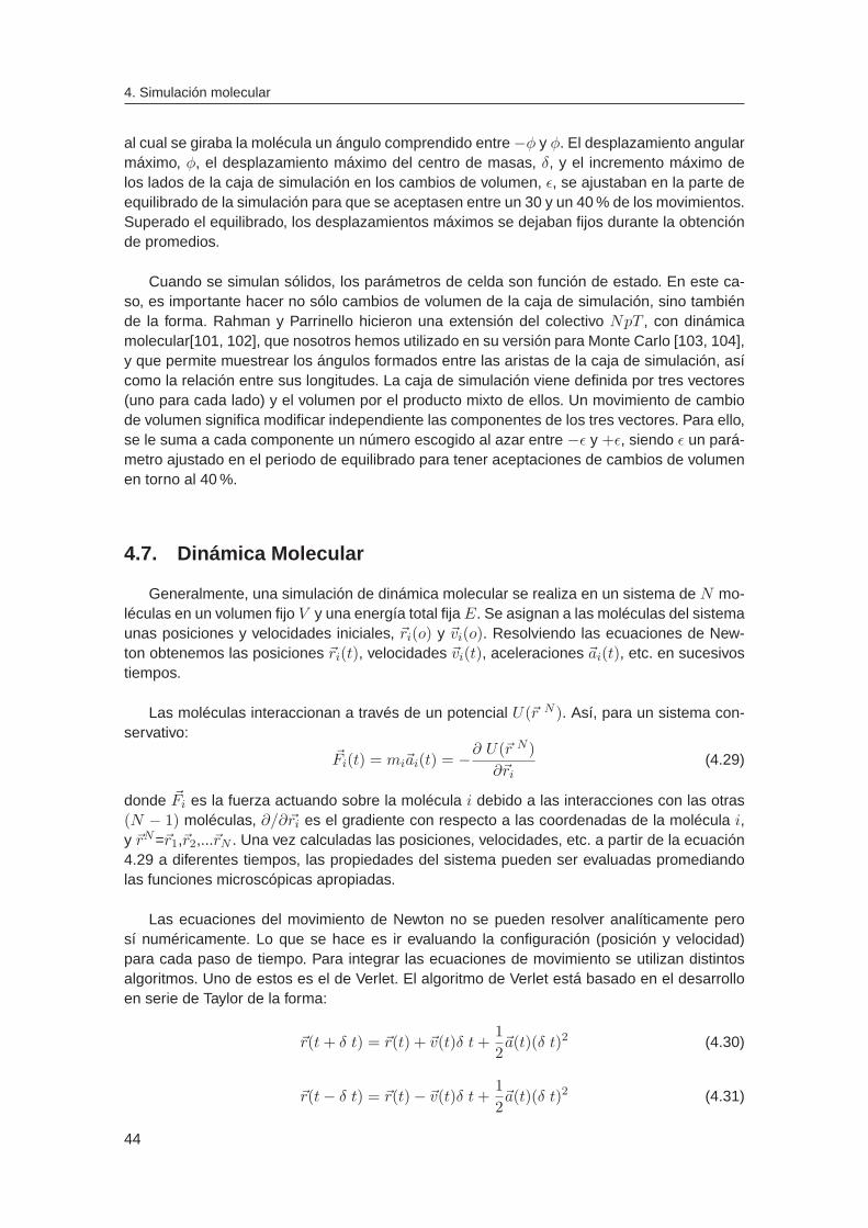
4. Simulación molecular
al cual se giraba la molécula un ángulo comprendido entre −φ y φ. El desplazamiento angularmáximo, φ, el desplazamiento máximo del centro de masas, δ, y el incremento máximo delos lados de la caja de simulación en los cambios de volumen, ǫ, se ajustaban en la parte deequilibrado de la simulación para que se aceptasen entre un 30 y un 40 % de los movimientos.Superado el equilibrado, los desplazamientos máximos se dejaban fijos durante la obtenciónde promedios.
Cuando se simulan sólidos, los parámetros de celda son función de estado. En este ca-so, es importante hacer no sólo cambios de volumen de la caja de simulación, sino tambiénde la forma. Rahman y Parrinello hicieron una extensión del colectivo NpT , con dinámicamolecular[101, 102], que nosotros hemos utilizado en su versión para Monte Carlo [103, 104],y que permite muestrear los ángulos formados entre las aristas de la caja de simulación, asícomo la relación entre sus longitudes. La caja de simulación viene definida por tres vectores(uno para cada lado) y el volumen por el producto mixto de ellos. Un movimiento de cambiode volumen significa modificar independiente las componentes de los tres vectores. Para ello,se le suma a cada componente un número escogido al azar entre −ǫ y +ǫ, siendo ǫ un pará-metro ajustado en el periodo de equilibrado para tener aceptaciones de cambios de volumenen torno al 40 %.
4.7. Dinámica Molecular
Generalmente, una simulación de dinámica molecular se realiza en un sistema de N mo-léculas en un volumen fijo V y una energía total fijaE. Se asignan a las moléculas del sistemaunas posiciones y velocidades iniciales, ~ri(o) y ~vi(o). Resolviendo las ecuaciones de New-ton obtenemos las posiciones ~ri(t), velocidades ~vi(t), aceleraciones ~ai(t), etc. en sucesivostiempos.
Las moléculas interaccionan a través de un potencial U(~r N ). Así, para un sistema con-servativo:
~Fi(t) = mi~ai(t) = −∂ U(~r N )
∂~ri(4.29)
donde ~Fi es la fuerza actuando sobre la molécula i debido a las interacciones con las otras(N − 1) moléculas, ∂/∂~ri es el gradiente con respecto a las coordenadas de la molécula i,y ~rN=~r1,~r2,...~rN . Una vez calculadas las posiciones, velocidades, etc. a partir de la ecuación4.29 a diferentes tiempos, las propiedades del sistema pueden ser evaluadas promediandolas funciones microscópicas apropiadas.
Las ecuaciones del movimiento de Newton no se pueden resolver analíticamente perosí numéricamente. Lo que se hace es ir evaluando la configuración (posición y velocidad)para cada paso de tiempo. Para integrar las ecuaciones de movimiento se utilizan distintosalgoritmos. Uno de estos es el de Verlet. El algoritmo de Verlet está basado en el desarrolloen serie de Taylor de la forma:
~r(t+ δ t) = ~r(t) + ~v(t)δ t+1
2~a(t)(δ t)2 (4.30)
~r(t− δ t) = ~r(t)− ~v(t)δ t+1
2~a(t)(δ t)2 (4.31)
44

4.8 Modelos de potencial de agua
Si se suman las dos expresiones se obtiene:
~r(t+ δ t) = 2~r(t)− ~r(t− δ t) + ~a(t)(δ t)2 (4.32)
Lo que nos indica que si sabemos donde está una cierta molécula y donde estuvo en elpaso anterior, calculando la aceleración se puede estimar donde se encontrará en el pasosiguiente.
~ai =~Fi
mi=
−∂ U∂~ri
mi(4.33)
δt debe ser muy pequeño para que se puedan resolver con exactitud las ecuaciones delmovimiento. A efectos prácticos se suele utilizar δ t = 10−15s. Por último, la velocidad aso-ciada a la molécula i se puede determinar a partir de:
~v(t) =~r(t+ δt)− ~r(t− δt)
2δt(4.34)
Mediante el método de dinámica molecular se pueden calcular tanto propiedades termo-dinámicas (al igual que en Monte Carlo) como dinámicas. El colectivo natural de la dinámicamolecular es el NV E. No obstante, es posible llevar a cabo simulaciones en otros colectivosmediante la introducción de términos adicionales en la ecuación 4.29, que nos permiten man-tener otras variables del sistema constantes. Por ejemplo, en el caso de simulaciones en elcolectivo canónico (NV T ), la temperatura del sistema se mantiene constante mediante la uti-lización de un termostato, que nos permite el reescalado de las velocidades de las moléculasdel sistema, a fin de que la temperatura del sistema sea constante. En el caso de simulacio-nes en el colectivo isotérmico–isobárico (NpT ), además de un termostato para mantener latemperatura constante, es necesaria la utilización de un barostato que permita fluctuacionesde volumen del sistema, y así mantener la presión constante.
4.8. Modelos de potencial de agua
Ahora estamos en disposición de calcular propiedades promedio de un sistema. El únicoingrediente que nos falta es definir las interacciones que existen entre los átomos o molécu-las de nuestro sistema. El elemento central de esta tesis ha sido la molécula de agua, asíque necesitamos un modelo de potencial para describir las interacciones entre moléculas deagua. Existe una gran variedad de modelos de agua dentro de la aproximación clásica quehemos estudiado. La utilización de cada uno de ellos depende del tipo de estudio. Los haymuy sencillos, como el de Molinero et al. [82], cuya principal ventaja es su reducido costecomputacional; lo que permite llevar a cabo largas simulaciones de sistemas muy grandes.Otro tipo de modelos son los estudiados en esta tesis, rígidos y no polarizables, que repre-sentan una descripción un poco más realista de la molécula de agua, al incluir enlaces dehidrógeno (como una interacción coulómbica). En la Tabla 4.1 se dan los parámetros paravarios de estos modelos de potencial de agua. A estos modelos realistas de agua se les pue-de incluir alguna característica más propia de la molécula de agua, como son la flexibilidad yla polarizabilidad. Esto permite estudiar el efecto de estas características en las propiedadesdel agua.
45

4. Simulación molecular
Figura 4.4: Representación esquemática de los modelos SPC/E y TIP4P. Los círculos verdesrepresentan las esferas LJ. Los círculos negros los puntos de carga negativa y los círculos azuleslos de carga positiva. Las líneas representan los enlaces. Tomada de la Ref. [105].
En este trabajo nos hemos limitado al estudio de algunos modelos de potencial de aguarígidos y no polarizables. En la figura 4.4 se puede ver un esquema de los dos tipos de mo-delos de potencial más utilizados. Todos estos modelos, presentan un centro Lennard-Jones(LJ) sobre el átomo de oxígeno, y tienen cargas positivas sobre los átomos de hidrógeno. Lasdiferencias entre ellos están en la geometría de la molécula de agua y principalmente en laubicación de la carga negativa.
En los modelos SPC, la carga negativa está localizada sobre el átomo de oxígeno y la po-sitiva repartida entre los dos átomos de hidrógeno. No se emplean los valores experimentalesde distancias O-H ni ángulos H-O-H; como distancias O-H se emplea 1 Å y para el ánguloformado por los hidrógenos se considera 109.5o . Ambos modelos, SPC y SPC/E fueron pro-puestos por Berendsen [106]. La diferencia entre uno y otro radica en que la carga para elSPC/E es ligeramente mayor, porque supone que la energía de auto-polarización puede sersumada a la energía interna del líquido cuando se ajustan los parámetros del potencial a laentalpía de vaporización del agua real[106].
En los modelos TIP, propuestos por Jorgensen [107], se emplean los valores experimen-tales de distancias O-H y ángulos H-O-H. Tienen un único sitio de interacción Lennard-Joneslocalizado en la posición del átomo de oxígeno. Las dos cargas puntuales positivas estánsituadas en las posiciones de los hidrógenos. La diferencia entre los modelos TIP4P, TIP5P yTIP3P radica en la ubicación de la carga negativa. En el modelo TIP4P [107] la carga nega-tiva está localizada en un centro M, localizado a una distancia dOM del átomo de oxígeno enla bisectriz del ángulo H-O-H en dirección a las cargas positivas. En el modelo TIP3P [107],la carga negativa se sitúa sobre el oxígeno. En el modelo TIP5P, propuesto en el 2000 porMahoney y Jorgensen [108], la carga negativa se divide en dos cargas parciales en las posi-ciones de los “pares de electrones no enlazantes". Es similar al modelo ST2 [109] utilizado enlos 70. Los parámetros de estos modelos han sido ajustados para reproducir determinadaspropiedades termodinámicas del agua líquida. En general, estos modelos no son capaces decorrectamente el máximo de densidad del agua ni el punto de fusión (el TIP5P sí)[110].
En los modelos TIP4P/Ew[111], TIP4P/2005 [34] y TIP4P/Ice [112], recientemente propu-estos, los parámetros han sido ajustados para reproducir las propiedades en las que los otrosmodelos fallaban. En los modelos TIP4P/Ew y TIP4P/2005 los parámetros han sido ajustadospara reproducir el máximo de densidad a presión ambiente del agua líquida en función de latemperatura y, en el TIP4P/Ice para reproducir la temperatura de fusión experimental.
46

4.8 Modelos de potencial de agua
Tabla 4.1: Parámetros de potencial para los distintos modelos de agua: Distancia entre oxígenoe hidrógenos (dOH ). Ángulo formado por los hidrógenos (H-O-H). El centro Lennard-Jones estálocalizado sobre el oxígeno con los parámetros σ y (ǫ/k). Carga del protón (qH ). Momento dipolary cuadrupolar de la molécula de agua (µ y QT ) en Debye y Debye por Å, respectivamente.
Modelo dOH (Å) H-O-H σ (Å) (ǫ/k) (K) qH (e) dOM (Å) dOL (Å) µ (D) QT (D Å)
SPC 1.0 109.47 3.1656 78.20 0.41 0 - 2.274 1.969
SPC/E 1.0 109.47 3.1656 78.20 0.423 0 - 2.350 2.035
TIP3P 0.9572 104.52 3.1506 76.54 0.417 0 - 2.347 1.721
TIP4P 0.9572 104.52 3.1540 78.02 0.52 0.15 - 2.177 2.147
TIP4P/Ew 0.9572 104.52 3.1643 81.90 0.524 0.125 - 2.321 2.164
TIP4P/2005 0.9572 104.52 3.1589 93.2 0.5564 0.1546 - 2.305 2.297
TIP4P/ice 0.9572 104.52 3.1668 106.1 0.5897 0.1577 - 2.425 2.434
TIP5P 0.9572 104.52 3.1200 80.51 0.241 - 0.70 2.29 1.560
Respecto al coste computacional, los modelos SPC requieren la determinación de 9distancias centro-centro, los TIP4P requieren 10 (9 distancias carga-carga y la interacciónLennard-Jones) y el modelo TIP5P necesita 17 (16 distancias carga-carga más la interac-ción Lennard-Jones). Esto quiere decir que el tiempo necesario para realizar una simulaciónescala como 9:10:17, respectivamente. Es decir, el TIP5P es aproximadamente el doble decostoso computacionalmente que el SPC. Los modelos TIP4P son un 10 % más caros compu-tacionalmente que el SPC o SPC/E.
47

4. Simulación molecular
48

CAPÍTULO 5
Metodología
“Reality leaves a lot to the imagination."John Lennon
Mediante la simulación molecular tenemos acceso a las propiedades termodinámicas pro-medio del sistema. En ocasiones es necesaria la utilización de técnicas especiales para teneracceso a propiedades que no se pueden calcular de forma inmediata en una simulación. Unode los objetivos principales de la simulación es el estudio de las transiciones de fase. Lastécnicas que se emplean en el estudio de diagramas de fases dependen del carácter de latransición bajo estudio. En este trabajo nos hemos centrado en el estudio de transiciones defase de primer orden, donde se suelen realizar cálculos de energía libre.
Experimentalmente, la localización de una transición de fase de primer orden es fácil: a lapresión y temperatura de la transición, se observará como el sistema inicialmente homogéneose separa en dos fases, divididas por una interfase. La estrategia a seguir sería, ir variandola presión y/o temperatura del sistema y esperar a que tenga lugar el cambio de fase. Pe-ro en simulación este tipo de estudios no son aplicables para la gran mayoría de sistemas.Por ejemplo, si tenemos un bloque de hielo y queremos saber a que temperatura funde, po-dríamos ir calentando el sólido a lo largo de una simulación y comprobar a que temperaturafunde. Esta forma de abordar el problema no suele tener éxito en simulación por ordenador.En simulación, las transiciones de fase de primer orden presentan histéresis, de manera queel sólido que estamos calentando fundiría a temperaturas por encima de la temperatura defusión termodinámica. Esto es debido a que la barrera de energía libre que separa ambasfases es demasiado alta cerca de la coexistencia. La altura de la barrera viene dada por laenergía libre de la interfase que separa ambas fases. Cuanto mayor es el área interfacial,mayor será la barrera de energía libre que separa ambas fases. Por este motivo el estudio deuna transición de fase de primer orden se puede llevar a cabo de dos formas, simulando am-bas fases en contacto a través de una interfase ya creada o eliminando la interfase, es decir,simulando ambas fases por separado. El primero se conoce como el método de coexistenciadirecta. En cambio, existen muchos enfoques posibles en estudios de coexistencia de fasesen ausencia de interfase:
1. Gibbs ensemble . Se emplea en estudios de coexistencia entre fases fluidas. Se obtie-ne las propiedades de coexistencia en una única simulación. El sistema está formadopor dos cajas separadas en equilibrio “químico´´ y mecánico.
2. Integración termodinámica . Permite el cálculo de diferencias de energía libre entredistintos estados del sistema, siempre que no se atraviesen transiciones de fase.
3. Cristal de Einstein . Cálculos de energía libre de sólidos.
4. Simulaciones Gibbs-Duhem . Se simulan las dos fases por separado y se obtienen laspropiedades de coexistencia, conocido un punto inicial de coexistencia. Permite trazarlíneas de coexistencia.

5. Metodología
5.1. Cálculos de energía libre
Como hemos comentado al principio del capítulo, en simulación, para calcular las condi-ciones de coexistencia entre dos fases, no es posible modificar una variable termodinámicadel sistema y esperar a observar el cambio de fase. Así que el enfoque en el estudio deequilibrio de fases debe ser distinto. Para una sustancia pura, dos fases están en equilibriocuando sus presiones, temperaturas y potenciales químicos son iguales. El potencial químicodel sistema no es una propiedad que pueda ser obtenida de forma directa en una simulación.Es necesario el uso de técnicas especiales. En esta sección estudiaremos las técnicas quese han utilizado en este trabajo para evaluar la energía libre de solidos y líquidos. En todoslos casos la estrategia a seguir es similar. Calculamos la diferencia de energía libre entre elsistema de interés y un sistema de referencia, para el que conocemos, o es posible calcularde forma sencilla, su energía libre. Los estados de referencia usados han sido, el cristal deEinstein en el caso de sólidos y un fluido Lennard-Jones en el caso de líquidos. Una vezconocida la energía libre del sistema en unas condiciones de p y T , es posible calcularla paracualquier otro estado termodinámico de la misma fase mediante integración termodinámica.
5.1.1. Integración termodinámica
En la integración termodinámica se integra una cierta función a lo largo de un caminoreversible para así obtener la diferencia de energía libre entre los dos estados elegidos. Estonos permite calcular la diferencia de energía libre entre dos estados termodinámicos de unamisma fase. Cuando las variables de integración son magnitudes termodinámicas del siste-ma como el volumen o la temperatura, es posible comparar con resultados experimentales.A este tipo de integración la denominaremos “no hamiltoniana”, debido a que el hamiltonianodel sistema no varía entre los estados inicial y final. Con la simulación podemos ir más lejos,puesto que es posible también manipular el hamiltoniano con que se describen las interaccio-nes del sistema. De esta manera, los parámetros del potencial intermolecular se conviertenen nuevas variables termodinámicas. Por tanto, mediante integración termodinámica se pue-den calcular también diferencias de energía libre debidos a un cambio en los parámetros deinteracción. A este tipo de integración la denominaremos “hamiltoniana”. A continuación sedetalla el uso de ambas variantes de integración termodinámica.
Integración termodinámica no hamiltoniana
Esta variante permite obtener la energía libre en cualquier estado termodinámico de unafase a partir de la energía libre conocida en estado de referencia. Se calcula la diferenciade energía libre entre el estado final y el estado de referencia, de energía libre conocida,integrando la ecuación de estado (EOS) del sistema (obtenida mediante simulaciones NpTo NV T ). Hemos utilizado tres tipos de integración termodinámica no hamiltoniana:
a) Cambio de energía libre a lo largo de una isoterma:Una vez conocida la energía libre de Helmholtz a una densidad ρ1 = N/V1, podemos calcularla energía libre a otra densidad ρ2 = N/V2 a la misma temperatura.
De la expresión dA = −SdT − pdV se tiene que
(∂A
∂V
)
T
= −p (5.1)
50

5.1 Cálculos de energía libre
Integrando la ecuación diferencial y dividiendo ambos miembros por NkBT se llega a:
A(ρ2, T )
NkBT=A(ρ1, T )
NkBT+
∫ ρ2
ρ1
p(ρ)
kBTρ2dρ (5.2)
Esta es la expresión que utilizaremos para calcular A a la densidad ρ2 -conocida la EOS- deuna isoterma una vez conocida A en un punto de la misma a la densidad de referencia, ρ1.El integrando se obtiene a partir de simulaciones NpT a distintas presiones a lo largo de unaisoterma para tener p(ρ). La función p(ρ)/kBTρ2 se evalúa para cada una de las simulacio-nes y se ajusta a un polinomio en función de ρ, integrable analíticamente.
b) Cambio de energía libre a lo largo de una isóbara:Nos permite obtener la energía libre de Gibbs a cualquier temperatura (o densidad) de unaisóbara a partir de la energía libre conocida a una temperatura de referencia de la isóbara.
La energía libre de Gibbs dividida por la temperatura es
G
T=H
T− S (5.3)
Diferenciando la expresión anterior
d
(G
T
)=
1
TdH +Hd
(1
T
)− dS (5.4)
Sustituyendo dH por TdS + V dp tenemos
d
(G
T
)=V
Tdp+Hd
(1
T
)(5.5)
Por lo que (∂(G/T )
∂(1/T )
)
p
= H (5.6)
O lo que es lo mismo (∂(G/T )
∂T
)
p
= −H
T 2(5.7)
Integrando la ecuación diferencial y dividiendo por NkB se obtiene
G(T2, p)
NkBT2=G(T1, p)
NkBT1−∫ T2
T1
H(T )
NkBT 2dT (5.8)
Que será la expresión utilizada en este tipo de integración termodinámica. La integral seresuelve haciendo simulaciones NpT a varias temperaturas a lo largo de una isóbara. Seevalúa el integrando a cada una de ellas ((U(T ) + pV (T ))/NkBT
2) y se ajusta a un polino-mio que será integrado analíticamente.
c) Cambio de energía libre a lo largo de una isócora:Permite obtener la energía libre de Helmholtz a cualquier temperatura (o presión) de unaisócora a partir de la energía libre conocida a una temperatura de dicha isócora.La deducción es totalmente análoga a la integración en isóbaras, pero haciendo uso de A enlugar de G y de dU en lugar de dH . La expresión final queda:
A(T2, V )
NkBT2=A(T1, V )
NkBT1−∫ T2
T1
U(T )
NkBT 2dT (5.9)
51

5. Metodología
El integrando se obtiene a partir de los resultados de varias simulaciones. En este caso serequiere hacer variosNV T a distintas temperaturas de una isocora. Se evalúa U(T )/NkBT
2
para cada una de ellas y los puntos se ajustan a un polinomio que se integra analíticamente.
Combinando estos tres tipos de integración termodinámica se puede conocer la energíalibre en cualquier estado (p, V, T ) a partir de la energía libre conocida en un estado de refe-rencia. La única limitación de la integración termodinámica es que no puede haber cambiosde fase en el camino de integración. En una transición de fase, el integrando de cualquie-ra de los tres tipos de integración termodinámica referidos presenta una discontinuidad. Portanto, sólo nos podemos mover en los puntos del espacio (p, V, T ) que correspondan al do-minio de la fase cuya energía libre se conoce. La integración se puede extender a zonas demetaestabilidad, siempre y cuando la fase conserve su estabilidad mecánica. Esto permite,por ejemplo, obtener la energía libre del agua subenfriada, que se conserva largo tiempo ensituación de equilibrio metaestable debido a la barrera de energía libre que separa el líquidosubenfriado del sólido.
5.1.2. Integración termodinámica hamiltoniana
En este tipo de integración el hamiltoniano del sistema varía entre los estados inicial yfinal. La variable de integración será un parámetro λ de la función que describe el potencialde interacción del sistema (U(λ)). Este parámetro puede ser, por ejemplo, el valor de la car-ga de las moléculas o de σ o ǫ en el caso de una interacción Lennard-Jones. Más adelanteaparecerán ejemplos concretos de U(λ). Describamos ahora como se realiza la integracióntermodinámica hamiltoniana.
El parámetro λ es una variable termodinámica de la que depende la energía libre:
A(N,V, T, λ) = −kBT lnQ(N,V, T, λ). (5.10)
Q(N,V, T, λ) es la función de partición que viene dada por (ecuación 2.13):
Q(N,V, T, λ) =qN
N !
∫exp[−βU(λ)]d1...dN (5.11)
Derivando ambos miembros de 5.68 con respecto a λ se llega a la ecuación diferencial
∂A(N,V, T, λ)
∂λ= −kBT
∂ lnQ(N,V, T, λ)
∂λ. (5.12)
La derivada con respecto a λ del logaritmo neperiano de Q(N,V, T, λ) es:
∂ lnQ(N,V, T, λ)
∂λ=
1
Q(N,V, T, λ)
∂Q(N,V, T, λ)
∂λ
=−β∫[∂U(λ)/∂λ] exp[−βU(λ)]d1...dN∫
exp[−βU(λ)]d1...dN
= −β⟨∂U(λ)
∂λ
⟩
N,V,T,λ
(5.13)
Por lo que∂A(N,V, T, λ)
∂λ=
⟨∂U(λ)
∂λ
⟩
N,V,T,λ
. (5.14)
52

5.1 Cálculos de energía libre
Integrando la ecuación diferencial queda
A(N,V, T, λ1)−A(N,V, T, λ0) =
∫ λ1
λ0
⟨∂U(λ)
∂λ
⟩
N,V,T,λ
dλ, (5.15)
que nos da la diferencia de energía libre de Helmholtz, por integración termodinámica, entrelos estados (N,V, T, λ1) y (N,V, T, λ0). La integración se hace a N,V y T constantes. Si loque se busca es la diferencia de energía libre de Gibbs, se obtiene una expresión análogapero manteniendo N, p y T constantes:
G(N, p, T, λ1)−G(N, p, T, λ0) =
∫ λ1
λ0
⟨∂U(λ)
∂λ
⟩
N,p,T,λ
dλ. (5.16)
La integral 5.15 se resuelve numéricamente evaluando la función 〈∂U(λ)/∂λ〉N,V,T,λ paradistintos valores de λ utilizando simulaciones en el colectivo NV T . El integrando es, por tan-to, una función que se obtiene como promedio de las simulaciones. La diferencia de energíaslibres de Gibbs, ecuación (5.16), requiere la evaluación del integrando en el colectivo NpT .
Del mismo modo que en el caso no hamiltoniano, la integración hamiltoniana tiene la limi-tación de no poder atravesar transiciones de fase debido a que el integrando (〈∂U(λ)/∂λ〉)sufriría una discontinuidad. Por tanto, hay que tener la cautela de asegurarse de que el cam-bio de hamiltoniano no supondrá un cambio de fases.
Si se conoce la energía libre en uno de los límites de integración (λ1 ó λ0), la energía li-bre en el otro límite puede obtenerse mediante integración termodinámica hamiltoniana. Estemétodo ha sido muy utilizado en esta tesis. En efecto se ha utilizado para calcular la energíalibre del agua líquida, de los haluros alcalinos en fase líquida, y de disoluciones de halurosalcalinos. Los métodos utilizados para el cálculo de la energía libre de fases sólidas tambiénson casos particulares de integración termodinámica. En todos los casos, el hamiltoniano delsistema de interés se transformó en otro para el que la energía libre era conocida.
5.1.3. Energía libre de líquidos
Aunque la energía libre de un líquido puede calcularse utilizando varias rutas, en esta te-sis la energía libre de todos los líquidos ha sido obtenida mediante integración termodinámicahamiltoniana (sección 5.1.2). Usando integración termodinámica hamiltoniana calculamos ladiferencia de energía libre entre el sistema de interés y un sistema de referencia cuya energíalibre es conocida. Tanto para evaluar la energía libre del agua líquida, como de haluros alca-linos en fase líquida o de disoluciones acuosas de iones, hemos escogido como referenciaun fluido Lennard-Jones, cuya energía libre ha sido determinada por Johnson et al. [113] yNezbeda et al. [114].
El camino que conecta el fluido bajo estudio (B) con el de referencia (A) -un Lennard-Jones- se establece a través del siguiente hamiltoniano acoplado:
U(λ) = λUA + (1− λ)UB. (5.17)
Donde λ es un parámetro que varía entre 0 y 1. Cuando λ vale 0 el hamiltoniano es el delsistema de interés y cuando vale 1 es el del sistema de referencia. Nosotros hemos utilizadouna función lineal de λ para definir el camino entre ambos sistemas (aunque no tiene por qué
53

5. Metodología
ser así necesariamente). Según la ecuación 5.15, la diferencia de energía entre A y B vendrádada por:
AA(N,V, T )−AB(N,V, T ) =
∫ 1
0〈UA − UB〉N,V,T,λ dλ. (5.18)
Siendo < UA−UB >N,V,T,λ un promedio que puede evaluarse en simulaciones de tipoNV Tcon un valor determinado de λ. La integral se evalua determinando numéricamente el inte-grando para distintos valores de λ comprendidos entre 0 y 1.
Como ya se ha comentado en la sección 5.1.1, un aspecto crucial a tener en cuenta cuan-do se hace integración termodinámica es que no se pueden atravesar transiciones de faseen el camino de integración. Por ello, hay que asegurarse de que en las condiciones N,V, Ten las que se hace la integración, tanto el sistema de interés como el Lennard-Jones de refe-rencia están en fase líquida. Esto determina la elección de los parámetros σ y ǫ del sistemaLennard-Jones de referencia. Habitualmente la elección de σ y ǫ se hizo para garantizar queρσ3 ≈ 1 y T *= T
ǫkB
≈ 2− 4, lo que garantiza que el sistema LJ esta en fase líquida.
5.1.4. Energía libre de sólidos
El cálculo de energía libre de sólidos ha tenido una importancia central en el desarro-llo de esta tesis. Buena parte del trabajo realizado se ha centrado en el equilibrio de fasessólido-líquido del agua. Esta metodología también ha sido utilizada en la determinación detemperaturas de fusión y solubilidad del NaCl. En ambos casos se ha empleado el métododel cristal de Einstein.
En la región de altas presiones del diagrama de fases del agua encontramos dos fasesde cristal plástico para varios modelos de potencial de agua (Capítulos 7 y 8). El método delcristal de Einstein no es aplicable a sólidos con desorden orientacional, así que en esta tesisextendimos el método del cristal de Einstein para el cálculo de energías libres de sólidos condesorden orientacional, como cristales plásticos. Este método se describe en las siguientessecciones.
En hielos con desorden de protón es posible aplicar el método del cristal de Einstein, yaque calculamos la energía libre de una única configuración de enlaces de hidrógeno. Comohemos visto en la sección anterior 5.5, las transiciones entre distintas configuraciones desor-denadas no tienen lugar en simulaciones tipo Metropolis. Aquí la clave es calcular la energíalibre para una configuración representativa del sistema y luego corregir el resultado con la en-tropía de Pauling, que corresponde a la entropía debida al desorden de protón. En un futurosería tremendamente interesante extender el método del cristal de Einstein para el cálculo deenergías libre de hielos desordenados de protón, muestreando las posibles configuracionesde enlaces de hidrógeno con el algoritmo de rotación de anillos.
Cristal de Einstein
Este método, propuesto por Frenkel y Ladd en 1984 [115], se ha convertido en un proce-dimiento muy empleado en el cálculo de energía libre de sólidos [61, 116–125]. La filosofíaconsiste en utilizar un cristal de Einstein como sistema de referencia y calcular la diferenciade energía libre entre el sistema de interés y el cristal de Einstein. Un cristal de Einstein es un
54

5.1 Cálculos de energía libre
sólido en el que las unidades constituyentes (átomos o moléculas) están anclados a sus po-siciones y orientaciones de equilibrio mediante un potencial armónico y en el que no existeninteracciones intermoleculares. Su energía libre se puede calcular de manera analítica parasólidos atómicos y numérica para sólidos moleculares.
Por razones prácticas, que se aclararán más adelante, es conveniente utilizar como sis-tema de referencia un cristal de Einstein (Ein) que tenga el centro de masas fijo (CM). Elcamino que hay que recorrer desde el cristal de Einstein con el centro de masas fijo hasta elsólido de interés se puede describir como:
Asol = ACMEin−id + (ACM
Ein−sol −ACMEin−id) + (ACM
sol −ACMEin−sol) + (Asol −ACM
sol ). (5.19)
donde ACMEin−id es la energía libre del sistema de referencia (cristal ideal de Einstein con
el centro de masas fijo). La primera etapa consiste en determinar la diferencia de energíalibre entre el cristal ideal de Einstein y el cristal de Einstein con interacciones, ambos conel CM fijo (∆A1 = ACM
Ein−sol − ACMEin−id). En la segunda etapa (∆A2 = ACM
sol − ACMEin−sol),
los muelles del cristal de Einstein con interacciones son gradualmente desenchufados paraobtener el sólido de interés (ambos con el centro de masas fijo). Finalmente, el sólido con elCM fijo se transforma en un sólido sin el centro de masas fijo (∆A3 = Asol−ACM
sol ). Podemosreescribir la ecuación 5.19 usando estas definiciones:
Asol = ACMEin−id + [∆A1 +∆A2] + ∆A3 (5.20)
Veamos como se pueden calcular cada uno de los términos:
1. Energía del cristal de Einstein con CM fijo.
En un cristal de Einstein las moléculas están ancladas a sus posiciones y orientacionesde red mediante unos muelles armónicos. Nos centraremos en el caso de moléculasrígidas no lineales. Aunque el campo traslacional siempre se aplica de la misma mane-ra, la expresión para el campo orientacional depende de la geometría de la moléculaa considerar. Aquí se describirá el procedimiento para una molécula con simetría C2v,como es el caso del agua.
La energía de un cristal ideal de Einstein viene dada por:
UEin−id = UEin−id,t + UEin,or (5.21)
UEin−id,t =N∑
i=1
[ΛE(ri − rio)
2]
(5.22)
UEin,or(C2v) =N∑
i=1
uEin,or,i =N∑
i=1
[ΛE,a sin
2 (ψa,i) + ΛE,b
(ψb,i
π
)2]
(5.23)
donde ri representa la posición instantánea del punto de referencia de la molécula i, yrio es la posición de equilibrio de este punto de referencia de la molécula i en el cristal(ri fluctuará a lo largo de la simulación pero rio no). Como hemos comentado, elegimosel CM de la molécula como punto de referencia. De hecho, la función de partición rota-cional de la molécula qr se calcula usando los momentos principales de inercia (I1, I2y I3) con origen en el centro de masas de la molécula. Las propiedades configuracio-nales no dependen del punto de referencia. Por este motivo, para calcular propiedades
55
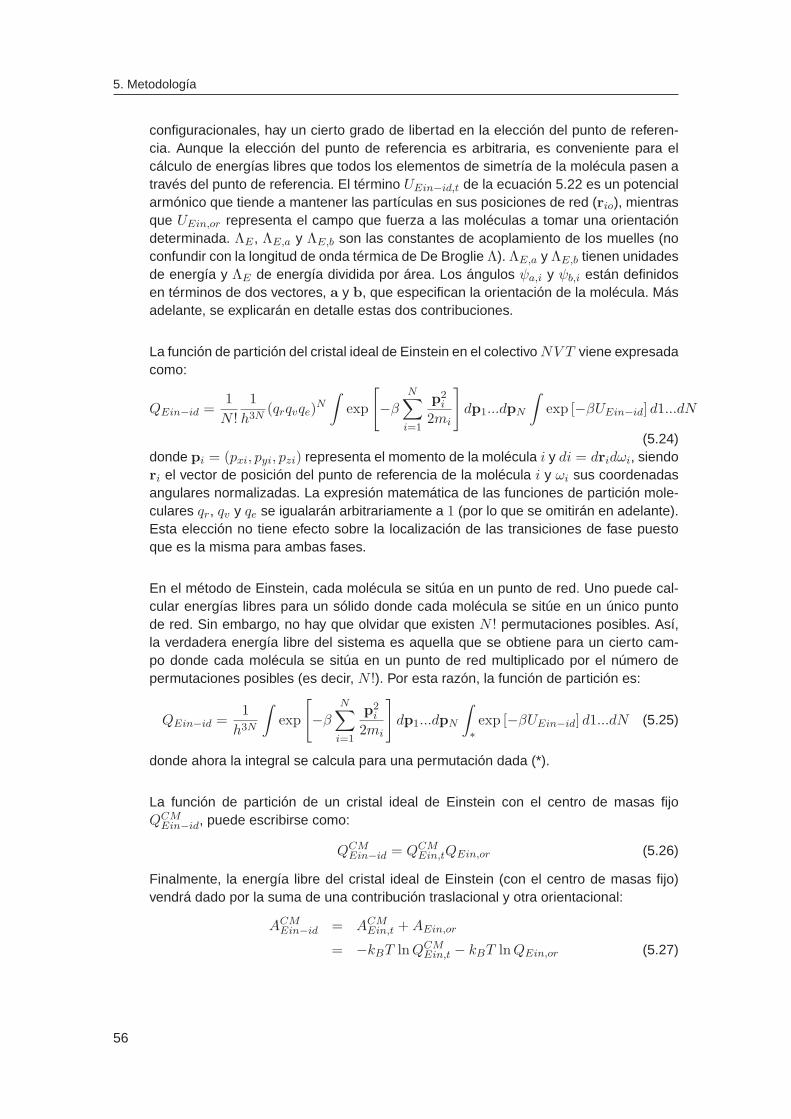
5. Metodología
configuracionales, hay un cierto grado de libertad en la elección del punto de referen-cia. Aunque la elección del punto de referencia es arbitraria, es conveniente para elcálculo de energías libres que todos los elementos de simetría de la molécula pasen através del punto de referencia. El término UEin−id,t de la ecuación 5.22 es un potencialarmónico que tiende a mantener las partículas en sus posiciones de red (rio), mientrasque UEin,or representa el campo que fuerza a las moléculas a tomar una orientacióndeterminada. ΛE , ΛE,a y ΛE,b son las constantes de acoplamiento de los muelles (noconfundir con la longitud de onda térmica de De Broglie Λ). ΛE,a y ΛE,b tienen unidadesde energía y ΛE de energía dividida por área. Los ángulos ψa,i y ψb,i están definidosen términos de dos vectores, a y b, que especifican la orientación de la molécula. Másadelante, se explicarán en detalle estas dos contribuciones.
La función de partición del cristal ideal de Einstein en el colectivoNV T viene expresadacomo:
QEin−id =1
N !
1
h3N(qrqvqe)
N
∫exp
[−β
N∑
i=1
p2i
2mi
]dp1...dpN
∫exp [−βUEin−id] d1...dN
(5.24)donde pi = (pxi, pyi, pzi) representa el momento de la molécula i y di = dridωi, siendori el vector de posición del punto de referencia de la molécula i y ωi sus coordenadasangulares normalizadas. La expresión matemática de las funciones de partición mole-culares qr, qv y qe se igualarán arbitrariamente a 1 (por lo que se omitirán en adelante).Esta elección no tiene efecto sobre la localización de las transiciones de fase puestoque es la misma para ambas fases.
En el método de Einstein, cada molécula se sitúa en un punto de red. Uno puede cal-cular energías libres para un sólido donde cada molécula se sitúe en un único puntode red. Sin embargo, no hay que olvidar que existen N ! permutaciones posibles. Así,la verdadera energía libre del sistema es aquella que se obtiene para un cierto cam-po donde cada molécula se sitúa en un punto de red multiplicado por el número depermutaciones posibles (es decir, N !). Por esta razón, la función de partición es:
QEin−id =1
h3N
∫exp
[−β
N∑
i=1
p2i
2mi
]dp1...dpN
∫
∗exp [−βUEin−id] d1...dN (5.25)
donde ahora la integral se calcula para una permutación dada (*).
La función de partición de un cristal ideal de Einstein con el centro de masas fijoQCM
Ein−id, puede escribirse como:
QCMEin−id = QCM
Ein,tQEin,or (5.26)
Finalmente, la energía libre del cristal ideal de Einstein (con el centro de masas fijo)vendrá dado por la suma de una contribución traslacional y otra orientacional:
ACMEin−id = ACM
Ein,t +AEin,or
= −kBT lnQCMEin,t − kBT lnQEin,or (5.27)
56

5.1 Cálculos de energía libre
a) Contribución traslacional: La parte traslacional de la función de partición del cristalde Einstein sin restricción alguna de la posición de su centro de masas viene dada por:
QCMEin,t =
1
h3(N−1)
∫exp
[−β
N∑
i=1
p2i
2mi
]dp1...dpN
∫exp
[−βΛE
N∑
i=1
(ri − rio)2
]dr1...drN (5.28)
Ahora imponemos la condición de fijar el CM de los puntos de referencia (oxígenos enel caso de molécula de agua). Esta restricción implica que su posición en cualquierinstante no difiera de la inicial:
RCM −RCMo = 0N∑
i=1
µiri −N∑
i=1
µirio = 0
N∑
i=1
µi(ri − rio) = 0 (5.29)
Siendo µi = mi/∑N
i=1mi, y mi la masa de la partícula i. Derivando la expresiónanterior con respecto al tiempo se obtiene la influencia del centro de masas fijo sobrelos momentos de las partículas:
N∑
i=1
pi = 0 (5.30)
Incluyendo las restricciones, tanto a las posiciones como a los momentos, en la funciónde partición del cristal de Einstein se llega a la función de partición del cristal de Einsteincon el centro de masas fijo:
QCMEin,t =
1
h3(N−1)
∫exp
[−β
N∑
i=1
p2i
2mi
]δ(
N∑
i=1
pi)dp1...dpN
∫exp
[−βΛE
N∑
i=1
(ri − rio)2
]δ(
N∑
i=1
1
N(ri − rio))dr1...drN (5.31)
La contribución traslacional a la energía libre del cristal de Einstein es −kBT lnQCMEin .
La resolución de la integral QCMEin,t se detalla en el apéndice J. El resultado es:
QCMEin,t = PCM
(π
βΛE
)3(N−1)/2
(N)3/2 (5.32)
donde PCM es la parte de momentos de la función de partición del cristal de Einsteincon el centro de masas fijo, que no se ha resuelto de manera explícita como la de po-siciones porque se cancelará más adelante. La contribución traslacional a la energíalibre de un cristal de Einstein con el centro de masas fijo es, por tanto:
ACMEin,t = −kBT ln[PCM
(π
βΛE
)3(N−1)/2
(N)3/2] (5.33)
57

5. Metodología
b) Contribución orientacional: La restricción de fijar el centro de masas de los puntosde referencia no afecta a la parte de orientaciones de la integral configuracional debidoa que la rotación de una molécula con respecto a un eje que pasa por su punto dereferencia no supone un desplazamiento del punto de referencia. Así que la contribuciónorientacional a la función de partición total será independiente del punto de referencia:
QEin,or =
[1
8π2
∫exp (−βuEin,or) sin θdφdθdγ
]N(5.34)
Para el caso concreto del agua con simetría C2v, vendrá dada por:
QEin,or =
[1
8π2
∫exp
(−βΛE,a sin
2 (ψa)− βΛE,b
(ψb
π
)2)sin θdθdφdχ
]N(5.35)
El elemento diferencial de las coordenadas angulares normalizadas, ωi, viene expre-sado por dωi = 1/(8π2) sen θidθidφidχi, siendo 8π2 el factor de normalización de losmismos. θ, φ y χ son los ángulos de Euler tal y como se definen en el libro de Gray yGubbins [126]. (θ) varia entre 0 y π y (φ) y (χ) entre 0 y 2π. ΛE,a y ΛE,b son las cons-tantes de acoplamiento de los muelles. ψa,i se define como el ángulo formado por elvector a de la molécula i en una configuración determinada (ai) y el vector a de dichamolécula en su orientación de red (ai,o). ψb,i se define de manera análoga pero con elvector b en lugar del a. La definición de los vectores a y b se esquematiza en la figura5.1. Los ángulos ψa y ψb se obtienen a través del producto escalar de los vectores a yai,o, y b y bi,o respectivamente:
ψa,i = arc cos
(~ai · ~ai,o
| ~ai | · | ~ai,o |
)
(5.36)
ψb,i = arc cos
(~bi ·~bi,o
| ~bi | · | ~bi,o |
)(5.37)
por lo que ψa,i y ψb,i están definidos entre 0 y π. En este caso se representa una molé-cula rígida angular con un eje de simetría de orden n = 2. El vector a es la diferenciaentre los vectores de enlace (l2 - l1) y el vector b es la suma. El potencial escogido parapreservar la orientación del vector a respeta la simetría de la molécula, repitiéndose elvalor del potencial con giros de π radianes (n=2). El valor de sen2(ψa,i) oscila entre 0(cuando ai es paralelo a ai,o) y 1 (cuando ai es perpendicular a ai,o). El ángulo ψb,i sedivide por π para que también éste término oscile entre 0 (cuando bi es paralelo a bi,o)y 1 (cuando bi y bi,o forman un ángulo de 180o) y tener así ambos muelles orientacio-nales compensados. Aunque se ha representado una molécula triatómica con un ejede simetría de orden 2, el esquema es válido para cualquier molécula rígida, bien seano lineal o lineal (en cuyo caso se suprimirá el término de ψb,i). Basta con definir a y b
a partir de dos vectores de enlace, teniendo el cuidado de colocar a perpendicular aleje de simetría de la molécula.
58

5.1 Cálculos de energía libre
a
ll
b
21
Figura 5.1: Definición de los vectores ~a y ~b en una molécula triatómica rígida con eje de simetríade orden 2. ~a es la resta de los vectores de enlace ~l2 y ~l1 y ~b es la suma.
Arbitrariamente, podemos hacer coincidir el vector ai,o con el eje z, en cuyo caso elángulo de Euler θ y el ψa son el mismo. Entonces la integral se puede redefinir como:
QEins,or =
(1
8π2
∫exp
(−βΛE,a sen
2(θ)− βΛE,b
(ψb
π
)2)sen θdθdφdχ
)N
(5.38)
El ángulo ψb, formado por el vector b y el bo no se identifica, en principio, con ningunode los ángulos de Euler, sino que es función de todos ellos. La integral resultante pue-de ser evaluada numéricamente utilizando integración Monte Carlo o a través de unaaproximación analítica propuesta por Vega y Monson [127].
Finalmente, la energía libre del cristal de Einstein (con el centro de masas fijo) vendrádado por la suma de una contribución traslacional y otra orientacional:
ACMEin = ACM
Ein,t +AEin,or
= −kBT lnQCMEin,t − kBT lnQEin,or (5.39)
2. Diferencia de energía libre entre el cristal de Einstein ide al y con interacciones(∆A1)
Ahora evaluaremos la diferencia de energía libre entre un cristal de Einstein ideal y elcristal de Einstein con las interacciones del sólido de interés, ambos con el centro demasas fijo. La diferencia de energía libre entre dos sistemas arbitrarios, que etiquetare-mos como 1 y 2, viene dada por:
A2 −A1 = −kBT lnQ2
Q1= −kBT ln
∫exp(−βU2)d1...dN∫exp(−βU1)d1...dN
(5.40)
Multiplicando y dividiendo el numerador del integrando por el factor exp(−βU1), seobtiene:
A2 −A1 = −kBT ln 〈exp [−β(U2 − U1)]〉1 (5.41)
donde 〈exp [−β(U2 − U1)]〉1 es un promedio sobre las configuraciones visitadas por elsistema 1. Tomando U2 = UEin−id + Usol y U1 = UEin−id (siendo Usol el potencialintermolecular del sólido), la expresión anterior se puede reescribir:
ACMEin−sol −ACM
Ein−id = −kBT ln 〈exp [−β(Usol)]〉Ein−id (5.42)
59

5. Metodología
Luego hay que promediar exp [−β(Usol)] a lo largo de las configuraciones de un cristalde Einstein. Esto se lleva a cabo en una simulación NV T con el centro de masas delsistema fijo. Normalmente, no es posible evaluar el cambio de energía libre según estáexpresado en la ecuación 5.42, debido a que el exponencial exp(−βUsol) adopta ge-neralmente valores altos que no pueden ser resueltos por el ordenador. Este problemase evita sumando y restando a la energía del sólido Usol la energía de red Ured:
∆A1 = ACMEin−sol −ACM
Ein−id = Ured − kBT ln 〈exp [−β(Usol − Ured)]〉Ein−id (5.43)
que no presenta problemas de divergencia en la exponencial que se promedia.
Si los sistemas 1 y 2 no son muy similares, el sistema 2 visitará, con probabilidad baja,configuraciones energéticamente favorables para el sistema 1, que además tienen unelevado factor de Boltzman 〈exp [−β(U2 − U1)]〉1. Eso ocasionaría un gran error es-tadístico en la evaluación de la diferencia de energía libre. Por ello, los sistemas 1 y2 tienen que ser lo más parecidos posible. Por otro lado, cuanto más grande sea laconstante de acoplamiento del cristal de Einstein (ΛE), más se parecerán las configu-raciones propias del cristal de Einstein con interacciones a las del cristal de Einsteinideal. Cuando dicha constante tiende hacia el infinito, la energía promedio del sólido enel cristal de Einstein tiende a la energía de red (energía del sólido con todas las mo-léculas en sus posiciones y orientaciones de equilibrio). Sin embargo, cuanto más altasea la constante, más largo será el camino termodinámico que va del sólido al cristalde Einstein con interacciones. Por tanto, hay que llegar a un compromiso para optimizarambas etapas del cálculo de energía libre. Una elección conveniente para ΛE,a y ΛE,b
es aquella que garantice un valor pequeño (alrededor de 0.02NkBT ) para el segun-do término de la ecuación 5.43. Cuando esto sucede, ∆A1 es bastante cercano a laenergía de red Ured.
3. Diferencia de energía entre el cristal de Einstein con inter acciones y el sólido(∆A2)
En este apartado vamos a calcular la diferencia de energía libre entre el sólido deinterés y un cristal de Einstein al que se le añaden las interacciones del sólido, amboscon el CM fijo. Para ellos definimos la energía del sistema en función de un parámetrode acoplamiento λ, de forma análoga a la integración termodinámica hamiltoniana (versección 5.1.2):
U(λ) = λUsol + (1− λ)(UEin−id + Usol) (5.44)
λ se define entre 0 y 1, así, cuando λ = 0 se tiene el sólido de Einstein y cuandoλ = 1 obtienes el sólido de interés. La variación de λ es el equivalente matemático air desenchufando los muelles armónicos gradualmente. El cambio de energía libre a lolargo de este camino se expresa como:
∆A2 = A(N,V, T, λ = 1)−A(N,V, T, λ = 0) =
=
∫ λ=1
λ=0
⟨∂U(λ)
∂λ
⟩
N,V,T,λ
dλ =
= −∫ λ=1
λ=0〈UEin−id〉N,V,T,λ dλ (5.45)
Esta integral se resuelve numéricamente evaluando el integrando, obtenido en simula-ciones NV T , para varios valores de λ. El valor efectivo de las constantes de fuerza de
60

5.1 Cálculos de energía libre
los muelles en cada simulación viene expresado por λΛE , λΛE,a y λΛE,b. Hemos esco-gido el valor de dichas constantes de tal manera que ΛE = ΛE,a = ΛE,b. Para valoresde λ cercanos a 1, las partículas están fuertemente unidas a sus posiciones de redy el cristal tenderá a comportarse como un cristal de Einstein (sin verse afectado porlas interacciones intermoleculares) cuya energía, UEin−id, vale 1/2kBT por grado delibertad. Por el contrario, para valores bajos de λ, los muelles que unen las partículasa sus posiciones de red son muy débiles y, debido a que los átomos o moléculas delsólido podrán separarse mucho de su posición de equilibrio, la energía del cristal delEinstein será muy elevada. Por tanto, el integrando de 5.45 será grande a bajos valoresde λ y muy pequeño a altos, lo que hace difícil la evaluación numérica de la integral.En realidad no hemos resuelto la integral 5.45 sino otra que surge como consecuenciade dos cambios de variable. En el primero cambiamos la variable de integración λ porλΛE :
∆A2 = ACMsol −ACM
Ein−sol = −∫ ΛE
0
〈UEin−id〉N,V,T,λ
ΛEd(λΛE) (5.46)
Y en el segundo cambiamos λΛE por ln(λΛE + c), siendo c una constante:
∆A2 = ACMsol −ACM
Ein−sol = ∆A2 = −∫ ln(ΛE+c)
ln(c)
〈UEin−id〉N,V,T,λ (λΛE + c)
ΛEd(ln(λΛE+c))
(5.47)Este segundo cambio de variable es el que resuelve el problema del cambio brus-co del integrando a lo largo del intervalo de integración; éste varía suavemente conln(λΛE + c). El integrando se evalúa para distintos valores de ln(λΛE + c) distribuidosconforme a un algoritmo de integración gaussiana entre ln(c) y ln(λΛE + c). Mediantesimulación molecular se evalúa < UEin−id > para cada uno de los valores de λ corres-pondientes a cada punto ln(λΛE + c). Se puede apreciar cómo el segundo integrandovaría más suavemente con su variable de integración que el primero. El valor utilizadopara la constante c ha sido exp(3.5), tal y como recomiendan Frenkel y Ladd [115].
Si no se fijase el centro de masas, el cristal podría desplazarse como un bloque cuan-do λ tiende a cero, lo que ocasionaría valores de < UEin−id > demasiado elevados.En ese caso, se haría necesario la evaluación del integrando en muchos valores deλ cercanos a cero para tener una buena estimación de la integral. Para conseguir unintegrando más suave, el centro de masas se fija en la integración.
4. Diferencia de energía libre entre el sólido y el sólido con el CM fijo ( ∆A3)
La diferencia de energía libre entre dos sistemas viene dada por el logaritmo neperianodel cociente de las funciones de partición (Eq. 5.40):
∆A3 = Asol −ACMsol = −kBT ln
Qsol
QCMsol
= kBT lnQCM
sol
Qsol(5.48)
donde QCMsol viene dado (después de integrar sobre los momentos) por:
QCMsol =
(qrqvqe)N
N !h3(N−1)
∫exp
[−β
N∑
i=1
p2i
2mi
]δ(
N∑
i=1
pi)dp1...dpN
∫exp [−βUsol(r1, ω1...rN, ωN)] δ(
N∑
i=1
µi(ri − rio))dr1dω1...drNdωN (5.49)
61

5. Metodología
y Qsol viene dado por una expresión similar a QCMsol pero sin las funciones delta (y con
h3N en el denominador en vez de h3(N−1)). El factor N ! se cancela cuando se calculanenergías libres, ya que aparece tanto en Qsol como en QCM
sol . La integración sobre elespacio de momento del sólido sin ligaduras es simplemente la integral del producto defunciones gausianas, cuya solución es:
P =
(2πmkBT
h2
)(3N)/2
=
(1
Λ
)3N
(5.50)
La integral sobre el espacio de momento del sólido con el centro de masas fijo es iguala la integral de los momentos del cristal ideal de Einstein con el centro de masas fijo,el cual se denota como PCM . Sustituyendo las funciones de partición en la ecuación5.48, se llega a la siguiente expresión:
∆A3 = Asol −ACMsol = kBT ln
(PCM
P
)+ (5.51)
+kBT ln
∫exp [−βUsol(r1, ω1...rN, ωN)] δ(
∑Ni=1(1/N)(ri − rio))dr1ω1...drNωN∫
exp [−βUsol(r1, ω1, ..rN, ωN)] dr1dω1...drNdωN
La energía de un sistema no se modifica si el sistema se traslada (mientras se manten-gan fijas las orientaciones relativas de las moléculas). La consecuencia matemática deeste hecho es queUsol(r1, ω1, ..rN, ωN) se puede reescribir comoUsol(ω1, r
′
2, ω2, ...r′
NωN)donde r
′
i = ri − r1. Además, localizamos el centro de masas del punto de red en elorigen del sistema de coordenadas tal que
∑(1/N)rio = RCMo = 0 y llevamos a
cabo el cambio de variables de r1, r2, ...rN a r′
2, ...RCM, donde RCM es la posicióndel centro de masas de los puntos de referencia y, sabiendo que el Jacobiano de estatransformación es N, podemos obtener para el segundo término de la ecuación 5.52:
kBT ln
∫exp(−βUsol(ω1, r
′
2, ω2, r′
3, ...r′
N, ωN))δ(RCM)Ndω1dr′
2dω2dr′
3..dr′
NdωNdRCM∫exp(−βUsol)(ω1, r
′
2, ω2, r′
3, ...r′
N, ωN))Ndω1dr′
2dω2dr′
3..dr′
NdωNdRCM
(5.52)Después de integrar con respecto a ω1r
′
2ω2...r′
NωN se obtiene:
kBT ln
∫δ(RCM )dRCM∫
dRCM= kBT ln
1∫dRCM
(5.53)
La integral en el denominador de la ecuación 5.53 es el volumen disponible para elcentro de masas. ¿Cuál es el valor de este volumen? Un interesante comentario ya loapuntó explícitamente Wilding [128–131] en el que hacía referencia a que la traslaciónde un cristal como un bloque bajo condiciones de contorno periódicas generaN permu-taciones entre las partículas. Cuando contamos el posible número de configuracionesusamos el valor de N ! para ir de la ecuación 5.24 a 5.25. De esta manera contamos to-das las posibles permutaciones, así, la integral en el denominador de la ecuación 5.53es el volumen disponible del centro de masas para una permutación dada. Este valores simplemente V/N . Usando V en vez de (V/N) en el denominador de la ecuación5.53 ya no sería correcto usar N ! para contar el número de permutaciones. En estesupuesto, las permutaciones serían contadas dos veces, la primera vez por el factorN !, y la segunda debido a la traslación del cristal como un todo (en el volumen V ). Portanto, la expresión correcta que nos queda es:
∆A3 = Asol −ACMsol = kBT
[ln(PCM/P )− ln(V/N)
](5.54)
62

5.1 Cálculos de energía libre
Como se puede ver, la expresión para ∆A3 es general y no depende del potencialintermolecular Usol. Nótese, que también sería correcto usar V en el denominador dela ecuación 5.53 (en el caso en el que el centro de masas se moviera en la totalidadde la caja de simulación) si se usa (N − 1)! para contar el número de permutaciones(es decir, contando todas las permutaciones obtenidas por la traslación del cristal bajocondiciones de contorno periódicas). En la ecuación 5.25, uno obtendría un término(N − 1)!/N !, el cual proporciona un factor de 1/N que unido con el término ln(1/V )de la ecuación 5.53 nos da un contribución de −kT ln(V/N) (idéntico al obtenido en laecuación 5.54). Así, ∆A3 tendrá un término de la forma −kT ln(V/N) si se consideranN ! permutaciones en ACM
Eins−id (como en los casos estudiados en el presente trabajo)o tendrá un término de la forma −kT ln(V ) si se incluyen (N − 1)! permutaciones enACM
Eins−id. Para simplificar, se recomienda unificar en un único término ACMEins−id y ∆A3
ya que ambos no dependen de la elección del número de permutaciones incluidas enACM
Eins−id.
5. Expresión final
Asol
NkBT= − 1
Nln
[(1
Λ
)3N ( π
βΛE
)3(N−1)/2
(N)3/2V
N
]+AEin,or
NkBT
+[Uo
NkBT− 1
Nln 〈exp [−β(Usol − Uo)]〉Ein]−
∫ λ=1
λ=0
⟨UEinCM
NkBT
⟩
N,V,T,λ
dλ (5.55)
Nótese que PCM no aparece en la expresión final, lo que indica que su valor es irrele-vante para el cálculo de energías libres. El término AEin,or viene dado por la ecuación5.38 y sólo aparece si estamos tratando con moléculas con grados de libertad orien-tacionales. El primer término es analítico, mientras que los dos últimos términos secalculan mediante simulación y representan a ∆A1 y ∆A2, respectivamente. Obsér-vese cómo el argumento del logaritmo del primer término es adimensional: el primerfactor (longitud de onda de De Broglie elevada a 3N ) tiene unidades de L−3N , el se-gundo de L3(N−1) (ΛE tiene unidades de energía dividida por área) y el tercero de L3
(siendo L longitud). En nuestras simulaciones, las coordenadas ri de las partículas vie-nen dadas en Å, por lo que ΛE tiene unidades de Energía/Å2. Por tanto, el volumen yla longitud de onda de De Broglie de 5.55 deben ser expresados en unidades de Å3 yÅ respectivamente.
Cristales plásticos
En el método del cristal de Einstein calculamos la energía libre de sólidos mediante laaplicación de dos campos externos; uno traslacional que obliga a las moléculas a permane-cer en una posición determinada, y otro orientacional que fuerza a las moléculas a adoptaruna orientación determinada. Sin embargo, la aplicación de esta metodología a un cristalplástico puede resultar problemática. A valores pequeños del campo orientacional se requie-ren simulaciones extremadamente largas para garantizar que las moléculas sean capaces derotar como en un cristal plástico. Para evitar este problema hemos desarrollado en esta tesisun nuevo método para el cálculo de energías libres de cristales plásticos. Con esta nuevametodología evitamos conectar muelles orientacionales a las moléculas. La diferencia conel método del cristal de Einstein tradicional es que para cristales plásticos sólo se empleanmuelles traslacionales. Este método fue inspirado en el método de Lindberg and Wang para
63

5. Metodología
el cálculo de constantes dieléctricas de hielos [132].
Igual que para el método original, el sistema de referencia que se ha usado es un cristalde Einstein ideal con el centro de masas fijo. Vamos a describir los pasos para el cálculo dela energía libre de un cristal plástico:
1. Energía libre de un cristal de Einstein ideal con muelles tra slacionales ( ACMEin−id,t).
Como hemos visto, en un cristal de Einstein ideal las moléculas están ligadas a suspuntos de red mediante muelles armónicos. En cristales plásticos sólo se usan muellestraslacionales - y no orientacionales -, esto previene la aparición de transiciones a lolargo del camino de integración. La energía del cristal de Einstein vendrá dada por:
UEin =N∑
i=1
ΛE(ri − ri0)2 (5.56)
donde ri representa la localización instantánea de la molécula i y ri0 es la posición deequilibrio de la molécula i. UEin es la energía total del término armónico que ancla lasmoléculas a su posición de red. ΛE es el parámetro de acoplamiento de los muellestraslacionales y tiene unidades de energía por longitud al cuadrado. La energía de uncristal de Einstein ideal con el centro de masas fijo y muelles traslacionales (ACM
Ein−id,t)viene dado por[121, 133]:
ACMEin−id,t = −kBT lnQCM
Ein,t (5.57)
= −kBT ln[PCM
(π
βΛE
)3(N−1)/2
(N)3/2] (5.58)
equivalente a la ecuación (5.33).
2. Diferencia de energía libre entre el cristal de Einstein ide al con muelles traslacio-nales y un cristal de Einstein con interacciones LJ ( ∆A1).Al cristal de Einstein ideal, se le incorporan interacciones intermoleculares en forma deun potencial Lennard-Jones (cuyos parámetros σ y ǫ son iguales a los del modelo deagual que se está considerando). La diferencia de energía libre entre el cristal de Eins-tein con interacciones LJ (ACM
Ein−LJ ) y el cristal de Einstein sin interacciones (ACMEin−id,t),
ambos con el CM fijo se obtiene de manera equivalente al método del cristal de Einsteinclásico (sección 5.1.4):
∆A1 = ACMEin−LJ −ACM
Ein−id,t
= Ulattice − kBT ln < exp[−β(Usol − Ulattice)] >Ein−id (5.59)
donde Ulattice es la energía del sistema cuando las moléculas están fijas a sus posi-ciones de red (energía de red de un LJ) y Usol es la energía LJ del sistema para laconfiguración considerada. El promedio se lleva a cabo sobre las configuraciones ge-neradas para un cristal de Einstein ideal.
64

5.1 Cálculos de energía libre
3. Diferencia de energía libre entre el cristal de Einstein con interacciones LJ y elcristal de Einstein con las interacciones del cristal plást ico (∆AQ).Evaluaremos ahora la diferencia de energía libre entre un cristal de Einstein con inter-acciones dadas por el potencial de agua bajo estudio (i.e TIP4P/2005, SPC/E ..) y uncristal de Einstein con interacciones LJ, ambos con el CM fijo. Para evaluar esta dife-rencia de energía libre, las cargas del modelo de agua se van conectando de formagradual, mientras se mantienen conectados los muelles traslacionales. El camino queconecta el sistema LJ con el modelo de agua se define como:
U(λQ) = (1− λQ)ULJ + λQUwater (5.60)
∆AQ = ACMEin−sol −ACM
Ein−LJ
=
∫ 1
0〈Uwater − ULJ〉N,V,T,λQ
dλQ (5.61)
donde <Uwater-ULJ>N,V,T,λQse obtiene a partir de simulaciones NV T a distintos va-
lores de λQ. Como sistema LJ de referencia escogemos un potencial con los mis-mos parámetros LJ que la parte LJ del modelo de agua. De esta manera, <Uwater-ULJ>N,V,T,λQ
es simplemente la contribución coulómbica a la energía del potencial deagua UQ, y la ecuación (8.6) se puede reescribir como:
∆AQ =
∫ 1
0〈UQ〉N,V,T,λQ
dλQ (5.62)
Como no se usan muelles orientacionales, la moléculas son libres de rotar al principio(cuando λQ = 0) y al final de la integración (cuando λQ = 1) evitando las posiblestransiciones de fase a lo largo del camino de integración. La integral se obtiene de nu-méricamente.
4. Diferencia de energía libre entre el cristal de Einstein con las interacciones delcristal plástico y el cristal plástico ( ∆A2).Ahora, los muelles traslacionales se suprimen gradualmente, igual que para el métodotradicional. El cambio de energía libre ∆A2 entre las moléculas de agua sujetas a susposiciones de red por muelles armónicos (ACM
Ein−sol) y el cristal plástico sin muelles(ambos con CM fijo) viene dado por la ecuación (5.45). Igual que en el caso anterior,el integrando cambia varios ordenes de magnitud, por lo que es conveniente, desde elpunto de vista numérico, hacer el cambio de variable de λΛE por ln(λΛE+c), donde ces una constante (c = exp(3.5)). Esto hace que el integrando sea mucho más suave.La expresión final para ∆A2 es:
∆A2 = −∫ ln(ΛE+c)
ln(c)
〈UEin−id〉N,V,T,λ (λΛE + c)
ΛEd(ln(λΛE + c)) (5.63)
Fijando el CM hemos evitado la cuasi-divergencia del integrando en la ecuación (5.45)cuando λ tiende a cero. Sin esta ligadura, el integrando cambiaría abruptamente eneste límite con lo que la evaluación del integrando sería difícil numéricamente.
65

5. Metodología
5. Diferencia de energía libre entre el cristal plástico con el CM fijo y sin ligaduras(∆A3).En el último paso evaluamos la diferencia de energía libre entre el cristal plástico sinligaduras y el cristal plástico con el centro de masas fijo. El cambio de energía librede este paso (∆A3) se obtiene de la misma forma que para el método del cristal deEinstein, obteniéndose la ecuación (5.54). ∆A3 no depende de la forma del potencialintermolecular Usol.
La expresión final para la energía libre del cristal plástico es:
Asol = (ACMEin−id,t +∆A3) + ∆A1 +∆AQ +∆A2
= A0 +∆A1 +∆AQ +∆A2 (5.64)
Juntando los términos ACMEin−id,t y ∆A3 (A0), la contribución PCM se cancela y la expresión
final para la energía libre del cristal plástico es:
Asol
NkBT= − 1
Nln
[(1
Λ
)3N ( π
βΛE
)3(N−1)/2
(N)3/2V
N
]
+
[Ulattice
NkBT− 1
Nln 〈exp [−β(Usol − Ulattice)]〉Ein−id
]
+
∫ 1
0
⟨UQ
NkBT
⟩
N,V,T,λQ
dλQ
−∫ 1
0
⟨UEin−id
NkBT
⟩
N,V,T,λ
dλ
(5.65)
5.1.5. Potencial químico de solutos
El equilibrio entre un sólido y una disolución de sus partículas ocurre cuando el potencialquímico de las partículas en el sólido y el de las partículas en la disolución se igualan. Laconcentración a la que esto sucede se denomina solubilidad del sólido en el disolvente y de-pende de la p y T consideradas.
El método del cristal de Einstein nos permite resolver la primera parte del problema, elcálculo del potencial químico del soluto. El cálculo del potencial químico del sólido en diso-lución dependerá del tipo de soluto bajo estudio. En el caso de haluros alcalinos en agua elproblema se vuelve tremendamente complejo. Además de todos los inconvenientes asocia-dos al cálculo de energías libres, debemos mantener la electroneutralidad del sistema.
Ha habido pocos intentos de evaluar la solubilidad de haluros alcalinos en agua usandodiferentes metodologías para el cálculo del potencial químico del soluto. Lynden-Bell et al.optaron por hacer un test de Widom [134] de las partículas sin carga por separado y luego,mediante integración termodinámica, calcular el trabajo para cargarlas [60]. Ferrario et al.[61] prefirieron convertir los iones, por separado, en partículas de gas ideal. Para mantener laelectroneutralidad del sistema en el proceso de cargado se sirvieron de una matriz de cargahomogénea opuesta a la de la partícula que se cargaba. Otros autores, prefieren cargar si-multáneamente ambos iones para conservar la electroneutralidad [135]. Además, cuando se
66

5.1 Cálculos de energía libre
carga una partícula en el sistema, hay que tener en cuenta que la interacción con sus imá-genes periódicas puede acarrear efectos de tamaño finito que hay que corregir [136]. Másrecientemente, Maginn et al. [64] y Lisal et al. [63], han calculado la solubilidad del NaCl enagua usando el método del colectivo ampliado (expanded ensemble) para evaluar la diferen-cia de potencial químico entre el soluto en disolución y en un estado de referencia. No hemosusado ninguna de las metodologías anteriores para el cálculo del potencial químico del solutoen disolución. Optamos por una aproximación más sencilla, propuesta por Sanz y Vega en el2007 [137], basada en integración termodinámica hamiltoniana. A continuación se describela metodología aplicada:
El potencial químico de una sal en disolución se define como:
µsolutionAX =
(∂Gsolution
∂NAX
)
T,p,NH2O
(5.66)
donde Gsolution es la energía libre de la disolución y NAX el número de moléculas de la salen disolución. Calculamos el potencial químico de la disolución a partir de la energía libre devarias disoluciones a distintas concentraciones de sal manteniendo constante el número demoléculas de agua constante. Gsolution viene dada por:
Gsolution = Asolution + pVsolution (5.67)
El término pVsolution se puede obtener fácilmente en una simulación NpT para una presión,temperatura y composición dadas. La energía libre de Helmholtz de la disolución Asolution sepuede dividir, a su vez, en dos contribuciones: una residual (Ares
solution) y otra ideal (Aidsolution).
Una propiedad termodinámica residual se define como la diferencia entre el valor de dichapropiedad termodinámica en el sistema bajo estudio y la que tendría un gas ideal a la mismatemperatura, densidad y composición. Según esto, la energía libre de Gibbs puede formularseen términos de las contribuciones residual e ideal:
Gsolution = Aidsolution +Ares
solution + pVsolution (5.68)
Gsolution se puede calcular a partir de estas tres contribuciones. Aressolution la hemos calcu-
lado mediante integración termodinámica hamiltoniana desde un fluido Lennard-Jones dereferencia (LJ,ref), para el que conocemos su energía libre residual [114], hasta nuestro sis-tema. En el camino de integración, tanto las moléculas de agua como los iones de la sal sontransformados en partículas LJ. El camino de integración se establece a través del siguienteHamiltoniano combinado:
U(λ) = λULJ,ref + (1− λ)U (5.69)
donde el parámetro de acoplamiento λ conecta el hamiltoniano del fluido LJ de referencia(λ=1) y el de la disolución (λ=0). Según esto, la energía libre residual de la disolución vendrádada por:
Aressolution = Ares
LJ,ref +
∫ 1
0〈U − ULJ,ref 〉N,V,T,λdλ (5.70)
〈U − ULJ,ref 〉N,V,T,λ se obtiene en simulaciones NV T para cada valor de λ, en simulacio-nes consecutivas, para ayudar al equilibrado del sistema. Puesto que vamos a calcular lasolubilidad en condiciones normales de presión y temperatura, estas simulaciones debenrealizarse a la densidad de equilibrio del sistema para cada composición, a la presión de1 bar y T=298 K.
67

5. Metodología
Para obtener Asolution, sumamos la contribución residual (Aressolution) y la ideal. La energía
libre de Helmholtz de un gas ideal formado por NH2O y NNaCl viene dada por (taratado comouna mezcla ternaria de H2O, Na+ y Cl−):
Aid
kBT= NH2Oln
(ρH2OΛ
3H2O
)+ 2NNaClln
(ρNaClΛ
3NaCl
)−NH2O − 2NNaCl (5.71)
donde ρi =Ni
V . Por conveniencia, hemos tomado el valor de la función de onda térmica deDe Broglie para todas las especies (Λi) como 1 Å . Esta elección implica que la densidaden la ecuación 11.11 debe ser dada en número de partículas por Å3. La elección de Λ = 1para la disolución es consistente con la hecha para la fase sólida. Una vez conocidas lastres contribuciones a Gsolution (Ec. 5.68), es posible calcular el potencial químico del NaCl endisolución. Se calculan las contribuciones de cada uno de los términos al potencial químico,es decir, µsolution,resNaCl y µsolution,idNaCl (incluimos el término pV en el término residual). µsolution,resNaCl
se obtiene ajustando la suma Aressolution y pVsolution a un polinomio cuadrático del número de
moléculas de NaCl. Por tanto la contribución residual al potencial químico del NaCl es dela forma µsolution,resNaCl = (
∂Gressolution
∂NNaCl)T,p = A + BNNaCl. La contribución de la parte ideal al
potencial químico de NaCl en disolución se puede obtener de forma analítica (ver ApéndiceK):
µidNaCl =
(∂Aid
∂NNaCl
)
T,p,NH2O
= 2ln(ρNaCl)− V (ρH2O + 2ρNaCl) (5.72)
donde V es el volumen molar parcial de NaCl (V = ( ∂V∂NNaCl
)T,p,NH2O). El potencial quími-
co del NaCl en disolución se obtiene fácilmente sumando ambas contribuciones, (µNaCl =µsolution,idNaCl + µsolution,resNaCl ).
Los métodos anteriormente propuestos por otros autores buscaban obtener directamenteel potencial químico del soluto. En el método aquí descrito se obtiene indirectamente a partirde cálculos de la energía libre de toda la disolución. Se evitan de esta manera los problemasde electroneutralidad e interacción entre imágenes periódicas que surgen cuando se carganiones por separado.
5.2. Simulaciones Gibbs-Duhem
Hasta ahora hemos presentado todas las herramientas necesarias para hallar puntos decoexistencia. Sabemos cómo calcular la energía libre de un líquido y de un sólido y cómo,por integración termodinámica no hamiltoniana, obtener la energía libre en cualquier estadotermodinámico de una fase. Un punto de coexistencia será aquel en el que nos encontremoscon que dos fases a la misma presión y temperatura tenga el mismo potencial químico conun sistema monocomponente. Si nos interesa calcular diagramas de fase, no podemos con-formarnos con un punto de coexistencia, sino que tenemos que ser capaces de obtener lalínea de coexistencia completa. Se podría utilizar la integración termodinámica para seguirbuscando puntos de coexistencia y trazar así la línea, pero ello supondría un esfuerzo ímpro-bo. En este apartado veremos cómo se resuelve el problema de manera muy sencilla.
68

5.2 Simulaciones Gibbs-Duhem
5.2.1. Integración Gibbs-Duhem no hamiltoniana
Kofke, en el año 1993 cayó en la cuenta de la idoneidad de la ecuación de Clapeyron paracalcular líneas de coexistencia a partir de un punto [138, 139]. Si dos fases coexisten, suspotenciales químicos (o energías libres de Gibbs por partícula para sustancias puras) soniguales. Se refieren con una letra minúscula a las magnitudes termodinámicas por partícula:
gI = gII
dgI = dgII
vIdp− sIdT = vIIdp− sIIdT (5.73)
Reordenando se llega a la ecuación de Clapeyron:
dp
dT=sII − sIvII − vI
=hII − hI
T (vII − vI)(5.74)
La integración de esta ecuación diferencial nos permite obtener, a partir de un punto inicial,toda la línea de coexistencia. La pendiente de la línea de coexistencia (∆h/T∆v) se obtienemediante simulación de las fases I y II.
Desde un punto de vista práctico resulta muy conveniente la paralelización de las simu-laciones: mientras un procesador calcula la entalpía y el volumen de la fase I, otro hace lopropio con la fase II. Finalizados los cálculos de ambos procesadores, se evalúa la pendien-te juntando los resultados de las dos fases, se estima el siguiente punto p, T , y se vuelven alanzar las simulaciones de cada una de las fases con las nuevas condiciones termodinámicas.
Tal y como está escrita la ecuación de Clapeyron (dp/dT ) la temperatura es la variableindependiente de la integración. Eso quiere decir que el algoritmo numérico va calculando laspresiones de coexistencia para las temperaturas a las que nosotros queremos que lo haga. Aefectos prácticos, a veces conviene invertir la ecuación y utilizar la presión como variable in-dependiente. Si la pendiente de la línea de coexistencia, en una representación p−T , tiendea cero es más adecuado utilizar la temperatura como variable independiente, mientras que sitiende hacia infinito lo mejor es utilizar la presión:
dT
dp=T∆v
∆h(5.75)
Para resolver las ecuaciones diferenciales (5.74) y (5.75) se ha utilizado el algoritmo deintegración Runge-Kutta de cuarto orden.
5.2.2. Integración Gibbs-Duhem hamiltoniana
Si consideramos un parámetro del potencial, λ, como variable termodinámica, surge unanueva dimensión en el espacio de fases y se pueden deducir ecuaciones de Clapeyron gene-ralizadas. Veamos cómo se obtienen. Para dos fases I y II que coexisten tenemos que
gI(T, p, λ) = gII(T, p, λ). (5.76)
Diferenciando a ambos lados de la igualdad,
vIdp− sIdT +
(∂gI∂λ
)dλ = vIIdp− sIIdT +
(∂gII∂λ
)dλ, (5.77)
69

5. Metodología
aparece un nuevo término con respecto a la ecuación 5.73 debido a la nueva variable λ. Siconsideramos λ constante, recuperamos la ecuación de Clapeyron original, que da la coexis-tencia en el plano p− T . Si lo que consideramos constante es la presión o la temperatura, seobtienen otras dos ecuaciones de Clapeyron. Con la presión constante, tenemos una ecua-ción que nos da la coexistencia en el plano λ − T y con la temperatura constante en el λ, p.Veamos cómo queda la ecuación con la presión constante:
−sIdT +
(∂gI∂λ
)dλ = −sIIdT +
(∂gII∂λ
)dλ (5.78)
Reordenando:dT
dλ=T [(∂gII/∂λ)− (∂gI/∂λ)]
hII − hI(5.79)
Esta ecuación se puede integrar numéricamente. La entalpía se obtiene como promedio deuna simulación NpT . De ∂g/∂λ ya hemos hablado en el apartado 5.1.2, donde se explicabala integración termodinámica hamiltoniana. Es igual al promedio de la derivada del potencialcon respecto al parámetro λ que hemos tomado como variable termodinámica:
∂g
∂λ=
⟨∂u(λ)
∂λ
⟩
N,p,T,λ
, (5.80)
que se evalúa como promedio en una simulación NpT . La ecuación 5.78 queda:
dT
dλ=T (< ∂uII(λ)/∂λ >N,p,T,λ − < ∂uI(λ)/∂λ >N,p,T,λ)
hII − hI(5.81)
Si en lugar de a presión constante, trabajamos a temperatura constante, se llega a la siguienteecuación de Clapeyron generalizada, que nos da la coexistencia en el plano λ− p:
dp
dλ= −< ∂uII(λ)/∂λ >N,p,T,λ − < ∂uI(λ)/∂λ >N,p,T,λ
vII − vI(5.82)
Las expresiones 5.82 y 5.81 son ecuaciones diferenciales que se pueden integrar numéri-camente. Nos dicen cómo varía la temperatura y la presión de coexistencia respectivamentecon el parámetro del potencial de interacción λ. Esta herramienta es muy poderosa, puespermite evaluar la influencia de los parámetros del potencial sobre la coexistencia. Por ejem-plo, uno podría estar interesado en saber cómo se ve afectada la temperatura de fusión porel valor de la carga de un modelo que describe las interacciones del agua; o cómo varía elpunto de fusión de los haluros alcalinos si modificamos los parámetros Lennard-Jones quedan cuenta de las interacciones dispersivas. La integración Gibbs-Duhem hamiltoniana estremendamente útil en el proceso de reparametrizado de modelos con el fin de mejorar laspredicciones de equilibrio de fases de una sustancia real: es capaz de aislar, una por una, lainfluencia de cada uno de los parámetros del potencial sobre las propiedades de coexistencia[112].
Sin embargo, la utilidad de la integración Gibbs-Duhem hamiltoniana no acaba en analizarla influencia que tienen sobre la coexistencia los parámetros de un solo modelo. Si elegimoscomo λ un parámetro que conecta los potenciales de dos modelos, podremos calcular laspropiedades de coexistencia de uno de ellos dadas las del otro:
U(λ) = λUB + (1− λ)UA. (5.83)
70

5.3 Coexistencia directa
Si λ vale 0 tenemos el potencial del modelo A, mientras que si vale 1 tenemos el del modeloB. Las ecuaciones 5.81 y 5.82 quedan:
dT
dλ=T (< uB − uA >
IIN,p,T,λ − < uB − uA >
IN,p,T,λ)
hII − hI(5.84)
dp
dλ= −
< uB − uA >IIN,p,T,λ − < uB − uA >
IN,p,T,λ
vII − vI(5.85)
Si se conoce el diagrama de fases del modelo A, se dispone de puntos (T, λ = 0) para co-menzar la integración numérica de la ecuación 5.81 que nos dará -para λ = 1- puntos deldiagrama de fases del modelo B. De la misma manera se aplica la ecuación 5.82, pero estavez haciendo la integración a temperatura constante y con puntos de partida (p, λ = 0).
Integrar las ecuaciones 5.82 ó 5.81 significa estimar las pendientes, dT/dλ o dp/dλ,mediante simulación. La diferencia con la integración Gibbs-Duhem no hamiltoniana es queahora varía el hamiltoniano durante la integración. Como en el caso de la integración Gibbs-Duhem no hamiltoniana, una paralelización en la que un procesador se encarga de la faseI y otro de la fase II resulta óptima. Al final, las simulaciones de ambas fases juntan susresultados para evaluar la pendiente y estimar, conforme al algoritmo de integración utilizado,el siguiente punto (T, λ) ó (p, λ). Para integrar estas ecuaciones hemos utilizado también unalgoritmo Runge-Kutta de cuarto orden.
5.3. Coexistencia directa
Como vimos al principio del capítulo, en estudios de coexistencia de fases existen dos en-foques posibles. Acabamos de estudiar uno de ellos, que consiste en estimar la energía librede cada una de las fases por separado, para luego calcular las condiciones y propiedades decoexistencia. Otro posible enfoque consiste en poner en contacto ambas fases a través deuna interfase. La presencia de la interfase evita la aparición de histéresis, y las condicionesde coexistencia determinadas de esta forma corresponderán a las condiciones de equilibrio.
Esta técnica fue propuesta por Ladd y Woodcock en 1978 para el estudio del equilibriolíquido-sólido [140–142]. En la caja de simulación introdujeron las fases fluida y sólida encontacto a través de la interfase y llevaron a cabo simulaciones de dinámica molecular (MD)en el colectivo NV E hasta lograr el equilibrio de las dos fases en coexistencia. Pero lo resul-tados iniciales para un sistema Lennard-Jones no tuvieron mucho éxito. El sistema era muypequeño y el tiempo de simulación demasiado corto, debido a las limitaciones computacio-nales de la época. En método se hecho más popular en los últimos años [143–145]. Ademásdel estudio del equilibrio líquido-sólido, esta técnica puede ser utilizada para el estudio delequilibrio sólido-vapor y coexistencia de tres fases (sólido-líquido-vapor) [81, 146].
La técnica es de extrema sencillez. La única parte delicada es generar la interfase. Paraello, se ponen en contacto las dos fases a lo largo de alguno de los ejes de la caja de simu-lación. Esto va depender del plano cristalográfico del sólido que queramos poner en contactocon la fase fluida. La termodinámica no depende del plano cristalográfico expuesto, pero lacinética del proceso sí es sensible al plano expuesto a la fase fluida, y por tanto las propie-dades de la interfase [147]. Para poder juntar ambas fases, deben tener el mismo área porel lado por el que se van a unir. Para ello, se hace un equilibrado previo a las condiciones
71

5. Metodología
termodinámicas de interés de la fase sólida para conseguir una configuración a la densidadde equilibro (y por tanto la forma de la caja de simulación). Fundimos el sólido manteniendola forma de la caja de equilibrio mediante un proceso no Markoviano [148] para obtener lafase líquida. Finalmente, unimos las cajas del sólido y del líquido a lo largo del eje elegido,dejando un espacio vacío entre ambas. De esta manera evitamos posibles solapamientosentre las moléculas de la interfase. Esta configuración se relaja en una simulación NV T , demanera que las moléculas de la fase fluida pasan a ocupar el espacio vacío.
Se pueden llevar a cabo simulaciones de Monte Carlo o de dinámica molecular (MD),los resultados son equivalentes. Mediante simulaciones MD se pueden calcular propieda-des dinámicas como la velocidad de crecimiento cristalino. La técnica de coexistencia directatambién puede usarse en los colectivos NV E, NV T , NpT y NpzT . Cada colectivo presentaventajas e inconvenientes. La elección del colectivo de simulación dependerá de la informa-ción que se quiera obtener. Solo hay dos de estos colectivos (NV E y NV T ) para los quees posible alcanzar el equilibrio de dos fases en coexistencia. Para el estudio de propiedadesinterfaciales, sólo los colectivos que permitan alcanzar el equilibrio deben ser utilizados.
Colectivo NVE. La idea es que el sistema evolucione hacia la temperatura y presión deequilibrio mediante el movimiento de la interfase (aumento de la la cantidad de sólido ode fluido). Si el sistema está por encima de la temperatura de fusión, el sólido fundirá,produciendo un descenso de la temperatura (la energía del sistema permanece cons-tante). Si el sistema está por debajo de la temperatura de fusión, el fluido solidificaráy la temperatura del sistema aumentará. La configuración inicial no debe estar alejadade la configuración de equilibrio para garantizar que quede algo de sólido o de fluido alfinal de la simulación. Al final de la simulación se obtendrán la temperatura y presiónde equilibrio. Al no conocer la presión de equilibrio, el parámetro de red que se usaen el plano xy (que permanece constante a lo largo de toda la simulación) puede nocorresponder al valor de equilibrio para el sólido a la presión de coexistencia. Y el es-trés introducido modifica la energía libre del solido, y por tanto su temperatura de fusión.
Colectivo NVT. El sistema evoluciona hacia el equilibrio mediante el cambio de la can-tidad fase fluida o sólida. En este caso, se modifica la presión hasta los valores de co-existencia. La cantidad de calor desprendido o absorbido en la cristalización o fusión,es ajustado de forma inmediata por el termostato, y por tanto el equilibrio se alcanzamás rápidamente que en simulaciones NV E. Es esta transferencia de calor con el ter-mostato la que controla la velocidad de cristalización y fusión (suelen ser mayores quelos valores experimentales). Igual que en el NV E, al sólido no se le permite que relajeen el plano xy, y el sistema podría presentar estrés.
Colectivo NpT. En este tipo de simulaciones solucionamos los dos problemas mencio-nados anteriormente: la dificultad del sistema para alcanzar el equilibrio térmico (esdecir, la lentidud en la transferencia de calor), y la posibilidad de estrés en el sólido.Se llevan a cabo simulaciones NpT anisotrópicas, en las que se permite que todos loslados de la caja de simulación varíen de forma independiente. Como el volumen pue-de fluctuar, el sólido es capaz de relajar hasta la configuración de equilibrio, y como latemperatura es fija, la transferencia de calor ocurre rápidamente gracias al termostato.El problema es que no es estrictamente correcto realizar simulaciones a presión cons-
72

5.4 Gibbs Ensemble
tante en presencia de una interfase. Esto se debe a que las componentes tangencialy normal del tensor de presiones no son iguales. Sin embargo, si se elige un sistemasuficientemente grande en la dirección perpendicular a la interfase, el error que se in-troduce debido a la presencia de la interfase será pequeño. Como la presión y tempera-tura permanecen fijas, no es posible tener una interfase en equilibrio. El procedimientopara determinar las propiedades de coexistencia es el siguiente. A una presión dada,se llevan a cabo varias simulaciones a diferentes temperaturas. Si la temperatura estápor encima de la temperatura de fusión (Tf ) el sólido fundirá, y la energía del sistemaaumentará. Si por el contrario la temperatura está por debajo de la Tf , el líquido soli-dificará y la temperatura del sistema disminuirá. De esta manera es posible establecerun límite superior e inferior para la Tf .
Colectivo NpzT. Hemos mencionado antes que, debido a la interfase las componentesnormal y tangencial del tensor de presiones son diferentes, y por tanto no es correc-to realizar simulaciones a presión constante en presencia de una interfase. La formacorrecta sería permitir cambios en la forma de la caja sólo a lo largo del eje normal ala interfase (en el caso de que la interfase sea paralela al plano-xy, sería el eje z). Elprocedimiento para determinar propiedades de coexistencia sería análogo al descritoanteriormente, sin embargo en este caso, es necesario preparar la configuración inicialpara cada valor de pz y T para eliminar la posible aparición de estrés a lo largo de lasdirecciones x e y.
5.4. Gibbs Ensemble
Hemos visto dos formas de abordar el estudio del equilibrio de fases usando la simulaciónpor ordenador. Una indirecta, en la que se evalua la energía libre de cada fase independien-temente. La razón por la que usamos esta forma indirecta en simulación es debido a quelos sistemas que se estudian son demasiado pequeños. Si atacamos el problema de formadirecta, simulando las dos fases en contacto a través de una interfase, la mayoría de las partí-culas del sistema se encontraran en la interfase o cerca de esta. La fracción de partículas enla interfase depende del tamaño del sistema, sistemas con menos de 1000 partículas estándominados por la interfase. Por tanto, debemos utilizar sistemas relativamente grandes (entre1000-4000 partículas) para obtener propiedades de coexistencia fiables. El problema es quesistemas tan grandes requieren tiempos muy largos de equilibrado y el coste computacionales muy grande.
El método de Gibbs ensemble, propuesto por Panagiotopoulos [149], presenta las ven-tajas de los dos enfoques anteriores y pocas desventajas. Con este método el equilibrio defases se puede estudiar con una única simulación, lo que implica una reducción significativadel tiempo de cálculo. La única desventaja es que su aplicación se limita a sistemas fluidosno muy densos. El método depende de que se consigan un número razonable de insercionesde partículas de una fase en otra que permita alcanzar el equilibrio. Una consecuencia deesto es que no es un método muy eficiente en el estudio de sistemas muy densos. Sin duda,la gran ventaja del método del Gibbs ensemble es que el sistema encuentra por si mismo lascondiciones de de coexistencia entre las dos fases.
73

5. Metodología
Figura 5.2: Representación esquemática del colectivo de Gibbs, el que un sistema formado pordos volúmenes V1 y V2 fluctúan de forma acoplada e intercambian partículas a través de unamembrana permeable. El sistema global esta a N, V y T constantes. Tomada de la Ref. [97]
La condición de equilibrio entre dos o más fases (I, II, ...) es que la presión (PI = PII =...), temperatura (TI = TII = ...) y potenciales químicos (µαI = µαII = ...) de todas las especiessean iguales. Por tanto, el mejor “colectivo´´ para el estudio de equilibrio de fases sería elµpT . Pero este no es un colectivo propiamente dicho. Un colectivo debe tener al menos unapropiedad extensiva (V, N, ...) que permanezca constante. El método del Gibbs ensemble fun-ciona porque aunque la diferencia de potenciales químicos entre las fases es constante nula,el valor absoluto está indeterminado. Del mismo modo, aunque implícitamente, se imponeque la diferencia entre las presiones de las dos fases sea nula, el valor absoluto de p estáindeterminado.
Veamos como se lleva a cabo una simulación en el colectivo de Gibbs. Imaginemos doscajas de simulación separadas por una membrana permeable (Fig. 5.2). Las dos cajas semantienen a T constante, el volumen total de las dos cajas también es constante, aunquela membrana puede desplazarse, es decir, el volumen de las cajas puede fluctuar de formaacoplada. El número de partículas del sistema también es una constante, aunque puedenatravesar la membrana, de manera que el número de partículas en cada caja varía a lo largode la simulación. Según esto, los tipos de movimientos necesarios para muestrear el colectivoson 4: movimientos de traslación y rotación (en el caso de moléculas), cambios de volumene intercambio de partículas entre las dos cajas del sistema (Fig. 5.3).
La función de partición de un sistema de N partículas distribuidas en dos volúmenes V1y V2 = V − V1, donde las partículas interaccionan unas con otras en el volumen 1 pero secomportan como un gas ideal en el volumen 2 (U(r2
N−n1) = 0):
Q(N,V1, V2, T ) =
N∑
n1=0
V n11 (V − V1)
N−n1
Λ3Nn1!(N − n1)
∫dr2
N−n1
∫dr1
n1exp(−βU(r1n1)) (5.86)
donde ri representa la posición y orientación de la partícula i. Ahora, supongamos que laspartículas de los volúmenes 1 y 2 poseen las mismas interacciones intermoleculares, y quelos volúmenes V1 y V2 pueden variar de manera que el volumen total permanece constante
74

5.4 Gibbs Ensemble
Figura 5.3: Representación esquemática de los movimientos que tienen lugar en el método deGibbs ensemble. Movimientos de traslación, cambio de volumen e intercambio de partículas.Tomada de la Ref. [97]
(V = V1 + V2). De esta manera, podemos integrar sobre el volumen V1, y obtenemos lafunción de partición [97, 149, 150]:
QG(N,V, T ) ≡N∑
n1=0
1
V Λ3Nn1!(N − n1)
∫ V
0dV1V
n11 (V − V1)
N−n1
×∫dr1
n1exp(−βU(r1n1))
∫dr2
N−n1exp(−βU(r2N−n1)) (5.87)
Con la función de partición del colectivo de Gibbs (ecuación (5.87)) podemos calcular cuál esla probabilidad de encontrar una configuración con n1 partículas en la caja 1 con un volumenV1, y posiciones r1n1 y r2N−n1 :
P (n1, V1, r1n1 , r2
N−n1) ∝ V n11 (V − V1)
N−n1
n1!(N − n1)exp(−β(U(r1
n1) + U(rsN−n1))) (5.88)
a partir de la cual podemos derivar las reglas de aceptación para los intentos de movimientoen las simulaciones en el colectivo de Gibbs.
El esquema que se sigue en una simulación Gibbs ensemble es el siguiente (Fig. 5.3).Cada ciclo de Monte Carlo se elige aleatoriamente un tipo de movimiento a realizar:
1. Desplazamiento aleatorio de una partícula en cada una de las cajas .
Este tipo de movimientos se realizan exactamente igual que en una simulación NV T ,donde la probabilidad de aceptación viene dada por:
acc(o→ n) = min(1, exp(−β(U(rnn1)− U(ro
n1)))) (5.89)
donde o es la configuración antes del movimiento y n después del movimiento.
75

5. Metodología
2. Cambio de volumen de manera que el volumen total del sistema p ermanezcaconstante .
Para un cambio de volumen de la caja 1 de ∆V , V n1 = V o
1 +∆V , el ratio de pesos esta-dísticos de las configuraciones antes y después (superíndices o y n, respectivamente)viene dado por:
P (n)
P (o)=
(V n1 )n1(V − V n
1 )N−n1
(V o1 )
n1(V − V o1 )
N−n1
exp[−βU(rnN )]
exp[−βU(roN )](5.90)
Imponiendo la condición de balance detallado obtenemos la regla de aceptación parael cambio de volumen:
acc(o→ n) = min
(1,
(V n1 )n1(V − V n
1 )N−n1
(V o1 )
n1(V − V o1 )
N−n1exp([−βU(rn
N )− U(roN )]
)(5.91)
Este tipo de movimientos se aplica de forma muy similar a una simulación NpT .
3. Transferencia de una partícula al azar de una caja a otra .
Vamos a suponer que eliminamos una partícula de la caja 1 y la insertamos en la caja2. El ratio de pesos estadísticos de las configuraciones viene dado por:
P (n)
P (o)=
n1!(N − n1)!Vn1−11 (V − V1)
N−(n1−1)
(n1 − 1)!(N − (n1 − 1))!V n11 (V − V1)N−n1
exp[−βU(rnN )− U(ro
N )]
(5.92)e imponiendo la condición de balance detallado:
acc(o→ n) = min
(1,
n1(V − V1)
(N − n1 + 1)V1exp([−βU(rn
N )− U(roN )]
)(5.93)
Esta etapa de transferencia de partículas es un proceso complicado. Cuando se insertauna partícula de forma aleatoria, es probable que solape con alguna otra del sistema,por lo que la energía de interacción sería muy grande y el movimiento sería rechazado(ec. (5.93)). De manera que la eficacia en el muestreo es muy pequeña. Esto es máscomplicado cuanto más denso es el sistema. Hay que ajustar los parámetros del siste-ma para hacer este muestreo lo más eficiente posible. En el caso del agua la inserciónes todavía más compleja, porqué la molécula no sólo debe encontrar un hueco, tambiéndebe encontrar una orientación adecuada. Las interacciones en el agua, debido a la for-mación enlaces de hidrógeno son fuertemente direccionales. En el trabajo publicado enPhysical Review Letters (Capítulo 10) calculamos el equilibrio líquido–vapor del aguaen presencia de un campo eléctrico. Para mejorar la eficiencia en la inserción de mo-léculas de agua, combinamos las simulaciones de Gibbs ensemble con configurationalbias [151]. El método configurational bias consiste en generar k posibles orientacionespara cada intento de inserción, y luego seleccionar una de ellas con una probabilidaddada por:
p(bn) =exp[−βuor(bn)]∑kj=1 exp[−βuor(bn)]
(5.94)
donde bn corresponde a una de las k posibles orientaciones y uor(bn) es la energía quele corresponde a cada configuración. De esta manera aseguramos que la configuraciónenergéticamente más favorable se escogerá con mayor probabilidad, y aumentamos laeficiencia en la inserción de moléculas de agua en fase líquida.
76

5.5 Movimientos de rotación de anillos
5.5. Movimientos de rotación de anillos
La mayoría de procesos moleculares tienen lugar en una escala de tiempos accesible a lasimulación. Sin embargo, existen procesos que están fuera del alcance ya que los tiempos enlos que tienen lugar son mucho más largos, se conocen como “rare events´´. En estos casos,también es necesario incluir movimientos especiales para poder muestrear correctamente elespacio de configuraciones. Un ejemplo de este tipo de movimientos, es la rotación de ani-llos. Este tipo de movimientos se ha empleado en esta tesis para el estudio del desorden deprotón de hielos.
Como hemos visto, los hielos pueden clasificarse en dos familias: hielos en los que losprotones están ordenados (hielos II, XI, IX, VIII, XIII, XIV), y aquellos en los que los proto-nes están desordenados (Ih,Ic, III, V, VI, VII, IV, XII). En estos últimos, los oxígenos se sitúanen posiciones cristalográficas bien definidas, mientras que los hidrógenos pueden ocuparcualquiera de las generadas por las seis posibles orientaciones de las moléculas de aguaen una red tetraédrica. Son, por tanto, cristales rotacionalmente desordenados, aunque elnúmero de configuraciones posibles está limitado a aquellas que obedezcan las reglas deBernal-Fowler [8]. Las posibles configuraciones desordenadas están separadas por barrerasde energía grandes (del orden de dos enlaces de hidrógeno), y por tanto el muestreo de lasorientaciones dentro del cristal es muy lento e ineficiente cuando se utilizan únicamente losmovimientos convencionales de traslación y rotación. Las transiciones entre diferentes con-figuraciones desordenadas son “rare events´´. Chan et al. [152] calcularon que el tiempo derelajación para el hielo Ih a 250 K es de 168 µs, y Johari y Whalley [153] estimaron que, a100 K este tiempo de relajación sería de varios años. Por esta razón, es necesario incluirmovimientos especiales en la simulación para muestrear de forma eficiente las posibles con-figuraciones desordenadas de protón.
En el algoritmo de Metropolis estándard sólo se incorporan intentos de desplazamientoy de rotación. Estos movimientos solo muestrean pequeñas vibraciones de red, pero no soncapaces de modificar la red de enlaces de hidrógenos impuesta al inicio de la simulación.Para muestrear correctamente el desorden de protón son necesarios movimientos colectivosde reorganización, que implican la rotación cooperativa de las moléculas de agua sobre unanillo. En esta tesis hemos implementado el algoritmo de rotación de anillos propuesto porRick y Haymet [154], que es una extensión a modelos off lattice del algoritmo original pro-puesto por Stillinger y Rahman para modelos de red tetraédricos (tetrahedral lattice models)[155].
El algoritmo de rotación de anillos consta de dos pasos. El primero consiste en encontrarun anillo cerrado de enlaces de hidrógeno en el cristal mediante un camino aleatorio. Elsegundo paso consiste en generar nuevas posiciones para los protones mediante el cambiodel patrón de enlaces de hidrógeno del anillo formado, imponiendo que se cumplan las reglasde Bernal-Fowler. El algoritmo se describe a continuación (Fig. 5.4):
1. Búsqueda de un anillo de enlaces de hidrógeno
a) Se elige de forma aleatoria una molécula i.
b) Se elige aleatoriamente una de las cuatro moléculas vecinas de i, por ejemplo lamolécula l.
77

5. Metodología
H i
Ho
l + 1l − 1
l
j
k
i
Figura 5.4: Representación esquemática de la rotación de anillos. Hi es el protón dador en elanillo que contiene los oxígenos l − 1,l y l + 1. La molécula l se rota sobre el vector k un ánguloτ , dado por el ángulo diedro entre los planos Ho −Ol −Ol−1 y Ho −Ol −Ol+1. De esta manera,el enlace Ol −Hi que estaba contenido en el plano Ho −Ol −Ol−1, pasa a estar sobre el planoHo −Ol −Ol+1. Tomada de la Ref. [156].
c) Si l forma un enlace de hidrógeno dador con i, entonces se elige aleatoriamenteuna de las dos moléculas vecinas de l que forman enlace de hidrógeno dador conl. Al contrario, si l forma enlace de hidrógeno aceptor con i, se escoge una de lasdos vecinas de l que forman enlace aceptor con l.
d) Se continua este camino aleatorio hasta que encontremos la conexión entre dosmoléculas del anillo (Fig. 5.5), no necesariamente con la primera molécula. Ensistemas finitos, este camino puede cruzar la caja de simulación en algún punto.Con condiciones de contorno periódicas, el anillo se cierra con la imagen periódicade una de las moléculas del anillo (Fig. 5.6).
e) Se calcula la energía de las N moléculas del anillo antes del movimiento (Ea).
2. Generar nuevas posiciones para los protones
a) Cada molécula l del anillo de N moléculas se rota sobre el ejeOl-Ho, donde Ho esel hidrógeno que no forma enlace de hidrógeno con las moléculas de anillo. Lasmoléculas se rotan un ángulo τ .
b) El ángulo τ corresponde al ángulo diedro formado por los planos Ho −Ol −Ol−1
y Ho − Ol − Ol+1. De esta manera, el ángulo de rotación se acomoda instantá-neamente a geometrías distorsionadas de la red.
c) Se calcula la energía de las N moléculas del anillo después del movimiento (Eb).
3. El movimiento se acepta o rechaza de acuerdo a Metropolis, la probabilidad de acepta-ción es igual a min(1, e−(Eb − Ea)/kT ).
Este es el algoritmo original propuesto por Rick y Haymet. Nosotros hemos añadido unpaso previo para optimizar la búsqueda de anillos. En simulaciones de hielos, las moléculas
78

5.5 Movimientos de rotación de anillos
de agua solo vibran en torno a su posición de red. Esto quiere decir que las moléculas ve-cinas a una dada son las mismas a lo largo de toda la simulación. Así, para reducir el costecomputacional, antes de iniciar la simulación construimos una lista de los enlaces de hidró-geno dadores y aceptores de cada molécula de agua. Esta lista evita tener que calcular lasmoléculas vecinas y los enlaces dadores/aceptores durante la búsqueda de anillos. La listase actualiza cada vez que se acepta un movimiento de rotación de anillo.
Figura 5.5: Anillo cerrado formado por seis moléculas de agua unidas mediante enlaces de hidró-geno antes del movimiento de rotación (izquierda) y después del movimiento de rotación (dere-cha).
La topología de los anillos que se pueden encontrar en un cristal fue estudiada por Rah-man y Stillinger [155]. Los anillos que aparecen se pueden clasificar en tres tipos: (i) Anilloscerrados de seis moléculas (Fig. 5.5), (ii) Anillos cerrados de más de seis moléculas (Fig.5.7) y (iii) Anillos percolantes (Fig. 5.6), aquellos que abarcan una dimensión lineal de la cajade simulación y son cerrados gracias a las condiciones de contorno periódicas. En principiotodas las configuraciones con desorden de protón podrían ser visitadas. Pero la probabilidadde aceptación de las rotaciones de anillo es fuertemente dependiente del tamaño del anillo.La mayoría de anillos que se encuentran en un hielo Ih están formados por seis moléculas,para los que el ratio de aceptación es pequeño pero significativo. Al aumentar el número demoléculas en un anillo, la tasa de aceptación va disminuyendo. Esto es un problema en elcaso de la evaluación de la constante dieléctrica, y en el estudio de transiciones entre fa-ses ordenadas y desordenadas, ya que en ambos casos se requiere el muestreo de anillospercolantes. Este tipo de anillos involucran un elevado número de moléculas, ya que debentener una extensión del orden de la longitud de la caja de simulación. Así, cuanto mayor seael tamaño del sistema, menor será la tasa de aceptación de este tipo de movimientos. Poreso conviene utilizar sistemas no demasiado grandes en el estudio de la constante dieléctrica.
79

5. Metodología
Figura 5.6: Anillo de 37 moléculas de agua unidas por enlaces de hidrógeno que percola unadimensión entera de la caja de simulación, y está virtualmente cerrado por las condiciones decontorno periódicas. A la izquierda antes del movimiento de rotación y a la derecha después dela rotación de todas las moléculas que forman el anillo.
Figura 5.7: Anillo cerrado formado por diez moléculas de agua unidas mediante enlaces de hidró-geno antes del movimiento de rotación (izquierda) y después del movimiento de rotación (dere-cha).
80

Parte II
RESULTADOS


CAPÍTULO 6
Properties of ices at 0 K : a test ofwater models
J.L. Aragones 1, E.G. Noya1, J.L.F. Abascal 1 and C. Vega 1
1Dep. Química Física, Fac. Química, Universidad Complutense de Madrid, 28040,Madrid, Spain
Journal of Chemical Physics, 127, 14518 (2007)
Abstract
The properties of ices Ih, II, III, V and VI at zero temperature and pressure are determi-ned by computer simulation for several rigid water models (SPC/E, TIP5P, TIP4P/Ice andTIP4P/2005). The energies of the different ices at zero temperature and pressure (relative tothe ice II energy) are compared to the experimental results of Whalley [E. Whalley, J. Chem.Phys. 81, 4087, 1984]. TIP4P/Ice and TIP4P/2005 provide a qualitatively correct descriptionof the relative energies of the ices at these conditions. In fact, only these two models providethe correct ordering in energies. For the SPC/E and TIP5P models, ice II is the most stablephase at zero temperature and pressure whereas for TIP4P/Ice and TIP4P/2005 ice Ih is themost stable polymorph. These results are in agreement with the relative stabilities found athigher temperatures. The solid-solid phase transitions at 0 K are determined. The predictedpressures are in good agreement with those obtained from free energy calculations.
Introduction
Taking into account the importance of water, it is not surprising that thousands of simu-lation studies of water have been performed since the the pioneering works of Barker andWatts [10] and Rahman and Stillinger [11]. Besides since water is the medium where life ta-kes places, describing water interactions is also important when performing simulation studiesof biological molecules in solution. For this reason the search of a water potential that des-cribes in a satisfactory way its properties has been a very active area of research in the lastyears [157, 158]. Many water potentials have been proposed in the literature. The potentialparameters are typically obtained to match the experimental density and enthalpy of vapori-zation of real water. In this way some successful potentials have been proposed. This is thecase of SPC [159], SPC/E [106], TIP4P [107] and TIP5P [108]. In these models [157] wateris treated classically as a rigid non-polarizable molecule with the positive charge often loca-ted at the hydrogen atoms and a Lennard-Jones (LJ) interaction site located on the oxygenatom. Differences appear in the location of the negative charge. When the negative charge islocated on the oxygen atom one has the family of models with three interaction sites such asTIP3P [107], SPC, and SPC/E. When the negative charge is located on the H-O-H bisector

Properties of ices at 0 K : a test of water models
the model has four interaction sites, as it is the case of TIP4P. When the negative charge islocated on the “lone pair electrons´´ one has a model with five interaction sites as TIP5P.
The emphasis when developing potentials has been the ability of the potential to reproducethe properties of liquid water. The existence of several types of amorphous phases at lowtemperatures [79, 160, 161], and the possible existence of a liquid-liquid phase transition inwater [69, 162–164] has extended the interest in water to the low temperature region. Thestudy by computer simulation of the solid phases of water has received less attention. Theexperimental study of the properties of ices and of the phase diagram of water has spannedthe entire 20th century, starting with the pioneering work of Tammann and Bridgman [23, 58,83, 165–167] up to the recent discovery of ices XII, XIII and XIV [25, 92]. Compared to theliquid, the study of ices by computer simulation has been more limited. In 1982 Morse and Rice[168] performed a systematic study of the ability of the water potential models available in theseventies to reproduce the properties of several water polymorphs. Since then the interest indetermining ice properties from computer simulation has been growing steadily [17, 26, 40,56, 117, 169–182]. It seems of interest to study by computer simulation the performance ofthe different water potentials to describe the properties of the solid phases of water (ices) asthis may help to improve our understanding of water interactions.
Motivated by this our group has studied in a systematic way the performance of SPC/E,TIP4P and TIP5P to describe the properties of ices [22, 88, 183–187]. We have found thatSPC/E and TIP5P yield a bad prediction of the phase diagram of water [22, 188]. In fact, forthese models, ice II was more stable than ice Ih at normal pressure and, besides, ices III and Vwere found to be metastable phases. Moreover, the melting temperature predicted by SPC/Emodels was quite low [187]. With respect to their ability to reproduce the densities of the dif-ferent solid polymorphs, it has been found that SPC/E and TIP5P overestimate the density ofices by about 3 per cent and 8 per cent, respectively [22, 186]. The failure of these modelsis in contrast with the success of the TIP4P model [107] which is the natural descendent ofthe very first model of water proposed by Bernal and Fowler [8]. In fact, the TIP4P modelis able to predict reasonably well the phase diagram of water [22]. It predicts ice Ih as thestable solid phase at ambient pressure. The prediction of the densities for the different solidphases of water appears as reasonable (it overestimates the experimental densities by abouttwo per cent) [186]. The main failure of the model seems to be a melting point about 40 Kbelow the experimental value.[17, 22, 81, 144, 189, 190] In view of these results, it was moreor less obvious that the parameters of the TIP4P model could be modified slightly to yieldimproved performance. It is with this idea in mind that the TIP4P/Ice [112] and TIP4P/2005[34] models were proposed. TIP4P/Ice [112] reproduces the melting temperature of water andTIP4P/2005 reproduces the maximum in density of liquid water at room pressure (the impossi-bility of reproducing simultaneously the temperature of maximum density and the melting pointfor non-polarizable models has been reported recently [110]). Besides providing good phasediagrams the two new models TIP4P/Ice and TIP4P/2005 predict quite well the densities ofthe different ice polymorphs; the typical deviation with respect to the experiment is about -1 %for TIP4P/Ice [112] and about 1 % for TIP4P/2005 [34].
In 1984 Whalley determined the experimental values of the energies of different ice poly-morphs (relative to that of ice Ih) at zero temperature and pressure [33]. The goal was toprovide data that could be useful to validate different water potentials. As stated in his paper“effective potentials that are used to simulate water ought to be tested on the many phasesof ice before being treated as serious representations of liquid water". In another subsequentwork published in 1987, Handa, Klug and Whalley determined the relative energies of the icesat zero pressure for a temperature close to 150 K. In this paper the zero temperature, zeropressure energies of ices Ih, II, III, V and VI will be determined for several water models. In
84

J. Chem. Phys., 127, 14518 (2007).
particular, we shall consider SPC/E, TIP5P and TIP4P/2005 and TIP4P/Ice. Our interest is tocheck whether these simple models are able to describe the experimental values of the relati-ve energies of the different ice polymorphs. A second benefit of the study is that it will allow todetermine the transition pressures at zero temperature between the different ice polymorphs(the same was already illustrated by Whalley using experimental data). We shall focus ourattention mainly on the transition between ice Ih and ice II. This is especially important sinceas stated above ice II has been found to be more stable than ice Ih at the melting point for themodels SPC/E and TIP5P and it would be of interest to establish whether this is also true atzero temperature and pressure. An extra benefit of this zero temperature calculations is thatthey allow to test in an indirect way the validity of previous free energy calculations. Indeed thecoexistence pressures at zero temperature obtained from free energy calculations should bein agreement with those obtained from the direct determination of the properties of the ices atzero temperature and pressure.
Properties at zero temperature
The third law of thermodynamics states that for a pure substance the entropy becomeszero at 0 K provided the substance appears in a perfectly ordered crystalline form. It is thenimportant to clarify several issues related with the properties of the systems when they ap-proach 0 K. The first concerns the limiting behavior of the thermodynamic properties at 0 Kand the appearance of the coexistence lines between two phases at 0 K (see Ref. [191] forinteresting annotations on the low temperature phase stability in connection to the Third Lawof Thermodynamics). It is also important to know how a classical statistical mechanics treat-ment affects the results at these conditions. Finally we want to discuss here possible methodsfor the calculation of coexistence properties between two phases at 0 K. In particular, we areinterested in the calculation of the coexistence pressure. If we denote as H, V and S the molarvalues of the enthalpy, volume and entropy, respectively, then the Clapeyron equation can bewritten as
dp
dT=
∆H
T∆V=
∆S
∆V. (6.1)
This means that the slope of a certain coexistence curve is the entropy change ∆S dividedby the volume change ∆V . In general, the difference in volume between two coexisting solidphases is not zero even at zero temperature. The entropy change depends on the consideredtransition. According to the Third Law of Thermodynamics, the entropy of a perfectly orderedsolid is zero at 0 K. Thus, solid-solid phase transitions between perfectly ordered phasesshow zero slope at 0 K. When one or both of the solid phases are not completely ordered,they have residual entropy at zero temperature and then the slope of the coexistence curveis not null even at zero temperature. It is well known that a number of solid phases of waterpresent residual entropy at zero temperature [85]. This is the case of ice Ih, III, V and VI. Inthese structures the oxygens are located on a lattice but the hydrogen atoms are disordered.However ice II is proton ordered and then it has zero entropy at 0 K. Thus, the coexistencecurves ice Ih-ice II, III-II, V-II and VI-II present non zero slope when approaching 0 K.
The idea of Whalley was to estimate the differences in energy between ices at 0 K fromthe known experimental values of the coexistence pressures at that temperature. Let us brieflysummarize the procedure used by Whalley. At zero temperature the condition of chemicalequilibrium between two phases, labeled as phase A and B, respectively, is given by:
UA(peq, T = 0) + peqVA(peq, T = 0) = UB(peq, T = 0) + peqVB(peq, T = 0) (6.2)
85

Properties of ices at 0 K : a test of water models
where U is the (molar) internal energy and peq is the coexistence pressure. Hence, phasetransitions between solid phases at zero temperature occur with zero enthalpy change. In thefollowing we shall drop the T = 0 K indication but it should be understood that the thermody-namic analysis in the rest of this Section is only valid at 0 K. The change of internal energy atthe equilibrium pressure between phases A and B can be obtained from the previous expres-sion as
UB(peq)− UA(peq) = peq[VA(peq)− VB(peq)] (6.3)
This equation can be further transformed. Let us define ∆X = X(B) − X(A) where X is acertain thermodynamic property. If one assumes that the isothermal compressibility κT doesnot depend on pressure, it follows[33] that
∆U(p = 0) = −peq∆V (p = 0) +1
2p2eq∆(V κT ) (6.4)
This equation was used by Whalley to estimate ∆U(p = 0) from the knowledge of ∆V (p = 0),peq and ∆(V κT ). Notice that whereas Eq.(6.3) is exact, Eq.(6.4) contains an approximation.The previous equation can be simplified even further if one assumes (which is a quite goodapproximation for ices) that ∆(V κT ) = 0. Then it follows
∆U(p = 0) = −peq∆V (p = 0) (6.5)
In summary, Eq.(6.3) is exact, Eq.(6.4) is an approximation which will be denoted here asfirst order approximation, and Eq.(6.5) is another approximation which will be referred to aszero order approximation. The nice feature of the zero order approximation is that it allows toestimate the coexistence pressure from the values of ∆U and ∆V at zero pressure
peq = −∆U(p = 0)/∆V (p = 0) (6.6)
In this study we shall perform classical Monte Carlo simulations at 0 K for several water modelsand for several solid structures. The coexistence pressures will be obtained either exactly fromEq.(6.2) (i.e, equating the enthalpies of the two phases at coexistence) or more simply fromthe zero order approximation Eq.(6.6).
Before continuing it seems important to discuss the properties of systems at 0 K whentreated with classical statistical mechanics. Of course thermodynamic relations like the Cla-peyron equation are still valid within a classical treatment (thermodynamics relations also holdfor classical systems except for the laws related to the third principle of thermodynamics). Ho-wever within classical statistical mechanics ∆S is in general different from zero at 0 K. This isbecause the entropy is not null at 0 K. In fact, within classical statistical mechanics the entropydiverges to −∞ as the temperature approaches zero [192]. This can be seen by using the fo-llowing reasoning. As shown in Fig. 6.2, in a classical treatment, the heat capacity at constantpressure (Cp) is not zero even at 0 K (the slope of the internal energy U remains finite up to0 K). The heat capacity has two contributions: the ideal term (6R/2) and the residual contribu-tion, which we have seen that is also finite and positive. Therefore, within a classical statisticalmechanics formalism, Cp is finite and positive at 0 K. The entropy at a given temperature canbe computed as:
S(T ) = S(T = 0) +
∫ T
0
Cp
TdT (6.7)
As Cp is finite and positive, the term Cp/T diverges as the temperature approaches zero. Onthe other hand the entropy increases with the temperature or, what is the same, the entropydecreases as the temperature is lowered. As Cp/T diverges at 0 K and the entropy decreases
86

J. Chem. Phys., 127, 14518 (2007).
as the temperatrure goes down, the entropy must go to minus infinite as the temperatureapproaches zero. However, in spite of this divergence of the entropy at 0 K, the differences inentropy between different solid phases remain finite. For instance, for hard spheres the entropygoes to minus infinity when the density tends to that of close packing whereas the differencein free energy between the fcc and hcp close packed structures remains finite [193–195]. Asa consequence, the coexistence lines between solid phases will present a non zero slope inthe p-T plane.
Simulation details
Simulations have been performed for the SPC/E, TIP5P and the two recently proposedmodels TIP4P/Ice and TIP4P/2005 models. Since SPC/E [106] and TIP5P [108] have beenoften described in the literature we shall just refer to the original references. TIP4P/Ice [112]and TIP4P/2005 [34] correspond to slight modifications of the TIP4P [107] model. The maindifferences between TIP4P and TIP4P/Ice is a larger value of the charge located on the Hatoms and a larger value of the dispersion energy of the LJ interaction site. The parametersof the TIP4P/2005 are just intermediate between those of TIP4P and TIP4P/Ice. NpT MonteCarlo (MC) simulations have been performed for the following solid structures of water: ice Ih,II, III, V, and VI. In the simulations described in this work the LJ potential was truncated at 8.5 Åfor all the phases. Standard long range corrections were added to the LJ energy. Ewald sumswere used to deal with the long range electrostatic forces. The real part of the electrostaticcontribution was also truncated at 8.5 Å. The screening parameter and the number of vectorsof reciprocal space considered had to be carefully selected for each crystal phase [97, 99].The number of molecules used for ice Ih, II, III, V and VI was 288, 432, 324, 504 and 360,respectively. These system sizes guarantee that the smallest edge of the simulation box isalways larger than twice the cutoff in the potential.
0 10 20 30 40
T/K0.9
1
1.1
1.2
1.3
ρ
Figura 6.1: Densities (in g/cm3) of ice Ih (solid line and open circles) and of ice II (dashed line andopen squares) for the TIP4P/2005 model of water along the p = 0 isobar.
Since the considered solid structures are not cubic [Ih (hexagonal), II (trigonal), III andVI (tetragonal) and V (monoclinic)] anisotropic NpT MC simulations (Parrinello-Rahman like
87

Properties of ices at 0 K : a test of water models
[102, 196]) were necessary for the solid phases, thus allowing both the shape and the relativedimensions of the unit cell to change. For the proton disordered phases (Ih and VI) the algo-rithm of Buch et al. [86] was used to generate an initial configuration where the hydrogens aredisordered (but not the oxygens) and satisfying the ice rules [8, 85] with a negligible dipolemoment. The remaining disordered polymorphs, ice III and ice V, required some additionalcare as they are known to exhibit only partial disorder [87]. In view of this, the algorithm givenin Ref. [86] was generalized [88] to construct an initial configuration with biased occupation ofthe hydrogen positions. Ice II presents proton ordering and thus crystallographic informationwas used to generate an initial solid configuration [197].
0 10 20 30 40
T/K
-15.1
-15
-14.9
-14.8
-14.7
-14.6
-14.5
U/(
kcal
/mol
)
Figura 6.2: Internal energies of ice Ih (solid line and open circles) and of ice II (dashed line andopen squares) for the TIP4P/2005 model of water along the p = 0 isobar
To obtain the zero temperature-zero pressure properties, several consecutive Parrinello-RahmanNpT simulations (at zero pressure) were performed between 40 K and 1 K. The simulationstarted at 40 K and after a run of about 20000 cycles for equilibration plus 40000 cycles toobtain thermodynamic averages the temperature was changed to a lower value (a cycle isdefined as a trial move per particle plus a trial volume change). The final configuration ofa run was used as the initial configuration of the next run at a lower temperature. Fig. 6.1shows the densities of TIP4P/2005 along the zero pressure isobar. In Fig. 6.2 the residualenergies of TIP4P/2005 along the zero pressure isobar are presented. As it can be seen inboth figures, these properties vary linearly with temperature. Hence, the properties at 0 K canbe obtained by fitting the simulation results to a straight line. Notice that the non-zero slopeof the results presented in Figs. 6.1 and 6.2 are due to the classical treatment of the model.According to the Third Law of Thermodynamics, both the coefficient of thermal expansion αand the heat capacity Cp should go to zero as the temperature goes to zero. For the particularcase of SPC/E simulations were also performed for other isobars (besides the zero pressureisobar). In particular, for ices Ih and II, simulations were performed for the following pressuresp = −500,−1000,−1500,−2000,−2500 bar (the reasons for choosing negative pressures inthe case of the SPC/E will be clarified in the next section).
88

J. Chem. Phys., 127, 14518 (2007).
In this work we have also performed Gibbs-Duhem simulations[138, 198] to determine thecoexistence line between ices Ih-II for the models SPC/E, TIP5P, TIP4P/2005 and TIP4P/Ice.Gibbs-Duhem simulations allow to determine the coexistence line between two phases provi-ded that an initial coexistence point is known. The Gibbs-Duhem technique is just a numericalintegration (using simulation results to estimate the volume and enthalpy change betweenphases) of the Clapeyron equation. For the Ih-II coexistence line initial coexistence points fora number of water models are available from a previous work [187]. For the integration of theClapeyron equation a fourth-order Runge-Kutta method algorithm is employed. Typically sixto seven temperatures were chosen to integrate the coexistence line between ices Ih and IIfrom 150 K up to temperature of about 20 K. The rest of simulation details (size of the system,cutoff, anisotropic scaling) were identical to those used in the NpT simulations along the iso-bars. In Table I the results of the Gibbs-Duhem simulations along the Ih-II coexistence line arepresented. For each model, the coexistence properties at selected temperatures (the initialtemperature, one or two intermediate temperatures and the final temperature) are given. Wereport the equilibrium pressure, volume change, enthalpy change, entropy change and slopeof the melting curve. A simple inspection of Table I shows that the enthalpy change of thetransition goes to zero when the temperature approaches zero. The entropy change also va-ries along the transition although it does not tends to zero when the temperature vanishes.The slope of the coexistence line does not change much with temperature so that the coexis-tence lines between these two solid phases do not deviate much from a straight line. Thus,the coexistence pressure at 0 K may be simply obtained by extrapolation of the results at aslightly higher temperature. The properties along the Ih-II coexistence line as obtained fromGibbs-Duhem simulations are plotted in Fig. 6.4.
Results
Let us start by presenting the results for the properties of the different ices at zero pressureand temperature. In Table 6.2 the internal energies and densities are given for the TIP4P/Ice,TIP4P/2005, SPC/E and TIP5P models. The internal energies differ significantly from onemodel to another. The higher internal energies (i.e the less negative value) correspond toTIP5P. This can be understood since the parameters of this model were chosen to matchthe experimental enthalpy of vaporization. The order of magnitude of the energies of SPC/Eand TIP4P/2005 are similar because these models reproduce the experimental enthalpy ofvaporization only when a self-polarization term is taken into account [106]. Finally the lowestvalues (i.e., the largest in absolute value) are given by the TIP4P/Ice because this modelprovides an enthalpy of vaporization much higher than the experimental one (even when theself-polarization term is added) which is required to match the ice Ih experimental meltingtemperature [112]. In Table 6.2 the results corresponding to the ice polymorph with the lowestenergy at zero temperature and pressure are presented in bold characters. For TIP4P/Ice andTIP4P/2005 ice Ih is the structure with the lowest energy. However for SPC/E and TIP5P thelowest internal energy corresponds to ice II. Thus, for TIP4P/2005 and TIP4P/Ice ice Ih is thestable phase at zero pressure and temperature whereas for SPC/E and TIP5P the stable pha-se is ice II.
89

Properties of ices at 0 K : a test of water models
Tabla 6.1: Simulation results for the transition between ices Ih and II as obtained from Gibbs-Duhem simulations. The changes in the properties of the coexisting phases are calculated asthe values for ice II minus those for ice Ih. The change in volume is given in cm3/mol, the ent-halpy change in kcal/mol, the entropy change in cal/K and the slope dp/dT in bar/K. The initialcoexistence point was taken from Ref. [187].
T/K p/bar ∆V ∆H ∆S (dp/dT )
TIP4P/Ice
180 2790 -0.224 -0.0906 -0.503 5.21
120 2490 -0.229 -0.0587 -0.489 4.95
60 2210 -0.233 -0.0300 -0.500 4.98
10 1960 -0.236 -0.0050 -0.498 4.90
TIP4P/2005
160 2900 -0.218 -0.0849 -0.530 5.64
80 2470 -0.226 -0.0405 -0.506 5.20
20 2160 -0.230 -0.0092 -0.457 4.62
SPC/E
150 -498 -0.234 -0.1122 -0.748 7.43
90 -940 -0.238 -0.0660 -0.735 7.17
20 -1430 -0.241 -0.0140 -0.683 6.57
TIP5P
150 -587 -0.209 0.0186 0.124 -1.37
90 -500 -0.207 0.0122 0.136 -1.52
25 -391 -0.205 0.0041 0.163 -1.85
Tabla 6.2: Properties of several ice polymorphs at T = 0 K and p = 0 for popular water models.
Ice TIP4P/Ice TIP4P/2005 SPC/E TIP5P
U(kcal/mol)
Ih -16.465 -15.059 -14.691 -14.128
II -16.268 -14.847 -14.854 -14.162
III -16.140 -14.741 -14.348 -13.320
V -16.049 -14.644 -14.169 -13.101
VI -15.917 -14.513 -13.946 -12.859
ρ(g/cm3)
Ih 0.938 0.954 0.981 1.045
II 1.212 1.230 1.279 1.326
III 1.169 1.184 1.181 1.200
V 1.277 1.297 1.325 1.383
VI 1.363 1.385 1.413 1.471
Let us now compute the coexistence pressures between the different ice phases. It is in-teresting to analyze first the performance of the zero order approximation given by Eq.(6.6).
90

J. Chem. Phys., 127, 14518 (2007).
According to this approximation, in order to determine the coexistence pressure it is sufficientto know the internal energy and density at zero density and pressure. Within this approxima-tion, the coexistence pressure at 0 K for the ice Ih-ice II line is −1590 bar for the SPC/E model.For the same model we have obtained by computer simulation the properties of ices Ih and IIat several pressures along the zero temperature isotherm. From these results it is possible todetermine exactly the location of the phase transition at zero temperature (from the conditionof equal enthalpy between the two phases).
-3000 -2500 -2000 -1500 -1000 -500 0
p/bar-67
-66
-65
-64
-63
-62
-61
H/(
kJ/m
ol)
Ice II
Ice Ih
SPC/E
Figura 6.3: Enthalpies of ices Ih and II at zero temperature for the SPC/E model of water.
In Fig. 6.3 the enthalpies of SPC/E for these two ices are shown. The enthalpies of ices Ihand II cross at a pressure of about −1570 bar. This is the coexistence pressure obtained in arigorous way. As it can be seen both estimations agree quite well which guarantees that theerror introduced by the zero approximation is small. For this reason it will be used in the restof this work to determine the coexistence pressures.
Tabla 6.3: Coexistence pressures (in bar) between solid phases at T = 0 K. The experimentalvalues were taken from Whalley.[33] d is a measure of the departures of the predictions for a givenmodel from the experimental values (see the text).
Phases Experimental TIP4P/Ice TIP4P/2005 SPC/E TIP5P
Ih-II 140 ± 200 1900 2090 -1590 -390
Ih-III 2400 ± 100 3580 3630 4600 15250
II-V 18500 ± 4000 12120 11230 58270 79600
II-VI 10500 ± 1000 8920 8530 28410 40690
III-V 3000 ± 100 2920 3060 4530 4610
V-VI 6200 ± 200 6210 6210 11010 12950
d 4 4 8 26
91

Properties of ices at 0 K : a test of water models
The coexistence pressures calculated within the zero order approximation are presentedin Table 6.3. We leave aside for the moment the comparison with the experimental coexistencepressures. The first thing to note from the results of Table 6.3 is that the coexistence pressurebetween ice Ih and ice II occurs at negative pressures for SPC/E and TIP5P. In fact, for theSPC/E model at zero temperature, ice Ih is more stable than ice II only at pressures below−1590 bar. For TIP5P the situation is not as dramatic as that for SPC/E, ice Ih being more sta-ble than ice II at pressures below −390 bar. For TIP4P/2005 and TIP4P/Ice the Ih-II transitionoccurs at positive pressures so that ice Ih is more stable than ice II for a certain range of posi-tive pressures. A second important question is to analyze whether the coexistence pressuresobtained from zero Kelvin calculations agree with the results from Gibbs-Duhem simulations.This is a severe test since any error in the free energy calculation of the solid phases or in thedetermination of the initial coexistence point or in the Gibbs-Duhem integration along the co-existence line gives rise to discrepancies. Therefore the comparison constitutes a cross checkof the calculations. In Table 6.4 the coexistence pressures for the TIP4P/2005 model extra-polated to 0 K from the Gibbs-Duhem simulations are compared to the values predicted fromthe zero Kelvin calculations. The agreement is satisfactory. This provides further evidence ofthe correctness of the phase diagram computed for TIP4P/2005. It is also interesting to pointout that the melting temperature of ice Ih obtained from free energy calculations was foundin agreement with the melting temperature obtained from direct fluid-solid coexistence runs[144] and from surface melting simulations [81]. Therefore the melting temperatures as deter-mined from free energy calculations seem to be correct for this model (and for other models aswell). This type of cross-checking is worth especially taking into account that free energy cal-culations of molecular solids are somewhat involved [19, 22, 115, 199–201]. In summary, theabove commented calculations provide further evidence of the validity of the phase diagramcomputed for the TIP4P/2005. Because of this, and considering that some coexistence lines(II-V, V-VI and II-VI) have been extended to lower temperatures than those previously reportedfor this model, we present in Fig. 6.5 the resulting phase diagram of TIP4P/2005 including thenew coexistence points.
Tabla 6.4: Coexistence pressures at 0 K (in bar) for TIP4P/2005 as obtained from extrapolationof the Gibbs-Duhem coexistence lines and from the analysis of the properties of the ices at zerotemperature.
Phases Gibbs-Duhem Eq.(6.6)
Ih-II 1990 2090
I-III 3600 3630
II-V 11530 11230
II-VI 9080 8530
V-VI 5990 6210
We now focus on the coexistence pressure between ices Ih and II for different water mo-dels. We have also plotted in Fig. 6.4 the predicted pressures using the calculations at 0 K(circles). It may be seen that these predictions agree quite well with the extrapolated values of
92

J. Chem. Phys., 127, 14518 (2007).
0 50 100 150 200
T/K-2000
-1000
0
1000
2000
3000
p/ba
r
TIP4P/2005
TIP4P/ICE
TIP5P
SPC/E
Figura 6.4: Coexistence lines between ices Ih and II as obtained from Gibbs-Duhem simulationsfor TIP4P/2005, TIP4P/Ice, SPC/E and TIP5P models (solid lines). The symbols represent thecoexistence pressures as obtained from the properties of the systems at zero temperature.
the Gibbs-Duhem simulations for the Ih-II coexistence line. Therefore, both set of results aremutually consistent. It is clear that ice II is more stable than ice Ih at zero temperature andpressure for the SPC/E and TIP5P models. For the TIP5P model the slope of the Ih-II line isnegative (this is because for this model the enthalpy of ice II is higher than that of ice Ih alongthe coexistence curve). This is an anomalous behavior since for the rest of the models the ent-halpy of ice Ih is higher than that of ice II along the coexistence curve. Because of the negativeslope the transition pressure between ices Ih and II at high temperatures (for instance at thetemperature of the normal melting point) is lower than at 0 K. In summary, for TIP5P at positivepressures ice II would be more stable than ice Ih at any temperature up to the melting point.For the SPC/E model the stability of ice Ih increases with temperature. Since for this modelthe ice Ih melting point is around 215K [110, 144], either ice Ih does not appear on the phasediagram at positive pressures or appears just in a very small region of the phase diagram inthe vicinity of the melting point. On the contrary, for TIP4P/Ice and TIP4P/2005 the transitionbetween ice Ih and ice II occurs at positive pressures at any temperature in accordance withthe experimental observation. Thus, the calculations in the region close to 0 K reinforce pre-vious reports about the dependence of the relative stability of these ice polymorphs on thewater models [22, 110].
Let us finally compare the computer simulation results for these models to the experimentaldata. First of all we compare the transition pressures between ices at 0 K (see Table 6.3). Inorder to give a numerical value more or less representative of the accuracy of the resultsand, taking into account the disparity of the values, we have calculated the mean weighteddeviations:
d = (1/N)∑
w|pmodel − pexpt| (6.8)
using the inverse of the experimental uncertainty as a weighting function w. The results forTIP5P do not agree with the experimental values. The d value indicate that the departuresof the TIP5P predictions from the experimental equilibrium pressures are (in average) more
93

Properties of ices at 0 K : a test of water models
0
2000
4000
6000
8000
10000
12000
0 50 100 150 200 250 300
p (b
ar)
Temperature (K)
liquid
Ih
II
III
V
VI
Figura 6.5: Phase diagram of the TIP4P/2005 model of water as obtained from free energy calcu-lations and Gibbs-Duhem simulations
than 25 times larger than the experimental uncertainty. The only exception is the ice Ih-II tran-sition for which the difference with respect to the experimental value is relatively small. Thesame applies, although to a minor extend, to the coexistence pressures yielded by the SPC/Emodel. The predictions for TIP4P/2005 are quite similar to those for TIP4P/Ice so we shalluse the latter model for our discussion. As it can be seen, the calculations for the TIP4P/Icemodel are in reasonable agreement with the experimental values. Although the largest dif-ference with experiment is that for the II-V coexistence, the discrepancy is in this case onlyslightly larger than the experimental uncertainty. The differences for the other solid-solid linesare lower than 2000 bar. The more significant departures appear when ice Ih is one of thecoexistence phases (i.e., Ih-II and Ih-III transitions). In the case of the Ih-II coexistence themodel overestimates the equilibrium pressure by about 1800 bar, a value considerably lar-ger than the experimental uncertainty. Taking into account the simplicity of the model (rigid,non-polarizable and classical) the predictions appear as quite reasonable. Probably the pre-dictions of the TIP4P/Ice and TIP4P/2005 models represent the limit of what can be achievedby simple water models.
Finally we present the relative energies of the ice phases at 0 K. The energy of ice II willbe taken as the zero of energies so that all the energies will be referred to that of ice II. InTable 6.5 the relative energies (with respect to that of ice II) of the different ice polymorphs (atzero temperature and pressure) are presented. Again, the predictions for TIP5P and SPC/Edo not agree with experiment. These models predict rather poorly the relative energies of thedifferent ices polymorphs. Therefore it is not surprising that they yield poor predictions for thephase diagram of water. In particular, the positive value of the relative energy of ice Ih, indica-tes that ice II is more stable than ice Ih at the considered thermodynamic state as commentedbefore. The relative energies predicted by the TIP4P/Ice and TIP4P/2005 are quite satisfac-tory. For both models, the difference of the predicted energies respect to the experimentalvalues is (in average) lower than 0.1 kcal/mol. Both models predict that the internal energy ofices at zero temperature and pressure increases in the order Ih, II, III, V, and VI which is in
94

J. Chem. Phys., 127, 14518 (2007).
Tabla 6.5: Relative internal energies (in kcal/mol) of several ice polymorphs with respect to ice II atzero temperature and pressure for the TIP4P/Ice, TIP4P/2005, SPC/E and TIP5P water models.For comparison, the experimental measurements of Whalley[33] are also included. d is the meandeviation with respect to the experimental results (calculated as in Eq.6.8 with w = 1 and with thepressures replaced by the relative internal energies).
Phase TIP4P/Ice TIP4P/2005 Exp SPC/E TIP5P
Ih -0.197 -0.212 -0.014 0.163 0.034
II 0 0 0 0 0
III 0.128 0.106 0.201 0.506 0.842
V 0.219 0.203 0.213 0.686 1.061
VI 0.351 0.334 0.373 0.908 1.303
d 0.07 0.08 0.37 0.62
agreement with experiment. It is indeed gratifying that such simple models are able to capturethe ordering of the energies of the ice phases. The correct ordering guarantees a qualitativelycorrect phase diagram. The relative energy of ices III, V and VI with respect to ice II is des-cribed quite well by these models. The main discrepancy is related to the energy of the ice Ihwith respect to ice II. This relative energy is found to be negative both in experiment and in theTIP4P/2005 and TIP4P/Ice models (so that ice Ih is the most stable phase at zero temperatureand pressure). However, the difference between the experimental value and the one obtainedin the simulation is larger for this polymorph than for the other ices. Thus, the stability of iceIh with respect to the rest of the polymorphs (ices II, ices III, V and VI) is overestimated in theTIP4P/Ice and TIP4P/2005 models. It is worth to mention that whereas the density of ice Ih inTIP4P/Ice is around 0.93 g/cm3, the densities of the rest of ices are in the range 1.20 − 1.36g/cm3. This important difference in density may affect the zero point energies (not taken in-to account in classical simulations) which can also be different in low density (Ih) and highdensity ices (II, III, V, VI). It may also have some effect on the effective dipole moment of thewater molecule in such a different environments. Further work (e.g., path integral simulationsor evaluation of the phonon dispersion curve, inclussion of polarizability) is needed to clarifythe origin of this feature.
Tabla 6.6: Relative internal energies (in kcal/mol) between ices at zero pressure for temperaturesaround 150 K. Experimental results were taken from Ref. [202] except for ice XII that were takenfrom Ref. [203]. Ice VIII melted for the SPC/E model at zero pressure and a temperature of 124 K.
Ice T(K) TIP4P/Ice TIP4P/2005 Exp. SPC/E TIP5P
Ih 162 -0.194 -0.209 0.004 0.164 0.038
II 162 0.000 0.000 0.000 0.000 0.000
III 143 0.132 0.112 0.230 0.511 0.874
V 144 0.231 0.218 0.235 0.704 1.083
VI 143 0.354 0.338 0.352 0.918 1.313
XII 150 0.304 0.295 0.307 0.830 1.277
VIII 124 1.903 1.798 0.650 — 2.449
95

Properties of ices at 0 K : a test of water models
Up to now we have compared the relative internal energies between ices at 0 K. However,in a later work, Whalley et al. [202] also reported the relative internal energies of the differentices at zero pressure and temperatures around T = 150 K. These were determined fromcalorimetric measurements. In Table 6.6 the relative internal energies at zero pressure arecompared for the different ices. Notice that the temperature at which the comparison is madeis not the same for all solid phases. As before we take as zero energy that of ice II at 162 K.Then the displayed result for the experimental energy of, let us say, ice III (0.23 kcal/mol)means that the internal energy of ice III at zero pressure and 143 K is 0.23 kcal/mol higherthan that of ice II at 162 K (the zero of energies). As it can be seen in Table 6.6 the experi-mental energies reported by Whalley et al. from calorimetric measurements are quite similarto those given at 0 K. Both sets of experimental results are mutually consistent and they alsoshow that the difference in internal energies between ices at zero pressure does not dependmuch on temperature. The relative energies for the different water models presented in Table6.6 are quite similar to those already discussed for the 0 K case. In addition to the energies ofices Ih, II, III, V and VI, the internal energies of ice VIII and XII are also given (those of ice XIIwere taken from Ref. [203]). TIP4P/Ice and TIP4P/2005 again describe quite well the energyof ice XII. However none of the models predicts correctly the energy of ice VIII. The energy ofice VIII for all models is much higher that found in experiment. This may explain why ice VIIIappears in the phase diagram of SPC/E and TIP4P at a much higher pressure that found inexperiment [22].
Conclusions
In this work the properties (density and internal energy) of ices Ih, II, III, V and VI at ze-ro temperature and pressure have been obtained from computer simulations. The followingmodels have been considered, namely, SPC/E, TIP5P, TIP4P/Ice and TIP4P/2005. It is foundthat ice II is the most stable phase at 0 K for SPC/E and TIP5P models. Ice Ih is the most sta-ble phase for TIP4P/2005 and TIP4P/Ice models. The phase transitions between the differentsolid phases occurring at 0 K have also been calculated. Only TIP4P-like models predict theequilibrium pressures reasonably well. Besides, the coexistence pressures calculated usingthe properties at 0 K agree quite well with those obtained from Gibbs-Duhem simulations (withan initial point obtained from free energy calculations). Both sets of results are fully consistentwhich is a guarantee of the validity of the free energy calculations and phase diagram pre-dictions. It was mentioned above that Gibbs-Duhem simulations require an initial coexistencepoint which is typically obtained from free energy calculations. Since the transition pressuresdetermined from the zero order approximation are in good agreement with those obtainedfrom Gibbs-Duhem simulations, one could (naively) think that free energy calculations maynot be needed to determine solid-solid coexistence lines. In principle, one could determinethe transition pressure at 0 K from the zero order approximation (or better from the isoenthal-pic condition) and then use it as the initial point to perform Gibbs-Duhem integration startingat 0 K. Unfortunately, this is not possible. The reason is that at 0 K both ∆H and T are null sothat its ratio (∆S) which certainly adopts a finite value can not be determined. Gibbs-Duhemsimulations can start from 0 K, but only if ∆S is known. Obviously, ∆S can only be obtainedthrough free energy calculations. In summary, although runs at 0 K enable to check the con-sistency of phase diagram calculations, they do not allow by themselves to draw the phasediagram of a certain model.
96

J. Chem. Phys., 127, 14518 (2007).
The relative energies of the different polymorphs have been computed and compared tothe experimental values reported by Whalley more than 20 years ago [33]. In general the re-lative energies between ices are quite small (about 0.2 kcal/mol). For this reason their correctprediction is a quite difficult test to pass for water models. Besides water models pass thetest with quite different marks! TIP5P fails completely in predicting the relative energy of thedifferent ices polymorphs. The results of SPC/E, although better than those for TIP5P, arenot satisfactory either. The relative energies predicted by TIP4P/Ice and TIP4P/2005 agreereasonably well with experiment, the main difference being an overstabilization of ice Ih. Furt-her work is needed to clarify the origin of this discrepancy for TIP4P-like models although itis likely that quantum effects and polarizability may be responsible of the difference. It wouldbe of interest to determine the relative stability between ices [204] from first principles (i.e abinitio calculations) although very precise calculations would be required.
As to why some models are more successful than others we have shown recently that thebalance between dipolar and quadrupolar forces varies significantly among the water models,and that this has a deep effect on the appearance of the phase diagram [205, 206]. Notice thatin order to predict the phase diagram correctly two conditions are required. First the relativestability of the different ices should be predicted correctly (this guarantees a good descrip-tion of the solid-solid coexistence lines). The calculations presented in this work illustrate thatthis is indeed achieved by TIP4P/2005 and TIP4P/Ice models. Second the relative stability ofthe ices with respect to the liquid should also be described correctly. This second aspect isnot discussed in this work. We just should point out that TIP4P/2005 and TIP4P/Ice predict[144, 187] a melting point for ice Ih of about 252 K and 272 K, respectively (to be comparedwith the experimental value of 273.15 K). Therefore these models describe also quite well therelative energy of the ices with respect to the liquid, the error in the melting point of thesemodels being about 20 K and 1 K, respectively. In the case of the TIP4P/2005 the critical tem-perature [207] and surface tension [208] of water are reproduced with extraordinary accuracy.Therefore, TIP4P/2005 is able to provide a coherent view of the phase diagram of water fromthe low temperature limit up to the critical point. Probably, significant further improvement canonly be achieved by the addition of polarizability [209] and quantum effects [210, 211].
Acknowledgements
This work was funded by grants FIS2007-66079-C02-01 from the DGI (Spain), S-0505/ESP/0229from the CAM, MTKD-CT-2004-509249 from the European Union and 910570 from the UCM.E.G.N. wishes to thank the Ministerio de Educación y Ciencia and the Universidad Complu-tense de Madrid for a Juan de la Cierva fellowship. We would like to thank B.Slater, E.Sanzand L.G.MacDowell for helpful discussions.
97

Properties of ices at 0 K : a test of water models
98

CAPÍTULO 7
The phase diagram of water at highpressures as obtained by computer
simulations of the TIP4P/2005 model:the appearance of a plastic crystal
phase
J.L. Aragones 1, M.M. Conde 1, E.G. Noya1 and C. Vega 1
1Dep. Química Física, Fac. Química, Universidad Complutense de Madrid, 28040,Madrid, Spain
Physcal Chemistry Chemical Physics, 11, 543-555 (2009)
Abstract
In this work the high pressure region of the phase diagram of water has been studied bycomputer simulation by using the TIP4P/2005 model of water. Free energy calculations wereperformed for ices VII and VIII and for the fluid phase to determine the melting curve ofthese ices. In addition molecular dynamics simulations were performed at high temperatures(440K) observing the spontaneous freezing of the liquid into a solid phase at pressures ofabout 80000 bar. The analysis of the structure obtained lead to the conclusion that a plasticcrystal phase was formed. In the plastic crystal phase the oxygen atoms were arrangedforming a body center cubic structure, as in ice VII, but the water molecules were able torotate almost freely. Free energy calculations were performed for this new phase, and it wasfound that for TIP4P/2005 this plastic crystal phase is thermodynamically stable with respectto ices VII and VIII for temperatures higher than about 400K, although the precise valuedepends on the pressure. By using Gibbs Duhem simulations, all coexistence lines weredetermined, and the phase diagram of the TIP4P/2005 model was obtained, including icesVIII and VII and the new plastic crystal phase. The TIP4P/2005 model is able to describequalitatively the phase diagram of water. It would be of interest to study if such a plasticcrystal phase does indeed exist for real water. The nearly spherical shape of water makespossible the formation of a plastic crystal phase at high temperatures. The formation of aplastic crystal phase at high temperatures (with a bcc arrangements of oxygen atoms) is fastfrom a kinetic point of view occurring in about 2ns. This is in contrast to the nucleation of iceIh which requires simulations of the order of hundreds of ns.

The phase diagram of water at high pressures as obtained by computer simulations of theTIP4P/2005 model: the appearance of a plastic crystal phase
Introduction
The study of the phase diagram of water started its way with the pioneering work of Tam-mann [23, 212] and Bridgman [24, 165, 213], who obtained a number of different solid phasesfor water. The story has not ended yet since in the last decade new solid phases have beendiscovered, as it is the case of ice XII [92], discovered in 1998 by Lobban, Finney and Kuhsand ices XIII and XIV discovered just two years ago by Salzmann et al. [25]. In addition to theexistence of new phases, water presents a number of interesting questions, as the possibilityof a liquid-liquid transition [69, 163], the relation between the different amorphous phases [79],the possibility of partial proton ordering [87] and the aspect of the phase diagram at high tem-peratures and pressures. Water is an important molecule since its liquid phase constitutes the"matrix of life"[5, 6]. Getting a molecular understanding of the behaviour of water [83] appearsas an interesting and challenging goal. For this reason thousands of computer simulation stu-dies have been reported since the pioneering work of Barker and Watts [10] and Rahmanand Stillinger [11]. Most of the studies have focused on the liquid phase. The study of thesolid phases have received less attention. Morse and Rice [168] analyzed the performanceof early water models to describe the different solid phases of water. In the recent years wehave analysed the performance of several popular models (SPC/E [106] and TIP4P [107]) todescribe the solid phases of water and its phase diagram [22, 185, 187, 188]. It was realizedthat TIP4P could be modified slightly to yield an overall better description of the water phasediagram. In this way we proposed two new models TIP4P/2005 [34] and TIP4P/Ice [112], thefirst describing correctly the maximum in density of water and the second reproducing the mel-ting point temperature of ice Ih. After analysing the behaviour of these two models for otherproperties (diffusion coefficients, surface tension, vapour-liquid equilibria) it has been conclu-ded that TIP4P/2005 provides a quite reasonable description of the properties of water. Infact it reproduces reasonably well the densities and relative energies of the water polymorphs[37, 214, 215], the vapour-liquid equilibria [207], the diffusion coefficient [34], the surface ten-sion [208] and the structure of the liquid and solid phase (as given by the radial distributionfunctions). In the original paper where TIP4P/2005 was proposed it was shown that it providesa reasonable description of the phase diagram of water [34] at low and moderate pressureswhere the polymorphs Ih, II, III, V and VI are thermodynamically stable. However, the highpressure and high temperature region was not considered. One of the goals of this paper isto determine the high temperature and the high pressure part of the phase diagram includingthe high pressure polymorphs, namely ices VII and VIII.
Another issue which motivated this research was the possibility of obtaining by computersimulation the nucleation of ice from liquid water. In principle, by cooling water at room pressu-re in a computer simulation, there is the possibility of nucleating ice Ih (or Ic). Svishchev andKusalik [170] were able to nucleate ice from liquid water by using an external field. Attempts toobtain ice from water without external fields were unsuccessful until the seminal work of Mat-sumoto, Saito and Ohmine [171], who in 2002 observed by the first time the nucleation of icefrom liquid water after very long runs (hundreds of ns). After these first attempts several otherauthors have been able to nucleate ice from water. Vrbka and Jungwirth [216] nucleated icefrom water in a very long run using a slab of liquid in contact with its vapour. Quigley and Rod-ger [217] nucleated ice by introducing bias in the simulations (via the metadynamics technique[218]). However, it is fair to say that nucleating ice Ih (or Ic) from liquid water in a computersimulation is rather difficult, and this can be achieved only either performing very long runs orintroducing bias within the simulations. However, in a very recent experimental study followingprevious work [219], Dolan et al. [220] showed that the formation of ice VII, from water occursin a few nanoseconds when the temperature was around 400K. In their work, Dolan et al.
100

Phys. Chem. Chem. Phys., 11, 543-555 (2009).
Tabla 7.1: Parameters of the TIP4P/2005 model. The distance between the oxygen and hydrogensites is dOH . The angle formed by hydrogen, oxygen, and the other hydrogen atom is denotedby H-O-H. The LJ site is located on the oxygen with parameters σ and ǫ/K. The charge on theproton is qH . The negative charge is placed in a pointM at a distance dOM from the oxygen alongthe H-O-H bisector.
dOH ( Å) H-O-H σ( Å) ǫ/kB(K) qH (e) dOM ( Å)
0.9572 104.52 3.1589 93.2 0.5564 0.1546
[220] suggested that such low nucleation time could be studied by computer simulation. Weintend to address this issue in this paper.
In the present work we shall determine by using free energy calculations the high pressureregion of the phase diagram of the TIP4P/2005 model. On the other hand we shall use thismodel to analyse if the nucleation of ice VII from the liquid does indeed occur in a few ns. As itwill be shown the answer is positive, and besides, as a surprise a new solid phase is found forwater. This new solid phase is a plastic crystal phase. It will be shown that for TIP4P/2005 thisplastic crystal phase is thermodynamically stable with respect to ices VII and VIII in the regionof high pressures and temperatures. The plastic crystal has also been found two months agoby Takii, Koga and Tanaka [221] for the TIP5P and TIP4P models of water. It would be ofinterest to determine if this plastic crystal phase does indeed exist for real water, especiallytaken into account that the interest in the high pressure phases of water is growing [222, 223].If so, that would be, ice XV (the precise value of the roman numeral depends on the order icesare found experimentally).
Simulation details
In this work Monte Carlo simulations have been performed for ices VIII, VII and liquid water.The TIP4P/2005 model will be used. This a rigid non-polarisable model, with a distribution ofcharges, similar to that of the TIP4P model. A Lennard-Jones (LJ) site is located on the oxygenatom, positive charges are located on the hydrogen atoms, and the negative charge is locatedin the H-O-H bisector. The parameters of the model are given in Table I. The TIP4P/2005model improves the description of water properties significantly with respect to the originalTIP4P model [35] and is becoming popular in computer simulations of water [224–227]. Acritical comparison of the performance of the model with respect to other water models hasbeen presented recently [35].
Ice VIII is formed by two sub-lattices, which are interpenetrated but not interconnected[58, 166]. In one of the sublattices all dipole moments of the water molecules are alignedalong the negative direction of the vector c of the unit cell, whereas in the other sublattice alldipole moments are aligned along the positive direction of the c vector of the unit cell. Thusthe net dipole moment of ice VIII is zero. Protons are ordered in ice VIII. Thus an initial confi-guration of ice VIII can be obtained easily from the neutron diffraction experimental data [228](adjusting slightly the bond length and angles from the experimental values to those of theTIP4P/2005 model). Ice VII is formed by two ice Ic sublattices which are interpenetrated butnot interconnected. Ice VII is a proton disordered phase [166, 229, 230]. The initial configura-tion of ice VII was obtained by generating first an ice Ic lattice, with no net dipole moment andsatisfying the Bernal Fowler rules [8, 85]. The algorithm of Buch et al. [86] was used to ob-tain such a proton disordered configuration. A second ice Ic lattice was obtained in the sameway. After these two independent ice Ic configurations were obtained, we generated the initial
101

The phase diagram of water at high pressures as obtained by computer simulations of theTIP4P/2005 model: the appearance of a plastic crystal phase
configuration of ice VII but putting together the two ice Ic sublattices, so that they are interpe-netrated but not interconnected. Thus, the density of ice VII is of about twice the density of iceIc.
The number of molecules used in the simulations were 600 (ice VIII), 432 (ice VII), 360 (iceVI) and for water we used either 432 or 360. In all cases the LJ potential was truncated at 8.5Å. Standard long range corrections to the LJ part of the potential were added (i.e., g(r) =1beyond the cutoff) [99]. Note that this simple prescription (i.e. assuming g(r) =1 beyondthe cutoff) might introduce an error in the estimate of the long range correction, especiallyin solid phases (where g(r) is not one even at large distances). The impact that this mighthave on the coexistence points is not easy to assess, as the effect is different for differentphases and at different densities. By analyzing the internal energy of solid phases for differentsystems sizes we conclude that the use of the simple prescription g(r) =1 to estimate thelong range correction of the LJ part of the potential may introduce an error of about 1.5 %in the determination of coexistence points ,which is enough for the purposes of this work.The importance of an adequate treatment of the long range coulombic forces when dealingwith water simulations has been pointed out in recent studies [231–233]. In this work, theEwald summation technique [97] has been employed for the calculation of the long rangeelectrostatic forces. Isotropic NpT simulations were used for the liquid phase and for ice VII(which is of cubic symmetry) while anisotropic Monte Carlo simulations (Parrinello-Rahmanlike) [102, 104] were used for ices VIII and VI (both tetragonal). A typical Monte Carlo runinvolves about 30000 cycles of equilibration and 70000 cycles to obtain averages (defining acycle as a trial move per particle plus a trial volume change).
The free energy was computed at a certain thermodynamic state for the ices VIII, VIIand for liquid water. Once obtained at a certain thermodynamic state the free energy canbe computed for any other thermodynamic conditions by using thermodynamic integration.Initial coexistence points were located by imposing the condition of equal chemical potential,temperature and pressure between coexistence phases. In particular we located coexistencepoints between several phases along the 70000 bar isobar, and along the 400K isotherm. Thefree energy of the liquid is calculated by computing the free energy change along a reversiblepath in which the water molecules are transformed into Lennard-Jones spheres by switchingoff the charges. The free energy of the reference Lennard-Jones fluid is taken from the workof Johnson et al. [113]. The free energy of ices VIII and VII was obtained by using the Einsteincrystal method [115], or its slightly variant recently proposed by us denoted as the Einsteinmolecule method [234]. In the case of ice VII, and due to the proton disorder, one must addat the end of the calculation the entropy contribution due to the degeneracy of the structure.Thus was estimated by Pauling [85] to be of about S/(NkB) = ln(3/2). Further details aboutthe free energy calculations, both for the liquid phase, and for the solid phases of water canbe found in our recent review paper about free energy calculations [133].
Once an initial coexistence point has been determined the rest of the coexistence curvecan be obtained by using Gibbs Duhem simulations [138, 198]. Gibbs Duhem simulations, firstproposed by Kofke, allow to determine the coexistence line between two phases, provided thatan initial coexistence point is known. Gibbs Duhem is just a numerical integration (using simu-lation results to estimate the volume and enthalpy change between phases) of the Clapeyronequation. For the integration of the Clapeyron equation a fourth-order Runge-Kutta methodalgorithm is employed. Anisotropic scaling (Rahman Parrinello like) was used to simulate icesVIII and VI (both are tetragonal) and isotropic NpT simulations are used for the liquid and forthe solid phases of cubic symmetry (ice VII and the plastic crystal solid). Rest of the details(size of the system, cutoff) were identical to that used in the NpT simulations.
In this work we have also performed Molecular Dynamic simulations to study the formation
102

Phys. Chem. Chem. Phys., 11, 543-555 (2009).
of solid phases from liquid water at high temperatures. The choice of Molecular Dynamics(instead of Monte Carlo) allows to determine the time required by the liquid to freeze so that acomparison with experiment is possible. The molecular dynamic simulations were performedwith the program Gromacs [235]. In the simulations the temperature is fixed with a Nose-Hoover thermostat [236, 237] with a relaxation time of 2 ps. To keep the pressure constant, anisotropic Parrinello-Rahman barostat [102, 238] was used. The relaxation time of the barostatwas 2 ps. The time step used in the simulations was 1 fs. The typical length of the simulationswas about 5 ns (five million time steps). The geometry of the water molecule is enforced usingconstraints. The LJ part of the potential was truncated at 8.5 Å and standard long rangecorrections were added. The real part of the coulombic potential was truncated at 8.5 Å. TheFourier part of the Ewald sums was evaluated by using the Particle Mesh Ewald (PME) methodof Essmann et al. [239] The width of the mesh was 1 Å and we used a fourth other polynomial.As it can be seen the conditions of the Molecular Dynamic simulations were quite similar tothose used in the Monte Carlo simulations.
Results
Let us start by presenting the results of Molecular Dynamics for the 440K isotherm. Thistemperature is close to temperature where fast nucleation of ice was observed experimen-tally [220]. We used 432 molecules in these molecular dynamic simulations. The choice ofthis number of molecules was motivated by the fact that we were expecting the formation ofice VII at high pressures. This number of molecules (432) would correspond to 216 unit cells(6x6x6) of ice VII. We started our simulations at low pressures (i.e about 10000 bar) wherethe system is in the liquid phase, and increased the pressure in consecutive runs. The finalconfiguration of a run was used as the initial configuration of the next run. When the pressurewas of 80000 bar we observed the spontaneous formation of a solid phase within a few ns.We repeated the runs several times (using different initial configurations) and the formation ofthe solid phase in less than 5ns was observed in almost all the cases. Thus the nucleationof a solid phase under these thermodynamic conditions can be reproduced easily. In Fig. 7.1the evolution of the density with time at 440K and 80000 bar is plotted for several indepen-dent runs (we performed five independent runs). The nucleation of ice is a stochastic eventso that each run freezes in a somewhat different time. However, it is clear that the formationof a solid phase occurs in about 1.5ns for the TIP4P/2005 model in this thermodynamic state(although for one of the five runs performed no freezing was observed after 5ns). Since thepackage Gromacs allows to visualise the trajectories, it was simple to identify the structure ofthe solid. The oxygen atoms of the water molecules formed a body centred cubic structure.The surprise was that the molecules of water were rotating rather wildly in the solid phase.Thus the system jumped from the liquid phase into a plastic crystal phase. Notice that icesVIII and VII are not plastic crystal phases, so that the phase obtained spontaneously is a newtype of solid. For small system sizes (N=128 and N=432) and NpT simulations the crystalformed tends to be commensurate with the simulation box. However, for larger system sizesor NVT simulations we found more often that the crystal grows in some direction that wasnot compatible with the simulation box, so that complete crystallisation could not be achieved.In summary, we have observed that the TIP4P/2005 model freezes spontaneously in about1.5ns (in average) into a plastic crystal phase at 440K. The formation of a plastic crystal, byheating ice VII at constant pressure has also been reported two months ago by Takii, Kogaand Tanaka [221] for the TIP5P and TIP4P models. The plastic crystal phase obtained in thiswork from the liquid is identical to that described by Takii, Koga and Tanaka [221]. Someti-
103

The phase diagram of water at high pressures as obtained by computer simulations of theTIP4P/2005 model: the appearance of a plastic crystal phase
mes when cooling/compressing liquids, the obtained solid phase is not the most stable froma thermodynamic point of view, but the more favourable from a kinetic point of view. Thus thethermodynamic stability of the plastic crystal phase with respect to ices VIII and VII should bedetermined.
0 1000 2000 3000Time (ps)
1,6
1,62
1,64
1,66
1,68
ρ (g
/cm
3 )
Figura 7.1: MD trajectories for four different initial configurations obtained with Gromacs at 440Kand 80000bar. The formation a plastic crystal phase is indicated by the jump in the density (fortwo of the runs freezing occurs at quite similar times).
After observing the formation of the plastic crystal phase we analysed in detail the me-chanical stability of ices VII and VIII when heated along the 70000 bar isobar. Starting at lowtemperatures, the temperature was increased (in jumps of 10-20K). For each temperature thelength of the run was of about 100000 cycles. The final configuration of each simulation wastaken as the initial configuration of the next run. For ice VII we observed a jump in the inter-nal energy and density starting at a temperature of about 380K and ending at a temperatureof about 390K. Visualisation of several snapshots revealed that the phase obtained at 390Kwas a plastic crystal phase. The density, radial distribution functions and internal energy wereidentical to those of the plastic crystal phase obtained from the freezing of the liquid (whencompared at the same thermodynamic conditions). This is illustrated for the radial distributionfunctions in Fig. 7.2.
After a long equilibration at 400K and 70000 bar of the plastic crystal phase obtained byheating ice VII, we proceed to cool the system along the isobar to see if the system was ableto return to the original state. The plastic crystal phase was mechanically stable up to 360K,and at a temperature of about 350K, the density and internal energy undergo a jump. Theresult of this heating-cooling cycle is plotted in Fig. 7.3. The presence of a hysteresis loopindicates clearly the existence of a first order phase transition between ice VII and the plasticcrystal phase. In fact the phase obtained by cooling the plastic crystal phase is ice VII.
In Fig. 7.4 the radial distribution functions (O-O, H-H and O-H) of ice VII and of the phaseobtained by cooling the plastic crystal phase are shown. As it can be seen they are nearlyidentical (and the same is true for other thermodynamic properties as density and internalenergy) providing further evidence of the fact that the solid phase obtained by cooling theplastic crystal is ice VII. By analyzing the average positions of the water molecules in the
104

Phys. Chem. Chem. Phys., 11, 543-555 (2009).
2 3 4 5 6 7r (Å)
00.5
11.5
g (r
)0
2
4
2 3 4 5 6 7
0
1
2
rO-O
(Å)
rO-H
(Å)
rH-H
(Å)
Figura 7.2: Oxygen-oxygen, oxygen-hydrogen and hydrogen-hydrogen radial distribution functionsat T=440K and p=80000 bar for the bcc plastic crystal as obtained by isothermal compression ofthe liquid state (solid line) and by isobaric heating of ice VII (filled circles).
340 350 360 370 380 390 400T (K)
-10,5
-10,2
-9,9
-9,6
-9,3
U (
Kca
l/mol
)
coolingheating
Plasticcrystal
Ice VII
Figura 7.3: Hysteresis loop obtained by heating ice VII to obtain the plastic crystal phase (dottedline) and by cooling the plastic crystal phase to recover ice VII (dashed line). Results were obtainedalong the 70000bar isobar. The residual part of the internal energy is plotted as a function of thetemperature.
phase obtained from the cooling of the plastic crystal phase, we found that the solid wasformed by two sublattices which are interpenetrated but not interconnected as in ice VII.
In each of the sublattices each molecule was forming four hydrogen bonds (in two actingas donor and in two acting as acceptor). Therefore, the phase obtained by cooling the plasticcrystal phase was indeed ice VII. We have repeated this heating-cooling cycle for the iceVII-plastic crystal transition at several pressures (70000 bar, 65000 bar and 60000 bar). InTable 7.2 the temperatures at which the ice VII to plastic crystal and plastic crystal to ice VIItransitions occur are presented.
105

The phase diagram of water at high pressures as obtained by computer simulations of theTIP4P/2005 model: the appearance of a plastic crystal phase
2 3 4 5 6 7r (Å)
0123
g (r
)0
2
4
6
2 3 4 5 6 7
0
1
2
rO-O
(Å)
rO-H
(Å)
rH-H
(Å)
Figura 7.4: Oxygen-oxygen, oxygen-hydrogen and hydrogen-hydrogen radial distribution functionsfor ice VII (solid line), for ice VII obtained from the cooling of the plastic crystal phase (filled circles)and for ice VIII (dashed-dotted line). The radial distribution functions were obtained at 300K and70000bar.
Tabla 7.2: Stability limits of ice VII when heated and of the plastic crystal phase when cooled asobtained from NpT simulations at three different pressures.
p/bar Ice VII-plastic crystal (heating) Plastic crystal-ice VII (cooling)
70000 390 350
65000 380 340
60000 360 310
From the results of Table 7.2 it is obvious that the ice VII to plastic crystal thermodyna-mic phase transition (where the chemical potential of both phases become identical) must bebetween 350K and 390K when the pressure is of 70000 bar, between 340K and 380K whenthe pressure is 65000 bar and between 310K and 360K when the pressure is of 60000 bar.Obviously only free energy calculations can determine the precise location of the coexistencepoint, which must be located between the two temperatures which bracket the hysteresis loop.
We also analysed the mechanical stability of ice VIII when heated along these three iso-bar. It was found that ice VIII was mechanically stable up to 390K for the p=70000bar isobar,up to 390K for the p=65000bar isobar and up to 380K for the p=60000bar isobar. At highertemperatures ice VIII also becomes a plastic crystal phase. Thus ice VIII becomes mecha-nically unstable (transforming into a plastic crystal phase) at temperatures similar to thosefound for ice VII. The mechanical stability limit of ice VIII (where it transforms into a plasticcrystal phase) seems to be about 10K higher than that of ice VII. We did not observe anyspontaneous transformation of ice VIII into ice VII when heated . This is not to say that thistransition does not exist from a thermodynamic point of view (in fact it will be shown laterthat this transition indeed exists) but rather that the system is not able to overcome the freeenergy nucleation barrier separating ice VIII from ice VII within the length of our simulations.
106

Phys. Chem. Chem. Phys., 11, 543-555 (2009).
In any case for pressures below 70000 bar it is not possible to have neither ice VIII nor ice VIIas mechanically stable phases for temperatures above 390K. This provides further evidencethat the plastic crystal phase obtained spontaneously from the liquid at 440K must indeed bethermodynamically stable at least at high temperatures. In any case, the definite proof of thatwill be provided by the free energy calculations.
2 3 4 5 6 7r (Å)
0123
g (r
)
0
2
4
6
2 3 4 5 6 7
0
1
2
rO-O
(Å)
rO-H
(Å)
rH-H
(Å)
Figura 7.5: Oxygen-oxygen, oxygen-hydrogen and hydrogen-hydrogen radial distribution functionsfor ice VII at 300K and 70000 bar (solid line) and for the plastic crystal phase at 400K and 70000bar(dashed-dotted line).
In Fig. 7.4 the radial distribution functions of ice VIII are compared to those of ice VII at300K and 70000 bar. They are clearly different showing that both solids are mechanicallystable (and clearly distinguishable) under these thermodynamic conditions.
Let us now present the structural properties for the plastic crystal phase. In Fig. 7.5, theradial distribution functions for the plastic crystal phase at 400K and 70000 bar are comparedto those of ice VII at 300K and 70000bar for the O-O, O-H and H-H correlation functions. As itcan be seen from the oxygen-oxygen correlation function, the peaks of the O-O distribution inthe plastic crystal phase correspond to those of ice VII, although the higher temperature andlower density of the plastic crystal solid provokes peaks with a more diffuse character. Chan-ges in the gO−H distribution function are significant, but the most important change occurs inthe gH−H correlation function. It has a liquid like aspect in the plastic crystal solid whereas itslong range order is clearly visible in ice VII. Thus the gH−H distribution function is quite usefulto identify the existence of a plastic crystal phase.
We have also determined the probability distribution of the polar angles (θ and φ of theOH bonds). The x axis is located on the a vector of the unit cell, the y axis is located onthe b vector of the unit cell, and the z axis is located along the c vector of the unit cell. Thedistribution function f(θ) is defined as :
f(θ) =N(θ)
2N∆θ(7.1)
where N(θ) denotes the number of OH bonds with polar angle between θ and θ + ∆θ and2N is the number of OH bonds (i.e twice the number of molecules N). The distribution function
107

The phase diagram of water at high pressures as obtained by computer simulations of theTIP4P/2005 model: the appearance of a plastic crystal phase
f(φ) is defined as :
f(φ) =N(φ)
2N∆φ(7.2)
0 50 100 150 200θ/degrees
0,000
0,005
0,010
0,015
0,020
0,025
0,030f(
θ)Ice VIIIce VIIIPlastic crystal
0 100 200 300φ/degrees
0,000
0,005
0,010
f(φ)
Ice VIIIce VIIIPlastic crystal
Figura 7.6: a) f(θ) as a function of θ angle for ices VII (solid line) and VIII (dashed-dotted line) at300K and 70000bar and for the plastic crystal phase (dotted line) at 400K and 70000bar.b) f(φ) as a function of φ angle for ices VII (solid line) and VIII (dashed-dotted line) at 300K and70000bar and for the plastic crystal phase (dotted line) at 400K and 70000bar. For clarity thefunction f(φ) of ice VIII has been shifted by 90 degrees to illustrate the similarity with that of iceVII.
In Fig. 7.6 the functions f(θ) and f(φ) are presented for ices VIII and VII at 300K and70000bar. As it can be seen the peaks of f(θ) are located at 54.74 and (180 − 54.74) where54.74 is the angle in ice VII between one of the diagonals of the cube and a line connectingthe center of two opposite faces. The four peaks in f(φ) are separated by 90 degrees as itshould be. In Fig. 7.6 the functions f(θ) and f(φ) are also presented for the plastic crystalphase at 400K and 70000bar. As it can be seen both distributions present less structure thanthe one of ices VII and VIII. It is also clear that even in the plastic crystal phase the OH vectors
108

Phys. Chem. Chem. Phys., 11, 543-555 (2009).
Tabla 7.3: Helmholtz free energy for ices VIII, VII and for the plastic crystal phase. The Gibbs freeenergy was computed after adding pV to the Helmholtz free energy. The data marked with anasterisk correspond to calculations using the structure ice VII as obtained from the cooling of theplastic crystal. The density is given in g/cm3.
Phase T/K p/bar ρ A/NkBT G/NkBT
Ice VIII 300 70000 1.709 -9.36 20.23
Ice VII 300 70000 1.707 -9.75 19.87
Ice VII∗ 300 70000 1.707 -9.74 19.88
Plastic 400 70000 1.638 -6.46 16.69
Water 300 1292 1.050 -15.45 -14.56
prefer to point out to the contiguous oxygens atoms. Therefore the angular distribution is notuniform even in the plastic crystal phase (i.e the OH vector does not distribute uniformly on thesurface of a sphere). The molecules, although able to rotate prefer to point out the OH vectorsto any of the 8 O atoms forming the first coordination layer. However, we checked that as thetemperature increases the f(θ) and f(φ) distributions become somewhat more uniform. Insummary the molecules rotate almost freely in the plastic crystal phase, but the OH vectorsprefer to point out to the contiguous oxygen atoms. An additional interesting comment is thatfor ices VIII and VII at 300K and 70000 bar and for the length of the simulations performed inthis work , a certain individual molecule presents a fixed value of θ and φ (except for a littlebit of thermal vibration). However for the plastic crystal phase each individual molecule jumpsquite often from one of the peaks of the distribution to another peak. These flipping or jumpingmoves occur quite often for each molecule within the length of the simulation runs consideredhere (at 400K in average each flipping requires about 8000 Monte Carlo cycles). The ice VIIIto ice VII transition represents the change from proton order to proton disorder within the twosub lattices of the solid, whereas the ice VII to plastic crystal phase transition represents thedisappearance of the two sublattices.
Let us now change to the determination of coexistence points. We have determined thefree energy for ices VIII, VII and for the plastic crystal phase (Table 8.1). The free energycalculation was performed for ice VIII at 300K and for a density which corresponds to that ofthe system at 70000 bar. The free energy of ice VII was computed at 300K and for a densitywhich corresponds to that of 70000bar. Finally the free energy of the plastic crystal phase wascomputed at 400K and for a density which corresponds to that of the system at 70000 bar.Details about the free energy calculations in water solid phases have been provided elsewhere[133]. Let just mention the procedure used to compute the free energy of the plastic crystalphase as it differs from that used for the rest of solid phases of water. Firstly translationalsprings connecting the oxygen atoms to the lattice positions of the bcc structure were switchedon (in the plastic crystal phase the oxygens form a bcc solid). After that, and while keeping thetranslational springs, the charges of the system were switched off ending with a system of LJatoms connected by springs to a bcc solid structure. Free energies changes can be computedeasily along this path in which the Hamiltonian of the system is changed. Notice that no phasetransition occurs along the integration since the system is in a plastic crystal phase along theentire integration path. Finally the free energy difference between a LJ particle connected withtranslational springs to a bcc lattice, and an ideal Einstein crystal (with springs connecting tothe bcc lattice but without intermolecular interactions) is computed by a perturbative approach.This integration path is inspired by a recent article by Lindberg and Wang in which the dielectric
109

The phase diagram of water at high pressures as obtained by computer simulations of theTIP4P/2005 model: the appearance of a plastic crystal phase
constant of ice Ih was computed by switching off the charges of the molecules while havingtranslational springs [132]. In Table III the free energies for the considered thermodynamicstates are reported. Let us just mention, that the Pauling degeneracy entropy was added tothe free energy of ice VII. This contribution was not added neither to ice VIII nor to the plasticcrystal phase.
As it can be seen the Gibbs free energy of ice VII is smaller than that of ice VIII. Bothphases have similar densities and internal energies and the higher stability of ice VII is mainlydue to the contribution of the Pauling entropy (which is not present in ice VIII). Therefore forT=300K and p=70000bar ice VII is more stable than ice VIII. By using thermodynamic inte-gration the ice VII to ice VIII transition at 70000 bar has been located at T=69K. In the sameway the VII to plastic crystal transition has been located to occur at 377K for a pressure of70000 bar. This value is consistent with the hysteresis loop found at 70000bar between thetemperatures 350 and 390. Finally by using thermodynamic integration the fluid-plastic crys-tal transition was found to occur at a pressure of p = 62000bar for the 400K isotherm. Thefluid-plastic crystal transition was also determined by using direct coexistence simulations.An equilibrated configuration of the plastic crystal phase (432 molecules) was located on theleft hand side of a simulation box, and put into contact with an equilibrated configuration ofthe fluid having 432 molecules. Molecules of the fluid phase overlapping with those of thesolid phase at the fluid-solid interface were deleted. Thus the total number of molecules inthe direct coexistence simulations was of 858. We then performed MD simulations using Gro-macs, while keeping the temperature at 400K. Runs at different pressures were performed.At pressures below the melting point the solid phase will melt, whereas at pressures higherthan the coexistence pressure the fluid phase will crystallise. The direct coexistence techni-que, was pioneered by Ladd and Woodcock [140–142], and used recently by several authors[143, 144, 190, 240–248].
0 50 100 150 200Time (ps)
1,5
1,55
1,6
1,65
Den
sity
(g
cm-3
)
70000 bar65000 bar58000 bar55000 bar
Figura 7.7: Evolution of the density with time as obtained from MD simulations. All resultswere obtained for T=400K. Lines from the top to the bottom correspond to the pressures70000,65000,58000 and 55000bar respectively.
In Fig. 7.7, the evolution of the density with time is shown for several pressures. As it canbe seen for the low pressures (55000 and 58000 bar) the density decreases quickly indicatingthe melting of the plastic crystal. For high pressures (i.e 65000, 70000 bar) the density of
110

Phys. Chem. Chem. Phys., 11, 543-555 (2009).
the system increases quickly indicating the freezing of the fluid into a plastic crystal phase.Thus the value of 62000 bar obtained from free energy calculations is consistent with theresults obtained from direct coexistence simulations [144]. Notice that in the direct coexistencesimulations the melting of the plastic crystal, or the freezing of the water occurs in about0.2ns, which is about two orders of magnitude smaller than the time required to determineaccurately the melting point of ice Ih at room pressure by direct coexistence simulations [144].This is probably due to two different facts. First, the temperature is high (400K instead of thetemperature of about 250K used in the ice Ih-water direct interface simulations). Secondlythe growth of the crystal is a somewhat more complex process for ice Ih since each watermolecule must be located in a certain position and with a certain orientation to allow the iceIh to grow. However, in the plastic crystal phase, the molecule must find the location, but theorientation is not so important since the molecules are rotating in the plastic crystal phaseanyway.
100 200 300 400 500
T (K)
100
1000
10000
1e+05
p (b
ar)
VIIPlastic crystal(XV?)
VIII
VI
V
Ih
IILiquid
III
100 200 300 400 500
T(K)100
1000
10000
1e+05
p(ba
r) LiquidII
III
I
V
VI
VIIVIII
Figura 7.8: a) Global phase diagram for the TIP4P/2005 model. The squares correspond to thestability limit of ice VII when heated, whereas the circles correspond to the stability limit of theplastic crystal phase when cooled. b) Experimental phase diagram of water.
111

The phase diagram of water at high pressures as obtained by computer simulations of theTIP4P/2005 model: the appearance of a plastic crystal phase
Tabla 7.4: Melting curve of the plastic crystal phase of the TIP4P/2005 as obtained from freeenergy calculations and Gibbs Duhem integration (with isotropic NpT simulation performed forthe fluid and for the cubic plastic crystal phase). The densities are given in g/cm3. The residualinternal energies are given in in kcal/mol.
T/K p/bar U1 U2 ρ1 ρ2
fluid-plastic crystal
340.00 60193 -10.45 -10.03 1.574 1.622
360.00 60486 -10.24 -9.85 1.572 1.613
380.00 61135 -10.04 -9.73 1.565 1.610
400.00 62000 -9.87 -9.58 1.562 1.609
420.00 63108 -9.75 -9.43 1.565 1.607
440.00 64390 -9.52 -9.30 1.564 1.608
460.00 66042 -9.35 -9.12 1.560 1.607
Once an initial coexistence point has been found for the VIII-VII, VII-plastic and VII-fluidtransitions, the rest of the coexistence lines will be obtained by Gibbs Duhem simulations. InFig. 7.8 these three coexistence lines are plotted. As it can be seen the fluid-plastic crystal andthe VII-plastic crystal coexistence lines met at a triple point located around 352K and 60375bar. This triple point can be used as initial coexistence point of the VII-fluid coexistence line.The fluid-VII coexistence line obtained from Gibbs Duhem simulations has also been plottedin Fig. 7.8. At 300K the Gibbs Duhem integration predicts a fluid-VII coexistence pressure ofabout 51000 bar, which is consistent with the coexistence pressure predicted from free energycalculations. The melting curve of ice VI intersects the melting curve of ice VII, generating afluid-VI-VII triple point (the precise location is 301K and 50742 bar). This triple point can beused as initial point for the VI-VII coexistence curve. The VI-VII coexistence curve intersectsthe VIII-VII coexistence curve at about 55000 bar and 69K. This generates an VI-VII-VIII triplepoint which can be used to initiate the VI-VIII coexistence line. The global phase diagram of theTIP4P/2005 (including the high pressure phases) is presented in Fig. 7.8. The experimentalphase diagram is also presented in Fig. 7.8. The coexistence lines are given in tabular form inTables 8.2-7.6. The triple points are given in Table 8.4.
As it can be seen the TIP4P/2005 reproduces qualitatively the phase diagram of water.Ice VIII is stable only at low temperatures. The coexistence line between ice VIII and ice VII isalmost a vertical line. This is due to the fact that the densities of ices VII and VIII are practicallyidentical for a certain temperature and pressure. There is a certain regime of temperatureswhere ice VII coexists with the liquid phase. There are three significant qualitative differencesbetween the phase diagram of TIP4P/2005 and the experimental one. The first is that the VIII-VII transition temperature seems to be low as compared to experiment. It seems that modelswith a TIP4P geometry tend to underestimate the temperature of the order-disorder transitions(between ices having the same arrangement of oxygens but differing in the proton ordering).In fact we found in previous work [188] that also the XI-Ih transition was predicted to occur forthe TIP4P model at a temperature lower than found experimentally.
The second is the appearance of a plastic crystal phase for the TIP4P/2005 model. Thisplastic crystal phase has not been reported so far for real water. The third is the appearanceof re-entrant melting in the melting curve of ice VI which is not found in the experimental pha-se diagram. The reason for the appearance of re-entrant melting in the melting curve of ices(from ice Ih up to ice VI) has been discussed previously [22]. The fluid-VI-VII triple point islocated at 301K and 50742 bar, to be compared with the experimental value which is locatedat a temperature of 355 K and a pressure of about 22000 bar. Thus, it seems that to bring
112

Phys. Chem. Chem. Phys., 11, 543-555 (2009).
Tabla 7.5: Melting curves of ices VI and VII for the TIP4P/2005 model as obtained from free energycalculations and Gibbs Duhem integration. The densities are given in g/cm3. The internal energiesin kcal/mol (only the residual part of the internal energy is reported).
T/K p/bar U1 U2 ρ1 ρ2
fluid-VI
244.97 8540 -12.23 -12.96 1.245 1.359
254.39 10000 -12.02 -12.91 1.265 1.365
265.14 12000 -11.98 -12.84 1.286 1.373
278.27 15000 -11.77 -12.76 1.316 1.385
293.67 20000 -11.55 -12.64 1.365 1.406
303.39 25000 -11.38 -12.55 1.396 1.427
309.21 30000 -11.26 -12.47 1.435 1.447
311.52 35000 -11.21 -12.39 1.464 1.467
311.39 40000 -11.15 -12.32 1.492 1.485
308.14 45000 -11.03 -12.26 1.518 1.503
302.87 50000 -10.98 -12.20 1.542 1.520
293.92 55000 -10.97 -12.15 1.572 1.537
281.74 60000 -10.89 -12.11 1.596 1.553
fluid-VII
352.00 60375 -10.30 -10.46 1.578 1.663
340.00 58066 -10.42 -10.57 1.570 1.658
320.00 54276 -10.74 -10.74 1.565 1.651
300.00 50988 -10.90 -10.90 1.549 1.646
113

The phase diagram of water at high pressures as obtained by computer simulations of theTIP4P/2005 model: the appearance of a plastic crystal phase
Tabla 7.6: Solid-solid coexistence lines of the TIP4P/2005 model for the high pressure polymorphs(ice VII,VIII and plastic crystal) as obtained from free energy calculations and Gibbs Duhem inte-gration. The densities are given in g/cm3. The internal energies in kcal/mol (only the residual partof the internal energy is reported).
T/K p/bar U1 U2 ρ1 ρ2
VII-plastic crystal
440.00 101354 -8.99 -8.49 1.749 1.728
420.00 90168 -9.44 -8.81 1.729 1.698
400.00 80146 -9.76 -9.19 1.707 1.674
390.00 75596 -9.82 -9.33 1.693 1.659
377.00 70000 -10.04 -9.53 1.681 1.645
360.00 63292 -10.27 -9.79 1.666 1.623
350.00 59665 -10.40 -9.95 1.656 1.617
VII-VIII
69.70 55000 -11.97 -12.01 1.719 1.718
69.00 70000 -11.67 -11.71 1.758 1.758
69.49 80000 -11.45 -11.48 1.781 1.782
VI-VII
301.00 50742 -12.19 -10.85 1.523 1.642
280.00 51549 -12.29 -11.03 1.529 1.655
240.00 52454 -12.50 -11.23 1.538 1.669
100.00 54767 -13.15 -11.85 1.567 1.712
50.00 55369 -13.38 -12.06 1.576 1.726
VI-VIII
69.00 55000 -12.14 -12.02 1.594 1.719
35.00 32974 -12.90 -12.58 1.519 1.660
Tabla 7.7: Triple points of the TIP4P/2005 model of water , between stable phases at high pressu-res
Phase boundary T/K p/bar
fluid-VI-VII 301 50742
fluid-VII-plastic 352 60375
VI-VII-VIII 69 55000
114

Phys. Chem. Chem. Phys., 11, 543-555 (2009).
1,55 1,6 1,65 1,7 1,75 1,8
ρ (g /cm3)
20000
30000
40000
50000
60000
70000
80000
p (b
ar)
VII 300KExperimentalVIII 300K
Figura 7.9: Equation of state of ices VII (open circles) and VIII (open squares) for T=300K asobtained from computer simulation for the TIP4P/2005 model. The solid line on the right handside correspond to the experimental results as given by Fei et al.[249].
the phase diagram of TIP4P/2005 into closer agreement with experiment the stability of iceVII should increase. In this way the fluid-VI-VII triple point would occur at lower pressures andthe re-entrant portion of the melting curve of ice VI would occur in the metastable part of themelting curve. In Fig. 7.9 the equation of state of ices VIII and VII at 300K are plotted as a fun-ction of pressure. For pressures below 35000 bar ice VIII (as described by TIP4P/2005) is notmechanically stable and melts into a liquid phase. For pressures below 40000 bar ice VII (asdescribed by TIP4P/2005) is not mechanically stable and melts into a liquid phase. As it canbe seen for a certain temperature and pressure ice VIII yields a slightly higher density than iceVII (the densities are quite similar anyway as also pointed out by Bartok and Baranyai [227]).As it can be seen the TIP4P/2005 model is not able to describe accurately the experimentalvalues of the densities of ice VII. In fact it tends to underestimate the experimental values ofthe densities by about 5 per cent. This is striking since the TIP4P/2005 is able to describe thedensities of ices Ih, II, III, IV, V, VI, IX and XII (for pressures up to 20000 bar ) within an errorof about 1 per cent and for liquid water up to pressures of about 40000 bar with an error ofabout 1 per cent. Thus it seems that there is something wrong in the model which preventsof describing accurately the densities of ices VIII and VII at high pressures. Notice that otherwater models as SPC, SPC/E and TIP4P do also underestimate significantly the density ofice VII at high pressures. Further work is needed to understand the origin of that. One maysuggest that the absence of polarisability, or the use of a non very accurate description of therepulsive part of the potential (by the LJ potential), or even the absence of LJ sites locatedon the hydrogen atoms (to introduce a further degree of anisotropy) may be responsible. Theonly model that reproduces the experimental densities of ice VII is TIP5P. This is shown inTable 7.8. However, this is not for free since this model overestimates by about 5-8 per cent[186] the densities of ices Ih, II, III, IV, V, VI, IX and XII. Thus TIP5P reproduces the densitiesof ice VII, but fails completely in describing the densities of the other polymorphs of water[58, 249, 250].
Let us finish by presenting the value of the dielectric constant of the plastic crystal phase.It should be pointed out that standard computer simulations (MD or standard MC) can notbe used to determine the dielectric constant of ices. Typical lengths of the simulations (seve-
115

The phase diagram of water at high pressures as obtained by computer simulations of theTIP4P/2005 model: the appearance of a plastic crystal phase
Tabla 7.8: Densities of ice VII as obtained from the NpT simulations of this work for the TIP4P/2005and TIP5P models of water. The experimental data for ice VII are taken from Ref. [249] and for therest of polymorphs from Ref. [58], except for ice II that was taken from Ref. [250]. Values of thedensities of the other polymorphs were taken from Ref. [214] for the TIP4P/2005 model and fromRef. [186] for the TIP5P model.
Phase T/K p/bar ρ/(gcm−3)
Expt TIP4P/2005 TIP5P
VII 300 45000 1.718 1.625 1.729
VII 300 70000 1.810 1.707 1.814
Ih 250 0 0.920 0.921 0.976
II 123 0 1.190 1.199 1.284
III 250 2800 1.165 1.160 1.185
IV 110 0 1.272 1.293 1.371
V 223 5300 1.283 1.272 1.331
VI 225 11000 1.373 1.380 1.447
IX 165 2800 1.194 1.190 1.231
XII 260 5 1.292 1.296 1.340
ral ns or hundred of thousands of cycles) are not sufficient to sample the fluctuations of thepolarisation of the solid. To compute dielectric constants of ices it is necessary either to intro-duce special moves within the Monte Carlo program, as those proposed by Rick and Haymet[154, 174] or to use special techniques as that proposed recently by Lindberg and Wang [132].Thus from our study we could not report the dielectric constant of ices VIII and VII. Howeverwe could compute the dielectric constant for the plastic crystal since the molecules are ableto rotate rather quickly provoking important fluctuations of the total polarisation. We obtaineda value of about 96(10) for the plastic crystal phase at 400K and 70000 bar. The dielectricconstant of the plastic crystal phase (assuming it exists in real water) has not been reported.The experimental value [251] of the dielectric constant of ice VII at room temperature and for apressure of 23300 bar is of 105. Although it is difficult to compare dielectric constants obtainedfor somewhat different structures (ice VII and the plastic crystal phase are not the same so-lid), and somewhat different thermodynamic conditions, the comparison between both valuesappears as reasonable. For liquid water at room temperature and pressure the TIP4P/2005predicts a dielectric constant of about 60, whereas the experimental value is of 78. Thus themodel underestimates the dielectric constant of liquid water by about 20 per cent. Also for iceIh, TIP4P models seriously underestimate the dielectric constant [132, 154, 174]. Assumingthat similar behaviour could be found for liquid water and the plastic ice, the prediction of themodel for the plastic crystal phase seems to be lower than the experimental value of ice VII.The absence of polarisability is likely to be responsible for this deviation.
Conclusions
In this work the high pressure region of the phase diagram of water has been determinedby computer simulation by using the TIP4P/2005 model. By performing free energy calcula-tions the relative stability of ices VIII and VII, and the melting curve of ice VII was obtained.When compressing water at 440K, the freezing of water into a solid phase occurred in a few
116

Phys. Chem. Chem. Phys., 11, 543-555 (2009).
ns. The analysis of the solid allows to conclude that it is formed by a body center cubic latticeof oxygens, with the molecules rotating significantly. In summary a plastic crystal phase. It hasalso been found that ices VIII and VII transform into a plastic crystal phases at temperaturesabove 390K and pressures below 70000 bar. By performing free energy calculations the mel-ting curve of the plastic crystal phase and the coexistence lines between the plastic crystalphase and ice VII could be determined. In this way a rather extensive region of the phase dia-gram for the TIP4P/2005 could be reported by the first time. The possible existence of othersolid phases or even of other plastic crystal phases for the model should not be discarded yet.The TIP4P/2005 is able to describe qualitatively the phase diagram of water. The model (incommon with the popular SPC/E and TIP4P models) fails to describe the density of ice VIIalong the room temperature isotherm, and underestimates with respect to experiment the sta-bility of ice VII. This is in contrast with the excellent description provided for other coexistencelines and for the densities of other polymorphs appearing at pressures below 20000 bar. Thusthe model does not allow to describe quantitatively the behaviour of water at high pressures.Further work is needed to understand the origin of that. On the other hand the model predictsthe existence of a new phase, a plastic crystal phase. Notice that all transitions found betweenthe plastic crystal phase and other phases (liquid or ice VII) were found to be first order, sothat if the plastic crystal phase exists in real water there should be a first order phase transi-tion separating it from ice VII. Interestly Takii, Koga and Tanaka suggested that the two set ofmelting curves reported experimentally at 100000 bar could be due to the fact that these twogroups were indeed measuring two different transitions, namely the ice VII to plastic crystal(that would correspond to the temperature of 600K given by Mishima and Endo [252]) andthe plastic crystal to liquid phase (that would correspond to the temperature of 687K givenby Datchi, Loubeyre and LeToullec [49]). Further experimental work is needed to clarify thispoint.
It would be of interest to study if such a plastic crystal phase does indeed exist for realwater. If so it would corresponds to ice XV (the precise roman numeral may change if othersolid phases of water are found experimentally before ), and would probably be one of thefew cases where computer simulation anticipates an experimental result. In case it exists itmay dominate the melting curve of water at high temperatures. The nearly spherical shape ofwater makes possible the formation of a plastic crystal phase at high temperatures where thestrength of the hydrogen bond in kBT units is rather small and where the molecular shape(i.e repulsive forces) play the leading role in the process of freezing. For hard dumbbells orspherocylinders the maximum anisotropy (as given by the ratio between the bond length andthe width of the molecule) which allows the formation of a plastic crystal phase is of about 0.4[199, 253–257]. Molecules with higher anisotropy freeze into an orientally ordered solid. Thusthe formation of plastic crystal phases requires moderate anisotropy in the repulsive part of thepotential (the importance of the attractive part decreases substantially at high temperatures).This seems to be the case of water, at least when described as a LJ center plus charges.Besides the experimental importance of finding a plastic crystal phase for water, its presenceor absence should also have an impact on the community performing computer simulations ofwater. Its presence would indicate that current water models are able to predict qualitativelythis new feature of the phase diagram of water. Its absence would also be significant since itwould indicate that current water models are too spherical and they should be modified so asto predict the disappearance of the plastic crystal phase.
Since a picture is worth a thousand words let us finish by presenting an instantaneoussnapshot of ices VII, VIII and of the plastic crystal. This is done in Fig. 7.10. The orientationaldisorder of the plastic crystal phase is shown clearly in the figure.
117

The phase diagram of water at high pressures as obtained by computer simulations of theTIP4P/2005 model: the appearance of a plastic crystal phase
Figura 7.10: Snapshots of ices. a) Snapshot of ice VIII at 300K and 70000bar. b) Snapshot of iceVII at 300K and 70000bar. c) Snapshot of the plastic crystal phase at 400K and 70000 bar.
Acknowledgements
This work was funded by grants FIS2007-66079-C02-01 from the DGI (Spain), S-0505/ESP/0229from the CAM, and 910570 from the UCM. M.M.Conde would like to thank Universidad Com-plutense by the award of a PhD grant. J. L. Aragones would like to thank the MEC by the awardof a pre-doctoral grant. E.G.N. wishes to thank the Ministerio de Educación y Ciencia and theUniversidad Complutense de Madrid for a Juan de la Cierva fellowship. Helpful discussionswith L.G.MacDowell and J.L.F.Abascal are gratefully acknowledged.
118

CAPÍTULO 8
Plastic crystal phases of simple watermodels
J.L. Aragones 1 and C. Vega 1
1Dep. Química Física, Fac. Química, Universidad Complutense de Madrid, 28040,Madrid, Spain
Journal of Chemical Physics, 130, 244504 (2009)
Abstract
We report the appearance of two plastic crystal phases of water at high pressure and tem-perature using computer simulations. In one of them the oxygen atoms form a body centeredcubic structure (bcc) and in the other they form a face centered cubic structure (fcc). In bothcases the water molecules were able to rotate almost freely. We have found that the bccplastic crystal transformed into a fcc plastic crystal via a Martensitic phase transition whenheated at constant pressure. We have performed the characterization and localization in thephase diagram of these plastic crystal phases for the SPC/E, TIP4P and TIP4P/2005 waterpotential models. For TIP4P/2005 model free energy calculations were carried out for thebcc plastic crystal and fcc plastic crystal using a new method (which is a slight variation ofthe Einstein crystal method) proposed for these types of solid. The initial coexistence pointsfor the SPC/E and TIP4P models were obtained using Hamiltonian Gibbs-Duhem integration.For all of these models these two plastic crystal phases appear in the high pressure and tem-perature region of the phase diagram. It would be of interest to study if such plastic crystalphases do indeed exist for real water. This would shed some light on the question of whet-her these models can describe satisfactorily the high pressure part of the phase diagram ofwater, and if not, where and why they fail.
Introduction
The phase diagram of water, although relatively well known, is far from being complete.Besides ice Ih, other solid phases were found at the beginning [23, 212, 258] of the lastcentury, towards the end [92] and even in this century [25]. The search of new solid phaseshas taken two principal routes. The first is the search (at low temperatures) for proton orderedanalogous of the high temperature proton disordered ices. This is the research that lead to thediscovery of ices VIII [259], XI [260], IX [261], XIII [25], XIV [25] (ice VI being probably the onlyproton disordered ice for which the proton ordered ice has not yet been found). The secondroute is the search of new ices at high pressures and/or temperatures. The discovery of iceVII, by Bridgmann [24] and the evidence of ice X [262] illustrate the fact that new solid phasescan be found under extreme pressures [223, 228, 263]. Notice that such extreme conditionsmay be found in other places within the solar system, so this is of interest for the planetary

Plastic crystal phases of simple water models
sciences [264]. However, it must be recognized that performing experiments at high pressuresis difficult, and so-far there is not a completely clear understanding of the aspect of the phasediagram of water at high pressures. Even the melting point curve of water at high pressuresis a subject of current interest [48–52, 251, 252, 265]. A quick look at Fig. 8.1 (where differentexperimental measurements of the melting curve of water at high pressures is presented)illustrates the fact that melting lines obtained by various groups are different, and that someconsensus about what is happening in this region of the phase diagram of water is required.
Computer simulations of water started with a delay of about 60 years with respect to expe-riments, the first simulations of water appeared about 40 years ago [10, 11]. At the beginningthe interest focused on finding reasonable water models that allowed one to understand thephysics of liquid water. The study of phase transitions in water by computer simulation startedsomewhat later. Firstly the vapor-liquid equilibria was considered [13–15], and more recentlythe study of fluid-solid and solid-solid equilibria [16–22]. Five years ago we presented for thefirst time the phase diagram of water as obtained from computer simulations [22], for two wa-ter models, the SPC/E [106] and the TIP4P [107] models. It was shown that the TIP4P modelwas able to provide a reasonable description of the phase diagram of water. The main two de-fects of the model were that the melting points were too low, and that the freezing pressureswere too high above the room temperature. We have since proposed a modified version of theTIP4P model, denoted as TIP4P/2005 [34], that improves the prediction of the melting pointtemperatures and provides an excellent description of the properties of water [35]. Initially wecomputed the low pressure region of the phase diagram for the TIP4P/2005 model, showinggood agreement with experiment. Later on and motivated by the experimental work of Dolanet al. [220] showing that at 400K and high pressures water freezes in a few nanoseconds, weperformed computer simulation studies of the kinetics of freezing at these conditions. It wasfound [29] that water freezes very quickly in the simulations at these high pressures and tem-peratures, in clear contrast with the extremely long runs required to freeze water into ice Ih atlow temperatures [170, 216, 217, 266]. The surprise was that in the simulations water does notfreeze into ice VII but into a new phase, which was a plastic crystal [29]. In this plastic crystalphase the oxygens are located in a bcc arrangement (as in ice VII) but the molecules wereable to rotate almost freely (i.e a plastic crystal phase). This plastic crystal (PC) phase wasalso found by Takii, Koga and Tanaka [221] for TIP5P, and for the TIP4P and SPC/E models.Therefore, it seems at this point necessary to recalculate the high pressure part of the phasediagram of TIP4P and SPC/E to include this new plastic crystal phase that was overlooked inour previous study [22]. This requires free energy calculations for the plastic crystal phase. Inthis work we shall describe in detail how to perform free energy calculations for these types ofsolid.
Another issue of interest is the layout of the phase diagram of these rigid water models(TIP4P, TIP4P/2005, SPC/E ) at extremely high pressures. In particular it would be of interestto establish if a solid with a fcc arrangement of the oxygens (i.e a close packed structure) mayappear for these models at extremely high pressures [221]. As will be shown, this is indeedthe case. A plastic crystal phase with an fcc arrangement of the oxygens appears at highpressures and temperatures , allowing a better packing of the molecules than the typical bccarrangement of ice VII or the bcc plastic crystal. These two plastic crystal phases (bcc andfcc) are also found for the TIP4P and SPC/E models so that they seem to be present in allwater models. In these models water is described by a Lennard-Jones center plus additionalpoint charges. At high temperatures, the hydrogen bond energy (in kBT units) is not sufficientto maintain the hydrogen bonding network and the molecules start to rotate. Once the impor-tance of the charges is reduced, the relatively spherical shape of water makes the existenceof a plastic crystal phase possible. Plastic crystal phases are also found experimentally for
120

J. Chem. Phys., 130, 244504 (2009).
0 10 20 30 40 50p (GPa)
400
600
800
1000
1200
1400
T (
K)
HemleyDubrovinskaiaGoncharovSchwager fitSchwager dataDatchi
Figura 8.1: Experimental data for the melting curve of the ice VII. Schwager [48], thick solid lineand diamonds; Datchi [49], open squares; Hemley [50], thin solid line; Dubrovinskaia [51],dashed-dotted line; Goncharov [52], open circles.
slightly anisotropic molecules as N2 or O2 [267].A word of caution is needed with respect to the conclusions of this work. Our main goal
is to accurately determine the complete phase diagram of popular water models. Since thesemodels are used in thousands of simulation studies it is important to know to what extent theycan describe satisfactorily the phase diagram of water, and where and why they fail to do so.However, it should be clearly pointed out that SPC/E, TIP4P and TIP4P/2005 are rigid modelsand they can not describe properly the formation or the breaking of chemical bonds. For thisreason these models are completely useless when it comes to understanding the formation ofice X. In ice X, the oxygens form a bcc lattice and the hydrogens are located in the middle ofthe O-O bonds. Also, at extremely high temperatures a super ionic solid has been proposed[31] (where the oxygens form a lattice and the hydrogens diffuse within the oxygen network).The rigid models of this work cannot describe these situations. Obviously only first principlecalculations can do that [31, 32]. Rather the phase diagram presented here corresponds towhat approximately would occur in the phase diagram of water in the absence of deformationor breaking of chemical bonds. It will be shown that for these models, water adopts closepacked structures at high pressures and plastic crystal phases at high temperatures. Whetherreal water does indeed form plastic crystal phases or fcc solid structures is an issue that canbe solved only by performing experimental work. Experimental studies proving or disprovingthe existence of a plastic crystal phase for water, should be of great interest not only for thepeople interested in high pressure studies of water but also for the broad research communityperforming computer simulations involving water.
Simulation details
We have performed Monte Carlo (MC) and molecular dynamics (MD) simulations for plas-tic crystal phases of water (bcc and fcc). We have used the TIP4P/2005 [34], TIP4P [107] andSPC/E [106] models. They are rigid and non-polarisable models. A Lennard-Jones (LJ) centeris located on the oxygen atom and positive charges are located on the hydrogen atoms. Thenegative charge is located on the H-O-H bisector for the TIP4P models and on the oxygen for
121

Plastic crystal phases of simple water models
the SPC/E model. In Ref. [35] one can find a critical comparison of the performance of thesethree popular water models.
The number of molecules used in the simulations were: 432 for the bcc plastic crystal(which corresponds to 216 units cells (6x6x6)), 500 for the fcc plastic crystal (125 units cells(5x5x5)), 432 for ice VII (216 units cells (6x6x6)), and either 360 or 432 molecules for the fluidphase. In all cases the LJ potential was truncated at 8.5 Å. Standard long range corrections tothe LJ part of the potential were added. The Ewald summation technique has been employedfor the calculation of the long range Coulombic forces. We have performed isotropic and an-isotropic NpT simulations. In the isotropic simulations the volume of the system fluctuates butthe shape of the simulation box remains constant. In anisotropic NpT the volume and the sha-pe of the simulation box are allowed to fluctuate [102, 104]. For fluid water and for the cubicsolids (ice VII and the two plastic crystals) we used isotropic scaling. In one case anisotropicscaling was used for the bcc plastic crystal to analyze its possible transformation into a fccplastic crystal through a Martensitic phase transition [238]. A typical Monte Carlo run involvesabout 30000 cycles of equilibration and 70000 cycles to obtain averages (defining a cycle asa trial move per particle plus a trial volume move).
To determine the phase diagram free energy calculations are required. Free energy cal-culations can be determined with the Einstein crystal method [115, 121, 257] or a modifiedversion denoted as the Einstein molecule approach [234]. The technique can be used forices and details have been provided elsewhere [133, 268]. By applying two external fields,one translational forcing the molecules to occupy a certain position, and another orientationalforcing the molecules to adopt a certain orientation we have been able to compute the freeenergy of a number of solid phases of water. However, the application of the technique toplastic crystals may be problematic as at low values of the orientational field very long runsshould be performed to guarantee that the molecules are able to rotate as in the plastic crys-tal. To avoid this issue we have developed a new method for free energy calculations of plasticcrystals, which allow us to avoid connecting orientational springs to the molecules. The diffe-rence with the traditional Einstein crystal as applied to other ices is that for the plastic crystalsonly translational springs will be used. The method is inspired in the methodology proposedby Lindberg and Wang to evaluate dielectric constants of ices [132].
An ideal Einstein crystal with the center of mass (CM) fixed is used as the reference sys-tem to compute the free energy. Let us describe the different steps to computing the freeenergy of a plastic crystal:
1. An ideal Einstein crystal is a solid in which the molecules are bound to their latticepositions by harmonic springs. For plastic crystals only translational (and not orientatio-nal) springs will be used (this prevents the appearance of phase transitions along theintegration). The energy of the ideal Einstein crystal is given by:
UEin =N∑
i=1
ΛE(ri − ri0)2 (8.1)
where ri represents the instantaneous location of the reference point of molecule i andri0 denotes its equilibrium position. UEin is a harmonic field that tends to keep themolecules at their lattice positions. ΛE is the coupling parameter of the translational
122

J. Chem. Phys., 130, 244504 (2009).
springs and has units of energy over a squared length. The free energy of the idealEinstein crystal (with translational springs) with fixed center of mass (ACM
Ein−id) is givenby [121, 133]:
ACMEin−id = −kBT lnQCM
Ein,t (8.2)
= −kBT ln[PCM
(π
βΛE
)3(N−1)/2
(N)3/2] (8.3)
where PCM = 1Λ3(N−1)N
−3/2 and Λ is the thermal De Broglie wavelength (Λ = ( h2
2πmkBT )1/2),
which has units of length.
2. To the ideal Einstein crystal described above we incorporate intermolecular interactionsin the form of a LJ potential (whose parameters σ and ǫ are identical to those of the watermodel under consideration). The difference in free energy between the the Einsteincrystal with LJ interactions (ACM
Ein−LJ ) and the non-interacting Einstein crystal (ACMEin−id)
both with fixed center of mass can be obtained in a perturbative way as :
∆A1 = ACMEin−LJ −ACM
Ein−id
= Ulattice − kBT ln < exp[−β(Usol − Ulattice)] >Ein−id (8.4)
where Ulattice is the energy of the system when the molecules stand fixed on the latticeposition (i.e the LJ lattice energy) and Usol is the LJ energy of the system for the con-sidered configuration. The average is performed over configurations generated for theideal Einstein crystal.
3. Then we evaluate the free energy difference between an Einstein crystal with waterinteractions (i.e TIP4P/2005, SPC/E ..) and an Einstein crystal with LJ interactions, bothwith fixed center of mass. To evaluate this free energy difference, the charges of thewater potential are turned on, while keeping the translational springs. The path linkingthe LJ potential to the water potential is defined as :
U(λQ) = (1− λQ)ULJ + λQUwater (8.5)
∆AQ = ACMEin−sol −ACM
Ein−LJ
=
∫ 1
0〈Uwater − ULJ〉N,V,T,λQ
dλQ (8.6)
where <Uwater-ULJ>N,V,T,λQcan be obtained in a NVT simulation at a given λQ. As the
reference LJ potential has the same parameters as the LJ part of the water potentialthen <Uwater-ULJ>N,V,T,λQ
is simply the Coulombic contribution to the energy of thewater potential UQ and equation (8.6) can be rewritten as.
∆AQ =
∫ 1
0〈UQ〉N,V,T,λQ
dλQ (8.7)
123

Plastic crystal phases of simple water models
Since we are not using orientational springs the molecules are able to rotate at thebeginning (when λQ = 0) and at the end (when λQ = 1) of the integration avoidingthe possible existence of a phase transition along the integration path. The value of theintegral is then obtained numerically.
4. Now the translational springs are turned off gradually. The free energy change ∆A2
between the water molecules bonded to their lattice positions by harmonic springs(ACM
Ein−sol) and the plastic crystal with no translational springs (both with fixed CM) isgiven by :
∆A2 = ACMsol −ACM
Ein−sol
= −∫ ΛE
0
〈UEin−id〉N,V,T,λ
ΛEd(λΛE) (8.8)
Since the integrand changes by several orders of magnitude it is convenient to performa change of variable [97, 115] from λΛE to ln(λΛE+c), where c is a constant. We shalluse c = exp(3.5) which significantly smoothes the integrand. The final expression for∆A2 is :
∆A2 = −∫ ln(ΛE+c)
ln(c)
〈UEin−id〉N,V,T,λ (λΛE + c)
ΛEd(ln(λΛE + c)) (8.9)
Fixing the CM avoids the quasi-divergence of the integrand of equation (8.9) when thecoupling parameter λ tends to zero. Without this constraint, the integrand would increasesharply in this limit, making the evaluation of the integral numerically involved.
5. The last step is to evaluate the free energy change between a plastic crystal with noconstraint and the plastic crystal with a fixed center of mass. The free energy change ofthis last step ∆A3 is given by:
∆A3 = Asol −ACMsol
= −kBT lnQsol
QCMsol
= kBT[ln(PCM/P )− ln(V/N)
](8.10)
where P= 1Λ3N . ∆A3 does not depend on the particular form of the intermolecular poten-
tial Usol.
The final expression of the free energy of the plastic crystal is
Asol = (ACMEin−id +∆A3) + ∆A1 +∆AQ +∆A2
= A0 +∆A1 +∆AQ +∆A2 (8.11)
Putting together the ACMEin−id and ∆A3 terms (A0), the PCM contribution cancels out and
the final expression of the free energy of the plastic crystal solid is :
124

J. Chem. Phys., 130, 244504 (2009).
Asol
NkBT= − 1
Nln
[(1
Λ
)3N ( π
βΛE
)3(N−1)/2
(N)3/2V
N
]
+
[Ulattice
NkBT− 1
Nln 〈exp [−β(Usol − Ulattice)]〉Ein−id
]
+
∫ 1
0
⟨UQ
NkBT
⟩
N,V,T,λQ
dλQ
−∫ 1
0
⟨UEin−id
NkBT
⟩
N,V,T,λ
dλ
(8.12)
The first term corresponds to A0, the second to ∆A1, the third to ∆AQ and the last term to∆A2.
The free energy was computed at a certain thermodynamic state. By using thermodyna-mic integration the free energy for other thermodynamic conditions can be obtained easily.The free energy of the fluid phase was obtained as described in our previous work [133]. Thechemical potential is easily obtained as µ
kBT = GNkBT = A
NkBT + pVNkBT . Once the free energies
(and chemical potentials) for the fluid and for the different solid phases are known initial co-existence points can be located by imposing the condition of equal chemical potential (µI=µII )at the same temperature and pressure. Having an initial coexistence point the rest of the co-existence curve can be obtained by using Gibbs-Duhem integration [138, 198]. This techniqueallows one to determine the coexistence line between two phases, provided that an initial co-existence point is known. Gibbs-Duhem is a numerical integration of the Clapeyron equation(and where volume and enthalpy changes are obtained by using computer simulations). TheClapeyron equation is given by :
dp
dT=sII − sIvII − vI
=hII − hI
T (vII − vI)(8.13)
The subscripts I and II label the corresponding phases and the thermodynamic propertieswritten with small letters are properties per particle (x=X
N ). For the integration of the Clapeyronequation a fourth-order Runge-Kutta integration is employed.
In this work free energy calculations were performed only for the TIP4P/2005 model. Toobtain initial coexistence points for the TIP4P and SPC/E models of water we shall use Ha-miltonian Gibbs-Duhem integration. Hamiltonian Gibbs-Duhem integration is a very powerfultechnique that allows one to determine the change in the coexistence conditions of a certaincoexistence line due to a change of the water potential. In this kind of integration the Ha-miltonian of the system is changed through a coupling parameter (so that λ=0 for the initialHamiltonian and λ=1 for the final Hamiltonian). When the coupling parameter (λ) is introducedwithin the expression of the potential energy of the system (U(λ)), then a set of generalizedClapeyron equations can be derived. The derivation is as follows. For two phases at coexis-tence:
gI(T, p, λ) = gII(T, p, λ) (8.14)
If the system is perturbed slightly while preserving the coexistence it must hold that:
125

Plastic crystal phases of simple water models
−sIdT + vIdp+ (∂gI∂λ
)dλ = −sIIdT + vIIdp+ (∂gII∂λ
)dλ (8.15)
If the coupling parameter remains constant when performing the perturbation then one re-covers the traditional Clapeyron equation (8.13)(coexistence on the p-T plane). If the pressureis kept constant when the perturbation is performed (coexistence on the λ-T plane) then oneobtains:
dT
dλ=T [∂gII∂λ − ∂gI
∂λ ]
hII − hI(8.16)
The property ∂g∂λ= <∂u(λ)
∂λ >N,p,T,λ, can be determined easily during the NpT simulations.Then Eq.8.16 can be rewritten as :
dT
dλ=T [< (∂uII(λ)
∂λ ) > − < (∂uI(λ)∂λ ) >]
hII − hI(8.17)
This generalized Clapeyron equation (8.16) can be integrated numerically (from λ = 0 toλ = 1) to obtain the coexistence temperature (at a certain fixed pressure) of the water po-tential of interest, provided that the coexistence temperature is known for the initial referencepotential.
A similar equation can be obtained when a perturbation is performed (whilst keeping thetemperature constant). In this case the coexistence pressure of the water potential of interestis obtained (at a certain fixed temperature) provided that the initial coexistence pressure isknown for the initial reference potential. The working expression is :
dp
dλ= −< (∂uII(λ)
∂λ ) > − < (∂uI(λ)∂λ ) >
vII − vI(8.18)
Let us assume that λ is as a coupling parameter leading the system from a certain refe-rence potential UA to the potential of interest UB . This can be done with a coupling of the form:
U(λ) = λUB + (1− λ)UA. (8.19)
with λ changing from zero (initial reference potential) to one (final potential of interest). Thegeneralized Clapeyron equations can be written as:
dT
dλ=T (< uB − uA >
IIN,p,T,λ − < uB − uA >
IN,p,T,λ)
hII − hI(8.20)
dp
dλ= −
< uB − uA >IIN,p,T,λ − < uB − uA >
IN,p,T,λ
vII − vI(8.21)
where uB is the internal energy per molecule when the interactions between moleculesare described by UB (and analogous definition is used for uA). If a coexistence point betweentwo phases is known for potential A then integration of the previous equations from λ = 0 toλ = 1 allows one to determine the coexistence point between these two phases for potentialB. This can be done either by fixing the temperature or the pressure along the integration.
To estimate nucleation times of the plastic crystal phases and to determine the meltingpoint of the fcc plastic crystal phase by direct coexistence technique we have performed Mo-lecular Dynamics (MD) simulations using the program Gromacs [235]. In these simulations
126

J. Chem. Phys., 130, 244504 (2009).
the temperature is kept constant by using a Nose-Hoover thermostat [236, 237] with a rela-xation time of 2 ps. To keep the pressure constant, a Parrinello-Rahman barostat [102, 238](isotropic or anisotropic) was used. The relaxation time of the barostat was 2 ps. The timestep was 1 fs and the typical length of the runs was of about 5 ns. The geometry of the watermolecules is enforced using constraints. The LJ part of the potential was truncated at 8.5 Åand standard long range correction were added. Ewald sums are used to deal with the longrange Coulombic interactions. Coulombic interactions in real space were truncated at 8.5 Å.The Fourier part of the Ewald sums was evaluated using the PME (Particle Mesh Ewald [239]).The width of the mesh was 1 Å and we used a fourth order interpolation.
Results
For the TIP4P/2005 model we found in previous work that ice VII transformed into a bccplastic crystal at 377K when heated along 70000 bar isobar [29]. We shall now explore thestability of this bcc plastic crystal. It is well known that a bcc solid can transform into a fcc solid,provided that the fcc is more stable, and that one uses anisotropic NpT simulations (Rahman-Parrinello NpT). We shall explore the behavior of the bcc plastic crystal solid when heatedalong the 70000 bar isobar. The bcc plastic crystal is stable when heating up to temperaturesof about 460K (even though we are using anisotropic NpT simulations and it could transforminto a fcc solid) but at 480K the properties of the system (energies, densities, and shape ofthe simulation box) undergo a clear jump. A Martensitic phase transition occurs in which thebcc lattice is transformed into a fcc lattice by increasing the c edge of the bcc structure. Thesimulation box that was originally cubic for the bcc PC becomes tetragonal (a sketch of thetransformation is given in Figure 8.2).
A
a
a
ayz
x
θH
H
B
2 a
2 a
a
2 a
2 a
a
C
2 a
2 a
2 a
HHθ
Figura 8.2: (a)Two bcc unit cells. (b) How the fcc lattice can be obtained from two bcc cells. Whenthe z direction is scaled by
√2a, the crystal is transformed into a fcc lattice. (c) fcc unit cell.
In Fig.8.3 the instantaneous values of the lengths of the sides of the simulation box are
127

Plastic crystal phases of simple water models
presented for a temperature of 440K and for a temperature of 480K. As can be seen at 440Kone sees fluctuations of three sides of identical (in average ) lengths. However, for the runperformed at 480K one of the sides increases slightly its length at the beginning of the runand after 40000 cycles increases its length dramatically. At the end of the 480K run the lengthof the sides are a=17.608: b=17.620; c=25.557. As can be seen the ratio c/a is close toc/a=
√2≃1.414 which is the value expected for the ratios of c and a in a Martensitic transfor-
mation from a bcc to a fcc solid (see the sketch of Fig.8.2). Therefore, the ratio c/a (actuallythe ratio between the longest and the shortest sides of the simulation box since since the Mar-tensitic transition may occur also along the x or y axis) is a good order parameter to detect thetransformation. In Fig.8.4 the c/a ratio is plotted as a function of temperature for runs perfor-med along the 60000, 70000 and 80000 bar isobars. For the pressure 60000 bar no bcc to fcctransition is observed. For the runs at 70000 bar the transition occurs at about 480K. For theruns at 80000 bar the transition occurs at about 420K. Therefore the transition temperaturedecreases as the pressure increases. That suggest a negative slope of the bcc-fcc coexisten-ce line. Notice that the jump in Fig.8.4 does not correspond to the true coexistence point (i.eidentical chemical potential) between these two phases. Packing considerations favour the fccstructure with respect to the bcc structure. In fact for a r−12 potential Wilding [269] has foundrecently that the fcc structure is more stable than the bcc.
0 20000 40000 60000MC cycles
15
20
25
30
Box
sid
es (
Å)
Side aSide bSide c
70000 bar440 K
A
0 20000 40000 60000MC cycles
15
20
25
30
Box
sid
es (
Å)
Side aSide bSide c
70000 bar480 K
B
Figura 8.3: Simulation box sides change along the MC run (anisotropic NpT ensemble) for the bccplastic crystal phase. A) 440 K and 70000 bar. B) 480 K and 70000 bar.
We have found that the fcc PC could also be generated easily by starting from a fcc arran-gement of the oxygen atoms (and introducing random orientations). In fact we generated thefcc PC starting from a fcc solid of 500 molecules (i.e 125 unit cells). In Fig.9.3 the oxygen-oxygen radial distribution function (gO−O) is shown. As can be seen the radial distributionfunction of the the solid obtained from the Martensitic transformation is identical to that ob-tained from an initial fcc arrangement of oxygens. The radial distribution function of the fccplastic crystal is clearly different from that of the bcc plastic crystal. In fact the bcc PC showsthe first peak of the gO−O at 2.81 Å, the second at 4.59 Å and the third at 5.50 Å, whereas fccplastic crystal has a first peak at 2.87 Å and the second and third peaks move apart and shiftto shorter distances, 4.16 and 5.10 Å, respectively (Figure 9.3).
We have computed the powder x-ray and neutron diffraction patterns. The intensity of thediffraction peaks is obtained as:
I =P (θ)
sen(θ)sen(2θ)mi | Fhkl |2 (8.22)
where mi is the multiplicity and P(θ) is the polarization factor (in neutron diffraction P(θ)=1
128

J. Chem. Phys., 130, 244504 (2009).
400 450 500 550 600T (K)
1
1.2
1.4
c/a
60000 bar70000 bar80000 bar1.414
Figura 8.4: Temperature dependence of the c/a ratio at different pressures, 60000 bar (open cir-cles), 70000 bar (open squares) and 80000 bar (open diamonds).
2 4 6 8
rO-O
(Å)
0
1
2
3
4
g (r
O-O
)
fcc obtained by heating a bcc PCfcc obatined by initial fcc arrangements of oxygensbcc plastic crystal
Figura 8.5: Oxygen-oxygen radial distribution functions at T = 440 K and p = 80000 bar for the fccplastic crystal phase and at T = 440 K and p = 70000 bar for the bcc plastic crystal. Fcc plasticcrystal obtained by heating the bcc plastic crystal (solid line), fcc plastic crystal obtained by thefcc lattice of the oxygens (filled circles) and bcc plastic crystal (dashed-dotted line). Notice that,the correct gO−O and gO−H in Figs. 2, 4 and 5 of our previous work [29] are obtained by shiftingthe curves 0.5 Å to the right.
and in x-ray diffraction P(θ)=( 1+cos2(2θ)2 )). In the x-ray diffraction pattern, the Fhkl is obtained
as:
Fhkl =1
N
N∑
n=1
fn(θ)e2πi(hxn+kyn+lzn) (8.23)
where fn(θ) is function of θ. Both oxygen and hydrogens were considered and fn(θ) was ob-
129

Plastic crystal phases of simple water models
tained from the fit proposed by Lee et al. [270]. The wavelength (λ) used was 0.4 Å [223, 271].In the neutron diffraction pattern (which was calculated for heavy water) Fhkl was obtained as:
Fhkl =1
N
N∑
n=1
bne2πi(hxn+kyn+lzn) (8.24)
where the neutron scattering amplitudes (bn) of the deuteron and the oxygen atom are0.6671 and 0.5803 fm, respectively and, do not depend on θ [272]. The wavelength used wasalso 0.4 Å. The number of molecules used in these simulations were 1024 (512 unit cells) andthe bcc PC also appears for this system size. Results are presented in Figure 8.6. The maindifference between the ice VII and bcc PC x-ray diffraction patterns is the intensity reduction,around 20 %, for the bcc PC peaks and the appearence of more peaks at large 2θ values forthe bcc PC. The same results are observed on the neutron diffraction pattern (Figure 8.6B).The intensity reduction of the diffraction peaks is not surprising if one takes into account thatin ice VII the hydrogen bonds maintain the location of the oxygen atoms more or less fixed(except for some slight thermal vibration). However in the plastic crystal phases the moleculesare free to rotate (frequently forming and breaking hydrogen bonds) so the oxygen atom isable to move significantly from its equilibrium lattice position. The bcc PC diffraction peakswere shifted to lower 2θ values with respect to ice VII due to the lower density of this phase.The conclusion of these results is that one of the signatures of the formation of a plastic crystalphase (say the bcc) will be a significant reduction in the intensity of the diffraction lines withrespect to ice VII. Observing the intensity ratio between the 011 and 111 peaks ( I011I111
) on theneutron diffraction pattern for ice VII and bcc PC, we can see that its value is of about 4 for iceVII and of about 15 for bcc PC. Therefore the ratio I011
I111could be used to detect the apperance
of the bcc PC.
5 10 15 20 25 30 352 θ / degrees
0
5000
10000
15000
20000
25000
Inte
nsity
/ a.
u.
Ice VIIbcc PC
011
011
002 00
2
112
112
022
013
222
123
A
5 10 15 20 25 30 352 θ / degrees
0
1000
2000
3000
4000
5000
6000
7000
Inte
nsity
/ a.
u.
Ice VIIbcc PC
011
011
111
111
112
022
022
122
222 12
3
033
033
233
Figura 8.6: (a) Simulated powder x-ray diffraction pattern for ice VII (dashed line) at 70000 bar and300 K and bcc PC (solid line) at 70000 bar and 400 K. The wavelength used was 0.4 Å. The Millerindices hkl are given for each peak. (b) Simulated neutron diffraction pattern for ice VII (dashedline) at 70000 bar and 300 K and bcc PC (solid line) at 70000 bar and 400 K. The wavelength was0.4 Å. The Miller indices hkl are given for each peak.
To gain further understanding of the orientational order in the plastic crystal phases wehave also determined the probability distribution of the polar angles (θ and φ of the OH bonds).The x axis is located on the a vector of the unit cell, the y axis is located on the b vector of theunit cell, and the z axis is located along the c vector of the unit cell (see Fig. 8.2A and 8.2C).The distribution function f(θ) is defined as :
f(θ) =N(θ)
2N∆θ(8.25)
130

J. Chem. Phys., 130, 244504 (2009).
where N(θ) denotes the number of OH bonds with polar angle between θ and θ + ∆θ and2N is the number of OH bonds (i.e twice the number of molecules N). The distribution functionf(φ) is defined as :
f(φ) =N(φ)
2N∆φ(8.26)
0 50 100 150 200
θ (degrees)
0
0.005
0.01
0.015
0.02
0.025
0.03
f(θ)
Ice VIIPlastic crystal bccPlastic crystal fcc
A
0 100 200 300φ (degrees)
0
0.002
0.004
0.006
0.008
0.01
0.012
f(φ)
Ice VIIPlastic crystal bccPlastic cristal fcc
B
Figura 8.7: (a) f(θ) as a function of θ angle for ice VII (dashed-dotted line) at 300 K and 70000 bar,for the bcc plastic crystal (dashed line) at 400 K and 70000 bar and for the fcc plastic crystal (solidline) at 440 K and 80000 bar. (b) f(φ) as a function of φ angle for the ice VII (dashed-dotted line)at 300 K and 70000 bar, for the bcc plastic crystal (dashed line) at 400 K and 70000 bar and forthe fcc plastic crystal (solid line) at 440 K and 80000 bar.
In Fig. 8.7 the functions f(θ) and f(φ) are presented for ice VII at 300 K and 70000 bar,bcc PC at 400 K and 70000 bar and fcc PC at 440 K and 80000 bar. For the plastic crystalphases, bcc and fcc, the distribution functions f(θ) and f(φ) are more uniform than those ofice VII. This is due to the fact that in the plastic crystal phases the molecules are able to rotatealmost freely. Nevertheless the angular distribution is not uniform even in the plastic crystalphase since the OH vectors still prefer to point out to the contiguous oxygen atoms. For bccplastic crystal and ice VII the peaks of f(θ) are located at 54.74 and (180−54.74) where 54.74is the angle between one of the diagonals of the cube and a line connecting the center of two
131

Plastic crystal phases of simple water models
Tabla 8.1: Helmholtz free energy for ice VII, bcc plastic crystal phase and fcc plastic crystal phase(as obtained with the Einstein crystal methodology). The Gibbs free energy was computed afteradding pV to the Helmholtz free energy. The density is given in g/cm3. The cubic fcc* phasecorrespond to the fcc plastic crystal phase obtained by heating the bcc plastic crystal phase.
Phase Molecules T/K p/bar ρ A/NkBT G/NkBT
Ice VII 432 300 70000 1.707 -9.75 19.87
Cubic bcc 432 440 80000 1.662 -3.93 19.78
Cubic fcc 500 440 80000 1.679 -4.86 19.23
Cubic fcc* 432 440 80000 1.679 -4.89 19.21
Cubic fcc 500 440 105000 1.749 -3.76 25.80
opposite faces (Figure 8.2A). However, for the fcc plastic crystal the peaks of f(θ) are locatedat 45, 90 and 135 degrees. Where 45 and 135 are the angles between one of the diagonalsthat is connecting the center of two perpendicular faces of the cube and the z edge (Figure8.2C) and 90 is the angle between the line connecting two oxygens resting on the same planewith the z edge. For the bcc plastic crystal the angles 0, 90 and 180 degrees in the f(θ)have non-zero probability. This provides some indication that in the bcc plastic crystal the OHvectors point sometimes (while rotating) to second nearest neighbors. For ice VII and the bccplastic crystal, the angular distribution f(φ) presents four peaks separated by 90 degrees asshould be the case. In the fcc plastic crystal the function f(φ) is almost uniform, indicatingthat the molecules can rotate quite freely. For ice VII at 300K and 70000 bar and for the lengthof the simulations performed in this work, a certain individual molecule presents a fixed valueof θ and φ (subject to some thermal vibration). However for the plastic crystal phases eachindividual molecule jumps quite often from one of the peaks of the distribution to another peak.These flipping or jumping moves occur quite often for each molecule within the length of thesimulation runs considered here. Another way to see this orientational disorder is by meansof the visualization of the MD trayectories. Multimedia mpg files for the MD trayectories of iceVII, bcc PC and fcc PC are provided as electronic supplementary information [? ].
Let us now determine coexistence points between the different solid phases consideredin this work (fluid, ice VII, bcc PC and fcc PC). This requires free energy calculations for thedifferent phases involved. Free energies for the liquid and for ice VII were obtained in our pre-vious work [29]. We have determined the Helmholtz free energy for the bcc PC and fcc PCat 440K and for the densities which correspond to that of the systems at 80000 bar. The freeenergies are presented in Table 8.1. For the fcc solid we have computed the free energy fora cubic simulation box (500 molecules) and for the tetragonal simulation box obtained fromthe Martensitic transition of the bcc PC (432 molecules). As can be seen the free energy ofthese two systems is the same.The small difference may be attributed to the different orien-tations of the crystallographic planes with respect to the periodic boundary conditions [273].For the studied thermodynamic state (80000 bar and 440 K), the fcc plastic crystal is morestable than bcc plastic crystal (it has a lower chemical potential). This is consistent with theresults presented in Fig. 8.4 where it was shown that when anisotropic NpT simulations wereused the bcc PC transformed into an fcc PC. Notice however that it is possible to have a me-chanically stable bcc PC at 80000 bar and 440K provided that isotropic NpT simulations areperformed (with this type of scaling the bcc PC remains mechanically stable) so it is possibleto compute thermodynamic properties even under conditions where the solid is metastable
132

J. Chem. Phys., 130, 244504 (2009).
from a thermodynamic point of view. In Table 8.1 the free energy is presented for two diffe-rent thermodynamic states of the fcc PC. By using thermodynamic integration it is possible toestimate the free energy at 440K and 105000 bar starting from the value at 440K and 80000bar. We obtain -3.77 NkBT which is good agreement with the value -3.76 NkBT obtained fromEinstein crystal calculation (Table 8.1).
By using thermodynamic integration the coexistence point between the fluid and the fccPC has been located at 440 K and 66790 bar. Once an initial coexistence point has been foundfor the fluid-fcc PC transition, the rest of the coexistence line will be obtained by Gibbs-Duhemintegration. The fluid-bcc PC was integrated from the coexistence point given in our previouswork at 400 K and 62000 bar, obtained by free energy calculations. The fluid-bcc PC andfluid-fcc PC coexistence lines meet at a triple point located around 570 K and 77124 bar. Thistriple point can be used as initial coexistence point of the bcc PC-fcc PC coexistence curve.This curve intersects the ice VII-bcc PC coexistence line, generating a new triple point at 393K and 77179 bar. This triple point was used as initial point for the ice VII-fcc PC coexistenceline. The new coexistence lines for the TIP4P/2005 model are given in tabular form in Tables8.2 and 8.3. The triple points generated by these coexistence lines are shown in Table 8.4.The rest of the triple points of these models can be found in Refs. [29] and [274].
Free energy calculation are somewhat involved and it is convenient to determine coexis-tence points by an independent procedure. For this reason we also used direct coexistencesimulations to determine the fluid-fcc PC transition. The direct coexistence technique, waspioneered by Ladd and Woodcok [140–142]. An equilibrated configuration of a fcc PC phase(500 molecules) was located on the left hand side of the simulation box and put into contactwith an equilibrated configuration of the fluid having 500 molecules. We then performed MDsimulations using Gromacs, while keeping the temperature at 600 K. We performed severalruns at different pressures. In Fig. 8.8, the evolution of the density with time is shown for seve-ral pressures. As we can see, for low pressures (70000 and 79000 bar) the density decreasesindicating the melting of the fcc plastic crystal. For high pressures (80500 and 90000 bar) thedensity of the system increases indicating the freezing of the fluid into a fcc PC. This gives acoexistence pressure of about 79750 bar. Thus, the value of about 80000 obtained from freeenergy calculations is consistent with the results obtained from direct coexistence.
Dolan et al. [219, 220], have shown that the formation of a high pressure ice phase (mostlikely ice VII) from liquid water occurs in a few ns when the temperature is around 400K.By using computer simulations we obtain further evidence of this by nucleating the bcc PCsolid from the fluid in a few ns [29]. This nucleation time is small compared to that foundpreviously for ice Ih [266] (hundred of ns). We will attempt here to nucleate the fcc PC solid.We performed MD simulations of the fluid phase with isotropic scaling using 500 molecules ina cubic simulation box (500 molecules is the number of water molecules required to form 125
133

Plastic crystal phases of simple water models
Tabla 8.2: Melting curves of the plastic crystal phases of the TIP4P/2005 as obtained from freeenergy calculations and Gibbs Duhem integration (with isotropic NpT simulation performed for thefluid and for the plastic crystal phases). The densities are given in g/cm3. The residual internalenergies are given in in kcal/mol. The * indicate the initial coexistence point.
T/K p/bar U1 U2 ρ1 ρ2
fluid-bcc plastic crystal
340.00 60193 -10.45 -10.03 1.574 1.622
* 400.00 62000 -9.87 -9.58 1.562 1.609
440.00 64390 -9.52 -9.30 1.564 1.608
460.00 66042 -9.35 -9.12 1.560 1.607
520.00 71653 -8.86 -8.71 1.563 1.615
?Metastable
600.00 80608 -8.20 -8.13 1.575 1.626
700.00 93249 -7.38 -7.37 1.599 1.646
900.00 121380 -5.77 -5.92 1.636 1.690
1000.00 137036 -4.96 -5.15 1.657 1.713
fluid-fcc plastic crystal
* 440.00 66790 -9.52 -9.06 1.575 1.628
500.00 70691 -9.00 -8.67 1.566 1.629
520.00 72435 -8.86 -8.54 1.569 1.629
540.00 74164 -8.68 -8.44 1.575 1.633
560.00 76115 -8.56 -8.29 1.569 1.6356
Metastable
600.00 80089 -8.21 -8.03 1.571 1.639
650.00 85533 -7.83 -7.71 1.581 1.648
700.00 91508 -7.44 -7.37 1.590 1.657
720.00 93955 -7.30 -7.21 1.593 1.661
740.00 96444 -7.14 -7.09 1.597 1.663
760.00 98973 -6.96 -6.97 1.599 1.667
780.00 101586 -6.81 -6.80 1.602 1.672
800.00 104216 -6.66 -6.67 1.607 1.677
900.00 118027 -5.85 -5.99 1.625 1.698
1000.00 132701 -5.10 -5.28 1.649 1.719
134

J. Chem. Phys., 130, 244504 (2009).
Tabla 8.3: Solid-solid coexistence lines of the TIP4P/2005 model for the high pressure polymorphs(ice VII, plastic crystal bcc and plastic crystal fcc) as obtained from free energy calculations andGibbs Duhem integration. The densities are given in g/cm3. The internal energies in kcal/mol (onlythe residual part of the internal energy is reported). The * indicate the initial coexistence point.
T/K p/bar U1 U2 ρ1 ρ2
VII-bcc plastic crystal
600.00 250304 -4.13 -3.54 1.979 1.972
550.00 190835 -6.11 -5.50 1.902 1.889
500.00 143221 -7.67 -7.04 1.828 1.810
440.00 101354 -8.99 -8.49 1.749 1.728
400.00 80146 -9.76 -9.19 1.707 1.6746
Metastable
* 377.00 70000 -10.04 -9.53 1.681 1.645
360.00 63292 -10.27 -9.79 1.666 1.623
350.00 59665 -10.40 -9.95 1.656 1.617
VII-fcc plastic crystal
* 393.00 77179 -9.94 -9.04 1.703 1.677
414.75 100000 -9.17 -8.34 1.752 1.740
446.94 200000 -6.73 -5.43 1.938 1.935
441.29 400000 -1.19 0.41 2.162 2.168
422.43 500000 1.61 3.29 2.244 2.251
400.00 592309 4.18 5.87 2.309 2.319
300.00 880106 12.12 13.76 2.474 2.489
250.00 980523 14.81 16.41 2.523 2.539
bcc plastic crystal-fcc plastic crystal
* 570.00 77124 -8.35 -8.22 1.621 1.635
520.00 74646 -8.65 -8.51 1.625 1.639
500.00 74495 -8.75 -8.61 1.630 1.643
460.00 74746 -8.97 -8.78 1.640 1.655
440.00 75551 -9.03 -8.85 1.648 1.661
400.00 78266 -9.20 -8.98 1.666 1.679
380.00 80876 -9.44 -9.02 1.691 1.692
Tabla 8.4: New triple points for the TIP4P/2005, TIP4P and SPC/E models. The rest of the triplepoints of the models were given in Ref. [29] and [274]
Phases TIP4P/2005 TIP4P SPC/E
T/K p/bar T/K p/bar T/K p/bar
L-VII-bcc 352 60375 322 58929 347 71284
L-bcc-fcc 570 77124 520 73100 683 103426
VII-bcc-fcc 393 77179 363 76091 434 112204
135

Plastic crystal phases of simple water models
0 50 100 150 200Time (ps)
1550
1600
1650
1700
1750
Den
sity
(K
g m-3
)
70000 bar79000 bar80500 bar90000 bar
Figura 8.8: Evolution of the density with the time as obtained from direct coexistence MD simu-lations. All results were obtained for T = 600 K. Lines from the top to the bottom correspond tothe pressures 90000, 80500, 79000 and 70000 bar, respectively. For the two first pressures theliquid water freezes, whereas for the last two pressures the solid melts. The estimate coexistencepressure at 600 K is 79750 bar.
unit cells of the fcc plastic crystal 4x(5x5x5)). The simulations were performed at 600K and100000 bar where the fcc PC is the thermodynamically stable phases. No nucleation of thefcc PC was observed after 12 ns. We then changed strategy and performed, with the sameconditions, MD simulations with isotropic scaling of the sides of the simulation box, usinga cubic box, containing 432 molecules. This number of molecules (432) correspond to 216unit cells of a bcc plastic crystal ( 2x(6x6x6)). In this case we observed in most of the casesthe formation of a bcc PC in a few ns (in fact the oxygen-oxygen radial distribution functionwas clearly that of the bcc PC). With this bcc PC nucleated from the fluid we then performedanisotropic NpT MD simulations. In most of the cases nothing happened, but in one of the runsthe bcc PC transformed into an fcc PC through a Martensitic transformation. This typicallyoccurred when the bcc PC obtained was free of defects and with their crystallographic axisaligned with the vectors of the simulation box. The overall picture is that the formation of thefcc PC from the fluid occurs in two steps. Firstly, the bcc PC is formed. Then the bcc PC istransformed into the fcc PC via a Martensitic transition. This two step process is the most likelypath to the nucleation of the fcc PC. It seems clear that the free energy nucleation barrier forthe formation of the bcc PC from the fluid is lower than the nucleation barrier for the formationof the fcc PC from the fluid [275].
The results of this work make it possible to plot for the first time the complete phasediagram of the TIP4P/2005 model. This is presented in Figure 10.2A. The model provides aqualitatively correct description of the phase diagram of water (see the correct location of icesIh to VI). It is seen that the two plastic crystals dominate the phase diagram of the TIP4P/2005model of water for temperatures above 400K. The bcc PC to fcc PC transition presents asmall negative slope. The slopes of the melting curves of the bcc PC and of the fcc PC arequite similar and relatively small compared to the slope in the melting curve of the rest ofthe ices. In fact we found a slope of the melting curve of the PC solids of about 100bar/K attemperatures around 550K. This slope is smaller than the slope found in the melting curveof ices Ih, III, V, VI and VII. In Fig.10.2 (lower panel) the phase diagrams of the TIP4P/2005
136

J. Chem. Phys., 130, 244504 (2009).
0 100 200 300 400 500 600 700 800T (K)
1000
10000
1e+05
1e+06
p (b
ar)
VII fcc PC (XVI?)
VIII
VI
V
Ih
II
Liquid
III
bcc PC (XV?)
A
Figura 8.9: a) Global phase diagram for the TIP4P/2005 model. b) What the phase diagram forthe TIP4P/2005 model would be like if the bcc plastic crystal phase would be excluded. c) Whatthe phase diagram for the TIP4P/2005 model would be like if the fcc plastic crystal phase wouldbe excluded.
are presented when the bcc PC (Fig. 10.2B) or fcc plastic (Fig. 10.2C) are not considered.These are virtual phase diagrams since for the TIP4P/2005 the fcc PC or bcc PC do indeedexists and the true phase diagram of the model is that of the upper panel. The purpose ofthe diagram of the Fig. 10.2C is to show that the coexistence curve between ice VII and thebcc PC always presents a positive slope. In other words ice VII is always more dense thanthe bcc PC at a given temperature and pressure. This is not surprising since both phasespresent the same arrangement of oxygen atoms, but the localized character of the hydrogenbonds in ice VII provokes a higher density. We do not expect any change in the sign of theslope in the coexistence line between ice VII and the bcc PC. However, in Fig. 10.2B wesee a change of slope in the transition between ice VII and the fcc PC. At low pressures iceVII is more dense than the fcc PC (the stronger hydrogen bonds in ice VII compensate theless efficient packing of molecules in the bcc arrangement). However the VII-fcc PC presentsre-entrant behavior. In fact a high pressures the fcc PC is more dense than ice VII. This isfurther illustrated in Fig.8.10A where the equation of state of ice VII and of the fcc PC at300K are shown, from pressures of about 70000 to extremely high pressures. The crossingin the densities is clear. Notice that the crossing does not indicate any phase transition. Theblack filled circles in Fig.8.10A indicate the coexistence point as obtained from Gibbs Duhemsimulations. At sufficiently high pressures the more efficient packing of the fcc arrangement
137

Plastic crystal phases of simple water models
of oxygens dominates the physics of the model. The density of the bcc PC is intermediatebetween that of the fluid and that of ice VII at the same T and p (Fig. 8.10B). The physicsof PC has been discussed before for simple models [276] such as hard diatomic molecules[199, 253–255, 277–280].
10 20 30 40 50 60 70 80 90 100p (GPa)
0.4
0.45
0.5
0.55
VM
(cm
3 mol
-1)
Ice VIIfcc plastic crystal
A
1.45 1.5 1.55 1.6 1.65 1.7 1.75
ρ (g cm-3
)
40000
50000
60000
70000
80000
90000
1e+05
p (b
ar)
Ice VIILiquid waterbcc PC
B
Fluid
bcc PC
Ice VII
Figura 8.10: a) Equation of state of ices VII (solid line) and fcc PC (crosses) for 300 K as obtainedfrom computer simulation for TIP4P/2005 model. Lines indicate thermodynamic stable phase foreach pressure. For low pressures the solid line corresponds to ice VII. At high pressures thedashed line with crosses corresponds to fcc PC. The coexistence point between the two ices isgiven by the filled circles. b) Equation of state of ice VII (thin solid line), bcc PC (dashed line) andliquid water (thick solid line) for 380 K as obtained by computer simulation for TIP4P/2005 model.The dotted lines gives the coexistence.
Let us now analyze if the plastic crystal phases also appear in other water models suchas TIP4P and SPC/E. Although we computed the phase diagram for these two models in ourprevious work [22] it seems necessary to recalculate the upper part of the phase diagramfor at least two reasons. Firstly because we did not consider the possibility of having plasticplastic crystal phases in the phase diagram. Secondly because the free energy calculationsfor ice VII were performed at a temperature and pressure where the system was already ina plastic crystal phase (443K and a pressure of about 78350 bar). Therefore our free energycalculations for ice VII (reported recently in Ref. [133]) of the TIP4P and SPC/E were incorrect.The rest of free energies and coexistence lines are correct. By performing Hamiltonian GibbsDuhem integration we estimate an initial coexistence point for the coexistence lines involvingice VII and the PC phases. Once this initial point was located the rest of the coexistenceline was obtained by Gibbs Duhem integration. The complete phase diagrams of TIP4P andSPC/E are presented in Fig. 8.11 along with the experimental phase diagram. The phasediagram for the TIP4P model is very similar to that of the TIP4P/2005 model but shifted tolower temperatures by about 20K (this shift is found for instance in the melting point of ice Ihfor these two models). The phase diagram of SPC/E is dominated by ice II ( ice Ih appearsat negative pressures and ices III and V disappear from the phase diagram). The pressure atthe fluid-ice VI-ice VII triple point for TIP4P and SPC/E is now about 55000 bar (compared toa value of about 85000 bar reported in our previous work). This new location of the triple pointis in better agreement with the experimental pressure at the triple point between ice VI, ice VIIand the fluid (which is about 30000 bar). The agreement is not yet quantitative though. It isclear that both PC phases appear in the phase diagram of these two water models. The maindifference between SPC/E and TIP4P is the size of the stability region of the bcc PC (largerfor the SPC/E). Notice also the change of slope of the ice VIII-ice VII transition observed inthe experimental phase diagram. According to our previous discussion of the ice VII- fcc PCtransition this change in the slope points to a greater density of the phase on the right (ice
138

J. Chem. Phys., 130, 244504 (2009).
VII) with respect to the phase on the left (ice VIII). It has been suggested [32, 271, 281–284]that the hydrogens become dynamically disordered in ice VII between the two positions alongthe O-O lines and finally occupies the central location of the O-O lines in ice X. This couldprovoke a more dense packing in ice VII, explaining the negative slope of the experimentalcoexistence line between ices VIII and VII (although it would be interesting to know whether iceVIII is affected or not by a similar possible resonance and symmetrization of the hydrogens).
Figura 8.11: Phase diagram of H2O. Left: simulation results for the TIP4P model; right: simulationresults for the SPC/E model; middle: experimental phase diagram. For the SPC/E the coexistencepressures have been shifted by 0.1 GPa to include results for the ice I (which appears for theSPC/E at slightly negative pressures). The Gibbs-Duhem coexistence lines for SPC/E and TIP4Pmodels can be found as electronic supplementary information [? ].
These plastic crystal phases have not been reported so far for real water. Schwager et al.[285] in a very recent experimental study suggests the existence of a new ice phase from 20 to42 GPa. The structure of this new solid is unknown but the melting curve has been reported.In Figure 8.12 the melting curve reported by Schwager et al. is plotted along with the meltingcurve of ice VII reported by several other groups. In Fig. 8.12A we present the upper part ofthe phase diagram of TIP4P/2005 as presented in Fig. 10.2C (i.e when the fcc PC solid isnot included). The similarity in the slopes between experiment and simulation is striking. Inparticular the slope of the melting curve reported by most of experimental groups seems tocorrespond to the ice VII- bcc PC obtained in computer simulations. However, the melting linereported by Schwager et al. [285] seems to correspond to the melting curve of the bcc PC ob-tained in simulations. Notice the small slope of the melting curve reported by Schwager et al.[285] As discussed above the small slope of the melting curve is a signature of PC phases. InFig. 8.12B we compare the fluid-fcc PC and VII-fcc PC coexistence lines with the experimentalmeasurements of the ice VII melting line (i.e when the bcc PC solid is not included). The fluid-fcc PC line is very similar to the melting curve reported by Schwager et al. [285] whereas theslope of the VII-fcc PC coexistence line is similar to the rest of the experimental melting linesgiven for ice VII. The main difference is that there a change of slope in the transition betweenice VII and the fcc PC. In view of this, it seems to be reasonable to think that the new phasereported by Schwager could be a plastic crystal phase (it is not clear what it could be, bcc PCor fcc PC). Obviously further work is needed to clarify this. The melting curve of Schwager etal. [285] increases its slope for temperatures above 1300K. The sharp increase in the slope ofthe melting curve could be due to the presence of molecular dissociation and proton diffusionin the solid before melting (typical behavior of type-II super-ionic solids [31]). This can notbe reproduced using rigid non-polarisable models and for this reason our simulations do notreproduce the sharp increase in the slope of the melting curve for temperatures greater than
139

Plastic crystal phases of simple water models
1300 K.
Figura 8.12: Experimental measurements of the ice VII melting curve. The open circles correspondto the Goncharov values Ref. [52], the dashed-dotted line is given by Dubronskaia Ref. [51], thethin solid line correspond to the Lin results Ref. [50], the open squares is taken from Datchi Ref.[49], the diamonds and and the thick solid line is given by Schwanger [48]. Left: The melting curveof the fcc plastic crystal obtained by simulations correspond to the dashed line with pluses, thesimulated coexistence curve ice VII-fcc plastic crystal phase is the dashed line with crosses andthe dashed line with stars correspond to the simulated melting line of the ice VII. Right: The meltingcurve of the bcc plastic crystal obtained by simulations correspond to the dashed line with pluses,the simulated coexistence curve ice VII-bcc plastic crystal phase is the dashed line with crossesand the dashed line with stars correspond to the simulated melting line of the ice VII.
Conclusions
In this work the characterization and localization in the phase diagram of water of a newfcc plastic crystal phase has been performed by computer simulation by using the TIP4P/2005model. This PC was obtained through a Martensitic transformation of the bcc PC. By perfor-ming free energy calculations it was further confirmed that it is thermodynamically stable atcertain T and p. Details about how to perform free energy calculations for plastic crystal pha-ses of water have been provided. Once the free energies for the fluid, ice VII and the twoplastic crystal phases were determined it was possible to determine the upper pressure partof the phase diagram of TIP4P/2005. Melting points predicted by free energy calculations werefurther confirmed by direct coexistence techniques.
We have recalculated the high pressure region of the phase diagram for the TIP4P andSPC/E models using Hamiltonian Gibbs-Duhem integration. It has been shown that for allthese water models these two plastic crystal phases appear in the upper region of the phasediagram. In fact for these water models the melting curves at high temperatures are dominatedby the plastic crystal phases.
It would be of interest to study if such plastic crystal phases do indeed exist for real water.As has been seen, the bcc plastic crystal phase (or the fcc PC) could be the new ice pha-se reported by Schwager et al. [285]. The discrepancies between the melting curve given bySchwager and the rest of the experimental groups could be due to the fact that Schwager isdetermining the plastic crystal-fluid transition, whereas the other groups may be determiningthe ice VII- plastic crystal transformation. The presence of plastic crystal phases for real water
140

J. Chem. Phys., 130, 244504 (2009).
would have consequences for the large community performing computer simulations of water.Its presence would indicate that current water models can still provide estimates of the beha-vior of water even at high pressures (provided that no dissociation of the molecules occurs).Its absence would also be significant since it would indicate that current water models are toospherical and they should be modified so as to predict the disappearance of the plastic crystalphases.
Acknowledgements
This work was funded by grants FIS2007-66079-C02-01 from the DGI (Spain), S-0505-/ESP/0299 from the CAM, and 910570 from the UCM. J. L. Aragones would like to thank theMEC by the award of a pre-doctoral grant. Helpful discussions with L.G.MacDowell, J.L.F.Abascaland E.G. Noya are gratefully acknowledged. We would like to thank Carl McBride for a criticalreading.
141

Plastic crystal phases of simple water models
142

CAPÍTULO 9
The dielectric constant of ices andwater: a lesson about water
interactions
J.L. Aragones 1, L.G. MacDowell 1 and C. Vega 1
1Dep. Química Física, Fac. Química, Universidad Complutense de Madrid, 28040,Madrid, Spain
Journal of Physical Chemistry A, 115, 5745-5758 (2011)
Abstract
In this paper the dielectric constant has been evaluated for ices Ih, III, V, and VI for several watermodels using two different methodologies. Using Monte Carlo simulations, with special moves to sam-ple proton disordered configurations, the dielectric constant has been rigorously evaluated. We alsoused an approximate route in which proton disordered configurations satisfying the Bernal Fowler ru-les were generated following the algorithm proposed by Buch et al. (V. Buch, P. Sandler and J. Sadlej,J.Phys.Chem.B, 102, 8641 (1998)) and the dielectric constant was estimated assuming that all con-figurations have the same statistical weight (as Pauling did when estimating the residual entropy ofice). The predictions of the Pauling model for the dielectric constant differ in general from those obtai-ned rigorously by computer simulations because proton disordered configurations satisfying the BernalFowler rules can differ in their energies by as much as 0.10-0.30 NkT (at 243K). These differences inenergy significantly affect properties that vary from one configuration to another such as polarization,leading to different values of the dielectric constant. The Pauling predictions differ from the simulationresults, especially for SPC/E and TIP5P, but yield reasonable results for TIP4P like models. We sug-gest that for three charge models the polarization factor (G) in condensed phases depends on the ratioof the dipole to the quadrupole moment. The SPC/E, TIP5P, TIP4P, TIP4P/2005, TIP4P/Ice models ofwater are unable to describe simultaneously both the experimental dielectric constants of water and iceIh. Non-polarizable models cannot describe the dielectric constants of the different condensed phasesof water because their dipole moments (about 2.3 D) are much smaller that those estimated from firstprinciples (of the order of 3 D). However the predictions of TIP4P models provide an overall qualitita-tively correct description of the dielectric constant of the condensed phases of water, when the dipolemoment of the model is scaled to the estimated value obtained from first principle calculations. Suchscaling fails completely for SPC/E, TIP3P and TIP5P as these models predict a completely differentdielectric constant for ice Ih and water at the melting point, in complete disagreement with experi-ment. The dielectric constant of ices, as the phase diagram predictions, seems to contain interestinginformation about the orientational dependence of water interactions.

The dielectric constant of ices and water: a lesson about water interactions
Introduction
Finding simple water models reproducing as many properties as possible constitutes animportant subject of research [83, 286, 287]. Within the Born-Oppenheimer approximationone could obtain condensed matter properties of water exactly by combining path integralsimulations (to incorporate quantum effects on the nuclei distribution) with electronic calcu-lations that would provide the energy of a certain configuration of the atoms of the system.Due to computer limitations, it is not possible right now to solve accurately the electronic Sch-rodinger equation for a system containing about 300 molecules (a typical number requiredto obtain condensed matter properties), for about 32 slices of imaginary time [288] (a typicalnumber required to describe properly nuclear quantum effects in water) , for about 100 000time steps (a typical number required to obtain good accuracy in water simulations). Approxi-mations are needed to obtain results within a reasonable time. Approximations can be doneeither in the description of the nuclear motion (classical versus quantum description) or in thedescription of the electronic energy (described by an empirical potential or from an approxi-mate treatment of the Schrodinger equation). Thus four approaches to water simulations arepossible. The first one is using path integral simulations combined with electronic structurecalculations. The second one is combining Newton equations for the motion the nuclei withelectronic structure calculations. The third possibility is to use an analytical expression for thewater interactions combined with path integral simulations. The fourth possibility is to use ananalytical water potential along with classical simulations. The analytical water potentials aretypically obtained by proposing an empirical expression and determining its parameters toreproduce either experimental properties (empirical potentials) or ab-initio results (theoreticalbased potentials).
In the last few years it has become clear that the potential parameters of empirical waterpotentials should be chosen to reproduce the complete room pressure isobar of water (from250K to 450K) [35]. In fact we have recently proposed a water model TIP4P/2005 [34] thataccurately reproduces the room pressure isobar (and the same is true for the TIP4P-Ew [289]potential). Notice that TIP5P [108] reproduces the location of the maximum in density of waterbut it fails in reproducing the complete room pressure isobar. The same is true when anempirical potential is used in path integral simulations (TIP4PQ/2005 [44] and the model q-TIP4P/F of Habershon et al. [290] both reproduce the room pressure isobar). The TIP4P/2005is a simple rigid non-polarizable model consisting of a Lennard-Jones (LJ) center and threecharges. It is somewhat surprising to see how many properties of water can be describedcorrectly by such a simple model [35, 71, 207]. In particular the model describes quite wellthe room pressure isobar (by design), the critical temperature and density [207], the diffusioncoefficient [34, 71], the isothermal compressibility [71], the coefficient of thermal expansion,the surface tension [208], the viscosity [291], the density of ices [34], the structure of waterand ice Ih [34, 214], the relative stability between ices [12, 33, 37], the equation of state up topressures of about 30 000 bar [34]. The model also provides a qualitative description of thephase diagram of water [22, 29, 34], and predicts the melting point of water with an error ofabout 23K [34].
The TIP4P/2005 is a simplification of the true interaction between water molecules andconsequently must fail to describe some properties. This is certainly the case and the modelfails in describing vapor properties (second virial coefficient, vapor pressure and critical pres-sure). This failure can be understood by considering that the dipole moment of the moleculein the vapor phase is of 1.85 D, whereas the model has a dipole moment of about 2.3 D. Thehigher dipole moment of the model with respect to that of the isolated molecule is an effectiveway of accounting for the higher dipole moment of water in the liquid phase with respect to
144

J. Phys. Chem. A, 115, 5745-5758 (2011).
the vapor phase. The lack of polarizability prevents the model for describing vapor and liquidproperties simultaneously. Also we have recently shown that to describe the heat capacity ofwater and ice nuclear quantum effect should be included [214, 292].
Overall TIP4P/2005 describes quite well the properties of water and when it fails (vaporproperties, heat capacities) there is a clear reason (lack of polarizability, classical treatmentof nuclei motion) for that. TIP4P/2005 represents an improvement over other more traditionalwater models such as TIP3P [107], TIP5P [108] or SPC/E [106] in the description of practi-cally all water properties. There is however one important exception: the dielectric constant inthe liquid phase at room temperature and pressure. For this property the value predicted byTIP4P/2005 was 60 (thus improving the prediction of the original TIP4P with a value of 54) butclearly inferior to the predictions of the models TIP3P, TIP5P and SPC/E which are 85, 82, and65 respectively [35] (the experimental value at room temperature and pressure is 78). Motiva-ted by this failure of the model we have decided to investigate in more detail the predictionsof the dielectric constant of the model for the solid phases of water (ices). We want to know ifthe model also fails for other phases besides water, and if the models that are successful inpredicting the dielectric constant of water (TIP3P, TIP5P, SPC/E) are also successful or not inthe solid phases.
Ices can be divided into two families. Those in which the protons are ordered (ices II, XI,IX, VIII, XIII, XIV) and those in which protons are disordered (Ih, Ic, III, V, VI, VII, IV, XII).From a microscopic point of view the dielectric constant is related to the fluctuations of thetotal polarization of the system, M . It can be obtained easily (although using long runs [293])for liquid water and for ices in which the protons are ordered. For ices with ordered protons,the molecules only undergo small vibrations around the equilibrium configuration and for thisreason the fluctuations of the total dipole moment are small yielding small dielectric constants(typically less than 5). Thus the behavior of the dielectric constant of proton ordered ices is notparticularly exciting. However the situation is completely different for ices with proton disorder.For proton disordered ices many configurations exist that have similar energies, separated bylarge energy barriers (of the order of two hydrogen bonds). These configurations may presentquite different values of the total polarization (M ) so the dielectric constants for these ices areusually large (between 90 and 170). Transitions between different disordered configurationsare rare events. Chan et al. [152] have estimated the relaxation time of ice Ih at 250K to beof about 168 microseconds and Johari and Whalley [153] suggested that it is of the order ofseveral years at 100K. For this reason special moves should be introduced in the simulation ofproton disordered ices to obtain dielectric constants. In a series of important papers Rick andcoworkers have shown that SPC/E, TIP4P and TIP5P underestimate the dielectric constantof ice Ih by a factor of two or three [154, 233, 294]. These results were confirmed by Wang etal. [132]. Recently two of us have found that TIP4P/2005 and TIP4P/Ice also underestimatethe dielectric constant of ice Ih [156]. Is there any reason for this failure of all water modelsstudied?
This paper has three goals. The first is to show that the technique proposed by Rick andHaymet [154] can be applied to determine the dielectric constant of other ices (besides iceIh and V [156]). We shall evaluate the dielectric constant for ices III, V, VI and VII for theTIP4P/2005 and TIP4P/Ice models. Secondly we will compare the dielectric constants obtai-ned for these ices to the experimental results obtained by Whalley [153, 251, 261, 295–297]to test if the failure in describing the dielectric constant of ice Ih, also extends to the otherices. The third goal is to analyze if the Pauling model can be used to estimate the dielectricconstant of ices. The Pauling model of ice contains two key ideas [84]. The first one is thatthe configurations that contribute most to ice properties are those satisfying the Bernal Fowlerrules [8]. The second is to assume that all configurations that satisfy the Bernal Fowler rules
145

The dielectric constant of ices and water: a lesson about water interactions
have the same statistical weight. In the Bernal Fowler rules, one assumes that ices are formedby water molecules (i.e two H form a covalent bond to each O) and that each water moleculeis forming four hydrogen bonds with the nearest water molecules of the solid, in two of themacting as donor and in the other two acting as acceptor. The model was successful in estima-ting the residual entropy of ice [298, 299] found experimentally and it is natural to ask if themodel can be used to describe the dielectric constant of proton disordered ices (Ih, III, V, VI,VII).
In short, the main conclusions of this paper are that the Pauling model can not be usedto estimate the dielectric constant of ices (although it yields reasonable predictions for TIP4Pmodels), and that the methodology proposed by Rick and Haymet can be used successfullyto determine the dielectric constant of water models in the solid phases (ices). Finally no rigidnon-polarizable model of water is able to describe the dielectric constant of ices. However, theresults obtained with the TIP4P/2005 provide a simple explanation for this failure. It is simplydue to the fact that the model has a dipole moment of about 2.3 D, whereas in condensedphase the dipole moment is closer to 3 D [56, 57, 300–302]. By re-scaling the dipole momentit will be shown that the results are in reasonable agreement for all the condensed phases ofwater.
Theory and simulation details
For solids the dielectric constant is a tensor. For a rigid non-polarizable model the elementsǫα,β of this tensor can be calculated in computer simulations (when using Ewald sums andconducting periodical boundary conditions) from the expression [98, 99, 156, 303–306]:
ǫα,β = δα,β +4π
kTV[< MαMβ > − < Mα >< Mβ >] (9.1)
where α, β = x, y, z (i.e. a set or orthogonal laboratory frame axes), δα,β is a Kroneckerdelta, V is the volume of the simulation box and Mα is the value of the component α of the to-tal dipole moment of the sample (in the absence of an electric field since the previous formulaholds within the linear response framework) and the bracket holds for ensemble average. Itshould be pointed out that for a polarizable model (or in the case of the experimental results)the first term on the right hand side (i.e that with the Kronecker delta) should be multipliedby the infinite frequency value of the tensor component (i.e ǫ∞,α,β). This is typically a smallnumber (i.e for liquid water its value is 1.8, being only slightly larger for ice Ih). For non ferroe-lectric materials (i.e. water and all the ices considered in this paper) the average value of thecomponent α of the polarization of the sample is zero (i.e < Mα >= 0 ) so that the elementsof the dielectric tensor can be written simply as:
ǫα,β = δα,β +4π
kTV< MαMβ > (9.2)
Like any other tensor, the values of the components α and β depend on the choice of thelaboratory reference frame (i.e. the location of the X, Y, Z axes with respect to the unit cellvectors of the solid). In general, components with α different from β will not be zero. However,there is a choice for the laboratory frame (with respect to the unit cell vectors) that convertsthe tensor into diagonal form [96]. The three values along the diagonal will be then the threeprincipal dielectric constants and they could be compared to the experimental values. Forcrystals of cubic (Ic, VII), tetragonal (III, VI) and orthorhombic symmetry the dielectric tensorbecomes diagonal when the laboratory frame axes X,Y,Z are located along the a, b, c axisof the unit cell. For crystals of hexagonal symmetry (Ih) the dielectric tensor will be diagonal
146

J. Phys. Chem. A, 115, 5745-5758 (2011).
when X, Z are chosen along the a and c unit cell vectors respectively, and Y is chosen inthe direction perpendicular to a [96]. For cubic crystals and fluid phases, the three principaldielectric constants will be identical, and for tetragonal and hexagonal crystals the first twoprincipal dielectric constants will be identical but different from the third one. In the case ofice V (monoclinic) it is more convenient to choose the X, Y axes along the a and b unitcell vectors respectively, and Z in the direction perpendicular to the a, b plane. With thischoice the dielectric tensor is not diagonal but could be compared easily to experimentalresults. In fact with this choice the xy(yx)yz(zy) are zero but the xz(zx) component is nonzero. Thus when reporting dielectric constants of solids one should report the three principaldielectric constants. In the case of a monoclinic crystal (ice V) it is more convenient to reportfour components (xx, yy, zz and xz for the laboratory frame described above). In may casesexperimental values of the three principal dielectric constants are not available. Quite often theproperties of a powder formed by many small crystals with random orientation with respectto the electric field are measured. In this case the experimental reported dielectric constant,denoted as ǫ, is simply the average of the three principal dielectric constants, which is relatedto the trace of the the dielectric tensor:
ǫ =1
3(ǫxx + ǫyy + ǫzz) (9.3)
The dielectric tensor changes when changing the laboratory frame as X−1ǫα,βX and thistransformation leaves the trace invariant. For this reason, the value of ǫ as given by the traceof the dielectric tensor is invariant to the choice of the laboratory frame. Therefore for themodels used in this work one simply obtains :
ǫ = 1 +4π
3kTV< M2
x +M2y +M2
z > (9.4)
and this is true regardless of the choice for the laboratory frame. For a polarizable model orin the case of the experiment the first term on the right hand side should be replaced by theinfinite frequency dielectric constant ǫ∞ which does not differ much from one. The previousequation can be rewritten (after dividing and multiplying by N, the number of molecules) as :
ǫ = 1 +4πρ
3kT[<M2 >
N] (9.5)
where ρ is the number density. Experimental measurements of the dielectric constant at acertain T and density allow to determine the experimental value of [<M2 > /N ]. Let us nowassume that one can identify a characteristic value of the dipole moment of each molecule inthe condensed phase. For a non-polarizable model that would just be the dipole moment ofthe molecule. Then the previous equation can be rewritten as :
ǫ = 1 +4πρ
3kTµ2[
<M2 >
Nµ2] (9.6)
Let us define the polarization factor G as the term in brackets in the previous equation so that:
G = [<M2 >
Nµ2] (9.7)
Then the dielectric constant is given by:
ǫ = 1 +4πρ
3kTµ2G (9.8)
147

The dielectric constant of ices and water: a lesson about water interactions
Thus for a non-polarizable model (in which all molecules have the same dipole moment)the value of G is well defined. Besides the expression for G can be further simplified by notingthat :
M =i=N∑
i=1
µi (9.9)
and then G is simply given by :
G =< (i=N∑
i=1
ui)2 > /N (9.10)
where ui is a unit vector along the direction of the dipole moment of the molecule.If simulations are performed using electronic structure calculations then the value of [<
M2 > /N ] is uniquely defined but this is not the case for G. One could still use Eq.9.7to define G by using the average of the squared dipole moment in the denominator of theexpression. However there are several “arbitrary” criteria to distribute the electronic chargedensity between the molecules that will lead to different values of the average dipole momentµ and consequently to slightly different values of G.
In this work we shall perform computer simulations to determine the dielectric constants (ormore generally the dielectric tensor) for several water models and for several ices. In particularwe shall consider the proton disordered ices Ih (at 1 bar), Ic (at 1 bar), III (at 2800 bar), V (at5300 bar), VI (at 11000 bar) and VII (at 70000 bar), and the clathrate structures sI and sII (at1000 bar). In most of the cases we shall use the TIP4P/2005 model although in a few caseswe have determined the dielectric constant for the models SPC/E, TIP4P/Ice and TIP5P. Tosample over proton disordered configurations we shall use the efficient algorithm proposedby Rick and Haymet [154] which can be regarded as the extension to non-lattice ice modelsof the algorithm proposed by Rahman and Stillinger [155]. We refer the reader to the originalpapers, and to our previous work [156], for a more comprehensive description of the algorithmand here we shall provide only the main details.
Monte Carlo simulations were carried out in the NpT ensemble [99]. Box deformationswere considered using the Parrinello–Rahman method [102]. Coulombic interactions werecalculated using the Ewald summation technique [97]. Conducting boundary conditions wereemployed in all simulations. For fluid phases one can use either Ewald sums or the ReactionField technique [305–308] to obtain the dielectric constant, but for solid phases Ewald sumsseems to be the natural choice. Both dispersive and screened–coulombic interactions up tothe cutoff distance were calculated by means of an efficient link cell list [309]. The LJ partof the potential and the real space contribution of the Coulombic interactions was truncatedat 8.5 Å for all models (except for ices Ic and V with cutoff 6.5 Å ) [99]. Usual long rangecorrections to the Lennard–Jones part of the potential were added.
It is well known that a standard Metropolis algorithm incorporating only displacement androtation attempts cannot properly sample ice proton disorder. These movements will only sam-ple small lattice vibrations, but are unable to modify the assumed hydrogen bond arrange-ments. An algorithm for exploring hydrogen bond arrangements was proposed by Rahmanand Stillinger for a simple tetrahedral lattice model [155]. This algorithm was also exploitedlater on to study the order/disorder transition of ice on a lattice [310, 311], and was extendedrecently for off lattice water models [154]. The method requires first to search for a closedloop of hydrogen bonds. Molecules belonging to the loop have one proton that is bond donorinside the loop (inner bond) and other that is not (outer bond). The attempted move consistsin rotating each of the molecules successively about the outer bond by 120 degrees until a full
148

J. Phys. Chem. A, 115, 5745-5758 (2011).
hydrogen bond arrangement with opposite sense has been established along the loop. Theattempted move is accepted or rejected according to the usual Monte Carlo criteria. Whereasthis algorithm works well for tetrahedral lattices, the acceptance may become too low in off lat-tice systems. Rick and Haymet have argued that a greater acceptance is achieved by rotatingthe molecule such that the new bond lies on the plane formed by the outer hydrogen, the oxy-gen atom of the rotating molecule and the next oxygen on the loop (see Fig. 2 of our previouspaper [156]). The topology of loops in a crystal was studied by Rahman and Stillinger [155].They found that rings could be classified into three classes. i) True closed loops with six mole-cules, ii) true closed loops with more than six molecules and iii) percolating loops, which spanone full linear dimension of the simulation box and are closed by virtue of the toroidal boun-dary conditions. By performing a Markov chain [99] over these three type of loops rotations, allthe hydrogen bond arrangements may be sampled in principle. Closed loops moves of type i)and ii) change very little the total dipole moment of the simulation box (in fact for a perfect Ih orIc lattice the change is exactly zero [310]). These moves provoke only small fluctuations in thetotal dipole moment within the Markov chain. However, percolating loops of type iii) providedramatic changes in the total dipole moment of the simulation box. For this reason percolatingloops are absolutely required to sample properly the fluctuations of the total dipole moment ofthe sample and to obtain reliable values of the dielectric constant. The probability acceptanceof loop rotations (of type ii) or iii)) decreases as the size of the loop increases. The size ofthe system should be chosen so that there is a small but reasonable probability of acceptingmoves of type iii) that really contribute to the evaluation of the dipole moment fluctuations. Forthis reason the algorithm of Rick and Haymet is more efficient for systems of moderate size. Inthis work, the number of molecules chosen for the simulations was Ih (360),Ic (216), III (324),V (224), VI (360), VII (432), sI (368) and sII (136). For each system 8-12 independent simu-lations of one million cycles each was done (after an initial equilibration run of about 40, 000cycles). A cycle is defined as N trial moves (being N the number of molecules of the system).MC translation, rotation and loop moves were performed in the ratio 45:45:10. The error wasestimated from the standard deviation between the results of the eight independent runs.
Finally we shall use the Pauling model to estimate the dielectric constant of proton disor-dered ices. In the Pauling model one assumes that the statistical significantly configurationssatisfy the Bernal-Fowler rules and all have the same probability. Therefore to evaluate thedielectric constant of ices using the Pauling model all that is needed is an algorithm that ge-nerates configurations satisfying Bernal Fowler without any energetic bias [86, 312]. We usedthe algorithm proposed by Buch et al. [86] to generate these configurations. The algorithm ofBuch et al. has been used by many authors in the last years to generate proton disorderedconfigurations in the study of ices. The algorithm of Buch et al. [86] is of topological type (i.e.no energy or temperature enters in the algorithm). We typically generated 50000 independentconfigurations satisfying the Bernal Fowler rules. Let us just explain briefly some technicalaspect of the calculations. Crystallographic positions (as determined from experimental data)were used to determine the position of the oxygens within the unit cell (the shape of the si-mulation box was obtained from an NpT run of the ice at the considered T and p ). Firstly itshould be noted that theO1−O−O2 angle between a central oxygen O and two of its nearestneighbors O1 and O2 is tetrahedral for ices Ih, Ic and VII but it can adopt values significantlydifferent from the tetrahedral value for ices III, V and VI. An excellent compilation of the O-O-Oangles present in ices III, V and VI can be found on the web page of Chaplin [167]. Besides thebond angle of the rigid model (i.e 105.4 for TIP4P and TIP5P models, and 109.5 for SPC/E)will in general be different to the O-O-O angle. Therefore a criterion to determine the preciseorientation of the water molecule within the ice should be provided. In this work the orientationof the water molecule was selected in such a way that the H-O-H bisector was coincident with
149

The dielectric constant of ices and water: a lesson about water interactions
the O1 − O − O2 bisector and that the H-O-H is on the same plane as the O1 − O − O2 (asillustrated in Fig. 9.1). Although there is no a unique criterion to locate the water moleculewhen forming hydrogen bonds to two nearest neighbors, the criterion chosen here appearsto be a reasonable one. An additional advantage of this criterion is that the direction of thedipole moment of each water molecule is the same regardless of the water model considered.Therefore the value of G obtained with this criterion does not depend on the selected watermodel (of course the dielectric constant will be different since the water models differ in theirdipole moment). Notice that the Pauling algorithm can be used to determine anisotropies ofthe dielectric constant. One can define the tensor:
0
1
2
H1
H2
θ
α 2
α 1
Figura 9.1: Sketch to illustrate the criterion used to determine the orientation of the water moleculewithin the ice for the Pauling model. The three oxygen atoms and the two hydrogens are on thesame plane. The O1-O0-O2 bisector and the H1 − O −H2 bisector are coincident. According tothat α1=α2. Notice that the direction of the bisector is the same regardless of the bond angle ofthe water model θ.
Gα,β =< MαMβ > /(Nµ2) (9.11)
so that the value of G is just the average of the trace of the Gα,β tensor. The dielectric tensorcan be obtained easily from the G tensor using the expression :
ǫα,β = δα,β +4πρ
3kTµ2Gα,β (9.12)
Results
The Pauling model
The values of the G factor as obtained in this work are presented in Table 9.1. Obviouslyfor the Pauling model the values of G do not depend on temperature (all configurations havethe same probability regardless of the temperature) although the dielectric constant still de-pends on temperature as can be concluded from the inspection of Eq. 14.1. G do not dependon the water model and the reason was described in the previous section (there is a very smalldependence on the model through the dependence of the unit cell parameters with the poten-tial model). Ices for which the 4 nearest neighbor oxygens of each oxygen atom form a perfecttetrahedral arrangement (Ih, Ic, VII) present a G factor of 3 (within the statistical uncertainty).This is in agreement with all previous estimates for ices Ih and Ic [313–317]. When the nearestneighbors form a distorted tetrahedron then the G factor is smaller than three, being of 2.5 for
150

J. Phys. Chem. A, 115, 5745-5758 (2011).
Tabla 9.1: Values of G for several solid phases of water obtained from 50000 proton disorderedconfigurations satisfying the Bernal Fowler ice rules (Pauling model). The values of G at 243Kobtained from computer simulations of TIP4P/2005 (this work) are also presented. For SPC/E andTIP5P the values of G for ice Ih were taken from the simulation results of Rick et al. [233] ForSPC/E the values of G for ices III and VI as obtained in the computer simulations of this work at243K are also presented.
Phase Pauling model TIP4P/2005 SPC/E TIP5P
Ih 3.02(4) 2.54(5) 1.74(10) 1.40(8)
Ic 3.01(4) 2.54(5) - -
III 2.49(3) 2.28(37) 1.24(41) -
V 2.50(4) 2.70(43) - -
VI 2.89(3) 2.85(26) 2.17(88) -
VII 3.01(5) 2.94(10) - -
ice III, 2.5 for ice V and of 2.9 for ice VI. The values of G reported here are in relative goodagreement with those estimated by Johari [318–322] which were obtained approximately forthe Pauling model counting all possible configurations between a central molecule and thesecond or third nearest neighbors.
We have also determined the value of the dielectric constant from NpT simulations inclu-ding loop moves as described in the previous section. The value of G can then be obtainedusing the expression :
G =(ǫ− 1)3kT
(4πρµ2)(9.13)
We found that G depends on T (increasing slightly as T increases) but the changes in thetemperature range 200-273K are rather small [156, 323]. Therefore we shall report the valueof G at 243K. In Table 9.1, the values of G obtained from NpT simulations for the TIP4P/2005at the temperature of 243K, are presented. Let us start by discussing the results for ice Ih.For ice Ih the Pauling model yields a value of 3, whereas the simulations results are G = 2.54for TIP4P/2005, 1.74 for SPC/E and 1.40 for TIP5P. The first conclusion to be drawn is thatfor ice Ih, the Pauling model is unable to predict the value of G obtained in the simulations.Furthermore the value of G found in the simulations changes dramatically from one waterpotential to another. Thus G is quite sensitive to the charge distribution used to describeCoulombic interactions in the water model. However in a previous work [156] we found thatthe value of G for ice Ih obtained with the TIP4P, TIP4P/2005 and TIP4P/Ice models waspractically the same. This is puzzling since all these water models present a dipole momentclose to 2.3 D. A possible explanation is that the value of G depends not on the value ofthe dipole moment, but rather on the value of the ratio of the dipole to quadrupole moment(µ/QT ). The suggestion that the quadrupole moment should be used to describe the dielectricconstant of water models was first proposed by Rick [294]. For the three TIP4P like modelsthe ratio of the dipole to the quadrupole moment is almost identical and very close to 1.0 −1.For the SPC/E the ratio of the dipole to quadrupole moment is of about 1.155 −1, and forthe TIP5P this ratio is of about 1.46 −1 [324]. This suggestion is consistent with the work ofSteinhauser et al. [293] where it was clearly shown that the value of G for liquid water waspractically identical for SPC and SPC/E (two models with different dipole moment but with the
151

The dielectric constant of ices and water: a lesson about water interactions
same value for the ratio µ/Q) and quite different for SPC and TIP3P (which present almostthe same dipole moment but a different value of the ratio of the dipole to quadrupole moment).
In previous work we have found that the phase diagram of water is quite sensitive to theratio of the dipole to the quadrupole moment [205, 206, 324]. When this ratio is high (as inSPC/E, TIP3P and TIP5P) one obtains phase diagrams that are not qualitatively correct (withice II being the stable phase at room pressure and with ices III and V disappearing from thephase diagram). Models with the negative charge located at the H-O-H bisector (as TIP4Por TIP4P/2005) have a dipole/quadrupole ratio of about one and yield qualitatively correctphase diagram predictions. Thus we conclude that both phase diagram predictions, and thevalues of G, are quite sensitive to the ratio of dipolar to quadrupolar forces. It seems thatthe different orientational dependence of the potential interactions at long distances betweendifferent water models dramatically affects these two properties. In fact the value of G can berewritten as:
G =<i=N∑
i=1
j=N∑
j=1
(ui.uj) > /N = 1+ <
j=N∑
j=2
u1.uj > (9.14)
and thus it is now more clear why G contains information about the orientational depen-dence of the water interactions.
Let us now focus on the prediction of the Pauling model for the rest of the ices. It is clearthat in the particular case of the TIP4P/2005 the Pauling model predictions for ices III, V, VIand VII agree reasonably well with those obtained from the simulations of the model. Thelargest difference between the Pauling model and the results of TIP4P/2005 are for ice Ih,be the difference is about 15 per cent. In summary, in general the Pauling model can notbe used to estimate the value of G for water rigid non-polarizable models. However, it canpredict the value of G for TIP4P models with an error below fifteen per cent. Interestingly thePauling model seems to work better for TIP4P geometries than for SPC/E or TIP5P chargedistributions.
What is the experimental value of G? G can not be obtained from experiments since theexperimental value of the dipole moment in condensed phases can not be measured. Byusing DFT and classical molecular dynamics Car et al. [56] determined that the average valueof the modulus of the dipole moment was 3.09 D for water and 3.32D for ice Ih when usingthe MLWF criterion to distribute the electronic charge [54]. These values are in line with someother estimates [57, 300–302]. Using the experimental value of the dielectric constant of iceat 273K, i.e 95, one obtains G = 2.55, in rather good agreement with the value obtained herefor the TIP4P models.
With the Pauling model one assumes that all configurations satisfying the Bernal Fowlerrules have the same statical weight. However, the idea that this assumption is not strictly truehas been in the air since 1952 [325–327]. To gain further understanding about the typicaldifferences in energy between different proton disordered configurations, we performed MDsimulations for about 0.2 ns of 2000 different proton disordered configurations obtained withthe algorithm of by Buch et al. [86]. The simulations were performed using Gromacs [328], andEwald sums (using PME to accelerate the calculations [239]), with a cutoff of 8.5 Å for both theLJ part of the potential and for the real part of the Ewald sum. We did not introduce Rick andHaymet Monte Carlo moves during the MD runs, so that in the MD simulations the moleculesjust vibrate around the equilibrium position without changing the proton configuration. Theaverage potential energies obtained in the MD runs are presented in Figs. 9.2 for ices Ihand III. The energies are shown as a function of the component y of the total dipole moment(My). As it can be seen the energies of different proton disordered configurations are quite
152

J. Phys. Chem. A, 115, 5745-5758 (2011).
-200 -100 0 100 200M
y / Debye
-34.5
-34.45
-34.4
-34.35
<U
> /
Nk B
T
-200 -100 0 100 200M
y / Debye
-27.6
-27.4
-27.2
-27
<U
> /
Nk B
T
Ih III
Ice IXIce XI
Figura 9.2: Average configuration internal energy (as obtained from MD runs) versus componenty of the total dipole moment (My) for ice Ih (left) and ice III (right). The results of 2000 differentproton disordered configurations satisfying the Bernal Fowler rules are presented. No loop moveswere used so that the plotted energies are the average energy of a certain proton disorderedconfiguration. Results for ice Ih were obtained at 200K , 1bar. Results for ice III were obtained at243K, 2800 bar. The results were obtained using the TIP4P/2005 model. Open squares representsthe average configurational energies of the proton ordered phases of the ices Ih and III, ices XIand IX respectively. The proton ordered phase XI corresponds to the antiferroelectric one [91]which is the ground state of this model.
similar but certainly not identical. The distribution of energies seems to be broader for ice IIIwhen compared to ices Ih. Differences in internal energies between different proton disorderedconfigurations are of about 0.10NkT for ice Ih and of about 0.30NkT for ice III. Obviouslythese differences in energy are important for those properties that change significantly fromone proton disordered configuration to another as for instance the polarization of the systemthus being relevant to understand the value of the dielectric constant of the system. Howeverthese differences in energy are not so relevant for those properties that are rather similar inthe different proton disordered configurations (as for instance the radial distribution function).In fact in Fig. 9.3 the radial distributions (O-O, H-H and O-H) obtained from a NpT run of asingle proton disordered configuration is compared to that obtained from an NpT simulationincluding loop moves (thus sampling the proton disorder). As it can be seen they are quitesimilar proving that radial distribution functions of ices can be estimated reasonably well fromjust a proton disordered configuration.
The dielectric constant of ice: experiment versus water models
In Table 9.2 the dielectric constant for ice Ih obtained in this work and the value of G arecompared to that obtained by other authors. There are very few calculations of the dielectricconstant of ices for common water models. For ice Ih there are only the results of Rick andHaymet [154, 233, 294] and those of Wang et al. [132]. For other ices, the only availableresults are those of Rick for argon and hydrogen sII clathrate hydrates [329], and those of
153

The dielectric constant of ices and water: a lesson about water interactions
0 2 4 6 80
1
2
3
4
5
Ih frustrated runIh non-frustrated
0 2 4 6 80
0.51
1.52
2.53
0 2 4 6 80
0.51
1.52
2.53
g(O-O)
g(O-H)
g(H-H)
A
0 2 4 6 80
1
2
3
4
5
III frustrated runIII non-frustrated
0 2 4 6 80
0.51
1.52
2.53
0 2 4 6 80
0.5
1
1.5
2
g(O-O)
g(O-H)
g(H-H)
B
Figura 9.3: A) Radial distribution functions (O-O, H-H, O-H) of ice Ih at 1 bar and 243 K as ob-tained from MC runs including loop moves (red symbols) and from simulations of a single protondisordered configuration (black solid line). B) Radial distribution functions (O-O, H-H, O-H) of iceIII at 2800 bar and 243 K as obtained from MC runs including loop moves (red symbols) and fromsimulations of a single proton disordered configuration (black solid line)
MacDowell and Vega for ice V [156]. The results of this work are in agreement with those ofother authors (i.e they agree within their respective error bars) and that gives us confidenceabout the methodology used in this work .
In Fig. 9.4 the probability distribution of p(My) is shown. The peaks appears for multiplesof the total dipole moment of a percolating loop (see the discussion of Rick where it is seen thatjumps in M occurs in multiples of the percolating loop [294]). As can be seen, configurationswith zero dipole moment have the highest probability.
In Table 9.3 the dielectric constants of ice Ih for TIP4P/2005, SPC/E and TIP5P at 243Kand for liquid water at 298K are presented, along with the experimental results. It is obviousthat all models fail in describing the dielectric constant of ice Ih, the deviation from experiment
154

J. Phys. Chem. A, 115, 5745-5758 (2011).
Tabla 9.2: Dielectric constants at room pressure of ice Ih as obtained in this work and in previouswork. Notice that for TIP4P and SPC/E Wang and Rick used the experimental value of the densityof ice at room T and p (0.92 g cm−3) to obtain G whereas we used the density of the model atroom pressure and at the considered T.
Model Author T / K ρ ǫ G
TIP4P Rick, Haymet (2003) 240 0.920 48(1) 2.54(5)
TIP4P MacDowell, Vega (2010) 240 0.940 47(1) 2.44
TIP4P Wang (2008) 240 0.920 51(1) 2.7
TIP4P/2005 MacDowell, Vega (2010) 240 0.922 53 2.5
TIP4P/2005 This work 243 0.922 53(2) 2.54(5)
TIP4P/Ice MacDowell, Vega (2010) 240 0.910 57 2.6
TIP5P Rick (2005) 240 0.976 30(3) 1.34
TIP5P This work 243 0.979 31 1.40
Experiment Whalley (1981) 240 107
SPC/E MacDowell, Vega (2010) 200 0.950 49 1.80
SPC/E Rick, Haymet (2003) 200 0.920 50 1.90
Experiment Whalley (1981) 200 130
-150 -100 -50 0 50 100 150
My / Debye
0
0.01
0.02
0.03
0.04
0.05
0.06
p (M
y)
-150 -100 -50 0 50 100 150
My / Debye
0
0.02
0.04
0.06
0.08p
(My)
-100 0 100M
y / Debye
0
0.01
0.02
0.03
0.04
0.05
p (M
y)
-150 -100 -50 0 50 100 150M
y / Debye
0
0.01
0.02
0.03
0.04
p (M
y)Ice I
hIce III
Ice VIIce V
Figura 9.4: Probability distribution of the component y of the total dipole moment (My) for ices Ih,III, V and VI obtained from MC runs of the TIP4P/2005 at 243K including loop moves. For eachice the considered pressure is that reported in Table 9.4.
increasing in the order TIP4P/2005, SPC/E, TIP5P. For water the situation is quite different.The model TIP5P overestimates the dielectric constant by about ten per cent. The modelSPC/E underestimates the dielectric constant by ten per cent. The model TIP4P/2005 unde-restimates the dielectric constant by about 25 per cent. In the fluid phase the values of G arelarger than those of ice Ih. Large values of G for the fluid phase are not so unusual for watermodels. For instance Steinhauser et al. [293] reported a value of G at room T and p higherthan five for the TIP3P model.
155

The dielectric constant of ices and water: a lesson about water interactions
Tabla 9.3: Dielectric constants at room pressure for water [34, 35, 71] at 298K and for ice Ih at243K for several water models. The effective dipole moments µefective needed to reproduce theexperimental values (assuming that the value of G is constant) of the dielectric constant (78.4 forwater at 298K and 107.2 for ice Ih at 243K ) are also reported.
Model Phase T/K ρ ǫ G µeffective
TIP4P/2005 Water 298 0.998 59 3.27 2.66
TIP4P/2005 Ih 243 0.922 53 2.54 3.32
TIP5P Water 298 0.983 91 5.13 2.12
TIP5P Ih 243 0.979 31 1.40 4.31
SPC/E Water 298 0.998 70 3.68 2.49
SPC/E Ih 243 0.946 39 1.74 3.93
Experiment Water 298 0.998 78.2 - -
Experiment Ih 243 0.917 107 - -
In Fig. 9.5 the experimental dielectric constants of ice Ih and water are presented. Inter-estingly the experimental curve of the dielectric constants of ice Ih seems to be a continuationof that obtained for liquid water. This suggests the existence of strong tetrahedral ordering inliquid water at the melting point. In fact, these models predict highly tetrahedral ordering ofliquid water near the melting point [147]. However, for TIP5P the dielectric constant drops bya factor of three when going from the liquid to the solid phase, in clear disagreement with theexperimental results. The results for the SPC/E model are presented in Fig. 9.6. Again, forthe SPC/E the dielectric constant drops by a factor of two when going from the liquid phaseto ice Ih. In Fig. 9.5 and Fig. 9.6 the results obtained using the TIP4P/2005 model have beenincluded. For this model the dielectric constants of ice Ih and water at the melting point arequite similar (although in this case the value found for the solid phase is somewhat smaller).Obviously all water models (SPC/E, TIP5P, TIP4P/2005) are only approximations to the trueinteraction between water molecules. What is the origin of the enormous difference betweenthe trends in the experimental values of the dielectric constant and those found for the mo-dels? In Table 9.3, we have included in the last column the value of the dipole moment that willbring the predictions of the model in agreement with the experimental values. We are implicitlyassuming that the value of G is not affected by the increase of charge required to increasethe magnitude of the dipole while keeping the charge distribution. In a previous work Abascaland Vega have shown that for a certain water model the value of the ratio µ/Q [206, 324] isnot modified when increasing the magnitude of the charges without changing its location. Ifthe hypotheses that G depends mainly on µ/Q is true, then the value of G of a certain watermodel would not change significantly when increasing the magnitude of the charges whilekeeping the charge distribution. In fact the dipole moment increase from TIP4P to TIP4P/2005to TIP4P/Ice without affecting the value of G ( notice that for these three models the chargedistribution is practically identical). We have further tested this assumption by evaluating thevalue of G for ice Ih (at 243K and 1bar) for a TIP4P like toy model, having the following pa-rameters µ = 3.32D, qH/e = 0.8014 , σ = 3.2123 Å , ǫ/k = 207.73K and dOM = 0.1546Å (this choice of parameters provides a reasonable prediction for the density of ice Ih) [330].We found that even for this TIP4P toy model (with a very high dipole moment) the value of Gwas 2.59 , in good agreement with the value found for the TIP4P/Ice (2.53) and TIP4P/2005(2.54) models at the same thermodynamic conditions. Also for liquid water Steinhauser et al.[293], found that the value of G for the SPC and SPC/E models [293] (two models differingin the dipole but having the same value for µ/Q) was practically identical. In fact we have
156

J. Phys. Chem. A, 115, 5745-5758 (2011).
also found that for ice Ih, the value of G was practically identical for SPC and SPC/E. Thus itseems reasonable to assume that the value of G is affected mostly by the way the chargesare distributed but not by their magnitude.
150 200 250 300T (K)
0
50
100
150
200
ε
Tm
LiquidIce Ih
Experimental
TIP4P/2005
TIP5P
Figura 9.5: Dielectric constant of ice Ih and water for TIP4P/2005 (circles and blue solid lines) andTIP5P (diamonds and black solid lines) compared to the experimental values (squares and blacksolid lines). The asterisk represents the dielectric constant of the TIP5P model at 240K calculatedby Rick [294].
150 200 250 300T (K)
0
50
100
150
200
ε
Tm
LiquidIce Ih
Experimental
TIP4P/2005
SPC/E
Figura 9.6: Dielectric constant of ice Ih and water for TIP4P/2005 (circles and blue solid lines) andSPC/E (diamonds and red solid lines) compared to the experimental values (squares and blacksolid lines).
The results of Table 9.3 are surprising. To bring the results of TIP5P in agreement withexperiment then the dipole moment in the liquid phase should be of 2.12 D and that of iceIh of 4.31 D. It is difficult to accept that the dipole moment multiplies by a factor of 2 whengoing from water to ice Ih. Also it is difficult to accept that the dipole moment of the molecule
157

The dielectric constant of ices and water: a lesson about water interactions
in the liquid phase is smaller than that obtained in a cluster of 6 water molecules [331]. Thusit is likely that the TIP5P model provides incorrect estimates of G, the reason being that itincorrectly predicts the orientational dependence of the water interactions. In fact Steinhausernicely illustrated how the function G(r) (i.e. the value of G obtained including correlationsbetween molecules up to a distance of r) can be related to orientational correlation functions[293]. Atom-atom correlation functions are well described by TIP5P but these functions arejust projections of the pair correlation function. The results for SPC/E are more reasonable,but still predicting a dipole moment in ice Ih about forty per cent higher than in the fluid phase.In the case of TIP4P/2005 it predicts that the dipole moment in the solid phase is about twentyper cent higher than in water. Although there is no unique way of determining the moleculardipole moment from first principle calculations (nor experimentally) it seems reasonable toassume that first principle calculations can provide reasonable hints about the ratio of thedipole moment in ice Ih and in liquid water provided that the same criterium is used in bothphases to distribute the electronic charge density among the molecules. Values of the dipolemoment reported for ice Ih span the range 3.1 - 3.3 D. Values of the dipole moment for liquidwater span the range 2.6 - 2.9 D. For instance the AMOEBA model [332] (which yields a goodvalue of the dielectric constant for liquid water) predicts 2.78 D for the liquid and 3.10 D for iceIh. Using these numbers the ratio of dipole moment of the water molecule in ice Ih and watershould be of about 1.1-1.3. The TIP5P model would require a ratio of about 2, the SPC/Erequires a ratio of about 1.6 and the TIP4P/2005 would require a ratio of about 1.25. Thesefindings suggest that TIP4P/2005 provides reasonable values of G, and fails in describing thedielectric constant of liquid water because it has a dipole moment of 2.3 D (instead of a valueof about 2.9 D that would be more appropriate for liquid water and a value of 3.3 D that wouldbe more appropriate for ice Ih).
To reproduce the energy of water (including nuclear quantum effects effectively throughthe values of the parameters of the potential), point charge models require a dipole momentof 2.3 D. In fact for about 30 years all rigid non polarizable models designed for water end upwith a dipole moment around this value. However, when performing a first principle calcula-tions, the energy of water is reproduced (when including nuclear quantum effects ) using amuch higher dipole moment. Why is this so? When performing first principle calculations theinteraction between water molecules is obtained by solving the Schrodinger equation, whe-reas it is obtained via an empirical expression when using simple water models. There is noreason to assume that single molecule properties should be identical, when different expres-sions are used to reproduce the vaporization enthalpy of water which provides an idea of thestrength of the intermolecular forces. Although it is gratifying to see how many properties canbe reproduce by using a rigid non polarizable model, such simplistic description is not enoughto describe either the properties of the gas phase (including small clusters) or the dielectricconstants in condensed phases.
In summary, it is unlikely that a non-polarizable model can describe the dielectric constantof the condensed phases of water (one can be successful for one phase, but one will faildramatically for the other phases). However, at least the results of TIP4P/2005 allow a simpleexplanation and allow to rationalize the obtained results. The structure predictions are good(i.e good G values) but the dipole moment used is wrong.
It may seem that we are taking our conclusions based only on the results for ice Ih andwater too far. Whalley determined the dielectric constant also for ices III, V , VI and VII[153, 251, 261, 295–297]. Therefore, it is possible to test these ideas to other solid phases. InTable 9.4 the dielectric constant for ices Ih, III, V and VI for TIP4P/2005 and TIP4P/Ice, andthe sI y sII clathrate structures for TIP4P/Ice are presented. In agreement with our previous
158

J. Phys. Chem. A, 115, 5745-5758 (2011).
Tabla 9.4: Dielectric constants and G factor for the different ice phases for the TIP4P/2005,TIP4P/Ice, SPC/E y TIP5P models. The experimental values are taken from Ref. [153] (ice Ih),Ref. [261] (ice III), Ref. [295] (ice V), Ref. [297] (ice VI) and Ref. [251] (ice VII). The column labe-led as AC gives the probability of acceptance of a trial loop move.
Model Phase p / bar T / K ρ / g cm−3 U / kcal mol−1 ǫ G AC
TIP4P/2005 Liquid 1 298 0.997 -11.43 59 3.27 -
TIP4P/2005 Ih 1 243 0.922 -13.41 53(2) 2.54 0.058
TIP4P/2005 Ic 1 243 0.924 -13.42 53(2) 2.54 0.050
TIP4P/2005 III 2800 243 1.168 -13.33 60(8) 2.28 0.013
TIP4P/2005 III 2800 220 1.175 -13.51 70(6) 2.40 0.011
TIP4P/2005 V 5300 243 1.268 -13.13 77(12) 2.70 0.005
TIP4P/2005 V 5300 180 1.288 -13.60 105(15) 2.69 0.002
TIP4P/2005 VI 11000 243 1.374 -12.99 88(8) 2.85 0.004
TIP4P/2005 VII 70000 243 1.721 -10.90 113(4) 2.94 0.021
SPC/E Ih 1 243 0.946 -13.02 39(3) 1.74 0.018
SPC/E III 2800 243 1.193 -13.11 35(11) 1.24 0.002
SPC/E VI 11000 243 1.396 -12.45 71(35) 2.17 0.004
TIP4P/Ice Liquid 1. 298 0.993 -11.25 65 3.20 -
TIP4P/Ice Ih 1 243 0.910 -14.84 57(2) 2.53 0.056
TIP4P/Ice III 2800 243 1.155 -14.78 75(6) 2.60 0.012
TIP4P/Ice V 5300 243 1.253 -14.56 76(11) 2.45 0.004
TIP4P/Ice VI 11000 243 1.355 -14.41 86(17) 2.57 0.003
TIP4P/Ice sI 1000 243 0.809 -14.58 45(1) 2.46 0.073
TIP4P/Ice sII 1000 243 0.798 -14.61 43(1) 2.38 0.064
TIP5P Liquid 1 298 0.983 -9.69 91 5.15 -
TIP5P Ih 1 243 0.979 -12.41 31(2) 1.40 0.010
TIP5P Ih 1 200 0.993 -12.79 35(4) 1.29 0.014
TIP5P(Rick data) Ih 1 240 0.976 - 30(3) 1.34 -
Experimental Liquid 1 298 0.996 - 78 - -
Experimental Ih 0 243 0.917 - 107 - -
Experimental III 2300 243 1.155 - 120 - -
Experimental V 5000 243 1.258 - 144 - -
Experimental VI 11000 243 1.350 - 176 - -
Experimental VII 23300 200 1.66 - 127 - -
159

The dielectric constant of ices and water: a lesson about water interactions
discussion the value of G obtained for these two TIP4P like models are quite similar. Expe-rimental results of the dielectric constant have also been included. The average value of thetotal dipole moment < M > (in Debye) along the run should be zero if the run is sufficientlylong. In most of the cases the average of the dipole moment is smaller than the dipole momentof one or two water molecules. The acceptance probability p of the Rick and Haymet movesis also reported. To obtain the number of successful Rick and Haymet moves one should mul-tiply the length of the runs (8 000 000 cycles) by the number of successfully trial attempts tochange the proton disordered configuration ( N x (10/100) x AC) where AC is the probability ofaccepting the trial move which is typically of about 0.003. Thus our runs were able to sampleabout 600 000 proton disordered configurations. We found that this was sufficient to obtainreliable dielectric constants. More evidence of that is obtained from the plots of the probabilitydistribution of p(My) presented in Fig. 9.4. They are symmetric with respect to My = 0 whichis an indirect indication that we are sampling with the same probability configurations withpositive and negative values of the polarization along the y axis.
0 2 4 6 8 10 12p (kbar)
50
100
150
200
ε
Whalley et al. TIP4P/2005Corrected values with µ=3.32 Debye
Ih
III
V
VI
Ih
III
V
VI
Figura 9.7: Dependence on pressure of the dielectric constant for ices Ih, III, V y VI at 243 K.Dielectric constant obtained for the TIP4P/2005 model (circles and dashed line) compared tothe experimental values (black solid lines). Corrected values of the dielectric constant for theTIP4P/2005 with a dipole moment of 3.32 Debye (diamonds and red dashed line).
A comparison of the dielectric constants obtained from experiment and from the simula-tions of the TIP4P/2005 model is shown in Fig. 9.7. As it can be seen the TIP4P/2005 doesnot describe the dielectric constant of ices III, V and VI (this is not surprising since it alreadyfailed for ice Ih). We know from previous work that the density predictions of TIP4P/2005 forices and hydrates are quite good [34, 333]. Let us now assume that the model yields reaso-nable predictions for G and that to compare to experiment one should rescale the moleculardipole moment to a more reasonable value , i.e. 3.32 D. For the time being we shall assumethat the dipole moment of water in ices III, V and VI is similar to that of of ice Ih (although notfully correct this appears at least as a reasonable approximation [334]). By scaling the die-lectric constant by this dipole moment the corrected values of the dielectric constants for icesIh, III, V and VI are 107, 123, 159, 181 to be compared with the experimental values of 107,120, 144, 176. This scaling is also shown in Fig. 9.7. To show that the scaling also providesa way to rationalize the dielectric constant at room pressure in Fig. 9.8 we plot the values of
160

J. Phys. Chem. A, 115, 5745-5758 (2011).
the dielectric constant of water and ice Ih as a function of temperature at this pressure. TheTIP4P/2005 does not match the experimental values of the dielectric constant. However, res-caling the dielectric constants of the TIP4P/2005 using a dipole moment of 3.32 D for ice Ih,and a dipole moment of 2.66 D for water the predictions are in much better agreement withexperiment. In summary by using the values of G predicted by TIP4P/2005, and rescaling thevalue of the dipole moment to a value closer to the value obtained from first principle calcula-tions it is possible for the first time to yield a qualitatively correct description of the dielectricconstant of the condensed phases of water.
150 200 250 300T (K)
0
50
100
150
200
ε
ExperimentalTIP4P/2005Corrected values with µ=3.32 D (Ih) and µ=2.66 D (liquid)
Tm
LiquidIce Ih
Figura 9.8: Dependence on temperature of the dielectric constant of ice Ih and liquid water. Dielec-tric constant obtained for the TIP4P/2005 model (circles and dashed line) compared to the expe-rimental values (black solid lines). Corrected values of the dielectric constant for the TIP4P/2005with a dipole moment of 3.32 D for ice Ih and 2.66 D for the fluid phase (diamonds and red dashedline).
The anisotropy of the dielectric constant
The dielectric constant is a tensor and contains information about the dependence of theresponse function of the system (polarization which is just the total dipole moment per volumeunit) with respect to the electric field. In fact one can write:
P = ǫ0(ǫ− I)E (9.15)
where P,E are vectors denoting the polarization of the system and the total electric field ac-ting on the solid (formed by the external electric field and the internal electric field due to thepolarization of the sample) and ǫ, I are the dielectric constant tensor and the identity matrixrespectively. In this work we have computed the dielectric tensor for several solid phases. Thelaboratory frame chosen to compute the dielectric tensor was described in the methodologysection. The dielectric tensor was computed along the Monte Carlo runs that included loopmoves. We present the results for the TIP4P/2005 model in Table 9.5. For cubic ices (Ic,VII)the three principal values of the dielectric constant are identical (within the error bar) as itshould be for a cubic crystal. For ice Ih, the hexagonal symmetry requires two identical com-ponents along the X,Y axes and allows a different one along the Z axis. It can be seen that theanisotropy of the dielectric constant of ice Ih (as given by the difference between the Z andthe X,Y components) is, at least for the TIP4P/2005 very small. This is in agreement with the
161

The dielectric constant of ices and water: a lesson about water interactions
results of Rick for ice Ih using other water models. For the tetragonal crystals (III, VI) the twocomponents X,Y should be identical and different from the component along the Z axis. Forice III this is clearly the case. The components along the X,Y are identical to within the errorbar, and clearly different from the component Z. The anisotropy of the dielectric constant in iceIII is large and the dielectric constant along the Z axis is less than one third of that along theX,Y axes. For ice VI, the anisotropy is similar to ice III. The components X,Y are equal (withinthe large error bar obtained in this case) and seems to be larger than the Z component. Theresults seem to indicate that the dielectric constant along the Z axis is about half of that foundalong the X,Y axis. For ice V (monoclinic) the XX, YY, ZZ can be different. Notice also that thechoice of laboratory frame chosen in this work for ice V has a non-zero XZ component. Forice V it is found that the X,Y components are rather similar. However the value of the dielectricconstant along the Z component is roughly half of the value along the Y component. From theresults of this work it is suggested that the dielectric constant along the Z axis is significantlysmaller (roughly speaking half) than the value of the dielectric constant along the X,Y axis.This has important consequences as it suggest that the energy of ices III, V and VI in the pre-sence of an external electric field would depend significantly on the orientation of the electricfield with respect to the crystal (and probable the phase transitions [335]). In fact the energyof a crystal in an electric field E is given by the expression [96]:
Uelectric =ǫ0V
2(ǫE).E =
ǫ0V
2
∑
i
∑
j
ǫijEjEi (9.16)
It is clear that the energy of a crystal in an electric field will adopt the smallest valuewhen the crystal is aligned to the field along the axis with the smallest value of the principaldielectric constant. It would be quite interesting to determine experimentally the anisotropy ofthe dielectric constant of ices III, V and VI. To the best of our knowledge nothing has been donein this area. For ice Ih there are some experimental results on the anisotropy of the dielectricconstant. However they are contradictory as certain measurements suggest strong anisotropywhereas others suggest small anisotropy [58]. Our results clearly support the presence ofsmall anisotropy for ice Ih.
Finally we have evaluated the anisotropy of the dielectric constant using the Pauling model.The Pauling model allows one to compute the generalized polarization tensorGαβ which doesnot depend on temperature. With the choice used in this work to locate the orientation of themolecules within the crystal it does not depend either on the considered water model. Thedependence of the dielectric tensor with the water model comes simply from the value of thedipole moment of the model. We have computed the Gαβ tensor using the Pauling model. Theobtained dielectric tensor predicted by the Pauling model for the TIP4P/2005 model is shown inTable 9.5. As it can be seen the Pauling model describes reasonably well the average dielectricconstants (i.e. the average of the trace) for ices III, V, VI and VII. As previously discussed,the largest difference is found for ices Ih, Ic (although the predictions are still reasonable).Concerning the predictions for the anisotropy it is clear that the Pauling model already predictsa lower value of the dielectric constant along the Z axis for ices III and VI ant to a less extentfor ice V. However the predicted anisotropy is smaller than that found in the simulations. Weconclude that the Pauling model provides hints about the trends that can be found in theanisotropy of the dielectric constant, but underestimate the anisotropy of the dielectric tensor.
Occupation analysis of the partial proton ordered phases
It is well known from experimental work that ices III and V present partial proton disorder[87, 336–338] and that affects the value of the estimated configurational entropy of those ices
162

J. Phys. Chem. A, 115, 5745-5758 (2011).
Tabla 9.5: Dielectric tensor of proton disorder phases of ice at 243 K as obtained by computersimulations (including loop moves to sample proton disorder) and using the TIP4P/2005 model.For each ice the pressure was the same as that presented in Table 9.4. For ices Ih, Ic, III, VI andVII the laboratory frame was chosen so that the dielectric tensor is diagonal and for this reasonthe xz component is zero. For ice V the laboratory frame was chosen so that X,Y, go along thedirection of the vectors a and b of the unit cell and Z was chosen along the direction perpendicularto the a,b plane. For this reason the dielectric tensor is not diagonal and there is a non-zero XZcomponent. We have also included the predictions of the Pauling model for TIP4P/2005. In thePauling model, the dielectric tensor does not depend on temperature.
Phase G ǫ ǫxx ǫyy ǫzz ǫxz
TIP4P/2005
Ih 2.54(5) 53(2) 53(2) 53(2) 53(2) 0
Ic 2.54(5) 53(2) 53(2) 53(2) 53(2) 0
III 2.28(37) 60(8) 80(15) 84(11) 15(5) 0
V 2.70(43) 77(12) 81(22) 97(12) 53(11) -5(7)
VI 2.85(26) 88(8) 102(40) 115(36) 41(10) 0
VII 2.94(10) 113(4) 111(7) 111(9) 117(5) 0
Pauling Model
Ih 3.02(4) 63 64 63 63 0
Ic 3.01(4) 63 63 62 63 0
III 2.49(3) 65 71 71 54 0
V 2.50(4) 71 71 76 61 -7
VI 2.89(3) 93 100 99 80 0
VII 3.01(5) 126 124 128 125 0
163

The dielectric constant of ices and water: a lesson about water interactions
Tabla 9.6: Fractional occupancy for the hydrogen atoms of ice III and V for the TIP4P/2005 modelas obtained from the MC runs of this work when including loop moves. For ice III there are only twotypes of hydrogen positions labeled as α and β (see Ref.[88] for details about these two kinds ofhydrogen positions). An occupancy of 50% represents full disorder whereas an occupancy of 0%or 100% represents full order. For ice V there are four types of hydrogen positions labeled as α, β,γ and δ ( see Ref.[88] for details about these four kinds of hydrogen positions). The experimentalvalues are taken from Ref. [87].
Phase p / bar T / K α / % β / % γ / % δ / %
III 2800 243 50.8(3) 25.6(2) - -
III 2800 220 50.9(3) 23.2(3) - -
III Exp. 2500 240 35(2) 52(4) - -
V 5300 243 53(1) 46(1) 55(1) 55(1)
V 5300 180 58(2) 44(2) 55(1) 55(2)
V Exp. 5000 237 43.5(1.5) 29.9(1.6) 50.2(1.2) 76.4 (1.9)
[88]. Proton ordering has also been found of the surface of ice Ih [339, 340]. The simulationsof this work which include loop moves allow to analyze the possible existence of partial protonordering for these ices. In fact one can obtain the populations of the different type of hydrogenpositions along the runs. Results for the hydrogen site occupancies for ices III and V obtai-ned from simulations of the TIP4P/2005 model are presented in Table 9.6. The calculatedpopulations are compared to the experimental ones. For ice V the occupancies predicted bythe model are close to 50% (fully disordered). Experimentally for ice V, the populations forhydrogens of type α and γ are close to 50%, but the populations of type β and δ are clearlydifferent. Notice that the experimental occupancies tend to a value of 50% as the tempera-ture increases. It is likely that the transition between a proton ordered phase (ice XIII [25])and a proton disordered phase (ice V) predicted by the TIP4P/2005 occurs at temperatureslower than found experimentally. That was already found for the XI-Ih transition, which occursat temperatures of about 25K for the model [41, 91, 156], whereas experimentally it occursat temperature of about 75K. That would explain why for a temperature of about 240K, themodel predicts full proton disorder of ice V whereas experimentally there is only partial protondisorder. For ice III, we have found noticeable proton ordering when using the TIP4P/2005(i.e the occupancies of the different type of hydrogen positions are not of 50% ). In fact inTable 9.6 it can be seen that for TIP4P/2005 the value of α is close to 50% whereas the valueof β is of about 25% thus indicating partial proton ordering. When comparing the results ofthe models with those obtained experimentally it is seen that experimentally the value of β isclose to 50% whereas the value of α is of about 35%. There are two possible explanationsfor this disagreement between the results of the model and those found experimentally. Eitherthe model fail in describing the experimental trends, or the labeling of α and β used in thiswork is the opposite to that adopted by Lobban et al. [87].
Conclusions
In this work we have computed the dielectric constant of several solid phases of water (icesIh, III,V and VI) using computer simulations that include moves able to sample the protondisorder. Most of the results were obtained for the TIP4P/2005, although in certain casesresults for TIP5P and SPC/E were also obtained. Also the Pauling model was used to estimate
164

J. Phys. Chem. A, 115, 5745-5758 (2011).
the dielectric constant by generating proton disordered configurations that satisfy the Bernal-Fowler rules and assuming that they have the same probability. Finally we compared thesimulation predictions for the dielectric constant to experimental results. The main conclusionsof this work are :
For ices with a perfect tetrahedral coordination the value of G obtained from the Paulingmodel is 3, whereas for ices that form distorted tetrahedron the value of G decreasesslightly to values around 2.6.
The Pauling model can not be used to estimate the value of the dielectric constant of acertain water model. In fact, for ice Ih, it predicts a value of G of 3, whereas the simulationresults for TIP5P and SPC/E yield that the value of G is of 1.4 and 1.9 respectively.However for TIP4P like models the predictions of the Pauling model seem to be closerto those obtained in the simulations.
Proton disordered configurations satisfying the Bernal-Fowler rules present in generaldifferent energies. Thus differences in the value of G between different water modelsarise from the differences between the successfuly selected configurations.
Certain thermodynamic properties, for instance radial distribution functions, do not differmuch between different configurations satisfying the Bernal Fowler rules. Thus using justan snapshot appears as a reasonable approximation. However, this is not the case ofthe dielectric constant, since different configurations differ significantly in their respectivepolarizations.
For three charge models, it is suggested that the value of the polarization factor G, de-pends only on the ratio of the dipolar to quadrupolar moment. Therefore we suggest thatfor three charge models G=G(µ/Q). Increasing the charges for a certain charge geome-try modifies the dielectric constant but not the value of G. Thus G, contains informationabout the orientational dependence of water interactions, and this is in common withphase diagram predictions that were found to be quite sensitive to this ratio.
Non-polarizable models fail in describing simultaneously the dielectric constant of iceIh and water. The only models that predicts (in agreement with experiment) a similardielectric constant for the fluid phase and ice Ih are TIP4P like models. We argue thatthis model predicts a reasonable value for the ratio of the dipole to quadrupole moment(of about one), whereas other common water models (TIP3P, TIP5P or SPC/E ) predicta large value for this ratio.
When the predictions of the dielectric constants of the TIP4P/2005 are scaled using adipole moment estimated from first principles, then the model is able to predict qualitati-vely the dielectric constant of the fluid phase and of the proton disordered ices Ih, III, Vand VI.
One concludes that if one wants to describe water by a LJ center and three charges,then the TIP4P geometry provides an overall better description of water. This is somewhatsurprising, since the first water model ever, the Bernal Fowler model of water, was indeed aTIP4P like model [8]. The model is able to predict the existence of many ice polymorphs [341].Interestingly most of the water models developed recently from first principle calculations forsmall clusters, use a fitting function, in which the negative charge is located at at the H-O-Hbisector (as in TIP4P), starting with the pioneering work of Clementi [342], and following withthe work of Jordan [343] or Xantheas [344]. Obviously these models also include polarization,
165

The dielectric constant of ices and water: a lesson about water interactions
a feature missing in the TIP4P like models. It is likely that the inclusion of polarizability within aTIP4P like geometry [329, 345] will improve the description of the dielectric constant of waterin condensed phases.
In summary, common non-polarizable models can not describe the dielectric constant ofthe condensed phases of water (you can be successful for one phase, but will fail dramaticallyfor the other phases). However, at least the results of TIP4P/2005 allow a simple explanationand a route to rationalize the results. The model yields good estimates of G but the modeluses an incorrect value of the dipole moment. It is gratifying to see that by using reasonablevalues of the dipole moment of water in the fluid and solid phases, the TIP4P/2005 predictionsfor the dielectric constants are in reasonable agreement with experiment. The inclusion ofnuclear quantum effects was crucial to understand the failure of popular water models inreproducing the heat capacity of water [292]. However for the dielectric constant the inclusionof nuclear quantum effects will improve (but not correct) the disagreement between experimentand theory found for TIP4P/2005. In fact, models optimized for path integral simulations havean slightly larger dipole moment than those optimized for classical simulations [44, 290]. Forinstance q-TIP4P/f has a dipole moment of about 2.35 D , whereas TIP4PQ/2005 has a dipolemoment of 2.38D (both values being slightly larger than the value of the TIP4P/2005, namely2.3D). This increase in the dipole moment would increase slightly the dielectric constant ( thevalue of G is not expected to be modified much by the inclusion of nuclear quantum effects)but will not bring the predictions into agreement to experiment. Thus nuclear quantum effectsseems not to be the key to improve the predictions of the dielectric constants obtained bysimple non polarizable models. It seems that only including polarization one could describequantitatively the dielectric constants of water in condensed phases.
Acknowledgments
This work was funded by grants FIS2010-16159 from the DGI (Spain), MODELICO-P2009/-ESP/1691 from the CAM, and 910570 from the UCM. J. L. Aragones would like to thank theMEC by the award of a pre-doctoral grant. We would like to thank J.L.F. Abascal and Carl Mc-Bride for helpful discussions and for a critical reading of the manuscript. One of us (CV) wouldlike to thank to the late Prof. Victoria Buch for very helpful discussions during the FaradayDiscussion 141 Conference that took place in Edinburg in August 2008.
166

CAPÍTULO 10
The phase diagram of water under anapplied electric field
J.L. Aragones 1,2, L.G. MacDowell 1, J.I. Siepmann 2 and C. Vega 1
1Dep. Química Física, Fac. Química, Universidad Complutense de Madrid, 28040,Madrid, Spain2Dep. of Chemistry and Chemical Theory Center, University of Minnesota, Minneapolis, Minnesota
55455, USA
Physical Review Letters, 107, 155702 (2011)
Abstract
Simulations are used to investigate by the first time the anisotropy of the dielectric responseand the effects of an applied electric field Eex on the phase diagram of water. In the pre-sence of electric fields ice II disappears from the phase diagram. When Eex is applied in thedirection perpendicular to the ac crystallographic plane the melting temperatures of ices IIIand V increase whereas that of ice Ih is hardly affected. Ice III also disappears as a stablephase when Eex is applied in the direction perpendicular to the ab plane. Eex increases by asmall amount the critical temperature and reduces slightly the temperature of the maximumdensity of liquid water. The presence Eex modifies all phase transitions of water but its effecton solid-solid and solid-fluid transitions seems to be more important and different dependingon the direction of Eex.
Applied electric fields, Eex, modify the properties of all phases of matter but to differentextents and, hence, can change the location of phase transitions. The phase diagram of wa-ter exhibits a large number of polymorphs. Thus, there is significant interest in exploring theeffects of Eex on the properties of water’s condensed phases and on its phase diagram. Attem-pts have been made to determine whether Eex affects the melting point of ice Ih [95]. Also, theeffects of Eex on the structural properties of liquid water and on gas-to-particle nucleation ra-tes have been investigated [346, 347], while recently it has been shown that |Eex| ≤ 0.3 V/nmleads to relatively small changes for water’s vapor–liquid phase envelope [335]. Theoreticallyit is known that an external field stabilizes phases with high dielectric constant. Since solidphases are generally anisotropic, the relative stabilization will depend on the magnitude andon the orientation of Eex with respect to the crystal. However, the dielectric constant has beenmeasured only for a limited set of state points for some solid phases of water, either experi-mentally [295] or from simulation [154, 348] and very little is known as to the anisotropy of itsdielectric response [349].
Here, we present a simulation study of the dielectric constant tensor for several solid pha-ses and the effects of Eex on the phase diagram of water, described by the non-polarizableTIP4P/2005 model [34]. We show that electric fields exhibit a dramatic effect for boundaries

The phase diagram of water under an applied electric field
between ordered/disordered phases. Particularly, we find that for Eex > 0, ice II, an orderedphase, is destabilized to the point of completely vanishing from the phase diagram. Eex ap-plied along the axis of smallest dielectric response further washes out ice III from the phasediagram. It should be recognized that a non-polarizable model with its effective dipole momentµeff , cannot quantitatively represent the dielectric properties over a wide range of state points.However, we have shown that the dielectric constants of ices can be reproduced reasonablywell when the calculated polarization factor, Gpol, for the TIP4P/2005 model is scaled to ac-count for the difference between the accurate average molecular dipole moment, µacc, in agiven phase and µeff of the model [156, 350]. This scaling approach is also used here for thedetermination of the phase boundaries.
For |Eex| > 0, the dipolar water molecules tend to align with the field direction. For liquidand vapor phases, molecules can re-orient without encountering large barriers, but the situa-tion is different for solid phases. Ices can be divided in to proton-ordered (II, VIII ...) and proton-disordered phases (Ih, III, V, VI ...). Molecular re-orientation is not permitted for proton-orderedphases, whereas the extent of the re-orientation depends on the crystalline structure andthermodynamic state for proton-disordered phases. The relaxation times in proton-disorderedstructures can be very long (µs) and for this reason it is necessary to bias the simulations(by introducing Monte Carlo moves that sample efficiently the proton re-arrangement) to de-termine the response of the system under a perturbation such as Eex. We have implementeda rotational loop algorithm [154, 155]. Under the presence of a homogeneous static electricfield, E, changes in the internal energy U (K + Vinter) can be written as [351]:
dU = T dS − p dV +E dM+ µ dN (10.1)
where M is the total dipole moment of the system. The value of the electric field E is in generaldifferent from the applied external field Eex due to the additional field generated by the polari-zed surface of the cavity [97] which depends on its geometry and the anisotropy of the dielec-tric constant [156]. Following Alberty [351] let us define GE = G−E·M and HE = H−E·Mthat are related through ∂(GE/T )/∂(1/T ) = HE . Phase transitions at constant Eex, T andp require that both phases have the same µ = GE/N . From a microscopic point of viewGE = −kT ln(Q′) with Q′:
Q′ ∝∫
exp(−β(Vinter + pV −MEex + Upol))drNdV (10.2)
When Ewald sums are used (as done in this work) Vinter includes the real and reciprocalspace contributions to the Coulombic energy of the system. The term Upol is the interactionenergy of the system with the polarized surface [97]. Here we shall assume a spherical sample(formed by many simulation boxes) under conducting periodic boundary conditions so thatUpol vanishes and E and Eex become identical [97]. Differentiating GE with respect to Eex
yields − <M > , and its integral allows one to evaluate how GE changes under the influenceof a field as follows
GE(Eex)−GE(0) = −∫ Eex
E=0< M‖ >N,p,T,Eex dEex (10.3)
The integrand of equation (13.4) (i.e., the polarization in the direction of the applied electricfield) is easily obtained by performing NpT simulations at different values of Eex, and GE(0)has been determined by Abascal and Vega for the phase diagram of the TIP4P/2005 watermodel [34]. Once GE(Eex) has been computed for a specific reference state of each phase,thermodynamic integration in p, T space can be used to locate a point where two phases
168

Phys. Rev. Lett., 107, 155702 (2011).
0 0.2 0.4 0.6E / V nm
-1
0
0.05
0.1
0.15
0.2
P /
C m
-2
Ice Ih (µ=2.305 D)Liquid (µ=2.305 D)Ice Ih scaled (µ=3.32 D)Liquid scaled (µ=2.66 D)
Figura 10.1: (Color online) Polarization (P ) as function of E for the liquid phase (open diamondsand solid line) and the ice Ih phase (open circles and solid line) computed for the TIP4P/2005model at 250 K and 1 bar. The corresponding values obtained by scaling the magnitude of themolecular dipole moment are indicated by filled symbols and dashed lines. For ice Ih the appliedfield was on the direction perpendicular to the ac plane and P stands for P⊥ac.
coexist. After that Gibbs–Duhem integration [138] is used to trace the coexistence line. Simu-lation details for the solid-phase simulations (constant-stress ensemble, system size, types ofmoves) follow those described in our previous work [156, 350].
The polarization response of liquid water and ice Ih to E is illustrated in Fig. 10.1. ForE < 0.1 V/nm, the polarization response is linear for both phases, but the slope is somewhatlarger for the liquid phase. For E > 0.1 V/nm, the polarization response is not linear. Let usdefine the degree of saturation as SM = 〈M〉/(Nµeff). For liquid water values close to unityare obtained for SM at high E as the molecules are free to orient their dipoles with the fielddirection. For ice Ih, however, SM reaches a limit of ≈ 0.58 at high E because the geometricconstraints of the solid structure of ice Ih prevent complete saturation.
For small E, the polarization of the system P = M/V is related to the field strengththrough the expression P = χE, where χ is the susceptibility tensor given by ǫ− I with ǫ andI being the dielectric constant tensor and the identity matrix [96]. In computer simulations thedielectric constant tensor can be determined either by analyzing the fluctuations of the systemdipole [154, 156, 294, 350] or through the polarization response of the system [352]. In thiswork, we have used the the latter method and applied E in different crystallographic directionsto resolve the anisotropy of the dielectric constant tensor. A comparison with literature data(see Table 10.1) shows good agreement between the two computational approaches.
The dielectric constant tensor exhibits significant anisotropy for ices III, V, and VI. TheTIP4P/2005 model under predicts the dielectric constants of liquid and solid phases by about25 %. However, it predicts correctly the polarization factor, Gpol = 〈M2〉/Nµ2, which containsinformation about the orientational structure of water, and the underestimation of the dielectricconstant is due to µeff = 2.305 D for this model being too small. First principles studies indi-cate that the average dipole moment of water molecules in the condensed phases is ≈ 2.7 Dfor liquid water and ≈ 3.3 D for ice Ih [56, 57]. Thus, the TIP4P/2005 model is capable of pre-dicting qualitatively the effects of Eex on the phase boundaries, but for quantitative predictionsa scaling of the dipole moment to an accurate value µacc is needed.
For Eex > 0, GE is lower than for Eex = 0 (see Eq.(13.4)), and the extent of the reductionis proportional to< M‖ >. Therefore, when Eex > 0, the phase with higher ǫ will become morestable (larger reduction inGE). Since the dielectric constant is a tensor the effect of an electricfield will depend on its direction with respect to the crystal. For ice Ih, the three components areabout equal, whereas ǫ for the other ice polymorphs is anisotropic (see Table 10.1). To study
169

The phase diagram of water under an applied electric field
Tabla 10.1: Dielectric constants obtained for the TIP4P/2005 model from equilibrium fluctuations[350] (Fluc) at Eex = 0 and from linear response (LR). For ices III and VI the laboratory framedefining x, y and z is chosen in the direction of the unit cell vectors a, b, and c [96]. For ices Ih andII, x and z are located along a and c; y is chosen in the direction perpendicular to the ac plane (iceII was described with an hexagonal unit cell instead of the trigonal one). With this choice of thelaboratory frame the susceptibility tensor is diagonal. For ice V, the x and y axes are located alongthe a and b vectors and z is perpendicular to the ab plane. The subscripts indicate the statisticaluncertainty. Using dipole scaling, the ǫ values increase by (2.66/2.305)2 and (3.32/2.305)2 for theliquid and solid phases, respectively.
phase p T ǫxx ǫyy ǫzz
(bar) (K) LR Fluc LR Fluc LR Fluc
L 1 250 588 563 – – – –
Ih 1 243 497 532 – 532 – 532
II 3016 180 213 – – – – –
III 2800 243 7510 8015 779 8411 48 155
V 5300 180 7910 7525 1189 16137 568 7113
VI 11000 260 8310 – – – 428 –
VI 11000 243 – 10240 – 11536 – 4110
the effect of Eex on the phase diagram of water, we have chosen to apply Eex in the directionperpendicular to the ac plane (i.e Eex⊥ac) for crystalline phases (c.f. caption to Table 10.1 fordetails) because ǫyy is larger than the other components, and this field direction allows forthe maximum reduction in GE for a given field strength. We assume that one studies a singlecrystal with a well defined orientation with respect to the field. For a polycrystalline sample,the orientations of the micro crystals with respect to Eex would be random, i.e., leading tobroadening of the melting temperature.
A comparison of the phase diagrams computed for the TIP4P/2005 water model at Eex⊥ac =0.3 V/nm with and without dipole scaling and that in the absence of a field is shown in Fig.10.2. Our choice of field strength is motivated by previous findings indicating that high fieldsare needed for statistically significant shifts in the phase boundaries [335]. A field strength of0.3 V/nm significantly exceeds the dielectric breakdown strength of bulk water samples, but isonly three times larger than the 0.1 V/nm reached recently in microfluidic channels [353]. Forthe TIP4P/2005 model the electric field removes ice II from the phase diagram and shifts themelting temperature of ice Ih down by about 10 K to lower temperatures. It is more interestingto analyze the behavior of TIP4P/2005 when using dipole scaling, since then dielectric cons-tants of condensed phases are reproduced reasonably well [350] so that the predictions of themodel should be closer to what is expected to occur in the experiment. With the dipole scalingice II again disappears from the phase diagram, ice V increases significantly its stability ran-ge, the melting point of ices III and V increase by about 15 K and the melting point of ice Ih ishardly affected by the field. This last prediction is consistent with experimental results at lowerfields [95]. The key to understand these changes is to realize that phases with high dielectricconstant increase their stability at the expense of phases with lower dielectric constant. Themelting line of ice Ih at Eex⊥ac = 0.3 V/nm closely traces that found without a field. The reasonis that the scaled polarization curves are quite similar for liquid water and ice Ih up to this fieldstrength (see Fig.10.1).
The principal effect of Eex⊥ac is the displacement of the phase boundaries. The slopes ofthe phase transitions are not much affected by the field. The only exception is the change of
170

Phys. Rev. Lett., 107, 155702 (2011).
175 200 225 250 275T / K
0
2
4
6
8
10
12
p / k
bar
Eex
= 0
Eex ac
Eex ac
(µ scaled)
175 200 225 250 275T / K
2
4
6
8
10
12E
ex = 0
Eex ab
Eex ab
(µ scaled)
Ih
V
VI
LiquidIII Liquid
V
VI
III
Ih
IIII
Figura 10.2: (Color online) Phase diagram for the TIP4P/2005 water model. Dotted black, dashedblue, solid magenta, dashed red and solid green lines indicate the phase boundaries for Eex = 0,Eex⊥ac = 0.3 V/nm with µeff , Eex⊥ac = 0.3 V/nm and dipole scaling using 2.66 and 3.32 D forthe liquid and crystalline phases, Eex⊥ab = 0.3 V/nm with µeff and Eex⊥ab = 0.3 V/nm and dipolescaling, respectively.
580 600 620 640T / K
0.1
0.2
0.3
0.4
0.5
0.6
0.7
ρ / g
cm
-3
240 260 280 300 320 340T / K
0.98
0.985
0.99
0.995
10.3 V nm
-1
0.0 V nm-1
Figura 10.3: (Color online) Vapor–liquid coexistence curve (left) and temperature dependence ofthe liquid density (right) for the TIP4P/2005 model at Eex = 0.3 V/nm (blue circles and solid lines)and in the absence of a field (black squares and dashed lines). The blue stars and black crossesdenote the corresponding critical points and temperatures of maximum density.
slope of the V—VI transition from positive to negative values. This is a consequence of thelower enthalpy of ice V with respect to ice VI in the presence of the field. Another interestingresult is obtained when the Eex is applied perpendicular to the ab plane (Fig. 10.2). Nowbesides ice II, ice III also disappears from the phase diagram because of its very small valueof ǫzz value.
Let us now focus on the effect of the field on fluid phases. Here, we have also studied theinfluence of Eex = 0.3 V/nm on the vapor–liquid coexistence curve (VLCC) for the TIP4P/2005model (without dipole scaling). Gibbs ensemble Monte Carlo [149] simulations were carriedout to compute the VLCC, and the simulation and analysis details follow those used previouslyfor the TIP4P model [335]. The VLCC exhibits a small increase in liquid density and smalldecrease in vapor density in the presence of the field (see Fig. 10.3). The critical temperatureis increased from 643 ± 1 to 648 ± 1 K, the critical density is reduced from 0.309 ± 0.004to 0.307 ± 0.003 g/cm3, and the normal boiling temperature is increased from 398.5 ± 0.6 to399.2± 0.7 K. The relatively small extent of these shifts agrees well with results for the TIP4Pmodel [335]. One of the fingerprint properties of water is the existence of a density maximum
171

The phase diagram of water under an applied electric field
occurring at Tmd = 277 K (at 1 bar). Here, we find that Tmd shifts downward to 272 K forEex = 0.3 V/nm (see Fig.10.3). The preferential alignment of the water molecules with thefield direction leads to a slight decrease in the tetrahedral order [335] and an increase in thedensity especially for T < 300 K.
In conclusion, efficient simulation algorithms have been used to investigated the effectof Eex on the phase behavior of the TIP4P/2005 water model. Dielectric constants obtainedfrom the linear response region are found to be in good agreement with those obtained fromfluctuations. The dielectric constants of ices III, V, and VI are highly anisotropic, but this isnot the case for ice Ih. With dipole scaling (correcting for the underestimation of µ by thenon-polarizable TIP4P/2005 model), the dielectric constants for the condensed phases are insatisfactory agreement with experiment [350]. For anisotropic crystalline phases, the changesin properties depend on the field direction, and we have focused on Eex⊥ac = 0.3 V/nm appliedin the direction of the largest diagonal element of the dielectric constant tensor. The main resultof this work is the prediction that ice II disappears from the phase diagram, ice V increasessignificantly its region of stability, the melting temperatures of ices III and V increases by about15 K and the melting point of ice Ih is hardly affected by Eex. Ice III also disappears when theelectric field is applied perpendicular to the ab plane. For fluid phases at Eex = 0.3 V/nm,the vapor–liquid coexistence curve is shifted slightly to higher temperatures (Tc increases by5 K) and Tmd is shifted downward by the same extent. The structure of cubic ice (Ic) allowsfor full saturation (SM = 1) [346] and we observe that ice Ic becomes more stable than iceIh for Eex > 0.15 V/nm at low pressure (withouth dipole scaling) for the TIP4P/2005 model.Thus, a transformation of ice Ih to Ic is not expected at field strength that are experimentallyaccessible for bulk samples (the dielectric breakdown of bulk water occurs at about 0.01 V/nm[95]). The results of this work support the hypotheses that only very small changes in phasetransitions should be expected in the experiments, with the exception of the disappearance ofice II which could indeed be experimentally accesible.
Support from grants FIS2010-16159 and FIS2010-22047-C05-05 (DGI) , P2009/ESP/1691(CAM) , 910570 (UCM) and CBET-0756641 (NSF) is gratefully acknowledged. J.L.A. would li-ke to thank the MEC for the award of a pre-doctoral grant and for support of an extendedvisit to Minnesota, EEBB-2011-43743. Part of the computer resources were provided by theMinnesota Supercomputing Institute.
172

CAPÍTULO 11
Solubility of NaCl in water bymolecular simulation revisited
J.L. Aragones 1, E. Sanz1 and C. Vega 1
1Dep. Química Física, Fac. Química, Universidad Complutense de Madrid, 28040,Madrid, Spain
Journal of Chemical Physics, Aceptado , (2012)
Abstract
In this paper the solubility of NaCl in water is evaluated by using computer simulations for three differentforce fields. The condition of chemical equilibrium (i.e equal chemical potential of the salt in the solidand in the solution) is obtained at room temperature and pressure to determine the solubility of thesalt. We used the same methodology that was described in our previous work (E.Sanz and C.Vega,J.Chem. Phys., 126, 014507 (2007)) although several modifications were introduced to improve theaccuracy of the calculations. It is found that the predictions of the solubility are quite sensitive to thedetails of the force field used. Certain force fields underestimate the experimental solubility of NaClin water by a factor of four, whereas the predictions of other force fields are within twenty per centof the experimental value. Direct coexistence molecular dynamic simulations were also performed todetermine the solubility of the salt. Reasonable agreement was found between the solubility obtainedfrom free energy calculations and that obtained from direct coexistence simulations. This work showsthat the evaluation of the solubility of salts in water can now be performed in computer simulations. Thesolubility depends on the ion-ion, ion-water and water-water interactions. For this reason, the predictionof the solubility can be quite useful in future work to develop force fields for ions in water.
Introduction
When a soluble salt is added to water there is a point where further addition of salt doesnot increase the concentration of salt dissolved in water. Any extra amount of salt added sim-ply precipitates and goes to the bottom of the vessel. The equilibrium concentration of saltdissolved in water in equilibrium with the solid phase of the salt is denoted as the solubilitylimit of the salt, or simply the solubility. The value of the solubility depends on the salt, the sol-vent, and the thermodynamic conditions (i.e the temperature and pressure). The presence ofsalts significantly modify the properties of pure water, and also affect the properties of biologi-cal molecules in water [354–356]. Many experimental studies have been performed to analyzethese issues [357, 358]. Experimental studies of both thermodynamic and kinetic aspects ofthe equilibrium between salts and their saturated solutions is also crucial in geological studies[359–363]. Sodium Chloride (NaCl) is one of the most abundant salts available on earth, andfor this reason many experimental studies have been devoted to determining the properties of

Solubility of NaCl in water by molecular simulation revisited
NaCl solutions, and the effect of NaCl on biological molecules [364, 365]. It is clear that com-puter simulations can complement these studies by supplying a molecular perspective of thebehavior of the system. For this reason many of simulation studies have been devoted to NaClsolutions [177, 366–376] and primitive models of ionic systems[377, 378]. The chemical po-tential of ions in solution has been calculated in many simulation studies [60, 136, 379–381].However it is somewhat surprising to realize that the number of studies devoted to determi-ne from molecular simulations the solubility of salts into water is quite small. Ferrario et al.determined for the first time the solubility of KF into water using computer simulations [61].Later on, Sanz and Vega determined the solubility of NaCl into water [137]. The interest in theproblem seems to be growing in the last few years. In fact, in 2010 Maginn and co-workersdetermined the solubility of NaCl in water [64], and quite recently another paper by Lisal andcoworkers on the same problem appeared [63]. This recent activity provides some indicationthat the interest in this problem may increase significantly in the near future. Why is the num-ber of computer simulation studies on solubility is so small? In our opinion the main reason forthis is that determining the solubility of a salt in water by computer simulation is not an easyproblem. The common route to evaluate the solubility by computer simulation is to determinethe chemical potential of the salt in the solid phase and the chemical potential of the salt intowater as a function of the composition of the solution. The composition of the solution at whichthe chemical potential of the salt is identical to that of the pure solid (at a certain T and p) de-termines the solubility of the salt. Why is that so involved? Firstly because determining thechemical potential of the salt in the solid phase requires in general using special techniquessuch as the Einstein crystal [115] or Einstein Molecule method [234, 382] that are generallynot implemented in standard molecular dynamics (MD) programs. Secondly, the evaluationof the chemical potential of the salt in water is far from trivial, and an accurate evaluation isneeded to have a reasonable estimate of the solubility.
Direct coexistence simulations could be an alternative route. The methodology, proposedby Ladd and coworkers has been implemented successfully to the LJ system [140, 141]. It canbe also used for molecular fluids as water as shown by Haymet et al. [20] and Fernandez etal. [144]. For the ice Ih-water equilibrium we have obtained that the melting point temperatureobtained from free energy calculations (i.e the thermodynamic route) is identical within theerror bar to that obtained from direct coexistence simulations [81]. That constitutes a cross-check of the robustness of the calculations. To the best of our knowledge, the only study of thesolubility problem by direct coexistence simulations was undertaken by Joung and Cheatham[65].
The first goal of this paper is methodological. We shall evaluate the solubility of NaCl inwater by a thermodynamic route, following the methodology described in our previous work[137] after incorporating some improvements. We shall also determine the solubility from di-rect coexistence simulations, to illustrate that there is reasonable agreement between the tworoutes. There is a second motivation for this study. When modeling the solubility of NaCl inwater it is necessary to define the potential used for ion–ion, ion–water and water–water in-teractions. The set of these three potentials will be denoted as the "force field". Since forcefields provide only an approximate description of molecular interactions, there is no guaranteethat the solubility evaluated by a force field will match the experimental value. In this work weshall explore how much the solubility of NaCl in water differs for different force fields. It will beshown that the solubility obtained for the considered force fields may be quite different. Theseare bad news since it means that the disagreement with the experimental values can be quitelarge. However, the sensitivity of the solubility to the force field can be used to discriminatebetween "good.and "bad"force fields, at least with respect to the solubility problem. It will beshown here that the model proposed by Joung and Cheatham [383] provides a reasonable
174

J. Chem. Phys., Aceptado (2012).
estimate of the solubility of NaCl into water. This model represents an improvement with res-pect to previous models. It is our impression that there is still room for improvement in the areaof force field developments for salts in water, and that the solubility could be used as a targetproperty in the development of force fields for this kind of systems.
In summary, in this work we shall try to illustrate that the evaluation of the solubility ofNaCl into water by computer simulation is feasible using current computational resources, andthat results obtained from thermodynamic integration are reasonably consistent with thoseobtained from direct coexistence simulations. Also it will be shown that one of the studiedmodels provides a quite reasonable estimate of the solubility of NaCl in water. We do hopethat this work attracts more researchers into the interesting problem of the determination ofthe solubility of salts into water by computer simulation.
Molecular models
In this work the solubility of NaCl in water has been determined for three different forcefields. In all cases, the SPC/E model [106] was used to describe the water–water interactions.All previous studies dealing with the solubility of NaCl in water used this water model, so thatour choice allows a comparison with the results of other authors. In the SPC/E model positivecharges are located on the position of the hydrogen atoms and a negative charge is locatedon the position of the oxygen atom. Besides the charges, a LJ potential is located on theoxygen atom (Table 12.2). For this model the water molecule geometry is d(OH) = 1 Å andθ(HOH) = 109.47o. Let us now present the three force fields considered in this work. In allcases a positive charge of magnitude e and a negative charge −e are located on the positionof the Na+ cation and Cl− anion, respectively. However the force fields differ in the way thatthe non-Coulombic part of the ion–ion or ion–water interactions are described.
Force field I (TF)
In the first force field considered in this work the ion–ion interactions are described by thepotential proposed by Tosi and Fumi for alkaline halides [384–387]. The potential parameterswere fitted to reproduce properties of the pure solid, and for this reason the Tosi–Fumi potentialis commonly used in studies of pure salts and melts of ionic systems [123, 388, 389]. The ion–ion potential is given by the expression :
uij = Aije−rij/ρij − Cij
r6ij− Dij
r8ij+
qiqj4πǫorij
(11.1)
The parameters of the ion–ion interactions for NaCl were described in detail in Ref. [137].Since the Tosi-Fumi potential was aimed to describe pure NaCl, these authors did not provideparameters to describe the water–ion interaction. In their pioneering study of solubility Ferrarioet al. [61], used the Tosi–Fumi potential to describe the ion–ion interactions (in KF) and a LJpotential to describe the ion–water interactions using the parameters proposed by Smith andDang [390]. This route was also followed by several authors for NaCl [63, 64, 137]. Thus,the first force field considered in this work, which will be denoted as "TF", is "hybridïn thesense that uses the Tosi–Fumi potential for ion–ion interactions and a LJ type for water–ioninteractions. The parameters for the ion–water interactions of the TF potential are presentedin Table 12.2.
175

Solubility of NaCl in water by molecular simulation revisited
Force field II (SD)
For the second force field considered in this work both the ion–ion and the ion–water inter-actions are described by the Lenard–Jones potential. For NaCl in SPC/E water the parametersare presented in Table 12.2, and they have taken directly from the original paper of Smith andDang [390, 391]. This force field will be simply be denoted as "SD". It is interesting to pointout that in the SD force field the ion–water interactions are simply a consequence of applyingthe Lorentz-Berthelot combinig rules to the ion–ion and water–water interactions. This forcefield is quite popular in studies of NaCl in water although somewhat surprisingly the solubilityof this model has never been computed before.
Force field III (JC)
This force field is similar in spirit to the the SD force field. Again the ion–ion and ion–water interactions are described by a LJ potential. Joung and Cheatham proposed a set ofNaCl force field each one tailored for the model considered to describe water [383]. Here weshall focus on the parameters of NaCl in SPC/E water to be consistent with the rest of theresults of the paper. Interestingly, even though Joung and Cheatham used a LJ potential todescribe ion–ion and ion–water interactions and the SPC/E to describe water, they proposeda set of parameters completely different from those proposed by Smith and Dang [390]. Theparameters of this force field are presented in Table 12.2. We shall denote this force field as"JC".
Solubility of salts from free energy calculations
The solubility limit of a salt AX at a certain temperature and pressure is just the concen-tration of the salt at which the chemical potential of the salt in the solution µsolutionAX becomesidentical to that of the the pure solid µsolidAX :
µsolidAX = µsolutionAX (11.2)
In this work we shall determine the solubility of NaCl in water at room temperature (298 K)and normal pressure (1 bar). For a certain phase let us denote as NA the number of cationsof a system, NX the number of anions and NAX the number of molecules of salt. Obviously italways holds that (if the salt is AiXj with i = j = 1):
NA = NX = NAX (11.3)
Let us denote as N the total number of particles of a certain phase. For the salt in the solidphases it holds:
N = NA +NX = 2NAX (11.4)
whereas for a solution of AX in water N is given by :
N = NA +NX +NH2O (11.5)
Let us first describe the procedure to obtain the chemical potential of salt in the solidphase.
176

J. Chem. Phys., Aceptado (2012).
Tabla 11.1: Parameters for the Smith–Dang, Joung–Cheatham and Tosi–Fumi force fields. Thecrossed interactions are obtained by the Lorentz-Bertheloth combining rules.
LJ interaction ǫ/kB (K) σ () Charge q (e)
Water SPC/E
O - O 78.20 3.166 O -0.8476
H 0.4238
Smith–Dang
Na+ - Na+ 65.42 2.35 Na+ +1.0
Cl− - Cl− 50.32 4.40 Cl− -1.0
Na+ - Cl− 57.375 3.375
Na+ - O 71.525 2.758
Cl− - O 62.730 3.783
Joung–Cheatham
Na+ - Na+ 177.457 2.159 Na+ +1.0
Cl− - Cl− 6.434 4.830 Cl− -1.0
Na+ - Cl− 33.789 3.495
Na+ - O 117.841 2.663
Cl− - O 22.430 3.998
Tosi–Fumi
Na+ - O 71.52 2.758
Cl− - O 62.73 3.783
Chemical potential of AX in the solid phase
The chemical potential of AX in the solid phase is simply:
µsolidAX =
(Gsolid
NAX
)=
(Asolid + pVsolid
NAX
)(11.6)
By performing NpT simulations of the AX solid at room temperature and pressure it ispossible to determine easily Vsolid. The term Asolid can be computed by using the Einsteincrystal [115] or Einstein molecule [234, 382] methodologies. In these methodologies NV Tsimulations are performed in which the Hamiltonian of the system is modified from the originalsolid to one for which the free energy can be computed analytically. Both in the Einsteincrystal and Einstein molecule methodologies the reference system consists of non-interactingparticles connected to the equilibrium lattice positions by harmonic springs (hence the nameEinstein crystal). In the Einstein crystal the center of mass of the system is fixed, whereasin the Einstein molecule the center of mass of just one particle in the system remains fixed.The calculations are performed at the equilibrium density of the system at the consideredtemperature and pressure. The final expression of the Helmholtz free energy of the solid ofEinstein crystal/molecule calculations is [133]:
A = A0 +∆A1 +∆A2 (11.7)
The term A0 is the free energy of the reference system. The analytical expression for A0 isslightly different in the Einstein crystal and Einstein molecule methodologies (see Ref. [133]).
177

Solubility of NaCl in water by molecular simulation revisited
The term A1 is just the difference in free energy between an Einstein crystal/molecule with nointermolecular interactions and an Einstein crystal/molecule with intermolecular interactions.The expression used to compute A1 is the same in the Einstein crystal and Einstein moleculemethodologies, being the only difference the choice of the reference point that remains fixed(center of mass of the system or center of mass of a reference particle). The term A2 gives thefree energy difference between the considered solid and a system with intermolecular interac-tions and additional harmonic springs (of strength ΛE) connecting the atoms to the equilibriumlattice positions. Again, the expression for A2 is the same in Einstein crystal/molecule calcu-lations the only being difference the choice of the particle that remains fixed. We refer thereader to the original references for further details, and specially to our review about freeenergy calculation of solid where the expression and all technical details are provided [133].It is convenient to assume that the thermal De Broglie wave length of all species is Λb = 1 Å,and that the rotational, vibrational and electronic partition function of all species is one. As dis-cussed in our previous work [133], these arbitrary choices affects the value of the free energybut does not affect phase equilibria (provided the same choice is adopted in all phases). Letus point out that free energies obtained from Einstein crystal calculations are identical to thatobtained from free Einstein molecule calculations. The free energy of a solid is unique anddoes not depend on the computational details. We found that this was indeed the case forhard spheres [234]. The same was found here for NaCl. We computed in all cases the freeenergy of the solid AX from Einstein crystal and Einstein molecule calculations and found thatthe free energies obtained by both routes was the same to within the statistical uncertainty.That was also a crosscheck of the calculations since it means that we have computed the freeenergy of the solid by two somewhat different routes.
The chemical potential of AX in the water phase
The procedure to obtain the chemical potential of the AX salt in solution used in this workis basically that first proposed by Sanz and Vega [137]. However, as will be discussed latersome technical details about the practical implementation of the method will differ from theoriginal work. We shall first describe the methodology, and discuss later on the details abouthow it was implemented in this work.
The chemical potential of an AX salt in water is defined as :
µsolutionAX =
(∂Gsolution
∂NAX
)
T,p,NH2O
(11.8)
where Gsolution is the total Gibbs free energy of the solution and NAX is the number of mo-lecules of salt in the solution. Notice that the number of water molecules should be constantwhen computing the derivative of the previous expression, in this work NH2O = 270. As usual,the Gibbs free energy of the solution is obtained from the sum of the Helhmoltz free energyAsolution and of the pVsolution term:
Gsolution = Asolution + pVsolution (11.9)
In short, our strategy is to compute Asolution and pVsolution for several solutions differing in thenumber of NaCl molecules NAX , but with the same number of water molecules NH2O. Fromthe computed value of Gsolution the chemical potential of the salt in the solution is obtained bythe derivative of Eq.(11.8). The pVsolution term is obtained easily from the NpT runs. Then,the cumbersome job is to compute Asolution. The total Helmholtz free energy of the solutioncan be divided into an ideal and a residual term. A residual property is defined as that of the
178

J. Chem. Phys., Aceptado (2012).
real system at the considered thermodynamic state and that of an ideal system at the sametemperature, density and composition:
Asolution = Aidsolution +Ares
solution (11.10)
The ideal term is obtained from the expression [392]:
Aidsolution
kBT= NH2Oln
(ρH2OΛ
3b
)+ 2NNaClln
(ρNaClΛ
3b
)−NH2O − 2NNaCl (11.11)
where ρi =Ni
V and where we have chosen the De Broglie thermal wave length of all speciesto be Λb=1 Å and set the internal partition function of all species to one to be consistent withour previous choice for the solid phase. Notice that we are treating the NaCl water solutionas a ternary mixture (although in practice we always take into account that NA = NX ). Tocompute Ares
solution the NaCl water solution is transformed into a pure Lennard–Jones fluid forwhich the residual free energy is known from the empirical expressions of Kolafa and Nezbeda[114], which is basically a reliable fit to simulation results of the LJ fluid. The transformation ofthe salt solution in a pure LJ fluid is done via a coupling parameter (λ) in the Hamiltonian ofthe system. The Hamiltonian of the system is written as a function of λ as:
U(λ) = λULJ,ref + (1− λ)U (11.12)
so that when (λ=1) the particles of the system interact through a LJ potential and when (λ=0)one recovers the original salt solution. Then, the residual free energy of the solution can beobtained from Hamiltonian integration as:
Aressolution = Ares
LJ,ref +
∫ 1
0〈U − ULJ,ref 〉N,V,T,λdλ = Ares
LJ,ref +Aintegral (11.13)
For each composition, the integrand of the equation above is computed for several valuesof λ using NV T runs. The value of the volume corresponds to that of the the system in theoriginal salt solution at the considered temperature, pressure and composition. The parame-ters of the LJ reference system were ǫref/kB = 78.2 K and σref = 3.14 Å. We check that notransition was detected along the integration path. Basically, all this methodology is the samethat used by Sanz and Vega [137]. Let us now describe the improvements over our previousmethodology that have been used in this work:
Improvement 1. Very long runs were used to determine the the density of NaCl solutions.Either runs of one million MC cycles or MD runs of up to 10ns were used to determinewith high accuracy the density of each of the considered solutions.
Improvement 2. The densities obtained from theNpT runs of the solutions were fitted toa polynomial expression as a function of NNaCl. That reduces the noise of each densityand probably reduces also the error in the estimate of the density for each composition.
Improvement 3. The error in the estimate ofAsolution was reduced significantly. That wasconsequence of several changes. Firstly, since Asolution is computed in NV T runs, themore accurate value of V obtained from the two previous improvements certainly helpedto increase the accuracy of the estimate of Asolution. Secondly, longer NVT runs wereused to evaluate the integrand of Eq.(11.13). While in our previous work we used runs of20000+30000 cycles, here we used runs of 80000+100000cycles. A cycle was definedas a trial move per particle of the system (translation or rotation in the case of water)
179

Solubility of NaCl in water by molecular simulation revisited
plus a trial volume change. Another important feature is that we increased the numberof values of λ considered to evaluate the integrand. Whereas in our earlier paper weused Gaussian integration with 11 values of λ, here we have used Simpson integrationand the number of values of λ has been increased to 21. The use of Simpson’s inte-gration allows more values of λ in regions where the integrand of Eq.(11.13) changesabruptly (region of λ values between 0.95 and 1). Besides since the final configurationof each value of λ was used as initial configuration of the following value of λ this alsohelps significantly the equilibration of the system. In summary, we have increased theaccuracy computing Asolution.
Improvement 4. This improvement concerns the evaluation of the derivative of Eq.(11.8), which yields the chemical potential of the salt. In our previous work we fittedGsolution to a quadratic function of NAX . As a consequence, is the chemical potentialbecame a linear function of NAX . This is fine when considering a narrow range of con-centrations (and that was indeed the aim of our original approach). But it is true that thechemical potential of NaCl in water presents a strong curvature at small concentrations,and this feature (consequence of logarithmic terms in the ideal contribution to the freeenergy) is not reproduced by the way we performed the analysis. For this reason Lisalet al. [63] and Maginn et al. [64] have criticized the approach used in our previous study.We admit the criticism and we have modified the way the chemical potential is obtained.
Let us re-write Gsolution as:
Gsolution = Aidsolution + [Ares
solution + pVsolution] = G1 + [G2] (11.14)
We have found that G2 can be fitted quite well by a cuadratic function of NAX ( it shouldbe noticed that the pVsolution term is quite small as compared to the term Ares
solution) sothat :
G2 = Aressolution + pVsolution = a+ bNNaCl + cN2
NaCl (11.15)
According to this, the contribution of these two terms (i.e. G2) to the chemical potentialof NaCl in the solution, which we shall denote as µsolutionNaCl,2 is simply:
µsolutionNaCl,2 = b+ 2cNNaCl (11.16)
The second contribution to the chemical potential µsolutionNaCl,1 is given by:
µsolutionNaCl,1 =
(∂Aid
solution
∂NAX
)
T,p,NH2O
(11.17)
It is possible to show that µsolNaCl,1 is given by (see Appendix K):
µsolutionNaCl,1 =
(∂Aid
solution
∂NNaCl
)
T,p,NH2O
= 2kBT ln (ρNaCl)− kBT V (ρH2O + 2ρNaCl)
(11.18)
where V is the partial molar volume of NaCl (V =(
∂V∂NNaCl
)T,p,NH2O
). Notice that the
derivative of the ideal Helhmoltz free energy is performed while keeping T, p and NH2O
constant (and not while keeping T, V and NH2O constant). That explains the appearanceof a partial volume contribution (see the Appendix K). To calculate Eq. (11.18) we getρNaCl, V and ρH2O from the ρ(NaCl) described in ïmprovemet 2". We have checked that
180

J. Chem. Phys., Aceptado (2012).
this is fully equivalent to evaluate numerically the derivative given by Eq. (11.17). Thetotal chemical potential of NaCl in the solution is obtained easily by adding these twocontributions:
µsolutionNaCl = µsolutionNaCl,1 + µsolutionNaCl,2 (11.19)
For all simulations aimed to compute the chemical potential of NaCl in the solution Ewaldsums were used to deal with Coulombic interactions. The LJ and the real part of the Coulombicinteractions were truncated at 9 Å . A home made program was used. We checked that theresults are totally consistent with those obtained from the MD package Gromacs [235] (seeAppendix 11). Standard corrections for the truncation of the potential were used for the LJcontribution. In the Ewald sums the term controlling the convergence of the reciprocal spacesum was chosen so that (α · rc = 2.98, 0.29 −1 for a cutoff of 9 Å ). All NpT runs usedisotropic scaling since we are dealing either with fluid phases or with cubic crystals (with theNaCl cubic structure).
Direct coexistence simulations
Experimentally, when a large amount of solid NaCl is introduced into water, one finds thatafter a certain amount of time, part of the NaCl dissolves into water, and the two phases (thesolid NaCl and the NaCl solution) reach the equilibrium. Then the concentration of NaCl inthe solution reach the solubility limit. That opens a possible route to determine the solubilityof NaCl in water in computer simulations. A block of NaCl is introduced in one side of thesimulation box, and water is introduced in the other side, and molecular dynamics simulationsare performed (MD) until the system reaches the equilibrium. We performed MD simulationsby putting pure NaCl in contact with pure water. Unfortunately this approach was not veryuseful as no single ion from the solid went to the fluid phase even after 500 ns. What isthe reason for this .apparent"disagreement between experiment and simulation? The reasonis that the solution of solid NaCl into water is a rare event", since it has a high activationenergy and it is necessary to wait times much longer than those used typically in computersimulations to see it. For this reason this does not seem to be a very useful route to determinesolubilities (it remains to be studied in future studies if the introduction of defects, kinks, stepsor even roughness on the surface of solid the NaCl could help to reduce the time required tosee the migration of ions from the solid to the solution.) The second possibility is to introducesolid NaCl in one side of the simulation box and a supersaturated water solution in the otherside. Since the solution is supersaturated part of the ions in the solution will precipitate, orin other words will incorporate to the solid phase until the system reaches the equilibriumconcentration. Can this second route work? This second route was recently employed byJoung and Cheatham [65]. It will be shown in this work that this second route can indeed beused to determine the solubility, although long runs, of the order of several microseconds, areneeded (at least for the force fields of NaCl considered in this work). The reason why still longruns are needed is that the incorporation of ions from the supersaturated solution to the solidphase is still an activated process with a free energy of activation. In fact the ions must getrid of part of the first solvation layer of water molecules before incorporating into the crystal.However it is likely that the activation energy of this process is lower than the activation energyof the opposite one.
Let us now provide some details about direct coexistence (NaCl solid- supersaturatedsolution) runs. Molecular dynamic simulations were performed using Gromacs [235] (version4.5). Unfortunately the Tosi–Fumi potential is not implemented within the program Gromacs,
181

Solubility of NaCl in water by molecular simulation revisited
so that direct coexistence simulations were performed only for the SD and JC force fields. Avelocity scaling thermostat [393] was used to keep T fixed and a Parrinello-Rahman barostat[102] was used to keep pressure constant. The shape of the simulation box was orthorhombicand the three sides of the simulation box were allowed to vary independently, to avoid thepresence of any stress in the solid phase (stress could change the free energy of the solidand affect the solubility). The relaxation time for the thermostat and barostat was of 2 ps.The time step was 2 fs. The LJ interaction was truncated at 8.5 and standard long rangecorrection was employed. Ewald sums were used to deal with the Coulombic interactions. Thereal part of the Coulombic interaction was truncated at 8.5 , and the reciprocal contributionwas evaluated by using PME [100]. The results were obtained by running Gromacs in parallelusing 4CPU’s. With this number of processors we typically obtained 30 ns/day so that about 3months were required to determine the solubility of a given force field. Constraints were usedto fix the geometry of the molecule of water by using the algorithm LINCS [394] which is quiteefficient in runs performed in parallel. The set up of the initial configuration for the MD runswas as follows. The solid NaCl contained in all cases 500 molecules (i.e 1000 ions). In thecase of the SD force field the supersaturated solution contained 1523 molecules of water and156 molecules of NaCl (i.e 312 ions) so that the initial concentration of NaCl in water phasewas of about 5.6 m. In the case of JC force field the supersaturated solution contained 1215molecules of water and 156 molecules of NaCl (i.e 312 ions) so that the initial concentrationof NaCl in the water phase was of about 7.2 m. Therefore the number of particles in oursimulations was of about 3000. The x direction was perpendicular to the solid NaCl-waterinterface. The concentration of NaCl in the supersaturated was obtained as a function of timeas follows. Typically after 200 ns, the average density profile of the individual ions Na+ andCl− in water phase was obtained. In general the density of Na+ and Cl− was found to be afunction of x, except for the central region of the water phase (sufficiently far away from theNaCl-water interface) where we found that the concentrations of Na+ and Cl− were practicallyidentical as it should be for a bulk NaCl solution. That also guarantees electroneutrality in thecentral slab of the water solution. The width of this central electroneutral region was typicallylarger than 20 Å . The molality of NaCl in the solution was obtained by computing the averagenumber density of NaCl and water in this central slab.
Results
As we have discussed previously, the evaluation of the solubility of NaCl in water involvesthe calculation of the chemical potential of the salt in the solid phase and it the solution. Weshall start by presenting the results for the chemical potential of the pure NaCl solid. The freeenergy of the NaCl solid was calculated at 298 K and 1 bar by the Einstein crystal/moleculemethod. The number of ions used in the calculations was N = 1000. The potential wastruncated at rc = 14 Å , and long range corrections were taken into account by assumingthat the radial distribution function was one beyond the cutoff distance. For the TF force fieldwe implemented the Einstein molecule method, whereas for the SD and JC force fields weused the Einstein crystal method. The different contributions to the Helhmoltz free energy(A0, A1 and A2) are presented in Table 11.2. The total value of the free energy, which is thesum of these three terms, is presented in the last column of Table 11.2. In our previous work[137] we calculated the free energy for the TF force field using the Einstein crystal technique.The result of this work, obtained by using the Einstein molecule, is practically identical to thatobtained in our previous work. The uncertainty of the free energy calculations presented inthis work is of about 0.05 NkBT , (a quite typical value of the Einstein crystal methodology) .
182

J. Chem. Phys., Aceptado (2012).
To obtain the chemical potential of NaCl in the solid phase one simply must add the pV termto the Helmholtz free energy obtained by the Einstein crystal/molecule method. At 298K thecontribution of the pV term is quite small (is of the order of 6 ·10−4 in NkBT units), so that G ispractically identical to A. The value of the chemical potential of NaCl in the solid phase (givenper mol of NaCl) is presented in Table 11.3.
Tabla 11.2: Free energy calculations for NaCl solid for Tosi–Fumi (TF), Smith–Dang (SD) andJoung–Cheatham (JC) potential models at 298 K and 1 bar. The free energy reported in the lastcolumn corresponds to the sum of all the terms (A0+∆A1+∆A2). The spring constant (ΛE) andthe number density ρ = N/V given in particles per 3 are reported. The number of ions used inthe calculations was 1000 and the cut–off was 14 Å. The thermal de Broglie wavelength (Λb) wasset to 1 , and all components of the internal partition function set to one qr = qv = qe = 1. Thesedefinitions correspond to our reference state 1 (ref1). EM and EC stands for Einsteim moleculeand Einstein crystal calculations respectively.
Model ρ (Nions/V) ΛE /kBT (−2) A0/NkBT ∆A1/NkBT ∆A2/NkBT Asol/NkBT
TF(EM) 0.04360 2500 10.006 -156.85 -6.27 -153.11
SD(EC) 0.03981 4000 10.70 -159.90 -6.37 -155.57
JC(EC) 0.04143 4000 10.70 -159.94 -6.34 -155.58
The numerical values of the chemical potential reported in Table 11.3 depend on the valueof the thermal De Broglie wave length (Λb) and on the value of the partition function of the in-ternal degrees of freedom. In this work we have set to one the intramolecular partition functionand to 1 the thermal de Broglie wave length, labeled as reference state 1 (µsol,ref1NaCl ). Althoughthis arbitrary choice does not affect phase equilibria (provided the same value is used for allphases) it does not allow a a comparison with the experimental values of the chemical poten-tial. It is necessary to correct our simulation results for the different choice of the referencesystem used in experiments and in this work. This is simply done by adding 386.8 kJ/mol tothe simulations results, and correspond to the reference state 2 (µsol,ref2NaCl ) The justification ofthe value of the shift is described in detail in the Appendix 11. As can be seen, the SD andJC force fields reproduce almost exactly the experimental value of the chemical potential. Ho-wever the TF force field provides a value that is about 12 kJ/mol higher (about two per cent).It is interesting to note that the chemical potential of NaCl in the solid phase was not used asa target property for determining the potential parameters of the SD and JC force field (andthe same is true for the TF force field). The fact that these two force fields, SD and JC, repro-duces the experimental value of the chemical potential of the solid should be regarded as asuccessful prediction of these two models.
We shall now discuss the results for the NaCl solutions. In Fig. 11.1 experimental densityof the NaCl in water is compared to the simulation results for the three force fields consideredin this work. The predictions of the TF and SD force fields are quite similar and agree quitewell with the experimental values for concentrations up to 4 m. For higher concentrationsthese two models seem to underestimate the experimental values. The TF and SD force fieldshave different ion–ion interactions but the same water–ion interactions. At low concentrationsof salt, the ion–ion interactions play a minor role. Ion–ion interactions become increasinglyimportant as the concentration of the salt increases. The density prediction of the JC forcefield tends to overestimate the experimental values by a small amount. The densities obtainedin this work for the TF force field are quite similar to those reported in our previous work(compare the results of Fig. 11.1 of this work with those of Fig. 2a of our previous work [137]).And in both cases it can be seen that the agreement with experiment is excellent. Paluch et al.
183

Solubility of NaCl in water by molecular simulation revisited
Tabla 11.3: Chemical potential for the NaCl solid at 298 K and 1 bar for TF, SD and JD models.The first column corresponds to the chemical potential of the solid using our choice of referencesystem (µsol,ref1
NaCl ), and the second column are the shifted values of the chemical potential in orderto compare with the experimental value (µsol,ref2
NaCl ). The experimental value was taken from Ref.[395].
Model µsol,ref1NaCl / kJ mol−1 µsol,ref2NaCl / kJ mol−1
TS -758.68 -371.88
SD -770.87 -384.07
JC -770.92 -384.12
Exp. -770.82 -384.02
claimed that our 2007 densities for the TF model did not agree with the experimental values[64]. This statement is incorrect as can be seen by simply looking at Fig. 2a of our previouswork (where the good agreement with experiment is clearly visible), or more simply convertingthe tabulated results for the number densities reported in Tables V and X from our previouswork to density in g cm−3. This can be done simply by using the formula:
ρ(g/cm3) = ρ(N/3)(xH2OMH2O + xCl−MCl− + xNa+MNa+)1024
NAvo(11.20)
where xi is the molar fractions of i (treating the system as a ternary mixture) and Mi isthe molecular/atomic weight. For example, since we are using 270 molecules of water, for asystem with 25 NaCl molecules, the mol fraction of water is 270/(270 + 25 + 25)) and themolar fraction of Na+ is 25/(270 + 25 + 25). For this reason the values presented in Fig. 8 ofRef. [64], labeled as Sanz and Vega, are incorrect.
The density varies smoothly as a function of the concentration of salt. For this reason itseems reasonable to fit the number densities to a quadratic polynomial of the number of NaClmolecules:
ρ(N/3) = d0 + d1NNaCl + d2N2NaCl. (11.21)
The coefficients of the fit are presented in Table 11.4. The NaCl concentration in molality units(mol of NaCl per kilogram of water) can be obtained as:
mNaCl =1000NNaCl
NH2OMH2O(11.22)
Tabla 11.4: Coefficients of the cuadratic fits to the number density ρ(N/3) as a function of thenumber of NaCl molecules for the three force fields considered in this work.
Model d0 · 10 d1 · 103 d2 · 105
TF 0.3344 0.1149 -0.1507
SD 0.3344 0.1186 -0.1729
JC 0.3355 0.1339 -0.1390
Let us now turn to the calculation of the chemical potential of the solution. Using the fitsjust described, the density of the NaCl solution was estimated for several numbers of NaClmolecules (remember that the number of water molecules is fixed to 270). The integrand ofEq. (11.13) was computed by using NV T simulations for different values of λ. In Fig. 11.2 the
184

J. Chem. Phys., Aceptado (2012).
0 2 4 6 8
m / mol kg-1
1
1.05
1.1
1.15
1.2
1.25
1.3ρ
/ g c
m-3
Tosi-FumiSmith-DangJoung-CheathamExperiment
Figura 11.1: Density versus NaCl molality for the considered force fields compared to the experi-mental values (as indicated in the legend).
integrand is shown for several solutions of the JC force field. In all cases the integrand is quitesmooth in the interval of λ from 0.1 to 0.9. The integrand decreases slightly from 0 to 0.1. Onthe other hand, the integrand decreases quickly λ from λ = 0.9 to λ = 1. For this reasonwe have evaluated the integrand for many values of λ in this region. Notice that the integranddoes not diverge either in λ=0 nor in λ=1. The accuracy obtained in this work for determiningthe integral of Eq. (11.13) is higher than in our previous work [137]. The main reasons arethat much longer runs were used and that 21 values of λ, distributed reasonably over theintegration range, were used instead of the 11 values of lambda employed in our previouswork which used Gaussian integration. Once the integral is evaluated, the following step tocompute Gsolution is to add the residual free energy of the LJ reference fluid (Ares
LJ,ref ) [114],the pVsolution term and the ideal gas contribution to the Helmholtz free energy (Eq. (11.14)).
We shall start the discussion by presenting the results for the SD force field. In Table 11.5the different contributions to the Gibbs free energy of the solution (ideal, residual and pVterms) are presented for the SD model. The values reported are free energies expressed inkJ per mol of simulation boxes (neither per mol of water nor per mol of molecules of salt).The value of the pVsolution term is quite small compared to the other contributions to the freeenergy. As described in the previous section, the total value of Gsolution is divided in twocontributions. The first one (G1) is the Aid
solution term, and the second one (G2) is the sum ofthe Ares
solution and the pVsolution term of Table 11.5. G2 is plotted as a function of the number ofmolecules of salt (NNaCl) in Fig. 11.3. The results are quite smooth and can be fitted nicelyto a second order polynomial curve. Although not obvious from the figure, we have checkedthat the sum of squared deviations of the fit is reduced by approximately a factor of two fromthe the linear to the cuadratic fit whereas further increasing the order of the polynomial did notimprove signficantly the fit. The coefficients of the fit are reported in Table 11.6. In our previouswork [137] the sum of G1 and G2 was fitted to a second order polynomial. That was not a good
185

Solubility of NaCl in water by molecular simulation revisited
0 0.2 0.4 0.6 0.8 1λ
0
10
20
30
40
50
60
70<
ULJ
,ref-U
> /
Nk B
T5 NaCl10 NaCl15 NaCl20 NaCl25 NaCl30 NaCl35 NaCl
Figura 11.2: Integrand of the transformation of Joung–Cheatham NaCl solution into a Lennard–Jones fluid for several NaCl solutions.
Tabla 11.5: Solution density and terms contributing to the solution Gibbs free energy for the SDmodel. All the solutions have 270 water molecules. Energies are given in kJ per mol of simulationboxes. The number density ρ = N/V is given in particles per 3. The chemical potential of NaCl isgiven in kJ per mol of NaCl.
NNaCl ρ Gsolution Aintegral AresLJ,ref pVsolution Aid
solution m / mol kg−1 µsolutionNaCl,ref2 / kJ mol−1
1 0.03356 -11082.05 -9573.96 1485.61 0.488 -2994.18 0.21 -391.5
2 0.03367 -11853.53 -10326.39 1511.91 0.490 -3039.55 0.41 -388.0
3 0.03378 -12629.48 -11085.67 1538.10 0.492 -3082.40 0.62 -385.9
4 0.03389 -13404.25 -11845.24 1564.15 0.494 -3123.65 0.82 -384.5
5 0.03400 -14174.89 -12603.93 1592.00 0.496 -3163.45 1.03 -383.3
7 0.03419 -15700.64 -14102.38 1642.40 0.500 -3241.16 1.44 -381.5
10 0.03445 -18017.48 -16381.43 1716.58 0.507 -3353.14 2.06 -379.5
12 0.03461 -19545.54 -17885.33 1764.88 0.511 -3425.60 2.47 -378.5
15 0.03483 -21833.55 -20137.47 1835.28 0.519 -3531.88 3.08 -377.2
17 0.03495 -23383.65 -21663.36 1880.64 0.524 -3601.45 3.50 -376.4
20 0.03511 -25634.34 -23876.56 1946.01 0.531 -3704.32 4.11 -375.4
22 0.03521 -27173.28 -25389.36 1987.61 0.537 -3772.07 4.52 -374.9
25 0.03533 -29468.87 -27643.45 2046.75 0.545 -3872.71 5.14 -374.1
idea as the G1 term exhibits a strong curvature. However, it seems quite reasonable to fit theG2 term to a second order polynomial as it can be seen in Fig. 11.3. The contribution of G2 tothe chemical potential is obtained from the derivative of G2 with respect to NNaCl. Therefore,this contribution increases linearly with the number of ions in the solution. The contributionof the ideal term to the chemical potential can be obtained easily by obtaining numericallythe derivative of G1 with respect to NNaCl using the previously described polynomial fit of the
186

J. Chem. Phys., Aceptado (2012).
number density of the system (Table 11.4). Alternatively, and certainly more elegantly, one canjust to compute the partial molar volume of the salt from the fitted values of the densities andusing Eq. 11.18.
0 10 20 30 40N
NaCl
-3.5e+04
-3.0e+04
-2.5e+04
-2.0e+04
-1.5e+04
-1.0e+04
G2 /
kJ m
ol-1
Smith-DangJoung-CheathamTosi-Fumi
Figura 11.3: G2 contribution to the Gibbs free energy of the solution as a function of the numberof NaCl molecules for the three studied force fields. The units of G2 are kJ per mol of simulationboxes.
Tabla 11.6: Cuadratic fit coefficients of the G2 (Aressolution + pVsolution) fits for the three force fields.
The units of G2 are kJ per mol of simulation boxes.
Model a ·10−4 b ·10−3 c
TF -0.7343 -0.7315 0.1588
SD -0.7354 -0.7311 0.0692
JC -0.7365 -0.7426 0.0982
Once we have calculated the chemical potential for the solid and for the solution phaseswe shall estimate the solubility. For the SD force field the results are presented in Fig. 11.4.The experimental values of the chemical potential of NaCl, both in the solid phase and insolution, are also shown. The intersection between the experimental values of the chemicalpotential occurs at a concentration of 6.15 m. This is indeed the experimental value of thethe solubility of NaCl in water. The intersection of the chemical potential curves of the SDforce field occurs at a concentration of 0.9 m. This differs from the experimental value byabout 5.2 units of molality. The solubility of NaCl in water predicted by the SD force field istotally incorrect. Since the SD model predicts correctly the chemical potential of the NaCl solidphase, the problem of this model is an incorrect prediction of the chemical potential of the saltin the solution, about 12 kJ/mol higher than the experimental value. It is clear from the resultsof Fig. 11.4 that the water–ions interactions in the SD force field are somewhat weak, and
187

Solubility of NaCl in water by molecular simulation revisited
should be slightly increased to bring the predictions of the model into closer agreement withthe experiment. Of course that should be done without modifying the ion–ion interaction, sinceotherwise the good agreement with the experiment found for the chemical potential of the solidwill be lost. The values of the chemical potential of NaCl in the solution reported recently byLisal et al. [63] for the SD force field are also presented in Fig 11.4. As can be seen our resultsagree rather well with those of Lisal et al., who use a completely different approach to thecalculation of the chemical potential of NaCl in solution. Taking into account the difficulties inthe determination of the chemical potential of NaCl in water this is gratifying.
0 1.5 3 4.5 6
m / mol kg-1
-390
-380
-370
µ NaC
l / kJ
mol-1
this workLisal 2011 (ES)Experimental
0.9 6.15
Figura 11.4: Chemical potential of NaCl versus molality for the Smith–Dang force field (black das-hed line with filled squares). The red open circles represent the results by Lisal et al. using Ewaldsumsi [63]. The solid magenta curve corresponds with the experimental values. Horizontal linesrepresent the chemical potential of the solid; experimental (solid line) and Smith–Dang (dashedline with filled squares).
Let us now turn to the results for the JC model. In Table 11.7 the different contributionsto the Gibbs free energy of the system are provided. Once again, we split G into two con-tributions, G1 (which just contains Aid
solution) and G2 with the sum of the other contributions(Ares
solution and pVsolution terms). Again G2 could be fitted nicely to a second order polynomial(Fig. 11.3) and the coefficients are given in Table 11.6. Taking the derivative of G1 and G2
with respect to NNaCl, and adding these two contributions one obtains the chemical potentialof NaCl in water. The chemical potentials of NaCl in the solid phase and in the solution arepresented in Fig. 11.5, and compared to the experimental values. As mentioned before, theJC force field predicts quite well the experimental value of the chemical potential of the solid.As to the solution , the predictions for the chemical potential are quite reasonable, but slightlyhigher than the experimental values. The intersect of the two chemical potentials of NaCl oc-curs at 4.8 m, which is the solubility of NaCl that follows from this force field. This is a quitereasonable result since the experimental value is 6.15 m. The chemical potential of NaCl insolution obtained by Lisal et al. [63] for the JC force field are also presented in Fig. 11.5. The
188

J. Chem. Phys., Aceptado (2012).
agreement with this work is quite good. To estimate the solubility of the JC force field Lisal etal. used the experimental value of the chemical potential of the NaCl solid [63]. They estima-ted the solubility to be 4.8 m, in perfect agreement with our result. The reason for that is thatthe chemical potential of NaCl in the solid phase for the JC force field is practically identicalto the experimental value. Notice also that the approach of Lisal et al. could also be used toestimate the solubility of the SD force field since also for this force field the chemical potentialof the model in the solid phase agrees quite well with the experimental value [63]. The goodnews is that there are at last two models (SD and JC) for which the solubility estimated by twodifferent groups agree within the estimated uncertainty of the calculations.
Tabla 11.7: Free energy components of Joung–Cheatham NaCl solutions at 298 K and 1 bar. Allthe solutions have 270 water molecules. Energies are given in kJ per mol of simulation boxes. Thenumber density ρ = N/V is given in particles per Å3. The chemical potential of NaCl is given inkJ per mol of NaCl.
NNaCl ρ Gsolution Aintegral AresLJ,ref pVsolution Aid
solution m (mol kg−1) µsolution,ref2NaCl / kJ mol−1
5 0.03419 -14228.47 -12687.63 1618.38 0.49 -3159.71 1.03 -394.0
10 0.03475 -18136.34 -16552.57 1762.66 0.50 -3346.94 2.06 -389.9
12 0.03496 -19681.54 -18083.66 1819.95 0.51 -3418.33 2.47 -388.8
15 0.03525 -22017.13 -20399.75 1905.02 0.51 -3522.91 3.08 -387.3
17 0.03543 -23540.83 -21911.05 1960.99 0.52 -3591.28 3.50 -386.4
20 0.03567 -25858.95 -24210.74 2043.49 0.52 -3692.23 4.11 -385.3
22 0.03583 -27419.62 -25758.86 2097.34 0.53 -3758.63 4.52 -384.5
25 0.03603 -29725.48 -28044.94 2176.05 0.53 -3857.13 5.14 -383.5
27 0.03615 -31278.67 -29584.00 2226.97 0.54 -3922.18 5.55 -382.9
30 0.03632 -33561.22 -31843.50 2300.70 0.55 -4018.97 6.17 -382.1
32 0.03641 -35111.01 -33376.39 2347.90 0.55 -4083.07 6.58 -381.5
35 0.03654 -37419.88 -35657.24 2415.48 0.56 -4178.68 7.20 -380.7
At this point we would like to test the predictions presented so far using a completelydifferent route. The motivation is twofold. Firstly to guarantee that SD and JC force fieldspresent a dramatically different solubility in water (i.e 0.9 m and 4.8 m) even though theypredict the same chemical potential for the solid phase, close to the experimental value. Thesecond reason is that Joung and Cheatham estimated the solubility for the JC force fieldusing direct coexistence simulations [65]. They performed simulations of solid NaCl in contactwith a supersaturated water solution of NaCl of about 0.4 ns. They estimate the solubility forthe JC force field was 7.2 m. Obviously, this value disagree with the values reported by usand by Lisal et al. [63]. To investigate this in further detail we performed direct coexistencemolecular dynamic runs. At variance with the work of Joung and Cheatham, the length ofour runs was of about 2800 ns (this is about 6-8 times longer than the runs of Joung andCheatham). The time evolution of the bulk density of NaCl in the solution is presented in Fig.11.6. The bulk density of NaCl was evaluated in a slab of the solution phase where the effectsof the interfaces are negligible. For this reason it is necessary to carry out simulations with alarge number of molecules in the solution phase. The initial solution was supersaturated, andthe concentration of the salt decreases with time in the first 1000 ns. That means that onecannot simply run for 200–400 ns to estimate the solubility. Notice that the initial concentrationof our runs was just the solubility of the two models predicted by Joung and Cheatham fromdirect coexistence runs [65]. After 1.5 µs the concentration of the salt becomes stable, andremains stable for up to one additional microsecond. The results presented in Fig. 11.6 arequite expensive from a computational point of view. It was required to run Gromacs using 4
189

Solubility of NaCl in water by molecular simulation revisited
0 2 4 6 8
m / mol kg-1
-410
-400
-390
-380
-370µ N
aCl /
kJ m
ol-1
this work (ES)Lisal 2011 (ES)Lisal 2011 (GRF)Experimental
6.154.8
Figura 11.5: Chemical potential of NaCl versus molality for the Joung–Cheatham model (blackdashed lines with filled squares). The results of Lisal et al. [63] are represented by blue opencircles (Ewald Sums) and red open squares (GRF). The magenta solid curve corresponds with theexperimental values. Horizontal lines represent the chemical potential of the solid; experimental(solid line) and JC (dashed line with filled squares).
CPU’s for about 3 months to obtain these curves. Certainly it would be nice to perform evenlonger runs to be sure that the concentration of NaCl in water has reached the equilibrium.However this is beyond of our current computer facilities. For this reason we shall assumethat the plateau of the salt concentration at times above 1.5 microseconds is just the solubilitylimit obtained from direct coexistence. The plateau in salt concentration cannot be ascribed todynamical arrest. We have computed the diffusion coefficient of ions and water for the range ofconcentration considered in this work. The results are shown in Table 11.8. The water diffusioncoefficient decreases as the concentration of salt increases. In fact, the diffusion coefficient ofwater can decrease up to half its value in the absence of salt. Concerning the ions, the Na+
presents the smallest diffusion coefficient, its value is roughly one third of water’s at the samethermodynamic conditions. The diffusion coefficient of Cl− is slightly higher than that of Na+
but smaller than that of water. The typical root mean square displacement of Na+ ions in ourMD simulations was about 775 Å. It is clear that the system is not glassy and that the plateauin the concentration versus time profile can not be due to a dynamic arrest.
Tabla 11.8: Diffusion coefficients at 298 K and 1 bar for the JD model.
NNaCl DNa+ ·105 / cm2 s−1 DCl− ·105 / cm2 s−1 DH2O·105 / cm2 s−1
10 0.44(9) 0.93(9) 1.61(9)
20 0.40(2) 0.58(9) 1.04(1)
35 0.22(1) 0.26(5) 0.54(4)
190

J. Chem. Phys., Aceptado (2012).
0 0.5 1 1.5 2 2.5time / µs
5
5.5
6
6.5
7
7.5m
/ m
ol k
g-1
JC force field
0 0.5 1 1.5 2 2.5 3time / µs
1
2
3
4
5
6
m /
mol
kg-1
SD force field
Figura 11.6: Molal concentration of NaCl versus simulation time for Smith–Dang (right) and Joung–Cheatham (left) force fields. The filled squares represent the solubility values reported by Joungand Cheatham in Ref. [65]. Dashed lines indicate the value at which the molality reaches a plateau.
The solubility of the SD and JC force fields obtained from free energy calculations anddirect coexistence simulations are presented in Table 11.9. The first thing to notice is thatdirect coexistence simulations indeed confirm that the solubility of the SD force field is about4m units smaller than that of the JC model. And secondly, the difference between the solubilityof the SD model from free energy calculations and from direct coexistence simulations is ofabout 1 m unit. In the case of JC force field this difference is of about 0.7 m units. Which ofthe two techniques offer the most reliable values? We can not provide a definitive answer tothis question. Firstly the hypothesis that still longer runs are needed in the direct coexistencesimulations can not be definitely ruled out. It could be that the concentration of the salt in thesupersaturated solutions occurs quickly initially, when the system is far from equilibrium, andthen the process is much slower since the driving force (i.e the degree of supersaturation)decreases considerably. The only way to clarify this is to perform much longer runs (probablyof the order of 10 microseconds). At this point this exceeds our computer capacities, but itcould be addressed in future work (the computer speed will always increases year after year).The previous reasoning may lead to the conclusion that the direct coexistence simulations maybe less reliable than the free energy results. However this is not completely true. In the directcoexistence simulations the size of the solution was rather large (i.e more than one thousandwater molecules and more than one hundred molecules of salt). When implementing freeenergy calculations we used a smaller system, containing 270 molecules of water and up toabout 40 molecules of NaCl. The reason of this choice of the size is three fold. Firstly, becausewe wanted to perform the calculations using the same size as was used in our previous study.In this way we could compare both results and analyze how to perform accurate calculationsfor a certain system size. In this work the same technique as in our previous has been used,but the results are more reliable. The second reason is that it is much cheaper to perform verylong runs for a small system than for a large one, so that there is also a limit in the computer
191

Solubility of NaCl in water by molecular simulation revisited
power even for free energy calculations. Thirdly, Lisal et al. [63] used exactly the same systemsize (i.e 270 water molecules plus a number of NaCl molecules of up to 40) so that this allowsa direct comparison with their results. However, neither this work nor the work of Lisal et al.have analyzed in detail the possible existence of finite size effects for the chemical potentialof NaCl in the solution [63]. The size of our system is rather small, so that the hypothesis thatthere may be finite size effects affecting the value of the chemical potential of NaCl in solutionwhen evaluated from free energy calculations cannot be completely ruled out. It is obviousthat further work is needed to clarify these issues. Taking all previous points into account, wehave decided to report the final value of the solubility of a certain force field in water as thearithmetic average of the value obtained from free energy calculations and that obtained fromdirect coexistence simulations, and to assign an error bar to the results which is equal to thedistance of the two simulations results to the arithmetic average. This estimated value of thesolubility is the central result of this work. From the previous discussion we found that the JCforce field yields a solubility of 5.1(3)m whereas the solubility of the SD model is of 1.4(5)m.It is clear that the JC model does a good job in predicting the chemical potential of the solid,the chemical potential of the solution and that of the solubility.
Tabla 11.9: Solubility results for the considered force fields.
Model solubility / mol kg−1
Free energy Direct coexistence Recommended
Tosi-Fumi 4.3(3) - -
Smith-Dang 0.9(4) 1.9(4) 1.4(5)
Joung-Cheatham 4.8(3) 5.5(4) 5.1(3)
Let us finish the paper by presenting the results for the TF force field. The chemical poten-tial of NaCl for the TF force field obtained in this work are presented in Fig. 11.7 for the solidand for the NaCl solution. Lisal et al. have also computed the chemical potential in the solutionfor this force field [63], and their values are also presented in Fig. 11.7. As can be seen, theagreement between the results of this work and those of Lisal et al. is quite good. For the solidphase the chemical potential obtained in this work is practically identical to that reported by usin 2007. The two chemical potentials curves intersect at 4.3 m. This value is smaller than ourestimate of the solubility reported in 2007, 5.4(8) m (although it is just slightly larger than theerror bar of our calculations estimated in 2007). As already discussed, the change betweenthe value of the solubility of this work and that of our 2007 work is due to some methodologicalimprovements that were introduced: longer runs, more values of the coupling parameter λ inthe integration of Eq. (11.13), higher accuracy in the estimate of the densities of the solutionsusing a fit to describe the densities of the system, and the separation of two contributionswhen computing the chemical potential. The combined effect of all these changes reducesthe solubility by about 1.1 m. The chemical potential of NaCl in the solution obtained in thiswork agrees quite well with that of Lisal et al. [63]. To estimate solubilities of salts Lisal et al.combine the simulation results for the solution, with the experimental value of the chemicalpotential of the salt. It is clear from the results of Fig. 11.7 that would yield an incorrect esti-mate of the solubility for the TF model, because for this force field the chemical potential ofthe solid phase is rather different from the experimental value. Notice also that the ions willstart to agregate/precipitate when the chemical potential of the salt in the solution becomeshigher than its value in the solid phase (this kind of agregation has been studied recently byAlejandre et al.[396, 397]) and not when its value becomes higher than the experimental value
192

J. Chem. Phys., Aceptado (2012).
of the chemical potential of the solid phase. It is interest to notice that although the TF forcefield does not reproduce well neither the chemical potential of the solid nor that of the solution,it yields a solubility only slightly worse than the one predicted by the JC force field.
Tabla 11.10: Solution density and terms contributing to the solution Gibbs free energy for theTosi–Fumi model. All the solutions have 270 water molecules. Energies are given in kJ per mol ofsimulation boxes. The number density ρ = N/V is given in particles per 3. The chemical potentialof NaCl is given in kJ per mol of NaCl.
NNaCl ρ Gsolution Aintegral AresLJ,ref pV Aid
solution m / mol kg−1 µsolutionNaCl / kJ mol−1
5 0.03399 -14159.23 -12586.08 1590.08 0.49 -3163.72 1.03 -382.7
7 0.03417 -15696.73 -14095.41 1639.72 0.49 -3241.53 1.44 -380.6
10 0.03444 -17993.39 -16354.88 1714.42 0.50 -3353.43 2.06 -378.1
12 0.03460 -19513.88 -17851.50 1762.97 0.51 -3425.86 2.47 -376.7
15 0.03481 -21818.82 -20119.88 1832.75 0.52 -3532.21 3.08 -374.9
17 0.03495 -23320.83 -21600.19 1880.33 0.53 -3601.50 3.50 -373.8
20 0.03512 -25602.13 -23844.81 1946.41 0.54 -3704.27 4.11 -372.3
22 0.03523 -27137.44 -25357.01 1990.71 0.54 -3771.68 4.52 -371.3
25 0.03536 -29404.79 -27585.35 2052.06 0.55 -3872.05 5.14 -370.0
27 0.03544 -30919.06 -29073.75 2092.35 0.55 -3938.21 5.55 -369.2
30 0.03553 -33197.07 -31308.67 2147.97 0.56 -4036.93 6.17 -368.0
32 0.03558 -34690.91 -32772.77 2183.55 0.56 -4102.25 6.58 -367.2
35 0.03563 -36960.99 -34994.23 2232.51 0.58 -4199.85 7.20 -366.1
37 0.03565 -38433.87 -36432.55 2262.73 0.59 -4264.64 7.61 -365.4
There is still an issue we would like to point out. Paluch et al. estimated the solubility ofthe TF force field to be 0.8 m from free energy calculations [64]. The deviation from the valueof the solubility reported in this work (4.3 m) is quite large. Let us investigate the origin of thediscrepancy. In Fig. 11.7 the chemical potential of the NaCl solution obtained by Paluch etal. [64] is compared with the results of this work and those of Lisal et al. [63]. The results ofPaluch et al. [64] are systematically higher than those obtained by Lisal and us. The differenceis not large, but significant (of about 5 kJ/mol). However, only this difference is not sufficientto explain the difference between the solubility of Paluch (0.8m) and that of this work (4.3m).There must be something else. The main difference is that the chemical potential obtained byPaluch et al. for the pure NaCl solid is 2 kBT lower than our value. This difference is not dueto the accuracy of the free energy calculations of the solid since, as we discussed above, thetypical uncertainty in the free energy of the solid phase is of about 0.05 NkBT units. The factthat the difference between the two set of values is 2 kBT is striking. We ascribe the originof the discrepancy to the inclussion by Paluch et al.[64] of an additional -2 kBT term whencomputing the chemical potential of the solid phase (see Eq. (7) of their paper [64]). In ouropinion this additional -2 kBT should not be included. In fact by adding a -2 kBT to our solidfree energies the predicted solubility of the SD and JC would have been extremely small andcompletely different from the value obtained from direct coexistence simulations.
Let us finish this section with a comparison of the chemical potential of NaCl in water aspredicted by the different force fields to the experimental results. This comparison is shownin Fig. 11.8. As it can be seen, the chemical potential of the JC force field agrees reasonablywell with the experimental results. The results from TF and SD are not so good as they tendto overestimate the chemical potential. The results of the TF and SD are practically identical
193

Solubility of NaCl in water by molecular simulation revisited
0 2 4 6
m / mol kg-1
-390
-380
-370
-360µ N
aCl /
kJ m
ol-1
this work (ES)Lisal 2011 (ES)Lisal 2011 (GRF)Paluch 2010 (ES)
4.3
Figura 11.7: Chemical potential of NaCl versus molal concentration for the Tosi–Fumi (black das-hed line with filled squares) at 298 K and 1 bar. The values computed by Lisal et al. [63] andPaluch et al. [64] are also plotted (as indicated in the legend). ES stands for Ewald sums and GRFfor generalized reaction field method. Horizontal line represents the solid chemical potential.
up to a concentration of 2 m, and are somewhat different for higher concentrations. As itwas stated above, the ion–water interaction of the TF and SD force fields are identical. Thatexplains that both models yields practically identical results at low salt concentrations, wherethe ion–ion interaction are virtually neglected. It seems that the ion–ion interactions start toaffect the magnitude of the chemical potential for concentrations above 2 m. An interestingconclusion of that is that for salts with very low solubility in water (i.e below 2 m) the ion–ioninteractions will play a minor role in determining the chemical potential of the salt in water(although, of course they will play a major role in determining the chemical potential of thepure solid phase). That means that for salts with low solubility in water the path to developa force field is to adjust the ion–ion interactions, first by forcing the model to reproduce theexperimental properties of the solid (density and chemical potential), and afterwards to adjustthe ion–water interactions to reproduce the experimental values of the chemical potential ofthe salt in water at low concentrations ( or eventually at infinite dilution) . A force field developedin this way will reproduce the chemical potential of both phases and the experimental value ofthe solubility. When the solubility of the salt in water is high, things are more difficult since theion–ion interactions will be important not only in determining the chemical potential of the solidphase but also in determining the chemical potential of the salt in water. In any case, it seemsa sensible approach to adjust the ion–ion interactions using mostly properties of the pure solidand to adjust the ion–water interactions using the properties of the salt in water [398–400]. Itseems that combining rules will not be very useful in the optimization process, and probablythe best route is to adjust simultaneously the A-A, X-X and A-X interactions, rather than toobtain the A-X interactions from combination rules. In this respect it is interesting to note thatin the TF force field the parameters for the A-X interactions were optimized and not obtained
194

J. Chem. Phys., Aceptado (2012).
from any combination rule. Even assuming that the model to describe water is fixed, andassuming two parameters for each interaction, one needs in total 10 parameters to describeall interactions of the system (A-A,X-X,A-X, A–water, X–water).
0 2 4 6
m / mol kg-1
-410
-400
-390
-380
-370
-360
µ NaC
l / kJ
mol-1
Joung-CheathamTosi-FumiSmith-DangExperimetal
-384.024
6.15
Figura 11.8: Chemical potential of NaCl versus molar concentration for all studied models com-pared to the experimental values. The dashed horizontal line represents the experimental solidchemical potential. Experimental values were obtained with the mean activity coefficients tabula-ted in Ref. [401] and the chemical potential at infinite dilution (Ref. [395]).
Conclusions
In this work we have determined the solubility of NaCl in water using computer simula-tions. Three different force fields were used, and two different methodologies: free energycalculations and direct coexistence simulations. The main conclusions of this work can besummarized as follows:
The chemical potential of NaCl in the solid phase can be computed with an accuracy ofabout 0.05 NkBT units by using the Einstein crystal/molecule methodology. The SD andJC force fields predict nicely the experimental value of the chemical potential of NaCl inthe solid phase. The TF force field overestimates the experimental value.
The JC force field predicts reasonably well the chemical potential of NaCl in water. Thepredictions from the TF and SD models are quite similar at low cocentrations and differsomewhat above 2m (where ion–ion interactions become more important). The TF andSD force fields over estimates the experimental value of the chemical potential. Thechemical potentials for NaCl in water obtained in this work agree quite well with thevalues recently obtained by Lisal et al. [63] for the three force fields considered.
195

Solubility of NaCl in water by molecular simulation revisited
The solubilities of the SD, TS and JC models evaluated from free energy calculationsare 0.9 m, 4.3 m and 4.8 m, respectively. The experimental value is 6.15 m. The solu-bility changes quite significantly with the force field. The SD predicts well the chemicalpotential of the solid and poorly that of the solution, the final result is a poor estimate ofthe solubility. The JC predicts quite well the chemical potential of the solid and reaso-nably well the chemical potential of the solution, so that it yields a reasonable estimateof the solubility. The TF does not predict correctly neither the chemical potential of thesolid nor that of the fluid phase but still is able to yield a reasonable prediction for thesolubility.
The solubilities of the SD and JC have also been determined from direct coexistencesimulations. Runs of 2.8 microseconds were needed to reach a plateau in the concen-tration of salt. The solubilities found from this route were respectivelty, 1 m and 0.6 mabove the values from free energy calculations. Taking into account the difficulties en-countered in all the calculations we find the agreement with the free energy route reaso-nable. However, further work is needed to clarify the origin of the difference (longer runsmay be needed in the direct coexistence simulations, or finite size effects in the freeenergy calculations can affect the value of the chemical potential of the solid). For thetime being we recommended value of the solubility is 5.1(3)m for the JC force field and1.4(5) m for the SD force field.
The solubility of the JC and SD models can be estimated quite well by computing thechemical potential of the solution and assuming that the chemical potential of the modelin the solid phase is identical to the experimental value. That was the approach followedby Lisal et al. [63] which seems to yield correct results for these two force fields. Howe-ver, this approach would yield an incorrect value of the solubility for the TF force field,as the chemical potential for the TF force field in the solid phase does not correspond tothe experimental value. The assumption that the chemical potential of the solid phasematches the experimental value (implicitly adopted by Lisal et al. [63]) will only work forcertain force fields but it will fail for others.
The solubility for the TF force field obtained in this work (4.3 m), somewhat lower thanthat obtained in our previous work (5.4(8) m). Longer runs and a more sensible dataanalysis have increased the accuracy of the calculations. The solubility found in thiswork still deviates signficantly from the estimate reported by Paluch et al. [64]. This isdue to a higher value of the chemical potential of NaCl in water reported by Paluch etal. as compared to the values reported by Lisal et al. [63] and reported in this work.Secondly and more significantly, the chemical potential of the solid phase reported byPaluch is 2 kBT units lower than the value reported here.
The reader may have the impression that finally there is a reliable force field for NaCl theJoung-Cheatham model. From the results presented so far this is a reasonable conclusion.However, things are not that simple. By using direct coexistence simulations we have deter-mined the melting point of NaCl (i.e the equilibrium between pure NaCl in the solid phase andpure NaCl in the liquid phase). We have found[389] that the melting point was 1286(10) Kwhich is above the experimental value of 1074 K. Thus, even though the JC force field descri-bes well the experimental value of the chemical potential of the NaCl solid at room temperatureit yields an incorrect melting point (either because the performance of the model deterioratesat high temperatures or because the model fails to describe the NaCl melt). Remember thatthe TF force reproduces almost exactly the melting point of NaCl [123, 402]. Definitely, things
196

J. Chem. Phys., Aceptado (2012).
are complicated and it is difficult to find a force field that match all these properties. Hopefullyone should expect progress on this area of research in the future.
The studies of the solubility of salts in water are scarce, and basically there are only 7papers dealing with this issue, the seminal work of Ferrario et al. [61], the two papers of Lisalet al. [63, 403], the paper of Paluch et al. [64], the work of Joung and Cheatham [65], and thetwo studies of our group, this paper and our previous work [137]. It is clear that the interestin the problem has increased significantly in the last five years. Likely more studies will sooncome on this interesting problem. It would be of interest to develop a force field for NaCl inwater able to describe the experimental value of the solubility, and also develop models forions obtained either from first principles [404] or from polarizable models [405].
Acknowledgments
This work was funded by grants FIS2010-16159, from the DGI (Spain), MODELICO-P2009/ESP/1691 from the CAM, and 910570 from the UCM. J. L. Aragones would like tothank the MEC by the award of FPI pre-doctoral grant. We would like to thanks C. McBride fora critical reading of the manuscript and J.L.F. Abascal for helpfull discussions.
197

Solubility of NaCl in water by molecular simulation revisited
APPENDIX
Evaluating the contribution of the G1 term to the chemical potential
The chemical potential of NaCl in the solution is given by the expression:
µsolutionNaCl =
(∂Gsolution
∂NNaCl
)
T,p,NH2O
(11.23)
where Gsolution is the Gibbs free energy (see eq. 11.14). We have splitted Gsolution in twoterms, the first one G1 = Aid
solution contains the ideal gas contribution to the Helmholtz freeenergy of the system. The second one G2 contained the other contributions to the Gibbs freeenergy, the residual contribution to the Helmholtz free energy and the pVsolution term. Thecontribution of the G1 term to the chemical potential will be denoted as µsolutionNaCl,1 and is givenby :
µsolutionNaCl,1 =
(∂Aid
solution
∂NNaCl
)
T,p,NH2O
(11.24)
The term Aidsolution is given by Eq. 11.11. By taking the derivative of Aid
solution with respectto the number of molecules of NaCl NNaCl while keeping T and p constant one obtains:
(∂(Aid
solution/kBT )
∂NNaCl
)
T,p,NH2O
= 2ln (ρNaCl)− 2 + V(2ρ′NaCl + ρ′H2O
)(11.25)
where ρ′H2Ostands for
(∂ρH2O
∂NNaCl
)T,p,NH2O
, being ρi =Ni
V the number density of compo-
nent i. The term ρ′H2Ocan be written as:
(∂ρH2O
∂NNaCl
)
T,p,NH2O
=∂(NH2O
V
)
∂NNaCl= −
NH2O
(∂V
∂NNaCl
)
V 2= −NH2OV
V 2(11.26)
where V stands for the volume of the system and V stands for the partial molar volume of
NaCl. Similarly, the term ρ′NaCl, that corresponds to(
∂ρNaCl
∂NNaCl
), can be written as:
(∂ρNaCl
∂NNaCl
)
T,p,NH2O
=1
V− NNaClV
V 2(11.27)
Taking into account the expressions for ρ′NaCl and ρ′H2Othe last term of Eq.K.3 can be
written as:
(2ρ′NaCl + ρ′H2O
)=
1
V
(−2NNaClV
V− NH2OV
V+ 2
)(11.28)
so that the final expression for µsolutionNaCl,1 is:
(∂(Aid/kBT )
∂NNaCl
)
T,p,NH2O
= 2ln (ρNaCl)− V (2ρNaCl + ρH2O) (11.29)
198

J. Chem. Phys., Aceptado (2012).
Converting the chemical potential to experimental units.
Let us describe briefly how to convert chemical potentials from the units of this work (whichimplicitly used 1 Å for the thermal De Broglie wave length and one for the internal partition fun-ction to one for all species) to the units used in experimental work which are also the units usedby Lisal et al. [63] when describing NaCl models in water. Firstly one should use the experi-mental values of the standard chemical potentials of Na+ y Cl−, as taken from NIST-JANAF[395] tables which amount to (µNa+
o = 574.317 kJmol−1 and µCl−o = −240.167kJmol−1)
. Implicitly our choice of setting the intramolecular partition function for all species equal toone means that these values were zero in our criterion. We can simply add the sum of thesetwo terms to our chemical potentials. The second point is that our reference state is a systemwith a particle per Å3, whereas experimentally the reference state is the volume occupy bya molecule per (kT/p0) where p0 = 1bar is the reference pressure. Therefore, the chemicalpotential of this work can be converted into experimental units by simply adding the constantC :
C(kJ/mol) = µNa+(kJ/mol) + µCl−(kJ/mol) +2RT
1000ln(kBT10
25) (11.30)
(where the 1025 term arises from a 1030 term to convert from m3 to Å3 divided by a 105 termwhich 1 bar of pressure in Pascals). By replacing the value of R (8.314 J/mol/K) and kB(1.3805 10−23J/K) one obtains C = 386.8kJ/mol. Thus the chemical potentials of this workcan be converted into the units used in experimental work by simply adding this constant C.
Comparing our Monte Carlo to Molecular Dynamics
We have also compared the results obtained using our own Monte Carlo program to thoseobtained from Molecular Dynamic simulations obtained running Gromacs. In both cases weused NpT simulations at 298 K and 1 bar for a solution composed by 270 water moleculesand 10 NaCl molecules (20 ions), N = 290. Results are shown in Table 11.11 for JC forcefield (for a solution of NaCl in water). As it can be the agreement for the densities and internalenergies is quite good.
Tabla 11.11: Comparison between number densities and residual internal energies (per mol ofparticles) obtained with Gromacs and with our MC program for the JC force field at 298K and 1bar.
Method U (kcal/mol) ρ(N / Å−3)
Joung-Cheatham
GROMACS -17.01 0.0347
MC -17.02 0.0348
Smith-Dang
GROMACS -16.86 0.0344
MC -16.88 0.0345
199

Solubility of NaCl in water by molecular simulation revisited
Chemical potential of a binary mixture using a simple model
To show the correctness of the thermodynamic route used in this work to determine thechemical potential of NaCl in water, it is useful to consider a very simple model, for which thecalculations can be implemented easily. We shall consider a binary mixture of hard bodiesdescribed with a virial expansion , truncated at the second virial coefficient. The expressionfor the compressibility factor (Z = p/(ρkT )) of the mixture is given by :
Z = 1 +B2ρ (11.31)
where ρ = (N/V ) = (N1 + N2)/V is the total number density of components 1 and 2 andthe second virial coefficient of the mixture is defined as :
B2 =∑∑
Bijxixj (11.32)
being xi the molar fraction of component i and Bij the second virial coefficient between amolecule of type i and a molecule of type j. Since we are assuming hard bodies the virialcoefficients will always be positive. The residual contribution to the Helmholtz free energy canbe obtained from the expression:
Ares/(NkT ) =
∫ ρ
0
(Z − 1)
ρ′dρ′ = B2ρ (11.33)
The ideal term to the Helmholtz free energy of the mixture is given by :
Aid/(NkT ) = x1ln(ρ1σ3) + x2ln(ρ2σ
3)− 1 (11.34)
where we have assumed that the De Broglie thermal length of the two species is identical andwe have set its value to a certain characteristic molecular length σ that will be used as unit oflength σ = 1.
By adding together the ideal and residual terms one obtains for A:
A = N1kT ln(ρ1σ3) +N2kT ln(ρ2σ
3)−N1kT −N2kT +NkTB2ρ (11.35)
Let us compute the chemical potential of component 2, from the expression :
µ2 = (∂A
∂N2)T,V,N1 (11.36)
Evaluating the derivatives analytically one obtains:
µ2 = kT ln(ρ2σ3) + 2kT (B11ρ2 +B12ρ1) (11.37)
The chemical potential can also be obtained from the derivative of the Gibbs free energyG = Aid +Ares + pV with respect to N2 at constant T and p :
µ2 =
(∂G
∂N2
)
T,p,N1
(11.38)
where the derivative is performed at constant pressure. For this simple mixture, the volumeof the system at a certain T, p, N1 and N2 can be obtained by simply solving a second orderpolynomial equation. Once this is done, the Aid, Ares and pV terms are computed triviallyfrom the expression described above. That allows one to compute the Gibbs free energy ofthe system G as a function of N2 ( for a certain fixed values of T,p,N1 ). The derivative of G
200

J. Chem. Phys., Aceptado (2012).
with respect to N2 provides the chemical potential µ2 from this route. Obviously the two routes(differenciating A with respect to N2 while keeping T,V and N1 constant and differenciatingG with respect to N2 while keeping T,p and N1 constant should be equivalent and shouldyield the same value of the chemical potential). Let us consider a system with B11/σ
3 =1,B22/σ
3 = 3,B12/σ3 = 1.6. Let us assume that N1 = 270 and N2 = 50 and p/(kT/σ3) = 1.
From the derivative of A , at constant T,V and N1 we obtained µ2/(kT ) = −0.26024 (-2.39108being the contribution of the ideal gas term and 2.13084 of the residual free energy term).From the derivative of G , at constant T,p and N1 we obtained µ2/(kT ) = −0.26024 (-3.68794from the ideal gas term, 1.21385 from the residual free energy term and 2.21385 from the pVterm). Obviously the chemical potential is the same regardless of the thermodynamic route.Notice that the derivative of A is done at constant T,V and N1, and the derivative of G isdone at constant T,p and N1. In this work we have always evaluated the chemical potential byperforming derivatives at constant T,p and N1 ( i.e the number of molecules of water).
201

Solubility of NaCl in water by molecular simulation revisited
202

CAPÍTULO 12
Calculation of the melting point ofalkali halides by means of computer
simulations
J.L. Aragones 1, E. Sanz1, C. Valeriani 1 and C. Vega 1
1Dep. Química Física, Fac. Química, Universidad Complutense de Madrid, 28040,Madrid, Spain
Journal of Chemical Physics, Enviado , (2012)
Abstract
In this manuscript we study the liquid-solid coexistence of NaCl-type alkali halides, described by inter-action potentials such as Tosi-Fumi (TF), Smith-Dang (SD) and Joung-Cheatham (JC), and computetheir melting temperature (Tm) at 1 bar via three independent routes: 1) liquid/solid direct coexistence,2) free-energy calculations and 3) Hamiltonian Gibbs-Duhem integration. The melting points obtainedby the three routes are consistent with each oter. The calculated Tm of the Tosi-Fumi model of NaClis in good agreement with the experimental value as well as other numerical calculations. However,the other two models considered for NaCl; SD and JC, overestimate the melting temperature of NaClby more than 200 K. We have also computed the melting temperature of other alkali halides usingthe Tosi-Fumi interaction potential and observed that the predictions are not always as close to theexperimental values as they are for NaCl. It seems that there is still room for improvement in the areaof force-fields for alkaline halides, given that most of models are still unable to describe a simple yetimportant property such as the melting point.
Introduction
Alkali halides are inorganic compounds composed of an alkali metal and a halogen. Themost abundant by far is sodium chloride (NaCl). NaCl in its solid form has a cubic structure(usually denoted as NaCl structure) and melts at a relatively high temperature (around 1070 Kat ambient pressure) as a consequence of its high lattice energy. NaCl dissolves in polarsolvents, such as water, to give ionic solutions that contain highly solvated anions and cations,relevant for the functioning of biological organisms.
In the last century, there have been many thorough studies aimed to quantitatively des-cribe physical properties of alkali halides. Back in 1919, Born developed a numerical modelto estimate the energy of an ionic crystal [406]. Later on, on the one side Pauling, basedon Born’s primitive model, studied the effect of the ions’sizes on ionic salts [407, 408], andon the other side Mayer evaluated the role of polarizability and dispersive forces on alka-li halides [384] and proposed, together with Huggins, a generalization of Born’s repulsive

Calculation of the melting point of alkali halides by means of computer simulations
energy [385]. More recently, several ion-ion interaction potentials have been developed in or-der to numerically simulate alkali halides. In 1962 Tosi and Fumi, fitting the Huggins-Mayerdispersive energy to crystallographic data, proposed an empirical potential parametrizing therepulsive part of the NaCl alkali halide interactions [386]. The Tosi-Fumi (TF) potential who-se adventages and disadventages have been underlined by Lewis and coworkers [409] wasused for the first time in a numerical simulation by Adams and McDonald [410], who simu-lated alkali halides obtaining a remarkably good agreement between numerical simulationsand experimental results. In recent years, the Tosi-Fumi potential has also been used to studyliquid/solid phase transitions in alkali halides: on the one side, Valeriani et al. studied homo-geneous crystal nucleation in molten NaCl [388] and Chen and Zhu carried out homogeneousnucleation studies of other alkali halides, such as KBr [411] and NaBr [412]. On the other si-de, Zykova-Timan et al. studied packing issues related to the interfacial free-energy betweenthe liquid and solid phases [413, 414]. In all these works it was implicitly relevant a knowled-ge of the melting temperature of the alkali halide at the given pressure. In fact the meltingpoint of NaCl has been determined for the TF model by several groups. In 2003, Anwar etal. determined by free energy calculations the melting temperature of NaCl for the Tosi-Fumimodel [123]. Similar results were obtained later on by Eike et al. [415] and Mastny et al. [416].There are also experimental studies where the melting curves of several alkali halides weredetermined. Also molecular simulations were carried out to verify and analyze the experimen-tal results [417, 418]. In these works the melting temperature was calculated by direct heatingof the solid, hence the thermal instability limit rather that the melting temperature was calcu-lated [419]. Later on, Belonoshko et al. performed two-phase simulations of NaCl and LiF todetermine Tm [419, 420].
Besides TF, another popular model used to describe NaCl is that was proposed morerecently by Smith and Dang (SD) [390, 391] who presented an interaction potential where theion-ion interactions were Lennard-Jones like. This model potential has become quite popularwhen studying NaCl in water solutions, even though the properties of its solid phase remainunknown. Similarly to the SD potential, Joung-Cheatham (JC) presented another interactionpotential where the ion-ion interactions were Lennard-Jones like and proposed several NaClforce-fields tailored to be used in a water solution [383]. Somewhat surprisingly the meltingpoint of the SD and JC NaCl potentials are still unknown.
The study of alkali halides in water solutions has also been extensive. Simulations of alkalihalides dissolved in water have proved useful to study thermodynamic mixing properties, suchas the cryoscopic descent of the melting temperature [375]. The properties of alkali halidessolutions have been studied at low temperatures in order to localize the hypothesized secondcritical point of water [163, 366, 369]. The solubility of NaCl in water has also received certaininterest [63, 65, 137, 403, 421]. Notice that in order to determine the solubility of a salt, thechemical potential of the solid should be known.
Thus, it is of interest to quantitatively compare several interaction potentials in order toestimate their efficiency in mimicking the properties of NaCl-type alkali halides. To this aim, inthis manuscript we evaluate the liquid-solid equilibrium properties of such systems. Performthe study of the melting temperature (at normal pressure) for three alkali halides, emphasizingNaCl, for three interaction models: the Born-Mayer-Huggins-Tosi-Fumi potential (TF) [384–387], the Smith-Dang potential (SD) [390] and the Joung-Cheatham (JC) potential [383]. Allthree are two-body and non-polarizable model potentials, characterized by repulsive term,a short-range attraction and a long-range Coulombic interaction term. We have calculatedthe melting temperature (Tm) of NaCl for these potentials using three independent routes: 1)liquid/solid direct coexistence 2) free-energy calculations and 3) Hamiltonian Gibbs-Duhemintegration. We have found that the value obtained for the Tm of the TF/NaCl is in good agree-
204

J. Chem. Phys., Enviado (2012).
ment with the experiment, different from the values calculated for the SD/NaCl and JC/NaCl.Therefore we can conclude that the TF/NaCl model is the most suitable for studies of pu-re NaCl. Using Hamiltonian Gibbs-Duhem integration we have also evaluated Tm for otherTF/alkali halides. We have observed that the quality of the results obtained with the TF po-tential depends on the alkali halide chosen. The TF model provides good predictions for alkalihalides that involve K+, Cl−, Na+, Br− and Li+ ions, whereas the predictions are poor foralkali halides involving Rb+ or F− ions.
The manuscript is organized as follows: we first introduce the interaction potentials of thealkali halides under study, i.e. Born-Mayer-Huggins-Tosi-Fumi potential (TF), the Smith-Dangpotential (SD) and the Joung-Cheatham (JC) potential. Then we describe the three simulationroutes followed to compute their melting temperature: 1) the liquid/solid direct coexistence 2)the Einstein crystal/molecule for the solid and the thermodynamic integration for the liquid; 3)the Hamiltonian Gibbs-Duhem integration. To conclude we will present our results obtainedfor different alkali halides.
Simulation methods
The interaction potentials we used are two-body and non-polarizable model potentials,each of them characterized by a repulsive term, a short-range attractive and a long-rangeCoulomb interaction term. The TF model potential has the following form:
U(rij) = Aije−rij/ρij − Cij
r6ij− Dij
r8ij+
qiqj4πǫorij
(12.1)
where rij is the distance between two ions with charge qi,j , the first term is the Born-Mayer
repulsive term; −Cij
r6ijand −Dij
r8ijare the Van der Waals attractive interaction terms; the last
term corresponds to the Coulomb interaction. The parameters Aij , ρij , Cij and Dij are givenin Table 12.1 for the TF/alkali halides we will discuss in the paper.
Both the SD and the JC model potentials can be written using the following expression:
U(rij) = 4ǫ
[(σijrij
)12
−(σijrij
)6]+
qiqj4πǫorij
(12.2)
where rij is the distance between two ions with charge qi,j . The first term is Lennard-Jones-like, and its parameters are given in Table 12.2. The last term in Eq. 12.2 corresponds to theCoulomb interaction. For the JC potential, we are going to use the parameters introduced tosimulate NaCl in SPC/E water [383].
For the SD and JC the crossed interaction parameters are obtained using the Lorentz-Berthelot combining rules [422, 423]. It is interesting to point that the TF model was developedto study ionic crystals and pure alkaly halides in the solid phase whereas the SD was obtainedto model Na+ and Cl− in water. The JC was fitted to model NaCl both in the solid phase andin aqueous solutions. In what follows, we shall refer to ions as particles.
In this manuscript, we compute the melting temperature at 1 bar for different alkali halides.When computing Tm for the TF/NaCl interaction potential, we follow three independent routes:1) liquid/solid direct coexistence, 2) free-energy calculations and 3)Hamiltonian Gibbs-Duhemintegration. For the SD/NaCl and JC/NaCl and for other TF/alkali halides we use the first andthe third route.
205

Calculation of the melting point of alkali halides by means of computer simulations
Tabla 12.1: Parameters of the TF ion-ion interaction potential for all alkali halides from Ref. [410]with units Aij([kj/mol]), ρij ([]), Cij ([6kj/mol]) and Dij ([8kj/mol]).
Aij ρij Cij Dij Aij ρij Cij Dij
Na+/Na+ 40870.5 0.317 101.2 48.2 K+-K+ 146278.3 0.338 1463.4 1445.3
Na+/Cl− 121075.5 0.317 674.5 837.0 K+-F− 50507.9 0.338 1174.3 1264.6
Cl−/Cl− 336258.6 0.317 6985.7 14031.6 F−-F− 16349.7 0.338 1120.1 1324.9
K+-K+ 150084.5 0.337 1463.4 1445.3 K+-K+ 158069.4 0.335 1463.4 1445.3
K+-Cl− 172444.1 0.337 2890.6 4396.2 K+-Br− 269108.5 0.335 3613.3 5961.9
Cl−-Cl− 185751.3 0.337 7497.6 15055.3 Br−-Br− 429515.0 0.335 12405.6 28304.0
Na+-Na+ 24805.3 0.340 101.2 48.2 Rb+-Rb+ 331402.3 0.335 3577.1 4938.2
Na+-Br− 98869.2 0.340 843.1 1144.2 Rb+-Br− 389655.9 0.335 5961.9 10839.8
Br−-Br− 369443.6 0.340 11803.4 27099.6 Br−-Br− 429515.0 0.335 12947.6 29508.5
Rb+-Rb+ 549956.0 0.318 3577.1 4938.2 Rb+-Rb+ 405668.1 0.328 3577.1 4938.2
Rb+-Cl− 437206.4 0.318 4757.5 8069.7 Rb+-F− 93549.4 0.328 1866.9 2408.9
Cl−-Cl− 325849.0 0.318 7828.8 15657.6 F−-F− 20224.7 0.328 1138.2 1385.1
Li+-Li+ 4809.7 0.342 4.4 1.8 Na+-Na+ 30557.7 0.330 101.2 48.2
Li+-Cl− 31327.1 0.342 120.4 144.5 Na+-F− 25122.0 0.330 271.0 228.8
Cl−-Cl− 161885.0 0.342 6684.6 13429.4 F−-F− 19362.4 0.330 993.7 1204.4
Tabla 12.2: Parameters of the SD (left-hand side) and JC (right-hand side) ion-ion interactionpotentials.
(SD) ǫ/kB [K] σij [] (JC) ǫ/kB [K] σij []
Na+/Na+ 65.42 2.35 177.457 2.159
Cl−/Cl− 50.32 4.40 6.434 4.830
Na+/Cl− 57.375 3.375 33.789 3.495
Route 1. Liquid/solid direct coexistence
The first route we follow to compute the melting temperature is by means of the liquid/soliddirect coexistence, originally proposed in Ref. [143, 242, 424–426].
To start with, we generate an equilibrated configuration of the NaCl solid phase in contactwith its liquid. The procedure we follow to prepare the solid is: first, we obtain an equilibratedconfiguration of the solid phase at the equilibrium density at 1 bar and the temperature ofinterest (Tini) in an NpT simulation. The liquid is obtained by melting the solid and keepingthe box shape at the solid equilibrium density (in the NVT ensemble). Then the liquid phaseis equilibrated in an NpT simulation where only box-length changes are allowed along thex-axis (the one perpendicular to the solid-liquid interface), so that the area of the yz-planeremains unchanged. Given that the two phases have been equilibrated with the same y-sideand z-side of the simulation box, we "glue"them together along the x-axis allowing an emptylayer of 3.5 Å between them to avoid overlapping between solid and liquid particles. Finally,the prepared liquid-solid configuration was equilibrated for a short time in an NpT ensemble
206

J. Chem. Phys., Enviado (2012).
at the temperature of Tini, so that the empty gap between the two phases is naturally filled bythe liquid particles.
After having prepared the liquid-solid configuration, we run several anisotropic NpT simu-lations at different temperatures and always at a pressure of 1 bar. Each box side changesindependly, in order not to cause stress in the solid phase. Depending on the temperature, thesystem evolves towards complete freezing or melting of the sample. Since we do not know thelocation of the melting temperature, we simulate the system in a wide range of temperaturesand identify the melting temperature Tm as the average of the highest temperature at whichthe liquid freezes and the lowest temperature at which the solid melts.
Route 2. Free-energy calculations
In this route, we first compute the Helmholtz free-energy of both the solid and the liquidphase; next, we estimate the Gibbs free-energy (G) by simply adding pV . To compute themelting temperature we perform thermodynamic integration as a function of temperature atconstant pressure to evaluate where the chemical potentials (µ = G/N ) of both phases coin-cide.
To estimate the free-energy of the bulk solid phase we use the Einstein crystal [115]and the Einstein molecule methods [234, 268]. Both methods are based on the calculationof the free-energy difference between the target solid and a reference system at the solidequilibrium-density for the given thermodynamic conditions (obtained with an NpT simula-tion). The reference system of the Einstein crystal method consists of an ideal solid whosefree-energy can be analytically computed (an “Einstein crystal” with the center of mass fixed,the inter-molecular interactions are neglected and particles are bound to their lattice positionsby a harmonic potential). The Einstein molecule method differs from the previous one due tothe fact that we fix only the position of one molecule: thus, the reference system is now theEinstein crystal with one fixed molecule.
Thermodynamic integration is performed in two steps [133]: 1) we evaluate the free-energy difference (∆ A1) between the ideal Einstein crystal, where particles, without any inter-molecular interaction are connected to their equilibrium lattice positions by harmonic springs(with strength ΛE), and the Einstein crystal in which particles interact through the Hamilto-nian of the original solid (“interacting” Einstein crystal); 2) next we calculate the free-energydifference (∆ A2) between the interacting Einstein crystal and the original solid, by means ofthermodynamic integration: U(λ) = λUsol + (1 − λ)(UEin−id + Usol)), where UEin−id repre-sents the energy of the interacting Einstein crystal, Usol the one of the original solid, and λthe coupling parameter that allows us to integrate from the interacting Einstein crystal (λ = 0)to the desired solid (λ = 1). The final expression of the Helmholtz free-energy ANaCl
sol (T, V )coming from the Einstein crystal/molecule calculations is [133]:
ANaClsol (T, V ) = A0(T, V ) + ∆A1(T, V ) + ∆A2(T, V ) (12.3)
where A0 is the free energy of the reference system, whose analytical expression is slightlydifferent in the Einstein crystal and Einstein molecule (see Ref. [133]). The expression used tocompute ∆A1 and ∆A2, are the same in the Einstein crystal and Einstein molecule methods(the only difference being the choice of the point that remains fixed in the simulations, whetherthe system’s center of mass or a reference particle’s center of mass). It has been shown that,since the free energy of a solid is uniquely defined, its value does not depend on the methodused to compute it and the two methodologies give exactly the same results [133]. It is conve-nient to set the thermal De Broglie wave length of all species to 1 Å, and the internal partition
207

Calculation of the melting point of alkali halides by means of computer simulations
functions of all species to one. These arbitrary choices affects the value of the free energy butdoes not affect phase equilibria (provided the same choice is adopted in all phases).
To estimate the free-energy of the bulk liquid we used Hamiltonian thermodynamic integra-tion as in Ref. [123], calculating the free-energy difference between the liquid alkali halide anda reference liquid of known free-energy, for which we choose a Lennard-Jones (LJ). Startingfrom an equilibrated NaCl liquid, we perturb the Hamiltonian of the system so that each ion isgradually transformed into a LJ atom. The path connecting both states is given by:
U(λ) = λULJ + (1− λ)UNaCl (12.4)
where ULJ /UNaCl are the total energies of the Lennard Jones and NaCl fluids, respectively,and λ is the coupling parameter (λ = 0 corresponds to NaCl whereas λ=1 to a LJ fluid). TheHelmholtz free-energy of a NaCl (ANaCl
liq ) is computed as:
ALJliq (T, V ) = ANaCl
liq (T, V ) +
∫ λ=1
λ=0〈ULJ − UNaCl〉N,V,T,λdλ = ANaCl
liq (T, V ) + ∆ALJliq (T, V )
(12.5)Since the Lennard-Jones free-energy (ALJ
liq ) is already known [114] and the integral in the
Eq. 12.5 (∆ALJliq ) can be numerically evaluated, we can determine the free-energy ANaCl
liq ofthe liquid alkali halide.
In order to estimate the integral in Eq. 12.5, we choose 20 values of λ between 0 and1, 10 of them equally spaced from 0.000 to 0.95 and the remaining 10 from 0.95 to 1.000,and integrate each region using the Simpson integration method. This choice originated fromthen fact that when λ has a value close to 1.0, the integrand changes abruptly dropping to thedispersive energy of a LJ.
The Lennard-Jones free-energy consists of two terms:ALJliq (T, V ) = ALJ,id
liq (T, V )+ALJ,resliq (T, V ),
where ALJ,resliq (T, V ) is the excess and ALJ,id
liq (T, V ) the ideal part. ALJ,resliq for a Lennard-
Jones fluid has been already computed for a broad range of temperatures and densities inRef. [113, 114]. The free energy of the ideal gas of a mixture of NNa and NCl is given by
1
kBTALJ,id
liq (T, V ) = NNaln(ρNaΛ3Na)−NNa +NClln(ρClΛ
3Cl)−NCl = N [ln(ρ/2)− 1]
(12.6)where N = NNa+ NCl is the total number of particles in the system with density ρ = N
V (and
ρNa = NNa
V = ρCl =NCl
V = ρ/2) and Λi is the De Broglie thermal length (Λi = h /√2πmikT ),
that we arbitrarily set to 1 Å, consistent with our choice for the solid phase.
Route 3. Hamiltonian Gibbs-Duhem integration
The third route we follow to compute the melting temperature is by means of Hamilto-nian Gibbs-Duhem thermodynamic integration as in Ref. [187, 427, 428]. Starting from theliquid-solid coexistence point of a reference system (A), the Hamiltonian Gibbs-Duhem ther-modynamic integration allows one to compute the coexistence point of the system of interest(whose Hamiltonian is B) by resolving a Clapeyron-like differential equation. In more detail,the Hamiltonian of the initial system (with energy UA), whose two-phases coexistence pointis known, is connected to the one of the final system of interest (with energy UB), via thefollowing expression:
U(λ) = λUB + (1− λ)UA (12.7)
where λ is the coupling parameter. When two phases coexist (labeled as I and II): µI(T, p, λ) =µII(T, p, λ), being µ = G/N the Gibbs free-energy per particle (the chemical potential of
208

J. Chem. Phys., Enviado (2012).
each phase). Therefore, differentiating µ in both phases, we can write generalized Clapeyronequations for two coexisting phases as
vI(T, p)dp−sI(T, p)dT+(∂µI(T, p, λ)
∂λ
)dλ = vII(T, p)dp−sII(T, p)dT+
(∂µII(T, p, λ)
∂λ
)dλ
(12.8)where v and s are properties per particle. If λ is constant we recover the well known Clapeyronequation. If the pressure is constant we obtain the slope of the coexistence line in the λ-Tplane:
dT
dλ=T [(∂µII/∂λ)− (∂µI/∂λ)]
hII − hI=T [(∂µII/∂λ)− (∂µI/∂λ)]
∆h(12.9)
knowing that, at coexistence
sII − sI =hII − hI
T. (12.10)
When a liquid coexists with a solid, (sII − sI ) is the melting entropy difference ∆sm, that canbe easily computed as ∆hm
Tm. ∆h is obtained from the NpT simulations at (p,λ,T) constants,
whereas ∂µ∂λ = 〈∂u(λ)∂λ 〉N,p,Tλ, computed with an NpT simulation at different values of λ in each
phase.Therefore, using Eq. 12.7, the generalized Clapeyron equation can be written as:
dT
dλ=T [〈uB − uA〉IIN,p,T,λ − 〈uB − uA〉IN,p,T,λ]
∆h(12.11)
where uB/uA is the internal energy per particle when the interaction between particles isdescribed by UB/UA. The numerical integration of the generalized Clapeyron equation inEq. 12.11 yields the change of the coexistence temperature (at constant pressure) due to thechange in the Hamiltonian of the system, starting from the initial coexistence point (whereinteractions are described by UA) to the final coexistence point (where interactions are des-cribed by UB).
Simulation Details
When using the liquid/solid direct coexistence route to compute the melting temperaturewe choose a system containing 1024 [512 solid/512 liquid] and 2000 ions [1000 solid/1000liquid] in an NpT ensemble. When using the free-energies calculations route to compute themelting temperature, we simulate systems of 512 and 1000 ions (the chosen system sizesbeing compatible with crystalline structures of 4x4x4 and 5x5x5 unit cells, respectively). Andfor the Hamiltonian Gibbs-Duhem integration route we simulate systems of 2000 ions.
We simulated NaCl using three interaction potentials: the TF, the SD and the JC interactionpotentials. For the other alkali halides considered in this work we used only the TF modelpotential. In the free-energy calculations and Hamiltonian Gibbs-Duhem integration routes,we truncated the non-Coulomb part of the potential at 10 Å for the 512 ions system and at14 Å for the 1000 ions system and added tail corrections. We used Ewald sums to deal withCoulomb interactions, truncating the real part of the Ewald sums at the same cut-off as thenon-Coulomb interactions and choosing the parameters of the Fourier part of the Ewald sumsso that α · rc = 2.98 [97, 99] (α = 0.25 Å−1 for the 512 ions system and α = 0.214 Å−1 forthe 1000 ions system). To calculate Tm for the SD and JC models via direct coexistence weperformed NpT Molecular Dynamics simulations (MD) with the Gromacs package [235], wherewe kept the temperature constant with a Nose-Hoover thermostat [429, 430] with a relaxation
209

Calculation of the melting point of alkali halides by means of computer simulations
time of 2 ps, and the pressure constant to 1 bar with a Parrinello-Rahman barostat [102]with a relaxation time of 2 ps. In our MD simulations, we allowed the different box lengths tofluctuate independently. We truncated the non-Coulombic part of the potential at 8.5 Å andadded tail corrections to both the energy and the pressure. We used Ewald sums to deal withCoulomb interactions, truncating the real part of the Ewald sums at the same cut-off as thenon-Coulombic interactions and choosing the Particle Mesh Ewald (PME) method [100] todeal with the Fourier part of the Coulomb interactions, with mesh width of 0.65 Å and a fourthother polynomial. For the TF alkali halides direct coexistence simulations we used NpT MonteCarlo simulations.
In the free-energy calculations, we used the Einstein Crystal and the Einstein Moleculemethods to compute the free-energy of the solid phase. We performed an initial equilibrationrun of the solid in the NpT ensemble of about 105 Monte Carlo (MC) cycles to obtain the equili-brium density at the given thermodynamic conditions. We define a MC cycle as a translationaltrial-move per particle and a trial-volume change. For the thermodynamic integration in theNVT ensemble we carried out 2x10⁴ equilibration and 8x10⁴ production cycles for every valueof λ and simulated 20 values of λ per thermodynamic state. We also used thermodynamicintegration to compute the free-energy of the liquid phase. We carried out 8x10⁴ equilibrationand 18x104 production cycles for every value of λ and simulated 21 values of λ per ther-modynamic state. Free-energy calculations were performed at 1083 K and 1 bar. To obtainthe equilibrium densities at these thermodynamic conditions, we run NpT MC simulations ofthe liquid and solid phases. Once equilibrated, we used those densities in the free energycalculations.
When performing the thermodynamic integration to compute the free-energy of the liquidphase (route 2), we tested the dependence of our results on the choice of the reference sys-tem by performing the thermodynamic integration to two Lennard-Jones models with differentparameters: the parameters set LJ1 used by Anwar et al. [123] and LJ2, whose parametershave been chosen in Ref. [114]. Both sets of parameters are represented in Table 12.3.
Tabla 12.3: LJ1 and LJ2 sets of parameter with units ǫ/kB([K]) and σ([]). ρ*=ρσ3 and T*=kBT/ǫ.
ǫ/kB [LJ1] σ ρ* T* ǫ/kB [ LJ2] σ ρ* T*
537.01 2.32 0.3766 2.02 358.00 3.00 0.8143 3.03
The values of ρ* and T* shown in Table 12.3 are obtained by scaling the density andtemperature of the liquid phase of the TF/NaCl at 1083 K and 1 bar to LJ reduced units. Thefree-energy should be independent of the choice of the LJ reference system. Notice that thefree-energy of the LJ system given by the Nezbeda EOS [114] has a lower error when usingLJ2 (at ρ*=0.8143 and T*=3.03) rather than at ρ*=0.3766 and T*=2.02 (when using LJ1) dueto the proximity of the LJ fluid critical point.
When using the third route to compute the melting temperature, we integrated the Hamilto-nian in Eq. 12.7 from the TF/NaCl to the SD and JC potentials and from the TF/NaCl potentialto other alkali halides potentials parametrized using TF. In all cases, we simulated 5 values ofλ per Hamiltonian Gibbs-Duhem integration.
210

J. Chem. Phys., Enviado (2012).
Results
Let us start by presenting the results for the melting point of NaCl for the models androutes considered in this work.
Route 1. Liquid/solid direct coexistence
Using the liquid/solid direct coexistence technique [424, 425] we determined the meltingtemperature at 1 bar not only of the TF/NaCl but also of the other NaCl potentials (the Smith-Dang and Joung-Cheatham). After having prepared the equilibrated liquid-solid configurationwe performed several anisotropic NpT Monte Carlo simulations (in the case of TF/NaCl) andmolecular dynamics simulations with an anisotropic barostat (in the case of SD/NaCl andJC/NaCl) for two different system sizes, N=1024 and N=2000, to analyze the finite-size effects.In Fig. 12.1 we plot the time evolution of the total energy of the TF/NaCl system equilibratedat 1 bar and at different temperatures for the two system sizes.
0 5×10⁴
1×10⁵
2×10⁵
MC cycles
-90
-89
-88
-87
-86
-85
U [k
cal/m
ol]
1085 K1084 K1083 K
0 5×10⁴
1×10⁵
2×10⁵
MC cycles
1090 K1080 K1077 K
Figura 12.1: Total energy versus MC cycles for the Tosi-Fumi NaCl at T= 1085 K, 1084 K and 1083K (from top to bottom) for the 1024 particles system (left-hand side) and T= 1090 K, 1080 K and1077 K (from top to bottom) for the 2000 particles system. Note the same x and y-axis in bothplots. The internal energy of the system is expressed in kcal per ion mol.
After an equilibration interval of about 104 MC cycles (where the energy stays constant),we observed that when the temperature is below melting the energy decreases until it reachesa plateau with a sudden change of slope, corresponding to the situation where the liquid hasfully crystallized. When the temperature is above melting, the energy presents a sudden in-crease until it reaches a plateau and stays constant: at this stage, the solid has completelymelted. The results obtained for the 1024 particles system (left-hand side of Fig. 12.1) showsthat when T=1083 K the liquid crystallizes, whereas when T > 1084 K the solid melts: there-fore, the estimated melting temperature for the 1024 particles system is Tm=1083(2) K. Theresults obtained for the 2000 particles system (right-hand side of Fig. 12.1) show that when <1077 K the liquid crystallizes, whereas when T > 1080 K and 1090 K the solid melts. There-fore, the estimated melting temperature for the 2000 particles system is Tm=1078(2) K. Sincethe melting temperature decreases when the system size increases, we concluded that therewere finite-size effects (although they seemed to be less than 1 %).
211

Calculation of the melting point of alkali halides by means of computer simulations
Hence, when computing Tm for the remaining interaction potentials, we chose a largeenough system with 2000 particles. In Fig. 12.2, we present the time evolution of the totalenergy of the NaCl/SD and NaCl/JC 2000 particles systems, equilibrated at 1 bar and at diffe-rent temperatures. The results obtained for the 2000 particles system show that the estimated
0 2×1024×10
26×10
28×10
21×10
3
t [ps]
-90
-89
-88
-87
-86
-85
-84
U [k
cal/m
ol] 1329 K
1328 K1327 K
0 2×1024×10
26×10
28×10
21×10
3
t [ps]
-180
-178
-176
-174
-172
-170
1286 K1285 K1284 K
Figura 12.2: Total energy versus time (in picoseconds) for the NaCl/SD system (left-hand side) atT=1329 K, 1328 K and 1327 K (from top to bottom), and for the SD/NaCl system (right-hand side)at T= 1284 K, 1285 K and 1286 K (from top to bottom). Note the different y-axis of both plots.
melting temperature is Tm= 1327(2) K for the NaCl/SD and Tm=1285(2) K for the NaCl/JC,respectively.
From these results, we can already conclude that the potential that gives the meltingtemperature closest to the experimental one (1074 K) is the Tosi-Fumi. For this reason theTF/NaCl model is the most suitable for simulations of pure NaCl. This conclusion is furtherconfirmed when calculating the melting curve for both TF/NaCl and JC/NaCl potentials. UsingGibbs Duhem integration [138] we calculated the p− T melting curve of the TF/NaCl and theJC/NaCl, presented in Fig. 12.3.
Concerning the results of the TF/NaCl, we observe that at low pressure our calculationsrecover the experimental slope of the melting curve ( dpdT = 30.6(5) bar/K), in good agreementwith previous calculations [123, 416], whereas at higher pressures the slope of the meltingline is lower than the experimental one.
On the other hand, concerning the results for the JC/NaCl, we observe that not onlythe melting temperature, but also the slope of the melting curve does not reproduce theexperimental one. The same conclusions can be drawn for the melting enthalpy difference(∆hm). The calculated melting enthalpy differences for the TF/NaCl, SD/NaCl and JC/NaClare 3.36 kcal/mol, 4.8 kcal/mol and 4.6 kcal/mol, respectively, that compared to the experimen-tal value (3.35 kcal/mol), confirms the better performance of the TF/NaCl model with respectto the other models.
Route 2. Free-energy calculations
According to the second route, we first computed the Helmholtz free-energy of the solidand liquid phase of the TF/NaCl, and then estimate the Gibbs free-energy of each phase (G)by adding the pV term. After that, we performed thermodynamic integration of G in the (p,T)
212

J. Chem. Phys., Enviado (2012).
1000 1200 1400 1600 1800 2000T (K)
0
20000
40000
60000
p (b
ar)
Exp. (Akella)Exp. (Boehler)Tosi-Fumi (TF)Joung-Cheatham (JC)
Figura 12.3: Melting curve for the TF/NaCl (open diamonds) and JC/NaCl (open circles). Experi-mental results are from Ref. [417] (open squares) and Ref. [431] (open triangles).
plane at constant pressure as in Eq. 12.12.
G(T2, p)
NkBT2=G(T1, p)
NkBT1−∫ T2
T1
H(T )
NkBT 2dT (12.12)
where the enthalpy H(T ) = U(T )+pV (T ) can be easily obtained in NpT simulations at eachtemperature. The melting point is defined as the state point where the two phases have thesame chemical potentials (µ = G/N ).
We computed the free-energy of the NaCl solid phase at 1083 K and 1 bar with Einsteincrystal (EC) [115] and Einstein molecule (EM) [234] algorithms. Our results are summarized inTable 12.4, where we present free-energies in NkBT units. To determine the normal meltingpoint any temperature could have been selected, the choice of 1083 K (coming from our directcoexistence results) is convenient from a practical point of view since it is expected to be closeto the Tm of the model so that the contribution of the second term on the right side of the Eq.12.12 would be small.
Tabla 12.4: Free energy from the Einstein Crystal/Einstein Molecule for the TF/NaCl solid phaseat 1 bar and different temperatures (T ) and system size (N being the total number of particles). ρthe number density (Nions/V ), ΛE the spring constant, A0, ∆A1, ∆A2 are the terms in Eq. 12.3and the free energy of the solid ANaCl
sol is represented in the last column and corresponds toA0 +∆A1 +∆A2.
T [K] N ρ (N/Å3) ΛE [kBT−2] A0[NkBT] ∆ A1[NkBT] ∆ A2[NkBT] ANaCl
sol [NkBT]
TF/EM 1083 512 0.03877 500 7.584 -42.77 -6.31 -41.500(9)
TF/EC 1083 1000 0.03856 500 7.583 -42.73 -6.33 -41.481(9)
TF/EM 1083 1000 0.03856 500 7.594 -42.73 -6.34 -41.477(9)
In Table 12.4, we observe a perfect agreement between the free-energy computed withthe Einstein Crystal and the one compute with the Einstein Molecule at the same pressure(1 bar), temperature (1083 K) and system size (1000 particles) (see the last column of thesecond and third row in Table 12.4). Next, in order to evaluate if our calculations at 1 barand 1083 K are subject to finite-size effects we repeat the evaluation of the free-energy with
213

Calculation of the melting point of alkali halides by means of computer simulations
Einstein Molecule for two different system sizes, N = 512 and N = 1000. The free energydifference between both system sizes (last column of the first and third row in Table 12.4) isaround 0.02 NkBT and this will be reflected in the calculation of the melting point.
Having computed the chemical potential of the solid phase, we calculated the Helmholtzfree-energy of the liquid phase using two Lennard-Jones reference systems LJ1 and LJ2 inorder to study the uncertainties associated to the choice of the reference system. Our resultsat 1 bar and T=1083K for the 1000 particles TF/NaCl system are summarized in Table 12.5.
Tabla 12.5: TF/NaCl free energy of the liquid phase (ANaClliq ) as in Eq. 12.5 at 1 bar and T=1083 K.
The results presented in the table refer to a system with N = 1000 particles and number density
of ρ = 0.03016 Å−3. ∆ALJ is the integral in Eq. 12.5.A
LJ,id
liq
NkBT= ln(ρ/2)− 1.00. ALJ,res
liq is obtainedfrom the EOS of Ref. [114].
∆ ALJliq [NkBT] ALJ,id
liq [NkBT] ALJ,resliq [NkBT] ANaCl
liq [NkBT]
TF/LJ1 35.95 -5.19 -0.327 -41.47(2)
TF/LJ2 37.12 -5.19 0.837 -41.48(2)
As it is shown in the Table 12.5, the value of the integral (∆ALJliq ) depends on the choice
of the LJ parameters of the reference LJ system. In Fig. 13.4 the integrand of Eq. 12.5 isshown when carrying out the thermodynamic integration from the liquid TF/NaCl to both LJreference systems LJ1 and LJ2. It is relevant to stress that, due to the abrupt change of〈ULJ − UNaCl〉N,V,T,λ for values of λ close to 1, many points were used in the integrationbetween λ = 0.95 and λ = 1.00.
0 0.2 0.4 0.6 0.8 1λ
0
10
20
30
40
50
<U
LJ-U
NaC
l > /
Nk B
T
LJ1LJ2
Figura 12.4: 〈ULJ−UNaCl〉N,V,T,λ from Eq. 12.5 at 1083 K and 1 bar. The two curves correspondto a different set of Lennard-Jones parameters for the reference system: LJ1 (open circles) andLJ2 (open squares).
To calculate the residual free energy of the reference LJ fluid at our thermodynamic con-ditions, we used the equation of state (EOS) for the LJ system proposed by Nezbeda etal. [114, 432]. Independently on the chosen reference system (whether LJ1 or LJ2), the twofree-energies ANaCl
liq [NkBT] coincide (last column in Table 12.5).After having computed the Helmholtz free-energy, we estimated the Gibbs free-energy (G)
by adding the pV term and performed thermodynamic integration of G at constant pressure
214

J. Chem. Phys., Enviado (2012).
(see Eq. 12.12) where we used NpT MC simulations to compute enthalpy H(T ) and to es-timate the equation of state of the liquid and solid phases (where a typical MC run consistsof 3x10⁴ equilibration and 7x10⁴ production cycles). The chemical potential of one phase isµ = G/N and the melting temperature is given by the point at which the two phases have thesame chemical potentials. Our results for the TF/NaCl are presented in Table 12.6.
Tabla 12.6: Melting temperature at 1 bar of the TF/NaCl model. The results presented in the tablerefer to a system with N = 1000 particles. The parameters for the interaction potentials of thereference systems (LJ1 and LJ2) are given in Table 12.3.
Tm[K] Tm[K]
TF/LJ1 1083(3) TF/LJ2 1084(3)
Both results are in perfect agreement with the Tm calculated by direct coexistence. OtherEOS could be used to calculate the residual free energy of the reference LJ fluid, such asthe one proposed by Johnson et al. [433]. When the LJ residual contribution is taken fromJohnson et al., the melting temperature turns out to be about 6 K higher than when it is takenfrom Nezbeda et al.. However, it is likely that the EOS proposed by Nezbeda is slightly moreaccurate than that by Johnson et al. [114]. In any case, the differences are small.
Route 3. Hamiltonian Gibbs-Duhem integration
The third route we followed to compute the melting temperature of several alkali halidesat 1 bar is by means of the Hamiltonian Gibbs-Duhem thermodynamic integration. We usedthe TF/NaCl as the reference Hamiltonian (UA in Eq. 12.7) and integrated the generalizedClapeyron equation (Eq. 12.11) using a 2000-particle system (that is less affected by finite-size effects). From the λ = 1 point of the Hamiltonian Gibbs-Duhem integration, we couldcompute the melting entropy difference ∆Sm (being ∆Sm = N∆sm, see Eq. 12.10) and themelting enthalpy difference (∆Hm = N∆hm) at coexistence. In the following table we presentour results for the melting temperature, ∆Sm, reporting also the experimental values of bothfor each alkali halide, and for ∆Hm.
We checked our Hamiltonian Gibbs Duhem calculations by computing the melting tempe-rature of TF/KF at 1 bar by means of liquid/solid direct coexistence. Figure 12.5 represents thetime evolution of the total energy of the TF/KF 2000-particle systems, equilibrated at 1 bar andat different temperatures. From these results we estimate Tm to be 860(5) K, that corroboratesthe result obtained with the Hamiltonian Gibbs Duhem integration in Table 12.7.
While the Tosi-Fumi potential predicts the NaCl melting temperature in good agreementwith its experimental value, the results for the rest of alkali halides are not as accurate. Thepredictions for KCl and NaBr are reasonable (differing only about 15 K and 10 K from theexperiments). Whereas for alkali halides involving Rb or F ions (such as KF, RbBr, RbCl, RbF,LiF and NaF) the calculated values differ strongly from the experimental ones (with deviationsof up to 100 K). From this we conclude that the TF model potential, being non-polarizable, failswhen describing alkali halides that involve big cations (such as Rb+) and small anions (suchas F−) ions. In general, when Tm of a given TF/alkali halide is lower than the experimentalvalue, also ∆Hm is smaller than the experiment, so that the predicted ∆Sm is in reasonableagreement with the experimental value for most of the studied alkali halides.
215

Calculation of the melting point of alkali halides by means of computer simulations
Tabla 12.7: Melting temperatures, ∆Sm and ∆Hm at 1 bar for several alkali halides simulatedusing the TF interaction potential with units Tm([K]), ∆Sm([cal/(Kmol)]) and ∆Hm([kcal/mol]).The experimental values of ∆Sm are from Ref. [434–436]. The bold fonts represent alkali halidesfor which there are good agreement with the experimental melting temperatures.
Alkali halide Tm Texpm ∆Sm ∆Sexp
m ∆Hm ∆Hexpm
NaCl 1078(5) 1074 3.12 3.12 3.36 3.35
KF 855(15) 1131 2.80 2.98 2.39 3.37
KBr 1039(15) 1003 3.17 3.03 3.29 3.04
KCl 1035(15) 1049 3.14 3.04 3.25 3.19
RbBr 1043(15) 955 3.37 2.88 3.51 2.75
RbCl 1088(15) 988 3.20 2.88 3.48 2.85
RbF 992(15) 1048 3.06 2.88 3.03 3.02
NaF 607(15) 1266 2.13 3.09 1.29 3.91
NaBr 1018(15) 1028 3.12 3.06 3.18 3.70
LiCl 776(15) 887 2.48 2.70 1.93 2.39
LiF 1006(15) 1118 2.96 2.88 2.97 3.22
0 2×10⁵
4×10⁵
6×10⁵
8×10⁵
MC cycles
-94.5
-94
-93.5
-93
-92.5
-92
-91.5
U [k
cal/m
ol]
865 K860 K855 K850 K
Figura 12.5: Total energy versus MC cycles for TF/KF at T = 865 K, 860 K, 855 K and 850 K (fromtop to bottom).
Discussions
We now compare our data for the melting temperature of NaCl at 1 bar with other valuestaken from the literature (see Table 12.8).
Concerning the calculations of the melting temperature with the Tosi-Fumi, we observe thatTm calculated in this work is in good agreement (within the error bar) with the one reported byAnwar et al. [123]. They calculated the coexistence pressure at 1074 K and −300 bar. Then,they evaluated the slope of the coexistence curve, dp
dT = 30 bar K−1, and recalculated themelting temperature at 1 bar obtaining 1064(14) K (nonetheless, using their values, we haveobtained the NaCl melting temperature at 1084(14) K, in perfect agreement with our results).Tosatti et al. [413] computed the melting temperature via liquid/solid direct coexistence and
216

J. Chem. Phys., Enviado (2012).
Tabla 12.8: Melting temperature of the NaCl computed using TF, SD and JC interaction potentialsat 1 bar. All results listed from the references are for a 512 particles system. ρliq and ρsol are theliquid and solid densities in gcm−3, respectively. The * represents the recalculated Tm at 1 barusing the values given by Anwar (pcoex=-300 bar at 1074 K and dp
dT= 30 bar K−1).
Tm[K] ρliq ρsol
TF/Anwar [123] 1064(14) – –
TF/Anwar* [123] 1084(14) – –
TF/Tosatti [413] 1066(20) – –
TF/de Pablo [416] 1050(3) – –
TF/Maginn [415] 1089(8) – –
TF/Luo [437] 1063(13) – –
TF/this work (N=2000) 1078(5) 1.465 1.876
TF/this work (N → ∞) 1074(5) – –
SD/this work 1327(10) 1.216 1.668
JC/this work 1286(10) 1.283 1.746
Experimets/Janz [438] 1074 – –
obtained a value for Tm in very good agreement with the one obtained in this work. In general,the agreement with the literature data is satisfactory.
When computing the melting temperature of the TF/NaCl model potential via liquid/soliddirect coexistence and free-energy calculations we have studied finite-size effects and obser-ved that the value of the melting temperature decreases when increasing the system size. ForN=512 we found that Tm= 1100(15) K, for N=1000 Tm=1084(10) K, for N=1024 Tm=1083(2) Kand for N=2000 Tm=1078(5) K (where the melting temperature for the 512 and 1000 particlessystems has been calculated via free-energy calculations, whereas the melting temperatu-re for the 1024 and 2000 ions system via liquid/solid direct coexistence). Extrapolating toan infinite-size system, we obtain a melting temperature for the TF/NaCl of Tm(N → ∞)= 1074(5) K. When calculating Tm via Hamiltonian Gibbs-Duhem integration, we have usedthe value of Tm=1078(5) K as the initial point for the Hamiltonian Gibbs Duhem integrationat coexistence. The tabulated values of Tm in Table 12.7 are for systems with N=2000: thusextrapolating for N → ∞, the values of Tm would be 4 K lower than in Table 12.7.
Concerning the calculation of the melting temperature with the Smith-Dang and Joung-Cheatham potentials, we computed these values via two independent routes (liquid/solid directcoexistence and Hamiltonian Gibbs-Duhem integration) and obtained the same results. TheTm of both models is reported here for first time. From our calculations we conclude that thesemodels overestimate the melting temperature of NaCl, being about 200-250 K higher than theexperimental value of 1074 K. Therefore, it is clear that the melting temperature that mostresembles the experimental one at 1 bar is the one calculated using the TF/NaCl. AlthoughJC/NaCl or SD/NaCl would work for NaCl solutions in water, they seem to be unsuitable forsimulations of pure NaCl.
Conclusions
In this manuscript, we have computed the melting temperature at 1 bar for different NaCl-type alkali halides. When computing Tm for the TF/NaCl interaction potential, we have followed
217

Calculation of the melting point of alkali halides by means of computer simulations
three independent routes: 1) liquid/solid direct coexistence, 2) free-energy calculations and 3)Hamiltonian Gibbs-Duhem integration. For the SD/NaCl and JC/NaCl, we have used the firstand third route; whereas for other TF/alkali halides we have applied only the third route.
The results obtained for the Tm of TF/NaCl are in good agreement with other numerical[123, 413] and with experimental results [438], giving Tm= 1078(5) K at 1 bar. For this system,we have also performed a thorough study of finite-size effects, suggesting the minimum sys-tem size one should simulate in order to avoid them (around 2000 particles). When computingTm for the SD/NaCl and JC/NaCl, we find a perfect agreement between the calculations ob-tained via liquid/solid direct coexistence and Hamiltonian Gibbs-Duhem integration. However,both models overestimate the melting temperature of NaCl by more than 200 K. We have alsodetermined the melting curve for the Tosi-Fumi and Joung-Cheatham models and found thatthe Tosi-Fumi correctly predicts the behavior of the curve ( dpdT ) at low pressures, but does notcapture the experimental behavior when the pressure increases. Therefore, we conclude thatthe SD/JC models are unable to reproduce the properties of pure alkali halides.
We have also computed the melting temperature of other alkali halides using the Tosi-Fumiinteraction potential and observed that this model gives good predictions for NaCl, NaBr andKCl; whereas for the other alkali halides the predictions are not as good, especially when itconcerns Rb+ and F− ions. The reason for this probably being that the Tosi-Fumi interactionpotential is not polarizable and cannot capture the highly polarizable/polarizability characterof these ions. The TF/alkali halide potentials have a serious transferability problem: the sameions present different potential parameters depending on the alkali halide in which they areinvolved (i.e. the Na-Na interaction is different in NaCl and NaF). In the case of LJ-like models,it seems that is not possible to describe NaCl accurately with a model consisting of pointcharges and a Lennard-Jones interaction site for each ion when Lorentz-Berthelot rules areused to describe the interaction between cations and anions. An interesting possiblility wouldbe incorporating deviations to the Lorentz-Berthelot combining rules to obtain the crossedinteractions between the ions or adjusting these interactions as in the TF model. Thus, itseems there is still room for improvement in the area of alkali-halides salts potential models.
Acknowledgments
This work was funded by grants FIS2010-16159. from the DGI (Spain), MODELICO-P2009/ESP/1691 from the CAM, and 910570 from the UCM. J. L. Aragones would like tothank the MEC by the award of a pre-doctoral grant. C.Valeriani acknowledgments financialsupport from a Juan de la Cierva Fellowship and from a Marie Curie Integration Grant. E.Sanz acknowledgments financial support from a Ramon y Cajal Fellowship.
218

Parte III
DISCUSIÓN DE RESULTADOS


CAPÍTULO 13
Discusión integradora
“Decidamos la verdad democráticamente."Paul Karl Feyerabend
Todos los estudios aquí presentados versan sobre el equilibrio de fases del agua y elestudio de sus propiedades mediante simulación por ordenador. Los siete trabajos aquí ex-puestos se pueden clasificar en tres bloques según los objetivos del estudio:
1. Estudio del diagrama de fases del agua . En este epígrafe se pueden encuadrar lostrabajos realizados sobre la región de altas presiones del diagrama de fases (Capítulos7 y 8) y el test de Whalley para evaluar la calidad de los cálculos del diagrama de fases(Capítulo 6).
2. Campos eléctricos y agua: Constante dieléctrica y efecto de aplicar campos eléc-tricos sobre el diagrama de fases del agua . Cálculo de la constante dieléctrica delagua líquida y los hielos (Capítulo 9), y cuál es el efecto de aplicar un campo eléctricosobre las diferentes transiciones de fase del agua (Capítulo 10).
3. Cálculo de la temperatura de fusión de sales y su solubilidad en agua mediantesimulación . ( Capítulos 11 y 12)
En el 2004 se calculó por primera vez el diagrama de fases del agua para los mode-los SPC/E y TIP4P, y se comprobó que daban descripciones muy distintas [22]. Hasta esemomento tampoco había consenso sobre las temperaturas de fusión de los modelos de po-tencial. Todos los modelos de agua reproducen algunas de las propiedades del agua líquidaa presión y temperatura ambiente, pero no todos se comportan igual cuando nos alejamosde las condiciones para las que fueron ajustados. La complejidad del diagrama de fases delagua, con un gran número de fases sólidas, es un excelente territorio para explorar las bon-dades y defectos de los distintos modelos de potencial. Esta idea de usar los hielos comoprueba de calidad de un modelo de potencial fue propuesta por Whalley ya en el año 1984[33]. Whalley sostenía que cualquier modelo de potencial de agua que pretenda dar unadescripción realista de las propiedades del agua, debería ser capaz de reproducir tambiénlas propiedades de los hielos. Siguiendo las ideas de Whalley, calculamos la energía en elcero de temperatura y presión para los hielos Ih, II, III, V y VI. A partir de estos resultadosobtuvimos las presiones de coexistencia entre pares de fases a 0 K. Si se comparan estosresultados con los que se obtienen mediante el cálculo de las lineas de coexistencia hasta0 K, la concordancia es muy buena. De manera que es posible estimar el orden de estabilidadde los hielos en el cero de temperaturas con unos cálculos rápidos y sencillos, y a partir deestos estimar las presiones de coexistencia entre los hielos a 0 K (p0Keq ). Con estos dos ele-mentos, podemos tener ya una estimación cualitativa del diagrama de fases del agua. Esto

13. Discusión integradora
convierte al test de Whalley en una potente herramienta para estimar la calidad de un modeloen su capacidad para predecir el diagrama de fases. Ahora, casi 30 años después de queWhalley sugiriese este tipo de test, se está empezando a aplicar para evaluar la calidad delos resultados de simulaciones DFT de hielos [38–41], modelos flexibles de agua [42, 43] ysimulaciones de path integral [44–47]. Además, el test resulta ser una herramienta tremenda-mente útil como test de consistencia en los cálculos de diagramas de fases [439].
El estudio de los hielos y el cálculo de nuevas propiedades del agua motivó el desarro-llo de nuevos modelos de potencial con el objetivo de reproducir estas características delagua. Esto dio origen a una nueva serie de modelos de potencial, como los TIP4P/2005 [34],TIP4P/Ew [111], TIP5P [108] y TIP4P/Ice [112]. Los tres primeros fueron ajustados usando latemperatura del máximo en densidad del agua (TMD) como propiedad objetivo. Como hemosvisto, la temperatura del máximo en densidad del agua es una de sus señas de identidad. Conla aparición de todos estos nuevos modelos el test de Whalley se revela como una herramien-ta tremendamente útil. Con unos rápidos cálculos podemos predecir que modelos darán unamala descripción del diagrama de fases, como es el caso del modelo TIP5P. Para el TIP5P lafase sólida más estable a la Tf es el hielo II. Y las únicas fases que aparecerían en el dia-grama de fases serían los hielos II y VI (Tabla 6.3). Después de estudiar y comparar muchosmodelos de potencial de agua, el modelo TIP4P/2005 ha demostrado ser el mejor modelo deagua para simulaciones clásicas [35]. En vista de que teníamos un buen modelo de agua, yque era capaz de reproducir propiedades para las que no había sido ajustado y fuera de loslímites del ajuste (un modelo muy robusto), nos propusimos explorar regiones del diagramade fases inexploradas y de difícil acceso experimental, y el cálculo de propiedades para lasque el modelo no había sido parametrizado.
En 2007, Dolan et al. [220] observaron la cristalización espontánea de una fase sólida deagua (en palabras del propio Dolan: “most likely ice VII") a altas presiones (70 GPa) en pocosnanosegundos. En simulación la cristalización de agua es un problema de máxima enverga-dura, porque tiene lugar en una escala de tiempos muy lejos del alcance de la simulación.Por ejemplo, el límite superior experimental de las de tasas de nucleación medidas para elhielo Ih es de 1015m−3s−1, lo que requeriría 109 segundos (≈ 32 años) de una trayectoriade simulación con un sistema de tamaño ≈ 1000nm3. De hecho, la nucleación, y la nuclea-ción de hielo en particular, es un tema de investigación muy activo [74–77]. En vista de losresultados de Dolan, intentamos la cristalización de agua líquida a altas presiones. El resul-tado fue la cristalización del agua en pocos nanosegundos (Fig. 7.1), pero la fase sólida quese obtuvo no correspondía a la que se esperaría en esa zona del diagrama de fases (hieloVII). En su lugar cristalizó una fase de cristal plástico con la misma simetría que el hielo VII(cúbica centrada en el cuerpo, bcc). Enfriando la fase de cristal plástico se obtuvo hielo VII, ypor calentamiento del hielo VII el cristal plástico (Fig. 7.3). Estábamos ante una transición defase de primer orden. Llevamos a cabo cálculos de energía libre para las fases implicadas ysituamos el cristal plástico bcc en el diagrama de fases (Fig. 7.8). Mientras explorábamos loslímites de estabilidad del cristal plástico, observamos que éste experimentaba una transiciónde fase de tipo martensítica (Fig. 8.2) a otro cristal plástico de simetría cúbica centrada enla caras (fcc) al aumentar la presión. Así que también localizamos la región de estabilidadde esta fase plástica fcc, que es la que domina el diagrama de fases a altas presiones paraestos modelos (Fig. 8.11). Estudiamos varios modelos de potencial para comprobar que laexistencia de cristales plásticos es común a todos los modelos rígidos y no polarizables. Caside forma simultanea, Tanaka et al. [221] observaron también la formación de un cristal plás-tico en la región de altas presiones del diagrama de fases del agua.
222

Figura 13.1: Medidas experimentales de la linea de fusión del hielo VII. Los círculos abiertos co-rresponden a los valores de Goncharov Ref. [52], la línea discontinua con puntos es la medidapor Dubronskaia Ref. [51], la línea verde continua corresponde a los resultados de Lin Ref. [50],los cuadrados abiertos son los resultados dados por Datchi Ref. [49], los rombos y la línea gruesaes la linea de coexistencia dada por Schwanger [48]. Izquierda: la línea de fusión del cristal plás-tico fcc obtenida por simulación corresponde a la línea discontinua con signos más, la curva decoexistencia hielo VII–cristal plástico fcc es la línea discontinua con cruces, y la línea discontinuacon asteriscos corresponde a la curva de fusión del hielo VII obtenida por simulación. Derecha:la línea de fusión del cristal plástico bcc obtenida por simulación corresponde a la línea disconti-nua con signos más, la curva de coexistencia hielo VII–cristal plástico bcc es la línea discontinuacon cruces, y la línea discontinua con asteriscos corresponde a la curva de fusión del hielo VIIobtenida por simulación.
Cuando la presión es muy alta es difícil llevar a cabo medidas experimentales, lo que ex-plica que varios grupos experimentales presenten resultados dispares en esta zona del dia-grama de fases. Estas diferencias podrían explicarse por la existencia de una fase de cristalplástico. En el segundo trabajo de esta serie exploramos esta posibilidad representando losresultados experimentales junto a nuestros resultados de simulación (Fig. 13.1). En vista deestos resultados, todo parece indicar que las discrepancias experimentales podrían explicar-se por la existencia de una fase de cristal plástico en la zona de altas presiones del diagramade fases. Sería altamente relevante la demostración experimental de la existencia o no de uncristal plástico a altas presiones. Ayudaría al modelado de agua, ya que en el caso de quefuesen artefactos de los modelos, habría que ver por qué fallan estos modelos. Una idea esque la parte repulsiva de estos modelos, optimizada para generar un enlace de hidrógenoa una distancia O-O de 2.82 Å, sea demasiado repulsiva para situaciones de alta presión,donde las moléculas están muy juntas. Prueba de esto es que el modelo TIP4P/2005 no escapaz de reproducir la densidad del hielo VII. La estructura del hielo VII puede entendersecomo dos redes cristalinas de hielo Ic (tipo diamante) interpenetradas pero no conectadas,de manera que cada molécula de agua tiene 8 moléculas vecinas a la misma distancia, perosólo forma enlace de hidrógeno con cuatro de ellas. El enlace de hidrógeno es muy direc-cional, de manera que las moléculas que no forman enlaces de hidrógeno están demasiadopenalizadas por la parte repulsiva del LJ. Esto lleva a una desestabilización de la estructuray el hielo VII aparece a presiones muy altas con respecto al experimento.
La calidad de los resultados en la descripción de las propiedades de los hielos y del dia-grama de fases cambian de unos modelos de potencial a otros. Los modelos de geometría
223

13. Discusión integradora
TIP4P son superiores a otros modelos como SPC/E, TIP5P y TIP3P en la descripción de lasfases sólidas del agua. A pesar de todo, la existencia de fases de cristal plástico es generalpara este tipo de modelos. Pero existen otras propiedades, como la constante dieléctrica delagua, para las que estos modelos TIP5P, SPC/E y TIP3P predicen valores próximos a losexperimentales, mientras que los resultados de los modelos TIP4P se alejan bastante del ex-perimento. A fin de comprender el origen de estas diferencias en los valores de la constantedieléctrica para estos modelos, comenzamos el estudio de las propiedades dieléctricas delagua.
La elevada constante dieléctrica del agua líquida es otra propiedad singular del agua,convirtiéndola en el disolvente universal. Pero no sólo el agua líquida tiene una constantedieléctrica alta, también la tienen algunas de sus fases sólidas. Como hemos comentado, al-gunos modelos de potencial reproducen la constante dieléctrica del agua líquida. ¿Qué haceque algunos modelos reproduzcan correctamente la constante dieléctrica y otros no? ¿Quécaracterística de los modelos SPC/E, TIP5P y TIP3P, que no se encuentra en los modelosTIP4P, hace que reproduzcan la constante dieléctrica del agua líquida? Estos modelos quecapturan esta característica del agua líquida, ¿reproducen también la constante dieléctricade las fases sólidas?
Desde el punto de vista microscópico, la constante dieléctrica está relacionada con lasfluctuaciones de la polarización total del sistema (M ). Las fluctuaciones de la polarizacióndel sistema se puede calcular fácilmente para el agua líquida y los hielos ordenados de pro-tón. Para el agua líquida basta con calcular la polarización del sistema para un gran númerode configuraciones a lo largo de una simulación. En los hielos ordenados de protón las molé-culas sólo vibran entorno a su posición de equilibrio en la red cristalina. De manera que lasfluctuaciones de M son pequeñas, y por tanto el valor de la constante dieléctrica es peque-ño. En cambio, en hielos desordenados de protón existen muchas configuraciones de energíasimilar pero que presentan valores muy distintos de M . De manera que estos hielos suelenpresentar valores altos de la constante dieléctrica. Las distintas configuraciones de protónestán separadas por altas barreras de energía, por lo que los tiempos de relajación puedenser muy largos (µs) [153], y es necesario incluir movimientos especiales para muestrear co-rrectamente las distintas configuraciones de protón (sección 5.5).
Incluimos en nuestras simulaciones el algoritmo de rotación de anillos propuesto por Ricky Haymet [154] y calculamos la constante dieléctrica de los hielos Ih, Ic, II, III, V, VI y VII paralos modelos TIP4P/2005, TIP4P/Ice, TIP5P y SPC/E (Tabla 9.4). Ninguno de estos modeloses capaz de reproducir la constante dieléctrica de las fases sólidas del agua, incluso aque-llos que predecían correctamente la constante dieléctrica del agua líquida. Por tanto, ningúnmodelo es capaz de reproducir simultáneamente la constante dieléctrica del agua líquida ydel hielo Ih. No obstante, los modelos de tipo TIP4P predicen, en concordancia con el expe-rimento, constantes dieléctricas similares para la fases líquida y de hielo Ih a la temperaturade fusión (Fig. 13.2). En cambio, modelos que daban valores de la constante dieléctrica parala fase líquida próximos a los experimentales como el TIP5P, dan valores entre 2 y 3 vecesinferiores para el hielo Ih (Fig. 13.2). Esto quiere decir que los modelos tipo TIP4P, aunque noreproducen los valores de la constante dieléctrica para ninguna de las fases, capturan la físicadel comportamiento de la constante dieléctrica en ambas fases. Esto es, valores similares ala temperatura de fusión. Con el objetivo de entender el origen de este comportamiento cal-culamos el factor de polarización (G), que para este tipo de modelos rígidos y no polarizables
224
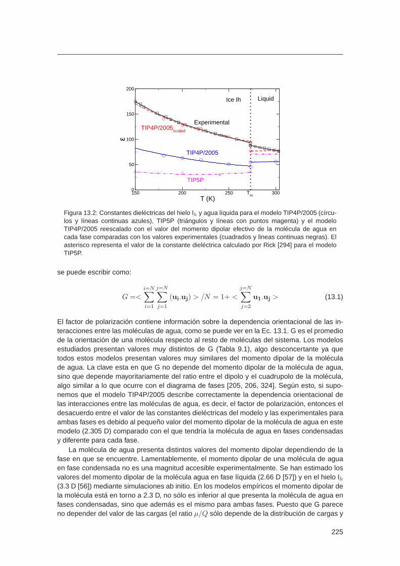
150 200 250 300T (K)
0
50
100
150
200
ε
Tm
LiquidIce Ih
Experimental
TIP4P/2005
TIP4P/2005scaled
TIP5P
Figura 13.2: Constantes dieléctricas del hielo Ih y agua líquida para el modelo TIP4P/2005 (círcu-los y líneas continuas azules), TIP5P (triángulos y líneas con puntos magenta) y el modeloTIP4P/2005 reescalado con el valor del momento dipolar efectivo de la molécula de agua encada fase comparadas con los valores experimentales (cuadrados y lineas continuas negras). Elasterisco representa el valor de la constante dieléctrica calculado por Rick [294] para el modeloTIP5P.
se puede escribir como:
G =<i=N∑
i=1
j=N∑
j=1
(ui.uj) > /N = 1+ <
j=N∑
j=2
u1.uj > (13.1)
El factor de polarización contiene información sobre la dependencia orientacional de las in-teracciones entre las moléculas de agua, como se puede ver en la Ec. 13.1. G es el promediode la orientación de una molécula respecto al resto de moléculas del sistema. Los modelosestudiados presentan valores muy distintos de G (Tabla 9.1), algo desconcertante ya quetodos estos modelos presentan valores muy similares del momento dipolar de la moléculade agua. La clave esta en que G no depende del momento dipolar de la molécula de agua,sino que depende mayoritariamente del ratio entre el dipolo y el cuadrupolo de la molécula,algo similar a lo que ocurre con el diagrama de fases [205, 206, 324]. Según esto, si supo-nemos que el modelo TIP4P/2005 describe correctamente la dependencia orientacional delas interacciones entre las moléculas de agua, es decir, el factor de polarización, entonces eldesacuerdo entre el valor de las constantes dieléctricas del modelo y las experimentales paraambas fases es debido al pequeño valor del momento dipolar de la molécula de agua en estemodelo (2.305 D) comparado con el que tendría la molécula de agua en fases condensadasy diferente para cada fase.
La molécula de agua presenta distintos valores del momento dipolar dependiendo de lafase en que se encuentre. Lamentablemente, el momento dipolar de una molécula de aguaen fase condensada no es una magnitud accesible experimentalmente. Se han estimado losvalores del momento dipolar de la molécula agua en fase líquida (2.66 D [57]) y en el hielo Ih(3.3 D [56]) mediante simulaciones ab initio. En los modelos empíricos el momento dipolar dela molécula está en torno a 2.3 D, no sólo es inferior al que presenta la molécula de agua enfases condensadas, sino que además es el mismo para ambas fases. Puesto que G pareceno depender del valor de las cargas (el ratio µ/Q sólo depende de la distribución de cargas y
225

13. Discusión integradora
no de su valor), podemos aumentar el momento dipolar de la molécula de agua en el modelosin estropear la descripción de las interacciones entre las moléculas (G). Reescalando losvalores de las constantes dieléctricas dadas por el modelo TIP4P/2005 con los valores delmomento dipolar que tendría la molécula de agua en cada fase (µeff ), los resultados estáncuantitativamente en concordancia con los resultados experimentales (Fig. 13.2). Lo mismoocurre reescalando la constante dieléctrica de las distintas fases de hielo con el momento di-polar de la molécula de agua en fase sólida (Fig. 9.7). En vista de estos resultados, podemosdecir que el modelo TIP4P/2005 no es capaz de reproducir el valor de la constante dieléctricade las distintas fases de agua. No obstante captura la dependencia orientacional de las in-teracciones en el agua. Esto quiere decir que el modelo contiene la física de las propiedadeseléctricas del agua, pero no reproduce cuantitativamente el valor de la constante dieléctricaporque el momento dipolar del modelo es el mismo para todas las fases (no es polarizable) einferior al valor de µH2O real del agua en fases condensadas.
La constante dieléctrica se puede calcular también mediante la respuesta de polarizaciónde un sistema a un campo eléctrico. Dependiendo de la dirección de aplicación del campo,es posible resolver la anisotropía de la constante dieléctrica. Comprobamos que las constan-tes dieléctricas que se obtienen por el método de fluctuaciones y el de respuesta lineal sonequivalentes (Tabla 10.1), y además resolvimos el tensor dieléctrico para los distintos hielos.El hielo Ih no presenta anisotropía de la constante dieléctrica, mientras que los hielos III, Vy VI son marcadamente anisotrópicos. La anisotropía en el tensor dieléctrico es relevante enel caso de aplicación de un campo eléctrico, ya que la energía de interacción con el campodependerá de la orientación del campo respecto al cristal. La anisotropía de la constante die-léctrica es una propiedad que todavía no ha sido medida experimentalmente, y esperamosque este trabajo anime a verificar los resultados aquí pronosticados.
Sabemos que el modelo TIP4P/2005 reproduce de forma cualitativa las propiedades eléc-tricas del agua. Estas predicciones pueden hacerse cuantitativas usando los valores del mo-mento dipolar de la molécula de agua en fase condensada. Esto es posible gracias a queel factor de polarización (G), ecuación (14.1), parece depender principalmente del cocientedipolo/cuadrupolo (µ/Q). Así que si aumentamos las cargas del modelo, G no cambia perosí aumenta el momento dipolar del modelo y podemos reproducir cualitativamente la cons-tante dieléctrica de las distintas fases de agua. Con toda esta información y las técnicas quehabíamos puesto a punto, decidimos estudiar el efecto que tiene aplicar un campo eléctricosobre el equilibrio de fases del agua.
Los campos eléctricos modifican las propiedades de todas las fases de la materia pero endiferente extensión, y por lo tanto, modifican los límites de coexistencia de fases. En presenciade un campo eléctrico las moléculas del sistema tienden a alinear sus dipolos con la direccióndel campo, y ésta interacción con el campo modifica la energía libre del sistema, en diferenteextensión según la fase. En presencia de un campo eléctrico (E) los cambios de la energíainterna del sistema (K + Vinter) se pueden escribir como:
dU = T dS − p dV +E dM+ µ dN (13.2)
donde M es momento dipolar total del sistema y E es el campo eléctrico microscópico, ge-neralmente distinto del campo aplicado o macroscópico (Eext) debido a la polarización desuperficie de la cavidad, que depende de su geometría y la anisotropía de la constante die-léctrica. En presencia de un campo eléctrico podemos definir un nuevo potencial termodi-námico GE = G − E·M (transformada de Legendre de G) que sólo depende de variables
226

intensivas del sistema, y se hace mínimo en el equilibrio para un sistema cerrado y a presión,temperatura y campo eléctrico constante. En presencia de un campo eléctrico dos fases deuna sustancia pura estarán en equilibrio cuando sus potenciales químicos sean iguales a T,p y Eext constantes. Así, para un sistema de moléculas rígidas en el colectivo donde N, p, T,Eext son constantes, GE viene dado por (después de integrar sobre los momentos):
GE [Eext] = −kBT ln(Q(N, p, T,Eext)) =
= −kBT ln[qN
N !
∫exp[−β(Vinter + pV −MEex + Upol))]dr
NdV ] (13.3)
Upol es la energía de interacción del sistema con la superficie polarizada, que bajo condi-ciones de contorno periódicas conductoras se anula, y E y Eex se igualan. Para evaluar loscambios de GE bajo la influencia de un campo eléctrico, diferenciamos GE respecto a Eex:
GE(Eex)−GE(0) = −∫ Eex
E=0< M‖ >N,p,T,Eex dEex (13.4)
Esto quiere decir que, conocidas las condiciones de coexistencia entre dos fases en ausenciadel campo, y determinando la polarización en la dirección del campo eléctrico, podemos cal-cular la integral de la ecuación 13.4 y determinar el cambio de energía libre para cada fase.Entonces, mediante integración termodinámica en el espacio p, T localizamos el nuevo puntode coexistencia de fases. Con este nuevo punto de coexistencia entre fases en presencia deun campo, podemos calcular las líneas de coexistencia mediante integración Gibbs-Duhem.
De esta manera hemos calculado el diagrama de fases para el modelo TIP4P/2005 en pre-sencia de un campo eléctrico (Fig. 13.3). El efecto más notable de aplicar un campo eléctricoes que el hielo II (fase ordenada de protón, ǫ ≈ 5), con una destacada región de estabili-dad, desaparece del diagrama de fases. Sabiendo que para obtener resultados cuantitativoscon el modelo TIP4P/2005 es necesario usar el momento dipolar efectivo de la molécula deagua para cada fase, recalculamos el diagrama de fases en presencia de un campo eléctricousando µH2O = 2.66 D para la fase líquida y µH2O = 3.32 D para las fases sólidas. Deesta manera, las predicciones sobre el efecto de un campo eléctrico en el equilibrio de fasesdel agua serán mucho más realistas (Fig. 10.2). La curva de coexistencia líquido–Ih no seve apenas afectada cuando aplicamos un campo eléctrico (la constante dieléctrica de ambasfases es prácticamente la misma). En el hielo Ih, desde el punto de vista de la constante die-léctrica aproximadamente isotrópico, la línea de coexistencia con el líquido no se ve afectadapor la dirección de aplicación del campo. En cambio, para el resto de hielos, con una marcadaanisotropía en ǫ, los efectos del campo dependen de la dirección de aplicación. Cuando apli-camos el campo en la dirección perpendicular al plano ab de los distintos sólidos, los hielos III,V y VI aumentan su región de estabilidad respecto al líquido alrededor de 15 K. Sin embargo,cuando el campo eléctrico es aplicado en la dirección perpendicular al plano cristalográfico acde los hielos (a lo largo de esta dirección la componente dieléctrica es mínima para todos lohielos), el hielo III desaparece del diagrama de fases en beneficio del hielo Ih, cuya constantedieléctrica es casi isotrópica. En estas condiciones, los V y VI ceden terreno al líquido. Tam-bién se evaluó el efecto de aplicar un campo eléctrico sobre el equilibrio líquido–vapor y latemperatura del máximo en densidad (TMD) (Fig. 10.3). El campo eléctrico no tiene un granefecto sobre las fases fluidas. En presencia de un campo eléctrico la densidad del líquido au-menta levemente y desciende la del vapor, con lo que la temperatura crítica aumenta 5 K. Enla misma extensión se reduce la TMD, debido al alineamiento preferencial de las moléculascon el campo, lo que conlleva una reducción del orden tetraédrico y aumento de la densidad.
227

13. Discusión integradora
175 200 225 250 275T / K
0
2
4
6
8
10
12
p / k
bar
Eex
= 0
Eex ac
Eex ac
(µ scaled)
175 200 225 250 275T / K
2
4
6
8
10
12E
ex = 0
Eex ab
Eex ab
(µ scaled)
Ih
V
VI
LiquidIII Liquid
V
VI
III
Ih
IIII
Figura 13.3: Diagrama de fases del modelo TIP4P/2005. La líneas negra de puntos, azul disconti-nua, magenta continua, roja discontinua y verde continua indican los límites de fase para Eex = 0,Eex⊥ac = 0.3 V/nm con µeff , Eex⊥ac = 0.3 V/nm y con reescalado del momento dipolar usando2.66 y 3.32 D para el líquido y las fases sólidas, Eex⊥ab = 0.3 V/nm con µeff y Eex⊥ab = 0.3 V/nmy reescalado dipolar, respectivamente.
La consecuencia fundamental de la alta constante dieléctrica del agua es su capacidadpara disociar sales. Así que el siguiente paso fue el estudio de las disoluciones de sales enagua, empezando por la sal más común, el cloruro sódico. La disolución más común del pla-neta y fundamental desde el punto de vista biológico. Para ello, es fundamental determinar lasolubilidad de esta sal en agua para distintos modelos de potencial.
Usando la metodología propuesta por Sanz y Vega [137] hemos calculado la solubilidadde disoluciones de NaCl en agua SPC/E usando tres modelos de potencial para el NaCl: losmodelos de Tosi–Fumi, Smith–Dang y Joung–Cheatham. En primer lugar se calculó el po-tencial químico del NaCl sólido con el método del cristal de Einstein (Sección 5.1.4). Para elcálculo del potencial químico del NaCl en disolución se llevó a cabo integración termodinámi-ca hamiltoniana (Sección 5.1.2) desde la disolución hasta un sistema con interacciones tipoLennard–Jones, sistema de referencia para el que conocemos la energía libre de Gibbs. Secalculó la energía libre de Gibbs para varias disoluciones con diferente número de moléculasde sal y el mismo número de moléculas de agua, y así obtuvimos el el potencial químico,µ =
(GN
)T,p,NH2O
, de la sal en disolución. Con esto pudimos calcular la solubilidad de NaCl
en agua para los tres modelos de potencial de NaCl en agua SPC/E. La solubilidad es laconcentración para la que se igualan los potenciales químicos del NaCl sólido y del NaCl endisolución. Para comprobar que los resultados obtenidos con esta metodología eran correc-tos calculamos la solubilidad del NaCl usando la técnica de coexistencia directa. Para ellopusimos en contacto un bloque NaCl sólido con una disolución supersaturada de NaCl enagua. Se llevaron a cabo simulaciones NpT de dinámica molecular hasta alcanzar el equi-librio. Los iones difunden desde la disolución supersaturada hacia el NaCl sólido hasta quese alcanza el equilibrio. En el equilibrio, la concentración de NaCl en disolución marcará lasolubilidad del modelo de potencial. El equilibrado de este sistema fue extremadamente largoya que la disolución estaba altamente supersaturada. La simulaciones tuvieron una duraciónde aproximadamente 3 µs.
228

Los valores de solubilidad de NaCl en agua obtenidos por ambas técnicas se dan en laTabla (11.9). Los resultados que hemos obtenido mediante el cálculo de energías libres dela disolución y con la técnica de coexistencia directa están en buena concordancia, teniendoen cuenta las barras de error. Las diferencias podrían ser debidas a dos factores. El primeroes que en las simulaciones de coexistencia directa no se haya alcanzado el equilibrio al finalde la simulación. Al principio, cuando la disolución está supersaturada, los iones difundenfácilmente de la disolución al sólido, pero cuando la concentración va disminuyendo, el dri-ving force (∆µi) es menor y se requiere más tiempo para alcanzar el equilibrio. El segundoes que los cálculos de energía libre se han llevado a cabo utilizando sistemas relativamen-te pequeños (270 moléculas de agua) con el objetivo de poder comparar con los resultadosdisponibles en la literatura. De manera que podrían existir efectos de tamaño finito. No pue-de descartarse que al aumentar el tamaño del sistema aumentase la solubilidad. Teniendoen cuenta estos dos factores, el valor recomendado de la solubilidad de cada modelo es lamedia aritmética de los resultados de los dos métodos. Con en este trabajo creemos haberestablecido un valor de referencia que podrá ser utilizado en un futuro en el desarrollo de nue-vos métodos de simulación para determinar la solubilidad. Con lo aprendido en este trabajosobre las sales en disolución, sería tremendamente interesante parametrizar un modelo desal entorno al modelo de agua TIP4P/2005, el mejor modelo de agua rígido y no polarizable.
El cálculo de la solubilidad de una sal en agua requiere el cálculo del potencial quími-co de la sal sólida. Por tanto, el que un force field reproduzca la solubilidad de una sal enagua, no sólo depende de hacer predicciones razonables del potencial químico del solutoen disolución, también debe reproducir el potencial químico de la sal sólida. Puede ocurrir,como en el caso del modelo Tosi–Fumi, que predice valores del potencial químico de la salen disolución superiores al experimental pero también para el potencial químico de la salsólida, con lo que se obtiene un valor razonable de la solubilidad. Mientras que el modeloSmith–Dang, que predice un potencial químico del NaCl sólido muy próximo al experimental,predice valores de solubilidad extremadamente bajos. A concentraciones bajas, dominan lasinteracciones ion–agua, pero al aumentar la concentración las interacciones ion–ion empie-zan a ser importantes. Por todas estas razones es interesante comprobar que modelos depotencial reproducen las propiedades de la sal pura (interacciones ion–ion).
Para ello evaluamos las propiedades sólido–líquido de la sal pura. Calculamos la tempe-ratura de fusión del NaCl para los tres modelos de potencial estudiados: Tosi–Fumi, Smith–Dang y Joung–Cheatham. La temperatura de fusión del NaCl para el modelo Tosi–Fumi cal-culada está en buena concordancia con los valores que se encuentran en la literatura y conel valor experimental. Algo que no ocurre con los otros dos modelos tipo LJ estudiados parael NaCl.
Además del NaCl, existen más parámetros propuestos por Tosi y Fumi para otros halurosalcalinos monovalentes. Calculamos la Tf del resto de haluros alcalinos encontrando un com-portamiento irregular. Las predicciones para las sales KCl y NaBr son razonables (desviacio-nes de 15 K y 10 K, respectivamente). En cambio, para los haluros alcalinos que contienen losiones Rb o F (KF, RbBr, RbCl, RbF, LiF y NaF), las predicciones son malas, con desviacionesdel orden de 100 K. La razón para esto puede ser que el potencial de interacción Tosi–Fumies no polarizable, y no es capaz de capturar el alto carácter polarizante/polarizable de estosiones. En el caso de los modelos tipo Lennard–Jones (SD y JC), parece que no es posibledescribir con exactitud el NaCl con un modelo formado por cargas y un centro de interacciónLJ. Una posibilidad interesante que podría ser explorada es incluir desviaciones de las reglasde Lorentz–Berthelot para obtener las interacciones cruzadas entre los iones para ajustar latemperatura de fusión del NaCl, y luego ajustar las interacciones ion–agua para reproducir el
229

13. Discusión integradora
valor de la solubilidad.
Para terminar me gustaría contextualizar (en palabras menos amables, criticar) este traba-jo. Como se comentó al principio de esta tesis, en simulación se deben hacer aproximaciones.De manera que es importante saber que se está haciendo y hasta dónde se puede llegar an-tes de sacar conclusiones. Esto, que se aplica a los estudios de simulación, es general acualquier estudio científico. En este trabajo el agua se ha tratado como una molécula rígiday no polarizable. Ciertamente el agua es mucho más que unas cargas en una determinadaposición geométrica. El agua es flexible, posee una nube electrónica que se polariza en pre-sencia de otras moléculas, presenta marcados efectos cuánticos, etc. El objetivo de haceresta severa simplificación de la molécula de agua es aprender que características de la mo-lécula son importantes para según que propiedades. De esta manera podremos saber, y másimportante conocer, cuales son las características moleculares que determinan las fascinan-tes propiedades del agua. Es un primer paso hacia una descripción cada vez más realista delagua, pero como todo avance científico relevante, aprendiendo por el camino.
Resumiendo, soy muy consciente de que estos trabajos no son “la última palabra´´ en elestudio del agua. No obstante, creo que representan un avance en el campo. Casi la totali-dad de los trabajos de investigación se sostienen sobre alguna aproximación o axioma, y portanto son susceptibles de sufrir críticas. Las criticas más útiles son las que hacen mejorarun trabajo, y ojalá este trabajo sea muy criticable, y espero que las que las críticas permitanavanzar en la descripción de esta peculiar sustancia, el agua.
230

CAPÍTULO 14
Conclusiones
“Los momentos finales de una experienciadeterminan el recuerdo que tenemos de ella."
Daniel Kahneman
Como se ha mencionado al inicio de este trabajo, el agua es una sustancia tremenda-mente interesante e importante, y han sido muchas las lecciones que hemos aprendido alo largo de nuestros estudios. Aquí se recogen los estudios realizados en la región de altaspresiones del diagrama de fases del agua; el cálculo de propiedades dieléctricas de agua ehielos, y su impacto en el equilibrio de fases en presencia de un campo eléctrico; el cálculode la temperatura de fusión de haluros alcalinos monovalentes, y el estudio de la solubilidadde NaCl en agua. Además de las conclusiones propias de estos estudios, se han extraídootras conclusiones de carácter más general sobre el comportamiento de la molécula de aguaen fase condensada y el modelado de agua.
El agua exhibe un gran número de propiedades que la convierten en un líquido muyespecial. Pero igualmente fascinante es el increíble número de fases sólidas que se puedenformar. Por esta razón, y como ya anticipó Whalley en 1984 [33], en el modelado del aguano nos debemos olvidar de los hielos. Un buen modelo de agua, además de dar una buenadescripción del agua líquida, debe ser capaz de reproducir propiedades de sus fases sólidas.
Modelos sencillos como los aquí estudiados, 1 centro LJ y 3 cargas, son capaces de cap-turar buena parte de la física del agua. Gracias al estudio llevado a cabo en nuestro grupodurante todos estos años, hemos llegado a un esquema general de hasta donde podemosllegar con estos modelos y como se podrían mejorar cuando se incluyan características de lamolécula de agua que no han sido contempladas hasta la fecha. Esta manera de acercarsea la “respuesta final´´ es tremendamente útil, pues permite ir comprendiendo no sólo la físicade la molécula de agua, sino que además, al compartimentar el problema, podemos conectarpropiedades moleculares con características físicas. Este enfoque nos ha permitido determi-nar qué se puede esperar, dadas las características generales de un modelo. También hemosaprendido qué implicaciones tienen las aproximaciones realizadas, y cuales son los objetivosa alcanzar en futuros estudios.
Las principales conclusiones que se derivan de los trabajos presentados en esta tesis seenumeran a continuación:
1. El test de Whalley, propuesto para evaluar los modelos de agua utilizando las propie-dades de los hielos, es una herramienta fácil y rápida que permite tener una primeraestimación sencilla del diagrama de fases del agua y conocer la calidad de los resulta-dos de simulación sobre las fases sólidas del agua. Cualquier modelo o descripción dela molécula de agua que pretenda ser realista deberia proporcionar resultados acepta-bles en esta prueba.
2. Para los modelos de potencial rígidos y no polarizables estudiados, aparecen dos fasesde cristal plástico en la región de altas presiones del diagrama de fases a ≈ 440 K.

14. Conclusiones
Cuando se comprime agua líquida, esta cristaliza en una fase solida en pocos nano-segundos. La estructura sólida obtenida corresponde a una red cúbica centrada enel cuerpo (bcc) de moléculas de agua que rotan significativamente entorno a sus po-siciones de equilibrio, en definitiva un cristal plástico. También es posible transformarlos hielos VIII y VII en este tipo de cristal plástico mediante calentamiento. Estas tran-siciones se pueden entender como un aumento del desorden con la temperatura: elhielo VIII, ordenado de protón, se transforma en hielo VII (desordenado de protón) alcalentarse, y el hielo VII se transforma en un cristal plástico al calentarse, en el quelas moléculas rotan casi libremente entorno a las posiciones de equilibrio. En las tresestructuras las posiciones cristalográficas de los oxígenos son las mismas. La apari-ción de una fase de cristal plástico en esta región del diagrama de fases (alta presióny alta temperatura) se entiende, porque a estas presiones la interacción LJ mantienelas moléculas en sus posiciones de red, pero la alta temperatura rompe los enlacesde hidrógeno y las moléculas son capaces de rotar entorno a su posición de equilibrio.Si se comprime el cristal plástico de simetría bcc, se transforma mediante una transi-ción martensítica en un cristal plástico de simetría cúbica centrada en las caras (fcc). Yes esta fase de cristal plástico fcc la que domina el diagrama de fases a altas presiones.
3. Los modelos utilizados infraestiman la estabilidad del hielo VII, que es estable a presio-nes muy superiores a las experimentales para estos modelos. La estructura del hieloVII puede entenderse como dos redes cristalinas de hielo Ic (tipo diamante) interpene-tradas, de manera que cada molécula de agua tiene 8 moléculas vecinas a la mismadistancia, pero sólo forma enlace de hidrógeno con cuatro de ellas. La parte repulsivadel centro LJ ha sido ajustada para que la distancia del enlace de hidrógeno sea de2.82 Å. El enlace de hidrógeno, descrito por una interacción coulómbica, es fuertemen-te direccional. De manera que las moléculas que no forman enlace de hidrógeno con lacentral, están energéticamente perjudicadas debido a la parte repulsiva del LJ, lo quese traduce en una inestabilización de toda la estructura. De hecho, la densidad del hieloVII que predice el modelo TIP4P/2005 se desvía notablemente del valor experimentalhacia menores densidades. Las moléculas que no forman enlace de hidrógeno están“repelidas"por la parte repulsiva del potencial LJ a distancias superiores a las que seencuentran el el hielo VII. Según esto, de encontrarse experimentalmente alguna deestas fases de cristal plástico sería a presiones inferiores a las que predice el modeloTIP4P/2005, alrededor de 30000 bar.
4. Los hielos desordenados de protón presentan muchas posibles configuraciones de des-orden de protón compatibles con las reglas de Bernal-Fowler. Estas configuracionespresentan pequeñas diferencias en la energía; las diferencias de energía entre las dis-tintas configuraciones varían entre 0.1-0.2 NkBT para el hielo Ih, y ≈0.5 NkBT para elhielo III. Ciertas propiedades termodinámicas no varían mucho de una configuración aotra. Sin embargo cada una de estas configuraciones presenta una polarización muydistinta. Por esta razón, la constante dieléctrica de los hielos desordenados de protónes alta (fluctuaciones de la polarización del sistema). Para muestrear correctamente eldesorden de protón de hielos desordenados, es necesario incluir movimientos de rota-ción de anillos.
5. Los modelos de potencial no polarizables no son capaces de reproducir simultánea-
232

mente la constante dieléctrica del agua líquida y del hielo Ih. Sin embargo, los modelostipo TIP4P (TIP4P/2005 y TIP4P/Ice) predicen correctamente que ǫIh ≈ ǫlq a la tem-peratura de fusión, aunque fallan en la predicción cuantitativa. La constante dieléctricapuede expresarse en términos del factor de polarización (G):
ǫ = 1 +4πρ
3kTµ2G (14.1)
Se ha comprobado que el valor de G sólo depende del ratio entre el momento dipolar ycuadrupolar (G = G(µ/Q)). De manera que, incrementando el valor de las cargas sinmodificar su distribución, se modifica la constante dieléctrica pero no el valor de G. Gcontiene información sobre la dependencia orientacional de las interacciones del agua.Así, cuando las predicciones de G del modelo TIP4P/2005 son reescaladas con el mo-mento dipolar estimado para la molécula de agua en las distintas fases condensadas(µliqH2O
= 2.66 D y µsolH2O= 3.32 D) es capaz de reproducir el valor de la constante
dieléctrica de la fase fluida y de los hielos Ih, III, V y VI.
6. Aplicando un campo eléctrico a un sistema es posible calcular la constante dieléctricadel sistema a partir de la respuesta de polarización de sistema. Las ǫ calculados me-diante respuesta de polarización concuerdan con las obtenidas mediante fluctuaciones.La respuesta dependerá de la dirección de aplicación del campo en fases cristalinas a-nisotrópicas. Este es el caso del tensor dieléctrico de los hielos III, V y VI, que presentauna fuerte anisotropía. Sin embargo el hielo Ih no presenta anisotropía en el tensordieléctrico.
7. Los campos eléctricos modifican las propiedades de todas las fases, pero en distintamedida, de manera que cambia la localización de las transiciones de fase. El diagramade fases del agua presenta un gran número de polimorfos, y hemos estudiado como semodifican las transiciones de fase en presencia de un campo eléctrico. La lineas de co-existencia sólido-líquido no se ven muy afectadas en presencia de un campo eléctrico,ya que la constante dieléctrica del líquido y de los hielos son muy similares, de maneraque la respuesta a un campo eléctrico también. Los tránsitos más afectados son losque involucran a dos fases sólidas. El hielo II (ordenado de protón) en presencia de uncampo eléctrico desaparece del diagrama de fases del agua. Cuando el campo eléctri-co se aplica en la dirección donde el hielo III presenta la componente dieléctrica máspequeña, esta fase también desaparece del diagrama de fases en favor de los hielos Ihy V, que presentan mayor valor de la constante dieléctrica. El efecto de un campo eléc-trico sobre las fases fluidas es también pequeño. La temperatura crítica (Tc) aumenta enunos 5 K y la temperatura del máximo en densidad disminuye una magnitud muy similar.
8. Se ha determinado la temperatura de fusión del NaCl para tres potenciales de inter-acción ión-ión: Tosi-Fumi, Smith-Dang y Joung-Cheatham. El modelo Tosi-Fumi repro-duce una temperatura de fusión próxima a la experimental, al contrario que los otrosdos modelos. También se calculó la Tf de otros haluros alcalinos monovalentes para-metrizados para el modelo Tosi-Fumi y se encontró un comportamiento irregular. Laspredicciones para las sales KCl and NaBr son razonables (desviaciones de 15 K y 10 K,respectivamente). En cambio, para los haluros alcalinos que contienen los iones Rb oF (KF, RbBr, RbCl, RbF, LiF y NaF), las predicciones son malas, con desviaciones del
233

14. Conclusiones
orden de 100 K.
9. Por último, hemos calculado la solubilidad de NaCl en agua SPC/E para tres modelosde interacción ión-ión: Tosi-Fumi, Smith-Dang y Joung-Cheatham, mediante integracióntermodinámica hamiltoniana y coexistencia directa NaClsolid - NaClsolution. Se ha com-probado que el modelo Joung-Cheatham es claramente superior a los demás modelosestudiados en la predición de la solubilidad del NaCl en agua. El modelo JC es supe-rior para simulaciones de disoluciones de NaCl en agua, mientras que el modelo TF essuperior para simulaciónes de NaCl puro. Con ambos modelos, y lo aprendido en estostrabajos, tenemos un buen punto de partida para la obtención de un modelo de NaClque reproduzca tanto la solubilidad del NaCl en agua como la temperatura de fusión.
234

Parte IV
APÉNDICES

APÉNDICE A
Colectivo microcanónico (N,V,E)
Un sistema aislado con energia E (colectivo N,V,E) viene determinado mecano-cuánticamentepor el número de microestados del sistema, Ω(N,V,E). En un colectivo microcanónico to-dos los microestados son igualmente probables, de modo que si Ω(N,V,E) es el númerode microestados, la probabilidad de encontrar uno de ellos en el colectivo es pi = 1
Ω(N,V,E) .Supongamos un sistema formado por N moléculas, un volumen V y una energía E, y que estadividido en dos subsistemas de energía E1 y E − E1. Entonces, la degeneración del primersubsitema será Ω(E1) y la del segundo Ω(E − E1). Por tanto, el número de formas de tenerenergía E1 en cada uno de los subsistemas será:
Ω(E1, E − E1) = Ω(E1)Ω(E − E1) (A.1)
Como todos los microestados son igualmente probables, el valor mas probable deE1 seráaquel al que le correspondan mayor número de microestados. Para hallar este punto, deriva-mos en la ecuación (D.3), que al ser un producto es más cómodo trabajar con logarítmos:
∂lnΩ(E1, E − E1)
∂E1=∂lnΩ(E1)
∂E1+lnΩ(E − E1)
∂(E − E1)
∂(E − E1)
∂E1(A.2)
∂lnΩ(E1)
∂E1=
∂lnΩ(E2)
∂(E2)(A.3)
β(N1, V1, E1) = β(N2, V2, E2) (A.4)
La condición de equilibrio establece que si la energíaE1es inicialmente grande, la energíafluirá hasta alcanzar el equilibrio, y viceversa. Análogamente, la termodinámica nos indica queel equilibrio se alcanza al maximizar la entropía, en tal caso se obtiene que ( ∂S∂E = 1
T ):
(∂S
∂E
)
1
=
(∂S
∂E
)
2
(A.5)
1
T1=
1
T2(A.6)
Entonces, se puede observar que la funcion lnΩ cumple las mismas propiedades que lafunción entropía:
1. Al extremarse da lugar al equilibrio del sistema.
2. Se corresponde a una propiedad β, igual en cada subsistema
3. β es una derivada respecto a la energía
4. Es máxima en el equilibrio para N,V,E.

A. Colectivo microcanónico (N,V,E)
Por tanto, a partir de la función de partición, Ω(N,V,E) =∑pi, podemos establecer una
relación con la termodinámica:
S = kBlnΩ (A.7)
de donde además se deduce que, β = 1/kBT
238

APÉNDICE B
Colectivo canónico (NVT)
El colectivo microcanónico, aunque es el más fundamental, es poco útil desde el puntode vista operativo. Asi que es necesario adaptar el colectivo a variables termodinámicas masaccesibles. El caso más inmediato es el de las variables de control N,V,T. Esto corresponde aun sistema que está acoplado con un termostato que permite intercambio de energía. Hay in-tercambio de energía con el entorno y el sistema podría adoptar cualquier valor de la energíaEi con probabilidad pi. La distribución de energias que maximiza el desorden vendrá dadapor las ligaduras:
L1 =∑
pi − 1 = 0 (B.1)
L2 =∑
Eipi = E (B.2)
Entonces tenemos que:
dS + λdL1 + βdL2 = 0 (B.3)
dS = −kB∑
(lnpi + 1)dpi (B.4)
dL1 =∑
dpi (B.5)
dL2 =∑
Eidpi (B.6)
Resolvemos,
∑(kBlnpi + kB + λ+ βEi)dpi = 0 (B.7)
de aqui tras despejar pi:
pi = e−1e−λe−βEi
kB (B.8)
Aplicando la ligadura 1,
∑pi − 1 = e−1e−λ
∑e−βEi
kB = 0 (B.9)
luego
e−1e−λ =1
∑e−βEi
kB
(B.10)

B. Colectivo canónico (NVT)
pi =e−βEi
kB
∑e−βEi
kB
=e−βEi
kB
Z(B.11)
Para resolver la ligadura 2, escribimos la entropía en función de la pi obtenida con laligadura 1:
− S
kB=
∑pilnpi =
1
Z
∑e
−βEikB (−βEi
kB− lnZ)
= −βEkB
− kBlnZ
−S = −βE − kBlnZ (B.12)
Comparando la ecuación (B.12) con la ecuación de la termodinámica, A = U − TS,podemos deducir por analogía que:
−S = −βE − kBlnZ (B.13)
−S =U
T− A
T(B.14)
De lo que se deduce que, β = 1/kBT y A = −kBT lnZ. Es decir, la distribución canónicaes aquella que maximiza el valor de la entropía bajo la condición de una energía promediodel sistema.
240

APÉNDICE C
Teorema de divergencia
La integral de la divergencia de un vector sobre un volumen V es igual a la integral desuperficie de la componente normal del vector sobre la superficie que limita V:
∫
VdivFdv =
∮
SF · nda (C.1)
Consideremos un volumen que se subdivide en un gran número de celdas. Sea ∆Vi elvolumen de la i-é sima celda que esta limitada por la superficie Si. Entonces:
∑
i
∮
Si
F · nda =
∮
SF · nda (C.2)
donde en cada integral de la izquierda la normal se dirige hacia fuera del volumen considera-do. Puesto que el sentido hacia fuera de una celda es el sentido hacia dentro de adyacente,todas las contribuciones del primer miembro de la Ec. C.3 se anulan excepto aquellas queprovienen de la superficie, demostrandose la ecuación. El teorema de divergencia se obtienehaciendo que el número de celdas se aproxime infinito, de modo que el volumen de cadacelda tienda a cero.
∑
i
∮
Si
F · nda = lım∆Vi→0
∑
i
(1
∆Vi
∮
SF · n
)∆Vida (C.3)

C. Teorema de divergencia
242

APÉNDICE D
Transformación de la ecuación 3.5
Vamos a transformar la ecuación 3.5 en una forma diferente
φ(r) =1
4πǫ0
∫
V0
P(r′)(r− r′)| r− r′ |3 dv′ (D.1)
Como | r− r′ | viene dado por:
| r− r′ |=√(x− x′)2 + (y − y′)2 + (z − z′)2 (D.2)
entonces
∇′(
1
| r− r′ |
)=
| r− r′ || r− r′ |3 (D.3)
por aplicación directa del operador gradiente en coordenadas cartesianas (derivadas respectoa r′). El integrando de la ecuación 3.5 puede transformase mediante D.3:
P(r′)(r− r′)| r− r′ |3 = P · ∇′
(1
| r− r′ |
)(D.4)
Consideremos la siguiente identidad vectorial sobre la ecuacion D.4,
∇′ · (fF) = f∇′ · F+ F · ∇′f (D.5)
donde f es cualquier función puntual escalar y F es una función puntual vectorial arbitraria. Si
aplicamos esta identidad (Ec. D.5) sobre la ecuación D.4, suponiendo f =(
1|r−r′|
)y F = P
se obtiene:P(r′)(r− r′)| r− r′ |3 = ∇′ ·
(P
| r− r′ |
)− 1
| r− r′ |∇′ ·P (D.6)
Finalmente, el potencial 3.5 puede expresarse como:
φ(r) =1
4πǫ0
∫
V0
(−∇′P) dv′
| r− r′ | +1
4πǫ0
∮
S0
P · nda′| r− r′ | (D.7)
donde la integral de volumen ∇′ ·(
P|r−r′|
)ha sido sustituida por una integral de superficie
aplicando el teorema de divergencia (ver apéndice C), y n es la normal hacia afuera delelemento de superficie da′.

D. Transformación de la ecuación 3.5
244

APÉNDICE E
Propiedades de la función Gaussiana
f(x) =1√2πσ
e−(x−x0)
2
2σ2 (E.1)
Si f(x) está centrada en 0, normalizada y a= 12σ2 .
f(x) =(aπ
)1/2e−ax2
(E.2)
∫ ∞
0f(x)dx =
1
2(E.3)
Entonces y, haciendo a = r2:
2√π
∫ ∞
0e−r2x2
dx =1
r(E.4)

E. Propiedades de la función Gaussiana
246

APÉNDICE F
Cambio de variable en la integral dela ec. (4.5)
∫ ∞
0e−r2ijρ
2
dρ (F.1)
Dividimos esta integral en dos partes:∫ ∞
0e−r2ijρ
2
dρ =
∫ g
0e−r2ijρ
2
dρ+
∫ ∞
ge−r2ijρ
2
dρ (F.2)
Haciendo el cambio de variable y = rρ, cuando ρ = g, y = rg:∫ ∞
ge−r2ρ2dρ =
1
r
∫ ∞
rge−y2dy (F.3)
Multiplicando y dividiendo por 2√π
:∫ ∞
ge−r2ρ2dρ =
1
r
∫ ∞
rge−y2dy(2/(π1/2))((π1/2)/2) (F.4)
donde podemos ver la función error complementaria (ver G):
∫ ∞
ge−r2ρ2dρ =
√π
2rerfc(rg) (F.5)

F. Cambio de variable en la integral de la ec. (4.5)
248

APÉNDICE G
Función error
f(x) =1√2πσ
e−(x−x0)
2
2σ2 (G.1)
Cuando x0 es cero y σ es 1, la función error es:
erf(x) = 2
∫ x
0
1√2πe−
x2
2 dx (G.2)
Haciendo un cambio de variable x′ = x√2
erf(x) = 2
∫ x′
0
1√2πe−
x′2
2
√2dx′ (G.3)
Obtenemos la función error:
erf(x) =2√π
∫ x′
0e−
x′2
2 dx′ (G.4)
De donde se deduce la complementaria de la función error:
erfc(x) =2√π
∫ ∞
x′
e−x′2
2 dx′ (G.5)
Para la función error y su complementaria se cumple que:
erf(x) + erfc(x) = 1 (G.6)
Como se puede ver en la Figura G.1 la función erfc(x) decae más rápidamente con xque la función 1
x . Por esta razón, la convergencia del sumatorio de E2 (ecuación (4.6)) es másrápida que en el caso de (4.4).
0
0.2
0.4
0.6
0.8
1
0 1 2 3 4 5
f(x)
x
1-erf(x)erf(x)
1/x
Figura G.1: Funciones erf(x), erfc(x) y 1/x.

G. Función error
250

APÉNDICE H
Vectores de espacio recíproco
Los vectores del espacio recíproco vienen dados por:
−→G = h
−→A + k
−→B + l
−→C (H.1)
donde h,k y l son enteros y−→A ,
−→B y
−→C son los vectores de la red recíproca y vienen
dados por:
−→A = 2π
−→b ×−→c
−→a · −→b ×−→c(H.2)
−→B = 2π
−→c ×−→a−→a · −→b ×−→c
(H.3)
−→C = 2π
−→a ×−→b
−→a · −→b ×−→c(H.4)
−→a ,−→b y −→c son los vectores de caja. No es casualidad que se denoten como hkl, ya que
la reflexión de los planos hkl ocurre en la dirección del punto−→G de la red reciproca obtenido
con los valores hkl.

H. Vectores de espacio recíproco
252

APÉNDICE I
Demostración del teorema 4.7
Se define la transformada de Fourier en una dimensión como:
f(k) =1√2π
∫ ∞
−∞f(x)e−ikxdx (I.1)
Una transformada de Fourier asocia una función f(x) con otra función f(k), que se ob-tiene mediante la ecuación (I.1). La utilidad de las transformadas de Fourier es que, conocidala función f(k), podemos averiguar cual es la función f(x) de la que viene mediante:
f(x) =1√2π
∫ ∞
−∞f(k)eikxdk (I.2)
Se puede comprobar (ver Kregszig, pag. 613) que la transformada de Fourier de unagaussiana es otra gaussiana:
f(k) =1√2π
∫ ∞
−∞e−ax2
eikxdx (I.3)
f(k) =1√2ae−
k2
4a (I.4)
Esta transformada de Fourier que hemos definido en una dimensión se puede extender a3 dimensiones:
f(k) =1√2π
∫ ∞
−∞f(−→r )e−ik·−→r (I.5)
donde −→r = (x, y, z) y k = (kx, ky, kz). Así, la transformada de Fourier de una gaussianaen tres dimensiones es:
2exp(−r2ijρ2)√π
=
∫exp(−k2/(4ρ2))exp(−ik · rij)dk
4π2ρ3(I.6)
Que para el sumatorio sobre las infinitas réplicas del sistema de las condiciones de con-torno periódicas es:
2√π
∑
l
exp(−rij2(l)ρ2) =
∫exp(−k2/(4ρ2))∑l exp(−ik · rij(l))dk
4π2ρ3(I.7)
Por otro lado, podemos descomponer rij(l) en (Figura I.1):
rij(l) = (rj(0)− ri(0)) + r(l) (I.8)

I. Demostración del teorema 4.7
l=0 l=1
i
j j
i
rij(l=0)rij(l=1)
Figura I.1: Esquema del vector rij en función de las réplicas del sistema
donde r(l) es el vector de translación de la red (contiene el orden del sólido). Si sustituimos(I.8) en la ecuación (I.7):
2√π
∑
l
exp(−r2ij(l)ρ2) =∫exp(−k2/(4ρ2))exp(ik.(rj(0)− ri(0))
∑l exp(ik.r(l))dk
4π2ρ3
(I.9)En esta ecuación (I.9), el sumatorio de la exponencial (exp(ik · r(l))), es la ecuación de
Laue sobre todas las réplicas del sistema. Este sumatorio es 0 a no ser que k·−→r valga nπ,es decir, es distinto de cero cuando miramos un punto de la red recíproca. De manera que:
∑
l
exp(ik.r(l)) =(2π)3
Vc
∑
G
δ(k−G) (I.10)
Y sustituyendo (I.10) en la ecuación (I.9):
2√π
∑
l
exp(−r2ij(l)ρ2) =2π∑
G
∫exp(−k2/(4ρ2))exp(ik.(rj(l = 0)− ri(l = 0))δ(k−G)dk
Vcρ3
(I.11)Haciendo uso de las propiedades de la función δ de Dirac, la ecuación (I.11) se simplifica
a:
2√π
∑
l
exp(−r2ij(l)ρ2) =2π∑
G exp(−G2/(4ρ2))exp(iG.(rj(l = 0)− ri(l = 0))
Vcρ3(I.12)
254

APÉNDICE J
Función de partición del cristal deEinstein con el centro de masas fijo
La contribución traslacional a la función de partición de un cristal de Einstein con el centrode masas fijo es:
QCMEin,t =
1
h3(N−1)
∫exp
[−β
N∑
i=1
p2i
2mi
]δ(
N∑
i=1
pi)dp1...dpN
∫exp
[−βΛE
N∑
i=1
(ri − rio)2
]δ(
N∑
i=1
µi(ri − rio))dr1...drN (J.1)
La integral sobre la parte de los momentos no es relevante para calcular energías libres y laincluiremos simplemente como un factor PCM :
PCM =1
h3(N−1)
∫exp
[−β
N∑
i=1
p2i
2mi
]δ(
N∑
i=1
pi)dp1...dpN (J.2)
Nos centraremos en la parte configuracional:
ZCMEin,t =
∫exp
[−βΛE
N∑
i=1
(ri − rio)2
]δ(
N∑
i=1
µi(ri − rio))dr1...drN (J.3)
Esta integral se puede expresar definiendo un cambio de variable de la forma, ri − rio = r′
i.El Jacobiano de esta transformación es 1, y la integral configuracional se puede reescribircomo:
ZCMEin,t =
∫exp
[−βΛE
N∑
i=1
(r′
i)2
]δ(
N∑
i=1
µir′
i)dr′
1...dr′
N (J.4)
donde la función de la delta de Dirac se define:
δ(N∑
i=1
µir′
i) =1
(2π)3
∫ ∞
−∞exp
[ik ·
(N∑
i=1
µir′
i
)]dk (J.5)
Así, la integral configuracional quedará de la forma:
ZCMEin,t =
1
(2π)3
∫exp
[−βΛE
N∑
i=1
((r
′
i)2 − ik
βΛE· µir
′
i
)]dkdr
′
1...dr′
N (J.6)
Jugando un poco con el contenido del sumatorio de la integral se obtiene:
(r′
i)2 − ik
βΛE· µir
′
i = (r′
i)2 − 2ik
2βΛE· µir
′
i +i2k2µ2i4β2Λ2
E
− i2k2µ2i4β2Λ2
E
(J.7)
=
(r′
i −ikµi2βΛE
)2
+k2µ2i4β2Λ2
E
(J.8)

J. Función de partición del cristal de Einstein con el centro de masas fijo
Por lo que:
ZCMein,t =
1
(2π)3
∫exp
[−βΛE
N∑
i=1
((r′
i −ikµi2βΛE
)2
+k2µ2i4β2Λ2
E
)]dkdr
′
1...dr′
N (J.9)
Ahora es conveniente realizar otro cambio de variable:
r′′
i = r′
i −ikµi2βΛE
(J.10)
Para hallar el jacobiano asociado a esta transformación supondremos el sistema más sencilloposible; un sistema con dimensionalidad uno y con dos partículas. El jacobiano, J , viene dadopor el siguiente determinante:
J =
∣∣∣∣∣∣∣∣∣∣
∂r′
1
∂r′′
1
∂r′
1
∂r′′
2
∂r′
1∂k
∂r′
2
∂r′′
1
∂r′
2
∂r′′
2
∂r′
2∂k
∂k
∂r′′
1
∂k
∂r′′
2
∂k∂k
∣∣∣∣∣∣∣∣∣∣
(J.11)
J =
∣∣∣∣∣∣∣
1 0 iµi
2βΛE
0 1 iµi
2βΛE
0 0 1
∣∣∣∣∣∣∣= 1 (J.12)
El determinante de una matriz triangular es el productorio de los elementos de la diagonal. Alvaler uno el jacobiano del cambio de variable, la integral queda simplificada a:
ZCMEin,t =
1
(2π)3
∫exp
[−βΛE
N∑
i=1
((r
′′
i )2 +
k2µ2i4β2Λ2
E
)]dkdr
′′
1 ...dr′′
N (J.13)
Separando en dos integrales:
ZCMEin,t =
1
(2π)3
∫exp
[−βΛE
N∑
i=1
(r′′
i )2
]dr
′′
1 ...dr′′
N
∫exp
[−k
2∑N
i=1 µ2i
4βΛE
]dk (J.14)
Ambas integrales son de tipo gausiano (∫∞−∞ exp(−ax2)dx =
√π/a), cuya solución es:
ZCMEin,t =
1
(2π)3
(π
βΛE
)N3/2(
4βπΛE∑Ni=1 µ
2i
)3/2
(J.15)
Haciendo un poco más de algebra se llega a:
ZCMEin,t =
(βΛE
π
)3/2( π
βΛE
)N3/2(
N∑
i=1
µ2i
)−3/2
(J.16)
o, sencillamente:
ZCMEin,t =
(π
βΛE
)3(N−1)/2(
N∑
i=1
µ2i
)−3/2
(J.17)
256

Así, se obtiene que la función de partición de un cristal de Einstein con el centro de masasfijo viene dado por:
QCMEin,t = PCM
(π
βΛE
)3(N−1)/2(
N∑
i=1
µ2i
)−3/2
(J.18)
Cuando todas las moléculas presentan la misma masa reducida, µi se reduce a 1/N . Portanto, la ecuación anterior se puede simplificar como:
QCMEin,t = PCM
(π
βΛE
)3(N−1)/2
(N)3/2 (J.19)
que corresponde con la expresión final para la energía libre de un cristal de Einstein conel centro de masas fijo. Una expresión explícita para PCM no es necesaria para el cálulode energías libres de un sólido ya que recordando la ecuación 5.54 se cancela con otrotérmino similar. Sin embargo, no es difícil obtener PCM realizando el mismo formalismo parala ecuación J.2 que el realizado para la ecuación J.3 (con µi = 1 y ΛE = 1/(2mi) y omitiendoel prefactor h3(N−1)). Lo que lleva a:
PCM =1
Λ3(N−1)N−3/2 (J.20)
Se obtiene que el cociente entre PCM/P adopta el valor de Λ3N−3/2. Si la ecuación J.20 sereemplaza por la ecuación J.19 se obtiene:
QCMEin,t =
1
Λ3(N−1)
(π
βΛE
)3(N−1)/2
(J.21)
257

J. Función de partición del cristal de Einstein con el centro de masas fijo
258

APÉNDICE K
Contribucion ideal al potencialquimico
El potencial quimico del NaCl en disolucion viene dado por la expresion:
µsolutionNaCl =
(∂Gsolution
∂NNaCl
)
T,p,NH2O
(K.1)
donde Gsolution es la energía libre de Gibbs (ver eq. 5.68). Hemos separado la Gsolution
en dos términos, el primero G1 = Aidsolution corresponde a la contribución de gas ideal a
la energía Helmholtz del sistema. El segundo, G2 contiene el resto de contribuciones a laenergía libre de Gibbs, la contribución residual a la energía Helmholtz del sistema y el términopVsolution. La contribución del término G1 al potencial químico se representara por µsolutionNaCl,1 yviene dada por:
µsolutionNaCl,1 =
(∂Aid
solution
∂NNaCl
)
T,p,NH2O
(K.2)
El término Aidsolution viene dado por la Ec. 11.11. Haciendo la derivada de Aid
solution res-pecto al número de moléculas de NaCl (NNaCl) a T y p constantes, se obtiene:
(∂(Aid
solution/kBT )
∂NNaCl
)
T,p,NH2O
= 2ln (ρNaCl)− 2 + V(2ρ′NaCl + ρ′H2O
)(K.3)
donde ρ′H2Orepresenta
(∂ρH2O
∂NNaCl
)T,p,NH2O
, siendo ρi =Ni
V el número en densidad del com-
ponente i. El término ρ′H2Opuede escribirse como:
(∂ρH2O
∂NNaCl
)
T,p,NH2O
=
∂(NH2O
V
)T,p,NH2O
∂NNaCl= −
NH2O
(∂V
∂NNaCl
)T,p,NH2O
V 2= −NH2OV
V 2
(K.4)donde V representa el volumen del sistema y V el volumen molar parcial de NaCl. Igualmente,
el término ρ′NaCl, que corresponde a(
∂ρNaCl
∂NNaCl
)T,p,NH2O
, se puede escribir como:
(∂ρNaCl
∂NNaCl
)
T,p,NH2O
=1
V− NNaClV
V 2(K.5)
Teniendo en cuenta las expresiones para ρ′NaCl y ρ′H2Oel último término de la Ec. K.3 se
puede escribir como:
(2ρ′NaCl + ρ′H2O
)=
1
V
(−2NNaClV
V− NH2OV
V+ 2
)(K.6)

K. Contribucion ideal al potencial quimico
así que la expresión final para µsolutionNaCl,1 es:
(∂(Aid/kBT )
∂NNaCl
)
T,p,NH2O
= 2ln (ρNaCl)− V (2ρNaCl + ρH2O) (K.7)
260

Bibliografía
[1] C.N. Pace, B.A. Shirley, M. McNutt, and K. Gajiwala. Forces contributing to the confor-mational stability of proteins. FASEB J., 10:75–83, 1996.
[2] C.N. Pace, S. Trevino, E. Prabhakaran, and J.M. Scholt. Protein structure, stability andsolubility in water and other solvent. Phil. Trans. R. Soc. Lond. B, 359:1225–1235, 2004.
[3] Y. Pocker. Water in enzyme reactions: biophysical aspects of hydration-dehydrationprocesses. Cell Mol Life Sci., 57:1008, 2000.
[4] J. P. Poirier. Rheology of ices: a key to the tectonics of the ice moons of Jupiter andSaturn. Nature, 299:683, 1982.
[5] F. Franks. Water a matrix of life. Royal Society of Chemistry, Cambridge, 2000.
[6] P. Ball. Life’s Matrix. A biography of Water. University of California Press, Berkeley,2001.
[7] Karl Popper. The Logic of Scientific Discovery. 1959.
[8] J. D. Bernal and R. H. Fowler. A theory of water and ionic solutions, with particularreference to hydrogen and hydroxyl ions. J. Chem. Phys., 1:515–548, 1933.
[9] N. Metropolis, A. W. Rosenbluth, M. N. Rosenbluth, A. H. Teller, and E. Teller. Equationof state calculations by fast computing machines. J. Chem. Phys., 21:1087, 1953.
[10] J. A. Barker and R. O. Watts. Structure of water; a monte carlo calculation. Chem.Phys. Lett., 3:144, 1969.
[11] Aneesur Rahman and Frank H. Stillinger. Molecular dynamics study of liquid water. J.Chem. Phys., 55:3336, 1971.
[12] Michael D. Morse and Stuart A. Rice. Tests of effective pair potentials for water: Predic-ted ice structures. J. Chem. Phys., 76:650, 1982.
[13] Georgios C. Boulougouris, Jeffrey R. Errington, Ioannis G. Economou, Athanassios Z.Panagiotopoulos, and Doros N. Theodorou. Molecular simulation of phase equilibria forwater-n-butane and water-n-hexane mixtures. J. Phys. Chem. B, 104:4958, 2000.
[14] M. Lisal, W. R. Smith, and I. Nezbeda. Accurate vapour–liquid equilibrium calculationsfor complex systems using the reaction gibbs ensemble Monte Carlo simulation method.Fluid Phase Equilib., 181:127–146, 2001.
[15] I. F. Will Kuo, C. J. Mundy, B. L. Eggimann, M. J. McGrath, J. I. Siepmann, B. Chen,J. Vieceli, and D. J. Tobias. Structure and dynamics of the aquous liquid-vapor interface:a comprehensive particle based simulation study. J. Phys. Chem. B, 110:3738, 2006.
[16] G. T. Gao, X. C. Zeng, and Hideki Tanaka. The melting temperature of proton-disorderedhexagonal ice: A computer simulation of 4-site transferable intermolecular potential mo-del of water. J. Chem. Phys., 112:8534, 2000.

Bibliografía
[17] Yuji Koyama, Hideki Tanaka, Guangtu Gao, and X.C.Zeng. Melting points and ther-mal expansivities of proton-disordered hexagonal ice with several model potentials. J.Chem. Phys., 121:7926–7931, 2004.
[18] Hiroki Nada and Jan P. J. M. van der Eerden. An intermolecular potential model for thesimulation of ice and water near the melting point: A six-site model of h2o. J. Chem.Phys., 118:7401, 2003.
[19] Margot J. Vlot, Jan Huinink, and Jan P. van der Eerden. Free energy calculations onsystems of rigid molecules: An application to the tip4p model of h2o. J. Chem. Phys.,110:55, 1999.
[20] O. A. Karim and A. D. J. Haymet. The ice/water interface: A molecular dynamics simu-lation study. J. Chem. Phys., 89:6889–6896, 1988.
[21] B. F. Nicholson, P. Clancy, and S. W. Rick. The interface response function and meltingpoint of the prism interface of ice i-h using a fluctuating charge model (tip4p-fq). Journalof Crystal Growth, 293:78, 2006.
[22] E. Sanz, C. Vega, J. L. F. Abascal, and L. G. MacDowell. Phase diagram of water fromcomputer simulation. Phys. Rev. Lett., 92:255701, 2004.
[23] G. Tammann. Kristallisieren und Schmelzen. Johann Ambrosius Barth, Leipzig, 1903.
[24] P. W. Bridgman. The phase diagram of water to 45000 kg/cm2. J. Chem. Phys., 5:964,1937.
[25] C. G. Salzmann, P. G. Radaelli, A. Hallbrucker, E. Mayer, and J. L. Finney. The pre-paration and structures of hydrogen ordered phases of ice. Science, 311:1758–1761,2006.
[26] G. A. Tribello, B. Slater, and C. G. Salzmann. A blind structure prediction of ice xiv. J.Am. Chem. Soc., 128:12594, 2006.
[27] C. J. Fennell and J. D. Gezelter. Computational free energy studies of a new ice poly-morph which exhibits greater stability than ice i-h. Journal of Chemical Theory andComputation, 1:662, 2005.
[28] C.G. Salzmann, P.G. Radaelli, E. Mayer, and J.L. Finney. Ice xv: A new thermodynami-cally stable phase of ice. Phys. Rev. Lett., 103:105701, 2009.
[29] J. L. Aragones, M. M. Conde, E. G. Noya, and C. Vega. The phase diagram of waterat high pressures as obtained by computer simulation of the tip4p/2005 model: theapparence of a plastic crystal phase. Phys. Chem. Chem. Phys., 11:543–555, 2009.
[30] J.L. Aragones and C. Vega. Plastic crystal phases of simple water models. J. Chem.Phys., 130:244504, 2009.
[31] E. Schwegler, M. Sharma, F. Gygi, and G. Galli. Melting of ice under pressure. Proc.Natl. Acad. Sci., 105:14779, 2008.
[32] M. Benoit, D. Marx, and M. Parrinello. Tunnelling and zero-point motion in high-pressureice. Nature, 392:258, 1998.
262

Bibliografía
[33] E. Whalley. Energies of the phases of ice at zero temperature and pressure. J. Chem.Phys., 81:4087–4092, 1984.
[34] J. L. F. Abascal and C. Vega. A general purpose model for the condensed phases ofwater: Tip4p/2005. J. Chem. Phys., 123:234505, 2005.
[35] C. Vega, J. L. F. Abascal, M. M. Conde, and J. L. Aragones. A critical comparison of theperformance of different water models. Faraday Discussions, 141:251–276, 2009.
[36] C. vega and J.L.F. Abascal. Simulating water with rigid non-polarizable models: a ge-neral perspective. Phys. Chem. Chem. Phys., 13:19663–19688, 2011.
[37] J. L. Aragones, E. G. Noya, J. L. F. Abascal, and C. Vega. Properties of ices at 0k : atest of water models. J. Chem. Phys., 127:154518, 2007.
[38] G.A. Tribello, B. Slater, M.A. Zwijnenburg, and R.G.Bell. Isomorphism between ice andsilica. Phys. Chem. Chem. Phys., 12:8597–8606, 2010.
[39] G.A. Tribello and B. Slater. A theoretical examination of known and hypothetical clath-rate hydrate materials. Phys. Chem. Chem. Phys., 131:024703, 2009.
[40] G. A. Tribello and B. Slater. Proton ordering energetics in ice phases. Chem. Phys.Lett., 425:246–250, 2006.
[41] M.M.Conde, C.Vega, G.A.Tribello, and B.Slater. The phase diagram of water at negativepressures: Virtual ices. J. Chem. Phys., 131:034510, 2009.
[42] M.A. Gonzalez and J.L.F. Abascal. A flexible model for water based on tip4p/2005. J.Chem. Phys., 135:224516, 2011.
[43] S. Habershon and D.E. Manolopoulos. Free energy calculations for a flexible watermodel. Phys. Chem. Chem. Phys., 13:19714–19727, 2011.
[44] C. McBride, C. Vega, E. G. Noya, R. Ramirez, and L.M.Sese. Quantum contributionin the ice phases: the path to a newempirical model for water: Tip4pq/2005. J. Chem.Phys., 131:024506, 2009.
[45] M.M. Conde and C. Vega. Can gas hydrate structures be described using classicalsimulations? J. Chem. Phys., 132:114503, 2010.
[46] E.G. Noya, L.M. Sese, R. Ramirez, C. McBride, M.M. Conde, and C. Vega. Path integralmonte carlo simulations for rigid rotors and their application to water. Molec. Phys., 109:149–168, 2011.
[47] E.G. Noya, C. Vega, and C. McBride. A quantum propagator for path-integral simula-tions of rigid molecules. J. Chem. Phys., 134:054117, 2011.
[48] B. Schwager, L. Chudinovskikh, A. Gavriliuk, and R. Boehler. Melting curve of h2o to 90gpa measured in a laser-heated diamond cell. Journal of Physics: Condensed Matter,18:S1177–S1179, 2004.
[49] F. Datchi, F. P. Loubeyre, and R. LeToullec. Extended and accurate determination of themelting curves of argon, helium, ice (h2o), and hydrogen (h2). Phys. Rev. B, 61:6535,2000.
263

Bibliografía
[50] J. Lin, B. Militzer, V. V. Struzhkin, E. Gregoryanz, R. Hemley, and H. Mao. High pressure-temperature raman measurements of h2o melting to 22 gpa and 900k. J. Chem. Phys.,121:8423, 2004.
[51] N. Dubrovinskaia and L. Dubrovinky. Melting curve of water studied in externally heateddiamond-anvil cell. High Pressure Research, 23:307–311, 2003.
[52] A. Goncharov, N. Goldman, L. E. Fried, J. C. Crowhurst, I. W. Kuo, C. J. Mundy, andJ. M. Zaug. Dynamic ionization of water under extreme conditions. Phys. Rev. Lett., 94:125508, 2005.
[53] R.J. Hemley, A.P. Jephcoat, H.K. Mao, C.S. Zha, L.W. Finger, and D.E. Cox. Staticcompression of h2o-ice to 128 gpa (1.28 mbar). Nature, 330:737–740, 1987.
[54] N. Marzari and D. Vanderbilt. Mlwf criterion. Phys. Rev. B, 56:12847, 2007.
[55] P.L. Silvestrelli and M. Parrinello. Water molecule dipole in the gas and in the liquidphase. Phys. Rev. Lett., 82:3308–3311, 1999.
[56] M. Sharma, R. Resta, and R. Car. Dipolar correlations and the dielectric permitivity ofwater. Phys. Rev. Lett., 98:247401, 2007.
[57] E.R. Batista, S.S. Xantheas, and H. Jonsson. Molecular multipole moments of watermolecules in ice ih. J. Chem. Phys., 112:4546, 1998.
[58] V. F. Petrenko and R. W. Whitworth. Physics of Ice. Oxford University Press, 1999.
[59] Isao Minagawa. Ferroelectric phase transition and anisotropy of dielectric constant inice ih. J. Phys. Soc. Jpn., 50:3669, 1981.
[60] R. M. Lynden-Bell, J. C. Rasaiah, and J. P. Noworyta. Using simulation to study solvationin water. Pure Appl. Chem., 73:1721–1731, 2001.
[61] Mauro Ferrario, Giovanni Ciccotti, Eckhard Spohr, Thierry Cartailler, and Pierre Turq.Solubility of kf in water by molecular dynamics using the kirkwood integration method.J. Chem. Phys., 117:4947, 2002.
[62] R. M. Lynden-Bell and W. A. Steele. A model for strongly hindered molecular reorienta-tion in liquids. J. Phys. Chem., 88:6514, 1984.
[63] F. Moucka, M. Lisal, J. Skvor, J. Jirsak, I. Nezbeda, and W.R. Smith. Molecular simula-tion of aqueous electrolyte solubility. 2. osmotic ensemble monte carlo methodology forfree energy and solubility calculations and application to nacl. J. Phys. Chem. B, 115:7849–7861, 2011.
[64] A.S. Paluch, S. Jayaraman, J.K. Shah, and E.J. Maginn. A method for computing thesolubility limit of solids: Application to sodium chloride in water and alcohols. J. Chem.Phys., 133:124504, 2010.
[65] I.S. Joung and T.E. Cheatham. Molecular dynamics simulations of the dynamic andenergetic properties fo alkali and halide ions using water-model-specific ion parameters.J. Phys. Chem. B, 113:13279–13290, 2009.
[66] M.-C. Bellissent-Funel. Is there a liquid-liquid phase transition in supercooled water?Europhys. Lett., 42:161, 1998.
264

Bibliografía
[67] P. G. Debenedetti and H. E. Stanley. Supercooled and glassy water. Phys.Today, 56:40–46, 2003.
[68] A. Scala, F. W. Starr, E. La Nave, F. Sciortino, and H. E. Stanley. Configurational entropyand diffusivity of supercooled water. Nature, 406:166, 2000.
[69] O. Mishima and H. E. Stanley. The relationship between liquid, supercooled and glassywater. Nature, 396:329, 1998.
[70] E. La Nave, A. Scala, F. W. Starr, H. E. Stanley, and F. Sciortino. Dynamics of super-cooled water in configuration space. Phys. Rev. E, 64:36102, 2001.
[71] H. L. Pi, J. L. Aragones, C. Vega, E. G. Noya, J. L. F. Abascal, M. A. Gonzalez,and C. McBride. Anomalies in water as obtained from computer simulations of thetip4p/2005 model: density maxima, and density, isothermal compressibility and heatcapacity minima. Mol. Phys., 107:365, 2009.
[72] J.L.F Abascal and C. Vega. Equation of state and compressibility of supercooled water:simulations and experiment. J. Chem. Phys., 134:186101, 2011.
[73] J.L.F. Abascal and C. Vega. Widom line and the liquid-liquid critical point for thetip4p/2005 water model. J. Chem. Phys., 133:234502, 2010.
[74] Y. Viisanen, R. Strey, and H. Reiss. Homogeneous nucleation rates for water. J. Chem.Phys., 119:4680, 1993.
[75] Joonas Merikanto, Hanna Vehkamaki, and Evgeni Zapadinsky. Monte carlo simulationsof critical cluster sizes and nucleation rates of water. J. Chem. Phys., 121:914, 2004.
[76] E. B. Moore and V. Molinero. Structural transformation in supercooled water controlsthe crystallization rate of ice. Nature, 479:506–508, 2011.
[77] A. Reinhardt and J.P.K. Doye. Free energy landscapes for homogeneous nucleation ofice for a monatomic water model. J. Chem. Phys., 136:054501, 2012.
[78] Hideki Tanaka. Phase behaviors of supercooled water: Reconciling a critical point ofamorphous ices with spinodal instability. J. Chem. Phys., 105:5099, 1996.
[79] Pablo G. Debenedetti. Supercooled and glassy water. J. Phys. Cond. Mat., 15:R1669,2003.
[80] Stillinger and Frank H. A topographic view of supercooled liquids and glass formation.Science, 267:1935, 1995.
[81] C. Vega, M. Martin-Conde, and A. Patrykiejew. Absence of superheating for ice ih with afree surface: a new method for determining the melting point of different water models.Molec. Phys., 104:3583, 2006.
[82] E. B. Moore and V. Molinero. Water modeled as an intermediate element betweencarbon and silicon. J. Phys. Chem. B, 113:4008–4016, 2009.
[83] J. L. Finney. Water ? what is so special about it ? Phil.Trans.R.Soc.Lond.B, 359:1145–1165, 2004.
[84] Linus Pauling. The structure and entropy of ice and of other crystals with some random-ness of atomic arrangement. J. Am. Chem. Soc., 57:2680, 1935.
265

Bibliografía
[85] L. Pauling. The structure and entropy of ice and other crystals with some randomnessof atomic arrangements. J. Am. Chem. Soc., 57:2680–2684, 1935.
[86] V. Buch, P. Sandler, and J. Sadlej. Simulations of H2O solid, liquid and clusters, with anemphasis on ferroelectric ordering transition in hexagonal ice. J. Phys. Chem. B, 102:8641–8653, 1998.
[87] Colin Lobban, John L. Finney, and Werner F. Kuhs. The structure and ordering of icesiii and v. J. Chem. Phys., 112:7169, 2000.
[88] L. G. MacDowell, E. Sanz, C. Vega, and L. F. Abascal. Combinatorial entropy and phasediagram of partially ordered ice phases. J. Chem. Phys., 121:10145–10158, 2004.
[89] M. M. Conde. Simulación del equilibrio de fases del agua: hielos e hidratos. PhD thesis,Universidad Complutense de Madrid, 2011.
[90] B. Kamb. Ice ii: A proton-ordered form of ice. Acta Cryst., 17:1437, 1964.
[91] Ernest R. Davidson and Keiji Morokuma. A proposed antiferroelectric structure for pro-ton ordered ice ih. J. Chem. Phys., 81:3741, 1984.
[92] C. Lobban, J. L. Finney, and W. F. Kuhs. The structure of a new phase of ice. Nature,391:268, 1998.
[93] D. A. McQuarrie. Statistical Mechanics. Harper and Row, New York, 1976.
[94] Reitz, Milford, and Christy. Fundamentos de la teoría electromagnética. Addison-Wesley Iberoamericana, 1986.
[95] C. A. Stan, S. K. Y. Tang, K. J. M. Bishop, and G. M. Whitesides. Externally appliedelectric fields up to 1.6x10⁵ v/m do no affect the homogeneous nucleation of ice insupercooled water. J. Phys. Chem. B, 115:1089, 2011.
[96] J. F. Nye. Physical properties of crystals. Oxford University Press, Oxford, 1985.
[97] D. Frenkel and B. Smit. Understanding Molecular Simulation. Academic Press, London,2002.
[98] Paul Ewald. Die berechnung optischer und electrostatischer gitterpotentiale. Annalender Physik, 64:253, 1921.
[99] M. P. Allen and D. J. Tildesley. Computer Simulation of Liquids. Oxford University Press,1987.
[100] U. Essmann, L. Perera, M. L. Berkowitz, T. Darden, H. Lee, and L. G. Pedersen. Asmooth particle mesh ewald method. J. Chem. Phys., 103, 1995.
[101] M. Parrinello and A. Rahman. Crystal structure and pair potentials: A molecular-dynamics study. Phys. Rev. Lett., 45:1196, 1980.
[102] M. Parrinello and A. Rahman. Polymorphic transitions in single crystals: A new mole-cular dynamics method. J. Appl. Phys., 52:7182–7190, 1981.
[103] P. Najafabadi and S. Yip. Scr. Metall., 17:1199, 1983.
266

Bibliografía
[104] S. Yashonath and C. N. R. Rao. A Monte Carlo study of crystal structure transforma-tions. Molec. Phys., 54:245–, 1985.
[105] C. McBride. Sklogwiki, www.sklogwiki.org, 2010.
[106] H. J. C. Berendsen, J. R. Grigera, and T. P. Straatsma. The missing term in effectivepair potentials. J. Phys. Chem., 91:6269, 1987.
[107] William L. Jorgensen, Jayaraman Chandrasekhar, Jeffry D. Madura, Roger W. Impey,and Michael L. Klein. Comparison of simple potential functions for simulating liquidwater. J. Chem. Phys., 79:926, 1983.
[108] Michael W. Mahoney and William L. Jorgensen. A five-site model for liquid water andthe reproduction of the density anomaly by rigid, nonpolarizable potential functions. J.Chem. Phys., 112:8910, 2000.
[109] F. H. Stillinger and A. Rahman. Improved simulation of liquid water by molecular dyna-mics. J. Chem. Phys., 60:1545–1557, 1974.
[110] C. Vega and J. L. F. Abascal. Relation between melting temperature and temperature ofmaximum density for the most common models of water. J. Chem. Phys., 123:144504,2005.
[111] Hans W. Horn, William C. Swope, Jed W. Pitera, Jeffry D. Madura, Thomas J. Dick,Greg L. Hura, and Teresa Head-Gordon. Development of an improved four-site watermodel for biomolecular simulations: Tip4p-ew. J. Chem. Phys., 120:9665, 2004.
[112] J. L. F. Abascal, E. Sanz, R. Garcia Fernandez, and C.Vega. A potential model for thestudy of ices and amorphous water: Tip4p/ice. J. Chem. Phys., 122:234511, 2005.
[113] J. K. Johnson, J. A. Zollweg, and K. E. Gubbins. The lennard-jones equation of staterevisited. Molec. Phys., 78:591, 1993.
[114] J. Kolafa I. Nezbeda. The lennard-jones fluid: An accurate analytic and theoretically-based equation of state. Fluid Phase Equilibria, 100:1–34, 1994.
[115] Daan Frenkel and Anthony J. C. Ladd. New monte carlo method to compute the freeenergy of arbitrary solids. application to the fcc and hcp phases of hard spheres. J.Chem. Phys., 81:3188, 1984.
[116] C. Vega, E. P. A. Paras, and P. A. Monson. Solid-fluid equilibria for hard dumbbells viamonte carlo simulation. J. Chem. Phys., 96:9060, 1992.
[117] Luis A. Baez and Paulette Clancy. Phase equilibria in extended simple point chargeice-water systems. J. Chem. Phys., 103:9744, 1995.
[118] C. Vega and P. A. Monson. Solid-fluid equilibria for quadrupolar hard dumbbells viaMonte Carlo simulation. J. Chem. Phys., 102:1361, 1995.
[119] Carlos Vega, Fernando Bresme, and Jose L. F. Abascal. Fluid-solid equilibrium of acharged hard-sphere model. Phys. Rev. E, 54:2746, 1996.
[120] A. P. Malanoski and P. A. Monson. The high density equation of state and solid-fluidequilibrium in systems of freely jointed chains of tangent hard spheres. J. Chem. Phys.,107:6899, 1997.
267

Bibliografía
[121] J. M. Polson, E. Trizac, S. Pronk, and D. Frenkel. Finite-size corrections to the freeenergies of crystalline solids. J. Chem. Phys., 112:5339, 2000.
[122] Enrique de Miguel and Carlos Vega. The global phase diagram of the gay-berne model.J. Chem. Phys., 117:6313, 2002.
[123] Jamshed Anwar, Daan Frenkel, and Massimo G. Noro. Calculation of the melting pointof nacl by molecular simulation. J. Chem. Phys., 118:728, 2003.
[124] Felipe J. Blas, Eduardo Sanz, Carlos Vega, and Amparo Galindo. Fluid-solid equilibriaof flexible and linear rigid tangent chains from wertheim’s thermodynamic perturbationtheory. J. Chem. Phys., 119:10958, 2003.
[125] Sander Pronk. Disorder in entropic solids. PhD thesis, University of Amsterdam, 2003.
[126] C. G. Gray and K. E. Gubbins. Theory of molecular fluids. Clarendon Press, Oxford,1984.
[127] C. Vega and P. A. Monson. Solid-fluid equilibrium for a molecular model with shortranged directional forces. J. Chem. Phys., 109:9938, 1998.
[128] A. D. Bruce, A. N. Jackson, G. J. Ackland, and N. B. Wilding. Lattice-switch monte carlomethod. Phys. Rev. E, 61:906, 2000.
[129] N. B. Wilding and A. D. Bruce. Freezing by monte carlo phase switch. Phys. Rev. Lett.,85(24):5138–5141, 2000.
[130] A. D. Bruce and N. B. Wilding. Computational strategies for mapping equilibrium phasediagrams. Adv. Chem. Phys., 127:1, 2003.
[131] G. C McNeil-Watson and N. B. Wilding. Freezing line of the lennard-jones fluid: A phaseswitch monte carlo study. J. Chem. Phys., 124:064504, 2006.
[132] G. E. Lindberg and F. Wang. Efficient sampling of ice structures by electrostatic swit-ching. J. Phys. Chem. B, 112:6436, 2008.
[133] C. Vega, E. Sanz, E. G. Noya, and J. L. F. Abascal. Determination of phase diagrams viacomputer simulation: methodology and applications to water, electrolytes and proteins.J. Phys. Condens. Matter, 20:153101, 2008.
[134] B. Widom. Some topics in the theory of fluids. J. Chem. Phys., 39:2808, 1963.
[135] K. M. Åberg, A. P. Lyubartsev, S. P. Jacobsson, and A. Laaksonen. Determination ofsolvation free energies by adaptive expanded ensemble molecular dynamics. J. Chem.Phys., 120:3770–3776, 2004.
[136] E.J. Smith, T. Bryk, and A.D.J. Haymet. Free energy of solvation of simple ions:Molecular-dynamics study of solvation of Cl− and Na+ in the ice/water interface. J.Chem. Phys., 123:034706, 2005.
[137] E. Sanz and C. Vega. Solubility of kf and nacl in water by molecular simulation. J.Chem. Phys., 126:014507, 2007.
[138] D. A. Kofke. Gibbs-duhem integration: A new method for direct evaluation of phasecoexistence by molecular simulation. Molec. Phys., 78:1331, 1993.
268

Bibliografía
[139] David A. Kofke. Direct evaluation of phase coexistence by molecular simulation viaintegration along the saturation line. J. Chem. Phys., 98:4149, 1993.
[140] A. J. C. Ladd and L. Woodcock. Triple-point coexistence properties of the lennard-jonessystem. Chem. Phys. Lett., 51:155, 1977.
[141] A. J. C. Ladd and L. Woodcock. Interfacial and co-existence properties of the lennard-jones system at the triple point. Molec. Phys., 36:611, 1978.
[142] J. Cape and L. Woodcock. Molecular dynamics calculation of phase coexistence pro-perties: the soft-sphere melting transition. Chem. Phys. Lett., 59:271, 1977.
[143] O. A. Karim and A. D. J. Haymet. The ice/water interface: A molecular dynamics simu-lation study. J. Chem. Phys., 89:6889, 1988.
[144] R. G. Fernandez, J. L. F. Abascal, and C. Vega. The melting point of ice ih for commonwarer models calculated from direct coexistence of the solid-liquid interface. J. Chem.Phys., 124:144506, 2006.
[145] T. Zykova-Timan, D.Ceresoli, U. Tartaglino, and E. Tosatti. Physics of solid and liquidalkali halide surfaces near the melting point. J. Chem. Phys., 123:164701, 2005.
[146] M. M. Conde and C.Vega. Determining the three phase coexistence line in methanehydrates using computer simulations. J. Chem. Phys., 133:064507, 2010.
[147] M. M. Conde, C. Vega, and A. Patrykiejew. The thickness of a liquid layer on the freesurface of ice as obtained from computer simulation. J. Chem. Phys., 129:014702,2008.
[148] Carl McBride, Carlos Vega, and Eduardo Sanz. Non-markovian melting: a novel pro-cedure to generate initial liquid like phases for small molecules for use in computersimulation studies. Computer Physics Communications, 170:137–143, 2005.
[149] A. Z. Panagiotopoulos. Direct determination of phase coexistence properties of fluidsby monte carlo simulation in a new ensemble. Molec. Phys., 61:813, 1987.
[150] Athanassios Z. Panagiotopoulos. Monte carlo methods for phase equilibria of fluids. J.Phys. Cond. Mat., 12:R25, 2000.
[151] J. I. Siepmann and D. Frenkel. Configurational bias monte carlo: a new sampling sche-me for flexible chains. Molec. Phys., 75:59–70, 1992.
[152] R. K. Chan, D. W. Davidson, and E. Whalley. Effect of pressure on the dielectric proper-ties of ice i. J. Chem. Phys., 43:2376, 1965.
[153] G.P. Johari and E. Whalley. The dielectric properties of ice ih in the range 272-133 k. J.Chem. Phys., 75:1333, 1981.
[154] Steven W. Rick and A. D. J. Haymet. Dielectric constant and proton order and disorderin ice ih: Monte carlo computer simulations. J. Chem. Phys., 118:9291, 2003.
[155] Aneesur Rahman and Frank H. Stillinger. Proton distribution in ice and the kirkwoodcorrelation factor. J. Chem. Phys., 57:4009, 1972.
[156] L. G. MacDowell and C. Vega. Dielectric constant of ice ih and ice v: A computersimulation study. J. Phys. Chem. B, 114:6089–6098, 2010.
269

Bibliografía
[157] B. Guillot. A reappraisal of what we have learnt during three decades of computersimulations on water. J. Molec. Liq., 101:219–260, 2002.
[158] W. L. Jorgensen and J. Tirado-Rives. Potential energy functions for atomic level simu-lations of water and organic and biomolecular systems. Proc. Natl. Acad. Sci., 102:6665–6670, 2005.
[159] H. J. C. Berendsen, J. P. M. Postma, W. F. van Gunsteren, and J. Hermans. Intermole-cular Forces, ed. B. Pullman, page 331. Reidel, Dordrecht, 1982.
[160] C. G. Venkatesh, S. A. Rice, and A. H. Narten. Amorphous solid water: an x-ray diffrac-tion study. Science, 186:927–928, 1974.
[161] O. Mishima, L. D. Calvert, and E. Whalley. Melting ice ih at 77 k and 10 kbar: a newmethod of making amorphous solids. Nature, 310:393, 1984.
[162] O. Mishima, L.D. Calvert, and E. Whalley. An apparently first-order transition betweentwo amorphous phases of ice induced by pressure. Nature, 314:76, 1985.
[163] P. H. Poole, F. Sciortino, U. Essmann, and H. E. Stanley. Phase behavior of metastablewater. Nature, 360:324, 1992.
[164] R. Martonak, D. Donadio, and M. Parrinello. Evolution of the structure of amorphousice: From low-density amorphous through high-density amorphous to very high-densityamorphous ice. J. Chem. Phys., 122:134501, 2005.
[165] P. W. Bridgman. Water, in the liquid and five solid forms under pressure. Proc. Natl.Acad. Sci., 47:441–558, 1912.
[166] D. Eisenberg and W. Kauzmann. The Structure and Properties of Water. Oxford Uni-versity Press, 1969.
[167] M. Chaplin. Water structure and behavior. http://www.lsbu.ac.uk/water/, 2005.
[168] M. D. Morse and S. A. Rice. Test of effective pair potentials for water: Predicted icestructures. J. Chem. Phys., 76:650–660, 1982.
[169] Roger W. Impey, Michael L. Klein, and John S. Tse. Effective pair potentials and thestructure of ices viii and ix. J. Chem. Phys., 81:6406, 1984.
[170] Igor Svishchev and Peter G. Kusalik. Crystallization of liquid water in a molecular dyna-mics simulation. Phys. Rev. Lett., 73:975–978, 1994.
[171] M. Matsumoto, S. Saito, and I. Ohmine. Molecular dynamics simulation of the ice nu-cleation and growth process leading to water freezing. Nature, 416:409–413, 2002.
[172] S. C. Gay, E. J. Smith, and A. D. J. Haymet. Dynamics of melting and stability of ice1h: Molecular-dynamics simulations of the spc/e model of water. J. Chem. Phys., 116:8876, 2002.
[173] R. B. Ayala and V. Tchijov. A molecular dynamics study of ices III and V using TIP4Pand TIP5P water models. Canadian Journal of Physics, 81:11–16, 2003.
[174] S. W. Rick. Simulation of proton order in ice ih. J. Chem. Phys., 122:094504, 2005.
270

Bibliografía
[175] Andras Baranyai, Albert Bartok, and Ariel A. Chialvo. Computer simulation of the 13crystalline phases of ice. J. Chem. Phys., 123:54502, 2005.
[176] András Baranyai and Albert Bartók. Classical interaction model for the water molecule.J. Chem. Phys., 126:184508, 2007.
[177] L. Vrbka and P. Jungwirth. Brine rejection from freezing salt solutions: A moleculardynamics study. Phys. Rev. Lett., 95:148501, 2005.
[178] M. A. Carignano, P. B. Shepson, and I. Szleifer. Molecular dynamics simulations of icegrowth from supercooled water. Molec. Phys., 103:2957–2967, 2005.
[179] J. Slovak and H. Tanaka. Computer simulation study of metastable ice vii and amporp-hous phases obtained by its melting. J. Chem. Phys., 122:204512, 2005.
[180] V. Buch, R. Martonák, and M. Parrinello. Exploration of nve classical trajectories as atool for molecular crystal structure prediction, with tests on ice polymorphs. J. Chem.Phys., 124:204705, 2006.
[181] S. Picaud. Dynamics of tip5p and tip4p/ice potentials. J. Chem. Phys., 125:174712,2006.
[182] P. Jedlovszky, L. Partay, P. N. M. Hoang, S. Picaud, P. von Hessberg, and J. N. Crowley.Determination of the adsorption isotherm of methanol on the surface of ice. An expe-rimental and Grand Canonical Monte Carlo simulation study. J. Am. Chem. Soc., 128:15300–15309, 2006.
[183] E. Sanz, C. Vega, J. L. F. Abascal, and L. G. MacDowell. Tracing the phase diagram ofthe four-site water potential (tip4p). J. Chem. Phys., 121:1165, 2004.
[184] Carl McBride, Carlos Vega, Eduardo Sanz, and Jose L. F. Abascal. Formation of highdensity amorphous ice by decompression of ice vii and ice viii at 135 k. J. Chem. Phys.,121:11907–11911, 2004.
[185] Carl McBride, Carlos Vega, Eduardo Sanz, Luis G. MacDowell, and Jose L. F. Abascal.The range of meta stability of ice-water melting for the tip4p and spc/e models. Molec.Phys., 103:1, 2005.
[186] C. Vega, C. McBride, E. Sanz, and J. L. Abascal. Radial distribution functionsand densities for the spc/e, tip4p and tip5p models for liquid water and icesih,ic,ii,iii,iv,v,vi,vii,viii,ix,xi and xii. Phys. Chem. Chem. Phys., 7:1450–1456, 2005.
[187] C. Vega, E. Sanz, and J. L. F. Abascal. The melting temperature of the most commonmodels of water. J. Chem. Phys., 122:114507, 2005.
[188] C. Vega, J. L. F. Abascal, E. Sanz, L. G. MacDowell, and C. McBride. Can simplemodels describe the phase diagram of water? J. Phys. Cond. Mat., 17:S3283, 2005.
[189] G. T. Gao, X. C. Zeng, and H. Tanaka. The melting temperature of proton–disorderedhexagonal ice: A computer simulation of 4–site transferable intermolecular potential mo-del of water. J. Chem. Phys., 112:8534–8538, 2000.
[190] J. Wang, S. Yoo, J. Bai, J. R. Morris, and X. C. Zeng. Melting temperature of ice ihcalculated from coexisting solid-liquid phases. J. Chem. Phys., 123:036101, 2005.
271
Bibliografía
[191] J. P. Abriata and D. E. Laughlin. The Third Law of Thermodynamics and low temperaturephase stability. Progress In Materials Science, 49:367–387, 2004.
[192] D. P. Landau and K. Binder. A guide to Monte Carlo simulations in Statistical Physics.Cambridge University Press, 2000.
[193] J. Alder, W. G. Hoover, and D. A. Young. Studies in molecular dynamics. v. high-densityequation of state and entropy for hard disks and spheres. J. Chem. Phys., 49:3688,1968.
[194] W. G. Hoover and F. H. Ree. Melting transition and communal entropy for hard spheres.J. Chem. Phys., 49:3609, 1968.
[195] A. D. Bruce, A. N. Jackson, G. J. Ackland, and N. B. Wilding. Lattice-switch monte carlomethod. Phys. Rev. E, 61:906–919, 2000.
[196] S. Yashonath and C. N. R. Rao. A monte carlo study of crystal structure transformations.Molec. Phys., 54:245, 1985.
[197] C. Lobban, J. L. Finney, and W. F. Kuhs. The p-t dependency of the ice ii crystal structureand the effect of helium inclusion. J. Chem. Phys., 117:3928, 2002.
[198] D. A. Kofke. Semigrand canonical monte carlo simulation: Integration along coexistencelines. In David M. Ferguson, J. Ilja Siepmann, and Donald G. Truhlar, editors, MonteCarlo Methods in Chemical Physics, volume 105, page 405. John Wiley and Sons,1998.
[199] C. Vega, E. P. A. Paras, and P. A. Monson. Solid–fluid equilibria for hard dumbbells viaMonte Carlo simulation. J. Chem. Phys., 96:9060–9072, 1992.
[200] C. Vega and P. A. Monson. Solid–fluid equilibrium for a molecular model with shortranged directional forces. J. Chem. Phys., 109:9938–9949, 1998.
[201] I. Saika-Voivod, F. Sciortino, T. Grande, and P. H. Poole. Phase diagram of silica fromcomputer simulation. Phys. Rev. E, 70:061507, 2004.
[202] Y. Paul Handa, D. D. Klug, and E. Whalley. Energies of the phases of ice at low tempe-rature and pressure relative to ice ih. Can. J. Chem., 66:919–924, 1988.
[203] C. G. Salzmann, I. Kohl, T. Loerting, E. Mayer, and A. Hallbrucker. The low-temperaturedynamics of recovered ice xii as studied by differential scanning calorimetry: a compa-rison with ice v. Phys. Chem. Chem. Phys., 5:3507, 2003.
[204] A. D. Fortes, I. G. Wood, J. P. Brodholt, and L. Vocadlo. Ab initio simulation of the ice iistructure. J. Chem. Phys., 119:4567–4572, 2003.
[205] J. L. F. Abascal and C. Vega. The melting point of hexagonal ice ih is strongly dependenton the quadrupole of the water models. Phys. Chem. Chem. Phys., 9:2775, 2007.
[206] J. L. F. Abascal and C. Vega. Dipole-quadrupole force ratios determine the ability ofpotential models to describe the phase diagram of water. Phys. Rev. Lett., 98:237801,2007.
[207] C. Vega, J. L. F. Abascal, and I. Nezbeda. The vapor liquid from the triple point up tothe critical point for the new generation of tip4p-like models: tip4p/ew, tip4p/2005 andtip4p/ice. J. Chem. Phys., 125:034503, 2006.
272

Bibliografía
[208] C. Vega and E. de Miguel. Surface tension of the most populat models of water by usingthe test-area simulation method. J. Chem. Phys., 126:154707, 2007.
[209] P. Paricaud, M. Predota, A. A. Chialvo, and P. T. Cummings. From dimer to conden-sed phases at extreme conditions: Accurate predictions of the properties of water by agaussian charge polarizable model. J. Chem. Phys., 122:244511, 2005.
[210] H. Tanaka. Thermodynamic stability and negative thermal expansion of hexagonal andcubic ices. J. Chem. Phys., 108:4887–4893, 1998.
[211] L. Hernandez de la Peña, M. S. Gulam Razul, and P. G. Kusalik. Quantum effects in iceih. J. Chem. Phys., 123:144506, 2005.
[212] G. Tammann. nose. Z.Phys.Chem., 68:205, 1910.
[213] P. W. Bridgman. The pressure-volume-temperature relations of the liquid, and the phasediagram of heavy water. J. Chem. Phys., 3:597–605, 1937.
[214] E. G. Noya, C. Menduina, J. L. Aragones, and C. Vega. Eos, thermal expansion coeffi-cient and isothermal compressibility for ices ih,ii,iii,v and vi as obtained from computersimulation. J. Phys. Chem. C, 111:15877, 2007.
[215] M. Martin-Conde, L. G. MacDowell, and C. Vega. Computer simulation of two new solidphases of water: Ice xiii and ice xiv. J. Chem. Phys., 125:116101, 2006.
[216] L. Vrbka and P. Jungwirth. Homogeneous freezing of water starts in the subsurface. J.Phys. Chem. B, 110:18126, 2006.
[217] D. Quigley and P. M. Rodger. Metadynamics simulations of ice nucleation and growth.J. Chem. Phys., 128:154518, 2008.
[218] A. Laio and M. Parrinello. Escaping free-energy minima. Proc. Natl. Acad. Sci., 99:12562, 2002.
[219] D. H. Dolan, J. N. Johnson, and Y. M. Gupta. Nanosecond freezing of water under mul-tiple shock wave compression: Continuum modeling and wavw profile measurements.J. Chem. Phys., 123:64702, 2005.
[220] D. H. Dolan, M. D. Knudson, C. A. Hall, and C. Deeney. A metastable limit for compres-sed liquid water. Nature Physics, 3:339, 2007.
[221] Y. Takii, K. Koga, and H. Tanaka. A plastic phase of water from computer simulation. J.Chem. Phys., 128:204501, 2008.
[222] R. Hemley, A. P. Jephcoat, H. K. Mao, C. S. Zha, L. W. Finger, and D. E. Cox. Staticcompression of h2o-ice to 128 gpa (1.28 mbar). Nature, 330:737, 1987.
[223] M. Somayazulu, J. Shu, C. Zha, A. F. Goncharov, O. Tschauner, H. Mao, and R. Hemley.In situ high-pressure x-ray diffraction study of h2o ice vii. J. Chem. Phys., 128:64510,2008.
[224] J. Kolafa, F. Moucka, and I. Nezbeda. Handling electrostatic interactions in molecularsimulations: A systematic study. Collect. Czech. Chem. Commun., 73:481, 2008.
273

Bibliografía
[225] P.J. Dyer, H. Docherty, and P.T. Cummings. The importance of polarizability in themodeling of solubility: Quantifying the effect of solute polarizability on the solubility ofsmall nonpolar solutes in popular models of water. J. Chem. Phys., 129:024508, 2008.
[226] A. Ghoufi, F. Goujon, V. Lachet, and P. Malfreyt. Surface tension of water and acid gasesfrom monte carlo simulations. J. Chem. Phys., 128:154716, 2008.
[227] A. Bartok and A. Baranyai. Disorder in ice polymorphs: A monte carlo simulation study.J.of on Crystalline Solids, 353:2698, 2007.
[228] W. F. Kuhs, J. L. Finney, C. Vettier, and D. V. Bliss. Structure and hydrogen ordering inices vi, vii, and viii by neutron powder diffraction. J. Chem. Phys., 81:3612, 1984.
[229] B. Kamb and B. L. Davis. Ice vii, the densest form of ice. Proc. Natl. Acad. Sci., 52:1433, 1964.
[230] G. P. Johari, A. Lavergne, and E. Whalley. Dielectric properties of ice vii and viii and thephase boundary between ice vi and vii. J. Chem. Phys., 61:4292, 1974.
[231] David van der Spoel, Paul J. van Maaren, and Herman J. C. Berendsen. A systematicstudy of water models for molecular simulation: Derivation of water models optimizedfor use with a reaction field. J. Chem. Phys., 108:10220, 1998.
[232] Martin Lísal, Jirí Kolafa, and Ivo Nezbeda. An examination of the five–site potential(tip5p) for water. J. Chem. Phys., 117:8892–8897, 2002.
[233] Steven W. Rick. A reoptimization of the five-site water potential (tip5p) for use with ewaldsums. J. Chem. Phys., 120:6085, 2004.
[234] C. Vega and E. G. Noya. Revisiting the frenkel-ladd method to compute the free energyof solids: The einstein molecule approach . J. Chem. Phys., 127:154113, 2007.
[235] D. Van der Spoel, E. Lindahl, B. Hess, G. Groenhof, A. E. Mark, and H. J. C. Berendsen.Gromacs: Fast , flexible and free. J. Comput. Chem., 26:1701, 2005.
[236] S. Nosé. A molecular dynamics method for simulations in the canonical ensemble.Molec. Phys., 52:255–268, 1984.
[237] W. G. Hoover. Canonical dynamics: equilibrium phase-space distributions. Phys. Rev.A, 31, 1985.
[238] S. Nosé and M. L. Klein. Constant pressure molecular dynamics for molecular-systems.Molec. Phys., 50:1055–1076, 1983.
[239] U. Essmann, L. Perera, M. L. Berkowitz, T. Darden, H. Lee, and L. G. Pedersen. Asmooth particle mesh ewald method. J. Chem. Phys., 103:8577–8593, 1995.
[240] J. Q. Broughton and G. H. Gilmer. Molecular dynamics of the crystal-fluid interface. v.structure and dynamics of crystal-melt systems. J. Chem. Phys., 84:5749, 1986.
[241] R. L. Davidchack and B. B. Laird. Simulation of the hard-sphere crystal-melt interface.J. Chem. Phys., 108:9452, 1998.
[242] J. R. Morris and X. Song. The melting lines of model systems calculated from coexis-tence simulations. J. Chem. Phys., 116:9352, 2002.
274

Bibliografía
[243] Paras M. Agrawal, Betsy M. Rice, and Donald L. Thompson. Molecular dynamics studyof the melting of nitromethane. J. Chem. Phys., 119:9617, 2003.
[244] T. Bryk and A. D. J. Haymet. Ice 1h/water interface of the spc/e model: Moleculardynamics simulations of the equilibrium basal and prism interfaces. J. Chem. Phys.,117:10258, 2002.
[245] J. L. F. Abascal, R. Garcia Fernandez, C. Vega, and M. A. Carignano. The meltingtemperature of the six site potential model of water. J. Chem. Phys., 125:166101, 2006.
[246] T. J. Frankcombe and G. J. Kroes. Molecular dynamics simulations of type-sii hydrogenclathrate hydrate close to equilibrium conditions. J.Phys.Chem.C, 111:13044, 2007.
[247] J. Vatamanu and P. G. Kusalik. Molecular insights into the heterogeneous crystal growthof si methane hydrate. J. Phys. Chem. B, 110:15896, 2006.
[248] E. G. Noya, C. Vega, and E. de Miguel. Determination of the melting point of hard sp-heres from direct coexistence simulation methods. J. Chem. Phys., 128:154507, 2008.
[249] Y. Fei, H.-K. Mao, and R. J. Hemley. Thermal expansivity, bulk modulus, and the meltingcurve of h2o-ice vii rto 20gpa. J. Chem. Phys., 99:5369, 1993.
[250] A. D. Fortes, I. G. Wood, M. Alfredsson, L. Vocadlo, and K. S. Knight. The incompressi-bility and thermal expansivity of d2o ice ii determined by powder neutron diffraction. J.Appl. Cryst., 38:612, 2005.
[251] G. P. Johari, A. Lavergne, and E. Whalley. Dielectric properties of ice vii and viii and thephase boundary between ice vi and vii. J. Chem. Phys., 61:4292, 1974.
[252] O. Mishima and S. Endo. xxxxxxx. J. Chem. Phys., 68:4417, 1978.
[253] C. Vega, E. P. A. Paras, and P. A. Monson. On the stability limit of the plastic crystalphase of hard dumbbell solids. J. Chem. Phys., 97:8543–8548, 1992.
[254] E. P. A. Paras, C. Vega, and P. A. Monson. Application of the cell theory to the ther-modynamic properties of hard dumbbell solids. Molec. Phys., 77:803, 1992.
[255] C. Vega and P. A. Monson. Plastic crystal phases of hard dumbbells and hard sphe-rocylinders. J. Chem. Phys., 107:2696, 1997.
[256] P. Bolhuis and D. Frenkel. Tracing the phase boundaries of hard spherocylinders. J.Chem. Phys., 106:666, 1997.
[257] P. A. Monson and D. A. Kofke. Solid fluid equilibrium: Insights from simple molecularmodels. In Ilya Prigogine and Stuart Alan Rice, editors, Advances in Chemical Physics,volume 115, page 113. John Wiley and Sons, 2000.
[258] P. W. Bridgman. Water in the liquid and five solid forms, under pressure. Proc. Amer.Acad. Arts Sci., XLVII:441, 1912.
[259] E. Whalley, D. W. Davidson, and J. B. R. Heath. Dielectric properties of ice vii. ice viii: anew phase of ice. J. Chem. Phys., 45:3976, 1966.
[260] Shuji Kawada. Dielectric dispersion and phase transition of koh doped ice. J. Phys.Soc. Jpn., 50:1442, 1972.
275

Bibliografía
[261] E. Whalley, J. B. R. Heath, and D. W. Davidson. Ice ix: An antiferroelectric phase relatedto ice iii. J. Chem. Phys., 48:2362, 1968.
[262] A. F. Goncharov, V. V. Struzhkin, M. S. Somayazulu, R. J. Hemley, and H. K. Mao.Compression of ice to 210 gpa: Infrared evidence for a symmetric hydrogen-bondedphase. Science, 273:218, 1996.
[263] E. Wolanin, Ph. Pruzan, J. C. Chervin, B. Canny, M. Gauthier, D. Häusermann, andM. Hanfland. Equation of state of ice VII up to 106 GPa. Phys. Rev. B, 56:5781–5785,1997.
[264] C. R. Bina and A. Navrotsky. Possible presence of high-pressure ice in cold subductingslabs. Nature, 408:844–847, 2000.
[265] Carl W. F. T. Pistorius, Eliezer Rapoport, and J. B. Clark. Phase diagrams of H2O andD2O at high pressures. J. Chem. Phys., 48:5509–5514, 1968.
[266] M. Matsumoto, S. Saito, and I. Ohmine. Molecular dynamics simulation of the ice nu-cleation and growth process leading to water freezing. Nature, 416:409, 2002.
[267] David A. Young. Phase diagram of the elements. University of California press, 1991.
[268] Eva G. Noya, M. M. Conde, and Carlos Vega. Computing the free energy of molecularsolids by the einstein molecule approach: Ices xiii and xiv, hard-dumbbells and a patchymodel of proteins. J. Chem. Phys., 129:104704, 2008.
[269] N. B. Wilding. Freezing parameters of soft spheres. Molecular Physics, page In press,2009.
[270] J. D. Lee and H. W. Pakes. Revised analytic constants for atomic scattering factors.Acta Cryst., A25:712, 1969.
[271] E. Wolanin, Ph. Pruzan, J. C. Chervin, B. Canny, M. Gauthier, D. Hausermann, andM. Hanfland. Equation of state of ice vii up to 106 gpa. Phys. Rev. B, 56:5781, 1997.
[272] L. Pusztai, O. Pizio, and S. Sokolowski. Comparison of interaction potentials of liquidwater with respect to their consistency with neutron diffraction data of pure heavy water.J. Chem. Phys., 129:184103, 2008.
[273] E. de Miguel, R. G. Marguta, and E. M. del Rio. System-size dependence of the freeenergy of crystalline solids. Journal of Chemical Physics, 127:154512, 2007.
[274] Jose L. F. Abascal, Eduardo Sanz, and Carlos Vega. Triple points and coexistenceproperties of the dense phases of water calculated using computer simulation. Phys.Chem. Chem. Phys., 11:556, 2009.
[275] W. Ostwald. Zeitschrift fur Physikalische Chemie, 22:289, 1897.
[276] D. Frenkel and B. M. Mulder. The hard ellipsoid-of-revolution fluid i. monte carlo simu-lations. Molec. Phys., 55:1171, 1985.
[277] E. P. A. Paras, C. Vega, and P. A. Monson. A generalized van der waals theory ofsolid-fluid equilibria for nonspherical molecules. Molec. Phys., 79:1063, 1993.
[278] C. Vega and P. A. Monson. Solid-fluid equilibria for quadrupolar hard dumbbells viamonte carlo simulation. J. Chem. Phys., 102:1361, 1995.
276

Bibliografía
[279] Sherwin J. Singer and Ruth Mumaugh. Monte carlo study of fluid¿plastic crystal coexis-tence in hard dumbbells. J. Chem. Phys., 93:1278, 1990.
[280] M. Marechal and M. Dijkstra. Stability of orientationally disordered crystal structures ofcolloidal hard dumbbells. Phys. Rev. E, 77:061405, 2008.
[281] R. J. Hemley, A. P. Jephcoat, H. K. Mao, C. S. Zha, L. W. Finger, and D. E. Cox. Staticcompression of H2O ice to 128 GPa (1.28 Mbar). Nature, 330:737, 1987.
[282] P. Loubeyre, R. LeToullec, E. Wolanin, M. Hanfland, and D. Hausermann. Modulatedphases and proton centring in ice observed by x-ray diffrraction up to 170 gpa. Nature,397:503, 1999.
[283] E. Sugimura, Y. Iitaka, K. Hirose, K. Kawamura, N. Sata, and Y. Ohishi. Compressionof h2o ice to 126 gpa and implications for hydrogen-bond symmetrization: Synchrotronx-ray diffraction measurements and density-functional calculations. Phys. Rev. B, 77:214103, 2008.
[284] M. Benoit, M. Bernasconi, P. Focher, and M. Parrinello. New high-pressure phase ofice. Phys. Rev. Lett., 76:2934, 1996.
[285] B. Schwager and R. Boehler. H2o: another ice phase and its melting curve. HighPressure Research, 28:431–433, 2008.
[286] John L. Finney. The water molecule and its interactions: the interaction between theory,modelling, and experiment. J. Molec. Liq., 90:303, 2001.
[287] Bertrand Guillot. A reappraisal of what we have learnt during three decades of computersimulations on water. J. Molec. Liq., 101:219, 2002.
[288] M. J. Gillan. The Path-Integral simulation of Quantum Systems, volume 293 of NATOASI Series C, chapter 6, pages 155–188. Kluwer Academic Publishers, 1990.
[289] Hans W. Horn, William C. Swope, Jed W. Pitera, Jeffry D. Madura, Thomas J. Dick,Greg L. Hura, and Teresa Head-Gordon. Development of an improved four-site watermodel for biomolecular simulations: TIP4P-Ew. J. Chem. Phys., 120:9665, 2004.
[290] Scott Habershon, Thomas E. Markland, and David E. Manolopoulos. Competing quan-tum effects in the dynamics of a flexible water model. J. Chem. Phys., 131:024501,2009.
[291] M. A. Gonzalez and J. L. F. Abascal. The shear viscosity of rigid water models. J. Chem.Phys., 132:096101, 2010.
[292] C. Vega, M. M. Conde, C. McBride, J. L. F. Abascal, E. G. Noya, R. Ramírez, and L. M.Sesé. Heat capacity of water: A signature of nuclear quantum effects. J. Chem. Phys.,132:046101, 2010.
[293] P.H. Hochtl, S. Boresch, W. Bitomsky, and O Steinhauser. Rationalizacion of the dielec-tric properties of common three-site water models in terms of their force field parame-ters. J. Chem. Phys., 109:4927, 1998.
[294] S. W. Rick. Simulations of proton order and disorder in ice ih. J. Chem. Phys., 122:094504, 2005.
277

Bibliografía
[295] G.J. Wilson, R.K. Chan, D.W. Davidson, and E. Whalley. Dielectric properties of ices ii,iii, v and vi. J. Chem. Phys., 43:2384, 1976.
[296] G.P. Johari and E. Whalley. The dielectric relaxation time of ice v, its partial anti-ferroelectric ordering and the role of bjerrum defects. J. Chem. Phys., 115:3274, 2001.
[297] G.P. Johari and E. Whalley. Dielectric properties of ice vi at low temperatures. J. Chem.Phys., 64:4484, 1976.
[298] W. F. Giauque and J. W. Stout. The entropy of water and the third law of thermodyna-mics. the heat capacity of ice from 15 to 273 k. J. Am. Chem. Soc., 58:1144, 1936.
[299] J. F. Nagle. Lattice statistics of hydrogen bonded crystals. I the residual entropy of ice.J. Math. Phys., 7:1484, 1966.
[300] Y.S. Badyal, M.L. Saboungi, D.L. Price, S.D. Shastri, D.R. Haeffner, and A. K. Soper.Electron distribution in water. J. Chem. Phys., 112:9206, 2000.
[301] A.V. Gubskaya and P.G. Kusalik. The total molecular dipole moment for liquid water. J.Chem. Phys., 117:5290, 1998.
[302] J.A. Morrone and R. Carr. Nuclear quantum effects in water. Phys. Rev. Lett., 101:017801, 2008.
[303] Frohlich. no se. Trans. Faraday Soc., 44:238, 1948.
[304] M. Neumann. Dipole moment fluctuation formulas in computer simulations of polarsystems. Molec. Phys., 50:841, 1983.
[305] M. Neumann. The dielectric constant of water. computer simulations with mcy potential.J. Chem. Phys., 82:5663, 1985.
[306] M. Neumann. Dielectric relaxation in water. computer simulations with the tip4p poten-tial. J. Chem. Phys., 85:1567, 1986.
[307] O. Steinhauser. Reaction field simulation of water. Molec. Phys., 45:335, 1982.
[308] B. Garzon, S. Lago, and C. Vega. Reaction field simulations of the vapor-liquid equili-bria of dipolar fluids : Does the reaction field dielectric constant affect the coexistenceproperties? Chem. Phys. Lett., 231:366, 1994.
[309] L. G. MacDowell. Termodinámica Estadística de Moléculas Flexibles: Teoría y Simula-ción. PhD thesis, Universidad Complutense de Madrid, 2000.
[310] G.T. Barkema and J. Boer. Properties of a statical model of ice at low temperatures. J.Chem. Phys., 99:2059, 1993.
[311] G.T. Barkema and M.E.J. Newman. Monte carlo simulation of ice models. Phys. Rev.E, 57:1155–1166, 1998.
[312] J. A. Hayward and J. R. Reimers. Unit cells for the simulation of hexagonal ice. J. Chem.Phys., 106:1518–1529, 1997.
[313] W. Gobush and C. A. J. Hoeve. Calculation of the dielectric correlation factor of cubicice. J. Chem. Phys., 57:3416, 1972.
278

Bibliografía
[314] J. F. Nagle. Dielectric constant of ice. J. Chem. Phys., 61:883, 1974.
[315] D.J. Adams. Theory of the dielectric constant of ice. Nature, 293:447, 1981.
[316] D.J. Adams. Monte carlo calculations for the ice-rules model, with and without bjerrumdefects. J. Phys. C: Solid State Phys., 17:4063, 1984.
[317] A. Yanagawa and J. F. Nagle. Calculations of correlation functions fot two-dimensionalsquare ice. Chem. Phys., 61:883, 1973.
[318] G.P. Johari and S.J. Jones. The orientational correlation tensor in ice i, iii, iv, v and vi.Phil. Mag. B, 50:L1–L4, 1984.
[319] G.P. Johari. The dipolar correlation factor and permittivity of ice iv and v. Phil. Mag. B,42:241–255, 1979.
[320] G.P. Johari. The dipolar correlation factor and dipole moment of a water molecule in iceiii. Phil. Mag. B, 39:219–228, 1978.
[321] G.P. Johari and E. Whalley. The orientational correlation parameter and the dipolemoment of a water molecule in ice vi. J. Chem. Phys., 72:3201, 1978.
[322] G. P. Johari, S. J. Jones, and J. Perez. The orientational correlation tensor in ice-i, ice-iii,ice-iv, ice-v and ice-vi. Philosophical Magazine B, 50:L1, 1984.
[323] B. A. Berg, C. Muguruma, and Y. Okamoto. Residual entropy of ordinary ice from mul-ticanonical simulations. Phys. Rev. B, 75:092202, 2007.
[324] J. L. F. Abascal and C. Vega. The water force field: Importance of quadrupolar interac-tions. J. Phys. Chem. C, 111:15811, 2007.
[325] N. Bjerrum. Structure and properties of ice. Science, 115:385–390, 1952.
[326] K.S. Pitzer. J. Am. Chem. Soc., 60:1140, 1959.
[327] R. Howe. J. Chem., C1:599, 1987.
[328] E. Lindahl, B. Hess, and D. van der Spoel. Gromacs 3.0: A package for molecularsimulation and trajectory analysis. J. Molecular Modeling, 7:306–317, 2001.
[329] S. W Rick and D.L. Freeman. Proton disorder and the dielectric constant of type iiclathrate hydrates. J. Chem. Phys., 132:054509, 2010.
[330] A. Baranyai, A. Bartok, and A. A. Chialvo. On the re-engineered tip4p water models forthe prediction of vapor liquid equilibrium. J. Mol. Liq., 129:120–124, 2006.
[331] J.K.Gregory, D.C. Clary, K. Liu, M.G. Brown, and R.J. Saykally. The water dipole mo-ment in water clusters. Science, 275:814–817, 1997.
[332] P. Ren and J.W. Ponder. Amoeba. J. Phys. Chem. B, 107:5933, 2003.
[333] H. Docherty, A. Galindo, C. Vega, and E. Sanz. A potential model for methane in waterdescribing correctly the solubility of the gas and the properties of the methane hydrate.J. Chem. Phys., 125:074510, 2006.
[334] G. P. Johari. The electrostatic field and the molecular dipole moment in the polymorphsof ice. J. Chem. Phys., 80:4413, 1984.
279

Bibliografía
[335] K.A. Maerzke and J.I. Siepmann. Effects of an applied electric field on the vapor-liquidequilibria of water, methanol, and dimethyl ether. J. Phys. Chem. B, 114:4261, 2010.
[336] S. J. Singer, J. L. Kuo, T. K. Hirsch, C. Knight, L. Ojamae, and M. L. Klein. no se. Phys.Rev. Lett., 94:135701, 2005.
[337] S. J. Singer and C. Knight. Hydrogen bond topology and proton ordering in ice andwater clusters. Advances in Chemical Physics, in press, 2010.
[338] C. Knight and S. J. Singer. A reexamination of the ice iii/ix hydrogen bond orderingphase transition. J. Chem. Phys., 125:064506, 2006.
[339] V. Buch, H. Groenzin, I. Li, M. J. Shultz, and E. Tosatti. Proton order in the ice crystalsurface. Proc. Natl. Acad. Sci., 105:5969, 2008.
[340] D. Pann, Li-Min Liu, G. A. Tribello, B.Slater, A. Michaelides, and E. Wang. Surfaceenergy and surface proton order of the ice ih basal and prism surfaces. J. Phys. Cond.Mat., 22:074209, 2010.
[341] V. Buch, R. Martonak, and M. Parrinello. Exploration of nve classical trajectories as atool for molecular crystal structure prediction, with tests on ice polymorphs. J. Chem.Phys., 124:204705, 2006.
[342] O. Matsuoka, E. Clementi, and M. Yoshimine. no se. J. Chem. Phys., 64:1351, 1976.
[343] R. Kumar, F. F. Wang, G. R. Jenness, and K. D. Jordan. A second generation distributedpoint polarizable water model. J. Chem. Phys., 132:014309, 2010.
[344] G.S. Fanourgakis and S.S. Xantheas. The flexible, polarizable, thole-type interactionpotential for water (ttm2-f) revisited. J. Phys. Chem. A, 110:4100, 2006.
[345] S. W. Rick, S. J. Stuart, and B. J. Berne. Dynamical fluctuating charge force fields:Application to liquid water. J. Chem. Phys., 101:6141, 1994.
[346] I.M. Svishchev and P.G. Kusalik. Electrofreezing of liquid water: A microscopic pers-pective. J. Am. Chem. Soc., 118:649, 1996.
[347] G.T. Gao, K.T. Oh, and X.C. Zeng. Effect of uniform electric field on homogeneous vapornucleation and phase equilibria ii. expended simple point charge model water. J. Chem.Phys., 110:2533, 1999.
[348] D. Lu, F. Gygi, and G. Galli. Dielectric properties of ice and liquid water from first-principles calculations. Phys. Rev. Lett., 100:147601, 2008.
[349] T. Matsuoka, S. Fujita, S. Shigerari, and S. Mae. Precise measurement of dielectricanisotropy in ice ih at 39 ghz. J. Appl. Phys., 81:2344, 1997.
[350] J.L. Aragones, L.G. MacDowell, and C. Vega. Dielectric constat of ices and water: Alesson about water interactions. J. Phys. Chem. A, 115:5745–5758, 2011.
[351] R. A. Alberty. Use of legendre transforms in chemical thermodynamics. Pure Appl.Chem., 73:1349–1380, 2001.
[352] H.E. Alper and R.M. Levy. Dielectric properties of water. J. Chem. Phys., 91:1242,1989.
280

Bibliografía
[353] C.R. Song and P.S. Wang. High electric field effects on gigahertz dielectric properties ofwater measured with microwave microfluidic devices. Rev. Sci. Inst., 81:054702, 2010.
[354] D. Williams. No se. Chem. Rev., 72:203, 1972.
[355] Gerald S. Manning. The molecular theory of polyelectrolyte solutions with applicationsto the electrostatic properties of polynucleotides. Quarterly Reviews of Biophysics, 11:179–246, 1978.
[356] D.J. Klein, P.B. Moore, and T.A. Steitz. The contribution of metal ions to the structuralstability of the large ribosomal subunit. RNA, 10:1366–1379, 2004.
[357] Jeffrey Vieregg, Wei Cheng, Carlos Bustamante, and Ignacio Tinoco. Measurementof the effect of monovalent cations on rna hairpin stability. Journal of the AmericanChemical Society, 129:14966–14973, 2007.
[358] Federica Sinibaldi, Barry D. Howes, Giulietta Smulevich, Chiara Ciaccio, Massimo Co-letta, and Roberto Santucci. Anion concentration modulates the conformation and sta-bility of the molten globule of cytochrome c. Journal of Biological Inorganic Chemistry,8:663–670, 2003.
[359] M. A. Carignano, E. Baskaran, P. B. Shepson, and I. Szleifer. Molecular dynamicssimulation of ice growth from supercooled pure water and from salt solution. Annals ofGlaciology, 44:44A195, 2006.
[360] D. Zahn. Atomistic mechanism of NaCl nucleation from an aqueous solution. Phys.Rev. Lett., 92:040801, 2004.
[361] I. Okada, Y. Namiki, H. Uchida, M. Aizawa, and K. Itatani. MD simulation of crystalgrowth of NaCl from its supersaturated aqueous solution. J. Molec. Liq., 118:131, 2005.
[362] Hiroyuki Shinto, Takashi Sakakibara, and Ko Higashitani. Molecular dynamics simu-lations of water at NaCl(001) and NaCl(011) surfaces. J. Phys. Chem. B, 102:1974,1998.
[363] Y. Yang, S. Meng, L. F. Xu, and E. G. Wang. Dissolution dynamics of NaCl nanocrystalin liquid water. Phys. Rev. E, 72:012602, 2005.
[364] Barry Wolf and Sue Hanlon. Structural transitions of deoxyribonucleic acid in aqueouselectrolyte solutions. ii. role of hydration. Biochemistry, 14:1661–1670, 1975.
[365] Charles C. Hardin, Eric Henderson, Thomas Watson, and Joyce K. Prosser. Monova-lent cation induced structural transitions in telomeric dnas: G-dna folding intermediates.Biochemistry, 30(18):4460–4472, 1991.
[366] D. Corradini, M. Rovere, and P. Gallo. A route to explain water anomalies from resultson an aqueous solution of salt. J. Chem. Phys., 132:134508, 2010.
[367] D. Corradini, P. Gallo, and M. Rovere. Molecular dynamics studies on the thermody-namics of supercooled sodium chloride aqueous solution at different concentrations. J.Phys. Cond. Mat., 22:284104, 2010.
[368] D. Corradini, P. Gallo, and M. Rovere. Effect of concentration on the thermodynamicsof sodium chloride aqueous solutions in the supercooled regime. J. Chem. Phys., 130:154511, 2009. doi: 10.1063/1.3119634.
281

Bibliografía
[369] D. Corradini, M. Rovere, and P. Gallo. Structural properties of high and low densitywater in a supercooled aqueous solution of salt. J. Phys. Chem. B, 115:1461–1468,2011. doi: 10.1021/jp1101237.
[370] D. Argyris, D. R. Cole, and A. Striolo. Ion-specific effects under confinement: The roleof interfacial water. ACS NANO, 4:2035, 2010.
[371] Y. S. Lin, B. M. Auer, and J. L. Skinner. Water structure, dynamics, and vibrationalspectroscopy in sodium bromide solutions. J. Chem. Phys., 131:144511, 2009.
[372] M. Salanne, C. Simon, P. Turq, and P. A. Madden. Calculation of activities of ions inmolten salts with potential application to the pyroprocessing of nuclear waste. J. Phys.Chem. B, 112:1177, 2008.
[373] Y. Laudernet, T. Cartailler, P. Turq, and M. Ferrario. A microscopic description ofconcentrated potassium fluoride aqueous solutions by molecular dynamics simulation.J.Phys.Chem.B, 107:2354, 2003.
[374] Marcelo A. Carignano, Paul B. Shepson, and Igal Szleifer. Ions at the ice/vapor interfa-ce. Chem. Phys. Lett., 436:99–103, 2007. doi: 10.1016/j.cplett.2007.01.016.
[375] Lubos Vrbka and Pavel Jungwirth. Molecular dynamics simulations of freezing of waterand salt solutions. J. Molec. Liq., 134:64–70, 2007. doi: 10.1016/j.molliq.2006.12.011.
[376] Sigurd Bauerecker, Peter Ulbig, Victoria Buch, Lubos Vrbka, and Pavel Jungwirth. Mo-nitoring ice nucleation in pure and salty water via high-speed imaging and computersimulations. J.Phys.Chem.C, 112:7631–7636, 2008. doi: 10.1021/jp711507f.
[377] J. Vincze, M. Valisko, and D. Boda. The nonmonotonic concentration dependence ofthe mean activity coefficient of electrolytes is a result of a balance between solvationand ion-ion correlations. J. Chem. Phys., 133:154507, 2010.
[378] A. P. Hynninen and A. Z. Panagiotopoulos. Simulations of phase transitions and freeenergies for ionic systems. Mol.Phys., 106:2039, 2008.
[379] T.P. Straatsma and H.J.C. Berendsen. Free-energy of ionic hydration: Analysis of athermodymamic integration technique to evaluate free-energy differences by molecular-dymamics simulaciont. J. Chem. Phys., 89:5876–5886, 1988.
[380] A.P. Lyubartsev, O.K. Forrisdahl, and A. Laaksonen. Solvation free energies of methaneand alkali halide ion pairs: An expanded ensemble molecular dynamics simulation study.J. Chem. Phys., 108:227–233, 1998.
[381] Gerhard Hummer, Lawrence R. Pratt, and Angel E. Garcia. Free energy of ionic hydra-tion. J. Phys. Chem., 100:1206–1215, 1996.
[382] E. G. Noya, M. M. Conde, and C. Vega. Computing the free energy of molecular solidsby the einstein molecule approach: Ices xiii and xiv, hard-dumbbells and a patchy modelof proteins. J. Chem. Phys., 129:104704, 2008. doi: 10.1063/1.2971188.
[383] I.S. Joung and T.E. Cheatham. Determination of alkali and halide monovalent ion para-meters for use in explicit solvated biomolecular simulation. J. Phys. Chem. B, 112:9020,2008.
282

Bibliografía
[384] Josehp E. Mayer. Dispersion and polarizability and the van der waals potential in thealkali halides. J. Chem. Phys., 1:270–279, 1933.
[385] Maurice L. Huggins and Joseph E. Mayer. Interatomic distances in crystals of the alkalihalides. J. Chem. Phys., 1:643, 1933.
[386] F.G Fumi and M.P. Tosi. Ionic sizes and born repulsive parameters in the nacl-type alkalihalides i. Journal of Physics and Chemistry of Solids, 25:31–43, 1964.
[387] D.J. Adams and I.R. McDonald. J. Phys. C: Solid State Phys., 25:00045, 1964.
[388] C. Valeriani, E. Sanz, and D. Frenkel. Rate of homogeneous crystal nucleation in moltennacl. J. Chem. Phys., 122:194501, 2005.
[389] J. L. Aragones, C. Valeriani, E. Sanz, and C. Vega. Melting point of alkali halides bymolecular simulation. J. Chem. Phys., Submitted, 2012.
[390] David E. Smith and Liem X. Dang. Computer simulations of nacl association in polari-zable water. J. Chem. Phys., 100:3757, 1994.
[391] L.X. Dang and D. E. Smith. Molecular dynamics simulations of aqueous ionic clustersusing polarizable water. J. Chem. Phys., 99:6950, 1993.
[392] Lloyd L. Lee. Hard Spheres and Hard-Core Fluids, chapter 8. Butterworths, 1988.
[393] Giovanni Bussi, Davide Donadio, and Michele Parrinello. Canonical sampling throughvelocity rescaling. J. Chem. Phys., 126:014101, 2007.
[394] Berk Hess, Henk Bekker, Herman J. C. Berendsen, and Johannes G. E. M. Fraaije.Lincs: A linear constraint solver for molecular simulations. J. Comput. Chem., 18:1463–1472, 1997.
[395] Jr. Chase. M. nist-janaf thermochemical tables. volume 9. Journal of Physical andChemical Reference Data Monograph, 1998.
[396] J. Alejandre and J. P. Hansen. Ions in water: From ion clustering to crystal nucleation.Phys.Rev.E, 76:061505, 2007.
[397] J. Alejandre, G. A. Chapela, F. Bresme, and J. P. Hansen. The short range anion-hinteraction is the driving force for crystal formation of ions in water. J. Chem. Phys.,130:174505, 2009.
[398] M. M. Reif and P. H. Huenenberger. Optimized lennard-jones interaction parameter setsfor the alkali and halide ions in water. J. Chem. Phys., 134:144104, 2011.
[399] Ivan Gladich, Paul Shepson, Igal Szleifer, and Marcelo Carignano. Halide and sodiumion parameters for modeling aqueous solutions in tip5p-ew water. Chem. Phys. Lett.,489:113–117, 2010. doi: 10.1016/j.cplett.2010.02.032.
[400] M. Fyta and R. R. Netz. Ionic force field optimization based on single-ion and ion-pairsolvation properties: Going beyond standard mixing rules. J. Chem. Phys., 136:124103,2012.
[401] D.D. Wagman. The nbs tables of chemical thermodynamic properties. selected valuesfor inorganic c1 and c2 organic substances in si units. J. Phys. Chem. Ref. Data, 11:supp. 2, 1982.
283

Bibliografía
[402] Jamshed Anwar and Dirk Zahn. Uncovering molecular processes in crystal nucleationand growth by using molecular simulation. Angewandte Chemie-Int. Edition, 50:1996–2013, 2011.
[403] M. Lisal, W.R. Smith, and J. Kolafa. Molecular simulation of aqueous electrolyte solu-bility. 1. the expanded-ensemble osmotic molecular dynamics method for the solutionphase. J. Phys. Chem. B, 109:12956–12965, 2005.
[404] Manuela Cavallari, Carlo Cavazzoni, and Mauro Ferrario. Structure of nacl and kclconcentrated aqueous solutions by ab initio molecular dynamics. Molec. Phys., 102:959, 2004.
[405] Erik Wernersson and Pavel Jungwirth. Effect of water polarizability on the properties ofsolutions of polyvalent ions: Simulations of aqueous sodium sulfate with different forcefields. J. Chem. Theory Comput., 6:3233–3240, 2010. doi: 10.1021/ct100465g.
[406] M. Born and D.d. Verh. Phys. Ges., 21:13, 1919.
[407] L. Pauling. The sizes of ions and their influence on the properties of salt-like com-pounds. Zeitschrift fur Kristallographie, 67:377, 1928.
[408] L. Pauling. The influence of relative ionic sizes on the properties of ionic compounds.J. Am. Chem. Soc., 50:1036, 1928.
[409] J.W.E. Lewis, K. Singer, and L.V. Woodcock. Thermodynamic and structural propertiesof liquid ionic salts obtained by monte carlo simulations. J. Chem. Soc. Faraday Trans.,71:301, 1975.
[410] D.J. Adams and I.R. McDonald. J. Phys. C: Solid State Phys., 7:2761, 1974.
[411] K. Chen, X. Zhu, and J.J. Wang. Molecular dynamics studies of phase transitions of kbrcluster. Chinese journal of Inorganic Chemistry, 20:1050, 2004.
[412] X. Zhu. Molecular dynamics studies of homegeneus nucleation in supercooled clusterof sodium bromide. J. Molec. Structure-Theochem., 680:137, 2004.
[413] T. Zykova-Timan, U. Tartaglino, D. Ceresoli, W. Sekkal-Zaoui, and E. Tosatti. Nacl nano-droplet on nacl(100) at the melting point. Surf. Sci., Volumes 566-568, Part 2:794–798,2004.
[414] T.Zykova-Timan, C.Valeriani, E.Sanz, D.Frenkel, and E.Tosatti. Irreducible finite-sizeeffects in the surface free energy of nacl crystals from crystal-nucleation data. Phys.Rev. Lett., 100:036103, 2008.
[415] D. M. Eike, J. F. Brennecke, and E. J. Maginn. J. Chem. Phys., 122:014115, 2005.
[416] E.A. Mastny and J.J. de Pablo. Direct calculation of solid-liquid equilibria from density-of-states monte carlo simulations. J. Chem. Phys., 122:124109, 2005.
[417] R. Boehler, M. Ross, and D.B. Boercker. Melting of lif and nacl to 1 mbar: Systematicsof ionic solids at extreme conditions. Phys. Rev. Lett., 78:4589, 1997.
[418] R. Boehler, M. Ross, and D.B. Boercker. High-pressure melting curves of alkali halides.Phys. Rev. B, 53:556, 1996.
284

Bibliografía
[419] A.B. Belonoshko, R. Ahuja, and B. Johansson. Molecular dynamics of lif melting. Phys.Rev. B, 61:11928, 2000.
[420] A.B. Belonoshko and L.S. Dubrovinsky. Molecular dynamics of nacl (b1 and b2) andmgo (b1) melting: Two-phase simulation. Am. Mineral., 81:303, 1996.
[421] J. L. Aragones, E. Sanz, and C. Vega. Solubility of nacl in water by molecular simulationrevisited. J. Chem. Phys., Accepted, 2012.
[422] H. A. Lorentz. Ueber die anwendung des satzes vom virial in der kinetischen theorieder gase. Annalen der Physik, 12 pp:127–136, 1881.
[423] D. Berthelot. Sur le melange des gaz. Comptes rendus hebdomadaires des seancesde l Academie des Sciences, 126:1703–1855, 1898.
[424] A. J. C. Ladd and L. V. Woodcock. Triple-point coexistence properties of the lennard-jones system. Chem. Phys. Lett., 51:155, 1977.
[425] A. J. C. Ladd and L. V. Woodcock. Interfacial and coexistence properties of lennard-jones system at triple point. Molec. Phys., 36:611–619, 1978.
[426] S. Yoo, X. C. Zeng, and J. R. Morris. The melting lines of model silicon calculated fromsolid-liquid coexisting phases. J. Chem. Phys., 120:1654, 2004.
[427] D. A. Kofke. Solid-fluid coexistence for inverse-power potentials. Phys. Rev. Lett., 74:122–125, 1995.
[428] R. Agrawal and D. A. Kofke. Thermodynamic and structural properties of model systemsat solid-fluid coexistence. i. fcc and bcc soft spheres. Molec. Phys., 85:23–42, 1995.
[429] Shuichi Nose. A molecular dynamics method for simulations in the canonical ensemble.Molec. Phys., 52:255, 1984.
[430] W. G. Hoover. Canonical dynamics: Equilibrium phase-space distributions. Phys. Rev.A, 31:1695, 1985.
[431] J. Akella, S.N. Vaidya, and G.C. Kennedy. Melting of sodium chloride at pressures to 65kbar. Phys. Rev., 185:1135, 1969.
[432] J. Kolafa and I. Nezbeda. Fortran code for the kolafa and nezbeda equation of state.Sklogwiki, www.sklogwiki.org, 2010.
[433] J. K. Johnson, E. A. Muller, and K. E. Gubbins. Equation of state for lennard-joneschains. J. Phys. Chem., 98:6413, 1994.
[434] A.R. Ubbelohde. In The molten state of matter melting and crystal structure. John Wileyand Sons, 1978.
[435] N.H. March and M.P. Tosi. In Coulomb liquids. Academic Press, 1984.
[436] B. Wunderlich. In Thermal analysis of polymeric materials. Springer, 2005.
[437] Q. An, L. Zheng, R. Fu, S. Ni, and S.Luo. Solid-liquid transitions of sodium chloride athigh pressures. J. Chem. Phys., 125:154510, 2006.
[438] G.J. Janz. In Molten Salts Handbook. Academic Press, 1967.
285

Bibliografía
[439] C. McBride, E.G. Noya, J.L. Aragones, M.M. Conde, and C. Vega. The phase diagramof water from quantum simulations. Phys. Chem. Chem. Phys., Accepted, 2012.
286