
Concepto jurídico del colaboracionismo - E-Prints Complutense
Upload
khangminh22Category
view
0download
0
UNIVERSIDAD COMPLUTENSE DE MADRID FACULTAD DE CIENCIAS FÍSICAS
Departamento de Física Teórica I
SOME COSMOLOGICAL AND ASTROPHYSICAL ASPECTS OF MODIFIED GRAVITY THEORIES
MEMORIA PARA OPTAR AL GRADO DE DOCTOR PRESENTADA POR
Álvaro de la Cruz Dombriz
Bajo la dirección de los doctores: Antonio Dobado González Antonio López Maroto
Madrid, 2010
• ISBN: 978-84-693-7628-7 ©Álvaro de la Cruz Dombriz, 2010

Some cosmological and astrophysical aspects
of modified gravity theories
Alvaro de la Cruz Dombriz1
PhD thesis
under the supervision of
Dr. Antonio Dobado Gonzalez and Dr. Antonio Lopez Maroto
Universidad Complutense de Madrid
2010

ii

iii
A Carmen y Julio Dombriz,
cuyos ojosno alcanzaron este dıa,
pero cuyas palabrasme ensenaron a hablar.

iv
Acknowledgements
It is my wish to thank my advisors, Dr. AntonioDobado Gonzalez and Dr. Antonio Lopez Maroto, forintroducing me to research in Theoretical Physics.It is always a pleasure to work with them. I alsowant to thank Dr. Jose Alberto Ruiz Cembranos, aneffective supervisor, for fruitful conversations and hiscontinuous both personal and professional encourage-ment during these years. I am also grateful to theDepartamento de Fısica Teorica I at the UniversidadComplutense de Madrid, the head of department andstaff, for providing the conditions allowing me to carryout this work. Part of it was done during a shortstay at the Department of Physics and Astronomyat University of California Irvine under the adviceof Dr. Jonathan Feng; I am greatly indebted to him.This work would not have been possible without thefinancial support of the Spanish Ministry of Education.
I would like to thank in a profound and sinceremanner my colleagues - and friends nevertheless - atthe office: Jose Beltran, Alejandro Bermudez andJuan M. Torres. A particular dedicatory must beoffered to Javier Almeida, Ruben Garcıa, SophieHirel, Gil Jannes, Carlos Tamarit, Ignacio Vlemingand Marc Wouts for their friendship and loyaltyduring these years, particularly in difficult moments.A special thought is for the two muses of my presentlife, Beatriz Seoane and Lourdes Tabares. Veraeamicitiae sempiternae sunt.
Lastly, but not the least, I want to thank my parents,for the opportunities they gave to me that they neverhad, and my family, who has been supporting me, evenwhen they did not understand very much what I wasdoing. Verba volant, sed scripta manent.

v
Beauty is truth, truth beauty,that is all Ye know on earth,and all ye need to know.
John Keats,Ode on a Grecian Urn

vi

Contents
Preface 1
1 Introduction to modified gravity theories 5
1.1 Motivation . . . . . . . . . . . . . . . . . . . . . . . . . . . . . . . . . . . . 5
1.2 Generalities . . . . . . . . . . . . . . . . . . . . . . . . . . . . . . . . . . . 8
1.3 Modified Einstein equations . . . . . . . . . . . . . . . . . . . . . . . . . . 10
1.4 Equivalence with Brans-Dicke theories . . . . . . . . . . . . . . . . . . . . 12
1.5 Geometrical results . . . . . . . . . . . . . . . . . . . . . . . . . . . . . . . 14
1.5.1 Vacuum solutions . . . . . . . . . . . . . . . . . . . . . . . . . . . . 14
1.5.2 Some EH solutions reproduced by f(R) theories . . . . . . . . . . 15
1.6 Constraints on f(R) theories to ensure viability . . . . . . . . . . . . . . . 17
1.7 Brane-world theories . . . . . . . . . . . . . . . . . . . . . . . . . . . . . . 18
1.8 Excitations in brane worlds: branons . . . . . . . . . . . . . . . . . . . . . 19
1.9 Brane-skyrmions . . . . . . . . . . . . . . . . . . . . . . . . . . . . . . . . 22
1.9.1 Static brane-skyrmions . . . . . . . . . . . . . . . . . . . . . . . . . 23
1.10 Gravitational signatures at the LHC . . . . . . . . . . . . . . . . . . . . . 25
2 Dark energy in f(R) theories 27
2.1 Introduction . . . . . . . . . . . . . . . . . . . . . . . . . . . . . . . . . . . 27
2.2 Standard Einstein equations in a FLRW universe . . . . . . . . . . . . . . 28
vii

viii CONTENTS
2.3 Modified Einstein equations in a FLRW universe . . . . . . . . . . . . . . . 30
2.4 Cosmological viability for f(R) dark energy models . . . . . . . . . . . . . 31
2.4.1 Critical points and stability . . . . . . . . . . . . . . . . . . . . . . 31
2.4.2 Classification of f(R) models . . . . . . . . . . . . . . . . . . . . . 31
2.5 Some cosmologically viable f(R) models . . . . . . . . . . . . . . . . . . . 33
2.6 f(R) with no cosmological constant . . . . . . . . . . . . . . . . . . . . . 35
2.6.1 Cosmological evolution in ΛCDM model . . . . . . . . . . . . . . . 36
2.6.2 f(R) case with no cosmological constant . . . . . . . . . . . . . . . 36
2.7 Effective fluid description of f(R) gravities . . . . . . . . . . . . . . . . . 41
2.7.1 Some examples . . . . . . . . . . . . . . . . . . . . . . . . . . . . . 43
2.8 Conclusions . . . . . . . . . . . . . . . . . . . . . . . . . . . . . . . . . . . 44
3 Cosmological perturbations in f(R) theories 45
3.1 Introduction . . . . . . . . . . . . . . . . . . . . . . . . . . . . . . . . . . . 45
3.2 Theory of cosmological perturbations . . . . . . . . . . . . . . . . . . . . . 46
3.2.1 Generalities . . . . . . . . . . . . . . . . . . . . . . . . . . . . . . . 46
3.2.2 Gauge-invariant variables and gauge choice . . . . . . . . . . . . . . 48
3.2.3 Equations for cosmological perturbations in EH gravity . . . . . . . 50
3.3 Cosmological perturbations in f(R) theories . . . . . . . . . . . . . . . . . 53
3.3.1 Perturbed Einstein equations in f(R) theories . . . . . . . . . . . . 53
3.3.2 Equation for density perturbations in f(R) theories . . . . . . . . . 55
3.3.3 Evolution of sub-Hubble modes and the quasi-static approximation 57
3.3.4 Some proposed models . . . . . . . . . . . . . . . . . . . . . . . . . 60
3.4 A viable f(R) model different from ΛCDM? . . . . . . . . . . . . . . . . 62
3.5 Conclusions . . . . . . . . . . . . . . . . . . . . . . . . . . . . . . . . . . . 66
4 Black holes in f(R) theories 69

CONTENTS ix
4.1 Introduction . . . . . . . . . . . . . . . . . . . . . . . . . . . . . . . . . . . 69
4.2 Constant curvature black-hole solutions . . . . . . . . . . . . . . . . . . . . 71
4.3 Perturbative results . . . . . . . . . . . . . . . . . . . . . . . . . . . . . . . 74
4.3.1 General expression to arbitrary order for constant curvature . . . . 77
4.4 Black-hole thermodynamics . . . . . . . . . . . . . . . . . . . . . . . . . . 79
4.5 Particular examples . . . . . . . . . . . . . . . . . . . . . . . . . . . . . . . 83
4.6 Figures for thermodynamical regions . . . . . . . . . . . . . . . . . . . . . 86
4.7 Conclusions . . . . . . . . . . . . . . . . . . . . . . . . . . . . . . . . . . . 92
5 Brane-skyrmions and the CMB cold spot 93
5.1 Introduction . . . . . . . . . . . . . . . . . . . . . . . . . . . . . . . . . . . 93
5.2 Spherically symmetric brane-skyrmions . . . . . . . . . . . . . . . . . . . . 94
5.3 Cold spot in WMAP data . . . . . . . . . . . . . . . . . . . . . . . . . . . 98
5.4 Cold spot as a cosmic texture . . . . . . . . . . . . . . . . . . . . . . . . . 99
5.5 Physical interpretation of the results and involved scales . . . . . . . . . . 100
5.5.1 Brane-skyrmions abundance . . . . . . . . . . . . . . . . . . . . . . 101
5.6 Future prospects and conclusions . . . . . . . . . . . . . . . . . . . . . . . 102
6 Conclusions and prospects 103
A Coefficients in f(R) cosmological perturbations 107
A.1 Appendix I : α′s and β ′s coefficients . . . . . . . . . . . . . . . . . . . . 107
A.2 Appendix II : c′s coefficients . . . . . . . . . . . . . . . . . . . . . . . . . 109
Bibliography 111

x CONTENTS

Preface
The twentieth century witnessed the development of both gravitation and cosmology asmodern scientific disciplines subjected to observations. These observations have been per-formed through terrestrial particle detection devices, telescopes and satellites that allowto verify theoretical predictions and to rule out proposed theoretical models. With theturning of the new century, called to be the century of precision cosmology, new pers-pectives have been unveiled with recent experiments such as WMAP, PLANCK or SDSS.These last experiments are able to determine with higher and higher accuracy the featuresof the Cosmic Microwave Background (CMB), the distribution of large scale structuresand the fundamental cosmological parameters which describe our universe on the largestscales. Despite the improvements in the observational side, a fundamental gravitationaltheory, which is renormalizable from a quantum field theory point of view and applicableto arbitrary scales, from micro-gravitational tests, passing through solar system tests, tocosmological scales, is still lacking.
General relativity, in spite of being the most successful gravitational theory in the lastone hundred years, has left some of these problems without satisfactory answer. Althoughwithin the string theory paradigm it would be possible to find a consistent quantum theoryof gravity, this is not the case of general relativity which turns out to be nonrenormalizableas a perturbative field theory. Moreover, if this theory is used to construct the standardcosmological model, where the fluid content is given by standard matter and radiation,it cannot account for the observed accelerated expansion of the universe on sufficientlylarge scales. In fact, it needs to be supplemented by some dark energy contribution to ac-commodate this accelerated regime. On the other hand, general relativity with gravitatingluminous matter cannot account either for the observed rotation curves of galaxies. A darkmatter contribution needs to be introduced to reconcile data with theoretical predictionswithin this paradigm.
Instead of adding new elements in the cosmological content, which try to accommo-date observations with general relativity, those problems might show that the theoreticalframework in cosmology should be enlarged by alternative gravity theories. This thesiswill try to contribute to the understanding of those still open issues by considering tworecently proposed alternative and complementary theories to general relativity. We shall
1

2 PREFACE
consider some relevant aspects of those models related to recent experimental results.
The present work is organized in the way that follows: First, we will briefly introducein Chapter 1 some modified gravity theories and their corresponding formalisms. In thischapter special attention will be paid to f(R) gravities by summarizing the main featuresof this paradigm in the metric formalism. Then some geometrical results for f(R) theoriesand both cosmological and gravitational constraints usually imposed over such functionswill be provided. Other alternative modified gravities, the brane worlds, will then bereviewed. Here we shall introduce both the notion of brane excitations, the branons, andsome topologically nontrivial solutions, the brane-skyrmions. We shall finish the chapterby providing some insight about the possibility of mini black holes detection in the LargeHadron Collider (LHC) as a signature for the validity of these modified gravity theories.
The second chapter will deal with f(R) theories which try to provide a cosmologicalacceleration mechanism with no need for introducing any extra dark energy contribution inthe cosmological components. To do so, we shall use some reconstruction procedures whichstart either from a given solution of the cosmological scale factor for an homogeneous andisotropic metric or from an effective equation of state. In particular, those f(R) functionsable to mimic Einstein-Hilbert plus cosmological constant solutions will be obtained. Inthis realm, f(R) theories will be shown to be able to mimic the cosmological evolutiongenerated by any perfect fluid with constant equation of state.
Then the third chapter will be devoted to the computation of cosmological perturba-tions for f(R) theories. Since in Chapter 2 the modified Einstein equations will have beenstudied as background equations, it is quite natural when modifying general relativity byf(R) models, to ask about the first order perturbed equations for these theories and whatconsequences in the growing of these perturbations may appear. This is the leitmotiv inthis chapter. Throughout it, special attention will be paid to the possibility of obtaininga completely general differential equation for the evolution of perturbations and its par-ticularization for the so-called sub-Hubble scales will be explicitly shown. The mentioneddifferential equation in those scales will be shown to be very useful to understand theregime validity of some approximations widely accepted in the literature and to rule outthat some proposed f(R) models could be cosmologically viable.
The introduction of modified gravity theories, with or without extra dimensions, maylead to the existence of new solutions with respect to those of general relativity. In thatsense, the research about spherically symmetric solutions is of particular interest. Forinstance, it may shed some light on the number of extra dimensions, the fundamental scaleof gravity or the required restrictions to be imposed over the parameters of those theories.The possible detection of mini black holes at the LHC in the coming years will be a turningpoint to discover certain properties of the underlying gravity theory. For this reason,chapters 4 and 5 will be devoted to the study of spherical solutions in extra dimensionstheories. In particular, spherically symmetric and static black-hole solutions coming from

3
f(R) theories in an arbitrary number of dimensions will be studied in Chapter 4 whereasChapter 5 will be focused on studying a particular topologically nontrivial solution withspherical symmetry appearing in brane-world models – different from the well-known black-hole solutions – the so-called brane-skyrmions.
Hence, in the fourth chapter we shall focus on the study of black holes in f(R) gravitytheories in an arbitrary number of dimensions. We shall concentrate on the existence ofblack-hole solutions and we shall study which will be their inherited or different featureswith respect to those in general relativity. With this purpose we shall study constant cur-vature solutions for f(R) theories as well as perturbative solutions around the standardSchwarzschild-anti-de Sitter geometry. An important part of this chapter will be then de-voted to the thermodynamics of Schwarzschild-anti-de Sitter black holes in f(R) theories.This research will prove that for f(R) gravities, there exists a thermodynamical viabilitycondition which is related to one of the conditions which ensure gravitational viability forf(R) models.
In the fifth chapter we will thoroughly study other kind of spherically symmetricsolutions in brane-world theories that are not black holes. These solutions, the brane-skyrmions, are topologically nontrivial configurations arising in the presence of these extradimensions theories. In this context, the recent claim of detection of an unexpected featurein the CMB, referred to as the cold spot, will be explained as a topological defect on thebrane. After performing some calculations, it will be shown that results obtained are incomplete agreement with those in the literature that tried to explain that cold spot asa texture of a non-linear sigma model. The physical interpretation of these results andfuture prospects will finish this chapter.
At the end of each chapter, we shall include the corresponding conclusions. Theseconclusions are summarized all together in the sixth chapter, which is followed by anappendix where more detailed formulae for the calculations performed in the third chapterare shown.

4 PREFACE

Chapter 1
Introduction to modified gravity
theories
1.1 Motivation
From its very beginning, it was questioned whether general relativity (GR) was the uniquecorrect theory among other theories for gravitation. Thus for instance Weyl in [1] and Ed-dington in [2] included higher order invariants in the gravitational action. Those attemptswere neither experimentally nor theoretically motivated, but it was soon proved that theEinstein-Hilbert (EH) action was not renormalizable and therefore could not be conven-tionally quantized. In fact, this action needs to be supplemented by higher order terms inorder for the resultant theory to be one-loop renormalizable [3, 4]. More recent researchhas shown that when quantum loop corrections in field theory or higher order correctionsin the low energy string dynamics are considered, the effective low energy gravitationalaction includes higher order curvature invariants [5, 6, 7].
Such results encouraged the interest in higher order gravity theories, i.e., modificationsof the EH gravitational action which include higher order curvature invariants. Nonethe-less, those new added contributions were thought to be relevant only in very strong gravityregimes, such as at scales close to the Planck scale and therefore in the early universe ornear black hole singularities. However, these corrections were not expected to affect gravi-tational phenomenology neither at low curvature nor at low energy regimes, and thereforethey were assumed to be negligible at large scales such as those involved in the late universeevolution.
Very recent evidence coming from both astrophysics and cosmology have revealed theunexpected accelerated expansion of the universe. Different data from type Ia supernovae(SNIa) surveys [8, 9, 10], large structure formation and delicate measurements of the CMB
5

6 Chapter 1. Introduction to modified gravity theories
anisotropies, particularly those from the Wilkinson Microwave Anisotropy Probe (WMAP)[11], have concluded that our universe is expanding at an increasing rate. This fact setsthe very urgent problem of finding the cause for this speed-up since standard GR withordinary matter and radiation is not able to do so. Usual explanations for this fact havebeen categorized to belong to one of the following three classes:
1. The first type of explanations reconciles this acceleration with GR by invoking astrange cosmic fluid, dark energy (DE) (see [12] and references therein), with a stateequation relating its pressure and energy density in the following way
PDE = ωDE ρDE (1.1)
where ωDE < −1/3 is required to provide acceleration in the usual Einstein equa-tions as is described in Section 2.2. This state equation shows that the DE fluidhas a large negative pressure. For the particular case ωDE = −1 , this fluid behavesjust as a cosmological constant Λ . Within this approach of DE in the form of acosmological constant, recent data obtained by WMAP [11] provide the followingcosmological content distribution: 4.6% corresponds to ordinary baryonic matter,22.7% to cold dark matter and 72.9% to DE. This is the so-called concordance orΛ -Cold Dark Matter model ( ΛCDM) which is supplemented with some inflationmechanism usually through some scalar field, the inflaton. The main problem ofthis kind of description is that the fitted Λ value seems to be about 55 orders ofmagnitude smaller than the expected vacuum energy of matter fields, this is theso-called cosmological constant problem. From a more philosophical point of view,the DE description also presents the so-called coincidence problem. This problemwonders why the DE and matter densities are so close in order of magnitudes pre-cisely in these days, i.e. in the present cosmological era, even though for both thecosmological past and future that is not the case. This kind of problems comes toclaim that the ΛCDM model could be regarded as an empirical fit to data with apoorly motivated gravitational theory behind and therefore, it should be consideredas a phenomenological approach of the underlying correct cosmological theory.
2. The second type of explanations consider a dynamical DE by introducing a newscalar field. They are the so-called quintessence theories. The theories which intro-duce an extra scalar field in the gravitational sector of the action are usually referredto as scalar-tensor theories. Some very interesting subcases of such theories are theso-called Brans-Dicke theories which are going to be explained in detail in the Section1.4.
3. Finally the third one consists of trying to explain the cosmic acceleration as aconsequence of new gravitational physics [13, 14]. For instance, modifications

1.1. Motivation 7
to the EH gravitational action have been widely considered in the literature[15, 16, 17, 18, 19, 20]. More recently, vector-tensor theories of gravity and theelectromagnetic field itself have also been proposed as compelling DE candidates[21].
Some of those theories add higher or lower powers of the scalar curvature, the Rie-mann and Ricci tensors or their derivatives [22]. Lovelock theories and f(R) gravitytheories are some examples of these attempts. In recent years, some f(R) proposalshave even tried to reconcile dark matter through a gravitational sector modification[23] or to explain both the current cosmic speed-up and early inflation simultaneously[24]. The core of Chapter 2 will thoroughly deal with some attempts of f(R) theoriesto circumvent the necessity of introducing DE to explain the cosmic acceleration.
On the other hand, other open issues in the Standard Model (SM) of elementary parti-cles, namely the hierarchy problem, could also be related to the fundamental gravity theory.Thus, this problem appears in the renormalization procedure in theories containing scalarfields. In such theories the renormalized scalar masses are expected to be given by thecut-off of the theory, i.e., the Planck scale. Therefore an extreme fine tuning is required inorder to get the expected mass for scalars, in particular the Higgs mass. If on the contrarythe fundamental scale of gravitation is close to the electroweak scale, the correspondingcut-off would be of the same order as the expected Higgs mass and an extreme fine tuningwould not be required.
With the aim of solving this problem, large extra dimensions theories have recentlybeen considered. Unlike ancient Kaluza-Klein theories, with compactified Planck scale sizeextra dimensions, recent brane-world models may contain much larger extra dimensions.In order to avoid the presence of Kaluza-Klein towers of copies of SM particles with similarmasses, these models restrict SM particles to propagate on the brane, whereas only gravitycan propagate in the whole bulk space. In this way, the fundamental gravity scale can bereduced to the electroweak scale and the gauge hierarchy problem is avoided.
Brane-world (BW) theories may also explain the observed accelerated expansion ofthe universe [19] and as will be shown in Section 1.8, they present excitations which canproduce weakly interacting massive particles (WIMPs), which are natural candidates forthe observed dark matter [25]. Let us finally remark that such modified extra dimensionsgravity theories, as will be explained in Section 1.10, may give rise to the production ofblack holes (BHs) of little size at the LHC whose eventual detection may give valuableinformation about the dimensionality of space-time.
In the following sections of this chapter we shall deal with different aspects of thealready mentioned modified gravity theories, both f(R) theories and brane-world theo-ries: in Section 1.2 we shall present some generalities about the formalism which will beused throughout the thesis. Thus in Section 1.3, the modified Einstein equations derived

8 Chapter 1. Introduction to modified gravity theories
from f(R) theories in the metric formalism will be presented. Then in Section 1.4, theequivalence of such theories with Brans-Dicke theories will be briefly sketched. Some geo-metrical results for f(R) gravities which were originally published in [26] will be presentedin Section 1.5. They deal with constant curvature solutions and analytical conditions toreproduce Einstein’s equations for the EH action with or without cosmological constant.Concerning BW theories, the main concepts for those models are analyzed in Section 1.7,while a study of BW excitations, called branons, is presented in Section 1.8. Topologi-cally nontrivial configurations, called skyrmions are introduced in Section 1.9 and somegravitational consequences of those theories will be summarized in the final Section 1.10.
1.2 Generalities
The gravitational action for GR in an arbitrary number of dimensions D is given by theso-called EH action
SEH =1
2κ
∫
dDx√
| g |R . (1.2)
Here, κ ≡ 8πGD where GD ≡M2−DD holds for the D -dimensional gravitational constant,
with MD the gravitational fundamental scale, g is the metric determinant and R is theRicci scalar defined from the metric tensor.
With the aim of modifying the EH action, gravitational action for f(R) theories, con-sidered as generalizations of GR, may be written as
SG =1
2κ
∫
dDx√
| g | (R + f(R)) . (1.3)
From either actions given in equations (1.2) or (1.3), the field equations, giving rise tothe so-called standard and modified Einstein equations respectively, can be derived byusing different variational principles. Two such variational principles have been mainlyconsidered in the literature: on the one hand, the standard metric formalism considers thatthe connection is metric dependent and therefore the only present fields in the gravitationalsector are those coming from the metric tensor. On the other hand, there exists theso-called Palatini variational principle where metric and connection are assumed to beindependent fields. In this case the action is varied with respect to both of them. Whereasfor an action linear in R such as that in expression (1.2) both formalisms lead to thesame field equations, this is no longer true for nonlinear gravity theories (see [27] for anexhaustive review on nonmetric formalisms). In this thesis, we shall restrict ourselves tothe metric formalism. For that purpose, we shall assume that the connection is the usual

1.2. Generalities 9
Levi-Civita connection given by
Γαµν ≡ 1
2gαγ
(
∂gγν
∂xµ+∂gµγ
∂xν− ∂gµν
∂xγ
)
(1.4)
where, as in the rest of the work, Einstein’s convention for implicit summation is assumed.
At this stage, let us point out that the convention to be used for the metric signaturewill be (+, −, ..., −) , i.e., positive sign for temporal coordinate whereas negative sign forspatial ones. With respect to the Riemann tensor definition, our conventions will be
Rµναβ ≡ ∂ Γµ
να
∂xβ−∂ Γµ
νβ
∂xα+ Γµ
σβΓσνα − Γµ
σαΓσνβ. (1.5)
From expression (1.5), the corresponding Ricci tensor and scalar curvature are obtainedstraightforwardly and they read respectively as follows
Rµν ≡ Rαµαν ; R ≡ Rα
α. (1.6)
In addition to the already explained gravitational sector, the energy content may beintroduced in the cosmological content through energy-momentum tensors, which will des-cribe the different components such as dust matter, radiation, dark matter, etc. whichare present in the cosmological content of the universe. For each different type of fluidcontent (α ), assumed from now on to behave as a perfect fluid, the corresponding energy-momentum tensor is given by
T (α)µν = (Pα + ρα)u(α)
µ u(α)ν − Pα gµν (1.7)
where Pα , ρα and uµ (α) are the pressure, energy density and 4-velocity of the α com-ponent respectively. Therefore the total energy-momentum tensor will be nothing but
Tµν ≡∑
α
T (α)µν (1.8)
for all possible fluid contributions. The most usual approach is to consider barotropicfluids where Pα = Pα(ρα) and very often the relation between these two quantities islinear through an equation of state
Pα = ωαρα (1.9)
where for instance ωα = −1, 0, 1/3 if cosmological constant, dust matter or radiation arethe considered fluids respectively. DE fluids with constant equation of state are given bythe condition ωDE < −1/3 whereas phantom candidates for DE obey ωDE < −1 . In ourapproach to modify GR, to be rigorously implemented in Chapter 2, DE will appear as amodification of the gravitational sector itself so no DE component will be explicitly includedin the content expressed by the summation (1.8). In this case the cosmic acceleration willbe a consequence of the modification of the gravitational action by the presence of a f(R)term. Let us finish this section by mentioning that each fluid component is assumed to beconserved separately since no interaction among fluids is considered. This fact also impliesthe conservation of the total energy-momentum tensor straightforwardly.

10 Chapter 1. Introduction to modified gravity theories
1.3 Modified Einstein equations
Now that the previous generalities have been presented, the modified Einstein equations inthe metric formalism for f(R) gravity theories may be found by performing variations ofthe gravitational action (1.3) with respect to the metric and equaling the result to minusthe energy-momentum tensor times κ providing the following equations:
(1 + fR)Rµν −1
2(R + f(R))gµν + DµνfR = −κTµν (1.10)
where fR ≡ df(R)/dR and
Dµν ≡ ∇µ∇ν − gµν (1.11)
with ≡ ∇α∇α and ∇ is the usual covariant derivative.
Taking the trace of the equation (1.10) we get:
R(1 + fR) − D
2(R + f(R)) + (1 −D)fR = −κT (1.12)
which provides a differential relation between R and T unlike GR where this relationis just algebraic. An interesting point to stress at this stage is that in general, vacuumsolutions, i.e. Tµν ≡ 0 , do not imply straightforwardly R = 0 solutions.
By computing the covariant derivative of (1.10), it is found that the l.h.s. of thoseequations vanishes identically, so the covariant derivative for the r.h.s. of equations (1.10)must obey the conservation equations
∇µTµν = 0 (1.13)
where this identity does not depend explicitly on f(R) but only on the energy-momentumtensor components and metric tensor elements.
Two particular simple choices for f(R) may be considered in the equations (1.10):
1. f(R) ≡ 0 , which allows to recover the standard Einstein equations without cosmo-logical constant, i.e.,
Gµν ≡ Rµν −1
2Rgµν = −κTµν (1.14)
where the conservation equations (1.13) still hold.
1.3. Modified Einstein equations 11
2. A second simple choice would be f(R) ≡ −(D−2) ΛD . This choice allows to recoverthe standard Einstein equations in D dimensions with nonvanishing cosmologicalconstant ΛD , i.e.,
Rµν −1
2Rgµν +
D − 2
2ΛDgµν = −κTµν (1.15)
where the particular choice of the ΛD normalization will be explained below. Letus note that the equations (1.13) again hold. Notice that in this case the new piecein the previous equation (1.15) proportional to ΛD can be moved to the r.h.s. andthen an energy-momentum tensor (TΛD
)µν can be defined as follows
(TΛD)µν ≡ D − 2
2
ΛD
κgµν . (1.16)
In this case, both density and pressure from the cosmological constant contributionmay be written for any number of dimensions as:
ρΛD≡ D − 2
2
ΛD
κ; PΛD
≡ −D − 2
2
ΛD
κ(1.17)
since PΛD= −ρΛD
is the state equation for a cosmological constant.
Finally let us point out that the equations (1.10) may be expressed a la Einstein bywriting all extra terms due to the f(R) presence on the r.h.s. One can try to recover thestandard form of the Einstein equations as follows
Gµν ≡ Rµν −1
2gµνR =
−κ1 + fR
(
Tµν + T effµν
)
(1.18)
where an effective energy-momentum tensor has been defined as
T effµν ≡ 1
κ
[
DµνfR − 1
2(f(R) − RfR)gµν
]
. (1.19)
This energy-momentum tensor does not necessarily obey the strong energy condition whichholds in ordinary fluids (dust matter, radiation, etc.) do.

12 Chapter 1. Introduction to modified gravity theories
1.4 Equivalence with Brans-Dicke theories
From a classical field theory perspective, it is always possible to redefine the fields of agiven theory in order to express the field equations in a more attractive way which wouldbe easier either to handle or to solve. The price to pay is to introduce new auxiliary fieldsand even to perform either renormalizations or conformal transformations.
It is widely assumed that two theories are dynamically equivalent if, under a suitableredefinition of either gravitational or matter fields, one can make the field equations tocoincide. Nevertheless, some controversy has appeared in recent times especially whenconformal transformations are used to redefine fields (see for instance [28] and [29] andreferences therein).
As mentioned in Section 1.1 a possibility to construct alternative theories of gravityare the scalar-tensor theories which are based upon the introduction of an extra scalarfield which modifies the gravitational sector. Those theories are still metric theories in thesense that the newly introduced fields do not couple to the fluid contributions.
The gravitational action for a general scalar-tensor theory in D dimensions is
SST =
∫
dDx√
| g |[
y(φ)
2R − ω(φ)
2(∂µφ ∂
µφ) − U(φ)
]
. (1.20)
By choosing y(φ) = φ/κ , ω(φ) = ω0/(κφ) and U(φ) = V (φ)/κ , the action
SBD =1
2κ
∫
dDx√
| g |[
φR− ω0
φ(∂µφ∂
µφ) − V (φ)
]
(1.21)
is obtained from (1.20). This is the action for the Brans-Dicke theories which is obviouslya particular case of scalar-tensor theories.
It can be shown that f(R) gravities within the metric formalism are nothing but aBrans-Dicke theory with Brans-Dicke parameter ω0 = 0 . This fact is easily proven asfollows: a new field χ is introduced and for the sake of simplicity let us define
F (R) ≡ R + f(R). (1.22)
Thus the action (1.3) can be seen to be equivalent to the action
Sχ =1
2κ
∫
dDx√
| g |[
F (χ) +dF (χ)
dχ(R− χ)
]
(1.23)
since if a variation of (1.23) with respect to χ is performed, the equation which is foundreads:
d2f(χ)
dχ2(R− χ) = 0 (1.24)

1.4. Equivalence with Brans-Dicke theories 13
and thus χ = R provided d2f(χ)/dχ2 6= 0 . Therefore the original action (1.3) is recovered.Defining now the scalar field φ as φ ≡ dF (χ)/dχ and introducing a potential V (φ) asfollows
V (φ) ≡ χ(φ)φ− F (χ(φ)) (1.25)
the action (1.23) takes the form
Sφ =1
2κ
∫
dDx√
| g | (φR− V (φ)) (1.26)
which is exactly the same as (1.21) if ω0 = 0 is imposed.
By including the corresponding fluid sector given by an energy-momentum tensor Tµν ,the field equations derived from (1.26) are
Gµν = −κφTµν −
1
2φgµνV (φ) +
1
φDµνφ (1.27)
R =dV (φ)
dφ(1.28)
where the trace of (1.27)
(D − 1)φ+D
2V (φ) +
2 −D
2φ
dV
dφ= −κT (1.29)
gives the dynamics of φ in terms of the matter content.
Let us finally note that if fRR ≡ d2f(R)/dR2 vanishes, the equivalence between thetwo theories cannot be guaranteed as can be seen from equation (1.24). On the other hand,the resulting Brans-Dicke equivalent theory makes clear that f(R) gravity theories havejust one more extra degree of freedom than standard EH gravity. The apparent absence ofkinetic term in the action (1.26) must not be thought of as the absence of dynamics in φsince this scalar is dynamically related to the matter fields, as can be seen from expression(1.29). Thus φ , or equivalently f(R) , is indeed a dynamical degree of freedom.

14 Chapter 1. Introduction to modified gravity theories
1.5 Geometrical results
In this section we present different geometrical results obtained from the modified Einsteinequations which were obtained in Section 1.3. Particular interest will be devoted in Sub-section 1.5.1 to vacuum solutions. Then, the possibility of mimicking the usual GR resultsusing f(R) functions will be addressed in Subsection 1.5.2. These results were originallypresented in [26].
1.5.1 Vacuum solutions
Let us consider the EH action (1.2) in D dimensions with nonvanishing cosmologicalconstant. In this case the equations (1.15) can be studied in vacuum, i.e. Tµν vanishes forall its components and therefore
Rµν −1
2Rgµν +
D − 2
2ΛD gµν = 0 (1.30)
whose solutions satisfy
Rµν = ΛDgµν ; R = DΛD (1.31)
which motivated our choice for ΛD normalization in Section 1.3. Equations (1.31) providethe conditions to be accomplished by a metric gµν to allow vacuum solution in this case.If now one considers the f(R) general case provided by the equations (1.10), one maywonder about the condition for the existence of constant curvature solutions, R0 fromnow on, in a vacuum scenario. Thus, the equations (1.10) may be simplified to become
Rµν (1 + fR) − 1
2gµν (R + f(R)) = 0. (1.32)
Note that the term involving DµνfR in (1.10) has disappeared since it vanishes whenconstant curvature is assumed. Taking the trace in the previous equation we get
2R (1 + fR) −D (R + f(R)) = 0. (1.33)
If R0 is a root of the previous equation, an effective cosmological constant may be definedas Λeff
D ≡ R0/D . Provided the condition 1 + f ′(R0) 6= 0 is satisfied, R0 fulfills:
Rµν =R0 + f(R0)
2(1 + fR(R0))gµν . (1.34)
Let us illustrate this procedure considering a simple model:
f(R) =g1
R+ g0 (1.35)

1.5. Geometrical results 15
which has been widely studied in the literature (see for instance [30] where D = 4 andg0 = 0 ). Then the constant curvature solutions – for an arbitrary number of dimensionsD – are
R0 =−Dg0 ±
√
D2(g20 − 4g1) + 16g1
2(D − 2)(1.36)
which reduce for D = 4 to the expression
R0 = −g0 ±√
g20 − 3g1 . (1.37)
For the EH case in D = 4 with cosmological constant Λ ≡ Λ4 , i.e. g1 = 0 andg0 = −2Λ , the constant curvature solutions are both R0 = 4Λ and R0 = 0 and for thevanishing cosmological constant case, i.e. g0 = 0 , R0 = ±√−3g1 is obtained.
As a different approach, one can consider equation (1.33) as a differential equation forthe f(R) function so that the corresponding solution would admit any curvature R value.The solution of (1.33) is just:
f(R) = αRD/2 − R (1.38)
where α is an arbitrary constant. Thus the gravitational action (1.3) becomes
SG =α
2κ
∫
dDx√
| g |RD/2 (1.39)
which has solutions of constant curvature for arbitrary R . The reason is that this actionis scale invariant since the ratio α/κ is a dimensionless constant.
1.5.2 Some EH solutions reproduced by f(R) theories
Now we shall address the issue of finding some general criteria to mimic, by using generalf(R) gravities, some solutions of the EH action not necessarily of constant scalar curvatureand either with or without a cosmological constant term.
Let the metric tensor gµν be a solution of EH gravity with cosmological constant, i.e.such that the equations (1.15) are fulfilled. Then the same metric tensor gµν will be asolution for (1.10) provided the following compatibility equation
fRRµν −1
2gµν [f(R) + (D − 2)ΛD] + DµνfR = 0 (1.40)
is fulfilled. Note that the fluid content comprised in Tµν has been considered to be strictlythe same as in (1.15). This allowed us to cancel this term out in order to obtain the
16 Chapter 1. Introduction to modified gravity theories
compatibility equation (1.40). In Section 2.6, a slight deviation of fluid contents betweenEH and f(R) approaches will be permitted.
Some particularly interesting cases in which to apply this approach are the following:
1. The simplest case is obviously vacuum, i.e. Tµν ≡ 0 , with vanishing cosmologicalconstant ΛD = 0 . Then the equations (1.15) become:
Rµν =1
2Rgµν (1.41)
which imply R0 = 0 and Rµν = 0 . Consequently gµν is also a solution of any f(R)gravity provided the following condition
f(0) = 0 (1.42)
is accomplished as seen from (1.40). This is for instance the case if f(R) is analyticalaround R = 0 and it can be written as follows:
f(R) =∞∑
n=1
fnRn. (1.43)
2. If the cosmological constant is different from zero (ΛD 6= 0 ), but still Tµν ≡ 0 , theconstant curvature results given in (1.31) are again obtained. Then the compatibilityequation (1.40) reduces to (1.33) with R0 = DΛD . In other words, gµν is also asolution of the f(R) case provided
f(DΛD) = ΛD(2 −D + 2 fR(DΛD)). (1.44)
Notice also that in this situation, i.e. nonvanishing ΛD and vacuum, according tothe result in (1.39) there would also be a solution for any R0 in the particular casef(R) = αRD/2 −R .
3. If the considered case is ΛD = 0 and conformal matter (T ≡ T µµ = 0 ), then the
equations (1.15) would imply
R0 = 0 ; Rµν = −κTµν (1.45)
which will have a metric tensor gµν as solution. Therefore, provided
f(0) = 0 ; fR(0) = 0, (1.46)
the same gµν is also a solution of any f(R) gravity. This result could have particu-lar interest in cosmological calculations for ultrarelativistic matter (i.e. conformal)dominated universes.

1.6. Constraints on f(R) theories to ensure viability 17
4. Again in the conformal matter case with nonvanishing ΛD , constant curvature
R0 = DΛD (1.47)
is a solution for (1.15) for a given metric gµν which is also a solution of f(R) pro-vided again that the condition (1.44) is satisfied.
5. Finally for the general case with no assumption about ΛD nor about Tµν , themetric tensor gµν will be a solution for any f(R) gravity but for a modified energymomentum tensor T µν given by:
T µν ≡ Tµν −1
κ
fR Rµν −1
2[f(R) + (D − 2)ΛD] gµν + DµνfR
.
(1.48)
1.6 Constraints on f(R) theories to ensure viability
f(R) gravity models turn out to be severely constrained in order to provide consistenttheories of gravity. In this section we review both cosmological and strictly gravitationalconditions presented in [31]. Some relevant bibliography will also be provided.
The usual four conditions that are required for a viable f(R) theory are:
1. fRR ≥ 0 for high curvatures [32]. This is the requirement for a classically stable high-curvature regime and for the existence of a matter dominated phase in the cosmologicalevolution. In the opposite case, an instability, referred to in the literature as the ’Dolgov-Kawasaki’ or ’Ricci scalar’ or ’matter’ instability, would appear. Indeed, if fRR is smallerthan zero, then the extra degree of freedom of the theory would behave as a ghost. Thisstability condition may also be recovered in studies of cosmological perturbations [33] and itcan be given a simple physical interpretation as in [34] where if an effective D dimensionalgravitational constant is defined as Geff ≡ GD/(1 + fR) then
dGeff
dR= − fRR
(1 + fR)2GD. (1.49)
It is easy to notice from the previous equation that if fRR < 0 , Geff would increase asR grows since R itself generates larger and larger curvature via equation (1.12). Such amechanism would act to destabilize the theory with no stable ground state since if a smallcurvature starts growing it will do so without limit and the system would run away. If onthe contrary fRR ≥ 0 , a negative feedback mechanism operates to compensate the growthof R and consequently the runaway behaviour will not appear 1.
1Note that in this analysis 1+fR has been supposed to be positive (i.e. Geff > 0 ) as will be requiredfrom the second condition below to ensure viability.

18 Chapter 1. Introduction to modified gravity theories
2. 1+ fR > 0 for all Ricci scalar curvature values. This condition ensures the effectiveNewton’s constant to be positive at all times as can be seen from equation (1.18) andthe graviton energy to be positive. This condition will also be proven in Chapter 4 to berequired to recover standard thermodynamics of Schwarzschild-anti-de Sitter BHs in f(R)theories.
3. fR < 0 ensures ordinary GR behaviour is recovered at early times. Together withthe condition fRR > 0 , it implies that fR should be negative and a monotonically growingfunction of R in the range −1 < fR < 0 .
4. |fR| ≪ 1 at recent epochs. This is imposed by local gravity tests [33], although it isstill not clear what is the actual limit on this parameter and some controversy still remainsabout the required |fR| value [20, 35]. This condition also implies that the cosmologicalevolution at late times resembles that of ΛCDM . In any case, this constraint is notrequired if one is only interested in building models for cosmic acceleration.
Let us summarize this section by saying that viable f(R) models can be constructedto be compatible with local gravity tests and other cosmological constraints [36].
1.7 Brane-world theories
As mentioned in the Motivation section, many of the SM extensions try to solve open issuesin modern physics such as the hierarchy problem. Some approaches try to answer thosequestions by introducing extra spatial dimensions, where the number of dimensions of thetotal space (bulk space) D = 4 + δ . Those attempts were first proposed independently byKaluza [37] and Klein [38] and many proposals followed throughout the twentieth century[39, 40].
First proposals for large extra dimensions were provided in [40]: in this model, the SMmatter is confined in a spatial 3-dimensional manifold and the brane itself is considered notto be a gravitational source. Hence the background metric is assumed to be Minkowskian.Gravitational fields are the only fields able to propagate through the whole bulk space.Therefore gravity also propagates in the extra δ dimensions which are for simplicity oftencompactified in a toroidal shape whereby all extra dimensions acquire a radius RB .
One of the most important consequences of this hypothesis is the relation between thefundamental gravitational scale in D dimensions MD and the Planck scale MP which isnot a fundamental constant any more but the effective gravitational constant in the theoryreduced to 4 dimensions. In fact one may write
M2P ≡ Vδ M
2+δD (1.50)
where Vδ is the compactified volume in δ dimensions [40], for instance in the toroidal

1.8. Excitations in brane worlds: branons 19
case Vδ = (2πRB)δ . The expression (1.50) allows to reduce the fundamental gravitationalscale to the electroweak scale, MD ∼ TeV, if extra dimensions are large enough. Forinstance, compactification scales of R−1
B ∼ 10−3 eV to 10 MeV provide this effect forextra dimensions δ ∼ 2 and 7 respectively. By reducing the fundamental scale to MD ,gravitational effects may be detectable in experiments involving energies of this order [40]as will be explained in the Section 1.9.
1.8 Excitations in brane worlds: branons
Since no relativistic object may be considered as rigid in relativistic theories, the 3-brane,when embedded in the total space-time, may present fluctuations. These fluctuations wereoriginally studied in [41]. In the extra dimensions of the BW models, such fluctuations areusually referred to as branons. They give rise to new states whose low energy dynamics hasbeen widely studied [42, 43, 44]. A vast bibliography can be found dealing with branons[45, 46], their predicted detection in future colliders experiments [47] and the explanationthat they may provide for the origin of dark matter [25, 48].
Let us consider a D dimensional bulk space MD wherein the brane lies embeddedand that for simplicity we shall assume to be factorized in the form MD = M4×B whereM4 is a 4-dimensional space-time and B is a δ -dimensional compactified manifold. Thebrane is therefore assumed to lie on the M4 space-time manifold. As already mentioned,the gravitational contribution of the brane itself will not be considered.
Let us denote the coordinates over the manifold MD as xµ, ym with µ = 0, 1, 2, 3and m = 1, 2, ..., δ and the ansatz for the total space MD bulk metric will be
GMN =
(
gµν(x)− g′mn(y)
)
(1.51)
with signature (+,−,−,− ; −, ...,−) .
In the absence of the 3-brane, this metric possesses an isometry group that is assumedto be of the form G(MD) = G(M4) × G(B) . The presence of the brane spontaneouslybreaks the symmetry to some subgroup G(M4) ×H with H ⊂ G(B) some subgroup ofG(B) . Therefore the quotient space K = G(MD)/(G(M4) × H) = G(B)/H may bedefined.
The position of the brane can be parameterized as Y M(x) ≡ xµ, Y m(x) where thefirst four coordinates of the total space have been chosen to be the space-time coordinatescorresponding to the brane xµ . Let us assume that the brane is located at a point onB , i.e., Y0 ≡ Y m(x) corresponds to the fundamental state of the brane. In this caseits induced metric in the ground state is just gµν ≡ gµν ≡ Gµν . However, when brane

20 Chapter 1. Introduction to modified gravity theories
Figure 1.1: Brane with trivial topology in M3 = M2 × S 1 as originally presented inreference [49]. The fundamental brane state is plotted on the left whereas on the right sidean excited state is presented.
excitations (branons) are present, the induced metric becomes
gµν = ∂µYM∂νY
N GMN = gµν − ∂µYm∂νY
ng′mn. (1.52)
This situation may be illustrated by the simple Figure 1.1 where a 1-brane (string) isrepresented within a total space with two spatial coordinates M3 = M2 × S1 .
Since the brane creation mechanism is in principle unknown, or at least out of the scopeof the present section, let us assume that the brane dynamics is described by an effectiveaction, so we are allowed to consider for this action the most general expression whichis invariant under brane coordinates reparametrizations. Therefore, it is very commonto perform an expansion in derivatives of the induced metric given by equation (1.52) todescribe the brane dynamics. Then, the first order of this effective action would describethe brane dynamics at low energies and it is usually referred to as the Dirac-Nambu-Goto(NG ) action:
SNG = −f 4
∫
d4x√
|g| (1.53)
where a constant f with energy units appears, which may be identified with the branetension τ ≡ f 4 and d4x
√
|g| is the brane volume element. As was mentioned above, thepresence of the brane will break any existing isometry of B except those which leave thepoint Y0 on B invariant. In other words, the group G(B) is spontaneously broken toH(Y0) denoting the Y0 isotropy group.
The brane excitations with respect to the broken Killing fields in B correspond to thezero modes and they are parameterized by the branon fields πα(x) , α = 1, ..., k wherek ≡ dim(G(B)) − dim(H) . These fields πα(x) may be interpreted like the correspondingcoordinates in the quotient manifold K = G(B)/H .

1.8. Excitations in brane worlds: branons 21
In particular, for a fundamental state independent of the position Y0 of the brane inthe B space, the action of an element of G(B) over Y0 will take Y0 to the point on Bwith coordinates
Y m(x) ≡ Y m(Y0, πα(x)) = Y m
0 +1√
2κf 2ξmα (Y0)π
α(x) + O(π2) (1.54)
where the branons fields normalization is performed through κ = 8π/M2P . At this stage
it is important to stress that coordinates for the transformed point given by (1.54) onlydepend on πα(x) , i.e., on the corresponding transformation parameters of the brokengenerators.
If B is considered to be an homogeneous space, the isotropy group does not dependon the particular chosen point where the brane lies, i.e. H(Y0) = H . In this case B ishomeomorphic to the coset K = G(B)/H which is the space of the Goldstone bosonsassociated to the spontaneous isometry breaking - transverse translations - produced bythe presence of the brane. Thus the transverse translations of the brane - branons - canbe considered as Goldstone bosons on the coset K and the branon fields can be defined ascoordinates πα on K , which are chosen to be proportional to B coordinates, since thenumber of Goldstone bosons is equal to dim(B) , as:
πα =v
RBδαm Y
m (1.55)
where
v = f 2RB (1.56)
is the typical size of the coset K and RB is the typical size, in length units, of thecompactified space B .
Therefore, according to the previous assumption (1.55), it is obvious that
∂µYm(x) =
∂Y m
∂πα∂µπ
α =1√
2κf 2ξmα (Y0) ∂µπ
α + O(π2) (1.57)
and the induced metric on the brane (1.52) is rewritten in terms of the branon fields π as
gµν = gµν −1
f 4hαβ(π)∂µπ
α ∂νπβ (1.58)
where hαβ is the K metric which is easily obtained from the B metric
hαβ(π) = f 4 g′mn(Y (π))∂Y m
∂πα
∂Y n
∂πβ(1.59)
as explained in [45]. In more complicated cases in which translational isometries in thebulk space are not only spontaneously but also explicitly broken, the metric gµν could also

22 Chapter 1. Introduction to modified gravity theories
be a function of the extra dimension coordinates ym . Then it is possible to show thatbranons may become massive. In fact in [25] these massive branons were shown to behaveas WIMPs and thus form natural candidates for dark matter in this kind of scenario.
Therefore for small brane excitations in a background metric gµν , the effective action(1.53) can be expressed as a derivative expansion as follows:
Seff [π] = S(0)eff [π] + S
(2)eff [π] + S
(4)eff [π] + ... (1.60)
where the corresponding zeroth order is
S(0)eff [π] = −f 4
∫
M4
d4x√
|g|. (1.61)
Note that S(2)eff [π] and S
(4)eff [π] hold for contributions to the effective action containing
two and four derivatives of the branon fields respectively. Let us finish this digression byremarking that the term S
(2)eff [π] , with two field derivatives, is nothing but the non-linear
sigma model action associated to the coset space K .
1.9 Brane-skyrmions
Apart from branons, the brane may support other states due to the nontrivial homotopiesof the coset space K such as strings, monopoles or skyrmions. This fact appears due tothe possibility of wrapping around the extra dimension space B giving rise to nontrivialtopological configurations as was studied in detail in the reference [49].
In fact, texture-like configurations, called brane-skyrmions, arise when the third homo-topy group of K is nontrivial. In particular, for
π3(B) = π3(K) = Z, (1.62)
the third homotopy group will be the minimal one supporting the existence of those non-trivial configurations2. Those brane-skyrmions can be nicely understood in geometricalterms as some kind of holes [50] in the brane which make it possible to pass through themalong the B space. This is because in the core of the topological defect the symmetryis reestablished. In particular, in the case we are interested in, the broken symmetry isbasically the translational symmetry along the extra-dimensions.
In order to simplify the calculations, we shall consider an homogeneous compactifiedmanifold B and the coset space K homeomorphic to SU(2) and equivalently to S3 .Then
B ≃ K ≃ SU(2) ≃ S3. (1.63)
2Note that π3(B) = π3(K) if B is an homogeneous space.
1.9. Brane-skyrmions 23
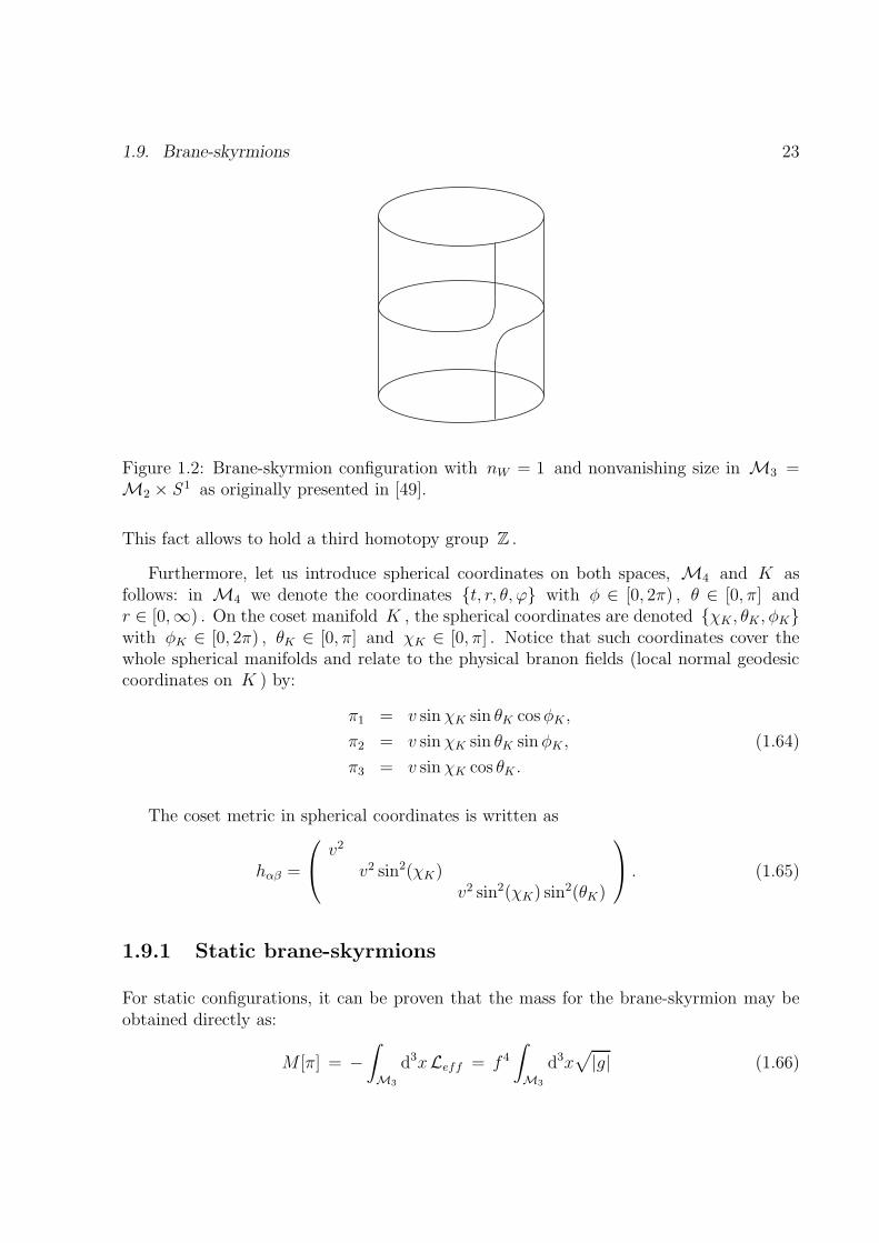
Figure 1.2: Brane-skyrmion configuration with nW = 1 and nonvanishing size in M3 =M2 × S 1 as originally presented in [49].
This fact allows to hold a third homotopy group Z .
Furthermore, let us introduce spherical coordinates on both spaces, M4 and K asfollows: in M4 we denote the coordinates t, r, θ, ϕ with φ ∈ [0, 2π) , θ ∈ [0, π] andr ∈ [0,∞) . On the coset manifold K , the spherical coordinates are denoted χK , θK , φKwith φK ∈ [0, 2π) , θK ∈ [0, π] and χK ∈ [0, π] . Notice that such coordinates cover thewhole spherical manifolds and relate to the physical branon fields (local normal geodesiccoordinates on K ) by:
π1 = v sinχK sin θK cosφK ,
π2 = v sinχK sin θK sinφK , (1.64)
π3 = v sinχK cos θK .
The coset metric in spherical coordinates is written as
hαβ =
v2
v2 sin2(χK)v2 sin2(χK) sin2(θK)
. (1.65)
1.9.1 Static brane-skyrmions
For static configurations, it can be proven that the mass for the brane-skyrmion may beobtained directly as:
M [π] = −∫
M3
d3xLeff = f 4
∫
M3
d3x√
|g| (1.66)

24 Chapter 1. Introduction to modified gravity theories
where the effective Lagrangian comes from the expression (1.53). In general this expressionis divergent due to the contribution of the zeroth order term when
√
|g| is expanded inbranon fields derivatives, reflecting the fact that the brane is an infinite object with finitetension. To prevent that, we substract this term in order to get a brane-skyrmion finitemass, i.e.:
MS[π] ≡ M [π] −M [0] = f 4
∫
M3
dx3√
|g| −M [0]. (1.67)
As was shown in the previous section, the πα fields are mappings from the M4 manifold tothe coset manifold K . For static, i.e. time independent, field configurations, these could beunderstood as mappings from the corresponding spatial 3-dimensional hypersurface (M3 )to the coset space (S3 in the case we are studying). For finite energy configurations, fieldsshould vanish at the spatial infinity and M3 can be compactified to S3 . Therefore onemay write πα : S3 → S3 . Since the third homotopy group of S3 is Z , the mappingscan be classified by an integer number nW . Thus, branons can be identified with thetopologically trivial configurations nW = 0 , whereas those configurations with nW 6= 0will be denoted as brane-skyrmions.
Consequently, for static skyrmions this mapping may be implemented in the followingway:
φK = φ ; θK = θ χK = F (r) (1.68)
with the boundary conditions F (0) − F (∞) = nWπ for a winding number nW 6= 0 .
In this case, MS[π] may be written as a F (r) functional and the correct mass for thiskind of skyrmions is obtained by minimizing MS[F ] in the space function with adequateboundary conditions.
From expression (1.67), it can be proven that the skyrmion is point-like, stable and itsmass becomes:
MS = 2π2f 4R3B (1.69)

1.10. Gravitational signatures at the LHC 25
1.10 Gravitational signatures at the LHC
As already mentioned, it can be seen from the equation (1.50), the fundamental gravita-tional scale could be as low as the electroweak scale if extra dimensions are large enough.Since the LHC is operating at a center of mass energy of
√s = 14 TeV , if the fundamental
scale of gravitation is MD ∼ TeV , both the production and decay of Schwarzschild miniBHs at high ratio becomes possible [51].
These BHs once produced would decay into SM particles with a clean signature anda low background. Several features of such objects could then be extracted from expe-rimental data: for instance BH masses MBH may be determined very precisely due tothe absence of missing energy and their temperature could be extracted from the energyspectrum of the products. Thus the correlation between these two quantities may providerelevant information able to determine the number of extra dimensions, and therefore thefundamental scale of gravity. On the other hand the Hawking evaporation law could betested experimentally.
The total cross section when two partons collide at the LHC with an impact parameterless than the Schwarzschild radius RS is of order
σ(MBH) ≈ πR2S =
1
M2D
[
MBH
MD
(
8Γ(D−12
)
D − 2
)]2
D−3
(1.70)
and it does not contain small coupling constants. If MD ∼ TeV the cross section is of orderTeV−2 ≈ 400 pb and therefore BHs will be produced copiously. The total production crosssection ranges from 0.5 nb for MD = 2 TeV , D = 11 to 120 fb for MD = 6 TeV D = 7 .For MD ∼ 1 TeV , the LHC – with a peak of luminosity of 30 fb−1/year – will produce107 BH/year.
Experimental signatures rely on two qualitative properties: on the one hand, theabsence of small couplings as seen from expression (1.70) and on the other hand, the flavorindependence nature of BHs decays as will be explained in the following paragraph. Notethat when MBH approaches MD , some stringy corrections to the previous assumptionsmay arise but semiclassical arguments remain valid as long as MBH ≫MD .
Once the BHs have been produced they decay following a process governed by theirHawking temperature TH ∼ 1/RS with an associated wavelength λ = 2π/TH larger thanthe BH size and therefore BHs would emit, in a first approximation, as point radiatorsmostly in the s-waves. This indicates that BHs decay equally to particles on the brane andin the bulk since the decay is only sensitive to the radial coordinate. If the approxima-tion MBH ≫ TH is made, the average multiplicity of particles 〈N〉 produced in the BH

26 Chapter 1. Introduction to modified gravity theories
evaporation is given by:
〈N〉 =2√π
D − 3
(
MBH
MD
)D−2D−3
(
8Γ(
D−12
)
D − 2
) 1D−3
. (1.71)
Since the decay is thermal, it does not discriminate between particle species (of the samemass and spin) and therefore BHs decay, roughly speaking, with the same probability toall SM particles. The signal of hard primary leptons and hard photons is quite clean witha negligible background since the production of SM leptons or photons occur at muchsmaller rate than BH production [51].
The way to determine MBH and TH deals with the study of decay products and thefits of the energy spectrum of those products to the Planck formula respectively. Oncethose two quantities are determined, they could provide some evidence of the Hawkingradiation and of the fact that the observed events indeed come from BH evaporation andnot from any other mechanism.
The relation between those two quantities, MBH and TH obtained independently, mayshed light about the dimensionality of the space since it can be proved that
log(TH) = − 1
D − 3log(MBH) + constant (1.72)
where the constant does not depend on MBH . Therefore the previous equation provides adirect method to determine the dimensionality D of the space as the slope of this relation.
The experimental signatures outlined above allow us to state that if the fundamentalscale of gravitation is of order TeV, as suggested in BW scenarios, some important physicalconsequences may appear. In fact, colliders study of BHs – eventually produced at a highrate in accelerators such as LHC – could help revealing the main features of physics in thevicinity of the electroweak scale or even determining the total number of dimensions of thespace-time.

Chapter 2
Dark energy in f(R) theories
2.1 Introduction
As was commented in Chapter 1, when the modified Einstein equations were rewrittena la Einstein, the presence of a function f(R) in the gravitational sector modifying theusual EH Lagrangian may be understood as the introduction of an effective fluid which isnot restricted to hold the usual energy conditions. Therefore f(R) functions may be usedto explain the present cosmological acceleration. Historically, some f(R) models wereproposed to modify GR at short scales, i.e., high energies trying to explain inflation, as forinstance f(R) ∝ R2 , but no interest was paid in those models to provide a mechanism tocause late time acceleration. First attempts to induce cosmological acceleration consideredf(R) ∝ 1/R but those models turned out to be in conflict with solar system tests [52] andeven to be unstable when matter is introduced [53].
Before studying these issues, let us mention that f(R) models, apart from satisfyingthose gravitational and cosmological conditions given in Section 1.6, should verify someextra conditions of cosmological viability. For instance, they have to include a backgroundevolution with Big Bang nucleosynthesis (BBN) and both radiation and matter dominatedcosmological eras. This fact will be explicitly studied in this chapter in Section 2.6. On theother hand, they must provide cosmological perturbations compatible with cosmologicalconstraints from CMB and large scale structures (LSS). This fact will be studied thoroughlyin Chapter 3.
The present chapter is organized as follows: in Section 2.2 we shall revise the standardapproach to describe the cosmological evolution in the ΛCDM model in a homogeneous,isotropic and spatially flat metric. In the following Section 2.3 we shall generalize theusual Einstein equations when f(R) gravity theories are present. Then we shall study inSection 2.4 the cosmological viability conditions for f(R) theories to hold a dust matter
27

28 Chapter 2. Dark energy in f(R) theories
dominated era followed by a late time acceleration and some interesting models which havebeen proposed to be viable will be provided in Section 2.5. Then, Section 2.6 will be thecore of the chapter and it will be devoted to study if f(R) theories are able to mimicstandard ΛCDM evolution. These f(R) models will possess vacuum solutions with nullscalar curvature what allows to recover some GR solutions usually considered.
To finish this chapter, we shall study in Section 2.7 how the modification of the gravi-tational sector by f(R) models may mimic the influence of perfect fluids (parameterizedby a constant equation of state) in the cosmological evolution without any presence ofsuch a fluid in the fluid content. The chapter will finish with Section 2.8 by drawing someattention over the main obtained conclusions.
The results presented in this chapter were originally published in [54].
2.2 Standard Einstein equations in a FLRW universe
Since the leitmotiv of this chapter is to study cosmological solutions, our universe, which isassumed to be isotropic and homogeneous at large enough scales for fundamental observers,may be represented with a D = 4 dimensional Friedmann-Lemaıtre-Robertson-Walker(FLRW) metric
ds2 = dt2 − a2(t)
(
dr2
1 − kr2+ r2dΩ2
2
)
(2.1)
expressed in cosmic time t and where a(t) is usually referred to as the scale factor.Alternatively, this metric may be expressed in conformal time τ , defined by the relationdt ≡ a(τ)dτ and thus this metric becomes
ds2 = a2(τ)
(
dτ 2 − dr2
1 − kr2− r2dΩ2
2
)
(2.2)
In this metric, the Hubble parameter may be defined in either cosmic or conformal timeas
H(t) ≡ da(t)/dt
a(t)≡ a
a; H ≡ da(τ)/dτ
a(τ)≡ a′(τ)
a(τ)(2.3)
respectively and the identity aH ≡ H is straightforwardly inferred.
For the values of the parameter k smaller, equal or bigger than zero, the universe isspatially hyperbolic, flat or spherical respectively. In the following calculations we shall beconsidering k = 0 . This choice is justified according to WMAP data [11] where the resultsobtained for ΛCDM model are: Ωk ≡ −k/H2
0 , with H0 ≡ H(ttoday) = 100h km s−1Mpc−1

2.2. Standard Einstein equations in a FLRW universe 29
and h = 0.699 ± 0.018 and −0.0133 < Ωk < 0.0084 ( 95% CL). Therefore terms relatedwith k will be subdominant in either Friedmann’s or generalized Friedmann equations tobe presented in following the section.
Considering the previously introduced metric (2.1) and perfect fluids given by (1.7)for the present fluids, the only two independent Einstein equations for D = 4 are theFriedmann and the acceleration equations respectively, which may be written in cosmictime as:
H2 ≡(
a
a
)2
=8πG
3
∑
α
ρα (2.4)
a
a= −8πG
6
∑
α
(ρα + 3Pα) (2.5)
where G ≡ G4 is the gravitational constant in four dimensions and the summation oversubindex α holds for the present fluids contributions (baryons, radiation, dark matter,DE, etc.). If positive cosmological acceleration is required, i.e. a > 0 , the condition to beaccomplished from expression (2.5) would be
∑
α(ρα + 3Pα) < 0 . This condition wouldrequire that if only a perfect fluid is present, its state equation would satisfy the conditionωα < −1/3 which is not the case for standard fluids, such as for instance dust matter andradiation. On the contrary a cosmological constant does provide positive acceleration inequation (2.5) since its state equation satisfies ωΛ = −1 .
For this metric, the energy-momentum conservation equations lead, in cosmic andconformal time respectively, to the following equations:
ρα + 3(1 + ωα)H ρα = 0
ρ′α + 3(1 + ωα)Hρα = 0 (2.6)
which hold separately for each fluid whose state equations are assumed to be Pα = ωαρα .Previous equation is integrated to give:
ρα(t) = ρα(t0)
(
a(t0)
a(t)
)3(1+ωα)
(2.7)
where t0 is an arbitrary time and the corresponding scale factor is a(t0) .
By using the definition given in (1.5) and (1.6), the Ricci scalar curvature for FLRWspatially flat metric is written in terms of the scale factor and its derivatives as follows
R = 6
[
(
a
a
)2
+a
a
]
=6
a2(H′ + H2). (2.8)

30 Chapter 2. Dark energy in f(R) theories
Let us finish this section by rewriting the previous Friedmann equation (2.4). To doso, let us divide that equation by H2
0 ≡ H2(t0) and consider as present fluids dust matter(ωM = 0 ), radiation (ωRad = 1/3 ) and cosmological constant Λ (ωΛ = −1 ). Thus,taking into account (2.7) for each present fluid, we get:
H2(t)
H20
= ΩM a(t)−3 + ΩRad a(t)−4 + ΩΛ (2.9)
where we have used the notation:
ΩM ≡ 8πGρM(t0)
3H20(t0)
; ΩRad ≡ 8πGρRad(t0)
3H20 (t0)
; ΩΛ ≡ Λ
3H20(t0)
(2.10)
and the normalization of the scale factor a(t0) = 1 has been used. Note that if expression(2.9) is evaluated at t = t0 , then ΩM + ΩRad + ΩΛ ≡ 1 .
2.3 Modified Einstein equations in a FLRW universe
Inserting the metric (2.1) for D = 4 in the equations (1.10) and assuming also energy-momentum tensor as given in (1.7) for a fluid with energy density ρ0 and pressure P0 ,the only independent modified Einstein equations are
3(1 + fR)a
a− 1
2(R + f(R)) − 3
a
aRfRR = −8πGρ0 (2.11)
(1 + fR)(H + 3H2) − 1
2(R + f(R)) − 1
a
d
dt
(
a2RfRR
)
= 8πGP0 (2.12)
and in conformal time τ , these equations are given by
3H′
a2(1 + fR) − 1
2(R + f(R)) − 3H
a2f ′
R = −8πGρ0 (2.13)
1
a2(H′ + 2H2)(1 + fR) − 1
2(R + f(R)) − 1
a2(Hf ′
R + f ′′R) = 8πGP0. (2.14)
Remind that dot denotes here derivative with respect to time t whereas τ derivative wasdenoted with prime. A very useful equation to use in the following calculations is thecombination (2.14) minus (2.13) which becomes
2(1 + fR)(−H′ + H2) + 2Hf ′R − f ′′
R = 8πG(ρ0 + P0)a2. (2.15)
At this stage we should note that, for instance, according to equations (2.11), (2.12)together with (2.8), it is clear that modified Einstein equations are not second order inderivatives any more, but at least third order in the scale factor derivatives providedfRR 6= 0 .

2.4. Cosmological viability for f(R) dark energy models 31
2.4 Cosmological viability for f(R) dark energy mo-
dels
In this section we shall revise the conditions that a model for DE given by a f(R) theorymust fulfill in order to be cosmologically viable: i.e., any viable f(R) model should havea matter dominated phase long enough to provide the adequate cosmological evolutionprior to a late time acceleration phase. As a matter of fact, equations (2.11) and (2.12)with dust matter as the unique present fluid, can be rewritten in the form of a system ofautonomous equations [55]. In that reference two variables, m and r are introduced asfollows:
m ≡ RfRR
1 + fR; r ≡ −R(1 + fR)
R + f(R). (2.16)
Both the dynamics and stability of that autonomous system are determined by six criticalpoints P1,...,6 – according to the notation in [55] – that appear in the system resolution.
2.4.1 Critical points and stability
According to the results presented in [55], both points P5 and P6 satisfy
m(r) = −r − 1. (2.17)
If in the previous equation m is assumed to be constant, the condition (2.17) holds straight-forwardly from two other equations in the autonomous system. In this case the points P2,...6
always exist while P1 and P4 are present for values m = 1 and m = −1 respectively.The critical points P5 and P6 which give the exact matter era evolution, i.e., a(t) ∝ t2/3 ,exist only for m = 0 (P5 ) or for m = −(5±
√73)/12 (P6 ) but the latter corresponds to
a vanishing matter density and obviously it does not give a standard matter era.
If on the contrary m is not assumed to be constant, the number of solutions dependson the particular f(R) choice, but only P1,5,6 can be accelerated and only P5 might giverise to matter era. This last situation would require m ≃ 0 to resemble the standardmatter era evolution. Summarizing the result in this case, only trajectories passing nearP5 with m ⋍ 0 at r ⋍ −1 and landing on an accelerated attractor would give a viablecosmological evolution.
2.4.2 Classification of f(R) models
By studying all possible trajectories in the m and r variables of the already mentionedautonomous system, it can be shown [55] that a classification of f(R) models can be

32 Chapter 2. Dark energy in f(R) theories
based entirely upon geometrical properties of the curve m(r) . These two variables allowto classify the f(R) models in four different classes: I, II, III and IV depending on theexistence of a standard matter epoch and a final accelerated expansion as follows: on theone hand, the viable matter dominated epoch requires
m ≈ +0 ;dm
dr> −1 (2.18)
at r ≈ −1 . On the other hand, the late time acceleration epoch requires to fulfill one ofthe following two conditions: a de Sitter acceleration follows the matter epoch if and onlyif
1. 0 ≤ m(r) ≤ 1 at r = −2 (2.19)
whereas a non-phantom accelerated attractor follows the matter dominated epoch if andonly if
2. m = −r − 1 ;
√3 − 1
2< m ≤ 1 ;
dm
dr< −1. (2.20)
For instance, according to the previous requirements over m and r variables, modelsof the type f(R) = αR−n − R and f(R) = αR−n do not satisfy these conditions for anyn > 0 and n < −1 and are consequently cosmologically nonviable.
The main features of each class of models are:
Class I: this class covers all the cases for which the curve m(r) does not connectthe accelerated attractor with the standard matter point (r,m) = (−1, 0) eitherbecause m(r) does not pass near that matter point, i.e., m(r → −1) 6= 0 , or be-cause the branch of m(r) that accelerates is not connected with the standard matterpoint. Moreover, instead of having a standard matter phase given by a scale factora(t) ∝ t2/3 , these f(R) models possess a peculiar scale factor behaviour a(t) ∝ t1/2
before accelerating epoch and are therefore unsuitable models.
Class II: for these f(R) models the m(r) curve does connect the upper vicinity(m > 0) of (r,m) = (−1, 0) with a critical point able to provide acceleration. There-fore models here have a matter epoch and are asymptotically equivalent (hardlydistinguishable) to ΛCDM model (ωeff ≡ −1 − 2H/3H2 = −1 ), i.e., they areasymptotically de Sitter and observationally acceptable. These models satisfy bothequations (2.18) and (2.19).
Class III: these f(R) models may possess an approximated matter era but as atransient state followed by a final and strongly phantom attractor at late-time. This

2.5. Some cosmologically viable f(R) models 33
f(R) models m(r) Class I Class II Class III
−R + αR−n −1 − n n > −0.713 − −1 < n < −0.713
αR−n −n(1+r)r n > 0 n ∈ (−1, 0), α < 0 −
−R + Rp [log (αR)]q (p+r)2
qr − 1 − r p 6= 1 p = 1, q > 0 −−R + Rpexp qR −r + p
r p 6= 1 − −−R + Rpexp(q/R) −p+r(2+r)
r p 6= 1 p = 1 −
Table 2.1: Classification of some f(R) DE models presented in [55]. None of these models belongsto Class IV. Models that belong to Class II for the provided parameter intervals, at least satisfy theconditions to have a matter era followed by a de Sitter attractor.
is due to the fact that the m(r) curve intersects the critical line m(r) = −r − 1 at−1/2 < m < 0 . The approximated matter era is a very fast transitient phase andonly a narrow range of initial conditions may allow it. Since matter era is practicallyunstable, these models are generally ruled out by the observations.
Class IV: for models of this class the connection between the upper vicinity of thepoint (r,m) = (−1, 0) to the region located on the critical line m(r) = −r − 1is possible. Therefore these models are observationally acceptable: they possess anapproximate standard matter epoch followed by a non-phantom acceleration with aneffective equation of state ωeff ≡ −1 − 2H/3H2 > −1 , thus these models posses astandard DE behaviour. These models satisfy both equations (2.18) and (2.20).
Classes II and IV have therefore some chance to be cosmologically viable but thebasin of the attractor has to be determined to provide acceptable trajectories according tothe already mentioned analysis fully performed in [55]. In Table 2.1 the previous analysishave been applied to some f(R) models usually considered in the literature.
2.5 Some cosmologically viable f(R) models
In this section we provide three f(R) models already presented in the literature whichclaim to be cosmologically viable.
a) f(R) = λR0
[
(
1 + R2
R20
)−n
− 1
]
This model was originally considered in reference [56] with n, λ > 0 and R0 of theorder of the presently observed effective cosmological constant. Then f(0) = 0 and thecosmological constant is claimed to disappear in flat space-time but fRR(0) is negativeand therefore, according to condition 1 in Section 1.6, flat space-time would be unstable.

34 Chapter 2. Dark energy in f(R) theories
For scalar curvatures R ≫ R0 , f(R) tends to λR0 and the model would behave asthe EH case with an effective cosmological constant. On the other hand, de Sitter space-time with curvature R1 > 0 is also a vacuum solution provided R1(fR(R1)− 1) = 2f(R1)according to equation (1.33) for D = 4 and R = R1 . Thus, this case would present aneffective cosmological constant Λ(R1) = R1/4 .
For this model it can be proved that conditions 1 and 2 of Section 1.6 are satisfiedin the curvature interval [R1,∞) if they are accomplished at R = R1 . Then these twoconditions hold if and only if
[
1 +
(
R1
R0
)2]n+2
> 1 + (n+ 2)
(
R1
R0
)2
+ (n + 1)(2n+ 1)
(
R1
R0
)4
. (2.21)
Note that condition 3 in that section is straightforwardly satisfied if as considered, pa-rameters λ and n are positive. On the other hand, this model also satisfies the requiredconditions to provide a matter dominated era at R≫ R0 and does not possess the alreadymentioned Dolgov-Kawasaki instability. The remaining condition 4 is easily accomplishedif R0 is considered much smaller than R at recent epochs.
A simple choice of parameters λ , n and R0 shows that this model obeys the conditions(2.18) and (2.19) and therefore according to the analysis in the previous section it possessa matter dominated epoch and a de Sitter late time acceleration.
b) f(R) = −αm1
(
Rα
)n [1 + β
(
Rα
)n]−1
This model was first proposed in reference [33] in order to mimic ΛCDM evolution inthe high-redshift regime and to accelerate at low redshift with an expansion history closeto ΛCDM model. In this model, the parameter n was considered to be positive and forconvenience the mass scale α was given by
α ≡ 8π Gρ0
3= (8315 Mpc)−2
(
ΩMh2
0.13
)
(2.22)
where ρ0 is the average density today. This model does not have a bare cosmologicalconstant since f(0) = 0 and its parameters m1 , β and n may be rewritten as [57]
m1
β≈ 6
1 − ΩM
ΩM(2.23)
m1
β2= −fR(R0)
n
(
12
ΩM− 9
)n+1
(2.24)
where ΩM is the effective matter energy density at the present time. Finally the constraint|fR(R0)| < 0.1 was imposed and R0 is the scalar curvature today as would be obtained

2.6. f(R) with no cosmological constant 35
from ΛCDM model, i.e.
R0 ≈ αm1
(
12
ΩM
− 9
)
. (2.25)
Setting the values n = 1 and ΩM = 0.3 , it was proven in reference [57] that this modelbelongs to the Class II presented in the previous section.
c) f(R) = −αR∗ log(
1 + RR∗
)
This two-parameter f(R) model presented in [58], where parameters α and R∗ arepositive, has claimed to be cosmologically viable and different from ΛCDM . In fact, itdoes satisfy both cosmological conditions (2.18) and (2.19) presented in previous Section2.4, provided α > 1 and regardless of the value of R∗ .
Conditions 1, 2 and 3 given in Section 1.6 are also satisfied but concerning the condition4 also given in that section, it will be shown in Section 3.4 that this f(R) theory does notsatisfy this condition, showing that this model is indeed distinct from ΛCDM . This factand its consequences will be studied in Section 3.4.
2.6 f(R) with no cosmological constant
Now that the modified Einstein equations have been presented for FLRW metric, someinteresting results at cosmological scales will be obtained in this section. The presentedapproach tries to mimic cosmological well-known GR results in different cosmological erasemploying adequate f(R) functions. Reconstruction procedures of this kind have beenwidely studied in the literature [59, 60, 61] where by rewriting the involved equations innew variables and assuming a given cosmological solution, mainly in vacuum, the requiredf(R) gravity is obtained.
In this section the addressed issue will be to find a f(R) gravity able to reproducethe current cosmic speed-up appearing in standard ΛCDM cosmology. This function isrequired to be analytical at R = 0 and to have R = 0 as a vacuum solution, thereforeit will not contain any cosmological constant contribution. From a more formal pointof view we are seeking for some f(R) gravity model having the same FLRW solutionas the standard EH action with cosmological constant for nonrelativistic matter (dustmatter, i.e. PM = 0 ). For the searched cosmological constant absence it is clear that thef(R) expansion at R = 0 must start at the R2 term to avoid, on the one hand, havingcosmological constant and, on the other hand, redefining the gravitational constant.

36 Chapter 2. Dark energy in f(R) theories
2.6.1 Cosmological evolution in ΛCDM model
Let us solve Einstein’s equations (1.15) for the standard EH action plus a cosmologicalconstant Λ with dust matter in the energy-momentum tensor side.
The most recent cosmological data quoted in reference [11] are compatible at late timeswith a cosmological model based on a spatially flat FLRW metric like (2.1) together withEinstein’s equations with a cosmological constant Λ 6= 0 and dust matter (including darkmatter). In this case, the equations (1.15) will be valid and matter content will be writtenin terms of a pressureless perfect fluid
T µν = diag (ρM0(t), 0, 0, 0). (2.26)
Equation µ = ν = 0 (time-time component) in (1.15) becomes(
a0(t)
a0(t)
)2
=8πG
3ρM0(t) +
Λ
3(2.27)
where ρM0(t) in previous equation is given by expression (2.7) if ωα=M is fixed to 0. Thus
ρM0(t) = ρM0(t0)
(
a0(t0)
a0(t)
)3
(2.28)
where the 0 subindex means that the standard EH equations (1.15) with a cosmologicalconstant are being considered. This notation will be relevant later on when standardΛCDM cosmology will be compared with the results coming from the action (1.3) for thef(R) function that we shall find in this section.
Substituting the expression (2.28) in the equation (2.27), the solution a0(t) , using thenotation introduced in Section 2.2 in this chapter, is found to be:
a0(t) =
(
ΩM
ΩΛ
)1/3
sinh2/3
(
3√
ΩΛ
2H0 t
)
. (2.29)
On the other hand, by taking the trace of (1.15) in this case, i.e. cosmological constantand dust matter, it is found that
R0(t) − 4Λ = 8πG ρM0(t). (2.30)
2.6.2 f(R) case with no cosmological constant
Now let us consider the equations (1.10) but in the case where no cosmological constantis considered and the energy-momentum tensor for dust matter will be
T µν = diag (ρM(t), 0, 0, 0). (2.31)

2.6. f(R) with no cosmological constant 37
Then the equation (2.11) becomes
3(1 + fR)a
a− 1
2(R + f(R)) − 3
a
aRfRR = −8πGρM (2.32)
where we have eliminated the subindex 0 in the different quantities to avoid any confusionwith the previous case presented in Subsection 2.6.1. As was already mentioned, it is clearthat the solutions for equation (2.32) will strongly depend on the function f(R) : differentchoices for this function will lead to different evolutions of the universe for the same initialconditions. However, our approach to the problem will be to find a function f(R) so thatthe solution a(t) of the equation (2.32) will be exactly the same as the solution providedby the expression (2.29) that we obtained by using GR with nonvanishing cosmologicalconstant and which seems to fit the present cosmological data. In other words, we wantto find the f(R) model such that the solution for the equation (2.32) is exactly the scalefactor (2.29), i.e.:
a(t) ≡ a0(t) (2.33)
for the same initial (or present, i.e. t = t0 ) conditions. If it were possible to find sucha function f(R) then, it would be possible to avoid the necessity for introducing anycosmological constant just by considering a gravitational action such that given in theexpression (1.3). In the following it will be shown that such a function happens to exist andits precise form will be provided. In order to do that one first notices that accomplishingthe condition (2.33) after radiation-matter equality clearly implies
R = R(t) ≡ R0(t) (2.34)
and then R(t) and R0(t) may be used indistinctly. On the other hand we shall writethe matter density as the former matter density provided by expression (2.7) plus a newcontribution, i.e.
ρM(t) = ρM0(t) + ∆ρ(t), (2.35)
accounting for a slight variation with respect to the density provided in the Subsection2.6.1. Assuming that matter for arbitrary f(R) is still nonrelativistic in this cosmologicalera we have
∆ρ(t) = ∆ρ(t0)
(
a0(t0)
a0(t)
)3
(2.36)
where according to the expression (2.7) particularized for the constraint (2.33) and consi-dering the relation given in (2.30) we can write
(
a0(t0)
a0(t)
)3
=R(t) − 4Λ
8πG ρM0(t0)(2.37)
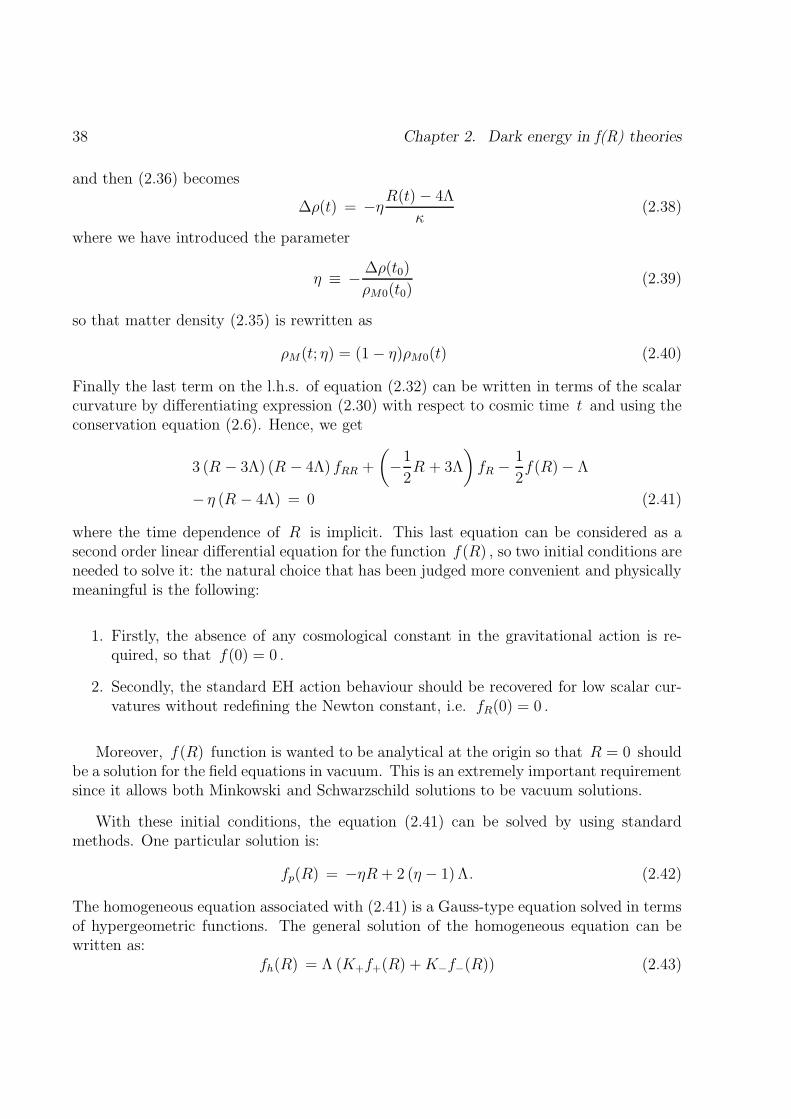
38 Chapter 2. Dark energy in f(R) theories
and then (2.36) becomes
∆ρ(t) = −ηR(t) − 4Λ
κ(2.38)
where we have introduced the parameter
η ≡ − ∆ρ(t0)
ρM0(t0)(2.39)
so that matter density (2.35) is rewritten as
ρM(t; η) = (1 − η)ρM0(t) (2.40)
Finally the last term on the l.h.s. of equation (2.32) can be written in terms of the scalarcurvature by differentiating expression (2.30) with respect to cosmic time t and using theconservation equation (2.6). Hence, we get
3 (R − 3Λ) (R − 4Λ) fRR +
(
−1
2R + 3Λ
)
fR − 1
2f(R) − Λ
− η (R − 4Λ) = 0 (2.41)
where the time dependence of R is implicit. This last equation can be considered as asecond order linear differential equation for the function f(R) , so two initial conditions areneeded to solve it: the natural choice that has been judged more convenient and physicallymeaningful is the following:
1. Firstly, the absence of any cosmological constant in the gravitational action is re-quired, so that f(0) = 0 .
2. Secondly, the standard EH action behaviour should be recovered for low scalar cur-vatures without redefining the Newton constant, i.e. fR(0) = 0 .
Moreover, f(R) function is wanted to be analytical at the origin so that R = 0 shouldbe a solution for the field equations in vacuum. This is an extremely important requirementsince it allows both Minkowski and Schwarzschild solutions to be vacuum solutions.
With these initial conditions, the equation (2.41) can be solved by using standardmethods. One particular solution is:
fp(R) = −ηR + 2 (η − 1) Λ. (2.42)
The homogeneous equation associated with (2.41) is a Gauss-type equation solved in termsof hypergeometric functions. The general solution of the homogeneous equation can bewritten as:
fh(R) = Λ (K+f+(R) +K−f−(R)) (2.43)

2.6. f(R) with no cosmological constant 39
where
f±(R) =
(
3 − R
Λ
)−a±
2F1
[
a±, 1 + a± − c, 1 + a± − a∓;−(
3 − R
Λ
)−1]
(2.44)
and the symbol 2F1 holds for hypergeometric functions and the constants
a± = − 112
(
7 ±√
73)
; c = −1/2 (2.45)
have been introduced. The η -dependent constants K+ and K− must be determined fromthe initial conditions given above. Numerically it is found that:
K+ = 0.6436 (−0.9058 η + 0.0596) ; K− = 0.6436 (−0.2423 η + 3.4465). (2.46)
The hypergeometric functions given in (2.44) are generally defined in the whole complexplane. However, a real gravitational action is wanted. In principle this requirement is veryeasy to achieve since the coefficients in the equation (2.41) and the constants K± are allreal. Then it is obvious that the real part of the functions appearing in the expression(2.44) is a proper solution of the homogeneous equation associated with (2.41). Thus thefunction we are seeking can be written as:
f(R) ≡ fp(R) + Re [fh(R)] . (2.47)
Nevertheless, the situation is more complicated. The homogeneous equation has threeregular singular points at R1 = 3Λ , R2 = 4Λ and R3 = ∞ . This results in thesolution fh(R) having two branch points R1 and R2 . More concretely there are two cutsalong the real axis: one from minus infinity to R1 and another from R2 to infinity. Thusone must be quite careful when interpreting (2.47). From minus infinity to R1 there isonly one Riemann sheet of fh(R) where f(0) and fR(0) vanish and therefore this is theone that we have to use to define f(R) . From R1 to R2 the real part of fh(R) is welldefined. Finally from R2 to infinity there is only one Riemann sheet producing a smoothbehaviour of f(R) . To reach this sheet one must understand R in the above equationas R + iǫ . At the present moment we do not know if this analytical structure has anyfundamental meaning or it is just an artefact of our construction. Much more importantis the fact that the function R + fp(R) + fh(R) , which is the analytical extension of ourLagrangian, is analytical at R = 0 , having at this point the local behaviour R + O(R2) .Therefore our generalized gravitational Lagrangian R+f(R) does guarantee that R = 0 isa vacuum solution as can be seen from expression (1.12). At the same time, this Lagrangianreproduces the current evolution of the universe without any cosmological constant.
Now that the f(R) function in (2.47) has been obtained, it is possible to check ourresult out by solving (2.11) in terms of a(t) for the f(R) given in (2.47). This is doneby rewriting the equation (2.32) in terms of a(t) by using (2.8) and (2.7) together withthe dust matter density in terms of η and a(t) as provided by expression (2.35). At this

40 Chapter 2. Dark energy in f(R) theories
stage, the consistency of our results has been checked out by introducing the scale factor(2.29) and f(R) given in (2.47) in (2.11) and both sides of the equation turned to be equalfor all η values. Thus it has been guaranteed that our gravitational action proportionalto R + f(R) provides the same cosmic evolution –in the required cosmological eras –as the EH action with cosmological constant Λ in a dust matter universe. Therefore,our model does verify, in the same range of precision, all the experimental tests that thestandard cosmological model does in the present era. Notice also that in principle this canbe achieved for any value of η , i.e. for any desired amount of matter. Nevertheless, somerestrictions should be imposed on the parameter η . For instance it is obvious that in adust matter dominated universe ρM(t; η) ≥ 0 implies η ≤ 1 .
Much more stringent bounds can be set on parameter η by demanding that this modelworks properly back in time up to Big Bang Nucleosynthesis (BBN) era. Observations in-dicate that the cosmological standard model fits correctly primordial light elements abun-dances during BBN , that means that the expansion rate H(t) cannot deviate from thatof standard cosmology H0(t) in more than 10% for the background evolution (see forinstance [62] for further details). Therefore by the time of BBN, departure of our modelfrom the standard cosmology must not be too large and the equation (2.11) should providea similar behaviour to the one given by the standard Friedmann equation (2.27) wherenow the density will include both dust and radiation contributions.
At BBN the DE contribution is negligible compared with dust and radiation densities.The scalar curvature is of order 10−39 eV2 (with ~ = c = 1 for these calculations)and by that time dust and radiation densities are of the order of 1016 eV4 and 1021 eV4
respectively. Since R ≃ R0 we can rewrite the equation (2.11) as a modified Friedmannequation as follows
H2(t) = H20 (t)
105R− ηR + 12(RfR − f(R))
105R [1 + fR − 3fRR(1 − η)R]
. (2.48)
As was commented above, to reproduce light elements abundances it is required thatH2(t) = H2
0 (t)(1±0.2) for curvatures of order RBBN . This implies that the second factoron the r.h.s. of the previous expression (2.48) should be between 0.8 and 1.2 by thatperiod. Thus in order to match our f(R) gravity model with the standard cosmology atthe BBN times we need to tune η to a value about 0.065 with a stringent fine tuning.Therefore the matter content of our model is not too different from the one in the standardcosmology and the difference is in fact smaller than experimental precision in [11].
Concerning the problem of viability for this particular f(R) model, if conditions 2,3 and 4 given in Section 1.6 are required to hold, the parameter η has to be fixed toa fine tuned value η ≈ −1.4311 but for this value fRR reverse its sign at high enoughcurvatures and therefore the condition 1 in that section is not accomplished. Therefore itmay be stated that the f(R) model given by expression (2.47) should be considered as an

2.7. Effective fluid description of f(R) gravities 41
effective model able to reproduce ΛCDM model cosmological expansion after radiation-matter equality but not as a consistent gravitational theory valid for all scales.
2.7 Effective fluid description of f(R) gravities
In this section we shall be interested in finding those f(R) functions such that the corres-ponding modified Einstein equations in vacuum exactly reproduce the cosmological evolu-tion of EH gravity with a given perfect fluid, i.e., the introduced modifications of the EHaction through a function f(R) will play the role of the fluid source.
Let us thus consider such a perfect fluid ’f’ obeying the following barotropic stateequation
Pf = ωf ρf (2.49)
with constant ωf and whose density ρf scales according to the conservation equation (2.7)with the scale factor a ≡ a(t) as
ρf(a) = ρf(a(t0))
(
1
a(t)
)3(1+ωf)
= ρf(a(t0)) x1+ωf (2.50)
where ρf(a(t0)) is the value of the fluid density for a given value of the scale factor a(t0) ≡1 . For the sake of simplicity a new variable x has been introduced in the previousexpression (2.50) defined as follows
x ≡ 1
a3. (2.51)
With this new variable x , if the only present (or at least the dominant one) fluid is thedefined above, the standard EH Friedmann and acceleration equations in cosmic time tare respectively
H2 =8πGρf
3= H2
0x1+ωf
a
a= −8πG
6ρf(1 + 3ωf) = −1
2H2
0 (1 + 3ωf)x1+ωf (2.52)
where as usual 8πGρf(a(t0)) ≡ 3H20 .
Analogously to the procedure in the previous section of this chapter, we shall considerthe modified Einstein equations where there will not be any fluid contribution. The solutionfor these equations is wanted to be the same scale factor as the one which is the solutionof equations (2.52). In other words, the presence of the fluid in the EH equations wants tobe replaced by the contribution of some f(R) function in the modified Einstein equations.
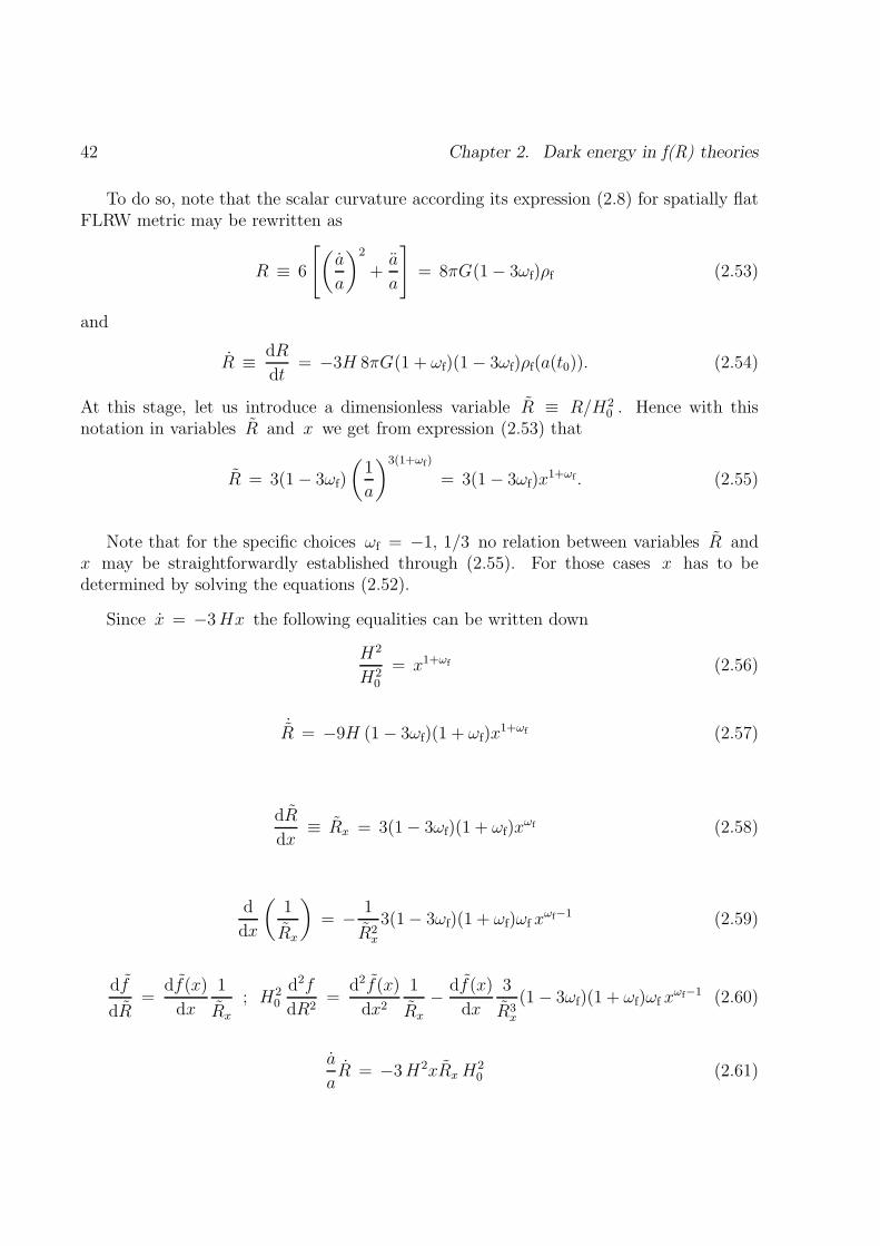
42 Chapter 2. Dark energy in f(R) theories
To do so, note that the scalar curvature according its expression (2.8) for spatially flatFLRW metric may be rewritten as
R ≡ 6
[
(
a
a
)2
+a
a
]
= 8πG(1 − 3ωf)ρf (2.53)
and
R ≡ dR
dt= −3H 8πG(1 + ωf)(1 − 3ωf)ρf(a(t0)). (2.54)
At this stage, let us introduce a dimensionless variable R ≡ R/H20 . Hence with this
notation in variables R and x we get from expression (2.53) that
R = 3(1 − 3ωf)
(
1
a
)3(1+ωf)
= 3(1 − 3ωf)x1+ωf . (2.55)
Note that for the specific choices ωf = −1, 1/3 no relation between variables R andx may be straightforwardly established through (2.55). For those cases x has to bedetermined by solving the equations (2.52).
Since x = −3Hx the following equalities can be written down
H2
H20
= x1+ωf (2.56)
˙R = −9H (1 − 3ωf)(1 + ωf)x1+ωf (2.57)
dR
dx≡ Rx = 3(1 − 3ωf)(1 + ωf)x
ωf (2.58)
d
dx
(
1
Rx
)
= − 1
R2x
3(1 − 3ωf)(1 + ωf)ωf xωf−1 (2.59)
df
dR=
df(x)
dx
1
Rx
; H20
d2f
dR2=
d2f(x)
dx2
1
Rx
− df(x)
dx
3
R3x
(1 − 3ωf)(1 + ωf)ωf xωf−1 (2.60)
a
aR = −3H2xRxH
20 (2.61)
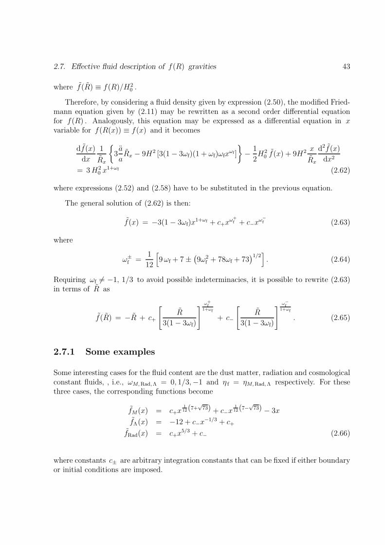
2.7. Effective fluid description of f(R) gravities 43
where f(R) ≡ f(R)/H20 .
Therefore, by considering a fluid density given by expression (2.50), the modified Fried-mann equation given by (2.11) may be rewritten as a second order differential equationfor f(R) . Analogously, this equation may be expressed as a differential equation in xvariable for f(R(x)) ≡ f(x) and it becomes
df(x)
dx
1
Rx
3a
aRx − 9H2 [3(1 − 3ωf)(1 + ωf)ωfx
ωf ]
− 1
2H2
0 f(x) + 9H2 x
Rx
d2f(x)
dx2
= 3H20 x
1+ωf (2.62)
where expressions (2.52) and (2.58) have to be substituted in the previous equation.
The general solution of (2.62) is then:
f(x) = −3(1 − 3ωf)x1+ωf + c+x
ω+f + c−x
ω−
f (2.63)
where
ω±f =
1
12
[
9ωf + 7 ±(
9ω2f + 78ωf + 73
)1/2]
. (2.64)
Requiring ωf 6= −1, 1/3 to avoid possible indeterminacies, it is possible to rewrite (2.63)in terms of R as
f(R) = −R + c+
[
R
3(1 − 3ωf)
]
ω+f
1+ωf
+ c−
[
R
3(1 − 3ωf)
]
ω−
f1+ωf
. (2.65)
2.7.1 Some examples
Some interesting cases for the fluid content are the dust matter, radiation and cosmologicalconstant fluids, , i.e., ωM, Rad,Λ = 0, 1/3,−1 and η f = ηM, Rad, Λ respectively. For thesethree cases, the corresponding functions become
fM(x) = c+x112(7+
√73) + c−x
112(7−
√73) − 3x
fΛ(x) = −12 + c−x−1/3 + c+
fRad(x) = c+x5/3 + c− (2.66)
where constants c± are arbitrary integration constants that can be fixed if either boundaryor initial conditions are imposed.

44 Chapter 2. Dark energy in f(R) theories
2.8 Conclusions
In this chapter we have found the f(R) gravity which exactly reproduces the same evolu-tion of the universe, from BNN up to the present time, as standard ΛCDM model does,but without the introduction of any form of DE or cosmological constant. The gravitatio-nal Lagrangian R+ f(R) is analytical at the origin and consequently R = 0 is a vacuumsolution for the field equations. Therefore Minkowski, Schwarzschild and other importantR = 0 GR solutions, with Λ = 0 , are also solutions for this f(R) gravity. This resultwas originally presented in [54].
The price that we have to pay for all those good properties is that our Lagrangian,considered as a function of R , has a very complicated analytical structure with cutsalong the real axis from infinity to R = 3Λ and from R = 4Λ to infinity. Obviouslythe only reasonable interpretation of our action is as some kind of effective action. Inclassical physics one typically starts from some action principle, obtains the correspondingfield equations and finally solves them for some initial or boundary conditions. In thiswork we have proceeded in the opposite way: we started from solutions obtained in thestandard cosmological model and then we have searched for an action that, possessingcertain properties, gives rise to field equations having the same solutions.
Classical actions are of course real but effective quantum actions usually have a complexstructure coming from loops and related to unitarity. The presence of an imaginary partin the action, evaluated on some classical configuration, indicates quantum lost of stabilityby particle emission of this configuration [63]. Therefore it is tempting to think that ouraction could have some interpretation in terms of an effective quantum action. However,our action determination procedure does not allow to make such a kind of statement.Complications in the action could be just an artifact of our construction. In any case itwas shown that such action exists and it reproduces the present universe evolution withoutDE having R = 0 as a vacuum solution. As a drawback of this result, we have shown thatthis f(R) function cannot be considered as a fully consistent gravitational theory since itdoes not obey the viability conditions revised in Chapter 1 and that therefore it should beregarded as an effective model to mimic ΛCDM cosmological background evolution.
To conclude the chapter a completely general procedure to reproduce EH gravity withan arbitrary perfect fluid by using f(R) theories has been implemented. It has beenexplicitly shown that any perfect fluid when is described by a constant equation of statecan be mimicked by an appropriate f(R) model. Standard cases for perfect fluids such asdust matter, radiation and cosmological constant have been presented in this analysis.

Chapter 3
Cosmological perturbations in f (R)theories
3.1 Introduction
This chapter will be devoted to a study of the evolution of scalar cosmological perturba-tions in f(R) theories. To do so, a completely general procedure will be implemented andseveral consequences will be analyzed. The importance for addressing the present problemlies in the necessity to discriminate among different DE models, including f(R) modifiedgravities, by using observations. It is well-known that by choosing adequate f(R) func-tions, one can mimic any expansion history, and in particular that of the ΛCDM model.Accordingly, the exclusive use of observations from SNIa [64], baryon acoustic oscillations[65] or CMB shift factor [11], based upon different distance measurements which are sen-sitive only to the cosmological expansion history, cannot settle the question of the DEnature [66].
However, there exists a different type of observations which are sensitive, not only to thecosmological expansion history, but also to the evolution of matter density perturbations.Pioneering work on density perturbations in FLRW cosmological models was presented in[67]. The fact that the evolution of perturbations depends on the specific gravity model,i.e., it differs in general from that of Einstein’s gravity even though the background evo-lution is the same, means that this kind of observations will help distinguishing betweendifferent models capable to explain cosmic acceleration. This is therefore the aim of thepresent chapter: to provide a completely exact method to determine how cosmologicalperturbations grow in f(R) theories and to settle the extracted consequences from thisresult. Such a problem has been exhaustively considered in the literature [68]. In this chap-ter we shall show that for f(R) theories the differential equation for the matter density
45

46 Chapter 3. Cosmological perturbations in f(R) theories
contrast is a fourth order differential equation in the longitudinal (also called conformalor Newtonian) gauge but it reduces to a second order differential equation for sub-Hubblemodes.
This general equation will be compared with the standard simplification procedure(so-called quasi-static approximation) widely used in the previous literature. This appro-ximation considers simplifications in the density equation determination from the verybeginning. We shall show that for general f(R) functions, the quasi-static approximationis not justified. However, for those f(R) adequately describing the present phase of acce-lerated expansion and satisfying local gravity tests, it does give a correct description forthe evolution of perturbations.
Once the general results are presented, some immediate applications may be imple-mented. For instance, our analysis may also be used to settle the validity of some proposedf(R) models, by comparing the predicted matter spectra with recent observations of LSS[69].
The present chapter is organized as follows: in Section 3.2 we briefly review the theoryof cosmological perturbations for the standard ΛCDM model, introducing the gauge-invariant variables and revising the well-known results for the EH theory in order to es-tablish a comparison with f(R) gravities. Next, Section 3.3 will be devoted to thoroughlystudy cosmological perturbations in f(R) theories. The perturbed modified Einstein equa-tions are obtained through a completely general procedure for those theories in the Sub-section 3.3.1. In Subsection 3.3.2 the density perturbations equation is obtained whereasthe Subsection 3.3.3 compares the obtained exact results with the ones given by using thequasi-static approximation. Finally in this section, in Subsection 3.3.4 we shall study thegrowth of perturbations for some particular f(R) models. Section 3.4 will then show howour previous results may be used to constrain or rule some f(R) models out and finallysome general conclusions for the presented results will be given in Section 3.5.
This chapter is based upon the results presented in references [70, 71, 72].
3.2 Theory of cosmological perturbations
3.2.1 Generalities
To study cosmological perturbations, the 4-dimensional full line element may be decoupledinto background and perturbed parts as follows
ds2 = g(0) µνdxµdxν + δgµνdx
µdxν (3.1)

3.2. Theory of cosmological perturbations 47
µ, ν = 0, 1, 2, 3 with g(0) µν representing the homogeneous FLRW background metric and
δgµν describing a small perturbation. This perturbation may be split [73] in three differenttypes: scalar (S), vector (V) and tensor (T) contributions as follows
δgµν = δgSµν + δgV
µν + δgTµν . (3.2)
This classification obviously refers to the way that fields included in δgµν transformunder three-space coordinate transformations on a constant time hypersurface. Tensor per-turbations produce gravitational waves which do not couple to energy density and pressureinhomogeneities and propagate freely. Vector perturbations are dumped with cosmologicalexpansion and are therefore negligible today. On the contrary, scalar perturbations maylead to growing inhomogeneities which will give rise to the large scale structures and theCMB anisotropies which are seen today. Thus let us explicitly implement each type ofperturbations:
- Scalar perturbations: the most general metric perturbations of this type are given byfour scalar functions: φ , ψ , E and B of the space-time coordinates, as follows
δgSµν = a2(τ)
(
2φ −B,i
−B,i 2(ψδij −E, ij)
)
(3.3)
where i, j = 1, 2, 3 from now on hold for spatial indices and subindex , i means ordinaryderivative with respect to ith -coordinate.
- Vector perturbations: these perturbations can be represented by two divergenceless three-vectors Fi and Si as follows:
δgVµν = −a2(τ)
(
0 −Si
−Si Fi, j + Fj, i
)
(3.4)
where divergenceless conditions - Einstein’s convention applied - mean
F i,i = Si
,i = 0 (3.5)
and shift from upper to lower indices –and viceversa– is performed through the spatialpart of spatially flat background metric tensor, i.e., δij and its inverse δij .
- Tensor perturbations: tensor perturbations are given by a symmetric three-tensor hij
satisfying the following conditions
hii = 0 ; hij
, j = 0 (3.6)
i.e., traceless and transversality conditions respectively, meaning that hij does not containany piece transforming as scalars nor as vectors. Thus, the metric contribution δgT
µν is

48 Chapter 3. Cosmological perturbations in f(R) theories
simply given by
δgTµν = −a2(τ)
(
0 00 hij
)
. (3.7)
The number of independent functions introduced to define δgµν without loss of generalityis ten: four scalar functions for scalar perturbations, two three-vectors for vector pertur-bations with one constraint each and one symmetric three-tensor with four conditions fortensor perturbations. This number coincides with the number of independent componentsof δgµν as a 4 × 4 symmetric tensor.
3.2.2 Gauge-invariant variables and gauge choice
Metric perturbations, as the ones defined above, are gauge-dependent, i.e. an infinitesi-mal coordinates transformation could give rise to two apparently different perturbationswhereas they indeed represent the same physical perturbation. This is the reason whyBardeen introduced [74] gauge-invariant quantities that are explicitly invariant under in-finitesimal coordinate transformations. The starting point is to consider infinitesimal co-ordinate transformations
xµ → xµ = xµ + ξµ(x). (3.8)
It can be proven very easily that in the new coordinates xµ the metric gµν(x) can bewritten as:
gµν(x) = gµν(x) + Lξgµν(x) + O(ξ2) (3.9)
what proves that two metrics gµν and gµν differing on a Lie derivative represent thesame physical perturbation 1. Let us consider a coordinate transformation given by theparameters (ξ0, ξi) , i.e.,
τ = τ + ξ0
xi = xi + ξi = xi + ξi+ δijξ,j (3.10)
where prime holds for derivative with respect to τ , and ξi is decomposed as ξi = ξi+
ξ,j δji , i.e., it is given by a solenoidal part, ξ
i, and an irrotational part ξ,jδ
ji according toHelmholtz’s theorem. Therefore dτ , dxi and a(τ) can be expressed in terms of the new
1Lie derivative of a twice covariant tensor gµν with respect to ξ is given by Lξgµν ≡ −gλµξλ;ν −
gλν ξλ;µ + gµν;λξλ where gµν;λ = 0 if Levi-Civita connection is considered.

3.2. Theory of cosmological perturbations 49
coordinates xµ as:
dτ = dτ − ξ0′dτ − ξ0,i dxi
dxi = dxi − ξi′dτ − ξi,j dxj
= dxi −(
ξ′
+ δijξi′, j
)
dτ − (ξi,j +δikξ, kj )dxj
a(τ) = a(τ ) − ξ0a′(τ ) . (3.11)
Therefore if identities (3.11) are applied to the expression (3.1), the obtained metric shouldhave the aspect of the original line element provided the involved quantities defined in ex-pressions (3.3), (3.4) and (3.7) transform as follows:
- Scalar perturbations:
Φ = φ−Hξ0 − ξ0′
Ψ = ψ + Hξ0
B = B + ξ0 − ξ′
E = E − ξ (3.12)
where only scalar contributions ξ0 and ξ are present.
- Vector perturbations:
Fi = Fi − ξi
Si = Si + ξi′
(3.13)
where only vector contribution ξi is present.
- Tensor perturbations:
hij = hij (3.14)
which turn out to be gauge-invariant.
From previous results, gauge-invariant quantities can be constructed. For scalar per-turbations, since four scalar functions were introduced and two scalar gauge parameters( ξ0 and ξ ) are present, two gauge-invariant quantities could be, for instance:
Φ = φ+1
a[(B − E ′)a]
′
; Ψ = ψ + H(B −E ′) (3.15)
where by construction Φ = Φ and Ψ = Ψ are known as the Bardeen’s potentials in [74].

50 Chapter 3. Cosmological perturbations in f(R) theories
For vector perturbations one gauge-invariant quantity could be
Si = Si + F′
i . (3.16)
With all previous results in mind, one can choose, i.e. one may specify in which coordinatesystem the scalar perturbations are going to be studied. There exist several possibili-ties for the gauge choice. Among them we can mention synchronous and longitudinal (orconformal-Newtonian) gauges.
Synchronous gauge : This gauge is defined by the conditions φ = B = 0 [67]. However,it can be shown that the required synchronous coordinates are not completely fixed sincea residual coordinate freedom remains, what renders the interpretation of calculations inthis gauge difficult.
Longitudinal gauge : This gauge is defined by the conditions B = E = 0 and, in thisgauge, coordinates are totally fixed since E = 0 determines ξ uniquely. Using this re-sult, B = 0 allows to fix determines ξ0 without any uncertainty. We draw the importantconclusion that in this gauge φ and ψ coincide with the gauge invariant variables (3.15)Φ and Ψ respectively which have a simple physical interpretation as the amplitudes ofthe metric perturbations in the usually so-called conformal-Newtonian coordinate system.
3.2.3 Equations for cosmological perturbations in EH gravity
In ΛCDM model within the metric formalism it is possible to obtain a second orderdifferential equation for the growth of matter density perturbation. Let us previouslydefine the density contrast δ as follows:
δ ≡ δρ
ρ0
≡ ρ− ρ0
ρ0
(3.17)
where ρ0 holds for the unperturbed mean cosmological energy density for a fluid and ρfor the perturbed energy density of the same cosmological fluid.
In the following, as was mentioned in the beginning of the chapter, the longitudinalgauge will be considered to perform our calculations. Thus, the flat FLRW D = 4 metrictensor with scalar perturbations expressed in this gauge and by using conformal time τ iswritten as:
ds2 = a2(τ)[
(1 + 2Φ)dτ 2 − (1 − 2Ψ)(dr2 + r2dΩ22)]
(3.18)
where Φ ≡ Φ(τ, ~x) and Ψ ≡ Ψ(τ, ~x) are the well-known Bardeen’s potentials [74]. Fromthis metric, the first order perturbed standard Einstein equations are obtained:
δGµν = −8πG δT µ
ν (3.19)

3.2. Theory of cosmological perturbations 51
Now that the metric with scalar perturbations is known, δGµν is straightforwardly de-
termined through Einstein’s tensor Gµν definition. Therefore the first order perturbed
standard Einstein equations, i.e., for EH gravity read:
δG00 = −6H2Φ − 6HΨ′ + 2∇2Ψ = 8πGa2δT 0
0
δG0i = (2HΦ + 2Ψ′),i = 8πGa2δT 0
i
δGij = (−4H′Φ − 2H2Φ − 2HΦ′ − 2Ψ′′ − 4HΨ′ −∇2D)δi
j +D, ij = 8πGa2δT ij
(3.20)
where D ≡ Φ − Ψ , the prime denotes derivative with respect to conformal time τ andthe subindex , i is the usual derivative with respect to the ith -spatial coordinate.
To study the growth rate of cosmological perturbations we shall consider models withconventional hydrodynamical matter described by a perfect fluid energy-momentum tensoras given in Section 1.2. It should be reminded that uµ ≡ dxµ/ds is the mean 4-velocityof the fluid. Unperturbed 4-velocity in FLRW conformal coordinates becomes:
uµ(0) =
1
a(τ)
(
1,~0)
(3.21)
and to first order in scalar perturbations, it can be shown that
uµ = a(τ)−1(1 − Φ, δui) (3.22)
where δui can be decomposed as follows:
δui = ui + v, i (3.23)
with ui and v, i being the solenoidal and irrotational components respectively. Note atthis stage that ui only contributes to the vector perturbations but not to the scalar onesand v is usually referred to as the potential for velocity perturbations.
Taking into account the previous digression, the perturbed energy-momentum tensorcomponents are proven to be:
δT 00 = δρ = ρ0δ
δT ij = −(δP )δi
j
δT 0i = −δT i
0 = − (ρ0 + P0)∂iv (3.24)
with δP pressure fluctuation. Substituting expressions (3.24) in (3.20), they become
−3H2Φ − 3HΨ′ + ∇2Ψ = 4πGa2δρ
(HΦ + Ψ′),i = 4πGa2(ρ0 + P0)v,i
(−2H′Φ −H2Φ −HΦ′ − Ψ′′ − 2HΨ′ − 1
2∇2D)δi
j +1
2D, ij = −4πGa2δPδi
j
(3.25)

52 Chapter 3. Cosmological perturbations in f(R) theories
For i 6= j considered, D, ij = 0 which in Fourier space means kikjDk = 0 for any i, j
values and then D is identically null and thus
Φ(τ, ~x) ≡ Ψ(τ, ~x). (3.26)
Such a result permits to simplify the previous equations (3.25) to become:
∇2Φ − 3H2Φ − 3HΦ′ = 4πGa2δρ
(aΦ),′
i = 4πGa3(ρ0 + P0)v,i
Φ′′ + 3HΦ′ + (H2 + 2H′)Φ = 4πGa2δP. (3.27)
At this stage, a short digression about the pressure P dependence may be valuable: thepressure is, in principle, a quantity depending on energy density and entropy per baryonratio. Thus, a pressure fluctuation δP can be expressed in terms of density and entropyperturbations as follows
δP =
(
∂P
∂ρ
)
S
δρ+
(
∂P
∂S
)
ρ
δS ≡ c2Sδρ+
(
∂P
∂S
)
ρ
δS (3.28)
where c2S can be understood as the squared sound velocity of the fluid perturbations.In a single component perfect fluid with constant equation of state there are no entropyperturbations. However, if the perturbation description needs to include more than onecomponent, entropy perturbations may be present.
In the following we shall restrict ourselves to adiabatic perturbations, i.e. δS = 0 andtherefore
δP = c2S δρ (3.29)
and equation of state for the fluid will be considered constant, i.e. P = ωρ with ωconstant. Thus, perturbed and unperturbed content matter are assumed to have the sameequation of state, i.e. δP/δρ ≡ c2S ≡ P0/ρ0 , where cS = 0 for dust matter adiabaticperturbations.
With the previous assumptions, the equations (3.27) can be combined to obtain thegrowth rate δ evolution in Fourier space 2. For instance, for dust matter the resultingdifferential equation is
δ′′ + H k4 − 6ρk2 − 18ρ2
k4 − ρ(3k2 + 9H2)δ′ − ρ
k4 + 9ρ(2ρ− 3H2) − k2(9ρ− 3H2)
k4 − ρ(3k2 + 9H2)δ = 0 (3.30)
2In the rest of the present chapter it must be understood that symbols δ , Φ , Ψ and v will hold forthe Fourier corresponding quantities but the subindex k will be omitted in order to simplify the notation.

3.3. Cosmological perturbations in f(R) theories 53
where ρ ≡ 4πGρ0a2 = −H′ + H2 according to the background standard Einstein equa-
tions, as seen for instance from (2.15) setting P0 ≡ 0 and f(R) constant. We point outthat in order to obtain the equation (3.30) it is not necessary to calculate the potentialsΦ and Ψ explicitly, but algebraic manipulations in the equations (3.27) are enough to getthis result.
Some limits can be taken in the previous equation: for instance, it is of particularinterest to consider those k modes whose wavelength is much smaller than the Hubbleradius. These modes are known as sub-Hubble modes and are identified by the conditionk ≫ H or equivalently kτ ≫ 1 . In this approximation the equation (3.30) reduces to thewell-known expression:
δ′′ + Hδ′ − 4πGρ0a2δ = 0. (3.31)
In this regime and at early times, the matter energy density dominates over the cosmo-logical constant term and it is easy to show that δ solutions for (3.31) grow as a(τ) . Atlate times (near today) the cosmological constant contribution is not negligible and thusthe equation (3.31) does not admit any more power-law solutions of the type δ ∝ a(τ)γ
for some γ . It is necessary in this case to assume an ansatz for δ : one which works verywell is that proposed in references [66] and [75] namely
δ(a)
a= exp
[∫ a
ai
(ΩM(a)γ − 1) dlna
]
(3.32)
where ΩM (a) ≡ ΩMH20
aH2 and ΩM was defined in expression (2.10). Expression (3.32) turnsout to fit with high precision the numerical solution for δ with a constant parameterγ = 6/11 .
3.3 Cosmological perturbations in f(R) theories
3.3.1 Perturbed Einstein equations in f(R) theories
Using the perturbed metric (3.1) and the perturbed energy-momentum tensor (3.24), thefirst order perturbed equations for f(R) theories in the metric formalism, assuming thatthe background equations given in expression (1.10) in Chapter 1 hold, may be written as:
(1 + fR)δGµν + ((R(0))
µν + ∇µ∇ν − δµ
ν )fRRδR+ [(δgµα)∇ν∇α − δµν (δgαβ)∇α∇β]fR
−[
gαµ(0)(δΓ
γαν) − δµ
ν gαβ(0)(δΓ
γβα)]
∂γfR = −8πGδT µν (3.33)
where (R(0))µν will denote here the Ricci tensor components corresponding to the un-
perturbed FLRW metric (2.2) in comoving coordinates whose trace provides the scalar

54 Chapter 3. Cosmological perturbations in f(R) theories
curvature already given in equation (2.8). Note that f(R) derivatives with respect toR(0) have been expressed as usually, i.e., fR ≡ df(R)/dR|R(0)
, fRR = d2f(R)/dR2|R(0)
and again ≡ ∇α∇α and ∇ is the usual covariant derivative with respect to the un-perturbed FLRW metric. Notice also that unlike the ordinary EH case where Einstein’sequations are second order, the equations (3.33) constitute a set of fourth order differentialequations.
For the linearized modified Einstein equations, the components (00) , (ii) , (0i) ≡ (i0)and (ij) , where i, j = 1, 2, 3 , i 6= j , in Fourier space, read respectively:
(1 + fR)[−k2(Φ + Ψ) − 3H(Φ′ + Ψ′) + (3H′ − 6H2)Φ − 3H′Ψ]
+ 3f ′R[H(−3Φ + Ψ) − Ψ′] = 2ρδ (3.34)
(1 + fR)[Φ′′ + Ψ′′ + 3H(Φ′ + Ψ′) + 3H′Φ + (H′ + 2H2)Ψ] + f ′R(3HΦ −HΨ + 3Φ′)
+f ′′R(3Φ − Ψ) = 2c2sρδ (3.35)
(1 + fR)[Φ′ + Ψ′ + H(Φ + Ψ)] + f ′R(2Φ − Ψ) = −2ρ(1 + c2S)v (3.36)
Φ − Ψ = − fRR
1 + fR
δR (3.37)
where δR ≡ R− R(0) is given by:
δR = − 2
a2
[
3Ψ′′ + 6(H′ + H2)Φ + 3H(Φ′ + 3Ψ′) − k2(Φ − 2Ψ)]
(3.38)
and δP = c2Sδρ has been again assumed.
By computing the covariant derivative with respect to the perturbed metric ∇ of theperturbed energy-momentum tensor T µ
ν , we find the conservation equations:
∇µTµν = 0 (3.39)
which do not depend on f(R) explicitly. To first order, the equations (3.39) read
3Ψ′(1 + c2S) − δ′ + k2(1 + c2S)v = 0 (3.40)
and
Φ +c2S
1 + c2Sδ + v′ + Hv(1 − 3c2S) = 0 (3.41)
for the temporal and spatial components respectively.
In a dust matter dominated universe, (3.40) and (3.41) can be combined to give
δ′′ + Hδ′ + k2Φ − 3Ψ′′ − 3HΨ′ = 0. (3.42)
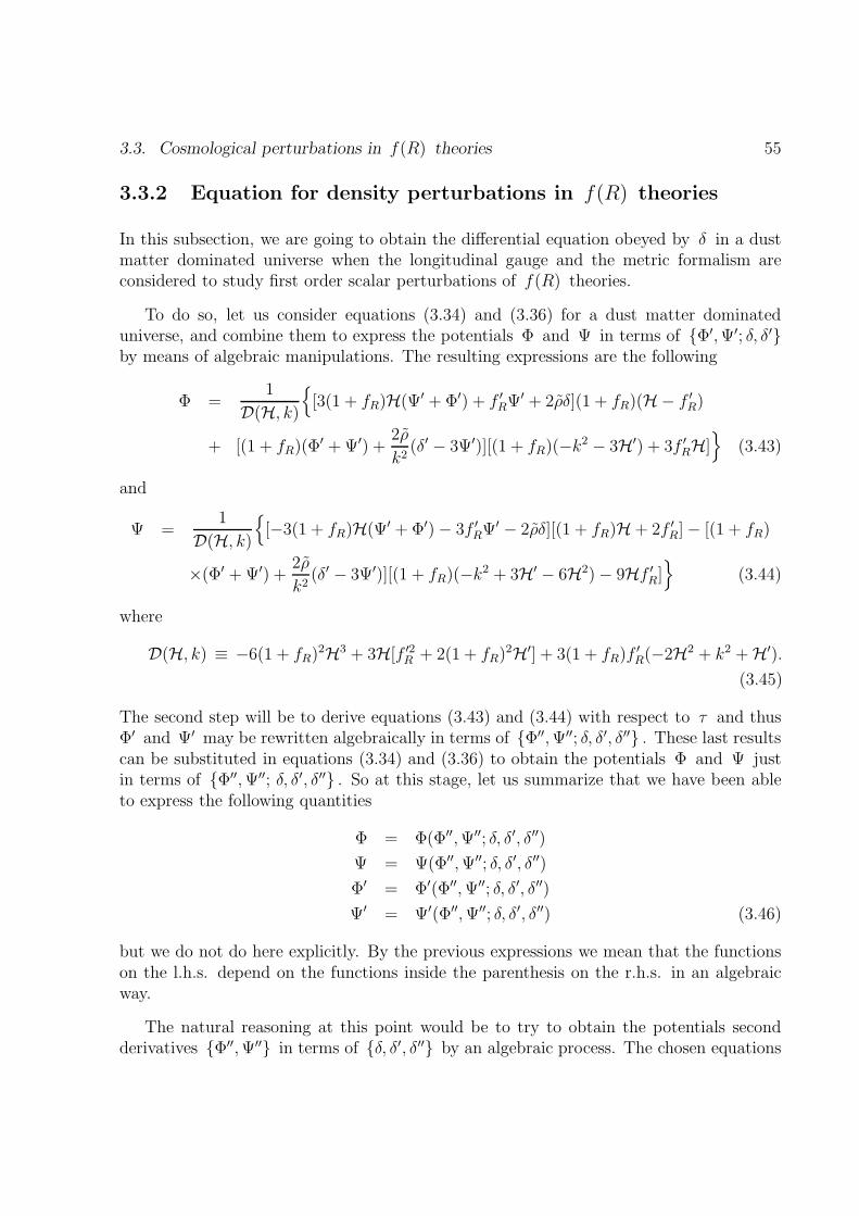
3.3. Cosmological perturbations in f(R) theories 55
3.3.2 Equation for density perturbations in f(R) theories
In this subsection, we are going to obtain the differential equation obeyed by δ in a dustmatter dominated universe when the longitudinal gauge and the metric formalism areconsidered to study first order scalar perturbations of f(R) theories.
To do so, let us consider equations (3.34) and (3.36) for a dust matter dominateduniverse, and combine them to express the potentials Φ and Ψ in terms of Φ′,Ψ′; δ, δ′by means of algebraic manipulations. The resulting expressions are the following
Φ =1
D(H, k)
[3(1 + fR)H(Ψ′ + Φ′) + f ′RΨ′ + 2ρδ](1 + fR)(H− f ′
R)
+ [(1 + fR)(Φ′ + Ψ′) +2ρ
k2(δ′ − 3Ψ′)][(1 + fR)(−k2 − 3H′) + 3f ′
RH]
(3.43)
and
Ψ =1
D(H, k)
[−3(1 + fR)H(Ψ′ + Φ′) − 3f ′RΨ′ − 2ρδ][(1 + fR)H + 2f ′
R] − [(1 + fR)
×(Φ′ + Ψ′) +2ρ
k2(δ′ − 3Ψ′)][(1 + fR)(−k2 + 3H′ − 6H2) − 9Hf ′
R]
(3.44)
where
D(H, k) ≡ −6(1 + fR)2H3 + 3H[f ′2R + 2(1 + fR)2H′] + 3(1 + fR)f ′
R(−2H2 + k2 + H′).
(3.45)
The second step will be to derive equations (3.43) and (3.44) with respect to τ and thusΦ′ and Ψ′ may be rewritten algebraically in terms of Φ′′,Ψ′′; δ, δ′, δ′′ . These last resultscan be substituted in equations (3.34) and (3.36) to obtain the potentials Φ and Ψ justin terms of Φ′′,Ψ′′; δ, δ′, δ′′ . So at this stage, let us summarize that we have been ableto express the following quantities
Φ = Φ(Φ′′,Ψ′′; δ, δ′, δ′′)
Ψ = Ψ(Φ′′,Ψ′′; δ, δ′, δ′′)
Φ′ = Φ′(Φ′′,Ψ′′; δ, δ′, δ′′)
Ψ′ = Ψ′(Φ′′,Ψ′′; δ, δ′, δ′′) (3.46)
but we do not do here explicitly. By the previous expressions we mean that the functionson the l.h.s. depend on the functions inside the parenthesis on the r.h.s. in an algebraicway.
The natural reasoning at this point would be to try to obtain the potentials secondderivatives Φ′′,Ψ′′ in terms of δ, δ′, δ′′ by an algebraic process. The chosen equations

56 Chapter 3. Cosmological perturbations in f(R) theories
to do so will be (3.42) and the first derivative of (3.37) with respect to τ . In (3.42) itis necessary to substitute Φ and Ψ′ by the expressions obtained in (3.46) whereas (3.37)first derivative may be sketched as follows
Φ′ − Ψ′ = − fRR
1 + fRδR′ +
[
fRRf′R − f ′
RR(1 + fR)
(1 + fR)2
]
δR. (3.47)
Before deriving, we are going to substitute Ψ′′ that appears on (3.37) by lower derivativespotentials Φ,Ψ,Φ′,Ψ′ , δ and its derivatives. To do so we consider (3.34) and (3.36)first derivatives with respect to τ where the quantity v has been previously substitutedby its expression in (3.40). Following this process we may express Ψ′′ as follows
Ψ′′ = Ψ′′(Φ,Ψ,Φ′,Ψ′; δ, δ′, δ′′) (3.48)
and now substituting the previous result (3.48) in δR definition given by expression (3.37),we can derive equation (3.37) with respect to τ . Solving a two algebraic equations systemwith equations (3.42) and (3.47) and introducing (3.46) we are able to express Φ′′,Ψ′′in terms of δ, δ′, δ′′, δ′′′ .
Φ′′ = Φ′′(δ, δ′, δ′′, δ′′′) ; Ψ′′ = Ψ′′(δ, δ′, δ′′, δ′′′). (3.49)
Thus we substitute the results obtained in (3.49) straightforwardly in (3.46) in order toexpress Φ,Ψ,Φ′,Ψ′ in terms of δ, δ′, δ′′, δ′′′ . With the two potentials and their firstderivatives as algebraic functions of δ, δ′, δ′′, δ′′′ , we perform the last step: We considerΦ(δ, δ, δ′′, δ′′′) and derive it with respect to τ . The result should be equal to Φ′(δ, δ′, δ′′, δ′′′)so we only need to express together these two results obtaining a fourth order differentialequation for δ . Once this fourth order differential equation has been solved we may gobackwards and by using the results for δ we obtain Φ′′,Ψ′′ from (3.49) as conformaltime τ functions. Analogously from (3.46) the behaviour of the potentials Φ,Ψ andtheir first derivatives could be determined.
The resulting equation for δ can be written as follows:
β4,fδiv + β3,fδ
′′′ + (α2,EH + β2,f)δ′′ + (α1,EH + β1,f)δ
′ + (α0,EH + β0,f )δ = 0 (3.50)
where the coefficients βi,f (i = 0, ..., 4) involve terms with f ′R and f ′′
R , i.e. termsdisappearing if the choice fR constant is made. Equivalently, αi,EH (i = 0, 1, 2) containterms coming from EH term and the linear part in R(0) of f(R) .
It is very useful to define the parameter ǫ ≡ H/k since it will allow us to perform aperturbative expansion of the previous coefficients α ’s and β ’s in the sub-Hubble limit.Other dimensionless parameters which will be used are the following:
κi ≡H(i)
Hi+1i = 1, 2, 3 ; fi ≡
f(i)R
HifRi = 1, 2. (3.51)

3.3. Cosmological perturbations in f(R) theories 57
where superindex (i) means ith derivative with respect to time τ . Expressing now theα ’s and β ’s coefficients as parameter ǫ expansions, we may write
αi,EH =3∑
k=1
α(k)i,EH i = 0, 1, 2
βi,f =7∑
k=1
β(k)i,f i = 3, 4
βi,f =8∑
k=1
β(k)i,f i = 0, 1, 2 (3.52)
where two consecutive terms in each series differ in a ǫ2 factor. The expressions for thecoefficients are too long to be written explicitly. Instead, in the following sections we shallshow different approximated formulae which are proven to be useful in certain limits. Asa consistency check, we find that, both in a matter dominated universe and in ΛCDM, allβ coefficients are absent since f1 and f2 defined by expression (3.51) vanish identically.For these cases, equation (3.50) becomes equation (3.31) as expected. For instance, inthe pure matter dominated case, coefficients κ ’s are constant and they take the followingvalues κ1 = −1/2 , κ2 = 1/2 , κ3 = −3/4 and κ4 = 3/2 .
Another important feature from our results is that, in general, without imposing |fR| ≪1 , the quotient
α1, EH + β1, f
α2, EH + β2, f(3.53)
is not always equal to H . In fact only the quotients
β(1)1, f
β(1)2, f
andα
(1)1,EH
α(1)2,EH
(3.54)
are identically equal to H . This last result, namely α(1)1,EH/α
(1)2,EH , is in perfect agreement
with δ′ coefficient in expression (3.31) when one is studying sub-Hubble modes in ΛCDMtheory, i.e., when βi, f i = 0, ..., 4 are not present.
3.3.3 Evolution of sub-Hubble modes and the quasi-static appro-
ximation
We are interested in the possible effects on the growth of density perturbations once theyenter the Hubble radius in the matter dominated era. In this case H ≪ k and therefore

58 Chapter 3. Cosmological perturbations in f(R) theories
the sub-Hubble limit ǫ ≪ 1 can be considered. It can be seen that the β4,f and β3,f
coefficients are suppressed by ǫ2 with respect to β2,f , β1,f and β0,f , i.e., in this limit theequation for perturbations reduces to the following second order expression:
δ′′ + Hδ′ + (1 + fR)5H2(−1 + κ1)(2κ1 − κ2) − 16a8 f
4RR(κ2 − 2)k88πGρ0a
2
(1 + fR)5(−1 + κ1) + 24a8 f
4RR(1 + fR)(κ2 − 2)k8
δ = 0 (3.55)
where we have taken only the leading terms in the ǫ expansion for both α and β coeffi-cients.
This expression can be compared with the one usually considered in the literatureby performing the so-called quasi-static approximation, obtained after performing strongsimplifications in the perturbed equations - (3.34), (3.35), (3.36), (3.37), (3.40) and (3.41)- by neglecting time derivatives of Φ and Ψ potentials, (see [76]). Thus, for instance inreferences [77] and [78], the quasi-static approximation is given by:
δ′′
+ Hδ′ −1 + 4k2
a2fRR
1+fR
1 + 3k2
a2fRR
1+fR
4πGρ0a2
1 + fRδ = 0. (3.56)
This approximation has been nonetheless considered as too aggressive in [79] sinceneglecting time derivatives can remove important information about the evolution of per-turbations.
Note also that in equation (3.55) there exists a difference in a power k8 between thoseterms coming from the f -part and those coming from the EH-part. This result differsfrom that in the quasi-static approximation where difference is in a power k2 accordingto expression (3.56).
In order to compare the evolution for both equations, we have considered a specificfunction
ftest(R) = −4R0.63 (3.57)
where H20 units have been used, which gives rise to a matter era followed by a late time
accelerated phase with the correct deceleration parameter today. In fact this model belongsto Class II f(R) models presented in Section 2.4 and it is therefore cosmologically viable.
Initial conditions in the matter era were given at redshift z = 485 where the EH-part was dominant. Results, for k = 0.2 hMpc−1 are presented in Figure 3.1. It can beseen that, as expected, both expressions give rise to the same evolutions at early times(large redshifts) where they also agree with the standard ΛCDM evolution. However, atlate times the quasi-static approximation fails to describe the evolution of perturbationscorrectly.

3.3. Cosmological perturbations in f(R) theories 59
0.0
0.1
0.2
0.3
0.4
0.5
0.6
0.7
0.8
1 10 100 0
0.1
0.2
0.3
0.4
0.5
0.6
0.7
0.8
δ κ
1+z
k = 0.2 h Mpc-1
δ δ quasi-static
δ ΛCDM
Figure 3.1: δk with k = 0.2 h Mpc−1 for ftest(R) model and ΛCDM . Both standard quasi-staticevolution and equation (3.55) have been plotted in the redshift range from 100 to 0.
Notice that this f(R) model given by expression (3.57) satisfies all the viability con-ditions described in Section 1.6 except for the local gravity tests implemented by thecondition 4 in that section. As is proven below, it is precisely this last condition namely
|fR| ≪ 1 (3.58)
which in fact ensures the validity of the quasi-static approximation. Therefore we shallnow restrict ourselves to f(R) models satisfying all the viability conditions, including|fR| ≪ 1 .
In Appendix A.1 we have reproduced all the α ’s and the first four β ’s coefficientsfor each δ term in (3.50). When the sub-Hubble modes are studied and the condition|fR| ≪ 1 is imposed, it can shown that the dominant contributions are the first fourβ coefficients of the f -part plus the first α coefficient of the EH-part for each term inequation (3.50). Thus in this case, the full differential equation (3.50) can be simplified as
c4δiv + c3δ
′′′
+ c2δ′′
+ c1δ′
+ c0δ = 0 (3.59)
where coefficients c0,1,...,4 are:
ci ≡ lim|fR|≪1
(
α(1)i, EH +
4∑
j=1
β(j)i, f
)
i = 0, 1, 2
ck ≡ lim|fR|≪1
4∑
j=1
β(j)k, f k = 3, 4 (3.60)

60 Chapter 3. Cosmological perturbations in f(R) theories
once the condition |fR| ≪ 1 has been imposed on the corresponding α ’s and β ’s contribu-tions. These coefficients c0,...,4 have been explicitly written in Appendix A.2. We see thatindeed in the sub-Hubble limit the c4 and c3 coefficients are negligible and the equationcan be reduced to a second order expression. Moreover, for our approximated expression(3.59) it is true that c1/c2 ≡ H as can be seen in Appendix A.2 straightforwardly.
From those expressions in Appendix A.2, the second order equation for δ becomes
δ′′ + Hδ′ − 4
3
[
6fRRk2
a2 + 94
(
1 −√
1 − 89
2κ1−κ2
−2+κ2
)] [
6fRRk2
a2 + 94
(
1 +√
1 − 89
2κ1−κ2
−2+κ2
)]
[
6fRRk2
a2 + 52
(
1 −√
1 − 2425
−1+κ1
−2+κ2
)] [
6fRRk2
a2 + 52
(
1 +√
1 − 2425
−1+κ1
−2+κ2
)]
×(1 − κ1)H2δ = 0 (3.61)
which can also be written as:
δ′′ + Hδ′ − 4
3
(
6fRRk2
a2 + 94
)2 − 8116
+ 92
2κ1−κ2
−2+κ2(
6fRRk2
a2 + 52
)2 − 254
+ 6−1+κ1
−2+κ2
(1 − κ1)H2δ = 0. (3.62)
Note that the quasi-static expression (3.56) is only recovered in the dust matter era (i.e.for H = 2/τ ) or for a pure ΛCDM evolution for the background dynamics. Nonetheless,in the considered limit |fR| ≪ 1 it can be proven, using the background equations ofmotion, that
1 + κ1 − κ2 ≈ 0 (3.63)
and therefore 2κ1 −κ2 ≈ −2 +κ2 ≈ −1 +κ1 what allows to simplify the expression (3.62)to become (3.56). This is nothing but the fact that for viable models the backgroundevolution resembles that of ΛCDM [31].
In other words, although for general f(R) functions the quasi-static approximationis not justified, for those viable f(R) functions describing the present phase of accelera-ted expansion and satisfying local gravity tests, it does give a correct description for theevolution of perturbations. This result has been here stated for the first time sheddingsome light about the controversy which remained about the validity of the quasi-staticapproximation.
3.3.4 Some proposed models
In order to illustrate the results obtained in the previous section, we propose two particularf(R) theories which allow us to determine - at least numerically - all the quantities involvedin the calculations and therefore to obtain solutions for the equation (3.61).

3.3. Cosmological perturbations in f(R) theories 61
0.0
0.1
0.2
0.3
0.4
0.5
0.6
0.7
0.8
1 10 100 0
0.1
0.2
0.3
0.4
0.5
0.6
0.7
0.8
δ κ
1+z
k = 1.67 h Mpc-1
δδ quasi-static
δ ΛCDM
Figure 3.2: δk with k = 1.67 h Mpc−1 for f(R) model A evolving according to equation (3.61),ΛCDM and quasi-static approximation given by equation (3.56) in the redshift range from 100 to 0. Thequasi-static evolution is indistinguishable from that coming from the equation (3.61), but diverges fromΛCDM behaviour as z decreases.
As was proven before, the background evolution for viable f(R) models resemblesthat of ΛCDM at low redshifts and that of a matter dominated universe at high redshifts.Nevertheless, the f(R) contribution gives the dominant contribution to the gravitationalaction (1.3) for small curvatures and therefore it may explain the cosmological accelera-tion. For the sake of concreteness, the models parameters have been fixed by imposing adeceleration parameter today q0 ≈ −0.6 .
Thus, our first model A will be:
f(R) = c1Rp. (3.64)
According to the results presented in references [55] and [80] viable models of this typebelong to Class II introduced in Chapter 2. As was mentioned there, they both includematter dominated and late time accelerated eras provided the parameters satisfy c1 < 0and 0 < p < 1 . We have chosen c1 = −4.3 and p = 0.01 in H2
0 units. This choice doesverify all the viability conditions, including |fR| ≪ 1 today.
As a second model B we have chosen:
f(R) =1
c1Re1 + c2(3.65)
with values c1 = 2.5 · 10−4 , e1 = 0.3 and c2 = −0.22 also in the same units.
For each model, we compare our result (3.61) with the standard ΛCDM evolution andthe quasi-static approximation (3.56) by plotting δ evolution in Figures 3.2 and 3.3 for

62 Chapter 3. Cosmological perturbations in f(R) theories
0.0
0.1
0.2
0.3
0.4
0.5
0.6
0.7
0.8
1 10 100 0
0.1
0.2
0.3
0.4
0.5
0.6
0.7
0.8
δ k
1+z
k = 1.67 h Mpc-1
δδ quasi-static
δ ΛCDM
Figure 3.3: δk with k = 1.67 h Mpc−1 for f(R) model B evolving according to equation (3.61),ΛCDM and quasi-static evolution given by equation (3.56) in the redshift range from 100 to 0. Thequasi-static evolution is indistinguishable from that coming from the equation (3.61), but diverges fromΛCDM behaviour as z decreases.
models A and B respectively. In both cases, the initial conditions are given at redshiftz = 1000 where δ is assumed to behave as in a matter dominated universe, i.e. δk(τ) ∝a(τ) with no k -dependence. We see that for both models, the quasi-static approximationgives a correct description for the evolution which clearly deviates from the ΛCDM case.
In Figure 3.4 the density contrast evaluated today was plotted as a function of k forboth models. The growing dependence of δ with respect to k is verified. This modifiedk -dependence with respect to the standard ΛCDM model could give rise to observableconsequences in the matter power spectrum, as shown in [56, 72], and could be used toconstrain or even to discard f(R) theories for cosmic acceleration as will be done in thenext section.
3.4 A viable f(R) model different from ΛCDM?
Some modified f(R) gravity models have recently been proposed (see for instance [58])claiming to be cosmologically viable in spite of having a cosmological behaviour clearlydistinguishable from ΛCDM . Contrary to already mentioned opinions which consider thatself-consistent f(R) gravity models distinct from ΛCDM are almost ruled out, authorsin [58] seem to claim that their proposed model would be cosmologically viable. We haveshown [72] that although that model does satisfy some consistency conditions, preciselybecause of its departure from ΛCDM behaviour, it does not satisfy local gravity constraints

3.4. A viable f(R) model different from ΛCDM? 63
0.5
0.6
0.7
0.8
0.9
1
5000 10000 15000 20000 25000 30000 35000 40000 0.5
0.6
0.7
0.8
0.9
1
δ tod
ay(k
)
k/H0
δtoday(k) f(R) model Aδtoday(k) f(R) model B
Figure 3.4: Scale dependence of δk evaluated today (z = 0) for k/H0 in the range from 103 to 4 ·104 .
and, in addition, the predicted matter power spectrum conflicts with SDSS data providedin reference [69]. The proposed f(R) model reads
f(R) = −αR∗log
(
1 +R
R∗
)
. (3.66)
This model does satisfy three of the usual viability conditions for f(R) theories providedin [31] and specified in Section 1.6. However, the model (3.66) does not satisfy the fourthof those conditions, namely, |fR| ≪ 1 at recent epochs, imposed by local gravity tests[33] from solar system. Although it is still not clear what is the actual limit on thisparameter, certain estimations give |fR| < 10−6 today. This condition also ensures thatthe cosmological evolution at late times resembles that of ΛCDM . However, for the model(3.66), |fR| ∼ 0.2 today for α = 2 and ΩM ∼ 0.25 .
If we are only interested in considering large scales, local gravity inconsistencies couldbe ignored, but still deviations from ΛCDM can have drastic cosmological consequenceson the evolution of density perturbations, as discussed by several authors [56, 70, 79].
Thus, the linear evolution of matter density perturbations for sub-Hubble ( k ≫ H )modes in ΛCDM is given by equation (3.31). Notice that in this equation the evolutionof the Fourier modes does not depend on k . This means that once the density contraststarts growing after matter-radiation equality, the mode evolution only changes the overallnormalization of the matter power-spectrum, but not its shape.
However, in f(R) theories for sub-Hubble modes, as was thoroughly studied in theprevious section, the corresponding equation reads as (3.55). Notice from this equationthe k8 dependence in the δ term which appears due to the fact that fRR 6= 0 . Moreover,

64 Chapter 3. Cosmological perturbations in f(R) theories
Redshift EH term (in H0 units) f term (in H0 units) RfRR
100 61.35 1.90 · 10−4 1.45 · 10−6
50 30.97 5.34 1.12 · 10−5
20 12.69 2.86 · 106 1.58 · 10−4
0 −0.45 1.01 · 1017 0.079
Table 3.1: Values (in H0 units) for both the first EH term and the first f term (the one proportional to
k8 ) in the numerator of the δ coefficient in equation (3.55) for this model (3.66). Different redshifts havebeen considered and the studied scale was k = 0.33 h Mpc−1 . The EH term, which is k independent,cannot be ignored at high redshift. In fact, the redshift at which EH and f terms contributions (forthis value of k ) equal is around z = 45 . The strong suppression with the redshift of the f -part term– which is proportional to k8 in the δ coefficient in equation (3.55) – comes from the rapid suppressionof f4
RR factor as the redshift increases. The dimensionless quantity R fRR has also been included in thelast column of the table and it is seen to grow as the redshift decreases ( z → 0 ).
a careful calculation of involved contributions in equation (3.55) shows that in the δ term3
there exist two contributions: one term is proportional to k8 , which is coming from the β ’scontribution, i.e. f -part, and another term coming from α ’s contribution, i.e. EH-part.At high enough redshift the EH-part term dominates, whereas at low redshift the situationis reversed and the f -part term becomes dominant. This is the crucial point that explainswhy k -independent terms both in numerator and denominator cannot be straightforwardlyremoved from δ coefficient in equation (3.55) but they have to be preserved for a correctsub-Hubble modes study. Thus for instance, for k = 0.33 hMpc−1 , we give explicit valuesin Table 3.1 for the terms in the numerator of the δ coefficient in equation (3.55).
As a consequence the matter power-spectrum Pf(R)k is further processed after equality
and would differ today from the standard ΛCDM power spectrum PΛCDMk . These two
quantities would be related by a linear transfer function T (k) given by:
Pf(R)k = T (k)PΛCDM
k . (3.67)
This fact changes the shape of the matter power spectrum dramatically, as shown in Figure3.5, where normalization to WMAP3 [81] was imposed. In this figure, SDSS data fromluminous red galaxies [69] and the ΛCDM power spectrum from the linear perturbationtheory with WMAP3 cosmological data [81] are also shown. Notice that ΛCDM givesan excellent fit to data with χ2 = 11.2 , whereas for the f(R) theory χ2 = 178.9 , i.e.13σ out. Even if the overall normalization is drastically reduced by a 20 % , which isthe present uncertainty over this parameter, the discrepancy would still remain at the 7 σlevel. Actually, leaving the power spectrum normalization as a free parameter, the bestfit would require a 32% normalization reduction and still would be 4.8σ away as seen inFigure 3.5.
3Let us consider the numerator of this term for simplicity. This does not mean any loss of generalitysince the denominator behaviour is completely analogous.

3.4. A viable f(R) model different from ΛCDM? 65
104
105
10-2 10-1
Pow
er s
pect
rum
P(k
) (h
-1M
pc)3
k [h Mpc-1]
LRG data
ΛCDM fit to WMAP3
f(R)
f(R) 32 % suppressed
Figure 3.5: Linear matter power-spectra for ΛCDM and f(R) in [58] with α = 2 . Data were takenfrom SDSS [69].
The linear transfer function (3.67) for this model has been plotted in Figure 3.6 andit has been seen that T (k) follows with a nice fit a power law in the plotted intervalT (k) = (k/keq)
0.19 where keq ≃ 10−2 hMpc−1 corresponds to the physical scale enteringthe Hubble radius when matter-radiation equality happened.

66 Chapter 3. Cosmological perturbations in f(R) theories
0.90
1.00
1.10
1.20
1.30
1.40
1.50
1.60
0.01 0.02 0.03 0.04 0.05 0.06 0.07 0.08 0.09 0.10
T(k
)
k [h Mpc-1]
Figure 3.6: Transfer function T (k) for f(R) model given in equation (3.66) with α = 2 and ΩM ∼0.25 . The k dependence for T (k) with this parameters choice was seen to be T (k) ∝ k0.19 in the plottedrange of scales. Both the numerical T (k) and the power law proportional to k0.19 were plotted in scalesk = 0.01 − 0.10 h Mpc−1 and no difference was observed.
3.5 Conclusions
In this chapter we have studied the evolution of matter density perturbations in f(R)theories of gravity. Thus we have presented a completely general procedure to obtain theexact fourth order differential equation for the evolution of scalar perturbations in thelongitudinal gauge. This expression is valid for any general f(R) theory and applicable atany scale k . If the EH gravitational action – both with and without cosmological constant– is considered in this general expression, well-known standard results are recovered.
We have also shown that for sub-Hubble modes, the obtained expression reduces to asecond order differential equation. Hence, we have been able to compare this result withthat obtained within the quasi-static approximation, widely used in the literature. Ourresearch has explicitly shown that for arbitrary f(R) functions such an approximation isnot justified.
However, if we limit ourselves to f(R) theories for which |fR| ≪ 1 today, then theperturbative calculation for sub-Hubble modes requires to take into account, not only thefirst terms, but also higher-order terms in the ǫ ≡ H/k parameter. In that case, theresummation of such terms modifies the equation. Thus, this equation can be seen to beequivalent to the quasi-static case but only if the universe expands approximately as in amatter dominated phase or in a ΛCDM model. Finally, the fact that for f(R) modelswith |fR| ≪ 1 the background behaves today precisely as that of ΛCDM makes the

3.5. Conclusions 67
quasi-static approximation correct in those cases.
We have finally applied our results to prove that no significant departure of f(R)theories from ΛCDM is allowed for those models that intend to be cosmologically viableaccording to recent data. In fact, the strong k -dependence appearing in the evolution ofperturbations has allowed to rule out f(R) gravities which have recently been claimed tobe cosmologically viable.

68 Chapter 3. Cosmological perturbations in f(R) theories

Chapter 4
Black holes in f (R) theories
4.1 Introduction
We finish the exposition of our research on f(R) modified gravities by considering someaspects derived from the study of BHs in these theories.
Following the motivation already explained in Section 1.1, f(R) models may presentBH solutions as GR and other alternative gravity theories do. Therefore it is quite naturalto ask about BHs features in those gravitational theories since, on the one hand, some BHssignatures may be peculiar to Einstein’s gravity and others may be robust features of allgenerally covariant theories of gravity. On the other hand, the results obtained may leadto rule out some models which will be in disagreement with expected physical results. Forthose purposes, research on thermodynamical quantities of BHs is of particular interest.
These attempts to detect particular signatures from these objects could be experimen-tally implemented, as was explained in Section 1.10, at the LHC in the coming years.Therefore the generation of mini BHs could provide important information about the co-rrect underlying gravity theory.
Previous literature on f(R) theories [82] proved, by previously performing a conformaltransformation in the gravitational action, that Schwarzschild solution is the only staticspherically symmetric solution for an action of the form R+aR2 in D = 4 . Also by usingthis conformal transformation, uniqueness theorems of spherically symmetric solutions forgeneral polynomial actions in arbitrary dimensions were proposed in [83] (see also [84] foradditional results and [85] for spherical solutions with sources).
Using the Euclidean action method [86, 87] in order to determine different thermody-namical quantities, anti-de Sitter (AdS ) BHs in f(R) models have been studied [88]. In
69

70 Chapter 4. Black holes in f(R) theories
[89] the entropy of Schwarzschild-de Sitter BHs was calculated for some particular cosmo-logically viable models in vacuum and their cosmological stability was discussed.
BH properties have also been widely studied in other modified gravity theories: forinstance, [90, 91] studied BHs in Einstein’s theory with a Gauss-Bonnet term plus a cos-mological constant. Different results were found depending on the dimension D and thesign of the constant horizon curvature k . For k = 0,−1 , the Gauss-Bonnet term doesnot modify AdS BHs thermodynamics at all (only the horizon position is modified withrespect to the EH theory) and BHs are not only locally thermodynamically stable, but alsoglobally preferred. Nevertheless, for k = +1 and D = 5 (for D ≥ 6 thermodynamics isagain essentially that for AdS BH) there exist some features not present in the absenceof Gauss-Bonnet term. Gauss-Bonnet and/or Riemann squared interaction terms werestudied in [92], where the authors concluded that in this case phase transitions may occurwith k = −1 .
Another approach is given by Lovelock gravities, which are free of ghosts and wherethe field equations contain no more than second derivatives of the metric. These theorieswere for instance studied in [93] and the corresponding entropy was evaluated.
The layout of this chapter is as follows: In Section 4.2 some generalities about BHs inf(R) theories such as several aspects of constant curvature solutions for static sphericallysymmetric cases with and without electric charge are presented. Then in Section 4.3 aperturbative approach around the EH action, with no previous imposition of constant cur-vature, is performed. There we shall find that up to second order in perturbations only BHsolutions of the Schwarzschild-AdS type are present. Explicit expressions for the effectivecosmological constant are obtained in terms of the f(R) function. To deal with suchdifferential equations we have used the algebraic manipulation package Mathematica [94].
Finally, we shall consider in Section 4.4 the BHs thermodynamics in AdS space-time.There it will be found that this kind of solutions can only exist provided the theory satisfiesR0 + f(R0) < 0 where R0 holds for the constant curvature solution. Interestingly, thisexpression is proved to be related to the condition which guarantees the positivity ofthe effective Newton’s constant in this type of theories. In addition, it also ensures thatthe thermodynamical properties in f(R) gravities are qualitatively similar to those ofstandard GR. Then, some consequences for local and global stability for some particularf(R) models will be provided in Section 4.5 and figures of thermodynamical regions willbe shown in Section 4.6. The present chapter is finished by Section 4.7 remarking someconclusions of the presented results.
This chapter is mainly based upon the results that have been presented in references[26] and [95].

4.2. Constant curvature black-hole solutions 71
4.2 Constant curvature black-hole solutions
The most general static and spherically symmetric D ≥ 4 dimensional metric can bewritten as (see [96]):
ds2 = e−2Φ(r)A(r)dt2 − A−1(r)dr2 − r2dΩ2D−2 (4.1)
or alternatively
ds2 = λ(r)dt2 − µ−1(r)dr2 − r2dΩ2D−2 (4.2)
where dΩ2D−2 is the metric on the SD−2 sphere. The identification λ(r) = e−2Φ(r)A(r)
and µ(r) = A(r) can be straightforwardly established. For obvious reasons, the Φ(r)function is called the anomalous redshift: notice that a photon emitted at r with properfrequency ω0 is measured at infinity with frequency ω∞ = ω0e
−Φ(r)√
A(r) .
Since the metric is static, the scalar curvature R in D dimensions depends only on rand it is given, for the metric parametrization (4.1), by:
R(r) =1
r2(D − 2) [(D − 3)(1 − A(r)) + 2r(A(r)Φ′(r) −A′(r))]
+ r2[
3A′(r)Φ′(r) −A′′(r) − 2A(r)(Φ′2(r) − Φ′′(r))]
(4.3)
where the prime denotes derivative with respect to r . At this stage it is interesting toask about which are the most general static and spherically symmetric metric tensors withconstant scalar curvature R0 . This metric tensor can be found by solving the equationR(r) = R0 . Thus, it is immediate to see that for a Φ(r) = Φ0 constant, this equationbecomes
R(r) ≡ R0 =1
r2
[
(D2 − 5D + 6)(1 − A(r)) + rA′(r)(−2D + 4) − r2A′′(r)]
(4.4)
whose general solution is
A(r) = 1 + a1r3−D + a2r
2−D − R0
D(D − 1)r2 (4.5)
with a1 and a2 arbitrary integration constants. In fact, for the particular case D = 4 ,R0 = 0 and Φ0 = 0 , the metric can be written exclusively in terms of the function:
A(r) = 1 +a1
r+a2
r2. (4.6)
By establishing the identifications a1 = −2GM and a2 = Q2 , this solution correspondsto a Reissner-Nordstrom solution, i.e. a charged massive BH solution with mass M andcharge Q . Further comments about this result will be made at the end of the section.

72 Chapter 4. Black holes in f(R) theories
Now that the general static and spherically symmetric solution for constant curvaturehas been obtained as given by expression (4.5), let us insert the metric (4.1) into thegeneral f(R) gravitational action (1.3), and let us also perform variations with respectto the functions A(r) and Φ(r) , in order to find the corresponding modified Einsteinequations for this parametrization. Thus, we obtain
(2 −D)(1 + fR)Φ′(r) − r[
fRRRR′(r)2 + fRR (Φ′(r)R′(r) +R′′(r))
]
= 0 (4.7)
and
2rA(r)fRRRR′(r)2 + fRR [2(D − 2)A(r)R′(r) + 2rA(r)R′′(r) + A′(r)rR′(r)]
+ (1 + fR)[
2r(A(r)Φ′′(r) − A(r)Φ′(r)2) + 2(D − 2)A(r)Φ′(r) − rA′′(r)
+A′(r)(2 −D + 3rΦ′(r))] − r(R + f(R)) = 0 (4.8)
where as in previous chapters fR ≡ df(R)/dR , fRR ≡ d2f(R)/dR2 and fRRR ≡d3f(R)/dR3 . The above equations look in principle quite difficult to solve. For thisreason we shall firstly consider the case with constant scalar curvature R = R0 solutions.In this simple case the two previous equations reduce to:
(2 −D) (1 + fR)Φ′(r) = 0 (4.9)
and
R + f(R) + (1 + fR)
[
A′′(r) +(D − 2)
r(A′(r) − 2A(r)Φ′(r)) − 3A′(r)Φ′(r)
+2A(r)(
Φ′(r)2 − Φ′′(r))]
= 0 (4.10)
As was commented in the Section 1.5, the constant curvature solutions in vacuum of f(R)gravities are given by the equation (1.33) which can be rewritten as:
R0 =D f(R0)
2(1 + fR(R0)) −D(4.11)
whenever 2(1 + fR(R0)) 6= D . Thus from (4.9) one obtains Φ′(r) = 0 and then, for aconstant scalar curvature R0 , the equation (4.10) becomes
R0 + f(R0) + (1 + fR(R0))
[
A′′(r) + (D − 2)A′(r)
r
]
= 0 . (4.12)
By inserting expression (4.11) in the previous equation (4.12), we get
A′′(r) + (D − 2)A′(r)
r= − 2
DR0 . (4.13)

4.2. Constant curvature black-hole solutions 73
This is a f(R) -independent linear second order inhomogeneous differential equation whichcan be easily integrated to give the general solution:
A(r) = c1 + c2r3−D − R0
D(D − 1)r2 (4.14)
which depends on two arbitrary constants c1 and c2 . However, this solution has noconstant curvature in the general case since, as was found above, the constant curvaturerequirement demands c1 = 1 . Then for negative R0 this solution is basically the Ddimensional generalization studied by Witten [86] of the BH in AdS space-time solutionconsidered by Hawking and Page [87]. With the natural choice Φ0 = 0 , that solution canbe written as:
A(r) = 1 −(
RS
r
)D−3
+r2
l2(4.15)
where
RD−3S =
16πGDM
(D − 2)µD−2(4.16)
with
µD−2 =2π
D−12
Γ(
D−12
) (4.17)
being the area of the D − 2 sphere,
l2 ≡ −D(D − 1)
R0(4.18)
is the asymptotic AdS space scale squared and M is the mass parameter usually foundin the literature.
Thus we have concluded that the only static and spherically symmetric vacuum solu-tions with constant curvature of any f(R) gravity (R0 < 0 provided) is just the Hawking-Page BH in AdS space. However, this kind of solution is not the more general static andspherically symmetric metric with constant curvature as can be seen by comparison withthe solutions found in expression (4.5). Therefore we have to conclude that there are cons-tant curvature BH solutions that cannot be obtained as vacuum solutions of any f(R)theory.
Let us now consider the case of charged BHs in f(R) theories. For the sake of simplicitywe shall limit ourselves to the D = 4 case. The action of the theory will be now:
Sf(R)-Maxwell =1
16πG
∫
d4x√
| g | (R + f(R) − FµνFµν) (4.19)
which is a generalization of the Einstein-Maxwell theory. The tensor Fµν is defined as:
Fµν ≡ ∂µAν − ∂νAµ . (4.20)

74 Chapter 4. Black holes in f(R) theories
Considering an electromagnetic potential of the form: Aµ =(
V (r), ~0)
and the static
spherically symmetric metric (4.2), we find that the solution with constant curvature R0
reads:
V (r) = −Qr,
λ(r) = µ(r) = 1 − 2GM
r+
(1 + fR(R0))Q2
r2− R0
12r2 . (4.21)
Notice that unlike the EH case, the contribution of the BH charge to the metric tensor iscorrected by a (1 + fR(R0)) factor.
4.3 Perturbative results
In the previous section we have considered static spherically symmetric solutions withconstant curvature. In EH theory it is trivial to show that the only static and sphericallysymmetric solution possess constant scalar curvature. However, it is not guaranteed thisto be the case in f(R) theories too. The problem of finding the general static sphericallysymmetric solution in arbitrary f(R) theories without imposing the constant curvaturecondition is in principle quite complicated. For that reason, we shall present in this sectiona perturbative analysis of the problem, assuming that the modified action given by theexpression (1.3) is a small perturbation around EH theory.
The computation we are about to sketch is quite an involved one since, in orderto calculate the solutions to a given order, it requires to introduce previous order re-sults. To deal with such large equations we have used the algebraic manipulation packageMathematica [94].
Therefore let us consider a f(R) function of the form
f(R) = −(D − 2)ΛD + αg(R) (4.22)
where α ≪ 1 is a dimensionless parameter and g(R) is assumed to be analytic whenexpanded for perturbative solutions. Note that nonanalytic functions in α are thereforeexcluded of this analysis.
By using the metric parametrization given by (4.2) the equations of motion become:
λ(r)(1 + fR) 2µ(r) [(D − 2)λ′(r) + rλ′′(r)] + rλ′(r)µ′(r)− 2λ(r)2
2µ(r)[(D − 2)R′(r)fRR + rfRRR R′(r)2 + rR′′(r)fRR] + rR′(r)µ′(r)fRR
− rµ(r)λ′(r)2(1 + fR) + 2rλ(r)2(R + f(R)) = 0 (4.23)

4.3. Perturbative results 75
and
µ(r)
2λ(r)R′(r) [2(D − 2)λ(r) + rλ′(r)] fRR + r(1 + fR)(λ′(r)2 − 2λ(r)λ′′(r))
−λ(r)µ′(r) [2(D − 2)λ(r) + rλ′(r)] (1 + fR) − 2rλ(r)2(R + f(R)) = 0 (4.24)
where R ≡ R(r) is given by expression (4.3). Now the λ(r) and µ(r) functions appearingin the metric (4.2) can be written as follows
λ(r) = λ0(r) +
∞∑
i=1
αiλi(r)
µ(r) = µ0(r) +∞∑
i=1
αiµi(r). (4.25)
Notice that λ0(r) and µ0(r) are the unperturbed solutions for the EH action with cos-mological constant given by
µ0(r) = 1 +C1
rD−3− ΛD
(D − 1)r2
λ0(r) = C2 µ0(r) (4.26)
which are the standard BH solutions in a D dimensional AdS spacetime ( ΛD < 0 pro-vided). Note that the factor C2 can be chosen by performing a coordinate t reparametriza-tion so that both functions, µ0(r) and λ0(r) , could be identified. For the moment, weshall keep the background solutions as given in (4.26) and we shall discuss the possibilityof getting λ(r) = µ(r) in the perturbative expansion later on.
By inserting the expressions (4.22) and (4.25) in the equations (4.23) and (4.24) weobtain the following
First order equations:
(D − 3)µ1(r) + rµ′1(r) +
2ΛDgR(R0) − g(R0)
D − 2r2 = 0 (4.27)
C2
[
C1(D − 1)r3−D − ΛDr2 +D − 1
]
g(R0)r2 +
[
C1(D − 3)r3−D +2ΛD
D − 1r2
]
λ1(r)
+ C2(D − 2)(D − 1)(
ΛDr2 −D + 3
)
µ1(r)
+
(
1 + C1r3−D − ΛDr
2
D − 1
)
[
2C2(1 −D)r2ΛDgR(R0) + rλ′1(r)]
= 0
(4.28)
76 Chapter 4. Black holes in f(R) theories
where gR(R0) ≡ dg(R)/dR|R=R0 and whose solutions are:
λ1(r) = C4(D − 1)(D − 2) +(C1C4 − C2C3)(D − 2)(D − 1)
rD−3
− [C4(D − 2)ΛD + C2 (g(R0) − 2ΛDgR(R0))] r2
(4.29)
µ1(r) =C3
rD−3+
(g(R0) − 2ΛDgR(R0))
(D − 2)(D − 1)r2 . (4.30)
Up to second order in α , we obtain the following
Second order equations:
(D − 3)µ2(r) + rµ′2(r) +
(g(R0) − 2ΛDgR(R0))
D − 2
(
gR(R0) −2D
D − 2ΛDgRR(R0)
)
r2 = 0
(4.31)
[
−C1(D − 3)r3−D − 2ΛDr2
D − 1
]
λ2(r) + C2(D − 2)(D − 1)(
−ΛDr2 +D − 3
)
µ2(r)
−(
C1r4−D + r − r3ΛD
D − 1
)
λ′2(r) − C3C4(D − 2)(D − 1)(
−ΛDr2 +D − 3
)
r3−D
− C2
[
(D − 1)(C1r3−D + 1) − ΛDr
2]
[
2ΛDgR(R0)2 + g(R0)
(
2DΛDgRR(R0)
D − 2− gR(R0)
)
− 4DΛ2DgR(R0)gRR(R0)
D − 2
]
r2 − C4
[
C1(D − 1)r3−D + 2]
[2ΛDgR(R0) − g(R0)] r2 = 0
(4.32)
where gRR(R0) ≡ d2g(R)/dR2|R=R0 and whose solutions are:
λ2(r) = C6 +C6C1 + (C3C4 − C2C5)(D − 2)(D − 1)
rD−3
+
[
−C6ΛD
D − 1+ (g(R0) − 2ΛDgR(R0))
(
C4 + C2gR(R0) −2C2DΛDgRR(R0)
D − 2
)]
r2
(4.33)
µ2(r) =C5
rD−3+
(g(R0) − 2ΛDgR(R0)) (2DΛDgRR(R0) − (D − 2)gR(R0))
(D − 2)2(D − 1)r2. (4.34)

4.3. Perturbative results 77
Further orders in α3,4,... can be obtained by inserting the previous results in the sub-sequent differential equations to get λ3,4,...(r), µ3,4,...(r) . Nevertheless, these equationsbecome increasingly complicated to be explicitly solved.
Notice that from the obtained results up to second order in α , the correspondingmetric has constant scalar curvature for any value of the parameters C1,2,...,6 . As a matterof fact, this metric is nothing but the corresponding one to the standard Schwarzschild-AdS geometry, and can be easily rewritten in the usual form by making a trivial timereparametrization as follows:
λ(r) ≡ λ(r)[
−C2(D2 + 3D − 2) + C4
(
D2 − 3D + 2)
α + C6α2 + O(α3)
]
µ(r) ≡ µ(r). (4.35)
Therefore, at least up to second order, the only static, spherically symmetric solutionswhich are analytical in α are the standard Schwarzschild-AdS space-times.
4.3.1 General expression to arbitrary order for constant curva-
ture
Let us now assume from the very beginning that the solutions for the equations (4.23) and(4.24) belong to Schwarzschild-AdS BH type at any order in the α expansion. Thus wecan write ( J > 0 provided):
λ(r) ≡ µ(r) = 1 −(
RS
r
)D−3
+ Jr2 (4.36)
as solutions for the modified Einstein equations (4.23) and (4.24) derived when the mo-dification in the gravitational Lagrangian is given by expression (4.22). If we expand thequantities RS and J in terms of parameter α we get:
RS ≡ RS +∞∑
i=1
Ciαi
J ≡ − ΛD
(D − 1)+
∞∑
i=1
Jiαi (4.37)
where RS and Ci are arbitrary constants. The Ji coefficients can be determined fromexpression (1.33), which here becomes:
R − (D − 2)ΛD + αg(R) + 2(D − 1)J(1 + αg′(R)) = 0 (4.38)

78 Chapter 4. Black holes in f(R) theories
with R = −D(D − 1)J is the obtained result when calculating R with functions givenby (4.36). Expanding equation (4.38) in powers of α it is possible to find a recurrenceequation for the Ji coefficients, namely for the Jl (with l > 0 ) coefficient, we find:
(2 −D)(D − 1)Jl +l−1∑
i=0
∑
cond.1
1
i1!i2! . . . il−1!(J1)
i1(J2)i2 . . . (Jl−1)
il−1g(i)(R0)
+ 2(D − 1)l−1∑
k=0
Jk
l−k−1∑
i=0
∑
cond.2
1
i1!i2! . . . il−k−1!(J1)
i1(J2)i2 . . . (Jl−k−1)
il−k−1g(i+1)(R0) = 0
(4.39)
with R0 = −D(D − 1)J0 ≡ DΛD and g(i)(R0) ≡ d(i)g(R)/dR(i)|R=R0 . In the previousrecurrence relation, the first sum is done under the condition 1 given by:
l−1∑
m=1
im = i, im ∈ N ∪ 0 and
l−1∑
m=1
mim = l − 1 (4.40)
and the second one under the condition 2:
l−k−1∑
m=1
im = i, im ∈ N ∪ 0 andl−k−1∑
m=1
mim = l − k − 1. (4.41)
For instance we have:
J1 =A(g ; D, ΛD)
(D − 2)(D − 1)
J2 = −A(g ; D, ΛD)[(D − 2)gR(R0) − 2DΛDgRR(R0)]
(D − 2)2(D − 1)(4.42)
where A(g ; D, ΛD) ≡ g(R0) − 2ΛDgR(R0)
Now we can consider the possibility of removing ΛD from the gravitational Lagrangian(4.22) from the very beginning and still getting an AdS BH solution with an effectivecosmological constant depending on g(R) and its derivatives evaluated at R0 ≡ 0 . In thiscase the results, order by order in α up to order α2 , are:
J0(ΛD = 0) = 0,
J1(ΛD = 0) =g(0)
(D − 2)(D − 1),
J2(ΛD = 0) = − g(0)gR(0)
(D − 2)(D − 1). (4.43)
As we see, in the context of f(R) gravities, it is therefore possible to have a BH in an AdS

4.4. Black-hole thermodynamics 79
asymptotic space-time even if the initial cosmological constant ΛD vanishes but α g(0) > 0and α small enough as considered in the explained reasoning.
To end this section we can summarize by saying that in the context of f(R) gravitiesthe only spherically symmetric and static solutions in the general case (without imposingconstant curvature) in perturbation theory up to second order are the standard BHs inAdS space. However, the possibility of having static and spherically symmetric solutionswith nonconstant curvature cannot be excluded in the case of f(R) functions which arenot analytical in α .
4.4 Black-hole thermodynamics
In order to consider the different thermodynamic quantities for the f(R) BHs in AdSspace-time, we start from the temperature. In principle, there are two different ways ofintroducing this quantity for the kind of solutions that we are considering here. Firstlywe can use the definition coming from Euclidean quantum gravity [97]. In this case oneintroduces the Euclidean time τ = it and the Euclidean metric ds2
E is defined as:
−ds2E = −dσ2 − r2dΩ2
D−2 (4.44)
where:dσ2 = e−2Φ(r)A(r)dτ 2 + A−1(r)dr2. (4.45)
The metric corresponds only to the region r > rH where rH is the outer horizon positionwith A(rH) = 0 . Expanding dσ2 near rH we have:
dσ2 = e−2Φ(rH )A′(rH)ρ dτ 2 +dρ2
A′(rH)ρ(4.46)
where ρ = r − rH . Now we introduce the new coordinates R and θ defined as:
θ =1
2e−Φ(rH)A′(rH)τ ; R = 2
√
ρ
A′(rH)(4.47)
so that:dσ2 = R2dθ2 + dR2. (4.48)
According to the Euclidean quantum gravity prescription, τ coordinate in expression(4.46) is included in the interval defined by 0 and βE = 1/TE . On the other hand, inorder to avoid conical singularities, θ must run between 0 and 2π . Thus it is found that
TE =1
4πe−Φ(rH)A′(rH) . (4.49)

80 Chapter 4. Black holes in f(R) theories
Another possible definition of temperature was firstly proposed in [98] stating thattemperature can be given in terms of the horizon gravity K as:
TK ≡ K4π
(4.50)
where K is given by:
K = limr→rH
∂rgtt√
|gttgrr|. (4.51)
Then it is straightforward to find:
TK = TE. (4.52)
Therefore, both definitions give the same result for this kind of metric tensors. Notice alsothat in any case the temperature depends only on the behaviour of the metric near thehorizon but it is independent from the gravitational action. By this we mean that differentactions having the same solutions have also the same temperature. This is not the casefor other thermodynamic quantities as we shall see later. Taking into account the resultsin previous sections for Schwarzschild-AdS BHs, we shall concentrate for simplicity onlyon those solutions, i.e. for a metric as (4.2) where A(r) is given by expression (4.15) andΦ = 0 is adopted as a natural choice.
Then, both definitions of temperature lead to:
β =1
T=
4πl2rH
(D − 1)r2H + (D − 3)l2
. (4.53)
Notice that the temperature is a function of rH only, i.e. it depends only on the BH size.In the limit rH going to zero the temperature diverges as T ∼ 1/rH and for rH going toinfinity T grows linearly with rH . Consequently T has a minimum at:
rH0 = l
√
D − 3
D − 1(4.54)
corresponding to a temperature:
T0 =
√
(D − 1)(D − 3)
2πl. (4.55)
The existence of this minimum was established in [87] for D = 4 by Hawking and Pagelong time ago and it is well-known. More recently Witten extended this result to higherdimensions [86]. This minimum in the temperature is important in order to set the regions
4.4. Black-hole thermodynamics 81
with different thermodynamic behaviours and stability properties. For D = 4 , an exactsolution can be found for rH :
rH = l
(
9RS
l+
√
12 + 81R2
S
l2
)2/3
− 121/3
181/3
(
9RS
l+
√
12 + 81R2
S
l2
)1/3. (4.56)
Thus, in the RS ≪ l limit, we find rH ⋍ RS , whereas in the opposite case l ≪ RS , weget rH ⋍ (l2RS)1/3 . For the particular case D = 5 , rH can also be exactly found to be:
r2H =
l2
2
(√
1 +4R2
S
l2− 1
)
(4.57)
which goes to R2S for RS ≪ l and to lRS for l ≪ RS . Notice that for any T > T0 , we
have two possible BH sizes: one corresponding to the small BH phase with rH < rH0 andthe other corresponding to the large BH phase with rH > rH0 .
In order to compute the remaining thermodynamic quantities, the Euclidean action
SE = − 1
16πGD
∫
dDx√gE (R + f(R)) (4.58)
is considered. Extending to the f(R) theories the computation by Hawking and Page[87] and Witten [86], we evaluate the gravitational Lagrangian in the Schwarzschild-AdSscalar curvature solution times the difference between the AdS space-time volume minusthe BH space-time volume. Thus, we may write:
∆SE = −R0 + f(R0)
16πGD
∆V (4.59)
where R0 = −D(D − 1)/l2 and ∆V is the volume difference between AdS and BHsolutions, which is given by:
∆V =βµD−2
2(D − 1)
(
l2rD−3H − rD−1
H
)
. (4.60)
Notice that from these expressions, it is straightforward to obtain the free energy F since∆SE = βF and therefore
∆SE = −(R0 + f(R0))βµD−2
36π(D − 1)GD
(
l2rD−3H − rD−1
H
)
= βF. (4.61)
We see that provided −(R0 + f(R0)) > 0 , which is the usual case in EH gravity, one hasF > 0 for rH < l and F < 0 for rH > l . The temperature corresponding to the horizonradius rH = l will be denoted T1 and it is given by:
T1 =D − 2
2πl. (4.62)

82 Chapter 4. Black holes in f(R) theories
Notice that for D > 2 we have T0 < T1 .
On the other hand, the total thermodynamical energy may now be obtained as:
E =∂∆SE
∂β= −(R0 + f(R0))Ml2
2(D − 1)(4.63)
where M is the mass defined in (4.16). This is one of the possible definitions for the BHenergy for f(R) theories, see for instance [99] for a more general discussion. For the EHaction with nonvanishing cosmological constant one has f(R) = −(D − 2)ΛD and thenit is immediate to find E = M . However, this is not the case for general f(R) actions.Notice that positive energy in AdS space-time requires R0 +f(R0) < 0 . Now the entropyS can be obtained from the well-known relation:
S = βE − βF. (4.64)
Then one gets:
S = −(R0 + f(R0))l2AD−2(rH)
8(D − 1)GD
(4.65)
where AD−2(rH) is the horizon area given by AD−2(rH) ≡ rD−2H µD−2 . Notice that once
again positive entropy requires R0 + f(R0) < 0 . For the EH action with nonvanishingcosmological constant one has f(R) = −(D − 2)ΛD one has R0 + f(R0) = −2(D − 1)/l2
and then the Hawking-Bekenstein result [100]
S =AD−2(rH)
4GD. (4.66)
is recovered. Finally, one can compute the heat capacity C which can be written as:
C =∂E
∂T=
∂E
∂rH
∂rH
∂T. (4.67)
Then it is easy to find
C =−(R0 + f(R0))(D − 2)µD−2r
D−2H l2
8GD(D − 1)
(D − 1)r2H + (D − 3)l2
(D − 1)r2H − (D − 3)l2
. (4.68)
For the already mentioned case of the EH action with nonvanishing cosmological constantone finds:
C =(D − 2)µD−2r
D−2H
4GD
(D − 1)r2H + (D − 3)l2
(D − 1)r2H − (D − 3)l2
. (4.69)
In the Schwarzschild limit l → ∞ , this formula gives:
C ⋍ −(D − 2)µD−2rD−2H
4GD< 0 (4.70)

4.5. Particular examples 83
which is the well-known negative result for standard BHs of this type. In the general case,assuming like in the EH case (R0 + f(R0)) < 0 , one finds C > 0 for rH > rH0 (the largeBH region) and C < 0 for rH < rH0 (the small BH region). For rH ∼ rH0 (T close toT0 ) C is divergent. Notice that in EH gravity, C < 0 necessarily implies F > 0 sinceT0 < T1 .
In any case, for f(R) theories with R0 +f(R0) < 0 , we have found an scenario similarto the one described in full detail by Hawking and Page in [87] long time ago for the EHcase.
For T < T0 , the only possible state of thermal equilibrium in an AdS space is pureradiation with negative free energy and there is no stable BH solutions. For T > T0 wehave two possible BH solutions: the small (and light) BH and the large (heavy) BH. Thesmall one has negative heat capacity and positive free energy as the standard SchwarzschildBH. Therefore this last configuration is unstable under Hawking radiation decay. For thelarge BH we have two possibilities: if T0 < T < T1 then both the heat capacity andthe free energy are positive and the BH will decay by tunnelling into radiation, but ifT > T1 then the heat capacity is still positive but the free energy becomes negative. Inthis case the free energy of the heavy BH will be less than that of pure radiation. Thenpure radiation will tend to tunnel or to collapse to the BH configuration in equilibriumwith thermal radiation.
In arbitrary f(R) theories one could in principle consider the possibility of havingR0+f(R0) > 0 . However, in this case both the energy and the entropy, given by expressions(4.63) and (4.65) respectively, would be negative and therefore in such theories the AdS BHsolutions would be unphysical. Therefore, R0 + f(R0) < 0 can be regarded as a necessarycondition for f(R) theories in order to support the existence of AdS BH solutions. Using(1.33), this condition implies 1+fR(R0) > 0 . Let us remind that this condition has a clearphysical interpretation in f(R) gravities already presented as the condition 2 in Section1.5.
4.5 Particular examples
In this section we are going to consider several f(R) models in order to calculate the heatcapacity C and the free energy F since, as was explained in the previous section, theseare the relevant thermodynamical quantities for local and global stability of BHs. Forthese particular models, R0 can be calculated exactly by using the relation (1.33) withR = R0 . In the following we will fix the D dimensional Schwarzschild radius in expression(4.16) as RD−3
S = 2 for simplicity.
The models that we consider in this section have been previously studied in the lite-

84 Chapter 4. Black holes in f(R) theories
rature, but attention there was drawn in studying their cosmological viability accordingto conditions provided in Section 1.5. Here we draw our attention on thermodynamics forSchwarzschild-AdS BH solutions for these f(R) gravities.
Both free energy and heat capacity signs are studied for the different values that param-eters which appear in these f(R) functions take. Once these signs are known, both localor global thermodynamical stability can be determined for these f(R) theories followingthe reasoning explained at the end of the previous section. The considered models are:
Model I: f(R) = α(−R)β
This model belongs to Class II of f(R) models presented in Section 2.4 if parame-ters satisfy α < 0 and 0 < β < 1 as seen from Table 2.1. and it could be thereforecosmologically viable.
Substituting in expression (1.33) for arbitrary dimensions we get
R
[(
1 − 2
D
)
− α(−R)β−1
(
1 − 2
Dβ
)]
= 0 . (4.71)
Since we are only considering nonvanishing curvature solutions, then we find:
R0 = −[
2 −D
(2β −D)α
]1/(β−1)
. (4.72)
Since D is assumed to be larger than 2, the condition (2β − D)α < 0 provides welldefined scalar curvatures R0 . Thus, two separated regions have to be studied: Region 1α < 0, β > D/2 and Region 2 α > 0, β < D/2 . For this model we also get
1 + fR(R0) =D(β − 1)
2β −D. (4.73)
Notice that in Region 1 , 1 + fR(R0) > 0 for D > 2 , since in this case β > 1 isstraightforwardly accomplished. In Region 2 , we find that for D > 2 , the requirementR0+f(R0) < 0 , i.e. 1+fR(R0) > 0 , fixes β < 1 , since this is the most stringent constraintover the parameter β in this region. Therefore the physical space of parameters in Region2 is restricted to be α > 0, β < 1 .
In Figures 4.1, 4.2 and 4.3 we plot the physical regions in the parameter space (α, β)corresponding to the different signs of (C, F ) .
Model II: f(R) = −(−R)α exp(q/R) − R
This model may also belong to Class II of f(R) models presented in Section 2.4 ifα = 1 as seen from Table 2.1 and could be therefore cosmologically viable.
4.5. Particular examples 85
In this case, a vanishing curvature solution appears provided α > 1 . In addition, wealso have:
R0 =2q
2α−D. (4.74)
To get R0 < 0 the condition q(2α−D) < 0 must hold and two separated regions will bestudied: Region 1 q > 0, α < D/2 and Region 2 q < 0, α > D/2 .
In Figures 4.4, 4.5 and 4.6 we plot the regions in the parameter space (α, q) corres-ponding to the different signs of (C, F ) .
Model III: f(R) = R [log (αR)]q − R
This model may also belong to Class II of f(R) models presented in Section 2.4 ifq > 0 condition is satisfied and could be therefore cosmologically viable.
A vanishing curvature solution also appears in this model. The nontrivial one is givenby
R0 =1
αexp
(
2q
D − 2
)
. (4.75)
Since R0 has to be negative, α must be negative as well, accomplishing αR0 > 0 . Ifq < 0 is considered then, for D > 2 , the expression (4.75) would imply αR0 < 1 andthen, from f(R) expression for this model, an inconsistency would appear since a negativenumber would be powered to a negative q value. Then q > 0 is the only allowed intervalfor this parameter and therefore there exists a unique accessible region for parameters inthis model: α < 0 and q > 0 .
In Figures 4.7 and 4.8 we plot the regions in the parameter space (α, q) correspondingto the different signs of (C, F ) .
Model IV: f(R) = −αm1
(
Rα
)n [1 + β
(
Rα
)n]−1
As was mentioned in Section 2.5, this model was originally proposed in [33] where itwas considered to satisfy both cosmological and solar system tests without a cosmologicalconstant. For this model, n = 1 was considered for simplicity. Hence denoting fR(R0) ≡ ǫwe get
m1 = −(D − 2(1 + ǫ))2
D2ǫ(4.76)
and a relation between m1 , D and ǫ can be imposed. Therefore this model would onlydepend on two parameters α and β . A vanishing curvature solution also appears in this

86 Chapter 4. Black holes in f(R) theories
model and two nontrivial curvature solutions are given by:
R±0 =
α
2β(D − 2)
[
D(m1 − 2) + 4 ±√m1
√
m1D2 − 8D + 16]
. (4.77)
The corresponding 1 + fR(R0) values for (4.77) are
1 + fR(R±0 ) = 1 − 4(D − 2)2
(√m1D2 − 8D + 16 ± D
√m1
)2 (4.78)
where m1 > 0 and m1 > (8D − 16)/D2 are required for R0 solutions to be real. Since1 + fR(R0) > 0 is also a condition to be fulfilled, that means that sign(R±
0 ) = sign(αβ) .
On the one hand, it can be shown that 1+fR(R−0 ) is not positive for any allowed value
of m1 and therefore this curvature solution R−0 is excluded of our research. On the other
hand, 1 + fR(R+0 ) > 0 only requires m1 > 0 for dimension D ≥ 4 and therefore ǫ < 0
is required according to (4.76). Therefore only two accessible regions need to be studied:Region 1 α > 0, β < 0 and Region 2 , α < 0, β > 0 .
In Figures 4.9 and 4.10 we plot the thermodynamical regions in the parameter space(α, β) for a chosen ǫ = −10−6 . Note that 1 + fR(R+
0 ) does not depend either on α noron β and that R+
0 only depends on the quotient α/β for a fixed m1 .
4.6 Figures for thermodynamical regions
In the following pages we have plotted accessible thermodynamical regions for previouslyproposed f(R) models I-IV. Thermodynamical regions have been plotted using differentcolors: red: C < 0 , F > 0 , green: C > 0 , F > 0 and blue: C > 0 , F < 0 .
Parameter spaces have been chosen in order to show possible thermodynamical transi-tions between regions.

4.6. Figures for thermodynamical regions 87
(a) Model I, D = 4 , Region 1, α < 0 , β > 2 . (b) Model I, D = 4 , Region 2, α > 0 , β < 1 .
Figure 4.1: Thermodynamical regions in the (α, β) plane for Model I in D = 4 . Region1(left), Region 2 (right).
(a) Model I, D = 5 , Region 1, α < 0 , β >2.5 .
(b) Model I, D = 5 , Region 2, α > 0 , β < 1 .
Figure 4.2: Thermodynamical regions in the (α, β) plane for Model I in D = 5 . Region1(left), Region 2 (right).

88 Chapter 4. Black holes in f(R) theories
(a) Model I, D = 10 , Region 1, α < 0 , β > 5 .(b) Model I, D = 10 , Region 2, α > 0 , β <1 .
Figure 4.3: Thermodynamical regions in the (α, β) plane for Model I in D = 10 . Region1(left), Region 2 (right).
(a) Model II, D = 4 , Region 1, α < 2 , q > 0 . (b) Model II, D = 4 , Region 2, α > 2 , q < 0 .
Figure 4.4: Thermodynamical regions in the (α, q) plane for Model II in D = 4 . Region1 (left), Region 2 (right).

4.6. Figures for thermodynamical regions 89
(a) Model II, D = 5 , Region 1, α < 2.5 , q > 0 . (b) Model II, D = 5 , Region 2, α > 2.5 , q < 0 .
Figure 4.5: Thermodynamical regions in the (α, q) plane for Model II in D = 5 . Region1(left), Region 2 (right).
(a) Model II, D = 10 , Region 1, α < 5 , q > 0 . (b) Model II, D = 10 , Region 2, α > 5 , q < 0 .
Figure 4.6: Thermodynamical regions in the (α, q) plane for Model II in D = 10 . Region1(left), Region 2 (right).

90 Chapter 4. Black holes in f(R) theories
(a) Model III, D = 4 , α < 0 , q > 0 . (b) Model III, D = 5 , α < 0 , q > 0 .
Figure 4.7: Thermodynamical regions in the (α, q) plane for Model III in D = 4 (left)and D = 5 (right).
(a) Model III, D = 10 , α < 0 , q > 0 .
Figure 4.8: Thermodynamical regions in the (α, q) plane for Model III in D = 10 .

4.6. Figures for thermodynamical regions 91
Figure 4.9: Thermodynamical regions in the (|α|, |β|) plane for Model IV in D = 4 (left)and D = 5 (right).
Figure 4.10: Thermodynamical regions in the (|α|, |β|) plane for Model IV in D = 10 .

92 Chapter 4. Black holes in f(R) theories
4.7 Conclusions
In this chapter we have considered static spherically symmetric solutions in f(R) theoriesof gravity in arbitrary dimensions. Firstly, we have discussed the constant curvature case(including charged BH in 4 dimensions). Then, the general case, without imposing a priorithe condition of constant curvature, has also been studied.
Another important result of this chapter was obtained by performing a perturbativeanalysis around the EH case, assuming regular f(R) functions. We have found explicitexpressions up to second order for the metric coefficients. These coefficients only gave riseto constant curvature (Schwarzschild-AdS ) solutions as in the EH case.
On the other hand, we have also calculated thermodynamical quantities for the AdSBHs and considered the issue of the stability of this kind of solutions. We have foundthat the condition for a f(R) theory of gravity to support this kind of BHs is given byR0+f(R0) < 0 where R0 is the constant curvature of the AdS space-time. This conditionalso implies that the effective Newton’s constant is positive and that the graviton doesnot become a ghost. Consequently thermodynamical and cosmological viabilities of f(R)theories turned out to be related as we have shown.
Finally we have considered several explicit examples of f(R) functions and studied theparameter regions in which BHs in such theories are locally stable and globally preferred.It was found that the qualitative behaviour is the same as in standard EH gravity but thethermodynamical regions are modified depending on the parameters values in each case.

Chapter 5
Brane-skyrmions and the CMB cold
spot
5.1 Introduction
Although the properties of BH solutions in BW models have been exhaustively studied inthe literature, this is not the case of a different type of (topological) spherically symmetricsolutions, the so-called brane-skyrmions. These configurations may appear in a naturalway in a broad class of BW theories.
On the one hand, this type of textures can be understood as holes in the brane whichmake possible to pass through them along the extra-dimensional space. For such objects,cosmological involved scales and consequences have not been already studied in the litera-ture. Therefore, the leitmotiv of this chapter will be precisely to study some astrophysicaland cosmological effects that those configurations may have in the CMB data.
On the other hand, some striking features have recently been discovered [101] in theCMB data such as the presence of an anomalous cold spot (CS) in the WMAP temperaturemaps. This CS has been interpreted in different manners by making use of different physicalmechanisms. Among them, one of the most exciting from the physical point of view couldjustify the appearance of cold spots as the result of a collapsing texture, perhaps comingfrom some early universe Grand Unified Theory (GUT) phase transition.
In this chapter we shall propose an alternative explanation to those in the existing lite-rature: it will be shown that the brane-skyrmions provide a natural scenario to reproducethe CS features and that typical involved scales, needed for the proposed brane-skyrmionsto describe correctly the observed CS, can be as low as the electroweak scale.
93

94 Chapter 5. Brane-skyrmions and the CMB cold spot
The present chapter is thus organized as follows: brane-skyrmions in brane-worlds arepresented in Section 5.2 and then we shall determine the possible distortion in the fractionalprofile of temperatures generated by the presence of these objects. Next, in Section 5.3 weshall present the most recent results that claim the existence of a CS in the CMB data.Different possible explanations that have been previously proposed in the literature willbe summarized in Section 5.4.
The subsequent physical interpretation of the calculations performed in Section 5.2will be presented in Section 5.5. In this section, we will also show that those results arein agreement with the CMB data and with other theoretical proposals. To conclude thechapter, possible future detection of these brane-skyrmions and some conclusions will bestudied in Section 5.6.
The results of this chapter were originally published in [102].
5.2 Spherically symmetric brane-skyrmions
In this section we are going to generalize the results presented in Section 1.8 for staticbrane-skyrmions. Here we shall allow time dependence for these objects but sphericalsymmetry will be preserved. Starting from the physical branon fields equations providedin equation (1.65), one may define the brane-skyrmion spherical coordinates with windingnumber nW by the nontrivial mapping πα : S3 −→ S3 as follows:
φK = φ , θK = θ , χK = F (t, r) (5.1)
with boundary conditions satisfying the requirement
F (t,∞) − F (t, 0) = nWπ. (5.2)
This map is usually referred to as the hedgehog ansatz. With these coordinates (5.1)introduced in the metric (1.58), the Nambu-Goto action given in expression (1.53) may berewritten in terms of the previous coordinates as follows:
SNG = −f 4
∫
d4x sinθ
(
2v2
f 4sin (F ) cos (F )
)[
1 − v2
f 4
(
F 2 − F ′2)
]1/2
. (5.3)
Varying this action with respect to the function F (t, r) the equation of motion for theskyrmion profile is obtained and it becomes:
sin(2F ) − 2rF ′ +(
r2 +v2
f 4sin2F
) F − F ′′ + v2
f4
(
FF ′2 + F ′′F 2 − 2F ′F F ′)
1 − v2
f4
(
F 2 − F ′2) = 0 (5.4)

5.2. Spherically symmetric brane-skyrmions 95
where dot and prime denote – throughout this section – derivatives with respect to t andr respectively.
In this chapter we are interested in the potential cosmological effects due to the presenceof a brane-skyrmion within our Hubble radius. For that purpose, gravitational field pertur-bations will be computed at large distances compared to the size of the extra dimensions,i.e., we are interested in the region
r2 ≫ R2B =
v2
f 4. (5.5)
Notice that in this region, gravity behaves essentially as in four dimensional space-timeand standard GR can be used in the calculations. Notice also that in order to simplifythese calculations, the effects due to the universe expansion will be ignored or at leastassumed negligible. This assumption is fully justified provided r ≪ H−1
0 . In such a casethe unperturbed (ignoring the presence of the defect) background metric can be taken asMinkowski, i.e., gµν = ηµν in expression (1.58). From assumptions in (5.5), the equationof motion (5.4) reduces to:
r2(
F0 − F ′′0
)
+ sin(2F0) − 2rF ′0 = 0 (5.6)
which is equivalent to expression (3) in reference [103]. Notice that this is an expectedresult since, as shown in [104, 105], at large distances, i.e. except in the microscopicunwinding regions, the dynamical evolution of the fields is completely independent from thesymmetry breaking mechanism, it simply depends on the geometry of the coset manifoldK . On small scales [104, 105] it is possible that higher-derivative terms could affect thedynamics and even stabilize the textures, this is also the case of brane-skyrmions [49],although generically they could unwind by means of quantum-mechanical effects.
The equation (5.6) admits an exact solution with winding number nW equals to unityof the following form:
F0(t, r) = 2 arctan(
−rt
)
(5.7)
with t < 0 since as explained below, we will be interested in photons passing the texturebefore it collapses.
Our approximated equation (5.6) is consistent with the complete equation (5.4) for theabove solution (5.7) since the second term in the numerator in equation (5.4) vanishes forF ≡ F0 and
F 20 − F ′2
0 = 4r2 − t2
(r2 + t2)2; sin2 F0 = 4
r2 t2
(r2 + t2)2(5.8)
so that in the considered regime, the neglected terms in equation (5.4) are indeed irrelevantfor all r and t values.

96 Chapter 5. Brane-skyrmions and the CMB cold spot
Now that F0(t, r) has been determined, we may calculate the energy-momentum tensorcomponents also in this region from the Nambu-Goto action (1.53) as:
T µν = 2|g|−1/2 δSNG
δgµν
(5.9)
where note that g is the involved metric to determine this tensor. In spherical coordinatesthey become
T00 = −2v2(r2 + 3t2)
(t2 + r2)2; Trr =
2v2(t2 − r2)
(t2 + r2)2
T0r =4v2rt
(t2 + r2)2; Tθθ =
2v2r2(t2 − r2)
(t2 + r2)2
Tφφ = sin2θ Tθθ (5.10)
and note that ∇µTµν identically vanishes.
We shall now determine the background metric gµν in the r ≫ RB region and inthe presence of the brane-skyrmion as a small perturbation on the Minkowski metric, i.e.gµν = ηµν + hµν .
Thus, for the scalar perturbation of the Minkowski space-time in the longitudinal gauge,the line element will adopt the form, straightforwardly obtained from equation (3.18) inChapter 3 if a(τ) ≡ 1 , that follows:
ds2 = (1 + 2Φ)dt2 − (1 − 2Ψ)(dr2 + r2dΩ22) (5.11)
and thus the perturbed Einstein tensor components in cartesian coordinates are the follow-ing (see [106]):
δG00 = 2∇2Ψ
δGji = −[2Ψ + ∇2(Φ − Ψ)]δj
i + ∂i∂j(Φ − Ψ)
δG0i = 2∂iΨ (5.12)
with i, j = 1, 2, 3 and ∇2 ≡∑3
i=1 ∂i∂i . Using Einstein’s equations δGµ
ν = −8πGT µν we
determine that the potentials Φ and Ψ are
Ψ ≡ Φ = 4πG v2 log
(
r2 + t2
t2
)
. (5.13)
The physical metric on which photons propagate is not the gµν we have just calculated,but the induced metric (1.58). However, using the solution in (5.7), we find that thecontribution from branons fields is O(R2
B/r2) , i.e. negligible in the region we are interested
in, so that gµν ≃ gµν .
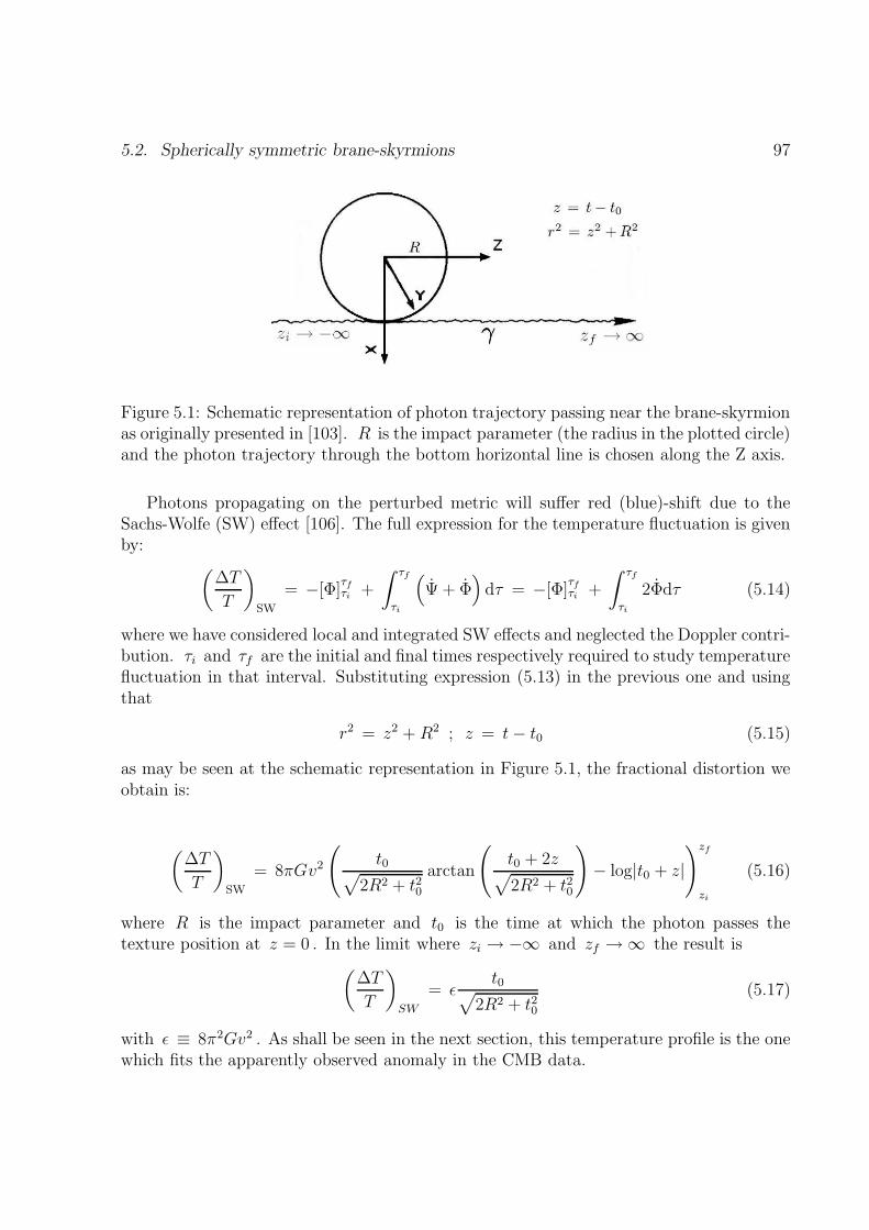
5.2. Spherically symmetric brane-skyrmions 97
Figure 5.1: Schematic representation of photon trajectory passing near the brane-skyrmionas originally presented in [103]. R is the impact parameter (the radius in the plotted circle)and the photon trajectory through the bottom horizontal line is chosen along the Z axis.
Photons propagating on the perturbed metric will suffer red (blue)-shift due to theSachs-Wolfe (SW) effect [106]. The full expression for the temperature fluctuation is givenby:
(
∆T
T
)
SW
= −[Φ]τfτi +
∫ τf
τi
(
Ψ + Φ)
dτ = −[Φ]τfτi +
∫ τf
τi
2Φdτ (5.14)
where we have considered local and integrated SW effects and neglected the Doppler contri-bution. τi and τf are the initial and final times respectively required to study temperaturefluctuation in that interval. Substituting expression (5.13) in the previous one and usingthat
r2 = z2 + R2 ; z = t− t0 (5.15)
as may be seen at the schematic representation in Figure 5.1, the fractional distortion weobtain is:
(
∆T
T
)
SW
= 8πGv2
(
t0√
2R2 + t20arctan
(
t0 + 2z√
2R2 + t20
)
− log|t0 + z|)zf
zi
(5.16)
where R is the impact parameter and t0 is the time at which the photon passes thetexture position at z = 0 . In the limit where zi → −∞ and zf → ∞ the result is
(
∆T
T
)
SW
= ǫt0
√
2R2 + t20(5.17)
with ǫ ≡ 8π2Gv2 . As shall be seen in the next section, this temperature profile is the onewhich fits the apparently observed anomaly in the CMB data.

98 Chapter 5. Brane-skyrmions and the CMB cold spot
Figure 5.2: The combined and foreground cleaned Q-V-W WMAP map after convolutionwith the SMHW at scale R9 as shown in [115]. The CS position is marked and seen atthe bottom left part of the plot.
5.3 Cold spot in WMAP data
One of the most important pieces of information about the history and nature of our uni-verse comes from the Cosmic Microwave Background (CMB). Measurements of the CMBtemperature anisotropies obtained by WMAP [11, 107] have been thoroughly studied inrecent years. Such anisotropies have been found to be Gaussian as expected in many stan-dard cosmological scenarios corresponding to density fluctuations of one part in a hundredthousand in the early universe. However, by means of a wavelet analysis, an anomalous CS,apparently inconsistent with homogeneous Gaussian fluctuations, was found in [101, 108]in the southern hemisphere centered at the position b = −57 , l = 209 in galacticcoordinates. 1 The characteristic scale in the sky of the CS is about 5 .
The CS position in usual WMAP plots is shown in Figure 5.2. The existence of thisCS has been claimed to be confirmed more recently in reference [109]. However, in recentreferences [110] it has been argued that there is no compelling evidence for deviations fromthe ΛCDM model in the WMAP data. In particular, it is claimed that the evidence thatthe CS is statistically anomalous is not robust.
1where b is the galactic latitude measured from the plane of the galaxy to the object using the Sun asvertex. The galactic longitude is referred to as l and it is measured in the plane of the galaxy using anaxis pointing from the Sun to the galactic center.

5.4. Cold spot as a cosmic texture 99
Concerning the origin of the CS, different explanations have been proposed in theliterature: in references [111, 112, 113] the CS was tried to be explained by voids in thematter distribution whereas the reference [114] dealt with possible string theory bubbleorigin. Other authors proposed in [115] the Sunyaev-Zeldovich (SZ) effect as possibleexplanation showing that the flat frequency dependence of the CS is incompatible withbeing caused by a SZ signal alone. However, a combination of CMB plus SZ effect mayexplain the spot and could have a sufficiently flat frequency spectrum.
5.4 Cold spot as a cosmic texture
A very interesting possibility about the CS origin has recently been proposed in [116].According to it, some theories of high energy physics predict the formation of varioustypes of topological defects, including cosmic textures [104] which would generate hotand cold spots in the CMB [103]. These textures would be the remnants of a symmetrybreaking phase transition that took place in the early universe.
In order to produce textures, the cosmic phase transition must be related to a globalsymmetry breaking pattern from one group G to a subgroup H so that the coset spaceK = G/H has a nontrivial third homotopy group. A typical example is K = SU(N) ,which has associated π3(K) = Z for N ≥ 2 . Notice that, as usual, in order to geta texture formed in the transition, the symmetry breaking must correspond to a globalsymmetry since if it were local it could be gauged away.
Textures can be understood as localized wrapped field configurations which collapseand unwind on progressively larger scales. These textures can produce a concentrationof energy which gives rise to a time dependent gravitational potential. CMB photonstraversing the texture region will suffer a red (blue) shift producing a cold (hot) spotin the CMB maps. In reference [116] the authors consider a SU(2) non-linear sigmamodel to build up a model of texture that could explain the observed CS. They simulatethe unwinding texture by using a spherically symmetric scaling solution and they find afractional temperature distortion given by:
∆T
T(θ) = ±ǫ 1
√
1 + 4(
θθc
)2(5.18)
where θ is the angle from the center, ǫ is a measure of the amplitude and θc is the scaleparameter that depends on the time at which the texture unwinds. The best fit of theCS is found for ǫ = 7.7 × 10⁻⁵ and θc = 5.1 . Furthermore, the parameter ǫ is givenby ǫ ≡ 8π2GΦ0 , where Φ0 is the fundamental symmetry breaking scale which is then setto be Φ0 ≃ 8.7 × 10¹⁵ GeV. This scale is nicely close to the GUT scale thus making theresults given in [116] extremely interesting.

100 Chapter 5. Brane-skyrmions and the CMB cold spot
Nonetheless, it is important to stress that textures require having a global symmetrybreaking but what one finds typically in GUTs is a local symmetry breaking producingthe Higgs mechanism and then destroying the topological meaning of texture or any otherpossible defect appearing in the cosmic transition.
5.5 Physical interpretation of the results and involved
scales
As has been shown in Sections 5.2 and 5.4, the results for the fractional temperaturedistortion provoked by the CS given by expression (5.18) coincides with the fractionaldistortion caused by a brane-skyrmion given by expression (5.17) provided that:
Φ0 = v ; 2
(
θ
θc
)
=R
t0(5.19)
where θc was defined in reference [116].
Let us now estimate the required scales in order for this kind of brane-skyrmion to beable to explain the observed CS. For the minimal model supporting brane-skyrmions withthree extra dimensions δ = 3 , the relation (1.50) approximately becomes
M2P ≃ R3
BM5D (5.20)
since gravitation is embedded in D = 7 dimensions and therefore R3B is the characteristic
volume for the compactified extra dimensions. Therefore
RB ≃(
M2P
M5D
)1/3
(5.21)
and consequently
v2 ≡ f 4R2B ≃ f 4
(
M2P
M5D
)2/3
. (5.22)
If the parameter ǫ needs to be fixed around 7.7 · 10−5 , then the required v would be
v ≃ 1.2 · 1016 GeV (5.23)
which in fact can be achieved with MD ∼ f ∼ TeV. Notice that for this parameter range,the radius of the extra dimension is around
RB ∼ 10−8 m, (5.24)

5.5. Physical interpretation of the results and involved scales 101
i.e., previous approximations in expression (5.5) are totally justified.
In addition to the previous estimations, we have also checked that the possible effectscoming from a nonvanishing branon mass are suppressed by O(M2/v2) . Therefore formass values also around M ∼ TeV, which are typical of branon as dark matter candidate,see [25], such effects are negligible.
In other words, brane-skyrmions provide an accurate description for the CS withoutany need of introducing very high energy (GUTs) scales since the correct temperaturefluctuation amplitude can be obtained with natural values around the electroweak scale.
5.5.1 Brane-skyrmions abundance
The abundance of brane-skyrmions in this model is given by its low-energy (large distance)dynamics as described by a non-linear sigma model as that in [116]. This is nothing but thewell-known fact that, except in the microscopic unwinding region, the field evolution onlydepends on the geometry of the coset space K , but not on the details of the symmetrybreaking mechanism. As was shown in [105] in a simple model with a potential term, thefinal abundance of defects and other properties of the pattern of density perturbations areexpected to be not very sensitive to the short distance physics, once the texture unwinds,making this kind of theories highly predictive. For that reason, we expect that providedthe same kind of initial conditions are imposed in both models, the predicted abundanceof hot and cold spots agree with that obtained from simulations in [116]. Such simulationsshow that the number of unwinding textures per comoving volume and conformal time τcan be estimated as
dn
dτ=
ν
τ 4(5.25)
with ν ≃ 2 . This allows to estimate the number of hot and cold spots in a given angularradius interval. As commented above, this is a quite robust result at late times with littleeffects for short distance dynamics. In the case of brane-skyrmions, the short distanceeffects will be embodied in the higher-derivative terms appearing in the expansion of theNambu-Goto action or even in possible induced curvature terms generated by quantumeffects [49]. Provided that such terms do not stabilize the brane-skyrmions, we expect thatsuch an abundance could be directly applied in our case.

102 Chapter 5. Brane-skyrmions and the CMB cold spot
5.6 Future prospects and conclusions
In this section we dedicate some lines to mention how both present and future experimentsmay confirm the validity of the BW models. Then we shall sketch the most importantconclusions and consequences of the brane-skyrmion model presented in this chapter as aviable explanation for the observed CS.
On the one hand, the fact that the fundamental scales of the theory are of the order ofthe TeV opens the possibility to test this explanation with collider experiments throughthe production of real or virtual branons and KK-gravitons. The expected signatures ofthe model [117] from the production of KK-gravitons come fundamentally from the singlephoton channel studied by LEP, which restrict MD > 1.2 TeV at 95% of confidence level.
On the other hand, the LHC accelerator will be able to test the model up to MD = 3.7TeV, analysing single photon and monojet production to establish the number of extradimensions as was explained in Section 1.10.
Finally, there also exists the possibility to find signatures of the model at low energiesassociated with branon phenomenology. This case is more interesting from the cosmologicalpoint of view, since branons can constitute the nonbaryonic dark matter abundance astypical WIMPs [25, 118]. Present constraints coming from the single photon analysisrealized by L3 (LEP) imply f > 122 GeV (at 95 % C.L.) [119, 120] and the LHC will beable to check this model up to f = 1080 GeV through monojet production [118]. Theidea to test the physics associated with the CS with the next generation of colliders at theTeV scale is a very intriguing and distinctive property of this texture.

Chapter 6
Conclusions and prospects
In this thesis we have studied some cosmological and astrophysical consequences in two di-fferent types of modified gravity theories: f(R) theories and brane-world extra dimensionstheories.
First, we have shown some relevant results for f(R) modified gravities. Thus, wehave studied how some features of general relativity can be mimicked by f(R) models ifcertain conditions are imposed on those models. We have also proved that there exists aclass of f(R) models which can indeed reproduce the present cosmological evolution –frommatter-radiation equality till today – as described by general relativity within the standardcosmological concordance model. These f(R) models allow to remove the cosmologicalconstant term and therefore the observed acceleration is understood to have a purelygeometrical interpretation with no dark energy origin. Furthermore, initial conditions maybe imposed on such a class of theories in order to recover a null scalar curvature solutionfor a vacuum scenario. Unfortunately such functions are not cosmologically viable andshould be considered as effective models to reproduce ΛCDM evolution.
Also, it has been proved that any perfect fluid parameterized by a constant equationof state can be reproduced by the presence of f(R) terms. Thus, these functions couldprovide a mechanism to reproduce the cosmological behaviour of dark energy type fluids.It therefore seems worthwhile to try to search for a unique phenomenological f(R) theoryable to explain the main features in the cosmological evolution, from inflation till late timeobserved acceleration.
Next, we have considered the modification introduced by the new f(R) terms in theevolution of cosmological perturbations. Here, an analysis concerning first order cosmolog-ical scalar perturbations has been performed. We have presented a general method in orderto obtain the evolution equation of the matter density contrast for arbitrary f(R) theories.That procedure was proven to be valid regardless of the chosen f(R) model or the size of
103
104 Chapter 6. Conclusions and prospects
the involved scales. An important by-product of the calculations is the conclusion that theusual approximations made in the literature for sub-Hubble modes are not always valid.In fact, the required hypotheses to get the so-called quasi-static approximation have beenestablished here. For those sub-Hubble modes, it was found that only for f(R) modelssatisfying the local gravity constraints, the evolution of perturbations is indistinguishablefrom that obtained using the quasi-static approximation but perfectly distinguishable fromthe evolution obtained by the ΛCDM model.
Now that those theoretical calculations were made, the correct evolution for matterperturbations in sub-Hubble modes for f(R) models is obtained. Therefore some robust-ness tests may be used to compare experimental data with expected theoretical results.Thus both the validity and certain constraints on those f(R) functions may be estab-lished. This procedure shows how our theoretical results may be used in order to confrontthe predictions made by a given f(R) theory with large scale structure observations.
As a final subject within our f(R) models research, we dealt with some features of blackholes in arbitrary dimensions. First, the scalar constant curvature case for static and spher-ically symmetric solutions in vacuum was studied. It was determined that the only possiblesolution for the modified Einstein equations in this case was the Schwarzschild-(anti-)deSitter solution. As a complementary result to the previous research, we studied the staticand spherically symmetric case without imposing the constant curvature condition. Todo so, a perturbative approach was performed around the standard Schwarzschild-anti-deSitter solution of general relativity. It was found that, up to second order in perturbations,the only solution was the generalized Schwarzschild-anti-de Sitter solution with modifiedcoefficients in terms of f(R) and its derivatives evaluated at the background curvature.
This part of the thesis was finished by studying the thermodynamic properties ofSchwarzschild-anti-de Sitter black holes in f(R) theories. Thus accessible thermodynami-cal regions for several f(R) models were studied in detail. In that realm, a very interestingproperty, which encourages further investigation, was found: it turned out that thermo-dynamical viability of f(R) theories in constant curvature solutions was embodied by thecondition 1 + df(R)/dR > 0 . This condition was also required to ensure gravitationalviability for f(R) models. Consequently two different aspects of the viability of f(R)theories have been brought together.
The last part of the thesis was devoted to a study of some consequences of the existenceof topologically nontrivial brane configurations, the so-called brane-skyrmions, in brane-world theories. In particular we have considered the effects of brane-skyrmions on thetemperature fluctuations of the CMB and their potential connection with the so-calledCMB cold spot. We have shown that brane-world theories can naturally accommodatethis striking cosmological feature by invoking these nontrivial topological configurations.A different type of textures related to Grand Unified Theories has also been consideredin the literature, but the model presented here shows that this type of defect could be
105
explained from the electroweak scale physics.
To conclude, the results included in this thesis have shown that modified gravity theo-ries remain compelling candidates to describe the properties of the gravitational interactionon very large scales. Both the validity and viability of these theories have still to be sub-jected to many theoretical and experimental tests. To do so, the possibility of reproducingstandard cosmological results, first order perturbations, black holes and features on theCMB temperature maps were considered as interesting aspects which could shed some lighton the fundamental properties of the gravitational interaction.

106 Chapter 6. Conclusions and prospects

Appendix A
Coefficients in f(R) cosmological perturbations
In this appendix we include the coefficients for the series expansions given in equation(3.50) in Chapter 3. All the α ’s terms (coming from EH-part) and the first four β ’sterms (coming from f -part) for each δ derivative, i.e. δiv, ..., δ, , in equation (3.50) havebeen included once the condition |fR| ≪ 1 has been imposed to simplify their expressions.For sub-Hubble scales the excluded β ’s terms are negligible with respect to the writtenones.
A.1 Appendix I : α′s and β ′s coefficients
Coefficients for δiv term:
β(1)4,f ≃ 8f 4
R(1 + fR)6f 41 ǫ
2
β(2)4,f ≃ 72f 3
Rf31 ǫ
4(−2 + κ2)
β(3)4,f ≃ 216f 2
Rf21 ǫ
6(−2 + κ2)2
β(4)4,f ≃ 216fRf1ǫ
8(−2 + κ2)3. (A.1)
Coefficients for δ′′′ term:
β(1)3,f ≃ 8f 4
R(1 + fR)5f 41Hǫ2[3 + fR(3 + f1)]
β(2)3,f ≃ 6f 3
Rf21Hǫ48f2(−2 + κ2) + 4f1[12κ1 + 9κ2 − 2(9 + κ3)]
β(3)3,f ≃ −72f 2
Rf1Hǫ6(−2 + κ2)[−4f2(−2 + κ2) + f1(19 − 23κ1 − 10κ2 + 4κ3)]
β(4)3,f ≃ −216fRHǫ8(−2 + κ2)
2[−2f2(−2 + κ2) + f1(7 − 11κ1 − 4κ2 + 2κ3)]. (A.2)
Coefficients for δ′′ term:
α(1)2,EH = 432(1 + fR)10H2ǫ8(−1 + κ1)(−2 + κ2)
3
α(2)2,EH = 1296(1 + fR)10H2ǫ10(−1 + κ1)
2(−2 + κ2)3
α(3)2,EH = 3888(1 + fR)10H2ǫ12(−1 + κ1)
2(−2 + κ2)3
β(1)2,f ≃ 8f 4
R(1 + fR)6f 41H2
β(2)2,f ≃ 88f 3
Rf31H2ǫ2(−2 + κ2)
β(3)2,f ≃ 24f 2
Rf21H2ǫ4(−2 + κ2)(−28 + 2κ1 + 13κ2)
β(4)2,f ≃ 72fRf1H2ǫ6(−2 + κ2)
2(−14 + 4κ1 + 5κ2). (A.3)
107

108 Appendix A. Coefficients in f(R) cosmological perturbations
Coefficients for δ′ term:
α(1)1,EH = 432(1 + fR)10H3ǫ8(−1 + κ1)(−2 + κ2)
3
α(2)1,EH = 2592(1 + fR)10H3ǫ10(−1 + κ1)
2(−2 + κ2)3
α(3)1,EH = −7776(1 + fR)10H3ǫ12(−1 + κ1)
3(−2 + κ2)3
β(1)1,f ≃ 8f 4
R(1 + fR)6f 41H3
β(2)1,f ≃ 88f 3
Rf31H3ǫ2(−2 + κ2)
β(3)1,f ≃ 24f 2
Rf21H3ǫ4(−2 + κ2)(−28 + 2κ1 + 13κ2)
β(4)1,f ≃ 72fRf1H3ǫ6(−2 + κ2)
2(−14 + 4κ1 + 5κ2). (A.4)
Coefficients for δ term:
α(1)0,EH = 432(1 + fR)10H4ǫ8(−1 + κ1)(2κ1 − κ2)(−2 + κ2)
3
α(2)0,EH = 1296(1 + fR)10H4ǫ10(−1 + κ1)
2(−1 + 4κ1 − κ2)(−2 + κ2)3
α(3)0,EH = 3888(1 + fR)10H4ǫ12(−1 + κ1)
2(2κ21 − κ2)(−2 + κ2)
3
β(1)0,f ≃ −16
3f 4
R(1 + fR)5f 41H4[2 + fR(2 + 2f1 − f2 − 2κ1) − 2κ1]
β(2)0,f ≃ 112f 3
Rf31H4ǫ2(−1 + κ1)(−2 + κ2)
β(3)0,f ≃ 48f 2
Rf21H4ǫ4(−1 + κ1)(−2 + κ2)(−16 + 2κ1 + 7κ2)
β(4)0,f ≃ 144fRf1H4ǫ6(−1 + κ1)(−2 + κ2)
2(−6 + 4κ1 + κ2). (A.5)

A.2. Appendix II : c′s coefficients 109
A.2 Appendix II : c′s coefficients
The coefficients appearing in equation (3.59) are explicitly provided here once the condition|fR| ≪ 1 has been imposed.
c4 = −fRf1[−fRf1k2 − 3H2(−2 + κ2)]
3
c3 = −3fRH[−fRf1k2 − 3H2(−2 + κ2)]f 2
Rf31k
4 + 6f2H4(−2 + κ2)2 + f1H2(−2 + κ2)
×[2fRf2k2 + 3H2(−7 + 11κ1 + 4κ2 − 2κ3)] + 2fRf1H2k2(−6 + 6κ1 + 3κ2 − κ3)
c2 = [−fRf1k2 − 3H2(−2 + κ2)]
2
×[f 2Rf
21k
4 + 5fRf1H2k2(−2 + κ2) + 6H4(−1 + κ1)(−2 + κ2)]
c1 = [−fRf1k2 − 3H2(−2 + κ2)]
2
×[f 2Rf
21k
4H + 5fRf1H3k2(−2 + κ2) + 6H5(−1 + κ1)(−2 + κ2)]
c0 =2
3H2(−1 + κ1)[−fRf1k
2 − 3H2(−2 + κ2)]2[2f 2
Rf21k
4 + 9fRf1H2k2(−2 + κ2)
+ 9H4(2κ1 − κ2)(−2 + κ2)]. (A.6)

110 Appendix A. Coefficients in f(R) cosmological perturbations
Bibliography
[1] H. Weyl, Annalen Phys. 59, 101 (1919) [Surveys High Energ. Phys. 5, 237 (1986)].
[2] A. S. Eddington, The mathematical theory of relativity, Cambridge University Press,Cambridge, (1923).
[3] R. Utiyama and B. S. DeWitt, J. Math. Phys. 3, 608 (1962).
[4] G. ’t Hooft and M. J. G. Veltman, Annales Poincare Phys. Theor. A 20, 69 (1974).
[5] N. D. Birrell, P. C. W. Davies, Quantum fields in curved space. Cambridge Mono-graphs on Mathematical Physics, vol. 7, Cambridge Univ. Press, New York, (1982).
[6] I. L. Buchbinder, S. D. Odintsov and I. L. Shapiro, Bristol, UK: IOP (1992) 413 p.
[7] G. A. Vilkovisky, Class. Quant. Grav. 9, 895 (1992).
[8] A. G. Riess et al. [Supernova Search Team Collaboration], Astrom. J. 116, 1009(1998).
[9] S. Perlmutter et al. [Supernova Cosmology Project Collaboration], Astrophys. J. 517,565 (1999).
[10] J. L. Tonry et al. Astrophys. J. 594, 1 (2003).
[11] http://lambda.gsfc.nasa.gov/product/map/current/params/olcdm sz lens wmap7 bao h0.cfm
[12] E. J. Copeland, M. Sami and S. Tsujikawa, Int. J. Mod. Phys. D15, 1753 (2006).
[13] S. M. Carroll, A. De Felice, V. Duvvuri, D. A. Easson, M. Trodden and M. S. Turner,Phys. Rev. D 71, 063513 (2005).
[14] S. Nojiri and S. D. Odintsov, Int. J. Geom. Meth. Mod. Phys. 4, 115 (2007).
[15] A. A. Starobinsky, Phys. Lett. 91B, 99 (1980).
111

112 BIBLIOGRAPHY
[16] J. D. Barrow and A. C. Ottewill, J. Phys. A 16, 2757 (1983).
[17] A. Dobado and A. L. Maroto, Phys. Rev. D 52, 1895 (1995).
[18] S. Nojiri and S. D. Odintsov, Gen. Rel. Grav. 36, 1765 (2004).
[19] G. Dvali, G. Gabadadze and M. Porrati, Phys. Lett. B485, 208 (2000).
[20] J. A. R. Cembranos, Phys. Rev. D 73, 064029 (2006).
[21] J. Beltran and A. L. Maroto, Phys. Rev. D 78, 063005 (2008); JCAP 0903, 016(2009); Phys. Rev. D 80, 063512 (2009); Int. J. Mod. Phys. D 18, 2243-2248 (2009).
[22] A. Dobado and A. L. Maroto, Phys. Lett. B 316, 250 (1993) [Erratum-ibid. B 321,435 (1994)].
[23] J. A. R. Cembranos, Phys. Rev. Lett. 102, 141301 (2009).
[24] S. Nojiri and S. D. Odintsov, Phys. Rev. D 68, 123512 (2003).
[25] J. A. R. Cembranos, A. Dobado and A. L. Maroto, Phys. Rev. Lett. 90, 241301(2003); Phys. Rev. D 68, 103505 (2003).
[26] A. de la Cruz-Dombriz, A. Dobado and A. L. Maroto, Phys. Rev. D 80, 124011(2009).
[27] T. P. Sotiriou and S. Liberati, Annals Phys. 322, 935 (2007).
[28] G. Magnano and L. M. Sokolowski, Phys. Rev. D 50, 5039 (1994).
[29] V. Faraoni and E. Gunzig, Int. J. Theor. Phys. 38, 217 (1999).
[30] S. M. Carroll, V. Duvvuri, M. Trodden and M. S. Turner, Phys. Rev. D 70, 043528(2004).
[31] L. Pogosian and A. Silvestri, Phys. Rev. D 77, 023503 (2008).
[32] V. Faraoni, Phys. Rev. D 74, 023529 (2006).
[33] W. Hu and I. Sawicki. Phys. Rev. D 76, 064004 (2007).
[34] V. Faraoni, Phys. Rev. D 75, 067302 (2007).
[35] G. J. Olmo, Phys. Rev. Lett. 95, 261102 (2005).
[36] T. P. Sotiriou, Gen. Rel. Grav. 38, 1407 (2006); O. Mena, J. Santiago and J. Weller,Phys. Rev. Lett. 96, 041103 (2006); S. Nojiri and S. D. Odintsov, Phys. Rev. D 74,086005 (2006).

BIBLIOGRAPHY 113
[37] T. Kaluza, Sitzungsber. Preuss. Akad. Wiss. Berlin (Math. Phys.) 966 (1921).
[38] O. Klein, Z. Phys. 37, 895 (1926) [Surveys High Energ. Phys. 5, 241 (1986)].
[39] L. Randall and R. Sundrum, Phys. Rev. Lett. 83, 3370 (1999) ; Phys. Rev. Lett.83, 4690 (1999).
[40] N. Arkani-Hamed, S. Dimopoulos and G. R. Dvali, Phys. Lett. B 429, 263 (1998) ;N. Arkani-Hamed, S. Dimopoulos and G. R. Dvali, Phys. Rev. D 59, 086004 (1999);I. Antoniadis, et al., Phys. Lett. B436, 257 (1998).
[41] R. Sundrum, Phys. Rev. D 59, 085009 (1999).
[42] M. Bando, T. Kugo, T. Noguchi and K. Yoshioka, Phys. Rev. Lett. 83, 3601 (1999).
[43] T. Kugo and K. Yoshioka, Nucl. Phys. B 594, 301 (2001).
[44] P. Creminelli and A. Strumia, Nucl. Phys. B 596, 125 (2001).
[45] A. Dobado and A. L. Maroto, Nuc. Phys. B592, 203 (2001).
[46] J. A. R. Cembranos, A. Dobado and A. L. Maroto, Int. J. Mod. Phys. D 13, 2275(2004) ; J. Phys. A 40, 6631 (2007).
[47] J. A. R. Cembranos, A. Dobado and A. L. Maroto, Phys. Rev. D 73, 035008 (2006) ;AIP Conf. Proc. 670, 235 (2003).
[48] A. L. Maroto, Phys. Rev. D 69, 043509 (2004) ; Phys. Rev. D 69, 101304 (2004) ;J. A. R. Cembranos, A. Dobado and A. L. Maroto, Phys. Rev. D 73, 057303 (2006) ;J. A. R. Cembranos and L. E. Strigari, Phys. Rev. D 77, 123519 (2008).
[49] J. A. R. Cembranos, A. Dobado and A. L. Maroto, Phys. Rev. D 65, 026005 (2002).
[50] G. R. Dvali, I. I. Kogan and M. A. Shifman, Phys. Rev. D 62, 106001 (2000).
[51] S. Dimopoulos and G. L. Landsberg, Phys. Rev. Lett. 87, 161602 (2001).
[52] T. Chiba, Phys. Lett. B 575, 1 (2003).
[53] A. D. Dolgov and M. Kawasaki, Phys. Lett. B 573, 1 (2003).
[54] A. de la Cruz-Dombriz and A. Dobado, Phys. Rev. D 74, 087501 (2006).
[55] L. Amendola, R. Gannouji, D. Polarski and S. Tsujikawa, Phys. Rev. D75, 083504(2007).
[56] A. A. Starobinsky, JETP Lett. 86, 157 (2007).

114 BIBLIOGRAPHY
[57] M. Martinelli, A. Melchiorri and L. Amendola, Phys. Rev. D 79, 123516 (2009).
[58] V. Miranda, S. E. Joras, I. Waga and M. Quartin, Phys. Rev. Lett. 102, 221101(2009).
[59] S. Nojiri and S. D. Odintsov, Phys. Rev. D 74, 086005 (2006).
[60] S. Nojiri, S. D. Odintsov and D. Saez-Gomez, Phys. Lett. B 681, 74 (2009).
[61] D. Saez-Gomez, Gen. Rel. Grav. 41, 1527 (2009).
[62] E. W. Kolb and M. S. Turner, The Early universe, Front. Phys. 69, 1 (1990).
[63] A. Dobado and A. L. Maroto, Phys. Rev. D 60, 104045 (1999).
[64] A. G. Riess et al. [Supernova Search Team Collaboration], Astron. J. 116, 1009(1998); S. Perlmutter et al.[Supernova Cosmology Project Collaboration], Astrophys.J. 517, 565 (1999).
[65] D. J. Eisenstein et al. Astrophys. J. 633, 560-574 (2005).
[66] E. Linder, Phys.Rev. D72, 043529 (2005).
[67] E. M. Lifshitz, Zh. Eksp. Teor. Fiz., 16, 587 (1946).
[68] J. C. Hwang and H. Noh, Phys. Rev. D 54, 1460 (1996); S. M. Carroll, I. Sawicki,A. Silvestri and M. Trodden, New J. Phys. 8, 323 (2006); Y. S. Song, W. Hu andI. Sawicki, Phys. Rev. D 75, 044004 (2007); S. Carloni, P. K. S. Dunsby and A. Troisi,Phys. Rev. D 77, 024024 (2008); S. Tsujikawa, Phys. Rev. D 77, 023507 (2008);S. Tsujikawa, K. Uddin, R. Tavakol, Phys. Rev. D 77, 043007 (2008).
[69] M. Tegmark et al. [SDSS Collaboration], Phys. Rev. D 74, 123507 (2006).
[70] A. de la Cruz-Dombriz, A. Dobado and A. L. Maroto, Phys. Rev. D 77, 123515(2008).
[71] A. de la Cruz-Dombriz, A. Dobado and A. L. Maroto, AIP Conf. Proc. 1122, 252(2009).
[72] A. de la Cruz-Dombriz, A. Dobado and A. L. Maroto, Phys. Rev. Lett. 103, 179001(2009).
[73] V. F. Mukhanov, H. A. Feldman and R. H. Brandenberger, Phys. Rept. 215, 203(1992).
[74] J. M. Bardeen, Phys. Rev. D 22, 1882 (1980).
[75] D. Huterer and E. Linder. Phys. Rev. D 75, 023519 (2007).

BIBLIOGRAPHY 115
[76] B. Boisseau, G. Esposito-Farese, D. Polarski and A. A. Starobinsky, Phys. Rev. Lett.85, 2236 (2000) ; G. Esposito-Farese and D. Polarski, Phys. Rev. D 63, 063504(2001).
[77] P. Zhang, Phys. Rev. D 73, 123504 (2006).
[78] S. Tsujikawa, Phys. Rev. D 76, 023514 (2007).
[79] R. Bean, D. Bernat, L. Pogosian, A. Silvestri and M. Trodden. Phys. Rev. D 75,064020 (2007).
[80] I. Sawicki and W. Hu, Phys. Rev. D 75, 127502 (2007).
[81] D. N. Spergel et al. [WMAP Collaboration], Astrophys. J. Suppl. 170, 377 (2007).
[82] B. Whitt, Phys. Lett. B 145, 176 (1984).
[83] S. Mignemi and D. L. Wiltshire, Phys. Rev. D 46, 1475 (1992).
[84] T. Multamaki and I. Vilja, Phys. Rev. D 74, 064022 (2006).
[85] G. J. Olmo, Phys. Rev. D 75, 023511 (2007).
[86] E. Witten, Adv. Theor. Math. Phys. 2, 505 (1998).
[87] S. W. Hawking and D. N. Page, Commun. Math. Phys. 87, 577 (1983).
[88] G. Cognola, E. Elizalde, S. Nojiri, S. D. Odintsov and S. Zerbini, JCAP 0502, 010(2005).
[89] F. Briscese and E. Elizalde, Phys. Rev. D 77, 044009 (2008).
[90] M. Cvetic, S. Nojiri and S. D. Odintsov, Nucl. Phys. B 628, 295 (2002).
[91] R. G. Cai, Phys. Rev. D 65, 084014 (2002).
[92] Y. M. Cho and I. P. Neupane, Phys. Rev. D 66, 024044 (2002).
[93] R. G. Cai, Phys. Lett. B 582, 237 (2004) ; J. Matyjasek, M. Telecka andD. Tryniecki, Phys. Rev. D 73, 124016 (2006).
[94] S. Wolfram, Mathematica, A System for Doing Mathematics by Computer Addison-Wesley, New-York, (1991).
[95] A. de la Cruz-Dombriz, A. Dobado and A. L. Maroto, Proceedings of the SpanishRelativity Meeting ERE 2009, Journal of Physics: Conference Series (JPCS).
[96] T. Ortın, Gravity and Strings, Cambridge University Press (2003).

116 BIBLIOGRAPHY
[97] J. B. Hartle and S. W. Hawking, Phys. Rev. D 13, 2188 (1976); G. W. Gibbonsand M. J. Perry, Proc. R. Soc. London A 358, 467 (1978); G. W. Gibbons andS. W. Hawking, Phys. Rev. D 15, 2752 (1977); G. W. Gibbons and S. W. Hawking,Euclidean Quantum Gravity, World Scientific, (1993).
[98] S. W. Hawking, Commun. Math. Phys. 43, 199 (1975) [Erratum-ibid. 46, 206 (1976)].
[99] T. Multamaki, A. Putaja, I. Vilja and E. C. Vagenas, Class. Quant. Grav. 25, 075017(2008).
[100] J. D. Bekenstein, Phys. Rev. D 7, 2333 (1973).
[101] P. Vielva, E. Martınez-Gonzalez, R. B. Barreiro, J. L. Sanz and L. Cayon, Astrophys.J. Suppl. 609, 22 (2004).
[102] J. A. R. Cembranos, A. de la Cruz-Dombriz, A. Dobado and A. L. Maroto, JCAP0810, 039 (2008).
[103] N. Turok and D. Spergel, Phys. Rev. Lett. 64, 2736 (1990).
[104] N. Turok, Phys. Rev. Lett. 63, 2625, (1989); Phys. Scripta T36, 135 (1991).
[105] D. N. Spergel, et al, Phys. Rev. D 43, 1038 (1991).
[106] M. Giovannini, Int. J. Mod. Phys. D 14, 363-510, (2005).
[107] Hinshaw et al., Astrophys. J. Suppl. 170, 288 (2007).
[108] M. Cruz, E. Martınez-Gonzalez, P. Vielva, and L. Cayon, MNRAS, 365, 29 (2005).
[109] P. D. Naselsky, P. R. Christensen, P. Coles, O. Verkhodanov, D. Novikov and J. Kim,arXiv:0712.1118 [astro-ph].
[110] C. L. Bennett et al., arXiv:1001.4758 [astro-ph.CO].
[111] K. T. Inoue and J. Silk, Astrophys. J. 664, 650 (2007).
[112] K. T. Inoue and J. Silk, Astrophys. J. 648, 23 (2006).
[113] L. Rudnick, S. Brown and L. R. Williams, Astrophys. J. 671, 40 (2007).
[114] S. Chang, M. Kleban and T. S. Levi, JCAP 0904, 025 (2009).
[115] M. Cruz, M. Tucci, E. Martınez-Gonzalez and P. Vielva, Mon. Not. Roy. Astron.Soc. 369, 57 (2006).
[116] M. Cruz, N. Turok, P. Vielva, E. Martınez-Gonzalez, M. Hobson, Science 318, 1612(2007).

117
[117] W. M. Yao et al. [Particle Data Group], J. Phys. G 33, 1 (2006); E. A. Mirabelli,M. Perelstein and M. E. Peskin, Phys. Rev. Lett. 82, 2236 (1999).
[118] J. A. R. Cembranos, A. Dobado and A. L. Maroto, Phys. Rev. D 70, 096001 (2004).
[119] J. Alcaraz et al., Phys. Rev. D 67, 075010 (2003).
[120] P. Achard et al. [L3 Collaboration], Phys. Lett. B 597, 145 (2004).

118

119
This thesis has given rise to the following publications in regular journals:
A. de la Cruz-Dombriz, A. Dobado and A. L. Maroto,Comment on ’Viable singularity-free f(R) gravity without a cosmological constant’[arXiv:0905.1941],Phys. Rev. Lett. 103, 179001 (2009) [arXiv:0910.1441 [astro-ph.CO]].
A. de la Cruz-Dombriz, A. Dobado and A. L. Maroto,Black Holes in f(R) theories,Phys. Rev. D 80, 124011 (2009) [arXiv:0907.3872 [gr-qc]].
J. A. R. Cembranos, A. de la Cruz-Dombriz, A. Dobado and A. L. Maroto,Is the CMB Cold Spot a gate to extra dimensions?,JCAP 0810, 039 (2008) [arXiv:0803.0694 [astro-ph]].
A. de la Cruz-Dombriz, A. Dobado and A. L. Maroto,On the evolution of density perturbations in f(R) theories of gravity,Phys. Rev. D 77, 123515 (2008) [arXiv:0802.2999 [astro-ph]].
A. de la Cruz-Dombriz and A. Dobado,A f(R) gravity without cosmological constant,Phys. Rev. D 74, 087501 (2006) [arXiv:0607118 [gr-qc]].
The work developed in this thesis has been presented in a series of scientific meetings withthe following contributions to the corresponding proceedings:
A. de la Cruz-Dombriz, A. Dobado and A. L. Maroto,Black holes in modified gravity theories,Proceedings of the Spanish Relativity Meeting ERE 2009,Journal of Physics: Conference Series (JPCS) [arXiv:1001.2454 [gr-qc]].
A. de la Cruz-Dombriz, A. Dobado and A. L. Maroto,Cosmological density perturbations in modified gravity theories,AIP Conf. Proc. 1122 252 (2009) [arXiv:0812.3048 [astro-ph]].

Algunos aspectos cosmologicos y astrofısicos
de las teorıas de gravedad modificada
RESUMEN EN CASTELLANO DE LA TESIS DOCTORAL
presentada por
Alvaro de la Cruz Dombriz
bajo de la direccion de
Dr. Antonio Dobado Gonzalez y Dr. Antonio Lopez Maroto
Universidad Complutense de Madrid2010

ii

Indice general
1. Introduccion a las teorıas de gravedad modificada 1
2. Energıa oscura en las teorıas f(R) 7
3. Perturbaciones cosmologicas en teorıas f(R) 11
4. Agujeros negros en teorıas f(R) 17
5. Skyrmiones y la mancha frıa del CMB 23
6. Conclusiones y perspectivas 27
iii

iv INDICE GENERAL

Capıtulo 1
Introduccion a las teorıas de
gravedad modificada
El siglo veinte ha presenciado el desarrollo de la gravitacion y la cosmologıa como dis-ciplinas cientıficas sujetas a datos experimentales. Detectores y aceleradores de partıculas,telescopios y satelites han permitido verificar predicciones teoricas y descartar algunos mo-delos teoricos propuestos en estas disciplinas. Con la llegada del nuevo siglo, se han abiertonuevas perspectivas a traves de los ultimos experimentos, tales como WMAP, PLANCKo SDSS, capaces de determinar cada vez con mayor precision las caracterısticas del fondocosmico de microondas (CMB), la distribucion de estructuras a gran escala (LSS) y mu-chas otras propiedades cosmologicas del Universo. Sin embargo, falta todavıa encontraruna teorıa fundamental de la gravitacion que sea renormalizable desde el punto de vista delas teorıas cuanticas de campos y aplicable a todas las escalas, desde los tests gravitatoriosmicroscopicos, pasando por los tests en el sistema solar, hasta las escalas cosmologicas.
La teorıa de la Relatividad General, incluso habiendo sido la teorıa gravitacional masexitosa de estos ultimos cien anos, no ha dado respuesta satisfactoria a algunos problemas.Esta teorıa por ejemplo no es renormalizable y, si se utiliza para construir el modelocosmologico estandar, con un contenido material que venga dado por materia ordinaria yradiacion, no puede explicar la expansion acelerada del Universo que se observa actualmentea grandes escalas, sino que necesita incluir una contribucion de energıa oscura. Por otrolado, la Relatividad General tampoco puede explicar las curvas de rotacion de galaxias si elcontenido material viene dado unicamente por la materia luminosa, requiriendo por tantola inclusion de materia oscura para reconciliar los datos con sus predicciones teoricas.
Tales problemas podrıan poner de manifiesto la necesidad de agrandar el marco teoricode la cosmologıa mediante teorıas de gravedad modificada. Estas teorıas tratan de ponerde acuerdo los resultados experimentales con sus predicciones sin invocar exoticos compo-
1

2 Capıtulo 1. Introduccion a las teorıas de gravedad modificada
nentes cosmologicos.
En efecto, ya en los comienzos de su andadura, se cuestiono que la Relatividad Generalfuera la unica teorıa gravitatoria correcta. No obstante, no fue hasta los anos sesenta delpasado siglo cuando invariantes de orden superior se introdujeron en la accion gravitacio-nal a fin de que la teorıa resultante fuera renormalizable a orden de un lazo. Recientesinvestigaciones han demostrado que si se consideran correcciones cuanticas en teorıa decampos o correcciones superiores en la dinamica de bajas energıas de la teorıa de cuerdas,la accion gravitacional efectiva a bajas energıas incluye estos invariantes de curvatura deorden superior. Estos resultados reavivaron el interes por las teorıas de gravedad de ordensuperior: al comienzo, las modificaciones consideradas eran solo relevantes en escenariosde alta energıa, tales como el estudio del Universo primitivo o en calculos para estudiarlas proximidades de agujeros negros. De esta manera dichas correcciones no afectabana la fenomenologıa gravitacional a curvaturas bajas, es decir, en la evolucion ultima delUniverso.
Por otra parte, recientes evidencias, tanto astrofısicas como cosmologicas, han demos-trado la homogeneidad e isotropıa del Universo a grandes escalas ası como su actual ex-pansion acelerada, planteando por tanto la urgente pregunta de encontrar una causa a estehecho. Como ya se ha mencionado, la Relatividad General con un contenido de materiaordinaria y radiacion no puede dar cuenta del mismo. Las explicaciones mas usuales pue-den clasificarse en una de las tres siguientes categorıas: la primera trata de reconciliar estaaceleracion con la Relatividad General, invocando para ello la presencia de un extranofluido, la energıa oscura, el cual posee una presion negativa y que incluye el caso de laconstante cosmologica Λ para el que la presion es igual y de signo opuesto a la densidadde energıa. Esta ultima configuracion da lugar al modelo ΛCDM que se suele complemen-tar con la presencia de un campo escalar, el inflaton, para proporcionar un mecanismode inflacion. No obstante esta descripcion presenta los llamados problema de la constante
cosmologica y el problema de la coincidencia que parecen indicar que este modelo es enrealidad una aproximacion fenomenologica de una teorıa gravitacional subyacente. El se-gundo tipo de explicaciones son las teorıas de quintaesencia que consideran una energıaoscura dinamica mediante un campo escalar. Si la introduccion del campo escalar se realizaen el sector gravitacional, las teorıas que aparecen pasan a conocerse como teorıas escalar-tensor. Finalmente una tercera explicacion intenta dar cuenta de esta aceleracion comoconsecuencia de una nueva fısica gravitacional. De este modo, la Relatividad General semodifica mediante la adicion de potencias de la curvatura escalar, los tensores de Riemanny Ricci e incluso sus derivadas, como por ejemplo hacen las teorıas Lovelock o las teorıasf(R) que estudiaremos en esta tesis. Las teorıas f(R) , dinamicamente equivalentes a uncaso particular de las teorıas de Brans-Dicke, pueden considerarse pues como una gene-ralizacion de la Relatividad General a traves de la inclusion de un termino f(R) en laaccion de Einstein-Hilbert (EH), de modo que la accion gravitacional generalizada para D
3
dimensiones resultarıa
S =1
16πG
∫
dDx√
|g| (R + f(R)) (1.1)
A partir de esta accion generalizada pueden derivarse las ecuaciones de Einstein modifi-cadas a traves de varios principios variacionales. En nuestros calculos se decidio emplearel formalismo metrico que considera la conexion como dependiente de la metrica y lasvariaciones se realizan por tanto unicamente respecto a este ultimo campo. Las ecuacionesobtenidas dejan de ser de segundo orden en las derivadas (como sucede en RelatividadGeneral) para convertirse en ecuaciones de cuarto orden y para las que la traza del tensorenergıa-momento y la curvatura escalar dejan de relacionarse mediante una ecuacion al-gebraica para hacerlo a traves de una expresion diferencial. Senalemos tambien que estasteorıas pueden presentar soluciones en vacıo que no tienen, a diferencia de las obtenidas enRelatividad General, curvatura escalar nula y que, cumpliendo determinadas condiciones,pueden tambien reproducir soluciones bien conocidas de Relatividad General.
Otro de los problemas aun abiertos en la Fısica se conoce como el problema de la
jerarquıa que presenta el modelo estandar de partıculas y que podrıa estar relacionadocon la escala fundamental de gravitacion. En efecto, este problema aparece en el procesode renormalizacion de teorıas que contienen campos escalares. En dichas teorıas se esperaque las masas renormalizadas de los escalares vengan dadas por el cut-off caracterısticode la teorıa, el cual se situa tıpicamente en energıas del orden de la escala gravitacional,es decir, la escala de Planck. Se requerirıa por tanto un ajuste muy fino para conseguir lamasa esperada, en particular la masa de la partıcula de Higgs. Si por el contrario la escalafundamental de gravitacion se situa cerca de la escala electrodebil, el correspondiente cut-off serıa del mismo orden que la masa esperada del Higgs y no se requerirıa un delicadoajuste fino.
Con el deseo de resolver este problema, recientemente se han considerado teorıas dedimensiones extra de gran tamano. A diferencia de las tradicionales teorıas de Kaluza-Klein, que poseen dimensiones extra compactificadas del tamano de la escala de Planck,los modelos de mundos brana pueden contener dimensiones extra de mayor tamano. Paraevitar la presencia de torres de Kaluza-Klein de copias de partıculas del modelo estandarcon masas similares, estas teorıas obligan a las partıculas del modelo estandar a propa-garse en la brana, mientras que unicamente la gravedad puede propagarse en el espaciototal. De esta manera, la escala fundamental de gravedad puede reducirse a la escala elec-trodebil y el problema de la jerarquıa desaparece. Algunas teorıas de mundos brana podrıantambien explicar la observada expansion acelerada del Universo y las excitaciones de labrana, los branones, pueden considerarse como partıculas masivas debilmente interactuan-tes (WIMPs) que serıan candidatos naturales de materia oscura. Senalemos finalmente quetales teorıas de gravedad con dimensiones extra podrıan dar lugar a la produccion de miniagujeros negros en el LHC, cuya deteccion proporcionarıa importante informacion sobre

4 Capıtulo 1. Introduccion a las teorıas de gravedad modificada
la dimensionalidad del espacio-tiempo y otras interesantes propiedades de la interacciongravitatoria.
En esta tesis vamos a profundizar pues en aspectos cosmologicos y astrofısicos queestas dos teorıas de gravedad modificada podrıan explicar. En primer lugar estudiaremosaquellas teorıas f(R) capaces de proporcionar un mecanismo de aceleracion cosmologicasin necesidad de introducir ninguna contribucion adicional de energıa oscura en el contenidoenergetico. Para ello, emplearemos metodos de reconstruccion que parten, bien de unasolucion dada para el factor de escala cosmologico para una metrica homogenea e isotropa,o bien de la ecuacion efectiva de estado. En particular presentaremos las funciones f(R)capaces de mimetizar las soluciones de EH con constante cosmologica en cuatro dimensionesy demostraremos que el comportamiento de cualquier fluido perfecto con ecuacion de estadoconstante puede tambien ser imitado por funciones f(R) .
Despues, el capıtulo segundo tratara del calculo de perturbaciones cosmologicas esca-lares para teorıas f(R) . Ya que las ecuaciones de Einstein modificadas se han presentadoen el capıtulo anterior como ecuaciones de fondo, resulta bastante natural preguntarsecomo la presencia de terminos f(R) afectarıa a las ecuaciones perturbadas a primer ordeny las consecuencias que estas teorıas provocarıan en el crecimiento de estructuras. A lolargo de este capıtulo, obtendremos una ecuacion diferencial completamente general parala evolucion de estas perturbaciones, la cual particularizaremos para las llamadas escalassub-Hubble. En estas escalas, dicha ecuacion diferencial se demostrara muy util para, porun lado entender el regimen de validez de las aproximaciones previamente realizadas en laliteratura y por otro, para excluir, de acuerdo con recientes experimentos, algunos modelosf(R) propuestos como cosmologicamente viables.
La introduccion de teorıas de gravedad modificada, con o sin dimensiones adicionales,podrıa conducir a la existencia de nuevas soluciones con respecto a las ya existentes enRelatividad General. A este respecto, la investigacion de soluciones esfericamente simetri-cas resulta de particular interes, puesto que podrıa dar informacion sobre, por ejemplo,el numero de dimensiones adicionales, la escala fundamental de gravitacion o el espacioaccesible de parametros de estas teorıas a fin de no entrar en conflicto con evidenciasexperimentales. Por estas razones, los capıtulos 3 y 4 estudiaran soluciones esfericas.
Mas concretamente, en el capıtulo 3 nos concentraremos en el estudio de agujerosnegros en teorıas f(R) en dimension arbitraria ya que, si estas teorıas afirman ser teorıasgravitatorias plausibles, resulta razonable preguntarse sobre si objetos gravitacionales comolos agujeros negros estaran presentes y si heredaran identicas o diferentes caracterısticasrespecto a aquellos que aparecen en Relatividad General. Con este proposito, estudiaremosprimero soluciones de curvatura constante para luego, mediante una expansion perturbativaen torno a la solucion estatica y esfericamente simetrica de Relatividad General, tratar deencontrar su generalizacion en estas teorıas. Finalmente, en la parte final de este capıtuloestudiaremos la termodinamica de los agujeros negros de tipo Schwarzschild-anti-de Sitter

5
en teorıas f(R) . Tal estudio, nos conducira a demostrar la existencia de una condicionde viabilidad termodinamica que se relacionara con una de las condiciones de viabilidadgravitacional de estos modelos.
Ya en el capıtulo 4, estudiaremos detenidamente otro tipo de soluciones esfericas enteorıas de mundos brana que no son agujeros negros sino configuraciones topologicamen-te no triviales, los skyrmiones, y que aparecen en teorıas con dimensiones extra. En estecontexto, la presencia de un objeto inesperado en el CMB, llamado mancha frıa, se expli-cara como un defecto topologico de la brana y se demostrara que los resultados obtenidosestan en estricto acuerdo con resultados previos en la literatura que han intentado explicareste objeto como consecuencia de una textura en un modelo sigma no lineal.

6 Capıtulo 1. Introduccion a las teorıas de gravedad modificada

Capıtulo 2
Energıa oscura en las teorıas f (R)
Las ecuaciones modificadas de Einstein en teorıas f(R) pueden reescribirse en la formausual si se define un tensor energıa-momento efectivo que incluya las contribuciones queestas funciones introducen en las ecuaciones de campo. La contribucion de los terminosprocedentes de f(R) a ese tensor efectivo de energıa-momento podrıa pues considerarsecomo que estas funciones actuan como un fluido de energıa oscura. En consecuencia, resultanatural considerar las teorıas f(R) como candidatos a explicar la aceleracion cosmologicaactual. Historicamente algunos modelos de funciones f(R) se propusieron para modificar laRelatividad General a altas energıas intentando proporcionar un mecanismo inflacionario,pero no fue hasta hace pocos anos cuando estas teorıas comenzaron a considerarse comocapaces de producir un mecanismo que explicase la aceleracion cosmologica.
A tal fin, las funciones f(R) que hubieran de proponerse, aparte de verificar diversascondiciones que aseguren su viabilidad gravitacional, deben ser compatibles con experimen-tos y verificar ciertas restricciones cosmologicas. Ası por ejemplo tales funciones deberıanincluir una evolucion cosmologica con nucleosıntesis tras la gran explosion, fases cosmologi-cas dominadas sucesivamente por radiacion y materia y generar perturbaciones cosmologi-cas que permitan la formacion de estructuras y esten en acuerdo con las observaciones delCMB y LSS.
La evolucion cosmologica a gran escala ha sido habitualmente descrita mediante unametrica cuadri-dimensional homogenea e isotropa, la metrica de Friedmann-Lemaıtre-Robertson-Walker (FLRW), la cual, de acuerdo con los datos mas recientes, parece serespacialmente plana. De este modo, la unica magnitud que aparece es el factor de escalaa(t) y, por lo tanto, la curvatura escalar R puede expresarse en funcion de a(t) y susderivadas.
Si se consideran la accion gravitacional de EH, la metrica anterior y se asume que el
7

8 Capıtulo 2. Energıa oscura en las teorıas f(R)
contenido material viene dado por fluidos perfectos, pueden obtenerse las ecuaciones deEinstein usuales para esa metrica. Estas resultan ser dos ecuaciones diferenciales indepen-dientes para el factor de escala: la ecuacion de Friedmann y la ecuacion de la aceleracion,que pueden escribirse respectivamente
H2 ≡(
a
a
)2
=8πG
3
∑
α
ρα (2.1)
a
a= −8πG
6
∑
α
(ρα + 3Pα) (2.2)
donde ˙ denota derivada respecto al tiempo cosmico y la suma en el subındice α representala contribucion de todos los fluidos presentes (bariones, radiacion, materia oscura, energıaoscura, etc.). Si se impone que la aceleracion cosmologica sea positiva, i.e. a > 0 , debecumplirse que Σα(ρα + 3Pα) < 0 . Sin embargo esta condicion requerirıa que, si s’olo ununico fluido perfecto estuviera presente, su ecuacion de estado deberıa satisfacer ωα <−1/3 . Esta condicion resulta no cumplirse para fluidos usuales como materia en polvoo radiacion. Por el contrario, una constante cosmologica Λ sı podrıa proporcionar unaaceleracion positiva en la ecuacion (2.2) ya que su ecuacion de estado satiface PΛ = −ρΛ .
Si por otro lado, la accion que se considera no es la accion de EH sino la accion dadapor la expresion (1.1), las ecuaciones que se obtienen al realizar variaciones respecto a lametrica de FLRW son las ecuaciones modificadas de Einstein que, para fluidos de densidadde energıa ρ0 y presion P0 , son:
3(1 + fR)a
a− 1
2(R + f(R)) − 3
a
aRfRR = −8πG ρ0 (2.3)
(1 + fR)(H + 3H2) − 1
2(R + f(R)) − 1
a
d
dt
(
a2RfRR
)
= 8πG P0 (2.4)
donde fR ≡ df(R)/dR y fRR ≡ d2f(R)/dR2 . Estas ecuaciones, a diferencia de las usualesecuaciones de Einstein, dejan de ser ecuaciones de segundo orden en las derivadas de lametrica y pasan a convertirse en ecuaciones de cuarto orden siempre que fRR 6= 0 .
Las ecuaciones de conservacion del tensor energıa-momento ∇µTµν = 0 coinciden en
el caso EH o en el caso con contribuciones f(R) , si bien es obvio que el factor de escalaobtenido dependera de la funcion f(R) elegida.
En este capıtulo se quiso determinar si el factor de escala que se obtiene a partir delas ecuaciones de Einstein usuales cuando se considera que el contenido material vienedado por una constante cosmologica y materia en polvo puede ser obtenido a partir de lasecuaciones de Einstein modificadas para alguna funcion f(R) . Para realizar este estudio se

9
considero un contenido material sin constante cosmologica y con materia en polvo identica ala del modelo ΛCDM salvo un factor multiplicativo (1−η) que expresa la posible diferenciaque puede introducir la presencia de esta teorıa f(R) en el contenido material. A fin degarantizar la ausencia de constante cosmologica y la recuperacion del comportamientoefectivo de la accion de EH a curvaturas bajas sin redefinir la constante de Newton, lascondiciones iniciales que se impusieron sobre esta funcion fueron f(0) = 0 y fR(0) =0 . De este modo el Lagrangiano gravitacional resultante sera analıtico en el origen ypresentara R = 0 como solucion de vacıo. Por consiguiente, las soluciones de Minkowski ySchwarzschild seran tambien soluciones de esta teorıa f(R) . Con estas condiciones inicialesla funcion f(R) solucion del problema anterior puede escribirse como la suma de dosfunciones fp(R) y fh(R) , a saber:
fp(R) = −ηR + 2 (η − 1)Λ ; fh(R) = Λ (K+f+(R) + K−f−(R)) (2.5)
donde
f±(R) =
(
3 − R
Λ
)−a±
2F1
[
a±, 1 + a± − c, 1 + a± − a∓;−(
3 − R
Λ
)−1]
(2.6)
con 2F1 funciones hipergeometricas y las constantes
a± = − 1
12
(
7 ±√
73)
; c = −1/2 (2.7)
Las constantes de integracion K± se fijan con las anteriormente mencionadas condicionesiniciales de modo que:
K+ = 0,6436 (−0,9058 η + 0,0596) ; K− = 0,6436 (−0,2423 η + 3,4465) (2.8)
Notar que el Lagrangiano gravitacional dado en la expresion (1.1) ha de ser real. No obs-tante las funciones hipergeometricas obtenidas se definen sobre el plano complejo. Pararesolver este problema basta considerar la parte real de fh(R) . Los tests de consisten-cia realizados muestran que esta funcion proporciona verdaderamente el factor de escaladeseado como solucion de las ecuaciones de Einstein modificadas para cualquier valor delparametro η , es decir, para cualquier valor de materia en polvo. Si bien, algunas res-tricciones pueden imponerse sobre este parametro. Por ejemplo η < 1 es la condicionque garantiza la positividad de la densidad de materia. Por otra parte lımites mucho masestrictos sobre el parametro η son necesarios si se desea que este modelo funcione correc-tamente hasta la era de nucleosıntesis. En este el parametro η debe fijarse a un valor de0,065 con un estricto ajuste.
Con respecto a la viabilidad cosmologica de este modelo, se demostro que si se deseansatisfacer las condiciones de viabilidad cosmologica 1 + fR > 0 , fR < 0 y |fR| ≪ 1 enepocas recientes, el parametro η debe ajustarse finamente a un valor de η ≈ −1,4311 pero
10 Capıtulo 2. Energıa oscura en las teorıas f(R)
para ese valor fRR cambia su signo a curvaturas altas y por tanto la condicion fRR > 0 nose cumple. En conclusion, el modelo f(R) presentado debe considerarse como un modeloefectivo capaz de reproducir la expansion cosmologica del modelo ΛCDM despues de laigualdad radiacion-materia pero no puede considerarse como una teorıa gravitacional validaen todas las escalas.
Por otra parte, la parte final de este capıtulo se dedico a estudiar como las teorıasf(R) pueden mimetizar la influencia de un fluido perfecto barotropico y con ecuacion deestado constante en la evolucion cosmologica. Se demostro que la modificacion del sectorgravitacional por estas funciones podrıa entenderse como la presencia efectiva de talesfluidos. Este hecho tiene especial relevancia cuando fluidos de energıa oscura con ecuacionde estado constante deseen entenderse como procedentes de una modificacion en el sectorgravitacional a traves de teorıas f(R) .

Capıtulo 3
Perturbaciones cosmologicas en
teorıas f (R)
En el capıtulo anterior nos hemos centrado en estudiar soluciones cosmologicas de lasteorıas f(R) que esten de acuerdo con la actual aceleracion del Universo a gran escala yque puedan reproducir el comportamiento de diversos fluidos perfectos. La pregunta quesurge inmediatamente es como discernir a traves de observaciones entre diferentes modelosde energıa oscura que procedan de diversos modelos de gravedad modificada. Para ellodebemos senalar que es bien conocido que cualquier expansion cosmologica, incluida laproporcionada por el modelo ΛCDM , puede ser imitada con funciones f(R) conveniente-mente elegidas y por lo tanto, la sola utilizacion de las observaciones de SNIa, oscilacionesacusticas de bariones y el factor de desplazamiento del CMB, basados en diferentes medidasde distancias, las cuales son solo sensibles a la historia de expansion, no pueden determinarla naturaleza de la energıa oscura.
Sin embargo, existe un tipo diferente de observaciones que sı son sensibles a la evolucionde las perturbaciones de densidad de materia. Por otra parte, el hecho de que la evolucionde las perturbaciones sı dependa del modelo de gravedad elegido, es decir, que difiera dela evolucion estandar, incluso aunque la evolucion de la metrica de fondo sea la misma,significa que esta clase de observaciones puede ayudar a distinguir experimentalmente entrediferentes modelos propuestos para explicar la actual aceleracion cosmologica.
Para determinar la evolucion de las perturbaciones escalares en teorıas f(R) consi-deraremos una metrica espacialmente plana FLRW perturbada en el gauge longitudinalmediante dos potenciales: Φ y Ψ . Por otra parte las perturbaciones en el tensor energıa-momento nos daran el contenido material perturbado en terminos de δ ≡ (ρ − ρ0)/ρ0
donde ρ y ρ0 son las densidades energeticas perturbada y sin perturbar respectivamente.
11

12 Capıtulo 3. Perturbaciones cosmologicas en teorıas f(R)
A partir de las perturbaciones escalares en la metrica y en el tensor energıa-momentoes posible obtener las ecuaciones de Einstein modificadas perturbadas a primer orden.Un aspecto importante a resaltar es que en estas teorıas, siempre que d2f(R)/dR2 6=0 , los potenciales Φ y Ψ no son iguales, a diferencia de lo que ocurre en RelatividadGeneral. Para estas ecuaciones perturbadas puede demostrarse que, tras ser manipuladasy combinadas adecuadamente, arrojan una ecuacion diferencial de cuarto orden para lamagnitud δ de modo que en la ecuacion resultante, los coeficientes de tercer y cuarto ordeninvolucran unicamente terminos proporcionales a d2f(R)/dR2 , los cuales desaparecerıanpara funciones f(R) lineales en R . Por otra parte los coeficientes de orden dos, uno y ceroen δ de esta ecuacion contienen tanto terminos como los anteriores como terminos linealesen f(R) . A fin de manipular esta ecuacion, podemos definir el parametro ǫ ≡ H/k , dondeH ≡ a′/a y el sımbolo prima denota derivada respecto al tiempo conforme. Este parametroǫ se utilizo para realizar una expansion perturbativa de los coeficientes anteriormentemencionados.
El llamado lımite sub-Hubble consiste en considerar escalas k ≫ H y por tanto ǫ ≪ 1 .Este es de hecho el lımite a considerar si se desea estudiar los posibles efectos del crecimientode las perturbaciones de densidad una vez que estas entran en el radio de Hubble en laepoca dominada por materia. En este lımite puede demostrarse que los coeficientes de ordentres y cuarto para la ecuacion diferencial de δ resultan estar suprimidos en un factor ǫ2
con respecto a los siguientes coeficientes y, por consiguiente, la ecuacion se reduce a unaecuacion de segundo orden, en la que si se consideran los terminos dominantes en ǫ seobtiene, en el espacio de Fourier, la siguiente ecuacion diferencial
δ′′ + Hδ′ +(1 + fR)5H2(−1 + κ1)(2κ1 − κ2) − 16
a8 f4RR(κ2 − 2)k88πGρ0a
2
(1 + fR)5(−1 + κ1) + 24a8 f 4
RR(1 + fR)(κ2 − 2)k8δ = 0 (3.1)
donde ′ denota derivada respecto al tiempo conforme y κi = H(i)/(Hi+1) i = 1, 2 . Estaecuacion puede ser comparada con la que se ha venido utilizando en la literatura, llama-da aproximacion cuasi-estatica. Esta aproximacion se obtiene tras realizar simplificacionesmuy agresivas en las ecuaciones perturbadas, desechando por ejemplo las derivadas tem-porales de los potenciales Φ y Ψ . Nuestras investigaciones han demostrado que parafunciones f(R) que satisfacen todas las condiciones de viabilidad cosmologica excepto lacondicion |fR| ≪ 1 para curvaturas proximas al momento actual, la ecuacion (3.1) y laecuacion derivada de la aproximacion cuasi-estatica no conducen a la misma evolucion delas perturbaciones. Por tanto, se demostro que dicha aproximacion cuasi-estatica resultademasiado agresiva en sus simplificaciones. Notese tambien que la evolucion de las pertur-baciones cuando se estudia con cualquiera de las dos ecuaciones anteriormente senaladas,difiere de la evolucion proporcionada por ΛCDM .
Sin embargo, si los modelos f(R) considerados satisfacen todas las condiciones deviabilidad, incluida la anteriormente no impuesta, i.e. |fR| ≪ 1 , puede demostrarse quela evolucion de fondo de las ecuaciones modificadas de Einstein pasa a parecerse a aquella

13
proporcionada por el modelo ΛCDM y que la ecuacion de segundo orden que determinala evolucion de los modos sub-Hubble, de nuevo en espacio de Fourier, pasa a ser
δ′′ + Hδ′ − 4
3
(
6fRRk2
a2 + 94
)2 − 8116
+ 92
2κ1−κ2
−2+κ2
(
6fRRk2
a2 + 52
)2 − 254
+ 6−1+κ1
−2+κ2
(1 − κ1)H2δ = 0 (3.2)
la cual sı se comporta, bajo esta hipotesis, como la ecuacion de las perturbaciones dada porla aproximacion cuasi-estatica. En otras palabras: aunque en general para funciones f(R)cualesquiera la aproximacion cuasi-estatica no esta justificada, para aquellas funciones quedescriben la fase acelerada de expansion cosmologica y que satisfacen los tests de gravedadlocal, esta aproximacion sı proporciona una descripcion correcta de la evolucion de lasperturbaciones.
Para comprobar nuestros resultados, se propusieron dos modelos de funciones f(R)que satisfacen todas las condiciones de viabilidad a fin de obtener soluciones usando laecuacion (3.2) y la aproximacion cuasi-estatica. Como ya se ha mencionado, para modelosviables, la evolucion del fondo reproduce la proporcionada por el modelo ΛCDM a bajosredshifts y la de un universo dominado por materia a altos redshifts. El primer modelo (A)estudiado es de la forma f(R) = c1R
p (en unidades H20 ). De acuerdo con los resultados
de la literatura, modelos de este tipo incluyen tanto una fase dominada por materia comoaceleracion final siempre que sus parametros satisfagan c1 < 0 and 0 < p < 1 . Losvalores elegidos fueron c1 = −4,3 and p = 0,01 de modo que este modelo sı satisfacela condicion | fR |≪ 1 . El segundo modelo (B) elegido fue f(R) = (c1R
e1 + c2)−1 con
valores c1 = 2,5 · 10−4 , e1 = 0,3 y c2 = −0,22 tambien en las mismas unidades.
Para cada uno de los modelos, hemos comparado nuestro resultado con el resultadoestandar de ΛCDM y la aproximacion cuasi-estatica en la Figura 1 para los modelosA y B respectivamente. En ambos casos, las condiciones iniciales se dieron en redshiftz = 1000 .
Para ambos modelos puede observarse que la aproximacion cuasi-estatica da una descrip-cion correcta de la evolucion, la cual claramente se desvıa de la proporcionada por el modeloΛCDM .
Por ultimo se estudio la viabilidad de modelos propuestos recientemente en la literatu-ra y que afirmaban ser cosmologicamente viables incluso cuando su comportamiento cos-mologico era claramente distinguible de ΛCDM . Estos modelos, aun satisfaciendo algunascondiciones de consistencia, no satisfacen los tests locales de gravedad y en consecuencia suespectro de potencias entra en conflicto con los datos de SDSS. Por ejemplo un modelo tal

14 Capıtulo 3. Perturbaciones cosmologicas en teorıas f(R)
0.0
0.1
0.2
0.3
0.4
0.5
0.6
0.7
0.8
1 10 100 0
0.1
0.2
0.3
0.4
0.5
0.6
0.7
0.8
δ κ
1+z
k = 1.67 h Mpc-1
δδ quasi-static
δ ΛCDM
0.0
0.1
0.2
0.3
0.4
0.5
0.6
0.7
0.8
1 10 100 0
0.1
0.2
0.3
0.4
0.5
0.6
0.7
0.8
δ k
1+z
k = 1.67 h Mpc-1
δδ quasi-static
δ ΛCDM
Figura 3.1: δk con k = 1,67 h Mpc−1 para modelos f(R) A (izquierda) y B (derecha) que evolucionande acuerdo a (3.2), ΛCDM y aproximacion cuasi-estatica en un rango de redshift desde 100 hasta 0. Laevolucion cuasi-estatica es indistinguible de la evolucion dada por la ecuacion (3.2) pero ambas divergendel comportamiento de ΛCDM cuando z disminuye.
como f(R) = −α R∗log(
1 + RR∗
)
satisface todas las condiciones de viabilidad cosmologi-
ca usuales pero sin embargo no satisface |fR| ≪ 1 en epocas recientes impuesto por testsde gravedad local en el sistema solar y la cual garantiza que la evolucion a tiempos largosse parezca a aquella del modelo ΛCDM . Para este modelo |fR| ∼ 0,2 hoy para α = 2 yΩM ∼ 0,25 . En este caso, el estudio del espectro de potencias revela su desacuerdo con losdatos de SDSS como puede verse en la Figura 3.2.
Podemos concluir este capıtulo afirmando que en el estudio de perturbaciones cos-mologicas escalares, la ecuacion diferencial para la evolucion de los modos sub-Hubble sereduce a una ecuacion de segundo orden que se ha comparado con la obtenida mediante lallamada aproximacion cuasi-estatica profusamente utilizada en la literatura. De este anali-sis se concluyo que la utilizacion de esta aproximacion no esta justificada para funcionesf(R) arbitrarias. Sin embargo para teorıas que satisfacen |fR| ≪ 1 hoy, el calculo pertur-bativo requiere no solo considerar los primeros terminos en el parametro ǫ sino terminosde orden mas alto en este parametro perturbativo. Este hecho, una vez realizado un proce-so de resumacion modifica la ecuacion de las perturbaciones de modo que se convierte enequivalente al caso cuasi-estatico, pero unicamente si el Universo se expande como en lafase dominada por materia o siguiendo el modelo ΛCDM . Por otra parte, el hecho de quepara modelos con |fR| ≪ 1 el fondo se comporte hoy precisamente como ΛCDM , haceque la aproximacion cuasi-estatica sea correcta en esos casos.

15
104
105
10-2 10-1
Pow
er s
pect
rum
P(k
) (h
-1M
pc)3
k [h Mpc-1]
LRG data
ΛCDM fit to WMAP3
f(R)
f(R) 32 % suppressed
Figura 3.2: Espectro lineal de potencias para los modelos ΛCDM y modelo f(R) con α = 2 condatos del espectro de potencias SDSS con normalizacion de WMAP3. Notese que ΛCDM proporciona unajuste excelente con χ2 = 11,2 , mientras que el modelo f(R) proporciona χ2 = 178,9 , es decir, 13σ
de desviacion. Incluso si la normalizacion global se reduce un 20 % , la discrepancia permanecerıa con unnivel de 7 σ . Si la normalizacion del espectro se deja como parametro libre, el mejor ajuste requerirıa unareduccion del 32 % en la normalizacion y se desviarıa en 4,8σ .
Hemos utilizado tambien nuestro analisis para poder excluir modelos f(R) que se hanpropuesto recientemente como viables y que hemos aquı demostrado que estan en desacuer-do con los datos de SDSS. De hecho la fuerte dependencia con la escala k , a diferenciade lo que ocurre en el modelo ΛCDM que aparece en la evolucion de las perturbacionespermite excluir esas teorıas.

16 Capıtulo 3. Perturbaciones cosmologicas en teorıas f(R)

Capıtulo 4
Agujeros negros en teorıas f (R)
Con este capıtulo terminaremos nuestras investigaciones sobre teorıas f(R) a travesdel estudio de algunos aspectos de los agujeros negros (BH) en estas teorıas. Siguiendola motivacion esbozada en la introduccion, las teorıas f(R) podrıan permitir la existen-cia de BH, de la misma manera que la Relatividad General y otras teorıas alternativasde la gravitacion los presentan. Es por consiguiente bastante natural preguntarse sobrelas caracterısticas de estos objetos en estas teorıas a fin de, por un lado encontrar cualesson las caracterısticas peculiares de los BH en la gravedad einsteniana y cuales se extien-den a las teorıas f(R) de gravedad modificada. Por otro lado los resultados obtenidospueden conducir a excluir algunos modelos que esten en desacuerdo con resultados fısi-cos esperados. Con este proposito, el estudio de magnitudes termodinamicas de BH detipo Schwarzschild-anti-de Sitter mediante el metodo de la accion euclıdea es de especialinteres. Como evidencia experimental, senalemos que mini BH podrıan ser generados enaceleradores hadronicos, como el LHC, proporcionando importante informacion sobre lateorıa subyacente de gravitacion.
Comencemos senalando que la metrica D dimensional estatica y esfericamente simetri-ca para el campo gravitacional generado por un objeto no rotante viene dada por
ds2 = e−2Φ(r)A(r)dt2 − A−1(r)dr2 − r2dΩ2D−2 ≡ λ(r)dt2 − µ−1(r)dr2 − r2dΩ2
D−2 .
En este caso, la curvatura escalar R en D dimensiones depende unicamente de lacoordenada r y puede escribirse como
R =1
r2
(D − 2)[(D − 3)(1 − A) + 2r(−A′ + AΦ′)] + r2[3A′Φ′ − A′′ − 2A(Φ′2 − Φ′′)]
(4.1)
donde prima denota aquı derivada con respecto a r . De esta forma, las metricas estatica
17

18 Capıtulo 4. Agujeros negros en teorıas f(R)
y esfericamente simetricas mas generales con curvatura cosntante R0 pueden encontrarseresolviendo la ecuacion R = R0 . Para un valor constante Φ(r) = Φ0 , la solucion esde la forma A(r) = 1 + a1r
3−D + a2r2−D − R0
D(D−1)r2 con a1,2 constantes arbitrarias
de integracion. Para el caso particular D = 4 , R0 = 0 y Φ0 = 0 , la metrica puedeescribirse exclusivamente en terminos de A(r) = 1 + a1r
−1 + a2r−2 donde si se realizan
las identificaciones a1 = −2GM y a2 = Q2 , esta solucion corresponde a un BH cargadomasivo con masa M y carga Q (solucion Reissner-Nordstrom).
Por otra parte, si se considera el caso de curvatura constante R = R0 , la ecuacion deEinstein modificada para teorıas f(R) para la funcion A(r) se reduce a:
R + f(R) + (1 + fR)
[
A′′ +(D − 2)
r(A′ − 2AΦ′) − 3A′Φ′ + 2A
(
Φ′2 − Φ′′)]
= 0 (4.2)
Como puede demostrarse a partir de las ecuaciones de Einstein modificadas con teorıasf(R) , las soluciones de curvatura constante en teorıas f(R) vienen dadas por:
R0 =D f(R0)
2(1 + fR0) − D
(4.3)
donde si se hace la hipotesis Φ′(r) = 0 , la ecuacion (4.2), utilizando (4.3), se reduce a
A′′ + (D − 2)A′
r= − 2
DR0 → A(r) = c1 + c2r
3−D − R0
D(D − 1)r2 (4.4)
con c1,2 son dos constantes arbitrarias. Sin embargo, esta solucion no tiene curvaturaconstante en el caso general puesto que como puede verse en los calculos anteriores, elcaso de curvatura constante requiere c1 = 1 . En ese caso, para R0 < 0 , esta solucion esbasicamente la generalizacion D dimensional obtenida por Witten en un espacio-tiempoanti-de Sitter de la solucion de Hawking y Page. Con la eleccion natural de Φ0 = 0 lasolucion puede escribirse como:
A(r) = 1 − (RS/r)D−3 + r2/l2 (4.5)
donde RS y l tienen la interpretacion usual. Ası, hemos concluido que las unicas solucio-nes estaticas y esfericamente simetricas en vacıo con curvatura constante (negativa) paracualquier teorıa f(R) son simplemente los BH de Hawking-Page en un espacio-tiempoanti-de Sitter. Sin embargo, se ha visto que este tipo de soluciones no proporcionan lametrica mas general estatica y esfericamente simetrica con curvatura constante.
Una vez que hemos estudiado las soluciones de curvatura constante, merece la penasubrayar que en la teorıa EH la solucion estatica y esfericamente simetrica posee curvaturaescalar constante. Este hecho no esta a priori garantizado para teorıas f(R) . El proble-ma por tanto de encontrar soluciones generales estaticas y esfericamente simetricas parateorıas f(R) arbitrarias sin imponer la condicion de curvatura constante es en principio

19
arduo complicado. Por esta razon, hemos realizado un analisis perturbativo del problema,asumiendo que la accion gravitacional puede escribirse como una pequena perturbacion entorno a la teorıa de EH de la forma f(R) = −(D − 2)ΛD + α g(R) donde α ≪ 1 es unparametro adimensional y g(R) es una funcion analıtica.
Si por otra parte se asume que las funciones λ(r) y µ(r) que aparecen en la segundaparametrizacion de la metrica presentada al principio del capıtulo son tambien analıticasen α , entonces podran escribirse de la siguiente forma
λ(r) = λ0(r) +
∞∑
i=1
αiλi(r) ; µ(r) = µ0(r) +
∞∑
i=1
αiµi(r) (4.6)
donde λ0(r) y µ0(r) corresponden a la solucion de la accion EH con constante cosmologicadadas por µ0(r) = 1+ C1
rD−3 − ΛD
(D−1)r2 que son las soluciones usuales de BH D dimensional
en un espacio-tiempo anti-de Sitter. Si entonces las expansiones propuestas de f(R) y lassoluciones λ(r), µ(r) se introducen en las ecuaciones modificadas de Einstein, se obtie-nen los diferentes sumandos, orden a orden en α , de las soluciones. Cuando este analisis serealiza, se encuentra que, hasta segundo orden, la solucion obtenida tiene curvatura cons-tante para cualesquiera constantes de integracion. De hecho, hasta este orden, esta metricano es mas que la correspondiente a la geometrıa estandar de Schwarzschild-anti-de Sitterque puede reescribirse en la forma habitual mediante una simple reparametrizacion de lacoordenada temporal. A ordenes superiores el proceso se complica, pero basta introducirlos resultados anteriores en las ecuaciones de orden α3,4,... y obtener las soluciones λ3,4,...(r)y µ3,4,...(r) . En conclusion, hasta segundo orden, las unicas soluciones estaticas y esferica-mente simetricas que son analıticas en el parametro perturbativo α son las habituales delos espacio-tiempos Schwarzschild-anti-de Sitter.
Para terminar este capıtulo hemos realizado un estudio de la termodinamica de BHen teorıas f(R) . Por simplicidad, nos hemos concentrado en el estudio de soluciones Ddimensionales de BH de curvatura constante en anti-de Sitter tomando Φ(r) ≡ 0 comoelecccion natural. De esta manera las definiciones usuales de Hawking y la obtenida me-diante el uso del metodo de la accion Euclıdea, conducen a que la temperatura de estosobjetos depende unicamente de la dimension D y del radio del horizonte rH que satisfaceA(rH) = 0 . Ademas esta temperatura posee un mınimo T0 en la posicion rH0 . De estemodo para cualquier T > T0 , existen dos posibles tamanos del BH: uno que corresponde ala fase de BH pequeno con rH < rH0 y el otro que corresponde a la fase de BH grande conrH > rH0 . Las restantes magnitudes termodinamicas en teorıas f(R) pueden calcularsepor el metodo euclıdeo: la energıa libre F una vez calculada, viene dada por una expresionen la que, si se cumple la condicion −(R0 + f(R0)) > 0 (la cual se presenta naturalmentepara el caso de gravedad EH) se cumple: F > 0 para rH < l y F < 0 para rH > l .Por otra parte, el calor especıfico C , una vez calculado, es una magnitud que depende deD , rH y es proporcional al factor −(R0 + f(R0)) . Se supondra de ahora en adelante que,analogamente al caso EH, se satisface la condicion (R0 + f(R0)) < 0 que es ademas la

20 Capıtulo 4. Agujeros negros en teorıas f(R)
Modelo f(R) R0 Regiones
α(−R)β −[
(2−D)α(2β−D)
]1/(β−1)1 α < 0, β > D
2 ;2 α > 0, β < D2
(−R)α exp( q
R
)
− R 2q2α−D 1 q > 0, α < D
2 ; 2 q < 0, α > D2
R [log (αR)]q − R 1αexp
(
2qD−2
)
Region unica α < 0 and q > 0
−αm1(Rα )
1+β(Rα )
αh
D(m1−2)+4+√
m2
1D2−8m1(D−2)
i
2β(D−2) 1 α > 0, β < 0 ; 2 α < 0, β > 0
Cuadro 4.1: Modelos f(R) I, II, III y IV que se han estudiado desde el punto de vista termodinamico.Se presentan las curvaturas escalares constantes en vacıo R0 < 0 para los cuatro modelos ası como lasregiones termodinamicas accesibles a fin de garantizar el cumplimiento de las condiciones R0 < 0 y
1 + fR(R0) > 0 . Para el modelo IV, se ha tomado fR(R0) ≡ ǫ lo que implica m1 = − (D−2(1+ǫ))2
D2ǫ. De
hecho para conseguir R0 < 0 se necesita m1 > 0 y por tanto se considero ǫ < 0 e igual a −10−6 en lafigura correspondiente.
condicion para garantizar que en estas teorıas tanto la energıa como la entropıa del BHsean positivas. Esta condicion implica a traves de la ecuacion (4.3) que 1+ fR(R0) > 0 , loque esta de acuerdo con los requisitos cosmologicos para la viabilidad de las teorıas f(R) .Con esta restriccion se encuentra que C > 0 para rH > rH0 (la region de BH grandes)y C < 0 para rH < rH0 (la region de BH pequenos). Para rH ∼ rH0 (T cerca de T0 )C es divergente. En cualquier caso, para teorıas f(R) con R0 + f(R0) < 0 , se ha encon-trado un escenario analogo al descrito en detalle por Hawking y Page para el caso EH:para T > T0 dos posibles soluciones de BH estan presentes, los BH pequenos y grandes:el pequeno tiene C < 0 y F > 0 como el BH estandar de Schwarzschild. Para el BHgrande aparecen dos posibilidades: si T0 < T < T (rH = l) entonces C > 0 y F > 0 yel BH decaera por efecto tunel a radiacion, pero si T > T (rH = l) entonces C > 0 andF < 0 . En este caso F del BH grande sera menor que la energıa libre de la radiacion pura.
Para ilustrar los calculos anteriores, se han elegido cuatro modelos de funciones f(R)(I, II, III y IV) que se presentan en el Cuadro 4.1. Estos modelos poseen curvaturas cons-tantes de vacıo R0 < 0 no nulas. Para todos ellos se han estudiado los signos del calorespecıfico C y la energıa libre F a fin de determinar las regiones de estabilidad local yglobal de los BH dependiendo de los valores que tomen los parametros de los que depen-den estos modelos. En todas ellas se considero por simplicidad un radio de SchwarzschildRS = 2 .
En las figuras 4.1, 4.2 y 4.3 se representaron las diferentes regiones termodinamicasaccesibles de los modelos I, II, III y IV para D = 4 .

21
Figura 4.1: Regiones termodinamicas en el plano (α, β) para el Modelo I in D = 4 : Region1(izquierda) y Region 2 (derecha).
Figura 4.2: Regiones termodinamicas en el plano (α, q) para el Modelo II in D = 4 :Region 1(izquierda) y Region 2 (derecha).

22 Capıtulo 4. Agujeros negros en teorıas f(R)
Figura 4.3: Regiones termodinamicas en el plano (α, β) para D = 4 en el Modelo III(izquierda) y en el plano (|α|, |β|) para D = 4 en el Modelo IV (derecha).

Capıtulo 5
Skyrmiones y la mancha frıa del
CMB
Como se ha mencionado en la introduccion, soluciones topologicamente no triviales yesfericamente simetricas, llamadas skyrmiones-brana o texturas, aparecen en teorıas demundos brana. Este tipo de texturas pueden entenderse como agujeros en la brana quepermiten pasar a lo largo del espacio extra. Este capıtulo se ha centrado en estudiar algunosefectos astrofısicos y cosmologicos que estas configuraciones pueden tener en el mapa detemperaturas del CMB. Recientemente una mancha frıa anomala ha sido descubierta en elCMB al estudiar los datos procedentes de WMAP, de modo que se han propuesto diferentesmecanismos fısicos a fin de interpretarla: entre ellos, uno de los mas interesantes podrıajustificar la presencia de manchas frıas como resultado del colapso de texturas procedentesde una transicion de fase en teorıas de gran unificacion en el Universo primitivo. Nuestrapropuesta consiste en demostrar por un lado que los skyrmiones-brana proporcionan unescenario natural que permite reproducir las caracterısticas de estas manchas y por otro,que las escalas implicadas, que permiten reproducir las observaciones, pueden llegar a sertan bajas como la escala electrodebil.
A partir de las ecuaciones de campo de branones es posible definir coordenadas esferi-cas para un skyrmion con numero de winding nW de modo que la aplicacion no trivial(ansatz del erizo) satisface φK = φ, θK = θ, χK = F (t, r) con condiciones de contornoF (t,∞) − F (t, 0) = nWπ . Con estas coordenadas, es posible derivar las ecuaciones demovimiento de la funcion F (t, r) a traves de la variacion de la accion de Nambu-Goto.Para distancias grandes con respecto al tamano de las dimensiones extra, la interacciongravitatoria se comporta esencialmente como lo hace en un espacio-tiempo cuadridimen-sional con Relatividad General estandar. Una vez resueltas estas ecuaciones se obtieneF(t, r) = 2 arctan
(
−rt
)
con t < 0 puesto que los fotones deberan pasar por la posicion
23
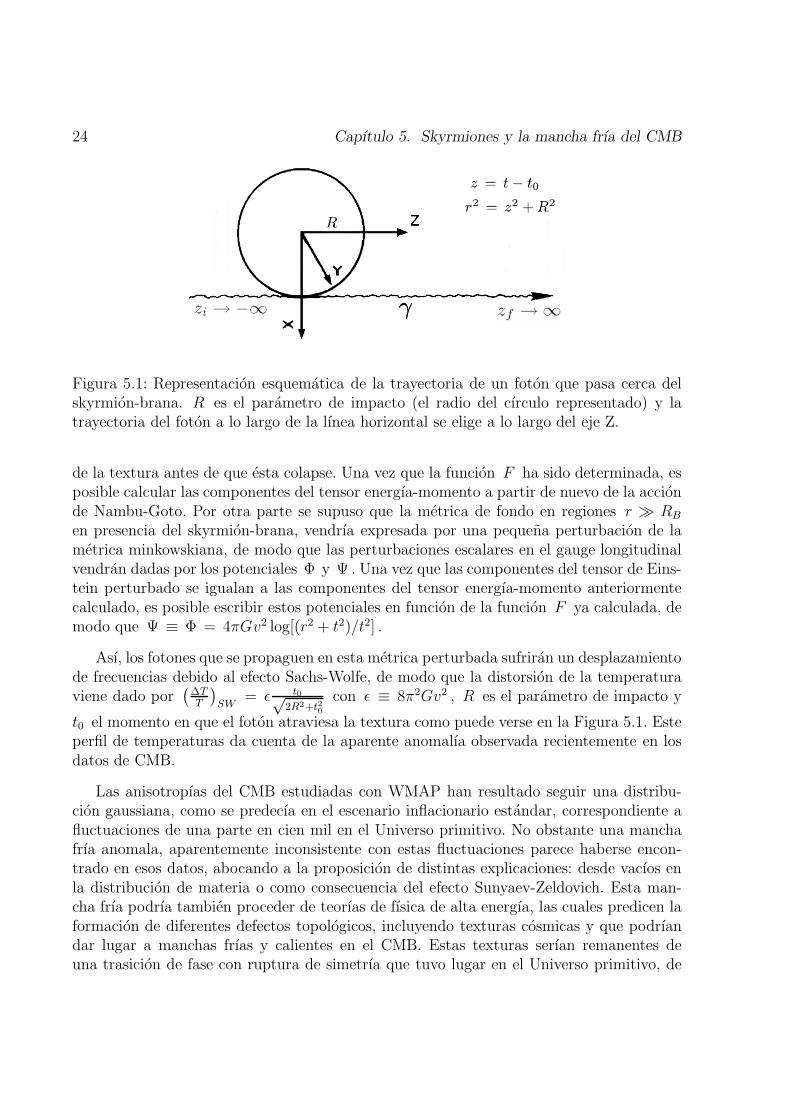
24 Capıtulo 5. Skyrmiones y la mancha frıa del CMB
Figura 5.1: Representacion esquematica de la trayectoria de un foton que pasa cerca delskyrmion-brana. R es el parametro de impacto (el radio del cırculo representado) y latrayectoria del foton a lo largo de la lınea horizontal se elige a lo largo del eje Z.
de la textura antes de que esta colapse. Una vez que la funcion F ha sido determinada, esposible calcular las componentes del tensor energıa-momento a partir de nuevo de la accionde Nambu-Goto. Por otra parte se supuso que la metrica de fondo en regiones r ≫ RB
en presencia del skyrmion-brana, vendrıa expresada por una pequena perturbacion de lametrica minkowskiana, de modo que las perturbaciones escalares en el gauge longitudinalvendran dadas por los potenciales Φ y Ψ . Una vez que las componentes del tensor de Eins-tein perturbado se igualan a las componentes del tensor energıa-momento anteriormentecalculado, es posible escribir estos potenciales en funcion de la funcion F ya calculada, demodo que Ψ ≡ Φ = 4πGv2 log[(r2 + t2)/t2] .
Ası, los fotones que se propaguen en esta metrica perturbada sufriran un desplazamientode frecuencias debido al efecto Sachs-Wolfe, de modo que la distorsion de la temperaturaviene dado por
(
∆TT
)
SW= ǫ t0√
2R2+t20
con ǫ ≡ 8π2Gv2 , R es el parametro de impacto y
t0 el momento en que el foton atraviesa la textura como puede verse en la Figura 5.1. Esteperfil de temperaturas da cuenta de la aparente anomalıa observada recientemente en losdatos de CMB.
Las anisotropıas del CMB estudiadas con WMAP han resultado seguir una distribu-cion gaussiana, como se predecıa en el escenario inflacionario estandar, correspondiente afluctuaciones de una parte en cien mil en el Universo primitivo. No obstante una manchafrıa anomala, aparentemente inconsistente con estas fluctuaciones parece haberse encon-trado en esos datos, abocando a la proposicion de distintas explicaciones: desde vacıos enla distribucion de materia o como consecuencia del efecto Sunyaev-Zeldovich. Esta man-cha frıa podrıa tambien proceder de teorıas de fısica de alta energıa, las cuales predicen laformacion de diferentes defectos topologicos, incluyendo texturas cosmicas y que podrıandar lugar a manchas frıas y calientes en el CMB. Estas texturas serıan remanentes deuna trasicion de fase con ruptura de simetrıa que tuvo lugar en el Universo primitivo, de

25
modo que la transicion de fase cosmica debe relacionarse con un patron de ruptura de unasimetrıa global de un grupo G a un subgrupo H de modo que el espacio coset K = G/Htenga un tercer grupo de homotopıa no trivial. Un ejemplo tıpico es K = SU(N) , quetiene asociado π3(K) = Z para N ≥ 2 . Notese que para lograr una textura formadadurante la transicion, la ruptura de simetrıa debe corresponder a una sımetria global yaque de ser local podrıa gaugearse y desaparecer. Estas texturas pueden entenderse comoconfiguraciones de campo enrolladas que colapsan y se deshacen en escalas cada vez mayo-res. Las texturas pueden ademas producir una concentracion de energıa que da lugar a unpotencial gravitacional que depende del tiempo provocando que los fotones del CMB queatraviesan la region proxima a la textura sufran un desplazamiento de frecuencias. Estedesplazamiento es el que darıa lugar a una mancha frıa o caliente en los mapas del CMB.
Por ejemplo, se han propuesto modelos sigma no lineales SU(2) para construir modelosde texturas que pudieran explicar la mancha frıa observada a traves de una textura quese deshace usando una solucion esfericamente simetrica que proporciona una distorsionrelativa de la temperatura dada por ∆T
T(θ) = ±ǫ 1
q
1+4( θθc
)2
donde θ es el angulo desde el
centro y el mejor ajuste a la mancha frıa corresponde a ǫ = 7,7 × 10⁻⁵ and θc = 5,1 . Elparametro ǫ viene dado por ǫ ≡ 8π2GΦ0 , con Φ0 la escala fundamental de ruptura desımetria que se ajusta a Φ0 ≃ 8,7×10¹⁵ GeV, escala razonablemente proxima a la escala degran unificacion. Sin embargo en las teorıas de gran unificacion lo que se encuentra es unaruptura local de simetrıa que produce el mecanismo de Higgs y que por tanto destruye elsignificado topologico de la textura o cualquier otro defecto que apareciera en la transicioncosmica.
Ası pues, los resultados de la distorsion relativa de temperaturas coinciden si se consi-dera un modelo sigma no lineal o si los calculos se realizan para un skyrmion realizando
las identificaciones Φ0 = v ; 2(
θθc
)
= Rt0
.
Una estimacion de las escalas requeridas para que el skyrmion pueda explicar la manchafrıa observada puede comenzar considerando un numero de dimensiones extra igual a tres(D = 7 ) de modo que para conseguir ǫ ≃ 7,7 · 10−5 debe cumplirse v ≃ 1,2 · 1016 GeV locual puede alcanzarse si la escala fundamental de gravitacion es MD ∼ f ∼ TeV. Noteseque para este rango de parametros, el radio de las dimensiones extras deberıa situarsealrededor de RB ∼ 10−8 m y las aproximaciones realizadas para determinar el perfil detemperaturas causado por un skyrmion estarıan totalmente justificadas. Se comprobo igual-mente que los posibles efectos procedentes de la masa del branon estarıan suprimidos al serde orden O(M2/v2) y los valores usuales de las masas para branones se situan en torno aM ∼ TeV a fin que estos puedan ser candidatos a materia oscura.
Se concluyo por lo tanto que los skyrmiones proporcionan una descripcion adecuadapara la mancha frıa observada en el CMB sin necesidad de introducir altas escalas deenergıa, es decir, sin recurrir a mecanismos de gran unificacion puesto que la amplitud

26 Capıtulo 5. Skyrmiones y la mancha frıa del CMB
correcta de las fluctuaciones de temperatura puede obtenerse con valores naturales de laescala electrodebil.

Capıtulo 6
Conclusiones y perspectivas
Los resultados que hemos presentado en esta tesis intentaron dar respuestas a algunascuestiones todavıa abiertas en la investigacion de teorıas de gravedad modificada, tanto enel ambito cosmologico como en el astrofısico. Estos resultados han proporcionado algunasconsecuencias relevantes, tanto desde el punto de vista teorico como experimental y hansugerido futuras investigaciones ya comenzadas. Entre las diferentes teorıas de gravedadmodificada, dos de particular interes se han estudiado en esta tesis: las teorıas f(R) degravedad modificada y las teorıas de dimensiones extra en mundos brana.
En primer lugar, para las teorıas f(R) hemos mostrado que estos modelos de gravedadpueden reproducir la evolucion cosmologica actual tal y como viene descrita por la Rela-tividad General dentro del modelo cosmologico estandar ΛCDM, desde el momento de laigualdad radiuacion-materia hasta la actualidad. En este orden de investigaciones, fuimostambien capaces de demostrar que la presencia de cualquier fluido perfecto parametriza-do por una ecuacion de estado constante puede ser imitado por la presencia de terminosprocedentes de modelos f(R) , de modo que la adicion de funciones f(R) a la acciongravitacional estandar de Einstein-Hilbert puede proporcionar un mecanismo que repro-duzca diversos tipos de como energıa oscura. Este hecho parece indicar la importancia de labusqueda de una unica funcion f(R) que pudiera explicar, al menos fenomenologicamen-te, las principales caracterısticas de la evolucion cosmologica, desde la epoca inflacionariahasta la actualmente observada expansion acelerada.
A continuacion, y dentro de las modificaciones que las teorıas f(R) introducen en laRelatividad General, se ha realizado en esta tesis un analisis acerca de las perturbacionescosmologicas escalares a primer orden. A este respecto, se ha obtenido un metodo com-pletamente general para encontrar la ecuacion diferencial que proporciona la evolucion delcontraste de densidad de materia. Este metodo es valido independientemente del modelof(R) que se considere y del tamano de las escalas implicadas. Una consecuencia inmedia-ta de estos calculos fue la conclusion de que las aproximaciones habituales que se venıan
27

28 Capıtulo 6. Conclusiones y perspectivas
realizando en la literatura para modos sub-Hubble no eran siempre validas, sino que deter-minadas hipotesis, que se han establecido en esta tesis, deben asumirse sobre las funcionesf(R) a fin de obtener la habitual aproximacion cuasi-estatica.
Como resultados subsiguientes, se decidio estudiar la evolucion del contraste de densi-dad en escalas cosmologicas sub-Hubble. A este respecto se determino que para modelosf(R) cosmologicamente viables, las perturbaciones en este regimen son indistinguibles delas obtenidas a traves de la aproximacion cuasi-estatica pero perfectamente distinguiblesde aquellas obtenidas a traves del modelo ΛCDM.
Con los anteriores calculos teoricos, que permitieron obtener la evolucion correcta de lasperturbaciones de materia en los modos sub-Hubble para modelos f(R) , pueden realizarsealgunos tests a fin de comparar los datos con los resultados teoricos esperados y poderası establecer la validez o algunas restricciones sobre esas funciones f(R) . Este tipo deprocedimientos muestra pues la relevancia de los resultados obtenidos cuando se deseacomprobar la viabilidad de un modelo f(R) que sea propuesto frente a los resultados derecientes experimentos.
Como punto final dentro de las investigaciones presentadas en modelos f(R) , setrato con diversas caracterısticas de agujeros negros en estas teorıas: en primer lugar se estu-dio el caso de soluciones estaticas y esfericamente simetricas en vacıo y se determino que, aligual que en Relatividad General, la unica solucion presente era la solucion Schwarzschild-(anti-)de Sitter. Como resultado complementario del anterior se realizo un estudio del casoestatico y esfericamente simetrico en vacıo. En este estudio no se asumio a priori curvaturaescalar constante, de modo que para el tratamiento de este problema se realizo un analisisperturbativo alrededor de la solucion Schwarzschild-de Sitter en Einstein-Hilbert con cons-tante cosmologica no nula. Una vez realizados los calculos se encontro que hasta segundoorden en perturbaciones, la unica solucion era la solucion generalizada Schwarzschild-deSitter con coeficientes modificados que se expresan en terminos de f(R) y sus derivadasevaluadas en el valor de la curvatura de fondo.
Esta parte de la tesis finalizo estudiando la termodinamica de agujeros negrosSchwarzschild-anti-de Sitter en teorıas f(R) : para ello se representaron, dependiendo delos parametros de diversos modelos que se propusieron, las regiones accesibles desde elpunto de vista termodinamico en terminos de los signos de la capacidad calorıfica y laenergıa libre, ya que la combinacion de signos de estas magnitudes proporciona la estabi-lidad local y global de estos objetos. A este respecto se encontro una caracterıstica muyimportante que anima a continuar la investigacion en estas lıneas: en efecto, se observo quela viabilidad termodinamica de teorıas f(R) en soluciones de curvatura constante estabasujeta al cumplimiento de la condicion 1 + fR > 0 que es de hecho una de las condicionesque se impone a estos modelos para ser cosmologicamente viables, por lo que dos aspectos,en principo diferentes y que condicionan la viabilidad de estas teorıas, fueron aquı y porprimera vez, expresados conjuntamente.

29
La ultima parte de esta tesis se dedico a estudiar algunas evidencias experimentales delos escenarios de mundos branas. Configuraciones topologicamente no triviales, los skyr-miones, que aparecen de forma natural en estas teorıas, parecen estar de acuerdo condatos procedentes del CMB, en particular con la recientemente descubierta mancha frıa.Se concluyo que los modelos de mundos brana con un numero suficiente de dimensionesextra pueden acomodar la presencia de la mancha frıa observada y al mismo tiempo soncapaces de rebajar la escala fundamental de gravitacion a valores del orden de la escalaelectrodebil.
Para concluir, los resultados que han sido incluidos en esta tesis han demostrado quetanto las teorıas f(R) como las teorıas de mundos-brana constituyen posibles candidataspara una mejor comprension de la naturaleza de la interaccion gravitatoria en grandesescalas. Tanto la validez como la viabilidad de estas teorıas necesitan aun ser sometidas atests teoricos y experimentales a fin de poder descartar o mantener como viables los mo-delos propuestos. Para ello, aspectos como la posible imitacion por parte de estos modelosde los resultados que proporciona la cosmologıa estandar, la evolucion de las perturba-ciones cosmologicas, las caracterısticas de objetos gravitatorios tan distinguidos como losagujeros negros y las caracterısticas de los mapas de temperaturas del CMB, fueron consi-derados en esta tesis como dignos de estudio que pueden arrojar luz sobre las propiedadesfundamentales de la interaccion gravitacional.

30 Capıtulo 6. Conclusiones y perspectivas
Copyright © 2022 FDOKUMEN