Course Instructor Karuna S. Brunk Instructor School of Business and Nonprofit Management (SBNM) North Park University

Contact Information Cell: (571) 332-2193 ksbrunk@northpark.edu Available by appointment

Syllabus North Park University SBNM 5212 Microeconomics for Managers (Online) Course Credit: 2 semester hours Prerequisite: None

REQUIRED TEXTBOOK

Steven E. Landsburg, Price Theory and Applications, Ninth edition, Cengage Learning, Stamford, Connecticut, 2014.

ISBN 13: 978-1-285-42352-4 ISBN 10: 10-1-285-42352-6

Information Site to Obtain the Text and eBook

Students can obtain the eBook through the link below. This link provides students with the option to purchase the hardback book, access the eBook, or purchase eChapters.

http://services.cengagebrain.com/course/site.html?id=1576913

https://www.cengagebrain.com/webapp/wcs/stores/servlet/ProductDisplay?langId=- 1&catalogId=10057&categoryId=&storeId=10151&krypto=5tBPLOvU%2BynQPXxGOoU lstXbApYx0RmUq1eXF2qfcXxsN%2B648A4JJWFl3ivizVVzG3p%2BErnT%2Br%2BIswl VTQgcmKvcTgsn3KVKDGL2C%2F1HHuMM321HFsDjKFvldbGTh0k1dg26dVQ%2B8v nRr%2F82ikVbdlVt2BCg44cregXUh08kzALBLFCha3Br8OuNUozPbfnBAkGAJAuhxUtPt t%2FdEh4MUPVc%2BR5B3RCJbxxluiRaiOKPpmevmZOctzP1Vxtxkrziuwkl0Ve%2F%2 BjXdnkZnt2t87O8OChUP9XOTAz1Ya4s%2Bm3wQKGNey7oU1BYRwc77G6YuL5i7zvk KO2uKaOD3fVPJcg%3D%3D

We will be using the text, Steven E. Landsburg, Price Theory and Applications, Ninth edition. Students will be introduced to a variety of material, including theory, applications, policy, and online references. Links to online data sources and information are provided in course Modules.

A Calculus Supplement is Included in the Text The text has a supplementary section in Appendix A devoted to the application of calculus to microeconomics. While students are not always required to use calculus in solving problems or answering questions, the methods are available. Students are encouraged to refer to this section for mathematical interpretations of microeconomic concepts.

CATALOG COURSE DESCRIPTION 5212 Microeconomics for Managers (2 sh) In this course, students explore how the economic fundamentals, such as scarcity, supply and demand, business cycles, elasticity and productivity, influence the planning and behaviors of both businesses and nonprofit organizations. Real world examples are used to apply content in professional context. Additionally, attention is paid to the ethical dilemmas and moral responsibilities that accompany managing firm.

INTRODUCTION Welcome to SBNM 5212, Microeconomics. The study of economics is based on scarcity and choice. Scarce, productive resources in the form land, labor, capital, and entrepreneurship are privately owned based on the institution of private property in a market economy. These resources are allocated among competing production processes, and receive payments known as rent, wages, interest, and profits. These payments represent the prices of resources, and serve as constraints on the amounts of these resources which can be purchased. Production processes take the form of business firms which turn out goods and services (supply) which serve to satisfy unlimited wants (demand) over time.

Microeconomics focuses on markets. Markets are based on two forces: supply and demand which serve to allocate (distribute) resources and goods and services throughout the economy. The method of allocation is known as a price system. In this way, microeconomics is also known as price theory.

We will present the study of microeconomics in terms of basic models. Using models, we explain the process of allocation, market structures, production and cost, and the distribution of income. Models provide us with the tools of economic analysis, and we constantly test our models in the real world. This ongoing process is deductive in nature, and constitutes what we call the scientific method.

The online format of the study of microeconomics helps us to tap into a variety of sources providing insights and perspectives into the contemporary economy.

Course Description To summarize the section above, microeconomics is based on the study of markets and how they serve to allocate scarce, productive resources in order to produce and distribute goods and services.

A market economy is an economic system in which exchanges are made based on the forces of supply and demand. Market economies are found throughout the world, and are becoming the most predominant system of exchange.

Adam Smith, a professor of moral philosophy, observed the market system as it was developing over two hundred and thirty years ago. He believed that individual self-interest worked to the advantage of the whole society. A seller’s self-interest in producing goods served a buyer’s self-interest in consuming goods.

Self-interest expressed in day-to-day economic behavior, can work to everyone’s mutual advantage. This interaction expressed in markets as supply and demand provides for an ethical symmetry in human economic behavior.

Microeconomics presents students with the analytical tools which can be applied to solving problems encountered in everyday business. Mathematics, including calculus, will also be available to provide essential quantitative methods.

Managerial decision-making and the role of strategy will be emphasized in the context of a changing business environment. Discussions will include the ethical dimensions of problems and issues in business.

Evaluation Procedures

There are 8 Modules.

There are 5 Discussion Board Posts. Each is worth 50 points, for a possible 250 total points. The corresponding Rubric: Discussion Board Posts and Questions Assignments is found below.

Students are asked to provide a Peer Response to one other Discussion Board Posts. There are 5 of these assignments. Each response is worth 10 points, a total of 50 points. Please see the corresponding Rubric: Peer Evaluation is found below.

There are 7 Questions Assignments. Please see the corresponding Rubric: Discussion Board Posts and Questions Assignments. Each of the first 6 completed sets of Questions Assignments is worth 50 points, a total of 300. The Final, Questions Assignment 7, has a possible point value of 200.

The overall possible point total is 800.

GRADES

NOTE: In the SBNM a grade below C does not receive course credit. As stated above, the maximum point total is 800.

Total Points Earned Grade

744 or above A

720 - 743 A-

696 – 719 B+

640 - 695 B

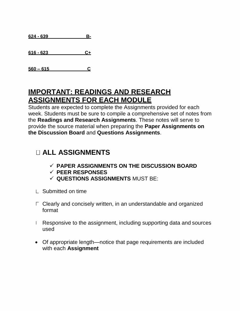
624 - 639 B-

616 - 623 C+

560 – 615 C

IMPORTANT: READINGS AND RESEARCH ASSIGNMENTS FOR EACH MODULE Students are expected to complete the Assignments provided for each week. Students must be sure to compile a comprehensive set of notes from the Readings and Research Assignments. These notes will serve to provide the source material when preparing the Paper Assignments on the Discussion Board and Questions Assignments.

ALL ASSIGNMENTS

PAPER ASSIGNMENTS ON THE DISCUSSION BOARD PEER RESPONSES QUESTIONS ASSIGNMENTS MUST BE:

Submitted on time

Clearly and concisely written, in an understandable and organized format

Responsive to the assignment, including supporting data and sources used

Of appropriate length—notice that page requirements are included with each Assignment

Students with Disabilities Students with disabilities who believe that they may need accommodations in this class are encouraged to contact the Student Success Learning Specialist by email at lmebner@northpark.edu or by phone at (773) 244-5737, or stop by the Student Engagement office located on the 1st floor of the Johnson Center. Please do so as soon as possible to better ensure that such accommodations are implemented in a timely manner. Title IX Students who believe they have been harassed, discriminated against, or involved in sexual violence should contact the Title IX Coordinator (773-244-6276 or TitleIX@northpark.edu) for information about reporting, campus resources and support services, including confidential counseling services. As members of the North Park faculty, we are concerned about the well-being and development of our students, and are available to discuss any concerns. Faculty are legally obligated to share information with the University’s Title IX coordinator in certain situations to help ensure that the student’s safety and welfare is being addressed, consistent with the requirements of the law. These disclosures include but are not limited to reports of sexual assault, relational/domestic violence, and stalking. Please refer to North Park’s Safe Community site for reporting, contact information and further details. http://www.northpark.edu/Campus-Life-and-Services/Safe-Community

SBNM POLICY STATEMENTS Academic Honesty In keeping with our Christian heritage and commitment, North Park University and the School of Business and Nonprofit Management are committed to the highest possible ethical and moral standards. Just as we will constantly strive to live up to these high standards, we expect our students to do the same. To that end, cheating of any sort will not be tolerated. Students who are discovered cheating are subject to discipline up to and including failure of a course and expulsion.

Our definition of cheating includes but is not limited to: 1. Plagiarism – the use of another’s work as one’s own without giving credit to the individual. This includes using materials from the internet. 2. Copying another’s answers on an examination. 3. Deliberately allowing another to copy one’s answers or work. 4. Signing an attendance roster for another who is not present.

In the special instance of group work, the instructor will make clear his/her expectations with respect to individual vs. collaborative work. A violation of these expectations may be considered cheating as well. For further information on this subject you may refer to the Academic Dishonesty section of the University’s online catalog.

In conclusion, it is our mission to prepare each student for a life of significance and service. Honesty and ethical behavior are the foundation upon which such lives are built. We therefore expect the highest standards of each student in this regard.

SBNM Attendance Policy for Graduate Courses The graduate courses in the SBNM are all 7 weeks in length. Missing one class session is allowed without penalty as long as all readings and assignments are made up by the student within a reasonable time period (the following week). Failing to log into an online course site for an entire week is allowed, but a penalty may be applied at the instructor’s discretion. Missing a second class session is allowed only in unusual circumstances by prior arrangement with the instructor. Since this represents almost 30% of the engagement time for the course, the student runs the risk of receiving a lower overall grade for the class. Faculty are encouraged to drop the course grade by a full letter grade in this situation. A student who

misses three classes (or the equivalent two weeks for an online class) will automatically fail the course, unless the student drops the course before the seventh week of class. Students who drop a course will be held responsible for tuition, based upon the current North Park University refund policy outlined in the University Catalog.

SBNM APA Requirements The School of Business and Nonprofit Management (SBNM) has adopted the Publication Manual of the American Psychological Association (APA) as the standard and required format for all written assignments in SBNM courses.

Our goal in adopting the APA Manual is to enhance student learning by: 1) Improving student’s writing skills. 2) Standardizing the required format of all written assignments in all SBNM courses. 3) Emphasizing the importance of paper mechanics, grammatical constructs, and the necessity of proper citations.

4) Holding students accountable for high quality written work.

If you are unfamiliar with the requirements of the APA Manual, we recommend that you purchase the reference manual and/or that you consult one or more of the suggested resources as listed on the Student Resources section of the SBNM website. It is your responsibility to learn and ensure that all written work is formatted according to the standards of the APA Manual.

Writing RUBRICS Each of the Discussion Board Posts is considered to be in the format of essay questions.

RUBRIC: Discussion Board Posts

Writing Model: Economics Essay Format For Assignments

POINT VALUES

CATEGORY

Excellent 10 points for each category (for the first five Questions Assignments)

20 (for the final)

Good 9 points for each category (for the first five Questions Assignments)

18 (for the final)

Fair 8 points for each category (for the first five Questions Assignments)

16 (for the final)

Poor 7 points for each category (for the first five Questions Assignments)

14 (for the final)

1. Introduction (Organization)

The introduction is inviting, states the main topic and previews the structure of the paper.

The introduction clearly states the main topic and previews the structure of the paper, but is not particularly inviting to the reader.

The introduction states the main topic, but does not adequately preview the structure of the paper nor is it particularly inviting to the reader.

There is no clear introduction of the main topic or structure of the paper.

2. Focus on Topic (Content)

There is one clear, well-focused topic. Main idea stands out and is supported by detailed information.

Main idea is clear but the supporting information is general.

Main idea is somewhat clear but there is a need for more supporting information.

The main idea is not clear. There is a seemingly random collection of information.

3. Grammar & Spelling (Conventions)

Writer makes no errors in grammar or spelling that distract from the content.

Writer makes 1-2 errors in grammar or spelling that distract from the content.

Writer makes 3-4 errors in grammar or spelling that distract from the content.

Writer makes more than 4 errors in grammar or spelling that distract from the content.

4. Accuracy of Facts (Content)

All supportive facts are reported accurately.

Almost all supportive facts are reported accurately.

Most supportive facts are reported accurately.

NO facts are reported OR most are inaccurately reported.

5. Conclusion (Organization)

The conclusion is strong and leaves the reader with a feeling that they understand what the writer is "getting at."

The conclusion is recognizable and ties up almost all the loose ends.

The conclusion is recognizable, but does not tie up several loose ends.

There is no clear conclusion, the paper just ends.

RUBRIC: PEER EVALUATION

Model for Peer Evaluation Responses on the Discussion Board

CATEGORY 1 Poor 2 Fair 3 Good 4 Excellent

How well was the presenter prepared?

The presenter did not have a good understanding of he subject.

The presenter was somewhat prepared to share with the group.

The presenter was well prepared to share with the group.

The presenter shared ideas, and it was obvious that they put some thought into the presentation.

How clear were the concepts being presented?

I don't have a good grasp of what they were talking about.

The basic points are fairly clear, but needed more explanation.

The concepts were very clear, I feel like I have a good understanding of them.

The concepts were very clear. The presenter used clear explanations, as well as examples to explain the concept clearly. I totally understand.

Did the presenter do anything extra to help you remember the material?

The presenter did not make the concepts very clear.

The presenter did not do anything really special to help me remember the concepts.

The presenter had a neat way to help me remember the concepts being summarized.

The presentation was memorable and interesting. They used a variety of methods to help me remember the information.

Overall evaluation-- Assign a number for each category, add together, and divide by 3 for the Average.

Preparation Clarity Remembering material presented

Average

NOTE: NO POINTS SHOULD BE AWARDED. Students should use the Peer Evaluation Categories to frame their responses. After reading a peer’s work, respond in a constructive and supportive way, and provide positive comments.

Learning Objectives Students should refer to the following website in order to better understand the purpose of the Learning Objectives. https://www.uvic.ca/services/counselling/assets/docs/Blooms%20taxonomy .pdf The site presents Benjamin Bloom’s taxonomy classifying competence and corresponding demonstrated learning skills.

Knowledge—retention of information

Comprehension—understanding information

Application—use information

Analysis—recognize patterns

Synthesis—use old/create new ideas and constructs

Evaluation—comparison and assessment

The following Learning Objectives for this course are established in order for students to become better able to:

1. Relate the concepts of supply, demand, market equilibrium. 2. Explain the determination of relative prices, and compare the concept to

that of absolute prices. 3. Analyze the process of resource allocation, and the relationship of

production to cost. 4. Apply the various concepts of elasticity: price, income, and cross elasticity. 5. Acquire a basic understanding of leading theories and models of the

structure of markets and industries. 6. Identify the major characteristics of the contemporary market economy: in

terms of exchange, transactions cost, utility, and profits/losses. 7. Learn how to interpret the behavior and choices made by consumers in

markets using indifference curve analysis. 8. Derive and apply the concept of profit maximization for business firms. 9. Apply the notion of economic time periods in terms of short run and long

run to production and cost. 10. Explore the basic concepts underlying the demand for factors of

production. 11. Appraise the effects of business strategy, game theory, and forms of

competition. 12. Use the competitive model as a standard of comparison for other market

structures. 13. Investigate and apply the concepts of positive and negative externalities. 14. Explain how the study of microeconomics can provide a strong set of

analytical tools for ethical managerial decision-making.

Unit/Weekly Learning Objectives will be found in Moodle for each week.

Student Learning Objectives: IDEA Course Rating System

North Park University uses the IDEA course rating system to measure student progress towards learning objectives and to measure student satisfaction with their overall learning experience. These course evaluations are administered at the end of the term, and you will be notified by email when they are ready for you to complete. The results of these evaluations are very important to us and we use them for ongoing efforts to improve the quality of our online courses. The overarching IDEA objectives for this course are the following.

(1) Students will gain factual knowledge in the form of terminology, classification methods, and trends.

(2) Students will become able to comprehend fundamental principles, generalizations, or theories.

(3) Students will become able to apply course material to improve thinking, problem solving, and decision-making.

END OF TERM COURSE EVALUATIONS North Park University uses the IDEA course rating system to measure student progress towards learning objectives and to measure student satisfaction with their overall learning experience. These course evaluations are administered at the end of the term, and students will be notified by email when they are ready for you to complete. The results of these evaluations are very important to us and we use them for ongoing efforts to improve the quality of our online courses.

To the Attention of All Students Computer Requirements: In order to effectively participate in and successfully complete this course, each participant will need to have access to a computer and a high-speed internet connection.

Participant Responsibilities: 1. Attendance, presence, and full participation are all required for this course.

2. Students are expected to collect a complete set of notes and data based on the Readings and Research Assignments. These notes and data provide the basis for completing Assignments.

3. Although I strongly suggest that all issues, questions, and problems be dealt with online, please feel free to call or email me regarding these issues. Please note office hours given on the first page, and below under Contact Information.

4. It is expected that students plan on spending 10-12 hours per week on course responsibilities.

Course Instructor Responsibilities (Also see Contact Information and General Time Schedule below): 1. The course instructor will design the course and learning Modules in such a way that students have every opportunity to achieve the Learning Objectives.

2. The course instructor will provide reactions to student responses and discussion as appropriate in order to clarify important ideas and concepts.

3. The course instructor may provide opportunities for group work that will include the Discussion Board and individual questions and exercises.

4. The course instructor may provide updated information on relevant resources for the various topics of interest.

5. The course instructor will read and critically assess the work of students, and provide feedback within about one week of receipt.

6. The course instructor will respond to all student emails and phone calls (Monday- Thursday) within 1 - 2 days of receipt.

General Time Schedule

Due dates/times are given in the Course Outline

Grades will be posted on Mondays (or, within one week of Assignment due date)

Instructor will read Email/respond (M – TH)

Instructor will post/check Discussion Board as required

Please Note:

1. Assignments in each of the Modules are meant to provide the basis for notes and data collected by students. These notes and data should serve as the basis for completing work on the Discussion Board and Questions Assignments.

2. All PowerPoint presentations are meant for use with this course only, and should not be copied and/or used with any other presentations not related to this course. This is a caution to students to avoid possible copyright infringement.

3. Opinions and views expressed in text readings, questions, problem sets, and related materials, as well those which may be encountered online, may not necessarily coincide with the opinions, views, and standards of the instructor.

SUMMARY COURSE OUTLINE Week 1 Beginning Tuesday, January 16, 2018

Module 1 Building an Online Community Discussion Board Post 1 (possible 50 points) Peer Response (possible 10 points)Due by Thursday, January 18, 2018

Module 2 Introductory Concepts: The Study of Economics; Supply, Demand, and

Gains from tradeText Chapters 1, 2, 19; Calculus in Appendix A Discussion Board Post 2 (possible 50 points) Peer Response (possible 10 points) Due by Saturday, January 20, 2018

Questions Assignment 1 (possible 50 points) Due by Monday, January 22, 2018

Week 2 Beginning Monday, January 22, 2018 Module 3 Consumer Behavior

Text Chapters 3, 4, 8, 18 is optional; Calculus in Appendix A Discussion Board Post 3 (possible 50 points) Peer Response (possible 10 points) Due by Wednesday, January 24, 2018

Questions Assignment 2 (possible 50 points) Due by Saturday, January 27, 2018

Week 3 Beginning Monday, January 29, 2018 Module 4 Behavior of Firms; Revenue and Cost

Text Chapters 5, 6; Calculus in Appendix A Questions Assignment 3 (possible 50 points) Due by Saturday, February 3, 2018

Week 4 Beginning Monday, February 5, 2018

Module 5 CompetitionText Chapter 7; Calculus in Appendix A Discussion Board Post 4 (possible 50 points) Peer Response (possible 10 points) Wednesday, February 7, 2018

Questions Assignment 4 (possible 50 points) Due by Saturday, February 10, 2018

Week 5, Monday, February 12, 2018 Module 6 Imperfect Competition

Text Chapters 10, 11; Calculus in Appendix A Discussion Board Post 5 (possible 50 points) Peer Response (possible 10 points) Due by Wednesday, February 14, 2018

Questions Assignment 5 (possible 50 points) Due by Monday, February 19, 2018

Week 6 Monday, February 19, 2018

Module 7 Game Theory, External Costs and Benefits, Public Goods, and the Distribution of Income

Chapters 12, 13, 14 is optional, 15; Calculus in Appendix A Questions Assignment 6 (possible 50 points) Due by Saturday, February 24, 2018

Week 7 Beginning Monday, February 26, 2018

Module 8 Review All Text Chapters, Notes, and Data

Questions Assignment 7 (Final, possible 200 points)

The Final will be posted in the 5th week

The completed Final is due no later than midnight, Tuesday, March 6, 2018

Complete Course Outline

Week 1: Beginning on Tuesday, January 16, 2018

Module 1 INTRODUCTIONS: Building an Online Community

An Online Community Students enrolled in this online course are here voluntarily. We are engaged in a common, shared learning experience. In this online, “situated” learning environment, students have common goals and interests. All of you are here because you are seeking credit toward certificates and/or degrees. We want to build a solid foundation for Student Centered Learning. The playing field is level for all, and we want to do our very best. We adhere to the following principles:

We are members of a shared learning community

Our dominant purpose is to learn

We trust each other and we will cooperate together

Our community is welcoming, supportive, and encouraging

PAPER ASSIGNMENT ON THE DISCUSSION BOARD 1 (possible 50 points)

Please post your answers to Discussion Board 1 (possible 50 points).

In order to get acquainted, let’s answer a few questions. Keep your answers relatively short. (2 pages total).

Who am I? Please describe yourself, and where you usually working from

(home, office, Starbucks)

Why have you joined this online community?

What are your expectations for this course? Chose your own words. There is no “set” answer.

How do I learn best? Choose one or more, and briefly describe your

learning process based on the following categories.

Words

Numbers

Pictures

Music

Self-reflection

Social interaction

Natural world experience

Peer Response: See the Rubric: Peer Response (p. 7) above. Students may not feel comfortable awarding points on the peer responses—DO NOT AWARD POINTS. Use the Rubric as a format for your response. Be positive, encouraging, and supportive in those responses. (possible 10 points)

Post your responses by Thursday, January 18, 2018

Week 1: Beginning Tuesday, January 16, 2018 MODULE 2

Module 2 Introductory Concepts: Supply, Demand, and Gains from Trade

Here are your Reading and Research Assignments. Notice how the author arranges his presentation. There are many examples, exercises, and problem sets. Be sure to pay attention to the Dangerous Curves.

Read Chapters 1 – 2, and 19 in the text

After reading Chapter 1, notice how the forces of supply and demand work to solve the basic economic problem known as scarcity. Markets send “signals” in the form of prices informing us about the relative scarcities of goods and services. Higher prices mean “greater scarcity,” and lower prices mean “less scarcity.”

Chapter 2 presents the concept of division and specialization of labor, and the resulting gains from trade. Think about how we use this model to analyze a economy’s production choices. Be sure to compare the concepts of relative prices and absolute prices, or “implicit” and “explicit” opportunity cost.

Topics: What is Economics? Students will learn about the basic concepts of supply, demand, and market equilibrium. In addition, the relationship between relative prices and absolute prices is presented, and we then move on to a discussion of specialization and the gains from trade.

Learning Objectives: Students will learn the fundamental process of economic analysis. Economic analysis involves the structuring and application of economic models. These models are applied to real-world problem solving, and the formulation of economic solutions, or “policies.” In addition, students will learn the basic principles of supply, demand and the functioning of markets. The division and specialization of labor, as well as other resources, leads to what is known as the “gains from trade.”

Chapter 1 Supply, Demand, and Equilibrium Chapter 2 Prices, Costs, and the Gains from Trade Chapter 19 What is Economics? Calculus in Appendix A

In Chapter 19 we find an introduction to economic model-building, or “economic analysis.” Economists use these models to apply in order to solve everyday problems. This chapter is important because it implicitly presents the application of the scientific method, the basis of analytical economics.

Barter and Money Economies Before we consider markets using money as a medium of exchange, consider exchange in a barter economy where there is no unit of money. In a barter economy, goods exchange for other goods in established ratios. For example, let’s suppose that it takes two apples (QA) to exchange for one orange (QO ). Because an oranges require two apples In exchange the orange is twice as expensive.

Barter Exchange Money System Ratio System

QA / QO = 2 / 1 = PO / PA

Because PO / PA 2 / 1, PO = 2 PA meaning that the price of oranges is twice the price of apples. The price ratio in a Money System is the reciprocal of the Barter System quantity ratio.

Every transaction in a Barter System requires that persons have goods which other people want in exchange. This makes the possibility of growth and expansion very difficult. The introduction of a commonly acceptable medium of exchange known as “money” makes exchange more efficient.

Notice that printed on U.S. paper currency we find the statement “This Note Is Legal Tender for All Debts Public and Private,” which identifies the bill as legal money, something which is commonly acceptable in exchange. There is no metal backing for U.S currency, making it “fiat money,” or money because the U.S. government says that it is money.

Why do people accept and trust fiat money? The answer is, simply because it is acceptable in exchange “for all debts public and private.” Can you think of economies in which currency became unacceptable? In Germany after World War I money became worthless as inflation reached 322% per month. Inflation was even worse in Hungary after World War II. See: http://www.econlib.org/library/Enc/Hyperinflation.html

Absolute and Relative Prices The following presentation distinguishes between Absolute and Relative prices.

The Market and Alfred Marshall This diagram of a market originated with Alfred Marshall in his Principles of Economics first published in 1890. Marshall’s Principles is the first comprehensive study of microeconomics, and much of what we learn about microeconomics today began with Marshall’s work.

The vertical axis is the price axis, and the horizontal axis is quantity. If buyers were willing to pay more than sellers were asking (dR > sR), quantity would increase fro R to H. Assuming that sellers were seeking a higher price than buyers were willing to pay (sR > dR), quantity would decline from R to H. Equilibrium would be found at A.

http://www.econlib.org/library/Marshall/marPNotes3.html#a19 Citation:

Marshall, Alfred. Principles of Economics. London: Macmillan and Co., Ltd, 1920. [Online] available from http://www.econlib.org/library/Marshall/marPNotes3.html; accessed 24 March 2008; Internet.

Absolute versus Relative Prices

• No money in world, people still trade

– Exchange goods

• Absolute prices

– Number of dollars exchanged for a specified quantity of a given good

• Relative prices

– The quantity of some other good that can be exchanged for a specified quantity of another good

Landsburg, Price Theory and Applications, 7th edition

th

Here is a picture of Cement market from the Landsburg text.

Changes in Quantity Demanded and Supplied, and Changes in Demand and Supply Students should be able to distinguish between changes in quantity demanded (changes in quantity demanded along a given demand line in response to changes in price), and changes in quantity supplied (changes in quantity supplied along a given supply line in response to changes in price), and changes in demand and supply, which means changes in the entire demand and supply lines, respectively.

Changes in demand and supply are shown below. Be sure to distinguish between increases and decreases in Demand (A and B, respectively), and increases and decreases in Supply (C and D, respectively).

EXHIBIT 1.7 Equilibrium in the Market for Cement

Landsburg, Price Theory and Applications, 7th edition

EXHIBIT 1.8

The Effects

of Supply

and Demand

Shifts

Landsburg, Price Theory and Applications, 7 edition

Online Reading Follow the links to an introduction to the study of Economics, and to an

understanding of the differences between Microeconomics and Macroeconomics. In addition, we will find the basic ideas behind demand and supply.

See Economics Basics: What is Economics? http://www.investopedia.com/university/economics/economics1.asp

The difference between Macroeconomics and Microeconomics: http://www.investopedia.com/terms/m/microeconomics.asp

Follow the link to Economics Basics--Supply and Demand

http://www.investopedia.com/university/economics/economics3.asp

This article is an excellent review of the basic principles of supply and demand with supporting diagrams. Students should be able to explain how markets reach equilibrium beginning with an initial imbalance between supply and demand. Also notice the very important differences between shifts in the supply and demand lines, and movement along a given supply or demand line.

Here we will find further information on Alfred Marshall, the founder of

Microeconomics.http://www.econlib.org/library/Enc/bios/Marshall.html

Paper Assignment on the Discussion Board 2 Post your 1-page answer to the Discussion Board 2 (possible 50 points).

Explain the difference between a measure of absolute price and relative prices. Think about 2 goods or services you have purchased this year and last year whose prices have changed over the time period. Assuming that the prices have changed discuss and compare the concepts of absolute price and relative price of these goods.

Peer Response: Respond to the answers of one other student. Follow the Peer Evaluation Rubric (Rubric above) in writing your response (possible 10 points).

Post your answers/responses by Saturday, January 20, 2018

QUESTIONS ASSIGNMENT 1 From the Landsburg text, answer the following questions to be submitted to the instructor. A 1-page maximum for each question (possible 50 points).

1. Questions R1, R3, and N1. For N1 set the right-hand

side of the equations equal to each other, and solve for P. Then substitute this P value into each equation, and solve for Q. pp. 23-24.

2. Problem Set: Question 6 and 13 on p. 25-26. 3. From your online reading, write a 1-page discussion of

Alfred Marshall’s contributions to economics. 4. Suppose that due to a winter snow storm, the demand

for snow shovels increases. The supply of snow shovels also increases, but not by as much as the increase in demand. Show a supply and demand diagram indicating the effects on price and quantity exchanged for snow shovels.

5. Show appropriate diagrams for the following, and explain/indicate the effects on price and quantity exchanged. (a) Demand increases while the supply line remains

the same. (b) Supply decreases while the demand line remains

the same.

Post your answers by Monday, January 22, 2018

Week 2 Beginning Monday, January 22, 2018

Module 3 Consumer Behavior

Here are your Reading and Research Assignments. Notice how the author arranges his presentation. There are many examples, exercises, problem sets, and be sure to pay attention to the Dangerous Curves.

Read Chapters 3 – 4, 8, and 18 (optional) in the text

After reading Chapter 3, notice that consumer behavior is based on tastes and preference expressed in the form of baskets of goods, and displayed in the context of indifference curves. The consumer attempts to attain the highest level of satisfaction subject to the constraints of income and the prices of goods expressed in the form of a budget line. In this way, we are studying a problem of constrained maximization. Consumer equilibrium is found at the point of tangency of an indifference curve and the budget line.

Chapter 4 presents the analysis of income and substitution effects using indifference curve analysis. These effects are encountered as the budget constraint components, income and prices, are changed. In addition, be sure to gain an understanding of the terms Engel curve, a Giffen good, and an inferior good. The next important section of this chapter begins on p.96 with an introduction to the concept of elasticity: price elasticity, income elasticity, and cross elasticity.

Topics: The economic behavior of consumers is explored, and students are introduced to a more complete understanding of the concept of demand. The effects on consumer behavior and choice are examined as we introduce changes in prices and income. An introduction to the concepts of consumer and producer surplus, and prices set by the government above and below the market equilibrium price level.

Learning Objectives: Students will learn how to interpret the effects on consumer behavior when prices and income are changed. Students will understand the effects of the imposition of prices different from the equilibrium prices in markets, and how goods may be inefficiently allocated in markets.

Chapter 3 and Appendix on the Behavior of Consumers Chapter 4 Consumers in the Marketplace Chapter 8 and Appendix Welfare Economics and the Gains from Trade Chapter 18 Risk and Uncertainty (optional)

Calculus in Appendix A

In Chapter 8 we find an introduction to the concepts of consumer and producer surplus. In addition, we find the presentation of the effects of price ceilings, and associated market inefficiency. These government-imposed prices are found below the market equilibrium price level, and may take the form of tariffs. Students should also be aware of the fact that markets may also be subjected to price floors, which appear as prices set above the equilibrium market price, and may take the form of a minimum wage.

Chapter 18 is optional, but students are encouraged to read about how attitudes toward risk are evaluated. The insurance market is analyzed, as is the general concept of the market for risky assets.

Indifference Curve Analysis An important concept in microeconomic analysis is the use and application of indifference curves.

An indifference curve is based on the assumption that a consumer is able to judge whether or not they prefer one market basket of goods to another, or if they are equally well off (indifferent) to taking either basket.

An indifference curve slopes downward to the right as seen in the diagrams below, and in the text. Each indifference curve represents a set of choices (baskets) of two goods. Each set provides the same amount of utility (satisfaction) for the consumer, and the consumer considers each of these sets “equally desirable.”

It is assumed that consumers are rational; that is, they are observed to be consistent in consumption choices over time. While consumer preferences tend to be consistent, they are affected by new information about products, by changes in the prices of goods, and by changes in income.

NOTE: On the left side of the diagram below, the price of Eggs declines as the budget line shifts to the right on the Eggs axis. The consumer purchases 2, 3, and 5 Eggs as their price falls from $6, to $3, and finally to $2. In the diagram on the right, we see the price and quantity combinations for Eggs, or what we call the demand curve for Eggs. Notice that the indifference curve/budget line diagram on the left has goods (Root Beer and Eggs) as the variables on each axis. The demand curve on the right has the price of Eggs on the vertical axis, and the quantity demanded of Eggs on the horizontal axis.

Measuring Elasticities: Price Elasticity, Income Elasticity, and Cross Elasticity

The Equation for Price Elasticity of Demand, or ED. is:

ED = (%Δ Quantity demanded) / (%Δ Price)

From the text we have:

Suppose that we use numbers from the diagram Constructing the Demand Curve, and we want to use the Price Elasticity of Demand equation. We calculate price elasticity of demand for Eggs as price declines from $3 to $2, and the quantity increases from 3 to 5. Then we have:

%Δ Q = 100 * (Ending number – Beginning number) / Beginning number

%Δ P = 100 * (Ending number – Beginning number) / Beginning number

Substituting with numbers, we have

%Δ Q = 100 * (5 – 3) / 3 = 66.67%,

%Δ P = 100 * (2 – 3) / 3 = - 33.33%

The result is that

ED = 66.67% / - 33.33% = - 2

Landsburg, Price Theory and Applications, 7th edition

%P 100 P / P Q P

=

Price elasticity

%Q 100 Q / Q P Q

Price Elasticity of Demand

NOTE: Price elasticity of demand is normally a negative number because of the law of demand (see p. 1 of the text—prices and quantities change in opposite directions). If absolute value is used, we can avoid a negative sign.

I ED I = | 66.67 | / | - 33.33 | = 2

Elastic demand is found when | ED | >1, or l %Δ Q l > l %Δ P lThis type of good is thought to be relatively expensive, and/or has many substitutes, and/or has many uses as price declines.

Unitary elasticity is found when, | ED | =1, or l %Δ Q l = l %Δ P lThe way to think about this type of good is that no matter how much the percentage change in price is, the percentage change in quantity demanded exactly matches this price change (in the opposite direction). Under these circumstances, the consumer always spends the same amount on the good as price changes. If you plan to spend a budgeted amount on gasoline no matter how much the price changes, gasoline (in your situation) would have unitary elasticity.

Inelastic demand is found when | ED | < 1, or l %Δ Q l < l %Δ P lThese types of goods are thought to be relatively inexpensive, and/or have few substitutes, and/or have few uses.

The Equation for Income Elasticity of Demand, EI, is:

EI = (%Δ Quantity demanded) / (%Δ Income)

0 < EI < 1 (a fraction), a normal good

EI > 1, a superior good/luxury

EI < 0 ( negative), an inferior good

The Equation for Cross Price Elasticity of Demand, Ec, is:

Ec = (%Δ Quantity demanded of good X) / (%Δ Price of good Y)

Ec > 0 (positive): X and Y are likely to be substitutes (Coca Cola and Pepsi Cola or butter and margarine, for example). An increase in the price of good Y would bring about an increase in the quantity demanded of good X.

Ec < 0 (negative): X and Y are likely to be complements (goods used together—

breakfast cereal and milk, or coffee and sugar, for example). An in crease in the price of Y would bring about a decline in the quantity demanded of good.

Ec = 0: goods X and Y are not related.

Price Elasticity and Total Revenue

Click on: http://en.wikipedia.org/wiki/Price_elasticity_of_demand

Here are some diagrams from the website:

Notice the diagrams in the section Elasticity and revenue show the relationship between demand and total revenue.

Demand is elastic as long as total revenue is increasing.

At the maximum point of total revenue demand is unitary.

When total revenue is declining, demand is inelastic.

NOTE: Suppose that the demand line in the picture has the equation P = 50 – 2Q where P is price and Q is quantity demanded. Then Total Revenue is TR = P * Q = (50 – 2Q) * Q, or TR = 50Q – 2Q2.

Marginal Revenue is MR = 50 – 4Q. MR = dTR / dQ, or the derivative of total revenue with respect to quantity. If we have a linear or straight line demand equation, as we have here, Marginal Revenue has the same intercept term, in this case 50, and twice the slope as the demand equation.

Pri

The revenue equations in this example are:

P = 50 – 2Q, which is the demand equation, and also Average Revenue. TR = P*Q, then P = TR / Q = AR (total revenue per unit),

TR = 50Q – 2Q2

MR = 50 – 4Q

In general, revenue equations may be written as follows:

P = a – bQ

TR = aQ – bQ2

[TR = P*Q, or TR = (a – bQ) * Q]

MR = a - 2bQ

NOTE: Given a TR equation, MR is the derivative of TR with respect to Q, or MR = dTR / dQ. This is known as a measure of continuous MR. If we measure MR using a table of numbers, we are measuring discrete MR written as, MR = ∆TR / ∆Q.

Here is the Demand curve (P = 50 – 2Q) with appropriate numerical intercepts on each axis. At P = 50, Q = 0, no units would be purchased at a price of 50. At Q = 25, P = 0 which tells us that in a given time period in this market, consumers would take no more than 25 units even at a price of zero.

P

50

25 Q

D

0

Pricing Strategy for the Firm Price elasticity is an important determinant of pricing strategy for a business firm, assuming that the firm is attempting to increase its total revenue (TR = P * Q).

If demand is elastic, a price decrease is required in order for the firm’s TR to increase.

If demand is inelastic, a price increase is required in order for the firm’s TR to increase.

A firm’s TR is maximized when the price elasticity of demand is unitary.*

In this way, price elasticity gives us a useful concept for formulating a pricing strategy, other things equal (ceteris paribus).

*Maximum Total Revenue

In the diagram below, notice that maximum TR is found where MR = 0 (QTR) and ½ the distance to the Price intercept (PTR). This is the Unitary range of Elasticity.

The Relationship Between Marginal Revenue, Price, and Elasticity of Demand The student should also see pp. 314 - 317 of the Landsburg text where we find the

following equation. The text uses the Greek letter eta ( ) whereas we use ED to represent price elasticity.

MR = P * [ 1– (1 / I ED I ) ]

*Using absolute value notation I ED I notice that if demand is elastic,

I ED I > 1, and MR > 0

*If demand is inelastic,

I ED I < 1, and MR < 0

*If demand is unitary,

I ED I = 1, and MR = 0

Here’s a picture of this relationship.

Below we find a picture showing the relationship between P, MR, TR, and ED. Notice that in this diagram, we assume that e is the same as I ED I. In the middle of the Demand curve we find unitary elasticity where e = I ED I = 1, (or, ED = - 1). At this point, we find maximum TR and MR = 0. From the diagram above, this is where price is PTR

and quantity is QTR.

Other Online Reading Follow the link to an informative discussion of price and income elasticity

measures, as well as elasticity of supply. http://www.investopedia.com/university/economics/economics4.asp

Follow the link to a discussion of cross price elasticity of demand as well as

related links to the other elasticity measures.http://economics.about.com/cs/micfrohelp/a/cross_price_d.htm

Review the following links for more information on price floors and price ceilings.

See the second diagram showing an effective price floor resulting in a surplus.

http://en.wikipedia.org/wiki/Price_floor

See the second diagram with a Binding price ceiling resulting in excess demand; that is, a shortage. http://en.wikipedia.org/wiki/Price_ceiling

Click on the link below for a discussion of indifference curve analysis.

http://www.cengage.com/resource_uploads/downloads/1111970211_322430.pdf

Discussion Board 3 Post your 1-2 page answer to the Discussion Board 3 (possible 50 points).

Present a discussion of the practical usefulness of indifference curve analysis in gaining an understanding of consumer behavior and consumer choice in everyday life. Include numerical examples and appropriate diagrams in your answer.

Peer Response: Respond to the answers of one other student. Follow the Peer Evaluation Rubric in writing your response. Remember, no points should be awarded. Be positive, encouraging, and supportive in your response. (possible 10 points).

Post your answers/responses by Wednesday, January 24, 2018

QUESTIONS ASSIGNMENT 2 From the Landsburg text, answer the following questions to be submitted to the instructor. 1–2 pages maximum for each question (possible 50 points). 1. Questions R1, R3, R4, R7 (see p. 54 in the text), and R8 on pp. 67-68. 2. Questions R2, R3, and R5 on pp. 103-104. 3. (a) Explain what is meant by “consumers’ surplus” and “producers’ surplus.” Show a market diagram and identify the areas of each type of surplus.

(b) Explain and use appropriate diagrams to distinguish between a price ceiling and a price floor.

(c) Why do price ceilings and floors make markets inefficient? 4. Explain how the concept of price elasticity of demand can be used to determine a

firm’s pricing strategy. Fully explain how once a business firm knows the price elasticity of demand for its product, it can determine a pricing strategy (that is, know whether to raise or lower price) in order to increase its total revenue.

5. (a) Explain how to use and apply Income elasticity of demand in order to Determine whether a good is normal, superior, or inferior. Give examples for each.

CONTINUED>>>>>>>>>>>>>>

5. (b) Explain how to use and apply Cross elasticity of demand in order to determine whether goods are substitutes, complements, or not related. Give examples for each. 6. A demand equation is given by P = 200 -.50Q What are the equations for TR and MR based on this demand equation? At what level of P and Q would we find maximum TR? Show your work. 7. Given the equation, MR = P * [ 1 – ( 1 / I ED I ) ], find the relationship between MR and P if ED = - 2. Then find the implied value of ED if price (P) is set 100% above MR. 8. According to online readings, explain how to use indifference curve analysis in order to determine consumer equilibrium. That is, explain how to use the combination of indifference curves and budget lines.

Post your answers to the instructor by Saturday, January 27, 2018

Week 3 Beginning Monday, January 29, 2018

Module 4 Behavior of Firms; Revenue and Cost

Here are your Reading and Research Assignments. Notice how the author arranges his presentation. There are many examples, exercises, problem sets, and be sure to pay attention to the Dangerous Curves.

Read Chapters 5–6 in the text

In Chapter 5, we find that firms are in business in order to make profits. Profits represent the reward for the ability of firms to produce sales revenues in excess of production costs.

In Chapter 6, students are introduced to the concept of production (supply), and the notion of a production function. Production and the costs of production are different sides of the same coin. Students should understand how firms gather productive resources (land, labor, capital and the organizing factor known as entrepreneurship) in order to produce goods and services on one side. The other side is the payments made to these factors of production by firms which constitute their costs

Topics: The economic behavior of business firms is examined, and students are introduced to a more complete understanding of the concept of supply. Firms exist in order to produce (supply) goods and services to buyers. If buyers attempted to produce goods and services for themselves, the transactions costs would be much higher, and the variety of goods and services available would be much smaller.

Learning Objectives: Students will learn how to calculate the marginal benefits and marginal costs generated by business firms, and the methodology of determining the optimum production level in order to maximize profits. Associated production measures will be introduced, including marginal product and average product. In addition, students will learn how to calculate and interpret derived measures of cost including average total, average variable, averaged fixed, and marginal cost.

Chapter 5 The Behavior of Firms Chapter 6 Production and Costs

Calculus in Appendix A

Production in the Short Run In the diagrams below, notice that the production function on the left relates the amount of output [Total product (TP)] to the amount of labor used. It is assumed that a fixed amount of capital is used for all levels of labor.

This is the short run because labor is variable, but capital is fixed. A firm does not have enough time to change its scale of plant; that is, it cannot add to its capital capacity.

On the right are the derived measures of production, Average product of labor (APL), and Marginal product of labor (MPL).

Notice that there is a consistent relationship between marginal and average measures which can apply to both production as well as cost. If a marginal measure > average measure, the average measure is increasing. Conversely, if a marginal measure is < an average measure, the average measure is declining. If the marginal measure = the average measure, the average measure is at a maximum or a minimum.

EXHIBIT 6.1 Total, Marginal and Average Products

Landsburg, Price Theory and Applications, 7th edition

Shape of MP and AP Curves

• AP – If number of workers large, additional workers cause

average product of labor to decrease

– Inverted U-shape

• MP – Inverted U-shape

• AP and MP relationship to one another – If MP > AP, MP lies above AP

– If MP < AP, MP lies below AP

– If MP = AP, AP at maximum or peak

Landsburg, Price Theory and Applications, 7th edition

Below we find a picture of typical cost curves in the short run. When MP is increasing (increasing returns), we find that MC declines. When MP declines (diminishing returns), MC increases. From the text, p. 143, MC = PL / MP. There is a reciprocal relationship between MC and MP.

When AP increases, (increasing efficiency of labor), AVC declines. When AP decreases (declining efficiency of labor), AVC rises. MC is declining. From the text, p. 141, AVC = PL / AVC. AVC and AP have a reciprocal relationship.

We should notice that MC = min AVC, and MC = min AC. AFC continuously declines because we have, AFC = TFC / Q. Here a fixed amount in the numerator (TFC) is divided by an increasing amount of Q as production increases on the horizontal axis.

Here are the simple equations for our cost functions.

TC = TFC + TVC

AC = TC/Q = AFC + AVC

AFC = TFC / Q

AVC = TVC / Q

MC = TC / Q = TVC /Q because TFC does not change

[If TC = TFC + TVC, then TC = TFC + TFC. TFC does not change in the short run.

Therefore, in the short run, TC = TVC].

MC = PL / MP

AVC = PL / AP

Be sure to review pp. 135-145 in the text: Production and Costs in the Short Run.

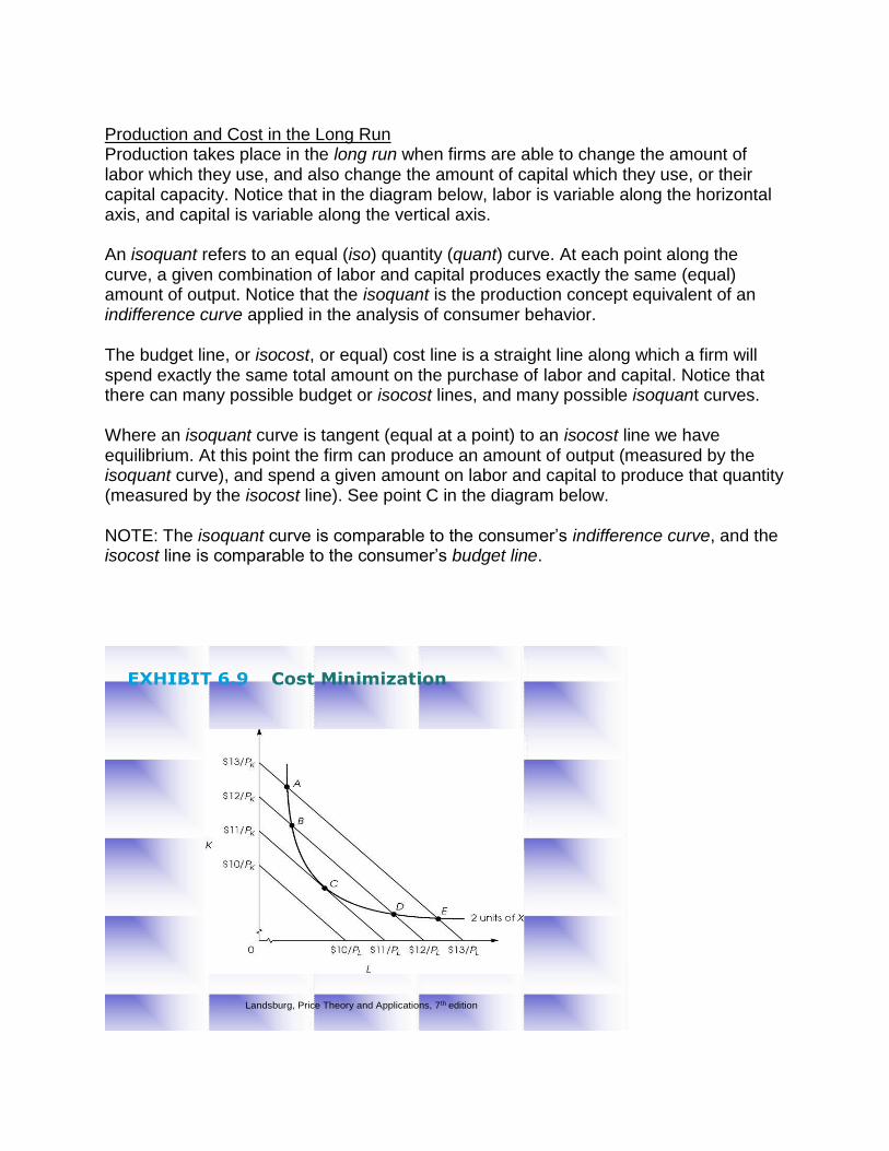
Production and Cost in the Long Run Production takes place in the long run when firms are able to change the amount of labor which they use, and also change the amount of capital which they use, or their capital capacity. Notice that in the diagram below, labor is variable along the horizontal axis, and capital is variable along the vertical axis.

An isoquant refers to an equal (iso) quantity (quant) curve. At each point along the curve, a given combination of labor and capital produces exactly the same (equal) amount of output. Notice that the isoquant is the production concept equivalent of an indifference curve applied in the analysis of consumer behavior.

The budget line, or isocost, or equal) cost line is a straight line along which a firm will spend exactly the same total amount on the purchase of labor and capital. Notice that there can many possible budget or isocost lines, and many possible isoquant curves.

Where an isoquant curve is tangent (equal at a point) to an isocost line we have equilibrium. At this point the firm can produce an amount of output (measured by the isoquant curve), and spend a given amount on labor and capital to produce that quantity (measured by the isocost line). See point C in the diagram below.

NOTE: The isoquant curve is comparable to the consumer’s indifference curve, and the isocost line is comparable to the consumer’s budget line.

EXHIBIT 6.9 Cost Minimization

Landsburg, Price Theory and Applications, 7th edition

Returns to Scale Returns to scale is a long run concept which refers input changes (labor and capital changes, or “changes in scale”) to changes in output. Increasing returns to scale results in declining long run average cost of production (AC ↓). Decreasing returns to scale results in increasing long run average cost of production (AC↑).

Profit Maximization (Loss Minimization) Profit maximization (loss minimization) applies to both competitive as well as imperfectly competitive firms to be studied in the following Modules. The point of profit maximization (loss minimization) is found at the level of output at which Marginal Revenue (MR) = Marginal Cost (MC).

Important Note: Because for the competitive firm P = MR we find that MR = MC means that P = MC.

Returns to Scale

• When all input quantities are increased by 1%, does output go up by – …more than 1%

• Increasing returns to scale

• Occurs at low levels of output

• Long-run average cost curve is decreasing

– …exactly 1%

• Constant returns to scale

• “What a firm can do one, it can do twice”

• Long-run average cost curve is flat

– …less than 1%

• Decreasing returns to scale

• Occurs at sufficiently high levels of output

• Long-run average cost curve is increasing

Landsburg, Price Theory and Applications, 7th edition

QUESTIONS ASSIGNMENT 3 From the Landsburg text, answer the following questions to be submitted to the instructor. 1–2 pages maximum for each question (possible 50 points).

1. Questions R1, R2, and R3 (a) and (b) on pp. 129 – 130.

NOTE for Question R2: The Marginal Revenue column numbers should be in the Total Cost column. Students should calculate the Marginal Revenue numbers.

2. Problem Set 11. on p. 132 (to maximize profits use MR = MC).

3. Questions R1, R2, R3, and R4 on p. 162. 4. Questions R6, R7, R8, and R 9 on p. 163. 5. Questions R10, R11, and R13 on p. 163. 6. Explain in detail why MR = MC is the rule for firms to

follow in order to maximize profits (minimize losses).

Post your answers to the instructor by Saturday, February 3, 2018.

Maximizing Profit

• Profit = TR – TC

• Method I – Scan profit information

– Choose largest number

– Graphically, find point where distance between TR and TC is largest

• Method II – Observe marginal values

– Produce where MR = MC

– As long as MR > MC, decide to increase production

– When MR < MC, no longer good for maximizing profit

– Graphically, find point where MR and MC intersect

Landsburg, Price Theory and Applications, 7th edition

Week 4 Beginning Monday, February 5, 2018 Module 5 Competition

Here are your Reading and Research Assignments. Notice how the author arranges his presentation. There are many examples, exercises, problem sets, and be sure to pay attention to the Dangerous Curves.

Read Chapter 7 in the text

Chapter 7 is a valuable introduction to the analysis of market structures. This introduction begins with Competition also known as Perfect Competition, and will be followed by an analysis of Imperfect Competition in Module 5. A (perfectly) competitive firm is a member of a (perfectly) competitive industry in which the market forces of supply and demand determine the price at which all firms sell their product. The firms are known as “price takers.”

Here are the characteristics of the Competitive (Perfectly Competitive) industry.

1. Many sellers and buyers 2. No individual seller has any affect on the market price, and there is no

collusion among sellers. 3. All sellers produce an identical (homogeneous) product. 4. Productive resources have perfect mobility to enter or leave the market

in the long run. 5. All sellers and buyers have perfect knowledge of the market price.

Topics: Here we begin the discussion of market structures. The first is known as Competition, or Perfect Competition. Although such a market structure is very rarely found in the economy, we use this model to help to understand market structures such as monopolistic competition, oligopoly, and monopoly which are not competitive, and which break the rules of perfect competition to a greater or lesser extent.

Learning Objectives: Students will learn how to evaluate market structures as to efficiency using the competitive model as an ideal type. In addition, students will learn about time dimensions, short and long run, for example, and how time plays a role in decisions made by firms. Students will come to understand that competitive firms have only limited choices in market production decisions, and likely will have any excess profits competed away by other firms. In addition, the demand curve for these firms is a horizontal line at a given price, and this price is determined by overall supply and demand in the industry in which the firm competes.

Chapter 7 Competition Calculus in Appendix A

Notice that in the text on p. 181, we are provided with diagrams comparing The Competitive Industry and the Competitive Firm. On the left, we have the industry (or, market) based on demand and supply. On the right we have the firm which must accept the industry (market-determined) price. The firm is a “price taker,” and has no control over price. The firm’s demand curve is a horizontal line at the level of the market price. The firm’s price is the same as its marginal revenue, P = MR. Read the explanation in the text, and review the diagram on p. 171 which shows the MR and TR curves for the competitor, Total and Marginal Revenue at the Competitive Firm.

Profit Maximization for the Competitive Firm Using The Competitive Firm’s Short Run Supply Curve diagram below, price and marginal revenue are equal (P = MR). Then, in order to maximize profits (or minimize losses), the competitive firm produces at that level at which P = MR = MC.

At any price above P’ the competitive firm’s price would be above AC, and profits would result.

At price P’, Price = MC = minimum Average cost (AC), and the firm finds its break-even point. Here TR = TC. Explain why.

If the competitor’s price is at level P, we find the “shut-down” point where Price = MC = minimum Average variable cost (AVC). At this level of Quantity, all variable costs are covered, but total fixed cost cannot be paid. Losses are equivalent to the firm’s Total variable cost (TVC). Explain why.

Note that the upward sloping BOLD portion of MC is the firm’s supply curve beginning at the shut-down level where MC = min AVC, and moving upward to the right.

EXHIBIT 7.8 The Competitive Firm’s Short-Run Supply Curve

Landsburg, Price Theory and Applications, 7th edition

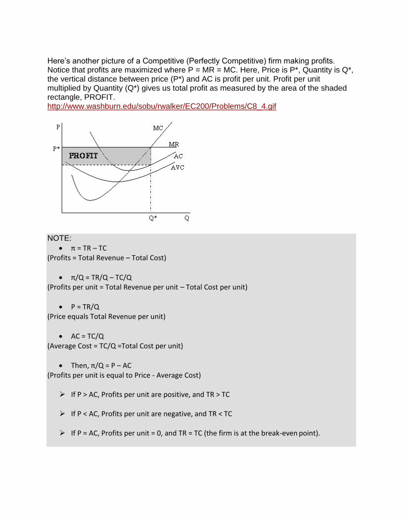
Here’s another picture of a Competitive (Perfectly Competitive) firm making profits. Notice that profits are maximized where P = MR = MC. Here, Price is P*, Quantity is Q*, the vertical distance between price (P*) and AC is profit per unit. Profit per unit multiplied by Quantity (Q*) gives us total profit as measured by the area of the shaded rectangle, PROFIT. http://www.washburn.edu/sobu/rwalker/EC200/Problems/C8_4.gif

NOTE:

π = TR – TC (Profits = Total Revenue – Total Cost)

π/Q = TR/Q – TC/Q (Profits per unit = Total Revenue per unit – Total Cost per unit)

P = TR/Q (Price equals Total Revenue per unit)

AC = TC/Q (Average Cost = TC/Q =Total Cost per unit)

Then, π/Q = P – AC (Profits per unit is equal to Price - Average Cost)

If P > AC, Profits per unit are positive, and TR > TC

If P < AC, Profits per unit are negative, and TR < TC

If P = AC, Profits per unit = 0, and TR = TC (the firm is at the break-even point).

Also review the diagrams at: http://members.shaw.ca/elementaleconomics/images/P&B/Fig.%2012.4%20Alt%20SR %20Outcomes.jpg

Notice that assume Price (P) is always the same as MR for the Competitive firm. We then find where (P) = MR = MC to maximize profits or minimize losses. Profits are found when P = MR is above ATC. Break-even is found where P = MR is equal to ATC. Losses are incurred when P = MR is less than ATC.

Online Reading Follow this link to a brief comparison of market structures, both perfect and

imperfect.http://www.investopedia.com/university/economics/economics6.asp

Discussion Board 4 Post your 1–2 page answer to the following question on the Discussion Board (possible 50 points).

If competition also known as perfect competition rarely exists in the economy, then why study such a model? Should we study “ideal types” even though they may not be duplicated in the real world economy? (NOTE: Consider Plato’s Republic and his use of ideal types in the “realm of the Forms”). Students are encouraged to supplement answers with numerical examples and diagrams.

Peer Response: Respond to the answers of one other student. Follow the Peer Evaluation Rubric (above) in writing your response (possible 10 points). Responses should be positive, encouraging, and supportive. NO POINTS SHOULD BE AWARDED.

Post your answers/responses by Wednesday, February 7, 2018.

QUESTIONS ASSIGNMENT 4 From the Landsburg text, answer the following questions to be submitted to the instructor. 1–2 pages maximum for each question (possible 50 points).

1. Questions R1, R2, and R3 on p. 208 2. Questions R7, R8, R9, and R10 on p. 208. 3. Questions R16, R17, and R18 on pp. 208-209. 4. Suppose that in a competitive wheat market, the forces

of supply and demand determine a price of $4 for a bushel of wheat. There are 50 farmers in this market, and each farmer produces 100 bushels of wheat at the market price in short-run equilibrium. Each farmer has an average total cost (ATC) of $3.25, and an average variable cost (AVC) of $2.25 at the output level of 100. Assume that the short-run equilibrium looks like this for a typical farmer where Q* = 100.

http://www.washburn.edu/sobu/rwalker/EC200/Problems/C8_4.gif

Determine the total revenue, total cost, and $amount of profits for each farmer.

Post your answers to the instructor by Saturday, February 10, 2018.

Week 5 Beginning Monday, February 12, 2018

Module 6 Imperfect Competition

Here are your Reading and Research Assignments. Notice how the author arranges his presentation. There are many examples, exercises, problem sets, and be sure to pay attention to the Dangerous Curves.

Read Chapters 10 – 11 in the text

Chapter 10 introduces students to the market structure known as monopoly, or a market in which there is only one seller of a product. In the U.S. monopolies are prohibited by legislation which takes the form of the “anti-trust (anti-monopoly) laws.” The text explains how monopolies may be formed, and presents the case for “legal monopolies,” or public utilities.

Chapter 11 presents two other types of imperfect competition known as monopolistic competition and oligopoly. Monopolistic competition finds many sellers of differentiated products. Product differentiation may be based on a variety formats. For example, product style, design, service, advertising, price, and the seller’s location are examples

Topics: The general industry structure known as imperfect competition includes monopoly, oligopoly, and monopolistic competition. All of these market structures differ compared to the characteristics of the perfectly competitive industry structure listed under Week 5 above. Recall that the perfectly competitive firm does not have any power over pricing decisions, and their demand curve is horizontal at a market determined price. All of the firms in imperfectly competitive industries have some degree of market power, and will have downward sloping demand curves.

Learning Objectives: Students will learn how to evaluate the implications for production and pricing in market structures which are not perfectly competitive. This analysis will include examples of how firms acquire market power, and how they attempt to retain it. Horizontal and vertical mergers will be discussed, and the antitrust laws will be introduced. Students will learn that some firms are not easily categorized into one of the three types of imperfect competition. They might be market leaders in industries where competition exists, or they may choose to produce in a variety of markets and are known as “conglomerates.”

Chapter 10 Monopoly Chapter 11 Market Power, Collusion, and Oligopoly Calculus in Appendix A

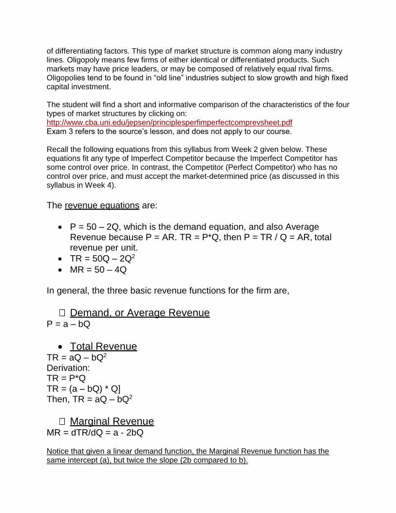
of differentiating factors. This type of market structure is common along many industry lines. Oligopoly means few firms of either identical or differentiated products. Such markets may have price leaders, or may be composed of relatively equal rival firms. Oligopolies tend to be found in “old line” industries subject to slow growth and high fixed capital investment.

The student will find a short and informative comparison of the characteristics of the four types of market structures by clicking on: http://www.cba.uni.edu/jepsen/principlesperfimperfectcomprevsheet.pdf Exam 3 refers to the source’s lesson, and does not apply to our course.

Recall the following equations from this syllabus from Week 2 given below. These equations fit any type of Imperfect Competitor because the Imperfect Competitor has some control over price. In contrast, the Competitor (Perfect Competitor) who has no control over price, and must accept the market-determined price (as discussed in this syllabus in Week 4).

The revenue equations are:

P = 50 – 2Q, which is the demand equation, and also Average Revenue because P = AR. TR = P*Q, then P = TR / Q = AR, total revenue per unit.

TR = 50Q – 2Q2

MR = 50 – 4Q

In general, the three basic revenue functions for the firm are,

Demand, or Average RevenueP = a – bQ

Total Revenue TR = aQ – bQ2 Derivation:TR = P*Q TR = (a – bQ) * Q] Then, TR = aQ – bQ2

Marginal RevenueMR = dTR/dQ = a - 2bQ

Notice that given a linear demand function, the Marginal Revenue function has the same intercept (a), but twice the slope (2b compared to b).

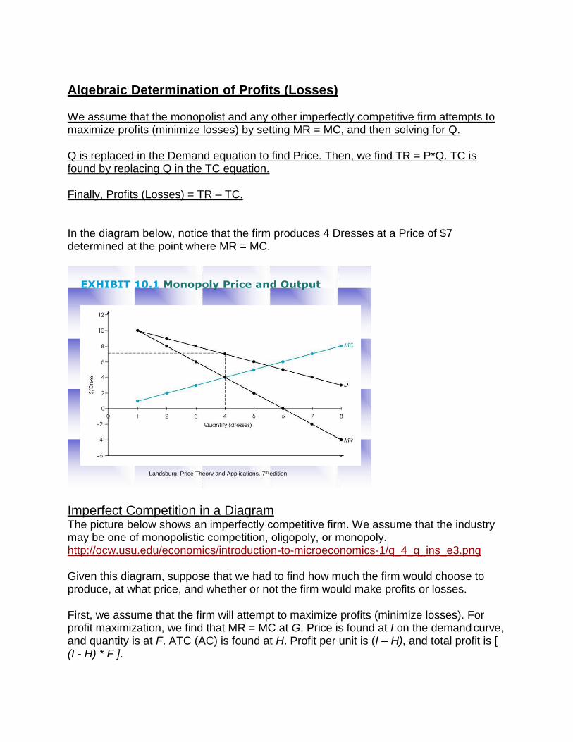
Algebraic Determination of Profits (Losses)

We assume that the monopolist and any other imperfectly competitive firm attempts to maximize profits (minimize losses) by setting MR = MC, and then solving for Q.

Q is replaced in the Demand equation to find Price. Then, we find TR = P*Q. TC is found by replacing Q in the TC equation.

Finally, Profits (Losses) = TR – TC.

In the diagram below, notice that the firm produces 4 Dresses at a Price of $7 determined at the point where MR = MC.

Imperfect Competition in a Diagram The picture below shows an imperfectly competitive firm. We assume that the industry may be one of monopolistic competition, oligopoly, or monopoly. http://ocw.usu.edu/economics/introduction-to-microeconomics-1/q_4_q_ins_e3.png

Given this diagram, suppose that we had to find how much the firm would choose to produce, at what price, and whether or not the firm would make profits or losses.

First, we assume that the firm will attempt to maximize profits (minimize losses). For profit maximization, we find that MR = MC at G. Price is found at I on the demand curve, and quantity is at F. ATC (AC) is found at H. Profit per unit is (I – H), and total profit is [ (I - H) * F ].

EXHIBIT 10.1 Monopoly Price and Output

Landsburg, Price Theory and Applications, 7th edition

On Business Strategy Click on the following links for a discussion of business strategy based on

Michael Porter’s “five forces.” model. http://en.wikipedia.org/wiki/Porter_5_forces_analysis http://www.valuebasedmanagement.net/methods_porter_five_forces.html

While a firm’s mission tells us why they are in business, and objectives and goals tell us what they are attempting to accomplish, the firm’s strategy tells us how they intend to attain their objectives and goals within the context of their mission.

Michael Porter has provided us with a model of strategy which attempts to answer a basic question faced by all business firm regarding strategy or “how do we best compete within our competitive environment?” Think about how you could apply this model to business firms with which you are familiar. Some of the five forces may be stronger than others within a given competitive environment. In addition, think about how Porter’s model compares with other models on the formulation of strategy, SWOT analysis, the BCG matrix, and PEST (STEP) analysis, for example.

For information on SWOT analysis click on: http://en.wikipedia.org/wiki/SWOT_analysis http://www.valuebasedmanagement.net/methods_swot_analysis.html

To take a look at the BCG matrix, click on: http://en.wikipedia.org/wiki/Boston_Consulting_Group http://www.valuebasedmanagement.net/methods_bcgmatrix.html

For information on PEST (or, STEP) analysis, click on: http://en.wikipedia.org/wiki/PEST_analysis http://valuebasedmanagement.net/methods_PEST_analysis.html

Discussion Board 5 Post your 1-2 page answer to the following Question on the Discussion Board (possible 50 points).

Suppose that you want to explain the meaning and applications of the concept of market structures to a friend who has never studied microeconomics. You want to emphasize that an understanding of this concept will help to recognize how firms operate in the U.S. economy. You may want to choose firms which fit (or nearly fit) into each category. Peer Response: Respond to the answers of one other student. Follow the Peer Evaluation Rubric (see Rubric above) in writing your response (possible 10 points). Responses should be positive, encouraging, and supportive. NO POINTS SHOULD BE AWARDED. Post your answers/responses by Wednesday, February 14, 2018.

QUESTIONS ASSIGNMENT 5 From the Landsburg text, answer the following questions to be submitted to the instructor. 1–2 page maximum for each question (possible 50 points).

1. According to the text, what are The Sources of Monopoly Power? Briefly explain each.

2. Questions R1, R2, R7, and R8 on p. 344. 3. Questions R1, R5, R6, R8, R9, and R10 on p. 389. 4. Present Michael Porter’s five forces model. 5. Present the SWOT analysis model. 6. Present the BCG matrix model. 7. Present the PEST (or, STEP) analysis. 8. What is the Lerner index? How is it used?

9. According to the text (Chapter 10) and these class notes for Weeks 4 and 5, how are Elasticity and Marginal Revenue related? Explain in detail.

10. Using Exhibit 10.1 in the Landsburg text, explain how the Price ($/Dress), and the Quantity (dresses) are determined in equilibrium. Why does the firm choose this Price and the corresponding Quantity?

Post your answers to the instructor by Monday, February 19, 2018.

Week 6 Beginning Monday, February 19, 2018

Module 7 Game Theory, External Costs and Benefits, Public Goods, and the Distribution of Income

Topics: In Module 7 students will encounter the topics of game theory, external costs and benefits, and the subject of public goods. All of these concepts can be related to problems and issues which we encounter every day. Game theory is basically a model of strategy that developed out of wartime planning in World War II. External costs and benefits can be viewed as costs which arise from the behavior of others. For example, one firm pollutes the air or water, and, if unchecked, forces others to pay the costs for the cleanup of dirty air and water. Public goods are those goods which everyone shares, public education, and police and fire protection are examples. The analysis of income distribution is based on supply and demand. Supply means the supply of factors of production. Demand arises from business firms purchasing these factors for use in production. Learning Objectives: Students will learn how to analyze problems in a new way by using the strategic methods of game theory. Students will encounter interesting ways of analyzing human behavior. While we may not think about it, we are often faced with costs and benefits which are not directly the result of our own personal actions. How do we prevent others from imposing costs onto us? Students will learn that axes are one way. What about benefits? How do we “repay” others for becoming vaccinated against the flu if we do not? Subsidies paid to those who receive vaccinations are a possible method of repayment. If a community is supplied with a public education system, what is a fair way for everyone to share in maintaining the system? Students will realize that this maintenance is provided by a tax system. Students will learn that the distribution of income among the factors of production (land, labor, capital, and entrepreneurship) depends on the factor market forces of supply and demand. Supply depends on the availability of the factor, while demand depends on productivity. The demand for a factor of production is a “derived demand” which is based on the demand for a business firm’s output.

Here are your Reading and Research Assignments. Notice how the author arranges his presentation. There are many examples, exercises, problem sets, and be sure to pay attention to the Dangerous Curves.

Read Chapters 12, 13, 14, and 15 in the text

Chapter 12 The Theory of Games

Chapter 13 deals with the analysis of external costs and external benefits. Here we encounter the names of Pigou and Coase. A. C. Pigou was a major contributor to the study of welfare economics, and a contemporary of J.M. Keynes. Coase is Ronald Coase, a winner of the Nobel Prize in Economics. External costs and benefits arise from the activities of one person or group, but have affects, both negative (costs) and positive (benefits) on the economic behavior of others. The existence of these activities opens the way for outside remedies, or regulations on markets imposed by government.

In Chapter 14 students are encouraged to read about the nature and basic analysis of the topic of public goods. Public goods are those goods and services supplied by all levels of government. Examples of such goods which the populace shares in common as “consumers” are police and fire protection (services), state and federal highways, national parks, forest preserves, public education (a service), and national defense (a service). The common method of payment for these goods is taxation. When some attempt to “consume” but not pay we encounter the “free rider” problem.

In Chapter 15 students will learn that a reciprocal relationship exists between the business firm’s cost of production and the distribution of those costs in the form of income back to the factors of production. How much of this income flows back to each of the factors depends on the individual factor’s productivity, and the available supply of that factor. In the case of labor, supply depends, for example, on the laborer’s choice of work versus leisure. The more the worker chooses work, the greater is the supply of labor.

The Distribution of Income The Distribution of Income refers to payments to the factors of production. For example, recall the pictures from Week 3, Production in the Short Run. Diagram A is the production function which relates the quantity of output to the amount of labor used. The diagrams below represent marginal product (B), and marginal revenue product MRP). MRP is marginal product multiplied by the product’s selling price, MP x P = MRP. The downward sloping portion of MRP is the firm’s demand for labor. When the wage rate (W) = MRP, the firm will hire the corresponding amount of labor. See Figure 15.1 and Exercise 15.1 in the Landsburg text.

Chapter 13 External Costs and Benefits Chapter 14 Common Property and Public Goods Chapter 15 The Distribution of Income Calculus in Appendix A In Chapter 12, students will study Game Theory. This topic represents “a system for studying strategic behavior,” according to the text, and the topic really begins back in Chapter 11 of the text. Here we find the names of Pareto and Nash, among others. Pareto is Vilfredo Pareto, an economist of the late 19th and early 20th century noted for his work in the analysis of general economic equilibrium. Nash is John Nash, a mathematician, winner of a Nobel Prize in Economics, and the central character of the movie A Beautiful Mind. Applications of game theory include the famous Prisoner’s Dilemma.

Online Reading Look up each writer by clicking on the Alphabetical Listing on the left side of the page. http://www.hetwebsite.net/het/

Ronald Coase

John Nash

Vilfredo Pareto

A.C. Pigou.

Click on the link below to view a number of sites for information on the topic of Game Theory. Explore sites as you research the topic of Game Theory. What is Game Theory? How is it used in the study of economics? What are some examples of Game Theory—Nash equilibrium or the Prisoner’s Dilemma, for example?

https://www.google.com/webhp?sourceid=chrome-instant&ion=1&espv=2&ie=UTF- 8#q=Game+Theory

Check the following sites site for information on public goods. http://en.wikipedia.org/wiki/Public_good http://www.econlib.org/library/Enc/PublicGoods.html

EXHIBIT 15.1

The Total,

Marginal,

and Marginal

Revenue

Products of

Labor

Landsburg, Price Theory and Applications, 7th edition

Questions Assignment 6 (possible 50 points)

1. Based on Chapter 15 in the text, discuss how to determine The Firm’s Demand for Factors in the Short Run. Be sure to explain how the following concepts are related: marginal revenue product, marginal cost, and the price of output.

2. What is Game Theory? Present a 2-page discussion including examples of Nash equilibrium and the Prisoner’s Dilemma.

3. The economists Pareto, Pigou, Nash, and Coase have contributed to the study of the following economic concepts: game theory strategic decision-making the analysis of property rights public goods welfare economics resource allocation

Use at least three of these concepts in a discussion of the contributions of each of the four economists in a 2- page discussion.

Post your answers to the instructor by Saturday, February 24, 2018.

Week 7 Beginning Monday, February 26, 2018

Module 8 Review All Text Chapters, Notes, and Data

Paper Assignment 7 is the Final Examination

The Final Examination questions will be posted in Week 5

Please post your answers to the instructor no later than midnight, Tuesday, March 6, 2018 (200 possible points)

*Instructor reserves the right to change this syllabus based on

her discretion.*