Survey Methodology Journal - Case Study in Record Linkage
123
Catalogue no. 12-001-XIE Survey Methodology 2005
-
Upload
khangminh22 -
Category
Documents
-
view
0 -
download
0
Transcript of Survey Methodology Journal - Case Study in Record Linkage

Catalogue no. 12-001-XIE
SurveyMethodology
2005

How to obtain more information
Specific inquiries about this product and related statistics or services should be directed to: Business Survey MethodsDivision, Statistics Canada, Ottawa, Ontario, K1A 0T6 (telephone: 1 800 263-1136).
For information on the wide range of data available from Statistics Canada, you can contact us by calling one of our toll-freenumbers. You can also contact us by e-mail or by visiting our website.
National inquiries line 1 800 263-1136National telecommunications device for the hearing impaired 1 800 363-7629Depository Services Program inquiries 1 800 700-1033Fax line for Depository Services Program 1 800 889-9734E-mail inquiries [email protected] www.statcan.ca
Ordering and subscription information
This product, catalogue no. 12-001-XIE, is published twice a year in electronic format at a price of CAN$23.00 per issue andCAN$44.00 for a one-year subscription. To obtain a single issue or to subscribe, visit our website at www.statcan.ca and selectOur Products and Services.
This product, catalogue no. 12-001-XPB, is also available as a standard printed publication at a price of CAN$30.00 per issueand CAN$58.00 for a one-year subscription. The following additional shipping charges apply for delivery outside Canada:
Single issue Annual subscription
United States CAN$6.00 CAN$12.00
Other countries CAN$15.00 CAN$30.00
All prices exclude sales taxes.
The printed version of this publication can be ordered
• by phone (Canada and United States) 1 800 267-6677• by fax (Canada and United States) 1 877 287-4369• by e-mail [email protected]• by mail Statistics Canada
Finance DivisionR.H. Coats Bldg., 6th Floor120 Parkdale AvenueOttawa, ON K1A 0T6
• In person from authorised agents and bookstores.
When notifying us of a change in your address, please provide both old and new addresses.
Standards of service to the public
Statistics Canada is committed to serving its clients in a prompt, reliable and courteous manner and in the official language oftheir choice. To this end, the Agency has developed standards of service which its employees observe in serving its clients. Toobtain a copy of these service standards, please contact Statistics Canada toll free at 1 800 263-1136. The service standardsare also published on www.statcan.ca under About Statistics Canada > Providing services to Canadians.

Statistics CanadaBusiness Survey Methods Division
SurveyMethodology2005
Note of appreciation
Canada owes the success of its statistical system to a long-standing partnership betweenStatistics Canada, the citizens of Canada, its businesses, governments and other institutions.Accurate and timely statistical information could not be produced without their continuedcooperation and goodwill.
Published by authority of the Minister responsible for Statistics Canada
© Minister of Industry, 2005
All rights reserved. Use of this product is limited to the licensee and its employees. The product cannot bereproduced and transmitted to any person or organization outside of the licensee’s organization.
Reasonable rights of use of the content of this product are granted solely for personal, corporate or public policyresearch, or educational purposes. This permission includes the use of the content in analyses and the reporting ofresults and conclusions, including the citation of limited amounts of supporting data extracted from the data productin these documents. These materials are solely for non-commercial purposes. In such cases, the source of the datamust be acknowledged as follows: Source (or “Adapted from,” if appropriate): Statistics Canada, name of product,catalogue, volume and issue numbers, reference period and page(s). Otherwise, users shall seek prior writtenpermission of Licensing Services, Marketing Division, Statistics Canada, Ottawa, Ontario, Canada, K1A 0T6.
July 2005
Catalogue no. 12-001-XIE, Vol. 31, no. 1
Frequency: Semi-Annual
ISSN 1492-0921
Ottawa
La version française de cette publication est disponible sur demande (no 12-001-XIF au catalogue).
Catalogue no. 12-001-XPB, Vol. 31, no. 1
ISSN 0714-0045

SURVEY METHODOLOGY
A Journal Published by Statistics Canada Survey Methodology is abstracted in The Survey Statistician, Statistical Theory and Methods Abstracts and SRM Database of Social Research Methodology, Erasmus University and is referenced in the Current Index to Statistics, and Journal Contents in Qualitative Methods. MANAGEMENT BOARD Chairman D. Royce Past Chairmen G.J. Brackstone R. Platek Members J. Gambino J. Kovar H. Mantel
E. Rancourt (Production Manager) D. Roy M.P. Singh
EDITORIAL BOARD Editor M.P. Singh, Statistics Canada Deputy Editor H. Mantel, Statistics Canada Associate Editors D.R. Bellhouse, University of Western Ontario D.A. Binder, Statistics Canada J.M. Brick, Westat, Inc. P. Cantwell, U.S. Bureau of the Census J.L. Eltinge, U.S. Bureau of Labor Statistics W.A. Fuller, Iowa State University J. Gambino, Statistics Canada M.A. Hidiroglou, Office for National Statistics G. Kalton, Westat, Inc. P. Kott, National Agricultural Statistics Service J. Kovar, Statistics Canada P. Lahiri, JPSM, University of Maryland G. Nathan, Hebrew University D. Pfeffermann, Hebrew University J.N.K. Rao, Carleton University T.J. Rao, Indian Statistical Institute
J. Reiter, Duke University L.-P. Rivest, Université Laval N. Schenker, National Center for Health Statistics F.J. Scheuren, National Opinion Research Center C.J. Skinner, University of Southampton E. Stasny, Ohio State University D. Steel, University of Wollongong L. Stokes, Southern Methodist University M. Thompson, University of Waterloo Y. Tillé, Université de Neuchâtel R. Valliant, JPSM, University of Michigan V.J. Verma, Università degli Studi di Siena J. Waksberg, Westat, Inc. K.M. Wolter, Iowa State University A. Zaslavsky, Harvard University
Assistant Editors J.-F. Beaumont, P. Dick and W. Yung, Statistics Canada EDITORIAL POLICY Survey Methodology publishes articles dealing with various aspects of statistical development relevant to a statistical agency, such as design issues in the context of practical constraints, use of different data sources and collection techniques, total survey error, survey evaluation, research in survey methodology, time series analysis, seasonal adjustment, demographic studies, data integration, estimation and data analysis methods, and general survey systems development. The emphasis is placed on the development and evaluation of specific methodologies as applied to data collection or the data themselves. All papers will be refereed. However, the authors retain full responsibility for the contents of their papers and opinions expressed are not necessarily those of the Editorial Board or of Statistics Canada. Submission of Manuscripts Survey Methodology is published twice a year. Authors are invited to submit their articles in English or French in electronic form, preferably in Word to the Editor, Dr. M.P. Singh, [email protected] (Household Survey Methods Division, Statistics Canada, Tunney’s Pasture, Ottawa, Ontario, Canada, K1A 0T6). For formatting instructions, please see the guidelines provided in the Journal. Subscription Rates The price of Survey Methodology (Catalogue No. 12-001-XPB) is CDN $58 per year. The price excludes Canadian sales taxes. Additional shipping charges apply for delivery outside Canada: United States, CDN $12 ($6 × 2 issues); Other Countries, CDN $30 ($15 × 2 issues). Subscription order should be sent to Statistics Canada, Dissemination Division, Circulation Management, 120 Parkdale Avenue, Ottawa, Ontario, Canada, K1A 0T6 or by dialling 1 800 700-1033, by fax 1 800 889-9734 or by E-mail: [email protected]. A reduced price is available to members of the American Statistical Association, the International Association of Survey Statisticians, the American Association for Public Opinion Research, the Statistical Society of Canada and l’Association des statisticiennes et statisticiens du Québec.

To Gordon J. Brackstone


Survey Methodology
A journal Published by Statistics Canada
Volume 31, Number 1, June 2005
Contents In This Issue...................................................................................................................................................................................... 1
M. Winglee, R. Valliant and F. Scheuren A Case Study in Record Linkage ........................................................................................................................................ 3 D. Krewski, A. Dewanji, Y. Wang, S. Bartlett, J.M. Zielinski and R. Mallick The Effect of Record Linkage Errors on Risk Estimates in Cohort Mortality Studies.................................................. 13 Jan A. van den Brakel and Robbert H. Renssen Analysis of Experiments Embedded in Complex Sampling Designs............................................................................. 23 Takahiro Tsuchiya Domain Estimators for the Item Count Technique .......................................................................................................... 41 Marco Di Zio, Ugo Guarnera and Orietta Luzi Editing Systematic Unity Measure Errors Through Mixture Modelling........................................................................ 53 Wai Fung Chiu, Recai M. Yucel, Elaine Zanutto and Alan M. Zaslavsky Using Matched Substitutes to Improve Imputations for Geographically Linked Databases......................................... 65 Balgobin Nandram and Jai Won Choi Hierarchical Bayesian Nonignorable Nonresponse Regression Models for Small Areas: An Application to the NHANES Data .............................................................................................................................. 73 Mingue Park and Wayne A. Fuller Towards Nonnegative Regression Weights for Survey Samples.................................................................................... 85 Short Notes Per Gösta Andersson and Daniel Thorburn An Optimal Calibration Distance Leading to the Optimal Regression Estimator.......................................................... 95 Peter Lynn and Siegfried Gabler Approximations to *b in the Prediction of Design Effects Due to Clustering ............................................................101 Jane L. Meza and P. Lahiri A Note on the PC Statistic Under the Nested Error Regression Model ......................................................................105


Survey Methodology, June 2005 1 Vol. 31, No. 1, pp. 1-2 Statistics Canada, Catalogue No. 12-001-XIE
Statistics Canada, Catalogue No. 12-001-XIE
In This Issue
This issue of Survey Methodology is dedicated to Gordon J. Brackstone, who recently retired from Statistics Canada. He was Assistant Chief Statistician for the Informatics and Methodology field and had been chairman of the Survey Methodology management board since 1987. His continuous support to the journal has been marked by great insight and motivated by a constant desire to foster high standards of methodology practices. Further, he also authored several articles that appeared in the journal. We wish to express our extreme gratitude to Gordon J. Brackstone.
The current issue contains eight regular papers on a variety of topics, and three short communications. As mentioned in the previous issue of the journal, we are introducing a new Short Communications section in Survey Methodology. This section will contain shorter papers, typically around four pages. Possible topics of short communications include presentation of new ideas without the full development of a regular paper, brief reports of empirical work, and discussions or supplements related to other papers published in the journal.
For the past four years the June issue of Survey Methodology has included an invited paper in honour of Joseph Waksberg. Starting this year, this annual invited paper will be published in the December issue of the journal, bringing it more in line with the associated Waksberg address delivered at Statistics Canada’s annual methodology symposium in the autumn. The author of this year’s Waksberg paper is J.N.K. Rao and his paper will be on the “Interplay Between Sample Survey Theory and Methods: an Appraisal”.
In the opening paper of this issue, Winglee, Valliant and Scheuren present a new simulation approach to estimation of error rates for threshold selection in record linkage. For each potential matched pair there is a vector of comparison outcomes that determines the linkage weight. A multinomial model is assumed for each comparison outcome, with different multinomial distributions for true matches and true non-matches. The distributions are estimated from a sample, and then used to simulate the distributions of the linkage weights for true matches and true non-matches. The method is illustrated in a case study using data from the U.S. Medical Expenditure Panel Survey (MEPS).
Krewski, Dewanji, Wang, Bartlett, Zielinski and Mallick investigate the effects of record linkage errors, both false positives and false negatives, on risk estimates in cohort studies. They show analytically how linkage errors introduce both bias and additional variability into observed and expected numbers of deaths, as well as into estimates of standardized mortality ratios and relative risk regression coefficients. They discuss their results in their conclusions, and point to further work that needs to be done in this area.
The paper by van den Brakel and Renssen addresses the problem of testing hypotheses between different survey implementations, such as different questionnaire designs, when a complex sampling design is used. A design-based theory is developed for cases where the survey implementations are assigned to subsamples through completely randomized experimental designs or randomized block experimental designs. The theory also makes use of measurement error models. Design-based Wald statistics are used to compare the different survey implementations.
Tsuchiya approaches the long-standing problem of asking respondents sensitive questions in an interesting fashion. Instead of using the randomized response approach that allows little control for the researcher, he proposes that the item count technique be adapted for sensitive questions. The item count technique presents the respondent with a list of several phrases, from which the respondent selects all that apply to him. The researcher constructs the list in two ways: the first list contains the sensitive phrase while the second list does not. Tsuchiya presents various estimators for this technique and gives an interesting example related to the Japanese national character.
In the paper by DiZio, Guarnera and Luzi, finite mixture models are used to detect errors that are due to an incorrect unit of measurement at the collection stage of the survey. In a multivariate context and assuming that the data are multivariate normal, the procedure can identify which variables are in error for a given sampled unit. The authors also provide diagnostics for prioritizing cases to be investigated more deeply through clerical review. The proposed methodology is illustrated through an example with simulated data and an example with real data.

2 In This Issue
Statistics Canada, Catalogue No. 12-001-XIE
Chiu, Yucel, Zanutto and Zaslavsky present a method for multiple imputation of missing contextual variables for use in regression analysis. For each record missing the variable, and for a sample of complete records, matched cases are selected based on a set of matching variables. The sample of complete records is then used to estimate a regression adjustment for other variables not included among the matching variables. The contextual variables for the incomplete records are then multiply imputed. The authors then show an application to a colorectal cancer study, and use simulations to compare their approach to three other nonresponse adjustment methods.
Nandram and Choi examine the important problem of nonignorable nonresponse in small-area estimation of a health status variable. When confronted with an example where the usual estimators are biased because of the excessive number of nonrespondents, they attempt to account for the differences through modeling. Nandram and Choi use two nonignorable nonresponse hierarchical Bayes models, a selection model and a pattern model, to analyze the health data. An important consideration to their modeling is the incorporation of the input from doctors concerning the nonresponse pattern and the outcome variable. The results give an accurate non-response adjustment and a better measure of precision.
Park and Fuller propose a method to reduce the probability of obtaining negative estimation weights when using a regression estimator. Their method consists of first approximating inclusion probabilities, conditional on Horvitz-Thompson estimates for a vector of auxiliary variables, and then using these approximate conditional inclusion probabilities as initial weights in a regression estimator. Their method is shown to work well in a simulation study. The weights obtained from this method are also compared to weights from quadratic programming, the raking ratio, the logit procedure and maximum likelihood.
In the first of three short communications included in this issue, Andersson and Thorburn show that the optimal regression estimator can be expressed as a calibration estimator with an appropriately chosen distance function. The resulting optimal estimator is asymptotically more efficient than the usual Generalized Regression (GREG) estimator. A small simulation study illustrates several situations where the optimal estimator if significantly more efficient than the GREG estimator.
Lynn and Gabler extend the results of Gabler, Hader and Lahiri (volume 25, 1999) on Kish’s expression for the design effect due to clustering. They give a practical approach to estimating Kish’s quantity at the sample design stage when only the total numbers of observations and of clusters are needed.
Meza and Lahiri examine the limitations of a standard regression model selection criterion, Mallows’ statistic, for nested error regression models. They show, that while a straightforward application of Mallows’ statistic may result inefficient model selection methods, a suitable transformation of the data may be the answer.
Finally, we would like to inform you that Harold Mantel will now hold the new position of Deputy Editor. Harold has been part of the Editorial Board for the last 15 years. His dedication to the journal has been notable and his continuous involvement in the editorial process has been instrumental in ensuring that Survey Methodology remains a high quality publication.
M.P. Singh
Survey Methodology, June 2005 3 Vol. 31, No. 1, pp. 3-11 Statistics Canada, Catalogue No. 12-001-XIE
A Case Study in Record Linkage
M. Winglee, R. Valliant and F. Scheuren 1
Abstract
Record linkage is a process of pairing records from two files and trying to select the pairs that belong to the same entity. The basic framework uses a match weight to measure the likelihood of a correct match and a decision rule to assign record pairs as “true” or “false” match pairs. Weight thresholds for selecting a record pair as matched or unmatched depend on the desired control over linkage errors. Current methods to determine the selection thresholds and estimate linkage errors can provide divergent results, depending on the type of linkage error and the approach to linkage. This paper presents a case study that uses existing linkage methods to link record pairs but a new simulation approach (SimRate) to help determine selection thresholds and estimate linkage errors. SimRate uses the observed distribution of data in matched and unmatched pairs to generate a large simulated set of record pairs, assigns a match weight to each pair based on specified match rules, and uses the weight curves of the simulated pairs for error estimation.
1. M. Winglee, Westat, Statistical Group, 1650 Research Boulevard, Rockville, MD 20850-3195, U.S.A.; R. Valliant, Joint Program for Survey
Methodology, University of Maryland and University of Michigan; F. Scheuren, NORC, University of Chicago.
Key Words: File matching; Linkage error rates; Match weight; Selection threshold; Medical records.
1. Introduction The basic record linkage framework by Newcombe
Kennedy, Axford and James (1959) and Fellegi and Sunter (1969) uses a match weight to measure the likelihood of a correct match and a decision rule to classify record pairs. The optimal decision rule uses two match weight thresholds for selection (an upper threshold above which a link is treated as a match and a lower threshold below which a link is treated as a nonmatch). The choice of these thresholds depends on the acceptable pre-set linkage error rate and the requirement to minimize the number of links with indeterminate status between the two thresholds. Nowadays, practitioners of computerized linkage systems often use a single selection threshold to avoid manual intervention of the indeterminate links. Linkage decisions are typically made automatically after the system is “tuned” to achieve pre-set error levels. The challenge is that current methods to determine the selection threshold and to estimate linkage errors can produce divergent results depending on the type of linkage error, the choice of comparison space, and the estimation method.
This paper shares our experience with fellow practi-tioners who need a method to guide linkage selection and error estimation. Our case study used medical event files from the US Medical Expenditure Panel Survey (MEPS). MEPS collects medical expenditure data from both household respondents and their medical providers. The purpose is to combine the data from both sources for supporting annual estimations of medical utilization and expenditures (see Agency for Healthcare Research and Quality 2001 for more details on MEPS).
Here we discuss the linkage with three sets of annual medical event files – MEPS 1996, MEPS 1997, and MEPS 1998. Each set consisted of a household file containing events reported by household respondents for a given year and a medical provider file containing the corresponding events reported by medical providers of the household respondents. On average, approximately 50,000 medical events were reported for close to 10,000 persons, and around 15,000 person-provider units each year.
We used two model-based alternatives for linkage error estimation. One of these uses simulation to develop a distribution of the weights for various levels of agreement. This technique, called SimRate, begins by generating weight distributions for matched and unmatched record pairs. Using these, SimRate can then provide estimates of linkage error rates for different threshold levels. The error rates can then be used as a guide to action and a way to measure success. SimRate is contrasted with a second modeling approach created by Belin and Rubin (1995). As we hope to show, there is a role for both approaches; each has strengths as illustrated in the comparisons.
2. Mixture Models and Simrate
Approaches
The mixture modeling method of linkage error esti-
mation, as presented in Belin and Rubin (1995), has several attractive features. It is flexible in a sense that the weight creation process does not have to be considered directly. Hence, this method can be applicable to many different ways of creating weights. Once a model is specified, error
4 Winglee, Valliant and Scheuren: A Case Study in Record Linkage
Statistics Canada, Catalogue No. 12-001-XIE
rates can be examined for a continuum of potential threshold values and confidence bands can be constructed to monitor the precision of error estimates (see section 7).
Mixture modeling does have limitations. While the method provides a particular kind of error rate – the pro-portion of linked records that are actually unmatched pairs, overall false positive and false negative error rates cannot be estimated since nonlinked pairs are not considered. The error rate that is estimated is conditional on the set of linked pairs of records. Furthermore model parameters may be hard to estimate if the weight distributions for the matched and unmatched sets are not separable (see Winkler 1994).
A key assumption in the Belin – Rubin approach is that it is possible to transform the distributions of the weights in the matched and unmatched sets to make them normal. Now a real difficulty exists here in that the transformed weights may be far from normal when the weight distribution for either the matched or unmatched sets is multimodal.
Another critical requirement is to have a training data set whose characteristics are very similar to those that are to be matched. Without a good training data set, the input para-meter estimates for the mixture model may be poor, affecting the final estimated error rates obtained. Based on our application using annual medical event data repeated over three years, the parameters were not stable over time. This instability necessitated a training set for each year, making the Belin – Rubin approach impractical in our appli-cation because of the cost and time it required.
The simulation approach, SimRate, like mixture modeling, has the ability to examine different thresholds, allowing the user to monitor both the sensitivity and specificity of the decision rule for selecting linked pairs. As long as the process used to create match weights can be realistically modeled, customized methods of weight assignment like the one used in the current case study can be accommodated. The method does require the generation of pairs of records using the distribution of characteristics for the matched and unmatched sets. Some effort is needed to realistically generate the populations of pairs. In our work we have been successful with multinomial models for generating these populations.
3. Threshold Weight and Linkage Error
Estimation Several methods are available in the literature for
selecting true matches and for estimating linkage errors (e.g., Bartlett, Krewski, Wang and Zielinski 1993, Armstrong and Mayda 1993, Belin 1993, Belin and Rubin 1995 and Winkler 1992, 1995). See Fellegi (1997) for an overview of evolutions in record linkage, Tepping (1968) and Larsen and Rubin (2001) for other linking methods, and
Scheuren (1983) for a capture-recapture method to estimate omission error.
Comparison of estimates from the different approaches is complicated by the fact that each approach tends to focus on different error components. In fact, the methods used in the linkage literature to construct linkage error rates are some-what inconsistent. We illustrate this problem below.
Table 1 shows a 22× contingency table tabulating the numbers of true matched and unmatched pairs and declared linked and nonlinked pairs selected by linkage systems. Estimates of linkage error rates can be constructed relative to the true totals shown in the columns. An estimate of false positive linkage error rate under the Fellegi and Sunter framework is 2121 /)|(μ •== nnUAP and that of false negative linkage error rate is 1213 /)|(ˆ
•==λ nnMAP (see also Armstrong and Mayda 1993). These are the rates that SimRate is designed to estimate. They answer the question – “Of the set of true matched (or unmatched) pairs, what proportion is not correctly identified?”
Table 1 A Contingency Table for Evaluating Linkage Errors
True set Declared set Match (M) Unmatch (U) Declared total
11n 12n Link )( 1A true positive false positive •1n
21n 22n Nonlink )( 3A false negative true negative •2n
True total 1•n 2•n ••n
Some linkage evaluations have also considered rates
relative to the declared totals in the rows. For instance, Gomatam, Carter, Ariet and Mitchell (2002) used •112 / nn and labeled it the positive predictive power of the linkage system. Others, however, have labeled this as the false match rate (Belin and Rubin 1995) or false positive declared rate (Bartlett et al. 1993). Rates constructed in this manner answer the question – “Of the declared linked (or nonlinked) pairs, what proportions are wrong?” Both questions are important in selecting matched pairs and should be addressed. That is one of the appeals in employing both SimRate and Belin – Rubin, if possible.
4. Simrate Weight Distribution
Methods to Estimate Linkage Error
How to best estimate the linkage errors, given a limited budget and time schedule, is a difficult question. Accurate estimation of linkage errors should depend on at least two factors – the power of the identifying fields to unambi-guously identify events that are true matches and the linkage method used. Taken together it is then possible, in a given setting, to specify linkage categories, estimate agreement probabilities, and determine match weights.
Survey Methodology, June 2005 5
Statistics Canada, Catalogue No. 12-001-XIE
Following Newcombe and Kennedy (1962) and Jaro (1989), we adopt a weight distribution approach in our application that can take all these factors into consideration. The basic step is to first compute the match weight and order all possible configurations of agreement and dis-agreement outcomes of the comparison fields by match weight. Then we plot the cumulative distribution function of the weights for matched and unmatched pairs, and use the resulting weight chart to determine thresholds to attain desired levels of false positive and false negative error rates.
An ideal method to develop these curves might be to begin with a set of record pairs for which the truth is known. If resources are available, we could use a large set of true matched pairs, order them by match weight, and observe what proportion is above or below a given threshold. Similarly, we could take a large set of pairs, known to be true unmatched pairs, order them by weights, and again tabulate the proportion on either side of the threshold. The proportion of true matched pairs with weights below the threshold and the proportion of true unmatched pairs with weights above the threshold would then be estimates of the error rates associated with the way in which the matching algorithm is implemented.
One method to approximate this “ideal” approach (see also Bartlett et al. 1993) is to sample record pairs and use manual review to determine the true match status. Once the true pairs are known, we can attach the match weights from whatever linkage system is being used and then develop cumulative weight distributions, as discussed above. This method is, of course, subject to the well-known time and other resource limitations of manual review and is seldom practical with a large sample.
An alternative method is to generate the cumulative weight distributions through simulation. That is the heart of the SimRate approach. To explain in some detail, denote a record pair by r and a comparison field by
Vvv ,,1( K= fields). The comparison outcome situations in our application included partial agreements and multiple outcome categories beyond the basic agreement and dis-agreement categories (see also Newcombe 1988). There-fore, we denote that each field v has vci ,,1 K= outcome categories. The outcome indicator is ),,,( 1 vrvcrvrv yy K=y a vector of indicators showing the category into which pair r falls. One of the values of rviy will be 1 and the others 0 for each field.
The particular theory supporting the SimRate approach is to assume that ,rvy has one multinomial distribution if pair r is a matched pair and a different multinomial distribution if it is an unmatched pair. We can then model the rvy vectors as having a multinomial distribution with para-meters ),,( 1 vvcvv mm K=m if the pair is a matched pair and parameters ),,( 1 vvcvv uu K=u if the pair is an
unmatched pair. Then the probability Pmvi = (field v category i agrees in pair )| Mrr ∈ is the conditional proba-bility of agreement for field v category I, given that the record pair r is in the set M of true matched pairs. In contrast, the probability Puvi = (field v category i agrees in pair )| Urr ∈ is the conditional probability of agreement for field v category I, given that the record pair r is in the set U of true unmatched pairs. Assuming independence of the matching variables, ,,,1 Vv K= we can specify the joint probability of ),,( 1 rVrr yy K=y if a pair r is a match, as
.)|(P11
ivrv
yvi
c
i
V
vr mMr ∏∏
===∈y
The corresponding probability of the same configuration of data, if the pair is really an unmatched pair, is
.)|(P11
irvv
yvi
c
i
V
vr uUr ∏∏
===∈y
SimRate uses Monte Carlo simulation methods to generate a large number of realizations of matched pairs and unmatched pairs using estimates of the probabilities vim and
.viu For each simulated pair, a match weight ,rw which applies to a given configuration of data, is calculated. For a given realization ,ry a weight rw is computed for the pair by summing the weights for the randomly generated categories that the pair fell into. The match weight rw of a record pair is typically estimated as
.log
11
112
⎥⎥⎥⎥
⎦
⎤
⎢⎢⎢⎢
⎣
⎡
=∏∏
∏∏
==
==
ivrv
ivrv
yvi
c
i
V
v
yvi
c
i
V
vr
u
mw
See section 6 on the match weights used in our simulation. The cumulative distribution of these weights for the
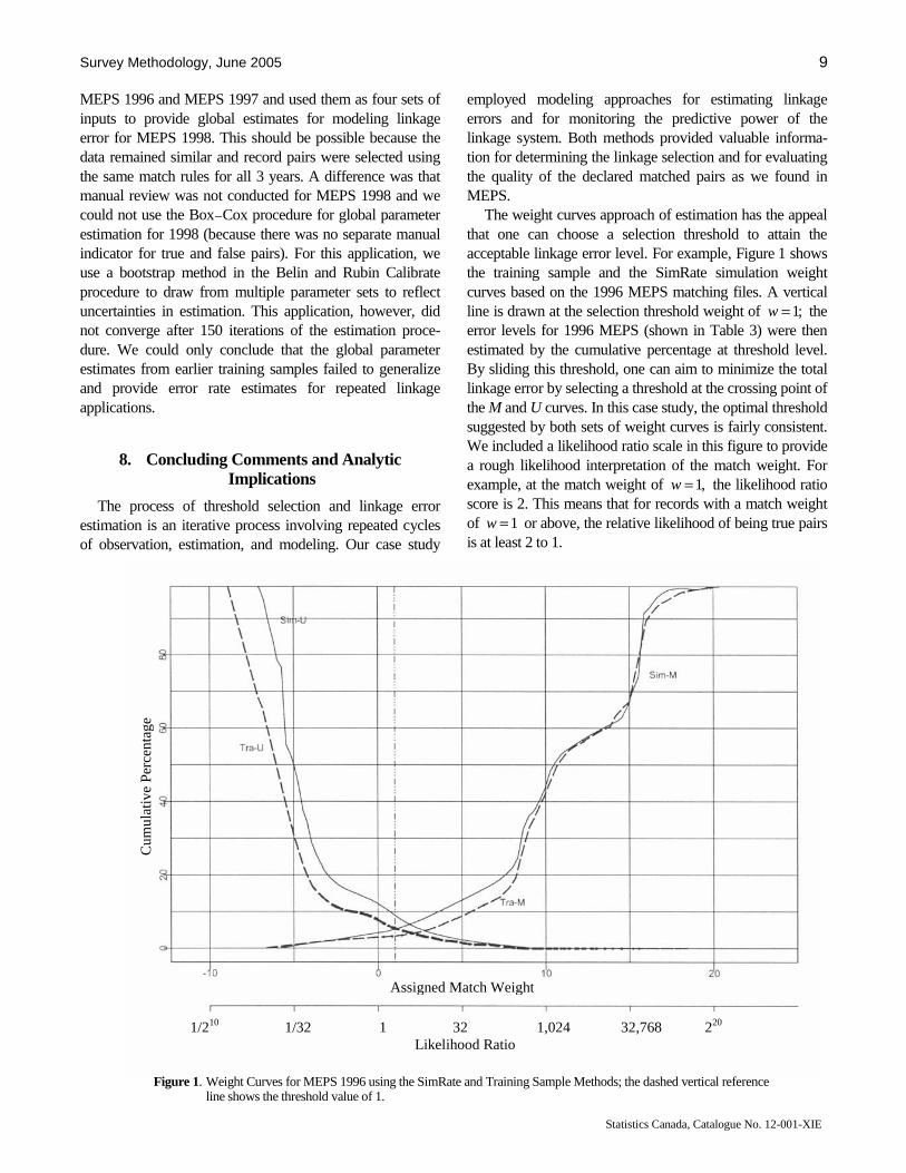
simulated matched pairs is then plotted as “Sim – M”. Similarly, the reverse cumulative distribution for the unmatched pairs is plotted to generate “Sim – U” (see Figure 1, section 8, for an example of the simulation curves used in this study). The simulated proportion of matched pairs whose weights are below the cutoff is the estimate of the false negative error rate. The simulation proportion of unmatched pairs whose weights are above the cutoff is the estimate of the false positive error rate.
This approach requires that empirical estimates be made of the distributions among the matching variables of both true matched and true unmatched pairs. Even though the weight algorithm may involve the assumption of inde-pendence among matching variables, the actual data may show dependence. As long as artificial pairs can be gene-rated that realistically follow the observed distribution of the data (incorporating any dependencies), then this method should provide suitable error rate estimates.
6 Winglee, Valliant and Scheuren: A Case Study in Record Linkage
Statistics Canada, Catalogue No. 12-001-XIE
In our case study, we modeled data fields as having inde-pendent multinomial distributions, but this may not be reasonable in other applications. The SimRate concept can apply to any algorithm where weights and a cutoff point are used for classification. Thus, methods other than Fellegi and Sunter (1969), like Belin and Rubin (1995), might also be evaluated in this way. If methods are needed to deal with dependent categorical variables, the multivariate multi-nomial distributions in Johnson, Kotz, and Balakrishnan (1997, Chapter 26) may be appropriate. However, in appli-cations similar to ours, the simplest procedure for accounting for dependence is to form cross-classifications of the variables that are related and to estimate probabilities for each cell in a cross-table. For example, if two variables with
1c and 2c categories are associated, then we can estimate the joint probability, ,ijp for each cell in the 21 *cc table and use those in the simulation. Sparse data will naturally limit the number of cells for which this is feasible. But in the presence of sparse data, the penalty for model failure must be small.
5. Record Linkage of MEPS Medical
Events Record linkage of MEPS medical events used five identi-
fying fields: event dates (year, month, day, and day-of-week), medical condition codes, procedure codes, global-fee codes, and lengths (number of days) of hospital stay. These fields are described in more detail in Winglee, Valliant, Brick and Machlin (2000). A training sample from MEPS 1996 was employed to derive match rules and outcome cate-gories and to estimate the probabilities of agreement for each category, allowing for partial agreement and value specific outcomes. The same match rules were repeated each year with minor adjustments of the matching para-meters.
For the training set we used the linkage system Auto-match (Matchware 1996) and the unique match algorithm to select linked pairs. In “unique” matching, a File A record is optimally linked to only one File B record (Jaro 1989). In addition, we used the many-to-many match algorithm to generate a random sample of nonlinked pairs to facilitate linkage error estimation. However, the methods for esti-mating error rates, described below, apply to any software that implements the linkage methods based on match weights. They are not specific to Automatch.
The tradeoff in determining the selection threshold for MEPS was between getting a high match rate and limiting mismatch linkage errors. A high threshold weight would minimize false positive (mismatch) errors at the expense of lowering the match rate and losing valuable data collected from medical providers. On the other hand, a low threshold
would increase false positive error and may affect the allocation of expenditure data in a way that would require special analytic techniques to overcome and even then only with uncertainty. Since both data sources had reported on ostensibly the same medical events for the same persons over the same period, the strategy was to maintain a reasonably high match rate and to conduct a manual review of a limited number of questionable linked pairs after selection to assess the analytic impact of falsely accepting them. Based on this decision the average match rate for the annual MEPS medical records files was about 85 percent.
The 1996 MEPS training sample M curve, labeled the “Tra – M” curve, was generated by applying match weights to “true” matched pairs for a random sample of 500 persons in MEPS 1996. For these persons, the manual review files contained 2,507 events from household respondents and 2,804 events from medical providers. Knowledgeable data managers reviewed the events and selected 1,501 pairs. We considered these as the true matched pairs in this evaluation. The manually matched pairs were assigned the weights derived from our match specification to generate a cumu-lative distribution function.
The 1996 training sample U curve, labeled the “Tra – U” curve, was generated using a random sample of unmatched pairs. We used a simple random sampling with replacement method to select 500 events each from the matching files and employed a many-to-many match algorithm to generate all 250,000 possible event pairs. For these randomly selected sets of pairs, the chance of there being any correctly matched pairs is negligible; thus, the entire set was taken to consist of unmatched pairs. We applied the match weights from our matching specification and plotted the “Tra – U” curve equal to 1 minus the cumulative distribution of the weights of these pairs. Figure 1 in section 8 shows both the Tra – M and Tra – U curves for the 1996 MEPS. The curves shown in this figure were smoothed using a nonparametric lowess function (Chamber, Cleveland, Kleiner and Tukey 1983) in S – PLUS 2000 (1999).
6. Simrate Implementation in MEPS The SimRate weight distribution method used Monte
Carlo simulation methods to generate separate sets of 10,000 simulated matched and unmatched pairs for creating the weight curves. To generate the “Sim – M” weight distributions we estimated the probabilities vim from linked pairs assigned by a unique matching algorithm. We used the “tuned” linkage system to select matched pairs from the 1996 annual matching files and tabulated the observed frequencies for each outcome category for each of the five matching fields. The proportion of pairs that fell into category i of field v was then used as the estimate vim of the probability .vim
Survey Methodology, June 2005 7
Statistics Canada, Catalogue No. 12-001-XIE
For the unmatched pairs and the “Sim – U” curve, the viu probabilities for unmatched pairs were estimated using the same sample of unmatched pairs used in creating the “Tra – U” curve. The difference is that we used these pairs to observe the relative frequencies for each outcome category for each of the five matching fields among unmatched pairs. The proportion of pairs that fell into category i of field v was then used as the estimate viu of the probability .viu
For a simulated matched pair, a realization of the multinomial random variable rvy was generated for each match field. For example, a configuration like (agreement on event date, agreement on length of hospital stay, agreement on the array of condition codes, joint agreement by type of procedure, and value specific agreement for a global-fee indicator) was generated using the match probabilities vim for each outcome category. Similarly, for each unmatched pair, a realization was generated of a category for each of the five fields using the unmatched probabilities viu discussed above.
For a given realization ,ry a weight rw was computed for the pair by summing the weights for the randomly generated categories that the pair fell into. The actual weights used in our simulation were adjusted ones that we specified rather than ones defined directly by the matching software (see Winglee, et al. 2000). Thus, we are simulating the way in which matching would actually be implemented. To do this we calculated the match weight for both the matched and unmatched sets of 10,000 pairs and plotted the simulated match weight functions.
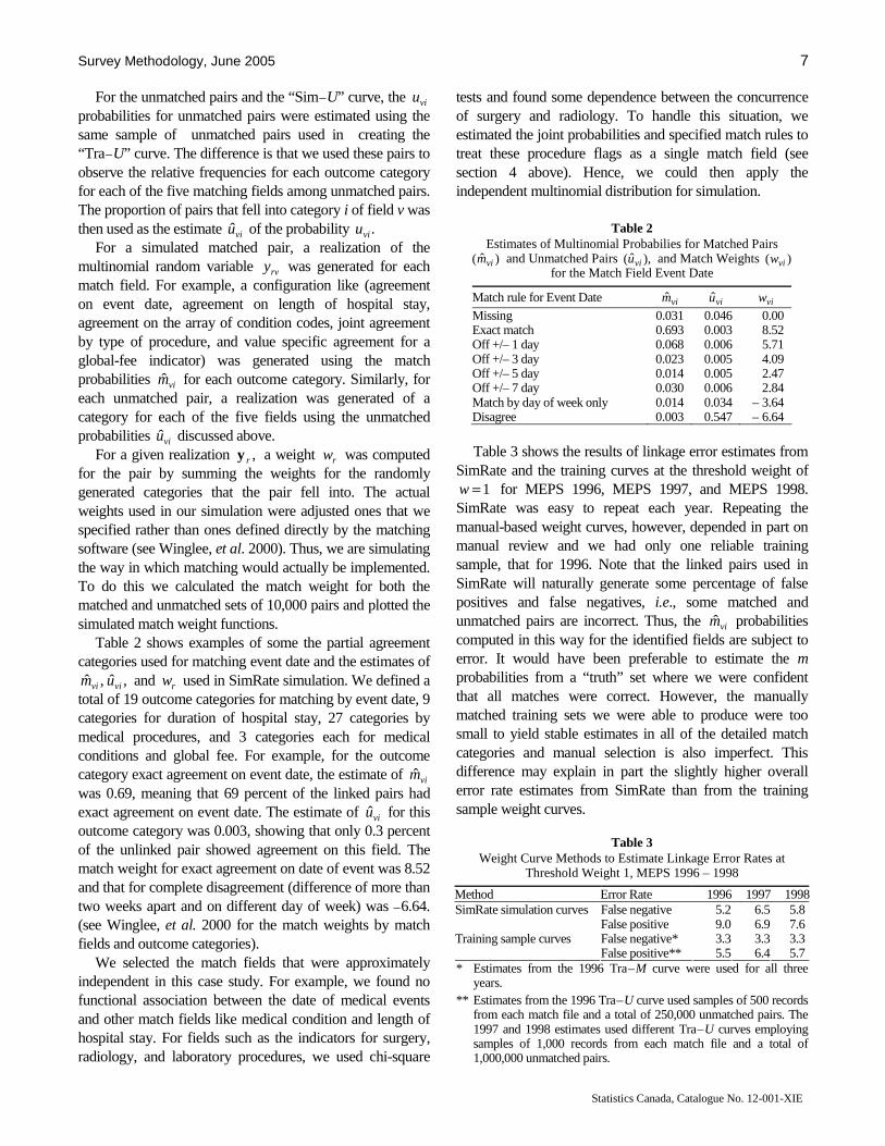
Table 2 shows examples of some the partial agreement categories used for matching event date and the estimates of
,ˆ,ˆ vivi um and rw used in SimRate simulation. We defined a total of 19 outcome categories for matching by event date, 9 categories for duration of hospital stay, 27 categories by medical procedures, and 3 categories each for medical conditions and global fee. For example, for the outcome category exact agreement on event date, the estimate of vim was 0.69, meaning that 69 percent of the linked pairs had exact agreement on event date. The estimate of viu for this outcome category was 0.003, showing that only 0.3 percent of the unlinked pair showed agreement on this field. The match weight for exact agreement on date of event was 8.52 and that for complete disagreement (difference of more than two weeks apart and on different day of week) was – 6.64. (see Winglee, et al. 2000 for the match weights by match fields and outcome categories).
We selected the match fields that were approximately independent in this case study. For example, we found no functional association between the date of medical events and other match fields like medical condition and length of hospital stay. For fields such as the indicators for surgery, radiology, and laboratory procedures, we used chi-square
tests and found some dependence between the concurrence of surgery and radiology. To handle this situation, we estimated the joint probabilities and specified match rules to treat these procedure flags as a single match field (see section 4 above). Hence, we could then apply the independent multinomial distribution for simulation.
Table 2 Estimates of Multinomial Probabilies for Matched Pairs
)ˆ( vim and Unmatched Pairs ),ˆ( viu and Match Weights )( viw for the Match Field Event Date
Match rule for Event Date vim viu viw
Missing 0.031 0.046 0.00 Exact match 0.693 0.003 8.52 Off +/– 1 day 0.068 0.006 5.71 Off +/– 3 day 0.023 0.005 4.09 Off +/– 5 day 0.014 0.005 2.47 Off +/– 7 day 0.030 0.006 2.84 Match by day of week only 0.014 0.034 – 3.64 Disagree 0.003 0.547 – 6.64 Table 3 shows the results of linkage error estimates from
SimRate and the training curves at the threshold weight of 1=w for MEPS 1996, MEPS 1997, and MEPS 1998.
SimRate was easy to repeat each year. Repeating the manual-based weight curves, however, depended in part on manual review and we had only one reliable training sample, that for 1996. Note that the linked pairs used in SimRate will naturally generate some percentage of false positives and false negatives, i.e., some matched and unmatched pairs are incorrect. Thus, the vim probabilities computed in this way for the identified fields are subject to error. It would have been preferable to estimate the m probabilities from a “truth” set where we were confident that all matches were correct. However, the manually matched training sets we were able to produce were too small to yield stable estimates in all of the detailed match categories and manual selection is also imperfect. This difference may explain in part the slightly higher overall error rate estimates from SimRate than from the training sample weight curves.
Table 3 Weight Curve Methods to Estimate Linkage Error Rates at
Threshold Weight 1, MEPS 1996 – 1998
Method Error Rate 1996 1997 1998False negative 5.2 6.5 5.8 SimRate simulation curves False positive 9.0 6.9 7.6 False negative* 3.3 3.3 3.3 Training sample curves False positive** 5.5 6.4 5.7
* Estimates from the 1996 Tra – M curve were used for all three years.
** Estimates from the 1996 Tra – U curve used samples of 500 records from each match file and a total of 250,000 unmatched pairs. The 1997 and 1998 estimates used different Tra – U curves employing samples of 1,000 records from each match file and a total of 1,000,000 unmatched pairs.

8 Winglee, Valliant and Scheuren: A Case Study in Record Linkage
Statistics Canada, Catalogue No. 12-001-XIE
7. Mixture Model Implementation in MEPS
A mixture modeling approach by Belin and Rubin (1995) views the distribution of observed match weights from a computerized linkage system as a mixture of weights for true matches and false matches. In principle, the mixture model method has two attractive features suitable for MEPS. First, it can handle repeated applications efficiently. When global parameter estimates of the transformed para-meters and the ratio of the variances of the two distributions are available, these estimates can be applied to similar data for estimation. Since the MEPS record linkage is done annually, global estimates derived from early training samples could conceivably be applied for linkage error esti-mation in later years when manual review samples were not available.
The second advantage is that the mixture model can draw from multiple sets of parameter estimates from different training samples and can reflect variations. This feature is especially appealing for MEPS because manual review is a complex process and not necessarily always accurate. Hence, an alternative is to view the computer system selection as the truth and use them to provide an alternative set of parameter estimates. This process can also be repeated using training samples from more than one year.
Our application of the Belin – Rubin approach used the same training samples from MEPS 1996 and a second training sample of the same size from 1997. Following Belin – Rubin’s examples, we applied the mixture modeling method using manually identified true and false match pairs from a one-to-one matching system (note that such systems provide relatively few false match pairs for estimation). We computed model estimates for MEPS 1996 and MEPS 1997 assuming the manual selection to be the truth, and for testing the behavior of the model, we computed a second set of estimates assuming computer system selected match pairs to be the true pairs.
Implementation involved two procedures – the Box and Cox (1964) procedure for global parameter estimation and the Calibrate procedure (Belin and Rubin 1995) to fit a mixture model for error rate estimation. Before applying Box – Cox, the weights were rescaled between 1 and 1,000. The Box – Cox transformation discussed by Belin and Rubin (1995) was
1
1)( −γ
γ
γ−=Ψ
w
ww r
r
where rw is the match weight for pair r, w is the geometric mean of the rw weight, and γ is a parameter that is dependent on whether the pair is in the matched or unmatched set.
For the mixture model procedure to be effective, the transformed weights should be approximately normally distributed. The untransformed weight distribution with our data showed bimodality and almost no overlap in match weight between matched and unmatched pairs (bimodality was also observed in Belin – Rubin 1995). For example, application of their transformation procedure to the 1996 MEPS system pairs resulted in parameter estimates of
7.585=w and 15.1=γ for the true matched pairs and 1.113=w and 48.0=γ for the false matched pairs. The
transformed weights, however, showed relatively little improvement towards normality. Since the match weights are the log of a product, or the sum of logs, we might hope that the weights would be normally distributed if there were many components in the sum. However, we had only five fields to use for matching. The small number of fields may have accounted in part for the lack of normality with our transformed data.
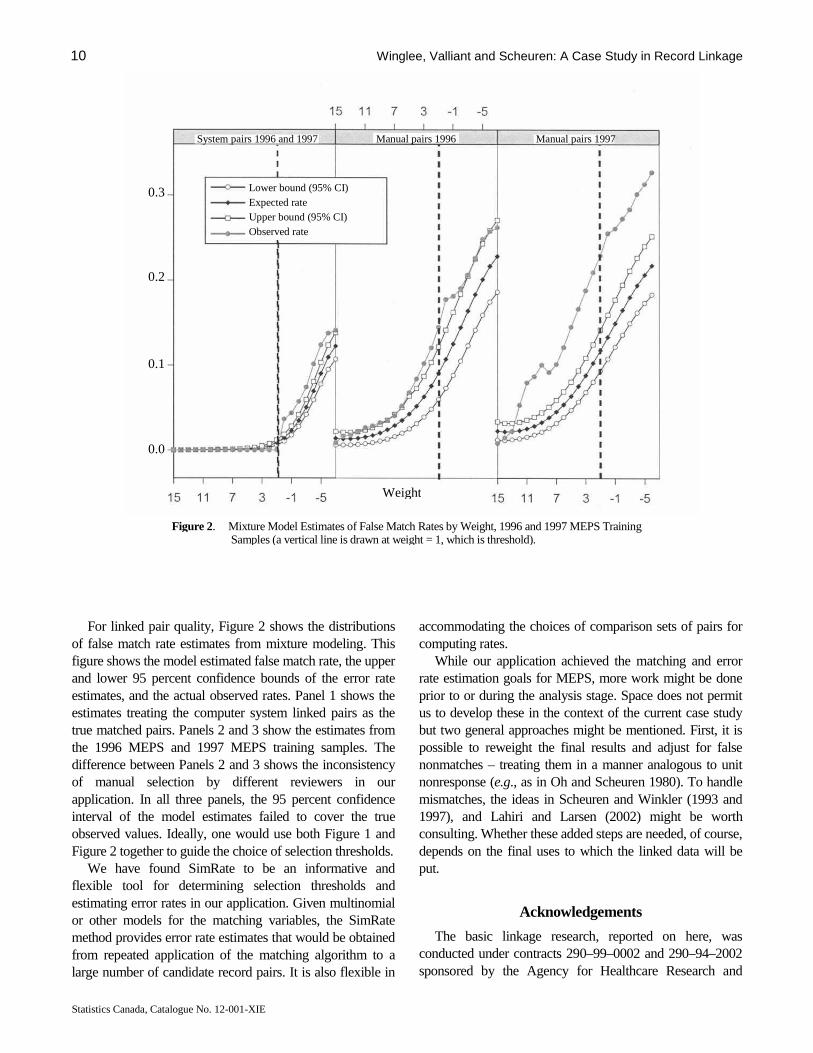
Table 4 shows the results of applying the Belin – Rubin mixture model to MEPS 1996. This table shows the model estimated false match rates, the 95 percent confidence interval of the estimated rate, and the actual observed false match rate at the threshold weight of 1. Using the manual review pairs as the true matched pairs, the model estimate of the expected false match rate at the threshold of 1=w was 9.1 percent, with a 95 percent confidence interval ranging between 6.0 and 12.2. The actual observed false match error rate, however, was 14.5 percent, which is higher than the upper 95 percent confidence bound. Note that these are rates of the form •112 / nn in Table 1. These are not the same rates estimated by SimRate and the weight curve approach.
Table 4 Mixture Model Linkage Error Estimates
Percentage false match error MEPS 1996 Expected
rate Lower
Bound* Upper
Bound* Observed
rate Manual match 9.1 6.0 12.2 14.5 System match 0.9 0.6 1.2 0.0 * The lower and upper bounds are the 95 percent confidence interval
of the expected error rate. Since manual review may not always be accurate, an
option, for the purpose of evaluation, is to treat the computer system linked pairs as the truth matched pairs, and use them for modeling. Under this assumption, the model estimate of the expected error rate is 0.9, and a 95 percent confidence interval between 0.6 and 1.2. The actual observed rate in this case, 0 percent, was a hypothetical outcome treating the computer-linked pairs as correct. Of course, in reality there will be some nonzero level of error so that the mixture model confidence interval is not necessarily wrong.
We generated global parameter estimates using both the training sample manual selections and system selections for
Survey Methodology, June 2005 9
Statistics Canada, Catalogue No. 12-001-XIE
MEPS 1996 and MEPS 1997 and used them as four sets of inputs to provide global estimates for modeling linkage error for MEPS 1998. This should be possible because the data remained similar and record pairs were selected using the same match rules for all 3 years. A difference was that manual review was not conducted for MEPS 1998 and we could not use the Box – Cox procedure for global parameter estimation for 1998 (because there was no separate manual indicator for true and false pairs). For this application, we use a bootstrap method in the Belin and Rubin Calibrate procedure to draw from multiple parameter sets to reflect uncertainties in estimation. This application, however, did not converge after 150 iterations of the estimation proce-dure. We could only conclude that the global parameter estimates from earlier training samples failed to generalize and provide error rate estimates for repeated linkage applications.
8. Concluding Comments and Analytic
Implications The process of threshold selection and linkage error
estimation is an iterative process involving repeated cycles of observation, estimation, and modeling. Our case study
employed modeling approaches for estimating linkage errors and for monitoring the predictive power of the linkage system. Both methods provided valuable informa-tion for determining the linkage selection and for evaluating the quality of the declared matched pairs as we found in MEPS.
The weight curves approach of estimation has the appeal that one can choose a selection threshold to attain the acceptable linkage error level. For example, Figure 1 shows the training sample and the SimRate simulation weight curves based on the 1996 MEPS matching files. A vertical line is drawn at the selection threshold weight of ;1=w the error levels for 1996 MEPS (shown in Table 3) were then estimated by the cumulative percentage at threshold level. By sliding this threshold, one can aim to minimize the total linkage error by selecting a threshold at the crossing point of the M and U curves. In this case study, the optimal threshold suggested by both sets of weight curves is fairly consistent. We included a likelihood ratio scale in this figure to provide a rough likelihood interpretation of the match weight. For example, at the match weight of ,1=w the likelihood ratio score is 2. This means that for records with a match weight of 1=w or above, the relative likelihood of being true pairs is at least 2 to 1.
Figure 1. Weight Curves for MEPS 1996 using the SimRate and Training Sample Methods; the dashed vertical reference line shows the threshold value of 1.
Cum
ulat
ive
Perc
enta
ge
Assigned Match Weight
1/210 1/32 1 32 1,024 32,768 220 Likelihood Ratio
10 Winglee, Valliant and Scheuren: A Case Study in Record Linkage
Statistics Canada, Catalogue No. 12-001-XIE
For linked pair quality, Figure 2 shows the distributions of false match rate estimates from mixture modeling. This figure shows the model estimated false match rate, the upper and lower 95 percent confidence bounds of the error rate estimates, and the actual observed rates. Panel 1 shows the estimates treating the computer system linked pairs as the true matched pairs. Panels 2 and 3 show the estimates from the 1996 MEPS and 1997 MEPS training samples. The difference between Panels 2 and 3 shows the inconsistency of manual selection by different reviewers in our application. In all three panels, the 95 percent confidence interval of the model estimates failed to cover the true observed values. Ideally, one would use both Figure 1 and Figure 2 together to guide the choice of selection thresholds.
We have found SimRate to be an informative and flexible tool for determining selection thresholds and estimating error rates in our application. Given multinomial or other models for the matching variables, the SimRate method provides error rate estimates that would be obtained from repeated application of the matching algorithm to a large number of candidate record pairs. It is also flexible in
accommodating the choices of comparison sets of pairs for computing rates.
While our application achieved the matching and error rate estimation goals for MEPS, more work might be done prior to or during the analysis stage. Space does not permit us to develop these in the context of the current case study but two general approaches might be mentioned. First, it is possible to reweight the final results and adjust for false nonmatches – treating them in a manner analogous to unit nonresponse (e.g., as in Oh and Scheuren 1980). To handle mismatches, the ideas in Scheuren and Winkler (1993 and 1997), and Lahiri and Larsen (2002) might be worth consulting. Whether these added steps are needed, of course, depends on the final uses to which the linked data will be put.
Acknowledgements The basic linkage research, reported on here, was
conducted under contracts 290–99–0002 and 290–94–2002 sponsored by the Agency for Healthcare Research and
Weight
0.3 0.2 0.1 0.0
Lower bound (95% CI) Expected rate Upper bound (95% CI) Observed rate
System pairs 1996 and 1997 Manual pairs 1996 Manual pairs 1997
Figure 2. Mixture Model Estimates of False Match Rates by Weight, 1996 and 1997 MEPS Training Samples (a vertical line is drawn at weight = 1, which is threshold).

Survey Methodology, June 2005 11
Statistics Canada, Catalogue No. 12-001-XIE
Quality and the National Center for Health Statistics. The authors would like to thank Steven B. Cohen, Steven Machlin, and Joel Cohen of the Agency for Healthcare Research and Quality for their comments on various stages of this research and Thomas Belin for his suggestions on an earlier draft.
References
Agency for Healthcare Research and Quality (2001). MEP – Medical Expenditure Panel Survey. <http://www.ahrq.gov/data/mepsix. htm>.
Armstrong, J.B., and Mayda, J.E. (1993). Model-based estimation of record linkage error rates. Survey Methodology, 19, 137-147.
Bartlett, S., Krewski, D., Wang, Y. and Zielinski, J.M. (1993). Evaluation of error rates in large scale computerized record linkage studies. Survey Methodology, 19, 3-12.
Box, G.E.P., and Cox, D.R. (1964). An analysis of transformations (with discussions). Journal of the Royal Statistical Society, Series B, 26, 206-252.
Belin, T.R. (1993). Evaluation of sources of variation in record linkage through a factorial experiment. Survey Methodology, 19, 13-29.
Belin, T.R., and Rubin, D.B. (1995). A method for calibrating false-match rates in record linkage. Journal of the American Statistical Association, 90, 694-707.
Chambers, J.M., Cleveland, W.S., Kleiner, B. and Tukey, P. (1983). Graphic Methods for Data Analysis, Duxbury Press, Boston.
Fellegi, I.P., and Sunter, A.B. (1969). A theory for record linkage. Journal of the American Statistical Association, 64, 1183-1210.
Fellegi, I.P. (1997). Record linkage and public policy – A Dynamic Evoluation. Proceedings of the International Workshop and Exposition, Federal Committee on Statistical Methodology, Office of Management and Budget, Washington, DC.
Gomatam, S., Carter, R., Ariet, A. and Mitchell, G. (2002). An empirical companion of record linkage procedures. Statistics in Medicine, 21, 1485-1496.
Jaro, M.A. (1989). Advances in record linkage methodology as applied to matching the 1985 Census of Tampa, Florida. Journal of the American Statistical Association, 84, 414-420.
Johnson, N.L., Kotz, S. and Balakrishnan, N. (1997). Discrete Multivariate Distributions. New York: John Wiley & Sons, Inc.
Lahiri, P., and Larsen, M.D. (2002). Regression analyses with linked data. (Draft manuscript).
Larsen, M.D., and Rubin, D.B. (2001). Iterative automated record linkage using mixture models. Journal of the American Statistical Association, 96, 32-41.
Matchware Technologies Inc. (1996). AutoMatch: Generalized Record Linkage System User’s Manual. Silver Spring, MD: Matchware Technologies, Inc.
Newcombe, H.B. (1988). Handbook of record linkage: Methods for health and statistical studies, administration, and business. Oxford University Press, New York.
Newcombe, H.B., Kennedy, J.M., Axford, S.J. and James, A.P. (1959). Automatic linkage of vital records. Science, 130, 954-959.
Newcombe, H.B., and Kennedy, J.M. (1962). Record linkage: Making maximum use of the discriminating power of identifying information. Communications of the Association for Computing Machinery, 5, 563-567.
Oh, H.L., and Scheuren, F.(1980). Fiddling around with nonmatches and mismatches, Studies from Interagency Data Linkages Series. Social Security Administration, Report No. 11.
Scheuren, F. (1983). Design and estimation for large federal surveys using administrative records. Proceeding of the Section on Survey Research Methods, American Statistical Association, 377-381.
Scheuren, F., and Winkler, W.E. (1993). Regression analyses of data files that are computer matched. Survey Methodology, 19, 35-58.
Scheuren, F., and Winkler, W.E. (1997). Regression analyses of data files that are computer matched, II. Survey Methodology, 23, 157-165.
S-Plus 2000 (1999). MathSoft, Inc. Data Analysis Products Division, Seattle, Washington.
Tepping, B.J. (1968). A model for optimum linkage of records. Journal of the American Statistical Association, 63, 1321-1332.
Winglee, M., Valliant, R., Brick, J.M. and Machlin, S. (2000). Probability matching of medical events. Journal of Economic and Social Measurement, 26, 129-140.
Winkler, W.E. (1992). Comparative analysis of record linkage decision rules. Proceedings of the Section on Survey Research Methods, American Statistical Association, 829-834.
Winkler, W.E. (1994). Advanced Methods for Record Linkage. Bureau of the Census Statistical Research Division, Statistical Research Report Series, RR 94/05.
Winkler, W.E. (1995). Matching and record linkage. In Business Survey Methods, (Eds. B.G. Cox, D.A. Binder, B.N. Chinnappa, A. Christianson, M.J. College and P.S. Kott). New York: John Wiley & Sons, Inc., 355-384.


Survey Methodology, June 2005 13 Vol. 31, No. 1, pp. 13-21 Statistics Canada, Catalogue No. 12-001-XIE
The Effect of Record Linkage Errors on Risk Estimates in Cohort Mortality Studies
D. Krewski, A. Dewanji, Y. Wang, S. Bartlett, J.M. Zielinski and R. Mallick 1
Abstract
The advent of computerized record linkage methodology has facilitated the conduct of cohort mortality studies in which exposure data in one database are electronically linked with mortality data from another database. This, however, introduces linkage errors due to mismatching an individual from one database with a different individual from the other database. In this article, the impact of linkage errors on estimates of epidemiological indicators of risk such as standardized mortality ratios and relative risk regression model parameters is explored. It is shown that the observed and expected number of deaths are affected in opposite direction and, as a result, these indicators can be subject to bias and additional variability in the presence of linkage errors.
1. D. Krewski, McLaughlin Centre for Population Health Risk Assessment, University of Ottawa, Ottawa, Ontario, Canada, K1N 6N5. School of
Mathematics & Statistics, Carleton University, Ottawa, Ontario, Canada, K1S 5B6. To whom correspondence should be addressed; A. Dewanji, Applied Statistics Unit, Indian Statistical Institute, Kolkata, India; Y. Wang, Healthy Environments and Consumer Safety Branch, Health Canada, Ottawa, Ontario, Canada, K1A 0L2; S. Bartlett, Healthy Environments and Consumer Safety Branch, Health Canada, Ottawa, Ontario, Canada, K1A 0L2; J.M. Zielinski, Healthy Environments and Consumer Safety Branch, Health Canada, Ottawa, Ontario, Canada, K1A 0L2; R. Mallick, McLaughlin Centre for Population Health Risk Assessment, University of Ottawa, Ottawa, Ontario, Canada, K1N 6N5. School of Mathematics & Statistics, Carleton University, Ottawa, Ontario, Canada, K1S 5B6.
Key Words: Cohort study; Computerized record linkage; Linkage errors; Linkage threshold weight; Poisson
regression; Relative risk regression; Standardized mortality ratio.
1. Introduction In recent years, a number of historical cohort studies
have been carried out in environmental epidemiology using existing administrative databases as information sources (Howe and Spasoff 1986; Carpenter and Fair 1990). In general terms, this involves linking records of human exposure to environmental hazards with records on health status, often using computerized methods for matching individual records from different databases. In a cohort mortality study, the vital status of each cohort member is determined by linkage with mortality records maintained by government agencies. Excess mortality within the cohort relative to the general population may be due to exposures experienced by the cohort members.
In specific terms, record linkage is the process of bringing together two or more separately recorded pieces of information pertaining to the same entity (Bartlett, Krewski, Wang and Zielinski 1993). Procedures for computerized record linkage (CRL) have become highly refined, using sophisticated algorithms to evaluate the likelihood of a correct match between two records (Hill 1988; Newcombe 1988). Statistics Canada has developed a CRL system called CANLINK which is capable of handling both single file linkages and linkages between two separate files (Howe and Lindsay 1981; Smith and Silins 1981). In this system, weights reflecting the likelihood of a match are attached to pairs of records. Two thresholds are set: potential matches
with linkage weights above the upper threshold are considered to be links whereas potential matches with weights below the lower threshold are considered to be nonlinks. Potential matches with weights between the upper and lower thresholds are resolved using additional in-formation when available. Otherwise, a single threshold is selected to discriminate between links and nonlinks.
The confidentiality of records protected under the Statistics Act is strictly maintained in any study in which record linkage is employed. All studies requiring linkage with protected data bases must satisfy a rigorous review and approval process prior to implementation, following well-established procedures for data confidentiality (Singh, Feder, Dunteman and Yu 2001). All linked files with identifying information remain in the custody of Statistics Canada (Labossière 1986).
Computerized record linkage methods have been used to link environmental exposure data to the Canadian Mortality Data Base (CMDB). For example, a study of Canadian farm operators was initiated to investigate possible relationships between causes of death in over 326,000 farm operators in Canada and various socio-demographic and farming variables, particularly pesticide use (Jordan-Simpson, Fair and Poliquin 1990). In this study, the CMDB was linked with the 1971 Census of Population and the 1971 Census of Agriculture. Another ongoing large-scale study is based on the National Dose Registry (NDR) of Canada (Ashmore and Grogan 1985, Ashmore and Davies 1989). The NDR

14 Krewski, Dewanji, Wang, Bartlett, Zielinski and Mallick: The Effect of Record Linkage Errors on Risk Estimates
Statistics Canada, Catalogue No. 12-001-XIE
contains information on occupational exposures to ionizing radiation experienced by over 400,000 Canadians dating back to 1950. The NDR has recently been linked to the CMDB to investigate associations between excess mortality due to cancer and occupational exposure to low levels of ionizing radiation (Ashmore, Krewski and Zielinski 1997; Ashmore, Krewski, Zielinski, Jiang, Semenciw and Létourneau 1998). More recently, the NDR has been linked to the Canadian Cancer Incidence Database (Sont, Zielinski, Ashmore, Jiang, Krewski, Fair, Band and Létourneau 2001). A comprehensive list of other health studies based on linking exposure data with the CMDB has been compiled by Fair (1989).
The success of record linkage studies depends on the quality of databases being linked (Roos, Soodeen and Jebamani 2001). Using population based longitudinal administrative data, Roos et al. examined data quality issues in studies of health and health care. Ardal and Ennis (2001) considered systematic errors in administrative databases involved in secondary analysis of health information. Although record linkage studies will benefit from the use high quality data, limitations in data quality may be offset to a certain extent by the large sample sizes found in many administrative data bases.
Record linkage studies have several advantages over traditional epidemiological studies. By using existing administrative databases, the need to collect new data for health studies is circumvented, and large sample sizes can often be achieved with relatively little effort. Depending on the nature of the databases utilized, record linkage provides an inexpensive way of exploring many possible associations in epidemiological studies. Record linkage also has certain disadvantages. There is generally little control over the information collected, and there can be appreciable loss to follow-up. Another disadvantage of record linkage is the occurrence of linkage errors, which is the focus of this paper. Inevitably, some records that match will fail to be linked, and other nonmatching records will be incorrectly linked.
Relatively little work has been done to determine the impact of these linkage errors on statistical inferences. Neter, Maynes and Ramanathan (1965) used a simple linear regression model to analyze the impact of errors introduced during the matching process. Their results indicate that linkage errors inflate the residual variance and introduce bias into the estimated slope parameter. Winkler and Scheuren (1991) derived an expression for the bias in estimates of linear regression coefficients due to linkage errors. Advances in the estimation of linkage error rates by Belin and Rubin (1991) enabled Scheuren and Winkler (1993) to implement an improved bias adjustment procedure. Linear regression methods for the analysis of
computer matched data files are further discussed by Scheuren and Winkler (1997).
The purpose of this paper is to explore the impact of linkage errors on statistical inferences in cohort mortality studies. Relative risk regression models employed in the analysis of data from such studies are described in section 2, and expressions for the observed and expected numbers of deaths based on these models developed. The impact of linkage errors on the observed and expected number of deaths and person-years at risk is discussed in section 3. An analysis of the impact of linkage errors on estimates of standardized mortality ratios (SMRs) and relative risk regression parameters is given in section 4. Both types of errors can cause bias and additional variability in estimates of these parameters. Our conclusions are presented in section 5.
2. Relative Risk Regression Models
Statistical methods for the analysis of cohort mortality studies are well established (Breslow and Day 1987). The primary objective of such analysis is to determine if the exposure to the agent of interest increases the mortality rate among cohort members. Mortality is characterized by the hazard function, which specifies the death rate as a function of time. Letting T denote the time of death, the hazard function at time u is formally defined as
.}|{Pr
lim)(0 u
uTuuTuu
u Δ≥Δ+<≤=λ
↓Δ (1)
Let )(uiλ denote the hazard function for a specific cause of death at time u for individual Ni ...,,1= in a cohort of size ,N and let )(uiz represent a corresponding vector of covariates specific to that individual. We assume that the effect of these covariates is to modify the baseline hazard
)(* uλ in accordance with the relative risk regression model
)},({)()( * uuu ii zβ′γλ=λ (2)
where γ is a positive function of the covariates and β is a vector of regression parameters.
Two special cases of the general relative risk regression model of particular interest are the multiplicative and additive risk regression models. Define the function γ in (2) by
.1)1(
)(logρ
−+=γρz
z (3)
When ,1=ρ the general relative risk regression model reduces to be the multiplicative risk regression model
)},({exp)()( * uuu ii zβ′λ=λ (4)
Survey Methodology, June 2005 15
Statistics Canada, Catalogue No. 12-001-XIE
This proportional hazards model was introduced by Cox (1972), and is widely used in the analysis of mortality data (Kalbfleish and Prentice 1980). The additive risk regression model
)()()( * uuu ii zβ′+λ=λ (5)
occurs as a limiting case as .0→ρ Let 0
it and 1it be the age at the time of entry into the
study, and the age at the time of loss to follow-up (due to withdrawal from the study, termination of the study, or death) for the thi subject of the cohort, respectively. Let
1=δi or 0, according to whether the thi individual has or has not died at the time of loss to follow-up. The log-likelihood function based on the relative risk model (2) may be written as
.)(})({
)})({(log
log1
0
*
1
1 ⎪⎭
⎪⎬
⎫
⎪⎩
⎪⎨
⎧
λβ′γ−
β′γδ=
∫∑
= i
i
t
t i
iiiN
i duuu
t
Lz
z
(6)
When there is a single covariate ,1)( ≡uzi the maximum likelihood estimate of }exp{β=θ reduces to the standard-ized mortality ratio SMR = OBS/EXP, where OBS = ∑ = δN
i i1 and EXP = ∑ =Ni ie1 are the observed and expected
numbers of deaths, respectively, with ∫ λ=1
0 .)(*i
i
t
ti duue Maximization of the likelihood function (6) can be
computationally burdensome with large sample sizes. Breslow, Lubin and Langholz (1983) simplify the likelihood by assuming that the covariates take on constant values within states through which a subject passes during the course of the study. The states are defined by cross-classification of the covariates of interest. Specifically, suppose that there are J such states }...,,1;{ JjS j = such that ji u zz =)( whenever the thi subject is in jS at time .u These states are mutually exclusive and exhaustive, so that at any given time ,u each member of the cohort will fall into one and only one state. The log-likelihood function (6) may then be written as
,}}{}){(log{log1
jjijj
J
j
edL zz β′γ−β′γ=∑=
(7)
where
duueji Su
N
ij )(*
])([1
λ= ∫∑ ∈=
z (8)
is the contribution to the expected number of deaths from all person-years of observation in the state ,jS and jjd denotes the total number of deaths in that state. Letting
}),{(log)( jzβ′γ=βΛ j the maximum likelihood estimate β of β is obtained as the solution to the score equation
.0})}ˆ({exp{)ˆ(log
1
=βΛ−β∂
βΛ∂=
β∂∂
∑=
jjjjj
J
j
edL
(9)
3. The Effect of Linkage Errors on the Observed and Expected Numbers of Deaths
Two principal types of errors can occur when linking data files in CRL (Fellegi and Sunter 1969). A false positive occurs when a member of the cohort who is alive is incorrectly identified as dead, and a false negative occurs when a deceased member is considered to be alive. More specifically, for the mathematical development to follow, a false positive occurs in a particular state when an individual who remains alive throughout this state is incorrectly labelled as dead in this state. Similarly, a false negative occurs in a particular state when a member, who died before or during the sojourn in this state, is considered to be alive throughout this state. Within a particular state, false positives and false negatives thus represent special cases of misclassification error discussed by Anderson (1974, chapter 6.2.1). In this section, we will discuss the effect of these two types of linkage errors on the observed and expected numbers of deaths, respectively. To do this, we first define sets of indices within states which will be used to represent sets of correctly matched and incorrectly matched records. 3.1 Linkage Errors
Let jA and jD denote the set of labels for those individ-uals in the cohort who remain alive throughout state ,jS and those who are dead in ,jS respectively. Write jjD as the subset of jD corresponding to those individuals who have died in .jS Let ,L
jA LjD and L
jjD denote the corre-sponding sets in the presence of linkage errors. We further define P
jD as the set of labels of those alive in jS (that is, in )jA but labeled as dead in jS corresponding to the false positives in .jS Similarly, N
jA is the set of those dead in
jS (that is, in )jD but labeled as alive in jS corresponding to the false negatives in .jS Let us also write P
jjD as the subset of P
jD corresponding to those who are labeled to have died in jS and, similary, N
jjA as the subset of NjA
who have died in jS (that is, in ).jjD These sets satisfy the relations =∪−= L
jNj
Pjj
Lj DADAA ,)( ,)( P
jNjj DAD ∪−
and .)( Pjj
Njjjj
Ljj DADD ∪−=
The effect of linkage errors on the likelihood function in (7) may be described as follows. Let 0
ijt denote the time at which the thi individual enters, actually or by linkage error, the thj state .jS Similarly, 1
ijt denotes the time of death (if it occurs, actually or by linkage error) for the thi individual in jS and 2
ijt the time of leaving ,jS actually or by linkage error. Note that, if 1
ijt exists, it is less than or equal to .2ijt
Let us, for the sake of simplicity, assume that ,1ijt if exists, is
equal to ;0ijt that is, all the deaths in a state occur at the
corresponding entry times in that state. Although this will underestimate the expected number of deaths, for the
16 Krewski, Dewanji, Wang, Bartlett, Zielinski and Mallick: The Effect of Record Linkage Errors on Risk Estimates
Statistics Canada, Catalogue No. 12-001-XIE
purpose of studying bias, it may not be that objectionable. Assuming all the deaths to occur at the times of leaving the corresponding states also offers similar simplification. Using (8) and the decomposition of ,L
jA the expected number of deaths L
je in jS the presence of linkage errors can be written as
,
)(
)()(
)(
2
0
2
0
2
0
2
0
*
**
*
jj
t
tDi
t
tAi
t
tAi
t
tAi
Lj
ee
duu
duuduu
duue
ij
ijPj
ij
ijNj
ij
ijj
ij
ijLj
Δ−=
λ−
λ+λ=
λ=
∫∑
∫∑∫∑
∫∑
∈
∈∈
∈
(10)
where
,)(2
0
*∫∑ λ=∈
ij
ijj
t
tAi
j duue and Nj
Pjj eee −=Δ (11)
with
∫∑ λ=∈
2
0)(*ij
ijPj
t
tDi
Pj duue and .)(
2
0
*∫∑ λ=∈
ij
ijNj
t
tAi
Nj duue (12)
For notational convenience, let us write ),( jiTλ for
∫ λ2
0 )(*ij
ij
t
tduu in what follows. The term jeΔ represents
the bias in the expected number of deaths in the thj state due to linkage errors. It follows from (10) and (11) that the false positives tend to reduce the expected number of deaths and the false negatives tend to increase the expected number of deaths.
Using the decomposition for ,LjjD the observed number
of deaths Ljjd in the presence of linkage errors may be
written as ,jjjj
Ljj ddd Δ+= (13)
where ,N
jjPjjjj add −=Δ (14)
with Pjjjj dd , and N
jja denoting the number of individuals in the sets P
jjjj DD , and ,NjjA respectively. The term jjdΔ
represents the difference between the observed number of deaths in the thj state due to linkage errors. It follows from (13) and (14) that the false positives will increase the observed number of deaths and the false negatives will reduce the observed number of deaths.
Vital status is often determined by linkage with the CMDB, which is generally much larger than the cohort of interest. When the exposure records of a live individual are incorrectly associated with those of a dead person, the deceased individual usually does not belong to the cohort. Thus, the person-years at risk contributed by the person remaining alive will end prematurely in the year of presumed death; the lost person-years at risk correspond to
the time period from the year of presumed death until the end of the follow-up. On the other hand, when the exposure records of a dead individual are incorrectly associated with those of a live person, the person-years at risk contributed by this individual will include an extra period from the actual death-year to the end of the follow-up. Thus, false positives will deflate the number of person-years at risk and false negatives will inflate the number of person-years at risk in the cohort. 3.2 Expectations and Variances of Differences
Between the Observed and Expected Numbers of Deaths
The effect of linkage errors on the observed and expected numbers of deaths depends on the false positive and false negative rates. Let P
jp and Njp denote the false positive
and false negative rates, respectively, in ...,,1for, =jS j ,J which are assumed to be constant within jS and same
for all the individuals in jA and ,jD respectively. This as-sumption is reasonable whenever individuals in the same state are highly homogeneous, particularly with respect to attributes such as the quality of personal identifiers that influence linkage error rates. Although this idealized as-sumption is unlikely to be fully satisfied in practice, it affords considerable simplification in the subsequent evalu-ation of the effects of linkage errors. Formally, )( N
jPj pp is
the conditional probability that an individual in )( jj DA is labeled dead (alive) in .jS That is, ]|[ j
Pj
Pj AiDiPp ∈∈=
and .]|[ jNj
Nj DiAiPp ∈∈=
Let us write Njjj ada ,, and P
jd as the number of individuals in N
jjj ADA ,, and ,PjD respectively. Then,
note that, Pjd follows a ),( P
jj paBinomial distribution and Nja follows a ),( N
jj pdBinomial distribution. Also, Pjjd
follows a ),( Pjjj paBinomial distribution, where P
jjp is the conditional probability that an individual in jA is labeled to have died in .jS That is, .]|[ j
Pjj
Pjj AiDiPp ∈∈= Clearly,
.Pj
Pjj pp ≤ Similarly, N
jja follows a ),( Njjjj pdBinomial
distribution, where Njjp is the conditional probability that an
individual in jjD is labeled as alive in .jS That is, =Njjp
.]|[ jjNjj DiAiP ∈∈ Although there is no trivial relationship
between Njp and N
jjp in general, it is reasonable to assume Njj
Nj pp = in this context of linkage errors. Assuming that linkage errors related to different
individuals are independent, the expectation and variance of the difference in the observed number of deaths in ,jS given by jjdΔ in (14), are
Njjj
Pjjj
Njj
Pjjjj pdpaaEdEdE −=−=Δ ][][][ (15)
and
).1()1(
][][][Nj
Njjj
Pjj
Pjjj
Njj
Pjjjj
ppdppa
aVdVdV
−+−=
+=Δ
(16)
Survey Methodology, June 2005 17
Statistics Canada, Catalogue No. 12-001-XIE
Since jA and jjD consist of different sets of individuals, Pjjd and N
jja are independent. Similarly, the expectation and variance of the difference
in the expected number of deaths in ,jS given by jeΔ in (11), can be calculated as follows. For this purpose, it is convenient to write P
je and Nje in terms of the following
indicator variables. For ,jAi ∈ define }{ Pjij DiI ∈=ξ and
}.{ Pjjijj DiI ∈=ξ Also, for ,jDi ∈ define }.{ N
jij AiI ∈=ψ Then, from (12) and the definitions of P
jD and ,NjA we
have
∑∈
λξ=jAi
ijPj jiTe ),( (17)
and
.),(∑∈
λψ=jDi
ijNj jiTe (18)
In particular, one can write ∑ ∈ ξ=jAi ijj
Pjjd and =N
jja ∑ ∈ ψ
jjDi ij , which are useful to derive (15) and (16). From (17) and (18), we have
,),(),(
][][][
∑∑∈
λ∈
λ −=
−=Δ
jj Di
Nj
Ai
Pj
Nj
Pjj
jiTpjiTp
eEeEeE (19)
and
,),()1(
),()1(
][][][
2
2
∑
∑
∈λ
∈λ
−+
−=
+=Δ
j
j
Di
Nj
Nj
Ai
Pj
Pj
Nj
Pjj
jiTpp
jiTpp
eVeVeV
(20)
since jA and jD consist of different sets of individuals. The results (15) – (16) and (19) – (20) indicate that
record linkage errors will lead to bias and additional variation in the observed and expected number of deaths. Minimizing the variance terms in (16) and (20) is difficult since the two error rates P
jp and Njp are not functionally
independent. Generally, decreasing Pjp will result in an
increase in Njp and vice versa (see section 5 for further
discussion of this point). Although these error rates are independent of the underlying relative risk regression model γ in (2), the mean square error obtained by combining the expectation and variance terms cannot be minimized without specification of the baseline hazard ,)(* uλ which appears in .λT
4. The Effect of Linkage Errors on Estimates of
SMRs and Regression Coefficients 4.1 Standardized Mortality Ratios
To determine the effect of linkage errors on the SMR, we replace the actual observed and expected numbers of deaths
jjd and je by the observed and expected number of deaths Ljjd and L
je in the presence of linkage errors in the expression SMR = ∑ ∑ ./ jjj ed Letting LSMR denote the standardized mortality ratios in the presence of linkage errors, we have
.11SMRSMR⎥⎥⎦
⎤
⎢⎢⎣
⎡ Δ−
⎥⎥⎦
⎤
⎢⎢⎣
⎡ Δ+=
∑∑
∑∑
j
j
jj
jjL e
e
d
d (21)
It follows, from (10) – (14), that the false positives will increase the SMR, whereas the false negatives will decrease the SMR.
By using a first order Taylor series approximation of
LSMR about SMR, the difference −=Δ LSMRSMR SMR can be expressed as
.SMR
SMR
jj
jj
jjj
jjj
e
e
d
d
∑∑
∑∑ Δ
+Δ
=Δ (22)
Then, the mean and variance of the relative difference in the SMR can be approximated by
jj
jj
jjj
jjj
e
eE
d
dEE
∑∑
∑∑ Δ
+Δ
−⎥⎦⎤
⎢⎣⎡Δ ][][
~SMR
SMR (23)
and
,,Cov2
~SMR
SMR
11
2
2
⎥⎦
⎤⎢⎣
⎡ΔΔ⎟⎟
⎠
⎞⎜⎜⎝
⎛⎟⎟⎠
⎞⎜⎜⎝
⎛+
⎥⎦
⎤⎢⎣
⎡Δ⎟⎟
⎠
⎞⎜⎜⎝
⎛+
⎥⎦
⎤⎢⎣
⎡Δ⎟⎟
⎠
⎞⎜⎜⎝
⎛−⎥⎦
⎤⎢⎣⎡Δ
∑ ∑∑∑
∑∑
∑∑
−−
−
−
j jjjj
jj
jjj
jj
jj
jjj
jjj
eded
eVe
dVdV
(24)
respectively. The right hand side of (23) can be easily calculated by using (15) and (19). In order to calculate the right hand side of (24), note that
,],[Cov2
][
jjjjjj
jjj
jjj
dd
dVdV
′′′<
ΔΔ+
Δ=⎥⎦⎤
⎢⎣⎡ Δ
∑
∑∑
(25)
,],[Cov2][ jjj jj
jj
j eeeVeV ′′<
ΔΔ+Δ=⎥⎦⎤
⎢⎣⎡ Δ ∑ ∑∑ (26)
and
.],[Cov],[Cov
,Cov
jjjj jj
jjj
j jjjj
eded
ed
′′≠
ΔΔ+ΔΔ=
⎥⎦⎤
⎢⎣⎡ ΔΔ
∑ ∑
∑ ∑
(27)
18 Krewski, Dewanji, Wang, Bartlett, Zielinski and Mallick: The Effect of Record Linkage Errors on Risk Estimates
Statistics Canada, Catalogue No. 12-001-XIE
Without loss of generality, let us assume, for ,jj ′< that 00jiij tt ′≤ for the same individual i (alive or dead) in jS and
;jS ′ that is, the entry time in jS is the same or earlier than that in .jS ′ We then have, for ,jj ′<
,
],[Cov
⎟⎟⎠
⎞⎜⎜⎝
⎛+−=
ΔΔ
′∩∈
′′∩∈
′′
∑∑′′′
Nj
Pjj
DAi
Pjj
Pjj
AAi
jjjj
pppp
dd
jjjjj
(28)
,),(),()1(
),(),(
),(),()1(
],[Cov
jiTjiTpp
jiTjiTpp
jiTjiTpp
ee
jj
jj
jj
DDi
Nj
Nj
DAi
Nj
Pj
AAi
Pj
Pj
jj
′−+
′+
′−=
ΔΔ
λ∩∈
λ′
λ∩∈
λ′
λ∩∈
λ′
′
∑
∑
∑
′
′
′
(29)
∑
∑
∈λ
∈λ
−+
−=ΔΔ
jj
j
Di
Nj
Nj
Ai
Pj
Pjj
jjj
jiTpp
jiTpp
ed
,),()1(
),()1(
],[Cov
(30)
and,),()1(
),(
),()1(
],[Cov
∑
∑
∑
′
′
′
∩∈λ′
∩∈λ′
∩∈λ′
′
′−+
′+
′−=
ΔΔ
jjj
jj
jj
DDi
Nj
Nj
DAi
Nj
Pjj
AAi
Pj
Pjj
jjj
jiTpp
jiTpp
jiTpp
ed
(31)
.),(
),(
],[Cov
∑
∑
′′
′
∩∈λ′
∩∈λ′′
′′
+
−=
ΔΔ
jjj
jj
DAi
Nj
Pj
AAi
Pjj
Pj
jjj
jiTpp
jiTpp
ed
(32)
Using (25) – (32), the variance of the relative difference SMR/SMRΔ can be approximated by the right hand side
of (24). Two conclusions can be drawn from (23) and (24). First, linkage errors can lead to bias in the estimate of the SMR. Second, both types of linkage errors introduce additional variation into estimates of the SMR. Note that the first term in (32) is dominated by the first term in (29) for
<′Pjp 0.5, and the negative covariance term (28) is
dominated in the calculation of the variance in (25). Therefore, the additional variance (24) is strictly positive, since both the false positive and false negative rates are positive. 4.2 Relative Risk Regression Parameters
To determine the effect of linkage errors on regression parameter estimates, consider first the general relative risk regression model (2). Replacing the observed and expected numbers of deaths jjd and je in the log-likelihood function
(7) with the observed and expected numbers of deaths in the presence of linkage errors L
jjd and ,Lje we have
∑=
β′γ−β′γ=J
j
Ljjj
Ljj edL
1
}.}{}){(log{log zz (33)
Let β and β~ denote the maximum likelihood estimates of β based on },{ jjj ed and },,{ L
jLjj ed respectively. The
score equation (9) can be written as
.0)])}(~
({exp[
)~
(
1
=Δ−βΛ−Δ+β∂
βΛ∂∑
=
jjjjjjj
J
j
j
eedd
(34)
Assuming that β−β=βΔ ˆ~ is small, a first order expansion
of )}~
({exp βΛ j around β gives
,ˆ
}ˆ{exp}ˆ{exp~)}~
({exp βΔβ∂
Λ∂Λ+Λ−βΛ j
jjj (35)
where )ˆ(ˆ βΛ=Λ jj and β∂Λ∂ /ˆj is β∂Λ∂ /j evaluated at
.β=β Substituting (35) into (34) leads to
.0~
ˆ}ˆ{
ˆ}ˆ{
}ˆ{
ˆ
]}ˆ{exp[ˆ
1
1
−
⎥⎥⎥⎥⎥⎥⎥⎥
⎦
⎤
⎢⎢⎢⎢⎢⎢⎢⎢
⎣
⎡
βΔβ∂
Λ′∂Δβ′γ+
βΔβ∂
Λ′∂β′γ−
Δβ′γ+Δ
β∂Λ∂
+
Λ−β∂
Λ∂
∑
∑
=
=
jjj
jjj
jjjj
J
j
j
jjjj
J
j
j
e
e
ed
ed
z
z
z
(36)
Using (9), the first summation in (36) is zero. Consequently, since βΔΔ je is small, βΔ may be approximated by
.}}ˆ{{ˆ
ˆ}ˆ{
ˆ~
1
jjjjj
j
jjj
j
j
ed
e
Δβ′γ+Δβ∂
Λ∂
⎟⎟⎠
⎞⎜⎜⎝
⎛
β∂Λ′∂
β′γβ∂
Λ∂−βΔ
∑
∑−
z
z
(37)
It follows from (37) that
,}ˆ{~][1
jj
jjjj
j
j eE αβ∂
Λ∂⎟⎟⎠
⎞⎜⎜⎝
⎛β∂
Λ′∂β′γ
β∂Λ∂
−βΔ ∑∑−
z (38)
where ,][}ˆ{][ jjjjj eEdE Δβ′γ+Δ=α z which can be calculated from (15) and (19). Further,
1
1
}ˆ{
}ˆ{~][
−
′′
′
−
⎟⎟⎠
⎞⎜⎜⎝
⎛β∂
Λ′∂β′γ
β∂Λ∂
⎟⎟⎠
⎞⎜⎜⎝
⎛β∂
Λ′∂Θ
β∂Λ∂
⎟⎟⎠
⎞⎜⎜⎝
⎛β∂
Λ′∂β′γ
β∂Λ∂
−βΔ
∑
∑∑
∑
jjj
j
j
j
jjj
j
j
jjj
j
j
e
eV
z
z
(39)
with
Survey Methodology, June 2005 19
Statistics Canada, Catalogue No. 12-001-XIE
,]}ˆ{,}ˆ{[Cov jjjjjjjjjj eded ′′′′′ Δβ′γ+ΔΔβ′γ+Δ=Θ zz
which can also be easily obtained using (16), (20) and ).32()28( −
In the special case of the multiplicative risk model (4), the difference βΔ due to linkage errors may be approximated by
( ) ( ),~ 1 WDXXWX Δ+Δ′′−βΔ − (40)
where ),...,,(,)...,,( 111 JJJ ddDX ΔΔ=′Δ′′=′ zz =W ,))ˆ(exp...,,)ˆ((expdiag 11 JJ ee β′β′ zz and =′ΔW
.))ˆ(exp...,,)ˆ((exp 11 JJ ee Δβ′Δβ′ zz Note that the weight matrix W is the Fisher information matrix for .β It follows from (38) that
( ) ,~][ 1 Π′′−βΔ − XXWXE (41)
where )...,,( 1 Jππ=Π′ with jπ being same as ,jα but }ˆ{ jzβ′γ replaced by .)ˆ(exp β′jz
Further,
( ) ( ) ,~][ 11 −− ′Ψ′′−βΔ XWXXXXWXV (42)
where Ψ is the matrix of jj ′Θ ’s with }ˆ{ jzβ′γ replaced by .)ˆ(exp β′
jz Note that (40) – (42) are special cases of −)37( (39), respectively, written in matrix notation.
With a single covariate ∑β=′= j ji eeXWXz ,,1 ˆ ∑=Δ′ j jjdDX and ∑ Δ=Δ′ β
j jeeWX .ˆ In this case,
.~ˆ
ˆ
∑∑ ∑
β
β Δ+Δ−βΔ
j j
j j jjj
ee
eed (43)
Since the ∑∑== βj jj jj ede ,/SMR ˆ with =βΔ
SMR/SMRΔ in this case, we have
.~∑∑
∑∑ Δ
+Δ
−βΔj j
j j
j jj
j jj
e
e
d
d (44)
Thus, (44) may be viewed as a special case of (22). The preceding results indicate that both false positives
and false negatives will introduce bias and additional variation into the estimates of relative risk regression parameters. The only negative contribution to this additional variance (39) is through ,],[Cov jjjj dd ′′ΔΔ given by (28), and the first term in (32) (see .)jj ′Θ Using the same argument as in section 4.1, it follows that this additional variance is strictly positive.
5. Conclusions
Record linkage is now a well-established technique in epidemological studies of population health risks. By linking information on individual exposures from one database to information on health outcomes in another database, it is possible to construct large-scale informative
databases on risks to health of populations and population subgroups. The success of such studies will depend to a large extent on the quality of the two databases being linked, including the amount of information on individual identifiers used to link individuals in the two databases. In most studies, the accuracy of the linkage is examined by estimating the false link (false positive) and false nonlink (false negative) rates associated with the linkage process. In practice, this is usually done by drawing a sample of linked and nonlinked records, and determining the accuracy of the linkages in the sample using auxiliary information drawn from other sources.
Although CRL has been used for some time in cohort mortality studies, the impact of linkage errors on the reliability of statistical inferences drawn from such studies has not been subjected to detailed investigation. The theoretical results presented in this paper address this issue.These results show that in addition to inflating the observed number of deaths, false positives will tend to deflate the expected number of deaths. Conversely, false negatives inflate the expected numbers of deaths and deflate the observed number of deaths. Linkage errors were shown to introduce bias into estimates of SMRs. Relative risk regression coefficients are also subject to bias, the direction of which depends on the nature of the regression coefficient. In addition to these biases, linkage errors introduce additional uncertainty into estimates of both SMRs and regression coefficients.
Although we make the simplifying assumption of ,01
ijij tt = one can derive the relevant expressions for bias and increased variability without this assumption; however, the expressions are too complex to offer additional insight into the effects of linkage errors. This is also true of the assumption that .N
jNjj pp = There is a technical issue with
the definition of jA for the state(s) corresponding to the last age interval, which is usually open up to ∞ on the right hand side. In such state(s), the assumption that 01
ijij tt = will be problematic if the probability of dying in this last interval is appreciable. This problem may be circumvented by assuming the human life span to have a finite upper limit.
As discussed at the end of section 3.1, false positives occur primarily when an individual who is alive at the end of the follow-up period is incorrectly linked with a dead person. However, a person who died in one of the states jS may be falsely linked with another person with an earlier death time. This leads to a false positive which persists until the actual time of death; the analysis in section 3 allows for this type of error. Similarly, a dead person may be falsely linked with another person dying at a later time, who is not alive at the end of follow-up. This case is treated as a false negative only up to the false death time. At this false time of death, this will contribute incorrectly to the number of
20 Krewski, Dewanji, Wang, Bartlett, Zielinski and Mallick: The Effect of Record Linkage Errors on Risk Estimates
Statistics Canada, Catalogue No. 12-001-XIE
deaths, an error which has not been considered in section 3. However, this type of error would not normally be detected in typical record linkage studies in which a simplified manual check is used to identify false positives and false negatives. Since this type of error is likely to be rare, the effect is expected to be small.
In order to further explore the potential impact of linkage errors, let jτ be the upper age limit for the thj state .jS (Note that some of the jτ ’s may be equal.) Then, letting α denote the probability of a linkage error (of either type), the false positive and negative rates, P
jp and ,Njp may be
written as ][ jTP τ≤α and ,][ jTP τ>α respectively. In particular, ,][ 1 jj
Pjj TPp τ≤<τα= − where 1−τ j is the
lower age limit for the thj state, and .Nj
Njj pp = Therefore,
the false positive rates may be greater than the false negative rates in the older age groups, with the reverse happening in the younger age groups. Assuming a similar pattern in the size of the jD ’s and jA ’s, some cancellation of terms may take place in the calculation of ][ jeE Δ in (19) and
][ jjdE Δ in (15). This cancellation effect will reduce the expected bias in the SMR and the relative risk regression parameters given in (23) and (38), respectively.
Although we have considered only all-cause mortality in this article, cause-specific mortality can be examined by simple modifications of the definitions of L
jjjj DD , and .P
jjD These sets should then consider only those deaths from the specific cause of interest. Consequently, jjd and
je should denote, respectively, the observed and expected number of deaths of the specific type in .jS The hazard function in (1) and (2) should relate to the specific type of death, with )(* uλ being the corresponding baseline cause-specific hazard rate. Finally, the indicator iδ in section 2 should indicate the specific type of death.
While the preceding analytical results shed considerable light on the effects of linkage errors in cohort mortality studies, it is important to investigate such effects under conditions as close as possible as may be encountered in practice. To this end, we conducted a computer simulation study based on actual data from the National Dose Registry of Canada, in which the introduction of false links and false nonlinks with known probabilities have been used to further evaluate the impact of linkage errors on estimates of cancer risk (Mallick, Krewski, Dewanji and Zielinski 2002). These simulation results corroborate the theoretical findings of this paper.
While the results reported here may help to clarify the impact of linkage errors on statistical inference, methods that take such errors into account in the statistical analyses remain to be developed. Such methods may be based on response error models employed in survey sampling, used in conjunction with traditional statistical methods for analyses of cohort mortality data. Research in this area is underway.
6. Acknowledgements This research was supported in part by a grant from the
National Science and Engineering Research Council of Canada to D. Krewski, who currently holds the NSERC/SSHRC/McLaughlin Chair in Population Health Risk Assessment at the University of Ottawa. Preliminary versions of this paper were presented at the Annual Joint Meeting of the American Statistical Association in San Francisco, August 8-12, 1993, and the Annual Meeting of the Statistical Society of Canada, Montreal, July 10-16, 1995. The final draft was presented in the session in honour of J.N.K. Rao at the Statistics Canada Symposium 2001 held in Ottawa on October 18, 2001. The first author (D. Krewski) is particularly grateful to have been invited to speak in the session in honour of J.N.K. Rao, who served as his doctoral thesis supervisor many years ago. This work was completed while A. Dewanji was a Visiting Scholar at the McLaughlin Centre for Population Health Risk Assessment in the summer of 2002 and 2003.
References
Anderson, T.W. (1974). An Introduction to Multivariate Statistical Analysis. New York: John Wiley & Sons, Inc.
Ardal, S., and Ennis, S. (2001). Data detectives: Uncovering systematic errors in administrative databases. Proceedings: Symposium 2001, Achieving Data Quality in a Statistical Agency: A Methodological Perspective, Statistics Canada, Ottawa.
Ashmore, J.-P., and Grogan, D. (1985). The national dose registry of Canada. Radiation Protection Dosimetry, 11, 95-100.
Ashmore, J.-P., and Davies, B.D. (1989). The national dose registry: A centralized record keeping system for radiation workers in Canada. In Applications of Computer Technology to Radiation Protection, IAEA-SR-136/58, J. Stephan Institute, Ljublyua, 505-520.
Ashmore, J.-P., Krewski, D. and Zielinski, J.M. (1997). Protocol for a cohort mortality study of occupational radiation exposure based on the national dose registry of Canada. European Journal of Cancer, 33, S10-S21.
Ashmore, J.-P., Krewski, D., Zielinski, J.M., Jiang, H., Semenciw, R. and Létourneau, E. (1998). First analysis of occupational radiation mortality based on the national dose registry of Canada. American Journal of Epidemiology, 148, 564-574.
Bartlett, S., Krewski, D., Wang, Y. and Zielinski, J.M. (1993). Evaluation of error rates in large scale computerized record linkage studies. Survey Methodology, 19, 3-12.
Belin, T.R., and Rubin, D.B. (1991). Recent developments in calibrating error rates for computer matching. Proceedings of the 1991 Annual Research Conference, U.S. Bureau of the Census, 657-668.
Breslow, N.E., Lubin, J.H. and Langholz, B. (1983). Multiplicative models and cohort analysis. Journal of the American Statistical Association, 78, 1-12.

Survey Methodology, June 2005 21
Statistics Canada, Catalogue No. 12-001-XIE
Breslow, N.E., and Day, N.E. (1987). Statistical Methods in Cancer Research, Vol. 2: The Design and Analysis of Cohort Studies. IARC scientific publication No. 82, international agency for research on cancer, Lyon, France.
Carpenter, M., and Fair, M.E. (Eds.) (1990). Canadian Epidemiology Research Conference – 1989: Proceedings of Record Linkage Sessions & Workshop. Ottawa Select Printing, Ottawa.
Cox, D.R. (1972). Regression models and life tables (with discussion). Journal of Royal Statistical Society, B, 34, 187-220.
Fair, M.E. (1989). Studies and References Relating to Uses of the Canadian Mortality Data Base. Report from the occupational and environmental health research unit, Health Division, Statistics Canada, Ottawa.
Fellegi, I., and Sunter, A. (1969). A theory for record linkage. Journal of the American Statistical Association, 64, 1183-1210.
Hill, T. (1988). Generalized Iterative Record Linkage System: GIRLS Strategy (Release 2.7). Report from research and general system, informatics services and development division, Statistics Canada, Ottawa.
Howe, G.R., and Lindsay, J. (1981). A generalized iterative record linkage computer system for use in medical follow-up studies. Computers and Biomedical Research, 14, 327-340.
Howe, G.R., and Spasoff, R.A. (Eds.) (1986). Proceeding of the Workshop on Computerized Linkage in Health Research. University of Toronto Press, Toronto.
Jordan-Simpson, D.A., Fair, M.E. and Poliquin, C. (1990). Canadian farm operator study: Methodology. Health Reports, 2, 141-155.
Kalbfleish, J.D., and Prentice, R.L. (1980). The Statistical Analysis of Failure Time Data. New York: John Wiley & Sons, Inc.
Labossière, G. (1986). Confidentiality and access to data: The practice at Statistics Canada. Proceedings of the Workshop on Computerized Record Linkage in Health Research, University of Toronto Press, Toronto.
Mallick, R., Krewski, D., Dewanji, A. and Zielinski, J.M. (2002). A simulation study of the effect of record linkage errors in cohort mortality data. Proceedings of International Conference in Recent Advances in Survey Sampling. Carleton University, Ottawa, to appear.
Neter, J., Maynes, E.S. and Ramanathan, R. (1965). The effect of mismatching on the measurement of response errors. Journal of the American Statistical Association, 60, 1005-1027.
Newcombe, H.B. (1988). Handbook of Record Linkage: Methods for Health and Statistical Studies, Administration, and Business. Oxford Medical Publications. Oxford.
Roos, L.L., Soodeen, R. and Jebamani, L. (2001). An information-rich environment: Linked-record systems and data quality in Canada. Proceedings: Symposium 2001, Achieving Data Quality in a Statistical Agency: A Methodological Perspective, Statistics Canada, Ottawa.
Scheuren, F., and Winkler, W.E. (1993). Regression analysis of data files that are computer matched. Survey Methodology, 19, 39-58.
Scheuren, F., and Winkler, W.E. (1997). Regression analysis of data files that are computer matched – Part II. Survey Methodology, 23, 157-165.
Singh, A.C., Feder, M., Dunteman, G. and Yu, F. (2001). Protecting confidentiality while preserving quality of public use micro data. Proceedings: Symposium 2001, Achieving Data Quality in a Statistical Agency: A Methodological Perspective. Statistics Canada, Ottawa.
Smith, M.E., and Silins, J. (1981). Generalized iterative record linkage system. Social Statistics Section, Proceedings of the American Statistical Association, 128-137.
Sont, W.N., Zielinski, J.M., Ashmore, J.P., Jiang, H., Krewski, D., Fair, M.E., Band, P. and Létourneau, E. (2001). First analysis of cancer incidence and occupational radiation exposure based on the national dose registry of Canada. American Journal of Epidemiology, 153, 309-318.
Winkler, W.E., and Scheuren, F. (1991). How computer matching error effect regression analysis: Exploratory and confirmatory analysis. Technical report, Statistical research division, U.S. Bureau of the Census, Washington, D.C.

Survey Methodology, June 2005 23 Vol. 31, No. 1, pp. 23-40 Statistics Canada, Catalogue No. 12-001-XIE
Analysis of Experiments Embedded in Complex Sampling Designs
Jan A. van den Brakel and Robbert H. Renssen 1
Abstract
At national statistical institutes, experiments embedded in ongoing sample surveys are conducted occasionally to investigate possible effects of alternative survey methodologies on estimates of finite population parameters. To test hypotheses about differences between sample estimates due to alternative survey implementations, a design-based theory is developed for the analysis of completely randomized designs or randomized block designs embedded in general complex sampling designs. For both experimental designs, design-based Wald statistics are derived for the Horvitz-Thompson estimator and the generalized regression estimator. The theory is illustrated with a simulation study.
1. Jan A. van den Brakel and Robbert H. Renssen, Statistics Netherlands, Department of Statistical Methods, P.O. Box 4481, 6401 CZ Heerlen, The
Netherlands.
Key Words: Design-based analysis; Measurement error models; Probability sampling; Randomized experiments;
Superimposition.
1. Introduction
A part of survey methodology is to consider and test alternative survey methods, to improve the quality and efficiency of sample survey processes at national statistical institutes. Large-scale field experiments embedded in ongoing surveys are particularly appropriate to quantify the effect of alternative survey implementations on response behavior or estimates of finite population parameters. At Statistics Netherlands, for example, the effects of alternative questionnaire designs, different approach strategies or different advance letters have been investigated on both kinds of parameters, see Van den Brakel and Renssen (1998), Van den Brakel (2001), and Van den Brakel and Van Berkel (2002). At national statistical institutes, sample surveys are generally kept unchanged as long as possible in order to construct uninterrupted time series of estimates of population parameters. It is inevitable, however, that survey processes are adjusted from time to time. Embedded experiments can be applied to detect and quantify possible trend disruptions in these time series due to necessary changes to a sample survey and provide a safe transition from an old to a new survey design. Running the old and new surveys concurrently by means of an embedded experiment creates the possibility of falling back on the old approach for regular publication purposes if the new approach turns out to be a failure.
Applications of embedded experiments in the literature are aimed at the estimation of the bias or the various variance components in total measurement error models. Mahalanobis (1946) introduced the idea of embedding experiments in ongoing sample surveys, probably for the first time, as interpenetrating subsampling to test interviewer differences under simple random sampling and unrestricted
randomization of sampling units to interviewers. Fellegi (1964) and Hartley and Rao (1978) generalized this approach to estimate response variances under more complex sampling designs and restricted randomization of sampling units. Fienberg and Tanur (1987, 1988, 1989) discuss the differences and parallels between the theory of experimental designs and finite population sampling and how the statistical methodology employed in both fields can be combined in a useful and natural way in the design and analysis of embedded experiments. In their 1988 article, they give a comprehensive overview of applications of embedded experiments mentioned in the literature.
The typical situation considered in this paper is a field experiment designed to compare the effect of K different survey implementations, i.e., the treatments, on the main estimates of the finite population parameters of a current survey. To this end, a probability sample that is drawn from a finite target population is randomly divided into K subsamples according to an experimental design. Each sub-sample is assigned to one of the K treatments. The experi-mental designs considered in this paper are completely randomized designs (CRD’s) and randomized block designs (RBD’s) where sampling structures like strata, primary sampling units (PSU’s), clusters or interviewers are potential block variables. Generally one large subsample is assigned to the regular survey, which will be used for official publication purposes and which will simultaneously serve as the control group in the experiment. The purpose of embedded experiments is the estimation of finite population parameters under the different survey implementations and to test hypotheses about the differences between estimates of those parameters.
At first instance, a standard model-based approach might be considered for this analysis. Since experimental units are
24 Van den Brakel and Renssen: Analysis of Experiments Embedded in Complex Sampling Designs
Statistics Canada, Catalogue No. 12-001-XIE
drawn by means of a complex sampling design without replacement from a finite population, the application of such an approach might result in design-biased parameter and variance estimates. This makes the analysis results incom-mensurate with the parameter and variance estimates of the ongoing survey, which complicates the interpretation of the results in the design-based setting of the sample survey. To make the analysis more robust to departures from the assumed model, a design-based analysis that accounts for the sampling design should be applied.
Before we present our design-based approach two alternatives are mentioned that, at first glance, seem to be correct. We briefly argue, however, that both alternatives generally give invalid results. The first alternative is to apply a design-based linear regression analysis that accounts for the sampling design to estimate and test hypotheses about the K treatment effects in the regression model. This approach easily results, however, in wrong design variances, since the randomization of the experimental design is ignored. The main analysis objective of embedded experi-ments is to compare the effect of alternative survey approaches on the main estimates of the current sample survey. A linear regression analysis doesn’t precisely meet this objective, since the treatment effects in the regression model are generally not equal to the differences between the subsample estimates.
The second alternative is to apply a design-based inference for comparing domain parameters, in which the K treatments are considered as K domains. The objective of an embedded experiment, however, is to compare estimates of the same parameter under different survey strategies or treatments, whereas in the case of domain parameters the objective is to compare estimates of different population parameters under basically the same survey strategy.
The approach presented in this paper can be summarized as follows. Based on the K subsamples, a design-based estimator for the population parameter observed under each of the K treatments, and a design-based estimator for the covariance matrix of the 1−K contrasts between these estimates are derived. This estimation procedure accounts for the probability structure of the sampling design, the random assignment of sampling units to treatments due to the experimental design, and the weighting procedure applied in the ongoing survey for the estimation of target parameters. This gives rise to a design-based Wald statistic to test the stated hypotheses about differences between sample survey estimates.
The main contribution of this paper is to provide a general framework for comparing K alternative survey approaches in the realistic situation of a full-scale sample survey process. The random selection of sampling units from a finite target population by means of a probability
sample is used in combination with randomization of the sampling units over different treatments according to an experimental design. This facilitates comparison of alter-native survey implementations on the main outcomes of a sample survey and the generalization of the observed results to populations larger than the sample included in the experiment. The analysis procedure proposed in this paper generalizes the analysis of two-treatment experiments embedded in sample surveys (Van den Brakel and Renssen (1998) and Van den Brakel and Van Berkel (2002)) to CRD’s and RBD’s with 2>K treatments. An important result is that the design-based estimator for the covariance matrix of the contrasts between the subsample estimates has a relatively simple structure, as if the sampling units were drawn with replacement and unequal selection probabilities. As a result neither joint inclusion probabilities nor design-covariances between the subsample estimates are required in the variance estimation procedure. This results in an attractive and relatively simple analysis procedure. A second advantage is that this procedure tests hypotheses on differences between the sample estimates of the survey, which facilitates the interpretation of the analysis results in many applications.
A design-based theory for the analysis of embedded experiments is presented in section 2. In section 3 it is explained in more detail why the design-based linear regression analysis is less appropriate. In section 4, the proposed design-based analysis procedure is evaluated in a simulation study. Conclusions are summarized in section 5.
2. Analysis of Embedded Experiments
2.1 Measurement Error Models Although the analysis procedure for embedded experi-
ments proposed in this section is design-based, some use is made of measurement error models. Testing systematic effects of different survey methodologies on the outcomes of a survey implies the existence of measurement errors. The traditional notion that observations obtained from sampling units are true fixed values observed without error, generally assumed in design-based sampling theory, is not tenable in such situations. Therefore a measurement error model is specified for the observations obtained under the different survey implementations or treatments of the experiment. This model links the treatment effects to systematic differences between finite population parameters.
Consider a finite population U of N individuals. Let variable ikly denote the potential response of the thi indi-vidual ),,2,1( Ni K= observed by means of the thk treatment ),,2,1( Kk K= and the thl interviewer
).,,2,1( Ll K= It is assumed that these observations are a
Survey Methodology, June 2005 25
Statistics Canada, Catalogue No. 12-001-XIE
realization of the measurement error model =ikly .ikilkiu ε+ψ+β+ Here iu is the true, intrinsic value of the
thi individual, kβ the effect of the thk treatment, ilψ the effect of the thl interviewer on the thi individual and ikε an error component of the thi individual observed by means of the thk treatment. The interviewer effect ilψ allows for systematic clustering and correlation between the responses of the individuals assigned to the same interviewer due to fixed and random interviewer effects, i.e., ,llil ξ+ψ=ψ with lψ the fixed and lξ the random effect of the thl interviewer. Besides interviewers, common factors such as coders and supervisors might also induce correlation between the responses of the individuals.
Since for each sampling unit a potential response variable is defined for each of the K different treatments, the measurement error model can be expressed in matrix notation as
,iiliil u εjβjy +ψ++= (1)
where ,),,(,),,( 11t
Kt
iKlliil yy ββ== KK βy =iε t
iKi ),,( 1 εε K and .)1,,1( tK=j Let mE and mCov denote the expectation and the covariance with respect to the measurement error model. The following model assumptions are made:
,)(E 0ε =im (2)
,:
:),(Cov
⎩⎨⎧
′≠′=
=′ii
iiitiim Oεε
∑ (3)
,0)(E =ξlm (4)
,:0
:),(Cov
2
⎩⎨⎧
′≠′=τ=ξξ ′
ll
lllllm (5)
,0),(Cov =ξε likm (6)
where 0 is a vector of order K with each element zero and O a matrix of order KK × with each element zero. If ,0=ψ l then a model with only random interviewer effects is obtained. If ,02 =τl then a model with only fixed inter-viewer effects is obtained. From the assumptions, it follows that
,)(E βjjy +ψ+= liilm u (7)
and
.
and:
and:
and:
),(Cov 2
2
⎪⎪⎩
⎪⎪⎨
⎧
′≠′≠′=′≠τ
′=′=τ+
=′′
llii
llii
llii
lt
lt
i
tliilm
O
jj
jj
yy
∑
(8)
Any correlation between the responses of different indi-viduals can be modeled by means of random interviewer effects. Any fixed interviewer effects influence the expected
response values. From now on, for notational convenience, the subscript l will be omited in ikly and .ily 2.2 Hypotheses Testing
The measurement error model for the observations obtained in the experiment enables us to relate systematic differences between population parameters to the different survey implementations. Suppose that L interviewers are available for the data collection. The population U of size N can conceptually be divided into L groups lU of size
,,,1, LlNl K= such that all individuals within a group are potentially interviewed by the same interviewer. Let
tKYYY ),,,( 21 K=Y denote the K dimensional vector of
population means of ,iy i.e.,
∑∑∑∑====
+ξ+ψ++=N
iil
L
l
ll
lL
li
N
i NN
N
N
Nu
N 1111
.11 εjjβjY (9)
The objective of the experiment is to investigate whether there are systematic differences between the K population means of Y due to the K different survey strategies or treatments. This can be accomplished by formulating hypo-theses about
,1
)(E11
βjjY +ψ+= ∑∑==
ll
L
li
N
im N
Nu
N (10)
where the expectation is taken over the measurement error model. This gives rise to the following hypothesis:
,0E:
,0E:
1
0
≠=
YC
YC
m
m
H
H
(11)
where C denotes a KK ×− )1( matrix with 1−K contrasts and 0 a 1−K vector of zeros. Since ,0Cj = it follows that
CβYC =mE and hypothesis (11) concerns the treatment effects as represented by β in the measurement error model (1). The contrasts between the population parameters neatly correspond to these treatment effects. For the randomized experiments considered in this paper, it holds that each experimental unit assigned to an interviewer l has a nonzero probability of being assigned to each of the K treatments. Therefore, the bias in the parameter estimates due to fixed interviewer effects is the same under each of the K treatments and cancels out in the 1−K contrasts between the K parameter estimates.
Hypothesis (11) will be tested by estimating YmE instead of ,β taking into account the sampling design, the experimental design, and the weighting procedure of the ongoing survey applied for the estimation of population parameters. To test (11), a probability sample drawn from a finite population is available. The sampling units (experimental units) are randomized over K subsamples and are assigned to one of the K treatments. In section 2.3 a
26 Van den Brakel and Renssen: Analysis of Experiments Embedded in Complex Sampling Designs
Statistics Canada, Catalogue No. 12-001-XIE
design-unbiased estimator for ,E Ym denoted Y is derived. For example Y may be the Horvitz-Thompson estimator or the generalized regression estimator. Let V denote the covariance matrix of .Y An (approximately) design-unbiased estimator for the covariance matrix of the 1−K contrasts of ,Y denoted ,ˆ tCVC will be derived in section 2.4. Now, hypothesis (11) can be tested by means of the following design-based Wald statistic:
.ˆ)ˆ(ˆ 1 YCCVCCY −= tttW (12)
For mathematical convenience, we prefer the contrast matrix ),( IjC −= M where j is a 1−K vector of ones and I the )1()1( −×− KK identity matrix. 2.3 Estimation of Treatment Effects 2.3.1 Horvitz-Thompson Estimator
Consider a sample s drawn by a generally complex sampling design, that can be described by the first and second order inclusion probabilities iπ and ii ′π of the thi and th, ii ′ sampling unit(s) respectively. In the case of a CRD, sample s is randomly divided into K subsamples ks of size .kn If k
Kk nn ∑ =+ = 1 denotes the number of sampling
units in s, then the conditional probability that the thi sampling unit is selected in subsample ,ks given that sample s is selected, is equal to ./ +nnk In the case of an RBD the sampling units are, conditionally on the realization of s, deterministically divided into J blocks .js Potential block variables are sampling structures like strata, clusters, PSU’s, interviewers and the like. Within each block, the sampling units are randomized over the K treatments. Let jkn denote the number of sampling units in block j assigned to treatment k. Then jk
Kkj nn ∑ =+ = 1
denotes the size of block jkJjk nnj ∑ =+ = 1, denotes the size
of subsample ks and jkJj
Kk nn ∑∑ ==++ = 11 denotes the size
of sample s. The conditional probability that the thi sampling unit is selected in subsample ,ks given that sample s is selected and ,jsi ∈ is equal to ./ +jjk nn
Each subsample ks can be considered as a two-phase sample, where the first order inclusion probabilities of the first phase sample are obtained from the sampling design and the conditional first order inclusion probabilities of the second phase sample are obtained from the experimental design. From this point of view, the first order inclusion probabilities for the elements of ks are equal to =π*
i
ik nn π+ )/( for CRD’s and ijjki nn π=π + )/(* for RBD’s if this thi sampling unit is assigned to the thj block. It follows that the Horvitz-Thompson estimator for ,kY based on the kn+ observations obtained from subsample ks can be defined as:
,11ˆ
1*
1HT; ∑∑
+++
== π≡
π=
n
i i
itik
i
ikn
ik N
y
NY
k yp (13)
where ikp are K–vectors that describe the randomization mechanism of the experimental design. For a CRD, it follows that
⎪⎩
⎪⎨⎧
∉
∈≡
+
,if
if
k
kkkik
si
sin
n
0
rp (14)
and for an RBD
⎪⎩
⎪⎨
⎧
∉
∈≡
+
,if
if
jk
jkkjk
j
ik
si
sin
n
0
rp (15)
where kr denotes the unit vector of order K with the thk element equal to one and the other elements equal to zero and 0 denotes a K vector of zeros. Properties of the vectors
ikp are given in the appendix. Now, since ks can be considered as a two-phase sample
it holds that ,),|ˆ(EE HT; kkes YmsY = where sE and eE denote the expectation with respect to the sample design and the experimental design, respectively. So, given m, the vector t
KYY )ˆ,,ˆ(ˆHT;HT1;HT K=Y is proposed as a design-
unbiased estimator for .Y But then, HTY is unbiased for .Em Y
2.3.2 The Generalized Regression Estimator In finite population sampling it is customary to increase
the accuracy of the Horvitz-Thompson estimator, if suitable auxiliary information is available, by means of the gene-ralized regression estimator, see e.g., Bethlehem and Keller (1987) and Särndal, Swensson and Wretman (1992). The generalized regression estimator enables us to incorporate the weighting scheme of the ongoing survey in the analysis of embedded experiments. This might decrease the design variance as well as the bias due to selective nonresponse and therefore it may increase the accuracy of the experiment. In the present context the generalized regression estimator therefore represents a design-based analogue of covariance analysis in standard experimental design methodology.
Besides the values of the response variable ,iy we also associate with each unit in the population an H–vector ,ix of auxiliary information. The finite population means of these auxiliary variables are assumed to be known and are denoted by .X It is also assumed that the auxiliary variables are intrinsic values, that can be observed without measure-ment errors, and so are not affected by the treatments. When the model assisted approach of Särndal et al. (1992) is followed, the intrinsic values iu in the measurement error model of section 2.1 for each unit in the population are assumed to be an independent realization of the following linear regression model:
Survey Methodology, June 2005 27
Statistics Canada, Catalogue No. 12-001-XIE
,iit
i eBu += x (16)
where B is an H–vectors containing the regression coefficients and the ie are the residuals. In the model assisted approach of Särndal et al. (1992), the intrinsic values iu are considered to be a realization of an underlying superpopulation model defined by (16). In this case the residuals ie are independent random variables with a variance .2
iω Then it is required that all 2iω are known up to
a common scale factor; that is 22 ω=ω ii v with iv known. From a strictly design-based point of view, proposed by Bethlehem and Keller (1987), there is no need to adopt a superpopulation model. In that case the residuals are fixed intrinsic values of the elements in the finite population and no model assumptions about the residuals are needed. In this paper, the model assisted approach of Särndal is adopted. This implies that expectations with respect to the measure-ment model, as in (7) and (10), are conditional on the realization of the intrinsic values ,,,1, Niui K= in the finite population according to the superpopulation model (16).
The regression coefficients of the linear model (16) in the finite population are defined as
.21
1
21 i
iiN
ii
tii
N
i
u
ω⎟⎟⎠
⎞⎜⎜⎝
⎛ω
= ∑∑=
−
=
xxxb (17)
The intrinsic values iu are not observable due to measurement errors and treatment effects. Consequently, (17) cannot be computed, even in the case of a complete enumeration of the finite population. In the case of a complete enumeration under the thk treatment
,,,2,1,~
21
1
21
Kky
i
ikiN
ii
tii
N
ik K=
ω⎟⎟⎠
⎞⎜⎜⎝
⎛
ω= ∑∑
=
−
=
xxxb (18)
denotes the finite population regression coefficients of the linear model (16). Conditional on the realization of
,,,1, Niui K= the expectation of the finite population regression coefficients kb~ with respect to the measurement error model is given by
.,,2,1
,)(~
E 21
1
21
Kk
uk
i
lkiiN
ii
tii
N
ikm
K=
≡ω
ψ+β+⎟⎟⎠
⎞⎜⎜⎝
⎛ω
= ∑∑=
−
=b
xxxb
(19)
The finite population regression coefficients kb~ and kb can be estimated using the sample data from subsample ,ks with the Horvitz-Thompson estimator:
.,,2,1,ˆ*2
1
1
*21
Kky
ii
ikin
iii
tii
n
ik
kk
K=πω⎟⎟
⎠
⎞⎜⎜⎝
⎛πω
= ∑∑++
=
−
=
xxxb
Now the generalized regression estimator for ,kY based on the kn+ observations of subsample ,ks is defined as
,,,2,1),ˆ(ˆˆˆHTHT;greg; KkYY t
kkk K=−+= XXb (20)
where HTX denotes the Horvitz-Thompson estimator for the population means of the auxiliary variables X based on the kn+ sampling units of subsample .ks
When expressing (20) as a function of ),ˆ,ˆ,ˆ( HTHT; XbkkY the generalized regression estimator can be approximated by means of a first order Taylor linearization about
),,,E( Xbkkm Y where kb is defined in (19). This gives:
,,,21,,ˆ)ˆ(ˆˆHT;HTHT;greg; KkEYY t
kktkkk K& =+=−+= XbXXb
with
,)(ˆˆˆ
HTHT;HT; ⎟⎟⎠
⎞⎜⎜⎝
⎛π
−=−= ∑∈ N
YEi
it
itik
si
tkkk
xBypXb
and where B is an KH × matrix of which the columns are the H–vectors .kb Now t
KYY )ˆ,,ˆ(ˆgreg;greg;1GREG K=Y is
proposed as an approximately design-unbiased estimator for .YmE
2.4 Variance Estimation of Treatment Effects Let V denote the covariance matrix of .ˆ
GREGY To estimate the covariance terms of V, vectors iy containing the observations of all K treatments obtained from each sampling unit are required. Since in the experimental designs under consideration each sampling unit is assigned to one of the K treatments, only one of the components of
,iy for ,si ∈ is actually observed. Consequently, a design-unbiased estimator for V cannot be derived. Van den Brakel and Binder (2000, 2004) tried to overcome this problem by imputing the unobserved components. The usefulness of their results, however, depends on the correctness of the imputation model. In the present paper, this problem is circumvented by deriving a design-based estimator for
,tCVC i.e., the covariance matrix of the contrasts of ,ˆ
GREGY which is sufficient for the Wald statistic (12). Expressions for the generalized regression estimator are
derived first. Results for the Horvitz-Thompson estimator are given as a special case. The covariance matrix of the contrasts of GREGY can be approximated by the covariance matrix of the contrasts of .)ˆ,,ˆ(ˆ
HT;HT1;HTt
KEE K=E Let
sCov and eCov denote the covariances with respect to the sample design and the experimental design respectively. Now, consider the following variance decomposition:
).,|ˆ(CovEE),|ˆ(ECovE
),|ˆ(EECov
HTHT
HT
smsm
sm
esmesm
esmt
ECEC
ECCVC
++
=
(21)
28 Van den Brakel and Renssen: Analysis of Experiments Embedded in Complex Sampling Designs
Statistics Canada, Catalogue No. 12-001-XIE
Since kike rp =)(E (see (42) in the appendix), it follows that
.)(
),|ˆ(E HT ⎟⎟⎠
⎞⎜⎜⎝
⎛π−=∑
∈ Nsm
i
it
i
sie
xByE (22)
Under the condition that a constant H–vector a exists such that 1=i
txa for all ,Ui ∈ it is proven in the appendix that
.)( iit
i εCxByC =− (23)
The stated condition implicitly assumes that the size of the finite population is known and is used as auxiliary informa-tion. This condition holds for weighting models that contain an intercept or one or more categorical variables that parti-tion the population into subpopulations. Using model assumptions (2) and (3), it follows from (22) and (23) that
,1
1Cov),|ˆ(EECov
12
1HT
ti
N
i
i
N
imesm
N
Nsm
CC
εCEC
∑∑
∑
=
=
=
⎟⎟⎠
⎞⎜⎜⎝
⎛=
(24)
and
.111
)(1
),|ˆ(ECovE
12
112HT
ti
i
N
iii
ttii
iiii
N
i
N
imesm
N
NEsm
CCCεεC
EC
∑⎟⎟⎠
⎞⎜⎜⎝
⎛−
π=
ππ×
ππ−π=
∑
∑∑
=′
′
′′=′=
(25)
For the third term in (21), it is proven in the appendix for an RBD that
,1
)(EE),|ˆ(CovEE
12
HT
i
ti
N
i
temesm
N
sm
π−
=
∑=
CC
CDCEC
∑ (26)
where D is a KK × diagonal matrix with diagonal elements
.)(1)(
1
11
2
1
2
1
11
jk
EJ
ji
itkkij
n
iji
itkikj
n
ijjk
J
jk
n
S
N
yn
nN
yn
nnd
jkj
j
∑∑
∑∑
=′
′′+
=′+
+
=+=
≡⎟⎟⎠
⎞⎜⎜⎝
⎛
π−
−π−
−=
+
+
xbxb(27)
If the results obtained in (24), (25) and (26) are inserted in (21), then it follows that
.EE tsm
t CDCCVC = (28)
Conditionally on the realization of m and s, an approxi-mately design-unbiased estimator for D in (28) can be derived. Therefore, tCVC can conveniently be stated implicitly as the expectation over the measurement error model and the sampling design. See Van den Brakel (2001) for explicit expressions for .tCVC Given the realization of
m and s, the allocation of the sampling units within each block to the subsamples jks can be considered as simple random sampling without replacement from block .js Consequently, for an RBD it follows that an approximately design-unbiased estimator for D is given by a KK × diagonal matrix D with diagonal elements
.ˆ)ˆ(1)ˆ(
111ˆ
2
1
2
1
11
jk
EJ
ji
itkkij
n
ijki
itkikj
n
ijkjk
J
jk
n
S
N
yn
nN
yn
nnd
jkjk
jk
∑∑
∑∑
=′
′′+
=′
+
==
≡⎟⎟⎠
⎞⎜⎜⎝
⎛
π−
−π−
−=
xbxb(29)
An approximately design-unbiased estimator for tCVC in (28) is given by .ˆ tCDC Results for a CRD follow directly as a special case from (27) and (29) where ++ == nnJ j,1 and kjk nn = . As an alternative, the residuals )ˆ( i
tkiky xb−
in (29) can be multiplied by the correction weights (also called g–weights, Särndal et al. 1992, result 6.6.1). Since,
tCVC in (28) is defined implicitly as the expectation over the sampling design, (29) is approximately design-unbiased under general complex sampling schemes. This variance estimator only requires that the fraction of sampling units assigned to the different treatments according to the experimental design is fixed in advance. The size of the sample as well as the blocks might be random with respect to the sample design, e.g., in the case of an RBD where clusters or PSU’s are the block variable.
The variance estimator tCDC ˆ has a structure as if the K subsamples had been drawn independently from each other, where the sampling units are selected with unequal proba-bilities )/( +π ni with replacement in the case of a CRD, or
)/( +π ji n with replacement within each block j in the case of an RBD (compare (29) with Cochran 1977, equation (9A.16)). It is remarkable that the second order inclusion probabilities of the sampling design have vanished. This is caused by:
1. The assumption of additive treatment effects in the measurement error model, i.e., kβ for all Ui ∈ observed under treatment k.
2. The assumption that measurement errors between individuals are independent.
2. A properly chosen weighting scheme such that the condition 1=i
txa for all Ui ∈ is satisfied. 4. The fact that variances are calculated for the
contrasts between the subsample means. The design variance of the first-order Taylor series approxi-mation of the generalized regression estimator consists of the residuals ).( i
tkiky xb− From the proof of (23) it follows
that under a weighting scheme that satisfies the condition
Survey Methodology, June 2005 29
Statistics Canada, Catalogue No. 12-001-XIE
1=itxa for all ,Ui ∈ the treatment effects kβ vanish from
the residuals )( itkiky xb− in (23). In these residuals three
terms remain: 1. The residual of the linear regression model of the
intrinsic value, i.e., .it
ii ue xb−= 2. A term concerning the bias due to the interviewer
effects. This term is equal to ,it
il xd−ψ where d denotes the regression coefficients from the regression function of the interviewer effects on the auxiliary variables ,ix (see proof of (23) in the appendix).
3. The measurement errors .ikε The residuals of the intrinsic values ie and the bias due to the interviewer effects do not depend on the different treat-ments and therefore cancel out in the contrasts of the resi-duals in (23). Only the measurement errors iε remain in the contrasts of the residuals in (23). As a result, the two terms
),|ˆ(EECov HT smesm EC and ),|ˆ(ECovE HT smesm EC only contain the measurement errors .ikε Due to the assumption of independence of the measurement errors between individuals, the cross products between individuals, which contain the second order inclusion probabilities in (24) and (25) vanish. The covariance structure of the third term of (21) is mainly determined by the randomization mechanism of the experimental design. For a CRD this comes down to the selection of K subsamples from s by means of simple random sampling without replacement. For an RBD this comes down to the selection of K subsamples from s by means of stratified simple random sampling without replacement where strata correspond to the blocks of the experiment. In the variance of the contrasts of the subsample means, the finite population corrections in the design variance of the subsample means cancel out against the design covariance between the subsample means. As a result, the leading term of (26), i.e., ,EE t
sm CDC has a structure as if the K subsamples were drawn independently of each other by means of simple random sampling with replacement in the case of a CRD, or stratified simple random sampling with replacement in the case of an RBD. Second order inclusion probabilities appear if the expectation with respect to the sampling design in (28) is made explicit, see Van den Brakel (2001).
The minimum use of auxiliary information is a weighting scheme where )1(=ix and 22 ω=ωi for all .Ui ∈ Under this weighting scheme it follows that
,~1ˆ*
1
1
*1
greg; ki
ikn
ii
n
ik y
yY
kk
≡⎟⎟⎠
⎞⎜⎜⎝
⎛π⎟⎟
⎠
⎞⎜⎜⎝
⎛π
= ∑∑++
=
−
= (30)
which can be recognized as the ratio estimator for a population mean, originally proposed by Hájek (1971). It also follows that )~(ˆ
kk y=b and that an approximately
design-unbiased estimator for the covariance matrix of the treatment effects is given by (29) with .~ˆ
kitk y=xb
If ,ˆ/1 *1 NNi
ni
k =≡π∑ += then the ratio estimator (30)
corresponds with the regular Horvitz-Thompson estimator. This condition is satisfied in the case of a CRD or an RBD embedded in a simple random sampling design, an RBD embedded in a stratified simple random sampling design where strata are used as block variables or a CRD embedded in a stratified simple random sampling design with proportional allocation. Under the condition ,ˆ NN = expressions for the design variance of the Horvitz-Thompson estimator are given by (27) and (29), where
itkiky xb− and i
tkiky xb− are replaced by .iky Variance
expressions for the Horvitz-Thompson estimator are more complicated if ,ˆ NN ≠ see Van den Brakel (2001). 2.5 The Wald Test
Inserting the design-unbiased estimators for the subsample means and the covariance matrix of the contrasts between these subsample means into (12) leads to the design-based Wald statistic
.ˆ)ˆ(ˆGREG
1GREG YCCDCCY −= tttW (31)
It is proven in the appendix that this expression can be simplified to:
.ˆ
ˆ
ˆ1
1ˆ
ˆ 2
greg;
11
2greg;
1⎟⎟
⎠
⎞
⎜⎜
⎝
⎛−= ∑∑
∑=
== k
kK
k
k
K
kk
kK
k d
Y
dd
YW (32)
For general sampling schemes, the asymptotic distribu-
tion of this test statistic will be unknown. However, if the sampling design is simple random sampling without replacement and the experimental design is a CRD, then Lehmann (1975, appendix 8), based on the work of Hájek (1960), gives sufficient conditions under which HTE is asymptotically multivariate normal distributed with mean
EE =),|ˆ(EE HT smes and covariance matrix sCov~ =V
),|ˆ(CovE),|ˆ(E HTHT smsm ess EE + if ∞→+kn and .
~,()|ˆ(:)( HT )VEE NmnN →∞→− ++ Hence, →)|ˆ( HT mEC
),~
,( tN CVCEC with .)/1( 1 iNiN εCEC ∑ == Since the iεC
are mutually independent random variables with means equal to zero and covariance matrix t
i CC∑ we have by the ordinary central limit theorem →)( EC
).)/1(,0( 12 t
iNiNN CC∑∑ = Combining both limit distri-
butions we obtain that unconditionally →HTEC ),0( tN CVC and thus ).,(ˆ
GREGtN CVCβCYC → As a
result it follows under the null hypothesis that W is asymptotically chi-squared distributed with 1−K degrees of freedom (Searle 1971, theorem 2, chapter 2). For more complex sampling designs it is usually conjectured that
30 Van den Brakel and Renssen: Analysis of Experiments Embedded in Complex Sampling Designs
Statistics Canada, Catalogue No. 12-001-XIE
).,(ˆGREG
tN CVCβCYC → Then W is still asymptotically chi-squared distributed with 1−K degrees of freedom. The validity of this conjecture has been confirmed by simulation studies, see section 4 and Van den Brakel (2001). 2.6 Pooled Variance Estimators
In the case of an RBD the ++n sampling units of s are divided into JK groups of size .jkn For each of these JK subsamples separate population variances 2ˆ
jkES have to be estimated. If the number of experimental units jkn available for the estimation of these population variances becomes too small, then these estimates might become unstable. In such situations, more stable estimates can be obtained by pooling estimates of the population variances within the blocks.
The residuals of the generalized regression estimator, ),( i
tkiky xb− only depend on the thk treatment effect
through the measurement errors .ikε Under the assumption that I2σ=i∑ in (3) for all ,Ui ∈ it follows that the 2
jkES within each block are identical parameters, i.e.,
,2221 jjKj EEE SSS ===K for .,,2,1 Jj K= Under this
assumption, it is efficient to use a pooled estimator for ;2jES
2
11
11
2;
)ˆ(1)ˆ(
)1(1ˆ
1
⎟⎟⎠
⎞⎜⎜⎝
⎛
π−
−π−
−=
+
==+
+
==+
∑∑
∑∑
i
itkikj
n
i
K
kji
itkikj
n
i
K
kjPE
N
yn
nN
yn
nS
jk
jk
j
xbxb
(33)
or alternatively
.)ˆ(1)ˆ(
)(
1ˆ
2
1
11
2; 2
⎟⎟⎠
⎞⎜⎜⎝
⎛
π−
−π−
−=
+
=
+
==+
∑
∑∑
i
itkikj
n
ijki
itkikj
n
i
K
kjPE
N
yn
nN
yn
KnS
jk
jk
j
xbxb
(34)
There are several special cases where the design-based Wald statistic coincides with the statistics−F known from more standard model-based analysis procedures. Consider an RBD embedded in a self-weighted sampling design where sampling units are allocated proportionally to the treatments over the blocks, i.e., Nni /++=π and
++++ = nnnn kjjk // for all .,,1 Jj K= Then, it follows from the results obtained for the ratio estimator (30) that
kiknikk yynY k
+=+ ≡= ∑ +1greg; /1ˆ and .ˆ
kitk y+=xb Denote
iknijj yny j∑ +=++ = 1/1 and ,/1 11 ik
ni
Kk yny k∑∑ +
==++++ = then it follows that
.1
ˆ1,
1
111 1
1 11 1
+++++
+
=+
+=+
= =+
= =++
= =+
===
==
∑∑∑∑
∑∑∑∑
yyn
ny
n
ny
n
nyy
n
kk
K
kk
j
jkK
kk
K
k
n
ij
itk
K
k
n
ijjik
K
k
n
ij
jk
jkjk
xb
If ,1−≈ ++ jj nn then it follows under the pooled variance estimator (33) that
.ˆ
)(11
ˆ1ˆ
1ˆ
12
111
2
11
111
k
Pjkik
n
i
K
k
J
jk
i
itkik
n
i
K
kji
itkik
n
i
K
kj
j
jk
jJ
jk
n
dyyyy
nn
N
y
nN
y
n
n
n
nd
jk
jk
jk
+++++
===+++
==+
==+
++
=
≡+−−≈
⎟⎟⎠
⎞⎜⎜⎝
⎛
π−−
π−
−=
∑∑∑
∑∑
∑∑∑
xbxb
(35)
Denote ./1 1 iknijkjk yny jk∑ == Under the pooled variance
estimator (34) it follows that
.ˆ
)(11
ˆ1ˆ
)ˆ
22
111
2
1
111
k
Pjkik
n
i
K
k
J
jk
i
itkik
n
ijki
itkik
n
i
K
kj
j
jk
jJ
jk
n
dyy
nn
N
y
nN
y
Kn
n
n
nd
jk
jk
jk
+===+++
=
==+
++
=
≡−≈
⎟⎟⎠
⎞⎜⎜⎝
⎛
π−−
π−
−=
∑∑∑
∑
∑∑∑
xbxb
(36)
Substituting these pooled variance estimators into the Wald statistic (32), leads to
,)()(ˆ1 22
1⎟⎟⎠
⎞⎜⎜⎝
⎛−= ++++++
=∑ ynyn
dW kk
K
kPa
(37)
where aPd is given by either (35) for 1=a or (36) for
.2=a It can be recognized that )1/( −KW in (37) with 1
ˆPd
the pooled variance estimator (35), corresponds with the statistics−F of an ANOVA for a two-way layout without
interactions. If 2
ˆPd (36) is inserted, then )1/( −KW
corresponds with the statistics−F of an ANOVA for a two-way layout with interactions (Scheffé 1959, chapter 4). A pooled variance estimator for a CRD follows as a special case from (35) and (36). Under both estimators it follows that )1/( −KW corresponds with the statistics−F of the one-way ANOVA (Scheffé 1959, chapter 3). 2.7 Advantages of RBD’s
The main advantage of RBD’s is the elimination of the variation between the blocks in the analysis of treatment effects. Sampling units from the same stratum, PSU or cluster generally have a higher degree of homogeneity compared with sampling units from different strata, PSU’s or clusters. This suggests using sampling structures like strata, PSU’s or clusters as block variables in an RBD (Fienberg and Tanur 1987, 1988). Using these sampling structures as a block variable in an RBD, ensures that each stratum, PSU or cluster is sufficiently represented within

Survey Methodology, June 2005 31
Statistics Canada, Catalogue No. 12-001-XIE
each subsample. Also interviewers are potential block variables, since this eliminates the variation in the observa-tions due to fixed or random interviewer effects specified in measurement error model (1). For surveys where inter-viewers collect data by means of CAPI in seperated geographical areas, blocking on interviewers also eliminates this regional variation from the target variable. The power of an experiment is maximized if sampling units are allocated proportionally to treatments over the blocks, i.e.,
++++ = nnnn kjjk // for all Jj ,,1 K= (see Van den Brakel 2001, chapter 6). This allocation is better preserved if interviewers are used as the block variables, since response rates between interviewers differ substantially. Unrestricted randomization by means of a CRD is not always feasible from a practical point of view. For example in CAPI surveys where interviewers collect data in geographical areas surrounding their places of residence, restricted randomization of sampling units within interviewers or geographical regions which are unions of adjacent inter-viewer regions might be required to avoid an unacceptable increase in the travel distance of the interviewers. This naturally leads to RBD’s with interviewers or regions as block variables.
3. Design-Based Linear Regression Analysis
A design-based linear regression might be considered as an alternative for the analysis of embedded experiments. The observations are assumed to be the outcome of a linear regression model ,i i
ti eBy += x with ix the vector
containing Q explanatory variables, B the vector containing the regression coefficients, and ie a residual. This model is mainly determined by the experimental design and contains the treatment factors, local control factors (e.g., blocks) and covariates as explanatory variables (see e.g., Montgomery 2001). Potential covariates are the auxiliary variables in the weighting scheme of the generalized regression estimator. The parameters of interest are the regression coefficients in the finite population, which are defined by =β
,)( 1 yXXX tt − where X is the QN × design matrix of the experimental design, and y a N vector containing the observations obtained under the different treatments, as if the entire finite population is included in the experiment. The design matrix conceptually divides the population into K subpopulations or domains, which are observed under each of the K treatments of the experiment. The size of each subpopulation is determined by the fraction of sampling units assigned to each treatment in the experiment. A design-based estimator for the regression coefficients is given by ,)(ˆ 111
ntnn
tn yΠXΧΠΧβ −−−= (Särndal et al. 1992,
section 5.10). Here nX is the Qn × design matrix, ny a vector containing n observations obtained under the
different treatments of the n units included in the sample, and Π a nn × diagonal matrix containing the first order inclusion probabilities iπ of the sampling design. The approximate covariance matrix of β , is given by (Särndal et al. 1992, section 5.10)
,)()()ˆ(Var 11- −= XXΛXXβ tt (38)
with ).(Var 11 βXΠXyΠXΛ ntnn
tns
−− −= The elements of Λ are given by
,,,1,,)( Qqqexex
i
iqi
i
iiqi
Ui Uiiiiqq K=′
ππππ−π=λ
′
′′′′
∈ ∈′′′ ∑∑
with .it
ii ye xβ−= Hypotheses about the subset of regression coefficients that reflect the treatment effects are tested with a Wald test, see e.g., Skinner (1989).
The major drawback of this approach is that the estimation procedure doesn’t account for the random assignment of sampling units to treatments according to the experimental design. In doing so the subsample estimates are erroneously treated as if they were domain estimates, which results in wrong design-variances. The covariance matrix of the treatment effects (28), derived in section 2.4, illustrates that the superimposition of the experimental design on the sampling design determines which specific features of the sampling design are nullified or preserved. For example, the effect of stratified sampling or two-stage sampling on the variance of the treatment effects is nullified under a CRD. This effect, however, is ignored by the linear regression approach, since )ˆ(Var β only accounts for the variance of the sample design. Disregarding the experi-mental design in the variance estimation procedure becomes even more obvious under a complete enumeration of the finite population. Due to the experimental design, the entire finite population is randomly divided into K subsamples and the parameters under the different treatments are still estimated with a nonzero design variance. In this situation it follows for the linear regression approach that ββ =ˆ and that )ˆ(Var β is equal to zero because the design-variance induced by the experimental design is ignored. This contrasts with (28) that under a complete enumeration still reflects the design-variance due to the experimental design.
It is not immediately evident how the linear regression approach can be adjusted to allow for the randomization due to the sampling design as well as the experimental design. Conditionally on the realization of the sample, the experimental design can be described by first and second order inclusion probabilities. Let k
si|π denote the first order inclusion probability that the thi sampling unit is assigned to the thk treatment and let kk
sii′
′π | denote the second order inclusion probability that thi sampling unit is assigned to the thk treatment and the thi′ sampling unit is assigned to the thk′ treatment. A design-based estimator for β that accounts for the sampling design and the experimental
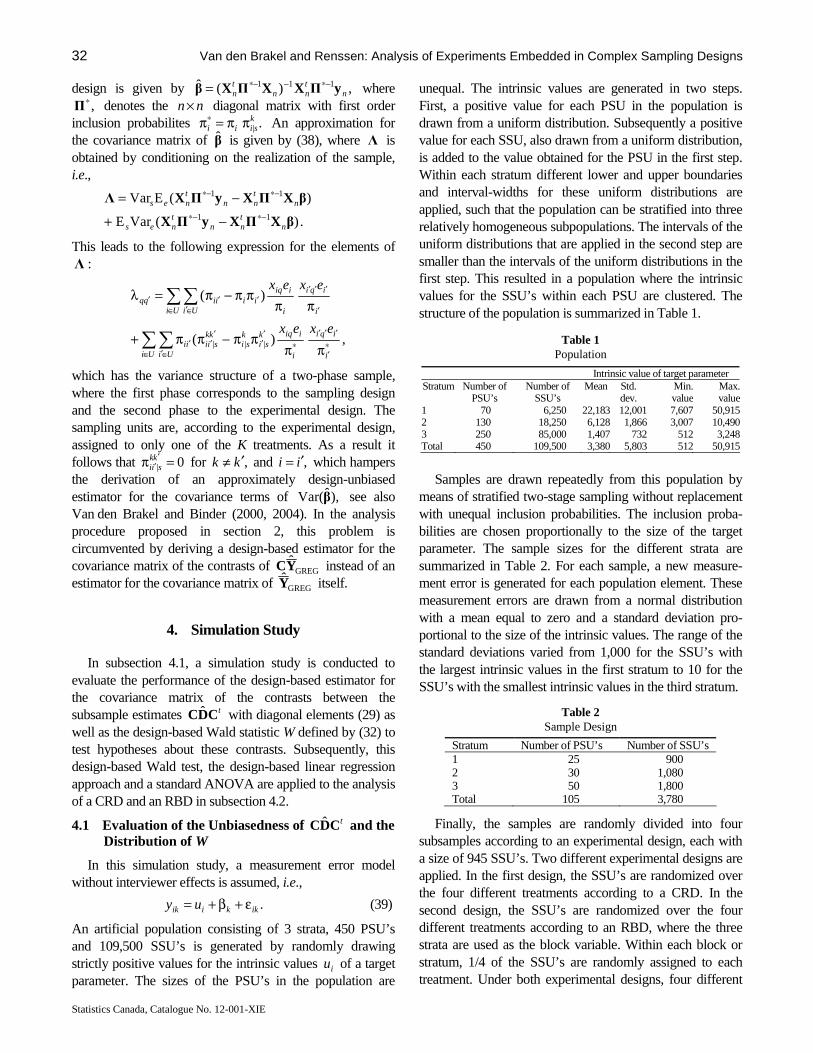
32 Van den Brakel and Renssen: Analysis of Experiments Embedded in Complex Sampling Designs
Statistics Canada, Catalogue No. 12-001-XIE
design is given by ,)(ˆ 111n
tnn
tn yΠXXΠXβ −∗−−∗= where
,∗Π denotes the nn × diagonal matrix with first order inclusion probabilites .|
ksiii ππ=π∗ An approximation for
the covariance matrix of β is given by (38), where Λ is obtained by conditioning on the realization of the sample, i.e.,
.)(VarE
)(EVar11
11
βXΠXyΠX
βXΠXyΠXΛ
ntnn
tnes
ntnn
tnes
−∗−∗
−∗−∗
−+
−=
This leads to the following expression for the elements of Λ :
,)(
)(
||| ∗′
′′′∗
′′
∈ ∈′
′′′
′
′′′′
∈ ∈′′′
ππππ−ππ+
ππππ−π=λ
∑∑
∑∑
i
iqi
i
iiqksi
ksi
Ui Ui
kksiiii
i
iqi
i
iiqi
Ui Uiiiiqq
exex
exex
which has the variance structure of a two-phase sample, where the first phase corresponds to the sampling design and the second phase to the experimental design. The sampling units are, according to the experimental design, assigned to only one of the K treatments. As a result it follows that 0| =π ′
′kk
sii for ,kk ′≠ and ,ii ′= which hampers the derivation of an approximately design-unbiased estimator for the covariance terms of ),ˆVar(β see also Van den Brakel and Binder (2000, 2004). In the analysis procedure proposed in section 2, this problem is circumvented by deriving a design-based estimator for the covariance matrix of the contrasts of GREGYC instead of an estimator for the covariance matrix of GREGY itself.
4. Simulation Study
In subsection 4.1, a simulation study is conducted to evaluate the performance of the design-based estimator for the covariance matrix of the contrasts between the subsample estimates tCDC ˆ with diagonal elements (29) as well as the design-based Wald statistic W defined by (32) to test hypotheses about these contrasts. Subsequently, this design-based Wald test, the design-based linear regression approach and a standard ANOVA are applied to the analysis of a CRD and an RBD in subsection 4.2. 4.1 Evaluation of the Unbiasedness of tCDC ˆ and the Distribution of W
In this simulation study, a measurement error model without interviewer effects is assumed, i.e.,
.ikkiik uy ε+β+= (39)
An artificial population consisting of 3 strata, 450 PSU’s and 109,500 SSU’s is generated by randomly drawing strictly positive values for the intrinsic values iu of a target parameter. The sizes of the PSU’s in the population are
unequal. The intrinsic values are generated in two steps. First, a positive value for each PSU in the population is drawn from a uniform distribution. Subsequently a positive value for each SSU, also drawn from a uniform distribution, is added to the value obtained for the PSU in the first step. Within each stratum different lower and upper boundaries and interval-widths for these uniform distributions are applied, such that the population can be stratified into three relatively homogeneous subpopulations. The intervals of the uniform distributions that are applied in the second step are smaller than the intervals of the uniform distributions in the first step. This resulted in a population where the intrinsic values for the SSU’s within each PSU are clustered. The structure of the population is summarized in Table 1.
Table 1 Population
Intrinsic value of target parameter Stratum Number of
PSU’s Number of
SSU’s Mean Std.
dev. Min. value
Max. value
1 70 6,250 22,183 12,001 7,607 50,9152 130 18,250 6,128 1,866 3,007 10,4903 250 85,000 1,407 732 512 3,248Total 450 109,500 3,380 5,803 512 50,915
Samples are drawn repeatedly from this population by
means of stratified two-stage sampling without replacement with unequal inclusion probabilities. The inclusion proba-bilities are chosen proportionally to the size of the target parameter. The sample sizes for the different strata are summarized in Table 2. For each sample, a new measure-ment error is generated for each population element. These measurement errors are drawn from a normal distribution with a mean equal to zero and a standard deviation pro-portional to the size of the intrinsic values. The range of the standard deviations varied from 1,000 for the SSU’s with the largest intrinsic values in the first stratum to 10 for the SSU’s with the smallest intrinsic values in the third stratum.
Table 2 Sample Design
Stratum Number of PSU’s Number of SSU’s 1 25 900 2 30 1,080 3 50 1,800 Total 105 3,780
Finally, the samples are randomly divided into four subsamples according to an experimental design, each with a size of 945 SSU’s. Two different experimental designs are applied. In the first design, the SSU’s are randomized over the four different treatments according to a CRD. In the second design, the SSU’s are randomized over the four different treatments according to an RBD, where the three strata are used as the block variable. Within each block or stratum, 1/4 of the SSU’s are randomly assigned to each treatment. Under both experimental designs, four different
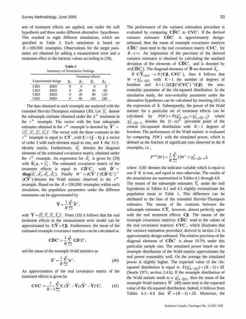
Survey Methodology, June 2005 33
Statistics Canada, Catalogue No. 12-001-XIE
sets of treatment effects are applied, one under the null hypothesis and three under different alternative hypotheses. This resulted in eight different simulations, which are specified in Table 3. Each simulation is based on
000,100=R resamples. Observations for the target para-meter are obtained by adding a measurement error and a treatment effect to the intrinsic values according to (39).
Table 3 Summary of Simulation Settings
Treatment effects Experimental design 1β 2β 3β 4β CRD RBD 0 0 0 0 CRD RBD 0 20 40 60 CRD RBD 0 40 80 120 CRD RBD 0 80 160 240
The data obtained in each resample are analyzed with the extended Horvitz-Thompson estimator (30). Let r
ky~ denote the subsample estimate obtained under the thk treatment in the thr resample. The vector with the four subsample estimates obtained in the thr resample is denoted by =rY~
.)~,~,~,~( 4321trrrr yyyy The vector with the three contrasts in the
thr resample is equal to jIjCYC ),(with,~ −= Mr a vector
of order 3 with each element equal to one, and I the 33× identity matrix. Furthermore, r
kd denotes the diagonal elements of the estimated covariance matrix, obtained under the thr resample. An expression for r
kd is given by (29) with r
kitk y~ˆ =xb . The estimated covariance matrix of the
treatment effects is equal to ,ˆ trCDC with =rD ).ˆ,ˆ,ˆ,ˆ( 4321
rrrr dddddiag Finally 1)ˆ()~
( −= trtrrW CDCYC )
~( rYC denotes the Wald statistic observed in the thr resample. Based on the 000,100=R resamples within each simulation, the population parameters under the different treatments can be approximated by
∑=
=R
r
r
R 1
,~1YY
with .),,,( 4321tYYYY=Y From (10) it follows that the real
treatment effects in the measurement error model can be approximated by .CβYC ≈ Furthermore, the mean of the estimated resample covariance matrices can be calculated as
,ˆ1
1
trR
r
t
RCDCCDC ∑
==
and the mean of the resample Wald statistics as
.1
1∑
==
R
r
rWR
W (40)
An approximation of the real covariance matrix of the treatment effects is given by
.)~
()~
(1
1
1
ttrR
r
rt
RCYYYYCCVC −−
−= ∑
= (41)
The performance of the variance estimation procedure is evaluated by comparing tCDC to .tCVC If the derived variance estimator tCDC ˆ is approximately design-unbiased, then the mean of resample covariance matrices
tCDC must tend to the real covariance matrix ,tCVC for .∞→R An impression of the precision of the derived
variance estimator is obtained by calculating the standard deviation of the elements of ,tCDC and is denoted by
).( tCDCσ The diagonal elements of D are denoted .kd If ),,(ˆ
GREGtN CVCβCYC → then it follows that
[ ][ ],2
1 δ−χ→ KW with 1−K the number of degrees of freedom and )()()(2/1 1 CβCVCCβ −=δ tt the non-centrality parameter of the chi-squared distribution. In the simulation study, the non-centrality parameter under the alternative hypotheses can be calculated by inserting (41) in the expression of .δ Subsequently, the power of the Wald statistic for a particular set of treatment effects can be calculated by [ ][ ] [ ][ ])()( 2
112
1 −α−δ− χ>χ= KKPWP where
[ ][ ]2
11 −α−χ K denotes the th)1( α− percentile point of the central chi-squared distribution with 1−K degrees of freedom. The performance of the Wald statistic is evaluated by comparing )(WP with the simulated power, which is defined as the fraction of significant runs observed in the R resamples, i.e.,
[ ][ ]∑=
−α−χ>=R
rK
rWIR
WP1
211
sim ),(1
)(
where )(BI denotes the indicator variable which is equal to one if B is true, and equal to zero otherwise. The results of the simulations are summarized in Tables 4.1 through 4.8. The means of the subsample estimates kY under the null hypotheses in Tables 4.1 and 4.5 slightly overestimate the population mean in Table 1. This difference can be attributed to the bias of the extended Horvitz-Thompson estimator. The means of the contrasts between the subsample estimates ,YC however, almost perfectly agree with the real treatment effects .Cβ The means of the resample covariance matrices tCDC tend to the values of the real covariance matrices ,tCVC which illustrates that the variance estimation procedure, derived in section 2.4, is approximately design-unbiased. The relative precision of the diagonal elements of tCDC is about 10.5% under this particular sample size. The simulated power based on the resample distribution of the Wald statistic approximates the real power reasonably well. On the average the simulated power is slightly higher. The expected value of the chi-squared distribution is equal to [ ][ ] δ+−=χ δ− 2)1()( 2
1 KE K (Searle 1971, section 2.4.h). If the resample distribution of the Wald statistic tends to a [ ][ ],
21 δ−χ K then the mean of the
resample Wald statistics W (40) must tend to the expected value of the chi-squared distribution. Indeed, it follows from Tables 8.41.4 − that δ+−≈ 2)1(KW . Moreover, the
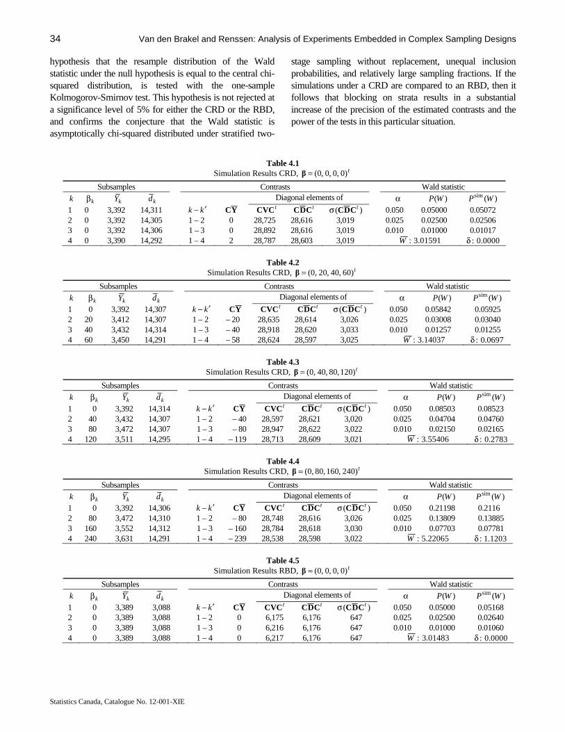
34 Van den Brakel and Renssen: Analysis of Experiments Embedded in Complex Sampling Designs
Statistics Canada, Catalogue No. 12-001-XIE
hypothesis that the resample distribution of the Wald statistic under the null hypothesis is equal to the central chi-squared distribution, is tested with the one-sample Kolmogorov-Smirnov test. This hypothesis is not rejected at a significance level of 5% for either the CRD or the RBD, and confirms the conjecture that the Wald statistic is asymptotically chi-squared distributed under stratified two-
stage sampling without replacement, unequal inclusion probabilities, and relatively large sampling fractions. If the simulations under a CRD are compared to an RBD, then it follows that blocking on strata results in a substantial increase of the precision of the estimated contrasts and the power of the tests in this particular situation.
Table 4.1
Simulation Results CRD, t)0,0,0,0(=β Subsamples Contrasts Wald statistic
k kβ kY kd Diagonal elements of α )(WP )(sim WP 1 0 3,392 14,311 kk ′− YC tCVC tCDC )( tCDCσ 0.050 0.05000 0.05072 2 0 3,392 14,305 1 – 2 0 28,725 28,616 3,019 0.025 0.02500 0.02506 3 0 3,392 14,306 1 – 3 0 28,892 28,616 3,019 0.010 0.01000 0.01017 4 0 3,390 14,292 1 – 4 2 28,787 28,603 3,019 01591.3:W 0000.0:δ
Table 4.2 Simulation Results CRD, t)60,40,20,0(=β
Subsamples Contrasts Wald statistic
k kβ kY kd Diagonal elements of α )(WP )(sim WP 1 0 3,392 14,307 kk ′− YC tCVC tCDC )( tCDCσ 0.050 0.05842 0.05925 2 20 3,412 14,307 1 – 2 – 20 28,635 28,614 3,026 0.025 0.03008 0.03040 3 40 3,432 14,314 1 – 3 – 40 28,918 28,620 3,033 0.010 0.01257 0.01255 4 60 3,450 14,291 1 – 4 – 58 28,624 28,597 3,025 14037.3:W 0697.0:δ
Table 4.3 Simulation Results CRD, t)120,80,40,0(=β
Subsamples Contrasts Wald statistic
k kβ kY kd Diagonal elements of α )(WP )(sim WP 1 0 3,392 14,314 kk ′− YC tCVC tCDC )( tCDCσ 0.050 0.08503 0.08523 2 40 3,432 14,307 1 – 2 – 40 28,597 28,621 3,020 0.025 0.04704 0.04760 3 80 3,472 14,307 1 – 3 – 80 28,947 28,622 3,022 0.010 0.02150 0.02165 4 120 3,511 14,295 1 – 4 – 119 28,713 28,609 3,021 55406.3:W 2783.0:δ
Table 4.4 Simulation Results CRD, t)240,160,80,0(=β
Subsamples Contrasts Wald statistic
k kβ kY kd Diagonal elements of α )(WP )(sim WP 1 0 3,392 14,306 kk ′− YC tCVC tCDC )( tCDCσ 0.050 0.21198 0.2116 2 80 3,472 14,310 1 – 2 – 80 28,748 28,616 3,026 0.025 0.13809 0.13885 3 160 3,552 14,312 1 – 3 – 160 28,784 28,618 3,030 0.010 0.07703 0.07781 4 240 3,631 14,291 1 – 4 – 239 28,538 28,598 3,022 22065.5:W 1203.1:δ
Table 4.5 Simulation Results RBD, t)0,0,0,0(=β
Subsamples Contrasts Wald statistic
k kβ kY kd Diagonal elements of α )(WP )(sim WP 1 0 3,389 3,088 kk ′− YC tCVC tCDC )( tCDCσ 0.050 0.05000 0.05168 2 0 3,389 3,088 1 – 2 0 6,175 6,176 647 0.025 0.02500 0.02640 3 0 3,389 3,088 1 – 3 0 6,216 6,176 647 0.010 0.01000 0.01060 4 0 3,389 3,088 1 – 4 0 6,217 6,176 647 01483.3:W 0000.0:δ
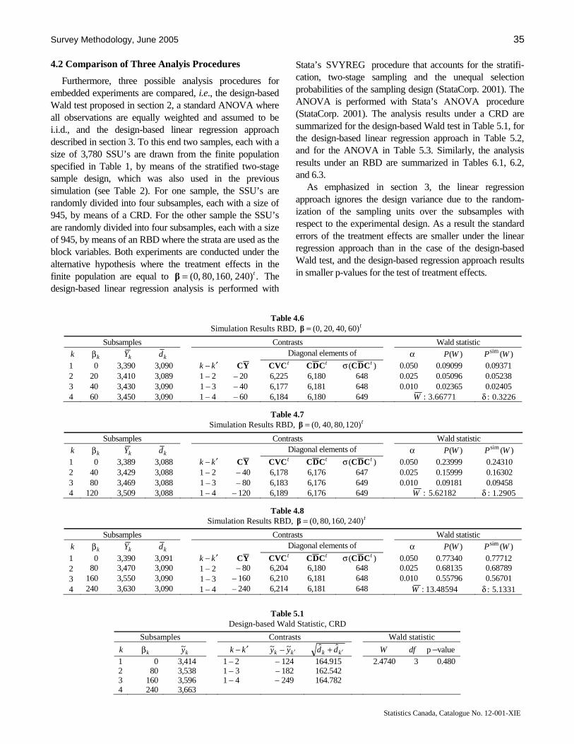
Survey Methodology, June 2005 35
Statistics Canada, Catalogue No. 12-001-XIE
4.2 Comparison of Three Analyis Procedures Furthermore, three possible analysis procedures for
embedded experiments are compared, i.e., the design-based Wald test proposed in section 2, a standard ANOVA where all observations are equally weighted and assumed to be i.i.d., and the design-based linear regression approach described in section 3. To this end two samples, each with a size of 3,780 SSU’s are drawn from the finite population specified in Table 1, by means of the stratified two-stage sample design, which was also used in the previous simulation (see Table 2). For one sample, the SSU’s are randomly divided into four subsamples, each with a size of 945, by means of a CRD. For the other sample the SSU’s are randomly divided into four subsamples, each with a size of 945, by means of an RBD where the strata are used as the block variables. Both experiments are conducted under the alternative hypothesis where the treatment effects in the finite population are equal to .)240,160,80,0( t=β The design-based linear regression analysis is performed with
Stata’s SVYREG procedure that accounts for the stratifi-cation, two-stage sampling and the unequal selection probabilities of the sampling design (StataCorp. 2001). The ANOVA is performed with Stata’s ΑΝΟVΑ procedure (StataCorp. 2001). The analysis results under a CRD are summarized for the design-based Wald test in Table 5.1, for the design-based linear regression approach in Table 5.2, and for the ANOVA in Table 5.3. Similarly, the analysis results under an RBD are summarized in Tables 6.1, 6.2, and 6.3.
As emphasized in section 3, the linear regression approach ignores the design variance due to the random-ization of the sampling units over the subsamples with respect to the experimental design. As a result the standard errors of the treatment effects are smaller under the linear regression approach than in the case of the design-based Wald test, and the design-based regression approach results in smaller p-values for the test of treatment effects.
Table 4.6
Simulation Results RBD, t)60,40,20,0(=β Subsamples Contrasts Wald statistic
k kβ kY kd Diagonal elements of α )(WP )(sim WP 1 0 3,390 3,090 kk ′− YC tCVC tCDC )( tCDCσ 0.050 0.09099 0.09371 2 20 3,410 3,089 1 – 2 – 20 6,225 6,180 648 0.025 0.05096 0.05238 3 40 3,430 3,090 1 – 3 – 40 6,177 6,181 648 0.010 0.02365 0.02405 4 60 3,450 3,090 1 – 4 – 60 6,184 6,180 649 66771.3:W 3226.0:δ
Table 4.7 Simulation Results RBD, t)120,80,40,0(=β
Subsamples Contrasts Wald statistic
k kβ kY kd Diagonal elements of α )(WP )(sim WP 1 0 3,389 3,088 kk ′− YC tCVC tCDC )( tCDCσ 0.050 0.23999 0.24310 2 40 3,429 3,088 1 – 2 – 40 6,178 6,176 647 0.025 0.15999 0.16302 3 80 3,469 3,088 1 – 3 – 80 6,183 6,176 649 0.010 0.09181 0.09458 4 120 3,509 3,088 1 – 4 – 120 6,189 6,176 649 62182.5:W 2905.1:δ
Table 4.8 Simulation Results RBD, t)240,160,80,0(=β
Subsamples Contrasts Wald statistic
k kβ kY kd Diagonal elements of α )(WP )(sim WP 1 0 3,390 3,091 kk ′− YC tCVC tCDC )( tCDCσ 0.050 0.77340 0.77712 2 80 3,470 3,090 1 – 2 – 80 6,204 6,180 648 0.025 0.68135 0.68789 3 160 3,550 3,090 1 – 3 – 160 6,210 6,181 648 0.010 0.55796 0.56701 4 240 3,630 3,090 1 – 4 – 240 6,214 6,181 648 48594.13:W 1331.5:δ
Table 5.1
Design-based Wald Statistic, CRD Subsamples Contrasts Wald statistic
k kβ ky~ kk ′− kk yy ′− ~~ kk dd ′+ ˆˆ W df p –value 1 0 3,414 1 – 2 – 124 164.915 2.4740 3 0.480 2 80 3,538 1 – 3 – 182 162.542 3 160 3,596 1 – 4 – 249 164.782 4 240 3,663
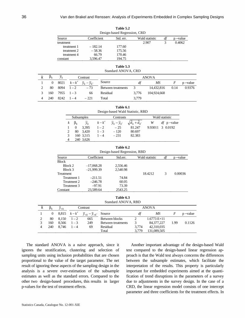
36 Van den Brakel and Renssen: Analysis of Experiments Embedded in Complex Sampling Designs
Statistics Canada, Catalogue No. 12-001-XIE
Table 5.2
Design-based Regression, CRD Source Coefficient Std. err. Wald statistic df p –value treatment 2.907 3 0.4062 treatment 1 – 182.14 177.60 treatment 2 – 58.36 175.56 treatment 4 66.79 170.46 constant 3,596.47 194.75
Table 5.3 Standard ANOVA, CRD
k kβ ky Contrast ANOVA 1 0 8021 kk ′− kk yy ′− Source df MS F p –value
2 80 8094 1 – 2 – 73 Between treatments 3 14,432,816 0.14 0.9376
3 160 7955 1 – 3 66 Residual 3,776 104,924,668
4 240 8242 1 – 4 – 221 Total 3,779
Table 6.1 Design-based Wald Statistic, RBD
Subsamples Contrasts Wald statistic
k kβ ky~ kk ′− kk yy ′− ~~ kk dd ′+ ˆˆ W df p –value 1 0 3,395 1 – 2 – 25 81.247 9.93011 3 0.0192 2 80 3,420 1 – 3 – 120 80.697 3 160 3,515 1 – 4 – 231 82.383 4 240 3,626
Table 6.2 Design-based Regression, RBD
Source Coefficient Std.err. Wald statistic df p –value Block Block 2 –17,068.28 2,556.46 Block 3 –21,999.39 2,540.98 Treatment 18.4212 3 0.00036 Treatment 1 –211.51 74.84 Treatment 2 –246.78 60.05 Treatment 3 –97.91 73.39 Constant 23,589.64 2543.25
Table 6.3 Standard ANOVA, RBD
k kβ ky+ Contrast ANOVA
1 0 8,815 kk ′− kk yy ′++ − Source df MS F p –value
2 80 8,150 1 – 2 665 Between blocks 2 1.6773 E+11 3 160 8,566 1 – 3 249 Between treatments 3 84,377,227 1.99 0.1126 4 240 8,746 1 – 4 69 Residual 3,774 42,310,035 Total 3,779 131,089,505
The standard ANOVA is a naive approach, since it
ignores the stratification, clustering and selection of sampling units using inclusion probabilities that are chosen proportional to the value of the target parameter. The net result of ignoring these aspects of the sampling design in the analysis is a severe over-estimation of the subsample estimates as well as the standard errors. Compared to the other two design-based procedures, this results in larger p-values for the test of treatment effects.
Another important advantage of the design-based Wald test compared to the design-based linear regression ap-proach is that the Wald test always concerns the differences between the subsample estimates, which facilitate the interpretation of the results. This property is particularly important for embedded experiments aimed at the quanti-fication of trend disruptions in the parameters of a survey due to adjustments in the survey design. In the case of a CRD, the linear regression model consists of one intercept parameter and three coefficients for the treatment effects. In
Survey Methodology, June 2005 37
Statistics Canada, Catalogue No. 12-001-XIE
this particularly simple situation, the coefficients for the treatment effects are exactly equal to the differences between the subsample estimates. This property, however, doesn’t hold for the treatment effects obtained under more complicated models, as for example in the case of the RBD.
5. Discussion and Conclusions
In this paper we discuss how the statistical methodology of randomized experiments and random survey sampling can support the design and analysis of experiments embedded in ongoing sample surveys. The sample survey design forms a prior framework for the application of principles, known from the theory of experimental designs, like randomization and local control by means of blocking on strata, PSU’s, clusters or interviewers. To test hypotheses about the estimates of finite population parameters observed under different treatments of the experiment, a design-based Wald statistic for the analysis of CRD’s and RBD’s embedded in general complex sampling designs is derived using the Horvitz-Thompson estimator and the generalized regression estimator. The application of randomized sampling from a finite population in combina-tion with this design-based analysis procedure enables us to generalize the results of the experiment observed in the specific sample to the entire survey population.
Since we allow for general complex sampling designs, a rather complicated expression for the covariance matrix of the treatment effects with nonzero off-diagonal entries is expected. The derived estimator for this covariance matrix, however, has a structure as if the sampling units were drawn with replacement and with unequal selection probabilities. No second order inclusion probabilities or design-cova-riances between the treatment effects are required, which simplifies the analysis considerably. For example, in the case of simple random sampling without replacement this result entails that the finite population correction factor should be disregarded in estimating the variance of contrasts. As a result a Wald statistic, derived from a design-based perspective under general complex sampling designs, is obtained that still has the appealing relatively simple structure of standard model-based analysis procedures.
For CRD’s and RBD’s embedded in a self-weighted sampling design analyzed with the extended Horvitz-Thompson estimator and a pooled variance estimator, the Wald statistic coincides with the statistic−F of an ANOVA for the one-way and two-way layouts. For the analysis of the embedded two-treatment experiment, a design-based version of the statistic−t can be derived as a special case of the Wald statistic. Expressions and more details about this design-based statistic−t and its relationship with Welch’s statistic−t and the standard
statistic−t can be found in Van den Brakel and Renssen (1998), Van den Brakel (2001) or Van den Brakel and Van Berkel (2002).
The analysis procedure proposed in this paper is implemented in a software package, called X–tool. This tool will become available as a component of the Blaise survey processing software package, developed by Statistics Netherlands.
Appendix
Properties of the randomization vectors ikp For CRD’s and RBD’s the randomization vectors ikp are
defined by (14) and (15). As a consequence of the random-ization mechanism of the experimental design, the vectors
ikp are random with the following conditional probability mass functions. For a CRD we have
.1)|0(and|++
+ −===⎟⎟⎠
⎞⎜⎜⎝
⎛=
n
nsP
n
ns
n
nP k
ikk
kk
ik prp
For an RBD we have
.1)|0(and|++
+ −===⎟⎟⎠
⎞⎜⎜⎝
⎛=
j
jkjik
j
jkjk
jk
jik n
nsP
n
ns
n
nP prp
Properties of these vectors are derived for an RBD. Properties for a CRD follow as a special, since a CRD can be considered as an RBD with one block. Let w. pr. denote “with probability”.
⎪⎩
⎪⎨⎧
∈
=
⎪⎪
⎩
⎪⎪
⎨
⎧
−
∈⎟⎟⎠
⎞⎜⎜⎝
⎛
=
′′
++
′
+
+
+
1:pr.w.
if0:pr.w.
1:pr.w.
if:pr.w.
2
O
rr
pp
O
rr
pp
jtkk
kj
j
jk
j
tkiik
j
jk
jj
jktkk
jk
j
tikik
sin
n
n
n
n
n
sin
n
n
n
⎪⎪⎪⎪⎪
⎩
⎪⎪⎪⎪⎪
⎨
⎧
∈′∈−
∈′∈
∈′∈−
−
∈′∈−
=
′+′
′′
+
′+′
′′
+′
′′
+′+
+
′
+
+
′
+′
′
++
′′
jjj
kj
j
jk
jjj
kj
j
jktkk
kj
j
jk
j
jjj
kj
j
jk
jjj
kj
j
jktkk
kj
j
jk
j
tkiik
sisin
n
n
n
sisin
n
n
n
n
n
n
n
sisin
n
n
n
sisin
n
n
n
n
n
n
n
,if,1:pr.w.
,if,:pr.w.
,if,)1(
1:pr.w.
,if,)1(
:pr.w.
O
rr
O
rr
pp
38 Van den Brakel and Renssen: Analysis of Experiments Embedded in Complex Sampling Designs
Statistics Canada, Catalogue No. 12-001-XIE
⎪⎪⎪⎪⎪
⎩
⎪⎪⎪⎪⎪
⎨
⎧
∈′∈−
∈′∈
∈′∈−−
−
∈′∈−−
⎟⎟⎠
⎞⎜⎜⎝
⎛
=
′+′
′
+
′+′
′
+′
+′+
++
++
+
′
jjj
kj
j
jk
jjj
kj
j
jktkk
kj
j
jk
j
jjj
jk
j
jk
jjj
jk
j
jktkk
jk
j
tkiik
sisin
n
n
n
sisin
n
n
n
n
n
n
n
sisin
n
n
n
sisin
n
n
n
n
n
if,1:pr.w.
if,:pr.w.
if,)1(
)1(1:pr.w.
,if,)1(
)1(:pr.w.
2
O
rr
O
rr
pp
The expectation of ikp with respect to the experimental design is given by:
.)()( kikkjk
jk
jk
jikike P
n
n
n
nPE r00prrpp ==+⎟
⎟⎠
⎞⎜⎜⎝
⎛== ++ (42)
The following covariances with respect to the experimental design can be derived:
tkk
jk
jkjtikike n
nnrrpp
)()(Cov
−= + (43)
tkk
tkiike ′′ −= rrpp )(Cov (44)
⎪⎩
⎪⎨⎧
∈′∈
∈′∈−=
′
′+′′
jj
jjtkk
jtkiike
sisi
sisin
andif
andif)1(
1
)(CovO
rrpp
(45)
⎪⎩
⎪⎨
⎧
∈′∈
∈′∈−
−−
=′
+
+
′
jj
jjtkk
jjk
jkj
tkiike
sisi
sisinn
nn
andif
andif)1(
1)(
)(Cov
O
rr
pp
(46)
Proof of formula (23)
Under the stated condition that a constant H–vector a exists such that 1=i
txa for all ,Ui ∈ and conditional on the realization of ,,,1, Niui K= according to super-population model (16), it follows that kb~ in (18) can be evaluated as
,
)(
)~
(
21
1
21
21
1
21
k
ki
liiN
ii
tii
N
i
i
ikiN
ii
tii
N
imkm
u
yEE
β++=
β+ω
ψ+⎟⎟⎠
⎞⎜⎜⎝
⎛ω
=
ω⎟⎟⎠
⎞⎜⎜⎝
⎛ω
=
∑∑
∑∑
=
−
=
=
−
=
adb
axxx
xxxb
(47)
where b denotes the regression coefficients defined by (17) and d denotes the regression coefficients from the regression function of the interviewer effects on the auxiliary variables .ix From result (47) it follows that
.)( βxdxbjxB ++= it
it
it Since 0jC = and from
measurement error model (1) and linear regression model (16) it follows that
.,
))(()(
QEDCεβxdbjεβjjCxByC
i
itt
iiliit
i u
=−+−++ψ+=−
Proof of formula (26) for an RBD First an expression for ),|ˆ(Cov HT sme EC is derived. Let
tiKii ee ),,( 1 K=e denote a K–vector with elements
.itkikik ye xb−= Consequently, .i
tii xBye −= Note that
tesmesm smsm CECEC ),|ˆ(CovEE),|ˆ(CovEE HTHT = with
.)ˆ,,ˆ(ˆHTK;HT1;HT
tEE K=E Futhermore note that
.)(ˆ
11HT; NN
Ei
itik
n
ii
it
itik
n
ik π
=⎟⎟⎠
⎞⎜⎜⎝
⎛π
−= ∑∑++++
==
epxByp (48)
Using (43) and (46), the diagonal elements of ),|ˆ(Cov HT sme E can be elaborated as
.1
)1(
1)1(
),|,(Cov
),|,(Cov
,|,Cov
),|ˆ(Var
2
11
2
11
1
1
11
1
11
HT;
⎟⎟⎟⎟⎟⎟
⎠
⎞
⎜⎜⎜⎜⎜⎜
⎝
⎛
⎟⎟⎠
⎞⎜⎜⎝
⎛
π−
π−−
⎟⎟⎠
⎞⎜⎜⎝
⎛
π−
π−=
⎟⎟⎟⎟⎟
⎠
⎞
⎜⎜⎜⎜⎜
⎝
⎛
ππ+
ππ=
⎟⎟⎠
⎞⎜⎜⎝
⎛ππ
=
∑∑
∑∑∑
∑∑∑
∑
∑∑
++
++
++
+
++++
=+=+
+
=+=
+
+
+
=
=
′
′′
=≠′=
=
′
′′
=′=
jj
jj
jj
j
n
i i
ik
ji
ikn
ij
j
n
i i
ik
ji
ikn
ijk
j
j
j
J
j
J
j
i
itkiike
i
ti
n
ii
n
i
i
itikike
i
ti
n
i
i
itki
n
ii
itik
n
ie
ke
N
e
nN
e
n
n
N
e
nN
e
n
n
n
n
Nsm
N
Nsm
N
smNN
smE
epp
e
epp
e
epep
(49)
Using (44) and (45), the off-diagonal elements of ),|ˆ(Cov HT sme E can be elaborated as
.1
1
)1(
),|,(Cov
),|,(Cov
,,Cov
),|ˆ,ˆ(Cov
1
111
1
11
1
11
HT;HT;
⎟⎟⎠
⎞⎜⎜⎝
⎛
π−
π
⎟⎟⎠
⎞⎜⎜⎝
⎛
π−
π−−=
⎟⎟⎟⎟⎟
⎠
⎞
⎜⎜⎜⎜⎜
⎝
⎛
ππ+
ππ=
⎟⎟⎠
⎞⎜⎜⎝
⎛ππ
=
∑
∑∑∑
∑∑∑
∑
∑∑
+
++
++
+
++++
=
′
+
′
=+=+
+
=
=
′
′′′
=≠′=
′=
′
′′′
=′=
′
j
jj
jj
j
n
i i
ki
ji
ki
n
i i
ik
ji
ikn
ij
jJ
j
J
j
i
itkiike
i
ti
n
ii
n
i
i
itkiike
i
ti
n
i
i
itki
n
ii
itik
n
ie
kke
N
e
nN
e
N
e
nN
e
n
n
Nsm
N
Nsm
N
smNN
smEE
epp
e
epp
e
epep
(50)
Survey Methodology, June 2005 39
Statistics Canada, Catalogue No. 12-001-XIE
The results (49) and (50) can be written in matrix notation;
tn
i i
ii
ji
itkik
n
i i
ii
ji
itkik
n
ij
jJ
j
e
j
jj
NnN
NnNn
n
sm
⎟⎟⎠
⎞⎜⎜⎝
⎛
π−−
π−
⎟⎟⎠
⎞⎜⎜⎝
⎛
π−−
π−
−−=
∑
∑∑∑
+
++
=′ ′
′′
+
=′ ′
′
+=+
+
=
1
111
HT
1
11
),|ˆ(Cov
BxyxBy
BxyxByD
E
where D denotes a KK × diagonal matrix with elements
.1
1
2
111⎟⎟⎠
⎞⎜⎜⎝
⎛
π−−
π−
−= ∑∑∑
++
=′ ′
′′
+=
+
+
+
=
jj n
i i
itkki
ji
itkik
n
ijk
j
j
jJ
jk N
y
nN
y
n
n
n
nd
xbxb
According to (23) it follows that
.1
11
),|ˆ(Cov
1
111
HT
tn
i i
i
ji
i
n
i i
i
ji
in
ij
jJ
j
t
e
j
jj
NnN
NnNn
n
sm
⎟⎟⎠
⎞⎜⎜⎝
⎛
π−
π
⎟⎟⎠
⎞⎜⎜⎝
⎛
π−
π−−=
∑
∑∑∑
+
++
=′ ′
′
+
=′ ′
′
+=+
+
=
CεCε
CεCεCDC
EC
(51)
The final part of the proof is to take the expectation of ),|ˆ(Cov HT sme EC with respect to the sampling design and
the measurement error model. The proof is given for RBD’s where PSU’s are block variables. In a two-stage sampling scheme, J blocks or PSU’s are drawn from a finite popu-lation of uJ blocks with first order inclusion probabilities
.Ijπ Within each PSU, +jn SSU’s are drawn in the second
stage with first and second order inclusion probabilities IIji|π
and .|II
jii ′π The first order inclusion probabilities of the individuals in the sample are .|
IIji
Iji ππ=π Furthermore, let
j
iN
ij N
j ε∑=
=Δ1
denote the population mean of the measurement errors of the individuals of block j. Then
IIjij
in
ij N
j
|1
ˆπ
=Δ ∑+
=
ε
denotes the Horvitz-Thompson estimator for .jΔ Now we have
( )( ).
ˆˆ1
1
1
11
||12
22
1
111 1
⎟⎟⎟⎟⎟⎟
⎠
⎞
⎜⎜⎜⎜⎜⎜
⎝
⎛
Δ−ΔΔ−Δ−
⎟⎟⎠
⎞⎜⎜⎝
⎛Δ−
π⎟⎟⎠
⎞⎜⎜⎝
⎛Δ−
π
⎟⎟⎠
⎞⎜⎜⎝
⎛⎟⎟⎠
⎞⎜⎜⎝
⎛
π=
⎟⎟⎠
⎞⎜⎜⎝
⎛
π−
π⎟⎟⎠
⎞⎜⎜⎝
⎛
π−
π
+
++
=+
=
′
′
=′+=′ ′
′
+= =
∑
∑
∑∑∑ ∑
+
+++
t
jjjjj
t
jIIjij
ijjII
jij
ijn
ij
jIj
J
j
t
i
in
iji
in
i i
i
ji
iJ
j
n
i
n
N
n
N
n
n
N
N
NnNNnN
j
jjj
εε
εεεε
(52)
Let IsE denote the expectation with respect to the first
stage of the sampling design and IIsE the expectation
with respect to the second stage of the sampling design. Taking the expectation with respect to the measurement error model and the sampling design of the first part of (52) and using model assumption (3) leads to
t
jIIjij
ijjII
jij
ijn
ijIj
J
jssm N
n
N
n
n
j
III ⎟⎟⎠
⎞⎜⎜⎝
⎛Δ−
π⎟⎟⎠
⎞⎜⎜⎝
⎛Δ−
π⎟⎟⎠
⎞⎜⎜⎝
⎛
π++
=+=∑∑
+
||12
2
1
11EEE
εε
.11
11EE
|12
|2
1
2
1
iIIji
jN
ijjIj
tjjII
jij
tiij
N
ijIj
J
jsm
n
Nn
N
n
n
j
j
I
∑⎟⎟⎠
⎞⎜⎜⎝
⎛−
ππ=
⎟⎟⎠
⎞⎜⎜⎝
⎛ΔΔ−
π⎟⎟⎠
⎞⎜⎜⎝
⎛
π=
+
=+
+
=+=
∑
∑∑εε
(53)
Note that tjjjjsII)ˆ)(ˆ(E Δ−ΔΔ−Δ in (52) equals the design
variance of jΔ with respect to the second stage of the sampling design in block j. Taking the expectation with respect to the measurement error model and the sampling design of the second part of (52) and using model assumption (3) leads to
( )( )
.111
)(1
E
ˆˆ11EEE
|12
|||||
112
2
1
iIIji
N
ijIj
IIji
IIji
tiiII
jiII
jiII
jii
N
i
N
ijIj
m
t
jjjjj
Ij
J
jssm
j
jj
III
N
N
n
∑⎟⎟⎠
⎞⎜⎜⎝
⎛−
ππ=
ππππ−π
π=
Δ−ΔΔ−Δ⎟⎟⎠
⎞⎜⎜⎝
⎛
π
∑
∑∑
∑
=
′
′′′
=′=
+=
εε
(54)
With results (52), (53) and (54) we can elaborate the second term on the right hand side of the equal sign of (51) as
.11
11
EE
12
1
111
i
ti
N
i
tn
i i
i
ji
i
n
i i
i
ji
in
ij
jJ
jsm
NNnN
NnNn
n
j
jj
π=⎟
⎟⎠
⎞⎜⎜⎝
⎛
π−
π
⎟⎟⎠
⎞⎜⎜⎝
⎛
π−
π−
∑∑
∑∑∑
==′ ′
′
+
=′ ′
′
+=+
+
=
+
++
CCCεCε
CεCε
∑
(55)
40 Van den Brakel and Renssen: Analysis of Experiments Embedded in Complex Sampling Designs
Statistics Canada, Catalogue No. 12-001-XIE
Finally, it follows from (51) and (55) that
.,1
EE
),|ˆ(CovEE
12
HT
QEDCC
CDC
EC
i
ti
N
i
tsm
esm
N
sm
π−
=
∑=
∑
The derivation for an RBD where strata are block variables follows directly as a special case from an RBD where PSU’s are block variables with ,,1 | i
IIji
Ij π=π=π
iiII
jii ′′ π=π | and .uJJ = The proof for an RBD where clusters are block variables follows directly as a special case from an RBD where PSU’s are block variables with 1| =πII
ji and .1| =π ′
IIjii
The expectation of ),|ˆ(Cov HT sme EC with respect to the sampling design and the measurement error model for an RBD where interviewers are the block variables does not follow as a special case from an RBD where PSU’s are block variables. Since the block variables are not directly linked with the sampling design, the blocks should be considered as domains where the block size +jn is random with respect to the sampling design. The derivation follows the same steps as in the proof for blocking on PSU’s and is given by Van den Brakel (2001).
Proof of formula (32) Matrix D can be partitioned as follows:
.ˆ
ˆˆ
*
1
⎟⎟⎠
⎞⎜⎜⎝
⎛=
D0
0D
td
According to Bartlett’s identity (Morisson 1990, chapter 2) it follows that:
.ˆˆ)ˆ(trace
1ˆ)ˆˆ()ˆ( 1*
1*1
1*
1*1
1 −−−
−−− −=+= DjjDD
DDjjCDC ttt d
From this result it follows that
.ˆˆ)ˆ(trace
1ˆ
ˆˆ)ˆ(trace
1ˆ)ˆ(
111
1
1*
1*1
1*
1
−−−
−
−−−
−−
−=
−=
DjjDD
D
CDjjDCD
CDCCCDCC
t
ttttt
(56)
Inserting (56) into (31) leads to (32), QED.
Acknowledgements
The authors wish to thank the Associate Editor, the referees, Paul Smith, and Rachel Vis-Visschers for their constructive comments on former drafts of this paper. Jan also thanks Prof. Stephen E. Fienberg and Prof. Peter Kooiman for their support as Ph. D. advisor during this research.
References Bethlehem, J.G., and Keller, W.G. (1987). Linear weighting of
sample survey data. Journal of Official Statistics, 3(2), 141-153. Cochran, W.G. (1977). Sampling Techniques. New York: John Wiley
& Sons, Inc. Fellegi, I.P. (1964). Response variance and its estimation. Journal of
the American Statistical Association, 59, 1016-1041. Fienberg, S.E., and Tanur, J.M. (1987). Experimental and sampling
structures: Parallels diverging and meeting. International Statistical Review, 55(1), 75-96.
Fienberg, S.E., and Tanur, J.M. (1988). From the inside out and the outside in: Combining experimental and sampling structures. The Canadian Journal of Statistics, 16(2), 135-151.
Fienberg, S.E., and Tanur, J.M. (1989). Combining cognitive and statistical approaches to survey design. Science, 243, 1017-1022.
Hájek, J. (1960). Limiting distributions in simple random sampling from a finite population. Mathematical Institute of the Hungarian Academy of Sciences, 5, 361-374.
Hájek, J. (1971). Comment on a paper by D. Basu. In Foundations of Statistical Inference, (Eds. V.P. Godambe and D.A. Sprott). Toronto: Holt, Rinehart and Winston. 236.
Hartley, H.O., and Rao, J.N.K. (1978). Estimation of nonsampling variance components in sample surveys. In Survey Sampling and Measurement, (Eds. N.K. Namboodiri). New York: Academic Press. 35-43.
Lehmann, E.L. (1975). Nonparametrics: Statistical Methods Based on Ranks. New York: McGraw-Hill.
Mahalanobis, P.C. (1946). Recent experiments in statistical sampling in the Indian statistical institute. Journal of the Royal Statistical Society, 109, 325-370.
Montgomery, D.C. (2001). Design and Analysis of Experiments. New York: John Wiley & Sons, Inc.
Morisson, D.F. (1990). Multivariate Statistical Methods. Singapore: McGraw-Hill.
Särndal, C.-E., Swensson, B. and Wretman, J.H. (1992). Model Assisted Survey Sampling. New York: Springer Verlag.
Scheffé, H. (1959). The Analysis of Variance. New York: John Wiley & Sons, Inc.
Searle, S.R. (1971). Linear Models. New York: John Wiley & Sons, Inc.
Skinner, C.J. (1989). Domain means, regression and multivariate analysis. In Analysis of Complex Surveys, (Eds. C.J. Skinner, D. Holt and T.M.F. Smith). Chichester: Wiley & Sons, Inc. 59-87.
Statacorp. (2001). Stata Reference Manual Release 7.0. College Station, Texas.
Van den Brakel, J.A. (2001). Design and Analysis of Experiments Embedded in Complex Sample Surveys. Ph.D. Thesis. Rotterdam: Erasmus University of Rotterdam.
Van den Brakel, J.A. and Binder, D. (2000). Variance estimation for experiments embedded in complex sampling schemes. Proceedings of the Section on Survey Research Methods, American Statistical Association. Indianapolis, August 13-17. 805-810.
Van den Brakel, J.A., and Binder, D. (2004). Variance estimation for experiments embedded in complex sampling designs. Unpublished research paper, BPA nr.: H894-04-TMO. Heerlen: Statistics Netherlands.
Van den Brakel, J.A., and Renssen, R.H. (1998). Design and analysis of experiments embedded in sample surveys. Journal of Official Statistics, 14(3), 277-295.
Van den Brakel, J.A., and Van Berkel, C.A.M. (2002). A design-based analysis procedure for two-treatment experiments embedded in sample surveys. An application in the Dutch labor force survey. Journal of Official Statistics, 18(2), 217-231.
Survey Methodology, June 2005 41 Vol. 31, No. 1, pp. 41 -51 Statistics Canada, Catalogue No. 12-001-XIE
Domain Estimators for the Item Count Technique
Takahiro Tsuchiya 1
Abstract
The item count technique, which is an indirect questioning technique, was devised to estimate the proportion of people for whom a sensitive key item holds true. This is achieved by having respondents report the number of descriptive phrases, from a list of several phrases, that they believe apply to themselves. The list for half the sample includes the key item, and the list for the other half does not include the key item. The difference in mean number of selected phrases is an estimator of the proportion. In this article, we propose two new methods, referred to as the cross-based method and the double cross-based method, by which proportions in subgroups or domains are estimated based on the data obtained via the item count technique. In order to assess the precision of the proposed methods, we conducted simulation experiments using data obtained from a survey of the Japanese national character. The results illustrate that the double cross-based method is much more accurate than the traditional stratified method, and is less likely to produce illogical estimates.
1. Takahiro Tsuchiya, The Institute of Statistical Mathematics, 4-6-7, Minami-Azabu, Minato-ku, Tokyo, 106-8569, Japan. E-mail: [email protected].
Key Words: Indirect questioning techniques; Item count technique; Domain estimators; Survey of Japanese national
character.
1. Introduction 1.1 Indirect Questioning Techniques
Suppose that a population U is divided into two sub-populations )(TU and ,)(
cTU where )(TU is a set of elements
having an attribute T, and cTU )( is a complement of .)(TU
One purpose of social surveys is to estimate ),1( ===π YPY where
⎩⎨⎧ ∈
=otherwise0
if1 )(Tk
UkY
and )(⋅P denotes the proportion of units having a particular value of the variable. For example, when T is “supporting the present cabinet,” π indicates the cabinet support rate, and when T is “using a certain illegal drug,” π denotes the prevalence rate of drug use.
In a direct questioning technique, researchers ask respondents “Do you belong to ?)(TU ,” and directly obtain the indicator value iy as “yes” or “no” (Cochran 1977, page 50). When every respondent has an equal inclusion proba-bility, a sample mean y serves as one estimator of π.
On the other hand, some indirect questioning techniques, including the randomized response technique (Warner 1965), the nominative technique (Miller 1985), the item count technique (Droitcour, Caspar, Hubbard, Parsley, Visscher and Ezzati 1991), and the three-card technique (Droitcour, Larson and Scheuren 2001), are devised because some respondents tend to evade sensitive questions, such as those concerning highly private matters, socially unaccepted or deviant behaviors or illegal acts. The essential feature of
indirect techniques is that instead of a direct observation of Y, another variable ),,( VYgX = which is some sort of function of Y and, if necessary, of other random variables V, is observed so that respondents feel that their true Y – values are not revealed. While this feature is expected to derive a truthful answer from evasive respondents, both the questioning and the estimation procedures are rather complicated compared to the direct questioning technique partly because the function )(⋅g sometimes includes some randomization processes. We shall outline two indirect techniques below.
The randomized response is the most popular among the indirect techniques, and various modifications have been proposed (Abul-Ela, Greenberg and Horvitz 1967; Warner 1971; Chaudhuri and Mukerjee 1988; Greenberg, Abul-Ela, Simmons and Horvitz 1969; Takahasi and Sakasegawa 1977). Although the randomized response is not the topic of this article, we shall briefly outline Warner’s original procedure here for reference, because this technique will be simulated in a later section.
1. Prepare two types of questionnaires. In question-
naire A, respondents are asked “Do you belong to ?)(TU ,” and in questionnaire B, respondents are
asked “Do you belong to ?)(cTU ”
2. Let )5.0( ≠p be the predetermined probability. Each respondent selects questionnaire A or B with probabilities p or p−1 respectively, but no one other than the respondent knows which questionnaire is selected.

42 Tsuchiya: Domain Estimators for the Item Count Technique
Statistics Canada, Catalogue No. 12-001-XIE
3. Suppose X is an indicator variable whose value is 1 if the response is “yes” or 0 if the response is “no.” The estimator of π is given by
,12
1ˆ
−+−=π
p
xp (1)
where x is a sample mean of X. Since the researchers have no information regarding the type of questionnaire selected by each respondent, more respondents are expected to give truthful answers than they would if asked direct questions.
The item count technique, which is the subject of this article, is not as popular despite its simplicity. The technique is also effective when posing sensitive questions, because respondents are asked not to answer sensitive questions directly but to merely report the number of items that hold true with them. The following are the processes of the item count technique:
1. Prepare the key item T, which is the primary focus of the study, and G other non-key items .,,1 GEE K For example, T is “using a certain illegal drug” as mentioned above, and gE is some sort of non-sensitive description such as “owning a bicycle.”
2. Prepare two types of questionnaires, A and B. In questionnaire A, respondents are asked to answer the number AC of items that are true with respect to themselves among G non-key items. In questionnaire B, respondents are asked to answer the number BC of items that are true with respect to themselves out of 1+G items, including the key item T. Table 1 lists examples of item lists. Our aim is to estimate the proportion of people who use a certain illegal drug. The key item is “using a certain illegal drug” in the questionnaire B and the other four items are non-key items. Except when a response to the questionnaire B is 0=BC or ,5=BC researchers cannot detect as to which items hold true with the respondent. For example, a respondent will reply that four items in the questionnaire B are true, but we cannot be sure that the respondent uses the drug at all. Hence, it is expected that more respondents using an illegal drug will report truthful answers in such a scenario than when asked a direct question.
3. Divide a total sample into two subgroups, A and B, randomly of size An and Bn so that each question-naire is assigned to a corresponding subgroup.
Table 1 Examples of Item Lists
Questionnaire A Questionnaire B How many of the following hold true for you?
How many of the following hold true for you?
– owning a bicycle – owning a bicycle – having travelled abroad – having travelled abroad – having called an ambulance – having called an ambulance – owning a summer villa – using a certain illegal drug – owning a summer villa
4. The estimator of π is given by
,ˆˆˆ AB CC −=π (2)
where AC and BC are the estimated means of AC and BC respectively. The justification of (2) is explained in section 2.1. When every unit in the sample has an equal inclusion probability, π can be written as
,ˆ0
1
0A
Ac
G
cB
Bc
G
c n
nc
n
nc ∑∑
=
+
=−=π (3)
where Acn and B
cn are the number of respondents whose answers are cC A = and ,cC B = respectively. Moreover, when an auxiliary variable Z is available and its distribution zmzZP == )( in the population is known, for example from a census, poststrati-fication is often used to adjust the sample distribution of Z to the population. That is, the poststratified estimator of π is given by
,
ˆ
0
1
0
0
1
0PS
AczA
z
z
z
G
c
BczB
z
z
z
G
c
A
Acz
Azz
G
cB
Bcz
Bzz
G
c
nn
mcn
n
mc
n
nvc
n
nvc
⋅=⋅
+
=
=
+
=
∑∑∑∑
∑∑∑∑
−=
−=π
(4)
where Aczn is the number of respondents for each
cC A = and ,zZ =
Az
AzA
zAz
z
AAcz
G
c
Az
n
nmvnnnn
.0
,, === ⋅=
⋅ ∑∑
and ,,, BBz
Bcz nnn ⋅ and B
zv are defined in analogous ways. One practical merit of the item count technique is that it
does not demand any randomization devices, which are required for the randomized response technique. It is not the respondent but a researcher who selects the questionnaire to be answered. Hence, the item count technique is easily implemented via any self-administered or telephone surveys. A more elaborate comparison between the randomized response and the item count technique is found in Hubbard, Casper and Lessler (1989).

Survey Methodology, June 2005 43
Statistics Canada, Catalogue No. 12-001-XIE
The questionnaire A is introduced to obtain the distri-bution of the number of non-key items. That is, respondents to the questionnaire A do not answer the sensitive question. Therefore, it is possible to increase the precision of the estimator using the double-list version of item count (Droitcour et al. 1991), which exchanges the roles between the two subgroups. However, we limit our argument in this article to a single-list version, because the extension of estimators to the double-list version is straightforward. 1.2 Purpose of this Article
Thus far, we have focused on the parameter )1( ===π YPY of a total population. However, esti-
mators in subpopulations or domains (Särndal, Swesson and Wretman 1992 page 5) are often required, i.e., either a conditional proportion )|1( zZYP == or a joint proportion
),1( zZYP == must be estimated, where a population is divided into several domains by the Z – value. We refer to the variable Z as the domain variable in this article. The domain variables often used are demographic characteristics such as gender or age. For example, government agencies would like to know the proportion of people who use a certain illegal drug at each age group. Even though the post-stratified estimator PSπ in (4) uses the domain variable Z, its aim is an estimation of )1( =YP in the entire population. Our aim in this article is to obtain separate estimations of
)|1( zZYP == within each domain. One simple estimation method is as follows: 1. Post-stratify the sample into strata or domains
based on the Z – value. 2. In each stratum or domain, separately determine
)|1( zZYp == using (1) or (2), where )(⋅p is a sample estimate of ).(⋅P
3. If necessary, estimate ),1( zZYp == by multi-plying a known domain proportion, ),( zZP = or an estimated domain proportion, ).( zZp =
The above method is referred to throughout this article as a stratified method because estimates are obtained separately in each stratum or domain. Although Rao (2003) refers to the above method as a direct estimate, we have avoided the use of the term “direct” in order to avoid confusion with the term “direct questioning technique.”
An advantage of the stratified method is that this method is applicable to any indirect questioning technique, including the randomized response and item count techniques. The U.S. General Accounting Office (1999) adopts the stratified method to estimate domains under the three-card technique. However, one of the serious problems of the stratified method is that it often produces illogical estimates, especially negative estimates, in the case of the randomized response and the item count, as explained later
in this article. This is mainly because the reduction of the sample size in each stratum increases the standard errors of the estimators (Lessler and O’Reilly 1997). For example, Droitcour et al. (1991, page 206) “calculated estimates separately for the three risk strata” and obtained negative prevalence rate estimates of drug use.
In the case of the randomized response, there is little possibility that domain estimators other than the stratified method are developed because information concerning the type of questionnaire selected by individual respondents is unavailable. In contrast, in the item count technique, the questionnaire answered by each respondent is known. Therefore, the precision of the domain estimators is expected to increase when auxiliary information is used, specifically contingency tables between Z and AC or .BC
In this article, we propose new domain estimators for the item count technique, which are referred to as the cross-based method and the double cross-based method. In addition, we will illustrate the fact that the new estimators are more efficient than the traditional stratified method by simulating the item count technique using data obtained from the survey of the Japanese national character concerning the significant attributes of the Japanese character.
2. Domain Estimators for the Item
Count Technique 2.1 Stratified Method
Here, we reformulate the stratified method. Let us assume that the following equations hold true for each value of c and z. Assumption 1.
.0)|0,1(
),|1,1(
)|0,()|(
===+=
==−=+
======
zZYGCP
zZYcCP
zZYcCPzZcCP
A
A
AB
These assumptions imply that the difference in the distribution between AC and BC depends solely on Y. Question effects, including order effects and context effects (Schuman and Presser 1981) are not considered.
We have the following result based on these assumptions. Stratified Method.
)|(
)|()|1(
0
1
0
zZcCPc
zZcCPczZYP
AG
c
BG
c
==−
=====
∑
∑
=
+
=
(5)
,Az
Bz CC −= (6)
44 Tsuchiya: Domain Estimators for the Item Count Technique
Statistics Canada, Catalogue No. 12-001-XIE
where AzC and B
zC are the domain means of AC and .BC Derivation.
).|1()|(
)|1,(
)}|1,()|0,({
)|1,()1()|0,(
)|1,1()|0,(
)|(
0
0
0
00
1
0
1
0
1
0
zZYPzZcCcP
zZYcCP
zZYcCPzZYcCPc
zZYcCPczZYcCcP
zZYcCcPzZYcCcP
zZcCcP
AG
c
AG
c
AAG
c
AG
c
AG
c
AG
c
AG
c
BG
c
==+===
===+
===+====
===++====
==−=+====
==
∑
∑
∑
∑∑
∑∑
∑
=
=
=
==
+
=
+
=
+
=
Transposing the first term to the left-hand side yields the stratified method (5).
The estimator )|1( zZYp == is obtained by substituting domain means A
zC and BzC with their estimators, A
zC and .ˆ B
zC
.ˆˆ)|1( Az
Bz CCzZYp −=== (7)
When the inclusion probabilities are equal for all units in the sample, the estimator of )|1( zZYP == is written as
∑∑= ⋅
+
= ⋅
−===G
cAz
Acz
G
cBz
Bcz
n
nc
n
nczZYp
0
1
0
,)|1( (8)
where ,,, Az
Bcz
Acz nnn ⋅ and B
zn⋅ are defined in the section 1.1. The equations (2) and (3) for the entire population are special cases of (7) and (8).
One merit of the stratified method is that the variance estimator of )|1( zZYp == is easily obtained by
).ˆ(arV)ˆ(arV))|1((arV Az
Bz CCzZYp +=== (9)
On the other hand, as noted in the previous section, the reduction of sample size in each stratum increases estimated variances in (9). Further, the marginal estimator )1( =Yp obtained by using (8) does not correspond to that obtained directly by (3), unless B
zAz nn ⋅⋅ = for all z. That is, when
)( zZp = is not known, its estimator is given by
)/()()( BABz
Az nnnnzZp ++== ⋅⋅
and
∑∑
∑∑∑
∑
=
⋅+
=
⋅
= ⋅
+
= ⋅
π=−≠
⎪⎭
⎪⎬⎫
⎪⎩
⎪⎨⎧
−++
=
===
G
cA
Ac
G
cB
Bc
G
cAz
Acz
G
cBz
Bcz
BA
Bz
Az
z
z
n
nc
n
nc
n
nc
n
nc
nn
nn
zZpzZYp
0
1
0
0
1
0
..
.ˆ
)()|1(
(10)
When the domain proportion zmzZp == )( is available, the marginal estimator corresponds to the poststratified estimator (4).
.ˆ
)()|1(
PS
0
1
0
π=⎭⎬⎫
⎩⎨⎧
−=
===
∑∑∑
∑
= ⋅
+
= ⋅
G
cAz
Acz
G
cBz
Bcz
zz
z
n
nc
n
ncm
zZPzZYp
These results indicate that we should use a poststratified estimator PSπ with the domain estimators if we use the stratified method. 2.2 Cross-based Method
In the stratified method, a total sample is divided into strata for the purpose of direct estimation of
),|1( zZYP == which causes sample size reduction. Hence, in the cross-based method proposed in this section, the joint proportion ),1( zZYP == is estimated first in order to use the entire sample, and the conditional proportion is subsequently obtained by
.)(
),1()|1(or
)(),1(
)|1(
zZP
zZYpzZYp
zZp
zZYpzZYp
======
======
The term ‘cross-based method’ is used because this method uses cross tabulations ),|( cCzZP B == as shown in (19).
For the cross-based method, we assume that the following equations hold for each value of c. Assumption 2.
),1,()1,1( ====+= YcCPYcCP AB (11)
,0)1,1()1,0( ==−==== YCPYCP AB (12)
.)0,()0,( ===== YcCPYcCP AB (13)
These assumptions also imply that the difference in the distribution between AC and BC depends only on Y.
We have the following result based on these assumptions. Cross-based Method.
,)|(),1( 1
1
1−
+
====== ∑ c
BG
c
QcCzZPzZYP (14)
where
.)}()({0∑
==−==
c
d
BAc dCPdCPQ
In addition, we assume that ==== )1,|( YcCzZP B )|( cCzZP B == for every .0>c This assumption
would be valid to some degree when both the key and non-key items describe the same type of stigmatizing behavior.
Survey Methodology, June 2005 45
Statistics Canada, Catalogue No. 12-001-XIE
Derivation. Based on the assumptions, we have
).0,()1,1(
)0,()1,()(
==+=−==
==+====
YcCPYcCP
YcCPYcCPcCPAA
BBB
(15)
The following equation holds for any c.
).1,()()0,( ==−==== YcCPcCPYcCP AAA (16)
Hence, substituting (16) in (15) gives
.)}1,()({
)1,1()(
==−=+
=−===
YcCPcCP
YcCPcCPAA
AB
(17)
Summing (17) over c up to some g, we obtain
).1,()(
)}1,()({
)1,1()(
0
0
00
==−==
==−=+
=−===
∑
∑
∑∑
=
=
==
YgCPcCP
YcCPcCP
YcCPcCP
AAg
c
AAg
c
Ag
c
Bg
c
By transposing the terms, we define .cQ
).1,1(
)1,(
)}()({0
=+==
===
=−== ∑=
YcCP
YcCP
dCPdCPQ
B
A
BAc
dc
(18)
Here, the joint proportion ),1( zZYP == is decomposed as
∑+
========
1
0
).1,()|(),1(G
c
BB YcCPcCzZPzZYP (19)
Substituting the equation (18) and the assumption (12) in (19) yields the cross-based method.
The joint estimator ),1( zZYP == is obtained by substituting each term of (14) for its estimators. When the sample is self-weighting, the estimator is given by
,),1(1
0
1
1∑∑
−
=
⋅⋅+
= ⋅⎟⎟⎠
⎞⎜⎜⎝
⎛−===
c
dB
Bd
A
Ad
G
cBc
Bcz
n
n
n
n
n
nzZYP (20)
where
.and Bcz
z
Bc
Acz
z
Ac nnnn ∑∑ == ⋅⋅
The conditional estimator )|1( zZYp == is obtained by dividing )|1( zZYp == by the domain proportions
)( zZP = or their estimators ).( zZp = As noted above, the main feature of the cross-based
method is that ),1( zZYp == is first estimated using the
entire sample. Hence, the variance of )|1( zZYp == for the cross-based method is expected to be smaller than that of )|1( zZYp == for the stratified method. Moreover, negative values will seldom be obtained in the case of the cross-based method, while the negative values will be often obtained in the case of the stratified method. Furthermore, the marginal estimator )1( =Yp obtained by summing (20) is equal to the estimator (3), unless 0=⋅
Bcn for some c:
.ˆ
11
),1(
0
1
0
11
1
1
0
1
1
1
0
1
1
π=−=
⎪⎭
⎪⎬⎫
⎪⎩
⎪⎨⎧
⎟⎟⎠
⎞⎜⎜⎝
⎛−−⎟⎟
⎠
⎞⎜⎜⎝
⎛−=
⎟⎟⎠
⎞⎜⎜⎝
⎛−=
⎟⎟⎠
⎞⎜⎜⎝
⎛−===
⋅
=
⋅+
=
⋅+
=
⋅
=
+
=
−
=
⋅⋅+
=
−
=
⋅⋅+
= ⋅
∑∑
∑∑∑
∑∑
∑∑∑∑
A
Ac
G
cB
Bc
G
c
B
Bd
G
cdA
Ad
G
cd
G
c
c
dB
Bd
A
Ad
G
c
c
dB
Bd
A
Ad
G
cBc
Bcz
zz
n
nc
n
nc
n
n
n
n
n
n
n
n
n
n
n
n
n
nzZYp
(21)
Of course, when the domain proportions zmzZP == )( are known, we can use them to obtain a poststratified estimator
)( dCp A = of )( dCP A = in 1−cQ of (14),
.)( BdzB
z
z
z
A nn
mdCp
⋅∑==
In this case, ),1( zZYpz ==∑ coincides with the post-stratified estimator .ˆ PSπ
One drawback of the cross-based method is that the variance of )|1( zZYp == is almost impossible to estimate algebraically. Hence, some resampling methods such as the jacknife or bootstrap would be necessary. Additionally, since it is impossible to determine the more efficient method between the stratified method and the cross-based method, simulation studies shall be conducted in a later section. 2.3 Double Cross-based Method
Before proceeding to the simulation study, we suggest a modified version of the cross-based method. In equation (19) of the cross-based method, we use ).|( cCzZP B == In the same way, when )|( cCzZP A == is used, we obtain
.)|(
)1,()|(),1(
0
0
cA
G
c
AAG
c
QcCzZP
YcCPcCzZPzZYP
===
=======
∑
∑
=
=
(22)
Hence, a double cross-based method is obtained by combining (14) and (22) as follows:
,)1|(
)|(),1(
0c
G
cBB
AA
QcCzZPw
cCzZPwzZYP ∑
= ⎪⎭
⎪⎬⎫
⎪⎩
⎪⎨⎧
+==+
===== (23)
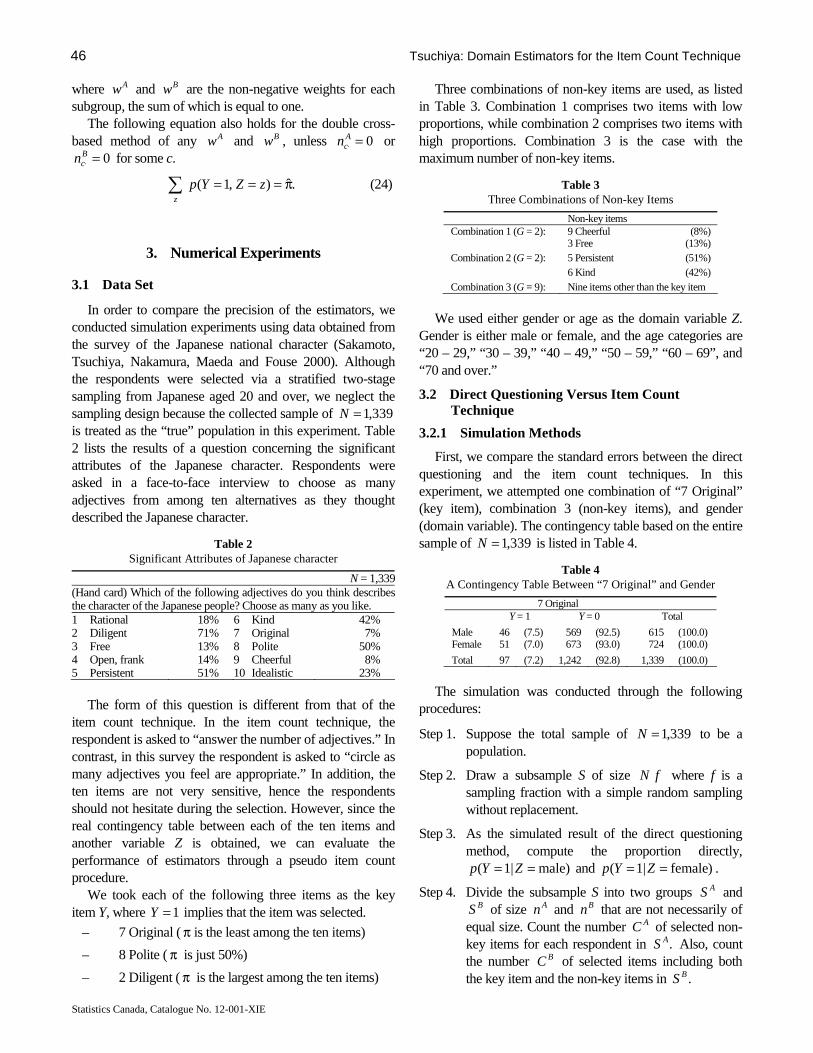
46 Tsuchiya: Domain Estimators for the Item Count Technique
Statistics Canada, Catalogue No. 12-001-XIE
where Aw and Bw are the non-negative weights for each subgroup, the sum of which is equal to one.
The following equation also holds for the double cross-based method of any Aw and Bw , unless 0=⋅
Acn or
0=⋅Bcn for some c.
.ˆ),1( π===∑ zZYpz
(24)
3. Numerical Experiments
3.1 Data Set In order to compare the precision of the estimators, we
conducted simulation experiments using data obtained from the survey of the Japanese national character (Sakamoto, Tsuchiya, Nakamura, Maeda and Fouse 2000). Although the respondents were selected via a stratified two-stage sampling from Japanese aged 20 and over, we neglect the sampling design because the collected sample of 339,1=N is treated as the “true” population in this experiment. Table 2 lists the results of a question concerning the significant attributes of the Japanese character. Respondents were asked in a face-to-face interview to choose as many adjectives from among ten alternatives as they thought described the Japanese character.
Table 2 Significant Attributes of Japanese character
N = 1,339(Hand card) Which of the following adjectives do you think describes the character of the Japanese people? Choose as many as you like. 1 Rational 18% 6 Kind 42% 2 Diligent 71% 7 Original 7% 3 Free 13% 8 Polite 50% 4 Open, frank 14% 9 Cheerful 8% 5 Persistent 51% 10 Idealistic 23%
The form of this question is different from that of the item count technique. In the item count technique, the respondent is asked to “answer the number of adjectives.” In contrast, in this survey the respondent is asked to “circle as many adjectives you feel are appropriate.” In addition, the ten items are not very sensitive, hence the respondents should not hesitate during the selection. However, since the real contingency table between each of the ten items and another variable Z is obtained, we can evaluate the performance of estimators through a pseudo item count procedure.
We took each of the following three items as the key item Y, where 1=Y implies that the item was selected.
– 7 Original ( π is the least among the ten items)
– 8 Polite ( π is just 50%)
– 2 Diligent ( π is the largest among the ten items)
Three combinations of non-key items are used, as listed in Table 3. Combination 1 comprises two items with low proportions, while combination 2 comprises two items with high proportions. Combination 3 is the case with the maximum number of non-key items.
Table 3 Three Combinations of Non-key Items
Non-key items Combination 1 (G = 2): 9 Cheerful
3 Free (8%)
(13%) Combination 2 (G = 2): 5 Persistent
6 Kind (51%) (42%)
Combination 3 (G = 9): Nine items other than the key item We used either gender or age as the domain variable Z.
Gender is either male or female, and the age categories are “20 – 29,” “30 – 39,” “40 – 49,” “50 – 59,” “60 – 69”, and “70 and over.” 3.2 Direct Questioning Versus Item Count Technique 3.2.1 Simulation Methods
First, we compare the standard errors between the direct questioning and the item count techniques. In this experiment, we attempted one combination of “7 Original” (key item), combination 3 (non-key items), and gender (domain variable). The contingency table based on the entire sample of 339,1=N is listed in Table 4.
Table 4 A Contingency Table Between “7 Original” and Gender
7 Original Y = 1 Y = 0 Total
Male 46 (7.5) 569 (92.5) 615 (100.0) Female 51 (7.0) 673 (93.0) 724 (100.0)
Total 97 (7.2) 1,242 (92.8) 1,339 (100.0) The simulation was conducted through the following
procedures: Step 1. Suppose the total sample of 339,1=N to be a
population. Step 2. Draw a subsample S of size fN where f is a
sampling fraction with a simple random sampling without replacement.
Step 3. As the simulated result of the direct questioning method, compute the proportion directly,
)male|1( == ZYp and )female|1( == ZYp . Step 4. Divide the subsample S into two groups AS and
BS of size An and Bn that are not necessarily of equal size. Count the number AC of selected non-key items for each respondent in .AS Also, count the number BC of selected items including both the key item and the non-key items in .BS
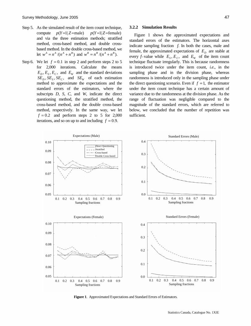
Survey Methodology, June 2005 47
Statistics Canada, Catalogue No. 1XIE
Step 5. As the simulated result of the item count technique, compute )male|1( == ZYp )female|1( == ZYp and via the three estimation methods; stratified method, cross-based method, and double cross-based method. In the double cross-based method, we let )/( BAAA nnnw += and )./( BABB nnnw +=
Step 6. We let 1.0=f in step 2 and perform steps 2 to 5 for 2,000 iterations. Calculate the means
,,, CSD EEE and WE and the standard deviations ,,, CSD SESESE and WSE of each estimation
method to approximate the expectations and the standard errors of the estimators, where the subscripts D, S, C, and W, indicate the direct questioning method, the stratified method, the cross-based method, and the double cross-based method, respectively. In the same way, we let
2.0=f and perform steps 2 to 5 for 2,000 iterations, and so on up to and including .9.0=f
3.2.2 Simulation Results Figure 1 shows the approximated expectations and
standard errors of the estimators. The horizontal axes indicate sampling fraction f. In both the cases, male and female, the approximated expectations of DE are stable at every f – value while ,, CS EE and WE of the item count technique fluctuate irregularly. This is because randomness is introduced twice under the item count, i.e., in the sampling phase and in the division phase, whereas randomness is introduced only in the sampling phase under the direct questioning scenario. Even if ,1=f the estimator under the item count technique has a certain amount of variance due to the randomness at the division phase. As the range of fluctuation was negligible compared to the magnitude of the standard errors, which are referred to below, we concluded that the number of repetition was sufficient.
Figure 1. Approximated Expectations and Standard Errors of Estimators.
Expectations (Male)
Expectations (Female)
Standard Errors (Male)
Standard Errors (Female)
Direct Questioning Stratified Cross-based Double Cross-based
0.1 0.2 0.3 0.4 0.5 0.6 0.7 0.8 0.9 Sampling fractions
0.1 0.2 0.3 0.4 0.5 0.6 0.7 0.8 0.9 Sampling fractions
0.1 0.2 0.3 0.4 0.5 0.6 0.7 0.8 0.9 Sampling fractions
0.1 0.2 0.3 0.4 0.5 0.6 0.7 0.8 0.9 Sampling fractions
0.10 0.09 0.08 0.07 0.06 0.05
0.10 0.09 0.08 0.07 0.06 0.05
0.4 0.3 0.2 0.1 0.0
0.4 0.3 0.2 0.1 0.0

48 Tsuchiya: Domain Estimators for the Item Count Technique
Statistics Canada, Catalogue No. 12-001-XIE
The standard errors, ,DSE of the direct questioning method is considerably small compared to those of the item count. In the case of the item count, standard errors do not converge to zero even if .1=f As noted above, this is because the randomness is also introduced in the division phase. The standard errors of the stratified method are obviously larger than those of the two cross-based methods. The lines indicating the results for the cross-based method and the double cross-based method almost overlap, and appear to have no outstanding differences.
In order to evaluate the amount of variances or standard errors of estimators, let us consider the following indices that are analogous to the design effect (Kish 1965),
,Def 2
2
,
2
1
21
M
MMM SE
SE=
where 1M and 2M indicate one of the four methods D, S, C, and W. Although we have omitted the detailed results, roughly summarized, DC ,Def ranges from 50 (when
1.0=f ) to 700 (when 9.0=f ). That is, even if we use the cross-based method, the standard errors of the item count inflate nearly seven- to twenty-six-fold as compared to the direct questioning. However, the variance reduction attained by using the double cross-based method instead of the stratified method ranges from 39.0Def , =SW (male) to 0.55 (female). In other words, the standard errors of the double cross-based method are reduced to about 62 percent of the stratified estimate at the minimum, and 74 percent at the maximum. 3.3 Stratified Versus Cross-based Method 3.3.1 Simulation Methods
In the previous section, the precision of the cross-based and the double cross-based method appeared to be larger than those of the stratified method. We shall check the precision of these methods for other combinations of the key item, the combination of non-key items, and the domain variable Z by simulation experiments.
In this section, we used all samples as follows: Step 1. Compute )|1( zZYP == for each z based on all
data of size .339,1=N Step 2. Divide the total sample ( 339,1=N ) randomly into
group A and group B of size An and Bn where .BA nnN +=
Step 3. Count the number AC of selected non-key items for each respondent of group A, and count the number BC of selected items, including both the key item and non-key items, in group B.
Step 4. Estimate )|1( zZYp == by the stratified method, the cross-based method, and the double cross-based method, respectively.
Step 5. Compute the chi-squared distance 2e between )|1( zZYP == and )|1( zZYp == for each
method.
∑ ====−===
z zZYP
zZYPzZYpe
)|1(
)}|1()|1({ 22
Step 6. Repeat the above procedure from step 2 through step 5 for 1,000 iterations. Calculate the means and the standard deviations of 2e for each method.
In addition, we simulated the stratified method under the randomized response for references via the following procedure: Step 1. Let p be a proportion as described below. Divide
the total sample )339,1( =N randomly into two groups. Group A is composed of Np respondents, and group B is composed of )1( pN − respondents.
Step 2. Let Azn be the number of respondents who selected
the key item and zZ = in group A. Let Bzn be the
number of respondents who did not select the key item and zZ = in group B. Let zn be the number of respondents with .zZ = Compute
.12
/)(1
339,1)|1( ⎟⎟
⎠
⎞⎜⎜⎝
⎛−++−===
p
nnnpnzZYp z
Bz
Azz
Step 3. Calculate 2e employing the same equation as used
in the item count technique. Step 4. Repeat the above procedure from step 1 through
step 3 for 1,000 iterations. Calculate the means and the standard deviations of 2e for each method.
We used three p values; ,3.0,2.0 == pp and .4.0=p 3.3.2 Simulation Results
Table 5 and Table 6 list the means and the standard deviations of 1,000 s2e for the domain variable Z of gender and age, respectively. A smaller mean of “ 2e –value” indi-cates that the domain estimators are more precise. In some repetitions, illogical estimates ),|1( zZYp == which deviate from the range [0, 1], were obtained. The columns of the tables denoted by “under” indicate the number of repetitions when at least one of the estimates
)|1( zZYp == was under 0, and “over” indicates that the estimates were over 1. Ideally, the figures of the columns of “illogical p” should be 0.
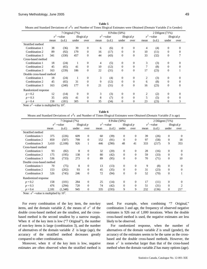
Survey Methodology, June 2005 49
Statistics Canada, Catalogue No. 12-001-XIE
Table 5 Means and Standard Deviations of s2e and Number of Times Illogical Estimates were Obtained (Domain Variable Z is Gender)
7 Original (7%) 8 Polite (50%) 2 Diligent (71%) 2e –value illogical p 2e –value illogical p 2e –value illogical p
mean (s.d.) under over mean (s.d.) under over mean (s.d.) under over Stratified method Combination 1 38 (36) 39 0 6 (6) 0 0 4 (4) 0 0 Combination 2 89 (92) 179 0 16 (17) 0 0 10 (11) 0 0 Combination 3 341 (330) 457 0 44 (43) 0 0 33 (32) 0 7 Cross-based method Combination 1 18 (24) 1 0 4 (5) 0 0 3 (3) 0 0 Combination 2 45 (65) 41 0 10 (12) 0 0 7 (8) 0 0 Combination 3 163 (239) 186 0 22 (31) 0 0 17 (23) 0 1 Double cross-based method Combination 1 18 (24) 1 0 3 (4) 0 0 2 (3) 0 0 Combination 2 45 (65) 31 0 9 (12) 0 0 6 (8) 0 0 Combination 3 163 (240) 177 0 21 (31) 0 0 16 (23) 0 0
Randomized response p = 0.2 12 (14) 0 0 3 (3) 0 0 2 (2) 0 0 p = 0.3 35 (43) 41 0 8 (7) 0 0 5 (5) 0 0 p = 0.4 158 (181) 305 0 35 (34) 0 0 23 (23) 0 3
Note: 2e –value is multiplied by 103. Table 6
Means and Standard Deviations of s2e and Number of Times Illogical Estimates were Obtained (Domain Variable Z is age)
7 Original (7%) 8 Polite (50%) 2 Diligent (71%) 2e –value illogical p 2e –value illogical p 2e –value illogical p
mean (s.d.) under over mean (s.d.) under over mean (s.d.) under over Stratified method Combination 1 375 (226) 609 0 60 (39) 0 0 39 (26) 0 0 Combination 2 859 (507) 799 0 152 (91) 0 0 97 (58) 0 18 Combination 3 3,410 (2,108) 926 1 446 (290) 48 41 333 (217) 9 353 Cross-based method Combination 1 93 (82) 8 0 32 (20) 0 0 28 (16) 0 0 Combination 2 175 (195) 138 0 80 (42) 0 0 59 (33) 0 0 Combination 3 536 (733) 273 0 89 (95) 0 0 70 (71) 0 10 Double cross-based method Combination 1 70 (75) 8 0 13 (13) 0 0 9 (8) 0 0 Combination 2 153 (202) 93 0 45 (35) 0 0 31 (23) 0 0 Combination 3 526 (745) 246 0 72 (94) 0 0 52 (70) 0 1
Randomized response p = 0.2 158 (101) 284 0 25 (14) 0 0 17 (11) 0 0 p = 0.3 476 (294) 720 0 74 (42) 0 0 51 (31) 0 2 p = 0.4 2,181 (1,348) 945 0 335 (193) 9 9 232 (136) 0 217
Note: 2e –value is multiplied by 103. For every combination of the key item, the non-key
items, and the domain variable Z, the means of 2e of the double cross-based method are the smallest, and the cross-based method is the second smallest by a narrow margin. When π of the key item is low (“7 Original”), the number of non-key items is large (combination 3), and the number of alternatives of the domain variable Z is large (age), the accuracy of the stratified method decreases greatly compared to other combinations.
Moreover, when π of the key item is low, negative estimates are often observed when the stratified method is
used. For example, when combining “7 Original,” combination 3 and age, the frequency of observed negative estimates is 926 out of 1,000 iterations. When the double cross-based method is used, the negative estimates are less likely to be observed.
For randomized response, when the number of alternatives of the domain variable Z is small (gender), the accuracy of the estimates seems to be the same as the cross-based and the double cross-based methods. However, the mean 2e is somewhat larger than that of the cross-based method when the domain variable Z has many options (age).
50 Tsuchiya: Domain Estimators for the Item Count Technique
Statistics Canada, Catalogue No. 12-001-XIE
The randomized response, for which only the stratified method is available, also suffers from negative estimates, particularly when π is small (“7 Original”).
4. Conclusion
The following results were obtained through simulation experiments:
– The cross-based method or the double cross-based method, which is proposed in this article, should be used to estimate domain parameters when the data is obtained via the item count technique. In the first simulation, the variances of cross-based estimators were reduced to 39 percent of the variance of the stratified estimate at the minimum to 55 percent at the maximum. In the simulation studies, the double cross-based method made no drastic improvement in precision as compared to the cross-based method.
– Even when the double cross-based method is used, the standard errors of the domain estimators are much larger than those of the direct questioning technique.
The true )1( ===π YPY of a question, to which respondents evade giving a truthful answer, would be often small. In addition, an indirect questioning technique is used in order to ensure protection of privacy. The respondents feel that their privacy is secured when many non-key items are included (Hubbard et al. 1989). The simulation studies show that in such situations, the cross-based method or double cross-based method is more efficient than the traditional stratified method.
The domain estimators obtained by the traditional stratified method are generally inconsistent with the estimator π as shown in (10). Poststratified estimator PSπ by the domain variable addressed is essential in order to ensure consistency. Alternatively, we have to divide the total sample into two subgroups so that the distributions of their domain variable match in advance. On the contrary, the domain estimators obtained by the cross-based and the double cross-based methods are consistent with π as shown in (21). However, it does not mean that the cross-based method automatically adjusts the two subgroups so that the sample distributions of the domain variable match between the two subgroups. For the cross-based method, post-stratification by the domain variables or other demographic variables is also admissible, but not indispensable.
Even when the double cross-based method is used, negative domain estimates are sometimes observed. It is
possible to avoid negative estimates by letting a negative estimate cq of cQ in (23) be zero. However, such an adjustment produces a positive bias in ).|1( zZYp ==
The data of the survey of the Japanese national character, which were used in the simulation experiments, are neither sensitive nor were they obtained via the item count technique. In the future, the performance of the proposed method should be assessed by applying it to data obtained via the item count technique.
Acknowledgements
The author is grateful to two anonymous reviewers and an assistant editor for their helpful comments on a previous version of this paper.
References
Abul-Ela, Abdel-Latif, A., Greenberg, B.G. and Horvitz, D.G. (1967). A multiproportions RR model. Journal of the American Statistical Association, 62, 990-1008.
Chaudhuri, A., and Mukerjee, R.M. (1988). Randomized Response: Theory and Techniques. New York: Marcel Dekker.
Cochran, W.G. (1977). Sampling Techniques, 3rd ed. New York: John Wiley & Sons, Inc.
Droitcour, J., Caspar, R.A., Hubbard, M.L., Parsley, T.L., Visscher, W. and Ezzati, T.M. (1991). The item count technique as a method of indirect questioning: A review of its development and a case study application. In Measurement Errors in Surveys (Eds. P.P. Biemer, et al.), New York: John Wiley & Sons, Inc.
Droitcour, J.A., Larson, E.M. and Scheuren, F.J. (2001). The three card method: Estimating sensitive survey items-with permanent anonymity of response. Proceedings of the Social Statistics Section of the American Statistical Association. Alexandria, V.A.: American Statistical Association.
Greenberg, B.G., Abul-Ela, Abdel-Latif, A., Simmons, W.R. and Horvitz, D.G. (1969). The unrelated question RR model: Theoretical framework. Journal of the American Statistical Association, 64, 520-539.
Hubbard, M.L., Casper, R.A. and Lessler, J.T. (1989). Respondent reactions to item count lists and randomized response. Proceedings of the Survey Research Section of the American Statistical Association. Washington, D.C.: American Statistical Association. 544-548.
Kish, L. (1965). Survey Sampling. New York: John Wiley & Sons, Inc.
Lessler, J.T., and O’Reilly J.M. (1997). Mode of interview and reporting sensitive issues: Design and implementation of audio computer-assisted self-interviewing. NIDA Research Monograph, 167, 366-382.
Miller, J.D. (1985). The nominative technique: A new method of estimating heroin prevalence. NIDA Research Monograph, 57, 104-124.
Rao, J.N.K. (2003). Small Area Estimation. New Jersey: John Wiley & Sons, Inc.

Survey Methodology, June 2005 51
Statistics Canada, Catalogue No. 12-001-XIE
Sakamoto, Y., Tsuchiya, T., Nakamura, T., Maeda, T. and Fouse, D.B. (2000). A Study of the Japanese National Character: The Tenth Nationwide Survey (1998). Tokyo: The Institute of Statistical Mathematics Research Report General Series 85.
Särndal, C.-E., Swesson, B. and Wretman, J. (1992). Model Assisted Survey Sampling. New York: Springer-Verlag.
Schuman, H., and Presser, S. (1981). Questions & Answers in Attitude Surveys. New York: Academic Press.
Takahasi, K., and Sakasegawa, H. (1977). A randomized response technique without making use of any randomizing device. Annals of the Institute of Statistical Mathematics, 29, 1-8.
U.S. General Accounting Office (1999). Survey Methodology. An Innovative Technique for Estimating Sensitive Items. Washington D.C.: General Accounting Office.
Warner, S.L. (1965). Randomized response: A survey technique for eliminating evasive answer bias. Journal of the American Statistical Association, 60, 63-69.
Warner, S.L. (1971). The linear randomized response model. Journal of the American Statistical Association, 66, 884-888.

Survey Methodology, June 2005 53 Vol. 31, No. 1, pp. 53-63 Statistics Canada, Catalogue No. 12-001-XIE
Editing Systematic Unity Measure Errors Through Mixture Modelling
Marco Di Zio, Ugo Guarnera and Orietta Luzi 1
Abstract
In Official Statistics, data editing process plays an important role in terms of timeliness, data accuracy, and survey costs. Techniques introduced to identify and eliminate errors from data are essentially required to consider all of these aspects simultaneously. Among others, a frequent and pervasive systematic error appearing in surveys collecting numerical data, is the unity measure error. It highly affects timeliness, data accuracy and costs of the editing and imputation phase. In this paper we propose a probabilistic formalisation of the problem based on finite mixture models. This setting allows us to deal with the problem in a multivariate context, and provides also a number of useful diagnostics for prioritising cases to be more deeply investigated through a clerical review. Prioritising units is important in order to increase data accuracy while avoiding waste of time due to the follow up of non-really critical units.
1. Marco Di Zio, Ugo Guarnera and Orietta Luzi, Italian National Statistical Institute, Via Cesare Balbo 16, 00184 Roma, Italy.
Key Words: Editing; Random error; Systematic error; Selective editing; Model-based cluster analysis.
1. Introduction Elements determining the quality of an Editing and
Imputation (E&I) process are various and have been widely discussed in literature (Granquist 1995). We deal with a particular non-sampling error that highly affects two main competing quality dimensions: timeliness and data accura-cy. As far as accuracy is concerned, we adopt the definition suggested in the Encyclopedia of Statistical Sciences, (1999): “accuracy concerns the agreement between statistics and target characteristics”. A number of factors can cause inaccuracy along the overall statistical survey process. Inaccuracy can be reduced during the E&I phase, which can be viewed as an “accuracy improvement tool by which erroneous or highly suspect data are found, and if necessary corrected (imputed)” (Federal Committee on Statistical Methodology 1990).
Due to the complexity of investigated phenomena and the existence of several types of non-sampling errors the E&I phase can be a very complex and time consuming task (Granquist 1996). In the specialised literature a common error classification leads to define two different error typologies: systematic error and random error. The former relates to errors which go in the same direction and lead to a bias in statistics, while the latter refers to errors which spread randomly around zero and affect the variance of estimates (Encyclopedia of Statistical Sciences 1999). Un-derstanding nature of errors is not only useful in order to identify their source and to assess their effects on estimates, but also to adopt the most appropriate methodology to deal with them (Di Zio and Luzi 2002). While the Fellegi – Holt approach (Fellegi and Holt 1976) is a well-established paradigm to deal with random errors, systematic errors are generally treated by means of ad hoc solutions (see for
instance Euredit 2003, Vol. 1, Chapter 5). Systematic errors are generally treated before dealing with random errors, particularly when the latter are tackled through automatic software, like for instance the Generalised Editing and Imputation System (GEIS) (Kovar, Mac Millan and Whitridge 1988) and more recently De Waal (2003).
In the family of systematic errors, one that has a high impact on final estimates and that frequently affects data in statistical surveys measuring quantitative characteristics (e.g., business surveys) is the unity measure error times a constant factor (e.g., 100 or 1,000). This error is due to the erroneous choice, by some respondents, of the unity measure in reporting the amount of some questionnaire items.
As real examples of surveys affected by this type of error, we selected two ISTAT investigations: the 1997 Italian Labour Cost Survey (LCS) and the 1999 Italian Water Survey System (WSS).
The LCS is a periodic sample survey that collects information on employment, worked hours, wages and salaries and labour cost on about 12,000 enterprises with more than 10 employees. In Figure 1 the logarithm of Labour Cost (LCOST), Number of Employees (LEMPLOY), Worked Hours (LWORKEDH) are repre-sented in a scatter plot matrix. Note that the employment variable at this editing stage is error free because of a preliminary check with respect to information from business registers (Cirianni, Di Zio, Luzi and Seeber 2000). The analysis of Figure 1 shows that Labour Cost is affected by two types of unity measure error (i.e., 1 million and 1,000 factor), while Worked Hours exhibits only the 1,000 factor error. These errors cause the different clusters in Figure 1. Note that the clusters in the low left corners of each scatter plot represent non-erroneous data.
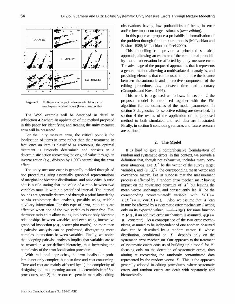
54 Di Zio, Guarnera and Luzi: Editing Systematic Unity Measure Errors Through Mixture Modelling
Statistics Canada, Catalogue No. 12-001-XIE
Figure 1. Multiple scatter plot between total labour cost, employees, worked hours (logarithmic scale). The WSS example will be described in detail in
subsection 4.2 where an application of the method proposed in this paper for identifying and treating the unity measure error will be presented.
For the unity measure error, the critical point is the localisation of items in error rather than their treatment. In fact, once an item is classified as erroneous, the optimal treatment is uniquely determined and consists in a deterministic action recovering the original value through an inverse action (e.g., division by 1,000) neutralising the error effect.
The unity measure error is generally tackled through ad hoc procedures using essentially graphical representations of marginal or bivariate distributions, and ratio edits. A ratio edit is a rule stating that the value of a ratio between two variables must lie within a predefined interval. The interval bounds are generally determined through a priori knowledge or via exploratory data analysis, possibly using reliable auxiliary information. For this type of error, ratio edits are effective when one of the two variables is error free. Fur-thermore ratio edits allow taking into account only bivariate relationships between variables and even using interactive graphical inspection (e.g., scatter plot matrix), no more than a pairwise analysis can be performed, disregarding more complex interactions between variables. Finally, we notice that adopting pairwise analyses implies that variables are to be treated in a pre-defined hierarchy, thus increasing the complexity of the error localisation procedure.
With traditional approaches, the error localisation prob-lem is not only complex, but also time and cost consuming. Time and cost are mainly affected by: 1) the complexity of designing and implementing automatic deterministic ad hoc procedures, and 2) the resources spent in manually editing
observations having low probabilities of being in error and/or low impact on target estimates (over-editing).
In this paper we propose a probabilistic formalisation of the problem through finite mixture models (McLachlan and Basford 1988; McLachlan and Peel 2000).
This modelling can provide a principled statistical approach, allowing an estimate of the conditional probabil-ity that an observation be affected by unity measure error. The advantage of the proposed approach is that it represents a general method allowing a multivariate data analysis, and providing elements that can be used to optimise the balance between the automatic and interactive components of the editing procedure, i.e., between time and accuracy (Granquist and Kovar 1997).
This work is organised as follows. In section 2 the proposed model is introduced together with the EM algorithm for the estimates of the model parameters. In section 3 diagnostics for selective editing are described. In section 4 the results of the application of the proposed method to both simulated and real data are illustrated. Finally, in section 5 concluding remarks and future research are outlined.
2. The Model
It is hard to give a comprehensive formalisation of random and systematic errors. In this context, we provide a definition that, though not exhaustive, includes many com-mon situations. Let *X be the vector of the survey target variables, and ),( ∑*μ the corresponding mean vector and covariance matrix. Let us suppose that the measurement process is affected by a random error mechanism R having impact on the covariance structure of *X but leaving the mean vector unchanged, and consequently let X be the corresponding “contaminated” variable, with =)(XE
=)( *XE =, )(Var Xμ .∑ Also, we assume that X can in turn be affected by a systematic error mechanism S acting only on its expected value: )(μ μϕ⎯→⎯S for some function ϕ (e.g., if an additive error mechanism is assumed, =ϕ )(μ
).constant+μ As a consequence of the two error mecha-nisms, assumed to be independent of one another, observed data can be described by a random vector Y whose distribution, conditional on ,X depends only on the systematic error mechanism. Our approach to the treatment of systematic errors consists of building up a model for Y focusing only on the detection of systematic errors, thus aiming at recovering the randomly contaminated data represented by the random vector .X This is the approach generally adopted in editing procedures, where systematic errors and random errors are dealt with separately and hierarchically.
LWORKEDH
LEMPLOY
LCOSTS
Survey Methodology, June 2005 55
Statistics Canada, Catalogue No. 12-001-XIE
The previous definition of systematic error includes unity measure error, once data have been transformed in loga-rithmic scale. In fact, unity measure error generally acts multiplying variables by a constant factor. Hence data in error appear in log-scale as translated by a vector of constants, that depends on which items are in error (“error pattern”), while the covariance structure is the same for each error pattern. Moreover, as matter of fact, in business sur-veys variables are frequently considered log-normal. Thus in logarithmic scale the Gaussian setting can be adopted.
Following the formalisation so far introduced, our goal becomes to assign each single observation to a specific “error pattern”, that corresponds to localise items in error. If we interpret each single error pattern as a “cluster”, the error localisation problem is transformed in a cluster analysis problem, and we can exploit experiences from the model-based cluster analysis theory (Fraley and Raftery 2002).
More in detail, let us suppose we have n independent observations ),...,,( 1 iqii YY=Y ,...,,1 ni = corresponding to the −q dimensional vectors )...,,( 1 iqii XX=X with p.d.f. ),;...,,( 1 θqxxf such that =)...,,( 1 qXXE
,= μ)μ...,,μ( 1 q and =)...,,(Var 1 qXX .∑ Based on the assumption that systematic errors affect the
random vector X only by transforming its expected value μ into ),(μgϕ where ,RR:)( qq
g →⋅ϕ for ,...,,1 hg = are a set of known functions, the functions gϕ characterise univocally h distinct clusters (error patterns), differing each other only on the location parameter. For instance, if the systematic error possibly affects all the variables sX for
,...,,1 qs = in the same manner by transforming their expected values sμ according to ,μμ Css +→ where C is a known constant, the number of clusters will be ,2qh = i.e., the number of different combinations of error occurrence on the q variables (including the case of no error). In this case, each function gϕ and each corresponding cluster, is associated with one of the q2 possible sub-sets of variables affected by the error; e.g., the group G characterised by the mean vector =Gμ
,)μ...,,μ,μ,μ,μ( 4321 qC+ is a cluster of units with error affecting only the variable 2X . We remark that we assume a common covariance matrix because we make the hypothesis that the possible random error acts in the same way on all the data.
For the error localisation purpose we follow a model-based approach based on finite mixture models, where each mixture component ,...,,1, hgGg = represents a single error pattern. Formally, we assume that ,)...,,( 1 iqii YY=Y for ,...,,1 ni = are iid w.r.t ),; (1 tt
ht t f θ⋅π∑ = where
1=π∑t t and 0≥πt . The mixing parameters tπ represent the probability that an observation belongs to the tht mixture component.
In order to classify an observation iy in one of the h groups, we compute the posterior probability
=τ ),;( πθig y pr( thi observation ),,;| πθigG y∈ that is
....,,1
);();(),;(1
hg
ffh
ttittiggig
=
ππ=τ ∑=
θθπθ yyy g
(1)
The thi observation is assigned to the cluster ,tG if
.;...,,1),;(),;( tghgigit ≠=πτ>τ θπθ yy
The previous allocation rule is the optimal solution for the classification problem, in the sense that it minimises the overall error rate (Anderson 1984, Chapter 6 ).
Since, in place of the parameters ,),( πθ generally unknown, we use the maximum likelihood estimates
),ˆ,ˆ( πθ the classification rule becomes:
.;...,,1)ˆ,ˆ;()ˆ,ˆ;( tghgigit ≠=πτ>πτ θθ yy (2)
We assume that the );( ttf θy is a multivariate normal density ,( tμMN )∑ and that each function )(⋅gϕ acts on the mean vector μ as a translation: ,)( gg C+=ϕ μμ where
gC represents the translation vector for the mean of the thg cluster, and it is supposed to be known. This setting, as already noticed, is suitable for dealing with unity measure error. In order to compute the likelihood estimates, we use the EM algorithm as suggested in McLachlan and Basford (1988). Nevertheless, an additional effort is necessary to adapt the algorithm to our particular situation, where the mean vectors of the mixture components are linked by a known functional relationship. Thus, while in the non-constrained case (McLachlan and Basford 1988) a different mean vector has to be estimated for each mixture component, in our constrained situation only one mean vector needs to be estimated. The resulting modified EM algorithm consists of defining some initial guess for the parameters to be estimated forˆ )0(
gπ ,...,,1 hg = ,ˆ( )0(μ )ˆ )0(∑ and applying until convergence the following
recursive scheme: i) compute the posterior probabilities =τ )(k
gi ) ,;()( πθi
kg yτ under the current estimates ,ˆ )(kπ
,ˆ )(kμ )(ˆ k∑ (k is the index referring to the thk cycle)
( ) ( )
( ) ( )⎪⎭
⎪⎬⎫
⎪⎩
⎪⎨⎧
−⎟⎠
⎞⎜⎝
⎛−−π
⎪⎭
⎪⎬⎫
⎪⎩
⎪⎨⎧
−⎟⎠
⎞⎜⎝
⎛−−π
=
τ
−
=
−
∑ )(1)(
)(
1
)(
)(1)(
)()(
)(
ˆˆ2
1expˆ
ˆˆ2
1expˆ
ˆ
ˆ
ˆ
kti
kk
ti
h
t
kt
kgi
kk
gik
g
kgi
'
'
μμ
μμ
yy
yy
∑
∑
56 Di Zio, Guarnera and Luzi: Editing Systematic Unity Measure Errors Through Mixture Modelling
Statistics Canada, Catalogue No. 12-001-XIE
ii) calculate the new estimates by the following recursive equations:
nn
i
kgi
kg /ˆˆ
1
)()1( ∑=
+ τ=π
∑∑∑=
+
==
+ π−τ=h
g
kgg
n
ii
kgi
h
g
k n1
)1(
1
)(
1
)1( ˆ/ˆˆ Cyμ
( )( ) .ˆ/
ˆ
)1()1()1(
1 1
)()1(ˆ
+++
= =
+
π−−
τ=∑∑
kg
kgi
kgi
h
g
n
i
kgi
k
n'μμ yy
∑
We remark that )(ˆ kgμ stands for g
k C+)(μ . In practical applications, it turns out that a crucial role is
played by the choice of starting points, as usual in the EM algorithms (see Biernacki, Celeux and Govaert 2003). To overcome this problem, we use an initialisation strategy, following Biernacki et al. (2003), consisting of several short runs in terms of number of iterations, of the algorithm from random initialisations followed by a long run of EM from the solution maximising the observed log-likelihood.
It is worth to mention that, due to the location constraints, the parameters to be estimated are sensibly fewer than those in a usual mixture problem. Actually the higher is the number of variables analysed the bigger is this difference; for instance in the case of three variables and 8 clusters we need to estimate 16 parameters instead of 37. This aspect is particularly important when we deal with small samples. Moreover, constraints on cluster locations make easier to identify “rare clusters”. In fact, being the relative distances between mean vectors fixed, the estimation problem reduces to estimate the location of the convex polyhedron whose vertices are the cluster centroids. In other words, since the location of one centroid univocally determines the positions of all the others, small cluster parameters are more easily estimated than if they were not constrained.
Since the introduced modelling is based on the assumption that observations are normally distributed, model validation is an issue to take into account. The problem of assessing normality in mixture models is well described in McLachlan and Basford (1988). It is essentially based on the quantities gia described in the following. Let
giy for gmi ˆ...,,1= be the observations assigned to the thg cluster for hg ...,,1= , according to the estimated
model. Let gip be the value calculated using the estimated parameters, following the formula:
,;ˆ,ˆ)1ˆ()(
;ˆ,)/ˆ(ˆ
ˆ
ˆ
⎟⎠⎞
⎜⎝⎛−−+ν
⎟⎠⎞
⎜⎝⎛ν
=∑
∑
ggigg
ggig
gi
Dmmq
Dqmp
μ
μ
y
y (3)
where );,(D M⋅⋅ is the Mahalanobis squared distance based on the metric ,M and .qhn −−=ν We define gia
as the area to the right of the gip value under the ν,qF distribution (for details see McLachlan and Basford 1988, Chapter 2).
Under the normality assumption, gia for gmi ˆ...,,1= is approximately uniformly distributed on (0,1). Hawkins (1981) suggests using the Anderson – Darling statistic for assessing the uniform distribution of gia . The gia are also useful to detect outliers, i.e., atypical observations with respect to the model. In McLachlan and Basford (1988) the lower is gia the higher is the probability of giy of being atypical, thus all observations with ,ˆ α<gia where α is a specified threshold, can be considered as atypical. Suggested threshold levels range from 05.0=α to
,005.0=α depending on which outlying observations (more or less extreme values) are to be selected.
3. Diagnostics for Selective Editing
Once the parameters of the mixture have been estimated, we are able to classify data into the different clusters, i.e., for each observation we can assess whether it is in error or not, and which variables are in error. However, different types of critical observations can be identified after the modelling phase: units classified in a cluster, but having a non-negligible probability of belonging to another cluster, and observations that are outliers with respect to the model.
In order to increase data accuracy it would be useful to make a double check on critical observations (through either a clerical review or, in the most difficult cases, a follow-up). On the other hand, in order to reduce possible over-editing and editing costs, the manual review and/or follow up should be concentrated on the most critical observations. The proposed mixture model directly provides diagnostics that can be used to this aim.
A first type of critical units is represented by possibly misclassified observations. In order to measure the degree of belief in the class assigned to an observation iy we can consider the corresponding probability resulting from (2). Observations, for which this probability is not very close to one, have a non-negligible probability to belong to another cluster. These observations are those in the region where the mixture components overlap each other.
In addition to the previous type of critical units, there are other observations that are far from all the clusters (all the mixture components), i.e., outliers with respect to the model. Also these observations represent critical situations. In order to identify this kind of outlier we refer to the quantities ija described in the previous section.
Classification probability and atypicality index gia should be used, according to a selective/significance editing approach (Latouche and Berthelot 1992; Lawrence and McKenzie 2000), to build up appropriate score functions to
Survey Methodology, June 2005 57
Statistics Canada, Catalogue No. 12-001-XIE
prioritise critical units. An example of how to use these diagnostics to this aim is given in subsection 4.2.
4. Illustrative Examples
In this section some experiments carried out in order to investigate the peculiarities of the proposed method are presented. Firstly, through a simulation study, we analyse the performance of the proposed model when applied to data that depart from normality. Secondly, through an application on real data, we describe how this approach can be applied in Official Statistics.
All the experiments are performed using the R environ-ment for statistical computing (http://www.r-project.org/). 4.1 Simulated Example: Departure from Normality
In this experiment we describe the results obtained by applying the mixture approach to the three different populations depicted in the first line of Figure 2. The first distribution is a bivariate normal (MN), hence it represents the case when the model is correctly specified. The second one corresponds to a bivariate t distribution (MT), i.e., it mimes the situation when the departure from normality is essentially in having heavier tails. The last one is a bivariate skew–t distribution (ST) (Azzalini and Capitanio 2003, Azzalini, Dal Cappello and Kotz 2003), and it represents a
population distributed according to an asymmetric distri-bution with heavy tails.
From these distributions we build a four components mixture model by adding to each unit one of the four translation vectors ),0,0(1 =C )),000,1log(,0(2 =C
),0),000,1log((3 =C ))000,1log(),000,1log((4 =C with probabilities ,5.01 =π ,1.02 =π ,1.03 =π and 3.04 =π respectively. These parameters represent the mixing proportions of the mixture model and refer respectively to the probabilities of no translation in the variables, translation in only one of the two variables, and translation in both variables. From each mixture, we draw 100 samples of 1,000 observations. In the second line of Figure 2, we report one of these samples (MN – Mixt, MT – Mixt, ST – Mixt), corresponding to the three different populations MN, MT, ST respectively.
For each sample, we compute the number of correct classifications obtained by using the mixture approach described in section 2. The mean number of correct classifications over the 100 samples is reported in Table 1.
As it can be seen in Table 1, the frequency of correct classifications decreases with the departure from normality. However it seems acceptable also in the critical case ST, where the population is characterised by both asymmetry and heavy tails.
Figure 2. Contour plots of the three bivariate distributions multinormal (MN), t – student (MT), skew – t (ST), and scatter plot of the corresponding mixtures MN – Mixt, MT – Mixt, ST – Mixt.
ST – Mixt MT – Mixt MN – Mixt
ST MT MN
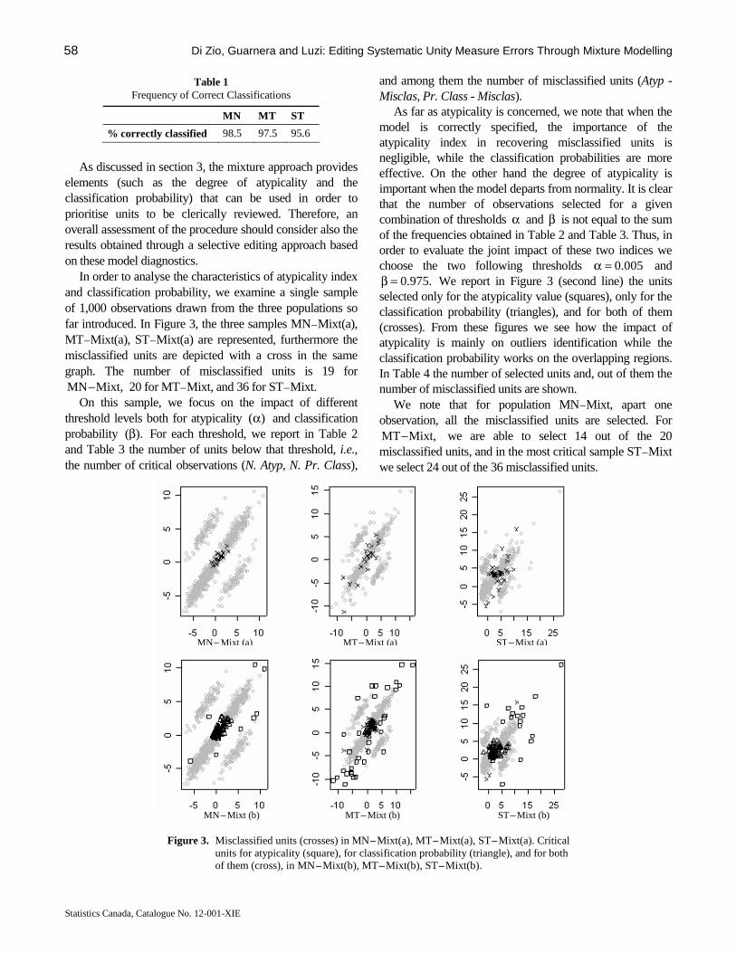
58 Di Zio, Guarnera and Luzi: Editing Systematic Unity Measure Errors Through Mixture Modelling
Statistics Canada, Catalogue No. 12-001-XIE
Table 1 Frequency of Correct Classifications
MN MT ST
% correctly classified 98.5 97.5 95.6
As discussed in section 3, the mixture approach provides
elements (such as the degree of atypicality and the classification probability) that can be used in order to prioritise units to be clerically reviewed. Therefore, an overall assessment of the procedure should consider also the results obtained through a selective editing approach based on these model diagnostics.
In order to analyse the characteristics of atypicality index and classification probability, we examine a single sample of 1,000 observations drawn from the three populations so far introduced. In Figure 3, the three samples MN – Mixt(a), MT – Mixt(a), ST – Mixt(a) are represented, furthermore the misclassified units are depicted with a cross in the same graph. The number of misclassified units is 19 for
Mixt,MN− 20 for MT – Mixt, and 36 for ST – Mixt. On this sample, we focus on the impact of different
threshold levels both for atypicality )(α and classification probability ).(β For each threshold, we report in Table 2 and Table 3 the number of units below that threshold, i.e., the number of critical observations (N. Atyp, N. Pr. Class),
and among them the number of misclassified units (Atyp - Misclas, Pr. Class - Misclas).
As far as atypicality is concerned, we note that when the model is correctly specified, the importance of the atypicality index in recovering misclassified units is negligible, while the classification probabilities are more effective. On the other hand the degree of atypicality is important when the model departs from normality. It is clear that the number of observations selected for a given combination of thresholds α and β is not equal to the sum of the frequencies obtained in Table 2 and Table 3. Thus, in order to evaluate the joint impact of these two indices we choose the two following thresholds 005.0=α and
.975.0=β We report in Figure 3 (second line) the units selected only for the atypicality value (squares), only for the classification probability (triangles), and for both of them (crosses). From these figures we see how the impact of atypicality is mainly on outliers identification while the classification probability works on the overlapping regions. In Table 4 the number of selected units and, out of them the number of misclassified units are shown.
We note that for population MN – Mixt, apart one observation, all the misclassified units are selected. For
Mixt,MT− we are able to select 14 out of the 20 misclassified units, and in the most critical sample ST – Mixt we select 24 out of the 36 misclassified units.
Figure 3. Misclassified units (crosses) in MN – Mixt(a), MT – Mixt(a), ST – Mixt(a). Critical units for atypicality (square), for classification probability (triangle), and for both of them (cross), in MN – Mixt(b), MT – Mixt(b), ST – Mixt(b).
MN – Mixt (b) MT – Mixt (b) ST – Mixt (b)
ST – Mixt (a) MT – Mixt (a) MN – Mixt (a)
Survey Methodology, June 2005 59
Statistics Canada, Catalogue No. 12-001-XIE
Table 2 Number of Critical Observations and Misclassified Units with Respect to Three Different Thresholds for Atypicality
MN – Mixt MT – Mixt ST – Mixt α N. Atyp Atyp – Misclas N. Atyp Atyp – Misclas N. Atyp Atyp – Misclas
0.05 50 1 84 9 68 14 0.01 15 0 50 7 33 8 0.005 8 0 39 7 20 5 0.001 4 0 25 4 14 2
Table 3
Number of Critical Observations and Misclassified Units with Respect to Three Different Thresholds for Classification Probability
MN – Mixt MT – Mixt ST – Mixt β N. Pr. Class Pr. Class – Misclas N. Pr. Class Pr. Class – Misclas N. Pr. Class Pr. Class – Misclas
0.99 119 19 63 12 182 26 0.975 76 18 46 11 82 26 0.95 55 14 35 9 66 21
Table 4
Number of Critical Observations and Misclassified Units with Respect to Atypicality and Classification Probability
MN – Mixt MT – Mixt ST – Mixt Thresholds N.Crit. Units N. Misclas N.Crit. Units N. Misclas N.Crit. Units N. Misclas
=α 0.005, =β 0.975 84 18 79 14 98 24
4.2 An Application to Real Data: The 1999 Italian
Water Survey System In this section we describe an application of the mixture
model approach to real survey data. The data are taken from the 1999 Italian Water Survey System (WSS). The WSS is a census that collects information on water abstraction, supply and usage for the 8,100 Italian municipalities. We restrict our analysis to the municipalities belonging to one of the data domains defined by altimetry (2,041 observations) and to the main variables Total Invoiced Water (TI) and Total Supplied Water (TS). Both these variables refer to water volumes and the respondents are requested to provide them in thousands of cubic meters. The scatter plot on log-scale of per capita water invoiced (WI) versus per capita water supplied (WS) (Figure 4) shows the presence of four clusters corresponding to unity measure error in one, both, or none of the target variables. This is probably due to the misunderstanding of some respondents that expressed water volumes in litres or in cubic meters rather than thousands of cubic meters, as requested. As expected, the two most populated clusters are those corresponding to non-erroneous units and to units where both variables are in error. Nevertheless, we can note the presence of two rare clusters corresponding to observations where the unity measure error affects only TI or only TS respectively.
In Table 5 a label is assigned to each group associated with a specific error pattern. For the sake of simplicity we introduce two flags ETS and ETI assuming value 1 or 0,
depending on whether the corresponding variables are affected by the unity measure error or not, respectively.
In order to identify and correct the unity measure error we apply the procedure described in sections 2 and 3. We classify each observation according to a specific error pattern, i.e., we assign each unit to one of the clusters ,tG for .4...,,1=t The results are reported in Table 6.
For each unit the atypicality index is also calculated and the threshold 005.0=α is chosen in order to flag atypical units. According to this threshold, 71 observations are selected as atypical, marked by “crosses” in Figure 7. Once the values gia are computed according to Formula (3), a test assessing the normality assumption can be performed. Actually, following McLachlan and Basford (1988, Chapter 2), the Anderson – Darling test on the uniformity of gia on each single estimated cluster is performed. The p – values are below 0.001 for the two largest clusters. Since the test is based on asymptotical approximations, we do not take into account the results on the other two rare populations. In Figure 5 we report the empirical sample quantiles versus the normal quantiles of the variables log(WI) and log(WS), focusing only on the subset of data classified as non-erroneous. We notice that departure from normality is mainly due to heavy tails. Based on the results obtained in section 4.1, where the method performed satisfactorily also in non-gaussian setting, we are confident about the good performance of the mixture approach on the survey data. This expected behaviour is confirmed by the application results showed in the following.
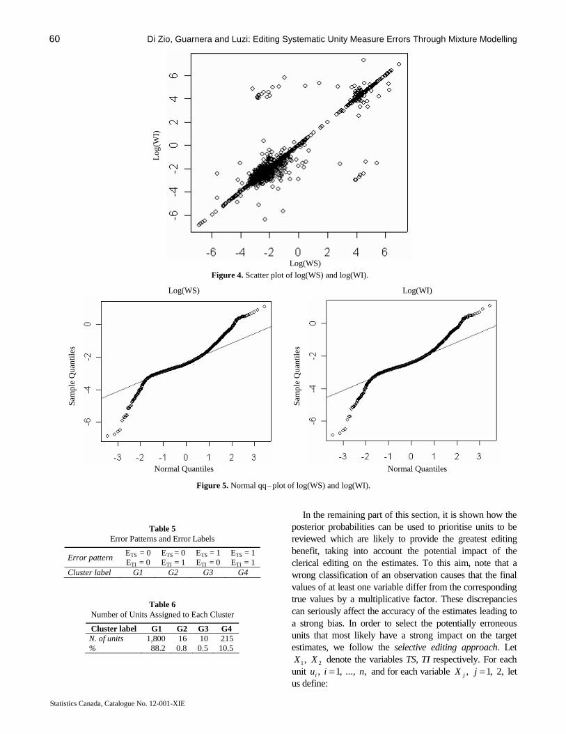
60 Di Zio, Guarnera and Luzi: Editing Systematic Unity Measure Errors Through Mixture Modelling
Statistics Canada, Catalogue No. 12-001-XIE
Figure 4. Scatter plot of log(WS) and log(WI).
Figure 5. Normal qq – plot of log(WS) and log(WI).
Table 5 Error Patterns and Error Labels
Error pattern ETS = 0 ETI = 0
ETS = 0 ETI = 1
ETS = 1 ETI = 0
ETS = 1 ETI = 1
Cluster label G1 G2 G3 G4
Table 6 Number of Units Assigned to Each Cluster
Cluster label G1 G2 G3 G4 N. of units 1,800 16 10 215 % 88.2 0.8 0.5 10.5
In the remaining part of this section, it is shown how the posterior probabilities can be used to prioritise units to be reviewed which are likely to provide the greatest editing benefit, taking into account the potential impact of the clerical editing on the estimates. To this aim, note that a wrong classification of an observation causes that the final values of at least one variable differ from the corresponding true values by a multiplicative factor. These discrepancies can seriously affect the accuracy of the estimates leading to a strong bias. In order to select the potentially erroneous units that most likely have a strong impact on the target estimates, we follow the selective editing approach. Let
21, XX denote the variables TS, TI respectively. For each unit ,...,,1, niui = and for each variable ,2,1, =jX j let us define:
Log
(WI)
Log(WS)
Normal Quantiles
Log(WS) Log(WI)
Normal Quantiles
Sam
ple
Qua
ntil
es
Sam
ple
Qua
ntil
es
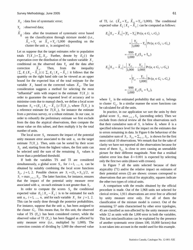
Survey Methodology, June 2005 61
Statistics Canada, Catalogue No. 12-001-XIE
ijX : data free of systematic error;
ijY : observed data;
ijX~
: data after the treatment of systematic error based on the classification through mixture model (i.e.,
ijij YX =~ or 000,1/~
ijij YX = depending on the cluster the unit iu is assigned to).
Let us suppose that the target estimates refer to population totals .)( ijij XXT ∑= Further, denote by )(⋅ξE the expectation over the distribution of the random variable jX conditional on the observed data ijY and the data after correction .
~ijX Then, from the inequality
≤−∑ |)~
(| ξ ijiji XE X |~
| ijiji XXE −∑ ξ it follows that the quantity on the right hand side can be viewed as an upper bound for the expected bias of the total estimate for the variable jX based on the corrected values .
~ijX The last
consideration suggests a method for selecting the most “influential” units with respect to the estimate :)( jXT in order to guarantee the requested level of accuracy and to minimise costs due to manual check, we define a local score function ,)(ˆ/)|
~|( jijijij XTXXES −= ξ where )(ˆ
jXT is a reference estimate for ),( jXT for instance the estimate from a previous survey, or a robust estimate. In our case, in order to robustify the preliminary estimate we first exclude from the data the atypical observations, then compute the mean value on this subset, and then multiply it by the total number of units.
The local score ijS measures the impact of the potential unity measure error associated to the unit iu on the target estimate ).( jXT Then, units can be sorted by their score
ijS and, starting from the highest values, the first units can be selected until the sum of the remaining ijS values is lower than a predefined threshold.
If both the variables TS and TI are considered simultaneously, a global score ,iS for ,...,,1 ni = can be obtained by suitably combining the local score functions
.2,1, =jSij Possible choices are ,2)( 21 iii SSS += or .max 2,1 ijji SS == The latter function, for instance, ensures
that the impact of the potential unity measure error associated with iu on each estimate is not greater than .iS
In order to compute the scores ijS the conditional expected value |
~| ijij XXE −ξ is to be estimated for each
unit ,...,,1, niui = and for each variable jX for .2,1=j This can be easily done through the posterior probabilities. For instance, suppose that the unit iu has been assigned to the cluster .2G This means that, for this unit, the observed value of TS )( 1iY has been considered correct, while the observed value of TI )( 2iY has been flagged as affected by unity measure error (i.e., multiplied by 1,000). The correction consists of dividing by 1,000 the observed value
of TI, i.e. ).000,1/~
,~
( 2211 iiii YXYX == The conditional expected value |
~| ijij XXE −ξ can be computed as follows:
)ˆˆ(000,1
999
)(Pr000,1
)(Pr~
431
4311
211111
iii
iii
iiiii
Y
GGuYY
GGuYYXXE
τ+τ=
∪∈−+
∪∈−=−ξ
),ˆˆ(000,1
999
)(Pr000,1
)(Pr000,1000,1
~
312
312
2
4222
22
iii
ii
i
iii
ii
Y
GGuY
Y
GGuYY
XXE
τ+τ=
∪∈−+
∪∈−=−ξ
where giτ is the estimated probability that unit iu belongs
to cluster .gG In a similar manner the score functions can be calculated for all the units.
In practice, in our application we sort the units by their global score ijji SS 2,1max, = (ascending order). Then we exclude from clerical review all the first observations such that their cumulative sum of iS is below ,δ where δ is a specified tolerance level for the impact on the estimates due to errors remaining in data. In Figure 6 the behaviour of the cumulative sum of ,, )( kikii SSS ≤∑= is shown for the first most critical 10 observations. We remark that for the sake of clarity we have not reported all the observations because for most of them )(iS is close to zero causing an unreadable picture for their different magnitude. Note that a residual relative error less than 001.0=δ is expected by selecting only the first two units (drawn with crosses).
In Figure 7 all the units selected because of their atypicality (71) and/or the relative impact on estimates of their potential errors (2) are shown: crosses correspond to observations that are critical for atypicality, squares indicate the other two types of critical units.
A comparison with the results obtained by the official procedure is made. Out of the 1,968 units not selected for clerical review, 1,911 observations are error free or affected by unity measure error only. For all of them the classification of the mixture model is correct. Out of the remaining 57 units characterised by other error typologies, 45 are classified as non-affected by the unity measure error, while 12 as units with the 1,000 error in both the variables. This last misclassification can be explained by the presence of another systematic error (times 100, 10,000 factors) that is not taken into account in the model used for this example.
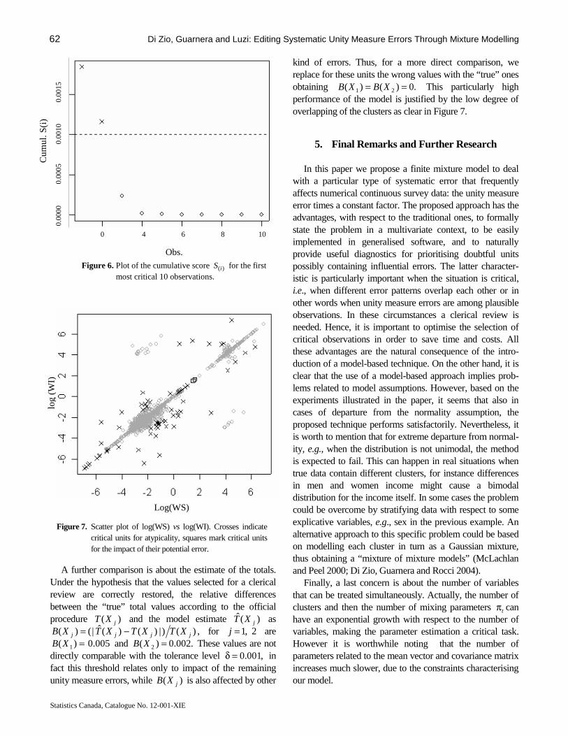
62 Di Zio, Guarnera and Luzi: Editing Systematic Unity Measure Errors Through Mixture Modelling
Statistics Canada, Catalogue No. 12-001-XIE
Figure 6. Plot of the cumulative score )(iS for the first
most critical 10 observations.
Figure 7. Scatter plot of log(WS) vs log(WI). Crosses indicate critical units for atypicality, squares mark critical units for the impact of their potential error.
A further comparison is about the estimate of the totals. Under the hypothesis that the values selected for a clerical review are correctly restored, the relative differences between the “true” total values according to the official procedure )( jXT and the model estimate )(ˆ
jXT as ,)()|)()(ˆ|()( jjjj XTXTXTXB −= for 2,1=j are
=)( 1XB 005.0 and .002.0)( 2 =XB These values are not directly comparable with the tolerance level ,001.0=δ in fact this threshold relates only to impact of the remaining unity measure errors, while )( jXB is also affected by other
kind of errors. Thus, for a more direct comparison, we replace for these units the wrong values with the “true” ones obtaining .0)()( 21 == XBXB This particularly high performance of the model is justified by the low degree of overlapping of the clusters as clear in Figure 7.
5. Final Remarks and Further Research
In this paper we propose a finite mixture model to deal with a particular type of systematic error that frequently affects numerical continuous survey data: the unity measure error times a constant factor. The proposed approach has the advantages, with respect to the traditional ones, to formally state the problem in a multivariate context, to be easily implemented in generalised software, and to naturally provide useful diagnostics for prioritising doubtful units possibly containing influential errors. The latter character-istic is particularly important when the situation is critical, i.e., when different error patterns overlap each other or in other words when unity measure errors are among plausible observations. In these circumstances a clerical review is needed. Hence, it is important to optimise the selection of critical observations in order to save time and costs. All these advantages are the natural consequence of the intro-duction of a model-based technique. On the other hand, it is clear that the use of a model-based approach implies prob-lems related to model assumptions. However, based on the experiments illustrated in the paper, it seems that also in cases of departure from the normality assumption, the proposed technique performs satisfactorily. Nevertheless, it is worth to mention that for extreme departure from normal-ity, e.g., when the distribution is not unimodal, the method is expected to fail. This can happen in real situations when true data contain different clusters, for instance differences in men and women income might cause a bimodal distribution for the income itself. In some cases the problem could be overcome by stratifying data with respect to some explicative variables, e.g., sex in the previous example. An alternative approach to this specific problem could be based on modelling each cluster in turn as a Gaussian mixture, thus obtaining a “mixture of mixture models” (McLachlan and Peel 2000; Di Zio, Guarnera and Rocci 2004).
Finally, a last concern is about the number of variables that can be treated simultaneously. Actually, the number of clusters and then the number of mixing parameters tπ can have an exponential growth with respect to the number of variables, making the parameter estimation a critical task. However it is worthwhile noting that the number of parameters related to the mean vector and covariance matrix increases much slower, due to the constraints characterising our model.
0.0
015
0.0
010
0.0
005
0.0
000
10 8 6 4 0
Cum
ul. S
(i)
Obs.
log
(WI)
Log(WS)

Survey Methodology, June 2005 63
Statistics Canada, Catalogue No. 12-001-XIE
Acknowledgements We are grateful to the referees and the Associate Editor
for their helpful comments.
References
Anderson, T.W. (1984). An introduction to Multivariate Statistical Analysis. Second Edition. New York: John Wiley & Sons, Inc.
Azzalini, A., and Capitanio, A. (2003). Distributions generated by perturbation of symmetry with emphasis on a multivariate skew – t distribution. Journal of the Royal Statistical Society (B), 65, 367-389.
Azzalini, A., Dal Cappello, T. and Kotz, S. (2003). Log-skew-normal and log-skew – t distributions as models for family income data. Journal of Income Distribution, 11, 13-21.
Biernacki, C., Celeux, G. and Govaert, G. (2003). Choosing starting values for the EM algorithm for getting the highest likelihood in multivariate Gaussian mixture models. Computational Statistics & Data Analysis, 41, 561-575.
Cirianni, A., Di Zio M., Luzi O. and Seeber, A.C. (2000). The new integrated data editing procedure for the Italian Labour Cost survey: Measuring the effects on data of combined techniques. Proceedings of the International Conference on Establishment Surveys II, Buffalo, 7-21.
De Waal, T. (2003). Solving the error localization problem by means of vertex generation. Survey Methodology, 29, 1, 71-79.
Di Zio, M., Guarnera, U. and Rocci, R. (2004). A mixture of mixture models to detect unity measure error. Proceedings in Computational Statistics, (Ed. Antoch Jaromir), 919-927, Physica Verlag, Prague, August 23-28.
Di Zio, M., and Luzi, O. (2002). Combining methodologies in a data editing procedure: an experiment on the survey of Balance Sheets of Agricultural Firms. Italian Journal of Applied Statistics, 14, 1, 59-80.
Encyclopedia of Statistical Sciences (1999). New York: John Wiley & Sons, Inc. Update 3, 621-629.
Euredit (2003). Towards Effective Statistical Editing and Imputation Strategies – Findings of the Euredit project, 1, 2. Forthcoming. Now available at http://www.cs.york.ac.uk/euredit/
Federal Committee on Statistical Methodology (1990). Data Editing in Federal Statistical Agencies. Statistical Policy Working Paper 18.
Fellegi, I.P., and Holt, D. (1976). A systematic approach to edit and imputation. Journal of the American Statistical Association, 71, 17-35.
Fraley, C., and Raftery, A. (2002). Model-Based clustering, discriminant analysis, and density estimation. Journal of the American Statistical Association, 97, 611-631.
Granquist, L. (1995). Improving the traditional editing process. In Business Survey Methods, (Eds. B.G. Cox and D.A. Binder).
Granquist, L. (1996). The new view on editing. International Statistical Review, 65, 3, 381-387.
Granquist, L., and Kovar, J. (1997). Editing of survey data: How much is enough? In Survey Measurement and Process Quality, (Eds. L. Lyberg, P. Biemer, M. Collins, E. de Leeuw, C. Dippo, N. Schwarz and D. Trewin), New York: John Wiley & Sons, Inc., 415-435.
Hawkins, D.M. (1981). A new test for multivariate normality and homoscedasticity. Technometrics, 23, 105-110.
Kovar, J.G., Mac Millian, I.H. and Whitridge, P. (1988). Overview and strategy for the generalized edit and imputation system, (updated February 1991). Statistics Canada, Methodology Branch Working Paper, BSMD-88-007E/F.
Latouche, M., and Berthelot, J.M. (1992). Use of a score function to prioritise and limit recontacts in business surveys. Journal of Official Statistics, 8, 389-400.
Lawrence, D., and McKenzie, R. (2000). The general application of significance editing. Journal of Official Statistics, 16, 243-253.
McLachlan, G.J., and Basford, K.E. (1988). Mixture Models: Inference and Applications to Clustering. Marcel Dekker.
McLachlan G.J., and Peel D. (2000). Finite Mixture Models. New York: John Wiley & Sons, Inc.


Survey Methodology, June 2005 65 Vol. 31, No. 1, pp. 65-72 Statistics Canada, Catalogue No. 12-001-XIE
Using Matched Substitutes to Improve Imputations for Geographically Linked Databases
Wai Fung Chiu, Recai M. Yucel, Elaine Zanutto and Alan M. Zaslavsky 1
Abstract
When administrative records are geographically linked to census block groups, local-area characteristics from the census can be used as contextual variables, which may be useful supplements to variables that are not directly observable from the administrative records. Often databases contain records that have insufficient address information to permit geographical links with census block groups; the contextual variables for these records are therefore unobserved. We propose a new method that uses information from “matched cases” and multivariate regression models to create multiple imputations for the unobserved variables. Our method outperformed alternative methods in simulation evaluations using census data, and was applied to the dataset for a study on treatment patterns for colorectal cancer patients.
1. Wai Fung Chiu, Department of Statistics, Harvard University, One Oxford Street, Cambridge MA 02138. E-mail: [email protected]; Recai M.
Yucel, Department of Biostatistics and Epidemiology, 408 Arnold House, School of Public Health and Health Sciences, University of Massachusetts, 715 North Pleasant Street, Amherst, MA 01003-9304. E-mail: [email protected]; Elaine Zanutto, The Wharton School, University of Pennsylvania, 466 Jon M. Huntsman Hall, 3730 Walnut Street, Philadelphia PA 19104. E-mail: [email protected]; Alan M. Zaslavsky, Department of Health Care Policy, Harvard Medical School, 180 Longwood Avenue, Boston MA 02115. E-mail: [email protected].
Key Words: Unit nonresponse; Multiple imputation; Contextual variables; Matched substitutes; Administrative
records.
1. Introduction In a study on treatment patterns for colorectal cancer
patients, income and education are desired variables for constructing statistical models of relevant scientific interest. Unfortunately, individual measurements for these variables are not directly observable from the cancer registry databases that are compiled from hospital records, which like many administrative databases contain primarily information required for administrative purposes. Instead, mean values of these variables for small geographical areas (census block groups or tracts) including the subject’s area of residence are used as regressors to estimate income and education effects. Analyses using such “contextual vari-ables” are common in epidemiological and health services research (Krieger, Williams and Andmoss 1997), and often produce results broadly similar to those based on individual variables. If both individual and contextual variables were available, it might be possible to separate the effects of indi-vidual characteristics and contexts; in a purely contextual analysis, these effects are confounded. Nonetheless, associa-tions between contextual socioeconomic characteristics and quality of care would suggest an equity problem, regardless of whether such associations primarily reflect individual or community-level relationships.
In the colorectal cancer treatment study, each contextual variable for a given patient record is assumed to be the variable’s census group (or tract) mean value obtained by geographically linking the record’s address to a census block group (or tract). A small but substantial percentage of
patient records (about 3.3% or 1,696 records) have insufficient address information to permit links with census block groups, hence making the corresponding contextual variables unobservable. Such records will be called ungeocodable records, while records that can be linked to census block groups will be referred to as geocodable. To generate multiple imputations for the unobserved contextual variables, we propose a strategy that uses information from more than one “matched case” to help build parametric/ nonparametric imputation models. In particular, information from the matched cases accounts for small area effects in our imputation models, so that there is no need to explicitly model such effects.
Rubin and Zanutto (2001) use the term “matched substitute” instead of “matched case”, and propose a parametric imputation model using only one matched substitute per record. The analyses resulted from their model were compared to those given by other analytic methods in an extensive simulation study, but was not applied to real data. We extend Rubin and Zanutto’s method by (1) allowing use of information from more than one matched case per record and (2) using an empirical rather than a parametric distribution of residuals.
This research was motivated by our need for multiple imputations for the partially observed variables in the study of treatment patterns for colorectal cancer patients. Ayanian, Zaslavsky, Fuchs, Guadagnoli, Creech, Cress, O’Connor, West, Allen, Wolf and Wright (2003) analyzed a dataset that included imputations generated by our method,

66 Chiu, Yucel, Zanutto and Zaslavsky: Using Matched Substitutes to Improve Imputations
Statistics Canada, Catalogue No. 12-001-XIE
referring to Rubin and Zanutto (2001) and a preliminary version of this paper that appeared in a proceedings publication (Chiu, Yucel, Zanutto and Zaslavsky 2001). This paper is the first comprehensive publication of our methodology and the first published report that describes an application of Rubin and Zanutto’s method to real data.
The organization for the rest of this paper is as follows. Section 2 summarizes Rubin and Zanutto’s method and gives a general description of our method. Section 3 outlines the application of our method to the colorectal cancer study. Section 4 illustrates in a simulation study the performance of our method relative to three other commonly-used nonresponse adjustment methods.
2. Imputation Methodology
This section will begin with a summary of Rubin and Zanutto’s method, followed by a general description of our method that includes a discussion on out-of-sample versus within-sample matching, the details of the modeling and multiply-imputing tasks, and an analysis of efficiency as a function of the number of matched cases used. 2.1 Matching, Modeling and Multiply Imputing
Rubin and Zanutto (2001) proposed a method called “matching, modeling, and multiply imputing” (MMM) that uses matched substitutes to help generate multiple impu-tations for nonrespondents in sample surveys, without requiring that substitutes be perfect replacements for the nonrespondents. Matched substitutes are responding survey units chosen to match the nonrespondents on one or more “matching covariates” – variables that are available prior to the survey and are convenient for matching but not neces-sarily for modeling. As a result of matching, nonrespondents and their substitutes may share similar values in their “field covariates” – variables that are only implicitly observed and are therefore not available for data analysis. “Modeling covariates” are variables that can be included in statistical models to adjust for observed differences between non-respondents and their substitutes, but that may not be available or used for matching. The essence of MMM is that both matching and modeling covariates are used, in the context of proper multiple imputation (Little and Rubin 1987, pages 258 – 259 and references therein).
Consider a simple example where age and address covariates are available for all units in a population prior to sampling. Finding substitutes matching nonrespondents with respect to both age and address may be difficult. An alternative is to match only on address (e.g., choosing a neighbor to be a substitute) and adjust for systematic age
differences between nonrespondents and matched substi-tutes through statistical modeling. If neighboring households were chosen as matched substitutes for nonresponding households, the substitutes and nonrespondents might have similar socioeconomic contexts (e.g., levels of crime, access to public transportation, etc.) even though these charac-teristics might have not been recorded. In this example, address is a matching covariate, age is a modeling covariate, and the contextual socioeconomic characteristics are field covariates.
In summary, MMM (i) chooses matched substitutes for nonrespondents and some respondents based on matching covariates, (ii) uses modeling covariates to fit a model estimating the systematic differences in responses between pairs of respondents and substitutes, (iii) multiply-imputes the unobserved values using the model in (ii) under the assumption that the same relationship holds between pairs of nonrespondents and substitutes, and (iv) discards all matched substitutes after imputation. 2.2 Out-of-Sample Versus Within-Sample Matching
Matched cases may be obtained from out-of-sample data or within-sample data. In the Rubin and Zanutto approach, matched substitutes are obtained from out-of-sample data after the missingness is detected. Their description empha-sizes that the matched substitutes must be discarded after imputation since including such additional cases in infer-ences would modify the sample design by adding extra cases in the “blocks” that contain unobserved data. Matched cases are considered within-sample data if they are obtained from the database that is available before imputing or even finding out which records in the database have unobserved variables. As far as the overall inferential goals are con-cerned, these matched cases are not additional cases, but are part of the original data collection, and therefore will be included in scientific analyses.
Assuming within-sample matching, we treat the un-geocodable records as nonrespondents and the geocodable records as respondents. For each ungeocodable record, a given number of matched cases are randomly chosen from a pool of geocodable records within the same small geograph-ical area (e.g., zip code, which is a postal delivery code usually representing an area served by a single main US post office). Similarly, the same number of matched cases are also chosen for each of the randomly sampled geo-codable records (see Rubin and Zanutto (2001) for recom-mendations on the size of such a sample relative to the total number of ungeocodable records in a given dataset). If more matched cases were needed than those are available in the same small area, the selection pool would be extended to the “nearest” geographical areas until the required number of matched cases was achieved.
Survey Methodology, June 2005 67
Statistics Canada, Catalogue No. 12-001-XIE
All matched cases in the colorectal cancer study came from the same cancer database. In general, matched cases need not be drawn from the same population in which the nonrespondents and respondents originated. For example, matched cases for colorectal cancer records can be obtained from a general population of cancer patients, and a model can then be fitted to correct for systematic differences. Note that, with matched cases from a more similar population, stronger models can be built with more covariates. In our example, since we used other patients with the same cancer type, relationships to treatment process and outcome variables are likely to be consistent. 2.3 Modeling and Multiply-imputing
A simple example of our method is given here to convey the basic idea; in practice, more complex models may often be required. Suppose the following relationship holds in the population,
,ikiTikiky ε+δ+= βx (1)
where i indexes small geographical area, k indexes unit within area, and iky and ikx are respectively the response and the characteristics of the thk unit in geographical area .i This model includes a regression prediction ,βT
ikx a small-area effect ,iδ and a unit-specific residual .ikε We assume that ikε follows some distribution εF with mean zero and variance .2σ Note that this development generalizes directly to multivariate .iky
We extend Rubin and Zanutto’s method to allow more than one match in the same small area, because having several matches in small areas is possible (often convenient and inexpensive) in census data or in large administrative datasets. Rubin and Zanutto’s assumption of a single match is appropriate to survey data collection that requires additional field work for each match.
The regression coefficients in equation (1) are estimated using any collection of observations with two or more records per small area to fit the regression model in which the iδ are treated as fixed effects. With only two cases per area, β can instead be estimated from the within-area regression
,)()()( 212121 iiTi
Tiii yy ε−ε+−=− βxx (2)
where the small area effect drops out. The residuals from this regression have a symmetrical distribution with vari-ance .2 2σ
Assuming for the moment that we have a draw from the posterior distribution of ,β we carry out the rest of this analysis conditional on that draw. Now suppose that we are interested in imputing for a new unit (indexed as 0=k ) in area ,i and that we have obtained 1≥iK matched cases for this unit. Denote the outcomes of these matched cases by
the vector TiKii i
yy )...,,( 1=y and the corresponding characteristics by the matrix .)...,,( 1
TiKii i
xxX = With a flat prior for ,iδ the posterior distribution for β,,| iii Xyδ has mean
βTiiy x− (3)
and variance ,/2iKσ where ∑ == iK
k iiki Kyy 1 / and =ix ∑ =
iKk ii K1 ./x Hence, the predictive distribution for
β,,,| 00 iiiiy xXy has mean
β)( 0Ti
Tiiy xx −+ (4)
and variance 2)/11( σ+ iK which is the sum of the predictive variance under the model conditional on all parameters and the posterior variance of .iδ These statements assume that the mean of the residuals is a sufficient statistic for .iδ This assumption is true for the normal distribution (or natural observations of any exponential family distribution); we assume it is at least approximately true for ,εF so that we can base inferences on that mean. Note that use of a flat prior leads to overdispersed draws relative to what would be obtained with a proper prior from a hierarchical model, but is much simpler (especially in analyses with the multivariate outcomes).
An imputation for 0iy can be generated by first drawing 2σ from its posterior distribution, second drawing β
conditional on the draw of ,2σ third computing the predictive mean in equation (4) from the draw of ,β and finally adding a residual of variance 2)/11( σ+ iK to the predictive mean. In simple surveys with β estimated by equation (2), the posterior distribution of β (conditional on
2σ and the data) under a flat prior is approximately ))(,ˆ(N 21 σ−XX Tβ where the thi row of X is
.)( 21Ti
Ti xx − In more complex designs, the posterior
distribution of β can be approximated using the point estimate and sampling variance calculated under the associated design.
The residual can be obtained through modeling or sampling. Modeling involves estimating 2σ using the residual variance of equation (1) and drawing the residual under univariate normality (see Rubin and Zanutto (2001) for the special case where only one matched case was ob-tained for each record) or some other parametric distri-bution. We refer to such an approach as parametric MMM (PMMM). An alternative is to randomly sample a regression residual from any area j whose residuals might be regarded as exchangeable with those from area i (Rubin 1987 pages 166 – 168). See also Lessler and Kalsbeek (1992, section 8.2.2.4), Kalton and Kasprzyk (1986), and Kalton (1983). Since the variance of such a residual is
,]/)1([ 2σ− jj KK we multiply the randomly-sampled residual by )]1/([]/)1([ −+ jjii KKKK to obtain the

68 Chiu, Yucel, Zanutto and Zaslavsky: Using Matched Substitutes to Improve Imputations
Statistics Canada, Catalogue No. 12-001-XIE
correct predictive variance. We call this approach nonparametric MMM (NpMMM).
In summary, our method consists of three basic steps:
1. Draw matched cases for the ungeocodable records and for some randomly sampled geocodable records;
2. Use the sampled geocodable records and their matched cases to fit equation (1) where the iδ are treated as fixed effects, and save the residuals;
3. Repeat the following for m (usually 5 to 10) times:
(a) Draw 2σ from its posterior distribution, then β conditional on the draw of 2σ ;
(b) For each ungeocodable record, treat the sum of the vector of predictive means obtained from equation (4) and a vector of residuals drawn using either PMMM or NpMMM as a realization of the unobserved vector of contextual variables.
2.4 Efficiency The efficiency of an imputation is related to the number
of matched cases used. Let KV be the predictive variance of an imputation model where K matched cases per record are used. For the model in section 2.3, .)/11( 2σ+= KVK Define efficiency as
,1)/11( 2
2
+=
σ+σ== ∞
K
K
KV
VE
kK (5)
for any positive integer .K Efficiency increases as the number of matched cases per record increases; for example,
,91.0,8.0,67.0 1042 ≈=≈ EEE and .95.020 ≈E Theoretically each record can have as many matched
cases as permitted by available resources. In practice, the number of matched cases used often depends on the cost of matched cases and the cost of computation involved in model fitting. In our method, the cost of computation for each added matched case per record is negligible. In the colorectal cancer study, while the matched cases were free, the ability to do the imputation based on a limited number of matched cases was crucial because confidentiality restrict-tions prevented investigators from using the entire dataset in modeling with zip codes (even in a coded form) attached. For illustrative purposes, we will use two matched cases per record in subsequent analyses.
3. Application: The Colorectal Cancer Study The colorectal cancer database has a total of 50,740
patient records, of which approximately 3.3% are un-geocodable. Among these, about half have P.O. box addresses (often in a rural area), and the rest are mistyped
addresses or addresses from newly developed areas that are not in address databases. In a study of factors predicting provision of chemotherapy for colorectal cancer patients, investigators believed that the following three census block-group means would be useful contextual variables:
1Y = median household income,
2Y = percent with no high school diploma, and
3Y = percent below poverty level.
These variables were observed in geocodable records but unobserved in ungeocodable records. The task was to generate multiple imputations for the unobserved census variables using the methods in section 2.
Each of the block-group means was reported in the census data for six race/ethnic groups, and the scientific analyses used only the set of block-group means corresponding to the race/ethnicity of each patient. For imputations used in Ayanian et al. (2003), we therefore fitted six separate models to impute all )36(18 × values for each ungeocodable patient and then selected the three variables pertinent to each patient; joint distributions for different race/ethnic groups were not important because each imputation only used values for a single group. An alternative would have been to use race as a matching variable, but this would have forced us to seek some matches at a much greater distance geographically, diluting the predictive value of the geographical match.
For expository purposes, we assume henceforth that only the block-group mean corresponding to the race of each respondent is available, but not the means corresponding to the other five races that are available simultaneously in the census data. This is more typical of data that would be collected directly from the respondent, where the race variable itself (as a modeling variable) is quite predictive because income data for people of different races reflect differences in income associated with race. 3.1 Matching and the Dataset
The addresses of over 90% of ungeocodable records have zip codes. Zip code was therefore chosen as a matching covariate. A simple diagnostic for its usefulness appears in section 3.2. The numerical sequence of zip codes does not always correspond to neighborhood distance relationships. For example, Cambridge, Massachusetts has a 02138 post office that also uses the 02238 zip code for mailboxes, and in nearby Boston there is a 02215 zip code that was carved out of the 02115 area. Instead of using the numerical sequence of zip codes, the distances between zip codes were computed based on latitudes and longitudes of their main post offices, under the assumption that two zip codes were closest to each other if their main post offices were closest to each other.
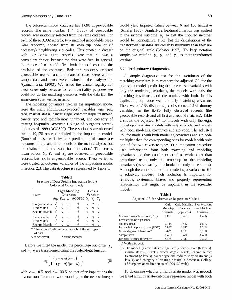
Survey Methodology, June 2005 69
Statistics Canada, Catalogue No. 12-001-XIE
The colorectal cancer database has 1,696 ungeocodable records. The same number )696,1( * =n of geocodable records was randomly selected from the same database. For each of these 3,392 records, two matched geocodable cases were randomly chosen from its own zip code or (if necessary) neighboring zip codes. This created a dataset with 176,103392,3 =× records. Note that *n was a convenient choice, because the data were free. In general, the choice of *n could affect both the total cost and the precision of the estimates. Both the randomly selected geocodable records and the matched cases were within-sample data and hence were retained in the analyses for Ayanian et al. (2003). We asked the cancer registry for these cases only because for confidentiality purposes we could not do the matching ourselves with the data (for the same cases) that we had in hand.
The modeling covariates used in the imputation model were the eight administrative-record variables: age, sex, race, marital status, cancer stage, chemotherapy treatment, cancer type and radiotherapy treatment, and category of treating hospital’s American College of Surgeons accred-itation as of 1999 (ACOS99). These variables are observed for all 10,176 records included in the imputation model. (Some of these variables are predictors and some are outcomes in the scientific models of the main analyses, but the distinction is irrelevant for imputation.) The census mean values 21, YY and 3Y are observed in geocodable records, but not in ungeocodable records. These variables were treated as outcome variables of the imputation model in section 2.3. The data structure is represented by Table 1.
Table 1 Structure of Data Used in Imputation for the
Colorectal Cancer Study
Eight Modeling Covariates
Census Variables Data*
Age Sex … ACOS99 1Y 2Y 3Y
Ungeocodable √ √ … √ ? ? ? First Match √ √ … √ √ √ √ Second Match √ √ … √ √ √ √
Geocodable √ √ … √ √ √ √ First Match √ √ … √ √ √ √ Second Match √ √ … √ √ √ √
* There were 1,696 records in each of the six types of data. √ = observed ? = unobserved
Before we fitted the model, the percentage outcomes 2y and 3y were transformed using the scaled-logit function:
,)/()(1
)/()(log ⎟⎟
⎠
⎞⎜⎜⎝
⎛−−−
−−abay
abay (6)
with 5.0−=a and 5.100=b so that after imputations the inverse transformation with rounding to the nearest integer
would yield imputed values between 0 and 100 inclusive (Schafer 1999). Similarly, a log-transformation was applied to the income outcome 1y so that the imputed incomes would be nonnegative. Note that the distributions of the transformed variables are closer to normality than they are on the original scale (Schafer 1997). To keep notation simple, we redefine 21, yy and 3y as their transformed versions. 3.2 Preliminary Diagnostics
A simple diagnostic test for the usefulness of the matching covariates is to compare the adjusted 2R for the regression models predicting the three census variables with only the modeling covariates, the models with only the matching covariates, and the models with both. In this application, zip code was the only matching covariate. There were 1,133 distinct zip codes (hence 1,132 dummy variables) in the 8,480 fully observed records (the geocodable records and all first and second matches). Table 2 shows the adjusted 2R for models with only the eight modeling covariates, models with only zip code, and models with both modeling covariates and zip code. The adjusted
2R for models with both modeling covariates and zip code are higher than the corresponding ones for models with only one of the two covariate types. Our imputation procedure uses information from both matching and modeling covariates and thus can be expected to work better than procedures using only the matching or the modeling covariates (as shown by the simulation study in section 4). Although the contribution of the modeling covariates to 2R is relatively modest, their inclusion is important for removing systematic biases and properly representing relationships that might be important in the scientific models.
Table 2 Adjusted 2R for Alternative Regression Models
Only Modeling Covariates
Only Matching Covariate
(Zip Code)
Both Modeling and Matching
Covariates Median household income (INC) 0.091 0.453 0.496 Percent with no high school diploma (EDU) 0.115 0.452 0.503 Percent below poverty level (POV) 0.047 0.327 0.343 Model degrees of freedom(a) 26(b) 1,133 1,158 Sample sizes 8,480 8,480 8,480 Residual degrees of freedom 8,454 7,347 7,322
(a) With intercept.
(b) The modeling covariates are age, sex (2 levels), race (6 levels), marital status (6 levels), cancer stage (6 levels), chemotherapy treatment (2 levels), cancer type and radiotherapy treatment (3 levels), and category of treating hospital’s American College of Surgeons accreditation as of 1999 (6 levels).
To determine whether a multivariate model was needed,
we fitted a multivariate-outcome regression model with both
70 Chiu, Yucel, Zanutto and Zaslavsky: Using Matched Substitutes to Improve Imputations
Statistics Canada, Catalogue No. 12-001-XIE
modeling covariates and zip code. The estimated correla-tions between the residuals were: ,194.012 −≈r
,297.013 −≈r and ,357.023 ≈r where “variable 1” is median household income, “variable 2” is percent with no high school diploma, and “variable 3” is percent below poverty level. These estimates were significantly different from zero, which therefore indicated that multivariate versions of the methods in section 2.3 should be used to generate imputations. 3.3 Multiple Imputation Results and Comparisons
Imputations under NpMMM were used in the study of factors predicting provision of chemotherapy for colorectal cancer patients (Ayanian et al. 2003). Their model included three indicator variables for ranges of contextual income, together with 21 other variables representing patient and hospital characteristics. The multiple imputation analysis shows that the information loss due to missing information is always less than 0.1%, which is much smaller than the fraction of ungeocodable records (3.3%). As expected, the largest fractions of missing information appeared for the income variables. The scientific results in Ayanian et al. (2003) would not have changed dramatically if the incomplete cases had been dropped. In this type of research, however, every case is precious and expensive, and saving the 3.3% with missing data was a contribution to the study.
For comparison, variances of parameters under the complete-case analysis were on the average 4.0% larger than those under multiple imputation analysis. Such percentage differences are close to the fraction of incomplete cases deleted for this analysis. When the imputations generated by our method were included in the scientific analysis, the precision of the estimate of the “rural” effect was dramatically improved (using only the complete cases led to 41.6% increase in variance), due to the concentration of ungeocodable records in rural areas (21.6% of rural records are ungeocodable, but only 3.1% of nonrural records are ungeocodable).
4. A Simulation Study
This simulation study compares performance of our new method with three other commonly-used nonresponse adjustment methods. The population of this study was the 1,696 fully observed triples – the 1,696 geocodable records and the corresponding first and second matches (one row from each of the last three horizontal blocks in Table 1) – or 5,088 observations. For simplicity, we assumed that the triples were from distinct zip codes (clusters), hence
.696,1...,,2,1 == Ii Each cluster i contained three units ,)3,2,1( =u and the record of each unit consisted of iux
(the covariates) and iuy (the census variables).
4.1 Simulated Data and Response Mechanism Assuming that the design was cluster sampling with
sample size 800, we drew random samples of 800 clusters. For each random sample, about half of the 800 clusters were randomly selected to have an ungeocodable record in which the census variables were unobserved, with the probability of missingness depending on an individual’s race and on the mean income of the cluster (zip code). We simulated missingness under a multinomial logit model where the outcomes are: nothing unobserved 10 ,)1( iiw y= unob-served 21 ,)1( iiw y= unobserved ,)1( 2 =iw and 3iy unobserved .)1( 3 =iw Specifically, for each ,...,,2,1 Ii = let 00 =iz and
)codezipinincomemean(
)Whiteisunit(
ic
iuIbaziu
×+×+=
(7)
where .3,2,1=u Then
.3,2,1,0for
)(exp)(exp)1(Pr3
0
=
== ∑=
u
zzwu
iuiuiu (8)
The results of this simulation study were based on datasets generated by the mechanism with 11,1 =−= ba and ,0003.0=c which made about 17% of the units in a random sample ungeocodable, with probability of geocoding positively related to White race and higher block-level income. The task was to use the random sample to estimate ,y the mean values of the population (1,696 clusters).
The simulation conditions described in the preceding paragraphs were designed to give a stringent test of the procedure and alternatives by exaggerating the impact of unobserved data and making the missingness strongly related to characteristics both of the individual and of the area. We were not attempting to simulate the exact con-ditions of the application in section 3 but rather to use an artificial population with similar distributions to those in the real population to illustrate the workings of our method and its competitors. 4.2 Inferential Methods and Measures of
Performance Preliminary results indicated that the performance of
PMMM and NpMMM is similar; NpMMM is, however, simpler (especially in analyses with multivariate outcomes), because the method does not require explicit parametric modeling of the residual variance. Our simulations com-pared performance of NpMMM (using two matched cases per record) with three other commonly-used nonresponse adjustment methods:
Survey Methodology, June 2005 71
Statistics Canada, Catalogue No. 12-001-XIE
1. Complete-case Method (CCM) The population means are estimated from all geo-codable units of a random sample.
2. Substitute Single Imputation (SSI) This is the traditional use of substitutes. The un-observed census variables of each ungeocodable unit are replaced by the values of the census variables of a randomly selected unit from the same cluster. The resulting sample is treated as if there had been no ungeocodable unit; all 800 clusters in such a sample are used for estimating the population means.
3. Multivariate Normal Multiple Imputation (MNMI) This method uses only one randomly selected unit from each of the fully observed clusters in a random sample to fit the multivariate normal linear regression
,),(N~ 0 ΣBβ Ti
TTi xy +
with a noninformative prior on the parameters. The model is then used to create m sets of multiple imputations for the unobserved census variables using a direct multivariate generalization of the algorithm given by Rubin (1987, page 167).
Note that CCM uses neither matching nor modeling covariates, SSI uses only the matching covariate (zip code), MNMI uses only the modeling covariates, and NpMMM uses both the matching covariate and the modeling covariates.
The CCM and SSI data are analyzed by the usual complete-data method which estimates the population mean from the data with the appropriate estimator for cluster sampling from a finite population, including the finite population correction (Cochran 1977, Chapters 9 – 10). Both MNMI and NpMMM produce m sets of complete data, each of which is analyzed by the same complete-data method used for the CCM and SSI data; the m sets of point and variance estimates are then combined using the multiple imputation combination rule (Rubin 1987; Schafer 1997, pages 108 – 110).
For each simulation ,}...,,2,1{ Tt ∈ we denote the point estimates from the four methods by ),(CC ty
),(),( MNSS tt yy and ),(Np ty and the means of these quantities across simulations are written as ,CCy
,, MNSS yy and .Npy Performance evaluation of the four nonresponse adjustment methods will be based on three measures:
1. Percent reduction in the average bias of an estimator relative to the average bias of the CCM estimator. Denote the average bias of an estimator by
.Eb Then ,E yyb −= E
where .}NpMN,SS,CC,{∈E We define the percent reduction in the average bias of an estimator relative to the average bias of the CCM estimator as
,||
||||),(
CC
ECCCCE b
bbbbR
−=
where Eb is an element of Eb and CCb is the corre-sponding element in .CCb By definition, ),( CCCC bbR is zero.
2. Estimated coverage of the nominal 95% confidence intervals for .y Intervals produced by the CCM or SSI estimates were constructed under appropriate
ons.distributi−t For intervals associated with the MNMI or NpMMM estimates, we followed the procedure outlined in Schafer (1997, pages 109 – 110) and replaced the degrees of freedom v with the updated version of Barnard and Rubin (1999).
3. Estimated fraction of missing information about .y For each of MNMI and NpMMM, we computed ,λ an estimate of the fraction of missing information
about y (see Barnard and Rubin (1999) for the most recent expression).
4.3 Results The simulation procedure was implemented 2,000 times,
and 10=m was used for MNMI and NpMMM. The mean values of the census variables in the population were
.)55.9,65.21,642,40( T=y The average bias of the CCM estimator was .)79.1,97.3,405,5(CCM
T−−−=b Other results are summarized in Table 3. NpMMM achieved large percent reductions in relative average bias (95.0% to 99.5%). SSI reduced biases more than MNMI, because the matching covariate (zip code) was much more informative than the set of modeling covariates (section 3.2). Since the response mechanism was nonignorable (the response probabilities depended partly on income), the poor performance of MNMI, which did not use the geographical information to help predict income, was expected. Note that MNMI is biased, and the bias is large enough so that with the sample size considered in this paper the confidence intervals never covered the hypothetical population values.
Under MNMI and NpMMM, the percent of missing information was much less than the average percent of unobserved data. The percent of missing information was smaller under NpMMM than under MNMI. Only NpMMM produced well calibrated intervals with correct coverage. In summary, NpMMM combines the best features of the other two methods – close-to-nominal coverage and less missing information.
72 Chiu, Yucel, Zanutto and Zaslavsky: Using Matched Substitutes to Improve Imputations
Statistics Canada, Catalogue No. 12-001-XIE
Table 3 Simulation Results(a): Bias Reduction, Coverage, and Fraction of
Missing Information
Method Measure Mean NpMMM MNMI SSI
INC 99.5 44.6 95.2 EDU 95.0 40.6 83.7
Percent bias Reduction
)b(CCM ),(100 bbR E POV 96.8 32.6 80.3
INC 95.1 0.00 89.8 EDU 94.8 0.00 65.7
Estimated Coverage of the 95% CIs(c) POV 95.2 0.00 66.0
INC 1.00 9.92 EDU 0.05 0.07
×100 Estimated fraction of missing information )d(λ POV 0.07 0.08
(a) Based on 2,000 replications and .10=m
(b) By definition, .0),(100 CCMCCM =bbR
(c) Results for the CCM estimates were all zeros.
(d) The average percent of unobserved data was approximately 17%. 5. Conclusion
This work extends Rubin and Zanutto (2001) in two respects. First, our method allows more than one matched case per record. We show theoretically that the efficiency of an imputation increases as the number of matched cases per record increases. When the cost of matched cases is rela-tively low, our method offers an option where information of more than one matched case per record is used to help fit imputation models at a negligible computational expense. Second, NpMMM does not require explicit parametric modeling of residual variance(s), hence simplifying the modeling task (especially for analyses with multivariate outcomes). This nonparametric approach makes it feasible to apply our method to datasets with complex model structures. In a simulation study, NpMMM estimates achieved substantial bias reductions, and NpMMM produced confidence intervals with correct coverage.
Although we have focused on geographically-based matching to complete unobserved geographically-linked variables, the procedures described in this paper can be generalized to other matching variables. For example, to impute clinical variables, it might be more appropriate to match to another patient in the same hospital, if clinical characteristics and therapies are likely to be more strongly associated with the hospital than with the geographic location of the patient’s residence.
Acknowledgements This research was supported in part by the Bureau of the
Census through a contract with the National Opinion Research Center and Datametrics, Inc., and by a grant from the Agency for Healthcare Research and Quality (AHRQ) and the National Cancer Institute (HS09869). The authors thank John Z. Ayanian for leadership of the Quality of Cancer Care research project, Mark Allen and Robert Wolf for preparation of data, Bill Wright for his support to this research, and the associated editor and two anonymous referees for their helpful comments.
References
Ayanian, J.Z., Zaslavsky, A.M., Fuchs, C.S., Guadagnoli, E., Creech, C.M., Cress, R.D., O’connor, L.C., West, D.W., Allen, M.E., Wolf, R.E. and Wright, W.E. (2003). Use of adjuvant chemotherapy and radiation therapy for colorectal cancer in a population-based cohort. Journal of Clinical Oncology, 21, 1293-1300.
Barnard, J., and Rubin, D.B. (1999). Small-sample degrees of freedom with multiple imputation. Biometrika, 86, 948-955.
Chiu, W.F., Yucel, R.M., Zanutto, E. and Zaslavsky, A.M. (2001). Using matched substitutes to improve imputations for geographically linked databases. Proceedings of the Survey Research Methods Section, American Statistical Association.
Cochran, W.G. (1977). Sampling Techniques. New York: John Wiley & Sons, Inc.
Kalton, G. (1983). Compensating for Missing Survey Data. Research Report Series, Ann Arbor, MI: Institute for Social Research.
Kalton, G., and Kasprzyk, D. (1986). The treatment of missing survey data. Survey Methodology, 12, 1-16.
Krieger, N.,Williams, D. and Andmoss, N. (1997). Measuring social class in U.S. public health research: Concepts, methodologies, and guidelines. Annual Review of Public Health, 18, 341-378.
Lessler, J.T., and Kalsbeek, W.D. (1992). Nonsampling Errors in Surveys. New York: John Wiley & Sons, Inc.
Little, R.J.A., and Rubin, D.B. (1987). Statistical Analysis with Missing Data. New York: John Wiley & Sons, Inc.
Rubin, D.B. (1987). Multiple Imputation for Nonresponse in Surveys. New York: John Wiley & Sons, Inc.
Rubin, D.B., and Zanutto, E. (2001). Using matched substitutes to adjust for nonignorable nonresponse through multiple imputations. In Survey Nonresponse, (Eds. R. Groves, R. Little and J. Eltinge), New York: John Wiley & Sons, Inc., 389- 402.
Schafer, J.L. (1997). Analysis of Incomplete Multivariate Data. London: Chapman & Hall.
Schafer, J.L. (1999). NORM: Multiple imputation of incomplete multivariate data under a normal model, version 2. Software for Windows 95/98/NT available at http://www.stat.psu.edu/ jls/~ misoftwa.html.

Survey Methodology, June 2005 73 Vol. 31, No. 1, pp. 73-84 Statistics Canada, Catalogue No. 12-001-XIE
Hierarchical Bayesian Nonignorable Nonresponse Regression Models for Small Areas: An Application to the NHANES Data
Balgobin Nandram and Jai Won Choi 1
Abstract
We use hierarchical Bayesian models to analyze body mass index (BMI) data of children and adolescents with nonignorable nonresponse from the Third National Health and Nutrition Examination Survey (NHANES III). Our objective is to predict the finite population mean BMI and the proportion of respondents for domains formed by age, race and sex (covariates in the regression models) in each of thirty five large counties, accounting for the nonrespondents. Markov chain Monte Carlo methods are used to fit the models (two selection and two pattern mixture) to the NHANES III BMI data. Using a deviance measure and a cross-validation study, we show that the nonignorable selection model is the best among the four models. We also show that inference about BMI is not too sensitive to the model choice. An improvement is obtained by including a spline regression into the selection model to reflect changes in the relationship between BMI and age.
1. Balgobin Nandram, Department of Mathematical Sciences, Worcester Polytechnic Institute, 100 Institute Road, Worcester, MA 01609-2280. E-mail:
[email protected]; Jai Won Choi, National Center for Health Statistics, 3311 Toledo Road, Hyattsville, MD 20782. E-mail: [email protected].
Key Words: Cross-validation; Deviance; Metropolis-Hastings sampler; Normal-logistic regression model; Spline
regression model.
1. Introduction
The National Health and Nutrition Examination Survey (NHANES III) is one of the surveys used by the National Center for Health Statistics (NCHS) to assess the health of the U.S. population. One of the variables in this survey is body mass index (BMI), and the World Health Organization has used BMI to define overweight and obesity. Under ignorability estimators from the NHANES III data are biased because there are many nonrespondents, and the main issue we address here is that nonresponse should not be ignored because respondents and nonrespondents may differ. The purpose of this work is to predict the finite population mean BMI for children and adolescents, post-stratified by county for each domain formed by age, race and sex and to investigate what adjustment needs to be made for nonignorable nonresponse. Our approach is to fit several hierarchical Bayesian models to accommodate the nonresponse mechanism.
Recently, several articles have been written about over-weight and obesity. In outlining the first national plan of action for overweight and obesity, the Surgeon General called for sweeping changes in schools, restaurants, workplaces and communities to help combat the growing epidemic of Americans who are overweight or obese. He said that the obesity report “Is not about esthetics and it’s not about appearances. We’re talking about health.” As noted by Squires (2001) “Health care costs for overweight and obesity total an estimated $117 billion annually.” Overweight children often become overweight in adulthood,
and overweight in adulthood is a health risk (Wright, Parker, Lamont and Craft 2001). In a very interesting article, using NHANES data Ogden, Flegal, Carroll and Johnson (2002) describe the most recent national estimates of the prevalence and trends in overweight among U.S. children and ado-lescents. Based on a limited analysis they conclude “The prevalence of overweight among children in the United States is continuing to increase especially among Mexican-American and non-Hispanic black adolescents.” Several disorders have been linked to overweight in childhood. A potential increase in type 2 diabetes mellitus is related to the increase in overweight among children (Fagot-Campagna 2000); so are cardiovascular risk factor, high cholesterol levels, and abnormal glucose levels (Dietz 1998). Thus, it would be helpful to study the BMIs for children and adolescents using methods that can provide accurate adjustment for nonresponse and better measure of precision.
Letting x denote covariates and y the response variable, Rubin (1987) and Little and Rubin (1987) describe three types of missing-data mechanism. These types differ according to whether the probability of response (a) is independent of x and y (b) depends on x but not on y and (c) depends on the y and possibly x. The missing data are missing completely at random (MCAR) in (a), missing at random (MAR) in (b) and one may say that the data are missing not at random (MNAR) in (c). Models for MCAR and MAR missing-data mechanisms are called ignorable if the parameters of the dependent variable and the response are distinct (Rubin 1976). Models for MNAR missing-data mechanisms are called nonignorable.
74 Nandram and Choi: Hierarchical Bayesian Nonignorable Nonresponse Regression Models for Small Areas
Statistics Canada, Catalogue No. 12-001-XIE
Nonresponse models can be classified very broadly into selection and pattern mixture models (e.g., see Little and Rubin 1987). Let ][ y and ][r denote respectively the density function of the response variable y, and the response indicator ,r with obvious notations for the joint and conditional densities. Then the selection model specifies that ][]|[],[ yyrry = and the pattern mixture model specifies ].[]|[],[ rryry = The selection approach was developed to study sample selection problems (e.g., Heckman 1976 and Olson 1980). While the two models have the same joint density, in practice the components
]|[ yr and ][ y for the selection model, and ]|[ ry and ][r for the pattern mixture model are specified. Thus, these models may differ.
Thus, we use two nonignorable nonresponse models, a selection model and a pattern mixture model, to analyze the NHANES III data. Each model is used in the hierarchical Bayesian frame work for our nonignorable nonresponse problem, and to study sensitivity to model choice the results are compared. In the selection model, the response propensity is related to BMI only, and then the model on BMI has a linear model on age, race, sex and the interaction of race and sex. In the pattern mixture model, the propensity to respond is related to age, race and sex (not BMI), and the model on BMI has two closely related linear forms on age, race, sex and the interaction of race and sex. These two models hold for the entire population. The BMI values of the nonrespondents and the nonsampled individuals are predicted from each model. We prefer the selection model because we can incorporate the structure in the NHANES III data, and based on statistical arguments this turns out to be true.
Greenlees, Reece and Zieschang (1982) developed a normal-logistic regression model for imputing missing values when the probability of response depends upon the variable being imputed. They applied the model to data on wages and salary in the Current Population Survey (CPS) data on wages. David, Little, Samuel and Triest (1986) compared the CPS hot deck method and the normal-logistic regression model to wages and salary from a similar data set, and they found very little difference between the two methods. We note that the normal-logistic regression model is a nonignorable nonresponse selection model, but it does not account for clustering. To accommodate clustering within counties in the NHANES III data, it is natural to start with the normal-logistic model.
Our hierarchical Bayesian selection model has a special structure. In NHANES III the propensity to respond increases with age (race and sex play a minor role), and doctors believe that obese individuals tend not to turn up for the physical examination. Thus, given the BMI values, like Greenlees et al. (1982) the response indicators follow a
logistic regression model with the logarithm of the BMI values being the covariate. In turn, the logarithms of the BMI values are distributed according to a linear model in which the covariates are age, race and sex. This is the most important information we incorporate into the selection model. In addition, unlike Greenlees et al. (1982) our model includes clustering effects to account for heterogeneity among counties through the response indicators and the BMI values. Here each county has its own set of para-meters, and there is a common distribution over these sets of parameters. This is also an important prior information we incorporate into our model, and it is one of the attractive features of the hierarchical Bayesian methodology.
In the Bayesian approach, the main difficulty is formu-lating the relationship between the respondents and non-respondents. This latter issue can be accommodated within the selection approach through the normal-logistic structure. We also consider a hierarchical Bayes model within the pattern mixture approach. The pattern mixture model is a useful alternative to study sensitivity to the assumption in the selection model. To assess the assumption of non-ignorable nonresponse, we also consider special cases of the selection and pattern mixture models to obtain two ignorable models. We found that a fifth model is required, in which we extend our selection model to a spline regression model to accommodate the dynamic relation between BMI and age.
Nandram, Han and Choi (2002) developed a methodo-logy to analyze the BMI data by age, race and sex when BMI is categorized into three intervals. This is a multi-nomial extension of the nonresponse nonignorable analysis of Stasny (1991) for binary data. This methodology applies generally to any number of cells in several areas (counties in our application). Nandram and Choi (2002 a,b) consider further extensions of the work of Stasny for binary data (i.e., data from the National Health Interview Survey and the National crime survey). Here we do not categorize the BMI values, but rather we treat them in their own right as continuous values. The quantities of interest are the finite population mean BMI and the proportion of responding individuals in each domain formed by age, race, sex and county.
The rest of the paper is organized as follows. In section 2, we briefly describe the NHANES III data. In section 3, we discuss the hierarchical Bayesian models for ignorable and nonignorable nonresponse. We also describe the model fitting, model selection and assessment which use predictive deviance and cross-validation. In section 4 we describe the analysis of NHANES III BMI data. Section 5 has a description of a spline regression model and comparisons. Finally, section 6 has concluding remarks about our approach.

Survey Methodology, June 2005 75
Statistics Canada, Catalogue No. 12-001-XIE
2. NHANES III Data
The sample design is a stratified multistage probability design which is representative of the total civilian non-institutionalized population, 2 months of age or older, in the United States. The number of sampled individuals in each age-race-sex group is known for each county. The sample size by county, age, race and sex are relatively sparse. Further details of the NHANES III sample design are available (National Center for Health Statistics 1992, 1994).
The NHANES III data collection consists of two parts: the first part is the sample selection and the interview of the members of a sampled household for their personal infor-mation, and the second part is the examination of those interviewed at the mobile examination center (MEC). The health examination has information on physical examina-tion, tests and measurements performed by technicians, and specimen collection.
The sample was selected from households in 81 counties across the continental United States during the period from October 1988 through September 1994, but for confi-dentiality reasons the final data of this study came from only the 35 largest counties (from 14 states) with population at least 500,000 for selected age categories by sex and race. In this paper, we analyze public use data from these 35 counties; the demographic variables are age, race and sex, and the health indicator of our interest is body mass index (BMI), weight in kilograms divided by the square of height in meters (Kuczmarski, Carrol, Flegal and Troiano 1997). The World Health Organization (WHO Consultation of Obesity 2000) has designated an adult with BMI at least 30 as obese; overweight refers to adults with BMI in the range [25, 30). For children 61− years old and adolescents 7–19 years old overweight and obesity are age-dependent.
Nonresponse occurs in the interview and examination parts of the survey. The interview nonresponse arises from sampled persons who did not respond for the interview. Some of those who were already interviewed and included in the subsample for a health examination missed the examination at home or at the MEC, thereby missing all or part of the examinations. Here we do not consider the small number of individuals whose BMI values and covariates (age, race and sex) are missing (i.e., unit nonresponse). For simplicity and for all practical purposes it is reasonable to include all individuals with their covariates (i.e., complete data and item nonresponse) reported in our data analysis. Cohen and Duffy (2002) point out that “Health surveys are a good example, where it seems plausible that propensity to respond may be related to health.” We note also that for children and adolescents the observed nonresponse rate is about 24%. A partial reason for the nonresponse for young children is that the parents or older mothers were extremely
protective and would not allow their children to leave home for a physical examination.
We study the BMI data for four age classes (02 – 04, 05 – 09, 10 – 14, 15 – 19 years). Recalling that there are 560 (35 × 4 × 2 × 2) domains, the sample sizes on the average are very small per domain (e.g., 2,647/560 ≈ 4). Thus, there is a need to “borrow strength” from the domains. Also, the sample size is small relative to the finite population size (e.g., 100 × (2,647/6,653,738) = 0.04%). The prediction problem needs much computation. The observed data indicate that there is an increasing trend of BMI with age with slightly increasing variability.
NHANES III data are adjusted by multiple stages of ratio weightings to be consistent with the population; see Mohadjar, Bell and Waksberg (1994). In this ratio-method, item nonresponse adjustment is done by ratio estimation within the same adjustment class and the distributions of the respondents and nonrespondents are assumed to be same. There is a need to consider methods for handling non-ignorable nonresponse other than the ratio-adjustment method. Here we present a Bayesian method as a possible alternative for studying NHANES III nonresponse.
Schafer, Ezzati-Rice, Johnson, Khare, Little and Rubin (1996) attempted a comprehensive multiple imputation project on the NHANES III data for many variables. The purpose was to impute the nonresponse data in order to provide several data sets for public use. As one of the limitations of the project they stated “the procedure used to create missingness corresponds to a purely ignorable mechanism; the simulation provides no information on the impact of possible deviations from ignorable nonresponse.” Another limitation is that the procedure did not include geographical clustering. Our purpose is different; we do not provide imputed public-use data. Unlike Schafer et al. (1996), we include clustering at the county level, although there may be a need to include clustering at the household level. For the complete data there are 6,440 households. Of these households 52.1% contributed one person to the sample, 22.5% two persons, and 21.4% at least three persons. We have calculated the correlation coefficient for the BMI values based on pairing the members within households (see Rao 1973, page 199). It is 0.19 which indicates that as a first approximation the clustering within households can be ignored.
For our current application, inference is required for each age, race and sex domain within county. One standard small area estimation method is to identify each small area by a parameter, and then assume a common stochastic process over the 560 parameters. But because of the sparseness of the data, this is not desirable. Thus, our models are constructed at county level, and at the same time age, race and sex are represented as covariates. Inference is made for
76 Nandram and Choi: Hierarchical Bayesian Nonignorable Nonresponse Regression Models for Small Areas
Statistics Canada, Catalogue No. 12-001-XIE
each domain formed by crossing age, race and sex within county through our regression models. This is a key point in our analysis.
3. Hierarchical Bayesian Methodology
In this section we describe two Bayesian models for non-ignorable nonresponse, and we deduce two additional ignorable models as special cases. We describe the model selection and assessment for the selected model (i.e., the selection model).
There are data from 35=l counties and each county has
iN (known) individuals. We assume a probability sample of in individuals is taken from the ith county. Let s denote the set of sampled units and ns the set of nonsampled units. Let ijr for lK,,2,1=i and iNj ,,2,1 K= be the response indicator ( 1=ijr for respondents and 0=ijr for non-respondents) for the jth individual within the ith county in the population. Also, let ijx be the logarithm of the BMI value. We found that the logarithm transformation gives a better representation, and we use it throughout. Note that ijr and
ijx are all observed in the sample s but they are unknown in ns. Let ij
nji rr i∑ == 1 (i.e., ir is the number of sampled
individuals that responded in the ith county). For convenience, we express the BMI ijx as ,,, 21 Kii xx
iii inirir xxx ,,, 1 K+ in s and ii iNin xx ,,1 K+ in ns for county i. A
key point that we note for what follows is that the ir indi-viduals are not necessarily random respondents from the in individuals randomly sampled. This is the nonresponse bias we need to address. It is clear that we need to predict the BMI value ijx for (a) the nonrespondents in s and (b) the individuals in ns. Thus, for the finite population of iN individuals, we need a Bayesian predictive inference for
,and 11
i
ijN
ji
i
ijN
ji N
rP
N
xX
ii ∑∑ == ==
for .,,1 lK=i Letting )/(,/ 1
),(1
),(iiij
nrj
nrsiiji
rj
rsi rnxxrxx i
i
i −== ∑∑ +== and ),/1
)(iiji
Nnj
sni nNxx i
i−= ∑ += we note that
{ } )(),()(),()( )1()1( nsii
nrsi
si
rsi
siii xfxgxgfX −+−+= (1)
where iii Nnf /= and ./)(ii
si nrg = Note that while the if
are fixed by design, the ig and ),( rsix are observed. Also,
letting iis
i Nrp /ˆ )( = and ),/()(ˆ 1)(
iiijN
njns
i nNrp i
i−= ∑ +=
,ˆ)1(ˆ )()( nsii
siii pfpfP −+= (2)
.,,1 lK=i We develop our hierarchical Bayesian models to perform predictive inference for quantities like (1) and (2) depending on the domain.
3.1 Competing Models Our models have two parts, one part for the response
mechanism and the other part for the distribution of BMI. These two parts are connected to form a single model under nonignorable nonresponse or ignorable nonresponse.
First, we describe the selection model. For Part 1 of this model the response depends on the BMI as follows
,1
Bernoulli~,|10
10
ββ
ββ
⎪⎭
⎪⎬⎫
⎪⎩
⎪⎨⎧
+ +
+
ijii
ijii
x
x
iijije
exr β (3)
),,,;,(BVNormal
,,,,|),(
122
2110
iid
121
211010
~ ρσσθθ
ρσσθθββ ii
(4)
1), 1,( Uniform~and
)2/,2/(Gamma~,),,(~
1
22
21
)0()0(
−ρσσΔ −− aaN θθ
(5)
where )0(, θa and )0(Δ are to be specified. Note that the prior densities in (5) are all jointly independent. The assumption (3) is important because it relates the response propensity to the BMI values; doctors believe that over-weight and obese individuals tend not to come to the MECs for the examinations. Clustering among the counties is accommodated by (4), and it is this assumption that permits a “borrowing of strength” among the counties.
The second part of the model is about the BMI. The single most important predictor of BMI is age, with race and sex playing a relatively minor role. One possibility is to take the BMI values to be
ijijijijijijij ax 10, α+α=μ∈+μ=
where ija denotes age and ~iid2
3| σ∈ij Normal ),0( 23σ for
lK,,1=i and .,,1 iNj K= Also, there is a need to under-stand the relationship between BMI and age, race and sex. We let 10 =ijz for an intercept, 11 =ijz for non-black and
01 =ijz for black, 12 =ijz for male and 02 =ijz for female,
213 ijijij zzz = for the interaction between race and sex, and we let ).,,,( 3210 ijijijijij zzzz=′z Then, for a regression of BMI on age adjusting for race and sex, letting
),,,( 040302011 αααα=′α and ),,,,( 141312112 αααα=′α we take iijij v010 +′=α αz and iijij v121 +′=α αz to get
ijiijiijij avv )()( 1201 +′++′=μ αα zz
where iv0 and iv1 are random effects centered at zero with bivariate normal distribution shown below for each model.
Thus, in Part 2 of the selection model, we assume
),,0(Normal|and
)()(
23
iid23
1201
~ σσ
++′++′=
ij
ijijiijiijij
e
eavvx αα zz
(6)
Survey Methodology, June 2005 77
Statistics Canada, Catalogue No. 12-001-XIE
).,,;0,0(BVNormal,,|),( 225
24
iid
225
2410 ~ ρσσρσσii vv (7)
Again, clustering among the counties is accommodated by (7), and it is this assumption that permits a “borrowing of strength” among the counties. For this part of the model, we use the prior
)1,1(Uniform
and)2/,2/(Gamma,,,
),,(Normal~and),(Normal~
~
~iid
2
iid2
52
42
3
)0(3
)0(32
)0(2
)0(21
−ρ
σσσ
ΔΔ
−−− aa
αααα
(8)
where )0(, ka α and 2,1,)0( =Δ kk are to be specified. Note that the prior densities in (8) are all jointly independent.
The nonignorable nonresponse pattern mixture model is presented in Appendix A. We have included race, sex and their interaction in the response part of the model, although these turn out to be unnecessary. The difference between the respondents and the nonrespondents in the pattern mixture model is that the intercepts in the regression vary with counties for the respondents but not for the nonrespondents; other parameters are the same. In this way we are able to “center” the nonignorable nonresponse model on the ignorable nonresponse model with some variation; see Nandram and Choi (2002 a) for a similar idea. We need to do so because the parameters become unidentifiable if substantial difference between the respondents and the nonrespondents is assumed in the nonignorable nonresponse model without the scientific knowledge. While we have used random effects to discriminate between the respondents and the nonrespondents, the parameters providing systematic difference between the respondents and nonrespondents in model of Rubin (1977), are not identifiable. Note that while in the pattern mixture model in (A.4) there are two specifications/patterns for ijx (i.e.,
0=ijr and ),1=ijr but in the selection model there is a single specification.
We show how to specify parameters like ,, )0()0( Δθ 2,1,, )0()0( =Δ kkkα in Appendix C. For a proper diffuse prior
we choose a to be a value like 0.002. One can also use a shrinkage prior on 2
1−σ and 2
2−σ (see Natarajan and Kass
2000; and Daniels 1999). But this is not necessary in the hierarchical model.
It is an attractive property of the hierarchical Bayesian model that it introduces correlation among the variables. For example, in the selection model, (4) and (7) introduce a correlation among the ijr and the ,ijx respectively. This is the clustering effect within the areas. Such an effect can be obtained directly, but it will not be as simple as in a hierarchical model. A further benefit of the hierarchical model is that it takes care of extraneous variations among
the areas; this is intimately connected to the cluster effect. Yet another benefit is that there is robustness in the model specifications at deeper levels beyond the sampling process (e.g., inference with (5) and (8) is fairly robust to moderate perturbations of the specifications of the hyperparameters). We have found this empirically here and elsewhere.
We obtain an ignorable nonresponse selection model by setting 01 =β i for all counties with appropriate adjustment in the selection model. For an ignorable nonresponse pattern mixture model we set ++′= )( 01 iijij vx αz )( 12 iij v+′ αz
ijija ∈+ for both values of the .ijr 3.2 Model Fitting
In this section we describe how to use the Metropolis-Hastings sampler to fit the models. We also use a deviance measure to select the best model among our four models. Then, we use a cross-validation analysis to assess the goodness of fit of the selected model, and because the same general principle applies to the four models, we describe model fitting for the selection model only.
Thus, we now combine the model for the response mechanism and the model for the BMI values to obtain the joint posterior density of all the parameters. The ijx for
lKK ,,1,,,1 =+= inrj ii are unknown; that is, they are latent variables. We denote these latent variables by ),( nrsx and the observed data are denoted by .obsx Using Bayes’ theorem to combine the likelihood function and joint prior distribution, we obtain the joint posterior density which, apart from the normalization constant, is
)|,,,,,,,( ),(21
2),( rsnrsp xvx ρρθβασ and is given in (B.1) in Appendix B.
The posterior density in (B.1) is complex, so we used Markov chain Monte Carlo (MCMC) methods to draw samples from it. Specifically, we used the Metropolis-Hastings sampler (see Chib and Greenberg 1995 for a pedagogical discussion). We also used the trace plots and autocorrelation diagnostics reviewed by Cowles and Carlin (1996) to study convergence and we used the suggestion of Gelman, Roberts and Gilks (1996) to monitor the jumping probability in each Metropolis step in our algorithm. In performing the computation, centering the BMI values help in achieving convergence (see Gelfand, Sahu and Carlin 1995). However, this is not quite a straightforward task because centering in the logistic regression affects the BMI part of the model as well.
We obtained a sample of 1,000 iterates which we used for inference and model checking. By using the trace plots we “burn in” 1,000 iterates, and to nullify the effect of autocorrelations, we picked every tenth iterate thereafter. This rule was obtained by trial and error while tuning the Metropolis steps. We maintain the jumping probabilities in (0.25, 0.50); see Gelman et al. (1996).
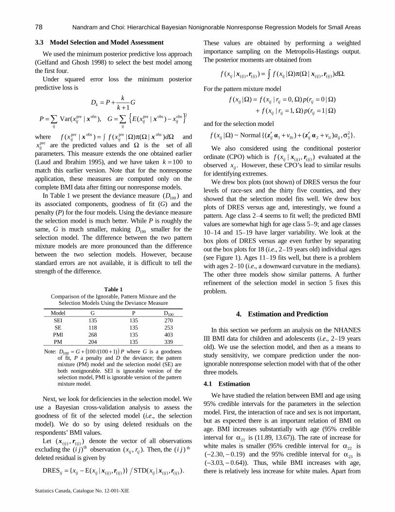
78 Nandram and Choi: Hierarchical Bayesian Nonignorable Nonresponse Regression Models for Small Areas
Statistics Canada, Catalogue No. 12-001-XIE
3.3 Model Selection and Model Assessment We used the minimum posterior predictive loss approach
(Gelfand and Ghosh 1998) to select the best model among the first four.
Under squared error loss the minimum posterior predictive loss is
{ }2obsobspreobspre )|(),|(Var
1
ijijij
ijij
k
xxEGxP
Gk
kPD
−==
++=
∑∑ xx
where ΩΩπΩ= ∫ dxfxf ijij )|()|()|( obspreobspre xx and preijx are the predicted values and Ω is the set of all
parameters. This measure extends the one obtained earlier (Laud and Ibrahim 1995), and we have taken 100=k to match this earlier version. Note that for the nonresponse application, these measures are computed only on the complete BMI data after fitting our nonresponse models.
In Table 1 we present the deviance measure )( 100D and its associated components, goodness of fit (G) and the penalty (P) for the four models. Using the deviance measure the selection model is much better. While P is roughly the same, G is much smaller, making 100D smaller for the selection model. The difference between the two pattern mixture models are more pronounced than the difference between the two selection models. However, because standard errors are not available, it is difficult to tell the strength of the difference.
Table 1 Comparison of the Ignorable, Pattern Mixture and the
Selection Models Using the Deviance Measure
Model G P D100
SEI 135 135 270 SE 118 135 253
PMI 268 135 403 PM 204 135 339
Note: ( ) PGD )1100/(100100 ++= where G is a goodness of fit, P a penalty and D the deviance; the pattern mixture (PM) model and the selection model (SE) are both nonignorable. SEI is ignorable version of the selection model, PMI is ignorable version of the pattern mixture model.
Next, we look for deficiencies in the selection model. We use a Bayesian cross-validation analysis to assess the goodness of fit of the selected model (i.e., the selection model). We do so by using deleted residuals on the respondents’ BMI values.
Let ),( )()( ijij rx denote the vector of all observations excluding the th)( ji observation ).,( ijij rx Then, the th)( ji deleted residual is given by
.),|STD()},|(E{DRES )()()()( ijijijijijijijij xxx rxrx−=
These values are obtained by performing a weighted importance sampling on the Metropolis-Hastings output. The posterior moments are obtained from
.),|()|(),|( )()()()( ΩΩπΩ= ∫ dxfxf ijijijijijij rxrx
For the pattern mixture model
)|1(),1|(
)|0(),0|()|(
Ω=Ω=+
Ω=Ω==Ω
ijijij
ijijijij
rprxf
rprxfxf
and for the selection model
}.,)(){(Normal~)|( 231201 σ+′++′Ω ijiijiijij avvxf αα zz
We also considered using the conditional posterior ordinate (CPO) which is ),|( )()( ijijijxf rx evaluated at the observed .ijx However, these CPO’s lead to similar results for identifying extremes.
We drew box plots (not shown) of DRES versus the four levels of race-sex and the thirty five counties, and they showed that the selection model fits well. We drew box plots of DRES versus age and, interestingly, we found a pattern. Age class 2 – 4 seems to fit well; the predicted BMI values are somewhat high for age class 5 – 9; and age classes 10 – 14 and 15 – 19 have larger variability. We look at the box plots of DRES versus age even further by separating out the box plots for 18 (i.e., 2 – 19 years old) individual ages (see Figure 1). Ages 11 – 19 fits well, but there is a problem with ages 2 – 10 (i.e., a downward curvature in the medians). The other three models show similar patterns. A further refinement of the selection model in section 5 fixes this problem.
4. Estimation and Prediction
In this section we perform an analysis on the NHANES III BMI data for children and adolescents (i.e., 2 – 19 years old). We use the selection model, and then as a means to study sensitivity, we compare prediction under the non-ignorable nonresponse selection model with that of the other three models. 4.1 Estimation
We have studied the relation between BMI and age using 95% credible intervals for the parameters in the selection model. First, the interaction of race and sex is not important, but as expected there is an important relation of BMI on age. BMI increases substantially with age (95% credible interval for 21α is (11.89, 13.67)). The rate of increase for white males is smaller (95% credible interval for 22α is
)19.0,30.2( −− and the 95% credible interval for 23α is )).64.0,03.3( −− Thus, while BMI increases with age,
there is relatively less increase for white males. Apart from
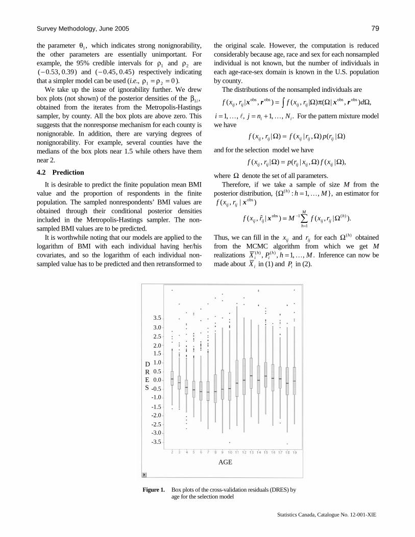
Survey Methodology, June 2005 79
Statistics Canada, Catalogue No. 12-001-XIE
the parameter ,1θ which indicates strong nonignorability, the other parameters are essentially unimportant. For example, the 95% credible intervals for 1ρ and 2ρ are
)39.0,53.0(− and )45.0,45.0(− respectively indicating that a simpler model can be used (i.e., 021 =ρ=ρ ).
We take up the issue of ignorability further. We drew box plots (not shown) of the posterior densities of the ,1iβ obtained from the iterates from the Metropolis-Hastings sampler, by county. All the box plots are above zero. This suggests that the nonresponse mechanism for each county is nonignorable. In addition, there are varying degrees of nonignorability. For example, several counties have the medians of the box plots near 1.5 while others have them near 2. 4.2 Prediction
It is desirable to predict the finite population mean BMI value and the proportion of respondents in the finite population. The sampled nonrespondents’ BMI values are obtained through their conditional posterior densities included in the Metropolis-Hastings sampler. The non-sampled BMI values are to be predicted.
It is worthwhile noting that our models are applied to the logarithm of BMI with each individual having her/his covariates, and so the logarithm of each individual non-sampled value has to be predicted and then retransformed to
the original scale. However, the computation is reduced considerably because age, race and sex for each nonsampled individual is not known, but the number of individuals in each age-race-sex domain is known in the U.S. population by county.
The distributions of the nonsampled individuals are
,),|()|,(),|,( obsobsobsobs ΩΩπΩ= ∫ drxfrxf ijijijij rxrx
.,,1,,,1 ii Nnji KlK +== For the pattern mixture model we have
)|(),|()|,( ΩΩ=Ω ijijijijij rprxfrxf
and for the selection model we have
),|(),|()|,( ΩΩ=Ω ijijijijij xfxrprxf
where Ω denote the set of all parameters. Therefore, if we take a sample of size M from the
posterior distribution, },,,1:{ )( Mhh K=Ω an estimator for )|,( obsxijij rxf
).|,()|ˆ,( )(
1
1obs hijij
M
hijij rxfMrxf Ω= ∑
=
−x
Thus, we can fill in the ijx and ijr for each )(hΩ obtained from the MCMC algorithm from which we get M realizations .,,1,, )()( MhPX h
ih
i K= Inference can now be made about iX in (1) and iP in (2).
Figure 1. Box plots of the cross-validation residuals (DRES) by age for the selection model
AGE
DRES
3.5
3.0 2.5 2.0 1.5 1.0 0.5 0.0
-0.5 -1.0
-1.5 -2.0 -2.5 -3.0 -3.5
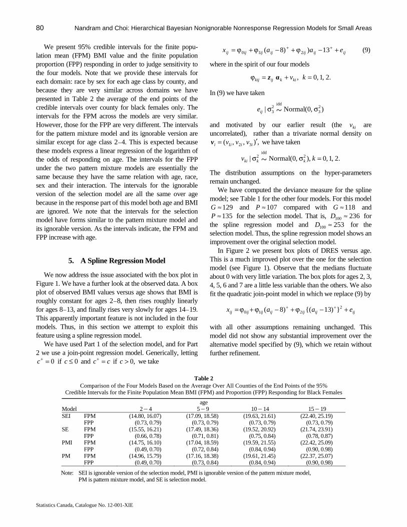
80 Nandram and Choi: Hierarchical Bayesian Nonignorable Nonresponse Regression Models for Small Areas
Statistics Canada, Catalogue No. 12-001-XIE
We present 95% credible intervals for the finite popu-lation mean (FPM) BMI value and the finite population proportion (FPP) responding in order to judge sensitivity to the four models. Note that we provide these intervals for each domain: race by sex for each age class by county, and because they are very similar across domains we have presented in Table 2 the average of the end points of the credible intervals over county for black females only. The intervals for the FPM across the models are very similar. However, those for the FPP are very different. The intervals for the pattern mixture model and its ignorable version are similar except for age class 2 – 4. This is expected because these models express a linear regression of the logarithm of the odds of responding on age. The intervals for the FPP under the two pattern mixture models are essentially the same because they have the same relation with age, race, sex and their interaction. The intervals for the ignorable version of the selection model are all the same over age because in the response part of this model both age and BMI are ignored. We note that the intervals for the selection model have forms similar to the pattern mixture model and its ignorable version. As the intervals indicate, the FPM and FPP increase with age.
5. A Spline Regression Model
We now address the issue associated with the box plot in Figure 1. We have a further look at the observed data. A box plot of observed BMI values versus age shows that BMI is roughly constant for ages 2 – 8, then rises roughly linearly for ages 8 – 13, and finally rises very slowly for ages 14 – 19. This apparently important feature is not included in the four models. Thus, in this section we attempt to exploit this feature using a spline regression model.
We have used Part 1 of the selection model, and for Part 2 we use a join-point regression model. Generically, letting
0=+c if 0≤c and cc =+ if ,0>c we take
ijijijijijijij eaax +−ϕ+−ϕ+ϕ= ++ 13))8( 210 (9)
where in the spirit of our four models
.2,1,0, =+=ϕ kvkikijkij αz
In (9) we have taken
),0(Normal| 23
idd23 ~ σσije
and motivated by our earlier result (the kiv are uncorrelated), rather than a trivariate normal density on
,),,( 321 ′= iiii vvvv we have taken
.2,1,0),,0(Normal| 2idd
2 ~ =σσ kv kkki
The distribution assumptions on the hyper-parameters remain unchanged.
We have computed the deviance measure for the spline model; see Table 1 for the other four models. For this model
129≈G and 107≈P compared with 118≈G and 135≈P for the selection model. That is, 236100 ≈D for
the spline regression model and 253100 ≈D for the selection model. Thus, the spline regression model shows an improvement over the original selection model.
In Figure 2 we present box plots of DRES versus age. This is a much improved plot over the one for the selection model (see Figure 1). Observe that the medians fluctuate about 0 with very little variation. The box plots for ages 2, 3, 4, 5, 6 and 7 are a little less variable than the others. We also fit the quadratic join-point model in which we replace (9) by
ijijijijijijij eaax +−ϕ+−ϕ+ϕ= ++ 2210 })13{()8(
with all other assumptions remaining unchanged. This model did not show any substantial improvement over the alternative model specified by (9), which we retain without further refinement.
Table 2
Comparison of the Four Models Based on the Average Over All Counties of the End Points of the 95% Credible Intervals for the Finite Population Mean BMI (FPM) and Proportion (FPP) Responding for Black Females
age Model 2 – 4 5 – 9 10 – 14 15 – 19 SEI FPM (14.80, 16.07) (17.09, 18.58) (19.63, 21.61) (22.40, 25.19) FPP (0.73, 0.79) (0.73, 0.79) (0.73, 0.79) (0.73, 0.79) SE FPM (15.55, 16.21) (17.49, 18.36) (19.52, 20.92) (21.74, 23.91) FPP (0.66, 0.78) (0.71, 0.81) (0.75, 0.84) (0.78, 0.87) PMI FPM (14.75, 16.10) (17.04, 18.59) (19.59, 21.55) (22.42, 25.09) FPP (0.49, 0.70) (0.72, 0.84) (0.84, 0.94) (0.90, 0.98) PM FPM (14.96, 15.79) (17.16, 18.38) (19.61, 21.45) (22.37, 25.07) FPP (0.49, 0.70) (0.73, 0.84) (0.84, 0.94) (0.90, 0.98)
Note: SEI is ignorable version of the selection model, PMI is ignorable version of the pattern mixture model, PM is pattern mixture model, and SE is selection model.
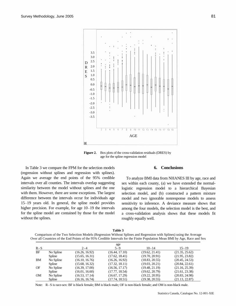
Survey Methodology, June 2005 81
Statistics Canada, Catalogue No. 12-001-XIE
Figure 2. Box plots of the cross-validation residuals (DRES) by age for the spline regression model
In Table 3 we compare the FPM for the selection models (regression without splines and regression with splines). Again we average the end points of the 95% credible intervals over all counties. The intervals overlap suggesting similarity between the model without splines and the one with them. However, there are some exceptions. The largest difference between the intervals occur for individuals age 15 – 19 years old. In general, the spline model provides higher precision. For example, for age 10 – 19 the intervals for the spline model are contained by those for the model without the splines.
6. Conclusions
To analyze BMI data from NHANES III by age, race and sex within each county, (a) we have extended the normal-logistic regression model to a hierarchical Bayesian selection model, and (b) constructed a pattern mixture model and two ignorable nonresponse models to assess sensitivity to inference. A deviance measure shows that among the four models, the selection model is the best, and a cross-validation analysis shows that these models fit roughly equally well.
Table 3 Comparison of the Two Selection Models (Regression Without Splines and Regression with Splines) using the Average
Over all Countries of the End Points of the 95% Credible Intervals for the Finite Population Mean BMI by Age, Race and Sex
age R – S 2 – 4 5 – 9 10 – 14 15 – 19 BF No Spline (16.26, 16.92) (16.44, 17.10) (19.62, 21.41) (21.35, 25.62) Spline (15.65, 16.31) (17.62, 18.41) (19.70, 20.91) (21.95, 23.82) BM No Spline (16.10, 16.76) (16.26, 16.92) (18.83, 20.55) (20.45, 24.53) Spline (15.68, 16.32) (17.32, 18.11) (19.03, 20.21) (20.84, 22.61) OF No Spline (16.39, 17.00) (16.56, 17.17) (19.48, 21.19) (21.16, 25.39) Spline (16.01, 16.60) (17.77, 18.54) (19.62, 20.79) (21.61, 23.38) OM No Spline (16.53, 17.14) (16.67, 17.29) (19.22, 20.95) (20.83, 24.98) Spline (16.16, 16.74) (17.74, 18.51) (19.38, 20.55) (21.13, 22.87)
Note: R – S is race-sex: BF is black female; BM is black male; OF is non-black female; and OM is non-black male.
AGE
D R E S
3.5 3.0 2.5 2.0 1.5 1.0 0.5 0.0
-0.5 -1.0 -1.5 -2.0 -2.5 -3.0 -3.5

82 Nandram and Choi: Hierarchical Bayesian Nonignorable Nonresponse Regression Models for Small Areas
Statistics Canada, Catalogue No. 12-001-XIE
Another contribution is the identification of a common deficiency in the selection model, the pattern mixture model and the two ignorable models. Based on the observed data, we have found that there is a dynamic relationship of BMI with age. Thus, we have further extended the selection model to include three linear splines. The cross validation analysis shows that there is an improvement over the selection model, and in fact, the deviance measure shows that the linear spline regression model is the best among the five models.
Our study on obesity is one of the key contributions in this work. The linear spline regression of BMI on age adjusting for race and sex, gives a better fit and improved precision than the selection model without splines. It is not easy to construct a model that is satisfactory for all aspects of the NHANES III data simultaneously. We have been able to do so for children and adolescents. BMI increases substantially with age; race and sex contributing negatively to this increase; there is relatively less increase for white males. In general, the effects of race and sex are relatively minor. There is some variation across the thirty five counties.
Appendix A The Pattern Mixture Model
For Part 1 of the pattern mixture model the response depends on age, race and sex, and the interaction of race and sex through the logistic regression
{ },)1/(
Bernoulli|
3423121034231210
~ind
ijiijiijiijiiijiijiijiijii zzzazzza
iij
ee
rβ+β+β+β+ββ+β+β+β+β +
β(A.1)
.,,1,,,1 iNjli KK == Now, letting, =iβ ,),,,,( 43210 ′βββββ iiiii note that while the vector iβ has
5=p components, the corresponding vector in (4) has two components. Analogous to (4) we take
),,(Normal~,|iid
ΔΔ θθβi (A.2)
and for the prior distribution,
,,},)Wishart{(~and
),(Normal~)0()0(1)0((0)1
)0()0(
pvvv >ΛΔ
Δ−−
θθ
(A.3)
where )0()0()0( ,, ΛΔθ and )0(v are to be specified. Part 2 of this model for BMI incorporates a dependence on the response indicators, letting ,,1 10 ijijij aww ==
).,0(Normal|
,1,0,)(
23
iid23
1
0
~ σσ
=++′=∑=
ij
ijijijttiijtijt
ij
e
rewvrx αz
(A.4)
The distributions on the ),( 10 ii vv are the same as in (7). The prior distributions are exactly those in Part 2 of the selection model (i.e., see (6) and (7)).
We take ,2)0( pv = a value that indicates near vagueness, maintains propriety and permits stability in computation. We show how to specify parameters like
)0()0()0()0()0( ,3,2,1,,,, Λ=ΔΔ tttαθ in Appendix C.
Appendix B
Metropolis-Hastings Algorithm for Fitting the Selection Model
For the nonignorable nonresponse selection model the joint posterior density is
)1.B(.
1
1
1
1
1
1
11
1
1
)|,,,,,,,(
)()(2
12
1
)()(2
12
12
2
5
1
2)1(2
1
22541
2)1(2
1
21211
}))({(2
1
311
}))({(2
1
311
),(21
2),(
)0(1)0()0(
)0(1)0()0(2
2
5
1
5
1
4
02
2
4
022
2
1
11
2
11
1
001
2
1
0021
10
210212
3
10
102
102123
⎪⎭
⎪⎬⎫
⎪⎩
⎪⎨⎧
×
⎪⎭
⎪⎬⎫
⎪⎩
⎪⎨⎧
⎪⎭
⎪⎬
⎫
⎪⎩
⎪⎨
⎧
⎟⎟⎠
⎞⎜⎜⎝
⎛
σ×
⎪⎭
⎪⎬
⎫
⎪⎩
⎪⎨
⎧
ρ−σσ×
⎪⎪⎭
⎪⎪⎬
⎫
⎪⎪⎩
⎪⎪⎨
⎧
ρ−σσ×
⎪⎭
⎪⎬⎫
⎪⎩
⎪⎨⎧
+σ×
⎪⎭
⎪⎬⎫
⎪⎩
⎪⎨⎧
+σ
∝ρρ
−Δ′−−
=
−Δ′−−σ−
+
=
⎥⎥
⎦
⎤
⎢⎢
⎣
⎡
⎟⎟⎠
⎞⎜⎜⎝
⎛
σ+⎟⎟⎠
⎞⎜⎜⎝
⎛
σ⎟⎟⎠
⎞⎜⎜⎝
⎛
σρ−⎟⎟
⎠
⎞⎜⎜⎝
⎛
σρ−−
=
⎥⎥
⎦
⎤
⎢⎢
⎣
⎡⎟⎟⎠
⎞⎜⎜⎝
⎛
σθ−β
+⎟⎟⎠
⎞⎜⎜⎝
⎛
σθ−β
⎟⎟⎠
⎞⎜⎜⎝
⎛
σθ−β
ρ−⎟⎟⎠
⎞⎜⎜⎝
⎛
σθ−β
ρ−−
=
β+β
+++′−σ
−
+==
β+β
β+β+++′−σ
−
==
−
−
∏
∏
∏
∏
∏∏
∏∏
kkkkk
k
iiii
iiii
ijii
ijiiijijiji
i
ijii
ijiiijiiijijiji
e
ee
e
e
ee
e
ee
p
k
aa
kk
vvvvl
i
l
i
x
avvaxn
rj
l
i
x
xavvaxr
j
l
i
rsnrs
αααα
θθθθ
αα
αα
θβασ
z
z
xvx
Let Ω denote the set of parameters ,,,, αθβ v
2123 ,, ψψσ and ),( nrsx where ),,( 1
22
211 ′ρσσ=ψ and
=2ψ .),,( 225
24 ′ρσσ Generically, let aΩ denote all
parameters in Ω except ;a for example, =Ωβ ),,,,,,,( ),(
2123
nrsxv ψψαθ σ so that the conditional posterior density (CPD) of β is denoted by
).,|( ),( rsp xββ Ω To perform the Metropolis-Hastings algorithm, one needs the CPD for each parameter given the others and .),( rsx Here we give a sketch of the algorithm.
The CPD for each of the parameters αθ ,, v and 23σ is
easy to write down. But we need Metropolis steps for the CPD’s of ,,, 21 ψψβ and .),( nrsx

Survey Methodology, June 2005 83
Statistics Canada, Catalogue No. 12-001-XIE
Conditioning on ,βΩ the parameters ,,,1 lββ K are independent with
,1
)|()()(
2
1
)(
)(
1
),(1
1
10
10 θβθββ
−Δ′−−
β+β
β+β
=
−
×⎪⎭
⎪⎬⎫
⎪⎩
⎪⎨⎧
+∝ ∏ ii
ijii
ijijiii
ee
ep
x
rxn
j
rsi x
where
⎟⎟⎠
⎞⎜⎜⎝
⎛
σσσρσσρσ
=Δ22211
21121
1
and lixij ,,1, K= and ii nrj ,,1 K+= are to be predicted; see below. We use a technique based on logistic regression to obtain a multivariate Student’s t proposal density in which tuning is obtained by varying its degree of freedom.
The method to draw from the CPD’s of =1ψ ),,( 1
22
21 ρσσ and ),,( 2
24
232 ρσσ=ψ is the same. The CPD
of 2ψ is
.)1(
1
1),|(
21
125
10154
220
124
22
25
24
2
121
)1(2
1
2/22
11
21
2
25
24
),(2
⎪⎭
⎪⎬⎫
⎪⎩
⎪⎨⎧
σ+ρ−
σρ−−
⎟⎟⎠
⎞⎜⎜⎝
⎛
σ+
σ−++
∑∑∑ ==σσ=
ρ−×
⎟⎟⎠
⎞⎜⎜⎝
⎛
σσ∝Ω
i
l
iii
l
ii
l
ivvvv
l
bla
rs
e
ep xψψ
We have used the Fisher’s z transformation (see Ruben 1966) to obtain a proposal density associated with normal distribution for )}1/(log{ 22 ρ−ρ and gamma distributions for 2
4σ and .25σ
Finally, we consider the Metropolis step for drawing .,| ),(),(
),(rsnrs
nrs xxx
Ω We note that in this CPD, ,,,1,,,1, iiij nrjlix KK +== are independent with
{ } .1
),|(1
]})({[2
1
),(
10
210212
3
−β+β
+++−σ
−
+
∝Ω
ijii
ijiiijijij
x
avvaxrs
ijij
e
expααz
x
We have constructed a proposal density using least squares techniques. We note that the proposal density Normal ),)(( 2
31021 σ+++ ijiiijij avva ααz did not perform well (see Chib and Greenberg 1995).
Appendix C
Specification of Hyperparameters We discuss how to specify the hyperparameters
),( )0()0( Δθ and ,2,1),,( )0()0( =Γ kkkα associated with θ and 2,1, =kkα in the selection model.
First, consider ).,( )0()0( Δθ For injli ,,1,,,1 KK == fit the logistic regression model ~
iid
ijr Bernoulli },)1({ 11010 −β+ββ+β + ijiiijii xx ee where ijx are obtained by
prediction (see Appendix A). Letting lii ,,1,ˆ K=β denote
the least squares estimators, we assume that ~iidˆ
iβ Normal )~
,( )0()0( Δθ to get ilil βθ ˆ/1 1
)0( ∑ == and
)ˆ()ˆ(1
1~)0()0(
1
)0( θβθβ −−−
=Δ ∑=
ii
l
il (C.1)
and we set ,~ )0(
1)0( Δκ=Δ where 1κ is to be selected.
Next, we consider how to specify .2,1),,( )0()0( =Γ kkkα We fit ,)( 21 ijijijij eax ++′= ααz where ija is the age of the
thj individual in the thi county, injli ,,1,,,1 KK == to get least squares estimators, )ˆ,ˆ(ˆ 21 ααα = and its covariance matrix .ˆ )0(Γ We set ,ˆ)0(
kk αα = and ,ˆ )0(2
)0(kk Γκ=Γ where
2,1,ˆ )0( =Γ kk is the corresponding block matrix of 2,1,ˆ )0( =Γ k and 2κ is to be specified.
We have experimented with 1κ in (C.1). We used 1001 =κ to provide a proper diffuse prior; a value of
000,11 =κ did not change our predictions. Similarly, we used .1002 =κ
References
Chib, S., and Greenberg, E. (1995). Understanding the metropolis-hastings algorithm. The American Statistician, 49, 327-335.
Cohen, G., and Duffy, J.C. (2002). Are nonrespondents to health surveys less healthy than respondents? Journal of Official Statistics, 18, 13-23.
Cowles, M., and Carlin, B. (1996). Markov chain Monte Carlo diagnostics: A comparative review. Journal of the American Statistical Association, 91, 883-904.
Daniels, M.J. (1999). A prior for the variance in hierarchical models. The Canadian Journal of Statistics, 27, 569-580.
David, M., Little, R.J.A., Samuel, M.E. and Triest, R.K. (1986). Alternative methods for CPS income imputation. Journal of the American Statistical Association, 81, 29-41.
Dietz, W.H. (1998). Health consequences of obesity in youth: Childhood predictors of adult disease. Pediatrics, 101, 518-525.
Fagot-Campagna, A. (2000). Emergence of type 2 diabetes mellitus in children: Epidemiological evidence. Journal of Pediatric Endocrinology Metabolism, 13, 1395-1405.
Gelfand, A., and Ghosh, S. (1998). Model choice: A minimum posterior predictive approach. Biometrika, 85, 1-11.
Gelfand, A., Sahu, S. and Carlin, B. (1995). Efficient parametrisations for normal linear mixed models. Biometrika, 82, 479-488.
Gelman, A., Roberts, G.O. and Gilks, W.R. (1996). Efficient Metropolis jumping rules. In Bayesian Statistics (Eds.J.M. Bernardo, J.O. Berger, A.P. Dawid and A.F.M. Smith, Oxford, U.K.: Oxford University Press, 599-607.
Greenlees, J.S., Reece, W.S. and Zieschang, K.D. (1982). Imputation of missing values when the probability of response depends on the variable being imputed. Journal of the American Statistical Association, 77, 251-261.
Heckman, J. (1976). The common structure of statistical models of truncation, sample selection and limited dependent variables and a simple estimator for such models. Annals of Economic and Social Measurement, 5, 475-492.

84 Nandram and Choi: Hierarchical Bayesian Nonignorable Nonresponse Regression Models for Small Areas
Statistics Canada, Catalogue No. 12-001-XIE
Kuczmarski, R.J., Carrol, M.D., Flegal, K.M. and Troiano, R.P. (1997). Varying body mass index cutoff points to describe overweight prevalence among U.S. adults: NHANES III (1988 to 1994). Obesity Research, 5, 542-548.
Laud, P., and Ibrahim, J. (1995). Predictive model selection. Journal of the Royal Statistical Society, Series B, 57, 247-262.
Little, R.J.A., and Rubin, D.B. (1987). Statistical Analysis with Missing Data, New York: John Wiley & Sons, Inc.
Mohadjar, L., Bell, B. and Waksberg, J. (1994). National health and Nutrition Examination Survey III-Accounting for item nonresponse bias. Internal Report, National Center for Health Statistics.
Nandram, B,. and Choi, J.W. (2002 a). A hierarchical Bayesian nonresponse model for binary data with uncertainty about ignorability. Journal of the American Statistical Association, 97, 381-388.
Nandram, B., and Choi, J.W. (2002 b). A Bayesian analysis of a proportion under nonignorable nonresponse. Statistics in Medicine, 21, 1189-1212.
Nandram, B., Han, G. and Choi, J.W. (2002). A hierarchical bayesian nonignorable nonresponse model for multinomial data from small areas. Survey Methodology, 28, 145-156.
Natarajan, R., and Kass, R.E. (2000). Reference Bayesian methods for generalized linear models. Journal of the American Statistical Association, 95, 227-237.
National Center for Health Statistics (1992). Third national health and nutrition examination survey. Vital and Health Statistics Series 2, 113.
National Center for Health Statistics (1994). Plan and operation of the third national health and nutrition examination survey. Vital and Health Statistics Series, 1, 32.
Ogden, C.L., Flegal, K.M., Carroll, M.D. and Johnson, C.L. (2002). Prevalence and trends in overweight among us children and adolescents, 1999-2000. Journal of the American Medical Association, 288, 1728-1732.
Olson, R.L. (1980). A least square correction for selectivity bias. Econometrica, 48, 1815-1820.
Rao, C.R. (1973). Linear Statistical Inference and Its Applications. New York: John Wiley & Sons, Inc.
Ruben, H. (1966). Some new results on the distribution of the sample correlation coefficient. Journal of the Royal Statistical society, Series B, 28, 513-525.
Rubin, D.B. (1976). Inference and missing data. Biometrika, 63, 581-590.
Rubin, D.B. (1977). Formalizing subjective notions about the effect of nonrespondents in sample surveys. Journal of the American Statistical Association, 72, 538-543.
Rubin D.B. (1987). Multiple Imputation for Nonresponse in Surveys. New York: John Wiley & Sons, Inc.
Schafer, J.L., Ezzati-Rice, T.M., Johnson, W., Khare, M. Little, R.J. A. and Rubin, D.B. (1996). The NHANES III multiple imputation project. Survey research methods, Proceedings of the American Statistical Association, 28-37.
Squires, S. (2001). National plan urges to combat obesity: Weight-related illnesses kill 300,000 Americans annually, Surgeon General says. The Washington Post, December 14, 2001.
Stasny, E.A. (1991). Hierarchical models for the probabilities of a survey classification and nonresponse: An example from the National Crime Survey. Journal of the American Statistical Association, 86, 296-303.
Who Consultation on Obesity (2000). Obesity: Preventing and managing the global epidemic. WHO Technical Report Series 894, Geneva, Switzerland: World Health Organization.
Wright, C.M., Parker, L., Lamont, D. and Craft, A.W. (2001). Implications of childhood obesity for adult health: Findings from thousand families cohort study. British Medical Journal, 323, 1280-1284.
Survey Methodology, June 2005 85 Vol. 31, No. 1, pp. 85-93 Statistics Canada, Catalogue No. 12-001-XIE
Towards Nonnegative Regression Weights for Survey Samples
Mingue Park and Wayne A. Fuller 1
Abstract
Procedures for constructing vectors of nonnegative regression weights are considered. A vector of regression weights in which initial weights are the inverse of the approximate conditional inclusion probabilities is introduced. Through a simulation study, the weighted regression weights, quadratic programming weights, raking ratio weights, weights from logit procedure, and weights of a likelihood-type are compared.
1. Mingue Park, University of Nebraska, 103 Miller Hall, Lincoln, NE, 68588-0712, U.S.A.; Wayne A. Fuller, Iowa State University, 221 Snedecor Hall,
Ames, IA 50011-1210, U.S.A.
Key Words: Raking ratio; Maximum likelihood; Quadratic programming; Simple Conditionally Weighted (SCW)
estimator.
1. Introduction In survey sampling, information about the population is
often available at the analysis stage. One method of using this information is through regression estimation. There are a number of ways to construct a regression estimator of the population mean or total. One regression estimator of the mean is
∑=
ππ −+==n
iNii yywy
1reg ,
~)( βxx (1)
where
,)( 1
1
1
1 −−
=
−π φ⎟⎟
⎠
⎞⎜⎜⎝
⎛φ′−+α= ∑ iii
n
jjjjjNiiw xxxxx (2)
∑∑∑==
−−
=ππ α=π⎟⎟
⎠
⎞⎜⎜⎝
⎛π=
n
iiii
n
iiii
n
ii yyy
11
1
1
1
1- ,),(:),(),( xxx
∑∑=
−−
=
− φ′⎟⎟⎠
⎞⎜⎜⎝
⎛φ′=
n
iiiii
n
iiiii y
1
1
1
1
1 ,~
xxxβ
,1
1
1
1 −−
=
− π⎟⎟⎠
⎞⎜⎜⎝
⎛π=α ∑ i
n
jji
)...,,(diag 11 nnφφ=Φ is a nonsingular diagonal matrix, the iπ ’s are the selection probabilities and Nx is the population mean of .x A possible choice of 1−φii is .iα A review of the use of such information in regression esti-mation for sample surveys is given by Fuller (2002).
It is well known that regression weights that are used to define a regression estimator such as (2) can be very large or (and) can be negative. If the regression weights are to be used to estimate a finite population total in a general pur-pose survey, it seems reasonable that no individual weight
should be less than one. Also, it seems reasonable, on robustness grounds, to avoid very large weights.
There are several ways to construct regression weights with a reduced range of values. Huang and Fuller (1978) defined a procedure to modify the iw so that there are no negative weights and no large weights. Husain (1969) sug-gested quadratic programming as a procedure to place bounds on the weights. Quadratic programming and a number of other procedures build on the fact that the weights can be defined as values that optimize some function. Deville and Särndal (1992) considered seven objective functions that can be used to construct weights. They suggested objective functions that can be used to produce weights which fall within a given range. Deville, Särndal and Sautory (1993) introduced the program, CALMAR, written as a SAS macro that can be used to calculate weights corresponding to four different objective functions when auxiliary information in the survey consists of known marginal counts in a frequency table.
Another modification of regression weights is to relax some of the restrictions used in constructing the estimator. Husain (1969) considered modifying weights for a simple random sample from a normal distribution. He derived the weights that minimize the mean square error (MSE) of the resulting estimator. Bardsley and Chambers (1984) con-sidered an estimator based on an objective function and the division of the auxiliary variable into two components. They studied the behavior of the estimator from a model perspective. Rao and Singh (1997) studied an estimator in which tolerances are given for the difference between the final estimator for part of the auxiliary variables vector and the corresponding elements of the population vector.
In this paper, we consider different types of regression weights including a procedure based on Tillé’s (1998) con-ditional selection probabilities. The approximate conditional
86 Park and Fuller: Towards Nonnegative Regression Weights for Survey Samples
Statistics Canada, Catalogue No. 12-001-XIE
inclusion probabilities are used to compute regression weights that are positive for most samples. These regression weights are compared to raking ratio weights, to quadratic programming weights, weights from logit procedure, and to weights based on a likelihood-type objective function.
2. Maximum Likelihood and
Raking Ratio Consider a two-way table with r rows and c columns.
The population cell ijU contains ijN elements; ...,,1=i ....,,1, cjr = Assume marginal counts ji NN ⋅⋅ , are
known. The population characteristics of interest are the
ijN or, equivalently, .1ijij NNp −= For a simple random
nonreplacement sample of size ,n Deming and Stephan (1940) suggested a raking ratio procedure to get the solution for the cell frequencies. See also Stephan (1942). If we assume the sample is a random sample from a multinomial distribution defined by the population entries in a two way table, we can construct an estimator using the maximum likelihood procedure.
Deville and Särndal (1992) defined a class of calibration estimators, ,caly of the population mean of y as
∑=
=n
iii ywy
1cal , (3)
where the iw ’s minimize the objective function ∑ = αn
i iiwG1 ),( subject to constraints
,and111∑∑
====
n
iNii
n
ii ww xx (4)
and ),( iiwG α is a measure of distance between an initial weight iα and a final weight .iw The raking ratio and maximum likelihood estimators of the population cell fraction, ,ijp belong to the class of calibration estimators.
The raking ratio weights for the population cell fraction, with a simple random sample, can be obtained by minimizing
∑=
−− +−⎟⎠⎞
⎜⎝⎛n
kk
kk nw
n
ww
1
11
,log (5)
subject to the constraints (4) with
,)...,,,...,,( 11 crk ⋅⋅⋅⋅ δδδδ=x (6)
where 1=δ ⋅i if thk element belongs to the thi row and 0=δ ⋅i otherwise, and 1=δ⋅ j if thk element belongs to the
thj column and 0=δ⋅ j otherwise. The raking ratio estimator for the population cell fraction ijp is the estimator (3) where 1=ky if the thk element belongs to cell ij and
0=ky otherwise.
For the maximum likelihood estimator of the population fraction, with a simple random sample, Deville and Särndal (1992) suggested minimizing
∑=
−−
− −+⎟⎠⎞
⎜⎝⎛−
n
kk
k nwn
wn
1
11
1 log (7)
subject to (4) with x defined in (6). Chen and Sitter (1999) suggested a pseudo empirical
likelihood estimator. They defined the population likelihood of iy as
∑=
N
iUiw
1, ,log (8)
where Uiw , is the density at observation .iy With a sample of size ,n they suggested the pseudo empirical likelihood estimator of the form
∑=
=n
iii ywy
1EL , (9)
where iw ’s are obtained by minimizing the function
∑=
−π−n
iii w
1
1 ,log (10)
under the restrictions (4). The resulting iw are equal to those obtained by minimizing (7) with iN π= under the restrictions (4).
Deville and Särndal (1992) showed that the raking ratio and maximum likelihood estimators are approximately equal to a regression estimator of the form (1), and, hence, have the same limiting distribution as the regression estimator. Weights for the raking ratio and maximum likelihood estimators are nonnegative if the solutions for the weights exist.
3. Weighted Regression Using Conditional Probabilities
Tillé (1998) suggested the use of approximate conditional inclusion probabilities, conditioning on the Horvitz-Thompson estimators of auxiliary variables, to compute an estimator for the population mean of the study variable. His approximation can be extended to produce regression weights that are nonnegative with high probability.
Assume that the vector of population means of auxiliary variables, ,Nx is known. Consider the Horvitz-Thompson estimator of Nx given by
,1
1HT ∑
= π=
n
i i
i
N
xx (11)
Survey Methodology, June 2005 87
Statistics Canada, Catalogue No. 12-001-XIE
where )...,,( 1 ipii xx=x and iπ is the unconditional inclusion probability. Tillé (1998) introduced the simple conditionally weighted (SCW) estimator,
,1
1 | HT
∑=
π π=
n
i xi
ip
y
Ny (12)
where HT|xiπ is the conditional inclusion probability of the
thi element conditioning on .HTx To construct the SCW-estimator of ,Ny the conditional inclusion probability
HT|xiπ is required. If HTx takes the value ,t we have
,}{
}|{
HT
HT| HT tx
tx=
∈=π=πP
AiPixi (13)
where A is the set of indices for the sample elements. In order to compute the conditional inclusion probabil-
ities, it is necessary to know the probability distribution of
HTx unconditionally and conditionally on the presence of each unit in the sample. Except for some particular cases, this probability distribution is very complex. For this reason, approximation of the conditional inclusion probability is considered.
Under the assumption that HTx has an approximately normal distribution unconditionally and conditionally on the presence of each unit in the sample, the conditional inclu-sion probability (13) can be approximated by
,)}(5.0{exp
ˆ
)(,
2/1
)(,
2/1
| HT
ixxxx
ixxxxixi
GG −
π=π−
∑∑ (14)
where ,},|{Var,}|x{Var HT)(,HT AiFF ixxxx ∈== x∑∑
,)()( HT1
HT ′−−= −NxxNxx xxxxG ∑
,)()( )(,HT1
)(,)(,HT)(, ′−−= −iNixxiNixx xxxxG ∑
,)()(
},|{
1
111
HT)(,
j
N
ijj
ijjiii
iN
NN
AiFE
xx
xx
∑≠=
−−− πππ+π
=∈=
A is the set of indices appearing in the sample and }...,,{ 1 NyyF = is the finite population. Tillé (1998) gives
an expression for )(, ixx∑ for the general case. Assume the design covariance matrices xx∑ and )(, ixx∑
are positive definite and assume the vector of auxiliary variables is normally distributed. Tillé (1999) showed that the SCW-estimator defined in (12) with the approximate conditional inclusion probabilities of (14) satisfies
)()( 1HTHT
−π +−+= nOyy pNNp βxx (15)
,)( 1reg
−+= nOy p (16)
where
,1yxxxN ∑∑β −=
,ˆ)( HTHTreg βxx −+= Nyy
,)(ˆˆˆ 1111 yXXX −−−− ′′== ΦΦ∑∑β yxxx
,)...,,(,)...,,( 11 ′=′′′= nn yyyxxX the thij element of 1−Φ is xxjiijjiijN ∑),()( 12 ππ−ππππ −− is the design
variance of ,HTx yx∑ is the design covariance of HTx and ,HTy xx∑ is the Horvitz-Thompson variance estimator of ,HTx and yx∑ is the Horvitz-Thompson estimator of the
covariance of HTx and .HTy Given a complex design, a number of the quantities in
(14) are difficult to compute. However, approximations giving the same large sample properties for the estimator are relatively easy to compute. We replace xx∑ and )(, ixx∑ with estimators, replace )(, iNx with ,
ixN dx + define
,)(ˆ 1ix
Aiiyx yN
idM ′+π=∑
∈
− (17)
and assume
,)()}ˆ({Var 1−=− nOn yxyx MM (18)
,)( 1−= nOpxid (19)
where ixd is a function of the sample and yxM is a
population quantity. Often yxM is the population covari-ance matrix ,yx∑ but this equality is not required in order for the estimator to be well defined. In many cases one can compute
ixd as a multiple of the jackknife deviate. Also in many situations, an adequate value for the estimator,
,~
)(, ixx∑ of )(, ixx∑ is .ˆ)1(1xxnn ∑−− We write our gener-
alization of (14) as
,)}~ˆ(5.0{exp
~ˆ~
)(,
2/1
)(,
2/1
| HT
ixxxx
ixxxxixi
GG −
π=π−
∑∑
(20)
where
,)(ˆ)(ˆHT
1HT ′−−= −
NxxNxx xxxxG ∑
.)(~
)(~
HT1
)(,HT)(, ′−−−−= −ii xNixxxNixx dxxdxxG ∑
Let the estimator (12) constructed with the HT|
~xiπ of (20) be
∑=
−−π π=
n
iixip yNy
1
1|
1~ .~
HT (21)
An approximate conditional inclusion probability with a simple random sample and a single auxiliary variable is
88 Park and Fuller: Towards Nonnegative Regression Weights for Survey Samples
Statistics Canada, Catalogue No. 12-001-XIE
,~)(
ˆ)(
2
1exp
~ˆ~
2)(,
2
2
2
)(,|
⎪⎭
⎪⎬⎫
⎪⎩
⎪⎨⎧
⎥⎥⎦
⎤
⎢⎢⎣
⎡
σ−−
−σ−
⎥⎥⎦
⎤
⎢⎢⎣
⎡
σσ=π
ix
xNn
x
Nn
ix
xxi
i
n
dxxxx
N
n
where
,)()(])1([ 1Nix xxnNNnd
i−−−= −
,ˆ1
)1(
)(
)2(
)1()(~ 22
22
22
)(, xni
xix n
n
N
xxNs
Nn
nnN σ−≈⎥⎦
⎤⎢⎣
⎡−−−
−−−=σ
,)(ˆ 2112xx sNn −− −=σ
and
.)()1(1
212 ∑=
− −−=n
inix xxns
In this case, NiNx xxdi
−= )(, and .),(Cov HTHT yxM yx = The SCW-estimator (21) with the approximate
conditional inclusion probabilities is not calibrated, that is, the estimator (21) for the mean of the vector of auxiliary variables is not the vector of population means. It is relatively easy to standardize the probabilities so that they sum to one or sum to the stratum fraction for stratified sampling. To construct a calibrated estimator for the general case, we suggest computing the regression estimator with
1|
11
1| HTHT
~]~[ −−=
− ππ∑ xinj xj as initial weights. The suggested
estimator is
∑=
=
−+=n
iii
ccNcw
yw
yy
1
1,reg
,
ˆ)( βxx
(22)
where
,),(),(1∑
=α=
n
iiiicc yy xx
( ) ,ˆ,ˆ1
1
11,0, ⎥
⎦
⎤⎢⎣
⎡′α⎥
⎦
⎤⎢⎣
⎡′α=
′β ∑∑
=
−
=
n
iiii
n
iiiicc yzzzβ
,),1( cii xxz −=
,~~ 1|
1
1
1| HTHT
−−
=
− π⎥⎦
⎤⎢⎣
⎡π=α ∑ xi
n
jxji
,)()()()(
1
1
′−α⎥⎦
⎤⎢⎣
⎡−′−α−+
α=−
=∑ cii
n
jcjcjjcN
iiw
xxxxxxxx
and HT|
~xiπ is the approximate conditional inclusion
probability of (20). We assume the vector of auxiliary variables contains one so that the estimator is location invariant.
The estimator (21) is approximately equal to a regression estimator and estimator (22) is also approximately equal to the same regression estimator. Theorem: Let a sequence of populations and samples,
,},{ NN AF satisfy
.)(),(),( 2/1HTHT
−=− nOyy pNN xx (23)
Assume that the sequences of estimated covariance matrices, xx∑ and ,
~)(, ixx∑ satisfy
[ ][ ] ,)(ˆ
~
11
2/12/1
12/1)(,
2/1
−−−−
−−−
=− nOpxx
ixx
DD
DD
∑
∑
(24)
where D denotes a diagonal matrix having the elements of the diagonal of xx∑ on its diagonal. Let
ixd be a function of the sample satisfying (19) and assume (18) holds. Assume the sequence of Horvitz-Thompson variance estimators satisfies
( )[ ]{ } ,)(ˆVechVar 1HT,
−=− nOn zzzz ∑∑ (25)
where ),( iii yxz = and zz∑ is positive definite. Assume }~{ 2
| HT
−π xiE is bounded, where HT|
~xiπ is defined in (20).
Then, the SCW– estimator π~py of (21) satisfies
,)(ˆ)(
)()(
1HTHT
1HTHT~
−
−π
+−+=
+−+=
nOy
nOyy
pN
pNNp
θ
θ
xx
xx
where yxxx Mˆˆ 1−= ∑θ and .1yxxxN M−= ∑θ
If ,0}{Var 11 >π∑ =
−ni i assume ix contains one as an
element. Assume .yxyx ∑=M Then the weighted regression estimator of (22) satisfies
.)(ˆ)( 1HTHTreg
−+−+= nOyy pNw θxx
For proof, see the appendix. To illustrate the nature of the different types of regression
weights, we selected a simple random sample of size 40 from a normal population with mean zero and variance one. The sample mean is – 0.614 and the population mean is zero. The weight for the regression estimator is given by (2) with .11 −− =φ=α niii The weights for the raking ratio and MLE are obtained by minimizing the objective functions (5) and (7), respectively, under the restriction (4). Weights for the SCW-weighted regression estimator are given in (22). The weights are plotted against the sample x values in Figure 1. Five of the simple regression weights are less than zero because of the large discrepancy between the sample and the population means. All weights for the SCW-weighted regression estimator, MLE and raking ratio are nonnegative. Figure 1 shows that the behaviors of raking ratio and SCW-weighted regression weights are similar and that MLE has an extremely large weight in this sample.
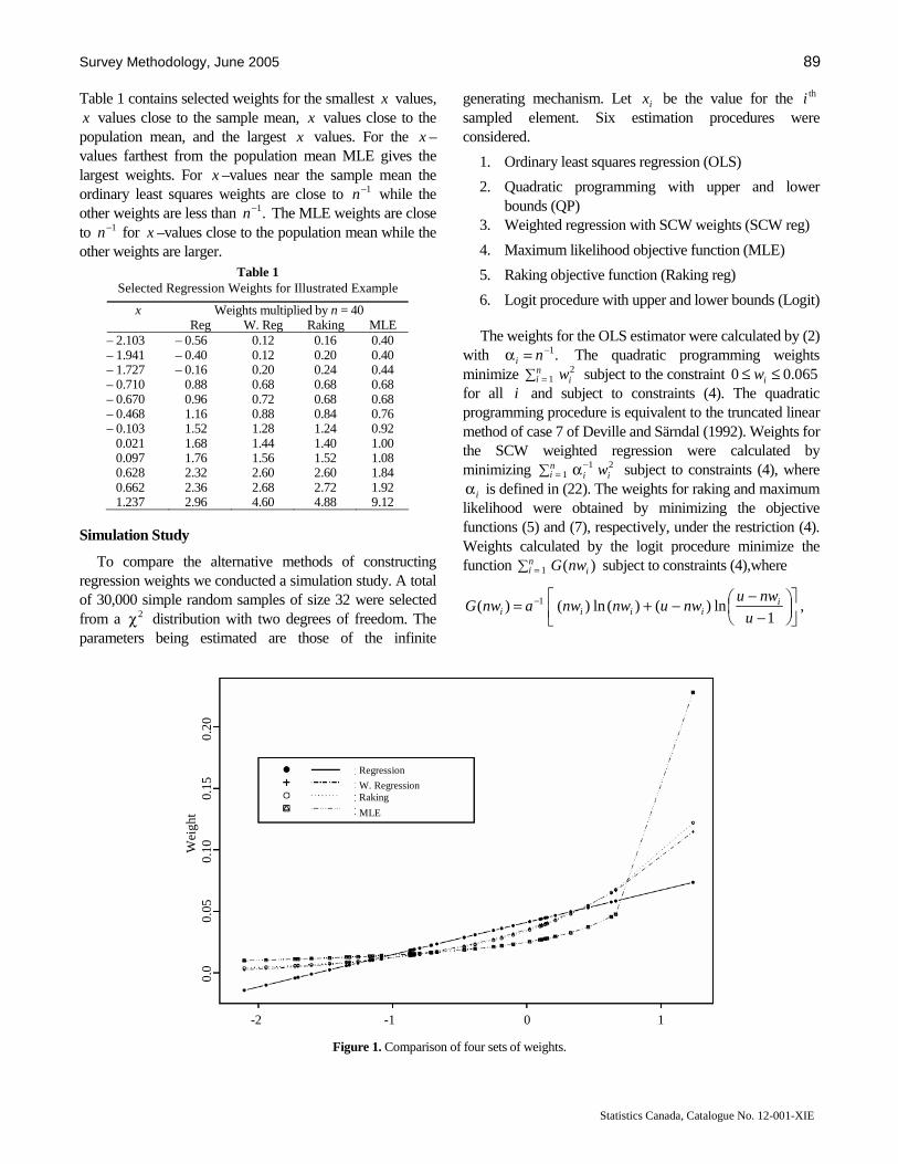
Survey Methodology, June 2005 89
Statistics Canada, Catalogue No. 12-001-XIE
Table 1 contains selected weights for the smallest x values, x values close to the sample mean, x values close to the population mean, and the largest x values. For the x –values farthest from the population mean MLE gives the largest weights. For x –values near the sample mean the ordinary least squares weights are close to 1−n while the other weights are less than .1−n The MLE weights are close to 1−n for x –values close to the population mean while the other weights are larger.
Table 1 Selected Regression Weights for Illustrated Example
x Weights multiplied by n = 40 Reg W. Reg Raking MLE
– 2.103 – 0.56 0.12 0.16 0.40 – 1.941 – 0.40 0.12 0.20 0.40 – 1.727 – 0.16 0.20 0.24 0.44 – 0.710 0.88 0.68 0.68 0.68 – 0.670 0.96 0.72 0.68 0.68 – 0.468 1.16 0.88 0.84 0.76 – 0.103 1.52 1.28 1.24 0.92
0.021 1.68 1.44 1.40 1.00 0.097 1.76 1.56 1.52 1.08 0.628 2.32 2.60 2.60 1.84 0.662 2.36 2.68 2.72 1.92 1.237 2.96 4.60 4.88 9.12
Simulation Study
To compare the alternative methods of constructing regression weights we conducted a simulation study. A total of 30,000 simple random samples of size 32 were selected from a 2χ distribution with two degrees of freedom. The parameters being estimated are those of the infinite
generating mechanism. Let ix be the value for the thi sampled element. Six estimation procedures were considered.
1. Ordinary least squares regression (OLS)
2. Quadratic programming with upper and lower bounds (QP)
3. Weighted regression with SCW weights (SCW reg)
4. Maximum likelihood objective function (MLE)
5. Raking objective function (Raking reg)
6. Logit procedure with upper and lower bounds (Logit) The weights for the OLS estimator were calculated by (2)
with .1−=α ni The quadratic programming weights minimize ∑ =
ni iw1
2 subject to the constraint 065.00 ≤≤ iw for all i and subject to constraints (4). The quadratic programming procedure is equivalent to the truncated linear method of case 7 of Deville and Särndal (1992). Weights for the SCW weighted regression were calculated by minimizing ∑ =
−αni ii w1
21 subject to constraints (4), where
iα is defined in (22). The weights for raking and maximum likelihood were obtained by minimizing the objective functions (5) and (7), respectively, under the restriction (4). Weights calculated by the logit procedure minimize the function ∑ =
ni inwG1 )( subject to constraints (4),where
,1
ln)()(ln)()( 1⎥⎦⎤
⎢⎣⎡
⎟⎠⎞
⎜⎝⎛
−−−+= −
u
nwunwunwnwanwG i
iiii
Figure 1. Comparison of four sets of weights.
Wei
ght
0.
0
0.
05
0.1
0
0.1
5
0.2
0
-2 -1 0 1
Regression
W. Regression Raking
MLE
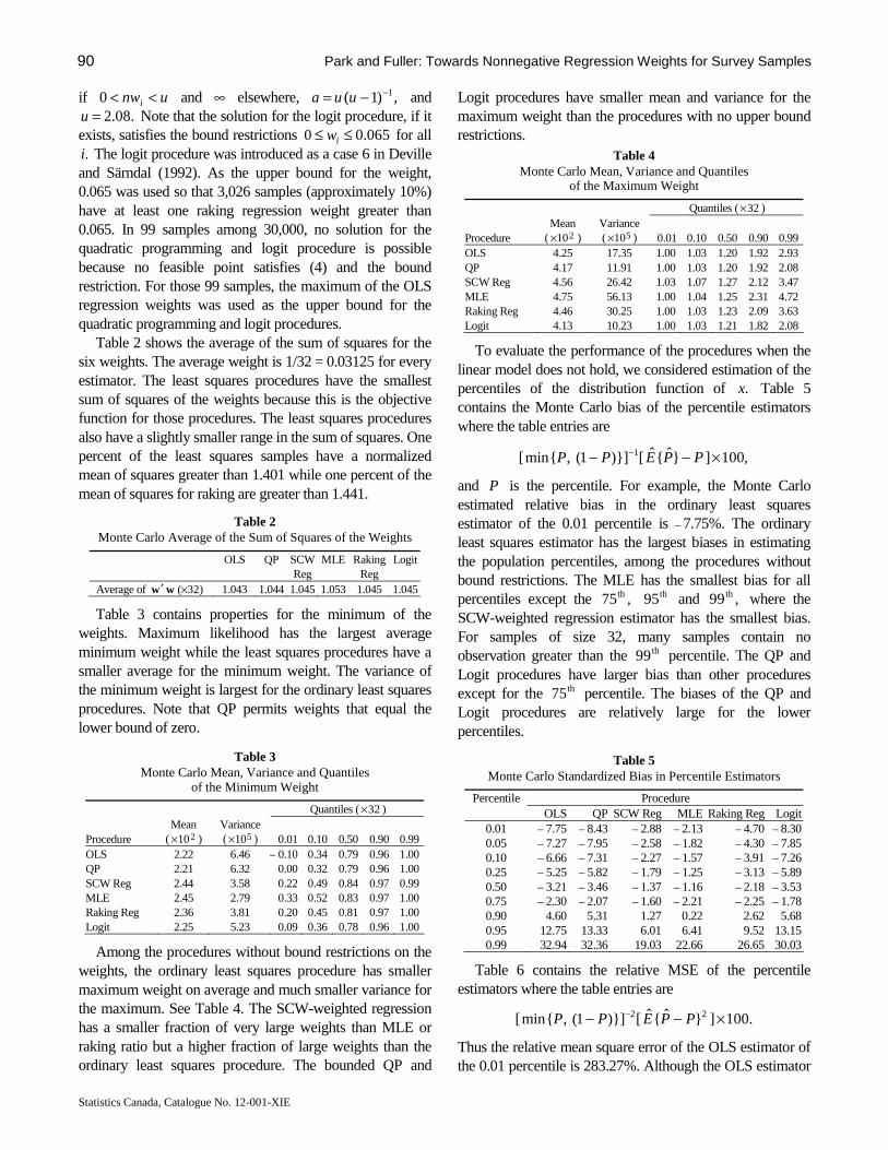
90 Park and Fuller: Towards Nonnegative Regression Weights for Survey Samples
Statistics Canada, Catalogue No. 12-001-XIE
if unwi <<0 and ∞ elsewhere, ,)1( 1−−= uua and .08.2=u Note that the solution for the logit procedure, if it
exists, satisfies the bound restrictions 065.00 ≤≤ iw for all .i The logit procedure was introduced as a case 6 in Deville
and Särndal (1992). As the upper bound for the weight, 0.065 was used so that 3,026 samples (approximately 10%) have at least one raking regression weight greater than 0.065. In 99 samples among 30,000, no solution for the quadratic programming and logit procedure is possible because no feasible point satisfies (4) and the bound restriction. For those 99 samples, the maximum of the OLS regression weights was used as the upper bound for the quadratic programming and logit procedures.
Table 2 shows the average of the sum of squares for the six weights. The average weight is 1/32 = 0.03125 for every estimator. The least squares procedures have the smallest sum of squares of the weights because this is the objective function for those procedures. The least squares procedures also have a slightly smaller range in the sum of squares. One percent of the least squares samples have a normalized mean of squares greater than 1.401 while one percent of the mean of squares for raking are greater than 1.441.
Table 2 Monte Carlo Average of the Sum of Squares of the Weights
OLS QP SCW Reg
MLE Raking Reg
Logit
Average of 32)(×′ ww 1.043 1.044 1.045 1.053 1.045 1.045 Table 3 contains properties for the minimum of the
weights. Maximum likelihood has the largest average minimum weight while the least squares procedures have a smaller average for the minimum weight. The variance of the minimum weight is largest for the ordinary least squares procedures. Note that QP permits weights that equal the lower bound of zero.
Table 3 Monte Carlo Mean, Variance and Quantiles
of the Minimum Weight
Quantiles ( 32× )
Procedure Mean
( 210× ) Variance ( 510× ) 0.01 0.10 0.50 0.90 0.99
OLS 2.22 6.46 – 0.10 0.34 0.79 0.96 1.00 QP 2.21 6.32 0.00 0.32 0.79 0.96 1.00 SCW Reg 2.44 3.58 0.22 0.49 0.84 0.97 0.99 MLE 2.45 2.79 0.33 0.52 0.83 0.97 1.00 Raking Reg 2.36 3.81 0.20 0.45 0.81 0.97 1.00 Logit 2.25 5.23 0.09 0.36 0.78 0.96 1.00
Among the procedures without bound restrictions on the weights, the ordinary least squares procedure has smaller maximum weight on average and much smaller variance for the maximum. See Table 4. The SCW-weighted regression has a smaller fraction of very large weights than MLE or raking ratio but a higher fraction of large weights than the ordinary least squares procedure. The bounded QP and
Logit procedures have smaller mean and variance for the maximum weight than the procedures with no upper bound restrictions.
Table 4 Monte Carlo Mean, Variance and Quantiles
of the Maximum Weight
Quantiles ( 32× )
Procedure Mean
( 210× ) Variance ( 510× ) 0.01 0.10 0.50 0.90 0.99
OLS 4.25 17.35 1.00 1.03 1.20 1.92 2.93 QP 4.17 11.91 1.00 1.03 1.20 1.92 2.08 SCW Reg 4.56 26.42 1.03 1.07 1.27 2.12 3.47 MLE 4.75 56.13 1.00 1.04 1.25 2.31 4.72 Raking Reg 4.46 30.25 1.00 1.03 1.23 2.09 3.63 Logit 4.13 10.23 1.00 1.03 1.21 1.82 2.08
To evaluate the performance of the procedures when the linear model does not hold, we considered estimation of the percentiles of the distribution function of .x Table 5 contains the Monte Carlo bias of the percentile estimators where the table entries are
,100]}ˆ{ˆ[)}]1(,{min[ 1 ×−− − PPEPP
and P is the percentile. For example, the Monte Carlo estimated relative bias in the ordinary least squares estimator of the 0.01 percentile is – 7.75%. The ordinary least squares estimator has the largest biases in estimating the population percentiles, among the procedures without bound restrictions. The MLE has the smallest bias for all percentiles except the ,75th th95 and ,99th where the SCW-weighted regression estimator has the smallest bias. For samples of size 32, many samples contain no observation greater than the th99 percentile. The QP and Logit procedures have larger bias than other procedures except for the th75 percentile. The biases of the QP and Logit procedures are relatively large for the lower percentiles.
Table 5 Monte Carlo Standardized Bias in Percentile Estimators
Percentile Procedure OLS QP SCW Reg MLE Raking Reg Logit
0.01 – 7.75 – 8.43 – 2.88 – 2.13 – 4.70 – 8.30 0.05 – 7.27 – 7.95 – 2.58 – 1.82 – 4.30 – 7.85 0.10 – 6.66 – 7.31 – 2.27 – 1.57 – 3.91 – 7.26 0.25 – 5.25 – 5.82 – 1.79 – 1.25 – 3.13 – 5.89 0.50 – 3.21 – 3.46 – 1.37 – 1.16 – 2.18 – 3.53 0.75 – 2.30 – 2.07 – 1.60 – 2.21 – 2.25 – 1.78 0.90 4.60 5.31 1.27 0.22 2.62 5.68 0.95 12.75 13.33 6.01 6.41 9.52 13.15 0.99 32.94 32.36 19.03 22.66 26.65 30.03
Table 6 contains the relative MSE of the percentile estimators where the table entries are
.100]}ˆ{ˆ[)}]1(,{min[ 22 ×−− − PPEPP
Thus the relative mean square error of the OLS estimator of the 0.01 percentile is 283.27%. Although the OLS estimator
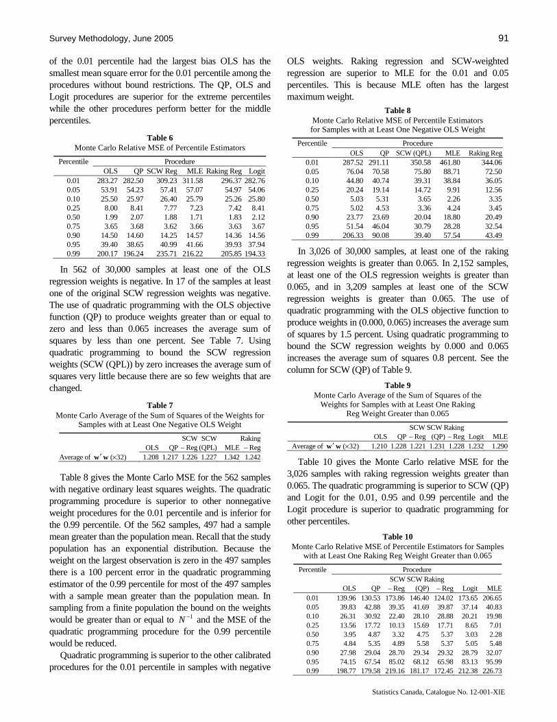
Survey Methodology, June 2005 91
Statistics Canada, Catalogue No. 12-001-XIE
of the 0.01 percentile had the largest bias OLS has the smallest mean square error for the 0.01 percentile among the procedures without bound restrictions. The QP, OLS and Logit procedures are superior for the extreme percentiles while the other procedures perform better for the middle percentiles.
Table 6 Monte Carlo Relative MSE of Percentile Estimators
Percentile Procedure OLS QP SCW Reg MLE Raking Reg Logit
0.01 283.27 282.50 309.23 311.58 296.37 282.76 0.05 53.91 54.23 57.41 57.07 54.97 54.06 0.10 25.50 25.97 26.40 25.79 25.26 25.80 0.25 8.00 8.41 7.77 7.23 7.42 8.41 0.50 1.99 2.07 1.88 1.71 1.83 2.12 0.75 3.65 3.68 3.62 3.66 3.63 3.67 0.90 14.50 14.60 14.25 14.57 14.36 14.56 0.95 39.40 38.65 40.99 41.66 39.93 37.94 0.99 200.17 196.24 235.71 216.22 205.85 194.33
In 562 of 30,000 samples at least one of the OLS regression weights is negative. In 17 of the samples at least one of the original SCW regression weights was negative. The use of quadratic programming with the OLS objective function (QP) to produce weights greater than or equal to zero and less than 0.065 increases the average sum of squares by less than one percent. See Table 7. Using quadratic programming to bound the SCW regression weights (SCW (QPL)) by zero increases the average sum of squares very little because there are so few weights that are changed.
Table 7 Monte Carlo Average of the Sum of Squares of the Weights for
Samples with at Least One Negative OLS Weight
OLS QP
SCW – Reg
SCW (QPL) MLE
Raking – Reg
Average of 32)(×′ ww 1.208 1.217 1.226 1.227 1.342 1.242 Table 8 gives the Monte Carlo MSE for the 562 samples
with negative ordinary least squares weights. The quadratic programming procedure is superior to other nonnegative weight procedures for the 0.01 percentile and is inferior for the 0.99 percentile. Of the 562 samples, 497 had a sample mean greater than the population mean. Recall that the study population has an exponential distribution. Because the weight on the largest observation is zero in the 497 samples there is a 100 percent error in the quadratic programming estimator of the 0.99 percentile for most of the 497 samples with a sample mean greater than the population mean. In sampling from a finite population the bound on the weights would be greater than or equal to 1−N and the MSE of the quadratic programming procedure for the 0.99 percentile would be reduced.
Quadratic programming is superior to the other calibrated procedures for the 0.01 percentile in samples with negative
OLS weights. Raking regression and SCW-weighted regression are superior to MLE for the 0.01 and 0.05 percentiles. This is because MLE often has the largest maximum weight.
Table 8 Monte Carlo Relative MSE of Percentile Estimators for Samples with at Least One Negative OLS Weight
Percentile Procedure OLS QP SCW (QPL) MLE Raking Reg
0.01 287.52 291.11 350.58 461.80 344.06 0.05 76.04 70.58 75.80 88.71 72.50 0.10 44.80 40.74 39.31 38.84 36.05 0.25 20.24 19.14 14.72 9.91 12.56 0.50 5.03 5.31 3.65 2.26 3.35 0.75 5.02 4.53 3.36 4.24 3.45 0.90 23.77 23.69 20.04 18.80 20.49 0.95 51.54 46.04 30.79 28.28 32.54 0.99 206.33 90.08 39.40 57.54 43.49
In 3,026 of 30,000 samples, at least one of the raking regression weights is greater than 0.065. In 2,152 samples, at least one of the OLS regression weights is greater than 0.065, and in 3,209 samples at least one of the SCW regression weights is greater than 0.065. The use of quadratic programming with the OLS objective function to produce weights in (0.000, 0.065) increases the average sum of squares by 1.5 percent. Using quadratic programming to bound the SCW regression weights by 0.000 and 0.065 increases the average sum of squares 0.8 percent. See the column for SCW (QP) of Table 9.
Table 9 Monte Carlo Average of the Sum of Squares of the
Weights for Samples with at Least One Raking Reg Weight Greater than 0.065
SCW SCW Raking OLS QP – Reg (QP) – Reg Logit MLE
Average of 32)(×′ ww 1.210 1.228 1.221 1.231 1.228 1.232 1.290 Table 10 gives the Monte Carlo relative MSE for the
3,026 samples with raking regression weights greater than 0.065. The quadratic programming is superior to SCW (QP) and Logit for the 0.01, 0.95 and 0.99 percentile and the Logit procedure is superior to quadratic programming for other percentiles.
Table 10 Monte Carlo Relative MSE of Percentile Estimators for Samples
with at Least One Raking Reg Weight Greater than 0.065
Percentile Procedure SCW SCW Raking OLS QP – Reg (QP) – Reg Logit MLE
0.01 139.96 130.53 173.86 146.40 124.02 173.65 206.65 0.05 39.83 42.88 39.35 41.69 39.87 37.14 40.83 0.10 26.31 30.92 22.40 28.10 28.88 20.21 19.98 0.25 13.56 17.72 10.13 15.69 17.71 8.65 7.01 0.50 3.95 4.87 3.32 4.75 5.37 3.03 2.28 0.75 4.84 5.35 4.89 5.58 5.37 5.05 5.48 0.90 27.98 29.04 28.70 29.34 29.32 28.79 32.07 0.95 74.15 67.54 85.02 68.12 65.98 83.13 95.99 0.99 198.77 179.58 219.16 181.17 172.45 212.38 226.73
92 Park and Fuller: Towards Nonnegative Regression Weights for Survey Samples
Statistics Canada, Catalogue No. 12-001-XIE
Discussion We began the research with the conjecture that starting
with the SCW weights in a regression estimator would produce weights that were almost always positive and that the weights would have desirable properties as measured by the ability to estimate the distribution function of .x To some extent these results support the conjectures. The minimum weights of the SCW regression are larger than those of OLS and comparable to those for raking. Quadratic programming can be used to remove the negative weights in the few samples with negative weights. If no upper bound is imposed, the maximum weights for the SCW weighted regression fall between those of least squares and raking.
It is known that all of the procedures in our simulation study have the same order 2/1−n properties. Our simulation and the study of generalized raking procedures done by Deville et al. (1993) indicate that there are also modest differences in small samples. No procedure is superior with respect to all criteria. Because of the poor performance for the extreme percentiles, we recommend against the use of the MLE objective function. The quadratic programming and Logit procedure produced weights with marginally smaller sums of squares, marginally smaller maximum weights, and marginally smaller MSE for extreme percentiles than the raking regression. The MLE, SCW regression and raking procedures give marginally larger minimum weights and marginally smaller MSE for the middle percentiles of the x distribution than quadratic programming and Logit procedure. The performances of quadratic programming and Logit procedures in estimating the distribution function of x are comparable.
Appendix
Proof. The ratio of the determinants of estimated covariance matrices in (20) is
)(1ˆ
~1)(, −+= nOp
xx
ixx
∑
∑ (26)
by assumptions (24) and (25). The difference xxixx GG ˆ~)(, −
is
( ).
~~)(2
)(ˆ~)(
1)(,
1)(,HT
HT11
)(,HT
iii xixxxxixxN
NxxixxN
dddxx
xxxx
′+′−−
′−−−−−
−−
∑∑
∑∑
By assumptions (23) and (24),
).(1
]})()ˆ~()[(5.0{exp
1
HT11
)(,HT
−
−−
+
=′−−−
nOp
NxxixxN xxxx ∑∑ (27)
Using assumptions (24) and (19), the Taylor expansion at 0=
ixd gives
).(ˆ)(1
)(~
)(1
]~
5.0~
)([exp
11HT
11)(,HT
1)(,
1)(,HT
−−
−−
−−
+′−+=
+′−+=
′+′−−
nO
nO
pxxxN
pxixxN
xixxxxixxN
i
i
iii
dxx
dxx
dddxx
∑
∑
∑∑
(28)
Thus, by (26), (27) and (28),
).(]ˆ)(1[)(]~[ 21HT
11| HT
−−−− +′−+π=π nONN pxxxNixi idxx ∑
By assumptions (18), (23) and (25), and using the fact that }~{ 2
| HT
−π xiE is bounded,
).()(
)(ˆ)(1
HTHT
1HTHT~
−
−π
+−+=
+−+=
nOy
nOyy
pNN
pNp
θ
θ
xx
xx
(29)
If one is an element of ix or Var ,0}{ 11 =π∑ =
−ni i and if
,yxyx ∑=M the SCW-estimator for the population mean of vector ),1( ii xq = satisfies
,)(),1(~ 1
1
1|
1~
HT
−
=
−−π +=π= ∑ nON p
n
iNixip xqq (30)
because the θ for x is the identity matrix. By (30),
.)(),(
),(~),(
1~~
~~
1
1
1| HT
−ππ
ππ
−
=
−
+=
⎥⎦
⎤⎢⎣
⎡π= ∑
nOy
yNy
ppp
pp
n
ixicc
x
xx
(31)
Thus,
,)(ˆ)(
)(
ˆ)()(ˆ)(
ˆ)(
1HTHT
1~
1,~~1,~~
1,reg
−
−π
ππππ
+−+=
+=
−+−+−+=
−+=
nOy
nOy
yyy
yy
pN
pp
ccppccpNp
ccNcw
θ
ββ
β
xx
xxxx
xx
by (30), (31) and (29).
Acknowledgements
This research was partly supported by Cooperative Agreement 43-3AEU-3-80088 between Iowa State University, the USDA National Agricultural Statistics Service and the U.S. Bureau of the Census, and by Cooperative Agreement 68-3A75-14 between the USDA Natural Resources Conservation Service and Iowa State University. We thank the Associate editor and referees for comments that improved the paper.

Survey Methodology, June 2005 93
Statistics Canada, Catalogue No. 12-001-XIE
References Bardsley, P., and Chambers, R.L. (1984). Multipurpose estimation
from unbalanced samples. Applied Statistics, 33, 290-299. Chen, J., and Sitter, R.R. (1999). A pseudo empirical likelihood
approach to the effective use of auxiliary information in complex surveys. Statistica Sinica, 9, 385-406.
Deming, W.E., and Stephan, F.F. (1940). On a least squares adjustment of a sampled frequency table when the expected marginal totals are known. Annals of Mathematical Statistics, 11, 427-444.
Deville, J.-C., and Särndal, C.-E. (1992). Calibration estimators in survey sampling. Journal of the American Statistical Association, 87, 376-382.
Deville, J.-C., Särndal, C.-E. and Sautory, O. (1993). Generalized raking procedures in survey sampling. Journal of the American Statistical Association, 88, 1013-1020.
Fuller, W.A. (2002). Regression estimation for survey samples. Survey Methodology, 28, 5-23.
Huang, E.T., and Fuller, W.A. (1978). Nonnegative regression estimation for sample survey data. Proceedings of the Social Statistics Section, American Statistical Association, 300-305.
Husain, M. (1969). Construction of Regression Weights for Estimation in Sample Surveys. Unpublished M.S. thesis, Iowa State University, Ames, Iowa.
Rao, J.N.K., and Singh, A.C. (1997). A ridge shrinkage method for range restricted weight calibration in survey sampling. Proceedings of the section on survey research methods, American Statistical Association, 57-64.
Stephan, F.F. (1942). An alternative method of adjusting sample frequency tables when expected marginal totals are known. Annals of Mathematical Statistics, 13, 166-178.
Tillé, Y. (1998). Estimation in surveys using conditional inclusion probabilities: Simple random sampling. International Statistical Review, 66, 303-322.
Tillé, Y. (1999). Estimation in surveys using conditional inclusion probabilities: complex design. Survey Methodology, 25, 57-66.

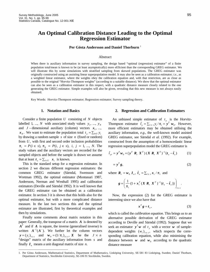
Survey Methodology, June 2005 95 Vol. 31, No. 1, pp. 95-99 Statistics Canada, Catalogue No. 12-001-XIE
An Optimal Calibration Distance Leading to the Optimal Regression Estimator
Per Gösta Andersson and Daniel Thorburn 1
Abstract
When there is auxiliary information in survey sampling, the design based “optimal (regression) estimator” of a finite population total/mean is known to be (at least asymptotically) more eEficient than the corresponding GREG estimator. We will illustrate this by some simulations with stratified sampling from skewed populations. The GREG estimator was originally constructed using an assisting linear superpopulation model. It may also be seen as a calibration estimator; i.e., as a weighted linear estimator, where the weights obey the calibration equation and, with that restriction, are as close as possible to the original “Horvitz-Thompson weights” (according to a suitable distance). We show that the optimal estimator can also be seen as a calibration estimator in this respect, with a quadratic distance measure closely related to the one generating the GREG estimator. Simple examples will also be given, revealing that this new measure is not always easily obtained.
1. Per Gösta Andersson, Mathematical Statistics, Department of Mathematics, Linköping University, SE-581 83 Linköping, Sweden; Daniel Thorburn,
Department of Statistics, Stockholm University, SE-106 91 Stockholm, Sweden.
Key Words: Horvitz-Thompson estimator; Regression estimator; Survey sampling theory.
1. Notation and Basics Consider a finite population U consisting of N objects
labelled N...,,1 with associated study values Nyy ...,,1 and −J dimensional auxiliary (column) vectors ...,,1x
.Nx We want to estimate the population total ∑ ∈= Ui iy yt by drawing a random sample s of size n (fixed or random) from ,U with first and second order inclusion probabilities
),,(),( sjiPsiP iji ∈=π∈=π ....,,1, Nji = The study values and the auxiliary vectors are recorded for the sampled objects and before the sample is drawn we assume that at least ∑ ∈= Ui ix xt is known.
This is the standard setup for a regression estimator. In section 2 we discuss different regression estimators: the common GREG estimator (Särndal, Swensson and Wretman 1992), the optimal estimator (Montanari 1987, Andersson, Nerman and Westhall 1995) and calibration estimators (Deville and Särndal 1992). It is well known that the GREG estimator can be obtained as a calibration estimator. In section 3 it is shown that this holds also for the optimal estimator, but with a more complicated distance measure. In the last two sections this and the optimal estimator are illustrated, first by theoretical examples and then by simulations.
Finally some comments about matrix notation in this paper: Generally, the transpose of a matrix A is denoted by
TA and if A is square, the inverse (generalised inverse) is written ).(1 −− AA We further let the column vectors
siiy ∈= )(y and X,)/1(0 sii ∈π=w be the nJ × “design” matrix of the auxiliary information from s and finally nI means a unit diagonal matrix of size .n
2. Regression and Calibration Estimators An unbiased simple estimator of yt is the Horvitz-
Thompson estimator ∑ ∈ =π= siT
iiy yt ./ˆ 0wy However, more efficient estimators may be obtained utilising the auxiliary information, e.g., the well-known model assisted GREG estimator, see Särndal et al. (1992). For example, constructed from the assumption of a homoscedastic linear regression superpopulation model the GREG estimator is
)ˆ()()(ˆ 10 xx
Tr
Tr
TTyrt ttXRXXRywy −+= − (1)
,gyT= (2)
where ∑ π== ∈ si iixnr /ˆ,0 xtIwR and
.))ˆ()(1(1 1
si
xxT
rTi
i ∈
−⎟⎟⎠
⎞⎜⎜⎝
⎛−+
π= ttXRXxg
Now, the expression (2) for the GREG estimator is interesting since we also have that
,xT tgx = (3)
which is called the calibration equation. This brings us to an alternative possible derivation of the GREG estimator according to Deville and Särndal (1992). Suppose that we seek an estimator wyT of yt with a vector w of sample-dependent weights ,)( siiw ∈ which respects the corre-sponding calibration equation, while also minimising the distance between w and 0w according to the quadratic distance measure
96 Andersson and Thorburn: An Optimal Calibration Distance Leading to the Optimal Regression Estimator
Statistics Canada, Catalogue No. 12-001-XIE
),()( 00 wwRww −− T
where .)( 10
−= nIwR This results in
,)ˆ()( 1110 xx
TT ttXRXxRww −+= −−− (4)
which means that ,gw = since here .1−= rRR Turning to the optimal estimator, consider first the vector
)ˆ,ˆ( Txtyt and let xy,∑ be the covariance (row) vector of yt
and xt and xx,∑ the covariance matrix of .ˆxt Now, the
minimum-variance, see Montanari (1987), unbiased linear estimator (in yt and xt ) of yt is the difference estimator
.)ˆ(ˆ 1,, xtt −+ −
xxxxyyt ∑∑ (5)
Since xy,∑ and xx,∑ in practice are unknown, we let the optimal estimator be
,)ˆ()()(ˆ
)ˆ(ˆˆˆ
1optopt
1,,0opt
xxTTT
y
xxxxxyT
y
t
t
ttXRXXRy
ttwy
−+=
−+=
−
−∑∑
(6)
where .))/()(( ,opt sjijiijjiij ∈πππππ−π=R In an asymptotic context, where ∞→n and
yxN ,ˆ, ∑∞→ and xx,∑ may be viewed as components of
the asymptotic covariance matrix of ).ˆ,ˆ( Txyt t Under the
assumption of consistency of yx,∑ and ,ˆ, xx∑ which holds
under very mild conditions, see Andersson et al. (1995), the optimal estimator has the same asymptotic variance as the difference estimator (5). In particular it follows that the optimal estimator is asymptotically better than the usual GREG estimator, see Rao (1994), Montanari (2000) and Andersson (2001), i.e., its asymptotic variance is never larger and usually smaller. In section 5 we actually present some simple simulations showing that the optimal estimator can be much more efficient than GREG. However, one does not know anything about the efficiency for finite samples, since the covariance estimator may converge slowly. The rate of convergence is illustrated in section 5. Note also that in some cases there exist asymptotically even better estimators which are not linear.
Now, the fact that the GREG estimator is also a calibration estimator using
)()( 01
0 wwRww −− −r
T (7)
as the distance measure and comparing (1) with (6), leads one to believe that replacing rR by optR in (7) should imply that we instead derive the optimal regression estimator as a calibration estimator. That this actually holds is shown below.
3. The Main Result In order to show existence of a distance measure
corresponding to the optimal estimator, we will first state and prove a result in the general case. Lemma: With R denoting an arbitrary positive definite
nn × matrix,
)()( 00 wwRww −− T (8)
subject to the constraint ,xtwX = is minimised by
.)ˆ()( 1110 xx
TT ttXRXXRww −+= −−−
Proof: Introducing the 1×J vector λ of Lagrange multipliers, we get after differentiation the equation system
0)(2 0 =+− λTXwwR (9)
0=− xtWX (10)
Multiplying (9) by ,1−XR using (10) and solving for ,λ yields with :ˆ
0 xtwX =
.)ˆ()(2 11xx
T ttXRX −= −−λ (11)
Putting this into (9) and solving for w finally leads to
.)ˆ()( 1110 xx
TT ttXRXXRww −+= −−−
From the lemma we thus have the following main result: Theorem: With optR being positive (semi –) definite and using the optimal calibration distance-measure, which we get by letting )( opt
1opt
−−= RRR in (8), the calibration estimator will become the optimal regression estimator. Remark: optR may in some cases be indefinite (see below). The only thing we know is that it is an unbiased estimator of a covariance matrix. If it is not positive semi-definite there also exist x – values such that TXRX opt is not positive semi-definite, but the probability of such x – values goes to zero as the population and sample sizes increase (and if
xx,∑ is positive definite). A strict minimisation of a distance with “a negative component” would lead to infinitely large corrections. This problem of the optimal estimator has, to our knowledge, not been pointed out previously.
The simplest way to find a distance which gives the optimal estimator as a calibration estimator is to find a matrix distR which has the same eigenvectors as optR but where the eigenvalues are replaced by their absolute values. (This result can be shown along the same lines as the proof of the lemma above. The distance can be seen as the sum of
Survey Methodology, June 2005 97
Statistics Canada, Catalogue No. 12-001-XIE
the products of the eigenvalues and the squared eigenvectors. Putting the derivatives equal to zero means that in the proposition we found the extremes i.e., the minima for positive eigenvalues and the maxima for negative eigenvalues. By changing all negative signs the extremes will all be minima).
4. Examples
Positive definite optR : Suppose that the objects in U are independently drawn with inclusion probabilities
Nππ ...,,1 (Poisson sampling); thus implying a random sample size ,n where .][ iUinE π∑= ∈ Due to the independence of drawings, optR is diagonal and specifically
.1
21
opt
sii
in
∈
−⎟⎟⎠
⎞⎜⎜⎝
⎛π−
π= IR
Positive semi-definite optR : Suppose n objects are drawn according to simple random sampling, i.e., each object has inclusion probability ./ Nni =π The elements of optR are
N
nN
n
Nji
−⎟⎠⎞
⎜⎝⎛=
2
:
.)1(
:2
−−
⎟⎠⎞
⎜⎝⎛≠
nN
Nn
n
Nji
This means that optR is singular with rank .1−n Suppose instead (as in the following simulation study)
that U is partitioned into L strata of sizes ,...,,1 LNN from which we draw independent simple random samples of sizes ....,,1 Lnn The elements of optR then are
h
hh
h
h
N
nN
n
Nji
−⎟⎟⎠
⎞⎜⎜⎝
⎛=
2
:
,)1(
:2
−−
⎟⎟⎠
⎞⎜⎜⎝
⎛≠
hh
hh
h
h
nN
Nn
n
Nji
when in the latter case i and j both belong to stratum Lhh ...,,1, = and 0 otherwise. Therefore optR has rank
.hN − Non positive semi-definite optR : Let U consist of four elements and s of two elements. Suppose that a systematic sample is taken with probability 0.94 and a simple random sample with probability 0.06, i.e., 48.02413 =π=π and
.01.034231412 =π=π=π=π In that case
⎟⎟⎠
⎞⎜⎜⎝
⎛=212/23
12/232optR (12)
with probability 0.96 and
⎟⎟⎠
⎞⎜⎜⎝
⎛−
−=
296
962optR (13)
with probability 0.04. The second matrix has a negative eigenvalue.
The problem does not necessarily disappear if N is large. Consider instead a population consisting of 4/N strata with four elements each. Suppose that the above sampling procedure is used independently in each stratum. In that case optR will consist of a matrix with the above
22 × – matrices along the diagonal and zeroes elsewhere.
5. A Simulation Study
5.1 Notation and Outline In order to make empirical comparisons between the
optimal estimator (OPT) and the GREG estimator (GREG) and also compare these estimators with the Horvitz-Thompson estimator (HT), we have conducted a small simulation study. In the previous sections we mentioned that OPT is Best Linear Asymptotic Efficient and a calibration estimator. Even though it has many nice properties it may for reasonable sample sizes be inefficient. Here we will in some simulated situations show that the optimal estimator can be a substantial improvement compared to GREG also for moderate sample sizes when the population is (deliberately) chosen to be unfavourable for GREG. A simple but non-trivial situation for which OPT is not equal to GREG arises for stratified simple random sampling, in particular, when the slopes differ between the different strata and the unstratified population. Consider therefore a population of size ,N which is partitioned into L strata of sizes ....,,1 LNN From each stratum h a simple random sample hs of size hn is drawn, where sss L =+ ...1 and
....1 nnn L =++ For simplicity we further assume that the auxiliary information is one-dimensional and global, i.e., only xt is known beforehand. For GREG we have chosen the homoscedastic simple linear regression model, see Särndal et al. (1992).
The resulting expressions for HT, OPT and GREG respectively are
)),(ˆ(ˆ
))(ˆ(ˆ
ˆ
optopt
strstyr
ststy
sty
xxByNt
xxByNt
yNt
−+=
−+=
=
where stsh
Lhsti
Ni xyNNyxNx
h(,)/1(,)/1( 11 == ∑=∑=
analogous) and
98 Andersson and Thorburn: An Optimal Calibration Distance Leading to the Optimal Regression Estimator
Statistics Canada, Catalogue No. 12-001-XIE
22
1
2
1
opt
)(11
1
)()(11
1ˆ
hh
hhh
sisihhh
hLh
sisisihhh
hLh
xxNnn
N
yyxxNnn
N
B
−∑⎟⎟⎠
⎞⎜⎜⎝
⎛−
−∑
−−∑⎟⎟⎠
⎞⎜⎜⎝
⎛−
−∑
=
∈=
∈=
.)(
)()(ˆ
21
1
stisih
hLh
stistisih
hLh
r
xxn
N
yyxxn
N
B
h
h
−∑∑
−−∑∑=
∈=
∈=
It is easily seen from these formulae that the optimal regression coefficient is the mean of the within stratum slopes and that the GREG regression coefficient is the global slope. When there is a large difference between these slopes the GREG correction becomes bad. We are here particularly interested in comparing the qualities of these estimators when the assisting (linear) model for GREG fails. We have thus generated −x and −y values from correlated lognormally distributed random variables X and
,Y where ln X is normally distributed with expectation 0 and variance )),0(( 1
21 σσ N and lnY is .),0( 2σN The
variances 21σ and 2
2σ and the correlation between ln X and lnY can then be chosen to obtain prespecified values of the variances 2
xσ of X and 2yσ of Y and their correlation
.),( YXρ Values generated from bivariate normal distributions were obtained by MATLAB (version 6.0). Twelve populations have in this manner been created, each of size N = 10,000, including four combinations of variances 2
xσ and 2yσ (10 and 100) and three values of the
correlation ),( YXρ (0.5, 0.7 and 0.9). For these populations a variance of 10 implies a skewness of 9.37 and the variance 100 leads to skewness 38.59.
Now, before stratification, the objects of each population are ordered with respect to ascending −y values. The number of strata is 5=L throughout with sizes
,000,41 =N 000,1,000,2,500,2 432 === NNN and .5005 =N These strata are constructed in such a way that
objects with the smallest −y values constitute stratum 1, and so forth. From each stratified population we have drawn samples of sizes 000,1,250=n and 2,500, where for each sample .... 51 nn == This means that we have created an approximate psπ (probability proportional to size) design, with for example, objects in stratum 5 having the largest inclusion probability .)/( 55 Nn The number of simulated samples was =K 25,000 for each of the 36312 =× cases and HT, OPT and GREG were then computed for each sample.
In general, common measures of quality for an estimator t of a total t from a sequence Ltt ˆ...,,1 are the estimated relative bias
t
tt −ˆ
and the estimated variance
,)ˆˆ(1
1
1
22 ∑=
−−
=K
ii tt
KS
where .ˆ)/1(ˆ 1 iKi tKt =∑=
Since we are mainly concerned with comparisons of OPT and GREG, we will only display results of the relative measures of variance (or equivalently standard deviation)
,and2
HT
2
2HT
2opt
y
ry
y
y
S
S
S
S
from which we can compare the estimated variances of OPT and GREG with HT and also determine which of OPT and GREG have the lowest estimated variance. 5.2 Results
Firstly, as reference, the absolute value of the estimated relative bias of the unbiased HT did not in any case exceed
.104 4−⋅ The corresponding maximum values for OPT and GREG were ,106 3−⋅ which means that we may concentrate on the ratios of estimated variances in order to evaluate relative efficiencies of HT, OPT and GREG.
As seen from Table 1, OPT is superior to both HT and GREG (with one exception: ,10,9.0),( 2 =σ=ρ xYX
1002 =σ y and ,250=n where GREG has slighly less estimated variance). For the lowest correlation though, the decrease in estimated variance for OPT compared with HT is not substantial. GREG on the other hand does not compete well with the others and this anomaly is particularly accentuated for the largest sample size
.500,2=n Changing ),( YXρ to 0.7 means improvement for both OPT and GREG, but GREG is also now for most cases inferior to HT. Finally, for 9.0),( =ρ YX GREG still displays poor behavior compared with HT for 500,2=n (with the exception of 1002 =σ x and .)102 =σ y In general GREG is closing in on OPT for increasing values of
),( YXρ (the assisting linear model becoming less misspecified), while OPT, on the other hand, is increasing its superiority over GREG for increasing sample sizes, which should come as no surprise since OPT is asymptotically well motivated.
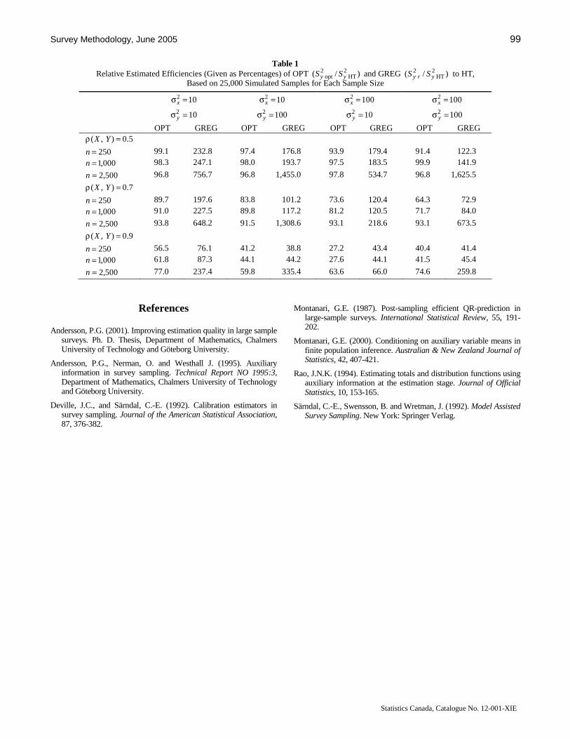
Survey Methodology, June 2005 99
Statistics Canada, Catalogue No. 12-001-XIE
Table 1 Relative Estimated Efficiencies (Given as Percentages) of OPT )/( 2
HT2
opt yy SS and GREG )/( 2HT
2yry SS to HT,
Based on 25,000 Simulated Samples for Each Sample Size
102 =σx 102 =σx 1002 =σx 1002 =σx
102 =σ y 1002 =σ y 102 =σ y 1002 =σ y
OPT GREG OPT GREG OPT GREG OPT GREG 5.0),( =ρ YX
250=n 99.1 232.8 97.4 176.8 93.9 179.4 91.4 122.3
000,1=n 98.3 247.1 98.0 193.7 97.5 183.5 99.9 141.9
500,2=n 96.8 756.7 96.8 1,455.0 97.8 534.7 96.8 1,625.5
7.0),( =ρ YX
250=n 89.7 197.6 83.8 101.2 73.6 120.4 64.3 72.9
000,1=n 91.0 227.5 89.8 117.2 81.2 120.5 71.7 84.0
500,2=n 93.8 648.2 91.5 1,308.6 93.1 218.6 93.1 673.5
9.0),( =ρ YX
250=n 56.5 76.1 41.2 38.8 27.2 43.4 40.4 41.4
000,1=n 61.8 87.3 44.1 44.2 27.6 44.1 41.5 45.4
500,2=n 77.0 237.4 59.8 335.4 63.6 66.0 74.6 259.8
References Andersson, P.G. (2001). Improving estimation quality in large sample
surveys. Ph. D. Thesis, Department of Mathematics, Chalmers University of Technology and Göteborg University.
Andersson, P.G., Nerman, O. and Westhall J. (1995). Auxiliary information in survey sampling. Technical Report NO 1995:3, Department of Mathematics, Chalmers University of Technology and Göteborg University.
Deville, J.C., and Särndal, C.-E. (1992). Calibration estimators in survey sampling. Journal of the American Statistical Association, 87, 376-382.
Montanari, G.E. (1987). Post-sampling efficient QR-prediction in large-sample surveys. International Statistical Review, 55, 191-202.
Montanari, G.E. (2000). Conditioning on auxiliary variable means in finite population inference. Australian & New Zealand Journal of Statistics, 42, 407-421.
Rao, J.N.K. (1994). Estimating totals and distribution functions using auxiliary information at the estimation stage. Journal of Official Statistics, 10, 153-165.
Särndal, C.-E., Swensson, B. and Wretman, J. (1992). Model Assisted Survey Sampling. New York: Springer Verlag.


Survey Methodology, June 2005 101 Vol. 31, No. 1, pp. 101-104 Statistics Canada, Catalogue No. 12-001-XIE
Approximations to *b in the Prediction of Design Effects Due to Clustering
Peter Lynn and Siegfried Gabler 1
Abstract
Kish’s well-known expression for the design effect due to clustering is often used to inform sample design, using an
approximation such as b in place of b. If the design involves either weighting or variation in cluster sample sizes, this can be a poor approximation. In this article we discuss the sensitivity of the approximation to departures from the implicit assumptions and propose an alternative approximation.
1. Peter Lynn, Institute for Social and Economic Research, University of Essex, Wivenhoe Park, Colchester, Essex CO4 3SQ, United Kingdom. E-mail:
[email protected]; Siegfried Gabler, Zentrum für Umfragen, Methoden und Analysen (ZUMA), Postfach 12 21 55, 68072 Mannheim, Germany. E-mail: [email protected].
Key Words: Complex sample design; Intracluster correlation coefficient; Selection probabilities; Weighting.
1. Alternative Functions of Cluster Size
Kish (1965) used an expression for the design effect (variance inflation factor) due to sample clustering,
ρ−+= )1(1deff b , where b is the number of observations in each cluster (primary sampling unit) and ρ is the intracluster correlation coefficient. This expression is well-known, is taught on courses on sampling theory, and is used by survey practitioners in designing and evaluating samples.
The expression holds when there is no variation in cluster sample size and the design is equal-probability (self-weighting). We can express these two criteria formally:
cc bb ∀= (1)
where Cc ...,,1= denote the clusters, and
iwwi ∀= (2)
where Ii ...,,1= denote the weighting classes, with iw the associated design weights.
However, most surveys involve departures from (1) and (2). In the general case, i.e., removing restrictions (1) and (2), Gabler, Häder and Lahiri (1999) showed that under an appropriate model, ,)1(1deff * ρ−+= bc where
∑∑∑ ∑∑∑ ∑= == === =
⎟⎟⎠
⎞⎜⎜⎝
⎛=⎟
⎠
⎞⎜⎝
⎛=C
c
b
jcj
C
c
b
jcj
I
iii
C
c
I
icii
cc
wwbwbwb1 1
2
1
2
11
2
1
2
1
* (3)
and cib is the number of observations in weighting class i in cluster ∑ == C
c cii bbc 1, (we have changed the notation from that of Gabler et al. (1999), to provide consistency) and cjw is the weight associated with the thj observation in cluster
....,,1, cbjc = The quantity *b can be calculated from survey micro-
data, provided the design weight and cluster membership is known for each observation. However, at the sample design stage it is not clear how *b can be predicted. Gabler et al.
(1999) interpreted Kish’s b as a form of weighted average cluster size:
∑ ∑∑∑
∑ ∑∑∑
= ===
= ===
⎟⎟⎠
⎞⎜⎜⎝
⎛=
⎟⎟⎠
⎞⎜⎜⎝
⎛=
C
c
b
jcj
b
jcjc
C
c
ci
C
c
I
iici
I
ii
C
ccw
cc
wwb
bwbwbb
1 1
2
1
2
1
1 1
2
1
2
1
(4)
where cb is the number of observations in cluster ∑ == I
i cic bbc 1 ., However, (4) is no easier than (3) to predict at the sample design stage. A simpler interpretation, perhaps commonly used in sample design, is the unweighted mean cluster size:
.1
CmCbbC
cc == ∑
= (5)
It is much easier to predict b at the sample design stage than either wb or ,*b as it requires knowledge only of the total number of observations, ,m and total number of clusters, .C
2. Relationship Between w
* b,b and b Under Alternative Assumptions
Let
,1
11 c
ciI
ii
b
jcj
cc b
bww
bw
c
∑∑==
==
2
12
1
222 1),(Cov c
C
cc
C
cccccc wb
C
mwb
Cwbb ∑∑
==−=
and
102 Lynn and Gabler: Approximations to *b in the Prediction of Design Effects Due to Clustering
Statistics Canada, Catalogue No. 12-001-XIE
.)(
)(1
)(Var
2
1
2
1
cwwb
b
wwb
w
ci
I
i c
ci
ccj
b
jccj
c
∀−=
−=
∑
∑
=
=
Then
.)(Var
),(Cov
1 1
2
1
22
*
∑ ∑
∑
= =
=
+⋅
+⋅=
C
c
C
ccccjc
C
cccccc
wbwb
wbbwbbC
b (6)
If (1) holds, then (6) becomes:
.)(Var
1 1
2
1
2
*
⎟⎟⎟⎟⎟
⎠
⎞
⎜⎜⎜⎜⎜
⎝
⎛
+=
∑ ∑
∑
= =
=C
c
C
cccj
C
cc
ww
w
bb (7)
So, in that circumstance, .* bb ≤ If, additionally, weights are equal within clusters, viz:
cjww ccj ∈∀= (8)
then bb =* . If (8) holds, but not (1), then
bb ≥* if and only if 0),(Cov 2 ≥ccc wbb
since .),(Cov
1
2
2*
∑=
⋅=−C
ccc
ccc
wb
wbbCbb
The covariance would be negative only if small cluster sizes coincide with large average weights within the clusters and vice versa. In section 4 below, we observe that this did not occur in any country on round 1 of the European Social Survey. Furthermore, from (3) and (4), we have:
∑∑==
==C
ccc
C
cccw bwbwbb
1
2
1
2* .)( (9)
If we additionally impose the restriction (1), then we have the obvious result .* cbbbb cw ∀===
The result in (9) would apply to surveys where the only variation in selection probabilities was due to dispropor-tionate sampling between domains that did not cross-cut clusters. A common example would involve dispropor-tionate stratification by region, with PSUs consisting of geographical areas hierarchical to regions.
A practical relaxation of the restriction on the variation in weights is:
., cim
bbb i
cci ∀⎟⎠⎞
⎜⎝⎛= (10)
In other words, we allow variation in weights within clusters, but we constrain the weights to have the same relative frequency distribution in each cluster, i.e., the means and the variances of the weights within clusters do not depend on the clusters.
Now, (3) simplifies as follows:
.2
1
2
1
2
2
1
1 1
22
2
1
2
1
2
2
1 1
*
m
b
bw
bw
bwmbwb
bwm
bbwb
C
cc
I
iii
i
I
ii
C
c
I
iii
I
iiic
I
iii
C
c
I
i
ici
∑
∑
∑
∑ ∑∑
∑∑ ∑
=
=
=
= ==
== =
⎟⎟⎠
⎞⎜⎜⎝
⎛
=
⎟⎟
⎠
⎞
⎜⎜
⎝
⎛⎟⎟⎠
⎞⎜⎜⎝
⎛=
⎟⎟⎠
⎞⎜⎜⎝
⎛=
(11)
Note that ),1(//))(( 21
221 w
Ii ii
Ii ii cmbwbw +=∑∑ ==
where 2wc is the squared coefficient of variation, across all
observations, of the weights. Also, =∑ =2
12 /)( mbC
c c ,/)1( 2 Ccb+ where 2
bc is the squared coefficient of variation, across all clusters, of the cluster sample sizes. Thus, (11) becomes:
.say,)1(
)1()1(
)1( 2
22
2* b
c
cb
C
c
c
mb
w
bb
w
t=
++=+
+= (12)
So, b will underestimate *b if 22wb cc > and vice versa.
In particular, if cjwwcj ,∀= and ,02 >bc then .* bb > The greater the variation in ,cb the greater the extent to which b will under-estimate .*b
Assumption (10) will rarely hold exactly, but this result might be useful in situations where the distribution of weights is expected to be similar across clusters. An example might be address-based samples where one person is selected per address. If the distribution of the number of persons per address is approximately constant across PSUs (in the population), then the distribution of weights will vary across clusters in the sample only due to sampling variation and disproportionate nonresponse (the effect of this could, of course, be substantial if cluster sample sizes are small).
If no restriction is imposed on the variation in weights, but 0)Var( >cjw for at least one ,c then, from (6),
bb ≥* if and only if .1)Var(
),Cov(
1
22
≥=ζ∑
=
C
ccjc
ccc
wbm
wbbC (13)
If (10) holds, then ./ 22wb cc=ζ
3. Implications for Sample Design
Expression (12) suggests that *b may be predicted by predicting the relative magnitudes of 2
bc and .2wc However,
this result applies to a special situation, where
Survey Methodology, June 2005 103
Statistics Canada, Catalogue No. 12-001-XIE
( )
( )
( )0
1
1
)(1
),(Cov
112
)10(from
1 1
1 1
=
⎟⎟⎠
⎞⎜⎜⎝
⎛−−=
⎟⎟⎠
⎞⎜⎜⎝
⎛−−=
−−=
∑∑
∑ ∑
∑ ∑
==
= =
= =
I
iii
C
ccc
C
c
I
icciic
c
C
c
b
jcjccj
wmbwbbbm
wbbwbbm
bbwwm
bwc
where
.)1(11
11
1 1 1
22
1 1 1
∑ ∑ ∑
∑ ∑ ∑
= = =
= = =
+===
==
C
c
b
j
C
cbcc
C
c
b
j
C
ccccj
c
c
cC
mb
mb
mb
wbm
wm
w
When this covariance is expected to be small, it may be appropriate to predict *b thus:
.)ˆ1(
)ˆ1(ˆˆˆ2
2*
w
b
c
cbbb
++==
t (14)
Both coefficients of variation can be estimated from knowledge of the proposed sample design. In the following section, we investigate sensitivity of predictions obtained in this way to assumption (10) using real data from different sample designs with .0),(Cov >ccj bw
4. Example: European Social Survey The European Social Survey (ESS) is a cross-national
survey for which great efforts have been made to achieve approximate functional equivalence in sample design between participating nations (Lynn, Häder, Gabler and Laaksonen 2004). Nevertheless, there is considerable vari-ety in the types of design used, primarily due to variation in the nature of available frames and in local objectives, such as a desire for sub-national analysis which may lead to disproportionate stratification by domain. We use here data from the first round of the ESS, for which fieldwork was carried out in 2002 – 2003. Of the 22 participating nations, 17 had a clustered sample design. Of these, two had not yet provided useable sample data at the time of writing. In Table 1 we present the sample values of ,*b ,b ,2
bc ,2wc
,),(Corr,|||,|, **ccj bwbbbbb −−
tt and ζ for the
remaining 15. Note that the United Kingdom and Poland both had a 2 – domain design with the sample clustered only in one domain, namely Great Britain (i.e., excluding Northern Ireland) and less densely-populated areas (i.e., all except the largest 42 towns) respectively. Figures presented in table 1 relate only to the clustered domain.
Table 1
Sample Values of 15for,and),,(Corr,||,||,,,, **22* ζ−− ccjwb bwbbbbbccbbtt
Surveys
Country *b b 2bc 2
wc bt
|| *bb −t
|| *bb −
),(Corr ccj bw
ζ
Austria AT 6.49 7.08 0.08 0.25 6.15 0.34 0.58 0.0036 0.4549
Belgium BE 6.56 5.79 0.13 0.00 6.56 0.00 0.77 . .
Switzerland CH 8.83 9.23 0.12 0.21 8.50 0.34 0.40 0.0223 0.7060
Czech Republic CZ 2.94 2.70 0.24 0.25 2.68 0.26 0.24 0.0225 1.7350
Germany DE 18.85 18.13 0.07 0.11 17.42 1.43 0.72 – 0.2287 .
Spain ES 4.96 5.04 0.17 0.22 4.80 0.15 0.08 – 0.0767 0.8757
Great Britain GB 11.11 12.27 0.08 0.22 10.90 0.21 1.16 0.0114 0.4198
Greece GR 5.47 5.86 0.09 0.22 5.25 0.22 0.39 – 0.0280 0.5207
Hungary HU 8.68 8.18 0.06 0.00 8.68 0.00 0.50 . .
Ireland IE 12.09 11.18 0.13 0.04 12.05 0.05 0.91 0.0006 3.1054
Israël IL 11.79 12.82 0.12 0.56 9.27 2.53 1.02 – 0.1271 0.4401
Italy IT 10.98 10.87 0.26 0.16 11.80 0.83 0.10 – 0.5589 1.3018
Norway NO 44.09 18.68 1.33 0.01 43.32 0.77 25.41 0.0807 .
Poland (rural) PL 10.07 9.45 0.06 0.01 9.88 0.19 0.62 0.2923 .
Slovenia SI 10.76 10.13 0.06 0.00 10.76 0.00 0.63 . .
104 Lynn and Gabler: Approximations to *b in the Prediction of Design Effects Due to Clustering
Statistics Canada, Catalogue No. 12-001-XIE
From (12), we would expect to observe *bb > when .ˆˆ 22
bw cc > A common sample design for which this inequality can be anticipated is one where, a) the selected cluster sample size is constant, so variation in bc will be limited to that caused by differential non-response; and b) the samples are equal-probability samples of addresses, with subsequent random selection of one person per address, leading to variation in design weights reflecting the variation in household size. There are six nations with sample designs of this type (AT, CH, ES, GB, GR, IL). It is indeed the case that for all of these nations, 1<ζ and
.*bb > Furthermore, for 5 of these 6 nations (AT, CH, ES, GB, GR, )5...,,1=h we might expect (10) to be a reasonable approximation as the only variation in weights is that due to selection within a household/address. For these, we might expect b
t to perform better than .b Indeed,
|||| ** bbbb −<−t
for 4 of the 5, and /)||( 51
*∑ = −h bbt
.48.0||5
1* =−∑ =h bb The one nation where b
t would not
provide an improvement is Spain and this is to be expected as b is small. Small cluster sample sizes leave them relatively more susceptible to the effects of nonresponse and also sampling variance, which will lead to violation of (10). In Israel, there was a further source of variation in design weights as there was disproportionate stratification by geographical areas. This too causes violation of (10), so we would not expect b
t necessarily to provide an improvement
on b as a predictor of .*b Of the nations where 22
wb cc < , there is only one (CZ) for which *bb < and 1>ζ . This is also the nation with the smallest value of b When cluster sample sizes are particularly small, deff will be small and the choice between estimators of *b may be less important.
There are five nations where sample units were individuals selected with equal probabilities (within clusters) from population registers (BE, DE, HU, PL, SI). In this case (8) (and, therefore, (10)) holds strictly, so we have
.*bb < For three of these nations (BE, HU, SI) the sample is equal-probability, so we observe .*bb =
t It is clear that b
t
is superior to b for equal-probability samples. For Germany and Poland, there is some variation in design weights between clusters (but not within). This variation is modest in Poland, and ,|||| ** bbbb −<−
t but the same is
not true in Germany, where the ex-East Germany was sampled at a considerably higher rate than the ex-West Germany.
The Norwegian sample design was the only one that resulted in considerable variation in cluster sample sizes at the selection stage. The dramatic impact of this on *bb − can clearly be seen. Again, this is a situation in which b
t is
likely to be preferable to b as a predictor of .*b The designs in Ireland and Italy both involved selecting
addresses from the electoral registers with probability
proportional to number of electors and then selecting one resident at random from each selected address. Such designs are not equal-probability, but are likely to result in considerably less variation in design weights than the address-based sample designs discussed earlier (Lynn and Pisati 2005). In both these cases, ,ˆˆ 22
bw cc < the difference being greater in the case of Italy where some cluster sample sizes (in the largest municipalities) were considerably larger than the others (in Ireland, all were equal at the selection stage). Aside from the Czech Republic, these are the only two nations with 1>ζ .
5. Conclusion
To aid prediction of the design effect due to clustering, we believe that b
t is likely to be a better choice than b as a
predictor of *b in situations where it can reasonably be expected that (10) will approximately hold. This includes, but is not restricted to, the following common types of sample design:
− Equal-probability designs where cluster sample sizes vary by design;
− Equal-probability designs where clusters do not vary by design but are likely to vary due to nonresponse;
− Address-based samples where one person is selected at each address, there is no other significant source of variation in selection probabilities, and cluster sizes do not vary by design.
Acknowledgement
This research was carried out while the first author was Guest Professor at the Center for Survey Research and Methodology (ZUMA), Mannheim, Germany.
References
Gabler, S., Häder, S. and Lahiri, P. (1999). A model based justification of Kish’s formula for design effects for weighting and clustering. Survey Methodology, 25, 105-106.
Kish, L. (1965). Survey Sampling. New York: John Wiley & Sons, Inc.
Lynn, P., Häder, S., Gabler, S. and Laaksonen, S. (2004). Methods for Achieving Equivalence of Samples in Cross-National Surveys. ISER Working Paper 2004-09. Available at http://www.iser.essex. ac.uk/pubs/workpaps/pdf/2004-09.pdf.
Lynn, P., and Pisati, M. (2005). Improving the quality of sample design for social surveys in Italy: Lessons from the European Social Survey. Forthcoming.
Survey Methodology, June 2005 105 Vol. 31, No. 1, pp. 105-109 Statistics Canada, Catalogue No. 12-001-XIE
A Note on the P
C Statistic Under the Nested Error Regression Model
Jane L. Meza and P. Lahiri 1
Abstract
Nested error regression models are frequently used in small-area estimation and related problems. Standard regression model selection criterion, when applied to nested error regression models, may result in inefficient model selection methods. We illustrate this point by examining the performance of the PC statistic through a Monte Carlo simulation study. The inefficiency of the PC statistic may, however, be rectified by a suitable transformation of the data.
1. Jane L. Meza, University of Nebraska Medical Center, 984350 Nebraska Medical Center, Omaha, NE 68198-4350. E-mail: [email protected]; P. Lahiri,
University of Maryland at College Park, 1218 Le Frak Hall, College Park, MD 20742-8241. E-mail: [email protected].
Key Words: PC statistics; Nester error regression model; Monte Carlo simulation.
1. Introduction This paper examines the limitations of a standard
regression model selection criterion, PC the statistic, for nested error regression models. The PC statistic (Mallows 1973) is defined by
pnC PP 2
ˆ
RSS2
+−σ
= (1)
where PRSS is the residual sum of squares and p is the number of parameters for model P, n is the number of observations and 2σ is an estimate of .2σ If the model is correct, the value of PC should be similar to or smaller than p. The PC model selection criterion is sensitive to outliers and departures from the normal i.i.d. assumption on the errors. The PC statistic therefore cannot be directly applied to the nested error regression model since here the error structure is not i.i.d.
We propose a transformation that adjusts for intracluster correlation and allows use of the standard PC model selection criterion. The method presented in this paper can be applied to select covariates in the analysis of complex survey data and small-area models. For example, our technique could be used to select covariates in the nested error regression model used by Battese, Harter and Fuller (1988) to estimate the area planted (in hectacres) with corn or soybeans for twelve Iowa counties. They used the following model:
,ijiijij evxy ++β′= (2)
for unit inj ,,1 K= in county ,,,1 mi K= where in is the sample size for small area i and the total sample size is
∑ == mi inn 1 . The county effects, ,iv are distributed as
),0( 2vN σ independent of the random errors ,ije which are
distributed as ).,0( 2eN σ The area (in hectacres) in unit j of
county i is denoted by ijy and ),,,1( 1 ijpijij xxx K= is a
1+p vector of the values of the covariates pxx ,,1 K for unit j in county i. The vector ),,,( 10 ′βββ=β pK is a
1+p vector of unknown parameters. The nested error regression model can be expressed in
matrix form as
ε+β= Xy (3)
where ,),,(),,,(,),,( 111 ′ε′ε′=ε=′′′′= miniim iyyyyyy KKK
.,),,( 1 ijiijinii evi
+=ε′εε=ε K Further, ),,( 1 mXXX ′′=′ K where iX is an )1( +× pni matrix with rows ijx for
),0(~,,,1 2VNnj i σε= K where Vev ,222 σ+σ=σ has block-diagonal form i
m V1⊕ with ii nni JIV ρ+ρ−= )1(
where 22 / σσ=ρ v is the common instrastratum correlation,
inI is the ii nn × identity matrix and inJ is the ii nn × unit
matrix. Since the nested error model does not have i.i.d errors,
standard regression procedures do not apply. The simulation study in section 3 reveals that the PC criterion does not perform well under the nested error regression model. The transformations considered in the next section are used to transform the nested error regression model into a standard regression model with i.i.d. errors. With these transformed observations, the PC criterion performs much better.
2. Adjusting for Intra-area Correlations
As noted in the previous section, conventional model
selection methods like the PC criterion are not appropriate since the instrastratum correlations are ignored. Wu, Holt and Holmes (1988) and Rao, Sutradhar and Yue (1993) studied the effect of conventional methods for the nested error regression model in a different context.
Consider the nested error regression model and let 222ev σ+σ=σ and ρ be the common intra-area correlation,
./ 22 σσ=ρ v As in Fuller and Battese (1973) and Rao et al.
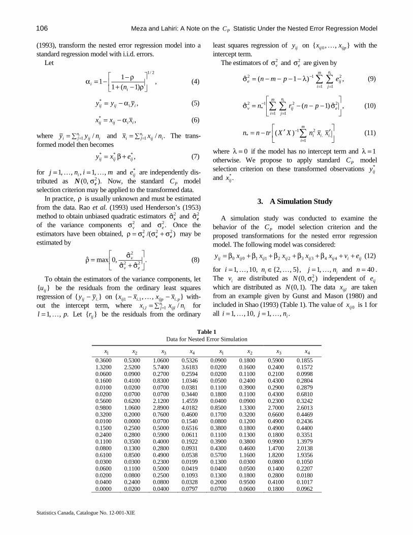
106 Meza and Lahiri: A Note on the PC Statistic Under the Nested Error Regression Model
Statistics Canada, Catalogue No. 12-001-XIE
(1993), transform the nested error regression model into a standard regression model with i.i.d. errors.
Let
,)1(1
11
2/1
⎥⎦
⎤⎢⎣
⎡ρ−+
ρ−−=αi
i n (4)
,*iiijij yyy α−= (5)
,*iiijij xxx α−= (6)
where ∑ == inj iiji nyy 1 / and ∑ == in
j iiji nxx 1 ./ The trans-formed model then becomes
,***ijijij exy +β= (7)
for minj i ,,1,,,1 KK == and *ije are independently dis-
tributed as ).,0( 2eN σ Now, the standard PC model
selection criterion may be applied to the transformed data. In practice, ρ is usually unknown and must be estimated
from the data. Rao et al. (1993) used Henderson’s (1953) method to obtain unbiased quadratic estimators 2ˆ vσ and 2ˆ eσ of the variance components 2
vσ and .2eσ Once the
estimators have been obtained, )/( 222evv σ+σσ=ρ may be
estimated by
.ˆˆ
ˆ,0maxˆ
22
2
⎥⎦
⎤⎢⎣
⎡σ+σ
σ=ρev
v (8)
To obtain the estimators of the variance components, let }{ iju be the residuals from the ordinary least squares
regression of }{ .iij yy − on },,{ .1.1 piijpiij xxxx −− K with-out the intercept term, where iijl
njli nxx i /1. ∑ == for
.,,1 pl K= Let }{ ijr be the residuals from the ordinary
least squares regression of ijy on },,{ 0 ijpij xx K with the intercept term.
The estimators of 2vσ and 2
eσ are given by
,)1(ˆ 2
11
12ij
n
j
m
ie epmn
i
∑∑==
−λ−−−−=σ (9)
,ˆ)1(ˆ 22
11
1*
2⎥⎦
⎤⎢⎣
⎡σ−−−=σ ∑∑
==
−eij
n
j
m
iv pnrn
i
(10)
⎥⎦
⎤⎢⎣
⎡ ′′−= ∑=
−..
2
1
1* )( iii
m
i
xxnXXtrnn (11)
where 0=λ if the model has no intercept term and 1=λ otherwise. We propose to apply standard PC model selection criterion on these transformed observations *
ijy and .*
ijx
3. A Simulation Study
A simulation study was conducted to examine the behavior of the PC model selection criterion and the proposed transformations for the nested error regression model. The following model was considered:
ijiijijijijijij evxxxxxy ++β+β+β+β+β= 4433221100 (12)
for },5,,2{,10,,1 KK ∈= ini inj ,,1 K= and 40=n . The iv are distributed as ),0( 2
vN σ independent of ije which are distributed as ).1,0(N The data ijlx are taken from an example given by Gunst and Mason (1980) and included in Shao (1993) (Table 1). The value of 0ijx is 1 for all .,,1,10,,1 inji KK ==
Table 1 Data for Nested Error Simulation
1x 2x 3x 4x 1x 2x 3x 4x
0.3600 0.5300 1.0600 0.5326 0.0900 0.1800 0.5900 0.1855 1.3200 2.5200 5.7400 3.6183 0.0200 0.1600 0.2400 0.1572 0.0600 0.0900 0.2700 0.2594 0.0200 0.1100 0.2100 0.0998 0.1600 0.4100 0.8300 1.0346 0.0500 0.2400 0.4300 0.2804 0.0100 0.0200 0.0700 0.0381 0.1100 0.3900 0.2900 0.2879 0.0200 0.0700 0.0700 0.3440 0.1800 0.1100 0.4300 0.6810 0.5600 0.6200 2.1200 1.4559 0.0400 0.0900 0.2300 0.3242 0.9800 1.0600 2.8900 4.0182 0.8500 1.3300 2.7000 2.6013 0.3200 0.2000 0.7600 0.4600 0.1700 0.3200 0.6600 0.4469 0.0100 0.0000 0.0700 0.1540 0.0800 0.1200 0.4900 0.2436 0.1500 0.2500 0.5000 0.6516 0.3800 0.1800 0.4900 0.4400 0.2400 0.2800 0.5900 0.0611 0.1100 0.1300 0.1800 0.3351 0.1100 0.3500 0.4000 0.1922 0.3900 0.3800 0.9900 1.3979 0.0800 0.1300 0.2800 0.0931 0.4300 0.4600 1.4700 2.0138 0.6100 0.8500 0.4900 0.0538 0.5700 1.1600 1.8200 1.9356 0.0300 0.0300 0.2300 0.0199 0.1300 0.0300 0.0800 0.1050 0.0600 0.1100 0.5000 0.0419 0.0400 0.0500 0.1400 0.2207 0.0200 0.0800 0.2500 0.1093 0.1300 0.1800 0.2800 0.0180 0.0400 0.2400 0.0800 0.0328 0.2000 0.9500 0.4100 0.1017 0.0000 0.0200 0.0400 0.0797 0.0700 0.0600 0.1800 0.0962
Survey Methodology, June 2005 107
Statistics Canada, Catalogue No. 12-001-XIE
Some of the kβ may be zero and thus various combinations of variables were chosen from
),,,,( 43210 xxxxx to be the predictors used to generate data coming from a nested error regression model. There are
3112 =−p possible models. Each model will be denoted by a subset of (0, 1, 2, 3, 4) that contains the indices of the variables lx in the model.
Data were generated using 1,000 simulations for several values of 2
vσ to estimate the probability of selecting each model using the PC criterion. The value of 2
eσ was taken to be 1 for all simulations. The results of the simulation are given in Table 2. The values of 2
vσ considered were 0, 1, 2,
5, 10 and 16 and the values of β′ were taken to be (2, 0, 0, 4, 0), (2, 0, 0, 4, 8), (2, 9, 0, 4, 8) and (2, 9, 6, 4, 8) as in Shao (1993). Models were categorized as optimal, category II (correct but not optimal), or category I (incorrect).
The PC criterion did not perform well for large values of .2
vσ For the model =β′ (2, 0, 0, 4, 0) with 12 =σv the estimated selection probabilities were: optimal model, 0.54; correct model, 0.46; incorrect model, 0. In contrast, when
,162 =σv the estimated selection probabilities were: optimal model, 0.43; correct model, 0.35; incorrect model, 0.22.
The PC criterion also did not perform well for larger models with large values of .2
vσ The PC criterion however Table 2
Probabilities of Model Selection Before Transformation
)0,4,0,0,2( ′=β
Model Category 02 =σv 12 =σv 22 =σv 52 =σv 102 =σv 162 =σv 0, 3 Optimal 0.62 0.54 0.49 0.46 0.45 0.43 0, 2, 3 II 0.11 0.09 0.09 0.10 0.07 0.06 0, 1, 3 II 0.09 0.14 0.19 0.17 0.15 0.12 0, 3, 4 II 0.09 0.13 0.13 0.14 0.11 0.10 0, 1, 2, 3 II 0.03 0.05 0.06 0.05 0.04 0.04 0, 1, 3, 4 II 0.02 0.03 0.02 0.02 0.02 0.01 0, 2, 3, 4 II 0.02 0.01 0.02 0.02 0.01 0.02 0, 1, 2, 3, 4 II 0.02 0.01 0.00 0.00 0.01 0.00 0, 1 I 0.00 0.00 0.00 0.01 0.07 0.09 0, 2 I 0.00 0.00 0.00 0.01 0.03 0.05 0, 4 I 0.00 0.00 0.00 0.00 0.01 0.04 0, 1, 2 I 0.00 0.00 0.00 0.01 0.01 0.01 0, 1, 4 I 0.00 0.00 0.00 0.01 0.02 0.03 0, 1, 2, 4 I 0.00 0.00 0.00 0.00 0.00 0.00
)8,4,0,0,2( ′=β
Model Category 02 =σv 12 =σv 22 =σv 52 =σv 102 =σv 162 =σv 0, 3, 4 Optimal 0.72 0.67 0.63 0.61 0.58 0.49 0, 2, 3, 4 II 0.12 0.12 0.14 0.14 0.11 0.09 0, 1, 3, 4 II 0.12 0.16 0.18 0.14 0.12 0.11 0, 1, 2, 3, 4 II 0.04 0.05 0.05 0.05 0.04 0.04 0, 4 I 0.00 0.00 0.00 0.00 0.01 0.06 0, 1, 4 I 0.00 0.00 0.00 0.02 0.05 0.10 0, 2, 4 I 0.00 0.00 0.00 0.03 0.07 0.10 0, 1, 2, 4 I 0.00 0.00 0.00 0.00 0.01 0.01
)8,4,0,9,2( ′=β
Model Category 02 =σv 12 =σv 22 =σv 52 =σv 102 =σv 162 =σv 0, 1, 3, 4 Optimal 0.83 0.78 0.75 0.63 0.39 0.25 0, 1, 2, 3, 4 II 0.17 0.20 0.18 0.13 0.09 0.07 0, 3, 4 I 0.00 0.01 0.03 0.13 0.29 0.35 0, 1, 4 I 0.00 0.00 0.00 0.03 0.11 0.15 0, 2, 3, 4 I 0.00 0.01 0.03 0.07 0.06 0.09 0, 2, 4 I 0.00 0.00 0.00 0.00 0.02 0.05 0, 1, 2, 4 I 0.00 0.00 0.00 0.02 0.04 0.04
)8,4,6,9,2( ′=β
Model Category 02 =σv 12 =σv 22 =σv 52 =σv 102 =σv 162 =σv 0, 1, 2, 3, 4 Optimal 1.00 0.98 0.90 0.60 0.29 0.11 0, 2, 3, 4 I 0.00 0.02 0.07 0.24 0.32 0.28 0, 1, 3, 4 I 0.00 0.00 0.02 0.11 0.18 0.23 0, 1, 2, 4 I 0.00 0.00 0.01 0.06 0.13 0.17 0, 3, 4 I 0.00 0.00 0.00 0.00 0.03 0.09 0, 2, 4 I 0.00 0.00 0.00 0.00 0.03 0.10 0, 1, 4 I 0.00 0.00 0.00 0.00 0.01 0.03 0, 1, 3 I 0.00 0.00 0.00 0.00 0.00 0.00

108 Meza and Lahiri: A Note on the PC Statistic Under the Nested Error Regression Model
Statistics Canada, Catalogue No. 12-001-XIE
did very well for large models with small values of .2vσ For
the full model =β′ (2, 9, 6, 4, 8) with ,12 =σv the estimated selection probabilities were: optimal model, 0.98; correct model, 0.02; incorrect model, 0. In contrast, when ,162 =σv the estimated selection probabilities were: optimal model, 0.11; incorrect model, 0.89. Note that in this scenario there are no correct models other than the optimal model.
In summary, when the PC criterion is applied to data following the nested error regression model:
1. For any particular model, the estimated probability of selecting the optimal model decreases as 2
vσ increases.
2. For any particular model, the estimated probability of selecting an incorrect model increases as 2
vσ increases.
3. As the number of variables included in the model increases and 2
vσ increases, the estimated proba-bility of selecting the optimal model decreases.
4. As the number of variables included in the model increases and 2
vσ increases, the estimated probability of selecting an incorrect model increases.
The data were then used to estimate the probability of selecting each model using the PC criterion under the transformation for ρ known. The results of the simulation are given in Table 3. For the model )0,4,0,0,2(=β′ with
02 =σv (standard regression model) the estimated selection probabilities were: optimal model, 0.62; correct model, 0.38; incorrect model, 0 (Table 2). Similarly, under the transformation for ρ known with ,162 =σv the estimated selection probabilities were: optimal model, 0.60; correct model, 0.40; incorrect model, 0 (Table 3). For the full model
=β′ (2, 9, 6, 4, 8), the estimated probability of selecting the optimal model was 1 for both the standard regression model (Table 2, )02 =σv and under the transformation for ρ known for all values of 2
vσ considered (Table 3). In practice, ρ is unknown and must be estimated from
the data. The transformation for ρ unknown is therefore more helpful for practitioners. The results for the trans-formation with ρ unknown are displayed in Table 4. When ρ was estimated, there was only a small decrease in the estimated probability of selecting the optimal model or a correct model. The largest decrease in the estimated probability of selecting the optimal model was 0.03 for the model with )0,4,0,2(=β′ and 61.0,12 =σv for ρ known (Table 3) compared to 0.58 for ρ unknown (Table 4).
Table 3
Probabilities of Model Selection After Transformation, ρ Known
)0,4,0,0,2( ′=β Model Category 12 =σv 22 =σv 52 =σv 102 =σv 162 =σv
0, 3 Optimal 0.61 0.60 0.61 0.61 0.60 0, 3, 4 II 0.11 0.10 0.11 0.11 0.11 0, 2, 3 II 0.10 0.11 0.11 0.10 0.11 0, 1, 3 II 0.09 0.10 0.08 0.09 0.09 0, 1, 2, 3 II 0.04 0.04 0.04 0.04 0.04 0, 1, 3, 4 II 0.03 0.03 0.03 0.02 0.02 0, 2, 3, 4 II 0.02 0.02 0.02 0.02 0.02 0, 1, 2, 3, 4 II 0.01 0.01 0.01 0.01 0.01
)8,4,0,0,2( ′=β Model Category 12 =σv 22 =σv 52 =σv 102 =σv 162 =σv
0, 3, 4 Optimal 0.71 0.71 0.73 0.72 0.71 0, 2, 3, 4 II 0.13 0.12 0.11 0.12 0.13 0, 1, 3, 4 II 0.11 0.12 0.10 0.11 0.11 0, 1, 2, 3, 4 II 0.05 0.05 0.05 0.05 0.05
)8,4,0,9,2( ′=β Model Category 12 =σv 22 =σv 52 =σv 102 =σv 162 =σv
0, 1, 3, 4 Optimal 0.82 0.83 0.83 0.82 0.83 0, 1, 2, 3, 4 II 0.18 0.17 0.17 0.18 0.17
)8,4,6,9,2( ′=β Model Category 12 =σv 22 =σv 52 =σv 102 =σv 162 =σv
0, 1, 2, 3, 4 Optimal 1.00 1.00 1.00 1.00 1.00
Survey Methodology, June 2005 109
Statistics Canada, Catalogue No. 12-001-XIE
Table 4 Probabilities of Model Selection After Transformation, ρ Unknown
)0,4,0,0,2( ′=β Model Category 12 =σv 22 =σv 52 =σv 102 =σv 162 =σv
0, 3 Optimal 0.58 0.59 0.60 0.61 0.60 0, 3, 4 II 0.11 0.10 0.11 0.10 0.10 0, 2, 3 II 0.11 0.10 0.11 0.11 0.11 0, 1, 3 II 0.08 0.09 0.10 0.09 0.09 0, 1, 2, 3 II 0.04 0.04 0.03 0.04 0.04 0, 1, 3, 4 II 0.03 0.03 0.02 0.02 0.02 0, 2, 3, 4 II 0.03 0.03 0.02 0.02 0.03 0, 1, 2, 3, 4 II 0.02 0.02 0.01 0.01 0.01
)8,4,0,0,2( ′=β Model Category 12 =σv 22 =σv 52 =σv 102 =σv 162 =σv
0, 3, 4 Optimal 0.70 0.70 0.70 0.71 0.70 0, 2, 3, 4 II 0.13 0.14 0.13 0.13 0.13 0, 1, 3, 4 II 0.13 0.11 0.12 0.11 0.12 0, 1, 2, 3, 4 II 0.04 0.05 0.05 0.05 0.05
)8,4,0,9,2( ′=β Model Category 12 =σv 22 =σv 52 =σv 102 =σv 162 =σv
0, 1, 3, 4 Optimal 0.82 0.82 0.81 0.83 0.83 0, 1, 2, 3, 4 II 0.18 0.18 0.19 0.17 0.17
)8,4,6,9,2( ′=β Model Category 12 =σv 22 =σv 52 =σv 102 =σv 162 =σv
0, 1, 2, 3, 4 Optimal 1.00 1.00 1.00 1.00 1.00 Based on our simulation results, when the PC criterion is
applied to data following the nested error regression model: 1. Under both transformations ( ρ known and ρ
unknown), the estimated probability of selecting an incorrect model was 0.
2. Under the transformation for ρ known, the probability of selecting the optimal model was similar to that of the standard regression model.
3. When ρ was estimated, there was only a small decrease in the estimated probability of selecting the optimal model or a correct model.
4. Under both transformations ( ρ known and ρ estimated), the PC criterion performed well, even for larger models with large values of 2
vσ . 5. The performance of the PC criterion for the nested
error regression model resembles that of the PC criterion for the standard regression model.
In summary, the PC criterion does not perform well under the nested error regression model when 2
vσ is large. When the transformation for ρ unknown (or ρ known) is applied, the model then becomes a standard regression model and the PC statistic performs accordingly.
Acknowledgements The research was supported in part by a grant from the
Gallup Organization.
References
Battese, G.E., Harter, R.M. and Fuller, W.A. (1988). An error-components model for prediction of county crop areas using survey and satellite data. Journal of the American Statistical Association, 83, 28-36.
Fuller, W.A., and Battese, G.E. (1973). Transformations for estimation of linear models with nested error structures. Journal of the American Statistical Association, 68, 626-632.
Gunst, G.F., and Mason, R.L. (1980). Regression Analysis and Its Application. New York: Marcel Dekker.
Henderson, C.R. (1953). Estimation of variance and variance components. Biometrics, 9, 226-252.
Mallows, C.L. (1973). Some comments on PC . Technometrics, 15, 661-675.
Rao, J.N.K., Sutradhar, B.C. and Yue, K. (1993). Generalized least squares F test in regression analysis with two-stage cluster samples. Journal of the American Statistical Association, 88, 1388-1391.
Shao, J. (1993). Linear model selection by cross-validation. Journal of the American Statistical Association, 88, 486-494.
Wu, C.F.J., Holt, D. and Holmes, D.J. (1988). The effect of two-stage sampling on the F Statistic. Journal of the American Statistical Association, 83, 150-159.

JOURNAL OF OFFICIAL STATISTICS
An International Review Published by Statistics Sweden JOS is a scholarly quarterly that specializes in statistical methodology and applications. Survey methodology and other issues pertinent to the production of statistics at national offices and other statistical organizations are emphasized. All manuscripts are rigorously reviewed by independent referees and members of the Editorial Board.
Contents
Volume 20, No. 3, 2004 The Twelfth Morris Hansen Lecture Simple Response Variance: Then and Now Paul P. Biemer ..................................................................................................................................................................417 Discussion Robert M. Groves .............................................................................................................................................................441 Keith Rust..........................................................................................................................................................................445 List-based Web Surveys: Quality, Timeliness, and Nonresponse in the Steps of the Participation Flow Monica Pratesi, Katja Lozar Manfreda, Silvia Biffignandi, and Vasja Vehovar .........................................................451 The Impact of Coding Error on Time Use Surveys Estimates Patrick Sturgis ...................................................................................................................................................................467 On the Distribution of Random Effects in a Population-based Multi-stage Cluster Sample Survey Obi C. Ukoumunne, Martin C. Gulliford, and Susan Chinn .........................................................................................481 Estimating Marginal Cohort Work Life Expectancies from Cross-sectional Survey Data Markku M. Nurminen, Christopher R. Heathcote, and Brett A. Davis ........................................................................495 Missing the Mark? Imputation Bias in the Current Population Survey’s State Income and Health Insurance Coverage Estimates Michael Davern, Lynn A. Blewett, Boris Bershadsky, and Noreen Arnold ................................................................519 Does Voice Matter? An Interactive Voice Response (IVR) Experiment Mick P. Couper, Eleanor Singer, and Roger Tourangeau..............................................................................................551 In Other Journals...........................................................................................................................................................................571

Volume 20, No. 4, 2004
Revisions to Official Data on U.S. GNP: A Multivariate Assessment of Different Vintages Kerry D. Patterson and S.M. Heravi................................................................................................................................573
Discussion Dennis Trewin...................................................................................................................................................................603 Peter van de Ven and George van Leeuwen...................................................................................................................607 Don M. Eggington ............................................................................................................................................................615 Robin Lynch and Craig Richardson ................................................................................................................................623
Rejoinder Kerry D. Patterson and S.M. Heravi................................................................................................................................631
The Best Approach to Domain Estimation Precludes Borrowing Strength Victor Estevao and Carl-Erik Särndal .............................................................................................................................645
Perceptions of Disability: The Effect of Self- and Proxy Response Sunghee Lee, Nancy A. Mathiowetz, and Roger Tourangeau ......................................................................................671
Maintaining Race and Ethnicity Trend Lines in U.S. Government Surveys Elizabeth Greenberg, Jon Cohen, and Dan Skidmore....................................................................................................687
Confidence Intervals for Proportions Estimated from Complex Sample Designs Alistair Gray, Stephen Haslett, and Geoffrey Kuzmicich..............................................................................................705
Editorial Collaborators .................................................................................................................................................................725
Index to Volume 20, 2004 ...........................................................................................................................................................729
Volume 21, No. 1, 2005
Inference for the Population Total from Probability-Proportional-to-Size Samples Based on Predictions from a Penalized Spline Nonparametric Model Hui Zheng and Roderick J.A. Little .................................................................................................................................... 1 The Accuracy of Estimators of Number of Signatories to a Petition Based on a Sample Duncan I. Hedderley and Stephen J. Haslett..................................................................................................................... 21 A Two-stage Nonparametric Sample Survey Approach for Testing the Association of Degree of Rurality with Health Services Utilization John S. Preisser, Cicely E. Mitchell, James M. Powers, Thomas A. Arcury, and Wilbert M. Gesler.......................... 39 Improving Comparability of Existing Data by Response Conversion Stef van Buuren, Sophie Eyres, Alan Tennant, and Marijke Hopman-Rock ................................................................. 53 The Nature of Nonresponse in a Medicaid Survey: Causes and Consequences Patricia M. Gallagher, Floyd Jackson Fowler, Jr., and Vickie L. Stringfellow.............................................................. 73 Telephone, Internet and Paper Data Collection Modes for the Census 2000 Short Form Sid J. Schneider, David Cantor, Lawrence Malakhoff, Carlos Arieira, Paul Segel, Khaan-Luu Nguyen, and Jennifer Guarino Tancreto........................................................................................................................................... 89 The Productivity of the Three-step Test-interview (TSTI) Compared to an Expert Review of a Self-administered Questionnaire on Alcohol Consumption Harrie Jansen and Tony Hak............................................................................................................................................103 Underpinning the E-Business Framework. Defining E-Business Concepts and Classifying E-Business Indicators Xander J. de Graaf and Robin H. Muurling....................................................................................................................121 In Other Journals...........................................................................................................................................................................137
All inquires about submissions and subscriptions should be directed to [email protected]

The Canadian Journal of Statistics La Revue Canadienne de Statistique CONTENTS TABLE DES MATIÈRES
Volume 33, No. 1, March/mars 2005, 1-148
Douglas P.WIENS Editor’s report/Rapport du rédacteur en chef .....................................................................................................................................1
Grace Y. YI & Mary E. THOMPSON Marginal and association regression models for longitudinal binary data with drop-outs: a likelihood-based approach...................3 Denis BOSQ Estimation suroptimale de la densité par projection.........................................................................................................................21
John BRAUN, Thierry DUCHESNE & James E. STAFFORD Local likelihood density estimation for interval censored data ........................................................................................................39
Zhigang ZHANG, Liuquan SUN, Xingqiu ZHAO & Jianguo SUN Regression analysis of interval-centored failure time data with linear transformation models ........................................................61
Alain G. VANDAL, Robert GENTLEMAN & Xuecheng LIU Constrained estimation and likelihood intervals for censored data ..................................................................................................71
Jianguo SUN & Liquan SUN Semiparametric linear transformation models for current status data ..............................................................................................85
Alexandre X. CARVALHO & Martin A. TANNER Modeling nonlinear time series with local mixtures of generalized linear models...........................................................................97
Mayer ALVO & Paul CABILIO General scores statistics on ranks in the analysis of unbalanced designs .......................................................................................115
Sudhir R. PAUL & Xing JIANG Testing the homogeneity of several two-parameter populations ....................................................................................................131
Acknowledgement of referees’ services/Remerciements aux membres des jurys.......................................................................................145
Forthcoming papers/Articles à paraître .......................................................................................................................................................146
Volume 33 (2005): Subscription rates/Frais d’abonnement ........................................................................................................................147


GUIDELINES FOR MANUSCRIPTS
Before having a manuscript typed for submission, please examine a recent issue of Survey Methodology (Vol. 19, No. 1 and onward) as a guide and note particularly the points below. Articles must be submitted in machine-readable form, preferably in Word. A paper copy may be required for formulas and figures. 1. Layout 1.1 Manuscripts should be typed on white bond paper of standard size (8½ × 11 inch), one side only, entirely double
spaced with margins of at least 1½ inches on all sides. 1.2 The manuscripts should be divided into numbered sections with suitable verbal titles. 1.3 The name and address of each author should be given as a footnote on the first page of the manuscript. 1.4 Acknowledgements should appear at the end of the text. 1.5 Any appendix should be placed after the acknowledgements but before the list of references. 2. Abstract The manuscript should begin with an abstract consisting of one paragraph followed by three to six key words. Avoid mathematical expressions in the abstract. 3. Style 3.1 Avoid footnotes, abbreviations, and acronyms. 3.2 Mathematical symbols will be italicized unless specified otherwise except for functional symbols such as “exp(·)”
and “log(·)”, etc. 3.3 Short formulae should be left in the text but everything in the text should fit in single spacing. Long and important
equations should be separated from the text and numbered consecutively with arabic numerals on the right if they are to be referred to later.
3.4 Write fractions in the text using a solidus. 3.5 Distinguish between ambiguous characters, (e.g., w, ; o, O, 0; l, 1). 3.6 Italics are used for emphasis. Indicate italics by underlining on the manuscript. 4. Figures and Tables 4.1 All figures and tables should be numbered consecutively with arabic numerals, with titles which are as nearly self
explanatory as possible, at the bottom for figures and at the top for tables. 4.2 They should be put on separate pages with an indication of their appropriate placement in the text. (Normally they
should appear near where they are first referred to). 5. References 5.1 References in the text should be cited with authors’ names and the date of publication. If part of a reference is cited,
indicate after the reference, e.g., Cochran (1977, page 164). 5.2 The list of references at the end of the manuscript should be arranged alphabetically and for the same author
chronologically. Distinguish publications of the same author in the same year by attaching a, b, c to the year of publication. Journal titles should not be abbreviated. Follow the same format used in recent issues.