Supervisory Control of Nondeterministic Systemswith Driven Events via Prioritized Synchronizationand Trajectory Models 1Mark A. ShaymanDepartment of Electrical Engineering andSystems Research CenterUniversity of MarylandCollege Park, MD 20742Email: shayman@src.umd.eduRatnesh KumarDepartment of Electrical EngineeringUniversity of KentuckyLexington, KY 40506-0046Email: kumar@engr.uky.eduApril 13, 19941This research was supported in part by Center for Robotics and Manufacturing, University ofKentucky, in part by by the National Science Foundation under the Engineering Research CentersProgram Grant CDR-8803012, the Minta Martin Fund for Aeronautical Research, and the GeneralResearch Board at the University of Maryland.

AbstractWe study the supervisory control of nondeterministic discrete event dynamical systems(DEDS's) with driven events in the setting of prioritized synchronization and trajectory mod-els introduced by Heymann. Prioritized synchronization captures the notions of controllable,uncontrollable, and driven events in a natural way, and we use it for constructing supervisorycontrollers. The trajectory model is used for characterizing the behavior of nondeterministicDEDS's since it is a su�ciently detailed model (in contrast to the less detailed languageor failures models), and serves as a language congruence with respect to the operation ofprioritized synchronization. We obtain results concerning controllability and observabilityin this general setting.Keywords: discrete event systems, supervisory control, nondeterministic automata, drivenevents, prioritized synchronization, trajectory modelsAMS (MOS) subject classi�cations: 68Q75, 93B25, 93C83

1 IntroductionSupervisory control of discrete event dynamical systems (DEDS's) was introduced byRamadge and Wonham [23]. In this approach, the behavior of a DEDS, called the plant,is described by its language, the collection of all possible sequences of events (traces) thatit can generate. The task is to design a controller, called a supervisor, which, based onthe observation of the sequence of events, disables some of the controllable events so thatthe language generated by the controlled plant either equals a prespeci�ed desired language,called a target language, or remains con�ned to a prespeci�ed range of languages. Variousextensions of this basic problem such as control under partial observation, decentralized andmodular control, hierarchical control, and optimal control have also been studied. Refer to[24] and references therein for an overview of research in this area (up to 1989).Most of the research on supervisory control of DEDS's assumes that the plant can bemodeled as a deterministic system [10]. In other words, given a state of the system andan event that occurs in that state, the state reached after the occurrence of the event isuniquely known. Such an assumption is not satis�ed whenever unmodeled dynamics, partialobservation, or inherent nondeterminism is present. Hence the assumption of a deterministicplant is quite strong. In this paper, we relax this assumption and consider the control of anondeterministic plant [10, 17, 18, 9, 12, 7].Amodeling frameworkm over a �nite event set � is an equivalence relation on all DEDS'srepresentable as state machines, with arbitrary state space (�nite or denumerable), having�-transitions and event set �. We identify m with the projection �m which maps each statemachine P to its equivalence class or model �m(P). If the equivalence class of P is uniquelycharacterized by an attribute which is common to its members, we will freely identify �m(P)with this attribute.We say that a modeling framework �m is more detailed than another modeling framework�n if the equivalence relation �m re�nes the equivalence relation �n. Obviously, it is desirableto use the least detailed modeling framework which is su�cient for the design task at hand. Acomplex system is generally synthesized by combining simpler systems using various types ofinterconnections. Since speci�cations for the logical behavior of a DEDS are typically givenin terms of the language of the system, a basic requirement is that the modeling frameworkshould contain su�cient detail so that if the models for each subsystem are known, then thelanguage of the interconnected system is uniquely determined. A modeling framework withsuch a property for a given class of admissible interconnections is referred to as a languagecongruence [7].The language modeling framework associates to a system its language, the collection ofall possible �nite traces which are executable. Thus, the language model of a system isa subset of ��, the set of all �nite sequences of events in � including �, the zero-lengthsequence. For deterministic systems and deterministic operators such as strict synchronouscomposition (SSC), the language modeling framework is a language congruence. If operatorswhich introduce nondeterminism (e.g., internal choice, event internalization) are admissible,then the language modeling framework is no longer a language congruence and a more1

detailed modeling framework such as the failures model introduced by Hoare [9] must beused in order to have a language congruence. The failures model consists of the set of allfailures of the system{pairs (s;�0) where s is a trace and �0 � � is a refusal set with theproperty that if the environment restricts the possible events to �0, the system can deadlockfollowing execution of s. Thus, a failures model is a subset of �� � 2�.1In the work of Kumar, Garg and Marcus [14], control design is accomplished by con-structing a supervisor which operates in strict synchronization with the plant. In the workof Balemi et al. [3], the set of events � is partitioned into two disjoint subsets{commandswhich are generated by the supervisor and sent to the plant, and responses which are gener-ated by the plant and sent to the supervisor. It is required that the plant and supervisor bemutually receptive, which means that the plant executes every command generated by thesupervisor and the supervisor executes every response generated by the plant. Thus, thisdesign also requires that every event be executed synchronously.There are several reasons to consider control designs which do not require complete syn-chronization between the plant and supervisor. Uncontrollable events are generated sponta-neously by the plant and the supervisor is not permitted to interfere with their execution.Consequently, there is no a priori reason to assume that the supervisor needs to \track"every such event by undergoing a transition synchronously with the plant. Also, certain un-controllable events in the plant may not be sensed and hence are invisible to the supervisor.It is unrealistic to require the supervisor to execute such events synchronously.In many applications, it is not realistic to expect (or require) the plant to respond syn-chronously to every event generated by the supervisor. (Such events are referred to as forcible[6], driven [7] or command [3] events in the literature.) By permitting the supervisor to placecommands which are not executed by the plant, nondeterminism in the plant may be re-solved and performance improved. For example, not every piece of equipment in a factorywill trigger an alarm upon breakdown. Breakdown may only be discovered when an actionis requested by the supervisor and not executed by the plant. Thus, the unsensed state ofthe plant is determined by a synchronization failure.Another motivation for relaxing the requirement of strict synchronization comes fromsystems in which a single supervisor controls more than one plant. For example, in a walkingmachine, there could be separate modules (viewed here as plants) which perform motioncontrol and vision control respectively. At a higher-level, there could be a single supervisorwhich controls and coordinates the two modules. Some of the commands issued by thesupervisor may apply to both the modules, while others may be relevant to only one of themand should be ignored by the other.Heymann [7] has proposed a type of interconnection, called prioritized synchronous com-position (PSC), which relaxes the synchronization requirements on the plant and supervisor.Each process in a PSC-interconnection is assigned a priority set of events. For an event tobe enabled in the interconnected system, it must be enabled in all processes whose prioritysets contain that event. Also, when an enabled event occurs, it occurs in each subsystem inwhich the event is enabled. In the context of supervisory control, the priority set of the plant1For simplicity, we ignore the possibility of divergence.2

contains the controllable and uncontrollable events, while the priority set of the supervisorcontains the controllable and driven events. Thus, controllable events require the participa-tion of both plant and supervisor; uncontrollable events require the participation of the plantand will occur synchronously in the supervisor whenever possible; driven events require theparticipation of the supervisor and will occur synchronously in the plant whenever possible.It is important to distinguish between PSC and other types of parallel composition in theliterature. For example, Hoare [9] de�nes a concurrent composition operator in which eachprocess has its own event set and the processes synchronize on the events in the intersectionof their event sets. This is generalized to trace-dependent event sets, called event-controlsets, by Inan-Varaiya [12]. The key di�erence between concurrent composition and PSCis that in PSC, although a process cannot block events which are outside its priority set,it may be able to execute these events{and, whenever possible, will execute these eventssynchronously when they occur in the other process.2It is shown in [7, Example 7] that two systems with the same failures model may yielddi�erent languages when composed in prioritized synchronization with a �xed system. Thus,if PSC is included as an admissible interconnection operator, a more detailed modelingframework than the failures model is required to serve as a language congruence. Onesuch modeling framework, called the trajectory model, is proposed by Heymann [7] andHeymann-Meyer [8].3 The trajectory model of a system consists of the set of all trajectoriesor refusal-traces{�nite sequences of the type �0(�1;�1) : : : (�k;�k), where �1 : : : �k is thetrace executed by the system, while �j � � (j = 0; : : : ; k) is a refusal set, a set of eventswhich can result in deadlock if presented to the system by the environment at the indicatedpoint in the refusal-trace. Thus, a trajectory model is a subset of 2� � (� � 2�)� and re�nesthe failures model by including the intermediate refusal sets.Although we use the trajectory model for describing the behavior of a nondeterministicplant, it is assumed that the desired speci�cation is given only in terms of a language model(as in [23]), and not in terms of a trajectory model. This is a reasonable assumption, forin most applications, we are only interested in the sequences of events that a system canexecute, and not in the events that the system may \refuse" to execute after execution of acertain event in a certain event sequence. Hence we address the following supervisory controlproblem:Given (i) a partition � = �c[�u[�d of the event set into subsets of controllable,uncontrollable and driven events, (ii) a nondeterministic plant with trajectory2If applied to so-called improper processes, the parallel operator de�ned by Inan [11] can be viewed asa generalized form of PSC, but only in the deterministic setting. However, when supervisory control isconsidered in this reference, the assumption is made that the plant is proper and has a constant eventcontrol set. This assumption excludes driven events.3The trajectory model is similar to the failure-trace model (also called the refusal-testing model) ofPhillips [20], but di�ers from this model in its treatment of silent transitions (transitions labeled with �).The trajectory model treats silent transitions in a way that is consistent with the failures model. Whilemore detailed than the failures model, the failure-trace model is less detailed than the ready-trace model[21, 1], and hence less detailed than the bisimulation model [19, 18]. Comparison of various semantics fornondeterministic systems can be found in [27, 2]. 3

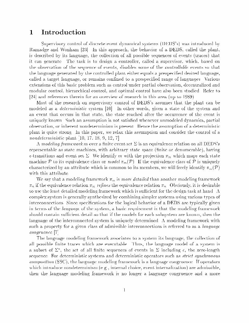
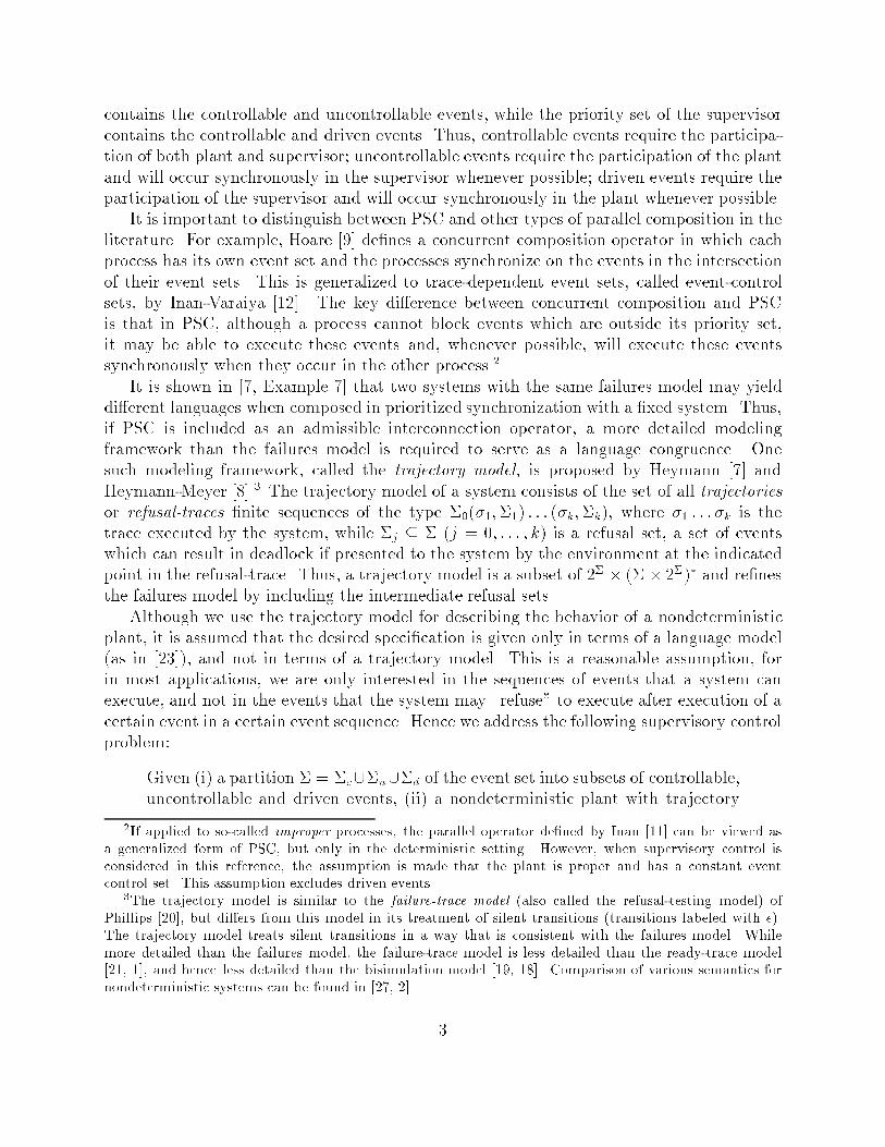
model P � 2� � (� � 2�)� whose priority set is A = �c [ �u, (iii) a (pre�x-closed) target language K � ��; design a supervisor{another trajectory model,denoted S � 2� � (� � 2�)�{whose priority set is B = �c [ �d, such that thelanguage of the PSC of P and S equals K.The interconnection of the plant and the supervisor by PSC results in disabling of some ofthe controllable events and forcing of some of the driven events, while never preventing anyof the uncontrollable events from occurring in the plant. Thus we investigate the supervi-sory control of DEDS's in the general setting of trajectory models and PSC, as opposed tolanguage models and SSC studied by Kumar, Garg and Marcus [14].We obtain a necessary and su�cient condition for the existence of a supervisor for thegeneral problem with driven events, and also provide a technique for synthesizing a super-visor. For ease of implementation, we design supervisors which are deterministic. We alsoaddress the control problem when some of the uncontrollable events are not observed bythe supervisor. While the primary goal of this paper is to obtain necessary and su�cientconditions for the control of nondeterministic systems with driven events, a secondary goalis to provide a rigorous mathematical foundation for the theory of trajectory models andPSC.The organization of this paper is as follows: In Section 2, an example is presented thatmotivates the design techniques to be developed in the remainder of the paper. In Section3, the trajectory model of a nondeterministic state machine (NSM) with �-moves is de�nedand its properties derived from those of NSM's. An algorithm to construct a canonical NSMfrom a given trajectory model is presented and its correctness proven. In Section 4, thePSC of NSM's is de�ned and it is shown that this induces a PSC operation on trajectorymodels. It is also proven that the trajectory modeling framework is a language congruencerelative to PSC. Properties of the PSC of trajectory models are described in Section 5, andthe technique of augmentation is introduced. In Section 6, the supervisory control problemwith driven events under both complete and partial observation is solved, and the resultsare applied to obtain a control design for the example system from Section 2.An abbreviated version of this paper appeared in the conference proceedings [25]. Exten-sions of many of the results to include non-closed speci�cations and marking can be foundin [15].2 Motivating ExampleIn this section, we describe an example that motivates the results described in thispaper. Figure 1(a) gives a deterministic model for a plant that processes a single typeof part. Event � represents inputting a part. Event �1 represents successful completionand outputting of the part. Event �2 represents completion and outputting of the partbut accompanied by an undetectable misalignment of an internal mechanism. If this hasoccurred, another part may be input, but this event � can be followed by an event � thatrepresents jamming of the machine. When this occurs, further processing is impossible. The4

event � represents realignment of the misaligned internal mechanism. Since the misalignmentof the internal mechanism is undetectable, the observation maskM(�) identi�es the events �1and �2{i.e., M(�1) = M(�2) := �. It is assumed that � is controllable and that �1; �2; � areuncontrollable. A natural performance speci�cation is that � should never occur and thatthat the closed-loop generated language should include (�(�1 + �2�))�{i.e., cyclic operationshould be possible.(a) (b) (c)

α β α αα

η

η

γ

λ

αβ

β

λ

2 2

1

λ

β

α

β

µ µ µ

β

1γFigure 1: Diagram illustrating example of Section 2Let us regard � as a controllable event and consider whether the speci�cations can be metby a supervisor S of the Ramadge-Wonham type that is consistent with the observation mask.Since � is uncontrollable, such a supervisor would need to disable � following any occurrenceof �2. Since the mask identi�es �1 and �2, the supervisor must also disable � following�1. Consequently, the generated closed-loop language imposed by any such supervisor iscontained in pr((��2�)���1) and thus fails to meet the lower-bound speci�cation. (pr(�)denotes the pre�x-closure operation.)The design problem is also not solvable using a forcing supervisor of the type consideredby Golaszewski-Ramadge [6]. If such a supervisor forces � following �2, it must also force �following �1. Since the plant cannot execute � after �1, the controlled system would deadlockafter the �rst occurrence of �1. Thus, the lower-bound speci�cation is not satis�ed.We could transform the partially observed deterministic system by identifying the events�1; �2 in the plant model and representing both of these events by their common mask value�. This yields the completely observed nondeterministic model depicted in Figure 1(b).However, this results in a loss of information. In the �rst model, �1; �2 are indistinguishableonly from the viewpoint of observation, while in the second model, they are indistinguishablefor speci�cation and control, as well as for observation. Since �1; �2 are uncontrollable,whether they are distinguishable for the purpose of control is irrelevant. However, in order tobe able to translate the original lower-bound speci�cation into a corresponding speci�cationon the transformed system, it is important that the events remain distinguishable fromthe viewpoint of speci�cation. This can be accomplished by replacing �1; �2 by the three-event sequences � 1�; � 2� respectively, where 1; 2 are completely unobservable{i.e., havemask value �. If M 0(�) denotes the mask for the transformed system, then M 0(� 1�) =M 0(�)M 0(�) = M 0(� 2�). Thus, the substitution preserves the modeling assumption thatthe events �1; �2 have the same mask value. On the other hand, since 1; 2 are distinct5

event labels, the distinguishability of �1; �2 for the purpose of speci�cation is also preserved.To model the uncontrollability of �1; �2, we designate �; 1; 2; � to be uncontrollable events.The \sandwiching" of the unobservable event i between the observable events �; � re ectsthe fact that in the original model, the occurrence of �i is known to the supervisor eventhough the supervisor cannot determine which of �1; �2 has occurred. With the new model,the supervisor knows that neither of the pair 1; 2 has occurred if � has not been observed.Similarly, it knows that one of the pair has occurred if � has been observed.The substituted events can also be given a physical interpretation. � represents com-menced processing of a part with or without internal undetectable misalignment. 1 and 2represent the registering of faultless processing and of faulty processing respectively. Theseare internal events that are modeled but whose occurrence is unobservable to an externalprocess such as a supervisor. � represents the completion of processing and outputting ofthe part.The transformed system is shown in Figure 1(c). It is a partially observed nondeter-ministic system in which the mask is a natural projection and the unobservable events areuncontrollable. We will treat � as a driven event, rather than a controllable event as wouldbe done in the Ramadge-Wonham theory. In the context of PSC-based control design, thisallows for the possibility that the plant may refuse a request from the supervisor to executethis event. Using the results of Section 6, we will construct a PSC-based supervisor thatmeets the control speci�cations. (See Example 5.) The exibility obtained by permittingthe plant to refuse a supervisor-initiated event is an essential feature of the successful controldesign.3 Trajectory ModelA plant, or a DEDS to be controlled, is modeled as an NSM with �-moves. LettingP denote an NSM, it is de�ned to be the four tuple [10]: P := (XP ;�; �P; x0P); where XPdenotes the state space of P, � denotes the event set of P, �P : XP ��[f�g ! 2XP denotesthe nondeterministic4 transition function of P, and x0P 2 XP denotes the initial state of P.A triple (x1; �; x2) 2 XP � (� [ f�g) �XP is called a transition in P if x2 2 �P(x1; �). Atransition (x1; �; x2) is referred to as a silent transition. We assume that the plant NSM is�nitely branching and cannot undergo an unbounded sequence of silent transitions.3.1 Language Model of a Nondeterministic State MachineAs mentioned in Section 1, although trajectory models are used for describing thebehaviors of nondeterministic systems, language or trace models are used for describing thedesired or target speci�cations. Hence in this subsection we de�ne the language model of4The transition function �P(�; �) is deterministic if and only if it is of the type, �P : XP � � ! XP , inwhich (i) there are no transitions labeled �, and (ii) given a state and an event, either a unique state isreached upon execution of that event in that state, or that event is unde�ned in that state.6

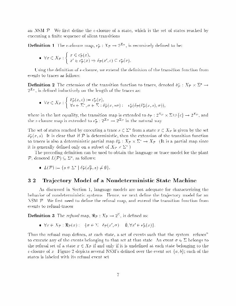
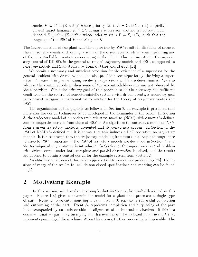
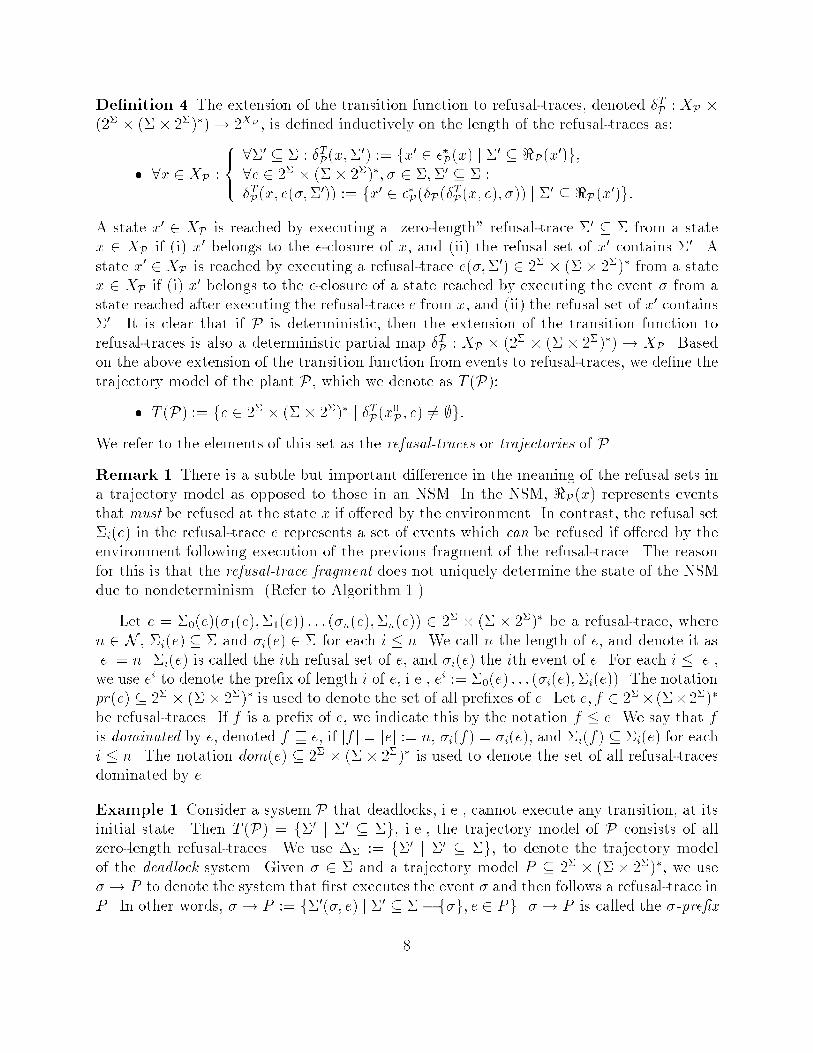
an NSM P. We �rst de�ne the �-closure of a state, which is the set of states reached byexecuting a �nite sequence of silent transitions.De�nition 1 The �-closure map, ��P : XP ! 2XP , is recursively de�ned to be:� 8x 2 XP : ( x 2 ��P(x);x0 2 ��P(x)) �P(x0; �) � ��P(x):Using the de�nition of �-closure, we extend the de�nition of the transition function fromevents to traces as follows:De�nition 2 The extension of the transition function to traces, denoted ��P : XP � �� !2XP , is de�ned inductively on the length of the traces as:� 8x 2 XP : ( ��P(x; �) := ��P(x);8s 2 ��; � 2 � : ��P(x; s�) := ��P(�P(��P(x; s); �));where in the last equality, the transition map is extended to �P : 2XP �� [ f�g ! 2XP , andthe �-closure map is extended to ��P : 2XP ! 2XP in the natural way.The set of states reached by executing a trace s 2 �� from a state x 2 XP is given by the set��P(x; s). It is clear that if P is deterministic, then the extension of the transition functionto traces is also a deterministic partial map ��P : XP � �� ! XP . (It is a partial map sinceit is generally de�ned only on a subset of XP � ��.)The preceding de�nition can be used to obtain the language or trace model for the plantP, denoted L(P) � ��, as follows:� L(P) := fs 2 �� j ��P(x0P; s) 6= ;g:3.2 Trajectory Model of a Nondeterministic State MachineAs discussed in Section 1, language models are not adequate for characterizing thebehavior of nondeterministic systems. Hence, we next de�ne the trajectory model for anNSM P. We �rst need to de�ne the refusal map, and extend the transition function fromevents to refusal-traces.De�nition 3 The refusal map, <P : XP ! 2�, is de�ned as:� 8x 2 XP : <P(x) := f� 2 � j �P(x0; �) = ;;8x0 2 ��P(x)g:Thus the refusal map de�nes, at each state, a set of events such that the system \refuses"to execute any of the events belonging to that set at that state. An event � 2 � belongs tothe refusal set of a state x 2 XP if and only if it is unde�ned at each state belonging to the�-closure of x. Figure 2 depicts several NSM's de�ned over the event set fa; bg; each of thestates is labeled with its refusal event set. 7

De�nition 4 The extension of the transition function to refusal-traces, denoted �TP : XP �(2� � (�� 2�)�)! 2XP , is de�ned inductively on the length of the refusal-traces as:� 8x 2 XP : 8><>: 8�0 � � : �TP(x;�0) := fx0 2 ��P(x) j �0 � <P(x0)g;8e 2 2� � (�� 2�)�; � 2 �;�0 � � :�TP(x; e(�;�0)) := fx0 2 ��P(�P(�TP(x; e); �)) j �0 � <P(x0)g:A state x0 2 XP is reached by executing a \zero-length" refusal-trace �0 � � from a statex 2 XP if (i) x0 belongs to the �-closure of x, and (ii) the refusal set of x0 contains �0. Astate x0 2 XP is reached by executing a refusal-trace e(�;�0) 2 2� � (�� 2�)� from a statex 2 XP if (i) x0 belongs to the �-closure of a state reached by executing the event � from astate reached after executing the refusal-trace e from x, and (ii) the refusal set of x0 contains�0. It is clear that if P is deterministic, then the extension of the transition function torefusal-traces is also a deterministic partial map �TP : XP � (2� � (�� 2�)�) ! XP . Basedon the above extension of the transition function from events to refusal-traces, we de�ne thetrajectory model of the plant P, which we denote as T (P):� T (P) := fe 2 2� � (�� 2�)� j �TP(x0P; e) 6= ;g:We refer to the elements of this set as the refusal-traces or trajectories of P.Remark 1 There is a subtle but important di�erence in the meaning of the refusal sets ina trajectory model as opposed to those in an NSM. In the NSM, <P(x) represents eventsthat must be refused at the state x if o�ered by the environment. In contrast, the refusal set�i(e) in the refusal-trace e represents a set of events which can be refused if o�ered by theenvironment following execution of the previous fragment of the refusal-trace. The reasonfor this is that the refusal-trace fragment does not uniquely determine the state of the NSMdue to nondeterminism. (Refer to Algorithm 1.)Let e = �0(e)(�1(e);�1(e)) : : : (�n(e);�n(e)) 2 2� � (�� 2�)� be a refusal-trace, wheren 2 N , �i(e) � � and �i(e) 2 � for each i � n. We call n the length of e, and denote it asjej = n. �i(e) is called the ith refusal set of e, and �i(e) the ith event of e. For each i � jej,we use ei to denote the pre�x of length i of e, i.e., ei := �0(e) : : : (�i(e);�i(e)). The notationpr(e) � 2� � (�� 2�)� is used to denote the set of all pre�xes of e. Let e; f 2 2�� (��2�)�be refusal-traces. If f is a pre�x of e, we indicate this by the notation f � e. We say that fis dominated by e, denoted f v e, if jf j = jej := n, �i(f) = �i(e), and �i(f) � �i(e) for eachi � n. The notation dom(e) � 2� � (�� 2�)� is used to denote the set of all refusal-tracesdominated by e.Example 1 Consider a system P that deadlocks, i.e., cannot execute any transition, at itsinitial state. Then T (P) = f�0 j �0 � �g, i.e., the trajectory model of P consists of allzero-length refusal-traces. We use �� := f�0 j �0 � �g, to denote the trajectory modelof the deadlock system. Given � 2 � and a trajectory model P � 2� � (�� 2�)�, we use�! P to denote the system that �rst executes the event � and then follows a refusal-trace inP . In other words, � ! P := f�0(�; e) j �0 � �� f�g; e 2 Pg. �! P is called the �-pre�x8

operation on the trajectory model P . Given trajectory models P1; P2 � 2� � (� � 2�)�, and�1; �2 2 � with �1 6= �2, the external choice between the trajectory models �1 ! P1 and�2 ! P2, denoted (�1 ! P1) + (�2 ! P2), is de�ned to be the trajectory model(�1 ! P1) + (�2 ! P2) := fe 2 (�1 ! P1) [ (�2 ! P2) j e0 2 (�1 ! P1) \ (�2 ! P2)g:This is a system which initially makes a deterministic choice between �1 and �2. If �i isexecuted, then the remainder of the refusal-trace is in Pi. The notation P1 � P2 denotesthe system that nondeterministically chooses to execute refusal-traces either in P1 or in P2.P1 � P2 is called the internal choice between P1 and P2, and P1 � P2 := P1 [ P2.{b}

{a,b}

{a,b} ba{}

{a,b} {a,b}

εε

a a b{b} {}

{}

{a,b} {a,b} {a,b}

(a) (b) (c) (d)

aFigure 2: Diagram illustrating Example 1Figures 2(a)-(d) depict NSM's de�ned over the event set fa; bg; each of the states islabeled with the set of events that are refused at that state. Figure 2(a) depicts an NSMthat deadlocks. Hence its trajectory model is �fa;bg. Figure 2(b) depicts an NSM thatinitially executes the event a and then deadlocks. Hence its trajectory model is a! �fa;bg.Figure 2(c) depicts an NSM that initially makes a deterministic choice between the eventsa and b and deadlocks after executing either of the events. Hence its trajectory model isgiven by (a ! �fa;bg) + (b ! �fa;bg). Figure 2(d) depicts an NSM that initially makes anondeterministic choice between the systems of Figures 2(b) and (c). Hence its trajectorymodel is (a! �fa;bg)� [(a! �fa;bg) + (b! �fa;bg)]:It follows from the de�nition of the trajectory model T (P) that it satis�es the following�ve properties, denoted T1, T2, T3, T4, and T5:Proposition 1 The trajectory model T (P) of an NSM P satis�es the following properties:T1 (nonemptiness): ; 2 T (P)) T (P) 6= ;,T2 (pre�x closure): 8e 2 T (P); f 2 2� � (�� 2�)� : f < e) f 2 T (P),T3 (dominance closure): 8e 2 T (P); f 2 2� � (�� 2�)� : f < e) f 2 T (P),T4 (refusal of infeasible): 8e 2 T (P); i � jej; � 2 � :ei(�; ;) 62 T (P)) ei�1(�i(e);�i(e) [ f�g) : : : (�jej;�jej) 2 T (P);T5 (persistence of refused): 8e 2 T (P); i � jej; � 2 � : � 2 �i(e)) �i+1(e) 6= �.9

Proof: T1, T2 and T5 follow immediately from the de�nition of the trajectory model. Toprove T3, we note that a straightforward induction on length of refusal-traces shows that iff < e, then �TP(x0P; e) � �TP(x0P; f), which immediately yields T3. It remains to prove T4.Fix i, and suppose that ei(�; ;) =2 T (P). Then �P(�TP(x0P ; ei); �) = ;. Since ��P(�TP(x0P; ei)) =�TP(x0P; ei), this implies that � 2 <P(x) for all x 2 �TP(x0P; ei). It follows immediately that if�e is obtained from e by replacing �i(e) with �i(e) [ f�g, then �TP(x0P; �e) = �TP(x0P; e) whichimplies that �e 2 T (P).Remark 2 In contrast to [8] where the properties of the trajectory model are de�ned ax-iomatically, we regard the NSM as the fundamental object and derive the properties of thetrajectory model from the properties of NSM's.3.3 Construction of Canonical Nondeterministic State MachineIn this subsection we develop an algorithm for constructing a canonical nondetermin-istic state machine for any given set of refusal-traces satisfying T1-T5.De�nition 5 Let P � 2� � (�� 2�)� be a refusal-trace set satisfying T1-T5. If e 2 P is anyrefusal-trace which has the property that for each i � jej, � 2 �i(e) whenever ei(�; ;) 62 P ,then we say that e is saturated. The saturated trajectory model, denoted Psat, of P is de�nedto be: Psat := fe 2 P j e is saturatedg:It is easy to see that a pre�x of a saturated refusal-trace is also saturated, and each refusal-trace of P is dominated by a saturated refusal-trace of P , so dom(Psat) = P . Thus Psat isequivalent in detail of description to P . So, we use the set of saturated refusal-traces forthe construction of the canonical nondeterministic state machine. Given a �nite number ofevent sets �1; : : : ;�n � � for some n 2 N , we use the notation min(�1; : : : ;�n) to denotethe collection of minimal sets from among the given n sets, i.e.,� min(�1; : : : ;�n) := f�i; 1 � i � n j6 9j such that 1 � j � n; j 6= i; �j � �ig:Lemma 1 Let P � 2� � (�� 2�)� satisfy T1-T5.1. Psat contains a unique minimal zero-length refusal-trace �0min := f�0 2 �j �0 62 L(P )g:2. If e 2 Psat and e(�; ;) 2 P , then the family f�0 � �j e(�;�0) 2 Psatg has a uniqueminimal element given by �(e;�)min := f�0 2 �j e(�; ;)(�0; ;) 62 Pg:Proof: The proof of the �rst part is similar to that of the second part, so we include onlythe latter. Since e(�; ;) 2 P , repeated application of T4 yields e(�;�(e;�)min ) 2 P . Sincee is saturated, in order to show that e(�;�(e;�)min ) is saturated, it su�ces to show that ife(�;�(e;�)min )(�0; ;) 62 P , then �0 2 �(e;�)min . Suppose �0 62 �(e;�)min . Then e(�; ;)(�0; ;) 2 P .By repeated application of T4, it follows that e(�;�(e;�)min )(�0; ;) 2 P , contradiction. Thus,e(�;�(e;�)min ) 2 Psat.Finally, suppose e(�;�0) 2 Psat and �0 2 �(e;�)min {i.e., e(�; ;)(�0; ;) 62 P . By T3, it followsthat e(�;�0)(�0; ;) 62 P . Since e(�;�0) is saturated, �0 2 �0, so �(e;�)min � �0.10

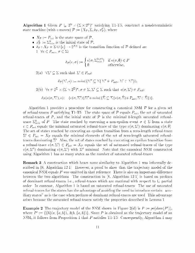
Algorithm 1 Given P � 2� � (�� 2�)� satisfying T1-T5, construct a nondeterministicstate machine (with �-moves) P := (XP ;�; �P; x0P), where� XP := Psat is the state space of P,� x0P := �0min is the initial state of P,� �P : XP � � [ f�g ! 2XP is the transition function of P de�ned as:1. 8e 2 Psat; � 2 �:�P(e; �) := ( e(�;�(e;�)min ) if e(�; ;) 2 P; otherwise,2(a). 8�0 � � such that �0 2 Psat:�P(�0; �) := min(f�00 � �j �00 2 Psat; �0 � �00g);2(b). 8e 2 2� � (� � 2�)�; � 2 �;�0 � � such that e(�;�0) 2 Psat:�P(e(�;�0); �) :=fe(�;�00) j�002min(f�̂ � � je(�; �̂)2Psat;�0� �̂g)g:Algorithm 1 provides a procedure for constructing a canonical NSM P for a given setof refusal-traces P satisfying T1-T5. The state space of P equals Psat, the set of saturatedrefusal-traces of P , and the initial state of P is the minimal 0-length saturated refusal-trace �0min of P . The state reached by executing a non-epsilon event � 2 � from a statee 2 Psat equals the minimal saturated refusal-trace of the type e(�;�0) dominating e(�; ;).The set of states reached by executing an epsilon transition from a zero-length refusal-trace�0 2 Psat = XP equals the minimal elements of the set of zero-length saturated refusal-traces dominating �0. Also, the set of states reached by executing an epsilon transition froma refusal-trace e(�;�0) 2 Psat = XP equals the set of saturated refusal-traces of the typee(�;�00) dominating e(�;�0) with �00 minimal. Note that the canonical NSM constructedusing Algorithm 1 has as many states as the number of saturated refusal-traces.Remark 3 A construction which bears some similarity to Algorithm 1 was informally de-scribed in [8, Algorithm 12.1]. However, a proof to show that the trajectory model of thecanonical NSM equals P was omitted in that reference. There is also an important di�erencebetween the two algorithms. The construction in [8, Algorithm 12.1] is based on pre�xesof dominant refusal-traces{i.e., refusal-traces which are maximal with respect to v partialorder. In contrast, Algorithm 1 is based on saturated refusal-traces. The use of saturatedrefusal-traces for the states has the advantage of avoiding the need to introduce certain \aux-iliary states" as is the case when pre�xes of dominant refusal-traces are used. This advantagearises because the saturated refusal-traces satisfy the properties described in Lemma 1.Example 2 The trajectory model of the NSM shown in Figure 2(d) is P := pr(dom(P 0)),where P 0 := ffbg(a; fa; bg); ;(b; fa; bg)g: Since P is obtained as the trajectory model of anNSM, it follows from Proposition 1 that P satis�es T1-T5. Consequently, Algorithm 1 may11

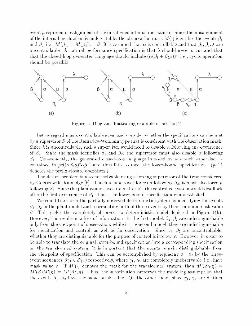
be applied to obtain the canonical NSM P with trajectory model P . The state space of Pis the set of saturated refusal-tracesPsat = pr(f;(a; fa; bg); fbg(a; fa; bg); ;(b; fa; bg)g);which contains �ve elements. The canonical NSM P with these �ve states is depicted inFigure 3(a). Each node is labeled with the name of the state{a saturated refusal-trace{thatit represents. The NSM depicted in Figure 3(b) with four states also has the same trajectorymodel.{}

{b}

{b}(a,{a,b})

{}(a,{a,b}) {}(b,{a,b})

ba

a

ε

a

bε

(b)(a)Figure 3: Diagram illustrating Example 2The equality of the failures models of the two NSM's shown in Figures 3(a) and (b)and the NSM shown in Figure 2(d) is an instance of a basic property of the failures modelconcerning the operations of external choice and event concealment [9, page 113, Law L10].Since the three NSM's have identical trajectory model, the additional detail present in thetrajectory model still does not distinguish between the three systems. However, the failure-trace model of Phillips does distinguish between the systems analogous to those in Figure 2(d)and Figure 3(b) with � in place of � [20, page 250, Example 3].We now prove the correctness of Algorithm 1{i.e., that the trajectory model of the canon-ical NSM P equals P .Proposition 2 Let P � 2� � (� � 2�)� satisfy T1-T5. Then T (P) = P , where P is asconstructed in Algorithm 1.Proof: We begin by showing that8 e = �e(�;�0) 2 Psat; <P(e) = �0: (1)It follows from the de�nition of �P that �0 2 <P(e) if and only if for each f = �e(�;�00) 2 Psatsuch that �0 � �00, f(�0; ;) 62 P . If �0 2 �0, then �0 2 �00 for all such �00. By T5, f(�0; ;) 62 P ,so �0 2 <P(e). Thus, �0 � <P(e). On the other hand, if �0 62 �0, then since e 2 Psat, itfollows that e(�0; ;) 2 P , so �0 62 <P(e). Thus, <P(e) � �0, proving (1).12

Next, we claim that�TP(x0P ; e) = ff 2 Psatj e v fg; 8 e 2 2� � (� � 2�)�: (2)We prove (2) by induction on jej. Let e = �0 � �, a zero-length refusal-trace. Using thede�nition of �P and (1) gives �TP(x0P ;�0) = f�00 2 ��P(x0P)j �0 � <P(�00)g = f�00 2 Psatj �0 ��00g: This establishes (2) in the zero-length case.For the induction step, let e = �e(�;�0) 2 2� � (�� 2�)�. Using the induction hypothesison �e, (1), and the fact that Psat is pre�x-closed gives�TP(x0P; e) = ff 2 ��P(�P(�TP(x0P; �e); �))j �0 � <P(f)g= ff 2 ��P(�P(f �f 2 Psatj �e v �fg; �))j �0 � <P(f)g= f �f (�;�00) 2 Psatj �e v �f; �0 � �00g= ff 2 Psatj e v fg:This completes the induction step and establishes (2).If e 2 Psat, (2) implies that e 2 �TP(x0P; e). Thus, �TP(x0P; e) is nonempty, so e 2 T (P).Hence, Psat � T (P). Since every refusal-trace in P is dominated by a saturated refusal-traceand T (P) satis�es T3, this implies that P � T (P).On the other hand, if e 2 T (P), then �TP(x0P; e) is nonempty, so there exists f 2 Psatwhich dominates e. Since P satis�es T3, this implies that e 2 P , so T (P) � P , whichcompletes the proof.The following result is an immediate consequence of the proof of Proposition 2.Corollary 1 If P is a trajectory model with canonical NSM P, then for each e 2 P ,�TP(x0P; e) = ff 2 Psatj e v fg.The following result is an immediate consequence of Propositions 1 and 2.Theorem 1 Let P � 2�� (�� 2�)�. Then P is the trajectory model of a nondeterministicstate machine (with �-moves) if and only if P satis�es properties T1-T5.3.4 Deterministic Trajectory ModelsRecall that a state machine P is deterministic if and only if its transition function is apartial map �P : XP � �! XP , i.e., there are no �-transitions and �P(x; �) is either emptyor contains exactly one element.De�nition 6 P � 2� � (�� 2�)� is called a deterministic trajectory model if and only ifthere exists a deterministic state machine P such that T (P) = P .For any NSM P, the language model can be obtained from the trajectory model viathe trace map de�ned below. In the special case when the system P is deterministic, thetrajectory model can be recovered from the language model via the inverse operation of thetrace map, called the trajectory map, also de�ned below. Consequently, for deterministicsystems, the language model is equivalent in detail of description to the trajectory model.13

De�nition 7 The trace map from refusal-traces to traces, denoted tr : 2��(��2�)� ! ��,is de�ned inductively on the length of the refusal-traces as:� 8�0 � � : tr(�0) := �,� 8e 2 2� � (�� 2�)�; � 2 �;�0 � � : tr(e(�;�0)) := tr(e)�.It is clear that tr(T (P)) = L(P), where the trace operator is extended to the set of trajectorymodels in the natural way. Given a trajectory model P � 2� � (�� 2�)�, we use L(P ) :=tr(P ) to denote the language model associated with P .De�nition 8 Let K � �� be a nonempty pre�x-closed language. The trajectory map fromtraces to refusal-traces for the language model K, denoted trjK : K ! 2� � (� � 2�)�, isde�ned inductively on the length of traces of K as:� trjK(�) := f� 2 � j � 62 Kg,� 8s 2 K;� 2 � s.t. s� 2 K : trjK(s�) := trjK(s)(�; f�0 2 � j s��0 62 Kg).Lemma 2 Let P be an NSM with language model K := L(P). Then1. trjK(K) � T (P),2. If P is deterministic, then trjK(K) = (T (P))sat.Proof: Let s 2 K be a trace of length r. If r = 0, then s = �; otherwise let s = �1�2 : : : �r.Let si denote the length-i pre�x of s, and de�ne �̂i = f� 2 �j si� 62 Kg. Sete := trjK(s) = �̂0(�1; �̂1) : : : (�r; �̂r):Since s 2 L(P) = L(T (P)), it follows from T3 that the refusal-trace ;(�1; ;) : : : (�r; ;) 2T (P). By repeated application of T4, this implies that e 2 T (P), proving the �rst part.Now assume that P is deterministic. To prove the second part, it su�ces to show thate is the unique refusal-trace in (T (P))sat with tr(e) = s. Also, since there must exist asaturated refusal-trace with trace s, it su�ces to show that if f 2 (T (P))sat with tr(f) = s,then f = e. We use induction on r = jej to prove this together with the assertion that�TP(x0P; e) = ��P(x0P ; tr(e)) (3)Note that since P is deterministic, ��P(x) = x, and given any s 2 K, there exists a uniquexs 2 ��P(x0P; s). Furthermore, <P(xs) = f� 2 � j s� 62 Kg.If r = 0, then f = �0 with �0 � <P(x0P) = �̂0. Since f is saturated, �̂0 � �0, so f = e.Also, �TP(x0P; e) = x0P = ��P(x0P; �) = ��P(x0P ; tr(e)); as required.For the induction step, express e and f as e = �e(�r; �̂r); f = �f(�r;�r). Since the pre�xof a saturated refusal-trace is saturated, �f 2 (T (P))sat. Therefore, by induction hypothesis,we may assume that �f = �e. Using (3) applied to �e, it follows that�TP(x0P; f) = fx 2 ��P(�P(�TP(x0P; �e); �r)) j �r � <P(x)g (4)= fx 2 �P(��P(x0P ; tr(�e)); �r) j �r � <P(x)g (5)= fx 2 ��P(x0P; tr(e)) j �r � <P(x)g (6)= �xs if �r � <P(xs); otherwise (7)14

Since f is a refusal-trace of P, �TP(x0P; f) is nonempty, so �r � <P(xs) = �̂r: Since f issaturated, �̂r � �r, so f = e. Also, by replacing f by e and �r by �̂r in the equalities(4)-(7), we get �TP(x0P; e) = xs = ��P(x0P; tr(e)): This completes the induction step.Proposition 3 Let K � �� be a nonempty pre�xed-closed language, and let det(K) :=dom(trjK(K)). Then1. det(K) is a deterministic trajectory model.2. If P is any trajectory model with L(P ) = K, then det(K) � P , with equality if andonly if P is deterministic.Proof: By a standard result, there exists a deterministic state machineQ such that L(Q) =K. Setting Q = T (Q) gives L(Q) = K. Since Q is deterministic, it follows from Lemma 2that trjK(K) = (T (Q))sat, which implies that det(K) = dom((T (Q))sat) = Q. Thus, det(K)is a deterministic trajectory model.Let P be any trajectory model with L(P ) = K. Then there exists a state machine Psuch that T (P) = P . By Lemma 2, trjK(K) � P , so det(K) � P . If P is deterministic,then we can take P to be deterministic, so Lemma 2 implies that trjK(K) = (T (P))sat, andhence det(K) = P . On the other hand, if det(K) = P , then P is deterministic by the �rstpart.Remark 4 It follows from Proposition 3 that given a nonempty pre�x-closed language K,there is a unique deterministic trajectory model with language K. Furthermore, this tra-jectory model det(K) can be constructed from K by applying the map trjK(�) and takingdominance closure. This trajectory model is the unique minimal element (with respect toinclusion) of the family of trajectory models having language K.4 Prioritized Synchronous CompositionIn this section, we de�ne the PSC of two NSM's (with �-moves), which induces a PSCoperation on trajectory models. We also prove that the trajectory modeling framework isa language congruence with respect to PSC. Our de�nition of the PSC of NSM's is moregeneral than the one in [7], since the silent transitions, i.e., transitions labeled �, were notincluded. As discussed in Section 1, a priority set is associated with a system. This meansthat for an event which belongs to the priority set of a system to occur in the PSC withanother system, the former system must participate.De�nition 9 Let P = (XP ;�; �P; x0P) and Q = (XQ;�; �Q; x0Q) be two NSM's (with �-moves). Let A;B � � be the priority sets of P;Q respectively. Then the PSC of P andQ, denoted P AkB Q, is another NSM de�ned as: P AkB Q := R := (XR;�; �R; x0R); whereXR := XP �XQ; x0R := (x0P; x0Q), and the transition function �R : XR � � [ f�g ! 2XR isde�ned as: 15

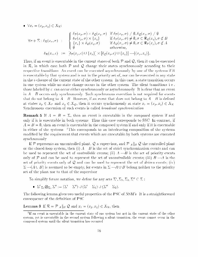
� 8xr = (xp; xq) 2 XR:8� 2 � : �R(xr; �) := 8>>><>>>: �P(xp; �)� �Q(xq; �) if �P(xp; �) 6= ;; �Q(xq; �) 6= ;�P(xp; �)� fxqg if �P(xp; �) 6= ;; � 2 <Q(xq); � 62 Bfxpg � �Q(xq; �) if �Q(xq; �) 6= ;; � 2 <P(xp); � 62 A; otherwise,�R(xr; �) := [�P(xp; �) [ fxpg]� [�Q(xq; �) [ fxqg]� f(xp; xq)g:Thus, if an event is executable in the current states of both P and Q, then it can be executedin R, in which case both P and Q change their states synchronously according to theirrespective transitions. An event can be executed asynchronously by one of the systems if itis executable by that system and is not in the priority set of, nor can be executed in any statein the �-closure of the current state of the other system. In this case, a state transition occursin one system while no state change occurs in the other system. The silent transitions{i.e.,those labeled by �{can occur either synchronously or asynchronously. It is clear that an eventin A \B occurs only synchronously. Such synchronous execution is not required for eventsthat do not belong to A\B. However, if an event that does not belong to A \B is de�nedat states xp 2 XP and xq 2 XQ, then it occurs synchronously at state xr = (xp; xq) 2 XR.Synchronous execution of such events is called broadcast synchronization.Remark 5 If A = B = �, then an event is executable in the composed system if andonly if it is executable in both systems. Thus this case corresponds to SSC. In contrast, ifA = B = ;, then an event is executable in the composed system if and only if it is executablein either of the systems. 5This corresponds to an interleaving composition of the systemsmodi�ed by the requirement that events which are executable by both systems are executedsynchronously.If P represents an uncontrolled plant, Q a supervisor, and P AkB Q the controlled plantor the closed-loop system, then (i) A \B is the set of strict synchronization events and canbe used to represent the set of controllable events; (ii) A � B is the set of priority eventsonly of P and can be used to represent the set of uncontrollable events; (iii) B � A is theset of priority events only of Q and can be used to represent the set of driven events; (iv)�� (A [B) is assumed to be empty, for events in ��A [B belong neither to the priorityset of the plant nor to that of the supervisor.To simplify future notation, we de�ne for any sets �0;�1;�2;�00 � � :� �0 �1N�2 �00 := (�0 \ �00) [ (�0 \ �1) [ (�00 \ �2):The following lemma gives two useful properties of the PSC of NSM's. It is a straightforwardconsequence of the de�nition of PSC.Lemma 3 If R = P AkB Q and xr = (xp; xq) 2 XR, then5If an event is executable in the current state of one system but not in the current state of the othersystem, yet is executable in the second system following a silent transition, the event cannot occur in thecomposed system until the silent transition has occurred.16

1. ��R(xr) = ��P(xp)� ��Q(xq);2. <R(xr) = <P(xp) ANB <Q(xq):In other words, a state x0r = (x0p; x0q) 2 XR belongs to the �-closure of xr = (xp; xq) if andonly if x0p (respectively, x0q) belongs to �-closure of xp (respectively, xq). Also, an event isrefused in P AkB Q if and only if either it is refused in both P and Q, or it belongs to thepriority set of P and is refused in P, or it belongs to the priority set of Q and is refused inQ. We next consider the trajectory model of the PSC of two systems, and obtain its relation-ship to the trajectory models of the component systems. Using the de�nition of P AkB Qand that of its refusal map <P AkB Q, the trajectory model T (P AkB Q) is easily obtainedfrom its de�nition developed in the previous subsection. In order to obtain the relationshipbetween T (P), T (Q) and T (P AkB Q), we �rst de�ne the PSC of a pair of refusal-traces.De�nition 10 Let ep 2 T (P) and eq 2 T (Q). Then the PSC of ep and eq (with respect toT (P) and T (Q)), denoted ep AkB eq, is de�ned inductively on jepj+ jeqj as follows:� 8�p;�q � � s.t. �p 2 T (P);�q 2 T (Q) :�p AkB �q := f�0 � �p ANB �qg;� 8ep 2 T (P); eq 2 T (Q);�p; �q 2 �;�p;�q � � s.t. ep(�p;�p) 2 T (P); eq(�q;�q) 2 T (Q) :ep(�p;�p) AkB eq(�q;�q) := T1 [ T2 [ T3;whereT1 := 8>>><>>>: fe(�p;�0) j e 2 ep AkB eq(�q;�q); �0 � �p ANB �qg if �p 62 B andeq(�q;�q)(�p; ;) 62 T (Q); otherwiseT2 := 8>>><>>>: fe(�q;�0) j e 2 ep(�p;�p) AkB eq; �0 � �p ANB �qg if �q 62 A andep(�p;�p)(�q; ;) 62 T (P); otherwiseT3 := 8><>: fe(�;�0) j e 2 ep AkB eq; �0 � �p ANB �qg if �p = �q := �; otherwiseIt should be noted that ep AkB eq is a set of refusal-traces that depends on T (P); T (Q) as wellas on the particular refusal-traces ep; eq. The dependence on T (P); T (Q) is not explicitlyindicated in the notation. 17

The PSC of two zero-length refusal-traces �p 2 T (P) and �q 2 T (Q), which correspondto initial refusal sets of T (P) and T (Q) respectively, is obtained by computing �p ANB �qwhich corresponds to an initial refusal set of T (P AkB Q). Next the PSC of two refusal-tracesep(�p;�p) 2 T (P) and eq(�q;�q) 2 T (Q) is obtained by considering these three possiblecases: (i) a refusal-trace belonging to ep AkB eq(�q;�q) has already been executed in thecomposed system, and at this point, �p is executable in P (indicated by ep(�p;�p) 2 T (P)),the occurrence of �p cannot be blocked byQ (indicated by �p 62 B), and Q cannot participatein the occurrence of �p (indicated by eq(�q;�q)(�p; ;) 62 T (Q)); (ii) a refusal-trace belongingto ep(�p;�p) AkB eq has already been executed in the composed system, and at this point,�q is executable in Q, and P can neither block the occurrence of �q, nor it can participatein the occurrence of �q; (iii) �p = �q := �; a refusal-trace belonging to ep AkB eq has alreadybeen executed in the composed system, and at this point, � is executable in both P and Q.Remark 6 It is clear from De�nition 10 that if A = B = �, which corresponds to the caseof SSC, then the sets T1 = T2 = ; since the conditions \�p 62 B" and \�q 62 A" both evaluateto \false". Hence the PSC of ep(�p;�p) 2 T (P) and eq(�q;�q) 2 T (Q) is nonempty if andonly if the set T3 is nonempty, which requires that �p = �q. Using induction, it can beeasily concluded that the SSC of refusal-traces ep 2 T (P) and eq 2 T (Q) is a nonempty setif and only if tr(ep) = tr(eq), in which case, tr(ep �k� eq) = tr(ep) = tr(eq), and for eachi � jepj = jeqj, the ith refusal set of any trace in ep �k� eq is any subset of the union of theith refusal set of ep and the ith refusal set of eq, since �i(ep) �N��i(eq) = �i(ep) [ �i(eq).We can extend the de�nition of the PSC of a pair of refusal-traces to the PSC of thetrajectory models. With a slight abuse of notation, we use the same symbol AkB for the PSCof the NSM's P;Q and for the PSC of their corresponding trajectory models T (P); T (Q).De�nition 11 The PSC of the trajectory models T (P); T (Q) is de�ned to be� T (P) AkB T (Q) := Sep2T (P);eq2T (Q) ep AkB eq:The following result shows that the trajectory model of the PSC of NSM's is the PSC of theircorresponding trajectory models. Equivalently, it states that the PSC operation on NSM'sinduces a PSC operation on trajectory models, and the induced operation is precisely theone described in De�nition 11.Theorem 2 For any NSM's P;Q, T (P AkB Q) = T (P) AkB T (Q):Proof: Refer to Appendix A.Corollary 2 The trajectory model is a language congruence with respect to the operationof PSC.Proof: Let P1;P2;Q1;Q2 be NSM's with T (P1) = T (P2) and T (Q1) = T (Q2). Theorem2 implies that T (P1 AkB Q1) = T (P2 AkB Q2). Hence L(P1 AkB Q1) = L(T (P1 AkB Q1)) =L(T (P2 AkB Q2)) = L(P2 AkB Q2).We will need the following result which shows that PSC of trajectory models preservesdeterminism. 18

Corollary 3 If P and Q are deterministic trajectory models, then so is P AkB Q.Proof: By de�nition, there exist deterministic state machines P;Q such that T (P) =P; T (Q) = Q. From De�nition 9, it is clear that P AkB Q is deterministic. Since Theorem2 implies that P AkB Q = T (P AkB Q), we conclude that P AkB Q is deterministic.Remark 7 Theorem 2 shows that the trajectory model of P AkB Q can be described usingonly T (P) and T (Q), and not P;Q directly. This is in contrast to the situation with thefailures model. Theorem 2 and Corollary 2 both fail if the trajectory model is replaced withthe failures model. The equality of failures models does not necessarily imply the equalityof failures models, or even language models, under prioritized synchronous composition witha �xed system [7, Example 7]. The result in Corollary 2 was mentioned without proof in[7, 8]. However, its rigorous demonstration depends on the precise de�nitions given abovefor the PSC of NSM's (with �-moves) as well as for the trajectory model of an NSM.5 Properties of Prioritized Synchronous CompositionIn this section we describe some of the properties of the PSC of two or more trajectorymodels, which are used in Section 6 for the synthesis of supervisors which control the behaviorof nondeterministic plants via PSC.5.1 AssociativityWe begin by providing a proof for the following result which is stated without proofas part of [8, Theorem 13.4]:Theorem 3 For any trajectory models P;Q;R and priority sets A;B;C � �(P AkB Q) A[BkC R = P AkB[C (QBkC R):Proof: Refer to Appendix A.This can be interpreted as an associative property as follows. Let P; Q denote trajectorymodels with event set �, and let A; B be subsets of �. We refer to the pairs (P;A); (Q;B)as prioritized systems, and de�ne their synchronous composition to be the prioritized system� (P;A) k (Q;B) := (P AkB Q; A [ B):Then Theorem 3 asserts that [(P;A) k (Q;B)] k (R;C) = (P;A) k [(Q;B) k (R;C)]: Thus,the result is simply the associative property for the synchronous composition of prioritizedsystems. 19

5.2 Augmentation and Prioritized Synchronous CompositionWe de�ne augmentation of both NSM's and trajectory models, and show that the pri-oritized synchronous composition of two trajectory models is identical to strict synchronouscomposition of their augmentations, provided the two priority sets exhaust the set of events.Let P be an NSM with event set �, and let D � �. We denote by D the deterministicstate machine with one state and self-loops labeled by every event in D. The augmentationof P by D, denoted PD, is de�ned to be the NSM PD := P ;k; D. The state space of PD canbe identi�ed with the state space of P, and PD is then obtained from P by adding self-loopsat each x 2 XP labeled by every event in D \ <P(x). It is clear that PD is deterministicwhenever P is deterministic.If P is a trajectory model, the augmentation of P by D, denoted PD, is de�ned to bethe trajectory model PD := P ;k; det(D�): Note that since both priority sets are empty,PD represents interleaving of P and det(D�) except that the broadcast synchronizationrequirement means that events in D which can also occur in P occur synchronously in bothP and det(D�).Remark 8 Since det(D�) can always execute every event in D and can never execute anyevent in ��D, it follows that for any A � ��D and any B � DPD := P ;k; det(D�) = P AkB det(D�):It follows from Theorem 2 that given an NSM P and an event set D � �, T (PD) =[T (P)]D, and it follows from Corollary 3 that if P is a deterministic trajectory model, thenso is its augmentation PD.The following result shows that augmentation can be used to reduce prioritized syn-chronous composition to strict synchronization.Proposition 4 If A [B = �, then P AkB Q = PB�A �kB Q = PB�A �k� QA�B:Proof: It su�ces to prove the �rst equality since the second equality follows from symmetryand a second application of the �rst equality. Using Remark 8 and Theorem 3 givesPB�A �kB Q = (P AkB�A det((B �A)�)) �kB Q= det((B �A)�)B�Ak� (P AkB Q)= P AkB Q:The �nal equality is an easy consequence of two facts: The priority set of P AkB Q is �, sodet((B�A)�) cannot execute any events which do not occur in P AkB Q. det((B�A)�) canalway execute each event in its priority set, so it cannot block any events in P AkB Q.6 Supervisory Control with Driven EventsIn this section, we derive results concerning supervisory control by prioritized syn-chronous composition in the presence of driven events.20

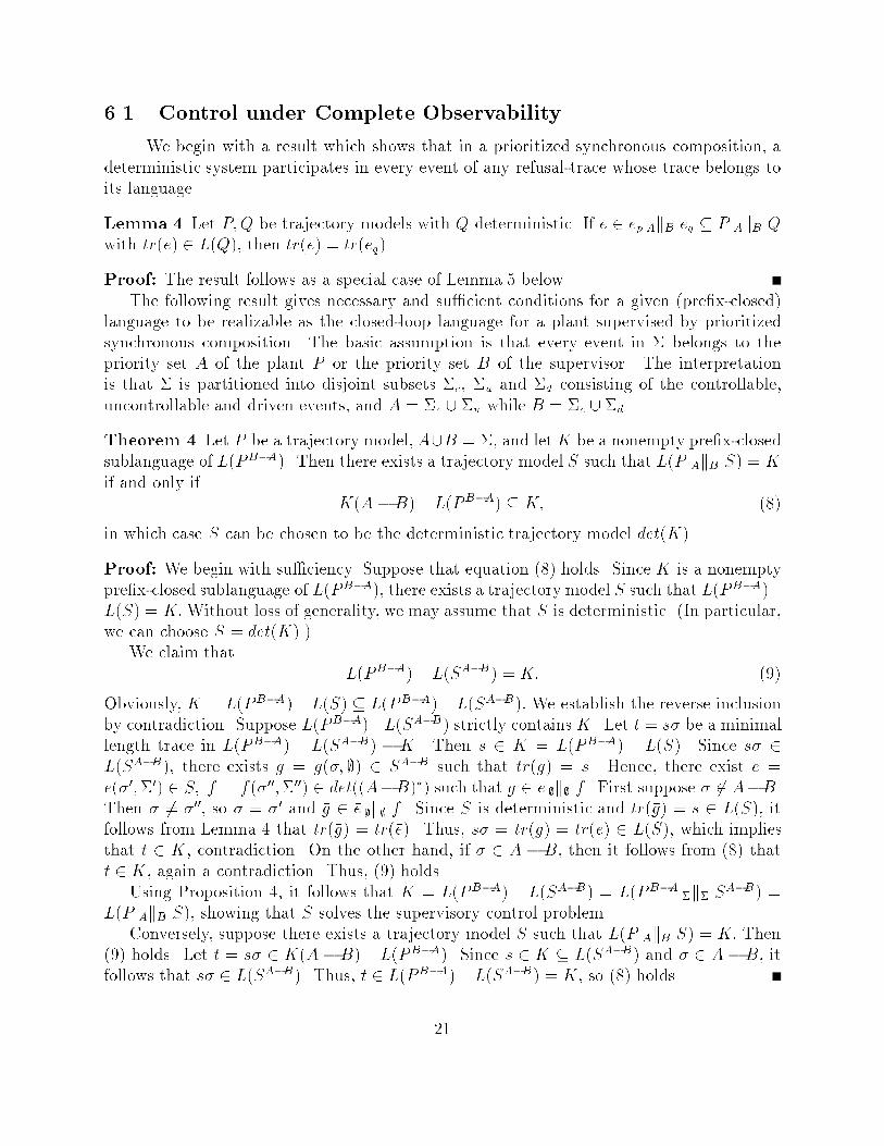
6.1 Control under Complete ObservabilityWe begin with a result which shows that in a prioritized synchronous composition, adeterministic system participates in every event of any refusal-trace whose trace belongs toits language.Lemma 4 Let P;Q be trajectory models with Q deterministic. If e 2 ep AkB eq � P AkB Qwith tr(e) 2 L(Q), then tr(e) = tr(eq).Proof: The result follows as a special case of Lemma 5 below.The following result gives necessary and su�cient conditions for a given (pre�x-closed)language to be realizable as the closed-loop language for a plant supervised by prioritizedsynchronous composition. The basic assumption is that every event in � belongs to thepriority set A of the plant P or the priority set B of the supervisor. The interpretationis that � is partitioned into disjoint subsets �c, �u and �d consisting of the controllable,uncontrollable and driven events, and A = �c [ �u while B = �c [ �d.Theorem 4 Let P be a trajectory model,A[B = �, and letK be a nonempty pre�x-closedsublanguage of L(PB�A). Then there exists a trajectory model S such that L(P AkB S) = Kif and only if K(A�B) \ L(PB�A) � K; (8)in which case S can be chosen to be the deterministic trajectory model det(K).Proof: We begin with su�ciency. Suppose that equation (8) holds. Since K is a nonemptypre�x-closed sublanguage of L(PB�A), there exists a trajectory model S such that L(PB�A)\L(S) = K:Without loss of generality, we may assume that S is deterministic. (In particular,we can choose S = det(K).)We claim that L(PB�A) \ L(SA�B) = K: (9)Obviously, K = L(PB�A) \ L(S) � L(PB�A) \ L(SA�B): We establish the reverse inclusionby contradiction. Suppose L(PB�A)\L(SA�B) strictly contains K. Let t = s� be a minimallength trace in L(PB�A) \ L(SA�B) � K. Then s 2 K = L(PB�A) \ L(S). Since s� 2L(SA�B), there exists g = �g(�; ;) 2 SA�B such that tr(�g) = s. Hence, there exist e =�e(�0;�0) 2 S; f = �f (�00;�00) 2 det((A�B)�) such that g 2 e ;k; f . First suppose � 62 A�B.Then � 6= �00, so � = �0 and �g 2 �e ;k; f . Since S is deterministic and tr(�g) = s 2 L(S), itfollows from Lemma 4 that tr(�g) = tr(�e). Thus, s� = tr(g) = tr(e) 2 L(S), which impliesthat t 2 K, contradiction. On the other hand, if � 2 A � B, then it follows from (8) thatt 2 K, again a contradiction. Thus, (9) holds.Using Proposition 4, it follows that K = L(PB�A) \ L(SA�B) = L(PB�A �k� SA�B) =L(P AkB S); showing that S solves the supervisory control problem.Conversely, suppose there exists a trajectory model S such that L(P AkB S) = K: Then(9) holds. Let t = s� 2 K(A�B) \ L(PB�A). Since s 2 K � L(SA�B) and � 2 A�B, itfollows that s� 2 L(SA�B). Thus, t 2 L(PB�A) \ L(SA�B) = K, so (8) holds.21

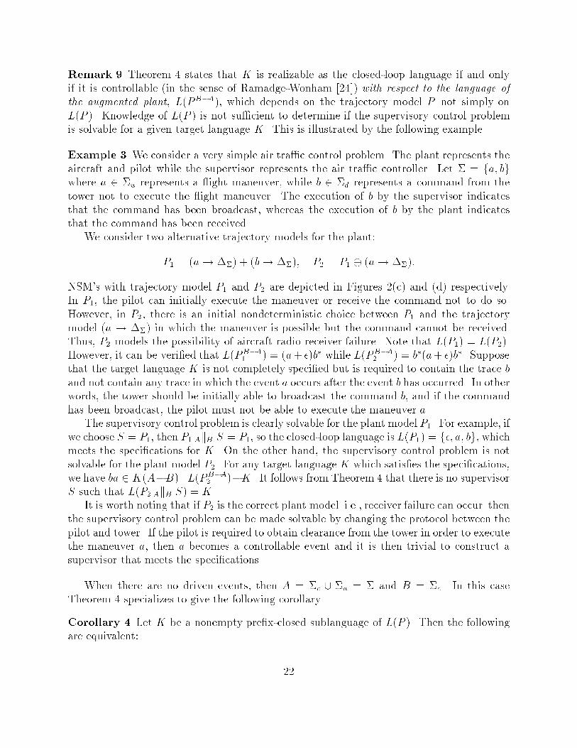
Remark 9 Theorem 4 states that K is realizable as the closed-loop language if and onlyif it is controllable (in the sense of Ramadge-Wonham [24]) with respect to the language ofthe augmented plant, L(PB�A), which depends on the trajectory model P{not simply onL(P ). Knowledge of L(P ) is not su�cient to determine if the supervisory control problemis solvable for a given target language K. This is illustrated by the following example.Example 3 We consider a very simple air tra�c control problem. The plant represents theaircraft and pilot while the supervisor represents the air tra�c controller. Let � = fa; bgwhere a 2 �u represents a ight maneuver, while b 2 �d represents a command from thetower not to execute the ight maneuver. The execution of b by the supervisor indicatesthat the command has been broadcast, whereas the execution of b by the plant indicatesthat the command has been received.We consider two alternative trajectory models for the plant:P1 = (a! ��) + (b! ��); P2 = P1 � (a! ��):NSM's with trajectory model P1 and P2 are depicted in Figures 2(c) and (d) respectively.In P1, the pilot can initially execute the maneuver or receive the command not to do so.However, in P2, there is an initial nondeterministic choice between P1 and the trajectorymodel (a ! ��) in which the maneuver is possible but the command cannot be received.Thus, P2 models the possibility of aircraft radio receiver failure. Note that L(P1) = L(P2).However, it can be veri�ed that L(PB�A1 ) = (a+ �)b� while L(PB�A2 ) = b�(a+ �)b�. Supposethat the target language K is not completely speci�ed but is required to contain the trace band not contain any trace in which the event a occurs after the event b has occurred. In otherwords, the tower should be initially able to broadcast the command b, and if the commandhas been broadcast, the pilot must not be able to execute the maneuver a.The supervisory control problem is clearly solvable for the plant model P1. For example, ifwe choose S = P1, then P1 AkB S = P1, so the closed-loop language is L(P1) = f�; a; bg, whichmeets the speci�cations for K. On the other hand, the supervisory control problem is notsolvable for the plant model P2. For any target language K which satis�es the speci�cations,we have ba 2 K(A�B)\L(PB�A2 )�K. It follows from Theorem 4 that there is no supervisorS such that L(P2 AkB S) = K.It is worth noting that if P2 is the correct plant model{i.e., receiver failure can occur{thenthe supervisory control problem can be made solvable by changing the protocol between thepilot and tower. If the pilot is required to obtain clearance from the tower in order to executethe maneuver a, then a becomes a controllable event and it is then trivial to construct asupervisor that meets the speci�cations.When there are no driven events, then A = �c [ �u = � and B = �c. In this caseTheorem 4 specializes to give the following corollary.Corollary 4 Let K be a nonempty pre�x-closed sublanguage of L(P ). Then the followingare equivalent: 22

1. There exists a trajectory model S such that L(P �k�c S) = K.2. L(P �k�c det(K)) = K.3. K�u \ L(P ) � K.Remark 10 Corollary 4 shows that when there are no driven events, the necessary andsu�cient conditions for supervisory control by prioritized synchronous composition are thesame as those in the Ramadge-Wonham framework [23]. The equivalence of the �rst andsecond conditions of Corollary 4 was stated without proof in [7, Theorem 1] and [8, Theorem14.2]. The equivalence of the �rst and third conditions of Corollary 4 was stated in [8,Theorem 14.1] accompanied by an incomplete proof.Remark 11 The proof of Theorem 4 shows that if K satis�es the condition (8) and ifN is any pre�x-closed sublanguage of �� with L(PB�A) \ N = K; then the deterministicsupervisor S := det(N) results in K as the closed-loop language L(P AkB S). Since K � N ,it follows from Lemma 4 that every event executed by the closed-loop system occurs in S. Inparticular, every uncontrollable event is executed by the supervisor even though such eventsdo not belong to its priority set. This behavior is induced by the broadcast synchronizationrequirement in prioritized synchronous composition.It is interesting to specialize this observation to the case where there are no driven events.Since A = �, the plant also participates in every event. Thus, the plant and supervisorfunction as though they are connected by strict synchronization rather than by prioritizedsynchronous composition. In particular, this is the case when the supervisor is chosen tobe det(K). The determinism of S is essential here. If S is a nondeterministic trajectorymodel with L(S) = N , there is no guarantee that the closed-loop language will be K. Thisis demonstrated by the next example.Example 4 Let � = fa; bg; �c = fag; �u = fbg; P = (a! ��) + (b! (a! ��)); S =(a ! ��) � (b ! ��). Then L(P ) = f�; a; b; bag; L(S) = f�; a; bg: Let K = L(S).Then K satis�es the controllability condition (the third condition of Corollary 4) as well asL(P ) \ L(S) = K. A straightforward calculation shows that P �k�c S = ((a! ��) + (b!(a ! ��)) � (b ! ��): Thus, L(P �k�c S) = f�; a; b; bag = L(P ) 6= K: What happens isthat since S is nondeterministic, the event b can be executed as the initial event solely in Peven though b 2 L(S). (This cannot happen for deterministic S by Lemma 4.) Thus, strictsynchronization is lost. This permits a trace of P �k�c S which is not a trace of S.6.2 Control under Restricted UnobservabilityWe continue to assume that A [ B = � where A = �c [ �u and B = �c [ �d. In theclosed-loop system P AkB S, the events in A � B{i.e., the uncontrollable events{are gener-ated by the plant P and are broadcast to the supervisor S where they are synchronouslyexecuted whenever enabled. It may happen that information about the occurrence of certainuncontrollable events is unavailable for broadcast due to lack of sensors, or it may be desired23

to implement a simpli�ed supervisor which ignores such information. This suggests a gen-eralization of prioritized synchronous composition in which the broadcast synchronizationrequirement is disregarded for a speci�ed subset � � A�B of uncontrollable events. Sinceevents in A�B cannot occur spontaneously in S, this e�ectively prevents S from ever exe-cuting the events in �. Thus, instead of modifying the de�nition of prioritized synchronouscomposition, it is equivalent to restrict the admissible supervisors to those which do notexecute events in �.Let �� : �! � denote the natural projection de�ned by� 8� 2 � : ��(�) := � � for � 2 �� for � 2 �� ���(�) extends to a map on �� in the obvious way. We de�ne the Restricted SupervisoryControl Problem (RSCP) to be as follows: Given a pre�x-closed sublanguage K of L(PB�A)and � � A�B, determine if there exists a supervisor S such that� L(P AkB S) = K; and ��(L(S)) = L(S).Remark 12 There are two di�erent ways to model an uncontrollable event in the plantwhich is unobservable to the supervisor. It can be completely suppressed and treated as an�-event in P . Alternatively, it can be treated as a labeled event � 2 � in the plant which doesnot label any transitions in the supervisor. The advantage of the second approach (whichis the one taken in the RSCP) is that such an event can be included in the performancespeci�cations{i.e., in the target language K. Hence, even though it is unobservable to thesupervisor, its occurrence in the closed-loop system can be controlled{albeit subject to theconditions that must be satis�ed by K for the solvability of the RSCP.The next result generalizes Lemma 4 to the case where certain events in A�B are notpresent in the second system Q.Lemma 5 Let � � A�B, and P;Q be trajectory models withQ deterministic and satisfying��(L(Q)) = L(Q). If e 2 ep AkB eq � P AkB Q with ��(tr(e)) 2 L(Q), then ��(tr(e)) =tr(eq).Proof: The proof is by induction on jej. The assertion holds trivially when jej = 0. Forthe induction step, write e = �e(�;�0) and let �ep; �eq denote the pre�xes of ep; eq obtained bydeleting the �nal event and refusal set from each refusal-trace.If � occurs synchronously in both P and Q, then �e 2 �ep AkB �eq. Then � 62 �, so��(tr(e)) = ��(tr(�e))�: Since L(Q) is pre�x-closed, ��(tr(�e)) 2 L(Q). Applying the induc-tion hypothesis gives ��(tr(�e)) = tr(�eq). Thus, ��(tr(e)) = ��(tr(�e))� = tr(�eq)� = tr(eq):The same argument applies in the case where �e 2 ep AkB �eq{i.e., when � occurs only in Q.Suppose �e 2 �ep AkB eq, i.e., � occurs only in P . If � 2 �, then ��(tr(e)) = ��(tr(�e)) =tr(eq); where the second equality follows from the induction hypothesis. Now suppose that� 62 �. Since � occurs only in P , it follows that eq(�; ;) 62 Q. Since Q is deterministic,Proposition 3 then implies that tr(eq)� 62 L(Q). Since L(Q) is pre�x-closed, ��(tr(�e)) 224

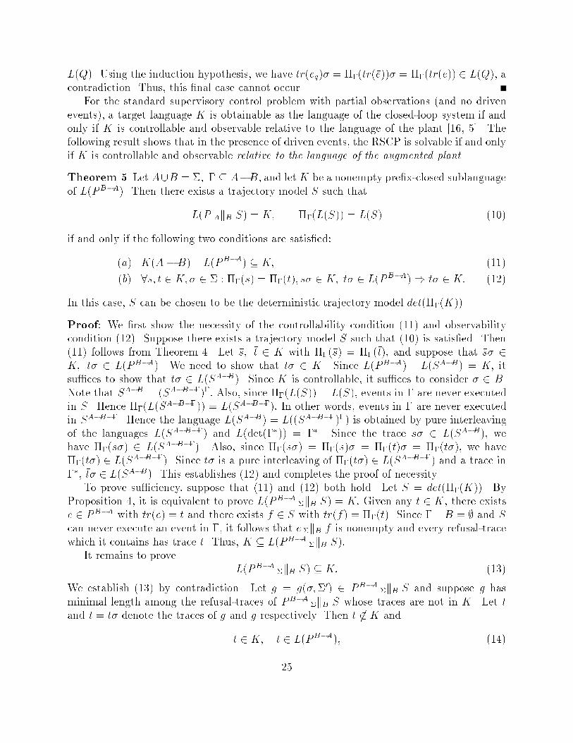
L(Q). Using the induction hypothesis, we have tr(eq)� = ��(tr(�e))� = ��(tr(e)) 2 L(Q); acontradiction. Thus, this �nal case cannot occur.For the standard supervisory control problem with partial observations (and no drivenevents), a target language K is obtainable as the language of the closed-loop system if andonly if K is controllable and observable relative to the language of the plant [16, 5]. Thefollowing result shows that in the presence of driven events, the RSCP is solvable if and onlyif K is controllable and observable relative to the language of the augmented plant.Theorem 5 Let A[B = �; � � A�B, and letK be a nonempty pre�x-closed sublanguageof L(PB�A). Then there exists a trajectory model S such thatL(P AkB S) = K; ��(L(S)) = L(S) (10)if and only if the following two conditions are satis�ed:(a) K(A�B) \ L(PB�A) � K; (11)(b) 8�s; �t 2 K;� 2 � : ��(�s) = ��(�t); �s� 2 K; �t� 2 L(PB�A)) �t� 2 K: (12)In this case, S can be chosen to be the deterministic trajectory model det(��(K)).Proof: We �rst show the necessity of the controllability condition (11) and observabilitycondition (12). Suppose there exists a trajectory model S such that (10) is satis�ed. Then(11) follows from Theorem 4. Let �s; �t 2 K with ��(�s) = ��(�t), and suppose that �s� 2K; �t� 2 L(PB�A). We need to show that �t� 2 K. Since L(PB�A) \ L(SA�B) = K; itsu�ces to show that �t� 2 L(SA�B). Since K is controllable, it su�ces to consider � 2 B.Note that SA�B = (SA�B��)�: Also, since ��(L(S)) = L(S), events in � are never executedin S. Hence ��(L(SA�B��)) = L(SA�B��): In other words, events in � are never executedin SA�B��. Hence the language L(SA�B) = L((SA�B��)�) is obtained by pure interleavingof the languages L(SA�B��) and L(det(��)) = ��. Since the trace �s� 2 L(SA�B), wehave ��(�s�) 2 L(SA�B��). Also, since ��(�s�) = ��(�s)� = ��(�t)� = ��(�t�), we have��(�t�) 2 L(SA�B��). Since �t� is a pure interleaving of ��(�t�) 2 L(SA�B��) and a trace in��, �t� 2 L(SA�B). This establishes (12) and completes the proof of necessity.To prove su�ciency, suppose that (11) and (12) both hold. Let S = det(��(K)). ByProposition 4, it is equivalent to prove L(PB�A �kB S) = K: Given any t 2 K, there existse 2 PB�A with tr(e) = t and there exists f 2 S with tr(f) = ��(t). Since � \B = ; and Scan never execute an event in �, it follows that e �kB f is nonempty and every refusal-tracewhich it contains has trace t. Thus, K � L(PB�A �kB S):It remains to prove L(PB�A �kB S) � K: (13)We establish (13) by contradiction. Let g = �g(�;�0) 2 PB�A �kB S and suppose g hasminimal length among the refusal-traces of PB�A �kB S whose traces are not in K. Let �tand t = �t� denote the traces of �g and g respectively. Then t 62 K and�t 2 K; t 2 L(PB�A); (14)25

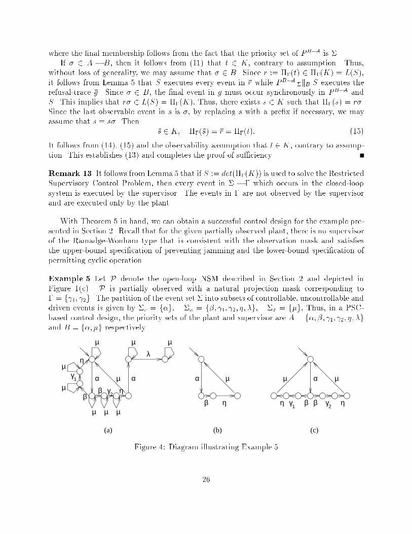
where the �nal membership follows from the fact that the priority set of PB�A is �.If � 2 A � B, then it follows from (11) that t 2 K, contrary to assumption. Thus,without loss of generality, we may assume that � 2 B. Since �r := ��(�t) 2 ��(K) = L(S);it follows from Lemma 5 that S executes every event in �r while PB�A �kB S executes therefusal-trace �g. Since � 2 B, the �nal event in g must occur synchronously in PB�A andS. This implies that �r� 2 L(S) = ��(K): Thus, there exists s 2 K such that ��(s) = �r�.Since the last observable event in s is �, by replacing s with a pre�x if necessary, we mayassume that s = �s�. Then �s 2 K; ��(�s) = �r = ��(�t): (15)It follows from (14), (15) and the observability assumption that t 2 K, contrary to assump-tion. This establishes (13) and completes the proof of su�ciency.Remark 13 It follows from Lemma 5 that if S := det(��(K)) is used to solve the RestrictedSupervisory Control Problem, then every event in � � � which occurs in the closed-loopsystem is executed by the supervisor. The events in � are not observed by the supervisorand are executed only by the plant.With Theorem 5 in hand, we can obtain a successful control design for the example pre-sented in Section 2. Recall that for the given partially observed plant, there is no supervisorof the Ramadge-Wonham type that is consistent with the observation mask and satis�esthe upper-bound speci�cation of preventing jamming and the lower-bound speci�cation ofpermitting cyclic operation.Example 5 Let P denote the open-loop NSM described in Section 2 and depicted inFigure 1(c). P is partially observed with a natural projection mask corresponding to� = f 1; 2g. The partition of the event set � into subsets of controllable, uncontrollable anddriven events is given by �c = f�g; �u = f�; 1; 2; �; �g; �d = f�g: Thus, in a PSC-based control design, the priority sets of the plant and supervisor are A = f�; �; 1; 2; �; �gand B = f�; �g respectively.αα

ηλ

γ2β ηµ

µ

µµµ

β

µ µ µ

β η

α α

ββ ηη γ γ1 2

µ µ µµ

(a) (b) (c)

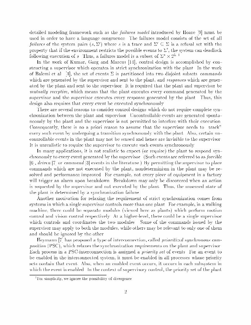
1γ Figure 4: Diagram illustrating Example 526

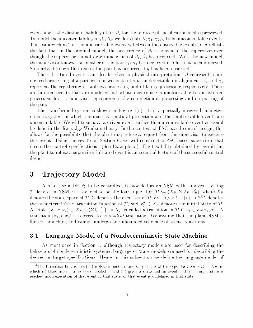
The augmented plant PB�A is shown in Figure 4(a). The requirement that the jam-ming event � never occur in the closed-loop system is represented by the speci�cationL(P AkB S) � K, where P is the trajectory model of P, S is the trajectory model ofa supervisor, and K := fs 2 L(PB�A) j no event in s is �g. Since s := �� 2�� 2 K,s� 2 L(PB�A)�K, and � 2 A�B = �u, K is not controllable with respect to A�B andL(PB�A), and a straightforward calculation yieldsK" = pr((��������( 1��� + 2����))�)as the supremal controllable sublanguage [22]. However, K" is not observable relative to theaugmented plant language L(PB�A) and mask ��(�). In particular, if �t 2 (��������( 1���+ 2����))��������� 2��� � K", then �t� 2 L(PB�A) � K", and 9�s 2 (��������( 1��� + 2����))��������� 1��� � K" such that ��(�s) = ��(�t) and �s� 2 K".It is easy to see that the supremal normal sublanguage [16, 4] of K" is given byK̂ = pr((��������( 1 + 2)����)�):Since K̂ is obtained from K" by disabling certain occurrences of the controllable event �, itis controllable. That K̂ is controllable also follows from the fact that it equals the closed andobservable sublanguage of K" computed using the formula given in [13, Equation 10], andthe fact that controllability is preserved under such a computation [13, Theorem 5]. Sincenormality implies observability [16], it follows from Theorem 5 that K̂ can be obtained asthe closed-loop language by using an appropriate PSC-based supervisor, one choice beingS := det(��(K̂)).While the supervisor S = det(��(K̂)) is minimally restrictive, it possesses an undesirabletrait: S can execute arbitrarily long sequences of the driven event �. Since the plant cannever execute more than one � in succession, all but at most one of a sequence of �'s requestedby the supervisor will be refused by the plant. We can remove this redundancy by replacingK̂ by the sublanguage K̂ 0 := pr((��( 1+ 2)��)�). K̂ 0 is obtained by removing the self-loopson � from K̂, and is also both controllable and observable. By Theorem 5, the PSC-basedsupervisor S 0 := det(��(K̂ 0)) will impose K̂ 0 as the closed-loop language. A minimal statemachine realization S 0 for the deterministic trajectory model S 0 is shown in Figure 4(b), andthe resulting closed-loop NSM P AkB S 0 is depicted in Figure 4(c). The closed-loop languageK̂ 0 does not contain � yet permits 1 and 2 to be executed arbitrarily many times. Hence,the dual objectives of preventing jamming and permitting cyclic operation are met.The supervisor S 0 implements the following control strategy: S 0 tracks the inputting,commencement of processing and completion/outputting of each part by executing �; � and� synchronously with P. Between the synchronous executions of � and �, the plant executeseither 1 or 2 without the participation or knowledge of the supervisor. Following thesynchronous execution of �, the supervisor requests execution of the realignment event �. Ifthe mechanism is misaligned{i.e., 2 has preceded �{then the plant executes � synchronouslywith the supervisor. This corrects the alignment and returns the plant to its initial state.On the other hand, if misalignment has not occurred{i.e., 1 has preceded �{then the plantrefuses � and this event occurs solely in the supervisor. The possibility that the plant canrefuse an event o�ered by the supervisor is an essential feature of this control design.27

7 ConclusionIn this paper we have studied the supervisory control of nondeterministic plants inthe presence of driven events under complete as well as partial observation. We have shownthat prioritized synchronous composition is an adequate control mechanism for this pur-pose. The trajectory model, used for describing the behavior of nondeterministic systems,is shown to be a language congruence with respect to prioritized synchronous composition.Hence it is quite useful for describing the behaviors of nondeterministic systems which maybe controlled via PSC. It is shown that the supervisory control problem with driven events issolvable if and only if the target language is controllable and observable with respect to thelanguage of the plant augmented by the set of driven events. In case the languages involvedare regular, one way to perform the test for controllability/observability is to construct adeterministic system, language equivalent to the augmented plant, and apply a known testfor controllability/observability [23, 14, 26]. However, it can be shown that by modifyingthe algorithms in these references, the tests can be performed without having to do such anondeterministic to deterministic conversion. Hence it is possible to obtain algorithms ofpolynomial complexity (polynomial in the product of the number of states in the given plantNSM and that in the deterministic generator of the desired language) for testing control-lability/observability. Due to the augmentation, the solvability depends on the trajectorymodel of the plant{not simply on its language. We have also described the associativity andaugmentation properties of PSC, which are useful in the analysis of supervisory control.A Proof of Theorems 2 and 3Proof of Theorem 2: Let R = P AkB Q. First we show thatT (R) � T (P) AkB T (Q): (16)We prove by induction on length of refusal-trace that if e 2 T (R) and xr = (xp; xq) 2�TR(x0R; e), then there exist ep 2 T (P); eq 2 T (Q) such that(i) the �nal refusal sets of ep; eq are <P(xp); <Q(xq) respectively,(ii) e 2 ep AkB eq,(iii) xr 2 �TP(x0P; ep)� �TQ(x0Q; eq).Consider a zero-length refusal-trace e = �0 2 T (R). Then there exists xr = (xp; xq) 2��R(x0R) such that �0 � <R(xr). Lemma 3 implies that xp 2 ��P(x0P); xq 2 ��Q(x0Q); �0 �<P(xp) ANB <Q(xq). Setting ep = <P(xp); eq = <Q(xq), it follows that (i), (ii), (iii) aresatis�ed.For the induction step, consider a refusal-trace e = �e(�;�0) 2 T (R). Then there exist�xr = (�xp; �xq) 2 �TR(x0R; �e); x0r = (x0p; x0q) 2 �R(�xr; �); xr = (xp; xq) 2 ��R(x0r) such that�0 � <R(xr). By induction hypothesis, there exist �ep 2 T (P); �eq 2 T (Q) with �nal refusalsets <P(�xp); <Q(�xq) respectively such that �e 2 �ep AkB �eq; �xp 2 �TP(x0P; �ep); �xq 2 �TQ(x0Q; �eq):Since � is executable in �xr, it follows from De�nition 9 that there are three cases:28

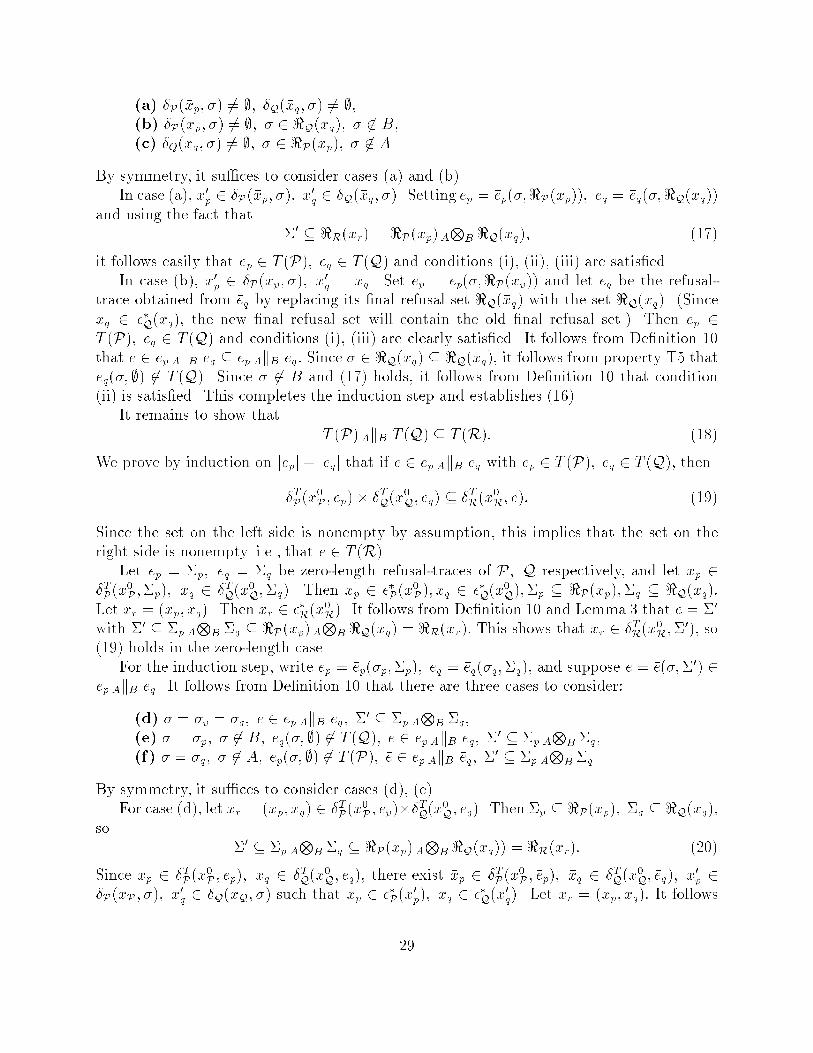
(a) �P(�xp; �) 6= ;; �Q(�xq; �) 6= ;,(b) �P(�xp; �) 6= ;; � 2 <Q(�xq); � 62 B,(c) �Q(�xq; �) 6= ;; � 2 <P(�xp); � 62 A.By symmetry, it su�ces to consider cases (a) and (b).In case (a), x0p 2 �P(�xp; �); x0q 2 �Q(�xq; �). Setting ep = �ep(�;<P(xp)); eq = �eq(�;<Q(xq))and using the fact that �0 � <R(xr) = <P(xp) ANB <Q(xq); (17)it follows easily that ep 2 T (P); eq 2 T (Q) and conditions (i), (ii), (iii) are satis�ed.In case (b), x0p 2 �P(�xp; �); x0q = �xq. Set ep = �ep(�;<P(xp)) and let eq be the refusal-trace obtained from �eq by replacing its �nal refusal set <Q(�xq) with the set <Q(xq). (Sincexq 2 ��Q(�xq), the new �nal refusal set will contain the old �nal refusal set.) Then ep 2T (P); eq 2 T (Q) and conditions (i), (iii) are clearly satis�ed. It follows from De�nition 10that �e 2 �ep AkB �eq � �ep AkB eq: Since � 2 <Q(�xq) � <Q(xq), it follows from property T5 thateq(�; ;) 62 T (Q). Since � 62 B and (17) holds, it follows from De�nition 10 that condition(ii) is satis�ed. This completes the induction step and establishes (16).It remains to show that T (P) AkB T (Q) � T (R): (18)We prove by induction on jepj+ jeqj that if e 2 ep AkB eq with ep 2 T (P); eq 2 T (Q), then�TP(x0P; ep)� �TQ(x0Q; eq) � �TR(x0R; e): (19)Since the set on the left side is nonempty by assumption, this implies that the set on theright side is nonempty{i.e., that e 2 T (R).Let ep = �p; eq = �q be zero-length refusal-traces of P; Q respectively, and let xp 2�TP(x0P;�p); xq 2 �TQ(x0Q;�q). Then xp 2 ��P(x0P); xq 2 ��Q(x0Q);�p � <P(xp);�q � <Q(xq):Let xr = (xp; xq). Then xr 2 ��R(x0R). It follows from De�nition 10 and Lemma 3 that e = �0with �0 � �p ANB �q � <P(xp) ANB <Q(xq) = <R(xr): This shows that xr 2 �TR(x0R;�0), so(19) holds in the zero-length case.For the induction step, write ep = �ep(�p;�p); eq = �eq(�q;�q), and suppose e = �e(�;�0) 2ep AkB eq. It follows from De�nition 10 that there are three cases to consider:(d) � = �p = �q; �e 2 �ep AkB �eq; �0 � �p ANB �q,(e) � = �p; � 62 B; eq(�; ;) 62 T (Q); �e 2 �ep AkB eq; �0 � �p ANB �q,(f) � = �q; � 62 A; ep(�; ;) 62 T (P); �e 2 ep AkB �eq; �0 � �p ANB �q.By symmetry, it su�ces to consider cases (d), (e).For case (d), let xr = (xp; xq) 2 �TP(x0P; ep)��TQ(x0Q; eq). Then �p � <P(xp); �q � <Q(xq),so �0 � �p ANB �q � <P(xp) ANB <Q(xq)) = <R(xr): (20)Since xp 2 �TP(x0P; ep); xq 2 �TQ(x0Q; eq), there exist �xp 2 �TP(x0P ; �ep); �xq 2 �TQ(x0Q; �eq); x0p 2�P(�xP; �); x0q 2 �Q(�xQ; �) such that xp 2 ��P(x0p); xq 2 ��Q(x0q). Let �xr = (�xp; �xq): It follows29

from De�nition 9 that (x0p; x0q) 2 �R(�xr; �), while by induction hypothesis, we may assumethat �xr 2 �TR(x0R; �e). Thenxr 2 ��R((x0p; x0q)) � ��R(�R(�xr; �)) � ��R(�R(�TR(x0R; �e); �)): (21)We conclude from (20) and (21) that xr 2 �TR(x0R; e) as required.For case (e), let xr = (xp; xq) 2 �TP(x0P ; ep)��TQ(x0Q; eq). The inclusions given by (20) holdas in the previous case. Since xp 2 �TP(x0P; ep), there exist �xp 2 �TP(x0P; �ep) and x0p 2 �P(�xP ; �)such that xp 2 ��P(x0p). Let �xr = (�xp; xq): We have �Q(��Q(xq); �) � �Q(�TQ(x0Q; eq); �) = ;;where the �nal equality follows from the assumption that eq(�; ;) 62 T (Q). This implies that� 2 <Q(xq). It then follows from De�nition 9 that (x0p; xq) 2 �R(�xr; �), while by inductionhypothesis, we may assume that �xr 2 �TR(x0R; �e). Thenxr 2 ��R((x0p; xq)) � ��R(�R(�xr; �)) � ��R(�R(�TR(x0R; �e); �)): (22)We conclude from (20) and (22) that xr 2 �TR(x0R; e) as required. This completes the induc-tion step and establishes (18).The following result was proved in the course of the proof of Theorem 2.Corollary 5 For NSM's P;Q and A;B � �, let R := P AkB Q. Then1. For each e 2 T (R) and xr = (xp; xq) 2 �TR(x0R; e), there exists ep 2 T (P) and eq 2 T (Q)such that �jepj(ep) = <P(xp);�jeq j(eq) = <Q(xq), e 2 ep AkB eq, and xr 2 �TP(x0P; ep)��TQ(x0Q; eq).2. For each ep 2 T (P); eq 2 T (Q) and e 2 ep AkB eq; �TP(x0P; ep)� �TQ(x0Q; eq) � �TR(x0R; e).In order the prove Theorem 3 we will use the following result which gives a monotonicityproperty of the PSC of refusal-traces with respect to the dominance partial order.Lemma 6 Let P;Q be trajectory models, A;B � �; fp; ep 2 P; fq; eq 2 Q, with fp vep; fq v eq. Then fp AkB fq � ep AkB eq:Proof: The proof is by induction on the sum of refusal-trace lengths jepj+jeqj. If jepj+jeqj =0, then fp = �̂p; ep = �p; fq = �̂q; eq = �q with �̂p � �p; �̂q � �q. Let f 2 fp AkB fq.Then f = �0 � �̂p ANB �̂q � �p ANB �q: Thus, f 2 ep AkB eq.For the induction step, write fp = �fp(�p; �̂p); ep = �ep(�p;�p); fq = �fq(�q; �̂q); eq =�eq(�q;�q) with �fp v �ep; �̂p � �p; �fq v �eq; �̂q � �q. Let f = �f(�;�0) 2 fp AkB fq. Thereare three cases to consider: (1) Suppose �f 2 �fp AkB �fq; � = �p = �q; �0 � �̂p ANB �̂q. Bythe induction hypothesis, �f 2 �ep AkB �eq. Since �0 � �̂p ANB �̂q � �p ANB �q, this impliesthat f 2 ep AkB eq. (2) Suppose �f 2 �fp AkB fq; � = �p 62 B; fq(�; ;) 62 Q; �0 � �̂p ANB �̂q.By induction hypothesis, �f 2 �ep AkB eq. Also, eq(�; ;) 62 Q, since otherwise T3 would implythat fq(�; ;) 2 Q, contradiction. Since �0 � �̂p ANB �̂q � �p ANB �q, this implies thatf 2 ep AkB eq. (3) Suppose �f 2 fp AkB �fq; � = �q 62 A; fp(�; ;) 62 P; �0 � �̂p ANB �̂q. Thiscase is analogous to case (2). Hence, the induction step is complete.30

Proof of Theorem 3: By symmetry, it su�ces to prove the inclusion(P AkB Q) A[BkC R � P AkB[C (QBkC R):By Lemma 6, it su�ces to show that if ep; eq; er are saturated refusal-traces of P; Q; Rrespectively, then (ep AkB eq) A[BkC er � P AkB[C (QBkC R): To prove this, we show byinduction on the sum of the lengths jepj+ jeqj+ jerj that(ep AkB eq) A[BkC er � ep AkB[C (eq BkC er): (23)For future reference, we note that the following identity holds:(�p ANB �q) A[BNC �r = (�p \ �q \ �r) [ (�p \A) [ (�q \ B) [ (�r \ C)= �p ANB[C(�q BNC �r) := �̂ (24)If ep = �p; eq = �q; er = �r each have zero-length, then (ep AkB eq) A[BkC er consistsof all subsets of (�p ANB �q) A[BNC �r while ep AkB[C (eq BkC er) consists of all subsets of�p ANB[C(�q BNC �r). Thus, (23) follows from (24).For the induction step, let ep = �ep(�p;�p); eq = �eq(�q;�q); er = �er(�r;�r). �ep; �eq; �erare saturated since they are pre�xes of saturated refusal-traces. Let f 2 ep AkB eq and leth 2 f A[BkC er � (ep AkB eq) A[BkC er. Let h = �h(�; �̂). (There is no loss of generality intaking the �nal refusal set of h to be the maximal set �̂.) To establish the induction step,we consider several cases. (Some cases will not apply if at least one of the refusal-tracesep; eq; er has zero-length.)(1) �h 2 f A[BkC �er; � 62 A[B; f(�; ;) 62 P AkB Q; � = �r. (This is when the �nal event inh occurs in R but not in P AkB Q.)(2a) �h 2 �f A[BkC er; � 62 C; er(�; ;) 62 R; � = �p; �f 2 �ep AkB eq; � 62 B; eq(�; ;) 62 Q.(This is when the �nal event in h occurs in P AkB Q but not in R, and within P AkB Q,it occurs in P but not in Q.)(2b) �h 2 �f A[BkC er; � 62 C; er(�; ;) 62 R; � = �q; �f 2 ep AkB �eq; � 62 A; ep(�; ;) 62 P .(This is when the �nal event in h occurs in P AkB Q but not in R, and within P AkB Q,it occurs in Q but not in P .)(2c) �h 2 �f A[BkC er; � 62 C; er(�; ;) 62 R; � = �p = �q; �f 2 �ep AkB �eq. (This is when the�nal event in h occurs in P AkB Q but not in R, and within P AkB Q, it occurs in bothP and Q.)(3a) �h 2 �f A[BkC �er; � = �p = �r; �f 2 �ep AkB eq; � 62 B; eq(�; ;) 62 Q. (This is when the�nal event in h occurs in P AkB Q and in R, and within P AkB Q, it occurs in P butnot in Q.)(3b) �h 2 �f A[BkC �er; � = �q = �r; �f 2 ep AkB �eq; � 62 A; ep(�; ;) 62 P . (This is when the�nal event in h occurs in P AkB Q and in R, and within P AkB Q, it occurs in Q butnot in P .) 31

(3c) �h 2 �f A[BkC �er; � = �p = �q = �r; �f 2 �ep AkB �eq. (This is when the �nal event in hoccurs in P AkB Q and in R, and within P AkB Q, it occurs in both P and Q.)We include a detailed proof for case (2a). The other cases are proven in a similar mannerand are left to the reader. Under the assumptions of (2a),�h 2 �f A[BkC er � (�ep AkB eq) A[BkC er � �ep AkB[C (eq BkC er);where the last inclusion is the induction hypothesis. Thus, there existsg = �g(�0;�q BNC �r) 2 eq BkC erwith �0 2 f�q; �rg such that �h 2 �ep AkB[C g: (By Lemma 6, there is no loss of generality intaking the �nal refusal set of g to be the maximal set �q BNC �r.) Since eq(�; ;) 62 Q ander(�; ;) 62 R, it follows from the assumption that eq and er are saturated that � 2 �q and� 2 �r. Thus, � 2 �q \ �r � �q BNC �r. By T5, g(�; ;) 62 QBkC R. This together with� 62 B [ C, implies thath = �h(�; �̂) = �h(�;�p ANB[C(�q BNC �r) 2 ep AkB[C g � ep AkB[C (eq BkC er);completing the induction step.References[1] J. C. M. Baeten, J. A. Bergstra, and J. W. Klop. Ready-trace semantics for concreteprocess algegra with the priority operator. The Computer Journal, 30(6):498{506, 1987.[2] J. C. M. Baeten and W. P. Weijland. Process Algebra. Cambridge University Press,Cambridge, 1990.[3] S. Balemi, G. J. Ho�mann, P. Gyugyi, H. W. Toi, and G. F. Franklin. Supervisorycontrol of a rapid thermal multiprocessor. IEEE Transactions on Automatic Control,38(7):1040{1059, July 1993.[4] R. D. Brandt, V. K. Garg, R. Kumar, F. Lin, S. I. Marcus, and W. M. Wonham.Formulas for calculating supremal controllable and normal sublanguages. Systems andControl Letters, 15(8):111{117, 1990.[5] R. Cieslak, C. Desclaux, A. Fawaz, and P. Varaiya. Supervisory control of discreteevent processes with partial observation. IEEE Transactions on Automatic Control,33(3):249{260, 1988.[6] C. H. Golaszewski and P. J. Ramadge. Control of discrete event processes with forcedevents. In Proceedings of 26th IEEE Conference on Decision and Control, pages 247{251, Los Angeles, CA, 1987. 32

[7] M. Heymann. Concurrency and discrete event control. IEEE Control Systems Magazine,10(4):103{112, 1990.[8] M. Heymann and G. Meyer. Algebra of discrete event processes. Technical ReportNASA 102848, NASA Ames Research Center, Mo�ett Field, CA, June 1991.[9] C. A. R. Hoare. Communicating Sequential Processes. Prentice Hall, Inc., EnglewoodCli�s, NJ, 1985.[10] J. E. Hopcroft and J. D. Ullman. Introduction to Automata Theory, Languages andComputation. Addison-Wesley, Reading, MA, 1979.[11] K. M. Inan. An algebraic approach to supervisory control. Mathematics of Control,Signals and Systems, 5:151{164, 1992.[12] K.M. Inan and P.P. Varaiya. Algebras of discrete event models. Proceedings of theIEEE, 77(1):24{38, 1989.[13] R. Kumar. Formulas for observability of discrete event dynamical systems. In Proceed-ings of 1993 Conference on Information Sciences and Systems, pages 581{586, JohnsHopkins University, Baltimore, MD, March 1993.[14] R. Kumar, V. K. Garg, and S. I. Marcus. On controllability and normality of discreteevent dynamical systems. Systems and Control Letters, 17(3):157{168, 1991.[15] R. Kumar and M. A. Shayman. Non-blocking supervisory control of nondeterminis-tic systems via prioritized synchronization. Technical Report TR 93-58, Institute forSystems Research, University of Maryland, College Park, Maryland, July 1993.[16] F. Lin and W. M. Wonham. On observability of discrete-event systems. InformationSciences, 44(3):173{198, 1988.[17] R. Milner. A Calculus of Communicating Systems. Springer Verlag, 1980.[18] R. Milner. Communication and Concurrency. Prentice Hall, New York, 1989.[19] D. M. R. Park. Concurrency and automata on in�nite sequences. In P. Deussen, editor,Proc. 5th GI Conference (Lecture Notes in Computer Science, 104), pages 167{183.Springer-Verlag, New York, 1981.[20] I. Phillips. Refusal testing. Theoretical Computer Science, 50:241{284, 1987.[21] A. Pnueli. Linear and branching structures in the semantics and logics of reactivesystems. In W. Brauer, editor, 12th ICALP (Lecture Notes in Computer Science, 194),pages 15{32. Springer-Verlag, New York, 1985.[22] P. J. Ramadge and W. M. Wonham. On the supremal controllable sublanguage of agiven language. SIAM Journal of Control and Optimization, 25(3):637{659, 1987.33

[23] P. J. Ramadge and W. M. Wonham. Supervisory control of a class of discrete eventprocesses. SIAM Journal of Control and Optimization, 25(1):206{230, 1987.[24] P. J. Ramadge and W. M. Wonham. The control of discrete event systems. Proceedingsof IEEE: Special Issue on Discrete Event Systems, 77:81{98, 1989.[25] M. A. Shayman and R. Kumar. Supervisory control of nondeterministic systems. InProceedings of 1993 Conference on Information Sciences and Systems, pages 587{592,Johns Hopkins University, Baltimore, MD, March 1993.[26] J. N. Tsitsiklis. On the control of discrete event dynamical systems. Mathematics ofControl Signals and Systems, 2(2):95{107, 1989.[27] R. J. van Glabbeek. Comparative Concurrency Semantics, With Re�nement of Actions.PhD thesis, Free University of Amsterdam, 1990.

34