
Submillimeter Properties of Sagittarius A - CFA Harvard
276
Submillimeter Properties of Sagittarius A*: The Polarization and Spectrum from 230 to 690 GHz and the Submillimeter Array Polarimeter A thesis presented by Daniel Patrick Marrone to The Department of Astronomy in partial fulfillment of the requirements for the degree of Doctor of Philosophy in the subject of Astronomy Harvard University Cambridge, Massachusetts 31 August 2006
-
Upload
khangminh22 -
Category
Documents
-
view
0 -
download
0
Transcript of Submillimeter Properties of Sagittarius A - CFA Harvard

Submillimeter Properties of Sagittarius A*:
The Polarization and Spectrum
from 230 to 690 GHz
and the Submillimeter Array Polarimeter
A thesis presented
by
Daniel Patrick Marrone
to
The Department of Astronomy
in partial fulfillment of the requirements
for the degree of
Doctor of Philosophy
in the subject of
Astronomy
Harvard University
Cambridge, Massachusetts
31 August 2006

©c 2006, by Daniel Patrick Marrone
All rights reserved.

iii
Advisors: Drs. Raymond Blundell and James M. Moran Daniel Patrick Marrone
Submillimeter Properties of Sagittarius A*:
The Polarization and Spectrum from 230 to 690 GHz
and the Submillimeter Array Polarimeter
Abstract
Sagittarius A* is the supermassive black hole at the center of our galaxy; as the
nearest example of a low-luminosity active galactic nucleus it provides an excellent
opportunity to understand these objects. Submillimeter data are particularly
important for examining this source because of the unique polarization and spectral
features in this band. In this thesis I report several new observations of the
polarization and spectrum of Sgr A* obtained with the Submillimeter Array (SMA).
I present the first measurement of Faraday rotation in Sgr A*. The rotation
measure is (−5.6 ± 0.7) × 105 rad m−2, restricting the accretion rate to the range
2 × 10⁻⁷ to 2 × 10⁻⁹ M¯ yr−1. These boundaries jointly increase if the magnetic
field is sub-equipartition or disordered. The stability in the rotation measure limits
accretion variability to 25%. I find large variations in the linear polarization on
timescales of minutes to months, the first measurements of variability on intraday
timescales. I report the observation of an interesting polarization variation that
may lead to future measurements of the black hole spin. I am also able to identify
variations in the intrinsic polarization direction of the source. These results
demonstrate the utility of polarization for examining changes very close to the black
hole. Finally, I show that the spectrum of Sgr A* peaks around 350 GHz, limiting
the luminosity of the source to 200 L¯, or 10−9LE.
The majority of these results rely on observations obtained with the polarimeter

iv
I constructed for the SMA. I discuss the design and testing of the instrument and
its expected performance. I review the principles of interferometric polarimetry,
polarization calibration, and the origins of non-ideal response (or “leakage”) in the
polarimeter. Extensive calibration observations show that the leakages are extremely
stable and exhibit the frequency behavior expected from theory. The precision of
the calibration represents a factor-of-several improvement over that attained with
the most similar instrument elsewhere; these careful measurements are crucial for
other results in this thesis. The polarimeter now operates as a facility instrument of
the SMA.

Contents
Abstract . . . . . . . . . . . . . . . . . . . . . . . . . . . . . . . . . . . . . iii
Acknowledgments . . . . . . . . . . . . . . . . . . . . . . . . . . . . . . . . x
1 Introduction 1
2 The Submillimeter Array Polarimeter 30
2.1 Introduction . . . . . . . . . . . . . . . . . . . . . . . . . . . . . . . . 30
2.2 Interferometric Polarimetry . . . . . . . . . . . . . . . . . . . . . . . 32
2.3 SMA Optical and Polarization Design . . . . . . . . . . . . . . . . . . 34
2.3.1 Optics Overview . . . . . . . . . . . . . . . . . . . . . . . . . 34
2.3.2 Polarization Implications . . . . . . . . . . . . . . . . . . . . . 37
2.4 Polarimeter Optics . . . . . . . . . . . . . . . . . . . . . . . . . . . . 40
2.4.1 Wave Plate Designs . . . . . . . . . . . . . . . . . . . . . . . . 40
2.4.2 Wave Plate Materials . . . . . . . . . . . . . . . . . . . . . . . 42
2.4.3 Anti-Reflection Coatings . . . . . . . . . . . . . . . . . . . . . 43
2.5 Positioning Hardware and Control System . . . . . . . . . . . . . . . 47
2.6 Wave Plate Alignment . . . . . . . . . . . . . . . . . . . . . . . . . . 52
2.6.1 Optical Alignment . . . . . . . . . . . . . . . . . . . . . . . . 52
2.6.2 Polarization Alignment . . . . . . . . . . . . . . . . . . . . . . 56
2.6.3 Fast Axis Verification . . . . . . . . . . . . . . . . . . . . . . . 57
2.7 Polarization Observations . . . . . . . . . . . . . . . . . . . . . . . . 58
v

CONTENTS vi
2.7.1 Polarization Switching . . . . . . . . . . . . . . . . . . . . . . 58
2.7.2 Sensitivity . . . . . . . . . . . . . . . . . . . . . . . . . . . . . 63
2.8 Future Modifications to the SMA Polarimeter . . . . . . . . . . . . . 64
3 Polarization Calibration 67
3.1 Introduction . . . . . . . . . . . . . . . . . . . . . . . . . . . . . . . . 67
3.2 Interferometer Polarization Response . . . . . . . . . . . . . . . . . . 68
3.3 Leakage Calibration Observations . . . . . . . . . . . . . . . . . . . . 72
3.4 Wave Plate Cross-Polarization . . . . . . . . . . . . . . . . . . . . . . 77
3.5 Leakage Measurements . . . . . . . . . . . . . . . . . . . . . . . . . . 81
3.5.1 Leakage Variability . . . . . . . . . . . . . . . . . . . . . . . . 82
3.5.2 Frequency Dependence . . . . . . . . . . . . . . . . . . . . . . 88
3.6 Modified Polarization Response . . . . . . . . . . . . . . . . . . . . . 92
3.6.1 Antenna Polarization . . . . . . . . . . . . . . . . . . . . . . . 92
3.6.2 Impact of the Antenna Polarization . . . . . . . . . . . . . . . 99
3.7 Astronomical Verification . . . . . . . . . . . . . . . . . . . . . . . . . 102
4 Sgr A*: Variable 340 GHz Linear Polarization 104
4.1 Introduction . . . . . . . . . . . . . . . . . . . . . . . . . . . . . . . . 105
4.2 Observations . . . . . . . . . . . . . . . . . . . . . . . . . . . . . . . . 109
4.3 Results . . . . . . . . . . . . . . . . . . . . . . . . . . . . . . . . . . . 114
4.3.1 Linear Polarization . . . . . . . . . . . . . . . . . . . . . . . . 114
4.3.2 Circular Polarization . . . . . . . . . . . . . . . . . . . . . . . 119
4.3.3 Intraday Variability . . . . . . . . . . . . . . . . . . . . . . . . 120
4.4 Discussion . . . . . . . . . . . . . . . . . . . . . . . . . . . . . . . . . 122
4.4.1 Rotation Measure . . . . . . . . . . . . . . . . . . . . . . . . . 122
4.4.2 Accretion Rate Constraints . . . . . . . . . . . . . . . . . . . 126
4.4.3 Linear Polarization and Variability . . . . . . . . . . . . . . . 132

CONTENTS vii
4.5 Conclusions . . . . . . . . . . . . . . . . . . . . . . . . . . . . . . . . 138
5 Sgr A*: Rotation Measure 141
5.1 Introduction . . . . . . . . . . . . . . . . . . . . . . . . . . . . . . . . 142
5.2 Observations . . . . . . . . . . . . . . . . . . . . . . . . . . . . . . . . 144
5.3 Rotation Measure and Intrinsic Polarization . . . . . . . . . . . . . . 148
5.4 Discussion . . . . . . . . . . . . . . . . . . . . . . . . . . . . . . . . . 151
6 Sgr A*: Submillimeter Spectrum 155
6.1 Introduction . . . . . . . . . . . . . . . . . . . . . . . . . . . . . . . . 155
6.2 Observations and Results . . . . . . . . . . . . . . . . . . . . . . . . . 157
6.3 Comparison with Previous Observations . . . . . . . . . . . . . . . . 161
6.3.1 Simultaneous Spectra . . . . . . . . . . . . . . . . . . . . . . . 161
6.3.2 High-Frequency Photometry . . . . . . . . . . . . . . . . . . . 165
6.3.3 Angular-Size Measurements . . . . . . . . . . . . . . . . . . . 166
6.4 Discussion . . . . . . . . . . . . . . . . . . . . . . . . . . . . . . . . . 167
7 Sgr A*: Light Curves 172
7.1 Introduction . . . . . . . . . . . . . . . . . . . . . . . . . . . . . . . . 172
7.2 Observations and Calibration . . . . . . . . . . . . . . . . . . . . . . 174
7.3 Light Curves . . . . . . . . . . . . . . . . . . . . . . . . . . . . . . . . 179
7.4 Variability Properties . . . . . . . . . . . . . . . . . . . . . . . . . . . 195
7.5 Polarization Orbits . . . . . . . . . . . . . . . . . . . . . . . . . . . . 198
7.5.1 Flares and Polarization Light Curves . . . . . . . . . . . . . . 198
7.5.2 Future Prospects . . . . . . . . . . . . . . . . . . . . . . . . . 200
8 Conclusions 204
A SMA Polarimetry System 218

CONTENTS viii
A.1 Hardware Components . . . . . . . . . . . . . . . . . . . . . . . . . . 218
A.1.1 Commercially Available Components . . . . . . . . . . . . . . 218
A.2 Wave Plates . . . . . . . . . . . . . . . . . . . . . . . . . . . . . . . . 219
A.2.1 Wave Plate Specifications . . . . . . . . . . . . . . . . . . . . 219
A.2.2 Anti-Reflection Coating Specifications . . . . . . . . . . . . . 221
A.2.3 Vendors . . . . . . . . . . . . . . . . . . . . . . . . . . . . . . 221
A.2.4 Measured Coating Properties . . . . . . . . . . . . . . . . . . 223
A.3 Software Interface . . . . . . . . . . . . . . . . . . . . . . . . . . . . . 223
B Optimal Walsh Functions 228
C Light Curve Data 234
C.1 Raw Data . . . . . . . . . . . . . . . . . . . . . . . . . . . . . . . . . 234
C.2 Q−U Light Curves . . . . . . . . . . . . . . . . . . . . . . . . . . . . 245
References 255

To Nicole and the rest of my family
ix

Acknowledgments
It has been my great fortune to have Ray Blundell as my advisor since early in
my first year of graduate school. Ray has directed me toward multiple interesting
paths, given me support to pursue them, and constantly contributed scientific and
general advice to keep me moving along. I have never wanted for opportunities,
resources, or attention as his student. Although Jim Moran has been my advisor
for a shorter period of time, he has been influencing my course since my first
months here. It was his suggestion that led me to meet with Ray and join the
Submillimeter Receiver Lab. In my second year, his excited talk on new results from
a Galactic center workshop later created the polarimeter project and led to this
thesis. He has been my mentor as I’ve tried to understand and relate the results of
my measurements and to devise new experiments. He has been the origin of any
scientific judgement I’ve developed in the last few years.
My time working in the Receiver Lab has been enormously beneficial to me.
Although I have experienced several other labs, I have never before found a group
of people so uniformly helpful, curious, creative, and interested. I’ve worked most
closely with Scott Paine and Cosmo Papa, both of whom have generously shared
their expertise and vast experience to make up for my lack of both. Everyone else in
the lab (Jack Barrett, Todd Hunter, Robert Kimberk, Steve Leiker, Pat Riddle, Mike
Smith, Edward Tong, Bob Wilson, the well-missed Hugh Gibson, and the predocs
Denis Meledin, Denis Loudkov, and Sergey Ryabchun) has also contributed to my
work, thoughts, knowledge, and happiness in individual interactions and through the
general atmosphere of the lab. Ramprasad Rao, Ken Young, and Jun-Hui Zhao have
x

CONTENTS xi
collaborated closely with me and been similarly giving of their time and knowledge.
My fellow graduate students have greatly improved my time at Harvard. Jenny
Greene has been my officemate throughout and has been an unfailingly loyal and
supportive friend. Brant Robertson has filled a similar role, although his chair
has been located at least 15 feet further away. Jenny and Brant have enhanced
my understanding of many areas of astronomy, provided what little information I
retain in many others, and probably influenced my thinking in many ways that I’m
not even aware of. Other students have also made my graduate experience happy
and instructive including Yosi Gelfand, Craig Heinke, Maryam Modjaz, and Scott
Schnee.
I thank my family for following along as I bounced from telescope to telescope
and putting up with the increasingly short visits Nicole and I could make to
Minnesota as we moved through graduate school. Of course, there’s a long history
of encouragement and interest from all of them that precedes the few years of work
represented here. Finally, I must acknowledge my innermost circle of family, my wife
Nicole and our dearly departed dog, Rukh. Nicole has propped me up for a very long
time now, and since our second year here she has had to do this via long-distance
telephone calls more often than either of us would like. The last two months of thesis
writing demonstrated quite starkly the degree to which I depend on her constant
support. Rukh spent many nights sleeping on my feet while I completed this work
and in that way he is imprinted throughout.

Chapter 1
Introduction
The study of nuclear black holes is currently a very active area of research. The
observation of a correlation between the mass of a black hole and the properties
of its host galaxy, particularly the velocity dispersion of the spherical component
(Gebhardt et al. 2000; Ferrarese & Merritt 2000), has sparked a wide variety of
investigations of black hole properties in high and low accretion states, at large
and small masses, at low and high redshift. The origin of the surprising connection
between a galaxy’s structure and the dynamically insignificant mass concentration
at its center can now be scrutinized with powerful numerical simulations (Springel
et al. 2005). Quasars at the edge of the universe are being used as backlights for
the interstellar medium (Fan et al. 2006) and tests of structure formation models
(Li et al. 2006), while their hosts are being examined by powerful telescopes (Walter
et al. 2003).
The nearest supermassive black hole, located in our own galaxy, is also receiving
great attention. 100 times closer than its nearest neighbor, it allows access to detail
1

CHAPTER 1. INTRODUCTION 2
on scales that cannot be observed in any other galaxy. It is the best available
testbed for general relativity in the strong gravity limit (Broderick & Loeb 2006c).
It provides a proving ground for models of accretion physics, in particular in the very
low accretion state that likely dominates the life cycle of these objects. It even shows
the stellar and gaseous vestiges of its more active past (Morris et al. 1999). Here I
outline some highlights in the development of our understanding of this important
object.
A Compact Mass
In February 1974, Balick & Brown (1974) detected a compact (sub-arcsecond) radio
source in the center of the Milky Way at frequencies of 2.7 and 8.1 GHz. Subsequent
connected-element and very-long-baseline interferometric (VLBI) observations (Lo
et al. 1975; Davies et al. 1976; Kellermann et al. 1977) at multiple frequencies
indicated that the angular size of Sgr A* varied like ν−2 as expected from foreground
scattering (Davies et al. 1976). The possibility that the size of the underlying source
might be less than the observed sizes, which were much too large to be a black
hole of plausible mass, caused Kellermann et al. (1977) to mention the possibility
that the radio source might harbor a black hole. These authors pointed to the
“ingenious hypothesis” of Lynden-Bell (1969) (a quote from the Nature News and
Views commentary on Lynden-Bell’s article) that there may be a “dead quasar” at
the center of the Milky Way.
Confirmation of the presence of a black hole, or a very compact mass, had
to wait for many more years. Genzel & Townes (1987) marshalled the available

CHAPTER 1. INTRODUCTION 3
dynamical indicators (H I, ionized gas, stellar velocity dispersions) to suggest that
the enclosed mass may approach a constant value inside 1 pc (25′′, or 3 × 10⁶
Schwarzschild radii for a 3.5 × 10⁶ M¯ black hole at 8.0 kpc). However, it was the
advent of diffraction-limited near-infrared imaging techniques in the mid-1990s that
finally solidified the case for a black hole in Sgr A*. Beginning in 1992, Eckart
& Genzel (1996, 1997) used the 3-meter New Technology Telescope (NTT) to
make diffraction-limited 2.2 µm images (0.15′′ resolution) of the Galactic center
through the shift-and-add speckle imaging technique. This was followed in 1995 by
Ghez et al. (1998) with the 10-meter Keck I telescope, achieving 0.05′′ (5800 rS)
resolution. Repeated observations of the inner few arcseconds yielded proper motion
measurements for tens of stars. No strong infrared source clearly identifiable as
Sgr A* was detected in these images. Careful registration of the radio frame (where
Sgr A* is readily identifiable at high-angular resolution) and the NIR frame, through
the alignment of SiO and H2O masers detected at radio frequencies and host stars
seen in IR images (Menten et al. 1997), nevertheless allowed measurements of the
distribution of two-dimensional velocity dispersions relative to Sgr A*. From the
radial variation of the velocity dispersion, these groups inferred the enclosed mass
distribution down to a radius of 0.01 pc (0.25′′, 3 × 10⁴rS). The distribution showed
a constant mass of 2.6 × 10⁶ M¯ at radii smaller than 0.1 pc, suggesting a dense
object confined to a region smaller than 0.01 pc (Figure 1.1, left).

CH
AP
TE
R1.
INT
RO
DU
CT
ION
4
Fig. 1.1.— (Left): The enclosed mass as a function of projected distance from Sgr A*, based on NIR observations of stellar
proper motions and radial velocities, and millimeter observations of molecular gas motions. Proper motion data are from
Eckart & Genzel (1996, 1997), and Ghez et al. (1998), and are shown as open and filled circles. NIR radial velocity data from
Genzel et al. (1996) are shown as open squares. The open triangles are from the millimeter data of Guesten et al. (1987).
In addition to the constant mass fit (solid line), various cluster profiles described in Ghez et al. (1998) are also plotted.
This figure appeared as Figure 7 in Ghez et al. (1998). (Right): Positions and orbital fits for seven stars in the Galactic
center, Figure 2 of Ghez et al. (2005a). The positions were obtained between 1995 and 2003 using the Keck telescopes.

CHAPTER 1. INTRODUCTION 5
The conversion of one- and two-dimensional positions and velocity dispersions
into enclosed mass measurements requires assumptions about the unknown phase
space coordinates of the test particles. These assumptions are particularly prone to
systematic error at small radii where the number of stars is limited. Fortunately,
after several years of observations Ghez et al. (2000) detected acceleration (later
confirmed by Eckart et al. 2002) in the proper motions of the closest stars. With
the addition of radial velocity measurements (Schodel et al. 2003; Ghez et al. 2003;
Eisenhauer et al. 2005), full orbital solutions became possible for the innermost
stars, allowing direct measurement of the position and mass of the central object.
The projected orbits of seven stars are shown in Figure 1.1 (right). Orbital solutions
showed that the star with the closest known approach (S0-16) reached 0.0002 pc in
1999 (Ghez et al. 2005a), restricting the central mass to a region 600rS in radius
and excluding most alternatives to a black hole. As of April 2006, the two groups
had converged on a mass of 3.6 ± 0.2 × 10⁶ M¯ for Sgr A* (Genzel et al., Ghez et
al., in prep.) located precisely at the position of the radio source (to within the
measurement error of 15 mas). An independent confirmation of the association of
the radio source with a large, compact mass was provided by the lack of proper
motion in Sgr A* (Reid & Brunthaler 2004).
Throughout this work I have adopted a mass of 3.5 × 10⁶ M¯ for Sgr A*, in
fortuitous agreement with the value eventually settled upon by the competing groups
observing IR orbits. The corresponding Schwarzschild radius (rS = 2GM/c2) is
1.03×1012 cm, or 0.069 AU, or 34 light seconds. The orbital determinations from the
NIR imaging and spectroscopy also provide a direct measurement of the distance to
the Galactic center. At the recent (April 2006) Galactic Center Workshop, the two

CHAPTER 1. INTRODUCTION 6
groups reported a consensus distance of 7.4 ± 0.2 kpc (Lu et al. 2006; Trippe et al.
2006). Nevertheless, throughout this thesis I have adopted a distance of 8.0 kpc, the
value suggested by Reid (1993) from a variety of different types of measurements,
which has been the standard value over the past decade. At 8 kpc, the angular size
of 1rS is 8.6 µas and 1′′ corresponds to 0.039 pc or 1.16 × 10⁵rS.
Source Structure
Although the mass measurements go a long way toward describing the space-time
around the black hole powering Sgr A*, the emission structures that form the radio
source Sgr A* must also be understood. Various classes of models for the emission
from Sgr A* have been proposed, including a thin accretion disk (Zylka et al. 1992;
Falcke et al. 1993a), analogues of the jets observed in external galaxies (Falcke et al.
1993b), and quasi-spherical accretion flows (Narayan & Yi 1994; Narayan et al.
1995). These models would be expected to present different (frequency-dependent)
morphologies at the high angular resolution afforded by VLBI observations.
Moreover, even the tightest constraints yet achieved on the size of the compact
mass through IR stellar orbits (Ghez et al. 2005a) are several hundred Schwarzschild
radii, not yet providing evidence of the general relativistic effects expected around a
black hole. These questions continue to provide a compelling case for the pursuit of
technically challenging VLBI observations.
Unfortunately, as mentioned above, the radio image of Sgr A* was found to
be broadened by interstellar scattering (Davies et al. 1976). As VLBI observations
pushed to higher frequencies, the ν−2 variation of the angular size was observed up

CHAPTER 1. INTRODUCTION 7
to 43 GHz (Lo et al. 1981, 1985; Alberdi et al. 1993; Backer et al. 1993; Bower &
Backer 1998). Lo et al. (1998) compiled the observations to show an axial ratio of
very nearly 2 in the scatter-broadened image, with the major axis position angle
around 80◦. The orientation is unfavorable because the VLBA (and other millimeter
antennas) are predominantly located at northerly latitudes, resulting in projected
baselines that are much longer (and provide much higher angular resolution) in
the E−W direction, along the major axis. Because the minor axis (N−S) is less
scattered, it should more easily show the deviations from ν−2 size variation that
would be evidence of intrinsic structure. In fact, Lo et al. (1998) claimed to detect
such deviations at 43 GHz along the minor axis, a claim that cannot be substantiated
after more careful data analysis (Bower et al. 2004). VLBI observations have been
extended to 86 GHz (Rogers et al. 1994; Krichbaum et al. 1998; Doeleman et al.
2001; Shen et al. 2005), and even one inconclusive one-baseline 215 GHz observation
(Krichbaum et al. 1998). Even at these frequencies deviations from the scattering
law, if any, are very small. Extrapolation of the major-axis scattering size predicts
that the scattering diameter will be larger than 2rS until 270 GHz (180 GHz for the
minor axis), so scattering remains the dominant contributor to the measured size at
all available frequencies. Recent measured sizes are shown in Figure 1.2.
The intrinsic source size is derived from the observed size through quadrature
subtraction of the extrapolated scattering size, so the derived sizes are strongly
dependent on the form and normalization of the scattering extrapolation. The
exponent of the frequency dependence can be determined to be very close to
−2 from the data (e.g. Bower et al. 2004). However, if the density variations in
the scattering screen have a bounded power-law spectrum (e.g. the Kolmogorov

CHAPTER 1. INTRODUCTION 8
0.1
1
10
100
10 100
θ�(m
as)
ν�(GHz)
Fig. 1.2.— Angular size measurements of Sgr A* through very-long-baseline interfer-
ometry. The data points shown are taken from Shen et al. (2005). Minor axis sizes
appear below major axis sizes at the frequencies where they are available. The minor
axis scattering law shown is the average of the Bower et al. (2004) and Shen et al.
(2005) curves, as their difference is not significant. The solid line through the major
axis points uses the Bower et al. (2006) normalization for the scattering law, which
is extrapolated from measurements near 1.4 GHz. The dashed curve has the Shen
et al. (2005) normalization, derived from the points below 50 GHz. The intrinsic
size of Sgr A* manifests itself as a deviation from the scattering law, with significant
deviations visible at the highest frequencies.

CHAPTER 1. INTRODUCTION 9
spectrum, which has a power-law index of 11/3), this exponent is identically −2
when the interferometer baselines are shorter than the inner scale of the turbulence
(e.g. Thompson et al. 2001). Note that observations through a scattering screen
with a single scale should also observe ν−2 scattering, while observations through
a screen described by a Kolmogorov spectrum on baselines longer than the inner
scale would measure an exponent of −11/5, but this is excluded by the observations.
The latest results by Bower et al. (2004, 2006) and Shen et al. (2005) adopted
ν−2 frequency dependence for the scattering law, but differed significantly on the
normalization by calibrating their scattering laws across different frequency ranges.
Shen et al. (2005) used nearly simultaneous 5 to 43 GHz data for calibration and
applied the scattering law to measurements at 43 and 86 GHz to determine intrinsic
sizes. They found an intrinsic source size of 14.7rS at 86 GHz with a frequency-size
relationship proportional to ν−β, with β = −1.09+0.34−0.32. Bower et al. (2004) calibrated
their scattering law between 1.4 and 15 GHz and determined that the intrinsic size
variation has exponent β = −1.6± 0.2 between 22 and 86 GHz. Finally, Bower et al.
(2006) revisited the calibration of the scattering size with new low-frequency data
(1.26 − 1.71 GHz), where the intrinsic size contribution can be completely neglected
but where any deviation from ν−2 in the scattering would be greatly amplified
at 43 GHz. With their lower normalization, they found measurable intrinsic size
starting at 8 GHz, with a β of −1.5 ± 0.1. If the normalization is moved toward the
Shen et al. (2005) value, β increases, although only to −1.3 for a 3σ change in the
normalization. The fairly small span in ν−2 of the calibration sample (less than a
factor of two) is a result of the frequency coverage of the VLA and will undoubtedly
be revisited when ongoing improvements to the VLA receivers are complete.

CHAPTER 1. INTRODUCTION 10
These measurements of the intrinsic size of Sgr A* are beginning to make
important contributions to our understanding of the source. First, the diameter of
the emission region around Sgr A* at 86 GHz appears to be 14.7−15.8rS, a volume
403 times smaller than the size constraints imposed by stellar orbits. The frequency
dependence of the size can also be compared to emission models, although this
work is just beginning. Falcke & Markoff (2000) predicted β = −1 for a jet model,
although Bower et al. (2006) suggest that more general jet models allow β as steep
as −1.4. Yuan et al. (2006) predict β = −1.1 for a quasi-spherical accretion flow
(Yuan et al. 2003), although that model is also somewhat poorly constrained. To
get tighter constraints, efforts are now underway to fit the VLBI visibilities directly
with jet models (Markoff 2006). Test observations have also been made for 230 GHz
VLBI observations of Sgr A*, where strong gravitational effects around the event
horizon could be visible if the optical depth is low enough (e.g. Falcke et al. 2000;
Broderick & Loeb 2006a).
Spectrum
Most of our current understanding of the physics of Sgr A* has been derived
from measurements of its spectral energy distribution (SED), shown in Figure 1.3.
Detections at the shortest wavelengths (near-IR, X-ray) were first obtained relatively
recently; for most of the thirty years since Sgr A* was discovered only radio-frequency
flux densities were available. Within the atmosphere’s radio window (0.1−1000 GHz),
Sgr A* has been detected from 0.33 GHz (Nord et al. 2004) to 850 GHz (Serabyn
et al. 1997; Yusef-Zadeh et al. 2006). The emission at the highest frequencies

CHAPTER 1. INTRODUCTION 11
show evidence for great variability, as discussed below. At frequencies where
interferometers have provided arcsecond or better angular resolution (≤230 GHz)
the many components of the crowded Galactic center field can be separated and the
flux density of Sgr A* reliably determined. At higher frequencies, single-aperture
instruments with angular resolution of 10′′ or more have difficulty isolating the
contribution of Sgr A* to the observed emission, as can be seen in the 350−650 GHz
maps of Zylka et al. (1995). The low-frequency (below 10 GHz) spectrum of
Sgr A* slowly rises, with a spectral index of 0.1−0.3, while at higher frequencies
it appears to rise more steeply, with an index closer to 0.5. This latter feature is
called the “submillimeter bump”. Given the uncertainty in the highest frequency
measurements, the bump may extend beyond 850 GHz. Uncertainty in this peak
of the spectrum contributes significantly to the uncertainty in the total luminosity.
Between 1000 GHz (300 µm) and 104 GHz (30 µm) the atmosphere is completely
opaque, apart from a few small windows at the driest locations (e.g. Paine et al.
2000; Marrone et al. 2005). Satellites and airborne observatories designed to observe
at these frequencies (e.g., Infrared Space Observatory, Kuiper Airborne Observatory)
have lacked the angular resolution required to separate Sgr A* from very strong dust
emission at the center of the Galaxy (e.g. Davidson et al. 1992). The atmosphere
again opens up to ground-based instruments between 30 and 0.3 µm, although new
problems arise for the detection of Sgr A*. Thirty magnitudes of visual extinction
through the Galactic plane ensure that Sgr A* is unobservable shortward of 1 µm.
Inadequate angular resolution, even on 10-meter telescopes, has prevented a clear
identification of Sgr A* amid a dusty and star-filled field longward of 4 µm. In
their review, Melia & Falcke (2001) compiled the mid-IR upper limits on emission

CHAPTER 1. INTRODUCTION 12
from Sgr A* based on the best available images between 8 µm and 30 µm (Telesco
et al. 1996; Cotera et al. 1999). They appear to err in quoting a limit of 1.4 Jy
at 30 µm, the Telesco et al. (1996) limit was 20 Jy and was shown correctly in
the Morris & Serabyn (1996) review. Subsequent VLT observations have tightened
these limits somewhat (Eckart et al. 2006a). Between 1.7 µm and 3.8 µm, adaptive
optics systems on the VLT and Keck have enabled detections of flares of Sgr A*,
with quiescent emission also possibly observed (e.g. Genzel et al. 2003), although
the low level of the emission and previous observations that appear to show lower
flux at other times (Hornstein et al. 2002; Ghez et al. 2005b) may indicate that truly
“quiescent” emission is not yet detected. At X-ray wavelengths, Sgr A* is again
observable, thanks to the sub-arcsecond angular resolution afforded by Chandra.
Baganoff et al. (2003) found faint, extended (1.4′′) emission at the position of Sgr A*,
with unresolved emission at the same location during flares.
The SED of Sgr A* shows it to be exceptionally faint. Its bolometric luminosity
is around LSgr A∗ = 1036 ergs s−1, just a few hundred times the luminosity of the sun
(Narayan & Quataert 2005). An instructive scale for the luminosity is the Eddington
luminosity (LE), the limit imposed by radiation pressure acting on infalling material.
LE is equal to
LE =4πGMmpc
σT
=3GMmpc
2r2e
= 1.3 × 1038
(
M
M¯
)
ergs s−1 , (1.1)
where M is the central mass and all other quantities are fundamental constants.
The Eddington luminosity of Sgr A* is 4 × 1044 ergs s−1 (for M = 3.5 × 10⁶ M¯),

CHAPTER 1. INTRODUCTION 13
-9
-8
-7
-6
-5
-4
-3
-2
-1
0
1
0 2 4 6 8 10
-4-20246L
og�Sν�
(Jy)
Log�ν�(GHz)
Log�λ�(µm)
Fig. 1.3.— The spectral energy distribution of Sgr A*. The spectrum covers the
range from 300 MHz to 10 keV (2.4 × 10⁹ GHz), the nearly 10 decades in fre-
quency/wavelength/energy over which Sgr A* has been detected. Blue points are
taken from Falcke et al. (1998), red from An et al. (2005), and green from Yusef-
Zadeh et al. (2006), all of which were multi-observatory campaigns to observe the
simultaneous spectrum of Sgr A*. Additional high-frequency radio observations are
provided by Serabyn et al. (1997) (grey). Mid-infrared upper limits are marked with
upside-down triangles and are taken from Cotera et al. (1999) and (two from) Eckart
et al. (2006a), in order of increasing frequency. The Telesco et al. (1996) 30 µm limit
is substantially weaker and is not shown. The three detections in the near infrared
were selected to represent quiescent emission rather than a flare, and are taken from
Genzel et al. (2003). The quiescent X-ray emission is from Baganoff et al. (2003).

CHAPTER 1. INTRODUCTION 14
at least 108 times larger than what is observed. This is an extremely low Eddington
ratio (L/LE); a study of nearby active galactic nuclei (AGN) with well-measured
SEDs found a few with ratios as small as a few times 10−6 (e.g., M84*, M87*,
M104*), while the black hole often cited as the nearest analogue of Sgr A*, M81*,
has an Eddington ratio of 2 × 10⁻⁵ (Ho 1999; black hole masses updated with the
measurements of Marconi & Hunt 2003). Sgr A* is almost certainly not the only
object with such a low Eddington ratio, but it would be difficult to detect an AGN
so faint in all but the nearest galaxies.
The low luminosity of Sgr A* can be partially explained by the accretion rate,
which is much lower than the Eddington rate. The resolved X-ray emission around
Sgr A* observed by Baganoff et al. (2003) allows an estimate of the gas captured
by the gravitational influence of the black hole. At the Bondi radius (Bondi 1952),
gravitational forces balance gas pressure and material inside this radius should fall
toward the black hole. The Bondi radius (rB) is determined by the sound speed
(c2s = γkT/µmH, for adiabatic index γ, temperature T , and mean atomic weight µ)
and the central mass (M)
rB =2GM
c2s. (1.2)
For Sgr A* rB should be a few times 105 rS or 1.6′′ (Baganoff et al. 2003; Yuan
et al. 2003). The temperature and density of the X-ray gas indicate that the
accretion rate at this radius (Bondi rate, MB) is around 10−5 M¯ yr−1, four orders of
magnitude below the Eddington accretion rate (LE/(0.1c2) ≡ ME ' 0.07 M¯ yr−1).
A comparable accretion rate (10−4 M¯ yr−1) had been predicted based on the
Bondi model and expected conditions in stellar winds (Melia 1992) and through
hydrodynamic simulations of the winds (Coker & Melia 1997; later, Cuadra et al.

CHAPTER 1. INTRODUCTION 15
2005, 2006). Radiatively efficient accretion at MB would produce a luminosity (LB)
several orders of magnitude greater than LSgr A∗ , although it is possible that gas
captured at large radius may be lost before reaching the black hole. The accretion
rate at very small radii is unknown and is one of the important unknown parameters
of Sgr A*.
Models
The enormous difference between expectations for LSgr A∗ (LE, LB) and observations
(Figure 1.3) has led to a variety of models for the emission from Sgr A*. The models
must explain the apparent radiative inefficiency of the accreted material in order
to explain the four orders of magnitude between LB and LSgr A∗ . Alternatively,
some of the captured material could be lost far from the black hole in the form of
an outflow, which could ease the stringent requirements on the radiative efficiency
somewhat. Such an outflow might even be a generic consequence of low efficiency, as
the accreted gas will be heated to higher temperatures if it cannot cool radiatively,
allowing the hottest material to escape the potential well.
The proposed models of Sgr A* can be crudely separated into two categories
based on the radiatively important component in the model. In the first class
of models, the accreting material is responsible for the observed emission. The
classic thin-disk accretion flow (Shakura & Sunyaev 1973) is an example of this
type of model. Thin disks were applied to Sgr A* (Zylka et al. 1992) before its
spectrum was well understood, when much higher luminosities were admitted by
the observations, but the current luminosity requires a very low accretion rate

CHAPTER 1. INTRODUCTION 16
(10−10 M¯ yr−1; Narayan 2002) and the spectrum does not resemble a thin disk. The
following models, which suppress radiation instead of (or in addition to) suppressing
accretion, fall under the general heading of radiatively-inefficient accretion flows
(RIAFs). Narayan & Yi (1994, 1995) proposed a two-temperature accretion flow
where the decoupling of the (radiating) electrons and (non-radiating) ions allowed
gravitational potential energy to be stored in the ions and swallowed by the black
hole (advected) without producing significant radiation. This type of flow is known
as an advection-dominated accretion flow (ADAF). The accretion is quasi-spherical,
although non-zero angular momentum in the accreted gas leads to circularization
rather than radial infall. The accretion rate in this type of flow is comparable to
the Bondi rate at all radii. Variants of this type of flow have also been proposed,
usually with lower accretion rates. Because the ADAF is convectively unstable,
the structural changes created by strong convection were incorporated into the
convection-dominated accretion flow (CDAF) by Narayan et al. (2000) and Quataert
& Gruzinov (2000b). The radial density profile (n) in this type of flow is much
flatter, n ∝ r−1/2 instead of r−3/2 in an ADAF, and the accretion rate is much lower
(M ∼ MB (rS/rB)). Blandford & Begelman (1999) proposed that the gas heated
in an ADAF is unbound and should form outflows. The resulting density profile
in the advection-dominated inflow-outflow solution (ADIOS) is a parameter in the
model and can vary between those of the ADAF and CDAF. Finally, Yuan et al.
(2003) introduced another variant of the ADAF in which the turbulent heating is
increased, the density profile is a parameter, and a small fraction of the electrons
are accelerated into a non-thermal distribution in order to match the radio and IR
spectrum (see also Mahadevan 1998; Ozel et al. 2000). It appears that many variants

CHAPTER 1. INTRODUCTION 17
of RIAFs provide a reasonable match to the SED of Sgr A* (e.g. Mahadevan 1998;
Yuan et al. 2003; Goldston et al. 2005). However, other constraints have caused
difficulty for some models, as discussed below.
The second type of model invokes a jet as the primary emission source. The
progenitor of the current line of jet models for Sgr A* was provided by Falcke et al.
(1993b), an extension of their accretion disk model (Falcke et al. 1993b). The
motivation for the addition of a jet was the 100 rS elongation (perpendicular to the
major axis of the scatter-broadening) observed by Krichbaum et al. (1993) in the
first 43 GHz VLBI image of Sgr A*, a feature that has never been observed since
and was almost certainly in error (Bower & Backer 1998). This model required a low
accretion rate (10−7 − 10−8.5 M¯ yr−1) to explain the faint emission from Sgr A*,
although the emission was assumed to be at least two orders of magnitude larger
than the current estimate. The model has since been revisited, most recently by
Falcke & Markoff (2000), who showed that it matched well with the spectrum of
Sgr A*, including the newly discovered X-ray emission (Baganoff et al. 2003), at
a similarly low accretion rate. The low-frequency radio spectrum is contributed
by self-absorbed synchrotron emission along the jet, while the submillimeter bump
originates in thermal (or nearly so) electrons at the “nozzle” from which the jet is
launched. The X-ray emission is the result of inverse-Compton (IC) scattering of the
submillimeter-bump photons, although the apparent thermal bremsstrahlung origin
of the extended X-ray emission caused a downward revision in the IC component
in Markoff & Falcke (2003). Near-IR emission is under-produced by the steep
electron distribution in the submillimeter bump, although the deficit may be resolved
through, for example, low-level flaring emission. The absence of an observable jet

CHAPTER 1. INTRODUCTION 18
can be understood from scaling arguments based on the small jet in M81* and the
broadened image of Sgr A*. Other jet models (e.g. Beckert & Falcke 2002) have
focused on polarization aspects of Sgr A* and are discussed below.
Finally, these classes of models have also been mixed to improve the match to
the SED of Sgr A*. Although jet models can match the observed X-ray emission,
its extended, thermal nature is more readily explained by the accreting plasma in
a RIAF model. Similarly, ADAF models without non-thermal electrons cannot
produce the flat low-frequency radio spectrum, and although a small power-law
component to the electron distribution can fill the deficiency, placing the power-law
component in a jet may be more aesthetically pleasing. An initial attempt at
merging of these models was made by Yuan et al. (2002).
Several models presently exist that adequately match the SED of Sgr A*
on their own or in combination. In addition to these analytic examples,
magnetohydrodynamic (MHD) simulations resembling RIAFs have been used to
calculate emergent spectra with some success (e.g. Goldston et al. 2005; Ohsuga
et al. 2005). The ability of a variety of models to match the spectrum leaves
the physics underlying the emission substantially unconstrained. Consensus may
have been reached on the most basic components of the source: optically thick,
non-thermal synchrotron emission producing radio emission below the submillimeter
bump, with a thermal or similarly steep non-thermal component very near to the
black hole producing the submillimeter photons. However, the overall accretion rate,
the density structure, the size of the emission region as a function of wavelength,
and polarization and variability properties discussed below remain undetermined.

CHAPTER 1. INTRODUCTION 19
Variability
Repeated observations of Sgr A* over more than thirty years have shown it to be
variable at all frequencies. The longest time baselines are available at low radio
frequencies, beginning with the three-year campaign of Brown & Lo (1982). Zhao
et al. (2001a) provided a 20-year data set from the VLA and the Green Bank
Interferometer, and Falcke (1999), Zhao et al. (2001a), and Herrnstein et al. (2004)
added shorter, well-sampled observational campaigns. Intraday variability at radio
frequencies has been observed as well, as in Bower et al. (2002c), Eckart et al.
(2006a), and Yusef-Zadeh et al. (2006). These observations have produced two
claims of periodic modulation (Falcke 1999; Zhao et al. 2001a), with periods of 57
and 106 days. The relative importance of intrinsic and extrinsic origins for the
radio variability, the latter due to refractive scintillation in the scattering medium
that broadens the radio image of Sgr A*, has long been debated. The presence of
periodicities in the modulation would strongly favor intrinsic origins for the changes.
However, in an analysis of the available data between 1.4 and 43 GHz, Macquart &
Bower (2006) concluded that no periodicities of statistical significance are present
on timescales longer than a few days, and that the characteristics of this variability
are consistent with expectations from scintillation. The 10% variation on timescales
shorter than four days does appear to be intrinsic.
At higher frequencies scintillation should not be an important source of
variability, as shown by Macquart & Bower (2006) and as measured with rapid
photometry by Gwinn et al. (1991). Variability was evident from the inconsistency
of early observations at and above ∼100 GHz (e.g. Zylka et al. 1992; Serabyn et al.

CHAPTER 1. INTRODUCTION 20
1992), although calibration errors were also present, and repeated observations with
the same instruments showed clear changes (e.g. Wright & Backer 1993). More
recent campaigns designed to measure these variations in a more systematic way,
including Zhao et al. (2003), Miyazaki et al. (2004), and Mauerhan et al. (2005),
have found 10% to 20% variations on timescales of hours to days, with occasional
large (factor of two or more) outbursts on the shorter timescales (Miyazaki et al.
2004). At the highest submillimeter frequencies, Sgr A* may be very variable
(compare Serabyn et al. 1997 and Yusef-Zadeh et al. 2006 at 850 GHz). Infrared
flares have also been observed (e.g. Genzel et al. 2003; Ghez et al. 2004, 2005a), with
amplitudes as large as several times the quiescent flux density. X-ray flares (e.g.
Baganoff et al. 2001; Goldwurm et al. 2003; Belanger et al. 2005) can be the most
dramatic of the known outbursts, with the largest flare representing a 160× increase
in X-ray emission (Porquet et al. 2003). The timescales of the flaring emission can
be quite short, with rise and fall times of just minutes in the IR and X-ray and total
durations of less than an hour. The rapidity of the changes suggests very compact
regions, most likely in the hot plasma in the immediate vicinity of the black hole.
When taken alone, flare data from a single wavelength provide little constraint
on the flare mechanism. Observations of the X-ray and NIR spectral indices during
flares (Ghez et al. 2005a; Eisenhauer et al. 2005; Gillessen et al. 2006b; Krabbe
et al. 2006) may be useful for determining emission mechanisms, but a wide variety
of spectral indices are observed. A few flares have been detected simultaneously
in the IR and X-ray bands (Eckart et al. 2004, 2006a; Yusef-Zadeh et al. 2006),
with one radio flare observed shortly after an X-ray flare (Zhao et al. 2004). These
observations provide more information about the flaring process and a variety of

CHAPTER 1. INTRODUCTION 21
attempts have been made to interpret them. These have included perturbations
(accretion rate changes, electron acceleration) to accretion models (Yuan et al.
2004), jet models (Markoff et al. 2001; Markoff & Falcke 2003), and somewhat
independent examination of electron population changes (Liu et al. 2004). Because
of the large energy separation between the IR and X-ray there is still a great deal of
freedom in these observations and various mechanisms are possible. Given the range
of submillimeter variability shown in these models, stronger constraints may come
from submillimeter/IR/X-ray observations.
Searches for periodic features in the variations of Sgr A* have attracted renewed
interest of late. However, the timescales currently of interest are those relevant to
orbits at very small radii, rather than the periods of months that were investigated
in radio frequency measurements. The orbital period (τ) for an object at radius r
around a black hole with spin parameter a is
τ = (108 s)
(
M
3.5 × 10⁶M¯
)
[
(
2r
rS
)3/2
± a
]
. (1.3)
The upper and lower signs refer to prograde and retrograde orbits, respectively. Not
all radii are permitted, the radius of the innermost stable orbit in a non-rotating
black hole is 3rS, and is rS/2 and 9rS/2 for prograde and retrograde orbits around a
maximally rotating black hole (a = 1, −1), respectively. These orbits have periods
of roughly 27, 4, and 47 minutes, respectively. Under the assumption that periodic
signals observed in Sgr A* are the result of a persistent plasma hot spot orbiting the
black hole, the identification of a period shorter than 27 minutes implies that Sgr A*
must be rotating and puts a lower bound on the spin parameter. Three such claims
have now been made, a period of 17 minutes in an IR flare (Genzel et al. 2003), a

CHAPTER 1. INTRODUCTION 22
period of 22.2 minutes in an X-ray flare (Belanger et al. 2006), and five different
periods in X-ray flares and quiescent emission (Aschenbach et al. 2004), although
this latter claim does not appear to be very significant. Periodic signals have not
been observed in other flares in these bands. Observations in the submillimeter,
where the synchrotron lifetime of flaring electrons should be much longer and thus
any of the putative hot spots should be visible for many orbits, may be a better
probe of these periodicities, although no well calibrated periodicity searches have
been undertaken to date.
Polarization
Although linear polarization (LP) is very common in AGN (e.g. Aller et al. 2003)
and very large polarization fractions can be generated in synchrotron sources, LP
was not observed in Sgr A* in any early observations, nor in focused multi-frequency
searches by Bower and collaborators. Using very sensitive VLA observations, Bower
et al. (1999a) limited the polarization at 4.8 and 8.4 GHz to 0.2%. Extending
the observations to much higher frequencies, Bower et al. (1999c) limited the LP
fraction to 0.2%, 0.4% and 1% at 22, 43, and 86 GHz. These observations did detect
variable circular polarization (CP) in Sgr A*, unusual for AGN in general and even
within the low-luminosity AGN subclass (Bower et al. 2002b). Bower et al. (1999b,
2002c) and Sault & Macquart (1999) found that the CP fraction and its variability
increased between 1.4 and 15 GHz, with variations observed within a single night
during a flare. The unusual circular polarization properties (and the lack of linear
polarization at the same frequencies) are only known to exist in one other object,

CHAPTER 1. INTRODUCTION 23
M81* (Brunthaler et al. 2001, 2006), suggesting that these low-luminosity AGN are
physically similar. A variety of possible mechanisms have been proposed to generate
the CP (see several options in Bower et al. 2002c; also Ruszkowski & Begelman 2002;
Beckert & Falcke 2002), but it remains poorly understood.
Propagation effects provide a possible explanation for the lack of linear
polarization at low frequencies. Of particular interest is Faraday rotation, a plasma
effect with a ν−2 frequency dependence. For electromagnetic radiation in a plasma
with a magnetic field parallel to the direction of propagation the indices of refraction
differ for left- and right-circular polarization, producing a rotation of the linear
polarization position angle (χ) that depends upon the integrated electron density
and magnetic field. This integral is known as the rotation measure (RM) and
the Faraday rotation at a given frequency is ∆χ = RMc2/ν2. At low frequencies,
a large RM can rotate the position angle several times across the bandwidth of
the observation and wash out the signal (bandwidth depolarization). Bower et al.
(1999a) searched for this polarization wrapping in their data, finding that there
was no evidence of any LP in their data for any RM up to 1.5 × 10⁷ rad m−2 (a
very large value compared to those measured in the region), the largest value they
could test with their spectral resolution. Alternatively, the known scattering screen
might have produced an inhomogeneous RM across the scattered image of Sgr A*,
leading to a cancellation of the source-integrated polarization (referred to as beam
depolarization). However, these authors excluded this possibility on the grounds
that the required ambient density and field were too large. Depolarization within
the accreting material or intrinsically low polarization in the emission remained
plausible explanations for the lack of LP.

CHAPTER 1. INTRODUCTION 24
Linear polarization was successfully detected in Sgr A* in 1999 at 150, 220,
375, and 400 GHz, by Aitken et al. (2000). The observations were made using
the 15-meter James Clerk Maxwell Telescope (JCMT), which provides an angular
resolution between 34′′ and 13′′ at these frequencies. They found polarization
fractions between 11 and 22%, with a possible rise toward high frequencies. The
lack of bandwidth depolarization across the 40 GHz-wide 150 GHz band placed
an upper limit of 106 rad m−2 on the magnitude of the RM, demonstrating that
the low-frequency non-detections of LP are not the result of a very large RM. In
order to determine the polarization arising in Sgr A* they were forced to subtract
the polarized and unpolarized contributions from the dust and free-free emission
within the beam at the position of Sgr A*, between 65% and 80% of the emission
in the central pixel. This made the polarization fractions very uncertain and
the detection itself was met with some skepticism. Bower et al. (2001) used the
Berkeley-Illinois-Maryland Association array (BIMA) to look for polarization at
112 GHz and found none at the level of 2%, well below the 150 GHz value. In
subsequent BIMA observations at 230 GHz Bower et al. (2003) detected LP of
7% in four epochs, with sufficient angular resolution that there was no longer any
possibility of significant polarized dust contamination. These authors boldly used
three of the χ measurements from Aitken et al. (2000), discarding the 220 GHz
point because it disagreed with their own, and found that the χ variation with
frequency was well fit by an RM of −4.3× 10⁵ rad m−2. Further BIMA observations
showed that the 230 GHz χ was variable, casting doubt on the RM determined
from widely separated measurements (Bower et al. 2005a). The variability in χ and
the stability in the polarization fraction (at the precision of the measurements) led

CHAPTER 1. INTRODUCTION 25
Bower et al. (2005a) to conclude that the position angle changes were probably
due to RM fluctuations in the accretion flow. If this mechanism were confirmed,
the variability in χ could be used to examine the turbulence in the flow, but with
repeated polarization measurements at just one frequency it was impossible to
separate intrinsic changes from RM changes. Recently Macquart et al. (2006) have
detected LP in Sgr A* at 83 GHz using the BIMA array. They used the very large
baseline in ν−2 between these data and all previous measurements (including some of
the results presented in this work) to claim a RM of −4.4×10⁵ rad m−2, although on
close inspection the evidence for this conclusion is very weak. Because the position
angle is 180◦-degenerate, they must select between unwrappings of the position angle
at 83 GHz and they do not have the statistical power to do so. Using the numbers
reported in the paper, the formal significance at which they can exclude a RM fit
with zero unwrappings (their preferred RM uses a −180◦ unwrapping) is 90%, which
is not usually considered significant. Achieving this level of significance requires
almost unsupportable choices about which data to include and how to define errors,
and more appropriate choices allow the alternate fit at 26% or greater probability.
Despite some concerns about the veracity of the result, the Aitken et al. (2000)
detection of linear polarization immediately advanced the theoretical understanding
of Sgr A*. Quataert & Gruzinov (2000a) and Agol (2000) pointed out that the
RM allowed by the LP detection was much smaller than would be predicted by
models, such as the ADAF, where the accretion rate at small radii is comparable
to MB. Thus the original form of the ADAF model, an acceptable model on the
basis of the SED alone, was excluded on the basis of the very different constraints
provided by polarization. Subsequent polarization observations have been examined

CHAPTER 1. INTRODUCTION 26
in context of the accretion rate that can be supported by measured upper limits on
the RM, although significant assumptions about field order, direction, strength, the
electron temperature variation with radius, and even viewing geometry are required
to perform such comparisons outside an individual model.
The theoretical discussion of the polarization properties of Sgr A* remains
somewhat underdeveloped. Immediately after the first polarization detection, Agol
(2000) and Melia et al. (2000) attempted to understand the origin of the rapid
polarization rise with frequency (between 86 and 150 GHz) as the revelation of a
compact central emission component revealed at higher frequencies as the optical
depth declines. Yuan et al. (2003) calculated the polarization expected from their
model, with results similar to those of Melia et al. (2000). These analytic approaches
to the polarization properties uniformly over-predict the polarization, which is
unsurprising given the large difference between the high intrinsic polarization of
the synchrotron radiation inputs to the models and the low observed polarization.
Beckert & Falcke (2002) and Beckert (2003) attempted to match the LP and CP
properties of Sgr A* through consideration of the turbulence and polarization
conversion in a jet, a technique that includes disorder as a parameter. Simulations
may be more successful in treating the polarization properties of this source.
Goldston et al. (2005) calculated the radiation (and polarization) from an MHD
simulation, producing a polarization spectrum and variability properties. The very
ordered field at small radius in this simulation led to a very large polarization
fraction, but the polarization variability spectrum may be useful for comparison to
observations. Future simulations will almost certainly have to include the effects
of radiative transfer in strong gravity (as in, e.g., Broderick & Loeb 2006a), as the

CHAPTER 1. INTRODUCTION 27
polarization is only observed in the submillimeter, which is expected to originate at
the smallest radii.
The Submillimeter Array
The Submillimeter Array (SMA, Figure 1.4) is the first dedicated submillimeter
interferometer, a predecessor to the Atacama Large Millimeter Array (ALMA),
and a successor to the various millimeter interferometers. It was conceived of at
the Smithsonian Astrophysical Observatory and is now a joint project between
the Smithsonian Astrophysical Observatory and the Academia Sinica Institute of
Astronomy and Astrophysics, with funding from the Smithsonian Institution and
the Academia Sinica. The SMA has been sited at one of the better submillimeter
sites, the summit of Mauna Kea, Hawaii, to provide access to higher frequency
emission that is absorbed by tropospheric water vapor at wetter locations. The
SMA is designed for observations between 183 and 900 GHz and is presently capable
of observations in three bands centered near 215, 310, and 650 GHz. With eight
6-meter antennas and a maximum baseline in excess of 500 meters, the collecting
area is slightly larger and the angular resolution is 30× finer than those of the largest
single-aperture submillimeter telescope. The SMA was dedicated in November 2003.
The SMA is a powerful new instrument for the study of the Galactic center.
Confusion in this region has magnified the uncertainty and limited the impact
of past submillimeter observations of Sgr A*. Although this wavelength regime
may contain the emission peak for this source, the location of this peak and the
variability in the spectrum are very poorly known because of the lack of angular

CHAPTER 1. INTRODUCTION 28
Fig. 1.4.— The Submillimeter Array on Mauna Kea, Hawaii. Photo by Nimesh Patel.
resolution. Arguably the most significant measurement of Sgr A* yet made at
these frequencies was the Aitken et al. (2000) detection of linear polarization, but
resolution problems led to very weak polarization constraints at most frequencies
and interferometric followup at 230 GHz (Bower et al. 2003) was required to confirm
the measurement. The Berkeley-Illinois-Maryland Association array (BIMA) has
routinely observed Sgr A* at 230 GHz with high angular resolution, but the northerly
latitude of the array, poor site, and narrow instrumental bandwidth have limited
the sensitivity of this instrument for this southern source. The SMA’s advantages
in all of these respects should yield a 230 GHz sensitivity 5 (or more) times better
than the BIMA sensitivity, a factor of 25(!) in integration time. This dramatic
improvement should increase the precision and temporal resolution of total intensity
and polarization measurements, in addition to opening up entirely new frequencies
for these observations, without interference from the surrounding contaminant
emission.

CHAPTER 1. INTRODUCTION 29
This Work
The completion of the Submillimeter Array was fortuitously timed for my graduate
career, providing me with an opportunity to exploit this new telescope for
observations of Sgr A*. The next chapter of this thesis describes the instrument
I have constructed to allow linear polarimetry with the SMA in all three of its
completed receiver bands. Because persistent linear polarization is unique to the
submillimeter band in Sgr A*, this capability greatly increases the potential impact
of the SMA for this source. Chapter 3 explains the polarization calibration that is
crucial for the observations that follow. Chapter 4 reports the first scientific results
of the SMA polarimeter, measurements of the linear polarization of Sgr A* at
340 GHz. These observations were the first of their kind and showed the sensitivity
advantages of the SMA in detecting polarization variability on timescales never
before accessible. Chapter 5 provides the first detection of the rotation measure
and intrinsic linear polarization changes (separated from the effects of rotation
measure fluctuations) in Sgr A*. The peak in the spectrum of Sgr A* is measured
in Chapter 6, without the uncertainty previously created by the large variability at
high frequencies. In Chapter 7 the very-short timescale variations of the polarization
of Sgr A* are shown and the signatures of orbiting material are considered for these
and future observations. Finally, Chapter 8 reviews the results of this thesis and the
associated improvements in our knowledge. Followup observations, pending results,
and prospects are also summarized.

Chapter 2
The Submillimeter Array
Polarimeter
2.1 Introduction
As the first dedicated submillimeter interferometer, the Submillimeter Array provides
an opportunity to extend the high-angular resolution polarization observations
made with millimeter interferometers to higher frequencies. Dust polarization
measurements, which trace the structure of the magnetic field in the plane of the
sky (B⊥), benefit greatly from the move to higher frequency because of the steep
dust spectrum. The flux density from optically thin warm dust emission (warm
enough to keep the spectral peak well above SMA frequencies, at least 10 − 20 K)
rises like ν3−4, multiplying the emission by factors of several even between the
two lowest SMA bands (230 and 345 GHz). The spectral advantages combined
with the resolution increase over past measurements made with single-aperture
30

CHAPTER 2. THE SUBMILLIMETER ARRAY POLARIMETER 31
instruments (e.g. CSO, JCMT, KAO) created great interest in adding polarization
capabilities to the array very early in the design process. As a result, significant
polarization considerations were included in the optics design and receiver plans, as
described below. Schemes for implementing polarimetry and recommendations for
future work were even outlined in a 1998 workshop that drew on the expertise of
other millimeter and submillimeter observatories (Wilner 1998). In particular, the
conferees concluded that:
The SMA should provide for computer controlled rapid switching
between polarizations using quarter wave plates. This simple hardware
extension will allow for some polarization experiments, in any SMA
band, without any new receivers and just half of the final correlator. This
mode of operation requires the construction of appropriate polarizers for
the frequencies of interest. Some investigation should be made into the
availability of achromatic polarizers.
Despite this recommendation, the required hardware was a low priority during the
construction and testing phases of the array and no attempt was made to field an
instrument for the subsequent five years. Although I was unaware of the memo at
the inception of this project, this is exactly the system I undertook to build.
The polarization system that exists today is not the result of the science case
made for dust (and CO) polarization observations early in the history of the SMA.
Instead, my interest in this instrument was attracted by Sgr A* and the recent
detections (Aitken et al. 2000; Bower et al. 2003) of polarized emission from the
immediate vicinity of the black hole, as described to the graduate students by Jim

CHAPTER 2. THE SUBMILLIMETER ARRAY POLARIMETER 32
Moran in late 2002. Along with fellow students Jenny Greene and Robin Herrnstein,
I offered to construct a simple instrument to allow polarimetry with a subset of SMA
antennas at 345 GHz. Our hope was that a small hardware effort, drawing on my
experience building a wave plate positioner for a CMB polarization experiment as a
freshman at Caltech, could allow a fast interferometric detection of polarization in
Sgr A* at a new frequency. The project has greatly evolved from my original plan of
a month’s work and a three antenna experiment. That initial system was deployed
in August 2003 with the assistance of many on the SMA project (particularly Ken
Young and Ram Rao), in the Receiver Lab, and Greene, who came to the SMA
to take half the observing load in the first run. In 2004 the hardware grew to
eight systems for 345 GHz, then in 2005 it was expanded again to cover all three
SMA bands. The full polarization system, now a facility instrument on the SMA,
is described in this chapter, with further details on its astronomical calibration
provided in Chapter 3. The scientific results, beyond the simple goal of a higher
frequency measurement of Sgr A* polarization, are discussed later.
2.2 Interferometric Polarimetry
The measurement of polarized emission from astronomical sources requires sensitivity
to both orthogonal components of the polarization; however, the choice of the
polarization basis sampled by the detectors must be carefully considered. The
common bases are the orthogonal linear polarizations (LP: X and Y), and circular
polarizations (CP: right- and left-circular, or R and L). For interferometers, complete
polarization measurements require all four correlations of the two polarization states

CHAPTER 2. THE SUBMILLIMETER ARRAY POLARIMETER 33
(e.g.: RR, RL, LR, LL). This is easily demonstrated for the circular basis; it can be
shown that full sampling of the uv-plane for measurement of LP requires both LR
and RL correlations (e.g. Roberts et al. 1994), while separation of the total intensity
and circular polarization requires both RR and LL.
The choice of feed polarization depends significantly on the type of polarization
to be investigated. In terms of the Stokes visibilities of the source emission (I, Q, U ,
and V ), the visibilities for the four cross correlations of perfect linear feeds are
VXX = gXag∗Xb (I +Qcos2φ+ Usin2φ)
VY Y = gY ag∗Y b (I −Qcos2φ− Usin2φ)
VXY = gXag∗Y b (−VQsin2φ+ Ucos2φ+ iV )
VY X = gY ag∗Xb (−VQsin2φ+ Ucos2φ− iV ) , (2.1)
where the gain of the X polarization feed in antenna a is gXa and φ is the parallactic
angle of the feed polarization on the sky. For alt-az telescopes, the feed polarization
rotates across the sky. For perfect CP feeds we have
VRR = gRag∗Rb (I + V )
VLL = gLag∗Lb (I − V )
VRL = gRag∗Lb (Q+ iU) e−2iφ
VLR = gLag∗Rb (Q− iU) e2iφ. (2.2)
Although feed imperfections alter these equations somewhat (see Chapter 3),
astronomical considerations allow us to discriminate between the two bases. The
significant polarization at submillimeter wavelengths is LP, represented by Q and U ,
while circular polarization (V ) has not been observed. The LP visibilities (eq. [2.1])

CHAPTER 2. THE SUBMILLIMETER ARRAY POLARIMETER 34
mix the small but interesting Stokes Q and U with the dominant I, so the gains must
be carefully determined in order to extract the linear polarization from differences
of visibilities without introducing contamination from I. The CP visibilities fully
separate the linear Stokes parameters from the total intensity, greatly reducing the
potential for contamination. For this reason, linear polarization is usually measured
interferometrically with CP feeds.
The SMA detectors are natively linearly polarized, so CP detection requires
some mechanism for converting the polarization sensitivity of the feeds. Moreover,
the SMA measures only a single polarization in each antenna at a time at a
given frequency (although this will change for some frequencies in the future, see
§ 2.8), so polarization modulation is necessary to completely determine the incident
polarization. The hardware described here serves to perform the linear-to-circular
conversion and to allow rapid switching of the polarization sensitivity between LCP
and RCP, so that all polarization information can be obtained nearly simultaneously.
2.3 SMA Optical and Polarization Design
2.3.1 Optics Overview
The Submillimeter Array is composed of eight 6-meter diameter antennas on alt-az
mounts. The optical system was designed by Scott Paine and is described in detail
in the SMA Project Book1. SMA antennas are Cassegrain telescopes with receivers
1http://sma-www.cfa.harvard.edu/private/eng pool/table.html

CHAPTER 2. THE SUBMILLIMETER ARRAY POLARIMETER 35
mounted in a fixed cryostat at a Nasmyth focus, as shown in Figure 2.1. This
receiver position assures that the receivers maintain a constant orientation relative
to gravity, unlike the Cassegrain focus-mounted ALMA cryostat; this trivially
eliminates the elevation-dependent changes in the receiver performance that might
be expected from tilting the closed-cycle refrigerators.
Following the primary and secondary, the (up to) eight receivers in each antenna
share mirrors 3 − 6 (Figure 2.1). Mirrors 3 (M3) and 6 (M6) are flat, when the
telescope is pointed to the zenith they combine to form a periscope relaying the
receiver beam to the secondary. M4 and M5 are curved and serve, with the lenses
that are specific to each receiver band, to image the feedhorn aperture onto the
secondary mirror. The lens and feed combination for each receiver creates a common
virtual image and the feed illumination of the secondary is roughly independent of
band and frequency. There is an intermediate image of the feed/secondary between
the two mirrors that is likewise frequency independent, intended for use as a location
for calibration loads and polarizing elements. M4 and M5 also form a periscope,
which counterbalances the distortion from the two off-axis reflections.
No more than two receivers are usable at any one time, with the receiver
selection made just after M6 through polarization splitting. In this design there
are two types of receiver positions, “low” and “high” frequency, distinguished by
their illumination. The low frequency receivers are illuminated by a rotating wire
grid (the “combiner grid”). The grid wires are oriented in the plane of the page
in Figure 2.2, so the reflected E-field polarization is also in the plane of the page.
Although Figure 2.2 suggests four positions for receivers of this type, mechanical
and polarization considerations make the primed positions (A’, B’) inconvenient

CHAPTER 2. THE SUBMILLIMETER ARRAY POLARIMETER 36
Fig. 2.1.— Scale drawing of the SMA optical system, adapted from the SMA Project
Book. Top: The first six reflections of the SMA optics, viewed from above with the
antenna pointed to the horizon. Bottom: An expanded view of the optics behind the
primary mirror. Mirrors 3 and 4 (M3 and M4) are positioned along the elevation axis
to relay the sky signal through a Nasmyth port. The 20 dB truncation levels for 216
and 460 GHz, representatives of the low and high frequency receiver beams are drawn
from M3 onward. The 216 GHz beam is the larger of the two and approximates the
largest receiver beam in the system. The receiver cryostat with its eight receiver ports
is shown as well. Between M4 and M5 the beam converges to form an image of the
secondary mirror (also the feed aperture) which is the approximate location of the
calibration loads and wave plates.

CHAPTER 2. THE SUBMILLIMETER ARRAY POLARIMETER 37
and it is unlikely that these two will be installed. Thus the grid always points to
position A or B and the low frequency receiver polarization at M6 is always along
the A−B diameter. The high frequency receivers are illuminated by the polarization
transmitted by the combiner grid, so their polarization at M6 is always perpendicular
to the A−B diameter.
There are presently three receivers installed in all eight SMA antennas, the
230 GHz band (183 − 247 GHz) at position A, the 345 GHz band (265 − 355 GHz)
at position B, and the 650 GHz band (600 − 700 GHz) at position E. The fourth
receiver (320 − 430 GHz) is being installed at position C this year. The fifth and
sixth bands will likely cover the 460 GHz atmospheric window and overlap with the
230 GHz band to provide dual polarization capabilities there, but it is not clear
which will be built first or whether both will be built.
2.3.2 Polarization Implications
The early interest in polarimetry influenced the SMA optics design, which is in
many ways very well suited for polarization observations. The Project Book specifies
polarization-related design requirements including providing for a wave plate and
limiting cross-polarization from the optics to less than that expected from the
combiner grid. The cross-polarization requirement led to the choice of the M4−M5
relay, rather than the original single mirror turn between M3 and M6, because the
smaller incidence angles on these mirrors reduced the induced cross-polarization.
The image of the secondary between M4 and M5 naturally accommodates a wave
plate.

CHAPTER 2. THE SUBMILLIMETER ARRAY POLARIMETER 38
Fig. 2.2.— Top: Side view of the optics after M6. The low frequency beam is
reflected off of the combiner grid (1L) and combined with the local oscillator (LO)
through a beamsplitter (2L) before entering the cryostat. The high frequency beam
is transmitted by the grid and directed toward the selected receiver by the combiner
mirror (1H). For the high frequency receivers the LO is injected through a Martin-
Puplett interferometer diplexer (2H), which more efficiently couples the LO to the
mixer. Bottom: Another view of the receiver cryostat, shown in the same orientation
as in Figure 2.1. Presently positions A, B, and E are occupied in all antennas by 230,
345, and 650 GHz receivers, respectively. Adapted from the SMA Project Book.

CHAPTER 2. THE SUBMILLIMETER ARRAY POLARIMETER 39
Other design requirements are also quite useful for polarimetry. The polarization
diplexing that allows two receivers to observe simultaneously in the same beam
will allow overlapping 345 GHz and 400 GHz receivers to obtain full polarization
information in each integration. It also allows polarimetry at 230 and 690 GHz
as discussed below. The combiner grid is also useful because it eliminates one
source of instrumental polarization. Because there is an efficient (25 to 35 dB
polarization purity) polarizer in the optical path (in transmission or reflection) the
cross polarization of the receivers is rejected before reaching the sky. Such cross
polarization can arise from angular misalignment of or imperfection in the feed.
While the instrumental polarization (“leakage”) would be calibrated out, it would be
expected to change each time a receiver insert is changed (a frequent occurrence with
the SMA). Such polarization changes are evident in polarization calibration data
from the BIMA array (Bower et al. 2002a), which shows large changes in polarization
due to receiver modifications. This instrumental variability limited their ability to
establish the stability of the instrumental polarization and required calibration after
each receiver modification, something that may not be necessary if the stability of
SMA leakages can be conclusively demonstrated.
The Nasmyth location of the SMA receivers differs from interferometers such
as the VLA, BIMA array, Plateau de Bure Interferometer, and ALMA, which have
their receivers at the Cassegrain focus. In alt-az antennas the feed polarization
rotates relative to a polarization vector on the sky while tracking sources, unlike in
equatorially-mounted antennas, but as discussed in Chapter 3 this behavior is useful
for calibrating polarization. The Nasmyth mount introduces an additional elevation
dependence to the parallactic angle that can be useful for calibration by further

CHAPTER 2. THE SUBMILLIMETER ARRAY POLARIMETER 40
modulating the parallactic angle, but it may also introduce problems that have not
been examined at other observatories. Because instrumental polarization can arise
on either side of M3, which creates the added elevation dependence of the parallactic
angle as it rotates about the elevation axis, effects from the primary and secondary
mirror are modulated differently than those from the receiver side of the mirror. The
importance of this effect is discussed in the next chapter.
2.4 Polarimeter Optics
2.4.1 Wave Plate Designs
The fundamental piece of the polarimetry hardware is the linear-to-circular
polarization converter, or quarter-wave plate (QWP). A QWP is an anisotropic
optical element that introduces a delay of a quarter wavelength, a 90◦ phase shift,
between orthogonal linear polarizations. The “fast axis” of the plate has a smaller
index of refraction than the “slow axis”, and the thickness is tuned so that the path
length difference is equivalent to a quarter of the observing wavelength. If the QWP
axes are oriented at 45◦ to incident linear polarization, the polarization component
along the slow axis is delayed relative to the component of equal magnitude along
the fast axis and the output is pure circular polarization. By rotating the QWP by
90◦ the handedness of the circular polarization can be reversed.
Wave plates are ubiquitous in polarimetric experiments. Half-wave plates
rotate linear polarization and are often used to modulate the polarization sensitivity
of a detector of fixed polarization. Examples include the polarimeters for the

CHAPTER 2. THE SUBMILLIMETER ARRAY POLARIMETER 41
submillimeter cameras on the JCMT and CSO: SCUBA (Greaves et al. 2003) and
SHARC (Novak et al. 2004), and various CMB polarization experiments including
MAXIPOL (Johnson et al. 2003). Quarter-wave plates are often employed to
generate circular polarization for interferometers with linear feeds, as was done with
the BIMA array (Rao 1999). In the simplest case, free space half- or quarter-wave
plates are single elements of birefringent material tuned in thickness to provide the
appropriate path delay at a specific frequency. Because the delay is a propagation
distance difference between the polarizations, the corresponding phase difference
changes linearly with frequency. Multiple element designs can provide a nearly
fixed phase delay over a large bandwidth, as was shown for three elements by
Pancharatnam (1955) and more generally by Title (1975). These designs are less
frequently used but may become common as a result of the bandwidth requirements
of bolometer-based CMB polarization experiments (e.g. Hanany et al. 2005).
The SMA polarimeter uses two sets of single-element quarter wave plates to
allow polarimetry in each of the three observing bands. One set of QWPs is tuned to
345 GHz, while the second set works as a QWP at 230 GHz and a three-quarter-wave
plate at 690 GHz, achieving the same linear-to-circular conversion. Using the
polarization diplexing discussed above, the 230/690 QWP allows polarimetry at
both frequencies simultaneously. This scheme results in QWPs that are much easier
to assemble and align than multi-element plates and limits internal absorption by
reducing their thickness. The 12 GHz inter-sideband span of frequencies in a single
observation is a small fractional bandwidth (5% at 230 GHz) and so this design
does not prevent both sidebands from being simultaneously useful for tunings near
to the design frequencies. A broadband design would allow coverage of the full

CHAPTER 2. THE SUBMILLIMETER ARRAY POLARIMETER 42
RF bandwidth of a given receiver band, or possibly all bands at once for very
complicated designs (e.g. Masson & Gallot 2006), but there are few spectral lines
that are interesting for polarimetry and little to be gained by continuum polarimetry
at two frequencies widely separated within a single receiver band. The current
QWPs do perform well at the CO lines, which have previously been seen to be
weakly polarized, as well as at the strong maser lines at 217 GHz (SiO), 325 GHz
(H2O), and 658 GHz (H2O).
2.4.2 Wave Plate Materials
Wave plates can be made from materials with natural or manufactured birefringence.
The SMA wave plates are made from low-loss naturally anisotropic crystals; all
of the plates are x-cut crystalline quartz except for a single sapphire plate from
the original polarimeter prototype. Quartz has indices of refraction of 2.106 and
2.154 for its ordinary and extraordinary axes, respectively, so the index of refraction
difference is ∆n = 0.048 ± 0.005 (Birch et al. 1994). For a design frequency ν, the
QWP thickness is given by:
tQWP =c
4ν∆n, (2.3)
so this 10% fractional uncertainty in ∆n translates directly to uncertainty in the
tuning frequency of the plates. However, calibration of the 340 GHz quartz QWPs
show them to be tuned to their design frequency to within 3%, indicating that the
literature value of ∆n is similarly accurate. Sapphire has larger indices of refraction,
3.064 and 3.404 (Afsar 1987), and a much larger birefringence, ∆n = 0.3390±0.0001,
which allows sapphire plates to be about seven times thinner than quartz plates.

CHAPTER 2. THE SUBMILLIMETER ARRAY POLARIMETER 43
2.4.3 Anti-Reflection Coatings
To minimize sensitivity loss and standing waves resulting from the QWPs, anti-
reflection (AR) coatings have been applied. The ideal (monochromatic) AR coating
is a quarter-wave thick with an index of refraction that is the geometric mean of the
indices of the materials on either side of it. For quartz in air this is roughly 1.46,
which is fairly close to the index of low-density polyethylene (LDPE), nLDPE = 1.514
(Lamb 1996). The larger index of sapphire is not particularly well matched by
common polymer materials although Hanany et al. (2005) use a form of fused quartz
known as Herasil with an index of refraction of 1.87 as an AR layer for a sapphire
wave plate. Despite the poorer match, the SMA sapphire plate was also coated with
LDPE. Figure 2.3 shows the expected normal-incidence transmission along both axes
of the 345 GHz quartz and sapphire plates, ignoring the small (< 1%) absorption
expected in the plates.
AR coatings were permanently bonded to the QWPs through a process described
in Paine (1992). The quartz or sapphire is sandwiched between sheets of LDPE
which have a total thickness approximately 10% larger than the desired coating
thickness. This stack is placed between sheets of polytetrafluoroethylene (PTFE, or
Teflon) to prevent the LDPE from adhering to surfaces other than those of the wave
plate. The whole stack was placed between two flat surfaces and baked at 170◦ C
for four hours under 0.25 psi pressure to melt the LDPE onto the substrate. The
345 GHz SMA QWPs coated in this way have a typical coating thickness accuracy
of ±10% and a similar degree of peak-to-peak thickness variation (wedge) across the
surface.

CHAPTER 2. THE SUBMILLIMETER ARRAY POLARIMETER 44
70
75
80
85
90
95
100
260 280 300 320 340 360 380 400 420 440
Tran
smiss
ion
(%)
Frequency (GHz)
Quartz, noQuartz, ne
Sapphire, noSapphire, ne
Fig. 2.3.— The expected transmission for quartz and sapphire QWPs with LDPE
AR coatings, with transmission shown for both axes of each crystal. The plates and
coatings are tuned for a frequency of 345 GHz. The sinusoidal modulation in the
transmission (c/2ntQWP ' 16 GHz for the quartz) results from reflection off of the
back surface of the birefringent material, so the slow modulation in the sapphire
reflects the fact that it is much thinner. The transmission calculation makes use of
the characteristic matrix technique of Born & Wolf (1999).

CHAPTER 2. THE SUBMILLIMETER ARRAY POLARIMETER 45
Because of the difficulty of observing in the 650 GHz band, greater coating
precision was desired for the 230/690 GHz QWPs to minimize their loss at 690 GHz.
These QWPs were given a thicker coating than the target thickness of 215 µm and
the LDPE was removed from three small pads at the edges on each side of the plate.
These bare surfaces provided references from which the thickness of the coating could
be measured directly. The coating thickness was then turned down in a precision
lathe and specially designed collet. The frequency of peak transmission was then
verified in the Fourier transform spectrometer (FTS), as shown in Figure 2.4. The
coating thickness was tuned in steps as small as 10 µm based on the peak frequency
measured with the FTS, corresponding to changes of approximately 16 GHz in the
location of the transmission peak. Typical peak transmission near 690 GHz was
around 95%, which reflects absorption in the quartz at this high frequency. At
230 GHz the absorption is expected to be less than 2%.
The transmission of the QWPs and their effect on SMA performance has also
been measured at the telescope. The receiver temperature was measured with
and without each QWP in the beam of one antenna and these were compared
to determine the transmission. Measurements were made with the QWPs tilted
slightly from the beam axis so that any reflected power was terminated in an
ambient temperature load, rather than being directed back toward the cold receiver,
just as the absorbed power is terminated in an ambient temperature QWP. The
results of these measurements are reported in Table 2.1. The 684 GHz result is
consistent with the transmission measured with the lab FTS for the 230/690 GHz
waveplates. The wavelength scaling of the transmission is also consistent with the
loss at all frequencies being due to absorption in the quartz, indicating that the AR

CHAPTER 2. THE SUBMILLIMETER ARRAY POLARIMETER 46
50
60
70
80
90
100
400 500 600 700 800 900 1000 1100 1200 1300 1400
Tran
smiss
ion
(%)
Frequency (GHz)
230/690-SN2
Fig. 2.4.— Transmission spectra of an SMA 230/690 GHz QWP. The spectrum was
obtained with the Receiver Lab Fourier transform spectrometer at a resolution of
8 GHz. The sensitivity is limited below 400 GHz by the weak emission of the thermal
backlight and above 1400 GHz by filters at the input to the bolometer detector.

CHAPTER 2. THE SUBMILLIMETER ARRAY POLARIMETER 47
coatings are well tuned to their design frequencies. The fractional change in receiver
temperature is also shown to indicate the impact the waveplates have on the receiver
performance. In real observations the waveplates are normal to the beam axis and
much of the reflected power is terminated at low temperature in the receiver, so it
is found that the change in Trx at frequencies away from the optimum for the AR
coating is not very much worse than that shown here.
2.5 Positioning Hardware and Control System
In order to convert the SMA to circular polarization sensitivity the QWPs must
be repeatably aligned to the feed polarization and be rotatable to select LCP or
RCP. This is achieved with a computer-controlled mount and rotation system, the
wave plate positioning hardware. The QWPs are held in a commercially available
rotation stage (Opto-Sigma Polarizer Holder 114-0250) with a PTFE slip ring
bearing. A gear with a large clear central aperture is mounted to the rotation stage
and driven by a gear attached to a small DC motor (Faulhaber Series 1319S). There
is no encoder to monitor the motor position, rather, the wavplate positions are
determined by two optical brakes (opto-interrupters) and four adjustable positioning
flags on the circumference of the rotation stage. These flags determine four angular
positions for the waveplate, two of which set the ±45◦ position angles that convert
the feed polarization to left- and right-circular polarization. The other two flags are
monitored by a second optical brake and set positions ±22.5◦, allowing half-wave
plates to switch a feed between two linear polarizations 90◦ apart. See Figures 2.5
and 2.6.

CHAPTER 2. THE SUBMILLIMETER ARRAY POLARIMETER 48
The wave plate positioning hardware operates and interfaces with the rest of
the array through dedicated control computers. Each wave plate mount is controlled
by a compact (PC-104 form-factor) disk-less computer with a 66 MHz 486 processor
and ethernet adapter, identical to those used to control the SMA optical guidescopes.
The computers run a version of Red Hat Linux through a virtual filesystem mounted
across the ethernet connection. A remote procedure call (RPC) server is kept
running to responds to requests for position changes from the central observing
computer, hal9000. The RPC server controls the plate movements, reports failures
in acquiring positions, keeps track of the current position, and can re-initialize the
rotation stage to re-establish the location should it be lost due to loss of power or a
failure in positioning. The computer is packaged with circuitry to drive the motor
and power supplies for the computer, motor, and opto-interrupters, so the entire
polarimetry system consists of just the computer box and the wave plate mount. A
single cable provides a connection between the motor, optical brakes, and computer,
and a second cable provides an ethernet connection, computer reset line, and console
output. The full system for eight antennas is shown in Figure 2.5. Circuit diagrams,
part lists, and cable pinouts are provided in Appendix A.
Stability of the polarization properties of the SMA requires precisely repeatable
positioning of the QWPs. Hard stops could be used to set the positions, but frequent
impact against stops (as often as every 15 seconds) could accelerate wear on the
drive system and cause the stop to move over time. Encoders were also deemed
inadequate as it would usually be impossible to detect errors in the encoder from the
appearance of the real time data and unnoticed position errors would render the data
useless. Instead we rely on the optical brakes and a two-step positioning cycle. In

CHAPTER 2. THE SUBMILLIMETER ARRAY POLARIMETER 49
Table 2.1. Measured QWP Transmission
Frequency1 Transmission ∆Trx/Trx
Waveplate (GHz) (%) (%)
345 342 97.9 9
230/690 227 98.4 10
230/690 684 94.4 8
1Denotes local oscillator frequency. The transmis-
sion measurement averages the response of the two side-
bands.
Fig. 2.5.— The SMA wave plate positioning system. The eight wave plates and their
positioning stages are in the foreground. See the rotation stage detail in Figure 2.6.
The control computers and associated electrical components are in the enclosures at
the back. The ruler in the foreground is 30 cm long.

CHAPTER 2. THE SUBMILLIMETER ARRAY POLARIMETER 50
Fig. 2.6.— Closeup of the rotation stage and QWP in a wave plate positioner. Optical
brakes are visible at the top and the bottom left. The adjustable flags that determine
the wave plate positions are visible on the circumference of the rotation stage at ±45◦
from the top and at ±22.5◦ from the optical brake at the bottom left. The drive gear
is visble at lower right. The alignment ring is affixed to the rear surface of the QWP.

CHAPTER 2. THE SUBMILLIMETER ARRAY POLARIMETER 51
the first step, the motor slews the QWP to the commanded position, stopping only
when the appropriate optical brake (opto-interrupter) is interrupted by a flag. The
rough angular difference between the initial and final positions allows the software
to estimate the switching time and slow switches are reported as invalid. Because of
the variable deceleration across the wave plate mounts, the position determined in
this way can be inaccurate by a degree or more and might be expected to change
with temperature as the frictional loading is changed. Much greater accuracy is
obtained in the second step, where the motor makes rapid pulsed movements until
the correct edge of the flag (depending on the initial and final positions) is driven out
of the opto-interrupter beam. Measurements of the positional repeatability achieved
through this procedure found it to be better than the measurement precision, around
0.2◦, which is more than adequate given the astronomical calibration limitations.
The SMA polarimetry system uses two different QWPs to cover the three
SMA receiver bands (§ 2.4.1), so provision has been made to allow the QWPs to
be interchanged without loss of angular alignment. After the alignment procedure
discussed below, an alignment ring is epoxied to each QWP. The ring fits snugly
into the clear aperture of the rotation stage, ensuring that any non-centrality of the
QWP in its mount is retained from installation to installation. The angular position
is marked by machining alignment slots into the ring and rotation stage along a
slightly off-center chord across the QWP. When switching plates, the position can
be recovered by inserting a shim matched to the chord length and slot width into
the alignment slots. The angular position can be established to around 20 µm on a
roughly 50 mm diameter, or roughly a twentieth of a degree.
The SMA QWPs must switch rapidly between the left- and right-circular

CHAPTER 2. THE SUBMILLIMETER ARRAY POLARIMETER 52
polarization states to limit the observing time lost to switching. The motor and gear
ratio have been chosen to ensure that the switch between the widely separated LCP
and RCP positions can be achieved in less than 2 seconds in either direction on all
bases. The friction of the commercial rotation stages was tuned by adjusting the
pressure applied to the PTFE slip ring. In the final configuration, all the positioners
switch in 1.5 − 1.9 seconds.
2.6 Wave Plate Alignment
The wave plate positioning hardware, when properly aligned, switches wave plates
through 90◦ with the QWP axes positioned exactly vertical or horizontal in each
position. This alignment was achieved in two steps, one to optically establish the
switching angle and transfer the vertical and horizontal axes to a polarizing grid,
and a second to align the QWP axes to the grid through measurements made at
the QWP operating frequency. A separate measurement was also made to verify
the identification of the fast axis of the QWPs (lower index of refraction), so that
the left- and right-circular polarization states could be properly identified. These
procedures are described in this section.
2.6.1 Optical Alignment
The initial alignment procedures for the SMA polarimetry system address mechanical
aspects of the system rather than polarization response, and therefore were performed
with visible light techniques. The optical alignment provided horizontal, vertical,

CHAPTER 2. THE SUBMILLIMETER ARRAY POLARIMETER 53
and beam center references that were later transferred to components throughout
the alignment setup. An alignment telescope with rotatable crosshairs was used to
retain and transfer the reference positions and directions. The telescope line of sight
was aligned to be parallel to the surface of the underlying optics bench (and aligned
to the grid of holes for the sake of convenience) through adjustment of the two
mirrors seen in Figure 2.7. The parallelism and height were set through observations
of a combination square at different distances along the line of sight. With the
reference line established, components used in the polarization alignment, such as
the bolometer, were centered on the reference line. The vertical axis (the normal to
the optics bench surface) was also obtained from the combination square. One axis
of the telescope crosshair was aligned to edge of the scale; for the telescope and scale
used in these measurements this crosshair should be normal to the surface to a small
fraction of a degree, limited by the distortion of the image of the scale at the edge of
the field.

CH
AP
TE
R2.
TH
ESU
BM
ILLIM
ET
ER
AR
RAY
PO
LA
RIM
ET
ER
54
Fig. 2.7.— The alignment setup used with the wave plate positioning hardware. Components are arranged on an optical
bench. For the optical alignment the components in the dashed box are removed and the other components are centered on
the axis established by the alignment telescope line of sight. The polarization alignment procedure makes use of a lock-in
amplifier, which synchronously detects the modulated power from the local oscillator (as measured by the bolometer) using
the reference signal (∼100 Hz) from the rotating chopper wheel.

CHAPTER 2. THE SUBMILLIMETER ARRAY POLARIMETER 55
The angular position of the rotation stage in each of the available polarization
states was also determined through optical alignment. The positions are determined
by the “flags”, seen in Figure 2.6, which interrupt the beam of the optical brakes.
A paper target, affixed with double-sided tape for easy repositioning, provided
diameters matched to the size of the rotation stage and spaced by 45◦. For each wave
plate positioner the paper target was iteratively centered on the axis of rotation of
the rotation stage and this axis aligned with the line of sight from the telescope.
Each flag was carefully adjusted to align a diameter on the target with the telescope
crosshairs. The upper two flags were set 90◦ apart for switching a QWP between
circular polarization states, while the lower two were set 45◦ apart for a half-wave
plate switching between linear polarization states. Based on the linewidth on the
target and the size of the split crosshair used for the fine alignment, each flag should
be correctly set to ±0.2◦. After all the flags were set for a given positioner, the
rotation stage was clamped in the position for left-circular polarization. The act of
immobilizing the stage can cause rotation, so the angular position was monitored
with a loupe while clamping. The monitoring ensured that the locked stages were
within 0.3◦ of the positions acquired under computer control. Finally, the alignment
telescope was used to align the nearest wire grid (Figure 2.7) so that its wires were
horizontal. This step tied polarization coordinates for the subsequent alignment
steps to the normal to the bench surface. With the optical alignment complete, the
paper target was removed, and the PTFE lens and local oscillator (LO) chain (Gunn
oscillator with frequency multiplier) were inserted along the optical axis.

CHAPTER 2. THE SUBMILLIMETER ARRAY POLARIMETER 56
2.6.2 Polarization Alignment
Polarization alignment was performed separately with each QWP through
measurements made at its design frequency (either 230 or 345 GHz). The alignment
procedure used crossed wire grids to null a large modulated signal from the LO, with
the bolometer readout synchronously detected in a lock-in amplifier (see Figure 2.7).
A QWP inserted between the crossed grids converts a component of the vertical
polarization transmitted by the first grid into horizontal polarization that will be
transmitted by the second grid, except when one of the QWP axes is aligned with
the incident polarization. This allowed direct access to the QWP axes for alignment
to the rotation stage.
The procedure outlined above produced very sensitive alignment of the QWPs.
The wire grids were manufactured in the lab and have 20 µm dia. wires on a 60 µm
pitch, with a typical r.m.s. pitch variation of a few microns. The far (vertical)
grid was aligned by minimizing the LO signal that reaches the bolometer in the
absence of a QWP. The power reflected by the grid was largely terminated on the
absorber, which has a 3 cm diameter aperture centered on the telescope line of sight,
and the grid is skewed from the beam axis to prevent polarization-converting back
reflections from the absorber and QWP. The signal attenuation from the crossed
grids (referenced to the signal transmitted by the first grid) was typically 33 and
30 dB for 230 and 345 GHz measurements. With the QWP installed the minimum
power was comparable to that measured without the plate, typically ±10% or less.
Small QWP rotations showed a quadratic variation of transmitted power with
angular shift, allowing calibration of position errors from measurements of power

CHAPTER 2. THE SUBMILLIMETER ARRAY POLARIMETER 57
changes. After locking the QWP in place, the transmitted power was measured
for both CP positions under computer control. The power in the state used for
alignment was well reproduced, indicating that the rotation stage was not rotated
when clamped at the level of 0.2◦. Power transmitted in the other circular position
was often different by several percent, probably indicating differences in the AR
coating performance along the two axes, but again corresponded to local minima at
the level of 0.3◦. Because the crystal axes are orthogonal, this indicates that the
switching angles are 90◦ to within approximately 0.3◦ in most cases. One exception
was observed where the switching angle was smaller by 0.5◦.
Each wave plate positioner required two polarization alignment steps to prepare
QWPs for both frequencies. After the alignment of each QWP an alignment ring
was installed and its alignment slot machined. The registration of the rotation
axis of the positioner to the line of sight in the alignment setup was re-established
through the use of stops or with new paper target measurements, depending on the
interval between the alignment of the first and second QWPs.
2.6.3 Fast Axis Verification
The circular polarization handedness is determined by the relative orientation of the
feed polarization and the fast axis of the QWP. For the SMA, with four reflections
between the QWP and the sky, each of which reverses the CP handedness, the fast
axis should be oriented vertically for detection of RCP, as shown in Figure 2.8. Here
we employ the handedness convention from IAU (1974), where the electric field from
the sky rotates counter-clockwise (position angle increases) with time when viewed

CHAPTER 2. THE SUBMILLIMETER ARRAY POLARIMETER 58
from the ground.
In order to establish the correct orientation of the QWPs we need only determine
the direction of the fast axis. The QWPs were manufactured with a small flat
marking the position of one axis, but the accompanying documentation was not clear
about whether the flat runs parallel or perpendicular to the direction of the fast axis.
To resolve the ambiguity, the fast axis orientation was measured directly in the lab.
A QWP was placed between a Gunn oscillator with a tripler and a detector. The
Gunn was locked to a harmonic of a synthesizer at 16−20 GHz and with a phase-lock
IF of 80 MHz provided by another synthesizer. The high frequency synthesizer was
used to down-convert the detected signal through a harmonic mixer. The resulting
IF signal was compared to the tripled 80 MHz signal in a vector voltmeter. The
phase change between the two QWP axes was noted and the sign of positive delay
was determined by introducing a sheet of paper to the beam and observing the sign
of the phase change. This experiment indicated that the flat is parallel to the fast
axis direction, as shown in Figure 2.8. This determines the expected polarization
handedness, a result which has been confirmed astronomically (§ 3.7).
2.7 Polarization Observations
2.7.1 Polarization Switching
At present the SMA has only a single feed in each band and therefore cannot
sample both polarizations at the same frequency simultaneously. To recover the
full polarization information we use the wave plates to switch the antennas between

CHAPTER 2. THE SUBMILLIMETER ARRAY POLARIMETER 59
Fig. 2.8.— Orientation of the SMA QWPs for the detection of right-circular polariza-
tion. The view is from M5 looking toward M4 (see Figure 2.1). The feed polarization
for low frequency receivers and the QWP fast axis are marked. The flat on the edge
of the QWP is also shown, exaggerated in size for clarity. This configuration is valid
for the SMA 230 and 345 GHz receivers, which have the same polarization at the
QWP. The 230/690 QWP oriented in this way also yields RCP at 690 GHz because
the orthogonal feed polarization for this receiver and the three-quarter wave delay of
the plate each reverse the handedness and result in no net change in sky polarization.

CHAPTER 2. THE SUBMILLIMETER ARRAY POLARIMETER 60
LCP and RCP in a coordinated temporal sequence. The switching patterns of
the antennas are described by orthogonal two-state sequences known as Walsh
functions. Walsh function phase modulation is already employed in the SMA to
permit separation of the sidebands from the double-sideband mixers and to suppress
low frequency noise. By carefully selecting from the 16 period-16 Walsh function
patterns, as described for up to seven antennas in Rao (1999), it is possible to
quickly sample all four polarized correlations on each baseline (Appendix B). In the
optimum choice of functions, 22 out of the 28 baselines in the full array obtain all
four polarizations each quarter cycle, four baselines sample all four polarizations
twice each half cycle, and two baselines require averaging over the full cycle of
16 steps to sample all the polarization states (four times each). Averaging the
visibilities over the cycle time (or shorter times with the loss of a few baselines)
results in quasi-simultaneous measurements of all polarizations.
Integrating the polarization switching into the existing SMA observing
infrastructure required a great deal of software development and the use of careful
observational techniques. The most significant change was the introduction of a
new correlator capability to reduce the data loss resulting from the wave plate
switching. Normally the SMA correlator runs continuously, accumulating data into
integrations of tens of seconds (typically 30 seconds), with several integrations
obtained consecutively on each source. Integrations obtained while slewing between
sources are automatically discarded, but these are a small fraction of the total
integration time. In polarimetry, however, the polarization of at least one antenna
(on average, half of the antennas) will be altered after each integration and during
the switch the incoming data samples are invalid because the wave plate is not yet

CHAPTER 2. THE SUBMILLIMETER ARRAY POLARIMETER 61
in position. Rather than discarding the first integration of each polarization state,
Ken Young has created a paused state for the correlator that is activated while the
wave plates switch. The correlator remains paused for integral periods of the SMA
phase switching cycle, 2.58111 seconds when 8 antennas are in use (although it could
be made a factor of four shorter with 7 antennas) and resumes once the software
is notified that all wave plates are ready. This correlator integration quantization
was the motivation for the 2 second upper limit on the switching time described in
§ 2.5, but in practice the correlator always remains paused for two cycles, most likely
because of the large number of communications across the summit network required
in order to notify all the relevant computers of the correlator pause, start the switch,
detect its completion, and start the next integration. With this 5 second loss per
integration, complete 16-step polarization cycles require 4−7 minutes for 10−20
second integrations, yielding temporal efficiency of 67%−80% within the cycle, rather
than the 50% that we would obtain without the pauses. Unfortunately, the pauses
make the correlator much more prone to losing synchronization than it otherwise
would be. This can manifest itself as complete stoppages of the correlator, or more
insidiously as a loss of synchronization in a subset of the (twelve) correlator crates.
This latter problem allows data from a previous integration in one sixth or more of
the bandpass (each crate correlates this fraction of the bandpass) to be combined
with the current integration on one or more of the baselines. This problem may be
present quite frequently, but it would not affect normal observations that integrate
on the same source for several integrations and flag all integrations at source
transitions. The modulation introduced into polarimetry data by the switching
requires that each integration be clean, otherwise the contamination makes it appear

CHAPTER 2. THE SUBMILLIMETER ARRAY POLARIMETER 62
that the polarized leakages (see Chapter 3) are unphysically large. As of April 2006
the correlator software problem that admits this loss of synchronization was still
unsolved, although there is some as-of-yet unconfirmed hope that a recent bug fix
will be the cure. In the face of this potentially catastrophic problem, polarization
observations have required heightened vigilance and real-time examination of the
correlations on strong sources to catch and correct the error immediately. A simple
restart of the correlator (typically requiring a few minutes) is usually adequate to
restore normal correlations.
To limit the signal loss resulting from rotation of the baseline vectors in the
uv-plane over the polarization cycle averaging interval we must keep the cycle length
short. Losses from time averaging depend on the direction of the baseline, source
declination, and offset from the phase center (there is no effect for sources located
at the phase center). To estimate the longest averaging time we could use, we
consider the longest baseline achievable with the SMA, around 500 meters, a source
point at the eastern or western edge of the primary beam, and for convenience
assume an east-west baseline (as in, e.g., Thompson et al. (2001); Taylor et al.
1999). For averaging time τ , synthesized beam radius θb, and angular offset from
the phase center θs, the small loss approximation of the response to a point source is
(Thompson et al. 2001 eq. [6.81]):
R ' 1 − 0.231
(
ωeτθs
θb
)2
, (2.4)
where ωe is the angular velocity of the Earth. Because θb and θs appear as a ratio,
the frequency dependences of the synthesized beam and the offset from the phase
center (bounded by the radius of the primary beam, θB below) cancel, and we are

CHAPTER 2. THE SUBMILLIMETER ARRAY POLARIMETER 63
left with the ratio of the baseline length to the antenna diameter (or the number of
synthesized beamwidths across the primary beam). For our 6 meter antennas this
ratio is around 100 for 500 meter baselines. We can then rewrite equation 2.4 as:
R ' 1 −( τ
300s
)2(
θs
θB
)2(D
500m
)2
. (2.5)
This suggests that for polarization observations in the very extended configuration,
we will lose significant information on the smallest angular scales at the edge of
our primary beam with our typical cycle times of a few minutes. However, the
losses drop quadratically as the distance from the center of the field decreases and
as the baseline length (D) decreases. While losses of this type may be of concern
for very long baselines and large fields, the effect will be 5 and 50 times smaller in
the extended and compact arrays, respectively. Polarimetry of an extended source
has not yet been attempted in even the extended configuration (although the point
source Sgr A* was observed with the very extended array in July 2006). On the
longest baselines in that configuration, using a 4 minute cycle, an image of the inner
quarter of the primary beam would produce a loss of only a few percent at the
edge of the field. For few minute cycles in the compact array, the effect should be
negligible across the field.
2.7.2 Sensitivity
The sensitivity achieved during SMA polarimetry is degraded relative to normal
observations by three effects: the switching overhead, the time-sharing between co-
and cross-polarized integrations, and the system temperature degradation caused by
the wave plates. As discussed above, the current dead time of 5 seconds leads to

CHAPTER 2. THE SUBMILLIMETER ARRAY POLARIMETER 64
67%−80% temporal efficiency for 10−20 second integrations. However, only half
of the remaining integration time can be counted toward the sensitivity in any
one Stokes parameter, because each polarization state (RR, LL, RL, LR) measures
just two of the four Stokes parameters. Therefore, within a one-hour segment of
polarimetric data, just 20−24 minutes of integration time will sample each Stokes
parameter. Finally, the reflectivity and absorptivity of the wave plates add roughly
10% to the receiver temperatures, as shown in Table 2.4.3. In total, the noise in
polarimetric data should be increased by a factor of 1.7−1.9 over conventional SMA
observations.
The noise in polarization maps is consistent with the measured system
temperatures, within the ∼10% uncertainties from pointing errors, variable antenna
efficiencies, and other low-level effects. For example, within a 230 GHz track on 2005
July 20, the predicted r.m.s. noise in each Stokes parameter is 5.7 and 6.3 mJy for
the observations of the quasars NRAO 530 and BL Lac, respectively. The observed
noise levels are 5.2 ± 0.5 and 6.9 ± 1.0 mJy. Similarly, in the 345 GHz track on
2005 June 6, the expected noise for the same sources is 12.3 and 17.2 mJy, while the
observed noise is 12.7 ± 0.5 and 15.6 ± 0.7 mJy.
2.8 Future Modifications to the SMA Polarimeter
The polarimeter is intended to be a permanent part of the SMA and has already
been made available for public proposals. To become a regular observing mode it
is important that the hardware transition from an experimental state to something
more integrated with normal SMA operations. For example, in all past observations

CHAPTER 2. THE SUBMILLIMETER ARRAY POLARIMETER 65
the wave plates had to be placed in the telescope beam manually. However, the new
SMA calibration load system has been designed with a mount for the wave plate
positioning hardware to allow automatic wave plate installation. The positioners
attach directly to a translation stage on the calibration system which inserts them
into the beam under computer control just as it does for the hot and ambient
calibration loads. This should allow polarimetry to be queue scheduled like other
observations and should reduce the danger to the array presented by manual
installations of hardware near to fragile optics. The control hardware for the wave
plates remains intact and the alignment is unaffected, so no changes are required in
the software or observing procedures.
The SMA is in the process of adding a fourth set of receivers to cover
320−430 GHz and provide overlap with the existing 345 GHz band (265−355 GHz).
In the SMA optics scheme these two bands can observe orthogonal polarizations at
the same frequency. The correlator can be configured to cross correlate the signal
from each band and across both bands on each baseline (four cross-correlations per
baseline), providing complete polarization information. For reasons discussed in §2.1
circular polarization is the preferred basis set for interferometric observations of
linearly polarized sources, so the wave plates will still be required for polarimetry
with two receivers. Sensitivity will increase by a factor of√
2 because we will measure
both polarizations simultaneously. However, because we can observe in a single wave
plate orientation for longer periods instead of switching at each integration, we will
greatly reduce the substantial switching overhead that presently degrades our time
efficiency. The combination of these effects should increase the sensitivity by up to
√3. The 230 GHz band may also be paired with a receiver of opposite polarization

CHAPTER 2. THE SUBMILLIMETER ARRAY POLARIMETER 66
but not before the fifth or sixth set of receivers, while the 650 GHz band can never
be paired because of the layout of the receiver selection scheme. For the foreseeable
future these two bands will require the rapid polarization switching technique used
for all polarimetry to date.

Chapter 3
Polarization Calibration
3.1 Introduction
Polarization is usually neglected in millimeter and submillimeter observations
because the thermal sources that dominate at these wavelengths typically have
very low linear polarization fractions and no circular polarization. Nevertheless, in
many types of objects there is important information encoded in the polarization
properties. The SMA provides the first opportunity to examine polarization at
both high frequencies and high angular resolution, but in order to obtain accurate
polarization measurements the response of the array must be carefully calibrated.
In this chapter I discuss the polarimeter calibration, beginning with the theory
of interferometer polarization response (§ 3.2) and the observational techniques
employed in calibration (§ 3.3). The relationship between wave plate properties
and instrumental polarization are examined in § 3.4. The calibration results, the
precision expected from the data, and other concerns are covered in the remaining
67

CHAPTER 3. POLARIZATION CALIBRATION 68
sections.
3.2 Interferometer Polarization Response
Interferometric polarimetry requires consideration of the polarization properties
of individual antennas, the joint response of two antennas, and the polarization
distribution of the sky. Single-antenna detection can be described with linear
transformations of the input electric field (described by two orthogonal polarizations)
to the output detection voltages. Through a product of these linear transformations,
represented as 2×2 matrices known as Jones matrices (Jones 1941), the many physical
effects of the antenna can be assembled into a single response function. As shown
in Hamaker et al. (1996), the transformation resulting from the cross-correlation of
two antennas (the interferometer response) can be described by the outer product of
the individual antenna Jones matrices. Such a 4×4 matrix is known as a Mueller
matrix (Mueller 1948) and relates the input distribution of polarized emission to
the cross-correlations measured by the interferometer. For complete details on their
mathematical framework and examples of its flexibility, see Hamaker et al. (1996).
Here I will briefly review several of their results, most of which are also reproduced
in similar forms in standard texts on interferometry (e.g. Thompson et al. 2001;
Taylor et al. 1999).
The antenna response Jones matrix, J, relates the input electric field (e) and
output voltage (v) according to
v = Je. (3.1)

CHAPTER 3. POLARIZATION CALIBRATION 69
The input and output signals are two-element column vectors, with one complex
element representing each polarization state. Here the polarization is expressed
in the right-circular, left-circular basis. The response can be decomposed into a
few generic Jones matrices representing the idealized gain, coupling between the
polarization states, and the rotation of the feed polarization,
J = GDP. (3.2)
The gain matrix, G, subsumes pointing, atmospheric, and electronic effects into two
coefficients
G =
gR 0
0 gL
. (3.3)
The cross polarization response, or “leakage”, is the deviation from the ideal gain
matrix
D =
1 dR
−dL 1
. (3.4)
The sources of leakage are obscured in the Jones matrix D ; connections between
physical properties of wave plates and the imperfections in this matrix are explored
in § 3.4. Finally, the parallactic angle of the feed (φ) creates a phase shift in the
measured circular polarization described by
P =
e−iφ 0
0 e+iφ
. (3.5)
With the antenna response defined, the interferometer response can be obtained
from the outer product1 of antenna matrices. The output (V) from an interferometer
1The outer product of two matrices, A⊗B, is the matrix formed by replacing each element (aij)

CHAPTER 3. POLARIZATION CALIBRATION 70
consisting of antennas a and b, in response to sky polarization s is
V = (Ja ⊗ J∗
b)Ss. (3.6)
Here V represents the four polarized cross correlations of the RCP and LCP feeds.
The sky polarization could be expressed as a similar time-averaged cross-correlation
of circular polarization (the circular polarization “coherency” vector), but these
correlations are not the quantities of astronomical interest. Instead, it is conventional
to express the sky polarization in terms of the Stokes visibilties (I, Q, U , V ); these
are the Fourier transform of the intensity distribution in each Stokes parameter
(definitions of the stokes parameters in terms of electric fields can be found in, e.g.,
Kraus 1966; Born & Wolf 1999).The conversion between the Stokes coordinates and
the circular coherency vector is specified by S,
vRR
vRL
vLR
vLL
= S
I
Q
U
V
, S =1
2
1 0 0 1
0 1 +i 0
0 1 −i 0
1 0 0 −1
. (3.7)
By use of equations (3.2) to (3.7), the interferometer response in all four polarized
of A with aijB. See Appendix A of Hamaker et al. (1996) for comments on the properties of this
operator.

CHAPTER 3. POLARIZATION CALIBRATION 71
visibilities can be written
VRR =1
2gRag
∗Rb
[
(I + V ) + dRad∗Rb (I − V )
+ dRa (Q− iU) e2iφ + d∗Rb (Q+ iU) e−2iφ]
, (3.8)
VRL =1
2gRag
∗Lb
[
(Q + iU)e−2iφ + dRa (I − V )
− d∗Lb (I + V ) − dRad∗Lb (Q− iU) e2iφ
]
, (3.9)
VLR =1
2gLag
∗Rb
[
(Q − iU)e2iφ − dLa (I + V )
+ d∗Rb (I − V ) − dLad∗Rb (Q+ iU) e−2iφ
]
, (3.10)
VLL =1
2gLag
∗Lb
[
(I − V ) + dLad∗Lb (I + V )
− dLa (Q+ iU) e−2iφ − d∗Lb (Q− iU) e2iφ]
. (3.11)
The terms are arranged with the leading term representing what would be observed
by ideal antennas, followed by the terms resulting from instrumental polarization. For
most sources of interest here, the linear polarization fraction (m =√
(Q2 + U 2)/I)
is less than a few to ten percent and the circular polarization fraction (mC = V/I)
is very small. Moreover, a well-performing system should have leakages (d) that
are 10% or less. Terms that are second or third order in m, mC , or d are therefore
often disregarded. In this case, the remaining terms make up the linearized response
equations
VRR ' 1
2gRag
∗Rb [I + V ] (3.12)
VRL ' 1
2gRag
∗Lb
[
(Q+ iU) e−2iφ + (dRa − d∗Lb) I]
(3.13)
VLR ' 1
2gLag
∗Rb
[
(Q− iU) e2iφ − (dLa − d∗Rb) I]
(3.14)
VLL ' 1
2gLag
∗Lb [I − V ] . (3.15)
These equations make clear the impact of the leakages in circularly polarized

CHAPTER 3. POLARIZATION CALIBRATION 72
antennas. To first order, the leakages transfer Stokes I into Q and U , the linear
polarization. Stokes I and V are relatively unaffected, although V measurements
remain difficult because the L and R gains must be perfectly matched to cancel the
dominant I when differencing VRR and VLL.
3.3 Leakage Calibration Observations
The linearized response equations show a clear path to calibration of the instrumental
polarization. First, the co-polar visibilities (VRR and VLL) can be used to solve
for the antenna gains without first order dependence on the unknown leakages.
Second, the leakage contribution can be separated from the source polarization in
the cross-polar visibilities (VRL and VLR) through the 2φ parallactic angle phase
rotation in the Q± iU terms. Thus, calibration of the leakages should be achievable
through observation of a point source over a range of parallactic angles.
The parallactic angle is the difference between north at the sky position being
observed and a fixed direction in the antenna (the vertical direction). The angle
is defined to increase east of north. In an alt-az telescope the feed polarization
direction matches this angle (plus or minus some fixed offset due to its orientation
in the antenna), which is given by
sinφalt−az =cosλ sinH
cosE, (3.16)
for latitude λ, hour angle H, and elevation angle E. A parallactic angle range
of 90◦ is typically adequate for leakage calibration. The parallactic angle of the
Nasmyth-mounted feeds in SMA (alt-az) antennas is somewhat different than that

CHAPTER 3. POLARIZATION CALIBRATION 73
given by equation (3.16). In particular, the rate of parallactic angle change is not
symmetric across zero hour angle. The origin of the difference is the additional
optics needed to relay the beam along the elevation axis; these optics add a rotation
by the source elevation to the parallactic angle change. After including a fixed 45◦
rotation of the SMA feed polarization from the vertical direction, the polarization
position angle of SMA receivers in “low frequency” receiver positions (the current
230 and 345 GHz band receivers, see § 2.3.1) is
φSMA = 45◦ − E + φalt−az. (3.17)
All “high frequency” positions have orthogonal polarization and thus have a position
angle different by 90◦. The addition of the E term destroys the simple hour
angle anti-symmetry present in equation (3.16). Instead, φSMA varies in a more
complicated fashion, as shown in Figure 3.1.
In the second paper of a series (after Hamaker et al. 1996), Sault et al. (1996)
explore polarization calibration in much greater detail than the simple discussion
above. They show that a long observation of a polarized point source with alt-az
antennas does provide adequate information to solve for both the instrumental
and the calibrator polarization. However, the calibration procedure leaves one
degree of freedom unconstrained, the phase difference between the R and L feeds,
which corresponds to a rotation of the linear polarization on the sky (Q ↔ U
contamination). This problem is circumvented at the VLA through observations
of one of a few polarization calibrators that are known to have stable polarization
position angles. None of the bright quasars observed with the SMA has shown
stability in its polarization position angle (χ). Fortunately, this final ambiguity is

CHAPTER 3. POLARIZATION CALIBRATION 74
0
15
30
45
60
75
90
105
120
135
150
165
180
-6 -5 -4 -3 -2 -1 0 1 2 3 4 5 6
φSMA
�(d
eg)
Hour�Angle
80°
-40°
-30°
-10°
0°
10°
15°
15°
-40°
25°
25°
30°
40°
50°
70°
80°
Fig. 3.1.— The parallactic angle of the SMA 230 and 345 GHz receivers (φSMA,
equation [3.17]) as a function of hour angle. A range of declinations are plotted,
with each curve limited to hour angles where the elevation is greater than 20◦. The
unlabeled curves correspond to unwrapped portions of the same declinations labeled
in the center of the plot.

CHAPTER 3. POLARIZATION CALIBRATION 75
removed from the SMA observations by the time-multiplexing technique used to
perform polarization observations. A phase difference cannot arise between SMA
R and L “feeds”, as just one linearly-polarized feed receives both RCP and LCP.
The polarization switching is achieved with the wave plate, with the handedness
alternating rapidly and both signals traversing the same RF and IF electronics
paths. Even if off-center rotation of the wave plates (not believed to exist) presented
different sections of the plate in the two polarization states and changed the optical
path length, the resulting phase change would be chromatic (a fixed length, not a
fixed phase difference) and would be removed by the passband calibration. However,
when dual-polarization observations become possible with the SMA (§ 2.8) some
wave plate switching will still be desirable in order to calibrate the electronic phase
difference between the two feeds.
Sault et al. (1996) also analyze the impact of errors in the gain and leakage
solutions. They point out that the single-baseline Mueller matrix has just seven
complex degrees of freedom, eight from the two four-element Jones matrices that
generate the Mueller matrix less one for the arbitrary phase of one element. This
suggests that there are just seven types of calibration errors. When properly
composed from combinations of errors in the real or imaginary parts of the gains and
leakages, each error can be identified with an interconversion of Stokes parameters
(six possible combinations) plus an overall error in the flux density scale. The
error definitions, causes, and effects for both linear and circularly-polarized feeds
are summarized in their Table 1. The three errors involving the complex gains
are the least troublesome for linear polarimetry with the SMA. These are the flux
scale error, R−L gain imbalance leading to I ↔ V conversion, and an R−L phase

CHAPTER 3. POLARIZATION CALIBRATION 76
offset discussed in the previous paragraph. The second of these is a reminder of the
difficulty of measuring very small V with circular feeds. The third is excluded by
the SMA observing technique. Real or imaginary offsets to the leakages produce
conversion of V to and from Q and U . Fortunately, the low fractional flux density in
all of these Stokes parameters ensures that errors of a percent or so of Q and U (10−3
or less of I) are unimportant. Finally, incorrect solutions for the calibrator linear
polarization lead to I ↔ Q,U corruption. This type of error is of most concern. The
possible magnitude of such errors is discussed by use of the scatter in the measured
leakages in § 3.5.
The Sault et al. (1996) leakage error analysis also allows us to understand the
limitations imposed by leakage calibration with an unpolarized calibrator. This may
be relevant for SMA 690 GHz polarimetry, as very bright quasars are only rarely
available at this frequency (3C 454.3 reached 20 Jy at 690 GHz in July 2005 in an
exceptional outburst). Instead, unresolved Solar system objects, such as asteroids or
planetary satellites, may be the only compact sources available for calibration. Sault
et al. (1996) show that calibration with an unpolarized source leaves three degrees
of freedom undetermined, the R−L phase and an arbitrary complex offset to the
leakages. Since the phase is not a problem for the SMA system and a leakage offset
merely leads to conversion between linear and circular polarization, this type of
calibration should be adequate. Unfortunately, planets are not free of polarization.
In the case of solid surfaces, the polarization of thermal emission from any point
on the surface of a planet depends on the angle between the surface and the line
of sight to the telescope, with maximum polarization achieved at the Brewster
angle for the emitting material (Heiles & Drake 1963). Thus the polarization of

CHAPTER 3. POLARIZATION CALIBRATION 77
a planet is radial at all points, although the full-disk average of a circular planet
will have no net polarization. Similarly, scattering by atmospheric particles will
polarize the emission from gas-enshrouded bodies (e.g., Titan). The importance
of this effect in interferometric observations depends on the degree to which the
planet is resolved. In particular, at the baseline distances where the total intensity is
resolved out (the nulls in the visibility function) the polarized intensity is maximum,
while the polarization is minimized when the total intensity is maximized. The
peak polarization fraction across a planetary disk is typically a few percent, so
by observing planets that are much smaller than the fringe spacing of the longest
baselines, good polarization calibration is possible.
3.4 Wave Plate Cross-Polarization
Under the Jones matrix formalism introduced above it is possible to make predictions
about the behavior of the leakages on the basis of certain effects expected in the
wave plates. The SMA optical path is fairly simple and has been designed to have
good polarization performance (low coupling of orthogonal linear polarization to the
linearly polarized SMA feeds), so it is expected that the wave plates will cause a
significant portion of the leakages measured in each antenna. The leakage signatures
of wave plate imperfections are derived here.
The product of the gain and leakage matrices (equations [3.3] and [3.4]) can
be further expanded into physically motivated Jones matrices. Note that in the
following discussion, the Jones matrices are defined for the linear polarization basis
to match the SMA feed polarization. Transformation to the circular basis assumed

CHAPTER 3. POLARIZATION CALIBRATION 78
for the component matrices of equation (3.2) is made explicitly in a later equation.
The first Jones matrix in an expansion of the wave plate behavior represents the
intended function of the plate, the imposition of a propagation delay (∆, expressed
as a phase) between radiation polarized along its two principle directions. This
retardation can be represented as
W (∆) =
e+i∆/2 0
0 e−i∆/2
. (3.18)
The difference in the indices of refraction along the two wave plate axes leads to
differential transmission/reflection, even in the presence of an anti-reflection coating
(§ 2.4.3 and Figure 2.3). The fractional difference (ε) in the electric field transmission
coefficient is expressed by
T (ε) =
1 + ε/2 0
0 1 − ε/2
. (3.19)
As discussed in the previous chapter, the wave plate axes must be oriented at
±45◦ to the feed polarization. Rotation of the coordinate system by an angle ψ is
described by the rotation matrix
R (ψ) =
cosψ − sinψ
sinψ cosψ
. (3.20)
Using these elements, the quarter wave plate can be expressed as a product of Jones
matrices
Q (θ, δ, ε) = R (π/4 + θ)W (π/2 + δ)T (ε)R (−π/4 − θ)C+ (3.21)
The arguments to the rotation, retardation, and transmission matrices are the
values for a perfect quarter-wave plate (e.g. /pi/2 in W) plus error quantities that

CHAPTER 3. POLARIZATION CALIBRATION 79
represent non-ideal behavior. For example, θ is the orientation error, the offset from
the ideal orientation with the crystal axes rotated 45◦ from the feed polarization
direction. Similarly, δ is the offset from the ideal quarter-wave retardation. The
final matrix (C+) acts to convert the input sky polarization, specified in circular
polarization coordinates, to the linear polarization coordinate system at the feed,
C+ =1√2
1 1
−i i
. (3.22)
For the rotations used in equation (3.21), Q represents the RCP orientation of the
QWP. To obtain the LCP orientation, the signs of the angles in the R matrices
should be negated. Because Q connects the sky polarization and feed polarization,
the linear polarization coordinate system is aligned with the polarization direction of
the SMA (low frequency) feed. The orthogonal polarization is directed to the high
frequency feed, thus the lower row of the matrix represents the properties of the
other receiver (the 690 GHz receiver, in the case of the 230/690 GHz wave plates)
rather than the LCP feed.
Matrix Q can be expanded in powers of the error quantities to determine their
effects. Recall that Q is a replacement for the product GD in equation (3.2).
The expansions will therefore determine the wave plate impact on the gains (g)
and leakages (d). Because the RCP and LCP orientations are represented by two
different matrices, only the top row of the Q matrix is relevant for a single receiver
band. Nevertheless, expansion of the two orientations yields identical results. The

CHAPTER 3. POLARIZATION CALIBRATION 80
expansions to second order in the error terms are
g ' 1 −(
θ2 +θε
2+δ2
8
)
+
(
−θ − θε
2+δε
4
)
i, (3.23)
d '(
−δ2
+ θ2 − θε
2
)
+
(
−θ +ε
2− θδ
2
)
i. (3.24)
By the convention2 of Sault et al. (1996), dL has opposite sign from dR, so the
expansion in equation (3.24) should be negated when used for dL. Equation (3.23)
shows that the gain has a single first order correction, from the wave plate
orientation. This is a frequency-independent quantity and should be small (0.5% for
a 0.3◦ error) because of the careful alignment of the SMA system. If the wave plates
are the dominant contributor to the leakage in the SMA the terms in equation (3.24)
can be used to determine properties of the plates and their alignment. At first
order, the real component of the leakage depends on the retardation error alone
and the imaginary component arises from the orientation error and the transmission
difference. In the SMA system the retardation error should be the same in both
wave plate orientations, so the real components of dR and dL should be equal. The
origin of the retardation error is the chromaticity of the wave plate; because the
wave plates produce a fixed path length difference between the two polarizations,
the phase delay is only a 90◦ at one frequency. Therefore, as pointed out in Rao
(1999), to lowest order the real part of the leakage should be
Re [d] ' − π
4ν0
(ν − ν0) , (3.25)
where ν0 is the frequency where the wave plate produces exactly λ/4 delay.
Equation (3.24) also shows that the imaginary part of the leakage should indicate
2Conventions vary. For example, Thompson et al. (2001) does not adopt this minus sign.

CHAPTER 3. POLARIZATION CALIBRATION 81
the alignment error in the absence of a transmission difference between its axes.
Although ε should depend sensitively on the AR coating thickness and observing
frequency, it should be constant between the two wave plate positions. The
orientation error will differ for the two positions, so the sum of the imaginary
components of dR and dL (with dL appropriately defined to be negative, as in
equation [3.4]) should measure the error in the nominal 90◦ rotation of the wave
plate between the LCP and RCP orientations. In most cases we expect the second
order terms to be negligible, although they may be significant when the observing
frequency is far from the tuned frequency of the AR coating or the wave plate.
3.5 Leakage Measurements
Scientifically useful polarimetric data have been obtained on nearly thirty nights
since May 2004. Leakage calibration observations have been included in the majority
of these tracks, although they were often skipped when observing at frequencies with
very recent calibration data. The frequency coverage of the leakage measurements
has been determined by the science goals of the polarimetric projects, resulting in
very redundant data at few frequencies. This type of sampling provides very good
measurements of stability and reproducibility in the leakage determinations. The
spectral properties of the leakages can also be examined from these data, but are
less well determined.

CHAPTER 3. POLARIZATION CALIBRATION 82
3.5.1 Leakage Variability
The calibration data include three fairly well-measured tunings, one in the 230 GHz
band and two in the 345 GHz band. During two months in the summer of
2005, calibration data were obtained five and four times at 221.9/231.9 GHz
and 338.0/348.0 GHz, respectively, as part of Sgr A* observations with very
stringent calibration requirements (Chapter 5). Two additional measurements at
221.9/231.9 GHz have been obtained in 2006. Four measurements at 336.5/346.5 GHz
were obtained in late 2005 and 2006. The ensemble of leakage measurements probes
possible instrumental polarization changes on short and long timescales. In addition,
the wave plates in a few antennas were swapped between 2005 and 2006 observations,
so the change or constancy of these leakages provides information on the antenna
contribution to the leakages.
Leakages at the three repeatedly observed tunings are shown in Figures 3.2 and
3.3. The plots provide a graphical representation of average values of the measured
leakages and their variability. At each frequency Re[dR] and Re[dL] are usually
systematically offset from each other (by as much as 1%), which is not predicted
for the wave plates themselves, as shown in § 3.4. This is probably the result of
instrumental polarization elsewhere in the system. The imaginary component of dR
or dL generally agrees across the two sidebands for each tuning, as would be expected
if this leakage arises from the orientation error in the wave plate. There are a few
exceptions in the 345 GHz leakages, but these may be a result of coupling between
the imaginary parts of the leakages across the antennas owing to a constraint in the
data reduction software. The MIRIAD (Sault et al. 1995) task GPCAL, used to

CHAPTER 3. POLARIZATION CALIBRATION 83
1
0
-1
1 2
1
0
-1
3 4
1
0
-1
Im[d
] (%
)
5 6
1
0
-1
43210
7
43210Re[d] (%)
8
Fig. 3.2.— Leakages measured in the 230 GHz band. Each plot represents a single
antenna, identified at the upper left. Leakages are plotted in the complex plane, with
with equal linear scales in the real and imaginary axes. The points at the left of
each subplot are measurements at 231.9 GHz; those at the right are 221.9 GHz. The
difference between them in the Re [d] direction is expected from equation (3.25). Red
points are dR, blue points are dL. The mean value of dR (dL) for each frequency is
represented by a large red (blue) +. Individual measurements from 2005 (×) and
2006 (¥) are marked with smaller symbols.

CHAPTER 3. POLARIZATION CALIBRATION 84
1
0
-1
1 2
4
2
0
3
-4 -2 2 4
4
-1
1
1
0
-1
Im[d
] (%
)
5 6
1
0
-1
3210-1
7
3210-1Re[d] (%)
8
Fig. 3.3.— Leakages measured in the 345 GHz band. Subplots and symbols are as
in Figure 3.2. Here the red and blue points represent dR and dL, respectively, at
338.0 GHz (points at right in each plot) and 348.0 GHz (points at left). Green and
black points represent dR and dL, respectively, at 336.5 GHz (right) and 346.5 GHz
(left). The subplot for antenna 3 has a linear scale twice as large as those for the
other antennas, as shown by its labels. At 338.0/348.0 GHz, leakages were measured
twice in the same track (2005 June 6) using different calibrators and both sets of
leakages are shown. The same is true at 336.5/346.5 GHz for 2006 April 7.

CHAPTER 3. POLARIZATION CALIBRATION 85
determine leakages, imposes the condition
∑
Ant
Im [dR] = −∑
Ant
Im [dL] , (3.26)
except in the rare case where the calibrator has greater than 5% polarization. This
possible imaginary offset is exactly the type that interconverts Stokes U and V ,
according to Table 1 of Sault et al. (1996), which causes no problems as long as neither
of these Stokes parameters is large. Thus the aberrant 345 GHz band behavior of the
antenna 3 imaginary components (a large difference between imaginary components
across the sidebands) may also impose the smaller inter-sideband imaginary offsets
observed in the other antennas.
Table 3.1 lists the average values and variability of the leakages at each
frequency in Figures 3.2 and 3.3. At the two 230 GHz frequencies, the average
leakage variations are 0.34%, while the four 345 GHz band frequencies have variations
between 0.30% and 0.53%. If these represent a random uncertainty in the leakages,
the expected false polarization signal introduced into an snapshot polarization
observation would be 0.1% to 0.2% (reduced by the square root of the number
of antennas). In a long synthesis this is further reduced by the parallactic angle
rotation of the source polarization. In the other extreme, if the leakage changes in
any given observation are fully correlated in a way that directly converts I to Q or
U (errors in the linear polarization derived for the calibrator), as much as the full
leakage error may be introduced into a snapshot polarization measurement. Just
as in the case of random errors, parallactic angle rotation will reduce the average
polarization error across the whole track. Although this type of fully-correlated and
maximally damaging error is unlikely to be realized, there may be some correlations

CHAPTER 3. POLARIZATION CALIBRATION 86
between the leakage changes from the effect discussed in § 3.6.
The precision expected in the leakage measurements can be estimated for the
case where systematic errors are unimportant. Holdaway et al. (1992) suggest that
for self calibration on a source of flux density S measured with noise σ on a single
baseline in an N antenna array, the expected error in the leakages (σd) is
σd =1√
N − 1 − 1
σ
S. (3.27)
A typical 230 GHz band observation in 2005, when 3C 454.3 had a flux density of
30−40 Jy, should yield σd ' 0.06%. For more typical conditions when calibrators are
a few to 10 Jy, the precision should be more like 0.2%. This approaches the level of
variation observed in the measured leakages. However, nearly all of the calibration
observations in 2005 (the majority of data points included in Table 3.1 and the
accompanying figures) were obtained with a flaring 3C 454.3 as the calibrator, so
finite signal to noise should not be responsible for most of the observed changes.
Leakages appear to be as stable on long (one year) timescales as they are across
periods of weeks. The 2005 and 2006 leakage points do not show obvious offsets from
each other, except possibly in antenna 5. In this antenna there may be an offset of
approximately 0.5% in Im[d] at 221.9/231.9 GHz and 336.5/346.5 GHz between the
two seasons. This could be explained by a change of 0.3◦ in the orientation of the
wave plates; since it is similar for both sets of wave plates it suggests that the entire
wave plate positioner is resting slightly differently than it was in 2005.
Between 2005 and 2006 the wave plates in antennas 2 and 4 were changed (to
those from antennas 8 and 7, respectively). In antenna 2 there is no perceptible
change in the leakages between the two years, in fact, this antenna has the most

CH
AP
TE
R3.
PO
LA
RIZ
AT
ION
CA
LIB
RAT
ION
87
Table 3.1. Measured Leakages
Frequency Ant. Re[dR] Im[dR] σR Re[dL] Im[dL] σL Npts Ant. Re[dR] Im[dR] σR Re[dL] Im[dL] σL Npts
(GHz) (%) (%) (%) (%) (%) (%) (%) (%) (%) (%) (%) (%)
221.9 1 3.56 0.24 0.23 3.88 -0.45 0.23 7 5 3.47 -0.37 0.51 4.09 0.50 0.43 7
2 3.79 -0.27 0.19 3.64 0.37 0.13 7 6 3.51 -0.20 0.30 4.04 0.53 0.34 6
3 4.28 0.11 0.26 3.38 0.01 0.30 7 7 4.36 0.65 0.52 3.46 -1.09 0.34 5
4 3.68 -0.08 0.40 3.94 0.19 0.31 5 8 3.82 0.58 0.54 4.15 -1.32 0.45 2
231.9 1 0.16 0.32 0.18 0.52 -0.43 0.27 7 5 -0.03 -0.36 0.39 0.66 0.59 0.47 7
2 0.46 -0.20 0.22 0.44 0.38 0.13 7 6 -0.03 -0.22 0.28 0.48 0.68 0.36 6
3 0.94 0.06 0.22 -0.09 -0.13 0.21 7 7 0.86 0.57 0.49 0.12 -1.06 0.36 5
4 0.28 -0.42 0.59 0.38 0.24 0.27 5 8 0.43 0.85 0.53 0.53 -1.38 0.41 2
336.5 1 1.82 -0.63 0.28 2.31 -0.70 0.38 5 5 2.25 -1.22 0.50 3.12 0.73 0.73 5
2 1.97 -1.17 0.23 2.40 0.61 0.24 5 6 2.60 -0.32 0.32 2.54 -0.40 0.39 5
3 1.27 3.72 0.49 1.32 1.73 0.27 5 7 2.89 -0.92 0.67 1.40 -0.65 0.78 5
4 2.37 0.24 0.27 2.47 -0.65 0.67 3 8 3.37 -0.16 0.05 2.46 -1.15 0.39 2
338.0 1 1.97 -1.04 0.31 1.74 -1.28 0.36 5 5 1.77 -1.19 0.36 2.68 0.91 0.13 5
2 2.05 -0.45 0.26 1.95 -0.21 0.21 5 6 1.75 0.02 0.35 2.50 -0.35 0.50 5
3 0.77 4.06 0.33 0.50 1.51 0.24 5 7 2.64 -1.02 0.32 1.43 -0.90 0.43 4
4 2.37 0.57 0.17 2.21 -1.29 0.21 3 8 · · · · · · · · · · · · · · · · · · 0
346.5 1 -0.14 0.17 0.58 0.03 -0.05 0.42 5 5 -0.07 -0.95 0.62 0.92 0.69 0.75 5
2 -0.44 -0.55 0.36 0.11 0.96 0.77 5 6 0.30 -0.55 0.62 0.29 -0.16 0.50 5
3 -2.87 1.70 0.54 -3.00 -0.12 0.53 5 7 0.85 -0.41 0.44 -0.20 0.05 0.56 5
4 0.71 0.39 0.61 0.42 -0.79 0.50 3 8 1.05 -0.35 0.19 0.15 -1.03 0.53 2
348.0 1 -0.91 -0.17 0.62 -1.25 -0.56 0.51 5 5 -0.49 -0.90 0.36 0.53 0.77 0.30 5
2 -0.28 -0.05 0.26 -0.42 0.46 0.32 5 6 -0.30 0.32 0.48 0.42 -0.15 0.52 5
3 -3.59 1.73 0.32 -3.87 -0.39 0.32 5 7 0.50 -0.37 0.24 -0.76 -0.26 0.56 4
4 0.20 0.28 0.22 0.24 -1.21 0.30 3 8 · · · · · · · · · · · · · · · · · · 0
Note. — The leakage errors (σR, σL) are the quadrature sums of the dispersions in the real and imaginary components. For the frequencies in the 345 GHz
band, all of the antennas were measured on four or fewer nights, but the statistics include two leakage measurements in the same night using different sources.

CHAPTER 3. POLARIZATION CALIBRATION 88
stable leakage at nearly all frequencies with measurements from both years. This
suggests good uniformity in the wave plates and their alignment, a conclusion that
is supported by the results of the next section. In antenna 4, some 2006 leakages
(230 GHz only) resemble those in antenna 7 in 2005, while others do not. Antenna 8
inherited the wave plate of antenna 4 in 2006, but the leakage properties of antenna
4 do not seem to have followed the plate. These results again imply uniform wave
plates, with the antenna 8 leakages suggesting a significant antenna impact on the
leakages. It therefore appears that leakages cannot be transferred from one antenna
to another when a wave plate is moved, an important result for calibration planning.
3.5.2 Frequency Dependence
With the limited frequency coverage available it is possible to investigate some of
the spectral properties predicted for the leakages in § 3.4. First, equation (3.25)
predicts that to first order the slope in the real part of the leakages should be
inversely proportional to the design frequency of the wave plate, the point at which
the real component goes to zero. The 230/690 GHz wave plates were designed to
have a λ/4 delay at 229.7 GHz (Appendix A), although the birefringence of quartz
is not known to better than a few percent (§ 2.4.2). Figure 3.4 shows the frequency
dependence of the real part of the 230 GHz band leakages. In order to eliminate
effects believed to arise outside the wave plate, the real parts of dR and dL have been
averaged together to produce this figure. The plates are remarkably uniform, the
measured Re[d] = 0 intercepts are ν0 = 233.0 ± 0.3 GHz, where the error represents
the scatter in the seven plates. The slopes, while less well measured, vary by just

CHAPTER 3. POLARIZATION CALIBRATION 89
2.5% from the mean of 0.342%/GHz, corresponding to a ν0 of 229 GHz, consistent
with the intercepts. The real components of the 345 GHz band leakages are plotted
in the same way in Figure 3.5. The unusual behavior of the sapphire wave plate in
antenna 3 is apparent in the plot, but the seven quartz plates match each other well.
The intercepts show ν0 = 347.7 ± 1.5 GHz, while the slopes have an average value of
0.223%/GHz with 7% variation, implying ν0 = 353 GHz. Reversing equation (2.3),
these measurements can be used to determine the birefringence of quartz. Both sets
of wave plates agree with a value of ∆n that is 1.5±0.1% lower than that assumed
in the wave plate design, or ∆n = 0.0473 ± 0.0001 after including the uncertainty
in the wave plate thicknesses. This is fifty times more precise than the error in the
literature value for this quantity.
Another prediction of § 3.4 is that the sum of the imaginary components of
dR and dL should indicate the error in the nominal 90◦ switch between the two
wave plate positions. A complication is introduced by the imaginary normalization
imposed by the reduction software (equation [3.26]). In any leakage solution the
total imaginary component (Im[dR + dL]) is constrained to be zero, so an offset from
90◦ that is constant across all antennas would be missed. With that caveat, the
230 GHz band leakage data (Figure 3.6) show small total imaginary components
that are roughly constant between the two frequencies, indicating switching errors
of 0.3◦ or less. The same result should be obtained in the 345 GHz band as both
sets of wave plates use the same rotation stages. However, the 345 GHz results in
Figure 3.7 are quite different from those in the previous figure. The total imaginary
component is not constant with frequency and is often large. This is most likely due
to the behavior of antenna 3, which has a large total imaginary component, coupling

CHAPTER 3. POLARIZATION CALIBRATION 90
-1
0
1
2
3
4
5
6
7
8
220 222 224 226 228 230 232
Re[d
] (%
)
Frequency (GHz)
1 (+0.0%)
2 (+0.5%)
3 (+1.0%)
4 (+1.5%)
5 (+2.0%)
6 (+2.5%)
7 (+3.0%)
Fig. 3.4.— The variation of the real part of SMA leakages with frequency in the
230 GHz band. The average of Re[dR] and Re[dL] is plotted for each antenna at the
two frequencies in the 230 GHz band where leakages have been measured more than
once. There is a progressively increasing vertical offset in the antennas for easier
interpretation. Linear fits, here a fully constrained line between the two data points,
are shown for each antenna. The error bars are plotted as the standard error of the
mean in the real component of the leakage for fitting purposes, as this accounts in
the fitting for the different number of samples at some 345 GHz frequencies.

CHAPTER 3. POLARIZATION CALIBRATION 91
-4
-3
-2
-1
0
1
2
3
4
5
6
336 338 340 342 344 346 348 350
Re[d
] (%
)
Frequency (GHz)
1 (+0.0%)
2 (+0.5%)
3 (+0.0%)
4 (+1.0%)
5 (+1.5%)
6 (+2.0%)
7 (+2.5%)
8 (+3.0%)
Fig. 3.5.— The variation of the real part of SMA leakages with frequency in the
345 GHz band. The points and fits are as in Figure 3.4. Antenna 3 is excepted from
the pattern of increasing vertical offsets because it is the sole sapphire wave plate and
behaves differently with frequency.

CHAPTER 3. POLARIZATION CALIBRATION 92
into the other antennas through the normalization constraint. The imaginary
components of antenna 3 are not believed to be the result of orientation error based
on the performance at 230 GHz in the same rotation stage. Instead, they probably
arise from large transmission differences between the axes created by the large
birefringence of sapphire.
3.6 Modified Polarization Response
3.6.1 Antenna Polarization
The polarization response theory described in § 3.4 is limited to effects from the
wave plates and therefore may not encompass all of the relevant cross-polarization
coupling processes. Evidence for leakage arising outside the wave plates is provided
by the significant offsets between the real parts of dR and dL at most frequencies, for
example. Because instrumental polarization and source polarization vary differently
with parallactic angle (equations [3.13] and [3.14]), the leakage solutions in each
track can be tested by generating polarization light curves of the polarized sources.
In particular, the quasar 3C 454.3, which was extremely bright (up to 40 Jy) during
the summer 2005 observing campaign, provides high signal-to-noise ratio polarized
light curves. Although the curves do not show evidence of source polarization
changes within a single night, there is a systematic pattern in the polarization versus
hour angle in all of the nights. The deviation from the average Q and U polarization
on each night as a function of hour angle is shown in Figures 3.8 and 3.9 for the 230
and 345 GHz bands, respectively.

CHAPTER 3. POLARIZATION CALIBRATION 93
-0.4-0.2
0 0.2 0.4
1
-0.4-0.2
0 0.2 0.4
2
-0.4-0.2
0 0.2 0.4
3
-0.4-0.2
0 0.2 0.4
Im[d
R+d L
] (%
)
4
-0.4-0.2
0 0.2 0.4
5
-0.4-0.2
0 0.2 0.4
6
-0.4-0.2
0 0.2 0.4
220 222 224 226 228 230 232 234Frequency (GHz)
7
Fig. 3.6.— The variation of Im[dR +dL] for the 230 GHz band. Ignoring the effect of
frequency-dependent ε (§ 3.4), this sum should represent the deviation from the ideal
switch of 90◦ between the two orientations of the wave plates and should be frequency
independent. In this interpretation, a total imaginary component of 1% corresponds
to a switching error of 0.6◦.

CHAPTER 3. POLARIZATION CALIBRATION 94
-2-1 0 1
1
-0.5
0
0.52
0 1 2 3 4 5
3
-0.5
0
0.54
-0.5
0
0.5
Im[d
R+d L
] (%
)
5
-0.5
0
0.56
-1.5-1
-0.5 0
7
-1.5-1
-0.5 0
336 338 340 342 344 346 348 350Frequency (GHz)
8
Fig. 3.7.— Same as Figure 3.6, for the 345 GHz band. The results for various
antennas are not as uniform as they are in the 230 GHz band. This is likely to be the
result of normalization imposed by the data reduction software, see the discussion in
§ 3.5.2.

CHAPTER 3. POLARIZATION CALIBRATION 95
-1.0
-0.5
0.0
0.5
1.0
∆Q
(%)
-1.0
-0.5
0.0
0.5
1.0
-5 -4 -3 -2 -1 0 1 2 3 4 5
∆U
(%)
Hour Angle
Jun 4Jun 9Jun 16Jul 20Jul 22Jul 30
Fig. 3.8.— Variations in the polarization of 3C 454.3 as a function of hour angle for
six 230 GHz band observations in 2005. In each epoch the two sidebands have been
summed to increase the signal-to-noise ratio, the two sidebands always show nearly
identical variations. The changes in Q and U are similar in all epochs, suggesting a
systematic error rather than intrinsic polarization changes.

CHAPTER 3. POLARIZATION CALIBRATION 96
-1.0
-0.5
0.0
0.5
1.0
∆Q
(%)
-1.0
-0.5
0.0
0.5
1.0
-5 -4 -3 -2 -1 0 1 2 3 4 5
∆U
(%)
Hour Angle
Jun 6Jun 15Jun 17Jul 21
Fig. 3.9.— Same as Figure 3.8, except using 345 GHz measurements from 2005.

CHAPTER 3. POLARIZATION CALIBRATION 97
The polarization deviations are believed to arise from a combination of two
symptoms. First, there is a smooth variation in both Q and U across the entire track
with an amplitude of approximately 0.2%, most pronounced in U near the end of
each track. Near transit (HA = 0) there is also a cusp in the polarization error, often
with large amplitude, superimposed on the smooth variation. The cusp is almost
certainly a side effect of the high transit elevation of 3C 454.3 (E = 86.35◦), as it
does not appear prominently in lower signal-to-noise ratio observations of the next
strongest quasar, 3C 279. Kesteven (1997) describes the field rotation introduced
by an antenna’s pointing model (particularly the tilt of the elevation and azimuth
axes) near transit, finding that these imperfections are magnified by the tangent
of the elevation (up to 16× for this source). His equations do not account for the
additional rotation caused by the Nasmyth position of the receivers, but it appears
that for typical SMA pointing models and this source, the resulting field rotation
can be as large as a degree, a significant fraction of the 2◦ − 5◦ position angle change
observed near transit. Another cause is suggested by the significant decrease in
visibility amplitude near transit (as much as 25%) visible on most baselines. These
are caused by pointing errors at high elevation. SMA visibility phases are also
known to be altered by pointing errors, so gain errors (both amplitude and phase)
may be corrupting the derived polarization properties through the phase difference
between RR and LL. Finally, the imprint of leakage errors during transit can also
resemble the observed polarization cusp, due to the rapid change in parallactic angle
near transit. Since these effects are all tied to the high transit elevation and since a
similar cusp is not seen in other objects, this type of error is not a cause for general
concern.

CHAPTER 3. POLARIZATION CALIBRATION 98
The smooth polarization variation is more important because it is seen in
all sources where adequate signal-to-noise ratio measurements are available. The
variation could be attributed to errors in the leakage measurements, so the leakages
have been investigated in several ways. In most of these observations 3C 454.3 was
also used as the polarization calibrator, so it is plausible that the gain changes near
transit could affect the leakage determination. However, excluding the high-elevation
data from the leakage solution does not change the shape of these deviations. The
July 20 and July 22 curves in Figure 3.8 were both derived with the transit data
(E > 82◦) excluded and show larger cusp amplitudes near transit but still retain the
overall pattern of variation. Using leakages derived from another calibrator (3C 279),
when available, similarly does not produce flat polarization. Light curves were also
derived using various forms of averaged leakages, including averages between real or
imaginary components of dR and dL, with no effect.
With simple leakage errors excluded as the cause of the smooth variation, the
most likely explanation arises from the Nasmyth optics configuration used in the
SMA. To this point it has been assumed that the cross-polarization coupling occurs
inside the receiver cabin, that is, after the full parallactic angle change specified in
equation (3.17) and thus with constant orientation relative to the receiver. This
is the behavior assumed in the MIRIAD software (Sault et al. 1995) that derives
the leakages from the data. However, any cross-polarization coupling caused by
the optics on the sky side of the elevation mirror (M3 in Figure 2.1) will rotate by
φalt−az (equation [3.16]) relative to the sky, but will also rotation by E relative to
the receiver. In principle, the Cassegrain SMA telescopes should not have significant
cross-polarization for on-axis sources because of the symmetry of the design, but

CHAPTER 3. POLARIZATION CALIBRATION 99
effects such as the illumination offsets measured in nearly all of the telescopes break
the symmetry.
Addition of leakage at a second point in the optical path significantly complicates
the response equations. The response can be calculated after appropriately redefining
J (equation [3.2]). Decomposing the leakage into one component (D) fixed relative
to the receiver and a second component (D′) referred to as the antenna polarization
or leakage, defined as in equation (3.4), and originating on the sky side of M3,
equation (3.2) becomes
J’ = G D P (π/4 − E) D′ P (φalt−az) . (3.28)
This equation can be used with (3.6) to determine analogues of equations (3.8−3.11).
When the antenna polarization (D′) is included, the response equations have
terms that vary with 2φalt−az, 2φSMA, 2E, and 2 (φalt−az + E), and the sums and
products of the two types of leakages, making them sufficiently complex that they
will not be reproduced here. Implementation of a polarization calibration routine
that incorporates these terms is underway. The program will be based on the
MIRIAD task GPCAL, which is used to determine leakages in the absence of this
complication. The modifications are being made by R. J. Sault, the author of the
original program, who will be resident in Cambridge in October 2006.
3.6.2 Impact of the Antenna Polarization
Because the antenna polarization cannot be corrected with existing software, it is
important to evaluate its impact on polarization data obtained from the SMA. The
data reduction procedures assume a constant leakage within each observation, while

CHAPTER 3. POLARIZATION CALIBRATION 100
the combination of antenna and wave plate leakages behave roughly like a total
leakage of the form(
d+ d′e−2iE)
, plus cross terms that should be unimportant.
The most obvious impact of this behavior is that the leakages derived in a given
observation will depend on the parallactic angle (or hour angle) coverage of the
track. This is almost certainly responsible for much of the interday variability
observed in the leakages (§ 3.5.1), as the expected measurement error is well below
the observed changes and time-ordered leakages do not show permanent shifts or
trends that might be expected from changes in the instrument. Because most of
the parallactic angle change on the usual calibrator, 3C 454.3, occurs within an
hour of transit, the derived leakages will depend heavily on the sampling within this
hour. The question of leakage variability will need to be revisited once the software
infrastructure required for determining antenna leakage has been completed. It
is important to note, however, that the leakage repeatability achieved thus far is
already five times better than was obtained at BIMA for 230 GHz band leakages,
the best previous example of polarimetry at comparable frequency. The ability to
measure these small effects is largely the result of the availability of very strong
calibrators, good weather, and a sensitive and stable instrument, rather than an
indication of poor performance.
The antenna polarization could also have consequences for the polarization
properties derived for science target sources. Since the leakage error enters as a
fractional contamination of the source polarization (in the case of leakage errors
corresponding to I ↔ Q,U corruption), the effects will be most important for
low-polarization sources. For a 1% polarized source, contamination of 0.2% could
change the measured position angle by as much as 12◦. At 5% polarization this

CHAPTER 3. POLARIZATION CALIBRATION 101
maximum position angle error is down to just 2◦. These represent the errors in
snapshot polarization observations, but as in the previous discussion of leakage
errors (§ 3.5.1), parallactic angle rotation will reduce the impact of these errors for
full-track averages.
Of particular concern are the effects on the precision polarimetry of Sgr A*
discussed in subsequent chapters. A primary motivation for the construction of
the polarimeter was the measurement of position angle changes with frequency
indicative of Faraday rotation. The results of Chapter 5 indicate that the position
angle difference introduced by Faraday rotation across the 10 GHz SMA sideband
separation is just 5◦ at 230 GHz and just 1◦ at 345 GHz. Given the variations of
several tenths of a percent in Q and U in Figures 3.8 and 3.9, it seems somewhat
implausible to measure position angle differences to such precision. Fortunately,
because the antenna polarization properties should change very slowly with frequency
(negligible change across a 10 GHz interval), the ∆Q and ∆U versus hour angle
curves for the two sidebands track each other well across the sky. As a result, there
is no systematic difference between the polarizations derived in the two sidebands
for polarized sources (excluding Sgr A*). The polarization data obtained in good
weather are also of such quality as to allow polarization light curves to be created for
Sgr A* with single-sample integration times as short as four minutes (Chapter 7).
At present, these curves are afflicted by the effects of antenna leakage at a low level.
The peak ∆U of approximately 0.5% could alter the instantaneous position angle
of Sgr A* by several degrees when it drops to 5% polarization, and much lower
polarization fractions are observed in these light curves. Although such changes are
small compared to the polarization variability of the source, they are a troublesome

CHAPTER 3. POLARIZATION CALIBRATION 102
contaminant and a primary motivation for the development of improved software.
3.7 Astronomical Verification
The sky at submillimeter wavelengths is almost devoid of sources with known
polarization for comparison with SMA results. Quasar polarimetry from the SMA
and other observatories at these frequencies (e.g. Nartallo et al. 1998) show that
the polarization of these objects is not often stable, so non-contemporaneous
measurements at the same frequency cannot usefully be compared. Comparison with
the VLA/VLBA Polarization Calibration Database3 (Taylor & Myers 2000) also
shows that the polarization at lower frequencies (5− 43 GHz) need not be correlated
with the submillimeter polarization. Although many galactic sources have measured
polarization properties, previous submillimeter polarimetry examines very different
angular scales than the SMA. There are, however, a very few sources that have been
observed with BIMA at 230 GHz at comparable angular resolution.
Two tests of the calibration of the absolute polarization position angles measured
with the SMA have been undertaken. First, the polarization of 3C 286 was measured
at 230 GHz in June 2005. This source is one of the position angle calibrators used
with the VLA and VLBA to determine absolute polarization directions because
it is believed to have a stable polarization direction at the relevant frequencies
(5 − 43 GHz). 3C 286 is a weak source (0.4 Jy in June 2005) in the submillimeter
band, so the 45 mJy polarization was detected at just 5σ. Nevertheless, the
3http://www.vla.nrao.edu/astro/calib/polar/

CHAPTER 3. POLARIZATION CALIBRATION 103
polarization fraction (11.5%±2.5%) and position angle (35.◦6±5.◦9) from the SMA
agree well with the 11−12% polarization reported in VLA/VLBA Polarization
Calibration Database and the 33◦ position angle assumed for this source in VLA
calibration. The second test compared polarization measured at 230 GHz by BIMA
in the binary protostar NGC 1333 IRAS4A (Girart et al. 1999) with observations
at 345 GHz with the SMA (Girart et al. 2006). After smoothing the SMA data
to the angular resolution of the earlier BIMA data, the polarization direction at
the total intensity peak is 143.◦0±1.◦6, compared to the 146◦±7◦measured by Girart
et al. (1999). Because the polarization direction is believed to be determined by
the ordered magnetic field of the system (Girart et al. 2006), we expect the true
polarization direction to be the same at these frequencies.

Chapter 4
Sgr A*: Variable 340 GHz Linear
Polarization
Daniel P. Marrone, James M. Moran, Jun-Hui Zhao & Ramprasad Rao 2006,
“Interferometric Measurements of Variable 340 GHz Linear Polarization in
Sagittarius A*”, The Astrophysical Journal, 640, 308
Abstract
Using the Submillimeter Array, we have made the first high angular resolution
measurements of the linear polarization of Sagittarius A* at submillimeter
wavelengths, and the first detection of intraday variability in its linear polarization.
We detected linear polarization at 340 GHz (880 µm) at several epochs. At the
typical resolution of 1.′′4×2.′′2, the expected contamination from the surrounding
(partially polarized) dust emission is negligible. We found that both the polarization
104

CHAPTER 4. Sgr A*: VARIABLE 340 GHz LINEAR POLARIZATION 105
fraction and the position angle are variable, with the polarization fraction dropping
from 8.5% to 2.3% over 3 days. This is the first significant measurement of variability
in the linear polarization fraction in this source. We also found variability in the
polarization and total intensity within single nights, although the relationship
between the two is not clear from these data. The simultaneous 332 and 342 GHz
position angles are the same, setting a 1σ rotation measure (RM) upper limit of
7 × 10⁵ rad m−2. From position angle variations and comparison of “quiescent”
position angles observed here and at 230 GHz we infer that the RM is a few times
105 rad m−2, a factor of a few below our direct detection limit. A generalized model
of the RM produced in the accretion flow suggests that the accretion rate at small
radii must be low, below 10−6 − 10−7 M¯ yr−1 depending on the radial density and
temperature profiles, but in all cases below the gas capture rate inferred from X-ray
observations.
4.1 Introduction
The radio source Sagittarius A* (Sgr A*) has been conclusively identified in the
radio and infrared with a black hole of mass ∼ 3.5 × 10⁶M¯ at the center of our
Galaxy (Reid & Brunthaler 2004; Schodel et al. 2003; Ghez et al. 2005a; Eisenhauer
et al. 2005). Sgr A* is the nearest supermassive black hole, 100 times closer than
its nearest neighbor, M31*, and therefore should provide a unique opportunity to
understand the physics and life cycle of these objects. For a black hole of its size,
Sgr A* is extremely under luminous, only a few hundred solar luminosities and
10−8LEdd. This surprisingly low luminosity has motivated many theoretical and

CHAPTER 4. Sgr A*: VARIABLE 340 GHz LINEAR POLARIZATION 106
observational efforts to understand the processes at work very near to Sgr A*.
Accretion models of Sgr A* generally seek to explain its faintness through
inefficient radiative and accretion processes. A variety of physical mechanisms can
be invoked to suppress accretion and radiation, including convection (Narayan et al.
2000; Quataert & Gruzinov 2000b), jets (Falcke et al. 1993b), advection of energy
stored in non radiating ions (Narayan & Yi 1994), and winds (Blandford & Begelman
1999). Many models incorporating combinations of these and other phenomena
are able to account for the spectrum and low luminosity of Sgr A*. Therefore, the
physics of this source is not well constrained by these observations alone.
In recent years, millimeter and submillimeter polarimetry has emerged as an
important tool for studies of Sgr A*. Linear polarization and its variability can
be used to understand the structure of the magnetic field in the emission region
and turbulence in the accretion flow, and possibly to constrain the mechanisms
responsible for the multi-wavelength variability of this source. Through Faraday
rotation of the linear polarization, we can examine the density and magnetic
field distributions along the line of sight, and eventually, in the context of more
comprehensive models of the accretion flow structure, infer an accretion rate at the
inner regions of the accretion flow (Quataert & Gruzinov 2000a; Agol 2000; Melia
et al. 2000).
Previous observations of the linear polarization of Sgr A* have found low
(<1%) upper limits at 22, 43, and 86 GHz (Bower et al. 1999c), with a 2% limit at
112 GHz (Bower et al. 2001). The lowest frequency detection of linear polarization
is at 150 GHz (Aitken et al. 2000), suggesting that these polarimetric probes of

CHAPTER 4. Sgr A*: VARIABLE 340 GHz LINEAR POLARIZATION 107
Sgr A* can only be exploited at short millimeter and submillimeter wavelengths.
Aitken et al. (2000) found that the polarization fraction rises steeply from 150 to
400 GHz, although these observations were made with a single-aperture instrument
and therefore required careful removal of contaminant emission within the telescope
beam. The steep spectrum and a jump in the polarization position angle between
230 and 350 GHz in the Aitken et al. (2000) data have been taken as evidence of
a transition to optically thin synchrotron emission (e.g., Aitken et al. 2000; Agol
2000; Melia et al. 2000). Subsequent interferometric monitoring of the 230 GHz
polarization, with angular resolution sufficient to avoid contamination from the
surrounding emission, has shown that the 230 GHz polarization fraction appears to
remain constant over 5 yr, despite variations in the position angle on timescales of
months to years (Bower et al. 2003, 2005a). This variability reduces the significance
of the observed position angle jump and demonstrates the need for contemporaneous
measurements at multiple frequencies. Bower et al. (2005a) attribute the variations
in the 230 GHz polarization to changes of a few times 105 rad m−2 in the rotation
measure (RM), probably in the accretion medium, rather than to changes in the
intrinsic source polarization. As of yet, no observations have been able to determine
the RM, but they can place upper limits on the magnitude of the RM and infer
temporal variations that are within a factor of a few of the upper limits.
Circular polarization has also been detected in this source, with a rising
polarization fraction from 1.4 to 15 GHz (Bower et al. 1999b; Sault & Macquart 1999;
Bower et al. 2002c). Some models seeking to explain the millimeter/submillimeter
linear polarization have also predicted appreciable circular polarization at these high
frequencies due to the conversion of linear to circular polarization in a turbulent jet

CHAPTER 4. Sgr A*: VARIABLE 340 GHz LINEAR POLARIZATION 108
(Beckert & Falcke 2002; Beckert 2003). However, measurements to date that are
at or above 100 GHz (e.g., Tsuboi et al. 2003; Bower et al. 2003, 2005a) have not
shown circular polarization at the percent level.
The Submillimeter Array (SMA) has the potential to contribute many new
capabilities to these studies. It provides the first opportunity to measure the
polarization above 230 GHz at an angular resolution sufficient to separate Sgr A*
from its surroundings. Its large bandwidth (2 GHz per sideband), low latitude,
and dry site make it far more sensitive for studies of this southern source than the
230 GHz observations of Bower et al. (2003, 2005a), which were made with the
Berkeley-Illinois-Maryland Association array at Hat Creek, California. Given the
sensitivity and the large (10 GHz) sideband separation, 340 GHz polarimetry with
the SMA should improve limits on the RM, and future 230 GHz polarimetry may
measure it directly. These advantages also apply to measurements of variability
in total intensity and polarization, and of circular polarization. Here we present
the first high angular resolution observations of the submillimeter polarization of
Sgr A*, using the newly dedicated SMA and its polarimetry system. We discuss
our observations and data reduction in § 4.2, the data and their relation to previous
polarimetry in this source in § 4.3, and the implications of these new results in § 4.4.
We offer concluding remarks in § 4.5.

CHAPTER 4. Sgr A*: VARIABLE 340 GHz LINEAR POLARIZATION 109
4.2 Observations
Sgr A* was observed on several nights in 2004 using the Submillimeter Array1
(Blundell 2004; Ho et al. 2004). The observing dates, zenith opacity, number of
antennas used in the reduction, and on-source time are given in Table 4.1. The local
oscillators were tuned to a frequency of 336.7 GHz, centering the 2 GHz wide upper
and lower sidebands (USB and LSB) on 341.7 and 331.7 GHz, respectively. This
frequency choice avoided strong spectral lines and provided a reasonable match to
the frequency response of the SMA polarimetry hardware, as discussed below. Our
Sgr A* tracks generally included source elevations between 20◦ and 41◦ (transit),
a period of 7 hr, although weather, calibration, and technical problems caused
variations in the coverage. In the SMA “Compact-North” configuration we sampled
projected baselines between 8 and 135 kλ. The average synthesized beam was
approximately 1.′′4×2.′′2. According to the estimate in Aitken et al. (2000), polarized
emission within the 14′′ beam of the James Clerk Maxwell Telescope (JCMT) at
350 GHz contributes 100 mJy of polarized flux density. With a beam smaller by
a factor of 60 and reduced sensitivity to large-scale emission, we expect that this
contaminant will be negligible in our data.
Each SMA antenna was equipped with a single linearly polarized (LP) feed
in each of its three observing bands. Ideally, interferometric observations of linear
polarization are made with dual circularly-polarized (CP) feeds as they separate the
1The Submillimeter Array is a joint project between the Smithsonian Astrophysical Observatory
and the Academia Sinica Institute of Astronomy and Astrophysics, and is funded by the Smithsonian
Institution and the Academia Sinica.

CHAPTER 4. Sgr A*: VARIABLE 340 GHz LINEAR POLARIZATION 110
Table 4.1. Observing Parameters
Date τ337a Nant tint (minutes)
2004 May 25 0.16 7 100
2004 May 26 0.28 6 160
2004 Jul 5 0.11 7 160
2004 Jul 6 0.15 7 180
2004 Jul 7 0.29 6 170
2004 Jul 14 0.23 6 100
aMean zenith opacity at the LO frequency
of 337 GHz.

CHAPTER 4. Sgr A*: VARIABLE 340 GHz LINEAR POLARIZATION 111
total intensity (Stokes I) from the linear polarization Stokes parameters (Q and U).
For polarimetry we have converted the 340 GHz LP feeds to left- and right-hand
circularly polarized (LCP and RCP) feeds using positionable quartz and sapphire
quarter-wave plates. The polarization handedness was selected by switching the
angular position of the wave plate crystal axes between two positions at ±45◦
from the polarization angle of the receiver. Although we could only measure a
single polarization in each antenna at a given time, we sampled all four polarized
correlations (LL, LR, RL, and RR) on each baseline by switching antennas between
LCP and RCP in period 16 Walsh function patterns (e.g., Rao 1999). For 20 s
integrations, a full cycle required just under 7 minutes. These observations were
made during the commissioning phase of the SMA polarimetry hardware; details of
this instrument can be found in D. P. Marrone (2005, in preparation).
The conversion of LP to CP was not perfect, but we calibrated the (frequency
dependent) leakage of cross-handed polarization into each CP state of each antenna
in order to properly determine source polarizations. We used a long observation
of a polarized point source (in this case, the quasar 3C 279) to simultaneously
solve for the quasar polarization and leakage terms (e.g., Sault et al. 1996). This
polarization calibration was performed twice, on May 25 and July 14, yielding
consistent leakages. The derived polarization leakages were at or below 3% in the
USB and 5% in the LSB, with the exception of antenna 3, which used a sapphire
wave plate with different frequency response and poorer performance (6% LSB
leakage) than the other wave plates. Theoretical considerations of our design suggest
that the real components of the L→R and R→L leakages should be identical for a
given wave plate at a given frequency, and a comparison of the results on the two

CHAPTER 4. Sgr A*: VARIABLE 340 GHz LINEAR POLARIZATION 112
nights (a total of four measurements of each real component) show that the rms
variations in the measured leakage terms were below 1% for all antennas except
antenna 7. One measured leakage on July 14 was responsible for this antenna’s large
rms, and because of the disagreement between the real part of the L→R and R→L
leakages, we know that this measurement was in error. Using the same comparison
on the other antennas, we found that on average the solutions for this date were of
poorer quality, probably due to the difference in weather. Accordingly, we adopted
the May 25 leakage values for all dates, although that required that we not use
antenna 8, which was absent from that calibration track. Errors in the leakage
calibration produce effects of varying importance, as outlined in Sault et al. (1996);
the most important for our purposes are the contamination of Q and U by Stokes
I due to errors in the determination of the leakage calibrator polarization. We have
examined this effect by comparing the Q and U fractions across sidebands on the
high signal-to-noise ratio 3C 279 data sets of May 25 and July 14; the two sidebands
should give identical measurements of Q and U from the source, and differences
can be ascribed to noise in the images and the difference of the independent errors
in the leakage solutions in the two sidebands. With this procedure we found no
inter-sideband differences that were consistent across the two data sets, and the
differences present were consistent with the noise level, roughly 0.3% or smaller.
Because an important part of our analysis is the comparison of position angles across
sidebands, we had to ensure that the calibration did not create a position angle
offset between the sidebands. Fortunately, although leakage errors could introduce
spurious Stokes Q or U polarization, the phase difference between the RCP and LCP
feeds, corresponding to a rotation of the sky polarization, is identically zero, because

CHAPTER 4. Sgr A*: VARIABLE 340 GHz LINEAR POLARIZATION 113
each pair of CP feeds is in reality a single LP feed looking through both crystal
axes of the same wave plate. Therefore, the only way to create a relative position
angle difference between the sidebands would be through the leakage errors and the
resulting contamination of Q and U , an effect that appears to be small in our data.
The flux density scale was derived from observations of Neptune on all nights
except May 25 and July 14. We expect that the absolute calibration will be accurate
to about 25% on these nights. The May 25 flux density scale was transferred from
three quasars that were also observed on May 26; these appeared to have the same
relative flux densities on both nights to better than 10%, consistent with the overall
uncertainty on that night, so we do not expect that the May 25 flux densities are any
more uncertain than the others. The July 14 data were obtained in an engineering
track primarily aimed at obtaining a second polarization calibration, so only three
sources are present (Sgr A*, 3C 279, and 1743-038). Fortunately, 1743-038 has
been very stable during more than two years of monitoring observations with the
SMA (an rms flux density variation of only 20% in that time; M. Gurwell, private
communication), with even smaller (< 10%) variations observed from July 5 to July
7, so we have used it as our flux density standard for the final track.
The data were averaged over the 7 minute polarization cycle to simulate
simultaneous measurement of all four polarized visibilities and were then phase
self-calibrated using the LL and RR visibilities. Quasars were interleaved into
the observations of Sgr A* to allow variability monitoring and independent gain
calibration. Transferring gains from the quasars, rather than self-calibrating,
generally resulted in slightly lower signal-to-noise ratios but did not change the
polarization. We attribute the increased noise (∼ 20%) to the 16◦−40◦ angular

CHAPTER 4. Sgr A*: VARIABLE 340 GHz LINEAR POLARIZATION 114
separation between Sgr A* and the quasars. Following calibration, each sideband
was separately imaged in Stokes I, Q, U , and V , using only baselines longer than
20 kλ, and then cleaned. Sample Stokes images are shown in Figure 4.1. On July
14, due to poorer coverage in the uv-plane in the short track, we increased the cut
to 30 kλ. Flux densities were extracted from the center pixel of each image, and
these are listed in Table 4.2. We also examined the polarization by fitting point
sources to the central parts of the images; the point-source flux densities matched
well with those obtained from the central pixel when the signal was well above the
noise, but the point-source positions and peak flux densities became erratic for low
signal-to-noise ratio images (most Stokes Q and V images). Table 4.2 also includes
the polarization fraction (m), which has been corrected for the noise bias (through
quadrature subtraction of a 1 σ noise contribution; e.g., Wardle & Kronberg 1974),
and the electric vector position angle (χ, determined as 2χ = tan−1 (U/Q)).
4.3 Results
4.3.1 Linear Polarization
The polarization fraction and position angle for each sideband on each night are
plotted in Figure 4.2. It can be seen from the figure and the data in Table 4.2
that we have clear detections of the linear polarization in both sidebands on all
nights. Among the six nights of our observations, July 7 stands out for its low
polarization fraction, around 2%. The polarization was only detected at the 2 − 3σ
level in each sideband, so the polarization position angle was poorly constrained.

CHAPTER 4. Sgr A*: VARIABLE 340 GHz LINEAR POLARIZATION 115
Fig. 4.1.— Sample Stokes images of Sgr A*, from the USB data (341.7 GHz) of 2004
May 25. The synthesized beam is 2.′′0×1.′′2. Panels clockwise from top left show I,
Q, V , U . Contours are spaced by geometrical factors of√
2. For Stokes I they are
drawn at -4.2 (absent), -3, 3, 4.2, 6, 8.5, 12, 17, 24, 34, 48, 68, 96, and 136 times the
25 mJy beam−1 noise in the image, and for Q, U and V they are drawn at -12, -8.5,
-6, -4.2, -3, 3, 4.2, and 6 (absent in all three images) times the 15 mJy beam−1 rms
noise in the Q and U images (0.4% of Ipeak). The V contours match the Q and U
contours to highlight the increased noise introduced by the contamination of V by I,
which is due to relative gain variations between LCP and RCP.

CHAPTER 4. Sgr A*: VARIABLE 340 GHz LINEAR POLARIZATION 116
Table 4.2. 340 GHz Polarization Measurements of Sagittarius A*
Date I Q U V m χ
(Jy) (mJy) (mJy) (mJy) (%) (deg)
2004 May 25:
USB . . . 3.79 ± 0.03 9 ± 15 -244 ± 15 -5 ± 22 6.43 ± 0.39 136.1 ± 1.7
LSB . . . . 3.79 ± 0.02 13 ± 17 -201 ± 17 -9 ± 21 5.28 ± 0.45 136.8 ± 2.4
Both . . . 3.79 ± 0.02 13 ± 11 -230 ± 11 -5 ± 17 6.07 ± 0.28 136.7 ± 1.3
2004 May 26:
USB . . . 3.19 ± 0.03 145 ± 20 -97 ± 20 -14 ± 21 5.43 ± 0.63 163.0 ± 3.3
LSB . . . . 3.11 ± 0.02 104 ± 18 -138 ± 18 -10 ± 22 5.53 ± 0.58 153.5 ± 3.0
Both . . . 3.16 ± 0.02 118 ± 13 -138 ± 13 -17 ± 19 5.75 ± 0.43 155.3 ± 2.1
2004 July 5:
USB . . . 3.23 ± 0.04 42 ± 14 -267 ± 14 -37 ± 17 8.35 ± 0.44 139.5 ± 1.5
LSB . . . . 3.13 ± 0.02 41 ± 12 -273 ± 12 -19 ± 17 8.84 ± 0.38 139.3 ± 1.2
Both . . . 3.20 ± 0.02 42 ± 10 -270 ± 10 -38 ± 13 8.52 ± 0.31 139.5 ± 1.0
2004 July 6:
USB . . . 3.19 ± 0.02 58 ± 21 -169 ± 21 -15 ± 25 5.56 ± 0.65 144.4 ± 3.3
LSB . . . . 3.15 ± 0.03 29 ± 18 -164 ± 18 -16 ± 22 5.27 ± 0.56 140.1 ± 3.0
Both . . . 3.18 ± 0.02 52 ± 15 -177 ± 15 -18 ± 19 5.78 ± 0.49 143.2 ± 2.4
2004 July 7:
USB . . . 2.71 ± 0.03 38 ± 22 -35 ± 22 -8 ± 29 1.72 ± 0.82 158.8 ± 13.7
LSB . . . . 2.78 ± 0.04 31 ± 22 -67 ± 22 -13 ± 38 2.53 ± 0.80 147.6 ± 9.0
Both . . . 2.75 ± 0.03 44 ± 17 -49 ± 17 -17 ± 25 2.32 ± 0.61 156.1 ± 7.5
2004 July 14:
USB . . . 3.00 ± 0.03 37 ± 27 -243 ± 27 14 ± 32 8.14 ± 0.91 139.3 ± 3.2
LSB . . . . 3.00 ± 0.03 29 ± 19 -175 ± 19 -17 ± 25 5.87 ± 0.64 139.7 ± 3.1
Both . . . 3.02 ± 0.03 75 ± 16 -236 ± 16 -15 ± 24 8.17 ± 0.55 143.8 ± 1.9
All days:
USB . . . 3.33 ± 0.02 57 ± 10 -197 ± 10 -9 ± 15 6.15 ± 0.29 143.1 ± 1.3
LSB . . . . 3.29 ± 0.02 49 ± 10 -202 ± 10 -8 ± 13 6.32 ± 0.29 141.8 ± 1.3
Both . . . 3.31 ± 0.02 59 ± 7 -204 ± 7 -17 ± 11 6.39 ± 0.23 143.1 ± 1.0
Note. — Errors in the flux density columns are from the image rms
only; they do not include the 25% absolute calibration uncertainty, which
applies equally to all flux densities and does not affect the m or χ
columns.

CHAPTER 4. Sgr A*: VARIABLE 340 GHz LINEAR POLARIZATION 117
This is the lowest linear polarization fraction measured at or above 150 GHz, the
lowest frequency at which polarization has been detected. The weather on this
night was the poorest of all the tracks, but only marginally worse than May 26,
which did not show an unusually low polarization. Other sources in the July 7 track
with measurable polarization, such as 3C 279, did not show a significantly lower
polarization than on other nights, as one might have expected from a systematic
problem in that track. An obvious systematic error would be a substantial change
in the leakages with respect to previous nights; this would most easily be caused
by large changes to the alignment of the polarization hardware. However, the
hardware was not moved between installation on July 5 and removal after the July
7 track, and the July 5 and 6 tracks show substantially larger polarization, so this
possibility seems very unlikely. Moreover, because the leakages measured on July 14
are consistent with the May 25 leakages, as discussed in § 4.2, any change between
July 6 and 7 would have to have been reversed when the hardware was reinstalled on
July 14. This low polarization fraction, along with the unusually high polarization
two nights before, clearly demonstrates that the polarization fraction is variable.
Moreover, the polarization variations are present both in the polarization fraction
and the polarized flux density, even after accounting for the 25% uncertainty in
the overall flux density scale, and are not merely the result of a constant polarized
emission component with a changing total intensity.
Variability was also observed in the polarization position angle. Polarization
over four of the nights ranged between roughly 137◦ and 143◦, at a weighted
average position angle of 139.◦6. The position angle determined for May 26 differed
significantly from this range, and July 7 had an extremely uncertain position angle

CHAPTER 4. Sgr A*: VARIABLE 340 GHz LINEAR POLARIZATION 118
0
2
4
6
8
10
m(%
)
0
2
4
6
8
10
m(%
)
170
160
150
140
130200195190185180175170165160155150145140
χ (d
egre
es)
Day of 2004
170
160
150
140
130200195190185180175170165160155150145140
χ (d
egre
es)
Day of 2004
Fig. 4.2.— Plots of the 340 GHz Sgr A* polarization fraction (m; top) and position
angle (χ; bottom). The USB (black squares) and LSB (gray triangles) data are plotted
separately for each night. The two sidebands are slightly offset in time for clarity,
but both sample the same time interval. The large χ error bars on day 189 (July 7)
are due to the low polarization signal on that night.

CHAPTER 4. Sgr A*: VARIABLE 340 GHz LINEAR POLARIZATION 119
due to the very low polarization fraction. Neither the combined six-night data
set nor the individual nights showed significant inter-sideband differences, with
the possible exception of May 26. On that night χLSB − χUSB = (153.◦5 ± 3.◦0) −
(163.◦0 ± 3.◦3) = −9.◦5 ± 4.◦5, which is marginally significant for the quoted errors. As
we discussed in § 4.2, although it is possible for Stokes I to contaminate Q and U
(which determine χ), this appears to be unimportant in these data. The 0.3% limit
on this effect is smaller than the Q and U errors on May 26, which are 0.6% of the
Stokes I. Furthermore, any other systematic source of inter-sideband position angle
offsets would show up equally on all nights, but the six-night average χLSB − χUSB is
1.◦3±1.◦8, which is consistent with zero. The May 26 result is considered further in
the context of a Faraday rotation measure in § 4.4.1.
4.3.2 Circular Polarization
Neither the averaged data nor the individual nights show CP at a level that
is significant. The greatest deviation from zero is −38 ± 13 mJy on July 5,
corresponding to −1.2%±0.4%. However, in addition to the quoted error, which
is the measured noise in the cleaned map, there are well-known systematic effects.
The MIRIAD reduction package (Sault et al. 1995) uses linearized equations when
solving for the polarized leakages, ignoring second-order terms in the leakages (d)
and linear polarization fraction. These terms contribute a systematic error in Stokes
V of the form Id2 and md (Roberts et al. 1994), which may be on the order of a
few tenths of a percent for our leakages and the polarization of Sgr A*. Moreover,
the small difference in the sample times of the LL and RR correlations on a given

CHAPTER 4. Sgr A*: VARIABLE 340 GHz LINEAR POLARIZATION 120
baseline permit gain differences due to weather, pointing, and system changes to
introduce differences between the LL and RR visibilities that would not be present
if these were actually measured simultaneously (as our reduction assumes). These
gain variations contaminate Stokes V with Stokes I and make the value of V at the
peak of the I map more uncertain than the map rms would indicate. The average
of all six tracks shows −0.5%±0.3% CP, consistent with zero, with an additional
systematic error of perhaps another 0.3%. The 0.5% sum of these errors can be
taken as a limit on any persistent level of CP across the six nights and is the most
stringent limit yet on CP in Sgr A* above 90 GHz.
4.3.3 Intraday Variability
Intraday variability in the total intensity (Stokes I), the polarization fraction, and
position angle are shown in Figure 4.3. The July 5−7 observations were obtained
as part of a coordinated multi wavelength Sgr A* monitoring program, and the
observed temporal variability in Stokes I on these nights is discussed in conjunction
with results at other wavelengths in Eckart et al. (2006a). In order to prevent
antennas with variable performance from falsely modulating Stokes I, we use only
the five antennas with the best gain stability for these light curves. Slow variations
in the gain of the other antennas are likely due to pointing errors. We have reduced
the effects of changing spatial sampling of extended emission by removing the two
baselines that project to less than 24 kλ (angular scales >9′′) during the Sgr A*
observations. Further details of the light curve reduction can be found in Eckart
et al. (2006a). The variability in the linear polarization is much harder to measure;

CHAPTER 4. Sgr A*: VARIABLE 340 GHz LINEAR POLARIZATION 121
5
4
3
2
1
0
Flux
Den
sity
(Jy)
May 255
4
3
2
1
0
Flux
Den
sity
(Jy)
May 255
4
3
2
1
0
Flux
Den
sity
(Jy)
May 255
4
3
2
1
0
Flux
Den
sity
(Jy)
May 25
Sgr A*
5
4
3
2
1
0
Flux
Den
sity
(Jy)
May 25
Sgr A*NRAO 530
5
4
3
2
1
0
Flux
Den
sity
(Jy)
May 25
Sgr A*NRAO 530
1921-293
5
4
3
2
1
0
Flux
Den
sity
(Jy)
May 25
Sgr A*NRAO 530
1921-2931741-038
5
4
3
2
1
0
Flux
Den
sity
(Jy)
May 25
Sgr A*NRAO 530
1921-2931741-0381749+096
July 5July 5July 5 July 6July 6July 6
10
8
6
4
2
0161514131211109
m(%
)
10
8
6
4
2
0161514131211109
m(%
)
10
8
6
4
2
0161514131211109
m(%
)
10
8
6
4
2
0161514131211109
m
m
10
8
6
4
2
0161514131211109
m
mχUSB
10
8
6
4
2
0161514131211109
m
mχUSBχLSB
131211109876UT Time
131211109876UT Time
131211109876UT Time
131211109876
180
168
156
144
132
120
χ (d
egre
es)
131211109876
180
168
156
144
132
120
χ (d
egre
es)
131211109876
180
168
156
144
132
120
χ (d
egre
es)
Fig. 4.3.— Variability in the total intensity (top) and polarization (fraction and posi-
tion angle; bottom) of Sgr A* at 340 GHz. The three nights with the best weather are
shown, as these permit the most accurate determinations of the polarization variation.
The total intensity light curves of the quasar calibrators, 1741−038, 1749+096, and
1921−293, are also shown. In the lower plots, the binned intervals are demarcated by
the horizontal bars on the polarization fraction points. This polarization fraction is
the double-sideband value. The USB and LSB position angles sample the same time
bin but have been offset slightly from the bin center for clarity.

CHAPTER 4. Sgr A*: VARIABLE 340 GHz LINEAR POLARIZATION 122
with signals 1 − 2 orders of magnitude weaker than Stokes I, it is difficult to obtain
reliable results from a subdivided track, and we could not be as selective about which
data to exclude in the hope of removing the imprint of instrumental variations from
the polarization variation. Accordingly, polarized light curves could not be reliably
extracted for May 26 and July 14 due to poor weather, nor for July 7, due to both
weather and very low polarization fraction. The remaining three nights have been
subdivided into two or three segments at boundaries in the Stokes I curves, and the
polarization has been extracted as described in § 4.2. The large (160 minute) gap on
May 25, due to instrument difficulties, served as one of the boundaries.
A great deal of variability is visible in the Stokes I curve on all three nights,
with the most notable feature being the ∼ 1.5 Jy difference between the flux densities
of the first and second halves of the May 25 data. No such difference shows up in
the light curve of the calibrator, 1921−293, a source at nearly identical declination,
suggesting that this result is not an instrumental artifact. Clear polarization
variability is also measured on May 25 and July 6 in both m and χ. At all times the
position angles in the USB and LSB are found to be very similar, as was observed in
the full track averages reported above.
4.4 Discussion
4.4.1 Rotation Measure
The rotation measure associated with a plasma screen located between the source
and observer can be inferred from the measurement of χ at two frequencies, since it

CHAPTER 4. Sgr A*: VARIABLE 340 GHz LINEAR POLARIZATION 123
introduces a frequency-dependent change in the position angle given by
χ(ν) = χ0 +c2
ν2RM, (4.1)
where the RM is given by (e.g., Gardner & Whiteoak 1966)
RM = 8.1 × 10⁵
∫
neB · dl (4.2)
for the electron density ne in units of cm−3, the path length dl in pc, and the
magnetic field B in Gauss. The greatest obstacle to such a detection, as previously
noted, is the variability in the polarization, which may prevent polarization measured
at different times from being reliably compared.
The best method for measuring the RM from our data comes from the observed
difference in the simultaneous position angles in the USB and LSB. If we apply
equation (4.1) to the two sideband frequencies of these observations, for position
angles in degrees, we obtain
RM =(
3.7 × 10⁵)
(χLSB − χUSB) . (4.3)
Equation (4.3) implicitly assumes that the Faraday rotation occurs outside of the
plasma responsible for the polarized emission. This assumption seems reasonable for
Sgr A*; very long baseline interferometry (VLBI) measurements (Krichbaum et al.
1998; Shen et al. 2005; Bower et al. 2004) suggest intrinsic sizes of 13 − 24rS at 215,
86, and 43 GHz, and for reasons described in § 4.4.2 we expect little contribution
to the RM inside 300rS. One other potential complication arises if the source
polarization changes with radius and the two frequencies being compared probe
different radii. For our 3% sideband separation, if we assume that the polarized
submillimeter emission is thermal synchrotron (as is expected in ADAF models;

CHAPTER 4. Sgr A*: VARIABLE 340 GHz LINEAR POLARIZATION 124
Yuan et al. 2003), we expect a 5% opacity difference between our sidebands, while
for nonthermal synchrotron emission (taking an electron energy spectral index of
2-3.5; e.g., Markoff et al. 2001; Yuan et al. 2003) the difference is 9%−12%. Emission
will be contributed from a range of radii around the τ = 1 surfaces, so we would
have to postulate a large gradient in the source polarization to produce a large
intrinsic inter-sideband polarization difference over such a small frequency range.
Finally, the 2 GHz bandwidth at 340 GHz limits the allowed RM to approximately
2× 10⁷ rad m−2 if polarization is detected, as this RM would rotate the polarization
by more than a radian across the band and wash out the signal (bandwidth
depolarization). For highly polarized emission, the vector average of the polarization
may still be detectable, but the position angles of the two sidebands are very unlikely
to agree in this case. We can therefore ignore the possibility of full 180◦ wraps
between sidebands, as a wrap requires a RM of 7 × 10⁷ rad m−2.
As is clear from Table 4.2, we do not see a significant change in the position
angle between the two SMA sidebands on most of the observing nights (disregarding
the uncertain position angle of July 7). In the most sensitive track, July 5, the
sideband difference places a 1σ limit of 7.1 × 10⁵ rad m−2 on the RM on that
particular night, which is the most sensitive limit to date from simultaneous
interferometric observations. If the full data set is considered together (i.e., with
Stokes images derived from the ensemble of data), the limit drops by a small amount
to 6.8 × 10⁵ rad m−2, although if the RM is varying between observations this
average will not actually represent a measurement of a RM. It should be noted here
that the broadband observations of Aitken et al. (2000) were able to place a similar
limit of approximately 5 × 10⁵ rad m−2 on the RM in 1999 August because of the

CHAPTER 4. Sgr A*: VARIABLE 340 GHz LINEAR POLARIZATION 125
large bandwidth of their 150 GHz bolometer.
The May 26 sideband difference of −9.5.◦±4.◦5 is possibly significant, with
an inferred rotation measure of (−3.5 ± 1.7) × 106 rad m−2. If this RM had
been present on the previous night, it would have shown up as a similarly large
sideband difference instead of the observed 0.◦7±3.◦1, which corresponds to a RM of
(0.3 ± 1.1) × 106 rad m−2. We can check the large RM by comparing the position
angles on May 25 and 26, on the assumption that the emitted polarization (χ0 from
eq. [4.1]) is constant over timescales of a few days and observed position angle
changes are due to RM changes. At this frequency, the relationship between the
position angle change (∆χ, in units of degrees) and the RM change is (see eq. [4.1])
∆RM =(
2.2 × 10⁴)
∆χ. (4.4)
We observed an increase in the position angle from May 25 to May 26 of 18.◦6±2.◦5.
If this is not a change in the intrinsic polarization, it corresponds to an increase
in the RM of 4 × 10⁵ rad m−2, which is inconsistent with the small sideband
difference on May 25 and the large difference on May 26. The position angle is
180◦ degenerate, however, and a change in χ of 18.◦6−180◦ = −161.◦4 requires a RM
change of −3.6× 10⁶ rad m−2, which agrees well with the RM inferred from the May
26 sideband difference. It is therefore possible that we have observed a large change
in the RM between these two nights, with the May 26 value far in excess of the
limits on the other five nights. We discuss this further in § 4.4.2.
In the existing polarization data at 230 and 340 GHz, the position angle seems
to frequently return to the same value. The Bower et al. (2005a) 230 GHz data
are clustered around 111◦ between 2002 October and 2004 January, while four of

CHAPTER 4. Sgr A*: VARIABLE 340 GHz LINEAR POLARIZATION 126
our observations at 340 GHz have a mean position angle of 140◦. Assuming that
these two angles sample the same χ0 (no source polarization changes between the
two observing periods or observing frequencies), we can infer a “quiescent” RM
of −5.1 × 10⁵ rad m−2. This is just below the RM upper limit from our most
sensitive night. If the idea of a quiescent RM is correct, then the change in the mean
230 GHz position angle observed between early 2002 (Bower et al. 2003) and 2003
(Bower et al. 2005a) merely reflects a change in this RM by −3 × 10⁵ rad m−2. This
implies that the quiescent RM in early 2002 was around −8 × 10⁵ rad m−2, which
is conveniently below the detection limit of the Bower et al. (2003) observations. If
this scenario is correct, the RM should be detectable by the SMA at 230 GHz, where
it would be observable as a 5◦ sideband difference.
4.4.2 Accretion Rate Constraints
Much of the importance placed on the RM determination stems from its use as a
probe of the accretion rate near the black hole. However, the interpretation of a RM
detection, or limit, in terms of an accretion rate requires a model for the density and
magnetic field in the accretion flow, as these quantities actually determine the RM
through equation (4.2).
To estimate the RM predicted for a variety of accretion models, we make several
simplifying assumptions. First, we assume a generic picture with a central emission
source surrounded by a roughly spherical accretion flow. Given the previously
mentioned limits on the millimeter size of Sgr A*, we could also accomodate models
where the observed 340 GHz emission arises in a small jet component, as the jet

CHAPTER 4. Sgr A*: VARIABLE 340 GHz LINEAR POLARIZATION 127
would have to lie within ∼ 10rS of the black hole and would effectively be a central
emission source as seen from a Faraday screen tens to hundreds of rS further out.
We characterize the radial density profile, n(r), as a power law,
n(r) = n0(r/rS)−β, (4.5)
where rS = 2GMBH/c2 is the Schwarzschild radius of Sgr A* (1012 cm for
MBH = 3.5 × 10⁶M¯), and n0 is the density at this radius. In the case of free-falling
gas we have M(r) ∝ rp with β = 3/2 − p, as in Blandford & Begelman (1999). For
spherical accretion (Bondi 1952) or an advection-dominated accretion flow (ADAF;
Narayan & Yi 1994), we have β = 3/2, while for a convection-dominated accretion
flow (CDAF; Narayan et al. 2000; Quataert & Gruzinov 2000b), formally an M = 0
limiting case of convection-frustrated accretion, we have β = 1/2. Intermediate
values are also possible: the best-fit radiatively inefficient accretion model in Yuan
et al. (2003) has β = 0.8, and accretion flow simulations (e.g., Pen et al. 2003)
typically produce values between 1/2 and 1 (Quataert 2003). We take the ADAF
and CDAF values as bounds on β (i.e., from 1/2 to 3/2).
Rather than using a separate parameter to describe the magnetic field profile,
we tie it to the density by assuming equipartition between magnetic, kinetic, and
gravitational energy, as many other modelers have done (e.g., Melia 1992). For pure
hydrogen gas, with the use of equation (4.5), we obtain
B(r) =√
4πc2mHno
(
r
rS
)−(β+1)/2
. (4.6)
We additionally assume that the magnetic field contains no reversals along the line
of sight and is entirely radial, which should contribute only a small error unless the
field is very nearly toroidal. The former simplification is a good approximation for

CHAPTER 4. Sgr A*: VARIABLE 340 GHz LINEAR POLARIZATION 128
strongly peaked RM versus r profiles (large β), where only a small radial range
contributes significantly. For smaller values of β and many field reversals, the
effective field will only drop as the square root of the number of reversals.
In the Sgr A* accretion flow we expect that the electron temperature (Te) will
rise to smaller radii, eventually bringing the electrons to relativistic temperatures
(Te > 6× 10⁹K = mec2/k) at some radius rin. The RM contribution from relativistic
electrons is suppressed [by as much as log(γ)/2γ2 for the Lorentz factor γ in
the ultra-relativistic thermal plasma limit; Quataert & Gruzinov 2000a], so we
approximate this effect by truncating the RM integration at rin and by treating rin
as a variable. From the density profile, if we assume that gas at rin is in free fall, we
can determine a mass flux across the r = rin surface:
Min = 4πr2inmHn (rin) v (rin)
= 4πr2SmHn0c (rin/rS)
3/2−β . (4.7)
This equation does not require that the density profile be followed down to r = rS;
n0 = n (rS) is merely a convenient quantity to normalize the power-law density
relation we are assuming for larger radii. The mass flux at rin (Min) can be taken to
be an upper limit on the accretion rate at rS, but the true rate of accretion onto the
black hole could be lower if the loosely bound plasma falling from rin escapes as a
wind or jet. By substituting equations (4.5), (4.6), and (4.7) into equation (4.2), and
converting Min to units of M¯ yr−1 and r to rS, we obtain
RM =(
3.4 × 10¹⁹)
(
MBH
3.5 × 10⁶M¯
)−2
(4.8)
× r(6β−9)/4in M
3/2in
∫ rout
rin
r−(3β+1)/2dr. (4.9)

CHAPTER 4. Sgr A*: VARIABLE 340 GHz LINEAR POLARIZATION 129
Integrating and simplifying yields
RM =(
3.4 × 10¹⁹)
[
1 − (rout/rin)−(3β−1)/2
]
(4.10)
×(
MBH
3.5 × 10⁶M¯
)−2(2
3β − 1
)
r−7/4in M
3/2in . (4.11)
To obtain an RM from a given β and Min we must also choose rin and rout. The inner
radius will vary by model, but it is typically around 300rS (e.g., Yuan et al. 2003).
For these calculations we consider values of rin from 300rS to 3rS in order to account
for variations among models and to allow for the possibility that the electrons do
not become highly relativistic interior to rin, in which case the RM would not be
strongly suppressed. The outer radius depends on the coherence of the radial field.
We examine two cases: a fully coherent field (rout ≈ ∞), and a field that persists for
a factor of 3 in radius from rin.
Figure 4.4 shows the accretion rate limits imposed by our RM limit of
7 × 10⁵ rad m−2, based on the model described above. From the two choices of rout
we see that the effect of the magnetic field coherence is larger at small values of β.
As mentioned before, for steep density profiles (large values of β) we expect that
only a small range in radius around rin contributes to the RM, making the inferred
accretion rate limit insensitive to the field coherence length. If we assume that the
density profile follows equation (4.5) down to r = rS, our model imposes accretion
rate limits that are a factor of M (rS) /Min = (rin/rS)β−3/2 lower than those in
Figure 4.4, but the transition to supersonic flow makes this density extrapolation
uncertain. However, in cases like the basic ADAF model (Narayan & Yi 1995) in
which the electron temperature ceases to rise at small radii and the electrons are
only marginally relativistic, integration to smaller radii (the lower sets of curves)

CHAPTER 4. Sgr A*: VARIABLE 340 GHz LINEAR POLARIZATION 130
1×10⁻⁶
1×10⁻⁷
1×10⁻⁸
1×10⁻⁹
0.5 0.75 1 1.25 1.5β
M (M
/yr
)•
Fig. 4.4.— Accretion rate limits imposed by the rotation measure limit of 7 ×10⁵ rad m−2 as a function of the density power law, given the accretion model de-
scribed in § 4.4.2. The accretion rate plotted here is measured at the radius where
the electrons become relativistic, rin; extrapolation to the black hole event horizon
is discussed in § 4.4.2. Two sets of curves are plotted (see eq. [4.11]): three for a
magnetic field that is coherent to large radius (solid lines), and three for a field that
is coherent over a smaller range (rout/rin = 3; dashed lines). Within each set, the
lines from thickest to thinnest represent rin = 300rS, then 30rS, and finally 3rS.

CHAPTER 4. Sgr A*: VARIABLE 340 GHz LINEAR POLARIZATION 131
may set more relevant (and lower) accretion rate limits. In fact, by taking β = 3/2
and rin = 30rS, we roughly have the ADAF Bondi model used in Quataert &
Gruzinov (2000a), and we reproduce their M limit of 10−7 M¯ yr−1. The high-
and low-β limits are similar, but the field coherence is a larger concern for shallow
profiles. Since the prototype for a low-β model is a highly convective flow, we can
expect a tangled field, but in this case the accretion rate limit (proportional to
B−2/3) will increase only as M ∝ N1/3 for N field reversals. In summary, the figure
shows that for any choice of density profile, the maximum allowed accretion rate is
10−6 M¯ yr−1 and may be much lower. This is an order of magnitude below the gas
capture rate of 10−5 M¯ yr−1 inferred from X-ray observations (Baganoff et al. 2003;
Yuan et al. 2003) and from simulations of stellar winds in the Galactic center (e.g.,
Quataert 2004; Cuadra et al. 2006). It is therefore likely that there is substantial
mass lost between the gas capture at r ∼ 105rS and the event horizon.
Finally, this model of the accretion flow can be used to examine the proposed
−3.5 × 10⁶ rad m−2 RM from May 26 (§ 4.4.1). This RM would require a change of
more than 2 × 10⁶ rad m−2 between consecutive nights. This is very large compared
to the RM changes implied by other position angle changes (again assuming that
the source polarization remains constant). On the basis of the four other nights
with strong polarization detections, all of which have position angles near 140◦, the
peak-to-peak change in χ corresponds to an RM change of 1.5 × 10⁵ rad m−2, and
the rms variation is only 5 × 10⁴ rad m−2. The largest change on similar timescales
(days to weeks) observed at 230 GHz is 3 × 10⁵ rad m−2 (between 2003 December
27 and 2004 January 5; Bower et al. 2005a). The longer timescale 230 GHz position
angle changes and the difference between our position angles and the Aitken et al.

CHAPTER 4. Sgr A*: VARIABLE 340 GHz LINEAR POLARIZATION 132
(2000) 350 GHz position angle (reinterpreted as described in § 4.4.3 or otherwise)
also correspond to RM changes of a few times 105 rad m−2. We expect that these
variations are not more than order unity fractional RM changes, so they are all
quite consistent with our inferred −5 × 10⁵ rad m−2 quiescent RM from § 4.4.1.
The May 26 RM would then correspond to a factor of 7 increase in the density or
line-of-sight magnetic field. Such a change is difficult to accomplish with any density
profile but is particularly difficult for small values of β, where the entire line of sight
contributes significantly to the RM. If the fluctuation is real, it suggests a steep
density profile, as the associated density/field change should not be extended over
decades of radius. Unless such an event is observed again in future observations, the
more likely interpretations appear to be that the position angle change from May 25
represents a RM fluctuation of 4 × 10⁵ rad m−2 observed between consecutive nights
or a transient change in the source polarization, and the May 26 difference in the
USB and LSB position angles is merely a 2 σ measurement noise event.
4.4.3 Linear Polarization and Variability
Our 340 GHz observations show a typical polarization fraction of 6.4%, with a range
of 2.3%−8.5%, and an rms variation of 2.0%. This is comparable to the ∼7.5%
mean, 4.6%−13.6% range, and 2.2% rms measured at 230 GHz by Bower et al.
(2003, 2005a). The range of observed polarization is lower at 340 GHz than it is at
230 GHz, and the mean is slightly lower as well. It is difficult to explain a lower
observed polarization fraction (and comparable variability) at higher frequencies
with beam depolarization models (Tribble 1991), as Faraday rotation and the

CHAPTER 4. Sgr A*: VARIABLE 340 GHz LINEAR POLARIZATION 133
resulting dispersion in polarization directions decreases with increasing frequency.
If the polarization fraction decrease is intrinsic to the source and not generated in
the propagation medium, it suggests that the magnetic field becomes increasingly
disordered at smaller radii, as these observations should probe slightly smaller radii
than the 230 GHz data. But across only 0.2 decades in frequency we expect little
change in intrinsic polarization, so the difference, if present, may be best explained by
time variability in the source polarization. To resolve this question, simultaneous or
nearly coincident polarimetry at multiple frequencies with interferometer resolution
is clearly desirable.
Bower et al. (2005a) used the apparent stability of the 230 GHz polarization
fraction to argue that the observed variations in the 230 GHz polarization position
angle were more likely to be the result of changes in the rotation measure than
due to intrinsic source changes. While our results do not refute this conclusion,
they demonstrate that the polarization fraction is not stable, even over a single
night. Note that two substantial excursions in the 230 GHz polarization fraction,
one of which is labeled an “outlier” in Bower et al. (2005a), probably represent
real variations similar to those seen here, but have lower significance because of the
poorer sensitivity of their instrument.
The polarization fraction presented here is considerably lower than those
measured in 1999 by Aitken et al. (2000): 13+10−4 % and 22+25
−9 % at 350 and 400 GHz,
respectively. However, to determine the flux density of Sgr A* Aitken et al. (2000)
had to correct for the contamination from dust and free-free emission in their large
primary beam (14′′−12.′′5 at the highest frequencies), and it is possible that they
over-corrected for the dust emission, which would make the polarized component

CHAPTER 4. Sgr A*: VARIABLE 340 GHz LINEAR POLARIZATION 134
appear to be a larger fraction of the total flux density of Sgr A*. There is some
support for this possibility from their measured flux densities: Sgr A* was found
to be only 2.3 and 1 Jy at 350 and 400 GHz, while our data (see Table 4.2) and
previous measurements between 300 and 400 GHz have found higher values of
2.6 − 3.8 Jy (Zylka et al. 1995; Serabyn et al. 1997; Pierce-Price et al. 2000). If
we assume that their 350 GHz data are well calibrated (the 400 GHz calibration is
more uncertain) and assume our 3.3 Jy flux density for Sgr A*, we can rederive the
intrinsic polarization of Sgr A* using their Stokes Q and U decomposition method
and find a polarization of 9% at 158◦. The polarization fraction drops further as
the assumed flux density for Sgr A* is increased, reaching 7.6% for 3.8 Jy. These
values are within the polarization fraction variations we observe; one might expect
that well-calibrated 400 GHz measurements could be interpreted similarly and that
the polarization fraction need not rise steeply to high frequencies. In arriving at a
flux density of 2.3 Jy for Sgr A*, Aitken et al. (2000) estimated the dust emission
in their central pixel from the average of the surrounding pixels, so by increasing
the contribution from Sgr A*, we are also suggesting that there is a deficit of dust
emission in the central 14′′at 350 GHz. Unfortunately, our observations are poorly
sampled at short spacings, but the available visibilities shortward of 20 kλ show
little excess over the point-source flux density, consistent with such a central hole in
the dust emission. The existence of this hole requires further confirmation, as could
be achieved through simultaneous single-aperture and interferometer observations;
our circumstantial evidence could be equally well explained if Sgr A* had a higher
polarization fraction and lower flux density in 1999 (at the time of the Aitken et al.
(2000) measurement) and if the emission in the central 30′′ is distributed smoothly

CHAPTER 4. Sgr A*: VARIABLE 340 GHz LINEAR POLARIZATION 135
on scales smaller than 10′′.
We observe variability on internight and intraday intervals in both the
polarization and total intensity. The single-night flux densities that we measure fall
within the range of previous observations, and the rms variation of 0.3 Jy, or 10%,
matches the recent results of Mauerhan et al. (2005) at 100 GHz. Within nights,
the Stokes I light curves in Figure 4.3 show unambiguous variations on timescales of
hours, reminiscent of those seen at 100 and 140 GHz by Miyazaki et al. (2004) and
Mauerhan et al. (2005). This is slower than the variations seen in the near-infrared
and X-ray (e.g., Baganoff et al. 2001; Genzel et al. 2003), which seem to vary on
hour timescales, with some features requiring only minutes. These slow changes
suggest that opacity is obscuring our view of the very inner regions of the accretion
flow, regions unobscured at NIR/X-ray wavelengths, even at 340 GHz. At slightly
higher frequencies the inner flow may become visible, although many estimates
of the optically thin transition frequency place it at or above 1 THz, a frequency
that is difficult to access from the ground. It should be possible to search for the
transition to optically thin emission using the change in the variability timescale;
the more frequently proposed technique of looking for the turnover in the spectrum
relies on precise flux density calibration at high frequencies, which is problematic
because of contaminating emission in single-aperture beams and lack of unresolved
calibrators in interferometers. A few instruments may be able to make these difficult
observations before the Atacama Large Millimeter Array (ALMA): the SMA, or
perhaps the Submillimeter Common-User Bolometer Array (SCUBA; Holland et al.
1999) on the JCMT at 650 GHz, and the Submillimeter High Angular Resolution
Camera (SHARC II; Dowell et al. 2003) on the Caltech Submillimeter Observatory

CHAPTER 4. Sgr A*: VARIABLE 340 GHz LINEAR POLARIZATION 136
(CSO) at 650 or 850 GHz.
The intraday variations in the linear polarization shown in Figure 4.3 are the
first linear polarization changes observed on intervals of hours rather than days.
The three nights with time-resolved polarization measurements do not demonstrate
a clear relationship between Stokes I and the polarization. For example, May 25
shows a very strong flare in I with m very close to our average values, followed in the
second half of the track by a lower I and a below-average m. July 5 has the highest
value of m of our six nights, along with 20% modulation in I, but the polarization
fraction is not modulated significantly with the total intensity. Finally, on July 6
we see below-average m in a period of high I and above-average m with low I,
the inverse of the relationship seen on May 25. That the polarization fraction may
vary in multiple ways during flares in the total intensity could suggest that there
are multiple mechanisms (of varying polarization) responsible for the submillimeter
Stokes I variability, or that the I and m changes are not closely related. Diverse
flare mechanisms could be expected to show different spectra at shorter wavelengths,
so simultaneous infrared and X-ray data may be useful. However, on the basis of
the infrequency of infrared and X-ray flares (Eckart et al. 2004) and the lack of
coincident activity in these bands during the SMA observations on July 6 and 7
(Eckart et al. 2006a), it seems that the small changes we observe in the submillimeter
are often imperceptible at shorter wavelengths. Therefore, the best way to determine
whether the polarization changes are internal or external may be to increase the
time resolution in the polarization light curves. In these data we observe changes
in m on the shortest interval we can measure, around 3 hr (on July 6). This is
close to the variability timescale observed in the total intensity, which suggests that,

CHAPTER 4. Sgr A*: VARIABLE 340 GHz LINEAR POLARIZATION 137
given better time resolution, we may see that the changes in I and m have similar
temporal characteristics and therefore arise from the same processes.
The m and χ curves seem to show more coordinated behavior than the total
intensity and polarization do. Of the seven sub-night intervals plotted in Figure 4.3,
five show position angles close to the observed quiescent χ-value of 140◦. Only
in the two intervals with the lowest polarization, on May 25 and July 6, does χ
deviate from this value, and if the deviations are caused by RM changes, then both
would represent increases in the RM. None of the intervals provide evidence for a
RM through inter-sideband differences in χ, but the largest change in χ between
intervals, −20.◦7±3.◦8 on July 6, only requires a RM decrease of 5 × 10⁵ rad m−2,
which is still below our detection limits. Here again we face the question of whether
the source polarization or an external process is responsible for the variability
we see. It is possible to explain the changes in χ with a two-component source,
where the dominant polarization component is polarized close to the quiescent
polarization direction and variable in amplitude, while the weaker component causes
the polarization to deviate from 140◦ when the dominant component weakens. In
this case we would expect to see a correlation between the polarization fraction and
the position angle, something that is not excluded by our data. Such a source model
is naturally identified with emission from a core and jet. A second model uses a
turbulent plasma screen, in addition to the screen responsible for the putative mean
RM (suggested by the difference in position angle between 230 and 340 GHz), to
partially beam-depolarize the emission. The fact that χ seems to faithfully return
to 140◦ implies that the source, or the source plus a stable RM component, is
separated from the changes that cause the depolarization and position angle change.

CHAPTER 4. Sgr A*: VARIABLE 340 GHz LINEAR POLARIZATION 138
With better time resolution and better sensitivity to RM, it should be possible to
distinguish between these models.
4.5 Conclusions
Using the Submillimeter Array outfitted with polarization conversion hardware
(D. P. Marrone, in preparation), we have made sensitive measurements of the
polarization of Sgr A* at 340 GHz with angular resolution sufficient to separate
the source from the surrounding contaminating emisssion. Our increased sensitivity
has allowed us to make unequivocal measurements of the variability of the linear
polarization of this source in both position angle and polarization fraction. This is
the first reliable detection of variation in the linear polarization fraction. Moreover,
we have made the first detection of linear polarization changes within a night. These
changes do not show an obvious correlation with the observed changes in the total
intensity, possibly because of the coarse time resolution available at our sensitivity
limits. The polarization variations occur on the shortest intervals we sample, around
3 hr, which is comparable to the modulation time observed in the total intensity here
and in Mauerhan et al. (2005) at 100 GHz. It is not clear from these data whether
the polarization variability can be best explained by changes in the source emission
or by changes in an external Faraday screen, but polarization light curves with
better time resolution should clarify the issue. The observed polarization fraction at
340 GHz is comparable to, and perhaps lower than, that observed at 230 GHz. This
contradicts the polarization spectrum measured from 150 to 400 GHz by Aitken
et al. (2000), but we show that their polarization fraction at 350 GHz can be brought
CHAPTER 4. Sgr A*: VARIABLE 340 GHz LINEAR POLARIZATION 139
into agreement with ours through changes in their correction for dust emission.
Whether or not the polarization fraction rises steeply to high frequency, as predicted
by synchrotron optical depth explanations of the early polarization results (Agol
2000; Melia et al. 2000), is no longer clear, but this question should be resolved by
future submillimeter polarimetry at 650 GHz.
We have also measured the circular polarization of this source to be less than
0.5% for a time-stable component, and we do not detect CP at a slightly higher level
in individual nights. This limit contradicts the predictions of the turbulence-driven
polarization conversion model of Beckert (2003), which was designed to match the
Aitken et al. (2000) linear polarization results, but can be matched to an earlier
version of the model (Beckert & Falcke 2002) in which the CP originated in a fully
turbulent jet.
By comparing the position angles in the two sidebands, we place new upper
limits on the RM allowed for this source. In single nights we obtain 1 σ upper limits
of less than 106 rad m−2 with our lowest limit of 7 × 10⁵ rad m−2 coming on July 5.
This is comparable to the lowest limit obtained in any other polarimetric observations
of this source and is well below the single-night limits of other interferometers. We
can use a model accretion flow (with energy equipartition), parameterized only by
the density power-law slope and the radius at which the electrons become relativistic,
to convert this RM to a mass accretion rate limit, and we find that, for any density
slope, Sgr A* is accreting at least an order of magnitude less matter than it should
gravitationally capture on the basis of X-ray measurements (Baganoff et al. 2003)
and may be accreting much less if the density profile is shallow. This result agrees
with earlier interpretations of polarization detections. We note that the position

CHAPTER 4. Sgr A*: VARIABLE 340 GHz LINEAR POLARIZATION 140
angle at 340 GHz seems to show a persistent stable state, much like that observed
at 230 GHz (Bower et al. 2005a), and we combine these two values to infer a stable
“quiescent” RM of −5 × 10⁻⁵ rad m−2. This value is just below the detection limit
of our observations. The possible proximity of the RM to the detection threshold,
the need for more time-resolved polarimetry, and the potential for coordinated
observations with other wavelengths suggests that expanded SMA capabilities may
contribute considerably more to this study.
Acknowledgements
The authors thank the entire SMA team for their contributions to the array and
to the new polarimetry system. In particular, we acknowledge the enormous
contribution of K. Young for his work on the real-time software changes essential
to these observations. We thank R. Narayan, E. Quataert, and G. Bower for useful
discussions, and J. Greene for discussions and her help in developing the prototypes
of the polarimetry system. D. P. M. was supported by an NSF Graduate Research
Fellowship. We thank an anonymous referee for a thorough reading and helpful
comments. Finally, we extend our gratitude to the Hawai’ian people, who allow us
the privilege of observing from atop the sacred mountain of Mauna Kea.

Chapter 5
Sgr A*: Rotation Measure
Daniel P. Marrone, James M. Moran, Jun-Hui Zhao & Ramprasad Rao 2006, “An
Unambiguous Detection of Faraday Rotation in Sagittarius A*”, The Astrophysical
Journal Letters, submitted
Abstract
The millimeter/submillimeter wavelength polarization of Sgr A* is known to be
variable in both magnitude and position angle on all time scales down to a few hours.
The unstable polarization has prevented measurements made at different frequencies
and different epochs from yielding convincing measurements of Faraday rotation
in this source. Here we present observations made with the Submillimeter Array
polarimeter at 227 and 343 GHz with sufficient sensitivity to determine the rotation
measure at each band without comparing position angles measured at separate
epochs. We find the rotation measure to be (−5.6 ± 0.7) × 105 rad m−2, with no
141

CHAPTER 5. Sgr A*: ROTATION MEASURE 142
evidence for variability at the level of the measurement error. We conservatively
assign a 3σ upper limit of 2 × 10⁵ rad m−2 to RM changes. This stability
constrains interday fluctuations in the accretion rate to be less than 25%. The
mean intrinsic position angle is 167◦±7◦ and we detect variations of 31+18−9 degrees.
The rotation measure restricts the accretion rate to the range 2 × 10⁻⁷ M¯ yr−1 to
2 × 10⁻⁹ M¯ yr−1, if the magnetic field is near equipartition and ordered. However,
the apparent long-term stability of the sign of the rotation measure, its short-term
stability, and past measurements of circular polarization suggest that a highly
reversed field is also possible, which would substantially raise the upper and lower
limits on the accretion rate.
5.1 Introduction
The linear polarization of Sgr A* was first detected by Aitken et al. (2000) above
100 GHz, after unsuccessful searches at lower frequencies (e.g. Bower et al. 1999a,c).
Subsequent interferometer observations have shown the polarization to vary in
position angle (Bower et al. 2005a) and fraction (Marrone et al. 2006), with
variability occurring on timescales comparable to those of the previously observed
total intensity variations (Marrone et al. 2006). The variability may be intrinsic to
the source or due to propagation effects, but the short timescales suggest processes
very close to the black hole and thus polarization should be a useful tool for the
study of Sgr A*.
One aspect of the polarization that has yet to be exploited is its variation
with frequency, particularly the frequency-dependent orientation change known

CHAPTER 5. Sgr A*: ROTATION MEASURE 143
as Faraday rotation. The presence of polarization was used immediately after its
detection to argue that the infalling plasma must be tenuous and the mass accretion
rate low (less than 10−6 M¯ yr−1), as larger accretion rates would depolarize the
emission through extreme Faraday rotation angles (Quataert & Gruzinov 2000a;
Agol 2000). Further progress on determining the accretion rate and its variability has
awaited measurement of the Faraday rotation measure (RM), a difficult task because
of the significant variability of this source and the diminished effect of rotation
at high frequencies. To date there have been three claims of a RM determination
through non-simultaneous observations, although none of them is robust. Bower
et al. (2003) used some of the available measurements to determine an RM of
−4.3 × 10⁵ rad m−2, but the discovery of polarization variability rendered the
result uncertain (Bower et al. 2005a). Marrone et al. (2006) compared average 230
and 345 GHz position angles to find −5 × 10⁵ rad m−2. Most recently, Macquart
et al. (2006) estimated the RM to be −4.4 × 10⁵ rad m−2 from their 83 GHz
polarization and all previous data. However, their analysis allows a much lower
RM due to the 180◦ degeneracy of the polarization position angle (see § 5.3).
Simultaneous measurements are a much more secure way to determine the RM, but
the instantaneous frequency coverage of available instruments has not been adequate
to show Faraday rotation. The lowest instantaneous upper limit on the magnitude
of the RM is presently 7 × 10⁵ rad m−2, using early Submillimeter Array1 (SMA)
345 GHz polarimetric observations (Marrone et al. 2006).
1The Submillimeter Array is a joint project between the Smithsonian Astrophysical Observatory
and the Academia Sinica Institute of Astronomy and Astrophysics, and is funded by the Smithsonian
Institution and the Academia Sinica.

CHAPTER 5. Sgr A*: ROTATION MEASURE 144
Multi-frequency data can be used to determine the RM, the intrinsic
polarization direction, and the variability of each. Isolating these changes is crucial
to understanding the conditions in the inner accretion flow. The RM can be used
to determine upper and lower limits on the accretion rate, while variations with
frequency and time can be used to examine the structure of the flow. Here we report
SMA measurements of the RM and intrinsic polarization changes of Sgr A*, the first
observations to detect the RM with statistical significance and the only measurement
made without resorting to comparisons between position angles measured at different
epochs. The observations and calibration procedures are detailed in § 5.2, the RM
and the variability of the RM and intrinsic polarization are examined in § 5.3, and
we discuss the implications for the accretion rate and properties of Sgr A* in § 5.4.
5.2 Observations
The SMA made polarimetric observations of Sgr A* in 2005 June and July during
polarimeter commissioning and as part of regular science programs. In the ten
nights without weather or technical problems there are six (four) tracks in the
230 GHz (345 GHz) band. The 230 GHz observations used a local oscillator (LO)
frequency of 226.9 GHz, providing simultaneous measurements of sidebands centered
on 221.9 and 231.9 GHz, except one observations made at LO=225.55 GHz. The
higher frequency data use LO=343 GHz. The weather was excellent in the usable
nights, with a typical zenith opacity at 225 GHz of 0.06 − 0.08, or 0.19 − 0.27
when scaled to 343 GHz. All data were obtained with five to seven antennas in
the compact configuration (7 − 70 meter baselines), resulting in a synthesized

CHAPTER 5. Sgr A*: ROTATION MEASURE 145
beam width of 2.′′0×4.′′0 at 230 GHz and 1.′′6×3.′′2 at 345 GHz on Sgr A*. For the
purposes of self-calibration and polarization extraction, baselines shorter than 20kλ
were removed to exclude the extended emission around Sgr A*. Gain calibrators
included J1743-038, J1733-130, J1924-292, and Ceres. Very similar polarization
results were obtained when the calibrator gains were applied and when Sgr A* was
self-calibrated. The flux density scale was derived from observations of planets and
their moons, with an expected accuracy of better than 10%. Flux densities in each
Stokes parameter were obtained through point-source fits to the visibilities. The
observed properties of Sgr A* in all ten epochs are shown in Table 5.1. Stokes V
(circular polarization) is not detected at the level of 1.5%.
To obtain full polarization information we used the SMA polarimeter, which was
introduced in Marrone et al. (2006) and will be further described in a forthcoming
paper (D. P. Marrone et al., 2006, in prep.). In 2005 a set of wave plates was
added to the polarimeter to allow simultaneous polarimetry in the SMA 230 GHz
and 690 GHz bands. These represent the first scientific data obtained with the new
capabilities.
Measurement of polarization relies on precise determination of the fractional
contamination (“leakage”) of each polarization state by the cross-handed polarization.
Uncalibrated leakage contaminates the linearly polarized Stokes parameters (Q and
U) with I. Leakages were measured each night by observing polarized quasars
(3C 279 or 3C 454.3) over a large range of parallactic angle. The leakages are stable,
approximately 1% in the upper sideband (USB) for each band, 4% for the 230 GHz
lower sideband (LSB), and 2% for the 345 GHz LSB. The r.m.s. leakage variability
is 0.3% at 230 GHz and 0.4% at 345 GHz. There are three potential sources of

CHAPTER 5. Sgr A*: ROTATION MEASURE 146
Table 5.1. Polarization and Rotation Measure of Sagittarius A*
Date ν Ia Qa Ua m χ RM χ0
(GHz) (Jy) (mJy) (mJy) (%) (deg) (105 rad/m2) (deg)
2005 Jun 4: · · · · · · · · · · · · · · · · · · −6.7 ± 2.9 215 ± 29
USB . . . 230.6 4.00 ± 0.04 100 ± 12 −176 ± 12 5.06 ± 0.29 149.8 ± 1.7
LSB . . . 220.6 3.91 ± 0.03 48 ± 11 −153 ± 11 4.08 ± 0.28 143.7 ± 2.0
2005 Jun 6: · · · · · · · · · · · · · · · · · · −23.1 ± 12.6 251 ± 56
USB . . . 348.0 4.22 ± 0.04 126 ± 19 −177 ± 20 5.13 ± 0.47 152.7 ± 2.6
LSB . . . 338.0 4.14 ± 0.03 94 ± 16 −214 ± 15 5.62 ± 0.38 146.8 ± 1.9
2005 Jun 9: · · · · · · · · · · · · · · · · · · −5.0 ± 1.7 138 ± 17
USB . . . 231.9 3.48 ± 0.02 −244 ± 9 −7 ± 8 7.01 ± 0.25 90.8 ± 1.0
LSB . . . 221.9 3.38 ± 0.02 −224 ± 8 28 ± 9 6.68 ± 0.24 86.4 ± 1.1
2005 Jun 15: · · · · · · · · · · · · · · · · · · −11.7 ± 13.6 192 ± 60
USB . . . 348.0 3.31 ± 0.02 45 ± 16 −166 ± 16 5.18 ± 0.48 142.5 ± 2.7
LSB . . . 338.0 3.32 ± 0.02 29 ± 14 −181 ± 13 5.52 ± 0.41 139.6 ± 2.2
2005 Jun 16: · · · · · · · · · · · · · · · · · · −5.4 ± 1.8 174 ± 18
USB . . . 231.9 3.94 ± 0.03 −93 ± 9 −196 ± 8 5.50 ± 0.22 122.3 ± 1.1
LSB . . . 221.9 3.79 ± 0.03 −109 ± 8 −157 ± 7 5.05 ± 0.19 117.6 ± 1.1
2005 Jun 17: · · · · · · · · · · · · · · · · · · −22.3 ± 7.4 246 ± 33
USB . . . 348.0 2.95 ± 0.02 148 ± 14 −228 ± 14 9.21 ± 0.48 151.5 ± 1.5
LSB . . . 338.0 3.02 ± 0.02 109 ± 12 −276 ± 12 9.81 ± 0.41 145.8 ± 1.2
2005 Jul 20: · · · · · · · · · · · · · · · · · · −7.5 ± 1.6 209 ± 16
USB . . . 231.9 3.82 ± 0.02 15 ± 6 −180 ± 6 4.73 ± 0.17 137.3 ± 1.0
LSB . . . 221.9 3.75 ± 0.02 −25 ± 6 −165 ± 6 4.45 ± 0.15 130.7 ± 1.0
2005 Jul 21: · · · · · · · · · · · · · · · · · · +1.1 ± 8.2 154 ± 36
USB . . . 348.0 3.87 ± 0.03 240 ± 18 −220 ± 17 8.39 ± 0.46 158.7 ± 1.6
LSB . . . 338.0 3.73 ± 0.03 225 ± 15 −203 ± 15 8.11 ± 0.40 159.0 ± 1.4
2005 Jul 22: · · · · · · · · · · · · · · · · · · −3.7 ± 1.8 152 ± 18
USB . . . 231.9 3.37 ± 0.02 −91 ± 6 −120 ± 6 4.46 ± 0.18 116.4 ± 1.1
LSB . . . 221.9 3.34 ± 0.02 −105 ± 6 −110 ± 6 4.55 ± 0.17 113.1 ± 1.1
2005 Jul 30: · · · · · · · · · · · · · · · · · · −4.8 ± 1.4 133 ± 14
USB . . . 231.9 4.16 ± 0.03 −223 ± 7 26 ± 6 5.39 ± 0.16 86.6 ± 0.8
LSB . . . 221.9 4.12 ± 0.03 −193 ± 7 53 ± 6 4.86 ± 0.15 82.4 ± 0.9
aStatistical errors only. Overall flux density scale uncertainty is 10%.

CHAPTER 5. Sgr A*: ROTATION MEASURE 147
variability: (1) real instrumental polarization changes between nights, (2) finite
signal-to-noise ratio, and (3) polarization leakage that is not constant across the sky,
resulting in leakage determinations that depend on the hour angle coverage. The
first of these may exist but is bounded by the small observed leakage variability. The
second is expected to yield variations at the level of 0.1% in the 345 GHz leakages and
less at 230 GHz. We know that the third effect is also present, at a level of around
0.2%, due to the fact that cross-polarization introduced skyward of the Nasmyth
relay mirror is rotated relative to the feed as a source is tracked in elevation, while
the cross-polarization of the wave plate and subsequent optics is fixed. This small
additional leakage imprints itself on the polarization of the calibrator and its effect
on the leakages derived in calibration (under the assumption of stationary leakage)
changes with the elevation coverage of the calibrator. Fortunately, the resulting
polarization changes are small. Leakage errors of 0.3%−0.4% contribute 0.2%
fractional contamination to the instantaneous polarization, significantly less when
averaged over a full track due to the parallactic angle rotation. For Sgr A*, which
we measure to be 5%−10% polarized, this results in at most 1◦ of position angle
error. We reduced the Sgr A* data using the average leakages at each frequency
instead of the single-night values to confirm this estimate. More importantly for this
purpose, the uncorrected instrumental polarization is very nearly constant across
the sidebands because properties such as the illumination pattern on the antenna
change slowly with frequency. We find the imprint of this additional leakage on the
calibrator to be very consistent between sidebands, so although the absolute position
angle varies by up to 1◦, the inter-sideband difference varies only by 0.1◦−0.2◦. We
take this as our systematic error for position angle differences, although it is much

CHAPTER 5. Sgr A*: ROTATION MEASURE 148
lower than the thermal noise.
5.3 Rotation Measure and Intrinsic Polarization
Faraday rotation changes the observed polarization position angle (χ) as a function
of frequency according to:
χ(ν) = χ0 +c2
ν2RM, (5.1)
where χ0 is the intrinsic position angle. The rotation measure (RM) is proportional
to the integral of the electron density and parallel magnetic field component along
the line of sight. From the observed LSB and USB position angles we derive a
RM and χ0 for each observation. We plot χ in both sidebands against λ2 for all
ten epochs in Figure 5.1, along with the average RM and χ0. The larger errors in
Table 5.1 for 345 GHz band RMs and χ0s result from the much smaller inter-sideband
difference in λ2 at the higher frequency. The average RM from all 10 epochs is
(−5.6 ± 0.7) × 105 rad m−2, while the 230 GHz and 345 GHz points alone yield
(−5.4 ± 0.7) × 105 rad m−2 and (−13 ± 5) × 105 rad m−2, respectively, consistent
within their errors. The ten single-night RM values are consistent with a constant
value (χ2r = 1.21, for 9 degrees of freedom). None of the 230 GHz points deviates
from the average by more than 1.2 times its measurement error, while the largest
deviation at 340 GHz is 2.2σ. We therefore place a conservative upper limit of three
times the averaged σ, or 2.1 × 10⁵ rad m−2 on RM variability. This agrees with
the small RM fluctuations inferred from the constancy of polarization at 83 GHz
(Macquart et al. 2006).

CHAPTER 5. Sgr A*: ROTATION MEASURE 149
These observations also constrain the intrinsic polarization direction of Sgr A*.
The average χ0 in our ten measurements is 167◦±7◦, or 162◦±7◦ and 210◦±21◦ from
230 and 345 GHz observations, respectively. The χ0 values vary by more than our
measurement errors predict, suggesting intrinsic polarization changes. Assuming a
constant χ0, we obtain χ2r = 2.8 (0.3% probability) using all data points, or χ2
r = 3.9
(0.16%) for the 230 GHz points only. The scatter in the full data set suggests an
intrinsic χ0 dispersion of 31+18−9 degrees, with very similar results obtained from just
the 230 GHz points.
This represents the first reliable measurement of the RM of Sgr A*, and the
only measurement made from simultaneous observations at multiple frequencies
and therefore able to isolate source polarization changes. Macquart et al. (2006)
derived an RM of −4.4 × 10⁵ rad m−2 from the average χ at four frequencies over
the last several years. However, their interpretation requires a 180◦ unwrapping
of the 83 GHz position angle and the non-wrapped position angle is not strongly
excluded. They report a χ2r of 2.1 for 3 degrees of freedom for the non-wrapped
fit (RM=−1.9 × 10⁵ rad m−2), which is only 90% confidence. Furthermore, this
confidence level relies on their poorly measured USB polarization (just two of five
measurements detect polarization at 3σ) and the standard error of the mean of just
two measurements at 216 GHz in order to provide additional degrees of freedom.
Discarding the former and using the 230 GHz variability to estimate the 216 GHz
variability increases the probability of the non-wrapped position angle to 26%.

CHAPTER 5. Sgr A*: ROTATION MEASURE 150
80
90
100
110
120
130
140
150
160
170
0 0.5 1 1.5 2
220250300350400450500600800
χ (d
eg)
λ2 (mm2)
ν (GHz)
Jun 4Jun 6
Jun 9
Jun 15
Jun 16
Jun 17
Jul 20
Jul 21
Jul 22
Jul 30
Fig. 5.1.— The position angles observed in each sideband on each of the ten epochs.
The slope between the two sidebands at each epoch is proportional to the RM and
the extrapolated intercept at the χ axis is χ0. The mean RM−χ0 fit is also plotted.
Variability in χ0 is visible in the 230 GHz points (at right), which show slopes similar
to the mean but are widely dispersed in χ.

CHAPTER 5. Sgr A*: ROTATION MEASURE 151
5.4 Discussion
The RM we observe is too large to be produced by material beyond the accretion
radius of Sgr A* (approximately 1′′ or 0.04 pc). Using the density determined by
Baganoff et al. (2003), the RM in the dense inner 10′′ is just 8 × 10³ rad m−2
assuming a 1 mG ambient field. RMs determined in nearby sources are as large as
70% of this estimate (e.g. Yusef-Zadeh & Morris 1987).
The RM can be used to determine the accretion rate at small radii around Sgr A*
if assumptions are made about the nature of the accretion flow. The procedure is
outlined in Marrone et al. (2006) and assumes a power-law radial density profile
(n ∝ r−β) and ordered, radial, equipartition-strength magnetic fields. Our RM
detection places upper limits that are 85% of those in their Figure 4. The important
parameter for determining the range of upper limits is rin, the radius at which
electrons become relativistic and their RM contribution begins to be suppressed
(Quataert & Gruzinov 2000a). In general, shallower density profiles approaching
that of the convection-dominated accretion flow (β → 1/2; Narayan et al. 2000;
Quataert & Gruzinov 2000b) yield hotter central temperatures and thus larger rin
(Quataert 2003). Simulations favor this type of flow, for example, Igumenshchev
et al. (2003) and Hawley & Balbus (2002) find β = 1, Pen et al. (2003) find β = 0.72,
and the analytic model of Yuan et al. (2003) shows β = 0.81. The simulations with
published temperature profiles show rin between 30 and 100 Schwarzschild radii (rS),
yielding accretion rate upper limits of 2× 10⁻⁷ to 5× 10⁻⁸ M¯ yr−1. Steeper profiles
(β → 3/2), as in Bondi-like or advection-dominated accretion flows (ADAF; Narayan
& Yi 1995) are marginally relativistic to small radii and may have rin of a few rS,

CHAPTER 5. Sgr A*: ROTATION MEASURE 152
indicating an accretion rate upper limit of 1.5 × 10⁻⁸ M¯ yr−1 for rin = 10rS. This
has been used to rule out the original ADAF model, which has an accretion rate
comparable to the Bondi rate (10−5 M¯ yr−1 for this source; Baganoff et al. 2003).
Note that the assumptions of the Marrone et al. (2006) formalism, which were
taken from previous related works (e.g. Melia 1992; Quataert & Gruzinov 2000a),
are not constrained by existing observations. In particular, the assumption of
equipartition-strength fields cannot be justified observationally, although simulations
may show a tendency to reach equipartition fractions of a few percent (Igumenshchev
et al. 2003). Magnetic fields that are a fraction ε of the equipartition strength will
raise the accretion rate limits by ε−2/3 (a factor of 10 for ε = 3%).
The assumption of an ordered field is also potentially suspect. The direction
of position angle change with frequency, and thus the sign of the RM, appears
unchanged since the Aitken et al. (2000) measurements in 1999. Based on the
observed stability of the sign of circular polarization (CP) and the large CP/LP ratio
at low frequencies (Bower et al. 2002c), Ruszkowski & Begelman (2002) suggested
that the observations could be explained by Faraday conversion of linear to circular
polarization in a highly reversed field with a small directional bias. In this case the
integrated product of the electron density and parallel magnetic field, without regard
for direction along the line of sight, would be large, as would the accretion rate, but
the net RM would be small and originate in the bias field. The bias field naturally
creates stability in the CP and RM signs if the bias field (Bb), random field (Brms),
and number of reversals (N) satisfy Bb À Brms/√N . Sign stability would not be
expected from turbulent accretion flows due to the motion of randomly oriented field
cells along the line of sight. Instead, such models must invoke a special geometry

CHAPTER 5. Sgr A*: ROTATION MEASURE 153
(such as the axial region in model A of Igumenshchev et al. 2003) or a rigid field
order (their model B) to create stability. The turbulent jet picture of Beckert &
Falcke (2002) also uses a random field with a small bias to produce stability. If the
stochastic field picture is correct, the accretion rate upper limits derived from our
RM detection would no longer hold.
Our RM also allows us to place lower limits on the accretion rate; these are not
subject to the caveats above since all of the uncertainties act to raise the minimum
accretion rate. If we take rin to be around 10rS or 3rS (smaller rin yields smaller
lower limits, so this is conservative for hot flows), we find that the accretion rate
must be greater than 1− 2× 10⁻⁸ M¯ yr−1 or 2− 4× 10⁻⁹ M¯ yr−1, respectively. If
the field is toroidal, reversed, or sub-equipartition, these lower limits are raised and
may pose problems for very low accretion rate models. Our limit on RM variability
(35%) also limits the accretion rate variability to 25% over two months.
Our detection of significant variability in χ0 is the first clear separation of
the effects of a variable RM and variable intrinsic polarization; disentangling these
effects requires multi-frequency observations. In the optically thin limit χ0 represents
the intrinsic polarization direction of Sgr A* at all frequencies. The dispersion in χ
should be similar at 230 and 345 GHz as RM fluctuations of 7×10⁴ rad m−2 produce
only 7◦ and 3◦ changes, respectively, at these frequencies. However, comparing all
previous measurements near 230 and 345 GHz (employing our RM to translate all
observations to a single frequency), we find a dispersion of 22◦ in 16 observations at
230 GHz and just 8◦ in 11 epochs at 345 GHz (Aitken et al. 2000; Bower et al. 2003,
2005a; Marrone et al. 2006; this work). These two dispersions scale by approximately
ν−2, suggesting RM fluctuations, but the required changes (2 × 10⁵ rad m−2) are

CHAPTER 5. Sgr A*: ROTATION MEASURE 154
disallowed by our data. The Macquart et al. (2006) 83 GHz measurements also show
just 8◦ of variability, much less than predicted for RM fluctuations. Instead, the
difference in the variability can probably be traced to opacity effects. Emission from
Sgr A* appears to become optically thin around 300 − 400 GHz (Marrone et al., in
prep), so the polarization at 345 GHz and higher frequencies represents structure just
outside the black hole. In this picture, the greater dispersion at 230 GHz arises from
changes in the polarization contribution from larger radii as the 230 GHz optical
depth fluctuates. The relationship between opacity and polarization fluctuations was
previously noted by Goldston et al. (2005).
Because we measure just two frequencies at a time, we cannot detect deviations
from the ν−2 dependence expected for Faraday rotation. If the Faraday screen
extends into the submillimeter emitting regions of the accretion flow (or jet), the
magnitude of the RM would be expected to increase with frequency because of the
decreasing optical depth. The difference between the Macquart et al. (2006) RM and
ours is small but the difference is of the right sign, suggesting that non-relativistic
plasma at small radii cannot be ruled out. Three-frequency observations, such as
SMA 230/690 GHz data or joint observations with the SMA and the Combined
Array for Research in Millimeter-wave Astronomy, may resolve this question.
Acknowledgements
The authors thank the SMA staff, particularly Ken Young, for assistance with the
polarimeter, and Avi Loeb and Ramesh Narayan for useful discussions.

Chapter 6
Sgr A*: Submillimeter Spectrum
6.1 Introduction
Sagittarius A* is the source associated with what is now known to be a supermassive
black hole at the center of our galaxy (e.g. Eisenhauer et al. 2005; Ghez et al. 2005a).
Despite its proximity, Sgr A* is difficult to observe even at wavelengths where it
is not obscured by Galactic extinction or the atmosphere because it sits amid a
crowded field of sources. The detection of a bright and unresolved sub-arcsecond
source at 2.7 and 8.1 GHz by Balick & Brown (1974) has been followed by high
angular resolution imaging throughout the radio window (e.g. Falcke et al. 1998;
An et al. 2005), which has demonstrated that Sgr A* has a rising spectrum across
three decades in frequency up to 300 GHz. At higher frequencies, adaptive optics
systems on ground-based telescopes and satellites have yielded detections of transient
near-infrared and X-ray counterparts and placed limits on quiescent flux densities
that are several orders of magnitude below the millimeter values (e.g. Genzel et al.
155

CHAPTER 6. Sgr A*: SUBMILLIMETER SPECTRUM 156
2003; Ghez et al. 2004; Baganoff et al. 2003). These data suggest that the primary
peak in the spectral energy distribution (SED) lies between 300 GHz and the
mid-infrared.
Submillimeter telescopes have been used to make observations of Sgr A*
between 300 and 950 GHz. Higher frequency observations are precluded at nearly
all ground-based telescopes by severe water vapor absorption (with a few notable
exceptions, e.g. Marrone et al. 2004). There are single-aperture detections of Sgr A*
up to 860 GHz (Serabyn et al. 1997; Yusef-Zadeh et al. 2006), including several
around 670 GHz (Zylka et al. 1995; Aitken et al. 2000; Pierce-Price et al. 2000;
Yusef-Zadeh et al. 2006). The scatter in these measurements and non-detections
with the same telescopes (Dent et al. 1993; Serabyn et al. 1997) suggest variability
in the source, as is seen at other wavelengths (Melia & Falcke 2001), but may also
indicate the difficulty of extracting a flux density for Sgr A* from observations with
angular resolution as coarse as 10 − 20′′ in the presence of contaminating dust and
free-free emission. Submillimeter interferometers may enable us to finally measure
the spectrum at these frequencies, an important constraint on emission models which
presently must assume a peak emission frequency that could be incorrect by a factor
of 10 or more. The turnover in the spectrum will indicate the transition to optically
thin emission, so observations above this peak will probe plasma in the immediate
vicinity of the black hole rather than larger photospheres.
Here we present measurements of the submillimeter spectrum of Sgr A* obtained
through simultaneous observations at two frequencies. These data were obtained
with the Submillimeter Array (SMA) and take advantage of its unprecedented
submillimeter angular resolution and its ability to observe simultaneously at 230 and

CHAPTER 6. Sgr A*: SUBMILLIMETER SPECTRUM 157
690 GHz. These observations provide the first high-angular resolution measurements
of the flux density of this source above 350 GHz. The accompanying 230 GHz data
allow registration to previous measurements of the instantaneous lower-frequency
spectrum of this source. In § 6.2 we describe the observations, their calibration,
and the resulting flux densities in the two observing bands. In § 6.3 we place our
data in the context of other measurements of this source and in 6.4 we discuss the
implications of the submillimeter spectrum for the properties of Sgr A* and future
submillimeter observations.
6.2 Observations and Results
The SMA1 (Blundell 2004; Ho et al. 2004) was used to observe Sgr A* on three
nights of excellent submillimeter weather in February and July 2005 (Table 6.1). The
array was operated in its dual-frequency mode, with the 230 and 690 GHz receivers
observing simultaneously at the frequencies listed in Table 6.1. There were between
5 and 7 antennas available in the two bands on each night. The 690 GHz band data
sampled projected baselines between 20 and 158 kλ, while the 230 GHz data covered
6 to 55 kλ. Only baselines longer than 20 kλ have been used to extract the flux
densities in order to exclude extended emission in this source (Bower et al. 2001).
Typical synthesized beams were 5.′′2×2.′′2 and 2.′′2×0.′′8 in the 230 and 690 GHz
bands, respectively. In February the 230 and 690 GHz receivers simultaneously
1The Submillimeter Array is a joint project between the Smithsonian Astrophysical Observatory
and the Academia Sinica Institute of Astronomy and Astrophysics, and is funded by the Smithsonian
Institution and the Academia Sinica.

CHAPTER 6. Sgr A*: SUBMILLIMETER SPECTRUM 158
sampled orthogonal linear polarizations. The signal amplitude measured with such
feeds is modulated across the sky due to the changing relative orientation of the
feed and source polarizations (e.g. Shinnaga et al. 2004), but the amplitude of this
modulation is limited to the polarization fraction, known to be ∼<10% in Sgr A* at
230−345 GHz (Aitken et al. 2000; Bower et al. 2005a; Marrone et al. 2006; Marrone
et al. 2006b, submitted). In July, both sets of receivers alternated between left-
and right-handed circular polarization (LCP and RCP, respectively) sensitivity; this
polarization conversion was effected by the SMA polarimeter (Marrone et. al 2006,
in prep.). Interferometric correlations of two RCP and two LCP elements measure
Stokes I + V and I − V , respectively, but their average yields Stokes I and the
circular polarization (V ) should be very small (e.g. Sault & Macquart 1999; Bower
et al. 2002c; Marrone et al. 2006).
Calibration and flux density extraction were performed similarly in both receiver
bands. At 230 GHz, gain calibration was performed at intervals of 8 − 15 minutes
on combinations of the quasars J1733−130 (NRAO 530) and J1924−292, and the
unresolved (< 0.6′′) asteroid Ceres. Phase self-calibration on Sgr A* with a solution
interval equal to the frequency of gain calibration was applied to correct small phase
offsets introduced by the angular distance between the calibrators and Sgr A*. The
flux density scales were derived from observations of the Solar system objects Ceres,
Ganymede, Uranus, and Neptune. The brightness temperatures of these and other
Solar system bodies underpin the flux density scale for all SMA data and their
determination is an ongoing project of the SMA (Gurwell, in prep). The models
account for limb darkening and the models of the gas giants also include corrections
for brightness temperature changes due to CO lines. 230 GHz flux densities derived

CHAPTER 6. Sgr A*: SUBMILLIMETER SPECTRUM 159
from them should be accurate to 5%. Ceres is an exception because its brightness
temperature changes significantly over its 10-hour rotation period, but on Feb
19 its brightness temperature was calibrated from observations of Ganymede and
Callisto so that it could be used as flux density standard. Sgr A* flux densities were
extracted using point-source fits to the visibilities (on baselines longer than 20 kλ).
At 690 GHz very few objects are bright enough to serve as gain calibrators. Gain
calibration was derived from Ganymede and Ceres in February, Ceres and 3C 454.3
in July, during the exceptional outburst of this quasar (Villata et al. 2006). The
signal-to-noise ratios in these calibrator observations were not always large enough
for reliable gain amplitude calibration, so they were used for phase monitoring only.
The observing strategy ensures that the lack of continuous (few-minute timescales)
amplitude calibration should not significantly impact these measurements. After
removal of atmospheric transmission effects (system temperature correction),
pointing errors are the dominant contributor to gain amplitude variations. Pointing
was therefore checked frequently, every 2 − 3 hours, with pointing measurements
showing small (3′′ r.m.s.) changes across the time intervals used for flux density
extraction. For the 17′′ half-power beam width of the SMA telescopes at 684 GHz,
the amplitude loss on a baseline where both telescopes are mis-pointed by 3′′
is 8%. Because pointing errors should be smallest immediately after pointing
measurements, it is unlikely that the average pointing error was as large as 3′′ for
the duration of the photometric periods. As at 230 GHz, phase self-calibration on
Sgr A* was used to remove phase offsets from the calibrators. The flux density
scale was derived from one or two of Ganymede, Neptune, and Uranus on each
night. These objects were detected on all baselines (except at baseline lengths

CHAPTER 6. Sgr A*: SUBMILLIMETER SPECTRUM 160
where nulls were predicted by the model); the data matched the models well at all
uv-distances, whether the planet was resolved (Uranus, Neptune, Ganymede) or
unresolved (Ceres), indicating that we were not impaired by decoherence on the
longer baselines. The calibrators were observed at elevation similar to that of Sgr A*
to ensure that any elevation-dependent gain changes were well compensated. Gain
calibrator flux densities were also constant over a larger range of elevations than the
25◦−41◦ spanned by the Sgr A* data. Flux densities were extracted from visibility
fitting, yielding similar results when the sidebands were considered separately or
together. Point source fitting to cleaned images also produced similar results.
The simultaneous flux densities in the two observing bands are shown in
Table 6.2. The dominant error at both frequencies is the uncertainty in the flux
density scale, rather than statistical errors. The 230 GHz measurements have a
uniform fractional error of 5%, while the 690 GHz errors vary from 15% to 20%
depending on the phase stability within the observing period. Because atmospheric
phase fluctuations due to water are approximately three times larger at 690 GHz
than at 230 GHz, periods of atmospheric instability were excised from the data. In
July this excluded the first few hours of the tracks, nearly the entire pre-transit
portion of the Sgr A* observations, due to unstable conditions before and just after
sunset. The low-elevation portions of the tracks (below approximately 25◦) were
also generally poor for all sources. The remaining data segments have a typical
duration of 2 hours, as shown in column 2. The February data were divided into
two intervals because a significant change in flux density was evident in the 230 GHz
light curve. The spectral index, α (Sν ∝ να), in each measurement epoch is provided
in column 5. The spectral indices are derived from the flux densities in Cols. (3)

CHAPTER 6. Sgr A*: SUBMILLIMETER SPECTRUM 161
and (4), which are averages over the time interval listed in Col (2), not by averaging
spectral indices measured on shorter timescales within each photometric interval.
The duration of these averages is comparable to the variability timescales observed
at 230 and 345 GHz (e.g., Marrone et al. 2006; Chapter 7), so these values should
be similar to those that might be obtained over shorter averaging intervals. The
spectrum between these frequencies is flat to declining, with a variance-weighted
mean value of α = −0.18.
6.3 Comparison with Previous Observations
6.3.1 Simultaneous Spectra
Observations of Sgr A* at radio frequencies show a slowly rising spectrum at low
frequencies (α = 0.1 − 0.3; Falcke et al. 1998; Zhao et al. 2001b; An et al. 2005),
typical of an inhomogeneous optically thick synchrotron source. The spectrum
is more difficult to characterize at higher frequencies because of the increasing
variability of Sgr A*. Interday variations of 20%−40% are observed above 100 GHz
(Zhao et al. 2003), with larger changes observed on few hour timescales (Miyazaki
et al. 2004; Mauerhan et al. 2005; Marrone et al. 2006). Two multi-facility campaigns
provide well-sampled simultaneous spectra of Sgr A* from ∼1 GHz to 200−300 GHz
(Falcke et al. 1998; An et al. 2005). These confirm the existence of a steeper
“submillimeter bump” (Melia & Falcke 2001) at frequencies above ∼10 GHz. The
8.5−236 GHz data of Falcke et al. (1998) show an average spectral index of α = 0.47,
while the An et al. (2005) data between 8.5 and 340 GHz indicate a spectral index of

CHAPTER 6. Sgr A*: SUBMILLIMETER SPECTRUM 162
Table 6.1. Observing Log
Date MJD ν230 ν690 τ225 τ690 N230 N690
(1) (2) (3) (4) (5) (6) (7) (8)
2005 Feb 19 53420 224.0 684.0 0.034 0.55 6 6
2005 Jul 22 53573 226.9 684.0 0.045 0.78 7 5
2005 Jul 30 53581 226.9 684.0 0.044 0.76 7 5
Note. — Col. (2): Modified Julian Day. Col. (3) & (4): Ob-
serving frequencies (GHz) in the 230 and 690 GHz bands. Col.
(5): Zenith opacity at 225 GHz, from the JCMT water vapor mon-
itor (Weferling, B., Phillips, R. & Jenness, T., 2006, in prep.).
Col. (6): Zenith opacity at the 690 GHz band local oscillator
frequency, based on scaling relations derived from the am atmo-
spheric model (Paine 2004). Col. (7) & (8): Number of antennas
used in each band.
Table 6.2. Sagittarius A* Flux Densities
MJD Span S230 S690 α
(1) (2) (3) (4) (5)
53420.69 2.5 3.86 ± 0.19 2.62 ± 0.39 −0.35 ± 0.14
53420.80 1.9 3.40 ± 0.17 2.04 ± 0.41 −0.46 ± 0.18
53573.43 2.6 3.44 ± 0.17 3.52 ± 0.53 0.02 ± 0.14
53581.40 2.5 4.28 ± 0.21 4.65 ± 0.93 0.08 ± 0.19
Note. — Col. (1): Center of photometric window. Col.
(2): Duration of photometric window (hours). Col. (3) &
(4): Flux densities (Jy) at frequencies given in Table 6.1,
respectively. Col. (5): Inter-band spectral index (Sν ∝ να).
The errors are 1σ values, which are dominated by the uncer-
tainties in the fluxes of the calibrators. See text for details.

CHAPTER 6. Sgr A*: SUBMILLIMETER SPECTRUM 163
0.41, or 0.47 between 8.5 and 43 GHz if the 340 GHz point is excluded. These data
are plotted in Figure 6.1, along with the three power-law fits to the spectra. The
agreement of these observations (the flux density normalizations match to within a
few percent) across an interval of nearly seven years suggests that the mean Sgr A*
spectrum is stable on long timescales. Yusef-Zadeh et al. (2006) also measured the
relevant portion of the Sgr A* SED over four nights in 2004 Mar. However, during
their observing period a radio transient (Bower et al. 2005b) just 3′′ from Sgr A*
interfered with flux density measurements at the lower frequencies, up to at least
43 GHz (see Figure 6.1). The contamination at these frequencies prevents a reliable
measurement of the spectral index from these data.
The spectral index below 300 GHz in the submillimeter bump (α ' 0.5) is
clearly very different from that at lower frequencies (∼0.2). At higher frequencies,
the four SMA epochs show that the spectrum is also considerably flatter than and
inconsistent with the bump index. The SMA measurements are shown with the
other simultaneous data in Figure 6.1. Most of the SMA 230 GHz points fall very
near to the extrapolated submillimeter bump spectra (ignoring the dot-dashed line
that includes the 340 GHz point from An et al. 2005), indicating that they are
representative of the typical Sgr A* SED. The exceptional 230 GHz point (2005 Jul
30) is also deviant at 690 GHz, suggesting that this measurement caught Sgr A* in a
flare state, perhaps associated with an X-ray flare a few hours earlier (F. Baganoff,
priv. comm.). The remaining epochs show 690 GHz flux densities that are between
2 and 4 Jy below the extrapolated (ν < 300 GHz) spectra and even fall below the
spectral fit that includes the 340 GHz point (dot-dashed line). We therefore conclude
that these observations straddle the peak in the Sgr A* SED.

CHAPTER 6. Sgr A*: SUBMILLIMETER SPECTRUM 164
1
10
10 100 1000
Sν�
(Jy)
ν�(GHz)
Fig. 6.1.— The 8 − 1000 GHz SED of Sgr A* from simultaneously measured flux
densities. Data from the Falcke et al. (1998), An et al. (2005), and Yusef-Zadeh
et al. (2006) campaigns are shown as open triangles, open circles, and open squares,
respectively. The dashed line is a fit to the Falcke et al. (1998) spectrum from 8.5 to
236 GHz. The dot-dashed line is a fit to the An et al. (2005) spectrum, including the
340 GHz point, while the dotted line excludes this point. The four epochs of SMA
observations from Table 6.2 are plotted as filled squares, with each epoch connected
by a solid line. The SMA points near 690 GHz have been plotted with half-σ error
bars for clarity.

CHAPTER 6. Sgr A*: SUBMILLIMETER SPECTRUM 165
6.3.2 High-Frequency Photometry
These observations are the first to measure the high-frequency (ν > 400 GHz)
flux density of Sgr A* with sufficient angular resolution to separate this source
from the surrounding emission. However, previous single-aperture measurements
with the James Clerk Maxwell Telescope (JCMT, 8′′ resolution) and the Caltech
Submillimeter Observatory (CSO, 11′′) have also detected Sgr A* near 690 GHz
(Dent et al. 1993; Zylka et al. 1995; Pierce-Price et al. 2000; Yusef-Zadeh et al. 2006)
and can be used to test our results. These authors found flux densities between 1 and
3 Jy (with one upper limit of 1.5 Jy), the upper half of this range overlapping with
our measurements. The single-aperture measurements will overestimate the emission
from Sgr A* if they are not corrected for contamination from the surrounding
emission and can underestimate the emission if the contamination is approximated
from nearby pixels but the central pixel has below-average contamination (as
was suggested by Marrone et al. 2006). In the SMA measurements, however,
contamination is unlikely to cause an overestimation of the flux density because the
interferometric observations are insensitive to any contaminant without significant
structure on arcsecond scales. The SMA observed very little contaminant emission
at 340 GHz at similar resolution (Marrone et al. 2006) and higher sensitivity. Errors
in the flux density scale could push our measurements (or those from the JCMT
and CSO) in either direction, but the independently calibrated single-aperture
measurements provide no evidence that we are underestimating the 690 GHz flux
density. Instead, historical observations of Sgr A* at this frequency seem to support
the idea of a turnover in the SED below 600 GHz.

CHAPTER 6. Sgr A*: SUBMILLIMETER SPECTRUM 166
Over the last several years the SMA has been used to observe Sgr A* many
times at 230 and 345 GHz; these high-angular resolution flux density measurements,
while not simultaneous with the spectral measurements presented here, can be used
to examine the average spectrum between these frequencies. Using a partially-
completed SMA, Zhao et al. (2003) found S230 = 2.61±0.67 Jy over 24 epochs. With
six additional epochs from Marrone et al. (2006b, submitted; Chapter 5) and two
more unpublished monitoring observations, the average increases to 2.85 ± 0.74 Jy
in 32 epochs. At 345 GHz, in 15 epochs (An et al. 2005; Marrone et al. 2006; 2006b,
submitted; plus unpublished data), the average flux density is 3.21 ± 0.43 Jy. While
the variability precludes any convincing detection of a decrement in flux density at
345 GHz, the average flux in this band is above the 230 GHz average and below the
3.95-4.15 Jy expected from the low-frequency extrapolation of the Falcke et al. (1998)
and An et al. (2005) data, consistent with a turnover between 230 and 690 GHz.
6.3.3 Angular-Size Measurements
Observations of Sgr A* with very-long-baseline interferometry (VLBI) at frequencies
between 40 and 100 GHz have been used to determine its intrinsic size (Bower et al.
2004; Shen et al. 2005). Krichbaum et al. (1998) may also have measured an intrinsic
size at 215 GHz. At these and lower frequencies the image of Sgr A* is broadened
by strong scattering, with the angular size varying as ν−2 (Bower et al. 2006). The
intrinsic size is inferred from deviations from the expected scatter-broadened size
at the highest frequencies. These sizes depend sensitively on the assumed form and
normalization of the scattering law (Bower et al. 2006). Nevertheless, from the

CHAPTER 6. Sgr A*: SUBMILLIMETER SPECTRUM 167
factor of 2−4 in frequency over which the intrinsic size can be discerned, the implied
frequency dependence of the size of the photosphere (r) appears to be between
r ∝ ν−1.1 and ν−1.7. A rough estimate of the frequency at which the emission
becomes optically thin can be obtained by extrapolating the size-frequency relations
to r = 2rS, the diameter of a Schwarzschild black hole. Using the frequency-size
relationship of Shen et al. (2005) (ν−1.1) this size occurs at ν = 530 GHz, while the
results of Bower et al. (2006) imply a steeper (ν−1.5) frequency-size relation that
reaches 2rS at 340 GHz. Both of these results are very consistent with our spectral
measurements.
6.4 Discussion
Evidence from new SMA observations of the spectrum of Sgr A* above 200 GHz,
older data at these frequencies, and angular size measurements indicate that the
peak in the SED occurs between 230 and 690 GHz. The spectrum between these
frequencies can be represented by a parabola in log ν and log Sν coordinates.
This choice of functional form is somewhat arbitrary, but it includes just three
parameters (two of which are fixed by the flux densities) and should be a reasonable
approximation for more physically-motivated spectral shapes over this narrow range
in frequency. To completely determine the model we impose the constraint that the
spectral slope at 230 GHz be 0.5, the spectral index measured in the submillimeter
bump. Using the average flux densities in the two bands (Table 6.2) the peak
frequency and flux density are 350 GHz and 4.2 Jy, or 330 GHz and 3.9 Jy if the
outlier 2005 Jul 30 data are excluded. These numbers are higher than the historical

CHAPTER 6. Sgr A*: SUBMILLIMETER SPECTRUM 168
average of SMA data at 345 GHz, but this is unsurprising because the 230 GHz
flux density in these four epochs is also higher than the 2.85 Jy average of all SMA
230 GHz measurements. The average 230 GHz flux density is also somewhat below
the extrapolation of the simultaneous spectra (3.3 − 3.4 Jy), so even this frequency
may be deviating from the submillimeter bump spectrum. Given the uncertainties
in the 230, 345, and 690 GHz flux densities and the average submillimeter bump
spectrum due to the significant variability of this source, we estimate that the peak
of the Sgr A* SED occurs between 300 and 350 GHz, with a flux density between
3.5 and 4.2 Jy. The peak in νSν falls between 700 and 830 GHz. A similar peak
in νSν was estimated by Yusef-Zadeh et al. (2006), based on the average of several
epochs of non-simultaneous 350 and 670 GHz observations and their single 850 GHz
detection of Sgr A*.
With the peak in the SED measured, we can estimate the luminosity of Sgr A*.
Note that the largest contribution to the luminosity originates near the peak in νSν ,
so the unknown shape of the spectrum just above this frequency may introduce errors
into our estimate. However, the spectrum between 690 GHz and the near-infrared
band is approximately Sν ∝ ν−1.3, steep enough that the error around the peak in
νSν should be small. We have taken the “quiescent” state data of Genzel et al. (2003)
as representative flux densities at 1.7 − 3.8 µm (6.4 − 2.8 mJy), although even these
values may represent low-level flaring in this source and the actual emission could
be weaker. This spectral extrapolation falls under the mid-infrared (30 − 8.4 µm)
upper limits of Telesco et al. (1996), Cotera et al. (1999), and Eckart et al. (2006a).
The quiescent X-ray emission measured by Baganoff et al. (2003) indicates a similar
average spectral index (−1.4) all the way to X-ray energies, consistent with the

CHAPTER 6. Sgr A*: SUBMILLIMETER SPECTRUM 169
spectral index measured across the 2−10 keV band (−1.7+1.3−0.9). Assuming a constant
spectral index of −1.3 above 690 GHz, the integrated luminosity at high frequencies
converges to 135 L¯ (assuming a distance of 8.0 kpc), with 75% of this luminosity
emitted between 690 GHz and 3.8 µm (79 THz). From the parabolic fit above,
the luminosity between 230 and 690 GHz is an additional 34 L¯. Using the ν−0.5
extrapolation between 10 and 230 GHz we recover another 11 L¯. Lower frequencies
contribute insignificant luminosity, yielding a total of 180 L¯, 7 × 1035 ergs s−1,
or 1.5 × 10⁻⁹ of the Eddington luminosity for a 3.5 × 10⁶ M¯ black hole. The
assumption of a constant spectral index between 690 GHz and 3.8 µm agrees well
with the accretion flow model of Yuan et al. (2003). The jet model of Falcke &
Markoff (2000) produces a spectrum with significant curvature in this range, which
would increase the luminosity by perhaps 20%.
The submillimeter bump in the spectrum of Sgr A* is attributed to synchrotron
emission from the innermost region around the black hole (Falcke et al. 1998), either
the central portion of an accretion flow (e.g. Melia et al. 2000) or the base of a small
jet (Falcke & Markoff 2000). The peak of this bump roughly indicates the frequency
at which opacity effects become unimportant, although Broderick & Loeb (2006a)
have shown that relativistic effects in an accretion flow with angular momentum
create significant inhomogeneity in the opacity across the “disk” of the black hole.
The low frequency of this transition is a favorable result for planned 230 GHz (and
higher frequency) VLBI observations of Sgr A* (Doeleman & Bower 2004). Were
the transition frequency as high as 1 THz, as assumed in many models, the resulting
images would likely be fairly featureless rather than showing the relativistic shadow
of the black hole (Broderick & Loeb 2006a).

CHAPTER 6. Sgr A*: SUBMILLIMETER SPECTRUM 170
The origin of the impression that the SED of Sgr A* should peak at or above
1 THz may be traced to the 850 GHz data of Serabyn et al. (1997). Using the
CSO, these authors measured a large flux density (7 ± 2 Jy) at this frequency, the
only published data from the highest-frequency atmospheric window accessible to
most submillimeter telescopes. This observation has often been used as a constraint
in emission models for this source (e.g. Falcke & Markoff 2000). In fact, Yuan
et al. (2003) explicitly constrain their model parameters to match the 850 GHz
flux density. However, Yusef-Zadeh et al. (2006) have now published a second
measurement at this frequency, a much fainter 2.7 ± 0.8 Jy (shown in Figure 6.1).
Although the higher-flux density detection is consistent with the extrapolated
low-frequency (α = 0.5) spectrum, it seems far more likely that this was obtained
during a flare. Given the variability observed at the highest accessible frequencies,
including the ranges near 690 and 345 GHz (including a 6.7 Jy flare at 345 GHz
reported by Zhao et al. 2003), such a large flare is not surprising.
With the new constraints on the Sgr A* SED determined here, the normalization
of many emission models should be revisited. For example, the model of Yuan
et al. (2003) can match the lower frequency and luminosity at the peak of the
submillimeter bump (a factor of two lower in νSν than they have assumed) by
lowering the fraction of turbulent energy that heats the thermal electron population
(thus lowering the central temperature). This may increase the rotation measure
expected from the model, which is already large compared to the value measured
in Chapter 5. This may be offset by increasing their parameter s, which specifies
the variation of accretion rate with radius (M ∝ rs), as a lower central density
would be allowed by the lower luminosity. These changes affect the submillimeter

CHAPTER 6. Sgr A*: SUBMILLIMETER SPECTRUM 171
bump and therefore also slightly change the inverse-Compton peak in this model.
However, this peak occurs around 40 eV, between the IR and X-ray constraints on
the spectrum, so the change does not contradict any other observational constraints.
The jet model of Falcke & Markoff (2000) would better fit the spectrum if the
characteristic electron Lorentz factor were lowered by as much as 20%, similar to
their Figure 3. This change has little effect at frequencies below the submillimeter
bump, although it does reduce the quiescent emission from the jet in the IR and
X-ray bands. The existence of truly “quiescent” emission in the IR is not yet certain,
so an under-prediction relative to, e.g., the Genzel et al. (2003) data points is not
a significant concern. Moreover, the quiescent X-ray emission is resolved (Baganoff
et al. 2003), not the point source emission expected from the jet contemplated by
this model. The X-ray spectrum is well-fit by thermal bremsstrahlung, which is
likely arising in the plasma at the Bondi capture radius, so a reduction of jet X-ray
emission is a favorable result, as acknowledged by Markoff & Falcke (2003).

Chapter 7
Sgr A*: Light Curves
7.1 Introduction
Studies of the variability of Sgr A* have been undertaken at all wavelengths where
this source has been detected. The variability on timescales of hours to years is
well studied at radio frequencies (Zhao et al. 2001a; Herrnstein et al. 2004) and
appears to result from a combination of interstellar scintillation and intrinsic changes
(Macquart & Bower 2006). At higher frequencies, external processes should be
unimportant and observed changes should be intrinsic in origin. Variability at
infrared and X-ray wavelengths is found on timescales of hours or less (e.g. Baganoff
et al. 2001; Goldwurm et al. 2003; Genzel et al. 2003; Eckart et al. 2004, 2006a). The
rise-times of tens of minutes in these observations are comparable to those expected
from the innermost region around the black hole. Candidate periodic signals have
been reported by Genzel et al. (2003) and Aschenbach et al. (2004), with Belanger
et al. (2006) recently reporting nearly seven full cycles of a 22.2-minute period in an
172

CHAPTER 7. Sgr A*: LIGHT CURVES 173
X-ray flare.
Millimeter/submillimeter observations have also been examined for variability
of Sgr A*. Above 100 GHz, extended monitoring observations have shown both
interday (e.g. Miyazaki et al. 2003; Zhao et al. 2003) and intraday changes Miyazaki
et al. (2004); Mauerhan et al. (2005); Marrone et al. (2006); Eckart et al. (2006a),
with the latter observed on timescales of a few hours or less. Submillimeter emission
should arise at the inner edge of the accretion flow in Sgr A* (Melia et al. 2001),
making the frequencies accessed by the Submillimeter Array (SMA) particularly
important for studies of this source. Moreover, both angular size (Bower et al.
2004; Shen et al. 2005) and spectral measurements (Chapter 6) indicate that
the submillimeter emission from Sgr A* is optically thin, unlike lower-frequency
emission, allowing direct observation of the interior changes.
The linear polarization of Sgr A*has yet to be used as a tool for understanding
Sgr A* variability. The polarization changes should reflect changes in the magnetic
field configuration and order in the emitting region, properties not constrained by
any other observations. Very sensitive multi-frequency polarization observations
may reveal RM fluctuations indicative of magnetic field or density changes; if
these properties are coupled, as is so often assumed when interpreting RMs, the
fluctuations can be directly translated into accretion rate changes. However, in
Chapter 5 I already placed a limit of around 12% on such changes. In addition, as
shown by Broderick & Loeb (2006b), the polarization changes during flares should
be an essential signature of strong gravity. All of these things make submillimeter
polarimetry immensely important, particularly at the highest accessible frequencies
where optical depth changes will have the smallest impact on the polarization

CHAPTER 7. Sgr A*: LIGHT CURVES 174
properties. Unfortunately, the temporal resolution of past linear polarization
observations has been limited to inter-day timescales by a lack of sensitivity at
the frequencies where polarization is observed (above 85 GHz, including a recent
NIR detection of polarization in a flare; Eckart et al. 2006b). The data of Marrone
et al. (2006) (Chapter 4) were the first to measure changes in polarization position
angle within a night and the first to confidently detect polarization fraction changes
on any timescale. Thanks to SMA sensitivity improvements in the 345 GHz band
and the addition of 230 GHz polarimetry hardware, it is now possible to examine
polarization changes on timescales of minutes rather than hours or days with the
SMA. Here I review the ten epochs of Sgr A* polarimetric observations from 2005,
in which the rapid polarization changes of Sgr A* are revealed for the first time.
7.2 Observations and Calibration
The SMA made polarimetric observations of Sgr A* on thirteen nights in 2005 during
commissioning of the 230/690 GHz upgrade to the polarimeter and as part of regular
science observations, including coordinated multi-wavelength Sgr A* monitoring
observations. Three of these nights were lost to weather or problems at the array.
In the ten remaining tracks, six and four were observed in the 230 and 345 GHz
bands, respectively. These tracks all enjoyed excellent weather, with zenith opacities
at 225 GHz between 0.04 and 0.10, typically within the range 0.06 − 0.08. Scaled to
343 GHz, these ranges become 0.12 − 0.34 and 0.19 − 0.27, respectively. The SMA
was in its compact array configuration at this time, with baselines up to 70 meters.
During the Sgr A* observations, typically limited to elevations greater than 20◦,

CHAPTER 7. Sgr A*: LIGHT CURVES 175
projected baselines in the 230 GHz band spanned 5 − 54 kλ and in the 345 GHz
band 7 − 80 kλ. Baselines shorter than 20 kλ were excluded for self-calibration,
polarization extraction, and imaging to remove the influence of extended structure
on the derived properties. This practice is consistent with previous high-frequency
observations of this source (e.g. Bower et al. 2005a; Marrone et al. 2006). Observing
parameters for all ten nights are provided in Table 7.1
Gain calibration was performed using 1−3 of several suitable quasars (and/or
an asteroid) in each track. The 230 GHz band calibrators included J1743−038,
J1733−130 (NRAO 530), J1924−292, and Ceres, while at 345 GHz only the first
two calibrators were used. Stokes I light curves were extracted from visibility fits to
the gain calibrated data, after a phase-only self-calibration to remove small residual
phase differences between the calibrators and Sgr A*. For periods when calibrator
data were unavailable due to instrument or weather problems were excluded from the
Stokes I light curves. Polarization light curves were generated from the data after
two different calibration paths; in one technique the Sgr A* data were calibrated as
described for the Stokes I light curve, while in the second technique only a phase
self-calibration was applied to data. Results of the two methods are very similar,
with the phase self-calibrated data producing slightly smaller inter-sample scatter
and smaller errors. The phase self-calibrated data are thus the preferred source for
the polarization light curves. Although these data may retain scale errors in the
individual light curve samples, the weather and interferometer were stable enough
to ensure that these errors were small and overall scale errors do not alter derived
quantities such as the fraction of emission in Q, U , and V , the total fraction of
linearly polarized emission (m), or the polarization position angle (χ). As in the

CHAPTER 7. Sgr A*: LIGHT CURVES 176
Table 7.1. Observing Parameters
Date Frequencya τ225b τ343
c Nant
2005 Jun 4 225.55 0.090 · · · 6
2005 Jun 6 343.00 0.055 0.18 6
2005 Jun 9 226.90 0.080 · · · 6
2005 Jun 15 343.00 0.050 0.16 6
2005 Jun 16 226.90 0.060 · · · 5
2005 Jun 17 343.00 0.055 0.18 7
2005 Jul 20 226.90 0.070 · · · 7
2005 Jul 21 343.00 0.075 0.25 7
2005 Jul 22 226.90 0.050 · · · 7
2005 Jul 30 226.90 0.045 · · · 7
aLocal oscillator frequency (GHz).
bNightly average values.
cScaled from the 225 GHz opacity, when ap-
plicable.

CHAPTER 7. Sgr A*: LIGHT CURVES 177
Stokes I light curves, the polarization light curves are obtained by fitting a point
source to the visibilities, with the constraint that it be located at the phase center.
The linearly polarized flux (P ) and fraction (m), each debiased through quadrature
subtraction of the measured noise, and the position angle were derived from the flux
densities extracted in each of the four Stokes parameters. The flux density scale was
derived from observations of planets and their moons, with an expected accuracy of
better than 10%.
These observations used the SMA polarimeter to allow measurement of full
polarization information. This mode of observation was introduced in Marrone
et al. (2006) and will be further discussed in a future paper (D. P. Marrone et
al., 2006, in prep.; see also Chapters 2 and 3). The polarimeter served to emulate
dual-circular polarization feeds in each antenna through conversion of the single
linearly-polarized feed available in each observing band. The polarization conversion
was achieved through a rotatable quarter-wave plate under computer control, which
was positioned in one of two orientations 90◦ apart, generating right- or left-circular
sky polarization sensitivity (RCP and LCP, or just R and L, respectively). Although
just a single polarization state was measured instantaneously, the four polarized
visibilities for each baseline (RR, RL, LR, and LL) were rapidly sampled through
coordinated switching of the wave plates in each antenna. In a single 16-step cycle,
each baseline measured each polarization state exactly four times. For the 230 GHz
band observations this cycle required 4 minutes. For the 345 GHz band observations,
a longer integration time increased the cycle duration to 5.5 minutes. The cycle
durations are the minimum time required to measure all polarization states on all
baselines and therefore form the smallest time intervals accessible to the light curves.

CHAPTER 7. Sgr A*: LIGHT CURVES 178
Polarization calibration was performed on all ten nights. Through observations
of a polarized quasar (here 3C 279 or 3C 454.3) over a large range of parallactic
angle, the instrumental and quasar polarizations were determined simultaneously.
The instrumental polarization parameters, or “leakages”, are found to be stable
between observations at the same frequency, with rms variability of 0.3% in the
230 GHz band and 0.4% in the 345 GHz band. For random variations about a true
leakage value, such changes would be expected to contribute 0.14% and 0.16% to the
instantaneous polarization for a six antenna array. For errors that are completely
correlated across the antennas, the polarization error introduced in a snapshot
observation may be as large as the full leakage error.
The leakage variations appear to have a systematic origin rather than random
noise or uncorrelated changes in the antennas. These observations were performed
during a recent outburst of 3C 454.3, during which its flux density in our receiver
bands was 30 − 40 Jy. This allowed very sensitive calibration measurements to
be made. From the signal-to-noise ratio on this source, the expected noise in the
measured leakages is around 0.1% for the 345 GHz band and even smaller for
the 230 GHz band. Instrumental changes are another potential source of leakage
variability, but no evidence for such changes has been observed in SMA leakages,
beyond the instabilities reported here. Instead, the measured leakage variability
is the result of small changes in SMA leakages as a function of antenna position.
Because of the relay optics required to illuminate the SMA receivers at a Nasmyth
focus, cross-polarization introduced skyward of the elevation relay mirror rotates
relative to the receiver, subtly changing the leakages. Leakages were derived from
the calibrator observations assuming that the leakages remain fixed. Therefore

CHAPTER 7. Sgr A*: LIGHT CURVES 179
the leakage solution determined for a given observation depend sensitively on the
parallactic and elevation angle sampling, particularly in the hour around transit
when the parallactic angle of 3C 454.3 varies by more than 100◦. Polarized light
curves of bright quasars, particularly the two calibrators, showed polarization
variations across the sky at the level of a few tenths of a percent, tracing out
a repeatable pattern between nights. The amplitude of these changes and their
stability indicates that a significant fraction of the leakage variation was the result
of this systematic error. The peak-to-peak modulation of Q and U due to this
effect is around 0.8%, with an rms modulation of 0.2% and a smooth variation
with hour angle. Within the much smaller range of parallactic angle and elevation
covered by Sgr A* the peak-to-peak modulation can be expected to be significantly
smaller, perhaps 0.4% to 0.5%. Thus, in any polarization snapshot the systematic
uncertainty is a few tenths of a percent, although on average the polarization error
distribution across the tracks should be described by the 0.2% rms. When the
polarization fraction is below 3%, the systematic error in the position angle may be
10◦ or more, if the polarization error happens to be directed circumferentially from
the source polarization in the Q−U plane.
7.3 Light Curves
Total intensity and polarization light curves for the ten epochs, extracted according
to the procedures described above, are shown in Figures 7.1 to 7.10. All data for
each band are plotted with the same range and scale for easy comparison. Significant
variability is obvious in all ten epochs. The position angle during periods of low

CHAPTER 7. Sgr A*: LIGHT CURVES 180
polarization is subject to increased uncertainty because of the systematic error,
although adjacent points should have very similar error polarization and can be
reliably compared. Position angles are not shown when the polarization is very low
(2σ or less) because of the great uncertainty in the U to Q ratio that determines
χ. All 230 GHz light curves are plotted together in Figures 7.11 and 7.12, while
the 345 GHz light curves are all plotted in 7.13 and 7.14. No obvious systematic
errors (in the form of repeated patterns of variability) are evident in the light curves.
The full set of polarization light curves expressed as fractional Q and U are also
provided. In these coordinates, systematic deviations from elevation/parallactic
angle dependent leakage errors might be more obvious since the relevant leakage
errors produce Q and/or U polarization contamination. It is clear from these
plots that the intrinsic source polarization variations dominate any changes due to
systematic errors. The raw data for these plots are included in Appendix C.
The light curves shown here represent a significant advance in the time resolution
of linear polarization measurements. Single samples include just a few minutes of
data, reaching a typical precision of 0.5%−1.0% at 230 GHz and 1.3%−1.8% at
345 GHz. Several samples are obtained per hour, providing an order of magnitude
finer sampling than that presented in the other time-resolved measurements
(Marrone et al. 2006; Chapter 4). The only other published polarization data
with sub-night sampling are the circular polarization measurements of Bower et al.
(2002c) at centimeter wavelengths.

CHAPTER 7. Sgr A*: LIGHT CURVES 181
6
5
4
3
2
1
0
I�(J
y)
230�GHz 2005�Jun�4
12
10
8
6
4
2
0
m�
(%)
160
140
120
100
80
60
40-4 -3 -2 -1 0 1 2 3 4
χ�
(deg
)
Hour�Angle
Fig. 7.1.— Polarization light curve for 2005 June 4. Points missing from the I light
curve indicate a temporary lack of reliable gain calibrator observations. Points missing
from both m and χ indicate observations obtained without the usual polarization
switching. Points missing from χ alone are poorly constrained because of a weak
polarization detection (less than 2σ).

CHAPTER 7. Sgr A*: LIGHT CURVES 182
6
5
4
3
2
1
0
I�(J
y)
345�GHz 2005�Jun�6
20181614121086420
m�
(%)
180
170
160
150
140
130
120
110
100
90-4 -3 -2 -1 0 1 2 3 4
χ�
(deg
)
Hour�Angle
Fig. 7.2.— Light curve for 2005 June 6. See caption of Figure 7.1 for details.

CHAPTER 7. Sgr A*: LIGHT CURVES 183
6
5
4
3
2
1
0
I�(J
y)
230�GHz 2005�Jun�9
12
10
8
6
4
2
0
m�
(%)
160
140
120
100
80
60
40-4 -3 -2 -1 0 1 2 3 4
χ�
(deg
)
Hour�Angle
Fig. 7.3.— Light curve for 2005 June 9. See caption of Figure 7.1 for details.

CHAPTER 7. Sgr A*: LIGHT CURVES 184
6
5
4
3
2
1
0
I�(J
y)
345�GHz 2005�Jun�15
20181614121086420
m�
(%)
180
170
160
150
140
130
120
110
100
90-4 -3 -2 -1 0 1 2 3 4
χ�
(deg
)
Hour�Angle
Fig. 7.4.— Light curve for 2005 June 15. See caption of Figure 7.1 for details.

CHAPTER 7. Sgr A*: LIGHT CURVES 185
6
5
4
3
2
1
0
I�(J
y)
230�GHz 2005�Jun�16
12
10
8
6
4
2
0
m�
(%)
160
140
120
100
80
60
40-4 -3 -2 -1 0 1 2 3 4
χ�
(deg
)
Hour�Angle
Fig. 7.5.— Light curve for 2005 June 16. See caption of Figure 7.1 for details.

CHAPTER 7. Sgr A*: LIGHT CURVES 186
6
5
4
3
2
1
0
I�(J
y)
345�GHz 2005�Jun�17
20181614121086420
m�
(%)
180
170
160
150
140
130
120
110
100
90-4 -3 -2 -1 0 1 2 3 4
χ�
(deg
)
Hour�Angle
Fig. 7.6.— Light curve for 2005 June 17. See caption of Figure 7.1 for details.

CHAPTER 7. Sgr A*: LIGHT CURVES 187
6
5
4
3
2
1
0
I�(J
y)
230�GHz 2005�Jul�20
12
10
8
6
4
2
0
m�
(%)
160
140
120
100
80
60
40-4 -3 -2 -1 0 1 2 3 4
χ�
(deg
)
Hour�Angle
Fig. 7.7.— Light curve for 2005 July 20. See caption of Figure 7.1 for details.

CHAPTER 7. Sgr A*: LIGHT CURVES 188
6
5
4
3
2
1
0
I�(J
y)
345�GHz 2005�Jul�21
20181614121086420
m�
(%)
180
170
160
150
140
130
120
110
100
90-4 -3 -2 -1 0 1 2 3 4
χ�
(deg
)
Hour�Angle
Fig. 7.8.— Light curve for 2005 July 21. See caption of Figure 7.1 for details.

CHAPTER 7. Sgr A*: LIGHT CURVES 189
6
5
4
3
2
1
0
I�(J
y)
230�GHz 2005�Jul�22
12
10
8
6
4
2
0
m�
(%)
160
140
120
100
80
60
40-4 -3 -2 -1 0 1 2 3 4
χ�
(deg
)
Hour�Angle
Fig. 7.9.— Light curve for 2005 July 22. See caption of Figure 7.1 for details.

CHAPTER 7. Sgr A*: LIGHT CURVES 190
6
5
4
3
2
1
0
I�(J
y)
230�GHz 2005�Jul�30
12
10
8
6
4
2
0
m�
(%)
160
140
120
100
80
60
40-4 -3 -2 -1 0 1 2 3 4
χ�
(deg
)
Hour�Angle
Fig. 7.10.— Light curve for 2005 July 30. See caption of Figure 7.1 for details.

CHAPTER 7. Sgr A*: LIGHT CURVES 191
6
5
4
3
2
1
0
I�(J
y)
Jun�4Jun�9Jun�16Jul�20Jul�22Jul�30
12
10
8
6
4
2
0
m�
(%)
160
140
120
100
80
60
40-4 -3 -2 -1 0 1 2 3 4
χ�
(deg
)
Hour�Angle
Fig. 7.11.— The full set of 230 GHz light curves from the summer of 2005. See
Figure 7.1 for details.

CHAPTER 7. Sgr A*: LIGHT CURVES 192
12
9
6
3
0
-3
-6
-9
-12
Q�
(%)
Jun�4Jun�9Jun�16Jul�20Jul�22Jul�30
12
9
6
3
0
-3
-6
-9
-12
-4 -3 -2 -1 0 1 2 3 4
U�
(%)
Hour�Angle
Fig. 7.12.— The full set of 230 GHz polarization light curves from the summer of
2005, plotted as fractional Q and U . In the event of leakage errors, these coordinates
directly show fractional contamination from Stokes I.

CHAPTER 7. Sgr A*: LIGHT CURVES 193
6
5
4
3
2
1
0
I�(J
y)
Jun�6Jun�15Jun�17Jul�21
20
18
16
14
12
10
8
6
4
2
0
m�
(%)
180
170
160
150
140
130
120
110
100
90-4 -3 -2 -1 0 1 2 3 4
χ�
(deg
)
Hour�Angle
Fig. 7.13.— The full set of 345 GHz light curves from the summer of 2005. See
Figure 7.1 for details.

CHAPTER 7. Sgr A*: LIGHT CURVES 194
16
12
8
4
0
-4
-8
-12
-16
Q�
(%)
Jun�6Jun�15Jun�17Jul�21
16
12
8
4
0
-4
-8
-12
-16
-4 -3 -2 -1 0 1 2 3 4
U�
(%)
Hour�Angle
Fig. 7.14.— Like Figure 7.12, but showing the 345 GHz observations.

CHAPTER 7. Sgr A*: LIGHT CURVES 195
7.4 Variability Properties
The variability in these light curves is far more complex than anything previously
observed in the polarization of Sgr A*. The region of the m−χ plane covered by the
observed variability is shown in Figures 7.15 and 7.16. It is clear that the polarization
variations do not uniformly cover these subsections of the plane. The polarization
ranges of the individual nights cover even less of the plane, with most nights having
clear preferred regions within the total area sampled on all nights. If the variability
were dominated by power on timescales short compared to the seven-hour coverage
of a single track, the polarization would be expected to be spread over a similar area
in the m−χ plane on most nights, with the observed variability in full-night averages
(Table 5.1 and § 5.4) possibly resulting from small contributions from power on
longer timescales. Instead, significant variability appears to be present on timescales
of a day or more, leading to offsets between the variations on different nights. This
suggests that the full-night averages can contribute useful information to the study
of polarization variability, information that is complementary to that obtained at
fine temporal resolution.
Despite the substantial night-to-night variations in the mean polarization (the
mean polarization for each night is shown in Table 5.1), the m and χ histograms show
peaks for both frequencies. From all polarization samples (including those with low
polarization), the noise-weighted average polarization fraction is 5.4% at 230 GHz
and 7.5% at 345 GHz. The root-mean-square variation is substantial in both bands,
2.4% and 3.5% at 230 and 345 GHz, respectively. After removing those points with
poorly detected polarization (less than 2σ), the noise-weighted average χ is 108.5◦

CHAPTER 7. Sgr A*: LIGHT CURVES 196
160
140
120
100
80
60
40121086420
χ�
(deg
)
m�(%)
Jun�4Jun�9Jun�16Jul�20Jul�22Jul�30
0 5 10 15 20
N
0
5
10
15
20N
Fig. 7.15.— Short timescale polarization variability of Sgr A* at 230 GHz. Points
are shown for each of the 4-minute polarization samples on six nights, 190 in all.
The distribution of polarization fraction (m) is shown at top in 0.5% bins. The
position angle (χ) distribution is compiled at right with 5◦ bins for all points where
the polarization is detected at 2σ. The four points where the polarization falls below
this threshold have very poorly constrained χ and are shown in the upper left at
arbitrary χ.

CHAPTER 7. Sgr A*: LIGHT CURVES 197
90
100
110
120
130
140
150
160
170
180
1815129630
χ�
(deg
)
m�(%)
Jun�6Jun�15Jun�17Jul�21
0 2 4 6 8 10 12 14
N
0
2
4
6
8
10
12
14
N
Fig. 7.16.— Short timescale polarization variability of Sgr A* at 345 GHz. The
polarization samples shown here are averages of two adjacent (in time) 5.5-minute
cycles to increase the signal-to-noise ratio of the points. The typical error in m after
averaging is 1.0%−1.3%, within a factor of two of that achieved at 230 GHz. There
are 62 averaged samples shown from the four nights. The distribution of polarization
fraction (m) is shown at top in 1% bins, while the distribution of well-detected position
angles is shown at right with 5◦ bins (see the caption of Figure 7.15 for more details).
Three points have insignificant polarization and are shown at arbitrary χ in the lower
left.

CHAPTER 7. Sgr A*: LIGHT CURVES 198
and 149.5◦ with rms variations of 25◦ and 15◦ at 230 and 345 GHz, respectively.
The rotation measure inferred from these average angles is −7.3 × 10⁵ rad m−2,
30% higher than what was derived in Chapter 5. The origin of this discrepancy is
clear, comparing averages relies on non-simultaneous measurements and is inherently
unreliable in a source as variable as Sgr A*.
7.5 Polarization Orbits
7.5.1 Flares and Polarization Light Curves
Flare models for Sgr A* typically involve transient electron heating from processes
such as magnetic reconnection, resulting in increased synchrotron emission in the
submillimeter and synchrotron or synchrotron self-Compton emission in the infrared
and X-ray (e.g. Markoff et al. 2001; Yuan et al. 2004; Liu et al. 2004). While the
highest-energy electrons should quickly cool through synchrotron losses, those that
emit at SMA frequencies can be expected to show emission for periods of hours
(e.g. Eckart et al. 2006a). Synchrotron emission from a localized population of
energetic electrons (a “hot spot”) should be significantly polarized; the polarization
of synchrotron emission depends on the optical depth, electron energy distribution,
and disorder in the magnetic field, but can reach 75% or more. Therfore, the small
flares seen in the submillimeter, typically 10%−20% (Marrone et al. 2006), could
contribute polarized emission of a few to 10% of the total flux density.
The signature of such a hot spot near the inner edge of a circularized accretion
flow has been investigated by Broderick & Loeb (2006b). For hot spots located at

CHAPTER 7. Sgr A*: LIGHT CURVES 199
small radii, general relativistic magnification and multiple photon paths significantly
affect the observed polarization during the flare. However, the temporal sampling
accessible in the current observations is still a little coarse compared to the timescales
relevant to very small radii. The orbital period (τ) for a hot spot at radius r around
a black hole of spin parameter a is
τ =2πGM
c3
[
(
r
rg
)3/2
± a
]
= (108 s)
(
M
3.5 × 10⁶M¯
)
[
(
r
rg
)3/2
± a
]
. (7.1)
Here rg is the gravitational radius, GM/c2, half the Schwarzschild radius (rS). The
upper and lower signs refer to prograde and retrograde orbits, respectively. For a
non-rotating black hole, the innermost stable orbit is at 6rg, a period of about 26.5
minutes, while a maximally rotating black hole has a prograde innermost stable orbit
of 1rg, an orbital period of just 3.6 minutes (the innermost retrograde orbit is at 9rg
and requires 47 minutes, see Bardeen et al. 1972). Although the SMA can detect
polarization in this source in just a few minutes, many samples would be required to
measure an orbital signature well, so our light curves are not very sensitive to orbital
periods shorter than an hour (radii greater than 10rg). For oscillatory behavior
visible over many periods, like that possibly observed by Belanger et al. (2006),
shorter periods may be accessible, although such a detection would be complicated
by the irregular sampling of these light curves. At ten or more rg from the black hole,
the relativistic effects should be less important (except for viewing angles near the
orbital plane) and a Newtonian picture can be considered. A hot spot with a fixed
polarization direction in a co-rotating frame will appear as a rotating polarization
vector added to the existing Sgr A* polarization. In the Q−U plane this would show

CHAPTER 7. Sgr A*: LIGHT CURVES 200
up as a “polarization orbit” around the quiescent polarization. Note that this plane
is a 360◦ mapping of the 180◦-degenerate position angle, so two orbits in the Q−U
plane represent a single orbit in real space. This fact further increases the number of
samples required for confident detection of such an orbit. Complexity can be added
to the simple orbit picture in a variety of ways: synchrotron losses and the decay
of the polarization contribution, radial motion, shearing, and relativistic effects. If
these effects are important, they may make it difficult to observe a polarization orbit.
The July 30 light curve (Figure 7.10) stands out from the others because of
the periodic-looking modulation in Stokes I and the correlated changes in m and
χ. When the post-transit portion of the light curve is plotted in the Q−U plane
(Figure 7.17), the modulations resemble the polarization orbit described above.
Over the last two hours the polarization completes nearly two complete circles of
the mean polarization. The final points are closest to the mean, suggesting decay of
the hot spot emission. If this is interpreted as an orbit, the period of roughly four
hours (two Q−U orbits per real space orbit) corresponds to a radius of 26rg (13rS)
for all a. Plots of the full Q−U -plane light curves on all ten nights are provided in
Appendix C.
7.5.2 Future Prospects
Polarization orbits at very small radii would be extremely interesting for their power
to constrain properties of the black hole and accretion geometry. Substantial effort
in the submillimeter and near infrared is now being directed toward constructing
instruments to observe Sgr A* at high-angular resolution with the goal of determining

CHAPTER 7. Sgr A*: LIGHT CURVES 201
-150
-100
-50
0
50
100
150
-350 -300 -250 -200 -150 -100 -50 0 50
U�
(mJy)
Q�(mJy)
Fig. 7.17.— The post-transit portion of the 2005 July 30 polarization light curve
(Figure 7.10), plotted in the Q−U plane. The mean polarization for the track is
marked with a grey cross, near Q = −210 mJy, U = 40 mJy. The time series
proceeds from the start at the upper right to the end at center (near Q = −140 mJy,
U = 0 mJy). The individual light curve points are shown with half-σ error bars
for clarity. The final four points of the light curve, measured between 24◦ and 19◦
elevation, have significantly greater noise and therefore have been averaged together
in pairs for this plot.

CHAPTER 7. Sgr A*: LIGHT CURVES 202
its spin through observations of hot spot motions and multiple images. Examples
include a submillimeter VLBI project involving the SMA and the GRAVITY
instrument for the Very Large Telescope Interferometer (Gillessen et al. 2006a). The
prospects for such measurements are reviewed in Broderick & Loeb (2006c). These
authors also note the promise of polarimetric measurements, as the polarization
evolution is very sensitive to the properties of the spacetime through which the
emission propagates. It seems plausible that a flare at small radius observed with
a sensitive submillimeter polarimeter could determine the spin of Sgr A* well in
advance of the high-angular resolution measurements.
The temporal resolution achieved in the measurements of this chapter can be
improved upon in the near future with the SMA. Even polarization orbits at the
smallest radii should be within reach of SMA polarimetry in a carefully designed
experiment. Current SMA 230 GHz observations provide enough sensitivity in good
weather to constrain the polarization to better than 1% in 4 minute samples. A
purely polarimetric experiment can rely on self-calibration on Sgr A* to monitor the
gains, with infrequent quasar observations to track gain amplitude changes. The
polarization calibrator observations that greatly decrease the Sgr A* sampling at the
beginnings and ends of the 2005 tracks can also be obviated due to the polarization
stability of the system, further improving the coverage. The 15 samples per hour
expected from continuous monitoring with four-minute cycles should be reachable.
In addition, a hoped-for improvement in the correlator overhead would decrease
the cycle time to 200 seconds, potentially allowing 18 cycles per hour with the
same total on-source integration time. Because of the lower optical depth at higher
frequencies, opportunities to detect hot spots at small radii should be better in the

CHAPTER 7. Sgr A*: LIGHT CURVES 203
345 GHz band. In the observations presented here, the sensitivity per 5.5-minute
cycle is a factor of two poorer than in 4-minute cycles at 230 GHz. However,
with the installation of the next SMA receiver band, dual-polarization observations
will improve the polarization sensitivity (including reduced switching overhead) at
345 GHz by between√
2 and√
3, making it competitive with the 230 GHz band
for polarimetry. With the correlator improvement, 1% sensitivity with 15 samples
per hour should also be possible in this band. Based on the receiver installation
schedule, this experiment should be feasible by the 2007 observing season.

Chapter 8
Conclusions
The completion of the Submillimeter Array (SMA) in 2003 dramatically improved
the observational capabilities in the submillimeter band. In my graduate work I
have attempted to make use of these new capabilities to examine Sagittarius A*,
our local supermassive black hole. As the linear polarization of Sgr A* is an
observable unique to the submillimeter, a portion of my work has been directed
toward enabling polarimetry with the SMA. Here I summarize that effort and the
scientific conclusions of the previous chapters. I also discuss results not included in
this thesis, and a few additional lines of investigation accessible to the SMA and
other instruments.
204

CHAPTER 8. CONCLUSIONS 205
Results
SMA Polarimetry
The construction and commissioning of a facility polarimeter for the SMA is one of
the significant achievements of this thesis. The polarimetry hardware and software
employ very simple designs and have proven to be robust over the first two years
of polarimetric observations. The cross-polarization of the system is well-measured,
allowing diagnostic checks on the performance of the system. The frequency behavior
of the leakages matches theoretical predictions, allowing a very precise measurement
of the birefringence of the quartz used in the wave plates, which is otherwise poorly
known. The leakages show no evidence of angular misalignment, which would
increase the cross polarization, nor is there evidence that the alignment is changing
over time, which might indicate degradation of the positioning system. Confidence
in this conclusion is enhanced by the detection of a 0.3◦ orientation change in one
positioner, likely due to a small change in the mounting surface of the instrument,
which demonstrates the sensitivity of the measurements. Leakage variability appears
to be dominated by a systematic effect resulting from the SMA optical design.
Nevertheless, the stability in the leakages represents a factor of several improvement
over that achieved at the Berkeley-Illinois-Maryland Association array (BIMA;
Bower et al. 2002a), the closest analogue to this system. The stability will improve
further when the calibration procedure is modified to remove the systematic error.
The polarimeter system is presently being integrated into the new SMA calibration
system, which will eliminate the need for manual installation of the polarimetry
hardware before each polarization track.

CHAPTER 8. CONCLUSIONS 206
The polarimeter now operates within the regular science program of the
SMA. In the current observing semester, four PIs (myself excluded) have received
polarimetric observing time, and seven other than myself have done so over the last
year (Table 8.1). In addition to the observations of Sgr A* presented here, significant
results in the field of star formation have been obtained from this instrument.
Girart, Rao & Marrone (2006) found the first well-defined hourglass morphology in
the magnetic field of a forming low-mass protostellar system, on the scales and with
the properties predicted by the standard theory (Figure 8.1). The result confirms
that star formation is slowed by the influence of magnetic fields. Other low- and
high-mass protostars have been observed following this discovery and also show
interesting magnetic properties.
Sagittarius A*
Our knowledge of the polarization properties of Sgr A* has advanced significantly
over the three years since I began constructing the SMA polarimeter. SMA data
have provided a second frequency with well measured polarization (345 GHz)
and greatly improved upon the previous measurements at 230 GHz. In 2003,
observations suggested that the polarization fraction rose like m ∝ ν2.5 (Aitken
et al. 2000; Bower et al. 2003). Now it is clear that m is quite flat between these
two frequencies (Chapters 4 and 5), with a longer low-frequency tail than previously
known (Macquart et al. 2006). Models and simulations that attempt to examine the
polarization spectrum (e.g. Melia et al. 2000; Beckert & Falcke 2002; Yuan et al.
2003; Goldston et al. 2005) typically predict steep rises to high polarization fractions,

CH
AP
TE
R8.
CO
NC
LU
SIO
NS
207
Table 8.1. Other SMA Polarization Projects
PI Title Tracks
R. Rao Magnetic Field Structure in NGC 1333 IRAS 4A 2 × 345
E. Keto Testing Theories for the Origin of the Galactic Center Arches 1 × 345
C. Brogan Dust Polarization Observations of Cepheus A East 2 × 345
R. Rao Mapping the Magnetic Field in the IRAS 16293 and NGC 7538 Protostars 3 × 345
R. Rao Mapping the Magnetic Field in the L1551 IRS5 and HL Tau Protostars 2 × 345
Y.-W. Tang Polarization Measurement of UCHII region G5.89-0.39 2 × 345
B. Matthews Polarimetry of a Protostellar Core with Unique Polarization Properties 2 × 3451
L. Greenhill Submillimeter Water Masers as Tracers of Magnetic Fields in Orion BN/KL 1 × 3451
M. Krejny Probing Grain Size in TTS Disks via Multi-wavelength Polarimetry 1 × 2301
1Observations pending

CHAPTER 8. CONCLUSIONS 208
Fig. 8.1.— The pattern of polarization in NGC 1333 IRAS 4A, as measured by the SMA
polarimeter. (A) Sketch of the axes of the system. The inter-core axis and its normal
are drawn as dashed lines, the solid line is the axis of symmetry of the observed magnetic
field. The red and blue arrows indicate the directions of the the molecular outflow. (B)
Contour map of the 340 GHz dust emission (Stokes I) superimposed on the color image
of the polarized flux intensity. Red vectors indicate the polarization direction, their length
is proportional to the polarization fraction. Contour levels are 1, 3, 6, 9, ... 30× 65 mJy
per beam. (C) Contours and color scale trace the dust emission, while the magnetic field
orientation (orthogonal to the polarization position angle) is shown with red vectors. The
accompanying black vectors show the best-fit parabolic model for the magnetic field. This
is the first clear detection of an hourglass-shaped magnetic field on the scales expected for
isolated star formation. See Girart et al. (2006) for further details.

CHAPTER 8. CONCLUSIONS 209
which may be hard to reconcile with these observations.
Polarization variability was not discovered until Bower et al. (2005a) found
position angle changes and even then the origin of these changes was ambiguous.
The first SMA observations at 340 GHz found clear variability in the polarization
fraction, in addition to the position angle, indicating that intrinsic polarization
changes were occurring (Chapter 4). Previously, the apparent stability of m at the
sensitivity of the data suggested that Faraday rotation measure (RM) fluctuations
were the more likely explanation. Subsequent SMA data at 230 and 345 GHz
(Chapter 7) showed that the polarization, like most aspects of Sgr A*, varies
dramatically on both interday and intraday timescales. Variations in the intrinsic
polarization angle (χ0), corrected for Faraday rotation, have also been detected
(Chapter 5), confirming our earlier inference.
The RM of Sgr A* was estimated through selective use of the available data
by Bower et al. (2003) and a more robust determination of the RM was the original
motivation for this work. The discovery of polarization variability made simultaneous
multi-frequency measurements essential to determining the RM. The 230 GHz
polarization system allowed us to determine the RM from simultaneous data, the first
measurement of Faraday rotation in this source (Chapter 5). The RM appears very
stable, all 230 GHz epochs agree with the mean value of (−5.6 ± 0.7) × 105 rad m−2
to within 1.2σ and we place an upper limit of roughly 35% on the variations. This
can be converted to a 25% limit on variation in the accretion rate, assuming that the
density and magnetic field vary together. A formalism for deriving accretion rates
from RM limits and detections was introduced with the first SMA results. It allows

CHAPTER 8. CONCLUSIONS 210
consideration of the skeletal outlines of a continuum of models and simulations of
Sgr A*. According to this formalism the accretion rate onto the black hole must lie
in the range 10−7 − 10−9 M¯ yr−1. Exceptions for special geometries are allowed.
The unknown radial temperature structure and equipartition fraction, orientation,
and order in the magnetic field within the plasma surrounding Sgr A* remain
unknown and soften the upper limit on the accretion rate.
The spectrum of Sgr A* has been difficult to measure because of its variability,
particularly near the expected peak where the fluctuations increase and the
atmosphere becomes opaque. Using the factor-of-three instantaneous spectral
coverage of the SMA, we have now measured this spectral peak (Chapter 6). Based
on the observed peak the luminosity of Sgr A* is just 200 L¯, or 1.5 × 10⁻⁹ LE,
similar to previous estimates.
Ongoing Work
Coordinated Monitoring
In both 2004 and 2005, the SMA participated in coordinated observations of Sgr A*,
with the goal of understanding the physics of the flaring emission observed at
near-IR and X-ray wavelengths. The 2004 campaign was built around two 50 ks
Chandra observations and results were reported in Eckart et al. (2006a). The VLA,
SMA, VLT, and Keck telescopes provided contemporaneous observations at 43 and
340 GHz and in the near-IR. One significant X-ray flare was observed, during a
period when Sgr A* was visible only to the VLT, and associated NIR variability

CHAPTER 8. CONCLUSIONS 211
was detected. A decaying emission component was visible during the VLA and
SMA observations beginning 2−3 hours after the flare, consistent with a model
based on the standard van der Laan (1966) description of an expanding synchrotron
source. No simultaneous flaring was observed in the IR and submillimeter bands and
the submillimeter polarization was remarkable only for the low (2%) polarization
fraction on July 7, following the X-ray flare.
The 2005 campaign was significantly larger, with five 50 ks Chandra observations;
both the SMA and CSO provided submillimeter data between 230 and 690 GHz.
Two X-ray flares were seen in four observations, again at times when only the VLT
could observe Sgr A*, while the fifth observation was aborted because of a solar
flare. Although we planned to coordinate IR and submillimeter polarimetry, after
the VLT triggered SMA polarimetric observations on July 30 degraded seeing at
the VLT prevented overlap between the two wavelengths. The VLT polarimetric
observations were well-timed and provided the first detection of IR polarization in
Sgr A* during one of the X-ray/IR flares (Eckart et al. 2006b). The SMA data were
also unusual, as discussed in Chapter 7. Further results of the campaign are not yet
known because the various data sets have not been aggregated.
Yusef-Zadeh et al. (2006) also conducted coordinated observations of Sgr A*
primarily using the CSO, VLA, XMM, and Hubble telescopes to cover a similar
frequency range. Although they did detect two X-ray flares, one with simultaneous
IR observations, neither occurred while the CSO was providing submillimeter data.
Although the X-ray and IR data are useful, particularly when spectral indices
can be derived with both bands (a main focus of the Keck observing strategy
for these observations), the models used to explain these flares have substantial

CHAPTER 8. CONCLUSIONS 212
freedom to adjust parameters because the luminosity and evolution of the flare in
the submillimeter band is not known. The freedom to relocate the peak of the flare
emission across a decade in frequency prevents a complete characterization of the
emission process. In particular, the relative roles of direct synchrotron and inverse
Compton emission in producing the IR flare are undetermined, leaving the trigger
for the flare completely unknown (e.g. Markoff et al. 2001; Yuan et al. 2003; Liu
et al. 2004; Eckart et al. 2004, 2006a; Yusef-Zadeh et al. 2006).
The previous flare detections have generally lacked spectral information at IR
wavelengths, important to the synchrotron/IC question, and have not managed
to catch a flare across the full submillimeter/IR/X-ray range. In a July 17, 2006
make-up observation for the lost Chandra time from the summer of 2005, the
SMA and CSO joined Keck in observing Sgr A*. The very recently reduced X-ray
data are shown in Figure 8.2 with the simultaneous 230 GHz SMA light curve.
The flare has a duration of 63 minutes and is a factor-of-22 increase over the
quiescent emission. There is a substantial delay between the two observing bands,
approximately 1.5 hours. The rise and fall of the 230 GHz light curve resembles the
simple expanding, self-absorbed synchrotron plasma model of van der Laan (1966),
although the delay in the onset of the rise requires a very large initial optical depth
in the plasmon, or a very hard particle spectrum, or a slow rate of expansion. The
flat spectral index in the submillimeter and X-ray bands is also consistent with a
very hard electron spectrum. The Keck observations failed to observe the peak
in the flare, although past observations have always found that the X-ray and IR
flares occur simultaneously. Within these observations we can examine the temporal
evolution of the flare and its change with wavelength, the spectral index in the

CHAPTER 8. CONCLUSIONS 213
submillimeter between 230 and 350 GHz, the IR spectral index from three-color
Keck measurements, and the X-ray spectral slope. The examination of these data is
just beginning, but they will likely yield the best constraints ever obtained on the
flare mechanism in Sgr A*.
New Experiments
The RM determination presented here is the first of its kind, but there remains a
great deal to be learned from further measurements. Variability in the RM can
constrain the accretion rate fluctuations in Sgr A* and the timescales observed in the
variability can be used to infer the radial location of the Faraday screen, as noted
by Bower et al. (2005a). Any measurement of variability timescales will require
instantaneous measurements of the RM, like those presented here, rather than
statistical measurements. Based on the stability inferred from past observations, the
typical 3−5σ RM detections achieved at 230 GHz with the SMA will be inadequate
for detecting RM changes. However, SMA 230/690 GHz measurements can increase
the RM sensitivity by a factor of several. These observations were a primary goal of
mine as I designed the upgrade to the polarimeter in early 2005. Although I spent
a great deal of time in Hawaii in 2005 attempting to make this measurement, the
weather did not reach the opacity and phase stability required. The best opportunity
thus far arose on April 8, 2006, during my last observing trip, when the opacity was
extremely low (τ225 ' 0.03) and the atmosphere was very stable. Unfortunately, this
weather came on the heels of a period of record wetness that had prevented SMA
observations for nearly six weeks, and very little of the 690 GHz system was working

CHAPTER 8. CONCLUSIONS 214
0
20
40
60
80
100
120
140
160
Rate
�(c
ts/kse
c)
X-ray�(Chandra)
0
1
2
3
4
5
6
7
8
Flu
x�
(mJy)
IR�(Keck)L’�(3.8µm)K’�(2.1µm)
2.0
2.2
2.4
2.6
2.8
3.0
3.2
3.4
3.6
4 5 6 7 8 9 10 11 12
Flu
x�
(mJy)
UT�Hour
Submillimeter�(SMA/CSO) 230�GHz350�GHz
Fig. 8.2.— The July 17, 2006, flare of Sgr A* in the X-ray, IR, and submillimeter
bands. The missing period in the 230 GHz (SMA) light curve during the peak of
the flare resulted from a pointing measurement and leakage calibration observations.
The missing 350 GHz (CSO) data are also due to unfortunately-timed calibration
observations. The X-ray data are binned at 3.5 minute intervals and plotted from zero
with an arbitrary scale. The peak in the 230 GHz light curve occurs approximately
1.5 hours after the 0608 UT peak in the X-ray data.
CHAPTER 8. CONCLUSIONS 215
on that night. From the three antennas that produced usable data it appears
that a polarization detection in Sgr A* at 690 GHz should be possible, although
polarization calibration could not be performed with just three baselines. I intend
to continue pursuing these observations in the coming year, both to determine the
690 GHz polarization fraction and to precisely measure the RM. In the near future,
the SHARP polarimeter (Novak et al. 2004) will begin science observations at 650
and 850 GHz on the CSO. From past coordinated monitoring observations with
the SMA and CSO we can determine the excess 650 GHz flux density in the CSO
beam at the position of Sgr A*and determine the polarization contribution of dust
at this location (expected to be low), so joint SMA-CSO observations at 230 and
650 GHz could also determine the RM to high precision with less stringent weather
requirements. Through my ongoing collaboration with the Northwestern University
SHARP team, I hope to attempt these observations in the coming year.
Although it is assumed that the variation of position angle with frequency
follows the ν−2 curve expected from Faraday rotation with a single RM, this
has never been measured and deviations from this behavior would be extremely
interesting. One origin for such a deviation could be a changing intrinsic polarization
direction (χ0) with frequency resulting from a magnetic field geometry that changes
with optical depth (equivalent to a radial coordinate through an accretion flow or a
jet nozzle, or a coordinate along a jet). A second origin would be a change in RM
with frequency, which would result from RM contributions from cooler than expected
plasma or very dense, mildly-relativistic plasma at small radii or near the base of
a jet. Although this is not predicted in most current models, it would be expected
from the original ADAF model, which could escape the accretion rate limits derived

CHAPTER 8. CONCLUSIONS 216
from the RM if the magnetic field is very tangled. As mentioned in Chapter 5,
the RM chosen by Macquart et al. (2006) is lower than observed by the SMA, as
would be expected in this scenario. Non-detection of this effect would confirm that
there is stable χ0 across the measured frequencies, a constraint for simulations, and
eliminate the possibility of marginally-relativistic plasma in the inner accretion flow.
A detection could be interpreted according to either of the two models proposed
here and would constrain the magnetic field morphology at small radii or require
cool plasma.
Observations with the SMA can provide polarimetry at three frequencies
simultaneously using the 230/690 GHz wave plates. However, the effect of RM
at 690 GHz is so small (6◦ total rotation for the RM derived in Chapter 5) that
this frequency is unsuitable for detecting frequency-dependent changes in the RM.
Now that linear polarization has apparently been discovered at 83 GHz (Macquart
et al. 2006), more sensitive measurements of the RM should be possible at low
frequencies where the span in ν−2 between sidebands is very large. Using the SMA
at 230 GHz and CARMA near 100 GHz in a coordinated observation would yield
four frequencies (or five with SMA 690 GHz data) and two measurements of the local
slope of the χ versus ν−2 curve, the local RM. This type of measurement also has the
advantage of distinguishing between frequency-dependent RM and χ0. Because it is
observationally simple, this experiment should be attempted as soon as the existing
3 mm BIMA polarimetry hardware (now part of CARMA) is usable.
Finally, as discussed in Chapter 7, the SMA polarization sensitivity is sufficient
to make very well-sampled light curves of polarization variations in Sgr A* at
230 GHz, with the 345 GHz sensitivity expected to be comparable in the coming

CHAPTER 8. CONCLUSIONS 217
year. Rapid modulation of the polarization that is attributed to noise in the 2005
light curves may be resolved into “polarization orbits” under more uniform and
continuous sampling. The radiative transfer models needed to predict the path
of true polarization orbits, accounting for the effects of the strong gravity in the
vicinity of a black hole, have been developed by Broderick & Loeb (2006b), and
realistic complications (e.g., radial motion, expansion, decay) now being added to
better represent real flares. We intend to propose focused polarimetric monitoring
observations of Sgr A* designed to search for such signatures, as outlined in
Chapter 7. These observations could be joined with the coordinated SMA/CARMA
polarimetry described above without significant adverse impact for either program.

Appendix A
SMA Polarimetry System:
Schematics and Part Lists
A.1 Hardware Components
A.1.1 Commercially Available Components
The following commercial components are used in each instrument. Miscellaneous
ICs, connectors, and simple components are excluded from this list. Each part is
listed with a short description, manufacturer, and part number.
• Drive gear
Spur gear (pin hub), Precision Industrial Components, MSG16-42
• Gear (mounted to rotation stage, must be modified after purchase: a ∅69 mm
clear aperture must be opened and screw holes added)
Spur gear (hubless), Precision Industrial Components, MHS8-168
• Optical brake
218

APPENDIX A. SMA POLARIMETRY SYSTEM 219
Opto-interrupter, Omron, EE-SX672
• Rotation stage for wave plate
Polarizer holder, Opto-Sigma, 114-0250
• Drive motor
DC micromotor, Faulhauber/MicroMo, 1319T024S+14/1
• Reduction gearhead (purchased with motor)
Gearhead, Faulhauber/MicroMo, 246:1+X0437
• Control computer, 486DX with 64MB RAM and 10/100 ethernet
PC104 computer, Micro/Sys, SBC0486 + 0486OPT3 + 0486OPT20
• Primary power supply
24V power supply, Acopian, 24WB125
• 24V to 5V DC-DC converter
DC-DC converter, Semiconductor Circuits, SC15A11-300-24
• Motor driver chip
Dual motor driver IC, Allegro, UDN2998W
The electrical schematic for the system is shown in Figure A.1.
A.2 Wave Plates
A.2.1 Wave Plate Specifications
• 230/690 GHz quartz quarter-wave plates
X-cut quartz
Assumed indices: no = 2.106, ne = 2.154 (Birch et al. 1994)
6.800 ± 0.003 mm thick
Nominal center frequency: 229.67/689 GHz
∅50.8 ± 0.1 mm
Optically polished
Fast axis direction marked with flat on perimeter

APPENDIX A. SMA POLARIMETRY SYSTEM 220
Fig. A.1.— Electrical schematic for the SMA polarimeter.

APPENDIX A. SMA POLARIMETRY SYSTEM 221
• 345 GHz quartz quarter-wave plates
X-cut quartz
Assumed indices: no = 2.106, ne = 2.154 (Birch et al. 1994)
4.566 ± 0.003 mm thick
Nominal center frequency: 342 GHz
∅50.8 ± 0.1 mm
Optically polished
Fast axis direction marked with flat on perimeter
• 345 GHz sapphire quarter-wave plates
A-cut Hemlux sapphire
Assumed indices: no = 3.064, ne = 3.404 (Afsar 1987)
0.640 ± 0.006 mm thick
Nominal center frequency: 345.5 GHz
∅50.8 mm
100-70 polish
Fast axis direction marked with flat on perimeter
A.2.2 Anti-Reflection Coating Specifications
Nominal properties, based on n = 1.514 (Lamb 1996):
• 230/690 GHz coatings: 215µm
• 345 GHz coatings: 144µm
A.2.3 Vendors
The recommended vendor for quartz products is Boston Piezo-Optics:
Boston Piezo-Optics, Inc.
38 B Maple Street
Bellingham, MA 02019
(508) 966-4988

APPENDIX A. SMA POLARIMETRY SYSTEM 222
BPO manufactured all of the 230/690 GHz quartz pieces and four of the 345 GHz
pieces. In addition to the eight 230/690 plates in use, one additional piece was
coated and machined to the proper thickness and remains as a spare, while three
other pieces with a “fine polished” finish (translucent, but optically dull) remain
unused.
Three 345 GHz pieces were also purchased from U-Oplaz Technologies (or
Photop Technologies, Inc.), a distributor for the Chinese manufacturer JDSU
CASIX. Delivery was very late on these pieces and another vendor (BPO) was
sought.
The final 345 GHz wave plate is a sapphire plate purchased from Crystal
Systems in 1993.
Crystal Systems, Inc.
27 Congress St.
Salem, MA 01970
(978) 745-0088
Five sapphire plates were purchased, three have been coated for use in the SMA.
The last two are unavailable.
Polyethylene coatings were made with low density polyethylene sheets of various
thicknesses purchased from Goodfellow.
Goodfellow Corp.
237 Lancaster Ave.
Suite 252
Devon, PA 19333
(800) 821-2870

APPENDIX A. SMA POLARIMETRY SYSTEM 223
A.2.4 Measured Coating Properties
Tables A.1 and A.2 list the measured thicknesses of the wave plate anti-reflection
coatings. The serial number of the wave plate positioner that holds each plate is also
provided. Because the 230/690 GHz wave plate coatings are turned down to their
final thickness in a lathe, they do not have measurable coating thickness gradients.
The coating on each side of these plates can be measured independently, while the
coatings on the 345 GHz plates can only be measured as (two-side) total thickness
increases.
A.3 Software Interface
The positioners are controlled through the remote procedure call (RPC) interface
from hal9000. The RPC client program is located in /application/wvpltCode
on this machine and is called wave. The usage of this program is provided if it is
invoked without arguments:

APPENDIX A. SMA POLARIMETRY SYSTEM 224
Table A.1. 230/690 GHz Waveplate Coatings
Plate SN Positioner SNa Thicknessb(µm) Thicknessc(µm)
1 1 224 218
2 2 216 221
3 3 234 229
4 4 231 231
5 5 231 229
6 6 229 231
7 7 218 221
8 8 218 224
9 Spare 216 218
aWave plate assembly associated with each plate
bMeasured thickness on receiver side of plate
cMeasured thickness on sky side

APPENDIX A. SMA POLARIMETRY SYSTEM 225
Table A.2. 345 GHz Waveplate Coatings
Plate SN Positioner SNa Thicknessb(µm) Wedgec(µm)
CASIX1 6 143 6
CASIX2 4 142 8
CASIX3 5 140 3
BPO1 1 160 14
BPO2 2 152 14
BPO3 8 155 14
BPO4 7 152 14
S1d Spare 132 11
S2d Spare 133 7
S3d 3 · · · · · ·
aWave plate assembly associated with each plate
bAverage single-side thickness (half of the total)
cHalf of the thickness gradient across the plate
dSapphire wave plate

APPENDIX A. SMA POLARIMETRY SYSTEM 226
wave -a<m> -o<n> [-s<C>] [-t] [-g | l]
-a <m> Antenna number m (m=1..8)
-o <n> Operation n:
1 -> initialize waveplate and set new state
2 -> set new state
3 -> shut down waveplate
-s <C> State C (C = R, L, H, V), not needed for -o 3
-t Test mode (just return 0 after each request)
-l Location: LAB. Server is polarX.cfa.harvard.edu
-g Location: GUIDESCOPE. Server is optelX.cfa.harvard.edu
Location defaults to polarX.sma.hawaii.edu
If both -l and -g are used, last one wins.
-<other> Print usage
The location changing flags (-l, -g) are unnecessary for operation at the SMA site,
they exist only for testing purposes. For operation in the Receiver Lab, the -l option
is required. During normal observing these calls are made automatically by the
polar control code, although occasionally a wave plate positioner must be reset after
a reboot or installation of a plate by shutting down and reinitializing the control
software (wave -a<m> -o3, followed by wave -a<m> -o1 -s<C>). There are a
variety of improper behaviors that will be caught by the program and reported with
informative errors if the call was made from the command line (instead of through
polar). Such failures are rare, but should be corrected by reinitializing. The most
common failures are “Operation failed to find Flag 1 in home routine.”,
which likely indicates that the positioner is not connected to the computer or the

APPENDIX A. SMA POLARIMETRY SYSTEM 227
motor is not being powered, and “Operation completed too quickly. State
likely invalid.”, which is usually caused when a wave plate is installed and a flag
is left rotated into the beam of an optical brake.
The computers lack hard disks, their filesystems are stored on ono.sma.hawaii.edu.
In the Receiver Lab they have been served from other1.cfa.harvard.edu.
The individual polarX.sma.hawaii.edu computers run the server program,
wave server. This program is automatically started when these computers are
rebooted. The polarX computers have the usual root password and are located at
IPs 128.171.116.161 to 128.171.116.168 for polar1 to polar8. Notes on compiling
the program for hal9000 and for the polarX computers are included in wvplt.h
in the code directory. The server program must be compiled on an external linux
machine and copied to the polarX computers.

Appendix B
Optimal Walsh Functions
In polarimetric observations the SMA feeds are switched between right- and
left-circular polarization sensitivity to completely sample the sky polarization on
each baseline. This switching is done efficiently by assigning a Walsh function
switching pattern to each antenna. An explanation of the origins and properties
of these orthogonal functions can be found in § 7.5 of Thompson et al. (2001).
The period-16 Walsh functions are labeled wal(n, t), where the sequency number
(n) ranges from 0 to 15, in order of increasing switching frequency. This order
corresponds to alternating cal() and sal() (even and odd) sequencies of the same
number, i.e., cal(0, t), sal(1, t), cal(1, t), sal(2, t), and so on.
The following are the Walsh sequencies that should be chosen to maximize the
number of baselines where all four polarization states are sampled in every quarter
of the 16-step cycle. The seven-antenna sequencies are provided in Table B.1, while
Table B.2 shows the polarized visibilites that these sequencies produce on all 21
baselines. Tables B.3 and B.4 show the equivalent information for an eight-antenna
228

APPENDIX B. OPTIMAL WALSH FUNCTIONS 229
array. The set of sequencies for the eight-antenna case is the same as that for seven
antennas with the addition of sequency 10. The choice of R and L is arbitrary and
the two states can be interchanged.
In the seven-antenna case, 16 baselines sample all four polarizations within each
quarter cycle, four baselines (A-B, A-C, D-E, F-G) require a half-cycle to sample all
states, and one baseline (B-C) requires a full cycle. In the eight-antenna case, 22
baselines sample four polarizations each quarter cycle, four require a half cycle (A-B,
A-C, D-F, G-H), and two require the full cycle (B-C, E-F).

APPENDIX B. OPTIMAL WALSH FUNCTIONS 230
Table B.1. Walsh Sequencies for Seven Antennas
Antenna
A B C D E F G
Sequency
5 6 7 8 11 12 15
R R R R R R R
R R R L L L L
L L L L L R R
L L L R R L L
L R R R L L R
L R R L R R L
R L L L R L R
R L L R L R L
L L R R R R R
L L R L L L L
R R L L L R R
R R L R R L L
R L R R L L R
R L R L R R L
L R L L R L R
L R L R L R L

AP
PE
ND
IXB
.O
PT
IMA
LW
ALSH
FU
NC
TIO
NS
231
Table B.2. Polarization Cycle for Seven Antennas
Baseline
A-B A-C A-D A-E A-F A-G B-C B-D B-E B-F B-G C-D C-E C-F C-G D-E D-F D-G E-F E-G F-G
RR RR RR RR RR RR RR RR RR RR RR RR RR RR RR RR RR RR RR RR RR
RR RR RL RL RL RL RR RL RL RL RL RL RL RL RL LL LL LL LL LL LL
LL LL LL LL LR LR LL LL LL LR LR LL LL LR LR LL LR LR LR LR RR
LL LL LR LR LL LL LL LR LR LL LL LR LR LL LL RR RL RL RL RL LL
LR LR LR LL LL LR RR RR RL RL RR RR RL RL RR RL RL RR LL LR LR
LR LR LL LR LR LL RR RL RR RR RL RL RR RR RL LR LR LL RR RL RL
RL RL RL RR RL RR LL LL LR LL LR LL LR LL LR LR LL LR RL RR LR
RL RL RR RL RR RL LL LR LL LR LL LR LL LR LL RL RR RL LR LL RL
LL LR LR LR LR LR LR LR LR LR LR RR RR RR RR RR RR RR RR RR RR
LL LR LL LL LL LL LR LL LL LL LL RL RL RL RL LL LL LL LL LL LL
RR RL RL RL RR RR RL RL RL RR RR LL LL LR LR LL LR LR LR LR RR
RR RL RR RR RL RL RL RR RR RL RL LR LR LL LL RR RL RL RL RL LL
RL RR RR RL RL RR LR LR LL LL LR RR RL RL RR RL RL RR LL LR LR
RL RR RL RR RR RL LR LL LR LR LL RL RR RR RL LR LR LL RR RL RL
LR LL LL LR LL LR RL RL RR RL RR LL LR LL LR LR LL LR RL RR LR
LR LL LR LL LR LL RL RR RL RR RL LR LL LR LL RL RR RL LR LL RL

APPENDIX B. OPTIMAL WALSH FUNCTIONS 232
Table B.3. Walsh Sequencies for Eight Antennas
Antenna
A B C D E F G H
Sequency
5 6 7 8 10 11 12 15
R R R R R R R R
R R R L L L L L
L L L L L L R R
L L L R R R L L
L R R R L L L R
L R R L R R R L
R L L L R R L R
R L L R L L R L
L L R R L R R R
L L R L R L L L
R R L L R L R R
R R L R L R L L
R L R R R L L R
R L R L L R R L
L R L L L R L R
L R L R R L R L

AP
PE
ND
IXB
.O
PT
IMA
LW
ALSH
FU
NC
TIO
NS
233
Table B.4. Polarization Cycle for Eight Antennas
Baseline
A-B A-C A-D A-E A-F A-G A-H B-C B-D B-E B-F B-G B-H C-D C-E C-F C-G C-H D-E D-F D-G D-H E-F E-G E-H F-G F-H G-H
RR RR RR RR RR RR RR RR RR RR RR RR RR RR RR RR RR RR RR RR RR RR RR RR RR RR RR RR
RR RR RL RL RL RL RL RR RL RL RL RL RL RL RL RL RL RL LL LL LL LL LL LL LL LL LL LL
LL LL LL LL LL LR LR LL LL LL LL LR LR LL LL LL LR LR LL LL LR LR LL LR LR LR LR RR
LL LL LR LR LR LL LL LL LR LR LR LL LL LR LR LR LL LL RR RR RL RL RR RL RL RL RL LL
LR LR LR LL LL LL LR RR RR RL RL RL RR RR RL RL RL RR RL RL RL RR LL LL LR LL LR LR
LR LR LL LR LR LR LL RR RL RR RR RR RL RL RR RR RR RL LR LR LR LL RR RR RL RR RL RL
RL RL RL RR RR RL RR LL LL LR LR LL LR LL LR LR LL LR LR LR LL LR RR RL RR RL RR LR
RL RL RR RL RL RR RL LL LR LL LL LR LL LR LL LL LR LL RL RL RR RL LL LR LL LR LL RL
LL LR LR LL LR LR LR LR LR LL LR LR LR RR RL RR RR RR RL RR RR RR LR LR LR RR RR RR
LL LR LL LR LL LL LL LR LL LR LL LL LL RL RR RL RL RL LR LL LL LL RL RL RL LL LL LL
RR RL RL RR RL RR RR RL RL RR RL RR RR LL LR LL LR LR LR LL LR LR RL RR RR LR LR RR
RR RL RR RL RR RL RL RL RR RL RR RL RL LR LL LR LL LL RL RR RL RL LR LL LL RL RL LL
RL RR RR RR RL RL RR LR LR LR LL LL LR RR RR RL RL RR RR RL RL RR RL RL RR LL LR LR
RL RR RL RL RR RR RL LR LL LL LR LR LL RL RL RR RR RL LL LR LR LL LR LR LL RR RL RL
LR LL LL LL LR LL LR RL RL RL RR RL RR LL LL LR LL LR LL LR LL LR LR LL LR RL RR LR
LR LL LR LR LL LR LL RL RR RR RL RR RL LR LR LL LR LL RR RL RR RL RL RR RL LR LL RL

Appendix C
2005 Sgr A* Light Curve Data
C.1 Raw Data
The following ten tables contain the raw data for the polarization light curves
in Chapter 7 and the Q−U tracks in the following section. The polarization
quantities were measured as described in § 7.2. No position angle (χ) is reported for
polarization samples where the polarization is not detected at 1.5σ.
Each table includes the polarization measured in every 16-step switching cycle
on Sgr A* (4 and 5.5 minute averaging intervals in the 230 and 345 GHz bands,
respectively). The average polarization properties of each track are reported in the
last line.
234

APPENDIX C. LIGHT CURVE DATA 235
Table C.1. Polarization data for 2005 June 4
UT Hour Hour Angle E I Q U m χ
(deg) (Jy) (mJy) (mJy) (%) (deg)
9.1172 -2.1162 32.4 4.744 ± 0.106 69.4 ± 33.6 −266.9 ± 38.0 5.76 ± 0.75 142.3 ± 3.5
9.1860 -2.0472 32.9 4.648 ± 0.085 7.5 ± 33.4 −292.5 ± 38.5 6.25 ± 0.77 135.7 ± 3.3
9.3294 -1.9034 33.9 4.723 ± 0.097 30.6 ± 29.9 −277.1 ± 28.4 5.87 ± 0.62 138.2 ± 3.1
9.4600 -1.7725 34.8 4.527 ± 0.107 −44.7 ± 32.0 −176.6 ± 34.0 3.96 ± 0.73 127.9 ± 5.1
10.1996 -1.0306 38.9 3.964 ± 0.081 235.9 ± 28.6 −126.8 ± 36.0 6.71 ± 0.81 165.9 ± 3.7
10.4368 -0.7933 39.8 3.936 ± 0.083 228.2 ± 39.6 −191.5 ± 23.1 7.53 ± 0.77 160.0 ± 3.0
10.6062 -0.6230 40.3 3.639 ± 0.111 78.2 ± 38.6 −97.0 ± 28.1 3.30 ± 0.91 154.4 ± 8.0
10.7325 -0.4964 40.6 3.652 ± 0.075 115.2 ± 27.8 −215.9 ± 29.1 6.66 ± 0.78 149.0 ± 3.3
10.8827 -0.3454 40.9 3.949 ± 0.060 42.3 ± 23.0 −127.5 ± 22.2 3.35 ± 0.57 144.2 ± 4.9
11.6450 0.4189 40.8 3.503 ± 0.096 72.3 ± 27.0 −220.0 ± 29.1 6.56 ± 0.80 144.1 ± 3.4
11.7968 0.5699 40.5 3.598 ± 0.069 89.6 ± 26.0 −187.1 ± 22.9 5.72 ± 0.68 147.8 ± 3.5
11.9487 0.7230 40.1 3.806 ± 0.077 105.7 ± 24.0 −146.7 ± 25.4 4.71 ± 0.65 152.9 ± 3.9
12.1194 0.8941 39.5 3.798 ± 0.073 59.3 ± 26.3 −141.2 ± 19.5 3.99 ± 0.60 146.4 ± 4.8
12.2662 1.0415 38.9 3.985 ± 0.067 36.4 ± 25.2 −27.8 ± 25.3 0.96 ± 0.63 . . . . . . . . . . .
12.4143 1.1904 38.2 3.435 ± 0.086 −55.2 ± 27.1 −42.1 ± 29.1 1.85 ± 0.82 108.7 ± 11.7
10.8984 -0.3301 · · · 3.956 ± 0.028 73.9 ± 8.3 −164.5 ± 7.9 4.55 ± 0.20 147.1 ± 1.3

APPENDIX C. LIGHT CURVE DATA 236
Table C.2. Polarization data for 2005 June 6
UT Hour Hour Angle E I Q U m χ
(deg) (Jy) (mJy) (mJy) (%) (deg)
7.7290 -3.3702 21.0 3.747 ± 0.128 262.0 ± 81.7 −181.4 ± 92.9 8.18 ± 2.33 162.6 ± 8.0
7.9943 -3.1028 23.7 3.658 ± 0.107 −17.0 ± 81.6 −374.0 ± 97.2 9.94 ± 2.44 133.7 ± 6.2
8.3569 -2.7390 27.1 3.819 ± 0.083 44.7 ± 93.5 −354.5 ± 75.6 9.09 ± 2.20 138.6 ± 7.5
8.5265 -2.5729 28.6 3.730 ± 0.076 −8.0 ± 62.0 −444.0 ± 63.0 11.79 ± 1.68 134.5 ± 4.0
8.9801 -2.1143 32.4 3.613 ± 0.117 163.0 ± 71.3 −229.5 ± 64.6 7.56 ± 1.88 152.7 ± 7.0
9.1500 -1.9467 33.6 3.544 ± 0.090 135.1 ± 53.4 −70.6 ± 68.1 3.95 ± 1.70 166.2 ± 12.3
9.6008 -1.4916 36.6 3.434 ± 0.101 120.1 ± 65.0 −239.7 ± 49.8 7.63 ± 1.66 148.3 ± 6.6
9.7716 -1.3241 37.5 3.414 ± 0.117 132.3 ± 52.9 −254.9 ± 65.1 8.24 ± 1.72 148.7 ± 5.6
10.3123 -0.7783 39.9 3.942 ± 0.119 118.8 ± 50.7 −102.3 ± 49.1 3.77 ± 1.27 159.6 ± 9.1
10.4836 -0.6093 40.4 3.690 ± 0.155 218.4 ± 46.2 −235.3 ± 54.9 8.59 ± 1.36 156.4 ± 4.5
10.6370 -0.4526 40.7 3.774 ± 0.134 53.8 ± 48.2 −208.0 ± 55.5 5.53 ± 1.37 142.3 ± 6.5
10.8337 -0.2506 41.0 3.803 ± 0.170 146.3 ± 65.0 −240.0 ± 57.5 7.21 ± 1.61 150.7 ± 6.4
11.0094 -0.0823 41.2 4.459 ± 0.114 81.5 ± 69.2 −169.0 ± 62.4 3.94 ± 1.47 147.9 ± 10.4
11.1635 0.0751 41.2 4.210 ± 0.089 33.4 ± 66.2 −133.0 ± 64.7 2.86 ± 1.55 . . . . . . . . . . .
11.3339 0.2433 41.0 4.208 ± 0.089 38.0 ± 53.2 −66.3 ± 67.7 1.13 ± 1.43 . . . . . . . . . . .
11.4876 0.4001 40.8 4.348 ± 0.106 43.0 ± 51.0 −5.8 ± 76.1 0.00 ± 1.43 . . . . . . . . . . .
11.6582 0.5683 40.5 4.497 ± 0.110 163.6 ± 58.7 −149.2 ± 62.2 4.74 ± 1.34 158.8 ± 7.8
11.8115 0.7250 40.1 4.474 ± 0.091 143.1 ± 64.6 −98.6 ± 60.0 3.63 ± 1.39 162.7 ± 10.1
12.0931 1.0076 39.0 4.750 ± 0.093 233.4 ± 62.6 −412.9 ± 67.2 9.89 ± 1.37 149.7 ± 3.9
12.2632 1.1751 38.3 4.747 ± 0.115 69.2 ± 52.5 −419.1 ± 69.8 8.86 ± 1.28 139.7 ± 3.6
12.5421 1.4576 36.8 4.660 ± 0.094 263.4 ± 61.4 −349.8 ± 55.8 9.31 ± 1.26 153.5 ± 3.9
12.7178 1.6338 35.7 4.758 ± 0.090 8.6 ± 66.4 −315.2 ± 73.8 6.46 ± 1.47 135.8 ± 6.0
13.0044 1.9214 33.8 4.637 ± 0.102 261.2 ± 64.7 −112.7 ± 64.7 5.97 ± 1.40 168.3 ± 6.5
13.1731 2.0874 32.6 5.041 ± 0.109 46.2 ± 63.3 54.6 ± 75.2 0.38 ± 1.37 . . . . . . . . . . .
13.4503 2.3685 30.3 4.914 ± 0.140 61.4 ± 69.4 −263.2 ± 60.9 5.34 ± 1.32 141.6 ± 7.3
13.6196 2.5346 28.9 4.829 ± 0.117 −151.8 ± 91.4 −128.8 ± 68.9 3.78 ± 1.64 110.2 ± 11.4
13.8957 2.8150 26.4 4.307 ± 0.130 122.7 ± 81.9 −236.6 ± 72.0 5.92 ± 1.78 148.7 ± 8.6
14.0643 2.9811 24.8 4.171 ± 0.156 92.0 ± 72.4 −136.0 ± 64.8 3.58 ± 1.64 152.0 ± 12.2
14.3341 3.2543 22.2 4.052 ± 0.132 110.4 ± 89.6 3.3 ± 78.1 1.78 ± 2.06 . . . . . . . . . . .
14.5022 3.4204 20.5 3.751 ± 0.120 288.1 ± 78.3 −114.6 ± 82.1 7.98 ± 2.14 169.2 ± 7.5
11.5113 0.4229 · · · 4.182 ± 0.024 109.9 ± 12.5 −195.3 ± 12.7 5.35 ± 0.30 149.7 ± 1.6

APPENDIX C. LIGHT CURVE DATA 237
Table C.3. Polarization data for 2005 June 9
UT Hour Hour Angle E I Q U m χ
(deg) (Jy) (mJy) (mJy) (%) (deg)
7.6864 -3.2210 22.5 3.188 ± 0.074 −220.9 ± 68.3 −39.8 ± 48.9 6.80 ± 1.81 95.1 ± 6.3
7.9058 -3.0031 24.6 3.011 ± 0.142 −262.9 ± 42.7 49.6 ± 57.8 8.73 ± 1.65 84.7 ± 6.1
8.5124 -2.3942 30.1 2.998 ± 0.090 −278.1 ± 33.2 −17.7 ± 28.7 9.24 ± 1.03 91.8 ± 3.0
8.7413 -2.1648 32.0 3.152 ± 0.062 −333.7 ± 30.8 −8.0 ± 36.0 10.54 ± 1.06 90.7 ± 3.1
8.8964 -2.0088 33.2 3.308 ± 0.061 −322.0 ± 34.5 28.3 ± 39.3 9.71 ± 1.11 87.5 ± 3.5
9.0862 -1.8190 34.5 3.293 ± 0.069 −283.2 ± 31.6 −5.4 ± 34.9 8.54 ± 1.01 90.5 ± 3.5
9.2304 -1.6745 35.5 3.230 ± 0.052 −262.1 ± 27.4 5.8 ± 34.8 8.06 ± 0.96 89.4 ± 3.8
9.3750 -1.5300 36.4 3.324 ± 0.059 −302.5 ± 27.1 46.5 ± 23.3 9.18 ± 0.76 85.6 ± 2.2
9.5132 -1.3905 37.2 3.314 ± 0.051 −434.6 ± 26.2 −17.6 ± 31.4 13.10 ± 0.87 91.2 ± 2.1
9.6532 -1.2511 37.9 3.354 ± 0.065 −433.1 ± 32.4 11.6 ± 30.7 12.88 ± 0.94 89.2 ± 2.0
9.7933 -1.1108 38.6 3.391 ± 0.063 −358.0 ± 26.3 27.5 ± 27.6 10.56 ± 0.79 87.8 ± 2.2
9.9317 -0.9721 39.2 3.326 ± 0.084 −323.1 ± 31.2 43.7 ± 38.8 9.75 ± 1.05 86.2 ± 3.4
10.0688 -0.8334 39.7 3.294 ± 0.059 −167.4 ± 28.4 4.2 ± 23.9 5.02 ± 0.79 89.3 ± 4.1
10.2075 -0.6946 40.1 3.381 ± 0.056 −172.1 ± 24.2 −54.6 ± 22.9 5.29 ± 0.70 98.8 ± 3.6
10.3454 -0.5558 40.5 3.302 ± 0.078 −158.8 ± 27.1 −137.5 ± 28.7 6.30 ± 0.84 110.4 ± 3.8
10.5048 -0.3963 40.8 3.357 ± 0.056 −238.2 ± 27.0 −148.6 ± 26.3 8.32 ± 0.80 106.0 ± 2.7
10.6800 -0.2208 41.1 3.265 ± 0.058 −148.3 ± 29.1 −51.3 ± 22.9 4.74 ± 0.79 99.5 ± 4.3
10.8178 -0.0828 41.2 3.209 ± 0.046 −116.8 ± 19.3 −64.2 ± 21.8 4.10 ± 0.64 104.4 ± 4.6
10.9550 0.0553 41.2 3.222 ± 0.054 −90.4 ± 25.4 −112.8 ± 26.0 4.42 ± 0.80 115.7 ± 5.1
11.1040 0.2041 41.1 3.188 ± 0.053 −110.3 ± 31.1 −120.4 ± 28.1 5.04 ± 0.93 113.8 ± 5.2
11.4559 0.5578 40.5 3.376 ± 0.071 −172.6 ± 27.4 −91.7 ± 26.3 5.74 ± 0.80 104.0 ± 3.9
11.6592 0.7613 39.9 3.441 ± 0.061 −249.7 ± 31.1 −41.7 ± 27.0 7.31 ± 0.84 94.7 ± 3.1
11.8570 0.9597 39.2 3.548 ± 0.089 −326.0 ± 26.1 48.3 ± 31.3 9.25 ± 0.81 85.8 ± 2.7
12.0538 1.1567 38.4 3.687 ± 0.084 −300.7 ± 32.1 117.1 ± 28.2 8.71 ± 0.82 79.4 ± 2.6
12.2490 1.3538 37.4 3.745 ± 0.092 −205.3 ± 31.1 189.0 ± 25.1 7.41 ± 0.74 68.7 ± 2.9
12.4462 1.5506 36.3 4.006 ± 0.072 −265.6 ± 39.2 231.4 ± 32.9 8.75 ± 0.90 69.5 ± 2.9
12.6889 1.7937 34.7 3.769 ± 0.105 −229.5 ± 21.6 112.6 ± 25.2 6.75 ± 0.62 76.9 ± 2.7
12.8124 1.9173 33.8 3.670 ± 0.111 −220.0 ± 30.0 185.5 ± 35.6 7.79 ± 0.89 69.9 ± 3.3
13.1101 2.2157 31.6 3.628 ± 0.072 −173.5 ± 33.3 15.1 ± 31.6 4.72 ± 0.89 87.5 ± 5.2
13.2330 2.3393 30.6 3.637 ± 0.081 −186.8 ± 39.2 24.6 ± 31.3 5.09 ± 0.96 86.2 ± 4.8
13.4592 2.5665 28.6 3.773 ± 0.068 −135.3 ± 40.6 68.0 ± 35.3 3.89 ± 1.00 76.7 ± 6.9
13.5829 2.6894 27.6 3.821 ± 0.068 −136.4 ± 34.5 18.1 ± 38.5 3.47 ± 0.95 86.2 ± 8.0
10.9114 0.0113 · · · 3.432 ± 0.015 −234.2 ± 6.0 10.5 ± 6.0 6.83 ± 0.18 88.7 ± 0.7

APPENDIX C. LIGHT CURVE DATA 238
Table C.4. Polarization data for 2005 June 15
UT Hour Hour Angle E I Q U m χ
(deg) (Jy) (mJy) (mJy) (%) (deg)
7.1279 -3.3778 20.9 2.854 ± 0.125 176.0 ± 84.7 −190.6 ± 107.5 8.45 ± 3.34 156.4 ± 10.6
7.2847 -3.2197 22.5 2.896 ± 0.114 33.0 ± 80.5 −167.2 ± 87.7 5.12 ± 2.90 140.6 ± 13.6
8.1242 -2.3799 30.2 3.151 ± 0.105 −27.1 ± 80.4 −109.5 ± 61.8 2.79 ± 2.24 128.1 ± 20.2
8.2960 -2.2059 31.7 3.255 ± 0.100 −22.8 ± 64.0 −204.9 ± 63.9 6.02 ± 1.96 131.8 ± 8.9
8.4789 -2.0226 33.1 3.461 ± 0.104 −106.3 ± 53.0 −304.7 ± 55.6 9.19 ± 1.57 125.4 ± 4.7
8.6423 -1.8587 34.2 3.585 ± 0.109 −307.6 ± 57.3 −319.1 ± 60.3 12.25 ± 1.64 113.0 ± 3.8
8.8008 -1.6998 35.3 3.705 ± 0.101 −319.3 ± 49.5 −150.3 ± 43.2 9.44 ± 1.25 102.6 ± 3.6
8.9592 -1.5409 36.3 3.708 ± 0.109 −215.6 ± 63.9 −76.4 ± 53.5 5.96 ± 1.58 99.8 ± 6.9
9.1180 -1.3821 37.2 3.592 ± 0.092 −37.4 ± 45.2 −185.1 ± 57.3 5.06 ± 1.42 129.3 ± 6.9
9.2761 -1.2231 38.1 3.289 ± 0.076 −1.1 ± 56.2 −431.7 ± 52.5 13.02 ± 1.65 134.9 ± 3.7
9.4346 -1.0642 38.8 3.232 ± 0.078 −62.7 ± 53.1 −268.5 ± 49.6 8.38 ± 1.59 128.4 ± 5.5
9.5931 -0.9054 39.4 3.272 ± 0.098 0.6 ± 55.0 −259.8 ± 57.4 7.75 ± 1.72 135.1 ± 6.1
9.7516 -0.7465 40.0 3.211 ± 0.074 −35.9 ± 51.5 −123.6 ± 53.7 3.66 ± 1.64 126.9 ± 11.5
9.9092 -0.5883 40.4 3.386 ± 0.097 65.8 ± 43.3 −155.4 ± 48.1 4.80 ± 1.35 146.5 ± 7.5
10.0677 -0.4294 40.8 3.181 ± 0.085 62.1 ± 44.9 −164.1 ± 48.0 5.32 ± 1.46 145.4 ± 7.4
10.2261 -0.2705 41.0 3.314 ± 0.077 −27.9 ± 54.4 −218.6 ± 50.0 6.46 ± 1.57 131.4 ± 7.1
10.3853 -0.1109 41.1 3.401 ± 0.086 88.1 ± 48.8 −71.8 ± 69.1 2.87 ± 1.71 160.4 ± 15.6
10.5430 0.0473 41.2 3.180 ± 0.103 33.0 ± 56.1 −27.9 ± 48.6 0.00 ± 1.64 . . . . . . . . . . .
10.7022 0.2068 41.1 3.431 ± 0.092 37.9 ± 45.2 42.7 ± 50.1 0.92 ± 1.39 . . . . . . . . . . .
10.8607 0.3657 40.9 3.549 ± 0.085 62.3 ± 48.5 −159.5 ± 45.6 4.64 ± 1.32 145.7 ± 8.1
11.0191 0.5246 40.6 3.824 ± 0.087 11.6 ± 46.3 −48.4 ± 50.9 0.29 ± 1.27 . . . . . . . . . . .
11.5877 1.0833 38.7 3.411 ± 0.095 −130.3 ± 48.5 −56.5 ± 50.3 3.90 ± 1.45 101.7 ± 10.1
11.7375 1.2450 37.9 3.201 ± 0.089 −149.3 ± 39.9 −78.9 ± 42.3 5.12 ± 1.28 103.9 ± 7.1
12.0179 1.5261 36.4 3.031 ± 0.066 10.4 ± 42.5 −150.8 ± 35.9 4.82 ± 1.29 137.0 ± 8.0
12.1740 1.6829 35.4 2.991 ± 0.083 39.2 ± 47.2 −241.1 ± 54.7 7.99 ± 1.70 139.6 ± 5.6
12.4681 1.9776 33.4 3.156 ± 0.074 17.1 ± 63.6 −177.3 ± 49.5 5.36 ± 1.78 137.8 ± 10.2
12.6245 2.1343 32.2 3.074 ± 0.096 14.1 ± 47.9 −262.4 ± 49.2 8.40 ± 1.58 136.5 ± 5.2
12.9040 2.4147 30.0 3.382 ± 0.093 123.2 ± 75.8 −258.9 ± 63.3 8.23 ± 2.05 147.7 ± 7.4
13.0603 2.5715 28.6 3.335 ± 0.089 176.2 ± 53.8 −279.7 ± 52.6 9.78 ± 1.60 151.1 ± 4.6
13.3399 2.8518 26.1 3.228 ± 0.083 396.9 ± 66.0 −131.6 ± 68.3 12.79 ± 2.08 170.8 ± 4.7
13.4963 3.0085 24.6 3.060 ± 0.078 379.9 ± 57.0 −91.8 ± 68.8 12.61 ± 2.05 173.2 ± 5.0
13.7787 3.2918 21.8 3.440 ± 0.089 470.2 ± 68.2 −202.7 ± 70.7 14.75 ± 2.02 168.3 ± 3.9
13.9349 3.4485 20.2 3.515 ± 0.097 547.6 ± 66.6 −244.9 ± 80.3 16.94 ± 2.08 167.9 ± 3.7
10.6226 0.1266 · · · 3.317 ± 0.017 37.0 ± 10.8 −173.8 ± 10.2 5.35 ± 0.32 141.0 ± 1.7
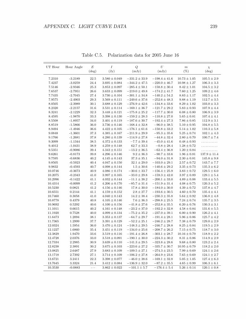
APPENDIX C. LIGHT CURVE DATA 239
Table C.5. Polarization data for 2005 June 16
UT Hour Hour Angle E I Q U m χ
(deg) (Jy) (mJy) (mJy) (%) (deg)
7.2310 -3.2189 22.5 3.580 ± 0.049 −331.2 ± 33.9 −198.4 ± 41.6 10.73 ± 1.05 105.5 ± 2.9
7.4237 -3.0259 24.4 3.695 ± 0.084 −344.2 ± 47.5 −220.0 ± 46.7 10.98 ± 1.27 106.3 ± 3.3
7.5146 -2.9346 25.3 3.853 ± 0.097 −285.4 ± 50.1 −158.8 ± 30.4 8.42 ± 1.01 104.5 ± 3.2
7.6537 -2.7951 26.6 3.633 ± 0.099 −219.0 ± 49.8 −174.2 ± 41.7 7.60 ± 1.25 109.2 ± 4.6
7.7435 -2.7045 27.4 3.730 ± 0.104 −301.1 ± 34.8 −140.2 ± 54.2 8.83 ± 1.17 102.5 ± 4.4
7.9575 -2.4903 29.3 3.569 ± 0.111 −249.6 ± 37.6 −252.6 ± 48.3 9.88 ± 1.19 112.7 ± 3.5
8.0505 -2.3989 30.1 3.688 ± 0.129 −276.9 ± 42.6 −134.8 ± 33.6 8.29 ± 1.02 103.0 ± 3.3
8.2320 -2.2157 31.6 3.531 ± 0.114 −169.1 ± 36.7 −121.7 ± 29.2 5.83 ± 0.93 107.9 ± 4.4
8.3241 -2.1229 32.3 3.448 ± 0.121 −175.8 ± 25.2 −117.7 ± 30.0 6.08 ± 0.80 106.9 ± 3.9
8.4595 -1.9870 33.3 3.398 ± 0.130 −159.2 ± 28.3 −110.8 ± 27.0 5.65 ± 0.81 107.4 ± 4.1
8.5508 -1.8957 34.0 3.401 ± 0.119 −187.6 ± 30.7 −192.4 ± 27.3 7.86 ± 0.85 112.9 ± 3.1
8.8519 -1.5866 36.0 3.736 ± 0.146 −168.4 ± 32.8 −96.0 ± 38.5 5.10 ± 0.95 104.8 ± 5.5
8.9494 -1.4946 36.6 4.422 ± 0.105 −176.1 ± 61.6 −150.8 ± 33.2 5.14 ± 1.02 110.3 ± 5.8
9.0848 -1.3601 37.3 4.385 ± 0.167 −211.9 ± 29.9 −95.3 ± 35.6 5.25 ± 0.74 102.1 ± 4.3
9.1766 -1.2681 37.8 4.280 ± 0.139 −114.9 ± 27.8 −44.8 ± 32.4 2.80 ± 0.70 100.7 ± 7.4
9.3099 -1.1344 38.5 4.372 ± 0.133 −7.7 ± 39.4 −45.0 ± 41.6 0.48 ± 0.93 . . . . . . . . . . .
9.4012 -1.0431 38.9 4.259 ± 0.148 62.7 ± 33.3 −0.8 ± 28.4 1.28 ± 0.72 . . . . . . . . . . .
9.5351 -0.9086 39.4 4.343 ± 0.151 −13.2 ± 36.5 −62.4 ± 36.8 1.20 ± 0.84 . . . . . . . . . . .
9.6261 -0.8173 39.8 4.296 ± 0.146 9.2 ± 36.3 −90.7 ± 33.6 1.96 ± 0.81 137.9 ± 11.4
9.7595 -0.6836 40.2 4.145 ± 0.143 37.3 ± 35.1 −94.0 ± 31.8 2.30 ± 0.81 145.8 ± 9.8
9.8505 -0.5923 40.4 4.047 ± 0.150 32.1 ± 29.0 −103.0 ± 29.1 2.57 ± 0.72 143.7 ± 7.7
9.9832 -0.4593 40.7 4.098 ± 0.144 1.5 ± 30.6 −140.6 ± 29.2 3.35 ± 0.73 135.3 ± 6.2
10.0746 -0.3673 40.9 4.086 ± 0.174 −30.6 ± 33.7 −156.4 ± 25.9 3.83 ± 0.72 129.5 ± 6.0
10.2075 -0.2343 41.0 3.997 ± 0.165 −33.0 ± 29.8 −159.3 ± 42.0 3.97 ± 0.89 129.1 ± 5.4
10.2996 -0.1422 41.1 4.032 ± 0.144 −11.1 ± 38.2 −200.1 ± 33.0 4.89 ± 0.88 133.4 ± 5.5
10.4314 -0.0099 41.2 4.206 ± 0.170 −85.7 ± 31.4 −151.9 ± 31.4 4.08 ± 0.75 120.3 ± 5.2
10.5230 0.0821 41.2 4.156 ± 0.146 17.8 ± 30.0 −184.0 ± 30.0 4.39 ± 0.72 137.8 ± 4.7
10.6551 0.2144 41.1 4.159 ± 0.152 2.8 ± 27.7 −193.6 ± 30.5 4.60 ± 0.70 135.4 ± 4.1
10.7460 0.3058 41.0 4.040 ± 0.143 14.2 ± 38.4 −230.3 ± 35.8 5.64 ± 0.92 136.8 ± 4.8
10.8778 0.4379 40.8 4.105 ± 0.146 7.6 ± 36.3 −298.8 ± 25.5 7.24 ± 0.74 135.7 ± 3.5
10.9692 0.5292 40.6 4.100 ± 0.156 −41.8 ± 27.6 −252.8 ± 35.5 6.20 ± 0.76 130.3 ± 3.1
11.1011 0.6615 40.2 4.161 ± 0.148 −23.2 ± 37.0 −192.2 ± 32.8 4.58 ± 0.84 131.6 ± 5.5
11.1920 0.7528 40.0 4.099 ± 0.134 −75.2 ± 35.2 −237.0 ± 39.1 6.00 ± 0.90 126.2 ± 4.1
11.6473 1.2094 38.1 3.353 ± 0.137 −64.7 ± 29.7 −191.4 ± 28.1 5.96 ± 0.86 125.7 ± 4.2
11.7365 1.2999 37.7 3.391 ± 0.129 −52.2 ± 25.1 −246.2 ± 28.7 7.38 ± 0.79 129.0 ± 2.9
12.0324 1.5954 36.0 3.470 ± 0.124 −148.3 ± 29.5 −246.7 ± 28.8 8.25 ± 0.84 119.5 ± 2.9
12.1227 1.6860 35.4 3.451 ± 0.119 −134.0 ± 25.6 −208.7 ± 26.2 7.15 ± 0.75 118.7 ± 3.0
12.3829 1.9470 33.6 3.519 ± 0.116 −191.4 ± 26.8 −303.1 ± 28.7 10.16 ± 0.79 118.9 ± 2.2
12.4728 2.0376 33.0 3.518 ± 0.091 −190.1 ± 30.0 −224.3 ± 30.2 8.31 ± 0.86 114.9 ± 2.9
12.7334 2.2985 30.9 3.639 ± 0.110 −141.3 ± 29.5 −323.8 ± 28.6 9.68 ± 0.80 123.2 ± 2.4
12.8238 2.3891 30.2 3.675 ± 0.103 −223.6 ± 27.2 −335.7 ± 30.7 10.95 ± 0.79 118.2 ± 2.0
13.0825 2.6487 27.9 3.683 ± 0.109 −109.5 ± 27.1 −274.3 ± 23.5 7.99 ± 0.69 124.1 ± 2.6
13.1718 2.7392 27.1 3.714 ± 0.109 −106.2 ± 27.8 −264.9 ± 23.6 7.65 ± 0.69 124.1 ± 2.7
13.6721 3.2411 22.3 3.398 ± 0.077 −46.0 ± 38.6 −169.1 ± 32.8 5.05 ± 1.05 127.4 ± 6.3
13.7645 3.3324 21.4 3.412 ± 0.084 −136.9 ± 32.0 −87.2 ± 35.5 4.65 ± 0.99 106.3 ± 6.1
10.3530 -0.0883 · · · 3.862 ± 0.022 −101.1 ± 5.7 −176.4 ± 5.4 5.26 ± 0.14 120.1 ± 0.8

APPENDIX C. LIGHT CURVE DATA 240
Table C.6. Polarization data for 2005 June 17
UT Hour Hour Angle E I Q U m χ
(deg) (Jy) (mJy) (mJy) (%) (deg)
6.9988 -3.3754 20.9 2.560 ± 0.103 248.8 ± 82.8 −133.9 ± 84.5 10.54 ± 3.27 165.9 ± 8.5
7.1550 -3.2186 22.5 2.653 ± 0.087 223.5 ± 67.2 −144.4 ± 84.1 9.62 ± 2.83 163.6 ± 8.6
7.7162 -2.6557 27.9 2.517 ± 0.062 118.3 ± 59.5 −252.7 ± 64.4 10.81 ± 2.46 147.5 ± 6.2
7.8728 -2.4989 29.2 2.579 ± 0.063 223.3 ± 53.0 −354.9 ± 60.3 16.11 ± 2.19 151.1 ± 3.8
8.2347 -2.1359 32.2 2.730 ± 0.066 223.2 ± 56.2 −524.8 ± 58.9 20.78 ± 2.11 146.5 ± 2.8
8.3911 -1.9792 33.4 2.666 ± 0.057 89.8 ± 55.0 −355.4 ± 54.6 13.60 ± 2.06 142.1 ± 4.3
8.5472 -1.8225 34.5 2.713 ± 0.084 97.4 ± 54.7 −446.4 ± 44.5 16.74 ± 1.82 141.2 ± 3.4
8.7036 -1.6658 35.5 2.562 ± 0.086 95.0 ± 64.5 −388.8 ± 71.8 15.39 ± 2.65 141.9 ± 4.6
8.8922 -1.4767 36.7 2.913 ± 0.080 54.0 ± 54.1 −352.7 ± 65.3 12.08 ± 2.04 139.3 ± 4.4
9.0504 -1.3192 37.6 3.128 ± 0.073 175.4 ± 56.4 −234.4 ± 48.1 9.21 ± 1.67 153.4 ± 5.2
9.2063 -1.1618 38.4 2.911 ± 0.091 177.5 ± 47.2 −233.2 ± 44.3 9.95 ± 1.57 153.6 ± 4.5
9.3633 -1.0043 39.0 3.284 ± 0.078 106.3 ± 50.1 −178.1 ± 54.2 6.11 ± 1.59 150.4 ± 7.1
9.5204 -0.8469 39.7 3.198 ± 0.070 223.2 ± 48.9 −209.7 ± 42.5 9.47 ± 1.43 158.4 ± 4.3
9.6779 -0.6887 40.2 3.067 ± 0.086 233.9 ± 52.5 −215.3 ± 50.8 10.23 ± 1.69 158.7 ± 4.7
9.8350 -0.5313 40.6 3.228 ± 0.068 267.1 ± 39.4 −255.1 ± 51.6 11.36 ± 1.40 158.2 ± 3.6
9.9920 -0.3738 40.9 3.293 ± 0.089 160.8 ± 40.2 −298.6 ± 39.3 10.23 ± 1.21 149.2 ± 3.4
10.1489 -0.2164 41.1 3.314 ± 0.066 108.4 ± 52.8 −295.6 ± 57.6 9.36 ± 1.66 145.1 ± 4.9
10.3061 -0.0589 41.2 3.402 ± 0.065 89.3 ± 44.5 −305.6 ± 49.3 9.26 ± 1.38 143.1 ± 4.0
10.4631 0.0985 41.1 3.377 ± 0.060 110.1 ± 53.2 −286.0 ± 55.9 8.93 ± 1.61 145.5 ± 5.0
10.6201 0.2560 41.0 3.478 ± 0.064 82.3 ± 52.8 −251.8 ± 36.5 7.51 ± 1.26 144.0 ± 5.6
10.7771 0.4134 40.8 3.488 ± 0.074 82.0 ± 42.0 −310.1 ± 44.7 9.11 ± 1.24 142.4 ± 3.8
11.0510 0.6881 40.2 3.159 ± 0.065 −2.3 ± 43.6 −250.1 ± 44.7 7.79 ± 1.40 134.7 ± 5.0
11.2080 0.8455 39.7 3.236 ± 0.091 148.6 ± 46.3 −182.4 ± 40.6 7.15 ± 1.34 154.6 ± 5.4
11.4899 1.1259 38.5 3.111 ± 0.083 158.9 ± 50.3 −193.1 ± 52.8 7.86 ± 1.66 154.7 ± 5.9
11.6439 1.2826 37.8 3.208 ± 0.072 18.6 ± 52.1 −310.2 ± 44.9 9.57 ± 1.51 136.7 ± 4.8
12.0139 1.6536 35.6 3.034 ± 0.066 −49.5 ± 41.9 −171.0 ± 42.0 5.70 ± 1.38 126.9 ± 6.7
12.2032 1.8434 34.4 2.864 ± 0.065 −13.7 ± 54.9 −205.8 ± 40.8 7.01 ± 1.65 133.1 ± 7.6
12.4993 2.1403 32.2 2.638 ± 0.050 124.8 ± 43.9 −56.8 ± 46.8 4.91 ± 1.72 167.7 ± 9.7
12.6556 2.2970 30.9 2.788 ± 0.048 −38.0 ± 50.3 −100.1 ± 41.5 3.47 ± 1.64 124.6 ± 13.2
13.1123 2.7550 27.0 2.954 ± 0.095 265.3 ± 58.1 −179.4 ± 61.2 10.65 ± 2.02 163.0 ± 5.4
13.2679 2.9110 25.5 3.012 ± 0.073 183.8 ± 59.9 −221.1 ± 65.8 9.32 ± 2.08 154.9 ± 6.2
13.5382 3.1822 22.9 2.448 ± 0.077 155.5 ± 60.7 −264.0 ± 58.6 12.28 ± 2.44 150.2 ± 5.6
13.6940 3.3381 21.3 2.343 ± 0.082 118.2 ± 59.7 −182.1 ± 59.9 8.91 ± 2.55 151.5 ± 7.9
10.3540 -0.0110 · · · 2.986 ± 0.015 128.6 ± 9.3 −251.9 ± 9.5 9.47 ± 0.32 148.5 ± 0.9

APPENDIX C. LIGHT CURVE DATA 241
Table C.7. Polarization data for 2005 July 20
UT Hour Hour Angle E I Q U m χ
(deg) (Jy) (mJy) (mJy) (%) (deg)
6.1872 -2.0318 33.0 3.751 ± 0.058 −32.9 ± 31.0 −214.8 ± 34.3 5.73 ± 0.87 130.6 ± 4.1
6.3336 -1.8851 34.1 3.748 ± 0.079 −81.6 ± 26.1 −215.9 ± 24.7 6.12 ± 0.68 124.6 ± 3.2
6.4237 -1.7944 34.7 3.688 ± 0.055 −91.7 ± 29.4 −249.1 ± 24.6 7.16 ± 0.73 124.9 ± 3.1
6.5135 -1.7039 35.3 3.788 ± 0.073 −121.9 ± 25.4 −138.1 ± 25.0 4.82 ± 0.67 114.3 ± 3.9
6.7917 -1.4257 37.0 3.726 ± 0.069 −151.6 ± 29.0 −165.3 ± 21.2 5.98 ± 0.67 113.7 ± 3.3
6.9659 -1.2510 37.9 3.639 ± 0.053 −4.5 ± 21.5 −127.2 ± 23.8 3.44 ± 0.62 134.0 ± 4.8
7.4342 -0.7808 39.9 3.849 ± 0.055 −8.4 ± 24.3 −111.7 ± 22.3 2.85 ± 0.60 132.9 ± 6.2
7.5807 -0.6341 40.3 4.031 ± 0.049 −59.6 ± 22.0 −113.5 ± 18.2 3.14 ± 0.50 121.2 ± 4.7
7.7141 -0.5004 40.6 3.959 ± 0.045 −37.1 ± 19.1 −67.6 ± 18.3 1.89 ± 0.47 120.6 ± 7.0
7.8051 -0.4091 40.8 3.979 ± 0.060 27.8 ± 23.1 −110.1 ± 25.1 2.79 ± 0.60 142.1 ± 5.9
7.9378 -0.2761 41.0 4.092 ± 0.042 47.4 ± 21.7 −180.8 ± 21.6 4.54 ± 0.53 142.3 ± 3.3
8.0690 -0.1445 41.1 4.040 ± 0.053 45.9 ± 24.0 −208.7 ± 27.6 5.25 ± 0.64 141.2 ± 3.2
8.2015 -0.0116 41.2 4.079 ± 0.055 −13.8 ± 21.8 −220.9 ± 14.9 5.41 ± 0.44 133.2 ± 2.8
8.3335 0.1207 41.1 4.160 ± 0.049 11.8 ± 21.0 −158.1 ± 22.4 3.78 ± 0.52 137.1 ± 3.8
8.4647 0.2524 41.0 4.046 ± 0.044 −77.3 ± 19.8 −182.2 ± 20.2 4.87 ± 0.49 123.5 ± 2.9
8.5963 0.3838 40.9 3.924 ± 0.044 −50.8 ± 22.8 −172.2 ± 18.6 4.54 ± 0.53 126.8 ± 3.6
8.7264 0.5147 40.6 3.904 ± 0.071 −20.5 ± 21.4 −184.9 ± 20.1 4.74 ± 0.53 131.8 ± 3.3
8.8575 0.6456 40.3 3.997 ± 0.065 −1.1 ± 21.6 −183.9 ± 19.4 4.57 ± 0.51 134.8 ± 3.4
9.1133 0.9029 39.4 4.143 ± 0.050 43.8 ± 17.8 −181.5 ± 22.3 4.48 ± 0.48 141.8 ± 2.8
9.2045 0.9942 39.1 3.984 ± 0.061 29.7 ± 20.1 −149.7 ± 20.6 3.80 ± 0.51 140.6 ± 3.8
9.4670 1.2574 37.9 4.042 ± 0.059 48.2 ± 19.7 −171.5 ± 20.5 4.38 ± 0.50 142.8 ± 3.2
9.5580 1.3487 37.4 3.966 ± 0.066 24.8 ± 20.1 −184.2 ± 16.3 4.66 ± 0.46 138.8 ± 3.1
9.9633 1.7549 35.0 3.396 ± 0.088 −31.2 ± 19.7 −123.9 ± 24.6 3.71 ± 0.65 127.9 ± 4.5
10.0527 1.8447 34.3 3.586 ± 0.065 11.2 ± 19.0 −124.5 ± 23.8 3.44 ± 0.59 137.6 ± 4.4
10.3165 2.1093 32.4 3.437 ± 0.068 87.1 ± 20.9 −193.7 ± 19.8 6.15 ± 0.59 147.1 ± 2.8
10.4076 2.1999 31.7 3.365 ± 0.070 88.2 ± 23.1 −167.4 ± 24.6 5.58 ± 0.71 148.9 ± 3.5
10.6665 2.4602 29.6 3.436 ± 0.054 27.1 ± 25.0 −155.6 ± 20.9 4.55 ± 0.67 139.9 ± 4.5
10.7813 2.5752 28.6 3.417 ± 0.072 17.7 ± 26.0 −201.5 ± 18.1 5.89 ± 0.63 137.5 ± 3.7
11.0408 2.8354 26.2 3.298 ± 0.088 32.3 ± 22.4 −204.6 ± 34.0 6.22 ± 0.84 139.5 ± 3.1
11.1312 2.9267 25.4 3.533 ± 0.067 15.3 ± 33.2 −186.9 ± 34.8 5.22 ± 0.96 137.3 ± 5.1
11.3848 3.1805 22.9 3.450 ± 0.082 38.4 ± 36.6 −244.4 ± 27.8 7.11 ± 0.93 139.5 ± 4.2
11.4763 3.2719 22.0 3.434 ± 0.071 −16.0 ± 24.7 −295.1 ± 37.8 8.56 ± 0.89 133.4 ± 2.4
8.7951 0.5836 · · · 3.787 ± 0.013 −5.1 ± 4.3 −172.8 ± 4.3 4.57 ± 0.11 134.2 ± 0.7

APPENDIX C. LIGHT CURVE DATA 242
Table C.8. Polarization data for 2005 July 21
UT Hour Hour Angle E I Q U m χ
(deg) (Jy) (mJy) (mJy) (%) (deg)
5.4617 -2.6835 27.6 3.620 ± 0.119 170.4 ± 71.5 −115.9 ± 86.2 5.26 ± 2.17 162.9 ± 11.4
5.6170 -2.5268 29.0 3.600 ± 0.145 27.4 ± 71.0 −177.9 ± 56.4 4.68 ± 1.76 139.4 ± 11.3
5.9944 -2.1626 32.0 3.720 ± 0.097 142.7 ± 63.8 −78.3 ± 62.0 4.04 ± 1.69 165.6 ± 11.0
6.1613 -1.9811 33.4 3.520 ± 0.087 308.1 ± 64.1 −52.1 ± 54.4 8.72 ± 1.68 175.2 ± 5.0
6.7765 -1.3642 37.3 3.729 ± 0.108 231.0 ± 46.3 −309.5 ± 57.2 10.26 ± 1.38 153.4 ± 3.7
6.9326 -1.2075 38.1 3.565 ± 0.083 78.7 ± 62.0 −247.2 ± 51.8 7.10 ± 1.59 143.8 ± 6.8
7.0889 -1.0508 38.9 3.345 ± 0.092 207.3 ± 54.5 −193.5 ± 52.1 8.33 ± 1.59 158.5 ± 5.4
7.2459 -0.8933 39.5 3.372 ± 0.077 32.0 ± 54.5 −236.5 ± 49.1 6.91 ± 1.53 138.9 ± 6.5
7.4026 -0.7359 40.0 3.346 ± 0.084 154.9 ± 46.4 −137.3 ± 47.7 6.03 ± 1.41 159.2 ± 6.5
7.5599 -0.5785 40.5 3.671 ± 0.092 217.4 ± 49.3 −61.9 ± 56.4 5.99 ± 1.44 172.1 ± 7.1
7.7167 -0.4210 40.8 3.649 ± 0.095 237.4 ± 46.8 −113.8 ± 45.7 7.10 ± 1.27 167.2 ± 5.0
7.8742 -0.2636 41.0 3.518 ± 0.078 328.0 ± 46.6 11.4 ± 42.5 9.24 ± 1.27 1.0 ± 3.7
8.0308 -0.1061 41.1 3.743 ± 0.094 388.1 ± 54.6 −165.6 ± 52.5 11.18 ± 1.43 168.4 ± 3.6
8.1873 0.0513 41.2 3.678 ± 0.085 385.4 ± 61.8 −185.9 ± 59.1 11.52 ± 1.64 167.1 ± 4.0
8.3453 0.2088 41.1 3.741 ± 0.100 395.3 ± 54.6 −226.5 ± 57.1 12.09 ± 1.49 165.1 ± 3.6
8.5026 0.3662 40.9 4.077 ± 0.102 296.7 ± 55.3 −337.2 ± 44.3 10.95 ± 1.21 155.7 ± 3.2
8.6601 0.5244 40.6 4.021 ± 0.078 312.7 ± 55.2 −291.2 ± 44.4 10.55 ± 1.23 158.5 ± 3.3
8.8172 0.6826 40.2 4.103 ± 0.079 253.5 ± 48.2 −302.9 ± 66.2 9.53 ± 1.38 155.0 ± 4.1
8.9744 0.8400 39.7 4.238 ± 0.092 344.3 ± 58.3 −383.8 ± 54.9 12.09 ± 1.33 155.9 ± 3.2
9.2289 1.0959 38.7 4.150 ± 0.088 282.6 ± 55.0 −286.4 ± 49.3 9.62 ± 1.25 157.3 ± 3.7
9.3860 1.2527 37.9 4.033 ± 0.075 184.8 ± 58.4 −321.1 ± 57.4 9.07 ± 1.44 150.0 ± 4.5
9.7087 1.5740 36.1 4.286 ± 0.094 211.8 ± 45.3 −377.1 ± 59.4 10.02 ± 1.21 149.7 ± 3.2
9.8622 1.7308 35.1 4.075 ± 0.083 190.3 ± 58.0 −294.4 ± 60.8 8.48 ± 1.46 151.4 ± 4.8
10.1931 2.0615 32.8 4.383 ± 0.130 162.0 ± 62.2 −324.5 ± 53.4 8.17 ± 1.32 148.3 ± 4.8
10.3487 2.2182 31.6 4.202 ± 0.100 258.5 ± 53.7 −183.3 ± 57.6 7.42 ± 1.32 162.3 ± 5.1
7.9359 -0.2025 · · · 3.803 ± 0.021 232.3 ± 11.6 −211.6 ± 11.6 8.26 ± 0.30 158.8 ± 1.1

APPENDIX C. LIGHT CURVE DATA 243
Table C.9. Polarization data for 2005 July 22
UT Hour Hour Angle E I Q U m χ
(deg) (Jy) (mJy) (mJy) (%) (deg)
6.1440 -1.9431 33.6 2.948 ± 0.080 −161.0 ± 25.2 −109.1 ± 21.5 6.55 ± 0.79 107.1 ± 3.3
6.2352 -1.8518 34.3 3.139 ± 0.064 −209.4 ± 24.3 −144.2 ± 24.2 8.06 ± 0.77 107.3 ± 2.7
6.3678 -1.7188 35.2 3.084 ± 0.062 −148.6 ± 19.4 −93.3 ± 20.2 5.65 ± 0.64 106.1 ± 3.3
6.4596 -1.6275 35.8 3.146 ± 0.050 −162.6 ± 19.6 −114.1 ± 20.9 6.28 ± 0.64 107.5 ± 3.0
6.8504 -1.2349 38.0 3.176 ± 0.055 −196.2 ± 16.6 −185.3 ± 20.8 8.48 ± 0.58 111.7 ± 2.0
6.9413 -1.1437 38.4 3.051 ± 0.054 −181.3 ± 18.7 −149.7 ± 21.1 7.68 ± 0.65 109.8 ± 2.5
7.0749 -1.0099 39.0 3.085 ± 0.037 −158.6 ± 17.5 −126.9 ± 17.9 6.56 ± 0.57 109.3 ± 2.5
7.1663 -0.9186 39.4 3.072 ± 0.046 −127.6 ± 20.9 −139.1 ± 17.4 6.11 ± 0.62 113.7 ± 2.9
7.5210 -0.5628 40.5 3.174 ± 0.063 −53.0 ± 19.2 −102.7 ± 19.3 3.59 ± 0.61 121.3 ± 4.8
7.6122 -0.4715 40.7 3.087 ± 0.081 −102.2 ± 26.7 −190.6 ± 22.2 6.96 ± 0.79 120.9 ± 3.4
7.7487 -0.3377 40.9 3.340 ± 0.061 −119.8 ± 20.5 −283.3 ± 19.8 9.19 ± 0.60 123.5 ± 1.9
7.8361 -0.2464 41.0 3.316 ± 0.054 −178.0 ± 25.6 −256.0 ± 19.0 9.38 ± 0.67 117.6 ± 2.2
7.9687 -0.1133 41.1 3.348 ± 0.074 −166.9 ± 19.3 −252.7 ± 19.7 9.02 ± 0.58 118.3 ± 1.8
8.0612 -0.0214 41.2 3.197 ± 0.071 −157.4 ± 20.3 −231.1 ± 16.7 8.73 ± 0.57 117.9 ± 2.0
8.1921 0.1102 41.1 3.462 ± 0.056 −174.8 ± 19.4 −224.0 ± 18.0 8.19 ± 0.54 116.0 ± 1.9
8.2837 0.2022 41.1 3.424 ± 0.062 −159.4 ± 19.3 −198.9 ± 16.0 7.43 ± 0.51 115.7 ± 2.0
8.4875 0.4064 40.8 3.648 ± 0.044 −25.6 ± 18.7 −183.8 ± 18.5 5.06 ± 0.51 131.0 ± 2.9
8.8422 0.7623 39.9 3.576 ± 0.061 −22.1 ± 19.9 −177.8 ± 20.3 4.98 ± 0.56 131.5 ± 3.2
8.9330 0.8537 39.6 3.578 ± 0.064 −40.3 ± 17.2 −143.4 ± 23.2 4.13 ± 0.56 127.1 ± 3.4
9.0647 0.9859 39.1 3.497 ± 0.074 −39.6 ± 20.1 −149.4 ± 19.2 4.38 ± 0.56 127.6 ± 3.7
9.3536 1.2749 37.8 3.011 ± 0.102 −21.0 ± 19.3 −77.8 ± 22.6 2.58 ± 0.69 127.4 ± 6.9
9.4441 1.3655 37.3 3.274 ± 0.075 −20.9 ± 21.5 −90.5 ± 16.6 2.78 ± 0.58 128.5 ± 6.6
9.8165 1.7394 35.1 3.417 ± 0.063 64.5 ± 20.3 −74.7 ± 17.5 2.83 ± 0.55 155.4 ± 5.6
9.9068 1.8299 34.4 3.303 ± 0.068 24.1 ± 20.9 −98.3 ± 20.5 3.00 ± 0.63 141.9 ± 5.9
10.3626 2.2872 31.0 3.524 ± 0.048 −124.9 ± 21.7 −21.1 ± 21.7 3.54 ± 0.62 94.8 ± 4.9
10.4536 2.3785 30.3 3.285 ± 0.108 −134.8 ± 22.3 −69.7 ± 20.2 4.57 ± 0.65 103.7 ± 3.9
10.6928 2.6179 28.2 3.554 ± 0.080 −61.5 ± 23.3 −51.2 ± 20.7 2.16 ± 0.62 109.9 ± 7.8
10.7829 2.7085 27.4 3.602 ± 0.079 −93.6 ± 19.8 −68.5 ± 26.5 3.15 ± 0.64 108.1 ± 6.0
10.9912 2.9170 25.5 3.742 ± 0.087 −66.8 ± 25.2 32.4 ± 22.7 1.88 ± 0.64 77.1 ± 8.9
11.0816 3.0076 24.6 3.742 ± 0.086 −31.9 ± 25.2 56.7 ± 24.3 1.61 ± 0.66 59.7 ± 11.0
11.2643 3.1909 22.8 3.823 ± 0.079 −96.7 ± 24.2 74.2 ± 31.0 3.11 ± 0.72 71.2 ± 6.7
11.3545 3.2815 21.9 3.623 ± 0.097 −47.7 ± 22.8 122.2 ± 29.8 3.55 ± 0.72 55.7 ± 5.2
11.5393 3.4670 20.0 3.547 ± 0.094 −70.9 ± 32.3 90.9 ± 25.5 3.15 ± 0.81 64.0 ± 7.4
8.7392 0.6589 · · · 3.356 ± 0.013 −98.1 ± 4.1 −115.0 ± 4.3 4.50 ± 0.12 114.8 ± 0.8

APPENDIX C. LIGHT CURVE DATA 244
Table C.10. Polarization data for 2005 July 30
UT Hour Hour Angle E I Q U m χ
(deg) (Jy) (mJy) (mJy) (%) (deg)
4.2189 -3.3486 21.2 4.214 ± 0.108 −302.1 ± 26.1 69.1 ± 42.9 7.31 ± 0.79 83.6 ± 3.9
4.3257 -3.2417 22.3 4.411 ± 0.093 −320.6 ± 26.8 116.5 ± 24.2 7.71 ± 0.58 80.0 ± 2.1
4.6204 -2.9562 25.1 3.811 ± 0.148 −266.8 ± 26.0 112.1 ± 34.5 7.55 ± 0.79 78.6 ± 3.3
4.8050 -2.7598 26.9 3.880 ± 0.195 −260.3 ± 31.5 48.3 ± 25.6 6.79 ± 0.73 84.7 ± 2.8
4.9072 -2.6584 27.8 3.943 ± 0.273 −206.3 ± 33.1 19.5 ± 36.3 5.18 ± 0.88 87.3 ± 5.0
5.1398 -2.4244 29.9 4.610 ± 0.199 −386.9 ± 26.8 30.3 ± 28.1 8.40 ± 0.59 87.8 ± 2.1
5.2374 -2.3323 30.6 4.355 ± 0.155 −350.4 ± 26.3 −74.3 ± 29.6 8.20 ± 0.64 96.0 ± 2.4
5.3263 -2.2528 31.3 3.568 ± 0.231 −237.2 ± 39.4 62.4 ± 33.0 6.80 ± 1.01 82.6 ± 3.9
6.9221 -0.6372 40.3 3.811 ± 0.147 −215.6 ± 21.3 106.3 ± 21.2 6.28 ± 0.56 76.9 ± 2.5
7.0548 -0.5042 40.6 4.231 ± 0.131 −309.6 ± 21.4 117.5 ± 20.9 7.81 ± 0.50 79.6 ± 1.8
7.1870 -0.3719 40.9 4.239 ± 0.061 −303.0 ± 17.0 111.6 ± 16.8 7.61 ± 0.40 79.9 ± 1.5
7.8083 0.2514 41.0 4.392 ± 0.064 −92.7 ± 18.6 111.3 ± 20.3 3.27 ± 0.44 64.9 ± 3.8
7.9387 0.3823 40.9 4.289 ± 0.066 −75.0 ± 21.0 138.1 ± 16.4 3.64 ± 0.43 59.2 ± 3.6
8.0709 0.5147 40.6 4.258 ± 0.067 −36.3 ± 21.4 106.6 ± 19.0 2.60 ± 0.47 54.4 ± 5.4
8.2387 0.6828 40.2 4.019 ± 0.086 −25.8 ± 20.5 73.3 ± 18.6 1.87 ± 0.49 54.7 ± 7.5
8.4929 0.9380 39.3 3.800 ± 0.092 −137.7 ± 21.8 69.9 ± 17.0 4.03 ± 0.51 76.5 ± 3.4
8.5848 1.0293 38.9 3.954 ± 0.083 −115.7 ± 21.6 119.0 ± 20.8 4.16 ± 0.54 67.1 ± 3.7
8.8674 1.3133 37.6 4.434 ± 0.047 −223.5 ± 20.5 37.2 ± 20.8 5.09 ± 0.47 85.3 ± 2.6
8.9577 1.4039 37.1 4.324 ± 0.058 −246.4 ± 21.1 −27.8 ± 17.5 5.72 ± 0.45 93.2 ± 2.0
9.1699 1.6167 35.8 4.377 ± 0.081 −290.2 ± 20.3 −24.5 ± 20.1 6.64 ± 0.46 92.4 ± 2.0
9.2609 1.7080 35.3 4.239 ± 0.086 −275.7 ± 22.6 −48.3 ± 19.7 6.58 ± 0.50 95.0 ± 2.0
9.3894 1.8367 34.4 4.154 ± 0.090 −203.1 ± 17.1 −57.5 ± 20.7 5.06 ± 0.45 97.9 ± 2.8
9.4800 1.9273 33.8 3.700 ± 0.111 −198.6 ± 20.5 −50.9 ± 18.0 5.52 ± 0.52 97.2 ± 2.5
9.9712 2.4198 29.9 3.898 ± 0.106 −119.6 ± 25.9 −66.2 ± 20.5 3.46 ± 0.59 104.5 ± 4.6
10.0616 2.5110 29.1 4.285 ± 0.077 −186.0 ± 19.0 −63.5 ± 23.0 4.56 ± 0.49 99.4 ± 3.3
10.1808 2.6304 28.1 4.622 ± 0.085 −191.0 ± 22.9 −6.8 ± 21.6 4.11 ± 0.48 91.0 ± 3.2
10.2709 2.7210 27.3 4.878 ± 0.077 −157.1 ± 22.9 41.6 ± 22.3 3.30 ± 0.46 82.6 ± 3.9
10.4748 2.9251 25.4 4.798 ± 0.118 −209.0 ± 26.5 86.6 ± 20.8 4.69 ± 0.49 78.8 ± 2.7
10.5651 3.0157 24.5 4.682 ± 0.155 −259.0 ± 30.6 87.0 ± 27.6 5.80 ± 0.62 80.7 ± 2.9
10.6848 3.1358 23.3 3.978 ± 0.134 −149.8 ± 30.2 28.7 ± 28.0 3.76 ± 0.73 84.6 ± 5.3
10.7754 3.2271 22.4 3.813 ± 0.111 −224.8 ± 39.6 2.2 ± 31.1 5.82 ± 0.92 89.7 ± 4.0
10.9744 3.4270 20.4 2.925 ± 0.207 −102.8 ± 37.8 47.9 ± 26.5 3.72 ± 1.08 77.5 ± 7.3
11.0661 3.5183 19.5 3.113 ± 0.224 −183.5 ± 35.3 −47.5 ± 36.6 5.98 ± 1.16 97.3 ± 5.5
8.1241 0.5670 · · · 4.140 ± 0.024 −208.1 ± 4.9 39.4 ± 4.5 5.12 ± 0.11 84.6 ± 0.6

APPENDIX C. LIGHT CURVE DATA 245
C.2 Q−U Light Curves
-600
-500
-400
-300
-200
-100
0
100
200
300
-400 -200 0 200 400 600
U�
(mJy)
Q�(mJy)
230�GHz 2005�Jun�4
Fig. C.1.— Polarization light curve for 2005 June 4, plotted in the Q−U plane. The
data are shown at full temporal resolution (one polarization switching cycle per point)
as in Figure 7.1 and Table C.1. The mean polarization for the track is marked with
a blue cross. The first and last points in the light curve are marked with green and
red points, respectively. The individual light curve points are shown with half-σ error
bars for clarity.

APPENDIX C. LIGHT CURVE DATA 246
-600
-500
-400
-300
-200
-100
0
100
200
300
-400 -200 0 200 400 600
U�
(mJy)
Q�(mJy)
345�GHz 2005�Jun�6
Fig. C.2.— Polarization light curve for 2005 June 6, plotted in the Q−U plane. The
data are shown at full temporal resolution (one polarization switching cycle per point)
as in Figure 7.2 and Table C.2. See caption of Figure C.1 for details.

APPENDIX C. LIGHT CURVE DATA 247
-600
-500
-400
-300
-200
-100
0
100
200
300
-400 -200 0 200 400 600
U�
(mJy)
Q�(mJy)
230�GHz 2005�Jun�9
Fig. C.3.— Polarization light curve for 2005 June 9, plotted in the Q−U plane. The
data are shown at full temporal resolution (one polarization switching cycle per point)
as in Figure 7.3 and Table C.3. See caption of Figure C.1 for details.

APPENDIX C. LIGHT CURVE DATA 248
-600
-500
-400
-300
-200
-100
0
100
200
300
-400 -200 0 200 400 600
U�
(mJy)
Q�(mJy)
345�GHz 2005�Jun�15
Fig. C.4.— Polarization light curve for 2005 June 15, plotted in the Q−U plane.
The data are shown at full temporal resolution (one polarization switching cycle per
point) as in Figure 7.4 and Table C.4. See caption of Figure C.1 for details.

APPENDIX C. LIGHT CURVE DATA 249
-600
-500
-400
-300
-200
-100
0
100
200
300
-400 -200 0 200 400 600
U�
(mJy)
Q�(mJy)
230�GHz 2005�Jun�16
Fig. C.5.— Polarization light curve for 2005 June 16, plotted in the Q−U plane.
The data are shown at full temporal resolution (one polarization switching cycle per
point) as in Figure 7.5 and Table C.5. See caption of Figure C.1 for details.

APPENDIX C. LIGHT CURVE DATA 250
-600
-500
-400
-300
-200
-100
0
100
200
300
-400 -200 0 200 400 600
U�
(mJy)
Q�(mJy)
345�GHz 2005�Jun�17
Fig. C.6.— Polarization light curve for 2005 June 17, plotted in the Q−U plane.
The data are shown at full temporal resolution (one polarization switching cycle per
point) as in Figure 7.6 and Table C.6. See caption of Figure C.1 for details.

APPENDIX C. LIGHT CURVE DATA 251
-600
-500
-400
-300
-200
-100
0
100
200
300
-400 -200 0 200 400 600
U�
(mJy)
Q�(mJy)
230�GHz 2005�Jul�20
Fig. C.7.— Polarization light curve for 2005 July 20, plotted in the Q−U plane.
The data are shown at full temporal resolution (one polarization switching cycle per
point) as in Figure 7.7 and Table C.7. See caption of Figure C.1 for details.

APPENDIX C. LIGHT CURVE DATA 252
-600
-500
-400
-300
-200
-100
0
100
200
300
-400 -200 0 200 400 600
U�
(mJy)
Q�(mJy)
345�GHz 2005�Jul�21
Fig. C.8.— Polarization light curve for 2005 July 21, plotted in the Q−U plane.
The data are shown at full temporal resolution (one polarization switching cycle per
point) as in Figure 7.8 and Table C.8. See caption of Figure C.1 for details.

APPENDIX C. LIGHT CURVE DATA 253
-600
-500
-400
-300
-200
-100
0
100
200
300
-400 -200 0 200 400 600
U�
(mJy)
Q�(mJy)
230�GHz 2005�Jul�22
Fig. C.9.— Polarization light curve for 2005 July 22, plotted in the Q−U plane.
The data are shown at full temporal resolution (one polarization switching cycle per
point) as in Figure 7.9 and Table C.9. See caption of Figure C.1 for details.

APPENDIX C. LIGHT CURVE DATA 254
-600
-500
-400
-300
-200
-100
0
100
200
300
-400 -200 0 200 400 600
U�
(mJy)
Q�(mJy)
230�GHz 2005�Jul�30
Fig. C.10.— Polarization light curve for 2005 July 30, plotted in the Q−U plane.
The data are shown at full temporal resolution (one polarization switching cycle per
point) as in Figure 7.10 and Table C.10. See caption of Figure C.1 for details.

References
Afsar, M. N. 1987, IEEE Transactions on Instrumentation Measurement, 36,
554
Agol, E. 2000, ApJ, 538, L121
Aitken, D. K., Greaves, J., Chrysostomou, A., Jenness, T., Holland, W.,
Hough, J. H., Pierce-Price, D., & Richer, J. 2000, ApJ, 534, L173
Alberdi, A., Lara, L., Marcaide, J. M., Elosegui, P., Shapiro, I. I., Cotton,
W. D., Diamond, P. J., Romney, J. D., & Preston, R. A. 1993, A&A, 277, L1
Aller, M. F., Aller, H. D., & Hughes, P. A. 2003, ApJ, 586, 33
An, T., Goss, W. M., Zhao, J.-H., Hong, X. Y., Roy, S., Rao, A. P., & Shen,
Z.-Q. 2005, ApJ, 634, L49
Aschenbach, B., Grosso, N., Porquet, D., & Predehl, P. 2004, A&A, 417, 71
Backer, D. C., Zensus, J. A., Kellermann, K. I., Reid, M., Moran, J. M., & Lo,
K. Y. 1993, Science, 262, 1414
Baganoff, F. K. et al. 2001, Nature, 413, 45
—. 2003, ApJ, 591, 891
Balick, B. & Brown, R. L. 1974, ApJ, 194, 265
Bardeen, J. M., Press, W. H., & Teukolsky, S. A. 1972, ApJ, 178, 347
Beckert, T. 2003, Astronomische Nachrichten Supplement, 324, 459
Beckert, T. & Falcke, H. 2002, A&A, 388, 1106
Belanger, G., Goldwurm, A., Melia, F., Ferrando, P., Grosso, N., Porquet, D.,
Warwick, R., & Yusef-Zadeh, F. 2005, ApJ, 635, 1095
255

REFERENCES 256
Belanger, G., Terrier, R., De Jager, O., Goldwurm, A., & Melia, F. 2006,
ArXiv Astrophysics e-prints
Birch, J. R. et al. 1994, IEEE Transactions on Microwave Theory Techniques,
42, 956
Blandford, R. D. & Begelman, M. C. 1999, MNRAS, 303, L1
Blundell, R. 2004, in 15th International Symposium on Space Terahertz
Technology, ed. G. Narayanan (Amherst: U Mass), 3, http://www.stt2004.org
Bondi, H. 1952, MNRAS, 112, 195
Born, M. & Wolf, E. 1999, Principles of optics : electromagnetic theory of
propagation, interference and diffraction of light (New York : Cambridge
University Press)
Bower, G., Wright, M. C. H., & Forster, J. R. 2002a, Polarization Stability
of the BIMA Array at 1.3mm, BIMA Memo 89, Berkeley-Illinois-Maryland
Association
Bower, G. C. & Backer, D. C. 1998, ApJ, 496, L97
Bower, G. C., Backer, D. C., Zhao, J.-H., Goss, M., & Falcke, H. 1999a, ApJ,
521, 582
Bower, G. C., Falcke, H., & Backer, D. C. 1999b, ApJ, 523, L29
Bower, G. C., Falcke, H., Herrnstein, R. M., Zhao, J.-H., Goss, W. M., &
Backer, D. C. 2004, Science, 304, 704
Bower, G. C., Falcke, H., & Mellon, R. R. 2002b, ApJ, 578, L103
Bower, G. C., Falcke, H., Sault, R. J., & Backer, D. C. 2002c, ApJ, 571, 843
Bower, G. C., Falcke, H., Wright, M. C., & Backer, D. C. 2005a, ApJ, 618, L29
Bower, G. C., Goss, W. M., Falcke, H., Backer, D. C., & Lithwick, Y. 2006,
ApJ, in press, astro-ph/0608004
Bower, G. C., Roberts, D. A., Yusef-Zadeh, F., Backer, D. C., Cotton, W. D.,
Goss, W. M., Lang, C. C., & Lithwick, Y. 2005b, ApJ, 633, 218
Bower, G. C., Wright, M. C. H., Backer, D. C., & Falcke, H. 1999c, ApJ, 527,
851

REFERENCES 257
Bower, G. C., Wright, M. C. H., Falcke, H., & Backer, D. C. 2001, ApJ, 555,
L103
—. 2003, ApJ, 588, 331
Broderick, A. E. & Loeb, A. 2006a, ApJ, 636, L109
—. 2006b, MNRAS, 367, 905
Broderick, A. E. & Loeb, A. 2006c, in From the Center of the Milky Way to
Nearby Low-Luminosity Galactic Nuclei, ed. R. Schodel et al. (Institute of
Physics), astro-ph/0607279
Brown, R. L. & Lo, K. Y. 1982, ApJ, 253, 108
Brunthaler, A., Bower, G. C., & Falcke, H. 2006, A&A, 451, 845
Brunthaler, A., Bower, G. C., Falcke, H., & Mellon, R. R. 2001, ApJ, 560,
L123
Coker, R. F. & Melia, F. 1997, ApJ, 488, L149
Cotera, A., Morris, M., Ghez, A. M., Becklin, E. E., Tanner, A. M., Werner,
M. W., & Stolovy, S. R. 1999, in ASP Conf. Ser. 186: The Central Parsecs of
the Galaxy, ed. H. Falcke, A. Cotera, W. J. Duschl, F. Melia, & M. J. Rieke,
240
Cuadra, J., Nayakshin, S., Springel, V., & Di Matteo, T. 2005, MNRAS, 360,
L55
Cuadra, J., Nayakshin, S., Springel, V., & di Matteo, T. 2006, MNRAS, 366,
358
Davidson, J. A., Werner, M. W., Wu, X., Lester, D. F., Harvey, P. M., Joy,
M., & Morris, M. 1992, ApJ, 387, 189
Davies, R. D., Walsh, D., & Booth, R. S. 1976, MNRAS, 177, 319
Dent, W. R. F., Matthews, H. E., Wade, R., & Duncan, W. D. 1993, ApJ, 410,
650
Doeleman, S. & Bower, G. 2004, Galactic Center Newsletter, 18, 6
Doeleman, S. S. et al. 2001, AJ, 121, 2610

REFERENCES 258
Dowell, C. D. et al. 2003, in Millimeter and Submillimeter Detectors for
Astronomy. Edited by T. G. Phillips & J. Zmuidzinas. Proc. SPIE, 4855, 73
Eckart, A., Baganoff, F. K., Schodel, R., Morris, M., Genzel, R., Bower, G. C.,
Marrone, D., Moran, J. M., Viehmann, T., Bautz, M. W., Brandt, W. N.,
Garmire, G. P., Ott, T., Trippe, S., Ricker, G. R., Straubmeier, C., Roberts,
D. A., Yusef-Zadeh, F., Zhao, J. H., & Rao, R. 2006a, A&A, 450, 535
Eckart, A. & Genzel, R. 1996, Nature, 383, 415
—. 1997, MNRAS, 284, 576
Eckart, A., Genzel, R., Ott, T., & Schodel, R. 2002, MNRAS, 331, 917
Eckart, A., Schodel, R., Meyer, L., Trippe, S., Ott, T., & Genzel, R. 2006b,
A&A, 455, 1
Eckart, A. et al. 2004, A&A, 427, 1
Eisenhauer, F. et al. 2005, ApJ, 628, 246
Falcke, H. 1999, in ASP Conf. Ser. 186: The Central Parsecs of the Galaxy, ed.
H. Falcke, A. Cotera, W. J. Duschl, F. Melia, & M. J. Rieke, 113
Falcke, H., Biermann, P. L., Duschl, W. J., & Mezger, P. G. 1993a, A&A, 270,
102
Falcke, H., Goss, W. M., Matsuo, H., Teuben, P., Zhao, J.-H., & Zylka, R.
1998, ApJ, 499, 731
Falcke, H., Mannheim, K., & Biermann, P. L. 1993b, A&A, 278, L1
Falcke, H. & Markoff, S. 2000, A&A, 362, 113
Falcke, H., Melia, F., & Agol, E. 2000, ApJ, 528, L13
Fan, X. et al. 2006, AJ, 132, 117
Ferrarese, L. & Merritt, D. 2000, ApJ, 539, L9
Gardner, F. F. & Whiteoak, J. B. 1966, ARA&A, 4, 245
Gebhardt, K. et al. 2000, ApJ, 539, L13
Genzel, R., Schodel, R., Ott, T., Eckart, A., Alexander, T., Lacombe, F.,
Rouan, D., & Aschenbach, B. 2003, Nature, 425, 934

REFERENCES 259
Genzel, R., Thatte, N., Krabbe, A., Kroker, H., & Tacconi-Garman, L. E.
1996, ApJ, 472, 153
Genzel, R. & Townes, C. H. 1987, ARA&A, 25, 377
Ghez, A. M., Becklin, E., Duchjne, G., Hornstein, S., Morris, M., Salim, S., &
Tanner, A. 2003, Astronomische Nachrichten Supplement, 324, 527
Ghez, A. M., Klein, B. L., Morris, M., & Becklin, E. E. 1998, ApJ, 509, 678
Ghez, A. M., Morris, M., Becklin, E. E., Tanner, A., & Kremenek, T. 2000,
Nature, 407, 349
Ghez, A. M., Salim, S., Hornstein, S. D., Tanner, A., Lu, J. R., Morris, M.,
Becklin, E. E., & Duchene, G. 2005a, ApJ, 620, 744
Ghez, A. M. et al. 2004, ApJ, 601, L159
—. 2005b, ApJ, 635, 1087
Gillessen, S. et al. 2006a, in Ground-based and Airborne Telescopes. Edited by
Stepp, Larry M.. Proceedings of the SPIE, Volume 6268, pp. 626811 (2006).
Gillessen, S. et al. 2006b, ApJ, 640, L163
Girart, J. M., Crutcher, R. M., & Rao, R. 1999, ApJ, 525, L109
Girart, J. M., Rao, R., & Marrone, D. P. 2006, Science, 313, 812
Goldston, J. E., Quataert, E., & Igumenshchev, I. V. 2005, ApJ, 621, 785
Goldwurm, A., Brion, E., Goldoni, P., Ferrando, P., Daigne, F., Decourchelle,
A., Warwick, R. S., & Predehl, P. 2003, ApJ, 584, 751
Greaves, J. S. et al. 2003, MNRAS, 340, 353
Guesten, R., Genzel, R., Wright, M. C. H., Jaffe, D. T., Stutzki, J., & Harris,
A. I. 1987, ApJ, 318, 124
Gwinn, C. R., Danen, R. M., Tran, T. K., Middleditch, J., & Ozernoy, L. M.
1991, ApJ, 381, L43
Hamaker, J. P., Bregman, J. D., & Sault, R. J. 1996, A&AS, 117, 137
Hanany, S., Hubmayr, J., Johnson, B. R., Matsumura, T., Oxley, P., &
Thibodeau, M. 2005, Appl. Opt., 44, 4666

REFERENCES 260
Hawley, J. F. & Balbus, S. A. 2002, ApJ, 573, 738
Heiles, C. E. & Drake, F. D. 1963, Icarus, 2, 281
Herrnstein, R. M., Zhao, J.-H., Bower, G. C., & Goss, W. M. 2004, AJ, 127,
3399
Ho, L. C. 1999, ApJ, 516, 672
Ho, P. T. P., Moran, J. M., & Lo, K. Y. 2004, ApJ, 616, L1
Holdaway, M., Carilli, C., & Owen, F. 1992, Possible Algorithms to Improve
the VLA’s Polarization Performance, VLA Memo 163, National Radio
Astronomy Observatory
Holland, W. S. et al. 1999, MNRAS, 303, 659
Hornstein, S. D., Ghez, A. M., Tanner, A., Morris, M., Becklin, E. E., &
Wizinowich, P. 2002, ApJ, 577, L9
IAU. 1974, Transactions of the International Astronomical Union, 15B, 166
Igumenshchev, I. V., Narayan, R., & Abramowicz, M. A. 2003, ApJ, 592, 1042
Johnson, B. R. et al. 2003, New Astronomy Review, 47, 1067
Jones, R. C. 1941, Journal of the Optical Society of America, 31, 488
Kellermann, K. I., Shaffer, D. B., Clark, B. G., & Geldzahler, B. J. 1977, ApJ,
214, L61
Kesteven, M. 1997, Field rotation due to an antenna’s pointing model, ATNF
Memo 39.3/071, Australia Telescope National Facility
Krabbe, A., Iserlohe, C., Larkin, J. E., Barczys, M., McElwain, M., Weiss, J.,
Wright, S. A., & Quirrenbach, A. 2006, ApJ, 642, L145
Kraus, J. D. 1966, Radio astronomy (New York: McGraw-Hill, 1966)
Krichbaum, T. P. et al. 1993, A&A, 274, L37
—. 1998, A&A, 335, L106
Lamb, J. W. 1996, Int. J. IR and Millimeter Waves, 17, 1997
Li, Y. et al. 2006, ArXiv Astrophysics e-prints

REFERENCES 261
Liu, S., Petrosian, V., & Melia, F. 2004, ApJ, 611, L101
Lo, K. Y., Backer, D. C., Ekers, R. D., Kellermann, K. I., Reid, M., & Moran,
J. M. 1985, Nature, 315, 124
Lo, K. Y., Cohen, M. H., Readhead, A. S. C., & Backer, D. C. 1981, ApJ, 249,
504
Lo, K. Y., Schilizzi, R. T., Cohen, M. H., & Ross, H. N. 1975, ApJ, 202, L63
Lo, K. Y., Shen, Z.-Q., Zhao, J.-H., & Ho, P. T. P. 1998, ApJ, 508, L61
Lu, J. R. et al. 2006, in From the Center of the Milky Way to Nearby
Low-Luminosity Galactic Nuclei, ed. R. Schodel et al. (Institute of Physics)
Lynden-Bell, D. 1969, Nature, 223, 690
Macquart, J.-P. & Bower, G. C. 2006, ApJ, 641, 302
Macquart, J.-P., Bower, G. C., Wright, M. C. H., Backer, D. C., & Falcke, H.
2006, ApJ, 646, L111
Mahadevan, R. 1998, Nature, 394, 651
Marconi, A. & Hunt, L. K. 2003, ApJ, 589, L21
Markoff, S. 2006, in From the Center of the Milky Way to Nearby
Low-Luminosity Galactic Nuclei, ed. R. Schodel et al. (Institute of Physics)
Markoff, S. & Falcke, H. 2003, Astronomische Nachrichten Supplement, 324,
445
Markoff, S., Falcke, H., Yuan, F., & Biermann, P. L. 2001, A&A, 379, L13
Marrone, D. P., Battat, J., Bensch, F., Blundell, R., Diaz, M., Gibson, H.,
Hunter, T., Meledin, D., Paine, S., Papa, D. C., Radford, S., Smith, M., &
Tong, E. 2004, ApJ, 612, 940
Marrone, D. P., Blundell, R., Tong, E., Paine, S. N., Loudkov, D., Kawamura,
J. H., Luhr, D., & Barrientos, C. 2005, in Proc. 16th Inter. Symp. on Space
Terahertz Technology, ed. M. Ingvarsson, J. Stake & H. Merkel, 64–67,
(astro-ph/0505273)
Marrone, D. P., Moran, J. M., Zhao, J.-H., & Rao, R. 2006, ApJ, 640, 308
Masson, J.-B. & Gallot, G. 2006, Optics Letters, 31, 265

REFERENCES 262
Mauerhan, J. C., Morris, M., Walter, F., & Baganoff, F. K. 2005, ApJ, 623,
L25
Melia, F. 1992, ApJ, 387, L25
Melia, F. & Falcke, H. 2001, ARA&A, 39, 309
Melia, F., Liu, S., & Coker, R. 2000, ApJ, 545, L117
—. 2001, ApJ, 553, 146
Menten, K. M., Reid, M. J., Eckart, A., & Genzel, R. 1997, ApJ, 475, L111
Miyazaki, A., Tsutsumi, T., & Tsuboi, M. 2003, Astronomische Nachrichten
Supplement, 324, 363
—. 2004, ApJ, 611, L97
Morris, M., Ghez, A. M., & Becklin, E. E. 1999, Advances in Space Research,
23, 959
Morris, M. & Serabyn, E. 1996, ARA&A, 34, 645
Mueller, H. 1948, Journal of the Optical Society of America, 38, 661
Narayan, R. 2002, in Lighthouses of the Universe, ed. M. Gilfanov, R. Sunyeav,
& E. Churazov (Berlin: Springer), 405
Narayan, R., Igumenshchev, I. V., & Abramowicz, M. A. 2000, ApJ, 539, 798
Narayan, R. & Quataert, E. 2005, Science, 307, 77
Narayan, R. & Yi, I. 1994, ApJ, 428, L13
—. 1995, ApJ, 452, 710
Narayan, R., Yi, I., & Mahadevan, R. 1995, Nature, 374, 623
Nartallo, R., Gear, W. K., Murray, A. G., Robson, E. I., & Hough, J. H. 1998,
MNRAS, 297, 667
Nord, M. E., Lazio, T. J. W., Kassim, N. E., Goss, W. M., & Duric, N. 2004,
ApJ, 601, L51
Novak, G. et al. 2004, in Astronomical Structures and Mechanisms Technology.
Edited by J. Zmuidzinas, W. S. Holland & S. Withington. Proc. SPIE, 5498,
278–289

REFERENCES 263
Ohsuga, K., Kato, Y., & Mineshige, S. 2005, ApJ, 627, 782
Ozel, F., Psaltis, D., & Narayan, R. 2000, ApJ, 541, 234
Paine, S. 2004, The am Atmospheric Model, SMA Memo 152, Smithsonian
Astrophysical Observatory, http://sma-www.harvard.edu
Paine, S., Blundell, R., Papa, D. C., Barrett, J. W., & Radford, S. J. E. 2000,
PASP, 112, 108
Paine, S. N. 1992, Ph.D. Thesis
Pancharatnam, S. 1955, Proc. Indian Acad. Sci., A41, 137
Pen, U.-L., Matzner, C. D., & Wong, S. 2003, ApJ, 596, L207
Pierce-Price, D. et al. 2000, ApJ, 545, L121
Porquet, D., Predehl, P., Aschenbach, B., Grosso, N., Goldwurm, A., Goldoni,
P., Warwick, R. S., & Decourchelle, A. 2003, A&A, 407, L17
Quataert, E. 2003, Astronomische Nachrichten Supplement, 324, 435
—. 2004, ApJ, 613, 322
Quataert, E. & Gruzinov, A. 2000a, ApJ, 545, 842
—. 2000b, ApJ, 539, 809
Rao, R. 1999, PhD thesis, University of Illinois,
http://cfa−www.harvard.edu/˜rrao/thesis.ps.gz
Reid, M. J. 1993, ARA&A, 31, 345
Reid, M. J. & Brunthaler, A. 2004, ApJ, 616, 872
Roberts, D. H., Wardle, J. F. C., & Brown, L. F. 1994, ApJ, 427, 718
Rogers, A. E. E. et al. 1994, ApJ, 434, L59
Ruszkowski, M. & Begelman, M. C. 2002, ApJ, 573, 485
Sault, R. J., Hamaker, J. P., & Bregman, J. D. 1996, A&AS, 117, 149
Sault, R. J. & Macquart, J.-P. 1999, ApJ, 526, L85
Sault, R. J., Teuben, P. J., & Wright, M. C. H. 1995, in ASP Conf. Ser. 77:
Astronomical Data Analysis Software and Systems IV, 433

REFERENCES 264
Schodel, R., Ott, T., Genzel, R., Eckart, A., Mouawad, N., & Alexander, T.
2003, ApJ, 596, 1015
Serabyn, E., Carlstrom, J., Lay, O., Lis, D. C., Hunter, T. R., & Lacy, J. H.
1997, ApJ, 490, L77
Serabyn, E., Carlstrom, J. E., & Scoville, N. Z. 1992, ApJ, 401, L87
Shakura, N. I. & Sunyaev, R. A. 1973, A&A, 24, 337
Shen, Z.-Q., Lo, K. Y., Liang, M.-C., Ho, P. T. P., & Zhao, J.-H. 2005, Nature,
438, 62
Shinnaga, H., Moran, J. M., Young, K. H., & Ho, P. T. P. 2004, ApJ, 616, L47
Springel, V., Di Matteo, T., & Hernquist, L. 2005, MNRAS, 361, 776
Taylor, G. B., Carilli, C. L., & Perley, R. A., eds. 1999, Synthesis Imaging in
Radio Astronomy II (San Francisco: Astronomical Society of the Pacific)
Taylor, G. B. & Myers, S. T. 2000, Polarization Angle Calibration Using
the VLA Monitoring Program, VLBA Memo 26, National Radio Astronomy
Observatory
Telesco, C. M., Davidson, J. A., & Werner, M. W. 1996, ApJ, 456, 541
Thompson, A. R., Moran, J. M., & Swenson, Jr., G. W. 2001, Interferometry
and Synthesis in Radio Astronomy (2nd ed.; New York : Wiley)
Title, A. M. 1975, Appl. Opt., 14, 229
Tribble, P. C. 1991, MNRAS, 250, 726
Trippe, S. et al. 2006, in From the Center of the Milky Way to Nearby
Low-Luminosity Galactic Nuclei, ed. R. Schodel et al. (Institute of Physics)
Tsuboi, M., Miyahara, H., Nomura, R., Kasuga, T., & Miyazaki, A. 2003,
Astronomische Nachrichten Supplement, 324, 431
van der Laan, H. 1966, Nature, 211, 1131
Villata, M. et al. 2006, A&A, 453, 817
Walter, F. et al. 2003, Nature, 424, 406
Wardle, J. F. C. & Kronberg, P. P. 1974, ApJ, 194, 249

REFERENCES 265
Wilner, D. 1998, Polarimetry with the SMA: Workshop Summary, SMA Memo
129, Smithsonian Astrophysical Observatory, http://sma-www.harvard.edu
Wright, M. C. H. & Backer, D. C. 1993, ApJ, 417, 560
Yuan, F., Markoff, S., & Falcke, H. 2002, A&A, 383, 854
Yuan, F., Quataert, E., & Narayan, R. 2003, ApJ, 598, 301
—. 2004, ApJ, 606, 894
Yuan, F., Shen, Z.-Q., & Huang, L. 2006, ApJ, 642, L45
Yusef-Zadeh, F., Bushouse, H., Dowell, C. D., Wardle, M., Roberts, D., Heinke,
C., Bower, G. C., Vila-Vilaro, B., Shapiro, S., Goldwurm, A., & Belanger, G.
2006, ApJ, 644, 198
Yusef-Zadeh, F. & Morris, M. 1987, ApJ, 322, 721
Zhao, J., Young, K. H., Herrnstein, R. M., Ho, P. T. P., Tsutsumi, T., Lo,
K. Y., Goss, W. M., & Bower, G. C. 2003, ApJ, 586, L29
Zhao, J.-H., Bower, G. C., & Goss, W. M. 2001a, ApJ, 547, L29
—. 2001b, ApJ, 547, L29
Zhao, J.-H., Herrnstein, R. M., Bower, G. C., Goss, W. M., & Liu, S. M. 2004,
ApJ, 603, L85
Zylka, R., Mezger, P. G., & Lesch, H. 1992, A&A, 261, 119
Zylka, R., Mezger, P. G., Ward-Thompson, D., Duschl, W. J., & Lesch, H.
1995, A&A, 297, 83