This article was published in an Elsevier journal. The attached copyis furnished to the author for non-commercial research and

education use, including for instruction at the author’s institution,sharing with colleagues and providing to institution administration.

Other uses, including reproduction and distribution, or selling orlicensing copies, or posting to personal, institutional or third party

websites are prohibited.

In most cases authors are permitted to post their version of thearticle (e.g. in Word or Tex form) to their personal website orinstitutional repository. Authors requiring further information

regarding Elsevier’s archiving and manuscript policies areencouraged to visit:

http://www.elsevier.com/copyright

Author's personal copy

Static analysis of beam structures under nonlinear geometricand constitutive behavior

P. Mata, S. Oller *, A.H. Barbat

Technical University of Catalonia, UPC, Edificio C1, Campus Nord, Gran Capita s/n, 08034 Barcelona, Spain

Received 6 July 2006; received in revised form 4 May 2007; accepted 10 May 2007Available online 23 May 2007

Abstract

In this article, the nonlinear constitutive behavior is considered in the geometrically nonlinear formulation for beams proposed bySimo and Vu-Quoc. The displacement based method is employed in solving the resulting nonlinear problem in the static case. Thermo-dynamically consistent three-dimensional constitutive laws are used in describing the material behavior, leading to a more precise esti-mation of the energy dissipated by the structures. The simple mixing rule is also applied in modeling materials which are composed byseveral simple components. An appropriated cross sectional analysis is implemented under the assumption and limitations of the planar-ity of the beam cross sections. Special attention is paid to the development of a method for defining the global damage state of a structurebased on a scalar damage index capable of describing the residual strength and the load carrying capacity. Several numerical examples,including composite materials and strain localization, are presented and discussed.� 2007 Elsevier B.V. All rights reserved.

Keywords: Geometric nonlinearity; Nonlinear analysis; Beam model; Composites; Reinforced concrete structures; Damage index; Mixing theory

1. Introduction

The three-dimensional nonlinear analysis of beam struc-tures has captured the interest of many researchers duringthe past decades. As mentioned by Nukala et al. [50], manycontributions have been focused on the formulation of geo-metrically consistent models of beams undergoing largedisplacements and rotations, but considering that the mate-rial behavior remains elastic and, therefore, employing sim-plified linear constitutive relations in terms of crosssectional forces and moments. On the contrary, the consti-tutive nonlinearity in beams has been described by meansof concentrated and distributed models, both of them for-mulated, in the most cases, for small strain and small dis-placement kinematic hypothesis. Only a few works havebeen carried out using fully geometrical and material non-linear formulations for beams, but they have been mainly

focused on plasticity. In the following we briefly describethe most frequently used formulations for simulating bothgeometric and constitutive nonlinear mechanical behaviorof beam structures, addressing the most relevant contribu-tions and highlighting their limitations.

One of the most invoked geometrically exact formu-lations is that of Simo [58], which generalize to thethree-dimensional dynamic case the formulation originallydeveloped by Reissner [51,52] for the plane static problem.According to Simo, this formulation constitutes a specificparametrization of the three-dimensional case of the classi-cal Kirchhoff–Love rod model due to Antman [1], employ-ing a director type approach for describing the configurationof the beam cross sections during the motion, which allowsto consider finite shearing and finite extension. Posteriorly,Simo and Vu-Quoc [59,60] implemented the numerical inte-gration of the equations of motion of the rods in the contextof the finite element (FE) framework for the static anddynamic cases. They considered a straight and unstressedrod as reference configuration and the hypothesis of planarsections, neglecting any kind of warping. The resulting

0045-7825/$ - see front matter � 2007 Elsevier B.V. All rights reserved.

doi:10.1016/j.cma.2007.05.005

* Corresponding author. Tel.: +34 934017401; fax: +34 934011048.E-mail address: sergio.oller@upc.edu (S. Oller).

www.elsevier.com/locate/cma

Comput. Methods Appl. Mech. Engrg. 196 (2007) 4458–4478

Author's personal copy

geometric stiffness, although non-symmetric away fromequilibrium [61], is always symmetric in the equilibriumconfiguration.

A great amount of works on both the theory and numer-ical implementation of the geometrically exact formula-tions for beams have been developed starting from theReissner and Simo and Vu-Quoc works. Particularly, inter-esting developments have been carried out by Ibrahimbeg-ovic to extend the formulation given in Ref. [58] to the caseof a curved reference configuration of the rod [24] and pro-posing alternative numerical treatments for the parametri-zation of the rotations [26]. Jelenic and Saje [30] develop aformulation based on the so called generalized principle ofvirtual work, eliminating the displacement variables of themodel and retaining only rotational degrees of freedom,avoiding thus the shear locking phenomenon in the numer-ical simulations.

The usual discretization procedures applied in imple-menting the strain measures in the FE method violatesthe objectivity condition of this tensor [53]; Jelenic andCrisfield in Refs. [14,29] propose a remedy for this prob-lem. In [27] several improvements in finite element imple-mentations are addressed to ensure the invariance of thecontinuum problem. In [7] a new objective beam finite ele-ment based on the exact theory is developed.

A formulation equivalent to that proposed by Simo hasbeen employed by Cardona and Huespe [9] for evaluatingthe bifurcation points along the nonlinear equilibrium tra-jectory of flexible mechanisms with large rotations and byIbrahimbegovic et al. in [25,28] for studying the bucklingand post buckling behavior of framed structures. A com-parative study between tangent and secant formulationsof Cosserat beams for the study of critical points is carriedout by Perez Moran [40] along with a generalization of theoriginal formulations allowing to use any kind of suitableparametrization for the rotational field. It is interesting tonote that other kind of geometrically nonlinear formula-tions for beams, the so called inexact or co-rotational arediscussed in detail by Crisfield in Ref. [13].

Works on constitutive nonlinearity have progressedbased on a different approach, that is, lumped and distributed

plasticity models [48]. The lumped plasticity models con-sider linear elastic structural elements equipped with plastichinges at the ends. Some of these models have been extendedto consider a wide variety of failure criteria; an example isshown in the work of Hyo-Gyoung Kwank and Sun-PilKim [22] where a moment–curvature relationship for thestudy of reinforced concrete (RC) beams subjected to cyclicloading is defined. This method is recommended by certainauthors due to its numerical efficiency when compared withthe full three-dimensional (3D) formulation of the problem.But it is important to note that the nonlinear constitutivelaws are valid only for specific geometries of the beam crosssections and that usually, the thermodynamical basis of thematerial behavior are violated [21].

In the case of distributed plasticity models, the constitu-tive nonlinearity is evaluated at a fixed number of cross sec-

tions along the beam axis, allowing to obtain a distributednonlinear behavior along the structural elements. These sec-tions are divided into a number of control points corre-sponding to fibers directed along the beam’s axis.Therefore, this approach is frequently referred as fiber

approach [56]. The employment of fibers allows predictinga more realistic strain–stress state at the cross sectional level,but it requires the definition of uniaxial constitutive laws foreach material point. A combination of both models, appliedto the study of the collapse loads of RC structures, is pro-posed by Kim and Lee [33].

Two versions of the distributed plasticity models can befound in literature: the stiffness (displacement based) andflexibility (force-based) methods [48]. The first one is basedon the interpolation of the strain field along the elements. Aprecise representation of forces and moments requires arefined FE mesh for each structural element in which inelas-tic behavior is expected to appear. In the flexibility method,the sectional forces and moments are obtained interpolatingthe nodal values and satisfying the equilibrium equationseven in the constitutive nonlinear range [55].

Both approaches are affected by the strain localizationphenomenon when materials with softening behavior areemployed. In the stiffness method, localization occurs ina specific element and, in the case of the flexibility method,nonlinearity is concentrated in the volume associated to aspecific section of the element undergoing softening. Inany case, the whole structural response becomes meshdependent if no appropriate corrections are considered.Several techniques have been proposed for ensuring objec-tivity of the structural element response: Scott and Fenves[55] develop a new integration method based on the Gauss–Radau quadrature that preserve the objectivity for force-based elements; Hanganu et al. [21] and Barbat et al. [6]regularize the energy dissipated at material point level, lim-iting its value to the specific fracture energy of the material[42]. These methods ensure that the whole structuralresponse remains objective, but the length of the zonewhere softening occurs is still mesh dependent. Recently,some developments employing strong discontinuities havebeen applied to the study of beam models but consideringconstitutive laws in terms of sectional forces, as it can beseen in [2] and in the references given therein.

One of the most common limitations of the distributedformulations lies in the fact that inelasticity is defined forthe component of the strain acting in the direction normalto the face of the cross section and, therefore, the shearingcomponents of the stress are treated elastically. Thisassumption does not allows to simulate the nonlinear cou-pling between different stress components at constitutivelevel, resulting in models where sectional shear forces andtorsion moments are transmitted elastically across the ele-ments [15,41]. Moreover, it predefines the way in whichthe failure of the members occurs, limiting the participationof shear forces to the equilibrium. A comparative study ofdifferent plasticity models applied to earthquake analysis ofbuildings can be reviewed in [16].

P. Mata et al. / Comput. Methods Appl. Mech. Engrg. 196 (2007) 4458–4478 4459

Author's personal copy

Works considering both constitutive and geometric non-linearity are scarce and they have been mainly restricted toplasticity [47,54]. For example, in [8,17] a higher orderapproximation is used for the calculation of the axial strainin truss elements and uniaxial constitutive descriptions areused for the materials. Outstanding works consideringwarping of arbitrary sections made of rate dependent andrate independent elastic–plastic material are proposed bySimo et al. [63] and Gruttmann et al. [20], respectively,while Kumar and White [50] develop a mixed finite elementfor studying the stability of steel structures.

In this work, the general nonlinear constitutive behavioris included in the static version of the geometrically exactformulation for beams proposed by Simo [58], consideringan intermediate curved reference configuration between thestraight reference beam and the current configuration. Thedisplacement based method is used for solving the resultingnonlinear problem. Plane cross sections remain plane afterthe deformation of the structure; therefore, no cross sec-tional warping is considered, avoiding to include additionalwarping variables in the formulation or iterative proce-dures to obtain corrected cross sectional strain fields. Anappropriated cross sectional analysis is applied for obtain-ing the cross sectional forces and moments [6] and the con-sistent tangential tensors in the linearized problem.Thermodynamically consistent constitutive laws are usedin describing the material behavior, which allows to obtaina more rational estimation of the energy dissipated by thestructures. The simple mixing rule is also considered inmodeling materials which are composed by several simplecomponents. Special attention is paid to the obtention ofa structural damage index capable of describe the load car-rying capacity of the structure.

2. Finite strain formulation for initially curved beams

The formulation of Simo and Vu-Quoc [58,59] forbeams that can undergo large deformations in space isexpanded considering an intermediate (free of stress)curved reference configuration between the straight refer-ence beam and the deformed beam in the current configu-ration [24]. The description of both the geometry and thekinematics of the beam is developed in the nonlinear differ-ential manifold R3 � SOð3Þ, where the rotation manifold isdenoted by SO(3) [59]. Details about the theory of finiterotations can be reviewed in [5,38,58].

Let fbEig and feig ði ¼ 1 . . . 3Þ be the spatially fixed(inertial) material and spatial frames, respectively. Thestraight reference beam is defined simply by the curveu00 ¼ SbE1, with S 2 ½0; L� � R its arch-length coordinate.Beam cross sections are described by means of the coordi-nates nb directed along fbEbg (b = 2,3) and, therefore, theposition vector bX of any material point is bX ¼ SbE1þP3

b¼2nbbEb.

The curved reference beam is defined by means of a spa-tially fixed curve with position vector given byu0 ¼

P3i¼1u0iðSÞei 2 R3, where S and [0, L] are the same

as for the straight reference beam. Additionally, each pointon this curve has rigidly attached an orthogonal localframe t0iðSÞ ¼ K0

bEi 2 R3, where K0 2 SO(3) is the orienta-tion tensor. The beam cross section AðSÞ is defined consid-ering the local coordinate system nb but directed alongft0bg. The planes of the cross sections are normal to thevector tangent to the reference curve, i.e., u0;S ¼ t01ðSÞ;8S 2 ½0; L�, (where the symbol (•),x is used to denote partialdifferentiation of (•) with respect to the variable x). Theposition vector x0 of any material point on the curved ref-erence beam is

x0 ¼ u0 þX3

b¼2

K0nbbEb 2AðSÞ � ½0; L�: ð1Þ

The motion deforms the centroid line of the curved ref-erence beam from u0ðSÞ to uðS; tÞ (at time t) adding atranslational displacement uðSÞ 2 R3, i.e. uðS; tÞ ¼ u0ðSÞþuðS; tÞ. The local orientation frame is simultaneouslyrotated together with the beam cross section, from K0(S)to K(S, t) by means of the incremental rotation tensorKn(S, t) [3,4], i.e., K ¼ KnK0 �

P3i¼1 ti � bEi 2 SOð3Þ for the

spatial updating of the new compound rotation (see Fig. 1).In general, the normal vector t1 does not coincides with

u;S because of the shearing [23]. The position vector x 2 R3

of any material point on the current beam is given by

xðS; n1; n2; tÞ ¼ uðS; tÞ þX3

b¼2

nb tbðS; tÞ ¼ uþX3

b¼2

KnbbEb:

ð2Þ

Eq. (2) implies that the current beam configuration is com-pletely determined by the pairs ðu;KÞ 2 R3 � SOð3Þ[10,38,59] and the spatial placement of the beam is definedas

Bt :¼ xðS; tÞ 2 R3 u0ðS; tÞ þX3

b¼2

KðS; tÞnbbEb; ðS; n2; n3Þ 2 ½0; L� �A

�����( )

:

ð3Þ

Fig. 1. Configurational description of the beam.

4460 P. Mata et al. / Comput. Methods Appl. Mech. Engrg. 196 (2007) 4458–4478

Author's personal copy

The tangent space to Bt at x is given byT xBt :¼ fdx 2 R3jx 2 Btg for any variation dx obtainedfrom the kinematically admissible variation of the variablesdefining current configuration i.e. ðdu; dhÞ 2 R3 � T spa

K , sothat dK ¼ ðdh� KÞ 2 T spa

K SOð3Þ [38].1 Fixing the timet = t0 or t = t00, it is possible to define the initial placementB0 and its tangent space T bX B0 for the curved referencebeam and B00 and TbX B00 for the straight reference beam.Table 1 summarizes the curvature tensors representingthe orientation change rate of the cross section with respectto the coordinate S, obtained from K = KnK0 by derivingwith respect to S and considering the pull-back and push-forward relationships between the material and spatialdescriptions [38,59]. In this table, eX, eX0, eXn 2 soð3Þ, withso(3) being the linear space of all skew-symmetric tensors,are the material form of the current curvature tensorreferred to the straight reference beam, the initial curvaturetensor in the curved reference beam and the current curva-ture tensor referred to the curved reference beam. Theirspatial counterparts are ex, ex0 and exn 2 soð3Þ, respectively.The corresponding associated axial vectors are X, X0, Xn,x, x0 and xn 2 R3 [31].

By the other hand, the deformation gradient (tensor) isdefined as the gradient of the deformation mapping anddetermines the strain measures at any material point ofthe beam cross section [59]. The deformation gradients ofthe curved reference beam and of the current beam referredto the straight reference configuration are denoted by F0

and F, respectively. Explicit expressions for them are [31]

F0 ¼ u0;S � t01 þX3

b¼2

ex0nb t0b

" #� bE1

þ K0 2 TbX B0 � TbX B00; ð4aÞ

F ¼ u;S � t1 þX3

b¼2

exnb tb

" #� bE1 þ K 2 T xB� TbX B00:

ð4bÞ

It is worth noting that in Eq. (4b) the term defined asc ¼ u;S � t1 corresponds to the reduced strain measure ofshearing and elongation [31,58] which, in conjunction withthe curvature tensor ex, allows measuring the strain state eexisting in each material point of the current beam crosssection referred to the straight reference beam, i.e.

e ¼ cþP3

b¼2 exnb tb (see Fig. 2). The material description2

of F0, F, c and e can be obtained by means of the pull-backoperation as: Fm

0 ¼ KT0 F0, Fm = KTF, C ¼ KTc and

E ¼ KTe, respectively.The deformation gradient Fn :¼ FF�1

0 : TbX B0 ! T xBt

relating the differential arch-length elements of the curvedreference configuration with the current placement isresponsible for the development of strains, and it can beexpressed as [31,43,62]

Fn ¼ FF�10 ¼

1

jF0ju;S � Knu0;S þ

X3

b¼2

exnnb tb

" #� t01 þ Kn;

ð5Þwhere jF0j is the determinant of F0. The material represen-tation of Fn is obtained as Fm

n ¼ KTFnK0. Removing the ri-gid body component Kn from Fn, it is possible to constructthe strain tensor en ¼ Fn � Kn 2 T xBt � TbX B0, conjugated

to the asymmetric First Piola Kirchhoff (FPK) stress tensorP ¼ bP j � t0j 2 T xBt � T bX B0, which is referred to the

curved reference beam [58]. bP j is the corresponding FPKstress vector acting on the deformed face in the currentbeam corresponding to the normal t0j in the curved refer-ence configuration.

By other hand, the spatial strain vector acting on thecurrent beam cross section relative to an element of areain the curved reference beam is obtained as en ¼ ent01.The spatial form of the stress resultant n and the stress cou-

ple m vectors can be estimated from the stress vector bP 1

according to

nðSÞ ¼ZA

bP 1 dA; mðSÞ ¼ZA

ðx� uÞ � bP 1 dA: ð6Þ

The material form of bP j, en, n and m are obtained by meansof the pull-back operation as bEn ¼ KTen, bP m

j ¼ KTbP j,mm ¼ KTn and mm ¼ KTm, respectively.

According to the developments presented in Ref. [1], theclassical form of the equations of motion of the Cosseratbeams for the static case are

Fig. 2. Spatial form of the reduced strain measures c and x.

Table 1Spatial and material descriptions of curvatures

Material SpatialeX0 � KT0 K0;S ¼ KT

0 ex0K0 ex0 � K0;SKT0eXn � KT

n Kn;S ¼ KT exnK ¼ KTK;S � KT0 K0;S exn � Kn;SK

TneX � KTK;S ¼ KT exK ¼ eXn þ eX0 ex � K;SK

T ¼ exn þ Kn ex0KTn

1 The symbol T spaK SOð3Þ denotes the spatial form of the tangential space

to SO(3), with base point K, and T spaK is the spatial linear vector space of

rotations, with base point K, as described in Ref. [38].

2 It is worth to note that even when the deformation gradient isintrinsically two point tensors, mathematically it is possible to obtain itsmaterial counterpart by means of pulling back by K its spatial leg to thematerial configuration [31,38].

P. Mata et al. / Comput. Methods Appl. Mech. Engrg. 196 (2007) 4458–4478 4461

Author's personal copy

n;S þ np ¼ 0; m;S þ u;S � nþ mp ¼ 0; ð7Þwhere npðS; tÞ and mpðS; tÞ are the external body force andbody moment per unit of reference length at time t.

Considering a kinematically admissible variationh � ðdu; dhÞ 2 R3 � T spa

K of the pair ðu;KÞ [59], taking thedot product with Eq. (7) and integrating over the lengthof the curved reference beam, we obtain the nonlinear func-tional Gwðu;K; hÞ corresponding to the virtual work princi-

ple, with the following form

Gwðu;K; hÞ ¼Z½0;L�

�du � ðn;S þ npÞ

þdh � ðm;S þ u;S � nþ �mpÞ�

dS: ð8Þ

Integrating by parts for the n;S and m;S terms, one mayobtains the spatial version of the weak form of the balance

equations [24,59] as

Gwðu;K; hÞ ¼Z½0;L�ðdu;S � dh� u;SÞ � nþ dh;S � mh i

dS

�Z½0;L�ðdu � np þ dh � mpÞdS

� ðdu � nÞjL0 þ ðdh � mÞjL0h i

¼ 0: ð9Þ

The terms d ½cn�O

¼ ðdu;S � dh� u;SÞ and d ½xn�O

¼ dh;Sappearing in Eq. (9) correspond to the co-rotated varia-tions of the reduced strain measures cn and xn in spatialdescription. Eq. (9) coincides with the variational form of

the internal power written in terms of reduced strains andstress resultants [58].

3. Nonlinear constitutive models

Frequently, the material properties have been assumedhyperelastic, isotropic and homogeneous [19,24,58,59]and, therefore, the reduced constitutive equations becamevery simple. Many times in engineering problems the inter-est is focused towards knowing the structural behaviorbeyond the linear elastic case and the modern design takesinto account the capacity of the structure to resist loadswith an adequate combination of strength, ductility andstiffness [18]. In this case, realistic studies involve constitu-tive nonlinearities as well as geometric effects. In this work,material points on the beam cross sections are consideredas formed by a composite material corresponding to ahomogeneous mixture of different simple components, eachof them with its own constitutive law (see Fig. 3). Thebehavior of the composite is obtained by means of the mix-

ing theory described in the following sections.

3.1. Simple components

Two kinds of nonlinear constitutive models for simplecomponents are used in this work: the damage and plastic-ity models. They have been chosen due to the fact thatcombining different mechanical parameters and using the

parallel version of the mixing rule for composites [46], awide variety of mechanical behaviors can be reproducede.g., concrete, fiber reinforced composites and masonryamong others. The models presented for both, damageand plasticity, correspond to a particular cases of moregeneral formulations, which can be consulted in[6,21,42,44], but formulated in a way such that it is possibleto include them in the geometrically exact formulation forbeams previously described.

In this sense, considering the kinematics hypothesis ofthe beam model, we obtain that the components of anyspatial vector or tensor described the local frame ftig arethe same (in terms of their numerical values) as those oftheir corresponding material forms described in the mate-rial frame fbEig [58]. Therefore, the constitutive modelsare formulated in terms of the material form of the FPKstress and strain vectors, bP m

1 and bEn, respectively. Theresulting components of the material form of the stressresultant and stress couple vectors have the same valuesas their spatial counterparts described in ftig.

3.1.1. Degrading materials: damage model

The behavior of most of the degrading materials is pre-sented attending to the fact that micro-fissuration ingeomaterials occurs mainly due to the lack of cohesionbetween the particles, however a large amount of otherprocesses are also involved as it can be consulted in [21].Different micro-fissures connects each with others generat-ing a distributed damage zone in the material. After a cer-tain loading level, a fractured zone appears. The damagetheory employed in this work is based on a special damageyielding function which differentiates the mechanicalresponse for the tension or compression components ofthe stress vector. In this case, fissuration is interpreted asa local effect depending on the evolution of a set of param-eters of the material and the corresponding evolution equa-tions. The progress of the damage is based on the evolutionof a scalar parameter which affects to all the components ofthe elastic constitutive tensor and in this sense, it consti-tutes an isotropic damage model [42].

From a purely mechanical point of view, a brief expla-nation about the numerical modeling of the damage canbe provided by means of considering a representative

Fig. 3. Cross section showing the composite associated to a material pointon the current configuration.

4462 P. Mata et al. / Comput. Methods Appl. Mech. Engrg. 196 (2007) 4458–4478

Author's personal copy

volume of material and an arbitrary cut with normal k, as itis shown in Fig. 4. In this Figure the undamaged area is Sk

and Sk is the effective area obtained subtracting the area ofthe defects from Sk. The damage variable associated to thissurface is defined as d ¼ 1� ðSk=SkÞ, which measures thedegradation level and is equal to zero before loading. Asdamage increases, the resisting area Sk ! 0 and therefore,d! 1 [6,21].

Constitutive equation and mechanical dissipation

In the case of thermally stable problems, this model hasassociated the following expression for the free energy den-sity W in terms of the elastic free energy density W0 and thedamage internal variable d [39]:

WðbEn;dÞ¼ ð1�dÞW0¼ð1�dÞ 1

2q0

bEn � ðCmeEnÞ� �

; ð10Þ

where bEn is the material form of the strain vector, q0 is themass density in the curved reference configuration andCme ¼ Diag½E0;G0;G0� is the material form of the elasticconstitutive tensor, with E0 and G0 the Young and shearundamaged elastic modulus.

In this case, considering that the Clausius Planck (CP)inequality for the mechanical dissipation is valid, its localform [34,39] can be written as

_Nm ¼1

q0

bP m1 �

_bEn � _W P 0

¼ 1

q0

bP m1 �

oW

obEn

� �� _bEn �

oWod

_d P 0; ð11Þ

where _Nm is the dissipation rate.For the unconditional fulfilment of the CP inequality

and applying the Coleman’s principle, we have that thearbitrary temporal variation of the free variable

_bEn mustbe null [34]. In this manner, the following constitutive rela-tion for the material form of the FPK stress vector actingon each material point of the beam cross section isobtained:

bP m1 ¼ ð1� dÞCmebEn ¼ CmsbEn ¼ ð1� dÞbP m

01; ð12Þ

where Cms ¼ ð1� dÞCme and bP m01 ¼ CmebEn are the material

form of the secant constitutive tensor and the elastic FPKstress vector, respectively. Inserting the result of Eq. (12)into (11) the following expression is obtained for the dissi-pation rate

_Nm ¼ �oWod

_d ¼ W0_d P 0: ð13Þ

Eq. (12) shows that the FPK stress vector is obtained fromits elastic (undamaged) counterpart by multiplying it by thedegrading factor (1 � d). The internal state variabled 2 [0, 1] measures the lack of secant stiffness of the mate-rial as it can be seen in Fig. 4. Moreover, Eq. (13) showsthat the temporal evolution of the damage _d is always po-sitive due to the fact that W0 P 0.

Damage yield criterion

By analogy with the developments presented in [6,21,44],the damage yield criterion denoted by the scalar value F isdefined as a function of the undamaged elastic free energydensity and written in terms of the components of thematerial form of the undamaged principal stresses, bP m

p0, as

F ¼ P� fc ¼ ½1þ rðn� 1Þ�

ffiffiffiffiffiffiffiffiffiffiffiffiffiffiffiffiffiffiffiffiX3

i¼1

ðP mp0iÞ

2

vuut � fc 6 0; ð14aÞ

where P is the equivalent (scalar) stress and the parametersr and n given in function of the tension and compressionstrengths fc and ft and the parts of the free energy densitydeveloped when the tension or compression limits arereached, ðW0

t ÞL and ðW0cÞL, respectively, are defined as

ðW0t;cÞL ¼

X3

i¼1

hP mp0iiEni

2q0

; W0L ¼ ðW0

t ÞL þ ðW0cÞL; ð14bÞ

ft ¼ ð2qW0t E0Þ

12L; f c ¼ ð2qW0

cE0Þ12L; ð14cÞ

n ¼ fc

ft

; r ¼P3

i¼1hP mp0iiP3

i¼1jP mp0ij

; ð14dÞ

Fig. 4. Schematic representation of the damage model.

P. Mata et al. / Comput. Methods Appl. Mech. Engrg. 196 (2007) 4458–4478 4463

Author's personal copy

where juj is the absolute value function and h ± ui =1/2(juj ± u) is the McAuley’s function, 8u 2 R. As shownin Ref. [21], other kind of damage yield criteria can be usedin substitution of P e.g., Mohr–Coulomb, Drucker–Prager, Von Mises etc., according to the mechanical behav-ior of the material.

A more general expression equivalent to that given inEq. (14a) [6] is the following:

�F ¼ GðPÞ � GðfcÞ; ð15Þ

where GðPÞ is a scalar monotonic function to be defined insuch way to ensure that the energy dissipated by the mate-rial on an specific integration point is limited to the specificenergy fracture of the material [42].

Evolution of the damage variable

The evolution law for the internal damage variable d isgiven by

_d ¼ _lo �F

oP¼ _l

oG

oP; ð16Þ

where _l P 0 is the damage consistency parameter. A dam-age yield condition �F ¼ 0 and consistency condition_�F ¼ 0 are defined analogously as in plasticity theory. By

one hand, the yield condition implies that

P ¼ fc;dGðPÞ

dP¼ dGðfcÞ

dfc

ð17Þ

and the consistency condition along with an appropriateddefinition of the damage variable (d ¼ GðfcÞ), allows to ob-tain the following expression for the damage consistencyparameter:

_l ¼ _P ¼ _f c ¼oP

obP m01

� _bP m01 ¼

oP

obP m01

� Cme _bEn: ð18Þ

Details regarding the deduction of Eqs. (17) and (18) canbe consulted in Refs. [6,21]. These results allow to rewriteEqs. (13) and (16) as

_Nm ¼ W0dG

dP

oP

obP m01

" #�Cme _bEn; ð19aÞ

_d ¼ dG

dP_P: ð19bÞ

Finally, the Kuhn–Tucker relations: (a) _l P 0, (b) �F 6 0,(c) _l �F ¼ 0, have to be employed to derive the unloading–reloading conditions i.e. if �F < 0 the condition (c) imposes_l ¼ 0, on the contrary, if _l > 0 then F ¼ 0.

Definition of G

The following expression is employed for the function Gof Eq. (15) [6,42]

GðvÞ ¼ 1� GðvÞv¼ 1� v

vej 1�v

vð Þ; ð20Þ

where the term GðvÞ gives the initial yield stress for certainvalue of the scalar parameter v = v* and for v!1 thefinal strength is zero. The parameter j of Eq. (20) iscalibrated to obtain an amount of dissipated energy equalto the specific fracture energy of the material when all thedeformation path is followed.

Integrating Eq. (11) for an uniaxial tension process witha monotonically increasing load, and considering that inthis case the elastic free energy density can be written asW0 ¼ P2=ð2n2E0Þ [6], it is possible to obtain that the totalenergy dissipated is [42]

Nmaxt ¼

Z 1

P

P2

2q0n2E0|fflfflfflffl{zfflfflfflffl}W0

dGðPÞ ¼ P2

2q0E0

1

2� 1

j

� �: ð21Þ

Therefore, the following expression is obtained for j

j ¼ 1Nmax

t n2q0E0

f 2c� 1

2

P 0; ð22Þ

where it has been assumed that the equivalent stress tensionP is equal to the initial damage stress fc.

The values of the maximum dissipation in tension Nmaxt

is a material parameter equal to the corresponding fractureenergy density gf, which is derived from the fracturemechanics as

gdf ¼ Gd

f =lc; ð23Þ

where Gdf the tensile fracture energy and lc is the character-

istic length of the fractured domain employed in the regu-larization process [35]. Typically, in the present beamtheory this length corresponds to the length of the fiberassociated to an integration point on the beam crosssection.

An identical procedure gives the fracture energy densitygd

c for a compression process yielding to the followingexpressions for j

j ¼ 1Nmax

c q0E0

f 2c� 1

2

P 0: ð24Þ

Due to the fact that the value of j have to be the same for acompression or tension test, we have that Nmax

c ¼ Nmaxt n2.

Tangent constitutive tensor

Starting from Eq. (12) and after several algebraic manip-ulations which can be reviewed in [6,21], we obtain that thematerial form of the tangent constitutive tensor Cmt can becalculated as

dbP m1 ¼ CmtdbEn

¼ ð1� dÞI� dG

dPbP m

01 �oP

obP m01

" #CmedbEn; ð25Þ

4464 P. Mata et al. / Comput. Methods Appl. Mech. Engrg. 196 (2007) 4458–4478

Author's personal copy

where I is the identity tensor. It is worth noting that Cmt isnon-symmetric and it depends on the elastic FPK stressvector.

A backward Euler scheme is used for the numerical inte-gration of the constitutive damage model. The flow chartwith the step-by-step algorithm used in numerical simula-tions is shown in Table 2.

3.1.2. Plastic materials

In case of materials which can undergo non-reversibledeformations the plasticity model formulated in the mate-rial configuration is used for predicting their mechanicalresponse. The model here presented is adequate to simulatethe mechanical behavior of metallic and ceramic materialsas well as geomaterials [45]. Assuming a thermally stableprocess and small elastic and finite plastic deformations,we have that the free energy density, W, is given by theaddition of the elastic and the plastic parts [35] as

W ¼ We þWP ¼ 1

2q0

ðbEen �CmebEe

nÞ þWPðkpÞ; ð26Þ

where the bEen is the elastic strain calculated subtracting the

plastic strain EPn from the total strain En, We and WP are the

elastic and plastic parts of the free energy density, respec-tively, q0 is the density in the material configuration andkp is the plastic damage internal variable.

Constitutive equation

Following analogous procedures as those for thedamage model i.e. employing the CP inequality and theColeman’s principle [34,39], the secant constitutive equa-tion and the mechanical dissipation take the followingforms:

bP m1 ¼ q0

oWðbEen; kpÞ

obEen

¼ Cms bEn � bEPn

¼ CmebEe

n; ð27aÞ

_Nm ¼bP m

1 �_EP

n

q0

� oWP

okp

_kp P 0; ð27bÞ

where the material description of the secant constitutivetensor Cms coincides with the elastic one Cme = Dia-g[E0,G0,G0]. It is worth to note that Eqs. (27a) and (27b)constitute particular cases of a more general formulationof the so called coupled plastic damage models as it canbe reviewed in [45].

Yield and plastic potential functions

Both, the yield function, Fp, and plastic potential func-tion, Gp, for the plasticity model, are formulated in termsof the material form of the FPK stress vector bP m

1 and theplastic damage internal variable kp as

FpðbP m1 ; kpÞ ¼ PpðbP m

1 Þ � fpðbP m1 ; kpÞ ¼ 0; ð28aÞ

GpðbP m1 ; kpÞ ¼K; ð28bÞ

where PpðbP m1 Þ is the (scalar) equivalent stress, which is

compared with the hardening function fpðbP m1 ; kpÞ depend-

ing on the damage plastic internal variable kp and the cur-rent stress state, and K is a constant value [37,45].Common choices for Fp and Gp are Tresca or Von Misesfor metals, Mohr–Coulomb or Drucker–Prager forgeomaterials.

According to the evolution of the plastic damage vari-able, kp, it is possible to treat materials considering isotro-pic hardening as in Refs. [20,49,63]. However, in this workkp constitutes a measure of the energy dissipated during the

Table 2Flow chart for the damage model

(1) INPUT: material form of the strain vector bEn existing on a given integration point on the beam cross section(2) Compute the material form of the elastic (undamaged) FPK stress vector, at the loading step k and global iteration j as

ðbP m01ÞðkÞj ¼ CmtðbEnÞðkÞj

(3) Integration of the constitutive equation (Backward Euler scheme) Loop over the inner iterations: lth iteration

For l ¼ 1 ! ðbP m1 Þðk;0Þj ¼ ðbP m

01ÞðkÞj

ðIÞ ðbP m1 Þðk;lÞj ¼ ð1� dðk;lÞj ÞðbP m

1 Þðk;0Þj

Pðk;lÞj ¼ PððbP m

1 Þðk;lÞj Þ Eq: ð14aÞ

IF �FðPðk;lÞj ; d ðk;lÞj Þ 6 0! no damage! GOTO 4

ELSE ! Damage

ðDdÞðk;lÞj ¼ GðPðk;lÞj Þ � dðk;l�1Þj Eq: ð20Þ

dðk;lÞj ¼ ðDdÞðk;lÞj þ dðk;l�1Þj

ðCmtÞðk;lÞj ¼ Cme ð1� dÞI� dGdP

bP m01 �

oP

obP m01

" #ðk;lÞj

l ¼ lþ 1! GO BACK TO ðIÞ

(4) OUTPUT: Updated values of the FPK stress vector and tangent constitutive tensor i.e. ðbP m1 ÞðkÞj ¼ ðbP m

1 Þðk;lÞj and ðCmtÞðkÞj ¼ ðCmtÞðk;lÞj

STOP

P. Mata et al. / Comput. Methods Appl. Mech. Engrg. 196 (2007) 4458–4478 4465

Author's personal copy

plastic process and, therefore, it is well suited for materialswith softening. In this case kp is defined [35,46] as

gPf ¼

GPf

lc

¼Z 1

t¼0

bP m1 � _EP

n dt; ð29aÞ

0 6 kp ¼1

gPf

Z t

t¼0

bP m1 � _EP

n dt� �

6 1; ð29bÞ

where GPf is the specific plastic fracture energy of the mate-

rial in tension and lc is the length of the fractured domaindefined in analogous manner as for the damage model. Theintegral term in Eq. (29b) corresponds to the energy dissi-pated by means of plastic work and, therefore, kp consti-tutes a measure of the part of the fracture energy thathas been consumed during the deformation. Similarly, itis possible to define the normalized plastic damage variablefor the case of a compressive test related with gP

c . If theplastic material is a part of a composite, the total fractureenergy of the composite, which is a experimental quantity,is obtained as the sum of the fracture energy of the compo-nents, i.e., GP

ðf ;cÞ ¼P

iGPðiÞðf ;cÞ.

Evolution laws for the internal variables

The flow rules for the internal variables bEPn and kp are

defined as usual for plastic models defined in the materialconfiguration [35,36] according to

_bEPn ¼ _k

oGp

obP m1

; ð30Þ

_kp ¼ _k.ðbP m1 ; kp;G

Pf Þ �

oGp

obP m1

¼ .ðbP m1 ; kp;G

Pf Þ �

_bEPn ; ð31Þ

where _k is the plastic consistency parameter and . is the fol-lowing hardening vector [35,45]

_kp ¼r

gPf

þ 1� rgP

c

� �bP m1 �

_bEPn ¼ b. � _bEP

n : ð32Þ

The term bP m1 �

_bEPn is the plastic dissipation and r is given in

Eq. (14d). It is interesting to note that the proposed evolu-tion rule allows to differentiate between tensile and com-pressive properties of the material, distributing the totalplastic dissipation as weighted parts of the compressiveand tensile fracture energy densities.

In what regards the hardening function of Eq. (28a), thefollowing evolution equation has been proposed [37]:

fpðbP m1 ; kpÞ ¼ rrtðkpÞ þ ð1� rÞrcðkpÞ; ð33Þ

where r has been defined in Eq. (14d) and the (scalar) func-tions rt(kp) and rc(kp) represent the evolution of the yield-ing threshold in uniaxial tension and compression tests,respectively. It is worth noting that in Eq. (33) a differenti-ated traction–compression behavior has been taken intoaccount.

As it is a standard practice in plasticity, the loading/unloading conditions are derived in the standard formfrom the Kuhn–Tucker relations formulated for problems

with unilateral restrictions, i.e., (a) _k P 0, (b) Fp 6 0and (c) _kFp ¼ 0.

By other hand, starting from the plastic consistency con-dition _Fp ¼ 0, and considering the flow rules of Eqs. (30)and (31), it is possible to deduce the explicit form of _k as[45,46]

_k ¼ �

oFp

obP m1

� ðCme _bEnÞ

oFp

obP m1

� ðCme oGp

obP m1

Þ � ofp

okp. � oGp

obP m1

� � : ð34Þ

Tangent constitutive tensor

The material form of the tangent constitutive tensor iscalculated taking the time derivative of Eq. (27a), consider-ing the flow rule of Eq. (30) and replacing the plastic con-sistency parameter of Eq. (34), and after several algebraicmanipulations, it is obtained as [45,46]

dbP m1 ¼ Cme �

Cme oGp

obP m1

� �� Cme oFp

obP m1

� �oFp

obP m1

� Cme oGp

obP m1

� �� oFp

okp

. � oGp

obP m1

!|fflfflfflfflfflfflfflfflfflfflfflffl{zfflfflfflfflfflfflfflfflfflfflfflffl}

Up

26666666664

37777777775dbEn

¼ CmtdbEn;

ð35Þwhere Up is the so called hardening parameter.

Perfect plasticity with Von Mises yield criterion. If theVon Mises criterion is chosen for the both the yieldingand potential functions, equal tension/compression yield-ing thresholds are considered i.e., n = 1 and Gf = Gc �1,one obtains that kp � 0, _kp � 0 and fp � fc with r* beingthe characteristic yielding threshold of the material, the fol-lowing expressions are obtained

Fp ¼ Pp � fp ¼ffiffiffiffiffiffiffiffiffiffiffiffiffiffiffiffiffiffiffiffiffibP m

1 �SbP m1

q� r; S ¼ diag½1; 3; 3�;

ð36aÞoFp

obP m1

¼ oGp

obP m1

¼SbP m1

Pp

:¼ N m1 ; ð36bÞ

_k ¼ � Nm1 � ðCme _bEnÞ

Nm1 � ðCmeNm

1 Þ; Cmt ¼ Cme �

CmeNm1

�� CmeN m

1

�Nm

1 � CmeN m1

� :

ð36cÞ

In this particular case, more simple expressions are ob-tained as it can be seen in Eqs. (36a)–(36c) including a sym-metric tangential tensor. Therefore, the perfect plasticitycase can be considered as a limit case of the present formu-lation, for materials with infinite fracture energy.

The backward Euler scheme is used for the numericalintegration of the constitutive plasticity model [45]. Theflow chart with the step-by-step algorithm used in numeri-cal simulations is shown in Table 3.

4466 P. Mata et al. / Comput. Methods Appl. Mech. Engrg. 196 (2007) 4458–4478

Author's personal copy

3.2. Mixing theory for composites

Each material point on the beam cross section is treated asa composite material according to the mixing theory [11,45]considering the following assumptions: (i) Each compositehas a finite number of components.3 (ii) Each componentparticipates in the mechanical behavior according to its vol-umetric participation. (iii) All the components are subjectedto the same strain field. Therefore, the interaction betweenall the components, defines the overall mechanical behaviorof the composite at material point level.

The assumption (i) implies that the N different compo-nents coexisting in a generic material point are subjectedto the same material strain bEn and, therefore, we havethe following closing equation:bEn � ðbEnÞ1 ¼ � � � ¼ ðbEnÞq ¼ � � � ¼ ðbEnÞN ð37Þ

which imposes the strain compatibility between compo-nents. The free energy density of the composite, �W, is writ-ten for the adiabatic case as

�WðbEn; apÞ �XN

q¼1

kqWqðbEn; apÞ; ð38Þ

where WqðbEn; apÞ ðq ¼ 1 . . . NÞ is the free energy density ofthe qth compounding substance which depends on p inter-nal variables, (ap)q, and kq = Vq/V, the quotient betweenthe volume of the qth component, Vq, and the total volume,V, is the volumetric fraction of the component and, there-fore,

Pqkq ¼ 1 [11]. As it has been explained, in the present

work only degrading and plastic materials are used as com-pounding substances, therefore, the values that the index pcan take, on the right side of Eq. (38), is limited to 1 for thedegrading materials, (the damage variable dq), and to 2 forthe plastic ones (the plastic strain vector ðbEPÞq and the plas-tic damage (kp)q). In any case, a generic notation has beenpreferred by simplicity, even though it is necessary to havein mid that different substances have associated a differentnumber of internal variables.

Starting from Eq. (38) and after applying the CPinequality and the Coleman’s principle [34,39], it is possibleto obtain the material form of the FPK stress vector bP m

1

and the mechanical dissipation _�Nm for the composite inanalogous way as for compounding subtances, i.e.

bP m1 � �q0

o �WðbEn; apÞobEn

¼XN

q¼1

kqðq0ÞqoWqðbEn; apÞ

obEn

¼XN

q

kqðbP m1 Þq;

ð39aÞ_�Nm � �

XN

q¼1

kqð _NmÞq ¼ �XN

q¼1

kq

Xp

m¼1

oWðbEn; amÞoam

_am

" #q

P 0;

ð39bÞ

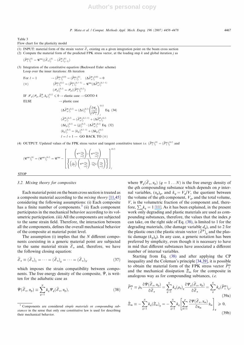
Table 3Flow chart for the plasticity model

(1) INPUT: material form of the strain vector bEn existing on a given integration point on the beam cross section(2) Compute the material form of the predicted FPK stress vector, at the loading step k and global iteration j as

ðbP m1 ÞðkÞj ¼ CmsððbEnÞðkÞj � ðbEP

n ÞðkÞðj�1ÞÞ

(3) Integration of the constitutive equation (Backward Euler scheme)Loop over the inner iterations: lth iteration

For l ¼ 1 ! ðbP m1 Þðk;0Þj ¼ ðbP m

1 ÞðkÞj ; ðDbEP

n Þðk;0Þj ¼ 0

ðIÞ ðbP m1 Þðk;lÞj ¼ ðbP m

1 Þðk;l�1Þj �CmsðDbEP

n Þðk;l�1Þj

ðPpÞðk;lÞj ¼ PpððbP m1 Þðk;lÞj Þ

IF FpðPp; bEPn ; kpÞðk;lÞj 6 0! elastic case! GOTO 4

ELSE ! plastic case

ðDbEPn Þðk;lÞj ¼ ðDkÞðk;lÞj

oGp

obP m1

!ðk;lÞj

Eq: ð34Þ

ðbEPn Þðk;lÞj ¼ ðbEP

n Þðk;l�1Þj þ ðDbEP

n Þðk;lÞj

ðDkpÞðk;lÞj ¼ ð.Þðk;lÞj � ðDbEPn Þðk;lÞj Eq: ð32Þ

ðkpÞðk;lÞj ¼ ðkpÞðk;l�1Þj þ ðDkpÞðk;lÞj

l ¼ lþ 1! GO BACK TO ðIÞ

(4) OUTPUT: Updated values of the FPK stress vector and tangent constitutive tensor i.e. ðbP m1 ÞðkÞj ¼ ðbP m

1 Þðk;lÞj and

ðCmtÞðkÞj ¼ ðCmtÞðk;lÞj ¼ Cme �Cms oGp

obP m1

!� Cme oFp

obP m1

!oFoPm

1

� Cms oGp

obP m1

!�oFp

okp.� oGp

obP m1

!( )266664

377775ðk;lÞ

j

STOP

3 Components are considered simple materials or compounding sub-

stances in the sense that only one constitutive law is used for describingtheir mechanical behavior.

P. Mata et al. / Comput. Methods Appl. Mech. Engrg. 196 (2007) 4458–4478 4467

Author's personal copy

where bP m1 is obtained as a weighted sum, according to the

volumetric fraction, of the material form of the stress vectorsðbP m

1 Þq corresponding to each one of the N components. Inthe same manner is obtained the total mechanical dissipa-tion, _�Nm, i.e., considering the contribution of the p internalvariables of each one the compounding substances ð _NmÞq.

The material form of the secant constitutive equation,the secant and tangent constitutive tensors, �Cms and �Cmt,for the composite are obtained as [45]

Cms �XN

q¼1

kqðCmsÞq ! bP m1 ¼ CmsðbEn � bEP

n Þ; ð40aÞ

bEPn ¼

XN

q¼1

kqðbEPn Þq; ð40bÞ

dbP m1 ¼ CmtdbEn ¼

XN

q¼1

kqðCmtÞqdbEn; ð40cÞ

where ðCmsÞq, ðCmtÞq and ðbEPn Þq are the material form of the

secant and tangent constitutive tensors and the materialform of the plastic strain vector of the qth component,respectively.

It is worth to comment the meaning of �q0 in Eq. (39a)and bEP

n in Eq. (40b); they corresponds to the average valueof the material forms of the density and the plastic strainvector of the composite and are obtained as a result ofapplying the mixing theory and, therefore, do not have aphysical meaning. The secant constitutive tensors of theright side of Eq. (40a) correspond to the elastic one if aplastic material is used and to these given in Eq. (12) if adamage model is used for the qth component.

Having calculated the material form of the FPK stressvector, the spatial form is obtained as bP 1 ¼ KbP m

1 . Stressresultant and couples are then calculated employingEq. (6).

Fiber reinforcements

The mechanical behavior of some advanced compositesare based on a main matrix component which is reinforcedwith oriented fibres, e.g., epoxy based materials with glassor carbon fibers or even reinforced concrete, where the steelreinforcing bars and stirrups can be seen as embedded rein-forcing fibers. The mixing rule provides an appropriatedframework to simulate these kind of composites [45], asso-ciating the one-dimensional version of the described consti-tutive laws to the reinforcements.

Due to the fact that the shape of the cross sections doesnot change during the motion, the incorporation of stirrupsor other kind of transversal reinforcements is not allowedin the present formulation. However, it is possible to sim-ulate the effect of this kind of reinforcement modifyingthe fracture energy and the limit stress of the matrix mate-rial. In the case of reinforced concrete, the shear resistance,ductility and strength increments due to confinement aresimulated using this last simplified approach.

4. Numerical implementation

In order to obtain a Newton type numerical solutionprocedure, the linearized form of the weak form of Eq.(9) is required, which can be written as

L½Gwðu;K; hÞ� ¼ Gwðu;K; hÞ þ DGwðu;K; hÞ � p;ð41Þ

where L½Gwðu;K; hÞ� is the linear part of the functionalGwðu;K; hÞ at the configuration defined by ðu;KÞ ¼ðu;KÞ and p � ðDu;DhÞ 2 R3 � T spa

K is an admissiblevariation. The term Gwðu;K; hÞ supplies the unbalanced

force and the differential DGwðu;K; hÞ � p, the tangential

stiffness [59] which is calculated as

DGwðu;K; hÞ � p

¼Z½0;L�

Dd½cn�O

d½xn�O

" #Tnm

� �0@ 1AdS þZ½0;L�

D hT np

mp

� �� �dS|fflfflfflfflfflfflfflfflfflfflfflfflfflfflfflfflfflffl{zfflfflfflfflfflfflfflfflfflfflfflfflfflfflfflfflfflffl}

KP

¼Z½0;L�

Dd½cn�O

Dd½xn�O

" #Tnm

� �þ

d½cn�O

d½xn�O

" #T

|fflfflfflfflfflfflfflffl{zfflfflfflfflfflfflfflffl}ð½B�hÞT

DnDm

� �0BBB@1CCCAdS þKP

¼Z½0;L�

hT0 0

�en ddS

� �0

" #|fflfflfflfflfflfflfflfflfflfflffl{zfflfflfflfflfflfflfflfflfflfflffl}

½nS�

p þ hT½B�TDnDm

� �0BBBB@1CCCCAdS þKP;

ð42Þ

where the subscript * has been written to indicate that theinvolved quantities have to be evaluated at ðu;KÞ ¼ðu;KÞ, the skew-symmetric tensor en is obtained fromits axial vector n, the operator ½ d

dS� is defined as½ ddS�v ¼ ½I�v;S 8v 2 R3, the operator [nS*] contributes to the

geometric part of the tangent stiffness, the term KP* corre-sponds to the part of the tangent stiffness which is depen-dent on the loading and the operator [B*] relates theadmissible variation h and the co-rotated variation of thereduced strain vectors. Explicit expressions for KP* and[B*] are omitted here and can be found in [31,59].

The estimation of the linearized form of the sectionalforce and moment vectors appearing in Eq. (42) requirestaking into account the linearized strain–stress relationsexisting between the material form of the FPK stress vectorbP m

1 , obtained in each material point on the beam cross sec-tion according to Eq. (40c), and the material form of thestrain vector bEn as follows

DbP m1 ¼ CmtDbEn; ð43aÞ

D ½bP 1�O

¼ KDbP m1 ¼ ðK �CmtKTÞKDbEn ¼ CstD ½en�

O

¼ KðDðKTbP 1ÞÞ ¼ DbP 1 � DehbP 1; ð43bÞ

DbP 1 ¼ D ½bP 1�O

�eP1Dh; ð43cÞ

4468 P. Mata et al. / Comput. Methods Appl. Mech. Engrg. 196 (2007) 4458–4478

Author's personal copy

where Cmt is the material forms of the tangential constitu-tive tensor for the composite which is obtained from Eq.(40c) and the corresponding spatial form is obtained asCst ¼ KCmtKT. The skew-symmetric tensors Deh and eP1

are obtained from the linear increment in the rotation vec-tor Dh and the FPK stress vector bP 1, respectively.

Starting from the material form of Eq. (6), and employ-ing Eq. (43a) it is possible to obtain linearized constitutiverelation between the material form of stress resultant andstress couple vectors and the reduced strain vectors as

Dnm

Dmm

� �¼ Cmt

11 Cmt12

Cmt21 Cmt

22

� �DCn

DXn

� �; ð44Þ

where Cmtpq, (p,q = 1,2) are the material form of the re-

duced tangential constitutive tensors, which are calculatedintegrating over the beam cross section, as

Cmt11 ¼

ZA

�Cmt dA; Cmt12 ¼ �

X3

b¼2

ZA

nb�CmteEb dA; ð45aÞ

Cmt21 ¼

ZA

e!Cmt dA; Cmt22 ¼ �

X3

b¼2

ZA

nbe!CmteEb dA;

ð45bÞ

where e! and eEb are the skew-symmetric tensors obtainedfrom the vectors � ¼ KTðx� uÞ and bEb, respectively. Thecorresponding spatial reduced tangential tensors areobtained as Cst

pq ¼ KCmtpq KT, which are configuration depen-

dent. The spatial form of the linearized relation of Eq. (44)can be obtained considering Eqs. (43b) and (43c) as

DnDm

� �¼ Cst

11 Cst12

Cst21 Cst

22

� �|fflfflfflfflfflfflfflfflffl{zfflfflfflfflfflfflfflfflffl}

½Cst�

D ½cn�OD ½xn�O

� �� 0 en

0 em� �|fflfflfflfflffl{zfflfflfflfflffl}

½eF�DuDh

� �;

ð46Þ

where em is the skew-symmetric tensor obtained from m. Fi-nally, Eq. (46) allows to rewrite Eq. (42) as

DGwðu;K; hÞ � p ¼Z½0;L�

hT½B�T½Cst �½B�p dS|fflfflfflfflfflfflfflfflfflfflfflfflfflfflfflfflfflfflfflffl{zfflfflfflfflfflfflfflfflfflfflfflfflfflfflfflfflfflfflfflffl}

KM

þZ½0;L�

hTð½enS� � ½B�T½eF�Þp dS|fflfflfflfflfflfflfflfflfflfflfflfflfflfflfflfflfflfflfflfflfflfflfflfflfflffl{zfflfflfflfflfflfflfflfflfflfflfflfflfflfflfflfflfflfflfflfflfflfflfflfflfflffl}KG

þKP

ð47Þ

which allows to rewrite Eq. (41) as

L½Gwðu;K; hÞ� ¼ Gwðu;K; hÞ þKM þKG þKP;

ð48Þ

where KG* and KM*, evaluated at the configurationðu;KÞ, give the geometric and material parts of the tan-gent stiffness, which considers the inelastic behavior ofthe composite materials of the beam.

The solution of the discrete form of Eq. (48) by using theFE method follows identical procedures as those described

in [59] for an iterative Newton–Raphson integrationscheme and it will not be repeated here. The inclusion ofmaterial nonlinearity implies the addition of two additionalintegration loops, which are carried out at any materialpoint on the cross section, but the rest of the integrationprocedure remains identical as for the case of elastic mate-rials as it is explained in the next section.

4.1. Cross sectional analysis

The cross section analysis is carried out expanding eachintegration point on the beam axis in a set of integrationpoints located on each fiber on cross section. In order toperform this operation, the beam cross section is meshedinto a grid of quadrilaterals, each of them correspondingto a fiber oriented along the beam axis (see Fig. 5). The esti-mation of the average stress level existing on each quadri-lateral is carried out by integrating the constitutiveequations of the compounding materials of the compositeassociated to the corresponding quadrilateral and applyingthe mixing rule. The geometry of each quadrilateral isdescribed by means of normalized bi-dimensional shapesfunctions and several integration points can be specifiedin order to estimate more precisely the value of a givenfunction according to a selected integration rule. In thecase of the average value of the material form of theFPK stress vector acting on a quadrilateral we have

bP m1 ¼

1

Ac

Z bP m1 dAc ¼

1

Ac

XNp

p¼1

XNq

q¼1

bP m1 ðyp; zqÞJ pqW pq; ð49Þ

where Ac is the area of the quadrilateral, Np and Nq are thenumber of integration points in the two directions of thenormalized geometry of the quadrilateral, bP m

1 ðyp; zqÞ isthe value of the FPK stress vector existing on a integrationpoint with coordinates (yp,zq) with respect to the referencebeam axis, which is obtained from the corresponding mate-rial strain vector bEn using the constitutive laws and themixing rule, Jpq is the Jacobian of the transformation be-tween normalized coordinates and cross sectional coordi-nates and Wpq are the weighting factors. The coefficientsof the tangent constitutive tensors can be estimated in ananalogous manner as in Eq. (49) but replacing bP m

1 ðyp; zqÞby Cmtðyp; zqÞ. Finally, having obtained the stress level oneach quadrilateral, the cross sectional forces and momentsare obtained by means of the discrete form of Eq. (6) as

nm ¼XNfiber

k¼1

ðAcÞkðbP m1 Þk; mm ¼

XNfiber

k¼1

ðAcÞk ‘k � ðbP m1 Þk; ð50Þ

were Nfiber is the number of quadrilaterals of the beamcross section, (Ac)k is the area of the k quadrilateral,ðbP m

1 Þk is the average value of the material form of theFPK stress vector and ‘k ¼ ð0; yk; zkÞ are the coordinatesof the gravity center of the kth quadrilateral with respectto the local beam reference frame.

By applying the same procedure as in Eq. (50), we havethat the material form of the reduced tangential tensors ofEqs. (45a) and (45b) are numerically estimated as

P. Mata et al. / Comput. Methods Appl. Mech. Engrg. 196 (2007) 4458–4478 4469

Author's personal copy

Cmt11 ¼

XNfiber

k¼1

ðAcÞkð �CmtÞk; ð51aÞ

Cmt12 ¼ �

XNfiber

k¼1

ðAcÞkðCmtÞkðykeE 2 þ zk

eE 3Þ; ð51bÞ

Cmt21 ¼

XNfiber

k¼1

ðAcÞke‘kðCmtÞk; ð51cÞ

Cmt22 ¼ �

XNfiber

k¼1

ðAcÞke‘kðCmtÞkðykeE 2 þ zk

eE 3Þ; ð51dÞ

where e‘k is the skew-symmetric tensor obtained from ‘k

and ðCmtÞk is the material form of the tangent constitutivetensor for the composite material of the kth quadrilateral.

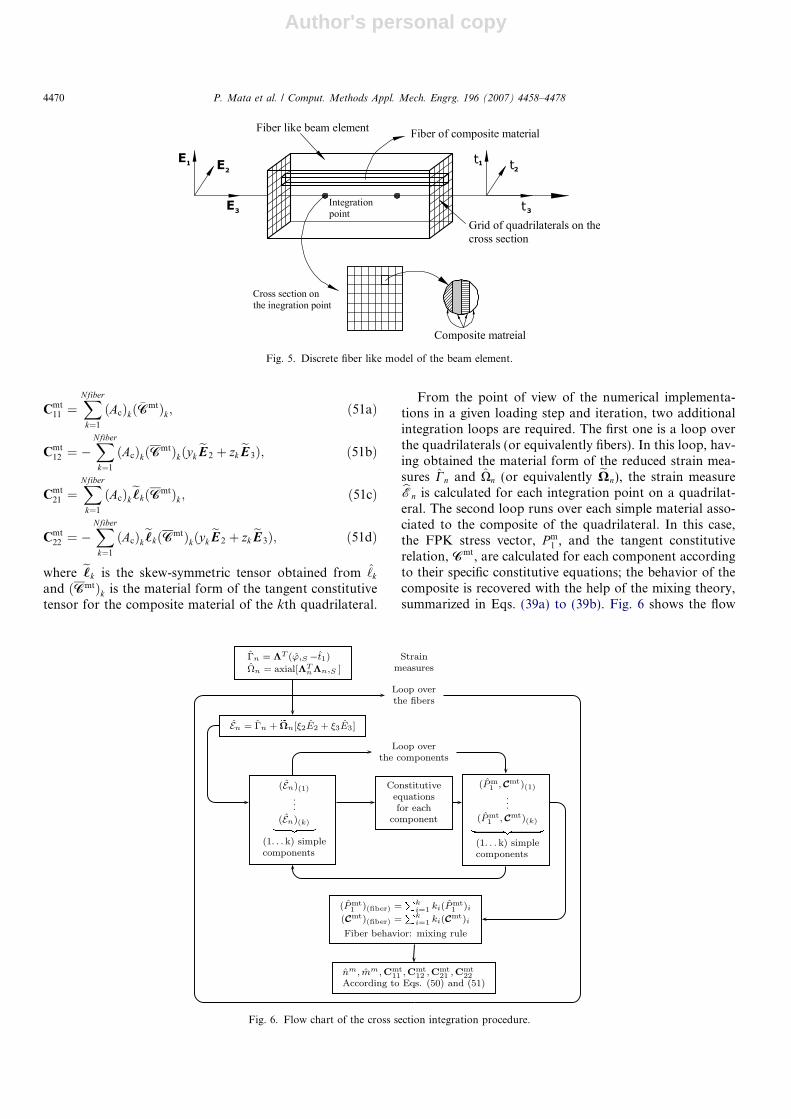
From the point of view of the numerical implementa-tions in a given loading step and iteration, two additionalintegration loops are required. The first one is a loop overthe quadrilaterals (or equivalently fibers). In this loop, hav-ing obtained the material form of the reduced strain mea-sures Cn and Xn (or equivalently eXn), the strain measurebEn is calculated for each integration point on a quadrilat-eral. The second loop runs over each simple material asso-ciated to the composite of the quadrilateral. In this case,the FPK stress vector, P m

1 , and the tangent constitutiverelation, Cmt, are calculated for each component accordingto their specific constitutive equations; the behavior of thecomposite is recovered with the help of the mixing theory,summarized in Eqs. (39a) to (39b). Fig. 6 shows the flow

Fig. 5. Discrete fiber like model of the beam element.

Fig. 6. Flow chart of the cross section integration procedure.

4470 P. Mata et al. / Comput. Methods Appl. Mech. Engrg. 196 (2007) 4458–4478

Author's personal copy

chart of the cross sectional analysis providing the resultantcross sectional forces and moments. Finally, the discreteversion of the spatial form of the reduced forces andmoments, n ¼ Kmm and m ¼ Kmm, and sectional tangentstiffness tensor Cst

ij = KCmtij KT (i, j = 1,2) are calculated

[31].As it has been previously explained, the sectional behav-

ior is obtained as the weighted sum of the contribution ofthe fibers, conversely to other works which develop globalsectional integration methods [66,67]. Material nonlinear-ity, such as degradation or plasticity, is captured by meansof the constitutive laws of the simple materials at eachquadrilateral. The nonlinear relation between the reducedstrain measures and cross sectional forces and momentsare obtained from Eq. (50). Each section is associated tothe volume of a part of the beam and, therefore, constitu-tive nonlinearity at beam element level is captured throughthe sectional analysis.

General shapes for cross sections can be analyzed bymeans of the proposed integration method. However, twolimitations have to be considered: (i) Mechanical problemsinvolving large deformations out of the cross sectionalplane can not be reproduced due to the planarity of thecross sections considered in the kinematical assumptions.(ii) Mechanical equilibrium at element level does notimplies mechanical equilibrium among fibers in the inelas-tic range due to the fact that the present beam model solvesthe constitutive equations for each fiber independently ofthe behavior of the contiguous ones.

5. Damage index

The estimation of damage indexes representative of thereal remaining loading capacity of a structure has becomea key issue in modern performance-based designapproaches of civil engineering [32]. Several criteria havebeen defined for estimating the damage level of structures[21]; some of them are defined for the global behavior ofthe structure, others can be applied to individual membersor subparts of the structure [12].

The damage index developed in this work is based on ananalogy with the problem at micro-scale (constitutive)level. A measure of the damage level of a material pointcan be obtained as the ratio of the existing stress level,obtained applying the mixing rule, to its (undamaged) elas-tic counter part. Following this idea, it is possible to definethe fictitious damage variable D as followsX3

i¼1

jP m1ij ¼ ð1� �DÞ

X3

i¼1

jP m1i0j ¼ ð1� �DÞ

X3

i¼1

jðCmbEnÞij;

�D ¼ 1�P3

i¼1jP m1ijP3

i¼1jP m1i0j

; ð52Þ

where jP m1ij and jP m

1i0j are the absolute values of the compo-nents of the existing and elastic stress vectors in materialform, respectively. It is worth to note that �D considers

any kind of stiffness degradation (damage, plasticity, etc.)at the material point level through the mixing rule and thenit constitutes a measure of the remaining load carryingcapacity. Initially, for low loading levels, the materialremains elastic and �D ¼ 0, but when the entire fractureenergy of the material has been dissipated jP m

1ij ! 0 and,therefore, �D! 1.

Eq. (52) can be extended to consider elements or eventhe whole structure by means of integrating the stressesover a finite volume of the structure. It allows definingthe local and global damage indices as follows:

�D ¼ 1�R

V p

PijP m

1ij �

dV pRV p

PijP m

1i0j �

dV p

; ð53Þ

where Vp is the volume of the part of the structure.By one hand, the local/global damage index defined in

Eq. (53) is a force-based criterium, which is able to discrim-inate the damage level assigned to a set of elements or tothe whole structure, according to the manner in which theyare loaded, in the same way as it has been explained in Ref.[21]. By the other hand, Eq. (53) is easily implemented in anstandard FEM code without requiring extra memory stor-age or time consuming calculations.

6. Numerical examples

6.1. Unrolling and rerolling of a circular beam

This validation example considers the unrolling andrerolling of the elastic circular cantilever beam shown inFig. 7. This example has been reported by Kapania andLi in Ref. [31] where four node initially curved FE elementsare used. The case of an initially straight cantilever beamhas been also reproduced in [24]. The initially circular beamhas a radio R = 5/p, unitary square cross sectional area

Fig. 7. Deformed configurations of the circular beam.

P. Mata et al. / Comput. Methods Appl. Mech. Engrg. 196 (2007) 4458–4478 4471

Author's personal copy

and the following properties for the material: elastic mod-ulus E = 1200 and Poisson coefficient m = 0.0. The FEmesh consist of ten equally spaced, quadratic, initiallycurved elements. An unitary bending moment M is appliedat the free end. Four loading steps are applied, each ofthem with a moment increment DM = 10p. The conver-gence tolerance is 1 · 10�7. The deformed configurationsof the beam are shown in Fig. 7. The displacements ofthe free end for an applied moment of 10p are 6.365 inthe vertical direction and �0.001 in the horizontal direc-tion. For an applied moment of 20p, the mentioned valuesare 0.003 and 9.998, respectively, and are very close tothose given in [31]. The number of iterations to reach theconvergence in the first and second loading steps are 18and 22, respectively.

6.2. Mesh independent response of a composite cantileverbeam

The RC cantilever beam shown in Fig. 8 is used to studyif, regularizing the dissipated energy at constitutive level, itis possible to obtain a mesh independent response whenincluding softening materials.

Forty increments of imposed displacements wereapplied in the Y direction to obtain the capacity curve ofthe beam. Four meshes of 10, 20, 40 and 80 quadratic ele-ments with the Gauss integration rule where considered inthe simulations. The beam cross section was meshed into20 equally spaced layers. The steel bars were included asa part of the composite material with a volumetric fractioncorresponding to their contributing area to the total area ofthe layer where they are located. The mechanical propertiesof the concrete and steel are summarized in Table 4, whereE and m are the elastic modulus and Poisson coefficient,respectively; Gf is the fracture energy, fc is the ultimatecompression limit and n is the ratio of the compressionto the tension yielding limits, according to Eq. (14c).

Fig. 9 shows the capacity curve relating the vertical reac-tion with the displacement of the free end. It is possible tosee that the numerical responses converge to that corre-sponding to the model with the greater number ofelements.

Further information can be obtained from the evolutionof the local damage index at cross sectional level, which isshown in Fig. 10 for the four meshes and the loading steps10, 25 and 40. In all the cases, strain localization occurs inthe first element but, in the case of the mesh with 10 ele-ments, localization occurs before than in the other cases

and a worse redistribution of the damage is obtained, whatcan explain the differences observed in Fig. 9.

Finally, Fig. 11 shows the evolution of the global dam-age index which allows to appreciate the mesh independentresponse of the structure.

6.3. Framed dome

The elastic and plastic mechanical behavior of frameddomes has been studied in several works. For example, inRef. [17] domes formed by trusses are studied; in [49] ini-tially straight beam elements are used to study the elasticplastic behavior of domes including isotropic and kine-matic hardening; in [64] a co-rotational formulation forbeam elements with lumped plasticity is presented; and in[65] a plastic hinge formulation assuming small strainsand the Euler–Bernoulli hypothesis is employed for study-ing the nonlinear behavior of domes including the mechan-ical buckling and post critical loading paths.

In this example, the nonlinear mechanical behavior ofthe framed dome shown in Fig. 12 is studied with the objec-tive of validating the proposed formulation in the inelastic

Fig. 8. RC cantilever beam.

Table 4Mechanical properties

E (MPa) m (MPa) fc n Gf (N mm�2)

Concrete 21000 0.20 25 8 1Steel 200000 0.15 500 1 500

0 0.2 0.4 0.6 0.8 1 1.2 1.4 1.6 1.8 20

2

4

6

8

10

12

14x 104

Tip displacement, (mm).

Verti

cal r

eact

ion

forc

e, (N

).

10 elements20 elements40 elements80 elements

Fig. 9. Vertical reaction versus tip displacement.

4472 P. Mata et al. / Comput. Methods Appl. Mech. Engrg. 196 (2007) 4458–4478

Author's personal copy

range. The linear elastic properties of the material are: elas-tic modulus 20700 MN m�2 and Poisson’s coefficient 0.17.Three constitutive relations are employed: (1) Linear elas-tic; (2) Perfect plasticity (Gf = 1 · 1010 N m�2) with associ-ated Von Mises yield criterion and an elastic limit offc = 80 N m�2; and (3) Damage model with equal tensileand compression limits, n = 1, a fracture energy ofGf,c = 50 N m�2 and the same elastic limit as in case (2).

Three elements with two Gauss integration points areused for each structural member. A vertical point load ofP0 = 123.8 N acting on the apex of the dome is applied

and the displacement control technique is used in the sim-ulations. Fig. 13 shows the deflection of the vertical apex infunction of the loading factor k = Pt/P0 (Pt is the currentapplied load) for the three constitutive relations. It is pos-sible to see in Fig. 13 a good agreement with the resultsgiven by Park and Lee in Ref. [49] for the stable branchof the elastic loading factor–displacement responses. Whencomparing both results for the elastic plastic case, it is pos-sible to see a good agreement for the elastic limit of thestructure; however, when deformation grows, the differ-ences can reach 30% for the predicted value of the load car-rying capacity of the dome. Moreover, the curvecorresponding to the damage model has been added toFig. 13. In both cases, when inelastic constitutive relationsare employed, the curve of the global structural responseshows a snap-through which couples constitutive and geo-metric effects.

6.4. Nonlinear response of a 45� cantilever bend

This example performs the coupled geometrically andconstitutive nonlinear analysis of a cantilever bend placedin the horizontal X–Y plane, with a vertical load F appliedat the free end, as shown in Fig. 14. The radius of the bendhas 100 mm with unitary cross section. The linear elasticcase of this example involves large 3D rotations and an ini-tially curved geometry; therefore, it has been considered inseveral works as a good validation test [24,31,59]. Themechanical properties for the elastic case are an elasticmodulus of 1 · 107 N mm�2 and a shear modulus of

Fig. 10. Evolution of the local cross sectional damage index: Strain localization. The symbols D and l are the damage index and the length of the beam,respectively.

0 5 10 15 20 25 30 35 400

0.1

0.2

0.3

0.4

0.5

0.6

0.7

0.8

0.9

1

Loading step.

Glo

bal d

amag

e in

dex.

10 elements20 elements40 elements80 elements

Fig. 11. Global damage index.

P. Mata et al. / Comput. Methods Appl. Mech. Engrg. 196 (2007) 4458–4478 4473

Author's personal copy

5 · 106 N mm�2. Four quadratic initially curved elementsare used in the FE discretization with two Gauss integra-tion points per element. Solutions are obtained by usingthirty equal load increments of 100 N. The history of thetip displacements is shown in Fig. 15. The tip displace-ments for an applied load of 600 N are: U1 = 13.56 mm.U2 = �23.81 mm and U3 = 53.51 mm (see Fig. 14) whichare values close to those obtained by other authors [31].

The coupled geometric and constitutive nonlinearresponse of the structure was obtained for three materials:(i) Elastic–plastic (Von Mises yield criterion, associatedflow rule, a fracture energy of Gf = 1 · 1010 N mm�2, anda tension to compression ratio n = 1). (ii) Degrading mate-rial (n = 1, Gf = 5 · 104 N mm�2) and (iii) a compositeformed by equal parts of the materials (i) and (ii). In allthe cases, the elastic limit is taken fc = 7 · 104 N mm�2.

The beam cross section was meshed into a grid of10 · 10 quadrilaterals with one integration point per fiber.A set of 35 imposed displacements of 2 mm was applied.The convergence tolerance was taken equal to 10�4 forresidual forces and displacements. Fig. 16 shows the resultsobtained from the numerical simulations for tip displace-ments superposed to the elastic response. It is possible toobserve in this figure that: (1) The elastic plastic case con-verges to a fixed value of 274 N for the vertical reactionafter the redistribution of the damage has occurred alongthe beam length, which can be considered the final stagein the formation of a plastic hinge in the structure. (2) In

Fig. 12. Framed dome and detail of the cross sectional mesh.

0 0.5 1 1.5 2 2.5 3 3.5 40

0.1

0.2

0.3

0.4

0.5

0.6

0.7

0.8

0.9

1

Vertical displacement

Load

ing

fact

or λ

ElasticDamagePlasticityPark & Lee plasticityPark & Lee elastic

Fig. 13. Loading factor–displacement curve of the vertical apex of thedome.

Fig. 14. Initial geometry and some examples of the deformed configura-tions for the linear elastic case of the 45 � cantilever bend.

0 500 1000 1500 2000 2500 3000—60

—40

—20

0

20

40

60

80

Load

Tip

disp

lace

men

ts

u1u2u3

Fig. 15. Different components of the tip displacement.

4474 P. Mata et al. / Comput. Methods Appl. Mech. Engrg. 196 (2007) 4458–4478

Author's personal copy

the case of the degrading material, the analyze werestopped in the loading step 29 due to lack of convergencywith an evident loss in the load carrying capacity. (3) Theresponse of the composite materials show two phases: thefirst one corresponds to the degradation of the damagingphase; during the second one the vertical reaction is stabi-lized in a value equal to 112 N, which is due to the mechan-ical response of the plastic phase.

In all the cases, a great amount of iterations wererequired to obtain convergence (>50 in the softeningphase). However, in the case of the material (ii) the analyzewere finalized after 300 iterations due to the fact that thedevelopment of axial forces in the deformed configurationliterally cuts the beam for vertical displacements beyond57 mm.

6.5. Nonlinear analysis of a right angle frame

The right angle frame of Fig. 17 is subjected to a concen-trated out of plane load P = 0.3 N acting on the middle ofthe span of one of the two members of length L = 100 mm.Forty equally sized loading steps have been used. Eachmember is modeled using four quadratic elements with

two Gauss integration points. The square beam cross sec-tions with a side length a = 3 mm are meshed into a gridof 4 · 4 quadrilaterals with four integration points perfiber. The convergence tolerance is taken as 1 · 10�4.

The constitutive and geometric nonlinear response ofthe frame is computed for four different materials withthe same elastic modulus E = 720 N mm�2, Poisson coeffi-cient m = 0.3 and yielding threshold fc = 1 N mm�2. Theother characteristics of the materials are: (i) associatedVon Mises plasticity with a compression to tension ration = 1 and fracture energy Gf = 1 · 105 N mm�2; (ii) a dam-age model with n = 2, Gf = 0.1 N mm�2; (iii) a compositewith a 20% of (i) and 80% of (iii). (iv) a composite with a10% of (i) a 80% of (ii) and a 10% of a material having onlylinear elastic properties.

Fig. 18 shows a comparison between the resultsobtained for the applied force versus the vertical deflectionof the point A (see Fig. 17) for the material (i) and theresults given in Refs. [49,57]. The results shown in Fig. 18are normalized considering that I is the inertia of thesquare cross section and M0 = a3fc/6. A good agreementwith the results obtained in the mentioned references isobtained.

—40 —30 —20 —10 0 10 20 30 40 50 60 700

100

200

300

400

500

600

Tip displacements

Load

u1u2 u3

Plasticity

Composite

Damage

Fig. 16. Different components of the tip displacement.

Fig. 17. Right bent.

0 0.1 0.2 0.3 0.4 0.5 0.6 0.70

1

2

3

4

5

6

Vertical deflection δ (EI/M0L2)

Load

(PL/

M0)

Park & LeeShi & AtluriPresent Plastic

Fig. 18. Load–deflection curve of the right bent.

P. Mata et al. / Comput. Methods Appl. Mech. Engrg. 196 (2007) 4458–4478 4475

Author's personal copy

Fig. 19a shows the load deflection curve of the point A

for the four considered materials. It is possible to appreciatethat in the case of the material (iii), after the damagingphase of the composite has been degraded, the responseof the structure is purely plastic. In the case of the material(iv), in the large displacements range of the response, theelastic phase dominates the mechanical behavior. Fig. 19bshows the evolution of the global damage index for the fourmaterials. It is worth to note that the damage index corre-sponding to material (iii) grows faster than the others,but, when the plastic phase dominates the the response(approx. loading step 32), the highest damage index is asso-ciated to the material (ii). In the large displacements range,the smallest values of global damage index corresponds tothe material (iv) due to the effect of the elastic component.

7. Conclusions

The geometrically exact formulation due to Reissnerand Simo for 3D beams is considered in the context of ini-tially curved beams and extended to include arbitrary dis-tribution of composite materials in the cross sections.The resulting formulation is used for studying the constitu-tive and geometric nonlinear behavior of framed structuresin the static case.

Constitutive laws for the simple materials are based onthermodynamically consistent formulations allowing toobtain more realistic estimations of the energy dissipationin the nonlinear range. The simple mixing rule for compos-ites is used for modeling complex material behaviors atmaterial point level.

A detailed cross sectional analysis, consistent with thekinematic hypothesis is presented. The proposed method,even when inexact from the point of view of the elasticitytheory, gives a computationally convenient way of approx-imating the strain–stress distribution in the section. Warp-ing variables or iterative procedures for obtaining correctedstrain fields are avoided in the present formulation. Consis-tent tangential constitutive tensors are considered to obtain

the tangential beam stiffness matrix by means of cross sec-tional integration.

A mesh independent response is obtained by means ofthe regularization of the energy dissipated at constitutivelevel considering the characteristic length of the volumeassociated to a specific integration point and the fractureenergy of the materials.

Local and global damage indices have been developedbased on the ratio between the elastic and nonlinear stres-ses. The proposed damage indices allow to identify the glo-bal load carrying capacity of the structure and the damagestate of the different members.

Several numerical examples have been included for thevalidation of the proposed formulation. The examplesinclude elastic and inelastic response of framed structureswith initially straight and curved beams. The verificationof the obtention of a mesh independent response for struc-tures presenting softening behavior is carried out. Compar-isons with existing literature is performed for the case ofplasticity and new results are presented for degrading andcomposite materials.

Acknowledgements

This research was partially supported by CEE-FP6 pro-ject FP6-505448 (GOCE), Risk Mitigation for Earthquakes

and Landslides (LESSLOSS); by the Spanish Government:Ministerio de Fomento and Ministerio de Ciencia y Tec-nologıa. Project Ref. MAT-2003-09768-C03-02, Delamina-tion of reinforced matrix composites (DECOMAR);Ministerio de Educacion y Ciencia. Project BIA2003-08700-C03-02, Numerical simulation of the seismic behavior

of structures with energy dissipation devices. ProjectBIA2005-06952, Study of composite materials for design,

reinforcement and retrofit of civil engineering structures

(RECOMP). The International Center for NumericalMethods in Enginnering (CIMNE) has also provided thesupport for this research. All this support is gratefullyacknowledged.

0 0.1 0.2 0.3 0.4 0.5 0.60

1

2

3

4

5

6

Vertical deflection δ (EI/M0L2)

Load

δ (P

L/M

0)

Material (i)Material (ii)Material (iii)Material (iv)

0 10 20 30 400

0.2

0.4

0.6

0.8

1

Loading step

Glo

bal d

amag

e in

dex

Material (i)Material (ii)Material (iii)Material (iv)

a b

Fig. 19. (a) Load deflection curves. (b) Global damage indices.

4476 P. Mata et al. / Comput. Methods Appl. Mech. Engrg. 196 (2007) 4458–4478

Author's personal copy

References

[1] S.S. Antman, Nonlinear Problems of Elasticity, Springer-Verlag,1991.

[2] F. Armero, D. Ehrlich, Numerical modeling of softening hinges in theEuler–Bernoulli beams, Comput. Struct. 84 (2005) 641–656.

[3] F. Armero, I. Romero, On the objective and conserving integration ofgeometrically exact rod models, Trends in Computational StructuralMechanics, Lake Constance, Austria, May 2001.

[4] F. Armero, I. Romero, Energy-dissipating momentum-conservingtime-stepping algorithms for the dynamic of nonlinear Cosserat rods,Comput. Mech. 31 (2003) 3–26.

[5] J. Argyris, An excursion into large rotations, Comput. Methods Appl.Mech. Engrg. 32 (1982) 85–155.

[6] A.H. Barbat, S. Oller, A. Hanganu, E. Onate, Viscous damage modelfor Timoshenko beam structures, Int. J. Solids Struct. 34 (1997) 3953–3976.

[7] P. Betsch, P. Steinmann, Frame-indifferent beam finite element basedupon the geometrically exact beam theory, Int. J. Numer. MethodsEngrg. 54 (2002) 1775–1788.

[8] G.E. Blandford, Large deformation analysis of inelastic space trussstructures, J. Struct. Engg. 122 (1996) 407–415.

[9] A. Cardona, A. Huespe, Evaluation of simple bifurcation points andpost-critical path in large finite rotations problems, Comput. MethodsAppl. Mech. Engrg. 175 (1999) 137–156.

[10] A. Cardona, M. Gerardin, A beam finite element non-linear theorywith finite rotations, Int. J. Numer. Methods Engrg. 26 (1988) 2403–2438.

[11] E. Car, S. Oller, E. Onate, An anisotropic elasto plastic constitutivemodel for large strain analysis of fiber reinforced composite materials,Comput. Methods Appl. Mech. Engrg. 185 (2000) 245–277.

[12] E. Cosenza, G. Manfredi, Damage indices and damage measures,Prog. Struct. Engrg. Mater. 2 (2000) 50–59.

[13] M.A. Crisfield, Non-Linear Finite Element Analysis of Solids andStructures, vols. 1 & 2, John Wiley & Sons, 1998.

[14] M.A. Crisfield, G. Jelenic, Objectivity of strain measures in thegeometrically exact three-dimensional beam theory and its finite-element implementation, Royal Soc. 455 (1999) 1125–1147.

[15] L. Davenne, F. Ragueneau, J. Mazars, A. Ibrahimbegovic, Efficientapproaches to finite element analysis in earthquake engineering,Comput. Struct. 81 (2003) 1223–1239.

[16] M.A. Dides, J.C. De La Llera, A comparative study of concentratedplasticity models in dynamic analysis of building structures, Earth-quake Engrg. Struct. Dynam. 34 (2005) 1005–1026.

[17] L. Driemeier, S.P. Baroncini, M. Alves, A contribution to thenumerical non-linear analysis of three-dimensional truss systemconsidering large strains, damage and plasticity, Commun. NonlinearSci. Numer. Simul. 10 (2005) 515–535.

[18] A.S. Elnashai, A.M. Mwafy, Overstrength and force reduction factorsof multistorey reinforced concrete buildings, Struct. Des. Tall Build.11 (2002) 329–351.

[19] C.A. Felippa, L.A. Crivelli, B. Haugen, A survey of the core-congruential formulation for geometrically nonlinear TL finiteelements, Arch. Comput. Methods Engrg. 1 (1994) 1–48.

[20] F. Gruttmann, R. Sauer, W. Wagner, Theory and numerics of three-dimensional beams with elastoplastic material behavior, Int. J.Numer. Methods Engrg. 48 (2000) 1675–1702.

[21] A.D. Hanganu, E. Onate, A.H. Barbat, Finite element methodologyfor local/global damage evaluation in civil engineering structures,Comput. Struct. 80 (2002) 1667–1687.

[22] HG. Kwak, SP. Kim, Nonlinear analysis of RC beam subject to cyclicloading, J. Struct. Engrg. 127 (2001) 1436–1444.

[23] M. Iura, S.N. Atluri, On a consistent theory, and variationalformulation of finitely stretched and rotated 3-D space-curved beams,Computat. Mech. 4 (1989) 73–88.

[24] A. Ibrahimbegovic, On finite element implementation of geometri-cally nonlinear Reissners beam theory: three-dimensional curved

beam elements, Comput. Methods Appl. Mech. Engrg. 122 (1995) 11–26.

[25] A. Ibrahimbegovic, M. Al Mikdad, Quadratically convergent directcalculation of critical points for 3D structures undergoing finiterotations, Comput. Methods Appl. Mech. Engrg. 189 (2000) 107–120.

[26] A. Ibrahimbegovic, On the choice of finite rotation parameters,Comput. Methods Appl. Mech. Engrg. 149 (1997) 49–71.

[27] A. Ibrahimbegovic, R.L. Taylor, On the role of frame-invariance instructural mechanics models at finite rotations, Comput. MethodsAppl. Mech. Engrg. 191 (2002) 5159–5176.

[28] A. Ibrahimbegovic, H. Shakourzadeh, J.L. Batoz, M. Al Mikdad,Y.Q. Guo, On the role of geometrically exact and second-ordertheories in buckling and post-buckling analysis of three-dimensionalbeam structures, Comput. Struct. 61 (1996) 1101–1114.

[29] G. Jelenic, M.A. Crisfield, Geometrically exact 3D beam theory:implementation of a strain-invariant finite element for static anddynamics, Comput. Methods Appl. Mech. Engrg. 171 (1999) 141–171.

[30] G. Jelenic, M. Saje, A kinematically exact space finite strain beammodel-finite element formulation by generalized virtual work princi-ple, Comput. Methods Appl. Mech. Engrg. 120 (1995) 131–161.

[31] R.K. Kapania, J. Li, On a geometrically exact curved/twisted beamtheory under rigid cross-section assumption, Comput. Mech. 30(2003) 428–443.

[32] A.J. Kappos, Seismic damage indices for RC buildings: evaluation ofconcepts and procedures, Prog. Struct. Engrg. Mater. 1 (1997) 78–87.

[33] J.K. Kim, T.G. Lee, Failure behavior of reinforced concrete framesby the combined layered and nonlayered method, Comput. Struct. 48(1993) 819–825.

[34] J. Lubliner, Thermomechanics of deformable bodies, Department ofCivil Engineering University of California, Berkeley, 1985.

[35] J. Lubliner, J. Oliver, S. Oller, Onate, A plastic-damage model forconcrete, Int. J. Solids Struct. 25 (1989) 299–326.

[36] J. Lubliner, On the thermodynamic foundations of non-linear solidmechanics, Int. J. Non-Linear Mech. 7 (1972) 237–254.

[37] B.M. Luccioni, V.C. Rougier, A plastic damage approach forconfined concrete, Comput. Struct. 83 (2005) 2238–2256.

[38] J. Makinen, H. Marjamaki, Total Lagrangian parametrization ofrotation manifold, in: Fifth EUROMECH Nonlinear DynamicsConference, Eindhoven, Netherlands, 2005, pp. 522–530.

[39] L.E. Malvern, Introduction to the mechanics of a continuousmedium, Department of Civil Engineering Englewood Cliffs, NJ,1969.

[40] A. Perez Moran, Formulaciones Tangente y Secante en Analisis noLineal de Vigas de Cosserat, Ph.D. Thesis, Universitat Politecnica deCatalunya, 2005.

[41] A. Neuenhofer, F.C. Filippou, Evaluation of the nonlinear framefinite-element models, J. Struct. Engrg. 123 (1997) 958–966.

[42] J. Oliver, M. Cervera, S. Oller, J. Lubliner, Isotropic damage modelsand smeared crack analysis of concrete, Proceedings 2nd ICCA-ADCS, Zell Am See, Austria, vol. 2, Pineridge Press, 1990, pp. 945–958.

[43] R.W. Ogden, Non-linear Elastic Deformations, Dover Publications,Inc., 1997.

[44] S. Oller, A.H. Barbat, Moment–curvature damage model for bridgessubjected to seismic loads, Comput. Methods Appl. Mech. Engrg. 195(2006) 4490–4511.

[45] S. Oller, E. Onate, J. Miquel, S. Botello, A plastic damage constitutivemodel for composites materials, Int. J. Solids Struct. 33 (1996) 2501–2518.

[46] S. Oller, E. Onate, J. Miquel, Mixing anisotropic formulation for theanalysis of composites, Commun. Numer. Methods Engrg. 12 (1996)471–482.

[47] S. Pajunen, Large elasto-plastic analysis of beams using kinematicallyexact elements, Commun. Numer. Methods Engrg. 16 (2000) 497–504.

P. Mata et al. / Comput. Methods Appl. Mech. Engrg. 196 (2007) 4458–4478 4477

Author's personal copy

[48] I. Papaioannou, M. Fragiadakis, M. Papadrakakis, Inelastic analysisof framed structures using the fiber approach, in: Proceedings of the5th International Congress on Computational Mechanics (GRACM05), Limassol, Cyprus, 2005, pp. 231–238.

[49] M.S. Park, B.C. Lee, Geometrically non-linear and elastoplastic three-dimensional shear flexible beam element of Von-Mises-type hardeningmaterial, Int. J. Numer. Methods Engrg. 39 (1996) 383–408.

[50] P.K.V.V. Nukala, D.W. White, A mixed finite element for three-dimensional nonlinear analysis of steel frames, Comput. MethodsAppl. Mech. Engrg. 193 (2004) 2507–2545.

[51] E. Reissner, On one-dimensional large-displacement finite-strainbeam theory, Stud. Appl. Math. 11 (1973) 87–95.

[52] E. Reissner, On one-dimensional finite-strain beam theory: the planeproblem, J. Appl. Math. Phys. 23 (1972) 795–804.

[53] I. Romero, F. Armero, An objective finite element formulation of thekinematics of geometrically exact rods and its use in the formulationof an energy–momentum conserving scheme in dynamics, Int. J.Numer. Methods Engrg. 54 (2002) 1683–1716.

[54] M. Saje, G. Turk, A. Kalagasidu, B. Vratanar, A kinematically exactfinite element formulation of elastic–plastic curved beams, Comput.Struct. 67 (1998) 197–214.

[55] M.H. Scott, G.L. Fenves, Plastic hinge integration methods for theforce-based beam-column elements, J. Struct. Engrg. 132 (2006) 244–252.

[56] Y. Shao, S. Aval, A. Mirmiran, Fiber-element model for cyclicanalysis of concrete-filled fiber reinforced polymer tubes, J. Struct.Engrg. 131 (2005) 292–303.

[57] G. Shi, S.N. Atluri, Elasto-plastic large deformation analysis ofspace-frames: a plastic hinge and stress-based explicit derivation oftangent stiffness, Int. J. Numer. Methods Engrg. 26 (1988) 589–615.

[58] J.C. Simo, A finite strain beam formulation. The three-dimensionaldynamic problem. Part I, Comput. Methods Appl. Mech. Engrg. 49(1985) 55–70.

[59] J.C. Simo, L. Vu-Quoc, A three-dimensional finite-strain rod model.Part II: Computational aspects, Comput. Methods Appl. Mech.Engrg. 58 (1986) 79–116.

[60] J.C. Simo, L. Vu-Quoc, On the dynamics in space of rods undergoinglarge motions – a geometrically exact approach, Comput. MethodsAppl. Mech. Engrg. 66 (1988) 125–161.

[61] J.C. Simo, The (symmetric) Hessian for geometrically nonlinearmodels in solid mechanics: intrinsic definition and geometric inter-pretation, Comput. Methods Appl. Mech. Engrg. 96 (1992) 189–200.

[62] J.C. Simo, L. Vu-Quoc, A geometrically exact rod model incorpo-rating shear and torsion-warping deformation, Int. J. Solids Struct. 27(1991) 371–393.

[63] J.C. Simo, K.D. Hjelmstad, R.L. Taylor, Numerical simulations ofelasto–viscoplastic response of beams accounting for the effect ofshear, Comput. Methods Appl. Mech. Engrg. 42 (1984) 301–330.

[64] M. Shugyo, Elastoplastic large deflection analysis of three-dimen-sional steel frames, Journal of Structural Engineering 129 (2003)1259–1267.

[65] G. Turkalj, J. Brnic, J. Prpic-Orsic, ESA formulation for largedisplacement analysis of framed structures with elastic-plasticity,Comput. Struct. 82 (2004) 2001–2013.

[66] A.M. Yu, X.G. Yang, G.H. Nie, Generalized coordinate for warpingof naturally curved and twisted beams with general cross-sectionalshapes, Int. J. Solids Struct. 43 (2006) 2853–2867.

[67] D. Zupan, M. Saje, Analytical integration of the stress field andtangent material moduli over concrete cross-sections, Comput. Struct.83 (2005) 2368–2380.

4478 P. Mata et al. / Comput. Methods Appl. Mech. Engrg. 196 (2007) 4458–4478