SCRS/2008/129 Collect. Vol. Sci. Pap. ICCAT, 64(5): 1509-1521 (2009)

1509

STANDARDIZED CATCH RATES FOR THE BLUE SHARK (PRIONACE GLAUCA)

AND SHORTFIN MAKO (ISURUS OXYRINCHUS) CAUGHT BY THE SPANISH SURFACE LONGLINE FLEET IN THE ATLANTIC OCEAN

DURING THE PERIOD 1990-2007

J. Mejuto1, B. García-Cortés, A. Ramos-Cartelle and J. M. De la Serna 2

SUMMARY Standardized catch per unit of effort were obtained for the shortfin mako and blue shark using General Linear Modeling (GLM) procedures from trips carried out by the Spanish surface longline fleet targeting swordfish in the North and South Atlantic Ocean over the periods 1990-2007 and 1997-2007, respectively. The main factors used for modeling were year, area, quarter, gear and ratio between swordfish and blue shark catches. The significant models explained around 80% and 40% of the CPUE variability for both species, respectively. As in the case of the Atlantic swordfish, an important fraction of the variability in the blue shark CPUE was attributed to the targeting criteria of the skipper represented by the ratio between the two most prevalent species in the landings. Other less important factors, were also identified as significant for this species. The area was identified as the most relevant factor to explain the CPUE variability in the shortfin mako. The standardized CPUEs obtained for both species generally suggest that the trend in the two Atlantic ‘stocks’ of each species was quite stable during the periods considered.

RÉSUMÉ Les taux standardisés de capture par unité d’effort ont été obtenus pour le requin taupe bleue et le requin peau bleue en utilisant des modèles linéaires généralisés (GLM) à partir des sorties réalisées par la flottille espagnole de palangre de surface qui capture l’espadon dans l’Atlantique Nord et Sud pendant les périodes 1990-2007 et 1997-2007 pour chaque espèce, respectivement. Les principaux facteurs considérés dans le modèle étaient l’année, la zone, le trimestre, l’engin et le ratio entre l’espadon et le requin peau bleue. Les modèles significatifs obtenus ont expliqué environ 80% et 40% de la variabilité de la CPUE pour les deux espèces, respectivement. Dans le cas de l’espadon de l’Atlantique, une importante fraction de la variabilité de la CPUE du requin peau bleue a été attribuée aux critères de ciblage des capitaines de pêche représentés par le ratio entre les deux espèces dominantes dans les débarquements. D’autres facteurs moins importants ont également été identifiés comme étant significatifs pour cette espèce. La zone a été identifiée comme étant le facteur le plus pertinent pour expliquer la variabilité de la CPUE chez le requin taupe bleue. Les CPUE standardisées obtenues pour les deux espèces suggèrent en général des tendances assez stables pour les deux « stocks » de l’Atlantique des deux espèces, pendant les périodes considérées.

RESUMEN

Tasas estandarizadas de captura por unidad de esfuerzo fueron obtenidas para el tiburón marrajo dientuso y para la tintorera usando Modelos Lineales Generalizados (GLM) a partir de mareas realizadas por la flota española de palangre de superficie que captura pez espada en el Atlántico norte y sur durante los periodos 1990-2007 y 1997-2007 para cada especie, respectivamente. Los factores principales considerados en el modelo fueron año, área, trimestre, arte y ratio entre el pez espada y la tintorera. Los modelos significativos obtenidos explicaron en torno al 80% y 40% de la variabilidad de la CPUE de esas especies, respectivamente. Como en el caso de los análisis de pez espada, una parte importante de la variabilidad de la CPUE de la tintorera es atribuible al criterio de direccionamiento de los patrones de pesca representado por el ratio entre las dos especies más prevalentes en los desembarcos. Otros factores fueron identificados también como significativos para esta

1 Instituto Español de Oceanografía, P.O. Box 130, 15080 A Coruña. Spain. 2 Instituto Español de Oceanografía, P.O. Box 285, 29640 Fuengirola, Málaga. Spain.

1510

especie, aunque fueron menos importantes. El factor área fue identificado como el más relevante para explicar la variabilidad de la CPUE del marrajo dientuso. Las CPUE estandarizadas obtenidas para ambas especies en general sugieren tendencias bastante estables para ambos ‘stocks’ del Atlántico de ambas especies, durante los periodos considerados.

KEYWORD

Bblue shark, shortfin mako, sharks, CPUE, GLM, longline, Spanish fleet

1. Introduction The Generalized Linear Modeling technique (GLM) (Robson 1966, Gavaris 1980, Kimura 1981) has been used to estimate standardized catch rates based on data from commercial fleets with unbalanced spatial and temporal activity. The standardized catch rates of the Atlantic swordfish (Xiphias gladius) were routinely obtained in recent decades by means of GLM based on data from commercial fleets, some of which targeted this species (Hoey et al. 1989, Anonymous 1989, 1991; Hoey et al. 1993, Nakano 1993, Mejuto 1993, Scott et al. 1993, Mejuto 1994, Mejuto and de la Serna 1995, Mejuto et al. 1999, Ortiz et al. 2007). This has become a basic routine task in the assessment of stocks in accordance with the scientific dynamics of the ICCAT. These standardized catch per unit of effort data (CPUE) from commercial fleets are frequently used as abundance indicators in a great number of fisheries targeting different large pelagic fish. These CPUEs are assumed to be reliable indicators of abundance for most large pelagic species due to the lack of direct abundance indicators, especially when the available data from the fishery cover oceanic areas where these species are broadly distributed. However, this interpretation may not necessarily be assumed 'a priori' in all cases. The CPUE indicators must be evaluated case by case, based on the empirical knowledge of the fishery and the quality of the data, the spatial-temporal coverage in relation to the stock distribution and taking into consideration the limits and risks involved in this assumption (Mejuto et al. 1999). The consistency in the fishing patterns of the fleets over time also facilitates the interpretation of these indices. The Spanish surface longline fleet targeting swordfish has historically used the traditional plurifilament longline gear with a similar number of hooks per basket, since the fishing activity only covers the surface layers, usually above 50 m depth, with night sets. However, important changes in the fishing strategy of the Spanish surface longline fleet in the Atlantic areas have been reported in recent years (Mejuto and De la Serna 1997, 2000, Mejuto et al. 1997, 1998, 1999). The recent introduction of the monofilament longline style imported from other countries and a targeting criteria of a more diffuse nature applied to swordfish and/or blue shark could be pointed out as the main changes in the fishing patterns of this fleet during the last decade. Other longline activities carried out by vessels flying other flags, targeting mostly tunas or having mixed or more diffuse fishing strategies on tuna-swordfish, may change the number of hooks per basket (or between buoys) according to the depth of the gear and/or to the hours of fishing selected, the targeted species, the respective local abundance of the different species or even the economic worth of the species on priority international markets. In such cases, the number of hooks per basket or between buoys, as well as other elements used as proxies, could help in CPUE standardization in order to identify, indirectly, the target species and fishing strategies or the priorities of skippers. Some of these factors may explain in certain cases the CPUE discrepancies detected between apparently similar longline styles (Saito and Yokawa 2001, 2003, Nishida and Wang 2006, Okamoto et al. 2001, Wang et al. 2006). In the latter case, the interpretation of CPUE data as abundance indices becomes even more difficult. The blue and shortfin mako sharks are highly migratory, oceanic-epipelagic and wide-ranging circumglobal species distributed mostly, but not exclusively, between 50ºN-50ºS. Both species cover tropical, subtropical and temperate waters although some specimens could also be observed in cold waters near the extreme areas of their distributions. Blue shark is one of the most prevalent fish species in the epipelagic layers because of its efficient ovoviviparous reproductive strategy. Shortfin mako is less prevalent but it is also a frequent large pelagic oceanic shark, ovoviviparous as well but with smaller litter sizes and a uterine cannibalism. Both species are within the range of the fishing areas-gears targeting tunas or swordfish around the world. Among other gears and fisheries, both large pelagic shark species are also caught as bycatch in the longline fishing operations targeting tunas or swordfish over the world. The Spanish surface longline fishery targeting

1511

swordfish began operating in the Mediterranean Sea and the Atlantic Ocean centuries ago and historically the most important shark bycatch in the Atlantic areas were mainly the blue shark (BSH) and secondly the shortfin mako (SMA). The blue shark and shortfin mako recently accounted for an average of 87% and 10%, respectively, of the shark landings by the Spanish surface longline fleet from Atlantic during the 1997-2006 period as a whole (Mejuto et al. 2009). Historically, the blue shark is a species frequently caught and discarded in many fisheries for several reasons (see Mejuto et al. 2009 for details). These discard practices were described for the Spanish longline fleets during the eighties and previous decades of the 20th century (Mejuto and González-Garcés 1984, Mejuto 1985). However, the blue sharks (bodies and fins) have been full retained onboard and landed by this fleet since the middle of the nineties when freezing systems were added. The shortfin mako is clearly a less prevalent species in the epipelagic system than blue shark, but individuals are also frequently observed as a regular bycatch in most trip. The shortfin mako was historically a marketable and highly prized species with full retention onboard by the Spanish fleet. Discards of this species have been merely incidental since the beginning of the Spanish longline fishery. So, landings and catches are historically equivalent concepts in the Spanish longline fisheries for the latter species. 2. Material and methods The methodology used in this paper is based on previous research carried out on the Spanish longline fleet in the Atlantic and used in the swordfish CPUE analysis of the Spanish as well as other Atlantic longline fleets (Mejuto and De la Serna 2000, Ortiz 2007). The data used consisted of trip records obtained in research projects covering the 1990-2007 period. Nominal effort was defined by thousands of hooks per set and fishing days. The nominal landings per unit of effort, assumed in this case as the CPUE of blue and shortfin mako sharks, were calculated as kilograms of gutted or round weight caught per thousand hooks, respectively. The CPUE in number of fish was also obtained for the shortfin mako. The standardized mean round weight of the shortfin mako was calculated as CPUE in weight / CPUE in number of fish. The variable ‘ratio’ was defined for each available record as the percentage of swordfish related to both the swordfish and blue shark caught. After analyzing the behavior of the Spanish fleet in different oceans, it was concluded that this ratio might be a good proxy indicator of target intensity, mainly and clearly directed towards swordfish at the beginning of the time series vs. a more diffuse fishing strategy aimed at the two main species caught combined or in favor of the blue shark in the recent period (Mejuto and De la Serna 2000, Anonymous 2001). These ratio values were categorized into ten ‘ratio’ levels of 10% intervals for modeling. A similar approach is frequently used for other longline fleets where the criteria for target species are diffuse. As previously indicated, two main types of longline were clearly identified: the Spanish traditional multifilament gear and the monofilament or ‘American style’ gear. The use of the traditional surface longline gear by the Spanish fleet remained relatively constant for decades in terms of general structure and configuration (Rey et al. 1988, Hoey et al. 1988). There have been some technological improvements in this traditional fishing gear over this period. The most common improvements were related to the introduction of new elements to facilitate handling, setting out and hauling back the fishing gear and also tended to allow for a greater number of hooks per set, which were appropriately considered as nominal effort in the analysis. However, at the end of the 20th century, the monofilament style or the so-called “American style” gear was largely introduced by the Spanish fleet in most fishing areas. Additionally, information on other gear characteristics or fishing practices was also compiled by means of skipper surveys (light sticks, clips, species declared as preference, etc.). A total of seven ‘gear’ levels were finally categorized. The standardized log (CPUE) analyses were done using the GLM procedure (SAS 9.1). The quarters and the spatial definitions used for GLM runs were the same as those used for the Atlantic swordfish (Mejuto et al. 1999, Mejuto and de la Serna 2000), assuming a hypothetical boundary line between North and South ‘stocks’ located at 5º N latitude (Figure 1). Five areas were finally categorized for each of the North or South Atlantic runs. The period 1990-2007 was considered for the shortfin mako runs. The period 1997-2007 was used for the blue shark runs because the available information suggested that discards became negligible during this period and landing rates can be assumed as catch rates. The model defined includes ‘year’, ‘quarter’, ‘area’, ‘ratio’ and ‘gear’ as main factors, as well as the ‘quarter*area’ interaction: LOG (CPUE) = u + Y + Q + A + R +G + Q * A + e. Where, u= overall mean, Y= effect year, Q= effect quarter, A= effect area, R= effect ratio, G= effect gear, e= logarithm of the normally

1512

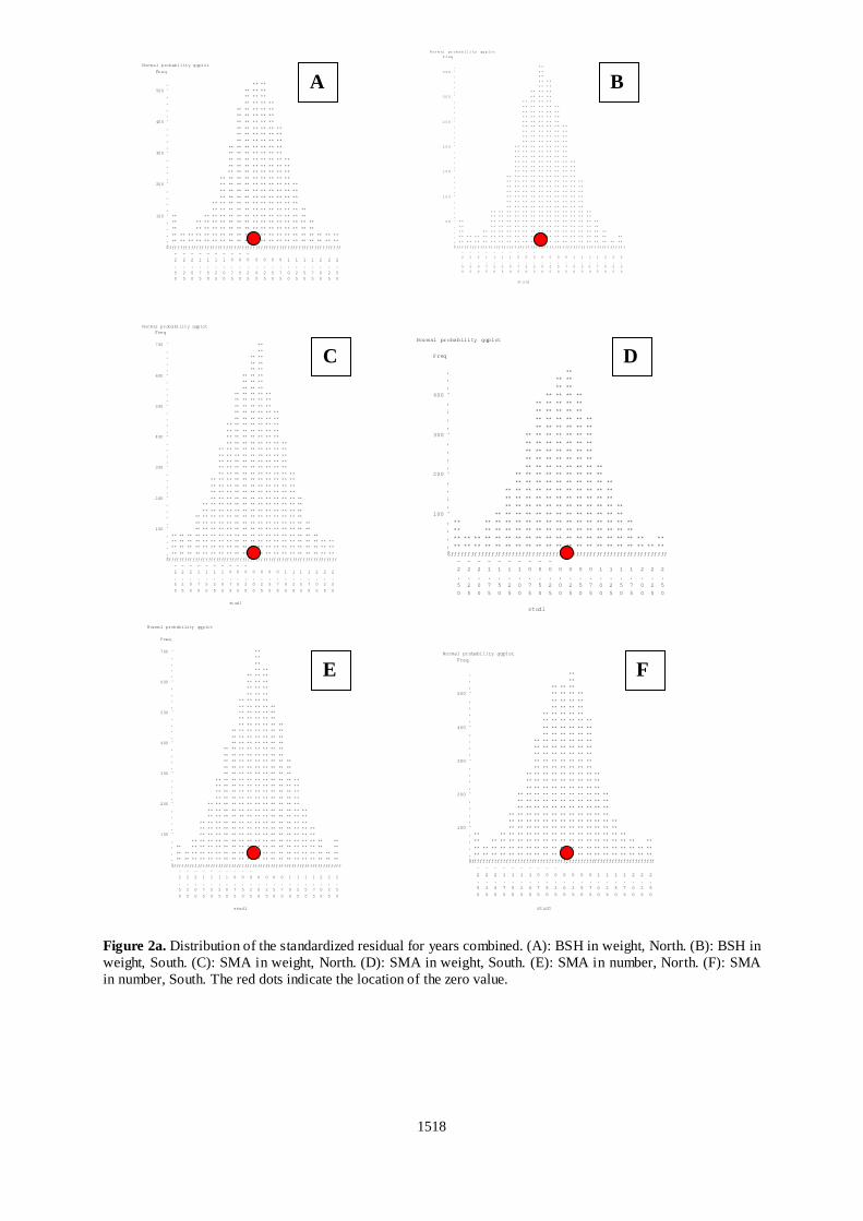
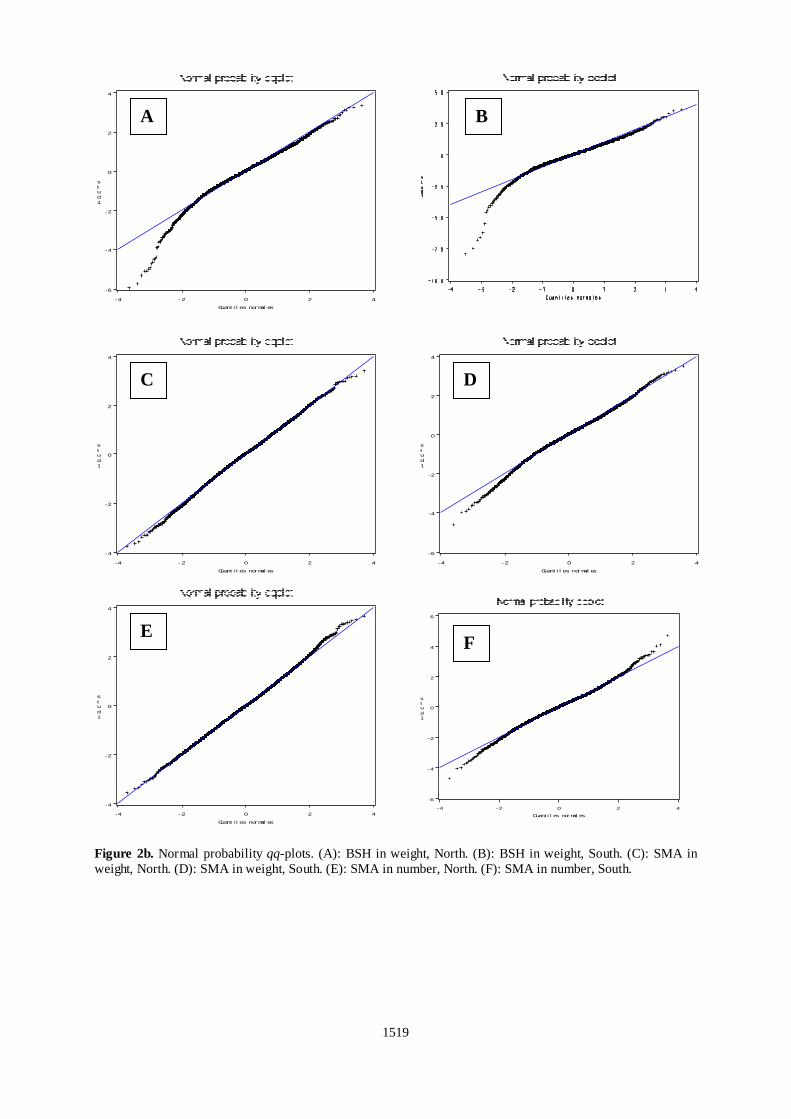
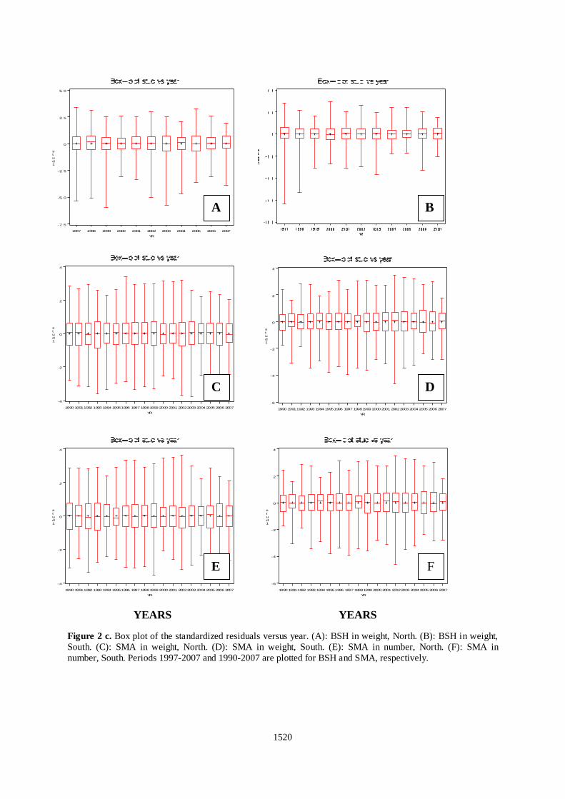
distributed error term. As in the case of several fleets operating in the Atlantic, Indian and Pacific oceans, the ‘ratio’ was considered to be a proxy indicator of the fishing criteria of the skipper during the fishing activity. 3. Results and discussion A total number of 7 511 and 11 244 trip records were available for the blue shark and shortfin mako during the periods 1997-2007 and 1990-2007, respectively. Spatial-temporal coverage was appropriate for blue shark. Some coverage limitations were observed for shortfin mako data at the beginning of the time series due to the progressive geographical expansion of the fleet during the initial period, specially in the South Atlantic. These limitations are often observed in the data sets obtained from most of the oceanic longline fleets especially when accessing new fishing areas during the geographical expansion periods or owing to shifts to other fishing areas. Tables 1 and 2 provide the ANOVA summary, including R-square, mean square error (root), F statistics and significance level as well as the Type III SS for each factor used. The significant model tested for the blue shark for the period 1997-2007 explained 83% and 86% of the CPUE variability for the North and South Atlantic, respectively. The significant model tested for the shortfin mako for the period 1990-2007 explained between 36% and 39% of the CPUE variability for the North and South Atlantic, depending of the region considered (North or South) and the units used (number of fish or weight). As in the case of the previous swordfish CPUE analyses, the CPUE variability (Type III SS) in blue shark may be attributed primarily to the ratio factor and, secondly, to the gear factor. The area, year and quarter factors were also significant although less important. The ratio factor takes into account the progressive change in the fishing practices and targeting criteria described for the Spanish longline fleet during the most recent period considered with implications on the preference of swordfish and/or in favor of blue shark catches during the most recent period (Mejuto and De la Serna 2000). The CPUE variability (Type III SS) of shortfin mako may be attributed mainly to the area and, secondly, to the other factors considered. Figures 2 (a, b and c) provide the studentized residual distribution by years aggregated, the normal probability qq-plot obtained for each run and box-plot of the standardized residuals obtained by year. The CPUE trends obtained by year and their respective confidence intervals (95%) are shown in Table 3 and Figure 3. The significance of the ‘ratio’ factor among the main species retained onboard has been described for several important oceanic longline fleets fishing in the North and South Atlantic areas and, more recently, in the Pacific and Indian ocean. These ratios have been used for the previous clustering of the data (categorized by ratio between species) or directly for modeling according to their respective fishing patterns (Chang et al. 2007, Hazin et al. 2007a,b, Mejuto and De la Serna 2000, Mourato et al. 2007, Ortiz 2007, Ortiz et al. 2007, Paul and Neilson 2007, Yokawa 2007). Of the different proxy methods simulated by the ICCAT Working Group on Stock Assessment Methods, the use of catch ratios was found to perform best, on average, and remained the preferred proxy, although this method may not necessarily provide the best performance in all cases (Anonymous 2001). The inclusion of this categorized factor in the modeling of some fleets has improved the interpretation of the CPUE as an abundance index when changes in the fishing strategy or other skipper’s factors related to changes in species preferences are detected over time. The importance of the ratio versus other factors in the CPUE of swordfish and blue shark of the Spanish longline fleet fishing in the Atlantic was explained based on micro-scale fits of the skippers among trips-sets according to the respective local prevalence selected for the two most abundant species of interest, swordfish and/or blue shark (Mejuto and De la Serna 2000). Both species frequently overlap in their areas of distribution, but their respective local abundance maximum probably do not coincide. In fact their maximum may even be mutually exclusive. The low swordfish CPUE was regularly observed in the Atlantic in association with high rates of blue shark bycatch. In contrast, high swordfish CPUEs were frequently related to lower rates of blue shark bycatch. This finding is not surprising since in different Atlantic areas and fleets, throughout the history of the fishery, fishermen have frequently reported that the optimal CPUEs of swordfish and blue shark rarely coincide in space and time and are generally mutually exclusive. This may be due to different reasons, such as the spatial-temporal exclusion between the maximum of two species and/or the different ranges of optimum temperatures sought by each of them for their respective biological processes in the epipelagic system. Historically, the shortfin mako was generally a full retained bycatch, highly prized and also used for human consumption. The ratio defined in this analysis also shows significant effect of the CPUE of this species but as expected clearly less important than other factors such us area. The results obtained show CPUE trends that are quite stable for both species during the respective periods considered. A moderate decrease in the CPUE for the North Atlantic shortfin mako was observed during the initial period 1990-1995 -when the highest longline activity on the North Atlantic swordfish fishery was achieved- and stability afterwards.

1513

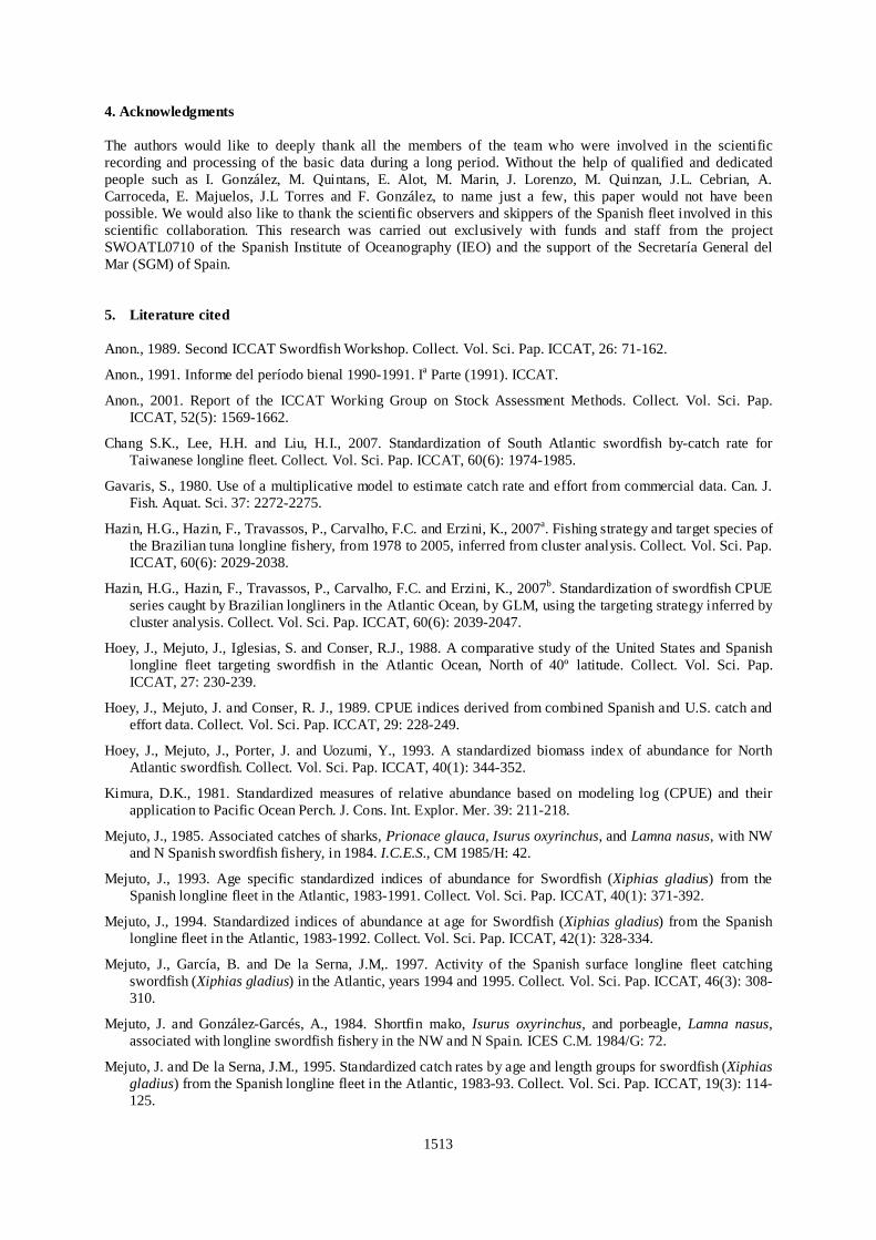
4. Acknowledgments The authors would like to deeply thank all the members of the team who were involved in the scientific recording and processing of the basic data during a long period. Without the help of qualified and dedicated people such as I. González, M. Quintans, E. Alot, M. Marin, J. Lorenzo, M. Quinzan, J.L. Cebrian, A. Carroceda, E. Majuelos, J.L Torres and F. González, to name just a few, this paper would not have been possible. We would also like to thank the scientific observers and skippers of the Spanish fleet involved in this scientific collaboration. This research was carried out exclusively with funds and staff from the project SWOATL0710 of the Spanish Institute of Oceanography (IEO) and the support of the Secretaría General del Mar (SGM) of Spain. 5. Literature cited Anon., 1989. Second ICCAT Swordfish Workshop. Collect. Vol. Sci. Pap. ICCAT, 26: 71-162.

Anon., 1991. Informe del período bienal 1990-1991. Ia Parte (1991). ICCAT.

Anon., 2001. Report of the ICCAT Working Group on Stock Assessment Methods. Collect. Vol. Sci. Pap. ICCAT, 52(5): 1569-1662.

Chang S.K., Lee, H.H. and Liu, H.I., 2007. Standardization of South Atlantic swordfish by-catch rate for Taiwanese longline fleet. Collect. Vol. Sci. Pap. ICCAT, 60(6): 1974-1985.

Gavaris, S., 1980. Use of a multiplicative model to estimate catch rate and effort from commercial data. Can. J. Fish. Aquat. Sci. 37: 2272-2275.

Hazin, H.G., Hazin, F., Travassos, P., Carvalho, F.C. and Erzini, K., 2007a. Fishing strategy and target species of the Brazilian tuna longline fishery, from 1978 to 2005, inferred from cluster analysis. Collect. Vol. Sci. Pap. ICCAT, 60(6): 2029-2038.

Hazin, H.G., Hazin, F., Travassos, P., Carvalho, F.C. and Erzini, K., 2007b. Standardization of swordfish CPUE series caught by Brazilian longliners in the Atlantic Ocean, by GLM, using the targeting strategy inferred by cluster analysis. Collect. Vol. Sci. Pap. ICCAT, 60(6): 2039-2047.

Hoey, J., Mejuto, J., Iglesias, S. and Conser, R.J., 1988. A comparative study of the United States and Spanish longline fleet targeting swordfish in the Atlantic Ocean, North of 40º latitude. Collect. Vol. Sci. Pap. ICCAT, 27: 230-239.

Hoey, J., Mejuto, J. and Conser, R. J., 1989. CPUE indices derived from combined Spanish and U.S. catch and effort data. Collect. Vol. Sci. Pap. ICCAT, 29: 228-249.

Hoey, J., Mejuto, J., Porter, J. and Uozumi, Y., 1993. A standardized biomass index of abundance for North Atlantic swordfish. Collect. Vol. Sci. Pap. ICCAT, 40(1): 344-352.

Kimura, D.K., 1981. Standardized measures of relative abundance based on modeling log (CPUE) and their application to Pacific Ocean Perch. J. Cons. Int. Explor. Mer. 39: 211-218.

Mejuto, J., 1985. Associated catches of sharks, Prionace glauca, Isurus oxyrinchus, and Lamna nasus, with NW and N Spanish swordfish fishery, in 1984. I.C.E.S., CM 1985/H: 42.

Mejuto, J., 1993. Age specific standardized indices of abundance for Swordfish (Xiphias gladius) from the Spanish longline fleet in the Atlantic, 1983-1991. Collect. Vol. Sci. Pap. ICCAT, 40(1): 371-392.

Mejuto, J., 1994. Standardized indices of abundance at age for Swordfish (Xiphias gladius) from the Spanish longline fleet in the Atlantic, 1983-1992. Collect. Vol. Sci. Pap. ICCAT, 42(1): 328-334.

Mejuto, J., García, B. and De la Serna, J.M,. 1997. Activity of the Spanish surface longline fleet catching swordfish (Xiphias gladius) in the Atlantic, years 1994 and 1995. Collect. Vol. Sci. Pap. ICCAT, 46(3): 308-310.

Mejuto, J. and González-Garcés, A., 1984. Shortfin mako, Isurus oxyrinchus, and porbeagle, Lamna nasus, associated with longline swordfish fishery in the NW and N Spain. ICES C.M. 1984/G: 72.

Mejuto, J. and De la Serna, J.M., 1995. Standardized catch rates by age and length groups for swordfish (Xiphias gladius) from the Spanish longline fleet in the Atlantic, 1983-93. Collect. Vol. Sci. Pap. ICCAT, 19(3): 114-125.

1514

Mejuto, J. and De la Serna, J.M., 1997. Updated standardized catch rates by age for swordfish (Xiphias gladius) from the Spanish longline fleet in the Atlantic, using commercial trips from the period 1983-1995 Collect. Vol. Sci. Pap. ICCAT, 46(3): 323-335.

Mejuto, J. and De la Serna, J.M., 2000. Standardized catch rates by age and biomass for the North Atlantic swordfish (Xiphias gladius) from the Spanish longline fleet for the period 1983-1998 and bias produced by changes in the fishing strategy. Collect. Vol. Sci. Pap. ICCAT, 51(5): 1387-1410.

Mejuto, J., De la Serna, J.M. and García, B., 1998. Updated standardized catch rates by age, sexes combined, for the swordfish (Xiphias gladius) from the Spanish longline fleet in the Atlantic, for the period 1983-1996 Collect. Vol. Sci. Pap. ICCAT, 48(1): 216-222.

Mejuto, J., De la Serna, J.M. and García, B., 1999. Updated standardized catch rates by age, combined sexes, for the swordfish (Xiphias gladius) from the Spanish longline fleet in the Atlantic, for the period 1983-1997. Collect. Vol. Sci. Pap. ICCAT, 49(1): 439-448.

Mejuto, J., García-Cortés, B., Ramos-Cartelle, A. and De la Serna, J.M., 2009. Scientific estimations of by-catch landed by the Spanish surface longline fleet targeting swordfish (Xiphias gladius) in the Atlantic ocean with special reference to the years 2005 and 2006. Collect. Vol. Sci. Pap. ICCAT, 64 (in this volume).

Mejuto, J., García-Cortés, B., Ortiz de Urbina, J., 2009. Ratios between the wet fin weight and body weights of blue shark (Prionace glauca) in the Spanish surface longline fleet during the period 1993-2006 and their impact on the ratio of sharks species combined. Collect. Vol. Sci. Pap. ICCAT, 64(5): 1513-1529..

Mourato B.L., Andrade, H.A., Amorim, A.F. and Arfelli, C.A., 2007. Standardized catch rate of swordfish (Xiphias gladius) caught by Santos longliners off southern Brazil (1971-2005) Collect. Vol. Sci. Pap. ICCAT, 60(6): 1943-1952.

Nakano, H., 1993. Estimation of standardized CPUE for the Atlantic swordfish using the data from the Japanese longline fishery Collect. Vol. Sci. Pap. ICCAT, 40(1): 357-370.

Nishida T. and Wang, S.P., 2006. Standardization of swordfish (Xiphias gladius) CPUE of the Japanese tuna longline fisheries in the Indian Ocean (1975-2004). IOTC-2006-WPB-07.

Okamoto, H., Miyabe, N. and Matsumoto, T., 2001. GLM analyses for standardization of Japanese longline CPUE for bigeye tuna in the Indian Ocean. IOTC-2001-WPTT-21, 38p.-377.

Ortiz. M., 2007. Update of standardized catch rates by sex and age for swordfish (Xiphias gladius) from the U.S. longline fleet 1981-2005 Collect. Vol. Sci. Pap. ICCAT, 60(6): 1994-2017.

Ortiz, M., Mejuto, J., Paul, S., Yokawa, K., Neves, M. and Hoey, J., 2007. An updated biomass index of abundance for North Atlantic swordfish 1963-2005. Collect. Vol. Sci. Pap. ICCAT, 60(6): 2048-2058.

Paul, S.D. and Neilson, J.D., 2007. Updated sex- and age-specific CPUE from the Canadian swordfish longline fishery, 1988-2005. Collect. Vol. Sci. Pap. ICCAT, 60(6): 1914-1942.

Rey, J.C., Mejuto, J. and Iglesias, S., 1988. Evolución histórica y situación actual de la pesquería de pez espada (Xiphias gladius). Collect. Vol. Sci. Pap. ICCAT, 27: 202-213.

Robson, D.S., 1966. Estimation of relative fishing power of individual ships. Res. Bull. Int. Comm. N.W. Atl. Fish, 3: 5-14.

Saito, H. and Yokawa, K., 2001. Preliminary analysis of catch pattern of Japanese and Taiwanese longliners laying stress on swordfish. IOTC-2001-WPB-02.

Saito, H. and Yokawa, K., 2003. Update of standardization of swordfish CPUE of Japanese longliners in the Indian ocean. IOTC-2003-WPB-02.

Scott, G.P., Restrepo, V.R. and Bertolino, A., 1993. Standardized catch rates for swordfish (Xiphias gladius) from the U.S. longline fleet though 1991 Collect. Vol. Sci. Pap. ICCAT, 40(1): 458-468.

Yokawa, K., 2007. Update of standardized CPUE of swordfish caught by Japanese longliners. Collect. Vol. Sci. Pap. ICCAT, 60(6): 1986-1993.

Wang, S.P., Chang, S.K., Nishida, T. and Ling, S.L., 2006. CPUE standardization of Indian Ocean swordfish from Taiwanese longline fishery for data up to 2003. IOTC-2006-WPB-09.

1515

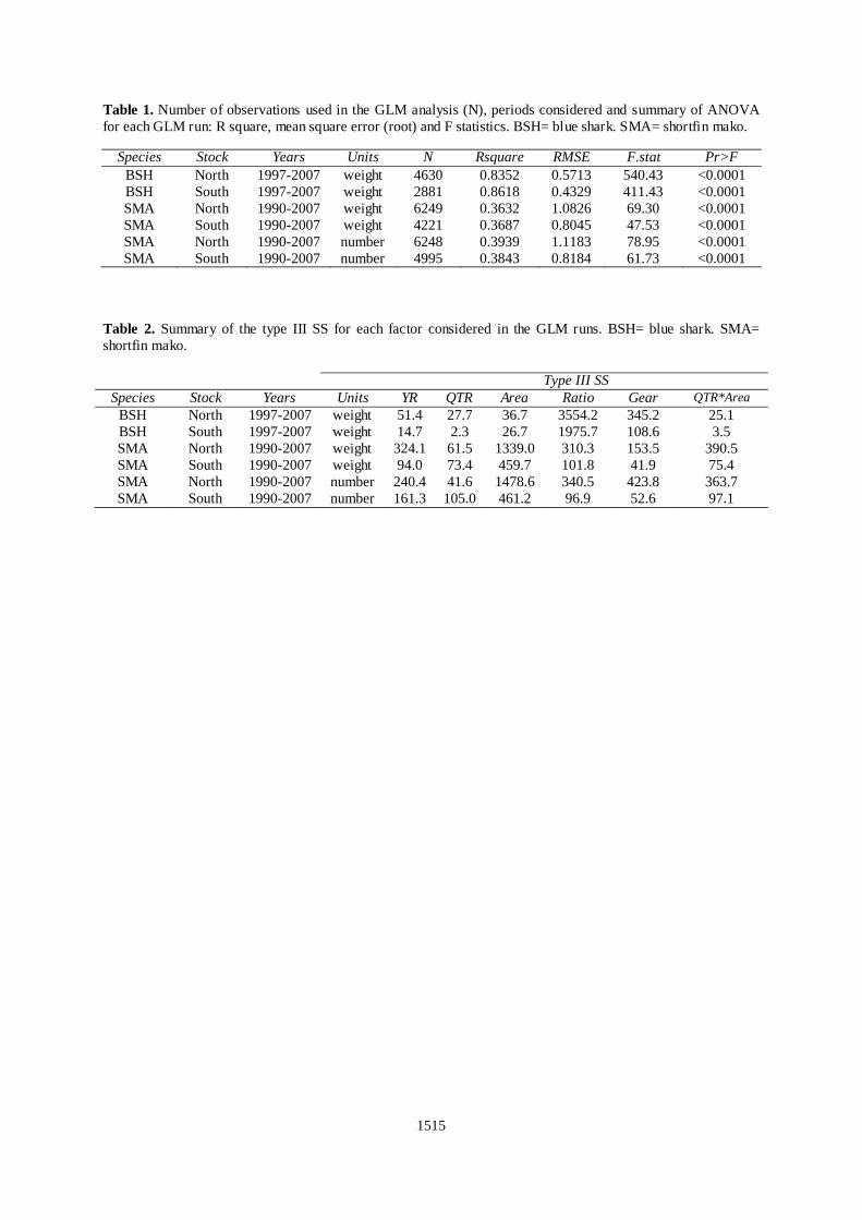
Table 1. Number of observations used in the GLM analysis (N), periods considered and summary of ANOVA for each GLM run: R square, mean square error (root) and F statistics. BSH= blue shark. SMA= shortfin mako.  

Species Stock Years Units N Rsquare RMSE F.stat Pr>F BSH North 1997-2007 weight 4630 0.8352 0.5713 540.43 <0.0001 BSH South 1997-2007 weight 2881 0.8618 0.4329 411.43 <0.0001 SMA North 1990-2007 weight 6249 0.3632 1.0826 69.30 <0.0001 SMA South 1990-2007 weight 4221 0.3687 0.8045 47.53 <0.0001 SMA North 1990-2007 number 6248 0.3939 1.1183 78.95 <0.0001 SMA South 1990-2007 number 4995 0.3843 0.8184 61.73 <0.0001

Table 2. Summary of the type III SS for each factor considered in the GLM runs. BSH= blue shark. SMA= shortfin mako.

Type III SS Species Stock Years Units YR QTR Area Ratio Gear QTR*Area

BSH North 1997-2007 weight 51.4 27.7 36.7 3554.2 345.2 25.1 BSH South 1997-2007 weight 14.7 2.3 26.7 1975.7 108.6 3.5 SMA North 1990-2007 weight 324.1 61.5 1339.0 310.3 153.5 390.5 SMA South 1990-2007 weight 94.0 73.4 459.7 101.8 41.9 75.4 SMA North 1990-2007 number 240.4 41.6 1478.6 340.5 423.8 363.7 SMA South 1990-2007 number 161.3 105.0 461.2 96.9 52.6 97.1

     

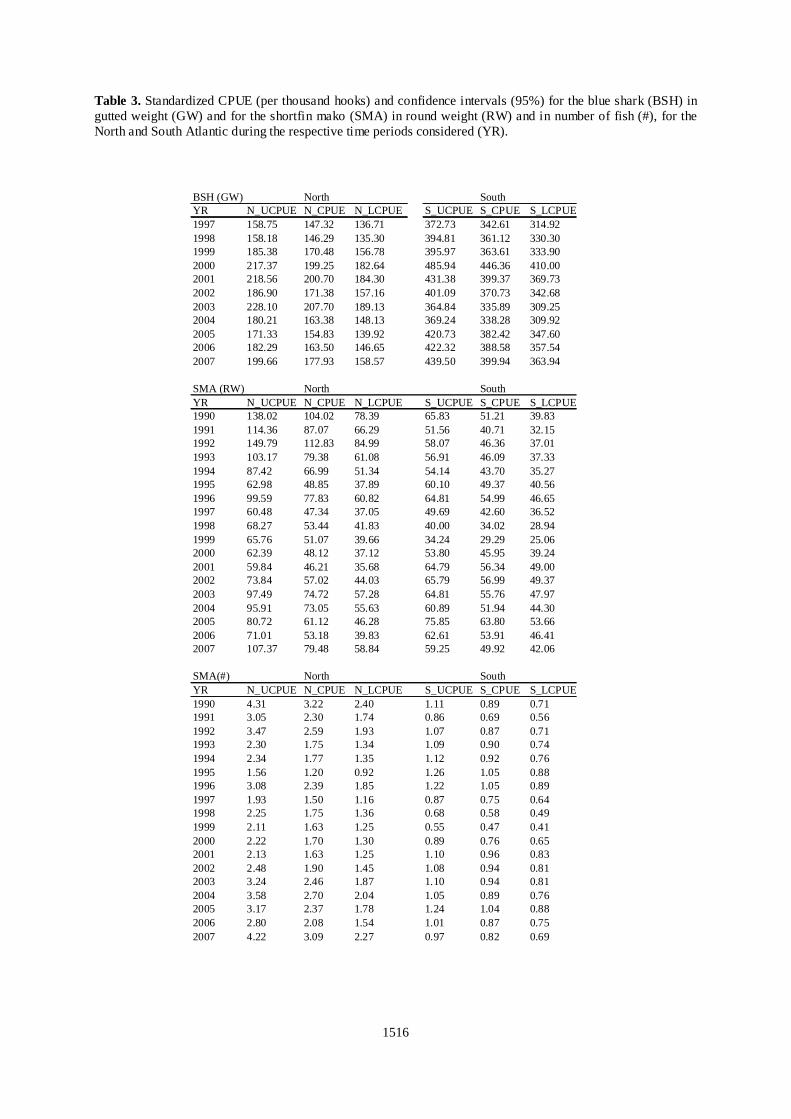
Table 3. Standardized CPUE (per thousand hooks) and confidence intervals (95%) for the blue shark (BSH) in gutted weight (GW) and for the shortfin mako (SMA) in round weight (RW) and in number of fish (#), for the North and South Atlantic during the respective time periods considered (YR).                 

1516

BSH (GW) North South YR N_UCPUE N_CPUE N_LCPUE S_UCPUE S_CPUE S_LCPUE1997 158.75 147.32 136.71 372.73 342.61 314.921998 158.18 146.29 135.30 394.81 361.12 330.301999 185.38 170.48 156.78 395.97 363.61 333.902000 217.37 199.25 182.64 485.94 446.36 410.002001 218.56 200.70 184.30 431.38 399.37 369.732002 186.90 171.38 157.16 401.09 370.73 342.682003 228.10 207.70 189.13 364.84 335.89 309.252004 180.21 163.38 148.13 369.24 338.28 309.922005 171.33 154.83 139.92 420.73 382.42 347.602006 182.29 163.50 146.65 422.32 388.58 357.542007 199.66 177.93 158.57 439.50 399.94 363.94

SMA (RW) North South YR N_UCPUE N_CPUE N_LCPUE S_UCPUE S_CPUE S_LCPUE1990 138.02 104.02 78.39 65.83 51.21 39.831991 114.36 87.07 66.29 51.56 40.71 32.151992 149.79 112.83 84.99 58.07 46.36 37.011993 103.17 79.38 61.08 56.91 46.09 37.331994 87.42 66.99 51.34 54.14 43.70 35.271995 62.98 48.85 37.89 60.10 49.37 40.561996 99.59 77.83 60.82 64.81 54.99 46.651997 60.48 47.34 37.05 49.69 42.60 36.521998 68.27 53.44 41.83 40.00 34.02 28.941999 65.76 51.07 39.66 34.24 29.29 25.062000 62.39 48.12 37.12 53.80 45.95 39.242001 59.84 46.21 35.68 64.79 56.34 49.002002 73.84 57.02 44.03 65.79 56.99 49.372003 97.49 74.72 57.28 64.81 55.76 47.972004 95.91 73.05 55.63 60.89 51.94 44.302005 80.72 61.12 46.28 75.85 63.80 53.662006 71.01 53.18 39.83 62.61 53.91 46.412007 107.37 79.48 58.84 59.25 49.92 42.06

SMA(#) North SouthYR N_UCPUE N_CPUE N_LCPUE S_UCPUE S_CPUE S_LCPUE1990 4.31 3.22 2.40 1.11 0.89 0.711991 3.05 2.30 1.74 0.86 0.69 0.561992 3.47 2.59 1.93 1.07 0.87 0.711993 2.30 1.75 1.34 1.09 0.90 0.741994 2.34 1.77 1.35 1.12 0.92 0.761995 1.56 1.20 0.92 1.26 1.05 0.881996 3.08 2.39 1.85 1.22 1.05 0.891997 1.93 1.50 1.16 0.87 0.75 0.641998 2.25 1.75 1.36 0.68 0.58 0.491999 2.11 1.63 1.25 0.55 0.47 0.412000 2.22 1.70 1.30 0.89 0.76 0.652001 2.13 1.63 1.25 1.10 0.96 0.832002 2.48 1.90 1.45 1.08 0.94 0.812003 3.24 2.46 1.87 1.10 0.94 0.812004 3.58 2.70 2.04 1.05 0.89 0.762005 3.17 2.37 1.78 1.24 1.04 0.882006 2.80 2.08 1.54 1.01 0.87 0.752007 4.22 3.09 2.27 0.97 0.82 0.69

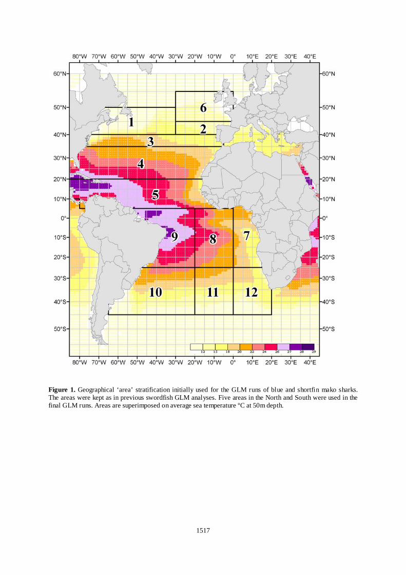
Figure 1. Geographical ‘area’ stratification initially used for the GLM runs of blue and shortfin mako sharks. The areas were kept as in previous swordfish GLM analyses. Five areas in the North and South were used in the final GLM runs. Areas are superimposed on average sea temperature ºC at 50m depth.

1517

1518

Normal probability qqplot

Freq

‚ ** **

500 ̂ ** ** **

N or m al pr o ba b il i ty qq p lo t F r eq ‚ * * 3 5 0 ˆ * * ‚ * * ‚ * * * * ‚ * * * * ‚ * * * * * *

‚ ** ** **

‚ ** ** ** **

‚ ** ** ** ** ** ‚ ** ** ** ** **

400 ̂ ** ** ** ** **

‚ ** ** ** ** ** ** ‚ ** ** ** ** ** **

‚ ** ** ** ** ** **

‚ ** ** ** ** ** ** ** 300 ̂ ** ** ** ** ** ** **

‚ ** ** ** ** ** ** ** **

‚ ** ** ** ** ** ** ** ** ‚ ** ** ** ** ** ** ** **

‚ ** ** ** ** ** ** ** ** ** 200 ̂ ** ** ** ** ** ** ** ** ** **

‚ ** ** ** ** ** ** ** ** ** **

‚ ** ** ** ** ** ** ** ** ** ** ‚ ** ** ** ** ** ** ** ** ** ** **

‚ ** ** ** ** ** ** ** ** ** ** ** **

100 ̂ ** ** ** ** ** ** ** ** ** ** ** ** ** ** ‚ ** ** ** ** ** ** ** ** ** ** ** ** ** ** ** **

‚ ** ** ** ** ** ** ** ** ** ** ** ** ** ** ** **

‚ ** ** ** ** ** ** ** ** ** ** ** ** ** ** ** ** ** ** ** ** ** ‚ ** ** ** ** ** ** ** ** ** ** ** ** ** ** ** ** ** ** ** ** **

Šƒƒƒƒƒƒƒƒƒƒƒƒƒƒƒƒƒƒƒƒƒƒƒƒƒƒƒƒƒƒƒƒƒƒƒƒƒƒƒƒƒƒƒƒƒƒƒƒƒƒƒƒƒƒƒƒƒƒƒƒƒƒƒƒ

- - - - - - - - - - 2 2 2 1 1 1 1 0 0 0 0 0 0 0 1 1 1 1 2 2 2

. . . . . . . . . . . . . . . . . . . . .

5 2 0 7 5 2 0 7 5 2 0 2 5 7 0 2 5 7 0 2 5 0 5 0 5 0 5 0 5 0 5 0 5 0 5 0 5 0 5 0 5 0

3 0 0 ˆ * * * * * * ‚ * * * * * * * * ‚ * * * * * * * * * * ‚ * * * * * * * * * * ‚ * * * * * * * * * * 2 5 0 ˆ * * * * * * * * * * ‚ * * * * * * * * * * * * ‚ * * * * * * * * * * * * ‚ * * * * * * * * * * * * ‚ * * * * * * * * * * * * 2 0 0 ˆ * * * * * * * * * * * * * * ‚ * * * * * * * * * * * * * * ‚ * * * * * * * * * * * * * * ‚ * * * * * * * * * * * * * * * * ‚ * * * * * * * * * * * * * * * * 1 5 0 ˆ * * * * * * * * * * * * * * * * ‚ * * * * * * * * * * * * * * * * * * ‚ * * * * * * * * * * * * * * * * * * * * ‚ * * * * * * * * * * * * * * * * * * * * ‚ * * * * * * * * * * * * * * * * * * * * 1 0 0 ˆ * * * * * * * * * * * * * * * * * * * * ‚ * * * * * * * * * * * * * * * * * * * * ‚ * * * * * * * * * * * * * * * * * * * * ‚ * * * * * * * * * * * * * * * * * * * * * * * * * * ‚ * * * * * * * * * * * * * * * * * * * * * * * * * * 5 0 ˆ * * * * * * * * * * * * * * * * * * * * * * * * * * * * ** ‚ * * * * * * * * * * * * * * * * * * * * * * * * * * * * ** ‚ * * * * * * * * * * * * * * * * * * * * * * * * * * * * * * ** ** ‚ * * * * * * * * * * * * * * * * * * * * * * * * * * * * * * * * * * ** ** ** ‚ * * * * * * * * * * * * * * * * * * * * * * * * * * * * * * * * * * ** ** ** ** Š ƒƒ ƒ ƒƒ ƒ ƒƒ ƒ ƒƒ ƒ ƒƒ ƒ ƒƒ ƒƒ ƒ ƒƒ ƒ ƒƒ ƒ ƒƒ ƒ ƒƒ ƒ ƒƒ ƒ ƒƒ ƒ ƒƒ ƒ ƒƒ ƒ ƒƒ ƒ ƒƒ ƒ ƒƒ ƒ ƒƒ ƒƒ ƒ ƒƒ ƒ ƒƒ ƒ - - - - - - - - - - 2 2 2 1 1 1 1 0 0 0 0 0 0 0 1 1 1 1 2 2 2 . . . . . . . . . . . . . . . . . . . . . 5 2 0 7 5 2 0 7 5 2 0 2 5 7 0 2 5 7 0 2 5 0 5 0 5 0 5 0 5 0 5 0 5 0 5 0 5 0 5 0 5 0 st u d1

Normal probability qqplot Freq

700 ̂ **

‚ ** ‚ ** **

‚ ** ** ‚ ** **

600 ̂ ** ** ** ‚ ** ** **

‚ ** ** ** ‚ ** ** ** ** ** ‚ ** ** ** ** **

500 ̂ ** ** ** ** ** ‚ ** ** ** ** ** **

‚ ** ** ** ** ** ** ‚ ** ** ** ** ** ** **

‚ ** ** ** ** ** ** ** 400 ̂ ** ** ** ** ** ** **

‚ ** ** ** ** ** ** ** ** ‚ ** ** ** ** ** ** ** ** **

‚ ** ** ** ** ** ** ** ** ** ‚ ** ** ** ** ** ** ** ** ** 300 ̂ ** ** ** ** ** ** ** ** **

‚ ** ** ** ** ** ** ** ** ** ** ‚ ** ** ** ** ** ** ** ** ** ** **

‚ ** ** ** ** ** ** ** ** ** ** ** ‚ ** ** ** ** ** ** ** ** ** ** **

200 ̂ ** ** ** ** ** ** ** ** ** ** ** ** ‚ ** ** ** ** ** ** ** ** ** ** ** ** **

‚ ** ** ** ** ** ** ** ** ** ** ** ** ** ‚ ** ** ** ** ** ** ** ** ** ** ** ** ** **

‚ ** ** ** ** ** ** ** ** ** ** ** ** ** ** ** 100 ̂ ** ** ** ** ** ** ** ** ** ** ** ** ** ** **

‚ ** ** ** ** ** ** ** ** ** ** ** ** ** ** ** ** ** ** ** ‚ ** ** ** ** ** ** ** ** ** ** ** ** ** ** ** ** ** ** ** ** ** ‚ ** ** ** ** ** ** ** ** ** ** ** ** ** ** ** ** ** ** ** ** **

‚ ** ** ** ** ** ** ** ** ** ** ** ** ** ** ** ** ** ** ** ** ** Šƒƒƒƒƒƒƒƒƒƒƒƒƒƒƒƒƒƒƒƒƒƒƒƒƒƒƒƒƒƒƒƒƒƒƒƒƒƒƒƒƒƒƒƒƒƒƒƒƒƒƒƒƒƒƒƒƒƒƒƒƒƒƒƒ

- - - - - - - - - - 2 2 2 1 1 1 1 0 0 0 0 0 0 0 1 1 1 1 2 2 2

. . . . . . . . . . . . . . . . . . . . . 5 2 0 7 5 2 0 7 5 2 0 2 5 7 0 2 5 7 0 2 5

0 5 0 5 0 5 0 5 0 5 0 5 0 5 0 5 0 5 0 5 0

stud1

Normal probability qqplot Freq ‚ ** ‚ ** ** ‚ ** ** 400 ˆ ** ** ** ** ‚ ** ** ** ** ** ‚ ** ** ** ** ** ‚ ** ** ** ** ** ** ‚ ** ** ** ** ** ** 300 ˆ ** ** ** ** ** ** ** ‚ ** ** ** ** ** ** ** ‚ ** ** ** ** ** ** ** ‚ ** ** ** ** ** ** ** ‚ ** ** ** ** ** ** ** ** 200 ˆ ** ** ** ** ** ** ** ** ** ‚ ** ** ** ** ** ** ** ** ** ** ‚ ** ** ** ** ** ** ** ** ** ** ** ‚ ** ** ** ** ** ** ** ** ** ** ** ‚ ** ** ** ** ** ** ** ** ** ** ** ** 100 ˆ ** ** ** ** ** ** ** ** ** ** ** ** ** ‚ ** ** ** ** ** ** ** ** ** ** ** ** ** ** ** ** ‚ ** ** ** ** ** ** ** ** ** ** ** ** ** ** ** ** ‚ ** ** ** ** ** ** ** ** ** ** ** ** ** ** ** ** ** ** ** ** ‚ ** ** ** ** ** ** ** ** ** ** ** ** ** ** ** ** ** ** ** ** ** Šƒƒƒƒƒƒƒƒƒƒƒƒƒƒƒƒƒƒƒƒƒƒƒƒƒƒƒƒƒƒƒƒƒƒƒƒƒƒƒƒƒƒƒƒƒƒƒƒƒƒƒƒƒƒƒƒƒƒƒƒƒƒƒƒ - - - - - - - - - - 2 2 2 1 1 1 1 0 0 0 0 0 0 0 1 1 1 1 2 2 2 . . . . . . . . . . . . . . . . . . . . . 5 2 0 7 5 2 0 7 5 2 0 2 5 7 0 2 5 7 0 2 5 0 5 0 5 0 5 0 5 0 5 0 5 0 5 0 5 0 5 0 5 0 stud1

Normal probability qqplot

Freq

700 ̂ ** ‚ **

‚ ** ‚ ** ** ‚ ** ** **

600 ̂ ** ** ** ‚ ** ** **

‚ ** ** ** ‚ ** ** ** **

‚ ** ** ** ** ** 500 ̂ ** ** ** ** ** ‚ ** ** ** ** **

‚ ** ** ** ** ** ** ‚ ** ** ** ** ** ** **

‚ ** ** ** ** ** ** ** 400 ̂ ** ** ** ** ** ** ** ‚ ** ** ** ** ** ** ** **

‚ ** ** ** ** ** ** ** ** ‚ ** ** ** ** ** ** ** ** **

‚ ** ** ** ** ** ** ** ** ** 300 ̂ ** ** ** ** ** ** ** ** **

‚ ** ** ** ** ** ** ** ** ** ** ** ‚ ** ** ** ** ** ** ** ** ** ** ** ‚ ** ** ** ** ** ** ** ** ** ** **

‚ ** ** ** ** ** ** ** ** ** ** ** 200 ̂ ** ** ** ** ** ** ** ** ** ** ** **

‚ ** ** ** ** ** ** ** ** ** ** ** ** ** ‚ ** ** ** ** ** ** ** ** ** ** ** ** **

‚ ** ** ** ** ** ** ** ** ** ** ** ** ** ** ‚ ** ** ** ** ** ** ** ** ** ** ** ** ** ** ** 100 ̂ ** ** ** ** ** ** ** ** ** ** ** ** ** ** **

‚ ** ** ** ** ** ** ** ** ** ** ** ** ** ** ** ** ** ** ‚ ** ** ** ** ** ** ** ** ** ** ** ** ** ** ** ** ** ** **

‚ ** ** ** ** ** ** ** ** ** ** ** ** ** ** ** ** ** ** ** ** ** ‚ ** ** ** ** ** ** ** ** ** ** ** ** ** ** ** ** ** ** ** ** **

Šƒƒƒƒƒƒƒƒƒƒƒƒƒƒƒƒƒƒƒƒƒƒƒƒƒƒƒƒƒƒƒƒƒƒƒƒƒƒƒƒƒƒƒƒƒƒƒƒƒƒƒƒƒƒƒƒƒƒƒƒƒƒƒƒ - - - - - - - - - - 2 2 2 1 1 1 1 0 0 0 0 0 0 0 1 1 1 1 2 2 2

. . . . . . . . . . . . . . . . . . . . . 5 2 0 7 5 2 0 7 5 2 0 2 5 7 0 2 5 7 0 2 5

0 5 0 5 0 5 0 5 0 5 0 5 0 5 0 5 0 5 0 5 0

stud1

Normal probability qqplot Freq

‚ ** ‚ ** ‚ ** ** ** 500 ˆ ** ** ** **

‚ ** ** ** ** ‚ ** ** ** ** ‚ ** ** ** ** ** ‚ ** ** ** ** ** **

400 ˆ ** ** ** ** ** ** ‚ ** ** ** ** ** ** ‚ ** ** ** ** ** ** ** ‚ ** ** ** ** ** ** ** ‚ ** ** ** ** ** ** **

300 ˆ ** ** ** ** ** ** ** ‚ ** ** ** ** ** ** ** ‚ ** ** ** ** ** ** ** ** ** ‚ ** ** ** ** ** ** ** ** **

‚ ** ** ** ** ** ** ** ** ** 200 ˆ ** ** ** ** ** ** ** ** ** ** ** ‚ ** ** ** ** ** ** ** ** ** ** ** ‚ ** ** ** ** ** ** ** ** ** ** **

‚ ** ** ** ** ** ** ** ** ** ** ** ** ‚ ** ** ** ** ** ** ** ** ** ** ** ** ** 100 ˆ ** ** ** ** ** ** ** ** ** ** ** ** ** ‚ ** ** ** ** ** ** ** ** ** ** ** ** ** ** ** ** ‚ ** ** ** ** ** ** ** ** ** ** ** ** ** ** ** ** ** ** **

‚ ** ** ** ** ** ** ** ** ** ** ** ** ** ** ** ** ** ** ** ** ** ‚ ** ** ** ** ** ** ** ** ** ** ** ** ** ** ** ** ** ** ** ** ** Šƒƒƒƒƒƒƒƒƒƒƒƒƒƒƒƒƒƒƒƒƒƒƒƒƒƒƒƒƒƒƒƒƒƒƒƒƒƒƒƒƒƒƒƒƒƒƒƒƒƒƒƒƒƒƒƒƒƒƒƒƒƒƒƒ - - - - - - - - - -

2 2 2 1 1 1 1 0 0 0 0 0 0 0 1 1 1 1 2 2 2 . . . . . . . . . . . . . . . . . . . . . 5 2 0 7 5 2 0 7 5 2 0 2 5 7 0 2 5 7 0 2 5 0 5 0 5 0 5 0 5 0 5 0 5 0 5 0 5 0 5 0 5 0

stud1

A B

C D

E F

Figure 2a. Distribution of the standardized residual for years combined. (A): BSH in weight, North. (B): BSH in weight, South. (C): SMA in weight, North. (D): SMA in weight, South. (E): SMA in number, North. (F): SMA in number, South. The red dots indicate the location of the zero value.

-4 - 2 0 2 4

-6

-4

-2

0

2

4

stud1

Cuant i l es nor mal es

-4 - 2 0 2 4

-4

-2

0

2

4

stud1

Cuant i l es nor mal es

-4 - 2 0 2 4

-6

-4

-2

0

2

4

stud1

Cuant i l es nor mal es

-4 - 2 0 2 4

-4

-2

0

2

4

stud1

Cuant i l es nor mal es

-4 -2 0 2 4

-6

-4

-2

0

2

4

6

stud1

Cuant i l es nor mal es

A B

C D

E F

Figure 2b. Normal probability qq-plots. (A): BSH in weight, North. (B): BSH in weight, South. (C): SMA in weight, North. (D): SMA in weight, South. (E): SMA in number, North. (F): SMA in number, South.

1519

1520

Figure 2 c. Box plot of the standardized residuals versus year. (A): BSH in weight, North. (B): BSH in weight, South. (C): SMA in weight, North. (D): SMA in weight, South. (E): SMA in number, North. (F): SMA in number, South. Periods 1997-2007 and 1990-2007 are plotted for BSH and SMA, respectively.

1997 1998 1999 2000 2001 2002 2003 2004 2005 2006 2007

-7.

-5.

-2.

2.

5. 0

stud1

5

0

5

0

5

YR

1990 19911992 1993 1994 19951996 1997 19981999 2000 2001 20022003 2004 2005 2006 2007

-4

-2

0

2

4

stud1

YR1990 19911992 1993 1994 19951996 1997 19981999 2000 2001 20022003 2004 2005 2006 2007

-6

-4

-2

0

2

4

stud1

YR

1990 19911992 1993 1994 19951996 1997 19981999 2000 2001 20022003 2004 2005 2006 2007

-4

-2

0

2

4

stud1

YR

1990 19911992 1993 1994 19951996 1997 19981999 2000 2001 20022003 2004 2005 2006 2007

-6

-4

-2

0

2

4

stud1

YR

A B

C D

E F

YEARS YEARS

Blue shark CPUE in weigth

0

100

200

300

400

500

600

700

800

1997 1998 1999 2000 2001 2002 2003 2004 2005 2006 2007

years

Stan

dard

ized

inde

x (w

eigh

t)N_UCPUEN_CPUEN_LCPUES_UCPUES_CPUES_LCPUE

Shortfin mako CPUE in weigth

020406080

100120140160180200

1990 1992 1994 1996 1998 2000 2002 2004 2006

years

Stan

dard

ized

inde

x (w

eigh

t)

N_UCPUEN_CPUE

N_LCPUES_UCPUE

S_CPUE

S_LCPUE

Shortfin mako CPUE in number

0

1

2

3

4

5

6

7

1990 1992 1994 1996 1998 2000 2002 2004 2006

years

Stan

dard

ized

inde

x

N_UCPUE

N_CPUE

N_LCPUE

S_UCPUE

S_CPUE

S_LCPUE

Shortfin mako: stand. mean weight

0102030405060708090

100

1990 1992 1994 1996 1998 2000 2002 2004 2006

years

Kg ro

und

wei

ght

N_mean WS_mean W

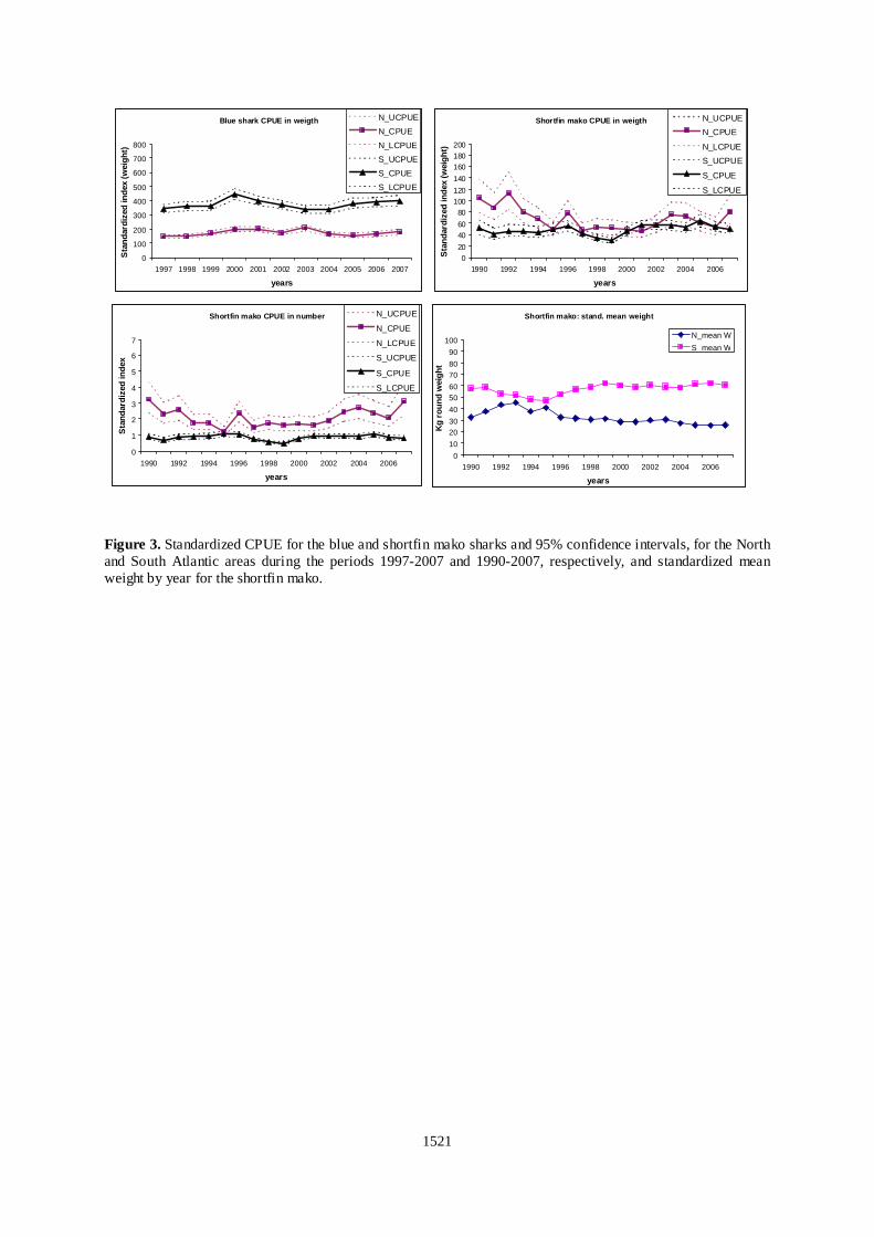
Figure 3. Standardized CPUE for the blue and shortfin mako sharks and 95% confidence intervals, for the North and South Atlantic areas during the periods 1997-2007 and 1990-2007, respectively, and standardized mean weight by year for the shortfin mako.

1521