SCRS/2001/106

STANDARDIZED CATCH RATES FOR SAILFISH (Istiophorus platypterus) FROM UNITED STATES RECREATIONAL FISHERY SURVEYS IN THE NORTHWEST

ATLANTIC AND GULF OF MEXICO.

Mauricio Ortiz and Craig Brown1

SUMMARY

Indices of abundance of sailfish from the United States recreational billfish tournaments and from a general statistical survey of recreational catches are presented for the period 1973-2000. The tournament index of weight (kg) per 100 hours fishing was estimated from numbers and size of sailfish caught and reported in the logbooks submitted by recreational tournament coordinators and NMFS observers under the Recreational Billfish Survey Program. A general index of numbers of fish per angler trip was estimated from intercept surveys conducted by the Marine Recreational Fisheries Statistics Survey. The standardized indices were estimated using Generalized Linear Mixed Models under a delta lognormal model approach.

RÉSUMÉ

Le présent document fait état des indices d=abondance du voilier provenant de championnats américains de pêche sportive et d=une enquête statistique générale sur les captures sportives pour les années 1973-2000. L=indice pondéral (kg) des championnats par 100 heures de pêche a été estimé d=après le nombre et la taille des voiliers capturés et déclarés dans les carnets de pêche remis par les coordinateurs des championnats de pêche sportive et les observateurs du NMFS dans le cadre du Recreational Billfish Survey Program. Un indice général du nombre de poissons par sortie de pêche à la ligne a été estimée d=après des prospections effectuées par la Marine Recreational Fisheries Statistics Survey. Les indices standardisés ont été estimés par le modèle linéaire généralisé mixte selon une approche delta-lognormale.

RESUMEN

Se presentan los índices de abundancia del pez vela para el periodo 1973-2000, procedentes de los torneos deportivos de marlines de Estados Unidos y de una encuesta general estadística de capturas deportivas. El índice de peso (kg) por cada 100 horas de pesca de los torneos se estimó a partir de los números y la talla de los peces vela capturados y declarados en los cuadernos de pesca presentados por los coordinadores de los torneos deportivos y los observadores del NMFS según el Programa de Encuestas Deportivas de Marlines. Se estimó un índice general de números de peces por salida de pescador a partir de encuestas realizadas por el Estudio de Estadísticas de Pesquerías Deportivas Marinas. Los índices estandarizados se estimaron utilizando modelos lineales mixtos generalizados según un enfoque de modelo delta lognormal.

KEYWORDS

Catch/effort, abundance, sport fishing, pelagic fisheries, multivariate analysis

1 U.S. Department of Commerce National Marine Fisheries Service Southeast Fisheries Science Center,75 Virginia Beach Drive, Miami, Florida 33149 U.S. email Mauricio.Ortiz@noaa.gov

1. INTRODUCTION

Information on the relative abundance of sailfish (Istiophorus platypterus) is necessary to tune stock assessment models. Two sources of this information were investigated in this document: 1) the Recreational Billfish Tournament Survey (RBS), and 2) the generalized Marine Recreational Fishery Statistics Survey (MRFSS).

Tournament catch and effort data from U.S. recreational tournaments along the Atlantic East coast

(including the Bahamas), Gulf of Mexico, and Caribbean (U.S. Virgin Islands and Puerto Rico) have been collected by the RBS Program since 1972. Beardsley and Conser (1981), and Prince et al (1990) have described the survey. Indices of abundance for blue marlin (Makaira nigricans), white marlin (Tetrapturus albidus), and for sailfish from this survey data were previously estimated by Ortiz and Farber (2001), and Farber (1994). Catch in numbers and effort data were obtained from tournament data documented by the RBS, which were voluntarily submitted to the National Marine Fisheries Service (NMFS) and from scientific observers that monitored selected billfish tournaments. This report documents the analytical methods applied to the available RBS data through 2000 and presents correspondent standardized CPUE indices for sailfish.

Recreational catch and effort are collected during the intercept survey component of the MRFSS,

in which anglers are intercepted, screened, and interviewed at assigned access sites upon completion of their fishing trips (U.S. Department of Commerce 1990). Intercepts are not conducted at tournament sites. Data from oceanic trips off the Florida East coast from 1981-2000 were used to develop standardized CPUE indices. 2. MATERIALS AND METHODS 2.1 RBS

Browder and Prince (1990) describe the main features of the recreational tournaments that take

place in the West Atlantic and Caribbean, and review the available catch and effort data from RBS data. Standardized catch rate indices of sailfish were previously estimated for the 1994 stock assessment using Generalized Linear Models (GLM) (Farber 1994). The present report, updates the catch and effort information through 2000 and includes analyses of variability associated with random factor interactions, particularly for the Year effect, following the suggestion of the billfish working group of the ICCAT Scientific Committee of Research and Statistics (SCRS). Logbook records from the recreational tournaments have been collected since 1972 either by NMFS personal or through voluntary submission by tournament organizers. Recent changes in U.S. regulations require all recreational tournaments to register and provide catch and effort data to the NMFS (Anonymous 1999).

The RBS data comprise a total of 14,744 records dating from 1973 through 2000. Each record

represents information on hooked and caught fish by tournament-day. Fishing effort is estimated from the number of boats registered in the tournament times the average-fishing hours per boat-day. Records also include total number of fish hooked, their fate (i.e. lost, release, tagged and released, or boated) by species, and morphometric information (size and weight) for boated fish. There are a total of 504 registered tournaments in the RBS database. From those the following selecting criteria were applied: a) data from tournament events only, excluding biological sampling programs and or dock sampling not associated with tournaments. And b) tournaments that have recorded at least one sailfish caught in their historical records. The final working data set included a total of 6,127 records representing 270 recreational tournaments from the North Atlantic, Gulf of Mexico, and the Caribbean. For the present analysis only recreational tournaments that have registered and submitted catch and effort information were included in analysis.

Figure 1 shows the geographical distribution of the included tournaments; markers represent the

main city/port from where the tournament operated. Tournaments were classified whether sailfish is a

principal target species (sailfish tournaments), and non-sailfish tournament if sailfish is an occasional catch not targeted (i.e. blue marlin and white marlin tournaments). Tournaments were also classified into one of six geographical regions for this analysis: (1) New England (Massachusetts and Rhode Island), (2) Mid Atlantic (New York, New Jersey, Delaware, Maryland, and Virginia), (3) South Atlantic (North Carolina, South Carolina, Georgia, and the East coast of Florida), (4) The Bahamas, (5) US Gulf of Mexico (Texas, Louisiana, Mississippi, Alabama and Florida West coast, and (6) the Caribbean (Puerto Rico and US Virgin Islands). Figure 2 shows the total number of tournaments registered that have reported sailfish catch per year, and the number of participant boats per year of these tournaments. In general, an increase of recreational tournament participating fishing effort has been observed from 1973 to 1990, since then the number of tournaments and participant boats that catch sailfish has declined. To account for seasonal characteristics, 3 season were defined: (1) January through April, (2) May through August, and (3) September through December.

Tournament logbooks record numbers of fish primarily and size or weight from boated fish. As

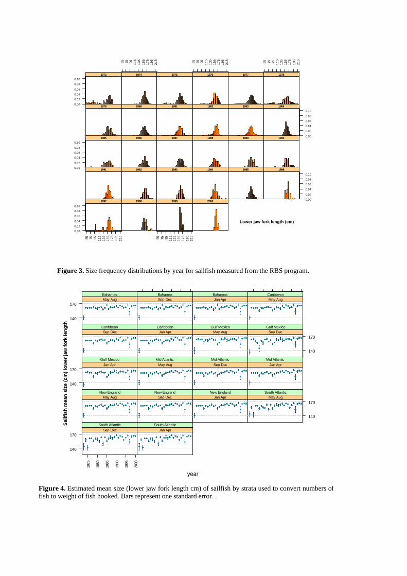
per suggestion of the Billfish SCRS working group, indices of abundance are reported in weight rather than numbers of fish. To convert numbers of fish to weight, size information on sailfish boated by recreational tournaments was retrieved from the RBS database. There were 3,764-recorded sizes for sailfish; Figure 3 shows the size frequency distributions by year. Mean size by each year area season stratum was estimated if there were 20 or more records per cell. For a cell with less than 20 fish, the annual mean size of the area was used, if for a given area-year, the number were still less than 20, the mean size by year across all areas was applied. Figure 4 shows the mean size by strata used for the conversion of numbers to weight of hooked sailfish. Mean size was converted to weight (kg) using the current size-weight relationships for sailfish-combined sex (Prager et al. 1995). Analysis of catch rates were done on the total number of hooked fish (including hooked and lost fish, caught and release fish, and boated fish) rather than the number of caught fish because of the implementation of minimum size regulations and the catch and release prevalence of US tournaments in particular for the latest years.

For the RBS tournament data, a relative index of abundance for sailfish was estimated by a

Generalized Linear Modeling approach assuming a delta lognormal model distribution. The delta model estimates separately the proportion of positive trip/day assuming a binomial error distribution, and the mean catch rate of trip/day where at least one sailfish was caught assuming a lognormal error distribution. The log-transformed frequency distributions of catch rates in weight and numbers for sailfish are shown in Figure 5. The estimated proportion of successful trip/sets per stratum is assumed to be the result of r positive trip/days of a total n number of trip/days, and each one is an independent Bernoulli-type realization. The estimated proportion is a linear function of fixed effects and interactions. The logit function was used as link between the linear factor component and the binomial error. For trip/days that caught at least one sailfish (i.e. positive observations), estimated catch rates were assumed to follow a lognormal error distribution (lnHPUE) of a linear function of fixed factors and random effect interactions, particularly when the Year effect was within the interaction. Year, area, season and sailfish-target tournament (TourSail), and their interactions were the factors included in the analysis.

A step-wise regression procedure was used to determine the set of systematic factors and

interactions that significantly explained the observed variability. Because the difference of deviance between two consecutive nested models follows a χ2 (Chi-square) distribution; this statistic was used to test for the significance of an additional factor in the model. The number of additional parameters associated with the added factor minus one corresponds to the number of degrees of freedom in the χ2

test (McCullagh and Nelder, 1989). Deviance analysis tables include the deviance for the proportion of positive observations (i.e. positive trips/total trips), and the deviance for the positive catch rates. Final selection of explanatory factors was conditional on: a) the relative percent of deviance explained by adding the factor in evaluation, normally factors that explained more than 5% were selected, b) the χ2 test significance, and c) the type III test significance within the final specified model.

Once a set of fixed factors was specified, possible interactions were evaluated, in particular interactions between the Year effect and other factors. Selection of the final mixed model was based on the Akaike’s Information Criterion (AIC), the Schwarz’s Bayesian Criterion (SBC), and a chi-square test of the difference between the [–2 loglikelihood] statistic of a successive nested model formulations (Littell et al. 1996). Relative indices for the delta model formulation were calculated as the product of the year effect least square means (LSmeans) from the binomial and the lognormal model components. The LSmeans estimates use a weighted factor of the proportional observed margins in the input data to account for the un-balance characteristics of the data. LSmeans of lognormal positive trips were bias corrected using Lo et al., (1992) algorithms. Analyses were done using the GLIMMIX and MIXED procedures from the SAS statistical computer software (SAS Institute Inc. 1997).

2.2 MRFSS

The survey methodology of the MRFSS is described by the U.S. Department of Commerce

(1990). The intercept data available for this study was restricted to the region off the eastern coast of Florida. Only oceanic fishing in the charter or private/rental modes were included. Since the MRFSS is a generalized survey of all saltwater recreational fishing and sailfish targeted effort represents only a small component of oceanic fishing, the data was further restricted to that representing effort directed at sailfish.

Observations were defined at the group level, that is, one or more individuals on a fishing trip

representing the smallest number of fishers to which catch and effort could be individually assigned. In many cases, more than one group could have fished during the same boat trip; for these cases, the observations are not truly independent. However, information required to total catch and effort for an entire boat trip was not collected until 1991. If all individuals within a group were not interviewed, it was necessary to expand the reported (but not observed by the interviewer) catch of the interviewed individuals proportionally so as to be representative of the entire group. Catch rate was defined as the

number of sailfish caught (kept plus released) divided by the number of angler.hours. The available variables included year, month, county (where intercepted), trip type (charter or

private/rental), and zone (< 3 miles offshore, > 3 miles offshore). Additionally, season was defined as either November-February or March-October. The geographic distribution of sailfish targeted effort (1981-2000) is shown in Figure 10; the relative catch rates at those locations are represented in Figure 11. The locations are approximate: latitude was defined based upon the mid-latitude of the intercept county and longitude was assigned at points 2 miles offshore or 15 miles offshore, depending upon zone.

Parameterization of the model was accomplished using a Generalized Linear Model (GLM)

structure in a manner similar to that used for the RBS analysis: The proportion of successful (i.e. positive observations) trips per stratum was assumed to follow a binomial distribution where the estimated probability was a linearized function of fixed factors. The logit function linked the linear

component and the assumed binomial distribution. Similarly, the estimated catch per angler.hour observed on positive trips was modeled as function of similar fixed factors with the log function as a link.

A stepwise approach was used to quantify the relative importance of the main factors explaining

the variance in catch rates. That is, first the Null model was run, in which no factors were entered in the model. These results reflect the distribution of the nominal data. Each potential factor was then tested one at a time. The results were then ranked from greatest to least reduction in deviance per degree of freedom when compared to the Null model. The factor which resulted in the greatest reduction in deviance per degree of freedom was then incorporated into the model, provided two conditions were met: 1) the effect of the factor was determined to be significant at at least the 5% level based upon a χ2 (Chi-Square) test, and 2) the deviance per degree of freedom was reduced by at

least 1% from the less complex model. This process was repeated, adding factors (including factor interactions) one at a time at each step, until no factor met the criteria for incorporation into the final model. Interactions between factors were not investigated for this analysis, which should be regarded as exploratory.

The product of the standardized proportion positives and the standardized positive catch rates was

used to calculate overall standardized catch rates. For comparative purposes, each relative index of abundance was obtained dividing the standardized catch rates by the mean value in each series. 3. RESULTS AND DISCUSSION 3.1 RBS

Table 1 shows the deviance analysis for sailfish from the recreational tournament data analyses. For sailfish the factors: Area, Sailfish-target, Season, Year*Area, and Year*Season were the main explanatory variables for the proportion of positive trip-days. And, for sailfish mean catch rate Area, Sailfish-target, Season, Year*Area, and Year*Season were significant factors. Once a set of fixed factors was selected, we evaluated first levels random interaction between the Year and other effects.

Table 2 shows the results from the random test analyses, for both marlin species, and the three

criteria statistics used for final model selection. In the case of the binomial model component, the proportion of positive/total observations estimation for white marlin did not improve by including random interaction(s) between the year, area and season factors. In contrast, for the mean catch rate of positive observations, all interactions were significant. In general area, season and sailfish-target are the main factors that correlate with catch rates for sailfish. Diagnostic plots of the fit to the proportion of positive model component (Fig 6) and fit of the positive observations model (Fig 7) corroborate the final model selection.

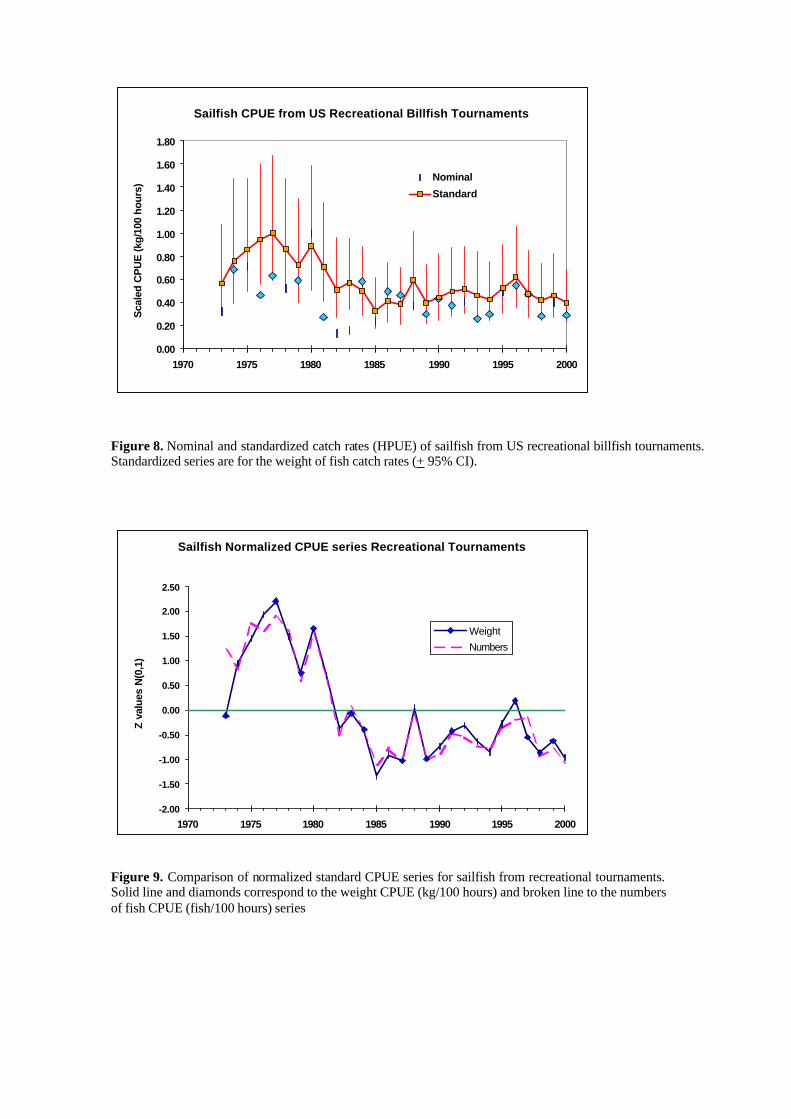
Standardized CPUE series for sailfish are shown in Table 3 and Figure 8. Catch rates of sailfish

increase from 1973 to the highest value in 1977, follow by a decline to a minimum in 1985, since then catch rates have been stable. Coefficient of variation ranged from 26% to 34%. The standardized CPUE series using numbers of fish as dependent variable instead of weight, show similar trend (Fig 9), with the exception for year 1973, when the average sailfish mean size was the lowest of all (Fig 4).

3.2 MRFSS

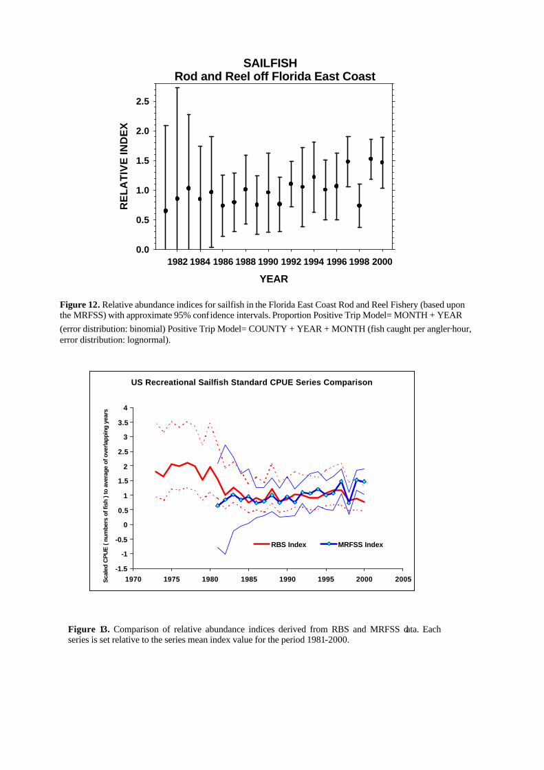
The stepwise construction of the model is shown in Table 4 for the proportion positive analysis and in Table 5 for the positive catch rate analysis. The results of the model fits for the indices are shown in Tables 6 and 7. The index values are shown in Table 8 and in Figure 12.

A comparison of the RBS and MRFSS trends during the period 1981-2000 is shown in Figure 13,

with each series set relative to the series mean. With the potential exceptions of 1981, 1994, and 1999-2000, the trends are quite similar.

One great difficulty in interpreting these results is the lack of data, which would accurately track

fishing methodology changes implemented by the fishermen over time. For example, anecdotal reports indicate that the increased use of live bait attached to kites when targeting sailfish has resulted in improved catch rates. Unfortunately, the available data only permits the analysis of factors related to general location, time of the year, and reported target.

LITERATURE CITED ANONYMOUS. 1999. Amendment 1 to the Atlantic Billfish Fishery Management Plan. U.S. Dept. of

Comm., NOAA-NMFS. April 1999.

BEARDSLEY, G.L. and R.J. Conser. 1981. An analysis of catch and effort data from the U.S. recreational fishery for billfishes (Istiophoridae) in the western North Atlantic Ocean and Gulf of Mexico, 1971-78. Fish. Bull. 79:49-68.

BROWDER, J.A. and E.D. Prince. 1990. Standardized estimates of recreational fishing success for blue marlin and white marlin in the western North Atlantic Ocean, 1972-1986. In: R.H. Stroud (ed.), Planning the Future of Billfishes, Research and Management in the 90’s and Beyond. Proceedings of the Second International Billfish Symposium, Kailua-Kona, HI. August 1-5, 1988. National Coalition for Marine Conservation, Inc. Savannah, GA. pp. 215-229.

FARBER, M. I. 1994. Standardization of U.S. recreational fishing success for sailfish (Istiophorus platypterus) 1973-92, using general linear model techniques. Col. Vol. Sci. Pap. ICCAT, XLII(2):346-352.

LITTELL, R.C., G.A. Milliken, W.W. Stroup, and R.D Wolfinger. 1996. SAS® System for Mixed Models, Cary NC:SAS Institute Inc., 1996. 663 pp.

LO, N.C., L.D. Jacobson, and J.L. Squire. 1992. Indices of relative abundance from fish spotter data based on delta-lognormal models. Can. J. Fish. Aquat. Sci. 49: 2515-2526.

MCCULLAGH, P. and J.A. Nelder. 1989. Generalized Linear Models 2nd edition. Chapman & Hall.

ORTIZ M and M.I. Farber. 2001. Standardized catch rates for blue marlin (Makaira nigricans) and white marlin (Tetrapturus albidus) from the US recreational tournaments fishery in the northwest Atlantic and the Gulf of Mexico. Col. Vol. Sci. Pap. ICCAT, LII:216-230.

PRAGER, M.H., E. D. Prince and D. W. Lee. 1995. Empirical length and weight conversion equation: for blue marlin, white marlin, and sailfish from the North Atlantic Ocean. Bull of Mar. Sci. 56(1):201-210.

PRINCE, E. D., A.R. Bertolino and A. M. Lopez. 1990. A comparison of fishing success and average weights of blue marlin and white marlin landed by the recreational fishery in the western Atlantic Ocean, Gulf of Mexico, and Caribbean Sea, 1972-1986. In: R.H. Stroud (ed.), Planning the Future of Billfishes, Research and Management in the 90’s and Beyond. Proceedings of the Second International Billfish Symposium, Kailua-Kona, HI. August 1-5, 1988. National Coalition for Marine Conservation, Inc. Savannah, GA. pp. 159-178.

SAS Institute Inc. 1997, SAS/STAT® Software: Changes and Enhancements through Release 6.12. Cary, NC, USA:Sas Institute Inc., 1997. 1167 pp.

U.S. Department of Commerce. 1990. Marine Recreational Fishery Statistics Survey, Atlantic and Gulf coasts, 1987 - 1989. Current Fishery Statistics No. 8904. Washington, DC. 363 pp.

Table 1. Deviance analysis table for sailfish using the delta lognormal model. Proportion positive/total observations assumed a binomial error distribution, positive catches assumed a lognormal error distribution. The dependent variable is the total hooked fish per hour (HPUE) in weight units. p refers to the Chi-square test probability (alpha 5%) test between two consecutive model specifications.

Recreational Billfish Survey data for Sailfish

Model factors positive catch rates values d. f. Residual deviance

Change in deviance

% of total deviance p

1 1 7233.92

YEAR 27 6954.54 279.4 6.3% < 0.001

YEAR AREA 5 4726.89 2227.6 50.0% < 0.001

YEAR AREA SEASON 2 3803.15 923.7 20.7% < 0.001

YEAR AREA SEASON TOURSAIL 1 3215.14 588.0 13.2% < 0.001

YEAR AREA SEASON TOURSAIL YEAR:AREA 80 2999.15 216.0 4.8% < 0.001

YEAR AREA SEASON TOURSAIL YEAR:AREA YEAR:SEASON 54 2868.99 130.2 2.9% < 0.001 YEAR AREA SEASON TOURSAIL YEAR:AREA YEAR:SEASON YEAR:TOURSAIL 27 2776.25 92.7 2.1% < 0.001

Model factors proportion positive/total observations d. f. Residual deviance

Change in deviance

% of total deviance p

1 1 8483.04

YEAR 27 8406.21 76.8 3.2% < 0.001

YEAR AREA 5 7402.81 1003.4 42.2% < 0.001

YEAR AREA SEASON 2 7247.03 155.8 6.5% < 0.001

YEAR AREA SEASON TOURSAIL 1 6541.37 705.7 29.7% < 0.001

YEAR AREA SEASON TOURSAIL YEAR:AREA 115 6297.03 244.3 10.3% < 0.001

YEAR AREA SEASON TOURSAIL YEAR:AREA YEAR:SEASON 54 6180.69 116.3 4.9% < 0.001 YEAR AREA SEASON TOURSAIL YEAR:AREA YEAR:SEASON YEAR:TOURSAIL 27 6103.17 77.5 3.3% < 0.001

Table 2. Random effects evaluation for sailfish delta lognormal mixed model specifications. (* refers to final model selected).

Sailfish model Numb obs

-2 REM Log likelihood

Akaike's Information

Criterion

Schwartz's Bayesian Criterion

Likelihood Ratio Test

Proportion Positives

* Year TourSail Area Season 342 1275.7 -638.9 -640.7

Year TourSail Area Season Year*Area 342 1275.7 -638.9 -640.4 0 1.0000

Year TourSail Area Season Year*Area Year*Season 342 1275.7 -638.9 -640.4 0 1.0000

Positive Catch

Year TourSail Area Season 3192 9183.1 -4592.6 -4595.6

Year TourSail Area Season Year*Area 3192 9126.1 -4565 -4567.8 57 0.0000

* Year TourSail Area Season Year*Area Year*Season 3192 9099.2 -4552.6 -4556.7 26.9 0.0000

Table 3. Nominal and standardized CPUE (kg/100 hours fishing) for sailfish from the Recreational Billfish Survey data.

Year Num Obs Nominal CPUE Standard

CPUE Coeff

Variation Std

Error Index Upp CI 95%

Low CI 95%

1973 101 49.41 41.44 33.3% 13.80 0.564 1.078 0.295

1974 101 104.05 56.00 34.1% 19.08 0.762 1.478 0.392

1975 148 108.44 63.05 27.6% 17.42 0.857 1.475 0.499

1976 165 71.46 69.76 26.6% 18.58 0.949 1.601 0.562

1977 177 96.61 73.54 26.5% 19.47 1.000 1.683 0.594

1978 183 79.73 63.75 27.3% 17.43 0.867 1.483 0.507

1979 165 90.09 53.23 30.2% 16.09 0.724 1.308 0.401

1980 211 152.23 65.85 29.2% 19.21 0.895 1.586 0.506

1981 207 41.52 52.66 29.0% 15.27 0.716 1.264 0.406

1982 189 20.50 37.60 32.6% 12.27 0.511 0.966 0.271

1983 247 23.99 42.01 26.3% 11.04 0.571 0.958 0.341

1984 264 88.80 37.50 28.2% 10.57 0.510 0.887 0.293

1985 236 35.80 24.50 31.1% 7.61 0.333 0.611 0.182

1986 238 75.80 30.39 30.4% 9.25 0.413 0.749 0.228

1987 258 71.00 28.67 30.6% 8.78 0.390 0.710 0.214

1988 311 58.25 43.49 27.5% 11.95 0.591 1.014 0.345

1989 329 46.06 29.35 31.2% 9.17 0.399 0.735 0.217

1990 315 65.64 32.82 31.7% 10.42 0.446 0.829 0.240

1991 315 57.52 36.95 28.7% 10.60 0.502 0.882 0.286

1992 307 61.58 38.47 26.7% 10.25 0.523 0.883 0.310

1993 227 39.14 34.02 30.5% 10.36 0.463 0.839 0.255

1994 217 45.63 31.25 29.2% 9.13 0.425 0.753 0.240

1995 252 75.63 38.94 27.4% 10.65 0.529 0.906 0.309

1996 243 84.21 45.50 27.3% 12.43 0.619 1.058 0.362

1997 244 71.81 35.37 29.2% 10.34 0.481 0.853 0.271

1998 169 43.80 31.02 28.6% 8.87 0.422 0.739 0.241

1999 185 60.69 34.28 29.1% 9.98 0.466 0.825 0.263

2000 123 44.22 29.63 27.2% 8.05 0.403 0.687 0.236

Table 4. Results of the stepwise procedure to develop the proportion positive catch rate model. % diff: percent difference in deviance/df between each factor and the null model; delta%: percent difference in deviance/df between the newly included factor and the previous factor entered into the model; L: log likelihood; ChiSquare: Pearson Chi-square statistic; Pr>Chi: significance level of the Chi-square statistic.

Proportion Positive Trips FACTOR df deviance deviance/df %diff. delta% L ChiSquare Pr>Chi NULL 1415 1942.534 1.3728 -971.27 . .

MONTH 1404 1782.245 1.2694 7.5 7.5 -891.12 160.2894 <0.00001

SEASON 1414 1805.099 1.2766 7.0 -902.55 137.4347 <0.00001

YEAR 1396 1830.357 1.3111 4.5 -915.18 112.1774 <0.00001

TRIPTYPE 1414 1928.007 1.3635 0.7 -964 14.5269 0.0001

COUNTY 1407 1924.784 1.368 0.3 -962.39 17.7504 0.0232

ZONE 1414 1941.599 1.3731 0.0 -970.8 0.9351 0.3335

MONTH+

YEAR 1385 1721.04 1.2426 9.5 2.0 -860.52 61.2044 <0.00001

COUNTY 1396 1760.043 1.2608 8.2 -880.02 22.2012 0.0046

TRIPTYPE 1403 1770.184 1.2617 8.1 -885.09 12.0601 0.0005

ZONE 1403 1780.16 1.2688 7.6 -890.08 2.0845 0.1488

MONTH+YEAR+

TRIP 1384 1708.199 1.2342 10.1 0.6 -854.1 12.8414 0.0003

COUN 1377 1703.147 1.2369 9.9 -851.57 17.8929 0.0220

ZONE 1384 1716.095 1.24 9.7 -858.05 4.9453 0.02616

FINAL MODEL: MONTH+YEAR

Table 5. Results of the stepwise procedure to develop the positive trip catch rate model. % diff: percent difference in deviance/df between each factor and the null model; delta%: percent difference in deviance/df between the newly included factor and the previous factor entered into the model; L: log likelihood; ChiSquare: Pearson Chi-square statistic; Pr>Chi: significance level of the Chi-square statistic

Positive Trips

FACTOR df deviance deviance/df %diff. delta% L ChiSquare Pr>Chi NULL 620 151.4073 0.2442 -442.9342 . .

COUNTY 613 140.2904 0.2289 6.3 6.3 -419.2558 47.3568 <0.00001

YEAR 601 140.3213 0.2335 4.4 -419.3244 47.2197 0.0003

MONTH 609 145.7731 0.2394 2.0 -431.1595 23.5494 0.0148

SEASON 619 148.286 0.2396 1.9 -436.4663 12.9359 0.0003

TRIPTYPE 619 149.6971 0.2418 1.0 -439.4071 7.0543 0.0079

ZONE 619 150.3684 0.2429 0.5 -440.7963 4.2758 0.0387

COUNTY+

YEAR 594 131.5744 0.2215 9.3 3.0 -399.3397 39.8322 0.0034

SEASON 612 139.1119 0.2273 6.9 -416.6365 5.2386 0.0221

MONTH 602 136.9036 0.2274 6.9 -411.668 15.1757 0.1746

TRIPTYPE 612 139.971 0.2287 6.3 -418.5482 1.4152 0.2342

ZONE 612 140.2627 0.2292 6.1 -419.1947 0.1223 0.7265

COUNTY+YEAR+

MONTH 583 126.9905 0.2178 10.8 1.5 -388.3294 22.0206 0.0242

SEASON 593 129.71 0.2187 10.4 -394.9086 8.8624 0.0029

TRIPTYPE 593 131.3232 0.2215 9.3 -398.7463 1.1868 0.2760

ZONE 593 131.5631 0.2219 9.1 -399.3132 0.0532 0.8177

COUNTY+YEAR+MONTH+

TRIPTYPE 582 126.7957 0.2179 10.8 0.0 -387.8528 0.9533 0.3289

ZONE 582 126.9575 0.2181 -388.2487 0.1613 0.6879

FINAL MODEL: COUNTY+YEAR+MONTH

Table 6. Results of the MRFSS analysis (1981-2000). Lo method with binomial error assumption for proportion positives.

Class Level Information Class Levels Values month 12 1 2 3 4 5 6 7 8 9 10 11 12 year 20 1981 1982 1983 1984 1985 1986 1987 1988 1989 1990 1991 1992 1993 1994 1995 1996 1997 1998 1999 2000 Criteria For Assessing Goodness Of Fit Criterion DF Value Value/DF Deviance 1385 1721.0400 1.2426 Scaled Deviance 1385 1721.0400 1.2426 Pearson Chi-Square 1385 1409.4340 1.0176 Scaled Pearson X2 1385 1409.4340 1.0176 Log Likelihood -860.5200 Analysis Of Parameter Estimates Standard Wald 95% Confidence Chi- Parameter DF Estimate Error Limits Square Pr > ChiSq Intercept 1 0.7388 0.2384 0.2715 1.2061 9.60 0.0019 month 1 1 0.3956 0.2032 -0.0027 0.7938 3.79 0.0516 month 2 1 -0.0635 0.2200 -0.4948 0.3678 0.08 0.7728 month 3 1 -0.8864 0.2639 -1.4036 -0.3693 11.29 0.0008 month 4 1 -0.8491 0.2633 -1.3652 -0.3331 10.40 0.0013 month 5 1 -0.9419 0.2804 -1.4915 -0.3923 11.28 0.0008 month 6 1 -1.3801 0.2947 -1.9577 -0.8024 21.92 <.0001 month 7 1 -1.3100 0.2809 -1.8606 -0.7595 21.75 <.0001 month 8 1 -1.4222 0.3191 -2.0476 -0.7969 19.87 <.0001 month 9 1 -1.0280 0.4058 -1.8234 -0.2326 6.42 0.0113 month 10 1 -1.0257 0.3221 -1.6571 -0.3943 10.14 0.0015 month 11 1 -0.1575 0.2587 -0.6645 0.3494 0.37 0.5425 month 12 0 0.0000 0.0000 0.0000 0.0000 . . year 1981 1 -0.7434 0.7371 -2.1880 0.7013 1.02 0.3132 year 1982 1 -1.0281 0.8305 -2.6558 0.5996 1.53 0.2157 year 1983 1 0.0323 0.6137 -1.1705 1.2351 0.00 0.9581 year 1984 1 -0.9987 0.4814 -1.9421 -0.0552 4.30 0.0380 year 1985 1 -0.1792 0.5379 -1.2335 0.8750 0.11 0.7390 year 1986 1 -1.2361 0.3371 -1.8967 -0.5755 13.45 0.0002 year 1987 1 -0.8995 0.3175 -1.5217 -0.2772 8.03 0.0046 year 1988 1 -0.9799 0.3271 -1.6209 -0.3388 8.98 0.0027 year 1989 1 -1.1912 0.3192 -1.8168 -0.5656 13.93 0.0002 year 1990 1 -1.0558 0.3569 -1.7553 -0.3563 8.75 0.0031 year 1991 1 -0.8381 0.3228 -1.4707 -0.2054 6.74 0.0094 year 1992 1 -0.3831 0.2671 -0.9067 0.1404 2.06 0.1515 year 1993 1 -0.4409 0.3769 -1.1796 0.2978 1.37 0.2421 year 1994 1 -0.5403 0.3462 -1.2189 0.1383 2.44 0.1186 year 1995 1 -0.3363 0.3340 -0.9909 0.3183 1.01 0.3139 year 1996 1 -0.6796 0.3410 -1.3480 -0.0113 3.97 0.0463 year 1997 1 0.0319 0.2967 -0.5495 0.6133 0.01 0.9143 year 1998 1 -0.6919 0.2843 -1.2491 -0.1348 5.93 0.0149 year 1999 1 0.1890 0.2670 -0.3342 0.7123 0.50 0.4789 year 2000 0 0.0000 0.0000 0.0000 0.0000 . . Scale 0 1.0000 0.0000 1.0000 1.0000 NOTE: The scale parameter was held fixed. LR Statistics For Type 3 Analysis Chi- Source DF Square Pr > ChiSq month 11 109.32 <.0001 year 19 61.20 <.0001

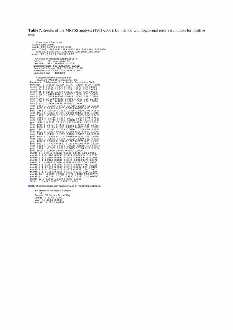
Table 7. Results of the MRFSS analysis (1981-2000). Lo method with lognormal error assumption for positive trips.

Class Level Information Class Levels Values county 8 23 24 25 26 27 29 30 32 year 20 1981 1982 1983 1984 1985 1986 1987 1988 1989 1990 1991 1992 1993 1994 1995 1996 1997 1998 1999 2000 month 12 1 2 3 4 5 6 7 8 9 10 11 12 Criteria For Assessing Goodness Of Fit Criterion DF Value Value/DF Deviance 583 126.9905 0.2178 Scaled Deviance 583 621.0000 1.0652 Pearson Chi-Square 583 126.9905 0.2178 Scaled Pearson X2 583 621.0000 1.0652 Log Likelihood -388.3294 Analysis Of Parameter Estimates Standard Wald 95% Confidence Chi- Parameter DF Estimate Error Limits Square Pr > ChiSq Intercept 1 -2.2615 0.3399 -2.9277 -1.5954 44.27 <.0001 county 23 1 0.8374 0.3392 0.1725 1.5023 6.09 0.0136 county 24 1 0.8728 0.3402 0.2059 1.5396 6.58 0.0103 county 25 1 0.8936 0.3378 0.2315 1.5557 7.00 0.0082 county 26 1 0.6403 0.3416 -0.0292 1.3099 3.51 0.0609 county 27 1 0.7029 0.4067 -0.0943 1.5000 2.99 0.0839 county 29 1 0.4102 0.3729 -0.3206 1.1410 1.21 0.2713 county 30 1 0.3541 0.4106 -0.4506 1.1588 0.74 0.3884 county 32 0 0.0000 0.0000 0.0000 0.0000 . . year 1981 1 -0.3295 0.2772 -0.8728 0.2138 1.41 0.2345 year 1982 1 0.1343 0.3425 -0.5370 0.8056 0.15 0.6951 year 1983 1 -0.3409 0.1998 -0.7325 0.0506 2.91 0.0879 year 1984 1 0.0426 0.1696 -0.2898 0.3750 0.06 0.8016 year 1985 1 -0.1559 0.1640 -0.4773 0.1655 0.90 0.3418 year 1986 1 -0.0336 0.1209 -0.2707 0.2034 0.08 0.7810 year 1987 1 -0.0719 0.1066 -0.2808 0.1371 0.45 0.5002 year 1988 1 0.2656 0.1173 0.0357 0.4955 5.13 0.0236 year 1989 1 0.1107 0.1136 -0.1121 0 .3334 0.95 0.3301 year 1990 1 0.2175 0.1299 -0.0372 0.4722 2.80 0.0942 year 1991 1 -0.0961 0.1059 -0.3036 0.1115 0.82 0.3643 year 1992 1 0.0037 0.0835 -0.1600 0.1674 0.00 0.9645 year 1993 1 -0.1601 0.1252 -0.4054 0.0852 1.64 0.2009 year 1994 1 0.1534 0.1072 -0.0568 0.3636 2.05 0.1526 year 1995 1 -0.1686 0.1008 -0.3662 0.0289 2.80 0.0943 year 1996 1 0.0848 0.1087 -0.1282 0.2979 0.61 0.4352 year 1997 1 0.0414 0.0840 -0.1232 0.2061 0.24 0.6220 year 1998 1 -0.2769 0.0883 -0.4500 -0.1039 9.84 0.0017 year 1999 1 -0.0332 0.0761 -0.1825 0.1160 0.19 0.6624 year 2000 0 0.0000 0.0000 0.0000 0.0000 . . month 1 1 0.0017 0.0563 -0.1086 0.1119 0.00 0.9765 month 2 1 -0.1487 0.0655 -0.2771 -0.0203 5.15 0.0233 month 3 1 -0.2309 0.0890 -0.4054 -0.0564 6.73 0.0095 month 4 1 -0.2166 0.0907 -0.3944 -0.0388 5.70 0.0170 month 5 1 0.0187 0.0984 -0.1741 0.2115 0.04 0.8492 month 6 1 -0.2474 0.1107 -0.4644 -0.0304 4.99 0.0255 month 7 1 -0.1818 0.1048 -0.3873 0.0237 3.01 0.0829 month 8 1 -0.1572 0.1227 -0.3977 0.0833 1.64 0.2002 month 9 1 -0.1965 0.1665 -0.5229 0.1298 1.39 0.2379 month 10 1 -0.1381 0.1220 -0.3772 0.1010 1.28 0.2575 month 11 1 -0.0361 0.0807 -0.1942 0.1221 0.20 0.6550 month 12 0 0.0000 0.0000 0.0000 0.0000 . . Scale 1 0.4522 0.0128 0.4277 0.4781 NOTE: The scale parameter was estimated by maximum likelihood. LR Statistics For Type 3 Analysis Chi- Source DF Square Pr > ChiSq county 7 32.53 <.0001 year 19 46.68 0.0004 month 11 22.02 0.0242

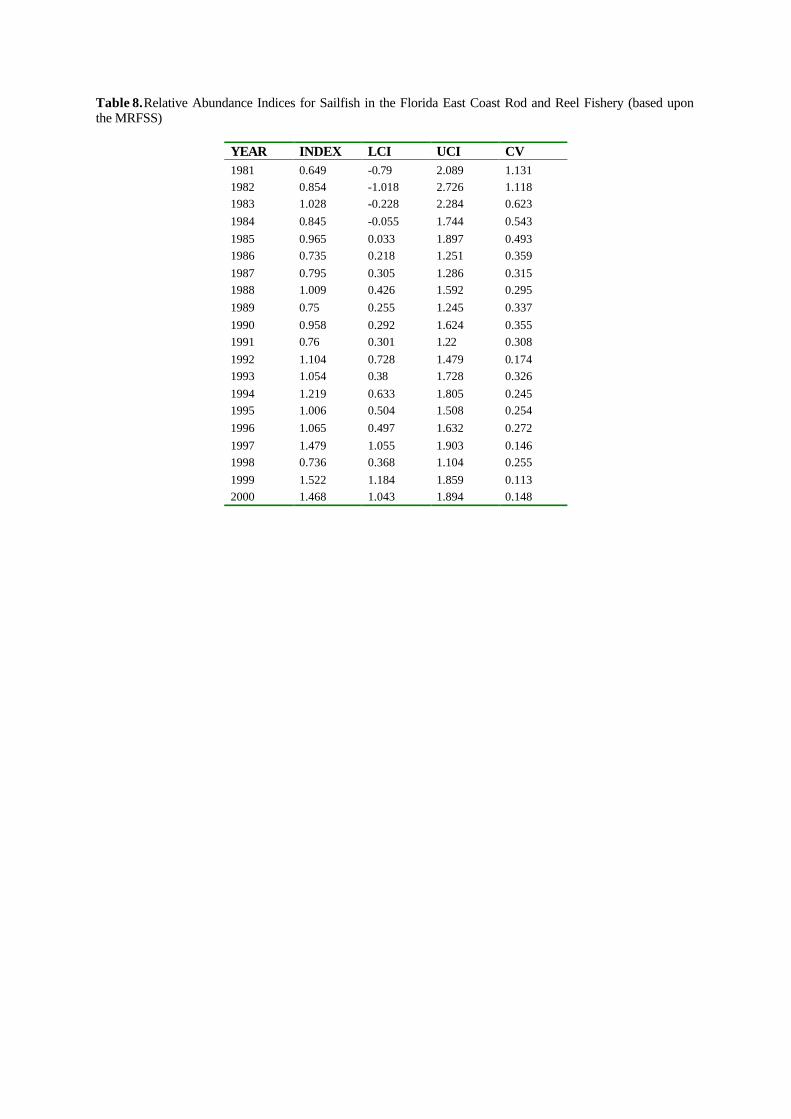
Table 8. Relative Abundance Indices for Sailfish in the Florida East Coast Rod and Reel Fishery (based upon the MRFSS)

YEAR INDEX LCI UCI CV 1981 0.649 -0.79 2.089 1.131

1982 0.854 -1.018 2.726 1.118

1983 1.028 -0.228 2.284 0.623

1984 0.845 -0.055 1.744 0.543

1985 0.965 0.033 1.897 0.493

1986 0.735 0.218 1.251 0.359

1987 0.795 0.305 1.286 0.315

1988 1.009 0.426 1.592 0.295

1989 0.75 0.255 1.245 0.337

1990 0.958 0.292 1.624 0.355

1991 0.76 0.301 1.22 0.308

1992 1.104 0.728 1.479 0.174

1993 1.054 0.38 1.728 0.326

1994 1.219 0.633 1.805 0.245

1995 1.006 0.504 1.508 0.254

1996 1.065 0.497 1.632 0.272

1997 1.479 1.055 1.903 0.146

1998 0.736 0.368 1.104 0.255

1999 1.522 1.184 1.859 0.113

2000 1.468 1.043 1.894 0.148

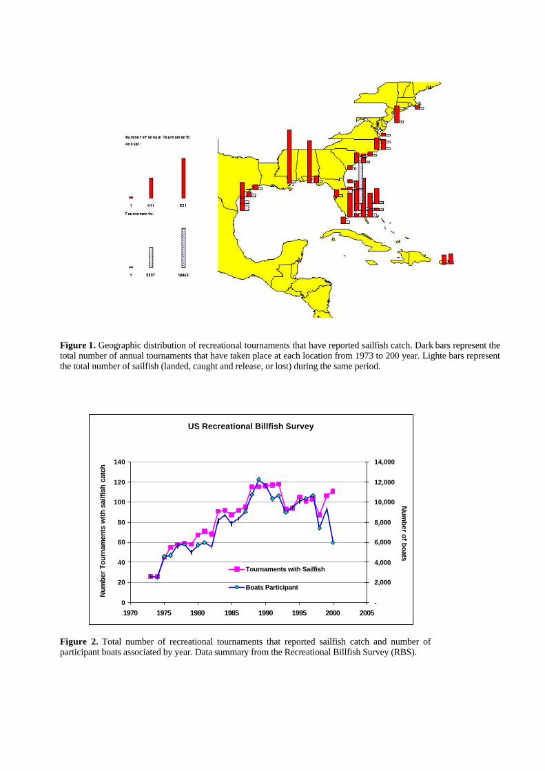
Figure 2. Total number of recreational tournaments that reported sailfish catch and number of participant boats associated by year. Data summary from the Recreational Billfish Survey (RBS).

US Recreational Billfish Survey

0

20

40

60

80

100

120

140

1970 1975 1980 1985 1990 1995 2000 2005

Num

ber

Tour

nam

ents

with

sai

lfish

cat

ch

-

2,000

4,000

6,000

8,000

10,000

12,000

14,000

Num

ber of boats

Tournaments with Sailfish

Boats Participant

Figure 1. Geographic distribution of recreational tournaments that have reported sailfish catch. Dark bars represent the total number of annual tournaments that have taken place at each location from 1973 to 200 year. Lighte bars represent the total number of sailfish (landed, caught and release, or lost) during the same period.

1975

1980

1985

1990

1995

2000

1975

1980

1985

1990

1995

2000

1975

1980

1985

1990

1995

2000

year

140

170

140

170

140

170

140

170

140

170

Sai

lfish

mea

n si

ze (c

m) l

ower

jaw

fork

leng

th

May Aug Sep Dec Jan Apr May Aug

Sep Dec Jan Apr May Aug Sep Dec

Jan Apr May Aug Sep Dec Jan Apr

May Aug Sep Dec Jan Apr May Aug

Sep Dec Jan Apr

Bahamas Bahamas Bahamas Caribbean

Caribbean Caribbean Gulf Mexico Gulf Mexico

Gulf Mexico Mid Atlantic Mid Atlantic Mid Atlantic

New England New England New England South Atlantic

South Atlantic South Atlantic

55 75 95 11

51

35

15

51

75

19

52

15

55 75 95 11

51

35

15

51

75

19

52

15

55 75 95 11

51

35

15

51

75

19

52

15

55 75 95 11

51

35

15

51

75

19

52

15

55 75 95 11

51

35

15

51

75

19

52

15

Lower jaw fork length (cm)

0.00

0.02

0.04

0.06

0.08

0.10

0.00

0.02

0.04

0.06

0.08

0.10

0.00

0.02

0.04

0.06

0.08

0.10

0.00

0.02

0.04

0.06

0.08

0.10

0.00

0.02

0.04

0.06

0.08

0.10

1973 1974 1975 1976 1977 1978

1979 1980 1981 1982 1983 1984

1985 1986 1987 1988 1989 1990

1991 1992 1993 1994 1995 1996

1997 1998 1999 2000

Figure 3. Size frequency distributions by year for sailfish measured from the RBS program.

Figure 4. Estimated mean size (lower jaw fork length cm) of sailfish by strata used to convert numbers of fish to weight of fish hooked. Bars represent one standard error. .

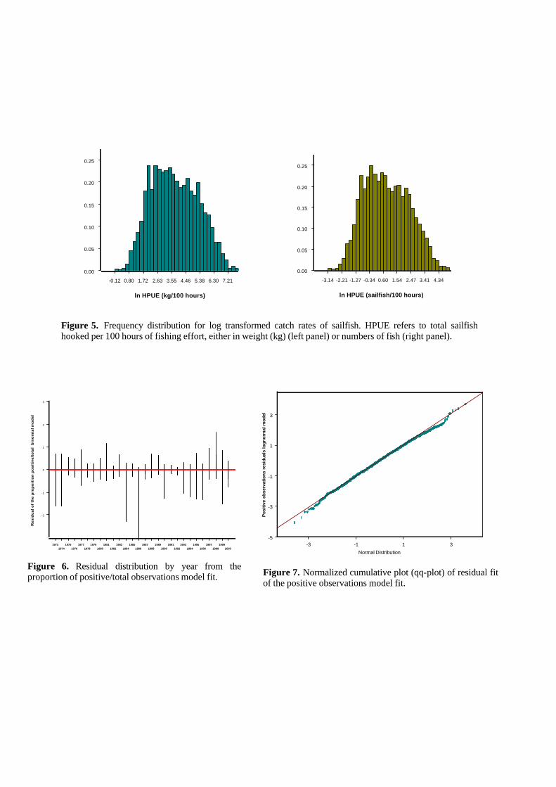
Figure 5. Frequency distribution for log transformed catch rates of sailfish. HPUE refers to total sailfish hooked per 100 hours of fishing effort, either in weight (kg) (left panel) or numbers of fish (right panel).

19731974

19751976

19771978

19791980

19811982

19831984

19851986

19871988

19891990

19911992

19931994

19951996

19971998

19992000

-2

-1

0

1

2

3

Res

idu

al o

f th

e p

rop

ort

ion

po

siti

ve/t

ota

l b

ino

mia

l mo

del

-3 -1 1 3

Normal Distribution

-5

-3

-1

1

3

Pos

itive

obs

erva

tions

res

idua

ls lo

gnor

mal

mod

el

Figure 6. Residual distribution by year from the proportion of positive/total observations model fit. Figure 7. Normalized cumulative plot (qq-plot) of residual fit

of the positive observations model fit.

-0.12 0.80 1.72 2.63 3.55 4.46 5.38 6.30 7.21

ln HPUE (kg/100 hours)

0.00

0.05

0.10

0.15

0.20

0.25

-3.14 -2.21 -1.27 -0.34 0.60 1.54 2.47 3.41 4.34

ln HPUE (sailfish/100 hours)

0.00

0.05

0.10

0.15

0.20

0.25

Sailfish CPUE from US Recreational Billfish Tournaments

0.00

0.20

0.40

0.60

0.80

1.00

1.20

1.40

1.60

1.80

1970 1975 1980 1985 1990 1995 2000

Sca

led

CP

UE

(kg/

100

hour

s)

Nominal

Standard

Sailfish Normalized CPUE series Recreational Tournaments

-2.00

-1.50

-1.00

-0.50

0.00

0.50

1.00

1.50

2.00

2.50

1970 1975 1980 1985 1990 1995 2000

Z va

lues

N(0

,1)

Weight

Numbers

Figure 8. Nominal and standardized catch rates (HPUE) of sailfish from US recreational billfish tournaments. Standardized series are for the weight of fish catch rates (+ 95% CI).

Figure 9. Comparison of normalized standard CPUE series for sailfish from recreational tournaments. Solid line and diamonds correspond to the weight CPUE (kg/100 hours) and broken line to the numbers of fish CPUE (fish/100 hours) series

Figure 10. The geographic distribution of sailfish directed rod and reel effort off the Florida East coast (1981-2000). Each symbol is scaled to reflect the total angler*hours expended at that location. The locations are approximate: latitude was defined based upon the mid-latitude of the intercept county and longitude was assigned at points 2 miles offshore or 15 miles offshore, depending upon zone.

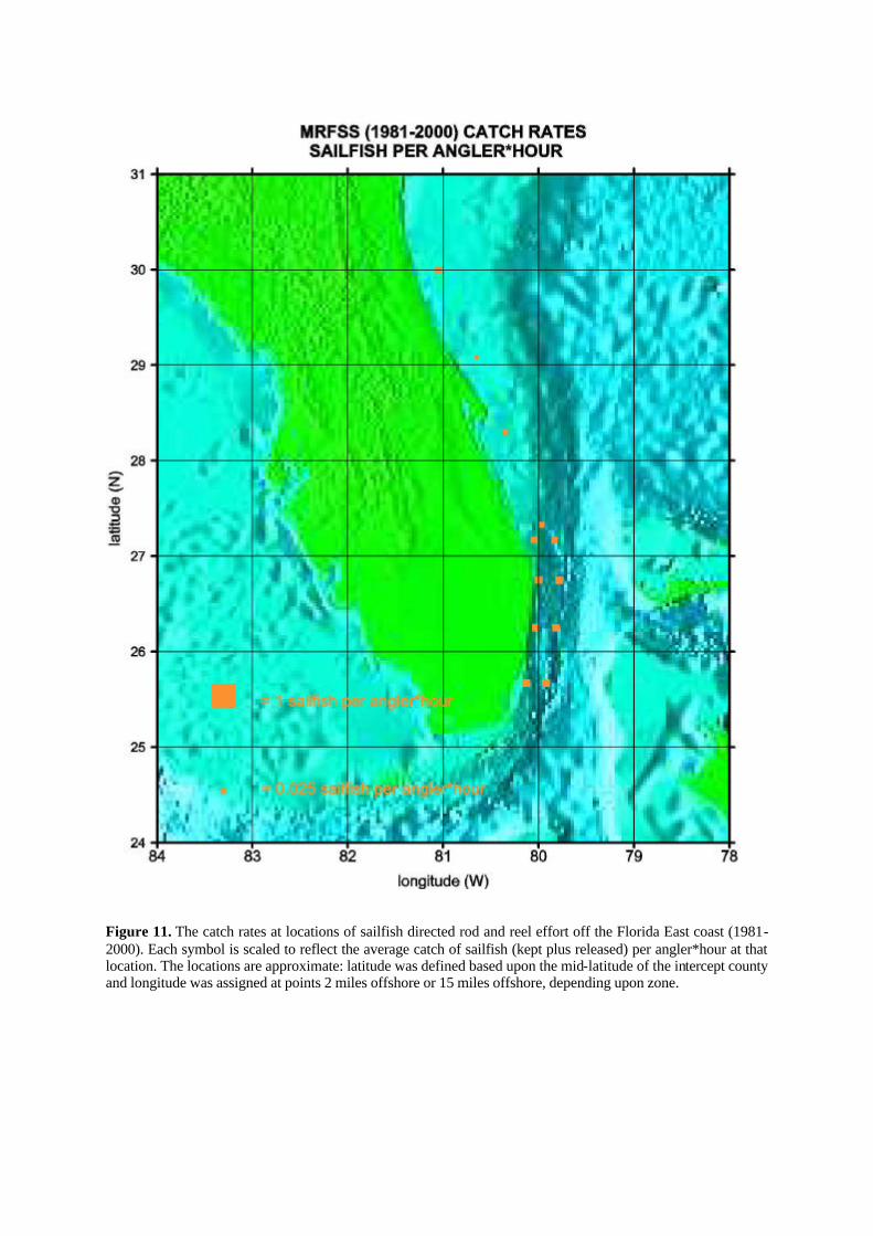
Figure 11. The catch rates at locations of sailfish directed rod and reel effort off the Florida East coast (1981-2000). Each symbol is scaled to reflect the average catch of sailfish (kept plus released) per angler*hour at that location. The locations are approximate: latitude was defined based upon the mid-latitude of the intercept county and longitude was assigned at points 2 miles offshore or 15 miles offshore, depending upon zone.

US Recreational Sailfish Standard CPUE Series Comparison

-1.5

-1

-0.5

0

0.5

1

1.5

2

2.5

3

3.5

4

1970 1975 1980 1985 1990 1995 2000 2005Sca

led

CP

UE

( nu

mbe

rs o

f fis

h ) t

o av

erag

e of

ove

rlapp

ing

year

s

RBS Index MRFSS Index

Figure 13. Comparison of relative abundance indices derived from RBS and MRFSS data. Each series is set relative to the series mean index value for the period 1981-2000.

SAILFISH Rod and Reel off Florida East Coast

YEAR

1982 1984 1986 1988 1990 1992 1994 1996 1998 2000

RE

LATI

VE

IND

EX

0.0

0.5

1.0

1.5

2.0

2.5

Figure 12. Relative abundance indices for sailfish in the Florida East Coast Rod and Reel Fishery (based upon the MRFSS) with approximate 95% conf idence intervals. Proportion Positive Trip Model= MONTH + YEAR

(error distribution: binomial) Positive Trip Model= COUNTY + YEAR + MONTH (fish caught per angler.hour, error distribution: lognormal).