SRB Measures for Anosov actions - arXiv
47
SRB MEASURES FOR ANOSOV ACTIONS YANNICK GUEDES BONTHONNEAU, COLIN GUILLARMOU, AND TOBIAS WEICH Abstract. Given a general Anosov R κ action on a closed manifold, we study properties of certain invariant measures that have recently been introduced in [GBGHW20] using the theory of Ruelle-Taylor resonances. We show that these measures share many properties of Sinai-Ruelle-Bowen measures for general Anosov flows such as smooth disintegrations along the unstable foliation, positive Lebesgue measure basins of attraction and a Bowen formula in terms of periodic orbits. Finally we show that if the action in the positive Weyl chamber is transitive, the measure is unique and has full support. Introduction On a closed, smooth Riemannian manifold (M,g) (normalized with volume 1) we consider a locally free abelian action τ : R κ → Diffeo(M). Assume that τ is Anosov, and denote by W⊂ R κ the maximal cone of tranversally hyperbolic elements (see Section 1.1 for a precise definition of all these terms). In [GBGHW20] it was proved that there exists a Radon probability measure μ, called the physical measure, such that for every function f ∈ C 0 (M) and every open proper 1 subcone C⊂W, μ(f )= lim T →+∞ 1 |C T | Z A∈C T Z M f (τ (-A)(x))dxdA. (0.1) Here C T = {A ∈C| e(A) ≤ T }, for some linear form e on R κ , positive on W. In this article we will explore the properties of the measure μ, proving in particular: Theorem 1. Let τ be a transitive, smooth, locally free, R κ Anosov action. Let μ be an invariant Radon probability measure on M, then the following conditions are equivalent: (1) μ is the physical measure. (2) For every continuous f , every open proper subcone C ⊂⊂ W, and Lebesgue almost every x ∈M, μ(f )= lim T →+∞ 1 |C T | Z A∈C T Z M f (τ (-A)(x))dA (3) μ has an absolute continuous disintegration w.r.t. to the local stable foliation, W s loc . (4) the measure μ has wave-front set WF(μ) ⊂ E * s . Such a measure μ is always ergodic. If in addition we assume that the action is positively transitive in the sense of Definition 2.9, then supp(μ)= M. These properties are very similar to the properties of the SRB measure for transitive Anosov flows, which was studied extensively by Sinai, Bowen and Ruelle [Sin68, Bow74, Rue76, BR75]. As for all our results, we also obtain a more general and more detailed version (Theorem 3) without the transitivity assumption. Date : November 10, 2021. 1 proper meaning that ∂C∩ ∂W = {0} 1 arXiv:2103.12127v3 [math.DS] 8 Nov 2021
-
Upload
khangminh22 -
Category
Documents
-
view
0 -
download
0
Transcript of SRB Measures for Anosov actions - arXiv
SRB MEASURES FOR ANOSOV ACTIONS
YANNICK GUEDES BONTHONNEAU, COLIN GUILLARMOU, AND TOBIAS WEICH
Abstract. Given a general Anosov Rκ action on a closed manifold, we study propertiesof certain invariant measures that have recently been introduced in [GBGHW20] using thetheory of Ruelle-Taylor resonances. We show that these measures share many properties ofSinai-Ruelle-Bowen measures for general Anosov flows such as smooth disintegrations alongthe unstable foliation, positive Lebesgue measure basins of attraction and a Bowen formulain terms of periodic orbits. Finally we show that if the action in the positive Weyl chamberis transitive, the measure is unique and has full support.
Introduction
On a closed, smooth Riemannian manifold (M, g) (normalized with volume 1) we considera locally free abelian action τ : Rκ → Diffeo(M). Assume that τ is Anosov, and denoteby W ⊂ Rκ the maximal cone of tranversally hyperbolic elements (see Section 1.1 for aprecise definition of all these terms). In [GBGHW20] it was proved that there exists a Radonprobability measure µ, called the physical measure, such that for every function f ∈ C0(M)and every open proper1 subcone C ⊂ W,
µ(f) = limT→+∞
1
|CT |
∫A∈CT
∫Mf(τ(−A)(x))dxdA. (0.1)
Here CT = A ∈ C | e(A) ≤ T, for some linear form e on Rκ, positive on W. In this articlewe will explore the properties of the measure µ, proving in particular:
Theorem 1. Let τ be a transitive, smooth, locally free, Rκ Anosov action. Let µ be aninvariant Radon probability measure on M, then the following conditions are equivalent:
(1) µ is the physical measure.(2) For every continuous f , every open proper subcone C ⊂⊂ W, and Lebesgue almost
every x ∈M,
µ(f) = limT→+∞
1
|CT |
∫A∈CT
∫Mf(τ(−A)(x))dA
(3) µ has an absolute continuous disintegration w.r.t. to the local stable foliation, W sloc.
(4) the measure µ has wave-front set WF(µ) ⊂ E∗s .
Such a measure µ is always ergodic. If in addition we assume that the action is positivelytransitive in the sense of Definition 2.9, then supp(µ) =M.
These properties are very similar to the properties of the SRB measure for transitive Anosovflows, which was studied extensively by Sinai, Bowen and Ruelle [Sin68, Bow74, Rue76, BR75].As for all our results, we also obtain a more general and more detailed version (Theorem 3)without the transitivity assumption.
Date: November 10, 2021.1proper meaning that ∂C ∩ ∂W = 0
1
arX
iv:2
103.
1212
7v3
[m
ath.
DS]
8 N
ov 2
021
2 Y. GUEDES BONTHONNEAU, C. GUILLARMOU, AND T. WEICH
For a given smooth Anosov flow, the structural stability implies that any small perturbationof the flow is again an Anosov flow. Furthermore for any fixed Anosov flow, one can associatewith each potential V a so-called invariant Gibbs measure that has positive entropy. Theworld of smooth Anosov flows is thus very rich and, for a fixed flow, there is also a richergodic theory due to the different Gibbs measures. In contrast, for higher rank Anosovaction the sitation is conjectured (and partially known) to be very rigid: in [KS94] Katok andSpatzier proved that for a list of algebraic Anosov actions, called standard Anosov actions,any small perturbation of the Anosov action is Holder conjugate to the original action. Moregenerally, Katok and Spatzier conjectured (see [Has07, Conjecture 16.8]) that whenever ahigher rank Ansosov action cannot be factored into a product of an Anosov flow with anotheraction, they are algebraic in the sense that they come from quotients of symmetric spaces orLie groups. Despite some important recent advances (see e.g. Spatzier-Vinhage [SV19]) thisconjecture is still widely open.
Assuming that this rigidity conjecture holds, the classification of invariant measures reducesto analyzing homogeneous dynamics, i.e Rκ invariant measures on homogeneous spaces. Suchmeasure classifiactions in homogeneous dynamics have been intensively studied in the pastdecades, starting with the works of Katok and Spatzier [KS95, KS98] and culminating inmore recent works of Einsiedler, Katok and Lindenstrauss [EKL06, EL15].
However, in order to make progress in the direction of Katok-Spatzier rigidity conjecture,it is obviously important to understand as many dynamical properties of Anosov actions aspossible, without assuming that these actions are homogeneous. In particular it is importantto understand and to construct meaningful invariant measures2. Let us mention some relatedresults in this direction: in [KKRH11], Kalinin-Katok-Rodriguez Hertz obtain the following:for a locally free abelian Anosov action with dimM = 2κ+1 with κ ≥ 2, an invariant ergodicmeasure µ which has positive entropy for some A ∈ Rκ is absolutely continuous under certainassumptions on the Lyapunov exponents and hyperplanes of µ (it is thus the same as ourSRB measure). Let us finally mention that independently, Carrasco-Rodriguez Hertz [CRH]have constucted an SRB measure using the thermodynamic formalism and also proved theabsolute continuity of the conditional measures. For general Anosov actions by smooth Liegroups they show that this is the equilibrium measure associated to the potential given bythe unstable Jacobian, as in the rank 1 case.
The second main result of our article concerns the distribution of regular periodic orbitsfor higher rank actions. We obtain a Bowen-like [Bow72, PP90] formula for the measure µ.A point x ∈ M is said to be a periodic point if there exists A ∈ Rκ such that τ(A)(x) =x. Periodic orbits may have a complicated shape in general, but it is well known that ifτ(A0)(x) = x for some A0 ∈ W, then the orbit set T = Tx := τ(A)(x) ∈ M|A ∈ Rκ is aκ-dimensional torus – we say that the orbit is regular. We denote by T the set of such periodictori of τ and, for T ∈ T , we denote by L(T ) := A ∈ Rκ | τ(A)(x) = x the associated lattice.
Theorem 2. Let τ be a transitive Rκ-Anosov action, with Weyl chamber W. Let C ⊂ Wbe a proper subcone and η ∈ Rκ∗ a dual element that is positive on a slightly larger conicneighbourhood of C. Define Ca,b := A ∈ C | η(A) ∈ [a, b] if a, b > 0. Let µ be the SRB
2As explained to us by Ralf Spatzier, the existence of ergodic measures with full support is an importanttool in the direction of proving the rigidity conjecture (see e.g. [KS07] where this assumption is crucially used,as well as the discussions in [SV19])
SRB MEASURES FOR ANOSOV ACTIONS 3
measure and a, b > 0. Then for each f ∈ C∞(M), we have
µ(f) = limN→∞
1
|CaN,bN |∑T∈T
∑A∈CaN,bN∩L(T )
∫T f
|det(1− PA)|(0.2)
where PA is the linearized Poincare map of the periodic orbit A restricted to Eu ⊕ Es.
This result is proved using microlocal methods inspired by Dyatlov-Zworski [DZ16] inthe rank 1 case: one needs in our setting to combine the Guillemin trace formula with theanalysis of the wave-front set of a certain meromorphic function Fλ(X1, . . . , Xκ) of the familyof commuting vector fields (X1, . . . , Xκ) generating the Anosov action, and this function has asimple pole at λ = 0 with residue given by µ(f). The result (0.2) shows some equidistributionof the periodic orbits just as in the rank 1 case, except that here the periodic orbits come asκ-dimensional tori. Notice that for the case of the Weyl chamber flow on a locally symmetricspaceM = Γ\G/M , the SRB measure is the Haar measure (by uniqueness), thus Theorem 2gives an expression of the Haar measure in terms of periodic tori: by (4.2), there is ε > 0 so
that for all A ∈ L(T ) ∩ C, det(1−PA) = e2ρ(A)(1 +O(e−ε|A|)) where ρ is the half sum of thepositive roots, therefore (0.2) reduces to
µ(f) = limN→∞
1
|CaN,bN |∑T∈T
∑A∈CaN,bN∩L(T )
e−2ρ(A)
∫Tf. (0.3)
We notice that even for locally symmetric space where µ is Haar measure, the formula (0.2)and (0.3) were not proved, and our result is new even in that setting.
As a rather direct consequence of (0.2) we get the following result on the counting ofperiodic tori:
Corollary 0.1. Assume there is a linear form η ∈ Rκ∗ that is positive on W and such thatfor any proper subcone C ⊂ W there is ε > 0 such that | det(1− PA)| = eη(A)(1−O(e−ε|A|))|for all A ∈ C. For any proper subcone C ⊂ W let CN := A ∈ C, η(A)/‖η‖ ≤ N then
limN→∞
1
Nlog(∑T∈T
∑A∈L(T )∩CN
vol(T ))
= ‖η‖.
Note that the assumptions are fulfilled for all standard Anosov actions (as introducedin [KS94, Sec. 2]). In the special case of Weyl chamber flows, Spatzier [Spa83] proved arelated result when the cone C is the whole Weyl chamber: more precisely he proved that ifs(T ) := min|A| |A ∈ L(T ) ∩W denotes the regular systole of a periodic torus T , then
limN→∞
1
Nlog( ∑T∈T ,s(T )≤N
Vol(T ))
= 2‖ρ‖.
Recall from above that for Weyl chamber flows one has η = 2ρ and 2‖ρ‖ corresponds alsoto the topological entropy of the associated geodesic flow. The same asymptotics for torusorbits of Weyl chamber flows has been obtained by Deitmar [Dei04] (yet with slightly differentcounting region) using trace formulae on higher rank locally symmetric spaces and Lefschetzformulae.
As a byproduct of the proof of Theorem 2, we also construct some zeta-like functions (seeTheorem 5). For each function ψ ∈ C∞c (W) with small enough support, we obtain a function
dψ(λ) holomorphic on Cκ that vanishes exactly when ψ(λ − ζ) = 1 for some Taylor-Ruelle
resonance ζ of the action (as was introduced in [GBGHW20]). Here ψ is the Laplace transform
4 Y. GUEDES BONTHONNEAU, C. GUILLARMOU, AND T. WEICH
of ψ. As far as we know this is the first example of a globally holomorphic zeta-like functionfor higher rank actions.
Let us mention two results that are related to the Bowen formula in Theorem 2 for thespecial case of the Anosov action being a Weyl chamber flow on a compact locally symmetricspace: Knieper [Kni05] studies the measure of maximal entropy for geodesic flows on compactlocally symmetric spaces and showed its uniqueness. From this uniqueness he derives aBowen formula for ε-separated geodesics. Furthermore, Einsiedler, Lindenstrauss, Michel andVenkatesh studied distribution of torus orbits of Weyl chamber flows in [ELMV09, ELMV11].In the special case of Weyl chamber flows on SL(3,R)/SL(3,Z) they obtain a strongequidistribution result of periodic torus orbits [ELMV11, Theorem 1.4] that among otherswould imply the Bowen type formula above3. In [ELMV09] the authors also study torusorbits on certain compact locally symmetric spaces that are constructed from orders incentral simple algebras. They also obtain equidistribution results (see [ELMV09, Corollary1.7]) which are, however, weaker then those obtained for SL(3,R)/SL(3,Z) and they seemnot to imply Theorem 2 for this special class of compact locally symmetric spaces.
Before closing this introduction, let us briefly mention the tools and techniques weemploy in this work. We build on our previous work [GBGHW20] using microlocal methodsin the spirit of Faure-Sjostrand and Dyatlov-Zworski [FS11, DZ16] in the framework ofanisotropic spaces (developped originally in dynamical systems by Blank, Keller, Liverani,Baladi, Tsujii, Gouezel, Butterley [BKL02, GL06, BL07, BT07]). These techniques have asuccessful history in the context of Anosov flows, and we use them intensively in this work.For the proof of Theorem 1, it is sufficient to be familiar with the notion of Hormanderwavefront set. For the proof of Theorems 2 and 5, however, we assume that the reader issomehow familiar with the work [DZ16] or [FRS08]. We will also be using some classical tech-niques from the study of dynamical foliations (absolute continuity, Rokhlin disintegrations...).
Outline of the paper.In section 1.1 we give the definition of Rκ-Anosov actions and introduce some related basic
notations.In Section 1.2 we collect and discuss crucial properties of the stable and unstable foliations
related to Anosov actions which we shall need in the sequel. In particular we give a proofthat the conditional densities of Lebesgue measure along the weak-(un)stable foliations aresmooth along the orbits. While this fact seems folklore, we couldn’t find a precise referenceand as we crucially need this in order to apply our microlocal methods, we took the effort towork this out in details.
In Section 1.3 we recall how invariant measures for Anosov actions can be constructed usingthe spectral theory of Ruelle-Taylor resonances as presented in [GBGHW20]. We also provesome new statements in this context such as Proposition 1.14 that will allow us to show thatthe measures defined by spectral theory are always absolutely continuous along the stablefoliation.
Section 2 and Section 3 are the core of the paper: Section 2 contains the proofs for thedifferent equivalent characterisations of SRB measures (Theorem 1 respectively the moregeneral version Theorem 3) whereas in Section 3 we prove the Bowen formula (Theorem 2).
3Note however that our result does not hold for SL(3,R)/SL(3,Z) due to the non compactness of this space
SRB MEASURES FOR ANOSOV ACTIONS 5
Finally in Section 4 we shortly discuss the applications to counting of periodic tori.
Acknowledgements. This project has received funding from the European ResearchCouncil (ERC) under the European Union’s Horizon 2020 research and innovation programme(grant agreement No. 725967) and from the Deutsche Forschungsgemeinschaft (DFG) (GrantNo. WE 6173/1-1 Emmy Noether group “Microlocal Methods for Hyperbolic Dynamics”).We thank Sebastien Gouezel for helpful discussions and explaining us the arguments in theproof of Proposition 1.6.
1. Anosov actions and dynamical foliations
1.1. Anosov actions. Let (M, g) be a closed, smooth Riemannian manifold and denote byvg its Riemannian measure which we assume to be normalized with volume 1. Note thatwhile g is fixed, all the results we shall discuss will be independent of the choice of g. Letτ : A → Diffeo(M) be a locally free action an abelian Lie group A ∼= Rκ on M. Leta := Lie(A) ∼= Rκ be the associated commutative Lie algebra and exp : a→ A the Lie groupexponential map. After identifying A ∼= a ∼= Rκ, this exponential is the identity, but it willbe useful to have a notation that distinguishes between transformations A and infinitesimaltransformations a. Taking the derivative of the A-action one obtains an injective Lie algebrahomomorphism
X :
a → C∞(M;TM)
A 7→ XA := ddt |t=0
τ(exp(At))(1.1)
which we call the infinitesimal action. By commutativity of a, ran(X) ⊂ C∞(M;TM) isa κ-dimensional subspace of commuting vector fields. Since the action is locally free, theyspan a κ-dimensional smooth subbundle which we call the neutral subbundle E0 ⊂ TM. Itis tangent to the A-orbits on M. We will often study the one-parameter flow generated by avector field XA which we denote by ϕAt . One has the obvious identity ϕAt = τ(exp(At)) fort ∈ R. The Riemannian metric onM induces norms on TM and T ∗M, both denoted by ‖ ·‖.
Definition 1.1. An element A ∈ a and its corresponding vector field XA are called trans-versely hyperbolic if there is a continuous splitting
TM = E0 ⊕ Eu ⊕ Es, (1.2)
that is invariant under the flow ϕAt and such that there are ν > 0, C > 0 with
‖dϕAt v‖ ≤ Ce−ν|t|‖v‖, ∀v ∈ Es, ∀t ≥ 0, (1.3)
‖dϕAt v‖ ≤ Ce−ν|t|‖v‖, ∀v ∈ Eu, ∀t ≤ 0. (1.4)
We say that the A-action is Anosov if there exists an A0 ∈ a such that XA0 is transverselyhyperbolic.
We define the dual bundles E∗u, E∗s , E
∗0 ⊂ T ∗M by4
E∗u(Eu ⊕ E0) = 0, E∗s (Es ⊕ E0) = 0, E0(Eu ⊕ Es) = 0. (1.5)
Given a transversely hyperbolic element A0 ∈ a we define the positive Weyl chamber W ⊂ a tobe the set of A ∈ a which are transversely hyperbolic with the same stable/unstable bundle as
4Note that E∗s/u are not the usual dual bundles of Es/u that vanish on Eu/s ⊕ E0. The notation that weuse has grown historically in the semiclassical approach to Ruelle resonances and is justified by the fact thatthe symplectic lift of τ to T ∗M is expanding in the E∗u fibre and contracting in the E∗s fibre.
6 Y. GUEDES BONTHONNEAU, C. GUILLARMOU, AND T. WEICH
A0. The following statement is well known – a proof can for example be found in [GBGHW20,Lemma 2.2].
Lemma 1.2. Given an Anosov action and a transversely hyperbolic element A0 ∈ a, thepositive Weyl chamber W ⊂ a is an open convex cone.
Note that there are different concrete constructions of Anosov actions and we refer to[KS94, Section 2.2] for examples.
1.2. Dynamical foliations and absolute continuity. Since the point of this article is tostudy in detail the SRB measure of Anosov actions, we will have to consider disintegration ofmeasures along stable and unstable foliations. For this kind of consideration, it will be crucialthat these foliations are absolutely continuous. This fact is well established. However, for ourpurposes, we will need that some conditional densities are C∞. This seems to be folklore, butwe have not found a complete proof written down. We have thus decided to recall the relevantdefinitions, and explain how the regularity of the conditional measures can be derived fromexisting results in the literature.
Definition 1.3. Let F be a partition of M and given m ∈ M let F (m) be the uniqueelement in F containing m. Given a neighbourhood U of m denote by Floc(m) the connectedcomponent of F (m) ∩ U containing m.
The partition F is called a continuous (resp. Holder) foliation with n-dimensional Ck-leavesif for any m ∈ M there is a neighbourhood U ⊂ M and a continuous (resp. Holder) mapf : U → Ck(Dn,M) such that for any m ∈ U , f(m) is a diffeomorphism of the n-dimensionalunit disk Dn onto Floc(m).
The foliation is called a C` foliation if for any m there is a neighbourhood U and a C`
chart ψ : U → Dn ×DdimM−n with Floc(ψ−1(0, y)) = ψ−1(Dn × y)
In the following we will be concerned with foliations which are Holder with C∞ leaves, butin practice, it would not make a difference to us if they were only continuous.
It turns out that for t > 0, ϕA0t is an example of a partially hyperbolic diffeomorphism,
specifically, it is partially hyperbolic in the narrow sense with respect to the splitting (1.2).Partially hyperbolic diffeomorphisms are the subject of many texts, and we will refer to Pesin’sbook [Pes04]. In particular Section 2.2 therein contains all the relevant definitions.
By the stable manifold theorem for partially hyperbolic diffeomorphisms (see e.g. [Pes04,Theorem 4.1] we get for any m ∈ M a unique ns-dimensional immersed C∞-submanifoldW s(m) ⊂M which is tangent to the stable foliation (i.e. Tx(W s(m)) = Esx). We call W s(m)the stable manifold of m ∈M and there are C > 0, ν > 0 such that it is given by
W s(m) =m′ ∈M
∣∣∣ dg(ϕA0t (m′), ϕA0
t (m)) ≤ Ce−νt for all t > 0. (1.6)
It is known that the partition ofM into stable manifolds is a Holder foliation with C∞ leavesof the manifold M, called the stable foliation. Note that by (1.6) and the commutativity ofthe Anosov action, we directly deduce that the foliation into stable leaves is invariant underthe Anosov action, i.e. for all a ∈ A, τ(a)(W s(m)) = W s(τ(a)(m)). This directly impliesthat we can define the weak stable manifolds
Wws(m) =⋃a∈A
W s(τ(a)(m)) =⋃
y∈W s(m)
τ(A)y (1.7)
which are immersed submanifolds tangent to the neutral and stable directions , i.e.Tx(Wws(m)) = E0
x ⊕ Esx. By construction the weak stable manifolds provide again a Holder
SRB MEASURES FOR ANOSOV ACTIONS 7
foliation of M with C∞-leaves of dimension nws = ns + κ. Precisely the same way one candefine the unstable manifolds W u(m) and the weak unstable manifolds Wwu(m) and theyprovide foliations with the same properties. Note that despite the fact that all foliations haveC∞-leaves, none of these dynamical foliations is known to be a C∞-foliation (or even a C1
foliation) in general (cf. [BFL92] for an example of what is expected to happen when oneassumes smoothness of such foliations).
In order to discuss the disintegration of measures along foliations let us first introduceproduct neighbourhoods. We consider given F and G two continuous foliations with smoothleaves and assume they are complementary (i.e TM = TF ⊕ TG). For δ > 0 we denote byBF (m, δ) ⊂ F (m) the ball of radius δ around m inside the leaf F (m). Then for any m ∈ Mthere is a δ > 0, a neighbourhood U called product neighbourhood (see [PS70, Theorem 3.2])such that the following map is a homeomorphism
P :
BF (m, δ)×BG(m, δ) → U
(x, y) 7→ Gloc(x) ∩ Floc(y). (1.8)
Given such a product neighbourhood U , we can introduce the Rokhlin disintegration of mea-sures along F in U .
Proposition 1.4 (Rokhlin’s theorem [Rok49]). For any Borel probability measure µ on Uthere exists a measure µ on BG(m, δ) and a measurable family of probability measures µy onFloc(y), called conditional measures, so that for f : U → C in L1(µ),∫
Ufdµ =
∫BG(m,δ)
(∫Floc(y)
f(P (x, y))dµy(x))dµ(y). (1.9)
The µy are unique almost surely.
The µy are called the conditional measures on the leaves Floc(y). Note that by (1.9) one hasthat µ is the pushforward of µ under the projection U ∼= BF (m, δ) × BG(m, δ) → BG(m, δ).Furthermore by the proof of Rokhlin’s theorem (see e.g. the easily accessible notes by Viana[Via]) one gets a description of the conditional measures µy. Let us therefore introduce theF -tubes
TF (y, ε) := P (BF (m, δ)×BG(y, ε)) ⊂ U.Then for µ almost all y ∈ BG(m, δ) the limit
limε→0
1TF (y,ε)µ
µ(TF (y, ε))
exists as a weak limit of probability measures on U . Obviously the limit is a probabilitymeasure supported on Floc(y) and coincides with the conditional measures µy (for the pointsy where the limit may not exist the measures µy can be chosen arbitrarily as they are a µ-zeroset).
Definition 1.5. Let F be a foliation on M. We say that F is absolutely continuous if theRiemannian volume measure vg on M can be disintegrated in all product neighbourhoods(with an arbitrarily chosen local smooth transversal foliation G of complementary dimension)such that all the conditional measures vg,y are absolutely continuous with respect to theRiemannian volume measures on the local leaves Floc(y).
We shall next denote by Lsx, Lux the Riemannian measure induced by restricting the metric g
on the local stable W sloc(x) and unstable W u
loc(x) manifolds, and call it the Lebesgue measure

8 Y. GUEDES BONTHONNEAU, C. GUILLARMOU, AND T. WEICH
on Ws/uloc (x). Similarly we write Lwsx , Lwux , L0
x, for the Riemannian measure on the weak
stable Wwsloc , weak unstable Wws
loc (x) and the action direction W 0loc(x) = ϕA1 (x) | |A| < ε,
and LGx is the Riemannian measure on Gloc(x) if G is a smooth foliation.
Note that if the foliation is Ck with k > 1 then, by Fubini’s theorem, the foliation isabsolutely continuous and the conditional measures have Ck−1 densities. It is worthwhileto note that if the foliation is not smooth anymore but only the leaves are, then absolutecontinuity does not hold in general. There are indeed examples of Holder foliations withsmooth leaves that are not absolutely continuous (see e.g. [Pes04, Section 7.4]). However, thestable and unstable foliations of Anosov actions are absolutely continuous. Even the followingsignificantly stronger statement holds:
Proposition 1.6. Let X be a smooth Anosov action, and let W s,W u be the associated stableand unstable foliations. Then, W s and W u are absolutely continuous in the sense of Definition1.5. Moreover if U ⊂M is a product neighbourhood around m ∈ U of W s/u and an arbitrarysmooth transversal complementary foliation G, and vg the Riemannian volume measure on Uthen there is a continuous function δW s/u : U → R+ such that∫
Ufdvg =
∫Gloc(m)
(∫Ws/uloc (y)
f(z)δW s/u(z)dLs/uy (z)
)dLGm(y) (1.10)
Furthermore δW s/u is uniformly smooth along the leaves Ws/uloc (y) i.e. if SW
s/uloc (y) is the
sphere bundle of Ws/uloc (y), then
‖δW s/u‖Ck(W
s/uloc (y))
:= supz∈W s/u
loc (y)
supX1,...,Xk∈SzW
s/uloc (y)
∣∣∣X1 · · ·Xk
((δW s/u)|W s/u
loc (y)
)∣∣∣are finite and ‖δW s/u‖
Ck(Ws/uloc (y))
varies continuously in y ∈ Gloc(m).
Proof. The absolute continuity of the stable and unstable foliation is well established in theliterature (see e.g. [Pes04, Theorem 7.1] for the statement for partially hyperbolic diffeomor-phisms which can once more be applied to our setting after passing to the partially hyperbolictime-one maps ϕA0
1 ). The absolute continuity is however not enough for our purpose of usingthe foliations in combination with microlocal analysis. We additionally need that the δW s/u
are smooth along the leaves Ws/uloc . This smoothness seems to be folklore among dynamical
systems specialists, but as the statement is not written down explicitly and is important forour further analysis, we explain how it can be deduced from existing results in the literature:
In order to simplify the notation we restrict ourselves to the case of the stable foliationW s. We follow the standard approach to express the density function δW s by holonomies andtheir Jacobians:
Let us consider around a point m ∈M a local C∞-foliation G that is transversal to W s andhas complementary dimension nwu. Let U be a product neighbourhood of these transversalfoliations. Now for any x1, x2 ∈W s
loc(m) we define the following holonomy map (cf. Figure 1)of the stable foliation
HW s
x1,x2
Gloc(x1) → Gloc(x2)
z 7→W sloc(z) ∩Gloc(x2).
As the stable foliation is not smooth in general, the holonomy maps are neither. But we have
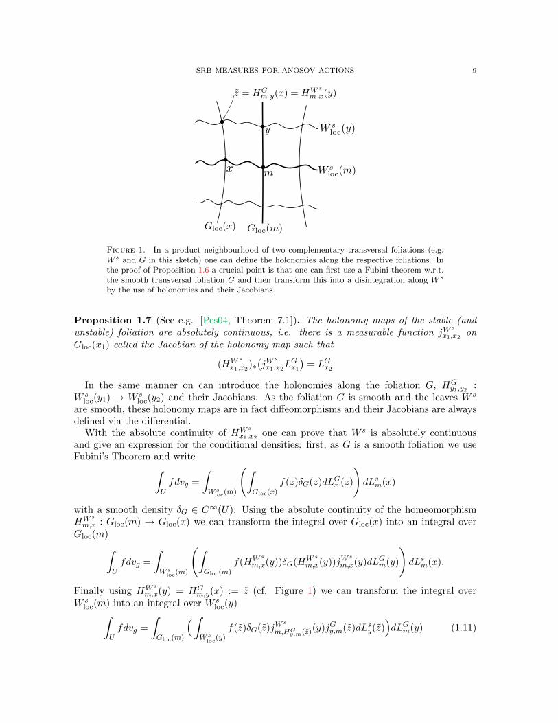
SRB MEASURES FOR ANOSOV ACTIONS 9
Figure 1. In a product neighbourhood of two complementary transversal foliations (e.g.W s and G in this sketch) one can define the holonomies along the respective foliations. Inthe proof of Proposition 1.6 a crucial point is that one can first use a Fubini theorem w.r.t.the smooth transversal foliation G and then transform this into a disintegration along W s
by the use of holonomies and their Jacobians.
Proposition 1.7 (See e.g. [Pes04, Theorem 7.1]). The holonomy maps of the stable (andunstable) foliation are absolutely continuous, i.e. there is a measurable function jW
s
x1,x2on
Gloc(x1) called the Jacobian of the holonomy map such that
(HW s
x1,x2)∗(jW
s
x1,x2LGx1
)= LGx2
In the same manner on can introduce the holonomies along the foliation G, HGy1,y2
:W s
loc(y1) → W sloc(y2) and their Jacobians. As the foliation G is smooth and the leaves W s
are smooth, these holonomy maps are in fact diffeomorphisms and their Jacobians are alwaysdefined via the differential.
With the absolute continuity of HW s
x1,x2one can prove that W s is absolutely continuous
and give an expression for the conditional densities: first, as G is a smooth foliation we useFubini’s Theorem and write∫
Ufdvg =
∫W s
loc(m)
(∫Gloc(x)
f(z)δG(z)dLGx (z)
)dLsm(x)
with a smooth density δG ∈ C∞(U): Using the absolute continuity of the homeomorphismHW s
m,x : Gloc(m) → Gloc(x) we can transform the integral over Gloc(x) into an integral overGloc(m)∫
Ufdvg =
∫W s
loc(m)
(∫Gloc(m)
f(HW s
m,x(y))δG(HW s
m,x(y))jWs
m,x(y)dLGm(y)
)dLsm(x).
Finally using HW s
m,x(y) = HGm,y(x) := z (cf. Figure 1) we can transform the integral over
W sloc(m) into an integral over W s
loc(y)∫Ufdvg =
∫Gloc(m)
(∫W s
loc(y)f(z)δG(z)jW
s
m,HGy,m(z)(y)jGy,m(z)dLsy(z)
)dLGm(y) (1.11)

10 Y. GUEDES BONTHONNEAU, C. GUILLARMOU, AND T. WEICH
making appear the Jacobian jGy,m of the holonomy map HGy,m. This proves the absolute
continuity of the stable foliation and shows that the conditional densities on W sloc(y) are given
by δG(z)jWs
m,HGy,m(z)
(y)jGy,m(z). As G was a smooth foliation δG, jGy,m and HG
m,y are smooth
so it only remains to show that jWs
m,x(y) is a smooth function in x ∈ W sloc(m) depending
continuously on y ∈ Gloc(m). However by [Pes04, Remark 7.2] there is an explicit formulafor the Jacobian for partially hyperbolic diffeomorphisms. In order to shorten the notationwe introduce Φ := ϕA0
1 and we can express the Jacobian by [Pes04, (7.3)] as5
jWs
m,x(y) =∞∏k=0
∣∣∣ det(
(dΦk(y)Φ)∣∣TΦk(y)
(Φk(Gloc(m))
))∣∣∣∣∣∣det(
(dΦk(HWsm,x(y))Φ)∣∣T
Φk(HWs
m,x(y))
(Φk(Gloc(x))
))∣∣∣In order to analyze the regularity of this infinite product we consider the espressionsdet((dΦk(y)Φ)|T
Φk(y)Φk(Gloc(m))) as functions on the Grassmanians: Let G →M be the Grass-
manian bundle of nwu-dimensional subspaces in TM. From the Riemannian metric on M,G inherits a Riemannian metric6. Note that the map Φ : TxM ⊃ V 7→ dΦx(V ) ⊂ TΦ(x)Mis a canonical lift of the diffeomorphism Φ to the Grassmanian bundle. Furthermore we candefine J : G 3 (x, V ) 7→ |det((dxΦ)|V )| ∈ R>0 which is a smooth function. We can thus write
log(jWs
m,x(y)) =∞∑k=0
logJ (Φk(TyGloc(m)))− logJ (Φk(THWsm,x(y)Gloc(x))). (1.12)
We note that by definition of the holonomies, y and HW s
m,x(y) lie on the same stable manifoldW s
loc(y) and the subspaces S(m) := TyGloc(m) and S(x) := THWsm,x(y)Gloc(x) are both transver-
sal and complementary to W sloc(y). An immediate consequence of the partial hyperbolicity of
Φ is that those two spaces (considered as points in the Grassmanian) become exponentially
close under the lifted action of Φ, i.e. there are C, ν > 0 such that
dG
(Φk(S(m)), Φk(S(x))
)≤ Ce−νkdG
(S(m), S(x)
). (1.13)
Now the compactness of G implies that J is uniformly Lipshitz and thus the series in (1.12)converges absolutely which implies that jW
s
m,x(y) is a continuous function (in the y variable aswell as in the x variable). We now show that it is even differentiable w.r.t. x: let us thereforetake a smooth curve γ : (−ε, ε)→Ws(m), γ(0) = x and ‖γ′(t)‖ ≤ 1 then
d
dt |t=0log jW
s
m,γ(t)(y) = −∞∑k=0
d(logJ )[ ddt |t=0
Φk(S(γ(t)))]. (1.14)
Using once more the hyperbolicity (in the form of (1.13)) we obtain the estimate∥∥∥∥ ddt |t=0Φk(S(γ(t)))
∥∥∥∥TS(x)G
≤ C ′e−νk
and this time the uniform Lipshitzness of d logJ ensures the absolute convergence of theright hand side of (1.14) which implies that d
dt |t=0log jW
s
m,γ(t)(y) exists and its value depends
5Be aware that Pesin uses the inverted diffeomorphism Φ−1 in his formula but the numerator and denomi-nator in his formula are also interchanged so that the formula agrees with the one that we use here.
6There might be different choices of metrics on the Grassmanian-fibres, but they all lead to equivalentmetrics.
SRB MEASURES FOR ANOSOV ACTIONS 11
continuously on y. Iteratively we obtain the same statement for higher derivatives. Indeed,we have that the n-th derivative of Φk(THWs
m,x(y)Gloc(x)) with respect to x ∈ Ws(m) decays
exponentially in k, this can be checked by writting S(x) := THWsm,x(y)Gloc(x) and by induc-
tion on n. Up to possibly multiplying A0 by a fixed positive integer, we can assume that‖dΦ(Φj(S(x)))‖ ≤ e−ν+ε for all j ≥ 0 and ε > 0 small by the discussion above. For n = 2,write
d(Φk(S(x))) = dΦ(Φk−1(S(x)))dΦ(Φk−2(S(x))) . . . dΦ(S(x))dS(x),
d2(Φk(S(x))) =k−1∑j=1
dΦ(Φk−1(S(x))) · · · d2Φ(Φj(S(x))d(Φj(S(x))) . . . dΦ(S(x))dS(x)
+ dΦ(Φk−1(S(x))) . . . dΦ(S(x))d2S(x).
This implies, using that d2Φ is uniformly bounded on G, that
‖d2(Φk(S(x)))‖ ≤ Cke−(ν−ε)(k−1).
Then repeating the same argument with an easy induction on n gives the result for derivativesof order n (we refer to the proof of [dlL92, Lemma 5.5] for example for more details). Com-bining this estimates with (1.11) we obtain the desired smoothness of δW s along the leavesW s
loc.
Note that the proof of Proposition 1.6 strongly depends on the fact that there is an expo-nential contraction along the stable, resp. unstable manifold and it would fail when workingdirectly on the weak-(un)stable foliation. Nevertheless thanks to the fact that the neutralfoliation is a smooth foliation we can establish the same result as Proposition 1.6. We will dothis in two steps: In a first step we show that there is a continuous density function δWws forthe weak-stable foliations7 and give an explicit expression in terms of δW s and some furtherquantitities which we introduce now: by (1.7) we have
Wws/wuloc (m) =
⋃y∈W s/u
loc (m)
W 0loc(m) =
⋃x∈W 0
loc(m)
Ws/uloc (x), (1.15)
where W 0loc(y) := (τ(A)y) ∩Wws/wu
loc (m) is simply the A-orbit through y. By the fact that
W s/u(τ(a)m) = τ(a)(W s/u(m)) and the smoothness of the Anosov action both partitions of
the leaf Wws/wuloc (m) are smooth foliations of W
ws/wuloc (m) and by Fubini there are strictly pos-
itive, smooth functions δWws/wuloc (m)
W 0 ∈ C∞(Wws/wuloc (m)) and δ
Wws/wuloc (m)
W s/u ∈ C∞(Wws/Wuloc (m))
such that∫Wws/wuloc (m)
f(y)dLws/wum (y)
=
∫Ws/uloc (m)
(∫W 0
loc(y′)f(z)δ
Wws/wuloc (m)
W 0 (z)dL0y′(z)
)dLs/um (y′) (1.16)
=
∫W 0
loc(m)
(∫Ws/uloc (y′)
f(z)δWws/wuloc (m)
W s/u (z)dLs/uy′ (z)
)dL0
m(y′). (1.17)
7Again the case of weak unstable foliation follows exactly the same way but we only focus on thw weakstable case to simplify the notation.
12 Y. GUEDES BONTHONNEAU, C. GUILLARMOU, AND T. WEICH
Now, in the proof of Proposition 1.6 we chose a transversal complementary smooth foliationG such that Gloc(m) = Wwu
loc (m). With (1.10), (1.16) and (1.17) this yields∫Uf dvg =
∫Wu
loc(m)
(∫Wws
loc (y)f(z)δWws(z)dLwsy (z)
)dLum(y). (1.18)
with
δWws(z) =δW s(z)δ
Wwuloc (m)
W 0
(prWws
loc (y)→W 0loc(y)(z)
)δWws
loc (y)
W s (z)
Here prWwsloc (y)→W 0
loc(y) is the projection along the smooth subfoliation (1.15) of Wwsloc (y). In
order to obtain an analogue to Proposition 1.6 it remains to analyze the regularity of δWws
along the leaves Wwsloc (y). Note that for fixed y by the smoothness of the subfoliations (1.15)
of Wwsloc (y) we conclude that the functions δ
Wwsloc (y)
W s (z) and δWwu
loc (m)
W 0
(prWws
loc (y)→W 0loc(y)(z)
)are
smooth on Wwsloc (y). By the Holder continuity of the weak stable foliation their CkWws
loc (y)-norms
vary continuously on y ∈W uloc(m). However, for δW s(z) we only know so far that this density
is smooth along W sloc(y). Using the smoothness of the Anosov action we can improve this
further: for any z ∈ W sloc(y) ⊂ U and any a ∈ V ⊂ A where V is a neighbourhood of the
identity such that τ(V )z ⊂ U we get the following equivariance property which can be derivedfrom a straightforward calculations using the A invariance of the weak-(un)stable foliationsas well as several occurences of the transformation formula:
δW s(τ(a)z) =|det(dτ(a))|(z)
|det(dτ(a)|Ewu)|(y) · | det(dτ(a)|Es)(z)|δW s(z).
All the appearing Jacobians here are understood with respect to the respective Riemannianvolume measures. As the Jacobians depend smoothly on a this shows that δW s has alsobounded derivatives of any order into the direction of the A-orbits. Summarizing we haveshown:
Proposition 1.8. Precisely the same statement as Proposition 1.6 holds when replacing the(un)stable foliation W s/u by the weak (un)stable foliation Wws/wu.
As a consequence of Proposition 1.8 we can prove the following crucial result which is aslightly more general version of [Wei17, Prop 6] for Anosov actions. It connects classicalregularity of functions into the directions of a dynamical Holder foliations with its microlocalregularity i.e. the wavefront set:
Lemma 1.9. Let τ be an Rκ-Anosov action, and consider its weak-unstable foliation. Letf be a measurable function on M, such that for Lebesgue almost all p ∈ M, f|Wwu
loc (p) issmooth with all derivatives along the leaves being uniformly bounded with respect to p. ThenWF(f) ⊂ E∗u.
Proof. We pick a point p ∈ M , ξ ∈ T ∗pM, such that ξ /∈ E∗u and a smooth function S suchthat dpS = ξ. Let G be a transverse foliation to Wwu near p, and we can assume for examplethat G(p) = W s(p). Then, using Proposition 1.6 or more particularly (1.18) (with the weak-unstable foliation instead of the weak-stable foliation), for each χ ∈ C∞(M) supported in asmall neighbourhood of p∣∣∣ ∫ χe
ihSfdvg
∣∣∣ ≤ ∫W s(p)
∣∣∣∣∣∫Wwu
loc (y)χ(x)e
ihS(x)f(x)δWwu(y)(x)dLwuy (x)
∣∣∣∣∣ dLsp(y).
SRB MEASURES FOR ANOSOV ACTIONS 13
Since each Wwuloc (y) is a smooth manifold, and f restricted to this manifold is smooth, we can
integrate by parts in the variable x. Here, it is crucial that δWwu(y)(x) is smooth in x. Wededuce (since the estimate on f are locally uniform) that this integral is O(h∞), as soon asdS|Wwu
loc (p) does not vanish. But the condition that ξ /∈ E∗u ensures this close enough to p,
since E∗u is exactly the set of covectors that vanish on Eu ⊕RX. So for χ supported close top one gets the desired result. This implies that ξ /∈WF(f).
1.3. Invariant measures via spectral theory. In this section we state the results aboutthe physical measures for general Anosov action as they have been obtained in [GBGHW20]and we also recall the essential constructions on which our analysis will be based.
The existence was obtained through the theory of Ruelle-Taylor resonances, which aredefined as a joint spectrum of the family of vector fields XA for A ∈ a in certain functionalspaces. More precisely, we say that λ ∈ a∗C is a Ruelle-Taylor resonance for τ if and onlyif there exists u ∈ C−∞(M) non-zero with WF(u) ⊂ E∗u (here WF denotes Hormanderwave-front set of the distribution [Hor03, Chapter 8]) and
∀A ∈ a, −XAu = λ(A)u. (1.19)
We say that u is a joint Ruelle resonant state of X. Using the operator dX : C−∞(M) →C∞(M)⊗ a∗ defined by (dXu)(A) := XAu for all A ∈ a, the system (1.19) can be rewrittenunder the form (−dX − λ)u = 0.
Given a general Anosov action X, we choose vectors A1, . . . , Aκ in the Weyl chamber W,which form a basis of a. The dual basis in a∗ is denoted (ej)j , and set Xj := XAj , and weuse dvg the smooth Riemannian probability measure onM. If we further pick a non-negativefunction ψj ∈ C∞c (R+) satisfying
∫∞0 ψj(t)dt = 1 then we can consider the operator
R :=
κ∏j=1
∫e−tjXjψj(tj)dtj . (1.20)
This operator appeared in a parametrix construction in a Taylor complex generated by theAnosov action and this parametrix was the central ingredient for establishing the existence ofthe Ruelle-Taylor resonances in [GBGHW20]. For the purpose of this paper we will not needto introduce the Taylor complexes and spectrum but we will only focus on the results neededfor our present work. In section 4.1 of [GBGHW20], we construct a function G ∈ C∞(T ∗M),called escape function for A1 ∈ W and satisfying the properties of [GBGHW20, Definition4.1]: in particular, there is R0 > 0, cX > 0 and a conic neighborhood ΓE∗0 of E∗0 in T ∗M suchthat
G(x, ξ) = m(x, ξ) log(1 + f(x, ξ)),f ∈ C∞(T ∗M,R+) positive and homogeneous of degree 1 in |ξ| > R0,m ∈ C∞(T ∗M, [−1/2, 8]) homogeneous of degree 0 in |ξ| > R0,m ≤ −1/4 in an arbitrarily small conic neighborhood Γu of E∗u if |ξ| > R0
m ≥ 1/2 outside an arbitrarily small conic neighborhood Γ′u of Γu if |ξ| > R0.
(⋃t∈[0,1] e
tXHA (x, ξ)) ∩ (ΓE∗0 ∪ |ξ| < R0) = ∅ ⇒ G(eX
HA (x, ξ))−G(x, ξ) ≤ −cX
(1.21)
where XHA is the Hamilton vector field of the principal symbol p := ξ(XA(x)) of the operator
−iXA (we note that its flow etXHA is the symplectic lift of ϕA1 ).
After fixing a quantization procedure Op mapping symbols on T ∗M to operators acting onC∞(M) (as in [Zwo12]), we consider the pseudo-differential operator Op(eNG) with variable
14 Y. GUEDES BONTHONNEAU, C. GUILLARMOU, AND T. WEICH
order and we define the Hilbert space
HNG := Op(eNG)−1L2(M).
where Op(eNG) can be made invertible by choosing appropriately G. For later, we will alsoneed a semi-classical parameter h ∈ (0, 1], to consider a semiclassical quantization Oph andto define
HNGh := (Oph(eNG))−1L2(M).
The spaces HNGh for different values of h are the same topological vector spaces but thenorms are different. For more details on the construction of the anisotropic spaces and theused microlocal techniques we refer to [GBGHW20, Section 4.1 and Appendix A].
Proposition 1.10 ([GBGHW20, Lemma 4.14, Lemma 5.1 and Lemma 5.2]). For N > 0large enough, the operator R of (1.20) is a bounded operator on HNG with essential spectrumcontained in the disk D(0, 1/2). The only eigenvalue s with |s| = 1 is s = 1 and this eigenvaluehas finite multiplicity and no Jordan blocks. Finally, if Π denotes the finite rank spectralprojector of R at s = 1, then the following convergence holds in L(HNG)
limk→+∞
Rk = Π.
We note that the same results hold on the spaces HNGh for all h ∈ (0, 1). We will alsoneed the technical Lemma (see [GBGHW20, Proof of Lemma 4.12]) which follows from theflexibility of the choice of the function G:
Lemma 1.11. A distribution u ∈ C−∞(M) having WF(u) ⊂ E∗u satisfies u ∈ HNG for someN > 0. Conversely, if there is N0 such that u ∈ HNG for all N ≥ N0 and all admissibleescape functions G (in the sense of [GBGHW20, Definition 4.1]), then WF(u) ⊂ E∗u.
If F ⊂ T ∗M is a conical closed set in T ∗M, we denote by C−∞F (M) := u ∈C−∞(M) | WF(u) ⊂ F.
The spectral projector Π satisfies RΠ = Π = ΠR, and by [GBGHW20, Lemma 5.3] itsSchwartz kernel is independent of N,G and has the form
Π =
r∑j=1
vj ⊗ ω∗j (1.22)
with vj ∈ HNG ∩C−∞E∗u (M) and w∗j ∈ (HNG)∗ ∩C−∞E∗s (M); moreover if N > 0 is large enough
we have by [GBGHW20, Lemma 5.3]
ran Π = u ∈ C−∞E∗u (M) | ∀A ∈ a, XAu = 0 = u ∈ HNG | ∀A ∈ a, XAu = 0. (1.23)
The relation of Π with the physical measure is explained by [GBGHW20, Proposition 5.4]as follows:
Proposition 1.12.
(1) For each v ∈ C∞(M,R+), the map
µv : u ∈ C∞(M) 7→ 〈Πu, v〉is a Radon measure with mass µv(M) =
∫M v dvg, invariant by Xj for all j = 1, . . . , κ
in the sense µv(Xju) = 0 for all u ∈ C∞(M). The space
spanµv | v ∈ C∞(M) = Π∗(C∞(M))
SRB MEASURES FOR ANOSOV ACTIONS 15
is, for N sufficiently large, a finite dimensional subspace of (HNG)∗ whose dimensionequals the space of joint resonant states. Furthermore Π(C∞(M)) is precisely spannedby the invariant measures µ with WF (µ) ⊂ E∗s .
(2) For each open cone C ⊂ W in the positive Weyl chamber with ∂C ∩∂W = 0, e1 ∈ a∗
so that e1 > 0 on C, and u, v ∈ C∞(M),
µv(u) = limT→∞
1
|CT |
∫A∈CT ,
〈ϕA−1u, v〉dA (1.24)
where dA is the Lebesgue-Haar measure on a and CT := A ∈ C | e1(A) ∈ (0, T ). Inparticular, µ1 is the physical measure.
(3) Let v1, v2 ∈ C∞(M,R+) with v1 ≤ Cv2 for some C > 0. Then µv1 is absolutelycontinuous with bounded density with respect to µv2. In particular any µv is absolutelycontinuous with respect to µ1.
(4) Consider a local stable manifold W sloc(x0), f ∈ C∞c (W s
loc(x0),R+) and Lsx0the
Lebesgue measure on W sloc(x0) with
∫fdLsx0
= 1. Then for C, CT as in (2), thelimit
µfLsx0(u) = lim
T→∞
1
|CT |
∫CT
∫Mu(ϕA−1)fdLsx0
dA (1.25)
exists and defines a probability measure in Π∗(C∞(M)).
Remark 1.13. We will see in Section 2 that in fact the whole space Π∗(C∞(M)) is spannedby measures of the form µfLsx0
.
Proof. The items (1), (2), (3) are proved in [GBGHW20, Proposition 5.4]. Let us prove the4th item. For this, we follow closely the proof of [GBGHW20, Proposition 5.4] but we replacethe smooth function v by the measure v′ := fLsx0
. Since W sloc(x0) is a smooth submanifold
of M we have that (see for instance [Hor03, Example 8.2.5]) WF(fLsx0) ⊂ E∗s ⊕ E∗0 . The
distribution v′ belongs to (HNG)∗: indeed for u ∈ C∞(M),
〈u, v′〉C∞,C−∞ = 〈Op(eNG)u, (Op(eNG)−1)∗v′〉C∞,C−∞
and (Op(eNG)−1)∗ is a pseudo-differential operator with variable order and with principal
symbol e−NG ≤ C|ξ|−N/2 in (x, ξ) ∈ T ∗M| ξ /∈ Γ′u, |ξ| > R0 by (1.21); since Γ′u∩(E∗0⊕E∗s ) =∅, we deduce that there is N > 0 large enough so that (Op(eNG)−1)∗v′ ∈ L2 (note that
v′ ∈ H−dim(M+1)/2(M)). Recalling that Op(eNG) : HNG → L2 is an isometry we see thatu 7→ 〈u, v〉C∞,C−∞ extends to a continuous functional on HNG
For u ∈ C∞(M) we thus have using Proposition 1.10 (notice that the result is independentof the choice of ψ in the definition of the operator R)
limk→∞〈Rku, v′〉HNG,(HNG)∗ = 〈Πu, v′〉HNG,(HNG)∗ =
r∑j=1
ω∗j (u)〈vj , v′〉HNG,(HNG)∗ (1.26)
which proves that µkv′ : u 7→ 〈Rku, v′〉HNG,(HNG)∗ is a Radon measure that converges to some
element in Π∗(C∞) depending only on v′. The limit is a probability measure since, usingR 1 = 1, one has µkv′(1) = 〈1, v′〉 = 1. Next, in the proof of Proposition 5.4 of [GBGHW20],we replaced the functions
∏κj=1 ψj(tj) by ψσ(t) =
∏κj=1 ψj(tj − σj) for σ ∈ Rκ ' a small in
the definition of Rk, and call Rkσ the resulting operator. Fixing one direction A1 ∈ C, e1 ∈ a∗
so that e1(A1) = 1, and taking a transverse hypersurface Σ = e−11 (1) to C, we obtain
coordinates (t1, . . . , tκ) with t1 = e1(A) on a and t = (t2, . . . , tκ) some linear coordinates on
16 Y. GUEDES BONTHONNEAU, C. GUILLARMOU, AND T. WEICH
Σ associated with a basis A2, . . . Aκ of ker e1. We prove in [GBGHW20, Lemma 5.5] thatif ω ∈ C∞c ((0, 1)) satisfies
∫ω = 1 and q ∈ C∞c (Σ ∩ C) satisfies
∫q = 1, then for each
v ∈ C∞(M)∣∣∣ 1
N
N∑k=1
ω( kN )〈Rkσ(t)u, v〉q(t)dt−1
Nκ
∫ N
0
∫Rκ−1
〈e−∑κj=1 tjXAju, v〉( t1N )1−κω( t1N )q( tt1 )dt1dt
∣∣∣≤ ε(N) sup
t1,t
|〈e−∑κj=1 tjXAju, v〉| ≤ ε(N)‖u‖C0(M)‖v‖(C0(M))∗
where σ(t) = (1, t) in the coordinates t1, . . . , tκ and ε(N)→ 0 as N →∞. We can then takea sequence vn → v′ in the topology (C0(M))∗ dual to C0(M) (i.e. Radon measures) and weobtain, using (1.26) and letting N →∞,
〈u,Πv′〉 = limN→∞
1
Nκ
∫ N
0
∫Rκ−1
〈e−∑nj=1 tjXAju, v′〉( t1N )1−κω( t1N )q( tt1 )dt1dt.
By finally letting ω(t1)q(t/t1) be arbitrarly close to tκ−11 1[0,1](t1)1Σ∩C(t/t1) in L∞, we obtain
that µfLsx0can be written as (1.25).
Now, using the usual proof for the decomposition of the SRB measures along stable leavesin rank 1, we can prove the
Proposition 1.14. For each x0 and f ∈ C∞c (W sloc(x0),R+) with
∫fdLsx0
= 1, the measureµfLsx0
defined by (1.25) has strictly positive smooth conditional measures on the local leaves
W sloc(x) with respect to Lebesgue measure Lsx, for each x ∈M.
Proof. We follow the proof of [You95, Theorem 6.3.1]. Call ν0 := fLsx0and νA = (ϕA−1)∗ν0 for
A ∈ W. This measure is supported on the piece of stable manifold ϕA−1(W sloc(x0)). We also
define νT := 1|CT |
∫CT νAdA. Let x1 ∈ M and consider a small neighborhood Ux1 such that
the disintegration along stable leaves can be done by Proposition 1.4. Let y ∈ Ux1 be suchthat ϕA1 (y) ∈W s
loc(x0) then the measure νA on a stable leaf W sloc(y) ⊂ Ux1 can be written as
νA = | det(dϕA1 |Es)|f ϕA1 Lsy
and | det(dϕA1 |Es)| is the Jacobian restricted to Es (computed w.r.t. Lebesgue), which isexponentially small as |A| is large. Then, let ν∞ := µfLsx0
= limT→∞ νT that we decompose
in Ux1 along stable leaves and we call ν∞x1the conditional on W s
loc(x1). If G is a transversesmooth foliation manifold to the stable foliation near x1, one can write
ν∞x1= lim
ε→0
1Fεν∞
ν∞(Fε)
where Fε = ∪y∈BG(x1,ε)Wsloc(y) is a tube of radius ε > 0 around W s
loc(x1), where BG(x1, ε) ⊂G(x1) is the ball of radius ε in G(x1). Now let V ⊂W s
loc(x1) be a small open ball and consider
Vε := ∪y∈VG(y)∩Fε. For |A| large, the leaf ϕA−1(W sloc(x0)) becomes long and intersect Vε into,
say kε(A) ∈ N∪+∞ connected components8 (W sloc(yj)∩Vε)j=1,...,kε(A) for yj(A) ∈ BG(x1, ε);
8The number of components with non-zero Lebesgue measure is countable.
SRB MEASURES FOR ANOSOV ACTIONS 17
note that yj(A) depends continuously on A. We then write
νT (Vε) =1
|CT |
∫CTνA(Vε)dA
=1
|CT |
∫CT
kε(A)∑j=1
∫W s
loc(yj(A))∩Vε| det(dϕA1 (z)|Es(z))|f(ϕA1 (z)) dLsyj(A)(z)dA.
(1.27)
We can now use the holonomy map HGx1,yj(A) as defined after Proposition 1.7 to rewrite the
W sloc(yj(A)) integral as a W s
loc(x1) integral:∫W s
loc(yj)∩Vε| det(dϕA1 (z)|Es(z))|f(ϕA1 (z)) dLsyj (z)
=
∫V| det(dϕA1 (HG
x1,yj(A)(z))|Es)|f(ϕA1 (HGx1,yj(A)(z)))j
Gx1,yj(A)(z) dL
sx1
(z)
where jGx1,yj is the Jacobian of HGx1,yj which is uniformly bounded above and below (with
respect to yj) by some positive constants C1, C2. Let us define the density
ρAj (z) = |det(dϕA1 (HGx1,yj(A)(z))|Es)|f(ϕA1 (HG
x1,yj(A)(z)))jGx1,yj(A)(z)
on a neighborhood of V inside W sloc(x1). Now we can show that there is C > 0 such that for
all y, z in W sloc(x1) ∩ V , all j ≤ kε(A) and all A ∈ C
ρAj (z)
ρAj (y)≤ eCdg(y,z). (1.28)
To obtain this estimate we can apply the argument in [You95, Proof of Theorem 5.2.1]: First,since HG
x1,yj (z), HGx1,yj (y) are on the same the stable leaf, there is a uniform C > 0 such that
for all A ∈ CT and j ≤ kε(A) and all y, z ∈W sloc(x1) ∩ V
f(ϕA1 (HGx1,yj(A)(y)))jGx1,yj(A)(y)
f(ϕA1 (HGx1,yj(A)(z))))j
Gx1,yj(A)(z)
≤ eCdg(y,z).
Next we get, letting A := A/|A| ∈ W and nA := [|A|] be the integral part of |A|, that thereare constants C0, . . . , C3 > 0 such that for all with A ∈ CT , j ≤ kε(A), y, z on W s
loc(yj(A))
log|det(dϕA1 |Es)(y)|| det(dϕA1 |Es)(z)|
≤ C0
nA∑n=0
∣∣∣ log |det(dϕA1 |Es)(ϕAn (y))| − log | det(dϕA1 |Es)(ϕAn (z))|∣∣∣
≤ C1
nA∑n=0
dg(ϕAn (y), ϕAn (z))
≤ C2
nA∑n=0
e−c0ndg(y, z) ≤ C3dg(y, z)
where c0 > 0 is less than the minimal contraction exponent of the flow in the direction A ∈ Cin the stable bundle. Such a uniform constant exists because the cone C does not touch theboundary of the Weyl chamber. Applying this with y = HG
x1,yj (y) and z = HGx1,yj(A)(z) we
obtain the desired estimate (1.28) since the holonomy map has uniformly Lipschitz boundwrt A ∈ CT and j ≤ kε(A).

18 Y. GUEDES BONTHONNEAU, C. GUILLARMOU, AND T. WEICH
Now, this clearly implies that there is C > 0 such that for all y, z ∈W sloc(x1) ∩ V
1|CT |
∫CT∑kε(A)
j=1 ρAj (z) dA
1|CT |
∫CT∑kε(A)
j=1 ρAj (y) dA≤ eCdg(y,z).
Coming back to (1.27) we get that
νT (Vε)νT (Fε)
=
∫V
(1|CT |
∫CT∑kε(A)
j=1 ρAj dA)dLsx1∫
W sloc(x1)
(1|CT |
∫CT∑kε(A)
j=1 ρAj dA)dLsx1
and the density on W sloc(x1)
dε(y) =
1|CT |
∫CT∑kε(A)
j=1 ρAj (y) dA∫W s
loc(x1)1|CT |
∫CT∑kε(A)
j=1 ρAj (y) dAdLsx1
is of mass 1 for Lsx1and its logarithm has a Lipschitz constant which is bounded independently
of T and ε, so it satisfies α ≤ dε ≤ β for some positive constant α, β uniform in ε, T . Thisimplies that
αLsx1(V ) ≤ νT (Vε)
νT (Fε)=
∫Vdε(y)dLsx1
(y) ≤ βLsx1(V )
which shows, by letting T →∞ and then ε→ 0, that the conditional measure ν∞x1is absolutely
continuous with respect to Lebesgue Lsx1on W s
loc(x1).Next, by Ledrappier-Young [LY85, p. 533], if ρ(y) is the density of the conditional ν∞x1
withrespect to Lebesgue Lsx1
, one has for A0 ∈ W and x, y ∈W sloc(x1)
ρ(y)
ρ(x)=
∏∞j=1 |det(dϕA0
−1|Es)|(ϕA0j (y))∏∞
j=1 | det(dϕA0−1|Es)|(ϕ
A0j (x))
Then, using this formula, an argument using the contraction on stable leaves and the chainrule for derivatives very similar to the proof of Proposition 1.7 shows that ρ must be smoothon W s
loc(x1). A detailed proof is done in [dlL92, Corollary 4.4 and Lemma 5.5].
2. Equivalent characterisation of SRB measures
In this section we will study the measures µv obtained by the Ruelle-Taylor spectral theory.Let us first introduce some notation:
Definition 2.1. For an invariant measure µ define the basin to be those points x ∈M suchthat for any f ∈ C0(M) and any proper subcone C ⊂ W we have
µ(f) = limT→∞
1
|CT |
∫A∈CT
f(ϕA−1(x))dA. (2.1)
We say that an invariant measure µ is an SRB measure for τ if the basin has positive Lebseguemeasure.
We show that they are linear combinations of SRB measures and give various other differentcharacterisations:
Theorem 3. Let τ be a smooth, locally free, Rκ Anosov action with generating map X, thenwe have:
SRB MEASURES FOR ANOSOV ACTIONS 19
1) The linear span over C of the SRB measures can be identified with the finite dimensionalspace ker dX |C−∞
E∗s.
2) The physical measure (0.1) is a linear combination of SRB measures.3) The union of the basins of the SRB measures has full Lebesgue measure in M.4) An ergodic Radon probability measure µ is a SRB measure if and only if it is invariant by
ϕAt for all A ∈ a and has wave-front set WF(µ) ⊂ E∗s .5) The conditional measures of the SRB measures of an Anosov abelian action are absolutely
continuous with respect to the Lebesgue measure on the stable manifolds, and they havesmooth densities with respect to Lebesgue. Vice versa any ergodic invariant Radon proba-bility measure that is absolutely continuous with respect to the Lebesgue measure (withoutassuming smooth densities) is a SRB measure.
We furthermore prove that if the Anosov action is transitive then there is a unique SRB-measure (see Corollary 2.4) and if it is positively transitive the SRB-measure has full support(see Proposition 2.10). Theorem 3 together with these two additional result then gives The-orem 1 stated in the introduction.
We will first study the ergodic decomposition of µ1 and identify the basins of attractions(recall that the notion of basin of attraction was defined in the Introduction). We will usesome arguments in the spirit of [BKL02, Proposition 2.3.2] to obtain
Lemma 2.2. Let X be an Anosov action, and let µ = µ1 be the physical measure. Thereexist disjoint measurable sets F1, . . . , Fr such that µ(Fi) = vg(Fi) 6= 0 for all i and µ(∪iFi) =
vg(∪iFi) = 1. Furthermore the ergodic components of µ are given by µi :=1Fiµ(Fi)
· µ and Fi is
the basin of µi. In particular each µi is an SRB measure. Finally the µi form a basis of thespace Π∗(C∞(M)).
Proof. For C ⊂ W a proper open subcone, e1 ∈ a∗ with e1 > 0 in C, and f ∈ C0(M), wedefine
Ω(f, C) :=
x ∈M
∣∣∣∣ f−(x) := limT→+∞
1
|CT |
∫A∈CT
f(ϕA−1(x))dA exists in R.
where CT = C ∩ e1(A) ∈ (0, T ). It follows from the ergodic Birkhoff Theorem for actions(see [Bew71, Theorem 3]) that for all such C and f , and every invariant Borel measure ν,Ω(f, C) has full ν-measure. By a dichotomy argument on the cones, and using the fact thatC0(M) is separable, we can improve this, by saying that
Ω :=⋂f,C
Ω(f, C),
also has full ν measure for every invariant Borel measure ν. Additionally, we observe that ifx ∈ Ω, then the weak unstable manifold satisfies Wwu(x) ⊂ Ω.
More generally, if a set F is a union of full weak unstable manifolds, we will say that F isunstable-invariant. Notice that Ω is unstable-invariant. According to Lemma 1.9, this impliesWF(1F ) ⊂ E∗u, and thus 1F ∈ HNG for N large enough. In particular, since XA1F = 0 for allA ∈ a, 1F belongs to the finite dimensional space ran Π by (1.23). This means that 1F = Π1Fin the distribution sense, thus Lebesgue almost everywhere since 1F is L1.
20 Y. GUEDES BONTHONNEAU, C. GUILLARMOU, AND T. WEICH
Since for v ∈ C∞, the identity µv(u) = 〈Πu, v〉 extends from smooth functions u to elementsu ∈ HNG, we have for each unstable-invariant set F ,
µv(F ) =
∫M
(Π1F )v dvg =
∫Fv dvg. (2.2)
In particular, since µ(Ω) = 1, Ω has full Lebesgue measure (even if the Lebesgue measureis not invariant by the action). If F is unstable invariant, then we also have µ(F ) = vg(F ).Since each such 1F is an element of the space of resonant states at λ = 0
H := Span 1F | F is unstable invariant / ∼ is a subspace of ran Π.
(here, ∼ is the equivalence relation of being equal Lebesgue a.e. or, equivalently µ a.e.).
Accordingly, we can find pairwise disjoint unstable invariant sets F1, . . . , Fr with r ≤ rank Π,so that the [1Fj ] form a basis of H. Since Ω has full-measure, we can assume that ∪Fj = Ω.
If f is a continuous function and C ⊂ W is an open proper subcone, we observe that thesets x ∈ Ω | f−(x) ≤ r are unstable-invariant for each r ∈ R, so they are finite unions of
Fj ’s, up to Lebesgue-null sets and by (2.2) also up to µ-null sets. This implies that f−(x) is
constant on each Fj , µ-a.e. and we denote f−,j that value. By Lebesgue theorem and theinvariance of µ by ϕA−1,
µ(Fj)f−,j =
∫Fj
f−(x)dµ(x) = limT→∞
∫Fj
1
|CT |
∫CTf(ϕA−1(x))dAdµ(x) =
∫Fj
f dµ. (2.3)
Thus, if we define µj := 1Fjµ/µ(Fj) we get f−,j = µj(f). Thus for arbitrary f ∈ C0(M)
and an arbitrary proper subcone C ⊂ W we have shown that for µ a.e. x ∈ Fj we havef−(x) = µj(f). Using as above that C0(M) is separable and that we can approximate anarbitrary cone by a countable number of cones, we deduce that the basin Fj of µj differs from
Fj by a µ nullset or equivalently a Lebesgue nullset.The same argument as in (2.3) can be done for µv, so we deduce that for v ∈ C∞,∫
fdµv =∑j
f−(Fj)µv(Fj) =∑j
µj(f)
∫Fj
vdvg. (2.4)
We have thus seen that the 1Fj form a meaningful basis of H. Now we prove that in fact
H = ran Π. Let π : L1(M, µ) → L1(M, µ) be the projector onto the set of XA invariantfunctions (for all A ∈ a) along the closed subspace generated by coboundaries ϕA1 f − f | f ∈L1(µ), A ∈ a. By the ergodic theorem of [Bew71], π is a continuous operator and for µalmost all x ∈M
πf(x) = limT→∞
1
|CT |
∫CTf(ϕA−1(x))dA.
We have just proved that π maps C0(M) to functions constant on the Fj ’s. In particular,by density of continuous functions in L1(µ), we deduce that the image of π only containsfunctions constant on the Fj ’s. This proves that the Fj , or more precisely, the µj are theergodic components of µ, and that Equation (2.4) is the ergodic decomposition (in the senseof Theorem 4.2.6 of [HK02]). One consequence of the above is that µ has at most rank Πergodic components. However, in µv | v ∈ C∞(M), we can find rank Π linearly independentprobability measures, absolutely continuous with respect to µ, and invariant under the action.This implies that the number of ergodic components is at least rank Π. We deduce thatH = ran Π, and that the 1Fj form a basis of ran Π.
SRB MEASURES FOR ANOSOV ACTIONS 21
It remains to show that the µj ’s form a basis of Π∗(C∞). Since they have pairwise disjointsupport, the µj are linearly independent and they span a space of the same dimension asΠ∗(C∞). It thus remains to prove that all µj lie in Π∗ which by Proposition 1.12 can beachieved by considering the wavefront sets of the µj : We can refine (2.4), since the LHS of(2.4) is equal to 〈Πf, v〉. We obtain
Π =r∑j=1
1Fj ⊗ ω∗j , (2.5)
for some ω∗j ∈ (HNG)∗, j = 1, . . . , rank Π. Now, we can write µv in two different ways:
µv(u) =∑j
w∗j (u)
∫Fj
vdvg =∑j
µj(u)
∫Fj
vdvg,
so that w∗j = µj . By Lemma 1.11, this shows that µj has wavefront set only in E∗s , while we
had a priori no information regarding the wavefront set of µj .
We thus have shown that the basins Fj of µj coverM up to a Lebesgue zero set. Accordinglyany SRB-measure must be equal to one of the µj and thus lie in µv | v ∈ C∞(M), v ≥ 0.In order to prove the uniqueness of SRB-measures for transitive actions, we will prove.
Lemma 2.3. For any SRB-measure µj with basin Fj there is an open set Uj ⊂M such thatνg(Uj ∩ Fj) = νg(Uj).
Corollary 2.4. It the Anosov action τ transitive then there is a unique SRB measure.
Proof. Assume that there are two SRB-measures µ1 and µ2 and U1, U2 the two open sets. Bythe transitivity there is A ∈ a such that U1 ∩ ϕA1 (U2) 6= ∅. Then we deduce that Lebesguea.e. x ∈ U1 ∩ ϕA1 (U2) lies in F1 and (by absolute continuity of φA1 w.r.t. Lebesgue) Lebesguea.e. x ∈ U1 ∩ ϕA1 (U2) lies in ϕA1 (F2). But as the basins are flow invariant this is not possibleexcept if F1 = F2.
In order to prove Lemma 2.3 we first show:
Lemma 2.5. For x0 ∈ M let Lsx0be the Lebesgue measure on W s
loc(x0) and call L the setof all these measures supported on small pieces of stable manifolds. Then the vector spaceΠ∗(C∞(M)) = spanµ1, . . . , µj is also equal to
spanµfLsx0
∣∣∣x0 ∈M, f ∈ C∞c (W sloc(x0),R+),
∫W s
loc(x0)fdLsx0
= 1, Lsx0∈ L
.
Proof. We already know that all µfLsx0are contained in the finite dimensional complex vector
space Π∗(C∞(M)) = spanµ1, . . . , µj. Suppose that they do not span the whole space, thenall µfLsx0
have to lie in a proper subspace and there is a linear functional on spanµ1, . . . , µjvanishing on all µfLsx0
. This would imply that there exists w =∑
j λj1Fj , with λj ∈ Cand Fj defined by (1.22), such that 〈w, fLsx0
〉 = 0 for any Lsx0and f as above. First take
v ∈ C∞(M,R+) so that 〈w, v〉 6= 0. We can decompose v =∑
i χiv in small charts (Ui)iwhere the disintegration along stable leaves can be performed as in (1.10): taking Gi some
22 Y. GUEDES BONTHONNEAU, C. GUILLARMOU, AND T. WEICH
local transverse manifolds to the W s foliation in Ui,
〈w,χiv〉 =
∫Ui
χi(x)v(x)w(x) dvg(x)
=
∫Gi
∫W s
loc(z)χi(y)w(y)v(y)δW s
loc(z)(y)dLsz(y) dLGi(z)
= 0
where we used our assumption with f = χivδW sloc(z) on W s
loc(z) and x0 = z to get the lastline. We obtain a contradiction.
We deduce, using Proposition 1.14 the
Corollary 2.6. The conditional measures µj are absolutely continuous with respect to theLebesgue measure on the stable manifolds, and they have smooth densities with respect toLebesgue.
We can now prove the Lemma 2.3.
Proof of Lemma 2.3. Recall that µj :=1Fjµ(Fj)
µ and that Fj are the basins of µj . Let us
construct these open sets Uj : We consider a point x0 ∈ suppµj and a small product neigh-borhood V of x0. Furthermore consider the disintegration of µj along the strong stablefoliation in V . By Corollary 2.6, this gives locally around x0 for any y ∈ Wwu
loc (x0) a
measure µjy on W sloc(y) with a smooth density with respect to the Lebesgue measure Lsy
on W sloc(y) and a transversal measure µj on Wwu
loc (x0). But we know that 1Fjµj = µj
and consequently for µj a.e. y ∈ Wwuloc (x0) we have 1Fj∩W s
loc(y)µjy = µjy. In particular
there is at least one y0 ∈ Wwu(x0) such that 1Fj∩W sloc(y0)µ
jy0 = µjy0 6= 0. But as µjy0
has a smooth density with respect to the Lebesgue measure on W sloc(y0) there exists an
nonempty open set U jy0 := int(suppµjy0) ⊂W sloc(y0) such that µjy0(Fj ∩W s
loc(y0)) = µjy0(U jy0).As the Fj are invariant in the weak-unstable directions we can consider the open setUj := ∪
z∈Ujy0Wwu
loc (z) ⊂ V . Using the absolute continuity of the weak unstable foliation,
one checks that vg(Fj ∩ Uj) = vg(Uj).
In a very similar way as the one presented above for the construction of the Uj we prove
Lemma 2.7. Let ν be an ergodic Radon measure on M that has an absolutely continuousdisintegration w.r.t. W s
loc then the basin of ν has positive Lebesgue measure.
Proof. Let Ω be the set of x ∈M such that for all f ∈ C0(M) and all cones C ⊂ W
f−(x) = limT→+∞
1
|CT |
∫A∈CT
f(ϕA−1(x))dA = ν(f)
By the ergodicity assumption Ω has full ν measure and is in particular a nonempty unstableinvariant set. Moreover 1Ων = ν. We now consider a point x0 ∈ Ω in the support of ν anda small neighborhood V of x0. Furthermore consider the disintegration of ν along the strongstable foliation in V : This gives locally around x0 for any y ∈ Wwu
loc (x0) a measure νy onW s
loc(y) with a density with respect to the Lebesgue measure Lsy on W sloc(y) and a transversal
measure ν on Wwuloc (x0). But we know that x0 is in the support of ν and consequently there is

SRB MEASURES FOR ANOSOV ACTIONS 23
at least one y0 ∈Wwuloc (x0) such that 1Ω∩W s
loc(y0)νy0 = νy0 6= 0. As νy0 is absolutely continuous
w.r.t Lsy0we conclude that Ω ∩ W s
loc(y0) has positive Lsy0measure. As the Ω is invariant
in the weak-unstable directions and as the holonomies along these weak unstable directionsare absolutely continuous we deduce, that Ω ∩W s
loc(y) has positive Lsy measure for all y inV . Now we can use that also the Lebesgue measure has absolutely continuous disintegrationalong W s
loc and conclude that V ∩ Ω has positive Lebesgue measure.
We already know that for a topologically transitive Anosov action only the physical measurecan have a basin of positive Lebesgue measure. Consequently for a topologically transitiveAnosov action any ergodic measure with absolutely continuous disintegration w.r.t. W s
loc isautomatically the physical measure. For the general case we consider:
Lemma 2.8. Let ν be a Radon measure onM that has an absolutely continuous disintegrationw.r.t. W s
loc and is invariant under the Anosov action τ . If supp(ν) ⊂ M is connected, thenν is ergodic, i.e. there is a full ν measure set F ⊂M such that for all x ∈ F , all f ∈ C0(M)and all proper subcones C ⊂ W one has f−(x) =
∫M fdν.
Proof. Let Ω be the set of x ∈M such that for all f ∈ C0(M) and all cones C ⊂ W
f−(x) = limT→+∞
1
|CT |
∫A∈CT
f(ϕA−1(x))dA = ν(f)
Then we know by the reasoning at the beginning of Lemma 2.2 that Ω has full ν measure.The function f− is thus a measurable function that is constant on weak unstable leaves. LetA ∈ W, then W s(x) are precisely the stable sets of the diffeomorphism ϕA1 . By [BS02, Lemma6.3.2] there is a ν nullset N such that for any x ∈M \N , f− is constant on W s(x) \N .
Now by the absolute continuity in any product neighbourhood U ⊂M we can write
0 =
∫U
1Ndν =
∫Wwu
loc (m)
(∫W s
loc(y)1N (z)δW s(z)dLsy(z)
)dν(y)
Accordingly for ν almost all y ∈Wwuloc (m) one has N ∩W s
loc(y) is a Lsy zero set. Pick one suchy0 and z0 ∈ W s
loc(y0). Then, by the definition of N for all z ∈ W sloc(y0) \N we have f−(z) =
f−(z0). Let y1 ∈ Wwuloc (m) by any other point. As f− is constant along the weak unstable
leaves we can use the holonomy along the weak unstable leaves HWwu
y0,y1: W s(y0) → W s(y1).
As we know that this holonomy is absolutely continuous we have that
f− = f−(z0) ∩W sloc(y1) ⊂ HWwu
y0,y1(W s
loc(y0)) ⊂W sloc(y1)
has full Lsy1measure. Using once more the absolute continuity of ν along the stable foliation
we get
ν(f− = f−(z0) ∩ U) = ν(U) (2.6)
Using the connectedness of supp(ν), we deduce that Ff := f− = f−(z0) has full ν measureand from [Bew71, Theorem 1 and 3] we get
f−(z0) =
∫Mf−dν =
∫fdν.
We finally take F = ∩f∈C0(M)Ff and use he fact that C0(M) is separable to reduce the
intersection to a countable set in C0(M), we obtain that F has full ν measure and satisfiesthe desired property.
24 Y. GUEDES BONTHONNEAU, C. GUILLARMOU, AND T. WEICH
Consequently for any Radon supp ν measure on M that has an absolutely continuousdisintegration w.r.t. W s
loc and is invariant under the Anosov action τ we can decompose
the support supp ν into its connected compontents Ci and we deduce that νi :=1Ciν(Ci)
ν are
SRB-measures. This proves property 5) of Theorem 3.
Definition 2.9. We call an Anosov action positively transitive if there is a proper subconeC ⊂ W such that for any two open sets U, V ∈M there is A ∈ C such that ϕA1 (U) ∩ V 6= ∅.
If the Anosov action is positively transitive then it is obviously transitive and we knowthat there is a unique SRB measure.
Proposition 2.10. If the Anosov action is positively transitive then the SRB measure µ hasfull support.
Proof. Assume that suppµ 6=M then there are m0 ∈M, ε, δ > 0 s.t. the product neighbour-hood (cf. (1.8)) U0 := BW s(m0, δ)× BWwu(m0, ε) is disjoint from suppµ. Let us also definethe set U1 := BW s(m0, δ)× BWwu(m0, ε/2). Recall that, after chosing an arbitrary norm ona, the transversal hyperbolicity of the Anosov action implies that there are C ′, ν > 0 suchthat for all A ∈ C, v ∈ Eu we have ‖dϕA1 v‖g > (1/C ′)eν|A|‖v‖g. As the splitting E0⊕Es⊕Euis continuous and M is compact, there is C > 1 so that g(v0, vu) ≤ (1− 1/C)‖v0‖g‖vu‖g forall vu ∈ Eu, v0 ∈ E0, and we deduce that there is C > 1 for all A ∈ C and v ∈ E0 ⊕ Euwe have ‖dϕA1 v‖g ≥ (1/C)‖v‖g. As a direct consequence we deduce that for all A ∈ C and
m ∈ ϕA1 (U1) there is δ > 0 such that
BW s(m, δ)×BWwu(m, ε/(2C)) ⊂ ϕA1 (U0) . (2.7)
Since the stable and weak unstable foliations are continuous, taking η > 0 small enough,we can ensure that for m ∈ M and y ∈ BW s(m, η), the weak unstable ball BWwu(y, ε/(2C))is large enough, in the sense that
BWwu(y, ε/(2C)) ∩ BW s(m, η)×BWwu(m, ε/(4C)) ⊂ BWwu(y, ε/(2C)).
Let us thus cover the manifold M with a finite open cover of product neighbourhoods Vj =BW s(mj , η)×BWwu(mj , ε/(4C)). As the SRB measure µ is nonzero, there is at least one Vksuch that µ|Vk 6= 0. By the positive transitivity of the Anosov action we can find A ∈ C andm ∈ ϕA1 (U1) ∩ Vk 6= ∅. By (2.7) applied with m and since BWwu(m, ε/(2C)) is large enough,
there is an open set O = BW s(m, δ) ∩BW s(mk, η) such that
O ×BWwu(mk, ε/(4C)) ⊂ Vk ∩ ϕA1 (U0).
Recall that we started with the assumption that µ(U0) = 0 and we deduce by the invarianceunder the Anosov action that µ(O ×BWwu(mk, ε/(4C))) = 0. But the latter cannot be true,because by the absolute continuity of the SRB measure (Proposition 1.14) we can desintegrateµ in the product neighbourhood Vk and obtain
µ(O ×BWwu(mk, ε/(4C))) =
∫BWwu (mk,ε/(4C))
(∫W s
loc(y)1HWwu
mk,y(O)(z)ρy(z)dL
sy(z)
)dµ(y)
for some smooth positive ρ. Now µ(O ×BWwu(mk, ε/(4C))) = 0 would imply that∫W s
loc(y)1HWwu
mk,y(O)(z)ρy(z)dL
sy(z) = 0
SRB MEASURES FOR ANOSOV ACTIONS 25
for µ almost all y, but this contradicts the fact that the conditional densities ρy are strictlypositive and that HWwu
mk,y(O) are nonempty open sets.
3. A Bowen type formula for the SRB measure and Guillemin trace formula
In this section we show that the SRB measure µ can be expressed in terms of the periodicorbits of the flow. We obtain thus a generalized Bowen formula. Before we can state ourresult, we have to recall some basic facts regarding the structure of periodic orbits of Anosovactions. We recall the classical Lemma
Lemma 3.1. Let τ be an Anosov action with positive Weyl chamber W. Let x ∈ M, andA ∈ W, such that ϕA1 (x) = x. Then there exists a lattice L ⊂ A, such that for all A′ ∈ L,
ϕA′
1 (x) = x, and T := τ(A)x ' A/L is an embedded torus in M. We denote L = L(T ).
Proof. It suffices to prove that the orbit of x under the action is closed. We denote Y thisorbit. Since the action is abelian, Y is comprised only of fixed points of ϕA1 , and thus so isY . However, since A is transversely hyperbolic, we can deduce that for each fixed point y ofϕA1 there is an open set U 3 y such that for y′ ∈ U , if ϕA1 (y′) = y′, then y′ is in the local orbitof y under the action. This proves that Y = Y .
We stress that there may be periodic orbits ϕA0t (x), t ∈ [0, 1] of the flow in direction
A0 ∈ a which are not contained in an invariant torus. However this can only happen if theorbit is periodic with respect to a direction A0 which is not transversely hyperbolic and thusin no positive Weyl chamber. In any case, we denote by T the set of invariant tori which areprecisely the compact orbits of the Anosov A action. According to the closing lemma (see[KS95, Theorem 2.4]), the periodic tori are locally discrete in the sense that for each compactset K ⊂ W,
K⋂( ⋃
T∈TL(T )
)is finite. (3.1)
Pushing forward the Lebesgue measure on a by the action, we obtain a natural measure onorbits, and in particular on the periodic tori. It thus makes sense to talk of averages overperiodic orbits.
Given T ∈ T , x ∈ T , and A ∈ L(T ) ∩ W, the map ϕA1 is hyperbolic transversal to T bydefinition of being an Anosov action. In particular, if we set PA(x) := dx(ϕA−1)|Eu(x)⊕Es(x),we find that
| det(1− PA(x))| 6= 0
and that it does not depend on x. We denote then by PA some choice of PA(x). Equippedwith these notations, we can now state our result
Theorem 4. Let τ be a transitive Anosov action, with Weyl chamber W. Let A1 ∈ W ande1 ∈ a∗ such that e1(A1) = 1. Let C ⊂ W be a small open cone containing A1 and defineCa,b := A ∈ C | e1(A) ∈ [a, b] if a, b > 0. Let µ be the SRB measure and a, b > 0. Then foreach f ∈ C∞(M), we have
µ(f) = limN→∞
1
|CaN,bN |∑T∈T
∑A∈CaN,bN∩L(T )
∫T f
|det(1− PA)|.
In the rank 1 situation, one way to prove such a formula is to consider the flat trace of theresolvent (X − s)−1, relating it with the periodic orbits on the one hand via the Guillemin

26 Y. GUEDES BONTHONNEAU, C. GUILLARMOU, AND T. WEICH
trace formula, and with the SRB measure on the other hand, using the spectral theory of Xon some anisotropic space.
In our case, the proof will be heuristically similar. However, it will be complicated by thefact that we do not have a resolvent at our disposal in the multiflow situation. Thankfully, wecan work around this. In the paper [GBGHW20], we introduced some averaged propagators(see (1.20) for the case λ = 0)
R(λ) :=
κ∏j=1
∫Rκe−tj(Xj+λj)ψj(tj)dt.
where Xj = XAj for some basis (Aj)j ∈ W of a. By definition, R(λ) commutes with the
action. We proved that given N > 0, for G well chosen, R(λ) is quasi-compact on HNG forall λ’s with Reλj > −N , j = 1, . . . , κ. Then we proved that given λ0, if λ is close enoughto λ0, λ is a Ruelle-Taylor resonance of X if and only if λ is in the joint spectrum of thefamily (X1, . . . , Xκ) acting on ker(R(λ0) − 1) (see [GBGHW20, Proposition 4.17]). For thisreason, the study of the Ruelle-Taylor resonances (and in particular 0, the leading resonance)can be done using the averaged propagators R(λ). More generally, we will take functionsψ ∈ C∞c (W), with
∫ψ = 1, and consider
Rψ(λ) :=
∫We−XA−λ(A)ψ(A)dA.
What will replace the propagator in our arguments will thus be the so-called shifted resolventT λψ,f (s), defined for f ∈ C∞(M),
T λψ,f (s) := fRψ(λ)(Rψ(λ)− s)−1.
We will show that T λψ,f (s) admits a flat trace, and express this flat trace in terms of the orbits.
Practically, one would rather consider the resolvent (Rψ(λ)− s)−1 of Rψ(λ) than the shiftedresolvent, but this operator would not satisfy the right wave-front set condition to define theflat trace.
3.1. Guillemin trace formula. To start with, we need to extend the Guillemin trace for-mula to the case of Anosov actions. We write n := dimM and κ the rank of the actionτ : A → Diffeo(M). We will follow the proof in rank 1 by Dyatlov-Zworski [DZ16]. Recallthat the flat trace is a regularized trace for certain operators that are not trace class. Theconormal to the diagonal ∆ of M×M is given by
N∗∆ = (x, x, ξ,−ξ) | x ∈M, ξ ∈ T ∗xM ⊂ T ∗(M×M).
If P : C∞(M)→ D′(M) is a continuous linear operator, one can consider its Schwartz kernelKP ∈ D′(M×M), and assuming that WF(KP ) ∩N∗∆ = ∅ we can set
Tr[(P ) := 〈ι∗∆KP , 1〉C−∞,C∞where ι∆ : x ∈M 7→ (x, x) ∈ ∆ ⊂M×M is the inclusion. Here the pull-back is well-definedthanks to the wave-front condition, see [Hor03, Theorem 8.2.4].
Proposition 3.2 (Guillemin Trace formula). Let τ : A → Diffeo(M) be an Anosov actionwith Weyl chamber W. Then the map
f ∈ C∞(M), ψ ∈ C∞c (W) 7→ Tr[(f
∫We−XAψ(A)dA
),
SRB MEASURES FOR ANOSOV ACTIONS 27
is well defined, and extends as a Radon measure on M×W. For each closed cone C ⊂ W,there exists a constant C > 0 such that if h ∈ C0(M×W) satisfies supph ⊂ M × C and
supx,∈M,A∈C eC|A||h(x,A)| <∞, then
Tr[(∫We−XAh dA
)=∑T∈T
∑A∈W∩L(T )
∫T h(x,A)dx
|det(1− PA)|.
Remark 3.3. This formula has a direct extension to the action on vector bundles whichwe do not directly need in this article but nevertheless mention for completeness: insteadof functions, let us consider the action on sections of some vector bundle E . For T ∈ T ,and A ∈ L(T ), and x ∈ T , we denote by M(A, x) the holonomy map on Ex. Then forf ∈ C∞(M×C) the formula becomes
Tr[E
(∫Wfe−XAdA
)=∑T∈T
∑A∈W∩L(T )
∫T f(x,A) TrM(A, x)dx
| det(1− PA)|.
Following the approach for flows in [GLP13, BWS20], this gives a method to get rid of thePoincare factor: We define for m ∈ [0, n− κ] the bundle
Em0 := ω ∈ ΛmT ∗M|∀A ∈ a, ιXAω = 0.
and denote by o(Es) the orientation bundle which is a flat line bundle (see e.g. [BWS20,Definition 1.4]). The Guillemin trace formula for the bundle Em0 ⊗ o(Es) reads
Tr[(∫
fe−XA |Em0 ⊗o(Es) dA)
=∑T∈T
∑A∈W∩L(T )
Tr(ΛmPA)sign(det(PA)|Es)∫T f(x,A)dx
| det(1− PA)|.
Using
det(1− PA) =n−κ∑m=0
(−1)mTr(ΛmPA) and sign(det(1− PA)) = (−1)1+dimEssign(det (PA)|Es)
we get a new formula where the determinant of the Poincare map disappears
n−κ∑m=0
(−1)m+dimEs Tr[(∫
fe−XA |Em0 ⊗o(Es) dA)
=∑T∈T
∑A∈W∩L(T )
∫Tf(x,A)dx. (3.2)
Proof of Proposition 3.2. The proof is divided into three steps. The first step consists inchecking the wavefront set condition necessary to define the flat trace. Next, we need tomake a local explicit computation to obtain the formula. Finally, we need to obtain someestimates to extend the formula to non-compactly supported functions.
For the first two parts of the proof, we can assume to be working with f(x)ψ(A), using thedensity of product functions in functions on M×W. We introduce the notation
Rψ := Rψ(0) =
∫Wψ(A)e−XAdA.
First step: Let us show that Rψ has a well defined flat trace, which means that its Schwartzkernel KRψ satisfies
WF(KRψ) ∩N∗∆ = ∅ (3.3)
28 Y. GUEDES BONTHONNEAU, C. GUILLARMOU, AND T. WEICH
if ∆ ⊂M×M is the diagonal. First, we consider e−X as an operator C∞c (M)⊗C∞c (W)→C∞(M) by f ⊗ ψ 7→ Rψf and we consider its Schwartz kernel Ke−X ∈ D′(W ×M×M).Using the formula for the wavefront set of a pushforward, we obtain
WF(KRψ) ⊂ (x, η, x′, η′) ∈ T ∗(M×M) | ∃A ∈ supp(ψ), (A, 0, x, η, x′, η′) ∈WF(Ke−X ).Since Ke−X (A, x, x′) = δx=ϕA1 (x′), one has, by [Hor03, Theorem 8.2.4],
WF(Ke−X ) ⊂
(A,−η(X•(ϕA1 (x′))), ϕA1 (x′), η, x′,− dϕA1 (x′)T η) ∈ T ∗(W ×M×M)∣∣A ∈ W, x′ ∈M, η ∈ T ∗
ϕA1 (x′)M\ 0.(3.4)
Thus a point of WF(KRψ) belongs to N∗∆ if and only if there exists x′ ∈M and A ∈ suppψ ⊂W such that ϕA1 (x′) = x′, η(XA′(ϕ
A1 (x′))) = 0 for all A′ ∈ a and η = dϕA1 (x′)T η 6= 0. Note
that η(XA′(ϕA1 (x′))) = 0 implies that η ∈ E∗u ⊕ E∗s , where dϕA1 (x′)T has no eigenvalues of
modulus 1 by normal hyperbolicity. This shows that (3.3) holds.For the second step we start with the following Lemma:
Lemma 3.4. Let x0 ∈ M and A0 ∈ W such that ϕA01 (x0) = x0. There is a neighborhood U
of x0 and ε > 0 such that if B(A0, ε) := A ∈ a | |A − A0| < ε one has ϕA1 (x0) ∈ U for all|A| < ε and for each h ∈ C∞c (B(A0, ε)× U),
Tr[(∫
h(A, x)e−XA dA)
=1
|det(1− PA0(x0))|
∫|A|<ε
h(A0, ϕA1 (x0))dA.
Proof. We follow the argument in [DZ16, Lemma B.1]. Take an arbitrary basis A1, . . . , Aκ ofa and take φ : U → BRn(0, ε) some diffeomorphism so that, if y = φ(x)
φ(x0) = 0, ∀x ∈ U, dφ(x)XAi = ∂yi
dφ(x0)(Eu(x0)⊕ Es(x0)) = span∂yκ+1 , . . . , ∂yn.Let F : BRn−κ(0, ε)→ BRκ(0, ε1) and G : BRn−κ(0, ε)→ BRn−κ(0, ε1) so that
φ e−XA0 φ−1(0, y′′) = (F (y′′), G(y′′)), y′′ ∈ Rn−κ, |y′′| < ε.
and F (0) = 0, G(0) = 0. For A ∈ U and (y′, y′′) ∈ BRn(0, ε) we thus have, identifying a withRκ
φ e−XA φ−1(y′, y′′) = (−A+A0 + y′ + F (y′′), G(y′′)).
Then for (z′, z′′) and (y′, y′′) in BRn(0, ε), we can write, using that Ke−X (A, x, x′) = δx=ϕA1 (x′),
Ke−X (A, φ−1(z′, z′′), φ−1(y′, y′′)) = δ(G(z′′)− y′′)δ(y′ +A−A0 − z′ − F (z′′)).
Taking the flat trace gives
Tr[(∫
he−XA dA)
=
∫ (h(A, φ−1(y′, y′′))δ(y′′ −G(y′′))δ(A−A0 − F (y′′))
)dy′dy′′dA
=
∫B(0,ε)
h(A0 + F (y′′), φ−1(y′, y′′))δ(y′′ −G(y′′))dy′dy′′.
Now Id − dG(0) is invertible by the normal hyperbolicity of the action (it is conjugated to
the Poincare map dx0ϕA0−1|Eu⊕Es), thus y′′ = G(y′′) has a unique solution y′′ = 0 for |y′′| < ε
if ε > 0 is small enough, and we thus get
Tr[(∫
he−XA dA)
=1
|det(1− dx0ϕA0−1|Eu⊕Es)|
∫|y′|<ε
h(A0, φ−1(y′, 0))dy′
SRB MEASURES FOR ANOSOV ACTIONS 29
this concludes the proof of Lemma 3.4.
Now, call Tx0 the periodic torus containing x0, then if h(A, x) = ψ(A)f(x) ∈ C∞c (W) ⊗C∞(M) is such that f is supported in a small neighborhood of Tx0 containing x0, and
(∪T∈T \Tx0(L(T )× T )) ∩ (supp(ψ)× supp(f)) = ∅,
(a choice of such ψ, f is possible thanks to (3.1)) we have by a partition of unity and Lemma3.4
Tr[(f
∫ψ(A)e−XA dA
)=
∑A∈W∩L(Tx0 )
ψ(A)∫Tx0
f
|det(1− PA)|.
Consequently, using (3.1), since the measure on the orbits is given by the push-forward of theLebesgue measure on A, the formula is thus established for compactly supported functions.
The remaining third step is to consider the convergence of the formula when the support isnon-compact. This follows from two observations. The first one is that we have an exponentialbound on the number of closed orbits
Lemma 3.5. Let n = dimM, let dA be the Haar measure on a and M =supA∈W,|A|=1 ‖ϕA1 ‖L(C2(M,R)). Then there is C > 0 such that for all ` ≥ 0
]A ∈ L(T ) | T ∈ T , |A| ≤ ` ≤ C`κe(n−κ)M`,
]T ∈ T | ∃A ∈ L(T ), |A| ≤ ` ≤ C`κe(n−κ)M`
and for each ε > 0 and δ > 0,
(vg ⊗ dA)((x,A) ∈M×W | |A| ∈ (δ, `), dg(x, ϕA1 (x)) < ε) ≤ CεnenM`. (3.5)
The proof of this lemma is the object of Appendix A. The second observation is that givena closed cone C ⊂ W, there exists C > 0 such that for T ∈ T , A ∈ L(T ) ∩ C, and x ∈ T ,
1
|det(1− PA(x))|≤ CeC|A|.
This follows from the fact that the hyperbolicity constants in formula (1.3) and (1.4) can onlydegenerate at the boundary of W.
We can apply the Guillemin trace formula to our integrated propagators. Given ψ ∈C∞c (W) with
∫ψ = 1 and supp(ψ) contained in a small neighborhood of an element A0 ∈ W,
and f ∈ C∞(M), we obtain
Tr[(fRψ(λ)k) =∑T∈T
∑A∈W∩L(T )
∫T f
|det(1− PA)|e−λ(A)ψ(k)(A) (3.6)
where ψ(k) is the k-th convolution power of ψ.
3.2. Flat trace of the shifted resolvent. The purpose of this section is to study theshifted resolvent, and its flat trace. That is to say that for f ∈ C∞(M), ψ ∈ C∞c (W) andλ ∈ a∗C, s ∈ C, we will consider
Zψ,f (s, λ) := Tr[(fRψ(λ)(s−Rψ(λ))−1) (3.7)
and prove the:
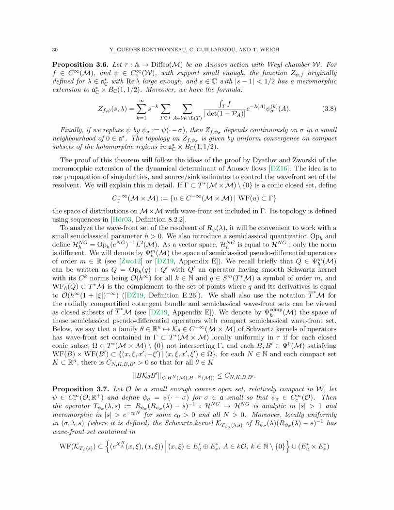
30 Y. GUEDES BONTHONNEAU, C. GUILLARMOU, AND T. WEICH
Proposition 3.6. Let τ : A → Diffeo(M) be an Anosov action with Weyl chamber W. Forf ∈ C∞(M), and ψ ∈ C∞c (W), with support small enough, the function Zψ,f originallydefined for λ ∈ a∗C with Reλ large enough, and s ∈ C with |s − 1| < 1/2 has a meromorphicextension to a∗C ×BC(1, 1/2). Moreover, we have the formula:
Zf,ψ(s, λ) =
∞∑k=1
s−k∑T∈T
∑A∈W∩L(T )
∫T f
| det(1− PA)|e−λ(A)ψ(k)
σ (A). (3.8)
Finally, if we replace ψ by ψσ := ψ(·−σ), then Zf,ψσ depends continuously on σ in a smallneighbourhood of 0 ∈ a∗. The topology on Zf,ψσ is given by uniform convergence on compactsubsets of the holomorphic regions in a∗C ×BC(1, 1/2).
The proof of this theorem will follow the ideas of the proof by Dyatlov and Zworski of themeromorphic extension of the dynamical determinant of Anosov flows [DZ16]. The idea is touse propagation of singularities, and source/sink estimates to control the wavefront set of theresolvent. We will explain this in detail. If Γ ⊂ T ∗(M×M) \ 0 is a conic closed set, define
C−∞Γ (M×M) := u ∈ C−∞(M×M) | WF(u) ⊂ Γ
the space of distributions onM×M with wave-front set included in Γ. Its topology is definedusing sequences in [Hor03, Definition 8.2.2].
To analyze the wave-front set of the resolvent of Rψ(λ), it will be convenient to work with asmall semiclassical parameter h > 0. We also introduce a semiclassical quantization Oph anddefine HNGh = Oph(eNG)−1L2(M). As a vector space, HNGh is equal to HNG ; only the normis different. We will denote by Ψm
h (M) the space of semiclassical pseudo-differential operatorsof order m ∈ R (see [Zwo12] or [DZ19, Appendix E]). We recall briefly that Q ∈ Ψm
h (M)can be written as Q = Oph(q) + Q′ with Q′ an operator having smooth Schwartz kernelwith its Ck norms being O(h∞) for all k ∈ N and q ∈ Sm(T ∗M) a symbol of order m, andWFh(Q) ⊂ T ∗M is the complement to the set of points where q and its derivatives is equal
to O(h∞(1 + |ξ|)−∞) ([DZ19, Definition E.26]). We shall also use the notation T∗M for
the radially compactified cotangent bundle and semiclassical wave-front sets can be viewedas closed subsets of T
∗M (see [DZ19, Appendix E]). We denote by Ψcomph (M) the space of
those semiclassical pseudo-differential operators with compact semiclassical wave-front set.Below, we say that a family θ ∈ Rn 7→ Kθ ∈ C−∞(M×M) of Schwartz kernels of operatorshas wave-front set contained in Γ ⊂ T ∗(M×M) locally uniformly in τ if for each closedconic subset Ω ∈ T ∗(M×M) \ 0 not intersecting Γ, and each B,B′ ∈ Ψ0(M) satisfyingWF(B)×WF(B′) ⊂ (x, ξ, x′,−ξ′) | (x, ξ, x′, ξ′) ∈ Ω, for each N ∈ N and each compact setK ⊂ Rn, there is CN,K,B,B′ > 0 so that for all θ ∈ K
‖BKθB′‖L(HN (M),H−N (M)) ≤ CN,K,B,B′ .
Proposition 3.7. Let O be a small enough convex open set, relatively compact in W, letψ ∈ C∞c (O;R+) and define ψσ = ψ(· − σ) for σ ∈ a small so that ψσ ∈ C∞c (O). Thenthe operator Tψσ(λ, s) := Rψσ(Rψσ(λ) − s)−1 : HNG → HNG is analytic in |s| > 1 and
meromorphic in |s| > e−c0N for some c0 > 0 and all N > 0. Moreover, locally uniformlyin (σ, λ, s) (where it is defined) the Schwartz kernel KTψσ (λ,s) of Rψσ(λ)(Rψσ(λ) − s)−1 haswave-front set contained in
WF(KTψ(s)) ⊂
(eXHA (x, ξ), (x, ξ))
∣∣∣ (x, ξ) ∈ E∗u ⊕ E∗s , A ∈ kO, k ∈ N \ 0∪ (E∗u × E∗s )
SRB MEASURES FOR ANOSOV ACTIONS 31
where XHA is the Hamilton flow of ξ(XA(x)), the principal symbol of −iXA for A ∈ W. There
is a cone Γ ⊂ T ∗(M×M) such that Γ ∩N∗∆ = ∅ and
(σ, λ, s) 7→ KTψσ (λ,s) ∈ C−∞Γ (M×M)
is continuous where it is defined.
This is the main technical result; it is similar to [DZ16, Proposition 3.3]. Using the toolsof [Hor03, Chapter 8], we deduce directly that Zf,ψ is well-defined as a meromorphic function(with the continuous dependence on σ for Zf,ψσ). It will remain to obtain Formula (3.8) toprove Proposition 3.6.
To prove Proposition 3.7, we will rely on a wavefront set estimate for a parametrix – muchas [DZ16]. This is in some sense a refinement of [GBGHW20, Lemma 4.14]:
Lemma 3.8. If O is small enough and A0 ∈ O, there exists c0, c1 > 0 and Q ∈ Ψcomph (M)
such Rψ(λ)(1−Q)− s has a bounded inverse on HNGh for |s| > e−c0N and Reλ(A0) > −c1N ,
| Imλ| < h−1/2 for all N > 0. In that region, its inverse TQψσ(λ, s) := (Rψσ(λ)(1−Q)− s)−1
is an analytic family of bounded operator in (λ, s) and its Schwartz kernel KTQψσ (λ,s)
satisfies
uniformly in (σ, λ, s)
WFh(KTQψσ (s)
) ∩ T ∗(M×M) ⊂ N∗∆ ∪ Ω+(O) (3.9)
Ω+(O) :=⋃k≥1
Ωk+(O), Ωk
+(O) :=
(eXHA (x, ξ), (x,−ξ))
∣∣∣ (x, ξ) ∈ E∗u ⊕ E∗s , A ∈ kO.
Proof. We start with the proof of existence of TQψ . For this, we pick ΓE∗0 ⊂ T ∗M, a conic
neighborhood of E∗0 , and then G ∈ C∞(T ∗M) an escape function for all A ∈ O compatiblewith cX > 0 and ΓE∗0 ⊂ T ∗M in the sense of [GBGHW20, Definition 4.1]. This is possible,because we can take such a function adapted to A0 ∈ O, and it remains adapted to all A’ssufficiently close to A0. (This is the first reason for assuming that O is small enough). Bythe properties (1.21) of the escape function, there is cX > 0 such that for A ∈ O, and somer > 0 large enough,⋃
t∈[0,1]
etXHA (x, ξ) ∩ ΓE∗0 = ∅, |ξ| > r =⇒ G(eX
HA (x, ξ))−G(x, ξ) ≤ −cX .
Since it will be used several times below, notice that for ψ ∈ C∞c (O), using the convexity ofO,
supp(ψ(k)) ⊂ supp(ψ) + · · ·+ supp(ψ) ⊂ kO.This is contained in a ball of radius δk centered at kA0 for some small δ, given that O is small.We imitate now the proof of [GBGHW20, Lemma 4.5] but with a semiclassical quantization.The idea here is that in the direction of the flow E∗0 , averaging the flow is regularizing, andin the transverse direction, we can use the escape function to obtain some compactness. LetΓ0 := ΓE∗0 ∩ |ξ| ≥ 1 and choose P ∈ Ψ0
h(M) which satisfies
WFh(P ) ⊂
(x, ξ) ∈ T ∗M∣∣∣ ∀t ∈ [0, 1], etX
HA (x, ξ) /∈ Γ0
and 0 ≤ σ(P ) ≤ 1. The operator P is microlocalizing away from the neutral direction E∗0 .We also pick Γ′0 a neighbourhood of Γ0 which is conic for |ξ| ≥ 1 and contained in |ξ| > 1/2,and assume that
WFh(1− P ) ⊂ Γ′0
32 Y. GUEDES BONTHONNEAU, C. GUILLARMOU, AND T. WEICH
(i.e. P is microlocally equal to 1 outside Γ0.) Note that we can chose Γ′0 such that T ∗M\Γ0 is for |ξ| > 1 an arbitrary small cone around E∗u ⊕ E∗s . Setting for A ∈ O, BA :=eXA Oph(eNG)e−XA , we have
Oph(eNG)e−XAP Oph(eNG)−1 = e−XABAP Oph(eNG)−1.
The semi-classical principal symbol of BAP Oph(eNG)−1 ∈ Ψ0h(M) is (by Egorov’s Lemma)
σ(BAP Oph(eNG)−1) = eN(GeXHA −G)σ(P ) mod hS−1.
Using the properties (1.21) of the escape function G, we find for r > 0 large enough and somecX > 0
sup|ξ|≥r|σ(BAP Oph(eNG)−1)(x, ξ)| ≤ e−cXN .
Next, we introduce Q0 ∈ Ψcomph (M) so that WFh(Q0) ⊂ |ξ| ≤ 2r and WFh(1 − Q0) ⊂
|ξ| ≥ r with 0 ≤ σ(Q0) ≤ 1. We also let CO := maxA∈O ‖e−XA‖L(L2(M)). The previousestimate implies that for all h > 0 small and A ∈ O,
‖e−XAP (1−Q0)‖L(HNGh ) ≤ COe−cXN +O(h). (3.10)
We used [Q0,Oph(eNG)−1] Oph(eNG) ∈ hΨ−1h (M). The operator e−XAPQ0 is compact and
smoothing. We get (using∫ψ = 1)
‖Rψ(λ)P (1−Q0)‖L(HNGh ) ≤ COe−cXN sup
A∈Oe−Reλ(A) +O(h).
We now recall how the smoothing effect in the direction of the flow appears. As in theproof of [GBGHW20, Lemma 4.14], for each A1, . . . , Am ∈ W we see by integration by partsthat
Rψ(λ)(XA1 + λ(A1)) . . . (XAm + λ(Am)) =
∫W
(∂A1 . . . ∂Amψ(A))e−XA−λ(A)dA.
Let us pick A1, . . . , Aκ ∈ W a local basis and let
∆0A(λ) := −
κ∑j=1
(∂Aj + λ(Aj))2, ∆A(λ) := τ∗∆
0A(λ) = −
κ∑j=1
(XAj + λ(Aj))2.
(The first one acts on A while the second acts onM.) Since we assumed that | Imλ| < h−1/2,h2∆A(λ) is elliptic on the wavefront set of 1−P , uniformly in λ. We can thus find uniformlyin λ for each m ∈ N a parametrix S(λ) ∈ Ψ−2m
h (M) so that
(h2∆A(λ))mS(λ)(1− P )− (1− P ) ∈ h∞Ψ−∞h (M)
(actually, S(λ) is a holomorphic function of hλ). We thus deduce that
Rψ(λ)(1− P )− h2m
∫W
[∆0A(λ)mψσ](A)e−XA−λ(A)S(λ)(1− P ) dA ∈ h∞Ψ−∞h (M).
(here the bound on the remainder does not depend on ψ since ‖ψ‖L1 = 1.) In particular, foreach m ≥ 0 there is Cm > 0 depending continuously on ‖D2mψ‖L1(O) such that
‖Rψ(λ)(1− P )‖L(HNGh ) ≤ Cmh2m. (3.11)
The same argument (using the operator ∆A(λ) acting on the other side) shows that
‖(1− P )Rψ(λ)‖L(HNGh ) ≤ Cmh2m. (3.12)
SRB MEASURES FOR ANOSOV ACTIONS 33
We thus conclude that there is c0 > 0 and c1 > 0 such that for all m > 0, all h > 0 smallenough and Reλ(A0) > −c1N and |Im(λ)| < h−1/2
Rψ(λ) = R0ψ(λ) +R1
ψ(λ) +Rψ(λ)Q,
R0ψ(λ) := Rψ(λ)P (1−Q0), R1
ψ(λ) := Rψ(λ)(1− P ), Q := PQ0,
‖R0ψ(λ)‖L(HNGh ) ≤ e
−c0N , ‖R1ψ(λ)‖L(HNGh ) ≤ Cmh
m.
(3.13)
This shows that Rψ(λ)(1 − Q) − s is invertible on HNGh for |s| > e−c0N and h > 0 small
enough, locally uniformly in ψ and λ. We call TQψ (λ, s) its inverse.
The second step is to prove the announced property of its wavefront set. We will assumethat ψσ = ψ(· −σ) is a family of C∞c (O) functions for some parameter σ ∈ a∗ small. We thus
have a family TQψσ(λ, s) of operators depending on θ := (λ, s, σ) and we will assume it lives in
a small compact set K where TQψσ(λ, s) is well-defined.
We start by recalling a few basic facts about wave-front sets for families of operators andtheir Schwartz kernels; we refer to [DZ16, Lemma 2.3] or [DGRS20, Lemma 6.2] for theparameter dependent version. A point (x, ξ, x′,−ξ′) ∈ T ∗(M×M) is not in WFh(K
TQψσ (λ,s))
uniformly in θ ∈ K if there are θ-independent neighborhoods U of (x′, ξ′) in T ∗M and V of(x, ξ) such that for any B,B′ ∈ Ψcomp
h (M) with WFh(B) ⊂ V and WFh(B′) ⊂ U , for anym ≥ 0 there is Cm so that for all h > 0 small and all θ ∈ K
‖BTQψσ(λ, s)B′‖L(L2) ≤ Cmhm.
For notational simplicity we shall say that the RHS is an O(h∞) uniformly in θ ∈ K.Let us start with the elliptic region. We observe that
TQψσ(λ, s) =− 1
s
(1−
Rψσ(λ)(1−Q)
s
)−1
=− 1
s−Rψσ(λ)(1−Q)
s2−Rψσ(λ)(1−Q)
s3TQψσ(λ, s)Rψσ(λ)(1−Q).
(3.14)
Applying respectively (1− P ) on the right and then on the left (for P chosen as above witha Γ′0 coming arbitrary cloese to E∗u ⊕E∗s ) and using that WFh(1−Q) ⊂ |ξ| ≥ r, we obtainusing (3.11) and (3.12) that there is r′ ∈ (0, r) such that uniformly in θ ∈ K,
WFh(KTQψσ (λ,s)
) ∩ T ∗(M×M) ⊂
N∗∆ ∪
(x, ξ, x′, ξ′)∣∣ (x, ξ) ∈ E∗u ⊕ E∗s and (x′, ξ′) ∈ E∗u ⊕ E∗s , and |ξ|, |ξ′| ≥ r′
.
(3.15)
It remains to consider the intersection of the wavefront set with (E∗u ⊕ E∗s )2. Expanding the
formula for TQψσ(λ, s), we get a convergent sum in L(HNGh )
TQψσ(λ, s) = −1
s
∑k≥0
(Rψσ(λ)(1−Q)
s
)k.
This is the inspiration for the wavefront set statement. However, since the terms in thesum are not increasingly smoothing, only smaller and smaller, we cannot directly obtain thedesired statement.
34 Y. GUEDES BONTHONNEAU, C. GUILLARMOU, AND T. WEICH
Let us rewrite exactly what we need to prove. For each B,B′ ∈ Ψcomph (M) microsupported
near (E∗u ⊕ E∗s ) ∩ |ξ| ≥ r′, so that WFh(B′) ∩ ΩB = ∅ with
ΩB :=
(x, ξ)∣∣∣ eXH
A (x, ξ) ∈WFh(B), A ∈ ∪k≥0kO,
it suffices to prove that uniformly for θ ∈ K
‖BTQψσ(λ, s)B′‖L(L2) = O(h∞) (3.16)
Note that the conormal region N∗∆ is covered because we now include k = 0 in the definitionof ΩB.
It will be convenient below to use that for |s| > e−c0N , if u = TQψσ(λ, s)f one has u =
(−f +R0ψσ
(λ)u+R1ψσ
(λ)u)/s, thus for each B ∈ Ψ0h(M) with |σ(B)| ≤ 1, we have uniformly
for θ ∈ K‖Bu‖HNGh ≤ |s|−1(‖Bf‖HNGh + ‖BR0
ψσ(λ)u‖HNGh ) +O(h∞). (3.17)
First we will need a so-called source estimate close to E∗s ∩ ∂T∗M in order to control the
wave-front set in that region.The source estimate. Let Vs ⊂ T
∗M be a small neighborhood of L := E∗s ∩ ∂T∗M so
that e−XHA (Vs) ⊂ Vs for all A ∈ O, m(x, ξ) is constant in Vs and P = 1 microlocally on Vs.
Now using the fact that L is a repulsor (a source) for the flow eXHA with A ∈ O, there is
b1, b2 ∈ S0(T ∗M) with supp(b2) ⊂ b1 = 1 so that b2 e−XHA = 1 on supp(b1) for all A ∈ O.
Notice that for v ∈ HNGh and B1/2 = Oph(b1/2)
‖B2v‖HNGh ≤ ‖B1B2v‖HNGh +O(h∞‖v‖HNGh ).
This means that, thanks to the Egorov’s Lemma, B1R0ψσ
(λ) − B1R0ψσ
(λ)B2 ∈ h∞Ψ−∞h (M).
The remainder here depends continuously on σ, λ as before. Thus, using (3.13) we get for allv ∈ C∞(M)
‖B1R0ψ(λ)v‖HNGh ≤ ‖B1R
0ψ(λ)B2v‖HNGh +O(h∞‖v‖HNGh ),
≤ e−c0N‖B2v‖HNGh +O(h∞‖v‖HNGh ),
≤ e−c0N‖B1v‖HNGh +O(h∞‖v‖HNGh ).
Combining with (3.17), and assuming e−c0N |s|−1 ≤ q < 1,this yields that there is C > 0 suchthat for all f ∈ C∞(M)
‖B1u‖HNGh = ‖B1TQψσ
(λ, s)f‖HNGh ≤ C‖B1f‖HNGh +O(h∞‖f‖HNGh ) (3.18)
uniformly for (σ, λ, s) ∈ K.2) Propagation estimate outside E∗u. We will next show how to use the source estimate
to obtain information on the wave-front set of KTψσ (λ,s) outside E∗u.
Assume that B ∈ Ψcomph (M) satisfies WFh(B) ∩ E∗u = ∅, 0 ≤ σ(B) ≤ 1 and WFh(B)
contained in a small neighborhood of E∗u ⊕ E∗s and B′ ∈ Ψcomph (M) satisfying WFh(B′) ∩
ΩB = ∅. Since L is an repulsor, there is k ∈ N large enough such that for all A ∈ kO,
e−XHA (WFh(B)) ⊂ Vs and WFh(B′) ∩ Vs = ∅ for some small enough neighborhood Vs of L,
invariant by e−XHA as in 1). We will use B1 as in 1) for this set Vs and we can assume, up to
taking k even larger, that e−XHA (WFh(B)) ⊂ supp(b1) for all A ∈ kO.
SRB MEASURES FOR ANOSOV ACTIONS 35
Iterating (3.17), we obtain for each k ≥ 1 and each f ∈ C∞(M) (with u = TQψσ(λ, s)f)
‖Bu‖HNGh ≤ (k−1∑j=0
|s|−j−1‖B(R0ψσ(λ))jf‖HNGh + |s|−1‖B(R0
ψσ(λ))ku‖HNGh ) +O(h∞‖f‖HNGh ).
(3.19)By Egorov theorem, locally uniformly in (σ, λ, s)
WFh(B(R0ψσ(λ))jf) ⊂WFh(B) ∩
⋃A∈jO
eXHA (WFh(f)).
Again by Egorov, we have B(R0ψσ
(λ))k −B(R0ψσ
(λ))kB1 ∈ h∞Ψ∞h (M) thus by (3.18)
‖BTQψσ(λ, s)f‖HNGh ≤ C(k−1∑j=0
|s|−j−1‖B(R0ψσ(λ))jf‖HNGh + |s|−1‖B1f‖HNGh ) +O(h∞‖f‖HNGh ).
with C > 0 and the remainder being locally uniform in (σ, λ, s). Applying this with B′finstead of f and using B1B
′ ∈ h∞Ψ−∞h (M) and B(R0ψσ
(λ))jB′ ∈ h∞Ψ−∞h (M) for j ∈ [0, k]
under our assumptions on B,B′, we obtain (3.16) uniformly in (σ, λ, s) ∈ K.3) Estimate near E∗u. As we already have the estimate (3.15) on WF(K
TQψσ) there remains
to study the case where WFh(B) and WFh(B′) are intersecting E∗u. By Egorov and the fact
that u := TQψσ(λ, s)B′f has WFh(u) contained in |ξ| ≥ r′ (which can be read off (3.14)),
we obtain that WFh(R0ψσ
(λ)u) ⊂ ∪A∈OeXHA (WFh(u)) is contained in |ξ| ≥ r′/C0 for some
C0 > 0. We can assume that WFh(B) is a small neighborhood of a point (x, ξ) ∈ E∗u ∩ |ξ| ≥r′, so that for k ≥ 2 large enough e−X
HA (WFh(B)) ∈ |ξ| ≤ r′/2C0 for all A ∈ (k − 1)O.
We then obtain by Egorov that ‖B(R0ψσ
(λ))k−1R0ψσ
(λ)u‖HNGh = O(h∞) uniformly in θ ∈ K.
The estimate (3.19) still holds and we deduce that uniformly for θ ∈ K
‖BTQψσ(λ, s)B′f‖HNGh ≤k−1∑j=0
|s|−j−1‖B(R0ψσ(λ))jB′f‖HNGh +O(h∞‖f‖HNGh ).
Assuming that WFh(B′) ∩ ΩB = ∅, the right hand side is an O(h∞) uniformly for θ ∈ K byEgorov theorem again.
We conclude that (3.9) holds.
We can now turn to
Proof of Proposition 3.7. Next we write (Rψσ(λ) − s)TQΨσ(λ, s) = 1 − Rψσ(λ)QTQΨσ(λ, s) and
TQΨσ(λ, s)(Rψσ(λ) − s) = 1 − TQΨσ(λ, s)Rψσ(λ)Q for |s| > e−c0N on HNGh . Denote by Q′ :=
Rψσ(λ)Q ∈ Ψcomph (M) which is compact on HNGh . We can then use Fredholm theorem to
show that (1−Q′TQΨσ(λ, s))−1 extends meromorphically in s ∈ |s| > e−c0N on HNGh and
(Rψσ(λ)− s)−1 = TQΨσ(λ, s)(1−Q′TQΨσ(λ, s))−1
is a meromorphic extension of (Rψσ(λ) − s)−1 ∈ L(HNGh ) to the region |s| > e−c0N. Thisalso implies that for |s| 1
(Rψσ(λ)− s)−1 = TQΨσ(λ, s) + TQΨσ(λ, s)Q′TQΨσ(λ, s) + TQΨσ(λ, s)Q′(Rψσ(λ)− s)−1Q′TQΨσ(λ, s).
36 Y. GUEDES BONTHONNEAU, C. GUILLARMOU, AND T. WEICH
By Lemma 3.8 and since Rψσ(λ) is h-independent, we have
WFh(TQψσ(λ, s)Q′TQψσ(λ, s)) ∩ T ∗(M×M) ⊂ Υ,
WFh(TQψσ(λ, s)Q′(Rψσ(λ)− s)−1Q′TQψσ(λ, s)) ∩ T ∗(M×M) ⊂ Υ,
Υ := (x, ξ, x′,−ξ′) ∈ T ∗(M×M) | (x, ξ) ∈ E∗u ⊕ E∗s , ∃k, k′ ∈ N,∃A ∈ kO,
∃A′ ∈ k′O, e−XHA (x, ξ) ∈WFh(Q′), eX
HA′ (x′, ξ′) ∈WFh(Q′)
and this holds uniformly in θ ∈ K. Since WFh(Rψσ(λ)) ⊂ Ω1+, this shows that
WFh(Rψσ(λ)(Rψσ(λ)− s)−1) ∩ T ∗(M×M) ⊂ Ω+(O) ∪Υ.
Now, using that WFh(Q′) is a compact set, we observe by hyperbolicity of the action that ifL 1 is large, then for the set
(x, ξ) ∈ T ∗M| |ξ| > L ∩⋃k≥0
⋃A∈kO
e±XHA (WFh(Q′) ∩ (E∗u ⊕ E∗s ))
is contained in |ξ| > L ∩ CL± where CL+ is a small conic neighborhood of E∗u and CL− isa small conic neighborhood of E∗s , with the size of the cone sections going to 0 as L →+∞. Since Tψσ(λ, s) = Rψσ(λ)(Rψσ(λ) − s)−1 is independent of h, we have WF(KTψσ (s)) =
WFh(KTψσ (s)) ∩ T ∗(M×M) \ 0, thus by taking L→∞ we obtain the desired statement,
and this holds uniformly in θ ∈ K. In particular, since Ω+(O) ∪ (E∗u × E∗s ) is disjoint fromN∗∆, we obtain the desired result by choosing a cone Γ containing Ω+(O) ∪ (E∗u × E∗s ).
By the wavefront estimates from Proposition 3.7 it follows that the flat trace Zf,ψσ(s, λ) iswell defined and depends meromorphically on s, λ: indeed, this is a consequence of the factthat the flat trace Tr[ is a continuous linear form on the space C−∞Γ (M×M) equipped withits natural topology given by [Hor03, Definition 8.2.2], provided Γ∩N∗∆ = ∅ (the meromor-phicity in λ can be seen by using the Cauchy characterization of holomorphic functions usingcontour integrals). To finish the proof of Proposition 3.6, it suffices to prove the expansion(3.8) for some open set of s, λ. For ψ ∈ C∞c (W,R+) with support near a given A0 ∈ W asabove and |σ| < ε small, since Rψσ(λ) is bounded on HNG, for |s| 1 we have as a convergingseries
Rψσ(λ)(s−Rψσ(λ))−1 =
∞∑k=1
s−kRψσ(λ)k. (3.20)
Formally, if we take the flat trace of the above identity multilied by f on both sides, we obtainusing (3.6) the desired identity (3.8).
Lemma 3.9. Let ψ ∈ C∞c (W,R+), |σ| < ε and ψσ = ψ(· − σ) as above. Then for eachλ ∈ a∗C, if |s| 1 is large enough, we obtain (3.8), which we recall:
Zf,ψσ(s, λ) =
∞∑k=1
s−k∑T∈T
∑A∈W∩L(T )
∫T f
| det(1− PA)|e−λ(A)ψ(k)
σ (A).
Proof. First, as in the rank 1 case, we need an exponential estimate on the number of periodicorbits in the region A ∈ W | |A| ≤ L as L → ∞, which will insure the convergence of theRHS of (3.8) when |s| 1 is large. This is the content of Lemma 3.5.
SRB MEASURES FOR ANOSOV ACTIONS 37
We then follow the argument of [DZ16] in the rank 1 case. By [DZ16, Section 2.4], there isa family of operators Eε with smooth integral kernels Eε(x, y) = Cε(x)F (dg(x, y)/ε) approx-imating the Identity as a bounded operator Hε0(M) → L2(M) as ε → 0 for any fixed smallε0 > 0, with Cε(x) = O(ε−n) where n := dimM. Furthermore for each A : C∞(M)→ D′(M)with WF(A) ∩N∗∆ = ∅ (see [DZ16, Lemma 2.8])
limε→0
Tr(EεAEε) = Tr[(A). (3.21)
Moreover, the proof of [DZ16, Lemma 4.1] yields that there is C > 0 such that for each
A ∈ W (with ‖ · ‖Tr the trace norm) ‖Eεe−XAEε‖Tr ≤ CeC|A|ε−n−2. Since supp(ψ(k)σ ) ⊂ A ∈
a | |A − kA0| < δk for some small δ > 0 (depending on supp(ψ)) and A0 ∈ W fixed, thisimplies that there is C > 0 such that for all ε > 0 and k ∈ N
‖EεRkψσ(λ)Eε‖Tr ≤ CeC〈λ〉kε−n−2. (3.22)
This proof also gives for some uniform C > 0
|Tr(EεRkψσ(λ)Eε)| ≤
∫We−Reλ(A)ψ(k)
σ (A)|Tr(Eεe−XAEε)|dA
≤∫Wψ(k)σ (A)e−Reλ(A)
∫M×M
Eε(x, y)Eε(ϕA−1(y), x)dvg(x)dvg(y)dA
≤Cε−2n
∫W×M×M
ψ(k)σ (A)e−Reλ(A)1dg(x,y)<c1ε,dg(x,ϕA−1(y))<c1εdvg(x)dvg(y)dA
≤Cε−n∫W×M
ψ(k)σ (A)e−Reλ(A)1dg(y,ϕA−1(y))<2c1εdvg(y)dA.
Using Lemma 3.5 and the support property of ψ(k)σ , this gives
|Tr(EεRkψσ(λ)Eε)| ≤ CeC〈λ〉k. (3.23)
Using respectively (3.20), (3.22) and (3.23) we can thus write for λ fixed and |s| large enough
Zf,ψσ(s, λ) = limε→0
Tr(
∞∑k=1
s−kEεRψσ(λ)kEε) = limε→0
∞∑k=1
s−kTr(EεRkψσ(λ)Eε)
=
∞∑k=1
s−k limε→0
Tr(EεRkψσ(λ)Eε) =
∞∑k=1
s−kTr[(Rkψσ(λ))
where we used (3.21) for the last identity. The formula (3.6) concludes the proof.
3.3. Proof of Theorem 4. Since our analysis is based on the use of the operators Rψ(λ),which are a kind of Laplace transform, it will be convenient to introduce the notation
ψ(λ) :=
∫aeλ(A)ψ(A)dA, λ ∈ a∗C.
(formally, Rψ(λ) = ψ(X + λ)). Using the analytic continuation of the function Zf,ψ, we canobtain the following result
38 Y. GUEDES BONTHONNEAU, C. GUILLARMOU, AND T. WEICH
Proposition 3.10. Let ψ ∈ C∞c (W;R+) with∫W ψ = 1. For real λ ∈ a∗ ⊂ a∗C, we denote
δ = log ψ(λ). We have for some ε > 0∑T∈T
∑A∈W∩L(T )
ψ(k)(A)e−λ(A)
∫T f
| det(1− PA)|= µ(f)eδk +O(e(δ−ε)k)
Additionally, if ψ = ψσ, the bound on the remainder is locally uniform in σ.
Proof. The terms we want to estimate are the coefficients ck in the expansion
Zf,ψ(λ, s) =∑k≥0
s−kck.
Since Zf,ψ is meromorphic in the s variable in C∗, according to Cauchy’s formula, we havefor every ρ ∈ R+ such that Zf,ψ(λ, ·) has no poles on the circle of radius ρ
ck =1
2iπ
∫ρS1
Zf,ψ(λ, s)sk−1ds+∑
poles of modulus >ρ
Res(Zf,ψ(λ, s)sk−1ds).
Let us assume that Zf,ψ(λ, ·) has a simple pole s0 with modulus strictly larger than all theother poles, and s0 is real. We denote K the residue at s0, and we find for some ε > 0
ck = Ksk−10 +O((e−εs0)k−1).
For this reason, we will be done if we can prove that eδ is indeed a real dominating pole oforder 1 (when λ is real), with residue
K = µ(f)eδ.
Let us describe the poles of Zf,ψ(λ, ·). As we have seen before, they are exactly the poles ofthe resolvent (s − Rψ(λ))−1. Let us investigate the structure of these poles. Let s0 ∈ C∗ bea pole of s 7→ (s−Rψ(λ))−1, and denote by Π(λ, s0) the corresponding spectral projector, sothat near s0,
(s−Rψ(λ))−1 =∑j≥0
(Rψ(λ)− s0)jΠ(λ, s0)
(s− s0)j+1+ holomorphic .
Since s0 − Rψ(λ) is Fredholm on some suitable anisotropic space, the characteristic spaceE(s0) is finite dimensional, and since Rψ(λ) commutes with the Anosov action, we can splitE(s0) into a sum of characteristic spaces for the action. We can thus find in E(s0) a non-zerovector u such that −XAu = λ0(A)u for some λ0 ∈ a∗C and all A ∈ W. Since the characteristicspace is contained in some suitable anisotropic space, we deduce that λ0 ∈ Res(X) whereRes(X) is the set of Ruelle-Taylor resonance of [GBGHW20] (and introduced in (1.19)). Itfollows that
Rψ(λ)u =
∫We−XA−λ(A)ψ(A)u dA = ψ(λ− λ0)u,
so that s0 = ψ(λ−λ0). The converse argument completes the proof of the fact that ran Π(λ, s0)is exactly equal to
u∣∣∣ λ0 ∈ Res(X), ψ(λ− λ0) = s0, u is a generalized resonant state at λ0
.

SRB MEASURES FOR ANOSOV ACTIONS 39
Now, we know from [GBGHW20, Theorem 2] that for all resonances λ0, and all A ∈ W,Re(λ0(A)) ≤ 0, with equality for λ0 = 0 (if the action is not mixing, there may be otherpurely imaginary resonances). Now, since we have chosen ψ to be real non-negative, we have∣∣∣∣∫
Weλ0(A)ψ(A)dA
∣∣∣∣ ≤ ∫WeRe(λ0(A))ψ(A)dt.
With equality if and only if eλ0(A)−Re(λ0(A)) is constant on the support of ψ. It follows thatfor λ real, and λ0 ∈ Res(X) with λ0 6= 0,∣∣∣ψ(λ− λ0)
∣∣∣ =
∣∣∣∣∫We(λ0−λ)(A)ψ(A)dA
∣∣∣∣ < ∫We−λ(A)ψ(A)dA = ψ(λ).
This implies that eδ = ψ(λ) is indeed a dominating pole. It remains to compute its orderand residue. However from [GBGHW20, Proposition 5.4], we know that there are no Jordanblocks at 0, so that the 0-characteristic space is equal to the 0-eigenspace, and that thecorresponding spectral projector Π(λ, eδ) does not depend on the choices – it was denotedΠ(0) in [GBGHW20]. We deduce that indeed eδ is a simple pole, with residue
Tr fRψ(λ)Π(0) = eδµ(f).
As a corollory of the proof, we find
Corollary 3.11. The function Z1,ψ(λ, ·) has simple poles, and
Res(Z1,ψ(λ, s)ds, s0) = s0
∑ζ∈Res(X),ψ(λ−ζ)=s0
dimu ∈ C−∞Eu∗ | ∃` > 0, (−X − ζ)`u = 0 .
Proof. Near a pole s0 of (s−Rψ(λ))−1, we come back to the formula
Rψ(λ)(s−Rψ(λ))−1 =∑j≥0
Rψ(λ)(Rψ(λ)− s0)jΠs0
(s− s0)j+1+ holomorphic around s0.
Since the trace of nilpotent operators is always 0, taking the trace eliminates the terms j > 0,and we deduce that around s0,
Z1,ψ(λ, s) =s0
s− s0Tr Πs0 + holomorphic around s0.
We have already seen that the range of Πs0 is the direct sum of the spaces
u ∈ C−∞Eu∗ | ∃` > 0, (−X − ζ)`u = 0 ,
for ψ(λ− ζ) = s0.
In the case that f 6= 1, the singularities could become more complicated because f couldinteract with the Jordan blocks of R. We can now turn to the proof of Theorem 4:
Proof of Theorem 4. If suffices to assume f ≥ 0. We will use some estimates from the proofof [GBGHW20, Proposition 5.4]. Let ν ∈ D′(W) be the measure9
ν =∑T∈T
∑A∈W∩L(T )
∫T f
|det(1− PA)|δA
9D′(W) denotes the space of distributions on the open cone C.
40 Y. GUEDES BONTHONNEAU, C. GUILLARMOU, AND T. WEICH
where δA is the Dirac mass at A. Choose a basis (Aj)κj=1 of a so that Aj ∈ ker e1 for j ≥ 2,
we then identify a ' Rκ by identifying the canonical basis of Rκ with the basis (Aj)j . We letΣ = C ∩ A1 +
∑κj=2 tjAj , | tj ∈ R be a hyperplane section of the cone C. Choose r > 0 but
smaller than the distance of Σ to the boundary of the Weyl chamber δW (where the distanceis the euclidean distance in the chosen coordinates. Next choose ψ ∈ C∞c ((−r/2, r/2)) to benon-negative and even with
∫R ψ = 1, and for each σ ∈ Rκ, define ψσ(t) :=
∏κj=1 ψ(tj − σj).
We view Σ as an open subset of (1, t) | t ∈ Rκ−1 and choose q ∈ C∞c (Σ;R+) with small
support and let Q =∫Rκ−1 q(t)dt > 0, and ω ∈ C∞c ((0, 1); [0, 1]) with W :=
∫ 10 ω > 0. We
consider limN→∞ ν(FN ) for σ(θ) := (1, θ) ∈ Σ where
FN (t) :=1
N
N∑k=1
∫Rκ−1
ω( kN )ψ(k)σ(θ)(t)q(θ)dθ.
By applying Proposition 3.10 with λ = 0, we have
WQµ(f) = limN→∞
ν(FN ). (3.24)
In the proof of [GBGHW20, Proposition 5.4], it is shown that if h(t) := t1−κ1 ω(t1)q(t/t1) witht = (t1, t), then with GN (t) := NκFN (tN)
‖GN (t)− h(t)‖L2(Rκ,dt) → 0 as N →∞.
The proof of this convergence is based on the following estimates on the Fourier transformGN of GN : for δ > 0 small, and all ` ∈ N there is C` > 0, C > 0, c0 > 0 so that
∀ξ, |ξ| > N1/2+δ, |GN (ξ)|2 ≤ C(1 + c0|ξ|2)−2εN ,
∀ξ, |ξ| ≤ N1/2+δ, |GN (ξ)|2 ≤ C`(|ξ|−` +N−`(12−δ))
and GN (ξ) → h(ξ) for each ξ ∈ Rκ. As a consequence, for each ` > 0 one can take N0 largeenough so that for all N > N0∫
|ξ|>N1/2+δ
〈ξ〉2`|GN (ξ)− h(ξ)|2dξ ≤ C`∫|ξ|>N1/2+δ
〈ξ〉−`dξ = o(1),
1|ξ|≤N1/2+δ〈ξ〉2`|GN (ξ)− h(ξ)|2 ≤ C`〈ξ〉−`,where C` > 0 is independent of N . Using Lebesgue dominated convergence theorem, weconclude that ‖〈ξ〉`(GN−h(ξ))‖L2 → 0 as N →∞, thus by Sobolev embedding ‖GN−h‖C0 →0 as N → 0. Therefore
‖FN (t)−N−κh(t/N)‖C0 = o(N−κ). (3.25)
Choosing q = 1 on an open set U ⊂ Σ and ω(t1) = tκ−11 in (ε, 1 − ε), we deduce that for N
large enough
FN (t) ≥ 1
2Nκ1[εN,N(1−ε)](t1)1U (t/t1).
This implies that if Ca,b(U) := (t1, t) | t1 ∈ [a, b], t/t1 ∈ U
ν(CεN,N(1−ε)(U)) ≤ 2Nκν(FN ) ≤ 3NκQWµ(f)
where we used (3.24). Thus we obtain ν(C0,N (U)) = O(Nκ) by letting ε→ 0. This estimatethus also implies by a covering argument that ν(C ∩ |A| < N) = O(Nκ). Coming back

SRB MEASURES FOR ANOSOV ACTIONS 41
to a general ω, q, using that supp(FN ) ∪ supp(h(·/N)) ⊂ C0,3N (U ′) for some open set U ′ ∈W ∩ t1 = 1, and since ν(C0,3N (U ′)) = O(Nκ), we obtain by (3.25)
limN→∞
N−κν(h(·/N)) = limN→∞
ν(FN ) = WQµ(f).
Next, let U be a small open ball in Σ, we can choose qj ∈ C∞c (Σ) supported near U forj = 1, 2 so that q1 ≤ 1U ≤ q2 and
∫qj = |U | + O(ε), and for 0 < a < b < 1, choose
ωj ∈ C∞c ((0, 1), [0, 1]) such that ω1 ≤ tκ−11[a,b] ≤ ω2 with∫ 1
0 ωj(t)dt =∫ ba t
κ−1dt + O(ε).
Write now hj(t) = t1−κ1 ωj(t1)qj(t/t1). One then has
N−κν(h1(·/N)) ≤ N−κν(CδN,(1−δ)N (U)) ≤ N−κν(h2(·/N))
thus if Va,b =∫ ba t
κ−1dt, we obtain for each ε > 0 small
(Va,b − ε)(|U | − ε)µ(f) ≤ lim infN→∞
N−κν(CaN,bN (U))
lim supN→∞
N−κν(CaN,bN (U)) ≤ (Va,b + ε)(|U |+ ε)µ(f).
We let ε→ 0 and deduce that
limN→∞
N−κν(CaN,bN (U)) = µ(f)Va,b|U | = µ(f)|Ca,b(U)| .
3.4. A dynamical zeta function. We conclude by some comments on links with dynamicalzeta functions. In [BT08], for an operator K, Baladi and Tsujii introduce the flat determinantas
det[(1− zK) := exp
−∑`≥0
z`
`Tr[K`
,
provided the LHS makes sense and converges. From the argument of the previous section, wesee that det[(1−zRψ(λ)) is well defined for |z| small enough, and has a holomorphic extensionto z ∈ C. Indeed for |z| small enough,
∂z det[(1− zRψ(λ))
det[(1− zRψ(λ))= −1
z
∑`≥1
z` Tr[Rψ(λ)` = −1
zZ1,ψ
(λ,
1
z
).
As the RHS is meromorphic on C in the z variable, it remains to show it has simple poles,with integer residue in order to deduce that det[(1 − zRψ(λ)) is holomorphic. According toCorollary 3.11, near a pole 1/s0, Z1,ψ takes the form
−1
zZ1,ψ
(λ,
1
z
)= − s0m
z(1/z − s0)+ holomorphic =
m
z − 1/s0+ holomorphic.
Here m is the dimension of some characteristic space, i.e an integer. This proves that λ, z 7→det[(1− zRψ(λ)) is holomorphic in a∗C × C. The parameter z here is auxiliary, so we can fixits value to 1, and obtain:
Theorem 5. Let X be an Anosov action of Rκ with positive Weyl chamber W, and letψ ∈ C∞c (W,R+) have
∫ψ = 1 and small enough support. Then
dψ(λ) := exp
−∑T∈T
∑A∈L(T )
vol(T )
| det(1− PA)|e−λ(A)
∑k
ψ(k)(A)
k
,
42 Y. GUEDES BONTHONNEAU, C. GUILLARMOU, AND T. WEICH
originally defined for Reλ large enough (in the sense of evaluating it in elements of the positiveWeyl chamber W), has a holomorphic continuation to a∗C. This continuation is a regularizedversion of the formal product ∏
ζ∈Res(−X)
(1− ψ(λ− ζ))multiplicity of ζ .
This means that for each λ0 ∈ Cκ, there exist only a finite number of ζ’s in Res(X) such that
|ψ(λ0 − ζ)− 1| < 1/2, and for λ close enough to λ0,
dψ(λ) =∏
ζ∈Res(X)
(1− ψ(λ− ζ))multiplicity of ζ × a holomorphic function.
As far as we know, this is the first appearance of a multi-parameter zeta function for actionswith a global meromorphic extension. The reader accustomed to the rank 1 case may findthe formula a bit surprising and wonder if it is possible to replace the term F :=
∑ψ(k)/k
by a simpler weight function. Let us explain briefly why this is not an easy question. Thenatural extension of the rank 1 case would be to replace it by
F := 1λj>0, j=1...κ,
having taken a basis comprised of elements ofW and λ = (λ1, . . . , λκ) in this basis. However,there seems to be no hope that this can define a globally meromorphic function. Indeed, letus consider the singular set of such a function. Each resonance ζ would contribute by(∏ 1
λj − ζj
)multiplicity of ζ
.
For the resulting product to be meromorphic, the singular set has to be (at least) locallyclosed. It is given by
λ ∈ Cκ | ∃ζ ∈ Res(X), ∃j = 1 . . . κ, λj = ζj .
For this to be locally closed, we need that for any sequence of resonances ζ`, each coordinate(ζ`j )` tends to infinity. For example for the resonances with small real part, this means thatthe imaginary parts cannot equidistribute in Rκ. This would certainly be a surprise to us,in particular as for Weyl chamber flows a Weyl-lower bound on the number of Ruelle Taylorresonances with Re(λ) = −ρ is known [HWW21, Theorem 1.1].
4. Application to lattice point counting
In this final section we will work out the consequences of the Bowen formula for the SRBmeasures in terms of the counting-problem of lattice points. We focus in particular on thecase of Weyl chamber flows, where we obtain precise estimates for the exponential growthrates.
Choose a proper subcone C ⊂ W and fix some ξ ∈ a∗ such that ξ is positive on a smallconical neighbourhood of C. For 0 ≤ a < b we define Ca,b := A ∈ C, ξ(A) ∈ [a, b] and thelattice point counting function
NCa,b :=∑T∈T
∑A∈L(T )∩Ca,b
vol(T ).
SRB MEASURES FOR ANOSOV ACTIONS 43
We furthermore introduce a counting function that is additionally weighted by the Jaco-bians | det(1− PA)|
NwCa,b :=
∑T∈T
∑A∈L(T )∩Ca,b
vol(T )
| det(1− PA)|.
Note that by Theorem 4 choosing the constant test function f = 1 we get for any q > 1
limn→∞
NwCqn−1,qn
qκ(n−1)= |C1,q| (4.1)
Let us define
m := lim infn→∞
log(
infA∈Cqn−1,qn∩(∪T∈T L(T )) |det(1− PA)|)
qn
M := lim supn→∞
log(
supA∈Cqn−1,qn∩(∪T∈T L(T )) |det(1− PA)|)
qn
Then for any ε > 0 there is N such that for n > N we have
e(m−ε)qnNwCqn−1,qn
≤ NCqn−1,qn≤ Nw
Cqn−1,qne(M+ε)qn
and taking additionally (4.1) into account we get
(|C1,q| − ε)qκ(n−1)e(m−ε)qn ≤ NCqn−1,qn≤ (|C1,q|+ ε)qκ(n−1)e(M+ε)qn .
Now, using NC0,qn = NC0,1 +∑n
k=0NCqk−1,qkwe deduce
m ≤ lim infn→∞
logNC0,qnqn
≤ lim supn→∞
logNC0,qnqn
≤M
Now let us assume that there is η ∈ a∗ positive onW such that for any proper subcone C ⊂ Wthere is ε > 0 such that |det(1 − PA)| = eη(A)(1 − O(e−ε|A|))| for all A ∈ C. If we now fixξ := η/‖η‖ then we get the particularly simple expressions M = ‖η‖ and m = ‖η‖/q. As wecan choose q > 1 arbitrary close to 1 we get:
Proposition 4.1. For an Anosov action for which there is η ∈ a∗ with the above properties,one has for each proper subcone C ⊂ W
limR→∞
logNC0,RR
= ‖η‖.
The assumption on | det(1−PA)| is fulfilled for all standard Anosov actions. For examplefor Weyl chamber flows, a periodic point x0 = Γg0M ∈ Γ\G/M =M under A0 ∈ W impliesthe existence γ0 ∈ Γ,m0 ∈ M such that γ0g0 exp(A0)m0 = g0. With these notation we cangive an explicit expression of |det(1− PA0)|
|det(1− PA0)| =∏α∈∆+
∣∣∣∣detgα
(1− e−α(A0)Ad(m−1
0 ))∣∣∣∣ ∣∣∣∣det
g−α
(1− eα(A0)Ad(m−1
0 ))∣∣∣∣
= e2ρ(A0)∏α∈∆+
∣∣∣∣detgα
(1− e−α(A0)Ad(m−1
0 ))∣∣∣∣ ∣∣∣∣det
g−α
(Ad(m−1
0 )− e−α(A0))∣∣∣∣
44 Y. GUEDES BONTHONNEAU, C. GUILLARMOU, AND T. WEICH
Here ∆+ ⊂ a∗ denotes the set of positive roots, g±α the corresponding root spaces, mα :=dim gα and we use the usual notation ρ :=
∑α∈∆+
mα2 α ∈ a∗ for the half sum of positive
roots. As the adjoint action of M on gα is orthogonal and for any proper subcone C ⊂ W,α(A) > ε|A| for all A ∈ C we deduce by the continutiy of the determinant
|det(1− PA)| = e2ρ(A)(1 +O(e−ε|A|) (4.2)
Appendix A. Upper bound on the number of periodic orbits (Lemma 3.5)
First, for δ0 > 0 small there are is a family of invertible linear maps Tx,y : TxM → TyMdepending continuously on dg(x, y) ≤ δ0 such that Tx,x = Id and Tx,y mapping Eu(x), Es(x),and E0(x) onto Eu(y), Es(y) and E0(y). Then exactly the same proof as [DZ16, Lemma A.1]shows that for each r > 0 there is δ ∈ (0, δ0) and C > 0 such that if dg(x, ϕ
A1 (x)) < δ, A ∈ W
with |A| > r and v ∈ Eu(x)⊕ Es(x), then
|v| ≤ C|(dϕA1 − Tx,ϕA1 (x))v|. (A.1)
This should be compared to the fact that for A ∈ W, ϕA1 (x) = x we know that(dxϕ
A1 − Id)|Eu(x)⊕Es(x) is invertible. (A.1) generalizes this invertibility to orbits that are
only approximately closed.Next, we have, by the group property of eX·, that there is C > 0,M > 0 such that for all
A ∈ W, x, x′ ∈M‖eXA‖C2→C2 ≤ CeM |A|, dg(ϕ
A1 (x), ϕA1 (x′)) ≤ CeM |A|dg(x, x′). (A.2)
Next, we show a separation estimate between periodic tori.
Lemma A.1. Let r > 0, then there is C, δ > 0 such that for all ε > 0 small, if dg(x, ϕA1 (x)) ≤
ε, dg(x′, ϕA
′1 (x′)) ≤ ε, A,A′ ∈ W with |A− A′| ≤ δ, dg(x, x
′) ≤ δe−M |A|, then |A− A′| ≤ Cε,
and furthermore there is A′′ ∈ a with |A′′| ≤ 1 such that dg(x, ϕA′′1 (x′)) ≤ Cε.
Letting ε→ 0 we get, as a direct consequence
Corollary A.2. If two periodic orbits ∪t∈[0,1]ϕAt (x) and ∪t∈[0,1]ϕ
A′t (x′) have minimal distance
≤ δe−M |A| and nearby period |A − A′| < δ, and A,A′ ∈ W, then A = A′ and there is aninvariant torus orbit T such that x, x′ ∈ T .
proof of Lemma A.1. We follow closely the proof of [DZ16, Lemma A.2]. Under our assump-
tions, x, x′, ϕA1 (x) and ϕA′
1 (x′) are all in a small chart in Rn and we will frequently identifypoints in M and vectors in TM via as elements in Rn via this chart. The norm | • | theninduces a metric that is equivalent to the Riemannian distance on M. We will furthermoreassume that chart is chosen small enough such that for any x, x′ in the chart, the angle ofEu(x)⊕Es(x) and E0(x′) is bounded from below. As Eu(x)⊕Es(x) is a slice of the A action,
there is A′′ ∈ a with |A′′| ≤ 1 such that ϕA′′
1 (x′)−x ∈ Eu(x)⊕Es(x). We write x′′ := ϕA′′(x′).
By the boundedness of the angles between Eu ⊕ Es and E0 there is a global C such that|x, x′′| ≤ C|x, x′|. Then by Taylor expansion there is C > 0 such that
|ϕA1 (x′′)− ϕA1 (x)− dϕA1 (x)(x′′ − x)| ≤ CeM |A||x− x′′|2 ≤ Cδ|x− x′′|,
|ϕA′1 (x′′)− ϕA1 (x′′)−XA′−A(ϕA1 (x′′))| ≤ C|A−A′|2 ≤ Cδ|A−A′|thus we obtain
|ϕA′1 (x′′)− ϕA1 (x)− dϕA1 (x)(x′′ − x)−XA′−A(ϕA1 (x′′))| ≤ Cδ(|x− x′′|+ |A−A′|).
SRB MEASURES FOR ANOSOV ACTIONS 45
Then, using dg(x, ϕA1 (x)) ≤ ε and dg(x
′′, ϕA′
1 (x′′)) ≤ Cε for some uniform C > 0,
|(dϕA1 (x)− Id)(x′′ − x) +XA′−A(ϕA1 (x′′))| ≤ Cδ(|x− x′′|+ |A′ −A|) + Cε.
Using that Tx,y is uniformly continuous in x, y, and dg(x, ϕA1 (x)) ≤ ε we get, if ε is chosen
small enough (depending on δ):
|(dϕA1 (x)− Tx,ϕA1 (x))(x′′ − x) +XA′−A(ϕA1 (x′′))| ≤ Cδ(|x′′ − x|+ |A′ −A|) + Cε.
Finally, using that (dϕA1 (x) − Tx,ϕA1 (x))(x′′ − x) ∈ (Eu ⊕ Es)(ϕ
A1 (x)), XA′−A(ϕA1 (x′′)) ∈
E0ϕA1 (x′′) together with the lowe bound on the angle of these subspaces as well as (A.1),
we conclude that
|A−A′|+ |x−x′′| ≤ C(|dϕA1 (x)−Tx,ϕA1 (x))(x′′−x)|+ |A′−A|) ≤ Cδ(|A′−A|+ |x′′−x|) +Cε
which gives the result by choosing δ small enough.
We now prove (3.5). Let ` > 0 be large. We take a maximal set of points (xj , Aj)j in
M× A ∈ W||A| ≤ ` so that dg(xj , xk) > δe−M`/2 or |Aj − Ak| > δ/2. The number of
such balls is O(`κenM`) and the polynomial term in ` can easily be absorbed (by changingM) such that we have O(enM`) balls. One has
Z := (x,A) ∈M×W | |A| ≤ `, dg(x, ϕA1 (x)) ≤ ε ⊂⋃j
Bj ,
Bj := (x,A) ∈M×W | |A−Aj | ≤ δ/2, dg(x, xj) ≤ δe−ML/2, dg(x, ϕA1 (x)) ≤ ε.
Now by Lemma A.1, if (x′, A′) ∈ Bj , Bj is contained in an ε-neighborhood of the orbit
ϕA′′(x′) | |A′′| ≤ 1 times a ε ball of A′ in W. The first neighbourhood has νg-measure
O(εn−κ) and the latter dA-measure O(εκ). This shows that (vg ⊗ dA)(Z) = O(εnenM`).We conclude with a bound on the number of periodic tori. By Corollary A.2, we see that
the periodic tori T so that L(T ) ∩ B(A, δ) 6= ∅ with B(A, δ) := A′ ∈ W | |A − A′| < δ are
separated by a distance at least δe−M |A|, thus there are tubular neighborhoods of volumebounded below by Cδn−κe−(n−κ)M |A| that do no intersect in M. By a covering argument wededuce that for each A ∈ L(T ) with T ∈ T
]T ′ ∈ T |L(T ′) ∩B(A, δ) 6= ∅ ≤ Cδκ−ne(n−κ)M |A|
]A′ ∈ L(T ′) ∩W |T ′ ∈ T , A′ ∈ B(A, δ) ≤ Cδκ−ne(n−κ)M |A|
and therefore again by covering W ∩ |A| ≤ ` by O(`κ) balls of radius δ we conclude that
]A ∈ L(T ) ∩W |T ∈ T , |A| ≤ ` ≤ C`κe(n−κ)M`.
References
[Bew71] T. Bewley, Extension of the Birkhoff and von Neumann ergodic theorems to semigroup actions,Ann. Inst. Fourier 7 (1971), no. 4, 183–291.
[BFL92] Y. Benoist, P. Foulon, and F. Labourie, Flots d’Anosov a distributions stable et instabledifferentiables, J. Am. Math. Soc. 5 (1992), no. 1, 33–74 (French).
[BKL02] M. Blank, G. Keller, and C. Liverani, Ruelle–Perron–Frobenius spectrum for Anosov maps,Nonlinearity 15 (2002), 1905.
[BL07] O. Butterley and C. Liverani, Smooth Anosov flows: Correlation spectra and stability, J. Mod.Dyn. 1 (2007), no. 2, 301–322.
[Bow72] R. Bowen, The equidistribution of closed geodesics, American journal of mathematics 94 (1972),no. 2, 413–423.
46 Y. GUEDES BONTHONNEAU, C. GUILLARMOU, AND T. WEICH
[Bow74] , Some systems with unique equilibrium states, Mathematical Systems Theory 8 (1974),no. 3, 193–202.
[BR75] R. Bowen and D. Ruelle, The ergodic theory of axiom A flows, Invent. Math. 29 (1975), no. 3,181–202.
[BS02] M. Brin and G. Stuck, Introduction to dynamical systems, Cambridge: Cambridge UniversityPress, 2002.
[BT07] V. Baladi and M. Tsujii, Anisotropic Holder and Sobolev spaces for hyperbolic diffeomorphisms,Ann. Inst. Fourier 57 (2007), no. 1, 127–154.
[BT08] V. Baladi and M. Tsujii, Dynamical determinants and spectrum for hyperbolic diffeomorphisms,Probabilistic and Geometric Structures in Dynamics, Contemp. Math., vol. 469, Amer. Math.Soc., 2008, pp. 29–68.
[BWS20] Y. Borns-Weil and S. Shen, Dynamical zeta functions in the nonorientable case, arXiv preprintarXiv:2007.08043 (2020).
[CRH] P.D. Carrasco and F. Rodriguez Hertz, Equilibrium states for center isometries, arXiv preprintarXiv 2103.07323.
[Dei04] A. Deitmar, A prime geodesic theorem for higher rank spaces, Geometric & Functional AnalysisGAFA 14 (2004), no. 6, 1238–1266.
[DGRS20] N.V. Dang, C. Guillarmou, G. Riviere, and S. Shen, The Fried conjecture in small dimensions,Invent. Math. 220 (2020), no. 525–579.
[dlL92] R. de la Llave, Smooth conjugacy and S-R-B measures for uniformly and non-uniformly hyperbolicsystems, Comm. Math. Phys. 150 (1992), no. 289–320.
[DZ16] S. Dyatlov and M. Zworski, Dynamical zeta functions for Anosov flows via microlocal analysis.,
Ann. Sci. Ec. Norm. Super. (4) 49 (2016), no. 3, 543–577 (English).[DZ19] S. Dyatlov and M. Zworski, Mathematical theory of scattering resonances, Graduate Studies in
Mathematics, vol. 200, AMS, 2019.[EKL06] M. Einsiedler, A. Katok, and E. Lindenstrauss, Invariant measures and the set of exceptions to
littlewood’s conjecture, Annals of mathematics (2006), 513–560.[EL15] M. Einsiedler and E. Lindenstrauss, On measures invariant under tori on quotients of semisimple
groups, Annals of Mathematics (2015), 993–1031.[ELMV09] M. Einsiedler, E. Lindenstrauss, P. Michel, and A. Venkatesh, Distribution of periodic torus
orbits on homogeneous spaces, Duke Math. J. 148 (2009), no. 1, 119–174 (English).[ELMV11] M Einsiedler, E. Lindenstrauss, P. Michel, and A. Venkatesh, Distribution of periodic torus orbits
and Duke’s theorem for cubic fields, Ann. Math. (2) 173 (2011), no. 2, 815–885 (English).[FRS08] F. Faure, N. Roy, and J. Sjostrand, Semi-classical approach for Anosov diffeomorphisms and
Ruelle resonances., Open Math. J. 1 (2008), 35–81 (English).[FS11] F. Faure and J. Sjostrand, Upper bound on the density of Ruelle resonances for Anosov flows,
Communications in Mathematical Physics 308 (2011), no. 2, 325–364.[GBGHW20] Y. Guedes-Bonthonneau, C. Guillarmou, J. Hilgert, and T. Weich, Ruelle-Taylor resonances of
Anosov actions, arXiv preprint arXiv:2007.14275 (2020).[GL06] S. Gouezel and C. Liverani, Banach spaces adapted to anosov systems, Ergodic Theory Dyn.
Syst. 26 (2006), 289–217.[GLP13] P. Giulietti, C. Liverani, and M. Pollicott, Anosov flows and dynamical zeta functions, Ann.
Math. (2) 178 (2013), no. 2, 687–773.[Has07] B. Hasselblatt, Problems in dynamical systems and related topics, Dynamics, Ergodic Theory,
and Geometry, MSRI Publications 54 (2007), 273–325.[HK02] B. Hasselblatt and A.. Katok, Handbook of dynamical systems. Volume 1A, Elsevier, 2002.[Hor03] L. Hormander, The analysis of linear partial differential operators. I. Distribution theory and
Fourier analysis. Reprint of the second (1990) edition, Springer, Berlin, 2003.[HWW21] J. Hilgert, T. Weich, and L. Wolf, Higher rank quantum-classical correspondence, arXiv preprint
arXiv:2103.05667 (2021).[KKRH11] B. Kalinin, A. Katok, and F. Rodriguez Hertz, Nonuniform measure rigidity, Annals of Mathe-
matics 174 (2011), 361–400.[Kni05] G. Knieper, The uniqueness of the maximal measure for geodesic flows on symmetric spaces of
higher rank, Israel. J. Math. 149 (2005), 171–183.

SRB MEASURES FOR ANOSOV ACTIONS 47
[KS94] A. Katok and R. Spatzier, First cohomology of Anosov actions of higher rank abelian groups and
applications to rigidity, Publications Mathematiques de l’IHES 79 (1994), 131–156.[KS95] K. Katok and R. Spatzier, Invariant measures for higher-rank hyperbolic abelian actions, Ergodic
Theory Dynam. Systems 16 (1995), no. 4, 751–778.[KS98] A. Katok and R. Spatzier, Corrections to “Invariant measures for higher rank hyperbolic abelian
actions”, Ergodic Theory Dyn. Syst. 18 (1998), 503–507.[KS07] B. Kalinin and R. Spatzier, On the classification of cartan actions, GAFA 17 (2007), no. 2,
468–490.[LY85] F. Ledrappier and L.S. Young, The metric entropy of diffeomorphisms: Part i: Characterization
of measures satisfying pesin’s entropy formula, Ann. of Math. (2) 122 (1985), no. 3, 509–539.[Pes04] Ya. Pesin, Lectures on partial hyperbolicity and stable ergodicity, Zurich lectures in advanced
mathematics, EMS, 2004.[PP90] W. Parry and M. Pollicott, Zeta functions and the periodic orbit structure of hyperbolic dynamics,
Asterisque (1990), no. 187-188, 268. MR 1085356[PS70] C. Pugh and M. Shub, The Ω-stability theorem for flows, Invent. Math. 11 (1970), 150–158.[Rok49] V. A. Rokhlin, On the fundamental ideas of measure theory, Matematicheskii Sbornik 67 (1949),
no. 1, 107–150.[Rue76] D. Ruelle, A measure associated with axiom-a attractors, American journal of mathematics 98
(1976), no. 3, 619–654.[Sin68] Y. Sinai, Markov partitions and c-diffeomorphisms, Functional Analysis and Its Applications 2
(1968), no. 1, 61–82.[Spa83] R. Spatzier, Dynamical properties of algebraic systems. a study in closed geodesics., Ph.D. thesis,
university of Warwick, 1983.[SV19] R. Spatzier and K. Vinhage, Cartan actions of higher rank abelian groups and their classification,
arXiv preprint arXiv:1901.06559 (2019).[Via] M. Viana, Desintegration into conditional measures: Rokhlin’s theorem, available at
http://w3.impa.br/viana/out/rokhlin.pdf.[Wei17] T. Weich, On the support of Pollicott-Ruelle resonant states for Anosov flows, Ann. Henri
Poincare 18 (2017), 37–52.[You95] L.S. Young, Ergodic theory of differentiable dynamical systems, Real and complex dynamical
systems (Branner and Kluwer Acad. Publ. Hjorth, eds.), 1995, pp. 293–336.[Zwo12] M. Zworski, Semiclassical analysis, vol. 138, American Mathematical Society, 2012.
Email address: [email protected]
LAGA, Institut Galilee, 99 avenue Jean Baptiste clement, 93430 Villetaneuse, France.
Email address: [email protected]
Universite Paris-Saclay, CNRS, Laboratoire de mathematiques d’Orsay, 91405, Orsay, France.
Email address: [email protected]
Universitat Paderborn, Warburgerstr. 100, 33098 Paderborn, Germany