Machine Learning Journal manuscript No.(will be inserted by the editor)

Sparse Conjugate Directions Pursuit with Application toFixed-size Kernel Models

Peter Karsmakers*, · Kristiaan Pelckmans, ·Kris De Brabanter, · Hugo Van hamme, ·Johan A.K. Suykens

Received: date / Accepted: date

Abstract This work studies an optimization scheme for computing sparse approxi-

mate solutions of over-determined linear systems. Sparse Conjugate Directions Pursuit

(SCDP) aims to construct a solution using only a small number of nonzero (i.e. non-

sparse) coefficients. Motivations of this work can be found in a setting of machine

learning where sparse models typically exhibit better generalization performance, lead

to fast evaluations, and might be exploited to define scalable algorithms. The main idea

is to build up iteratively a conjugate set of vectors of increasing cardinality, in each

iteration solving a small linear subsystem. By exploiting the structure of this conjugate

basis, an algorithm is found (i) converging in at most D iterations for D-dimensional

systems, (ii) with computational complexity close to the classical conjugate gradient

algorithm, and (iii) which is especially efficient when a few iterations suffice to produce

a good approximation. As an example, the application of SCDP to Fixed-Size Least

Squares Support Vector Machines (FS-LSSVM) is discussed resulting in a scheme which

efficiently finds a good model size (M) for the FS-LSSVM setting, and is scalable to

large-scale machine learning tasks. The algorithm is empirically verified in a classifica-

tion context. Further discussion includes algorithmic issues such as component selection

criteria, computational analysis, influence of additional hyper-parameters, and deter-

mination of a suitable stopping criterion.

Keywords sparse approximation, greedy heuristic, matching pursuit, linear system,

kernel methods

*Corresponding author, Kasteelpark Arenberg 10, B-3001, Heverlee,Belgium; Tel: +32 16 3217 09; Fax: +32 16 32 19 86P. Karsmakers, K. De Brabanter, H. Van hamme and J.A.K SuykensDepartment of Electrical Engineering, K.U.Leuven, B-3001 Heverlee, Belgium.E-mail: peter.karsmakers@esat.kuleuven.be, kris.debrabanter@esat.kuleuven.be,hugo.vanhamme@esat.kuleuven.be, johan.suykens@esat.kuleuven.be

K. PelckmansDivision of Systems and Control, Department of Information Technology, Uppsala University,SE-751 05 Uppsala, Sweden. E-mail: kp@it.uu.se

P. Karsmakers is also affiliated toDepartment IBW, K.H.Kempen (Association K.U.Leuven), B-2440 Geel, Belgium.

2

(a) (b) (c)

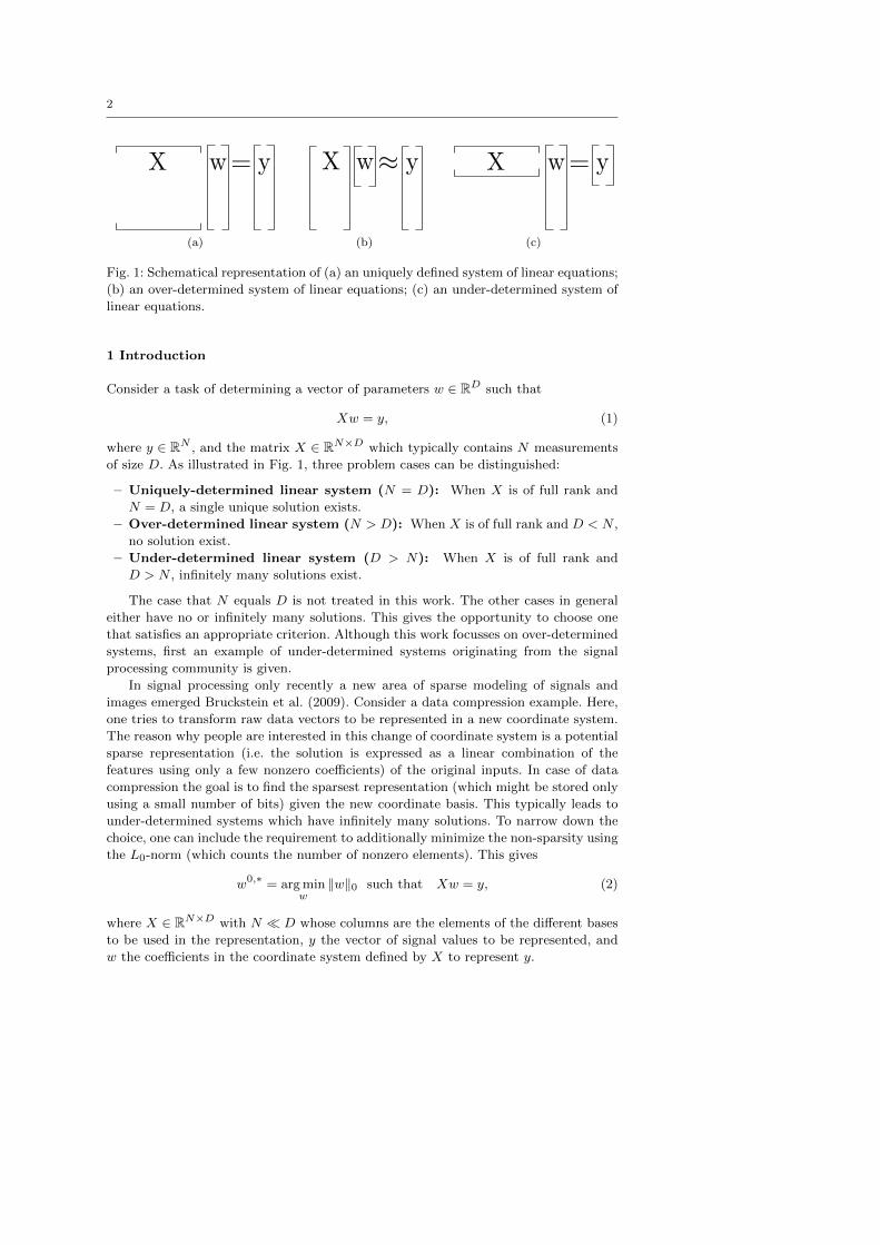
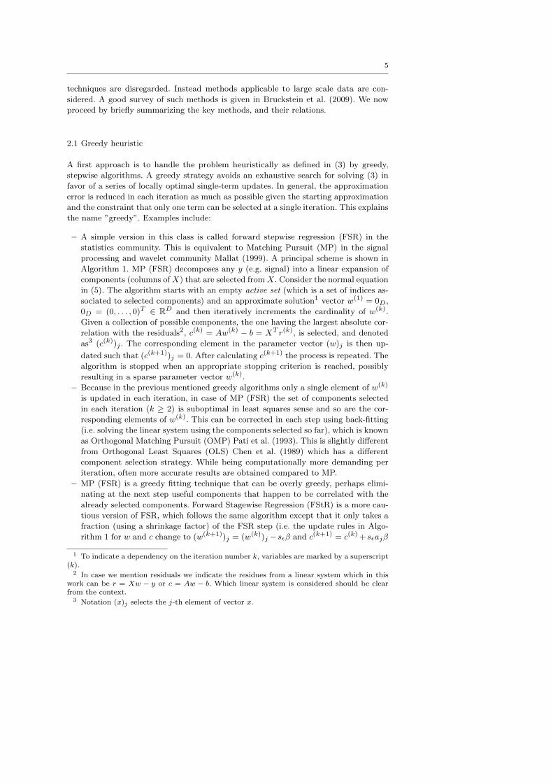
Fig. 1: Schematical representation of (a) an uniquely defined system of linear equations;

(b) an over-determined system of linear equations; (c) an under-determined system of

linear equations.

1 Introduction

Consider a task of determining a vector of parameters w ∈ RD such that

Xw = y, (1)

where y ∈ RN , and the matrix X ∈ RN×D which typically contains N measurements

of size D. As illustrated in Fig. 1, three problem cases can be distinguished:

– Uniquely-determined linear system (N = D): When X is of full rank and

N = D, a single unique solution exists.

– Over-determined linear system (N > D): When X is of full rank and D < N ,

no solution exist.

– Under-determined linear system (D > N): When X is of full rank and

D > N , infinitely many solutions exist.

The case that N equals D is not treated in this work. The other cases in general

either have no or infinitely many solutions. This gives the opportunity to choose one

that satisfies an appropriate criterion. Although this work focusses on over-determined

systems, first an example of under-determined systems originating from the signal

processing community is given.

In signal processing only recently a new area of sparse modeling of signals and

images emerged Bruckstein et al. (2009). Consider a data compression example. Here,

one tries to transform raw data vectors to be represented in a new coordinate system.

The reason why people are interested in this change of coordinate system is a potential

sparse representation (i.e. the solution is expressed as a linear combination of the

features using only a few nonzero coefficients) of the original inputs. In case of data

compression the goal is to find the sparsest representation (which might be stored only

using a small number of bits) given the new coordinate basis. This typically leads to

under-determined systems which have infinitely many solutions. To narrow down the

choice, one can include the requirement to additionally minimize the non-sparsity using

the L0-norm (which counts the number of nonzero elements). This gives

w0,∗ = arg minw

‖w‖0 such that Xw = y, (2)

where X ∈ RN×D with N D whose columns are the elements of the different bases

to be used in the representation, y the vector of signal values to be represented, and

w the coefficients in the coordinate system defined by X to represent y.

3

Often the exact constraint Xw = y is relaxed to tolerate a slight discrepancy be-

tweenXw and y. In case the L2 norm is used for evaluating the error, the approximation

of the optimization problem in the under-determined setting becomes

w0,∗ = arg minw

‖w‖0 such that ‖Xw − y‖22 ≤ δ. (3)

This work focusses on solving over-determined systems originating from least squares

estimation problems with sparse solutions. As will be explained next, this goal can be

formulated such as given in (3). Since over-determined systems in general cannot be

exactly solved, one typically prefers the solution solving the system (1) with minimal

least squares residuals r = Xw − y, or

w∗ = arg minw

1

2‖Xw − y‖22, (4)

which is equivalent to solving the normal equations defined as

Aw = b, (5)

if A is invertible and where we define A = XTX ∈ RD×D and b = XT y ∈ RD. Several

methods have been developed for solving such sets of linear equations. See the reference

works Press et al. (1993) and citations. One of the most successful iterative algorithm

for solving such large linear systems is the Conjugate Gradient (CG) algorithm. The

CG method for linear systems was first proposed by Hestenes and Stiefel Hestenes

and Stiefel (1952) in the 1950s as an iterative method for solving linear systems with

positive definite matrices. Later on, the same ideas were used for solving non-convex

optimization problems, notably in a context of artificial neural networks Moller (1993).

Solving (4) will not result in a sparse solution. The goal of this work is to devise

an algorithm which approximately solves (5) resulting in a sparse solution for w. Our

motivations to obtain a sparse approximative solution to equation (4) are:

– When dealing with estimation problems, sparse coefficients can be interpreted typ-

ically as a form of feature selection.

– When working in the context of machine learning, sparse predictor rules lead typ-

ically to improved generalization Floyd and Warmuth (1995); Vapnik (1998).

– Sparseness can often be exploited to yield more computation and memory-efficient

numerical techniques, e.g. for evaluating the estimated model.

– Sparseness in the solution might be exploited when scaling algorithms up to handle

large data sets.

In order to obtain a sparse solution for w in (1), one may again search for the

minimal L0-norm of a solution approximatively solving (4). In that case, the ob-

jective reduces again to (3), and we can as such handle the under-determined and

over-determined case by similar tools. The aim of the present work is to devise a com-

putationally efficient algorithm which gives a sparse approximate solution of such a

(possibly large-scale) system. For this purpose CG is adapted such that the iteratively

constructed conjugate basis yields solutions of increasing cardinality. In case the al-

gorithm can be terminated in less than D steps a sparse solutions is obtained. The

resulting algorithm will be called Sparse Conjugate Directions Pursuit (SCDP).

A second focus of the paper is to apply SCDP in the context of Least Squares Sup-

port Vector Machines (LS-SVMs) Suykens et al. (2002b). Compared to Support Vector

Machines (SVMs) Vapnik (1998), LS-SVMs are based on solving a system of linear

4

equations instead of solving a Quadratic Program (QP) problem. Although learning

can be performed using a simpler optimization strategy, the LS-SVM solution is not

sparse as opposed to SVM. In order to obtain faster model evaluation, in Suykens et al.

(2002a, 2000) the authors proposed a pruning mechanism based on sorting the absolute

values of the elements of the solution of LS-SVM. A more sophisticated pruning scheme

is explained in de Kruif and de Vries (2003) for function estimation and in Zeng and

Chen (2005) a Sequential Minimization Optimization (SMO) based pruning method is

proposed. However, in case of large-scale problems these methods are not feasible since

they all solve a large linear system which is iteratively shrunken.

The proposed algorithm iteratively constructs a model with increasing cardinality

and, if stopped early (number of iterations smaller than the dimension of the train-

ing examples), provides a sparse solution. For this purpose the primal formulation

of the LS-SVM problem is first approximated using the ideas described in Brabanter

et al. (2010); Suykens et al. (2002b) to formulate a method called Fixed-Size LS-SVM

(FS-LSSVM). This gives an over-determined linear system which might be solved using

SCDP. We will discuss the connections to other methods found in the literature such as

Kernel Matching Pursuit (KMP) Vincent and Bengio (2002), Sparse Greedy Gaussian

Process (SGGP) Smola and Bartlett (2001), Orthogonal Least Squares (OLS) regres-

sion Chen et al. (2009), other sparse LS-SVM versions Cawley and Talbot (2002); Jiao

et al. (2007).

The main contributions of this work can be summarized as follows:

– An integration of the conjugate gradient algorithm with matching pursuit Mallat

(1999).

– The use of SCDP for estimating fixed-size kernel models.

– A detailed description of all components of the model selection process including

algorithmic parameters, and Cross-Validation (CV). As a result of this process a

”good” model size is automatically obtained.

– An empirical comparison with other methods in terms of training complexity, clas-

sification performance, and sparseness.

Different approaches to solve (3) found in the literature are discussed in Section 2.

Then details about, and relations to, existing alternatives of SCDP are given in Sec-

tion 3. The application of the resulting algorithm to the LS-SVM framework is given

in Section 4. The final algorithm is validated on several publicly available data sets as

reported in Section 5 and conclusions are drawn in Section 6.

2 Heuristics to obtain a sparse approximation

In this section, methods to tackle the optimization described in (3) are briefly sum-

marized without making a distinction whether or not the method originates from an

under-determined or over-determined setting.

Since the problem defined in (3) is NP-hard in general Natarajan (1995), the most

efficient known algorithms use heuristics to accomplish results. One such heuristic is

backward Stepwise Regression (BSR) Hastie et al. (2001). Starting from a model ob-

tained using all components, BSR sequentially deletes components from the solution.

However, since one of the goals of this work is to tackle large scale problems for which

solving the full problem (as required for BSR) might be unfeasible, backward selection

5

techniques are disregarded. Instead methods applicable to large scale data are con-

sidered. A good survey of such methods is given in Bruckstein et al. (2009). We now

proceed by briefly summarizing the key methods, and their relations.

2.1 Greedy heuristic

A first approach is to handle the problem heuristically as defined in (3) by greedy,

stepwise algorithms. A greedy strategy avoids an exhaustive search for solving (3) in

favor of a series of locally optimal single-term updates. In general, the approximation

error is reduced in each iteration as much as possible given the starting approximation

and the constraint that only one term can be selected at a single iteration. This explains

the name ”greedy”. Examples include:

– A simple version in this class is called forward stepwise regression (FSR) in the

statistics community. This is equivalent to Matching Pursuit (MP) in the signal

processing and wavelet community Mallat (1999). A principal scheme is shown in

Algorithm 1. MP (FSR) decomposes any y (e.g. signal) into a linear expansion of

components (columns of X) that are selected from X. Consider the normal equation

in (5). The algorithm starts with an empty active set (which is a set of indices as-

sociated to selected components) and an approximate solution1 vector w(1) = 0D,

0D = (0, . . . , 0)T ∈ RD and then iteratively increments the cardinality of w(k).

Given a collection of possible components, the one having the largest absolute cor-

relation with the residuals2, c(k) = Aw(k) − b = XT r(k), is selected, and denoted

as3 (c(k))j . The corresponding element in the parameter vector (w)j is then up-

dated such that (c(k+1))j = 0. After calculating c(k+1) the process is repeated. The

algorithm is stopped when an appropriate stopping criterion is reached, possibly

resulting in a sparse parameter vector w(k).

– Because in the previous mentioned greedy algorithms only a single element of w(k)

is updated in each iteration, in case of MP (FSR) the set of components selected

in each iteration (k ≥ 2) is suboptimal in least squares sense and so are the cor-

responding elements of w(k). This can be corrected in each step using back-fitting

(i.e. solving the linear system using the components selected so far), which is known

as Orthogonal Matching Pursuit (OMP) Pati et al. (1993). This is slightly different

from Orthogonal Least Squares (OLS) Chen et al. (1989) which has a different

component selection strategy. While being computationally more demanding per

iteration, often more accurate results are obtained compared to MP.

– MP (FSR) is a greedy fitting technique that can be overly greedy, perhaps elimi-

nating at the next step useful components that happen to be correlated with the

already selected components. Forward Stagewise Regression (FStR) is a more cau-

tious version of FSR, which follows the same algorithm except that it only takes a

fraction (using a shrinkage factor) of the FSR step (i.e. the update rules in Algo-

rithm 1 for w and c change to (w(k+1))j = (w(k))j −sεβ and c(k+1) = c(k) +sεajβ

1 To indicate a dependency on the iteration number k, variables are marked by a superscript(k).

2 In case we mention residuals we indicate the residues from a linear system which in thiswork can be r = Xw − y or c = Aw − b. Which linear system is considered should be clearfrom the context.

3 Notation (x)j selects the j-th element of vector x.

6

with sε the shrinkage factor). This results in smaller steps which may increase the

computation time.

– Since greedy strategies add only a single component at each iteration to the active

set, they require at least as many iterations as there are nonzero elements in the

solution vector w. A recently proposed promising variant of OMP is called stagewise

OMP Donoho et al. (2006) which selects more than one component at each iteration

using a thresholding procedure. Such approach can result in reducing the final

number of iterations, but requires slightly more work in each iteration.

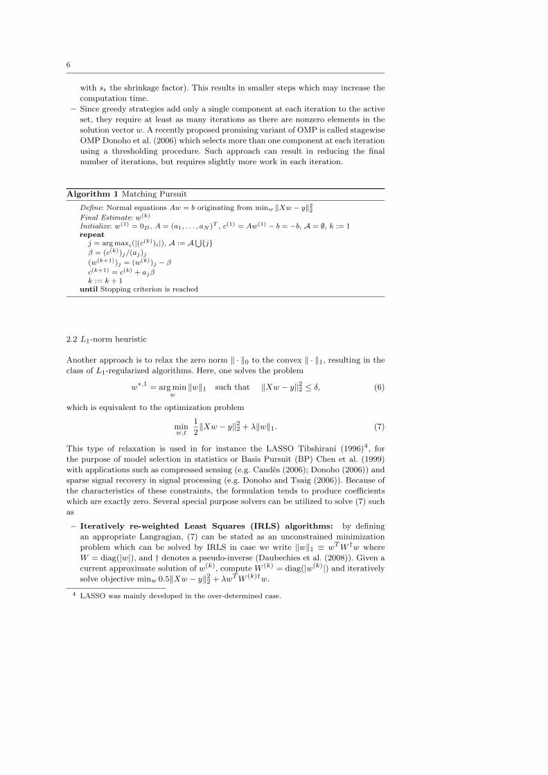
Algorithm 1 Matching Pursuit

Define: Normal equations Aw = b originating from minw ‖Xw − y‖22Final Estimate: w(k)

Initialize: w(1) = 0D, A = (a1, . . . , aN )T , c(1) = Aw(1) − b = −b, A = ∅, k := 1repeatj = arg maxi(|(c(k))i|), A := A

⋃j

β = (c(k))j/(aj)j(w(k+1))j = (w(k))j − βc(k+1) = c(k) + ajβk := k + 1

until Stopping criterion is reached

2.2 L1-norm heuristic

Another approach is to relax the zero norm ‖ · ‖0 to the convex ‖ · ‖1, resulting in the

class of L1-regularized algorithms. Here, one solves the problem

w∗,1 = arg minw

‖w‖1 such that ‖Xw − y‖22 ≤ δ, (6)

which is equivalent to the optimization problem

minw,t

1

2‖Xw − y‖22 + λ‖w‖1. (7)

This type of relaxation is used in for instance the LASSO Tibshirani (1996)4, for

the purpose of model selection in statistics or Basis Pursuit (BP) Chen et al. (1999)

with applications such as compressed sensing (e.g. Candes (2006); Donoho (2006)) and

sparse signal recovery in signal processing (e.g. Donoho and Tsaig (2006)). Because of

the characteristics of these constraints, the formulation tends to produce coefficients

which are exactly zero. Several special purpose solvers can be utilized to solve (7) such

as

– Iteratively re-weighted Least Squares (IRLS) algorithms: by defining

an appropriate Langragian, (7) can be stated as an unconstrained minimization

problem which can be solved by IRLS in case we write ‖w‖1 ≡ wTW †w where

W = diag(|w|), and † denotes a pseudo-inverse (Daubechies et al. (2008)). Given a

current approximate solution of w(k), compute W (k) = diag(|w(k)|) and iteratively

solve objective minw 0.5‖Xw − y‖22 + λwTW (k)†w.

4 LASSO was mainly developed in the over-determined case.

7

– Iterative shrinkage methods: for large scale problems an approximate strat-

egy is more realistic. Iterative shrinkage methods iteratively use a simple one di-

mensional operation that set small entries to zeros and shrinking the other en-

tries towards zero. Assume a square unitary matrix X. As a first step find an

intermediate solution w = XT y, which hopefully has only a few large entries ex-

ceeding many small noisy ones. Secondly, apply shrinkage function f((w)i;λt) =

sign((w)i)(|(w)i|−λt)+5 for i = 1, ..., D. In the general case where X is not unitary

this idea is applied iteratively. These methods can compete with greedy methods

both in simplicity and efficiency but are not yet as mature as the greedy alternatives

(see Bruckstein et al. (2009) and the reference therein for a discussion).

– Stepwise algorithms: are heuristic methods, inspired by L1 solvers, which iter-

atively add or remove components from the active set. Examples are (Least Angle

RegreSsion) LARS Efron et al. (2004) and the homotopy method Osborne et al.

(2000). Consider the problem (7). It was observed in Efron et al. (2004), and Os-

borne et al. (2000) that the regularization path (i.e. the sequence of solutions, as λ

varies from 0 to ∞) is piecewise linear, changing only at critical values of λ. Each

vertex on this regularization path indicates a different sparse solution, i.e. vectors

having nonzero elements only on a subset of the potential components. At each

vertex the active set is updated through the addition and removal of components.

Based on this observation a heuristic algorithm was developed that, starting from

an empty active set, iteratively adds and removes components. Note the difference

with the greedy approaches which can only increase the number of indices in the

active set. Once a component is in the active set it remains there.

– Dedicated solvers: by exploiting the structure of the resulting quadratic pro-

gram, efficient dedicated solvers are described, see e.g. Kim et al. (2007) which uses

a specialized interior-point algorithm, or Figueiredo et al. (2007) where the authors

propose to use an efficient gradient projection algorithm.

Remark 1 Using an L1 penalty introduces a bias which is often undesirable. As a

consequence (i) the intermediate solutions are not exactly equal to the least squares

estimates (ii) component selection is based on a biased estimator. To overcome the

former, a de-bias step can be performed (see e.g. Figueiredo et al. (2007); Moghaddam

et al. (2006)). After finding an approximate solution, the de-biased solution is found by

fixing the sparsity pattern, and solving for the remaining coefficients using an ordinary

least squares method. Put in other words, having selected the components, a reduced

linear system is solved in these components alone. Greedy techniques are also biased in

their component selection strategy but provide the intermediate least squares estimates

directly.

2.3 Relations

In Efron et al. (2004) the LARS algorithm was proposed. LARS is a less greedy algo-

rithm than OMP (FSR with back-fitting), it uses a similar strategy but only uses as

much of a component as it ”deserves”:

– Consider the normal equations defined in (5) and let the index set of currently

selected components be A = s1, . . . , sNA, the set of not yet selected components

5 Operator (·)+ sets negative values to zero while positives remain unchanged.

8

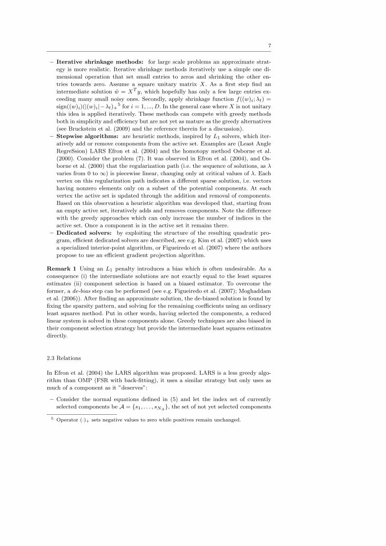
Fig. 2: Overview of different approaches to tackle (3).

A, selection matrix ΣA = (es1 , . . . , esNA), ΣA ∈ RD×NA where ei ∈ RD the i-th

unit vector of size D, and a submatrix AA = ΣTAAΣA of A.

– Start by selecting the j∗-th column of X which correlates the most with Xw(1)−yor j∗ = arg maxj |bj | (since w(1) = 0).

– The parameter vector w(2) is changed6 according to the direction defined by the

joint least squares solution of the currently selected components AAΣTAw

(2) −ΣTAb = 0 until a competitor j ∈ A has as much correlation with the current

least squares residuals (|AAΣTAw(2) − ΣTAb|)i = |eTj AΣAΣ

TAw

(2) − eTj b| for i ∈1, . . . , NA.

– Then this new component is inserted in A and removed from A, and the process

is continued.

The following observations bridged the gap between L1-minimization and greedy OMP

Donoho and Tsaig (2006) Efron et al. (2004):

– Only a simple modification to LARS (when a nonzero coefficient hits zero, drop it

from A and recompute the current joint least squares direction to LARS) is needed

to make LARS exactly reproduce the LASSO regularization path (the resulting

algorithm is very similar to the homotopy method described in Osborne et al.

(2000)).

– LARS and OMP are based on the same fundamental principle, which solves a

sequence of least-squares problems on an increasingly larger subspace, defined by

the active set.

This helps explaining the similarity of both approaches in several theoretical and

numerical studies (e.g. Bruckstein et al. (2009); Tropp (2004)). Since its simplicity

and the fact that OMP has similar behavior as the more sophisticated L1-norm based

optimization methods, we now proceed by defining an efficient algorithm for (greedy)

OMP and present in the experimental section that it can outperform an L1 related

alternative in terms of speed while having comparable accuracy. Fig. 2 schematically

summarizes the different approaches to tackle (3).

6 In Efron et al. (2004) the authors observed that both LASSO and FStR behaved verysimilar. In an attempt to reduce the number of iterations of FStR, the authors defined LARSwhich ”optimizes” the small FStR steps to larger steps, but smaller than the FSR stepsize,which greatly reduces the computer processing time.

9

3 Greedy heuristic: Sparse Conjugate Directions

This section describes a new approach to solve (3) which belongs to the category of

greedy heuristics.

Similar to the ideas in Blumensath and Davies (2008); Lutz and Buhlmann (2006)

this work adapts CG such that the iteratively constructed conjugate basis yields so-

lutions of increasing cardinality. In case the algorithm can be terminated in less than

D steps a sparse solution is obtained. Adapting CG in this way results in an efficient

implementation of OMP, which is a greedy based heuristic to solve (3) as pointed out

in the previous section.

3.1 Conjugate Gradient Method

Consider a linear system with a symmetric positive definite matrix, such as in (5). This

linear system is found as the solution of the following optimization problem

w = arg minw

Ψ(w) =1

2wTAw − bTw. (8)

Now the first order condition for optimality coincides with the linear system, as the

gradient c ∈ RD becomes

∇Ψ(w) = Aw − b = c. (9)

We now state two interesting properties of CG without proof, further details can be

found in Nocedal and Wright (2006). One of the remarkable properties of the conjugate

gradient method is its ability to generate very cheaply a set of conjugate vectors. A set

of nonzero vectors7 p(1), p(2), ..., p(D) ⊂ RD is said to be conjugate with respect to

the positive definite matrix A if and only if

p(i)TAp(j) = 0, ∀i 6= j. (10)

Therefore, given a starting point w(1) ∈ RD and a set of conjugate vectors p(1), p(2), ...,

p(D) one can solve the linear system by iteratively minimizing over the individual

directions by setting

w(k) = w(k−1) + η(k)p(k), (11)

where η(k) is the minimizer along the direction w(k) = w(k−1) + ηp(k) and the super-

script (k) denotes the dependency of the variable on the iteration number k. This term

is given explicitly as

η(k) = − c(k)T p(k)

p(k)TAp(k). (12)

Note that c(k) is defined as c in (9). Since for a matrix A ∈ RD×D, only D different

conjugate vectors can be constructed, the following result follows immediately:

Proposition 1 Nocedal and Wright (2006) The CG algorithm converges to the solu-

tion w(L) of (8) in at most D steps.

7 For simplicity we first assume that all conjugate directions are given beforehand. However,we already denote the different conjugate directions via p(k) since the set will be iterativelygenerated in the final algorithm such that p(k) is generated in the k-th iteration.

10

For example, if the Hessian A would be diagonal then the subspace spanned by the unit

vectors es1 , es2 , ..., esk would be minimized after k one-dimensional minimizations

along the corresponding unit vectors directions.

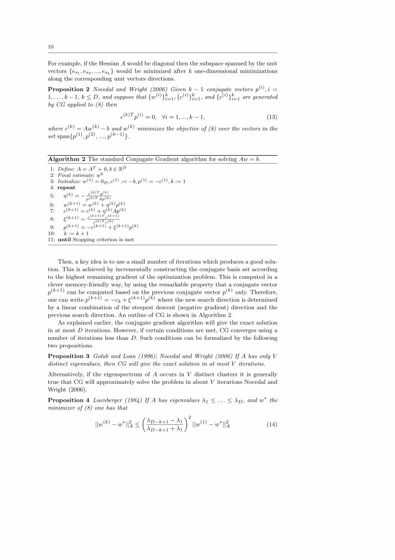
Proposition 2 Nocedal and Wright (2006) Given k − 1 conjugate vectors p(i), i =

1, . . . , k− 1, k ≤ D, and suppose that w(i)ki=1, c(i)ki=1, and c(i)ki=1 are generated

by CG applied to (8) then

c(k)T p(i) = 0, ∀i = 1, ..., k − 1, (13)

where c(k) = Aw(k) − b and w(k) minimizes the objective of (8) over the vectors in the

set spanp(1), p(2), ..., p(k−1).

Algorithm 2 The standard Conjugate Gradient algorithm for solving Aw = b.

1: Define: A = AT 0, b ∈ RD2: Final estimate: wk

3: Initialize: w(1) = 0D, c(1) := −b, p(1) = −c(1), k := 1

4: repeat

5: η(k) = − c(k)T p(k)

p(k)TAp(k)

6: w(k+1) = w(k) + η(k)p(k)

7: c(k+1) = c(k) + η(k)Ap(k)

8: ξ(k+1) = c(k+1)T c(k+1)

c(k)T c(k)

9: p(k+1) = −c(k+1) + ξ(k+1)p(k)

10: k := k + 111: until Stopping criterion is met

Then, a key idea is to use a small number of iterations which produces a good solu-

tion. This is achieved by incrementally constructing the conjugate basis set according

to the highest remaining gradient of the optimization problem. This is computed in a

clever memory-friendly way, by using the remarkable property that a conjugate vector

p(k+1) can be computed based on the previous conjugate vector p(k) only. Therefore,

one can write p(k+1) = −ck + ξ(k+1)p(k) where the new search direction is determined

by a linear combination of the steepest descent (negative gradient) direction and the

previous search direction. An outline of CG is shown in Algorithm 2.

As explained earlier, the conjugate gradient algorithm will give the exact solution

in at most D iterations. However, if certain conditions are met, CG converges using a

number of iterations less than D. Such conditions can be formalized by the following

two propositions.

Proposition 3 Golub and Loan (1996); Nocedal and Wright (2006) If A has only V

distinct eigenvalues, then CG will give the exact solution in at most V iterations.

Alternatively, if the eigenspectrum of A occurs in V distinct clusters it is generally

true that CG will approximately solve the problem in about V iterations Nocedal and

Wright (2006).

Proposition 4 Luenberger (1984) If A has eigenvalues λ1 ≤ . . . ≤ λD, and w∗ the

minimizer of (8) one has that

||w(k) − w∗||2A ≤(λD−k+1 − λ1

λD−k+1 + λ1

)2

||w(1) − w∗||2A (14)

11

One can interpret this result by considering the case where a small number of L eigen-

values of A are large and the other D − L smaller eigenvalues are clustered around 1.

After L+ 1 iterations one could approximately write

||w(L+1) − w∗||A ≈ ε||w(1) − w∗||A, (15)

where ε = λD−L − λ1. In case ε is small then the CG method might provide good

estimates of the solution after only L+1 iterations. Other convergence measures based

on the condition number have been discussed in Smale (1997), Golub and Loan (1996),

and Nocedal and Wright (2006).

These results indicate that CG, in case some conditions are met, can approximate

using a significantly smaller number of iterations than D. In case this property is pre-

served while using a sparse conjugate directions basis, a sparse (approximate) solution

can be obtained.

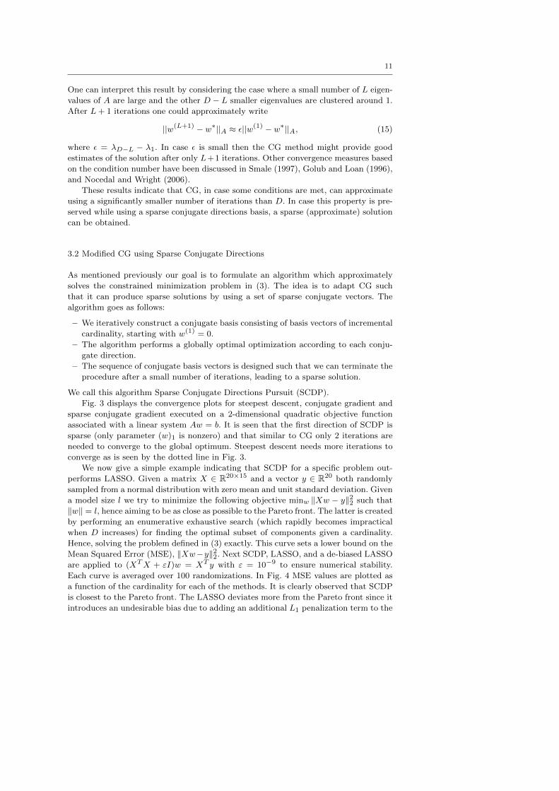
3.2 Modified CG using Sparse Conjugate Directions

As mentioned previously our goal is to formulate an algorithm which approximately

solves the constrained minimization problem in (3). The idea is to adapt CG such

that it can produce sparse solutions by using a set of sparse conjugate vectors. The

algorithm goes as follows:

– We iteratively construct a conjugate basis consisting of basis vectors of incremental

cardinality, starting with w(1) = 0.

– The algorithm performs a globally optimal optimization according to each conju-

gate direction.

– The sequence of conjugate basis vectors is designed such that we can terminate the

procedure after a small number of iterations, leading to a sparse solution.

We call this algorithm Sparse Conjugate Directions Pursuit (SCDP).

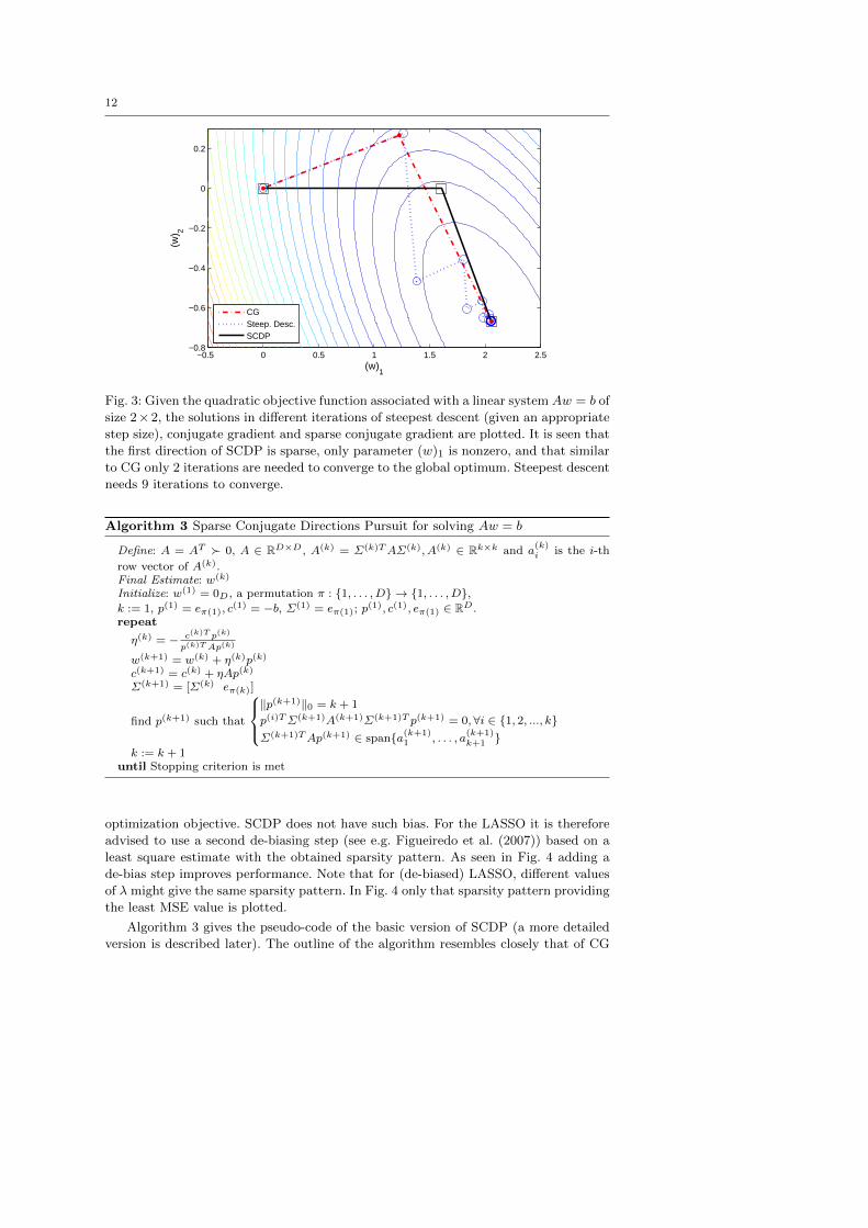
Fig. 3 displays the convergence plots for steepest descent, conjugate gradient and

sparse conjugate gradient executed on a 2-dimensional quadratic objective function

associated with a linear system Aw = b. It is seen that the first direction of SCDP is

sparse (only parameter (w)1 is nonzero) and that similar to CG only 2 iterations are

needed to converge to the global optimum. Steepest descent needs more iterations to

converge as is seen by the dotted line in Fig. 3.

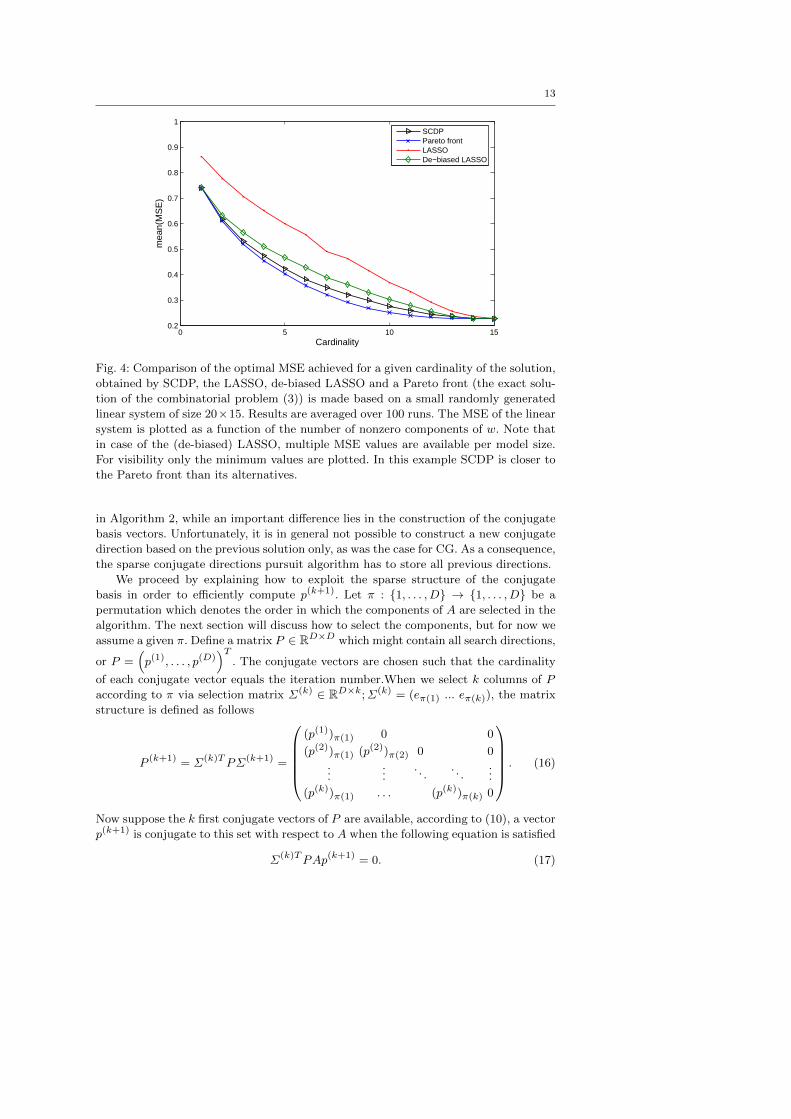
We now give a simple example indicating that SCDP for a specific problem out-

performs LASSO. Given a matrix X ∈ R20×15 and a vector y ∈ R20 both randomly

sampled from a normal distribution with zero mean and unit standard deviation. Given

a model size l we try to minimize the following objective minw ‖Xw − y‖22 such that

‖w‖ = l, hence aiming to be as close as possible to the Pareto front. The latter is created

by performing an enumerative exhaustive search (which rapidly becomes impractical

when D increases) for finding the optimal subset of components given a cardinality.

Hence, solving the problem defined in (3) exactly. This curve sets a lower bound on the

Mean Squared Error (MSE), ‖Xw−y‖22. Next SCDP, LASSO, and a de-biased LASSO

are applied to (XTX + εI)w = XT y with ε = 10−9 to ensure numerical stability.

Each curve is averaged over 100 randomizations. In Fig. 4 MSE values are plotted as

a function of the cardinality for each of the methods. It is clearly observed that SCDP

is closest to the Pareto front. The LASSO deviates more from the Pareto front since it

introduces an undesirable bias due to adding an additional L1 penalization term to the

12

−0.5 0 0.5 1 1.5 2 2.5−0.8

−0.6

−0.4

−0.2

0

0.2

(w)1

(w) 2

CGSteep. Desc.SCDP

Fig. 3: Given the quadratic objective function associated with a linear system Aw = b of

size 2×2, the solutions in different iterations of steepest descent (given an appropriate

step size), conjugate gradient and sparse conjugate gradient are plotted. It is seen that

the first direction of SCDP is sparse, only parameter (w)1 is nonzero, and that similar

to CG only 2 iterations are needed to converge to the global optimum. Steepest descent

needs 9 iterations to converge.

Algorithm 3 Sparse Conjugate Directions Pursuit for solving Aw = b

Define: A = AT 0, A ∈ RD×D, A(k) = Σ(k)TAΣ(k), A(k) ∈ Rk×k and a(k)i is the i-th

row vector of A(k).Final Estimate: w(k)

Initialize: w(1) = 0D, a permutation π : 1, . . . , D → 1, . . . , D,k := 1, p(1) = eπ(1), c

(1) = −b, Σ(1) = eπ(1); p(1), c(1), eπ(1) ∈ RD.

repeat

η(k) = − c(k)T p(k)

p(k)TAp(k)

w(k+1) = w(k) + η(k)p(k)

c(k+1) = c(k) + ηAp(k)

Σ(k+1) = [Σ(k) eπ(k)]

find p(k+1) such that

‖p(k+1)‖0 = k + 1

p(i)TΣ(k+1)A(k+1)Σ(k+1)T p(k+1) = 0, ∀i ∈ 1, 2, ..., kΣ(k+1)TAp(k+1) ∈ spana(k+1)

1 , . . . , a(k+1)k+1

k := k + 1until Stopping criterion is met

optimization objective. SCDP does not have such bias. For the LASSO it is therefore

advised to use a second de-biasing step (see e.g. Figueiredo et al. (2007)) based on a

least square estimate with the obtained sparsity pattern. As seen in Fig. 4 adding a

de-bias step improves performance. Note that for (de-biased) LASSO, different values

of λ might give the same sparsity pattern. In Fig. 4 only that sparsity pattern providing

the least MSE value is plotted.

Algorithm 3 gives the pseudo-code of the basic version of SCDP (a more detailed

version is described later). The outline of the algorithm resembles closely that of CG

13

0 5 10 150.2

0.3

0.4

0.5

0.6

0.7

0.8

0.9

1

Cardinality

mea

n(M

SE

)

SCDPPareto frontLASSODe−biased LASSO

Fig. 4: Comparison of the optimal MSE achieved for a given cardinality of the solution,

obtained by SCDP, the LASSO, de-biased LASSO and a Pareto front (the exact solu-

tion of the combinatorial problem (3)) is made based on a small randomly generated

linear system of size 20×15. Results are averaged over 100 runs. The MSE of the linear

system is plotted as a function of the number of nonzero components of w. Note that

in case of the (de-biased) LASSO, multiple MSE values are available per model size.

For visibility only the minimum values are plotted. In this example SCDP is closer to

the Pareto front than its alternatives.

in Algorithm 2, while an important difference lies in the construction of the conjugate

basis vectors. Unfortunately, it is in general not possible to construct a new conjugate

direction based on the previous solution only, as was the case for CG. As a consequence,

the sparse conjugate directions pursuit algorithm has to store all previous directions.

We proceed by explaining how to exploit the sparse structure of the conjugate

basis in order to efficiently compute p(k+1). Let π : 1, . . . , D → 1, . . . , D be a

permutation which denotes the order in which the components of A are selected in the

algorithm. The next section will discuss how to select the components, but for now we

assume a given π. Define a matrix P ∈ RD×D which might contain all search directions,

or P =(p(1), . . . , p(D)

)T. The conjugate vectors are chosen such that the cardinality

of each conjugate vector equals the iteration number.When we select k columns of P

according to π via selection matrix Σ(k) ∈ RD×k;Σ(k) = (eπ(1) ... eπ(k)), the matrix

structure is defined as follows

P (k+1) = Σ(k)TPΣ(k+1) =

(p(1))π(1) 0 0

(p(2))π(1) (p(2))π(2) 0 0...

.... . .

. . ....

(p(k))π(1) . . . (p(k))π(k) 0

. (16)

Now suppose the k first conjugate vectors of P are available, according to (10), a vector

p(k+1) is conjugate to this set with respect to A when the following equation is satisfied

Σ(k)TPAp(k+1) = 0. (17)

14

Since the set of vectors in P possesses a certain sparsity pattern, (17) can be written

as P (k+1)A(k+1)(Σ(k+1)T p(k+1)

)= 0 where A(k+1) = Σ(k+1)TAΣ(k+1). In order to

obtain the desired sparse pattern for p(k+1), i.e. a cardinality that equals the iteration

number, additional constraints are added. Hence, the new sparse conjugate direction

p(k+1) must then satisfy the following

P (k+1)A(k+1)(Σ(k+1)T p(k+1)

)= 0,

such that

Σ(k+1)TAp(k+1) ∈ spana(k+1)

1 , . . . , a(k+1)k+1 , ∀k,

‖p(k+1)‖0 = k + 1(18)

where the span of a set of vectors in a vector space is the intersection of all subspaces

containing that set, and a(k+1)i is the i-th row or column vector of A(k+1). The first

constraint determines which components of pk+1 may be updated, i.e. those that cor-

respond to the selected columns and rows in A. The second ensures that the cardinality

of the solution equals the iteration number. As such, given a permutation π, one can

compute a sequence of search directions by solving iteratively for p(k+1). Let us define

B(k+1) = P (k+1)A(k+1), then

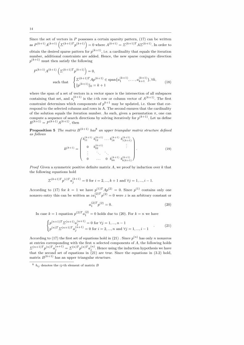
Proposition 5 The matrix B(k+1) has8 an upper triangular matrix structure definedas follows

B(k+1) =

b(k+1)11 b

(k+1)12 . . . b

(k+1)1k b

(k+1)1(k+1)

0 b(k+1)22

......

. . .. . .

0 . . . 0 b(k+1)kk b

(k+1)k(k+1)

. (19)

Proof Given a symmetric positive definite matrix A, we proof by induction over k that

the following equations hold

Σ(k+1)T p(i)T a(k+1)j = 0 for i = 2, ..., k + 1 and ∀j = 1, ..., i− 1.

According to (17) for k = 1 we have p(1)TAp(2) = 0. Since p(1) contains only one

nonzero entry this can be written as za(2)T1 p(2) = 0 were z is an arbitrary constant or

a(2)T1 p(2) = 0. (20)

In case k = 1 equation p(2)T a(2)1 = 0 holds due to (20). For k = n we have

p(n+1)TΣ(n+1)a(n+1)j = 0 for ∀j = 1, ..., n− 1

p(n)TΣ(n+1)T a(n+1)j = 0 for i = 2, ..., n and ∀j = 1, ..., i− 1

. (21)

According to (17) the first set of equations hold in (21) . Since p(n) has only n nonzeros

at entries corresponding with the first n selected components of A, the following holds

Σ(n+1)T p(n)T a(n+1)j = Σ(n)T p(n)T a

(n)j . Hence using the induction hypothesis we have

that the second set of equations in (21) are true. Since the equations in (3.2) hold,

matrix B(k+1) has an upper triangular structure.

8 bij denotes the ij-th element of matrix B

15

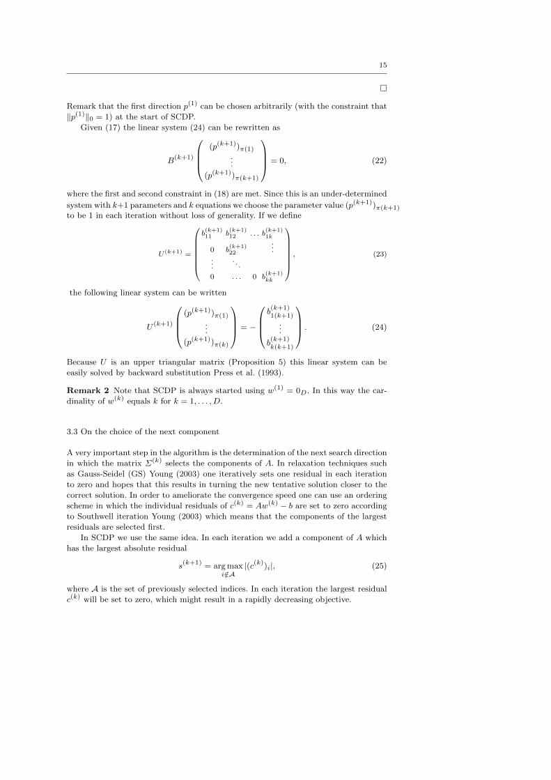
Remark that the first direction p(1) can be chosen arbitrarily (with the constraint that

‖p(1)‖0 = 1) at the start of SCDP.

Given (17) the linear system (24) can be rewritten as

B(k+1)

(p(k+1))π(1)

...

(p(k+1))π(k+1)

= 0, (22)

where the first and second constraint in (18) are met. Since this is an under-determined

system with k+1 parameters and k equations we choose the parameter value (p(k+1))π(k+1)

to be 1 in each iteration without loss of generality. If we define

U(k+1) =

b(k+1)11 b

(k+1)12 . . . b

(k+1)1k

0 b(k+1)22

......

. . .

0 . . . 0 b(k+1)kk

, (23)

the following linear system can be written

U (k+1)

(p(k+1))π(1)

...

(p(k+1))π(k)

= −

b(k+1)1(k+1)

...

b(k+1)k(k+1)

. (24)

Because U is an upper triangular matrix (Proposition 5) this linear system can be

easily solved by backward substitution Press et al. (1993).

Remark 2 Note that SCDP is always started using w(1) = 0D. In this way the car-

dinality of w(k) equals k for k = 1, . . . , D.

3.3 On the choice of the next component

A very important step in the algorithm is the determination of the next search direction

in which the matrix Σ(k) selects the components of A. In relaxation techniques such

as Gauss-Seidel (GS) Young (2003) one iteratively sets one residual in each iteration

to zero and hopes that this results in turning the new tentative solution closer to the

correct solution. In order to ameliorate the convergence speed one can use an ordering

scheme in which the individual residuals of c(k) = Aw(k) − b are set to zero according

to Southwell iteration Young (2003) which means that the components of the largest

residuals are selected first.

In SCDP we use the same idea. In each iteration we add a component of A which

has the largest absolute residual

s(k+1) = arg maxi/∈A

|(c(k))i|, (25)

where A is the set of previously selected indices. In each iteration the largest residual

c(k) will be set to zero, which might result in a rapidly decreasing objective.

16

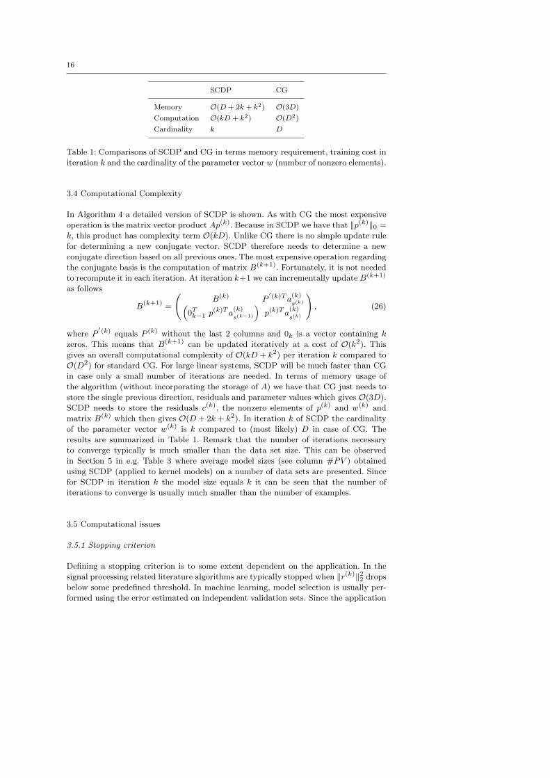
SCDP CG

Memory O(D + 2k + k2) O(3D)

Computation O(kD + k2) O(D2)

Cardinality k D

Table 1: Comparisons of SCDP and CG in terms memory requirement, training cost in

iteration k and the cardinality of the parameter vector w (number of nonzero elements).

3.4 Computational Complexity

In Algorithm 4 a detailed version of SCDP is shown. As with CG the most expensive

operation is the matrix vector product Ap(k). Because in SCDP we have that ‖p(k)‖0 =

k, this product has complexity term O(kD). Unlike CG there is no simple update rule

for determining a new conjugate vector. SCDP therefore needs to determine a new

conjugate direction based on all previous ones. The most expensive operation regarding

the conjugate basis is the computation of matrix B(k+1). Fortunately, it is not needed

to recompute it in each iteration. At iteration k+1 we can incrementally update B(k+1)

as follows

B(k+1) =

(B(k) P

′(k)T a(k)

s(k)(0Tk−1 p

(k)T a(k)

s(k−1)

)p(k)T a

(k)

s(k)

), (26)

where P′(k) equals P (k) without the last 2 columns and 0k is a vector containing k

zeros. This means that B(k+1) can be updated iteratively at a cost of O(k2). This

gives an overall computational complexity of O(kD + k2) per iteration k compared to

O(D2) for standard CG. For large linear systems, SCDP will be much faster than CG

in case only a small number of iterations are needed. In terms of memory usage of

the algorithm (without incorporating the storage of A) we have that CG just needs to

store the single previous direction, residuals and parameter values which gives O(3D).

SCDP needs to store the residuals c(k), the nonzero elements of p(k) and w(k) and

matrix B(k) which then gives O(D + 2k + k2). In iteration k of SCDP the cardinality

of the parameter vector w(k) is k compared to (most likely) D in case of CG. The

results are summarized in Table 1. Remark that the number of iterations necessary

to converge typically is much smaller than the data set size. This can be observed

in Section 5 in e.g. Table 3 where average model sizes (see column #PV ) obtained

using SCDP (applied to kernel models) on a number of data sets are presented. Since

for SCDP in iteration k the model size equals k it can be seen that the number of

iterations to converge is usually much smaller than the number of examples.

3.5 Computational issues

3.5.1 Stopping criterion

Defining a stopping criterion is to some extent dependent on the application. In the

signal processing related literature algorithms are typically stopped when ‖r(k)‖22 drops

below some predefined threshold. In machine learning, model selection is usually per-

formed using the error estimated on independent validation sets. Since the application

17

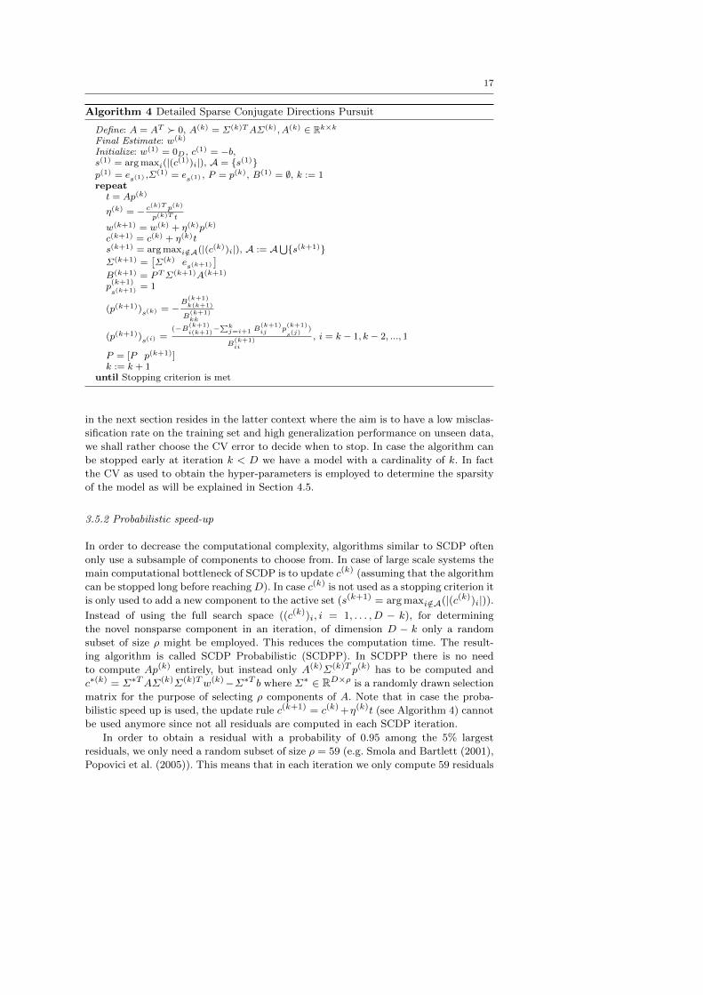
Algorithm 4 Detailed Sparse Conjugate Directions Pursuit

Define: A = AT 0, A(k) = Σ(k)TAΣ(k), A(k) ∈ Rk×kFinal Estimate: w(k)

Initialize: w(1) = 0D, c(1) = −b,s(1) = arg maxi(|(c(1))i|), A = s(1)p(1) = es(1) ,Σ(1) = es(1) , P = p(k), B(1) = ∅, k := 1repeatt = Ap(k)

η(k) = − c(k)T p(k)

p(k)T t

w(k+1) = w(k) + η(k)p(k)

c(k+1) = c(k) + η(k)ts(k+1) = arg maxi/∈A(|(c(k))i|), A := A

⋃s(k+1)

Σ(k+1) =[Σ(k) es(k+1)

]B(k+1) = PTΣ(k+1)A(k+1)

p(k+1)

s(k+1) = 1

(p(k+1))s(k) = −B

(k+1)k(k+1)

B(k+1)kk

(p(k+1))s(i) =(−B(k+1)

i(k+1)−∑k

j=i+1 B(k+1)ij p

(k+1)

s(j))

B(k+1)ii

, i = k − 1, k − 2, ..., 1

P = [P p(k+1)]k := k + 1

until Stopping criterion is met

in the next section resides in the latter context where the aim is to have a low misclas-

sification rate on the training set and high generalization performance on unseen data,

we shall rather choose the CV error to decide when to stop. In case the algorithm can

be stopped early at iteration k < D we have a model with a cardinality of k. In fact

the CV as used to obtain the hyper-parameters is employed to determine the sparsity

of the model as will be explained in Section 4.5.

3.5.2 Probabilistic speed-up

In order to decrease the computational complexity, algorithms similar to SCDP often

only use a subsample of components to choose from. In case of large scale systems the

main computational bottleneck of SCDP is to update c(k) (assuming that the algorithm

can be stopped long before reaching D). In case c(k) is not used as a stopping criterion it

is only used to add a new component to the active set (s(k+1) = arg maxi/∈A(|(c(k))i|)).Instead of using the full search space ((c(k))i, i = 1, . . . , D − k), for determining

the novel nonsparse component in an iteration, of dimension D − k only a random

subset of size ρ might be employed. This reduces the computation time. The result-

ing algorithm is called SCDP Probabilistic (SCDPP). In SCDPP there is no need

to compute Ap(k) entirely, but instead only A(k)Σ(k)T p(k) has to be computed and

c∗(k) = Σ∗TAΣ(k)Σ(k)Tw(k)−Σ∗T b where Σ∗ ∈ RD×ρ is a randomly drawn selection

matrix for the purpose of selecting ρ components of A. Note that in case the proba-

bilistic speed up is used, the update rule c(k+1) = c(k) +η(k)t (see Algorithm 4) cannot

be used anymore since not all residuals are computed in each SCDP iteration.

In order to obtain a residual with a probability of 0.95 among the 5% largest

residuals, we only need a random subset of size ρ = 59 (e.g. Smola and Bartlett (2001),

Popovici et al. (2005)). This means that in each iteration we only compute 59 residuals

18

and select from within that set the largest residual and corresponding component of A.

In case the A is available in memory, the training complexity can now approximately be

written as O(ρk+k2). The total memory used by the algorithm is now O(ρ+2k+k2).

Note that repeating SCDP on a certain problem gives identical solutions. However,

using the described speed-up affects reproducibility of the results since each run of the

algorithm might give a different solution. As will be shown in the experimental section

in some cases the results may deviate strongly from those of standard SCDP, resulting

in less accurate predictions.

A more cleaver way of reducing computations might be to apply shrinking tech-

niques such as used in the SVM literature Joachims (1999). Leaving out examples (rows

of X) with small corresponding r(k) (examples that are fitted correctly) in the compu-

tation of c(k) is not likely to harm the process of selection a new candidate. Therefor,

it might be interesting to first select a set of examples with corresponding large r(k)

values. Then do a number of iterations using lightweight updates only operating on the

reduced set (ρ equals size of reduced set). Once in a while r(k) can be fully computed

to change the reduced set.

4 Application: using SCDP for sparse reduced LS-SVMs

In this section a kernel-based learning method derived within the LS-SVM setting, is

given. We will proceed as follows:

1. First the kernel-based LS-SVM primal-dual context is briefly reviewed.

2. Since this work aims at large-scale systems with N D, it is more advantageous

to solve in the primal space.

3. In case of using kernels other than the linear one, the feature map in the primal

formulation is not explicitly known. Therefore, an approximation is needed which

in this work is obtained using the Nystrom approximation. (see Section 4.2)

4. As a result an over-determined linear system is obtained which may be solved using

SCDP to get sparser models.

4.1 Least Squares Support Vector Machines

An overview of Least Squares Support Vector Machine (LS-SVM) models has been

given in Suykens et al. (2002b). Although the LS-SVM framework is studied in many

other contexts as well, we will only consider it here in case of classification problems

which is directly related to the regression case. Given a training set, the convex primal

problem of the LS-SVM classifier can be formulated as

minw,e′i,b0

1

2wTw +

γ

2

N∑i=1

e′2i such that yif(xi) = 1− e′i, i = 1, ..., N, (27)

where a quadratic loss is used (instead of the hinge loss function typically employed in

SVMs) where f(x) = wTϕ(x)+b0. Another difference is the use of equality constraints

instead of inequality constraints. The e′i are slack variables allowing deviation form the

19

target labels yi. The formulation can be considered as a regression on the labels yi and

is equivalent to

minw,ei,b0

1

2wTw +

γ

2

N∑i=1

e2i such that f(xi) = yi − ei, i = 1, ..., N, (28)

where e′i = yiei. Given a positive definite kernel function K : RD × RD → R+ with

K(x, x′) = ϕ(x)Tϕ(x′) and a regularization constant γ ∈ R+0 , the solution to (28) is

given by the following dual problem (according to Suykens and Vandewalle (1999)):Ω + 1γ I 1N

1TN 0

α

b0

=

y

0

, (29)

where 1N = (1, . . . , 1)T ∈ RN , y = (y1, ..., yN )T , α = (α1, ..., αN )T , Ωij = K(xi, xj)

and the identity matrix I = diag(1, . . . , 1) ∈ RN×N . Note that this dual problem was

also studied in Saunders et al. (1998) without the use of a bias term. Efficient CG

based solvers exist to compute (29) Chu et al. (2005).

4.2 Fixed-size method: Nystrom approximation and estimation in the primal

Suppose one takes a finite dimensional feature map (e.g. a linear kernel K(x, x′) =

xT x′). Then one can equally well solve the primal (28) as the dual (29) problem. In

fact solving the primal problem might be more advantageous for larger data sets where

the dimension of the parameters w ∈ RD is smaller compared to that of α ∈ RN .

In order to work in the primal space using a kernel function other than the linear

one, it is required to compute an explicit approximation of the nonlinear mapping

ϕ : RD → RN , such that Ωij ≈ ϕ(xi)T ϕ(xj).

Based on Williams and Seeger (2001), the Nystrom method is used to compute the

approximated feature map ϕi : RD → R, i = 1, . . . , N for a training point, or for any

new point x∗, with ϕ = (ϕ1, . . . , ϕN )T , is given as

ϕi(x∗) =

1√λsi

N∑j=1

(ui)jK(xj , x∗), (30)

where λsi and ui are respectively the eigenvalues and eigenvectors of the kernel matrix

Ω ∈ RN×N , Ωij = K(xi, xj), xi and xj ∈ XTR with XTR the set of training examples.

Instead of using ϕ ∈ RN , in Williams and Seeger (2001) it was motivated to use

a subsample of size M N to compute an approximate feature map of size M . The

M vectors are called Prototype Vectors (PVs) which might, but do not necessarily,

coincidence with training examples.

Let M be the size of the PV set, U = (u1, . . . , uM ) the square matrix of eigen-

vectors of Ω, ui = ((ui)1, . . . , (ui)M )T , and Λ = diag(λs1, . . . , λsN ) a diagonal matrix

of nonnegative eigenvalues in decreasing order, Ω′ ∈ RN×M , Ω′ij = K(xi, xj), xi ∈XTR, xj ∈ XPV with XPV the set of selected PVs. Then, the computation of the

features in matrix notation can be written as

Φ = Ω′US, (31)

20

with matrix Φ ∈ RN×M defined as

Φ =

ϕ1(x1) . . . ϕM (x1)...

. . ....

ϕ1(xN ) . . . ϕM (xN )

, (32)

and S = Λ−12 .

Given M N , the goal is to find an approximate solution for the over-determined

system(Φ 1N

) (wT b

)T= y. Solving (28) with an approximate feature map Φ (i.e.

the FS-LSSVM training) boils down to solving the following linear system (see e.g.

Brabanter et al. (2010)), ΦT Φ+ 1γ I Φ

T 1N

1TN Φ 1TN1N

w

b0

=

ΦT y

1TNy

, (33)

where Φ ∈ RN×M is defined according to (32), w ∈ RM are the model parameters and

y ∈ RN the class labels in case of classification. Solving the primal as in (33) leads to

a sparse representation.

Given an unseen data point x∗, the final classifier can be written as

y∗ = sign(wT ϕ(x∗) + b0). (34)

Given a value M , PV selection concerns the process of selecting a set of PVs

which represent the training data distribution well. This set of PVs is then used to

calculate the approximate feature map ϕ. One approach might be to randomly select

a subsample of the training set. Other techniques approach this selection using an

appropriate selection criterion: (i) In Suykens et al. (2002b), and Brabanter et al.

(2010) this is performed using a Renyi entropy based selection method; (ii) In Zhang

et al. (2008) the observation is made that the Nystrom low-rank approximation depends

crucially on the quantization error induced by encoding the sample set with landmark

points. This suggests that one can simply use the clusters obtained with a k-center

(such as k-means) algorithm, which finds a local minimum of the quantization error

(note that using this technique the PVs do not necessarily coincidence with the training

data). A simple and fast greedy algorithm which approximates the k-center clustering

problem is proposed in Gonzalez (1985) and called farthest-point clustering.

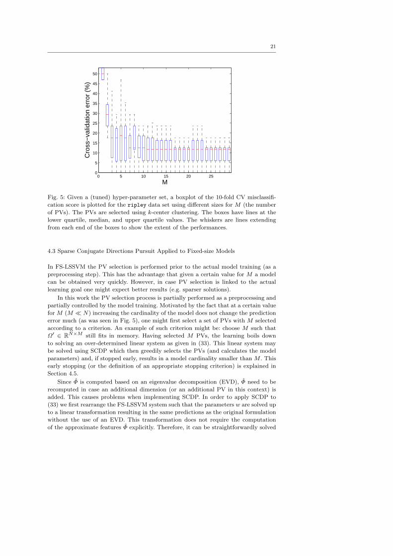
According to Suykens et al. (2002b), Brabanter et al. (2010) the CV prediction error

of FS-LSSVM decreases with respect to the number of selected Prototype Vectors (PV)

(or put in other words, cardinality of the model) until it does not change much anymore.

In Suykens et al. (2002b), Brabanter et al. (2010) empirical evidences indicates that

this point of ”saturation” might be obtained for values M N . In Fig. 5 this is

illustrated for the ripley data set (see Appendix A for more details about this data

set). It is seen that the 10-fold cross-validation misclassification score does not improve

much when more than 11 PVs are added.

Remark 3 Note that also in classical Radial Basis Function (RBF) network learning,

methods have been developed where one separates the training of the centers from the

training of the output weights. In RBF networks the centers are often determined by

means of clustering Chen et al. (1992, 1991) or using a vector quantization method

eventually in combination with self-organizing maps Kohonen (1990) to visualize the

input space of the network.

21

0 5 10 15 20 250

5

10

15

20

25

30

35

40

45

50

Cro

ss−

valid

atio

n er

ror

(%)

M

Fig. 5: Given a (tuned) hyper-parameter set, a boxplot of the 10-fold CV misclassifi-

cation score is plotted for the ripley data set using different sizes for M (the number

of PVs). The PVs are selected using k-center clustering. The boxes have lines at the

lower quartile, median, and upper quartile values. The whiskers are lines extending

from each end of the boxes to show the extent of the performances.

4.3 Sparse Conjugate Directions Pursuit Applied to Fixed-size Models

In FS-LSSVM the PV selection is performed prior to the actual model training (as a

preprocessing step). This has the advantage that given a certain value for M a model

can be obtained very quickly. However, in case PV selection is linked to the actual

learning goal one might expect better results (e.g. sparser solutions).

In this work the PV selection process is partially performed as a preprocessing and

partially controlled by the model training. Motivated by the fact that at a certain value

for M (M N) increasing the cardinality of the model does not change the prediction

error much (as was seen in Fig. 5), one might first select a set of PVs with M selected

according to a criterion. An example of such criterion might be: choose M such that

Ω′ ∈ RN×M still fits in memory. Having selected M PVs, the learning boils down

to solving an over-determined linear system as given in (33). This linear system may

be solved using SCDP which then greedily selects the PVs (and calculates the model

parameters) and, if stopped early, results in a model cardinality smaller than M . This

early stopping (or the definition of an appropriate stopping criterion) is explained in

Section 4.5.

Since Φ is computed based on an eigenvalue decomposition (EVD), Φ need to be

recomputed in case an additional dimension (or an additional PV in this context) is

added. This causes problems when implementing SCDP. In order to apply SCDP to

(33) we first rearrange the FS-LSSVM system such that the parameters w are solved up

to a linear transformation resulting in the same predictions as the original formulation

without the use of an EVD. This transformation does not require the computation

of the approximate features Φ explicitly. Therefore, it can be straightforwardly solved

22

using the previously explained SCDP algorithm. This transformation is explained in

Lemma 41.

Theorem 41 The linear system (33) is equivalent toΩ′TΩ′ + 1γΩ Ω′T 1N

1TNΩ′ 1TN1N

w

b0

=

Ω′T y

1TNy

, (35)

where Ωij = K(xi, xj) with xi, xj ∈ XPV and XPV the set of selected PVs, Ω ∈RM×M ; Ω′ ∈ RN×M with Ω′ij = K(xi, xj), xi ∈ Xtr, and xj ∈ XPV with Xtr the set

of training vectors; ΩU = UΛ; w = USw with S = Λ−12 . Λ is assumed to be a diagonal

matrix containing strictly positive eigenvalues.

Proof Recall that the computation of the approximate feature map ϕ is based on the

eigenvectors and values of a reduced kernel matrix ΩU = UΛ, Ω ∈ RM×M resulting

in

Φ = Ω′US, (36)

where Ω′ ∈ RN×M , Ω′ij = K(xi, xj), xi ∈ Xtr, xj ∈ XPV with XPV the set of selected

PVs and Xtr the set of training vectors and S = Λ−12 (where we assume that the

eigenvalues in Λ are strictly positive). Combining (36) and (33) givesSUTΩ′TΩ′US + 1γ I SU

TΩ′T 1N

1TNΩ′US 1TN1N

w

b0

=

SUTΩ′y

1TNy

⇒

Ω′TΩ′US + 1γ (SUT )−1 Ω′T 1N

1TNΩ′US 1TN1N

w

b0

=

Ω′y

1TNy

⇒

Ω′TΩ′ + 1γUS

−2UT Ω′T 1N

1TNΩ′ 1TN1N

w

b0

=

Ω′y

1TNy

,

(37)

where

w = USw. (38)

Since Λ = S−2, ΩU = UΛ and UTU = I we can write US−2UT = Ω. If we substitute

this result in the latter linear system we get (35).

The classifier y∗ = sign(wT ϕ(x∗) + b0

)can be written as y∗ = sign (Ω∗USw + b0)

according to (36) where Ω∗ ∈ R1×M , Ω∗1i = K(x∗, xi). Combining the latter and (38)

we have y∗ = sign (Ω∗w + b0). This gives

y∗ = sign(wT ϕ(x∗) + b0)

= sign

(M∑i=1

wiK(x∗, xi) + b0

). (39)

In order to ensure positive definiteness of the matrix in (35) we add a L2 penaliza-

tion term on the intercept term b0 controlled by a small predefined positive regular-

ization constant ν (in our experiments set to 10−8). Lemma 42 indicates the positive

definite characteristic of the matrix in the considered linear system.

23

Theorem 42 For ν > 0 and γ > 0, the matrixΩ′TΩ′ + 1γΩ Ω′T 1N

1TNΩ′ 1TN1N + ν

, (40)

is positive definite.

Proof An N ×N real symmetric matrix A is positive semi-definite if pTAp ≥ 0 for all

nonzero vectors p ∈ RM with real entries. By applying such multiplication to (42) we

can write 9

h =

(dT c

)Ω′TΩ′ + 1γΩ Ω′T 1N

1TNΩ′ 1TN1N + ν

d

c

,

which can be written as

h = (1c)T 1c+ νc2 + 2(

(1c)TΩ′d)

+ (Ω′d)TΩ′d+1

γdTΩd

= (1c+Ω′d)T (1c+Ω′d) +1

γdTΩd+ νc2.

Since the kernel matrix Ω by definition is positive semi-definite the product dTΩd is

greater or equal than zero and hence because γ > 0, ν > 0, we have h > 0. Thus, the

matrix (42) is positive definite.

Remark 4 In case the probabilistic speed-up is used (see Section 3.5.2), only a small

fraction of the kernel matrix Ω′ need to be available. However, in each iteration kernel

evaluations need to be recalculated. Keeping a cache of kernel evaluations to exclude

or reduce the number of kernel recalculations will increase training time. Although

intelligent caching methods (see the remark about shrinking in Section 3.5.2) could be

defined, we simply choose an initial set of PVs, from which the SCDP algorithm can

choose from, such that the corresponding entire Ω′ matrix fits in memory.

Remark 5 Note that our setup allows to select PVs other than those in the training

set alone using e.g. k-center clustering.

4.4 Model selection

In order to assess the hyper-parameters such as the regularization constant γ in (35)

and the RBF-kernel bandwidth parameter σ2, a v-fold CV based method is used. In the

v-th iteration, a hyper-parameter pair is given a score according to some model selection

criterion. A typical criterion expresses the number of misclassifications. However, we

prefer a continuous function that is more amenable to numerical optimization routines.

9 For clarity note that Ω′ ∈ RN×M , Ω ∈ RM×M , 1 ∈ RN , c ∈ R, and d ∈ RM .

24

Therefore in this work the press statistic Allan (1974) is used, to compute the v-fold

CV error fcv, which is defined as

fcv =1

Nv

Nv∑v=1

(1TNv

(y(Sv)− yv(Sv))2), (41)

where the indices of the CV subsample sets (Nv the number of sets (folds)) are denoted

as Sv, v = 1, ..., Nv, S1⋂. . .⋂SNv

= ∅, and yv = (fv(x1), . . . , fv(xN ))T with fv the

model which was trained in the v-th CV iteration. In Cawley (2006) the use of this

press statistic for classification problems was empirically found to give good results.

To calculate a fast v-fold CV score, this work opts to use the simple approach given

in Brabanter et al. (2010) to calculate a fast v-fold CV (see Brabanter et al. (2010) for

references to other alternatives). The technique is described in Algorithm 5. Consider

the shorthand notation Af w = bf for the full linear system defined in (35). Consider a

certain iteration in CV and let the matrix Atr be the matrix based on a subset of the

training samples (all folds except one). Instead of computing A(v)tr (and corresponding

b(v)tr ) from scratch in each v-th CV iteration, the following was proposed. At first the

following results are computed: Ω′ ∈ RN×M , Ω ∈ RM×M with M the number of PVs

(which do not have to coincidence with the training set), Af , and bf . Then based on

the fact that we can use the same PVs for each of the folds we can compute A(v)tr and

b(v)tr for CV iteration v as follows

A(v)tr = Af −

(Ω′(v)TΩ′(v) Ω′(v)T 1N(v)

1TN(v)Ω′(v) N (v)

), (42)

with N (v) the number of examples of the v-th fold and Ω′(v) is the selection of rows of

Ω′ corresponding with the samples in the v-th fold. A similar approach is used for b(v)tr

b(v)tr = bf −

(Ω′(v)y(v)

1TN(v)y(v)

), (43)

where y(v) are the labels corresponding to the v-th fold.

Remark 6 The matrices Ω′ and Ω for different kernel parameters can be computed

more efficiently depending on which kernel function is used. For example consider the

RBF kernel which is defined as K(x, x′) = exp(n/σ2) where n = −||x−x′||22. Instead of

recomputing each kernel function from scratch one can proceed as follows: (i) compute

n only once; (ii) compute RBF kernel evaluations using n with different values for σ2.

The actual hyper-parameter search process is a non-convex task which typically is

tackled via a simple grid-search based procedure. The model selection score is evaluated

at a set of points, forming a regular grid with even logarithmic spacing. An alternative

strategy is using Nelder-Mead simplex optimization Nelder and Mead (1965). This

procedure can be used as long as the number of hyper-parameters is relatively small

(in this work we tune two parameters, γ and a kernel bandwidth σ2). In order to

determine good initial start values for this simplex method we use the method of

Coupled Simulated Annealing with variance control (CSA) de Souza et al. (2009) whose

working principle was inspired by the effect of coupling in Coupled Local Minimizers

(CLM) Suykens et al. (2001) compared to the uncoupled case i.e. multi-start based

25

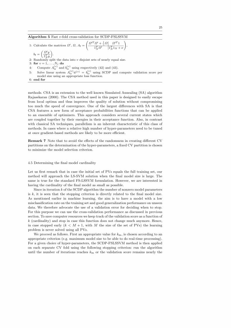
Algorithm 5 Fast v-fold cross-validation for SCDP-FSLSSVM

1: Calculate the matrices Ω′, Ω, Af =

(Ω′TΩ′ + 1

γΩ Ω′T 1

1TNΩ′ 1TN1N + ν

),

bf =

(Ω′y1TNy

).

2: Randomly split the data into v disjoint sets of nearly equal size.3: for v = 1, . . . , Nv do

4: Compute A(v)tr and b

(v)tr using respectively (42) and (43).

5: Solve linear system A(v)tr w

(v) = b(v)tr using SCDP and compute validation score per

model size using an appropriate loss function.6: end for

methods. CSA is an extension to the well known Simulated Annealing (SA) algorithm

Rajasekaran (2000). The CSA method used in this paper is designed to easily escape

from local optima and thus improves the quality of solution without compromising

too much the speed of convergence. One of the largest differences with SA is that

CSA features a new form of acceptance probabilities functions that can be applied

to an ensemble of optimizers. This approach considers several current states which

are coupled together by their energies in their acceptance function. Also, in contrast

with classical SA techniques, parallelism is an inherent characteristic of this class of

methods. In cases where a relative high number of hyper-parameters need to be tuned

at once gradient-based methods are likely to be more efficient.

Remark 7 Note that to avoid the effects of the randomness in creating different CV

partitions on the determination of the hyper-parameters, a fixed CV partition is chosen

to minimize the model selection criterion.

4.5 Determining the final model cardinality

Let us first remark that in case the initial set of PVs equals the full training set, our

method will approach the LS-SVM solution when the final model size is large. The

same is true for the standard FS-LSSVM formulation. However, we are interested in

having the cardinality of the final model as small as possible.

Since in iteration k of the SCDP algorithm the number of nonzero model parameters

is k, it is seen that the stopping criterion is directly related to the final model size.

As mentioned earlier in machine learning, the aim is to have a model with a low

misclassification rate on the training set and good generalization performance on unseen

data. We therefore advocate the use of a validation error for deciding when to stop.

For this purpose we can use the cross-validation performance as discussed in previous

section. To save computer resources we keep track of the validation score as a function of

k (cardinality) and stop in case this function does not change much anymore. Hence,

in case stopped early (k < M + 1, with M the size of the set of PVs) the learning

problem is never solved using all PVs.

We proceed as follows. First an appropriate value for km, is chosen according to an

appropriate criterion (e.g. maximum model size to be able to do real-time processing).

For a given choice of hyper-parameters, the SCDP-FSLSSVM method is then applied

on each separate CV fold using the following stopping criterion: run the algorithm

until the number of iterations reaches km or the validation score remains nearly the

26

same. Combining the results for each fold gives an estimate of the v-fold CV error for

each model size ranging from 1 to at most km. After combination of the results of the

different folds, we select the final model size such that the CV criterion is the smallest

value within one tenth of the standard deviation of the best cross-validation score

(standard deviation was calculated from the different estimates computed using CV).

See Hastie et al. (2001) (Section 7.10, page 216) where a similar approach, referred

to as the ”one-standard-error”, is given. This procedure can be repeated for different

hyper-parameter values.

Remark 8 Note that in case the probabilistic speed-up is used, the random selection

of candidate directions is fixed in order to exclude undesirable influence of the random

effects in this tuning process. Thus, at iteration k, the different SCDP runs (using

different values for the hyper-parameters) will choose the same random sets from which

a new PV can be selected.

Remark 9 We found empirically that an adequate stopping rule is

| 1∆k

∑∆k

i=1 f(k−i)cv − f (k)

cv |

|f (k)cv |

< ε, (44)

where f(k)cv defined as in (41) (where an extra superscript (k) denotes the iteration

dependency), and ∆k is a fixed integer which determines the window size from which

an average validation performance is calculated.

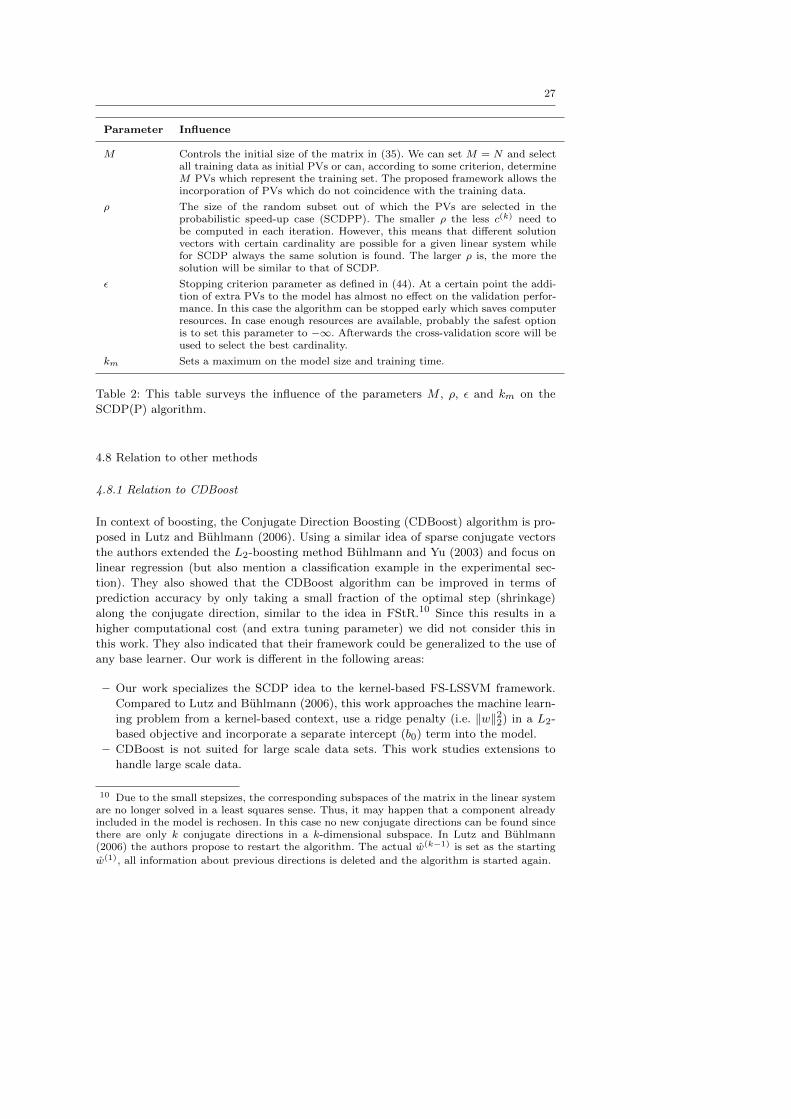
4.6 Algorithmic parameters

As illustrated in the previous section, four parameters: M , ρ, ε and km control the

processor and memory use of the algorithm and can have impact on the prediction

accuracy of the final model. We therefore briefly summarize the effect of the different

parameters in Table 2.

4.7 Comparison of computational complexity

Assuming an initial set of PVs of size M , the two most computational expensive oper-

ations in SCDP-FSLSSVM are: (i) the computation of Ω′TΩ in (35) with an approxi-

mate computational cost of O(NM2) and (ii) solving the system using SCDP with an

approximate cost of O(∑Mk=1(kN + k2)), or using O(

∑Mk=1(kρ + k2)) operations in

case the probabilistic speed up (with ρ = 59 in our experiments).

Assuming a ”good” fixed set of PVs of size M , the cost of computing a classical FS-

LSSVM model is dominated by three parts: (i) the computation of Φ (which includes

an eigenvalue decomposition of the reduced kernel matrix Ω) with an associated cost

of O(M3 + M2N), (ii) the computation of ΦT Φ in (33) with a computational cost of

O(NM2) and (iii) solving the linear system using for instance CG (in case the intercept

term is regularized) with a cost O(k1M2) (k1 the number of iterations to converge).

27

Parameter Influence

M Controls the initial size of the matrix in (35). We can set M = N and selectall training data as initial PVs or can, according to some criterion, determineM PVs which represent the training set. The proposed framework allows theincorporation of PVs which do not coincidence with the training data.

ρ The size of the random subset out of which the PVs are selected in theprobabilistic speed-up case (SCDPP). The smaller ρ the less c(k) need tobe computed in each iteration. However, this means that different solutionvectors with certain cardinality are possible for a given linear system whilefor SCDP always the same solution is found. The larger ρ is, the more thesolution will be similar to that of SCDP.

ε Stopping criterion parameter as defined in (44). At a certain point the addi-tion of extra PVs to the model has almost no effect on the validation perfor-mance. In this case the algorithm can be stopped early which saves computerresources. In case enough resources are available, probably the safest optionis to set this parameter to −∞. Afterwards the cross-validation score will beused to select the best cardinality.

km Sets a maximum on the model size and training time.

Table 2: This table surveys the influence of the parameters M , ρ, ε and km on the

SCDP(P) algorithm.

4.8 Relation to other methods

4.8.1 Relation to CDBoost

In context of boosting, the Conjugate Direction Boosting (CDBoost) algorithm is pro-

posed in Lutz and Buhlmann (2006). Using a similar idea of sparse conjugate vectors

the authors extended the L2-boosting method Buhlmann and Yu (2003) and focus on

linear regression (but also mention a classification example in the experimental sec-

tion). They also showed that the CDBoost algorithm can be improved in terms of

prediction accuracy by only taking a small fraction of the optimal step (shrinkage)

along the conjugate direction, similar to the idea in FStR.10 Since this results in a

higher computational cost (and extra tuning parameter) we did not consider this in

this work. They also indicated that their framework could be generalized to the use of

any base learner. Our work is different in the following areas:

– Our work specializes the SCDP idea to the kernel-based FS-LSSVM framework.

Compared to Lutz and Buhlmann (2006), this work approaches the machine learn-

ing problem from a kernel-based context, use a ridge penalty (i.e. ‖w‖22) in a L2-

based objective and incorporate a separate intercept (b0) term into the model.

– CDBoost is not suited for large scale data sets. This work studies extensions to

handle large scale data.

10 Due to the small stepsizes, the corresponding subspaces of the matrix in the linear systemare no longer solved in a least squares sense. Thus, it may happen that a component alreadyincluded in the model is rechosen. In this case no new conjugate directions can be found sincethere are only k conjugate directions in a k-dimensional subspace. In Lutz and Buhlmann(2006) the authors propose to restart the algorithm. The actual w(k−1) is set as the starting

w(1), all information about previous directions is deleted and the algorithm is started again.

28

– Opposed to CDBoost, SCDP-FSLSSVM is presented with an efficient and complete

model selection framework with a clear stopping criterion to automatically select

the hyper-parameters, and final model size.

4.8.2 Relation to other kernel-based methods

In the literature there are several kernel-based methods which employ a greedy ap-

proach such as in SCDP-FSLSSVM in order to increase the model complexity during

the training process. Some examples, which also work in the context of a L2 loss func-

tion, include

– In Cawley and Talbot (2002) the primal LS-SVM objective (as in (27)) is approx-

imated using a sparse approximate kernel expansion where only a relatively small

number M < N of vectors contribute

w =∑

xi∈Xpv

βiϕ(xi). (45)

Eliminating in (28) the error variables ei by substituting the constraint in the

objective and combining with (28), the same linear system is obtained as in (35).

However, our approach is based on the FS-LSSVM method which gives additional

insight in how to initially select PVs. Consequently, the underlying algorithm is

different. Note that in the context of SVMs the same sparse approximate kernel

expansion is proposed in Keerthi et al. (2006) resulting in a scheme which iteratively

solves (35).

– Instead of approximating the primal using a sparse model, in Jiao et al. (2007)

the authors directly approximate the dual LS-SVM formulation (29) and obtain

a sparse model. Although, such a setup does not require the additional compu-

tation of a (numerical unstable) kernel matrix product Ω′TΩ′, we conclude from

preliminary experiments11 that it requires more iterations to converge, resulting in

a less sparse model and it requires comparable or even longer training times than

SCDP-FSLSSVM (note that the authors Jiao et al. (2007) made the same obser-

vation when comparing to Kernel Matching Pursuit (KMP) Vincent and Bengio

(2002)). Jiao et al. (2007) further elaborates on the comparison of this technique,

Kernel Matching Pursuit (KMP), and Sparse Greedy Gaussian Process (SGGP)

Smola and Bartlett (2001).

– The idea of KMP is mainly to select basis functions in a greedy manner for

non-regularized kernel least-squares problems. The authors describe 3 versions of

KMP of which the back-fitting procedure is very similar to SCDP-FSLSSVM. Be-

sides the absence of a regularization term and an intercept term, the order se-

lection criterion is also different to that of SCDP-FSLSSVM. In case of KMP

this is s = arg maxi/∈A |(r)i|, r = Ωw − y while for SCDP-FSLSSVM this is

s = arg maxi/∈A |(c)i|, c = ΩT (Ωw − y).

– In Chen et al. (2009) the authors propose a general kernel learning framework based

on Orthogonal Least Squares (OLS) regression. Given an orthogonal decomposition

11 One such experiment was performed on the image data set (see Appendix A) were N =1, 300, and D = 18. Given a tuned set of hyper-parameters, applying SCDP directly on thedual (29) gave a model size of 961 while applying it on (35) gave a model size of 321. Bothmethods had comparable accuracies.

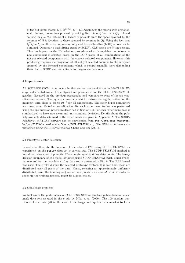
29

of the full kernel matrix Ω ∈ RN×N , Ω = QR where Q is the matrix with orthonor-

mal columns, the authors proceed by writing Ωw = b as QRw = b or Qg = b and

solving for g = Rw instead of w (which is possible since the space spanned by the

columns of Ω is identical to those spanned by columns in Q). Using the fact that

QTQ = I, an efficient computation of g and Leave-One-Out (LOO) scores can be

obtained. Opposed to back-fitting (used by SCDP), OLS uses a pre-fitting scheme.

This has impact on the PV selection procedure which is explained as follows. A

new component is selected based on the LOO scores of all combinations of the

not yet selected components with the current selected components. However, this

pre-fitting requires the projection of all not yet selected columns to the subspace

spanned by the selected components which is computationally more demanding

than that of SCDP and not suitable for large-scale data sets.

5 Experiments

All SCDP-FSLSSVM experiments in this section are carried out in MATLAB. We

empirically tested some of the algorithmic parameters for the SCDP-FSLSSVM al-

gorithm discussed in the previous paragraphs and compare to state-of-the-art clas-

sification methods. The hyper-parameter ν which controls the regularization for the

intercept term alone is set to 10−8 for all experiments. The other hyper-parameters

are tuned using 10-fold cross-validation. For each experiment tuning was performed

using the optimization procedure described in Section 4.4. For each experiment data is

standardized to have zero mean and unit standard deviation. Details about the pub-

licly available data sets used in the experiments are given in Appendix A. The SCDP-

FSLSSVM MATLAB software can be downloaded from ftp://ftp.esat.kuleuven.

be/pub/SISTA/karsmakers/software/SCDP-FSLSSVM.zip. The SVM experiments are

performed using the LIBSVM toolbox Chang and Lin (2001).

5.1 Prototype Vector Selection

In order to illustrate the location of the selected PVs using SCDP-FSLSSVM, an

experiment on the ripley data set is carried out. The SCDP-FSLSSVM method is

initialized using a set of potential PVs containing all training data points. The binary

decision boundary of the model obtained using SCDP-FSLSSVM (with tuned hyper-

parameters) on the two-class ripley data set is presented in Fig. 6. The RBF kernel

was used. The circles display the selected prototype vectors. It is seen that these are

distributed over all parts of the data. Hence, selecting an approximately uniformly

distributed (over the training set) set of data points with size M < N in order to

speed-up the training process, might be a good choice.

5.2 Small scale problems

We first assess the performance of SCDP-FSLSSVM on thirteen public domain bench-

mark data sets as used in the study by Mika et al. (2000). The 100 random par-

titions of the data (20 in the case of the image and splice benchmarks) to form

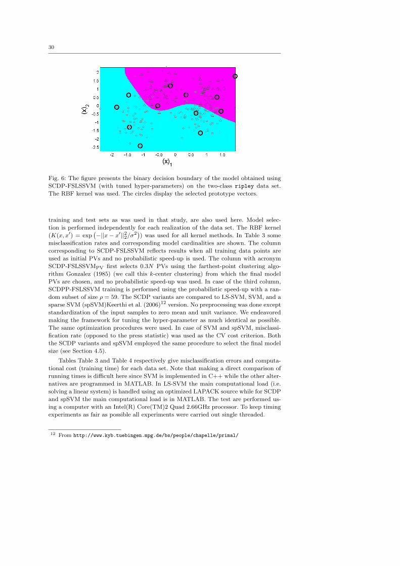
30

Fig. 6: The figure presents the binary decision boundary of the model obtained using

SCDP-FSLSSVM (with tuned hyper-parameters) on the two-class ripley data set.

The RBF kernel was used. The circles display the selected prototype vectors.

training and test sets as was used in that study, are also used here. Model selec-

tion is performed independently for each realization of the data set. The RBF kernel

(K(x, x′) = exp(−||x− x′||22/σ2

)) was used for all kernel methods. In Table 3 some

misclassification rates and corresponding model cardinalities are shown. The column

corresponding to SCDP-FSLSSVM reflects results when all training data points are

used as initial PVs and no probabilistic speed-up is used. The column with acronym

SCDP-FSLSSVMPV first selects 0.3N PVs using the farthest-point clustering algo-

rithm Gonzalez (1985) (we call this k-center clustering) from which the final model

PVs are chosen, and no probabilistic speed-up was used. In case of the third column,

SCDPP-FSLSSVM training is performed using the probabilistic speed-up with a ran-

dom subset of size ρ = 59. The SCDP variants are compared to LS-SVM, SVM, and a

sparse SVM (spSVM)Keerthi et al. (2006)12 version. No preprocessing was done except

standardization of the input samples to zero mean and unit variance. We endeavored

making the framework for tuning the hyper-parameter as much identical as possible.

The same optimization procedures were used. In case of SVM and spSVM, misclassi-

fication rate (opposed to the press statistic) was used as the CV cost criterion. Both

the SCDP variants and spSVM employed the same procedure to select the final model

size (see Section 4.5).

Tables Table 3 and Table 4 respectively give misclassification errors and computa-

tional cost (training time) for each data set. Note that making a direct comparison of

running times is difficult here since SVM is implemented in C++ while the other alter-

natives are programmed in MATLAB. In LS-SVM the main computational load (i.e.

solving a linear system) is handled using an optimized LAPACK source while for SCDP

and spSVM the main computational load is in MATLAB. The test are performed us-

ing a computer with an Intel(R) Core(TM)2 Quad 2.66GHz processor. To keep timing

experiments as fair as possible all experiments were carried out single threaded.

12 From http://www.kyb.tuebingen.mpg.de/bs/people/chapelle/primal/

31

It is seen that the sparse SCDP variants give comparable performance compared

to the state-of-the-art methods: (non-sparse) LS-SVM, SVM and spSVM. When con-

sidering model sizes, all share comparable model complexities except for LS-SVM and

SVM. By definition LS-SVM is non-sparse and SVM models have much larger car-

dinalities. Note that for SVM the model size indicates the number of nonzero dual

variables while for the other alternatives the number of non-zero values in the primal

model is meant. Table 4 presents (averaged) training times in milliseconds. Since choice

of hyper-parameters affects training time and since the meaning of a ”good” hyper-

parameter set can be different for each method, training times are measured using a

tuned hyper-parameter set. From Table 4 it is seen that, while giving of-the-art accu-

racies, SCDP-FSLSSVMFS in general is the fastest method. SCDP-FSLSSVMFS de-

creases the training speed considerably by selecting an initial PV set of size M = 0.3N .

Compared to the SCDP variants in most cases spSVM is much slower. Similar to the

SCDP variants spSVM iteratively increases the model size starting with size 1. A single

iteration is more costly compared to the SCDP variants since a piecewise quadratic

function needs to be solved using Newtons’ method.13 Remark that in case the subset

size (ρ) is close to the number of data points, the probabilistic speed-up (SCDPP-

FSLSSVM) gives only a small or even negative gain compared to SCDP-FSLSSVM.

The advantage of using this probabilistic speed-up is seen more clearly in the experi-

ments given in Section 5.3.

In case the probabilistic speed-up is used (SCDPP-FSLSSVM with ρ = 59) the clas-

sification accuracies for data sets ringnorm and titanic deviate strongly from those of

the other SCDP-FSLSSVM alternatives. The corresponding large standard deviations

indicate that models with nontypical performance (outliers) are present. The same phe-

nomena can be seen when plotting the Pareto frontiers (see Fig. 7, and Fig. 8) for both

SCDP- and SCDPP-FSLSSVM given a single realization and tuned hyper-parameter

set. SCDPP-FSLSSVM was repeated 50 times to display the boxplots. The boxes have

horizontal lines at the lower quartile, median, and upper quartile values of the perfor-

mances corresponding to the 50 experiments.14 The dotted line is the SCDP-FSLSSVM

Pareto front. It is seen that in most cases SCDPP-FSLSSVM performs slightly worse

or similar in terms of misclassification rate compared to SCDP-FSLSSVM for differ-

ent cardinalities. It is seen that for some data sets using SCDPP-FSLSSVM can give

significant differences in terms of misclassification rate compared to the SCDP vari-

ant. In case ρ is increased the SCDPP-FSLSSVM models converge towards those of

SCDP-FSLSSVM but still, although less frequently, models with nontypical perfor-

mance might occur. Note that for spSVM, which also uses a probabilistic speed-up

(ρ = 59) this effect is only observed for the titanic data set. It is therefor adviced to

use this probabilistic speed-up with care.

13 As the authors suggested in Keerthi et al. (2006) the Newton optimization is only per-formed from time to time to save computer resources.14 Additionally the following markers are used in the boxplot. The whiskers are lines extend-

ing from each end of the boxes to show the extent of the rest of the data. Outliers (+) aredata with values beyond the ends of the whiskers.

32S

CD

P-

SC

DP

-S

CD

PP

-

FS

LS

SV

MF

SL

SS

VM

FS

FS

LS

SV

ML

S-S

VM

SV

Msp

SV

M

err

(%)

#P

Ver

r(%

)#

PV

err

(%)

#P

Ver

r(%

)er

r(%

)#

SV

err

(%)

#P

V

banana

10.4

6(±

0.4

4)

32.4

(±6)

10.5

2(±

0.4

2)

34.3

(±7.1

)10.5

8(±

0.5

2)

33.3

(±7.7

)10.6

1(±

0.5

3)

11.0

7(±

0.8

2)

100.7

(±20.2

)11.8

2(±

2)

17(±

7.3

)

breast-cancer

27.2

1(±

4.2

3)

6.4

(±5.4

)26.4

7(±

4.5

1)

13.5

(±9.3

)27.0

4(±

4.3

8)

11(±

8.6

)27.1

(±4.7

2)

26.7

5(±

4.8

8)

125.8

(±10.6

)27.3

2(±

4.4

1)

13.4

(±9.1

)

diabetis

23.7

3(±

1.9

4)

8.9

(±4.2

)23.3

9(±

1.9

4)

14.9

(±8.2

)23.4

1(±

1.8

8)

14.1

(±7.8

)23.3

6(±

1.7

4)

23.4

9(±

1.8

5)

269.9

(±16.4

)23.9

9(±

2.7

1)

13.4

(±8.4

)

flare-solar

34.8

2(±

1.8

8)

13.4

(±6.6

)34.0

1(±

1.6

)11.6

(±8.2

)35(±

2.0

8)

13.8

(±6.7

)34.2

5(±

1.8

7)

32.5

9(±

1.7

8)

475.9

(±25)

33.9

(±1.1

0)

8.5

(±1.1

)

german

24.0

1(±

2.2

4)

26(±

9.1

)24.3

(±2.2

1)

13.8

(±6.3

)24.2

(±2.2

5)

22.5

(±9.4

)23.5

5(±

2.2

2)

24.0

7(±

2.2

3)

382.2

(±14.2

)27.1

(±2.9

)16.6

(±11.5

)

heart

16.2

(±3.2

7)

4.9

(±2.9

)16.2

2(±

3.2

5)

6.5

(±3.7

)16.7

1(±

3.1

6)

4.8

(±3)

16.4

1(±

3.4

5)

15.8

4(±

3.2

6)

105.5

(±16.9

)15.9

(±1.2

)4.3

(±2.3

)

image

2.8

6(±

0.5

5)

317.8

(±5.6

)3.2

1(±

0.7

9)

308.3

(±10.3

)3.3

(±0.8

3)

318.2

(±12)

2.9

5(±

0.7

6)

3.1

1(±

0.5

6)

310.7

(±76.8

)3.3

(±0.9

)301.2

(±5.3

)

ringnorm

1.6

1(±

0.1

4)

11.8

(±8.2

)1.5

2(±

0.1

2)

6.6

(±4.2

)9.9

1(±

8.3

2)

11.9

(±7.8

)1.6

5(±

0.1

6)

1.7

7(±

0.2

6)

160.7

(±53)

2.2

8(±

0.4

9)

11.5

(±5)

splice

11.3

6(±

0.5

8)

311.2

(±10.6

)12.5

4(±

0.6

8)

188.1

(±29)

11.2

9(±

0.6

2)

313(±

11.6

)10.5

7(±

0.6

6)

10.7

6(±

0.6

9)

669.6

(±97.9

)12.3

7(±

0.7

1)

229(±

10.4

)

thyroid

4.4

4(±

2.0

5)

18.9

(±9.9

)4.1

3(±

2.1

4)

12.8

(±7.8

)4.2

9(±

2.0

6)

16.8

(±9.4

)4.6

1(±

2.2

8)

4.4

(±2.3

2)

76.1

(±24.2

)22.7

8(±

0.7

7)

5.6

(±2.4

)

titanic

22.8

4(±

0.9

6)

6.3

(±3)

22.9

7(±

1.3

)5.4

(±2.7

)25.3

2(±

12.3

4)

7.4

(±3.1

)22.5

7(±

1.3

5)

22.4

9(±

0.7

)69.8

(±10.4

)24.8

(±3.5

2)

4.3

(±2.1

)

twonorm

2.6

6(±

0.1

4)

38.2

(±9.4

)2.5

6(±

0.1

6)

37.5

(±10.1

)2.7

5(±

0.2

2)

26.9

(±12.6

)2.8

2(±

0.2

)2.8

9(±

0.2

3)

240.3

(±99.6

)2.9

5(±

0.8

2)

8.9

(±3.5

)

waveform

9.8

6(±

0.3

8)

26.3

(±7.7

)9.9

(±0.3

7)

24.8

(±7.7

)9.8

5(±

0.3

9)

27.2

(±7.1

)9.8

2(±

0.4

5)

10.0

5(±

0.5

2)

171.2

(±28)

11.0

8(±

0.5

3)

11.1

(±3.4

)

Table

3:

The

table

show

sth

em

iscl

ass

ifica

tion

rate

sand

ifapplica

ble

the

num

ber

of

finally

sele

cted

pro

toty

pe

vec

tors

(PV

)of

3ver

sions

of

SC

DP

-FSL

SSV

Mand

LS-S

VM

over

thir

teen

ben

chm

ark

data

sets

.k-c

ente

rcl

ust

erin

gw

as

use

das

the

PV

sele

ctio

npro

cedure

.T

he

resu

lts

for

each

met

hod

are

pre

sente

din

the

inth

efo

rmof

the

mea

ner

ror

rate

over

test

data

for

100

realiza

tions

of

each

data

set

(20

inth

eca

se

of

the

image

and

splice

data

sets

),alo

ng

wit

hth

eass

oci

ate

dst

andard

erro

r.T

he

colu

mn

den

ote

dby

SC

DP

-FSL

SSV

Mre

flec

tsre

sult

sof

the

SC

DP

-FSL

SSV

Malg

ori

thm

whic

huse

sall

train

ing

data

poin

tsas

init

ial

PV

sand

no

pro

babilis

tic

spee

d-u

p.

The

colu

mn

wit

hacr

onym

SC

DP

-FSL

SSV

MP

Vfirs

tse

lect

s0.3N

PV

susi

ng

the

fart

hes

t-p

oin

tcl

ust

erin

galg

ori

thm

Gonza

lez

(1985)

from

whic

hP

Vs

for

the

final

model

are

chose

n,

no

pro

babilis

tic

spee

d-u

pw

as

use

d.

Inca

seof

the

thir

dco

lum

nSC

DP

P-F

SL

SSV

Mtr

ain

ing

isp

erfo

rmed

usi

ng

the

pro

babilis

tic

spee

d-u

pw

ith

ara

ndom

subse

tof

sizeρ

=59.

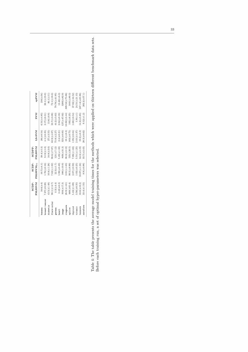
33S

CD

P-

SC

DP

-S

CD

PP

-

FS

LS

SV

MF

SL

SS

VM

FS

FS

LS

SV

ML

S-S

VM

SV

Msp

SV

M

banana

34.6

(±4)

10.7

(±4.1

)38.4

(±5.3

)20(±

0.5

4)

6.5

1(±

4.8

5)

216(±

34)

breast-cancer

7.8

7(±

8.2

8)

1.7

6(±

0.1

6)

9.1

3(±

1.8

)4.1

(±0.3

5)

3.1

7(±

0.3

1)

28.1

(±19.8

)

diabetis

43.5

(±1.4

8)

10.8

(±1.2

8)

34.8

(±3.0

)27(±

3.5

5)

13.6

(±0.8

)46.1

(±11)

flare-solar

98.1

(±14.7

)7.6

2(±

1.0

2)

98.6

(±7.0

7)

63.9

(±4.8

7)

33.7

(±3.0

8)

72.1

(±18.6

)

german

113(±

4.4

)22.3

(±1.7

)121(±

7.1

2)

75.8

(±2.2

7)

44.2

(±5.6

3)

79.7

8(±

41.9

5)

heart

3.4

2(±

0.3

)1.9

8(±

0.4

9)

5.4

9(±

1.3

3)

2.4

(±0.2

1)

2.0

4(±

0.1

8)

13.4

6(±

6.3

)

image

910(±

17.3

)180(±

10.9

)849(±

31.3

)321(±

0.8

3)

127(±

47.0

2)

3283(±

82.9

)

ringnorm

26.9

(±1.6

1)

3.8

1(±

1.6

3)

30.3

(±2.1

2)

18.1

(±0.3

)10.8

2(±

3.4

4)

309.5

2(±

75.0

6)

splice

669(±

65.4

)90.5

(±8.9

9)

535(±

20.5

)183(±

0.7

5)

193(±

6.2

5)

3441(±

80.3

)

thyroid

5.4

3(±

1.0

9)

2.0

7(±

0.5

9)

7.0

9(±

1.8

3)

1.9

5(±

0.0

4)

1.6

9(±

0.5

4)

37.9

2(±

16.5

2)

titanic

3.5

6(±

0.3

5)

1.0

2(±

0.2

5)

5.5

1(±

1.2

5)

2.4

1(±

1.3

7)

1.9

1(±

1)

24.5

1(±

21.1

3)

twonorm

33.6

(±10.2

)10.8

7(±

1.2

4)

34.3

(±3.1

9)

19.2

(±0.3

)14.3

(±5.8

5)

247.1

4(±

65.9

6)

waveform

33.4

(±1.5

5)

8.9

(±0.8

8)

33.7

(±2.4

3)

20.3

(±0.6

2)

9.1

2(±

1.2

)202.2

(±57.1

)

Table

4:

The

table

pre

sents

the

aver

age

model

train

ing

tim

esfo

rth

em

ethods

whic

hw

ere

applied

on

thir

teen

diff

eren

tb

ench

mark

data

sets

.

Bef

ore

each

train

ing

run,

ase

tof

opti

mal

hyp

er-p

ara

met

ers

was

sele

cted

.

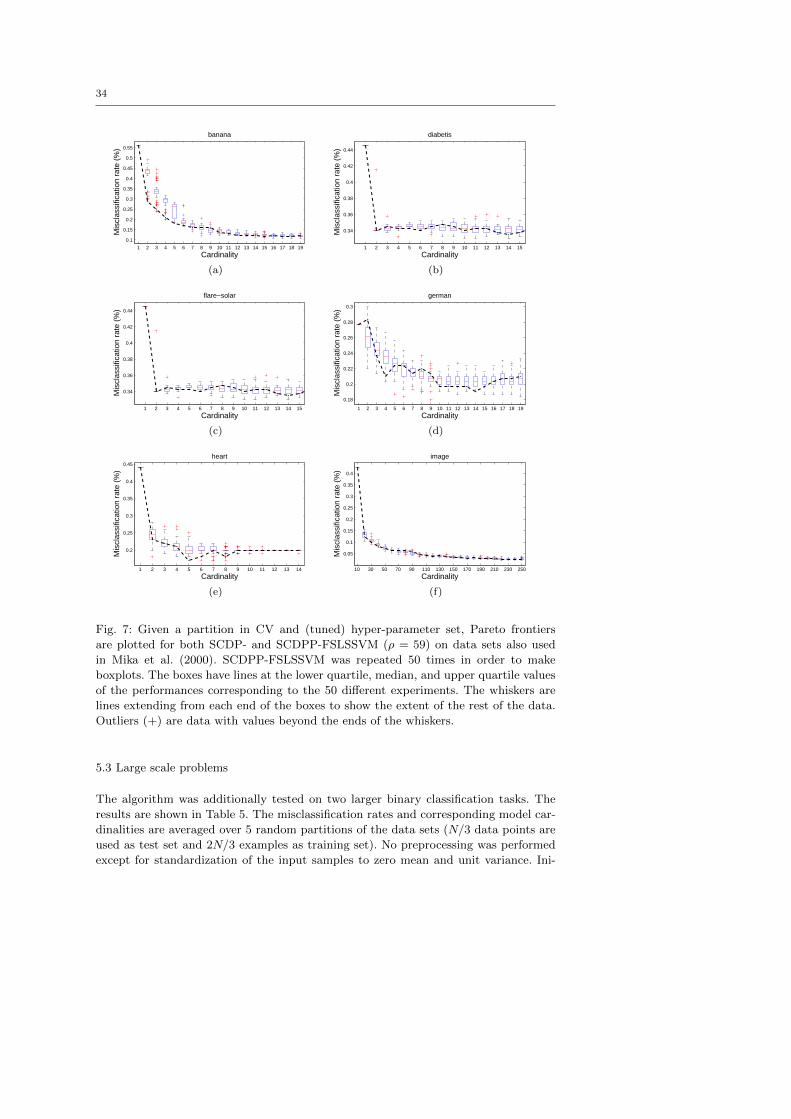
34

1 2 3 4 5 6 7 8 9 10 11 12 13 14 15 16 17 18 19

0.1

0.15

0.2

0.25

0.3

0.35

0.4

0.45

0.5

0.55

Mis

clas

sific

atio

n ra

te (

%)

Cardinality

banana

(a)

1 2 3 4 5 6 7 8 9 10 11 12 13 14 15

0.34

0.36

0.38

0.4

0.42

0.44

Mis

clas

sific

atio

n ra

te (

%)

Cardinality

diabetis

(b)

1 2 3 4 5 6 7 8 9 10 11 12 13 14 15

0.34

0.36

0.38

0.4

0.42

0.44

Mis

clas

sific

atio

n ra

te (

%)

Cardinality

flare−solar

(c)

1 2 3 4 5 6 7 8 9 10 11 12 13 14 15 16 17 18 19

0.18

0.2

0.22

0.24

0.26

0.28

0.3

Mis

clas

sific

atio

n ra

te (

%)

Cardinality

german

(d)

1 2 3 4 5 6 7 8 9 10 11 12 13 14

0.2

0.25

0.3

0.35

0.4

0.45

Mis

clas

sific

atio

n ra

te (

%)

Cardinality

heart

(e)

10 30 50 70 90 110 130 150 170 190 210 230 250

0.05

0.1

0.15

0.2

0.25

0.3

0.35

0.4

Mis

clas

sific

atio

n ra

te (

%)

Cardinality

image

(f)

Fig. 7: Given a partition in CV and (tuned) hyper-parameter set, Pareto frontiers

are plotted for both SCDP- and SCDPP-FSLSSVM (ρ = 59) on data sets also used

in Mika et al. (2000). SCDPP-FSLSSVM was repeated 50 times in order to make

boxplots. The boxes have lines at the lower quartile, median, and upper quartile values

of the performances corresponding to the 50 different experiments. The whiskers are

lines extending from each end of the boxes to show the extent of the rest of the data.

Outliers (+) are data with values beyond the ends of the whiskers.

5.3 Large scale problems

The algorithm was additionally tested on two larger binary classification tasks. The

results are shown in Table 5. The misclassification rates and corresponding model car-

dinalities are averaged over 5 random partitions of the data sets (N/3 data points are

used as test set and 2N/3 examples as training set). No preprocessing was performed

except for standardization of the input samples to zero mean and unit variance. Ini-

35

1 2 3 4 5 6 7 8 9 10 11 12 13 14 15 16 17 18 19 20 21 22 23 240

0.05

0.1

0.15

0.2

0.25

0.3

0.35

0.4

0.45

0.5

Mis

clas

sific

atio

n ra

te (

%)

Cardinality

ringnorm

(a)

10 30 50 70 90 110 130 150 170 190 210 230 250

0.1

0.15

0.2

0.25

0.3

0.35

0.4

0.45

splice

Cardinality

Mis

clas

sific

atio

n ra

te (

%)

(b)

1 2 3 4 5 6 7 8 9 1011121314151617181920212223242526272829

0

0.05

0.1

0.15

0.2

0.25

0.3

0.35

Mis

clas

sific

atio

n ra

te (

%)

Cardinality

thyroid

(c)

1 2 3 4 5 6 7 8 9 10 11 120.2

0.22

0.24

0.26

0.28

0.3

0.32

0.34

0.36

0.38

Mis

clas

sific

atio

n ra

te (

%)

Cardinality

titanic

(d)

1 2 3 4 5 6 7 8 9 10 11 12 13 14 150

0.05

0.1

0.15

0.2

0.25

0.3

0.35

0.4

0.45

0.5

Mis

clas

sific

atio

n ra

te (

%)

Cardinality

twonorm

(e)

1 2 3 4 5 6 7 8 9 10 11 12 13 14 15 16 17 18 19 20 21 22 23 24

0.1

0.15

0.2

0.25

0.3

Mis

clas

sific

atio

n ra

te (

%)

Cardinality

waveform

(f)

Fig. 8: Given a partition in CV and (tuned) hyper-parameter set, Pareto frontiers

are plotted for both SCDP- and SCDPP-FSLSSVM (ρ = 59) on data sets also used

in Mika et al. (2000). SCDPP-FSLSSVM was repeated 50 times in order to make

boxplots. The boxes have lines at the lower quartile, median, and upper quartile values

of the performances corresponding to the 50 different experiments. The whiskers are

lines extending from each end of the boxes to show the extent of the rest of the data.

Outliers (+) are data with values beyond the ends of the whiskers.

tially, 2, 000 PVs were selected using k-center clustering. From Table 5 again it is seen

that compared to SVM, SCDP-FSLSSVM and spSVM give similar performance while

producing much sparser models.

These larger data sets are now used to illustrate the effect of the probabilistic

speed-up on training time. In Fig. 9 for both the adult and gamma telescope data

sets the misclassification rate is plotted in function of the training time for four SCDP-

FSLSSVM variants. Notice that all methods more or less end-up in the same minimum.

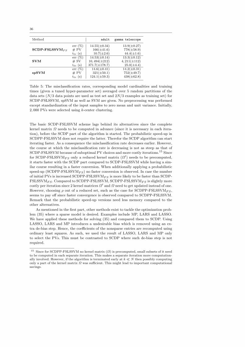
36

Method adult gamma telescope

SCDP-FSLSSVMFS

err (%) 14.55(±0.34) 13.9(±0.27)# PV 166(±41.6) 778(±58.9)ttr (s) 10.7(±2.6) 44.4(±1.6)

SVMerr (%) 14.53(±0.14) 13.3(±0.12)# SV 10, 494(±212) 4, 211(±112)ttr (s) 371.7(±178.7) 25.0(±4.4)

spSVMerr (%) 14.6(±0.41) 14.2(±0.31)# PV 321(±50.1) 752(±49.7)ttr (s) 124.1(±59.3) 438(±62.8)

Table 5: The misclassification rates, corresponding model cardinalities and training

times (given a tuned hyper-parameter set) averaged over 5 random partitions of the

data sets (N/3 data points are used as test set and 2N/3 examples as training set) for

SCDP-FSLSSVM, spSVM as well as SVM are given. No preprocessing was performed

except standardization of the input samples to zero mean and unit variance. Initially,

2, 000 PVs were selected using k-center clustering.

The basic SCDP-FSLSSVM scheme lags behind its alternatives since the complete

kernel matrix Ω needs to be computed in advance (since it is necessary in each itera-

tion), before the SCDP part of the algorithm is started. The probabilistic speed-up in

SCDPP-FSLSSVM does not require the latter. Therefor the SCDP algorithm can start

iterating faster. As a consequence the misclassification rate decreases earlier. However,

the course at which the misclassification rate is decreasing is not as steep as that of

SCDP-FSLSSVM because of suboptimal PV choices and more costly iterations.15 Since

for SCDP-FSLSSVMFS only a reduced kernel matrix (Ω′) needs to be precomputed,

it starts faster with the SCDP part compared to SCDP-FSLSSVM while having a sim-

ilar course resulting in a faster conversion. When additionally applying a probabilistic

speed-up (SCDPP-FSLSSVMFS) no faster conversion is observed. In case the number

of initial PVs is increased SCDPP-FSLSSVMFS is more likely to be faster than SCDP-

FSLSSVMFS . Compared to SCDPP-FSLSSVM, SCDPP-FSLSSVMFS is slightly more

costly per iteration since 2 kernel matrices Ω′ and Ω need to get updated instead of one.

However, choosing ρ out of a reduced set, such as the case for SCDPP-FSLSSVMFS ,

seems to pay off since faster convergence is observed compared to SCDPP-FSLSSVM.

Remark that the probabilistic speed-up versions need less memory compared to the

other alternatives.

As mentioned in the first part, other methods exist to tackle the optimization prob-

lem (35) where a sparse model is desired. Examples include MP, LARS and LASSO.

We have applied these methods for solving (35) and compared them to SCDP. Using

LASSO, LARS and MP introduces a undesirable bias which is removed using an ex-

tra de-bias step. Hence, the coefficients of the nonsparse entries are recomputed using

ordinary least squares. As such, we used the result of LASSO, LARS and MP only

to select the PVs. This must be contrasted to SCDP where such de-bias step is not

required.

15 Since for SCDPP-FSLSSVM no kernel matrix (Ω) is precomputed, small subsets of it needto be computed in each separate iteration. This makes a separate iteration more computation-ally involved. However, if the algorithm is terminated early at k N then possibly computingonly a part of the kernel matrix Ω was sufficient. This might lead to important computationalsavings.

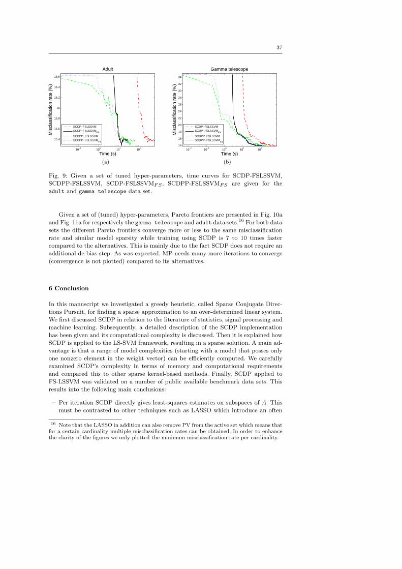
37

10−1

100

101

102

15.4

15.6

15.8

16

16.2

16.4

16.6

Time (s)

Mis

clas

sific

atio

n ra

te (

%)

Adult

SCDP−FSLSSVMSCDP−FSLSSVM

FS

SCDPP−FSLSSVMSCDPP−FSLSSVM

FS

(a)

10−2

10−1

100

101

102

14

16

18

20

22

24

26

28

30

32

34

Time (s)

Mis

clas

sific

atio

n ra

te (

%)

Gamma telescope

SCDP−FSLSSVMSCDP−FSLSSVM

FS

SCDPP−FSLSSVMSCDPP−FSLSSVM

FS

(b)

Fig. 9: Given a set of tuned hyper-parameters, time curves for SCDP-FSLSSVM,

SCDPP-FSLSSVM, SCDP-FSLSSVMFS , SCDPP-FSLSSVMFS are given for the

adult and gamma telescope data set.

Given a set of (tuned) hyper-parameters, Pareto frontiers are presented in Fig. 10a

and Fig. 11a for respectively the gamma telescope and adult data sets.16 For both data

sets the different Pareto frontiers converge more or less to the same misclassification

rate and similar model sparsity while training using SCDP is 7 to 10 times faster

compared to the alternatives. This is mainly due to the fact SCDP does not require an

additional de-bias step. As was expected, MP needs many more iterations to converge

(convergence is not plotted) compared to its alternatives.

6 Conclusion

In this manuscript we investigated a greedy heuristic, called Sparse Conjugate Direc-

tions Pursuit, for finding a sparse approximation to an over-determined linear system.

We first discussed SCDP in relation to the literature of statistics, signal processing and

machine learning. Subsequently, a detailed description of the SCDP implementation

has been given and its computational complexity is discussed. Then it is explained how

SCDP is applied to the LS-SVM framework, resulting in a sparse solution. A main ad-

vantage is that a range of model complexities (starting with a model that posses only

one nonzero element in the weight vector) can be efficiently computed. We carefully

examined SCDP’s complexity in terms of memory and computational requirements

and compared this to other sparse kernel-based methods. Finally, SCDP applied to

FS-LSSVM was validated on a number of public available benchmark data sets. This

results into the following main conclusions:

– Per iteration SCDP directly gives least-squares estimates on subspaces of A. This

must be contrasted to other techniques such as LASSO which introduce an often

16 Note that the LASSO in addition can also remove PV from the active set which means thatfor a certain cardinality multiple misclassification rates can be obtained. In order to enhancethe clarity of the figures we only plotted the minimum misclassification rate per cardinality.

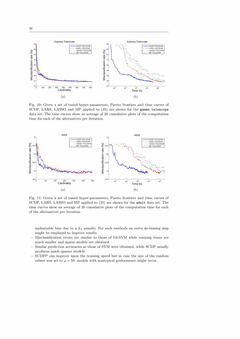
38

0 100 200 300 400 500 600 700 80012

14

16

18

20

22

24

26

28

Cardinality

Mis

clas

sific

atio

n ra

te (

%)

Gamma Telescope

SCDP−FSLSSVMLARS−FSLSSVMLASSO−FSLSSVMMP−FSLSSVM

(a)

10−2

10−1

100

101

102

12

14

16

18

20

22

24

26

28

Time (s)

Mis

clas

sific

atio

n ra

te (

%)

Gamma Telescope

SCDP−FSLSSVMLARS−FSLSSVMLASSO−FSLSSVMMP−FSLSSVM

(b)

Fig. 10: Given a set of tuned hyper-parameters, Pareto frontiers and time curves of

SCDP, LARS, LASSO and MP applied to (35) are shown for the gamma telescope

data set. The time curves show an average of 20 cumulative plots of the computation

time for each of the alternatives per iteration.

0 50 100 150 200 250 30014.5

15

15.5

16

16.5

17

Cardinality

Mis

clas

sific

atio

n ra

te (

%)

Adult

SCDP−FSLSSVMLARS−FSLSSVMLASSO−FSLSSVMMP−FSLSSVM

(a)

10−2

10−1

100

101

102

14.5

15

15.5

16

16.5

17

Time (s)

Mis

clas

sific

atio

n ra

te (

%)

Adult

SCDP−FSLSSVMLARS−FSLSSVMLASSO−FSLSSVMMP−FSLSSVM

(b)

Fig. 11: Given a set of tuned hyper-parameters, Pareto frontiers and time curves of

SCDP, LARS, LASSO and MP applied to (35) are shown for the adult data set. The

time curves show an average of 20 cumulative plots of the computation time for each

of the alternatives per iteration.

undesirable bias due to a L1 penalty. For such methods an extra de-biasing step

might be employed to improve results.

– Misclassification errors are similar to those of LS-SVM while training times are

much smaller and sparse models are obtained.

– Similar prediction accuracies as those of SVM were obtained, while SCDP usually

produces much sparser models.

– SCDPP can improve upon the training speed but in case the size of the random

subset was set to ρ = 59, models with nontypical performance might occur.

39

– Compared to SVM and LS-SVM, SCDP-FSLSSVM is not a convex learning method.

The solution of SCDP-FSLSSVM depends on the set of PVs selected by k-center

clustering. However, for a given set of initial PVs (possibly all training data) and

a zero solution vector w(1) = 0D in iteration 1, SCDP-FSLSSVM gives a unique

solution.

– k-center clustering as a preprocessing step to select the initial set of PVs is a

valuable tool to speed-up the training process. These PVs need not to be a member

of the training set.

– We indicated that, when applying to FS-LSSVM, SCDP usually outperforms MP,

LARS and LASSO in terms of speed while having a comparable accuracy.

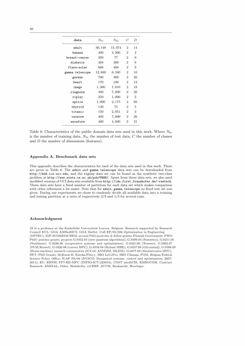
40

data Ntr Nte C D

adult 30, 148 15, 074 2 14

banana 400 4, 900 2 2

breast-cancer 200 77 2 9

diabetis 468 300 2 8

flare-solar 666 400 2 9

gamma telescope 12, 680 6, 340 2 10

german 700 300 2 20

heart 170 100 2 13

image 1, 300 1, 010 2 18

ringnorm 400 7, 000 2 20

ripley 250 1, 000 2 2

splice 1, 000 2, 175 2 60

thyroid 140 75 2 5

titanic 150 2, 051 2 3

twonorm 400 7, 000 2 20

waveform 400 4, 600 2 21

Table 6: Characteristics of the public domain data sets used in this work. Where Ntr

is the number of training data, Nte the number of test data, C the number of classes

and D the number of dimensions (features).

Appendix A. Benchmark data sets

This appendix describes the characteristics for each of the data sets used in this work. Theseare given in Table 6. The adult and gamma telescope data sets can be downloaded fromhttp://kdd.ics.uci.edu, and the ripley data set can be found as the synthetic two-classproblem at http://www.stats.ox.ac.uk/pub/PRNN/. Apart from those data sets, we also usedmodified versions of UCI data sets available from http://ida.first.fraunhofer.de/~raetsch.These data sets have a fixed number of partitions for each data set which makes comparisonwith other references a lot easier. Note that for adult, gamma telescope no fixed test set wasgiven. During our experiments we chose to randomly divide all available data into a trainingand testing partition at a ratio of respectively 2/3 and 1/3 for several runs.

Acknowledgment

JS is a professor at the Katholieke Universiteit Leuven, Belgium. Research supported by Research

Council KUL: GOA AMBioRICS, GOA MaNet, CoE EF/05/006 Optimization in Engineering

(OPTEC), IOF-SCORES4CHEM, several PhD/post-doc & fellow grants; Flemish Government: FWO:

PhD/ postdoc grants, projects G.0452.04 (new quantum algorithms), G.0499.04 (Statistics), G.0211.05

(Nonlinear), G.0226.06 (cooperative systems and optimization), G.0321.06 (Tensors), G.0302.07

(SVM/Kernel), G.0320.08 (convex MPC), G.0558.08 (Robust MHE), G.0557.08 (Glycemia2), G.0588.09

(Brain-machine) research communities (ICCoS, ANMMM, MLDM); G.0377.09 (Mechatronics MPC),

IWT: PhD Grants, McKnow-E, Eureka-Flite+, SBO LeCoPro, SBO Climaqs, POM, Belgian Federal

Science Policy Office: IUAP P6/04 (DYSCO, Dynamical systems, control and optimization, 2007-

2011); EU: ERNSI; FP7-HD-MPC (INFSO-ICT-223854), COST intelliCIS, EMBOCOM, Contract

Research: AMINAL, Other: Helmholtz, viCERP, ACCM, Bauknecht, Hoerbiger.

41

References

Allan, D., 1974. The relationship between variable selection and prediction. Technometrics 16,125–127.

Blumensath, T., Davies, M. E., 2008. Gradient pursuits. IEEE Transactions on Signal Pro-cessing 56 (6), 2370–2382.

Brabanter, K. D., Brabanter, J. D., Suykens, J. A. K., Moor, B. D., 2010. Optimized fixed-size kernel models for large data sets. Computational Statistics & Data Analysis 54 (6),1484–1504.

Bruckstein, A. M., Donoho, D. L., Elad, M., 2009. From sparse solutions of systems of equationsto sparse modeling of signals and images. SIAM Review 51 (1), 34–81.

Buhlmann, P., Yu, B., 2003. Boosting with the l2-loss: Regression and classification. Journalof the American Statistical Association 98, 324–339.

Candes, E., 2006. Compressive sampling. In: Proc. of the International Congress of Mathe-matics.

Cawley, G. C., 2006. Leave-one-out cross-validation based model selection criteria for weightedLS-SVMs. In: Proc. of the International Joint Conference on Neural Networks (IJCNN-2006). Vol. 2415. Vancouver, Canada, pp. 1661–1668.

Cawley, G. C., Talbot, N. L. C., 2002. A greedy training algorithm for sparse least-squaressupport vector machines. In: Proc. of the International Conference on Artificial NeuralNetworks. Vol. 2415. Madrid, Spain, pp. 681–686.

Chang, C. C., Lin, C. J., 2001. Libsvm : a library for support vector machines. http://www.csie.ntu.edu.tw/~cjlin/libsvm.

Chen, S., Billings, S. A., Grant, M., 1992. Recursive hybrid algorithm for non-linear systemidentification using radial basis function networks. International Journal of Control 55 (5),1051–1070.

Chen, S., Billings, S. A., Luo, W., 1989. Orthogonal least squares methods and their applicationto non-linear system identification. International Journal of Control 50 (5), 1873–1896.

Chen, S., Cowan, C., Grant, P., 1991. Orthogonal least squares learning algorithm for radialbasis function networks. IEEE Transactions on Neural Networks 2 (2), 302–309.

Chen, S., Hong, X., Luk, B. L., Harris, C. J., 2009. Orthogonal-least-squares regression: Aunified approach for data modelling. Neurocomputing 72 (10-12), 2670–2681.

Chen, S. S., Donoho, D. L., Saunders, M. A., 1999. Atomic decomposition by basis pursuit.SIAM Journal on Scientific Computing 20 (1), 33–61.

Chu, W., Keerthi, S. S., Ong, C., 2005. An improved conjugate gradient scheme to the solutionof least squares SVM. IEEE Transactions on Neural Networks 16 (2), 498–501.

Daubechies, I., Vore, R. D., Fornasier, M., Gunturk, S., 2008. Iteratively re-weighted leastsquares minimization: Proof of faster than linear rate for sparse recovery. In: Proc. of theInformation Sciences and Systems. Princeton, NJ, pp. 26–29.

de Kruif, B. J., de Vries, T. J. A., 2003. Pruning error minimization in least squares supportvector machines. IEEE Transactions on Neural Networks 14 (3), 696–702.

de Souza, S. X., Suykens, J. A. K., Vandewalle, J., Bolle, D., 2009. Coupled simulated anneal-ing. In press.

Donoho, D. L., 2006. Compressed sensing. IEEE Transactions on Information Theory 52 (4),1289–1306.

Donoho, D. L., Tsaig, Y., 2006. Fast solution of l1-norm minimization problems when thesolution may be sparse. Tech. rep., Stanford University.

Donoho, D. L., Tsaig, Y., Drori, I., Starck, J., 2006. Sparse solution of underdetermined linearequations by stagewise orthogonal matching pursuit. Tech. rep., Stanford University.

Efron, B., Hastie, T., Johnstone, I., Tibshirani, R., 2004. Least angle regression. Annals ofStatistics (with discussion) 32 (2), 407–499.

Figueiredo, M. A. T., Nowak, R. D., Wright, S. J., 2007. Gradient projection for sparse recon-struction: Application to compressed sensing and other inverse problems. IEEE Journal ofSelected Topics in Signal Processing 1 (4), 586–597.

Floyd, S., Warmuth, M., 1995. Sample compression, learnability, and the Vapnik-Chervonenkisdimension. Machine Learning Journal 21, 269–304.

Golub, G. H., Loan, C. F. V., 1996. Matrix Computations, 3th edition. Baltimore MD: JohnsHopkins University Press.

Gonzalez, T., 1985. Clustering to minimize the maximum intercluster distance. TheoreticalComputer Science 38, 293–306.

42

Hastie, T., Tibshirani, R., Friedman, J., 2001. The Elements of Statistical Learning. Springer.Hestenes, M. R., Stiefel, E., 1952. Methods of conjugate gradients for solving linear systems.

J. Res. Natl. Bur. Stand. 49, 409–436.Jiao, L., Bo, L., Wang, L., 2007. Fast sparse approximation for least squares support vector

machine. IEEE Transactions on Neural Networks 18 (3), 685–697.Joachims, T., 1999. Making large-scale SVM learning practical. In: Schlkopf, B., Burges, C.,

Smola, A. (Eds.), Advances in Kernel Methods - Support Vector Learning. MIT Press,Cambridge, MA, Ch. 11.URL http://www.cs.cornell.edu/People/tj/publications/joachims_99a.pdf

Keerthi, S. S., Chapelle, O., Decoste, D., Bennett, P., Parrado-hernandez, E., 2006. Buildingsupport vector machines with reduced classifier complexity. Journal of Machine LearningResearch 7, 1493–1515.

Kim, S. J., Koh, K., Lustig, M., Boyd, S., Gorinevsky, D., 2007. An interior-point method forlarge-scale l1-regularized least squares. IEEE Journal on Selected Topics in Signal Processing1 (4), 606–617.

Kohonen, T., 1990. The self-organizing map. Proc. IEEE 78 (9), 1464–1480.Luenberger, D., 1984. Introduction to Linear and Nonlinear Programming, second edition.

Addison Wesley.Lutz, R. W., Buhlmann, P., 2006. Conjugate direction boosting. Journal of Computational

and Graphical Statistics 15 (2), 287–311.Mallat, S., 1999. A Wavelet Tour of Signal Processing. Academic press.Mika, S., Ratsch, G., Weston, J., Scholkopf, B., Smola, A., Muller, K. R., 2000. Invariant feature

extraction and classification in feature spaces. Advances in Neural Information ProcessingSystems 12, 526–532.

Moghaddam, B., Weiss, Y., Avidan, S., 2006. Spectral bounds for sparse PCA: exact andgreedy algorithms. Advances in Neural Information Processing Systems 18, 915–922.

Moller, M. F., 1993. A scaled conjugate gradient algorithm for fast supervised learning. NeuralNetworks 6, 525–533.

Natarajan, B. K., 1995. Sparse approximate solutions to linear systems. SIAM Journal onComputing 24, 227–234.

Nelder, J. A., Mead, R., 1965. A simplex method for function minimization. Computer Journal7, 308–313.

Nocedal, J., Wright, S. J., 2006. Numerical Optimization, second edition. Springer.Osborne, M. R., Presnell, B., Turlach, B. A., 2000. A new approach to variable selection in

least squares problems. IMA J. Numerical Analysis 20, 389–403.Pati, Y. C., Rezaifar, R., Krishnaprasad, P. S., 1993. Orthogonal matching pursuit: recursive

function approximation with applications to wavelet decomposition. In: Proc. of the 27-thAnnual Asilomar Conference on Signals, Systems, and Computers. pp. 40–44.

Popovici, V., Bengio, S., Thiran, J. P., 2005. Kernel matching pursuit for large datasets.Pattern Recognition 38 (12), 2385–2390.

Press, W. H., Cornell, B. P. F., Teukolsky, S. A., Vetterling, W. T., 1993. Numerical Recipesin C: The Art of Scientific Computing 2nd Edition. Press Harvard University.

Rajasekaran, S., 2000. On simulated annealing and nested annealing. Journal of Global Opti-mization 16, 43–56.

Saunders, C., Gammerman, A., Vovk, V., 1998. Ridge regression learning algorithm in dualvariables. In: Proc. of the 15th Int. Conf. on Machine Learning (ICML-98). pp. 515–521.

Smale, S., 1997. Complexity theory and numerical analysis. Acta Numerica, 523–551.Smola, A. J., Bartlett, P. L., 2001. Sparse greedy gaussian process regression. In: Proc. Neural

Information Processing Systems. Vol. 13. pp. 619–625.Suykens, J. A. K., Brabanter, J. D., Lukas, L., Vandewalle, J., 2002a. Weighted least squares

support vector machines: robustness and sparse approximation. Neurocomputing 48 (1-4),85–105.

Suykens, J. A. K., Gestel, T. V., Brabanter, J. D., Moor, B. D., Vandewalle, J., 2002b. LeastSquares Support Vector Machines. World Scientific.

Suykens, J. A. K., Lukas, L., Vandewalle, J., 2000. Sparse approximation using least squaressupport vector machines. In: IEEE Proc. Int. Symp. Circuits Syst. Geneva, Switzerland, pp.757–760.

Suykens, J. A. K., Vandewalle, J., 1999. Least squares support vector machine classifiers.Neural Processing Letters 9 (3), 293–300.

43

Suykens, J. A. K., Vandewalle, J., Moor, B. D., 2001. Intelligence and cooperative search bycoupled local minimizers. International Journal of Bifurcation and Chaos 11 (8), 2133–2144.

Tibshirani, R., 1996. Regression shrinkage and selection via the LASSO. J. Royal. Statist. SocB. 58 (1).

Tropp, J. A., 2004. Greed is good: algorithmic results for sparse approximation. IEEE Trans-actions on Information Theory 50 (10), 2231–2242.

Vapnik, V. N., 1998. Statistical learning theory. Wiley.Vincent, P., Bengio, Y., 2002. Kernel matching pursuit. Machine Learning 48, 165–187.Williams, C. K. I., Seeger, M., 2001. Using the Nystrom method to speed up kernel machines.

Advances in Neural Information Processing Systems 13, 682–688.Young, D., 2003. Iterative Solution of Large Linear Systems. Courier Dover Publications.Zeng, X. Y., Chen, X. W., 2005. Smo-based pruning methods for sparse least squares support

vector machines. IEEE Transactions in Neural Networks 16 (6), 1541–1546.Zhang, K., Tsang, I. W., Kwok, J. T., 2008. Improved Nystrom low-rank approximation and

error analysis. In: Proc. of the 25th International Conference on Machine Learning. Helsinki,Finland, pp. 1232–1239.