ARTICLE IN PRESS

1352-2310/$ - se

doi:10.1016/j.at

�CorrespondE-mail addr

Atmospheric Environment 38 (2004) 5375–5388

www.elsevier.com/locate/atmosenv

South Pole NOx Chemistry: an assessment of factorscontrolling variability and absolute levels

D. Davisa,�, G. Chena,b, M. Buhra,c, J. Crawfordb, D. Lenschowd, B. Leferd,R. Shetterd, F. Eiseled, L. Mauldind, A. Hogane

aEnvironmental Science and Technology Buildings, School of Earth and Atmospheric Sciences, Georgia Institute of Technology,

311 frest st, Atlanta, GA 30332, USAbNASA Langley Research Center, Hampton, VA, USA

cSonoma Tech and Air Quality Design, Golden, CO, USAdAtmospheric Chemistry Division, National Center for Atmospheric Research, Boulder, CO, USA

eRetired, formerly at US CRREL, Geochemical Sciences Division, USA

Received 5 April 2003; accepted 12 April 2004

Abstract

Several groups have now shown that snow covered polar areas can lead to the release of NOx to the atmosphere as a

result of the UV photolysis of nitrate ions. Here we focus on a detailed examination of the NO observations recorded at

South Pole (SP). Topics explored include: (1) why SP NOx levels greatly exceed those at other polar sites; (2) what

processes are responsible for the observed large day to day NO concentration shifts at SP; and (3) possible explanations

for the large variability in NO seen between SP studies in 1998 and 2000. As discussed in the main body of the text, the

answer to all three questions lies in the uniqueness of the summertime SP environment. Among these characteristics is

the presence of a large plateau region just to the east of SP. This region defines one of the world’s largest air drainage

fields, being nearly 1000 km across and having elevation of � 3km: In addition, summertime SP surface temperatures

typically do not exceed �251C; leading to frequent cases where strong near surface temperature inversions occur. It

experiences 24 h of continuous sunlight, giving rise to non-stop photochemical reactions both within the snowpack and

in the atmosphere. The latter chemistry is unique at SP in that increasing levels of NOx lead to an enhanced lifetime for

NOx; thereby producing non-linear increases in NOx: In addition, the rapid atmospheric oxidation of NOx; in

conjunction with very rapid dry deposition of the products (HNO3 and HO2NO2), results in a very efficient recycling of

NOx back to the snowpack. Details concerning these unique SP characteristics and the extension of these findings to the

greater plateau region are discussed. Finally, the relationship of NOx recycling and total nitrogen deposition to the

plateau is explored.

r 2004 Elsevier Ltd. All rights reserved.

Keywords: Antarctica; South Pole; Photochemistry; NO; NOx snow emissions; ISCAT

e front matter r 2004 Elsevier Ltd. All rights reserved.

mosenv.2004.04.039

ing author. Fax: +1-770-414-1221.

ess: douglas.davis@eas.gatech.edu (D. Davis).

ARTICLE IN PRESSD. Davis et al. / Atmospheric Environment 38 (2004) 5375–53885376

1. Introduction

As discussed in Davis et al., 2000 (this issue), the year

2000 Investigation of Sulfur Chemistry in the Antarctic

Troposphere (ISCAT) field study was configured sub-

stantially different from ISCAT 1998 due to the

unexpected findings of the 1998 study. Most important

among these were finding significant quantities of NO

being generated from the UV photolysis of nitrate ions

within the snowpack (e.g., Davis et al., 2001 and

references therein). Similar observations, but involving

lower concentrations, have also been reported by

Honrath et al. (1999, 2000), Jones et al. (2000), and

Ridley et al. (2000). In addition, laboratory photochemi-

cal studies involving liquid phase solutions of nitrate have

provided confirming results (Mack and Bolton, 1999).

Of great importance in the 1998 study was establish-

ing that in addition to highly elevated NO levels (e.g.,

median value of 225 pptv), hydroxyl radical concentra-

tions were also greatly enhanced (24 h average,

� 2� 106 molec cm�3). This NOx–HOx chemical cou-

pling led to yet a final surprise, during summer months

in near surface air there is the net photochemical

production of O3 (Crawford et al., 2001).

Given the unexpected observations of 1998, a large

number of questions related to NOx remained at the

outset of ISCAT 2000. Having now completed ISCAT

2000, many of these questions have now taken on a

sharper focus. High on this list are: (a) what atmospheric

factors are most responsible for the large day-to-day

variability seen in SP NO levels; (b) what factors are most

responsible for the order-of-magnitude higher values of

NOx seen at SP versus other polar sites; (c) what processes

within the snowpack are responsible for the formation of

NO, NO2; and possibly other NOy species; (d) what

factors are responsible for the large difference seen in NO

levels between the 1998 and 2000 ISCAT campaigns; (e)

what are the levels of NO on the Antarctic plateau itself;

(f) what is the NOx flux from SP surface snow; and

finally, (g) what is the magnitude of the primary nitrogen

source to this region and from where does it originate?

This paper will primarily focus on two issues: the

exceptionally large variability seen in NO levels at SP; and

why the median values of NO at this site are nearly an order

of magnitude higher than at any other polar site currently

investigated. The important issue related to defining the

magnitude of the NOx flux at SP has been addressed in a

companion paper by Oncley et al. (this issue).

2. NO measurement technique and model description

2.1. Measurement technique

As during ISCAT 1998 (Davis et al., 2001), the

primary NO sampling location for ISCAT 2000 was the

second floor of the Atmospheric Research Observatory

(ARO) building operated by NOAA/CMDL. The

standard sampling configuration involved a sample inlet

line that extended out from the ARO building � 1m: Itwas located � 10m above the snow surface on the side

of the building facing the prevailing wind. For a very

limited time (i.e., 26 November–1 December), a second-

ary sampling location during ISCAT 2000 was the SP

MET tower, located � 90m from ARO. (Note, the

ARO building as well as the MET tower are both

upwind of any station contamination.) The NO instru-

ment when used in the MET tower study was housed in

a specially constructed environmental enclosure and had

an inlet equipped with a solenoid valve to enable

sampling at three different elevations on the tower

(i.e., 0.5, 4.7, and 21.8m) at different times. The clear 14

in OD Teflon sampling lines were of equal length (23m)

so as to minimize any differences in wall losses which

were themselves quite small (o3%). During the last 10

days of ISCAT 2000 (20–30 December), sampling was

also carried out at three different locations. The first

location was the standard position on the second floor of

ARO, and the second was located 16m above the snow

surface on the ARO roof. The third sampling location

had two positions, either 0.5m above the snow surface

or 0.01–0.9m below the surface. The low elevation

sampling operations were physically located 5m in front

of the ARO building, thus ensuring sampling on the

windward side of ARO.

As in 1998, the 2000 study used an NO chemilumi-

nescence instrument that was significantly modified in

design relative to commercial instruments (e.g., see

Davis et al., 2001). The typical sampling flow rate for

this system was 1 lmin�1: Two standard addition

calibrations and zero air (artifact) tests were performed

each day. The NO calibration gas used in the current

study was intercompared with other NIST traceable

standards both before and after the mission with very

good agreement being found. The 2s detection limit for

the chemiluminescence instrument at SP was estimated

at � 6 pptv:In addition to the primary chemiluminescence NO

instrument cited above, a second commercial chemilu-

minescence NOx–NO instrument (Thermo Environmen-

tal Instruments Model 42S) was also available during

the 2000 study. This instrument provided an indepen-

dent check on the 1998 and 2000 ISCAT NO observa-

tions. It was independently operated by other ISCAT

investigators. Although this system had a much higher

NO detection threshold (e.g., 50 pptv), measurements

with a good signal/noise ratio were frequently possible

due to the elevated levels of NOx at SP. When high levels

of NO did occur, the results from the commercial

instrument were typically overlapped within the un-

certainties of each respective instrument. Because of its

reduced sensitivity, however, during much of the 2000

ARTICLE IN PRESSD. Davis et al. / Atmospheric Environment 38 (2004) 5375–5388 5377

study this instrument was used to continuously monitor

NO and NOx ðNOþNO2Þ levels within the snowpack

(e.g., see Section 4.1.1). The latter instrument was

always housed in the ARO building.

Both the primary NO and the TECO instruments

were used in measurements of NO in interstitial air. The

procedure used in this sampling involved first removing

a plug of snow down to some predetermined depth

followed by the insertion of a Teflon sampling line down

to this depth and then the packing of snow around this

line. The sampling line itself was fitted with a filter to

prevent the entrance of any loose snow. Very low flow

rates (1 lmin�1) were used in these studies to prevent

sampling surface air.

2.2. Model

The photochemical box model used in this study was

similar to that described previously by our group

(Crawford et al., 1999). This model assumes all

calculated species to be in steady state, and includes

250 reactions. It is typically constrained by observa-

tional values for O3; NO, CO, H2O; CH4; NMHC,

pressure, and temperature; however, it can also accom-

modate observational constraints based on measure-

ments of OH, HO2;HNO3;HO2NO2;H2O2; CH2O; andHONO.

Gas kinetic rate coefficients were taken from Demore

et al. (1997) and Atkinson et al. (1992) with updated

values being used when available. The photolysis

coefficients were derived from in situ actinic flux

measurements (Davis et al., 2000, this issue). Thus,

variation in values due to shifts in the overhead O3

column density and/or clouds/fog conditions were

accounted for. Since no diurnal UV flux variations

occur at SP during the Austral summer, photochemical

steady state was assumed for all model calculated

species. NO2 could therefore be readily calculated from

the known levels of NO, O3; and JNO2: Note, in some

places in the text the quantity NOx (e.g.,

NOþNO2 ¼ NOx) is used. When this atmospheric

NOx relates to the primary NO instrument (used for

ISCAT 1998

12/24 12/25 12/26 12/27Date

0

100

200

300

400

500

600

NO

(pp

tv)

NOT(22m)-T(1.6m)

(a) (b

Fig. 1. Time series plots of observed NO and vertical temperature dif

2000. Note, the trend in DT illustrates the strong correlation between

90% of all atmospheric measurements), the required

NO2 value has been calculated from the cited model.

When NOx is reported for in snow measurements, the

TECO instrument (with converter) was used to provided

independent measurements of NO and NOx:

3. Comparison of ISCAT 1998 and 2000 atmospheric NO

data and related variables

NO sampling during the 1998 study occurred over the

time period of 30 November 1998 to 4 January 1999.

For the 2000 study, it started on 15 November and

ended 30 December. As revealed in the representative

data plots presented in Figs. 1a and b, NO values during

both the 1998 and 2000 ISCAT studies ranged over

nearly two-orders-of magnitude. (For the full ISCAT

1998 and 2000 data sets the reader can go to: http://

nsidc.org/usadcc/.) As one of the most isolated sites on

the planet, the SP environment was assumed to be

virtually free of NO prior to the ISCAT observations

(Schnell et al., 1991). Yet, as seen in Figs. 1a and b, NO

levels range from 10 to 600 pptv and can be seen shifting

between these extremes in times of less than 24 h. When

evaluated in terms of monthly medians, SP NO (as well

as NOx) mixing ratios are found to be nearly an order of

magnitude higher than at other polar sites. Even at SP

itself, a comparison of one field study to another (e.g.,

ISCAT 1998 versus ISCAT 2000) reveals monthly

medians that differ by more than a factor of 2 (i.e.,

1998 median, 225 pptv; 2000 median, 86 pptv).

When the 1998 and 2000 December data are plotted in

the form of wind roses (Figs. 2a and b), the difference

between them does not appear to be a strong function of

wind direction. It also does not appear to be strongly

related to major shifts in wind speed. For both years the

bulk of the data tends to lie in the 0–90� quadrant with

the second most populated sector being 270–360�: Thewind field pattern shown in Figs. 2a and b is interesting

in that for both years it shows that ‘‘downslope’’ flow of

cold–dry air draining off the plateau toward the coast

dominates (Parish, 1988). In fact, for most years this

ISCAT 2000

12/13 12/14 12/15 12/16Date

-0.500.511.522.53

T(22m

)-

T(1.6m

)(

C)

NOT(22m)-T(1.6m)

)

ference ðDTÞ between 22 and 1.6m for (a) ISCAT 1998 and (b)

atmospheric stability and the presence of high NO levels.

ARTICLE IN PRESS

ISCAT 2000

0

45

90

135

180

225

270

315

02

2

4

4

6

6

8

8

10

10

ISCAT 1998

0

45

90

135

180

225

270

315

02

2

4

4

6

6

8

8

10

10

NO L evel(pptv)

300+240 to 300180 to 240120 to 18060 to 1200 to 60

(a)(b)

Fig. 2. SP wind rose plots for ISCAT 1998 and 2000: polar plot of wind speed and wind direction color coded with observed NO levels.

Data presented here are hourly averages for December only. Note: wind direction measurements may be subject to large uncertainties

for speeds under 2m s�1:

0 2 4 6 8 10Wind Speed (m/s) Wind Speed (m/s)

0

100

200

300

400

500

600

NO

(pp

tv)

0 2 4 6 8 100

100

200

300

400

500

600

NO

(pp

tv)

-40 -38 -36 -34 -32 -30 -28 -26 -24Dewpoint (deg. C )

0

100

200

300

400

500

600

NO

(pp

tv)

-40 -38 -36 -34 -32 -30 -28 -26 -24Dewpoint (deg. C )

0

100

200

300

400

500

600

NO

(pp

tv)

(a) (b)

ISCAT 1998 ISC AT 2000

(c) (d)

-34 -32 -30 -28 -26 -24 -22 -20Temperature @ 1.6m (°C)

0

100

200

300

400

500

600

NO

(pp

tv)

-34 -32 -30 -28 -26 -24 -22 -20Temperature @ 1.6m (°C)

0

100

200

300

400

500

600

NO

(pp

tv)

(e) (f)

Fig. 3. Binned 1998 and 2000 ISCAT data used in correlation plots of observed NO vs. wind speed, (a) and (b); NO vs. surface dew

point, (c) and (d); and NO vs. surface temperature (e) and (f). Symbols and error bars represent median values and inner quartiles (25th

and 75th percentiles). Data used in the plots are 10min averages for December only.

D. Davis et al. / Atmospheric Environment 38 (2004) 5375–53885378

ARTICLE IN PRESSD. Davis et al. / Atmospheric Environment 38 (2004) 5375–5388 5379

‘‘downslope’’ flow prevails 85–90% of the time (Hogan

et al., 1993 and references therein), and gives rise to

extremely low dew points at SP. The plots do suggest,

however, that there was a somewhat larger percentage of

‘‘upslope’’ flow (180–350�) in 1998 than 2000; but, this

population when compared to the total data set is a

rather small.

For both years one also sees a similar trend in NO

values versus wind speed. That is, the highest NO values

tend to be found at some of the lowest wind speeds. This

relationship is better illustrated here in the form of

Figs. 3a and b where ‘‘binned’’ NO and wind speed data

(30 points) have been used. From Fig. 3a it can be seen

that 1998 median values range from 105 to 425 pptv, and

show a clear trend of decreasing values with increasing

wind speed. For 2000, with the exception of the lowest

wind speed bin, a similar trend can be seen though the

range of values is smaller (i.e., 75–160 pptv).

The perturbation seen in the low wind speed ISCAT

2000 data is interesting in that although it does not

involve a large data population (i.e., 30 points), it does

suggest that some form of shift most likely occurred in

the meteorology between studies. This point is further

emphasized in the form of Figs. 3c and d. These plots

show the ISCAT 1998 and 2000 NO data plotted against

dew point, and reveal a significant difference in trends.

For example, in 1998 some of the highest NO values

occur when the corresponding dew-point values are the

lowest. During ISCAT 2000, no such simple trend is

evident. In fact, the highest NO values occur in the

middle of the dew-point range, e.g., �35 to �32� C: Bycontrast, when the comparison is between ambient

temperature and the NO concentration (i.e., Figs. 3e

and f), a very similar trend is evident for both 1998 and

2000 though the 1998 data set encompasses a much

(b12/29/00 12/30/00

Date

0

500

1000

1500

2000

2500

3000

NO

and

NO

x(p

ptv

)

(a)

Snow NOx

Snow NO

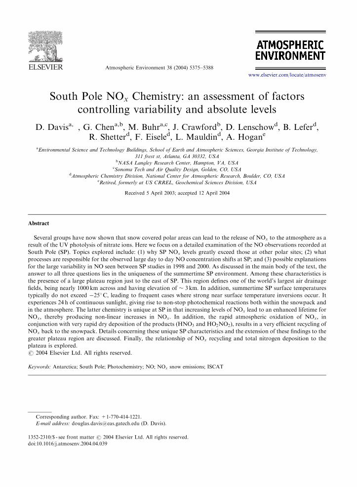
Fig. 4. Observed temporal variation in NO and NOx for: (a) snow

December 2000. The large value for the ratio of NOx to NO at �20

depth. At �1 cm this ratio approaches the same value as that in the a

end of 29th December 2000 is due to the sampling site in front of th

illustrating the potential impact that can result from overhead clouds

larger temperature range than for 2000 (e.g., �34 vs:�31 and �21 vs: �24).

4. Discussion

From the ISCAT 1998 and 2000 observations cited

above, it is quite apparent that although some very

important similarities can be found between the two NO

data sets, there are also some significant differences.

Perhaps more importantly, very large differences have

been found between the ISCAT results and those

reported at other polar sites. Below, these and related

issues are explored.

4.1. Major factors controlling South Pole NOx

Given that the major source of NOx at SP is its release

from the snowpack following the UV photolysis of

nitrate ions, it follows that the near surface atmospheric

concentration of NOx at any point in time should be a

function of at least four factors. These would include: (1)

the net flux of NOx from the snowpack ðF ðNOxÞSAÞ; (2)the net NOx advection flux ðF ðNOxÞAdvÞ; (3) the atmo-

spheric lifetime of NOxtNOx; and (4) the depth of

atmospheric mixing (i.e., planetary boundary layer

depth, PBL). Here we explore the effect of each of these

factors at SP; and ,when possible, compare the relative

magnitudes of these factors at different polar sites.

4.1.1. Snowpack NO–NOx levels and NOx flux

Representative SP snowpack measurements of NO

and NOx during ISCAT 2000 are shown in Fig. 4a.

These data were recorded with the sample inlet

� 20 cm below the snow surface. They unequivocally

12/29/00 12/30/00

Date

0

100

200

300

400

NO

(pp

tv)

)

Air NO

and (b) atmosphere (NO only) on a representative day, 29th

cm primarily reflects the attenuation of solar radiation at this

tmosphere. Note, the dip in NOx and NO at the beginning and

e ARO building falling into the shadow of the ARO building,

.

ARTICLE IN PRESS

90.0S

70.5S 64.5S

74.5N

82.5N

South Pole Neumayer PalmerStation

Summit,Greenland

Alert, Canada

0

50

100

150

200

250

300

350

400

NO

x(p

ptv

)

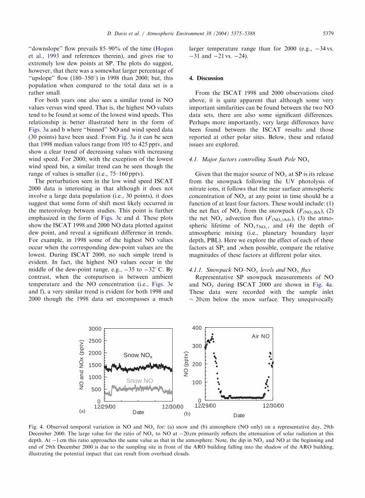
Fig. 5. Comparison of NO observations recorded at several

different polar sites. Data shown were taken from Davis et al.

(2001 this issue), Jones et al. (2000), Jefferson et al. (1998),

Yang et al. (2002), and Ridley et al. (2000). Note, the NOx

value for SP was that estimated from NO2 calculated from a

photochemical box model as described in the main text.

D. Davis et al. / Atmospheric Environment 38 (2004) 5375–53885380

demonstrate that the snowpack at SP is a major source

of atmospheric NOx: For example, a typical sampling

day on 29 December reveals � 1500pptv of NOx and

600 pptv of NO. This NO value is nearly seven times

larger than the median value estimated from all ISCAT

2000 data. More importantly, as shown in Fig. 4b, over

the same daytime period the difference between snow-

pack and atmospheric levels of NO varies by a factor

ranging from 2 to nearly 60. Since the atmospheric ratio

of NO:NO2 at SP is typically around 2:1, it follows that

the snowpack-to-atmospheric concentration difference

for NOx would, in most cases, be even larger.

The emission rate of NOx from the snowpack at SP

has been addressed by Oncley et al., (this issue), with the

finding that over a 6 day period of time (26 November to

1 December 2000) the flux was relatively constant. These

investigators used the modified Bowen ratio technique

involving simultaneous measurements of the eddy-

covariance surface heat flux along with the temperature

and NO concentration at two elevations. The estimated

NOx flux over the stated time period had an average

value of 3:9� 108 molec cm�2 s�1: (In this study, the

initially derived NO flux was converted to a NOx flux

from photochemical considerations where photochemi-

cal equilibrium values of NO2 were estimated for SP

conditions.) This SP value can be contrasted with that

estimated at Neumayer, Antarctica by Jones et al.

(2001). These authors measured the gradient in NOx at

two heights (e.g., 2 cm and 2.5m) over a two day period

in February. Their results were based on using an

estimated eddy diffusivity value that gave a 24 h

emission flux for NOx of 1:3� 108 molec cm�2 s�1: A

third site, Summit, Greenland, has also reported a NOx

flux value. In the latter case the flux estimate was based

on vertical gradient measurements of NOx at 1 and 2m

above the snowpack in conjunction with simultaneous

measurements of the atmospheric turbulence (Honrath

et al., 2002). The 24 h average vertical flux estimated via

eddy covariance for 5 June to 3 July 2001 was 2:5�108 molec cm�2 s�1:A comparison of these three independent fluxes

suggests that the differences do not scale with the

known snow nitrate ion concentrations and estimated

UV irradiance for each site. For example, if the flux were

controlled by the product of snow nitrate concentration

and nitrate photolysis rate, Summit, Greenland should

have recorded the highest value. This would reflect the

fact that snow nitrate levels are somewhat higher there

(e.g., 3 nmol g�1vs: 2nmol g�1at SP in the top 45 cm

(Dibb et al., 2004)) and that the measurements were

carried out at the time of summer solstice. Neumayer, on

the other hand, because of the study’s February

execution date would be expected to have one of the

lower NOx flux values; however, snow nitrate levels at

this site are closer to those found at Summit rather than

SP. Given this, the Neumayer flux also does not seem to

fit into any simple analysis that compares sites based

only on UV irradiance and nitrate levels. Currently,

therefore, too many uncertainties still remain as related

to the overall NOx production rate, its release to the

atmosphere, and in the reliability of the flux measure-

ments themselves to be able to assess the real differences

between sites.

What is apparent from the above assessment is that

the NOx flux values from three different sites vary by

only a factor of three. By contrast, the differences in the

median atmospheric NOx mixing ratio at SP versus

other polar sites are far larger than what might be

predicted from any adjusted differences in the NOx

fluxes (see Fig. 5). Thus, while differences in the values

of F ðNOxÞSA between sites is one of the contributing

factors to the observed difference in concentration, it is

most likely not the dominant one.

4.1.2. Planetary boundary layer depth

All other things being equal, for a fixed surface-to-

atmosphere NOx flux value, the larger the atmospheric

volume element filled the lower will be the resulting

steady-state concentration. Placed in the context of the

SP study, this means that the observed NOx concentra-

tion should be inversely proportional to the depth of the

planetary boundary layer (PBL). The PBL factor

therefore emerges as a critical variable in understanding

the large scale variations in the NOx mixing ratio.

Estimates of the PBL depth during ISCAT 2000 were

made using wind turbulence data collected with sonic

anemometers mounted on the SP MET tower. These

data when processed in conjunction with empirically

derived relationships relating the integral scales resulted

in the estimated PBL values cited in this study. For those

cases involving stable meteorological conditions, the

PBL depth was defined as that height at which the

ARTICLE IN PRESS

(b)(a)

1000

800

600

400

200

0

PB

L D

epth

(m

)

11/26 12/1 12/6 12/11 12/16 12/21 12/26

DateDate

h(3.5 m) h(7.2 m) h(unstable)

300

250

200

150

100

50

0

NO

(pp

tv)

11/26 12/1 12/6 12/11 12/16 12/21 12/26

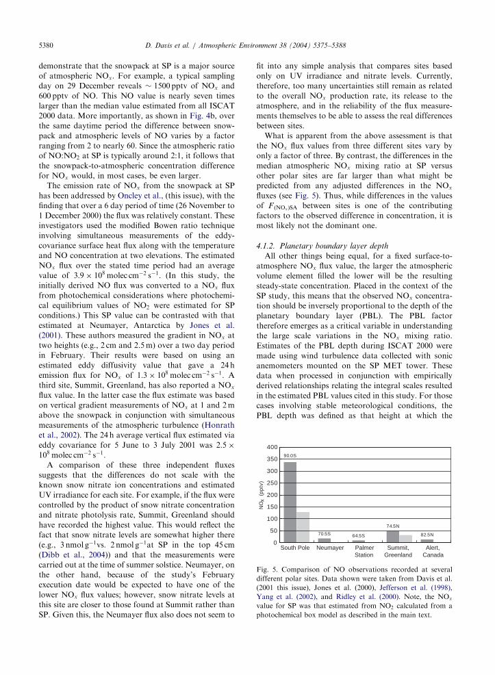
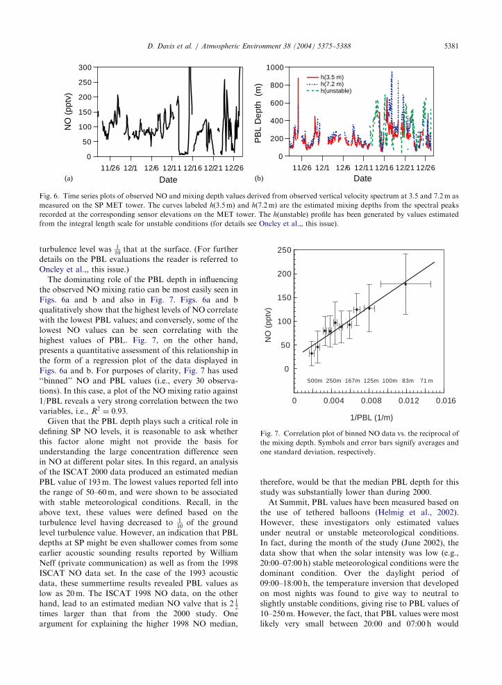
Fig. 6. Time series plots of observed NO and mixing depth values derived from observed vertical velocity spectrum at 3.5 and 7.2m as

measured on the SP MET tower. The curves labeled h(3.5m) and h(7.2m) are the estimated mixing depths from the spectral peaks

recorded at the corresponding sensor elevations on the MET tower. The h(unstable) profile has been generated by values estimated

from the integral length scale for unstable conditions (for details see Oncley et al.,, this issue).

0 0.004 0.008 0.012 0.016

1/PBL (1/m)

0

50

100

150

200

250

NO

(pp

tv)

500m 250m 167m 125m 100m 83m 71 m

Fig. 7. Correlation plot of binned NO data vs. the reciprocal of

the mixing depth. Symbols and error bars signify averages and

one standard deviation, respectively.

D. Davis et al. / Atmospheric Environment 38 (2004) 5375–5388 5381

turbulence level was 110

that at the surface. (For further

details on the PBL evaluations the reader is referred to

Oncley et al.,, this issue.)

The dominating role of the PBL depth in influencing

the observed NO mixing ratio can be most easily seen in

Figs. 6a and b and also in Fig. 7. Figs. 6a and b

qualitatively show that the highest levels of NO correlate

with the lowest PBL values; and conversely, some of the

lowest NO values can be seen correlating with the

highest values of PBL. Fig. 7, on the other hand,

presents a quantitative assessment of this relationship in

the form of a regression plot of the data displayed in

Figs. 6a and b. For purposes of clarity, Fig. 7 has used

‘‘binned’’ NO and PBL values (i.e., every 30 observa-

tions). In this case, a plot of the NO mixing ratio against

1/PBL reveals a very strong correlation between the two

variables, i.e., R2 ¼ 0:93:Given that the PBL depth plays such a critical role in

defining SP NO levels, it is reasonable to ask whether

this factor alone might not provide the basis for

understanding the large concentration difference seen

in NO at different polar sites. In this regard, an analysis

of the ISCAT 2000 data produced an estimated median

PBL value of 193m. The lowest values reported fell into

the range of 50–60m, and were shown to be associated

with stable meteorological conditions. Recall, in the

above text, these values were defined based on the

turbulence level having decreased to 110

of the ground

level turbulence value. However, an indication that PBL

depths at SP might be even shallower comes from some

earlier acoustic sounding results reported by William

Neff (private communication) as well as from the 1998

ISCAT NO data set. In the case of the 1993 acoustic

data, these summertime results revealed PBL values as

low as 20m. The ISCAT 1998 NO data, on the other

hand, lead to an estimated median NO valve that is 2 12

times larger than that from the 2000 study. One

argument for explaining the higher 1998 NO median,

therefore, would be that the median PBL depth for this

study was substantially lower than during 2000.

At Summit, PBL values have been measured based on

the use of tethered balloons (Helmig et al., 2002).

However, these investigators only estimated values

under neutral or unstable meteorological conditions.

In fact, during the month of the study (June 2002), the

data show that when the solar intensity was low (e.g.,

20:00–07:00 h) stable meteorological conditions were the

dominant condition. Over the daylight period of

09:00–18:00 h, the temperature inversion that developed

on most nights was found to give way to neutral to

slightly unstable conditions, giving rise to PBL values of

10–250m. However, the fact, that PBL values were most

likely very small between 20:00 and 07:00 h would

ARTICLE IN PRESS

0 100 200 300 400 500 600 700 800

NOx (pptv)

5

10

15

20

25

30

Life

time

(hou

rs)

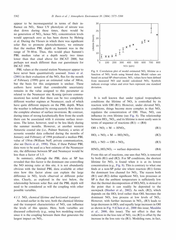
Fig. 8. Correlation plot of model estimated NOx lifetime as a

function of NOx levels using binned data. Model values are

based on actual SP observations. NOx values have been defined

from measured NO and model calculated NO2: Symbols

indicate average values and error bars represent one standard

deviation.

D. Davis et al. / Atmospheric Environment 38 (2004) 5375–53885382

appear to be inconsequential in terms of their in-

fluence on NOx: Since UV photolysis of nitrate was

shut down during these times, there would be

no generation of NOx; hence NOx concentration levels

would approach zero as has been shown by Helmig

et al. During the 9 hours in which there was significant

solar flux to promote photochemistry, we estimate

that the median PBL depth at Summit was in the

range of 70–80m. Thus, this would place Summit’s

PBL median value at a depth nearly two times

lower than that cited above for ISCAT 2000, but

perhaps not much different than our guesstimate for

ISCAT 1998.

PBL values at the coastal station Neumayer appear to

have never been quantitatively assessed. Jones et al.

(2001) in their evaluation of the NOx flux for the month

of February (1999) gave an estimated value of 300m,

but the basis for this assignment is unclear. These

authors have noted that considerable uncertainty

remains in the value assigned to this parameter as

related to the Neumayer site. Koenig (private commu-

nication) has noted that there can be two completely

different weather regimes at Neumayer, each of which

have quite different impacts on the PBL depth. When

the weather is influenced by strong easterly flow there is

the complete absence of surface inversions. By contrast,

during times of strong katabatically flow from the south

there can be associated with it extreme surface inver-

sions. The latter, however, tend to be less likely during

the summer months. However, at another western

Antarctic coastal site (i.e., Palmer Station), a series of

acoustic sounder data collected during the months of

January and February of 1994 produced a median PBL

value of 150m (William Neff, private communication,

also see Davis et al., 1998). Thus, if these Palmer PBL

data were to be used as a best estimate of the Neumayer

site, the difference between SP and Neumayer would be

less than a factor of 1.5.

In summary, although the PBL data at SP has

revealed that this factor is the dominant one controlling

the NO mixing ratio at this site, it is not abundantly

obvious with the limited PBL data available at other

sites how this factor alone can explain the large

difference in NOx levels observed at different polar

sites. Clearly, as explored in the text below, the

relationship between solar flux and the PBL depth will

need to be considered as will the coupling with other

possible variables.

4.1.3. NOx chemical lifetime and horizontal transport

As noted earlier in the text, both the chemical lifetime

and the transport characteristics of NOx can influence

the levels of this species. Here, both variables are

discussed collectively (e.g., using box modeling results)

since it is the coupling between them that generates the

largest impact on NOx:

It is well known that under typical tropospheric

conditions the lifetime of NOx is controlled by its

reaction with OH (R1). However, under elevated NOx

conditions, things become more complex in that NOx

regulates the concentration of OH. Thus, NOx can

influence its own lifetime (see Fig. 8). The relationship

between HOx;NOx; and its lifetime is most easily seen in

terms of sequence of reactions (R1Þ ! ðR4)

OHþNO2 þM ! HNO3; ðR1Þ

HO2 þNO2 þM ! HO2NO2; ðR2Þ

HO2 þNO ! OHþNO2; ðR3Þ

HNO3;HO2NO2 ! surface deposition: ðR4Þ

From this set of reactions, one sees that NO2 is removed

by both (R1) and (R2). For SP conditions, the shortest

lifetime for NOx is found when it is at its lowest

concentration (e.g., Fig. 8). This is contrary to what one

finds at a non-SP polar site where reaction (R1) forms

the dominant loss channel for NOx: The reason both

(R1) and (R2) define significant NOx loss processes at

SP is that the ambient temperature is sufficiently low

that the thermal decomposition of HO2NO2 is slowed to

the point that it can readily be deposited to the

snowpack (Slusher et al., 2002). As such, (R2), which

depends on the HO2 level rather than OH, becomes the

dominant NOx loss process at low levels of NOx:However, with further increases in NOx; (R3) leads to

large decreases in HO2 and equally large increases in OH

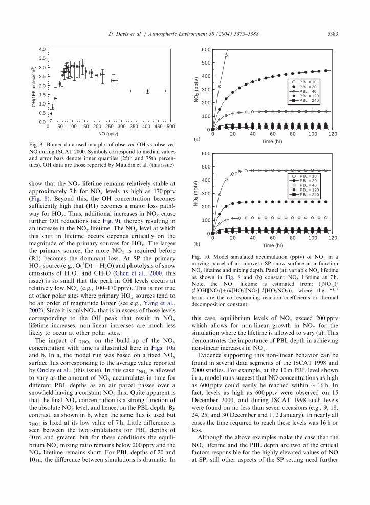
as shown in Fig. 9 (Chen et al., 2000 this issue; Mauldin

et al., 2000, this issue). The net effect is that the

reduction in the loss rate of NOx via (R2) is offset by the

increase in the loss rate via (R1). Modeling runs, in fact,

ARTICLE IN PRESS

0 50 100 150 200 250 300 350 400 450 500

NO (pptv)

0.0

0.5

1.0

1.5

2.0

2.5

3.0

3.5

4.0

OH

(1E

6 m

olec

/cm

3 )

Fig. 9. Binned data used in a plot of observed OH vs. observed

NO during ISCAT 2000. Symbols correspond to median values

and error bars denote inner quartiles (25th and 75th percen-

tiles). OH data are those reported by Mauldin et al. (this issue).

0 20 40 60 80 100 120

Time (hr)

Time (hr)

0

100

200

300

400

500

600

NO

x(p

ptv

)

PBL = 10PBL = 20PBL = 40P BL = 120P BL = 240

(a)

0 20 40 60 80 100 1200

100

200

300

400

500

600

NO

x(p

ptv

)

PBL = 10PBL = 20PBL = 40PBL = 120PBL = 240

(b)

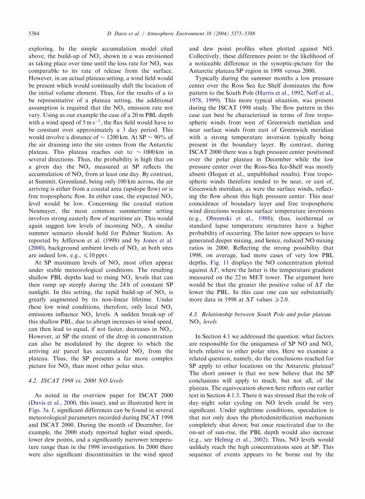
Fig. 10. Model simulated accumulation (pptv) of NOx in a

moving parcel of air above a SP snow surface as a function

NOx lifetime and mixing depth. Panel (a): variable NOx lifetime

as shown in Fig. 8 and (b) constant NOx lifetime at 7 h.

Note, the NOx lifetime is estimated from: ([NOx])/

(k[OH][NO2]+(k[HO2][NO2]–k[HO2NO2)), where the ‘‘k’’

terms are the corresponding reaction coefficients or thermal

decomposition constant.

D. Davis et al. / Atmospheric Environment 38 (2004) 5375–5388 5383

show that the NOx lifetime remains relatively stable at

approximately 7 h for NOx levels as high as 170 pptv

(Fig. 8). Beyond this, the OH concentration becomes

sufficiently high that (R1) becomes a major loss path!-

way for HOx: Thus, additional increases in NOx cause

further OH reductions (see Fig. 9), thereby resulting in

an increase in the NOx lifetime. The NOx level at which

this shift in lifetime occurs depends critically on the

magnitude of the primary sources for HOx: The larger

the primary source, the more NOx is required before

(R1) becomes the dominant loss. At SP the primary

HOx source (e.g., Oð1DÞ þH2O) and photolysis of snow

emissions of H2O2 and CH2O (Chen et al., 2000, this

issue) is so small that the peak in OH levels occurs at

relatively low NOx (e.g., 100–170 pptv). This is not true

at other polar sites where primary HOx sources tend to

be an order of magnitude larger (see e.g., Yang et al.,

2002). Since it is onlyNOx that is in excess of those levels

corresponding to the OH peak that result in NOx

lifetime increases, non-linear increases are much less

likely to occur at other polar sites.

The impact of tNOxon the build-up of the NOx

concentration with time is illustrated here in Figs. 10a

and b. In a, the model run was based on a fixed NOx

surface flux corresponding to the average value reported

by Oncley et al., (this issue). In this case tNOxis allowed

to vary as the amount of NOx accumulates in time for

different PBL depths as an air parcel passes over a

snowfield having a constant NOx flux. Quite apparent is

that the final NOx concentration is a strong function of

the absolute NOx level, and hence, on the PBL depth. By

contrast, as shown in b, when the same flux is used but

tNOxis fixed at its low value of 7 h. Little difference is

seen between the two simulations for PBL depths of

40m and greater, but for these conditions the equili-

brium NOx mixing ratio remains below 200 pptv and the

NOx lifetime remains short. For PBL depths of 20 and

10m, the difference between simulations is dramatic. In

this case, equilibrium levels of NOx exceed 200 pptv

which allows for non-linear growth in NOx for the

simulation where the lifetime is allowed to vary (a). This

demonstrates the importance of PBL depth in achieving

non-linear increases in NOx:Evidence supporting this non-linear behavior can be

found in several data segments of the ISCAT 1998 and

2000 studies. For example, at the 10m PBL level shown

in a, model runs suggest that NO concentrations as high

as 600 pptv could easily be reached within � 16h: Infact, levels as high as 600 pptv were observed on 15

December 2000, and during ISCAT 1998 such levels

were found on no less than seven occasions (e.g., 9, 18,

24, 25, and 30 December and 1, 2 January). In nearly all

cases the time required to reach these levels was 16 h or

less.

Although the above examples make the case that the

NOx lifetime and the PBL depth are two of the critical

factors responsible for the highly elevated values of NO

at SP, still other aspects of the SP setting need further

ARTICLE IN PRESSD. Davis et al. / Atmospheric Environment 38 (2004) 5375–53885384

exploring. In the simple accumulation model cited

above, the build-up of NOx shown in a was envisioned

as taking place over time until the loss rate for NOx was

comparable to its rate of release from the surface.

However, in an actual plateau setting, a wind field would

be present which would continually shift the location of

the initial volume element. Thus, for the results of a to

be representative of a plateau setting, the additional

assumption is required that the NOx emission rate not

vary. Using as our example the case of a 20m PBL depth

with a wind speed of 5m s�1; the flux field would have to

be constant over approximately a 3 day period. This

would involve a distance of � 1200 km: At SP � 90% of

the air draining into the site comes from the Antarctic

plateau. This plateau reaches out to � 1000km in

several directions. Thus, the probability is high that on

a given day the NOx measured at SP reflects the

accumulation of NOx from at least one day. By contrast,

at Summit, Greenland, being only 100 km across, the air

arriving is either from a coastal area (upslope flow) or is

free tropospheric flow. In either case, the expected NOx

level would be low. Concerning the coastal station

Neumayer, the most common summertime setting

involves strong easterly flow of maritime air. This would

again suggest low levels of incoming NOx: A similar

summer scenario should hold for Palmer Station. As

reported by Jefferson et al. (1998) and by Jones et al.

(2000), background ambient levels of NOx at both sites

are indeed low, e.g., p10 pptv:At SP maximum levels of NOx most often appear

under stable meteorological conditions. The resulting

shallow PBL depths lead to rising NOx levels that can

then ramp up steeply during the 24 h of constant SP

sunlight. In this setting, the rapid build-up of NOx is

greatly augmented by its non-linear lifetime. Under

these low wind conditions, therefore, only local NOx

emissions influence NOx levels. A sudden break-up of

this shallow PBL, due to abrupt increases in wind speed,

can then lead to equal, if not faster, decreases in NOx:However, at SP the extent of the drop in concentration

can also be modulated by the degree to which the

arriving air parcel has accumulated NOx from the

plateau. Thus, the SP presents a far more complex

picture for NOx than most other polar sites.

4.2. ISCAT 1998 vs. 2000 NO levels

As noted in the overview paper for ISCAT 2000

(Davis et al., 2000, this issue), and as illustrated here in

Figs. 3a–f, significant differences can be found in several

meteorological parameters recorded during ISCAT 1998

and ISCAT 2000. During the month of December, for

example, the 2000 study reported higher wind speeds,

lower dew points, and a significantly narrower tempera-

ture range than in the 1998 investigation. In 2000 there

were also significant discontinuities in the wind speed

and dew point profiles when plotted against NO.

Collectively, these differences point to the likelihood of

a noticeable difference in the synoptic-picture for the

Antarctic plateau/SP region in 1998 versus 2000.

Typically during the summer months a low pressure

center over the Ross Sea Ice Shelf dominates the flow

pattern to the South Pole (Harris et al., 1992, Neff et al.,

1978, 1999). This more typical situation, was present

during the ISCAT 1998 study. The flow pattern in this

case can best be characterized in terms of free tropo-

spheric winds from west of Greenwich meridian and

near surface winds from east of Greenwich meridian

with a strong temperature inversion typically being

present in the boundary layer. By contrast, during

ISCAT 2000 there was a high pressure center positioned

over the polar plateau in December while the low

pressure center over the Ross-Sea Ice-Shelf was mostly

absent (Hogan et al., unpublished results). Free tropo-

spheric winds therefore tended to be near, or east of,

Greenwich meridian, as were the surface winds, reflect-

ing the flow about this high pressure center. This near

coincidence of boundary layer and free tropospheric

wind directions weakens surface temperature inversions

(e.g., Obremski et al., 1988); thus, isothermal or

standard lapse temperature structures have a higher

probability of occurring. The latter now appears to have

generated deeper mixing, and hence, reduced NO mixing

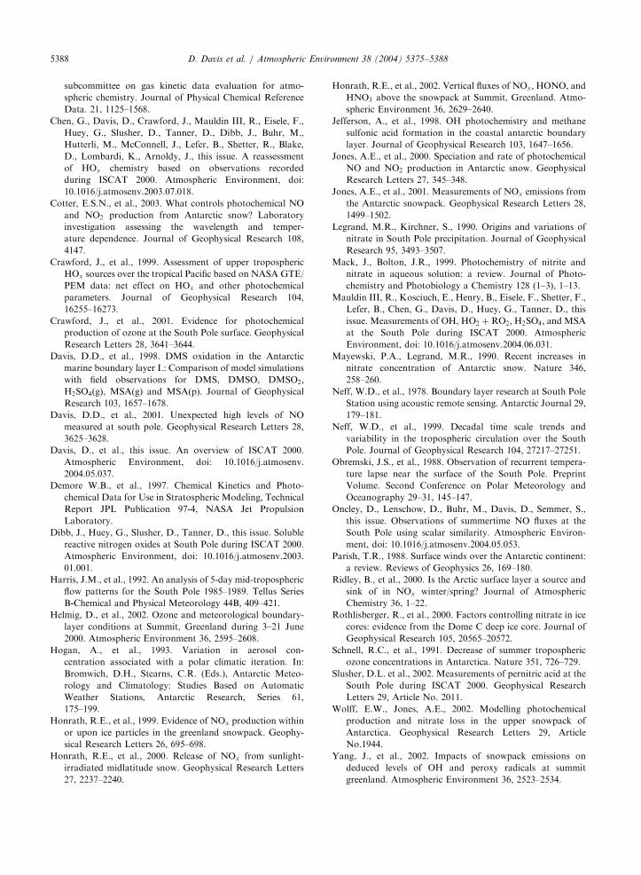
ratios in 2000. Reflecting the strong possibility that

1998, on average, had more cases of very low PBL

depths, Fig. 11 displays the NO concentration plotted

against DT ; where the latter is the temperature gradient

measured on the 22m MET tower. The argument here

would be that the greater the positive value of DT the

lower the PBL. In this case one can see substantially

more data in 1998 at DT values X2:0:

4.3. Relationship between South Pole and polar plateau

NOx levels

In Section 4.1 we addressed the question: what factors

are responsible for the uniqueness of SP NO and NOx

levels relative to other polar sites. Here we examine a

related question, namely, do the conclusions reached for

SP apply to other locations on the Antarctic plateau?

The short answer is that we now believe that the SP

conclusions will apply to much, but not all, of the

plateau. The equivocation shown here reflects our earlier

text in Section 4.1.3. There it was stressed that the role of

day–night solar cycling on NO levels could be very

significant. Under nighttime conditions, speculation is

that not only does the photodenitrification mechanism

completely shut down; but once reactivated due to the

on-set of sun-rise, the PBL depth would also increase

(e.g., see Helmig et al., 2002). Thus, NO levels would

unlikely reach the high concentrations seen at SP. This

sequence of events appears to be borne out by the

ARTICLE IN PRESS

-1 -0.5 0 0.5 1 1.5 2 2.5 30

100

200

300

400

500

600

NO

(pp

tv)

(a)

-1 -0.5 0 0.5 1 1.5 2 2.5 3

T(22m) - T(1.6m) (deg C)T(22m) - T(1.6m) (deg C)

0

100

200

300

400

500

600

NO

(pp

tv)

(b)

Fig. 11. Relation between observed NO levels and temperature gradient as measured on the SP MET tower, e.g., T(22m)–T(1.6m) in�C: Binned data are for: (a) ISCAT 1998; (b) ISCAT 2000.

D. Davis et al. / Atmospheric Environment 38 (2004) 5375–5388 5385

studies reported by Jones et al. (2001) and Honrath et al.

(2002), both of which involve sites experiencing solar

cycling. Their results suggest that most of the reservoir

NOx in the snowpack is lost during dark hours, possibly

due to heterogeneous processes operating within the

snowpack. With the return of daylight, the NOx

generating mechanism is re-initialized, but new reservoir

levels of NOx then need to be re-established before

significant releases can occur to the atmosphere. This

would suggest that the levels of NO observed on the

plateau might be latitude dependent, leading to the

further conclusion that some areas of the plateau may

never experience the effects resulting from a non-linear

NOx lifetime. If so, these areas would be expected to

have much lower average values of NOx than observed

at SP.

Based on the assumption that the photolysis fre-

quency for labile nitrogen in the snowpack would be

similar to that for JðHNO3Þ (Cotter et al., 2003; Wolff

and Jones, 2002), the latitude at which a substantial roll-

off (e.g., a factor of 2) in photolysis rate might be

observed is estimated to be � 77� S: This would mean

that � 23of the Antarctic plateau is likely to experience

highly elevated NOx levels. However, considering the

fact that only 50–70 pptv of NO is required to drive OH

from levels of 3� 105 to 2–3� 106 molec cm�3; even

very modest levels of NO at these lower latitudes could

still have a major impact on the oxidizing power and/or

O3 generating capacity of near surface air over the

plateau (e.g., see Crawford et al., 2001; Chen et al., 2000

this issue).

4.4. Importance of NOx recycling to the net deposition of

nitrogen

It is now clear from the observations of ISCAT 1998

and 2000 that snowpack emissions of NOx have a

profound effect on the photochemistry within the PBL.

But it is also of interest to examine whether this release

of nitrogen is large enough to have a significant

impact on the total nitrogen deposited to the surface

at SP and the greater plateau region. Based on SP core

samples, Legrand and Kirchner (1990) estimated the

mean deposition flux for nitrate at SP (over the last

hundred years) to be 9.5 kg NO3 km�2 yr�1 (or

2.1 kgNkm�2 yr�1). This number, however, must be

viewed as a net deposition flux given the photochemi-

cally driven emission of NOx as observed during ISCAT

1998 and 2000. This net deposition flux can be compared

with the NOx emission flux reported here (i.e.,

3:9� 108 molec cm�2 s�1). If one assumes that this

emission flux is fairly constant during the 4 months of

significant sunlight (e.g., 130 days with solar zenith

angles o80�) at South Pole, the annual NOx emission

flux would be 1:0kgNkm�2 yr�1; which is roughly half

the value of the net deposition flux. (Note, assuming a

constant flux across the entire plateau, the 6� 106 km2

surface area of the plateau would release a yearly flux of

0.006TgN.)

Despite the photochemical liberation of roughly half

as much nitrogen as is annually buried at SP, much of

this nitrogen is expected to be redeposited to the snow

based on the short lifetime for NOx (e.g., median value

of � 8h). As shown in Fig. 12, NOx released from the

Antarctic plateau is rapidly recycled back to the oxidized

form, HNO3 and HO2NO2: But, both HNO3 and

HO2NO2 have relatively short lifetimes due to their

efficient deposition to the snow surface (e.g., � 3h;Slusher et al., 2002). Thus, NOx reappears as snowpack

nitrate in less than a day. Given the persistence and

speed of katabatic windflow (e.g., 2–10m s�1), NOx may

be transported up to several hundred kilometers down-

slope before redeposition occurs. However, for katabatic

flow occurring along the outer perimeter of the plateau

(within 12

day flow time) there would result a net

loss of nitrogen from the plateau as there would be for

vertical mixing which would move NOy into the free

troposphere.

ARTICLE IN PRESS

Fig. 12. Nitrogen budget schematic illustrating the recycling of reactive nitrogen on the Antarctic plateau as well as possible nitrogen

loss processes that would lead to a requirement for a new primary nitrogen source.

D. Davis et al. / Atmospheric Environment 38 (2004) 5375–53885386

Returning to the down-slope redeposition scenario,

such a flow pattern suggests that there might be a

gradient in net deposition across the plateau. Mayewski

and Legrand (1990) have expressed difficulty in explain-

ing the large geographical variation of nitrate across the

Antarctic plateau with core samples from SP containing

as much as five times more nitrate than samples from

Vostok and Dome C. However, SP is located on the

lower edge of the plateau and typically receives down-

slope flow from the greater plateau. Thus, redeposition

of nitrogen from upslope emissions could offset the local

emission at SP. By contrast, Vostok and Dome C are

located much further up the plateau and experience little

to no downslope flow (see Parish, 1988). Relative to SP,

then, they would experience much less redeposition to

offset the emission of NOx:Evidence for redeposition can be found in the

measurements of nitrate within the first few centimeters

of snow. Measurements from SP indicate that nitrate

decreases by roughly an order of magnitude between the

surface and 10 cm (Dibb et al. (2004), and references

therein). Similar observations have been reported for

Dome C (Rothlisberger et al., 2000). The emission of

nitrate photolyzed within the upper several centimeters

of snow followed by the rapid redeposition of nitrate at

the surface would provide a plausible explanation for

the sharp gradient in nitrate observed by these

investigators.

Accumulation rate is another factor relevant to

understanding differences in nitrate between core

samples from SP, Vostok, and Dome C. Annual

accumulation at Vostok and Dome C is 2–3 times lower

than that at SP (Mayewski and Legrand, 1990). Thus,

fresh snow at the former sites resides in the upper 10 cm

for a longer period of time, thereby allowing photo-

chemical processes to release a larger fraction of the

initially deposited nitrate. The prolonged exposure to

the photodenitrification process, coupled with the more

limited opportunity for redeposition, would at least

qualitatively appear to explain much of the large

difference found in nitrate levels at SP relative to

Vostok and Dome C.

The collective processes of photo-induced emission of

NOx; followed by chemical oxidation and transport, and

finally redeposition would seem to allow for a major

redistribution of any nitrate initially deposited to the

Antarctic plateau. Differences in the length of exposure

to photochemistry as a function of accumulation rate

would also appear to significantly influence the degree of

nitrate redistribution. Differences in ice core samples as

well as estimates for nitrate deposition and NOx

emission flux estimates support the contention that this

redistribution appears to influence a large fraction of the

nitrate annually deposited to the plateau. Such a

redistribution further complicates the use of nitrate as

a proxy species for interpreting major geophysical events

ARTICLE IN PRESSD. Davis et al. / Atmospheric Environment 38 (2004) 5375–5388 5387

and climate changes as deduced from ice cores collected

from various plateau sites.

5. Summary and conclusions

The ISCAT 2000 field study has generated the most

extensive SP NO data base yet. These data have

provided significant answers to many of the questions

remaining after ISCAT 1998. Two independent instru-

ments operated by independent investigators have

unequivocally established that near surface SP NO

levels reach extraordinarily high levels (e.g., 600+pptv)

during the summer months. These measurements also

convincingly demonstrated that the source of NO is its

emission from the snowpack. The chemical process

responsible at SP has clearly been identified as photo-

chemical in nature, as it has also been shown by other

investigators at other polar sites. Many of the details

concerning the overall mechanism, however, still remain

conjecture. The data further indicate that at SP

photochemical processes within the snowpack operate

24 h a day. It follows that modulation of this subsurface

production of NOx can occur from both shifts in

overhead cloud coverage as well as from changes in the

overhead ozone column density (e.g., see Davis et al.,

2001; Mauldin et al., 2000 this issue).

One of the major tasks undertaken in this work has

been to address the question: why does SP generate such

high concentration levels of NO relative to other polar

sites? The answer now appears to lie in the unique

interplay that occurs between four factors: (1) 24 h of

continuous sunlight, (2) regularly occurring meteorolo-

gical conditions leading to very shallow PBL depths, (3)

being downwind from one of the world’s largest air

drainage fields, and (4) having a HOx–NOx chemical

environment where increasing NOx levels leads to a non-

linear response in NOx lifetime. Of the polar sites that

have been investigated, none but the SP reaches

sufficiently high levels of NOx that factor (4) becomes

significant. At no other polar site is it likely that surface

air parcels accumulate NOx over time periods of one to

two days. And, at no other polar site do shallow PBL

depths occur on a regular basis at the same time that

there is relatively continuous solar activity.

One of the strongest correlations found between the

NO mixing ratio and a meteorological parameter was

that involving the PBL depth ðR2 ¼ 0:93Þ: Thus, dailyshifts in the PBL depth were a major factor responsible

for the frequently observed abrupt changes in the

concentration level of NO. This has led to our

speculating that a systematic shift in the average PBL

value between the 1998 and 2000 study is mostly likely

the basis for the much higher NO median value during

ISCAT 1998. This hypothesis appears to be generally

consistent with the synoptic picture generated for the

Antarctic continent for the years 2000 and 1998. For

example, unlike in 1998, during December of 2000 high

pressure dominated over the entire polar plateau. This

produced near surface and free tropospheric winds over

the plateau that had nearly the same direction, a

meteorological setting leading to a weakening of the

surface temperature inversion, and hence, greater

vertical mixing.

Two final conclusions from the current analysis

address first the question of what the similarity might

be between the SP NO levels and those on the Antarctic

plateau. At this point in time, there are no direct

observations of NO or NOx over this expansive region.

Speculation here is that given the solar flux and nitrate

levels available on the plateau, high values of NO should

be found over a very large fraction of the plateau. The

second conclusion involves the importance of NOx

recycling to the plateau. It now appears that the

recycling of NOx due to its photo-induced emission

from the snowpack can explain most of the sharp

decreases seen in nitrate levels with depth at SP and

other plateau sites. It also appears to offer an explana-

tion for the variation seen in the average buried nitrogen

level found at SP versus higher elevation sites like Dome

C and Vostok.

Looking to the future, clearly the expansion of the

current SP observations to include a significant portion

of the Antarctic plateau must be viewed as a high

priority. Equally important will be collecting detailed

vertical profiles of NO and other species at SP to assess

the extent of the hypothesized oxidizing canopy over the

Antarctic plateau. And finally, a renewed effort is

needed to define the primary sources of plateau reactive

nitrogen as well as the loss processes operating in this

unique environment.

Acknowledgements

The authors would like to thank NOAA’s CMDL

personnel for their ready support of all our ISCAT

efforts at the ARO facility at South Pole, with special

thanks going to Pauline Roberts. The author D.D.

Davis would also like to express his appreciation to the

National Science Foundation’s Office of Polar Programs

(Grant # OPP-9725465) and the Division of Atmo-

spheric Chemistry for their partial support of this

research. Finally, D.D. Davis would like to acknowledge

the efforts of Joe Arnoldy in helping with the graphics of

this paper.

References

Atkinson, R., et al., 1992. Evaluated kinetic and photochemical

data for atmospheric chemistry, Supplement IV, IUPAC

ARTICLE IN PRESSD. Davis et al. / Atmospheric Environment 38 (2004) 5375–53885388

subcommittee on gas kinetic data evaluation for atmo-

spheric chemistry. Journal of Physical Chemical Reference

Data. 21, 1125–1568.

Chen, G., Davis, D., Crawford, J., Mauldin III, R., Eisele, F.,

Huey, G., Slusher, D., Tanner, D., Dibb, J., Buhr, M.,

Hutterli, M., McConnell, J., Lefer, B., Shetter, R., Blake,

D., Lombardi, K., Arnoldy, J., this issue. A reassessment

of HOx chemistry based on observations recorded

during ISCAT 2000. Atmospheric Environment, doi:

10.1016/j.atmosenv.2003.07.018.

Cotter, E.S.N., et al., 2003. What controls photochemical NO

and NO2 production from Antarctic snow? Laboratory

investigation assessing the wavelength and temper-

ature dependence. Journal of Geophysical Research 108,

4147.

Crawford, J., et al., 1999. Assessment of upper tropospheric

HOx sources over the tropical Pacific based on NASA GTE/

PEM data: net effect on HOx and other photochemical

parameters. Journal of Geophysical Research 104,

16255–16273.

Crawford, J., et al., 2001. Evidence for photochemical

production of ozone at the South Pole surface. Geophysical

Research Letters 28, 3641–3644.

Davis, D.D., et al., 1998. DMS oxidation in the Antarctic

marine boundary layer I.: Comparison of model simulations

with field observations for DMS, DMSO, DMSO2;H2SO4(g), MSA(g) and MSA(p). Journal of Geophysical

Research 103, 1657–1678.

Davis, D.D., et al., 2001. Unexpected high levels of NO

measured at south pole. Geophysical Research Letters 28,

3625–3628.

Davis, D., et al., this issue. An overview of ISCAT 2000.

Atmospheric Environment, doi: 10.1016/j.atmosenv.

2004.05.037.

Demore W.B., et al., 1997. Chemical Kinetics and Photo-

chemical Data for Use in Stratospheric Modeling, Technical

Report JPL Publication 97-4, NASA Jet Propulsion

Laboratory.

Dibb, J., Huey, G., Slusher, D., Tanner, D., this issue. Soluble

reactive nitrogen oxides at South Pole during ISCAT 2000.

Atmospheric Environment, doi: 10.1016/j.atmosenv.2003.

01.001.

Harris, J.M., et al., 1992. An analysis of 5-day mid-tropospheric

flow patterns for the South Pole 1985–1989. Tellus Series

B-Chemical and Physical Meteorology 44B, 409–421.

Helmig, D., et al., 2002. Ozone and meteorological boundary-

layer conditions at Summit, Greenland during 3–21 June

2000. Atmospheric Environment 36, 2595–2608.

Hogan, A., et al., 1993. Variation in aerosol con-

centration associated with a polar climatic iteration. In:

Bromwich, D.H., Stearns, C.R. (Eds.), Antarctic Meteo-

rology and Climatology: Studies Based on Automatic

Weather Stations, Antarctic Research, Series 61,

175–199.

Honrath, R.E., et al., 1999. Evidence of NOx production within

or upon ice particles in the greenland snowpack. Geophy-

sical Research Letters 26, 695–698.

Honrath, R.E., et al., 2000. Release of NOx from sunlight-

irradiated midlatitude snow. Geophysical Research Letters

27, 2237–2240.

Honrath, R.E., et al., 2002. Vertical fluxes of NOx; HONO, and

HNO3 above the snowpack at Summit, Greenland. Atmo-

spheric Environment 36, 2629–2640.

Jefferson, A., et al., 1998. OH photochemistry and methane

sulfonic acid formation in the coastal antarctic boundary

layer. Journal of Geophysical Research 103, 1647–1656.

Jones, A.E., et al., 2000. Speciation and rate of photochemical

NO and NO2 production in Antarctic snow. Geophysical

Research Letters 27, 345–348.

Jones, A.E., et al., 2001. Measurements of NOx emissions from

the Antarctic snowpack. Geophysical Research Letters 28,

1499–1502.

Legrand, M.R., Kirchner, S., 1990. Origins and variations of

nitrate in South Pole precipitation. Journal of Geophysical

Research 95, 3493–3507.

Mack, J., Bolton, J.R., 1999. Photochemistry of nitrite and

nitrate in aqueous solution: a review. Journal of Photo-

chemistry and Photobiology a Chemistry 128 (1–3), 1–13.

Mauldin III, R., Kosciuch, E., Henry, B., Eisele, F., Shetter, F.,

Lefer, B., Chen, G., Davis, D., Huey, G., Tanner, D., this

issue. Measurements of OH, HO2 þRO2; H2SO4; and MSA

at the South Pole during ISCAT 2000. Atmospheric

Environment, doi: 10.1016/j.atmosenv.2004.06.031.

Mayewski, P.A., Legrand, M.R., 1990. Recent increases in

nitrate concentration of Antarctic snow. Nature 346,

258–260.

Neff, W.D., et al., 1978. Boundary layer research at South Pole

Station using acoustic remote sensing. Antarctic Journal 29,

179–181.

Neff, W.D., et al., 1999. Decadal time scale trends and

variability in the tropospheric circulation over the South

Pole. Journal of Geophysical Research 104, 27217–27251.

Obremski, J.S., et al., 1988. Observation of recurrent tempera-

ture lapse near the surface of the South Pole. Preprint

Volume. Second Conference on Polar Meteorology and

Oceanography 29–31, 145–147.

Oncley, D., Lenschow, D., Buhr, M., Davis, D., Semmer, S.,

this issue. Observations of summertime NO fluxes at the

South Pole using scalar similarity. Atmospheric Environ-

ment, doi: 10.1016/j.atmosenv.2004.05.053.

Parish, T.R., 1988. Surface winds over the Antarctic continent:

a review. Reviews of Geophysics 26, 169–180.

Ridley, B., et al., 2000. Is the Arctic surface layer a source and

sink of in NOx winter/spring? Journal of Atmospheric

Chemistry 36, 1–22.

Rothlisberger, R., et al., 2000. Factors controlling nitrate in ice

cores: evidence from the Dome C deep ice core. Journal of

Geophysical Research 105, 20565–20572.

Schnell, R.C., et al., 1991. Decrease of summer tropospheric

ozone concentrations in Antarctica. Nature 351, 726–729.

Slusher, D.L. et al., 2002. Measurements of pernitric acid at the

South Pole during ISCAT 2000. Geophysical Research

Letters 29, Article No. 2011.

Wolff, E.W., Jones, A.E., 2002. Modelling photochemical

production and nitrate loss in the upper snowpack of

Antarctica. Geophysical Research Letters 29, Article

No.1944.

Yang, J., et al., 2002. Impacts of snowpack emissions on

deduced levels of OH and peroxy radicals at summit

greenland. Atmospheric Environment 36, 2523–2534.