volume 116number 5/6

South AfricanJournal of Science

Marine plastic debris in

South Africa: From sources to solutions

First findings of lead isotopes as palaeodietary indicators

in the Western Cape

Marama: A climate change friendly crop for

southern Africa

Medical geology and its relevance in Africa

Governance of gene editing in South Africa

eISSN: 1996-7489

EDITOR-IN-CHIEFJane Carruthers Academy of Science of South Africa

MANAGING EDITORLinda Fick Academy of Science of South Africa

ONLINE PUBLISHING SYSTEMS ADMINISTRATOR Nadia Grobler Academy of Science of South Africa

ASSOCIATE EDITORSMargaret AveryCenozoic Studies, Iziko Museums of South Africa, South Africa

Priscilla Baker Department of Chemistry, University of the Western Cape, South Africa

Pascal Bessong HIV/AIDS & Global Health Research Programme, University of Venda, South Africa

Jennifer Case Department of Engineering Education, Virginia Tech, Blacksburg, VA, USA

Teresa CoutinhoDepartment of Microbiology and Plant Pathology, University of Pretoria, South Africa

Tania Douglas Division of Biomedical Engineering, University of Cape Town, South Africa

Bettine van Vuuren Department of Zoology, Centre for Ecological Genomics and Wildlife Conservation, University of Johannesburg, South Africa

Amanda Weltman Department of Mathematics and Applied Mathematics, University of Cape Town, South Africa

Yali Woyessa Department of Civil Engineering, Central University of Technology, South Africa

ASSOCIATE EDITOR MENTEESNtombizodwa Mathe National Laser Centre, CSIR, South Africa

Salmina Mokgehle Vegetable and Ornamental Plants, Agricultural Research Council, South Africa

South AfricanJournal of Science

May/June 2020

Volume 116Number 5/6

Guest Leader

Are there gaps in our understanding of marine plastic pollution?Linda Godfrey ........................................................................................................................ 1

News & Views

Governance of gene editing in South Africa: Towards addressing the ethico-legal hiatusAmes Dhai, Glenda Gray, Martin Veller & Daynia Ballot ........................................................... 2

Obituary

Remembering Rein Arndt, 1929–2020Marina Joubert, Helgard Raubenheimer & Roy Siegfried ......................................................... 5

Maarten de Wit 1947–2020: An appreciationPeter Vale ............................................................................................................................... 7

Opinion

A philosophical perspective on pulmonary hypertension: What is ‘rare’?Gerald J. Maarman ................................................................................................................. 8

Book Review

Uniting botanical science and artBrian W. van Wilgen ................................................................................................................ 9

Not the peace train but the piece trainBill Nasson ........................................................................................................................... 10

‘Meet people where they are’: An approach to opioids and harm reduction in South AfricaDanielle A. Millar & Caradee Y. Wright ................................................................................... 11

Commentary

Why are black South African students less likely to consider studying biological sciences?Nicoli Nattrass ...................................................................................................................... 12

Medical Geology and its relevance in AfricaHassina Mouri ....................................................................................................................... 14

Cover captionPlastic waste on a South African beach. A series of reviews in this issue provides the latest information on the sources, pathways, impacts and monitoring of marine plastic debris in South Africa. Photo: Douw Steyn, PlasticsSA.

EDITORIAL ADVISORY BOARDLaura Czerniewicz Centre for Higher Education Development, University of Cape Town, South Africa

Hassina MouriDepartment of Geology, University of Johannesburg, South Africa

Johann MoutonCentre for Research on Science and Technology, Stellenbosch University, South Africa

Sershen NaidooSchool of Life Sciences, University of KwaZulu-Natal, South Africa

Maano RamutsindelaDepartment of Environmental & Geographical Science, University of Cape Town, South Africa

Himla Soodyall Academy of Science of South Africa

Published bythe Academy of Science of South Africa (www.assaf.org.za) with financial assistance from the Department of Science & Technology.

Design and layoutSUN MeDIA Bloemfontein T: 051 444 2552 E: publish@sunbloem.co.za

Correspondence and enquiriessajs@assaf.org.za

CopyrightAll articles are published under a Creative Commons Attribution Licence. Copyright is retained by the authors.

DisclaimerThe publisher and editors accept no responsibility for statements made by the authors.

SubmissionsSubmissions should be made at www.sajs.co.za

Marine Plastic Debris: News and Views

South African Initiative to End Plastic Pollution in the EnvironmentAnton Hanekom .................................................................................................................... 16

A circular economy response to plastic pollution: Current policy landscape and consumer perceptionLorren de Kock, Zaynab Sadan, Reinhardt Arp & Prabhat Upadhyaya ..................................... 18

The African Marine Waste Network and its aim to achieve ‘Zero Plastics to the Seas of Africa’Danica Marlin & Anthony J. Ribbink ....................................................................................... 20

Marine Plastic Debris: Commentary

Framing the plastic pollution problem within the water quality–health nexus: Current understandings and policy recommendationsEunice Ubomba-Jaswa & Nonhlanhla Kalebaila ...................................................................... 22

Marine Plastic Debris: Review Article

Land-based sources and pathways of marine plastics in a South African contextCarina Verster & Hindrik Bouwman ........................................................................................ 25

The transport and fate of marine plastics in South Africa and adjacent oceansPeter G. Ryan ........................................................................................................................ 34

Impacts of plastic debris on biota and implications for human health: A South African perspectiveTrishan Naidoo, Anusha Rajkaran & Sershen ......................................................................... 43

Impacts of marine plastic on ecosystem services and economy: State of South African researchSumaiya Arabi & Anton Nahman ............................................................................................ 51

Monitoring marine plastics – will we know if we are making a difference?Peter G. Ryan, Lorien Pichegru, Vonica Perold & Coleen L. Moloney ...................................... 58

Review Article

Forensic entomology research and application in southern Africa: A scoping reviewDanisile Tembe & Samson Mukaratirwa.................................................................................. 67

Research Article

Updated lower limb stature estimation equations for a South African population groupMubarak A. Bidmos & Desiré Brits ......................................................................................... 75

Large mammal exploitation during the c. 14–11 ka Oakhurst techno-complex at Klipdrift Cave, South AfricaEmmanuel Discamps, Christopher S. Henshilwood & Karen L. van Niekerk ............................ 82

Lead and strontium isotopes as palaeodietary indicators in the Western Cape of South AfricaMari Scott, Petrus le Roux, Judith Sealy & Robyn Pickering ................................................... 89

Proximate and starch composition of marama (Tylosema esculentum) storage roots during an annual growth periodMaria H. Hamunyela, Emmanuel Nepolo & Mohammad N. Emmambux.................................. 97

1 Volume 116| Number 5/6 May/June 2020

Guest Leaderhttps://doi.org/10.17159/sajs.2020/8170

The leakage of waste plastic into the environment, especially the marine environment, has become an issue of global concern. In response, governments have implemented various measures from plastic product bans1, requirements for greater producer responsibility and product design, to ambitious new recycling targets2-4. Given the emotive nature of this topic, scientific evidence is crucial to assess the magnitude of the threat posed by marine plastic; to inform public and private sector responses; and to monitor the effectiveness of these responses.

A large body of research has been conducted on the state and ecological impacts of plastic in the South African marine environment over the past five decades. Hughes5 was one of the first ecologists to report the impacts of plastic ingestion and entanglement in turtles. Shaughnessy’s6 research on entanglement of Cape fur seals off South Africa in the 1970s, and Ryan’s7 work on plastic ingestion by seabirds from southern Africa to Antarctica in the 1980s, provided early insights into the impact of macro- and microplastics. Ryan and Moloney’s8 research on trends in abundance and composition of beach plastic from 1984 to 1989, published 30 years ago in the South African Journal of Science, is now thought to be the first use of the term ‘microplastics’ in the context of marine plastic pollution.

However, little has been done to consolidate this extensive body of research in order to support decision-makers in assessing the threat of marine plastic to South African ecosystems, human health and the economy. The Department of Science and Innovation, through the Waste RDI Roadmap, initiated a process in May 2019 to produce a ‘science review of marine plastic pollution in South Africa’. The aim of this review was to consolidate existing scientific evidence and to use this evidence to assess the current gaps in knowledge and the implications of these evidence gaps. This would inform whether a targeted research agenda on marine plastic pollution is needed for South Africa. Five science review papers were prepared and are presented in this issue of the South African Journal of Science. They provide valuable insights into the sources, pathways, fates and resultant impacts of marine plastic debris in South Africa, highlighting key evidence gaps. Some of these evidence gaps are summarised here.

Verster and Bouwman estimate that between 15 000 and 40 000 tonnes per year of waste plastic is carried into South Africa’s oceans from land-based sources. This is six-fold less than the estimate by Jambeck et al.9 who placed South Africa 11th in the world in terms of mass of mismanaged plastic waste. However, the authors acknowledge that while most marine plastic originates inland, scientific evidence on the land-based sources of marine plastic and the role of inland water systems (rivers, dams, estuaries) as temporary sinks and potential long-term secondary sources, is scarce. The potential impact of microplastics on drinking water sources, the efficacy of waste-water treatment works in removing plastics, and the resultant management of treatment sludge, need to be better understood.

This paucity of data on land-based sources of plastics entering the ocean is reconfirmed by Ryan, who notes that ‘either we are greatly overestimating the amounts of plastic entering the sea, or we are failing to measure a major sink of marine plastics’. The amounts of litter stranding on our beaches and floating at sea are at least an order of magnitude less than those predicted by the model of global leakage.9 The transport and fate of plastics in the South African marine environment, and changes over time, are relatively well understood given the amount of research already undertaken on these topics. The coastal surveys that have been conducted since the 1980s provide an important foundation from which to build future monitoring programmes.

Research on the ecological impacts of plastics in the marine environment has the longest track record in South Africa. However, Naidoo et al. note that our understanding of the ecological impacts on populations of marine species is limited, and the transfer of plastics along the food chain to

humans, and associated impacts on human health, remain unknown. Given the economic importance of South Africa’s fishing industry, further research on the effects of plastic on commercial species of fish and invertebrates, including species processed to fish meal, is recommended. As noted by the authors: ‘This gap must be filled in order to make predictive decisions in regard to safety for consumption.’ Given the limited R&D funding available in South Africa, we need to decide what research we should undertake ourselves, and what we can leave to the international research community.

Despite decades of research on plastics in South Africa’s oceans, research on the impacts on ecosystem services and the economy is almost non-existent. Arabi and Nahman point out that while pockets of information are available on the impacts on recreation and tourism, there is an urgent need ‘to quantify the environmental and social impacts of marine plastic debris in economic terms, in order to provide an understanding of the costs of inaction’. In particular, research is needed on the impacts on ecosystem services relating to fisheries and aquaculture, heritage, habitat provision, biodiversity and nutrient cycles, as well as the associated direct and indirect economic impacts and non-market costs.

The series of review papers is well summed up by Ryan et al. who note: ‘In South Africa, we have a long history of studying marine plastics, and we already know enough about their impacts on marine systems to justify implementing policies to reduce the leakage of waste plastic into the environment.’ Monitoring programmes will be critical to assessing the effectiveness of these policy interventions. Given that most of South Africa’s marine plastic pollution originates on land, it is important to implement monitoring programmes close to the points of leakage.

References1. United Nations Environment Programme. Single-use plastics: A roadmap for

sustainability [webpage on the Internet]. c2018 [cited 2020 Apr 15]. Available from: https://wedocs.unep.org/handle/20.500.11822/25496

2. European Commission. A new Circular Economy Action Plan: For a cleaner and more competitive Europe [document on the Internet]. c2019 [cited 2020 Apr 15]. Available from: https://eur-lex.europa.eu/resource.html?uri=cellar:9903b325-6388-11ea-b735-01aa75ed71a1.0017.02/DOC_1&format=PDF

3. European Union. Directive (EU) 2018/852 of the European Parliament and of the Council of 30 May 2018 amending Directive 94/62/EC on packaging and packaging waste [document on the Internet]. c2018 [cited 2020 Apr 15]. Available from: https://eur-lex.europa.eu/legal-content/EN/TXT/PDF/?uri=CELEX:32018L0852&from=EN

4. European Union. Directive (EU) 2019/904 of the European Parliament and of the Council of 5 June 2019 on the reduction of the impact of certain plastic products on the environment [document on the Internet]. c2020 [cited 2020 Apr 15]. Available from: https://eur-lex.europa.eu/legal-content/EN/TXT/PDF/?uri=CELEX:32019L0904&from=EN

5. Hughes GR. The sea turtles of south-east Africa. 1: Status, morphology and distributions. Oceanographic Research Institute investigative report. Durban: South African Association for Marine Biological Research; 1974.

6. Shaughnessy P. Entanglement of Cape fur seals with man-made objects. Mar Pollut Bull. 1980;11(11):332–336. https://doi.org/10.1016/0025-326x(80)90052-1

7. Ryan PG. The incidence and characteristics of plastic particles ingested by seabirds. Mar Environ Res. 1987;23:175–206. https://doi.org/10.1016/0141-1136(87)90028-6

8. Ryan PG, Moloney CL. Plastic and other artefacts on South African beaches: Temporal trends in abundance and composition. S Afr J Sci. 1990;86:450–452.

9. Jambeck J, Geyer R, Wilcox C, Siegler TR, Perryman M, Andrady A, et al. Plastic waste inputs from land into the ocean. Science. 2015;347(6223):768–771. https://doi.org/10.1126/science.1260352

Are there gaps in our understanding of marine plastic pollution?

HOW TO CITE: Godfrey L. Are there gaps in our understanding of marine plastic pollution? S Afr J Sci. 2020;116(5/6), Art. #8170, 1 page. https://doi.org/10.17159/sajs.2020/8170

Guest Editor Professor Linda Godfrey is Manager of South Africa’s Waste RDI Roadmap Implementation Unit, under which the suite of Marine Plastic Debris papers was prepared. Prof. Godfrey has a PhD in Engineering and an interest in waste management in developing countries, including the opportunities of ‘waste’ within a circular economy context. EMAIL: LGodfrey@csir.co.za

2 Volume 116| Number 5/6 May/June 2020

News and Viewshttps://doi.org/10.17159/sajs.2020/7933

© 2020. The Author(s). Published under a Creative Commons Attribution Licence.

Governance of gene editing in South Africa: Towards addressing the ethico-legal hiatusAUTHORS:

Ames Dhai1

Glenda Gray1,2

Martin Veller1

Daynia Ballot1

AFFILIATIONS: 1Faculty of Health Sciences, University of the Witwatersrand, Johannesburg, South Africa2South African Medical Research Council, Cape Town, South Africa

CORRESPONDENCE TO: Ames Dhai

EMAIL: ames.dhai@wits.ac.za

HOW TO CITE: Dhai A, Gray G, Veller M, Ballot D. Governance of gene editing in South Africa: Towards addressing the ethico-legal hiatus. S Afr J Sci. 2020;116(5/6), Art. #7933, 3 pages. https://doi.org/10.17159/sajs.2020/7933

ARTICLE INCLUDES:☐ Peer review ☐ Supplementary material

KEYWORDS: human genome, biotechnology, CRISPR-Cas9

PUBLISHED: 27 May 2020

Advances in biotechnology have made human gene editing a reality. Progress in the field is gaining momentum and promises for well-being at a level not previously imagined emerge. This progress also raises ethical, legal and social considerations together with valid concerns that the law and ethics are lagging behind. Gene editing involves precise additions, deletions and alterations to the genome. Basic science research in gene editing is already underway in laboratories globally. Clinical applications involving somatic (non-reproductive) cells are in the early stages and, going forward, there is great potential for the use of this technology in germline cells. Currently, South Africa does not have an ethico-legal framework in place for the governance of gene editing, and while we contemplate catching up in this regard, the first CRISPR-edited babies have already arrived.1 The First South African Conference on Gene Editing – an initiative of the South African Medical Research Council (SAMRC) and the Faculty of Health Sciences of the University of the Witwatersrand – brought together local and international experts at the end of November 2019 to discuss and debate these issues and to inform appropriate and relevant recommendations. The conference organisers were Professors Glenda Gray, Ames Dhai, Martin Veller and Daynia Ballot.

Gene editing: The global situationSeven years ago, researchers discovered that CRISPR-Cas9, a molecular defence system used by microbes to resist viruses and other invaders, could be utilised to edit human genes. Following this discovery, CRISPR’s ability to disable or correct problematic genes in cells as a therapeutic modality for a number of diseases was, and continues to be, researched. Treating diseases with the use of the genome-editing tool CRISPR is rapidly becoming a reality with applications to medical uses of CRISPR-Cas9 gaining momentum in 2019. Several trials were launched and the results from some of the first trials were available during the course of the year. More than a dozen active therapeutic studies testing the ability of CRISPR-Cas9 to treat a range of diseases from cancer to HIV and blood disorders had been listed on the US government’s clinicaltrials.gov database in 2019. However, robust conclusions on the safety and efficacy of CRISPR-Cas9 therapies cannot yet be drawn, because thus far only a few people have been treated in these trials. Despite the promising CRISPR gene-editing results, it is premature to make conclusions as to whether the technique will be as safe or effective as medical therapy. In addition, some gene-editing tools like prime editors that were first reported late last year, while holding the promise of being more precise and controllable than CRISPR-Cas9, are currently too large to fit inside commonly used gene-therapy viruses. Nevertheless, scientists and researchers are confident that in the future there will be more sophisticated applications of CRISPR gene editing that could underpin the treatment of a host of diseases. The benefits include gains in public health with gene editing assisting in eradicating diseases of poverty, including those that are infectious.2

Gene editing for medical therapeutic applications using somatic cells, while scientifically complex, is not controversial. Genetic changes made to somatic cells in gene therapy is an established modality of treatment and gene editing for somatic applications would not be dissimilar.3,4 However, gene editing has the potential to modify embryos (germline gene editing), raising ethical, legal, and social complexities, in particular when those embryos are allowed to fully develop to parturition. The importance of gene-editing research of germline cells is that the understanding of human development and fertility will be enhanced, allowing for progress in fertility treatments, regenerative therapies, and other related medical applications. Prevention of disease transmission is currently possible with the use of prenatal and preimplantation genetic diagnosis. The problem, however, is that these technologies do not work in some cases, and where they do work, this could result in discarding affected embryos, or in selective abortion, giving rise to ‘beginning of life’ debates. Some families could be provided with the most suitable option for averting disease transmission with germline gene editing and the resulting genetic changes would then be passed down the generations. It is this shift from individual level effects and, in particular, the responsibility to future generations that some people consider contentious. Social and ethical concerns also include the acceptance of children with disabilities, the risk of inheriting off-target genome effects, equitable access, and enhancement with slippery slope arguments in the context of eugenics. Enriching traits and capacities beyond levels considered adequate for health are realistic possibilities. Considerations involving fairness, social norms, and the need for both public debate and regulations hence arise.3-5

Other concerns hinge on biosecurity and the potential of gene editing for dual use research where gene-edited bioweapons or out-of-control gene drives could be produced. Fears have also been raised over unforeseen ecological impacts. In addition, gene drives could be weaponised to wipe out agricultural systems or to spread a deadly disease. The US Defense Advanced Research Projects Agency (DARPA) believes that adverse events in clinical trials or the nefarious use of genome editors may only be recognised well after these occur and therefore CRISPR must be contained. DARPA, in 2017, launched the Safe Genes programme, a 4-year initiative with the purpose of combating the dangers of CRISPR technologies.6

In 2017, the US National Academy of Sciences, pursuant to broad consultation, recommended that heritable genome editing clinical trials be permitted within a framework of due care and responsible science and stipulated that the following criteria be satisfied5:

• absence of reasonable alternatives;

• restriction to preventing a serious disease or condition;

• restriction to editing genes that have been convincingly demonstrated to cause, or to strongly predispose to, the disease or condition;

3 Volume 116| Number 5/6 May/June 2020

News and Viewshttps://doi.org/10.17159/sajs.2020/7933

• restriction to converting such genes to versions that are prevalent in the population and are known to be associated with ordinary health with little or no evidence of adverse effects;

• availability of credible preclinical and/or clinical data on risks and potential health benefits of the procedures;

• ongoing, rigorous oversight during clinical trials of the effects of the procedure on the health and safety of the research participants;

• comprehensive plans for long-term, multigenerational follow-up that still respect personal autonomy;

• maximum transparency consistent with patient privacy;

• continued reassessment of both health and societal benefits and risks, with broad ongoing participation and input by the public; and

• reliable oversight mechanisms to prevent extension to uses other than preventing a serious disease or condition.

The US Academy further proposed seven principles for the governance of human genome editing: promoting well-being, transparency, due care, responsible science, respect for persons, fairness and transnational cooperation.5

In 2018, the UK's Nuffield Council of Bioethics proposed two principles on the ethical acceptability of genome editing in the context of reproduction that must be met7:

• Firstly, the intention of the intervention should be to secure the welfare of the individual born as a result of such technology. In addition, the intervention must be consistent with the welfare of such a person.

• Secondly, principles of social justice and solidarity must be upheld, and the intervention should not result in an intensifying of social divides or marginalising disadvantaged groups in society.

In November 2018, the US Academy, in collaboration with the Hong Kong Academy of Sciences, convened a major international meeting on gene editing with a key goal being to reach international consensus on how germline editing should proceed. Many scientists and ethicists had been pushing for the creation of ethical guidelines as they believed it was inevitable that genome-editing tools would be used by some to make changes to human embryos for implantation into women. Just prior to the summit, He Jiankui, a Chinese biophysicist, announced that he had created the world’s first gene-edited babies.8

He Jiankui created a global outcry when he announced that his team at Southern University of Science and Technology in Shenzhen had made and implanted human embryos less susceptible to HIV by editing their DNA with the use of the CRISPR gene-editing system. His actions were condemned because gene-editing technology was regarded as too premature to be used for reproductive purposes and there was a risk of introducing mutations with potentially harmful effects. In addition, because the babies were not at high risk of contracting HIV, the gene editing conferred little benefit. There were speculations and concerns that other scientists would follow in his footsteps.8 He was fired from his University in January 2019. The following December a Chinese court sentenced him to 3 years in prison for illegal medical practice and a fine of 3 million yuan (USD430 000). Shorter sentences and fines were handed down to two colleagues who assisted him. They too have been banned from working with human reproductive technology ever again by the health ministry and from applying for research funding from the science ministry. Chinese scientists believe that the punishments are likely to deter others from similar conduct.9

Hot on He Jiankui’s heels, Denis Rebrikov, a Russian scientist, announced his plans to produce HIV-resistant babies in June last year.10 Once again, there was an outcry from international researchers who claimed that the benefits, i.e. possible resistance to HIV, were not worth the unknown risks of gene editing, and that there were other ways to prevent mother-to-child transmission of the virus. The Ministry of Health of the Russian Federation subsequently released a statement stating that the production of gene-edited babies was premature, halting Rebrikov’s plans to implant the embryos.11

Soon after He’s announcement in November 2018, the World Health Organization (WHO) established a committee of global experts to develop an international framework for the governance of the clinical use of gene editing. In August 2019, this WHO committee launched an international registry of clinical research that used gene editing in humans in order to oversee this practice. The US National Academy of Sciences, the US National Academy of Medicine and the Royal Society of the United Kingdom also established an international commission to prepare a framework to guide clinical research in germline gene editing. This framework is expected to be released towards the middle of 2020.11

Many researchers have reacted by calling for a moratorium on gene editing in embryos and germline cells.12 However, recent surveys suggest that the public supports genome editing in embryos for the treatment of disease-causing mutations. A survey conducted by the Nuffield Council of Bioethics in the UK in December 2017 showed that almost 70% of the 319 participants supported germline gene editing for the treatment of infertility, or for altering a disease-causing mutation in an embryo.13 A larger survey involving 4196 Chinese citizens reported a similar level of support for germline gene editing with the aim only of avoiding disease. These respondents were opposed to using it to enhance IQ or athletic ability, or to change skin colour.8

Outcomes of the First South African Gene Editing ConferenceThere was general agreement at the First South African Gene Editing Conference14 that Africa is ready for somatic gene editing, and that this technology has a major role to play in addressing the African disease burden. The role of gene editing in inherited bleeding disorders, and in the context of a cure for chronic hepatitis B virus infection, was highlighted. Arguments based on scientific and human equality were used to stress that Africa is definitely a home for human gene editing. All humans, including Africans, have equal dignity and potentially possess equal capabilities, despite having unequal capacity, opportunities and incentives. If Africa is deprived of gene editing research, this could result in creating further health inequalities and perpetuate the 10–90 gap. Scientific equity should be considered as the means and process of achieving equality.

The following values, norms and standards were emphasised repeatedly by delegates and presenters at the conference:

• There is a need for transparency in scientific and gover-nance processes.

• Vigorous communication is required at several levels including with the public.

• The justice principle must be foremost, in that there ought to be equitable access to these technologies.

• Gene editing should not be allowed to result in increasing our current disparities.

• Patient centricity, autonomy, the public and common good are essential considerations.

• Safety is paramount with protections extending to future generations.

• Research must be conducted responsibly with integrity being pivotal.

There was agreement that a robust and enforceable ethico-regulatory framework for gene editing, which includes these norms and standards, is needed as a matter of urgency. To this end, there was an undertaking by Professor Glenda Gray, President of the SAMRC, to establish a Working Group comprising multidisciplinary experts and representatives from relevant government departments to develop a national framework for the governance of gene editing.

AcknowledgementsWe thank the presenters and delegates at the conference for their valuable insights and contributions. The Conference was funded by the SAMRC and the Steve Biko Centre for Bioethics, Faculty of Health Sciences, University of the Witwatersrand, Johannesburg, South Africa.

Gene editing in South Africa Page 2 of 3

4 Volume 116| Number 5/6 May/June 2020

News and Viewshttps://doi.org/10.17159/sajs.2020/7933

References1. Opar A. CRISPR-edited babies arrived, and regulators are still racing to catch

up. Nature Med. 2019;25:1634–1636. https://doi.org/10.1038/s41591-019-0641-x

2. Ledford H. Quest to use CRISPR against disease gains ground. Nature. 2020;577:156. https://doi.org/10.1038/d41586-019-03919-0

3. Dhai A. Advances in biotechnology: Human genome editing, artificial intelligence and the Fourth Industrial Revolution. The law and ethics should not lag behind. S Afr J Bioethics Law. 2018;11(2):58–59. https://doi.org/10.7196/SAJBL.2018.v11i2.00667

4. Dhai A. Genetics, genomics, biobanks and health databases in health research. In: Health research ethics: Safeguarding the interests of research participants. Cape Town: Juta; 2019.p. 165–213.

5. The National Academies of Sciences Engineering Medicine. Human genome editing: Science, ethics and governance. Washington DC: The National Academies Press; 2017. https://doi.org/10.17226/24623

6. Dolgin E. The kill-switch for CRISPR that could make gene-editing safer. Nature. 2020;577:308–310. https://doi.org/10.1038/d41586-020-00053-0

7. Nuffield Council on Bioethics. Genome editing and human reproduction: Social and ethical issues. London: Nuffield Council on Bioethics; 2018. Available from: http://nuffieldbioethics.org/wp-content/uploads/Genome-editing-and-human-reproduction-FINAL-website.pdf Accessed on 02/11/2018

8. Cyranoski D, Ledford H. Genome-edited baby claim provokes international outcry. Nature. 2018;563:607–608. https://doi.org/10.1038/d41586-018-07545-0

9. Cyranoski D. What CRISPR-baby prison sentences mean for research. Nature. 2020;577:154–155. https://doi.org/10.1038/d41586-020-00001-y

10. Kravchenko S. Future of genetically modified babies may lie in Putin’s hands. Bloomberg. 2019 September 29. Available from: https://www.bloomberg.com/news/articles/2019-09-29/future-of-genetically-modified-babies-may-lie-in-putin-s-hands

11. Cyranoski D. Russian ‘CRISPR-baby’ scientist has started editing genes in human eggs with goal of altering deaf gene. Nature. 2019;574:465–466. https://doi.org/10.1038/d41586-019-03018-0

12. Lander E, Baylis F, Zhang F, Charpentier E, Berg P. Adopt a moratorium on heritable genome editing. Nature. 2019;567:165–168. https://doi.org/10.1038/d41586-019-00726-5

13. Nuffield Council of Bioethics. Genome editing and human reproduction [document on the Internet]. c2017 [cited 2020 Jan 01]. Available from: https://nuffieldbioethics.org/wp-content/uploads/Summary-of-GEHR-public-survey-2018_for-web.pdf

14. Dhai A. Gene editing: Does it have a place in Africa? S Afr J Bioethics Law. 2019;12(2):49. https://doi.org/10.7196/SAJBL.2019.v12i2.00702

Gene editing in South Africa Page 3 of 3

5 Volume 116| Number 5/6 May/June 2020

Obituaryhttps://doi.org/10.17159/sajs.2020/8266

© 2020. The Author(s). Published under a Creative Commons Attribution Licence.

Remembering Rein Arndt, 1929–2020AUTHORS: Marina Joubert1

Helgard Raubenheimer2

Roy Siegfried3

AFFILIATIONS: 1Centre for Research on Evaluation, Science and Technology, Stellenbosch University, Stellenbosch, South Africa2Department of Chemistry and Polymer Science, Stellenbosch University, Stellenbosch, South Africa3Percy Fitzpatrick Institute of African Ornithology, University of Cape Town, Cape Town, South Africa

CORRESPONDENCE TO: Marina Joubert

EMAIL: marinajoubert@sun.ac.za

HOW TO CITE: Joubert M, Raubenheimer H, Siegfried R. Remembering Rein Arndt, 1929–2020. S Afr J Sci. 2020;116(5/6), Art. #8266, 2 pages. https://doi.org/10.17159/sajs.2020/8266

ARTICLE INCLUDES:☐ Peer review ☐ Supplementary material

PUBLISHED: 27 May 2020

Reinhard Richard Arndt died on 1 January 2020 at the age of 90, and 23 years after his retirement from his presidency of the Foundation for Research Development in 1996. A detailed account of Arndt’s professional career is given in Christopher Vaughan’s book A Biography of the Academic Rating System in South Africa (National Research Foundation; 2015). This collage of personal tributes and reminiscences commemorate the passing of a remarkable man who played a significant role in the development of science in South Africa.

On 1 January 2020, the Arndt family lost a husband, doting father and grandfather, who was immensely proud of his daughters and grandchildren. South Africa lost an intellectual giant, a visionary and maverick who could be both intimidating and inspiring in equal measure, a philosopher who was stimulated by works written by English, Afrikaans and German thinkers, but sadly one who was not necessarily given fitting recognition for his transformational achievements, even though his very nature would have rendered him embarrassed by any such recognitions. Like many other young people that Rein seemed to continuously attract to himself, I lost an inspirational mentor who transformed my life, offered me the world to conquer and became a lifelong friend.

These words were part of a poignant eulogy delivered by Dr Khotso Mokhele at a service to commemorate the life of Dr Reinhard Arndt, held at the Lutheran Church in Stellenbosch on 14 January 2020. Talking about the depth of their friendship, Mokhele said: ‘I was the son he never had.’

Mokhele, who succeeded Arndt as President of the Foundation for Research Development (FRD, now the National Research Foundation/NRF), presented a moving account of their joint professional and personal journeys, and a captivating glimpse at the people and imperatives that shaped South African science history. He explained how Arndt’s visionary thinking changed the research funding landscape and helped to make South African science internationally competitive. Mokhele also paid tribute to Arndt’s determination to advance the careers of black academics and historically black research institutions, and outlined how Arndt brought the former technikons into the research fold and built bridges between research and industry.

Read Mokhele’s full eulogy here.

Rein Arndt – The exceptional mentor, by Marina JoubertEarly in my career, I was privileged to work closely with Dr Rein Arndt for about 7 years – a period that marked a special and exciting time in the history of science in our country. I joined the CSIR in 1990, months before the FRD became an autonomous science funding agency. As the inaugural President of the independent FRD, Dr Arndt spearheaded a wide array of new initiatives that would shape the South African research landscape for years to come and earned him a reputation as one of the outstanding science visionaries of South Africa.

Rein was instrumental in the development of the unique system for the peer evaluation and rating of researchers in South Africa. This system, designed to recognise and reward exceptional and promising researchers, remains in use 30 years later at the NRF. The core idea of this peer review system was to identify excellent researchers, based on their recent track record, and then to support them to reach even greater heights in future. He carried this philosophy through to his core staff members. He challenged us to deliver and he provided us with the resources we needed to do so. I was encouraged and empowered by his favourite bit of advice: ‘Rather ask forgiveness than permission!’ His example and unwavering commitment to excellence undoubtedly inspired his team to work hard and to give our absolute best. Amongst us we joked that one could tell Rein was on leave when he came to work without a tie.

In my experience, Rein was one of the first science strategists in South Africa to recognise the importance of closer dialogue between science and society. He supported the notion of public communication of science enthusiastically, long before its value was recognised in mainstream science policy. Under his leadership, the FRD started the process of proactive communication about the research funded through its grants, reaching out to the mass media and many different sectors of society. Driven by his passion for inspiring future scientists, we organised a series of unforgettable ‘Prestige Lecture Days’ at which promising learners and students could engage with global science leaders and Nobel laureates.

His mentorship and our friendship continued for many years after his retirement. I cherish the memories of our conversations in his study at his Pretoria home, and later in Stellenbosch. It was immensely enriching to draw inspiration from his razor-sharp intellect and extensive knowledge of not only science, but also history, politics, philosophy and the arts. As the grandson of German missionaries on both sides, Dr Arndt knew this part of South African history in detail, and told fascinating stories about the roles of German missionaries, his own grandfathers included, during times of war and depression in the country.

His legacy will live on in the lives and careers of many scientists who were inspired and supported through his passion for young scientific talent and leaders in the scientific world.

6 Volume 116| Number 5/6 May/June 2020

Obituaryhttps://doi.org/10.17159/sajs.2020/8266

Rein Arndt – The man, by Helgard RaubenheimerThe formal career of Rein Arndt has been sketched skilfully and in detail by others. Here I would like to pay tribute to Rein Arndt, the man and scientist, as experienced by myself, a younger colleague at Rand Afrikaans University or RAU (now University of Johannesburg), and whose path subsequently often crossed that of Arndt’s.

As a result of his physical size, Arndt was an imposing figure, but he was also an impressive individual and an exceptional leader. Although he was not a natural orator, he was able to use his positive attitude to life and his unusual power of persuasion to convince others of his view. He was surprisingly engaging and a good listener, and this created confidence and self-confidence in younger people and students. He was never disparaging, but always searched for the positive on which to build. His strong sense of humour was contagious. Yet, his feet were squarely on the ground, leaving no time for daydreaming, pettiness or fretting about trivialities.

Disloyalty was unforgiveable to Arndt. However, he was never revengeful, and never held a grudge. Arndt, who acted as a mentor to young staff members and students, often referred to his own role models: Flippie Groenewoud and Chris van der Merwe Brink (both organic chemists), the academic Gerrit Viljoen, and his father, the mathematician W.F.C. Arndt. And from his time at the ETH Zurich (formerly known as the Swiss Federal Institute of Technology), Arndt fostered the ideas of philosopher Carl Jung. He remained an active member of the Lutheran Church until his death.

Arndt was passionate about his subject, organic chemistry. At RAU he was in the laboratory daily at 07:00, white jacket and all. During his three sabbaticals, he insisted on working in the laboratory amongst the students. When at Cambridge, in 1978, this unusual behaviour met with the utter astonishment of his host, Stuart Warren, author of Organic Synthesis: The Disconnection Approach (Wiley; 1982). Rein’s best work – on alkaloid extraction, characterisation and synthesis – was done in the 1960s and included a few highly cited articles in collaboration with Carl Djerassi of Stanford University. He continued to publish while he was at RAU and Stellenbosch.

When required, Arndt could act quickly and decisively. When laboratory manager at RAU, Hannes Bezuidenhout (at about 100 kg), suddenly collapsed from cyanide poisoning; Rein picked him up and carried him down the fire escape to the parking lot and took him to hospital. A life was almost certainly saved.

Chris Garbers’ invitation to Arndt to become Vice-President of the CSIR paved the way for the establishment of a separate research foundation – the FRD, with Arndt as the first President. Arndt had big ideas and, as described elsewhere, he knew how to set them forth persuasively. The FRD, which led to the establishment of the NRF, was his greatest achievement and for it he was suitably honoured in various ways.

His family was very important and dear to Arndt. He instilled the same values and attitudes in his home as he did in his work. One of his daughters told my son: ‘My dad says we can do everything better than any boy.’

Arndt loved sport. In his department at RAU, he arranged numerous friendly soccer matches in which he keenly participated, and he played squash until he was in his 70s.

Rein Arndt, the man, will be missed.

Rein Arndt – The man, by Roy SiegfriedRein Arndt was big, bold and bluff. His bluster was exactly that, being without insult or personal malice. He knew how to get things done, and how to make the best out of things that did not go his way. Subtlety and nuance were not his forte.

I recall trying to explain the LBW (leg-before-wicket) rule to Rein, during the early phase of the FRD’s evaluation and rating programme: the batter gets the benefit where there is doubt involved. Rein, not having grown up in a cricket culture, did not get it! Right is right and wrong is wrong. There was no in-between in Rein’s thinking. His principles and integrity were rock solid. His sometimes bluntness and prejudice in applying his principles did not sit well with all, but he was never offensive. Indeed, he was a good listener and could be deeply introspective when sifting the counsel that he actively sought before making decisions.

Rein obtained an MBA in addition to his PhD in organic chemistry. He told me that the MBA course did not help him as an administrator of science. Moreover, Rein believed that the world of business was much easier than the world of science, in which competition can be brutally acute. According to Rein, one could default and fail in business and rise again without any stigma. In competitive science, however, integrity was all. Lose it and you fail for good.

Rein’s mission in life was to raise the cost-effectiveness and the quality of scientific research in South African institutions of higher learning. It is beyond doubt that he succeeded in this mission admirably. While readily conceding his achievements, Rein’s detractors point out that his success was not gained without certain selective losses to the overall science base in the country.

Be that as it may, Rein Arndt’s positive legacy was built on a cultural revolution initiated and implemented by him. Central to its staying power is integrity – the kind of integrity and steely resolve that characterised Rein Arndt’s life.

Photo: National Research Foundation Archives

Dr Rein Arndt during his time as President of the Foundation for Research Development.

Remembering Rein Arndt Page 2 of 2

7 Volume 116| Number 5/6 May/June 2020

Obituaryhttps://doi.org/10.17159/sajs.2020/8211

© 2020. The Author(s). Published under a Creative Commons Attribution Licence.

Maarten de Wit 1947–2020: An appreciationAUTHOR: Peter Vale1,2

AFFILIATIONS:1Centre for the Advancement of Scholarship, University of Pretoria, Pretoria, South Africa2Africa Earth Observatory Network, Nelson Mandela University, Port Elizabeth, South Africa

CORRESPONDENCE TO: Peter Vale

EMAIL: petercjvale@gmail.com

HOW TO CITE: Vale P. Maarten de Wit 1947–2020: An appreciation. S Afr J Sci. 2020;116(5/6), Art. #8211, 1 page. https://doi.org/10.17159/sajs.2020/8211

ARTICLE INCLUDES:☐ Peer review ☐ Supplementary material

PUBLISHED: 27 May 2020

Maarten de Wit and I met at a raucous party in a ramshackle mansion on West Street in Sandton (Johannesburg, South Africa) 42 years ago.

At the time, his arrival in South Africa seemed counter-intuitive: what could a Dutch-born, Irish-raised, Cambridge-educated geologist teach South Africans: didn’t the country produce the world’s best in this field? Beyond this particular apartheid conceit, another tugged in the opposite direction: was he breaking the academic boycott?

It did not take too long for all to realise that he was no ordinary newcomer, or geologist, or, indeed, academic. The central mission of his life’s project then – as it was on 15 April 2020, the day he died – was to do something for Africa. In delivering on this mission he produced scientific literature which, surely, is unsurpassed amongst his cohort, not only in its volume but in its quality. He founded and sustained a pioneering institution and inspired academic-activists in the natural sciences, social sciences and humanities.

The sliver of his work with which I was first acquainted displayed his uncanny ability to connect the scientific with the social and political. To explain: when we met, I was writing up a doctoral thesis on Western security interests in South Africa, especially the dependence on the country’s strategic minerals. De Wit immediately saw the link between this work and the nascent debate over mining the Antarctic; the result was his book, Minerals and Mining in Antarctica: Science and Technology, Economics and Politics published in 1985.1

His argument was that mining in the Antarctic might provide an alternative to South Africa’s monopoly over platinum. This would be difficult from an ethical point of view, but it could reduce the West’s dependency on the apartheid state. Although this never came to pass, De Wit’s intriguing suggestion was mentioned in the citation for the Honorary Doctorate he received from Queens University (Kingston, Canada) in 1993. This award was one of multiple academic honours, all of which, it must be said, he wore lightly, as he did his association with the world’s great educational institutions.

This architectural ability to explore the spaces between different fields of knowledge was to mark his life’s work. What drove it was intellectual curiosity, an emancipatory politics and a deep concern for the future. But its anchor was geology – he never left the field and never stopped thinking about ways to explain humans and their interaction with the planet. Importantly, too, he never stopped reading in the natural sciences – but he also read far beyond them, and voraciously so.

De Wit’s early work on the Barberton Greenstone Belt and the evolution of Africa and Gondwana brought paradigmatic shifts in thinking on the young earth and the evolution of the continents. The Queens University citation called these ‘fundamental contributions to the application of pure science to increase our understandings of the earth and assessment of its mineral endowment’. This work suggested that humans could only secure their future if their understanding of the Anthropocene was read against the geological notion of ‘deep time’. The trick was to bring this thinking into all forms of knowledge. Could this happen in the university?

The record shows that building new academic institutions is very difficult. Invariably, academic disciplines push back against change, particularly change like De Wit’s, which was difficult to pigeonhole within the organisational logic of the academy. Did he want to create a centre for research on social equality? Was it to be a unit for advocacy around climate change? Or was he proposing a graduate institute which published articles in the best geology journals which would be highly cited? What this was, of course, was transdisciplinarity at its finest. Clearly, Maarten de Wit had understood the centrality of the charge (not always fully understood) brought against higher education – ‘people have problems, universities have faculties’. But with charm, scientific argument, and not a little plain speaking – for which the Dutch are famed – he persisted.

What helped to smooth the way was the label ‘Earth Stewardship’, the expanded role of science in society, and the engagement of publics in the reduction of rates of anthropogenic damage to the biosphere. This came to capture, if not quite a science in the orthodox sense, then certainly the spirit of the project. The Zulu word Iphakade, ‘to observe the present and consider the past to ponder the future’, has been helpful in bringing the idea home.

The result was the creation, in mid-2006, of the Africa Earth Observatory Network (AEON). At the time, De Wit occupied the Philipson–Stow Chair of Geology and Mineralogy at the University of Cape Town. In 2011, he moved to the Chair of Earth Stewardship Science at the Nelson Mandela University, Port Elizabeth, taking AEON with him. In this setting, AEON has reached out in an astonishing number of directions – many, but by no means all, centred on the Karoo. These range from groundbreaking geological research on the Cape Fold Belt, an in-depth exposition of shale gas exploration, to excavating Khoisan narratives and identity.

These topics suggest why AEON remains a captivating intellectual initiative and why it has been so enthusiastically embraced by young academics. Almost without exception, they have been drawn to AEON, not only by concern for the planet’s future, but also by the infectious enthusiasm (and generosity) of Maarten de Wit – who placed students at the very centre of AEON’s work. AEON is Maarten de Wit’s gift to the academy – and the fulfilment of the promise he made to do something for Africa.

We spoke hours before the start of the Covid-19 lockdown: he was keen for us to write something together – as we had done decades before. Of course, this will not be possible now, but AEON must continue his life’s work and his legacy.

If this is to succeed, De Wit’s understandings of ‘intellectual’ must continue. The first of these is that scientific rigour – in whatever the field – matters the most. Second, the idea of ‘science for society’ needs to be more than a cliché. And finally, to change lives and to preserve the planet, is to understand humans in the context of their own and earth’s stories.

Reference1. De Wit M. Minerals and mining in Antarctica: Science and technology, economics and politics. Oxford: Oxford University

Press; 1985.

8 Volume 116| Number 5/6 May/June 2020

Opinionhttps://doi.org/10.17159/sajs.2020/7939

© 2020. The Author(s). Published under a Creative Commons Attribution Licence.

A philosophical perspective on pulmonary hypertension: What is ‘rare’?AUTHOR:

Gerald J. Maarman1

AFFILIATION: 1CARMA: Centre for Cardio-Metabolic Research in Africa, Tygerberg Medical School, Stellenbosch University, Cape Town, South Africa

CORRESPONDENCE TO: Gerald Maarman

EMAIL: gmaarman@sun.ac.za

HOW TO CITE: Maarman GJ. A philosophical perspective on pulmonary hypertension: What is ‘rare’? S Afr J Sci. 2020;116(5/6), Art. #7939, 1 page. https://doi.org/10.17159/sajs.2020/7939

ARTICLE INCLUDES:☐ Peer review ☐ Supplementary material

KEYWORDS: pulmonary hypertension, rare disease, South Africa, comorbidity

PUBLISHED: 27 May 2020

Pulmonary hypertension (PH) is a fatal disease and public health concern.1 The global prevalence of PH is not known1 and a major focus is to establish registries in order to determine the actual prevalence of PH per country2. PH prevalence is largely subject to aetiology, geographical region and the tools used to make a diagnosis (e.g. echocardiography or right heart catheterisation).1 In Africa, the prevalence of PH that is secondary to HIV differs from its prevalence that is secondary to rheumatic heart disease or schistosomiasis. For example, PH prevalence in HIV is approximately 14%3, while the prevalence can be 1% or 10% in schistosomiasis4. In comparison with a world population of some eight billion people, the relatively ‘low’ number of people who have been diagnosed with or who have succumbed to PH has triggered the assumption that it is a rare disease, which is how it is also reported throughout the literature.

However, let us consider the following. In one study of 277 people living with HIV, 18 were diagnosed with PH.5 In a recent systematic review and meta-analysis of studies with 42 642 people living with HIV from 17 countries, the overall PH prevalence was 8.3% in adults – a total of about 3 540 people with PH.3 Surely this is not ‘rare’ disease if one considers that this is ultimately the number of people who might die due to PH? To add an interesting dimension, during the 2019 festive season in South Africa, approximately 600 people died in motor accidents (based on public reports of the National Minister of Transport). The count of these deaths is always met with shock, sadness, and calls for urgent action for prevention – and rightly so. However, that fewer deaths are reported for car accidents compared to other causes (e.g. infectious diseases that kill millions of people), does not make the one ‘rare’ and the other not. More importantly, simply because fewer people have died from one disease than from another, does not make that one disease less important. PH causes morbidity and mortality, period, and should be considered a formidable health threat.

PH is a clinical complication of many diseases that are highly prevalent in South Africa. Altogether, millions of South Africans suffer from heart disease, tuberculosis, HIV and schistosomiasis.6 Thus, many people who currently have these diseases may later develop and succumb to PH, especially considering that the symptoms of PH are often misperceived, and patients may remain undiagnosed or are diagnosed too late. This may be considered an oversimplification or romanticised exaggeration of a poorly understood reality. However, the matter should be settled: PH is not a ‘rare’ disease7 because it has already cost many lives and, from a patient’s perspective, the identification of a disease as ‘rare’ is irrelevant, because their own clinical reality takes precedence8. From a philosophical viewpoint, I believe that we should challenge the persistent portrayal of PH as ‘rare’.

Suggesting that PH is a rare disease has negative consequences for PH research and public health efforts. The use of the term ‘rare’ may create several negative impressions in the PH research/clinical sector, two of which I highlight here. First, describing PH as a ‘rare’ disease may create the impression that more research funding should not be funnelled towards PH research. Second, it can create the erroneous impression that it is not necessary to make targeted therapy available and affordable to all patients (those with and without medical aid insurance, and those in developing countries). As the clinical and research community, and other stakeholders, we should begin to consider that PH might become a greater health concern in South Africa, given the high prevalence of diseases or risk factors, like heart disease, tuberculosis, HIV and schistosomiasis. It is perhaps time that we reflect on this matter with due diligence and we ask ourselves this important philosophical question: What is rare?

References1. Mocumbi AO, Thienemann F, Sliwa K. A global perspective on the epidemiology of pulmonary hypertension. Can J Cardiol.

2015;31(4):375–381. https://doi.org/10.1016/j.cjca.2015.01.030

2. Wijeratne DT, Lajkosz K, Brogly SB, Lougheed MD, Jiang L, Housin A, et al. Increasing incidence and prevalence of World Health Organization Groups 1 to 4 Pulmonary Hypertension: A population-based cohort study in Ontario, Canada. Circ Cardiovasc Qual Outcomes. 2018;11(2), e003973. https://doi.org/10.1161/CIRCOUTCOMES.117.003973

3. Bigna JJ, Nansseu JR, Noubiap JJ. Pulmonary hypertension in the global population of adolescents and adults living with HIV: A systematic review and meta-analysis. Sci Reports. 2019;9, Art. #7837. https://doi.org/10.1038/s41598-019-44300-5

4. Papamatheakis DG, Mocumbi AOH, Kim NH, Mandel J. Schistosomiasis-associated pulmonary hypertension. Pulm Circ. 2014;4(4):596–611. https://doi.org/10.1086/678507

5. Sitbon O, Lascoux-Combe C, Delfraissy JF, Yeni PG, Raffi F, De Zuttere D, et al. Prevalence of HIV-related pulmonary arterial hypertension in the current antiretroviral therapy era. Am J Respir Crit Care Med. 2008;177(1):108–113. https://doi.org/10.1164/rccm.200704-541OC

6. Bigna JJ, Noubiap JJ, Nansseu JR, Aminde LN. Prevalence and etiologies of pulmonary hypertension in Africa: A systematic review and meta-analysis. BMC Pulm Med. 2017;17, Art. #183. https://doi.org/10.1186/s12890-017-0549-5

7. Hoeper MM, Humbert M, Souza R, Idrees M, Kawut SM, Sliwa-Hahnle K, et al. A global view of pulmonary hypertension. Lancet Resp Med. 2016;4(4):306–322. https://doi.org/10.1016/S2213-2600(15)00543-3

8. McGoon MD, Ferrari P, Armstrong I, Denis M, Howard LS, Lowe G, et al. The importance of patient perspectives in pulmonary hypertension. Eur Respir J. 2019;53(1), Art. #1801919. https://doi.org/10.1183/13993003.01919-2018

9 Volume 116| Number 5/6 May/June 2020

Book Reviewhttps://doi.org/10.17159/sajs.2020/7960

© 2020. The Author(s). Published under a Creative Commons Attribution Licence.

Uniting botanical science and artBOOK TITLE: The Amaryllidaceae of southern Africa

AUTHORS: Graham Duncan, Barbara Jeppe, Leigh Voigt

ISBN: 9781919766508 (hardcover, 709 pp)

PUBLISHER: Umdaus Press, Pretoria; ZAR1299

PUBLISHED: 2017

REVIEWER: Brian W. van Wilgen

AFFILIATION: Centre for Invasion Biology, Department of Botany and Zoology, Stellenbosch University, Stellenbosch, South Africa

EMAIL: bvanwilgen@sun.ac.za

HOW TO CITE: Van Wilgen BW. Uniting botanical science and art. S Afr J Sci. 2020;116(5/6), Art. #7960, 1 page. https://doi.org/10.17159/sajs.2020/7960

ARTICLE INCLUDES:☐ Peer review ☐ Supplementary material

PUBLISHED: 27 May 2020

The Amaryllidaceae is a large family of flowering plants, with over 800 species in more than 50 genera, distributed across warm temperate and tropical parts of the world. The largest proportion of species is in South America, but southern Africa is home to approximately 250 species in 18 genera and they are found in a wide range of habitats. The family includes many popular garden plants, such as daffodils, snowdrops and clivias, and vegetables, such as onions, chives and garlic. There are three subfamilies: Agapanthoideae (with the single endemic southern African genus Agapanthus), Allioideae (onions and chives) and Amaryllidoideae. This book is dedicated to the Amaryllidoideae, and thus does not include the eight species of Agapanthus, nor the approximately 20 species of the African genus Tulbaghia (wild garlic).

The bulbs of wild amaryllids were collected by Dutch sailors at the Cape as early as 1603, but the family was only formally described in 1805 by the French naturalist Jean St Hilaire, who named it after Amaryllis, a beautiful maiden who, in Greek mythology, fell in love with the handsome shepherd Alteo, who had a passion for flowers. James G. Baker, Keeper of the Herbarium and Library of the Royal Gardens, Kew, made enormous contributions to the taxonomy of the family in the late 19th century, single-handedly writing the entire text of Volume 6 of the Flora Capensis (Haemodoraceae to Liliaceae) in 1896, as well as full descriptions of the family in the Flora of Tropical Africa in 1898. During the 20th century, several publications dealing with the southern African Amaryllidaceae appeared, including reviews of Cyrtanthus in 1939, Nerine in 1967, Crinum in 1973 and Haemanthus in 1984. All are, of course, now outdated, and a modern review was necessary.

This book brings together the scattered accounts of these species, and provides an up-to-date synthesis of the taxonomy, distinguishing features, distribution, ecology, conservation status and cultivation of 289 taxa (species, subspecies and varieties). The book is arranged in alphabetical order of genera, and there is an introduction to each genus that provides information on its history of discovery, ecology, distribution, and medicinal and poisonous properties. The extensive scientific text was prepared by Graham Duncan, curator of the indigenous bulb collection at the Kirstenbosch National Botanical Garden. Duncan has drawn on both his qualifications in botanical taxonomy and extensive experience as a professional horticulturalist to provide a thorough, comprehensive, and highly informative review on the state of our knowledge on these plants.

This hefty book is not, however, only a dry treatise of a plant family – the story of how the book eventually came about is, itself, intriguing. The book owes its existence to Barbara Jeppe and Leigh Voigt, a mother-and-daughter team of artists who together spent 45 years collecting and illustrating individual species. The art of accurately illustrating plant specimens has been vital to botanical science for centuries. Before modern photography, and particularly recently digital photography, it was a necessary aspect of botany that took time, patience and great skill. In 1972, botanical artist Barbara Jeppe began to paint the various Nerine and Haemanthus species near her home at Lake Sibaya, initiating a collection of paintings of the amaryllids of the area. Later this collection was supplemented with species from as far afield as the Western Cape and the Richtersveld, and, over time, she conceived the idea of illustrating a complete work on the family. The process of accurate rendering was time-consuming, often requiring visits to remote sites to get access to fresh material, with multiple trips required to each site to depict the leaves and flowers which do not appear simultaneously. When it became apparent to Barbara that she would not be able to finish the task in her lifetime, her daughter Leigh Voigt, also an accomplished botanical artist, promised to complete the work. Over the next 16 years, Leigh set about filling in the gaps, often having to fly to wherever a new species had been found in order to paint it in situ. Following the completion of the plates, Graham Duncan spent a further 2 years drafting the text.

The final product, a sizeable book of over 700 pages, is illustrated with 248 full-page colour plates and a distribution map for each species. Not every taxon is illustrated with a colour plate, and one or two have more than one plate, but the coverage is close to comprehensive. In addition, the book has over 120 informative colour photographs of the plants flowering in their natural habitats. The originals for all of the painted plates were purchased by Louis Norval, and now form part of the Homestead Art Collection housed at the Norval Foundation in Cape Town.

By combining traditional botanical art with outstanding photography, this book, published by Umdaus Press, sets a new standard for botanical publishing in southern Africa. Although not a book to be taken easily into the field as an identification guide, it will have wide appeal to professional botanists and conservationists, as well as those with an interest in growing the many amaryllid species. I also have no doubt that, in time, this publication will become one of the most collectable texts in the field of botanical Africana.

10 Volume 116| Number 5/6 May/June 2020

Book Reviewhttps://doi.org/10.17159/sajs.2020/8136

© 2020. The Author(s). Published under a Creative Commons Attribution Licence.

Not the peace train but the piece trainBOOK TITLE: The night trains: Moving Mozambican miners to and from South Africa, circa. 1902–1955

AUTHOR: Charles van Onselen

ISBN: 9781868429943 (softcover, 264 pp)

PUBLISHER: Jonathan Ball Publishers, Johannesburg; ZAR260

PUBLISHED: 2019

REVIEWER: Bill Nasson

AFFILIATION: Department of History, Stellenbosch University, Stellenbosch, South Africa

EMAIL: bnasson@sun.ac.za

HOW TO CITE: Nasson B. Not the peace train but the piece train. S Afr J Sci. 2020;116(5/6), Art. #8136, 1 page. https://doi.org/10.17159/sajs.2020/8136

ARTICLE INCLUDES:☐ Peer review ☐ Supplementary material

PUBLISHED: 27 May 2020

In what should fall foul of any literary trades description Act, Charles van Onselen describes his latest work as a ‘little book’ (p.14). It is, as anyone who opens The Night Trains will quickly discover, anything but that. Forged as a ‘self-contained outgrowth’ of a larger regional study underway into the historical nexus between ‘industrial and Protestant South Africa’ and ‘rural, commercial and Catholic Mozambique’ (p.209), this is a pioneering, relentlessly nightmarish transnational story of human exploitation. More than anything, what The Night Trains resembles is an insistently high-octane treatise or an extended forensic investigation with unimaginably disturbing recurring findings.

In his introduction, Professor Van Onselen suggests that any choice of the technological innovations of the early 19th century that had the deepest and most enduring influence on the making of world history well into the first half of the 20th century, would surely have to include the locomotive. Indeed, far more so than, say, the telegraph or the steamship, the locomotive train has long enjoyed the lion’s share of attention, with various notable writers having singled it out as a dazzling element of material progress by the age of iron.

Thus, in Tony Judt’s 2016 When the Facts Change: Essays, 1995-2010, the marvel of rail is its stupendous conquest of space and time. More cosily, J.M. Barrie of Peter Pan fame makes a showing in the lovingly crafted The Arbroath & Forfar Railway (2000) by Niall Ferguson – the obscure Scottish railway historian, not the other Niall Ferguson, Harvard University’s pugnacious praise-singer of modern empire. Even as the lethal carrier of industrial warfare, as in Christian Wolmar’s 2010 Engines of War: How Wars were Won & Lost on the Railways, the train still constitutes a tainted epic of ‘blood on the tracks’, or ‘an awe-inspiring tale of industrial might’. The author of The Night Trains is, though, far too acute an historian, and far too sensitive to ‘bitter historical experiences’ (p.8) to augment evocation with celebration.

As is to be expected of this country’s leading social historian, Van Onselen’s searing tale of the regional up-trains and down-trains of the Eastern Main Line between Mozambique and Johannesburg is composed not in a dining car, but is bellowed out from a stoker’s platform. Capturing the terrible dominion of South African industrial capitalism through the first half of the 20th century, this meticulous reconstruction of a night-time colonial conveyor belt which shuttled impoverished rural Mozambican migrants between a labour-repressive Portuguese East Africa and a labour-repressive Witwatersrand is about as close as it gets to history as nightmare.

Befitting so cold-blooded an operation, the privately operated night trains are characterised as ravenous snakes in a book which charts every inch and every hideous dimension of the rail journeys taken by ‘East Coast boys’ between Ressano Garcia on the Mozambican border and Johannesburg’s Booysens Station. Displaying his enviable capacity for making crucial connections, Van Onselen is always urging readers to see the links between the confined world of regimented labour portrayed here, and South Africa’s malformed society and politics in which what counted was not exposing ‘a squeamish white public’ to ‘the labour entrails of the mining economy’ (p.67). The hidden, squalid world of the night trains was the perfect oxygen to feed an ideal universe in which ‘African labour was recruited out of sight, delivered to the industrial centres invisibly, and then made to disappear into the darkness of the underground workings of the mines before being smuggled back home, also unseen, in the middle of the night … All whites knew that the prosperity of the country depended on the mining industry but nobody wanted to see the coerced black labour that rendered the system possible and profitable.’ (p.66)

The real importance of this book, rooted in microscopic archival burrowing, is not that it is a further acerbic chapter on the usual staple elements of modern South African history – squalor and misery, exploitation and discontent, succumbing and enduring. The importance lies in it being a major milestone in historical retrieval. This portrayal of the miserable story of how some five million Mozambican migrant labourers came to be transported as imprisoned human cargo to the Witwatersrand and absorbed by its mines has been, in that often-overused phrase, hidden from history. The Night Trains is, in essence, a Southern African ‘tale of a parallel universe, one deliberately concealed and, with the passing of time, one now in danger of becoming completely forgotten’ (p.194).

Van Onselen’s approach to the railway is to bring it within the analytical ambience of his typically probing field of historical vision. To put it more plainly, this sombre account of the Main Line takes in the importance of branch lines. These convey a dazzling array of elements that shaped the lives of those propelled into coaches and of those who organised and implemented the whole shabby business, from the workings of alcohol, syphilis, tuberculosis and transport accidents to locomotive types and train speeds, mine compounds and wages, storekeepers, witchcraft and much else besides.

This puffing panorama of interlocking railway realities includes examination of the ways in which racist ideology became coupled to the ‘quasi-militaristic…operational realities’ (p.166) of the rail system. Fittingly, that is also neatly illustrated by the late-19th and early-20th century incidents involving the ejection from first-class carriages of Mohandas Gandhi and of the early ANC notable, Pixley ka Isaka Seme. These illustrated the high risk of assuming that class, education, status and a first-class rail ticket would surmount the barrier of train racism. In one of the instances in which he turns to inspired conjecture, Van Onselen ventures that the crude personal discrimination experienced on trains by educated and well-to-do Africans and Indians may have helped to feed later movements of political resistance.

As a powerful antidote to amnesia, The Night Trains is also a telling illustration that all past history is also present history. All works of history, the author reminds readers in a movingly personal Afterword, are products of their times. In South Africa’s xenophobic present, its inhabitants, ‘especially those who owned and own the coal- and gold-mining industries, need to acknowledge that much of the country’s past prosperity, wealth and relatively advanced infrastructure were built on the backs of black labour pushed and pulled out of colonial Mozambique’ (p.197).

Instead of that kind of weighty reckoning, what is on offer is an increasingly shop-worn nationalist display of re-reckonings of the grand figures of black liberation, the tinny sounds of ubuntu, the nagging mantras of continental African solidarity, and the conceit of this country’s selective ‘heritage-peddlers’ who trade in mostly ‘imagined versions of the past’ (p.13). Those familiar with the hallmarks of Charles van Onselen’s works will not be short-changed by the tone of The Night Trains. Deeply humane towards underdogs and contemptuous of top dogs, it is impassioned, strident and morally indignant.

11 Volume 116| Number 5/6 May/June 2020

Book Reviewhttps://doi.org/10.17159/sajs.2020/8141

© 2020. The Author(s). Published under a Creative Commons Attribution Licence.

‘Meet people where they are’: An approach to opioids and harm reduction in South AfricaBOOK TITLE:

Opioids in South Africa: Towards a policy of harm reduction

EDITOR: Thembisa Waetjen

ISBN: 9780796925756 (softcover, 184 pp)

PUBLISHER: HSRC Press, Pretoria; ZAR250

PUBLISHED: 2019

REVIEWERS: Danielle A. Millar1 Caradee Y. Wright1,2

AFFILIATIONS: 1Environment and Health Research Unit, South African Medical Research Council, Pretoria, South Africa 2Department of Geography, Geoinformatics and Meteorology, University of Pretoria, Pretoria, South Africa

CORRESPONDENCE TO:Caradee Wright

EMAIL: Caradee.Wright@mrc.ac.za

HOW TO CITE: Millar DA, Wright CY. ‘Meet people where they are’: An approach to opioids and harm reduction in South Africa. S Afr J Sci. 2020;116(5/6), Art. #8141, 1 page. https://doi.org/10.17159/sajs.2020/8141

ARTICLE INCLUDES:☐ Peer review ☐ Supplementary material

PUBLISHED: 27 May 2020

Use of psychoactive and opioid substances is under-researched in South Africa. Traditionally, the approach towards treatment of opioid misuse was established in prejudice: stereotyping, stigmatisation, and connotations of its criminalisation. Opioids in South Africa: Towards a Policy of Harm Reduction presents a shift in mindset that will undoubtably bend the mind of its readers. The text challenges normative thinking pertaining to opioid substance use with case studies and reflections. It opens with an historical account of opioids in South Africa using graphics from archives. It introduces dilemmas of reducing harm among people who use drugs and shows that regulation and criminalisation of opioids and their use serves to exacerbate social division. Addressing these issues calls for a practical and compassionate social response.

Focus is given to paradigms of scheduling and use of drugs and medicines. A key example is methadone: a drug needed for opioid substitution therapy (OST), which is expensive and is not readily available. The OST Demonstration in Durban suggests success of OST and that it be applied as an evidence-based intervention to inform policy change. Also, the landmark cases which led to an amendment in the Constitution for the personal and private growth and use of cannabis, and its consequent rulings, are discussed and questioned for what these may mean for opioid use.

In Tshwane, a collaboration has given rise to the Community Oriented Substance Use Programme (COSUP) – a service which is a low-threshold response to drug use that seeks to reduce harm and is integrated into primary health care, including the provision, collection and safe disposal of sterile needles and syringes. The interplay between health and disease is analogous to a soccer game, where the playing field extends beyond the hospital, to clinics and ‘the streets’. The motto ‘Sport is your gang’ culminates with a soccer tournament between the South African Police Service and the community, including community members who use drugs.

‘Drugs are the biggest problem we have’ was a preconception in Cape Town based on the stereotypes surrounding tuberculosis (TB) patients who use drugs. Some TB strains are drug-resistant, leading to an intensive daily drug regime to which it may be difficult to adhere. Non-conforming patients are considered those who take other substances that interfere with TB treatment. Attitudes of health-care workers towards these patients has created an environment of fear for patients who then give false information about substance use habits for fear of being denied TB treatment. Harm reduction was introduced to these clinics and has promoted honesty, trust and medication adherence.

Generally, South Africa’s punitive approach creates an overall negative experience and outcome of rehabilitation programmes. They are limited, expensive and inaccessible. A case of a person using nyaope (a mix of heroin, cannabis and bulking agents such as rat poison, washing detergent and antiretroviral drugs) in Gauteng tells of the challenges with rehabilitation. Stories from the Sowetan ‘Bombtsubi’ illustrate the personal dilemma of nyaope use: there is a dependence, not necessarily on the high it brings, but on avoiding the awful ‘down’. Nyaope is considered a social ill and its users a threat to society, making them easy scapegoats for any crime. There is the story of whoonga, another term for nyaope, in Durban, where users are typically among economically disadvantaged communities, who work in the informal sector, or commit petty crimes and get blamed for all crime. Work done in Durban on a low-threshold OST programme has made a tremendous impact on its participants who are progressively able to reintegrate into society.

Several organisations exist to uplift drug users and provide them with skills and tools to conduct research about drugs and drug use – an excellent approach to research which bypasses participants’ scepticism as they are talking to someone who understands their unique position, as opposed to an ‘outsider’. Participation in a Cape Town research team was voluntary and based on the perception of creating something that would benefit others, and maybe themselves, and that their input was invaluable to this process. The project discussed how people who use drugs make, expend and sustain income, challenging the ‘lazy layabouts’ misconception. Being a research team member improved the members’ sense of confidence and self-worth as they went from feeling that they ‘had nothing to offer’, to feeling ‘proud and gave us a sense that, despite our drug use, we are able to achieve something in life’.

Substances can be hailed as life-changing or vilified depending on social and cultural understanding. Moreover, these perceptions can change over time, as they did for tobacco and cocaine, for example. The manufacture, use and cultivation of drugs, and the consequent drug treatment and drug laws, also change over time due to the fluid definition of ‘drugs’. Drug use has been seen as a ‘natural force… the fourth drive for people to seek intoxication’1. Historically, use of drugs is ever-present, and the approach to eradication has been ineffective. Harm reduction can resolve issues of habituated and dependent drug use. Prohibitionist approaches dominate policies about drug use and significantly increase direct harms of drugs. Harm reduction is adaptable; it is based on a central aim as opposed to a strict frame, i.e. it ‘meets the person where they are rather than where others expect them to be’.

Harm reduction is more than treatment; it is a complex, patient-led treatment model. Continued social stigma contributes to limited access to resources, health inequities and ultimately to harms associated with drug use. The concept of harm reduction is founded on the radical assertion of drug users’ humanity. A contemporary harm reduction view includes long-term OST and decriminalisation of substances. This approach will help to integrate and accept drug users into society and eliminate the stigmatisation surrounding them. Throughout this book, voices of different groups of people are heard, from those who use opioids to their family members, health-care professionals, and the police. Thembisa Waetjen and the authors are to be congratulated for 11 fascinating chapters. The book encourages the reader to re-think opioids and their users, and the ways in which to reduce harm that people using opioids face in South Africa.

Reference1. Siegel RK. Intoxication: The universal drive for mind-altering substances. 2nd ed. Rochester: Park Street Press; 2005.

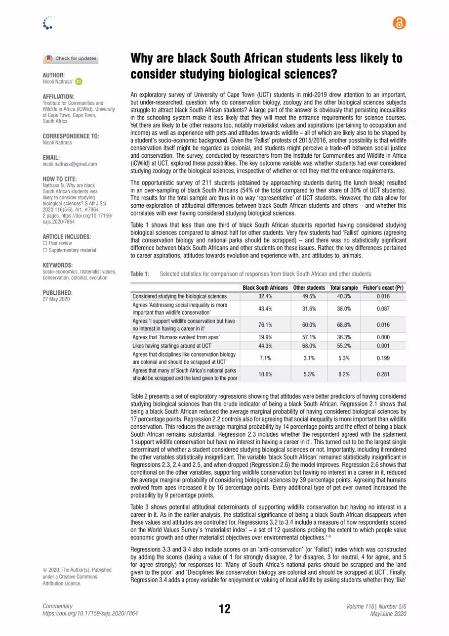
12 Volume 116| Number 5/6 May/June 2020

Commentaryhttps://doi.org/10.17159/sajs.2020/7864

© 2020. The Author(s). Published under a Creative Commons Attribution Licence.

Why are black South African students less likely to consider studying biological sciences?AUTHOR:

Nicoli Nattrass1

AFFILIATION:

1Institute for Communities and Wildlife in Africa (iCWild), University of Cape Town, Cape Town, South Africa

CORRESPONDENCE TO: Nicoli Nattrass

EMAIL: nicoli.nattrass@gmail.com

HOW TO CITE: Nattrass N. Why are black South African students less likely to consider studying biological sciences? S Afr J Sci. 2020;116(5/6), Art. #7864, 2 pages. https://doi.org/10.17159/sajs.2020/7864

ARTICLE INCLUDES:☐ Peer review ☐ Supplementary material

KEYWORDS: socio-economics, materialist values, conservation, colonial, evolution

PUBLISHED: 27 May 2020

An exploratory survey of University of Cape Town (UCT) students in mid-2019 drew attention to an important, but under-researched, question: why do conservation biology, zoology and the other biological sciences subjects struggle to attract black South African students? A large part of the answer is obviously that persisting inequalities in the schooling system make it less likely that they will meet the entrance requirements for science courses. Yet there are likely to be other reasons too, notably materialist values and aspirations (pertaining to occupation and income) as well as experience with pets and attitudes towards wildlife – all of which are likely also to be shaped by a student’s socio-economic background. Given the ‘Fallist’ protests of 2015/2016, another possibility is that wildlife conservation itself might be regarded as colonial, and students might perceive a trade-off between social justice and conservation. The survey, conducted by researchers from the Institute for Communities and Wildlife in Africa (iCWild) at UCT, explored these possibilities. The key outcome variable was whether students had ever considered studying zoology or the biological sciences, irrespective of whether or not they met the entrance requirements.

The opportunistic survey of 211 students (obtained by approaching students during the lunch break) resulted in an over-sampling of black South Africans (54% of the total compared to their share of 30% of UCT students). The results for the total sample are thus in no way ‘representative’ of UCT students. However, the data allow for some exploration of attitudinal differences between black South African students and others – and whether this correlates with ever having considered studying biological sciences.

Table 1 shows that less than one third of black South African students reported having considered studying biological sciences compared to almost half for other students. Very few students had ‘Fallist’ opinions (agreeing that conservation biology and national parks should be scrapped) – and there was no statistically significant difference between black South Africans and other students on these issues. Rather, the key differences pertained to career aspirations, attitudes towards evolution and experience with, and attitudes to, animals.

Table 1: Selected statistics for comparison of responses from black South African and other students

Black South Africans Other students Total sample Fisher’s exact (Pr)

Considered studying the biological sciences 32.4% 49.5% 40.3% 0.016

Agrees ‘Addressing social inequality is more important than wildlife conservation’

43.4% 31.6% 38.0% 0.087

Agrees ‘I support wildlife conservation but have no interest in having a career in it’

76.1% 60.0% 68.8% 0.016

Agrees that ‘Humans evolved from apes’ 19.9% 57.1% 36.3% 0.000

Likes having starlings around at UCT 44.3% 68.0% 55.2% 0.001

Agrees that disciplines like conservation biology are colonial and should be scrapped at UCT

7.1% 3.1% 5.3% 0.199

Agrees that many of South Africa’s national parks should be scrapped and the land given to the poor

10.6% 5.3% 8.2% 0.281

Table 2 presents a set of exploratory regressions showing that attitudes were better predictors of having considered studying biological sciences than the crude indicator of being a black South African. Regression 2.1 shows that being a black South African reduced the average marginal probability of having considered biological sciences by 17 percentage points. Regression 2.2 controls also for agreeing that social inequality is more important than wildlife conservation. This reduces the average marginal probability by 14 percentage points and the effect of being a black South African remains substantial. Regression 2.3 includes whether the respondent agreed with the statement ‘I support wildlife conservation but have no interest in having a career in it’. This turned out to be the largest single determinant of whether a student considered studying biological sciences or not. Importantly, including it rendered the other variables statistically insignificant. The variable ‘black South African’ remained statistically insignificant in Regressions 2.3, 2.4 and 2.5, and when dropped (Regression 2.6) the model improves. Regression 2.6 shows that conditional on the other variables, supporting wildlife conservation but having no interest in a career in it, reduced the average marginal probability of considering biological sciences by 39 percentage points. Agreeing that humans evolved from apes increased it by 16 percentage points. Every additional type of pet ever owned increased the probability by 9 percentage points.

Table 3 shows potential attitudinal determinants of supporting wildlife conservation but having no interest in a career in it. As in the earlier analysis, the statistical significance of being a black South African disappears when these values and attitudes are controlled for. Regressions 3.2 to 3.4 include a measure of how respondents scored on the World Values Survey’s ‘materialist index’ – a set of 12 questions probing the extent to which people value economic growth and other materialist objectives over environmental objectives.1-3

Regressions 3.3 and 3.4 also include scores on an ‘anti-conservation’ (or ‘Fallist’) index which was constructed by adding the scores (taking a value of 1 for strongly disagree, 2 for disagree, 3 for neutral, 4 for agree, and 5 for agree strongly) for responses to: ‘Many of South Africa’s national parks should be scrapped and the land given to the poor’ and ‘Disciplines like conservation biology are colonial and should be scrapped at UCT’. Finally, Regression 3.4 adds a proxy variable for enjoyment or valuing of local wildlife by asking students whether they ‘like’

13 Volume 116| Number 5/6 May/June 2020

Commentaryhttps://doi.org/10.17159/sajs.2020/7864

having starlings at UCT. Redwing starlings are common on the campus and bolder individuals have been known to ‘raid’ people’s lunches. Regression 3.4 (the strongest model) shows that, conditional on the other variables, a one unit increase in the materialism scale and a one unit increase in the anti-conservation scale, both increased the average marginal probability of having no interest in a career in conservation by 5 percentage points and that liking UCT’s starlings reduced it by 28 percentage points.

Table 3: Exploratory regressions on ‘Supports wildlife conservation but have no interest in pursuing a career in it’

VariableRegression

3.1 3.2 3.3 3.4

Black South African0.16*

(0.064) p=0.012

0.13 (0.068)

p=0.055

0.11 (0.068)

p=0.105

0.03 (0.067)

p=0.656

Score on the World Values Survey ‘materialist index’

0.06* (0.026)

p=0.028

0.05* (0.026)

p=0.042

0.05* (0.024)

p=0.031

Score on the ‘anti-conservation stance’ index

0.05** (0.021)

p=0.015

0.05* (0.020)

p=0.010

Likes having starlings around at UCT

-0.28*** (0.064)

p=0.000

Prob>chi2

Pseudo-R2

0.0125 0.0241

0.0064 0.0428

0.001 0.0682

0.000 0.1560

AIC BIC

256.14 262.81

232.04 241.80

227.36 240.35

210.68 230.16

Reporting average marginal effects for the coefficients (dy/dx) *p<0.05, **p<0.01, ***p<0.00

In short, the survey results suggest that black South African students are less likely to consider studying biological sciences than other students, and that this stance was linked primarily with career aspirations (supporting conservation but not wanting a career in it) – and these were associated with materialist values and attitudes to local wildlife.

Agreeing that ‘humans evolved from apes’ was the second biggest predictor of considering studying biological sciences, and the relatively high proportion of black South Africans who disagreed with this probably speaks to failures at school level with regard to the teaching of biological sciences and to the strength of religiosity in South Africa. We also found a strong relationship between the number of different pets owned by students and whether they had considered studying biological sciences. This variable is probably picking up attitudes towards and experience of companion animals as well as socio-economic status (pet ownership is more affordable for middle- and upper-income groups).

Materialist values (a key determinant of not desiring a career in conservation) are probably another indicator of socio-economic status as cross-national research shows that dominant social values shift from materialist to postmaterialist with economic development.2,3 This suggests that black South Africans may be interested in careers other than in conservation in part because of their relatively disadvantaged backgrounds which could prime them towards considering primarily the higher-paying occupations (accountancy, law). This, together with the fact that very few students were hostile to conservation, suggests that interest in conservation as a career and in studying biological sciences might increase as the black middle-class grows.

It is worth emphasising, however, that these findings are tentative and that all the regression models left a great deal of the variation unexplained. More research is needed on potential socio-economic and cultural correlates of having considered studying biological sciences or a career in conservation biology.

References1. Inglehart R Modernization and postmodernization: Cultural, economic

and political change in 43 societies. Princeton, NJ: Princeton University Press; 1997.

2. Inglehart R, Abramson PR. Measuring postmaterialism. Am Polit Sci Rev. 1999;93(3):665–677. https://doi.org/10.2307/2585581

3. Loubser J. Understanding the role of post-materialism in the trade-off between economic growth and the environment in BRICS countries. CSSR Working Paper no. 424. Cape Town: Centre for Social Science Research, University of Cape Town; 2018.

Black South African students and biological sciences Page 2 of 2

Table 2: Exploratory regressions on ‘Considered studying zoology or the biological sciences’

VariableRegression

2.1 2.2 2.3 2.4 2.5 2.6

Black South African-0.17* (0.068)

p=0.012

-0.16* (0.069)

p=0.020

-0.10 (0.065)

p=0.117

-0.04 (0.068)

p=0.584

-0.00 (0.068)

p=0.986

Agrees ‘Addressing social inequality is more important than wildlife conservation’

-0.14* (0.069)

p=0.037

-0.07 (0.066)

p=0.309

-0.09 (0.065)

p=0.187

-0.11 (0.065)

p=0.091

-0.11 (0.064)

p=0.088

Agrees ‘I support wildlife conservation but have no interest in having a career in it’

-0.41*** (0.073)

p=0.000

-0.43*** (0.071)

p=0.000

-0.39*** (0.074)

p=0.000

-0.39*** (0.074)

p=0.000

Agrees that ‘Humans evolved from apes’0.18*

(0.071) p=0.010

0.16* (0.071)

p=0.022

0.16* (0.066)

p=0.013

Number of different kinds of pets ever owned0.09** (0.034)

p=0.007

0.09** (0.037)

p=0.005

Prob>chi2

Pseudo-R2

0.0128 0.0223

0.0048 0.0389

0.000 0.1474

0.000 0.1790

0.000 0.2049

0.000 0.2049

AIC BIC

275.57 282.22

269.21 279.15

238.71 251.94

231.45 247.87

226.42 246.18

224.42 240.88

Reporting average marginal effects for the coefficients (dy/dx) *p<0.05, **p<0.01, ***p<0.000

14 Volume 116| Number 5/6 May/June 2020

Commentaryhttps://doi.org/10.17159/sajs.2020/7699

© 2020. The Author(s). Published under a Creative Commons Attribution Licence.

Medical Geology and its relevance in AfricaAUTHOR: Hassina Mouri1

AFFILIATION: 1Department of Geology, University of Johannesburg, Johannesburg, South Africa

CORRESPONDENCE TO: Hassina Mouri

EMAIL: hmouri@uj.ac.za

HOW TO CITE: Mouri H. Medical Geology and its relevance in Africa. S Afr J Sci. 2020;116(5/6), Art. #7699, 2 pages. https://doi.org/10.17159/sajs.2020/7699

ARTICLE INCLUDES:☐ Peer review ☐ Supplementary material

KEYWORDS: health, geology, Africa, University of Johannesburg, postgraduate studies

PUBLISHED: 27 May 2020

Medical GeologyMedical Geology is a relatively new discipline that is growing in importance. It is the field of science that deals with the impacts (positive or negative) of the geo-environment (including factors, processes and materials) on the health of humans and the ecosystem in general.1 It is based on multi-, cross- and inter-disciplinary approaches bringing together experts from various fields of science including epidemiology, toxicology, geoscience, the environmental disciplines and public health. Only by understanding the geological history and background of our environment will we be able to contribute towards a better and deeper insight into the range of natural hazards that can (directly or indirectly) affect our health and that of the ecosystem. This understanding may result in the mitigation or minimisation of impacts and in preventing some of the widespread and serious health problems, and may even save lives. For these reasons, Medical Geology is a highly significant field of research that contributes to the well-being of our community in line with the 2030 United Nations Agenda for Sustainable Development.2

The link between geology and health in briefRocks are made of minerals, and minerals are composed of chemical elements that can be released into our environment (soil, air and water) by natural processes, such as volcanic activity, earthquakes, weathering of rocks and rock–water interaction. Furthermore, mining activities can play a significant role in enhancing the release of chemical elements and minerals into the environment. Some minerals, such as talc, and certain forms of quartz and fibrous forms classified under the commercial name ‘asbestos’, can be harmful if they are present in the air as breathable particles. These minerals can cause serious pulmonary health problems including silicosis, talcosis and mesothelioma. Some chemical elements are, of course, essential for our well-being, among them calcium, magnesium, iron, iodine, fluoride and lithium for example. However, deficiency or excess of these elements in food or water can be detrimental to health. Some other elements such as arsenic, lead, cadmium and mercury, and radioactive elements such as uranium, thorium and radon are toxic, and their presence in the environment can be detrimental to human health.

The relevance of Medical Geology in AfricaAlthough Africa is rich in natural resources, poverty and disease levels are high when compared to some other regions in the world.3 Certainly, communicable diseases are among the leading causes of morbidity and mortality. However, we should not continue to underestimate the real and potential risks associated with the geogenic as well as the anthropogenic factors related to the exploitation of natural resources. These can contribute dramatically to the high rate of non-communicable diseases and mortality on the continent. The sections below on the geology of Africa and the health of its population outline the importance of developing the field of Medical Geology in Africa.

Geology of AfricaAfrica has a complex and dynamic geological evolution, which is characterised by frequent earthquakes and volcanic activity in regions like the East African Rift Valley. Throughout the continent, there are also pervasive dust storms and water toxicity due to interaction with the geo-environment. These geological processes, factors and materials can have negative impacts on the natural environment as well as on human and animal health. Our continent also has enormous geological wealth, which is subjected to anthropogenic activities, such as widespread mining activities and abandoned open mining sites. While mining is important for economic growth and sustainable development, if not properly managed, it can enhance the release of naturally occurring harmful minerals and elements into the environment, which in turn can have deleterious impacts. Geological research in Africa has been dominated by studies on geological evolution and on the identification and exploration of potential natural resources. However, very little attention is given to the possible impacts on health and ecosystems in general.

Health in AfricaGlobally, Africa has the highest neonatal mortality rate and the highest maternal mortality.3 It is worth noting that non-communicable diseases, such as diabetes, cancer and chronic respiratory tract and cardiovascular diseases, are the leading causes of morbidity and mortality in Africa, accounting for more than 50% of all deaths in some countries such as the Seychelles (59%) and Algeria (56%).3 Unfortunately, the primary causes of such diseases and mortality in general remain unclear in many cases and attention is instead focused on risk factors and treatment.

Medical Geology initiative at the University of JohannesburgFor the reasons above, in 2013 an attempt was made to develop Medical Geology at the postgraduate level at the University of Johannesburg in South Africa in collaboration with researchers from national and international institutions and industry. Since then, 16 students from different African countries, namely Nigeria, Ghana, Kenya, Namibia and South Africa, have registered for either an MSc or PhD on Medical Geology related research projects. Student support has come mainly from the National Research Foundation of South Africa through the Collaborative Postgraduate Training Programme and the University of Johannesburg’s prestigious Global Excellence and Stature Programme and University Research Committee funds. In addition, the initiative has benefitted from support by international organisations such as the International Union of Geological Science and the International Medical Geology Association in organising symposia and workshops in the field.

Recently completed research projects So far, the projects within this initiative have mainly dealt with establishing a relationship between environmental geochemistry/mineralogy and human and animal health in specific African countries. More than 30 research

15 Volume 116| Number 5/6 May/June 2020

Commentaryhttps://doi.org/10.17159/sajs.2020/7699

papers in international, peer-reviewed journals and conference abstract volumes have been published since the start of the initiative. Selected examples follow:

• High fluorine and dental fluorosis prevalence from the Nakuru area, Kenyan Rift. For the first time, this study established a clear link between the high fluorine content in water and dental fluorosis as well as the spatial distribution of fluorine concentrations in this area.4,5

• Impact of toxic elements present in geophagic material on pregnant women in Onangama village, northern Namibia. This is the first detailed geochemical and mineralogical study of this kind in Namibia, despite the high prevalence of the geophagic practice amongst pregnant women especially. This study enabled the discovery that the consumed materials contain high concentrations of several toxic elements including arsenic and mercury, which are detrimental to the health of consumers and unborn babies.6,7

• The uranium and radon gas concentration and their impacts on human health with reference to a case study from abandoned gold mine tailings in the West Rand area, Krugersdorp, South Africa. This study demonstrated that mine tailings in the area have high uranium concentrations (up to 149.76 ppm) and high levels of radon (up to 1068.8 Bq/m3) – more than 10-fold the recommended value of 1 mSv/y proposed by the National Nuclear Regulator of South Africa and the International Commission on Radiological Protection. These high levels are a serious health risk to the people of the area where there is a high percentage of deaths from lung cancer.8

Concluding remarksMedical Geology is a relatively developed field in some regions of the world. However, in Africa it is still developing, although it is on this continent that the application of this research would be most relevant. Considering the significance of the geo-environmental materials, factors and processes including geogenic and anthropogenic activities and the frequency of the occurrence of non-communicable diseases, it is important to develop this field through collaborative research projects as well as through training of a new generation of researchers to investigate possible correlations.

The development of Medical Geology at the University of Johannesburg has attracted several postgraduate students from Africa. Furthermore, the results obtained from completed research projects show promising and interesting correlations between geo-environmental factors, materials and processes and certain common non-communicable diseases. The programme clearly demonstrates that Medical Geology has a broad and strong pan-African appeal and is an essential part of African development. With dedicated leadership and financial support, this field of research can be attractive to students and contribute to the health and well-being of our society as well as the economic growth of the continent.

This Commentary draws on my unpublished Professorial Inaugural Lecture at the University of Johannesburg on 15 October 20199 and a

chapter10 accepted for publication in an upcoming book on the practical application of Medical Geology.

AcknowledgementsI acknowledge the financial support provided by the University of Johannesburg through the Global Excellence and Stature Programme and University Research Committee and Faculty Research Committee funds, and by the National Research Foundation (South Africa) through funding for Rated Researchers and the Collaborative Postgraduate Training Programme. Special thanks to all colleagues involved for their support.

References1. Buck BJ, Londono SC, McLaurin BT, Metcalf R, Mouri H, Selinus O, et al.

The emerging field of medical geology in brief: Some examples. Environ Earth Sci. 2016;75:449. https://doi.org/10.1007/s12665-016-5362-6

2. United Nations General Assembly. Draft outcome document of the United Nations summit for the adoption of the post-2015 development agenda [document on the Internet]. c2015 [cited 2020 Jan 30]. Available from: https://digitallibrary.un.org/record/800852?ln=en

3. The state of health in the WHO African Region: An analysis of the status of health, health services and health systems in the context of the Sustainable Development Goals. Brazzaville: WHO Regional Office for Africa; 2018.

4. Gevera P, Mouri H. Natural occurrence of potentially harmful fluoride contamination in groundwater: An example from Nakuru County, the Kenyan Rift Valley. Environ Earth Sci. 2018;77:365. https://doi.org/10.1007/s12665-018-7466-7

5. Gevera P, Mouri H, Maronga G. Occurrence of fluorosis in a population living in a high-fluoride groundwater area: Nakuru area in the Central Kenyan Rift Valley. Environ Geochem Health. 2019;41:829–840. https://doi.org/10.1007/s10653-018-0180-2

6. Kambunga SN, Candeias C, Hasheela I, Mouri H. Review of the nature of some geophagic materials and their potential health effects on pregnant women: Some examples from Africa. Environ Geochem Health. 2019;41:2949–2975. https://doi.org/10.1007/s10653-019-00288-5

7. Kambunga SN, Candeias C, Hasheela I, Mouri H. The geochemistry of geophagic material consumed in Onangama Village, Northern Namibia: A potential health hazard for pregnant women in the area. Environ Geochem Health. 2019;41:1987–2009. https://doi.org/10.1007/s10653-019-00253-2

8. Moshupya P, Abiye T, Mouri H, Levin M, Strauss M, Strydom R. Assessment of radon levels and impact on human health in a region dominated by abandoned gold mine tailings: A case from the West Rand area, Krugersdorp, South Africa. Geosciences. 2019;9(11):466. https://doi.org/10.3390/geosciences9110466

9. Mouri H. Medical geology and its relevance in Africa. Professorial Inauguration Lecture; 2019 October 15; University of Johannesburg, South Africa. Available from: https://www.youtube.com/watch?v=y8tY9bOhmwA

10. Mouri H. Medical geology in Africa: An example of a successful educational and research initiative at the University of Johannesburg, South Africa. In: Siegel M, Finkelman R, Selinus O, editors. Practical applications of medical geology. In press 2019.

Medical Geology and its relevance in Africa Page 2 of 2

Staff and postgraduate students of Medical Geology at the ‘Second International Symposium on Medical Geology in Africa’ in November 2018.

16 Volume 116| Number 5/6 May/June 2020

Marine Plastic Debris: News and Viewshttps://doi.org/10.17159/sajs.2020/8095

© 2020. The Author(s). Published under a Creative Commons Attribution Licence.

South African Initiative to End Plastic Pollution in the EnvironmentAUTHOR:

Anton Hanekom1

AFFILIATION: 1Plastics South Africa, Johannesburg, South Africa

CORRESPONDENCE TO: Anton Hanekom

EMAIL: anton.hanekom@plasticssa.co.za

HOW TO CITE: Hanekom A. South African Initiative to End Plastic Pollution in the Environment. S Afr J Sci. 2020;116(5/6), Art. #8095, 2 pages. https://doi.org/10.17159/sajs.2020/8095

ARTICLE INCLUDES:☐ Peer review ☐ Supplementary material

KEYWORDS: plastics industry, waste management infrastructure, working groups

PUBLISHED: 27 May 2020

Never before has the issue of plastic pollution – and specifically plastics in our oceans – received so much public attention. During the last 2 years in particular, global initiatives such as the New Plastic Economy Global Commitments1 and the Alliance to End Plastic Waste2 were created with the aim of encouraging players in the global plastics industry to pledge their commitment to reducing plastic pollution in the oceans.

Whilst these efforts are commendable, they fail to address the unique challenges we face in South Africa with regard to waste management infrastructure, education and awareness. These are all issues that need to be addressed urgently and directly, and we cannot afford to wait 5 years for these international alliances eventually to shift their focus to South Africa.

The South African Initiative to End Plastic Pollution in the EnvironmentRecognising the need to develop a workable local plan that would fit the South African context and address our unique environmental, social, economic and political issues, the South African Initiative to End Plastic Pollution in the Environment3 was formed in 2019.

As part of this alliance, all players in the local plastics packaging value chain are represented, including the chemicals sector, polymer and/or raw material producers, importers, packaging converters, retailers, international and local brand owners, fast food franchises, producer responsibility organisations together with many other stakeholders, such as the Department of Environment, Forestry and Fisheries, the Department of Trade and Industry, and the United Nations Environment Programme. All members have committed to join forces and collaborate in order to have a positive impact on the environment by working towards the prevention, and ultimately the end, of plastic pollution in the environment.

Working groupsCoordinated by the Consumer Goods Council of South Africa, finding solutions and developing the best environmentally sustainable application for problematic ‘single-use’ packaging is top of the agenda for the South African Initiative. This priority is closely followed by the need to develop a plan of action that will increase the collection and recycling rate of plastics in South Africa and to manufacture more products with increased recycled content.

Six working groups were formed to look inter alia at: (1) technology, innovation and design; (2) infrastructure; (3) bioplastics and alternatives; (4) education and awareness in combatting litter; (5) standards and compliance; and (6) integrating waste pickers into the circular economy. The mandate of these working groups is to find solutions to specific problems based on sustainable life-cycle assessments, updated information obtained from research facilities and technological landscapes, and ensuring support and buy-in from government, business, NGOs, existing environmental and community networks, and consumers. Solutions must be based on international best practices but developed specifically for the South African context and with the purpose of changing human behaviour in the process.

Technology, innovation and design Improving the South African plastics industry’s success with design for sustainability; increasing recycled content in products; securing demand for recyclate; scaling the generation of energy from waste; developing end-markets for recycled plastic; and developing refuse-derived fuels, form part of the remit of the Technology, Innovation and Design Working Group. This is done by considering the country’s waste management system, exploring existing networks and drawing on existing local and international research and technology.

InfrastructureAccording to The State of Waste Report4, 34% of South Africans do not have access to any waste management or removal services. An estimated 70% of all materials recycled originate from landfill and other post-consumer sources.5 It is a sad reality that in South Africa, recyclables are still being sourced from landfill at high cost and under poor working conditions for informal waste pickers. This is far from an ideal situation, as recyclable plastic is a valuable resource and should be removed from the solid waste stream before reaching landfill where it becomes contaminated and extraction becomes costly. One of our biggest challenges to improve the collection and recycling rate of plastics in South Africa has been getting access to this high value material before it gets sent to landfill or ends up in our oceans via rivers and streams. The only way this can be done is through developing and implementing effective waste management services and infrastructure. This is the primary focus area of the Infrastructure Working Group, which is currently investigating how best to divert plastic waste from landfill and the environment by evaluating existing infrastructure, river catchment projects, the recently launched Good Green Deeds campaign6 as well as linking existing local and global networks. The ultimate objective is to support infrastructure, create blueprint model(s) for implementation, and roll out relevant waste management projects.

One possibility that is currently on the table for communities that are without waste management infrastructure, is to create materials recovery or technology hubs. These hubs will be facilities established in central points and which operate within a short distance from the sources of waste. These hubs will accept and sort all types of packaging waste, from where it will be baled either for selling to recyclers (high-value waste) or for processing and converting into furniture, building materials or other products to meet community needs (low-value or non-recyclable waste). The idea behind these hubs is to work as much as possible with local communities in creating beneficiation

17 Volume 116| Number 5/6 May/June 2020

Marine Plastic Debris: News and Viewshttps://doi.org/10.17159/sajs.2020/8095

enterprises and jobs, determining what products are required for the local community and identifying suitable entrepreneurs to be trained and set up in self-funded, sustainable businesses. This type of blueprint will then be applied to identified crisis areas and will be scalable according to the community’s location.

Bioplastics and alternatives The introduction of biodegradable and compostable material remains a major concern for the plastic recycling industry, as the required infrastructure to separately collect and process these materials (e.g. commercial composting facilities) does not currently exist in South Africa. These alternatives to conventional plastic packaging also do not change consumer behaviour when it comes to littering. If these materials inadvertently end up contaminating the recycling stream, there is the potential of simply replacing one problem with another.

In an effort to investigate and address these issues, a special Bioplastics and Alternatives Working Group has been formed. This group is currently developing a position paper on the topic in partnership with the Moss Group. However, the Working Group is also urging retailers and brand owners to consider various factors before introducing such packaging products, for example, emphasising the importance of using appropriate labels and logos to ensure they are easily differentiated from their conventional counterparts.

Education and awarenessThe Education and Awareness Working Group’s goals are centred around raising awareness about recycling through various educational campaigns that make use of information booklets, pamphlets, websites, mobile apps and clean-up events. The group is developing a plan of action that builds on existing and new networks in communities, industry and government, in order to improve awareness among schools, townships and suburbs, consumers, industry and retailers, government and waste management companies. The group also aims to enhance the development of skills among entrepreneurs, waste pickers and waste management businesses when it comes to identifying, collecting, reusing and recycling plastic.

Standards and compliance, integration of waste pickersFollowing a briefing meeting between representatives of the South African Initiative to End Plastic Pollution and the Minister of Environment, Forestry and Fisheries, to inform her of progress made to date by the various working groups, Minister Creecy requested that two more working groups be formed: one with a specific focus on standards and compliance, and another to look at the integration of waste pickers into the circular economy. These two streams play a critical part in stopping plastic pollution and improving the collection and recycling rates of plastics in South Africa.

Building on recycling successesDespite the inadequate waste management infrastructure and other challenges mentioned earlier, it is important to note that plastic waste is being collected and recycled in South Africa thanks to a dynamic, growing and well-supported plastic recycling industry.

During 2018, 46.3% of plastic waste was collected for recycling, making South Africa one of the best mechanical recyclers in the world.5 More than 519 370 tons of plastic waste was collected for recycling, providing direct employment to more than 7800 people and creating a further 58 500 income-generating jobs. Moreover, ZAR2.3 billion was injected into the informal sector through the purchasing of recyclable plastic waste.

In addition, in 2018 plastic recycling saved 246 000 tons of CO2 – the equivalent emissions of 51 200 cars and saved enough oil to fuel 200 000 cars for 1 year travelling 30 000 km/annum. Although more can, and should, be done to encourage South African households to recycle, the plastics industry has already made some important strides forward in recent years. One such achievement has been getting the manufacturers of plastic bags to remove fillers in order to produce bags that are fully

recyclable. In addition, 100% certified recycled plastic material is now used to produce some carrier bags. This creates an end-market for recycled plastic products and helps to reduce waste to landfill.

Plans of actionThere are various external factors that need to be taken into consideration and that could impact the timeline of implementing the various plans that are currently being developed by the South African Initiative. Most notably would be the impact of Minister Creecy’s announcement in December 2019 that she has decided to scrap the Section 28 plan for developing an Industry Waste Management Plan for the paper and packaging industry, in favour of a new Section 18 plan of the Waste Management Act7 that would allow for an industry-managed extended producer responsibility scheme.

The plastics industry welcomed this decision as it has always advocated for an industry-managed plan where the producers of packaging materials are held responsible for managing their waste, by belonging to industry bodies that represent their interests and drive their own recycling and collection efforts. This process needs to be managed in a manner that allows for close cooperation and direct accountability to government, but with the highest commitment to proper governance, transparency and credibility, leaving the industry in control of their own funds and projects.

The framework for the new Section 18 plan is currently being developed in close consultation with industry representatives, and the aims, objectives and progress made to date by the South African Initiative to End Plastic Pollution are also being considered and incorporated into the new strategy.

ConclusionIt is clear that the growing problem of plastic pollution in the environment cannot be solved by one organisation or a single individual. Multiple, supportive projects that run concurrently are needed to be truly effective and create greater change. Such change does not happen overnight: it starts with the desire, and one small step in the right direction.

This Initiative is a collaborative effort and the plastics industry is relieved and excited to have the complete value chain represented as we stand together to find effective and environmentally friendly solutions for our specific waste problems. Whilst much of the detail still needs to be determined, every journey of a thousand miles begins with a single step. Will you join us?

References1. Ellen MacArthur Foundation. Global commitment: A circular economy for

plastic in which it never becomes waste [webpage on the Internet]. c2018 [cited 2020 Mar 25]. Available from: https://www.newplasticseconomy.org/projects/global-commitment

2. Alliance to End Plastic Waste [webpage on the Internet]. c2019 [cited 2020 Mar 25]. Available from: https://endplasticwaste.org

3. Plastics SA. South African Initiative to end Plastic Pollution [webpage on the Internet]. c2019 [cited 2020 Mar 25]. Available from: https://www.plasticsinfo.co.za/2019/07/23/plastics-sa-announces-pollution-alliance/

4. South African Department of Environmental Affairs. South Africa state of waste report [document on the Internet]. c2018 [cited 2020 Mar 25]. Available from: http://sawic.environment.gov.za/documents/11132.pdf

5. Plastics SA. Plastics Recycling in SA [document on the Internet]. c2018 [cited 2020 Mar 25]. Available from: https://www.plasticsinfo.co.za/wp-content/uploads/2019/12/Plastics-Recycling-in-SA-July-2018-Executive-Summary-final.pdf

6. South African Department of Environmental Affairs. Good Green Deeds campaign [webpage on the Internet]. c2019 [cited 2020 Mar 25]. Available from: https://www.environment.gov.za/event/deptactivity/goodgreendeeds

7. Withdrawal of The Section 28 Notice Calling for Paper and Packing Industry, Electrical and Electronic Industry and Lighting Industry Waste Management Plans in Terms of Section 28 of the National Environmental Management: Waste Act 208 [document on the Internet]. c2019 [cited 2020 Mar 25]. Available from:https://www.gov.za/sites/default/files/gcis_document/201912/42909gon1659.pdf

Marine Plastic Debris: A South African initiative Page 2 of 2

18 Volume 116| Number 5/6 May/June 2020

Marine Plastic Debris: News and Viewshttps://doi.org/10.17159/sajs.2020/8097

© 2020. The Author(s). Published under a Creative Commons Attribution Licence.

A circular economy response to plastic pollution: Current policy landscape and consumer perceptionAUTHORS:

Lorren de Kock1 Zaynab Sadan1

Reinhardt Arp1

Prabhat Upadhyaya1

AFFILIATION: 1WWF South Africa, Cape Town, South Africa

CORRESPONDENCE TO: Lorren de Kock

EMAIL: ldekock@wwf.org.za

HOW TO CITE: De Kock L, Sadan Z, Arp R, Upadhyaya P. A circular economy response to plastic pollution: Current policy landscape and consumer perception. S Afr J Sci. 2020;116(5/6), Art. #8097, 2 pages. https://doi.org/10.17159/sajs.2020/8097

ARTICLE INCLUDES:☐ Peer review ☐ Supplementary material

KEYWORDS: plastics value chain, extended producer responsibility, accountability

PUBLISHED: 27 May 2020

The increasing volume of plastic pollution in South Africa clogs our waterways and litters our landscapes, placing an increasing strain on our land, freshwater and marine environments that provide goods and services vital for sustaining life, human well-being, and economic development. Globally, as of 2015, approximately 6300 million metric tons (MT) of plastic waste had been generated, and of that around 9% had been recycled, 12% incinerated and 79% accumulated in landfills or in the natural environment.1 Research shows that approximately 8 MT of plastic leaks into the ocean every year.2

The ever-increasing demand for plastic has seen production grow from 5 MT in 1950 to over 380 MT in 2015, at a compound annual growth rate of 8.4%. It is predicted that production will increase by 40% between 2015 and 2030 under a business-as-usual scenario.3 This deluge of plastic exceeds the current waste collection capacity and hence the natural environment becomes the final sink for plastic pollution. The largest volume of global plastic production is used in packaging applications. It is this plastic that is leaking into the environment at an unprecedented scale.3 One of the main reasons for this is the increasing consumption of on-the-go snack products and ready-made meals which, by virtue of their application, require lightweight, smaller and durable packaging materials. Until recently, the focus has been on end-of-pipe solutions which include downstream processing of waste, such as environmental clean-ups and waste collection. This requires huge resources to be dedicated to environmental clean-ups, as well as to scaling up collection and management systems to tackle plastic waste. Whilst such interventions are important, they do not go to the root of the problem – the production and consumption systems that promote unnecessary and avoidable plastics. Owing to the complex and systemic nature of the plastic pollution, multiple interventions are needed across all stages of the plastics life cycle and value chain if we are to have meaningful impact on reducing plastic pollution.

Derived from fossil fuels, plastics contribute to climate change by releasing greenhouse gas (GHG) emissions during their production, processing and disposal.4 Global life-cycle GHG emissions from plastic are expected to increase by 382%, from 1.7 to 6.5 gigatons of carbon dioxide equivalent5 (GtCO2e), between 2015 and 2050. This is primarily due to the push from petrochemical companies and plastic manufacturers to increase plastics production to meet the forecasted demand, with subsequent emissions from incineration.6

The circular economy is a ‘framework for an economy that is restorative and regenerative by design’7 and mimics the functioning of nature. The circular economy concept provides a solution to the plastic pollution quandary by providing a way forward to decouple material consumption from economic growth, and increase the value of secondary material, ultimately decreasing waste and pollution. Transitioning to a circular economy is critical for achieving deep emissions reductions and transitioning to a low-carbon economy.8 In addition, reusing or recycling materials after use into a secondary resource, reduces the need for virgin resources and thus can also lower the carbon intensity of the system.

In addition to environmental benefits, the circular economy model could provide socio-economic benefits as it is expected to create approximately 45–50 million jobs globally in both the waste management and service sectors.9 The plastics sector is ideally poised to capture some of these employment benefits by creating new opportunities in redesigning products for circularity (ensuring they are reusable, recyclable and repairable); redesigning and implementing circular delivery models; developing infrastructure for secondary resource material recovery; and reskilling workers in the current system to take advantage of these new opportunities.

Plastic pollution is a global challenge that calls for systemic change in the way we produce, use and dispose of plastics at national and global levels. The focus needs to move away from solely end-of-pipe solutions to include systemic interventions at the level of policy and governance, as well as actions across the plastics value chain, taking local consumer perceptions into account. Plastic is a valuable material when used and managed effectively. It continues to hold economic value even after it is thrown away and therefore should be circulated within the economy. How to get to a state of circular plastic flow is the key question.

Policy landscapeGlobal and regional policy on plasticsAt a global level, a number of international strategies and legal frameworks exist.10 However, there are shortcomings in these existing frameworks because only a limited number of countries participate; the approach to addressing plastic pollution is fragmented; and there are no compliance mechanisms, funding systems or effective implementation support architectures. As a result, assigning accountability remains a fundamental flaw in these strategies and frameworks. WWF recognises and supports the need for an effective global response to plastic pollution through a new global legally binding agreement. Such a treaty would make reducing plastic pollution a joint global undertaking, setting clear responsibilities for states and ensuring accountability for the growing production, consumption and leakage of plastics into the environment.

The United Nations Environment Assembly (UNEA) has adopted resolutions on marine litter and microplastics from its first meeting in 2014. They call for strengthening the United Nations Environment Programme’s role in taking action on marine debris and microplastics in UNEA-1; establishing the Ad-Hoc Open-Ended Expert Group on Marine Litter and Microplastics in UNEA-3; and re-emphasising the issue of marine plastic litter and microplastics and acknowledging single-use plastics in UNEA-4. The resolutions also call for greater efforts at collaboration

19 Volume 116| Number 5/6 May/June 2020

Marine Plastic Debris: News and Viewshttps://doi.org/10.17159/sajs.2020/8097

and coordination. These resolutions are the first steps in developing a systemic understanding of plastic pollution in order to inform collective global action going forward.

The African Ministerial Conference on the Environment (AMCEN) held in Durban, South Africa, in November 2019 was crucial in emphasising the need to address plastic pollution. All 54 member states supported a declaration calling for global action on plastic pollution and suggested the possibility of exploring a new global agreement. With Minister Creecy President of AMCEN until 2021, South Africa can be instrumental in leading other African environmental ministers to take a strong position on plastic pollution. African governments have now joined the Nordic, Caribbean, South East Asian and Pacific states in their call for strong global action on plastic pollution.

National and sub-national policySouth Africa already has some regulatory and economic instruments in place, such as the ban and levy on plastic carrier bags (2003), regulations requiring the licencing of waste facilities, and the development of waste management standards. However, other instruments such as (dis)incentives to move away from problematic and unnecessary plastic products and packaging need to be implemented to better enable the transition to a circular plastics economy. For example, the adoption of Section 18 of the National Waste Management Act as a mechanism for implementing extended producer responsibility. The proposed landfill taxation is commendable but constraints – such as infrastructure, capacity and accurate reporting – will need to be overcome before taking this forward. With regard to information-based instruments, a Packaging Guideline and Packaging Certification scheme is being developed through Operation Phakisa: Chemicals and Waste in consultation with industry stakeholders.

The recent emergence of global voluntary agreements, such as the national Plastic Pact network of the Ellen MacArthur Foundation, complements the policy instruments already under development in many countries. The South African Plastics Pact was launched in January 2020 and provides an appropriate platform for multi-stakeholder collaboration across the plastics value chain, while also promoting accountability in achieving 2025 targets through annual public reporting. It is to be noted that voluntary agreements on sustainability challenges, such as plastics and food waste, which are cross-sectoral in nature, need to take a multi-sector and multi-stakeholder approach in order to obtain the systemic shifts that are required to address sustainability concerns. Through the Plastics Pact, South Africa has initiated the journey to develop and implement these actions, but this will need to be complemented by policy interventions to overcome the current barriers and inertia that prevent transition to a circular plastics economy.

Owing to the complex and systemic nature of the plastics value chain, a suite of policy interventions is required at multiple levels of influence. Taking an evidence-based policy approach is critical for the transition from the current linear model to a circular plastic material flow. Appropriate policy instruments need to be deployed across the material and product life cycle of plastics, such as potential taxes on virgin material at production, targets for recycled content in products for convertors and eco-modulated extended producer responsibility, amongst others. Focusing solely on end-of-pipe solutions shifts the locus of action on consumers and addresses only the symptoms, whilst it is action at all stages and in each sector that is required.

Current consumer perceptionsIn 2019, WWF-SA commissioned a study to determine consumer perceptions of plastic products and packaging in South Africa. It aimed to define different segments within the local consumer market based

on attitudes and perceptions around plastic pollution, including levels of awareness about plastic pollution and perceptions of who is responsible for the current predicament.

The findings indicated that plastic pollution is ranked relatively low compared with other issues that South Africans face, such as unemployment, crime and climate change. While there has been growing awareness of the negative impacts of plastic pollution, it has not led to consistent action, due to barriers that include misinformation, disempowerment, convenience and cost. Recycling is perceived as the only action required to clean up the environment, even though only a small proportion of plastic packaging is effectively recycled in South Africa. The main incentive for the majority of consumers to recycle plastics appears to be economic gain. Interestingly, no one in the study sample mentioned reducing the consumption of plastics in order to curb leakage into the environment and reduce the increasing volumes of plastic waste that are generated.

In terms of responsibility, most survey respondents identified littering as a problem, indicating that the current narrative from industry and government, that plastic pollution is a nuisance issue, has taken hold. This makes it difficult to appreciate the wider implications of plastic pollution. However, there is consensus that consumers can have positive impacts by taking responsibility for what they buy, and that solutions lie with manufacturers, government, retailers and brand owners.

WWF views the current idea that consumers are the only ones who can take action as a flawed one, and we encourage consumers to be more vociferous in demanding accountability higher in the plastics value chain.

References1. Geyer R, Jambeck JR, Law KL. Production, use, and fate of all plastics ever

made. Sci Adv. 2017;3(7):25–29. https://doi.org/10.1126/sciadv.1700782

2. Ellen MacArthur Foundation. New economy of plastics: Catalysing action. Geneva / Isle of Wight: World Economic Forum / Ellen MacArthur Foundation; 2017. Available from: http://www.ellenmacarthurfoundation.org/publications)

3. Hamilton A, Scheer R, Stakes T, Allan S. Solving plastic pollution through accountability. Gland: WWF; 2019. Available from: https://c402277.ssl.cf1.rackcdn.com/publications/1212/files/original/SOLVING_PLASTIC_POLLUTION_THROUGH_ACCOUNTABILITY_ENF_SINGLE.pdf?1551798060

4. Hamilton LA, Feit S, Muffett C, Kelso M. Plastic & climate: The hidden costs of plastic planet. Washington DC: Center of International Environmental Law; 2019. Available from: https://www.ciel.org/wp-content/uploads/2019/05/Plastic-and-Climate-FINAL-2019.pdf

5. OECD Glossary of Statistical Terms. Carbon dioxide equivalent [webpage on the Internet]. No date [cited 2020 Mar 10]. Available from: https://stats.oecd.org/glossary/detail.asp?ID=285

6. Zheng J, Suh S. Strategies to reduce the global carbon footprint of plastics. Nat Clim Change. 2019;9(5):374–378. http://dx.doi.org/10.1038/s41558-019-0459-z

7. Ellen MacArthur Foundation. What is the circular economy? [webpage on the Internet]. No date [cited 2020 Feb 14]. Available from: https://www.ellenmacarthurfoundation.org/circular-economy/what-is-the-circular-economy

8. Ellen MacArthur Foundation. Completing the picture: How the circular economy tackles climate change [webpage on the Internet]. No date [cited 2020 Feb 14]. Available from: www.ellenmacarthurfoundation.org/publications

9. International Labour Organization (ILO). World employment and social outlook 2018: Greening with jobs. Geneva: ILO; 2018. Available from: https://www.ilo.org/wcmsp5/groups/public/---dgreports/---dcomm/---publ/documents/publication/wcms_628654.pdf

10. Lindebjerg E. WWF Policy paper: Tackling marine plastic pollution. Gland: WWF; 2019.

Marine Plastic Debris: A circular economy response Page 2 of 2

20 Volume 116| Number 5/6 May/June 2020

Marine Plastic Debris: News and Viewshttps://doi.org/10.17159/sajs.2020/8104

© 2020. The Author(s). Published under a Creative Commons Attribution Licence.

The African Marine Waste Network and its aim to achieve ‘Zero Plastics to the Seas of Africa’AUTHORS:

Danica Marlin1 Anthony J. Ribbink1

AFFILIATION: 1Sustainable Seas Trust, Port Elizabeth, South Africa

CORRESPONDENCE TO: Danica Marlin

EMAIL: dani@sstafrica.org.za

HOW TO CITE: Marlin D, Ribbink AJ. The African Marine Waste Network and its aim to achieve ‘Zero Plastics to the Seas of Africa’. S Afr J Sci. 2020;116(5/6), Art. #8104, 2 pages. https://doi.org/10.17159/sajs.2020/8104

ARTICLE INCLUDES:☐ Peer review ☐ Supplementary material

KEYWORDS: plastic pollution, waste management, education, communication, research

PUBLISHED: 27 May 2020

In response to the global pollution crisis, the United Nations Environmental Assembly has called upon all people to commit to its initiative ‘Towards a Pollution-Free Planet’.1 In support, the African Marine Waste Network (AMWN) was launched in 2016 as the main programme of the Sustainable Seas Trust and has committed to work with all 54 African countries to assist them in improving waste management, thereby reducing the amount of plastic entering the sea. Africa faces many waste management challenges, which are compounded by high population growth rates; a rapid rate of urbanisation; a growing middle-class, which is increasing consumption rates2; and high levels of poverty. Collectively, these factors are said to account for Africa potentially becoming the most plastic-polluted continent within a few decades.3

The Inaugural International Conference of the AMWN was held in 2017, at which, through guidance from African and global experts, the ‘Towards Zero Plastics to the Seas of Africa’ objective was developed. The focus of the AMWN is to prevent marine pollution from both land- and marine-based sources by 2035. The conference revealed that Africa: is data poor and therefore has no measurable aspects upon which to build strategies and against which to monitor progress; does not have adequate education and capacity, including municipal capacity, to handle issues around pollution and waste management; has decision-makers and ordinary citizens who are not informed about plastic waste issues.

Purpose and aims of the African Marine Waste NetworkThe AMWN aims to be an active platform for collaboration and resource and knowledge sharing across Africa. This aim is to be achieved by building and strengthening networks among civil society, industry, NGOs and governments. The greatest challenge is to motivate people to care for the environment and convince them to reduce and to responsibly manage the plastics they use. Waste management facilities and services are poor in most of Africa, and it is therefore important to work with municipalities to appreciate the value of waste and thus encourage investment in the necessary infrastructure. The AMWN aims to support African governments to develop and implement appropriate waste management. Creative and novel methods to educate and communicate are needed to change public thinking and behaviour, and opportunities for local business development within communities need to be explored. The approach of the AMWN is to find solutions and to develop strategies based on solid evidence and that are measurable so that progress can be evaluated.

Monitoring programmesA role of the AMWN is to test monitoring programmes that serve waste management objectives, and to roll out the successful methods to all African countries. In 2018, the AMWN began developing methods for measuring waste and for addressing issues such as waste education and economic incentives. Nelson Mandela Bay Municipality (NMBM), South Africa, was selected as the area in which to test proof of concept as it is large enough to be representative of a large African coastal city yet small enough to be manageable. Feasibility studies to test methods that quantify and monitor waste were conducted to provide baselines for the amounts of litter in South Africa. These are some of the first studies used to try to quantify mismanaged waste in Africa.

In 2019, the AMWN worked closely with the Western Indian Ocean Marine Science Association (WIOMSA) and rolled out the ‘Zero Plastics to the Seas of Africa’ project in Kenya, Madagascar, Mauritius, Mozambique, Seychelles, South Africa and Tanzania – the first multinational, regional litter monitoring project in Africa. These seven countries use the same techniques to sample macro- and mesolitter found on beaches, in rivers and mangroves. Preliminary results from an accumulation survey of one beach in NMBM during 2019 indicated that 65% of litter items are plastic, but that these accounted for only 12% of the items by weight (Sustainable Seas Trust, unpublished data). This project will continue until the end of 2021. The project aims to start monitoring street litter in 2020, and to roll out the methods in interested coastal and island countries in the east and west of Africa. Subsequently, the project hopes to reach those African countries with coastlines along the Red and Mediterranean Seas. In partnership with WIOMSA, AMWN is also compiling a Litter Monitoring Manual, to ensure that the methods described in the manual account for the variable human and funding resources, as well as the highly variable amounts of litter found in Africa. The Manual will be translated into three languages (Portuguese, Swahili and French) in 2020, and into other languages spoken in Africa in following years.

ResearchAnother research project of the AMWN investigates microplastic-related pollutants (MRPs) in organisms at different levels of the food web in Algoa Bay, South Africa. Data from this project will be used to create awareness of the health consequences of plastic waste entering the seas. During 2018, methods were tested to determine whether MRPs could be detected in selected organisms in Algoa Bay. The following year it was confirmed that the methods positively detected MRPs in the organisms and therefore other organisms will be tested in 2020 and 2021 to give a holistic picture of MRPs in the food web.

Owing to Africa’s vast size and the challenge of accessibility in many areas, the use of remote-sensing techniques to measure litter has been tested. At the beginning of 2019, unmanned aerial vehicles were used to survey a selected area of NMBM for litter. Tested methods and resolutions were used to determine whether litter loads could be quantified from the imagery obtained from these vehicles. Based on the findings from this initial survey, five

21 Volume 116| Number 5/6 May/June 2020

Marine Plastic Debris: News and Viewshttps://doi.org/10.17159/sajs.2020/8104

sites were selected and surveyed early in 2020. These sites and more will continue to be surveyed at least twice a year to monitor whether litter loads in NMBM are decreasing.

At the end of 2019, the AMWN started developing a mobile application designed for citizens and scientists that will teach users about plastic waste. Whilst there are already many litter monitoring mobile apps, there is a need for an app that is specific to African conditions. This app must cater to citizens who have a low level of education, and the data obtained must be stored with an African data server to ensure that it is readily available at costs lower than those for data from servers outside Africa. Additionally, the litter monitoring mobile app is being designed to complement the above-mentioned Litter Monitoring Manual (i.e. litter items to be monitored via the app are based on the datasheets of the Manual), ensuring that litter data will be collected in a comparable manner.

To increase the network’s reach and connect stakeholders, the AMWN is developing the ‘Are you on the map?’ project. Three online interactive maps fall under this project: (1) a Waste and Recycle map showing all recycling drop-off points, recycling companies and municipal waste facilities throughout South Africa, (2) a map depicting all industries that relate to the AMWN in some way, and (3) a ‘Clean up PE’ map that aims to show areas of NMBM that are consistently cleaned by members of the public. As the project grows, the maps will include other African countries. The aim of this research-communication project is to connect stakeholders of the AMWN and allow them to distribute waste-related information.

EducationIf Africa is successfully to overcome waste management challenges, it is vital that each country grows its capacity in tertiary and secondary education, research organisations, industry, governments and municipalities. Currently, very few schools include marine waste and plastics issues in their curricula, if at all.4 At present, the Education Department of the AMWN is in discussion with South African national education authorities about introducing plastic pollution and other waste issues into schools. To ensure that educators are well informed, and do not spread misconceptions regarding waste, the AMWN is developing a comprehensive and accurate Education Resource Book for Africa from which teaching modules may be extracted. The book is a collaboration between global and African specialists and will be available online at the end of 2020.

In the last quarter of 2019, a total of 4000 learners in the Eastern Cape were educated about marine waste, and 40 teachers were given educational resources to begin structuring their curricula on marine waste. Moreover, throughout 2019 the AMWN invited experts in marine waste and recycling to give 14 webinars that were streamed across Africa, which will continue in the future. An e-learning facility is being developed so that education courses can be shared across all 54 African states.

Two years ago, the African Youth Waste Network was launched by the South African Minister of Environmental Affairs and the Norwegian Minister of Education, to harness the enthusiasm of Africa’s youth, as this cohort is predicted to exceed 60% of sub-Saharan Africa’s population.5 The youth can influence their parents and communities in changing perceptions on waste-related issues and can contribute to the ‘Zero Plastics to the Seas of Africa’ campaign. The Youth Network educates through fun activities such

as clean-ups, rocky shore exploration and outings to recycling plants, and thus complements formal education modules. In October 2019, the first annual youth march took place and was attended by about 500 school learners from 13 schools in the NMBM.

Economic enterprise developmentPoor communities often do not have municipal waste removal services, resulting in huge accumulations of litter close to where people live. To help alleviate poverty in Africa, the value of waste needs to be communicated. Providing people with incentives – such as money or food – for collecting waste, can provide jobs in low-income communities whilst simultaneously alleviating litter in a small but tangible way. The AMWN is investigating possible solutions to alleviate poverty and litter loads through enterprise development, and thus integrate the circular economy into Africa.

Currently, the AMWN is working with the Polyolefin Responsibility Organization (Polyco) to roll out mobile buy-back facilities, through their Packa-Ching programme. In South Africa, Packa-Ching works on a ‘cash for trash’ system in which individuals can exchange their recyclable waste (tins, plastic, glass and paper) for ‘cash’. Funds are loaded onto the individual’s mobile phone which, through banking apps, can be used in the same manner as bank cards. A project that the AMWN will begin in April 2020 aims to link producers of plastic pellets made from recycled plastic with stakeholders in the fishing industry, with the idea of using discarded fishing gear to make plastic pellets.

CommunicationTo effect change in stakeholder behaviour around waste and its management, it is essential not only to communicate correct information, but to communicate it in such a way that it will be remembered and acted upon. The goal of communication in combatting marine waste is to reach and influence masses of people so as to inspire behavioural change and the adoption of positive habits in responsible waste management. The Communication Department of the AMWN uses print, social and visual media to appropriately communicate with various stakeholders, with the aim of becoming the central source of reliable information. An additional aim is to create communication hubs across Africa to allow further connection, collaboration and knowledge sharing.

References1. United Nations Environment Programme (UNEP). Towards a pollution-free

planet: Background report. Nairobi: UNEP; 2017.

2. Fenech C, Perkins B. The Deloitte consumer review Africa: A 21st-century view. London: Deloitte; 2014.

3. United Nations Environment Programme (UNEP). Africa waste management outlook. Nairobi: UNEP; 2018.

4. Sustainable Seas Trust Education Workshop: Towards Zero Plastics to the Seas of Africa through Education; 2019 November 20–21; Port Elizabeth, South Africa.

5. United Nations. Youth population trends and sustainable development: Population facts 2015 [document on the Internet]. c2015 [cited 2020 Mar 31]. Available from: https://www.un.org/esa/socdev/documents/youth/fact-sheets/YouthPOP.pdf

Marine Plastic Debris: African Marine Waste Network Page 2 of 2

22 Volume 116| Number 5/6 May/June 2020

Marine Plastic Debris: Commentaryhttps://doi.org/10.17159/sajs.2020/8115

© 2020. The Author(s). Published under a Creative Commons Attribution Licence.

Framing the plastic pollution problem within the water quality–health nexus: Current understandings and policy recommendations

AUTHORS: Eunice Ubomba-Jaswa1 Nonhlanhla Kalebaila1

AFFILIATION: 1Water Research Commission, Pretoria, South Africa

CORRESPONDENCE TO: Eunice Ubomba-Jaswa

EMAIL: euniceuj@wrc.org.za

HOW TO CITE: Ubomba-Jaswa E, Kalebaila N. Framing the plastic pollution problem within the water quality–health nexus: Current understandings and policy recommendations. S Afr J Sci. 2020;116(5/6), Art. #8115, 3 pages. https://doi.org/10.17159/sajs.2020/8115

ARTICLE INCLUDES:☐ Peer review ☐ Supplementary material

KEYWORDS: plastics production, human health and well-being, water treatment, ecotoxicology

PUBLISHED: 27 May 2020

Plastic pollution in the environment has become a serious global concern, as it negatively impacts ecosystem and related services. South Africa is no exception. It is very difficult to imagine a world without plastics. Since plastics were first made, production has increased from 1.5 million tons in the 1950s to approximately 322 million tons today.1 On the African continent, South Africa tops the list with a production of 8987 kilotons of plastic, followed by Egypt (3977 kilotons) and Nigeria (2308 kilotons).2 Plastic consumption, unlike production, reveals a clear link to GDP with countries such as South Africa, Egypt, Algeria and Morocco (13–19 kg/year) having on average twice the per capita consumption of plastic than countries such as Nigeria, Kenya and Ghana (4.4–8 kg/year).2 Huge amounts of plastic are also imported into Africa, contributing further to local plastic consumption. In order to maximise the beneficial properties, additives such as plasticisers, flame retardants, thermal stabilisers, light and heat stabilisers, are added to some plastics.3,4

Sources, material flow pathways and fate of plastics in the environmentWithin a year of production, most plastic generated for single use (packaging, straws, bottles, bags) has been disposed of as waste, often incorrectly. Rapid urbanisation in many African cities, compounded with failing or a lack of, appropriate waste management infrastructure and policy implementation, has resulted in plastic waste not being properly collected. Plastic often ends up in landfills or is burnt or illegally dumped into the surrounding environment.5 Although most of the highest plastic producer and consumer countries in Africa are located on the coastline, it is still not known exactly how much plastic waste in our oceans originates from land. However, it is estimated that globally 4.8–12.7 MT (metric tons) of plastic transported by rivers or wind enters the ocean every year.6 Transport models of plastics are still to be better understood. Complexities that exist between particulate movement in different hydrological catchments (atmospheric, terrestrial, and fresh water) hamper that understanding. However, there is consensus that marine environments are plastic sinks with very little flow of plastics out of them.7 Freshwater environments such as streams, rivers and lakes, which are in close proximity to plastic waste on land are, to a large extent, the pathways for marine plastics.7

As plastics are not biodegradable, they never truly disappear but continue to break down into smaller and smaller pieces. Despite their origin (soil, fresh water, air), macroplastics invariably are found in the marine environment in their manufactured sizes. Through exposure to UV, mechanical action or animal interaction, macroplastics break down into secondary microplastics and eventually nanoplastics.8 On average, 8 million tons of secondary microplastics enter the ocean annually.9,10 Primary microplastics on the other hand are produced at a small size to enable their functionality. Primary microplastics have various shapes and occur as fragments, fibres, foam, spheres, pellets and film.

Literature on land-based flows on the African continent is available, and so is research related to land-based solid waste management inventories, public health risk associated with mismanaged waste, and action plans for plastics. However, when it comes to plastics in the marine and freshwater environments in Africa, research is only now gaining momentum.11 It is clear that more research is needed on the leakage of land-based plastic into the environment and their movement through freshwater systems, in order to better protect the marine environment.

Potential human and ecosystem health risks due to exposure to plasticsDespite these gaps in knowledge, studies are emerging on the risks posed by the presence and use of plastic to human and environmental health.12 The negative physical effects of plastics on marine biota is now quite well documented. Less visible, and highly insidious, is the effect that plastics have on nutrient and water flow, surface temperature of sand and sediment, as well as on food webs (zooplankton and crustaceans). Changes in the above-mentioned parameters lead to changes in habitat, breeding conditions and food availability of various marine species which could result in marked population declines.13,14

The presence of plastic particles in freshwater resources used for drinking water is an emerging area of research. So far, available information has clearly demonstrated that microplastics are present in both raw water resources and treated (drinking water) sources that reach the consumer. Concentrations ranging from 0.00015 to 12.6 microplastic particles per litre have been reported from studies conducted on raw water sources in China, Europe and the USA. However, to date, very few studies have quantified levels of microplastic particles in drinking water. In a study commissioned by the Water Research Commission (WRC), plastic particles were detected in surface water, groundwater and drinking water in samples collected from two metropolitan cities in Gauteng Province, South Africa.15 Concentrations of plastic particles were much lower in comparison to those in freshwater environments in industrialised countries. Total microplastic particle concentrations of up to 0.189/L and microfibre counts up to 1.8/L were reported. Preliminary findings from the study also indicated a higher proportion (88%) of finer microplastic particles (sizes of between 20 µm and 300 µm) than that of larger particles in the final treated water.15 Similarly, 83% of samples analysed in a global survey of tap (drinking) water were found to contain microplastic particles. Almost all of these (99.7%) were fibres in the concentration range 0–57 particles per litre.16 Due to the lack of standard protocols for microplastics detection and quantification in drinking water, there is narrow scope to compare findings between different reports.

23 Volume 116| Number 5/6 May/June 2020

Marine Plastic Debris: Commentaryhttps://doi.org/10.17159/sajs.2020/8115

It is clear that wastes generated from both the industrial use and manufacture of microplastic particles and abrasions from plastic materials, as well those from domestic use, are the main contributors of microplastics entering the aquatic environment. The discharge of inadequately treated waste-water effluent is one route by which microplastics enter the drinking water value chain and also the marine environment. Consequently, water service institutions are under pressure to retrofit existing treatment trains to optimise the retention and removal of microplastics during water treatment. Conventional treatment processes, such as filtration, are reportedly able to remove up to 97% of microplastic particles larger than 300 µm. Advanced treatment processes, such membrane filtration, have been reported to remove 85–99.9% of microplastics in water.17 Other technologies that have been investigated include dissolved air flotation that is capable of removing up to 95%, and disc filter, with a removal efficiency of 40–98.5%.17 In most studies, higher removal efficiencies have been reported for larger microplastics, whereas lower efficiencies have been observed for particles of 20–300 µm diameter. Thus, depending on the size and composition, microplastics may not be completely removed during waste-water treatment and there is a high chance that they may enter receiving raw waters, potentially even accumulating in the final treated (tap) water. Removed particles from waste-water treatment plants have been detected in sludge. The routine practice of applying biosolids from waste-water treatment plants to agricultural lands as fertiliser results in the accumulation, over time, of microplastics in the soil, indicating that sludge could be a driver for microplastic contamination in soil.18 Although still to be explored, there is potential for plastic to be remobilised in soil under certain conditions, such as flash flooding, resulting in the contamination of freshwater systems.18

Attempts to understand the uptake of fine particles, including plastic particles, in mammalian (including human) systems and associated risks have not yielded conclusive findings. The inconsistencies in microplastic detection and quantification protocols, as well as lack of epidemiological data, limit the interpretation of the current concentration data sets into meaningful risk assessment. Therefore, more collaborative research among the science community (both academia and water service institutions) is needed in order to understand the flow of microplastics from source to sea, and their removal during water treatment, both waste water and drinking water, and to assess the potential exposure, and risks, to consumers via drinking water. Since April 2019, the WRC has funded Project K5/2919, a study that aims to develop methods from an ecotoxicology perspective to enable the effective biomonitoring of microplastics in South African water resources. When completed in 2022, there should be greater understanding of novel endpoints in organism growth, development and survival that can be used as accurate predictors of the effect of short-term and long-term exposure to various shapes and sizes of plastic monomers as well as their additives. A greater understanding of the unique eco-threat that microfibres pose will also be elucidated from the WRC project. This will be a key finding as, historically, the unique health effects of microfibres when compared to microbeads have been difficult to assess, even in the marine environment.

There is a definite relationship between the abnormalities visible in humans and other animals versus the timing and type of plastic exposure that has occurred.19,20 Exposure to the same plastic as that of an adult, but in utero, results in distinct health outcomes. Phthalate exposure can cause allergies and asthma while BPA (bisphenol A) exposure shows in social and behavioural problems (particularly in childhood).21,22 Population groups with the highest risk of developing a plastic exposure related condition include those that work directly in the plastic industry (extraction and transport, refining and manufacture and waste management) as well as communities situated next to plastic production centres or plastic dumpsites, and whose air and water quality are affected by various plastic emissions.12 Although the body of evidence of the health effects of nano- and microplastics continues to grow, there is still a great deal of experimental and observational research needed before a direct link between exposure to these particles and subsequent illnesses can be confirmed. Preliminary research findings do show that nano- and microplastics may be even more harmful, because not only do they serve as carriers and vectors for other harmful chemicals, metals and pathogens, but due to their size, they

themselves might be able to physically injure the lung and gut at a cellular level through ingestion or inhalation.

Any accurate determination of the health risk of exposure to plastics is largely unknown in Africa or among African populations. Consumption patterns of microplastics and subsequent health implications depend on the concentration of exposure and the type of plastic involved. For this reason, human health risk values calculated for population groups outside Africa are not reliable as a true reflection of exposure, because exposure patterns are different and cannot necessarily be extrapolated. A 3-year WRC-funded study that began in April 2020, seeks to develop appropriate models for determining the ecological and human health effects of microplastic contaminants in the Diep and Plankenburg Rivers in the Western Cape Province. By the conclusion of the study, there should be baseline data on the human health effects and risk that the local population around those two rivers will face. Health and ecological risk models and training information should be available for use by other African countries which have similar plastic and waste management practices or the lack thereof.

Summary and way forwardSouth Africa is actively involved in the global fight against environmental pollution and is a signatory to numerous global initiatives supporting environmental sustainability, including those specifically addressing plastic pollution. Commitment to the UN Environment’s Clean Seas Campaign and Assembly, are among the most recent and notable examples. Over and above our own National Development Plan, South Africa has also committed to the UN’s Sustainable Development Goals (SDGs), which are centred around water quality (SDG 6), with SDG 14 aimed at addressing marine pollution of all kinds. All these initiatives complement and strengthen the country’s commitment to addressing environmental pollution and thereby curbing the negative effects that environmental pollution has on water quality and human health.

In support of the above campaigns, and based on the 2018 microplastics in freshwater environments scoping study, the WRC will continue to fund and support research that determines the presence and quantity of plastics in freshwater systems and to assess the health risks attributable to exposure to plastic-contaminated water for various uses. Particular focus will be on appropriate and realistic studies that reflect the current nature of chemical/plastic exposure that is in the form of mixtures rather than a single chemical so that data gathered from these mixture studies can be readily applied. It will be important to pursue toxicity studies that consider increased exposure and dosage concentrations to plastics in light of extreme weather events. Cohort studies which, for instance, involve pregnant women and their children until they reach adulthood, are key to understanding the long-term effects of plastic exposure in relation to different illnesses (developmental disorders, cardiovascular diseases, etc.).

As we gain a better understanding of how best to mitigate against the negative effects of plastic on our health, it is clear that reducing the production, use and disposal of plastic in South Africa and throughout Africa will be key to protecting human and environmental health.

References1. Geyer R, Jambeck JR, Law KL. Production, use, and fate of all plastics ever

made. Sci Adv. 2017;3(7):25–29. https://doi.org/10.1126/sciadv.1700782

2. Babayemi JO, Nnorom IC, Osibanjo O, Weber R. Ensuring sustainability in plastics use in Africa: Consumption, waste generation, and projections. Environ Sci Eur. 2019;31(60):1–20. https://doi.org/10.1186/s12302-019-0254-5.

3. Hahladakis JN, Velis CA, Weber R, Iacovidou E, Purnell P. An overview of chemical additives present in plastics: Migration, release, fate and environmental impact during their use, disposal and recycling. J Hazard Mater. 2018;344:179–199. https://doi.org/10.1016/j.jhazmat.2017.10.014

4. United Nations Environment Programme (UNEP). Plastic and toxic additives, and the circular economy: The role of the Basel and Stockholm Conventions. UNEP/CHW.14/INF/29/Add.1UNEP/POPS/COP.9/INF/28. Nairobi: UNEP; 2019.

Marine Plastic Debris: Water quality–health nexus Page 2 of 3

24 Volume 116| Number 5/6 May/June 2020

Marine Plastic Debris: Commentaryhttps://doi.org/10.17159/sajs.2020/8115

5. Ferronato N, Torretta V. Waste management in developing countries: A review of global issues. Int J Environ Res Public Health. 2019;16(6):1060. https://doi.org/10.3390/ijerph16061060

6. Law KL. Plastics in the marine environment. Annu Rev Mar Sci. 2017;9:205–229. https://doi.org/10.1146/annurev-marine-010816-060409

7. Windsor FM, Durance I, Horton AA, Thompson RC, Tyler CR, Ormerod SJ. A catchment-scale perspective of plastic 2019;25(4):1207–1221. https://doi.org/10.1111/gcb.14572

8. Song YK, Hong SH, Jang M, Han GM, Jung SW, Shim WJ. Combined effects of UV exposure duration and mechanical abrasion on microplastic fragmentation by polymer type. Environ. Sci. Technol. 2017;51(8):4368–4376. https://doi.org/10.1021/acs.est.6b06155.

9. Gourmelon G. Global plastic production rises, recycling lags. Vital Signs. 2015 January 27.

10. Smith M, Love DC, Rochman CM, Neff RA. Microplastics in seafood and the implications for human health. Curr Environ Health Rep. 2018;5:375–386. https://doi.org/10.1007/s40572-018-0206-z

11. Khan FR, Sosthenes B, Fares M, Biginagwa J, Syberg K. Microplastics in inland African waters: Presence, sources, and fate. In: Wagner M, Lambert S, editors. Freshwater microplastics. The handbook of environmental chemistry vol 58. Cham: Springer; 2018. https://doi.org/10.1007/978-3-319-61615-5_6

12. Center for International and Environmental Law. Plastic & health: The hidden costs of a plastic planet. Washington DC: Center for International and Environmental Law; 2019. Available from: www.ciel.org/plasticandhealth

13. Galloway TS, Lewis CN. Marine microplastics spell big problems for future generations. Proc Natl Acad Sci USA. 2016;113(9):2331–2333. https://doi.org/10.1073/pnas.1600715113

14. Villarrubia-Gómez P, Cornell SE, Fabres J. Marine plastic pollution as a planetary boundary threat – The drifting piece in the sustainability puzzle. Mar Policy. 2018;96:213–220. https://doi.org/10.1016/j.marpol.2017.11.035

15. Bouwman H, Minnaar K, Bezuidenhout C, Verster C. Microplastics in freshwater environments – a scoping study. WRC Report no. 2610/1/18. Pretoria: WRC; 2018. Available from: http://www.wrc.org.za/wp-content/uploads/mdocs/2610-1-18.pdf

16. Kosuth M, Wattenberg EV, Mason SA, Tyree C, Morrison D. Synthetic polymer contamination in global drinking water [document on the Internet]. 2017 [cited 2020 Apr 01]. Available from: https://orbmedia.org/stories/invisibles_final_report/multimedia

17. Talvitie J, Mikola A, Koistinen A, Setala O. Solutions to microplastic pollution – Removal of microplastics from wastewater effluent with advanced wastewater treatment technologies. Water Res. 2017;123:401–407. https://doi.org/10.1016/j.watres.2017.07.005

18. Corradini F, Meza P, Eguiluz R, Casado F, Huerta-Lwanga E, Geissen V. Evidence of microplastic accumulation in agricultural soils from sewage sludge disposal. Sci Total Environ. 2019;671:411–420. https://doi.org/10.1016/j.scitotenv.2019.03.368

19. Talsness CE, Andrade AJM, Kuriyama SN, Taylor JA, Vom Saal FS. Components of plastic: Experimental studies in animals and relevance for human health. Phil Trans R Soc B. 2009;364:2079–2096. https://doi.org/10.1098/rstb.2008.0281

20. Thompson RC, Moore CJ, Vom Saal FS, Swan SH. Plastics, the environment and human health: Current consensus and future trends. Phil Trans R Soc B. 2009;364:2153–2166. https://doi.org/10.1098/rstb.2009.0053

21. Kim EH, Jeon BH, Kim J, Kim YM, Han Y, Ahn K, et al. Exposure to phthalates and bisphenol A are associated with atopic dermatitis symptoms in children: A time-series analysis. Environ Health. 2017;16, Art. #24, 8 pages. https://doi.org/10.1186/s12940-017-0225-5

22. Gounden V, Zain Warasally M, Magwai T, Naidoo R, Chuturgoon A. A pilot study: Bisphenol-A and bisphenol-A glucuronide levels in mother and child pairs in a South African population. Reprod Toxicol. 2019;89:93–99. https://doi.org/10.1016/j.reprotox.2019.07.008

Marine Plastic Debris: Water quality–health nexus Page 3 of 3

25 Volume 116| Number 5/6 May/June 2020

Marine Plastic Debris: Review Articlehttps://doi.org/10.17159/sajs.2020/7700

© 2020. The Author(s). Published under a Creative Commons Attribution Licence.

Land-based sources and pathways of marine plastics in a South African contextAUTHORS:

Carina Verster1

Hindrik Bouwman1

AFFILIATION:

1Unit for Environmental Sciences and Management, North-West University, Potchefstroom, South Africa

CORRESPONDENCE TO: Carina Verster

EMAIL: cverstersa@gmail.com

DATES:Received: 04 Dec. 2019Revised: 20 Mar. 2020Accepted: 15 Apr. 2020Published: 27 May 2020

HOW TO CITE: Verster C, Bouwman H. Land-based sources and pathways of marine plastics in a South African context. S Afr J Sci. 2020;116(5/6), Art. #7700, 9 pages. https://doi.org/10.17159/sajs.2020/7700

ARTICLE INCLUDES:☒ Peer review ☐ Supplementary material

DATA AVAILABILITY:☐ Open data set ☐ All data included☐ On request from author(s)☐ Not available☒ Not applicable

EDITORS: Jane Carruthers Linda Godfrey

KEYWORDS: microplastic, waste management, socio-economics, industry, transport

FUNDING: Waste RDI Roadmap, Council for Scientific and Industrial Research, Department of Science and Innovation (South Africa); Commonwealth Litter Programme, Centre for Environment, Fisheries and Aquaculture Science, Department for Environment, Food and Rural Affairs (UK); Water Research Commission (South Africa); National Research Foundation (South Africa)

We review and evaluate the major land-based sources and pathways of plastic waste that lead to marine pollution in a South African context. Many of the formal solid waste and waste-water management facilities in South Africa are not fully functional, contributing towards plastic releases to the environment. Much plastic also enters the environment directly by informal and illegal dumping. Once in the environment, plastic is transported and distributed by air, inland waterways and human activity, with complex dynamics that are not fully understood. Depending on the size and type of plastic and environmental factors like wind action and run-off, plastic can be deposited into sinks such as soil, river sediments and vegetation, or carried to the ocean. Contrary to an initial assumption that South Africa is the 11th worst contributor to marine plastic pollution, we estimate from more accurate and recent data that between 15 000 and 40 000 tonnes per year is carried to the oceans. This amount is six-fold less than a previous estimate. Despite many data and information gaps that require urgent attention through research and monitoring, it is clear that the status quo will lead to a worsening of already severe plastic pollution of all environments. South Africa needs to reduce plastic entering the environment by reducing illegal and informal dumping, effectively implementing and improving waste management infrastructure, and intensifying long-term awareness campaigns. Most importantly, however, immediate and effective mitigation is required.

Significance:• More accurate and recent data show that between 15 000 and 40 000 tonnes of plastic is carried to the

oceans from South Africa per year – six-fold less than the widely used previous estimate.

• Riverine sediments are potentially major sinks for plastic en route to the ocean.

• Management of treated waste-water sludge, as well as the state of waste-water treatment plants (WWTPs) are key concerns. WWTPs are reported to remove most plastic from the water content. The state of South African WWTPs have deteriorated to such an extent that up to 40% of the country’s waste water is untreated and data and management practices of sludge are unavailable.

• There are major data gaps in the South African waste sector, which lead to miscalculations and uncertainties about the country’s contribution to marine plastic debris.

IntroductionMarine plastic debris is a global concern that needs urgent attention and mitigation.1 Although numerical estimates differ2, the majority of plastic reaching the marine environment comes from land-based sources. Li et al.3 estimate that up to 80% of marine plastic debris is from land-based sources3, but this estimate is largely based on data from the Caribbean islands and the proportions of land-based to sea-based sources show great regional variation4. Land-based plastic debris enters the marine environment mainly as formal, informal and illegal debris, carried by rivers, waste- and storm-water outlets, or is blown directly into the oceans by wind.5 Recently, microplastic has also been found in air6,7 – a finding that expands our knowledge of plastic mobility and long-range distribution. Although most literature on plastic pollution remains marine based, more attention is being given to riverine research as rivers act as a major transport pathway of plastics to the oceans.8-13 Rivers play a role in the transformation of plastic into smaller pieces through abrasion, chemical, biological or UV degradation.14 Freshwater sediments also act as sinks for plastic that may become secondary sources during floods or high-flow conditions.

Generally, one can distinguish three major categories of plastics found in the environment. Large plastic items, arbitrarily termed macroplastics (>5 mm in longest dimension) are items such as packaging, foams, plastic bags and ear bud stems. Large debris breaks down through a myriad of processes into smaller pieces called microplastics (<5 mm in longest dimension). Fibres released from fabrics (often from washing of clothes) are also considered microplastics due to their size. Not only do macroplastics cause direct harm to larger animals through ingestion, suffocation and entanglement15, but microplastics cause similar problems to smaller animals.

Many plastics are manufactured as complex mixtures of chemicals. Plastics can also take up additional chemicals from the environment such as persistent organic pollutants and metals such as mercury. The incorporated and accumulated chemicals could be transferred to terrestrial, freshwater and marine organisms that have taken them up through ingestion or assimilation, posing a threat to human, biotic and ecosystem health.16,17

Here, in a South African context, we consider the land-based sources of macro- and microplastics. We discuss the sources of plastic that can become marine plastic, its distribution mechanisms, and how plastics eventually reach the oceans. An understanding of the underpinning factors and knowledge gaps is necessary to inform effective and integrated land-based remediation and intervention options and policies.

Plastics are complexThere are many types of polymers and many ways to characterise their properties, such as chemical and crystalline structures, production processes, design, density, hardness, capacity to absorb water, electrical conductivity, and

26 Volume 116| Number 5/6 May/June 2020

Marine Plastic Debris: Review Articlehttps://doi.org/10.17159/sajs.2020/7700

degradability.18 Table 1 provides a summary of common polymers, some common uses, as well as their typical densities. The density of a polymer is important as it relates to buoyancy in fresh and marine water which is pertinent to the current series of articles. It should be noted that densities given here are approximate.

Table 1: Types and some uses of selected polymers arranged according to their typical densities, as well as the densities of different waters (adapted19-21)

Type of polymer Density (g/cm3) Common uses

Natural rubber 0.016–0.36 Cool boxes, floats, cups

Polyethylene – low density 0.91–0.93 Plastic bags, outdoor furniture

Polyethylene – high density 0.94–0.97 Bottles, pipes

Polypropylene 0.85–0.94Rope, bottle caps, gear, strapping

Polystyrene – expanded 0.016–0.36 Cool boxes, floats, cups

Polystyrene 0.96–1.05Utensils, containers, microbeads

Polystyrene – high impact 1.04 Shelves, printed graphics

Polyamide (‘– nylon’) 1.12–1.14 Fishing nets, rope

Polycarbonate (bisphenol-A)

1.2 CDs, glass alternative, lenses

Polyurethane 1.2 Rubbers, sealants, paints

Methacrylate (acrylic) 1.19 Alternative for plate glass

Cellulose acetate 1.28 Cigarette filters, fabric fibre

Cellulose nitrate 1.35 Printing inks, nail polish, foil

Polyvinyl chloride 1.38 Film, pipe, containers

Polylactic acid (biodegradable)

1.21–1.43 Packaging, cups

Polyethylene terephthalate (PET)

1.34 - 1.39 Bottles, strapping bands

Melamine 1.57Flooring, dinnerware, dry boards

Polytetrafluoroethylene 2.15–2.20Bearings, lining of pipes, non-stick cookware

Distilled water 1.00

Brackish water 1.005–1.012

Sea water 1.025–1.027

Although many plastic items consist of only one monomer such as ethylene or propylene, there are plastic products that consist of multiple monomers called co-polymers15,22 to address existing or specific needs. Depending on polymerisation efficiency, monomers trapped in the polymer matrix may leach or desorb to the environment, or into organisms that have ingested them. Bisphenol-A is one such monomer that is known to leach and has endocrine disruptive properties.15,22

Many kinds of additives are incorporated into plastics to attain desired properties; some are listed in Table 2.19 Some of these additives (up to 70% of the mass) may be released from the article to the environment and to organisms that have ingested them. There are many known toxicological implications associated with both the monomers and additives.15

In addition to the chemicals incorporated during manufacture, synthetic polymers that are mostly made up of non-water soluble organic materials, act as organisms do by absorbing or adsorbing pollutants such as metals and persistent organic pollutants from the environment, concentrating pollutants from land, refuse dumps, water, and perhaps even from air.23-25 Mercury and DDT for instance, have been detected at higher concentrations in plastics than in water, supporting a concentration effect

Marine Plastic Debris: Land-based sources and pathways Page 2 of 9

akin to bio-concentration. Plastics, suspended matter, and biota passively concentrate hydrophobic molecules from water through adsorption (therefore remaining in solution in the plastic matrix), absorption (such as ionic, steric or covalent binding), or a combination thereof depending on matrix volume, polymer characteristics and ambient concentrations.26 Plastics that thus had their chemical compositions altered in fresh water and reach the marine environment via rivers and outflows (such as industrial and sewage outflows) should therefore be considered as transport facilitators of concentrated chemicals to the oceans. The incorporated and accumulated chemicals could be transferred to terrestrial, freshwater and marine organisms that take them up through ingestion or assimilation, posing a threat to human, biotic and ecosystem health.16,17

Table 2: Examples of additive type, function and chemical name that can be found in manufactured plastics19

Additive Function Chemical name

Accelerants Speeds up curing Ethylene thiourea

Antidegradants Reduces degradationN,N’-bis(1,4-Dimethylpentyl)-p-phenylenediamine

Antioxidants Slows down oxidation2-2-Hydroxy-5-tert-octyphenyl-benzotriazole

AntizonantsSlows degradation by ozone

Nickel dibutyldithiocarbamate

Cross-linking additives Links polymer chains 2-Mercaptobenzothiazole

Flame retardants Reduces flammability Tetradecachloro-p-terphenyl

Photosensitisers Absorbs radiation Benzophenones

PlasticisersMakes the material more pliable

Bis(2-Ethylhexyl)terephthalate

SurfactantsModifies surface properties

Polysiloxanes

UV stabilisersProtects against UV damage

2-(2-Hydroxy-5-methylphenyl)benzotriazole

Sources of plastic in the environmentWaste in South AfricaJambeck et al.27 ranked South Africa 11th in a list of countries contributing an estimated 90 000 to 250 000 tonnes to marine plastic in 2010, based on an estimate of 56% mismanaged waste with little actual supporting data. Key reasons considered for the loss of plastics to the environment were lack of waste removal infrastructure, logistical challenges in informal settlements and out-lying communities, poorly managed waste, and littering.28 There are, however, concerns that some of the quantitative assumptions used in various assessments may not be accurate and therefore result in an over-estimation of the actual amounts that enter the South African marine environment.2

Solid waste removal is primarily a function of local government.29 According to the 2018 South African State of Waste report (SoWR)30, total non-mining waste generated in South Africa for 2017 was 54.2 million tonnes, which is 1.0 tonne per capita of 56.5 million people. South Africa generated 1.1 million tonnes of plastic waste in 201730 equating to 19 kg plastic per capita per year, or 53 g per person per day. Jambeck et al.27 used a figure of 2 kg per day of all waste (not only plastic waste) and an estimate of 12.9 million people living within 50 km of the coast of South Africa, to obtain an amount of 505 000 tonnes of plastic waste per year in the coastal areas (assuming equal distribution between inland and coastal plastic waste generation figures).

SoWR30 reported that 43.7% of plastic waste is recovered and/or recycled, with the remainder disposed of (618 880 tonnes). Assuming that 29% of the 12.7 million tonnes of household waste does not enter the formal waste management stream, 3.67 million tonnes of waste is mismanaged plastic in South Africa31 (Figure 1). Of the domestic waste handled (GW01, GW50, GW51, GW52, GW54), 11% per mass is plastic

27 Volume 116| Number 5/6 May/June 2020

Marine Plastic Debris: Review Articlehttps://doi.org/10.17159/sajs.2020/7700

and tyre waste.30 Assuming a similar proportion of unmanaged waste is plastic and tyre waste, South Africa releases 440 000 tonnes of unmanaged plastic waste into the environment. The 12.9 million coastal inhabitants living within 50 km from the coast release 100 000 tonnes of plastic waste into the coastal environment. Jambeck et al.27 assumed that 15–40% of the mismanaged plastic waste would enter the oceans. For South Africa’s coastal population, we calculate that 15 000–40 000 tonnes of plastic could reach the oceans (Figure 1) – more than six-fold less than Jambeck et al.’s27 estimate of 90 000 to 250 000 tonnes coastal plastic waste. Although this figure does not include formally managed waste that also enters the environment via secondary pathways and other factors, such as burning of portions of formally unmanaged waste, we highlight that the estimated contribution of South Africa’s plastic input to the ocean is significantly less than previously claimed.

However, an important data uncertainty remains: illegal and informal waste dumping. Illegal waste was recognised in the SoWR30, but no estimates were provided. However, we do not believe that the difference between estimates can be made up by illegal waste dumping. For higher-resolution and more accurate numbers, more data should be collected locally and used to improve estimates.

Data sources in red

Figure 1: Breakdown of available data on household and plastic waste in South Africa.

Socio-economics and mismanagement of wasteMajor drivers associated with plastic debris in the environment of an area are economic challenges and disadvantaged communities.30 Most South African households (91%) are low-income households.29 In urban municipalities, 82.7% of households have weekly solid waste removal services, while only 4.9% make use of their own dumpsites.29 In rural municipalities, only 1% of households have formal waste collection at least once a week, while 75.1% make use of own refuse dumps.29 Poverty combined with rapid urbanisation and insufficient waste management

results in logistical challenges in waste collection.30 Roads in informal settlements are often too narrow to be accessed by garbage trucks. Weak waste management by municipalities leaves many individuals, households and communities with the responsibility of disposing of their own domestic waste. Waste that is not formally collected is disposed of on communal dumps.30 Without proper infrastructure, plastic and other waste is lost to the environment through wind and water run-off.30 Vandalism of fencing at waste management sites also allows the leakage of plastic through wind (personal observations of C.V. and H.B.).

Waste removal includes removal by local authorities, private companies or community members (Table 3). It ranges from 92% in the Western Cape to 20% in the Limpopo Province. Of the South African provinces, the Western Cape and Gauteng have the most efficient formal waste collection systems, while Limpopo and the Eastern Cape have the lowest formal waste collection availability and inevitably the highest portions of informal or communal refuse dumps.30

Table 3: Breakdown of waste collection services in each province for 201630

ProvinceFormal waste

removalCommunal/own

refuse dump

Communal container/central collection point

Other

Western Cape* 92% 4% 4% 1%

Eastern Cape* 39% 53% 1% 8%

Northern Cape* 68% 25% 1% 6%

Free State 74% 21% 1% 5%

KwaZulu-Natal* 43% 49% 2% 6%

North West 58% 37% 1% 4%

Gauteng 88% 7% 2% 3%

Mpumalanga 40% 52% 1% 8%

Limpopo 20% 72% 0% 7%

*Coastal provinces

Excluded from the SoWR and data used for national waste estimates is the portion of mismanaged waste.31 Of total domestic waste generated in South Africa, 29% (3.67 million tonnes per annum) is not collected or treated via formal waste management processes.31 Because of inadequate waste management and a lack of consumer awareness and education, waste that is not collected is littered or illegally dumped30,31 (Figure 2). Rural communities may be largely ignorant of the adverse effects of plastics in the environment, resulting in a lack of motivation to keep the area clean.32 We highlight the need for education about proper waste disposal practices and the provision of formal waste management services, especially in rural communities, as both income and settlement type largely determine the efficiency of waste management.31

Coastal cities report large debris loads deposited into the ocean directly via storm-water drainage systems.33-36 Between 2000 and 2002, some 3000 to 4000 tonnes of debris were estimated to be deposited into the ocean by the City of Cape Town each year, most of which originated from informal settlements on the banks of canals.33 Data from beach clean-ups and debris booms in Cape Town suggest an increase in the plastic load during rainy seasons.35 Recent beach clean-up data from Cape Town shows 9 of the 10 most frequently found items are associated with fast food containers, with the 10th being earbud sticks.37

Access to running water for households is related to microplastic concentrations in rivers – particularly to the concentration of fibres.38 If access to running water and proper waste-water treatment is limited, as is the case for many rural communities in South Africa, waste water is discharged directly from households into river systems and clothes are often washed directly in rivers. As mechanical19 and handwashing of fabrics in water releases fibres, washing may contribute significant amounts of fibres to rivers. An average mechanical wash load of 6 kg of clothes can release more than 700 000 fibres per wash.39 However, we could find no useful data on laundry activities in South Africa.

Marine Plastic Debris: Land-based sources and pathways Page 3 of 9

28 Volume 116| Number 5/6 May/June 2020

Marine Plastic Debris: Review Articlehttps://doi.org/10.17159/sajs.2020/7700

Waste management in South Africa is mainly not compliant with applicable regulations.30 Some issues that were identified at disposal sites were lack of access control, daily covering, auditing, and monitoring. To tackle this problem, infrastructure is needed, and waste removal and treatment services should be delivered to all communities. Education and awareness will lay the groundwork to reduce littering and burning. Education campaigns in schools and local authorities have been implemented in Gauteng, North West, Western Cape and the Free State.

The informal waste sector is an integral part of the South African waste removal and recycling system, with more than 25 000 trolley pickers at kerbside and 36 000 landfill waste pickers in 2014.30 Waste pickers tend to select high-value products and often leave the rest, which can then enter the environment.

Photo: C. Verster

Figure 2: Illegal dumpsite next to a river in the Free State Province.

Transport sectorGlobal estimates conclude that automotive tyre wear or ‘rubber dust’ contributes up to 0.81 kg/year/person to the environmental microplastic load.40 Road transport is the dominant mode of transport in South Africa. It will continue to be so in the foreseeable future as 71% of the national transport infrastructure budget in 2018 went to road infrastructure improvement.41 Although no data are available on tyre wear in South Africa, it is likely to be a source contributing to the environmental microplastic load that will also reach the oceans.

IndustryThe plastic manufacturing and packaging industries contribute to the load of environmental plastic debris, but the amount of leakage is poorly understood. Much of the leakage is in the form of primary pellets, recyclate flakes, and powders released to the environment during manufacturing or transport. During the 2015 coastal clean-up campaign, 53.9% of the number of microplastics found on beaches were industrial pellets.42 Microscopic plastic particles are mixed with silica and other materials as abrasives and in sandblasting, and are likely to leak to the environment if not properly contained.19

Operation Clean Sweep was initiated in the USA and globally launched in 2011 to contain primary plastic and recyclates within the manufacturing process; which is a goal endorsed by Plastics SA to combat the release of plastics into the environment during production and recycling.28

MicroplasticsMicroplastics in aquatic ecosystems come from sources such as waste-water treatment plant (WWTP) effluent, sewer overflows, discharge, and run-off from sludge used in agricultural applications and industries.43 In South Africa, urban run-off and informal settlements are other possible sources due to littering and inadequate waste management.

Microplastics may enter an aquatic system in two different forms. They can enter the system as primary microplastics44 or as secondary microplastics that form as breakdown products of larger items. When using cosmetic products like facial scrubs, between 4600 and 94 500 microbeads, which are primary microplastics, can be released45

Marine Plastic Debris: Land-based sources and pathways Page 4 of 9

but little data are available on their retention by WWTPs44. Microbeads are also used in other applications such as sandblasting, soaps and washing powder. Although microbeads have not been banned in South Africa unlike in Canada, the USA, United Kingdom, France, Sweden, Taiwan, South Korea and New Zealand, the South African cosmetics industry has implemented some initiatives to replace microbeads with other materials. Where WWTP outflows are directly to the sea, any microplastics that remain in the effluent will also be directly released to the sea.

When released into the environment untreated, waste water can add large amounts of microplastics, especially microbeads, to riverine loads. Even though international results show that WWTPs can remove 97–99% of microplastics, treated waste water still releases large numbers of microplastics due to the high initial volume.43,44 Many of the WWTPs in South Africa are no longer fully functional. Of 68 audited WWTPs, only 8.2% were compliant with effluent quality.30 In 2014, about 30% of the country’s sewage treatment plants were considered to be in a ‘critical state’ (needing urgent intervention), and another 25% in a ‘high risk’ state.46 This leaves up to 40% of the country’s waste water untreated47, increasing the likelihood of increased microplastic release to receiving marine and fresh waters. This plastic then becomes trapped in sludge, which is then often deposited on agricultural land.48 Run-off by water and pickup of microplastics by wind from agricultural land should therefore be considered a possible source of microplastic to rivers and oceans.

Only a handful of studies have looked at microplastics in South African freshwater systems.19,49 High concentrations of microplastic fragments were found in sections of the Vaal River associated with more turbulent flow19 (Figure 3). Urban rivers like the Crocodile and Klip Rivers had microplastic levels up to 4.5 particles per litre (Figure 3). Levels of microplastic in sediments of the Bloukrans River ranged between 6 and 160 particles per kg dry sediment in summer (high flow) and winter (low flow), respectively.49

Figure 3: Distributions of total particles (fragments and fibres) per litre. The tallest bar represents 56 particles per litre.19

29 Volume 116| Number 5/6 May/June 2020

Marine Plastic Debris: Review Articlehttps://doi.org/10.17159/sajs.2020/7700

Marine Plastic Debris: Land-based sources and pathways Page 5 of 9

PathwaysThe size of a plastic item influences its environmental transport after release. Small microplastics (<200 µm), even heavier-than-water polymers like PET (Table 1), tend to be retained in the water column, while larger particles precipitate faster.48 Larger, less buoyant items like bottles with air trapped inside, foams, and low-density polymer items, are found in surface water and riparian zones.

Plastic in the water column becomes covered by layers of biofilm through biofouling.50 The more biotic material attaches to the plastic particle, the heavier it becomes, and sinks. This happens quicker for smaller particles. This process affects the movement and distribution of plastic particles and debris in fresh water50, and probably its transportation potential to the marine environment.

Figures 4 and 5 illustrate the major sources and pathways of examples of macro- and microplastics reaching the marine environment. The reality is, however, far more complex and nuanced. Plastic in the environment is subjected to many factors that influence its movement, distribution, shape and toxicity. Rivers act as the main conduits for marine plastic (Figure 4). Rivers also play a role in the transformation of plastic. As plastic can sink, especially in less dense fresh water (Table 1), riverbeds can act as temporary sinks for plastic that can get resuspended and carried further downstream during high flow events.

Hydrodynamics and the effect of impoundments play a critical role in the movement and distribution of plastics in any freshwater system.49 These movements and interactions are quite well documented for marine systems51,52, but such understanding for riverine systems is lacking for South Africa. A scoping study on microplastic for riverine surface water found microplastic concentrations (both fibres and fragments at near equal proportions) ranging between 0.32 particles per litre in the Suikerbosrand River to 56 particles per litre in the Vaal River after heavy rains.19 Preliminary results for South African groundwater indicate the presence of predominantly fibres at 0.17 particles per litre.19

AirborneMicroplastic fibres have been found all over the globe in the remotest of environments.53 It is assumed that these fibres are deposited via air (Figures 4 and 5). Although the study of microplastic pollution in air is in its infancy, significant numbers of plastic, especially fibres, have been found in settled dust and atmospheric fallout.53 It is estimated that between 1600 and 11 000 fibres/m2/day can be deposited in urban areas.7 Most are natural fibres like cellulose and an estimated 29% are petrochemical-based synthetic fibres.6 There is a strong correlation between anthropogenic activity in an area and the amount of fibres found in the air.6 Although a novel field of enquiry19, microplastics have been shown to travel more than 95 km from point sources54. An estimated 7% of the number of ocean plastic may be deposited

Source: Peter Kershaw15, with permission; adapted to South African conditions.

Figure 4: Schematic representation of generic land-based pathways of representative macroplastics reaching the ocean.

Source: Peter Kershaw15, with permission; adapted to South African conditions.

PCPs, personal care products

Figure 5: Schematic representation of generic land-based pathways of representative primary and secondary microplastics reaching the ocean.

30 Volume 116| Number 5/6 May/June 2020

Marine Plastic Debris: Review Articlehttps://doi.org/10.17159/sajs.2020/7700

through atmospheric fallout.5 Although no data have been published for airborne plastic settling in South Africa, preliminary results indicate the presence of fibres in remote arid areas in the country, suggesting deposition of plastic much further than the 95 km suggested by Bank and Hansson54. Plastic fibres were found in dry run-off sediments (up to 315 particles/m2; Louw J 2019 October, personal communication, and H.B. personal observations) in the Nama Karoo near Brandvlei where it had not rained for many years.

Lightweight macro- and microplastics are also transported by wind. Distances travelled might not be as far as those of smaller particles and fibres, but Jambeck et al.55 suggest that areas downwind from sources act as plastic sinks. Especially in rural areas without proper waste disposal infrastructure, plastic debris can spread quickly outside the bounds of informal dumps, contaminating large areas of rural land. Plastic debris can thus be directly transported to the ocean, carried by wind or blown into rivers that carry debris to the ocean (Figures 4 and 5).

SinksRiverine sediments can act as a sink for plastics released into the environment, containing 40 times more microplastic than in surface waters.56 Sediments in weirs had increased levels of plastic because particles settle in these slower flowing parts of rivers.43 Some 16–38% of microplastic denser than water settles out into sediments.50 Particles larger than 200 µm are also retained in riverine sediment with possible resuspension during high flow periods.48 From 0 to 567 fibres/dm3 was found in sediments of lower reaches of water catchments along the South African coast.38 Although no data are available, this is likely to be the case for macro-debris as well. Microfibre content in river sediments of KwaZulu-Natal and the Eastern Cape also show a very strong association with socio-economic development indicators like access to water.38

Elevated levels of micro-litter are found in rivers associated with densely populated areas.43 There are some conflicting findings in the literature as to how far plastic will flow down a river before it becomes stuck in sediment or vegetation. Mani et al.43 claim that plastic loads increase immediately downstream of sources, while Jambeck et al.55 states that downstream areas of high plastic input in rivers act as plastic sinks. Bouwman et al.19 suggest that in the Gauteng study area, microplastics show little pattern in terms of population or downstream accumulation. Larger fragments were slightly more common upstream closer to the Vaal Dam, while smaller particles dominated downstream sites of presumed sources, which suggest that larger particles do not stay suspended in the water column as long, and sites downstream of sources most likely act as sinks for larger plastic pieces. This is in accordance with findings by Nel et al.49 in the Bloukrans River system in the Eastern Cape where low-flow winter periods yielded higher sediment microplastic concentrations (160 particles per kilogram dry mass) when compared with high-flow periods (6.3 particles per kilogram dry mass). There are indications of very high microplastic loadings in sediment from rivers flowing through the Kruger National Park (Shikwambana P 2018, personal communication). Although not conclusive, flow rate seems to be an important hydrodynamic factor with the greatest effect on the plastic load in rivers of South Africa due to settling out in low-flow areas and seasons.

SoilAlthough images of land-based environmental macro-debris are common, scant data are available in a South African context on amounts and distribution. The largest data sets available in this regard report amounts and composition of plastic on beaches42, which indicate a recent increase in disposable nappies on beaches close to informal settlements. Interaction with biota on land is also less reported on, but examples include reports of cattle eating plastic in grazing areas.32

Current uncertaintiesCompared with marine plastic debris research, information and data on inland sources and pathways in South Africa are scarce. To some extent, data, findings and models can be extrapolated from research done elsewhere. However, as pointed out by Jambeck et al.55, South Africa faces distinct socio-economic challenges and unique environmental and

ecological dynamics affecting the load and movement of land-based plastic. Wrong assumptions may lead to wrong conclusions that may adversely affect policy and interventions. Here we discuss some of these uncertainties in terms of difficulties to extrapolate global findings to a South African context.

• Although visibly an issue, volumes and hotspots of illegal dumping and informal dumps are still unknown and need to be quantified in order to motivate mitigation.

• Considering the unique socio-economic issues faced by South Africa when compared with countries with more complete data sets for sources and pathways of plastic, plastic management and regulations implemented in other parts of the world might not be as effective here or have unintended consequences.57 In order to tailor a plastic policy for South Africa, more spatial and temporal data are needed for freshwater bodies to determine areas in need of protection, areas of highest threat, and processes that may be targeted for intervention.

• The deposition of plastic in riverine sediment as a possible plastic sink49 correlates with global findings. Deposition or transport of plastic in or by rivers in these different regions need to be better understood and might be part of the answer to the missing plastic problem.2 If rivers do act as a temporary sink for plastic, more emphasis will have to be placed on determining the amounts and impacts of plastic in freshwater systems.

• Freshwater and estuarine sediments may act as a long-term secondary source of plastics to the oceans, possibly long after effective mitigation on plastic releases has been achieved.

• Preliminary results19 show low microbead counts in South African rivers compared with those of developed countries. Although surface water microplastic concentrations in the Gauteng and North West Province rivers ranged between 0.33 and 56 particles per litre, microbeads were found at only two of the sites, and in very low concentrations (<0.01 particle per litre). Microbead data from South Africa’s freshwater sediments are yet to be reported but can be expected to be higher than that of surface water – international data range up to 103 beads per litre of sediment.11 Global estimates show microbeads originating from cosmetics make up only 2% of the marine plastic load by number.5 It would be beneficial to consider import, production, application and distribution of plastic microbeads as it attracts much international attention. South Africa needs to determine whether banning microbeads is a realistic and achievable national priority, and an easy first action to reduce the release of manufactured microplastics.

• A lack of data about polymer and pollutant composition of plastic debris in the environment is another area of study that will help refine, identify and mitigate the greatest threats.

• Recently it has been suggested that antimicrobial resistance genes are associated with microplastic biofilms. These microplastic particles act as vectors for these genes, especially in plastics released by WWTPs.58 This will possibly translate to agricultural sludge applications as media in which antimicrobial resistance genes spread through the environment. The movement of antimicrobial genes from land-based sources to the sea is a threat that needs further investigation.

Evidence gaps• Plastic debris from land-based sources reaches the ocean largely

by means of rivers and rivers could act as sinks for plastic. When considering that many out-lying communities in South Africa source water, often untreated, directly from these systems and the country has limited freshwater resources, several concerns arise. Knowledge gaps in this regard include the volume of plastic trapped in freshwater systems and the retention time of plastic in freshwater sediment acting as a temporary sink and possible secondary source of plastic debris.

Marine Plastic Debris: Land-based sources and pathways Page 6 of 9

31 Volume 116| Number 5/6 May/June 2020

Marine Plastic Debris: Review Articlehttps://doi.org/10.17159/sajs.2020/7700

• Due to the diverse marine and freshwater aquatic biodiversity of South Africa, very little is known about specific ecosystem health risks of plastic debris in South Africa. To our knowledge, no published toxicity tests or ecological risk assessments have been conducted on freshwater organisms. Because it is evident that plastic is present in South African aquatic systems, we need to know its effect on freshwater ecosystems.

• Factors affecting the breakdown of plastic in terrestrial and freshwater ecosystems are inadequately quantified in South African conditions. There are many physical and biological factors that play a role and the effects on eventual microplastic and nanoplastic (<100 nm in longest dimension) formation remains unknown.

• Global estimates show that WWTPs remove more than 99% of microplastic from waste water.59 Sludge from the waste-water treatment process is often applied as fertiliser to agricultural soils, transferring microplastics to agricultural soil.48 However, the retention rate of South Africa’s WWTPs has not been tested, and the extent of sludge addition is not well documented. It is thus necessary to determine the amount of plastic in sludge. Sludge is also a secondary source via wind and run-off. Therefore, more information is needed on how sludge is managed in South Africa, to determine whether intervention is needed.

• Vehicle tyre wear could be a significant source of microplastics in developed countries. The South African transportation system relies heavily on road transport. One can therefore expect notable additions to the freshwater and marine environments. This topic has not yet been considered in South Africa.

• Preliminary results indicate the cosmopolitan distribution of microplastic fibres.60 The extent to which this is true in South Africa is worth examining. Certain aspects of dust models are available for South Africa and may be adapted, but this will require additional information on the plastic content of dust in air. Long-range transport of plastic is an issue of concern as it can lead to contamination of remote environments, including marine ecosystems.

Implications and actionsMunicipalities should prioritise improvements in waste removal and management – especially in informal settlements, for hygienic and environmental reasons. Systems must be designed and/or implemented for the needs and conditions of communities5 to improve recycle supply chains, and lose less plastic to the environment.

We encourage the development of a standardised solid waste monitoring programme to monitor high risk areas.61 Issues such as illegal dumping need to be monitored and enforced.

Further public and private sector incentives, awareness raising, and civil society pressures are needed to improve the situation to reduce land-based sources to both freshwater and marine environments. Risk communication and education efforts about the environmental and possible health effects of plastic are of great importance if public participation is to be expected.19 Public realisation of the value of plastic as an economic resource could motivate public participation in recycling and clean-up efforts.28 Public sector assistance in extended producer responsibility programmes will assist industry mediators, e.g. PETCO62, to encourage and administer producer responsibility and contribute to the circular economy concept.

In moving towards a circular economy, research and development resources must be applied to develop alternatives for difficult-to-recycle plastics, e.g. polystyrene.28 As certain polymers and polymer compositions are less economically rewarding to recycle, much of these are sent to landfill. However, it should be noted that landfill space is limited and so diversion from landfill is ideal.30

However, it is clear that maintaining the status quo in the face of increasing population growth, industry, consumerism and wealth, will increase the land-based plastic loadings to the sea. Urgent interventions, awareness, voluntary actions, and regulations are needed to stem the

flow of plastics to our oceans. An understanding of the underpinning factors and knowledge gaps is necessary to inform effective and integrated land-based remediation and intervention options and policies.

AcknowledgementsWe acknowledge the funding support for the preparation of this review paper from the South African Department of Science and Innovation (DSI), through the Waste RDI Roadmap, managed by the Council for Scientific and Industrial Research (CSIR). Subsidiary funding was provided under the umbrella of the Commonwealth Litter Programme (CLiP) implemented by the Centre for Environment, Fisheries and Aquaculture Science (Cefas), funded by the United Kingdom Government’s Department for Environment, Food and Rural Affairs (Defra). Parts of this work are based on research supported by the South African Water Research Commission (K5/2610) and parts were funded by the National Research Foundation of South Africa (grant no. 117400). Opinions expressed and conclusions arrived at are our own and are not necessarily attributed to any of the funders. We also acknowledge and value the reviews and inputs of Fiona Preston-Whyte, Linda Godfrey, Peter Ryan and the anonymous reviewers.

Authors’ contributionsC.V.: Writing – the initial draft; writing – revisions; project management. H.B.: Writing – revisions; student supervision; funding acquisition; project leadership.

References1. Kühn S, Bravo Rebolledo EL, Van Franeker JA. Deleterious effects of litter on

marine life. In: Bergmann M, Gutow L, Klages M, editors. Marine anthropogenic litter. Cham: Springer; 2015. p. 75–116. https://doi.org/10.1007/978-3-319-16510-3_4

2. Ryan PG. The transport and fate of marine plastics in South Africa and adjacent oceans. S Afr J Sci. 2020;116(5/6), Art. #7677, 9 pages. https://doi.org/10.17159/sajs.2020/7677

3. Li W, Tse HF, Fok L. Plastic waste in the marine environment: A review of sources, occurrence and effects. Sci Total Environ. 2016;566–567:333–349. https://doi.org/10.1016/j.scitotenv.2016.05.084

4. Ryan P, Dilleya BJ, Ronconi RA, Connan M. Rapid increase in Asian bottles in the South Atlantic Ocean indicates major debris inputs from ships. Proc Natl Acad Sci USA. 2019;116(42):20892–20897. https://doi.org/10.1073/pnas.1909816116

5. Boucher J, Friot D. Primary microplastics in the oceans: A global evaluation of sources. Gland: International Union for Conservation of Nature; 2017. https://doi.org/10.2305/IUCN.CH.2017.01.en

6. Dris R, Gasprei J, Saad M, Mirande C, Tassin B. Synthetic fibres in atmospheric fallout: A source of microplastics in the environment? Mar Pollut Bull. 2016;104:290–293. https://doi.org/10.1016/j.marpolbul.2016.01.006

7. Dris R, Gasperi J, Mirande C, Mandin C, Guerrouache M, Langlois V, et al. A first overview of textile fibres, including microplastics, in indoor and outdoor environments. Environ Pollut. 2017;221:453–458. https://doi.org/10.1016/j.envpol.2016.12.013

8. Eriksen M, Lebreton LCM, Carson HS, Thiel M, Moore CJ, et al. Plastic pollution in the world’s oceans. More than 5 trillion pieces weighing over 250,000 tons afloat at sea. PLoS ONE. 2014;10;9(12), e111913. https://doi.org/10.1371/journal.pone.0111913

9. Leslie H, Van Velzen MJM, Vethaak AD. Microplastic survey of the Dutch environment: Novel data set of microplastics in North Sea sediments, treated wastewater effluents and marine biota. Amsterdam: Institute for Environmental Studies, Vrije Universiteit; 2013.

10. Gasprei J, Dris R, Bonin T, Rocher V, Tassin B. Assessment of floating plastic debris in surface water along the Seine River. Environ Pollut. 2014;195:163–166. https://doi.org/10.1016/j.envpol.2014.09.001

11. Castaneda R, Avlijas S, Simard MA, Ricciardi A. Microplastic pollution in St. Lawrence River sediments. Can J Fish Aquat Sci. 2014;71:1–5. https://doi.org/10.1139/cjfas-2014-0281

12. Zhang K, Gong W, Lv J, Xiong X, Wu C. Accumulation of floating microplastics behind the Three Gorges Dam. Environ Pollut. 2015;204:117–123. https://doi.org/10.1016/j.envpol.2015.04.023

Marine Plastic Debris: Land-based sources and pathways Page 7 of 9

32 Volume 116| Number 5/6 May/June 2020

Marine Plastic Debris: Review Articlehttps://doi.org/10.17159/sajs.2020/7700

13. Lebreton L, Greer SD, Borrero JC. Numerical modelling of floating debris in the world’s oceans. Mar Pollut Bull. 2012;64(3):653–661. https://doi.org/10.1016/j.marpolbul.2011.10.027

14. Andrady A. Microplastics in the marine environment. Mar Pollut Bull. 2011;62:1596–1605. https://doi.org/10.1016/j.marpolbul.2011.05.030

15. Kershaw PJ, Rochman CM, editors. IMO/FAO/UNESCO-IOC/UNIDO/WMO/IAEA/UN/ UNEP/UNDP Joint Group of Experts on the Scientific Aspects of Marine Environmental Protection (GESAMP) Report no. 93. Sources, fate and effects of microplastics in the marine environment: A global assessment. London: International Maritime Organization; 2015.

16. Van Cauwenberghe L, Claessens M, Vandegehuchte MB, Janssen CR. Microplastics are taken up by mussels (Mytilus edulis) and lugworms (Arenicola marina) living in natural habitats. Environ Pollut. 2015;199:10–17. https://doi.org/10.1016/j.envpol.2015.01.008

17. Woodall L, Robinson CL, Rogers AD, Narayanaswamy BE, Paterson GE. Deep-sea litter: A comparison of seamounts, banks and a ridge in the Atlantic and Indian Oceans reveals both environmental and anthropogenic factors impact accumulation and composition. Front Mar Sci. 2015;2, Art. #3, 10 pages. https://doi.org/10.3389/fmars.2015.00003

18. Elberg F, Schirber H, Huberth H, Schlor N. Polymer materials handbook. Würzburg: Plastics Federation of South Africa; 1995.

19. Bouwman H, Minnaar K, Bezuidenhout C, Verster C. Microplastic in freshwater environments – A scoping study. Pretoria: Water Research Commission; 2018.

20. Schwarz O, Ebling F, Lupke G. Plastic processing. Durban: Process Litho; 1995.

21. Lehner R, Weder C, Petri-Fink A, Rothen-Rutishauser B. Emergence of nanoplastic in the environment and possible impact on human health. Environ Sci Technol. 2019;53(4):1748–1765. https://doi.org/10.1021/acs.est.8b05512

22. Hahladakis J, Velis CA, Weber R, Iacovidou E, Purnell P. An overview of chemical additives presents in plastics: Migration, release, fate, and environmental impact during their use, disposal and recycling. J Hazard Mater. 2018;344:179–199. https://doi.org/10.1016/j.jhazmat.2017.10.014

23. Wagner M, Lambert S. Freshwater microplastics. Emerging environmental contaminants? The handbook of environmental chemistry vol. 5. Cham: Springer Open; 2018. https://doi.org/10.1007/978-3-319-61615-5

24. Eriksson C, Burton H, Fitch S, Schulz M, Van den Hoff J. Daily accumulation rates of marine debris on sub-Antarctic island beaches. Mar Pollut Bull. 2013;66:199–208. https://doi.org/10.1016/j.marpolbul.2012.08.026

25. Graca B, Bełdowska M, Wrzesień P, Zgrundo A. Styrofoam debris as a potential carrier of mercury within ecosystems. Environ Sci Pollut Res. 2014;21:2263–2271. https://doi.org/10.1007/s11356-013-2153-4

26. Hartmann N, Rist S, Bodin J, Jensen LSH, Schmidt SN, Mayer P, et al. Microplastics as vectors for environmental contaminants: Exploring sorption, desorption, and transfer to biota. Integr Environ Assess Manag. 2017;13(3):488–493. https://doi.org/10.1002/ieam.1904

27. Jambeck J, Geyer R, Wilcox C, Siegler TR, Perryman M, Andrady A, et al. Plastic waste inputs from land into the ocean. Science. 2015;347(6223):768–771. https://doi.org/10.1126/science.1260352

28. Plastics S. National plastics recycling survey 2018. Executive summary. Johannesburg: Plastics SA; 2019.

29. Statistics South Africa (Stats SA). The state of basic service delivery in South Africa: In-depth analysis of the Community Survey 2016 data. Pretoria: Stats SA; 2016.

30. South African Department of Environmental Affairs (DEA). South African state of waste. A report on the state of the environment. Final draft report. Pretoria: DEA; 2018.

31. Rodseth C, Notten P, Von Blottnitz H. A revised approach for estimating informally disposed domestic waste in rural versus urban South Africa and implications for waste management. S Afr J Sci. 2020;116(1/2), Art. #5635, 6 pages. https://doi.org/10.17159/sajs.2020/5635

32. Wiseman M, Vurayayi MR. The incidence of plastic debris along Tyume river in Alice, South Africa. Int J Asian Stud. 2012;2(10):1801–1814.

33. Marais M, Armitage N, Wise C. The measurement and reduction of urban litter entering stormwater drainage systems: Paper 1 – Quantifying the problem using the City of Cape Town as a case study. Water SA. 2004;30(4):469–482. https://doi.org/10.4314/wsa.v30i4.5099

34. Marais M, Armitage N. The measurement and reduction of urban litter entering stormwater drainage systems: Paper 2 – Strategies for reducing the litter in the stormwater drainage systems. Water SA. 2004;30(4):483–492. https://doi.org/10.4314/wsa.v30i4.5100

35. Armitage N, Rooseboom A. The removal of urban litter from stormwater conduits and streams: Paper 1 – The quantities involved and catchment litter management options. Water SA. 2000;26(2):181–188.

36. Armitage N, Rooseboom A. The removal of urban litter from stormwater conduits and streams: Paper 2 – Model studies of potential trapping structures. Water SA. 2000;26(2):189–194.

37. Chitaka T, Von Blottnitz H. Accumulation and characteristics of plastic debris along five beaches in Cape Town, South Africa. Mar Pollut Bull. 2019;138:451–457. https://doi.org/10.1016/j.marpolbul.2018.11.065

38. De Villiers S. Microfibre pollution hotspots in river sediments adjacent to South Africa’s coastline. Water SA. 2019;45(1):97–102. https://doi.org/10.4314/wsa.v45i1.11

39. Napper I, Thompson RC. Release of synthetic microplastic plastic fibres from domestic washing machines: Effects of fabric type and washing conditions. Mar Pollut Bull. 2016;112:39–45. https://doi.org/10.1016/j.marpolbul.2016.09.025

40. Kole P, Löhr AJ, Van Belleghem FGAJ, Ragas AMJ. Wear and tear of tyres: A stealthy source of microplastics in the environment. Int J Environ Res Public Health. 2017;14(1265):1–35. https://doi.org/10.3390/ijerph14101265

41. South African Department of Transport (DoT). Transport statistics bulletin: 2015. Pretoria: DoT; 2018.

42. Plastics, people and partnerships: An annual review. Johannesburg: Plastics SA; 2015.

43. Mani T, Hauk A, Walter U, Burkhardt-Holm P. Microplastics profile along the Rhine River. Sci Rep. 2016;5(1), Art. #17988, 7 pages. https://doi.org/10.1038/srep17988

44. Mintenig S, Int-Veen I, Löder M, Primpke S, Gerdts G. Identification of microplastic in effluents of waste water treatment plants using focal plane array-based micro-Fourier-transform infrared imaging. Water Res. 2017;108:365–372. https://doi.org/10.1016/j.watres.2016.11.015

45. Napper I, Bakir A, Rowland SJ, Thompson RC. Characterisation, quantity and sorptive properties of microplastics extracted from cosmetics. Mar Pollut Bull. 2015;99:178–185. https://doi.org/10.1016/j.marpolbul.2015.07.029

46. South African Department of Water and Sanitation (DWS). Executive summary for the 2014 Green Drop PAT report. Pretoria: DWS; 2014.

47. Donnenfeld D, Crookes C, Hedden S. A delicate balance: Water scarcity in South Africa. Pretoria: Institute for Security Studies; 2018.

48. Nizzetto L, Bussy G, Futter NM, Butterfield D, Whitehead PG. A theoretical assessment of microplastic transport in river catchments and their retention by soils and river sediments. Environ Sci Process Impacts. 2016;18(8):1050–1059. https://doi.org/10.1039/C6EM00206D

49. Nel H, Dalu T, Wasserman RJ. Sinks and sources: Assessing microplastic abundance in river sediment and deposit feeders in an Austral temperate urban river system. Sci Total Environ. 2018;612:950–956. https://doi.org/10.1016/j.scitotenv.2017.08.298

50. Fazey F, Ryan PG. Biofouling on buoyant marine plastics: An experimental study into the effect of size on surface longevity. Environ Pollut. 2016;210:354–360. https://doi.org/10.1016/j.envpol.2016.01.026

51. Sherman P, Van Sebille E. Modeling marine surface microplastic transport to assess optimal removal locations. Environ Res Lett. 2016;11(1), Art. #041001, 6 pages. https://doi.org/10.1088/1748-9326/11/1/014006

52. Hardesty B, Harari J, Isobe A, Lebreton L, Maximenko N, Potemra J, et al. Using numerical model simulations to improve the understanding of micro-plastic distribution and pathways in the marine environment. Front Mar Sci. 2017;4, Art. #30, 9 pages. https://doi.org/10.3389/fmars.2017.00030

53. Prata J. Airborne microplastics: Consequences to human health? Environ Pollut. 2018;234:115–126. https://doi.org/10.1016/j.envpol.2017.11.043

Marine Plastic Debris: Land-based sources and pathways Page 8 of 9

33 Volume 116| Number 5/6 May/June 2020

Marine Plastic Debris: Review Articlehttps://doi.org/10.17159/sajs.2020/7700

54. Bank M, Hansson SV. The plastic cycle: A novel and holistic paradigm for the Anthropocene. Environ Sci Technol. 2019;53:7177−7179. https://doi.org/10.1021/acs.est.9b02942

55. Jambeck J, Hardesty BD, Brooks AL, Friends T, Teleki K, Fabres J, et al. Challenges and emerging solutions to the land-based plastic waste issue in Africa. Mar Pollut Bull. 2018;96:256–263. https://doi.org/10.1016/j.marpol.2017.10.041

56. Kawecki D, Nowack B. Polymer-specific modeling of the environmental emissions of seven commodity plastics as macro- and microplastics. Environ Sci Technol. 2019;53(16):9664–9676. https://doi.org/10.1021/acs.est.9b02900

57. Verster C, Minnaar K, Bouwman H. Marine and freshwater microplastic research in South Africa. Integr Environ Assess Manag. 2017;13(3):533–535. https://doi.org/10.1002/ieam.1900

58. Eckert E, Di Cesare A, Kettner MT, Arias-Andres M, Fontaneto D, Grossart HP, et al. Microplastics increase impact of treated wastewater on freshwater microbial community. Environ Pollut. 2018;234:495–502. https://doi.org/10.1016/j.envpol.2017.11.070

59. UK Water Industry Research (UKWIR). Sink to river – river to tap: A review of potential risks from nanoparticles and microplastics. London: UKWIR; 2019.

60. Gasprei J, Dris R, Rocher V, Tassin B. Microplastics in the continental area: An emerging challenge. The Norman Network Bulletin. 2015;4:18–19.

61. Ryan PG, Moore CJ, Van Franeker JA, Moloney CL. Monitoring the abundance of plastic debris in the marine environment. Phil Trans R Soc B. 2009;364(1526):1999–2012. https://doi.org/10.1098/rstb.2008.0207

62. Sustainable Seas Trust. Strategies for marine waste: A guide to action for Africa. Port Elizabeth: Sustainable Seas Trust; 2017.

Marine Plastic Debris: Land-based sources and pathways Page 9 of 9

34 Volume 116| Number 5/6 May/June 2020

Marine Plastic Debris: Review Articlehttps://doi.org/10.17159/sajs.2020/7677

© 2020. The Author(s). Published under a Creative Commons Attribution Licence.

The transport and fate of marine plastics in South Africa and adjacent oceansAUTHOR:

Peter G. Ryan1

AFFILIATION:1FitzPatrick Institute of African Ornithology, DST-NRF Centre of Excellence, University of Cape Town, Cape Town, South Africa

CORRESPONDENCE TO: Peter Ryan

EMAIL: peter.ryan@uct.ac.za

DATES:Received: 17 Nov. 2019Revised: 26 Feb. 2020Accepted: 18 Mar. 2020Published: 27 May 2020

HOW TO CITE: Ryan PG. The transport and fate of marine plastics in South Africa and adjacent oceans. S Afr J Sci. 2020;116(5/6), Art. #7677, 9 pages. https://doi.org/10.17159/sajs.2020/7677

ARTICLE INCLUDES:☒ Peer review ☐ Supplementary material

DATA AVAILABILITY:☐ Open data set ☐ All data included☐ On request from author(s)☐ Not available☒ Not applicable

EDITORS: Jane Carruthers Linda Godfrey

KEYWORDS: beach debris, floating debris, seabed debris, biofouling, sedimentation, ocean transport, burial, exhumation

FUNDING: Waste RDI Roadmap, Council for Scientific and Industrial Research, Department of Science and Innovation (South Africa); Commonwealth Litter Programme, Centre for Environment, Fisheries and Aquaculture Science, Department for Environment, Food and Rural Affairs (UK)

South Africa is thought to be one of the worst contributors of plastic into the sea globally. Although some plastic items derive from offshore sources (mainly fishing and other maritime activities, but also long-distance transport), the importance of local, land-based sources is indicated by the composition of beach debris and the concentration of macro-, meso- and microplastics close to urban source areas. Some 60–90% of plastic from land-based sources is expected to strand on beaches, but plastic standing stocks on beaches are much lower than global model predictions of land-based pollution. Burial in beaches and transport into backshore vegetation are significant sinks, although this plastic is likely to be released as the climate crisis leads to rising sea levels and more extreme storms. Most buried items are fairly small, while many larger items, which account for most of the mass of plastic, are removed from beaches by cleaning efforts. However, even daily accumulation rate estimates – which exclude the effects of cleaning – fall well short of model predictions of plastic leakage from land-based sources. Oceanographic models predict that plastics entering the sea from South Africa are exported to the South Atlantic and Indian Oceans, with the proportion depending on source location and item density. At sea, floating macroplastic is concentrated close to urban centres. Farther offshore, plastic items tend to be large and buoyant because biofouling causes small, low buoyancy items to sink. Size-selective removal of plastics by biota might also contribute to the paucity of floating microplastics (<1 mm). The seabed is likely to be the main long-term sink for waste plastics, but the limited data available indicate low levels of plastics on the seabed off South Africa. Only a small proportion of plastic predicted to leak into the sea from South Africa can be accounted for. However, this should not delay the implementation of effective mitigation measures to limit plastic leakage.

Significance:• High densities of waste plastic around urban centres indicate that most macro- and microplastics come

from local, land-based sources and do not disperse far at sea.

• Beach clean-ups remove up to 90% of the mass of stranded plastic, largely found in macroplastic items (>25 mm).

• The seabed is a long-term sink for marine plastics, but densities of plastic on the seabed around South Africa are still modest.

• The global model prediction of plastic leakage from South Africa into the sea probably is a gross overestimate.

IntroductionSouth Africa is predicted to be the 11th worst global offender in terms of leaking land-based plastic into the ocean, ranking third in Africa after Egypt and Nigeria.1 Although the projected growth in plastic from South African land-based sources is more modest than most other African countries, without significant interventions South Africa is likely to remain a significant polluter for at least the next decade.2 Verster and Bouwman3 report the sources and pathways by which plastics reach the South African marine environment from land-based sources. Here the relative importance of land- and offshore-based plastic sources are assessed and the fate of plastic items once they enter the seas around South Africa is discussed.

Land or sea? Inferring the origins of marine plasticsMost marine plastics are assumed to derive from land-based sources.4 If this is the case, we might expect the composition of marine debris to be broadly similar to terrestrial litter, at least close to urban sources. There are differences in the proportions of macro-debris types on South African beaches and in urban litter (Table 1), but most of these discrepancies can be explained in terms of differential transport and environmental lifespans. For example, paper and cardboard comprises 25% of street litter, but <1% of beach litter (Table 1), presumably because it is less likely to disperse and is less long-lasting than plastic. Dense materials, such as glass and metal, are also under-represented on beaches, with only floating items made from these materials regularly washing up on beaches (e.g. sealed glass bottles, lightbulbs, aerosols, gas bottles). Amongst plastic categories, cotton bud sticks are disproportionately abundant on beaches as most come from waste-water treatment facilities rather than street litter. Lids and hard plastic fragments are also more common on beaches, probably because they disperse well and have long lifespans (in part because they are small, and thus less likely to be removed by cleaning efforts than larger items such as bottles and bags, and in part because their greater thickness than flexible packaging makes them more resistant to UV and/or mechanical degradation). Bottles have similar properties, but are more common in street litter because of differential cleaning of large items from most South African beaches.5 Polystyrene trays are the most common macroplastic item on beaches, greatly outnumbering their occurrence in urban litter, largely because they tend to break up in the environment, thus inflating the number (but not mass) of items.6 Mass is a better currency to track changes in debris composition, and there is a steady increase in the proportion of plastic

35 Volume 116| Number 5/6 May/June 2020

Marine Plastic Debris: Review Articlehttps://doi.org/10.17159/sajs.2020/7677

by mass as one moves away from continental source areas (Figure 1), reflecting the differential dispersal and persistence of plastics compared to other debris types.

0

40

80

20

60

100

% p

last

ic b

y m

ass

urban beaches oceanic

Fishing and maritime items

Other plastic items

Figure 1: A comparison of the proportion of macro-debris by mass comprising plastic of urban terrestrial litter with that on South African beaches and on a remote oceanic island (Inaccessible Island) in the central South Atlantic Ocean (FitzPatrick Institute unpublished data).

Durban

EastLondon

PortElizabethMossel

BayCapeTown

400 items.m-1

50-100 items.m-1

20-50 items.m-1

10-20 items.m-1

5-10 items.m-1

1-5 items.m-1

<1 item.m-1

Mac

ropl

astic

dens

ity

Figure 2: The density of macro-debris (>90% plastic items) at 82 South African beaches in 2015 showing concentrations around urban source areas despite the greater cleaning efforts on urban beaches (FitzPatrick Institute unpublished data).

The dumping of plastic and other persistent wastes at sea was banned in 1989, when Annex V of MARPOL, the International Convention for the Prevention of Pollution from Ships, came into force. However, fishing and other marine activities are still responsible for a substantial amount of marine debris, often accounting for a large proportion of the mass of marine plastic at sites far from land-based sources (Figure 1).7-9 It is hard to assess how much of this ‘maritime’ debris is lost at sea accidentally (e.g. as a result of damage to fishing gear or washing overboard during storms) and how much is dumped deliberately. However, in South Africa, fishery-related debris accounts for less than 5% of beach debris by number (12% by mass), much less than food packaging and other single-use plastics typical of street litter (Table 1, Figure 1). Other marine plastics may result from shipping accidents (e.g. 49 tonnes of plastic pellets lost from containers that fell off a ship into Durban harbour in 2017).10 More problematic to assess, however, is the potential contribution of general waste plastic still dumped at sea in contravention of MARPOL Annex V.6,11 In this regard, the relative importance of land-based versus offshore sources (fishing, shipping and long-distance drift) can be inferred by examining the distribution and composition of plastic along the coastline.

Marine Plastic Debris: Fate of marine plastics Page 2 of 9

Table 1: Proportions of macro-debris types at 82 South African beaches sampled in 2015 (n=54 488), in descending order of abundance, compared to Cape Town street and river litter (n=2257). See Figure 2 for the distribution of beaches sampled.

Debris type Beach Urban

Polystyrene trays 17.5% 3.5%

Plastic lids and caps (including lid sealing rings) 17.5% 4.0%

Hard plastic fragments 14.4% 1.2%

Cotton buds (earbuds) 8.9% 0.8%

Snack food wrappers (chips, sweets, ice-cream, etc.) 6.6% 12.8%

Plastic straws 5.1% 2.0%

Commercial fishing gear (ropes, netting, floats, light-sticks, etc.)

3.5% 0.0%

Plastic bags (HDPE carrier bags, LDPE bags, mesh bags, etc.) 3.4% 3.9%

Plastic lolly sticks 3.2% 0.2%

Other plastic food wrappers 3.2% 3.9%

Cigarette butts 2.4% 20.5%

Plastic user items (toys, pipes, buckets, etc.) 2.0% 1.8%

Plastic bottles and tubs 1.8% 4.1%

Other packaging (bubble wrap, packing foam, packing strips, etc.)

1.6% 1.3%

Polystyrene lumps 1.6% 0.3%

Disposable plastic items (cutlery, lighters, pens, toothbrushes, etc.)

1.3% 4.2%

Glass items (bottles, lightbulbs, etc.) 1.2% 2.7%

Recreational fishing gear (including monofilament line) 1.2% <0.1%

Metal items (cans, tins, metal lids, ring pulls, etc.) 0.8% 5.4%

Medical/sewage waste (syringes, condoms, nappies, etc.) 0.6% 0.4%

Shoes, hats, gloves, etc. 0.6% <0.1%

Paper and cardboard 0.6% 25.5%

Wood (worked timber) 0.5% 0.8%

Other non-plastic items 0.4% 1.7%

All plastic and related synthetic items 96.5% 63.9%

Regular surveys of debris on sandy beaches around the South African coast, since the 1980s, show that densities of both macro- and mesoplastic items are consistently greater close to urban centres than at more remote beaches (Figure 2).12,13 This pattern is found among macroplastics even though urban beaches are subject to much greater beach cleaning efforts than remote beaches.5,14 The distribution of small microplastics (mainly microfibres <1 mm) reported from sandy beaches around the South African coast have differed to some extent between studies15-17 but the most comprehensive survey to date also found a strong correlation with local urban source areas.18

The higher densities of plastics close to urban areas (typically two to three orders of magnitude greater than remote beaches13,17; Figure 2) suggest that most plastic on the South African coast derives from local, land-based sources. This is not to say that physical factors do not play a role in the distribution of plastic items along the coast.19 At a local scale, beach structure and nearshore currents tend to concentrate plastics at some beaches more than at others10, as evidenced by the correlation between plastic and pumice, a neutral marker of oceanic floating debris12. The distribution of plastic standing stocks also is determined by the turnover rate at beaches.20,21 However, if most plastics were dumped from ships or had drifted from distant sources, we would observe a more uniform distribution of plastic around the coast13,17 (Figure 2). This conclusion is supported by the greater proportion of locally versus foreign-manufactured items on beaches close to urban source areas than on more remote beaches.12 Similarly, the proportion of newly stranded plastics carrying bryozoans and goose barnacles (Lepas spp.), which is indicative of items that have drifted at sea for some time, increases with distance from urban centres.22

All these indicators show that plastics from offshore sources become relatively more abundant with distance from urban centres, which is

36 Volume 116| Number 5/6 May/June 2020

Marine Plastic Debris: Review Articlehttps://doi.org/10.17159/sajs.2020/7677

consistent with land-based litter being responsible for most of the plastic on beaches close to urban centres. Surveys of stranded bottles are currently being conducted to provide a better indication of the relative proportion of land- and ship-based plastics around the South African coast.6,11 Preliminary results show that most soft-drink bottles derive from local sources, but that many water bottles are from offshore sources, with the proportion of foreign-manufactured water bottles ranging from 15% at urban beaches to nearly 90% at remote beaches (compared to <2% in street litter). The recent manufacture dates and lack of epibionts (organisms that live on the surface of other organisms) on foreign water bottles suggests that they mainly come from shipping passing around the Cape,6 whereas many of the HDPE bottles manufactured in South East Asia that are found all along the east African coast from Kenya to Cape Agulhas may have drifted across the Indian Ocean because they typically are colonised by bryozoans and often have bite marks from fish (FitzPatrick Institute unpublished data).

Lost at sea – where is all the plastic?Due to their low density and long lifespan in the environment, plastics can disperse vast distances.23,24 About two thirds of plastics produced by mass are polymers less dense than seawater25, and even items made from more dense polymers can float large distances if they contain trapped air pockets (e.g. sealed PET bottles)6. Oceanographic models, drifter tracks and observations of debris at sea all indicate that plastic floating at the ocean surface tends to accumulate in the centre of ocean gyres in so-called ‘garbage patches’.26-29 However, there is a large mismatch between estimates of the amount of plastic entering the sea each year from land-based sources (5–12 million tonnes in 2010)1 and the amount floating at the sea surface (~250 000 tonnes)29. Even allowing for the fact that this estimate of floating plastic is conservative8 and that Jambeck et al.1 probably overestimated land-based inputs, the amount of plastic entering the sea each year is at least an order of magnitude greater than the amount floating at sea.25 This discrepancy adds a new twist to the question ‘Where is all the plastic?’ posed by the seminal paper highlighting concerns about marine microplastics.30

Koelmans et al.31 suggested that rapid fragmentation and sedimentation of floating plastic could account for the relatively small amount of plastic floating at sea. Their model of global plastic flux, fitted by matching known production figures to the observed amount of plastic floating at sea,29 suggests that more than 99% of plastic that has entered the sea since the 1950s has already sunk to the seabed, with a mean surface retention period of only 3 years. If correct, this means that the sea surface will lose floating plastic fairly rapidly if leakage into the environment ceases.8 However, only 1 of 50 dated items found in the North Pacific garbage patch in 2015 was less than 5 years old8, which is consistent with the long travel times predicted from surface drifter models for floating items to reach the accumulation zones in ocean gyres25,28. The Koelmans et al.31 model excludes stranded items from the global mass balance of marine plastics, treating beach plastic as still on land. Lebreton et al.25 adopted a more realistic three-compartment model for floating macroplastic that tracks items in beaches, as well as floating at sea in coastal and oceanic waters. Using a Lagrangian drift model, with the amount of plastic released from coastal areas related to human population density and waste mismanagement, 96% of particles (or 98% if wind-induced forcing is added to the model) are predicted to strand within 1 year of release.25 Stranded items can be resuspended and transported offshore, but in order for the model to match observed estimates of floating plastics, only 1% of stranded/seabed macroplastic is resuspended and returned to coastal surface waters each year, and 33% of floating plastic disperses from coastal to oceanic surface waters each year.25 These estimates appear to be modest, but they depend in part on the assumed degradation rate from macro- to microplastics of 3% per year across all three compartments, which may be slow for plastic on beaches and fast for plastic floating at sea.24,32 We need better estimates of the fluxes between the main environmental compartments (beaches, sea surface, water column, seabed and biota), as well as plastic degradation rates within each compartment. However, Lebreton et al.’s25 model predicts that coastlines are important short- to medium-term sinks for marine plastics irrespective of the exact parameter values,

which concurs with oceanographic model predictions for the fate of plastics entering the sea from South African urban areas.19

Are beaches major sinks for marine plastics?In a South African context, the fact that plastic densities are greatest close to major urban centres not only indicates that most marine plastic comes from local sources, it also suggests that a large proportion of land-based plastic does not disperse far from source areas. This is consistent with the rapid decrease in the density of floating macroplastic at sea moving away from urban source areas, although sedimentation to the seabed might also contribute to this pattern.33 Oceanographic models predict that more than 60% of buoyant items entering the sea from South Africa wash up on beaches19 (Figure 3). The proportion is expected to be much greater for plastic emanating from urban centres along the country’s east coast (>90%) than Cape Town (19%, but all Cape Town litter was simplistically assumed to release into Table Bay; litter entering the semi-enclosed False Bay is less likely to be transported offshore). Fewer plastics with densities greater than seawater are predicted to strand, but even this proportion (35% overall19) appears to be rather high given the general paucity of items that sink stranded on South African beaches. Empirical support is needed for these estimates, because the oceanographic model used fails to account for the complex physical dynamics in nearshore environments (waves and tides).19 In fact, it is likely that the proportion stranding close to major emission points (river mouths and storm drain outfalls) depends on the nature of the receiving environment (e.g. exposure and wave action) as well as the size and buoyancy of the items. Microplastics and low-buoyancy macroplastics (such as bags and flexible packaging, Figure 4a) tend to be transported offshore through surf zones more easily than more buoyant macroplastics (such as bottles and expanded polystyrene, Figure 4b) because they are more prone to be carried offshore in the undertow.34,35

Figure 3: The proportion of plastic items (buoyant and sinking combined) predicted to be exported to the Atlantic or Indian Oceans, or stranded ashore, from the five major urban areas along the South African coast, in relation to ocean currents. Arrow length indicates the relative importance of each pathway. The heat map shading along the coast shows where most debris is predicted to strand (= tracer accumulation factor, adapted from Collins and Hermes19 with thanks to C. Collins). Cape Town litter was all released off Table Bay (none in False Bay).

Plastic items have been predicted to accumulate along specific areas of the South African coast, mostly downstream from the major urban source areas.19 However, at a local scale, the predicted zones do not closely match observed hotspots for macro- (Figure 2) or meso/microplastics.13 These discrepancies probably reflect at least in part differences in shoreline type and associated plastic residence times. For example, concentrations of plastic along the south-central KwaZulu-Natal

Marine Plastic Debris: Fate of marine plastics Page 3 of 9

37 Volume 116| Number 5/6 May/June 2020

Marine Plastic Debris: Review Articlehttps://doi.org/10.17159/sajs.2020/7677

coast are lower than expected given the high human population densities and large plastic industry in the Durban area13 (Figure 2). This is not because of reduced plastic input in this area – the amounts of litter stranding on Durban beaches after rain events are quite shocking and regularly attract media attention. A more likely explanation is that the steep, coarse beaches in this area, together with clean-up efforts, result in fast turnover rates for plastic items.21

a

b

c

Figure 4: Plastic transport at sea differs between buoyant items with significant windage such as bottles which are blown faster than surface currents even at low wind speeds (a), whereas flexible packaging is close to neutrally buoyant and travels with surface currents (b). After some time at sea, biofouling can cause even large plastic items made from polymers less dense than seawater to sink (c).

One way to test predictions about the proportion of plastic washing ashore is through a mass balance exercise. At least 105 tonnes of waste plastic is estimated to reach the sea from land-based sources in South Africa each year.1-3 How does this figure compare to the amount of plastic stranded on beaches? The average plastic standing stock on South African sandy beaches is <0.1 kg/m, with even the most heavily polluted beaches having 1–2 kg/m (FitzPatrick Institute unpublished data). Extrapolating this estimate along the entire South African coast (3000 km, not all of which is sandy beach) gives a total of ~103 tonnes, appreciably less than the estimated land-based sources. If some 50% of all plastic washes ashore,19 why do we not see more plastic on our beaches? Several factors might explain this discrepancy: (1) the estimated amount of plastic entering the sea from land-based sources is inflated, (2) the proportion of plastic entering the sea from land-based sources that strands on beaches is lower than expected, and/or (3) turnover rates of plastic items on sandy beaches are rapid, and thus standing stocks underestimate the amount of plastic washing ashore. To resolve the relative importance of these factors, we need direct estimates of the amounts of litter entering the sea,3 and of the proportion that strands on beaches, but we can make some inferences about how representative standing stocks of beach plastic are of the amount washing ashore.

Marine Plastic Debris: Fate of marine plastics Page 4 of 9

Burial, export and the impact of beach cleaningBeaches are dynamic environments, with numerous processes influencing the amount of visible macroplastic.5,21 Traditional surveys of beach macroplastics only sample superficial items, ignoring buried items.36,37 In order to estimate the contribution of buried macroplastics, 50-m transects for superficial macroplastics were combined with 1-m wide transects (8-mm sieve) to sample buried macroplastics to a depth of 15 cm. Sampling was conducted at two beaches that are seldom if ever cleaned: a remote beach in the West Coast National Park and at a beach in a restricted area on the False Bay coast. Most macroplastic items were buried at both beaches, but buried items tend to be smaller than surface items because small items are much more readily buried by windblown sand. As a result, buried macroplastics accounted for only 6–34% of the mass of beach plastics (FitzPatrick Institute unpublished data). These estimates suggest that burial is not a major factor in terms of the mass of plastics on beaches. However, they exclude deeply buried plastic items. For example, industrial pellets can occur up to 2 m deep in heavily polluted beaches.38 Also, sampling did not go far above the storm strand line; substantial amounts of stranded plastic may become trapped particularly on prograding shorelines, which are common locally in southern Africa. Unfortunately, the rapid post-industrial increase in atmospheric greenhouse gases means that we are already committed to substantial sea-level increases (5–10 m) in the near future.39 Coupled with increasingly severe storm events, it is likely that not only plastic trapped in beaches will be released into the sea through beach erosion, but landfills close to the coast also will be at risk of being washed away (e.g. Coastal Park on the False Bay coast of Cape Town).

There is little information on plastic turnover rates on South African beaches, but they could be fairly rapid, especially for lightweight items given the windy conditions prevalent along the coast. Daily sampling collects 2–5 times more macroplastics by number and 1.3–2.3 times more by mass than weekly sampling, with faster turnover rates for low density items such as expanded polystyrene.40 The fate of windblown plastic is not well understood; onshore winds blow plastic inland, where much of it is trapped in vegetation along the back shore,20 whereas offshore winds blow it into the sea. In the surf zone, its fate once again depends on size and buoyancy, with low density items such as sealed bottles and expanded polystyrene being carried back to shore by waves despite their high windage, whereas items such as bags and other flexible packaging, which are much less buoyant, are more likely to be carried offshore.

Beach cleaning efforts likely play a more significant role in removing plastics from marine systems. In South Africa, it is becoming increasingly difficult to find beaches that are not cleaned at least once or twice a year. ‘Working for the Coast’, part of the government’s Expanded Public Works Programme41, employs teams of people to inter alia clean much of the coastline, augmenting the already substantial municipal cleaning efforts18 and the ever-growing volunteer cleaning effort. The impact of beach cleaning on plastic standing stocks depends on the frequency and intensity of cleaning, with the intensity largely dependent on the number of cleaners and their level of motivation. There tends to be a strong size bias in cleaning efforts, with larger items more likely to be collected by cleaning teams than small items5 (Table 2). For example, the beach with the highest macroplastic density sampled along the South African coast in a survey of 82 beaches in 2015 (Figure 2) was an urban beach with daily municipal-funded cleaning. This beach had an average density of 399 items/m of beach, including 66 bottle lids and caps, 52 earbuds, 39 straws and 124 pieces of polystyrene food trays/cups. However, most of the mass of plastic resides in large items. This is illustrated by the comparison of two adjacent beaches on the False Bay coast: one open-access beach that is cleaned regularly by the municipality, and an adjacent beach in a restricted-access area that is seldom, if ever, cleaned. The uncleaned beach has about twice the number of macroplastic items than does the cleaned beach, but the mass of plastic is almost 20 times greater at the uncleaned beach (and 80 times greater if only surface plastic is considered; Table 2). Interestingly, there is more non-plastic debris at the cleaned beach (Table 2), due to littering by beachgoers. This comparison of two adjacent beaches suggests that beach cleaning could account for the removal of over 90% of the mass of plastic stranding

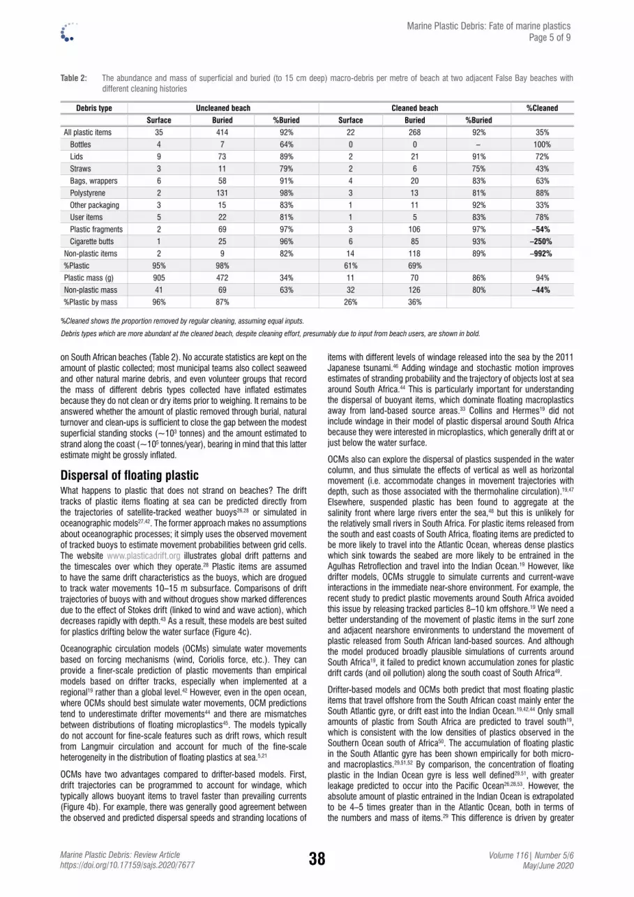
38 Volume 116| Number 5/6 May/June 2020

Marine Plastic Debris: Review Articlehttps://doi.org/10.17159/sajs.2020/7677

Marine Plastic Debris: Fate of marine plastics Page 5 of 9

on South African beaches (Table 2). No accurate statistics are kept on the amount of plastic collected; most municipal teams also collect seaweed and other natural marine debris, and even volunteer groups that record the mass of different debris types collected have inflated estimates because they do not clean or dry items prior to weighing. It remains to be answered whether the amount of plastic removed through burial, natural turnover and clean-ups is sufficient to close the gap between the modest superficial standing stocks (~103 tonnes) and the amount estimated to strand along the coast (~105 tonnes/year), bearing in mind that this latter estimate might be grossly inflated.

Dispersal of floating plasticWhat happens to plastic that does not strand on beaches? The drift tracks of plastic items floating at sea can be predicted directly from the trajectories of satellite-tracked weather buoys26,28 or simulated in oceanographic models27,42. The former approach makes no assumptions about oceanographic processes; it simply uses the observed movement of tracked buoys to estimate movement probabilities between grid cells. The website www.plasticadrift.org illustrates global drift patterns and the timescales over which they operate.28 Plastic items are assumed to have the same drift characteristics as the buoys, which are drogued to track water movements 10–15 m subsurface. Comparisons of drift trajectories of buoys with and without drogues show marked differences due to the effect of Stokes drift (linked to wind and wave action), which decreases rapidly with depth.43 As a result, these models are best suited for plastics drifting below the water surface (Figure 4c).

Oceanographic circulation models (OCMs) simulate water movements based on forcing mechanisms (wind, Coriolis force, etc.). They can provide a finer-scale prediction of plastic movements than empirical models based on drifter tracks, especially when implemented at a regional19 rather than a global level.42 However, even in the open ocean, where OCMs should best simulate water movements, OCM predictions tend to underestimate drifter movements44 and there are mismatches between distributions of floating microplastics45. The models typically do not account for fine-scale features such as drift rows, which result from Langmuir circulation and account for much of the fine-scale heterogeneity in the distribution of floating plastics at sea.5,21

OCMs have two advantages compared to drifter-based models. First, drift trajectories can be programmed to account for windage, which typically allows buoyant items to travel faster than prevailing currents (Figure 4b). For example, there was generally good agreement between the observed and predicted dispersal speeds and stranding locations of

items with different levels of windage released into the sea by the 2011 Japanese tsunami.46 Adding windage and stochastic motion improves estimates of stranding probability and the trajectory of objects lost at sea around South Africa.44 This is particularly important for understanding the dispersal of buoyant items, which dominate floating macroplastics away from land-based source areas.33 Collins and Hermes19 did not include windage in their model of plastic dispersal around South Africa because they were interested in microplastics, which generally drift at or just below the water surface.

OCMs also can explore the dispersal of plastics suspended in the water column, and thus simulate the effects of vertical as well as horizontal movement (i.e. accommodate changes in movement trajectories with depth, such as those associated with the thermohaline circulation).19,47 Elsewhere, suspended plastic has been found to aggregate at the salinity front where large rivers enter the sea,48 but this is unlikely for the relatively small rivers in South Africa. For plastic items released from the south and east coasts of South Africa, floating items are predicted to be more likely to travel into the Atlantic Ocean, whereas dense plastics which sink towards the seabed are more likely to be entrained in the Agulhas Retroflection and travel into the Indian Ocean.19 However, like drifter models, OCMs struggle to simulate currents and current-wave interactions in the immediate near-shore environment. For example, the recent study to predict plastic movements around South Africa avoided this issue by releasing tracked particles 8–10 km offshore.19 We need a better understanding of the movement of plastic items in the surf zone and adjacent nearshore environments to understand the movement of plastic released from South African land-based sources. And although the model produced broadly plausible simulations of currents around South Africa19, it failed to predict known accumulation zones for plastic drift cards (and oil pollution) along the south coast of South Africa49.

Drifter-based models and OCMs both predict that most floating plastic items that travel offshore from the South African coast mainly enter the South Atlantic gyre, or drift east into the Indian Ocean.19,42,44 Only small amounts of plastic from South Africa are predicted to travel south19, which is consistent with the low densities of plastics observed in the Southern Ocean south of Africa50. The accumulation of floating plastic in the South Atlantic gyre has been shown empirically for both micro- and macroplastics.29,51,52 By comparison, the concentration of floating plastic in the Indian Ocean gyre is less well defined29,51, with greater leakage predicted to occur into the Pacific Ocean26,28,53. However, the absolute amount of plastic entrained in the Indian Ocean is extrapolated to be 4–5 times greater than in the Atlantic Ocean, both in terms of the numbers and mass of items.29 This difference is driven by greater

Table 2: The abundance and mass of superficial and buried (to 15 cm deep) macro-debris per metre of beach at two adjacent False Bay beaches with different cleaning histories

Debris type Uncleaned beach Cleaned beach %Cleaned

Surface Buried %Buried Surface Buried %Buried

All plastic items 35 414 92% 22 268 92% 35%

Bottles 4 7 64% 0 0 – 100%

Lids 9 73 89% 2 21 91% 72%

Straws 3 11 79% 2 6 75% 43%

Bags, wrappers 6 58 91% 4 20 83% 63%

Polystyrene 2 131 98% 3 13 81% 88%

Other packaging 3 15 83% 1 11 92% 33%

User items 5 22 81% 1 5 83% 78%

Plastic fragments 2 69 97% 3 106 97% –54%

Cigarette butts 1 25 96% 6 85 93% –250%

Non-plastic items 2 9 82% 14 118 89% –992%

%Plastic 95% 98% 61% 69%

Plastic mass (g) 905 472 34% 11 70 86% 94%

Non-plastic mass 41 69 63% 32 126 80% –44%

%Plastic by mass 96% 87% 26% 36%

%Cleaned shows the proportion removed by regular cleaning, assuming equal inputs.

Debris types which are more abundant at the cleaned beach, despite cleaning effort, presumably due to input from beach users, are shown in bold.

39 Volume 116| Number 5/6 May/June 2020

Marine Plastic Debris: Review Articlehttps://doi.org/10.17159/sajs.2020/7677

amounts of macroplastics floating in the Indian Ocean, linked to the much larger input of plastics from South East Asia than from regions bordering the South Atlantic Ocean.1,53

Sedimentation of floating plastic and transport by biotaUntil recently, models of plastic drifting at sea typically assumed that items less dense than seawater remain at the water surface for protracted periods.28 However, items drifting at the sea surface tend to lose buoyancy as they become fouled by epibionts, resulting in them sinking.54 Because fouling occurs on the surface of plastic items, and buoyancy is a function of volume, plastic items with large surface area to volume ratios are expected to sink more quickly.33 This has been demonstrated experimentally with tethered polyethylene pieces in South African coastal waters, with small (5x5 mm), thin (0.1 mm) pieces sinking within 2–3 weeks, whereas larger (50x50 mm), thicker (4 mm) pieces take more than 2 months to sink.55 However, it is unclear what impact tethering has on fouling rates and whether fouling in inshore waters is typical of rates experienced farther offshore; fouling rates probably vary seasonally.56

Despite these uncertainties, sedimentation probably accounts for the increase in the size and buoyancy of macroplastic items with distance from urban source areas.33,57 However, there is debate as to the fate of items that sink in this way. In shallow waters, they probably sink to the seabed, where they become fouled by benthic organisms and weighed down by sediment and thus remain trapped on the seabed.25 This is demonstrated by the fact that most plastic items (77%) collected in trawls on the South African continental shelf are made from polymers less dense than seawater and float once cleaned.58 Sinking times are of the same order as predicted from the tethered experiments, with a bread bag bearing pelagic goose barnacles (Lepas anserifera) trawled up from the seabed within 3 months of being manufactured.58 In deeper waters, it has been suggested that such items ‘yo-yo’ up and down in the water column as they start to lose epibionts once they sink below the photic zone.54,59 Lebreton et al.25 assumed that this occurred in waters more than 200 m deep. However, the South African trawl survey found a polypropylene margarine tub still bearing pelagic goose barnacles at 685 m.58 The tub might have travelled down the continental slope after sinking, but it was already colonised by a diverse array of benthic biota, and thus appeared to be unlikely to float again.

Biofouling is not the only process that facilitates the sedimentation of plastics from the sea surface. Microplastics frequently adhere to marine ‘snow’ (particles of organic detritus60), which increases the likelihood of sinking out of surface waters.61 Sinking is also promoted for microplastics incorporated into zooplankton faecal pellets and larvacean mucous filters62,63, although microplastics can reduce the sink rate of faecal pellets64. Zooplankton may also export plastics directly to deeper waters. Many species forage near the sea surface at night and then migrate vertically to deeper waters during the day, where ingested plastic could be entrained if the zooplankton is eaten in the deep.65-67 Recent studies suggest that many planktonic organisms now contain ingested microplastics.65-68 This is particularly true in heavily polluted areas such as the North Pacific ‘garbage patch’68 and near the mouth of the Yangtze River in the Yellow Sea65, but high incidences of microplastics have been found in mesopelagic fish even in oceanic waters far from the subtropical gyres66. Most small pelagic fish off South Africa also contain microfibres (44–80% of individuals of five species contained at least some fibres69), but it is not known what proportion of these fibres are synthetic. However, it is questionable whether these items account for a significant proportion of the mass of plastics at sea because they are typically very small fragments and fibres. For example, even in the Yellow Sea, where microplastics are estimated to be almost two orders of magnitude more abundant in zooplankton than in the water column,65 the mass of ingested plastic is <1 mg/m2, even if we assume zooplankton occurs to 300 m deep.

Animals might also transport plastics among other environmental compartments. Marine predators, such as seabirds and seals, that come ashore to breed or moult import some plastics to land (e.g. seabirds

using plastics collected at sea as nest material).70 This is probably most significant for ingested plastic in seabirds, which can be released on land through mortality, regurgitation or excretion.71-73 Off South Africa, petrels in particular often contain large amounts of ingested plastic74, with adults transferring much of their accumulated plastics to their chicks75. However, this is only likely to account for a relatively small amount of plastic, even given the large populations of some species (106–107 individuals),76 given average plastic loads of <0.1 g per bird.

The seabed as a long-term sinkThe sedimentation of floating plastics, together with the direct sinking of about one third of all polymers that are more dense than seawater, suggests that the seabed is likely to be the ultimate long-term sink for most plastics that enter the marine environment.77,78 However, very little is published on the composition and abundance of seabed debris in South Africa.79-81 A recent study of macro-debris in 235 demersal trawls made across the continental shelf (30–900 m deep) between the Orange River and Port Alfred found that plastic was most common in the area north of Cape Town and that densities increased with water depth.58 Most plastic debris was packaging and other single use items (77%) but these items accounted for only 16% of the mass of plastics.58 Fishing gear was the next most common category of plastic items (21% by number and 48% by mass). The proportion of fishing gear on the seabed likely increases with distance from land-based sources, particularly on favoured fishing areas such as sea mounts.82 Overall, the densities of plastics (3 items/km2 and 0.3 kg/km2) were markedly lower than in other trawl surveys around the world (typically 20–500 items/km2 and 2–20 kg/km2).58,78 This might be related in part to the nature of the trawl gear used, but examination of remotely operated vehicle camera footage collected for biodiversity surveys across a range of habitats from the continental shelf and slope all suggest very low densities of debris on the seabed around South Africa (Sink K, SANBI, personal communication).

Closer to shore, occasional mass strandings of seabed debris indicate the presence of a pool of plastics on the seabed at least close to urban source areas.80 For example, monthly spring-low clean-ups of a stretch of rocky intertidal shoreline in False Bay collected an average of 1.65±1.30 plastic items/m (12±10 g/m, n=36 months), except one month when more than 65 items (72 g/m) were recorded (FitzPatrick Institute unpublished data). Many items were made of polymers denser than seawater (polyamide cable ties, polystyrene cutlery, etc.). The conditions driving such events have not been studied in South Africa, but probably are related to intense wind-driven upwelling.83 However, the location of this plastic on the seabed remains unknown, with no plastic items seen in any of 421 images of the False Bay seabed taken to classify benthic communities (FitzPatrick Institute unpublished data).

Current uncertainties and evidence gapsThe gross discrepancy between estimates of the amount of plastic in marine environments around South Africa and the amount thought to be released from local, land-based sources mirrors our inability to produce a plausible mass balance for waste plastics globally.25,31 Either we are greatly overestimating the amounts of plastic entering the sea, or we are failing to measure a major sink for marine plastics. To solve this dilemma, we need a better understanding of the origins, transport and fates of macroplastics, because they account for almost all of the mass of plastics in marine ecosystems.8,29

Although much remains to be learned about the distribution and abundance of plastics on the seabed, all indications are that macroplastic items are scarce on the seabed off South Africa, especially when compared to other densely populated continental margins. As a result, it is unlikely that seabed plastic will fill the deficit in the mass budget. We know even less about plastics suspended in the water column, including how they move vertically with biotic-induced changes in buoyancy.47,59 Sampling macroplastics in mid-water trawls is perhaps the most practical way to gain useful data in this regard. However, anecdotal reports from fishers and fishery biologists indicate that this compartment is unlikely to explain the thousands of tonnes of ‘missing’ plastic. Better estimates of plastics removed from beaches might partly

Marine Plastic Debris: Fate of marine plastics Page 6 of 9

40 Volume 116| Number 5/6 May/June 2020

Marine Plastic Debris: Review Articlehttps://doi.org/10.17159/sajs.2020/7677

explain the deficit, but estimates of daily arrival rates of macroplastics at urban beaches84-86 are modest relative to the global model prediction. Paradoxically, the biggest knowledge gap pertains to estimates of land-based plastics entering the sea. This should be one of the easiest fluxes to measure, but it is symptomatic of the history of the plastic pollution problem, which started in marine ecosystems and has only recently started to focus on plastics in freshwater and terrestrial ecosystems.87

Implications for tackling the plastics problemThe fact that we cannot account for much of the mass of plastic estimated to be leaking from South Africa into the ocean has little bearing on how we go about tackling the plastics problem. Although the exact amounts are poorly known, it is clear that the country is responsible for a significant amount of plastic waste entering the sea, and that this situation needs to be addressed. There are many ways to reduce plastic wastes, including incentives to reuse or recycle plastics; improved product design to reduce plastic use and facilitate recycling; adopting extended producer responsibility for packaging beyond the point of sale; material substitution; and even banning plastics in high-risk applications. However, the ultimate goal is to reduce the amount of plastic and other solid wastes entering the sea. Here, the biggest short-term gains will be made by improving solid waste management on land and intercepting debris in run-off, particularly from urban areas. Installing and servicing effective litter traps in urban rivers will go a long way towards reducing plastic leakage into the sea. However, there is also a need to ensure better compliance with legislation prohibiting the dumping of plastics and other persistent wastes by ships at sea.

AcknowledgementsI acknowledge the funding support for the preparation of this review paper from the South African Department of Science and Innovation (DSI), through the Waste RDI Roadmap, managed by the Council for Scientific and Industrial Research (CSIR). Subsidiary funding was provided under the umbrella of the Commonwealth Litter Programme (CLiP) implemented by the Centre for Environment, Fisheries and Aquaculture Science (Cefas), funded by the United Kingdom Government’s Department for Environment, Food and Rural Affairs (Defra). Plastics SA have helped to fund beach debris surveys around the South African coast since 1994. I thank my many collaborators for assistance in the field, especially Coleen Moloney, Vonica Perold, Eleanor Weideman and Maëlle Connan. Umberto Binetti, Charine Collins, Linda Godfrey, Michael Hart-Davis, Juliet Hermes and Eleanor Weideman provided helpful comments on an earlier draft. Charine Collins kindly provided the base map for Figure 3.

References1. Jambeck JR, Geyer R, Wilcox C, Siegler TR, Perryman M, Andrady AL, et al.

Plastic waste inputs from land into the ocean. Science. 2015;347:768–771. https://doi.org/10.1126/science.1260352

2. Jambeck J, Hardesty BD, Brooks AL, Friend T, Teleki K, Fabres J, et al. Challenges and emerging solutions to the land-based plastic waste issue in Africa. Mar Policy. 2018;96:256–263. https://doi.org/10.1016/j.marpol.2017.10.041

3. Verster C, Bouwman H. Land-based sources and pathways of marine plastics in a South African context. S Afr J Sci. 2020;116(5/6), Art. #7700, 9 pages. https://doi.org/10.17159/sajs.2020/7700

4. Coe JM, Rogers DB, editors. Marine debris: Sources, impacts, and solutions. New York: Springer-Verlag; 1997. https://doi.org/10.1007/978-1-4613-8486-1

5. Ryan PG, Moore CJ, Van Franeker JA, Moloney CL. Monitoring the abundance of plastic debris in the marine environment. Phil Trans R Soc B. 2009;364:1999–2012. https://doi.org/10.1098/rstb.2008.0207

6. Ryan PG, Dilley BJ, Ronconi RA, Connan M. Rapid increase in Asian bottles in the South Atlantic Ocean indicates major debris inputs from ships. Proc Natl Acad Sci USA. 2019;116:20892–20897. https://doi.org/10.1073/pnas.1909816116

7. Santos IR, Friedrich AC, Barretto FP. Overseas garbage pollution on beaches of northeast Brazil. Mar Pollut Bull. 2005;50:782–786. https://doi.org/10.1016/j.marpolbul.2005.04.044

8. Lebreton L, Slat B, Ferrari F, Sainte-Rose B, Aitken J, Marthouse R, et al. Evidence that the Great Pacific Garbage Patch is rapidly expanding. Sci Rep. 2018;8, Art. #4666, 15 pages. https://doi.org/10.1038/s41598-018-22939-w

9. Monteiro RCP, Ivar do Sul JA, Costa MF. Plastic pollution in islands of the Atlantic Ocean. Environ Pollut. 2018;238:103–110. https://doi.org/10.1016/j.envpol.2018.01.096

10. Schumann EH, MacKay CF, Strydom NA. Nurdle drifters around South Africa as indicators of ocean structures and dispersion. S Afr J Sci. 2019;115(5/6), Art. #5372, 9 pages. https://doi.org/10.17159/sajs.2019/5372

11. Smith SDA, Banister K, Fraser N, Edgar RJ. Tracing the source of marine debris on the beaches of northern New South Wales, Australia: The bottles on beaches program. Mar Pollut Bull. 2018;126:304–307. https://doi.org/10.1016/j.marpolbul.2017.11.022

12. Ryan PG, Moloney CL. Plastic and other artefacts on South African beaches: Temporal trends in abundance and composition. S Afr J Sci. 1990;86:450–452.

13. Ryan PG, Perold V, Osborne A, Moloney CL. Consistent patterns of debris on South African beaches indicate that industrial pellets and other mesoplastic items mostly derive from local sources. Environ Pollut. 2018;238:1008–1016. https://doi.org/10.1016/j.envpol.2018.02.017

14. Ryan PG, Swanepoel D. Cleaning beaches: Sweeping litter under the carpet. S Afr J Sci 1996;92:275–276.

15. Naidoo T, Glassom D, Smit AJ. Plastic pollution in five urban estuaries of KwaZulu-Natal, South Africa. Mar Pollut Bull. 2015;101:473–480. https://doi.org/10.1016/j.marpolbul.2015.09.044

16. Nel HA, Froneman PW. A quantitative analysis of microplastic pollution along the south-eastern coastline of South Africa. Mar Pollut Bull. 2015;101:274–279. https://doi.org/10.1016/j.marpolbul.2015.09.043

17. Nel HA, Hean JW, Noundou XS, Froneman PW. Do microplastic loads reflect the population demographics along the southern African coastline? Mar Pollut Bull. 2017;115:115–119. https://doi.org/10.1016/j.marpolbul.2016.11.056

18. De Villiers S. Quantification of microfibre levels in South Africa’s beach sediments, and evaluation of spatial and temporal variability from 2016 to 2017. Mar Pollut Bull. 2018;135:481–489. https://doi.org/10.1016/j.marpolbul.2018.07.058

19. Collins C, Hermes JC. Modelling the accumulation and transport of floating marine micro-plastics around South Africa. Mar Pollut Bull. 2019;139:46–58. https://doi.org/10.1016/j.marpolbul.2018.12.028

20. Brennan E, Wilcox C, Hardesty BD. Connecting flux, deposition and resuspension in coastal debris surveys. Sci Total Environ. 2018;644:1019–1026. https://doi.org/10.1016/j.scitotenv.2018.06.352

21. Ryan PG, Pichegru L, Perold V, Moloney CL. Monitoring marine plastics – will we know if we’re making a difference? S Afr J Sci. 2020;116(5/6), Art. #7678, 9 pages. https://doi.org/10.17159/sajs.2020/7678

22. Fazey FMC, Ryan PG. Debris size and buoyancy influence the dispersal distance of stranded litter. Mar Pollut Bull. 2016;110:371–377. https://doi.org/10.1016/j.marpolbul.2016.06.039

23. Ryan PG. The origin and fate of artefacts stranded on islands in the African sector of the Southern Ocean. Environ Conserv. 1987;14:341–346. https://doi.org/10.1017/S0376892900016854

24. Barnes DKA, Galgani F, Thompson RC, Barlaz M. Accumulation and fragmentation of plastic debris in global environments. Phil Trans R Soc B. 2009;364:1985–1998. https://doi.org/10.1098/rstb.2008.0205

25. Lebreton L, Egger M, Slat B. A global mass budget for positively buoyant macroplastic debris in the ocean. Sci Rep. 2019;9, Art. #12922, 10 pages. https://doi.org/10.1038/s41598-019-49413-5

26. Maximenko N, Hafner J, Niiler P. Pathways of marine debris derived from trajectories of Lagrangian drifters. Mar Pollut Bull. 2012;65:51–62. https://doi.org/10.1016/j.marpolbul.2011.04.016

27. Potemra J. Numerical modeling with application to tracking marine debris. Mar Pollut Bull. 2012;65:42–50. https://doi.org/10.1016/j.marpolbul.2011.06.026

28. Van Sebille E, England MH, Froyland G. Origin, dynamics and evolution of ocean garbage patches from observed surface drifters. Environ Res Lett. 2012;7, 044040, 6 pages. https://doi.org/10.1088/1748-9326/7/4/044040

Marine Plastic Debris: Fate of marine plastics Page 7 of 9

41 Volume 116| Number 5/6 May/June 2020

Marine Plastic Debris: Review Articlehttps://doi.org/10.17159/sajs.2020/7677

29. Eriksen M, Lebreton LCM, Carson HS, Thiel M, Moore CJ, Borerro JC, et al. Plastic pollution in the world’s oceans: More than 5 trillion plastic pieces weighing over 250,000 tons afloat at sea. PLoS ONE. 2014;9(12), e111913, 15 pages. https://doi.org/10.1371/journal.pone.0111913

30. Thompson RC, Olsen Y, Mitchell RP, Davis A, Rowland SJ, John AW, et al. Lost at sea: Where is all the plastic? Science. 2004;304:838. https://doi.org/10.1126/science.1094559

31. Koelmans AA, Kooi M, Law KL, Van Sebille E. All is not lost: Deriving a top-down mass budget of plastic at sea. Environ Res Lett. 2017;12:114028. https://doi.org/10.1088/1748-9326/aa9500

32. Andrady AL. Microplastics in the marine environment. Mar Pollut Bull. 2011;62:1596–1605. https://doi.org/10.1016/j.marpolbul.2011.05.030

33. Ryan PG. Does size and buoyancy affect the long-distance transport of floating debris? Environ Res Lett. 2015;10:084019. https://doi.org/10.1088/1748-9326/10/8/084019

34. Isobe A, Kubo K, Tamura Y, Nakashima E, Fujii N. Selective transport of microplastics and mesoplastics by drifting in coastal waters. Mar Pollut Bull. 2014;89:324–330. https://doi.org/10.1016/j.marpolbul.2014.09.041

35. Hinata H, Kataoka T. A belt transect setting strategy for mark-recapture experiments to evaluate the 1D diffusion coefficient of beached litter in the cross-shore direction. Mar Pollut Bull. 2016;109:490–494. https://doi.org/10.1016/j.marpolbul.2016.05.016

36. Williams AT, Tudor DT. Litter burial and exhumation: Spatial and temporal distribution on a cobble pocket beach. Mar Pollut Bull. 2001;42:1031–1039. https://doi.org/10.1016/S0025-326X(01)00058-3

37. Kusui T, Noda M. International survey on the distribution of stranded and buried litter on beaches along the Sea of Japan. Mar Pollut Bull. 2003;47:175–179. https://doi.org/10.1016/S0025-326X(02)00478-2

38. Turra A, Manzano AB, Dias RJS, Mahiques MM, Barbosa L, Balthazar-Silva D, et al. Three-dimensional distribution of plastic pellets in sandy beaches: Shifting paradigms. Sci Rep. 2014;4, Art. #4435, 7 pages. https://doi.org/10.1038/srep04435

39. Dutton A, Carlson AE, Long AJ, Milne GA, Clark PU, De Conto R, et al. Sea-level rise due to polar ice-sheet mass loss during past warm periods. Science. 2015;349(6244), aaa4019, 9 pages. https://doi.org/10.1126/science.aaa4019

40. Ryan PG, Lamprecht A, Swanepoel D, Moloney CL. The effect of fine-scale sampling frequency on estimates of beach litter accumulation. Mar Pollut Bull. 2014;88:249–254. https://doi.org/10.1016/j.marpolbul.2014.08.036

41. Glovovic BC, Boonzaaier S. Confronting coastal poverty: Building sustainable coastal livelihoods in South Africa. Ocean Coastal Managem. 2007;50:1–23. https://doi.org/10.1016/j.ocecoaman.2006.07.001

42. Lebreton LCM, Greer SD, Borrero JC. Numerical modelling of floating debris in the world’s oceans. Mar Pollut Bull. 2012;64:653–661. https://doi.org/10.1016/j.marpolbul.2011.10.027

43. Fraser CI, Morrison AK, Van Sebille E, Macaya EC, Hogg AM, Ryan PG, et al. Antarctica’s ecological isolation will be broken by storm-driven dispersal and warming. Nat Clim Change. 2018;8:704–708. https://doi.org/10.1038/s41558-018-0209-7

44. Hart-Davis MG, Backeberg BC, Halo I, Van Sebille E, Johannessen JA. Assessing the accuracy of satellite derived ocean currents by comparing observed and virtual buoys in the Greater Agulhas Region. Remote Sens Environ. 2018;216:735–746. https://doi.org/10.1016/j.rse.2018.03.040

45. Onink V, Wichmann D, Delandmeter P, Van Sebille E. The role of Ekman currents, geostrophy and Stokes drift in the accumulation of floating microplastic. J Geophys Res Oceans. 2019;124:1474–1490. https://doi.org/10.1029/2018JC014547

46. Maximenko N, Hafner J, Kamachi M, MacFadyen A. Numerical simulations of debris drift from the Great Japan Tsunami of 2011 and their verification with observational reports Mar Pollut Bull. 2018;132:5–25. https://doi.org/10.1016/j.marpolbul.2018.03.056

47. Erni-Cassola G, Zadjelovic V, Gibson MI, Christie-Oleza JA. Distribution of plastic polymer types in the marine environment: A meta-analysis. J Hazard Mater. 2019;369:691–698. https://doi.org/10.1016/j.jhazmat.2019.02.067

48. Acha EM, Mianzan HW, Iribarne O, Gagliardini DA, Lasta C, Daleo P. The role of the Río de la Plata salinity front in accumulating debris. Mar Pollut Bull. 2003;46:197–202. https://doi.org/10.1016/S0025-326X(02)00356-9

49. Shannon LV, Chapman P. Suggested mechanism for the chronic pollution by oil of beaches east of Cape Agulhas, South Africa. S Afr J Mar Sci. 1983;1:231–244. https://doi.org/10.2989/025776183784447520

50. Ryan PG, Musker S, Rink A. Low densities of drifting litter in the African sector of the Southern Ocean. Mar Pollut Bull. 2014;89:16–19. https://doi.org/10.1016/j.marpolbul.2014.10.043

51. Cózar A, Echevarría F, Gonzalez-Gordillo JI, Irigoien X, Ubeda B, Hernandez-León S, et al. Plastic debris in the open ocean. Proc Natl Acad Sci USA. 2014;111:10239–10244. https://doi.org/10.1073/pnas.1314705111

52. Ryan PG. Litter survey detects the South Atlantic ‘garbage patch’. Mar Pollut Bull. 2014;79:220–224. https://doi.org/10.1016/j.marpolbul.2013.12.010

53. Van Sebille E, Wilcox C, Lebreton LCM, Maximenko NA, Hardesty BD, Van Franeker JA, et al. A global inventory of small floating plastic debris. Environ Res Lett. 2015;10(12), Art.#124006, 11 pages. https://doi.org/10.1088/1748-9326/10/12/124006

54. Ye S, Andrady AL. Fouling of floating plastic debris under Biscayne Bay exposure conditions. Mar Pollut Bull. 1991;22:608–613. https://doi.org/10.1016/0025-326X(91)90249-R

55. Fazey FMC, Ryan PG. Biofouling on buoyant marine plastics: an experimental study into the effect of size on surface longevity. Environ Pollut 2016;210:354–360. https://doi.org/10.1016/j.envpol.2016.01.026

56. Chen X, Xiong X, Jiang X, Shi H, Wu C. Sinking of floating plastic debris caused by biofilm development in a freshwater lake. Chemosphere. 2019;222:856–864. https://doi.org/10.1016/j.chemosphere.2019.02.015

57. Fazey FMC, Ryan PG. Debris size and buoyancy influence the dispersal distance of stranded litter. Mar Pollut Bull. 2016;110:371–377. https://doi.org/10.1016/j.marpolbul.2016.06.039

58. Ryan PG, Weideman EA, Perold V, Durholz D, Fairweather TP. A trawl survey of seabed macrolitter on the South African continental shelf. Mar Pollut Bull. 2020;150, Art.#110741, 6 pages. https://doi.org/10.1016/j.marpolbul.2019.110741

59. Kooi M, Van Nes E, Scheffer M, Koelmans A. Ups and downs in the ocean: Effects of biofouling on vertical transport of microplastics. Environ Sci Technol. 2017;51:7963–7971. https://doi.org/10.1021/acs.est.6b04702

60. Zhao S, Ward JE, Danley M, Mincer TJ. Field-based evidence for microplastic in marine aggregates and mussels: Implications for trophic transfer. Environ Sci Technol. 2018;52:11038–11048. https://doi.org/10.1021/acs.est.8b03467

61. Ploug H, Iversen MH, Fisher G. Ballast, sinking velocity, and apparent diffusivity within marine snow and zooplankton fecal pellets: Implications for substrate turnover by attached bacteria. Limnol Oceanogr. 2008;53:1878–1886. https://doi.org/10.4319/lo.2008.53.5.1878

62. Cole M, Lindeque PK, Fileman E, Halsband C, Goodhead R, Moger J, et al. Microplastic ingestion by zooplankton. Environ Sci Technol. 2013;47:6646−6655. https://doi.org/10.1021/es400663f

63. Katija K, Choy CA, Sherlock RE, Sherman AD, Robison BH. From the surface to the seafloor: How giant larvaceans transport microplastics into the deep sea. Sci Adv. 2017;3, e1700715, 5 pages. https://doi.org/10.1126/sciadv.1700715

64. Cole M, Lindeque PK, Fileman E, Clark J, Lewis C, Halsband C, et al. Microplastics alter the properties and sinking rates of zooplankton faecal pellets. Environ Sci Technol. 2016;50:3239–3246. https://doi.org/10.1021/acs.est.5b05905

65. Sun X, Liang J, Zhu M, Zhao Y, Zhang B. Microplastics in seawater and zooplankton from the Yellow Sea. Environ Pollut. 2018;242:585–595. https://doi.org/10.1016/j.envpol.2018.07.014

66. Wieczorek AM, Morrison L, Croot PL, Allcock AL, MacLoughlin E, Savard O, et al. Frequency of microplastics in mesopelagic fishes from the Northwest Atlantic. Front Mar Sci. 2018;5, Art. #039, 9 pages. https://doi.org/10.3389/fmars.2018.00039

67. Choy CA, Robison BH, Gagne TO, Erwin B, Firl E, Halden RU, et al. The vertical distribution and biological transport of marine microplastics across the epipelagic and mesopelagic water column. Sci Rep. 2019;9, Art.#7843, 9 pages. https://doi.org/10.1038/s41598-019-44117-2

68. Boerger CM, Lattin GL, Moore SL, Moore CJ. Plastic ingestion by planktivorous fishes in the North Pacific central gyre. Mar Pollut Bull. 2010;60:2275–2278. https://doi.org/10.1016/j.marpolbul.2010.08.007

Marine Plastic Debris: Fate of marine plastics Page 8 of 9

42 Volume 116| Number 5/6 May/June 2020

Marine Plastic Debris: Review Articlehttps://doi.org/10.17159/sajs.2020/7677

69. Ross KJ. Ingestion of microplastics by epipelagic and mesopelagic fish in South African waters: A species comparison [Hons report]. Cape Town: University of Cape Town; 2017. https://bit.ly/2kbWp64

70. Hartwig E, Clemens T, Heckroth M. Plastic debris as nesting material in a kittiwake (Rissa tridactyla) colony at the Jammerbugt, northwest Denmark. Mar Pollut Bull. 2007;54:595–597. https://doi.org/10.1016/j.marpolbul.2007.01.027

71. Ryan PG, Fraser MW. The use of Great Skua pellets as indicators of plastic pollution in seabirds. Emu 1988;88:16–19. https://doi.org/10.1071/MU9880016

72. Buxton RT, Currey CA, Lyver PO, Jones CJ. Incidence of plastic fragments among burrow-nesting seabird colonies on offshore islands in northern New Zealand. Mar Pollut Bull. 2013;74:420424. https://doi.org/10.1016/j.marpolbul.2013.07.011

73. Provencher JF, Vermaire JC, Avery-Gomm S, Braune BM, Mallory ML. Garbage in guano? Microplastic debris found in faecal precursors of seabirds known to ingest plastic. Sci Tot Environ. 2018;644:1477–1484. https://doi.org/10.1016/j.scitotenv.2018.07.101

74. Ryan PG. The incidence and characteristics of plastic particles ingested by seabirds. Mar Environ Res. 1987;23:175–206. https://doi.org/10.1016/0141-1136(87)90028-6

75. Ryan PG. Intraspecific variation in plastic ingestion by seabirds and the flux of plastic through seabird populations. Condor. 1988;90:446–452. https://doi.org/10.2307/1368572

76. Brooke MDL. The food consumption of the world’s seabirds. Proc R Soc Lond B. 2004;271:S246–S248. https://doi.org/10.1098/rsbl.2003.0153

77. Woodall LC, Sanchez-Vidal A, Canals M, Paterson GLJ, Coppock R, Sleight V, et al. The deep sea is a major sink for microplastic debris. R Soc Open Sci. 2014;1:140317. https://doi.org/10.1098/rsos.140317

78. Ioakeimidis C, Galgani F, Papatheodorou G. Occurrence of marine litter in the marine environment: A world panorama of floating and seafloor plastics. In: Takada H, Karapanagioti HK, editors. Hazardous chemicals associated with plastics in the environment. Handbook Environ Chem. 2017;78:93–120. https://doi.org/10.1007/698_2017_22

79. Rundgren CD. Aspects of pollution in False Bay, South Africa (with special reference to subtidal pollution) [MSc thesis]. Cape Town: University of Cape Town; 1992. http://hdl.handle.net/11427/18330

80. Pfaff MC, Logston RC, Raemaekers SJPN, Hermes JC, Blamey LK, Cawthra HC, et al. A synthesis of three decades of socio-ecological change in False Bay, South Africa: Setting the scene for multidisciplinary research and management. Elementa Sci Anthrop. 2019;7, Art.#32, 49 pages. https://doi.org/10.1525/elementa.367

81. Matsuguma Y, Takada H, Kumata H, Kanke H, Sakurai S, Suzuki T, et al. Microplastics in sediment cores from Asia and Africa as indicators of temporal trends in plastic pollution. Arch Environ Contam Toxicol. 2017;73:230–239. https://doi.org/10.1007/s00244-017-0414-9

82. Woodall LC, Robins LF, Rogers AD, Narayanaswamy BE, Paterson GLJ. Deep-sea litter: A comparison of seamounts, banks and a ridge in the Atlantic and Indian Oceans reveals both environmental and anthropogenic factors impact accumulation and composition. Front Mar Sci. 2015;2, Art. #3, 10 pages. https://doi.org/10.3389/fmars.2015.00003

83. Chubarenko I, Stepanovs N. Microplastics in sea coastal zone: Lessons learned from the Baltic amber. Environ Pollut. 2017;224:243–254. https://doi.org/10.1016/j.envpol.2017.01.085

84. Swanepoel D. An analysis of beach debris accumulation in Table Bay, South Africa [MSc thesis]. Cape Town: University of Cape Town; 1995. http://hdl.handle.net/11427/28474

85. Lamprecht A. The abundance, distribution and accumulation of plastic debris in Table Bay, Cape Town, South Africa [MSc thesis]. Cape Town: University of Cape Town; 2013. http://hdl.handle.net/11427/6633

86. Chitaka TY, Von Blottnitz H. Accumulation and characteristics of plastic debris along five beaches in Cape Town. Mar Pollut Bull. 2019;138:451–457. https://doi.org/10.1016/j.marpolbul.2018.11.065

87. Ryan PG. A brief history of marine litter research. In: Bergmann M, Gutow L, Klages M, editors. Marine anthropogenic litter. Cham: Springer International Publishing; 2015. p. 1–25. https://doi.org/10.1007/978-3-319-16510-3_1

Marine Plastic Debris: Fate of marine plastics Page 9 of 9

43 Volume 116| Number 5/6 May/June 2020

Marine Plastic Debris: Review Articlehttps://doi.org/10.17159/sajs.2020/7693

© 2020. The Author(s). Published under a Creative Commons Attribution Licence.

Impacts of plastic debris on biota and implications for human health: A South African perspectiveAUTHORS:

Trishan Naidoo1 Anusha Rajkaran1 Sershen1

AFFILIATION:

1Department for Biodiversity and Conservation Biology, University of the Western Cape, Cape Town, South Africa

CORRESPONDENCE TO: Trishan Naidoo

EMAIL: trishan.naidoo2@gmail.com

DATES:Received: 03 Dec. 2019Revised: 05 Mar. 2020Accepted: 18 Mar. 2020Published: 27 May 2020

HOW TO CITE: Naidoo T, Rajkaran A, Sershen. Impacts of plastic debris on biota and implications for human health: A South African perspective. S Afr J Sci. 2020;116(5/6), Art. #7693, 8 pages. https://doi.org/10.17159/sajs.2020/7693

ARTICLE INCLUDES:☒ Peer review ☒ Supplementary material

DATA AVAILABILITY:☐ Open data set ☐ All data included☐ On request from author(s)☐ Not available☒ Not applicable

EDITORS: Jane Carruthers Linda Godfrey

KEYWORDS: pollution, microplastic, entanglement, ingestion, ecology

FUNDING: Waste RDI Roadmap, Council for Scientific and Industrial Research, Department of Science and Innovation (South Africa); Commonwealth Litter Programme, Centre for Environment, Fisheries and Aquaculture Science, Department for Environment, Food and Rural Affairs (UK)

Entanglement and ingestion of plastics are the main ecological impacts of marine plastic debris on marine biota, but indirect effects such as the transport of alien species and benthic smothering are also important to note. Entanglement of invertebrates, sharks, turtles, birds and marine mammals is mainly caused by macroplastics (>5 mm), and leads to reduced mobility, ineffective foraging and subsequent mortality. The main plastic types associated with entanglement are improperly discarded fishing nets, lines, ropes and straps. In South Africa and surrounding waters, plastic ingestion has been reported in a number of marine species: sharks (n=10), fish (n=7), turtles (n=1) and birds (n=36). Lethal (macroplastic) and sub-lethal effects (microplastic ≤5 mm) of marine debris on biota have been noted, but at the time of this review there were no published reports on impacts at the population level. Consumed shellfish are possible vectors for the introduction of microplastics into humans. The specific impacts of microplastic ingestion on human health are largely unknown, but additives associated with plastics represent a threat. The research infrastructure in South Africa is insufficient to monitor and characterise marine plastic debris and, in many cases, not in line with global standards. More research effort is needed to understand the impacts of marine plastic debris on humans and marine biota in South Africa, particularly at the population level.

Significance • Macroplastics affect marine biota mainly via entanglement and microplastics largely through ingestion.

• Macro- and microplastic interactions with biota can result in sub-lethal effects and mortality but no population effects have been reported for South Africa.

• Consumed shellfish are a potential source of microplastics for humans but their potential effects in humans remain unknown.

• Better infrastructure is needed for improved monitoring and research on the effects of marine debris in South Africa.

Status of the ecological impact of plastics in South AfricaGlobal records of the number of organisms that interact with plastic debris indicate an increase from 265 species in 19971 to 557 in 20152. Records were initially detailed in higher order organisms such as mammals, birds and reptiles; however, more recently fish and invertebrates have become research interests, especially in terms of their interaction with microplastics.2 ‘Microplastics’ is now a globally relevant theme that has received increased attention in South Africa over the last decade. Ryan and Moloney3 provided the first account of these smaller plastics around the South African coastline in 1984 and 1989 and offshore in the 1970s,4 but there are still many gaps in our understanding of the prevalence and typology of marine plastic debris in general in South Africa. The widespread bioavailability of microplastics to marine organisms, their potential to act as vectors for both chemicals and microflora, and the resultant impacts on humans and other biota that consume them also represent many unknowns, both in South Africa and globally. This lack of data has hindered the design and implementation of appropriate mitigation strategies.

The marine environment around South Africa supports over 13 000 species, many of which (up to 33%) are endemic5, necessitating focused research on the impact of plastic debris on marine biota in the country’s waters. The South African coastline has unique currents, bioregions and coastal geomorphological features.5 Early research on marine debris in South African coastal environments focused on the impacts on seabirds and began in the mid-1980s6,7, although incidental reports of plastic ingestion in turtles were made in the 1970s8. Since then, a number of fish, sea turtle, bird and mammal species in South African oceans have been found to be affected by plastics (Table 1 and Supplementary table 1)9,10; the effects on these species are expanded on below. However, a comprehensive assessment of the variety and degree to which South African biota are affected is lacking. While the World Health Organization rates the risk of plastics to humans as low, there is still a need to evaluate the potential effects of microplastics on the South African human population given the country’s reliance on many edible marine species. This need provided the motivation for this review, which assesses the impact of marine plastic debris on biota and the potential implications on human health in South Africa, by drawing on data available for organisms sampled from waters extending from South Africa to more southerly regions, up to the Prince Edward Islands. Where South African data on these aspects were lacking, examples from international studies were used to draw parallels. The objectives of this review were to: (1) review South African literature on marine biota impacted by plastic debris, through entanglement, ingestion, benthic smothering and alien transport; (2) determine the potential for, pathways of and potential impacts of microplastic ingestion on human health, particularly in relation to species of commercial value; and (3) identify the gaps in our understanding of the impacts of marine plastic debris on South African marine biota and human health. This review also comments on how South African literature on marine plastic debris (and its impacts) contributes to the global understanding of the phenomenon.

44 Volume 116| Number 5/6 May/June 2020

Marine Plastic Debris: Review Articlehttps://doi.org/10.17159/sajs.2020/7693

The impacts of plastic debris on marine biotaEntanglementA major impact of discarded macroplastics is the potential to physically trap marine organisms.10 Kühn et al.2 provided the most comprehensive global assessment on entanglement in 2015, which lists 344 species including invertebrates, sharks, fish, sea turtles, birds and mammals. This assessment expands on the previous effort by Laist in 1997 of 136 species, which focused on higher order organisms.1 In general, most entanglement occurs with improperly discarded or accidentally lost fishing gear such as nets, lines, ropes and straps from bait boxes.11,12 This impact has received the most public attention, partly driven by social media, especially when organisms are physically injured for long periods before mortality. South African entanglement records prior to 1990 include 6 shark, 2 turtle, 13 seabird and 5 marine mammal species.9 A brief overview of the prevalence of entanglement in South African marine species is presented herein, together with recommendations for future research. It must be noted that in many cases of entanglement by fishing gear, it is often challenging to discriminate between active and ghost gear.10

InvertebratesPublished entanglement records for South African invertebrate species were not available at the time of this review. Globally, an assessment in 2015 lists 25 mollusc, 21 echinoderm and 46 crustacean species affected by entanglement.2 These numbers are higher than those of the assessment in 1997 which lists 8 species, most of which were crustaceans, and probably reflects an increase in research effort.1 Based on the global literature, pelagic invertebrates are usually smaller and therefore possibly more susceptible to plastic ingestion than entanglement. However, sessile taxa are also at risk; for example, Lamb et al.13 estimated that 11.1 billion plastic items are currently entangled on corals in the Asia-Pacific. This entanglement will likely affect feeding and gaseous exchange in these coral systems.14

Sharks and other fish South African literature identified plastic straps, from bait boxes and land-based packaging, to be the main plastic types associated with sharks caught in gill nets (or shark nets).11 Shark nets are put in place by government agencies to protect bathers.11 Between 1978 and 2000, 53 of the 28 000 sharks (0.18%) caught were found to be entangled by marine debris, and although a wide variety of species was observed, only the dusky shark, Carcharhinus obscurus, showed an increase in entanglement over time.11 Shark fins are not retractable, increasing their vulnerability to entanglement.11 Discarded fishing nets can also entangle and capture fish and other marine biota, a phenomenon known as ghost fishing.14 There were no South African studies that provided quantitative data on this phenomenon, possibly because it is difficult to distinguish between active and ghost gear. However, discarded fishing gill nets are removed daily from estuaries around South Africa, some of which appear to have been abandoned. For example, on the Mlalazi Estuary, conservation officers recovered 51 monofilament gill nets, holding 195 fish of 12 species, from 21 April 2018 to 28 March 2019 (Buthelezi T, Ezemvelo KZN Wildlife, 2020, personal communication, February 27). Globally, lost or discarded fishing gear continue to capture fish, which could affect fish populations.14 The United Nations Environment Programme estimated that 640 000 tons of discarded fishing gear is added to the oceans annually, which captures a wide variety of both commercial and non-target species.15 As marine organisms trapped in these nets decompose, they attract and entangle scavengers in a cyclic manner, making it difficult to acquire a reliable global estimate of mortalities, but localised international monitoring has seen high mortality rates in some places. For example, Good et al.16 reported that from 2002 to 2010, 32 000 marine organisms, mainly fish and invertebrates, were recovered from abandoned fishing gear in inland waters of Washington (USA).

Sea turtlesMost reports on entanglement of turtles in South Africa have been made by aquariums along the coastline (Prof. Nel R, Nelson Mandela University, 2019, personal communication, October 17). In addition to this, Ryan9

Marine Plastic Debris: Ecological impacts Page 2 of 8

has reported two South African turtle species that have been entangled by rope. Drawing from global literature, the impact of turtle entanglement involves the restriction of movement, which compromises their ability to surface for air.12 Tightly wound lines can also restrict blood flow, causing decreased mobility and the potential loss of limbs.12 Plastic rings around turtles’ necks can also asphyxiate them as they grow, eventually leading to mortality.14 The impact on sea turtles is therefore partially dependent on the plastic types they encounter. As turtles are particularly vulnerable to many other anthropogenic perturbations17, plastics represent an additional factor that can lead to population declines. Although plastics left on beaches may not necessarily contribute to entanglement, they can result in a decrease in the number of turtles nesting on beaches. Fujisaki and Lamont18 found a 200% increase in nests when beaches in Florida were cleared of natural and anthropogenic debris. As the sex of turtle hatchlings is dependent on nest temperature, any temperature anomalies caused by plastic debris in the sediment could also affect the sex distribution of turtle populations.19

BirdsAn extensive review of entanglement of birds by plastic and other marine debris is provided in Ryan10. As many as 265 bird species, many of which are found in South Africa, were found entangled in plastic or similar types of debris. Fishing line seems to be the major plastic type affecting seabirds and virtually all bird species associated with the marine environment appear to be at risk.10 However, there are some differences in the risk posed to seabirds by different plastic types. For example, plunge diving birds get entangled more often by plastic bags as they dive for juvenile fish, that shelter under the bags, than do other birds.10 Birds that frequent mangroves may be more at risk to fishing line entanglement as these plastics get caught up in aerial mangrove roots.10 Self-removal of plastics is difficult in species that have backward serrations on their beaks.10 Entangled birds often get injured, have reduced feeding efficiency and become startled, which can sometimes attract unaffected birds that then also get trapped.10 Birds that use plastic debris to build their nest can also be at risk of entanglement.10

Mammals Research in South Africa on entanglement of marine mammals has largely focused on Cape fur seals (Arctocephalus pusillus) and whales.20,21 In the case of seals, a study that dates back to 1979 indicated that marine debris was encountered in generally less than 1% per colony of seals that were harvested from locations in the Western Cape; harvesters recorded removing rope, string, fishing line and plastic straps from seals.20 Of the 72 000 seals observed, 84 were found to be entangled by plastics, suggesting that this was not a major impact on their population numbers at the time. Debris was mostly observed around the neck and was seen to cut into flesh as individuals grew. However, on Marion Island, a territory of South Africa, entanglement was recorded in 101 sub-Antarctic (Arctocephalus tropicalis) and Antarctic (A. gazella) fur seals and 5 elephant seals (Mirounga leonina) over a 10-year period (1991–2001).22 These numbers imply that only 0.24% of the seal population on this island were observed to be affected over this period, but both entanglement and increase in debris types closely coincided with a longline fishery that was implemented around Marion in 1996. This fishery has since ceased; however, it should be noted that seals are generally inquisitive, and the prevalence of marine debris has escalated globally, which may increase their risk of entanglement.14 In the case of whales along the South African coastline, most cases of entanglement have been attributed to fishing gear (associated with a lobster fishery) or shark nets.21 Humpback whales (Megaptera novaeangliae) and southern right whales (Eubalaena australis) are the species that are commonly entangled, but it was concluded that the entanglement rates of 9.5–21.6% were not affecting populations.21

Although the possibility of population-level effects by entanglement of organisms appears to be low, in general, reducing the disposal of items such as packing rings associated with canned and bottled drinks, monofilament line and bait box straps will decrease the risk of entanglement.10 This was the reasoning behind banning packaging rings and ring pulls on drink cans in South Africa, in the 1980s. Measures

45 Volume 116| Number 5/6 May/June 2020

Marine Plastic Debris: Review Articlehttps://doi.org/10.17159/sajs.2020/7693

such as introducing discard bins near popular fishing spots with accompanying sign posts may also reduce the line and plastic straps from bait boxes entering the marine environment.10

SmotheringBenthic invertebrates can be smothered by macroplastics that have settled out of the water column, on the seabed, reefs or on beaches.14 While the diversity of South African coral reefs and that of sediments have been well characterised5, it is unclear how susceptible these systems are to disruption of species assemblages by debris. Smothering could affect filter feeding in sessile species or food location in mobile organisms. For example, beached plastic debris decreased the foraging efficiency of the gastropod Nassarius pullus23, and in the same way may affect benthic species in South Africa. Alteration of physical characteristics of these benthic habitats by debris (e.g. porosity of the sediment and its heat transfer capacity9) has also not been assessed in South Africa. The global literature indicates that plastic accumulation may alter temperature, water permeability and gaseous exchange in marine sediments, which could cause physiological stress to meiofaunal communities.14,19 Plastic debris on beaches may lead to anoxic conditions, altering infaunal communities.24

Transport Plastics have the potential to transport alien species.14 Bacteria, cyanobacteria, dinoflagellates, coccolithophores, corals, bryozoans, hydroids, and others have all been found on plastics in marine environments globally.25 While marine debris can assist invasions of alien species26, the prevalence of this phenomenon in South African systems has not been well characterised, with the exception of a record from gooseneck barnacles27. Nevertheless, the epiplastic community, now termed the ‘plastisphere’25,28, can potentially impact marine biota through transfer by ingestion if pathogenic bacteria are transferred from the environment to biota via plastics. This possibility is concerning for South African marine species, as high levels of pathogenic bacteria, like Escherichia coli, can be present in urban estuaries.29 Coral reefs can also suffer from diseases vectored by plastics, as Lamb et al.13 found that plastics on corals increased the likelihood of disease from 4% to 89% in the Asia-Pacific.

Ingestion To date, ingestion of plastics has been recorded for more species than has entanglement.2,30 Globally, plastic ingestion has been recorded in many taxa, ranging from annelids to mammals, but South African research has focused on fewer groups (Table 1). Factors influencing plastic ingestion by organisms that actively ingest plastic, include the abundance, type, size and colour of plastics, as well as feeding strategy.31 Plastic shape and chemical factors such as chemical additives, and external pollutants that are associated with plastics, determine the risk(s) posed to specific organisms.32 In addition, exposure and gut retention time also determine the impacts of different plastics on specific species.30 Organisms can be classed as those that (1) regurgitate plastics after ingestion, (2) excrete most plastics or (3) retain much of the ingested plastics for long periods.30 These differences need to be considered when investigating plastic ingestion in organisms, especially when investigating the effects of persistent organic pollutant (POP) transfer via plastics. For instance, organisms that regurgitate plastics after ingestion may have limited digestive transfer of POPs compared with organisms that retain plastics.30 Mortalities have been noted mainly from macro/mesoplastic ingestion and can be caused by gut blockage and subsequent starvation, as shown for some South African bird and turtle species.9,33 However, it must be noted that mortality is a rare phenomenon for most taxa.

Smaller particles usually have sub-lethal effects, primarily caused by the chemicals associated with plastics.32 An investigation of 55 different plastic polymers found that polyurethanes, polyacrylonitriles, polyvinyl chloride, epoxy resins and styrenes were likely to be the most hazardous, due to the mutagenic and carcinogenic monomers they contain.34 Fortunately these are not the dominant plastic types recorded in South African systems.4,35,36 Plastic additives such as phthalates, bisphenol A, polybrominated diphenyl ethers and tetrabromobisphenol A can leach out from plastics and may affect reproduction as well as increase the risk of genetic aberrations and hormonal imbalances.37,38

Coupled with this, metals and POPs such as polychlorinated biphenyls, dichloro-diphenyl-trichloroethanes, polycyclic aromatic hydrocarbons, aliphatic hydrocarbons and hexachlorocyclohexanes have been found to adhere to the surface of plastics.38-40 POPs are of particular concern as they can act as endocrine disruptors or carcinogens in organisms41; however, assesments of pellets show that POPs have decreased over the last few decades in South Africa42.

Plastics ingested by marine organisms can also release associated pollutants, as some simulated desorption experiments have shown.43 This can depend on stomach conditions, such as the type of oil present in the stomach and also the retention time of particles.44 If this is the case, organisms around urban centres in South Africa may be at a higher risk of exposure to pollutants associated with plastics, as urban harbours and other estuaries in South Africa have been shown to exhibit elevated levels of metals45 and organic pollutants46,47. These areas are therefore ideal sites for ecotoxicological investigations on plastics. However, it must be noted that coal and wood can also transport equally high, if not higher, amounts of external pollutants to biota than microplastics48, and if these sites exhibit both plastic and non-plastic debris, this should be factored into the sampling framework.

InvertebratesMicroplastics are generally the bioavailable size class to marine invertebrates such as filter-feeding mussels and barnacles.49,50 The South African brown mussel (Perna perna) for example, has been shown to ingest fibres51, although the polymer identity was not confirmed. Ingestion in brown mussels ranged from 4 fibres/g tissue (wet weight, ww) (collected near an estuarine mouth) to 1 fibre/g tissue (ww) (collected 2 km away).51 However, this trend was not consistent across estuaries51, suggesting that catchment activities and possibly biogeomorphology, play a role in determining microplastic ingestion levels in rocky shore invertebrates within estuarine systems.

Fibrous microplastics have the potential to form bundles, which can increase their gut residence time, as found in Norwegian lobsters, Nephrops norvegicus.52 Active feeding invertebrates such as fiddler crabs, Uca rapax, were also shown to consume microplastics in experiments by Brennecke et al.53 These authors showed that fragments of polystyrene pellets (180–250 µm) can transfer to the stomach, hepatopancreas and gills of crabs; however, no harmful effects were observed, at least for a period of up to 2 months.

FishGlobal observations of plastic ingestion by fish were made soon after mainstream plastic production commenced in the 1950s.54,55 The limited South African literature on the phenomenon focuses almost exclusively on plastic ingestion in estuarine environments.56,57 These environments are the pathways for plastics to the ocean, as storm-water drains, canals and treated waste-water effluent often flow into these estuaries in South Africa. Estuaries are also nursery areas for fish fry, and up to 160 South African fish species are dependent on estuaries at some stage of their life cycle.58 Chronic exposure of the estuarine glassfish (Ambassis dussumieri) to virgin and harbour-collected microplastics compromised their growth and survival in experimental tanks, possibly due to energy normally used for growth being redirected to ridding the body of plastics and their associated pollutants.59 Juvenile fish fed virgin and harbour-collected microplastics grew shorter on average, in standard length, than control fish, after a 3-month exposure period.59 Kaplan–Meier curves showed significant reductions in survival probability in fish fed plastic relative to the control, mainly after 50 days of exposure.59 Importantly, four species of juvenile fish (Oreochromis mossambicus, Terapon jarbua, Ambassis dussumieri and Mugil sp.), collected from four mangrove forests in KwaZulu-Natal, were shown to have ingested fibres and fragments of rayon, polyester, nylon and polyvinylchloride in proportions of 70.4%, 10.4%, 5.2% and 3.0% of the total particles consumed, respectively.60 Generalist feeding fish such as mullet may consume larger numbers of particles than fish that feed on specific prey61; however, particles seem to pass through the gastrointestinal tract without physical influence56. In this regard, it is important to consider

Marine Plastic Debris: Ecological impacts Page 3 of 8

46 Volume 116| Number 5/6 May/June 2020

Marine Plastic Debris: Review Articlehttps://doi.org/10.17159/sajs.2020/7693

the residence time of particles in fish, as some fish, such as herbivores, tend to have longer guts and therefore particles may remain in the gut for longer periods. Mullet that were force-fed plastic fibres showed gut residence times of up to five-fold longer than those of control fish that were fed food only.62 Increased residence time allows for surface contaminants (e.g. POPs) and inherent additives to dissociate from particles and enter the organism. However, the global literature reveals no clear trend of net influx of pollutants adhering to plastics transferring to organisms by dissociation in the gut, compared with natural routes, such as ingesting wood.48 Currently there are also no published estimates of microplastic concentrations in the commercially important South African species.

Sea turtlesKühn et al.2 observed plastic ingestion in all seven sea turtle species; this observation is concerning as, in addition to plastic ingestion often being fatal to turtles, their conservation status is either threatened or data deficient. A global review on this phenomenon is provided by Schuyler et al.17, who found that green turtles (Chelonia mydas) and leatherback turtles (Dermochelys coriacea) were the most prone to consuming plastic debris, with an increase in ingestion probability from 1985. Turtles are particularly prone to plastic ingestion and the effects of ingesting mesoplastics can be fatal.33 Possibly the earliest report of plastic ingestion in turtles from South Africa was made by Hughes in 19748, who reported plastic pellets in the digestive system of stranded loggerhead (Caretta caretta) hatchlings. In the South African context, Ryan et al.33 noted that mesoplastics could block and rupture the digestive tract of turtles, and subsequently break into the bladder with peristaltic movement, which may lead to death. Post-hatchlings are at risk because they drift on the surface along drift lines that accumulate marine debris.33 A variety of plastic types are ingested with a high incidence of ingestion (Supplementary table 1). Those authors noted that post-hatchling loggerhead turtles off South Africa mainly consumed white and blue mesoplastics.

BirdsAs with entanglement, records of plastic ingestion by South African seabirds has been well documented.6,30,63 Ryan6 recorded plastic ingestion in 36 of 60 seabird species in South Africa and the African sector of the Southern Ocean, noting that birds consume mesoplastics based on colour and foraging strategy. Birds with a mixed or omnivorous diet had a higher incidence of ingested plastic and consumed darker-coloured plastics. Ingestion by members of the Procellariiformes, such as petrels, albatrosses and shearwaters (Supplementary table 1), is of concern, as they forage at the sea surface, consume a wide range of prey items and many members do not usually regurgitate indigestible material. Bird size and plastic size also influence ingestion, with smaller birds having a higher incidence of ingestion, ingesting smaller plastics and being less colour selective than larger birds. These birds could possibly also be consuming microplastic fibres, as observed in freshwater duck species from South Africa.64 Reynolds and Ryan64 found that duck faecal samples from areas near a sewage facility had higher (1–17%) numbers of microplastic fibres than faecal pellets collected from a site without this

Marine Plastic Debris: Ecological impacts Page 4 of 8

facility (1–3%). This supports the suggestion that these facilities are a potential source of plastic fibres to marine environments.65

Pellets, fragments, fibres and foams are the major plastic types consumed by seabirds.6 Consumption of these particles can potentially have negative impacts on birds, as experiments on chickens fed polyethylene pellets resulted in decreased appetite and growth.7 However, it must be noted that this did not hold true during short exposure times in similar experiments on white-chinned petrels.66 Ogata et al.67 showed that pre-production pellets collected from South Africa also contained high concentrations of hexachlorocyclohexanes, and this is a concern near the main industrial hubs where plastics can accumulate and concentrate chemical pollutants.42 However, the incidence of pellets being ingested by seabirds in South Africa has decreased relative to other plastic types.63 This suggests that the concentration of pellets in the environment may have decreased over time, which may be attributed to increased education and awareness, resulting in less spillage from industry.63

MammalsPublished literature on the ingestion of plastics in South African mammals is scarce compared with that for the rest of the world. However, seals and whales are a common feature of the South African coastline, and plastics can be unintentionally ingested by filter-feeding whales, or enter via primary and secondary ingestion in toothed species.30 These larger organisms are thought to ingest larger fragments of plastic and possibly, in the case of baleen whales, a higher abundance of microplastics than other groups of organisms, although this supposition has yet to be confirmed.68 An analysis of the scat from fur seals on Macquarie Island suggests that they mainly consume plastic fragments through their diet of small pelagic fish69, yet this is not common in South African species30. In a similar way, dolphins and other species feeding on filter-feeding pelagic fish may ingest plastics. No population responses that were directly linked to plastic ingestion had been published at the time of this review.

Potential impacts on human healthFish consumption in South Africa grew by more than 26% between 1994 and 2009. This figure poses a potential threat to human health, as the consumption of some marine species (such as invertebrates and fish) can result in the transfer of microplastics and associated chemicals and microbes to humans.70 It must be noted, however, that the World Health Organization regards the threat of microplastics to humans as minor.71 While current literature focuses on the fate and movement of microplastics, nanoplastics (<1 µm) also pose a threat to human health.50 Countries in Europe, the Persian Gulf and China have quantified the amount of plastics humans consumed from specific food groups (mussels, shrimp)70; these amounts vary across different regions and are subject to the dependence of the population on seafood. Additionally, these organisms are consumed whole, unlike fish which in most cases are usually gutted first, which removes microplastics in the gastrointestinal tract. As mentioned earlier, edible marine organisms in South Africa that have been investigated for microplastics are brown mussels51 and four species of estuarine fish60. At the time of this review, data on levels of transferral of microplastics from edible aquatic species

Table 1: Summary of records of South African vertebrates found to be entangled or to have ingested plastics

Organisms*Entanglement Ingestion

Number of species Main plastic type Number of species Main plastic type

Sharks 8 Plastic bands/straps 10 Plastic bags and sheets

Bony fish Not distinguished from active gear 7 Fragments and fibres

Turtles 2 Rope 1 Fragments, films and pellets

Birds 265 Plastic bags and line 36 Fragments, pellets and foams

Mammals 5 Nets, rope, line and straps 0 –

*Species names and metadata for ingestion are given in Supplementary table 1.Note: These figures would be higher if unpublished reports were considered.

47 Volume 116| Number 5/6 May/June 2020

Marine Plastic Debris: Review Articlehttps://doi.org/10.17159/sajs.2020/7693

Marine Plastic Debris: Ecological impacts Page 5 of 8

to humans were unavailable for South Africa. Nevertheless, there is a possible route of microplastic uptake for people who consume a number of marine species that include filter feeders (e.g. mussels and oysters).72

Dried fish may pose a higher threat to consumers than fish that are gutted, because even though the former may have the viscera and gills removed, microplastics may still be present in the gut.70,73 This is relevant in the South African context, as the production or processing of dried fish or ‘bokkoms’ traces back to the 17th century, with mullet (Chelon richardsonii) being dried and salted in the Western Cape.74 Unlike dried fish from other parts of the world, these are generally gutted before drying and the microplastics in the gut may therefore be removed, but the danger still exists for the bioaccumulation of other chemicals in fish tissue. Salt is also a source of microplastics that may be directly added to our diets. Salt from more than eight countries, including South Africa, tested positive for microplastics, with 1–3 microplastic particles per kilogram found for the size range of 160–980 µm.75

The fate of consumed microplastics may depend on the size of the particle. Some studies have identified microplastics in the faeces of humans, showing that most particles (90%) are excreted.75,76 Particles that are <150 µm may move from the gut to the lymph and circulatory systems, with particles <20 µm likely to penetrate the organs and those within the smallest fraction likely to move through cell membranes, the blood-brain barrier and the placenta.70,75 The body responds to the presence of these particles by triggering a number of responses such as immunosuppression, immune activation and abnormal inflammatory responses.70,77 Unfortunately, at the time of this review no published studies had been conducted in South Africa but given the high dietary seafood content of a considerable proportion of the country’s population, future research in this area should be prioritised. However, drinking water and inhalation seem to be the dominant uptake routes for microplastics in humans, with ingestion a secondary route.71 Microplastics are classified as toxic vectors and may facilitate transfer of chemicals in organisms consumed by humans; associated chemical ingestion may be a more important issue than the consumption of the plastics themselves.

Key uncertainties, existing knowledge gaps and research challengesMuch of our uncertainties around the impacts of marine plastic debris on South African biota stem from the lack of monitoring marine debris in the country’s water bodies, more especially microplastics. Additionally, reports of plastic ingestion in a wide range of biota (sharks, fish, turtles, birds and mammals) in South African waters9 point to the need to monitor trends in the amount and composition of debris ingested by indicator species, as well as those species that are regularly consumed78. Indicator species should be studied from different trophic levels and feeding guilds, to determine whether the transfer of plastics and their associated pollutants are an issue. The need for continuous monitoring in the South African context is emphasised by the fact that, while the number of biota recorded with plastics in their guts has increased over time, with a wider diversity of plastic types33, some types of ingested plastics seem to be decreasing (e.g. pellets in seabirds)63. These fluctuations in plastic prevalence are important considerations, as some plastic types are considered to be more toxic than others. The transfer of microplastics into organs of biota has been shown, but the level of toxicity has not been established.50 Fibres are the most common microplastics in marine organisms (Supplementary table 1), and may be overlooked in some of the larger biota, but many probably are not actually synthetic. Assessing the impacts of fibres is also important, because the width of fibres is usually small and they may therefore be transferred to organs. The impacts of fibres on biota with regard to ingestion, inhalation, assimilation and their ability or inability to carry associated pollutants, remain largely unknown globally.

As alluded to above, data on the transfer of plastics along the food chain is limited in South Africa (and globally). These data are needed to ensure the quality and market acceptance of commercial species, which have the potential to transfer microplastics to humans. Research on plastics in South African biota exists for relatively few focal groups.

However, even within a group of organisms there are differences in feeding strategies, gut biology and residence times that can affect their interaction with plastics. A suite of indicator species should therefore be selected to account for this potential variability. South African fisheries are regionally important (fish and invertebrates in particular).72 While there have been reports of microplastic ingestion in fish and invertebrate species associated with the country’s coastline, data for commercially important species are virtually non-existent (Supplementary table 1). Plastic ingestion in commercially important invertebrates in other parts of the world, e.g. Norway lobster in Scotland52 and brown shrimp in the North Sea79, suggests the need for South Africa to consider the effects of marine debris on the country’s wide variety of commercially important species (e.g. prawns, lobster, mussels and abalone)80,81. There is a need to determine if there are harmful effects of consuming these species and if this can be linked to the secondary ingestion of plastics by humans. Pilchards and anchovies are also processed for fish meal and exported to other countries which could make secondary ingestion also important in cultured species.82

At the time of this review, an evident knowledge gap was the lack of understanding around the amounts of pollutants that are transferred, dissociated or bioaccumulated in biota as a consequence of plastic ingestion. This gap must be filled in order to make predictive decisions in regard to safety for consumption. Given the short gut retention times of some fish and invertebrates, plastic particles may pass without much interference, but chronic exposure does show changes in organisms59, and research into these key interactions will help us understand the risk of plastic ingestion to both biota and humans.

Some of South Africa’s research challenges with regard to the impacts of marine plastics are, however, similar to those faced globally. This challenge is largely due to the lack of standardised protocols for investigating the uptake and biological effects of plastics on biota. A primary step for efficient monitoring is the development of consolidated protocols for the isolation of plastics from different organisms. Challenges associated with the development of these protocols include directly observing for plastics under the microscope in organisms, while gut contents hamper visualisation. Furthermore, in some instances, chemicals are used to digest organic materials in the hope of leaving microplastics behind83, but certain polymers can be degraded depending on the chemical(s) used, for example, nitric acid disintegrates polyamides57. The lack of access to instrumentation such as micro-Fourier transform infrared spectroscopy, which is used for the characterisation of plastic polymers84, is a further challenge in developing countries such as South Africa. Given that many studies conducted in South Africa to date have not used these analytical methods56,85, comparison with global trends is difficult. Contamination also represents a major research challenge in many laboratories in South Africa; plastic microfibres are often airborne and can thus contaminate samples, especially when working with small organisms and small plastics. The lack of sufficient contamination control measures in many of the laboratories involved in plastic research in South Africa must be urgently addressed. Ways to minimise the risk of contamination include the route taken by researchers at the University of Plymouth (United Kingdom) who have designed laboratories dedicated to microplastic work, in which ventilation systems are isolated from the rest of the building and air that enters the working area is filtered.

Implications if the gaps are not addressedDespite the research gaps and challenges described above, South Africa has been at the forefront of research on marine plastics. For example, studies by Ryan4 and Ryan and Moloney3, both of which quantified microplastics in South African marine systems, are regarded as seminal research in this field of research. However, microplastic pollution is fast becoming a ‘hot topic’ globally, and South African research is falling behind in terms of its coverage, depth and methodological approach. This is largely because some of South Africa’s health (HIV/Aids) and developmental challenges (large-scale unemployment and lack of adequate water and sanitation) are considered research priorities86 by the government and funders alike. Greater investment in human capacity and infrastructure for marine plastic research needs to be made by all

48 Volume 116| Number 5/6 May/June 2020

Marine Plastic Debris: Review Articlehttps://doi.org/10.17159/sajs.2020/7693

stakeholders within governmental, research and environmental sectors. The lack of evidence-based research on marine plastic pollution will also hamper the development of policies and practices to mitigate its effects in the country. For instance, no published data on declining biota populations due to interaction with plastics were found for South Africa. Also, the potential effects of plastic ingestion on humans as a consequence of consuming marine biota have yet to be confirmed. Many of the impacts, particularly in relation to microplastic ingestion, are sub-lethal, but the consequence of not continuously monitoring these products is that the sub-lethal impacts may go unnoticed, which could directly impact consumers both locally and abroad. Major efforts also need to be made to encourage and upskill researchers presently working in the area to transition from empirical to more interpretative, predictive and systems-based science. However, given the paucity of data on many research topics related to marine plastic pollution in South Africa, it is essential (at least in the short to medium term) to draw on the international literature to predict possible impacts of this type of pollution on organisms (including humans), to design policy to mitigate its effects, and to drive the research agenda on the topic.

AcknowledgementsWe acknowledge funding support for the preparation of this review paper from the South African Department of Science and Innovation (DSI), through the Waste RDI Roadmap, managed by the Council for Scientific and Industrial Research (CSIR). Subsidiary funding was provided under the umbrella of the Commonwealth Litter Programme (CLiP) implemented by the Centre for Environment, Fisheries and Aquaculture Science (Cefas), funded by the United Kingdom Government’s Department for Environment, Food and Rural Affairs (Defra). We also thank these organisations for platforms to present and revise this review. Comments made on an earlier draft by members of CLiP, the CSIR, Coleen Moloney and Peter Ryan and Reviewers who performed the blind review are appreciated. Sipho Mkize is also acknowledged for assistance with the compilation of Supplementary table 1.

Authors’ contributionsT.N. undertook the literature review and the write-up of the draft manuscript. S. helped develop ideas and was involved in the write-up and editing of the manuscript. A.R. helped develop ideas and was involved in the write-up and editing of the manuscript.

References1. Laist DW. Impacts of marine debris: Entanglement of marine life in marine debris

including a comprehensive list of species with entanglement and ingestion records. In: Coe JM, Rogers DB, editors. Marine debris: Sources, impacts, and solutions. Springer Series on Environmental Management. New York: Springer; 1997. p. 99—139. https://doi.org/10.1007/978-1-4613-8486-1_10

2. Kühn S, Rebolledo ELB, Van Franeker JA. Deleterious effects of litter on marine life. Cham: Springer; 2015. p. 75–116. https://doi.org/10.1007/978-3-319-16510-3_4

3. Ryan PG, Moloney CL. Plastic and other artefacts on South African beaches: Temporal trends in abundance and composition. S Afr J Sci. 1990;86:450–452.

4. Ryan PG. The characteristics and distribution of plastic particles at the sea-surface off the southwestern Cape Province, South Africa. Mar Environ Res. 1988;25(4):249–273. https://doi.org/10.1016/0141-1136(88)90015-3

5. Sink KJ, Van der Bank MG, Majiedt PA, Harris LR, Atkinson LJ, Kirkman SP, et al. South African National Biodiversity assessment 2018. Technical report volume 4: Marine realm. Pretoria: South African National Biodiversity Institute; 2019.

6. Ryan PG. The incidence and characteristics of plastic particles ingested by seabirds. Mar Environ Res. 1987;23(3):175–206. https://doi.org/10.1016/0141-1136(87)90028-6

7. Ryan PG. Effects of ingested plastic on seabird feeding: Evidence from chickens. Mar Pollut Bull. 1988;19(3):125–128. https://doi.org/10.1016/0025-326x(88)90708-4

8. Hughes GR. The sea turtles of south-east Africa. 1: Status, morphology and distributions. Oceanographic Research Institute investigative report. Durban: South African Association for Marine Biological Research; 1974.

9. Ryan PG. The marine plastic debris problem off southern Africa: Types of debris, their environmental effects, and control measures. In: Proceedings of the Second International Conference on Marine Debris; 1989 April 2–7; Honolulu, Hawaii. Washington DC: NOAA; 1990. p. 85–102.

10. Ryan PG. Entanglement of birds in plastics and other synthetic materials. Mar Pollut Bull. 2018;135:159–164. https://doi.org/10.1016/j.mar-polbul. 2018.06.057

11. Cliff G, Dudley SF, Ryan PG, Singleton N. Large sharks and plastic debris in KwaZulu-Natal, South Africa. Mar Freshwater Res. 2002;53(2):575–581. https://doi.org/10.1071/MF01146

12. Wabnitz C, Nichols W. Editorial: Plastic pollution: An ocean emergency. Marine Turtle Newsletter. 2010;129:1–4.

13. Lamb JB, Willis BL, Fiorenza EA, Couch CS, Howard R, Rader DN, et al. Plastic waste associated with disease on coral reefs. Science. 2018;359(6374):460–462. https://doi.org/10.1126/science.aar3320

14. Gregory MR. Environmental implications of plastic debris in marine settings – entanglement, ingestion, smothering, hangers-on, hitch-hiking and alien invasions. Phil Trans R Soc Lond,B. 2009;364:2013–2025. https://doi.org/10.1098/rstb.2008.0265

15. Macfadyen G, Huntington T, Cappell R. Abandoned, lost or otherwise discarded fishing gear. UNEP Regional Seas Reports and Studies no. 185. FAO Fisheries and Aquaculture Technical Paper no. 523. Rome: UNEP/FAO; 2009.

16. Good TP, June JA, Etnier MA, Broadhurst G. Derelict fishing nets in Puget Sound and the Northwest Straits: Patterns and threats to marine fauna. Mar Pollut Bull. 2010;60(1):39–50. https://doi.org/10.1016/j.marpolbul.2009.09.005

17. Schuyler Q, Hardesty BD, Wilcox C, Townsend K. Global analysis of anthropogenic debris ingestion by sea turtles. Conserv Biol. 2014;28(1):129–139. https://doi.org/10.1111/cobi.12126

18. Fujisaki I, Lamont MM. The effects of large beach debris on nesting sea turtles. J Exp Mar Biol Ecol. 2016;482:33–37. https://doi.org/10.1016/j.jembe.2016.04.005

19. Carson HS, Colbert SL, Kaylor MJ, McDermid KJ. Small plastic debris changes water movement and heat transfer through beach sediments. Mar Pollut Bull. 2011;62(8):1708–1713. https://doi.org/10.1016/j.marpolbul.2011.05.032

20. Shaughnessy P. Entanglement of Cape fur seals with man-made objects. Mar Pollut Bull. 1980;11(11):332–336. https://doi.org/10.1016/0025-326x(80)90052-1

21. Meÿer M, Best P, Anderson-Reade M, Cliff G, Dudley S, Kirkman S. Trends and interventions in large whale entanglement along the South African coast. Afr J Mar Sci. 2011;33(3):429–439. https://doi.org/10.2989/1814232x.2011.619064

22. Hofmeyr G, De Maine M, Beste M, Kirkman S, Pistorius P, Makhado A. Entanglement of pinnipeds at Marion Island, Southern Ocean: 1991-2001. Aust Mammal. 2002;24(1):141–146. https://doi.org/10.1071/am02141

23. Aloy AB, Vallejo Jr BM, Juinio-Meñez MA. Increased plastic litter cover affects the foraging activity of the sandy intertidal gastropod Nassarius pullus. Mar Pollut Bull. 2011;62(8):1772–1779. https://doi.org/10.1016/j.marpolbul.2011.05.021

24. Green DS, Boots B, Blockley DJ, Rocha C, Thompson R. Impacts of discarded plastic bags on marine assemblages and ecosystem functioning. Environ Sci Technol. 2015;49(9):5380–5389. https://doi.org/10.1021/acs.est.5b00277

25. Reisser J, Shaw J, Hallegraeff G, Proietti M, Barnes DK, Thums M, et al. Millimeter-sized marine plastics: A new pelagic habitat for microorganisms and invertebrates. PLoS ONE. 2014;9(6), e100289, 11 pages. https://doi.org/10.1371/journal.pone.0100289

26. Barnes D, Milner P. Drifting plastic and its consequences for sessile organism dispersal in the Atlantic Ocean. Mar Biol. 2005;146(4):815–825. https://doi.org/10.1007/s00227-004-1474-8

27. Whitehead TO, Biccard A, Griffiths CL. South African pelagic goose barnacles (Cirripedia, Thoracica): Substratum preferences and influence of plastic debris on abundance and distribution. Crustaceana. 2011:635–649. https://doi.org/10.1163/001121611X574290

28. Zettler ER, Mincer TJ, Amaral-Zettler LA. Life in the “plastisphere”: Microbial communities on plastic marine debris. Environ Sci Technol. 2013;47(13):7137–7146. https://doi.org/10.1021/es401288x

Marine Plastic Debris: Ecological impacts Page 6 of 8

49 Volume 116| Number 5/6 May/June 2020

Marine Plastic Debris: Review Articlehttps://doi.org/10.17159/sajs.2020/7693

29. Shozi MZ. A study of the chemical and pathogenic status of Umgeni Estuary, Durban [Hons dissertation]. Durban: University of KwaZulu-Natal; 2011.

30. Ryan PG. Ingestion of plastics by marine organisms. In: Takada H, Karapanagioti HK, editors. Hazardous chemicals associated with plastics in the marine environment. Cham: Springer; 2016. p. 235–266. https://doi.org/10.1007/698_2016_21

31. Wright SL, Thompson RC, Galloway TS. The physical impacts of microplastics on marine organisms: A review. Environ Pollut. 2013;178:483–492. https://doi.org/10.1016/j.envpol.2013.02.031

32. Rochman CM, Hoh E, Kurobe T, Teh S. Ingested plastic transfers hazardous chemicals to fish and induces hepatic stress. Sci Rep. 2013;3:1–7. https://doi.org/10.1038/srep03263

33. Ryan PG, Cole G, Spiby K, Nel R, Osborne A, Perold V. Impacts of plastic ingestion on post-hatchling loggerhead turtles off South Africa. Mar Pollut Bull. 2016;107(1):155–160. https://doi.org/10.1016/j.marpolbul.2016.04.005

34. Lithner D, Larsson Å, Dave G. Environmental and health hazard ranking and assessment of plastic polymers based on chemical composition. Sci Total Environ. 2011;409(18):3309–3324. https://doi.org/10.1016/j.scitotenv.2011.04.038

35. Naidoo T, Glassom D, Smit AJ. Plastic pollution in five urban estuaries of KwaZulu-Natal, South Africa. Mar Pollut Bull. 2015;101:473–480. https://doi.org/10.1016/j.marpolbul.2015.09.044

36. Naidoo T, Glassom D. Sea-surface microplastic concentrations along the coastal shelf off KwaZulu–Natal, South Africa. Mar Pollut Bull. 2019;149:110514. https://doi.org/10.1016/j.marpolbul.2019.110514

37. Thompson RC, Moore CJ, Vom Saal FS, Swan SH. Plastics, the environment and human health: Current consensus and future trends. Phil Trans R Soc Lond B. 2009;364(1526):2153–2166. https://doi.org/10.1039/9781788013314-00177

38. Hammer J, Kraak MH, Parsons JR. Plastics in the marine environment: The dark side of a modern gift. Rev Environ Contam Toxicol. 2012;220:1–44. https://doi.org/10.1007/978-1-4614-3414-6_1

39. Ashton K, Holmes L, Turner A. Association of metals with plastic production pellets in the marine environment. Mar Pollut Bull. 2010;60(11):2050–2055. https://doi.org/10.1016/j.marpolbul.2010.07.014

40. Rios LM, Moore C, Jones PR. Persistent organic pollutants carried by synthetic polymers in the ocean environment. Mar Pollut Bull. 2007;54(8):1230–1237. https://doi.org/10.1016/j.marpolbul.2007.03.022

41. Rios LM, Jones PR, Moore C, Narayan UV. Quantitation of persistent organic pollutants adsorbed on plastic debris from the Northern Pacific Gyre’s “eastern garbage patch”. J Environ Monitor. 2010;12(12):2226–2236. https://doi.org/10.1039/c0em00239a

42. Ryan PG, Bouwman H, Moloney CL, Yuyama M, Takada H. Long-term decreases in persistent organic pollutants in South African coastal waters detected from beached polyethylene pellets. Mar Pollut Bull. 2012;64(12):2756–2760. https://doi.org/10.1016/j.marpolbul.2012.09.013

43. Bakir A, Rowland SJ, Thompson RC. Enhanced desorption of persistent organic pollutants from microplastics under simulated physiological conditions. Environ Pollut. 2014;185:16–23. https://doi.org/10.1016/j.envpol.2013.10.007

44. Tanaka K, Takada H, Yamashita R, Mizukawa K, Fukuwaka M-a, Watanuki Y. Facilitated leaching of additive-derived PBDEs from plastic by seabirds’ stomach oil and accumulation in tissues. Environ Sci Technol. 2015;49(19):11799–117807. https://doi.org/10.1016/j.envpol.2013.10.007

45. Wepener V, Vermeulen L. A note on the concentrations and bioavailability of selected metals in sediments of Richards Bay Harbour, South Africa. WaterSA. 2005;31(4):589–596. https://doi.org/10.4314/wsa.v31i4.5149

46. Bouwman H. South Africa and the stockholm convention on persistent organic pollutants: Science policy. S Afr J Sci. 2004;100(7-8):323–328.

47. Vosloo R, Bouwman H. Survey of certain persistent organic pollutants in major South African waters. Pretoria: Water Research Commission; 2005.

48. Beckingham B, Ghosh U. Differential bioavailability of polychlorinated biphenyls associated with environmental particles: Microplastic in comparison to wood, coal and biochar. Environ Pollut. 2017;220:150–158. https://doi.org/10.1016/j.envpol.2016.09.033

49. Thompson RC, Olsen Y, Mitchell RP, Davis A, Rowland SJ, John AWG, et al. Lost at sea: Where is all the plastic? Science. 2004;304:838. https://doi.org/10.1126/science.1094559

50. Browne MA, Dissanayake A, Galloway TS, Lowe DM, Thompson RC. Ingested microscopic plastic translocates to the circulatory system of the mussel, Mytilus edulis (L.). Environ Sci Technol. 2008;42(13):5026–5031. https://doi.org/10.1021/es800249a

51. Gerber G. More than just food: Mussels as biomonitors of microplastic pollution in the KwaZulu-Natal coastal environment [MSc thesis]. Durban: University of KwaZulu-Natal; 2017.

52. Murray F, Cowie PR. Plastic contamination in the decapod crustacean Nephrops norvegicus (Linnaeus, 1758). Mar Pollut Bull. 2011;62(6):1207–1217. https://doi.org/10.1016/j.marpolbul.2011.03.032

53. Brennecke D, Ferreira EC, Costa TMM, Appel D, Da Gama BAP, Lenz M. Ingested microplastics (>100 µm) are translocated to organs of the tropical fiddler crab Uca rapax. Mar Pollut Bull. 2015;96(1–2):491–495. https://doi.org/10.1016/j.marpolbul.2015.05.001

54. Harris DK. Some hazards in the manufacture and use of plastics. Br J Ind M. 1959;16(3):221–229. https://doi.org/10.1136/oem.16.3.221

55. Carpenter EJ, Anderson SJ, Harvey GR, Miklas HP, Peck BB. Polystyrene spherules in coastal waters. Science. 1972;178(4062):749–750. https://doi.org/10.1126/science.178.4062.749

56. Naidoo T, Glassom D, Smit AJ. Plastic ingestion by estuarine mullet, Mugil cephalus (L., 1758), in an urban harbour, KwaZulu-Natal, South Africa. Afr J Mar Sci. 2016;38(1):145–149. https://doi.org/10.2989/1814232x.2016.1159616

57. Naidoo T, Goordiyal K, Glassom D. Are nitric acid (HNO3) digestions efficient in isolating microplastics from juvenile fish? Water Air Soil Pollut. 2017;228(12):1–11. https://doi.org/10.1007/s11270-017-3654-4

58. Lamberth S, Turpie J. The role of estuaries in South African fisheries: Economic importance and management implications. Afr J Mar Sci. 2003;25(1):131–157. https://doi.org/10.2989/18142320309504005

59. Naidoo T, Glassom D. Decreased growth and survival in small juvenile fish, after chronic exposure to environmentally relevant concentrations of microplastic. Mar Pollut Bull. 2019;145:254–259. https://doi.org/10.1016/j.marpolbul.2019.02.037

60. Naidoo T, Sershen, Thompson RC, Rajkaran A. Quantification and characterisation of microplastics ingested by selected juvenile fish species associated with mangroves in KwaZulu-Natal, South Africa. Environ Pollut. 2020;257:113635. https://doi.org/10.1016/j.envpol.2019.113635

61. Mizraji R, Ahrendt C, Perez-Venegas D, Vargas J, Pulgar J, Aldana M, et al. Is the feeding type related with the content of microplastics in intertidal fish gut? Mar Pollut Bull. 2017;116(1):498–500. https://doi.org/10.1016/j.marpolbul.2017.01.008

62. Coote MW. An investigation into the bioavailablity, gut retention, and assimilation of microplastic particles in marine filter-feeding fish (Mugil cephalus L., 1758) [MSc thesis]. Durban: University of Kwa-Zulu-Natal; 2018.

63. Ryan PG. Seabirds indicate changes in the composition of plastic litter in the Atlantic and south-western Indian Oceans. Mar Pollut Bull. 2008;56(8):1406–1409. https://doi.org/10.1016/j.marpolbul.2008.05.004

64. Reynolds C, Ryan PG. Micro-plastic ingestion by waterbirds from contaminated wetlands in South Africa. Mar Pollut Bull. 2018;126:330–333. https://doi.org/10.1016/j.marpolbul.2017.11.021

65. Browne MA, Crump P, Niven SJ, Teuten E, Tonkin A, Galloway T, et al. Accumulation of microplastic on shorelines worldwide: Sources and sinks. Environ Sci Technol. 2011;45:9175–9179. https://doi.org/10.1021/es201811s

66. Ryan P, Jackson S. The lifespan of ingested plastic particles in seabirds and their effect on digestive efficiency. Mar Pollut Bull. 1987;18(5):217–219. https://doi.org/10.1016/0025-326x(87)90461-9

67. Ogata Y, Takada H, Mizukawa K, Hirai H, Iwasa S, Endo S, et al. International pellet watch: Global monitoring of persistent organic pollutants (POPs) in coastal waters. 1: Initial phase data on PCBs, DDTs, and HCHs. Mar Pollut Bull. 2009;58(10):1437–1446. https://doi.org/10.1016/j.marpolbul.2009.06.014

68. Germanov ES, Marshall AD, Bejder L, Fossi MC, Loneragan NR. Microplastics: No small problem for filter-feeding megafauna. Trends Ecol Evol. 2018;33(4):227–232. https://doi.org/10.1016/j.tree.2018.01.005

Marine Plastic Debris: Ecological impacts Page 7 of 8

50 Volume 116| Number 5/6 May/June 2020

Marine Plastic Debris: Review Articlehttps://doi.org/10.17159/sajs.2020/7693

69. Eriksson C, Burton H. Origins and biological accumulation of small plastic particles in fur seals from Macquarie Island. AMBIO. 2003;32(6):380–384. https://doi.org/10.1579/0044-7447-32.6.380

70. Barboza LGA, Vethaak AD, Lavorante BR, Lundebye A-K, Guilhermino L. Marine microplastic debris: An emerging issue for food security, food safety and human health. Mar Pollut Bull. 2018;133:336–348. https://doi.org/10.1016/j.marpolbul.2018.05.047

71. World Health Organization (WHO). Microplastics in drinking water. Geneva: WHO; 2019.

72. Jeebhay M, Lopata A, Robins T. Seafood processing in South Africa: A study of working practices, occupational health services and allergic health problems in the industry. Occup Med. 2000;50(6):406–413. https://doi.org/10.1093/occmed/50.6.406

73. Karami A, Golieskardi A, Ho YB, Larat V, Salamatinia B. Microplastics in eviscerated flesh and excised organs of dried fish. Sci Rep. 2017;7(5473):1–9. https://doi.org/10.1038/s41598-017-05828-6

74. Hutchings K, Lamberth S. Catch-and-effort estimates for the gillnet and beach-seine fisheries in the Western Cape, South Africa. S Afr J Mar Sci. 2002;24(1):205–225. https://doi.org/10.2989/025776102784528529

75. Peixoto D, Pinheiro C, Amorim J, Oliva-Teles L, Guilhermino L, Vieira MN. Microplastic pollution in commercial salt for human consumption: A review. Estuar Coast Shelf Sci. 2019;219:161–168. https://doi.org/10.1016/j.ecss.2019.02.018

76. Wang W, Gao H, Jin S, Li R, Na G. The ecotoxicological effects of microplastics on aquatic food web, from primary producer to human: A review. Ecotox Environ Safe. 2019;173:110–117. https://doi.org/10.1016/j.ecoenv.2019.01.113

77. Imran M, Das KR, Naik MM. Co-selection of multi-antibiotic resistance in bacterial pathogens in metal and microplastic contaminated environments: An emerging health threat. Chemosphere. 2018;215:846–857. https://doi.org/10.1016/j.chemosphere.2018.10.114

78. Su L, Nan B, Hassell KL, Craig NJ, Pettigrove V. Microplastics biomonitoring in Australian urban wetlands using a common noxious fish (Gambusia holbrooki). Chemosphere. 2019;228:65–74. https://doi.org/10.1016/j.chemosphere.2019.04.114

79. Devriese LI, Van der Meulen MD, Maes T, Bekaert K, Paul-Pont I, Frère L, et al. Microplastic contamination in brown shrimp (Crangon crangon, Linnaeus 1758) from coastal waters of the southern North Sea and channel area. Mar Pollut Bull. 2015;98(1):179–187. https://doi.org/10.1016/j.marpolbul.2015.06.051

80. Fennessy S, Groeneveld J. A review of the offshore trawl fishery for crustaceans on the east coast of South Africa. Fish Manag Ecol. 1997;4(2):135–147. https://doi.org/10.1046/j.1365-2400.1997.00104.x

81. Griffiths C, Branch G. The exploitation of coastal invertebrates and seaweeds in South Africa: Historical trends, ecological impacts and implications for management. Trans R Soc S Afr. 1997;52(1):121–148. https://doi.org/10.1080/00359199709520619

82. De Koning AJ. Properties of South African fish meal: A review. S Afr J Sci. 2005;101(1–2):21–25.

83. Claessens M, Van Cauwenberghe L, Vandegehuchte MB, Janssen CR. New techniques for the detection of microplastics in sediments and field collected organisms. Mar Pollut Bull. 2013;70(1–2):227–233. https://doi.org/10.1016/j.marpolbul.2013.03.009

84. Hidalgo-Ruz V, Gutow L, Thompson RC, Thiel M. Microplastics in the marine environment: A review of the methods used for identification and quantification. Environ Sci Technol. 2012;46:3060–3075. https://doi.org/10.1021/es2031505

85. Nel HA, Dalu T, Wasserman RJ. Sinks and sources: Assessing microplastic abundance in river sediment and deposit feeders in an Austral temperate urban river system. Sci Total Environ. 2018;612:950–956. https://doi.org/10.1016/j.scitotenv.2017.08.298

86. Verster C, Minnaar K, Bouwman H. Marine and freshwater microplastic research in South Africa. Integr Environ Assess Manag. 2017;13(3):533–535. https://doi.org/10.1002/ieam.1900

Marine Plastic Debris: Ecological impacts Page 8 of 8

51 Volume 116| Number 5/6 May/June 2020

Marine Plastic Debris: Review Articlehttps://doi.org/10.17159/sajs.2020/7695

© 2020. The Author(s). Published under a Creative Commons Attribution Licence.

Impacts of marine plastic on ecosystem services and economy: State of South African researchAUTHORS:

Sumaiya Arabi1

Anton Nahman2

AFFILIATIONS:1Smart Places, Council for Scientific and Industrial Research (CSIR), Durban, South Africa2Smart Places, Council for Scientific and Industrial Research (CSIR), Stellenbosch, South Africa

CORRESPONDENCE TO: Anton Nahman

EMAIL: anahman@csir.co.za

DATES:Received: 03 Dec. 2019Revised: 25 Feb. 2020Accepted: 18 Mar. 2020Published: 27 May 2020

HOW TO CITE: Arabi S, Nahman A. Impacts of marine plastic on ecosystem services and economy: State of South African research. S Afr J Sci. 2020;116(5/6), Art. #7695, 7 pages. https://doi.org/10.17159/sajs.2020/7695

ARTICLE INCLUDES:☒ Peer review ☐ Supplementary material

DATA AVAILABILITY:☐ Open data set ☐ All data included☐ On request from author(s)☐ Not available☒ Not applicable

EDITORS: Jane Carruthers Linda Godfrey

KEYWORDS: marine plastic debris, plastic pollution, economic impacts

FUNDING: Waste RDI Roadmap, Council for Scientific and Industrial Research, Department of Science and Innovation (South Africa); Commonwealth Litter Programme, Centre for Environment, Fisheries and Aquaculture Science, Department for Environment, Food and Rural Affairs (UK)

In addition to its direct impacts on marine ecology and biota, marine plastic debris can affect the delivery of ecosystem services, with resulting impacts on human well-being, society and the economy. It is important to quantify these impacts in economic terms, so as to be able to provide evidence-based support for an appropriate policy response. We review the South African literature on the impacts of marine plastic debris on ecosystem services and on the economy, in order to identify relevant knowledge gaps. The gaps are found to be significant. Some research has been conducted in terms of impacts relating to recreation, aesthetics and tourism and the costs of beach and harbour clean-ups. However, there is a significant lack of research regarding impacts on ecosystem services relating to fisheries and aquaculture, heritage, habitat provision, biodiversity, and nutrient cycles. There is also a significant lack of research regarding direct economic impacts on the transport/shipping and fisheries industries, indirect economic impacts (such as costs associated with health-related impacts), and non-market costs (e.g. impacts on scenic, cultural and spiritual values). More research is needed in South Africa to address these gaps, in order to inform policy aimed at addressing plastic waste and marine plastic debris.

Significance:• This review highlights the knowledge gaps in terms of the impacts of marine plastics on ecosystem

services and on the economy in South Africa, which are important to understand in order to be able to direct funding for future research in this domain. Without better knowledge of the economic impacts of marine plastic debris, it is difficult to assess the costs of inaction, and therefore to inform an appropriate policy response for tackling the problem of marine plastic debris.

IntroductionGlobally, the impacts of plastic debris on the marine environment have received increasing attention over the past decade. Jambeck et al.1 estimated that between 4.8 and 12.7 million metric tons of plastic waste entered the ocean from land-based sources in 2010, and that flows of plastic waste to the marine environment are likely to increase significantly in the absence of improved management. In Africa, the estimated total mismanaged waste in 2010 was 4.4 million metric tons, which is projected to increase to 10.5 million metric tons by 2025 if no significant changes are implemented.2

In South Africa, plastic recycling rates are relatively high (46.3% in 2018), exceeding the average for Europe,3 with 70% of the recycled tonnages coming from landfill and other post-consumer sources. Plastics recycling provided 7892 formal jobs in 20183, as well as livelihoods for 58 470 informal waste pickers and smaller entrepreneurial collectors3. The procurement of plastic recyclables in 2018 contributed ZAR2.3 billion to the South African economy at primary sourcing level.3

However, generally speaking, the state of waste management in South Africa is poor, with significant leakage of plastic debris to the environment, largely as a result of inadequate waste collection and disposal. Although Jambeck et al.’s1 oft-cited figures (suggesting that South Africa ranks 11th in the world in regard to the amount of plastic waste leaking into the ocean) are subject to debate4, there is evidence of an upward trend in marine plastic debris from land-based sources in South Africa5. For example, plastic items make up a higher proportion of macro-debris found on South African beaches in more recent studies as compared to older studies.5

Naidoo et al.6 provide an overview of the impacts of plastic debris on marine ecology and biota. In addition, however, to the extent that marine plastic debris can affect the structure and functioning of ecosystems more broadly, the increasing volume of plastics in the ocean could potentially have negative impacts on the delivery of marine ecosystem services, and in turn, on human well-being, society and the economy.

Ecosystem services refer to the valuable goods and services provided by ecosystems to human societies. While classification systems vary, they are generally understood as including supporting services (such as habitat provision and biodiversity), provisioning services (such as food, water and other resources), regulating services (such as climate regulation and nutrient cycles), and cultural services (such as recreation and education).7 The provision of such services to humankind is vital to human livelihoods and to sustained economic activity, and therefore has an intrinsic (although typically unaccounted for) economic value.7

However, the by-products of human activities, such as pollution and waste, can have a negative impact on ecosystem structure and functioning, and therefore on the continued ability of ecosystems to provide these services.7 In turn, this can have a negative impact on the economic value derived from such services. For example, to the extent that marine plastic debris has a negative impact on marine habitats and biodiversity, fishing stocks for commercial and recreational fishers may be negatively affected, which in turn has a negative economic impact. These negative impacts are referred to as externalities, that is, the side-effects of human activities which are not internalised in market prices. To the extent that these impacts are not quantified in economic terms, the benefits of a policy response (in terms of avoided damages) are difficult for policymakers to assess. It is therefore vital to be able to quantify the

52 Volume 116| Number 5/6 May/June 2020

Marine Plastic Debris: Review Articlehttps://doi.org/10.17159/sajs.2020/7695

impacts of marine plastic debris on the economy, so as to be able to provide evidence-based support for an appropriate policy response.

We review the South African literature on the impacts of marine plastic debris on ecosystem services and on the economy, in order to be able to identify gaps. Research on ecological impacts is specifically excluded; for a review of this research, see Naidoo et al.6 in this issue. The following section provides a brief overview of the typical impacts of marine plastic debris on ecosystem services and on the economy as identified in international literature. The intention is to provide a framework against which to assess the current state of South African literature on each of these impacts, in order to identify gaps.

Ecosystem service and economic impacts of marine plastic debris identified in international literatureImpacts on ecosystem servicesAccording to the Millennium Ecosystem Assessment (MA)7 and The Economics of Ecosystems and Biodiversity (TEEB)8 frameworks, ecosystem services can be classified into four categories: supporting services, provisioning services, regulating services, and cultural services. While some classification systems (such as the Common International Classification of Ecosystem Services, CICES)9 differ slightly, for the purposes of this paper, the MA and TEEB systems provide a useful framework for structuring the discussion.

The main impacts of marine plastics on ecosystem services relate to provisioning services (fisheries and aquaculture), cultural services (recreation, aesthetics and heritage), and supporting services (e.g. impacts on habitat provision and biodiversity).10,11 There are also some suggestions of potential impacts on regulating services (e.g. nutrient cycles).10 In this section, we briefly review the typical expected impacts of marine plastic debris on each of these categories of ecosystem services.

Impacts on provisioning services: Fisheries and aquacultureSeafood is an important food and protein source, making up 20% of the food intake (by weight) of 1.4 billion people worldwide.11 Naidoo et al.6 provide an overview of the impacts of marine plastic debris on individual organisms, through ingestion, entanglement, etc. Although there is currently a lack of knowledge regarding the resulting impacts on populations, to the extent that fish stocks could be impacted by marine plastic debris, the efficiency of commercial fisheries and aquaculture farms could potentially be negatively affected.

Ingestion can take place directly from the marine environment, or through the food chain.11-13 Studies have shown uptake of microplastics by mussels, which are filter-feeding organisms. Mussels are not only ecologically important, they are also important for subsistence and commercial harvesting.14 Impacts of exposure via the food chain can be detrimental due to possible accumulation and bio-magnification of microbial pathogens and toxic persistent organic pollutants in higher predators, although there is a lack of conclusive evidence in current research.15 The impacts of marine plastic debris on ecosystems – together with the cumulative impacts of climate change, ocean acidification and over-exploitation of marine resources – could potentially put the fishing and aquaculture industries at risk.15

Finally, there is potential for marine plastics to affect human health when entire contaminated organisms are ingested. This is further impacted by the accumulation of synthetic microfibres, toxic chemicals and persistent organic pollutants in shellfish and fish tissue, which have the potential to cause birth defects, cancer, and compromised immune systems, although there is currently a lack of scientific evidence regarding these health-related impacts.11,12 While some studies suggest that the risks for human health due to ingestion of plastic in contaminated species are minimal11,12, the high dependency on seafood by a large part of the world’s population suggests that further research is required to clarify the extent of these risks11.

Marine Plastic Debris: Ecosystem services and economic impacts Page 2 of 7

Impacts on cultural services: Recreation, aesthetics and heritageIn many parts of the world, visitors to coastal areas are frequently exposed to plastic debris.11 The presence of plastic debris has been found to be a key reason for visitors to the coastline to shorten their visits to a particular beach and sometimes even avoid a specific area.11 Furthermore, the presence of debris can impact both physical and mental health. Visitors and workers on the coastline can incur physical injuries such as cuts due to sharp debris, entanglement in nets, as well as exposure to unsanitary items.11 Exposure to polluted coastlines has also been shown to have a negative impact on individual’s mental well-being and mood.11 Visiting beaches has important health benefits, such as promoting physical activity and social interactions, thereby improving physical and mental well-being.11 As such, in attempting to avoid the risks associated with polluted coastlines by not visiting beaches, health and well-being is likely to be negatively impacted.11 In addition, marine debris can negatively affect peoples’ quality of life by reducing the aesthetic appeal of the marine environment.15

The presence of marine plastics can also have negative impacts on the heritage of communities and individuals. People tend to have an emotional and/or cultural attachment to marine organisms such as turtles, seabirds and cetaceans. According to Beaumont et al.11, the expectation that these marine organisms exist and will continue to exist in future has an impact on the well-being of humans, irrespective of whether they ever get to see or interact with these animals. The potential loss of these animals (e.g. through ingestion, entanglement, or reduced reproductive success), which has gained significant public attention in recent years, could therefore have a negative impact on the well-being of humans.11

Impacts on supporting services: Habitat provision, biodiversity and invasive species transportAccording to Mouat et al.15, approximately 70% of marine debris accumulates on the ocean floor, where it can significantly impact benthic organisms and habitats. In particular, such debris can prevent gas exchanges and reduce the amount of oxygen in sediments, which impacts negatively on ecosystem functioning, benthic organisms and the composition of biota on the ocean floor. It can also physically damage benthic habitats through abrasion, scouring, and breaking; while derelict fishing gear has the potential to translocate organisms and sea-bed features.15

In addition, marine plastic debris has the potential to significantly impact marine ecology and biodiversity, which could in turn severely impact the resilience of such ecosystems in the face of global change.11 However, there is currently a lack of understanding regarding the extent to which impacts associated with ingestion, entanglement, damage to benthic environments and loss of biodiversity will interact to cause deterioration of marine ecosystems in the long term.15

Finally, marine plastic provides a habitat on which invasive species can become attached and be transported over long distances (see also Naidoo et al.6). Floating plastics allow for the attachment and transport of alien species and disease, thereby potentially modifying pelagic ecosystems.11,13,16,17 Plastic, unlike natural flotsam, is able to withstand UV exposure and wave action, and is able to remain buoyant for extended periods, thereby travelling great distances with the colonised species attached.11 For example, a study along the Catalan coast showed primarily benthic diatoms and small flagellates (<20 µm) attached to plastic debris. Potentially harmful dinoflagellates, resting cysts of unidentified dinoflagellates and both temporary cysts and vegetative cells of the harmful algal bloom species, Alexandrium taylori, were also found.18

Impacts on regulating services: Nutrient cyclesWhile there is less information regarding the impacts of marine plastic debris on regulating services compared with the other categories of ecosystem services, there are some suggestions of a potential impact on nutrient cycles. For example, plastic could affect the buoyancy of faecal matter discharged from marine outfalls, thereby affecting the movement of nutrients and carbon into the deep ocean, potentially disrupting nutrient

53 Volume 116| Number 5/6 May/June 2020

Marine Plastic Debris: Review Articlehttps://doi.org/10.17159/sajs.2020/7695

cycles,10 although the small volumes involved relative to global nutrient and carbon cycles implies that this impact is likely to be negligible.

Economic impactsIn 2011, marine ecosystem services were estimated to contribute USD49.7 trillion per year in terms of benefits to global society.11 These values were calculated based on actual or hypothetical maximum sustainable use of natural or semi-natural systems with minimal anthropogenic impacts. Although there are limitations to the accuracy of the method, the figure above has been acknowledged for its use in global analysis and to determine the decline in value of marine ecosystem services due to the impacts of marine plastics. This figure can therefore be used as a baseline to provide an order of magnitude estimate of the costs of marine plastic debris, in terms of various levels of decline in ecosystem service delivery.11 While it is difficult to accurately quantify the loss of ecosystem services due to marine plastic debris, Beaumont et al.11 estimated a 1–5% decline in ecosystem services as a result of marine plastics in 2011. Based on the value of marine services to society of USD49.7 trillion per year, this equates to a loss of USD0.5–2.5 trillion in the value of benefits derived from marine ecosystem services annually, as a result of marine plastic debris. Based on a 2011 estimate of 75–150 million tonnes of plastic in the marine environment, the annual cost in terms of reduced marine natural capital is between USD3300 and USD33 000 per tonne of plastic. It is important to note that this calculated cost covers only the impact on marine natural capital, and is therefore lower than the full economic cost of marine plastic debris.11

Mouat et al.15 identified a number of specific economic impacts associated with marine debris, including cleaning costs; losses to tourism; losses to fisheries; losses to aquaculture; costs to shipping; costs of control and eradication of invasive non-native species; costs to coastal agriculture; costs to power stations; and costs of environmental damage and ecosystem degradation. These impacts are also for the most part discussed in McIlgorm et al.19 who distinguish three broad categories of costs resulting from marine debris:

1. direct economic costs, arising from damage to an industry or economic activity, e.g. impacts on the fishing, transportation/shipping and tourism industries (relatively straightforward to quantify);

2. indirect economic costs, e.g. the impacts on human health resulting from marine life ingesting plastic and contaminating the food chain (more difficult to quantify); and

3. ‘non-market’ costs, which impact the value that humans place on the marine environment over and above the value associated with the actual use of marine resources, such as scenic value, cultural value, and spiritual value (most difficult to quantify).

These categories are briefly discussed in turn below.

Direct economic costsMcIlgorm et al.19 estimated the direct economic costs of marine debris on the Asia-Pacific Economic Cooperation region. They found that the main impacts were on the fishing industry (USD364 million in 2008), transportation/shipping (USD279 million), and the tourism industry (USD622 million), with a combined impact of USD1.265 billion in 2008.19

These results suggest that the main economic impact of marine plastics is on tourism revenue. This is particularly significant in areas that rely heavily on tourism. For example, researchers in Florida (USA) have found that debris is considered undesirable for a popular tourist destination, and highlighted the importance to Florida’s economy of ensuring that an attractive environment is maintained.20 A study of marine debris on the US East Coast in 1987–1988 estimated a loss of between USD379 and USD1 598 million.21 In South Korea, a heavy rainfall event which increased coastal waste resulted in a 63% drop in tourism, and an associated loss in revenue of USD33 million.21

Leggett et al.22 found that marine debris impacted on residents of Orange County in California (USA) in terms of additional costs spent to avoid degraded areas. Residents were willing to travel to clean beaches even it if meant more time and money being spent, costing locals millions

of dollars per year. It was found that a 50% reduction in marine debris would save residents USD67 million in total over a period of 3 months.

In order to avoid losses in terms of tourism revenue, some municipalities incur high costs for clean-up operations to remove debris from beaches and public use areas.21 For example, municipalities in Belgium, the Netherlands and the UK spend between EUR10–20 million (USD10.7–21.5 million) per year to clean up debris affecting coastal tourism.21,23 Funding requirements for clean-ups and implementation of litter prevention strategies increased in the archipelago of Svalbard from NOK20 million in 2016 to NOK280 million in 2018 (USD2.15–30.1 million).24

Marine plastic debris can negatively impact the shipping industry, e.g. due to fouling of propellers, damage to drive shafts, fouled anchors, clogging of intake pipes, and increasing maintenance and repair costs.19,23,25 McIlgorm et al.19 found that marine debris causes approximately USD19 000 worth of damage per vessel per year to Hong Kong’s high-speed ferry network. Like the clean-up operations undertaken by municipalities to reduce tourism-related impacts, some harbours incur clean-up costs to reduce impacts on the shipping industry. For example, harbours in the UK spend approximately EUR2.4 million (USD2.6 million) annually on marine waste removal.23 Werner et al.23 reported that the Spanish Port of Barcelona carries out daily clean-ups of floating debris, collecting over 117 tonnes in 2012 at a cost of approximately EUR300 000 (USD330 000).

In addition, marine plastic debris has negative impacts on the fishing industry. For example, marine debris has been found to result in restricted catch due to litter in nets for 86% of Scottish fishing vessels, costing these fleets on average EUR11.7–13 million (USD12.8–14.2 million) per year. This equates to approximately 5% of the total revenue of affected fisheries.26

Finally, both the shipping and fisheries industries can be affected by derelict fishing gear through damage to vessels (e.g. fouled propellers), the costs of replacing lost gear, as well as the potential loss of catch (reduced fishing time and contaminated catch), resulting in reduced revenue.15 In 2002, losses of approximately USD21 000 in fishing gear and USD38 000 in fishing time were experienced by a single trap fisher in the Scottish Clyde fishery.15 An estimated USD250 million worth of marketable lobster is lost to ‘ghost’ fishing annually in the USA, and between 4–10 million blue crabs are trapped in ghost fishing gear annually in Louisiana, USA.15

Indirect and non-market economic costsIndirect costs associated with marine plastic debris include human health and safety costs (from consumption of contaminated species, navigational hazards, injuries to recreational users, leaching of poisonous chemicals, etc.).15 Current literature does not provide clarity on the health risks associated with marine plastic11,12,27, although some research suggests that it is minimal11. It is therefore difficult to quantify the associated economic impacts.

Non-market costs associated with marine plastic debris, such as impacts on scenic value, heritage value, and spiritual value, have not been assessed in any great depth, based on our brief review of the international literature.

Status quo: South African research on ecosystem service and economic impacts of marine plastic debrisIn this section, we review the South African research that has been undertaken in assessing the impacts of marine plastic debris on ecosystem services and on the economy, under each of the categories identified above, in order to identify gaps. A comprehensive review was undertaken using a wide range of databases (Scopus, ScienceDirect, Taylor and Francis, SpringerLink, and Google Scholar) and various combinations of all relevant keywords, as identified based on the framework established from the international review. The keywords were: economic, marine litter, South Africa, socio-economic, human health, agriculture, fisheries, commercial fisheries, recreational fishing, aquaculture, harbours, ports, shipping, marine plastic litter, marine plastic debris, ecosystem service, ecosystem service impact, plastic, ecosystem services, Africa, food contamination, pollutant accumulation, litter, nutrient

Marine Plastic Debris: Ecosystem services and economic impacts Page 3 of 7

54 Volume 116| Number 5/6 May/June 2020

Marine Plastic Debris: Review Articlehttps://doi.org/10.17159/sajs.2020/7695

cycles, marine debris, pollution, plastic pollution, marine plastic pollution, economic cost, economic impact, coastal communities, livelihoods, food security, microplastics, human health, human safety, recreation impacts, cultural impacts, shipping hazards, ghost gear, subsistence fishing, beach clean-ups, beach aesthetics, beach cleanliness, biodiversity, habitats destruction, invasive species, species transport, tourism costs, and port clean-up costs. We also consulted with a number of South African experts to identify any other relevant literature that had been missed.

Impacts on ecosystem servicesVery little research could be found that specifically assessed the impacts of marine plastic debris on ecosystem services in South Africa. The following sub-sections provide an overview of South African research on each of the specific categories of ecosystem services identified in the previous section.

Impacts on provisioning services: Fisheries and aquacultureOver 12 million people engage in the fisheries sector in Africa. In addition, subsistence fishing in Africa is practised by multiple communities, and plastic pollution could potentially have a significant impact on their livelihoods and food security.2 However, no research could be found specifically assessing the impacts of marine plastic debris on fisheries and aquaculture in South Africa.

Impacts on cultural services: Recreation, aesthetics and heritageThere has been some research in South Africa on the impacts of marine debris on tourism, which includes aspects related to recreation and aesthetics. All of this research is focused on identifying the economic impacts on the tourism industry, or the costs of beach clean-ups to mitigate such impacts. As such, this research is discussed in the section below on economic impacts. No research could be found regarding impacts on ecosystem services associated with heritage.

Impacts on supporting services: Habitat provision, biodiversity and invasive species transportWhile a fair amount of research has been conducted on the impacts of plastic pollution on marine biota in South Africa (see Naidoo et al.6), much less literature is available on supporting ecosystem services such as habitat provision and biodiversity.

A number of studies have, however, examined the issue of marine plastics acting as a substrate for the attachment and transport of species, although not for invasive alien species specifically. Whitehead et al.28 sampled 22 beaches in South Africa for debris that had been colonised by goose barnacles (Lepas spp). It was found that plastic was one of the two most colonised substrate types, at 29% of all colonised items; second only to kelp at 33% (although given that significantly more kelp is stranded on beaches than plastic, plastic appears to have a higher likelihood of being colonised). All species identified were found to colonise plastic debris, thereby impacting the abundance and distribution of goose barnacles, where large, natural substrata are not commonly available.28 Similarly, Fazey and Ryan17 found a range of epibionts on marine plastic debris, including red and green algae, bryozoans, barnacles, polychaetes and mussels.

Although the above studies found evidence of the attachment and transport of species on plastic, there is little evidence of plastic serving as a substrate for alien species entering South African waters. Robinson et al.29 found that the main vectors of transport for these species included attachment to shipping vessels, via ballast water and through mariculture operations. Marine plastic debris was not identified as a possible vector of invasive species transport in their 2005 review, although it would be interesting to see whether this may have changed more recently.

Impacts on regulating services: Nutrient cyclesNo South African research was found relating to the impacts of marine plastic debris on regulating services, such as nutrient cycles.

Marine Plastic Debris: Ecosystem services and economic impacts Page 4 of 7

Economic impacts

Direct economic costsAs a popular tourist destination, South Africa’s tourism industry is a significant contributor to the economy, employing 1.5 million workers (9.8% of total employment) and contributing ZAR125 billion (USD8.2 billion) directly to GDP in 2016 (2.9% of GDP), or ZAR422.6 billion (USD27.7 billion) including indirect and induced effects (9.2% of GDP).30 Marine ecotourism specifically contributed approximately ZAR400 million (USD26 million) directly, and over ZAR2 billion (USD130 million) indirectly, to the South African economy in 2014.31 In Cape Town, for example, visiting the beach makes up 12% of foreign visitors’ activities in the city.31

There has been some research in South Africa on the impacts of marine debris on tourism. To the extent that marine debris impacts on the aesthetic value of the coast, and decreases the number of visitors to polluted beaches, increasing quantities of marine plastic debris can be expected to negatively affect the tourism industry, and therefore the economy.32-34 Ballance et al.32 found that cleanliness was the primary factor influencing visitors to the Cape Peninsula when choosing a beach, particularly for international tourists. Almost 50% of residents would be prepared to spend more to visit clean beaches further away; while litter densities of more than 10 large items per metre of beach would deter 40% of foreign tourists, and 60% of domestic tourists, from returning to Cape Town, with a significant potential impact on the local economy.32 If beaches had more than 10 large debris items per metre, 97% of visitors would not visit them, leading to a decline in total recreational value of approximately ZAR300 000 (USD19 600) per year, and a loss of ZAR8 million (USD520 000) for the regional economy (based on 1996 values; equivalent to approximately ZAR1 million and ZAR27 million, respectively, in current values).32

A number of studies have also assessed the costs of beach clean-ups aimed at mitigating negative impacts on the tourism industry, although most were undertaken in the mid-1990s. According to Swanepoel35, the Cape Town City Council spent ZAR2.7 million (USD176 000) on beach clean-ups in 1992–1993; equivalent to approximately ZAR12 million in current values. Compared to the domestic refuse removal cost of approximately ZAR75 (USD4.9) per tonne, the cost for removal of beach debris amounted to ZAR3000 (USD190) per tonne.35 According to Ballance et al.32, given the large amount of expenditure on beach cleaning in Cape Town (ZAR3 million / USD196 000 during 1994–1995), alternative means of reducing debris at source are required.

Ryan and Swanepoel34 carried out a study in 1994–1995 of 63 coastal authorities in South Africa to assess the amount of effort spent on cleaning beaches. A total of 34 authorities estimated their annual costs for beach cleaning to be ZAR5.5 million (USD360 000), with the Cape Town metropolitan region alone spending in excess of R3.5 million (USD229 000) annually. Costs varied depending on the location of the beaches, with west coast beaches (ZAR397/km) costing more than those on the east coast (ZAR68/km) due to larger volumes of kelp. When the data were extrapolated for areas that did not provide estimates, the total cost for cleaning in 1994–1995 across the 63 authorities exceeded ZAR8 million (USD520 0000) – equivalent to approximately ZAR31 million in current terms.34

Finally, one of the projects under the South African Department of Environment, Forestry and Fisheries’ national Working for the Coast programme involves beach clean-ups, although the costs of such clean-ups could not be found in published sources.

In terms of damage to the shipping industry, debris (including plastic) in and around the Port of Durban can become a shipping hazard, particularly after periods of rainfall. However, there has been little assessment of the associated economic impacts. The Port incurs costs in debris clearing operations, while there are also public volunteer clean-ups of plastic from the Port. There are also public clean-ups of estuaries and beaches in eThekwini, although the costs of these operations have not been quantified in published sources. Based on information received from the Port through personal communication, clean up-costs due to storm events in April/May 2019 ranged between ZAR52 800 (USD3400) and

55 Volume 116| Number 5/6 May/June 2020

Marine Plastic Debris: Review Articlehttps://doi.org/10.17159/sajs.2020/7695

Marine Plastic Debris: Ecosystem services and economic impacts Page 5 of 7

ZAR1 046 000 (USD68 400), and totalled ZAR4 350 000 (USD284 800) in that period alone (Transnet 2019, written communication, August 22).

There is a lack of research regarding the impacts of marine plastics on the fishing industry in South Africa. In 2012, the commercial fisheries sector produced ZAR5.8 billion (USD370 million) in output, while the estimated economic value of the recreational fishing sector in 2017 was ZAR1.6 billion (USD104 million).31 The aquaculture sector contributed approximately 0.8% to South Africa’s fish production in 2012.31 However, there is a significant lack of information regarding the impacts of marine plastics on these sectors.

Finally, no South African research could be found regarding the impacts of ghost fishing gear on the shipping or fisheries industries.

Indirect and non-market economic costsNo South African research could be found on indirect costs associated with marine plastic debris, e.g. costs associated with impacts on human health and safety; or on non-market costs, such as impacts on scenic value, cultural value, or spiritual value.

Current uncertaintiesGlobally, there is generally a lack of evidence regarding the overall effects of marine plastics on populations of marine species, or on ecosystem structure and functioning, and, therefore, on the provision of ecosystem services, as well as on human health, society and the economy. There are some studies that provide insight into the impacts of plastics on ecosystem services and the economy at a local level, but it is difficult to extrapolate these results more widely. In the South African context, for example, most studies focus on the impacts on tourism and the costs of beach clean-ups in the Cape Town area. There is a clear need to quantify the impacts of marine plastics on ecosystem services and on the South African economy more broadly.

Even in the international literature, there is a lack of evidence with regard to the impacts of marine plastics on ecosystem services, human health and on the economy, with much of the research seemingly focused instead on impacts on marine biota. Globally, it remains challenging to accurately quantify the loss of ecosystem services due to marine plastic debris. In addition, there are uncertainties around the long-term impacts of plastic pollution on marine ecosystems, that is, regarding how impacts such as ingestion, entanglement, damage to benthic environments and loss of biodiversity may interact and affect marine ecosystems over the long term.15

More research is also required to assess the risks of marine debris for human health and safety, e.g. in terms of the impact of consuming

contaminated seafood, navigational hazards, injuries to recreational users, and the leaching of poisonous chemicals.15,16 In particular, there is a need for research into the effects of microplastic pollution on aquatic and marine ecosystems, and on human health.15,36,37 For example, there is a need to assess whether microplastic and microfibre pollution has ecosystem or human health implications such as chemical toxicity or fibre-induced mesothelioma, which would have negative impacts on both river biota and downstream communities as well as marine ecosystems.36,37

Finally, there is a need for more research to quantify the environmental and social impacts of marine plastic debris in economic terms, in order to provide an understanding of the costs of inaction.15 In particular, Beaumont et al.11 suggest that there is a need to quantify and assess a broader range of social and economic costs, e.g. direct and indirect impacts on the tourism, transport and fisheries sectors, as well as on human health. It is also important to take into account spatial and temporal heterogeneity and non-linearity with respect to the impact of each additional tonne of marine plastic debris entering the marine environment.11

Evidence gapsFrom an economic and ecosystem services perspective, there is very little research that has been done in South Africa regarding the impacts of marine plastics, and therefore the gaps in local knowledge are significant. Table 1 provides a summary of the key impacts that have been identified in the international literature. The last column summarises the state of current South African research on each impact. Some research has been conducted regarding impacts on recreation, aesthetics and tourism, and the costs of beach and harbour clean-ups. However, there is a significant lack of research regarding impacts on ecosystem services relating to fisheries and aquaculture, heritage, habitat provision, biodiversity, and nutrient cycles. There is also a significant lack of research regarding direct economic impacts on the transport/shipping and fisheries industries, indirect economic impacts (such as costs associated with health-related impacts), and non-market costs (e.g. impacts on scenic, cultural and spiritual values). More research is required in South Africa to address these gaps, in order to be able to inform policy decisions.

ImplicationsWithout better knowledge of the economic impacts of marine plastic debris, it is difficult to assess the costs of inaction, and therefore to inform an appropriate policy response. While it is potentially possible to apply the quantified estimates from other countries to South Africa in order to estimate orders of magnitude, those numbers should first be interrogated to ensure that this can be done with confidence, while the South African context needs to be taken into account in adapting these

Table 1: State of South African research on the impacts of marine plastic debris on ecosystem services and the economy

Category Sub-category Impacts South African research

Impacts on ecosystem services

Provisioning services Impacts on fisheries and aquaculture –

Cultural servicesImpacts on recreation and aesthetics Some research on the impacts on tourism (see below)

Impacts on heritage –

Supporting services

Impacts on habitat provision –

Impacts on biodiversity –

Invasive species transportSome studies on plastic as a vector for transport

of species,13,14,26 but not for invasive alien species specifically

Regulating services Nutrient cycles –

Economic impacts

Direct costs

Impacts on the tourism industrySome research conducted on the impacts on tourism and on beach clean-up costs, although fairly dated

and largely confined to Cape Town32,34,35

Impacts on the transport/shipping industry

Information on harbour clean-up costs in Durban obtained through personal communication; no

published information could be found

Impacts on the fisheries industry –

Indirect and non-market costsHealth costs –

Non-market costs –

Note: – indicates that no relevant South African research was found in this review.

56 Volume 116| Number 5/6 May/June 2020

Marine Plastic Debris: Review Articlehttps://doi.org/10.17159/sajs.2020/7695

figures. However, primary research conducted in South Africa should be considered preferable.

Finally, a more holistic understanding of the impacts of marine plastics is needed in order to change the way we make, use and reuse plastics, and therefore to reduce its negative impacts. This will also inform changes in behaviour by the public, legislative and governance changes, and changes to the plastic industry, towards the sustainable use, management and disposal of plastics11, and the development of a circular plastics economy.

AcknowledgementsWe acknowledge the funding support for the preparation of this review paper from the South African Department of Science and Innovation (DSI), through the Waste RDI Roadmap, managed by the Council for Scientific and Industrial Research (CSIR). Subsidiary funding was provided under the umbrella of the Commonwealth Litter Programme (CLiP) implemented by the Centre for Environment, Fisheries and Aquaculture Science (Cefas), funded by the United Kingdom Government’s Department for Environment, Food and Rural Affairs (Defra). Steven Weerts and Krishni Krishna (both CSIR), Peter Ryan (University of Cape Town), David Lerpiniere (Resource Futures) and Takunda Chitaka provided guidance in identifying key literature sources. Linda Godfrey (CSIR), Takunda Chitaka and Peter Ryan provided valuable comments on an earlier draft, and a number of individuals including Henry Roman (DSI), Reza Daniels (UCT) and Lara van Niekerk (CSIR) provided further comments following a presentation of the draft paper in October 2019. The two anonymous reviewers are also gratefully acknowledged.

References1. Jambeck JR, Geyer R, Wilcox C, Siegler TR, Perryman M, Andrady A, et al. Plastic

waste inputs from land into the Ocean. Science. 2015;347(6223):768–771. https://doi.org/10.1126/science.1260352

2. Jambeck J, Hardesty BD, Brooks AL, Friend T, Teleki K, Fabres J, et al. Challenges and emerging solutions to the land-based plastic waste issue in Africa. Mar Policy. 2018;96:256–263. https://doi.org/10.1016/j.marpol.2017.10.041

3. Plastics SA. National Plastics Recycling Survey 2018 – Executive Summary 2019 [document on the Internet]. c2019 [cited 2020 Feb 25]. Available from: https://www.plasticsinfo.co.za/wp-content/uploads/2019/08/Plastics-Recycling-in-SA-July-2018-Executive-Summary-final.pdf

4. Ryan PG. The transport and fate of marine plastics in South Africa and adjacent oceans. S Afr J Sci. 2020;116(5/6), Art. #7677, 9 pages. https://doi.org/10.17159/sajs.2020/7677

5. Chitaka TY, Von Blottnitz H. Accumulation and characteristics of plastic debris along five beaches in Cape Town. Mar Pollut Bull. 2019;138:451–457. https://doi.org/10.1016/j.marpolbul.2018.11.065

6. Naidoo T, Rajkaran A, Sershen. Impacts of plastic debris on biota and implications for human health: A South African perspective. S Afr J Sci. 2020;116(5/6), Art. #7693, 8 pages. https://doi.org/10.17159/sajs.2020/7693

7. Millennium Ecosystem Assessment. Ecosystems and human well-being: Synthesis. Washington, DC: Island Press; 2005. Available from: https://www.millenniumassessment.org/documents/document.356.aspx.pdf

8. The Economics of Ecosystems and Biodiversity (TEEB). Mainstreaming the economics of nature: A synthesis of the approach, conclusions and recommendations of TEEB [webpage on the Internet]. c2010 [cited 2020 Feb 25]. Available from: http://www.teebweb.org/publication/mainstreaming-the-economics-of-nature-a-synthesis-of-the-approach-conclusions-and-recommendations-of-teeb/

9. Haines-Young R, Potschin M. Common International Classification of Ecosystem Services (CICES V5.1): A policy brief. One Ecosystem. 2018;3, e27108, 6 pages. https://doi.org/10.3897/oneeco.3.e27108

10. Mendenhall E. Oceans of plastic: A research agenda to propel policy development. Mar Policy. 2018;96:291–298. https://doi.org/10.1016/j.marpol.2018.05.005

11. Beaumont NJ, Aanesen M, Austen MC, Börger T, Clark JR, Cole M, et al. Global ecological, social and economic impacts of marine plastic. Mar Pollut Bull. 2019;142:189–195. https://doi.org/10.1016/j.marpolbul.2019.03.022

12. Hamid FS, Bhatti MS, Anuar N, Anuar N, Mohan P, Periathamby A. Worldwide distribution and abundance of microplastic: How dire is the situation? Waste Manag Res. 2018;36:873–897. https://doi.org/10.1177%2F0734242X18785730

13. Fazey FMC, Ryan PG. Debris size and buoyancy influence the dispersal distance of stranded litter. Mar Pollut Bull. 2016;110:371–377. http://dx.doi.org/10.1016/j.marpolbul.2016.06.039

14. Gerber G. More than just food: Mussels as biomonitors of microplastic pollution in the Kwazulu-Natal coastal environment [MSc thesis] Durban: UKZN; 2017. https://researchspace.ukzn.ac.za/bitstream/handle/10413/16224/Gerber_Gemma_2017.pdf

15. Mouat J, Lozano R, Bateson H. Economic impacts of marine litter [document on the Internet]. c2010 [cited 2020 Feb 25]. Available from: http://www.kimointernational.org/wp/wp-content/uploads/2017/09/KIMO_Economic-Impacts-of-Marine-Litter.pdf

16. Almroth BC, Eggert H. Marine plastic pollution: Sources, impacts, and policy issues. Rev Environ Econ Policy. 2019;13:317–326. https://doi.org/10.1093/reep/rez012

17. Fazey FMC, Ryan PG. Biofouling on buoyant marine plastics: An experimental study into the effect of size on surface longevity. Environ Pollut. 2016;210:354–360. http://dx.doi.org/10.1016/j.envpol.2016.01.026

18. Masó M, Garcés E, Pagès F, Camp J. Drifting plastic debris as a potential vector for dispersing Harmful Algal Bloom (HAB) species. Sci Mar. 2003;67:107–111. https://doi.org/10.3989/scimar.2003.67n1107

19. McIlgorm A, Campbell HF, Rule MJ. Understanding the economic benefits and costs of controlling marine debris in the APEC region. A report to the Asia-Pacific Economic Cooperation Marine Resource Conservation Working Group by the National Marine Science Centre (University of New England and Southern Cross University), Coffs Harbour, NSW; 2008.

20. Marais M, Armitage NPS. Proposed catchment management strategies to reduce litter loadings in South African urban drainage systems. Paper presented at: WISA 2000 Biennial Conference; 2000 May 28 – June 01; Sun City, South Africa.

21. Hardesty BD, Lawson T, Van der Velde T, Lansdell M, Wilcox C. Estimating quantities and sources of marine debris at a continental scale. Front Ecol Environ. 2017;15:18–25. https://doi.org/10.1002/fee.1447

22. Leggett C, Scherer N, Curry M, Bailey R, Haab T. Assessing the economic benefits of reductions in marine debris: A pilot study of beach recreation in Orange County, California [document on the Internet]. c2014 [cited 2020 Feb 25]. Available from: https://marinedebris.noaa.gov/sites/default/files/publications-files/MarineDebrisEconomicStudy_0.pdf

23. Werner S, Budziak A, Van J, Galgani F, Hanke G, Maes T, et al. JRC Technical Report: Harm caused by marine litter. MSFD GES TG Marine Litter – Thematic Report. Luxembourg: European Union; 2016. http://dx.doi.org/10.2788/690366

24. Abate TG, Börger T, Aanesen M, Falk-Andersson J, Wyles KJ, Beaumont N. Valuation of marine plastic pollution in the European Arctic: Applying an integrated choice and latent variable model to contingent valuation. Ecol Econ. 2020;169:1–10. https://doi.org/10.1016/j.ecolecon.2019.106521

25. Madzena A, Lasiak T. Spatial and temporal variations in beach litter on the Transkei coast of South Africa. Mar Pollut Bull. 1997;34(11):900–907. Available from: https://doi.org/10.1016/S0025-326X(97)00052-0

26. Oosterhuis F, Papyrakis E, Boteler B. Economic instruments and marine litter control. Ocean Coast Manag. 2014;102:47–54. http://dx.doi.org/10.1016/j.ocecoaman.2014.08.005

27. Keswani A, Oliver DM, Gutierrez T, Quilliam RS. Microbial hitchhikers on marine plastic debris: Human exposure risks at bathing waters and beach environments. Mar Environ Res. 2016;118:10–19. Available from: http://dx.doi.org/10.1016/j.marenvres.2016.04.006

28. Whitehead TO, Biccard A, Griffiths CL. South African pelagic goose barnacles (Cirripedia, Thoracica): Substratum preferences and influence of plastic debris on abundance and distribution. Crustaceana. 2011;84:635–649. Available from: https://www.jstor.org/stable/23034314

29. Robinson T, Griffiths C, McQuaid C, Rius M. Marine alien species of South Africa – status and impacts. Afr J Mar Sci. 2005;27:297–306. https://doi.org/10.2989/18142320509504088

Marine Plastic Debris: Ecosystem services and economic impacts Page 6 of 7

57 Volume 116| Number 5/6 May/June 2020

Marine Plastic Debris: Review Articlehttps://doi.org/10.17159/sajs.2020/7695

30. South African Department of Tourism. South Africa: State of tourism report, 2016/17. c2018 [cited 2019 Sep 03]. Available from: https://www.tourism.gov.za/AboutNDT/Publications/State%20of%20Tourism%20Repor t%202016-17.pdf

31. WWF-SA. Oceans facts and futures: Valuing South Africa’s ocean economy. Cape Town: WWF-SA; 2016.

32. Ballance A, Ryan P, Turpie J. How much is a clean beach worth? The impact of litter on beach users in the Cape Peninsula, South Africa. S Afr J Sci. 2000;96:210–213.

33. Ryan P. The marine plastic debris problem off southern Africa: Types of debris, their environmental effects, and control measures; 1990. In: Shomura RS, Godfrey L, editors. Proceedings of the Second International Conference on Marine Debris; 1989 April 2–7; Honolulu, Hawaii. U.S. Dep. Commer., NOAA Technical Memo. NMFS, NOAA-TM-NMFS-SWFSC-154.

34. Ryan PG, Swanepoel D. Cleaning beaches: Sweeping the rubbish under the carpet. S Afr J Sci. 1996;92(June):275–276.

35. Swanepoel D. An analysis of beach debris accumulation in Table Bay, Cape Town, South Africa [MSc thesis]. Cape Town: University of Cape Town; 1995. https://open.uct.ac.za/bitstream/handle/11427/28474/Swanepoel_An_Analysis_Beach_Debris_1995_1.pdf

36. De Villiers S. Quantification of microfibre levels in South Africa’s beach sediments, and evaluation of spatial and temporal variability from 2016 to 2017. Mar Pollut Bull. 2018;135:481–489. https://doi.org/10.1016/j.marpolbul.2018.07.058

37. De Villiers S. Short communication: Microfibre pollution hotspots in river sediments adjacent to South Africa’s coastline. Water SA. 2019;45:97–102. https://doi.org/10.4314/wsa.v45i1.11

Marine Plastic Debris: Ecosystem services and economic impacts Page 7 of 7

58 Volume 116| Number 5/6 May/June 2020

Marine Plastic Debris: Review Articlehttps://doi.org/10.17159/sajs.2020/7678

© 2020. The Author(s). Published under a Creative Commons Attribution Licence.

Monitoring marine plastics – will we know if we are making a difference?AUTHORS:

Peter G. Ryan1

Lorien Pichegru2

Vonica Perold1

Coleen L. Moloney3

AFFILIATIONS:1FitzPatrick Institute of African Ornithology, DST-NRF Centre of Excellence, University of Cape Town, Cape Town, South Africa2Institute for Coastal and Marine Research, Department of Zoology, Nelson Mandela University, Port Elizabeth, South Africa3Department of Biological Sciences and Marine Research Institute, University of Cape Town, Cape Town, South Africa

CORRESPONDENCE TO: Peter Ryan

EMAIL: peter.ryan@uct.ac.za

DATES:Received: 27 Nov. 2019Revised: 26 Feb. 2020 Accepted: 18 Mar. 2020Published: 27 May 2020

HOW TO CITE: Ryan PG, Pichegru L, Perold V, Moloney CL. Monitoring marine plastics – will we know if we are making a difference? S Afr J Sci. 2020;116(5/6), Art. #7678, 9 pages. https://doi.org/10.17159/sajs.2020/7678

ARTICLE INCLUDES:☒ Peer review ☒ Supplementary material

DATA AVAILABILITY:☐ Open data set ☐ All data included☐ On request from author(s)☐ Not available☒ Not applicable

EDITORS: Jane Carruthers Linda Godfrey

KEYWORDS: adaptive management, marine debris surveys, bioindicators, turnover, upstream monitoring

FUNDING: Waste RDI Roadmap, Council for Scientific and Industrial Research, Department of Science and Innovation (South Africa); Commonwealth Litter Programme, Centre for Environment, Fisheries and Aquaculture Science, Department for Environment, Food and Rural Affairs (UK)

In the context of marine anthropogenic debris management, monitoring is essential to assess whether mitigation measures to reduce the amounts of waste plastic entering the environment are being effective. In South Africa, baselines against which changes can be assessed include data from the 1970s to the 1990s on microplastics floating at sea, on macro- and microplastic beach debris, and interactions with biota. However, detecting changes in the abundance of microplastics at sea is complicated by high spatial and temporal heterogeneity in net samples. Beach debris data are easier to gather, but their interpretation is complicated by the dynamic nature of debris fluxes on beaches and the increase in beach cleaning effort over time. Sampling plastic ingested by biota is a powerful approach, because animals that retain ingested plastic for protracted periods integrate plastics over space and time, but there are ethical issues to using biota as bioindicators, particularly for species that require destructive sampling (e.g. turtles, seabirds). Bioindicators could be established among fish and invertebrates, but there are technical challenges with sampling microplastics smaller than 1 mm. Fine-scale debris accumulation on beaches provides an index of macroplastic abundance in coastal waters, and offers a practical way to track changes in the amounts and composition of debris in coastal waters. However, upstream flux measures (i.e. in catchments, rivers and storm-water run-off) provide a more direct assessment of mitigation measures for land-based sources. Similarly, monitoring refuse returned to port by vessels is the best way to ensure compliance with legislation prohibiting the dumping of plastics at sea.

Significance:• Monitoring is required to assess whether mitigation measures to reduce waste plastics at sea are

making a difference.

• Monitoring the leakage of plastic from land-based sources is best addressed on land (e.g. in storm drains and river run-off) before the plastic reaches the sea.

• Illegal dumping from ships is best addressed by monitoring the use of port waste reception facilities.

• Sampling plastic ingested by biota is a powerful approach, using fish and invertebrates as bioindicators for larger microplastic fragments.

IntroductionIt has long been recognised that waste plastics in the environment have significant ecological and economic impacts, particularly in marine systems.1 By the early 1990s, the focus of research shifted from documenting these impacts to devising solutions to the marine debris ‘problem’.2 Monitoring – the repeated measurement of variables to detect change – is a key component of this process, as it forms part of the adaptive management cycle.3 Only by detecting a change in the amounts and types of debris can we assess the efficacy of mitigation measures designed to reduce the amounts of waste plastic entering the environment.4 Monitoring can also detect novel threats, e.g. repeated sampling of beach debris around the South African coast has detected the emergence of novel pollutants such as the switch from card to plastic earbud sticks. And monitoring can be used to ensure compliance to standards, e.g. that levels of microplastics in seafood remain within acceptable levels, although there are currently no international standards for plastic contamination levels. The options for monitoring marine plastics in the four marine compartments – at sea, on the seabed, on beaches and in biota – recently have been reviewed in an attempt to harmonise approaches and improve the comparability of data across studies.5 Here, we summarise existing baseline data that can be used to monitor changes in marine plastics in South Africa (Supplementary table 1), and suggest preferred strategies for monitoring changes in marine debris in the region in relation to some of the most pressing questions regarding marine macro- and microplastics (Table 1).

Monitoring: Why, what and whereMonitoring is a purpose-driven exercise that requires a significant investment in data gathering, analysis and archiving, so the goal needs to be well defined and the process subject to regular review.3 It is thus essential to decide why we want to monitor marine plastics and the extent of the change we want to be able to detect, as this determines the amount of sampling needed.5 We propose five questions pertaining to marine plastic pollution that might justify monitoring programmes in South Africa (Table 1). This list is not exhaustive, and not all of these questions need monitoring programmes.

Once the goal has been identified, the what to monitor can be decided. The key questions in Table 1 are divided into those pertaining to macro- and microplastics. The divisions between plastic size categories are arbitrary,5 and the recognition of three size classes (macro, meso and micro) makes sense in as much as these classes mirror different sampling approaches: macroplastic items are large enough to be recorded visually at sea, or collected by hand on beaches; mesoplastics are caught in neuston nets or sieved from beach sand; and microplastics can be filtered from bulk water samples or separated from sediment samples using density gradient extractions.5 However, there remains debate about the boundaries between these size classes (Figure 1).

59 Volume 116| Number 5/6 May/June 2020

Marine Plastic Debris: Review Articlehttps://doi.org/10.17159/sajs.2020/7678

Table 1: Recommended research approaches for key questions in monitoring of plastics in marine ecosystems

Monitoring questions Recommended research approaches

Macroplastics

Is the amount/composition of debris from local land-based sources changing?

1. Monitor inputs in storm drains and rivers

2. Beach accumulation studies (frequency depending on level of beach use)

Is the amount/composition of debris from offshore sources changing?

1. Monitor origins of beach debris

2. Monitor use of port reception facilities*

Is the amount/composition of debris on the seabed changing?

1. Monitor debris in benthic fish trawls

2. ROV surveys of accumulation zones

Microplastics

Is the amount/composition changing?

1. Monitor ingestion by biota

2. Sample soft sediment cores from the seabed

3. Beach arrival studies (tidal stranding)

Are marine foodwebs being contaminated?

Monitor microplastics and/or selected contaminants (plastic-specific additives) in biota (mussels, fish, top predators)

*Monitoring at a regional or global level, as many ships round South Africa without calling at a port.

Figure 1: The size categories of plastic debris items in the environment, and their relationship to abundance, mass, environmental risk, ease of sampling and the ability to infer debris origins (and hence target mitigation measures). Hashed areas on the size spectrum indicate where boundaries between size classes are controversial, and ? denotes areas where there are insufficient data to confirm size-based trends. The minimum size threshold below which microplastics cannot be discriminated from organic particles is currently ~5 µm.5

The size of items monitored has significant implications, both in terms of sampling constraints as well as what can be learned from their study (Figure 1). Microplastics dominate plastic pollution numerically, and arguably have a greater environmental impact through plastic ingestion, although ingestion by large marine organisms mainly involves meso- and macroplastics. By comparison, macroplastics are responsible for most entanglement and economic impacts of plastic pollution6,7 and account for the vast majority of marine plastic pollution in terms of mass8. Indeed, most leakage of plastics into the environment occurs through macroplastics (with steps being taken to phase out the few sources of primary microplastics, such as in cosmetics). The origins of macroplastics in marine environments are also easier to infer, through manufacturers’ labels and the presence of epibionts,9 and sampling macroplastics does not require sophisticated analytical approaches. Currently there is limited capacity in South Africa to identify particles towards the lower end of the microplastics size spectrum. Even globally, there is as yet no way to

Marine Plastic Debris: Monitoring marine plastics Page 2 of 9

identify nanoplastic particles unless they are made with specific tracers.5 As a result, we suggest that monitoring should focus on macroplastics and larger microplastics (mainly >1 mm), which are easy to sample and identify, and pose little risk of sample contamination.

Other questions that should be considered include the spatial scale of the monitoring exercise (local, national, regional or global), and the suite of items to be monitored.4 One of the challenges of sampling macroplastics is deciding on the appropriate level of detail to collect on each item. The minimum should be some idea of size/mass, type of material and broad functional group. However, for many debris types it is possible to record additional information (e.g. brand, date produced, production facility), which can help to infer the origins of marine debris9 but requires considerable effort to collect. If the goal is to track broad trends in debris amounts, it might be better to only record a subset of macro-debris items selected as indicators of specific debris sources.10 Ultimately, the decision of what to monitor comes down to the question being asked.

Having decided what you want to monitor, and identified the best approach to do so, the next step is to design a statistically robust monitoring programme able to detect the desired level of change in pollution levels. This requires a power analysis to decide how many sites need to be monitored, and the sampling intensity and frequency at each site,5,11 which needs an estimate of within-sample variance (the greater the variance, the larger the required sample size) and a decision as to the desired level of change to be detected (e.g. a 50% reduction in plastic input per year requires much less sampling effort to detect than a 10% reduction per year). The outcome from this exercise has to be compared with available resources to decide whether it is worth investing in a given monitoring programme. Finally, should monitoring go ahead, it is important to select study sites that will remain accessible and not be subject to undue structural changes over the lifespan of the monitoring programme.3

The following sections summarise existing baseline data for marine plastics in the four main environmental compartments off South Africa, and discuss the pros and cons of attempting to use these data sets to monitor changes in the amounts, types and impacts of marine plastics in the region. Additional data sources are listed in Supplementary table 1.

Debris floating at sea and in the water columnFloating plastics at sea typically are sampled by neuston or manta trawls at the sea surface, which target larger micro-plastics (0.5–5 mm).5 These nets usually are at most 1–2 m wide with a mesh size of 200–500 µm, so they are too small to sample the large macro-debris items that account for most of the mass of plastics at sea8 and are too coarse to sample the very small microplastics that account for most plastics by number of items12. One of the first such surveys globally was conducted off the Western Cape in 1977/1978, when 120 stations were sampled monthly for a year.13 Although the net used was unusually coarse (900 µm) and tow durations short (2 min), this large sampling effort collected more than 800 plastic fragments at an average density of 3600 plastic items/km2 (bootstrapped 95% confidence interval [CI] of the mean 2900–4600 items/km2), similar to the density recorded in oceanic waters of the southeast Atlantic in the 1970s.14 As is typical of such surveys, variances were large due to marked spatial and temporal heterogeneity in the distribution of floating debris.4

The only subsequent surveys of floating microplastics off South Africa have occurred since 2016: 43 manta trawls off KwaZulu-Natal15 and 30 neuston trawls throughout the South African Exclusive Economic Zone (FitzPatrick Institute unpublished data). Both studies used a finer mesh (200–333 µm), complicating comparisons of the density of floating microplastic items with the samples from the 1970s. Restricting analysis to particles greater than 1 mm, the average density in 2016–2019 is around 11 000 plastic items/km2 (95% CI 8200–14 600 items/km2), about three times that in the 1970s. This increase is modest given the seven-fold increase in annual plastic production over the last 40 years,16 but confidence in this estimate of change is low given the different areas sampled, large variances among net tows and small number of recent samples. The increase has been driven by increases in user plastics (mostly fragments of hard plastic items). The average density of industrial pellets decreased from 850/km2 (95% CI 545–1020/km2) in

60 Volume 116| Number 5/6 May/June 2020

Marine Plastic Debris: Review Articlehttps://doi.org/10.17159/sajs.2020/7678

1977/1978 to 190/km2 (40–420/km2) in 2016–2019, and the difference is even more marked when comparing the proportion of pellets now (2%) to that in the 1970s (23%; χ2=79.7, d.f.=1, p<0.001). This change in microplastic composition is consistent with the marked decrease in the proportion of pellets ingested by seabirds17 and juvenile turtles18 in the region in the last three to four decades, and mirrors the steady decrease in the abundance of pellets in the North Atlantic Gyre from ~1000/km2 in the mid-1980s to ~250/km2 by 201019.

In comparison to microplastics, there has been less focus on estimating the abundance of floating macroplastic debris at sea, both off South Africa and globally. Most surveys rely on direct observation from vessels or aircraft, although attempts are being made to use remote sensing or camera-based approaches.5,20 The only published historical data on macroplastic debris floating at sea off South Africa are from an aerial survey in 1985 showing a density of debris items an order of magnitude greater 10 km off the Western Cape coast than 50 km offshore.13 Subsequent ship-based surveys have confirmed this spatial pattern, with very high debris concentrations close to urban source areas.21 However, the ship-based observations cannot be compared directly with aerial survey data, so it is not possible to assess whether there has been a change in debris densities over the last three decades.

Very little is known about plastics suspended in the water column around South Africa. The concentration of plastics typically decreases rapidly with water depth, but the pattern depends on item size, buoyancy and the strength of vertical mixing (related to wind stress and other physical processes).5,22 Generally, smaller and less buoyant items are more dispersed vertically throughout surface waters, whereas larger, more buoyant items tend to remain close to the surface (although buoyancy is reduced by biofouling).23 However, even among microfibres, which are the most abundant anthropogenic particulate pollutants in seawater24, the density sampled at 5 m below the surface is 2.5 times lower than at the surface25. Current best practice for sampling subsurface microplastic requires specialised underwater pumps to filter large water volumes.26,27 Macroplastics can be sampled using subsurface trawls28, and this might be a useful approach given the apparently rapid sinking23,29,30 and possible mid-water accumulation31 of near-neutrally buoyant macroplastics such as plastic bags and food wrappers.

Recommendations for monitoringIn terms of future monitoring efforts, three factors argue against using net sampling for monitoring microplastics at sea off South Africa: (1) the very large sample sizes needed to detect changes in plastic concentrations4; (2) the need for dedicated ship’s time to sample (typically slowing the ship to 2–3 knots); and (3) the generally exposed nature of the coastline and the often windy conditions, which make it hard to sample from small boats and reduce the efficiency of neuston/manta nets to sample floating plastics due to vertical mixing. The same limitations apply to subsurface sampling, with the added complication of lower plastic concentrations reducing the ability to detect change. The only advantage of routine subsurface sampling would be the set-up of automated filter systems on ships’ underway water supplies. However, this sampling would require the use of relatively coarse filters to prevent clogging by organic material, and the larger plastic particles that might be captured by such an approach are seldom found 3–5 m beneath the surface, at the depth at which ships’ water intakes are located. Continuous plankton recorders have proved useful in tracking long-term changes in microplastics in the North Atlantic32 and have been deployed on numerous research cruises off South Africa, but have not been examined for plastics. However, most items captured are fibres32, which are challenging to identify, and recent studies show that most are not synthetic33,34. A more promising approach would be to couple plastic sampling with surveys for commercially important fish eggs and other zooplankton.35,36 Filtering replicate 10-L bulk water samples through a <1-µm fibreglass filter (which requires vacuum filtration) or a 20–25-µm mesh filter (which allows for gravity filtration) is a simple method to assess the abundance of smaller microplastics (<0.5 mm), but sample variance is large, and the risk of sample contamination is high,25 thus reducing the value of this approach for monitoring.

Recording floating macro-debris at sea provides useful insights into broadscale patterns of debris dispersal,21,37 and could be used to monitor changes locally (e.g. fine-scale changes in relation to rainfall events in coastal waters). However, given the limited options to use vessels of opportunity for routine sampling around the South African coast (the Robben Island ferry being the only regular ferry service) and the challenges posed by rough sea conditions37, coupled with the subjective nature of direct debris observations which result in significant inter-observer effects4, this approach is not well suited for long-term monitoring. We thus do not recommend at sea sampling of plastics as a monitoring approach to address the most pressing questions regarding marine plastics in the region (Table 1).

Debris on the seabedThe seabed is likely to be the long-term sink for most plastics globally5,38,39, yet it is the compartment about which we know the least in terms of plastic debris off South Africa40. Survey approaches depend on water depth, seabed type and size of plastics to be sampled.5 For macro-debris, observations by divers or remotely operated vehicles (ROVs) are ideal in shallow water (up to 30 m deep), whereas trawls and ROVs can sample in deeper waters.

In South Africa, recreational divers conduct clean-ups, mainly in heavily impacted areas such as harbours. Such initiatives can generate useful monitoring data as well as raise awareness of the marine debris problem.5,41 The first systematic attempt to assess seabed debris in South Africa, conducted in False Bay in 1991, found low densities of flexible packaging and plastic bottles in shallow subtidal environments.42,43 Monthly surveys at one site suggested that most debris derived from local, land-based sources. Attempts to repeat this survey in 2014 were shelved when initial sampling failed to locate any macro-debris on soft sediments at the sites studied in 1991. Similarly, examination of 421 images of the False Bay seabed taken to classify benthic communities failed to detect any debris items (FitzPatrick Institute unpublished data). However, occasional upwelling of dense debris onto False Bay beaches43 indicates a substantial pool of seabed debris somewhere in the Bay.

In deeper waters of the continental shelf, very little debris is seen in video footage of the seabed (Sink K, SANBI, personal communication). Systematic collection of debris caught in hake (Merluccius spp.) stock assessment trawls (which use a finer mesh than commercial trawls at a large number of randomly selected sites) offers a pragmatic tool to monitor changes in macro-debris on the seabed in the region, although capture rates are low and sampling is limited to soft bottoms.30 ROV footage is needed to establish a baseline for debris in deep-water canyons where seabed debris tends to accumulate.44,45

Even less is known about microplastics in seabed sediments around South Africa. The only published data on subtidal microplastics are from a single core collected at a polluted site in Durban Bay.46 Sediment cores can be used to track changes in plastic density over time. For example, the density of microplastics (>300 µm) in the Durban core was four times higher at 2.5–5 cm deep (~1750 particles/kg dry mass) than at 20–22.5 cm deep (~400 particles/kg dry mass).46 At more remote sites, microplastics were found at relatively low densities (<5 microfibres per 50 mL sediment) in all three sediment grabs collected from seamounts south of Madagascar.40 Further samples are needed of especially deep-sea sediments to establish a baseline against which future changes in the region can be monitored (Table 1).

Beach debrisPlastic stranded on beaches provides the easiest way to assess marine plastics.4,5 We have a fairly good understanding of the abundance and composition of beach debris around the South African coast, with information on macroplastics and larger microplastics (mesoplastics) dating back to the 1980s.47,48 A consistent pattern found in all these surveys has been for higher densities of plastic debris close to urban centres,40,48 suggesting that most debris derives from local, land-based sources. More recently, surveys of smaller microplastics (mainly microfibres) also report a strong correlation with local urban source areas.49

Marine Plastic Debris: Monitoring marine plastics Page 3 of 9

61 Volume 116| Number 5/6 May/June 2020

Marine Plastic Debris: Review Articlehttps://doi.org/10.17159/sajs.2020/7678

Interpreting standing stock dataBeach debris surveys can be divided into two distinct types: those that sample debris standing stocks and those that measure debris accumulation.4,10 Both provide useful information on the abundance and distribution of marine plastics, but interpreting changes in standing stocks over time requires a thorough understanding of beach debris dynamics. The amount of debris on a beach is influenced by numerous interacting factors (Figure 2), some of which are episodic (e.g. storm-driven undercutting events). Even if we assume these dynamics are fairly constant, little is known about the turnover rate of debris on South African beaches, and this rate plays a key role in determining long-term trends in standing stocks. For example, a modest increase in standing stocks over 50 years could result from an increase in debris washing ashore, no change or even a decrease in the amount washing ashore, depending on the beach debris turnover rate (Figure 2). To add to the complexity, turnover rates differ between debris types.50 For example, lightweight items such as expanded polystyrene turn over more quickly than items less prone to being blown off the beach.51 Similarly, small items are buried more rapidly than larger items and are thus ‘lost’ from traditional beach surveys that only sample superficial debris.

Figure 2: The factors affecting plastic debris standing stocks on sandy beaches. Most debris typically washes ashore, but beach visitors and wind-blown debris from the land also contribute debris inputs (blue arrows). Debris (green circles) tends to accumulate in a series of strand lines linked to wave action, tidal cycles and storm events. Within the beach, debris is moved by the wind, tides and waves (grey arrows), which may carry debris back into the sea, into the backshore where it is often trapped by vegetation, or along the shore, or debris may be buried (darker circles) and can be re-exposed if the beach is cut back by storm seas. Over the long term, items exposed to UV radiation become brittle and break down, aided by mechanical abrasion. Beach cleaning (red arrows), which selectively removes larger debris items from beaches, typically has increased over time.

However, the biggest challenge to interpreting standing stock data for macro-debris on beaches is the systematic change in beach cleaning effort that has occurred over the last 50 years. Beach cleaning effort increased exponentially in South Africa up to 199552, and has continued to increase since then thanks to initiatives such as the government-sponsored ‘Working for the Coast’ Programme53. As a result, turnover rates for macro-debris items have changed dramatically over time, confounding attempts to infer changes in debris loads at sea based on beach standing stocks. Such cleaning tends to focus mainly on larger debris items, and thus we see different trajectories in the abundance of large and small debris items recorded during 5-yearly standing stock surveys at South African beaches.4

Marine Plastic Debris: Monitoring marine plastics Page 4 of 9

Accumulation surveysIf the goal is to assess changes in the amount of debris at sea, accumulation studies obviate many of the challenges posed by standing stock beach surveys because they estimate the rate of debris arriving at a beach. This requires thoroughly cleaning a section of beach, and then checking the amount of debris arriving over a known period. In most studies to date, sampling has been repeated every 1–3 months54,55, but can be as seldom as once a year56. Such infrequent samples underestimate the actual amount of debris washing ashore, especially for items that turn over rapidly.51 The magnitude of this effect depends on the frequency of sampling as well as on beach type and local conditions. For example, at two beaches near Cape Town, daily sampling collected 2–5 times more debris by number and 1.3–2.3 times more by mass than weekly sampling.51 And in the sub-Antarctic, daily sampling collected 10 times more debris than monthly sampling.57 This is not a problem for monitoring as long as conditions affecting debris turnover rates are more or less constant, and the sampling interval remains the same. However, there are two significant challenges to accumulation studies: one is exhumation of buried debris, and the other is the need to limit beach cleaning. Buried debris can be exposed by beach goers, fossorial animals (e.g. dune mole rats, Bathyergus spp.) or by storm seas, which inflates estimates of stranding debris. By comparison, beach cleaning deflates estimates of debris stranding rates, and is increasingly difficult to control at open-access beaches due to growing public awareness of the marine debris problem (Figure 2).

Accumulation surveys could be conducted at remote beaches to assess background debris stranding rates. However, if monitoring is designed to assess changes in local, land-based sources of marine litter and the main goal is to determine the efficacy of mitigation measures to reduce plastic leakage into the environment, surveys should focus on urban beaches (Table 1).39,47 Unfortunately, it is difficult to prevent informal cleaning at such beaches, particularly over a period of weeks or months. As a result, daily accumulation studies were initiated at two beaches in Table Bay in 1994/1995: one urban beach and one more remote beach.58 A 500-m stretch of beach was cleaned at each site, and then checked daily for newly arriving debris, for several 10–14-day periods (Box 1). The study was repeated in 2012, but the area sampled at the urban beach was reduced to 250 m due to the marked increase in the amount of debris washing ashore.59 The results show a consistent difference between the two beaches, with 13 times more debris washing ashore at Milnerton (6 km from central Cape Town, and close to the mouths of the Riet and Black Rivers) than at Koeberg (30 km from central Cape Town). The number of debris items increased three-fold over the 18-year period between surveys, greatly exceeding human population growth in Cape Town over the same period (~50%). However, the increase in the mass of debris was more modest, due to a decrease in the average mass per debris item (driven in part by increased packaging of foodstuffs, such as the introduction of individual sweet wrappers, sports drinks with caps on their lids, etc.). Shorter accumulation studies recently have been completed at other Cape beaches60 and similar studies have been initiated as part of an integrated marine debris monitoring programme throughout the western Indian Ocean region61.

Accumulation studies are much harder to perform for microplastics, because it is virtually impossible to clean a beach prior to the start of an accumulation study, or to remove all newly arrived microplastics. Perhaps the only practical option is to monitor the arrival rate of larger microplastic items on successive tidal cycles (i.e. record numbers stranding on fresh swash lines on each tidal cycle,62 although it is hard to ensure that items are not being recirculated within the beach system). Regular surveys of standing stocks of larger microplastics at 50 South African beaches monitored every 5 years since 1989 show no consistent temporal trend, presumably because beaches differ in turnover rates. User plastics have increased at 12 beaches, decreased at 9 beaches, and show no strong trend at 29 beaches (FitzPatrick Institute unpublished data). By comparison, industrial pellets have decreased at 29 beaches, remained constant at 19 beaches, and increased at only 2 beaches. This difference reflects the apparent decrease in pellets at sea (see above). Both beaches where pellets continue to increase fall within predicted accumulation zones for

62 Volume 116| Number 5/6 May/June 2020

Marine Plastic Debris: Review Articlehttps://doi.org/10.17159/sajs.2020/7678

Marine Plastic Debris: Monitoring marine plastics Page 5 of 9

local-source microplastics63 and at least one appears to be a long-term sink (i.e. it has a very low turnover rate, cf. Figure 3), with many of the pellets likely having been there for decades. Turnover rates can be estimated for the largest microplastics using marked debris items,64 but this seldom has been attempted and the accuracy of such estimates is uncertain (especially given the challenges posed by microplastic burial). As a result, we do not recommend routine monitoring of microplastics on beaches.

Figure 3: Trends in plastic standing stocks on beaches over 50 years in relation to debris turnover rates, given different trends in arrival rates (growth rates in amounts of litter stranding, in % per year). The three bold curves show that it is difficult to differentiate the debris trend at a beach with increasing input and a fast turnover rate (top right) from one with decreasing input and low turnover rate (bottom left) or one with a constant input and moderate turnover rate (centre). All simulations start with 100 items in 1984 and an initial input rate of 20 items per year. Note different y-axis scales among plots.

Bioindicators: Interactions with biotaMonitoring plastic interactions with biota can be a valuable approach, particularly if the interactions integrate exposure to plastics over space and time (e.g. plastic ingestion by species that tend to retain ingested plastic for protracted periods).65 Parameters that can be monitored include the proportions of biota that contain ingested plastic, that are entangled in marine debris, or use plastic items for construction material or shelter (e.g. seabird nests, hermit crabs, tube-building annelids, echinoderms). It is also feasible to track levels of contaminants associated with plastic ingestion, which can have direct relevance for human health.5,66 One of the challenges of monitoring through biota is the wide range of potential interactions.

Plastic ingestionGlobally, the incidence of plastic ingestion among marine top predators, and the size of ingested plastic loads, generally increased from the 1960s to the 1980s, but there has been relatively little change since then.65,67 In South Africa, plastic ingestion was first recorded among turtles in the late 1960s, when 12% of stranded post-hatchling loggerhead turtles (Caretta caretta) contained ingested plastic; this figure increased to 60% by 2015.17 However, there was little change in the amount of plastic in procellariiform seabirds from the 1980s to 2000s,16,68 and this pattern has largely continued to date (FitzPatrick Institute unpublished data). Similarly, there was no increase in the incidence of plastic ingestion by sharks killed in shark nets off the KwaZulu-Natal coast between 1978 and 2000.69

Routine sampling of ingested plastic in seabirds in Europe has led to an Ecological Quality Objective target of less than 10% of northern fulmars (Fulmarus glacialis) containing more than 0.1 g of ingested plastic.18 Similarly, loggerhead turtles have been chosen as an indicator of ingested pollution in the Mediterranean70, although there is the added complication of changes in the size and type of plastic eaten by turtles as they grow62. Unfortunately, monitoring of plastic ingestion in these taxa typically requires dissecting the animal to examine the gut contents, because non-lethal sampling approaches fail to recover all ingested plastics71 or have serious side effects72. Ethical concerns prevent killing these animals for such research, and so monitoring therefore relies on opportunistic sampling from animals found dead (e.g. strandings)

BOX 1: Conducting a daily beach debris accumulation studyRepeated daily accumulation studies of macro-debris on sandy beaches provide arguably the best measure of changes in the abundance and composition of plastic debris in coastal waters. To conduct such a study:

• Select sites where the land use is unlikely to change substantially, and long-term access is guaranteed. Restricted areas are ideal, because it is easier to control beach cleaning efforts during data collection periods, but at least some sites should be close to urban source areas. If beach access is not restricted, erect signage and use the media to alert beach users to the study, asking that people do not clean the beach during sampling periods.

• Select study periods of at least 10 days to integrate across a range of weather conditions, with sampling blocks in winter/summer and wet/dry seasons. If possible, select the start and end dates to avoid spring tides, because exhumation of buried debris is most likely during spring tides.

• Mark out the study area. The length of the study area should be sufficient to collect enough debris daily to give a reasonable signal of debris input. The length should be at least 500 m at remote beaches with relatively little debris input, but can be shorter for urban sites with high debris input rates.

• Conduct a thorough initial clean-up, removing all debris from the beach and adjacent dunes/vegetation throughout the study area and an adjacent buffer zone of 50 m on either end of the study area to limit the risk of lateral drift. The initial clean-up is best done with a large group of volunteers, and then followed up to ensure that no old debris remains visible. Record any large items that cannot be removed.

• Each day, collect all washed-up debris along the strand line, keeping it separate from debris dumped by beach visitors (e.g. items collected on the dry sand) or exposed buried debris. Note that lightweight items such as bags, bottles and expanded polystyrene trapped by backshore vegetation could be blown inland, and thus should be included in stranded debris.

• Record the number and mass of all newly arrived debris (wash items to remove sand and dry before weighing), scoring by material (plastic, glass, metal, etc.) and functional groups (packaging, user items, etc.). If possible, record presence of epibionts and country of manufacture to help to infer local vs distant water sources of stranded debris.

• Record environmental conditions (wind strength, direction, sea state and precipitation) throughout the study, and use these data to help interpret fine-scale differences in debris accumulation rates.

A similar approach can be used to estimate daily littering/dumping rates in terrestrial habitats.

63 Volume 116| Number 5/6 May/June 2020

Marine Plastic Debris: Review Articlehttps://doi.org/10.17159/sajs.2020/7678

or killed accidentally (e.g. in fishing gear or shark nets). Undertaking regular patrols along the South African coast could provide ingestion and entanglement data for a range of seabirds, turtles and marine mammals. However, caution is needed when extrapolating ingestion data from stranded animals to the entire population, because stranded individuals might have a greater propensity to ingest plastic immediately prior to death68, which may possibly even contribute to the cause of death73, although it is very hard to tell whether stranded seabirds die as a result of plastic ingestion74. Another approach for seabirds is to score the plastic in regurgitations of brown skuas (Stercorarius antarcticus) that prey on petrels, which allows large numbers of petrels to be sampled with minimal human impact.16 Unfortunately, this is most feasible at islands where petrels dominate the diets of skuas (e.g. Prince Edward Island, Inaccessible Island), and these islands are seldom visited.

Fish offer an easier means to monitor plastic ingestion because there are fewer restrictions on their collection, and it is possible to sample from commercial fish catches. Data on plastic ingestion by bony fish off South Africa have only been collected in the last few years.75,76 Most mullet (Mugil cephalus) sampled in Durban Harbour in 2014 contained plastics, although half of these items were fibres and their synthetic nature was not confirmed.75 Fibres also were found in most small pelagic fish of five species examined from the Benguela upwelling region, but only two hard plastic fragments were found in the 125 fish examined76 – a much lower proportion than in mullet from the more polluted Durban Harbour. Any monitoring programme designed to track changes in ingested plastic loads thus needs to be cognisant of regional and local differences in ingestion.77 Ingested plastic loads also differ in relation to feeding method, habitat, diet and age, given indeterminate growth in fish.65

Internationally, there has been a call to use mussels as bioindicators of microplastic pollution.78 Mussels have been used to monitor other types of marine pollution since the 1970s79 and are widely distributed, easy to collect, play an important role in the ecology of intertidal and shallow-subtidal habitats, and are often eaten by people. Mussels also have been the subject of numerous studies of plastic ingestion, and can reflect local differences in microplastic densities.78 However, there are several challenges to using mussels in this regard, and standardised protocols are required to select mussels, extract and identify microplastics, and limit contamination, before monitoring can commence.78 It is critical to fully understand the turnover rate of ingested plastics of different sizes/types in relation to mussel size and feeding conditions.65

Entanglement and other plastic interactionsEntanglement affects a wide range of marine organisms, including sessile species such as corals.5 Changes in the proportion of entangled individuals within populations can indicate changes in the abundance of the items responsible for entanglement4, even though entanglement is generally less frequent than ingestion80. For example, entanglement of dusky sharks (Carcharhinus obscurus) off the KwaZulu-Natal coast increased between 1978 and 2000, with over 1% of individuals entangled in the last 3 years of the study, but there was no increase in the proportion of other sharks entangled over this period.69 There are baseline data on entanglement rates of Cape fur seals (Arctocephalus pusillus) from the 1970s81, against which more recent data can be compared, although such comparisons need to be made at the same colonies, and consider the possible effects of changes in population size on entanglement rates82. Similar data exist for seals breeding at Marion Island.83

Tracking the amount of debris that seabirds incorporate in their nests provides another measure of change in the abundance of marine plastics.84 However, the incidence depends not only on the abundance of plastics in the vicinity of each colony, but also the availability of other nest materials.85 The occurrence of plastic in a suite of seabird species’ nests was recorded at various colonies during the 1990s and early 2000s (Department of Environment, Forestry and Fisheries, personal communication), and these surveys are now being repeated. Spatial and temporal changes in microplastics might also be monitored by measuring their incorporation into polychaete worm tubes.86

Finally, it is feasible to monitor plastic-associated compounds in biota (e.g. brominated flame retardants, UV stabilisers), which is particularly relevant given concerns about the impact of these compounds on marine organisms and humans who consume seafood.66 This is perhaps best done among top predators, which could accumulate toxins through biomagnification. Analysis of preen gland oil from seabirds that regularly ingest plastics is a non-destructive way of monitoring such compounds87, but they are easier to assay in fat tissue from dead birds (e.g. those killed accidentally by fisheries) which provide larger samples with less risk of contamination88. It may also be possible to analyse such compounds in the serum or organs of fish.89,90 Assays of plastic-associated compounds should be conducted in conjunction with other contaminants (e.g. heavy metals) as they may have synergistic impacts on biota.91 However, such assays are analytically complex, especially at the very low concentrations typical of most plastic-associated compounds.

Uncertainties, evidence gaps and implications for monitoringThe goal of this review series was to identify key uncertainties and evidence gaps needed to inform policy- and decision-making on marine plastics, and, particularly, the implications of not plugging those knowledge gaps. In South Africa, we have a long history of studying marine plastics, and we already know enough about their impacts on marine systems to justify implementing policies to reduce the leakage of waste plastic into the environment. As a result, the most important monitoring goal should be to assess the efficacy of these mitigation measures. Because most leakage occurs as macroplastics, monitoring should focus on this size class of debris. Monitoring should estimate flows of materials rather than standing stocks, because we lack sufficient understanding of turnover rates in any environmental compartment to interpret changes in input rates from standing stock assessments. Sampling at sea or on beaches is not the most direct way to monitor leakage from either land-based or ship-based sources, and thus is subject to greater uncertainty regarding the link between action and response. Monitoring the efficacy of mitigation measures ideally should occur as close to the leakage as possible.

Most plastic inputs into the sea come from land-based sources, which can be assessed by monitoring debris in rivers, storm-water drains and effluent from waste-water treatment plants. However, water-borne inputs of at least macro-debris tend to be episodic, linked to rainfall events, with little or no leakage occurring during dry spells. With rainfall predicted to become increasingly variable throughout South Africa, monitoring plastics in run-off will be increasingly challenging. A better approach might be to monitor plastic flux on land (through fine-scale accumulation studies similar to daily beach debris surveys) as an index of land-based leakage. For plastics dumped illegally from ships, the best approach probably is to ensure compliance with regulations through monitoring the use of port reception facilities for waste from ships.92 However, such monitoring needs to be conducted and coordinated at an international level, because many vessels operating in and around South African waters do not call in South African ports.

Finally, there is benefit to monitoring plastic in marine environments by taking advantage of existing surveys (e.g. annual fish stock assessments) and continuing existing long-term studies (e.g. beach litter surveys) if they are cheap to conduct and can serve other useful purposes (e.g. student training). Monitoring interactions with biota (e.g. debris in seabird nests and plastic ingestion in selected taxa) also may form a useful and cost-effective adjunct to track ecological impacts in the region.

AcknowledgementsWe acknowledge the funding support for the preparation of this review paper from the South African Department of Science and Innovation (DSI), through the Waste RDI Roadmap, managed by the Council for Scientific and Industrial Research (CSIR). Subsidiary funding was provided under the umbrella of the Commonwealth Litter Programme (CLiP) implemented by the Centre for Environment, Fisheries and Aquaculture Science (Cefas), funded by the United Kingdom Government’s Department for Environment, Food and Rural Affairs (Defra). We thank our many collaborators for assistance in the field, especially Eleanor Weideman.

Marine Plastic Debris: Monitoring marine plastics Page 6 of 9

64 Volume 116| Number 5/6 May/June 2020

Marine Plastic Debris: Review Articlehttps://doi.org/10.17159/sajs.2020/7678

Trishan Naidoo and David Glassom kindly shared the raw data from their manta trawl samples. Thomas Maes, Eleanor Weideman and Linda Godfrey provided useful comments on an earlier draft.

Authors’ contributionsP.G.R., V.P. and C.L.M. contributed unpublished data; P.G.R. wrote the first draft; all authors commented on the draft.

References1. Coe JM, Rogers DB, editors. Marine debris: Sources, impacts, and solutions.

New York: Springer-Verlag; 1997. https://doi.org/10.1007/978-1-4613-8486-1

2. Ryan PG. A brief history of marine litter research. In: Bergmann M, Gutow L, Klages M, editors. Marine anthropogenic litter. Cham: Springer International Publishing: 2015. p. 1–25. https://doi.org/10.1007/978-3-319-16510-3_1

3. Goldsmith FB, editor. Monitoring for conservation and ecology. London: Chapman and Hall; 1991. https://doi.org/10.1007/978-94-011-3086-8

4. Ryan PG, Moore CJ, Van Franeker JA, Moloney CL. Monitoring the abundance of plastic debris in the marine environment. Phil Trans R Soc B. 2009;364:1999–2012. https://doi.org/10.1098/rstb.2008.0207

5. Kershaw PJ, Turra A, Galgani F, editors. IMO/FAO/UNESCO-IOC/UNIDO/WMO/IAEA/UN/UNEP/UNDP/ISA Joint Group of Experts on the Scientific Aspects of Marine Environmental Protection (GESAMP). Guidelines for the monitoring and assessment of plastic litter and microplastics in the ocean. Report Study 99. Nairobi: United Nations Environment Programme; 2019.

6. Naidoo T, Rajkaran A, Sershen. Impacts of plastic debris on biota and implications for human health: A South African perspective. S Afr J Sci. 2020;116(5/6), Art. #7693, 8 pages. https://doi.org/10.17159/sajs.2020/7693

7. Arabi S, Nahman A. Impacts of marine plastic on ecosystem services and economy: State of South African research. S Afr J Sci. 2020;116(5/6), Art. #7695, 7 pages. https://doi.org/10.17159/sajs.2020/7695

8. Lebreton L, Slat B, Ferrari F, Sainte-Rose B, Aitken J, Marthouse R, et al. Evidence that the Great Pacific Garbage Patch is rapidly expanding. Sci Rep. 2018;8, Art. #4666, 15 pages. https://doi.org/10.1038/s41598-018-22939-w

9. Ryan PG, Dilley BJ, Ronconi RA, Connan M. Rapid increase in Asian bottles in the South Atlantic Ocean indicates major debris inputs from ships. Proc Natl Acad Sci USA. 2019;116:20892–20897. https://doi.org/10.1073/pnas.1909816116

10. Escardó-Boomsma J, O’Hara K, Ribic CA. National Marine Debris Monitoring Program. Vol. 1–2. Washington,DC: US EPA Office of Water, 1995.

11. Ribic CA, Ganio LM. Power analysis for beach surveys of marine debris. Mar Pollut Bull. 1996;32:554–557. https://doi.org/10.1016/0025-326X(96)84575-9

12. Primpke S, Lorenz C, Rascher-Friesenhausen R, Gerdts G. An automated approach for microplastics analysis using focal plane array (FPA) FTIR microscopy and image analysis. Anal Methods. 2017;9:1499–1511. https://doi.org/10.1039/C6AY02476A

13. Ryan PG. The characteristics and distribution of plastic particles at the sea-surface off the southwestern Cape Province, South Africa. Mar Environ Res. 1988;25:249–273. https://doi.org/10.1016/0141-1136(88)90015-3

14. Morris RJ. Plastic debris in the surface waters of the South Atlantic. Mar Pollut Bull. 1980;11:164–166. https://doi.org/10.1016/0025-326X(80)90144-7

15. Naidoo T, Glassom D. Sea-surface microplastic concentrations along the coastal shelf of KwaZulu-Natal, South Africa. Mar Pollut Bull. 2019;149:110514. https://doi.org/10.1016/j.marpolbul. 2019.110514

16. Geyer R, Jambeck JR, Law KL. Production, use, and fate of all plastics ever made. Sci Adv 2017;3, e1700782, 5 pages. https://doi.org/10.1126/sciadv.1700782

17. Ryan PG. Seabirds indicate decreases in plastic pellet litter in the Atlantic and south-western Indian Ocean. Mar Pollut Bull. 2008;56:1406–1409. https://doi.org/10.1016/j.marpolbul.2008.05.004

18. Ryan PG, Cole G, Spiby K, Nel R, Osborne A, Perold V. Impacts of plastic ingestion on post-hatchling loggerhead turtles off South Africa. Mar Pollut Bull. 2016;107:155–160. https://doi.org/10.1016/j.marpolbul.2016.04.005

19. Van Franeker JA, Law KL. Seabirds, gyres and global trends in plastic pollution. Environ Pollut. 2015;203:89–96. https://doi.org/10.1016/j.envpol.2015.02.034

20. Maximenko N, Corradi P, Law KL, Van Sebille E, Garaba SP, Lampitt RS, et al. Toward the Integrated Marine Debris Observing System. Front Mar Sci. 2019;6, Art.#447, 25 pages. https://doi.org/10.3389/fmars.2019.00447

21. Ryan PG. Does size and buoyancy affect the long-distance transport of floating debris? Environ Res Lett. 2015;10:084019. https://doi.org/10.1088/1748-9326/10/8/084019

22. Reisser J, Slat B, Noble K, Du Plessis K, Epp M, Proieti M, et al. The vertical distribution of buoyant plastics at sea: An observational study in the North Atlantic Gyre. Biogeosciences. 2015;12:1249–1256. https://doi.org/10.5194/bgd-11-16207-2014

23. Fazey FMC, Ryan PG. Biofouling on buoyant marine plastics: An experimental study into the effect of size on surface longevity. Environ Pollut. 2016;210:354–360. https://doi.org/10.1016/j.envpol.2016.01.026

24. Barrows APW, Cathey SE, Petersen CW. Marine environment microfiber contamination: Global patterns and the diversity of microparticle origins. Environ Pollut. 2018;237:275–284. https://doi.org/10.1016/j.envpol.2018.02.062

25. Ryan PG, Suaria G, Perold V, Pierucci A, Bornman TG, Aliani S. Sampling microfibres at the sea surface: The effects of mesh size, sample volume and water depth. Environ Pollut. 2019;258:113413. https://doi.org/10.1016/j.envpol.2019.113413

26. Li K, Zhang F, Song Z, Zong C, Wei N, Li D. A novel method enabling the accurate quantification of microplastics in the water column of deep ocean. Mar Pollut Bull. 2019;146:462–465. https://doi.org/10.1016/j.marpolbul.2019.07.008

27. Zobkov MB, Esiukova EE, Zyubin AY, Samusev IG. Microplastic content variation in water column: The observations employing a novel sampling tool in stratified Baltic Sea. Mar Pollut Bull. 2019;138:193–205. https://doi.org/10.1016/j.marpolbul.2018.11.047

28. Grøsvik BE, Prokhorova T, Eriksen E, Krivosheya P, Horneland PA, Prozorkevich D. Assessment of marine litter in the Barents Sea, a part of the joint Norwegian-Russian Ecosystem Survey. Front Mar Sci. 2018;5:72. https://doi.org/10.3389/fmars.2018.00072

29. Fazey FMC, Ryan PG. Debris size and buoyancy influence the dispersal distance of stranded litter. Mar Pollut Bull. 2016;110:371–377. https://doi.org/10.1016/j.marpolbul.2016.06.039

30. Ryan PG, Weideman EA, Perold V, Durholz D, Fairweather TP. A trawl survey of seabed macrolitter on the South African continental shelf. Mar Pollut Bull. 2020;150, Art.#110741, 6 pages. https://doi.10.1016/j.marpolbul.2019.110741

31. Kooi M, Van Nes E, Scheffer M, Koelmans A. Ups and downs in the ocean: Effects of biofouling on vertical transport of microplastics. Environ Sci Technol. 2017;51:7963–7971. https://doi.org/10.1021/acs.est.6b04702

32. Thompson RC, Olsen Y, Mitchell RP, Davis A, Rowland SJ, John AWG, et al. Lost at sea: where is all the plastic? Science. 2004;304:838. https://doi.org/10.1126/science.1094559

33. Stanton T, Johnson M, Nathanail P, MacNaughtan W, Gomes RL. Freshwater and airborne textile fibre populations are dominated by ‘natural’, not microplastic, fibres. Sci Total Environ. 2019;666:377–389. https://doi.org/10.1016/j.scitotenv.2019.02.278

34. Suaria G, Achtypi A, Perold V, Lee JR, Pierucci A, Bornman T, et al. A global characterization of textile fibers in the open ocean surface layers. Sci Adv. In press; 2020.

35. Sono S, Moloney CL, Van der Lingen CD. Assessing the utility of a continuous, underway fish egg sampler (CUFES) for sampling zooplankton. Afr J Mar Sci. 2009;31:181–189. https://doi.org/10.2989/AJMS.2009.31.2.6.878

36. Pitois SG, Bouch P, Creach V, Van der Kooij J. Comparison of zooplankton data collected by a continuous semi-automatic sampler (CALPS) and a traditional vertical ring net. J Plankton Res. 2016;38:931–943. https://doi.org/10.1093/plankt/fbw044

37. Ryan PG. A simple technique for counting marine debris at sea reveals steep litter gradients between the Straits of Malacca and the Bay of Bengal. Mar Pollut Bull. 2013;69:128–136. https://doi.org/10.1016/j.marpolbul.2013.01.016

38. Galgani F, Souplet A, Cadiou Y. Accumulation of debris on the deep sea floor off the French Mediterranean coast. Mar Ecol Prog Ser. 1996;142:225–234. https://doi.org/10.3354/meps142225

Marine Plastic Debris: Monitoring marine plastics Page 7 of 9

65 Volume 116| Number 5/6 May/June 2020

Marine Plastic Debris: Review Articlehttps://doi.org/10.17159/sajs.2020/7678

39. Woodall LC, Sanchez-Vidal A, Canals M, Paterson GLJ, Coppock R, Sleight V, et al. The deep sea is a major sink for microplastic debris. R Soc Open Sci. 2014;1:140317. https://doi.org/10.1098/rsos.140317

40. Ryan PG. The transport and fate of marine plastics in South Africa and adjacent oceans. S Afr J Sci. 2020;116(5/6), Art. #7677, 9 pages. https://doi.org/10.17159/sajs.2020/7677

41. Smith SDA, Edgar RJ. Documenting the density of subtidal marine debris across multiple marine and coastal habitats. PLoS ONE. 2014;9(4), e94593. https://doi.org/10.1371/journal.pone.0094593

42. Rundgren CD. Aspects of pollution in False Bay, South Africa (with special reference to subtidal pollution) [MSc thesis]. Cape Town: University of Cape Town; 1992. http://hdl.handle.net/11427/18330

43. Pfaff MC, Logston RC, Raemaekers SJPN, Hermes JC, Blamey LK, Cawthra HC, et al. A synthesis of three decades of socio-ecological change in False Bay, South Africa: Setting the scene for multidisciplinary research and management. Elementa Sci Anthrop. 2019;7, Art.#32, 49 pages. https://doi.org/10.1525/elementa.367

44. Schlining K, Thun S, Kuhnz L, Schlining B, Lundsten L, Stout NJ, et al. Debris in the deep: Using a 22-year video annotation database to survey marine litter in Monterey Canyon, central California, USA. Deep-Sea Res. II 2013;79:96–105. https://doi.org/10.1016/j.dsr.2013.05.006

45. Peng X, Dasgupta S, Zhong G, Du M, Xu H, Chen M, et al. Large debris dumps in the northern South China Sea. Mar Pollut Bull. 2019;142:164–168. https://doi.org/10.1016/j.marpolbul.2019.03.041

46. Matsuguma Y, Takada H, Kumata H, Kanke H, Sakurai S, Suzuki T, et al. Microplastics in sediment cores from Asia and Africa as indicators of temporal trends in plastic pollution. Arch Environ Contam Toxicol. 2017;73:230–239. https://doi.org/10.1007/s00244-017-0414-9

47. Ryan PG, Moloney CL. Plastic and other artefacts on South African beaches: Temporal trends in abundance and composition. S Afr J Sci. 1990;86:450–452.

48. Ryan PG, Perold V, Osborne A, Moloney CL. Consistent patterns of debris on South African beaches indicate that industrial pellets and other mesoplastic items mostly derive from local sources. Environ Pollut. 2018;238:1008–1016. https://doi.org/10.1016/j.envpol.2018.02.017

49. De Villiers S. Quantification of microfibre levels in South Africa’s beach sediments, and evaluation of spatial and temporal variability from 2016 to 2017. Mar Pollut Bull. 2018;135:481–489. https://doi.org/10.1016/j.marpolbul.2018.07.058

50. Dixon TR, Cooke AJ. Discarded containers on a Kent Beach. Mar Pollut Bull. 1977;8:105–109. https://doi.org/10.1016/0025-326X(77)90132-1

51. Ryan PG, Lamprecht A, Swanepoel D, Moloney CL. The effect of fine-scale sampling frequency on estimates of beach litter accumulation. Mar Pollut Bull 2014;88:249–254. https://doi.org/10.1016/j.marpolbul.2014.08.036

52. Ryan PG, Swanepoel D. Cleaning beaches: Sweeping litter under the carpet. S Afr J Sci. 1996;92:275–276.

53. Glovovic BC, Boonzaaier S. Confronting coastal poverty: Building sustainable coastal livelihoods in South Africa. Ocean Coastal Managem. 2007;50:1–23. https://doi.org/10.1016/j.ocecoaman.2006.07.001

54. Ribic CA, Sheavly SB, Rugg DJ, Erdmann ES. Trends and drivers of marine debris on the Atlantic coast of the United States 1997-2007. Mar Pollut Bull. 2010;60:1231–1242. https://doi.org/10.1016/j.marpolbul.2010.03.021

55. Schulz M, Neumann D, Fleet DM, Matthies M. A multi-criteria evaluation system for marine litter pollution based on statistical analyses of OSPAR beach litter monitoring time series. Mar Environ Res. 2013;92:61–70. https://doi.org/10.1016/j.marenvres. 2013.08.013

56. Edyvane KS, Dalgetty A, Hone PW, Higham JS, Wace NM. Long-term marine litter monitoring in the remote Great Australian Bight, South Australia. Mar Pollut Bull. 2004;48:1060–1075. https://doi.org/10.1016/j.marpolbul.2003.12.012

57. Eriksson C, Burton H, Fitch S, Schulz M. Daily accumulation rates of marine debris on sub-Antarctic island beaches. Mar Pollut Bull. 2013;66:199–208. https://doi.org/10.1016/j.marpolbul.2012.08.026

58. Swanepoel D. An analysis of beach debris accumulation in Table Bay, South Africa [MSc thesis]. Cape Town: University of Cape Town; 1995.

59. Lamprecht A. The abundance, distribution and accumulation of plastic debris in Table Bay, Cape Town, South Africa [MSc thesis]. Cape Town: University of Cape Town; 2013.

60. Chitaka TY, Von Blottnitz H. Accumulation and characteristics of plastic debris along five beaches in Cape Town. Mar Pollut Bull. 2019;138:451–457. https://doi.org/10.1016/j.marpolbul.2018.11.065

61. Barnardo T, Ribbink AJ, editors. African Marine Litter Monitoring Manual. Port Elizabeth: African Marine Waste Network / Sustainable Seas Trust; 2020.

62. Moreira FT, Prantoni AL, Martini B, De Abreu MA, Stoiev SB, Turra A. Small-scale temporal and spatial variability in the abundance of plastic pellets on sandy beaches: Methodological considerations for estimating the input of microplastics. Mar Pollut Bull. 2016;102:114–121. https://doi.org/10.1016/j.marpolbul.2015.11.051

63. Collins C, Hermes JC. Modelling the accumulation and transport of floating marine micro-plastics around South Africa. Mar Pollut Bull. 2019;139:46–58. https://doi.org/10.1016/j.marpolbul.2018.12.028

64. Hinata H, Mori K, Ohno K, Miyao Y, Kataoka T. An estimation of the average residence times and onshore-offshore diffusivities of beached microplastics based on the population decay of tagged meso- and macrolitter. Mar Pollut Bull. 2017;122:17–26. https://doi.org/10.1016/j.marpolbul.2017.05.012

65. Ryan PG. Ingestion of plastics by marine organisms. In: Takada H, Karapanagioti HK, editors. Hazardous chemicals associated with plastics in the environment. The handbook of environmental chemistry. Vol. 78. Cham: Springer; 2016. p. 235–266. https://doi.org/10.1007/698_2016_21

66. Rochman CM, Browne MA, Underwood AJ, Van Franeker JA, Thompson RC, Amaral-Zettler LA. The ecological impacts of marine debris: Unraveling the demonstrated evidence from what is perceived. Ecology. 2016;97:302–312. https://doi.org/10.1890/14-2070.1

67. Beer S, Garm A, Huwer B, Dierking J, Nielsen TG. No increase in marine microplastic concentration over the last three decades – A case study from the Baltic Sea. Sci Total Environ. 2018;621:1272–1279. https://doi.org/10.1016/j.scitotenv.2017.10.101

68. Ryan PG. The incidence and characteristics of plastic particles ingested by seabirds. Mar Environ Res. 1987;23:175–206. https://doi.org/10.1016/0141-1136(87)90028-6

69. Cliff G, Dudley SFJ, Ryan PG, Singleton N. Large sharks and plastic debris in KwaZulu-Natal, South Africa. Mar Freshw Res. 2002;53:575–581. https://doi.org/10.1071/MF01146

70. Matiddi M, Hochsheid S, Camedda A, Baini M, Cocumelli C, Serena F, et al. Loggerhead sea turtles (Caretta caretta): A target species for monitoring litter ingested by marine organisms in the Mediterranean Sea. Environ Pollut. 2017;230:199–209. https://doi.org/10.1016/j.envpol.2017.06.054

71. Ryan PG, Jackson S. Stomach pumping: Is killing seabirds necessary? Auk. 1986;103:427–428. https://doi.org/10.1093/auk/103.2.427

72. Bond AL, Lavers JL. Effectiveness of emetics to study plastic ingestion by Leach’s Storm-petrels (Oceanodroma leucorhoa). Mar Pollut Bull. 2013;70:171–175. https://doi.org/10.1016/j.marpolbul.2013.02.030

73. Roman L, Hardesty BD, Hindell MA, Wilcox C. A quantitative analysis linking seabird mortality and marine debris ingestion. Sci Rep. 2019;9:3202. https://doi.org/10.1038/s41598-018-36585-9

74. Ryan PG, Jackson S. The lifespan of ingested plastic particles in seabirds and their effect on digestive efficiency. Mar Pollut Bull. 1987;18:217–219. https://doi.org/10.1016/0025-326X(87)90461-9

75. Naidoo T, Smit AJ, Glassom D. Plastic ingestion by estuarine mullet Mugil cephalus (Mugilidae) in an urban harbour, KwaZulu-Natal, South Africa. Afr J Mar Sci. 2016;38:145–149. https://doi.org/10.2989/1814232X.2016.1159616

76. Ross KJ. Ingestion of microplastics by epipelagic and mesopelagic fish in South African waters: A species comparison [Hons report]. Cape Town: University of Cape Town; 2017. https://bit.ly/2kbWp64

77. Ryan PG, De Bruyn PJN, Bester MN. Regional differences in plastic ingestion among Southern Ocean fur seals and albatrosses. Mar Pollut Bull. 2016;104:207–210. https://doi.org/10.1016/j.marpolbul.2016.01.032

78. Li J, Lusher AL, Rotchell JM, Deudero S, Turra A, Bråte ILN, et al. Using mussel as a global bioindicator of coastal microplastic pollution. Environ Pollut. 2019;244:522–533. https://doi.org/10.1016/j.envpol.2018.10.032

Marine Plastic Debris: Monitoring marine plastics Page 8 of 9

66 Volume 116| Number 5/6 May/June 2020

Marine Plastic Debris: Review Articlehttps://doi.org/10.17159/sajs.2020/7678

79. Schöne BR, Krause RA. Retrospective environmental biomonitoring – Mussel Watch expanded. Glob Planet Change. 2016;144:228–251. https://doi.org/10.1016/j.gloplacha.2016.08.002

80. Ryan PG. Entanglement of birds in plastics and other synthetic materials. Mar Pollut Bull. 2018;135:159–164. https://doi.org/10.1016/j.marpolbul.2018.06.057

81. Shaughnessy PD. Entanglement of Cape fur seals with man-made objects. Mar Pollut Bull. 1980;11:332–336. https://doi.org/10.1016/0025-326X(80)90052-1

82. Arnould JPY, Croxall JP. Trends in entanglement of Antarctic fur seals (Arctocephalus gazella) in man-made debris at South Georgia. Mar Pollut Bull. 1995;30:707–712. https://doi.org/10.1016/0025-326X(95)00054-Q

83. Hofmeyr GJG, Bester MN. Entanglement of pinnipeds at Marion Island. S Afr J Mar Sci. 2002;24:383–386. https://doi.org/10.2989/025776102784528295

84. Hartwig E, Clemens T, Heckroth M. Plastic debris as nesting material in a kittiwake (Rissa tridactyla) colony at the Jammerbugt, northwest Denmark. Mar Pollut Bull. 2007;54:595–597. https://doi.org/10.1016/j.marpolbul.2007.01.027

85. Witteveen M, Brown M, Ryan PG. Anthropogenic debris in the nests of kelp gulls in South Africa. Mar Pollut Bull. 2017;114:699–704. https://doi.org/10.1016/j.marpolbul.2016.10.052

86. Nel HA, Froneman PW. Presence of microplastics in the tube structure of the reef-building polychaete Gunnarea gaimardi (Quatrefages 1848). Afr J Mar Sci. 2018;40:87–89. https://doi.org/10.2989/1814232X.2018.1443835

87. Hardesty BD, Holdsworth D, Revill AT, Wilcox C. A biochemical approach for identifying plastics exposure in live wildlife. Meth Ecol Evol. 2015;6:92–98. https://doi.org/10.1111/2041-210X.12277

88. Tanaka K, Takada H, Yamashita R, Mizukawa K, Fukuwaka MA, Watanuki Y. Accumulation of plastic-derived chemicals in tissues of seabirds ingesting marine plastics. Mar Pollut Bull. 2013;69:219–222. https://doi.org/10.1016/j.marpolbul.2012.12.010

89. Wardrop P, Shimeta J, Nugegoda D, Morrison PD, Miranda A, Tang M, et al. Chemical pollutants sorbed to ingested microbeads from personal care products accumulate in fish. Env Sci Tech. 2016;50:4037–4044. https://doi.org/10.1021/acs.est.5b06280

90. Makinwa T, Uaadia P. Occurrence of bisphenol A (BPA) in ponds, rivers and lagoons in south-western Nigeria and uptake in cat fish – evidence of environmental contamination. Food Publ Health. 2017;7:1–6. https://doi.org/10.5923/j.fph.20170701.01

91. Jinhui S, Sudong X, Yan N, Xia P, Jiahao Q, Yongjian X. Effects of microplastics and attached heavy metals on growth, immunity, and heavy metal accumulation in the yellow seahorse, Hippocampus kuda Bleeker. Mar Pollut Bull. 2019;149:110510. https://doi.org/10.1016/j.marpolbul.2019.110510

92. Carpenter A, Macgill SM. The EU Directive on port reception facilities for ship-generated waste and cargo residues: The results of a second survey on the provision and uptake of facilities in North Sea ports. Mar Pollut Bull. 2005;50:1541–1547. https://doi.org/10.1016/j.marpolbul.2005.06.021

Marine Plastic Debris: Monitoring marine plastics Page 9 of 9

67 Volume 116| Number 5/6 May/June 2020

Review Articlehttps://doi.org/10.17159/sajs.2020/6065

© 2020. The Author(s). Published under a Creative Commons Attribution Licence.

Forensic entomology research and application in southern Africa: A scoping reviewAUTHORS:

Danisile Tembe1

Samson Mukaratirwa1*

AFFILIATIONS:

1School of Life Sciences, College of Agriculture, Engineering and Science, University of KwaZulu-Natal, Durban, South Africa*Current: One Health Center for Zoonoses and Tropical and Veterinary Medicine, Ross University School of Veterinary Medicine, Basseterre, West Indies

CORRESPONDENCE TO: Danisile Tembe

EMAIL: danoetembe@yahoo.com

DATES:Received: 21 Feb. 2019Revised: 22 May 2019Accepted: 30 Mar. 2020Published: 27 May 2020

HOW TO CITE: Tembe D, Mukaratirwa S. Forensic entomology research and application in southern Africa: A scoping review. S Afr J Sci. 2020;116(5/6), Art. #6065, 8 pages. https://doi.org/10.17159/sajs.2020/6065

ARTICLE INCLUDES:☒ Peer review ☐ Supplementary material

DATA AVAILABILITY:☐ Open data set ☐ All data included☐ On request from author(s)☐ Not available☒ Not applicable

EDITOR: Pascal Bessong

KEYWORDS: forensic science, arthropods, post-mortem interval, stages of decomposition, insect diversity

FUNDING: National Research Foundation (South Africa)

The use of forensic entomology is well established in the northern hemisphere, but is still emerging in the southern hemisphere, where most of the current research is not explicitly undertaken in the context of forensics. In this review, we provide an update on the current status of forensic entomology research and its application in relation to estimation of post-mortem interval in various criminal investigations ranging from murder cases, cases of human neglect and the poaching of wildlife in southern Africa, among other issues. A literature search was conducted using Google Scholar, PubMed, Scopus and EBSCOhost databases. The studies reviewed were focused on arthropod diversity during different stages of carcass decomposition, effect of seasons on the abundance and diversity of carrion feeding arthropod species during carcass decomposition, and diurnal and nocturnal oviposition of forensically important insect species during carcass decomposition. It was further observed that arthropod species that established on a decomposing carcass are potentially useful in the estimation of post-mortem interval and determining clues in cases of criminal investigations. The review confirmed the paucity of research in forensic entomology, and its application in southern Africa. Future studies on the research and application of forensic entomology in various criminal investigation scenarios – such as murder cases, human neglect, and wildlife poaching in southern Africa – are therefore needed.

Significance:• Forensic entomology research and its application is lagging in southern Africa.

• There is seasonal variation in the arthropod species used for estimation of post-mortem intervals in southern Africa.

• Identification of arthropod species diversity in the region has potential for application in forensic investigations.

IntroductionForensic entomology has been applied in forensic investigations for decades1-3 and is now recognised as an important investigative tool3,4. Forensic entomology can be classified into urban, stored-product and medico-legal divisions.5,6 According to Goff5, urban forensic entomology involves civil actions regarding insect activity associated with construction as in cases of termite damage. Stored-product forensic entomology deals with cases involving commercial property that is infested or damaged by insects. Medico-legal forensic entomology deals with insect evidence collected at a crime scene.5-7 Such evidence is commonly used to estimate the time of death or post-mortem interval (PMI) of the decomposing remains of animals or humans.5,8 This field has been gaining more recognition than have urban and stored-product forensic entomology worldwide.5,9 Therefore, we focus on medico-legal forensic entomology in this review.

Insects have been used mainly for estimating PMI4,10-12, drug verification9,11,13, determination of ante-mortem trauma, and confirmation of the relocation of carcasses9,14,15. This is achieved by analysing the carrion-feeding insect communities recovered from crime scenes and on the carcasses to produce evidence in forensic investigation cases such as human neglect, suicide, homicide, animal poaching and accidental death.16-20

The stage of decomposition as well as other processes that lead to complete decomposition and that are likely to affect the remains of a person or animal, all need to be considered for the accurate estimation of PMI.16,21,22 Harvey et al.3 note that the application of forensic entomology to estimate the PMI requires accuracy and consideration of several factors, such as the ability to correctly identify the insect species colonising the carcass (i.e. insect community)10,20; the understanding of the role of different insect species and their colonisation process throughout carcass decomposition20,23; the effect of temperature, seasons and climatic zones; and the presence of toxins11,24.

Forensically significant insects and other arthropods vary among regions due to varying geographical conditions. Therefore, data obtained from the northern hemisphere cannot be applied to the southern hemisphere.16,20 The application of forensic entomology has been successfully explored mainly in developed countries such as the USA, Britain and Australia20,25,26 as well as some European countries, while only a few studies have been conducted in African countries, including South Africa, Cameroon, Egypt, Ghana and Nigeria26,27.

Although Villet20 reported that the southern hemisphere is recognised as home to many forensically important insect species not found in the northern hemisphere, there is a paucity of information on the geographical distribution and abundance of these forensically important insect species.3,20 These species have not been fully studied and exploited to determine their importance and role in forensic investigations3,28; the majority of research on carrion insects conducted in southern Africa was not undertaken in the context of forensic investigation28. Consequently, lack of information on the importance of these insects in forensics limits the application of entomology in forensic investigation.

According to Villet20, African scientists have been aware of the potential application of entomology in forensic investigation for several years. For example, in South Africa and Zimbabwe, there have been cases in which entomological evidence was used in solving criminal cases.3,16,28 To date, southern African forensic entomology research has been carried out on animals (i.e. pigs) as models for solving human cases.5 In the study of Smith15, the

68 Volume 116| Number 5/6 May/June 2020

Review Articlehttps://doi.org/10.17159/sajs.2020/6065

carcasses of several vertebrates were used as models to study different insect communities on a decaying human body but there have been no applications in cases of animal poaching or neglect.5,16,20 As such, the application of forensic entomology in cases that involve animal remains is still needed, given the high rate of wildlife poaching taking place in southern Africa.16

Research conducted in southern Africa to date has generated useful results that can be used as evidence in forensic investigations if assessed carefully. Consequently, research in forensic entomology in southern Africa has great potential as a complementary investigative technique in criminal investigations taking place in countries in southern Africa. According to Villet et al.6, southern African research has focused more on species that are useful for urban or stored-product forensic entomology cases than on insects that are important in medico-legal cases.6 This calls for more research on insects of medico-legal importance to assist in solving criminal cases.

Molecular research in species identification in forensic entomology is established19,29,30 but an understanding of the role of quantitative genetics in the development and behaviour of arthropods found at crime scenes has been less appreciated in forensic entomology19. Quantitative genetics is used to identify and analyse differences in phenotypes19,31, which reduces error in estimating the PMI with insects as evidence because each insect species has its own unique phenotype and developmental profile28,32,33. Hence, it is essential to accurately identify the insect species collected as evidence in solving criminal cases.19,32

In view of the above, the present review aims to provide an update on the current status of forensic entomology research and its application in relation to estimation of PMI in various criminal investigations such as murder cases, human neglect, and poaching of animals in the southern Africa region.

Materials and methodsScoping review The results of this scoping review address the question: What is known from the existing literature about forensic entomology research and its application in relation to estimation of PMI in various criminal investigations in southern Africa? Peer-reviewed research articles from southern Africa that explicitly report on forensic entomology research in a country or countries within southern Africa were collected through a comprehensive approach in order to answer this question. The procedure

Forensic entomology research and application in southern Africa Page 2 of 8

followed was consistent with a scoping review approach, which is to synthesise what is known about a particular matter across various literature forms in order to achieve clarity about the state of knowledge and evidence that exists.34 The scoping review approach outlined by Arksey and O’ Malley35 was followed: (1) identify the research question; (2) identify relevant literature; (3) select the literature; (4) chart the data; and (5) collate, summate and report the results.

Search strategy and selection of the literatureA literature search was conducted by one of the authors (D.T.) on four databases – Google Scholar, PubMed, Scopus and EBSCOhost – and the search was executed using the Boolean operators AND, OR and the following search terms: forensic entomology, post-mortem interval and/or index, forensic entomology research in southern Africa (Angola, Botswana, Madagascar, Mozambique, Namibia, South Africa, Zambia and Zimbabwe), identification of forensically important insects and southern Africa, and application and limitations of forensic entomology in southern Africa. Selected search terms were relevant to the scoping question and were developed in consultation with a librarian. Articles that were identified were then screened by reading through their titles and abstracts. Consistent with the scoping review protocol, post-hoc inclusion criteria were developed.35 Two exclusion criteria were also identified: (1) no focus on forensic entomology research, such as articles that dealt with identification or distribution of arthropods in southern African countries, but not undertaken in the context of forensic entomology; (2) no information points that contributed to answering the scoping question.

Once the titles and abstracts had been reviewed, articles meeting the criteria were reviewed in full. Some articles were screened for any additional relevant information to be included in the review by manually scanning the reference lists.34 Additional inclusion criteria were developed during the full review stage: peer-reviewed research articles from southern Africa explicitly reporting on forensic entomology research in a country or countries from southern Africa, including (1) colonisation and succession pattern of arthropods during different stages of decomposition; (2) variation spectrum of carrion-feeding insects; and (3) diversity and/or abundance of arthropods colonising a carcass during different seasons. The selection process and search flow are shown in Figure 1.

Charting, collating and summarising the dataA spreadsheet was created to chart the data extracted from the articles which contributed to answering the research question. Details regarding

Figure 1: Selection process and search flow.

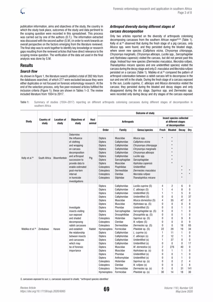
69 Volume 116| Number 5/6 May/June 2020

Review Articlehttps://doi.org/10.17159/sajs.2020/6065

Forensic entomology research and application in southern Africa Page 3 of 8

Table 1: Summary of studies (1934–2017) reporting on different arthropods colonising carcasses during different stages of decomposition in southern Africa

StudyCountry of

studyLocation of

studyObjectives of

studyHost

animal

Outcome of study

ArthropodsInsect species collected

at different stages of decomposition

Order Family Genus/species Fresh Bloated Decay Dry

Kelly et al.36 South Africa Bloemfontein

Determine the influence of clothing and wrapping on carcass decomposition and arthropod succession to provide data to enable estimated post-mortem interval in homicide investigations

Pig

Diptera Diptera Diptera Diptera Diptera Diptera Diptera Diptera Coleoptera Coleoptera Coleoptera Coleoptera

Muscidae Calliphoridae Calliphoridae Calliphoridae Calliphoridae Calliphoridae Sarcophagidae Muscidae Piophilidae Dermestidae Cleridae Silphidae

Musca spp. Calliphora vicina Chrysomya chloropyga Chrysomya marginalis Chrysomya albiceps Lucilia spp. Sarcophagidae Hydrotea capensis Unidentified Dermestes maculatus Necrobia rufipes Thanatophilus micans

*

* * * * * * * *

* * * *

* *

Mabika et al.26 Zimbabwe Harare

Investigate insects visiting sun exposed and shaded decomposing rabbit carcasses and establish the relationship between insects and carcasses which may be of forensic importance

Rabbit

Diptera Diptera Diptera Diptera Diptera Diptera Diptera Diptera Diptera Coleoptera Coleoptera Coleoptera Hymenoptera Diptera Diptera Diptera Diptera Diptera Diptera Diptera Diptera Coleoptera Coleoptera Coleoptera Hymenoptera

Calliphoridae Calliphoridae Calliphoridae Calliphoridae Muscidae Muscidae Phoridae Sarcophagidae Drosophilidae Histeridae Cleridae Dermestidae Formicidae Calliphoridae Calliphoridae Calliphoridae Calliphoridae Muscidae Muscidae Phoridae Anthomyiidae Histeridae Cleridae Dermestidae Formicidae

Lucilia cuprina (S) C. albiceps (S) Unidentified (S) Unidentified (S) Musca domestica (S) Hydrotaea sp. (S) Unidentified (S) Sarcophagidae sp. (S) Drosophilia sp. (S) Saprinus sp. (S) N. rufipes (S) Dermestes sp. (S) Pheidole sp. (S) L. cuprina (s) C. albiceps (s) Unidentified (s) Unidentified (s) M. domestica (s) Hydrotaea sp. (s) Unidentified (s) Unidentified (s) Saprinus sp. (s) N. rufipes (s) Dermestes sp. (s) Pheidole sp. (s)

4 1 1 0 4 0 0 0 0 0 0 0

22 1 2 1 0 2 0 0 0 0 0 0

30

2 4 1 0 55 0 0 0 0 0 0 0

29 11 12 27 0

276 1 0 0 0 0 0

14

6 8 5 0 47 0 1 1 1 9 0

18 19 1 1 0 0

40 1 1 1 2 3 31 18

0 0 0 37 0 8 0 0 0 8 9 65 34 0 0 0

17 0 0 0 0 4 8

141 30

S, carcasses exposed to sun; s, carcasses exposed to shade; *arthropod species identified

publication information, aims and objectives of the study, the country in which the study took place, outcomes of the study and data pertinent to the scoping question were recorded in this spreadsheet. This process was carried out by one of the authors (D.T.). The information extracted was discussed with the second author (S.M.) in order to work towards an overall perspective on the factors emerging from the literature reviewed. The final step was to work together to identify key knowledge or research gaps resulting from the reviewed articles that have direct relevance to the scoping review question. The verification of the data set used in the final analysis was done by S.M.

ResultsSearch flowAs shown in Figure 1, the literature search yielded a total of 282 hits from the databases searched, of which 277 were excluded because they were either duplicates or not focused on forensic entomology research. At the end of the selection process, only five peer-reviewed articles fulfilled the inclusion criteria (Figure 1); these are shown in Tables 1–3. The review included literature from 1934 to 2017.

Arthropod diversity during different stages of carcass decomposition Only two articles reported on the diversity of arthropods colonising decomposing carcasses from the southern African region26,36 (Table 1). Kelly et al.36 observed that during the fresh stage of a pig carcass, only Musca spp. were found, and they persisted during the bloated stage, where seven new species (Calliphora vicina, Chrysomya chloropyga, Chrysomya marginalis, Chrysomya albiceps, Lucilia spp., Sarcophagidae and Hydrotaea capensis) visited the carcass, but did not persist past this stage. Instead four new species (Dermestes maculatus, Necrobia rufipes, Thanatophilus micans species and one unidentified species) visited the carcass during the decay stage and only D. maculatus and Necrobia rufipes persisted on a carcass (Table 1). Mabika et al.26 compared the pattern of arthropod colonisation between a rabbit carcass left to decompose in the sun and one left in the shade. During the fresh stage of a carcass exposed to the sun, Lucilia cuprina, C. albiceps and Musca domestica visited the carcass; they persisted during the bloated and decay stages and only disappeared during the dry stage. Saprinus spp. and Dermestes spp. were recorded only during decay and dry stages of the carcass exposed

70 Volume 116| Number 5/6 May/June 2020

Review Articlehttps://doi.org/10.17159/sajs.2020/6065

Table 2: Summary of studies (1934–2017) on the diversity and abundance of carrion-feeding arthropods collected during different seasons in southern Africa

Study Country of study

Location of study Objectives of study Host

animal

Outcome of study

Order/family/speciesAverage number of carrion-

feeding arthropods

Dry season Rainy season

Braack37 South AfricaKruger National Park

To collect and identify the species found on the large mammal carcasses during both summer and winter

Impala

Anisolabis sp. Bormansia meridionalis Burr Euborellia annulipes (Lucas) Fusius rubricosus (Stal) Lisarda rhodesiensis Miller Rhinocoris albopunctatus (StaI) R. violentus (Germar) Xylocoris (Proxylocoris) afer Reuter Solenostethium liligerum Metagonum sp. Platymetopus curtulus (Peringuey) Xenodochus melanarius (Boheman) Histeridae Fabricius Staphylinidae Trogidae Allogymnopleurus thalassinus (Klug) Anachalcos convexus (Boheman) Aphodius sp. Caccobius convexifrons (Roth) C. nigritulus (Klug) Catharsius philus (Kolbe) Copris amyntor (Klug) C. elphenor (Klug) C. evanidus (Klug) C. mesacanthus (Harold) Garreta nitens (Olivier) Gymnopleurus virens (Erichson) Metacatharsius opacus (Waterhouse) Milichus sp. probably apicalis (Fahraeus) Onitis fulgidus (Klug) O. granulisetosus (Ferreira) O. inversidens (van Lansberge) O. obenbergeri (Balthasar) O. picticollis (Boheman) Onthophagus (Proagoderus) dives (Klug) Pedaria sp. Phaeochrous madagascariensis (Westwood) Phalops ardea (Klug) Sarophorus costatus (Fahraeus) Scarabaeus ebenus (Klug) Sisyphus calcaratus (Klug) S. goryi (Harold) S. impressipennis (van Lansberge) S. injuscatus (Klug) S. seminulum (Gerstaecker) Sybax distortus (Schaum) Tiniocellus spinipes (Peringuey) Dermestes maculatus (De Geer) Necrobia rufipes (De Geer) Phloeocopus sp. Carpophilus nr. quadrisignatus Er. Carpophilus sp. Bactria sp. Euscelidia rapax (Westwood) Hoplistomerus nobilis Loew Neolophonotus (Lophopeltis) sp. Ommatius sp. Stichopogon caffer (Hermann)

– – – – – – – – – – –

662 – – – – – – – – – – – – – – – – – – – – – – – – – – – – – – – – – – –

191 – – – – – – – – – – –

<10 <10 <10 <10 <10 <10 <10 ±60 <10 <10 <10 <10

– 265 625 422 <30 164

<100 <30 <30 <30 <30 <30 <30 <30 <30 <30 <30 <30 <30 <30 <30 <30 <30 670 <30 486 <30 304 <30 <30 <30 <30 <30 <30 <30 <30

– 572 1

<10 <10 <10 <10 <10 <10 <10 <10

Forensic entomology research and application in southern Africa Page 4 of 8

Table 2 continues...

71 Volume 116| Number 5/6 May/June 2020

Review Articlehttps://doi.org/10.17159/sajs.2020/6065

Study Country of study

Location of study Objectives of study Host

animal

Outcome of study

Order/family/speciesAverage number of carrion-

feeding arthropods

Dry season Rainy season

S. punctus (Loew) Crossopalpus n. sp. Hypocerides spinulicosta (Beyer) Megaselia curtineura Megaselia sp. n. pauculitincta Plethysmochaeta sp. Australosepsis niveipennis (Becker) Paratoxopoda depilis (Walker) Xenosepsis sp. Piophilidae Cestrotus n. sp. Homoneura (Keisomyia) n. sp. Curtonotum cuthbertsoni (Duda) Sphaeroceridae Chlorichaeta albipennis (Loew.) Discomyza eritrea (Cresson) Mosillus beckeri (Cresson) Apotropina n. sp. Chloropsina sp. Conioscinella sp. Oscinella sp. Siphunculina ornatifrons (Loew) S. punctifrons (Sabrosky) Siphunculina sp. Desmometopa m-nigrum (Zetterstedt) Leptometopa latipes (Meigen) Leptometopa n. sp. Meoneura n. sp. Milichiella lacteipennis (Loew) Muscidae Fannia leucosticta (Meigen) Graphomya leucomelas (Wiedemann) Gymnodia mervinia (Walker) Gymnodia tonitrui (Wiedemann) Haematobosca latifrons (Malloch) H. spinigera (Malloch) H. thirouxi ssp. potans (Bezzi) Morellia nilotica (Loew) Ophyra capensis (Wiedemann) Lucilia sp. Nasonia vitripennis Trichopria lewisi (Nixon) Lardoglyphus sp. Macrocheles muscaedomesticae Pygmephorus sp.

– – – – – – – – – – – – – – – – – – – – – – – – – – – – – – – – – – – – – – 47 – – – – –

<10 <10 <10 <10 <10 <10 <50 97

<50 849 <10 <10 <10 223 <10 <10 <10 <40 <40 <40 <40 250 <40 <40 <40 <40 <40 574 <40 289 1 1 5 3 1 6 7 3

303 –

<40 >35 <100 <100 <100

Ellison38 South AfricaKlaserie Private Nature Reserve

The effect of scavenger mutilation on the subsequent rate of decomposition and insect colonisation of such carcasses

Impala

Saprinus spp. Necrobia rufipes Dermestes maculatus Aleochara spp. Thanatophilus spp. Mycetophagidae spp. Onthophagus spp. Piophila spp. Ophyra capensis Musca spp. Chrysomya albiceps Chrysomya chloropyga Chrysomya marginalis Chrysomya putoria Tricyclea spp. Lucilia spp. Sarcophaga spp. Auchmeromyia luteola Ceratophaga vastella Brachynieria spp. Acrididae spp.

1.3 6.6 9.2 <1 <1 <1 <1 36.5 3.4 10.9 3.4 <1 4

<1 9.7 11

0.75 0.25 <1 <1 <1

– – – – – – – – – – – – – – – – – – – – –

–, None present or identified

Forensic entomology research and application in southern Africa Page 5 of 8

...Table 2 continued

72 Volume 116| Number 5/6 May/June 2020

Review Articlehttps://doi.org/10.17159/sajs.2020/6065

to the sun, whereas Pheidole spp. persisted throughout the four stages of decomposition on the carcass exposed to the sun. Similarly, L. cuprina, C. albiceps and M. domestica species visited the carcass in the shade during the fresh stage and persisted during the bloated and decay stages, but then disappeared during the dry stage. Saprinus spp. and Dermestes spp. visited the carcass in the shade only during the decay and dry stages, whereas Pheidole spp. visited the carcass in the shade throughout the four stages of decomposition. It was further observed that N. rufipes only visited the carcass exposed to the sun during the dry stage but persisted during both decay and dry stages on the carcass in the shade. Similarly, Hydrotaea spp. appeared on the carcass exposed to the sun during the dry stage only, but during both bloated and decay stages of the carcass in the shade. However, Sarcophangidae spp. and Drosophilia spp. persisted during the decay stage only on the carcass exposed to the sun. In the study of Kelly et al.36, L. cuprina and C. albiceps visited the carcass only during the bloat stage, whereas in Mabika et al.’s26 study, L. cuprina and C. albiceps persisted during the fresh, bloated and decay stages. Furthermore, in both studies, Dermestes spp. visited the carcass during decay and dry stages only.

Seasonal abundance and diversity of carrion-feeding arthropodsThere was an observed difference in the abundance and diversity of arthropods colonising impala carcasses during different seasons (Table 2). More arthropod species were identified during the rainy season37 than the dry season38. Necrobia rufipes was found on the carcass during the dry season by Ellison38; however, Braack37 found and identified the same species during the warm season. In both studies, D. maculatus and Lucilia spp. were found on decomposing carcasses during the dry season only.

Diurnal and nocturnal oviposition of forensically important insect species While attempting to determine the nocturnal oviposition behaviour of blowflies in the southern hemisphere, Williams et al.39 found that Lucilia spp., Chrysomya putoria and C. chloropyga laid eggs during the day and night (Table 3). However, Chrysomya megacephala laid eggs only during the day and at a lower rate than the above-mentioned species. For all species, oviposition rate was generally higher during the day than at night.

DiscussionTo date, there has been limited research published on forensic entomology in southern Africa – a finding supported by the review by Villet et al.6 on the history of forensic entomology Available studies are limited to identification of insect taxa found on carcasses during different stages of decomposition, and presumably this information can then be used in determining PMI.26 Several factors affect the rate and pattern of decomposition, and thereby influence the abundance and diversity of arthropod species found colonising the carcass40, which in turn affects the accuracy of PMI and consequently any legal investigation11. These factors include season, temperature, geographical distribution and vertebrate class (category) studied.26,41

Arthropod diversity during different stages of carcass decompositionDifferent stages of decomposition of a carcass attract different arthropod species. Kelly et al.17 observed and described these stages as follows:

Forensic entomology research and application in southern Africa Page 6 of 8

1. Fresh stage – the stage commencing directly after the animal is killed, characterised by a soft torso and flexible limbs. This stage is very short and associated with no odour.

2. Bloat/bloated stage – this stage is when the torso begins to harden and the abdomen becomes inflated as a result of a build-up of gases. The carcass appears like a balloon, and the body colour changes. Oviposition by arthropods takes place during this stage.

3. Decay stage – at the beginning of this stage, the carcass is deflated as a result of maggots feeding on the carcass tissue which consequently allows gases to be released. Limbs collapse into the resting position, and the skin begins to peel, allowing maggots to feed underneath. At the end of this stage, little tissue remains on the carcass and thus the bones of the skull, ribs and legs are often visible.

4. Dry stage – this stage is characterised by little to no moisture. The gut contents are dried out, with only hair and small patches of skin remaining.

Mabika et al.26 observed that L.a cuprina, C. albiceps and M. domestica, from the families Calliphoridae and Muscidae, were the first to colonise rabbit carrion during the first three stages of decomposition (fresh, bloat and decay stages). However, these species were found only during the bloated stage of a pig carcass.36 Results were consistent with a report by several authors that species from the Calliphoridae and Muscidae families are the first to colonise any carcass as the tissue is still soft41-

44, and the arthropod species from these two families can potentially be useful in the estimation of PMI and determining clues in cases of criminal investigations41. The difference in arrival pattern and colonisation time of the same arthropod species on different carcasses of different animal species as observed by Kelly et al.36 and Mabika et al.26 could be associated with the difference in body size22. According to Sutherland et al.45, smaller animals decompose faster than larger animals and this faster decomposition leads to earlier attraction of arthropods. This in turn influences the sequence of arthropod colonisation, hence, L. cuprina, C. albiceps and M. domestica were found during the fresh, bloat and decay stages of a rabbit18 but only at the bloating stage of a pig carcass36.

The environmental or physical conditions (sun, shade, buried, housed) under which a carcass is disposed of also influence the type of arthropods arriving and colonising the carcass.40 For instance, Mabika et al.26 observed that N. rufipes colonised a carcass exposed to the sun during the dry stage but were found during both decay and dry stages of a carcass in the shade. Hydrotaea spp. were also found on the carcass exposed to the sun during the dry stage but were found during both bloated and decay stages of the carcass in the shade. This variation in insect arrival and colonisation pattern may be because of the difference in relative temperature and humidity – higher temperature and lower humidity lead to chemical reactions that often result in faster decomposition of the carcass.41 Pheidole spp. (Family: Formicidae) were found throughout the decomposition stages.26 Although Morreti et al.46 showed that these species feed on both carcasses and maggots, they do not affect the decomposition process26.

Seasonal abundance and diversity of carrion-feeding arthropodsThe abundance and diversity of arthropod species seem to vary with seasons.37 Braack37 collected and identified more arthropod species during the rainy (summer) season than during the dry (winter) season.

Table 3: Summary of the diurnal and nocturnal oviposition by forensically important arthropods on pig carcasses in southern Africa

Study Country of studyLocation of

studyObjective of study Host animal

Outcome of study

Species identified Day Night

Williams et al.39 South Africa GrahamstownTo determine the nocturnal

oviposition behaviour of blowflies in the southern hemisphere

Pig

Chrysomya megacephala Lucilia sericata Chrysomya putoria Chrysomya chloropyga

1 8 7 2

0 1 1 1

73 Volume 116| Number 5/6 May/June 2020

Review Articlehttps://doi.org/10.17159/sajs.2020/6065

Forensic entomology research and application in southern Africa Page 7 of 8

This observation is congruent with that of Kelly et al.36 and Parry et al.47, who observed more arthropod species colonising carcasses during summer as compared to winter. The authors also observed that there were no other factors influencing the difference in abundance and the diversity of these arthropod species other than the change in season, which subsequently influenced temperature. For instance, the dry season is characterised by low temperatures, which consequently result in reduced arthropod activity, subsequently leading to a gradual decrease in the number of arthropods colonising carcasses.48 Although PMI can still be estimated during the winter (dry) seasons, the reduction in the number of arthropod species present in this season often leads to difficulties in estimating the PMI accurately.36

The absence of certain species during a particular season is expected, as many species are specific to a season and geographical area or locality.20 Arthropod species colonising an impala carcass, as observed by Braack37 and Ellison38, varied from season to season, with few exceptions. Ellison38 surprisingly found N. rufipes colonising an impala carcass during the dry season, which was previously found by Braack37 on an impala carcass during the warm (wet) season. Kelly et al.36 found this species during both seasons. It can be suggested that the presence of this species during both seasons might be because it occurs throughout the year, as was observed and reported by Bensaada et al.49 in Turkey. Furthermore, Ellison38 and Kelly et al.36 found Dermestes maculatus DeGeer and Lucilia spp. on decomposing carcasses during the dry season only. This observation contradicts that of Villet20 who stated that although other Dermestes species such D. peruvianus and D. haemorrhoidalis are common in winter, D. maculatus and Lucilia spp. are typically common and more active in summer, and rare in winter. Therefore, knowledge of the seasonal occurrence of arthropod species is important as it provides useful information about which insect to expect during a given season, and is thus essential in determining PMI in forensic investigations.24

Diurnal and nocturnal oviposition of forensically important insect speciesKnowledge of the developmental stages of breeding arthropods on the carcass, estimating the date and time of egg or larva deposition, and taking into consideration the influence of environmental factors, can all assist in estimating the PMI of a carcass.24,39 Williams et al.39 observed that Lucilia spp., C. putoria and C. chloropyga species laid eggs during both the day and night, and C. megacephala only laid during the day. The authors observed that oviposition was higher during the day than night. This observation may have been due to the fact that ambient temperatures were very low at night, and according to Digby50 and Nicholson51, temperature is one of the important factors influencing flying activity. Williams24 also observed that numerous blowfly species are unable to fly in ambient temperatures below 15 °C, and Richards et al.52 observed that C. marginalis, C. albiceps and C. chloropyga were unable to fly in temperatures below 20.8 °C, 21.7 °C and 23 °C, respectively. Therefore, William et al.39 concluded that the low number of species of arthropods colonising the carcass, and low oviposition at night, may have been due to lower temperatures and less light, which hindered the arthropod’s ability to fly and lay eggs on the carcass. However, those species which were closer to the body were able to walk to the carcass, which explains why eggs from other arthropod species were found during the night.

In view of the above studies, arthropods can be an excellent source of evidence in forensic investigations. For instance, if the stage of a decomposing body is not known, it can be easily estimated by observing the species of arthropods colonising the carcass (i.e. Dermestes species can only be found during decay and dry stages). Furthermore, knowledge of seasonal occurrence of certain arthropod species provides useful information in determining PMI because arthropod species vary with season. Animal species also play a significant role in determining which arthropod species are attracted to them during different stages of decomposition. As such, there is need to document the variation of arthropod species attracted to different animal species in different geographical regions/locations. Lack of ideal tools for identification of arthropods to species level in southern African countries might have hampered the wide use of insects in forensic investigations. Although morphological tools have been widely used to identify important arthropod species for forensic studies,

there are limitations. For example, morphological techniques require expertise in taxonomy and the ability to identify and differentiate arthropod species using identification keys which are lacking in many southern African countries. Furthermore, differentiation of some species at larval stage, using morphological approaches, is challenging. With the current advances in DNA technology, molecular tools are now available to facilitate species identification based on genetic examination. In view of the above, we can anticipate that estimates of PMI based on arthropod evidence will become more accurate and probably contribute to accurate interpretation and application of entomology data in medico-legal forensic investigation in southern Africa. Forensic entomology data or research have not been incorporated in cases of poaching, which are reported frequently in southern African countries including South Africa. Therefore, more studies need to be conducted and incorporated with available research so that research can be applied to solve cases of poaching of game animals. Additionally, occurrence of diurnal oviposition by carrion-feeding insects is well known, whereas there is still great debate about the occurrence of nocturnal oviposition, as most forensic entomologists assume that flies are nocturnally inactive. Therefore, future studies on nocturnal oviposition may be necessary, because a high number of deaths occur at night and nocturnal oviposition may be used in the determination of PMI.

ConclusionAlthough forensic entomology is useful in criminal investigations, it is still an emerging field in southern Africa. Studies completed to date have been limited to identification of insect taxa found on carcasses during different stages of decomposition, and this information can subsequently be used to determine PMI. Some of the research conducted in southern African on carrion-feeding insects was not undertaken in a forensic context; however, it has generated useful results which can be used as evidence in forensic investigations and improve the current status of forensic entomology in southern Africa. Nonetheless, future studies on the application of forensic entomology in various criminal investigation such as murder cases, human neglect, and the poaching of animals in southern Africa are recommended. Additionally, few studies have investigated nocturnal oviposition in southern Africa, despite many of deaths occurring at night and nocturnal oviposition therefore being applicable for the estimation of PMI.

AcknowledgementsWe acknowledge the National Research Foundation (South Africa) for their financial support. We further acknowledge the anonymous reviewers for their comments which greatly improved the manuscript.

Authors’ contributionsD.T.: Collected the data and wrote the manuscript. S.M.: Conceptualised the idea, verified the data set used in the final analysis and participated in the revision of the manuscript.

References1. Amendt J, Campobasso CP, Gaudry E, Reiter C, LeBlanc HN, Hall MJR. Best

practice in forensic entomology – standards and guidelines. Int J Legal Med. 2007;121(2):90–104. https://doi.org/10.1007/s00414-006-0086-x

2. Amendt J, Richards CS, Campobasso CP, Zehner R, Hall MJR. Forensic entomology: Applications and limitations. Forensic Sci Med Pat. 2011;7(4):379–392. https://doi.org/10.1007/s12024-010-9209-2

3. Harvey ML, Mansell MW, Villet MH, Dadour IR. Molecular identification of some forensically important blowflies of southern Africa and Australia. Med Vet Entomol. 2003;17(4):363–369. https://doi.org/10.1111/j.1365-2915.2003.00452.x

4. Greenberg B. Flies as forensic indicators. J Med Entomol. 1991;28(5):565–577. https://doi.org/10.1093/jmedent/28.5.565

5. Goff ML. Estimation of postmortem interval using arthropod development and successional patterns. Forensic Sci Rev. 1993;5(2):81–94.

6. Villet MH, MacKenzie B, Muller WJ. Larval development of the carrion-breeding flesh fly Sarcophaga (Liosarcophaga) tibialis Macquart (Diptera: Sarcophagidae) at constant temperatures. Afr Entomol. 2006;14(2):357–366.

7. Anderson GS. Forensic entomology in British Columbia: A brief history. J Entomol Soc B C. 2001;9:127–135.

74 Volume 116| Number 5/6 May/June 2020

Review Articlehttps://doi.org/10.17159/sajs.2020/6065

Forensic entomology research and application in southern Africa Page 8 of 8

8. Goff ML. Comparison of insect species associated with decomposing remains recovered inside dwellings and outdoors on the island of Oahu, Hawaii. J Forensic Sci. 1991;36(3):748–753. https://doi.org/10.1520/JFS13085J

9. Sukontason K, Narongchai P, Kanchai C, Vichairat K, Sribanditmongkol P, Bhoopat T, et al. Forensic entomology cases in Thailand: A review of cases from 2000 to 2006. Parasitol Res. 2007;101:1417–1423. https://doi.org/10.1007/s00436-007-0659-8

10. Badenhorst R, Villet MH. The uses of Chrysomya megacephala (Fabricius, 1794) (Diptera: Calliphoridae) in forensic entomology. Forensic Sci Res. 2018;3(1):2–15. https://doi.org/10.1080/20961790.2018.1426136

11. Catts EP. Problems in estimating the postmortem interval in death investigations. J Agric Entomol. 1992;9(4):245–255.

12. Greenberg B. Nocturnal oviposition behaviour of blow flies (Diptera: Calliphoridae). J Med Entomol. 1990;27(5):807–810. https://doi.org/10.1093/jmedent/27.5.807

13. Dupont FYF, Champlain DL, Cyrille AA, Felix BB. A preliminary study of arthropod associated with carrion in Yaounde, Cameroon: A first step in forensic entomology in Central Africa. J Ecol Nat Environ. 2011;3(6):215–220.

14. Prichard JD, Kossoris PD, Leibovitch RA, Robertson LD, Lovell FW. Implications of trombiculid mite bites: Reports of a case and submission of evidence in a murder trial. J Forensic Sci. 1986;31(1):301–306. https://doi.org/10.1520/JFS11887J

15. Smith KGV. A manual of forensic entomology. London: British Museum (Natural History) and Cornell University Press; 1986.

16. Brundage A, Byrd JH. Forensic entomology in animal cruelty cases. Vet Pathol. 2016;53(5):898–909. https://doi.org/10.1177/0300985816651683

17. Kelly JA, Van der Linde TC, Anderson GS. The influence of clothing and wrapping on carcass decomposition and arthropod succession during the warmer seasons in central South Africa. J Forensic Sci. 2009;54(5):1105–1112. https://doi.org/10.1111/j.1556-4029. 2009.011 13.x

18. Louw SVDM, Van der Linde TC. Insects frequenting decomposing corpses in central South Africa. Afr Entomol. 1993;1(2):265–269.

19. Tomberlin JK, Mohr R, Benbow ME, Tarone AM, VanLaerhoven S. A roadmap for bridging basic and applied research in forensic entomology. Annu Rev Entomol. 2011;56:401–421. https://doi.org/10.1146/annurev-ento-051710-103143

20. Villet MH. African carrion ecosystems and their insect communities in relation to forensic entomology. Pest Tech. 2011;5(1):1–15.

21. Megyesi MS, Nawrocki SP, Haskell NH. Using accumulated degree-days to estimate the postmortem interval from decomposed human remains. J Forensic Sci. 2005; 50(3):618–622. https://doi.org/10.1520/JFS2004017

22. Simmons T, Adlam RE, Moffatt C. Debugging decomposition data comparative taphonomic studies and the influence of insects and carcass size on decomposition rate. J Forensic Sci. 2010;55(1):8–13. https://doi.org/10.1111/j.1556-4029.2009.01206.x

23. Denno RF, Cothran WR. Niche relationships of a guild of necrophagous flies. Ann Entomol Soc Am. 1975;68(4):741–754. https://doi.org/10.1093/aesa/68.4.741

24. Williams KA. Spatial and temporal occurrence of forensically important South African blowflies (Diptera: Calliphoridae) [MSc thesis]. Grahamstown: Rhodes University; 2003.

25. Byrd JH, Castner JL. Forensic entomology: The utility of arthropods in legal investigations. 2nd ed. Boca Raton, FL: CRC Press; 2010.

26. Mabika N, Masendu R, Mawera G. An initial study of insect succession on decomposing rabbit carrions in Harare, Zimbabwe. Asian Pac J Trop Biomed. 2014;4(7):561–565. https://doi.org/10.12980/APJTB.4.2014C1031

27. Okiwelu SN, Ikpamii T, Umeozor OC. Arthropods associated with mammalian carcasses in Rivers State, Nigeria. Afr J Biomed Res. 2008;11(3):339–342. http://doi.org/10. 4314/ajbr.v11i3.50754

28. Williams KA, Villet MH. A history of southern African research relevant to forensic entomology. S Afr J Sci. 2006;102(1–2):59–65.

29. Boehme P, Amendt J, Zehner R. The use of COI barcodes for molecular identification of forensically important fly species in Germany. Parasitol Res. 2012;110(6):2325–2332. https://doi.org/10.1007/s00436-011-2767-8

30. Florin AB, Gyllenstrand N. Isolation and characterization of polymorphic microsatellite markers in the blowflies Lucilia illustris and Lucilia sericata. Mol Ecol Notes. 2002;2(2):113–116. https://doi.org/10.1046/j.1471-8286.2002.00165.x

31. Wayne RK, Ostrander EA. Lessons learned from the dog genome. Trends Genet. 2007;23(11):557–567. https://doi.org/10.1016/j.tig.2007.08.013

32. Velasquez Y, Magana C, Martinez-Sanchez A, Rojo S. Diptera of forensic importance in the Iberian Peninsula: Larval identification key. Med Vet Entomol. 2010;24(3):293–308. https://doi.org/10.1111/j.1365-2915.2010.00879.x

33. Wells JD, Stevens JR. Application of DNA-based methods in forensic entomology. Annu Rev Entomol. 2008;53:103–120. https://doi.org/10.1146/annurev.ento.52.110405.091423

34. Johnston R, Crooks VA, Snyder J, Kingsbury P. What is known about the effects of medical tourism in destination and departure countries? A scoping review. Int J Equity Health. 2010;9, Art. #24, 13 pages. https://doi.org/10.1186/1475-9276-9-24

35. Arksey H, O’Malley L. Scoping studies: Towards a methodological framework. Int J Soc Res Methodol. 2005;8(1):19–32. https://doi.org/10.1080/1364557032000119616

36. Kelly JA, Van der Linde TC, Anderson GS. The influence of wounds, severe trauma, and clothing on carcass decomposition and arthropod succession in South Africa. Can Soc Forensic Sci J. 2011;44(4):144–157. https://doi.org/10.1080/00085030.2011.10768149

37. Braack LEO. Arthropods associated with carcasses in the northern Kruger National Park. S Afr J Wildl Res. 1986;16(3):91–98.

38. Ellison GTH. The effect of scavenger mutilation on insect succession at impala carcasses in southern Africa. J Zool. 1990;220(4):679–688. https://doi.org/10.1111/j.1469-7998 .1990.tb04742.x

39. Williams KA, Wallman JF, Lessard BD. Nocturnal oviposition behavior of blowflies (Diptera: Calliphoridae) in the southern hemisphere (South Africa and Australia) and its forensic implications. Forensic Sci Med Pathol. 2017;13(2):123–134. https://doi.org/10.1007/s12024-017-9861-x

40. Braack LEO. Visitation patterns of principal species of the insect-complex at carcasses in the Kruger National Park. Koedoe. 1981;24(1):33–49. https://doi.org/10.4102/koedoe.v24i1.617

41. Padonou GG, Gnanguenon V, Osse R, Oussou O, Odjo E, Akinro B, et al. First evidence of forensic entomology revealed the presence of arthropods on rabbit carrion in Cotonou, Benin (West Africa). Int J Entomol Res. 2017;2(6):94–98.

42. Abajue MC, Ewuim SC, Akunne CE. Preliminary checklist of flies associated with pig carrions decomposition in Okija, Anambra State, Nigeria. Anim Res Int. 2014;11(1):1899–1904. https://www.ajol.info/index.php/ari/article/viewFile/102778/93043

43. Carvalho LML, Linhares AX. Seasonality of insect succession and pig carcass decomposition in a natural forest area in southern eastern Brazil. J Forensic Sci. 2001;46(3):604–608. https://doi.org/10.1520/jfs15011j

44. Picard CJ, Wells JD. Survey of the genetic diversity of Phormia regina (Diptera: Calliphoridae) using amplified fragment length polymorphisms. J Med Entomol. 2009;46(3):664–670. https://doi.org/10.1603/033.046.0334

45. Sutherland A, Myburgh J, Steyn M, Becker PJ. The effect of body size on the rate of decomposition in a temperate region of South Africa. Forensic Sci Int. 2013;231(1–3):257–262. https://doi.org/10.1016/j.forsciint.2013.05.035

46. Moretti T, Solis DR, Godoy WA. Ants (Hymenoptera: Formicidae) collected with carrion-baited traps in Southeast Brazil. Open Forensic Sci J. 2013;6:1–5. https://doi.org/10.2174/1874402801306010001

47. Parry NJ, Mansell MW, Weldon CW. Seasonal, locality, and habitat variation in assemblages of carrion-associated Diptera in Gauteng province, South Africa. J Med Entomol. 2016;53(6):1322–1329. https://doi.org/10.1093/jme/tjw104

48. Gruner SV, Slone DH, Capinera JL. Forensically important Calliphoridae (Diptera) associated with pig carrion in rural north-central Florida. J Med Entomol. 2007; 44(3):509–515. https://doi.org/10.1093/jmedent/44.3.509

49. Bensaada F, Nadir BA, Saifi M, Doumandji S. First data on insects to forensic interest in the region of Gouraya, Algeria. Int J Agric Innov Res. 2014;3(2):461–466.

50. Digby PSB. Flight activity in the blowfly Calliphora erythrocephala, in relation to light and radiant heat, with special reference to adaptation. J Exp Biol. 1958;35(1):1–19.

51. Nicholson AJ. The influence of temperature on the activity of sheep-blowflies. Bull Entomol Res. 1934;25(1):85–99. https://doi.org/10.1017/S0007485300012529

52. Richards CS, Williams KA, Villet MH. Predicting geographic distribution of seven forensically significant blowfly species (Diptera: Calliphoridae) in South Africa. Afr Entomol. 2009;17(2):170–182. https://doi.org/10.4001/003.017.020

75 Volume 116| Number 5/6 May/June 2020

Research Articlehttps://doi.org/10.17159/sajs.2020/6871

© 2020. The Author(s). Published under a Creative Commons Attribution Licence.

Updated lower limb stature estimation equations for a South African population groupAUTHORS:

Mubarak A. Bidmos1

Desiré Brits2

AFFILIATIONS:

1College of Medicine, QU Health, Qatar University, Doha, Qatar2Human Variation and Identification Research Unit, School of Anatomical Sciences, University of the Witwatersrand, Johannesburg, South Africa

CORRESPONDENCE TO: Mubarak Bidmos

EMAIL: mbidmos@qu.edu.qa

DATES:Received: 30 Aug. 2019Revised: 24 Jan. 2020Accepted: 12 Feb. 2020Published: 27 May 2020

HOW TO CITE: Bidmos MA, Brits D. Updated lower limb stature estimation equations for a South African population group. S Afr J Sci. 2020;116(5/6), Art. #6871, 7 pages. https://doi.org/10.17159/sajs.2020/6871

ARTICLE INCLUDES:☒ Peer review ☒ Supplementary material

DATA AVAILABILITY:☐ Open data set ☐ All data included☒ On request from author(s)☐ Not available☐ Not applicable

EDITORS: Margaret Avery Maryna Steyn

KEYWORDS: living stature, estimation, forensic anthropology, MRI scanogram

FUNDING: Carnegie Corporation (NY, USA); National Research Foundation (South Africa)

One of the main steps in the identification of an unknown person, from their skeletal remains, is the estimation of stature. Measurements of intact long bones of the upper and lower extremities are widely used for this purpose because of the high correlation that exists between these bones and stature. In 1987, Lundy and Feldesman presented regression equations for stature estimation for the black South African population group based on measurements of bones from the Raymond A. Dart Collection of Human Skeletons. Local anthropologists have questioned the validity of these equations. Living stature measurement and magnetic resonance imaging scanograms of 58 adult volunteers (28 males and 30 females) representing the modern black South African population group were obtained. Physiological length of the femur (FEPL) and physiological length of the tibia (TPL) were measured on each scanogram and substituted into appropriate equations of Lundy and Feldesman (S Afr J Sci. 1987;83:54–55) to obtain total skeletal height (TSHL&F). Measured total skeletal height (TSHMeas) for each subject from scanograms was compared with TSHL&F. Both FEPL and TPL presented with significantly high positive correlations with TSHMeas. A comparison between TSHL&F and TSHMeas using a paired t-test, showed a statistically significant difference – an indication of non-validity of Lundy and Feldesman’s equations. New regression equations for estimation of living stature were formulated separately for male and female subjects. The standard error of estimate was low, which compared well with those reported for other studies that used long limb bones.

Significance: • Statistically significant differences were observed between measured and estimated skeletal height,

thus confirming non-validity of Lundy and Fieldsman’s (1987) equations for lower limb bones.

• New regression equations for living stature estimation were formulated for femur and tibia lengths, and the low standard error of estimates of equations compared well to results from other studies.

IntroductionEstimation of stature from complete skeletons (anatomical method) or from individual/combination measurements of bones (mathematical method) forms a necessary part of the process of establishing the biological profile of an individual from recovered or discovered skeletons. The former method has been reported to produce accurate estimates of stature and is neither population nor sex-specific.1-3 However, it has the disadvantages of being time consuming and very tedious.2 In addition, the anatomical method can be used for estimation of stature only if an intact and complete skeleton is available, which is considered a luxury in forensic cases. Consequently, the latter method, i.e. the mathematical method, is the most often used method in the absence of a complete skeleton or when bones are recovered in fragmentary states.

The mathematical method is based mainly on a statistical theorem known as regression analysis. This involves the formulation of regression equations from individual measurements or combinations of measurements of intact and fragmentary bones of the skeleton and percutaneous bones. This method is less time-consuming and tedious than the anatomical method and is considered more applicable in most forensic cases. However, the mathematical method is both population and sex specific. It therefore requires that equations for the estimation of stature need to be formulated for different population groups and at appropriate intervals in order to account for temporal changes.4 There has been a plethora of studies on stature reconstruction using measurements of long bones of upper and lower limbs in different parts of the world following the publication of arguably the largest study on stature reconstruction by Trotter and Gleser4 in 1958. Regression equations have been formulated for populations including, but not limited to, the Portuguese5, Germans6, Bulgarian7, Polish8, Turks9, Croatians10, Mexicans11, Spaniards12, Koreans13 and Japanese14. Regression equations have also been formulated from measurements of fragments of long bones for stature reconstruction15 and other bony elements (e.g. clavicle16, skull17, scapulae18, metacarpals,19 vertebrae20, sacrum21, calcaneus22 and metatarsals23) as long limb bones are often recovered in forensic and archaeological practice in fragmentary states.

In South Africa, a country with a high crime rate, similar regression equations have been formulated from intact long bones24,25, fragments of long bones26, the skull27, sacrum28, metatarsals29 and calcaneus30. In 1983, Lundy31 conducted the first ever study on stature reconstruction in South Africa. Lundy31 used Fully’s1 method in calculating total skeletal height (TSH) which was later regressed on maximum lengths of humeri, radii, ulnae, femora, tibiae and fibulae. Regression equations were derived separately for male and female black South Africans.31 Lundy and Feldesman24 revised the regression equations due to some errors in the computer program handling some data. The regression equations developed by Lundy and Feldesman24 are the most frequently used stature estimation equations when dealing with black South African skeletal remains; however, results from an unpublished study by Arendse32 highlighted the need to re-examine these equations, specifically in modern black South Africans. The validity of these equations on a contemporary black South African population has been questioned, as these equations were derived more than three decades ago, using skeletal remains housed in the Raymond A. Dart Collection of Human Skeletons. Regrettably, many skeletal collections do not represent the populations from which

76 Volume 116| Number 5/6 May/June 2020

Research Articlehttps://doi.org/10.17159/sajs.2020/6871

they were derived as collections often have an over-representation of the elderly and individuals from lower socio-economic strata.33,34 Additionally, the effects of secular trends on populations also often render skeletal collections unrepresentative of their modern counterparts.35,36 As such, many studies are using modern image modalities of living individuals to study skeletonised remains.12,18,20,37,38 Because there has not been any attempt to test the validity of these equations on living individuals, the aim of this study was to investigate the validity of some of Lundy and Feldesman’s equations24 on a sample of living black South Africans using data collected from magnetic resonance imaging (MRI) scanograms and to calculate new equations, if necessary.

Subjects and methodsParticipants Prior to the commencement of the study, ethics approval was obtained from the Human Research Ethics Committee of the University of the Witwatersrand, Johannesburg, South Africa (clearance certificate number M180788) to access data collected in two previous studies by Bidmos and Manger37 and Brits et al.38 Data used in the current study and how they were obtained have been described in previous studies.37,38 Participants in these studies37,38 were individuals from diverse South African black ethnological groups. As previous studies31,39 have shown little intertribal variations amongst black South Africans, they were considered a single homologous group. Furthermore, Franklin et al.40 reported the disappearance of tribal subdivisions, possibly due to inter-marriage between individuals of different groups. More than 88 individuals were approached to participate in both studies.37,38 However, only data from a final sample of 58 participants (28 males and 30 females) were analysed. The individual measurements of each participant are provided in Supplementary table 1.

MeasurementsLiving stature of participants was measured, and thereafter, full body MRI scans were collected. Measurement of the living stature (LSM) of each of the participants was taken with a stadiometer on the morning of the MRI scan. This procedure became necessary because of the documented loss of stature during the day.41 Full body MRI scans were carried out at the Wits Donald Gordon Medical Centre in Johannesburg, South Africa. Each participant was scanned in a supine position as documented in previous studies37,38 and the scanned images were then transferred to a DVD. A suite of measurements as described in previous studies37,38 was taken on each scanogram using OsiriX42. These measurements are height of cranium, height of axis (C2), height of vertebrae (C3 to L5), height of first sacral vertebra, physiological (bicondylar) length of the femur, physiological length of tibia and talus-calcaneal height. The sum total of these measurements gave the measured total skeletal height (TSHMeas). Two of these measurements defined and illustrated below were used in the assessment of the validity of Lundy and Feldesman equations24:

1. Physiological (bicondylar) length of the femur (FEPL): The linear measurement between the most superior projecting point of the head of the femur and a line connecting the most inferior aspects of the femoral condyles38 (Figure 1). This measurement was taken on coronal images.

2. Physiological length of the tibia (TPL): The physiological length of the tibia as described by Lundy43 was measured by excluding the intercondylar eminence of the tibia while including the medial malleolus. In the female sample, the physiological length of the tibia was measured between the tip of the medial malleolus and a line drawn parallel to the superior aspect of the lateral tibial condyle38 (Figure 2a). For the male sample, the physiological length of the tibia was measured from the tip of the medial malleolus to the superior aspect of the medial condyle37 (Figure 2b). This measurement was taken on coronal images. As no guidelines are available for osteometric data collection from MRI scans, the two studies explored various ways to collect the tibial length as reliably and accurately as possible.

Updated stature estimation equations for South Africans Page 2 of 7

Scale = 5 cm

Figure 1: A coronal view of the MRI scanogram illustrating the physiological length of the femur.

Scale = 5 cm

Figure 2: A coronal view of a MRI scanogram illustrating how the physiological length of the tibia was measured in (a) female and (b) male subjects.

77 Volume 116| Number 5/6 May/June 2020

Research Articlehttps://doi.org/10.17159/sajs.2020/6871

Updated stature estimation equations for South Africans Page 3 of 7

The FEPL and TPL measurements were summed to produce an additional skeletal measurement. These measurements were used in conjunction with the stature estimation equations for the femur and tibia developed by Lundy and Feldesman24 to estimate total skeletal height (TSHL&F), as per the equations below:

Males

Total skeletal height = 45.721 x 2.403(femur – physiol) ±2.777

Total skeletal height = 60.789 x 2.427(tibia – physiol) ±2.78

Total skeletal height = 46.543 x 1.288(femur + tibia) ±2.371

Females

Total skeletal height = 27.424 x 2.769(femur – physiol) ±2.789

Total skeletal height = 55.968 x 2.485(tibia – physiol) ±3.056

Total skeletal height = 34.617 x 1.41(femur + tibia) ±2.497

Data analysisPrior to data collection for the current study, a test of intra-observer repeatability was performed using Lin’s concordance co-efficient of reproducibility.44 A total of 20 individuals were measured for this purpose and after confirming that the measuring technique was satisfactory (Lin’s concordance correlation coefficients for all measurements were between 0.95 and 0.99), data were collected separately for males and females and captured into MS Excel sheets. Thereafter, descriptive statistics were obtained separately for male and female samples using IBM SPSS (version 24). In addition, normality of data was tested and verified for both sexes.

The accuracy of regression equations derived by Lundy and Feldesman24 for estimation of stature of male and female black South Africans using FEPL, TPL and a combination of both measurements was assessed. For each subject, total skeletal heights (TSHL&F) were calculated from (1) FEPL, (2) TPL and (3) a combination of FEPL and TPL using the appropriate regression equation of Lundy and Feldesman24. The estimated total skeletal height using Lundy and Feldesman’s24 equations (TSHL&F) was compared with the measured total skeletal height on the MRI scanograms (TSHMeas) published by Bidmos and Manger37 and Brits et al.38, using a

paired t-test. Regression analyses were subsequently performed. Firstly, living stature was regressed on FEPL and TPL. Secondly, a regression equation for a combination of both measurements was obtained for both sexes separately. From these analyses, the unstandardised coefficients and constants were obtained in addition to the correlation coefficient (r) and standard error of estimate (SEE).

ResultsThe ages of female subjects ranged between 19 and 60 years, with a mean of 38 years (s.d.=11.2). Male subjects were of a similar age – between 18 and 56 years with a mean age of 35 years (s.d.=10.5). The majority of male and female subjects (70%) fell within the 21–45-year age bracket. There is no statistically significant difference between the mean ages of both sexes (Table 1). The means and standard deviations for LSM, TSHMeas, FEPL and TPL are also shown in Table 1. Mean values of all measurements of male subjects were statistically significantly higher than those for female subjects (Table 1).

Measured values of FEPL, TPL and the combined measurement of FEPL and TPL were substituted into the appropriate sex-specific regression equations of Lundy and Feldesman24 to estimate total skeletal height (TSHL&F). TSHL&F was compared with TSHMeas using a paired t-test. Table 2 shows that a statistically significant difference exists between TSHMeas and calculated TSHL&F using Lundy and Feldesman’s24 equations for FEML, TPL and the sum of FEML and TPL. These results indicate that regression equations previously derived for skeletal height estimation by Lundy and Feldesman24 using FEPL, TPL and a combination of these measurements are no longer valid for male and female black South Africans (Table 2).

Therefore, new regression equations specific for the direct estimation of living stature were calculated from FEPL, TPL and the sum thereof for black South Africans. The correlations between LSM and each of the measured variables – namely FEPL, TPL and a combination of FEPL and TPL – were strong and statistically significant (p<0.0001; Table 3).

In the female sample, FEPL displayed the strongest correlation with LSM (r=0.879, r2=0.773) while the lowest correlation was obtained for the regression equation generated for TPL (r=0.792, r2=0.627). The SEE for the equations ranged between 2.56 and 3.28 cm (Table 3). In the male

Table 1: Descriptive statistics of measurements in previous studies

Lundy43 Bidmos and Manger37 Brits et al.38

Variables Males Females Males Females t-statistic p-value

N Mean s.d. N Mean s.d. N Mean s.d. N Mean s.d.

Age 28 35.00 10.50 30 38.00 11.20 1.050 0.298

LSM 28 170.79 5.29 30 159.10 5.28 -8.418 0.000

TSHMeas 28 144.00 4.77 30 141.10 5.56 -2.198 0.032

FEPL 177 44.78 2.32 125 42.29 2.06 28 45.18 2.28 30 43.30 1.96 11.359 0.001

TPL 177 38.12 2.30 125 35.62 2.22 28 38.17 2.07 30 36.45 2.09 9.803 0.003

LSM, living stature measurement; TSHMeas, measured total skeletal height; FEPL, femur physiological length; TPL, tibia physiological length

Table 2: Comparison of measured total skeletal height and calculated skeletal height using Lundy and Feldesman24 equations for femora and tibiae

Variables Males Females

Correlation Mean difference t p-value Correlation Mean difference t p-value

TSHMeas & TSHL&F (FEPL) 0.857 9.36 17.532 0.000 0.895 6.18 13.419 0.000

TSHMeas & TSHL&F (TPL) 0.830 8.51 15.706 0.000 0.827 5.44 9.349 0.000

TSHMeas & TSHL&F (FEPL+TPL) 0.885 8.98 19.135 0.000 0.885 5.94 12.189 0.000

TSHMeas, measured total skeletal height; TSHL&F, calculated TSH using Lundy and Feldesman's equations; FEPL, femur physiological length; TPL, tibia physiological length

78 Volume 116| Number 5/6 May/June 2020

Research Articlehttps://doi.org/10.17159/sajs.2020/6871

sample, a combination of FEPL and TPL was most strongly correlated (r=0.921, r2=0.848) with LSM. FEPL and TPL each presented similar correlations (r=0.878, r2=0.771) with LSM. The lowest SEE was obtained for the regression equation derived using a combination of FEPL and TPL (2.10 cm). The SEE for regression equations formulated separately for FEPL and TPL was 2.58 cm (Table 3).

DiscussionIn the current study, MRI was used to study the components of the skeletons that constitute stature of living individuals. MRI was selected as the imaging modality as it does not expose participants to high doses of harmful ionising radiation as is the case with X-ray and computed tomography (CT).45 Although MRI is not usually used to examine skeletal remains, it has been found that measurements obtained from these scans are comparable to those obtained from CT and dry bones.45 Furthermore, as is evident from the intra-observer repeatability scores, MRI measurements are easily reproducible. By studying living individuals, the researchers were able to measure living stature as opposed to relying on often over-reported statures46 or questionable cadaveric lengths reported in skeletal collections31. It has been shown that cadaveric length is greater than living stature47 and therefore stature estimation methods using cadaveric length tends to overestimate living stature48. To adjust for this, a correction factor of 25 mm was proposed by Trotter and Gleser49. However, a recent study by Cardoso et al.47 showed that the difference between cadaveric length and living stature is greater than initially proposed with an average difference of about 40 mm, and, as such, there is no consensus yet on the adjustment factor required.

By using measured living stature, researchers also did not have to make use of estimates of living stature produced using the anatomical (Fully1) method. This method is considered to be an accurate method for the estimation of skeletal height because it takes into account all the skeletal elements that constitute stature.2 It remains the most extensively used method in the formulation of regression equations for stature estimation in South Africa.24,25,30,31 Recently, a number of studies3,37,38 have challenged the accuracy of the anatomical method because of uncertainties regarding applicability of the correction factors for soft tissue that were recommended by Fully1. The stature estimation equations derived by Lundy and Feldesman24 were calculated using the anatomical method and as such the validity and accuracy of these equations need to be assessed in a modern living black South African population. In this study, measurements of living stature ranged between 161 cm and 180 cm (mean = 170.79 cm) for males and between 146 cm and 171 cm (mean = 159.1 cm) for females. These measured living statures are similar to living statures recorded for black South African military personnel50 and are therefore considered representative of the modern black South African population group. The members of the South African military50 represent a sample of living adult population. Consequently, their mean height was compared with the mean height of the individuals in the current study. On average, black South Africans are shorter than

Updated stature estimation equations for South Africans Page 4 of 7

black and white North Americans51, white South Africans50 and Spanish males12. However, they are slightly taller than the Portuguese5 and Japanese14 based on cadaveric heights which have been converted to living stature. Direct comparisons of stature are often limited as most stature estimation research relies on either cadaveric height or heights measured during autopsies.8,10,13

The mean femoral and tibial length measurements from scanograms were 45.2 cm (±2.3 cm) and 38.2 cm (±2.1 cm) for males and 43.3 cm (±2.0 cm) and 36.5 cm (±2.1 cm) for females. The mean femoral measurement from the current study for males was smaller compared to those of black and white North Americans49, Spanish12 and white South Africans25 but slightly larger than that reported for Japanese14. The mean femoral measurement for the current sample was comparable to that of black South Africans reported by Lundy43. The mean femoral measurement for females was larger than those reported for Japanese14 but smaller than the average recorded by Lundy43. The measurement is comparable to that of black North Americans49, white South Africans25 and Spaniards12. In addition, mean tibial measurement for females was longer than those reported for black43 and white South Africans25 while the mean tibial measurement for males was comparable to that reported for black24,43 and white South Africans25. A direct comparison of bone lengths with other studies were difficult as some studies report cutaneous bone measurements11, measurements with cartilage7 or maximum measurements as opposed to physiological/bicondylar measurements10,11. Comparisons of tibial measurements were also limited due to variations in the way in which the tibiae were measured.52,53 Furthermore, tibial differences or the lack thereof can also be contributed to the MRI techniques used to measure the bone. No standards for the measurement of skeletal remains from MRI scanograms or other image modalities are currently available or are yet to be validated. However, a pilot study has found no significant difference between the tibial lengths measured from MRI scans and the corresponding dry bone measurement.54 As such, efforts were made to collect data in line with current standard osteometric practices. The differences highlighted above between the various population groups support the need for population-specific equations. All measurements for male subjects were significantly greater than those for female subjects, thus confirming the need for sex-specific regression equations.

Of importance are the differences noted between the femoral and tibial measurements of female black South Africans in the current study compared to those presented by Lundy43. These differences hint at secular trends. Secular trends are often associated with changes in environmental conditions such as nutrition, health and medical care55 and in South Africa could also be related to the abolishment of apartheid. Previously, a lack of secular change in stature and measurements of the femur and tibia were noted in black South African individuals from the early 20th century.56 However, more recent results have found a positive secular increase in stature in black South Africans along with an increase in lower limb lengths in relation to stature.57 The reason for the lack of

Table 3: Equations for stature estimation (in cm), correlation and standard error of estimate

Equations Correlation F-statistic p-value Standard error of estimate

Females

2.366 (FEPL) + 56.623 0.879 95.074 0.000* 2.56

1.997 (TPL) + 86.261 0.792 47.047 0.000* 3.28

1.150 (FEPL + TPL) + 67.319 0.858 78.346 0.000* 2.76

Males

2.039 (FEPL) + 78.666 0.878 87.453 0.000* 2.58

2.247 (TPL) + 85.006 0.878 87.697 0.000* 2.58

1.176 (FEPL + TPL) + 72.723 0.921 145.72 0.000* 2.10

FEPL, femur physiological length; TPL, tibia physiological length;*p<0.05

79 Volume 116| Number 5/6 May/June 2020

Research Articlehttps://doi.org/10.17159/sajs.2020/6871

Updated stature estimation equations for South Africans Page 5 of 7

secular change in males is not fully understood and warrants further research; however, it could in part be related to the small sample sizes in the study. Further supporting secular changes are the statistically significant differences observed between measured total skeletal height and all estimates of total skeletal height using Lundy and Feldesman’s24 stature estimation equations. Therefore, as suggested by Meadows and Jantz35 and Myburgh57, new stature estimation equations from lower limb bone measurements of modern black South Africans were calculated in the current study.

All measured variables along with associated regression equations had very strong statistically significant correlations with measured living stature (Table 3). The correlation between stature and the bicondylar length of the femur was similar between males and females; however, the correlation between the physiological length of the tibia and stature was stronger in males. The association between the femoral and tibial measurements, and stature had an equivalent correlation in males; however, the femur had a stronger association with stature in females. The association between the femur and stature in males in the current study was stronger than that reported for black and white Americans49, Spaniards12 and Koreans13, but weaker than that noted for white South Africans25 and black South Africans24 (Table 4). The relationship between the femur and stature in females was stronger than that reported for White Americans49 and Spaniards12, but weaker than associations reported for black South Africans24, white South Africans25 and Koreans13 (Table 4).

The association between the tibia and stature in the current male sample was comparable to that reported for Spaniards12 and white South Africans25 but stronger than that previously noted by Lundy and Feldesman24 for black South Africans (Table 4). The correlation between stature and the tibia in females was weaker than that documented for Spaniards12 and white South Africans25 and that of black South Africans noted by Lundy and Feldesman24 (Table 4). Interestingly, the correlation of the combined femur and tibia measurement and stature in females was not stronger than that of the femur alone, while the combined measurement in males showed the strongest correlation to stature. Many studies have reported very strong associations between lower limb long bones and stature (Table 4), because these bones directly contribute to the overall height of a person.58

The SEE of equations are considered as a measure of accuracy of regression equations.49 The SEE for stature estimation equations derived from the femoral and tibial measurements in the current male sample was smaller than that reported by various authors for different populations, including that reported for black South Africans by Lundy and Feldesman24 (Table 4). This was also true for female femoral measurements with the exception of the SEE reported for white South Africans.25 Interestingly, SEEs from other populations were smaller than the SEE noted for the stature estimation regression equations derived from the tibia in the current female sample (Table 4). The higher SEE related to the female tibial regression equation is not fully understood and could in part be

related to secular trends that have been observed in the distal limb of female black South Africans57 or could be associated with the slightly larger standard deviation observed for the female tibial measurement, which might hint at greater variation in this measurement in females.

Presented in Table 3 are equations for the estimation of living stature as opposed to the estimation of total skeletal height which is often the case in South Africa.24,25,27,29 Lundy and Feldesman24 derived their total skeletal height estimation equations using the anatomical method in conjunction with soft tissue correction factors proposed by Fully1 to provide an estimate of stature. A number of researchers3,37,38 have questioned the accuracy and applicability of Fully’s1 soft tissue correction factors. Consequently, alternative soft tissue correction factors have been proposed by various authors3,37,38 but there is no consensus on the validity of these factors.

In conclusion, we provide regression equations for the estimation of living stature of black South Africans from measurements of the femur and tibia. These equations, with reasonably low SEEs, do not require the addition of soft tissue correction factors. Regrettably, the sample size of this study was very small due to expenses associated with the collection of full body MRI scans as well as difficulties related to the recruitment of willing participants. As the regression equations proposed here were derived from a small sample size, future studies are encouraged to explore larger sample sizes to validate these equations and also to generate additional stature estimation equations from various skeletal elements, as research has shown that secular trends affect all limbs, especially in black South African populations.57

AcknowledgementsWe thank all those who participated in the study. We also acknowledge the invaluable assistance of staff members from the Department of Radiology, Wits Donald Gordon Medical Centre, especially Dr Haagensen, Ms Bussy, Ms Gibbs and Ms Benade. The assistance of Mr Du Plessis from the School of Anatomical Sciences, University of the Witwatersrand, is also acknowledged. This publication was in part made possible by a grant from the Carnegie Corporation of New York. ‘The statements made and views expressed are, however, solely the responsibility of the authors.’ Additional funding was received from the National Research Foundation (NRF) of South Africa (grant 80655). ‘Any opinion, findings and conclusions or recommendations expressed in this material are those of the authors and therefore the NRF does not accept any liability in regard thereto.’

Authors’ contributionsBoth M.B. and D.B. were responsible for the conception and design of the study; data acquisition, analysis and interpretation; drafting and critically reviewing the manuscript and editing the final version for publication.

Table 4: Comparison of standard errors of estimate (SEE) for the present study and previous studies

Males Females

Study Population Femur Tibia Femur Tibia

r SEE r SEE r SEE r SEE

Trotter and Gleser49 White Americans (military – males; Terry – females) 0.869 3.27 – – 0.851 3.78 – –

Black Americans (military) 0.769 3.93 – –

Lundy and Feldesman24 Black South Africans 0.896 2.78 0.869 2.78 0.896 2.79 0.873 3.06

Muñoz et al.12 Spaniards 0.854 – 0.876 – 0.851 – 0.812 –

Dayal et al.25 White South Africans 0.920 2.64 0.880 3.16 0.930 2.40 0.910 2.59

Lee et al.13 Koreans (max femur length) 0.859 3.21 – – 0.886 3.47

Chiba et al.14 Japanese – 3.81 – – – 3.61 – –

Current study Black South Africans 0.878 2.58 0.878 2.58 0.879 2.56 0.792 3.28

80 Volume 116| Number 5/6 May/June 2020

Research Articlehttps://doi.org/10.17159/sajs.2020/6871

Updated stature estimation equations for South Africans Page 6 of 7

References1. Fully G. Une nouvelle methode de determination de la taille [A new method for

determining size]. Ann Med Leg. 1956;35:266–273. French.

2. Lundy JK. A report on the use of Fully’s anatomical method to estimate stature in military skeletal remains. J Forensic Sci. 1988;33(2):534–539. https://doi.org/10.1520/JFS11969J

3. Raxter MH, Auerbach BM, Ruff CB. Revision of the Fully technique for estimating statures. Am J Phys Anthropol. 2006;130(3):374–384. https://doi.org/10.1002/ajpa.20361

4. Trotter M, Gleser GC. A re-evaluation of estimation of stature based on measurements of stature taken during life and of bones after death. Am J Phys Anthropol. 1958;16(1):79–124. https://doi.org/10.1002/ajpa.1330160106

5. De Mendonça MC. Estimation of height from the length of long bones in a Portuguese adult population. Am J Phys Anthropol. 2000;112(1):39–48. https://doi.org/10.1002/(SICI)1096-8644(200005)112:1<39::AID-AJPA5>3.0.CO;2-%23

6. Mall G, Hubig M, Buttner A, Kuznik J, Penning R, Graw M. Sex determination and estimation of stature from the long bones of the arm. Forensic Sci Int. 2001;117(1–2):23–30. https://doi.org/10.1016/S0379-0738(00)00445-X

7. Radoinova D, Tenekedjiev K, Yordanov Y. Stature estimation from long bone lengths in Bulgarians. Homo. 2002;52(3):221–232. https://doi.org/10.1078/0018-442X-00030

8. Hauser R, Smoliński J, Gos T. The estimation of stature on the basis of measurements of the femur. Forensic Sci Int. 2005;147(2–3):185–190. https://doi.org/10.1016/j.forsciint.2004.09.070

9. Sargin OO, Duyar I, Demirçin S. Estimation of stature from the lengths of ulna and tibia: A cadaveric study based on group-specific regression equations. Euras J Anthropol. 2012;3(1):1–9.

10. Petrovečki V, Mayer D, Šlaus M, Strinović D, Škavić J. Prediction of stature based on radiographic measurements of cadaver long bones: A study of the Croatian population. J Forensic Sci. 2007;52(3):547–552. https://doi.org/10.1111/j.1556-4029.2007.00419.x

11. Garmendia AM, Sanchez-Mejorada G, Gómez-Valdés JA. Stature estimation formulae for Mexican contemporary population: A sample-based study of long bones. J Forensic Leg Med. 2018;54:87–90. https://doi.org/10.1016/j.jflm.2017.12.019

12. Muñoz JI, Linares-Iglesias M, Suarez-Penaranda JM, Mayo M, Miguens X, Rodriguez-Calvo MS, et al. Stature estimation from radiographically determined long bone length in a Spanish population sample. J Forensic Sci. 2001;46(2):363–366. https://doi.org/10.1520/JFS14973J

13. Lee JH, Kim YS, Lee UY, Park DK, Jeong YK, Lee NS, et al. Stature estimation from partial measurements and maximum length of lower limb bones in Koreans. Aust J Forensic Sci. 2014;46(2):330–338. https://doi.org/10.1080/00450618.2013.877078

14. Chiba F, Makino Y, Torimitsu S, Motomura A, Inokuchi G, Ishii N, et al. Stature estimation based on femoral measurements in the modern Japanese population: A cadaveric study using multidetector computed tomography. Int J Legal Med. 2018;132(5):1485–1491. https://doi.org/10.1007/s00414-018-1834-4

15. Simmons T, Jantz RL, Bass WM. Stature estimation from fragmentary femora: A revision of the Steele method. J Forensic Sci. 1990;35(3):628–636. https://doi.org/10.1520/JFS12868J

16. Torimitsu S, Makino Y, Saitoh H, Sakuma A, Ishii N, Yajima D, et al. Stature estimation in a contemporary Japanese population based on clavicular measurements using multidetector computed tomography. Forensic Sci Int. 2017;275:316.e1–316.e6. https://doi.org/10.1016/j.forsciint.2017.02.037

17. Kyllonen KM, Simmons-Ehrhardt T, Monson L. Stature estimation using measurements of the cranium for populations in the United States. Forensic Sci Int. 2017;281:184.e1–184.e9. https://doi.org/10.1016/j.forsciint.2017.10.01

18. Zhang K, Cui JH, Luo YZ, Fan F, Yang M, Li XH, et al. Estimation of stature and sex from scapular measurements by three-dimensional volume-rendering technique using in Chinese. Leg Med. 2016;21:58–63. https://doi.org/10.1016/j.legalmed.2016.06.004

19. Zaher JK, Al-Ameen NFM, Seedhom AE. Stature estimation using anthropometric measurements from computed tomography of metacarpal bones among Egyptian population. Egypt J Forensic Sci. 2011;1(2):103–108. https://doi.org/10.1016/j.ejfs.2011.03.002

20. Milani C, Di Stefano M, Isaia G, Panattoni GL. Stature estimation based on vertebral morphometry by dual energy X-rays absorptiometry imaging in Italian females. J Biol Res. 2017;90, Art. #6430. https://doi.org/10.4081/jbr.2017.6430

21. Pelin C, Duyar I, Kayahan EM, Zagyapan R, Agildere AM, Erar A. Body height estimation based on dimensions of sacral and coccygeal vertebrae. J Forensic Sci. 2005;50(2):294–297. https://doi.org/10.1520/JFS2004010

22. Zhang K, Fan F, Tu M, Wang YH, Deng ZH. Estimation of stature and sex from calcaneal measurements in Chinese. Aust J Forensic Sci. 2017;49(1):69–77. https://doi.org/10.1080/00450618.2015.1128967

23. Ibrahim MA, Elelemi AH, Ibrahim MS, Bandy AH. Adult stature estimation from radiographically determined metatarsal length in Egyptian population. J Forensic Radiol Imaging. 2017;11:28–32. https://doi.org/10.1016/j.jofri.2017.10.002

24. Lundy JK, Feldesman MR. Revised equations for estimating living stature from the long bones of the South African Negro. S Afr J Sci. 1987;83:54–55.

25. Dayal MR, Steyn M, Kuykendall KL. Stature estimation from bones of South African whites. S Afr J Sci. 2008;104(3–4):124–128.

26. Bidmos MA. Estimation of stature using fragmentary femora in indigenous South Africans. Int J Legal Med. 2008;122(4):293–299. https://doi.org/10.1007/s00414-007-0206-2

27. Ryan I, Bidmos MA. Skeletal height reconstruction from measurements of the skull in indigenous South Africans. Forensic Sci Int. 2007;167(1):16–21. https://doi.org/10.1016/j.forsciint.2006.06.003

28. Pininski M, Brits D. Estimating stature in South African populations using various measures of the sacrum. Forensic Sci Int. 2014;234:182.e1–182.e7. https://doi.org/10.1016/j.forsciint.2013.08.030

29. Bidmos MA. Metatarsals in the estimation of stature in South Africans. J Forensic Leg Med. 2008;15(8):505–509. https://doi.org/10.1016/j.jflm.2008.05.007

30. Bidmos MA. Adult stature reconstruction from the calcaneus of South Africans of European descent. J Clin Forensic Med. 2006;13(5):247–252. https://doi.org/10.1016/j.jcfm.2005.11.010

31. Lundy JK. Regression equations for estimating living stature from long limb bones in the South African Negro. S Afr J Sci. 1983;79:337–338.

32. Arendse LM. Stature estimation: Evaluating regression equations for different population groups in South Africa [MSc dissertation]. Cape Town: University of Cape Town; 2018.

33. L’Abbé EN, Loots M, Meiring J. The Pretoria Bone Collection: A modern South African skeletal sample. HOMO. 2005;56(2):197–205. https://doi.org/10.1016/j.jchb.2004.10.004

34. Dayal MR, Kegley AD, Štrkalj G, Bidmos MA, Kuykendall KL. The history and composition of the Raymond A. Dart Collection of human skeletons at the University of the Witwatersrand, Johannesburg, South Africa. Am J Phys Anthropol. 2009;140(2):324–335. https://doi.org/10.1002/ajpa.21072.

35. Meadows L, Jantz RL. Allometric secular change in the long bones from the 1800 to the present. J Forensic Sci. 1995;40(5):762–767. https://doi.org/10.1520/JFS15380J

36. Wilson RJ, Herrmann NP, Jantz LM. Evaluation of stature estimation from the database for forensic anthropology. J Forensic Sci. 2010;55(3):684–689. https://doi.org/10.1111/j.1556-4029.2010.01343

37. Bidmos MA, Manger PR. New soft tissue correction factors for stature estimation: Results from magnetic resonance imaging. Forensic Sci Int. 2012;214(1–3):212.e1–212.e7. https://doi.org/10.1016/j.forsciint.2011.08.020

38. Brits D, Manger PR, Bidmos MA. The accuracy of the anatomical method for stature estimation in black South African females. Forensic Sci Int. 2017;278:409.e1–409.e10. https://doi.org/10.1016/j.forsciint.2017.06.004

39. De Villiers H. Sexual dimorphism of the skull of the South African Bantu speaking Negro. S Afr J Sci. 1968;64(2):118–124.

40. Franklin D, O’Higgins P, Oxnard CE, Dadour I. Discriminant function sexing of the mandible of indigenous South Africans. Forensic Sci Int. 2008;179(1):84.e1–84.e5. https://doi.org/10.1016/j.forsciint.2008.03.014

41. Sjøvold T. Stature estimation from the skeleton. In: Siegel JA, Saukko PJ, Knupfer GC, editors. Encyclopaedia of forensic sciences. London: Academic Press; 2000. p. 276–284.

81 Volume 116| Number 5/6 May/June 2020

Research Articlehttps://doi.org/10.17159/sajs.2020/6871

42. Rosset A, Spadola L, Ratib O. OsiriX: An open-source software for navigating in multidimensional DICOM images. J Digit Imaging. 2004;17(3):205–216. https://doi.org/10.1007/s10278-004-1014-6

43. Lundy JK. Selected aspects of metrical and morphological infracranial skeletal variations in the South African Negro [PhD thesis]. Johannesburg: University of the Witwatersrand; 1984.

44. Lin LI. A concordance correlation coefficient to evaluate reproducibility. Biometrics. 1989;45:255–268. https://doi.org/10.2307/2532051

45. Rathnayaka K, Momot KI, Noser H, Volp A, Schuetz MA, Sahama T, et al. Quantification of the accuracy of MRI generated 3D models of long bones compared to CT generated 3D models. Med Eng Phys. 2012;34(3):357–363. http://dx.doi.org/10.1016/j.medengphy.2011.07.027

46. Maijanen H, Jeong Y. Discrepancies between reported and cadaveric body size measurements associated with modern donated skeletal collections. HOMO. 2018;69(3):86–97. https://doi.org/10.1016/j.jchb.2018.06.005

47. Cardoso HF, Marinho L, Albanese J. The relationship between cadaver, living and forensic stature: A review of current knowledge and a test using a sample of adult Portuguese males. Forensic Sci Int. 2016;258:55–63. https://doi.org/10.1016/j.forsciint.2015.10.012

48. Cardoso HF. A test of three methods for estimating stature from immature skeletal remains using long bone lengths. J Forensic Sci. 2009;54(1):13–19. https://doi.org/10.1111/j.1556-4029.2008.00916.x

49. Trotter M, Gleser GC. Estimation of stature from long bones of American whites and negroes. Am J Phys Anthropol. 1952;10(4):463–514. https://doi.org/10.1002/ajpa.1330100407

50. Steyn M, Smith JR. Interpretation of ante-mortem stature estimates in South Africans. Forensic Sci Int. 2007;171(2–3):97–102. http://dx.doi.org/10.1016/j.forsciint.2006.10.006

51. Fryar CD, Gu Q, Ogden CL. Anthropometric reference data for children and adults: United States, 2007-2010. Vital and Health Statistics Series 11 no. 252. Hyattsville, MD: National Centre for Health Statistics, 2012.

52. Jantz RL, Hunt DR, Meadows L. The measure and mismeasure of the tibia: Implications for stature estimation. J Forensic Sci. 1995;40(5):758–761. https://doi.org/10.1520/JFS15379J

53. Lynch JJ, Brown C, Palmiotto A, Maijanen H, Damann F. Reanalysis of the Trotter tibia quandary and its continued effect on stature estimation of past-conflict service members. J Forensic Sci. 2019;64(1):171–174. https://doi.org/10.1111/1556-4029.13806

54. Brits DM. Stature estimation in South African juveniles and adult females [PhD thesis]. Johannesburg: University of the Witwatersrand; 2016.

55. Jantz LM, Jantz RL. Secular change in long bone length and proportion in the United States, 1800-1970. Am J Phys Anthropol. 1999;110(1):57–67. https://doi.org/10.1002/(SICI)1096-8644(199909)110:1<57::AID-AJPA5>3.0.CO;2-1

56. Tobias PV. Adult stature in Southern African Negroes – further evidence on the absence of a positive secular trend. S Afr Med J. 1990;78(7):97–101.

57. Myburgh J. Limb proportions in South Africans: Secular changes, population differences and implications for stature estimation [PhD thesis]. Pretoria: University of Pretoria; 2016.

58. Ruff C. Body size prediction from juvenile skeletal remains. Am J Phys Anthropol. 2007;133(1):698–716. https://doi.org/10.1002/ajpa.20568

Updated stature estimation equations for South Africans Page 7 of 7

82 Volume 116| Number 5/6 May/June 2020

Research Articlehttps://doi.org/10.17159/sajs.2020/6754

© 2020. The Author(s). Published under a Creative Commons Attribution Licence.

Large mammal exploitation during the c. 14–11 ka Oakhurst techno-complex at Klipdrift Cave, South Africa

AUTHORS: Emmanuel Discamps1

Christopher S. Henshilwood2,3

Karen L. van Niekerk2

AFFILIATIONS:1CNRS UMR5608 TRACES, University of Toulouse Jean Jaurès, Toulouse, France 2SFF Centre for Early Sapiens Behaviour, University of Bergen, Bergen, Norway 3Evolutionary Studies Institute, University of the Witwatersrand, Johannesburg, South Africa

CORRESPONDENCE TO: Emmanuel Discamps

EMAIL: ediscamps@gmail.com

DATES:Received: 14 Aug. 2019Revised: 31 Jan. 2020Accepted: 03 Feb. 2020Published: 27 May 2020

HOW TO CITE: Discamps E, Henshilwood CS, Van Niekerk KL. Large mammal exploitation during the c. 14–11 ka Oakhurst techno-complex at Klipdrift Cave, South Africa. S Afr J Sci. 2020;116(5/6), Art. #6754, 7 pages. https://doi.org/10.17159/sajs.2020/6754

ARTICLE INCLUDES:☒ Peer review ☐ Supplementary material

DATA AVAILABILITY:☐ Open data set ☒ All data included☐ On request from authors☐ Not available☐ Not applicable

EDITOR: Maryna Steyn

KEYWORDS: zooarchaeology, Later Stone Age, southern Cape, South Africa, palaeoenvironment

FUNDING: European Research Council (grant no. 249587); University of Bergen; Research Council of Norway (SapienCE project number 262618); National Research Foundation (South Africa)

Understanding how hunter-gatherers adapted to the marked environmental changes of the last glacial-interglacial transition (~18 to 11.7 ka cal. BP) remains a key question for archaeologists. South Africa, with its rich and well-preserved archaeological sequences, has a major role to play in this study. Reconstructing the subsistence strategies of people during the Later Stone Age (LSA) is crucial for investigating human–environment interactions at this period in South Africa, yet data are scarce. Recent excavations at a new LSA site, Klipdrift Cave, in the southern Cape, revealed c. 14–11 ka levels with excellent faunal preservation associated with an Oakhurst lithic industry. Taphonomic and zooarchaeological analyses of these levels show an almost exclusive accumulation of large mammal remains by LSA groups, with evidence of meat removal, marrow extraction, fire use and the preferential import of nutritious elements back to the site. Large mammals from the site indicate a relatively stable environment dominated by open grasslands that is in accordance with isotopic analyses, with only subtle diachronic variability. Comparison of faunal dynamics with changes in lithic industries, shellfish density and composition reflects complex, asynchronous changes in the macromammal, micromammal, shellfish and lithic records throughout the Oakhurst levels. Rather than evidence of a strong impact of global climate change, Klipdrift Cave shows subtle shifts in subsistence patterns and technology that are better explained by internal societal dynamics and the history of the Oakhurst techno-complex, or local changes in site occupation and direct environment.

Significance• LSA archaeological sequences can document the impact of the marked environmental changes of the

Pleistocene–Holocene transition on hunter-gatherer societies. Studies of past subsistence strategies are central to our understanding of human–environment interactions in these contexts.

• Zooarchaeological, taphonomical and palaeoecological analyses of the large mammal remains from the excavated LSA sequence at Klipdrift Cave provide new data on these interactions. The data highlight asynchronous changes in subsistence patterns, lithic technology and local environment, supporting a complex interplay between climate change, local environment, societal changes and human prehistory.

• Klipdrift Cave data set also shows that excavation and analytical choices can strongly bias faunal analysis and environmental reconstructions based thereon.

IntroductionArchaeologists have long tried to understand how hunter-gatherers adapted to the marked environmental changes that characterised the last glacial-interglacial transition from 18 to 11.7 ka cal. BP internationally and in South Africa.1 Such studies are hindered by the scarcity of reliable data on the subsistence strategies of human populations during this period named the Later Stone Age (LSA) in southern Africa. In 2010 and 2011, we (C.S.H. and K.L.v.N.) excavated a new site located in the southern Cape: Klipdrift Cave. Faunal preservation at the site is excellent, and the remains of a number of taxa were excavated, of which shellfish and tortoise are the most abundant,2–4 together with remains of dune mole rat, hyrax, micromammals, fish, birds (including ostriches and raptors) and large mammals. The latter are unpublished and form the focus of this study. Zooarchaeological analysis of large mammal remains allows us to provide new data on subsistence strategies and faunal exploitation patterns by LSA hunter-gatherers during the c. 14–11 ka Oakhurst lithic techno-complex in the southern Cape, showing that environmental change around the Late Pleistocene–Holocene transition cannot be simplistically linked to changes in subsistence and technology.

Material and methodsKlipdrift Cave site and stratigraphyThe Klipdrift Complex (34°27.0963’S, 20°43.4582’E), located on the coast of the southern Cape in the De Hoop Nature Reserve (Figure 1a), comprises three sectors (Figure 1b): Klipdrift Shelter (KDS, with Middle Stone Age c. 66–59 ka Howiesons Poort deposits), Klipdrift Cave (KDC) and Klipdrift Cave Lower (KDCL c. 70 ka). KDC, the focus of this paper, consists of several superimposed LSA layers containing hearths, stone and bone artefacts, ostrich eggshell beads, ochre and abundant faunal remains (macro- and micromammals, shellfish, fish, tortoise and bird). KDC, set in a steep quartzite cliff is c. 17 m above sea level and next to a rocky shoreline with few sandy beaches. Detailed information about the site context are available in Ryano et al.3 and Henshilwood et al.5

KDC was excavated in 2010 and 2011 over an area of 2.75 m2 (Figure 1c). Excavation was done by brush and trowel in 50x50-cm quadrates, and a Trimble VX Total Station was used to plot key artefacts and features. KDC layers are named, from top to bottom, JY, JYA, JZ, JZA, JZB, KAB, KAC, KAD and KAE (Figure 1d). Five accelerator mass spectrometry radiocarbon dates on charcoal samples place the site’s occupations between 13.8 and 10.7 ka cal. BP (Figure 1e). Typo-technological analysis identified a homogeneous lithic industry pertaining to the early phases of the Oakhurst lithic techno-complex.2,3

83 Volume 116| Number 5/6 May/June 2020

Research Articlehttps://doi.org/10.17159/sajs.2020/6754

Faunal sampleAll plotted remains of large mammals (i.e. larger than hyrax) were included in this study, as well as fragments of large mammals from coarse fractions (sieve residues) from a selection of quadrates, hereafter referred to as ‘main sample’ (Figure 1c). This main sample includes material from quadrates at the centre of the excavation (all layers from quadrates L11d, M11b, M12a, M12b) and others for key layers (L12d for layer JZ, M12d and M13a for layer KAD). Remains of large mammals (including long bone shaft fragments) from the coarse fraction of the main sample that could be identified anatomically were isolated and allocated a unique ID number. For the key layers JZ and KAD, this represents the sorting of coarse fractions from about 75% of the excavated volume, and, for other layers, about 50% of the excavated volume. The extended sample adds to the main sample by including plotted bones from all the other quadrates. Thus, main sample = plotted remains and coarse fractions from quadrates L11d, M11b, M12a, M12b (all layers), L12d (layer JZ only), M12d and M13a (layer KAD only); extended sample = main sample + plotted remains from other quadrates (Figure 1c).

Analysis of large mammal remainsFaunal remains were identified to skeletal element, taxon and/or size classes (adapted from Brain6; Table 1), using primarily the Ditsong Museum comparative collections, as well as skeletons acquired and processed by the rangers of the De Hoop Nature Reserve and E.D. Each fragment was entered in a FileMaker database after observation of its surface under low-angled light with a 30x hand lens and a stereomicroscope when necessary. Bone surface modifications pertinent to assessing the agent that accumulated the remains were coded (cut marks, percussion marks, tooth marks, digested bones and degree of burning7–9) for the 950 remains, including 270 long bone fragments. Fracture patterns on long bones were recorded as recent, green or dry break following criteria developed by Villa

Large mammal exploitation during the Oakhurst at Klipdrift Cave Page 2 of 7

and Mahieu10. Skeletal-part representation was assessed using NNISP, or normed number of identified specimens.11

To best compare proportions of taxonomic groups between layers of very different sample size, we computed adjusted Wald proportions and confidence intervals.12 The graphical representation of proportions with 95% confidence intervals allows for quick and efficient comparison while considering biases due to small sample sizes. Chi-square tests and Spearman correlations between variables were performed using the PAST software suite.13

ResultsTaxonomic identificationsOf the 950 remains entered in the database (886 from the main sample), 101 could be identified beyond a size class attribution (Table 1). Carnivores are rare, with only five remains of Cape fur seal and four of unidentified small carnivores (potentially caracal and a smaller felid). Herbivores, notably bovids, dominate. Most are grazers that are often found in open grassland/savanna ecosystems. No strong diachronic patterning is evident in terms of species present throughout the sequence (Figure 2a). Even if some variations exist (e.g. hippopotamus, southern reedbuck and buffalo are only present in the lower part of the sequence – layers KAC to KAE – while elephant is present only in JZA), most might best be explained by sample size.

Comparisons between the main sample (that includes both plotted and coarse fraction remains) and the extended sample (only plotted remains from other quadrates) shows strong differences: large herbivores are considerably over-represented when only plotted remains are included in the analysis (70.3%, instead of 25.7% for the main sample; Table 2), a highly significant difference (chi-square = 63.743; p<0.001). This is to be expected considering that the larger remains of large herbivores

KDC

KDCL KDS

quadrates where only some layers were excavated

quadrates where nearly all layers were excavated

quadrates selected for the “main sample”

ba

dc

L

M

11 12 13

1 m

X XX XX

XX

X

KDC 2010-2011 excavation map

Klipdrift150 km

JY

JZBKAB

KAD

KAE

Beta-347865

Beta-347866

Beta-347867

Beta-347869

Beta-347868

50 c

m

JY

JYA

JZ

JZA

JZBKAB

KAC

KAD

KAE

a

c

d e

b

Figure 1: (a) General location and (b) map (modified from Henshilwood et al.5) of the Klipdrift Complex. (c) Klipdrift Cave (KDC) excavation map (with quadrates included in the ‘main sample’ marked by a cross, cf. section 2.2), (d) stratigraphy and (e) radiocarbon dates (calibrated in OxCal with the SHCal13 curve25).

84 Volume 116| Number 5/6 May/June 2020

Research Articlehttps://doi.org/10.17159/sajs.2020/6754

Large mammal exploitation during the Oakhurst at Klipdrift Cave Page 3 of 7

Table 1: Numbers of identified specimens by taxa (extended sample). Bovid size class 1 includes Raphicerus, size class 2 includes Redunca, size class 3 includes Hippotragus, and size class 4 includes Taurotragus and Syncerus (Damaliscus is considered as 2/3). Small herbivores include bovid size classes 1 and 2, large herbivores include bovid size classes 3, 4 and 5 as well as equids, hippopotamus and elephant.

JY JYA JZ JZA JZB KAB KAC KAD KAE Total

Raphicerus sp. (grysbok or steenbok) 1 1 1 2 11 22 3 41

Redunca arundinum (southern reedbuck) 1 1 2

Damaliscus pygargus (blesbok or bontebok) 4 2 1 7

Hippotragus sp. (blue, roan or sable antelope)* 1 1 2 10 4 18

Equus sp. (zebra) 1 1 3 1 5 1 12

Taurotragus oryx (eland) 2 1 4 7

Syncerus caffer (African buffalo) 6 1 7

Hippopotamus amphibius (hippopotamus) 1 1

Loxodonta africana (elephant) 1 1

Arctocephalus pusillus (Cape fur seal) 1 2 1 1 5

Unidentified bovid, size 1 14 17 3 19 73 151 31 308

Unidentified bovid, size 1/2 8 5 1 3 26 2 45

Unidentified bovid, size 2 1 26 12 5 13 55 121 19 252

Unidentified bovid, size 2/3 1 4 1 2 5 13

Unidentified bovid, size 3 2 9 6 2 8 38 8 73

Unidentified bovid, size 3/4 3 2 2 6 5 18

Unidentified bovid, size 4 1 2 1 1 2 20 4 31

Unidentified bovid, size 4/5 1 1

Unidentified bovid, size 5 1 1 2

Unidentified large herbivore 2 18 7 1 3 13 48 10 102

Unidentified small carnivore 1 1 2 4

Total 7 3 95 60 10 44 175 467 89 950

*Most Hippotragus remains could not be identified to species. Comparison of measurements of upper teeth (all with an occlusal length of 20–23.5 mm, n=8) with data from Klein27 and Faith28 seem to support at least the presence of the blue antelope Hippotragus leucophaeus. The potential presence of the roan antelope Hippotragus equinus is supported by one first phalanx of large dimensions (compatible with H. equinus modern specimens from the Ditsong Museum). However, the fragmented state of KDC Hippotragus remains does not allow decisive identifications.

a b

Figure 2: Data summary of identifications of Klipdrift Cave large mammals. (a) Species presence (extended sample; species are grouped according to their general pattern of distribution in the sequence, as either present throughout most of the sequence, only in the lower part of the sequence, or only in layer JZA) and (b) percentage of small herbivores (adjusted proportions with 95% confidence intervals, main sample only).

have more chance of being plotted during excavation, distorting faunal compositions.14 Considering this bias, subsequent analyses in this study only consider the main sample.

Percentages by size classes show a slight but statistically supported diachronic pattern: the proportion of small herbivores (compared to large herbivores) is about 70% in layers KAD and KAE, increases slightly in layers KAB and KAC to about 85%, before reducing to about 60% in layer JZ (Figure 2b). Both these trends are statistically significant (between KAD and KAC: chi-square = 15.937, p<0.001; between KAB and JZA: chi-square = 4.80, p<0.05).

85 Volume 116| Number 5/6 May/June 2020

Research Articlehttps://doi.org/10.17159/sajs.2020/6754

Taphonomic observationsBone surfaces are generally well preserved at KDC. Anthropic action on bones is evident (Table 3) in the form of cut marks (6.7%, n=57), percussion marks (4.3%, n=38, including percussion striae, notches, bone flakes and peeling fractures of ribs) and, most notably, burnt bones (24.8% of the remains entered in the database for the main sample, n=203, without counting the thousands of small unidentifiable fragments in the coarse fractions). The assemblage is highly fragmented, with only 6.1% (n=51) being complete or sub-complete bones, mostly small ones (e.g. carpals, tarsals, sesamoids, third phalanges and caudal vertebras). Long bone shafts have fracture morphologies characteristic of green-bone breakage in 95% of cases (n=113 out of 119 diagnostic fractures; Table 3). Conversely, only two bones have evidence of digestion and one bone has tooth marks. None of the carnivores documented (Table 1) could be responsible for the KDC accumulation of large mammals (seal and small carnivores are rarely responsible for accumulating terrestrial large mammal remains). All these data point to a nearly exclusive accumulation of large mammal remains by LSA humans in KDC, with evidence of meat removal, marrow extraction and fire use.

Skeletal-part profilesThe small sample sizes per taxa and layer preclude detailed analysis of skeletal-part profiles. Transport strategies are thus generalised by merging

Large mammal exploitation during the Oakhurst at Klipdrift Cave Page 4 of 7

all layers together in the main sample, and only distinguishing between small and large herbivores (Table 4, Figures 3 and 4). Nearly all elements were found in KDC, but in varying abundance. Elements rich in marrow or meat are over-represented (long bones), while the less nutritious short bones (carpals, tarsals, sesamoids and phalanges) are rare. Correlations between skeletal element abundance (expressed as %NNISP) and bone density are not statistically significant (p>0.05 for both small and large herbivores, Figure 3). This absence of correlation, together with the fact that bone surfaces are excellently preserved and that several foetal bones were found in the bone assemblage, point to a limited impact of post-depositional processes on body-part profiles. Skeletal-part profiles could reflect human transport decisions (i.e. preferential import of nutritious elements to KDC) and bone-processing techniques. With respect to the latter, the scarcity of carpals and tarsals – bones that are relatively robust and easily identifiable – is problematic. Considering the abundance of metapodials, tibia and radial bones (those that are anatomically connected to carpals and tarsals), the most parsimonious explanation is that short bones were brought back to KDC, but later destroyed by human activity, for example, by burning, whether intentional or not. This hypothesis is supported by the high percentage of carpals and tarsals that are burnt (44.4%).

When body part data are analysed by size classes (Figure 4), skeletal-part profiles appear more balanced for small herbivores (i.e. relatively

Table 2: Total numbers of identified specimens by size classes for the main sample and for other quadrates included in the extended sample

Main sample (plotted and coarse fraction remains)

JY JYA JZ JZA JZB KAB KAC KAD KAE Total

Bovid 1 15 18 3 19 83 170 32 340

Bovid 1/2 8 5 1 3 26 2 45

Bovid 2 1 25 11 5 13 55 119 19 248

Bovid 2/3 1 7 4 5 17

Bovid 3 1 10 5 1 6 42 5 70

Bovid 3/4 3 1 2 6 5 17

Bovid 4 1 2 1 2 26 4 36

Bovid 5 1 1

Large herbivores unidentified 1 1 18 8 1 3 11 52 9 104

Carnivores 1 3 2 1 1 8

Total for small herbivores (1/2) 1 0 48 34 8 33 141 315 53 633

Total for large herbivores (3–5) 3 1 33 15 1 4 21 127 23 228

Total for others 1 1 10 2 0 1 4 6 0 25

Other quadrates (only plotted remains)

JY JYA JZ JZA JZB KAB KAC KAD KAE Total

Bovid 1 1 2 1 3 2 9

Bovid 2 1 1 1 3 6

Bovid 2/3 1 1 1 3

Bovid 3 1 2 1 4 6 7 21

Bovid 3/4 1 1

Bovid 4 2 1 1 4 1 9

Bovid 4/5 1 1

Bovid 5 1 1

Large herbivores unidentified 1 1 3 1 2 1 3 12

Carnivores 1 1

Total for small herbivores (1/2) 0 0 1 1 1 2 2 6 2 15

Total for large herbivores (3–5) 1 1 2 8 0 3 7 12 11 45

Total for others 1 0 1 0 0 1 0 1 0 4

‘Others’ includes carnivores and bovid size 2/3.

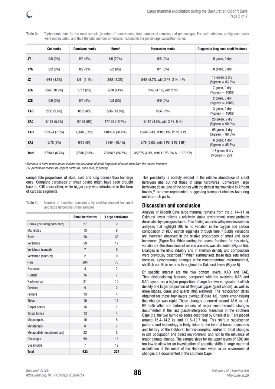
86 Volume 116| Number 5/6 May/June 2020

Research Articlehttps://doi.org/10.17159/sajs.2020/6754

Large mammal exploitation during the Oakhurst at Klipdrift Cave Page 5 of 7

comparable proportions of skull, axial and long bones) than for large ones. Complete carcasses of small bovids might have been brought back to KDC more often, while bigger prey was introduced in the form of carcass segments.

Table 4: Number of identified specimens by skeletal element for small and large herbivores (main sample)

Small herbivores Large herbivores

Crania (including horn core) 27 2

Mandibles 13 9

Teeth 28 33

Vertebrae 59 12

Vertebrae (caudal) 7 0

Vertebrae (sacrum) 2 0

Ribs 284 75

Scapulae 4 2

Humeri 16 7

Radio-ulnae 21 10

Pelvises 9 2

Femurs 13 4

Tibiae 15 17

Carpal bones 16 1

Tarsal bones 13 4

Metacarpals 10 8

Metatarsals 8 7

Metapodials (indeterminate) 22 5

Phalanges 59 18

Sesamoids 7 12

Total 633 228

This possibility is notably evident in the relative abundance of small herbivore ribs but not those of large herbivores. Conversely, large herbivore tibiae, one of the bones with the richest marrow yield in African bovids,15 are over-represented, suggesting transport choices favouring nutrition-rich parts.

Discussion and conclusionAnalysis of Klipdrift Cave large mammal remains from the c. 14–11 ka Oakhurst levels reflects a relatively stable environment, most probably dominated by open grasslands. This finding accords with previous isotopic analyses that highlight little to no variation in the oxygen and carbon composition of KDC ostrich eggshells through time.16 Subtle variations are, however, observed in the relative proportions of small and large herbivores (Figure 5a). While sorting the coarse fractions for this study, variations in the abundance of micromammals was also noted (Figure 5b). Changes in the lithic industry and in shellfish density and composition were previously described.2,3 When summarised, these data sets reflect complex, asynchronous changes in the macromammal, micromammal, shellfish and lithic records throughout the Oakhurst levels (Figure 5).

Of specific interest are the two bottom layers, KAD and KAE. Their distinguishing features, compared with the overlying KAB and KAC layers, are a higher proportion of large herbivores, greater shellfish density and larger proportion of Dinoplax gigas (giant chiton), as well as more blades, cores and quartz lithic elements. The radiocarbon dates obtained for these four layers overlap (Figure 1e), hence emphasising that change was rapid. These changes occurred around 13.5 ka cal. BP, both after and before periods of major environmental changes documented at the last glacial-interglacial transition in the southern Cape (i.e. the two humid episodes described by Chase et al.17 are placed around 15.4–14.2 ka and 11.8–10.7 ka). This shift in subsistence patterns and technology is likely linked to the internal human dynamics and history of the Oakhurst techno-complex, and/or to local changes in site occupation and direct environment, and not to the influence of major climate change. The sample sizes for the upper layers of KDC are too low to allow for an investigation of potential shifts in large mammal exploitation at the onset of the Holocene, when major environmental changes are documented in the southern Cape.1

Table 3: Taphonomic data for the main sample (number of occurrences, total number of remains and percentage). For each criterion, ambiguous cases were not included, and thus the total number of remains included in the percentage calculation varies.

Cut marks Carnivore marks Burnt* Percussion marks Diagnostic long bone shaft fractures

JY 0/5 (0%) 0/5 (0%) 1/5 (20%) 0/5 (0%) 0 green, 0 dry

JYA 0/2 (0%) 0/2 (0%) 0/2 (0%) 0/1 (0%) 0 green, 0 dry

JZ 4/88 (4.5%) 1/91 (1.1%) 2/88 (2.3%) 5/88 (5.7%, with 2 PS, 2 IN, 1 P)10 green, 2 dry

(%green = 83.3%)

JZA 5/46 (10.9%) 1/51 (2%) 7/50 (14%) 2/49 (4.1%, with 2 IN)7 green, 0 dry

(%green = 100%)

JZB 0/9 (0%) 0/9 (0%) 0/8 (0%) 0/9 (0%)2 green, 0 dry

(%green = 100%)

KAB 2/36 (5.6%) 0/38 (0%) 5/36 (13.9%) 0/37 (0%)3 green, 0 dry

(%green = 100%)

KAC 9/163 (5.5%) 0/166 (0%) 17/159 (10.7%) 8/164 (4.9%, with 3 PS, 5 IN)20 green, 2 dry

(%green = 90.9%)

KAD 31/424 (7.3%) 1/448 (0.2%) 140/405 (34.6%) 18/446 (4%, with 5 PS, 12 IN, 1 P)65 green, 1 dry

(%green = 98.5%)

KAE 6/75 (8%) 0/76 (0%) 31/64 (48.4%) 5/76 (6.6%, with 1 PS, 3 IN, 1 BF)6 green, 1 dry

(%green = 85.7%)

Total 57/848 (6.7%) 3/886 (0.3%) 203/817 (24.8%) 38/875 (4.3%, with 11 PS, 24 IN, 1 BF, 2 P)113 green, 6 dry (%green = 95%)

*Numbers of burnt bones do not include the thousands of small fragments of burnt bone from the coarse fractions. PS, percussion marks; IN, impact notch; BF, bone flake; P, peeling

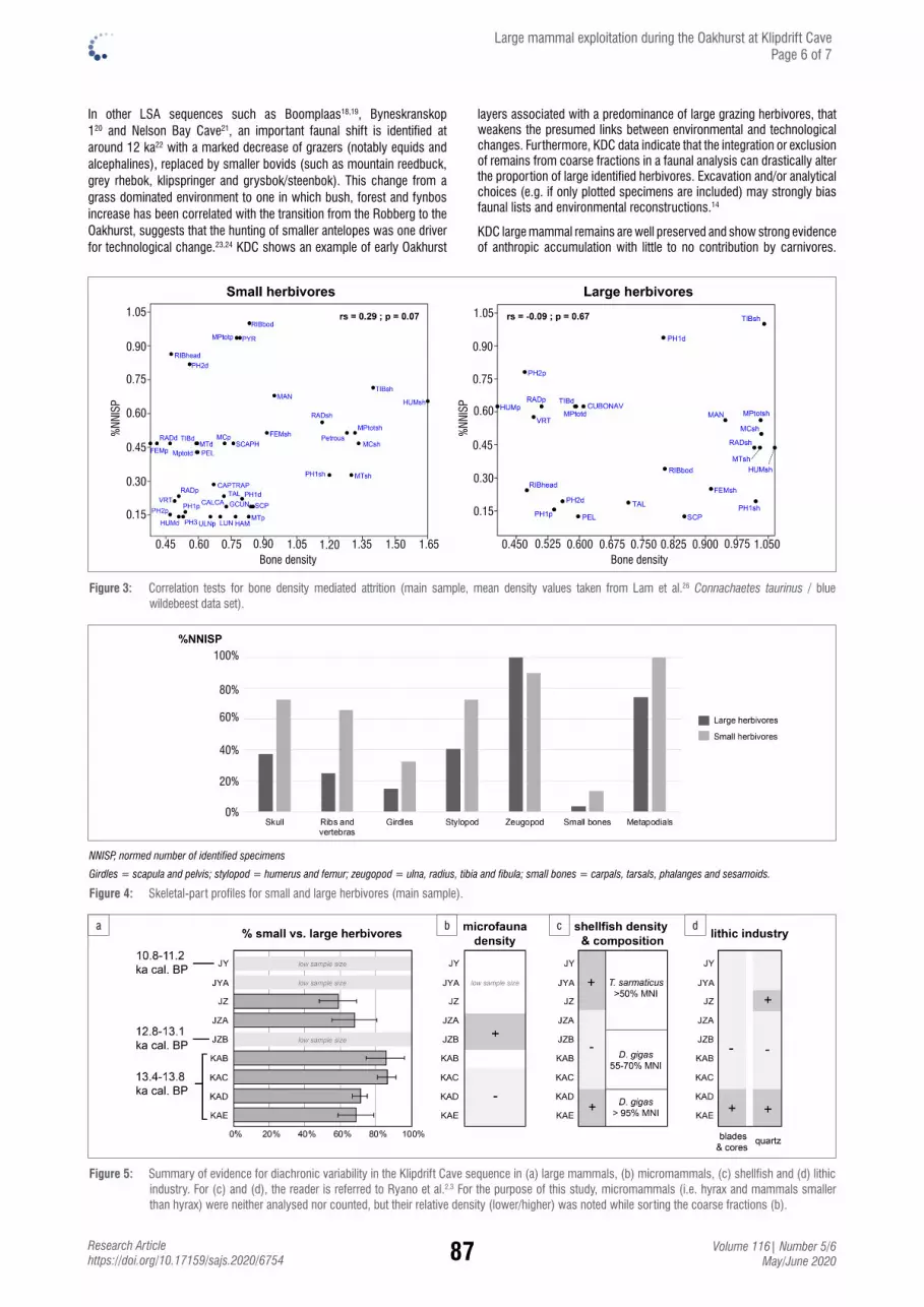
87 Volume 116| Number 5/6 May/June 2020

Research Articlehttps://doi.org/10.17159/sajs.2020/6754

Large mammal exploitation during the Oakhurst at Klipdrift Cave Page 6 of 7

1.051.05

0.900.90

0.750.75

0.450.45

0.600.60

0.300.30

0.150.15

0.45 0.60 0.75 0.90 1.05 1.20 1.35 1.50 1.65Bone density

%NN

ISP

%NN

ISP

Bone density0.450 0.525 0.600 0.675 0.750 0.825 0.900 0.975 1.050

Figure 3: Correlation tests for bone density mediated attrition (main sample, mean density values taken from Lam et al.26 Connachaetes taurinus / blue wildebeest data set).

100%

80%

60%

40%

20%

0%

NNISP, normed number of identified specimens

Girdles = scapula and pelvis; stylopod = humerus and femur; zeugopod = ulna, radius, tibia and fibula; small bones = carpals, tarsals, phalanges and sesamoids.

Figure 4: Skeletal-part profiles for small and large herbivores (main sample).

a b c d

Figure 5: Summary of evidence for diachronic variability in the Klipdrift Cave sequence in (a) large mammals, (b) micromammals, (c) shellfish and (d) lithic industry. For (c) and (d), the reader is referred to Ryano et al.2,3 For the purpose of this study, micromammals (i.e. hyrax and mammals smaller than hyrax) were neither analysed nor counted, but their relative density (lower/higher) was noted while sorting the coarse fractions (b).

In other LSA sequences such as Boomplaas18,19, Byneskranskop 120 and Nelson Bay Cave21, an important faunal shift is identified at around 12 ka22 with a marked decrease of grazers (notably equids and alcephalines), replaced by smaller bovids (such as mountain reedbuck, grey rhebok, klipspringer and grysbok/steenbok). This change from a grass dominated environment to one in which bush, forest and fynbos increase has been correlated with the transition from the Robberg to the Oakhurst, suggests that the hunting of smaller antelopes was one driver for technological change.23,24 KDC shows an example of early Oakhurst

layers associated with a predominance of large grazing herbivores, that weakens the presumed links between environmental and technological changes. Furthermore, KDC data indicate that the integration or exclusion of remains from coarse fractions in a faunal analysis can drastically alter the proportion of large identified herbivores. Excavation and/or analytical choices (e.g. if only plotted specimens are included) may strongly bias faunal lists and environmental reconstructions.14

KDC large mammal remains are well preserved and show strong evidence of anthropic accumulation with little to no contribution by carnivores.

88 Volume 116| Number 5/6 May/June 2020

Research Articlehttps://doi.org/10.17159/sajs.2020/6754

However, the small sample size per species limits zooarchaeological analyses. Preliminary data suggest that KDC was used by LSA people as a site to which they preferentially brought nutritious-rich carcass segments, especially those of large herbivores, considering that smaller herbivore prey may have been brought to the site as complete carcasses. Future excavations at Klipdrift Cave will provide more information on the subsistence strategies of LSA people during the Oakhurst, both before and during the marked environmental changes of the last glacial-interglacial transition.

AcknowledgementsThis research was funded in part by the European Research Council (ERC) under the European Union’s Seventh Framework Programme (FP7/2007–2013)/ERC grant agreement no. 249587 awarded to C.S.H. Additional funding for this research was provided to E.D. by the University of Bergen; to C.S.H. and K.L.v.N. by the Research Council of Norway through its Centres of Excellence funding scheme, Centre for Early Sapiens Behaviour (SapienCE), project number 262618; to C.S.H. by a South African National Research Foundation Chair (SARChI) held at the Evolutionary Studies Institute, University of the Witwatersrand.

Authors’ contributionsE.D.: Conceptualisation, methodology, data collection, sample analysis, data analysis, writing – the initial draft. C.S.H., K.L.v.N.: Klipdrift Cave site excavation, project leadership, project management, funding acquisition, writing – revisions.

References1. Chase BM, Faith JT, Mackay A, Chevalier M, Carr AS, Boom A, et al. Climatic

controls on Later Stone Age human adaptation in Africa’s southern Cape. J Hum Evol. 2018;114:35–44. https://doi.org/10.1016/j.jhevol.2017.09.006

2. Ryano KP. The Later Stone Age in the Southern Cape, South Africa, during the Terminal Pleistocene/Early Holocene with a focus on Klipdrift Cave [PhD thesis]. Johannesburg: University of the Witwatersrand; 2014.

3. Ryano KP, Wurz S, Van Niekerk KL, Henshilwood CS. The technology of the early Oakhurst lithic techno-complex from Klipdrift Cave, Southern Cape, South Africa. Afr Archaeol Rev. 2017;34(1):93–119. https://doi.org/10.1007/s10437-017-9246-2

4. Ryano KP, Van Niekerk KL, Wurz S, Henshilwood CS. Shellfish exploitation during the Oakhurst at Klipdrift Cave, southern Cape, South Africa. S Afr J Sci. 2019;115(9/10), Art. #5578. https://doi.org/10.17159/sajs.2019/5578

5. Henshilwood CS, Van Niekerk KL, Wurz S, Delagnes A, Armitage SJ, Rifkin RF, et al. Klipdrift shelter, southern Cape, South Africa: Preliminary report on the Howiesons Poort layers. J Archaeol Sci. 2014;45:284–303. https://doi.org/10.1016/j.jas.2014.01.033

6. Brain CK. Some suggested procedures in the analysis of bone accumulations from southern African Quaternary sites. Ann Transv Mus. 1974;29(1):1–8.

7. Stiner MC, Kuhn SL, Weiner S, Bar-Yosef O. Differential burning, recrystallization, and fragmentation of archaeological bone. J Archaeol Sci. 1995;22:223–237. https://doi.org/10.1006/jasc.1995.0024

8. Costamagno S, Théry I, Castel JC, Brugal JP. Combustible ou non? Analyse multifactorielle et modèles explicatifs sur des ossements brûlés paléolithiques [Fuel or not? Multifactorial analysis and explanatory models on Paleolithic burnt bones]. In: Théry I, Costamagno S, Henry A, editors. Gestion des combustibles au Paléolithique et au Mésolithique: nouveaux outils, nouvelles interprétations [Palaeolithic and mesolithic fuel management: New tools, new interpretations]. British International Series S1914. Oxford: Archaeopress; 2009. p. 65–84. Available from: http://halshs.archives-ouvertes.fr/halshs-00409188/

9. Fernandez-Jalvo Y, Andrews P. Atlas of taphonomic identifications. Dordrecht: Springer; 2016. https://doi.org/10.1007/978-94-017-7432-1_1

10. Villa P, Mahieu E. Breakage patterns of human long bones. J Hum Evol. 1991;21(1):27–48. https://doi.org/10.1016/0047-2484(91)90034-S

11. Grayson DK, Frey CJ. Measuring skeletal part representation in archaeological faunas. J Taphon. 2004;2(1):27–42.

12. Agresti A, Coull BA. Approximate is better than ‘exact’ for interval estimation of binomial proportions. Am Stat. 1998;52(2):119–126. https://doi.org/10.1080/00031305.1998.10480550

13. Hammer Ø, Harper DA, Ryan PD. PAST: Paleontological statistics software package for education and data analysis. Palaeontol Electron. 2001;4(1):9.

14. Discamps E, Faivre J-P. Substantial biases affecting Combe-Grenal faunal record cast doubts on previous models of Neanderthal subsistence and environmental context. J Archaeol Sci. 2017;81:128–132. https://doi.org/10.1016/j.jas.2017.03.009

15. Blumenschine RJ, Madrigal TC. Variability in long bone marrow yields of East African ungulates and its zooarchaeological implications. J Archaeol Sci. 1993;20(5):555–587. https://doi.org/10.1006/jasc.1993.1034

16. Roberts P. Stable carbon and oxygen isotope analysis of ostrich eggshell (OES) samples from LSA and MSA levels at Blombos Cave, Klipdrift Shelter, and Klipdrift Cave (South Africa) [MSc thesis]. Oxford: University of Oxford; 2013.

17. Chase BM, Chevalier M, Boom A, Carr AS. The dynamic relationship between temperate and tropical circulation systems across South Africa since the last glacial maximum. Quat Sci Rev. 2017;174:54–62. https://doi.org/10.1016/j.quascirev.2017.08.011

18. Klein RG. A preliminary report on the larger mammals from the Boomplaas Stone Age cave site, Cango Valley, Oudtshoorn District, South Africa. South Afr Archaeol Bull. 1978:66–75. https://doi.org/10.2307/3888252

19. Faith JT. Taphonomic and paleoecological change in the large mammal sequence from Boomplaas Cave, western Cape, South Africa. J Hum Evol. 2013;65(6):715–730. https://doi.org/10.1016/j.jhevol.2013.09.001

20. Schweitzer FR, Wilson ML. Byneskranskop 1: A late Quaternary living site in the southern Cape Province, South Africa. Ann S Afr Mus. 1982;88:1–203.

21. Klein RG. The late Quaternary mammalian fauna of Nelson Bay Cave (Cape Province, South Africa): Its implications for megafaunal extinctions and environmental and cultural change. Quat Res. 1972;2(2):135–142. https://doi.org/10.1016/0033-5894(72)90034-8

22. Klein RG. Palaeoenvironmental implications of Quaternary large mammals in the fynbos region. Fynbos Palaeoecol Prelim Synth. 1983;75:116–138.

23. Deacon J. The Later Stone Age in the southern Cape, South Africa [PhD dissertation]. Cape Town: University of Cape Town; 1982.

24. Ambrose SH, Lorenz KG. Social and ecological models for the Middle Stone Age in southern Africa. In: Mellars P, editor. The emergence of modern humans: An archaeological perspective. Ithaca, NY: Cornell University Press; 1990. p. 3–33.

25. Hogg AG, Hua Q, Blackwell PG, Niu M, Buck CE, Guilderson TP, et al. SHCal13 Southern Hemisphere calibration, 0–50,000 years cal BP. Radiocarbon. 2013;55(4):1889–1903. https://doi.org/10.2458/azu_js_rc.55.16783

26. Lam YM, Chen X, Pearson OM. Intertaxonomic variability in patterns of bone density and the differential representation of bovid, cervid, and equid elements in the archaeological record. Am Antiq. 1999;64(2):343–362. https://doi.org/10.2307/2694283

27. Klein RG. On the taxonomic status, distribution and ecology of the blue antelope, Hippotragus leucophaeus (Pallas, 1766). Ann S Afr Mus. 1974;65(4):99–143.

28. Faith JT. Conservation implications of fossil roan antelope (Hippotragus equinus) in southern Africa’s Cape Floristic Region. In: Louys J, editor. Paleontology in ecology and conservation. Berlin: Springer; 2012. p. 239–251. https://doi.org/10.1007/978-3-642-25038-5_12

Large mammal exploitation during the Oakhurst at Klipdrift Cave Page 7 of 7

89 Volume 116| Number 5/6 May/June 2020

Research Articlehttps://doi.org/10.17159/sajs.2020/6700

© 2020. The Author(s). Published under a Creative Commons Attribution Licence.

Lead and strontium isotopes as palaeodietary indicators in the Western Cape of South AfricaAUTHORS:

Mari Scott1

Petrus le Roux1

Judith Sealy2

Robyn Pickering1,3

AFFILIATIONS:

1Department of Geological Sciences, University of Cape Town, Cape Town, South Africa 2Department of Archaeology, University of Cape Town, Cape Town, South Africa3Human Evolution Research Institute, University of Cape Town, Cape Town, South Africa

CORRESPONDENCE TO: Mari Scott

EMAIL: mari.scott@uct.ac.za

DATES:Received: 22 July 2019Revised: 26 Feb. 2020Accepted: 01 Mar. 2020Published: 27 May 2020

HOW TO CITE: Scott M, Le Roux P, Sealy J, Pickering R. Lead and strontium isotopes as palaeodietary indicators in the Western Cape of South Africa. S Afr J Sci. 2020;116(5/6), Art. #6700, 8 pages. https://doi.org/10.17159/sajs.2020/6700

ARTICLE INCLUDES:☒ Peer review ☒ Supplementary material

DATA AVAILABILITY:☐ Open data set ☒ All data included☐ On request from author(s)☐ Not available☐ Not applicable

EDITOR: Priscilla Baker

KEYWORDS: Sr isotopes, Pb isotopes, palaeodiet, archaeology, southwestern South Africa

FUNDING: National Research Foundation (South Africa) (grant no. 84407)

We analysed the isotopic compositions of bioavailable strontium (Sr) and lead (Pb) in 47 samples of animals and plants derived from the various geological substrates of southwestern South Africa, to explore the utility of these isotope systems as dietary tracers. Measurements were made using high-resolution multi-collector inductively-coupled-plasma mass spectrometry (MC-ICP-MS). 87Sr/86Sr could efficiently discriminate between geologically recent sediments of marine origin in near-coastal environments and older geologies further inland. However, 87Sr/86Sr was not able to distinguish between the Cape Granite Suite and the Cape System (Table Mountain sandstones), whereas Pb isotopes could, demonstrating the utility of this hitherto underused isotope system. Bioavailable 87Sr/86Sr in near-coastal terrestrial environments is influenced by marine input, whereas Pb isotopic ratios are not, because of low concentrations of Pb in seawater. There is considerable potential to use Pb isotopes as a dietary and palaeodietary tracer in near-coastal systems in fields as diverse as archaeology, palaeontology, wildlife ecology and forensics.

Significance:• This study is the first investigation of the potential of Pb isotopes as a dietary tracer in southwestern

South Africa.

• Pb isotopes are a valuable dietary tracer; used in combination with 87Sr/86Sr, they can extend our knowledge of landscape usage in coastal-marine environments.

• Pb isotopes have also shown to be useful in samples from the 1980s, collected during the time when leaded petrol was in use in South Africa; however, these samples were from remote areas with low motor vehicle emissions.

IntroductionWe examined strontium (87Sr/86Sr) and lead (206Pb/204Pb, 207Pb/204Pb and 208Pb/204Pb) isotopes as biogeochemical tracers for studying diet and landscape usage in the (semi-)arid, coastal regions of southwestern South Africa, with application in both contemporary and ancient (archaeological and palaeontological) contexts. Consumer body tissues record the isotopic composition of food and water ingested in life.1 Where these isotopes vary across the landscape, they provide a natural tracer of diet and migration. We measured Sr and Pb concentrations and isotopic compositions in animals and isotope compositions in plants collected from the major geological substrates of southwestern South Africa (shales, sandstones, granites and recent marine-derived sands), ranging in age from pre-Cambrian to Quaternary (Figure 1). We were thus able to characterise isotope ratios of bioavailable Sr and Pb for each substrate. Our work expands on previous studies of 87Sr/86Sr isotopes as a (palaeo)dietary indicator in this region2-5; however, this study is the first to investigate Pb isotopes for this purpose. In addition, we aimed to determine the utility of Pb isotope measurements on archival samples that were collected during the time when leaded petrol was in use in South Africa. This is important because there is a large body of materials in museum and other collections that can be drawn from in future studies.

Sr isotopes in the geosphere and biosphereSr2+ substitutes for Ca2+ in minerals including plagioclase feldspar, calcite, dolomite, aragonite, gypsum and, most importantly regarding archaeological materials, apatite in bones and teeth. 87Sr/86Sr in biological materials is increasingly widely used to track animal migrations1, in forensics6, and in archaeology and palaeontology7. 87Sr is radiogenic (87Rb → 87Sr, t1/2 = 88x1010 years), whereas 86Sr is not.8,9 87Sr/86Sr therefore increases gradually through time and is highest in geologically ancient rocks, and those with high Rb contents relative to Sr.9,10 Sr is released from rocks through chemical weathering and moves (without fractionation of 87Sr/86Sr) from the source rock into the soils and groundwater.9,11,12 Different components of rocks with different 87Sr/86Sr may weather at different rates, so bioavailable 87Sr/86Sr may differ from the average underlying bedrock.13 Measurement of local animals and plants is the best way to characterise bioavailable 87Sr/86Sr13,14 because Sr passes through the food chain from plants to animals and humans without significant fractionation of its isotopes7,11,15.

87Sr/86Sr in soil and water may be altered by admixing of non-local Sr from rivers flowing through different geologies, precipitation and wind-blown dust.16 Sr is homogeneously distributed in the ocean, with a residence time of 2x107 years and a concentration of 7.62 ppm.12 An important limitation of the Sr isotope system worldwide is the tendency of coastal terrestrial areas to have 87Sr/86Sr values reflecting the composition of present-day seawater at 0.709241±0.000032.17 This is due to the presence of geologically recent marine-derived calcareous sediments with high fractions of shell3,4, and Sr contributed by sea spray and mists16.

Pb isotopes in the geosphere and biospherePb has four stable, naturally occurring isotopes, of which 206Pb (238U →206Pb, t1/2 = 4.47x109 years)9, 207Pb (235U → 207Pb, t1/2 = 0.70x109 years)9, and 208Pb (232Th → 208Pb, t1/2 = 14.01x109 years)9 are all radiogenic. 204Pb is not radiogenic and is therefore a good reference isotope. 206Pb/204Pb, 207Pb/204Pb and 208Pb/204Pb can increase over geological timescales and are highest in geologically ancient rocks, and those with high elemental U and Th content relative to Pb.18 204Pb may suffer isobaric interference from 204Hg which, if not corrected for, can pose a problem in inductively-coupled-plasma mass spectrometry (ICP-MS). That being the case, Pb isotopic ratios over 206Pb are often used.

90 Volume 116| Number 5/6 May/June 2020

Research Articlehttps://doi.org/10.17159/sajs.2020/6700

Lead and strontium isotopes as a dietary tracer Page 2 of 8

Figure 1: Geological map (base map derived from the Council for Geoscience) showing sample collection locations: 1. Churchhaven and Koeberg Nature Reserve consist mainly of unconsolidated calcareous sand (modern coastal-marine sands); 2. De Hoop Nature Reserve with some Table Mountain sandstone, and mostly Wankoe/Waenhuiskrans limestones of the Bredasdorp Group; 3. Doringbos (between Clanwilliam and Calvinia) with Karoo sedimentary deposits of mostly sandstones and shales, with some mudrock and siltstone; 4. Bontebok National Park with Table Mountain sandstone and Malmesbury shale; 5. Rooiheuwel farm with granite rocks of the Vredenburg pluton of the Cape Granite Suite; 6. Richtersveld National Park with volcanic, igneous, metamorphic and sedimentary rock formations (e.g. granites, syenites, pegmatites, schists, quartzites, shales, greywackes and conglomerates); 7. Dabidas farm with granites of the Namaqua-Natal Metamorphic Province; 8. Namaqua National Park with ultrametamorphic rocks, gneisses, schists, quartzites, granites and conglomerates of the Namaqua-Natal Metamorphic Province .

Like Sr, bioavailable Pb moves through the food chain without significant fractionation of its isotopes19,20 from the source bedrock via chemical weathering to soils and groundwater, and is then taken up by plants through their roots21. Industrial discharges and atmospheric transport and deposition of airborne Pb increase the Pb levels in soils, surface waters and the food chain.22 Pb in modern rainwater seems to be mainly from airborne particles derived from industrial sources, most of which appears to be taken up by surface soils.23 The introduction of alkyl-lead as an anti-knock agent in petrol resulted in raised atmospheric Pb levels worldwide.24 In South Africa, leaded petrol reached its peak between the 1980s and 1990s.25 Since 1996, unleaded petrol has been available to motorists and its use gradually increased until 2006, when all leaded petrol was phased out and only lead-free petrol was available in South Africa.

In the oceans, Pb is not homogeneously distributed and has a much shorter residence time (80–100 years)26 than Sr (2x107 years)12, resulting in Pb fluctuating with time as well as space. When comparing

the Pb concentration and isotopic ratios of current surface waters in the South Atlantic Ocean to those measured in the 1990s, a decrease in the Pb concentration can be observed from 29 pmol/kg in 199027 to 17.7 pmol/kg in 201028. Also, the 206Pb/204Pb ratio has decreased from 18.3800 in May/June 199629 to 18.0730 in October 201028. Conversely, the 208Pb/206Pb ratio has increased from 2.0900 in May/June 199629 to 2.1040 in October 201028.

Pb and Sr as palaeodietary tracers in southwestern South AfricaA number of archaeological and palaeontological studies have analysed Pb isotopes in bones and teeth for examining past mobility and geographical origins of archaeological specimens.30-33 Progressively more studies are comparing Pb with Sr isotopes, and concluding that whilst Pb and Sr isotopic systems alone can provide valuable information, a combination of the two techniques is a very powerful tool.30,32,33

91 Volume 116| Number 5/6 May/June 2020

Research Articlehttps://doi.org/10.17159/sajs.2020/6700

Lead and strontium isotopes as a dietary tracer Page 3 of 8

Extensive research has been done on the bioavailable and whole-rock 87Sr/86Sr in southwestern South Africa (Table 1). Allsopp and Kolbe34 analysed whole-rock 87Sr/86Sr from the Malmesbury shale (0.7208–0.7873) and Cape Granite (0.7701–1.1602) for geological age determination. Sealy et al.2 analysed animal bones to estimate bioavailable 87Sr/86Sr. They reported values for shales (0.7178–0.7179) and sandstones (0.7154–0.7175) based on a limited number of samples from carefully chosen sites some distance from the coast, where the soils derived from the underlying geological formations. As a result, this study showed a clear separation between the values for shales and sandstones, and those for near-coastal marine sands (0.7094–0.7117).2 Copeland et al.4 and Lehmann et al.5 also assessed bioavailable 87Sr/86Sr by analysing plants from the south coast and animal bone and teeth samples from the west coast of southern Africa. They employed much wider-ranging sampling strategies and included samples from shales, granites and sandstones near the coast, with significant marine Sr input. This is reflected in the very broad 87Sr/86Sr ranges, with marine Sr input contributing to the lower extremes: 0.7095–0.7204 for the Malmesbury shales, 0.7095–0.7236 for the Cape Granite Suite and 0.7092–0.7237 for the Cape Supergroup.

Radloff et al.3 reported bioavailable 87Sr/86Sr values of different geological substrates in the De Hoop Nature Reserve in southwestern South Africa, measured on modern rodent teeth. There is a distinction between higher values for shales (0.7101–0.7104) and sandstones (0.7098–0.7100) and lower values for the coastal sands (0.7092–0.7093) and limestones (0.7091–0.7099)3, but the values for shales and sandstones are very low, reflecting a substantial contribution from seawater-derived Sr.

Limited research has been done on whole-rock or bioavailable Pb isotopic ratios in southwestern South Africa. Soderberg and Compton35 reported 206Pb/207Pb (1.141±0.008) and 208Pb/207Pb (2.404±0.017) for a protea sample derived from the Table Mountain substrate of the Cape Floristic Region.

MethodsSample collectionThe details of the samples analysed are given in Supplementary table 1. Those collected specifically for this project comprise a variety of bones and teeth from animals that had recently died natural deaths, as well as some plants. As the goal of this study was to characterise bioavailable Pb and Sr isotopic ratios, diversity in the plant and animal species is irrelevant. It is, however, important to avoid cultivated areas where artificial fertilisers may have been used. Most samples were collected in the last few years, and therefore date from the post-2006 era of unleaded petrol. The sample set includes a few samples from the 1980s, when leaded petrol was still in use in South Africa, but these samples are from remote areas where there is likely to have been little influence from motor vehicle emissions. Small mammals from De Hoop Nature Reserve were trapped and euthanised in 2010 for a previous study.3 The set of samples was derived from all of the major geological substrates of

the Western Cape. Figure 1 is a geological map showing the sample collection locations.

Sample preparation Bones and teeth were lightly sanded to remove superficial contamination. Pieces weighing approximately 50 mg were placed in vials filled with MilliQ-water in an ultrasonic bath for about 10 min, then left to dry on watch glasses in an oven at 40 °C overnight, after which they were ready for chemical processing. As most teeth were from small animals, they were processed as ‘whole-tooth’ samples. In only two cases (both antelope teeth) were dentine and enamel separated and processed individually.

Plant samples were placed in quartz crucibles (uncovered) in a muffle furnace at an initial temperature of 300 °C and the temperature was increased by 100 °C every hour until a temperature of 650 °C was reached; thereafter the samples were left overnight. Possible Pb loss through volatilisation was minimised by increasing the temperature of the furnace gradually and keeping it well below the boiling point of Pb (1749 °C). The resulting ashed samples were ground to a fine powder using a mortar and pestle. Approximately 50 mg of each ash was weighed out (masses were recorded) and placed in a 7-mL Teflon vial.

The combined Sr-Pb elemental separation method used in this study is based on that of Pin et al.36, with minor modifications (see supplementary material for laboratory protocol). Sr and Pb, present in only trace amounts, were concentrated and matrix elements were removed by passing the samples through Savillex Teflon columns filled with Sr.Spec resin (Eichrom), using 0.05 M HNO3. Samples were processed in batches of eight, along with a total procedural blank and a reference material (NM95 in-house carbonate standard for the bone and tooth samples, and ALR33G in-house basalt standard for the plant-derived mineral ash samples).

Measuring Sr and Pb concentrations and isotope ratios Elemental concentrations of Sr and Pb were determined on a Thermo X-series II quadrupole ICP-MS, to assess the quantity of sample required for isotopic analysis. Because there is no published Sr or Pb concentration data for NM95, the in-house standard solutions were run as unknowns to assess accuracy. Calibration curves were obtained using artificial multi-element standards, from which standard solutions were made.

Isotopic ratios of Sr and Pb were determined on a NuPlasma HR multi-collector (MC)-ICP-MS from Nu Instruments. Samples were introduced into the MC-ICP-MS as solutions, using the Nu Instruments DSN-100 desolvating nebuliser. Solution analysis typically requires at least 50 ng of the element of interest, achieved through Sr-Pb elemental separation chemistry as described above.

The separated Sr fraction for each sample, dissolved in 2 mL 0.2% HNO3, was diluted to 200 ppb Sr for isotope analysis. Analyses were referenced to bracketing analyses of NIST SRM987, using an 87Sr/86Sr reference value of 0.710255. All Sr isotope data were corrected for

Table 1: Previously published 87Sr/86Sr in biological and geological samples from southwestern South Africa

Study Sample typeLocation in

South AfricaMalmesbury

shalesCape Granite

SuiteCape Supergroup

Karoo Supergroup

Bredasdorp Group

Quaternary coastal sands

Allsopp and Kolbe34 Rocks Cape Peninsula 0.7208–0.7873 0.7701–1.1602

Sealy et al.2 Modern bone of mammals

Southwestern coast

0.7178–0.7179 0.7154–0.7175 0.7094–0.7117

Soderberg and Compton35 Plant and soil

Cape Floristic Region

Plants = 0.722 and 0.724; Soil = 0.735

Radloff et al.3 Modern teeth of rodents

De Hoop Nature Reserve

0.7101–0.7104 0.7098–0.7100 0.7091–0.7099 0.7092–0.7093

Copeland et al.4 Plants Southern Cape 0.7095–0.7157 0.7095–0.7177 0.7092–0.7237 0.7124–0.7237 0.7092–0.7101

Lehmann et al.5 Modern bone and teeth, and plants

Southwestern coast

0.7141–0.7204 0.7114–0.7236 0.7141–0.7204 0.7094–0.7117

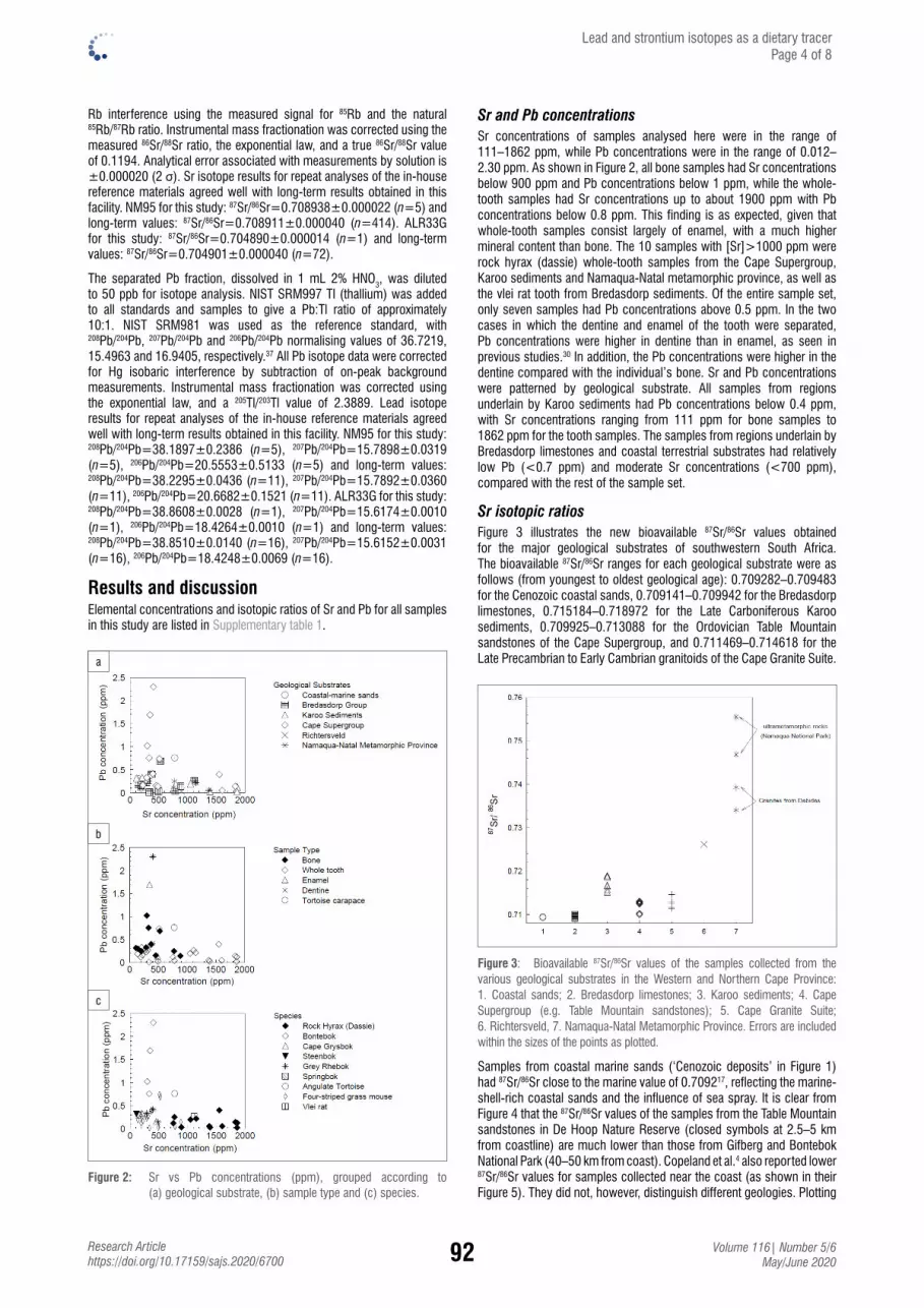
92 Volume 116| Number 5/6 May/June 2020

Research Articlehttps://doi.org/10.17159/sajs.2020/6700

Rb interference using the measured signal for 85Rb and the natural 85Rb/87Rb ratio. Instrumental mass fractionation was corrected using the measured 86Sr/88Sr ratio, the exponential law, and a true 86Sr/88Sr value of 0.1194. Analytical error associated with measurements by solution is ±0.000020 (2 σ). Sr isotope results for repeat analyses of the in-house reference materials agreed well with long-term results obtained in this facility. NM95 for this study: 87Sr/86Sr=0.708938±0.000022 (n=5) and long-term values: 87Sr/86Sr=0.708911±0.000040 (n=414). ALR33G for this study: 87Sr/86Sr=0.704890±0.000014 (n=1) and long-term values: 87Sr/86Sr=0.704901±0.000040 (n=72).

The separated Pb fraction, dissolved in 1 mL 2% HNO3, was diluted to 50 ppb for isotope analysis. NIST SRM997 Tl (thallium) was added to all standards and samples to give a Pb:Tl ratio of approximately 10:1. NIST SRM981 was used as the reference standard, with 208Pb/204Pb, 207Pb/204Pb and 206Pb/204Pb normalising values of 36.7219, 15.4963 and 16.9405, respectively.37 All Pb isotope data were corrected for Hg isobaric interference by subtraction of on-peak background measurements. Instrumental mass fractionation was corrected using the exponential law, and a 205Tl/203Tl value of 2.3889. Lead isotope results for repeat analyses of the in-house reference materials agreed well with long-term results obtained in this facility. NM95 for this study: 208Pb/204Pb=38.1897±0.2386 (n=5), 207Pb/204Pb=15.7898±0.0319 (n=5), 206Pb/204Pb=20.5553±0.5133 (n=5) and long-term values: 208Pb/204Pb=38.2295±0.0436 (n=11), 207Pb/204Pb=15.7892±0.0360 (n=11), 206Pb/204Pb=20.6682±0.1521 (n=11). ALR33G for this study: 208Pb/204Pb=38.8608±0.0028 (n=1), 207Pb/204Pb=15.6174±0.0010 (n=1), 206Pb/204Pb=18.4264±0.0010 (n=1) and long-term values: 208Pb/204Pb=38.8510±0.0140 (n=16), 207Pb/204Pb=15.6152±0.0031 (n=16), 206Pb/204Pb=18.4248±0.0069 (n=16).

Results and discussionElemental concentrations and isotopic ratios of Sr and Pb for all samples in this study are listed in Supplementary table 1.

a

b

c

Figure 2: Sr vs Pb concentrations (ppm), grouped according to (a) geological substrate, (b) sample type and (c) species.

Lead and strontium isotopes as a dietary tracer Page 4 of 8

Sr and Pb concentrations Sr concentrations of samples analysed here were in the range of 111–1862 ppm, while Pb concentrations were in the range of 0.012–2.30 ppm. As shown in Figure 2, all bone samples had Sr concentrations below 900 ppm and Pb concentrations below 1 ppm, while the whole-tooth samples had Sr concentrations up to about 1900 ppm with Pb concentrations below 0.8 ppm. This finding is as expected, given that whole-tooth samples consist largely of enamel, with a much higher mineral content than bone. The 10 samples with [Sr]>1000 ppm were rock hyrax (dassie) whole-tooth samples from the Cape Supergroup, Karoo sediments and Namaqua-Natal metamorphic province, as well as the vlei rat tooth from Bredasdorp sediments. Of the entire sample set, only seven samples had Pb concentrations above 0.5 ppm. In the two cases in which the dentine and enamel of the tooth were separated, Pb concentrations were higher in dentine than in enamel, as seen in previous studies.30 In addition, the Pb concentrations were higher in the dentine compared with the individual’s bone. Sr and Pb concentrations were patterned by geological substrate. All samples from regions underlain by Karoo sediments had Pb concentrations below 0.4 ppm, with Sr concentrations ranging from 111 ppm for bone samples to 1862 ppm for the tooth samples. The samples from regions underlain by Bredasdorp limestones and coastal terrestrial substrates had relatively low Pb (<0.7 ppm) and moderate Sr concentrations (<700 ppm), compared with the rest of the sample set.

Sr isotopic ratios Figure 3 illustrates the new bioavailable 87Sr/86Sr values obtained for the major geological substrates of southwestern South Africa. The bioavailable 87Sr/86Sr ranges for each geological substrate were as follows (from youngest to oldest geological age): 0.709282–0.709483 for the Cenozoic coastal sands, 0.709141–0.709942 for the Bredasdorp limestones, 0.715184–0.718972 for the Late Carboniferous Karoo sediments, 0.709925–0.713088 for the Ordovician Table Mountain sandstones of the Cape Supergroup, and 0.711469–0.714618 for the Late Precambrian to Early Cambrian granitoids of the Cape Granite Suite.

Figure 3: Bioavailable 87Sr/86Sr values of the samples collected from the various geological substrates in the Western and Northern Cape Province: 1. Coastal sands; 2. Bredasdorp limestones; 3. Karoo sediments; 4. Cape Supergroup (e.g. Table Mountain sandstones); 5. Cape Granite Suite; 6. Richtersveld, 7. Namaqua-Natal Metamorphic Province. Errors are included within the sizes of the points as plotted.

Samples from coastal marine sands (‘Cenozoic deposits’ in Figure 1) had 87Sr/86Sr close to the marine value of 0.709217, reflecting the marine-shell-rich coastal sands and the influence of sea spray. It is clear from Figure 4 that the 87Sr/86Sr values of the samples from the Table Mountain sandstones in De Hoop Nature Reserve (closed symbols at 2.5–5 km from coastline) are much lower than those from Gifberg and Bontebok National Park (40–50 km from coast). Copeland et al.4 also reported lower 87Sr/86Sr values for samples collected near the coast (as shown in their Figure 5). They did not, however, distinguish different geologies. Plotting

93 Volume 116| Number 5/6 May/June 2020

Research Articlehttps://doi.org/10.17159/sajs.2020/6700

Lead and strontium isotopes as a dietary tracer Page 5 of 8

87Sr/86Sr of both their and our samples from Table Mountain sandstones against distance from the coast shows increasing 87Sr/86Sr as one moves further inland (Figure 4), i.e. falling off of marine-derived Sr. The effect of marine-derived Sr appears to extend as far as 40 km inland. Similar results have been reported by other researchers38,39; the magnitude of the effect depends on atmospheric circulation and is greater in soils with low Sr concentrations. Setting aside samples from older substrates close to the coast (e.g. Cape granites at Vredenburg Peninsula), the older substrates (Cape granites, Table Mountain sandstones, Malmesbury shales) show higher 87Sr/86Sr than the Cenozoic sands and Bredasdorp formation, which have values closer to seawater.

Figure 4: Bioavailable 87Sr/86Sr values compared to distance from coast for rodent and plant samples collected from the Table Mountain sandstones in this study (closed symbols) and Copeland et al.’s4 study (open symbols).

Figure 5 shows the ranges of bioavailable 87Sr/86Sr found in this study compared with those found in previous studies. We report much narrower Sr isotopic ranges for each substrate than Copeland et al.4 and Lehman et al.5, although the same analytical methods were applied using the same analytical facility. In this study, the ranges of the Cape and Karoo geologies are distinct, whereas Copeland et al.4 found them to overlap. This difference may in part be a sample population effect, as sample

populations in this study (n=8 for the Karoo, 15 for Cape Supergroup) were smaller than those of Copeland et al.4 (50 and 35 respectively).

The bioavailable 87Sr/86Sr ranges for the older geological substrates from northwestern South Africa were as follows: 0.734004–0.755445 for the Namaqua-Natal metamorphic province and 0.726132 for the sample from the Richtersveld. High values are consistent with the underlying older Mesoproterozoic rocks, comprising highly deformed ultrametamorphic rocks, gneisses and migmatites.40

Pb isotopic ratios The new bioavailable 208Pb/204Pb, 207Pb/204Pb and 206Pb/204Pb ranges for the geological substrates from the Western Cape (from youngest to oldest geological age) are given in Table 2.

Table 2: Bioavailable Pb isotope ranges for the geological substrates from the Western Cape

Geological substrate 208Pb/204Pb 207Pb/204Pb 206Pb/204Pb

Cenozoic coastal sands 36.99 and 37.16 15.53 and 15.55 17.17 and 17.41

Bredasdorp limestones 37.38–38.46 15.56–15.65 17.49–18.51

Karoo and Cape Supergroup

37.10–38.25 15.48–15.64 17.28–18.39

Cape granites 37.32–38.11 15.61–15.66 17.37–18.06

The Cape granites at Rooiheuwel farm have narrower bioavailable Pb isotopic ranges compared with the Karoo and Cape samples and show a slight offset from the rest of the samples. This offset is only seen in Figure 6a (207Pb/204Pb vs 206Pb/204P) and not in Figure 6b (208Pb/204Pb vs 206Pb/204Pb). This result is not unexpected, as the Cape granites are known to have high concentrations of U and Th relative to Pb.41,42 The half-life of 235U → 207Pb (0.70x109 years) is much shorter than that of 238U → 206Pb (4.47x109 years) and 232Th → 208Pb (14.01x109 years), therefore the initial production of 207Pb is much more rapid than 206Pb and 208Pb.43 This results in the initial rapid increase in the 207Pb/204Pb ratio of a geological system, as observed here for the Cape granites. For the Namaqua-Natal metamorphic province, the two samples from the granites on Dabidas farm plot between the Cape granites and the rest of the samples, while the two samples from the ultrametamorphic rocks of the Namaqua National Park had very different Pb isotopic ratios from the rest of the samples (Figure 6).

Figure 5: Comparisons between the bioavailable 87Sr/86Sr ranges found in this study and those from previous studies, for each geological substrate: 1. Coastal sands; 2. Bredasdorp limestones; 3. Karoo sediments; 4. Cape Supergroup; 5. Cape Granite Suite; 6. Malmesbury shales.

94 Volume 116| Number 5/6 May/June 2020

Research Articlehttps://doi.org/10.17159/sajs.2020/6700

Lead and strontium isotopes as a dietary tracer Page 6 of 8

Figure 6 presents the new bioavailable Pb isotopic data of samples collected from various geological substrates of the Western and Northern Cape Provinces compared with the marine Pb isotopic signal, as measured in South Atlantic surface water sampled in 2010.28 Figure 7 compares the bioavailable 87Sr/86Sr and 206Pb/204Pb values with the respective marine values. Although samples from the Cenozoic coastal marine sands exhibited strongly marine Sr signals, their Pb isotopic ratios were quite unlike the marine Pb signal. The 206Pb/204Pb values for the Bredasdorp limestones are more varied, ranging between 17.49 and 18.51, compared with their 87Sr/86Sr values which range between 0.709141 and 0.709942. The marine contribution to bioavailable Sr in the terrestrial environment is much greater than the contribution to bioavailable Pb, due to the higher concentration of Sr (7.62 ppm)12 compared with Pb (5.22x10-6 ppm) in seawater.28

a

Figure 7: Bioavailable 87Sr/86Sr vs 206Pb/204Pb values of the samples collected from various geological substrates of the Western and Northern Cape Provinces, compared with the marine Pb isotopic signal (blue circle), as measured in South Atlantic surface water sampled in 2010.28 Errors are included within the sizes of the points as plotted. Refer to Figure 3 for geological substrates.

Some samples in this study were collected during the 1980s, when leaded petrol was still in use (it was phased out in 2006). The 208Pb/207Pb (2.353–2.358) and 206Pb/207Pb (1.085–1.090) ratios of Cape Town aerosols in 199824 were somewhat higher than the leaded petrol signature of 2.335 and 1.05524, respectively (Figure 8). The 1980s samples had 208Pb/207Pb and 206Pb/207Pb values distinctly higher than Cape Town’s aerosols in 1998 and even higher than the leaded petrol

signature. The lowest 208Pb/207Pb (2.3812) and 206Pb/207Pb (1.1054) values were measured in a tortoise from Koeberg (coastal terrestrial substrate), collected in 1982. Figure 8 shows that the red circled points (samples from the 1980s leaded petrol era) cover the same range as the non-circled points, so there appears to be no contribution from leaded petrol. These 1980s samples were collected from national parks in the Western Cape, or in coastal areas where emissions from motor vehicles are much lower than in urban areas.

Figure 8: Bioavailable 208Pb/207Pb vs 206Pb/207Pb values of all the samples collected within the various geological substrates of the Western Cape region of South Africa, compared with the values for leaded petrol and for aerosols in Cape Town in 1998. Samples collected in the 1980s (leaded petrol era) are circled in red. Refer to Figure 3 for geological substrates.

ConclusionsThis study has added to our database of measurements of bioavailable 87Sr/86Sr from the Western Cape Province of South Africa. 87Sr/86Sr can efficiently discriminate between coastal-marine environments and older geological substrates lying further inland. Organisms living on older geological substrates close to the coast have lowered 87Sr/86Sr as a result of marine Sr input. This decreases with increasing distance from the coast; the effects may be seen up to 40 km inland.4 87Sr/86Sr measurements alone cannot distinguish between the Cape Granite Suite and the Cape

Figure 6: (a) 207Pb/204Pb vs 206Pb/204Pb and (b) 208Pb/204Pb vs 206Pb/204Pb of the samples collected from various geological substrates of the Western and Northern Cape Provinces, compared with the marine Pb isotopic signal, as measured in South Atlantic surface water sampled in 2010.28 Errors are included within the sizes of the points as plotted. Refer to Figure 3 for geological substrates.

95 Volume 116| Number 5/6 May/June 2020

Research Articlehttps://doi.org/10.17159/sajs.2020/6700

Supergroup (Table Mountain sandstones), whereas Pb isotopes can, as shown in this study. Pb isotopic ratios of terrestrial plants and animals living close to the coast are distinct from seawater values. There does not appear to be significant alteration from marine-derived Pb in sea spray or similar sources. Pb is much less abundant in seawater than Sr12,28, which could explain why the marine contribution to bioavailable Sr in the terrestrial environment is much greater than the contribution to bioavailable Pb. Ultimately, Pb isotope data can give valuable information on palaeolandscape usage, and can be used as an additional isotope system to extend interpretations based solely on Sr isotopes.

Samples collected from relatively remote localities in the 1980s had Pb isotope ratios similar to those of more recent samples from the same geologies, and distinct from leaded petrol. They do not appear to be compromised by contamination from leaded petrol. It should therefore be possible to use historical samples, e.g. from museum collections, in studies of this kind.

In conclusion, we have demonstrated the value of using a combination of both 87Sr/86Sr and Pb isotope systems in coastal terrestrial environments to trace mobility or migration and landscape usage. This use has applications in archaeology, palaeontology, studies of animal migration, wildlife forensics and more.

AcknowledgementsWe thank the South African Research Chairs Initiative of the Department of Science and Innovation and the National Research Foundation of South Africa (grant no. 84407) for their generous bursary support which made this project possible. We also thank Fayrooza Rawoot, Kerryn Gray and Christel Tinguely of the Department of Geological Sciences at UCT, for their assistance in preparing and analysing the samples. Lastly, we thank Mr Danie Kotzé from Rooiheuwel farm, who allowed us to collect necessary samples on his farm, as well as Frans Radloff for making available samples from his earlier studies. This publication is an output of the Biogeochemistry Research Infrastructure Platform of the Department of Science and Innovation of South Africa.

Authors’ contributionsM.S.: Methodology; data collection; sample collection; data analysis; validation; data curation; writing – the initial draft; writing – revisions; project leadership and management. P.l.R.: Conceptualisation; methodology; validation; data curation; writing – revisions; student supervision; project leadership and management. J.S.: Conceptualisation; data curation; writing – revisions; student supervision; project leadership and management. R.P.: Data curation; writing – revisions; student supervision; project leadership and management.

References1. Hobson KA, Barnett-Johnson R, Cerling T. Using isoscapes to track animal

migration. In: West J, Bowen G, Dawson T, Tu K, editors. Isoscapes. Dordrecht: Springer; 2010. p. 273–298. https://doi.org/10.1007/978-90-481-3354-3_13

2. Sealy JC, Van der Merwe NJ, Sillen A, Kruger FJ, Krueger HW. 87Sr/86Sr as a dietary indicator in modern and archaeological bone. J Archaeol Sci. 1991;18(3):399–416. https://doi.org/10.1016/0305-4403(91)90074-Y

3. Radloff FGT, Mucina L, Bond WJ, Le Roux PJ. Strontium isotope analyses of large herbivore habitat use in the Cape Fynbos region of South Africa. Oecologia. 2010;164:567–578. https://doi.org/10.1007/s00442-010-1731-0

4. Copeland SR, Cawthra HC, Fisher EC, Lee-Thorp JA, Cowling RM, Le Roux PJ, et al. Strontium isotope investigation of ungulate movement patterns on the Pleistocene Paleo-Agulhas Plain of the Greater Cape Floristic Region, South Africa. Quat Sci Rev. 2016;141:65–84. https://doi.org/10.1016/j.quascirev.2016.04.002

5. Lehmann SB, Levin NE, Braun DR, Stynder DD, Zhu M, Le Roux PJ, et al. Environmental and ecological implications of strontium isotope ratios in mid-Pleistocene fossil teeth from Elandsfontein, South Africa. Palaeogeogr Palaeoclimatol Palaeoecol. 2018;490:84–94. https://doi.org/10.1016/j.palaeo.2017.10.008

6. Aggarwal J, Habicht-Mauche J, Juarez C. Application of heavy stable isotopes in forensic isotope geochemistry: A review. Appl Geochem. 2008;23(9):2658–2666. https://doi.org/10.1016/j.apgeochem.2008.05.016

7. Bentley RA. Strontium isotopes from the earth to the archaeological skeleton: A review. J Archaeol Method Theory. 2006;13(3):135–187. https://doi.org/10.1007/s10816-006-9009-x

8. Rankama K. Isotope geology. London: Pergamon Press; 1954.

9. Faure G. Principles of isotope geology. 2nd ed. New York: John Wiley & Sons Inc.; 1986. https://doi.org/10.1017/S0016756800017453

10. Pollard M, Batt C, Stern B, Young SMM. Analytical chemistry in archaeology. New York: Cambridge University Press; 2007. https://doi.org/10.1017/CBO9780511607431

11. Graustein WC. 87Sr/86Sr ratios measure the sources and flow of strontium in terrestrial ecosystems. In: Rundel PW, Ehleringer JR, Nagy KA, editors. Stable isotopes in ecological research. New York: Springer, 1989 p. 491–512. https://doi.org/10.1007/978-1-4612-3498-2_28

12. Capo RC, Steward BW, Chadwick OA. Strontium isotopes as tracers of ecosystem processes: Theory and methods. Geoderma. 1998;82(1–3):197–225. https://doi.org/10.1016/S0016-7061(97)00102-X

13. Sillen A, Hall G, Richardson S, Armstrong R. 87Sr/86Sr ratios in modern and fossil food-webs of the Sterkfontein Valley: Implications for early hominid habitat preference. Geochim Cosmochim Acta. 1998;62(14):2463–2473. https://doi.org/10.1016/S0016-7037(98)00182-3

14. Price TD, Burton JH, Bentley RA. The characterization of biologically available strontium isotope ratios for the study of prehistoric migration. Archaeometry. 2002;44(1):117–135. https://doi.org/10.1111/1475-4754.00047

15. Ericson JE. Strontium isotope characterization in the study of prehistoric human ecology. J Hum Evol. 1985;14(5):503–514. https://doi.org/10.1016/S0047-2484(85)80029-4

16. Whipkey CE, Capo RC, Chadwick OA, Steward BW. The importance of sea spray to the cation budget of a coastal Hawaiian soil: A strontium isotope approach. Chem Geol. 2000;168(1–2):37–48. https://doi.org/10.1016/S0009-2541(00)00187-X

17. Veizer J. Strontium isotopes in seawater through time. Ann Rev Earth Planet Sci. 1989;17:141–167. https://doi.org/10.1146/annurev.ea.17.050189.001041

18. Bilström K. Radiogenic isotopes and their applications within a range of scientific fields. In: Subías I, Bauluz B, editors. Instrumental techniques applied to mineralogy and geochemistry. Madrid: Spanish Society of Mineralogy; 2008. p. 111–131.

19. Gulson BL. Lead isotopes in mineral exploration. Amsterdam: Elsevier Science Publishers; 1986.

20. Hoefs J. Stable isotope geochemistry. 3rd ed. Berlin: Springer-Verlag; 1997. https://doi.org/10.1007/978-3-662-03377-7

21. Adriano DC. Trace elements in the terrestrial environment. Berlin: Springer-Verlag; 1986. https://doi.org/10.1007/978-1-4757-1907-9

22. Ghazi MA, Millette JR. Lead. In: Morrison RD, Murphy BL, editors. Environmental forensics. Burlington, MA: Academic Press; 2006. p. 56–74.

23. Bacon J, Bain D. Characterization of environmental water samples using strontium and lead stable-isotope compositions. Environ Geochem Health. 1995;17(1):39–49. https://doi.org/10.1007/BF00188631

24. Bollhӧfer A, Rosman KJR. Isotopic source signatures for atmospheric lead: The southern hemisphere. Geochim Cosmochim Acta. 2000;64(19):-3251–3262. https://doi.org/10.1016/S0016-7037(00)00436-1

25. Mathee A, Röllin H, Von Schirnding Y, Levin J, Naik I. Reductions in blood lead levels among school children following the introduction of unleaded petrol in South Africa. Environ Res. 2006;100(3):319–322. https://doi.org/10.1016/j.envres.2005.08.001

26. Libes SM. An introduction to marine biochemistry. Chichester: John Wiley & Sons; 1992.

27. Helmers E, Van der Loeff M. Lead and aluminum in Atlantic surface waters (50°N to 50°S) reflecting anthropogenic and natural sources in the eolian transport. J Geophys Res. 1993;98(C11):20261-20273. https://doi.org/10.1029/93JC01623

Lead and strontium isotopes as a dietary tracer Page 7 of 8

96 Volume 116| Number 5/6 May/June 2020

Research Articlehttps://doi.org/10.17159/sajs.2020/6700

28. Paul M, Bridgestock L, Rehkämper M, Van DeFlierdt T, Weiss D. High-precision measurements of seawater Pb isotope compositions by double spike thermal ionization mass spectrometry. Anal Chim Acta. 2015;863:59–69. https://doi.org/10.1016/j.aca.2014.12.012

29. Alleman LY, Church TM, Veron AJ, Kim G, Hamelin B, Flegal AR. Isotopic evidence of contaminant lead in the South Atlantic troposphere and surface waters. Deep Sea Res Part II. 2001;48(13):2811–2827. https://doi.org/10.1016/S0967-0645(01)00019-4

30. Montgomery J. Lead and strontium isotope compositions of human dental tissues as an indicator of ancient exposure and population dynamics [PhD thesis]. Bradford: University of Bradford; 2002. https://doi.org/10.5284/1000249

31. Ghazi AM. Lead in archaeological samples: An isotopic study by ICP-MS. Appl Geochem. 1994;9(6):627–636. https://doi.org/10.1016/0883-2927(94)90023-X

32. Shaw H, Montgomery J, Redfern R, Gowland R, Evans J. Identifying migrants in Roman London using lead and strontium stable isotopes. J Archaeol Sci. 2016;66:57–68. https://doi.org/10.1016/j.jas.2015.12.001

33. Dudas FÖ, LeBlanc SA, Carter SW, Bowring SA. Pb and Sr concentrations and isotopic compositions in prehistoric North American teeth: A methodological study. Chem. Geol. 2016; 429:21–32. https://doi.org/10.1016/j.chemgeo.2016.03.003

34. Allsopp HL, Kolbe P. Isotopic age determinations on the Cape granite and intruded Malmesbury sediments, Cape Peninsula, South Africa. Geochim Cosmochim Acta. 1965;29(10):1115–1130. https://doi.org/10.1016/0016-7037(65)90115-8

35. Soderberg K, Compton JS. Dust as a nutrient source for fynbos ecosystems, South Africa. Ecosystems. 2007;10:550–561. https://doi.org/10.1007/s10021-007-9032-0

36. Pin C, Gannoun A, Dupont A. Rapid, simultaneous separation of Sr, Pb, and Nd by extraction chromatography prior to isotope ratios determination by TIMS and MC-ICP-MS. J Anal At Spectrom. 2014;29(10):1858–1870. https://doi.org/10.1039/C4JA00169A

37. Galer S, Abouchami W. Practical application of lead triple spiking for correction of instrumental mass discrimination. Mineralogical Magazine. 1998;62A(1):491–492.

38. Quade J, Chivas AR, McCulloch MT. Strontium and carbon isotope tracers and the origins of soil carbonate in South Australia and Victoria. Palaeogeogr Palaeoclimatol Palaeoecol. 1995;113(1):103–117. https://doi.org/10.1016/0031-0182(95)00065-T

39. Evans J. Biosphere isotope domain map GB (V1): Strontium isotope data. British Geological Survey. 2018. http://dx.doi.org/10.5285/ba36de6f-5a20-476b-965d-48182166114a

40. Cornell DH, Thomas RJ, Moen HFG, Reid DL, Moore JM, Gibson RL. The Namaqua-Natal Province. In: Johnson MR, Anhaeusser CR, Thomas RJ, editors. The geology of South Africa. Johannesburg: Geological Society of South Africa and Council for Geoscience; 2016.

41. Schoch AE, Leygonie FE, Burger AJ. U-Pb ages for Cape granites from the Saldanha Batholith: A preliminary report. Trans Geol Soc S Afr. 1975;78(1):97–100.

42. Scheepers R, Poujol M. U-Pb zircon age of Cape Granite Suite ignimbrites: Characteristics of the last phases of the Saldanian magmatism. S Afr J Geol. 2002;105(2):209–224. https://doi.org/10.2113/105.2.163

43. Dickin AP. Radiogenic isotope geology. Cambridge: Cambridge University Press; 1995.

Lead and strontium isotopes as a dietary tracer Page 8 of 8

97 Volume 116| Number 5/6 May/June 2020

Research Articlehttps://doi.org/10.17159/sajs.2020/6782

© 2020. The Author(s). Published under a Creative Commons Attribution Licence.

Proximate and starch composition of marama (Tylosema esculentum) storage roots during an annual growth period

AUTHORS: Maria H. Hamunyela1,2

Emmanuel Nepolo3

Mohammad N. Emmambux4

AFFILIATIONS:

1Department of Biological Sciences, University of Namibia, Windhoek, Namibia2Department of Food Science and Technology, University of Namibia, Windhoek, Namibia 3Department of Biochemistry and Microbiology, University of Namibia, Windhoek, Namibia4Department of Consumer and Food Sciences, University of Pretoria, Pretoria, South Africa

CORRESPONDENCE TO: Mohammad Emmambux

EMAIL: naushad.emmambux@up.ac.za

DATES:Received: 07 Aug. 2019Revised: 04 Jan. 2020Accepted: 24 Jan. 2020Published: 27 May 2020

HOW TO CITE: Hamunyela MH, Nepolo E, Emmambux MN. Proximate and starch composition of marama (Tylosema esculentum) storage roots during an annual growth period. S Afr J Sci. 2020;116(5/6), Art. #6782, 6 pages. https://doi.org/10.17159/sajs.2020/6782

ARTICLE INCLUDES:☒ Peer review ☐ Supplementary material

DATA AVAILABILITY:☐ Open data set ☐ All data included☒ On request from author(s)☐ Not available☐ Not applicable

EDITORS: Teresa Coutinho Salmina Mokgehle

KEYWORDS: marama root, marama root starch, proximate analysis, starch granules, total starch, high amylose starch

FUNDING: National Research Foundation (South Africa)

The aim of this study was to determine the most suitable time for harvesting marama (Tylosema esculentum) root as an alternative source of novel starch by evaluating the quality of marama root and its starch during growth periods of 12 months. The effects of time on the proximate analysis of marama roots as well as the thermal properties, size and physicochemical properties of the starch were also investigated. Marama was planted in September and total starch of marama roots on both as is and dry bases increased significantly (p<0.05) from 24 g/kg to 115 g/kg and 259 g/kg to 601 g/kg, respectively, from 2 to 12 months after planting. Amylose content significantly (p<0.05) decreased from about 50.7% to 21.4% of the starch for the same time period. The size of marama root starch granules significantly (p<0.05) increased from 8.6 µm to 15.1 µm. The marama root harvested after 2 months had the highest crude protein content (33.6%). In terms of thermal properties, the peak temperature decreased significantly with time (ranging from 93.0 °C to 73.4 °C), while the ΔH increased significantly with time. The findings indicate that marama should be planted early in summer and harvested between 4 and 8 months for optimal starch before winter.

Significance:Proximate and starch characteristics of marama storage roots differ significantly with time of harvest. This suggests that desired functional properties can be achieved by controlling growth time. The marama root harvested at 4 months is highly nutritious, it has high protein content, starch that is high in amylose and is suitable for consumption as a fresh root vegetable in arid to semi-arid regions where few conventional crops are able to survive. Marama root is a climate smart crop and it could potentially contribute to food security in arid regions. The results obtained in this study suggest that the optimum time for harvesting marama as a root vegetable is at 4 months while the optimum time for harvesting marama for its starch is at 8 months. Younger roots have higher amylose, and hence higher gelatinisation temperatures, and therefore may be more suitable to be used as a coating during frying.

IntroductionStarch is the most common carbon reserve stored in plants; it is of great significance for both food and non-food industrial uses.1 About 75 million tonnes of starch is produced for worldwide industrial applications2 and about 54% of the starch produced globally is utilised for food applications3. Starch is also a major source of energy in the human diet. It accounts for approximately 50% of calorie intake in developed countries and 90% of calorie intake in developing countries.4 Current sources of commercially available starch are a restricted range of crops, the most important being maize, potato, wheat and cassava with smaller amounts from rice, sorghum, sweet potato, arrowroot, sago and mung beans.5 The main crops in sub-Saharan Africa are maize, rice, pearl millet, sorghum, cassava, yam and sweet potatoes.6 However, there is no commercialised starch from indigenous staple crops in Namibia and they are underutilised. The underutilised crops may provide starches or flours with novel physicochemical properties.

Marama is a wild-growing and drought-tolerant legume, native to the arid and semi-arid regions of southern Africa. It produces protein and oil rich seeds and is a storage root used as food.7 In Namibia it grows wild mainly in the Omaheke and Otjizondjupa regions, while it grows in the Limpopo, Gauteng and Northern Cape Provinces of South Africa.8 Marama is a storage root bearing plant that is indigenous to the Kalahari sandy region,9 and could prove to be a starch alternative due to its ability to survive aridity. Plant roots such as cassava and tubers such as potato are rich in starch and they are among the sources of starch for consumption or industrial use.10 According to Huang et al.11, roots and tubers contain 70–80% water, 16–24% starch and trace amounts of protein and lipids. The dry matter of roots and tubers mainly consists of starch, which accounts for approximately 70% of the total solids, thus making it the major component.12 Due to their high starch content, root and tuber crops are thus important staple foods and are also used as ingredients in processed foods across the world.12 Previous reports show that starch morphology, starch composition and the proximate composition of roots and tuber crops such as yam, cassava, potato and sweet potato are affected by the time of harvest. It has been shown that starch content and starch granule size increase with crop maturity in all roots and tubers while starch granule shapes remain the same.13-16

Both the seeds and the storage root of marama are used for consumption by local people.8 The seeds are roasted and eaten as a snack17 while the root is boiled or roasted for consumption as a vegetable18. Marama seeds and the storage root have a high nutrient value, and are rich in protein, oil and starch. Marama is a potential crop for arid areas where few conventional crops can survive because of its ability to grow naturally in the poor soil and dry conditions of Namibia. Marama has potential to be a climate change friendly food crop for southern Africa. It thrives in arid conditions due to the plant’s ability to employ several mechanisms to grow and survive in drought-stricken environments. Marama is able to withstand temperatures of up to 50 °C, it is also able to withstand limited water by reduced surface area of the leaves to reduce water loss and it can survive by making use of water stored in

98 Volume 116| Number 5/6 May/June 2020

Research Articlehttps://doi.org/10.17159/sajs.2020/6782

the tuberous root. It also has a tap root that penetrates deep below the surface to allow access to subsoil water.19 The starch accumulation and physicochemical properties of the marama root have not been studied extensively. Marama root starch reportedly has a high viscosity and therefore has potential as a thickener in food products.20 Thus, research and product development are needed to exploit marama root starch. The objective of this study was therefore to investigate the influence of time on the proximate analysis of marama roots and the influence of time on the starch granule size, thermal and physicochemical properties of the marama root starch. The published paper by Adeboye and Emmambux20 concentrated on the physicochemical, morphological, thermal and pasting properties of marama storage root starch but did not study the effects of harvest time on the marama root starch. The marama roots used in their study were harvested 6 months after planting. We report the changes in the physicochemical properties of starch from marama roots over a period of 12 months. In addition, we provide the first report on changes during tuberous root development. The main aim of this study was to determine the most suitable time for harvesting by evaluating the quality of marama root and its starch at different times during a 12-month period.

Materials and methodsSamplesMarama plants were grown in a greenhouse on the University of Namibia NEUDAM campus, which is located at 22°30.105‟S and 017°20.824‟E, 30 km east of Windhoek, the capital city of Namibia. Marama seeds were collected from an experimental field in Omitara which is located in the Omaheke region in the central eastern part of Namibia. Marama seeds (n=144) were planted in a greenhouse; each seed was planted in a 20-L pot. Seeds were planted in September when the daily average temperature was 28 °C and grown for 12 months. Roots were randomly selected at different stages of development for analysis. The roots were harvested in November, January, May and finally in September, equivalent to 2, 4, 8 and 12 months after planting, respectively. The analyses were done in harvested months. Some of the analyses were done on fresh roots while some were performed on freeze-dried roots. The roots were freeze dried and ground into flour for proximate, total starch content, amylose content and thermal properties analyses.

Analyses

Size determinationThe fresh mass of the roots was determined using a weighing balance, while the diameter of roots was determined using a vernier calliper. The diameter was measured in the middle longitudinal section of the marama root. The measurements were done at 2, 4, 8 and 12 months after planting.

Determination of total soluble solidsFreeze-dried marama root was mixed with distilled water (10% slurry), filtered and the total soluble solids were measured using a digital refractometer. The total soluble solids were expressed as a Brix percentage. The refractometer was calibrated with distilled water before taking the measurements.

Proximate compositionMoisture, ash and crude fibre of freeze-dried marama roots were determined using Association of Official Analytical Chemists (AOAC) methods 925.45B, 942.05 and 962.09, respectively.21 Crude protein (Nx-6.25) was determined by the Dumas method, using the Leco CHN 628 series nitrogen combustion system, which is an AOAC method (990.03).22

Total starch contentThe Megazyme total starch assay kit (K-TSTA 07/11) (Megazyme International, Bray, Ireland) was used to determine the percentage composition of total starch in freeze-dried marama roots as described by McCleary et al.23 Thermostable α-amylase and amyloglucosidase enzymes were used to enzymatically hydrolyse starch to glucose and the glucose was quantified using glucose oxidase-peroxidase reaction.

Proximate and starch composition of marama Page 2 of 6

The absorbance for each sample was read at 510 nm against the reagent blank using a spectrophotometer.

Amylose:amylopectin ratioMegazyme amylose:amylopectin assay kit (K-AMYL 07/11) (Megazyme International Bray, Ireland) was used to determine the amylose:amylopectin ratio of freeze-dried marama roots as described by Gibson et al.24 who used a modification of a procedure described by Yun and Matheson25. The amylose was determined by the precipitation of amylopectin with lectin concanavalin-A protein; amylose was then enzymatically hydrolysed to glucose and quantified using glucose oxidase-peroxidase. The absorbance for each sample was read at 510 nm against the reagent blank using a spectrophotometer.

Determination of thermal propertiesThermal properties of ground freeze-dried marama root were determined using the method described by Wokadala et al.26 Thermal properties were analysed using a high-pressure differential scanning calorimetry system with STARe software (HPDSC-827, Mettler Toledo, Greifensee, Switzerland). A mass of 10 mg (dry weight basis) of freeze-dried marama root flour was dissolved in 30 mg distilled water and allowed to equilibrate for at least 2 h at room temperature. Scanning was done at temperatures from 40 °C to 125 °C at a rate of 10 °C/min. Indium (Tp=156.61 °C, 28.45 J/g) was used as a standard to calibrate the differential scanning calorimetry system and an empty pan was used as a blank reference.

Root microstructureA protocol was developed using fixing and staining procedures described by Ruzin27. The storage root (2-cm slices) was fixed in formalin–acetic acid and then dehydrated in an ethanol series, wax infiltrated and embedded. Cross sections of 10-µm thickness were prepared and mounted on slides before staining with periodic acid–Schiff, and counter staining with amido black 10B. Periodic acid–Schiff stains starch a bright fuchsia and amido black stains proteins in the cell walls a deep blue colour. Slides were viewed using a Zeiss Axio Imager 2 microscope (Oberkochen, Germany) and digital images were taken using an Axiocam ERC5S camera to determine starch accumulation, granule size and shape of the starch.

Statistical analyses Statistical analyses were conducted using the SPSS 21 statistical package (Chicago, IL, USA). The data were subjected to a one-way analysis of variance (ANOVA); p≤0.05 was considered significant. Duncan’s multiple range test was used to further compare the means to determine which of the means is significantly different. Data were presented as means±standard deviation. The independent variable in this study is time, while the dependent variables are the root and starch characteristics.

Results and discussionMorphology and proximate compositionThe marama root morphology and proximate composition of marama roots harvested at different times are presented in Table 1. As expected, the fresh mass and diameter of the marama root significantly increased (p<0.05) with time up until 8 months after planting. The root attained a weight of up to 420 g in 8 months. Bousquet28 reported that the marama storage root can reach a weight of up to 12 kg within a few unspecified years. However, roots can grow larger and a root weighing 277 kg has been found in Botswana.29 The 8-month root weighed more than the 12-month root did – a difference which may be related to the winter months (June, July and August). Marama leaves and vines are lost during winter and sprout back after winter. Consequently, the plants could not produce photosynthate and thus the 12-month root weighed less than the 8-month root, although it was older. Because 12-month roots were harvested right after winter, it is suspected that the plants would then have had to rely on their reserves to survive winter.

The average moisture content of the fresh marama storage root significantly (p<0.05) decreased from 91% to 81% as root development progressed. The older roots appeared to be more fibrous then the younger roots, but the youngest roots appeared to consist mostly of

99 Volume 116| Number 5/6 May/June 2020

Research Articlehttps://doi.org/10.17159/sajs.2020/6782

Proximate and starch composition of marama Page 3 of 6

water. Similarly, young cassava roots contain less starch than older roots which also have a higher fibre content.13 The ash content of the ground marama storage root flour also significantly (p<0.05) decreased with time from about 6.3% to 3.1% from month 2 to 12. Ash content of yam tubers was also reported to be higher in tubers harvested during the early stages of growth than at later stages.11

The same trend was observed for the total soluble solids that significantly (p<0.05) decreased with time from 6.4% to 2.3% from month 2 to 12. Glucose is the first precursor of starch biosynthesis in the roots and tubers. Glucose and sucrose are soluble sugars; soluble sugars decreased significantly during the development of potato tubers.14 There was a general increase in starch and a decrease in sugars during potato tuber development. Maturing of tubers is hence marked by the decline in sugars which is associated with an increase in starch.14

A high sugar load correlated with the onset of starch accumulation at the beginning of tuber development and starch content increased rapidly thereafter.30 The decrease in total soluble solids in this study is probably due to a decrease in total soluble sugars (during starch biosynthesis and accumulation); further determinations are, however, necessary.

The crude protein content significantly (p<0.05) reduced from 33.6% to 2.7% from month 2 to 12. Similarly, there was a decrease in protein content during potato tuber development.31 A reduction of protein in this study is probably an indication of a decrease in protein synthesis. Potato tuber maturity is characterised by a progressive inactivation of the protein synthesis system.31 In general, marama storage root has a high protein content29 – higher than that of cassava (0.95–6.42%), sweet potato (3.15%), taro (6.28%) and yam (10.46%).32,33

Starch composition and thermal properties The total starch content of the ground marama storage roots (Table 2) significantly increased from 259 g/kg to 601 g/kg on a dry basis from month 2 to 12. The total starch content (fresh basis) of the marama root increased from 24 g/kg to 115 g/kg from month 2 to 12. As expected, both the dry weight basis and fresh basis total starch content of the marama root increased significantly with age (p<0.05). Similarly, a variation in the starch content of potato tubers and cassava roots harvested at different times has been reported, with the highest starch content recorded at 2–3 months for potato tubers.34 A previous report indicates that the total starch content of cassava roots increased with time until it reached its maximum at the 14th month.16 Changes in starch content are indicators of a variety of different plant development processes.35 Starch accumulation in roots is determined by a higher starch synthesis enzyme activity, a lower amylase activity (starch degradation) in the roots, the stem transport capacity and the expression of sugar transport genes. The starch synthesis capacity and low starch degradation in roots are strongly associated with a high accumulation of starch in storage roots at late growth stages.36

The total starch content on a fresh basis of the marama root for all the root samples was lower than 15%, with the lowest content being 24 g/kg and the highest being 115 g/kg. Nepolo37 reported that fresh marama root harvested after 3 months contains 87 g/kg total starch content. Their finding is in agreement with results in this study that show that the major component of the fresh marama root is water. In addition, besides water, other non-starch components also affect the total starch content of the marama root.20 The starch content in fresh potato tubers

reportedly increased from 110 g/kg to 135 g/kg during potato growth.34

The young marama root therefore contains very low starch content and genetic modifications might be required to increase the starch production of the roots. In order to establish marama root starch as an alternative source of starch and increase its economic value, it would be beneficial to increase starch production in marama roots.

Table 2: Starch composition results of marama storage root

Harvesting month

Starch composition

Total starch (g/kg dry weight)

Total starch (g/kg fresh weight)

Amylose content (% starch basis)

2 259a±0.69 24a±0.06 50.7a±0.89

4 265a±0.75 28b±0.08 40.6b±5.14

8 490b±0.83 66c±0.11 26.6c±1.33

12 601c±1.47 115d±0.28 21.4c±0.40

Mean values followed by a different superscript letter in the same column are signifi-cantly different (p<0.05; n=3).

The amylose content of the marama storage root starch (Table 2) determined by the precipitation of amylopectin significantly decreased with the maturity of the storage root (p<0.05) from 50.7% to 21.4% from month 2 to 12. A similar trend was observed for sweet potatoes, whereby the amylose content decreased with harvest time – the values reduced from 23.1% to 19.7%.15 Similarly, the amylose content of cassava root starch was also highest in the roots harvested early; it varied from 20.6% to 24.1%.16 Noda et al.38 also reported that the amylose content of potato starch decreased with time – the starch of the tubers harvested early in the trial had the highest amylose content (21.2%) compared to the tubers harvested late in the trial (20.2%). Our findings suggest that the amylose content decreases as the total starch content increases during storage root development, which is an indication of a delay in amylopectin synthesis as compared to amylose. The activity of granule-bound starch synthase, which is responsible for the synthesis of amylose, decreased, while that of soluble starch synthase, which is responsible for the synthesis of amylopectin, increased during the development of potato tubers.13 The results suggest that younger roots contain high amylose starch. High amylose starch is highly sought after due to its unique functional properties. The starch in younger roots is higher than any amylose content reported in the literature for root and tuber starches. The roots and tuber starches are reported to have an amylose content ranging from 10% to 38%.39 High amylose starch is considered to be an important source of food with highly resistant starch. High amylose starch could be used as an ingredient in the preparation of novel starch food to improve resistant starch content and hence decrease glycaemic load.40 When domesticated, farmers could decide when to harvest depending on the amylose content and thus the functional properties of the starch. The desired functional properties of starch can therefore be achieved by controlling growth time without the need for chemical or physical modifications of the starch for specific applications.34 However more analyses and research are recommended to study the mechanism of amylose and amylopectin accumulation in marama root.

Table 1: Morphology and proximate analysis results of marama storage root

Harvesting month Moisture (%) Mass (g) Diameter (cm)Composition (% dry weight)

Ash Crude protein Total soluble solids Crude fibre

2 90.9a±1.36 14.6a±3.38 1.4a±0.19 6.3a±0.12 33.6a±0.06 6.4a±0.0 7.2a±0.26

4 89.4a±0.51 38.9a±4.70 2.7b±0.34 5.9a±0.34 14.0b±0.06 5.8b±0.06 6.7b±0.17

8 86.6b ±0.10 420.4b±62.61 6.5c±1.36 4.3b±0.25 3.3c±0.06 3.7c±0.11 6.8b±0.18

12 80.8c±1.42 326.4c±37.07 5.7c±0.30 3.1c±0.06 2.7d±0.05 2.3d±0.10 5.6c±0.13

Mean values followed by a different superscript letter in the same column are significantly different (p<0.05).

100 Volume 116| Number 5/6 May/June 2020

Research Articlehttps://doi.org/10.17159/sajs.2020/6782

The endothermic peaks of marama root flour samples are presented in Figure 1. The endothermic peaks yielded were probably due to starch gelatinisation and not protein denaturation. It was observed that the onset (To), peak gelatinisation (Tp) and conclusion (Tc) temperatures decreased with harvesting time while enthalpy change (ΔH) increased significantly (p<0.05). In contradiction, the temperatures of taro root increased with harvesting time, as did ΔH.41 The To, Tp and Tc for the 4-month roots were 77.4 °C, 84.9 °C and 93.0 °C, respectively, while To, Tp and Tc for the 12-month root samples were 74.18 °C, 79.1 °C and 84.6 °C, respectively. The ΔH for the 4-, 8- and 12-month root samples were 2.2 J/g, 8.2 J/g and 12.3 J/g, respectively.

Figure 1: Differential scanning calorimetry curves of marama root harvested at different months (on a dry starch basis).

As expected, time had an effect on the thermal properties of the marama root starch, this finding may be attributed to the difference in the amylose content and starch granule size and also to the difference in other non-starch components of the ground root flour samples. Thermal stability is a property that is influenced by various factors. No endothermic peak was yielded by the 2-month root flour sample in the temperature range 30–120 °C; this was probably due to low starch content, high concentration of non-starch components and high amylose starch in this root sample. It is difficult to accurately define the gelatinisation temperature of high amylose starch because of the flat endotherm.42 High amylose starch has high gelatinisation temperatures; it is fully gelatinised at temperatures higher than 130 °C. 43-45

To, Tp and Tc decreased with crop maturity – this finding is positively linked with a decrease in other components of the root, such as protein, total soluble solids, ash content and fibre content. Thus, the younger roots had higher endotherm temperatures than the older roots. The higher endothermic temperatures could be due to the interactions of the starch with other starch components. The study of starch gelatinisation in flour samples is more complex due to the interactions that can occur between starch and other components present.46 Starch gelatinisation is delayed by the presence of sugars, because sugars decrease the water activity and interact with the starch chains.47 The effect of sugars on the gelatinisation of potato starch has been reported previously. Similarly, there was a decrease in peak temperature in this study as the total soluble solids decreased. The Tp for the gelatinisation of potato starch increased due to the interactions of the sugar with the starch and also the immobilisation of the water molecules.48 Moreover, proteins have an effect on the availability of water needed to interact with starch, thereby causing an increase in gelatinisation temperatures.49 The proteins form complexes with starch on the starch granule surface, decreasing amylose leaching and affecting water availability.50

Furthermore, ΔH increased with the maturity of the marama storage roots – this finding is positively linked with a decrease in amylose and an increase in amylopectin from 2 to 12 months, thus the crystallinity of the starch increased with crop maturity. Amylopectin content is a determining factor for starch crystallinity and hence thermal properties.43 As the stability of the crystallites increase with crop maturity, ΔH also increases. A similar trend was observed in sweet potatoes, whereby ΔH was lowest in sweet potatoes harvested earlier.15 When amylopectin

Proximate and starch composition of marama Page 4 of 6

content increases, ΔH also increases, thus normal starch has a lower ΔH than waxy starch. Waxy starch displays a higher ΔH, which reflects the higher percentage of crystallinity of the amylopectin.51 However ΔH is not only a function of the crystallinity but is also determined by a variety of other factors, such as interactions between non-starch components and the starch content of samples.

The powdered marama roots harvested at 4 and 8 months had a higher range (To–Tc) of endothermic peaks compared with powdered marama roots harvested at 12 months. This finding indicates that the thermal stability of the powdered marama roots harvested at 2, 4 and 8 months was higher than the thermal stability of the powdered marama root harvested at 12 months. A higher thermally stable flour will take longer to cook, but may have desirable functional properties in the food industry, such as coating during deep frying.

Root microstructureFigure 2 shows cross sections of marama storage roots harvested at different times. All the roots were characterised by parenchyma cells which contained the starch granules. Starch accumulation was observed in all marama roots regardless of age and was reflected by a purple or magenta colour. The periodic acid–Schiff stained the cell walls and the starch granules purple/magenta while the amido black stained the starch granule surface proteins and cell wall proteins a blue colour. The 2-month root had more cells that contained no starch granules than did the other root samples; hence this sample contained a lower total starch content than the other root samples. The periodic acid–Schiff stains insoluble carbohydrates that contain one or two glycol groups.52 The marama starch granules are contained in parenchyma cells where they are synthesised in the amyloplasts. The micrographs of the marama storage roots cross sections were similar to those that were prepared by Rouse-Miller et al.53 for cassava roots. All micrographs showed purple/magenta-stained starch granules contained in parenchyma cells. The marama starch granules are stained a blue to black colour on the surface by the amido blue, which indicates the presence of surface proteins on the marama starch granules. Starch granules contain a small amount of granule-bound proteins; the granule proteins are found on the surface of the granules and on the interior parts.54

a

c d

b

Scale bar = 20 µm

Figure 2: Micrographs of marama root harvested at (a) 2 months, (b) 4 months (cell walls are not intact, probably due to poor fixation of the root), (c) 8 months and (d) 12 months. The starch granules are stained magenta with periodic acid–Schiff, which stains carbohydrates a purple or magenta colour, while amido black stains cell wall proteins and granule proteins blue.

The sizes of the marama root starch granules appeared to be normally distributed (Figure 3). The average starch granule size of the marama root

101 Volume 116| Number 5/6 May/June 2020

Research Articlehttps://doi.org/10.17159/sajs.2020/6782

Proximate and starch composition of marama Page 5 of 6

starch significantly increased with time (p<0.05). The roots harvested after 2, 4, 8 and 12 months have an average granule size of 8.3, 9.3, 11.9 and 15.1 µm, respectively. A similar trend was also observed in potato tubers during growth: the average granule size of potato tubers increased from 19.1 µm to 21.1 µm as potato growth time increased until it reached its highest level and then it decreased.34 Similarly, the average granule size of two different varieties of sweet potatoes increased with the stage of development (time), from 8.58 µm to 11.0 µm.15 Our findings are in agreement with the observations of Noda et al.38, who showed that the average starch granule size of potatoes also increased with the stage of development. Previous research shows a positive correlation between potato tuber size and potato starch granule size.34 Similarly, an increase in marama root size positively correlated with the marama root starch granule size. There was a very strong positive correlation between marama root size and marama root starch granule size (r=0.798).

Figure 3: Size distribution curve of marama root starch granules from roots harvested at 2, 4, 8 and 12 months.

The shapes of the marama starch granules are similar in all the marama root samples and time had no effect on the shape of the starch granules. The marama starch granules are spherical, oval or lenticular in shape. This observation is in agreement with that of Adebola and Emmambux20 who reported that the shapes of marama starch granules were rounded, oval or lenticular, similar to those of potatoes but smaller in size. However, very few irregular-shaped granules were also observed in this study. Marama starch granules are almost similar in shape to the cassava starch granules, apart from the truncated shape of some of the cassava starch granules. Cassava starch granules were described as round, oval or truncated in shape.55

ConclusionsThe chemical composition of marama storage root was affected by the age of the root. Marama root should be harvested for its starch at about 8 months and planting should be undertaken at the beginning of summer for optimal starch. Marama roots can also be harvested at 4 months as a fresh vegetable due to the high nutritional value at this age. Young roots are high in protein and amylose starch. Our findings suggest that marama root can be used as an alternative source of starch and fresh root vegetable. Desired functional properties can be achieved by controlling growth time. The accumulation of starch, starch amylose and amylopectin, and starch molecular structure is different at different growth periods and further research is needed.

AcknowledgementsWe thank the National Research Foundation (South Africa) for funding received for the joint research grant under the South African–Namibian Bilateral Agreement.

Authors’ contributionsM.H.H.: Conceptualisation, methodology, data collection, sample analysis, data analysis, writing – the initial draft, writing – revisions, project management. E.N.: Conceptualisation, student supervision, project management, funding acquisition. M.N.E.: Conceptualisation, writing – revisions, student supervision, project leadership, project management, funding acquisition.

References1. Geigenberger P. Regulation of sucrose to starch conversion in growing potato

tubers. J Exp Bot. 2003;54(382):457–465. https://doi.org/10.1093/jxb/erg074

2. Waterschoot J, Gomand SV, Fierens E, Delcour JA. Production, structure, physicochemical and functional properties of maize, cassava, wheat, potato and rice starches. Starch/Stärke. 2015;67:14–29. https://doi.org/10.1002/star.201300238

3. Omojola M. Tacca starch: A review of its production, physiochemical properties, modification and industrial uses. AJFAND. 2013;13(4):7972–7985.

4. Xu J, Kuang Q, Wang K, Zhou S, Wang S, Liu X. Insights into molecular structure and digestion rate of oat starch. Food Chem. 2017;220:25–30. https://doi.org/10.1016/j.foodchem.2016.09.191

5. Wang TL, Bogracheva TY, Hedley CL. Starch: As simple as A, B, C. J Exp Bot. 1998;49:481–502. https://doi.org/10.1093/jxb/49.320.481

6. Eriksson D, Akoroda M, Azmach G, Labuschagne M, Mahungu N, Ortiz R. Measuring the impact of plant breeding on sub-Saharan African staple crops. Outlook Agr. 2018;47(3):163–180. https://doi.org/10.1177/0030727018800723

7. Travlos IS, Liakopoulos G, Karabourniotis G, Fasseas C, Karamanos AJ. Circadian leaflet movements of Tylosema esculentum (Burch) A. Schreib, and the abolishment of these diurnal movements by potassium deficiency. J Arid Environ. 2008;72:1745–1750. https://doi.org/10.1016/j.jaridenv.2008.03.020

8. Jackson JC, Duodu KG, Holse M, Lima de Faria MD, Jordaan D, Chingwaru W, et al. The morama bean (Tylosema esculentum). A potential crop for southern Africa. Adv Food Nutr Res. 2010;61:187–246. https://doi.org/10.1016/B978-0-12-374468-5.00005-2

9. Hartley ML, Tshamekeng E, Thomas SM. Functional heterostyly in Tylosema esculentum (Caesalpinioideae). Ann Bot. 2002;89(1):67–76. https://doi.org/10.1093/aob/mcf006

10. Shewry PR. Tuber storage proteins. Ann Bot. 2003;91:755–769. https://doi.org/10.1093/aob/mcg084

11. Huang CC, Lin MC, Wang CCR. Changes in morphological, thermal and pasting properties of yam (Dioscorea alata) starch during growth. Carbohydr Polym. 2006;64:524–531. https://doi.org/10.1016/j.carbpol.2005.11.009

12. Huang CC. Physicochemical, pasting and thermal properties of tuber starches as modified by guar gum and locust bean gum. Int J Food Sci Technol. 2009;44:50–57. https://doi.org/10.1111/j.1365-2621.2007.01634.x

13. Trèche S, Agbor-Egbe T. Biochemical changes occurring during growth and storage of two yam species. Int J Food Sci Nutr. 1996;47(2):93–102. https://doi.org/10.3109/09637489609012570

14. Lewis CE, Lancaster JE, Meredith P, Walker JRL. Starch metabolism during growth and storage of tubers of two New Zealand potato cultivars. New Zeal J Crop Hort. 1994;22(3):295–304. https://doi.org/10.1080/01140671.1994.9513838

15. Noda T, Takahata Y, Kumamoto TN. Developmental changes in properties of sweet potato starches. Starch/Stärke. 1992;44:405–409. https://doi.org/10.1002/star.19920441102

16. Sriroth K, Santisopasri K, Petchalanuwat C, Kurotjanawong K, Piyachomkwan K, Oates CG. Cassava starch granule structure-function properties: Influence of time and conditions at harvest on four cultivars of cassava starch. Carbohydr Polym. 1999;38:161–170. https://doi.org/10.1016/S0144-8617(98)00117-9

17. Nepolo E, Takundwa M, Chimwamurombe PM, Cullis CA, Kunert K. A review of geographical distribution of marama bean [Tylosema esculentum (Burchell) Schreiber] and genetic diversity in the Namibian germplasm. Afr J Biotechnol. 2009;8(10):2088–2093. https://doi.org/10.5897/AJB09.089

18. Keith ME, Renew A. Notes on some edible wild plants found in the Kalahari. Koedoe. 1975;18:1–12. https://doi.org/10.4102/koedoe.v18i1.911

19. Cullis C, Chimwamurombe P, Barker N, Kunert K, Vorster J. Orphan legumes growing in dry environments: Marama bean as a case study. Front Plant Sci. 2018;9:1–7. https://doi.org/10.3389/fpls.2018.01199

20. Adeboye AS, Emmambux NM. Physicochemical, morphological, thermal and pasting properties of marama (Tylosema esculentum) storage root starch. Starch/Stärke. 2016;68:1–9. https://doi.org/10.1002/star.201600084

21. Williams H. Official Methods of Analysis of AOAC International. 17th edn. Gaithersburg: AOAC; 2000.

102 Volume 116| Number 5/6 May/June 2020

Research Articlehttps://doi.org/10.17159/sajs.2020/6782

Proximate and starch composition of marama Page 6 of 6

22. Latimer GW. Official Methods of Analysis of AOAC International. 20th edn. Gaithersburg: AOAC; 2016.

23. McCleary BV, Solah V, Gibson TS. Quantitative measurement of total starch in cereal flours and products. J Cereal Sci. 1994;20:51–58. https://doi.org/10.1006/jcrs.1994.1044

24. Gibson TS, Solah VA, McCleary BV. A procedure to measure amylose in cereal starches and flours with concanavalin-A. J Cereal Sci. 1997;25:111–119. https://doi.org/10.1006/jcrs.1996.0086

25. Yun SH, Matheson NK. Estimation of amylose content of starches after precipitation of amylopectin by concanavalin-A. Starch/Stärke. 1990;42:302–305. https://doi.org/10.1002/star.19900420805

26. Wokadala OC, Ray SS, Emmambux MN. Occurrence of amylose-lipid complexes during maize and teff starch biphasic pasting. Carbohydr Polym. 2012;90:616–622. https://doi.org/10.1016/j.carbpol.2012.05.086

27. Ruzin SE. Plant microtechnique and microscopy. New York: Oxford University Press; 1999.

28. Bousquet J. The morama bean of the Kalahari desert as a potential food crop , with a summary of current research in texas the morama bean of the Kalahari desert as a potential food crop, with a summary of current research in Texas. Desert Plants. 1982;3:213–215.

29. National Research Council. Lost crops of Africa: Volume II: Vegetables. Washington DC: The National Academies Press; 2006. https://doi.org/10.17226/11763

30. Turesson H, Carlsson AS, Marttila S, Gustavsson KE, Hofvander P, Olsson ME, et al. Characterization of oil and starch accumulation in tubers of Cyperus esculentus var. sativus (Cyperaceae): A novel model system to study oil reserves in nonseed tissues. Am J Bot. 2010;97(11):1884–1893. https://doi.org/10.3732/ajb.1000200

31. Cocucci SM, Garlaschi FM, Bianchi E, Marre E. Changes of the protein synthesis system during the maturation of potato tubers. Physiol Plant. 1972;27:220–225. https://doi.org/10.1111/j.1399-3054.1972.tb03604.x

32. Cellabos H, Sanchez T, Chaves AL, Iglesias C, Debouck D, Mafla G, et al. Variation in crude protein content in cassava (Manihot esculenta Crantz) roots. J Food Compos Anal. 2006;19:589–593. https://doi.org/10.1016/j.jfca.2005.11.001

33. Aprianita A, Purwandari U, Watson B, Vasiljevic T. Physico-chemical properties of flours and starches from selected commercial tubers available in Australia. Int Food Res J. 2009;16:507–520.

34. Liu Q, Webera E, Currieb V, Yada R. Physicochemical properties of starches during potato growth. Carbohydr Polym. 2003;51:213–221. https://doi.org/10.1016/S0144-8617(02)00138-8

35. Rodrigo J, Rivas E, Herrero M. Starch determination in plant tissues using a computerized image analysis system. Physiol Plant. 1997;99(1):105–110. https://doi.org/10.1034/j.1399-3054.1997.990115.x

36. Li YZ, Zhao JY, Wu SM, Fan XW, Luo XL, Chen BS. Characters related to higher starch accumulation in cassava storage roots. Sci Rep. 2016;6:1–17. http://doi.org/10.1038/srep19823

37. Nepolo E. Isolation and characterization of starch, starch biosynthetic genes and protease inhibitors from marama bean (Tylosema esculentum) [dissertation]. Windhoek: University of Namibia; 2014.

38. Noda T, Tsuda S, Mori M. The effect of harvest dates on the starch properties of various potato cultivars. Food Chem. 2004;86:119–125. https://doi.org/10.1016/j.foodchem.2003.09.035

39. Schwall GP, Safford R, Westcott RJ, Jeffcoat R, Tayal A, Shi Y-C. Production of very-high-amylose potato starch by inhibition of SBE A and B. Nat Biotechnol. 2000;18(5):551. https://doi.org/10.1038/75427

40. Zhong Y, Zhu H, Liang W, Li X, Liu L, Zhang X. High-amylose starch as a new ingredient to balance nutrition and texture of food. J Cereal Sci. 2018;81:8–14. http://doi.org/10.1016/j.jcs.2018.02.009

41. Himeda M, Njintang YN, Gaiani C, Nguimbou RM, Scher J, Facho B, et al. Physicochemical and thermal properties of taro (Colocasia esculenta sp.) powders as affected by state of maturity and drying method. J Food Sci Technol. 2014;51(9):1857–1865. http://doi.org/10.1007/s13197-012-0697-9

42. Tester RF. Influence of growth conditions on barley. Int J Biol Macromol. 1997;21:37–45. https://doi.org/10.1016/S0141-8130(97)00039-1

43. Jane J, Chen YY, Lee LF, McPherson AE, Wong KS, Radosavljevic M, et al. Effects of amylopectin branch chain length and amylose content on the gelatinization and pasting properties of starch. Cereal Chem. 1999;76:629–637. https://doi.org/10.1094/CCHEM.1999.76.5.629

44. Qin F, Man J, Cai C, Xu B, Gu M, Zhu L, et al. Physicochemical properties of high-amylose rice starches during kernel development. Carbohydr Polym. 2012;88(2):690–698. http://doi.org/10.1016/j.carbpol.2012.01.013

45. Case SE, Capitani T, Whaley JK, Shi YC, Trzasko P, Jeffcoat R. et al. Physical properties and gelation behavior of a low-amylopectin maize starch and other high-amylose maize starches. J Cereal Sci. 27:301-314. https://doi.org/10.1006/jcrs.1997.0164

46. Torres MD, Moreira R, Chenlo F, Morel MH. Effect of water and guar gum content on thermal properties of chestnut flour and its starch. Food Hydrocolloid. 2013;33:192–198. https://doi.org/10.1016/j.foodhyd.2013.03.004

47. Moreira R, Chenlo F, Torres MD. Rheological properties of commercial chestnut flour doughs with different gums. Int J Food Sci Technol. 2011;46:2085–2095. https://doi.org/10.1111/j.1365-2621.2011.02720.x

48. Kohyama K, Nishinari K. Effect of soluble sugars on gelatinization and retrogradation of sweet potato starch. J Agric Food Chem. 1991;39:1406–1410. https://doi.org/10.1021/jf00008a010

49. Larrosa V, Lorenzo G, Zaritzky NE, Califano AN. Effect of the addition of proteins and hydrocolloids on the water mobility in gluten-free pasta formulations. Water. 2012;4:1–17. https://doi.org/10.14294/water.2012.2

50. Şumnu G, Ndife MK, Bayındırlı L. Effects of sugar , protein and water content on wheat starch gelatinization due to microwave heating. Eur Food Res Technol. 1999;209:68–71. https://doi.org/10.1007/s002170050459

51. Tester RF, Morrison WR. Swelling and gelatinization of cereal starches I: Effects of amylopectin, amylose, and lipids. Cereal Chem. 1990;67(6):551–557.

52. Mosele MM, Hansena ÅS, Hansen M, Schulz A, Martens HJ. Proximate composition, histochemical analysis and microstructural localisation of nutrients in immature and mature seeds of marama bean (Tylosema esculentum) – An underutilised food legume. Food Chem. 2011;127:1555–1561. https://doi.org/10.1016/j.foodchem.2011.02.017

53. Rouse-Miller J, Bowrin V, Sirju-Charran G, Sutton F. Inverse oriented stem cuttings generate tuberous stems in cassava Manihot esculenta Crantz: An alternative sink site. J Plant Biochem Physiol. 2013;1:4–6. https://doi.org/10.4172/2329-9029.1000117

54. Pérez S, Bertoft E. The molecular structures of starch components and their contribution to the architecture of starch granules: A comprehensive review. Starch/Stärke. 2010;62:389–420. https://doi.org/10.1002/star.201000013

55. Zhu F. Composition, structure, physicochemical properties, and modifications of cassava starch. Carbohydr Polym. 2015;122:456–480. https://doi.org/10.1016/j.carbpol.2014.10.063