
Some Problems on the Analysis and Control of Electrical ...
153
HAL Id: tel-02613958 https://tel.archives-ouvertes.fr/tel-02613958 Submitted on 20 May 2020 HAL is a multi-disciplinary open access archive for the deposit and dissemination of sci- entific research documents, whether they are pub- lished or not. The documents may come from teaching and research institutions in France or abroad, or from public or private research centers. L’archive ouverte pluridisciplinaire HAL, est destinée au dépôt et à la diffusion de documents scientifiques de niveau recherche, publiés ou non, émanant des établissements d’enseignement et de recherche français ou étrangers, des laboratoires publics ou privés. Some Problems on the Analysis and Control of Electrical Networks with Constant Power Loads Juan Eduardo Machado Martinez To cite this version: Juan Eduardo Machado Martinez. Some Problems on the Analysis and Control of Electrical Net- works with Constant Power Loads. Automatic. Université Paris-Saclay, 2019. English. NNT : 2019SACLS445. tel-02613958
-
Upload
khangminh22 -
Category
Documents
-
view
3 -
download
0
Transcript of Some Problems on the Analysis and Control of Electrical ...

HAL Id: tel-02613958https://tel.archives-ouvertes.fr/tel-02613958
Submitted on 20 May 2020
HAL is a multi-disciplinary open accessarchive for the deposit and dissemination of sci-entific research documents, whether they are pub-lished or not. The documents may come fromteaching and research institutions in France orabroad, or from public or private research centers.
L’archive ouverte pluridisciplinaire HAL, estdestinée au dépôt et à la diffusion de documentsscientifiques de niveau recherche, publiés ou non,émanant des établissements d’enseignement et derecherche français ou étrangers, des laboratoirespublics ou privés.
Some Problems on the Analysis and Control ofElectrical Networks with Constant Power Loads
Juan Eduardo Machado Martinez
To cite this version:Juan Eduardo Machado Martinez. Some Problems on the Analysis and Control of Electrical Net-works with Constant Power Loads. Automatic. Université Paris-Saclay, 2019. English. NNT :2019SACLS445. tel-02613958

Thes
ede
doct
orat
NN
T:2
019S
AC
LS44
5
Some Problems on the Analysis andControl of Electrical Networks with
Constant Power LoadsThese de doctorat de l’Universite Paris-Saclay
preparee a L’Universite Paris-Sud
Ecole doctorale n580 Sciences et Technologies de l’Information et de laCommunication (STIC)
Specialite de doctorat : Automatique
These presentee et soutenue a Gif-sur-Yvette, le 22 novembre 2019, par
JUAN EDUARDO MACHADO MARTINEZ
Composition du Jury :
Francoise Lamnabhi-LagarrigueDirecteur de Recherche, L2S (CNRS, UMR 8506) Presidente
Aleksandar StankovicProfessor, Tufts University Rapporteur
John W. Simpson-PorcoAssistant Professor, University of Waterloo Rapporteur
Robert GrinoProfessor, Universitat Politecnica de Catalunya Examinateur
Luca GrecoMaıtre de conferences, Universite Paris-Sud (UMR 8506) Examinateur
Romeo OrtegaDirecteur de Recherche, L2S (CNRS, UMR 8506) Directeur de these

Abstract
The continuously increasing demand of electrical energy has led to the conceptionof power systems of great complexity that may extend even through entire coun-tries. In the vast majority of large-scale power systems the main primary sourceof energy are fossil fuels. Nonetheless, environmental concerns are pushing a majorchange in electric energy production practices, with a marked shift from fossil fuelsto renewables and from centralized architectures to more distributed ones. One ofthe main challenges that distributed power systems face are the stability problemsarising from the presence of the so-called Constant Power Loads (CPLs). Theseloads, which are commonly found in information and communication technologyfacilities, are known to reduce the effective damping of the circuits that energizethem, which can cause voltage oscillations or even voltage collapse. In this thesis,the main contributions are focused in understanding and solving diverse problemsfound in the analysis and control of electrical power systems containing CPLs. Thecontributions are listed as follows. (i) Simply verifiable conditions are proposed tocertify the non existence of steady states in general, multi-port, alternating current(AC) networks with a distributed array of CPLs. These conditions, which are basedon Linear Matrix Inequalities (LMIs), allow to discard the values of the loads’ pow-ers that would certainly produce a voltage collapse in the whole network. (ii) Forgeneral models of some modern power systems, including High-Voltage Direct Cur-rent (HVDC) transmission networks and microgrids, it is shown that if equilibriaexist, then there is a characteristic high-voltage equilibrium that dominates, entry-wise, all the other ones. Furthermore, for the case of AC power systems under thestandard decoupling assumption, this characteristic equilibrium is shown to be long-term stable. (iii) A class of port-Hamiltonian systems, in which the control variablesact directly on the power balance equation, is explored. These systems are shownto be shifted passive when their trajectories are constrained to easily definable sets.The latter properties are exploited to analyze the stability of their—intrinsicallynon zero—equilibria. It is also shown that the stability of multi-port DC electricalnetworks and synchronous generators, both with CPLs, can be naturally studiedwith the proposed framework. (iv) The problem of regulating the output voltage ofthe versatile DC buck-boost converter feeding an unknown CPL is addressed. Oneof the main obstacles for conventional linear control design stems from the fact thatthe system’s model is non-minimum phase with respect to each of its state variables.As a possible solution to this problem, this thesis reports a nonlinear, adaptive con-troller that is able to render a desired equilibrium asymptotically stable; furthermorean estimate of the region of attraction can be computed. (v) The last contributionconcerns the active damping of a DC small-scale power system with a CPL. Insteadof connecting impractical, energetically inefficient passive elements to the existingnetwork, the addition of a controlled DC-DC power converter is explored. The main
ii

contribution reported here is the design of a nonlinear, observer-based control lawfor the converter. The novelty of the proposal lies in the non necessity of measuringthe network’s electrical current nor the value of the CPL, highlighting its practicalapplicability. The effectiveness of the control scheme is further validated throughexperiments on a real DC network.
iii

To Anna Karen.
iv

Acknowledgements
First, I want to express my deepest and most sincere gratitude to Professor RomeoOrtega, who so kindly accepted my request to become his PhD student around fouryears ago. All his support, encouragement and valuable advice throughout this years— both in the professional and personal realm — are something for which I will beforever indebted. I would like to also thank here Sra. Amparo, who showed nothingbut kindness and sincere care towards me and my little family.
I thank all my co-authors — I have been so lucky to work side-by-side with suchtalented and kind people.
I thank the jury members of my thesis defense, Dr. Francoise Lamnabhi-Lagarrigue,Prof. Aleksandar Stankovic, Prof. Robert Grino, Prof. John Simpson-Porco, Dr.Luca Greco, for dedicating their valuable time to read my thesis and for giving mesuch insightful remarks aimed at improving my work.
I thank the Mexican Consejo Nacional de Ciencia y Tecnologıa (CONACyT) forfunding this thesis.
I thank the project Ecos-Nord between Mexico and France (No. M14M02) forfunding a research stay in Mexico City and in Guadalajara, where I worked underthe guidance of Prof. Gerardo Espinosa and Prof. Emmanuel Nuno; I acknowledgetheir kind support too.
I thank Antonio, Elena and William for their encouragement, constant advice andkindness.
I thank all my labmates — Rafael, Pablo, Missie, Mohammed, Mattia, Alessio,Bowen, Dongjun, Adel — and many more, for their honest friendship. A specialmention goes to Rafael, Pablo and Missie for helping me getting installed at L2Sand for tirelessly assisting me in completing the (many) associated administrativetasks. A heartfelt thanks goes to Adel, for his generous time and feedback whilepreparing my thesis defense.
Lastly — and most importantly — I thank all my family. I thank my wife, AnnaKaren, for jumping into this adventure with closed eyes but with the confidence thattogether we can overcome whatever obstacle comes in the way. You have given methe greatest gift I could ever ask — our beautiful Lucas — and I am the luckiestfor sharing my life with you two. I thank my parents, Maricela and Juan, who havealways been there for me and have had to make incredible sacrifices so I could havea good life. To my little brother and sister, thank you for always supporting my
v

dreams even if they imply living far away from each other. To my grandmother,Hermelinda, for being my No. 1 supporter, thank you.
Hubo alguien quien me amo como a un hijo y a quien ame como a una madre. Lucıa, con extrema
tristeza escribo que tu hermosa vida se extinguio antes de que pudieras ver culminados mis estudios,
pero yo se desde el fondo de mi corazon que ese pasado 22 de noviembre tu amor sin barreras me
ayudo a defender con exito mi tesis. Honrare tu memoria viviendo una vida de la cual tu estarıas
orgullosa. Gracias por tu amor incondicional. Siempre me haces falta. Te amo.
Sincerely,Juan E. MachadoLa Paz (BCS), Mexico - December 2019.
vi
Contents
I PROLOGUE 1
1 Overview 21.1 The problem . . . . . . . . . . . . . . . . . . . . . . . . . . . . . . . . 31.2 A general literature review . . . . . . . . . . . . . . . . . . . . . . . . 31.3 Main contributions and outline . . . . . . . . . . . . . . . . . . . . . 41.4 Publications . . . . . . . . . . . . . . . . . . . . . . . . . . . . . . . . 6
2 Preliminaries and models 72.1 Notation and mathematical foundations . . . . . . . . . . . . . . . . 72.2 Nonlinear dynamical systems . . . . . . . . . . . . . . . . . . . . . . 9
2.2.1 Stability in the sense of Lyapunov . . . . . . . . . . . . . . . . 102.2.2 Passive systems . . . . . . . . . . . . . . . . . . . . . . . . . . 112.2.3 Port-Hamiltonian systems . . . . . . . . . . . . . . . . . . . . 12
2.3 Electric Power Grids . . . . . . . . . . . . . . . . . . . . . . . . . . . 13
II EQUILIBRIA ANALYSIS: EXISTENCE AND STA-BILITY 17
3 Equilibria of LTI-AC Networks with CPLs 183.1 Introduction . . . . . . . . . . . . . . . . . . . . . . . . . . . . . . . . 183.2 Problem Formulation . . . . . . . . . . . . . . . . . . . . . . . . . . . 19
3.2.1 Mathematical model of AC networks with CPLs . . . . . . . . 193.2.2 Compact representation and comparison with DC networks . . 213.2.3 Considered scenario and characterization of the loads . . . . . 21
3.3 Three Preliminary Lemmata . . . . . . . . . . . . . . . . . . . . . . . 223.3.1 A real representation of (3.5), (3.6) . . . . . . . . . . . . . . . 233.3.2 Necessary condition for the solution of quadratic equations . . 233.3.3 Sufficient condition for the solution of two equations . . . . . . 24
3.4 Necessary Conditions For Existence of a Steady State for m-port Net-works . . . . . . . . . . . . . . . . . . . . . . . . . . . . . . . . . . . . 243.4.1 An LMI-based inadmissibility condition . . . . . . . . . . . . . 243.4.2 Bound on the extracted active power . . . . . . . . . . . . . . 25
3.5 Necessary and Sufficient Conditions for Load Admissibility for One-or Two-port Networks . . . . . . . . . . . . . . . . . . . . . . . . . . 253.5.1 Single-port networks with fixed active and reactive power . . . 263.5.2 Two-port networks with free active or reactive power . . . . . 26
3.6 Admissibility and Inadmissibility Sets . . . . . . . . . . . . . . . . . . 273.6.1 Inadmissibility sets for m-port networks . . . . . . . . . . . . 27
vii

Contents
3.6.2 Admissibility sets for one- or two-port networks . . . . . . . . 283.7 Two Illustrative Examples . . . . . . . . . . . . . . . . . . . . . . . . 28
3.7.1 A single-port RLC circuit . . . . . . . . . . . . . . . . . . . . 283.7.2 A two-port system . . . . . . . . . . . . . . . . . . . . . . . . 30
3.8 Summary . . . . . . . . . . . . . . . . . . . . . . . . . . . . . . . . . 33Technical Appendices of the Chapter . . . . . . . . . . . . . . . . . . . . . 333.A Proof of Lemma 3.2 . . . . . . . . . . . . . . . . . . . . . . . . . . . . 333.B Proof of Lemma 3.3 . . . . . . . . . . . . . . . . . . . . . . . . . . . . 343.C Proof of Proposition 3.1 . . . . . . . . . . . . . . . . . . . . . . . . . 353.D Proof of Proposition 3.2 . . . . . . . . . . . . . . . . . . . . . . . . . 363.E Proof of Proposition 3.3 . . . . . . . . . . . . . . . . . . . . . . . . . 363.F Proofs of Propositions 3.4 and 3.5 . . . . . . . . . . . . . . . . . . . . 38
4 Decoupled AC power flow and DC power networks with CPLs 394.1 Introduction . . . . . . . . . . . . . . . . . . . . . . . . . . . . . . . . 394.2 Analysis of the ODE of Interest . . . . . . . . . . . . . . . . . . . . . 41
4.2.1 The simplest example . . . . . . . . . . . . . . . . . . . . . . . 424.2.2 An extra assumption . . . . . . . . . . . . . . . . . . . . . . . 444.2.3 Main results on the system (4.3) . . . . . . . . . . . . . . . . . 44
4.3 A Numerical Procedure and a Robustness Analysis . . . . . . . . . . 464.3.1 A numerical procedure to verify Propositions 4.1 and 4.2 . . . 464.3.2 Robustness vis-a-vis uncertain parameters . . . . . . . . . . . 474.3.3 Answers to the queries Q1-Q6 in Section 4.2 . . . . . . . . . . 48
4.4 Application to Some Canonical Power Systems . . . . . . . . . . . . . 484.4.1 Voltage stability (in a static sense) of AC power systems . . . 494.4.2 Multi-terminal HVDC transmission networks with constant
power devices . . . . . . . . . . . . . . . . . . . . . . . . . . . 504.4.3 DC microgrids with constant power loads . . . . . . . . . . . . 51
4.5 Numerical simulations . . . . . . . . . . . . . . . . . . . . . . . . . . 524.5.1 An RLC circuit with constant power loads . . . . . . . . . . . 534.5.2 An HVDC transmission system . . . . . . . . . . . . . . . . . 54
4.6 Summary . . . . . . . . . . . . . . . . . . . . . . . . . . . . . . . . . 57Technical Appendices of the Chapter . . . . . . . . . . . . . . . . . . . . . 574.A Proofs of Remark 4.1 and Lemma 4.1 . . . . . . . . . . . . . . . . . 574.B Proof of Lemma 4.2 . . . . . . . . . . . . . . . . . . . . . . . . . . . . 584.C Claims underlying Propositions 4.1 and 4.2 . . . . . . . . . . . . . . 594.D Proofs of Propositions 4.1, 4.2, and 4.3 . . . . . . . . . . . . . . . . . 62
5 Power-Controlled Hamiltonian Systems: Application to Power Sys-tems with CPLs 675.1 Introduction . . . . . . . . . . . . . . . . . . . . . . . . . . . . . . . . 675.2 Model . . . . . . . . . . . . . . . . . . . . . . . . . . . . . . . . . . . 685.3 Main Result: Shifted Passivity . . . . . . . . . . . . . . . . . . . . . . 705.4 Stability Analysis for Constant Inputs . . . . . . . . . . . . . . . . . 71
5.4.1 Local stability . . . . . . . . . . . . . . . . . . . . . . . . . . . 725.4.2 Characterizing an estimate of the ROA . . . . . . . . . . . . . 72
5.5 Application to DC Networks with Constant Power Loads (CPL) . . . 745.5.1 Single-port system . . . . . . . . . . . . . . . . . . . . . . . . 745.5.2 Multi-port networks . . . . . . . . . . . . . . . . . . . . . . . 77
viii
Contents
5.6 Application to a Synchronous Generator Connected to a CPL . . . . 785.7 Summary . . . . . . . . . . . . . . . . . . . . . . . . . . . . . . . . . 80
III STABILIZATION: AN ADAPTIVE CONTROL AP-PROACH 81
6 Voltage Control of a Buck-Boost Converter 826.1 Introduction . . . . . . . . . . . . . . . . . . . . . . . . . . . . . . . . 826.2 System Model, Problem Formation and Zero Dynamics Analysis . . . 84
6.2.1 Model of buck-boost converter with a CPL . . . . . . . . . . . 846.2.2 Control problem formulation . . . . . . . . . . . . . . . . . . . 846.2.3 Stability analysis of the systems zero dynamics . . . . . . . . . 85
6.3 IDA-PBC design . . . . . . . . . . . . . . . . . . . . . . . . . . . . . 876.4 Adaptive IDA-PBC Using an Immersion and Invariance Power Esti-
mator . . . . . . . . . . . . . . . . . . . . . . . . . . . . . . . . . . . 896.5 Simulation Results . . . . . . . . . . . . . . . . . . . . . . . . . . . . 89
6.5.1 PD controller . . . . . . . . . . . . . . . . . . . . . . . . . . . 906.5.2 IDA-PBC vs PD: Phase plots and transient response . . . . . 916.5.3 Adaptive IDA-PBC with time-varying D . . . . . . . . . . . . 94
6.6 Summary . . . . . . . . . . . . . . . . . . . . . . . . . . . . . . . . . 95Technical Appendices of the Chapter . . . . . . . . . . . . . . . . . . . . . 956.A Proof of Proposition 6.3 . . . . . . . . . . . . . . . . . . . . . . . . . 956.B Proof of Proposition 6.4 . . . . . . . . . . . . . . . . . . . . . . . . . 976.C Explicit form of ∇Hd . . . . . . . . . . . . . . . . . . . . . . . . . . . 986.D Components of the Hessian matrix ∇2Hd . . . . . . . . . . . . . . . . 996.E Values of the constants a0 and b0. . . . . . . . . . . . . . . . . . . . . 1006.F Value of the constant k2 . . . . . . . . . . . . . . . . . . . . . . . . . 100
7 Damping Injection on a Small-scale, DC Power System 1017.1 Introduction . . . . . . . . . . . . . . . . . . . . . . . . . . . . . . . . 1017.2 Problem Formulation . . . . . . . . . . . . . . . . . . . . . . . . . . . 102
7.2.1 Description of the system without the shunt damper . . . . . 1027.2.2 Equilibrium analysis . . . . . . . . . . . . . . . . . . . . . . . 1037.2.3 Objectives and methodology . . . . . . . . . . . . . . . . . . . 103
7.3 Augmented Circuit Model . . . . . . . . . . . . . . . . . . . . . . . . 1047.4 Main results . . . . . . . . . . . . . . . . . . . . . . . . . . . . . . . . 105
7.4.1 Existence of equilibria . . . . . . . . . . . . . . . . . . . . . . 1057.4.2 Design of a full information stabilizing control law . . . . . . . 1077.4.3 Stabilization with unknown CPL power . . . . . . . . . . . . . 108
7.5 Numerical simulations . . . . . . . . . . . . . . . . . . . . . . . . . . 1097.5.1 Simulation 1 . . . . . . . . . . . . . . . . . . . . . . . . . . . . 1097.5.2 Simulation 2 . . . . . . . . . . . . . . . . . . . . . . . . . . . . 110
7.6 Experimental validation . . . . . . . . . . . . . . . . . . . . . . . . . 1107.6.1 Experiment 1: system without the shunt damper . . . . . . . 1147.6.2 Experiment 2: system with the controlled shunt damper . . . 117
7.7 Summary . . . . . . . . . . . . . . . . . . . . . . . . . . . . . . . . . 119Technical Appendices of the Chapter . . . . . . . . . . . . . . . . . . . . . 1197.A Proof of Proposition 7.2 . . . . . . . . . . . . . . . . . . . . . . . . . 119
ix

Contents
7.B Proof of Proposition 7.3 . . . . . . . . . . . . . . . . . . . . . . . . . 1207.C Proof of Proposition 7.5 . . . . . . . . . . . . . . . . . . . . . . . . . 1217.D Proof of Proposition 7.6 . . . . . . . . . . . . . . . . . . . . . . . . . 121
IV EPILOGUE 122
8 Conclusions 123
Bibliography 125
V APPENDIX 135
A Resume substantiel en langue francaise 136A.1 Introduction . . . . . . . . . . . . . . . . . . . . . . . . . . . . . . . . 136A.2 Le probleme . . . . . . . . . . . . . . . . . . . . . . . . . . . . . . . . 137A.3 Une examination generale de la litterature . . . . . . . . . . . . . . . 138A.4 Principales contributions et organisation . . . . . . . . . . . . . . . . 139A.5 Des publications . . . . . . . . . . . . . . . . . . . . . . . . . . . . . . 140
x

Part I
PROLOGUE
Chapter 1
Overview
The energy needs of a modern society are mainly supplied in the form of electricalenergy [4]. The commercial use of electricity began in the late 1870’s with verysmall scale networks that provided enough energy to supply arc lamps for lighthouseillumination and street lighting [56]. In order to satisfy the ever increasing demandof electrical energy, industrially developed societies have built large and complexpower systems that can extend through entire countries [4, 56].
Electric energy is traditionally produced in thermal power plants, where a com-bustion process of fossil fuels release thermal energy that is transformed into consumer-useful electric energy. The most common fuels used in the commercial productionof electricity are coal, natural gas, nuclear fuel and oil [56, 67, 40]. The combustionof fossil fuels in electric power plants represents a major contributor of greenhousegases emission to the atmosphere [67, 90, 15, 29]. Furthermore, it is consideredthat the emission of greenhouse gases from human activity is one of the biggestresponsible factors in climate change and global warming [15, 63, 87].
A number of strategies have been proposed to reduce greenhouse gas emissionsin the electric industry, for example, to increase the number of nuclear plants orto remove the carbon dioxide from exhaust gases of traditional thermal generation[67]. A radical alternative to these options consists in changing from traditionalfossil-fueled electric plants to renewable energies-based ones. Renewable energiesare energy sources that are continually replenished by nature and derived directlyfrom the sun (e.g. thermal, photo-electric), indirectly from the sun (e.g. wind,hydropower, biomass), or from other natural movements and mechanisms of theenvironment (e.g. geothermal) [36].
Renewable energy markets have been continuously growing during the last years.The deployment of established technologies, such as hydro, as well as newer tech-nologies, such as wind and solar, has risen quickly, which has increased confidencein the technologies and reduced costs [36].
The increasing penetration of renewable energy markets may require a majorshift to current electric production practices. The thermal power plants of a tradi-tional electric system are generally large in terms of power and located far from theend-consumers. To efficiently transport the electricity through large distances, theoperation voltages must be tapped up to very high levels using a complex system ofsubstations and transmission grids. Conversely, renewable energy sources tend to bevery small in terms of capacity with respect to thermal power plants, which impliesthat in order to supply the same amount of electric energy, many renewable energy
2

Chapter 1. Overview
sources must be installed. Nonetheless, due to a low energy density, these sourcesare situated in a distributed array rather than a centralized one as in traditionalpower plants [67].
Recent advances in power electronics have elucidated possible answers to thequestion of how to better integrate renewable sources into the conventional powersystem. A proposal that has gained much attention is the concept of microgrid[62]. A microgrid consists of a collection of generation units—mostly based onrenewable energy sources—residential loads and energy storage elements that canbe operated either interconnected/disconnected to/from the main grid [62]. Thereader is referred to [96, 97] for a more extensive discussion on microgrids.
1.1 The problem
In many electric power distribution systems and particularly in microgrids, stabilityproblems may occur when a major proportion of the loads are electronic equipment.This kind of equipment is usually powered by cascade distributed architectures whichare characterized by the presence of different voltage levels and power electronic con-verters. These converters act as interfaces between sections of different voltages inwhich, at last stage, loads are a combination of power electronic converters tightlyregulating their output voltage, behaving as Constant Power Loads (CPLs). Thisarchitectures are common in information and communication technology facilitieswhere the many telecom switches, wireless communication base stations, and datacenter servers act as CPLs [38, 59, 122]. It is well-known that CPLs introducea destabilizing effect that gives rise to significant oscillations or even voltage col-lapse [38], and hence they are considered to be the most challenging component ofthe standard load model—referred to as the ZIP model [106, 30] in power systemstability analysis.
Stability assessment in networks containing CPLs is a defying challenge, mainlybecause of the nonlinearities introduced by the dynamics of this kind of load, but alsoby the nonlinear nature of electronic converters itself. Additionally, the uncertaintiesassociated with renewable energies and the interconnection of several subsystemsfurther aggravate the problem. Hence, the overall system stability can be difficultto be ensured, even if individual subsystems are stable [109].
Considering the relevant economical and environmental implications of understand-ing the conditions ensuring the stable and safe operation of networks containingConstant Power Loads, this thesis is concerned with this objective
1.2 A general literature review
The main objective of a power system is to provide electric energy to the consumersin a reliable manner, with a minimum cost, minimum ecological impact, and withspecified quality standards [56, 67]. Stability analysis of a power system is concernedwith the system’s ability to withstand perturbations and still be able to fulfill itsmain objective [4]. Typical disturbances in power systems are, for example, changesin the demand, outages of power plants, or failures in the transmission system [56].Given the high complexity of the power system of a modern society, the problem
3

Chapter 1. Overview
of guaranteeing a safe and stable operation of the system is still an active researchfield [39, 61, 98, 117, 41].
A sine qua non condition to perform stability analyses, and for the correct op-eration of power systems, is the existence of a steady state that, moreover, shouldbe robust in the presence of perturbations [56]. The analysis of these equilibria iscomplicated by the presence of CPLs, which introduce “strong” nonlinearities. Thismotivates the development of new methods to analyze their the existence of steadystates. In [69, 9, 14] some analysis of existence of equilibria is carried out, whereasin [106], sufficient conditions are derived for all operating points of purely resistivenetworks with constant power loads to lie in a desirable set. It should be pointed outthat the power systems community debates now new definitions of stability, whichmove away from the equilibrium-disturbance-equilibrium paradigm [57]. However,analysis of equilibria in direct current and alternating current systems is still anactive research field; see, e.g., [74] and [123].
Stability analysis has been carried out in [3, 9] using linearization methods, seealso [69]. In [10], and recently in [20], the Brayton-Moser potential theory [16] isemployed, where, however, constraints on individual grid components are imposed.Moreover, as shown in [69], the provided estimate of the region of attraction (ROA)of the equilibria based on the Brayton-Moser potential is rather conservative.
Regarding the stabilization of networks with CPLs, there are two main ap-proaches, respectively referred as passive and active damping methods. For a passivestabilization, additional hardware is connected to the network, e.g., a resistor maybe connected in parallel with the CPL or a larger capacitive effect can be obtainedby including additional filters [59, 21]. However, the main drawback of these ap-proaches is that they are typically energetically inefficient and the added cost or sizemay not be practical. On the other hand, active damping methods aim at achievingthe same behavior of these passive components through the modification of existingor added control loops [59, 122, 68, 46, 7].
1.3 Main contributions and outline
The main contributions of this thesis are on the analysis and control of networkscontaining constant power loads and they can be listed as follows.
C1 The problem of existence of equilibria of a general class of alternating currentnetworks that have a distributed array of constant power loads is addressed.This thesis provides algebraic, necessary conditions on the power values of theloads for the existence of equilibria, that is, if these conditions are met, thenthe network does not admit a sinusoidal equilibrium regime. By exploitingthe framework of quadratic forms [86, 118] these conditions are expressed interms of the feasibility of simple linear matrix inequalities (LMIs) for whichreliable software is available. Additionally, a refinement is made for the caseof one-ported networks where a condition that is both necessary and sufficientfor the existence of equilibria is reported.
C2 It is shown that general models of alternating current and direct current net-works with constant power loads, e.g., multi-terminal high voltage transmis-sion systems and microgrids, are described in steady state by a nonlinear vector
4
Chapter 1. Overview
field that, when is associated to a set of ordinary differential equations, ex-hibits properties of monotonicity. These properties are then used to establishthat if the aforementioned models admit steady state solutions, then one ofthem dominates, component-wise, all the other ones. Furthermore, for thecase of alternating current networks under some rather standard decouplingassumptions, this equilibrium is shown to be voltage regular; see [65, 45].
C3 A class of port-Hamiltonian systems in which the control variables act di-rectly on the power balance equation is explored; these systems are thencoined power-controlled Hamiltonian systems . In these dynamical systems,the equilibrium points are intrinsically non-zero, which hampers the use ofthe known passivity properties of more conventional port-Hamiltonian sys-tems (with constant input matrix) to analyze their stability. The conditionsunder which these systems are shifted passive are studied; this is further usedto perform a stability analysis on the system’s equilibria. Interestingly, in casethat the Hamiltonian is quadratic, an estimate of the region of attraction canbe provided. These results are applied to study the stability of a general classof direct current electrical networks with constant power loads, and of a syn-chronous generator modeled by the improved swing equation connected to aconstant power load.
C4 The problem of regulating the output voltage of the widely popular and versa-tile DC buck-boost converter is addressed; the converter is assumed to supplyenergy to a CPL. The bilinear model describing this network is shown to benon-minimum phase with respect to each of the state variables, which compli-cates the design of linear controllers. A novel nonlinear, adaptive control lawis designed following the Interconnection and Damping Assignment Passivity-Based Control (IDA-PBC) design methodology. The controller is renderedadaptive by incorporating an online estimator of the—practically difficult tomeasure—value of the constant power load.
C5 The stabilization of a DC microgrid whose main electric power source is con-nected to a constant power load is explored. The source is assumed be non-controllable and hence the network is first augmented by adding a controllablepower converter. Then, an adaptive observer-based nonlinear control law, thatprovably achieves the overall network’s stabilization, is proposed to control theconverter. The design is particularly challenging due to the existence of statesthat are difficult to measure in a practical scenario—the current of the DCnetwork—and due to the unknown power consumption of the load. The the-oretical developments have been validated through physical experiments on areal small-scale, DC network; these experimental results are also reported inthe thesis.
The rest of the thesis is structured as follows. Some preliminaries on nonlineardynamical systems and power systems are presented in Chapter 2. The main con-tributions, from C1 to C5, are reported in chapters 3 to 7, respectively. The thesisis concluded with Chapter 8, which contains a brief summary and a discussion onplausible future research.
5

Chapter 1. Overview
1.4 Publications
This thesis is based on the following articles, some of which have already beenpublished or are under review.
J1 Juan E. Machado, Robert Grino, Nikita Barabanov, Romeo Ortega, and BorisPolyak, “On Existence of Equilibria of Multi-Port Linear AC Networks WithConstant-Power Loads,”, IEEE Transactions on Circuits and Systems I: Reg-ular Papers, Vol. 64, No. 10, pp. 2772–2782, 2017.
J2 Wei He, Romeo Ortega, Juan E. Machado, and Shihua Li, “An AdaptivePassivity-Based Controller of a Buck-Boost Converter With a Constant PowerLoad,” Asian Journal of Control, Vo. 21, No. 2, pp. 1–15, 2018.
J3 Pooya Monshizadeh, Juan E. Machado, Romeo Ortega, and Arjan van derSchaft, “Power-Controlled Hamiltonian Systems: Application to ElectricalSystems with Constant Power Loads,” Automatica, 2019. (to appear)
J4 Alexey Matveev, Juan E. Machado, Romeo Ortega, Johannes Schiffer, andAnton Pyrkin, “On the Existence and Long-Term Stability of Voltage Equi-libria in Power Systems with Constant Power Loads,” IEEE Transactions onAutomatic Control, 2019. (provisionally accepted)
J5 Juan E. Machado, Romeo Ortega, Alessandro Astolfi, Jose Arocas-Perez, An-ton Pyrkin, Alexey Bobtsov, and Robert Grino, “Active Damping of a DCNetwork with a Constant Power Load: An Adaptive Observer-based Design,”IEEE Transactions on Control Systems Technology, 2019. (submitted)
6

Chapter 2
Preliminaries and models
Synopsis This chapter presents the notation and theoretical foundations that areused throughout the thesis. The content regarding nonlinear dynamical systemsreported in Section 2.2 is the base of the stability analysis of Chapters 4 and 5 andof the control design that is reported in Chapters 6 and 7. The concepts of passivitypresented in section 2.2.2 and the port-Hamiltonian framework introduced in section2.2.3 are also extensively used in the latter chapter. The brief introduction to electricpower systems in Section 2.3 is helpful to better understand the developments thatare presented in Chapters 3 and 4.1
2.1 Notation and mathematical foundations
Sets and Numbers: The sets of natural, real and complex numbers are denotedby N, R, and C, respectively. The notation x ∈ A ⊂ R means that x is a memberof A and that A is a subset of R. A complex number z ∈ C is usually written inits Cartesian form as z = a + jb, where a, b ∈ R and j =
√−1 is the imaginary
unit, conj(z) denotes its complex conjugate, and the real and imaginary parts of zare denoted by Re(z) and Im(z), respectively. For a set V , with a finite number ofelements, |V| denotes its cardinality.
Vectors and Matrices: The Euclidean n-space is denoted by Rn and any x ∈ Rnis written as an n× 1 matrix x = col(x1, x2, ..., xn); the notation col(xi) or stack(xi)is considered equivalent in the text. The positive orthant of Rn is denoted byKn+ = x ∈ Rn : xi > 0 ∀i. The n-vectors of all unit and all zero entries arewritten as 1n and 0n, respectively; whenever clear from the context, the sub-indexn may be dropped. The n× n identity matrix is In. Given x ∈ Rn, diag(x) denotesa diagonal matrix with x on the diagonal; an equivalent notation is diag(xi). Forx ∈ Rn, ‖x‖1 =
∑ni=1 |xi|, ‖x‖2 = (
∑ni=1 x
2i )
1/2, and ‖x‖∞ = maxi |xi|. Inequalitiesbetween real, n-vectors is meant component-wise.
An m×n matrix A of real (complex) entries is denoted by A ∈ Rm×n (A ∈ Cm×n).For A ∈ Rm×n, its transpose is A>. For B ∈ Cm×n, its conjugate transpose is BH.For a square, symmetric matrix A, its smallest and largest eigenvalues are denoted byλm(A) and λM(A), respectively. The nullspace of a matrix is denoted by ker(A). For
1The structure and content of this chapter borrows heavily from the analogous chapters of thetheses [96, 105, 78, 131], yet primary bibliographic sources are signaled whenever necessary.
7

Chapter 2. Preliminaries and models
A1, A2, ..., Ak ∈ Rn×n, diag(A1, A2, ..., Ak) is a block-diagonal matrix of appropriatesize.
Functions: The notation f : A ⊂ R → R means that f maps the domain Ainto R. A function f of argument x is denoted by x 7→ f(x) yet, for ease ofnotation, f(x) may be used to represent the function itself. For a vector fieldf : Rn → Rm, the partial derivative of fi with respect to xj is equivalently written
as ∂fi(x)∂xj
and ∇xjfi(x). The Jacobian matrix of f is written as ∇f(x); the argument
x is omitted whenever clear from the context and, for the particular case whenm = 1, ∇f(x) represents the transposed gradient of f . For a map F : Rn → Rn×mand the distinguished vector x ∈ Rn, F = F(x)|x=x; analogously, for f : Rn → Rk,∇f = ∇f(x)|x=x. In the text, every function is assumed to be sufficiently smooth.
Graph Theory2: A finite, undirected, graph is defined as a pair G = (V , E) whereV = 1, 2, ..., n is the set of vertices (also referred as nodes, or buses), E ⊂ V ×V isthe set of edges (or branches, or lines). The set of edges consists of elements of theform (i, j) such that i, j = 1, 2, ..., n and i 6= j.3 Two vertices i, j ∈ V are said to beadjacent if i, j ∈ E ; in this case, the edge i, j is said to be incident with verticesi and j. The neighborhood Ni ⊂ V of a vertex i ∈ V is the set j ∈ V : i, j ∈ E.A path of length m in G is a sequence of distinct vertices vi0 , vi1 , ..., vim ⊂ Vsuch that for k = 0, 1, ...,m − 1, the vertices vik and vik+1
are adjacent, that is,vik , vik+1
∈ E ; the vertices vi0 and vim are called the end vertices of the path. Agraph G is said to be connected if, for every pair of (different) vertices in V , there isa path that has them as its end vertices; notice that the graphs considered in thisthesis do not admit self loops, i.e., for any i ∈ V , i, i /∈ E .
Although this thesis deals only with simple graphs, the following discussion ispertinent for the analysis carried in Section 2.3. An orientation o of the edgesset E assigns a direction to the edges in the sense that o : E → −1, 1, witho(i, j) = −o(j, i). An edge is said to originate in i (tail) and terminate in j (head) ifo(i, j) = 1, and vice versa if o(i, j) = −1. Assume that the edges of a simple graph Ghave been arbitrarily oriented and that a unique number ` ∈ 1, 2, ..., |E| is assignedto each edge i, j ∈ E , then the node-to-edge, incidence matrix, B ∈ Rn×|E|, isdefined as
B = [di`] , di` =
-1 if i is the tail of the edge associated to `,1 if i is the head of the edge associated to `,0 otherwise.
(2.1)
Notice that for x ∈ Rn, B>x ∈ R|E| is the vector of edge-wise differences xi − xj.Assume now that, together with the edge and vertex sets, a function w : E → Ris given that associates a value to each edge, then the resulting graph, denoted asG = (V , E , w), is a weighted graph. The weighted graph Laplacian matrix associatedwith the weighted graph G = (V , E , w) is defined as
L = BWB> ∈ Rn×n, (2.2)
where W is a |E| × |E| diagonal matrix, with w(`), ` = 1, 2, ..., |E|, on the diagonal.
2The information of this section has been taken from [72, Chapter 2].3The notation i, j is used in the sequel to identify the pair (i, j) ∈ E and (j, i) ∈ E as the
same edge.
8
Chapter 2. Preliminaries and models
The discussion on weighted, simple graphs is wrapped-up with the following claim,which is instrumental in this thesis; see [72, Chapter 2].
(i) If the graph is connected, then ker(B>) = ker(L) = span(1n), and all n − 1non-zero eigenvalues of L are strictly positive.
More information about graph theory can be found in [13] and [12].
2.2 Nonlinear dynamical systems
Let J ⊂ R be an interval and X ⊂ Rn, U ⊂ Rm open subsets. Let f : J ×X ×U →Rn and h : J ×X ×U → Rk be continuously differentiable. The dynamical systemsthat are studied in this work are represented by a system of first-order ordinarydifferential equations (ODEs) of the form
x(t) = f(t, x(t), u(t)),
y(t) = h(t, x(t), u(t)),(2.3)
where the dot denotes differentiation with respect to the independent variable t,which in the text represents the time, the dependent variable is the state vector x,u is an input signal, which is used to represent either a control signal or a distur-bance, and y may codify variables of particular interest as, for example, physicallymeasurable variables. A system in the form of equation (2.3) is accompanied, butusually not written together, by a third equation, namely
x(t0) = x0, (t0, x0) ∈ J × X , (2.4)
which is called an initial condition. In the text, the initial condition is alwaysspecified when making reference to particular solutions of (2.3). For the purposesof the thesis, the set J is usually represented by an interval of the form [a,∞).
In some scenarios, the ODEs under study do not depend explicitly on t and donot include the input nor the output vectors. In that case, the second equation in(2.3) is dropped and the independent variable t and the input u are omitted fromthe arguments of f , giving the following reduced form of (2.3).
x(t) = f(x(t)). (2.5)
The ODEs written in this form are referred as autonomous or time-invariant sys-tems. A particular property of time-invariant systems is that they are invariantwith respect to shifts in the time origin t0; notice that changing the time variablefrom t to τ = t − t0 does not change the right hand side of (2.5). Hence, withoutloss of generality, it is assumed throughout that J = [0,∞) and that t0 ≡ 0, unlessspecified otherwise.
An important concept used in the text is that of equilibrium point. For thesystem (2.5) notice that if f(x0) = 0 for some x0 ∈ Rn, then the constant functionφ : R → Rn defined by φ(t) ≡ x0 is a solution of (2.5). This kind of solutions arealso referred as steady state, a rest point, or a zero (of the associated vector field).Given the possibly nonlinear nature of the vector field f , a given system may have asingle equilibrium point, finite or infinitely many of them, or none. An equilibrium
9
Chapter 2. Preliminaries and models
point can be either isolated, which means that there are no other equilibrium pointsin its vicinity, or there could also be a continuum of them.
When the input vector is considered in (2.3), but still in the time-invariantcontext, the concept of equilibrium pair is also relevant. The pair (x, u) ∈ X ×U issaid to be an equilibrium pair of (2.3) if and only if for a given x ∈ X there existsu ∈ U such that f(x, u) = 0n.
2.2.1 Stability in the sense of Lyapunov
The following stability concept and results are stated for autonomous ODEs underthe assumption that x ≡ 0n is an equilibrium point. This is done without loss ofgenerality since if x ∈ Rn \0n is an equilibrium point of (2.5), then the equivalentsystem z(t) = f(z), with z(t) := x(t)− x, has an equilibrium at the origin.
Definition 2.1. The equilibrium point x = 0n of (2.5) is
• stable if, for each ε > 0, there exists δ > 0 such that
‖x(0)‖ < δ ⇒ ‖x(t)‖ < ε, ∀t ≥ 0
• unstable if it is not stable, and
• asymptotically stable if it is stable and δ can be chosen such that
‖x(0)‖ < δ ⇒ limt→∞
x(t) = 0.
The following theorem and its proof can be found in [54, Chapter 4].
Theorem 2.1. Let the origin be an equilibrium point of (2.5) and let D ⊂ X bean open set containing it. Let V : D → R be a continuously differentiable functionsuch that
V (0) = 0 and V (x) > 0 in D \ 0n (2.6)
V (x) ≤ 0 in D. (2.7)
Then, the origin is stable. Moreover, if
V (x) < 0 in D \ 0n (2.8)
then the origin is asymptotically stable.
A continuously differentiable function V (x) satisfying (2.6) and (2.7) is called aLyapunov function and we may refer to it as strict Lyapunov function if the strongercondition (2.8) is met. In many physical systems however the condition (2.8) maynot be met, nonetheless, asymptotic stability can still be concluded by means ofLaSalle’s invariance principle which is presented next; see [54, Chapter 4.2] for aproof of Theorem 2.2.
Definition 2.2. A set M is said to be invariant if
x(0) ∈M ⇒ x(t) ∈M, ∀t,and positively invariant if
x(0) ∈M ⇒ x(t) ∈M, ∀t > 0.
10

Chapter 2. Preliminaries and models
Theorem 2.2. Let Ω ⊂ X be a compact set that is positively invariant with respectto (2.5). Let V : X → R be continuously differentiable function satisfying (2.7). LetF be the set of all points in X where V (x) = 0. Let M be the largest invariant setin F . Then every solution starting in Ω approaches M as t→∞.
Definition 2.3. Let φ(t, x0) denote a solution of (2.5) with initial condition x0 ∈ X .Assume that x ∈ X is an equilibrium point. Then, the region (or domain) ofattraction of x is defined as the set of points s ∈ X for which φ(t, s) is defined forall t ≥ 0 and limt→∞ φ(t, s) = x.
Lyapunov functions can be used to obtain subsets of the region of attraction.Indeed, let D ⊂ X be open and suppose x ∈ D is an equilibrium point. Assume thatV : D → R is a strict Lyapunov function for x and that Ωc = x ∈ D : V (x) ≤ cis a bounded set. Then, Ωc is positively invariant and every solution with initialcondition x0 ∈ Ωc approaches x as t goes to infinity. Consequently, Ωc is containedin the region of attraction of x.
2.2.2 Passive systems
The topics of this and the following subsection are heavily referred in Chapter 5;see [94] and [95] for more details about passive and port-Hamiltonian systems.
The following two concepts concern systems of the form (2.3) under the assump-tion that neither f nor h depend explicitly on t, and that k ≡ m, i.e., that the sizeof the input and output vectors is the same.
Definition 2.4. A dynamic system of the form x = f(x, u) and y = h(x, u) issaid to be passive if there exists a differentiable storage function S : X → R, withS(x) ≥ 0 for all x ∈ X , satisfying the differential dissipation inequality
S(x) ≤ u>y, (2.9)
along all solutions x ∈ X corresponding to input functions u ∈ U .
For physical systems, the right-hand of inequality (2.9) is usually interpreted asthe supplied power, and S(x) as the stored energy. The system is called lossless if(2.9) is satisfied with an equality. Hence, a passive system cannot store more energythan it is supplied with and, in the lossless case, the stored energy is exactly equalto the supplied one [95, Chapter 7].
Definition 2.5. Consider the dynamic system x = f(x, u) with input u and outputy = h(x, u). Let (x, u) ∈ E denote an equilibrium pair of the system and definey := h(x, u). Then the system is said to be shifted passive if there exists a functionS : X → R, S(x) ≥ 0 for all x ∈ X , such that
S(x) ≤ (u− u)>(y − y) (2.10)
along all solutions x ∈ X .
Remark 2.1. Shifted passivity is a particular case of the more general property ofincremental passivity [32, 85], i.e., the latter implies the former. Incremental pas-sivity is established with respect to two arbitrary input-output pairs of the system,whereas in shifted passivity only one input-output pair is arbitrary and the other
11
Chapter 2. Preliminaries and models
one is fixed to a given non-zero equilibrium (x, u) ∈ E . While incremental passiv-ity is used for well-posedness results in closed-loop configurations and for derivingthe convergence of solutions to each other, the more modest requirement of shiftedpassivity is used to analyze the system behavior for non-zero constant input, and inparticular its stability with respect to the corresponding non-zero equilibrium.Shifted passivity with respect to any (x, u) was coined in [6] as equilibrium indepen-dent passivity.
2.2.3 Port-Hamiltonian systems
In this work, a port-Hamiltonian system is a dynamical system admitting the form[95, Chapter 4.2]
x = (J(x)−R(x))∇H(x) + g(x)u, x ∈ X , u ∈ Uy = g>(x)∇H(x),
(2.11)
where the n×n matrices J(x) = −J>(x) and R(x) = R>(x) have entries dependingsmoothly on x. The matrix J(x) is referred as the interconnection matrix and R(x)is called the damping matrix. The continuously differentiable function H : X → Ris the Hamiltonian.4 The specific output y defined is usually referred as naturaloutput.
Remark 2.2. Port-Hamiltonian systems are passive. Indeed, assume that theHamiltonian H(x) ≥ 0 for all x ∈ X and compute
H(x) = (∇H(x))> [(J(x)−R(x))∇H(x) + g(x)u]
= −(∇H(x))>R(x)∇H(x) + u>y
≤ u>y,
which establish the passivity claim with respect the input-output pair (u, y) andstorage function H . The interpretation of this is that the increase in the storedenergy H(x) is always smaller than or equal to the supplied power u>y.
Theorem 2.3. For a port-Hamiltonian system assume that H(x) is convex. Thenthe system is shifted passive if the matrices J , R and g are all constant.
The proof of this theorem, which can be deduced from [49, Remark 3], relies onthe use of the storage function
H(x) = H(x)− (x− x)>∇H(x)−H(x). (2.12)
This function is referred here as shifted Hamiltonian and it is closely related tothe Bregman distance with respect to an equilibrium point; see [17]. These conceptsare used in Chapter 5 of this thesis to establish shifted passivity of a class of port-Hamiltonian systems in which the matrix g(x) is not necessarily constant.
4Recall that for a scalar function H, its transposed gradient is denoted by ∇H.
12
Chapter 2. Preliminaries and models
2.3 Electric Power Grids
This work treats both direct current (DC) and alternating current (AC) electricpower systems. In a DC system, the relevant variables of interest are voltages andcurrents and at a steady state they shall remain constant with respect to time. Thevariables of interest are the same in AC power systems, nonetheless at a steady statethey have a sinusoidal characteristic of the form A sin(w0t+ θ), where A is the am-plitude, w0 is the angular frequency, and θ is the phase. However, a given sinusoidalsignal x(t) = A sin(w0t+θ) is more conveniently represented as the complex numberAejθ, which is called the phasor of x(t); see [31, Chapter 7.2] for more details onphasorial representation of sinusoidal signals.
An AC power grid is modeled in steady state as an simple, connected andcomplex-weighted graph G = (V , E , w), where V is the set of buses5 and E ⊂ V × Vis the set of transmission lines. The buses are partitioned in two mutually exclusivesets as V = L∪S with L being the load buses and S the generation buses and theircardinality is conveniently expressed by the numbers n := |L| and m := |S|, for atotal of n + m buses. The weight function of the graph, w, is defined as complex-valued admittance w(i, j) := gij + jbij ∈ C, where gij is the conductance and bijthe susceptance of the line associated to the edge i, j; these parameters codify theresistive and inductive effects of said line, respectively. The incidence matrix of thenetwork is denoted as B ∈ R(n+m)×|E| and is built assuming an arbitrary orientationof the network’s associated graph.
The phasors of voltage and current of the j-th element in L are denoted, re-spectively, as V `
j ∈ C and I`j ∈ C. Conversely, the variables V si ∈ C and Isi ∈ C
respectively denote those same phasors for each i ∈ S. In addition, each transmis-sion line j, k has an associated voltage difference vjk
6 and a current ijk ∈ C.Regarding the elements of L consider the following remark.
Remark 2.3. For each load j ∈ L there exists a function Fj : C×C→ C such that
Fj(V`j , I
`j ) = 0. (2.13)
The structure of Fj depends on the model adopted; here, the conventional ZIP-load model is used: ZIP is a composition of a constant impedance (Z), constantcurrent (I) and constant power (P) load. Nonetheless, the focus is, primarily, onconstant power loads, hence, the other two terms are dropped in certain cases.Particularly, in Chapter 3, the loads are assumed to be purely constant power loadsand Fj takes the form
Fj(V`j , I
`j ) := V `
j conj(I`j ) + Sj, j ∈ L, (2.14)
where Sj ∈ C is the load’s complex power, whose real Pj := Re(Sj) and imaginaryQj := Im(Sj) parts are called active and reactive power; a detailed explanation of thephysical meaning of these terms can be found in [31, Chapter 7.7]. In the literatureof power systems, these kind of buses are referred as PQ buses.
Regarding the elements of S, consider the following assumption.
5In Chapter 3, the buses are referred as ports.6For convenience, the directions of reference for this difference are taken as the same as those
used in the definition of the incidence matrix.
13

Chapter 2. Preliminaries and models
Assumption 2.1. There exists, in S, a unique bus for which the voltage phasor isknown a priori, that is, the phase angle and the magnitude are both specified.7 Inaddition, for the other elements in S a standard PV model can be adopted; in thelatter kind of buses, referred as voltage-controlled buses, the active power injectionand the magnitude of the voltage phasor are assumed to be known.
The aforementioned partition of V allows the incidence matrix B to be row-partitioned as
B =
[BLBS
], (2.15)
where BL ∈ Rn×|E| is the loads-to-lines incidence matrix and BS ∈ Rm×|E| is thesources-to-lines incidence matrix. Then, from Kirchhoff’s and Ohm’s laws the fol-lowing equivalences are established.
col(vjk)(j,k)∈E = B>[col(V `
i )i∈Lcol(V s
i )i∈S
],
Bcol(ijk)(j,k)∈E =
[col(I`i )i∈Lcol(Isi )i∈S
],
col (ijk)j,k∈E = diag (yjk)j,k∈E col (vjk)j,k∈E .
(2.16)
After the elimination of col (ijk)j,k∈E and col (vjk)j,k∈E from (2.16), it follows that
Y
[col(V `
i )i∈Lcol(V s
i )i∈S
]=
[col(I`i )i∈Lcol(Isi )i∈S
], (2.17)
where the matrix Y := Bdiag(yjk)(j,k)∈EB> admits the block-decomposition
Y =
[BLdiag(yjk)j,k∈EB>L BLdiag(yjk)j,k∈EB>SBSdiag(yjk)j,k∈EB>L BSdiag(yjk)j,k∈EB>S
],
=:
[Y11 Y12
Y >12 Y22
],
(2.18)
due to (2.15). Since the network is assumed to be connected, it can be shown thatthe Hermitian parts of the matrices
Y11 = BLdiag(yjk)j,k∈EB>Land
Y22 = BSdiag(yjk)j,k∈EB>Sare positive semi-definite, respectively.
Remark 2.4. For power networks in which all the elements in L are PQ buses (seeRemark 2.3) and S is uniquely conformed by a slack node, the matrices Y11 andY22 can be shown to be positive definite if each transmission line is assumed to be“lossy”, i.e., if gij > 0 for all i, j ∈ E ; the latter scenario is the one consideredin Chapter 3 and the condition Y11 > 0 is reflected in the expression (3.2) of saidchapter. The described scenario regarding the conforming elements of L and S ispertinent for the analysis of existence of equilibria in AC distribution networks asstudied, for example, in [123] and [14].
7This type of bus is referred as a slack node in [67, Section 3.6.2].
14

Chapter 2. Preliminaries and models
Combining (2.17) and (2.18), the following expression is isolated
Y11col(V `i )i∈L + Y12col(V s
i )i∈S = col(I`i )i∈L, (2.19)
which combined with an specific load model, for example (2.14), provides the ACpower flow equations of the network. The solvability of the power flow equationsis necessary and sufficient for the existence of a sinusoidal steady state of specificfrequency ω0. For the purposes of Chapter 3, the model (2.19) is used. However, asimplified expression that is used in Chapter 4 is developed next.
Assume that L is conformed of PQ buses only. Denote the load voltage phasorin a polar form as V `
i = Eiejθi and write Y11 = G + jB,8 where G ∈ Rn×n is the
conductance matrix, and B ∈ Rn×n is the susceptance matrix. Then, a widely usedexpression of the power flow equations reads as9
Pi =∑j∈L
BijEiEj sin(θi − θj) +∑j∈L
GijEiEj cos(θi − θj), i ∈ L
Qi = −∑j∈L
BijEiEj cos(θi − θj) +∑j∈L
GijEiEj sin(θi − θj), i ∈ L.(2.20)
By invoking the so-called decoupling assumption (see [56, Chapter 14.3.3] and [99,Assumption 1]), reading as
(i) the phase angle differences θi − θj are constant and approximately zero,
and further assuming that the transmission lines are purely inductive, i.e., G = 0 ∈Rn×n, then (2.20) can be simplified as
Pi =∑j∈L
BijEiEj sin(θi − θj) i ∈ L
Qi = −∑j∈L
BijEiEj, i ∈ L.(2.21)
These are called the decoupled power flow equations and each of them may be referredas to active power flow and reactive power flow, respectively. Notice that the secondequation in (2.21) is equivalent to
Qi = Ei∑j∈L
Bij(Ei − Ej), (2.22)
which is an expression used in Chapter 4 to analyze the existence of equilibriaassuming a ZIP-load model for the reactive power Qi.
10
Remark 2.5. The power flow equations of DC power systems can be obtained asa particular case of the AC power flow. Indeed, if in the latter equations the funda-mental frequency is assumed to be ω0 = 0, then all the signals become real constantsand the complex, phasorial notation can be dropped. The buses representing sources
8The subindices (·)11 are dropped in the matrices G and B for simplicity reasons.9See the developments presented in [67, Chapter 3.5] and [105, Chapter 2.2].
10This expression can be derived by recalling the properties of the incidence matrix discussedby the end of Section 2.1.
15

Chapter 2. Preliminaries and models
would now be DC voltage-controlled, i.e., assigning a constant voltage value to thesource buses, and for every transmission line the admittance value would have onlyits real part, i.e., the conductance. The DC equivalent of the constant power load(2.14) would now specify only the active power and the reactive power would bezero. Consequently, the combination of (2.14) and (2.19) would provide a set ofreal, quadratic equations for either col(V `
i )i∈L or col(I`i )i∈L.
16

Part II
EQUILIBRIA ANALYSIS:EXISTENCE AND STABILITY
Chapter 3
Equilibria of LTI-AC Networkswith CPLs
Synopsis Given a multi-port, linear AC network with instantaneous constantpower loads, this chapter identifies a set of active and reactive load powers for whichthere is no steady state operating condition—in this case it is said that the powerload is inadmissible. The identification is given in terms of feasibility of simple linearmatrix inequalities, hence it can be easily verified with existing software. For one-or two-port networks the proposed feasibility test is necessary and sufficient for loadpower admissibility with the test for the former case depending only on the networkdata. Two benchmark numerical examples illustrate the results.
3.1 Introduction
This chapter explores the problem of existence of equilibria of linear time-invariant(LTI), multi-port AC circuits with instantaneous constant power loads (CPLs). Thistype of analysis is essential to identify proper operative conditions of the networkand could be further used in the controller design of the different equipment in it.
Existence of equilibria for AC networks containing CPLs has been studied withinthe context of the well-known power-flow (or load-flow) equations. In [5], sufficientconditions for the existence of solutions are given, under the assumption that theCPLs constrains only the active power term. Within the same context, in [23]sufficient conditions for existence and uniqueness of solutions are given for radialnetworks, i.e., with a single energy source, considering a simultaneous treatment ofthe active and reactive power terms of the loads. More recently, in [73], using the im-plicit function theorem, sufficient conditions for the existence of equilibria are givenfor a lossless network. In Section IV of the same paper, the authors propose nec-essary conditions for existence of equilibria based on convex relaxation techniques.Using this approach, the authors give an index on how the power values should bemodified so the network could potentially attain an equilibrium regime. The pa-per [107] explores, for general multi-port, resistive networks with constant powerdevices and of arbitrary topology, a sufficient condition on the circuit parameterswhich guarantees that any load flow solution, if exists, belongs to a specified set.Back to AC networks, in [14], using fixed-point theorems, sufficient conditions forexistence of a unique equilibrium state are derived. In [126], sufficient conditionsfor the solvability of the power-flow equations are given using bifurcation theory.
18

Chapter 3. Equilibria of LTI-AC Networks with CPLs
Sufficient conditions for existence of a unique high-voltage power flow solution oflossless networks are proposed in [103, 104]; an iterative algorithm to approximatethis solution is also considered. More recently, in [52], the authors show that theload flow equations of unbalanced, polyphase power systems can be written as a setof quadratic equations of several variables; under certain assumptions the authorsthen propose a decoupling of this algebraic system and provide conditions for theirsolvability.
In this chapter, necessary conditions on the CPLs active and reactive powers,for existence of equilibria of general multi-port AC networks, are proposed. If theseconditions are not satisfied, the loads are called inadmissible. For one- or two-portnetworks with free reactive (or active) power these conditions are also sufficient—providing a full characterization of the power that can be extracted from the ACnetwork through the CPLs. Using the framework of quadratic forms—see [86] and[118]—these conditions are expressed in terms of the feasibility of simple linearmatrix inequalities (LMIs), for which reliable software is available. Moreover, forsingle-port networks, the admissibility test depends only on the network data, avoid-ing the need for an LMI analysis.
The contributions presented here are an extension, to the case of AC networks,of the results on DC power systems reported in [9]; see also [91]. The extension isnon-trivial for two main reasons: (i) The mappings associated with the quadraticequations, whose solvability has to be studied in this problem, have complex domainand co-domain—in contrast with the ones of DC networks where these sets are real.It is shown, however, that these complex quadratic equations are equivalent to aset of real quadratic ones that can, in certain practical scenarios, have twice thenumber of unknowns than equations, stymieing the application of the tools used forDC networks, which treat the case of same number of equations and unknowns. (ii)The characterization of CPLs in AC networks involve the simultaneous treatmentof an active and reactive component, whereas in DC networks only active power isconsidered.
The remainder of the chapter is structured as follows. In Section 3.2 the prob-lem addressed in the chapter is formulated and the difference with respect to DCnetworks is highlighted. Section 3.3 contains three lemmata that are instrumentalto establish the main results. Section 3.4 gives necessary conditions for existence ofequilibria for multi-port networks. In Section 3.5 necessary and sufficient conditionsfor the case of one- or two-port networks are studied and in Section 3.6 these previ-ous results are used to provide a characterization of the admissible and inadmissibleloads, while in Section 3.7 the results are illustrated with two benchmark exam-ples. The chapter is wrapped-up in Section 3.8 with a brief summary. To enhancereadability all proofs are given in technical appendices at the end of the chapter.
3.2 Problem Formulation
3.2.1 Mathematical model of AC networks with CPLs
This chapter deals with LTI AC electrical networks with CPLs working in sinusoidalsteady state at a frequency ω0 ≥ 0; see Fig. 3.1. The description of this regime in
19

Chapter 3. Equilibria of LTI-AC Networks with CPLs
+
is1vs1
+
vsnisn
..
.
CPL1
+
v1
i1
CPLm
+
vm
im
..
.
Figure 3.1: Schematic representation of multi-port AC LTI electrical networks withn external voltage and current sources feeding m CPLs.
the frequency domain is1
V (jω0) = G(jω0)I(jω0) +K(jω0), (3.1)
where2 V ∈ Cm and I ∈ Cm are the vectors of generalized Fourier transforms of theport voltages and injected currents, respectively, and K ∈ Cm captures the effectof the AC sources, all evaluated at the frequency ω0. Equation (3.1) can also beseen as the Thevenin equivalent model of the m-port AC linear network includingthe voltage and current sources and, then, G ∈ Cm×m should be interpreted as thefrequency domain impedance matrix of the network at the frequency ω0.
In virtue of Remark 2.4 in the previous chapter, the following expression holds.
G(jω) +GH(jω) > 0, ∀ω ∈ R; (3.2)
the reader is reminded that (·)H denotes the complex conjugate transpose.
The complex power of the i-th CPL is defined as the complex number
Si := Pi + jQi, i ∈ 1, . . .m, (3.3)
where Pi ∈ R and Qi ∈ R are the active and reactive power at the i−th port,respectively. Then, the CPLs constraint the network through the nonlinear relation
Vi conj(Ii) + Si = 0, (3.4)
where conj(·) is the complex conjugate. In equation (3.4), and throughout the restof the chapter, the qualifier i ∈ 1, . . .m is omitted.
It is established then that a necessary and sufficient condition for the existenceof a sinusoidal steady–state (at a given frequency ω0) is that the complex equations(3.1), (3.3) and (3.4) have a solution, which is the question addressed in this chapter.
1A comprehensive development of this description is followed in the chapter of preliminaries;see, particularly, Assumption 2.1 and Remark 2.4.
2To simplify the notation the argument jω0 is omitted in the sequel.
20
Chapter 3. Equilibria of LTI-AC Networks with CPLs
3.2.2 Compact representation and comparison with DC net-works
Notice that, eliminating the voltage vector V , the system of equations (3.1), (3.3)and (3.4) can be compactly represented by the set of complex quadratic equations
fi(I) = 0, (3.5)
where the complex mappings fi : Cm → C are defined as
fi(I) := IH(eie>i G)I + IHKiei + Si, (3.6)
where ei ∈ Rm is the i-th Euclidean basis vector. The fact that the mappingsfi(·) have complex domain and co-domain represents a major technical difficulty toestablish conditions for existence of solutions of equations (3.5), (3.6).
This situation should be contrasted with the case of DC networks where themappings have real domain and co-domain. Indeed, there exists a constant steadystate if and only if the real quadratic equations ϑi(I) = 0 have a real solution, withthe mappings ϑi : Rm → R given by
ϑi(I) := I>[eie>i G(0)]I + I>siei + Pi, (3.7)
where I ∈ Rm are the currents, G(0) ∈ Rm×m is the DC gain of the impedancematrix, and si ∈ R are the external (voltage or current) DC sources; see [9].
3.2.3 Considered scenario and characterization of the loads
Finding conditions for the solvability of equations (3.5) and (3.6), for arbitraryPi, Qi, G and K, is a nonlinear analysis daunting task. In practical scenarios, how-ever, the values of Pi and-or Qi are fixed and conditions on G and K, such that anequilibrium exists, are looked for.3 Interestingly, it is shown next that this makes theproblem mathematically tractable. The powers Pi and Qi for which an equilibriumexists are said to be admissible, otherwise, they are called inadmissible.
To state the problem formulation in a compact manner, define the vectors
P := col(P1, . . . , Pm) ∈ RmQ := col(Q1, . . . , Qm) ∈ RmS := col(S1, . . . , Sm) ∈ Cm,
which are assumed given. Then, the conditions under which P and-or Q belong toeither one of the following sets are identified.
• PIFAQ ⊂ Rm denotes the set of P that are inadmissible for all Q. That is, if
P ∈ PIFAQ there is no steady state no matter what Q is.
• QIFAP ⊂ Rm is the set of Q that are inadmissible for all P . That is, if Q ∈ QI
FAP
there is no steady state no matter what P is.
• SI ⊂ Rm × Rm represents the set of (P,Q) that are inadmissible. That is, if(P,Q) ∈ SI there is no steady state.
3Nominal values of G and K are usually available too.
21

Chapter 3. Equilibria of LTI-AC Networks with CPLs
The first contribution is the definition of LMIs—parameterised in P and Q—whose feasibility implies that P and-or Q belong to either one of the aforementionedsets.
A second contribution is that, for the case of one- or two-port networks, i.e.,m ≤ 2, a full characterization of the following sets is provided.
• PAFSQ ⊂ Rm set of P that are admissible for some Q. That is, if P ∈ PA
FSQ thereis a Q (that can be computed) for which there is a steady state.
• QAFSP ⊂ Rm set of Q that are admissible for some P . That is, if Q ∈ PA
FSP thereis a P (that can be computed) for which there is a steady state.
• (For m = 1) SA ⊂ Rm × Rm set of (P,Q) that are admissible. That is, if(P,Q) ∈ SA there is a steady state.
By full characterization of the sets it is meant that
PAFSQ ∪ PI
FAQ = Rm (for m ≤ 2)
QAFSP ∪QI
FAP = Rm (for m ≤ 2)
SA ∪ SI = Rm × Rm (for m = 1).
In other words, that the conditions of admissibility for P or Q are necessary andsufficient.
From the practical viewpoint, the inadmissibility sets PIFAQ and QI
FAP allows torule out “bad” Ps and Qs, respectively. The set SI is useful in the scenario when thedevices at the ports transfer constant power with a specified power factor PFi = Pi
Si,
in which case S is fixed. Another scenario of practical interest where the set SI isinstrumental is when P is fixed (possibly some elements zero) and some Qi are fixedand the others are free. The main question in this case is if some specific values ofthe free Qi can enlarge the set of admissible P .
Finally, for m ≤ 2, the sets PAFSQ and QA
FSP provide a complete answer to theadmissibility question when P is fixed and Q is free and, vice versa, when Q isfixed and P is free, respectively. Additionally, for the special case m = 1, a fullcharacterization of the set SA is provided. See Section 3.5 for an illustration of thesescenarios in two numerical examples.
3.3 Three Preliminary Lemmata
This section presents three lemmata that are instrumental to establish the mainresults of the chapter. The first lemma shows that the m complex quadratic equa-tions (3.5) and (3.6) admit a solution if and only if a system of 2m real quadraticequations with 2m unknowns are solvable. In AC networks the complex power hasactive and reactive components, which in some practical situations may give riseto a new situation where the number of equations is different from the number ofunknowns. The second lemma gives necessary conditions for the solvability of such asystem of equations and is an extension of Lemma 1 of [9], where these numbers arethe same. Finally, the third lemma shows that these conditions are also sufficient ifthe number of equations is smaller than three—provided an additional assumptionis verified. The latter always holds true in DC networks, but it has to be verified inthe AC case.
22
Chapter 3. Equilibria of LTI-AC Networks with CPLs
3.3.1 A real representation of (3.5), (3.6)
To streamline the presentation of the following lemma, define the real mappingsgi, hi : R2m → R
gi(d) := d>Aid+ 2d>bi + 2Pi
hi(d) := d>Bid+ 2d>qi + 2Qi, (3.8)
where
d :=
[ReIImI
], bi :=
[ReKieiImKiei
], qi :=
[ImKiei−ReKiei
]Ai:=
[eie>i
(ReG+ ReG>
)eie>i
(−ImG+ ImG>
)eie>i
(ImG − ImG>
)eie>i
(ReG+ ReG>
) ]Bi:=
[eie>i
(ImG+ ImG>
)eie>i
(ReG − ReG>
)eie>i
(−ReG+ ReG>
)eie>i
(ImG+ ImG>
)]. (3.9)
Lemma 3.1. The set of complex mappings fi : Cm → C given in (3.6) verifies
gi(d) = Refi(I)hi(d) = Imfi(I). (3.10)
Consequently,
∃I ∈ Cm | fi(I) = 0 ⇔ ∃ d ∈ R2m | gi(d) = hi(d) = 0.
The proof of this lemma can be established by direct, but lengthy, computations.
3.3.2 Necessary condition for the solution of quadratic equa-tions
Lemma 3.2. Consider the real mappings vk : Rn → R where4 k ∈ ¯ := 1, 2, . . . , `,
vk(x) := x>Akx+ 2x>bk + ck, (3.11)
x ∈ Rn, bk ∈ Rn, ck ∈ R, and Ak are symmetric n × n matrices with n ≥ 2—notnecessarily equal to `. Define the following (n+ 1)× (n+ 1) real matrices
Ak :=
[Ak bkb>k ck
]. (3.12)
Then, the following implication is true.
∃ tk ∈ R |∑k=1
tkAk > 0 ⇒ x ∈ Rn | vk(x) = 0, ∀k = ∅. (3.13)
Remark 3.1. Lemma 3.2, which gives necessary conditions for existence of solutionsof ` quadratic equations with n unknowns, is an extension of Lemma 1 presented in[9]; therein, the particular case n = ` is treated.
4In the sequel, the clarification that k ∈ l is omitted.
23
Chapter 3. Equilibria of LTI-AC Networks with CPLs
3.3.3 Sufficient condition for the solution of two equations
Lemma 3.3. Consider two mappings v1(x), v2(x) as given in (3.11) and two matricesA1,A2 as in (3.12). Assume there exists s1, s2 ∈ R, such that
s1A1 + s2A2 > 0. (3.14)
Then, the following implication is true.
∃ t1, t2 ∈ R | t1A1 + t2A2 > 0
⇐ x ∈ Rn | v1(x) = v2(x) = 0 = ∅. (3.15)
Remark 3.2. Lemma 3.3, which gives sufficient conditions for existence of solutionsof two quadratic equations with n unknowns, is related with Proposition 3 of [9]where the condition (3.14) is not explicitly stated because it is always satisfied inDC networks. However, as explained in Section 3.5, this is not always the case forAC networks. Notice that the need for (3.14) is clearly stated in Theorem 2.2 of [86].Moreover, as indicated in Remark 3.1, in Proposition 3 of [9] only the particular casen = ` is treated.
Remark 3.3. Invoking Lemma 3.2, it can be seen that the “only if” condition (3.15)for two-port equations is actually an “if and only if”—with the “if” part holding evenwithout (3.14).
3.4 Necessary Conditions For Existence of a Steady
State for m-port Networks
A direct application of Lemmata 3.1 and 3.2 provides a way to determine the in-admissibility of P and-or Q from the feasibility of parameterised LMIs. Also, aninterpretation of the results in terms of the extracted active power is given.
3.4.1 An LMI-based inadmissibility condition
Proposition 3.1. Fix P,Q ∈ Rm. If there exist T = diag (ti)mi=1 ∈ Rm×m and
T = diag (ti)mi=1 ∈ Rm×m such that
RP (T ) +RQ(T ) > 0, (3.16)
where RP (T ) and RQ(T ) are (2m+ 1)× (2m+ 1) real matrices given by
RP (T ) :=
TReG+ ReG>T −T ImG+ ImG>T TReKT ImG − ImG>T TReG+ ReG>T T ImK
ReK>T ImK>T 2P>T1m
(3.17)
and
RQ(T ) :=
T ImG+ ImG>T TReG − ReG>T T ImK−TReG+ ReG>T T ImG+ ImG>T −TReK
ImK>T −ReK>T 2Q>T1m
. (3.18)
Then, there is no sinusoidal steady state for the network.
Remark 3.4. In Proposition 3.1 the values of P and Q are fixed a priori, then thepositivity condition (3.16) is a simple LMI in (T, T ) for which reliable software isavailable. Otherwise, it represents a bilinear matrix inequality in (T, T , P,Q), whosesolution is far from trivial.
24

Chapter 3. Equilibria of LTI-AC Networks with CPLs
3.4.2 Bound on the extracted active power
In this subsection it is assumed that the active power flows only from the networkto the loads, then an upper bound on the admissible overall extracted power isprovided.
To streamline the result, define the 2m× 2m real, symmetric matrix
M :=
[ReG+ ReG> −ImG+ ImG>−ImG> + ImG ReG+ ReG>
], (3.19)
that, in view of (3.2), is positive definite.
Proposition 3.2. Suppose that all the CPLs extract active power from the network,that is Pi ≥ 0. A necessary condition for the existence of a sinusoidal steady stateis that the overall extracted power is upper bounded as follows
m∑i=1
Pi ≤1
2
[ReKImK
]>M−1
[ReKImK
]. (3.20)
The condition above is similar to the necessary condition for existence of a con-stant steady state regime for LTI DC networks with CPLs presented in Proposition2 of [9]. The condition for DC networks is the existence of a positive definite diagonalmatrix T such that
m∑i=1
tiPi ≤1
2(TK)>[TG(0) +G>(0)T ]−1TK. (3.21)
To compare this bound with (3.20) recall that in the DC case ω0 = 0 and the vectorof external sources K is real—whose elements were denoted as si in (3.7). Therefore,(3.20) reduces to (3.21) but with T = Im. The presence of the free matrix T makesthe bound for DC networks tighter.
3.5 Necessary and Sufficient Conditions for Load
Admissibility for One- or Two-port Networks
To make the conditions for existence of a steady state not only necessary, but alsosufficient, in this section the case of one- or two-port networks, i.e., m ≤ 2, isconsidered. In [9], Proposition 3, a similar scenario is treated for DC networks.However, as indicated in Remark 3.2, this proposition is inapplicable in the AC case,hence the need to invoke Lemma 3.3, which requires the verification of condition(3.14).
As done in the previous section, the scenarios where P is fixed and Q is free or,vice versa, where Q is fixed and P is free, are considered. Lastly, for the particularcase of m = 1, both P and Q are assumed fixed. The latter case is presented first,since it is a natural complement to Proposition 3.1 [for m = 1].
25

Chapter 3. Equilibria of LTI-AC Networks with CPLs
3.5.1 Single-port networks with fixed active and reactivepower
The next result pertains to single-port networks and gives two different necessaryand sufficient conditions for a pair (P,Q) to be admissible. The first condition isgiven in the spirit of Proposition 3.1, that is, it relates the existence of a sinusoidalsteady state with the feasibility of an LMI. In addition, a radically different condi-tion is given exclusively in terms of the data of the problem.
Proposition 3.3. For a one-port network fix P and Q. Then, the following threestatements are equivalent.
• The system admits a sinusoidal steady state.
• There are no real scalars T and T such that
RP (T ) +RQ(T ) > 0. (3.22)
• The inequality
|K|2 ≥ 2 (|S||G|+ Reconj(S)G) , (3.23)
holds true, where | · | is the magnitude of the complex number.
It is important to underscore that inequality (3.23) is written only in terms ofthe original parameters of the system, that is G,K and S, and it does not includeadditional variables. Also, this inequality reduces to the necessary and sufficientcondition for existence of equilibria for LTI DC circuits for the case m = 1 presentedin [91], Section II.
3.5.2 Two-port networks with free active or reactive power
Suppose that the network is constrained to satisfy the active power demand but thereactive power is unconstrained, i.e., the reactive power term Q can be arbitrarilyassigned. Now, as seen from (3.8), the quadratic mappings gi(d) are independentof the reactive power Q and the quadratic mappings hi(d) are independent of theactive power P . Since the Q is free the equations hi(d) = 0 are trivialised, reducingto the definition
Qi := −1
2(d>Bid+ d>ci),
where d ∈ R2m is the solution of the equations gi(d) = 0. The case where the networkis constrained to satisfy a given reactive power, with unconstrained active power, isanalogous to the scenario just described and now the existence of a sinusoidal steadystate is equivalent to the solvability of the system hi(d) = 0.
For two-port networks there are only two quadratic equations, in which case,Lemma 3.3 states that their solvability is equivalent to the feasibility of its associ-ated LMI—provided condition (3.14) is satisfied.
Proposition 3.4. For a two-port network, fix P and suppose Q is unconstrained.The following two statements are equivalent.
26
Chapter 3. Equilibria of LTI-AC Networks with CPLs
• The network admits a sinusoidal steady state.
• There is no diagonal matrix T such that RP (T ) > 0.
Proposition 3.5. For a two-port network, fix Q and suppose P unconstrained.Assume there exists s1, s2 ∈ R, such that
s1B1 + s2B2 > 0. (3.24)
The following two statements are equivalent.
• The network admits a sinusoidal steady state.
• There is no diagonal matrix T such that RQ(T ) > 0.
Remark 3.5. Notice from the propositions above that for the case of fixed reactivepower the additional assumption (3.24) is imposed on the network. This assumptionis absent when the active power is fixed—a distinction that is clarified in the proofs.It is worth remarking that (3.24) is verified in both benchmark examples given inSection 3.6.
Remark 3.6. Unfortunately, for m ≥ 2, conditions that are simultaneously neces-sary and sufficient for power load admissibility, when both P and Q are fixed, arenot provided in this chapter. This stems from the fact that the proof of sufficiencyrelies, either on Finsler’s Lemma as in Lemma 3.3 or on establishing convexity of theimage of the mapping defined by the quadratic equations as done in Proposition 3 of[9]. To the extent of the author’s knowledge, there are no general results concerningthe (global) convexity of these mappings nor extensions of Finsler’s Lemma whenthere are more than two equations. As explained in Subsection 3.2.2 this corre-sponds in the AC case to single-port networks, while in the DC case is applicable totwo-port networks.
3.6 Admissibility and Inadmissibility Sets
The results of Propositions 3.1 and 3.3-3.5 are applied in this section to identify thesets that characterize the admissible and inadmissible loads described in Subsection3.2.3.
3.6.1 Inadmissibility sets for m-port networks
The identification of the inadmissibility sets PIFAQ, QI
FAP and SI follows as a directcorollary of Proposition 3.1. First, notice that RP (0) = 0 and RQ(0) = 0. Therefore,setting T = 0 in (3.16), RP (T ) > 0 implies the non-existence of a sinusoidal steadystate for the system—with a similar situation for RQ(T ) > 0 and T = 0. Second,matrix RP is independent of Q and matrix RQ is independent of P . On the otherhand, matrix RP (T ) +RQ(T ) is dependent on both P and Q simultaneously.
In view of the observations above it is clear that the following implications hold:
27
Chapter 3. Equilibria of LTI-AC Networks with CPLs
• ∃ T such that RP (T ) > 0 ⇒ P ∈ PIFAQ
• ∃ T such that RQ(T ) > 0 ⇒ Q ∈ QIFAP
• ∃ T, T such that RP (T ) +RQ(T ) > 0 ⇒ (P,Q) ∈ SI.
3.6.2 Admissibility sets for one- or two-port networks
The following characterization for the admissibility sets described in Section 3.2follows directly from Propositions 3.3-3.5.
• (m ≤ 2) @ T such that RP (T ) > 0⇔ P ∈ PAFSQ.
• (m ≤ 2) @ T such that RQ(T ) > 0⇔ Q ∈ QAFSP.
• (m = 1) @ T, T such that RP (T ) +RQ(T ) > 0⇔ (P,Q) ∈ SA.• (m = 1) (3.23) holds ⇔ (P,Q) ∈ SA.
3.7 Two Illustrative Examples
3.7.1 A single-port RLC circuit
The linear RLC circuit shown in Fig. 3.2 has been previously used in studies withCPLs [9], but considering a constant voltage source instead of a sinusoidal ACvoltage source as in the present chapter. If the voltage source is defined as
vg =√
2Vg cos(ω0t) V, (3.25)
then G and K, evaluated a jω0, are given by
G =r1 + jL1w0
(1 + r1rc− L1C1w2
0) + j(r1C1 + L1
rc
)w0
K =Vg
(1 + r1rc− L1C1w2
0) + j(r1C1 + L1
rc
)w0
.
Using the circuit parameters from Table 3.1, and with the particular value of rc =5 kΩ, the above expressions result in
G = 0.0412 + j0.0238, K = 24.3592− j0.6219.
Since m = 1, Proposition 3.3 gives a full characterization of the set SA for this circuiteither in terms of the feasibility of the LMI (3.22) or via the simple inequality (3.23).
Fig. 3.3 shows the feasibility and infeasibility regions on the P -Q plane for thecondition given in (3.22). The graph has been obtained by taking fixed values ofP and Q in the discretized set [0, 5000]× [−12400, 4300]. According to Proposition3.3, any pair (P,Q) in the infeasibility region corresponds to an admissible pair, i.e.,(P,Q) ∈ SA. On the other hand, any pair (P,Q) in the feasibility region correspondsto an inadmissible pair, i.e., (P,Q) ∈ SI.
In Fig. 3.4 the exact boundary of existence of solutions of fi(I) = 0—that wascomputed numerically—and the feasibility boundary of the inequality (3.23) areshown; as predicted by the theory they are identical and also coincide with theboundary of of the plot shown in Fig. 3.3.
28

Chapter 3. Equilibria of LTI-AC Networks with CPLs
vg
r1 L1 i
C1
−
+
v1 rc
+
−
CPL
icpl
Figure 3.2: AC Linear RLC circuit with a CPL.
Table 3.1: Parameters for the circuit in Figs. 3.2 and 3.5
r1 = 0.04 Ω L1 = 78.0 µH C1 = 2.0 mF Vg = 24 Vr2 = 0.06 Ω L2 = 98.0 µH C2 = 1.0 mF ω0 = 2π50 rad/s
−12,400 −9,400 −6,400 −3,400 −400 2,6000
1,500
3,000
4,500
6,000
Q [var]
P[W
]
infeasibility
feasibility
Figure 3.3: Feasibility and infeasibility regions of RP (T )+RQ(T ) > 0 for the circuitof Fig. 3.2.
−12,400 −9,400 −6,400 −3,400 −400 2,6000
1,500
3,000
4,500
6,000
Q [var]
P[W
]
admis. boundary of gi(d) = hi(d) = 0
feas. boundary of |K|2 ≥ 2 (|S||G|+ReS∗G)
Figure 3.4: Boundary of the admissibility set SA and feasibility boundary of theinequality |K|2 ≥ 2 (|S||G|+ Reconj(S)G).
29
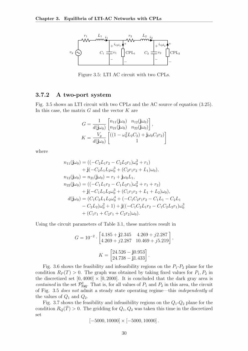
Chapter 3. Equilibria of LTI-AC Networks with CPLs
vg
r1 L1 i1r2 L2 i2
+
−
CPL2
icpl2
C1
−
+
v1
+
−
CPL1
icpl1
C2
−
+
v2
Figure 3.5: LTI AC circuit with two CPLs.
3.7.2 A two-port system
Fig. 3.5 shows an LTI circuit with two CPLs and the AC source of equation (3.25).In this case, the matrix G and the vector K are
G =1
d(jω0)
[n11(jω0) n12(jω0)n21(jω0) n22(jω0)
],
K =Vg
d(jω0)
[((1− ω2
0L2C2) + jω0C2r2)1
]where
n11(jω0) = ((−C2L1r2 − C2L2r1)ω20 + r1)
+ j(−C2L1L2ω30 + (C2r1r2 + L1)ω0),
n12(jω0) = n21(jω0) = r1 + jω0L1,
n22(jω0) = ((−C1L1r2 − C1L2r1)ω20 + r1 + r2)
+ j(−C1L1L2ω30 + (C1r1r2 + L1 + L2)ω0),
d(jω0) = (C1C2L1L2ω40 + (−C1C2r1r2 − C1L1 − C2L1
− C2L2)ω20 + 1) + j((−C1C2L1r2 − C1C2L2r1)ω3
0
+ (C1r1 + C2r1 + C2r2)ω0).
Using the circuit parameters of Table 3.1, these matrices result in
G = 10−2 ·[
4.185 + j2.345 4.269 + j2.2874.269 + j2.287 10.469 + j5.219
],
K =
[24.526− j0.95324.738− j1.433
].
Fig. 3.6 shows the feasibility and infeasibility regions on the P1-P2 plane for thecondition RP (T ) > 0. The graph was obtained by taking fixed values for P1, P2 inthe discretized set [0, 4000] × [0, 2000]. It is concluded that the dark gray area iscontained in the set PI
FAQ. That is, for all values of P1 and P2 in this area, the circuitof Fig. 3.5 does not admit a steady state operating regime—this independently ofthe values of Q1 and Q2.
Fig. 3.7 shows the feasibility and infeasibility regions on the Q1-Q2 plane for thecondition RQ(T ) > 0. The gridding for Q1, Q2 was taken this time in the discretizedset
[−5000, 10000]× [−5000, 10000] .
30
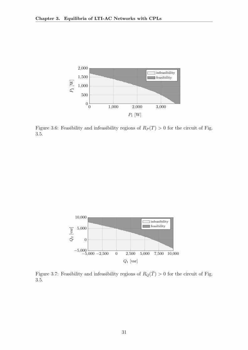
Chapter 3. Equilibria of LTI-AC Networks with CPLs
0 1,000 2,000 3,0000
500
1,000
1,500
2,000
P1 [W]
P2[W
]infeasibility
feasibility
Figure 3.6: Feasibility and infeasibility regions of RP (T ) > 0 for the circuit of Fig.3.5.
−5,000 −2,500 0 2,500 5,000 7,500 10,000−5,000
0
5,000
10,000
Q1 [var]
Q2[var]
infeasibility
feasibility
Figure 3.7: Feasibility and infeasibility regions of RQ(T ) > 0 for the circuit of Fig.3.5.
31
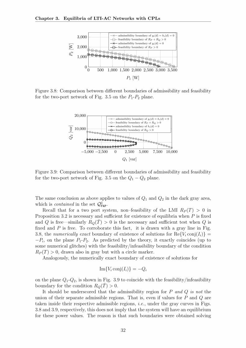
Chapter 3. Equilibria of LTI-AC Networks with CPLs
0 500 1,000 1,500 2,000 2,500 3,000 3,5000
1,000
2,000
3,000
P1 [W]
P2[W
]
admissibility boundary of gi(d) = hi(d) = 0
feasibility boundary of RP +RQ > 0
admissibility boundary of gi(d) = 0
feasibility boundary of RP > 0
Figure 3.8: Comparison between different boundaries of admissibility and feasibilityfor the two-port network of Fig. 3.5 on the P1-P2 plane.
−5,000 −2,500 0 2,500 5,000 7,500 10,000
0
10,000
20,000
Q1 [var]
Q2[var]
admissibility boundary of gi(d) = hi(d) = 0
feasibility boundary of RP +RQ > 0
admissibility boundary of hi(d) = 0
feasibility boundary of RQ > 0
Figure 3.9: Comparison between different boundaries of admissibility and feasibilityfor the two-port network of Fig. 3.5 on the Q1 −Q2 plane.
The same conclusion as above applies to values of Q1 and Q2 in the dark gray area,which is contained in the set QI
FAP.Recall that for a two port system, non–feasibility of the LMI RP (T ) > 0 in
Proposition 3.2 is necessary and sufficient for existence of equilibria when P is fixedand Q is free—similarly RQ(T ) > 0 is the necessary and sufficient test when Q isfixed and P is free. To corroborate this fact, it is drawn with a gray line in Fig.3.8, the numerically exact boundary of existence of solutions for ReVi conj(Ii) =−Pi, on the plane P1-P2. As predicted by the theory, it exactly coincides (up tosome numerical glitches) with the feasibility/infeasibility boundary of the conditionRP (T ) > 0, drawn also in gray but with a circle marker.
Analogously, the numerically exact boundary of existence of solutions for
ImVi conj(Ii) = −Qi
on the plane Q1-Q2, is shown in Fig. 3.9 to coincide with the feasibility/infeasibilityboundary for the condition RQ(T ) > 0.
It should be underscored that the admissibility region for P and Q is not theunion of their separate admissible regions. That is, even if values for P and Q aretaken inside their respective admissible regions, i.e., under the gray curves in Figs.3.8 and 3.9, respectively, this does not imply that the system will have an equilibriumfor these power values. The reason is that such boundaries were obtained solving
32

Chapter 3. Equilibria of LTI-AC Networks with CPLs
the real and the imaginary part of (3.4) independently and not simultaneously. Theblack curves with an ‘x’ marker in Figs. 3.8 and 3.9 represent the numerically exactboundaries of existence for (3.4), solving its real and imaginary parts simultaneously,and taking fixed values of Q1 = 1000 and Q2 = 0 for the former, and taking fixedvalues of P1 = 500 and P2 = 500 for the latter. It can be observed that in bothcases the admissibility regions are reduced. However, they are bounded by thefeasibility/infeasibility boundaries of RP (T ) > 0 and RQ(T ) > 0.
Finally, the black curves with circle marker in Figs. 3.8 and 3.9 correspond tothe feasibility/infeasibility boundaries of the LMI
RP (T ) +RQ(T ) > 0
plotted for some fixed values of P and Q, respectively. Although not predicted bythe theory, they coincide with the boundaries of numerically exact solution of thequadratic equations (3.4) for these fixed values.
3.8 Summary
For general, multi-port, linear AC networks with constant power loads, this chap-ter has proposed conditions that are necessary for load admissibility, i.e., if thisconditions are satisfied, then the network does not admit a sinusoidal steady stateregime at certain specified frequency. For the case of one- or two-port networks andfree active (or reactive) power of the CPLs’ components, these conditions are alsosufficient. Interestingly, for single-port networks the admissibility condition can betested directly from the data of the problem. Similarly to the case of DC networks[9, 91] the analysis boils down to the study of solvability of a set of quadratic equa-tions in several variables. In the DC case these equations define mappings from Rmto R, while in the AC case the mappings are from Cm to C, which as it has beenverified here, may give rise to a different mathematical problem in certain situations;see Section 3.5.2.
Technical Appendices of the Chapter
3.A Proof of Lemma 3.2
To streamline the presentation, define the set
Ev := x ∈ Rn | vk(x) = 0, ∀k,
where vk(x) is defined in (3.11).The proof of the implication (3.13) is established by contraposition. Therefore,
suppose that Ev is not empty. It is proven next that there are no real numbers tksuch that ∑
k=1
tkAk > 0. (3.26)
33
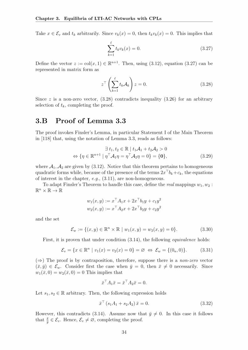
Chapter 3. Equilibria of LTI-AC Networks with CPLs
Take x ∈ Ev and tk arbitrarily. Since vk(x) = 0, then tkvk(x) = 0. This implies that
∑k=1
tkvk(x) = 0. (3.27)
Define the vector z := col(x, 1) ∈ Rn+1. Then, using (3.12), equation (3.27) can berepresented in matrix form as
z>(∑k=1
tkAk)z = 0. (3.28)
Since z is a non-zero vector, (3.28) contradicts inequality (3.26) for an arbitraryselection of tk, completing the proof.
3.B Proof of Lemma 3.3
The proof invokes Finsler’s Lemma, in particular Statement I of the Main Theoremin [118] that, using the notation of Lemma 3.3, reads as follows:
∃ t1, t2 ∈ R | t1A1 + t2A2 > 0
⇔ η ∈ Rn+1 | η>A1η = η>A2η = 0 = 0, (3.29)
where A1,A2 are given by (3.12). Notice that this theorem pertains to homogeneousquadratic forms while, because of the presence of the terms 2x>bk+ck, the equationsof interest in the chapter, e.g., (3.11), are non-homogeneous.
To adapt Finsler’s Theorem to handle this case, define the real mappings w1, w2 :Rn × R→ R
w1(x, y) := x>A1x+ 2x>b1y + c1y2
w2(x, y) := x>A2x+ 2x>b2y + c2y2
and the set
Ew := (x, y) ∈ Rn × R | w1(x, y) = w2(x, y) = 0. (3.30)
First, it is proven that under condition (3.14), the following equivalence holds:
Ev = x ∈ Rn | v1(x) = v2(x) = 0 = ∅ ⇔ Ew = (0n, 0). (3.31)
(⇒) The proof is by contraposition, therefore, suppose there is a non-zero vector(x, y) ∈ Ew. Consider first the case when y = 0, then x 6= 0 necessarily. Sincew1(x, 0) = w2(x, 0) = 0 This implies that
x>A1x = x>A2x = 0.
Let s1, s2 ∈ R arbitrary. Then, the following expression holds
x> (s1A1 + s2A2) x = 0. (3.32)
However, this contradicts (3.14). Assume now that y 6= 0. In this case it followsthat x
y∈ Ev. Hence, Ev 6= ∅, completing the proof.
34
Chapter 3. Equilibria of LTI-AC Networks with CPLs
(⇐) Once again by contraposition. Hence, suppose that Ev 6= ∅ and take x ∈ Ev,then (x, 1) is a non-zero vector in Ew and, consequently, Ew 6= 0n, completing theproof.
The proof of the implication (3.15) follows next. Suppose Ev = ∅. Then, theequivalence (3.31) implies that Ew = (0n, 0). Recalling that
w1(x, y) = η>A1η, w2(x, y) = η>A2η
with η := (x, y), Finsler’s Lemma ensures the existence of t1, t2 ∈ R such that
t1A1 + t2A2 > 0. (3.33)
Hence, the lemma is proved.
3.C Proof of Proposition 3.1
Define the following (2m+ 1)× (2m+ 1) real matrices
Ai :=
[Ai bib>i 2Pi
], Bi :=
[Bi qiq>i 2Qi
]. (3.34)
Notice that
gi(d) =[d> 1
]Ai[d1
]hi(d) =
[d> 1
]Bi[d1
]. (3.35)
Suppose there exist ti, ti such that5
m∑i=1
tiAi +m∑i=1
tiBi > 0.
Referring to Lemma 3.2 with ` = 2m, x = d and
v1 = g1, . . . , vm = gm, vm+1 = h1, . . . , v2m = hm,
it is concluded that there are no solutions for the system
gi(d) = hi(d) = 0.
This implies that there is no sinusoidal steady state for the network. The proof iscompleted noting that
m∑i=1
tiAi = RP (T ),m∑i=1
tiBi = RQ(T ). (3.36)
5The symbol ti is introduced for ease of reference in the subsequent material.
35
Chapter 3. Equilibria of LTI-AC Networks with CPLs
3.D Proof of Proposition 3.2
Consider the matrix RP , given in (3.17), for T = Im. Notice that the uppermostcorner of RP is given by M , defined in (3.19). Since M > 0, it follows that RP > 0if and only if the Schur complement of M is positive. The proof is completed notingthat the latter is equivalent to (3.20).
3.E Proof of Proposition 3.3
The equivalence between the first two statements is a direct corollary of the laststatement in Lemma 3.3, which states that for ` = 2 (that is m = 1)
g1(d) = h1(d) = 0 ⇔ ∃ t1, t1 | t1A1 + t1B1 > 0.
The proof is completed invoking the identity (3.36) with T = t1, T = t1.The equivalence with the last statement is shown next. Towards this end, re-
write the model of the network in complex form as
G|I|2 + conj(I)K + S = 0. (3.37)
Inequality (3.2) implies that G 6= 0. Divide (3.37) by G and split it into real andimaginary parts. Then, the complex equation (3.37) is equivalent to
x2 + y2 + ax+ by + P ′ = 0 (3.38)
bx− ay +Q′ = 0 (3.39)
where
K
G:= a+ jb,
S
G:= P ′ + jQ′, I := x+ jy.
Suppose that a 6= 0, then from (3.39) y is obtained as
y =bx+Q′
a. (3.40)
Substituting the above value for y into (3.38), the following quadratic equation forx is obtained.
(a2 + b2)x2 +[2bQ′ + a(a2 + b2)
]x +
(Q′2 + abQ′ + a2P ′
)= 0. (3.41)
This equation has a real solution if and only if its discriminant is non-negative, thatis, if and only if(
2bQ′ + a(a2 + b2))2 ≥ 4(a2 + b2)(Q′2 + abQ′ + a2P ′).
Develop the left and right-hand side expressions, then the inequality above is equiv-alent to
4b2Q′2 + 4abQ′(a2 + b2) + a2(a2 + b2)2
≥4a2Q′2 + 4b2Q′2 + 4abQ′(a2 + b2) + 4a2P ′(a2 + b2)
36

Chapter 3. Equilibria of LTI-AC Networks with CPLs
which can be written in a simplified form as
(a2 + b2)2 − 4P ′(a2 + b2)− 4Q′2 ≥ 0.
This expression holds if and only if
(a2 + b2) ≥ 2(P ′ +√P ′2 +Q′2). (3.42)
Notice that
a2 + b2 =|K|2|G|2 ,
P ′ =PReG+QImG
|G|2 ,
Q′ =QReG − P ImG
|G|2 .
Then, inequality (3.42) can be equivalently written in the original coefficients as inin (3.23).
Now suppose that a = 0. If b 6= 0, then from (3.39) it follows that
x = −Q′
b.
If this value of x is substituted into (3.38), then, a quadratic equation for y isobtained:
b2y2 + b3y +(Q′2 + b2P ′
)= 0.
This equation has a real solution if and only if its discriminant is non negative, thatis if and only if
b6 − 4b2(Q′2 + b2P ′
)≥ 0.
This inequality is equivalent to(b2)2 − 4P ′(b2)− 4Q′2 ≥ 0,
which holds if and only if
b2 ≥ 2(P ′ +
√P ′2 +Q′2
).
Clearly, the above expression corresponds with (3.42) by taking a = 0.To conclude the proof, suppose that a = 0 and b = 0 simultaneously. In this
case, system conformed by equations (3.38) and (3.39), has a solution if and only ifQ′ = 0 and P ′ ≤ 0. This last case has little practical relevance since if a = 0 andb = 0 simultaneously, then K = 0, which would correspond to a single-port networkwithout a source.
37
Chapter 3. Equilibria of LTI-AC Networks with CPLs
3.F Proofs of Propositions 3.4 and 3.5
The proofs follow as direct corollaries of Lemma 3.3. First, notice that
g1(d) = g2(d) = 0 ⇔ ∃ t1, t2 such that t1A1 + t2A2 > 0
h1(d) = h2(d) = 0 ⇔ ∃ t1, t2 such that t1B1 + t2B2 > 0,
and
t1A1 + t2A2 = RP (diag (t1, t2))
t1B1 + t2B2 = RQ (diag (t1, t2)) .
It only remains to verify (3.14). For Proposition 3.4, it follows that
A1 + A2 = M,
with M , given in (3.19), being positive definite. Therefore, (3.14) is satisfied withs1 = s2 = 1. On the other hand, for Proposition 3.5 it is not clear when there existss1, s2 ∈ R such that
s1B1 + s2B2 > 0,
with B1, B2 given in (3.9). Therefore, it is necessary to impose assumption (3.24).
38
Chapter 4
Decoupled AC power flow and DCpower networks with CPLs
Synopsis In AC and DC power systems with constant power loads, the analysisof existence of steady states is cast as the analysis of solutions of a set of nonlinearalgebraic equations of the form f(x) = 0, where f : Rn → Rn. In this chapter, thevector field f is associated to the ordinary differential equation x = f(x) and byinvoking advanced concepts of dynamical systems theory and effectively exploitingsome exhibited monotonicity features, the following traits are established. (i) Proofthat, if there are equilibria, there is a distinguished one that is stable and attractive,and give conditions such that it is unique. (ii) Establishment of a simple on-lineprocedure to decide whether equilibria exist or not, and to compute the distinguishedone. (iii) Proof that the method is also applicable for the case when the parametersof the system are not exactly known. It is shown how the proposed tool can beapplied to the analysis of voltage regularity in AC power systems, and to the studyof existence of steady states of multi-terminal high-voltage DC systems and DCmicrogrids.
4.1 Introduction
This chapter explores a methodological approach to determine the existence andstability of the equilibria in diverse power systems problems. The specific problemsare enlisted as
P1 Analysis of voltage regularity1 in AC power systems with “light” active powerload. The study of this important property, also called “static (or long-term)voltage stability” [56, Chapter 14] or “loadability limit” [119, Chapter 7], isstandard in the power systems community.
P2 Study of existence of steady states of two emerging power system concepts,namely multi-terminal high-voltage (MT-HV) DC networks [120, 50] and DCmicrogrids [37, 33].
P3 In addition, if stationary voltage solutions exist, the proposed method alsoallows to identify the solution with the highest voltage magnitudes, which isthe desired operating condition in these applications.
1Prof David Hill is graciously acknowledged for suggesting this, most appropriate, terminology.
39
Chapter 4. Decoupled AC power flow and DC power networks with CPLs
In these three examples, the key problem is the study of a nonlinear algebraicequation f(x) = 0, with f : Rn → Rn, where only solutions x with positive com-ponents are of interest. The approach adopted in the chapter is to associate tof(x) the ordinary differential equation (ODE) x = f(x), which is shown to be well-defined on the positive orthant of Rn, and to apply to it tools of dynamical systems[43]—in particular, monotone systems [114]—to study existence and stability of itsequilibria, which are the solutions of the primal algebraic equation.
The main contributions of this chapter are the proofs of the following propertiesof the ODE.
C1 If there are no equilibria then, in all the solutions of the ODE, one or morecomponents converge to zero in finite time.
C2 If equilibria exist, there is a distinguished equilibrium, say xmax, among themthat dominates component-wise all the other ones. This equilibrium xmax isstable and attracts all trajectories that start in a certain well-defined domain.Moreover, physically-interpretable conditions on the problem data that ensurexmax is the only stable equilibrium, are provided.
C3 By solving a system of n convex algebraic inequalities in n positive unknowns,a set of initial conditions are explicitly identified. These initial conditionsposses the following properties. (i) All trajectories starting there monotoni-cally decay in all components. (ii) Either some component converges to zeroin a finite time for all those trajectories or, for all of them, all components re-main separated from zero on the infinite time horizon. Moreover, in the lattercase, the trajectory is forward complete and converges to xmax. An additionaloutcome of this analysis is the generation of an estimate for the domain ofattraction of asymptotically stable equilibia.
C4 Proof that the method is applicable even if the parameters of f(x) are un-known, and only upper and lower bounds for them are available.
In [34], the authors propose conditions for the solvability of affinely parameter-ized quadratic equations that contain, as a particular case, the kind of nonlinearequations studied in the present chapter. Nonetheless, a standing assumption inthat paper is that a solution exists, and the focus is to derive conditions underwhich the solutions belong to a certain pre-specified set. Conversely, in this chap-ter the existence of solutions is not taken for granted; instead the conditions underwhich they exist (or not) are given. Additionally, the identification of the dominantequilibrium xmax and the analysis of its regularity properties—from the viewpointof reactive power flow analysis—is carried out thanks to the stability identificationof the ODE’s equilibria; the latter central analytical aspect reported in this chaptercannot be addressed with the tools used in [34]. More recently, in [123], analyticalconditions for the existence of solutions of the (full) power flow equations are given.2
However, by invoking the standard “decoupling” assumption, only the problem ofreactive power flow is addressed in the present chapter. Finally, in [1], the au-thors propose a numerical method to solve the load flow equations, which is by now
2Recall the preliminaries on power systems in Chapter 2.
40
Chapter 4. Decoupled AC power flow and DC power networks with CPLs
standard and implemented in many commercial software packages, such as DigSi-lent PowerFactory. Nevertheless, as already mentioned, this problem is beyond thescope of this chapter.
The remainder of the chapter is organized as follows. Section 4.2 describes theODE x = f(x) of interest and gives the main theoretical results pertaining to it,with some practical extensions given in Section 4.3. In Section 4.4 these results areillustrated with three canonical power systems examples. Section 4.5 presents somenumerical simulation results. The chapter is wrapped-up with a brief summary inSection 4.6. To enhance readability, all proofs of the technical results are given in atechnical appendix at the end of the chapter.
4.2 Analysis of the ODE of Interest
As indicated in the introduction, one of the main interests of the chapter is theanalysis of voltage regularity of steady solutions of AC power systems (under thecommon decoupling assumption [56]), and on the study of the existence of steadystates of MT-HVDC networks as well as DC microgrids—the three of them withCPLs. In Section 4.3, it is shown that these studies boil down to the analysis ofsolutions of the following algebraic equations in x ∈ Kn+3
ai1x1 + ai2x2 + · · ·+ ainxn +bixi
= wi, i ∈ 1, . . . , n, (4.1)
where aij ∈ R, wi ∈ R and bi ∈ R. These equations can be written in compact formas
Ax+ stack
(bixi
)− w = 0. (4.2)
In the chapter, the following assumption is adopted.
Assumption 4.1. The matrix A = A> is positive definite, its off-diagonal elementsare non-positive and bi 6= 0 for all i.
To study the solutions of (4.2), the following ODE is considered.
x = f(x) := −Ax− stack
(bixi
)+ w. (4.3)
The main interest of the chapter is in studying the existence, and stability, of theequilibria of (4.3). In particular, the answers to the following questions are provided.
Q1 When do equilibria exist? Is it possible to offer a simple test to establish theirexistence?
Q2 If there are equilibria, is there a distinguished element among them?
Q3 Is this equilibrium stable and/or attractive?
Q4 If it is attractive, can its domain of attraction be estimated?
3Recall from the preliminaries that Kn+ denotes the positive orthant of Rn.
41

Chapter 4. Decoupled AC power flow and DC power networks with CPLs
Q5 Is it possible to propose a simple procedure to compute this special equilibriumusing the system data (A, b, w)?
Q6 Are there other stable equilibria?
Instrumental to answer to the queries Q1-Q6 is the fact that the system (4.3) ismonotone. That is, for any two solutions xa(·), xb(·) of (4.3), defined on a commoninterval [0, T ], the inequality xa(0) ≤ xb(0) implies that xa(t) ≤ xb(t) ∀t ∈ [0, T ].This can be verified by noticing that equation (4.3) satisfies the necessary and suf-ficient condition for monotonicity [114, Proposition 1.1 and Remark 1.1, Ch. III]
∂fi(x)
∂xj≥ 0, ∀i 6= j, ∀x ∈ Kn+. (4.4)
In the sequel, x(t, x0) denotes the solution of (4.3) with initial conditions x(0) =x0 > 0, and use the following.
Definition 4.1. An equilibrium x > 0 of (4.3) is said to be attractive from aboveif for any x0 ≥ x, the solution x(t, x0) is defined on [0,∞) and converges to x ast→∞. The equilibrium is said to be hyperbolic if the Jacobian matrix ∇f(x) hasno eigenvalue with zero real part [43].
Remark 4.1. Along the lines of the standard Kron reduction, the findings of thechapter can be extended to the case where some of the coefficients bi are equal tozero.4
The proof of this remark is given in Appendix 4.A.
4.2.1 The simplest example
To gain an understanding of some key traits of possible results, it is instructive tostart with the simplest case n = 1. Then, x ∈ R and (4.3) is the scalar equation
x = −ax− b
x+ w, (4.5)
and a > 0, b 6= 0. Feasible behaviors of the system are exhaustively described inFigure 4.1.
The following can be inferred from this figure.
B1 The system either has no equilibria, or it has finitely many equilibria, or it hasa single equilibrium.
B2 If the system has equilibria, the rightmost of them is attractive from above.
B3 Non-hyperbolic equilibria may be attractive from above but unstable; more-over, there may be no other equilibria.
B4 Hyperbolic and attractive from above equilibria are stable.
B5 If b > 0, globally attractive equilibria do not exist.
It is shown next that several of the traits occurring in the scalar case are inheritedby the n-th order ODE (4.3).
4An anonymous reviewer is acknowledged for indicating this.
42
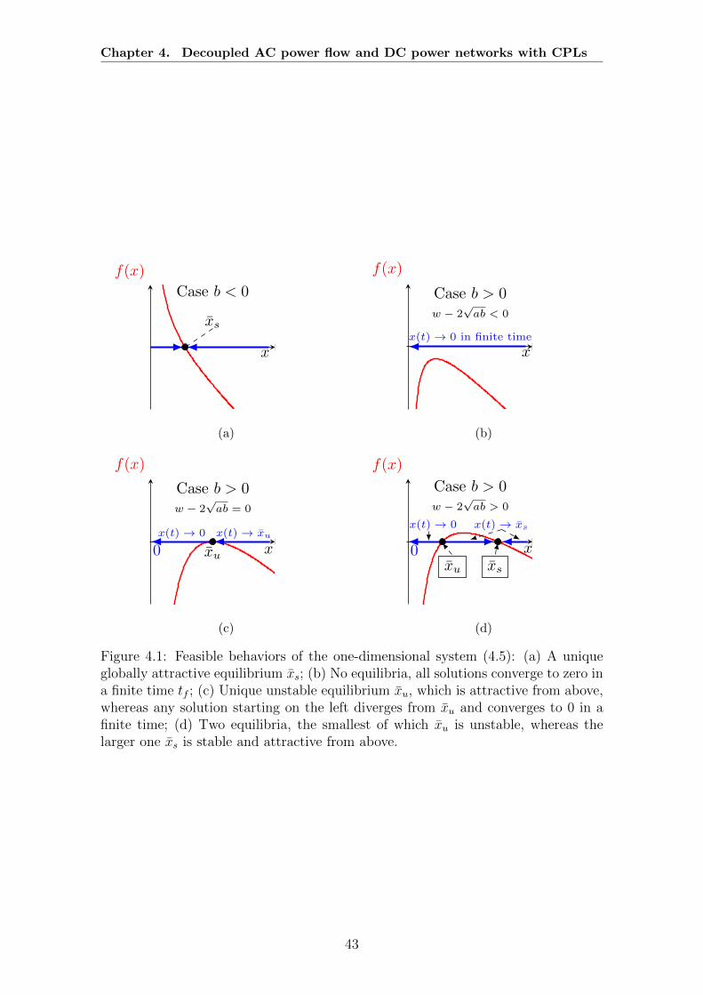
Chapter 4. Decoupled AC power flow and DC power networks with CPLs
x
xs
Case b < 0
f(x)
(a)
xx(t)→ 0 in finite time
Case b > 0w − 2
√ab < 0
f(x)
(b)
xxu
x(t)→ 0 x(t)→ xu
0
Case b > 0w − 2
√ab = 0
f(x)
(c)
x
x(t)→ 0 x(t)→ xs
0
Case b > 0w − 2
√ab > 0
xu xs
f(x)
(d)
Figure 4.1: Feasible behaviors of the one-dimensional system (4.5): (a) A uniqueglobally attractive equilibrium xs; (b) No equilibria, all solutions converge to zero ina finite time tf ; (c) Unique unstable equilibrium xu, which is attractive from above,whereas any solution starting on the left diverges from xu and converges to 0 in afinite time; (d) Two equilibria, the smallest of which xu is unstable, whereas thelarger one xs is stable and attractive from above.
43
Chapter 4. Decoupled AC power flow and DC power networks with CPLs
4.2.2 An extra assumption
The situation described in item B3 above may happen in the general case —e.g.,considering a diagonal matrix A. However, some evidence suggesting that this situ-ation “almost never” occurs is now given. This forms a ground to treat the oppositesituation as “typical”, “regular”, and “prevalent” and to pay special attention to it.
To be specific, a case where item B3 is impossible is identified.
Assumption 4.2. There are no non-hyperbolic equilibria of the system (4.3). Inother words, the following set identity holdsx ∈ Kn+
∣∣∣∣∣∣ det[A− diag
(bix2i
)]= 0,
w = Ax+ stack(bixi
) = ∅. (4.6)
The lemma below proves that Assumption 4.2 is almost surely true.
Lemma 4.1. For any given A and bi 6= 0, the set of all w ∈ Rn for which Assump-tion 4.2 does not hold has zero Lebesgue measure and is nowhere dense.
Proof. See Appendix 4.A at the end of the chapter.
4.2.3 Main results on the system (4.3)
The first claim contains a qualitative analysis of the system.
Proposition 4.1. Consider the system (4.3) verifying Assumption 4.1. One andonly one of the following two mutually exclusive statements holds.
S1 There are no equilibria x, either stable or unstable, and any solution x(·) isdefined only on a finite time interval [0, tf ) ⊂ [0,∞), since there exists atleast one coordinate xi such that xi(t) → 0, xi(t) → −∞ as t → tf . Such acoordinate is necessarily associated with bi > 0.5
S2 Equilibria xk do exist. One of them xmax > 0 verifies xmax ≥ xk, ∀k, and isattractive from above.
Suppose that Assumption 4.2 is also met. Then in the case S2 there are finitelymany equilibria and xmax is locally asymptotically stable. If in addition all bi’s areof the same sign, then there are no other stable equilibria apart from xmax.
Proof. See Appendix 4.D at the end of the chapter.
Lemma 4.1 allows to claim that the traits described in the last two sentences ofProposition 4.1 occur almost surely.
A constructive test to identify which of the cases S1 or S2 holds, as well as amethod to find xmax in the case S2, are presented. To this end, the following conceptis introduced.
5This implies that the case in claim S1 does not occur if bj < 0, ∀ j.
44
Chapter 4. Decoupled AC power flow and DC power networks with CPLs
Definition 4.2. A solution x(·) of the ODE (4.3) is said to be distinguished if itsinitial condition lives in the set
E :=
x ∈ Kn+ | Ax > stack
(〈wi〉+
〈−bi〉xi
).6 (4.7)
If bi > 0 for all i, then the set (4.7) reduces to the (convex open polyhedral) conex ∈ Kn+ | Ax > stack (〈wi〉)
.
Proposition 4.2. Consider the system (4.3) verifying Assumption 4.1.
I The set E is non-empty, consequently there are distinguished solutions.
II All such solutions strictly decay, in the sense that x(t) < 0, for all t in thedomain of definition of x(·).
III One and only one of the following two mutually exclusive statements holdssimultaneously for all distinguished solutions x(·):
i For a finite time tf ∈ (0,∞), some coordinate xi(·) approaches zero, thatis,
limt→tf
xi(t) = 0, (4.8)
and the solution x(·) is defined only on a finite time interval [0, tf ).
ii There is no coordinate approaching zero, the solution is defined on [0,∞),and the following limit exists and verifies
limt→∞
x(t) > 0. (4.9)
This limit is the same for all distinguished solutions.
IV If the case III.i holds for a distinguished solution, the situation S1 from Propo-sition 4.1 occurs.
V If the case III.ii holds for a distinguished solution, the situation S2 from Propo-sition 4.1 occurs, and the dominant equilibrium xmax is equal to the limit (4.9).
Proof. See Appendix 4.D at the end of the chapter.
Remark 4.2 (Additional properties of (4.3)).
P1 In III.i, there may be several components xi with the described property, butnot all of them necessarily possess it.
P2 The claim S1 in Proposition 4.1 and IV in Proposition 4.2 yield that (4.8) isnecessarily associated with bi > 0 and xi(t)→ −∞ as t→ tf .
P3 Regarding the claim S2 in Proposition 4.1 the basin of attraction of the equi-librium xmax contains all states x ≥ xmax. Under Assumption 4.2, this basin isopen.
6The operator 〈·〉 denotes the clipping function 〈a〉 := maxa, 0.
45

Chapter 4. Decoupled AC power flow and DC power networks with CPLs
P4 The linear programming problem of finding elements in the setx ∈ Kn+ | Ax > 0
has been widely studied in the literature [28, 100, 11]. There is a wholevariety of computationally efficient methods to solve this problem, includingthe Fourier-Motzkin elimination, the simplex method, interior-point/barrier-like approaches, and many others; for a recent survey, the reader is referred to[35].
4.3 A Numerical Procedure and a Robustness Anal-
ysis
With the aim of extending the realm of application of the previous results, thissection addresses the issues of numerical computation and robustness of the claims.Additionally, explicit answers to the questions raised at the beginning of Section 4.2are given.
4.3.1 A numerical procedure to verify Propositions 4.1 and4.2
Proposition 4.2 suggests a computational procedure to verify whether the systemhas equilibria and, if they do exist, to find the dominant one xmax among them.Specifically, it suffices to find an element of the set E defined in (4.7), to launch thesolution of the differential equation (4.3) from this vector, and to check whether—asthe solution decays—there is a coordinate approaching zero or, conversely, all ofthem remain separated from zero. In the last case, the solution has a limit, whichis precisely the dominant equilibrium of the system.
The statement I of Proposition 4.2 ensures that the first step of this algorithm,i.e., generating an element of the set E defined in (4.7), is feasible. Technically, thisstep consists in solving a system of feasible convex inequalities given by
〈wi〉+〈−bi〉xi−
n∑j=1
aijxj < 0, xi > 0, ∀i.
This problem falls within the area of convex programming and so there is an arma-mentarium of effective tools to solve it. Nevertheless, this problem can be furthersimplified through transition from nonlinear convex inequalities to linear ones, mod-ulo closed-form solution of finitely many scalar quadratic equations. The basis forthis is given by the following lemma, whose proof is given in Appendix 4.B.
Lemma 4.2. Pick any vector z > 0 such that Az > 0.7 Then, the scaled vectorx := µz verifies x ∈ E , provided that
µ >〈wi〉+
√〈wi〉2 + 4(Az)i
〈−bi〉zi
2(Az)i, ∀i. (4.10)
7In Appendix 4.B it is shown that, under Assumption 4.1, this system of linear inequalities isfeasible.
46

Chapter 4. Decoupled AC power flow and DC power networks with CPLs
For any i with bi > 0, relation (4.10) simplifies into
µ >〈wi〉(Az)i
.
4.3.2 Robustness vis-a-vis uncertain parameters
The proposition below extends the results of Proposition 4.1 to the case where theparameters C := (A, bii, w) of the system (4.2) are not known, but only theircomponent-wise bounds are available, i.e.,
A+ ≤ A ≤ A−, b+i ≤ bi ≤ b−i , w− ≤ w ≤ w+. (4.11)
To streamline the presentation of the proposition, define the bounding sets C± :=(A±, b±i i, w±).
Proposition 4.3. Suppose that C verifies Assumption 4.1, and (4.11) holds. Then,the following statements are true.
i If the case of claim S1 from Proposition 4.1 holds for C+, this case also holdsfor both C and C−.
ii If the case S2 from Proposition 4.1 hold for C−, this case also holds for bothC and C+.
iii In the situation ii, the dominant equilibria x−max, xmax, x+max related to C−,C,C+,
respectively, are such that
x−max ≤ xmax ≤ x+max. (4.12)
Moreover, x+max → x−max as A+ → A−, b+
i → b−i , w+ → w−.
Proof. See Appendix 4.D at the end of the chapter.
Proposition 4.3 can be used to estimate the distance from the initial state x ∈ Eof the employed distinguished solution to the dominant equilibrium xmax. This can bedone picking C− and noting that, due to (4.12) and II in Proposition 4.2, the distanceof interest does not exceed ‖x−x−max‖. Certainly, C−’s with easily computable x−max areof especial interest. An example is obtained via “zeroing” all off-diagonal elementsof A in C if for any i either bi < 0 or bi > 0 and wi ≥ 2
√aiibi. Then
x−max = stack(wi +
√w2i − 4aiibi
2aii
).
Thanks to S2 in Proposition 4.1 and (4.12), x−max can be used, instead of a vectorfrom the set (4.7), as the initial state when seeking xmax via integration of the ODE(4.3). An example of this situation, happens when bi > 0 ∀i. Then, in (4.11), takeA+ := A,w+ := w, and b+
i > 0 arbitrarily close to 0, and moreover, finally letb+i → 0+. Then, by using Lemma 4.3, it can be shown that integration of the ODE
can be started with A−1w provided that A−1w > 0.
47

Chapter 4. Decoupled AC power flow and DC power networks with CPLs
4.3.3 Answers to the queries Q1-Q6 in Section 4.2
Now, the previous discussion of this section is put into a nutshell by giving a synopsisof the answers to Q1-Q6.Answer to Q1
• Equilibria exist if and only if neither distinguished solution of the ODE (4.3)approaches the boundary of the positive cone Kn+ for a finite time.
• To check this existence criterion, it suffices to examine the behavior of anarbitrary distinguished solution.
• To accomplish the latter, a solution x ∈ Rn for a certain convex or a lessconservative linear programming problem should be found and then the ODE(4.3) should be integrated from this vector x.
Answer to Q2
• There exists a distinguished equilibrium, xmax, that satisfies xmax ≥ xeq, for anyother system’s equilibrium, xeq.
Answer to Q3
• The equilibrium xmax is attractive from above and “almost surely” is stableand locally asymptotically stable.
Answer to Q4
• This domain covers the set (4.7); the latter set contains any vector built as isdiscussed in Lemma 4.2.
Answer to Q5
• It suffices to invoke the solution of the ODE (4.3) from the answer to Q1 andto compute it until it converges.
Answer to Q6
• If in (4.2), all bi’s are of the same sign and Assumption 4.2 holds, there are noother stable equilibria.
4.4 Application to Some Canonical Power Sys-
tems
In this section, the results of Section 4.2 are applied to three different problems ofpower systems containing constant power loads. These comprise the standard volt-age stability (in a static sense) of AC power systems with “light” active power loadand the study of existence of equilibria of MT-HVDC networks and DC microgrids
48
Chapter 4. Decoupled AC power flow and DC power networks with CPLs
4.4.1 Voltage stability (in a static sense) of AC power sys-tems
The standard static analysis of voltage stability in AC power systems assumes thedynamics is in steady state, and concentrates its attention on the algebraic equationsrelating the active and reactive power, with the voltages and the phase angles—thewell-known power flow equations. In [121] it was first suggested to investigate thesign of the real parts of the eigenvalues of the power flow Jacobian matrix as anindicator of voltage stability. This sensitivity analysis of the voltage magnitudeswith respect to changes in the active and reactive power flows is the prevailingapproach to analyze voltage stability in AC networks as explained in power systemstextbooks, i.e., [56, Chapter 14] and [119, Chapter 7]. In this subsection it is shownhow the analysis framework developed in Section 4.2 can be applied to carry out thisanalysis, for the particular case of power systems with “light” active power load.
Consider a high-voltage AC power network with n ≥ 1 PQ nodes. Denote byVi > 0, δi and Qi the voltage magnitude, phase angle and the reactive power loaddemand at node i, respectively. The analysis is restricted to scenarios in which thefollowing standard “light” active power load (also called “decoupling”) assumptionis satisfied [56, Chapter 14.3.3], [99, Assumption 1].
Assumption 4.3. δi − δj ≈ 0 for all i, j ∈ 1, . . . , n.
With Assumption 4.3, the reactive power flow at node i is given by [56, 108, 99]8
QZIP,i = Vi
n∑j=1
|Bij|(Vi − Vj),
where Bij < 0 if nodes i and j are connected via a power line and Bij = 0 otherwise.The reactive power demand QZIP,i at the i-th node is described by a, so-called, ZIPmodel, namely
QZIP,i :=(YiV 2
i + kiVi +Qi
).
The term ZIP load refers to a parallel connection of a constant susceptance Yi ∈ R,a constant reactive current ki ∈ R, and a constant power Qi ∈ R load. Then, the(algebraic) reactive power balance equation is obtained as
(YiV 2
i + kiVi +Qi
)= Vi
n∑j=1
|Bij|(Vi − Vj), i ∈ 1, . . . , n, (4.13)
which by defining x := stack (Vi) ∈ Kn+, A ∈ Rn×n with
Aii =n∑j=1
|Bij| − Yi, Aij = −|Bij|,
w = stack(ki), bi = −Qi, (4.14)
8The reader is referred here to Chapter 2 for a detailed derivation of the power flow equationsand particularly to the developments leading to equation (2.22) which appears by the end saidchapter.
49

Chapter 4. Decoupled AC power flow and DC power networks with CPLs
can be rewritten as (4.2). If the reasonable assumption that Yi < 0 for at least onenode is considered, then the matrix A satisfies Assumption 4.1.
Consider the following notion of voltage stability, called voltage regularity—alsoreferred as static (or long-term) voltage stabilty—for the system (4.2) with the pa-rameters (4.14), which relates the analysis of Section 4.2 to standard power systempractice, see [56, Chapter 14], [119, Chapter 7] and the more recent work [108].
Definition 4.3 (cf. [65, 45]). A positive root x of the system (4.2) is voltage-regularif the Jacobian ∇f(x)
∣∣x=x
, with f(x) given in (4.3) with the parameters (4.14), isHurwitz.
The following remarks concerning the application of the results of Section 4.2 tothis particular problem are in order.
R1 The coefficients −bi are the constant reactive powers extracted or injectedinto the network, being positive (capacitive) in the former case, and negative(inductive) in the latter. As indicated in Section 4.2, sharper results—i.e.,that xmax is the only stable equilibrium, and a simpler structure of the set Eof initial conditions for the distinguished solutions—are available if the signsof the coefficients bi are known. Hence, the proposed conditions have a directinterpretation in terms of reactive power demand.
R2 The solution xmax of the system (4.13) represents the physically admissiblesteady state with the highest values of voltage magnitudes at each node, whichis the usually desired high-voltage operating point.
R3 Lemma 4.5 in the Appendix implies that the Jacobian of the dynamics (4.3)evaluated at any stable equilibrium point is Hurwitz. Hence, if case V ofProposition 4.2 applies then the dominant equilibrium is voltage-regular in thesense of Definition 4.3. Consequently, Proposition 4.2 provides a constructiveprocedure to evaluate the existence of a unique dominant and voltage-regularsolution in power systems with constant power loads.
4.4.2 Multi-terminal HVDC transmission networks with con-stant power devices
An MT-HVDC network with n power-controlled nodes (P-nodes) and s voltage-controlled nodes (V-nodes), interconnected by m resistive-inductive (RL) transmis-sion lines, can be modeled by [92]
τ It = −It − h(V ),
LI = −RI + B>PV + B>V VV ,CV = It − BPI −GV,
(4.15)
where It ∈ Rn, V ∈ Kn+, I ∈ Rm and VV ∈ Rs. The matrices R, L, G, C, and τare diagonal, positive definite of appropriate sizes. The physical meaning of eachstate variable and of every matrix of parameters is given in Table 4.1. Furthermore,B = stack (BV ,BP) ∈ R(s+n)×m denotes the, appropriately split, node-edge incidence
50
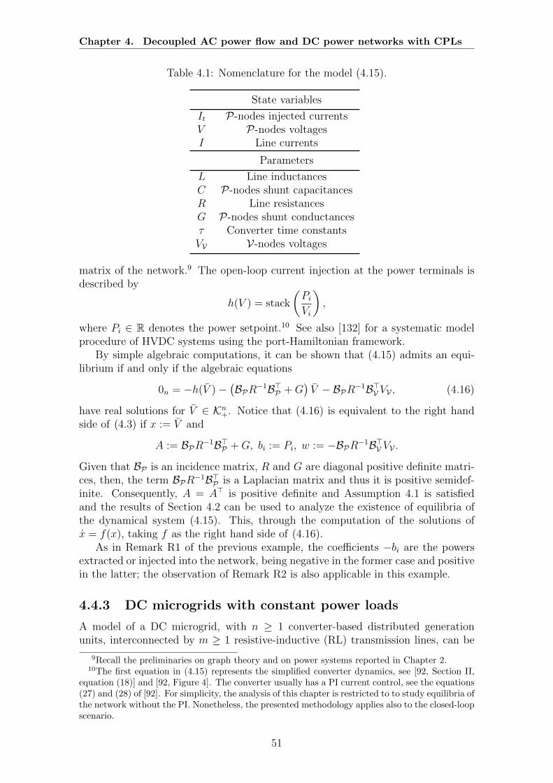
Chapter 4. Decoupled AC power flow and DC power networks with CPLs
Table 4.1: Nomenclature for the model (4.15).
State variables
It P-nodes injected currentsV P-nodes voltagesI Line currents
Parameters
L Line inductancesC P-nodes shunt capacitancesR Line resistancesG P-nodes shunt conductancesτ Converter time constantsVV V-nodes voltages
matrix of the network.9 The open-loop current injection at the power terminals isdescribed by
h(V ) = stack
(PiVi
),
where Pi ∈ R denotes the power setpoint.10 See also [132] for a systematic modelprocedure of HVDC systems using the port-Hamiltonian framework.
By simple algebraic computations, it can be shown that (4.15) admits an equi-librium if and only if the algebraic equations
0n = −h(V )−(BPR−1B>P +G
)V − BPR−1B>V VV , (4.16)
have real solutions for V ∈ Kn+. Notice that (4.16) is equivalent to the right handside of (4.3) if x := V and
A := BPR−1B>P +G, bi := Pi, w := −BPR−1B>V VV .Given that BP is an incidence matrix, R and G are diagonal positive definite matri-ces, then, the term BPR−1B>P is a Laplacian matrix and thus it is positive semidef-inite. Consequently, A = A> is positive definite and Assumption 4.1 is satisfiedand the results of Section 4.2 can be used to analyze the existence of equilibria ofthe dynamical system (4.15). This, through the computation of the solutions ofx = f(x), taking f as the right hand side of (4.16).
As in Remark R1 of the previous example, the coefficients −bi are the powersextracted or injected into the network, being negative in the former case and positivein the latter; the observation of Remark R2 is also applicable in this example.
4.4.3 DC microgrids with constant power loads
A model of a DC microgrid, with n ≥ 1 converter-based distributed generationunits, interconnected by m ≥ 1 resistive-inductive (RL) transmission lines, can be
9Recall the preliminaries on graph theory and on power systems reported in Chapter 2.10The first equation in (4.15) represents the simplified converter dynamics, see [92, Section II,
equation (18)] and [92, Figure 4]. The converter usually has a PI current control, see the equations(27) and (28) of [92]. For simplicity, the analysis of this chapter is restricted to to study equilibria ofthe network without the PI. Nonetheless, the presented methodology applies also to the closed-loopscenario.
51
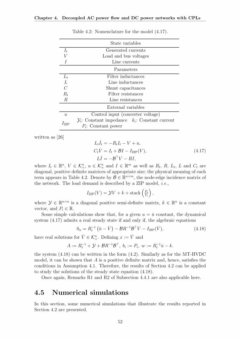
Chapter 4. Decoupled AC power flow and DC power networks with CPLs
Table 4.2: Nomenclature for the model (4.17).
State variables
It Generated currentsV Load and bus voltagesI Line currents
Parameters
Lt Filter inductancesL Line inductancesC Shunt capacitancesRt Filter resistancesR Line resistances
External variables
u Control input (converter voltage)
IZIPYi: Constant impedance ki: Constant currentPi: Constant power
written as [26]LtIt = −RtIt − V + u,
CtV = It + BI − IZIP(V ),
LI = −B>V −RI,(4.17)
where It ∈ Rn, V ∈ Kn+, u ∈ Kn+ and I ∈ Rm as well as Rt, R, Lt, L and Ct arediagonal, positive definite matrices of appropriate size; the physical meaning of eachterm appears in Table 4.2. Denote by B ∈ Rn×m, the node-edge incidence matrix ofthe network. The load demand is described by a ZIP model, i.e.,
IZIP(V ) = YV + k + stack(Pi
Vi
),
where Y ∈ Rn×n is a diagonal positive semi-definite matrix, k ∈ Rn is a constantvector, and Pi ∈ R.
Some simple calculations show that, for a given u = u constant, the dynamicalsystem (4.17) admits a real steady state if and only if, the algebraic equations
0n = R−1t
(u− V
)− BR−1B>V − IZIP(V ), (4.18)
have real solutions for V ∈ Kn+. Defining x := V and
A := R−1t + Y + BR−1B>, bi := Pi, w := R−1
t u− k.the system (4.18) can be written in the form (4.2). Similarly as for the MT-HVDCmodel, it can be shown that A is a positive definite matrix and, hence, satisfies theconditions in Assumption 4.1. Therefore, the results of Section 4.2 can be appliedto study the solutions of the steady state equation (4.18).
Once again, Remarks R1 and R2 of Subsection 4.4.1 are also applicable here.
4.5 Numerical simulations
In this section, some numerical simulations that illustrate the results reported inSection 4.2 are presented.
52
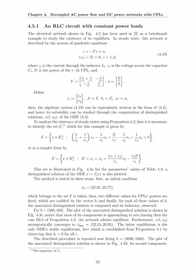
Chapter 4. Decoupled AC power flow and DC power networks with CPLs
4.5.1 An RLC circuit with constant power loads
The electrical network shown in Fig. 4.2 has been used in [9] as a benchmarkexample to study the existence of its equilibria. In steady state, this network isdescribed by the system of quadratic equations
z = −Y v + u,
vizi = Pi > 0, i = 1, 2,(4.19)
where zi is the current through the inductor Li, vi is the voltage across the capacitorCi, Pi is the power of the i−th CPL, and
Y =
[ 1r2
+ 1r1− 1r2
− 1r2
1r2
], u =
[Er1
0
].
Define
x :=
[v1
v2
], A := Y, bi = Pi, w := u,
then, the algebraic system (4.19) can be equivalently written in the form of (4.2),and hence its solvability can be studied through the computation of distinguishedsolutions, x(t, x0), of the ODE (4.3).
To analyze the existence of steady states using Proposition 4.2, first it is necessaryto identify the set E ,11 which for this example is given by
E =
x ∈ Kn+ :
(1
r2
+1
r1
)x1 −
1
r2
x2 >E
r1
, − 1
r2
x1 +1
r2
x2 > 0
,
or in a simpler form by
E =
x ∈ Kn+ : E < x1 < x2 <
(r1 + r2)
r1
x1 −r2E
r1
.
This set is illustrated in Fig. 4.3a for the parameters’ values of Table 4.3; adistinguished solution of the ODE x = f(x) is also plotted.
The method is tested in three steps: first, an initial condition
x0 = (25.01, 25.77),
which belongs to the set E is taken; then, two different values for CPLs’ powers arefixed, which are codified by the vector b; and finally, for each of these values of b,the associated distinguished solution is computed and its behavior, observed.
Fix b = (500, 450). The plot of the associated distinguished solution is shown inFig. 4.3c; notice that none of its components is approaching to zero having then thecase III.ii of Proposition 4.2: the network admits equilibria. Furthermore, x(t, x0)asymptotically converges to xmax = (22.24, 20.95). The latter equilibrium is theonly ODE’s stable equilibrium, fact which is established from Proposition 4.1 byobserving that bi > 0 for all i.
The described procedure is repeated now fixing b = (3000, 1000). The plot ofthe associated distinguished solution is shown in Fig. 4.3d; its second component,
11See equation (4.7).
53
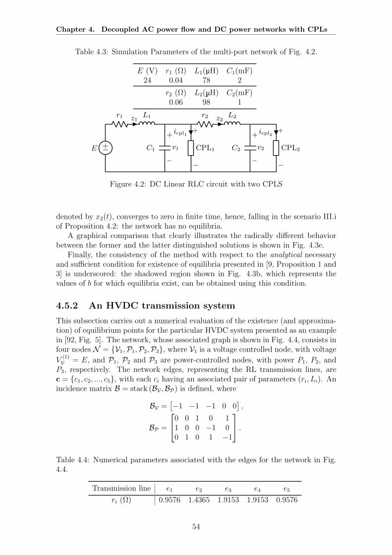
Chapter 4. Decoupled AC power flow and DC power networks with CPLs
Table 4.3: Simulation Parameters of the multi-port network of Fig. 4.2.
E (V) r1 (Ω) L1(µH) C1(mF)24 0.04 78 2
r2 (Ω) L2(µH) C2(mF)0.06 98 1
+−E
r1 L1z1r2 L2z2
+
−
CPL2
icpl2
C1
−
+
v1
+
−
CPL1
icpl1
C2
−
+
v2
1
Figure 4.2: DC Linear RLC circuit with two CPLS
denoted by x2(t), converges to zero in finite time, hence, falling in the scenario III.iof Proposition 4.2: the network has no equilibria.
A graphical comparison that clearly illustrates the radically different behaviorbetween the former and the latter distinguished solutions is shown in Fig. 4.3e.
Finally, the consistency of the method with respect to the analytical necessaryand sufficient condition for existence of equilibria presented in [9, Proposition 1 and3] is underscored: the shadowed region shown in Fig. 4.3b, which represents thevalues of b for which equilibria exist, can be obtained using this condition.
4.5.2 An HVDC transmission system
This subsection carries out a numerical evaluation of the existence (and approxima-tion) of equilibrium points for the particular HVDC system presented as an examplein [92, Fig. 5]. The network, whose associated graph is shown in Fig. 4.4, consists infour nodes N = V1,P1,P2,P3, where V1 is a voltage controlled node, with voltage
V(1)V = E, and P1, P2 and P3 are power-controlled nodes, with power P1, P2, andP3, respectively. The network edges, representing the RL transmission lines, arec = c1, c2, ..., c5, with each ci having an associated pair of parameters (ri, Li). Anincidence matrix B = stack (BV ,BP) is defined, where
BV =[−1 −1 −1 0 0
],
BP =
0 0 1 0 11 0 0 −1 00 1 0 1 −1
.Table 4.4: Numerical parameters associated with the edges for the network in Fig.4.4.
Transmission line e1 e2 e3 e4 e5
ri (Ω) 0.9576 1.4365 1.9153 1.9153 0.9576
54
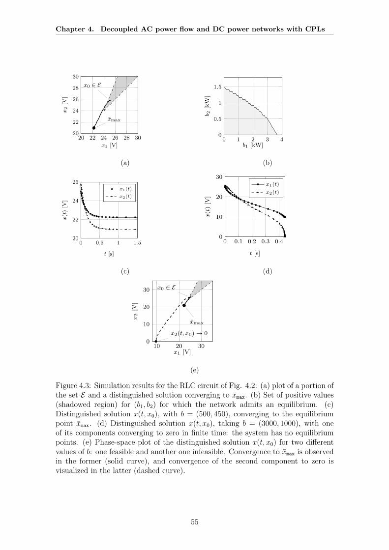
Chapter 4. Decoupled AC power flow and DC power networks with CPLs
20 22 24 26 28 3020
22
24
26
28
30
x0 ∈ E
xmax
x1 [V]
x2
[V]
(a)
0 1 2 3 40
0.5
1
1.5
b1 [kW]
b 2[kW
]
(b)
0 0.5 1 1.520
22
24
26
t [s]
x(t)[V
]
x1(t)
x2(t)
(c)
0 0.1 0.2 0.3 0.40
10
20
30
t [s]
x(t)[V
]
x1(t)
x2(t)
(d)
10 20 300
10
20
30 x0 ∈ E
xmax
x2(t, x0) → 0
x1 [V]
x2
[V]
(e)
Figure 4.3: Simulation results for the RLC circuit of Fig. 4.2: (a) plot of a portion ofthe set E and a distinguished solution converging to xmax. (b) Set of positive values(shadowed region) for (b1, b2) for which the network admits an equilibrium. (c)Distinguished solution x(t, x0), with b = (500, 450), converging to the equilibriumpoint xmax. (d) Distinguished solution x(t, x0), taking b = (3000, 1000), with oneof its components converging to zero in finite time: the system has no equilibriumpoints. (e) Phase-space plot of the distinguished solution x(t, x0) for two differentvalues of b: one feasible and another one infeasible. Convergence to xmax is observedin the former (solid curve), and convergence of the second component to zero isvisualized in the latter (dashed curve).
55
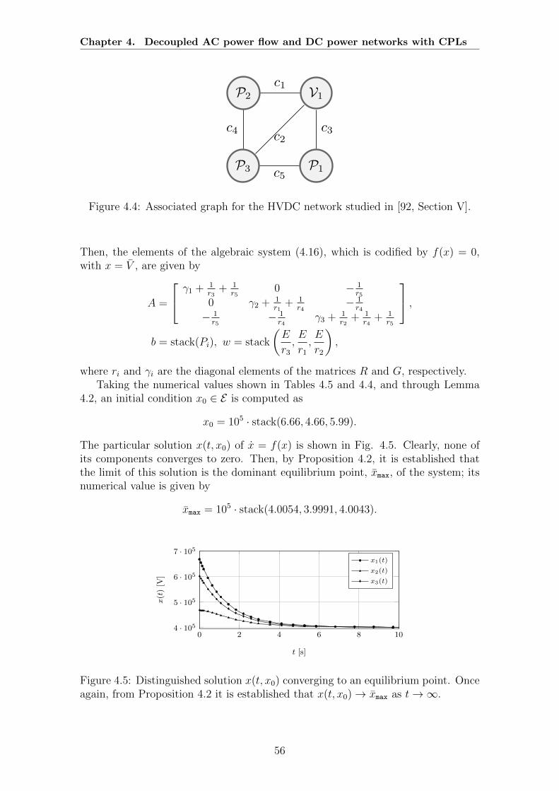
Chapter 4. Decoupled AC power flow and DC power networks with CPLs
V1
P1
P2
P3
c1
c2c3c4
c5
Figure 4.4: Associated graph for the HVDC network studied in [92, Section V].
Then, the elements of the algebraic system (4.16), which is codified by f(x) = 0,with x = V , are given by
A =
γ1 + 1r3
+ 1r5
0 − 1r5
0 γ2 + 1r1
+ 1r4
− 1r4
− 1r5
− 1r4
γ3 + 1r2
+ 1r4
+ 1r5
,b = stack(Pi), w = stack
(E
r3
,E
r1
,E
r2
),
where ri and γi are the diagonal elements of the matrices R and G, respectively.Taking the numerical values shown in Tables 4.5 and 4.4, and through Lemma
4.2, an initial condition x0 ∈ E is computed as
x0 = 105 · stack(6.66, 4.66, 5.99).
The particular solution x(t, x0) of x = f(x) is shown in Fig. 4.5. Clearly, none ofits components converges to zero. Then, by Proposition 4.2, it is established thatthe limit of this solution is the dominant equilibrium point, xmax, of the system; itsnumerical value is given by
xmax = 105 · stack(4.0054, 3.9991, 4.0043).
0 2 4 6 8 104 · 105
5 · 105
6 · 105
7 · 105
t [s]
x(t)[V
]
x1(t)
x2(t)
x3(t)
Figure 4.5: Distinguished solution x(t, x0) converging to an equilibrium point. Onceagain, from Proposition 4.2 it is established that x(t, x0)→ xmax as t→∞.
56
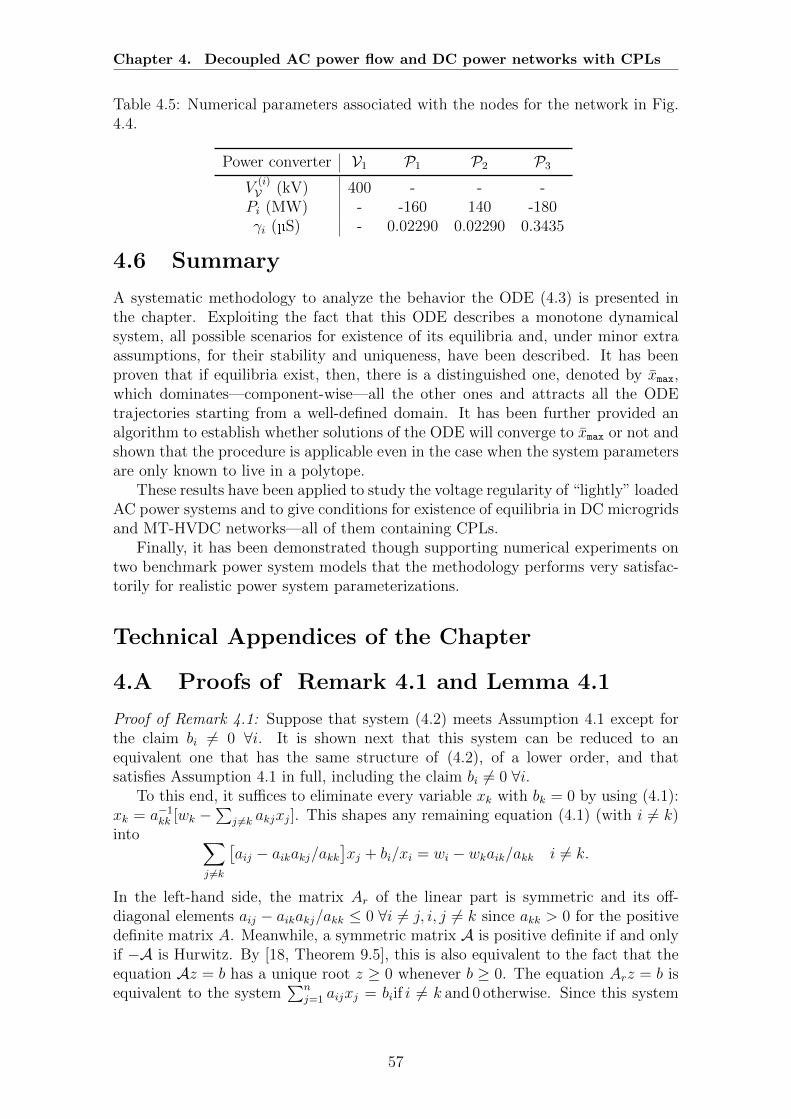
Chapter 4. Decoupled AC power flow and DC power networks with CPLs
Table 4.5: Numerical parameters associated with the nodes for the network in Fig.4.4.
Power converter V1 P1 P2 P3
V(i)V (kV) 400 - - -Pi (MW) - -160 140 -180γi (µS) - 0.02290 0.02290 0.3435
4.6 Summary
A systematic methodology to analyze the behavior the ODE (4.3) is presented inthe chapter. Exploiting the fact that this ODE describes a monotone dynamicalsystem, all possible scenarios for existence of its equilibria and, under minor extraassumptions, for their stability and uniqueness, have been described. It has beenproven that if equilibria exist, then, there is a distinguished one, denoted by xmax,which dominates—component-wise—all the other ones and attracts all the ODEtrajectories starting from a well-defined domain. It has been further provided analgorithm to establish whether solutions of the ODE will converge to xmax or not andshown that the procedure is applicable even in the case when the system parametersare only known to live in a polytope.
These results have been applied to study the voltage regularity of “lightly” loadedAC power systems and to give conditions for existence of equilibria in DC microgridsand MT-HVDC networks—all of them containing CPLs.
Finally, it has been demonstrated though supporting numerical experiments ontwo benchmark power system models that the methodology performs very satisfac-torily for realistic power system parameterizations.
Technical Appendices of the Chapter
4.A Proofs of Remark 4.1 and Lemma 4.1
Proof of Remark 4.1: Suppose that system (4.2) meets Assumption 4.1 except forthe claim bi 6= 0 ∀i. It is shown next that this system can be reduced to anequivalent one that has the same structure of (4.2), of a lower order, and thatsatisfies Assumption 4.1 in full, including the claim bi 6= 0 ∀i.
To this end, it suffices to eliminate every variable xk with bk = 0 by using (4.1):xk = a−1
kk [wk −∑
j 6=k akjxj]. This shapes any remaining equation (4.1) (with i 6= k)into ∑
j 6=k
[aij − aikakj/akk
]xj + bi/xi = wi − wkaik/akk i 6= k.
In the left-hand side, the matrix Ar of the linear part is symmetric and its off-diagonal elements aij − aikakj/akk ≤ 0 ∀i 6= j, i, j 6= k since akk > 0 for the positivedefinite matrix A. Meanwhile, a symmetric matrix A is positive definite if and onlyif −A is Hurwitz. By [18, Theorem 9.5], this is also equivalent to the fact that theequation Az = b has a unique root z ≥ 0 whenever b ≥ 0. The equation Arz = b isequivalent to the system
∑nj=1 aijxj = biif i 6= k and 0 otherwise. Since this system
57

Chapter 4. Decoupled AC power flow and DC power networks with CPLs
has a unique nonnegative solution x, and dropping xk in x results in the solution z,it is seen that Ar is positive definite.
Consecutively eliminating all xi with bi = 0, an equivalent system (4.2), thatmeets Assumption 4.1 in full, is obtained.
Proof of Lemma 4.1: The set Π :=z ∈ Rn : det
[A− diag (zi)
]= 0
is closed andfor any i and given zj’s with j 6= i, its section
zi ∈ R : stack (z1, . . . , zn) ∈ Π
has no more than n elements. So the measure of Π is zero by the Fubini theorem.The function x ∈ Kn+ 7→ g(x) := stack
(bix−2i
)diffeomorphically maps Kn+ onto an
open subset of Rn. Hence the inverse image Π↓ := g−1(Π) is closed, has the zeromeasure and, due to these two properties, is nowhere dense.
Let C be the set of all critical points of the semi-algebraic map [25] x ∈ Kn+ 7→h(x) := Ax+stack
(bix−2i
)∈ Rn, i.e., points x such that the Jacobian matrix ∇h(x)
is singular. By the extended Sard theorem [58], the set of critical values h(C) hasthe zero measure and is nowhere dense. Meanwhile, the restriction hKn
+\C is a localdiffeomorphism and so the image h(Π↓ \ C) is nowhere dense and has the zeroLebesgue measure. It remains to note that the set of w’s for which Assumption 4.2does not hold lies in h(Π↓ \ C) ∪ h(C).
4.B Proof of Lemma 4.2
Consider first the following lemma and its proof.
Lemma 4.3. The following system of inequalities is feasible
Az > 0, z > 0. (4.20)
Proof. Suppose that the system (4.20) is infeasible. Then two open convex conesAKn+ and Kn+ are disjoint and so can be separated by a hyperplane: there exists
τ ∈ Rn, τ 6= 0 (4.21)
such thatτ>x ≥ 0 ∀x ∈ Kn+, τ>x ≤ 0 ∀x ∈ AKn+.
By continuity argument, these inequalities extend on the closures of the concernedsets:
τ>x ≥ 0 ∀x ∈ Kn+ = x : xi ≥ 0,τ>x ≤ 0 ∀x ∈ AKn+ ⊃ AKn+.
Here the first relation implies that τ ∈ Kn+⇒ Aτ ∈ AKn+ and so τ>Aτ ≤ 0 bythe second one. Since A is positive definite by Assumption 4.1, the last inequalityyields that τ = 0, in violation of the second relation from (4.21). This contradictioncompletes the proof.
58
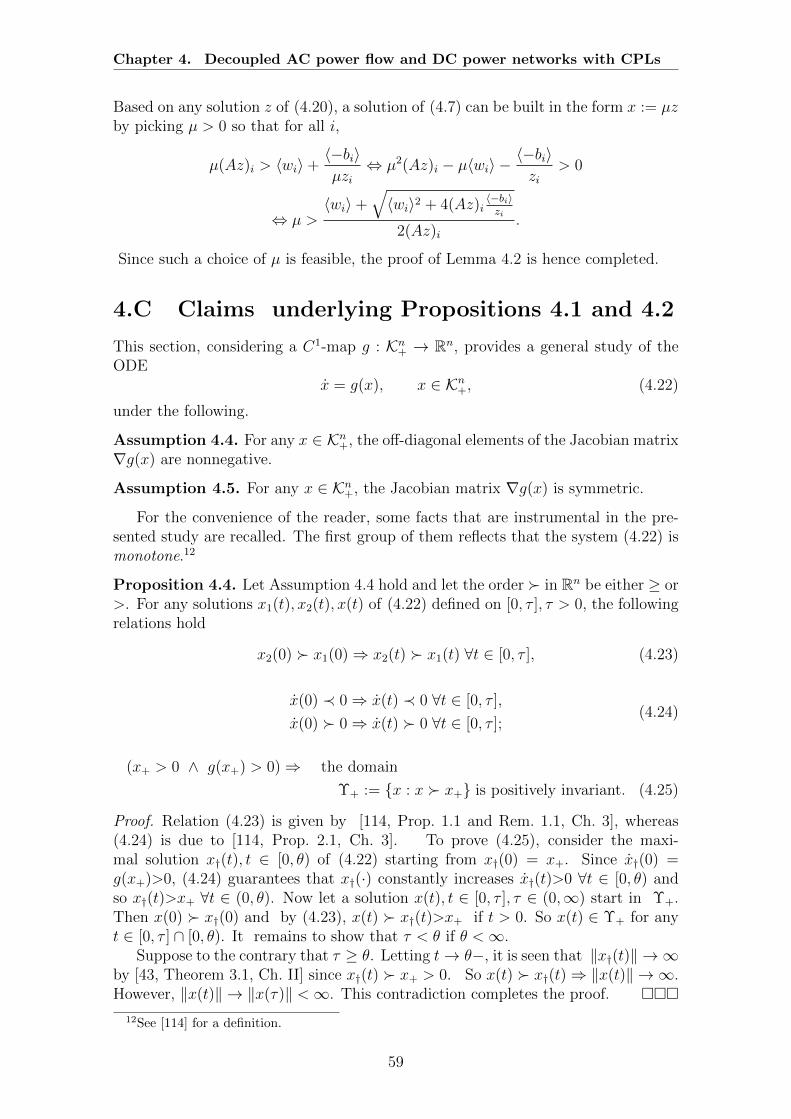
Chapter 4. Decoupled AC power flow and DC power networks with CPLs
Based on any solution z of (4.20), a solution of (4.7) can be built in the form x := µzby picking µ > 0 so that for all i,
µ(Az)i > 〈wi〉+〈−bi〉µzi
⇔ µ2(Az)i − µ〈wi〉 −〈−bi〉zi
> 0
⇔ µ >〈wi〉+
√〈wi〉2 + 4(Az)i
〈−bi〉zi
2(Az)i.
Since such a choice of µ is feasible, the proof of Lemma 4.2 is hence completed.
4.C Claims underlying Propositions 4.1 and 4.2
This section, considering a C1-map g : Kn+ → Rn, provides a general study of theODE
x = g(x), x ∈ Kn+, (4.22)
under the following.
Assumption 4.4. For any x ∈ Kn+, the off-diagonal elements of the Jacobian matrix∇g(x) are nonnegative.
Assumption 4.5. For any x ∈ Kn+, the Jacobian matrix ∇g(x) is symmetric.
For the convenience of the reader, some facts that are instrumental in the pre-sented study are recalled. The first group of them reflects that the system (4.22) ismonotone.12
Proposition 4.4. Let Assumption 4.4 hold and let the order in Rn be either ≥ or>. For any solutions x1(t), x2(t), x(t) of (4.22) defined on [0, τ ], τ > 0, the followingrelations hold
x2(0) x1(0)⇒ x2(t) x1(t) ∀t ∈ [0, τ ], (4.23)
x(0) ≺ 0⇒ x(t) ≺ 0 ∀t ∈ [0, τ ],
x(0) 0⇒ x(t) 0 ∀t ∈ [0, τ ];(4.24)
(x+ > 0 ∧ g(x+) > 0)⇒ the domain
Υ+ := x : x x+ is positively invariant. (4.25)
Proof. Relation (4.23) is given by [114, Prop. 1.1 and Rem. 1.1, Ch. 3], whereas(4.24) is due to [114, Prop. 2.1, Ch. 3]. To prove (4.25), consider the maxi-mal solution x†(t), t ∈ [0, θ) of (4.22) starting from x†(0) = x+. Since x†(0) =g(x+)>0, (4.24) guarantees that x†(·) constantly increases x†(t)>0 ∀t ∈ [0, θ) andso x†(t)>x+ ∀t ∈ (0, θ). Now let a solution x(t), t ∈ [0, τ ], τ ∈ (0,∞) start in Υ+.Then x(0) x†(0) and by (4.23), x(t) x†(t)>x+ if t > 0. So x(t) ∈ Υ+ for anyt ∈ [0, τ ] ∩ [0, θ). It remains to show that τ < θ if θ <∞.
Suppose to the contrary that τ ≥ θ. Letting t→ θ−, it is seen that ‖x†(t)‖ → ∞by [43, Theorem 3.1, Ch. II] since x†(t) x+ > 0. So x(t) x†(t)⇒ ‖x(t)‖ → ∞.However, ‖x(t)‖ → ‖x(τ)‖ <∞. This contradiction completes the proof.
12See [114] for a definition.
59
Chapter 4. Decoupled AC power flow and DC power networks with CPLs
Let x(t, a), t ∈ [0, τa) stand for the maximal solution of (4.22) that starts at t = 0with a > 0. The distance infx′∈A ‖x − x′‖ from point x ∈ Rn to a set A ⊂ Rn isdenoted by dist(x,A).
Corollary 4.1. Whenever 0 < a1 ≤ a ≤ a2, it follows that τa ≥ minτa1 , τa2.
The following lemma is a trivial corollary of [18, Theorem 9.5].13
Lemma 4.4. A nonsingular matrix A = A> with nonnegative off-diagonal elementsis Hurwitz if
Ah > 0⇒ h ≤ 0. (4.26)
Lemma 4.5. Let Assumptions 4.4 and 4.5 hold. Suppose that a solution x(t), t ∈[0,∞) of (4.22) decays x(t) < 0 ∀t and converges to x > 0 as t → ∞. Then xis an equilibrium of the ODE (4.22). If this equilibrium is hyperbolic, it is locallyasymptotically stable.
Proof. The first claim is given by [114, Prop. 2.1, Ch. 3]. By Lemma 4.4, it sufficesto show that A := ∇g(x) meets (4.26) to prove the second claim. Suppose to thecontrary that Ah > 0 and hi > 0 for some i and h ∈ Rn. For x0
ε := x+εh and smallenough ε > 0, it follows that g(x0
ε) = g(x) + εAh + O(ε) = εAh + O(ε) > 0, x0ε > 0,
x0ε,i > xi , and x(0) ∈ Υ+ = x : x > x0
ε. Since the set Υ+ is positively invariantby (4.25), x(t) ∈ Υ+ ⇒ xi(t) > xε,i > xi, in violation of x(t) → x as t → ∞. Thiscontradiction completes the proof.
For any x′ ≤ x′′ ∈ Rn, it is denoted by x′, x′′ := x ∈ Rn : x′ ≤ x ≤ x′′.
Lemma 4.6. Suppose that Assumption 4.4 holds and x > 0 is a locally asymptoti-cally stable equilibrium. Its domain of attraction A(x) ⊂ Kn+ is open and
a′, a′′ ∈ A(x) ∧ a′ ≤ a′′ ⇒ a′, a′′ ⊂ A(x). (4.27)
Proof. Let B(r, x) stand for the open ball with a radius of r > 0 centered at x.For any a ∈ A(x), it follows that τa = ∞ and x(t, a) → x as t → ∞, whereasB(2ε, x) ⊂ A(x) for a sufficiently small ε > 0 since x is locally asymptotically stable.Clearly, there is θ > 0 such that x(θ, a) ∈ B(ε, x). By [43, Theorem 2.1, Ch. V],there exists δ > 0 such that whenever ‖a† − a‖ < δ, the solution x(·, a†) is definedat least on [0, θ] and ‖x(θ, a†)− x(θ, a)‖ < ε. It follows that x(θ, a†) ∈ B(2ε, x) andso x(·, a†) is in fact defined on [0,∞) and converges to x as t→∞. Thus, it is seenthat ‖a† − a‖ < δ ⇒ a† ∈ A(x), i.e., the set A(x) is open.
Let a ∈ a′, a′′ . By Corollary 4.1 and (4.23), τa = ∞ and x(t, a′) ≤ x(t, a) ≤x(t, a′′) ∀t ≥ 0. Letting t→∞ shows that x(t, a)→ x and so a ∈ A(x).
Lemma 4.7. Let x− ≤ x+ and let D ⊂ Ξ := x−, x+ be an open (in Ξ) set suchthat
i) x′, x′′ ⊂ D ∀x′, x′′ ∈ D.
13An anonymous reviewer is acknowledged for indicating this.
60
Chapter 4. Decoupled AC power flow and DC power networks with CPLs
ii) either x− ∈ D or x+ ∈ D.
iii) D 6= Ξ.
Then there exists a continuous map M : Ξ→ Ξ such that M [Ξ] ⊂ Ξ− := Ξ \D andM [x] = x ∀x ∈ Ξ−.14
Proof. Let x+ ∈ D for the definiteness; then x− 6∈ D by i) and iii). It can be assumedthat 0 = x− < x+. Denote by χx(θ) := maxx − θζ; 0, where ζ := stack(1, . . . , 1)and the max is meant component-wise. Then, Θ(x) :=
θ ≥ 0 : χx(θ) ∈ D
=
[0, τ(x)), x ∈ D, where 0 < τ(x) < ∞. For x 6∈ D, put τ(x) := 0. It is shownfirst that the function τ(·) is continuous on Ξ. To this end, it suffices to prove thatτ(x) = τ∗ whenever
x = limk→∞
xk, xk ∈ Ξ, and τ∗ = limk→∞
τ(xk).
Passing to a subsequence ensures that either xk 6∈ D ∀k or xk ∈ D ∀k. In the firstcase, x 6∈ D since D is open. Then τ(x) = 0 = τ(xk) = τ∗. Let xk ∈ D ∀k. Sinceχxk [τ(xk)] 6∈ D and D is open, letting k → ∞ yields χx[τ∗] 6∈ D ⇒ τ(x) ≤ τ∗. Sothe claim holds if τ∗ = 0. If τ∗ > 0, pick 0 < θ < τ∗. Then θ < τ(xk) for k ≈ ∞,i.e., χxk(θ) ∈ D. Let xνi be the i-th component of xν ∈ Rp. Then
τ ′k := maxτ ≥ 0 : χx(τ) ≥ χxk(θ)
= max
i:xki≥θ
[xi − xki + θ
].
Here the second max is over a nonempty set since χxk(θ) ∈ D 63 0. Thus τ ′k → θ as
k → ∞. By i), χx(τ′k) ∈ D and so τ(x) ≥ τ ′k
k→∞===⇒ τ(x) ≥ θ ∀θ < τ∗ ⇒ τ(x) ≥
τ∗ ⇒ τ(x) = τ∗. Thus the function τ(·) is continuous indeed. The needed map M isgiven by M(x) := χx[τ(x)].
Lemma 4.8. Let Assumption 4.4 hold and 0 < x− ≤ x+, x− 6= x+ be two locallyasymptotically stable equilibria. Then there exists a third equilibrium x in betweenthem x− ≤ x ≤ x+, x 6= x−, x+.
Proof. Denote by Ξ := [x−, x+], like in Lemma 4.7. By Lemma 4.6, the set D± :=A(x±) ∩ Ξ meets the assumptions of Lemma 4.7, which associates D± with a mapM±. Since the sets D± are open and disjoint, they do not cover the connected setΞ. So the set Ξ := Ξ \ (D− ∪ D+) of all fixed points of the map M = M− M+
is non-empty and compact. For all a ∈ Ξ, the solution x(·, a) is defined on [0,∞)by Corollary 4.1 and x(t, a) ∈ Ξ by (4.23). So the flow Φt(a) := x(t, a)t≥0 is welldefined on Ξ, acts from Ξ into Ξ, and is continuous by [43, Theorem 2.1, Ch. V].The sets D± are positively and negatively invariant with respect to it:
a ∈D± ⇒ Φt(a) ∈ D± ∀t ≥ 0,
a ∈Ξ ∧[∃t ≥ 0 : Φt(a) ∈ D±
]⇒ a ∈ D±.
It follows that Ξ is positively invariant with respect to this flow. By the Brouwerfixed point theorem, the continuous map Φt M : Ξ → Ξ ⊂ Ξ has a fixed point
14In brief, this lemma says that Ξ− is a retract of the convex set Ξ.
61
Chapter 4. Decoupled AC power flow and DC power networks with CPLs
at = Φt M(at) ∈ Ξ. Since M(at) ∈ Ξ and Φt(Ξ) ⊂ Ξ, it is seen that at ∈ Ξ
and so M(at) = at and at = Φt(at).Since Ξ is compact, there exists a sequence tk > 0∞k=1 such that tk → 0 and
atk → x as k → ∞ for some point x ∈ Ξ. Since x± 6∈ Ξ, it follows that x 6= x±;meanwhile x ∈ Ξ ⊂ Ξ⇒ x− ≤ x ≤ x+. Furthermore,
0 =Φtk(atk)− atk
tk= t−1
k
∫ tk
0
g[x(t, atk)] dtk→∞−−−→ g(x).
Thus, it is seen that g(x) = 0, i.e., x is an equilibrium.
4.D Proofs of Propositions 4.1, 4.2, and 4.3
The system (4.3) under Assumption 4.1 is studied next.
Lemma 4.9. Suppose that y belongs to the set (4.7). There exists θ ∈ (0, 1) suchthat the domain Ξ−(θ) := x : 0 < x ≤ θy is globally absorbing, i.e., the followingstatements hold:
i This domain is positively invariant: if a solution starts in Ξ−(θ), it does notleave Ξ−(θ);
ii Any solution defined on [0,∞) eventually enters Ξ−(θ) and then never leavesthis set.
Proof. Thanks to (4.7), there exists δ > 0 such that
Ay > stack
(〈wi〉+
〈−bi〉yi
+ 3δ
). (4.28)
The value θ ∈ (0, 1) is picked so close to 1 that for any i, the following holds.
[θ − 1]〈wi〉+ δθ ≥ 0, [θ − θ−1]〈−bi〉y−1i + δθ ≥ 0. (4.29)
Let x(·) be a solution of (4.3). By the Danskin theorem [27], the function %(t) :=maxi∈1,...,n xi(t)/yi is absolutely continuous and for almost all t, the following equa-tion holds
%(t) = maxi∈I(t)
xi(t)/yi, where
I(t) := i : xi(t)/yi = %(t) .(4.30)
If i ∈ I(t) and j, it follows that xi(t) = yi%(t), xj(t) ≤ yj%(t), and
xi(t)(4.3)= −aiixi(t) +
∑j 6=i
[ −ai,j ]︸ ︷︷ ︸≥0 by Asm. 4.1
xj(t)−bixi(t)
+ wi
≤ −%(t)
(aiiyi +
∑j 6=i
ai,jyj
)− %(t)−1 bi
yi+ wi
(4.28)
≤ −%(t)
[〈wi〉+
〈−bi〉yi
+ 3δ
]+ %(t)−1 〈−bi〉
yi+ 〈wi〉
= −δ%(t)− [%(t)− 1]〈wi〉+ δ%(t)
−
[%(t)− %(t)−1]〈−bi〉yi
+ δ%(t)
. (4.31)
62
Chapter 4. Decoupled AC power flow and DC power networks with CPLs
Hence whenever %(t) ≥ θ ∈ (0, 1),
xi(t) ≤ −δ%(t)− [θ − 1]〈wi〉+ + δθ
−
[θ − θ−1]〈bi〉−yi
+ δθ
(4.29)
≤ −δ%(t).
So (4.30) implies that %(t) > θ ⇒ %(t) ≤ −δ%(t) ≤ −δθ.15 Claims (i) and (ii) areimmediate from this entailment.
Lemma 4.10. Claim II of Proposition 4.2 holds.
Proof. This is immediate from (4.24) since for any distinguished solution x(·) andy := x(0),
x(0)(4.3)= − Ay + stack
(− biyi
+ wi
)≤− Ay + stack
(〈−bi〉yi
+ 〈wi〉)
(4.7)< 0.
Lemma 4.11. Suppose that a solution x(·) of (4.3) cannot be extended from [0, τ)with τ <∞ to the right. Then there is i such that bi > 0 and xi(t)→ 0, xi(t)→ −∞as t→ τ−.
Proof. By Lemma 4.2, there is a solution y > 0 for (4.7). Via multiplying y by a largeenough factor, it is ensured that y > x(0). Let x↑(·) be the distinguished solutionstarting with x↑(0) = y. By Lemma 4.10, x↑(t) ≤ y for t ≥ 0, and x(t) ≤ x↑(t) onthe intersection of the domains of definitions of x(·) and x↑ by (4.23). Then by[43, Theorem 3.1, Ch. II], x(t) converges to the boundary of Kn+ as t → τ− and isbounded, i.e.,
minixi(t)→ 0 as t→ τ−, c := sup
t∈[0,τ)
‖x(t)‖ <∞. (4.32)
Putting W := maxi[|wi|+ c
∑j |aij|
], it is seen that
xi(t)(4.31)= −
∑j
ai,jxj(t)−bixi(t)
+ wi
∈[−W − bi
xi(t),W − bi
xi(t)
],
bi < 0 ∧ xi(t) ≤|bi|2W⇒ xi(t) ≥ W > 0, (4.33)
bi > 0 ∧ xi(t) ≤|bi|2W⇒ xi(t) ≤ −
bi2xi(t)
< 0
⇒ x2i (θ) ≤ x2
i (t)− bi(θ − t) ∀θ ∈ [t, τ).
(4.34)
15 In fact, this holds for almost all t such that the premises are true.
63
Chapter 4. Decoupled AC power flow and DC power networks with CPLs
Due to (4.33), xi(t) is separated from zero if bi < 0. So by (4.32), there exists isuch that bi > 0 and for any ε > 0, arbitrarily small left vicinity (τ−δ, τ), δ ≈ 0 of τ
contains points t with xi(t) < ε. Then for ε < |bi|2W
, formula (4.34) guarantees thatxi(t
′) < ε ∀t′ ∈ (t, τ). Overall, it is seen that xi(t)→ 0 as t→ τ−; then xi(t)→ −∞as t→ τ− by (4.34).
Lemma 4.12. Suppose that Assumption 4.2 holds. Then the following claims holdtrue.
i) Stable equilibria of (4.3) (if exist) are locally asymptotically stable.
ii) Let 0 < x− ≤ x0 ≤ x+ be equilibria of (4.3). If x± are stable and all bi’s areof the same sign, x0 is also stable.
Proof. By Assumption 4.2 and (4.3), the Jacobian matrix
∇f(x) = A(k) := −A+ diag (ki) ,
k := k(x) := stack(bix−2i
) (4.35)
has no eigenvalues with the zero real part at any equilibrium x. So for any stableequilibrium x, the matrix (4.35) is Hurwitz and so x is locally asymptotically stable.Since A(k)> = A(k) by Assumption 4.1, A(k) is Hurwitz if and only if the followingquadratic form in h ∈ Rn is negative definite
Qx(h) := −h>Ah+n∑i=1
ki(x)h2i .
Thus both forms Qx± are negative definite. Meanwhile, ki(x0) ≤ ki(x
−) ∀i if bi >0 ∀i, whereas ki(x
0) ≤ ki(x+) ∀i if bi < 0 ∀i. In any case, Qx0 is upper estimated
by a negative definite quadratic form (either Qx− or Qx+) and so is negative definiteas well.
Corollary 4.2. Suppose that Assumption 4.2 holds, 0 < x(0) ≤ x(1) are stableequilibria of (4.3) and all bi’s are of the same sign. Then x(0) = x(1).
Proof. Suppose to the contrary that x(0) 6= x(1). By Lemma 4.8 and (i) of Lemma 4.12,there exists one more equilibrium x(1/2) in between x(0) and x(1), i.e., x(0) ≤ x(1/2) ≤x(1) and x(1/2) 6= x(0), x(1). By (ii) of Lemma 4.12, this newcoming equilibrium x(1/2)
is stable. This allows to repeat the foregoing arguments first for x(0) and x(1/2) andsecond for x(1/2) and x(1). As a result, it is seen that there exist two more stableequilibria x(1/4) ∈ x(0), x(1/2) and x(3/4) ∈ x(1/2), x(1) that differ from all pre-viously introduced equilibria. This allows to repeat the foregoing arguments oncemore to show that there exist stable equilibria x(1/8), x(3/8), x(5/8), x(7/8) such thatx(i/8) ≤ x(j/8) ∀0 ≤ i ≤ j ≤ 8 and x(i/8) 6= x(j/8) ∀0 ≤ i, j ≤ 8, i 6= j. By contin-uing likewise, a stable equilibrium x(r) is assigned to any number r ∈ [0, 1] whoserepresentation in the base-2 numeral system is finite (i.e., number representable inthe form r = j2−k for some k = 1, 2, . . . and j = 0, . . . , 2k) and ensure that these
64
Chapter 4. Decoupled AC power flow and DC power networks with CPLs
equilibria are pairwise distinct and depend on r monotonically: x(r) ≤ x(%) whenever0 ≤ r ≤ % ≤ 1.
Since all they lie in the compact set x(0), x(1) , there is a sequence rk∞k=1
of pairwise distinct numbers r’s for which ∃x = limk→∞ x(rk). Then x ∈ x(0), x(1) and so x > 0 and f(x) = limk→∞ f [x(rk)] = 0, i.e., x is an equilibrium. Then theJacobian matrix ∇f(x) is nonsingular, as was remarked just after (4.35). However,this implies that in a sufficiently small vicinity V of x, the equation f(x) = 0 has noroots apart from x in violation of x(rk) ∈ V ∀k ≈ ∞ and x(rk) 6= x(rl) ∀k 6= l. Thecontradiction obtained completes the proof.
Proof of Proposition 4.2: Claim I is given by Lemma 4.2.
Claim II is justified by Lemma 4.10.
For Claim III, let x(t), t ∈ [0, tf ) be a distinguished solution. If tf < ∞, then III.iof Proposition 4.2 holds by Lemma 4.11. Suppose that tf = ∞. Then the limit xfrom (4.9) exists due to Claim II, and x ≥ 0. It is shown next that in fact x > 0.
Suppose to the contrary that xi = 0 for some i. Then xi(t)→ 0 as t→∞, (4.33)means that bi > 0, and (4.34) (where τ = ∞ now) implies that ‖x(θ)‖2 assumesnegative values for large enough θ. This assures that x > 0 and so (4.9) does hold.By Lemma 4.5, x is an equilibrium.
Now suppose that III.i holds for a distinguished solution x†(·). Suppose thatthere is another distinguished solution x(·) for which III.i is not true. Then x(·) isdefined on [0,∞) by Lemma 4.11 and also ∃x = limt→∞ x(t) > 0 by the foregoing.By (ii) of Lemma 4.9 (with y := x†(0)), x(σ) ≤ θx†(0) ≤ x†(0) for large enoughσ. By applying (4.23) to x1(t) := x(t + σ) and x2(t) = x†(t), is follows thatx(t + σ) ≤ x†(t) and so xi(t) goes to zero in a finite time, in violation of x > 0and II. This contradiction proves that III.i holds simultaneously for all distinguishedsolutions.
Since III.i and III.ii are mutually exclusive and complementary, it is noticed thateither III.i holds for all distinguished solutions, or III.ii holds for all of them.
Let III.ii hold. As it has been shown in the paragraph prior to the previousparagraph, x(t+σ) ≤ x†(t) for any two distinguished solutions x(·) and x†(·). Hencelimt→∞ x(t) ≤ limt→∞ x†(t). By flipping x(·) and x†(·) here, it is appreciated thatthese limits coincide, i.e., the limit (4.9) is the same for all distinguished solutions.
Claim IV follows from Lemmata 4.9 and 4.11 since any equilibrium is related to aconstant solution defined on [0,∞).
To establish Claim V, suppose that III.ii holds. Let xmax stand for the limit (4.9).By (4.9) and Lemma 4.5, xmax is an equilibrium. Consider a solution x(·) defined on[0,∞) and a distinguished solution x†(·). By retracing the above arguments basedon (ii) of Lemma 4.9, is is observed that x(ς + t) ≤ x†(t) ∀t ≥ 0 for some ς ≥ 0.By considering here a constant solution x(·) and letting t→∞, it follows that xmaxdominates any other equilibrium.
Let x(0) ≥ xmax. By (4.23), x(t) ≥ xmax on the domain ∆ of definition of x(·) andso ∆ = [0,∞) by Lemma 4.11. Thus, it is observed that xmax ≤ x(ς+t) ≤ x†(t) ∀t ≥
65

Chapter 4. Decoupled AC power flow and DC power networks with CPLs
0 for some ς ≥ 0. It follows that x(t)→ xmax as t→∞, i.e., the equilibrium xmax isattractive from above by Definition 4.1.
Proof of Proposition 4.1: This proposition is immediate from Proposition 4.2, ex-cept for the concluding claims that refer to Assumption 4.2.
Let this assumption and S2 in Proposition 4.1 hold. Then xmax is locally asymp-totically stable by Lemma 4.5 and Claims II, V in Proposition 4.2. The last sentenceof Proposition 4.1 is given by Corollary 4.2. It remains to show that there exist onlyfinitely many equilibria xk.
Suppose the contrary. Since all equilibria lie in the compact set x : 0 ≤ x ≤xmax, there exists an infinite sequence xks∞s=1 of pairwise different equilibria thatconverges xks → x as t → ∞ to a point x ≥ 0. The estimates (4.33), (4.34)applied to any equilibrium solution x(·) assure that xi ≥ |bi|/(2W ) on it, whereW := maxi
[|wi|+ c
∑j |aij|
]and c is any upper bound on ‖x(t)‖. For the solutions
related to the convergent and so bounded sequence xks∞s=1, this bound can bechosen common. As a result, it is inferred that x > 0 and so f(x) = lims→∞ f [xks ] =0, i.e., x is an equilibrium. Then the Jacobian matrix ∇f(x) is nonsingular, as wasremarked just after (4.35). This implies that in a sufficiently small vicinity V of x,the equation f(x) = 0 has no roots apart from x, in violation of xks ∈ V ∀s ≈ ∞and xks 6= xkr ∀s 6= r. This contradiction completes the proof.
Proof of Proposition 4.3: Let f−(·), f(·), f+(·) be defined by (4.3) for C−, C, C+,respectively. Retracing the proof of Lemma 4.2 demonstrates existence of a ∈ Kn+such that
A+a > stack(
max〈w−i 〉; 〈wi〉〈w+i 〉+
max〈−b−i 〉; 〈−bi〉〈−b+i 〉
ai
).
By Definition 4.2, the solutions of x = f(x) and x± = f±(x±) that start with a aredistinguished for the respective ODEs (4.3). Here f−(x) ≤ f(x) ≤ f+(x) ∀x ∈ Kn+due to (4.11). So by [115, Theorem 8.1, Ch. II],
x−(t) ≤ x(t) ≤ x+(t),
where each inequality holds whenever its both sides are defined for the concerned t.So the claims i-iii are immediate from III-V in Proposition 4.2.
Now let A+ → A−, b+i → b−i , w
+ → w−. For the left hand sides of these relations,
there exist respective constant upper bounds A+, b+i , w
+ that satisfy Assumption 4.1.Let xmax be the dominant equilibrium related to these bounds. By (4.12), x−max ≤x+max ≤ x+
max and so the variety of x+max’s is bounded. For any limit point x of x+
max’s,it holds that 0 < x−max ≤ x and x is the equilibrium of the C−-related system by thecontinuity argument. So x−max = x by the definition of the dominant equilibrium.Thus all limit points of x+
max’s are the same and equal x−max. Hence x+max → x−max.
66

Chapter 5
Power-Controlled HamiltonianSystems: Application to PowerSystems with CPLs
Synopsis This chapter explores a type of port-Hamiltonian system in which thecontroller or disturbance acts directly on the system’s power balance equation—a scenario that appears in many practical applications. A suitable framework isprovided to model these systems and to investigate their shifted passivity properties,based on which a stability analysis is carried out. The applicability of the results isillustrated with the stability analysis of electrical circuits with constant power loads.
5.1 Introduction
In recent years, port-Hamiltonian (pH) modeling of physical systems has gained ex-tensive attention. pH systems theory provides a systematic framework for modelingand analysis of physical systems and processes [93, 70, 84, 82, 95]. Typically, theexternal inputs (controls or disturbances) in pH systems act on the flow variables—that is on the derivative of the energy storing coordinates. However, in some casesof practical interest, the external inputs act on the systems power balance equa-tion, either as a control variable, or as power that is extracted from (or injectedto) the system. These kind of systems are referred as Power-controlled Hamiltonian(PwH) systems. PwH systems cannot be modeled with constant control input matri-ces, which is the scenario considered in [49]. Consequently, to analyze its passivityproperties, the development of new mathematical tools is required.
The objectives of the chapter are to propose a suitable framework to modelPwH systems and to develop analytical tools to infer stability properties of their—intrinsically non-zero—equilibrium points. The latter objective is achieved by iden-tifying a class of PwH systems that are shifted passive [93]. Following [49], a shiftedstorage function is used to address this issue. This shifted function is closely relatedto the notion of availability function used in thermodynamics [2, 51], and is associ-ated with the Bregman divergence of the Hamiltonian with respect to an equilibriumof the system for constant non-zero input [17]. Therefore, the shifted Hamiltonianis used as a candidate Lyapunov function, which is based on the physical energy ofthe system, and, unlike the Brayton-Moser potential, is trivially computed. Twoimmediate corollaries of the shifted passivity property are: (i) that the shifted equi-
67
Chapter 5. Power-Controlled Hamiltonian Systems: Application to Power
Systems with CPLs
librium can be stabilized with simple PI controllers [49]; (ii) that in the uncontrolledcase, when a constant input power or load is imposed, stability of this equilibriumcan be established. This chapter focuses on the latter issue, that was first studied inthe standard pH systems framework in [70]. Furthermore, the framework proposedin the chapter allows to give an analytic characterization of an estimate of the ROAin the case of a quadratic Hamiltonian and a positive definite dissipation matrix.
The remainder of this chapter is organized as follows. The proposed model forPwH systems is introduced in Section 5.2. The main result, that is, the derivationof conditions for their shifted passivity, is provided in Section 5.3. The stabilityanalysis is given in Section 5.4. The utility of the main result is illustrated inSection 5.5 with its application to electrical systems with CPLs, and in Section 5.6with the application to synchronous generators. Finally, some concluding remarksare provided in Section 5.7.
5.2 Model
Consider the pH system driven by the flow f ∈ Rm [93]
x = (J −R)∇H(x) +Bf
e = B>∇H(x) ,
where x ∈ Rn is the state vector (with n ≥ m), e ∈ Rm is the effort, H is thesystem Hamiltonian (energy) function, and the n × n constant matrices J = −J>and R ≥ 0, are the structure and the dissipation matrices, respectively. The pHsystem satisfies the power-balance
H = −∇H>(x)R∇H(x) + e>f .
Now consider the scenario where the external signals ui act directly on the powerbalance equation of the system. Define the control power input u ∈ Rm as theelement-wise product of effort and flow, i.e., u := diag (e)diag (f)1m. Hence, f =diag (e)−1u. Without loss of generality, by re-arranging the actuated and the non-actuated states, the constant matrix B is defined as
B :=
[Im
0(n−m)×m
]. (5.1)
Accordingly, the vector ∇H is decomposed into
∇H =
[Gu(x)G0(x)
],
where Gu(x) ∈ Rm is associated with the actuated states. It follows that
Bf = Bdiag (e)−1u = Bdiag(B>∇H(x)
)−1u
= Bdiag (Gu(x))−1u
= G(x)u ,
where the power input matrix G(x) ∈ Rn×m is defined as
G(x) :=
[diag (Gu(x))−1
0(n−m)×m
]. (5.2)
68
Chapter 5. Power-Controlled Hamiltonian Systems: Application to Power
Systems with CPLs
The input matrix G(x) is well-defined in the set Ω+ characterized as
Ω+ := x ∈ Rn : diag (Gu(x)) > 0.
Then the dynamics of the Power-controlled Hamiltonian (PwH) system is given by
x = (J −R)∇H(x) +G(x)u , x ∈ Ω+ , (5.3)
with the first m components of x corresponding to the power controlled states. Thenit is easy to see that the power balance equation takes the form
H = −∇H>(x)R∇H(x) + 1>mu ,
implying that the natural output corresponding to the input u is given as the con-stant vector 1m, in accordance with the fact that the total supplied power is 1>mu.The natural operating points for PwH systems are non-zero equilibria correspondingto non-zero constant inputs u. Therefore, it is convenient to describe the systemdynamics using the shifted model. Towards this end, the following steady-staterelation is identified.
E := (x, u) ∈ Rn × Rm : (J −R)∇H(x) +G(x)u = 0,
Following [49], the shifted Hamiltonian is defined as
H(x) := H(x)− (x− x)>∇H − H , (5.4)
which is, in fact, the Bregman divergence of the Hamiltonian with respect to x [17].This function, as shown below, is instrumental to obtain a suitable representationof the shifted dynamics.
Lemma 5.1. Fix (x, u) ∈ E , then the system (5.3), with the input matrix G asdefined in (5.2), can be rewritten as
x =[J −
(R + Z(x)
)]∇H(x) +G(x)(u− u) , (5.5)
whereZ(x) := Gdiag (u)G>(x) . (5.6)
Proof. Subtracting the steady-state equation from (5.3) gives
x = (J −R)(∇H(x)−∇H
)+G(x)u− Gu .
Notice that∇H(x) = ∇H(x)−∇H, (5.7)
it follows that
x =(J −R)∇H(x) +G(x)u− Gu−G(x)u+G(x)u
=(J −R)∇H(x) +G(x)(u− u)
+(G(x)− G
)u
69
Chapter 5. Power-Controlled Hamiltonian Systems: Application to Power
Systems with CPLs
Observe that(G(x)− G
)u =−
(diag (∇H(x))− diag
(∇H
))GG>(x)Bu
=− Gdiag (u)G>(x)(∇H(x)−∇H
)=− Z(x)∇H ,
where B is given in (5.1) and the fact that for all a, b ∈ Rn, it holds that diag (a)b =diag (b)a has been used. Hence
x =(J −
(R + Z(x)
))∇H(x) +G(x)(u− u) ,
as claimed.
The natural output of the shifted model (5.5) is defined as
y = G>(x)∇H(x) . (5.8)
The next section investigates the conditions under which the system (5.5), withoutput (5.8), satisfies the following notion of shifted passivity; this concept is studiedfor general and pH systems in [93].
Definition 5.1. Consider the system (5.5) with output (5.8). Let (x, u) ∈ E anddefine y = G>(x)∇H(x). Then, the system is shifted passive if the mapping (u −u) 7→ (y − y) is passive, i.e., if there exists a function S : Rn → R, S(x) ≥ 0 ∀x,such that, along trajectories of (5.5), satisfies
S = (∇S)>x ≤ (u− u)>(y − y), (5.9)
for all (x, u) ∈ Rn × Rm.1
5.3 Main Result: Shifted Passivity
This section explores the passivity properties of the mapping u− u 7→ y− y definedby the PwH model (5.5), (5.8)—where y is the value of the output y at an equilibriumpoint.
To establish the shifted passivity property, the trajectories are further restrictedto be inside the set
Ωp := x ∈ Ω+ : R + Z(x) ≥ 0 , (5.10)
that is the closure of the open set
Ωp := x ∈ Ω+ : R + Z(x) > 0 . (5.11)
Assumption 5.1. The set Ωp defined in (5.10) is non-empty.
1This concept is also defined in Chapter 2, however, it is included here to enhance readability.
70
Chapter 5. Power-Controlled Hamiltonian Systems: Application to Power
Systems with CPLs
Theorem 5.1. Consider the system (5.3), (5.8), where Assumption 5.1 holds. Fix(x, u) ∈ E , and the corresponding output y. For all trajectories x ∈ Ωp, it holds that
H ≤ (y − y)>(u− u) . (5.12)
Moreover, if H is convex, the system is shifted passive [93], i.e., the mapping (u −u) 7→ (y − y) is passive.
Proof. Using Lemma 5.1, the system can be written as in (5.5). Therefore,
H = −∇H>(R + Z(x)
)∇H + y>(u− u) .
Notice that y = 0. Indeed, using (5.7) in (5.8), y can be written as
y = G>(x)(∇H(x)−∇H
),
and hence y = 0. The proof of (5.12) is completed restricting the trajectories tosatisfy x ∈ Ωp. To establish the passivity claim, notice that since H is convex, H(x)has a minimum at x, and hence is non-negative.
Remark 5.1. In case the control input includes only power sources, i.e.,
diag (u) ≥ 0,
it can be seen from (5.6) and the fact that x ∈ Ω+, that Z(x) ≥ 0, and henceΩp = Ω+. In this case, Assumption 5.1 is trivially satisfied.Therefore, throughout this chapter, the cases where at least one control input ele-ment is acting as a power load, i.e., diag (u) 0, is investigated. Although, in thiscase, Assumption 5.1 might be restrictive, it is shown that it is satisfied for both ofthe numerical case studies. Furthermore, a suitable control design, and in particularPI controllers, can guarantee Ωp to be non-empty. As the focus of the chapter is onmodeling and stability of the uncontrolled system, the control design is not pursuedhere.
Remark 5.2. Theorem 5.1 holds also for systems with an additional constant input,i.e.,
x = (J −R)∇H(x) +G(x)u+ uc ,
since the constant input uc ∈ Rn disappears in the shifted model (5.5).
5.4 Stability Analysis for Constant Inputs
Consider the system (5.3) with a constant input u = u. Then the dynamics readsas
x = (J −R)∇H(x) +G(x)u . (5.13)
In this section is investigated the local stability of the equilibria of the system (5.13),that is, points x such that (x, u) ∈ E . Then, an estimate of their region of attraction(ROA) is provided. To establish these results, Assumption 5.1 is strengthened asfollows.
Assumption 5.2. The set Ωp defined in (5.11) is non-empty.
Naturally, only equilibrium points x ∈ Ωp are considered.
71
Chapter 5. Power-Controlled Hamiltonian Systems: Application to Power
Systems with CPLs
5.4.1 Local stability
Using the result of Theorem 5.1, consider the following corollary:
Corollary 5.1. Consider the system (5.13) satisfying Assumption 5.2, and havinga point x ∈ Ωp such that (x, u) ∈ E and ∇2H(x) > 0. Then, the equilibrium x = xof the system (5.13) is asymptotically stable.
Proof. Since R+Z(x) > 0 and ∇2H(x) > 0, there exists a ball B(x), centered in x,such that H(x) > 0 and R+Z(x) > 0 for all x ∈ B(x), x 6= x. Moreover, H satisfies
H = −∇H>(R + Z(x)
)∇H < 0, ∀x ∈ B(x), x 6= x,
making it a strict Lyapunov function. This completes the proof.
Remark 5.3. The physical interpretation of Assumption 5.2 is that the systemshould have a non-zero damping on all states. Apparently this assumption is re-strictive in many cases, however, it can be relaxed to Assumption 5.1 if a detectabil-ity condition is satisfied, guaranteeing asymptotic stability by the use of LaSalle’sInvariance principle; see [95, Chapter 8].
5.4.2 Characterizing an estimate of the ROA
As is well-known, all bounded level sets of Lyapunov functions are invariant sets.However, the proof of asymptotic stability is restricted to the domain Ωp. Conse-quently, to provide an estimate of the ROA of x it is necessary to find a constant ksuch that the corresponding sublevel set of H
Lk := x ∈ Rn : H(x) < k, k > 0, (5.14)
is bounded and is contained in Ωp. To solve this, otherwise daunting task, twoadditional assumptions are made on the system.
Assumption 5.3. The dissipation matrix is positive definite, that is, R > 0.
Given this assumption, it is possible to construct a set—defined in terms of lowerbounds on the elements of ∇H—that is strictly contained in Ωp.
Lemma 5.2. Take Assumption 5.3 as true. Then the set ΩΓ defined as
ΩΓ :=
x ∈ Ω+ : diag (Gu(x)) > −diag
(Gu
)−1diag (u)
λmR
, (5.15)
is contained in Ωp.
Proof. For all x ∈ ΩΓ it holds that
λmRIm + diag(Gu
)−1diag (u)diag (Gu(x))−1 > 0
Recall from (5.1) that B =[Im 0m×(n−m)
]>. Then
λmR+Bdiag(Gu
)−1diag (u)diag (Gu(x))−1B> > 0 ,
where the fact that λmR > 0 is used. Hence
λmRIn + Gdiag (u)G>(x) > 0 ,
The proof is completed by noticing that the second left-hand term above is Z(x),and by recalling that R ≥ λmRIn.
72

Chapter 5. Power-Controlled Hamiltonian Systems: Application to Power
Systems with CPLs
A second assumption is on the Hamiltonian.
Assumption 5.4. The Hamiltonian is quadratic of the form
H(x) =1
2x>Mx, M > 0. (5.16)
In this case, the shifted Hamiltonian (5.4) reduces to
H(x) =1
2(x− x)>M(x− x). (5.17)
Moreover, all the sublevel sets Lk, given in (5.14), are bounded. Therefore, in viewof Lemma 5.2, it is necessary to find a constant kc > 0 such that Lkc ⊂ ΩΓ, and thissublevel set provides an estimate of the ROA of x.
Theorem 5.2. Consider the system (5.13) with Assumptions 5.3 and 5.4 satisfied.Assume that x ∈ ΩΓ where ΩΓ is given by (5.15). Define
kc :=1
2λMMmin
i=1,...,m
(γi − (Mx)i
)2,
with
γi := max0,− uiλmRGui
,
where (Mx)i and Gui are the i-th element of the vectors Mx and Gu. Then, anestimate of the ROA of the equilibrium x is the sublevel set Lkc of the shiftedHamiltonian function H(x) defined in (5.17).
Proof. From (5.17),
H(x) =1
2(Mx−Mx)>M−1(Mx−Mx).
Hence,
H(x) ≥ |Mx−Mx|22λMM
with | · | the Euclidean norm. This bound, together with H(x) < kc, ensures thatfor all i ∈ 1, · · · ,m,
((Mx)i − (Mx)i)2 < (γi − (Mx)i)
2.
Notice that since x ∈ ΩΓ, it follows that (Mx)i > γi. Hence γi − (Mx)i < 0.Consequently,
γi − (Mx)i < (Mx)i − (Mx)i < −γi + (Mx)i .
The left hand side of the inequality above guarantees (Mx)i > γi. Therefore, usingLemma 5.2, it follows that R + Z(x) > 0. The proof is completed by noticing thatthe latter ensures H(x) is a strict Lyapunov function of the system.
73
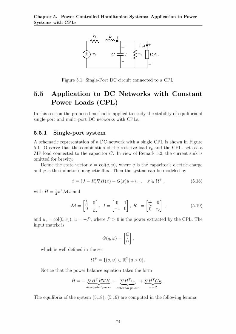
Chapter 5. Power-Controlled Hamiltonian Systems: Application to Power
Systems with CPLs
Figure 5.1: Single-Port DC circuit connected to a CPL.
5.5 Application to DC Networks with Constant
Power Loads (CPL)
In this section the proposed method is applied to study the stability of equilibria ofsingle-port and multi-port DC networks with CPLs.
5.5.1 Single-port system
A schematic representation of a DC network with a single CPL is shown in Figure5.1. Observe that the combination of the resistive load rp and the CPL, acts as aZIP load connected to the capacitor C. In view of Remark 5.2, the current sink isomitted for brevity.
Define the state vector x = col(q, ϕ), where q is the capacitor’s electric chargeand ϕ is the inductor’s magnetic flux. Then the system can be modeled by
x = (J −R)∇H(x) +G(x)u+ uc , x ∈ Ω+ , (5.18)
with H = 12x>Mx and
M =
[1C
00 1
L
], J =
[0 1−1 0
], R =
[ 1rp
0
0 r`
], (5.19)
and uc = col(0, vg), u = −P , where P > 0 is the power extracted by the CPL. Theinput matrix is
G(q, ϕ) =
[Cq
0
],
which is well defined in the set
Ω+ = (q, ϕ) ∈ R2 | q > 0.
Notice that the power balance equation takes the form
H = − ∇HTR∇H︸ ︷︷ ︸dissipated power
+ ∇HTuc︸ ︷︷ ︸external power
+∇HTGu︸ ︷︷ ︸=−P
.
The equilibria of the system (5.18), (5.19) are computed in the following lemma.
74

Chapter 5. Power-Controlled Hamiltonian Systems: Application to Power
Systems with CPLs
Lemma 5.3. The system (5.18)-(5.19) admits two equilibria given by
qs = Crpvg +
√∆
(r` + rp), ϕs = L
rpvg −√
∆
r`(r` + rp)
and
qu = Crpvg −
√∆
(r` + rp), ϕu = L
rpvg +√
∆
r`(r` + rp),
where
∆ := v2g − 4
r`(rp + r`)
rpP.
The equilibrium points are real if and only if ∆ ≥ 0 or equivalently
P ≤ P emax, P e
max :=rpv
2g
4r`(r` + rp). (5.20)
Through straightforward computations, it can be shown that the Jacobian of thevector field in the right hand side of (5.18) has a positive eigenvalue at the equilib-rium point (qu, ϕu), and hence this equilibrium is unstable. Furthermore, it can beshown that for small values of the load power, the Jacobian is negative definite atthe equilibrium point (qs, ϕs).
Considering the results of Lemma 5.3, the equilibrium (qs, ϕs) is proposed asthe candidate for nonlinear stability analysis. To use the results of Corollary 5.1,compute
R + Z(q, ϕ) =
[1rp− C2P
qsq0
0 r`
]. (5.21)
Next, observe that R + Z(qs, ϕs) > 0 if and only if
P < P smax, P s
max :=rpv
2g
(rp + 2r`)2. (5.22)
Hence, according to Corollary 5.1, if the condition (5.22) is satisfied, then theequilibrium (qs, ϕs) is asymptotically stable. Notice that if P < minP e
max, Psmax,
then the existence of the asymptotically stable equilibrium point (qs, ϕs) is guaran-teed.
Remark 5.4. Let v := qsC
denote the voltage of the CPL at the equilibrium (qs, ϕs).
Then the physical equivalent of the term −C2Pqsq
in (5.21), is the inverse of a nonlinearnegative resistor with the resistance
rCPL(v) :=(C2P
qsq
)−1
=v
Pv .
This resistor is in parallel with rp, i.e.,
R + Z(q, ϕ) =
[ 1req
0
0 r`
],
where req(v) :=(
1rp− 1
rCPL(v)
)−1is the equivalent resistor. Interestingly, the physical
interpretation of the condition (5.22) is that the equivalent resistance is positive(and thus a passive element) at the equilibrium point, i.e., req(v) > 0.
75

Chapter 5. Power-Controlled Hamiltonian Systems: Application to Power
Systems with CPLs
As the dissipation matrix R is diagonal, and the Hamiltonian of the states aredecoupled, the largest k in (5.14)—and hence the largest Lk contained in Ωp—canbe constructed explicitly.
To streamline the presentation of the result, consider the constants
ηi := − uiRiiGui
, (5.23)
and the constant vectors
`i := col(x1, x2, · · · , xi−1,ηiMii
, xi+1, · · · , xn) . (5.24)
Corollary 5.2. Consider the system (5.13) with the quadratic Hamiltonian (5.16)with diagonal R > 0 and M > 0. Assume that x ∈ Ωp. Define
kd := mini=1,...,m
H(`i)
,
with (5.23) and (5.24). Then, an estimate of the ROA of the equilibrium x is thesublevel set Lkd of the shifted Hamiltonian function H(x) defined in (5.17).
Proof. The proof follows analogously to the proof of Theorem 5.2, and hence isomitted.
Remark 5.5. Notice that the set Lk in the case considered in the corollary is theellipsoid
n∑i=1
(xi − xi√
2kMii
)2
< 1 . (5.25)
Now, using Corollary 5.2, an estimate of the ROA of (qs, ϕs) can be derived.Bearing in mind that the dissipation matrix R is diagonal, and using Lemma 5.2,Ωp is computed as
Ωp = (q, ϕ) ∈ R2 : q > qmin,
where
qmin := PrpC2
qs
=P
P smax
qs > 0 . (5.26)
Remark 5.6. The interpretation of (5.26) is that the closer the load power to P smax
is, the smaller the ROA is. According to (5.22), this means that, with a fixed qs,larger resistances r` and rp result in a larger ROA. Hence, in the proposed method,small parasitic elements provide a small region of attraction in the absence of theload resistance and the voltage source output resistance.
Now assume that (5.22) holds. Using Corollary 5.2, the set Lkd with
kd = H(qmin, ϕs) ,
is an estimate of the ROA. Furthermore, using (5.25), this set can be written as theoval ( q − qs√
2Ckd
)2
+(ϕ− ϕs√
2Lkd
)2
< 1 . (5.27)
76

Chapter 5. Power-Controlled Hamiltonian Systems: Application to Power
Systems with CPLs
Table 5.1: Simulation Parameters of the Single-Port CPL
vg(V) r` (Ω) rp(Ω) L(µH) C(mF) P (kW)
24 0.04 0.1 78 2 1
Figure 5.2: Phase plane of the system (5.18)-(5.19) with the parameters given inTable 5.1.
This set guarantees q > qmin for all solutions starting within the oval.The results are evaluated by a numerical example of the network shown in Figure
5.1, with the parameters given in Table 5.1. The maximal power for existence ofthe equilibrium and its local stability is computed as P e
max = 2.57 kW and P smax =
2.33 kW, respectively. Notice that the CPL satisfies the conditions (5.20) and (5.22),since
P < P smax < P e
max.
Figure 5.2 shows the phase plane of the system (5.18)-(5.19). The estimate ofthe ROA (the oval (5.27)) is shown in blue, and all other converging solutions areshown in light gray. It is evident that the proposed method provides an appropriateestimate of the ROA, as the solutions just beneath this region (in dark gray), divergefrom the equilibrium.
5.5.2 Multi-port networks
The stability of a complete multi-port DC network with CPLs can be investigatedin a similar fashion. It is assumed that the capacitors and the inductors are notideal, i.e., it is considered that all the inductors have a resistance in series and thecapacitors posses a resistor in parallel. Moreover, it is assumed that the constantpower loads are connected to a capacitor in parallel. This feature amounts to thecapacitive effect of the input filters for this type of loads; see [10, 20, 22]. Let iM ∈ Rlrepresent the currents through the inductors, and vC ∈ Rc denote the voltagesacross the capacitors, where l and c are the number of inductors and capacitors,respectively. With a little abuse of notation, define the state vector x = col(q, ϕ) ∈Rc+l and the control vector u = −P ∈ Rc, where q ∈ Rc denotes the electric chargeof the capacitors, and ϕ ∈ Rl denotes the magnetic flux of the inductors. Then thenetwork dynamics of a multi-port network admits a port-Hamiltonian representation
77
Chapter 5. Power-Controlled Hamiltonian Systems: Application to Power
Systems with CPLs
given byx = (J −R)∇H(x) +G(x)u+ uc,
with H = 12x>Mx and
M =
[C−1 00 L−1
], J =
[0 −Γ>
Γ 0
], R =
[Y 00 Z
],
where C > 0 ∈ Rc×c and L > 0 ∈ Rl×l are matrices associated with the magnitudeof capacitors and inductors (and mutual inductances), Y ∈ Rc×c and Z ∈ Rl×lare positive definite matrices associated with the resistances, and Γ ∈ Rl×c is thematrix associated with the network topology. The vector uc ∈ Rc+l is constant andits components are linear combinations of the voltages and currents of the sourcesin the network. Similar to the case of the single-port RLC circuit with a CPL, andusing Theorem 5.2, an ellipsoid can be computed here as an estimate of the ROA.
5.6 Application to a Synchronous Generator Con-
nected to a CPL
In this section, the results are applied to the case of a synchronous generator con-nected to a CPL. This system can be modeled by2
p = (J −R)∇H(p) +G(p)u+ uc, (5.28)
with
p = Mω, J = 0, R = Dm +Dd, G(p) =M
p= ω−1,
H =1
2Mp2, u = −Pe, uc = τm +Ddω
∗,
(5.29)
where p > 0 is the angular momentum, M > 0 is the total moment of inertia of theturbine and generator rotor, ω ∈ R+ is the rotor shaft velocity, ω∗ > 0 is the angularvelocity associated with the nominal frequency of 50 Hz, Dm > 0 is the dampingcoefficient of the mechanical losses, Dd > 0 is the damping-torque coefficient of thedamper windings, τm > 0 is the constant mechanical torque (physical input), andPe is the constant power load.
Let∆ := (Ddω
∗ + τm)2 − 4(Dd +Dm)Pe ,
and assume that ∆ > 0, i.e.,
Pe <(Ddω
∗ + τm)2
4(Dd +Dm).
Then, the dynamics (5.28), (5.29) has the following two equilibria
ωs =Ddω
∗ + τm +√
∆
2(Dd +Dm), ωu =
Ddω∗ + τm −
√∆
2(Dd +Dm).
2This model is called the improved swing equation in [130, 76]. An inverter with a capacitiveinertia can be modeled by similar dynamics; see [77].
78

Chapter 5. Power-Controlled Hamiltonian Systems: Application to Power
Systems with CPLs
Table 5.2: Simulation Parameters of the Synchronous Generator (p.u.)
M Dm Dd Pe τm
0.2 10−6 10−4 3 0.0027
0 10 20 30 40 50 60 700
20
40
60
80
Figure 5.3: Solutions of the system (5.28),(5.29) with different initial conditions.
Moreover,
R + Z(ω) =Dd +Dm −Peωsω
.
The equilibrium point ω = ωs is asymptotically stable since
R + Z(ωs) =τm +Ddω
∗
ωs
> 0.
Through straightforward computations, it can be shown that the set Ωp in (5.11)can be written as
Ωp = ω ∈ R+ : ω > ωu . (5.30)
In this set, the shifted Hamiltonian H = 12M(ω− ωs)
2 is strictly decreasing. There-fore the solutions tend to the equilibrium ωs and move away from the point ωu
when time increases. Consequently the set Ωp in (5.30) is forward invariant, andrepresents an estimate of the ROA.
Figure 5.3 shows the trajectories of a number of solutions of the system (5.28)-(5.29), with the parameters given by Table 5.2, and with different initial conditions.It is clear that the proposed method successfully identifies a very precise estimate ofthe ROA (blue), as all the solutions starting from outside the ROA estimate (black)diverge from the equilibrium. The result, which is derived from the systematicapproach proposed in the chapter, shows an improvement over the results of [76],as both derived ROAs have the same lower bound, while here, the estimate has noupper bound.
Interestingly, it can be shown that any solution that does not start in Ωp, divergesfrom the stable equilibrium ωs. Therefore, here, the set Ωp is not only an estimate,but is the exact region of attraction.
79

Chapter 5. Power-Controlled Hamiltonian Systems: Application to Power
Systems with CPLs
5.7 Summary
This chapter has explored a class of pH systems in which the control input (ordisturbance) acts on the power of the system. These systems have been referred hereas Power-controlled Hamiltonian (PwH) systems. First, a model for such systemswas proposed, and second, a condition for shifted passivity was derived. Using theseresults, the stability of equilibria was investigated. Furthermore, an estimate of theregion of attraction was derived for PwH systems with quadratic Hamiltonian.
The proposed modeling procedure and stability analysis were illustrated withtwo cases of practical interest: A DC circuit and a synchronous generator, bothconnected to constant power loads. The validity and utility of the proposed methodwas confirmed by numerical simulations of these case studies.
80

Part III
STABILIZATION: ANADAPTIVE CONTROL
APPROACH

Chapter 6
Voltage Control of a Buck-BoostConverter
Synopsis This chapter addresses the problem of regulating the output voltageof a DC-DC buck-boost converter that supplies electric energy to a constant powerload. The model of the network is a nonlinear, second order dynamical systemthat is shown to be non-minimum phase with respect to both states. Moreover, todesign a high-performance controller, the knowledge of the extracted load power,which is difficult to measure in industrial applications, is required. In this chapter,an adaptive interconnection and damping assignment passivity-based control—thatincorporates the immersion and invariance parameter estimator for the load power—is proposed to stabilize the system around a desired equilibrium. Some detailedsimulations are provided to validate the transient behavior of the proposed controllerand compare it with the performance of a classical proportional-derivative scheme.
6.1 Introduction
The DC-DC buck-boost power converter is increasingly utilized in power distri-bution systems since it can step up or down the voltage between the source andload, providing flexibility in choosing the voltage rating of the DC source [125, 116,124]. Although the control of these converters in the face of classical loads is well-understood, this is not the case when constant power loads (CPLs) are considered.This scenario significantly differs from the classical one and poses a new challengeto control theorist, see [9, 71, 38, 53, 80, 128] for further discussion on the topicand [110] for a recent literature review. It should be underscored that the typicalapplication of this device requires large variations of the operating point—therefore,the dynamic description of its behavior cannot be captured by a linearized model,requiring instead a nonlinear one.
To address the voltage regulation of a buck-boost converter with a CPL, severaltechniques have been proposed in the power electronics literature, but without anonlinear stability analysis. In [88], the active-damping approach is utilized toaddress the negative impedance instability problem raised by the CPL. The mainidea of this method is that a virtual resistance is considered in the original circuit toincrease the system damping. However, the stability result is obtained by applyingsmall-signal analysis, which is valid only in a small neighborhood of the operatingpoint. A new nonlinear feedback controller, which is called “Loop Cancellation”, has
82

Chapter 6. Voltage Control of a Buck-Boost Converter
been proposed to stabilize the buck-boost converter by “canceling the destabilizingbehavior caused by CPL” [89]. The control problem turns into the design of acontroller for the linear system by using loop cancellation method. However, theconstruction is based on feedback linearization [47] that, as is well-known, is highlynon-robust. A sliding mode controller is designed in [111] for this problem. However,for the considered nonlinear system, the stability result is obtained by adopting thelinear system theory. In addition, as it is widely acknowledged, the drawbacks of thismethod are that the proposed control law suffers from chattering and its relay actioninjects a high switching gain. The deleterious effect of these factors is illustrated inexperiments shown in [111], which exhibit a very poor performance.
Aware of the need to deal with the intrinsic nonlinearities of power converterssome authors of this community have applied passivity-based controllers (PBCs),which is a natural candidate in these applications. Unfortunately, in many of thesereports the theoretical requirements of the PBC methodology are not rigorouslyrespected. For instance, in [60], the well-known standard PBC [83] is used for thebuck-boost with a CPL. Unfortunately, the given result is theoretically incorrectdue to the fact that the authors fail to validate the stability of the zero dynamicsof the system with respect to the controlled output that, as explained in [83], is anessential step for the stability analysis and, as shown in this chapter, it turns out tobe violated.
An additional drawback of the existing results is that all of them require theknowledge of the power extracted by the CPL, which is difficult to measure inindustrial applications. Designing an estimator for the power is a hard task becausethe original system is nonlinear and the only available measurements are the inductorcurrent and the output voltage.
In this chapter, the well-known interconnection and damping assignment (IDA)PBC, first reported in [82] and reviewed in [81], is applied to stabilize the buck-boostconverter with a CPL. The main contributions are enlisted as follows.
1) Derivation of an IDA-PBC that ensures the desired operating point is a (lo-cally) asymptotically stable equilibrium with a guaranteed region of attraction.
2) Design of an estimator of the load’s power, which is based on the Immersionand Invariance (I&I) technique[8] and has guaranteed stability properties, tomake the IDA-PBC adaptive.
3) Proof that the zero dynamics of the system, with respect to both states, isunstable—limiting the achievable performance of classical PD controllers to“low-gain tunings”.
The rest of the chapter is organized as follows. Section 6.2 contains the modelof the system and the analysis of its zero dynamics with respect to its two states.Section 6.3 proposes the IDA-PBC assuming that the power extraction of the loadis known. To make the latter scheme adaptive, in Section 6.4 an on-line powerestimator is designed and some simulations, carried out in MATLAB, are providedin Section 6.5. The chapter is wrapped-up with some concluding remarks in Section6.6. To enhance readability, the derivation of the IDA-PBC, that is conceptuallysimple but computationally involved, is given in a Technical Appendix at the endof the chapter.
83

Chapter 6. Voltage Control of a Buck-Boost Converter
Figure 6.1: Circuit representation of the DC-DC buck-boost converter with a CPL
6.2 System Model, Problem Formation and Zero
Dynamics Analysis
In this section, the average model1 of the buck-boost converter supplying electricenergy to a CPL is presented and an analysis of its zero dynamics is carried out.
6.2.1 Model of buck-boost converter with a CPL
The topology of a buck-boost converter supplying electric energy to a CPL is shownin Fig. 6.1. Under the standard assumption that it operates in continuous conduc-tion mode, the average model is given by
Ldi
dt= −(1− u)v + uE,
Cdv
dt= (1− u)i− P
v, (6.1)
where i > 0 is the current through the inductor L, v > 0 the voltage across thecapacitor C, P ≥ 0 the power extracted by the CPL, E > 0 is the input voltageand u ∈ [0, 1] is the converter’s duty ratio, which is the control signal.
Some simple calculations show that the assignable equilibrium set is given by
E :=
(i, v) ∈ R2 : i− P
(1
v+
1
E
)= 0, v > 0
. (6.2)
6.2.2 Control problem formulation
Consider the system (6.1) verifying the following conditions.
Assumption 6.1. The power load P is unknown but the parameters L,C and Eare known and fixed.
Assumption 6.2. The state (i, v) is available for measurement.
Fix a desired output voltage v? > 0 and compute the associated assignable equilib-rium point (i?, v?) ∈ E . Design a static state-feedback control law with the followingfeatures.
(F1) (i?, v?) is an asymptotically stable equilibrium of the closed-loop, with a well-defined region of attraction.
1The reader is referred to the introduction of [112] for a detailed explanation on average modelsof power converters in general.
84

Chapter 6. Voltage Control of a Buck-Boost Converter
(F2) It is possible to define a subset Ω, in the positive orthant of R2, which ispositively-invariant and inside the region of attraction of the equilibrium. Thatis, a set inside the positive orthant verifying
[(i(0), v(0)) ∈ Ω ⇒ (i(t), v(t)) ∈ Ω,∀t ≥ 0]
limt→∞
(i(t), v(t)) = (i?, v?).
To simplify the notation, and without loss of generality, a normalized model ofthe system is to be used. This normalized form is obtained through the change ofcoordinates
x1 :=1
E
√L
Ci
x2 :=1
Ev, (6.3)
and doing the time scale change τ = t√LC
that yields the model
x1 = −(1− u)x2 + u
x2 = (1− u)x1 −D
x2
(6.4)
where
D :=P
E2
√L
C.
Also, ˙(·) denotes ddτ
(·) and all signals are expressed in the new time scale τ . Theassignable equilibrium set E in the coordinates x is given by
Ex :=
x ∈ R2 : x1 −
D
x2
−D = 0, x2 > 0
(6.5)
Notice that, under Assumptions 6.1 and 6.2, the control problem is translatedinto the design of a state feedback for the system (6.4), with unknown D, such thata given x? ∈ Ex is asymptotically stable.
It is important to recall that the signal of interest is the output voltage v, there-fore, for the fixed x2? > 0, the x1? > 0 is defined via
x1? =D
x2?
+D. (6.6)
Remark 6.1. As indicated by Assumption 6.1, the value for the input voltage E isassumed to be known and fixed. A non-trivial extension of the present work wouldimply the relaxation of this assumption. It is worth mentioning that this problemhas been addressed in [64] and [113] but for the case of standard impedance loads.
6.2.3 Stability analysis of the systems zero dynamics
The design of a stabilizing controller for (6.4) is complicated by the fact that, asshown in the proposition below, its zero dynamics with respect to both states isunstable. This means that, if the controller injects high gain, the closed-loop system
85
Chapter 6. Voltage Control of a Buck-Boost Converter
will be unstable—as it stems from the fact that the poles will move towards the un-stable zeros. This situation hampers the design of high performance PD controllers,which require high proportional gains to speed up the transients. See Section 6.5for an illustration of this fact.
Proposition 6.1. Consider the system (6.4) and an assignable equilibrium x? ∈ Ex.The zero dynamics with respect to the outputs x1 − x1? or x2 − x2? are unstable.
Proof Fixing x1 = x1? and using the first equation in (6.4), it follows that
u =x2
x2 + 1,
which substituted in the second equation of (6.4) yields the zero dynamics
x2 =D
x2?x2(x2 + 1)(x2 − x2?) =: s(x2). (6.7)
The slope of s(x2) evaluated at x2 = x2? gives
s′(x2)|x2=x2? =D
x22?(1 + x2?)
.
Since x2? > 0, this is a positive number proving that the equilibrium x2? of thedynamics (6.7) is unstable—as claimed by the proposition.
Analogously, by fixing x2 = x2? and using the second equation of (6.4) the expression
u = 1− D
x1x2?
, (6.8)
is obtained, which substituted in the first equation of (6.4) yields
x1 = 1− x1? −Dx1
=: w(x1). (6.9)
Proceeding as done for the case above, it follows that
w′(x1)|x1=x1? =x1? −Dx2
1?
.
The proof is completed noting from (6.5) that x1? = D(1 + 1x2?
) > D and the slopeis, again, positive.
The proof that the zero dynamics of (6.4) with respect to x1 − x1? is unstableinvalidates the stability claim made in Section IV of [60]. In that paper, a standardPBC is designed fixing x1 = x1?. It is well-known [83] that this kind of controllerimplements an inversion of the systems zero dynamics, therefore the controller willbe unstable if the zero dynamics is unstable, which is the case of the PBC of [60].
86

Chapter 6. Voltage Control of a Buck-Boost Converter
6.3 IDA-PBC design
In this section, the IDA-PBC approach is proposed to stabilize the buck-boost con-verter feeding a CPL by assuming that the power of the load, D, is known. Thiscondition is later relaxed in Proposition 6.4, where an estimator of D is added tothe IDA-PBC.
To make this chapter self-contained the main result of the IDA-PBC methodologyand its proof are presented next. For more details on IDA-PBC the reader is referredto [81].
Proposition 6.2. Consider the nonlinear system
x = f(x) + g(x)u (6.10)
with state x ∈ Rn and control u ∈ Rm and a desired operating point
x? ∈ x ∈ Rn : g⊥(x)f(x) = 0,
where g⊥(x) is a full rank left annihilator of g(x). Fix the target dynamics as
x = Fd(x)∇Hd(x), (6.11)
where ∇Hd(x) :=(∂Hd(x)∂x
)>with the function Hd(x) a solution of the PDE
g⊥(x) [f(x)− Fd(x)∇Hd(x)] = 0, (6.12)
verifyingx? = arg minHd(x), (6.13)
and the matrix Fd(x) is such that
F>d (x) + Fd(x) < 0, ∀x. (6.14)
Then, the system (6.10) in closed-loop with
u(x) := [g>(x)g(x)]−1g>(x)[Fd(x)∇Hd(x)− f(x)] (6.15)
has an asymptotically stable equilibrium at x? with strict Lyapunov function Hd(x).
Proof From the fact that the n × n matrix
[g>(x)g⊥(x)
]is full rank, the following
equivalence holds.
f(x) + g(x)u(x) = Fd(x)∇Hd(x) ⇔ (6.12), (6.15).
Hence, the closed-loop is given by (6.11). Now, (6.13) ensures Hd(x) is positive def-inite (with respect to x?). Computing the derivative of Hd(x) along the trajectoriesof (6.11) and invoking (6.14) it follows that
Hd = (∇Hd(x))>Fd(x)∇Hd(x) < 0, ∀x 6= x?
and, therefore, Hd(x) is a strict Lyapunov function for the closed-loop system, com-pleting the proof.
The next proposition is a direct application of IDA-PBC that provides a solutionto considered problem.
87
Chapter 6. Voltage Control of a Buck-Boost Converter
Proposition 6.3. Consider the system (6.4) under Assumption 6.2. Further assumethat D is known and satisfies the bounds
0 < D <x2
2?√2√
1 + x2?
. (6.16)
Fix x2? > 0 and compute x1? > 0 from equation (6.6). Define the IDA-PBC
u =1
u0
(u1 + u2), (6.17)
where
u0 = −x1 (x2 + 1) 2(2x2
1 + x22
)2,
u1 =(2x2
1 + x22
) (x1x2
(2x2
1 + x22
) (k1 (2x2 + 1)
(2(k2 + x2
1
)+ x2
2
)−x2 − 2)−D (x2 + 1)
(−2x2
1 + x22 + x2
)),
u2 =√
2Dx1x2
√2x2
1 + x22 (2x2 + 1) arctanh
x1√x2
1 +x222
,
(6.18)
k1 is a tuning gain satisfying
k1 > max− a0(4D2(x2?+1)2
x22?
) , − b0(x42?−2D2(x2?+1)
x32?
), (6.19)
with the constants a0 and b0 defined in Appendix 6.E, and k2 is a constant definedin Appendix 6.F.
Then, the following claims hold true.
P1: x? is an asymptotically stable equilibrium of the closed-loop system, with Lya-punov function
Hd(x) = −1
2
(x2 +
√2D arctan
(√2x1x2
))−
−
D arctanh
x1√x21+
x222
2
√x2
1 +x222
+k1
2(x2
1 +x2
2
2+ k2)2. (6.20)
P2: There exists a sufficiently small positive constant c such that the sublevel setof the function Hd(x)
Ωx := x ∈ R2 : Hd(x) ≤ c, (6.21)
is strictly contained in the positive orthant of R2 , being hence an estimateof the region of attraction. That is, for all x(0) ∈ Ωx, it follows that x(t) ⊂Ωx,∀t ≥ 0, and limt→∞ x(t) = x?.
Proof. See Appendix 6.A.
88

Chapter 6. Voltage Control of a Buck-Boost Converter
6.4 Adaptive IDA-PBC Using an Immersion and
Invariance Power Estimator
In this section, the case of unknown power D is considered and an estimator of thisparameter, based on the I&I technique [8], is presented.
Proposition 6.4. Consider the model (6.4), under Assumptions 6.1 and 6.2, inclosed-loop with an adaptive version of the control (6.17), which is defined as
u =1
u0
(u1 + u2) |D≡D, (6.22)
where u0, u1 and u2 are defined in (6.18) and D(t) is an on-line estimate of D,generated with the I&I estimator
D =− 1
2γx2
2 +DI , (6.23)
DI =γx1x2(1− u) +1
2γ2x2
2 − γDI , (6.24)
where γ > 0 is a free parameter. Then, there exists kmin1 such that for all k1 > kmin
1
the overall system has an asymptotically stable equilibrium at (x, D) = (x?, D) .Moreover, for all initial conditions of the closed-loop system and all DI(0), then
D(t) = e−γtD(0), (6.25)
where D := D −D is the parameter estimation error.
Proof. See Appendix 6.B.
Remark 6.2. The experimental implementation of the proposed controller, de-scribed by eqs. (6.17) and (6.22), requires an initialisation stage that will ramp-upthe output voltage to a neighbourhood of the input voltage. Nonetheless, this is avery common practice in many applications.
6.5 Simulation Results
In this section the performance of the proposed adaptive IDA-PBC is illustrated viasome computer simulations. Moreover, its transient behavior is compared with theone of a PD controller that has been designed adopting the classical linearizationtechnique.
In simulations, the boost mode and buck mode are tested under the proposedIDA-PBC, respectively. The system parameters of the boost mode are given in [60],which read as P = 61.25 W, C = 500 µF, L = 470 µH, E = 10 V, v? = 40 V . Thedesired equilibrium is fixed as x? = (0.7423, 4). Additionally, the system parametersof the buck mode are chosen as P = 6 W, E = 25 V, v? = 15 V and the desiredequilibrium is fixed as x? = (0.01489, 0.6). For simplicity, only the scaled system(6.4) is simulated; however, depending on the context, the plots are shown eitherfor x or for the original coordinates (i, v)—recalling that they are simply related bythe scaling factors given in (6.3).
89

Chapter 6. Voltage Control of a Buck-Boost Converter
6.5.1 PD controller
To underscore the limitations of the PD controller and the difficulties related withits tuning, the local stability analysis of such a controller is presented. From (6.4),the error dynamics is obtained as
e1 = −(1− eu − u?)(e2 + x2?) + eu + u?,
e2 = (1− eu − u?)(e1 + x1?)−D
e2 + x2?
,
with error functions
e1 := x1 − x1?, e2 := x2 − x2?, eu := u− u?,
and u? := x2?1+x2?
. A standard PD controller for the error dynamics is given by
eu = kpe1 + kde2, (6.26)
where kp, kd are tuning gains. Notice that, for the computation of x1?, the imple-mentation of this controller requires the knowledge of D. The Jacobian matrix ofthe closed-loop system, e = F (e), evaluated at the equilibrium point, is given by
J : =
[∇e1F1(e) ∇e2F1(e)∇e1F2(e) ∇e2F2(e)
] ∣∣∣∣∣e=0
=
[kp(1 + x2?) kd + kdx2? − 1
1+x2?1
1+x2?− Dkp(1+x2?)
x2?−D(−1+kdx2?(1+x2?))
x22?
],
where ∇eiFj(e) :=∂Fj(e)
∂ei. The matrix J is Hurwitz if and only if its trace is negative
and its determinant is positive, which are given by
tr(J) = kp(1 + x2?)− kdD(1
x2?
+ 1) +D
x22?
,
det(J) = kpD
x22?
− kd +1
(x2? + 1)2.
Defining the positive constants
m1 :=x2?
D, b1 :=
1
x2? + x22?
,
m2 :=D
x22?
, b2 :=1
(1 + x2?)2.
The trace-determinant stability conditions can be written as the two-sided in-equality
m2kp + b2 > kd > m1kp + b1, (6.27)
which is a conic section in the plane kd − kp, that reveals the conflicting role of thetwo gains. Notice that the extracted power D enters in the first slope m1 in thedenominator, while it appears in the nominator in m2—rendering harder the gaintuning task regarding this uncertain parameter.
90
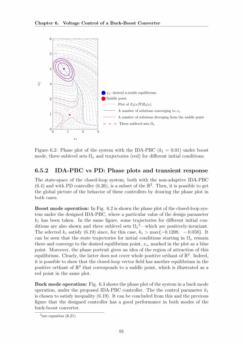
Chapter 6. Voltage Control of a Buck-Boost Converter
0 1 2 30
1
2
3
4
5
6
x1
x2
x?: desired a-stable equilibrium
Saddle point
—– Plot of Fd(x)∇Hd(x)
—– A number of solutions converging to x?
—– A number of solutions diverging from the saddle point
- - - Three sublevel sets Ωx
Figure 6.2: Phase plot of the system with the IDA-PBC (k1 = 0.01) under boostmode, three sublevel sets Ωx and trajectories (red) for different initial conditions.
6.5.2 IDA-PBC vs PD: Phase plots and transient response
The state-space of the closed-loop system, both with the non-adaptive IDA-PBC(6.4) and with PD controller (6.26), is a subset of the R2. Then, it is possible to getthe global picture of the behavior of these controllers by drawing the phase plot inboth cases.
Boost mode operation: In Fig. 6.2 is shown the phase plot of the closed-loop sys-tem under the designed IDA-PBC, where a particular value of the design parameterk1 has been taken. In the same figure, some trajectories for different initial con-ditions are also shown and three sublevel sets Ωx
2—which are positively-invariant.The selected k1 satisfy (6.19) since, for this case, k1 > max−0.1208, − 0.058. Itcan be seen that the state trajectories for initial conditions starting in Ωx remainthere and converge to the desired equilibrium point, x?, marked in the plot as a bluepoint. Moreover, the phase portrait gives an idea of the region of attraction of thisequilibrium. Clearly, the latter does not cover whole positive orthant of R2. Indeed,it is possible to show that the closed-loop vector field has another equilibrium in thepositive orthant of R2 that corresponds to a saddle point, which is illustrated as ared point in the same plot.
Buck mode operation: Fig. 6.3 shows the phase plot of the system in a buck modeoperation, under the proposed IDA-PBC controller. The the control parameter k1
is chosen to satisfy inequality (6.19). It can be concluded from this and the previousfigure that the designed controller has a good performance in both modes of thebuck-boost converter.
2see equation (6.21)
91

Chapter 6. Voltage Control of a Buck-Boost Converter
2 4 6
·10−2
0.56
0.58
0.6
0.62
0.64
x1
x2
x?: desired a-stable equilibrium
—– Plot of Fd(x)∇Hd(x)
—– A number of solutions converging to x?
- - - Largest sublevel set Ωx in R2>0
Figure 6.3: Phase portrait of the system with the IDA-PBC (k1 = 0.01) under buckmode, three sublevel sets Ωx and trajectories (red) for different initial conditions.
Buck mode (PD controller) In Fig. 6.4 is presented the phase plot of the systemin closed-loop with the PD controller of equation (6.26). The controller’s parametersare chosen as kp = −0.4, kd = −1.5, which satisfy the condition (6.27), numericallygiven in this scenario by
0.037kp + 0.04 > kd > 6.7358kp + 0.0588.
Only those trajectories starting very close to the equilibrium remain in the positiveorthant of R2 and converge to x?. Compared with Fig. 6.2, the IDA-PBC provides amuch bigger region of attraction and, moreover, gives explicit estimates of it. Othervalues for the gains kp and kd have been tried yielding very similar inadmissiblebehaviors and are hence not reported here.
92

Chapter 6. Voltage Control of a Buck-Boost Converter
0 1 2 30
1
2
3
4
5
6
x1
x2
Figure 6.4: Phase portrait of the system with a PD controller.
Transient response comparison: Considering once again the boost mode, in Fig.6.5 the transient responses of the output voltage v and the duty ratio u under theIDA-PBC and the PD controller, taking the same initial condition of x(0) = (0.4, 3.9)are presented. The control gains are k1 = 0.01 for the former and kp = −0.4, kd =−1.5 for the latter. It can be observed that the IDA-PBC has a faster transientperformance with a smaller control signal.
0 0.01 0.02 0.03 0.04 0.05 0.0638.6
38.8
39
39.2
39.4
39.6
39.8
40
40.2
40.4
t(s)
Out
put v
olta
ge
IDA−PBCPD
Figure 6.5: Response curves of DC-DC buck-boost converter with a CPL for theIDA-PBC and the PD controller.
93
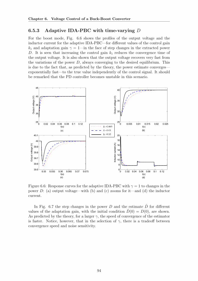
Chapter 6. Voltage Control of a Buck-Boost Converter
6.5.3 Adaptive IDA-PBC with time-varying D
For the boost mode, Fig. 6.6 shows the profiles of the output voltage and theinductor current for the adaptive IDA-PBC—for different values of the control gaink1 and adaptation gain γ = 1—in the face of step changes in the extracted powerD. It is seen that increasing the control gain k1 reduces the convergence time ofthe output voltage. It is also shown that the output voltage recovers very fast fromthe variations of the power D, always converging to the desired equilibrium. Thisis due to the fact that, as predicted by the theory, the power estimate converges—exponentially fast—to the true value independently of the control signal. It shouldbe remarked that the PD controller becomes unstable in this scenario.
Figure 6.6: Response curves for the adaptive IDA-PBC with γ = 1 to changes in thepower D: (a) output voltage—with (b) and (c) zooms for it—and (d) the inductorcurrent.
In Fig. 6.7 the step changes in the power D and the estimate D for differentvalues of the adaptation gain, with the initial condition D(0) = D(0), are shown.As predicted by the theory, for a larger γ, the speed of convergence of the estimatoris faster. Notice, however, that in the selection of γ, there is a tradeoff betweenconvergence speed and noise sensitivity.
94

Chapter 6. Voltage Control of a Buck-Boost Converter
Figure 6.7: Transient performance of the estimate D under step changes of theparameter D for various adaptation gains γ and a zoom of the first step.
6.6 Summary
The challenging problem of regulation of the output voltage of a buck-boost con-verter supplying electric energy to a CPL with unknown power has been addressedin this chapter. First, assuming the power is known, an IDA-PBC that renders adesired equilibrium point asymptotically stable has been proposed. Subsequently,an on-line I&I estimator with global convergence property has been presented torenders the scheme adaptive, preserving the asymptotic stability property. It hasalso been illustrated the performance limitations of the classical PD controller stem-ming from the fact that, due to the presence of the CPL, the system is non-minimumphase. Some realistic simulations have been provided to confirm the effectiveness ofthe proposed method.
Technical Appendices of the Chapter
6.A Proof of Proposition 6.3
Proof of Claim P1: It is shown first that the control (6.17) can be derived using theIDA-PBC method of Proposition 6.2.
First, assign the matrix Fd as
Fd(x) :=
[ −x2x1
− 2x2x2+1
2x2x2+1
− 2x1(x2+1)2
],
that, for x in the positive orthant of R2, satisfies the condition (6.14).3 Now, observethat the system (6.4) can be rewritten in the form (6.10), with
f(x) :=
[ −x2
x1 − Dx2
], g(x) =
[x2 + 1−x1
].
3It is well-known [81] that a key step for the successful application of the method is a suitableselection of this matrix, which is usually guided by the study of the solvability of the PDE (6.12).See [44] for some guidelines for its selection in this example.
95

Chapter 6. Voltage Control of a Buck-Boost Converter
The left annihilator of g(x) is then g⊥(x) := [x1 x2 + 1]. It follows that the PDE(6.12) can be written explicitly as
−x2∇x1Hd(x) + 2x1∇x2Hd(x) = D − x1 +D
x2
. (6.28)
Using the symbolic language Mathematica, the solution of the PDE (6.28) is com-puted as
Hd(x) =− 1
2
(x2 +
√2D arctan
(√2x1x2
))
−
D arctanh
x1√x21+
x222
2
√x2
1 +x222
+ Φ(x21 +
x22
2),
where Φ(·) is any function with argument(x2
1 +x222
), which is selected as
Φ(z) :=k1
2(z + k2)2,
with k1 and k2 arbitrary constants.
The existence of constants k1 and k2 guaranteeing that x? is a critical point of Hd
and that, furthermore, is a local minimum of it, are verified next.Evaluate the gradient of Hd(x), shown in Appendix 6.C, at the equilibrium x?
4
and substitute k2 as presented in Appendix 6.F, which results in ∇Hd|x=x?= 0,
implying that x? is a critical point of Hd.Now, a sufficient condition for x? to be a local minimum of Hd, is that
M := ∇2Hd|x=x? > 0.
Being ∇2Hd a 2× 2 real matrix,5 the above condition is equivalent to
m11 > 0, det(M) > 0,
where m11 is the (1,1) entry of M . Regarding these expressions, the followingequivalences hold.
m11 = a0 + k1
(4D2 (x2? + 1) 2
x22?
)det(M) = b0 + k1
(x4
2? − 2D2 (x2? + 1)
x32?
),
where a0 and b0 are real constants defined in Appendix 6.E. Notice that both ex-pressions are linear with respect to k1 and that, furthermore, the coefficients of k1
are positive if
0 < D <x2
2?√2√
1 + x2?
.
4Recall equation (6.6).5For completeness, the entries of ∇2Hd are included in Appendix 6.D.
96

Chapter 6. Voltage Control of a Buck-Boost Converter
Consequently, M > 0 if and only if the latter inequality on D, and
k1 > max− a0(4D2(x2?+1)2
x22?
) , − b0(x42?−2D2(x2?+1)
x32?
)⇒
m11 > 0 ∧ det(M) > 0,
are satisfied simultaneously, which hold by assumption. The proof is completedshowing that the IDA-PBC (6.17) results replacing the data in (6.15).
Proof of Claim P2: It has been shown that Hd(x) has a positive definite Hessianmatrix at x?, therefore it is locally convex. Then, for sufficiently small c, the sublevelset Ωx defined in (6.21) is bounded and strictly contained in the positive orthant ofR2. The proof is completed recalling that sublevel sets of strict Lyapunov functionsare inside the region of attraction of the equilibrium.
6.B Proof of Proposition 6.4
Computing the time-derivative of the estimation error, D, along the trajectories of(6.4), and using the expression (6.23), it follows that
˙D = −γx2x2 + DI
= −γx1x2(1− u) + γD + DI .
Substituting (6.24) in the last equation yields
˙D = γD +1
2γ2x2
2 − γDI
= −γD,
from which (6.25) follows immediately.
To prove the asymptotic stability of (x, D) = (x?, D), the adaptive controller (6.22)is written as
u :=1
u0
(u1 + u2) |D≡D.
Then, the following holds
u = u|D (exact) + δ(x, D),
where u|D (exact) denotes the controller (6.17). That is, the controller that assumes
an exact knowledge of D is recovered, plus an additive disturbance δ(x, D); themapping δ can be proved to satisfy δ(x, 0) = 0.
Invoking the proof of Proposition 6.3, the closed-loop system is now a cascadedsystem of the form
x = Fd(x)∇Hd(x) + g(x)δ(x, D, k1)˙D = −γD,
97

Chapter 6. Voltage Control of a Buck-Boost Converter
where
g(x) :=
[x2 + 1−x1
],
is the systems input matrix. The signal D(t) tends to zero exponentially fast for allinitial conditions, and for sufficiently large k1, i.e., such that (6.19) is satisfied, thesystem above with D = 0 is asymptotically stable. Invoking well-known results ofasymptotic stability of cascaded systems, e.g., Proposition 4.1 of [101], the proof of(local) asymptotic stability is completed.
6.C Explicit form of ∇Hd
∇x1Hd = k1x1
(2(k2 + x2
1
)+ x2
2
)− D (x2 + 1)
2x21 + x2
2
+
√2Dx1 arctanh
x1√x21+
x222
(2x2
1 + x22) 3/2
∇x2Hd =Dx1 (x2 + 1)
x32 + 2x2
1x2
+1
2k1x
32 + k1x
21x2 + 2k1k2x2 −
1
2
+
√2Dx2 arctanh
x1√x21+
x222
(2x2
1 + x22) 3/2
98
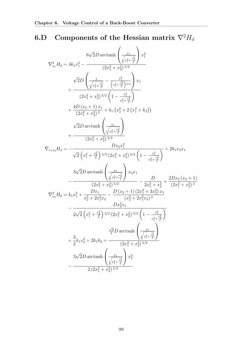
Chapter 6. Voltage Control of a Buck-Boost Converter
6.D Components of the Hessian matrix ∇2Hd
∇2x1Hd = 4k1x
21 −
6√
2D arctanh
x1√x21+
x222
x21
(2x21 + x2
2) 5/2
+
√2D
1√x21+
x222
− x21(x21+
x222
)3/2
x1
(2x21 + x2
2) 3/2
(1− x21
x21+x222
)+
4D (x2 + 1)x1
(2x21 + x2
2) 2+ k1
(x2
2 + 2(x2
1 + k2
))
+
√2D arctanh
x1√x21+
x222
(2x2
1 + x22) 3/2
∇x1x2Hd = − Dx2x21
√2(x2
1 +x222
)3/2 (2x2
1 + x22) 3/2
(1− x21
x21+x222
) + 2k1x2x1
−
3√
2D arctanh
x1√x21+
x222
x2x1
(2x21 + x2
2) 5/2− D
2x21 + x2
2
+2Dx2 (x2 + 1)
(2x21 + x2
2) 2
∇2x2Hd = k1x
21 +
Dx1
x32 + 2x2
1x2
− D (x2 + 1) (2x21 + 3x2
2)x1
(x32 + 2x2
1x2) 2
− Dx22x1
2√
2(x2
1 +x222
)3/2 (2x2
1 + x22) 3/2
(1− x21
x21+x222
)
+3
2k1x
22 + 2k1k2 +
√2
2D arctanh
x1√x21+
x222
(2x2
1 + x22) 3/2
−
3√
2D arctanh
x1√x21+
x222
x22
2 (2x21 + x2
2) 5/2
99

Chapter 6. Voltage Control of a Buck-Boost Converter
6.E Values of the constants a0 and b0.
a0 =x32s
(2D2(x2s+1)2+x42s)3(a′0 + a′′0) ,
a′0 =(2D2 (x2s + 1) 2 + x4
2s
) (2D2 (x2s + 1) (3x2s + 4) + x4
2s
),
a′′0 = −6√
2D3x2s (x2s + 1) 2
√2D2(x2s+1)2+x42s
x22sarctanh
D(
1x2s
+1)
√D2(
1x2s
+1)2+
x22s2
.
b0 =x22s
2(D2(x2s+1)2+x42s)3(b′0 + b′′0)
b′0 = −4D4 (x2s + 1) 2 (x2s (x2s + 5) + 5)− 2D2 (3x2s + 4)x42s
b′′0 = −3√
2Dx2s
(x4
2s − 2D2 (x2s + 1))×
×√
2D2(x2s+1)2+x42sx22s
arctanh
D(
1x2s
+1)
√D2(
1x2s
+1)2+
x22s2
+ x82s
6.F Value of the constant k2
k2 =1
k′2(k′′2 + k′′′2 )
wherek′2 = −2k1x
22?
(2D2 (x2? + 1) 2 + x4
2?
)2
k′′2 =√
2Dx62?
√2D2(x2?+1)2+x42?
x22?arctanh
D(
1x2?
+1)
√D2(
1x2?
+1)2+
x22?2
k′′′2 =
(2D2 (x2? + 1) 2 + x4
2?
) (4D4k1 (x2? + 1) 4
+4D2k1 (x2? + 1) 2x42? + x5
2?
(k1x
32? − 1
))
100

Chapter 7
Damping Injection on aSmall-scale, DC Power System
Synopsis This chapter explores a nonlinear, adaptive controller aimed at in-creasing the stability margin of a direct-current (DC), small-scale, electrical net-work containing an unknown constant power load. Due to its negative incrementalimpedance, this load reduces the effective damping of the network, which may leadto voltage oscillations and even to voltage collapse. To overcome this drawback thischapter considers the incorporation of a controlled DC-DC power converter in par-allel with the load. The design of the control law for the converter is particularlychallenging due to the existence of states that are difficult to measure in a practicalcontext, and due to the presence of unknown parameters. To tackle these obstacles,a standard input-output linearization stage, in combination with a suitably tailoredadaptive observer, is proposed. The good performance of the controller is evaluatedthrough experiments on a small-scale network.
7.1 Introduction
Various techniques have been explored for the stabilization of DC networks withCPLs—a survey may be found in [109]. These techniques are categorized into pas-sive and active damping methods: the former are based on open-loop hardware al-terations, whereas the latter imply the modification of existing—or added—controlloops. In an active damping strategy the control loops can be modified at threedifferent network’s positions [109]: at the source’s side, at the load’s side, and at amidpoint between them. In the present chapter, the interest is in using the latterapproach, which was firstly explored in [19], [129], and [55], for the stabilization ofa small-scale network with a single CPL. In these references the network’s stabi-lization is achieved by adding a controlled power converter in parallel with the loadand then designing a suitable feedback control law for it: in [19] the converter ismodeled as a simple controlled current source and a linear control law is designed tostabilize the overall network; a similar approach, but using a full model for the powerconverter, is used in [129]. Their stabilization result is based on the linearization ofthe network’s dynamics. Lastly, in [55] a large signal stability analysis, but usingapproximate techniques, such as the Takagi-Sugeno fuzzy model, is carried out toevaluate the performance of a linear controller.
The main contribution of this chapter is described next. Following [19] and [129],
101

Chapter 7. Damping Injection on a Small-scale, DC Power System
the stabilization problem for a small-scale DC network supplying electrical energyto a CPL is studied here. First, the network is augmented by placing a controlledpower converter between the load and the source. Then, for the converter’s con-troller design, instead of relying on linear-feedback techniques, this chapter proposesan adaptive observer-based nonlinear control law that provably achieves overall net-work’s stabilization. The control design is particularly challenging due to the ex-istence of unmeasured states—the current of the DC network—and the unknownpower of the CPL. The construction of the proposed controller is based on the useof standard input-output linearization to which a suitably tailored adaptive observeris added; its good performance is evaluated via experiments on a small-scale DCnetwork.
The stabilization problem addressed here, as well as the proposed controllertopology, have previously been studied in [66], where a full state-feedback adaptivepassivity-based control has been proposed. As discussed in Subsection 7.4.1, besidesthe impractical requirement of full state measurement, the approach adopted inthat paper suffers from significant energy efficiency drawbacks, which renders theproposed controller design practically unfeasible. Both limitations are overcome inthis chapter.
The rest of the chapter is structured as follows. In Section 7.2 the model ofthe system under study is presented and its stability properties are summarized.The proposed controller configuration, adopted from [19] and [129], is presented inSection 7.3. The main contributions of the chapter are developed in Section 7.4 andsome preliminary realistic simulations are shown in Section 7.5. The results of twophysical experimental are reported in Section 7.6 and the chapter is wrapped-upwith a brief summary in Section 7.7.
7.2 Problem Formulation
7.2.1 Description of the system without the shunt damper
The electrical circuit diagram of the network under study is shown in Fig. 7.1.It represents a simplified model of a DC power system and has been used in theliterature, e.g., in [129], [79] and [127], to study the stability problems associatedwith CPLs. It is composed of a DC voltage source supplying energy to an instan-taneous CPL and the transmission line is simply represented by the lossy inductorL1 > 0. The CPL is assumed to be connected through the bus capacitor C1 > 0.The network’s dynamics are described by
L1x1 = −r1x1 − x2 + E,
C1x2 = x1 −P
x2
,(7.1)
where x1 and x2 denote the current through L1 and the voltage across C1, respec-tively. The constant parameter P corresponds to the power extracted from, orinjected to, the network by the CPL, being positive in the former case and negativein the latter—in the sequel, only the case P ≥ 0 is studied. The state space for thissystem is defined as the set
(x1, x2) ∈ R2 : x2 > 0.
102
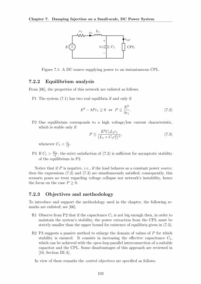
Chapter 7. Damping Injection on a Small-scale, DC Power System
−+E
r1 L1x1
C1
+
−x2 CPL
icpl
1Figure 7.1: A DC source supplying power to an instantaneous CPL.
7.2.2 Equilibrium analysis
From [66], the properties of this network are enlisted as follows.
P1 The system (7.1) has two real equilibria if and only if
E2 − 4Pr1 ≥ 0 ⇔ P ≤ E2
4r1
. (7.2)
P2 One equilibrium corresponds to a high voltage/low current characteristic,which is stable only if
P ≤ E2C1L1r1
(L1 + C1r21) 2
, (7.3)
whenever C1 <L1
r21.
P3 If C1 >4L1
r21, the strict satisfaction of (7.2) is sufficient for asymptotic stability
of the equilibrium in P2.
Notice that if P is negative, i.e., if the load behaves as a constant power source,then the expressions (7.2) and (7.3) are simultaneously satisfied; consequently, thisscenario poses no treat regarding voltage collapse nor network’s instability, hencethe focus on the case P ≥ 0.
7.2.3 Objectives and methodology
To introduce and support the methodology used in the chapter, the following re-marks are enlisted; see [66].
R1 Observe from P2 that if the capacitance C1 is not big enough then, in order tomaintain the system’s stability, the power extraction from the CPL must bestrictly smaller than the upper bound for existence of equilibria given in (7.3).
R2 P3 suggests a passive method to enlarge the domain of values of P for whichstability is ensured. It consists in increasing the effective capacitance C1,which can be achieved with the open-loop parallel interconnection of a suitablecapacitor and the CPL. Some disadvantages of this approach are reviewed in[19, Section III.A].
In view of these remarks the control objectives are specified as follows.
103

Chapter 7. Damping Injection on a Small-scale, DC Power System
O1 Regulate the voltage x2 around a constant value.
O2 Relax the upper bound for P established in (7.3).
O3 Achieve these objectives without the knowledge of P .
Following the work of [19] and [129], to achieve these objectives a power converteris connected in parallel with the CPL and design a control strategy that stabilizesthe overall network to a desired equilibrium point. The detailed description of theaugmented circuit is carried out in the next section and the presentation of thecontrol law—which is the main contribution of the chapter—is done in Section 7.4.
7.3 Augmented Circuit Model
As proposed in [19] and [129], the network of Fig. 7.1 is augmented by adding acontrolled DC-DC power converter in parallel with the load, which results in thecircuit shown in Fig. 7.2. The converter, which in the sequel is referred to as shuntdamper, is composed of two complementary switches u and (1−u), a lossy inductorL2 > 0, a capacitor C2 > 0, and a resistor r3 > 0; the latter models the lossesassociated with the switching devices.
−+ E
r1 L1 x1
C1
+
−x2
icpl
r2 L2 x3
1− u
u
r3 C2
+
−x4
Switches’ states:
1 ⇒ closed
0 ⇒ open
1Figure 7.2: The network of Fig. 7.1 is augmented by adding a power converter inparallel with the load.
The averaged dynamic model of the augmented system is given by
L1x1 = −r1x1 − x2 + E,
C1x2 = x1 −P
x2
− x3,
L2x3 = −r2x3 − ux4 + x2,
C2x4 = −(
1r3
)x4 + ux3,
(7.4)
where x3 is the current through L2, x4 is the voltage across C2, and u ∈ (0, 1)—which is the system’s control variable—represents a duty cycle. The state space of
104

Chapter 7. Damping Injection on a Small-scale, DC Power System
the system is given as
X := x ∈ R4 : x2 > 0, x4 > 0.
It shall be underscored that x1—being the current of a reduced model of the network—is not measurable, and the power P is unknown.
For future reference, the system (7.4) is written in an input-affine form, x = f(x) +g(x)u, by defining
f(x) :=
− r1L1x1 − x2
L1+ E
L1x1C1− P
C1x2− x3
C1
− r2L2x3 + x2
L2
−( 1r3
) x4C2
, g(x) :=
00− x4L2x3C2
, (7.5)
the i-th entries of which are denoted as fi or gi, respectively.
7.4 Main results
This section reports a nonlinear, adaptive, state-feedback controller that is suchthat the augmented network of Fig. 7.2 complies with the control objectives de-scribed in Subsection 7.2.3. Towards this end, first the existence of equilibria of(7.4) is analyzed and constraints, on the system’s parameters, for their physical fea-sibility are established. Secondly, under the assumption that x1 can be measured,and the constant parameter P is known, a full-information input-output lineariza-tion controller [48], that asymptotically stabilizes a specified equilibrium state, ispresented. Finally, this controller is complemented with an observer for x1 and anon-line estimator for P—yielding an adaptive, state-feedback controller design.
7.4.1 Existence of equilibria
A pair (x, u) ∈ X × (0, 1) is an equilibrium of (7.4) if and only if it belongs to theset
E := (x, u) ∈ X × R : f(x) + g(x)u = 0,where the mappings f and g are given in (7.5). An important issue in the design isto ensure that the power consumption of the shunt damper is minimal. In order tocarry-out this analysis, it is convenient to parametrize x in terms of u, as follows.
Proposition 7.1. Consider the augmented circuit model (7.4). Fix 0 < u < 1 as adesired steady state duty cycle. Then the following conditions hold true.
C1 (x, u) ∈ E if and only if
∆(P ) := E2`2 − 4Pr1`1 ≥ 0, (7.6)
where`1 := r3u
2 + r1 + r2, `2 := r3u2 + r2
105
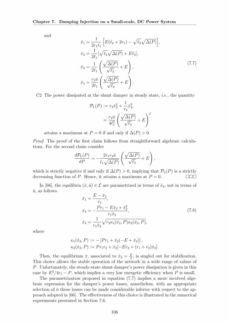
Chapter 7. Damping Injection on a Small-scale, DC Power System
and
x1 =1
2r1`1
[E(`2 + 2r1)−
√`2
√∆(P )
],
x2 =1
2`1
[√`2
√∆(P ) + E`2],
x3 =1
2`1
(√∆(P )√`2
+ E
),
x4 =r3u
2`1
(√∆(P )√`2
+ E
).
(7.7)
C2 The power dissipated at the shunt damper in steady state, i.e., the quantity
PL(P ) := r2x23 +
1
r3
x24,
=r3u
4`21
(√∆(P )√`2
+ E
)2
attains a maximum at P = 0 if and only if ∆(P ) > 0.
Proof. The proof of the first claim follows from straightforward algebraic calcula-tions. For the second claim consider
dPL(P )
dP= − 2r1r3u
`1
√∆(P )
(√∆(P )√`2
+ E
),
which is strictly negative if and only if ∆(P ) > 0, implying that PL(P ) is a strictlydecreasing function of P . Hence, it attains a maximum at P = 0.
In [66], the equilibria (x, u) ∈ E are parametrized in terms of x2, not in terms ofu, as follows
x1 =E − x2
r1
,
x3 = −Pr1 − Ex2 + x22
r1x2
,
x4 =1
r1x2
√r3κ1(x2, P )κ2(x2, P ),
(7.8)
where
κ1(x2, P ) := − [Pr1 + x2(−E + x2)] ,
κ2(x2, P ) := Pr1r2 + x2[−Er2 + (r1 + r2)x2].
Then, the equilibrium x, associated to x2 = E2
, is singled out for stabilization.This choice allows the stable operation of the network in a wide range of values ofP . Unfortunately, the steady-state shunt-damper’s power dissipation is given in thiscase by E2/4r1 − P , which implies a very low energetic efficiency when P is small.
The parametrization proposed in equation (7.7) implies a more involved alge-braic expression for the damper’s power losses, nonetheless, with an appropriateselection of u these losses can be made considerable inferior with respect to the ap-proach adopted in [66]. The effectiveness of this choice is illustrated in the numericalexperiments presented in Section 7.6.
106
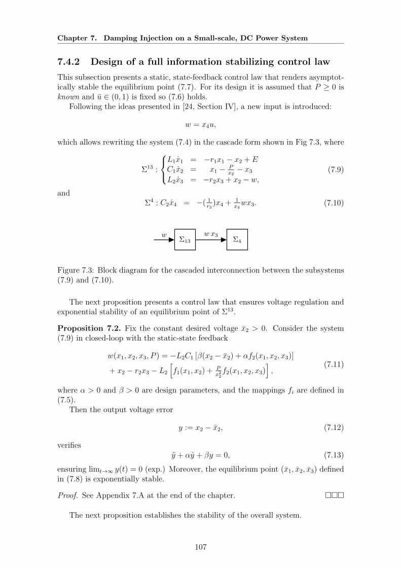
Chapter 7. Damping Injection on a Small-scale, DC Power System
7.4.2 Design of a full information stabilizing control law
This subsection presents a static, state-feedback control law that renders asymptot-ically stable the equilibrium point (7.7). For its design it is assumed that P ≥ 0 isknown and u ∈ (0, 1) is fixed so (7.6) holds.
Following the ideas presented in [24, Section IV], a new input is introduced:
w = x4u,
which allows rewriting the system (7.4) in the cascade form shown in Fig 7.3, where
Σ13 :
L1x1 = −r1x1 − x2 + EC1x2 = x1 − P
x2− x3
L2x3 = −r2x3 + x2 − w,(7.9)
andΣ4 : C2x4 = −( 1
r3)x4 + 1
x4wx3. (7.10)
Σ13 Σ4w w x3
Figure 7.3: Block diagram for the cascaded interconnection between the subsystems(7.9) and (7.10).
The next proposition presents a control law that ensures voltage regulation andexponential stability of an equilibrium point of Σ13.
Proposition 7.2. Fix the constant desired voltage x2 > 0. Consider the system(7.9) in closed-loop with the static-state feedback
w(x1, x2, x3, P ) = −L2C1 [β(x2 − x2) + αf2(x1, x2, x3)]
+ x2 − r2x3 − L2
[f1(x1, x2) + P
x22f2(x1, x2, x3)
],
(7.11)
where α > 0 and β > 0 are design parameters, and the mappings fi are defined in(7.5).
Then the output voltage error
y := x2 − x2, (7.12)
verifiesy + αy + βy = 0, (7.13)
ensuring limt→∞ y(t) = 0 (exp.) Moreover, the equilibrium point (x1, x2, x3) definedin (7.8) is exponentially stable.
Proof. See Appendix 7.A at the end of the chapter.
The next proposition establishes the stability of the overall system.
107
Chapter 7. Damping Injection on a Small-scale, DC Power System
Proposition 7.3. Fix the constant desired voltage x2 > 0. Consider the system(7.9), (7.10) in closed-loop with the static-state feedback (7.11). Assume the sys-tem’s initial condition is sufficiently close to the equilibrium x defined in (7.8). Then,x4(t) > 0, for all t ≥ 0 and limt→∞ x(t) = x, exponentially.
Proof. See Appendix 7.B at the end of the chapter.
As a direct application of Propositions 7.2 and 7.3, the full-information input-output linearizing controller of the overall dynamics (7.4) is presented next.
Proposition 7.4. Consider the system (7.4) in closed-loop with the static state-feedback control law
u = 1x4w(x1, x2, x3, P ), (7.14)
where w is given in (7.11). Then, x ∈ E is a locally, exponentially stable equilibriumpoint of the closed-loop system.
7.4.3 Stabilization with unknown CPL power
An adaptive version of controller (7.14) is established now by adding an observer forx1 and an on-line estimator for the constant parameter P , which are now assumedto be unmeasured and unknown, respectively.
Proposition 7.5. Consider the system (7.1) and assume that x2 is positive andbelongs to the interval [xmin
2 , xmax2 ]. Define the adaptive observer
q1 =E
L1
− x2
L1
− r1
L1
x1 + k1P − k1x2x1 + k1x2x3,
q2 = −k2P + k2x2x1 − k2x2x3,
x1 = q1 +1
2k1C1x
22,
P = q2 −1
2k2C1x
22,
(7.15)
where k1 and k2 are such that
− r1
xmax2 L1
< k1 ≤ 0,
T1(xmax2 )− 2T2(xmax
2 ) < k2 < T1(xmax2 ) + 2T2(xmax
2 ),(7.16)
where
T1(ω) :=ωk1L1 + 2r1
ω2L1
,
T2(ω) :=1
L1ω2
√ωk1L1r1 + r2
1.
Thenlimt→∞|x1(t)− x1(t)| = 0, lim
t→∞P (t) = P,
exponentially.
Proof. See Appendix 7.C at the end of the chapter.
108
Chapter 7. Damping Injection on a Small-scale, DC Power System
The stability of the system (7.4) in closed-loop with an adaptive version of thecontrol law (7.14) is established next.
Proposition 7.6. Let k1 and k2 be such that (7.16) hold. Fix u and compute xfrom (7.7). Define the adaptive control law
u = 1x4w(x1, x2, x3, P ), (7.17)
where w is given in (7.11), and x1, P are generated by the adaptive observer (7.15).Then, (x, x1, P ) = (x, x1, P ) is an asymptotically stable equilibrium point of theoverall system.
Proof. See Appendix 7.D at the end of the chapter.
Remark 7.1. A key extension with respect to the research done in [66] is the use ofan adaptive, observer-based feedback law, the implementation of which requires onlythe measurement of the variables x2 and x3, which is easy to obtain in a physicalsetup.
Remark 7.2. The computation of the control law (7.11), (7.17) requires the knowl-edge of x2, which is dependent on the unknown P ; see equation (7.7). In theexperiments reported in Section 7.6, the value of x2 is computed from the estimateof P , i.e. P , discretely, not continuously in time. This approach is common inhierarchical and supervisory control of AC and DC microgrids [42] and preventsintroducing x2 to the controller if an overshoot of the time-varying signal P occurs,it also simplifies the controller design.
Remark 7.3. Through direct, but lengthy, computations, it can be shown that thecondition (7.16) may be replaced by the conditions
0 < k1 <8r1(xmin
2 + xmax2 )
L1(xmax2 − xmin
2 )2,
T1(xmin2 )− 2T2(xmin
2 ) < k2 < T1(xmax2 ) + 2T2(xmax
2 ).
(7.18)
7.5 Numerical simulations
This sections reports two simulations that illustrate the good performance of theproposed controller. The physical parameters of the system (7.4) are given in Table7.1, and the parameters for the adaptive output-feedback controller of equation(7.11), (7.15), (7.17) are selected as
α = 3× 10⁴, β =α2
4, k1 = 10, k2 = 25.
In all simulations a saturation function has been used to keep u ∈ (0, 1).
7.5.1 Simulation 1
The value u = 0.5 is fixed and the equilibrium point to be stabilized x is computedvia (7.7) for P = 0. The initial condition has been fixed at that equilibrium point.Then, at t = 3 s, a step change in the CPL power, from P = 0 W to P = 479 W, is
109
Chapter 7. Damping Injection on a Small-scale, DC Power System
introduced, this yields a new equilibrium point to be stabilized: x|P=479. Addition-ally, at t = 6 s, the CPL is stepped down to 0 W once again. It should be pointed outthat P = 479 W still verifies the necessary and sufficient condition for existence ofequilibria of the network without the shunt damper established in Subsection 7.2.2.However, it is well above the necessary bound for stability given in (7.3), which isgiven by
E2C1L1r1
(L1 + C1r21) 2
= 276.9 W.
Hence, without the shunt damper the equilibria are unstable.
Table 7.1: Parameters for the circuit in Fig. 7.2
r1 = 0.3 Ω L1 = 85.0 µH C1 = 200 µF E = 24.0 Vr2 = 5 mΩ L2 = 100 µH C2 = 1.0 mF r3 = 1 kΩ
Fig. 7.4 shows the time history of each component of the state x against theirequilibrium values, respectively; a zoom of these plots around the second transient isshown in Fig. 7.5. It is clear from these figures that fast convergence is achieved. InFigs. 7.6 and 7.7 are plotted the control variable u. It can be seen from the figuresthat, except from some peaks at the instants of power change where the saturationenters into play, the control signal remains all the time within the admissible bounds.The figures also show the errors in the state and parameter estimates, which convergeto zero very fast. Finally, the plots of the power consumption of the shunt damper,i.e., the product PL = x2x3, shows that the controller is energetically efficient.
7.5.2 Simulation 2
This simulation shows in detail the performance of the adaptive observer. Thesimulation starts from the initial condition x(0) = x|P=10, then, at t = 3 s, a largestep change in the CPL power, from P = 10 W to P = 300 W, is introduced. Figs.7.8 and 7.9 show the excellent performance of the state observer and the slightlyslower tracking of the power estimator.
7.6 Experimental validation
In order to investigate the practical feasibility of the proposed control scheme, anexperimental setup has been designed and built according to the electrical schemeshown in Fig. 7.2. The test bench is composed of a DC voltage source DeltaElektronika SM-52-AR-60, the passive components of the RLC circuit (r1, L1 andC1), a DC boost converter and a custom-designed and built CPL. The CPL has amaximum allowed current Imax = 40 A and a maximum power in steady state ofPmax = 900 W. The physical setup of the experiments is shown in Fig. 7.10.
The measured parameters of the system are the same as in Table 7.1, except forr1 that in the physical setup is r1 = 0.314 Ω. The gains of the adaptive controllerare the same as in section 7.5.
It is underscored that the CPL has been designed to approximate an ideal alge-braic behavior, i.e., with a much wider bandwidth than the expected dynamics ofthe whole system. Particularly, in a LTspice simulation with an ideal DC voltage
110
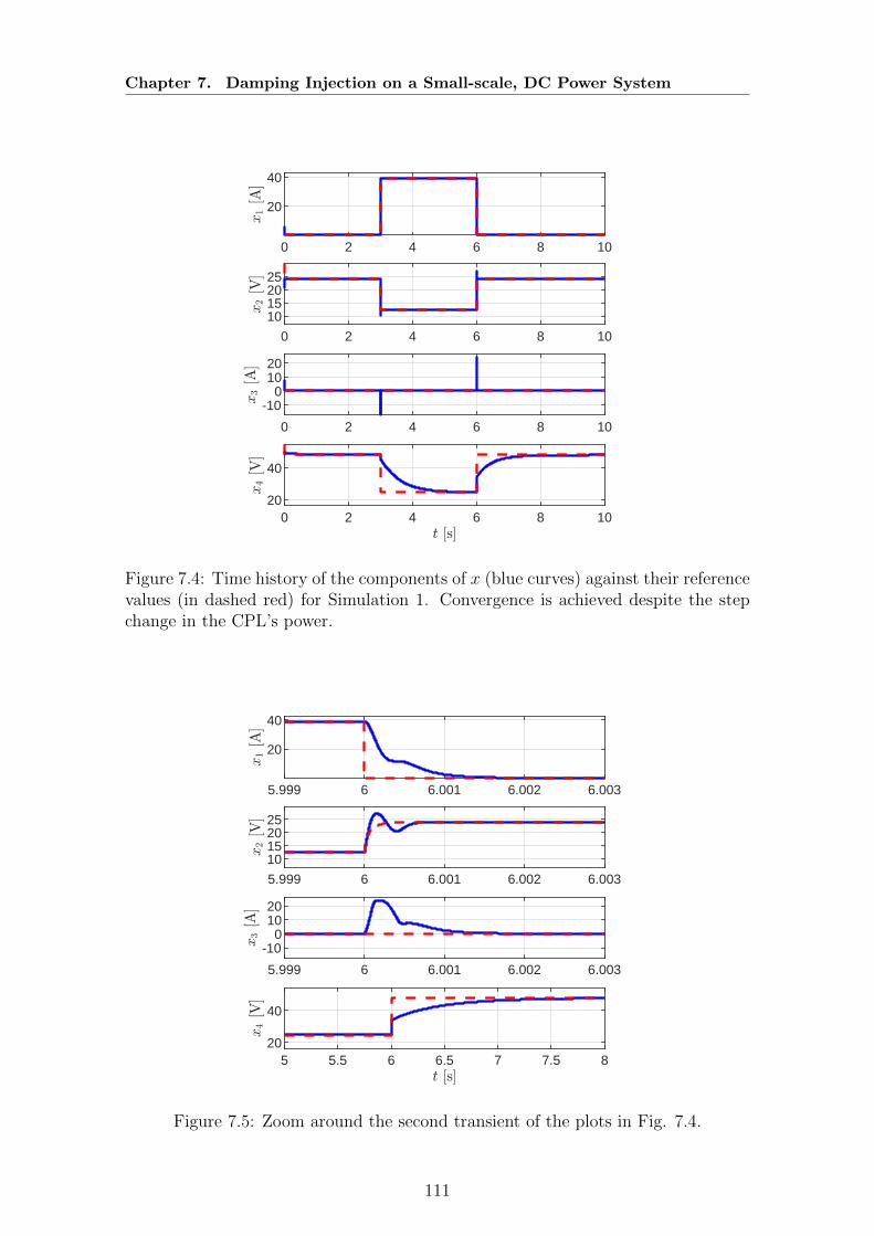
Chapter 7. Damping Injection on a Small-scale, DC Power System
0 2 4 6 8 10
20
40
0 2 4 6 8 10
10152025
0 2 4 6 8 10
-100
1020
0 2 4 6 8 1020
40
Figure 7.4: Time history of the components of x (blue curves) against their referencevalues (in dashed red) for Simulation 1. Convergence is achieved despite the stepchange in the CPL’s power.
5.999 6 6.001 6.002 6.003
20
40
5.999 6 6.001 6.002 6.003
10152025
5.999 6 6.001 6.002 6.003
-100
1020
5 5.5 6 6.5 7 7.5 820
40
Figure 7.5: Zoom around the second transient of the plots in Fig. 7.4.
111

Chapter 7. Damping Injection on a Small-scale, DC Power System
0 2 4 6 8 100
0.5
1
0 2 4 6 8 10-400-200
0200400
0 2 4 6 8 10-0.2
00.20.4
0 2 4 6 8 10-200
0200400600
Figure 7.6: Time history of u, the power estimation error P , the observer error x1
and the power losses PL = x2 · x3 (in blue) against their respective reference values(in dashed red) for Simulation 1.
5.5 6 6.5 7 7.5 80
0.5
1
6 6.0002 6.0004 6.0006 6.0008 6.0010
200400
6 6.0005 6.001 6.00150
0.2
0.4
6 6.0005 6.001 6.0015 6.0020
200400600
Figure 7.7: Zoom around the second transient of the plots in Fig. 7.6.
112
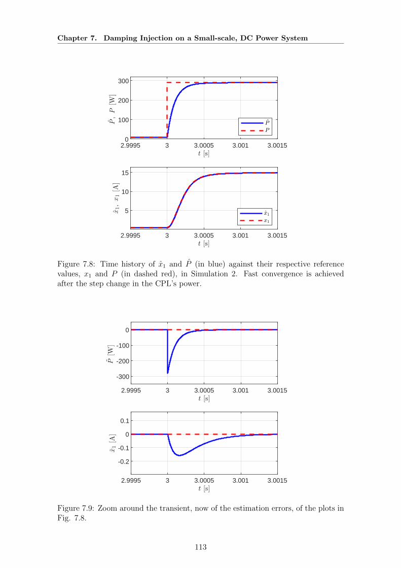
Chapter 7. Damping Injection on a Small-scale, DC Power System
2.9995 3 3.0005 3.001 3.00150
100
200
300
2.9995 3 3.0005 3.001 3.0015
5
10
15
Figure 7.8: Time history of x1 and P (in blue) against their respective referencevalues, x1 and P (in dashed red), in Simulation 2. Fast convergence is achievedafter the step change in the CPL’s power.
2.9995 3 3.0005 3.001 3.0015
-300
-200
-100
0
2.9995 3 3.0005 3.001 3.0015
-0.2
-0.1
0
0.1
Figure 7.9: Zoom around the transient, now of the estimation errors, of the plots inFig. 7.8.
113
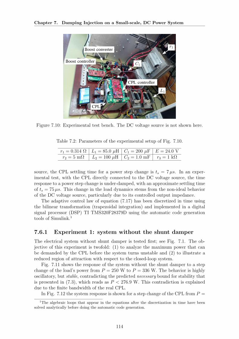
Chapter 7. Damping Injection on a Small-scale, DC Power System
Figure 7.10: Experimental test bench. The DC voltage source is not shown here.
Table 7.2: Parameters of the experimental setup of Fig. 7.10.
r1 = 0.314 Ω L1 = 85.0 µH C1 = 200 µF E = 24.0 Vr2 = 5 mΩ L2 = 100 µH C2 = 1.0 mF r3 = 1 kΩ
source, the CPL settling time for a power step change is ts = 7µs. In an exper-imental test, with the CPL directly connected to the DC voltage source, the timeresponse to a power step change is under-damped, with an approximate settling timeof ts = 75µs. This change in the load dynamics stems from the non-ideal behaviorof the DC voltage source, particularly due to its controlled output impedance.
The adaptive control law of equation (7.17) has been discretized in time usingthe bilinear transformation (trapezoidal integration) and implemented in a digitalsignal processor (DSP) TI TMS320F28379D using the automatic code generationtools of Simulink.1
7.6.1 Experiment 1: system without the shunt damper
The electrical system without shunt damper is tested first; see Fig. 7.1. The ob-jective of this experiment is twofold: (1) to analyze the maximum power that canbe demanded by the CPL before the system turns unstable and (2) to illustrate areduced region of attraction with respect to the closed-loop system.
Fig. 7.11 shows the response of the system without the shunt damper to a stepchange of the load’s power from P = 250 W to P = 336 W. The behavior is highlyoscillatory, but stable, contradicting the predicted necessary bound for stability thatis presented in (7.3), which reads as P < 276.9 W. This contradiction is explaineddue to the finite bandwidth of the real CPL.
In Fig. 7.12 the system response is shown for a step change of the CPL from P =
1The algebraic loops that appear in the equations after the discretization in time have beensolved analytically before doing the automatic code generation.
114

Chapter 7. Damping Injection on a Small-scale, DC Power System
250 W to P = 338 W, where an unstable behavior is observed.2 It is concluded thenthat the upper bound for the system’s stability is within the interval [336, 338] W.
The unstable behavior of the system without the shunt damper to a power stepchange from P = 10 W to P = 300 W can be observed in Fig. 7.13. Notice thateven if the load’s power is lower than the necessary upper bound for stability, adrastic load change can also destabilize the system. Clearly, in this scenario, theformer system’s equilibrium lies outside the domain of attraction of the latter one.This behavior is to be contrasted with respect to the operation with the controlledshunt damper, which is discussed next.
-4.99 -4.98 -4.97 -4.96 -4.95
10-3
10
15
20
25
-4.99 -4.98 -4.97 -4.96 -4.95
10-3
10
20
30
Figure 7.11: System response to a step from P = 250 W to P = 336 W without thecontrolled shunt damper. The blue curve (above) corresponds to the voltage x2; thered curve (below), the current x1.
2In all the unstable experiments the CPL stops, i.e., abruptly goes to zero, either because thecurrent goes outside of the operating range, which is [0, 40] A, or because the voltage at the CPLinput terminals falls below the safety limit, which has been situated at a value considerably lowerthan that corresponding to the maximum power (≈ 12 V).
115

Chapter 7. Damping Injection on a Small-scale, DC Power System
-3.5 -3 -2.5 -2
10-3
10
20
30
40
-3.5 -3 -2.5 -2
10-3
-10
0
10
20
30
Figure 7.12: System response to a step from P = 250 W to P = 338 W without thecontrolled shunt damper. The blue curve (above) corresponds to the voltage x2; thered curve (below), the current x1.
-4 -3.5 -3 -2.5 -2
10-3
0
10
20
30
-4 -3.5 -3 -2.5 -2
10-3
0
10
20
Figure 7.13: System response to a step from P = 10 W to P = 300 W without thecontrolled shunt damper. The blue curve (above) corresponds to the voltage x2; thered curve (below), the current x1.
116

Chapter 7. Damping Injection on a Small-scale, DC Power System
7.6.2 Experiment 2: system with the controlled shunt damper
The stable response of the system with the controlled shunt damper in the presenceof a step change in the CPL’s power, from P = 250 W to P = 380W, is shown inFig. 7.14. Notice that the CPL power is stepped up to a value much bigger thanthose reported for Experiment 1, yet the system is able to keep operating in a stablemanner, which implies a relaxation of the necessary bound for stability of the systemin without the shunt damper.
The system response to a CPL step change from P = 10 W to P = 300 W isshown in Fig. 7.15, where a stable behavior is observed. By making a comparisonwith the results reported in Fig. 7.13, it can be concluded that the domain ofattraction of the system with the controlled shunt damper has been successfullyincreased with respect to its operation without the shunt damper.
To study the energetic efficiency of the proposed active damping scheme, Fig.7.16 reports the measured power consumption of the shunt damper during its oper-ation and in the presence of a step change in the CPL’s power from P = 10 W toP = 300W. Clearly, a low power consumption is evidenced. Before the change inthe CPL’s power, when the system is in steady state, it can appreciated that thepower losses are nearly zero (approximately 4 W), these losses are due to the passivecomponents of the converter and the mosfets switching losses. During the first 2 msof the transient, the average power is negative, that is, the shunt damper is injectspower to the system to stabilize it. After the transient the system reaches anotherstable equilibrium and the average power losses of the damper return to a minimum.
Finally, from successive experiments with different power steps in the CPL, ithas been determined that the experimental limit for the stable operation of thesystem with the controlled shunt damper is in the range [410, 420] W. This valuerepresents, approximately, the 90% of the range of power for existence of equilibriumin the system, which from (7.2) reads as P < 458.6 W.3 Clearly, the former value isdrastically superior with respect to the operation of the network without the shuntdamper.
3Without taking into account the power needed to supply the operating losses of the boostconverter.
117

Chapter 7. Damping Injection on a Small-scale, DC Power System
-0.035 -0.03 -0.025 -0.02
12
14
16
18
20
22
-0.035 -0.03 -0.025 -0.02
15
20
25
Figure 7.14: System response to a step from P = 250 W to P = 380 W with thecontrolled shunt damper. The blue curve (above) corresponds to the voltage x2; thered curve (below), the current x1.
0 5 10 15
10-3
15
20
25
0 5 10 15
10-3
5
10
15
Figure 7.15: System response to a step from P = 10 W to P = 300 W with thecontrolled shunt damper. The blue curve (above) corresponds to the voltage x2; thered curve (below), the current x1.
118

Chapter 7. Damping Injection on a Small-scale, DC Power System
-10 -8 -6 -4 -2
10-4
15
20
25
-10 -8 -6 -4 -2
10-4
-15-10
-505
-10 -8 -6 -4 -2
10-4
-300-200-100
0100
Figure 7.16: Measured power consumption of the shunt damper (Bottom figure).The closed-loop system is subject to a step change in the load’s power from P = 10 Wto P = 300 W.
7.7 Summary
In this chapter, a nonlinear stabilization method for a DC small-scale power systemthat supplies electric energy to a CPL has been explored. By adding a controlledDC-DC power converter in parallel with the load and using standard input-outputlinearization with a suitable tailored adaptive observer, a nonlinear adaptive controllaw for the stabilization of the overall network has been proposed. Furthermore,the proposed design permits the stable operation of the network for a wide rangeof values of the CPL and is able to relax some necessary stability bounds that areimposed if the system were to be operated without the shunt damper. Finally, thegood performance of the controller has been validated through experiments on areal small-scale DC network.
Technical Appendices of the Chapter
7.A Proof of Proposition 7.2
From (7.9) a and (7.12) it follows that
y = x2 =1
C1
(x1 −
P
x2
− x3
)=: F2(x1, x2, x3),
119
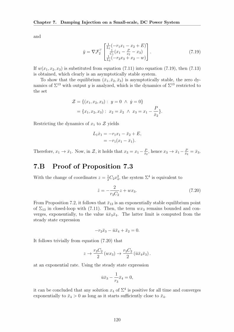
Chapter 7. Damping Injection on a Small-scale, DC Power System
and
y = ∇F>2
1L1
(−r1x1 − x2 + E)1C1
(x1 − Px2− x3)
1L2
(−r2x3 + x2 − w)
. (7.19)
If w(x1, x2, x3) is substituted from equation (7.11) into equation (7.19), then (7.13)is obtained, which clearly is an asymptotically stable system.
To show that the equilibrium (x1, x2, x3) is asymptotically stable, the zero dy-namics of Σ13 with output y is analyzed, which is the dynamics of Σ13 restricted tothe set
Z = (x1, x2, x3) : y = 0 ∧ y = 0
= x1, x2, x3) : x2 = x2 ∧ x3 = x1 −P
x2
.
Restricting the dynamics of x1 to Z yields
L1x1 = −r1x1 − x2 + E,
= −r1(x1 − x1).
Therefore, x1 → x1. Now, in Z, it holds that x3 = x1− Px2
, hence x3 → x1− Px2
= x3.
7.B Proof of Proposition 7.3
With the change of coordinates z = 12C2x
24, the system Σ4 is equivalent to
z = − 2
r3C2
z + wx3. (7.20)
From Proposition 7.2, it follows that x13 is an exponentially stable equilibrium pointof Σ13 in closed-loop with (7.11). Then, the term wx3 remains bounded and con-verges, exponentially, to the value ux3x4. The latter limit is computed from thesteady state expression
−r2x3 − ux4 + x2 = 0.
It follows trivially from equation (7.20) that
z → r3C2
2(wx3)→ r3C2
2(ux4x3) .
at an exponential rate. Using the steady state expression
ux3 −1
r3
x4 = 0,
it can be concluded that any solution x4 of Σ4 is positive for all time and convergesexponentially to x4 > 0 as long as it starts sufficiently close to x4.
120

Chapter 7. Damping Injection on a Small-scale, DC Power System
7.C Proof of Proposition 7.5
The derivatives of the errors x1 := x1 − x1 and P := P − P are given by
˙x1 = − r1
L1
x1 − k1x2x1 + k1P ,
˙P = −k2P + k2x2x1.
(7.21)
To show that the origin of (7.21) is exponentially stable, consider then the Lyapunovfunction candidate
V :=1
2x2
1 +1
2P 2
and its derivative with respect to t, along the trajectories of (7.21), given by
V = x1˙x1 + P ˙P
= −(r1
L1
)x2
1 − k1x2x21 + k1P x1
− k2P2 + k2x2x1P
= −[x1
P
]>M(x2)
[x1
P
],
where
M(x2) =
[r1L1
+ k1x2 −12(k1 + k2x2)
−12(k1 + k2x2) k2
].
Clearly, V is a strict Lyapunov function if and only if M(x2) > 0. The latter issatisfied if and only if
r1L1
+ k1x2 > 0,
detM(x2) = k2
(r1
L1
+ k1x2
)− 1
4(k1 − k2x2)2 > 0,
hold simultaneously. Through lengthy but direct computations, it can be verifiedthat these conditions hold—in the domain x2 ∈ [xmin
2 , xmax2 ]— whenever (7.16) (or
(7.18)) hold. This concludes the proof.
7.D Proof of Proposition 7.6
Recall from the proof of Proposition 7.5 that the observer’s error dynamics is givenby (7.21). On the other hand, it can be shown through lengthy (but straightforward)computations that (7.4) in closed-loop with (7.17) has the form
x =
[f(x) + g(x)
w(x1, x2, x3, P )
x4
]+ g(x)ε(x, x1, P ), (7.22)
where the mapping ε is such that ε(x, 0, 0) = 0 for all x.From Proposition 7.4 it follows that if ε ≡ 0 for all t, then x is an asymptotically
stable equilibrium of (7.22). Furthermore, Proposition 7.5 establishes that the originof the observer’s error dynamics is exponentially stable. Consequently, invoking [102,Proposition 4.1], it is concluded that (x, x1, P ) = (x, 0, 0) is an asymptotically stableequilibrium point of the overall system.
121

Part IV
EPILOGUE

Chapter 8
Conclusions
This thesis has explored different problems that emerge in the analysis and controlof electrical power systems with constant power loads. The novel contributions ofthe present document, which are aimed at better understanding and possibly solvethese problems, are summarized in the following list.
• For general multi-port linear AC networks with constant power loads, neces-sary LMI-based conditions for the existence of a sinusoidal steady state regimehave been established. For one- or two-port networks and free active (or re-active) power of the load’s components, these conditions are also sufficient.Particularly, for single-port networks, the admissibility condition can be testeddirectly from the data of the problem.
These results may be extended in two main directions: (i) establish if theproposed LMI test is also sufficient for existence of steady states, and (ii) if asteady state exists, study its stability or attractivity properties.
• For general models in modern and conventional AC and DC power systems, ithas been shown that their steady states satisfy a system of nonlinear algebraicequations whose vector field, when associated to an ODE, possesses propertiesof monotonicity. It has been established that if these models do admit steadystates, then there is a distinguished one that dominates, component-wise, allthe other ones and that furthermore is asymptotically stable. An algorithm toverify if the solutions of the ODE will converge to the distinguished equilibriumor not has also been proposed. In the treated power system models, the latterresults imply the existence of a high-voltage steady state that is also voltageregular.
The analysis of diverse ODEs’ integration technique to identify efficient ways ofimplementing the proposed numerical algorithm when dealing with large-scalesystems is an interesting path of future research.
• A class of port-Hamiltonian systems, in which the control input directly actson the power balance equation, has been extensively investigated. These sys-tems, coined power-controlled Hamiltonian systems, have been shown to beshifted passive, as long as the trajectories remain in a clearly specified set.The exhibited shifted passivity properties have been used to establish the sta-bility of the intrinsically non zero equilibrium and to even provide an easy
123
Chapter 8. Conclusions
to compute domain of attraction of them, under some simplifying assump-tions. The introduced framework has been applied to analyze the stability ofDC power systems with constant power loads that include general multi-portnetworks and the synchronous generator.
As a line of further research, the design of simple, high-performance con-trollers with guaranteed stability domains may be explored. In addition, themore general case of state-dependent interconnection and dissipation matrices[75], needs to be further investigated. Also the applicability of the methodol-ogy to AC circuits with constant power loads and higher order models of thesynchronous generator [39] may be addressed.
• The control problem of regulating the output voltage of a buck-boost convertersupplying electric energy to a CPL with unknown power has been addressed.A control law designed following the IDA-PBC technique in combination ofan online estimator for the load power, has been presented. Moreover, per-formance limitations of classical PD controller have also been reviewed. Inaddition, the effectiveness of the proposed control scheme has been verifiedthrough realistic simulations.
The designed control law is of great algebraic complexity, which may stymieits practical application, hence further research can be carried out to simplifyit. Furthermore, the design of a current observer to remove the need for itsmeasurement, which is an issue of practical interest, may also be investigated.
• The nonlinear active damping of a DC small-scale power system with a CPLhas been addressed. The proposed scheme considers the addition of a con-trolled DC-DC power converter for which a nonlinear adaptive control law isdesigned. The stable operation of the network for a wide range of values ofthe CPL is guaranteed, and a clear extension of the CPL’s operation range,with respect to the open-loop case, is verified. Moreover, the performance ofthe controller has been validated through experiments on a real small-scaleDC network.
Some directions of further research include: (i) computation of estimates of theregion of attraction, (ii) analyze the robustness against parameter uncertainty,and (iii) extend the analysis to networks with several loads distributed in ameshed topology.
124
Bibliography
[1] V. Ajjarapu and C. Christy. “The continuation power flow: a tool for steadystate voltage stability analysis”. In: IEEE Transactions on Power Systems7.1 (1992), pp. 416–423 (cited on page 40).
[2] A. Alonso and B. Ydstie. “Stabilization of distributed systems using irre-versible thermodynamics”. In: Automatica 37.11 (2001), pp. 1739–1755 (citedon page 67).
[3] S. Anand and B. Fernandes. “Reduced-Order Model and Stability Analysis ofLow-Voltage DC Microgrid”. In: IEEE Transactions on Industrial Electronics60.11 (2013), pp. 5040–5049 (cited on pages 4, 138).
[4] P. Anderson and A. Fouad. Power System Control and Stability. J.Wiley &Sons, 2002 (cited on pages 2, 3, 136, 138).
[5] A. Araposthatis, A. Sastry, and P. Varaiya. “Analysis of power-flow equa-tion”. In: International Journal of Electrical Power & Energy Systems 3(1981), pp. 115–126 (cited on page 18).
[6] M. Arcak, C. Meissen, and A. Packard. Networks of dissipative systems: com-positional certification of stability, performance, and safety. Springer, 2016(cited on page 12).
[7] D. Ariyasinghe and D. Vilathgamuwa. “Stability analysis of microgrids withconstant power loads”. In: IEEE International Conference on SustainableEnergy Technologies. 2008, pp. 279–284 (cited on page 4).
[8] A. Astolfi, D. Karagiannis, and R. Ortega. Nonlinear and Adaptive Controlwith Applications. Berlin: Springer-Verlag, 2008 (cited on pages 83, 89).
[9] N. Barabanov, R. Ortega, R. Grino, and B. Polyak. “On existence andstability of equilibria of linear time-invariant systems with constant powerloads”. In: IEEE Transactions on Circuits and Systems I: Regular Papers63.1 (2016), pp. 114–121 (cited on pages 4, 19, 21–25, 27, 28, 33, 53, 54, 82,138).
[10] M. Belkhayat, R. Cooley, and A. Witulski. “Large signal stability criteriafor distributed systems with constant power loads”. In: Power ElectronicsSpecialists Conference, 1995. PESC ’95 Record., 26th Annual IEEE. Vol. 2.1995, pp. 1333–1338 (cited on pages 4, 77, 138).
[11] D. Bertsimas and J. Tsitsiklis. Introduction to Linear Programming. AthenaScientific, 1997 (cited on page 46).
[12] N. Biggs. Algebraic graph theory. Cambridge university press, 1993 (cited onpage 9).
125
Bibliography
[13] B. Bollobas. Modern graph theory. Springer Science & Business Media, 1998(cited on page 9).
[14] S. Bolognani and S. Zampieri. “On the existence and linear approximationof the power flow solution in power distribution networks”. In: IEEE Trans.Power Syst. 31.1 (2016), 163–172 (cited on pages 4, 14, 18, 138).
[15] B. Bose. “Global warming: Energy, environmental pollution, and the impactof power electronics”. In: IEEE Industrial Electronics Magazine 4.1 (2010),pp. 6–17 (cited on pages 2, 136).
[16] R. Brayton and J. Moser. “A theory of nonlinear networks. I”. In: Quarterlyof Applied Mathematics 22.1 (1964), pp. 1–33 (cited on pages 4, 138).
[17] L. Bregman. “The relaxation method of finding the common point of convexsets and its application to the solution of problems in convex programming”.In: USSR Computational Mathematics and Mathematical Physics 7.3 (1967),pp. 200 –217 (cited on pages 12, 67, 69).
[18] F. Bullo. Lectures on Network Systems. 1st ed. With contributions by J.Cortes, F. Dorfler, and S. Martinez. CreateSpace, 2018 (cited on pages 57,60).
[19] M. Carmeli, D. Forlani, S. Grillo, R. Pinetti, E. Ragaini, and E. Tironi. “Astabilization method for DC networks with constant-power loads”. In: IEEEInternational Energy Conference and Exhibition (ENERGYCON). Florence,Italy, 2012, pp. 617–622 (cited on pages 101–104).
[20] K. Cavanagh, J. Belk, and K. Turitsyn. “Transient stability guarantees for adhoc DC microgrids”. In: IEEE Control Systems Letters 2.1 (2017), pp. 139–144 (cited on pages 4, 77, 138).
[21] M. Cespedes, L. Xing, and J. Sun. “Constant-Power Load System Stabiliza-tion by Passive Damping”. In: IEEE Transactions on Power Electronics 26.7(2011), pp. 1832–1836 (cited on pages 4, 138).
[22] G. Cezar, R. Rajagopal, and B. Zhang. “Stability of interconnected DC con-verters”. In: IEEE 54th Annual Conference on Decision and Control (CDC).2015, pp. 9–14 (cited on page 77).
[23] H. Chiang and M. Baran. “On the existence and uniqueness of load flowsolution for radial distribution power networks”. In: IEEE Trans. CircuitsSyst. 37.3 (1990), 410–416 (cited on page 18).
[24] R. Cisneros, F. Mancilla, and R. Ortega. “Passivity-Based Control of a Grid-Connected Small-Scale Windmill With Limited Control Authority”. In: IEEEJournal of Emerging and Selected Topics in Power Electronics 1.4 (2013),pp. 247–259 (cited on page 107).
[25] M. Coste. An Introduction to Semialgebraic Geometry. Institut de RechercheMathematiques de Rennes, 2002 (cited on page 58).
[26] M. Cucuzzella, S. Trip, C. De Persis, X. Cheng, A. Ferrara, and A. van derSchaft. “A Robust Consensus Algorithm for Current Sharing and VoltageRegulation in DC Microgrids”. In: IEEE Transactions on Control SystemsTechnology (2018) (cited on page 52).
126
Bibliography
[27] J. Danskin. “The Theory of Max-Min, with Applications”. In: SIAM Journalon Applied Mathematics 14.4 (1966), pp. 641–664 (cited on page 62).
[28] G. Dantzig. Linear Programming and Extensions. Princeton university press,1966 (cited on page 46).
[29] S. Davis and K. Caldeira. “Consumption-based accounting of CO2 emis-sions”. In: Proceedings of the National Academy of Sciences. Vol. 107. 12.2010, pp. 5687–5692 (cited on pages 2, 136).
[30] C. De Persis, E. Weitenberg, and F. Dorfler. “A power consensus algorithmfor DC microgrids”. In: Automatica 89 (2018), pp. 364 –375 (cited on pages 3,137).
[31] C. Desoer and E. Kuh. Basic Circuit Theory. McGraw-Hill, 1969 (cited onpage 13).
[32] C. Desoer and M. Vidyasagar. Feedback Systems: Input-Output Properties.SIAM, 2009 (cited on page 11).
[33] T. Dragicevic, X. Lu, J. C. Vasquez, and J. M. Guerrero. “DC Microgrids—PartI: A Review of Control Strategies and Stabilization Techniques”. In: IEEETransactions on Power Electronics 31.7 (2016), pp. 4876–4891 (cited onpage 39).
[34] K. Dvijotham, H. Nguyen, and K. Turitsyn. “Solvability regions of affinelyparameterized quadratic equations”. In: IEEE Control Systems Letters 2.1(2017), pp. 25–30 (cited on page 40).
[35] M. Dyer, B. Gartner, N. Megiddo, and E. Welzl. “Linear Programming”. In:Handbook of Discrete and Computational Geometry. 3rd ed. CRC Press, 2018(cited on page 46).
[36] O. Ellabban, H. Abu-Rub, and F. Blaabjerg. “Renewable energy resources:Current status, future prospects and their enabling technology”. In: Renew-able and Sustainable Energy Reviews 39 (2014), pp. 748–764 (cited on pages 2,136, 137).
[37] A. Elsayed, A. Mohamed, and O. Mohammed. “DC Microgrids and Distri-bution Systems: An Overview”. In: Electric Power Systems Research 119(2015), pp. 407–417 (cited on page 39).
[38] A. Emadi, A. Khaligh, C. Rivetta, and G. Williamson. “Constant power loadsand negative impedance instability in automotive systems: definition, mod-eling, stability, and control of power electronic converters and motor drives”.In: IEEE Transactions on Vehicular Technology 55.4 (2006), pp. 1112–1125(cited on pages 3, 82, 137).
[39] S. Fiaz, D. Zonetti, R. Ortega, J. Scherpen, and A. van der Schaft. “A port-Hamiltonian approach to power network modeling and analysis”. In: Euro-pean Journal of Control 19.6 (2013), pp. 477–485 (cited on pages 4, 124,138).
[40] J. Glover, M. Sarma, and T. Overbye. Power system analysis and design.Cengage Learning, 2011 (cited on pages 2, 136).
127

Bibliography
[41] D. Gross, C. Arghir, and F. Dorfler. “On the steady-state behavior of anonlinear power system model”. In: Automatica 90 (2018), pp. 248–254 (citedon pages 4, 138).
[42] J. M. Guerrero, J. C. Vasquez, J. Matas, L. De Vicuna, and M. Castilla.“Hierarchical control of droop-controlled AC and DC microgrids—A generalapproach toward standardization”. In: IEEE Transactions on industrial elec-tronics 58.1 (2011), pp. 158–172 (cited on page 109).
[43] P. Hartman. Ordinary Differential Equations. Birkhauser, 1982 (cited onpages 40, 42, 59–61, 63).
[44] W. He, R. Ortega, R. Cisneros, F. Mancilla, and S. Li. Passivity- based controlfor DC-DC power converters with a constant power load. Tech. rep. LSS-Supelec, 2017 (cited on page 95).
[45] D. Hill. “Nonlinear dynamic load models with recovery for voltage stabilitystudies”. In: IEEE transactions on power systems 8.1 (1993), pp. 166–176(cited on pages 5, 50, 139).
[46] S. Huddy and J. Skufca. “Amplitude death solutions for stabilization of dcmicrogrids with instantaneous constant-power loads”. In: IEEE Transactionson Power Electronics 28.1 (2013), pp. 247–253 (cited on page 4).
[47] A. Isidori. Nonlinear Control Systems. 3rd ed. Berlin: Springer-Verlag, 1995(cited on page 83).
[48] A. Isidori. Nonlinear control systems. Springer Science & Business Media,2013 (cited on page 105).
[49] B. Jayawardhana, R. Ortega, E. Garcıa-Canseco, and F. Castanos. “Passivityof nonlinear incremental systems: Application to PI stabilization of nonlinearRLC circuits”. In: Systems & Control Letters 56.9 (2007), pp. 618–622 (citedon pages 12, 67–69).
[50] D. Jovcic, D. Van Hertem, K. Linden, J. Taisne, and W. Grieshaber. “Feasi-bility of DC Transmission Networks”. In: Proc. 2nd IEEE Power Energy Soc.Int. Conf. and Exhibit. Innovative Smart Grid Technol. IEEE. 2011, pp. 1–8(cited on page 39).
[51] J. Keenan. “Availability and irreversibility in thermodynamics”. In: BritishJournal of Applied Physics 2.7 (1951), p. 183 (cited on page 67).
[52] A. Kettner and M. Paolone. “A Generalized Index for Static Voltage Stabilityof Unbalanced Polyphase Power Systems including Thevenin Equivalents andPolynomial Models”. In: IEEE Transactions on Power Systems (2019) (citedon page 19).
[53] A. Khaligh, A. M. Rahimi, and A. Emadi. “Modified pulse-adjustment tech-nique to control DC/DC converters driving variable constant-power loads”.In: IEEE Trans. on Ind. Electron 55.3 (2008), pp. 1133–1146 (cited on page 82).
[54] H. Khalil. Nonlinear Systems. 3rd ed. Prentice Hall, 2002 (cited on page 10).
[55] H. Kim, S. Kang, G. Seo, P. Jang, and B. Cho. “Large-Signal Stability Analy-sis of DC Power System With Shunt Active Damper”. In: IEEE Transactionson Industrial Electronics 63.10 (2016), pp. 6270–6280 (cited on page 101).
128
Bibliography
[56] P. Kundur. Power system stability and control. McGraw-Hill, 1994 (cited onpages 2–4, 15, 39, 41, 49, 50, 136, 138).
[57] P. Kundur et al. “Definition and classification of power system stability”. In:IEEE Transactions on Power Systems 19.2 (2004), pp. 1387–1401 (cited onpages 4, 138).
[58] K. Kurdyka, P. Orro, S. Simon, and et al. “Semialgebraic Sard Theoremfor Generalized Critical Values”. In: Journal of Differential Geometry 56.1(2000), pp. 67–92 (cited on page 58).
[59] A. Kwasinski and C. Onwuchekwa. “Dynamic Behavior and Stabilization ofDC Microgrids With Instantaneous Constant-Power Loads”. In: IEEE Trans-actions on Power Electronics 26.3 (2011), pp. 822–834 (cited on pages 3, 4,137, 138).
[60] A. Kwasinski and P. Krein. “Stabilization of constant power loads in DC- DCconverters using passivity-based control”. In: In Proc. 29th Int. Telecommun.Energy Conf. 2007, pp. 867–874 (cited on pages 83, 86, 89).
[61] D. Langarica, R. Ortega, and D. Casagrande. “Transient stabilization of mul-timachine power systems: Towards a global decentralized solution”. In: Eu-ropean Journal of Control 26 (2015), pp. 44–52 (cited on pages 4, 138).
[62] R. Lasseter. “Microgrids”. In: IEEE Power Engineering Society Winter Meet-ing 1 (2002), pp. 305–308 (cited on pages 3, 137).
[63] F. Lima, M. Lopes Nunes, and J. Cunha. “Energy indicators framework andclimate change policy implications”. In: IEEE 14th International Conferenceon the European Energy Market (EEM). 2017 (cited on pages 2, 136).
[64] J. Linares-Flores, A. Hernandez-Mendez, C. Garca-Rodrıguez, and H. Sira-Ramrez. “Robust nonlinear adaptive control of a boost converter via alge-braic parameter identification”. In: IEEE Trans. Ind. Electron 61.8 (2014),pp. 4105–4114 (cited on page 85).
[65] P. LOf, D. Hill, S. Arnborg, and G. Andersson. “On the Analysis of Long-Term Voltage Stability”. In: International Journal of Electrical Power & En-ergy Systems 15.4 (1993), pp. 229–237 (cited on pages 5, 50, 139).
[66] J. E. Machado, J. Arocas-Perez, W. He, R. Ortega, and R. Grino. “Ac-tive Damping of a DC Network with a Constant Power Load: An AdaptivePassivity-based Control Approach”. In: Congreso Nacional de Control Au-tomatico (CNCA). San Luis Potosi, Mexico, 2018 (cited on pages 102, 103,106, 109).
[67] J. Machowski, J. Bialek, and J. Bumby. Power system dynamics: stabilityand control. J.Wiley & Sons, 2008 (cited on pages 2, 3, 14, 15, 136–138).
[68] P. Magne, B. Nahid-Mobarakeh, and S. Perfedierici. “A design method for afault-tolerant multi-agent stabilizing system for DC microgrids with constantpower loads”. In: IEEE Transportation and Electrification Conference andExpo (ITEC). 2012 (cited on page 4).
[69] D. Marx, P. Magne, B. Nahid-Mobarakeh, S. Pierfederici, and B. Davat.“Large signal stability analysis tools in DC power systems with constantpower loads and variable power loads—A review”. In: IEEE Transactions onPower Electronics 27.4 (2012), pp. 1773–1787 (cited on pages 4, 138).
129
Bibliography
[70] B. Maschke, R. Ortega, and A. van der Schaft. “Energy-Based LyapunovFunctions for Forced Hamiltonian Systems with Dissipation”. In: IEEE Trans-actions on Automatic Control 45.8 (2000), pp. 1498–1502 (cited on pages 67,68).
[71] Y. Massaoudi, E. Dorsaf, and J.P. Gaubert. “Experimental implementationof new sliding mode control law applied to a DC-DC boost converter”. In:Asian Journal of Control 18.6 (2016), pp. 2221–2233 (cited on page 82).
[72] M. Mesbahi and M. Egerstedt. Graph theoretic methods in multiagent net-works. Vol. 33. Princeton University Press, 2010 (cited on pages 8, 9).
[73] D. Molzahn, B. Lesieutre, and C. DeMarco. “A sufficient condition for powerflow insolvability with applications to voltage stability margins”. In: IEEETransactions on Power Systems 28.3 (2013), 2592–2601 (cited on page 18).
[74] D. Molzahn, I. Hiskens, and et al. “A survey of relaxations and approxima-tions of the power flow equations”. In: Foundations and Trends R© in ElectricEnergy Systems 4.1-2 (2019), pp. 1–221 (cited on pages 4, 138).
[75] N. Monshizadeh, P. Monshizadeh, R. Ortega, and A. van der Schaft. “Con-ditions on Shifted Passivity of Port-Hamiltonian Systems”. In: Systems &Control Letters (2018). (accepted for publication) (cited on page 124).
[76] P. Monshizadeh, C. De Persis, N. Monshizadeh, and A. van der Schaft. “Non-linear analysis of an improved swing equation”. In: IEEE 55th Conference onDecision and Control (CDC). 2016, pp. 4116–4121 (cited on pages 78, 79).
[77] P. Monshizadeh, C. De Persis, T. Stegink, N. Monshizadeh, and A. van derSchaft. “Stability and Frequency Regulation of Inverters with Capacitive In-ertia”. In: arXiv preprint arXiv:1704.01545 (2017) (cited on page 78).
[78] P. Monshizadeh Naini. “Modeling and control of power systems in micro-grids”. PhD thesis. University of Groningen, 2018 (cited on page 7).
[79] H. Mosskull. “Optimal DC-Link Stabilization Design”. In: IEEE Transac-tions on Industrial Electronics 62.8 (2015), pp. 5031–5044 (cited on page 102).
[80] H. Mosskull. “Optimal stabilization of constant power loads with input LC-filters”. In: Control Engineering Practice 27 (2014), pp. 61–73 (cited onpage 82).
[81] R. Ortega and E. Garcia-Canseco. “Interconnection and damping assignmentpassivity-based control: A survey”. In: European Journal of Control 10.5(2004), pp. 432–450 (cited on pages 83, 87, 95).
[82] R. Ortega, A. van der Schaft, B. Maschke, and G. Escobar. “Interconnectionand damping assignment passivity-based control of port-controlled Hamilto-nian systems”. In: Automatica 38.4 (2002), pp. 585–596 (cited on pages 67,83).
[83] R. Ortega, A. Lorıa, P. J. Nicklasson, and H. Sira-Ramirez. Passivity-BasedControl of Euler-Lagrange Systems: Mechanical, Electrical and Electrome-chanical Applications. Communications and Control Engineering. Springer-Verlag, 1998 (cited on pages 83, 86).
130

Bibliography
[84] R. Ortega, A. van der Schaft, I. Mareels, and B. Maschke. “Putting energyback in control”. In: IEEE Control Systems 21.2 (2001), pp. 18–33 (cited onpage 67).
[85] A. Pavlov and L. Marconi. “Incremental passivity and output regulation”.In: Systems & Control Letters 57.5 (2008), pp. 400–409 (cited on page 11).
[86] B. Polyak. “Convexity of quadratic transformations and its use in controland optimization”. In: Journal of Optimization Theory and Applications 99.3(1998), pp. 553–583 (cited on pages 4, 19, 24, 139).
[87] R. Quadrelli and S. Peterson. “The energy–climate challenge: recent trendsin CO 2 emissions from fuel combustion”. In: Energy policy 35.11 (2007),pp. 5938–5952 (cited on pages 2, 136).
[88] A. Rahimi and A. Emadi. “Active damping in DC/DC power electronic con-verters: A novel method to overcome the problems of constant power loads”.In: IEEE Trans. Ind. Electron. 56.5 (2009), pp. 1428–1439 (cited on page 82).
[89] A. Rahimi, G. Williamson, and A. Emadi. “Loop-cancellation technique: Anovel nonlinear feedback to overcome the destabilizing effect of constant-power loads”. In: IEEE Trans. Veh. Technol. 59.2 (2010), pp. 650–661 (citedon page 83).
[90] S. Rahman and A. de Castro. “Environmental impacts of electricity gener-ation: A global perspective”. In: IEEE Transactions on energy Conversion10.2 (1995), pp. 307–314 (cited on pages 2, 136).
[91] S. Sanchez, R. Ortega, R. Grino, G. Bergna, and M. Molinas. “Conditionsfor existence of equilibrium points of systems with constant power loads”. In:IEEE Transactions on Circuits and Systems I: Regular Papers 61.7 (2014),pp. 2204–2211 (cited on pages 19, 26, 33).
[92] S. Sanchez, A. Garces, G. Berna, and E. Tedeschi. “Dynamics and Stability ofMeshed Multiterminal HVDC Networks”. In: arXiv preprint arXiv:1803.06892(2018) (cited on pages 50, 51, 54, 56).
[93] A. van der Schaft. L2-Gain and Passivity Techniques in Nonlinear Con-trol. 3rd Revised, Enlarged Edition (1st edition 1996, 2nd edition 2000),Springer Communications, and Control Engineering series, Springer Inter-national, 2017 (cited on pages 67, 68, 70, 71).
[94] A. van der Schaft. L2-gain and passivity techniques in nonlinear control.2nd ed. Springer, 2000 (cited on page 11).
[95] A. van der Schaft and D. Jeltsema. Port-Hamiltonian Systems Theory: An In-troductory Overview. Now Foundations and Trends, 2014 (cited on pages 11,12, 67, 72).
[96] J. Schiffer. “Stability and Power Sharing in Microgrids”. PhD thesis. Tech-nical University of Berlin, 2015 (cited on pages 3, 7, 137).
[97] J. Schiffer, J. Zonetti, R. Ortega, A. Stankovic, T. Seizi, and J. Raisch. “Asurvey on modeling of microgrids–From fundamental physics to phasors andvoltage sources”. In: Automatica 74 (2016), pp. 135–150 (cited on pages 3,137).
131

Bibliography
[98] J. Schiffer, P. Aristidou, and R. Ortega. “Online Estimation of Power SystemInertia Using Dynamic Regressor Extension and Mixing”. In: IEEE Trans-actions on Power Systems (2019) (cited on pages 4, 138).
[99] J. Schiffer, T. Seel, J. Raisch, and T. Sezi. “Voltage Stability and Reac-tive Power Sharing in Inverter-Based Microgrids With Consensus-Based Dis-tributed Voltage Control.” In: IEEE Trans. Contr. Sys. Techn. 24.1 (2016),pp. 96–109 (cited on pages 15, 49).
[100] A. Schrijver. Theory of Linear and Integer Programming. John Wiley andSons, 1998 (cited on page 46).
[101] R. Sepulchre, M. Jankovic, and P. Kokotovic. Constructive Nonlinear Con-trol. London: Springer-Verlag, 1997 (cited on page 98).
[102] R. Sepulchre, M. Jankovic, and P. Kokotovic. Constructive nonlinear control.Springer Science & Business Media, 2012 (cited on page 121).
[103] J. Simpson-Porco. “A theory of solvability for lossless power flow equations—PartI: Fixed-point power flow”. In: IEEE Transactions on Control of NetworkSystems 5.3 (2017), pp. 1361–1372 (cited on page 19).
[104] J. Simpson-Porco. “A theory of solvability for lossless power flow equations—PartII: Conditions for radial networks”. In: IEEE Transactions on Control of Net-work Systems 5.3 (2017), pp. 1373–1385 (cited on page 19).
[105] J. Simpson-Porco. “Distributed Control of Inverter-Based Power Grids”. PhDthesis. University of California Santa Barbara, 2015 (cited on pages 7, 15).
[106] J. Simpson-Porco, F. Dorfler, and F. Bullo. “On Resistive Networks of Constant-Power Devices”. In: IEEE Transactions on Circuits and Systems II 62.8(2015), pp. 811–815 (cited on pages 3, 4, 137, 138).
[107] J. Simpson-Porco, F. Dorfler, and F. Bullo. “On resistive networks of constant-power devices”. In: IEEE Transactions on Circuits and Systems II: ExpressBriefs 62.8 (2015), pp. 811–815 (cited on page 18).
[108] J. Simpson-Porco, F. Dorfler, and F. Bullo. “Voltage Collapse in ComplexPower Grids”. In: Nature communications 7 (2016) (cited on pages 49, 50).
[109] S. Singh, A. Gautam, and D. Fulwani. “Constant power loads and their effectsin DC distributed power systems: A review”. In: Renewable and SustainableEnergy Reviews 72 (2017), pp. 407–421 (cited on pages 3, 101, 138).
[110] S. Singh, A. Gautam, and D. Fulwani. “Constant power loads and their effectsin DC distributed power systems: A review”. In: Renewable and SustainableEnergy Reviews 72 (2017), pp. 407–421 (cited on page 82).
[111] S. Singh, N. Rathore, and D. Fulwani. “Mitigation of negative impedance in-stabilities in a DC/DC buck-boost converter with composite load”. In: Jour-nal of Power Electronics 16.3 (2016), pp. 1046–1055 (cited on page 83).
[112] H. Sira-Ramirez, R. Perez-Moreno, R. Ortega, and M. Garcia-Esteban. “Passivity-based controllers for the stabilization of DC-to-DC power converters”. In:automatica 33.4 (1997), pp. 499–513 (cited on page 84).
[113] H. Sira-Ramirez, A. Hernandez-Mendez, J. Linares-Flores, and A. Luviano-Jurez. “Robust flat filtering DSP based control of the boost converter”. In:Control Theory Technology 14.3 (2016), pp. 224–236 (cited on page 85).
132
Bibliography
[114] H. Smith. Monotone Dynamical Systems: An Introduction to the Theory ofCompetitive and Cooperative Systems. American Mathematical Society, 2008(cited on pages 40, 42, 59, 60).
[115] J. Szarski. Differential Ineqialities. Panstwowe Wydawnictwo Naukowe, 1967(cited on page 66).
[116] A. Tahri, H. El Fadil, and F. Giri. “Nonlinear adaptive control of a hybrid fuelcell power system for electric vehicles-a Lyapunov stability based approach”.In: Asian Journal of Control 18.1 (2016), pp. 166–177 (cited on page 82).
[117] S. Trip, M. Cucuzzella, C. De Persis, A. Ferrara, and J. Scherpen. “Robustload frequency control of nonlinear power networks”. In: International Jour-nal of Control (2018), pp. 1–14 (cited on pages 4, 138).
[118] F. Uhlig. “A recurring theorem about pairs of quadratic forms and extensions:A survey”. In: Linear Algebra and its Applications 25 (1979), pp. 219–237(cited on pages 4, 19, 34, 139).
[119] T. Van Cutsem and C. Vournas. Voltage Stability of Electric Power Systems.Springer Science & Business Media, 2007 (cited on pages 39, 49, 50).
[120] D. Van Hertem and M. Ghandhari. “Multi-Terminal VSC HVDC for the Eu-ropean Supergrid: Obstacles”. In: Renewable and Sustainable Energy Reviews14.9 (2010), pp. 3156–3163 (cited on page 39).
[121] V. Venikov, V. Stroev, V. Idelchick, and V. Tarasov. “Estimation of ElectricalPower System Steady-State Stability in Load Flow Calculations”. In: IEEETransactions on Power Apparatus and Systems 94.3 (1975), pp. 1034–1041(cited on page 49).
[122] D. Vilathgamuwa, X. Zhang, S. Jayasinghe, B. Bhangu, C. Gajanayake, andK. Tseng. “Virtual resistance based active damping solution for constantpower instability in AC microgrids”. In: IECON 2011-37th Annual Confer-ence of the IEEE Industrial Electronics Society. IEEE. 2011, pp. 3646–3651(cited on pages 3, 4, 137).
[123] C. Wang, A. Bernstein, J. Le Boudec, and M. Paolone. “Explicit conditionson existence and uniqueness of load-flow solutions in distribution networks”.In: IEEE Transactions on Smart Grid 9.2 (2018), pp. 953–962 (cited onpages 4, 14, 40, 138).
[124] J. Wang, S. Li, Yang. J., B. Wu, and Q. Li. “Extended state observer-basedsliding mode control for PWM-based DC-DC buck power converter systemswith mismatched disturbances”. In: IET Control Theory & Applications 9.4(2015), pp. 579–586 (cited on page 82).
[125] J. X. Wang, C. L. Zhang, S. Li, J. Yang, and Q. Li. “Finite-time output feed-back control for PWM-based DC-DC buck power converters of current sen-sorless mode”. In: IEEE Trans. on Control Systems Technology 25.4 (2017),pp. 1359–1371 (cited on page 82).
[126] Z. Wang, B. Cui, and J. Wang. “A necessary condition for power flow in-solvability in power distribution systems with distributed generators”. In:IEEE Transactions on Power Systems 32.2 (2016), pp. 1440 –1450 (cited onpage 18).
133
Bibliography
[127] M. Wu and D. Lu. “A Novel Stabilization Method of LC Input Filter WithConstant Power Loads Without Load Performance Compromise in DC Micro-grids”. In: IEEE Transactions on Industrial Electronics 62.7 (2015), pp. 4552–4562 (cited on page 102).
[128] C. Zhang, J. Wang, S. Li, Wu. B., and C. Qian. “Robust control for PWM-based DC-DC buck power converters with uncertainty via sampled-data out-put feedback”. In: IEEE Trans. on Power Electron. 30.1 (2015), pp. 504–515(cited on page 82).
[129] X. Zhang, X. Ruan, H. Kim, and K. Chi. “Adaptive active capacitor con-verter for improving stability of cascaded DC power supply system”. In:IEEE Transactions on Power Electronics 28.4 (2013), pp. 1807–1816 (citedon pages 101, 102, 104).
[130] J. Zhou and Y. Ohsawa. “Improved Swing Equation and Its Properties inSynchronous Generators”. In: Circuits and Systems I: Regular Papers, IEEETransactions on 56.1 (2009), pp. 200–209 (cited on page 78).
[131] D. Zonetti. “Energy-based modelling and control of electric power systemswith guaranteed stability properties”. PhD thesis. Universite Paris-Saclay,2016 (cited on page 7).
[132] D. Zonetti and R. Ortega. “Control of HVDC transmission systems: Fromtheory to practice and back”. In: Mathematical Control Theory I: Nonlinearand Hybrid Control Systems. Ed. by M.N. Belur, M.K. Camlibel, P. Rapis-arda, and J.M.A Scherpen. Berlin/Heidelberg: Springer, 2015, pp. 153–177(cited on page 51).
134

Part V
APPENDIX

Appendix A
Resume substantiel en languefrancaise
A.1 Introduction
Les besoins en energie d’une societe moderne sont principalement fournis sous formed’energie electrique [4]. L’utilisation commerciale de l’electricite a commence ala fin des annees 1870 avec des reseaux de tres petite taille fournissant suffisam-ment d’energie pour alimenter les lampes a arc destinees a l’eclairage des pharesmaritimes et a l’eclairage des rues [56]. Afin de satisfaire la demande croissanteen energie electrique, des societes industriellement developpees ont construit dessystemes electriques tres vastes et complexes pouvant s’etendre a des pays entiers[4, 56].
L’energie electrique est traditionnellement produite dans des centrales thermiques,ou un processus de combustion de combustibles fossiles libere de l’energie thermiquequi est transformee en energie electrique utile pour le consommateur. Les com-bustibles les plus couramment utilises dans la production commerciale d’electricitesont le charbon, le gaz naturel, le combustible nucleaire et le petrole [56, 67, 40].La combustion de combustibles fossiles dans les centrales electriques represente unesource majeure d’emissions de gaz a effet de serre dans l’atmosphere [67, 90, 15,29]. En outre, il est considere que les emissions de gaz a effet de serre provenant desactivites humaines sont l’un des principaux facteurs responsables du changementclimatique et du rechauffement de la planete [15, 63, 87].
Differentes strategies ont ete proposees pour reduire les emissions de gaz a ef-fet de serre dans l’industrie electrique, par exemple, augmenter le nombre de cen-trales nucleaires ou eliminer le dioxyde de carbone des gaz d’echappement de lageneration thermique traditionnelle grace a une technologie de captage et de stock-age specialisee [67] . Une alternative radicale a ces strategies consiste a passerdes centrales electriques traditionnelles alimentees aux combustibles fossiles auxenergies renouvelables. Les energies renouvelables sont des sources d’energie contin-uellement reconstituees par la nature et derivees directement du soleil (thermique,photoelectrique, par exemple), indirectement du soleil (vent, energie hydraulique,biomasse) ou d’autres mouvements et mecanismes naturels de l’environnement (geothermique, par exemple) [36].
Les marches des energies renouvelables ont connu une croissance continue aucours des dernieres annees. Le deploiement de technologies eprouvees, telles que
136

Appendix A. Resume substantiel en langue francaise
l’hydroelectricite, ainsi que de nouvelles technologies, telles que l’eolien et le solaire,a rapidement augmente, ce qui a renforce la confiance dans les technologies et reduitles couts [36].
La penetration croissante des marches des energies renouvelables necessite unchangement majeur des pratiques de production electrique actuelles. Les centralesthermiques d’un systeme electrique traditionnel ont generalement une tres grandepuissance et se trouvent tres loin des consommateurs. Pour transporter efficace-ment l’electricite sur de grandes distances, les tensions de fonctionnement doiventetre augmentes a des niveaux tres eleves a l’aide d’un systeme complexe de sous-stations et de reseaux de transport. Inversement, les sources d’energie renouvelablestendent a etre tres petites en termes de capacite en ce qui concerne les centralesthermiques, ce qui implique que, pour fournir la meme quantite d’energie electrique,de nombreuses sources d’energie renouvelables doivent etre installees. Neanmoins,en raison d’une faible densite d’energie, ces sources sont reparties d’une manieredistribuee plutot que centralise comme dans les installations traditionnelles [67].
Les progres recents de l’electronique de puissance ont elucide les reponses pos-sibles a la question de comment mieux integrer les sources d’energie renouvelablesdans le reseaux electrique conventionnel. Le concept de microreseaux [62] a beau-coup retenu l’attention. Un microreseau est constitue d’un ensemble d’unites deproduction—principalement basees sur des sources d’energie renouvelables—de char-ges residentielles et d’elements de stockage d’energie qui pouvent etre operes enconnectes ou deconnectes du reseau electrique principal [62]. Le lecteur est invitea consulter les travaux [96, 97] pour une discussion plus approfondie sur les mi-croreseaux.
A.2 Le probleme
Dans de nombreux systemes de distribution d’energie electrique, en particulier dansles microreseaux, des problemes de stabilite peuvent survenir lorsqu’une propor-tion importante des charges est constituee d’equipements electroniques. Ce typed’equipement est generalement alimente par des architectures distribuees en cascadecaracterisees par la presence de differents niveaux de tension et de convertisseurselectroniques de puissance. Ces convertisseurs agissent comme des interfaces entredes sections de tensions differentes dans lesquelles, au dernier etage, les charges sontune combinaison de convertisseurs electroniques de puissance regulant etroitementsa tension de sortie, se comportant comme des charges a puissance constante. Cesarchitectures sont communs dans les installations de technologies de l’informationet de la communication ou de nombreux commutateurs de telecommunication, sta-tions de base de communications sans fil et serveurs de centres de donnees agissentcomme des charges a puissance constante [38, 59, 122]. Il est bien connu que lescharges a puissance constante introduisent un effet destabilisateur qui provoque desoscillations importantes ou un effondrement du reseau [38]. Ils constituent donc lecomposant le plus difficile du modele de charge standard, appele ZIP. model [106,30] dans l’analyse de la stabilite du systeme d’alimentation.
L’evaluation de la stabilite dans les reseaux contenant des charges a puissanceconstante est un defi de taille, principalement en raison des non-linearites introduitespar la dynamique de ce type de charge, mais egalement par la nature non lineaire desconvertisseurs electroniques eux-memes. De plus, les incertitudes liees aux energies
137
Appendix A. Resume substantiel en langue francaise
renouvelables et a l’interconnexion de plusieurs sous-systemes aggravent encore leprobleme. Par consequent, la stabilite globale du systeme peut etre difficile a assurer,meme si les sous-systemes individuels sont stables [109].
Considerant les implications economiques et environnementales pertinentes de lacomprehension des conditions assurant le fonctionnement stable et sur des reseauxcontenant des charges a puissance constante, cette these s’interesse a cet objectif.
A.3 Une examination generale de la litterature
L’objectif principal d’un systeme electrique est de fournir de l’energie electriqueaux consommateurs de maniere fiable, avec un cout minimal, un impact ecologiqueminimal et des normes de qualite specifiees [56, 67]. L’analyse de la stabilite d’unsysteme electrique concerne sa capacite a resister aux perturbations tout en perme-ttant de remplir son objectif principal [4]. Les perturbations typiques des systemeselectriques sont, par exemple, des modifications de la demande, des pannes de cen-trales ou des defaillances du systeme de transmission [56]. Compte tenu de la grandecomplexite du systeme energetique d’une societe moderne, le probleme de la garantied’un fonctionnement sur et stable du systeme reste un domaine de recherche actif[39, 61, 98, 117, 41].
Une condition tres importante pour effectuer des analyses de stabilite et pourle bon fonctionnement des systemes electriques est l’existence d’un etat stable qui,de plus, devrait etre robuste en presence de perturbations [56]. L’analyse de cesequilibres est compliquee par la presence de charges de puissance constante, quiintroduisent des “fortes” non linearites. Cela motive le developpement de nouvellesmethodes pour analyser l’existence d’etats stationnaires. En [69, 9, 14] une analysede existence d’equilibres est effectuee alors que, dans [106], des conditions suffisantessont definies pour que tous les points de fonctionnement de reseaux purement resistifssoient maintenus. Il est a noter que la communaute des systemes electriques debatactuellement de nouvelles definitions de la stabilite, qui s’eloignent du paradigmeequilibre-perturbation-equilibre [57]. Cependant, l’analyse des equilibres dans lessystemes a courant continu et alternatif est toujours un domaine de recherche actif;voir, e.g., [74] et [123].
Une analyse de stabilite a ete reportee dans [3, 9] a l’aide de methodes delinearisation, voir aussi [69]. Dans [10] et recemment dans [20], la theorie du po-tentiel de Brayton-Moser [16] ete employee, mais les contraintes qui garantissent lastabilite du systeme sont imposees aux composants individuels du meme. De plus,comme indique dans [69], l’estimation fournie de la region d’attraction des equilibresbasee sur le potentiel de Brayton-Moser est plutot conservatrice.
Il existe deux methodes principales de stabilisation des reseaux avec des chargesde puissance constantes. Elles sont respectivement appelees methodes d’amorti-ssement actif et passif. Pour une stabilisation passive, un materiel supplementaireest connecte au reseau, e.g., une resistance peut etre connectee en parallele avec lacharge a puissance constante ou un effet capacitif plus important peut etre obtenu enincluant des filtres supplementaires [59, 21]. Cependant, le principal inconvenient deces approches est qu’elles sont generalement inefficaces du point de vue energetiqueet que les couts ou la taille supplementaires risquent de ne pas etre pratiques. D’autrepart, les methodes d’amortissement actif visent a obtenir le meme comportement de
138

Appendix A. Resume substantiel en langue francaise
ces composants passifs par la modification de boucles de commande deja existantesou supplementaires.
A.4 Principales contributions et organisation
Les principales contributions de cette these portent sur l’analyse et le controle dereseaux contenant des charges de puissance constantes. Elles peuvent etre reperto-riees comme suit.
C1 Le probleme de l’existence d’equilibres d’une classe generale de reseaux acourant alternatif qui energize des charges a puissance constante est traite.Cette these fournit des conditions necessaires sur les valeurs de puissance descharges pour l’existence d’equilibres, c’est-a-dire que si ces conditions ne sontpas remplies, le reseau n’admet pas de regime d’equilibre sinusoıdal. En ex-ploitant le cadre de formes quadratiques [86, 118], ces conditions sont exprimeesen termes de faisabilite d’inegalites lineaires de matrices, pour lesquelles deslogiciels fiables sont disponible. De plus, un raffinement est apporte pour lecas des reseaux a port unique ou une condition a la fois necessaire et suffisantepour l’existence d’equilibres est signalee.
C2 On montre que des modeles generaux des reseaux de courant alternatif etde courant continu avec des charges a puissance constante—qui incluent dessystemes de transmission haute tension multi-terminaux et des microreseaux—sont decrits en regime stationnaire par un champ vectoriel non lineaire qui,lorsqu’il est associe a un ensemble d’equations differentielles ordinaires, pre-sente des proprietes de monotonie. Ces proprietes sont ensuite utilisees pouretablir que si les modeles susmentionnes admettent des solutions d’equilibre,l’un d’eux domine, en termes de composants, tous les autres. En outre, dans lecas de reseaux a courant alternatif sous certaines hypotheses plutot standard,cet equilibre s’avere etre voltage regular; voir [65, 45].
C3 Une classe de systemes port-Hamiltoniens dans lesquels les variables de controleagissent directement sur l’equation du rapport de puissance est exploree; cessystemes sont ensuite appeles systemes Hamiltoniens controles par puissance.Dans ces systemes dynamiques, les points d’equilibre sont intrinsequementnon nuls, ce qui empeche l’utilisation des proprietes de passivite connues desystemes plus classiques port-hamiltoniens (avec matrice a entrees constantes)pour analyser leur stabilite. Les conditions dans lesquelles ces systemes sontshifted passive sont etudiees; Cette methode est egalement utilisee pour ef-fectuer une analyse de stabilite des equilibres du systeme. Fait interessant,dans le cas ou l’Hamiltonien est quadratique, une estimation de la regiond’attraction peut etre fournie. Ces resultats sont appliques a l’etude de lastabilite d’une classe generale de reseaux electriques a courant continu et d’ungenerateur synchrone, avec des charges a puissance constante.
C4 Le probleme de la regulation de la tension de sortie du tres populaire et polyva-lent convertisseur DC buck-boost est aborde, dans l’hypothese ou il fournit del’energie a une charge de puissance constante. Le modele bilineaire decrivant
139

Appendix A. Resume substantiel en langue francaise
ce reseau s’avere etre une phase non minimale par rapport a chacune des vari-ables d’etat, ce qui complique la conception des controleurs lineaires. Unenouvelle loi de controle adaptatif, non lineaire, est concue conformement a lamethodologie de conception IDA-PBC. Le controleur est rendu adaptatif enincorporant un estimateur en ligne pour la valeur—pratiquement difficile amesurer—de la charge a puissance constante.
C5 La stabilisation d’un microreseau a courant continu dont la source d’alimenta-tion principale est connectee a une charge a puissance constante est exploree.La source etant supposee non controlable, le reseau est d’abord augmente parl’ajout d’un convertisseur de puissance controlable. Ensuite, une loi de com-mande non lineaire et adaptative, qui permet de stabiliser le reseau dans sonensemble, est proposee pour controler le convertisseur. La conception est par-ticulierement difficile en raison de l’existence d’etats difficiles a mesurer dansun scenario pratique—le courant du reseau a courant continu—et en raison dela consommation d’energie inconnue de la charge. Il convient de souligner queles developpements theoriques ont ete valides par des experiments physiquessur un reseau a courant continu a petite echelle; ces resultats experimentauxsont rapportes dans la these.
Le reste de la these est structure comme suit. Quelques preliminaires sur lessystemes dynamiques non lineaires et les systemes electriques sont presentes auchapitre 2. Les principales contributions, de C1 a C5, sont rapportees dans leschapitres 3 a 7, respectivement. La these se termine par le chapitre 8, qui contientun bref resume et une discussion sur les recherches futures plausibles.
A.5 Des publications
Cette these est basee sur les articles suivants, dont certains ont deja ete publies ousont en cours de revision.
J1 Juan E. Machado, Robert Grino, Nikita Barabanov, Romeo Ortega, and BorisPolyak, “On Existence of Equilibria of Multi-Port Linear AC Networks WithConstant-Power Loads,”, IEEE Transactions on Circuits and Systems I: Reg-ular Papers, Vol. 64, No. 10, pp. 2772–2782, 2017.
J2 Wei He, Romeo Ortega, Juan E. Machado, and Shihua Li, “An AdaptivePassivity-Based Controller of a Buck-Boost Converter With a Constant PowerLoad,” Asian Journal of Control, Vo. 21, No. 2, pp. 1–15, 2018.
J3 Pooya Monshizadeh, Juan E. Machado, Romeo Ortega, and Arjan van derSchaft, “Power-Controlled Hamiltonian Systems: Application to ElectricalSystems with Constant Power Loads,” Automatica, 2019. (a apparaıtre)
J4 Alexey Matveev, Juan E. Machado, Romeo Ortega, Johannes Schiffer, andAnton Pyrkin, “On the Existence and Long-Term Stability of Voltage Equi-libria in Power Systems with Constant Power Loads,” IEEE Transactions onAutomatic Control, 2019. (accepte provisoirement)
140

Appendix A. Resume substantiel en langue francaise
J5 Juan E. Machado, Romeo Ortega, Alessandro Astolfi, Jose Arocas-Perez, An-ton Pyrkin, Alexey Bobtsov, and Robert Grino, “Active Damping of a DCNetwork with a Constant Power Load: An Adaptive Observer-based Design,”IEEE Transactions on Control Systems Technology, 2019. (envoye)
141

Titre : Quelques problèmes dans l’analyse et la commande des réseaux électriques avec des charges à puissance constante
Mots clés : Réseaux électriques, Charges à Puissance Constante, Analyse, Commande
Résumé : La croissante demande d’énergie électrique aconduit à la conception de systèmes électriques de grandecomplexité où les combustibles fossiles constituent la princi-pale source d’énergie. Néanmoins, les préoccupations environ-nementales poussent à un changement majeur dans les pra-tiques de production d’électricité, avec un passage marqué desénergies fossiles aux énergies renouvelables et des architec-tures centralisées à distribuées. Les problèmes de stabilité dusà la présence de ce qu’on appelle les Charges à PuissanceConstante (CPLs) constituent l’un des principaux défis aux-quels sont confrontés les systèmes électriques distribués. Onsait que ces charges, que l’on trouve couramment dans lesinstallations de technologie de l’information et de la commu-nication, réduisent l’amortissement effectif des circuits qui lesalimentent, ce qui peut provoquer des oscillations de tension,voire une chute. Dans cette thèse, les principales contributionssont centrées sur la compréhension et la résolution de diversproblèmes rencontrés dans l’analyse et le contrôle de systèmesélectriques contenant des CPLs. Les contributions sont énu-mérées comme suit. (i) Des conditions simplement vérifiablessont proposées pour certifier la non existence d’états en régimepermanent pour des réseaux multi-ports, à courant alternatifavec une distribution de CPLs. Ces conditions, qui reposentsur les inégalités matricielles linéaires, permettent d’écarter lesvaleurs des puissances des charges qui produiraient certai-nement un effondrement de la tension sur l’ensemble du ré-seau. (ii) Pour des modèles généraux de certains systèmesélectriques modernes, y compris les réseaux de transmission àcourant continu haute tension et les microréseaux, il est mon-tré que, si des équilibres existent, il existe un équilibre ca-ractéristique à haute tension qui domine tous les autres. Enoutre, dans le cas des systèmes d’alimentation en courant al-ternatif sous l’hypothèse de découplage standard, cet équi-
libre caractéristique s’avère stable à long terme. (iii) Une classede systèmes port-Hamiltoniens, dans laquelle les variables decontrôle agissent directement sur l’équation de puissance, estexplorée. Il est démontré que ces systèmes sont décalés demanière passive lorsque leurs trajectoires sont contraintes àdes ensembles facilement définissables. Ces dernières proprié-tés sont exploitées pour analyser la stabilité de leurs équilibresintrinsèquement non nuls. Il a également été montré que lastabilité des réseaux électriques à courant continu multiportset des générateurs synchrones, tous deux connectés à desCPLs, peuvent naturellement être étudiée dans le cadre pro-posé. (iv) Le problème de la régulation de la tension de sor-tie du convertisseur buck-boost alimentant une CPL non connuest résolu. L’un des principaux obstacles à la conception decommandes linéaires classiques provient du fait que le mo-dèle du système est de phase non minimale par rapport à cha-cune de ses variables d’état. Cette thèse rapporte un contrô-leur adaptatif non linéaire capable de rendre un équilibre sou-haité asymptotiquement stable; de plus, une estimation de larégion d’attraction peut être calculée. (v) La dernière contribu-tion concerne l’amortissement actif d’un système d’alimenta-tion de petite taille à courant continu avec une CPL. Au lieude connecter des éléments passifs peu pratiques et énergéti-quement inefficaces au réseau existant, l’ajout d’un convertis-seur de puissance contrôlé est exploré. La contribution princi-pale rapportée ici est la conception d’une loi de contrôle nonlinéaire basée sur l’observateur pour le convertisseur. La nou-veauté de la proposition réside dans le fait qu’il n’est pas néces-saire de mesurer le courant électrique du réseau ni la valeur dela CPL, soulignant ainsi son applicabilité pratique. L’efficacitédu schéma de contrôle est ensuite validée par des expériencessur un réseau à courant continu réel.
Title: Some Problems on the Analysis and Control of Electrical Networks with Constant Power Loads
Keywords: Power systems, Constant Power Loads (CPLs), Analysis, Control
Abstract: The continuously increasing demand of electricalenergy has led to the conception of power systems of greatcomplexity that may extend even through entire countries. Inthe vast majority of large-scale power systems the main pri-mary source of energy are fossil fuels. Nonetheless, environ-mental concerns are pushing a major change in electric energyproduction practices, with a marked shift from fossil fuels to re-newables and from centralized architectures to more distributedones. One of the main challenges that distributed power sys-tems face are the stability problems arising from the presenceof the so-called Constant Power Loads (CPLs). These loads,which are commonly found in information and communicationtechnology facilities, are known to reduce the effective damp-ing of the circuits that energize them, which can cause voltageoscillations or even voltage collapse. In this thesis, the maincontributions are focused in understanding and solving diverseproblems found in the analysis and control of electrical powersystems containing CPLs. The contributions are listed as fol-lows. (i) Simply verifiable conditions are proposed to certifythe non existence of steady states in general, multi-port, alter-nating current (AC) networks with a distributed array of CPLs.These conditions, which are based on Linear Matrix Inequali-ties, allow to discard the values of the loads’ powers that wouldcertainly produce a voltage collapse in the whole network. (ii)For general models of some modern power systems, includingHigh-Voltage Direct Current transmission networks and micro-grids, it is shown that if equilibria exist, then there is a charac-teristic high-voltage equilibrium that dominates, entry-wise, allthe other ones. Furthermore, for the case of AC power sys-
tems under the standard decoupling assumption, this charac-teristic equilibrium is shown to be long-term stable. (iii) A classof port-Hamiltonian systems, in which the control variables actdirectly on the power balance equation, is explored. These sys-tems are shown to be shifted passive when their trajectoriesare constrained to easily definable sets. The latter propertiesare exploited to analyze the stability of their—intrinsically nonzero—equilibria. It is also shown that the stability of multi-portDC electrical networks and synchronous generators, both withCPLs, can be naturally studied with the proposed framework.(iv) The problem of regulating the output voltage of the versa-tile DC buck-boost converter feeding an unknown CPL is ad-dressed. One of the main obstacles for conventional linear con-trol design stems from the fact that the system’s model is non-minimum phase with respect to each of its state variables. As apossible solution to this problem, this thesis reports a nonlinear,adaptive controller that is able to render a desired equilibriumasymptotically stable; furthermore an estimate of the region ofattraction can be computed. (v) The last contribution concernsthe active damping of a DC small-scale power system with aCPL. Instead of connecting impractical, energetically inefficientpassive elements to the existing network, the addition of a con-trolled DC-DC power converter is explored. The main contribu-tion reported here is the design of a nonlinear, observer-basedcontrol law for the converter. The novelty of the proposal lies inthe non necessity of measuring the network’s electrical currentnor the value of the CPL, highlighting its practical applicabil-ity. The effectiveness of the control scheme is further validatedthrough experiments on a real DC network.
Université Paris-SaclayEspace Technologique / Immeuble DiscoveryRoute de l’Orme aux Merisiers RD 128 / 91190 Saint-Aubin, France