Socio-Economic Gaps in University Enrollment: The Role of ...

Socio-Economic Gaps in University Enrollment: TheRole of Perceived Pecuniary and Non-Pecuniary

Returns

Teodora Boneva and Christopher Rauh∗

June 5, 2019

Abstract

We elicit students’ beliefs about different pecuniary and non-pecuniary benefits ofuniversity education in a sample of 2,540 secondary school students. Estimates ofa dynamic choice model reveal that differences in perceived returns across socio-economic groups explain a substantial share of the socio-economic gap in intentionsto enroll. Students who would be the first generation in their family to go to uni-versity perceive both the pecuniary and the non-pecuniary returns to universityeducation as significantly lower. Among the non-pecuniary factors, beliefs aboutwhether one would enjoy studying, perceptions about parental approval, and ex-pected job satisfaction play the most important role.JEL: I24, I26, J13, J24, J62Keywords: Higher education, beliefs, socio-economic inequality, intergenerationalmobility

∗Boneva: University of Oxford (email: [email protected]). Rauh: University ofMontreal (email: [email protected]). We thank Akash Raja and Jack Light fortheir excellent research assistance. We are further grateful to Victor Aguirregabiria, Orazio Attana-sio, Kai Barron, Richard Blundell, Mariacristina De Nardi, Armin Falk, Christina Gravert, JamesHeckman, Stephanie Heger, Simon Jäger, Katja Kaufmann, Emir Kamenica, Alice Kügler, MichaelLovenheim, Pierre-Carl Michaud, Emily Nix, Kate Orkin, Imran Rasul, Uta Schönberg, JennyWilliamsand Basit Zafar, as well as many seminar and conference participants for helpful comments and sug-gestions. Part of this project was developed when Boneva visited the CIREQ in Montreal. Bonevaacknowledges support from the British Academy and the Jacobs Foundation. This study has beenapproved by the UCL Research Ethics Committee (Project ID number: 9287/002).

1

1 Introduction

Students from low socio-economic backgrounds are significantly less likely to attend

university compared to students from more advantaged backgrounds with similar levels

of prior academic achievement.1 In the UK, students with at least one parent holding

a university degree are about 14 percentage points more likely to go to university

compared to students with similar levels of skills but less well educated parents.2 The

decision to attend university is a life-changing decision with a large impact on labor

market, health, marriage, and crime outcomes.3 It is therefore essential to understand

why students with low socio-economic status are less likely to go to university. This

open question is of high policy relevance given the low levels of socio-economic mobility

in the UK and in many other countries where educational attainment and income are

highly correlated across generations (Blanden, Gregg and Macmillan 2007; Black and

Devereux 2011; Chetty et al. 2014).

While traditional models have emphasized the importance of credit constraints in

explaining the socio-economic gap in enrollment (see Keane and Wolpin 2001; Carneiro

and Heckman 2002; Gayle, Berridge and Davies 2002; Cunha et al. 2006; Belley and

Lochner 2007; Lochner and Monge-Naranjo 2012), it is not well understood why we

observe socio-economic differences in university attendance in countries in which grants

and loans are available to students from disadvantaged backgrounds.4 Traditional choice

models based on rational expectations about discounted future income streams fail to

generate the enrollment gaps observed in the data. Instead, the models need to rely1See, for example, Machin and Vignoles (2004); Chowdry et al. (2013) for the UK and Bailey and

Dynarski (2011); Chetty et al. (2014) for the US.2We use data from the British Household Panel Study (BHPS) and the UK Longitudinal Household

Survey (UKLHS) to calculate the socio-economic gap in university attendance conditional on a rangeof cognitive and non-cognitive skills. The results of this analysis are reported in Table A.1 in theAppendix and are robust to the inclusion of cohort fixed effects.

3See, for example, Oreopoulos and Salvanes (2011), Oreopoulos and Petronjievic (2013), and Heck-man, Humphries and Veramendi (2018) for evidence on the pecuniary and non-pecuniary benefits ofuniversity education.

4All students resident in the UK are eligible for student loans that cover tuition and maintenanceirrespective of their socio-economic background (https://www.gov.uk/student-finance). Students onlyneed to repay the loan if they find a job in which they earn above a certain threshold. Students fromlow-income households are also eligible for maintenance grants which do not need to be repaid.

2

on a residual catch-all-term generally referred to as ‘psychic cost’ or ‘consumption

value’, which is allowed to vary across groups with different background characteris-

tics.5 Summarizing the results in the literature, Heckman, Lochner and Todd (2006)

note: “The evidence against strict income maximization is overwhelming. However, ex-

planations based on psychic costs are intrinsically unsatisfactory. One can rationalize

any economic choice data by an appeal to psychic costs [p. 436]”. To better under-

stand socio-economic gaps in university enrollment, it seems crucial to obtain a better

understanding of what ‘psychic costs’ actually represent, and whether these costs vary

systematically across socio-economic groups.

In this paper, we shed light on students’ motives to obtain university education

and explore to what extent differences in beliefs can account for the socio-economic

gap in enrollment. First, we elicit students’ beliefs about different pecuniary and non-

pecuniary returns to university education in a sample of 2,540 secondary school students

in England (ages 13-18), and we document how students’ beliefs about returns differ by

socio-economic status (SES). Here we do not only focus on students’ beliefs about their

likely labor market outcomes later in life but also on students’ perceptions about what

their lives are likely to be like during the 3-4 years after they finish secondary school.

We classify students as low or high SES depending on whether students would be the

first generation in their family to attend university. Second, we estimate a dynamic

choice model that allows for different sources of heterogeneity across socio-economic

groups, and we investigate the relative importance of students’ beliefs in their decision

to go to university. Finally, we investigate to what extent the socio-economic gap in

university enrollment can be explained by differences in students’ beliefs about the

different immediate and later-life returns to university education.

To investigate the role of beliefs in educational investment decisions, it is not possible

to rely on choice data alone. Observed choices can be consistent with many different

combinations of beliefs and preferences (Manski 2004). To overcome this identification5See, e.g., Carneiro, Hansen and Heckman (2003); Cunha, Heckman and Navarro (2005); Heckman,

Lochner and Todd (2006); Cunha, Heckman and Navarro (2006); Cunha and Heckman (2007, 2008);Carneiro, Heckman and Vytlacil (2011).

3

problem, it is important to obtain direct measures of individual beliefs about returns.

For this purpose, we collect primary survey data and elicit individual intentions to

attend university as well as beliefs about a range of different immediate and later-life

benefits of university education that are of a pecuniary and non-pecuniary nature. More

specifically, we ask students to imagine scenarios in which they attend or do not attend

university during the 3-4 years after they finish secondary school. We then elicit their

perceptions about different immediate outcomes that relate to their lives during these

3-4 years (e.g. enjoyment of social life, enjoyment of study/work, parental support,

financial struggles). Moreover, we elicit their beliefs about different later-life outcomes

(at age 30) that relate to their experiences in the labor market (e.g. earnings, probability

of job enjoyment). To account for potential differences in students’ beliefs about the

probability of succeeding at university, we further elicit individual perceptions about the

likelihood of graduating and obtaining high grades, and we present students with three

scenarios when eliciting their beliefs about later-life outcomes (no university degree,

university degree with low grades, university degree with high grades). Finally, we also

ask students to state how likely they think it is they would have to work alongside their

studies if they chose to go to university and what their preferred field of study would

be.

We use this rich individual-level data to estimate a dynamic choice model in which

students face the following sequential decisions. First, students decide whether to at-

tend university or not and whether to work alongside their studies. Second, conditional

on enrollment, students face the choice of whether to complete university or drop out.

Third, students decide whether or not to work once they have completed their education.

We allow for different sources of observed and unobserved heterogeneity across socio-

economic groups and for heterogeneity across individuals in terms of perceived returns,

gender, perceived ability and probability of obtaining high grades at university. We

model students’ decisions to work alongside their studies as a function of their financial

situation, and allow different immediate non-pecuniary benefits and costs of university

education to differ depending on whether the student decides to work alongside uni-

4

versity or not. We estimate the parameters of the model using simulated method of

moments (SMM). We assess the model fit in different ways and find that we can closely

match both targeted and not targeted moments in the data.

Our analyses reveal three main findings which contribute to our understanding of

what drives socio-economic differences in university attendance. First, relative to high

SES students, low SES students perceive both the immediate as well as the later-life

benefits of university education as significantly lower. For example, while both low

and high SES students believe they are more likely to enjoy studying than working

and more likely to earn more money later in life if they go to university, these differ-

ences are markedly more pronounced for high SES students. Second, the estimates of

our dynamic choice model reveal that perceptions about the non-pecuniary returns to

university play an important role in students’ enrollment decisions. Students’ beliefs

about their own ability are also found to be important. Third, we find that 25% of

the socio-economic gap in students’ intentions to go to university can be explained by

differences in students’ beliefs about returns. Among the non-pecuniary factors, stu-

dents’ beliefs about the likelihood that they would enjoy studying, perceptions about

parental approval, and expected job satisfaction are most important in explaining the

socio-economic gap.

Given the large socio-economic gaps in students’ beliefs about the returns to uni-

versity education, a natural question to ask is whether students are on average correct

in their beliefs. Are the pecuniary and non-pecuniary returns to university education

actually lower for first-generation students? As students self-select into university, we

cannot provide a definite answer to this question, but we provide supplementary evi-

dence on socio-economic differences in university earnings premia and students’ actual

experiences at university. The evidence suggests that returns to university education

may indeed vary with socio-economic background. More research will be needed into

understanding what may be driving these gaps in returns and which policies may be

effective in narrowing socio-economic gaps in returns and enrollment.

Our study builds on and contributes to several strands of the literature. First, the

5

study relates to the growing literature which investigates the role of beliefs in human

capital investment decisions. Previous work has mainly focused on the role of actual

and perceived pecuniary returns in explaining educational attainment (e.g. Dominitz

and Manski 1996, Jensen 2010, Abramitzky and Lavy 2014, Attanasio and Kaufmann

2014, Kaufmann 2014, Almas et al. 2016). To the best of our knowledge, we are the first

to elicit students’ beliefs about different immediate and later-life benefits of university

education that are of a pecuniary and non-pecuniary nature and to use this data to

estimate a dynamic model of schooling to understand students’ motives for university

attendance.6 Indeed, we find that perceptions about immediate non-pecuniary benefits

play a very important role for the decision to enroll in university as well as for explaining

the socio-economic gap in enrollment.

Second, our paper relates to the literature documenting how additional services and

amenities provided by universities influence enrollment. Jacob, McCall and Stange

(2018) find that demand-side pressures have pushed US colleges to increase expendi-

tures on consumption amenities, such as student activities, sports, and dormitories.

The number of applications received by a specific university has been shown to increase

after successful basketball and football seasons (Pope and Pope 2009) and after im-

provements in a quality-of-life ranking focusing on non-academic amenities (Alter and

Reback 2014). While these studies provide indirect evidence that students value non-

pecuniary attributes of university life, we directly measure beliefs about a wide range of

different pecuniary and non-pecuniary benefits, allowing us to examine how they relate

to choices and differ across socio-economic groups.

Third, our study relates to the literature which examines the role of beliefs about pe-

cuniary and non-pecuniary benefits in students’ choice of major (Montmarquette, Can-

nings and Mahseredjian 2002; Arcidiacono 2004; Arcidiacono, Hotz and Kang 2012;

Beffy, Fougere and Maurel 2012; Zafar 2013; Stinebrickner and Stinebrickner 2014;6Notable recent exceptions include Attanasio and Kaufmann (2017) who investigate the role of

perceived marriage market returns and Belfield et al. (2019) who show that there is a strong positiveassociation between perceived enjoyment of university and stated intentions to continue in highereducation.

6

Wiswall and Zafar 2015a,b; Hastings et al. 2016; Wiswall and Zafar 2018), high-school

track (Giustinelli 2016), and which specific university to attend (Delavande and Za-

far forthcoming). In contrast to these studies, our analysis addresses the question of

whether or not to go to university (i.e. the extensive margin), rather than which specific

major, high-school track or university to choose. Given the large potential gains from

a college degree (Heckman, Humphries and Veramendi 2018), the decision whether or

not to enroll is crucial for many later-life outcomes as well as for social mobility.

This paper is organized as follows. Section 2 provides details on the survey design we

use to elicit students’ beliefs. Section 3 provides details on the sample and the survey

data. Section 4 documents how students with different socio-economic backgrounds

perceive the pecuniary and non-pecuniary returns to attending university. Section 5

presents the dynamic choice model and estimation approach. Section 6 presents the

estimates of the dynamic choice model, while Section 7 provides the results of different

policy simulations. Section 8 discusses how beliefs may be formed and how beliefs may

relate to actual returns while Section 9 concludes.

2 Eliciting Student Beliefs

To investigate the role of students’ beliefs in their decision to go to university, we develop

a novel survey tool to elicit students’ intentions to attend university and their beliefs

about the returns to university education. Section 2.1 explains the main features of

our survey design, while Sections 2.2 and 2.3 present the methodology we use to elicit

beliefs about different immediate and later-life benefits, respectively. The full list of

questions can be found in Appendix B.

2.1 Survey Design

We elicit students’ intentions to go to university and their beliefs about the returns

to university education in a sample of 2,540 secondary school students (ages 13-18).

7

We ask all questions prospectively to minimize potential bias that could arise due to

ex-post rationalization. Similar to other studies (e.g. Bleemer and Zafar 2018), we use

the self-reported likelihood of continuing in full-time education as our main outcome

measure. More specifically, we ask students to state how likely they think it is that they

will go to university if they get the required grades (0-100%). This survey methodology

has the advantage that it allows students to express uncertainty about their choice.

It also allows us to obtain a measure of intended choices that is not conflated by

students’ beliefs about whether they would get accepted. In the UK, 48% of a given

cohort of students continues to higher education (Department for Education Statistical

Fiscal Releases 2016).

We elicit students’ beliefs about different immediate and later-life returns to univer-

sity education using hypothetical investment scenarios. In addition, we elicit students’

perceptions about the likelihood of obtaining the required grades to go to university,

graduating conditional on enrolling, and obtaining high grades conditional on graduat-

ing. Finally, we elicit their beliefs about how likely it is they would work alongside their

studies if they decided to go to university. We use students’ responses to these questions

when estimating the dynamic choice model, as described in detail in Section 5.

We validate our survey tool in multiple ways. First, we re-survey a subsample

of participants two months after the initial survey. This allows us to compute test-

retest correlations to assess the reliability of our main outcome measure. Second, for

final year students, we compare stated intentions to continue in full-time education

against actual decisions to apply to university. In the UK, all students who wish to go

to university need to apply through a centralized application system (Universities &

College Admissions Service – UCAS) by a specific date. We re-survey individuals after

the application deadline, which allows us to obtain information on whether students

actually applied to university or not, and if yes, which subject field they chose to apply

to. Third, we assess the reliability of responses by examining how students respond to

questions that are similar but reverse-coded. Finally, we merge our survey data with

administrative data on the schools the students currently attend, which allows us to

8

assess whether the mean responses of students within a given school are consistent with

information at the school level.

We took great care to emphasize that the survey is completely anonymous. We did

not collect any personal information such as names or addresses, and it was made clear

to the students that neither the researchers nor the students’ teachers can identify any

individual respondent. We matched students across survey waves using a survey ID.

2.2 Beliefs about Immediate Outcomes

To elicit student beliefs about different immediate benefits and costs of higher educa-

tion, we ask students to imagine what their lives are likely to be like during the 3-4

years after they complete secondary school (i) if they go to university and enroll in the

subject field of their choice and (ii) if they do not go to university but start working

instead. A typical undergraduate degree in the UK takes 3-4 years to be completed. We

deliberately chose to make it explicit that the alternative is to start working because we

did not want students to think about the possibility of doing a gap year before start-

ing in higher education. We use probabilistic questions to elicit student beliefs about

13 different immediate outcomes that are of a pecuniary and non-pecuniary nature (see

Table 1). The use of the probabilistic scale has the advantage that the responses are

interpersonally comparable and more informative than responses on a Likert-scale (see

Manski 2004). For example, we ask students the following two questions:

1. If you go to university, how likely do you think it is that you will meet people

with whom you easily get along with? [0-100%]

2. If you start working, how likely do you think it is that you will meet people with

whom you easily get along with? [0-100%]

As is standard in the literature, the subjective probability questions are preceded

by a section which explains the use of the 0-100% chance scale and asks respondents to

9

answer some warm-up questions.7

The set of questions we ask relate to different aspects of the students’ lives after

they finish secondary school. To reduce the dimensionality and measurement error, and

deal with the correlation between students’ responses to conceptually related questions,

we group the 13 stated likelihoods into six categories:

1. Social life: enjoy social life and activities; meet people you easily get along with;

lose contact with family and friends; feel lonely

2. Subject interest: find material/work tasks interesting; enjoy studying/work

3. Stress: find material hard/workload high; feel stressed

4. Parental support: have parental support in choice

5. Life partner: find life partner

6. Financial struggle: struggle financially; have enough money; have financial sup-

port from parents

For all 13 survey items which relate to students’ experiences during the 3-4 years

after finishing school, we first calculate individual differences in stated likelihoods across

the two scenarios (university minus work). When several responses are aggregated into

a single category, we extract the first factor from the differences in responses. The

resulting factors have a mean of zero and a standard deviation of one. For comparability,

we also standardize the other differences in responses which only correspond to one

survey item (parental support in choice and finding a life partner).

Before we present students with these questions, we ask them to report which field

of study they would be most likely to choose if they decided to go to university. More

specifically, students are able to choose between five different subject fields: (i) Arts and

Humanities (e.g. languages, history, music, architecture, philosophy), (ii) Life Sciences7In order to familiarize students with the nature of probabilistic questions, we ask: ‘What do you

think is the percent chance that it will rain tomorrow?’.

10

(e.g. biology, medicine, pharmacy, psychology), (iii) Physical Sciences and Engineering

(e.g. mathematics, computer science, physics, engineering), (iv) Social Sciences (e.g.

economics, law, business) and (v) Education. In the scenario in which we ask students

to imagine that they attend university, we explicitly ask them to imagine that they

enroll in the degree of their choice.

Table 1: Overview of belief elicitation questions

Scenarios OutcomesImmediate Outcomes

(1) Attend university Enjoy social life and activities (0-100%)(2) Do not attend university Meet people you easily get along with (0-100%)

Lose contact with family and friends (0-100%)Feel lonely (0-100%)Find material/work tasks interesting (0-100%)Enjoy studying/work (0-100%)Find material hard/workload high(0-100%)Feel stressed (0-100%)Have parental support in choice (0-100%)Find life partner (0-100%)Struggle financially (0-100%)Have enough money (0-100%)Have financial support from parents (0-100%)

Later-life Outcomes(1) University degree with high grades Earnings (conditional on working)(2) University degree with low grades Have job (0-100%)(3) No university degree Enjoy job (0-100%)Notes: Students are asked 26 questions regarding potential outcomes during the 3-4 years after finishingsecondary school (2× 13) and a total of 9 questions regarding potential outcomes at age 30 (3× 3).

2.3 Beliefs about Later-life Outcomes

To elicit individual beliefs about the returns to university education on different later-

life outcomes, we present students with three different scenarios: (i) going to university

and graduating with high grades (First-class honors or Upper Second-class honors),

(ii) going to university and graduating with low grades (Lower Second-class honors or

Third-class honors), and (iii) not going to university, which we treat the same as going

to university but not graduating. For each of these three scenarios, we ask students how

likely they think it is they will have a job at age 30, enjoy the job they will be doing,

11

and what their likely earnings will be (conditional on working full-time and assuming

no inflation).

To obtain a better understanding of how students think about their likely future

performance, we also ask students how likely they think it is they will graduate if they

go to university and how likely they think it is they will obtain high grades (First-class

honors or Upper Second-class honors) conditional on graduating. Unlike in the US,

dropout rates in the UK are low with only 10.6% of all students who start a degree

failing to qualify.8 There is, however, heterogeneity in how well students do at university.

Conditional on starting a degree and graduating, 73% of all student obtain First-class or

Upper Second-class honors, while 27% obtain Lower Second-class honors or Third-class

honors. Our questionnaire design allows us to capture heterogeneity across respondents

regarding how well students think they will do. This seems especially relevant in our

context as students from different socio-economic backgrounds may hold different beliefs

about their likely future performance.

Potential caveats of our study include that we do not elicit the perceived growth or

variance of earnings conditional on full-time work. We do, however, capture important

sources of uncertainty by allowing for differences in beliefs about the probability of

completing university, obtaining high grades, and having a full-time job. Moreover,

as explained in Section 5, utility from earnings is assumed to be concave in earnings

allowing for risk aversion and diminishing marginal utility. Another simplification is

that in terms of outcomes at age 30, we treat the scenario of dropping out of university

the same as not attending. We pooled these two categories because returns to college

attendance for students who do not graduate have been shown to be small and roughly

offset by the costs in terms of forgone earnings (Hendricks and Leukhina 2018).8The percentage of full-time first-degree students who do not continue in higher education beyond

their first year is 6.4%, while the percentage who do not obtain a degree at the end of their studies is10.6%. We also note that 3.8% of all full-time first-degree students switch to and complete anotherdegree at the same higher education institution and that 5.4% transfer to and complete a degree at adifferent higher education institution.

12

3 Data

In order to examine which beliefs are important for students’ decisions to enroll in

higher education and to gain a better understanding of what drives the socio-economic

gap in enrollment, we collect primary survey data from secondary school students in

England. In the following, we describe the characteristics of our sample (Section 3.1)

and assess the validity of responses (Section 3.2).

3.1 The Sample

The study sample consists of 2,540 students aged 13-18 from 37 schools in England

who are at a critical age as they are about to make the decision of whether or not to

go to university. We collected the data using an online survey, which was distributed

via the student mailing lists of schools that agreed to participate in the research study

(see map in Appendix Figure A.1).9 Approximately 10% of all students who were

contacted to participate in the study chose to participate. The main survey data was

collected in November 2016 (wave 1). A short follow-up survey was administered in

January 2017 (wave 2), for which 319 of the 2,540 students participated. Students

were incentivized to participate in the surveys through a prize draw of a voucher worth

£100. The median time students needed to complete the survey was 13 minutes. 37%

of the students in our sample are male with the average student being in Year 11 (see

Table A.2).10 759 students in our sample are in their final year of secondary school

education (Year 13).

While socio-economic status or social standing in society is based on a combination9We did not use any specific selection criteria to select the schools we contacted. The Department

for Education provides lists of all secondary schools and sixth form colleges in England. We used theselists of potential schools and contacted the head teachers of a random subset of these schools in nospecific order.

10Out of the 37 schools that participated, 6 are all-girls and 2 are all-boys schools. 45% of allrespondents from mixed schools are male. Gender is balanced across socio-economic groups; amonglow SES students, the fraction of male respondents is 36.4% while it is 36.9% among high SES students(p-value=0.79). On average, both female and male students are in Year 11, which is also true for lowand high SES students.

13

of different variables such as occupation, education and income, we focus on one par-

ticular facet of socio-economic status, namely parental education. We define students

as high SES if at least one of their parents went to university and as low SES if they

would be the first generation in their family to go to university. 55% of students in our

sample report that at least one of their parents obtained university education. To shed

more light on whether socio-economic differences in beliefs may be related to differences

in access to information, we ask students about the number of people they know whom

they could ask about university life and whether they have a sibling or older friend

who has been to university. On average, low SES students know 4.5 people whom they

can ask about their experiences at university, while high SES students report knowing

7.2 people (p-value<0.001).11 54% of low SES students and 68% of high SES students

report having a sibling or older friend who has attended university (p-value<0.001).

Compared to the average school in England, the schools in our sample have a lower

proportion of students who are eligible for free school meals (23% vs. 29%) and they

send a higher proportion of students to university (67% vs. 48%). Consistent with those

patterns, a higher proportion of students in our sample has at least one parent with

a university degree relative to what would be expected in a nationally representative

sample (55% vs. 40%).12 Figure A.2 in the Appendix compares the distribution of

GCSE English Literature and Mathematics grades in our sample to (i) the distribution

of grades within the sampled schools and (ii) the distribution of grades in England.

The students in our sample have higher grades compared to the average student in the

sampled schools as well as the average student in England. While more research will

be needed into how our results generalize to representative samples, we note that we

oversample those students whom we are most interested in: the high-achieving students

for whom going to university is actually a realistic option.11All p-values reported in parentheses are for two-sided t-tests testing differences in means across

socio-economic groups.12Source: Family Resources Survey.

14

3.2 Survey Validation

In order to assess the reliability of survey responses to the question how likely students

think it is they will go to university if they get the grades, we re-survey a subsample

of all students two months after the initial survey. Whilst it is possible that beliefs can

change between the two survey waves, we would not expect major shifts in beliefs for

most respondents. The Spearman rank correlation between individual beliefs about the

perceived probability of going to university stated in waves 1 and 2 for those students

who were not in their final year is 0.532 (N=202), which is comparable to the test-retest

correlation other survey studies find for individual survey items (e.g. Falk et al. 2016).

As explained in Section 2.1, students in the UK who wish to go to university need

to apply via a centralized system by a specific date. Given that we re-survey students

after this deadline, we can examine whether the stated intentions of final year students

correlate with their actual decisions to apply. Panel A of Figure 1 shows the mean

perceived likelihood of going to university stated in the initial survey for final year

students who chose to apply to university and final year students who did not apply

to university (N=117). We can see that stated intentions correlate highly with actual

choices. For students who chose to apply to university, the average stated probability

in wave 1 is 93% compared to 28% for students who did not apply. The two means are

statistically different from each other at the 1% level. Consistent with those results,

Appendix Figure A.3 shows that the fraction of students who applied is increasing in

students’ stated intentions to apply. For students who were in their final year, we

included an additional question to the second wave in which we ask students, who did

not apply, about their perceived likelihood of applying in the future. The correlation

between stated intentions to apply to university in wave 1 and stated intentions to

apply to university in the future (for final year students who did not apply) is 0.82,

which suggests that those students who did not carry out their plans yet are very likely

to do so in the future.1313While attrition between the surveys is non-random, with students stating a higher likelihood of

going to university being more likely to fill out the follow-up survey (82.6% vs. 77.8%), we find similar

15

We also investigate students’ stated subject choices and how those relate to actual

application decisions. In wave 1, 27% of all students stated that they would study Arts

and Humanities, 27% Life Sciences, 21% Physical Sciences and Engineering, 20% Social

Sciences and 6% Education.14 Among the students who applied, 90% did indeed apply

to a subject in the subject field they stated was their most preferred in wave 1. As

can be seen in Appendix Figure A.4, low SES students intend to study similar subject

fields as high SES students.

We additionally assess the reliability of our survey tool by investigating the Spear-

man rank correlations between different survey items, some of which are reverse-coded

(see Appendix Tables A.3 and A.4). As expected, we do find that similar survey items

correlate positively (e.g. enjoy social life and meet people with whom you easily get

along with), while similar reverse-coded survey items correlate negatively (e.g. enjoy

social life and feel lonely). We have illustrated some of the joint distributions of survey

responses in Appendix Figure A.5. Similar patterns can be found for low and high SES

students.

To further investigate the reliability of our response measures, we investigate whether

students’ mean responses within a given school correlate with school-level information

we obtain from administrative data (see Appendix Figure A.6). The following findings

emerge. First, students who attend schools in which a high proportion of students

continue to higher education are more likely to perceive the likelihood of attending uni-

versity to be higher. Second, students who attend schools with high results on national

standardized tests (measured by the average Attainment 8 score, which is based on the

students’ GCSE results in Year 11) perceive the probability of obtaining the grades to

go to university to be higher. Overall, we conclude that these patterns are consistent

which strengthens our confidence in the reliability of the survey data.

results in terms of validity of the survey measure for both socio-economic groups. More specifically,the test-retest correlation is 0.503 for low SES students and 0.478 for high SES students, and for bothgroups the stated intentions significantly differ by actual application decisions (at the 1% level).

14These numbers are comparable to statistics from the Higher Education Statistics Authority.Among all students, 22% study Arts & Humanities, 27% study Life Sciences, 20% study PhysicalSciences and Engineering, 24% study Social Sciences and 7% study Education.

16

4 Socio-economic Differences in Beliefs

In this section, we investigate how students from different socio-economic groups differ

in their intentions to go to university as well as in their beliefs about the future. We

first examine students’ responses to our main outcome measure, namely the perceived

likelihood of going to university conditional on achieving the required entry grades (see

Table 2). Panel B of Figure 1 shows the distribution of responses, separately for low

and high socio-economic status individuals. The mean perceived probability of going to

university is 83% for students who have at least one parent who attended university and

74% for students whose parents have not attended university (p-value<0.001). Whilst

the figure shows a significant proportion of students in our sample who are virtually

certain that they want to go to university (46% for high SES and 36% for low SES

students), there are also a non-trivial proportion of respondents who are either not

likely or deem it more unlikely than likely that they will go to university, thereby

showing a substantial degree of heterogeneity in beliefs in our sample.

Table 2: Differences in intentions and perceived performance

All SES

Variable Low SES High SES Difference (p-value)Attend university 0.784 0.741 0.830 0.089***

(0.291) (0.311) (0.262) (0.000)Achieve required grades 0.699 0.671 0.734 0.062***

(0.222) (0.220) (0.211) (0.000)Graduate from university 0.826 0.815 0.849 0.034***

(0.207) (0.219) (0.182) (0.000)Obtain high grades 0.672 0.646 0.705 0.058***

(0.205) (0.209) (0.190) (0.000)Work alongside studies 0.660 0.706 0.632 -0.074***

(0.277) (0.263) (0.283) (0.000)Notes. Column 1 presents the mean across all respondents while columns 2 and 3 show the meansfor low SES and high SES students, respectively. Column 4 displays the difference in means alongwith the corresponding p-value testing differences in means. High SES is defined as having at leastone parent who has a university degree. Attend university: Stated likelihood of attending universityif the required grades are obtained. Achieve required grades: Stated likelihood of obtaining therequired A-level grades to go to university. Graduate from university: Stated likelihood of graduat-ing from university conditional on enrolling. Obtain high grades: Stated likelihood of obtaining aFirst or 2.1 conditional on graduating. Work alongside studies: Stated likelihood of having to workalongside if enrolled in university. * p<0.10, ** p<0.05, *** p<0.01.

17

Figure 1: Perceived probability of going to university

0.2

.4.6

.81

Me

an

pe

rce

ive

d p

rob

ab

ility

of

go

ing

to

un

ive

rsity (

wa

ve

1)

Did not apply Did apply

A: By actual outcome

0.1

.2.3

.4.5

Pro

port

ion o

f re

spondents

0 .2 .4 .6 .8 1Prob. of attending university if grades obtained

Low SES High SES

B: By SES

Notes: Panel A shows the probability of going to university stated in wave 1, separately averaged across individuals intheir final year who applied to university and those who did not (with 95% confidence intervals). Panel B shows thedistribution of stated beliefs of attending university separately for low and high SES students. High SES students aredefined as those students who have at least one parent with university education.

As can be seen in Table 2, students from low SES backgrounds think it is less likely

they will obtain the required grades to go to university (67% vs. 73%, p-vale<0.001),

graduate if they enroll (82% vs. 85%, p-vale<0.001), and obtain high grades if they

graduate (65% vs. 71%, p-vale<0.001). At the same time, they state a higher likelihood

of having to work alongside their studies if they go to university (71% vs. 63%, p-

vale<0.001).

Turning to socio-economic differences in beliefs about returns, low SES students

perceive both the immediate and later-life returns to attending university as lower.

Figure 2 shows average perceived immediate returns to attending university by SES

(see Table 1 for a full list of questions).15 Several notable findings emerge. On average,

students in both socio-economic groups believe it is more likely they will enjoy their15Appendix Table A.5 presents average beliefs about each immediate outcome in each of the two

scenarios as well as average beliefs about returns separately for low and high SES respondents.

18

Figure 2: Perceived immediate returns by SES

*** ***

***

***

***

**

***

*

***

***

**

−.1

0.1

.2.3

Mea

n di

ffere

nce

(uni

vers

ity −

wor

k)

Enjoy s

ocial

Mee

t peo

ple

Lose

cont

act

Lone

ly

Inte

resti

ngEnjo

yHar

d

Stress

Paren

tal s

uppo

rt

Life

partn

er

Strugg

le Fina

ncial

ly

Enoug

h m

oney

Financ

ial su

ppor

t

Low SES High SES

Notes: The figure shows average differences in beliefs (university-work) regarding the immediate outcomes separatelyby socio-economic status. High SES students are defined as those students who have at least one parent with universityeducation. Stars indicate differences by SES: * p<0.10, ** p<0.05, *** p<0.01.

social life and meet people they easily get along with if they go to university rather

than start working instead. They also think that it is less likely they will feel lonely

but also more likely they will lose contact to their family/friends. Notice that there are

significant differences across the two socio-economic groups in terms of how large these

perceived immediate non-pecuniary benefits/costs are. In particular, students with low

SES backgrounds perceive the return in terms of the likelihood of enjoying their social

life (p-value=0.004) and meeting people (p-value=0.003) to be significantly lower, while

they perceive the cost in terms of feeling lonely (p-value<0.001) and losing contact to

their family/friends (p-value=0.005) to be higher.

When it comes to the tasks and workload associated with the different choices, we

find that both groups on average expect the material/work tasks to be more interesting

19

if they go to university. They also think they would enjoy studying more than working.

At the same time, they believe it is more likely they will find the material hard or the

workload too high and that they will feel stressed. Students with low SES perceive the

benefit in terms of how interesting (p-value=0.011) or enjoyable (p-value=0.077) the

tasks are to be lower, but there is no SES gap in terms of finding the material too hard

and there is only a small perceived gap in terms of the cost of feeling stressed. More-

over, we find large differences across socio-economic groups in terms of the perceived

difference in parental approval. Both groups believe that parents will approve of their

choice more if they go to university, but this difference is 10 percentage points larger

for high SES students (p-value<0.001). Both groups perceive it to be somewhat more

likely to meet their life partner if they go to university. The difference is again greater

for high SES students (p-value=0.068).

In terms of financial factors, both groups of students are more likely to think they

will struggle financially if they go to university and less likely to have enough money to

do what they enjoy. They also think they will be more likely to be supported financially

by their parents. Again there are stark differences across socio-economic groups that

are likely to reflect the availability of financial resources in the home. Compared to

high SES students, low SES students are more likely to think they will struggle more

financially if they go to university (p-value<0.001). They also perceive the difference

in terms of having enough money to do what they enjoy as higher (p-value<0.001).

The difference in the likelihood of receiving financial support from their parents is

significantly lower (p-value=0.020).

As described in Section 2.2, we summarize the 13 variables into six standardized

variables for the analysis. Table 3 and Appendix Figure A.7 show mean belief factor

scores by SES for each of the six categories. Compared to low SES students, high SES

students are more likely to expect to enjoy their social life (0.19 standard deviations)

and be interested in the subject/material (0.10 sd). There is a negative but insignificant

gap in terms of feeling stressed (-0.06 sd). High SES students are more likely to think

they will have parental support in their choice (0.27 sd) and find their life partner

20

(0.08 sd), and less likely to think they will struggle financially (-0.24 sd).

Table 3: Differences in belief factor scores

All SES

Low SES High SES Difference (p-value)Social life 0.000 -0.083 0.107 0.191***

(1.000) (1.027) (0.974) (0.000)Subject interest 0.000 -0.035 0.062 0.097**

(1.000) (1.033) (0.981) (0.018)Stress 0.000 0.044 -0.017 -0.061

(1.000) (1.026) (0.981) (0.135)Parental support 0.000 -0.126 0.142 0.268***

(1.000) (0.983) (1.001) (0.000)Life partner 0.000 -0.031 0.044 0.075*

(1.000) (0.962) (1.033) (0.068)Financial struggle 0.000 0.143 -0.101 -0.244***

(1.000) (1.019) (0.982) (0.000)Notes. Column 1 presents the mean across all respondents while columns 2 and 3 show themeans for low SES and high SES students, respectively. Column 4 displays the differencein means along with the corresponding p-value testing differences in means. High SES isdefined as having at least one parent who has a university degree. The six variables corre-spond to the extracted factors from the different survey items as described in Section 2.2.* p<0.10, ** p<0.05, *** p<0.01.

We also find significant differences across socio-economic groups in terms of the

perceived later-life returns to university education. Figure 3 and Appendix Table A.6

show differences in perceived returns in terms of (log) earnings, the probability of being

employed, and the probability of enjoying the job one will be doing. Both groups

perceive the returns to obtaining a university degree and the returns to obtaining high

grades to be positive for all later-life outcomes that we measure. Turning to socio-

economic differences, most notably, students from low SES backgrounds believe that

the earnings boost they will obtain from going to university is significantly lower.16

They also believe that the additional value of obtaining high grades at university is

not as high. While the differences for job-enjoyment premia exhibited in Figure 3 are

insignificant, we note that the SES gap in the perceived increase in job enjoyment from16As can be seen in Appendix Figure A.8, which presents earnings and the probability of employment

by parental education in levels rather than differences, high SES students perceive earnings to besignificantly higher in all three scenarios, with the gap increasing with the level of education. Differencesin returns to education in terms of the likelihood of having a job, on the other hand, are driven byhigh SES students perceiving the likelihood of having a job to be lower if they do not go to university.

21

getting good grades compared to not going to university is significant. Taken together,

students from low SES backgrounds do not only think that they will reach less favorable

terminal nodes (Table 2) but they also think that the returns to reaching those nodes

is significantly lower.

Figure 3: Perceived later-life returns by SES

*****

050

0010

000

Ear

ning

s

Low grades − No uni High grades − Low grades

A: Earnings

**

***

0.1

.2.3

.4Lo

g(E

arni

ngs)


B: Log(Earnings)

***

0.0

5.1

.15

.2E

mpl

oyed


C: Employed

0.0

5.1

.15

.2E

njoy

job


D: Enjoy job

Low SES High SES

Notes: This figure shows the average perceived later-life returns separately by SES. ‘Low grades - No uni’ refers to theperceived difference between the scenario in which the student graduates with low grades and the scenario in which thestudent obtains no university degree. ‘High grades - Low grades’ refers to the perceived difference between the scenario inwhich the student graduates with high grades and the scenario in which the student graduates with low grades. Panel Ashows differences in perceived earnings, panel B differences in log perceived earnings, panel C differences in perceivedemployment probabilities and panel D differences in perceived probability of job enjoyment. Stars indicate differencesby SES: * p<0.10, ** p<0.05, *** p<0.01.

Before we proceed to the estimation of the choice model, we would like to note

that average beliefs about potential earnings in our sample are remarkably close to the

earnings statistics we obtain from the 2015 Labour Force Survey (LFS). On average,

students in our sample expect to earn £34,194 if they go to university (conditional on

being employed), while they expect to earn £23,912 if they start working instead.17

17The reported averages are computed as weighted averages of expected earnings, where the weights

22

Using information on individuals in the LFS aged 25-34 who are employed full-time,

we document that the actual realized earnings are £33,642 for individuals who went to

university while they are £24,752 for individuals who did not go to university. Whether

or not realized outcomes differ across socio-economic groups is a question we discuss in

Section 8.

5 The Dynamic Choice Model

The aim of this study is to understand why students decide to attend university and

why we observe such a large SES gap in enrollment. In order to model this important

life decision, we treat the decision to enroll as the first stage of a dynamic choice

problem in which students are forward-looking and take future decisions and their

associated returns into account when making contemporaneous choices. Students differ

across several key dimensions. First, they differ in terms of gender and socio-economic

background, both assumed to be constant. Second, students hold heterogeneous beliefs

about the pecuniary and non-pecuniary returns to university attendance. Some of these

returns relate to the university experience itself, while others relate to returns accruing

later in life on the labor market. Finally, students hold different beliefs about their own

ability and probability of obtaining good grades in case of university completion. While

all of the previously mentioned characteristics and beliefs differ across individuals, for

notational convenience, we suppress indexing them by i in what follows.

Students from different socio-economic backgrounds might not only hold different

beliefs, they may also have different preferences. On the one hand, preferences might

differ in terms of the level of utility students derive from choosing a specific alternative.

Our model allows for such level differences across socio-economic groups. On the other

hand, differences in preferences might go deeper than that. In particular, there might be

differences in terms of the weight low and high SES students place on different aspects

of each decision. For example, students from low SES background may place more or

are the perceived probabilities of reaching a given terminal node.

23

less weight on non-pecuniary factors when making their decision of whether to enroll

in university. We use a flexible model specification in which we allow all preference

parameters to vary by SES by estimating the model separately for high and low SES

students. For notational convenience we also suppress this group-level heterogeneity in

the exposition of the model.

Students face either two or three sequential decisions, depending on whether they

initially decide to enroll in university. More specifically, students face the following

choices: first, students face the choice s between not going to university but starting to

work instead (s0), enrolling in university while working alongside their studies (s1), or

enrolling in university but not working alongside their studies (s2); second, conditional

on enrollment students face the decision c whether to complete university (c1) or drop

out (c0); and third, at age 30, all individuals face the choice l whether to work (l1)

or not (l0). Strictly speaking, individuals contemplate three different work decisions

ld across the final decision nodes of not obtaining a university degree (d = 0), or

obtaining a university degree with lower (d = 1) or higher grades (d = 2). For notational

convenience, we will occasionally summarize the three work choices by l. Let the set of

all choices be denoted by j ∈ {s, c, l}.

At each of these decision nodes, individuals draw independently distributed random

utility shocks εj for each option, each of which is distributed according to an extreme

value distribution. These unobserved state variables can be interpreted as transitory

and idiosyncratic shocks to the utility from the respective decisions. Since only differ-

ences in utilities are of importance in this type of decision problem, we define εj0 ≡ 0

so that εj is relative to option zero.

In addition to the shocks εj, which are not known to the individual until the re-

spective decision node is reached, two students with identical characteristics and beliefs

may still make different choices due to additive utility components which are known to

the individuals ex ante but are not observable to the researcher. In order to capture

this possibility, we add unobserved heterogeneity in the form of additive components

ξj for j ∈ {s1, s2, c, l} which are assumed to be normally distributed with mean zero.

24

For the sake of dimensionality reduction, individuals only possess one single unobserved

component ξl across the three possible work decision nodes.18 The variance of the un-

observed heterogeneity is normalized to one for the employment decision (l), while the

variances (and covariances) of the remaining three components are estimated.

In what follows each decision is assigned a time subscript t ∈ {0, 1, 2}. Let us

assume that expected utility of each subsequent decision is discounted at rate β. The

corresponding value functions are denoted by V jt of decision j. Moreover, values of

choosing j = 1 are indicated by V j1t , while values of choosing j = 0 are represented

by V j0t . The direct utility for each period and choice will be denoted analogously by

Uj, with the subscript indicating decision j. Since only differences in utility matter, the

direct utilities of not enrolling, not completing, and not working at age 30 are assumed

to be zero, i.e. Us0 = Uc0 = Uld0 = 0. Xj is the vector of individual characteristics

pertinent to the direct utility associated with decision j. Given that with probability

pj an individual chooses j, future values are convex combinations of V j1t and V j0

t ; i.e.

V jt = pjV

j1t + (1− pj)V j0

t .

5.1 The Enrollment Decision

Attending university is associated with different immediate non-pecuniary benefits and

costs that are perceived differently by each individual. If an individual decides to

attend university during the 3-4 years after finishing high school, she derives utility

from N different non-pecuniary benefits/costs qn associated with university life, each

of which is weighted by a corresponding parameter θn. The immediate non-pecuniary

benefits/costs of university attendance relate to students’ (i) social life, (ii) interest

in the subject, (iii) stress, (iv) parental support in the choice, and (v) finding a life

partner (see Section 2.2 for details). For each of these non-pecuniary benefits/costs, qnis defined as the difference in the benefits/costs if the student attends university vs. if

18Conceptually, one can also imagine that an unobserved (dis)taste of work is independent of whichtype of job is faced.

25

the student starts working instead.19

At the first node, the student decides between not attending university, attending

university and working alongside her studies, or attending university but not working

alongside her studies. This decision is influenced by her perceived financial situation as

well as other factors. We allow some of the non-pecuniary benefits/costs of university

education to vary with the decision whether to work alongside her studies or not. In

particular, we allow students’ social life, interest in subject, and stress to have an

endogenous component affected by the choice of whether or not to work. Conceptually,

we do not think that parental support in the students’ choice to go to university or

the probability of finding a life partner should be seen as a function of the decision

to work alongside their studies, which is why we do not let these benefits/costs to be

affected by the decision. We denote the potential non-pecuniary benefits/costs derived

from university attendance if working alongside as qs1n and if not working alongside

as qs2n . While perceived non-pecuniary benefits/costs are allowed to differ across all

individuals, the difference between the potential non-pecuniary benefits/costs when not

working alongside studies versus working alongside studies (∆qn ≡ qs1n −qs2

n ) is assumed

to be the same for all individuals, but is allowed to differ from one aspect n to another.

While working alongside studies might have a large influence on whether a student

feels stressed or not, it might only have a minor impact on whether the student enjoys

the subject she studies. Motivated by cross-sectional evidence in our data, we assume

no effect of working alongside studies on perceived completion probabilities. We also

assume that working alongside studies does not affect expected wages, for example,

through the accumulation of occupation specific human capital. We summarize the

potential non-pecuniary benefits/costs of university attendance when working alongside

university by vector Qs1 and when not working alongside university by Qs2 , while the

vector of relative weights on each item n is denoted as Θ.

Including the decision to work alongside studies in the choice model is motivated19The variables qn are standardized to have a mean of zero and a standard deviation of one, as

explained in Section 2.2.

26

by the following three patterns in the data: (i) according to a nationally representative

survey of university students in the UK, a large majority of university students (77%)

works for a considerable number of hours alongside their studies (Endsleigh Student

Survey 2015);20 (ii) our data reveals that there is a sizeable socio-economic gap in stu-

dents’ intentions to work alongside their studies (see Section 2); (iii) students’ intentions

to work are significantly related to how they perceive their financial situation. At the

same time, students who intend to work while studying believe they are less likely to

enjoy their social lives, less likely to enjoy their studies, and more likely to feel stressed.

We provide further details in Section 5.5.

A student makes her decision given the direct utility and future values of either

choice. At t = 0 the student will choose between the three options of not going to

university, going to university and working alongside her studies, or going to university

and not working alongside her studies according to the following:

V0 = maxsj

[s1Us1(Xs) + s2Us2(Xs) + E[V s1 ]] (1)

where in case of enrollment the student enjoys direct utility for each j ∈ 1, 2

Usj(Xs) = κsj

+ ΘQsj + µsj∗male+ ψsj

∗ fin_struggle+ εsj+ ξsj

. (2)

We assume that the direct utility derived from attendance while working alongside her

studies, s1, and without working alongside her studies, s2, have intercepts κs1 and κs2 ,

and change for males by µs1 and µs2 , respectively. Students worrying about struggling

financially value these concerns relative to not attending university with parameters

ψs1 and ψs2 . The random utility shocks are denoted by εs1 and εs2 , while ξs1 and ξs2

capture unobserved heterogeneity across individuals.20Students earn about £412 per month, which, assuming they earn the minimum wage, would imply

that students work about 15 hours/week .

27

5.2 The Completion Decision

If a student does not enroll in university, then no completion decision is to be made.

The value at period t = 1, if the student has not enrolled in university, is the future

discounted value at age 30:

V s01 = βE[V c0

2 ], (3)

i.e. the utility in the intermediate period is normalized to zero and the next decision

the student will face is whether to work at age 30 or not.

If enrolled in university, then the student needs to decide c in period t = 1, i.e.

whether to complete university or drop out:

V s11 = V s2

1 = maxc

[cUc(Xc) + βE[V c2 ]] (4)

where the direct utility associated with completion c is given by

Uc(Xc) = κc + µc ∗male+ αc ∗ ability + εc + ξc. (5)

The direct utility from completion has an intercept κc, changes for males by µc, and

might be increase by αc for a student with ability due to lower effort costs. εc is the

random utility shock, while ξc captures unobserved heterogeneity across individuals.

In case of university completion, a student receives the news γ whether she graduated

with higher (γG) grades, which occurs with her perceived probability p, or lower grades

(γB) with probability (1− p). This will affect wages and the likelihood of her enjoying

her job (if she works). Given the student does not know her grades in the case of

completion, she uses her perceived probability of graduating with high or low grades to

form expectations according to:

E[V c12 ] = pE[Vl2 ] + (1− p)E[Vl1 ] (6)

28

while in case of not attending university or not graduating

V c02 = E[Vl0 ]. (7)

5.3 The Work Decision

If an individual works at age 30, she derives utility λ from enjoying the job and values

earnings wd by the function v(wd) = log(wd) with associated weight τ . Individuals hold

beliefs concerning the likelihood of enjoying their job πd and expected wages wd across

the three final decision nodes of not obtaining a university degree (d = 0), or obtaining

a university degree with lower (d = 1) or higher grades (d = 2).

The direct utility in period t = 2 depends on whether the individual decides to work

(l = 1) or not (l = 0) and can be summarized by:

Vld = maxld

[ld(τv(wd) + λπd + Uld(Xl)] (8)

where v(w) = log(w), τ is the relative weight attached to perceived monetary returns,

and the direct utility is

Uld(Xl) = κld + αl ∗ ν + εld + ξl. (9)

κld are the intercepts and ν is the individual propensity to work, which is estimated

outside the model and discussed in the following section. εld is the random utility shock,

while ξl captures unobserved heterogeneity across individuals. The utility associated

with not working is assumed to be zero.

Figure 4 displays all decision nodes, shocks as well as the associated utility an

individual derives.

29

Figure 4: Decision tree

Draw εs1 ,εs2

0Draw εl

0no work

τv(w0) + λπ0 + Ul0

work

does n

otenr

oll

Us1Draw εcenroll & work

Uc

comple

te

Draw εl

grades

γB

1−p

Draw εl

grades γGp

nowork

τv(w2) + λπ2 + Ul2work

0

no work

τv(w1) + λπ1 + Ul1

work

0Draw εl

0no work

τv(w0) + π0λ+ Ul0

work

drop out

Us2Draw εc

enroll & no work drop o

ut

Uc

complete

Draw εl

grades

γB

1−p

Draw εl

grades γGp


0

nowork


no work

5.4 Estimation and Identification

As outlined in Figure 4 and Appendix C, solving the full dynamic programming prob-

lem involves five decisions for each individual, which are associated with the following

probabilities of choosing a specific alternative:

1. Probabilities of working pld under three scenarios:

(a) No university degree (d = 0).

(b) University degree with lower grades (d = 1).

(c) University degree with high grades (d = 2).

2. University completion probability pc.

3. Enrollment probability working alongside studies ps1 or not working alongside

studies ps2 .

30

We write the probability of enrolling in university as ps ≡ ps1 + ps2 , i.e. as the sum of

the probability of going to university and working and the probability of going to uni-

versity but not working alongside studies. The probability of working alongside studies

conditional on going to university is denoted as pw. The model contains 20 free pa-

rameters which determine these decision probabilities and 9 additional free parameters

for the variance-covariance matrix of the unobserved heterogeneity. In the following,

we outline which parameters are determined outside the model and how the remaining

parameters are estimated through simulated method of moments.

5.5 Parameterization

For all decisions, we include an intercept κj to allow for baseline levels of utility to

differ across alternatives. For the initial choice of whether to attend university and

work alongside as well as for the choice of university completion, we additionally include

parameters µj to allow for the level of utility derived from enrollment and completion

to differ across gender. We do not include the gender dummy for the decisions to

work at the final node. For the utility derived from work, we can make use of the

fact that we have three different scenarios d (no degree, university with lower grades,

university with good grades) for which we know each individual’s perceived probability

of working. Therefore, outside the model, we run a regression pooling all students and

adding individual fixed effects in order to gauge each student’s individual affinity to

work given a wage, job enjoyment level, and scenario fixed effect χd. More specifically,

the regression takes the form:

pld = ν + β1 ∗ wd + β2 ∗ λd + χd + ε. (10)

We can then use the estimated individual fixed effects ν as a proxy for each student’s

willingness to work.

Working alongside university might affect students’ non-pecuniary benefits/costs

from attending university. Given that we did not elicit students’ perceived bene-

31

fits/costs for both scenarios, i.e. working alongside university versus not working along-

side university, we derive the impact from the cross-sectional variation by regressing

individual perceived benefits/costs on the probability of working alongside university

conditional on enrollment, pw, as well as controls. The controls include a constant,

gender and SES dummies, the perceived probability of obtaining the necessary grades,

and school fixed effects. Throughout our analysis, we use the stated probability of

attaining the necessary grades to attend university as a proxy for perceived ability.21

The regression takes the following form:

qn = β0 + β1 ∗ pw + β2 ∗male+ β3 ∗ SES + β4 ∗ ability + χ+ ε (11)

where χ are school fixed effects. In Table 4 we summarize the impact of working

while studying on the perceived experiences. The impact can be interpreted in terms

of standard deviations. More specifically, working alongside university is estimated to

reduce the perceived non-pecuniary benefit of university attendance in terms of social

life by 0.36 standard deviations, reduce the perceived non-pecuniary benefit in terms

of enjoyment of the subject by 0.28, and increase the perceived non-pecuniary costs in

terms of stress by 0.21.

From this exercise we can construct counterfactual non-pecuniary benefits/costs of

attending university for each individual depending on whether or not the individual

works alongside her studies:

qs2n = qn − β1 ∗ pw if s2 = 1

qs1n = qn + β1 ∗ (1− pw) if s1 = 1

(12)

where pw is the stated individual probability of working alongside university and qn is

the extracted factor for item n concerning the experience at university relative to not21We find that the stated probability of attaining necessary grades correlates highly with Math and

English grades. However, we only observe grades for a relatively small sample, which is why we usethe probability of attaining necessary grades as a measure for ability instead. We would like to notethat there is no significant SES gap in the probability of attaining necessary grades once we controlfor test scores.

32

Table 4: Effect of working part-time on immediate non-pecuniary factors

Dependent variable: Costs/benefits of university attendance(Social life) (Enjoy subject) (Stress)

Work alongside studies (0-1) -0.36*** -0.28*** 0.21***(0.08) (0.07) (0.08)

Controls Yes Yes YesR2 0.092 0.126 0.053Observations 2356 2356 2356

Notes: *p<0.10, **p<0.05, and ***p<0.01. The estimation technique is OLS. Standard errors are in parenthesis. Thedependent variable is indicated in the top of the column. The effect size is in terms of standard deviations of therespective extracted factor. The controls include a constant, gender and SES dummies, the perceived probability ofobtaining the necessary grades, and school fixed effects. Work alongside studies is the perceived probability of workingalongside university, measured on a 0-1 scale.

attending.

Assuming that the yearly discount rate is about 0.96 and age 30 follows about 5-6

years after graduation, we use a discount rate β of 0.80 for expected utility at age 30.

We summarize the parameters fixed outside the model in Table 5.

Table 5: Parameters set outside the model

Parameter Description Valuesβ Discount rate 0.8∆q1 Difference in social life at university when working alongside -0.36∆q2 Difference in interest in subject at university when working alongside -0.28∆q3 Difference in stress at university when working alongside 0.21

For each socio-economic group, the model contains 29 free parameters; 20 preference

parameters summarized in Table 6 and nine parameters for the variance-covariance ma-

trix of the unobserved heterogeneity. To pin down the free parameters, we target 70

data moments for each socio-economic group related to the five decisions, which are

computed using the microdata. In order to identify parameters related to each decision

in a static sense, we target the mean expected choice, and correlations between choices

and expected immediate returns. To add a dynamic component, following Eisenhauer,

Heckman and Mosso (2015), we target regression coefficients of future returns on con-

33

Table 6: Parameters estimated inside the model

N DescriptionEnrollment

Θ 5 Utility gain/loss from experiences at universityψ1 1 Utility cost of financial struggles when working alongside studiesψ2 1 Utility cost of financial struggles when not working alongside studiesµs1 1 Male preference for enrollment and working alongside studiesµs2 1 Male preference for enrollment w/o working alongside studiesκs1 1 Preference for enrollment and working alongside studiesκs2 1 Preference for enrollment w/o working alongside studies

Completionαc 1 Utility from ability in case of completionµc 1 Male preference for completionκc 1 Preference for completion

Workτ 1 Relative weight on monetary returnsλ 1 Utility gain from job one enjoysαl 1 Utility from individual work propensity in case of workingκl0 1 Preference for work (no degree)κl1 1 Preference for work (low grades)κl2 1 Preference for work (high grades)

Otherξ 9 Unobserved heterogeneity (variance-covariance matrix)Total 29

temporaneous decisions. For instance, beliefs about the university premium might play

a role when deciding whether or not to go to university. For this purpose, we regress

expected choices on items influencing the direct utility as well as future returns. The

full list of moments we target is presented in Table 7.

Note that for identification of the preference weights on perceived returns, we have

both the correlation coefficients between perceived returns and decisions as well as

the OLS coefficients. Given the potential importance of gender, gender dummies are

identified by OLS coefficients and mean decisions by males. Hence we have at least two,

albeit not fully independent, targeted moments to discipline each of these parameters.

Utility intercepts are identified by mean decisions.

34

Table 7: Targeted moments

Moments NMeans

Mean choice of all six decisions 6Mean choice of enrolling and working alongside studies 1Mean choice by males of all six decisions 6

CorrelationsCorrelation between wages and work choice for all three work nodes 3Correlation between job enjoyment and work choice for all three work nodes 3Correlation between work propensity and work choice for all three work nodes 3Correlation between ability and completion 1Correlation between probability of good grades and completion 1Correlation between non-pecuniary returns at uni and enrollment 5Correlation between financial struggles and enrollment 1Correlation between financial struggles and working alongside studies 1

Auxiliary regressionsOLS coefficients of enrollment without working alongside regressed on non-pecuniaryreturns to uni, ability, probability of good grades, gender, financial struggles, expectedjob enjoyment, and expected wages 11OLS coefficients of enrollment and working alongside regressed on non-pecuniaryreturns to uni, ability, probability of good grades, gender, financial struggles, expectedjob enjoyment, and expected wages 11OLS coefficients of completion regressed on ability, probability of good grades, gender,expected job enjoyment, and expected wages 5OLS coefficients of work decisions regressed on gender, wages, job enjoyment, andpropensity to work 3x4Total 70

In order to estimate the parameters, we use simulated method of moments in which

we minimize the weighted distance between data moments and moments generated by

the model. One advantage of using SMM in our context is that we do not require

ad-hoc transformations of zeros and ones. Written formally, let M represent the vector

of these 70 moments. A vector of the analogous 70 moments can be obtained from the

estimated model. The moments for the model are a function of the parameters to be

estimated. LetM(P) represent this vector of moments, where P denotes the vector of

29 parameters to be estimated. Define the vector of deviations between the data and

the model by G(P) ≡ M−M(P). Minimum distance estimation picks the parameter

vector, P, to minimize a weighted sum of the squared deviations between the data and

35

the model, i.e.,

P̂ = arg min G(P)′WG(P).

The estimated parameter vector P̂ is consistent for any semi-definite matrix W. As

a weighting matrix, we choose the diagonal matrix containing the inverse variances of

the respective moments based on 10,000 bootstrapped draws. The variance-covariance

matrix for P̂ is consistently estimated as

var(P̂) =[D(P̂)′WD(P̂)

]−1D(P̂)′WQ̂WD(P̂)

[D(P̂)′WD(P̂)

]−1, (13)

where D(P̂) is a matrix of partial derivatives of the moments included inM(P) with

respect to the parameters included in P, and Q̂ is an estimate of the variance-covariance

matrix of the moments in the data.22 Given the extreme value distribution of the

random utility shocks, the decisions can be written in logit-form. The unobserved

heterogeneity is integrated out using 100 draws from a Halton sequence.

6 Results

6.1 Choice Model Estimates

We separately estimate the model for low SES students (N = 1055) and high SES

students (N = 1301). Table 8 presents the results for low (left) and high (right) SES

students. All variables have been standardized to have a mean of zero and a standard

deviation of one, so the coefficients can be interpreted relative to each other. We see

that students place significant value on non-pecuniary returns of university attendance

when deciding upon enrolling, amongst which subject interest and parental support

play the largest role. For both high and low SES students, parental support in their

choice plays the most important role. In contrast, concerns about social life do not

significantly enter students’ decisions and finding one’s life partner during the course22When we estimate Q̂, we include both variance and covariance terms. Our procedure follows,

among others, Llull (2018), equation A42.

36

of one’s studies, if anything, is valued negatively by high SES students. Worries about

financial struggles make students less likely to want to enroll in university without

working alongside their studies. Boys are significantly less likely to enroll in university

and work alongside their studies, whereas for enrollment without part-time work the

coefficient is negative but insignificant. Despite having detailed information on beliefs

about returns, we find that factors not captured by beliefs but correlated with SES

still play a significant role in the enrollment decision, which is indicated by the larger

intercepts for high SES students.

Table 8: Estimated parameters

Low SES High SESDescription Parameter Value 95% CI Value 95% CI

EnrollmentSocial life θ1 -0.024 [-0.065, 0.017] -0.021 [-0.054, 0.011]Subject interest θ2 0.056 [0.011, 0.101] 0.038 [0.004, 0.071]Stress θ3 -0.049 [-0.104, 0.006] -0.06 [-0.096, -0.024]Parental support in choice θ4 0.093 [0.051, 0.134] 0.06 [0.029, 0.09]Finding partner θ5 0.011 [-0.031, 0.053] -0.036 [-0.069, -0.004]Financial struggle work ψ1 -0.028 [-0.074, 0.019] 0.006 [-0.029, 0.042]Fin. struggle no work ψ2 -0.083 [-0.133, -0.032] -0.037 [-0.075, 0.001]Male enroll and work µs1 -0.465 [-0.67, -0.26] -0.376 [-0.574, -0.177]Male enrollment µs2 -0.085 [-0.325, 0.156] -0.117 [-0.335, 0.101]Intercept enroll and work κs1 -0.034 [-0.174, 0.105] 0.134 [0.005, 0.264]Intercept enrollment κs2 -1.301 [-1.451, -1.151] -0.538 [-0.676, -0.401]

CompletionAbility αc 0.155 [0.111, 0.199] 0.145 [0.109, 0.18]Male completion µc -0.125 [-0.26, 0.01] -0.05 [-0.178, 0.078]Intercept completion κc 1.005 [0.896, 1.114] 1.045 [0.951, 1.139]

WorkWage τ 0.457 [0.432, 0.482] 0.472 [0.456, 0.489]Job enjoyment λ 0.637 [0.602, 0.673] 0.605 [0.573, 0.638]Propensity to work αl 1.106 [1.075, 1.138] 1.107 [1.077, 1.137]Intercept working (no degree) κl0 1.854 [1.747, 1.96] 1.73 [1.628, 1.833]Intercept working (low grades) κl1 1.77 [1.675, 1.866] 1.823 [1.729, 1.917]Intercept working (high grades) κl2 2.298 [2.192, 2.403] 2.267 [2.175, 2.359]

Notes: The estimation technique is SMM. Confidence intervals are computed using the Delta method. The model isestimated separately for low and high SES students.

37

For the completion decision, we find that perceived ability plays a significant and

similar role for both low and high SES students. Completion, in general, seems to be

valued similarly across SES as indicated by the comparable intercepts. Boys seem to

place a lower value on completion than girls. This gender gap is statistically significant

for low SES students but not for high SES students.

Concerning the decision to work, job enjoyment plays a greater role than wages for

both high and low SES students. While high SES students tend to place slightly more

weight on wages than low SES students, the opposite holds true for job enjoyment.

Concerning the general valuation of work under the three different scenarios, we find

that low SES students value work with no degree more than high SES students do,

while we do not see substantial differences for work with low or high grades.

Summarizing the results from the estimation, we see that low SES students tend to

place more weight on non-pecuniary factors such as subject interest, parental support,

and job enjoyment, while high SES students seem to care more about expected wages

and enrollment in general.

In Table 9 we present the fit for the main decisions in the model. Data moments are

on the left and model moments on the right followed by the 95% confidence intervals

obtained by simulating 1,000 bootstrapped draws from the respective samples with pa-

rameters drawn from the variance-covariance matrix computed using the Delta method.

In the top panel of Table 9 we present the fit for low SES (left) and high SES students

(right) and add a range of unconditional moments which were not targeted directly.

The following panels contain the sample of low SES (middle) and high SES students

(bottom) broken down by girls (left) and boys (right). For all of the conditional de-

cisions, which are the ones we target, the data moment lies within the relatively tight

95% confidence interval around the model moment.

38

Table 9: Model fit by SES

Decision Data Model 95% CI Data Model 95% CILow SES High SES

Enroll 0.742 0.741 [0.722, 0.76] 0.831 0.83 [0.815, 0.843]Work alongside studies 0.705 0.707 [0.693, 0.72] 0.633 0.633 [0.618, 0.647]Complete 0.817 0.812 [0.799, 0.824] 0.85 0.849 [0.839, 0.858]Complete (unconditional) 0.634 0.614 [0.593, 0.634] 0.726 0.712 [0.695, 0.727]Complete (low grades) 0.191 0.2 [0.19, 0.209] 0.188 0.196 [0.188, 0.203]Complete (high grades) 0.442 0.414 [0.399, 0.432] 0.539 0.516 [0.501, 0.531]Work no uni 0.715 0.715 [0.698, 0.734] 0.677 0.68 [0.662, 0.697]Work uni low grades 0.781 0.778 [0.762, 0.793] 0.774 0.777 [0.763, 0.791]Work uni high grades 0.861 0.86 [0.848, 0.873] 0.863 0.861 [0.85, 0.872]Work no uni (uncond.) 0.262 0.271 [0.255, 0.288] 0.181 0.192 [0.18, 0.205]Work uni low grades (uncond.) 0.148 0.157 [0.148, 0.165] 0.144 0.152 [0.145, 0.159]Work uni high grades (uncond.) 0.392 0.37 [0.354, 0.388] 0.479 0.457 [0.442, 0.472]χ2 5.18 (0.952) 4.87 (0.962)

Low SES Girls BoysEnroll 0.771 0.769 [0.745, 0.79] 0.691 0.694 [0.664, 0.725]Work alongside studies 0.724 0.73 [0.712, 0.748] 0.672 0.666 [0.643, 0.691]Complete 0.826 0.818 [0.803, 0.832] 0.802 0.801 [0.781, 0.82]Work no uni 0.698 0.697 [0.676, 0.72] 0.744 0.746 [0.719, 0.77]Work uni low grades 0.761 0.763 [0.745, 0.781] 0.816 0.803 [0.782, 0.824]Work uni high grades 0.849 0.852 [0.838, 0.867] 0.88 0.874 [0.857, 0.892]χ2 0.09 (>0.999) 0.12 (>0.999)

High SES Girls BoysEnroll 0.837 0.835 [0.817, 0.851] 0.821 0.821 [0.797, 0.842]Work alongside studies 0.642 0.653 [0.635, 0.67] 0.617 0.599 [0.574, 0.623]Complete 0.844 0.845 [0.832, 0.856] 0.859 0.856 [0.842, 0.869]Work uni low grades 0.756 0.759 [0.743, 0.776] 0.805 0.81 [0.791, 0.827]Work uni high grades 0.85 0.849 [0.836, 0.86] 0.886 0.883 [0.868, 0.895]χ2 0.2 (>0.999) 0.28 (>0.999)

Notes: Unless specified otherwise, decisions are conditional on arriving at the respective node. Unconditional momentsare not targeted directly. Confidence intervals are computed based on 1,000 bootstrapped samples and random parameterdraws from the estimated parameter variance-covariance matrix. χ2-statistics of goodness of fit are presented at thebottom of each panel with p-values in brackets.

As proposed in Heckman (1984) and Heckman and Walker (1990), we evaluate the

goodness of fit using χ2-tests. In the top panel of Table 9, which includes six targeted

and six not directly targeted moments, the model predictions are such that we cannot

reject the null that the data moments and the simulated moments are the same at any

39

conventional level. The χ2-statistics are 5.18 and 4.87 for low and high SES students,

respectively, which are substantially lower than the critical value for a test at the 10%

significance level. If we only investigate the model fit for the six targeted moments,

the χ2-statistics drop to 0.05 and 0.06, respectively, indicating a very high model fit.

Similarly, when breaking down low and high SES students by gender, we find very low

values for the χ2-statistics that do not allow us to reject the null that the data moments

and the simulated moments are the same. Finally, we investigate the goodness of fit

across all moments presented in Table 9. We obtain a χ2-statistic of 10.74 which again

does not allow us to reject the null at any conventional level.23

6.2 Model Validation

Despite the model clearly providing a close match to decisions taken by students, we

conduct a range of exercises to increase the confidence in the model’s validity by follow-

ing different steps proposed in Eisenhauer, Heckman and Mosso (2015). First, we begin

the estimation algorithm with random initial values for the parameters in order to safe-

guard against local optima. We find that this makes no difference for the parameters

the algorithm settles on. Second, we simulate students’ decisions based on the esti-

mated parameters and then re-estimate the model on the simulated data. We recover

the same parameters as in the benchmark model. Third, in Appendix Figure C.1 we

plot the behavior of the criterion function when each parameter is shifted by up to two

standard deviations to the left and right from the optimum. We see that the criterion

function behaves smoothly for each parameter further increasing our confidence that

we have found the global minimum.

In order to obtain a better sense of the model’s sensitivity to each parameter, we

simulate the model while shifting parameters by 0.5 standard deviations and look at

the impact on the five conditional decisions students make in the model in Appendix

Figure C.2. The results of this exercise are discussed in detail in Appendix C.3. In23We correct the number of degrees of freedom for the fact that when including the shares of girls,

the shares of boys are linearly dependent when combined with the aggregate shares from the top panel.

40

summary, the sensitivity analysis reveals several model characteristics. First, no sin-

gle parameter dominates decisions, i.e. shifting any single parameter by 0.5 standard

deviations does not lead to dramatic shifts in decisions. Second, while shifts are not

dramatic, each parameter at least affects the respective decision, thereby strengthening

the identification argument. Third, dynamic considerations become very clear as chang-

ing returns to decisions later in life, e.g. the work decision, trickles down to changes in

decisions earlier in life, e.g. enrollment. For example, an increase in the value placed

on job enjoyment λ increases the probability of working with a high degree, because

expected job enjoyment tends to be greater for this case, whereas the probability of

working with no university degree decreases, as expected job enjoyment tends to be

smaller in this situation. This shift in preferences trickles down to earlier decisions as

well. Now that high-degree jobs have become more attractive, students become more

likely to complete university. This, in turn, also increases the probability of enrolling

in university in the first place.

7 Simulations

In the following, we examine to what extent beliefs about pecuniary and non-pecuniary

returns contribute to the decision to enroll in university, and what share of the SES

gap in enrollment can be attributed to differences in beliefs versus preferences.

7.1 Why Do Students Go to University?

In order to gauge the importance of differences in beliefs across students in their deci-

sions to go to university, we run counterfactual simulations in which we assign average

beliefs to all individuals in the sample. We then examine the model performance for

the enrollment decision in terms of the correlation between data and model enrollment

probabilities. We present the relative performance to the benchmark, which is scaled

to 100, in Table 10.

41

Table 10: Importance of perceived returns for enrollment decision

CorrelationBenchmark 100All returns 55.0Non-pecuniary returns 69.6Non-pecuniary returns at uni 86.0Pecuniary returns 98.2Labor returns 77.5Ability 85.3

Notes: Each row stands for an experiment in which we assign mean beliefs to all individuals in the model. The left columnspecifies which beliefs are altered. The second column represents the correlation between data and model enrollmentprobabilities. All values are relative to the benchmark which is normalized to 100.

Disregarding variation in students’ beliefs about all of the pecuniary and non-

pecuniary returns we measure reduces the correlation by 45%. Disregarding variation

in beliefs about non-pecuniary returns alone reduces the correlation by 30%, while dis-

regarding variation in beliefs about pecuniary returns reduces the correlation by only

2%. We find that differential beliefs about ability play an equally important role as

perceived non-pecuniary returns that relate to students’ experiences at university, both

accounting for about 15% of the model’s capability to explain enrollment decisions.

Finally, disregarding differences in perceptions about all labor market returns reduces

the correlation by 22%.

7.2 SES Gap - Differences in Beliefs

To gain a better understanding of the extent to which differences in beliefs contribute

to the socio-economic gap in enrollment, we first simulate counterfactuals in which low

SES students draw from the belief distribution of high SES students. More specifically,

we compute the mean and variance of high SES students’ beliefs concerning a particular

perceived return, e.g. perceived stress. Then for each low SES student, we draw a belief

from a normal distribution with the corresponding mean and variance and simulate

decisions. We repeat this procedure 1,000 times and present the average share of the

SES gap which has been closed and the corresponding 95% confidence intervals.

42

In Table 11 we present the results and see that 25% of the SES gap in enrollment

can be explained by differences in perceived returns. Non-pecuniary returns account for

13%, while pecuniary returns for 15%. Amongst non-pecuniary returns at university,

parental support (6%) and subject interest (7%) contribute most to the gap. The

former suggests that parents influence children’s decisions to obtain further education

through more than only material support but also through emotional support in their

decision. The latter indicates that children from more educated backgrounds have a

greater thirst for obtaining knowledge in an academic environment. Taken together, the

importance of the differences in beliefs across these two dimensions provides evidence

that the family environment has a powerful impact on how students perceive university.

In terms of returns at the labor market, differences in job enjoyment expectations close

the gap by 11%, while wage expectations explain 13% of the SES gap in enrollment.

While the origins of differences in beliefs about labor market returns could potentially be

traced back to the observation of parental outcomes or outcomes in the neighborhood,

it is clear that these belief gaps can account for a substantial proportion of the gap in

enrollment decisions.

Next we investigate whether some of the SES gap in enrollment can be accounted

for by differences in students’ beliefs about their skills. Indeed we find that differences

in perceived capabilities also play a key role accounting for 14% of the gap. While

differences in perceived ability account for 11%, differences in the expected probability

of getting good grades explain 4% of the gap.

We note that there may be other pecuniary and/or non-pecuniary factors we are

not capturing with our survey which could also play a role in students’ decisions to go

to university. On the one hand, we cannot rule out that beliefs about omitted factors,

which are correlated with the beliefs we elicit, might be biasing some individual factors

upwards. On the other hand, the fact that we are not capturing all potentially relevant

perceived returns associated with the respective decisions suggests that in the aggregate

our estimates can be regarded as a lower bound.

43

Table 11: Share of SES enrollment gap closed when assigning beliefs of high to low SES

Gap closed 95% CIAll returns 0.251 [0.194, 0.309]Non-pecuniary returns 0.134 [0.083, 0.19]Pecuniary returns 0.154 [0.125, 0.184]Non-pecuniary returns at uni 0.089 [0.073, 0.104]

Social factors q1 -0.036 [-0.039, -0.033]Subject interest q2 0.068 [0.062, 0.074]Stress q3 -0.005 [-0.012, 0.0]Parental support q4 0.06 [0.048, 0.071]Life partner q5 0.003 [0.001, 0.004]

Financial struggles 0.021 [0.016, 0.026]Labor returns 0.211 [0.155, 0.265]

Job enjoyment 0.108 [0.057, 0.155]Wages 0.133 [0.103, 0.164]

Capabilities 0.144 [0.121, 0.167]Ability 0.105 [0.087, 0.123]Getting good grades 0.042 [0.027, 0.057]

Notes: Each row stands for an experiment in which we randomly assign beliefs to low SES students drawn from the highSES belief distribution. The far left column specifies which beliefs are altered. ‘Gap closed’ indicates the share of SESgap accounted for. 95% confidence intervals are computed by bootstrapping the sample and drawing beliefs across 1000simulations.

7.3 SES Gap - Differences in Preferences

To understand the role of differences in preferences across socio-economic groups, we

assign preference parameters of high SES students to low SES students and investigate

how this closes the gap in students’ enrollment decisions. In Table 12 we present the

share of the SES gap accounted for by these experiments and the corresponding 95%

confidence intervals.

We see that preference parameters for the non-pecuniary returns at university ex-

plain 2.8% of the gap. We find that despite having detailed information on perceived

returns, unexplained preference differences for enrollment correlated with SES still ac-

count for 49% of the gap. The extracted utility from completion also plays a role

contributing 7.6% of the SES gap. Taking all utility intercepts, i.e. unexplained prefer-

44

ences for each decision correlated with SES, together, we find that nearly two thirds of

the SES gap is closed.

Table 12: Share of SES gap explained by preference differences

Parameter Gap closed 95% CINon-pecuniary returns at uni 0.028 [0.021, 0.035]Labor market returns -0.013 [-0.015, -0.01]Utility from enrollment 0.493 [0.461, 0.533]Utility from completion 0.076 [0.07, 0.083]Utility from enrollment and completion 0.561 [0.525, 0.602]Utility from work (no degree) 0.115 [0.104, 0.127]Utility from work (degree with low grades) 0.026 [0.023, 0.028]Utility from work (degree with high grades) -0.029 [-0.032, -0.027]Utility from work (all three) 0.112 [0.102, 0.124]All utility intercepts 0.655 [0.608, 0.708]

Notes: The table shows the share of the SES gap explained by assigning preferences of high SES students to low SESstudents. 95% confidence intervals are computed by bootstrapping the sample across 1000 simulations.

7.4 SES Gap - Summary

In Figure 5 we present the aggregate SES gap in the data vs. the heterogeneous prefer-

ence model in the first bar. We show that the dynamic choice model (blue bar) is able

to generate the entire gap observed in the data. In the second bar we present how much

of the model gap can be accounted for by differences in preferences by SES (65%). The

third bar shows that beliefs about pecuniary and non-pecuniary returns are also able

to close a significant proportion of the model gap in enrollment (25%). The fourth bar

exhibits the share of the gap explained by beliefs about pecuniary returns (15%), while

the last bar shows the gap explained by beliefs about non-pecuniary returns (13%).

The latter include beliefs about the immediate benefits/costs of attending university

itself as well as beliefs about job enjoyment.

45

Figure 5: Decomposition of SES gap in enrollment decision

Total Preferences Beliefs Pecuniary Non-pecuniary

0.00

0.02

0.04

0.06

0.08

SE

S g

ap

ExplainedNot explained

Notes: Bar 1 displays the total SES gap in the data and how much of it can be explained by our model (100%); bar 2displays the fraction of the predicted gap that can be explained by differences in preferences across SES (65%); bar 3displays the fraction of the predicted gap that can be explained by differences in beliefs about pecuniary and non-pecuniary returns (25%); bars 4 and 5 show the fraction of the predicted gap that can be explained by pecuniary (15%)and non-pecuniary factors (13%), respectively.

8 Discussion

Our study provides insights into which perceived returns play a role for university en-

rollment in general, and the SES gap in particular. Two questions that emerge are ad-

dressed in the following. First, are perceived returns comparable to observed university

earnings premia (Section 8.1) and differences in university experiences (Section 8.2)?

Second, where could these beliefs come from? In order to gain some understanding

of the potential origins, we correlate beliefs with further background characteristics in

Section 8.3.

As a disclaimer, we would like to note that we cannot make claims about whether

beliefs about monetary and non-monetary returns are correct out of multiple reasons,

one being that the observed returns are not causal due to self-selection. Even if we had

credible causal estimates which we could compare to perceived returns, students in our

sample might possess private information about their returns which we cannot observe,

46

further complicating our judgement about students’ predictive accuracy. With these

caveats in mind we compare perceived returns to descriptive differences.

8.1 Differences in realized earnings premia

In order to compare perceived monetary returns to college earnings premia observed in

the data, we use the Labour Force Survey (LFS) data for individuals aged 27-33 in 2015.

More specifically, we estimate college earnings premia and the returns to high grades

while allowing the returns to differ by SES.24 The results are reported in columns 1

and 3 of Table Table 13. We compare these estimates to students’ perceptions about

returns which we report in columns 2 and 4 of the same table. In order to compute

these columns, we take each student as two observations. For column 2 we once take

the observation of the student with perceived earnings without going to university as a

dependent variable and once with expected earnings from graduating from university,

i.e. the convex combination of perceived earnings with low and high grades weighted by

the perceived probability of getting high grades. For column 4 we take one observation

of each student’s perceived earnings with low grades and another with high grades.

In the first column of Table 13 we show that the average earnings premium for full-

time high SES workers aged around 30 years in the UK is 42 log points. Computing

the same return in our sample, in the second column we find that the average perceived

return is 49 log points. The interaction between university and low SES in the data is

insignificant at -8 log points, whereas the perceived low SES penalty is 12 log points and

significant. The coefficient on the low SES dummy is -9 log points both for observed

and perceived returns.24In the LFS, low and high SES families are defined as those for whom the main wage earner falls

into categories 1-3 and categories 4-9 of the ONS standard occupation classification, respectively.

47

Table 13: Comparison between observed and perceived returns to university and goodgrades in terms of log earnings

Return to uni Return to good grades

LFS Beliefs LFS BeliefsUniversity degree 0.42∗∗∗ 0.49∗∗∗

(0.04) (0.03)

Low SES x Uni -0.08 -0.12∗∗∗(0.05) (0.04)

Good grades 0.23∗∗∗ 0.21∗∗∗(0.05) (0.03)

Low SES x Good grades -0.07 -0.06(0.08) (0.04)

Female -0.19∗∗∗ -0.28∗∗∗ -0.09** -0.30∗∗∗(0.03) (0.02) (0.04) (0.02)

Low SES -0.09** -0.09∗∗∗ -0.09 -0.16∗∗∗(0.04) (0.03) (0.07) (0.03)

Constant 10.10∗∗∗ 10.05∗∗∗ 10.29∗∗∗ 10.38∗∗∗(0.03) (0.03) (0.05) (0.03)

R-squared 0.251 0.110 0.208 0.062Observations 1105 4750 408 4750Notes: The first and third column are estimated using the 2015 Labour Force Survey whilerestricting the sample to individuals aged 27-33 and controlling for age distance from 30.The second and fourth column are estimated using our sample while taking each individualtwice, once for each scenario. The first two columns estimate the difference between thelog of earnings of the full sample in order to capture the college premium, while the last tocolumns focus on the return to good grades conditional on having graduated from univer-sity. Estimation technique is OLS. Standard errors in parentheses. * p < 0.10, ** p < 0.05,*** p < 0.01.

We repeat the same exercise for the observed and perceived returns to good grades.

For high SES the earnings gap between lower and higher grades is 23 log points, com-

pared to perceived 21 log points in our sample. The interaction between good grades

and low SES is an insignificant negative 7 and negative 6 log points in the LFS and

our sample, respectively. It is remarkable that, on average, low and high SES students

have beliefs about earnings premia and levels which line up relatively closely with what

is observed in the data.

48

8.2 Differences in actual university experiences

We document large and systematic SES gaps in student beliefs about different imme-

diate benefits and costs of attending university. A natural question to ask is whether

the immediate returns to attending university actually differ between low and high SES

students. While we cannot observe students’ outcomes in the counterfactual state in

which they choose a different education path, we shed some light on this question by

studying a representative sample of 1,002 university students in England. The analy-

sis is presented in more detail in Boneva, Golin and Rauh (2019) and reveals striking

differences between first- and continuing-generation university students’ self-reported

current experiences.25

Compared to first-generation students, continuing-generation students enjoy their

social life more and they find the subject they are studying more interesting. There is

no difference across these two groups in terms of how stressful the students perceive

studying to be. Continuing-generation students further report higher parental approval

in their choice to go to university and they are less likely to report that they struggle

financially. As illustrated in Figure 6 it is remarkable how closely these average dif-

ferences in actual experiences line up with the differences in beliefs that we measure.

Boneva, Golin and Rauh (2019) further find that first-generation students are less likely

to agree with the statement that life at university is better than expected. The time

use data reported in that study also reveals that low SES students spend more time

working for pay alongside their studies and less time socializing with friends. While

this evidence is solely indicative, it does suggest that actual differences exist in terms

of how students from different backgrounds experience university life. Further research

will be needed to better understand what might be driving these differences and which

policies may narrow these socio-economic gaps.25Other recent studies investigating gaps in university experiences across students of different back-

ground include Janke et al. (2017) and Delavande, Del Bono and Holford (2019).

49

Figure 6: Perceived vs. Actual Gaps in University Experiences

−.4

−.2

0.2

.4S

ES

diff

eren

ce in

fact

or s

core

Social

life

Subjec

t inte

rest

Stress

Paren

tal s

uppo

rt

Financ

ial st

rugg

le

Beliefs gap Experience gap

Notes: The grey bars illustrate the socio-economic differences in secondary school students’ beliefs about the immediatebenefits/costs of university education calculated from the data presented in this paper. The blue bars use the datapresented in Boneva, Golin and Rauh (2019) and illustrate the gap in actual experiences of university students. Theblack lines represent 95% confidence intervals. See Boneva, Golin and Rauh (2019) for a complete description of thedata.

8.3 Determinants of beliefs about returns

To gain a better understanding of potential determinants of perceived returns, we look

at how individual and school neighborhood characteristics correlate with perceived re-

turns. Appendix Tables A.7 and A.8 show how these characteristics are related to

students’ beliefs about the immediate and later-life returns to university, respectively.

As described in detail above, students from a high SES background perceive the bene-

fits of university attendance as higher and the immediate costs as lower. Interestingly,

students who report that they have an older friend or sibling who has been to university

and students who report a higher number of people they can ask about university life

perceive the benefits in terms of their social life to be higher and the costs in terms of

stress and financial struggles to be lower.

We also find that the number of people the student can ask about university is

50

positively related to students’ perceptions about the labor market returns in terms of

earnings and job enjoyment. Finally, students who go to school in areas where a higher

proportion of adults have university degrees perceive the returns in terms of subject

interest, parental support and earnings to be higher, while they perceive the costs in

terms of financial struggles to be lower. Given that these variables are endogenous

and may in part be determined by students’ socio-economic background, we cannot

interpret this evidence as causal. The results are, however, consistent with a model

in which exposure to people who have experienced university life positively affects

students’ views about their likely university experience and the monetary returns to

university education.

9 Conclusion

In this study, we elicit beliefs about different pecuniary and non-pecuniary benefits and

costs of university education. We first document that there is a significant amount of

heterogeneity in these beliefs and that there are significant differences in perceptions

about returns across socio-economic groups. We build and estimate a dynamic choice

model, in which we allow students to decide whether to study, work alongside their

studies, complete their degree and work once they have completed their education. We

model students’ decisions to work alongside their studies as a function of their financial

situation, and allow different immediate non-pecuniary benefits and costs of univer-

sity education to differ depending on whether the student decides to work alongside

university or not.

Overall, the dynamic model can explain the entire SES gap in university enrollment.

Differences in beliefs about pecuniary and non-pecuniary returns can account for 25%

of the predicted gap, while 13% of the predicted gap can be explained by differences in

beliefs about non-pecuniary returns alone. Amongst the non-pecuniary factors, we find

that students’ interest in the subject/material, students’ beliefs about whether their

parents will support them in their choice, and students’ beliefs about the likelihood

51

of enjoying the job they will be doing are particularly important, both in students’

enrollment decisions as well as in explaining the socio-economic gap.

Students’ beliefs about pecuniary returns seem to be remarkably similar to descrip-

tive college-earnings premia. Moreover, SES gaps in students’ beliefs about immediate

non-pecuniary returns seem to line up well with actual SES gaps in university experi-

ences. More research will be needed into why the actual experiences of students from

different backgrounds differ and which policies can be put in place to mitigate the SES

gap in experiences as well as the SES gap in enrollment.

52

References

Abramitzky, Ran, and Victor Lavy. 2014. “How responsive is investment in school-

ing to changes in redistributive policies and in returns?” Econometrica, 82(4): 1241–

1272.

Almas, Ingvild, Alexander Cappelen, Kjell Salvanes, Erik Sorensen, and

Bertil Tungodden. 2016. “What explains the gender gap in college track dropout?

Experimental and administrative evidence.” American Economic Review: Papers &

Proceedings, 106(5): 296–302.

Alter, Molly, and Randall Reback. 2014. “True for your school? How changing rep-

utations alter demand for selective US colleges.” Educational Evaluation and Policy

Analysis, 20(10): 1–25.

Arcidiacono, Peter. 2004. “Ability sorting and the returns to college major.” Journal

of Econometrics, 121(1): 343–375.

Arcidiacono, Peter, V Joseph Hotz, and Songman Kang. 2012. “Modeling

College Major Choices using Elicited Measures of Expectations and Counterfactuals.”

Journal of Econometrics, 166(1): 3–16.

Attanasio, Orazio, and Katja Kaufmann. 2014. “Education Choices and Returns

to Schooling: Intra-household Decision Making, Gender and Subjective Expecta-

tions.” Journal of Development Economics, 109: 203–216.

Attanasio, Orazio, and Katja Kaufmann. 2017. “Education choices and returns

on the labor and marriage markets: Evidence from data on subjective expectations.”

Journal of Economic Behavior and Organization, 140: 35–55.

Bailey, Martha, and Susan Dynarski. 2011. “Inequality in Postsecondary Educa-

tion.” In: G. Duncan and R. Murnane, eds., Whither Opportunity: Rising Inequality,

Schools, and Children’s Life Chances. New York: Russell Sage Foundation.

Beffy, Magali, Denis Fougere, and Arnaud Maurel. 2012. “Choosing the field

of study in postsecondary education: Do expected earnings matter?” Review of

Economics and Statistics, 94(1): 334–347.

53

Belfield, Chris, Teodora Boneva, Christopher Rauh, and Jonathan Shaw.

2019. “What Drives Enrollment Gaps in Further Education? The Role of Beliefs in

Sequential Schooling Decisions.” Economica.

Belley, Philippe, and Lance Lochner. 2007. “The changing role of family income

and ability in determining educational achievement.” Journal of Human Capital,

1(1): 37–89.

Black, Sandra E., and Paul J. Devereux. 2011. “Recent Developments in Inter-

generational Mobility.” Handbook of Labor Economics, 4(b): 1487–1541.

Blanden, Jo, Paul Gregg, and Lindsey Macmillan. 2007. “Accounting for in-

tergenerational income persistence: noncognitive skills, ability and education.” The

Economic Journal, 117(519): C43–C60.

Bleemer, Zach, and Basit Zafar. 2018. “Intended College Attendance: Evidence

from an Experiment on College Returns and Costs.” Journal of Public Economics,

157: 184–211.

Boneva, Teodora, Marta Golin, and Christopher Rauh. 2019. “Can perceived re-

turns explain enrollment gaps in postgraduate education?” Unpublished manuscript.

Carneiro, Pedro, and James J. Heckman. 2002. “The evidence on credit con-

straints in post-secondary schooling.” The Economic Journal, 112: 705–736.

Carneiro, Pedro, James J Heckman, and Edward J Vytlacil. 2011. “Estimating

Marginal Returns to Education.” American Economic Review, 101: 2754–2781.

Carneiro, P, KT Hansen, and JJ Heckman. 2003. “Estimating distributions

of treatment effects with an application to the returns to schooling and measure-

ment of the effects of uncertainty on college choice.” International Economic Review,

44(2): 361–422.

Chetty, Raj, Nathaniel Hendren, Patrick Kline, and Emmanuel Saez. 2014.

“Where is the land of opportunity? The geography of intergenerational mobility in

the United States.” The Quarterly Journal of Economics, 129(4): 1553–1623.

Chowdry, Harron, Claire Crawford, Lorraine Dearden, Alissa Goodman, and

Anna Vignoles. 2013. “Widening participation in higher education: analysis using

54

linked administrative data.” Journal of the Royal Statistical Society, 176(2): 431–457.

Cunha, Flavio, and James Heckman. 2008. “A new framework for the analysis of

inequality.” Macroeconomic Dynamics, 12(S2): 315–354.

Cunha, Flavio, and James J Heckman. 2007. “Identifying and estimating the dis-

tributions of ex post and ex ante returns to schooling.” Labour Economics, 14(6): 870–

893.

Cunha, Flavio, James Heckman, and Salvador Navarro. 2005. “Separating

uncertainty from heterogeneity in life cycle earnings.” Oxford Economic Papers,

57(2): 191–261.

Cunha, Flavio, James J Heckman, and Salvador Navarro. 2006. “Counterfactual

Analysis of Inequality and Social Mobility.” Mobility and Inequality: Frontiers of

Research in Sociology and Economics, 290–348.

Cunha, Flavio, James J. Heckman, Lance Lochner, and Dimitriy Masterov.

2006. “Interpreting the evidence on life cycle skill formation.” Handbook of the Eco-

nomics of Education, 1(12): 697–812.

Delavande, Adelina, Emilia Del Bono, and Angus Holford. 2019. “Academic

and non-academic investments at university: The role of expectations, preferences

and constraints.” mimeo.

Delavande, Adeline, and Basit Zafar. forthcoming. “University choice: the role

of expected earnings, non-pecuniary outcomes, and financial constraints.” Journal of

Political Economy.

Department for Education Statistical Fiscal Releases, SFR. 2016. “Participa-

tion Rates in Higher Education.” Academic Years 2006/7 - 2014/15, 45.

Dominitz, Jeff, and Charles Manski. 1996. “Eliciting Student Expectations of the

Returns to Schooling.” Journal of Human Resources, 31(1): 1–26.

Eisenhauer, Philipp, James J. Heckman, and Stefano Mosso. 2015. “Estimation

of dynamic discrete choice models by maximum likelihood and the simulated method

of moments.” International Economic Review, 56(2).

Falk, Armin, Anke Becker, Thomas Dohmen, David Huffman, and Uwe

55

Sunde. 2016. “The Preference Survey Module: A Validated Instrument for Measur-

ing Risk, Time, and Social Preferences.” Working Paper.

Gayle, Vernon, Damon Berridge, and Richard Davies. 2002. “Young people’s

entry into higher education: quantifying influential factors.” Oxford Review of Edu-

cation, 28(1): 5–20.

Giustinelli, Pamela. 2016. “Group decision making with uncertain outcomes: un-

packing child-parent choice of the high school track.” International Economic Review,

57(2).

Hastings, Justine, Christopher Neilson, Anely Ramirez, and Seth Zimmer-

man. 2016. “(Un)informed college and major choice: Evidence from linked survey

and administrative data.” Economics of Education Review, 51: 136–151.

Heckman, James J. 1984. “The χ 2 goodness of fit statistic for models with param-

eters estimated from microdata.” Econometrica, 1543–1547.

Heckman, James J, and James R Walker. 1990. “The relationship between wages

and income and the timing and spacing of births: Evidence from Swedish longitudinal

data.” Econometrica, 1411–1441.

Heckman, James J., John Eric Humphries, and Gregory Veramendi. 2018.

“Returns to education: The causal effects of education on earnings, health and smok-

ing.” Journal of Political Economy, 126(1): 197–246.

Heckman, James J, Lance J Lochner, and Petra E Todd. 2006. “Earnings

functions, rates of return and treatment effects: The Mincer equation and beyond.”

In Handbook of the Economics of Education. Vol. 1, , ed. Erik A Hanushek and Finis

Welch, 307–458. Elsevier.

Hendricks, Lutz, and Oksana Leukhina. 2018. “The return to college: selection

and dropout risk.” International Economic Review, 59(3): 1077–1102.

Jacob, Brian, Brian McCall, and Kevin M Stange. 2018. “College as Country

Club: Do Colleges Cater to Students’ Preferences for Consumption?” Journal of

Labor Economics, 36(2): 309–348.

Janke, Stefan, Selma C Rudert, Tamara Marksteiner, and Oliver Dick-

56

häuser. 2017. “Knowing one’s place: parental educational background influences

social identification with academia, test anxiety, and satisfaction with studying at

university.” Frontiers in psychology, 8.

Jensen, Robert. 2010. “The (perceived) returns to education and the demand for

schooling.” The Quarterly Journal of Economics, 125(2): 515–548.

Kaufmann, Katja. 2014. “Understanding the Income Gradient in College Attendance

in Mexico: The Role of Heterogeneity in Expected Returns.” Quantitative Economics,

5(3): 583–630.

Keane, Michael P, and Kenneth I Wolpin. 2001. “The effect of parental trans-

fers and borrowing constraints on educational attainment.” International Economic

Review, 42(4): 1051–1103.

Llull, Joan. 2018. “Immigration, Wages, and Education: A Labour Market Equilib-

rium Structural Model.” The Review of Economic Studies, 85(3): 1852–1896.

Lochner, Lance, and Alexander Monge-Naranjo. 2012. “Credit constraints in

education.” Annual Review of Economics, 4: 225–256.

Machin, Stephen, and Anna Vignoles. 2004. “Educational inequality: The widen-

ing socio-economic gap.” Fiscal Studies, 25(2): 107–128.

Manski, Charles. 2004. “Measuring Expectations.” Econometrica, 72(5): 1329–1376.

Montmarquette, Claude, Kathy Cannings, and Sophie Mahseredjian. 2002.

“How do young people choose college majors?” Economics of Educaion Review,

21: 543–556.

Oreopoulos, Philip, and Kjell G Salvanes. 2011. “Priceless: The nonpecuniary

benefits of schooling.” The Journal of Economic Perspectiveso, 25(1): 159–184.

Oreopoulos, Philip, and Uros Petronjievic. 2013. “Who benefits from college?

A review of research on the returns to higher education.” The Future of Children,

23(1): 41–65.

Pope, Devin G, and Jaren C Pope. 2009. “The Impact of College Sports Success

on the Quantity and Quality of Student Applications.” Southern Economic Journal,

75(3): 750–780.

57

Stinebrickner, Ralph, and Todd R Stinebrickner. 2014. “A major in science?

Initial beliefs and final outcomes for college major and dropout.” The Review of

Economic Studies, 81(1): 426–472.

Wiswall, Matthew, and Basit Zafar. 2015a. “Determinants of college major choice:

Identification using an information experiment.” The Review of Economic Studies,

82(2): 791–824.

Wiswall, Matthew, and Basit Zafar. 2015b. “How do college students respond to

public information about earnings?” Journal of Human Capital, 9(2): 117–169.

Wiswall, Matthew, and Basit Zafar. 2018. “Preference for the workplace, human

capital and gender.” Quarterly Journal of Economics, 133(1): 457–507.

Zafar, Basit. 2013. “College major choice and the gender gap.” Journal of Human

Resources, 48(3): 545–595.

58

Online Appendix

A Supplementary Analyses

Table A.1: University enrollment gap

Dependent variable: Attended further education (dummy)(1) (2) (3)

Female 0.039∗∗∗ 0.091∗∗∗ 0.077∗∗∗(0.01) (0.01) (0.01)

University (parent) 0.189∗∗∗ 0.138∗∗∗ 0.152∗∗∗(0.01) (0.02) (0.01)

Controls No Yes YesCohort dummy No No YesR-Squared 0.03 0.08 0.23N 7173 5153 5153Datasource: BHPS, UKHLS.Notes: Estimation technique is OLS. Standard errors in parentheses. * p < 0.10,** p < 0.05, *** p < 0.01. The sample includes all respondents born after 1980that are surveyed at least once after the age of 18 residing in England. Allregressions include a constant. University (parent) is a dummy taking the valueone if at least one parent has a university degree. Controls include a constant,scores from each of the Big Five personality traits (openness, agreeableness,conscientiousness, extraversion, neuroticism) and from both cognitive and verbaltests. The Cohort dummy includes a dummy for each year of birth.

Table A.2: Summary statistics

Variable Mean Std. Dev. Min Max NMale respondent 0.371 0.483 0 1 2540School year 11.223 1.570 9 13 2540At least one parent has degree 0.553 0.497 0 1 2411People to ask about university 5.957 3.792 0 11 2515Older sibling/friend university 0.611 0.488 0 1 2351Notes: ‘People to ask about university’ refers to the stated number of people the respondent knowswhom he/she can ask about university life.

59

Figure A.1: Location of schools in sample

Note: This map shows the location of the schools in our sample. The schools which aremarked in blue offer a sixth form (i.e. Years 12 and 13) while the schools marked in yellow donot offer a sixth form.

60

Figure A.2: Distribution of GCSE grades

Note: The two panels display the distribution of GCSE English Literature and Mathematics grades, respectively, for (i)the UK student population, (ii) the population of students in the surveyed schools and (iii) the survey sample.

61

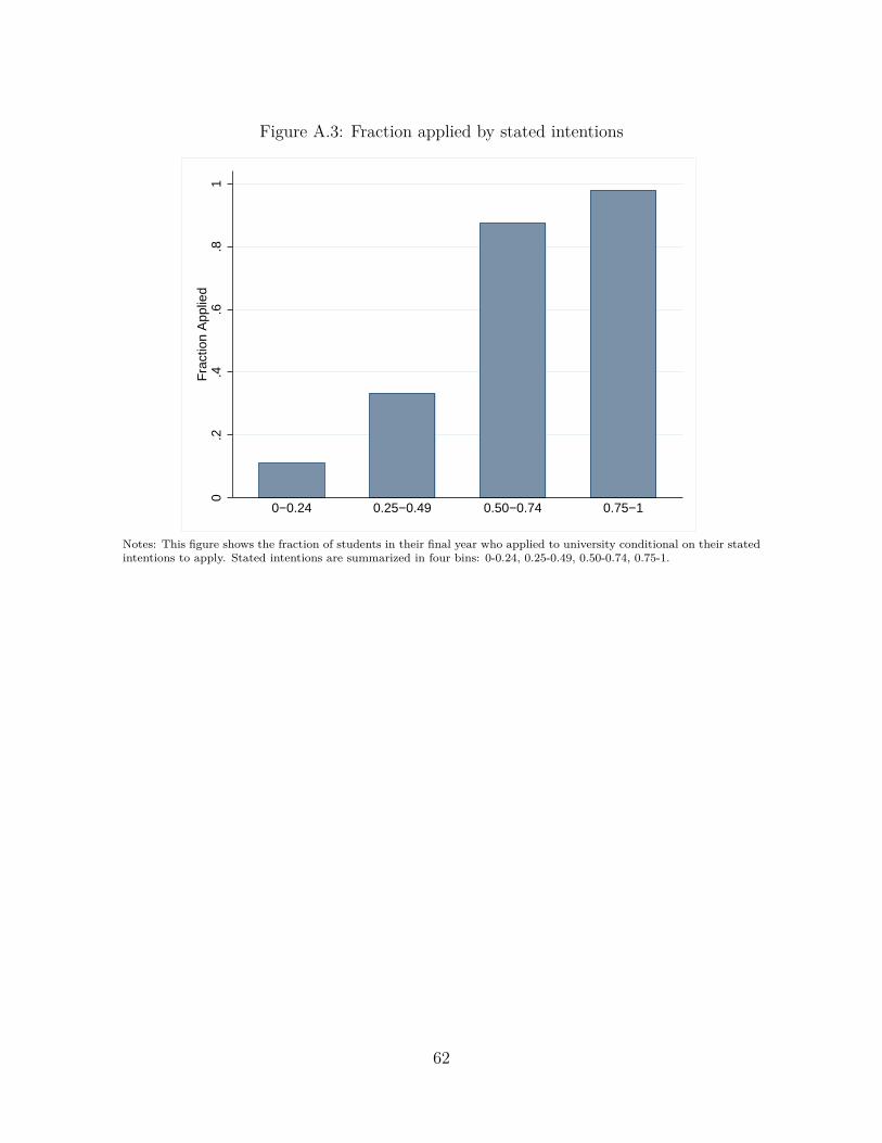
Figure A.3: Fraction applied by stated intentions

0.2

.4.6

.81

Fra

ctio

n A

pplie

d

0−0.24 0.25−0.49 0.50−0.74 0.75−1

Notes: This figure shows the fraction of students in their final year who applied to university conditional on their statedintentions to apply. Stated intentions are summarized in four bins: 0-0.24, 0.25-0.49, 0.50-0.74, 0.75-1.

62

Figure A.4: Intended university subject field by socio-economic status

0.1

.2.3

Pro

port

ion

Arts/humanities Life Sciences Phy Sci/Engineering Social Sciences Education

Low SES High SES

Note: This graph shows the proportion of respondents intending to study each of the fivespecified subject fields, separately by socio-economic status. 95% confidence intervals areprovided.

63

Table A.3: Spearman rank correlations of university beliefs

Enjoy Meet Lose Lonely Interest Enjoy Hard Stress Parental Life Struggle Enough Financialsocial people contact support partner financiallymoney support

Enjoy social 1.000Meet people 0.593 1.000Lose contact -0.067 -0.108 1.000Lonely -0.299 -0.376 0.342 1.000Interest 0.309 0.323 -0.054 -0.056 1.000Enjoy 0.330 0.316 -0.086 -0.141 0.647 1.000Hard -0.050 -0.103 0.197 0.298 -0.130 -0.181 1.000Stress -0.122 -0.172 0.198 0.418 -0.097 -0.188 0.580 1.000Parental support 0.219 0.216 -0.112 -0.099 0.280 0.235 -0.036 -0.012 1.000Life partner 0.139 0.197 -0.009 -0.092 0.089 0.094 -0.024 -0.072 0.047 1.000Struggle financially -0.039 -0.078 0.233 0.289 -0.036 -0.121 0.400 0.443 -0.042 -0.097 1.000Enough money 0.160 0.192 -0.110 -0.153 0.154 0.217 -0.149 -0.179 0.136 0.191 -0.426 1.000Financial support 0.115 0.115 -0.086 -0.038 0.110 0.098 0.064 0.056 0.263 0.103 -0.081 0.299 1.000Notes: This table shows Spearman rank correlations for beliefs about immediate outcomes in the scenario in which students are asked to imagine that they go to university. The sample size is 2,540students. See Table 1 for a full list of questions.

64

Table A.4: Spearman rank correlations of work beliefs

Enjoy Meet Lose Lonely Interest Enjoy Hard Stress Parental Life Struggle Enough Financialsocial people contact support partner financiallymoney support

Enjoy social 1.000Meet people 0.628 1.000Lose contact -0.122 -0.103 1.000Lonely -0.306 -0.353 0.353 1.000Interest 0.469 0.469 -0.043 -0.238 1.000Enjoy 0.456 0.467 -0.057 -0.219 0.762 1.000Hard -0.010 0.006 0.235 0.205 0.129 0.087 1.000Stress -0.110 -0.083 0.250 0.342 0.033 0.004 0.630 1.000Parental support 0.251 0.239 -0.109 -0.149 0.295 0.275 0.087 0.033 1.000Life partner 0.268 0.293 0.026 -0.142 0.270 0.241 0.063 -0.007 0.146 1.000Struggle financially -0.092 -0.079 0.272 0.290 -0.039 -0.081 0.374 0.455 -0.048 0.003 1.000Enough money 0.280 0.258 -0.103 -0.166 0.253 0.280 -0.038 -0.133 0.207 0.177 -0.398 1.000Financial support 0.118 0.125 0.009 -0.024 0.202 0.163 0.184 0.157 0.246 0.137 0.198 0.085 1.000Notes: This table shows Spearman rank correlations for beliefs about immediate outcomes in the scenario in which students are asked to imagine that they do not go to university but start workinginstead. The sample size is 2,540 students. See Table 1 for a full list of questions.

65

Figure A.5: Distribution of beliefs

A: Enjoy social life and feel lonely

-0.2 0 0.2 0.4 0.6 0.8 1 1.2

Enjoy social

-0.2

0

0.2

0.4

0.6

0.8

1

1.2

Lo

ne

ly

10.8

10.6 0.8

Lonely

0.4 0.6

Enjoy social

0.40.20.20 0

B: Enjoy social life and lose contact

-0.2 0 0.2 0.4 0.6 0.8 1 1.2

Enjoy social

-0.2

0

0.2

0.4

0.6

0.8

1

1.2

Lo

se

co

nta

ct

10.8

10.6 0.8

Lose contact

0.4 0.6

Enjoy social

0.40.20.20 0

C: Enjoy social life and meet people

0.2 0.4 0.6 0.8 1 1.2

Enjoy social

0.2

0.4

0.6

0.8

1

1.2

Me

et

pe

op

le

10.8

0.6

Meet people

10.40.8

0.2

Enjoy social

0.60.40 0.2

0

Notes: This figure shows the joint distributions of the perceived likelihood of two social outcomes conditional on goingto university. The left panels give the contour plots, while the right panels show density distributions. Panel A looks atthe joint distribution of the belief that you will enjoy the social life and feel lonely conditional on going to university,while Panel B looks at the likelihood of enjoying the social life and losing contact with family and friends. Panel Cshows the joint distribution for the perceived likelihood of enjoying the social life and meeting people.

Figure A.6: Mean beliefs and school level data

50

60

70

80

90

100

Avera

ge b

elie

f of attendin

g u

niv

ers

ity for

school x s

tudents

30 40 50 60 70 80% of sixth form students in school x continuing to higher education

Higher education

50

60

70

80

90

Avg. belie

f of gettin

g A

−le

vel gra

des for

school x s

tudents

30 40 50 60 70 80Average Attainment 8 score of school x

Grades

Notes: These graphs plot average school level beliefs against actual school level averages. The vertical red line indicates the national average.

Figure A.7: Mean belief factor scores by SES

***

**

***

*

***

−.2

−.1

0.1

.2M

ean

fact

or s

core

Social

life

Subjec

t inte

rest

Stress

Paren

tal s

uppo

rt

Life

partn

er

Financ

ial st

rugg

le

Low SES High SES

Notes: The figure shows average factor scores for the immediate returns to university separately by socio-economicstatus. High SES students are defined as those students who have at least one parent with university education. Starsindicate differences by SES: * p<0.10, ** p<0.05, *** p<0.01.

Figure A.8: Perceived earnings and probability of employment by SES

***

***

***

010

000

2000

030

000

4000

0E

arni

ngs

Work Low Grades High Grades

Low SES High SES

A: Earnings

***

0.1

.2.3

.4.5

.6.7

.8.9

1P

rob.

Em

ploy

ed

Work Low Grades High Grades

Low SES High SES

B: Prob. Employed

Notes: Panel A shows average perceived earnings (cond. on having a job) while Panel B shows the average perceivedprobability of having a full-time job separately for the scenarios: (i) work rather than go to university, (ii) go to universityand graduate with low grades, and (iii) go to university and graduate with high grades. High SES students are definedas those students who have at least one parent with university education. Stars indicate differences by SES: * p<0.10,** p<0.05, *** p<0.01.

Table A.5: Differences in beliefs about immediate outcomes

Low SES High SES Diff-in-diff Diff-in-var

Belief University Work Difference N University Work Difference N P-valueEnjoy social life and activities 74.91 63.77 11.14∗∗∗ 1,077 77.19 63.04 14.14∗∗∗ 1,334 3.01∗∗∗ 0.035

[21.49] [24.50] [26.62] [20.56] [24.03] [25.05] (1.06)Meet people 71.69 61.47 10.22∗∗∗ 1,077 74.84 61.68 13.15∗∗∗ 1,334 2.94∗∗∗ 0.107

[21.67] [23.88] [24.71] [19.75] [22.88] [23.58] (0.99)Lose contact with family/friends 27.98 21.26 6.72∗∗∗ 1,077 28.64 24.69 3.95∗∗∗ 1,334 -2.77∗∗∗ 0.208

[26.97] [24.35] [24.71] [25.85] [24.74] [23.83] (0.99)Feel lonely 32.37 35.69 -3.33∗∗∗ 1,077 30.57 38.99 -8.42∗∗∗ 1,334 -5.09∗∗∗ 0.743

[26.17] [27.92] [27.06] [25.77] [28.69] [26.81] (1.10)Find material/work tasks interesting 69.13 53.99 15.14∗∗∗ 1,077 73.49 55.03 18.46∗∗∗ 1,334 3.31∗∗ 0.032

[21.88] [25.92] [32.64] [20.36] [25.43] [30.68] (1.29)Enjoy studying/work 69.61 56.90 12.71∗∗∗ 1,077 72.06 57.23 14.82∗∗∗ 1,334 2.12∗ 0.292

[22.15] [25.33] [29.72] [21.55] [24.29] [28.83] (1.20)Find material hard/workload high 54.12 42.64 11.48∗∗∗ 1,077 52.31 41.44 10.88∗∗∗ 1,334 -0.60 0.246

[23.81] [24.34] [27.60] [23.97] [24.93] [26.69] (1.11)Feel stressed 54.68 42.59 12.09∗∗∗ 1,077 51.73 42.09 9.64∗∗∗ 1,334 -2.45∗∗ 0.149

[28.18] [28.09] [29.52] [29.17] [28.09] [28.32] (1.18)Have parental support in choice 82.55 62.92 19.63∗∗∗ 1,077 88.45 58.76 29.69∗∗∗ 1,334 10.06∗∗∗ 0.543

[25.31] [33.91] [36.92] [20.55] [34.73] [37.58] (1.53)Meet life partner 42.63 38.48 4.15∗∗∗ 1,077 46.20 40.34 5.85∗∗∗ 1,334 1.71∗ 0.014

[26.06] [26.46] [21.94] [25.49] [25.95] [23.56] (0.94)Struggle financially 56.24 37.63 18.61∗∗∗ 1,077 50.44 38.19 12.25∗∗∗ 1,334 -6.37∗∗∗ 0.212

[29.11] [28.11] [33.88] [29.95] [27.20] [32.68] (1.36)Have enough money 46.49 56.94 -10.45∗∗∗ 1,077 54.18 56.08 -1.90∗∗ 1,334 8.54∗∗∗ 0.677

[25.23] [25.67] [29.25] [24.79] [24.96] [28.90] (1.19)Have financial support from parents 60.12 45.94 14.17∗∗∗ 1,077 67.33 50.33 17.00∗∗∗ 1,334 2.82∗∗ 0.721

[31.32] [33.14] [29.45] [27.73] [31.43] [29.76] (1.21)Notes: Standard deviations given in square brackets, and standard errors given in parentheses. * p<0.10, ** p<0.05, *** p<0.01. This table providesmean beliefs about immediate outcomes separately by SES. Columns 1-4 are for respondents for whom neither parent went to university, while Columns5-8 are for respondents for whom at least one parent went to university. Within each group, the first two columns give mean beliefs for the respectiveaspect under the scenarios of going to university and and not going to university, respectively. Mean beliefs are given on a 0-100 scale. The third columngives the mean difference between these two beliefs. T-tests are used to test for equality of means. Column 9 (‘Diff-in-diff’) gives the average differencefor respondents for whom at least one parent has a degree minus the average difference for respondents for whom neither parent has a degree. Column 10(‘Diff-in-var’) gives the p-value for a test of equality of variances between the perceived returns.

71

Table A.6: Differences in beliefs about later-life outcomes

All SES

Low SES High SES Difference (p-value)

A: No degreeEarnings 23,912 22,966 24,867 1,902**

(18,379) (17,259) (18,609) (0.010)Employed 0.687 0.715 0.671 -0.044***

(0.259) (0.255) (0.257) (0.000)Enjoy job 0.518 0.528 0.510 -0.019*

(0.256) (0.260) (0.250) (0.075)

B: Degree with low gradesEarnings 31,256 29,499 33,051 3,552***

(22,156) (21,370) (22,212) (0.000)Employed 0.771 0.780 0.772 -0.008

(0.213) (0.217) (0.203) (0.334)Enjoy job 0.666 0.672 0.665 -0.007

(0.215) (0.222) (0.207) (0.411)

C: Degree with high gradesEarnings 37,450 34,144 40,410 6,266***

(24,995) (23,756) (25,028) (0.000)Employed 0.856 0.860 0.862 0.002

(0.175) (0.177) (0.163) (0.792)Enjoy job 0.730 0.730 0.734 0.003

(0.192) (0.196) (0.184) (0.672)

D: Difference (low grades - no degree)Earnings 7,344 6,533 8,187 1,651**

(16,640) (15,411) (17,265) (0.014)Employed 0.084 0.065 0.101 0.035***

(0.230) (0.218) (0.232) (0.000)Enjoy job 0.148 0.144 0.155 0.011

(0.247) (0.244) (0.245) (0.257)

E: Difference (high grades - low grades)Earnings 6,194 4,645 7,359 2,714***

(15,726) (14,390) (16,275) (0.000)Employed 0.084 0.080 0.090 0.010

(0.176) (0.172) (0.175) (0.154)Enjoy job 0.064 0.059 0.069 0.010

(0.196) (0.194) (0.196) (0.190)Notes: Column 1 presents the mean across all respondents while columns 2and 3 show the means for low SES and high SES students, respectively. Column4 displays the difference in means along with the corresponding p-value testingdifferences in means. High SES is defined as having at least one parent who has auniversity degree. Panels A, B and C present average responses for earnings condi-tional on working full-time, the stated likelihood of being employed and enjoyingthe job one will be doing in the scenarios in which one does not obtain a universitydegree (A), obtains a degree with a low grade (B) and obtains a degree with a highgrade (C). Panels D and E present the means in differences in responses acrossscenarios as well as socio-economic differences in perceived differences. * p<0.10,** p<0.05, *** p<0.01.

72

Table A.7: Determinants of beliefs about immediate returns

(1) (2) (3) (4) (5) (6)Social Subject Stress Parental Life Financiallife interest support partner struggle

High SES 0.156∗∗∗ 0.142∗∗∗ 0.002 0.175∗∗∗ 0.075∗ -0.104∗∗(0.04) (0.04) (0.04) (0.04) (0.04) (0.04)

Older sibling/friend university 0.135∗∗∗ -0.030 -0.033 0.050 -0.006 -0.157∗∗∗(0.04) (0.04) (0.04) (0.04) (0.05) (0.04)

People to ask about university 0.019∗∗∗ 0.001 -0.011∗ 0.009 0.008 -0.011∗(0.01) (0.01) (0.01) (0.01) (0.01) (0.01)

Male student -0.022 -0.002 -0.138∗∗∗ 0.014 -0.005 -0.057(0.04) (0.04) (0.04) (0.04) (0.04) (0.04)

% University degree (area) 0.002 0.003∗ 0.000 0.017∗∗∗ 0.000 -0.008∗∗∗(0.00) (0.00) (0.00) (0.00) (0.00) (0.00)

School year FEs Yes Yes Yes Yes Yes YesR-squared 0.05 0.06 0.03 0.07 0.01 0.08N 2347 2347 2347 2347 2347 2347Notes: Estimation technique is OLS. Standard errors in parentheses. * p < 0.10, ** p < 0.05, *** p < 0.01. The indepen-dent variables are the six extracted factors summarizing perceived immediate returns to university. High SES students aredefined as those students who have at least one parent with a university degree. The regression additionally controls for aconstant, whether or not the student has an older friend or sibling who has gone to university, the number of people thestudent can think of he/she can ask about university life, a male dummy, the percent of adults with a university degree inthe local area and school year fixed effects.

73

Table A.8: Determinants of beliefs about later-life returns

Low grades - no uni High grades - low grades

(1) (2) (3) (4)Earnings Enjoy job Earnings Enjoy job

High SES 421.977 0.012 1844.040∗∗∗ 0.001(740.43) (0.01) (644.65) (0.01)

Older sibling/friend university -880.404 -0.001 1035.210 0.004(731.71) (0.01) (695.97) (0.01)

People to ask about university 370.743∗∗∗ -0.001 130.666 0.003∗∗(101.28) (0.00) (94.47) (0.00)

Male student 3004.702∗∗∗ 0.000 1328.603∗ -0.013(753.35) (0.01) (682.41) (0.01)

% University degree (area) 70.629∗∗ 0.001 44.436 0.001(31.30) (0.00) (28.24) (0.00)

School year FEs Yes Yes Yes YesR-squared 0.02 0.00 0.02 0.01N 2347 2347 2347 2347Notes: Estimation technique is OLS. Standard errors in parentheses. * p < 0.10, ** p < 0.05, *** p < 0.01.The independent variables are perceived later-life returns in terms of earnings and job enjoyment. Columns 1and 2 display perceived returns to graduating with low grades versus not having a university degree whilecolumns 3 and 4 show perceived returns to graduating with high grades versus graduating with low grades.High SES students are defined as those students who have at least one parent with a university degree. Theregression additionally controls for a constant, whether or not the student has an older friend or sibling whohas gone to university, the number of people the student can think of he/she can ask about university life, amale dummy, the percent of adults with a university degree in the local area and school year fixed effects.

B Questionnaires

B.1 Plans for the future

1. How likely do you think it is that you will obtain the required A-level grades to

go to university? [0-100 scale where 0 means very unlikely and 100 means very

likely]

2. Assuming you do get the grades in sixth form/college to go to university, how

likely do you think it is that you will go to university? [0-100 scale]

3. Which field of study would you be most likely to choose if you decided to go to

university? We know this is a difficult question. Please select one field of study

which you think interests you most, even if you are unsure about which field of

study best fits your interests

(a) Arts and Humanities (e.g. languages, history, music, architecture, philoso-

phy)

(b) Life Sciences (e.g. biology, medicine, pharmacy, psychology)

(c) Physical Sciences and Engineering (e.g. mathematics, computer science, physics,

engineering)

(d) Social Sciences (e.g. economics, law, business)

(e) Education

Now imagine you have been admitted to university and you started an undergraduate

degree in the field of [insert chosen subject from Question 3 above].

1. How likely do you think it is that you would complete your degree? [0-100 scale]

2. Assuming that you graduate, how likely do you think it is that you would get a

First or a 2.1? [0-100 scale]

B.2 Hypothetical Scenarios

Now we would like you to think about the 3-4 years of your life that will come after

you leave sixth form/college. Imagine that during those 3-4 years you go to university.

What do you think your life during those 3-4 years will be like?

If you go to university, how likely do you think it is that you will... [0-100 scale]

1. ...enjoy the social life and activities you engage in?

2. ...meet people with whom you easily get along with?

3. ...lose contact with your family and current friends?

4. ...feel lonely and not part of a group?

5. ...find the material that is covered interesting?

6. ...enjoy studying for the course?

7. ...find the material too hard and/or work load too high?

8. ...be stressed and anxious about not being able to cope?

9. ...struggle financially?

10. ...receive financial support from your family?

11. ...have enough money to do what you enjoy?

12. ...have support from your parents in your decision to go to university rather than

work immediately?

13. ...meet your future partner

14. ...have to work alongside your studies?

Please keep thinking about the 3-4 years of your life that will come after you leave sixth

form/college. This time imagine that during those 3-4 years you do not go to university but

start working instead. What do you think your life during those 3-4 years will be like?

If you start working, how likely do you think it is that you will... [0-100 scale]

1. ...enjoy the social life and activities you engage in?

2. ...meet people with whom you easily get along with?

3. ...lose contact with your family and current friends?

4. ...feel lonely and not part of a group?

5. ...find the tasks at work interesting?

6. ...enjoy performing the different tasks at work?

7. ...find the tasks at work too hard and/or work load too high?

8. ...be stressed and anxious about not being able to cope?

9. ...struggle financially?

10. ...receive financial support from your family?

11. ...have enough money to do what you enjoy?

12. ...have support from your parents in your decision to work rather than attend

university?

13. ...meet your future partner

Now we would like you to think about what your life might be like when you are

30 years old. What do you think your life will be like if you did enroll in a [insert stated subject choice]

degree and graduated with a First or a 2.1? Try to think about the types of jobs that

would be available to you and answer the following questions.

1. How likely do you think it is that you will have a paid job at age 30? [0-100 scale]

2. Assuming that you work full-time, how likely do you think it is that you would

enjoy the job that you would be doing? [0-100 scale]

3. Assuming that you work full-time and that there is no inflation, what do you think

your pre-tax earnings are likely to be per year? [£0, £1,000, £2,000,... £99,000,

£100,000, More than £100,000]

Please continue to think about what your life might be like when you are 30 years old.

What do you think your life will be like if you did enroll in a [insert stated subject choice] degree and

graduated but NOT a First or a 2.1? Try to think about the types of jobs that would be

available to you and answer the following questions.






£100,000, More than £100,000]

Please continue to think about what your life might be like when you are 30 years old.

What do you think your life will be like if you did not go to university or did go to university but did

not graduate? Try to think about the types of jobs that would be available to you and

answer the following questions.






£100,000, More than £100,000]

B.3 Follow-up survey (wave 2)

1. How likely do you think it is that you will obtain the required A-level grades to go

to university? [0-100 scale]

2. Assuming you do get the grades in sixth form/college to go to university, how

likely do you think it is that you will go to university [0-100 scale]

3. Did you apply to university? [Yes, No] (only asked to respondents in Year 13)

(a) Which field of study did you choose? (if answer was ‘Yes’)

i. Arts and Humanities (e.g. languages, history, music, architecture, phi-

losophy)

ii. Life Sciences (e.g. biology, medicine, pharmacy, psychology)

iii. Physical Sciences and Engineering (e.g. mathematics, computer science,

physics, engineering)

iv. Social Sciences (e.g. economics, law, business)

v. Education

vi. Other

C The Dynamic Choice Problem

C.1 Solving Choice Problem Backwards

Note that all choices are made ex-ante and therefore are not binary but are in terms

of probabilities pj for j ∈ {s, c, l} as individuals are not aware of their future shock

realizations and can only anticipate them based on their distributions. Given the closed

form solution of the difference of two extreme value distribution shocks, we can write

down the solutions to the decisions of the model. At t = 3 when the student decides

whether to work or not for each of the three final decision nodes d, the student will

work if:

τv(wd) + λπd + Uld(Xl) ≥ −εld

⇐⇒ pld = 11 + e−(τv(wd)+λπd+U

ld(Xd))

These three decision probabilities pl0 , pl1 , and pl2 will allow the student to compute the

expected values from the final period. This will allow her to think about her decision

at t = 1, in case she is enrolled in university, where she will complete university if

E[V c12 ] + Uc(Xc) + εc ≥ E[V c0

2 ]

⇐⇒ E[V c12 ]− E[V c0

2 ] + Uc(Xc) ≥ −εc

⇐⇒ pc = 11 + e−(E[V c1

2 ]−E[V c02 ]+Uc(Xc))

Now knowing both pc and pld , at t = 0 the student is ready to decide between three

options: (i) not enrolling, (ii) enrolling and working alongside university (s1), (iii) en-

rolling without working alongside (s2). The student will choose s1 if:

E[V s11 ] + Us1(Xs) + εs1 ≥ E[V s0

1 ] ∧ E[V s11 ] + Us1(Xs) + εs1 ≥ E[V s2

1 ]

⇐⇒ E[V s11 ]− E[V s0

1 ] + Us1(Xs) ≥ −εs1 ∧ E[V s11 ]− E[V s2

1 ] + Us1(Xs) ≥ −εs1

⇐⇒ ps1 = eE[V s11 ]+Us1 (Xs)

1 + eE[V s11 ]+Us1 (Xs) + eE[V s2

1 ]+Us2 (Xs)

and analogously will choose s2 with:

ps2 = eE[V s21 ]+Us2 (Xs)

1 + eE[V s11 ]+Us1 (Xs) + eE[V s2

1 ]+Us2 (Xs).

C.2 Estimation Details

In Table C.1 we present the variance-covariance matrix for the unobserved heterogene-

ity for low (top) and high (bottom) SES students. The variance for the unobserved

heterogeneity of the work decision is normalized to unity. We see that for low SES the

decision to enroll and not to work alongside studies has the next highest variance (0.60).

The highest correlation between unobserved heterogeneity of low SES is between the

heterogeneity in terms of completion and enrolling without working alongside (-0.84).

For high SES students, unobserved heterogeneity in terms of the decision to work

during studies also has the highest variance (0.17) after the work decision but is substan-

tially lower than for low SES students. In terms of correlated unobserved heterogeneity

again completion and enrolling without working alongside exhibits the strongest corre-

lation. However, for high SES students this correlation is positive (0.97).

Table C.1: Variance-covariance matrix of unobserved heterogeneity

Enroll & not work Enroll & work Complete WorkLow SES

Enroll and not work 0.602Enroll and work 0.023 0.061Complete 0.057 -0.031 0.023Work 0.156 0.016 -0.083 1.0

High SESEnroll and not work 0.167Enroll and work 0.005 0.092Complete -0.143 0.114 0.15Work -0.072 -0.063 -0.037 1.0

C.3 Sensitivity Analysis

In Figure C.1 we look at how the criterion function behaves in the neighborhood of the

optimum. In order to so we incrementally decrease and increase parameters moving

them up to two standard deviations away from their optimal value. While this is

no definite proof that we have identified the global maximum, the smooth behavior

around the identified optimum increases our confidence that indeed we have chosen

optimal values for each parameter for both the low (orange solid line) and high (black

dotted line) SES model.

Figure C.1: Response of criterion function to +/- 2 standard deviation change in eachparameter

-2 -1 0 1 21.00001.00251.00501.00751.0100

1

-2 -1 0 1 21.0021.0051.0081.011

2

-2 -1 0 1 21.0001.0021.0041.0061.008

3

-2 -1 0 1 21.0001.0011.0021.0031.0041.0051.006

4

-2 -1 0 1 21.0001.0011.0021.0031.0041.0051.006

5

-2 -1 0 1 21.001.051.101.151.20

1

-2 -1 0 1 21.001.051.101.151.20

2

-2 -1 0 1 21.0001.0021.0041.006

-2 -1 0 1 21.00001.00251.00501.00751.0100

-2 -1 0 1 21.001.051.101.15

s1

-2 -1 0 1 21.0001.0251.0501.0751.1001.125

s2

-2 -1 0 1 21.001.021.041.061.08

c

-2 -1 0 1 21.001.021.041.06

l0

-2 -1 0 1 21.001.011.021.031.041.051.06

l1

-2 -1 0 1 21.021.051.081.11

l2

-2 -1 0 1 21.001.251.501.752.00

s1

-2 -1 0 1 21.21.51.82.1

s2

-2 -1 0 1 21.0001.0051.0101.015

c

-2 -1 0 1 21.001.021.041.06

c

-2 -1 0 1 21.0001.0251.0501.0751.100

l

Notes: The y-axis shows the relative total error of the criterion function in response to changes to the parametersspecified in the subtitles. The x-axis represents changes in terms of standard deviations. The orange solid line representschanges for low SES while the black dotted lines represents changes for high SES.

In Figure C.2 we see the relative change in each decision (y-axis) for low and high

SES students as a response to a 0.5 standard-deviation increase in a parameter (x-axis).

Red cells indicate increases, whereas blue cells indicate a decrease. The darker a cell,

the stronger a response, where the magnitude of the change in percentage terms can

be gauged from the scale on the left hand side of the figure. The idea is to understand

the sensitivity of key moments to changes in parameters.

Figure C.2: Response of decisions to 0.5 standard deviation increase in each parameter

θ1 θ2 θ3 θ4 θ5ψ1ψ2 τ λ κs1κs2κc κl0κl1κl2μs1μs2μμ αμ αl

LEnroll

H

LWork while studying

H

LComplete

H

LWork no degree

H

LWork low degree

H

LWork high degree

H

−1.0

−0.5

0.0

0.5

1.0

Notes: Each cell represents the relative response of the model moment on the y-axis for low SES (bottom) and high SES(top) to a 0.5-standard deviation shift in the model parameter on the x-axis. The magnitude of the response is indicatedby the shade of the cell as outlined in the scale on the right.

The first observation is that neither of the targets is too sensitive to any single

parameter. We see that for both high and low SES students the maximum relative

change is to the enrollment probability and the probability of working alongside studies

when the respective direct utility intercepts κs2 and κs1 are shifted by 0.5 standard

deviations. However, the relative change in the respective probabilities is around 1%

and therefore not too volatile. The second observation is that we can see the difference

in the responsiveness of low and high SES students to changes in parameters, which are

related to differences in perceived returns. For instance, increasing θ4, the parameter

governing the importance of parental support in the choice, reduces attendance more

for low SES students than for high SES students. Interestingly, it reduces attendance

for both groups despite its positive sign. Remember that inputs are standardized, i.e.

many students will have negative values for parental support in their choice, so a higher

parameter value can lead to a lower utility from enrollment. The third observation is

that the dynamic component of the model becomes apparent. If we increase κc, the

intercept for the additional utility from completion, more students not only complete

but also attend university in the first place. Now that more students are anticipating to

complete university (because the utility from completion has increased), more students

decide to enroll in university in the first place. Similarly, an increase in the value

placed on job enjoyment λ increases the probability of working with a high degree.

As a result high-degree jobs become more attractive, students become more likely to

complete university and they are more likely to enroll in university in the first place.

Socio-Economic Gaps in University Enrollment: The Role of ...

Documents

Transcript of Socio-Economic Gaps in University Enrollment: The Role of ...