Sobre la Detección en Tiempo Real de Caras en Secuencias ...

CMÍ)S!J^-

m^^' Í6Ítíé-

UNIVERSIDAD DE LAS PALMAS DE GRAN

CANARIA

Departamento de Informática y Sistemas

TESIS DOCTORAL

Sobre la Detección en Tiempo Real de Caras en

Secuencias de Vídeo. Una Aproximación Oportunista.

(On Real-Time Face Detection in Video Streams. An Opportunistic Approach.)

Modesto Femando Castrillón Santana

Diciembre 2002

UNIVERSIDAD DE LAS PALMAS DE GRAN CANARIA

Departamento de Informática y Sistemas

Tesis Titulada Sobre la Detección en Tiempo Real de Caras en Secuencias de

Vídeo. Una Aproximación Oportunista., que presenta D. Modesto Femando Cas-

trillón Santana, realizada bajo la dirección del Doctor D. Francisco Mario Hernán

dez Tejera y la codirección del Doctor D. Jorge Cabrera Gámez.

Las Palmas de Gran Canaria, Diciembre de 2002

Francisco ández Tejera

El codirector

Jorge ÍZabrera Gámez

El doctorando

Modesto Fernando Castrillón Santana

A mis padres y a Regirte.

Agradecimientos

Comenzar a escribir los agradecimientos resulta inesperado, tras unos cuan

tos años parece ser síntoma de un nuevo paso en mi historia académica. Al llegar a

este punto no puedo evitar recordar una conversación telefónica algunos años atrás

con el Dr. Antonio Falcón Martel que me convencía para seguir el camino investir

gador en la Universidad de Las Palmas de Gran Canaria.

La maduración de este trabajo ha sido a fuego lento hasta encontrar el mo

mento y el tema adecuados. En este proceso agradezco las facilidades ofrecidas den

tro del Grupo de Inteligencia Artificial y Sistemas formado años atrás por los doc

tores Juan Méndez Rodríguez, Antonio Falcón Martel y Francisco Mario Hernández

Tejera. En este ambiente he podido realizar mi aprendizaje y trabajar en distintos

proyectos que tienen su significado en la consecución de este documento.

Más concretamente agradezco a Francisco Mario Hernández Tejera porque no

sólo ha aceptado dirigir y estimular enormemente el desarrollo de estas líneas, sino

que además ha aportado su sentido del humor y sus dotes de de cuentacuentos para

hacemos más familiares las jomadas en el laboratorio. También quiero agradecer al

también doctor Jorge Cabrera Gámez por su apoyo, sus aportaciones y su continuo

espíritu crítico y constructivo.

Agradezco a todos los compañeros y amigos del laboratorio por su apoyo y

ganas en nuestros proyectos, así como a aquellos que han aportado comentarios en

la elaboración de este documento, y a quienes han ofrecido su cara para las secuencias

utilizadas en los experimentos. Quisiera también agradecer al Dr. Rowley por su

generosidad y valentía a la hora de proporcionar sus ficheros binarios para facilitar

la comparación a otros investigadores. También quiero hacer mención de diversas

entidades que han confiado en nosotros a la hora de financiar o colaborar en parte de

los trabajos desarrollados en este documento y sus posibles ampliaciones futuras, y

concretamente a la Fundación Canaria Universitaria de Las Palmas patrocinada por

Beleyma y Unelco, que permitirán continuar en esta línea en el futuro inmediato.

Y para concluir, quiero agradecer especialmente a mis padres que han hecho

posible con su amor y esfuerzo que pueda haber dedicado mi vida al estudio, y

además porque en todo este tiempo no han preguntado demasiado a menudo por

el estado de la tesis.

Gracias a todos.

Contents

Resumen xxi

Abstract xxiii 1 Introduction

1

1.1 Perceptual User Interaction 5

1.1.1 Human Interaction / Face to face Interaction 11

1.1.2 Computer Vision 13

1.1.2.1 Body/Hand description and communication 15

1.1.2.2 Person awareness 16

1.1.2.3 Face Description 17

1.1.2.4 Computer expression/Affective computíng 18

1.2 Objectíves 21

2 Face detection & Applications 23

2.1 Face detection 26

2.1.1 Face detection approaches 28

2.1.1.1 Pattern based (Implicit, Probabilistic) approaches . . 32

2.1.1.2 BCnowledge based (Explicit) approaches 41

2.1.1.3 Face Detection Benchmark 59

2.1.2 Facial features detection 63

2.1.2.1 Facial Features detection approaches 64

i

2.1.2.2 Automatic Normalization based on facial features . 71

2.1.3 Real Time Detection 71

2.2 Post-face detection applications 76

2.2.1 Static face description. The problem 76

2.2.1.1 Face recognition. Face authentication 77

I.IX.T. Other facial features 101

2.2.1.3 Performance analysis 103

2.2.2 Dynamic face description: Gestures and Expressions 103

2.2.2.1 Facial Expressions 104

2.2.2.2 Facial Expression Representation 105

2.2.2.3 Gestures and expression analysis . 105

2.2.2.4 Gestures and expressions analyzed in the literature . 107

3 A Framework for Face Detection 111

3.1 Classification 115

3.2 Cascade Classification 119

3.3 Cues for Face Detection 122

3.3.1 Spatial and Temporal coherence 122

3.3.1.1 Spatial coherence 122

3.3.1.2 Temporal coherence 126

3.4 Summary 131

4 ENCARA: Description, Implementation and Empirical Evaluation 133

4.1 ENCARA Solutions: A General View 134

4.1.1 The Basic Solution 138

4.1.1.1 Techniques integrated 138

4.1.1.2 ENCARA Basic Solution Processes 139

4.1.2 Experimental Evaluation: Environment, Data Sets and Exper

imental Setup 155

ii

4.1.3 Experimental Evaluation of the Basic Solutíon 160

4.1.4 Appearance/Texture integration: Pattem matching confírma-

tion 164

4.1.4.1 Introduction 164


4.1.4.3 PCA reconstruction error 166

4.1.4.4 Rectangle features 168

4.1.4.5 PCA+SVM 171

4.1.4.6 ENCARA Appearance Solution Processes 173

4.1.5 Experimental Evaluatiori of the Appearance Solution 173

4.1.6 Integration of Similarity with Previous Detection 177


4.1.6.2 ENCARA Appearance and Similarity Solution Pro

cesses 178

4.1.7 Experimental Evaluation of Similarity and Appearance Solution 184

4.2 Summary 188

4.3 Applications experiments. Interaction experiences in our laboratory . 194

4.3.1 Designing a PUI system 196

4.3.1.1 Casimiro 197

4.3.2 Recognition in our lab 201

4.3.2.1 Recognition experiments 201

4.3.3 Gestures: preliminary results 205

4.3.3.1 Facial features motion analysis 205

4.3.3.2 Using the face as a pointer 207

5 Conclusions and Future Work 209

5.1 Future Work 212

6 Resumen extendido 215

6.1 Introducción 215

iii

6.1.1 Interacción Hombre Máquina 215

6.1.2 Interacción perceptiva de usuario 219

6.1.2.1 Interacción Humana / Interacción Cara a Cara . . . 223

6.1.2.2 Visión por Computador 225

6.1.3 Objetivos 228

6.2 Detección de la Cara y Aplicaciones 229

6.2.1 Detección Facial 231

6.2.1.1 Aproximaciones de Detección de Caras 233

6.2.2 Detección de Elementos Faciales 236

6.2.2.1 Aproximaciones para la detección de elementos fa

ciales 237

6.2.2.2 Normalización automática basada en elementos fa

ciales 237

6.2.3 Aplicaciones de la Detección Facial . ; . . 238

6.2.3.1 Descripción de la cara estática. El problema 238

6.2.3.2 Descripción de la cara en movimiento: Gestos y Ex

presiones 244

6.3 Un Marco para la Detección Facial 248

6.3.1 Detección de Cara 248

6.3.1.1 Elementos para Detección Facial 250

6.4 ENCARA: Descripción, Puesta en Práctica y Evaluación Experimental 259

6.4.1 ENCARA: Vista General 260

6.4.1.1 ENCARA 263

6.4.1.2 Evaluación experimental: Entorno, Conjuntos de Datos275

6.4.2 Sumario 277

6.4.3 Experimentos de Aplicación. Experiencias de Interacción en

nuestro laboratorio 282

6.4.3.1 Experimentos de reconocimiento 282

6.4.3.2 Gestos: resultados preliminares 286

iv

6.5 Conclusiones 288

6.6 Trabajo Futuro 290

A GDMeasure 293

A.l Mantaras Distance 294

A.2 GD Measure Definition 295

B Boosting 299

C Color Spaces 301

C.l HSV 301

C.2 CÍE L*a*b* 302

C.3 YCrCb 303

C.4 TSL 303

C.5 YUVsource 304

D Experimental Evaluation Detailed Results 305

D.l Rowley's Technique Results 305

D.2 Basic Solution Results 306

D.3 Appearance Solution Results 315

D.4 Appearance and Similarity Solution Results 315

D.5 ENCARA vs. Rowley's Technique 331

D.6 Recognition Results 341

List of Figures

1.1 Put-That-There (Bolt, 1980) was an early multimodal interface prototype. 7

1.2 Aviewofeldi 20

2.1 Duchenne du Boulogne's photographs (Duchenne de Boulogne, 1862). 24

2.2 Ekman's expressions samples (Ekman, 1973). 24

2.3 Do you notice anything strange? No? Then turn thé page. 26

2.4 Classificatíon of Face Detection Methods 31

2.5 a) Canonical face view sample, b) mask applied, c) resultad canonical

view masked (Sung and Poggio, 1998) 33

2.6 Face clusters and gaussians (Sung and Poggio, 1998) 34

2.7 Non-face clusters and gaussians (Sung and Poggio, 1998) 34

2.8 a) Hyperplane with small margin, b) hyperplane with larger margin.

Extracted from (Osuna eí flL, 1997) 36

2.9 Integral image at point (x, y) is the sum of all points contained in the

dark rectangle (extracted from (Viola and Jones, 2001fc)) 39

2.10 Partial Face Groups (PFG) considered in (Yow and CipoUa, 1996), and

their división in vertical and horizontal pairs 43

2.11 Shape Model example (Cootes and Taylor, 2000) 44

2.12 Active Shape Model example (Cootes and Taylor, 2000) 45

2.13 Frame taken under natural light. Average normalized red and green

valúes recovered for rectangles taken in those zones: A(0.311,0.328),

5(0.307,0.337), C(0.329,0.338) and 0(0.318,0.326) 47

vii

2.14 Frame taken under artificial light. Average normalized red and green

valúes recovered for rectangles taken in those zones: A(0.241,0.335),

B(0.24,0.334), C(0.239,0.334) and 0(0.273,0.316) 48

2.15 Nogatech Camera Skin Locus (Soriano et al, 2000fl), considering NCC

color space. The skin locus is modelled using two intersecting quadratic

functions 55

2.16 Sample of CMU datábase (Rowley eí fl/., 1998). 61

2.17 Receiver Operating Characteristic (ROC) example curve extracted from

(Viola and Jones, 2001fc) 62

2.18 Symmetry maximal sample 65

2.19 Peaks and valleys on a face. 69

2.20 Projection sample. 69

2.21 Can you recognize them? 81

2.22 Sample eigenfaces, sorted by eigenvalue 89

2.23 A comparison of PCA and FLD extracted from (Belhumeur et al, 1997). 93

2.24 PCAICA samples 95

2.25 Sample technique to extract from a 2D image for using ID HMMs

(Samarla, 1993) 98

2.26 Process used for aligning faces extracted from (Moghaddam et al, 1996). 100

2.27 Example of face images variations created from a single one, extracted

from (Simg and Poggio, 1994) 101

3.1 Window definition 114

3.2 Detection function 114

3.3 How many faces can you see? Nine? 115

3.4 a) Individual and b) múltiple classifier. 116

3.5 a) Fusión, b) Cooperative and c) Hierarchy. classifier 117

3.6 T means tracking and CS Candidate Selection, D are data, M¿ is the

i-th module, C¿ the i-th classifier, Ei the i-th evidence, A accept, R

Reject, F/F face/nonface, di the i-th evidence computation and $ the

video stream 120

viii

3.7 Curve shape for false positive and detection rates of the cascade clas-

sifier for different K 121

3.8 Appearance of a face. Input image, gray levéis, 3 pixelation, 5 pixela-

tion, edges image and binary. 123

3.9 Face prototype 124

3.10 Relevant aspects of a face 124

3.11 Leonardo drawing sample 125

3.12 Gala Nude Watching the Sea which, at a distance of 20 meters, Turns

into the Portrait of Abraham Lincoln (Hommage to Rothko). (Dalí,

1976) 126

3.13 Self-portrait. César Manrique 1975 127

3.14 Ideal facial proportions . . . . . . . ' . 128

3.15 Traditional Automatic Face Detector . 128

3.16 Traditional Automatic Face Detector applied to a sequence . . . . . . 128

3.17 Automatic Face Detector Adapted to a Sequence 129

3.18 Frames O, 2,11,19, 26, 36, 41, 47, 50 130

3.19 Movement of right eye tn a 450 frames sequence. Some extracted

frames are presentedin Figure 3.18 131

4.1 ENCARA main modules 136

4.2 Input image with two different skin regions, i.e., face candidates. . . 137

4.3 Flow diagram of ENCARA Basic Solution 137

4.4 Dilation example 140

4.5 Input image and skin color blob detected 140

4.6 Skin color detection sample using skin color definition A 141

4.7 Skin color detection sample using skin color defínition B 142

4.8 Skin color detection sample using skin color definition A 143

4.9 Skin color detection sample using skin color definition B 143

4.10 Flow diagram of ENCARA Basic Solution M2 module 145

4.11 EUipse parameters 146

ix

4.12 Input image and skin color blob detected 146

4.13 Blob rotation example 147

4.14 Input image and rotated image. Each image needs to define its coor

dínate system 147

4.15 Neck elimination 148

4.16 Example of resulting blob after neck elimination 149

4.17 Integral projections considering the whole face : . . . . . . . . 149

4.18 Zone computed for projections . . : 150

4.19 Integral projections on eyes área considering hemifaces. : 151

4.20 Search área according to skin color blob 152

4.21 Integral projection test. Comparing the integration of projections for

locating eyes search windows. The left image does not make use of

projections and the eye search área contatns eyebrows, while the right

image avoids eyebrows bounding the search área with projections. . 152

4.22 Too cióse eyes test. Bottom image presents the reduced search área

for left eye, in the image, after the first search failed the too cióse eyes

test 153

4.23 Input and normalized masked image 154

4.24 Determination of position between eyes 155

4.25 Determination of mouth center position 155

4.26 Average position for eyes and mouth center. 156

4.27 Áreas for searching mouth and nose 156

4.28 First frame extracted from each sequence, labelled Sl-Sll, used for

experiments 157

4.29 Rowley's technique summary results 159

4.30 Eye detection error example using Rowley's technique, only one eye

location was retumed, and it was uncorrectly located 160

4.31 Results summary using Basic Solution for sequences S1-S6 162

4.32 Results summary using Basic Solution for sequences S7-S11 163

4.33 Example of false detection using the basic solution 164

X

4.34 Flow diagram of ENCARA Appearance Solution 165

4.35 Rectangle features applied over integral image (see Figure 2.9) as de-

fined iiT (Li eí fl/., 2002b) 168

4.36 Rectangle feature configuration for the best weak classifier for face set

for 20x20 images of faces as the sample on the left 170

4.37 Rectangle feature configuration for the best weak classifier for right

eye set (built with 11x11 images) 170

4.38 Rectangle feature configuration for the best weak classifier for left eye

set for 11x11 images of faces as the sample on the left 171

4.39 First weak classifier, based on rectangle features, selected for right

eye. Red means positive gaussian, while blue means negative. . . . 171

4.40 Face sample extraction for facial appearance training set 173

4.41 Results summaryusing Appearance Solution for sequences S1-S3. . . 176

4.42 Results summary ustng Appearance Solution for sequences S4-S6. . . 177

4.43 Results summary using Appearance Solution for sequences S7-S9. . . 178

4.44 Results summary using Appearance Solution for sequences SlO-Sll. 179

4.45 Flow diagram of ENCARA Similarity Solution 180

4.46 Flow diagram of ENCARA MO module 181

4.47 Upper plots represent the differences for eye position in a sequence

for X and y respectively bottom plot shows the ínter eye distance for

the secuence 182

4.48 This surface reflects the normalized difference image that results from

a pattem search, where three local mínima are clearly visible 183

4.49 Search áreas, red (dark) rectangle for previous, white rectangle for

next frame 183

4.50 Example of an eye whose pupil is not the gray mínimum 184

4.51 Examples of eye pattem adjustment 184

4.52 Candidate áreas for searchíng: On the right using previous detected

position; on the left using color 186

4.53 Results summary using Appearance and Similarity Solution for sequences S1-S2 188

xi

4.54 Results summary using Appearance and Similarity Solution for se-

quencesS3-S4 189


quencesS5-S6 190


quencesS7-S8 191


quences S9-S10 192


quence Si l . . 193

4.59 Results summary for face detection rate comparing ENCARA vari-

ants Sim29-Sim30 and Sim35-Sitn36 with Rowley's technique 194

4.60 Results summary for eye detection rate comparing ENCARA variants

Szm29-Sím30 and Sím35-,Sim36 with Rowley's technique 196

4.61. Results summary comparing ENCARA variants considering Possible

Rectangle as Face Detection with Rowley's technique 197

4.62 System description 198

4.63 Casimiro 201

4.64 Identity and gender recognition results using PCA+NNC 202

4.65 Identity and gender recognition results using PCA+SVM 204

4.66 Gender recognition results comparison 204

4.67 For a sequence of 450 frames (x axis), upper plots represent the x

valué of left and right iris (y axis), bottom plots represent the y valué

of left and right iris 205

4.68 For a sequence of 450 frames, upper left graph plots differences among

X valúes of both eyes, while upper right plot is a zoom from 50 to 135

frame (x axis). Bottom left curve plots differences among y valúes of

both eyes, right zooming from O to 135 frame 206

4.69 Example use of the face tracker to command a simple calculator. . . . 208

4.70 Expression samples used for training 208

6.1 Función de detección 250

xii

6.2 Apariencia de una cara. Imagen de entrada, niveles de grises, pixe-

lado 3, pixelado 5, contomos e imagen de dos niveles 252

6.3 Prototipo facial 253

6.4 Autorretrato. César Manrique 1975 255

6.5 Detector facial traditional 256

6.6 Detector facial tradicional aplicado a una secuencia 257

6.7 Detector facial aplicado a una secuencia. 258

6.8 Imágenes0,2,11,19,26,36,41,47,50 258

6.9 Imagen de entrada con dos zonas de piel, es decir, candidatos 262

6.10 Principales módulos de ENCARA 263

6.11 Imagen de entrada y zonas de color pieldetéctadas. . . . . . . . . . . 267

6.12 Ejemplo de rotación de zona de color. 270

6.13 Eliminación del cuello 270

6.14 Proyecciones integrales considerando toda la cara 271

6.15 Proyecciones integrales sobre la zona de los ojos considerando la cara

dividida en dos lados 272

6.16 Imagen de entrada y normalizada 274

6.17 Primera imagen de cada secuencia empleada para los experimentos,

etiquetadas Sl-Sll 276

6.18 Sumario de resultados para el ratio de detección facial comparando

las variantes Sim29-Sim30 y Sim35-Sim36 de ENCARA con la técnica

deRowley. 280

6.19 Sumario de resultados para el ratio de detección ocular comparando

las variantes Sim29-Stm30 y Sim35-Sim36 de ENCARA con la técnica

deRowley. 281

6.20 Sumario de resultados comparando el ratio de detección facial de

las variantes seleccionadas de ENCARA incorporando el rectángulo

posible con la técnica de Rowley. 282

6.21 Resultados de clasificación identidad y género empleando PCA+CVC. 284

6.22 Resultados recnocimiento idenidad y género empleando PCA+MSV. 285

xiii

6.23 Comparativa resultados de reconocimiento de género 286

6.24 Ejemplo de uso como pincel 287

6.25 Ejemplo de uso de ENCARA para interactuar con una calculadora. . 287

6.26 Muestras ejemplos del conjunto de entrenamiento de expresiones de

un individuo 288

XIV

List of Tables

2.1 Still image resources for facial analysis 60

2.2 Sequences resources for facial analysis 61

4.1 Results of color components discrimination test 142,

4.2 Summary of variants for ENCARA basic solution. Each variant indi- •

cates whether a test is included. These labels are used in Figures 4.31

and 4.32. : . 1 6 1

4.3 Summary of variants for ENCARA appearance solution tests. These labels are used in Figures 4.41-4.44 174

4.4 Summary of variants of ENCARA appearance and similarity solution

(the too clase eyes test and integral projection test are integrated) plus

appearance and similarity tests. These labels are used in Figures 4.53-

4.58 185

6.1 Resultados del test sobre las componentes discriminantes 268

6.2 Etiquetas utilizadas por las variantes de ENCARA 278

D.l Results of face detection using Rowley's face detector (Rowley et al.,

1998) 306

D.2 Comparison of results of face and eye detection using Rowley's face

detector (Rowley et al, 1998) and manually marked 306

D.3 Results obtained with basic solution and variants 307

D.4 Eyes location error summary for basic solution and variations, if too

cióse eyes test and integral projection test are used 308

XV

D.5 Results obtained integrating appearance tests for sequences S1-S4.

Time measures in msecs. are obtained using standard C/C++ com-

mand clock 309



mand clock 310



mand clock 311

D.8 Eyes location error summary integrating appearance tests for sequences

S1-S3. . 312

D.9 Eyes location error summary integrating appearance tests for sequences

S4-S6 313

D.IO Eyes location error summary integrating appearance tests for sequences

S7-S9 314

D.ll Eyes location error summary integrating appearance tests for sequences

SlO-Sll 315

D.12 Results obtained integrating tracking for sequence SI. Time measures

in msecs. are obtained using standard C command clock 316

D.13 Eyes location error summary integrating appearance tests and track

ing for sequence SI 317

D.14 Results obtained integrating tracking for sequence S2. Time measures



ing for sequence 82 319




ing for sequence S3 321



xvi

D.19 Eyes location error summary integrating appearance tests and track-


D.20 Results obtained integrating tracking for sequences S5. Time mea-

sures in msecs. are obtained using standard C command dock. . . . 324



D.22 Results obtained integrating tracking for sequences S6. Time mea-

sures in msecs. are obtained using standard C command clock. . . . 326















D.30 Results obtained integrating tracking for sequence SIO. Time mea-



ing for sequence SIO 335

D.32 Results obtained integrating tracking for sequence Sil . Time mea-



ing for sequence Sil 337

D.34 Comparison ENCARA vs. Rowley's in terms of detection rate and

average time for sequences Sl-Sll 338

xvii

D.35 Comparison ENCARA vs. Rowley's in terins of eye detection errors

for sequences Sl-Sll 339

D.36 Comparison ENCARA vs. Rowley's in terms of detection rate and

average time for sequences Sl-Sll 340

D.37 Results of recognition experiments using PCA for representation and

NNC for classification 341

D.38 Results of gender recognition experiments using PCA for representa

tion and NNC for classification 342

D.39 Results of recognition experiments using PCA for representation and

SVM for classification. 342

D.40 Results of gender recognition experiments using PCA for representa

tion and SVM for classification 343

D.41 Results comparison PCA+NNC and PCA+SVM for identity and gender. 343

D.42 Results PCA+SVM for gender using temporal coherence 344

xviu

List of Algorithms

1 ENCARA algorithm 195

2 Adaboost algorithm 300

XIX

Resumen

Este trabajo considera la necesidad de realizar un cambio de filosofía de diseño para

la elaboración de los procedimientos de acceso a la tecnología por parte de los hu

manos, ante la ausencia de un acceso intuitivo en los ordenadores actuales.

Si observamos el comportamiento humano, se evidencian las facilidades de

adaptación y flexibilidad que un ser humano dispone al relacionarse con los seres

de su especie, siendo obvia la influencia de la percepción humana. En cambio, un

ordenador actual ignora casi totalmente las posibilidades de percepción que la tec

nología hoy día permite, siendo este un camino a seguir para facilitar que un orde

nador disponga de información contextual en la actualidad no empleada.

Entre los elementos que un humano utiliza y analiza durante la interacción

con otros humanos, destaca el rostro humano. La cara humana proporciona infor

mación que caracteriza la comunicación a muy diversos niveles. La posibilidad de

percibir esta información por parte de un ordenador, le abre una poderosa fuente de

información. Este trabajo analiza el problema de detección facial automática, elabo

rando un marco para desarrollar un prototipo que permita detectar caras en tiempo

real para interacción.

El documento contiene una amplia revisión de las técnicas existentes en la

literatura para la detección y el análisis facial, abordando posteriormente la concep

ción de un esquema para resolver un problema complejo como el que nos ocupa.

Fundamentado en esta concepción y cuidando la restricción de tiempo real, se desar

rolla un prototipo que combina diversas técnicas que de forma individual no cubren

las restricciones del diseño. Para concluir y validar la bondad de los datos propor

cionados por el detector facial, se aplican esquemas básicos de reconocimiento e

interacción.

Los resultados obtenidos avalan la calidad de la aproximación para aplica

ciones de interacción en tiempo real como exigían las restricciones de diseño.

XXI

Abstract

This work considers the need of a philosophy change to design the mechanisms

of human computer interaction (HCI), due to the absence of an intuitive access in

current computers.

If human behavior is ánalyzed, it is obvious the possibilities of adaptation

aríd flexibility that a human being has to interact with others thánks to perception.

Hówever, a current computer avoids almost completely the perceptual inputs that

technology provides nowadays. The use of perception traces the path to intégrate

contextual information in HCI.

Among the elements that a human being uses during human interaction, the

face is a main one. Human face provides information that characterizes the com-

munication at different levéis. The possibility of perceiving this information opens

a great data source. This document analyzes the problem of face detection, devel-

oping a framework to elabórate a prototype that allows real-time face detection for

interaction.

The document endoses a survey of current techniques in the literature for

face detection and analysis. Later, the conception of an schema to solve the prob

lem is tackled. Considering this schema and the real-time restriction, the resulting

prototype combines different techniques that do not provide individuaUy a reliable

solution. To conclude, the data provided by the face detector are used for simple

recognition and interaction applications.

The results achieved prove the quality of the approach for real-time interac

tion purposes as it was established in design stage.

xxiu

Chapter 1

Introduction

CURRENT society is characterized by an incremental and notorious integration

of computéis in daily life, both in social and individual contexts. However,

two major opinions are commonly expressed by people to a computer scientist (me)

when they discover, my professional background in a first contact (human interac-

tion):

1. 1 lo ve computers (technology),

2. I hate computers (technology).

How is this possible? What is wrong with computers that they are not com-

pletely accepted and in many cases refused? Are not computers a tool to help hu-

mans for unpleasant tasks? Are they creating new unpleasant tasks? This feeling

has been expressed by different authors:

"... if the role of technology is to serve people, then why must the non

technical user spend so much time and effort getting technology to do its

Job?" (Picard, 2001)

"The real problem with an interface is that it is an interface. Interfaces

get in the way. I don't want to focus my energies on an interface. I want

to focus on the job." (Norman, 1990)

This situation happens because people are urged to interact with computers,

i. e., there must be an interaction between two unrelated entities. What does inter-

action explicitly means?

1

"It reflects the physical properties of the interactors, the functions to

be performed, and the balance of power and control." (Laurel, 1990)

From a technological point of view, an interaction is a reciprocity action be-

tween entities, i.e. interactors, which have a contact surface, known as interface. In

this context, those entities are humans and computers (or machines). An interface:

"... encompasses the place where the person and the system meet. It's

the point of contact, the boundary and the bridge between the context

and the reader." (Gould, 1995)

As it was mentioned above, it happens that sometimes those machines that

have been designed to help humans provoke a rejection, stress or annoy among

them. This is mainly due to the fact that Human Computer Interaction (HCI) is

currently based on the use of certain devices or tools that are clearly unnatural for

humans. This situation establishes differences among humans, as some of them are

not used to deal with computers and therefore do not vmderstand the way to use

them (functional illiterateness).

Due to these difficulties, interface design has deserved a lot of attention as

it affects the success of a product. Donald A. Norman (Norman, 1990) summarizes

four basic principies of good interface design:

1. Visibility: Good visibility means that a participant can look at a device and see

the altemative possibilities for action.

2. Conceptual Model: A good conceptual model refers to consistency in presen-

tation of operations and a coherent, consistent system image, i.e., the model makes

sense.

3. Mapping: If the user can easily determine the relationship between actions

and results, and control and effects, the design ñas a good mapping system.

4. Feedback: Receiving feedback about user actions.

Unfortunately, even today, access to these interaction tools requires leam-

ing and training. This is due to the fact that users must adapt themselves instead

of being computers adapted to humans (Lisetti and Schiano, 2000). Certainly this

learning stage is not new. Humans have to leam how to use everything (in certain

scenarios): a bicycle, a washing machine, a car, an oven, a coffee machine, etc. Any

device needs some kind of interface and any interface requires a leaming process.

The leaming procedure is assisted by social conventions creating conceptual models

about how things work, e.g., a bicycle model. This model allows humans to recog-

nize and to use a new bicycle. A simple learning procedure means an easy use.

Computers can be considered as another device. However, it should be no-

ticed that there is a main difference among these everyday objects (bicycle, chair,

car, etc.) and computers: Computers have processing capabilities that could allow

some levéis of adaptation. Thus, a computer can increase their capabilities v/hile a

bicycle keeps having the same functions. Could all computers/systems make use

of the same interface even v/hen their functions could evolve? or, will users have to

leam a new interaction action (which could also become each time more complex)

for having new capabilities with a computer?

Everyday objects are also changing. Processing units, decreasing their size

continuously, are today being integrated into classic objects, and thus, interaction

habits with everyday objects are entering into new dimensions. New functionali-

ties or technological enhancements are available for these objects, however their in-

struction manuals are more complex. A design recipe is that simple things that will

adhere to well-known conceptual models, should not need any further explanation.

What does an user expect? An user expects simplicity. The best interface is no

interface (van Dam, 1997). New systems would be even more difficult to use than

current systems, so interface design would affect their success (Pentland, 2000b). An

interface is basically a translator or intermediary between the user and the system.

Both entities reach a common ground, a groundrng stage, where an exchange pro

cess takes place (Thorisson, 1996). Grounding is achieved today by means of the use

of explicit interaction (Schmidt, 2000), the user performs a direct explanation to the

computer as he/she expects some action from the computer. This explicit command

is leamed and will affect the complexity of a system with an increasing amount of

functionality. Before going on, it is interesting to have a look to current and past

HCI frameworks.

Since its beginning, the evolution of HCI tools has been large but also not

trivial (Negroponte, 1995). In HCI, a metaphor is commonly used to refer to an

abstract concept in a closer or more familiar manner. An illustration of this is the

carry return code added at the end of each line. This ñame comes from oíd writ-

ing machines who performed a physical carry return movement each time a line

was ended. HCI models adopt a metaphor to allow the user the conception of the

interaction environment.

In the beginning, 40s-60s, computéis were completely a black art. Switches

and punch cards were the tools to command computers, while LEDs were the out-

puts. Thus, no metaphor or the toaster metaphor (Thorisson, 1996) can be referred.

The keyboard appeared in the 60s-70s introducing the writing machine metaphor.

The 80s were the moment for covering a great gap towards user friendly comput-

ing by means of Graphical User Interfaces (GUIs) and the desktop metaphor. In

1980 Xerox launched Star (Buxton, 2001) the first commercial system integrating

that metaphor.

GUIs emerged taking into consideration Shneiderman's direct manipulation

principies (Shneiderman, 1982):

• Visibility of objects of interest.

• Display the result of an action immediately.

• Reversibility of all actions.

• Replacement of command languages by actions pornting and selecting.

Easiness of use/learn, or how much user friendly the system is, was a vari

able directly rclated with the interface, i.e., application success. Under this p'^radigm,

the goal is to develop environments where the user gets a clear understanding of the

situation and feels that he/she has the control (Maes and Shneiderman, 1997). GUIs

provided users a common environment which is platform independent, integrating

also the use of a new device called tnouse. This fact was expressed: "No one reads

manuals anymore" (van Dam, 1997).

This metaphor would later evolve in the 90s to the immersive metaphor (Co

hén et al, 1999) where the user was perceived in a scenery and integrated in a

virtual world by means of devices such as datagloves and Virtual Reality helmets

(Cruz Neira et al, 1992). However, this metaphor has still little commercial use.

Some deficiencies, or drawbacks, have been pointed out by different authors

about GUIs, commonly also referred as WIMP (windows, icons, mouse, pointer)

interfaces. For example, in (Thorisson, 1996; van Dam, 1997; Maes and Shneider-

man, 1997; Turk, 1998fl) the authors pointed out the passive status of these inter

faces which are waiting for some input instead of observing the user and acting.

The interaction, supported by GUIs, is half-duplex, there is no feedback, no haptic

interface, there is no use of speech, hearing and touch. Computers are nowadays

isolated (Pentland, 2000Í7).

"... WIMP GUIs based on the keyboard and the mouse are the perfect

interface only for creatures with a single eye, one or more single-jointed

fingers, and no other sensory organs." (van Dam, 1997)

These authors observe that many tasks do not need complete predictabil-

ity, they promote the use of not only direct manipulation interfaces but introduce

also software agents. These agents would act, when extra interaction capabilities

are needed (Thorisson, 1996; Oviatt, 1999), as personalized extra eyes or extra ears

who could be responsible for certain tasks that the users delégate on them. The

main reason argued, is based on the increasing complexity of today large applica-

tions/systems where users tend to use accelerators instead of pointing and clicking.

These applications spread each day more widely: more complex use for a less spe-

cialized user.

1.1 Perceptual User Interaction

The GUIs approach has been dominant for the last two decades. Moores's law^ has

not had effect on HCI.

"As someone in the profession of designing computer systems, I have

to confess to being tom between two conflicting sentiments concerning

technology. One is a sense of excitement about its potential benefits and

what might be. The other is a sense of disappotntment, bordering on

embarrassment, at the state of what is."(Buxton, 2001)

Two decades have brought massive changes to size, power, cost and inter-

connections of computer while the mechanisms of interacting keep being basically

the same. One size fits all is the prevalent non-declared assumption, the tools are

the same for everyone: keyboard, mouse and screen. Computers are engines with

increasing complexity but humans still have the same tools to interact with them.

Nowadays common interaction devices as mice, keyboards and monitors are

just, current technology artifacts. This fact is illustrated in (Quek, 1995) quoting the

film Star Trek IV: The Journey Home, when one of the characters, Scotty, in a time

travel from XXIII century to our days tried to use a mouse (contemporary for us)

as a microphone to speak to the computer. New devices and concepts will change

HCI.

The main problem of HCI is to offer a way of recovering information stored,

i.e., to ease users to make use of that information. Nowadays publication is much

more developed than accessability, that has not evolved similarly during the last fif-

teen years. A main drawback of current interaction procedures is that a human will

be able to interact only if he/she leams to use available interaction devices. Inter

action is centered on these devices, instead of being centered on the user. Humans

should not be restricted by the tools, but instead the users and their needs should

be studied, basically it is needed to learn how to know the users.

Oíd fiction film computers had understanding capabilities which are still far

from being available in computers today. As pointed out in (Picard, 2001), the HAL

9000 Computer of Kubrick's film 2001; A Space Odyssey displayed perceptual and

emotional abilities designed to facilítate communication with humáns characters,

as crewman Da ve Bowman says:

"Well, he [HAL] acts like he has genuine emotions. Of course he's

programmed that way to make it easier for us to talk with him ..."

i'he focus in the human-centered view of multimodal interaction is on multi-

modal perception and control (Raisamo, 1999). A new revolution in that direction,

similar to the one leaded by GUIs, must be faced thanks also to hardware evolu-

tion. Today, computer uses are changing, becoming more pervasive and ubiqui-

tous (Turk, 1998fl), concepts where GUIs can not support every kind of interaction

or are not well suited to the requirements. The success of the grounding process

(Thorisson, 1996) for these new contexts depends on multimodal Communications

mechanisms which are out of GUIs scope.

It seems that multimodality (at least input) has been assumed in fiction: C3PO

in Star Wars, Robbie The Robot in Forbidden Planet, etc. (Thorisson, 1996). However,

it has been only in recent years when multimodality have attracted researchers' at-

tention. Recently, post-WIMP pursuits interaction techniques such as desktop 3D

graphics, multimodal interfaces, virtual or augmented reality (van Dam, 1997) make

use of multimodality. The combination of voice and gesture has demonstrated a

significant increase in speed and robustness over GUIs and speech-only interfaces.

They all need powerful, flexible, efficient and expressive interaction techniques,

which provide an easy leaming and using procedure (Oviatt and Wahlster, 1997;

Turk, 1998íz).

Multimodal systems shift away from WIMP interfaces providing greater ex

pressive power. Raisamo gives an intuitiva approach defíning a multimodal user

interface when a systetn accepts many dijferent inputs that are combined in a meaningful

way (Raisamo, 1999). Multimodal interfaces will also need the fuU feedback loop

from user to machine and back, to get its fuU benefit (Thorisson, 1996).

In a multimodal system the user interacts with several modalities like voice,

gestures, sight, devices, etc. So, multimodal interaction models the stüdy of mecha-

nisms that intégrate modalities to improve man-machine interaction.

"Multimodal interfaces combine many simultaneous input modali

ties and may present the Information using sjmergistic representation

of many different output modalities (...) New perception technologies

that are based on speech, visión, electrical impulses or gestures usually

require much more processing power than the current user interfaces."

(Raisamo, 1999)

Figure 1.1: Put-That-There (Bolt, 1980) was an early multimodal interface proíotype.

Some features of multimodal systems can be observed in virtual reality (VR)

(Raisamo, 1999), as the use of parallel modalities/inputs is considered, but the dif-

ference is clear as VR aims at the creation of immersive illusions while multimodal

interfaces attempts to improve human-computer interaction. In the following some

prototypes extracted from (Wu et al, 1999b; Thorisson, 1996; Raisamo, 1999; Buxton

et al, 2002) will be briefly described. The history of these systems, presents a main

influence of pointing and speaking. However, it should be noticed that multimodal

systems do not need to be limited to point and speak combination of earlier seminal

systems. Improvement of perception will increase the use of different modalities.

The first system referred, that took into account fhe notion of multimodality,

was Put-That-There (Bolt, 1980), see Figure 1.1. This system processed speech to in-

terpret commands about moving objects on the screen selected by manual pointing.

The assumptions of this system were expressed as foUows:

"There is a strong tendency to look where onc thinks, even if the itcms

of concern are no longer on view, as with jottings erased from a black-

board. Overall, patterns of eye movement and eye fixations have been

found to be serviceable indicators of the distribution of visual attention

as well as useful cues to cognitive processes." (Bolt, 1984)

Later, gaze or eye tracking was used as a confirmation for the pointing gesture

and/or speech: gaze was used as a focus of attention indication and level of inter-

est (Starker and Bolt, 1990; Koons et al, 1993; Thórisson, 1994), or integrated in a

system that allowed the user to manipúlate graphics with semi-iconic gestures (Bolt

and Herranz, 1992), see gestures classification tn section 1.1.1. Combining modali

ties will likely be redundant but also will provide altérnate inputs when one input

is' not cleaf. A robot is commanded in (Cannon, 1992) by means of speech and de-

ictic gestures recognized with a camera. In (Bers, 1995) the system allows the user

to combine speech and gesture to direct a bee to move its wings. The user com-

municates his intention to the system by saying "Fly like this", showing the wings

action with either his arms, fingers or hands. The salient gesture is mapped onto

the bee's body. Another multimodal system was used for VR scenarios in Virtual

World (Codella et al, 1992), where speech, hand motion and gestures, 3D graphics

and sound were used for the immersive environment. Other systems tn the liter-

ature are Finger-pointer (Fukumoto et al, 1994), VisualMan (Wang, 1995), and Jeanie

(Vo and Wood, 1996).

Natural language, via keyboard, was first introduced for ShopTalk (Cohén

et al, 1989). The combination of speech and mouse pointing was considered in

CUBRICON (Neal and S.C, 1991). Quickset (Cohén et al, 1997) integrated speech

with pen input including drawn graphics, gestures, symbols and pointing. A good

example of appropriate non verbal gestures generation is described tn (Cassell et al,

8

1994).

More recent examples intégrate Computer Vision advanees. ALIVE (Maes

et al, 1996) based the interaction with autonomous agents on gesture and full body

recognition. Tracking of facial features is used in (Yang et al, 1998a) for interaction.

Recent prototypes have also proven useful for education (Davis and Bobick, 1998)

and entertainment (Bobick et al, 1998) while integrating full body trackers (Wren

et al, 1997; Haritaoglu et al, 2000). Kidsroom (Bobick et al, 1998) uses computer

visión (tracking, movement detection, action recognition) to enable simultaneous

interaction for múltiple individuáis that cooperate integrating the context for some

kind of narrative through an adventure episode. Gandalf (Thorisson, 1996) is an-

other interface with fuUy conversational capabilities with voice and gesture under-

standing, applied to educational tasks. Unfortunately this interface requires gloves,

and body and eye trackers.

llie advantages of multimodal interfaces (Thorisson, 1996; van Dam, 1997;

Turk, 1998fl; Raisamo, 1999), without forgetting misconceptions (Oviatt, 1999), are:

• Naturalness: Humans are used to interact multimodally

• Efficiency: Each modality can be applied to its better task.

• Redundancy: Multimodality increases redundancy, reducing errors.

• Accuracy: A minor modality can increase accuracy of the main modalit}'.

• Synergy: CoUaboration can benefit all input channels.

Multimodal interfaces intégrate different channels that are, from the user's

point of view, perceptual and control channels. The final purpose is to develop

devices with which interacting would be natural. Natural human interaction tech-

niques are those that humans use with their environment, i.e., sensing and perceiv-

ing with social abilities and conventions acquired (Turk, 1998fl). The robustness

of social communication is based on the use of múltiple modes (facial expressions,

various types of gestures, intonation, words, body language, etc.), which are com-

bined djmamically and switched (Thorisson, 1994). In this sense, perceptual capa

bilities provide a transparent and invisible metaphor where implicit interaction is

integrated. Thus, a computer is expected to be able to perceive a person in a non

intrusive way. The user would make use of this interaction without cost, building a

bridge between physical and bits (Negroponte, 1995; Crowley et al, 2000).

9

"Implicit human computer interaction is an action, performed by the

user that is not primarily aimed to interact with a computerized system

but which such a system understand as input." (Schmidt, 2000)

Trying to use a natural way of interaction for humans, means to make use of

inputs (modalities) analogous to humans: visual, auditive, tactile, olfactory, gusta-

tory and vestibular (Raisamo, 1999; Pentland and Choudhury, 2000). But according

to M. Turk: "Present-day computers are deaf, dumb and blind" (Turk, 1998fl). Per-

ceptual User Interfaces (PUIs) will take into account both human and machine ca-

pabilities to seiise, perceive and reason. Some advantages of PUIs are (Turk, 1998fl):

• Reduces proximity dependency required by mouse and keyboard.

• Avoids GUIs model based on commands and responses to a more natural

model of dialog.

• The use of social skills make learntng easier.

• User centered.

• Transparent sensing.

• Wider range of users and tasks.

Could PUIs provide an independent platform framework similar to GUls?

(Turk, 1998a) Certainly, there is still a lot of work to do both in explicit and implicit

HCI áreas. It is necessary to allow systems to interact perceiving visual, audio and

other inputs in order to accept voice, gestures commands or just to predict human

behavior and to assist him. My coUeagues or my relatives do that, they are able to

recognize or interpret me after hearing or seeing me.

These systems are currently considered part of the next fourth generation of

computing (Pentland, 2000fl), when computers arrive at home, not for just resting on

a desk. This nev^ trend of non intrusive interfaces based on natural communication

and the use of informational artefacts is being developed using perceptual capabili-

ties similar to humans and soft and hardware architectures integrated in objects. As

referred in the Disappearing Computer initiative:

"The mission of the initiative is to see how Information technology

can be diffused into everyday objects and settings, and to see how this

10

can lead to new ways of supporting and enhancing people's Uves that

go above and beyond what is possible with the computar today." (EU-

funded, 2000)

PUIs have mainly used visión and speech as perceptual inputs. Data received

by these perceptual inputs can be used for control and awareness. The first is related

with explicit interaction where an explicit communication with the system is per-

formed. The second pro vides Information to the system without an explicit attempt

to commimicate, which is basically implicit interaction. In the foUowing, first some

aspects about human interaction are described, and finally Computer Vision will be

focused.

1.1.1 Human Interaction / Face to face Interaction

Human beings are sociable by nature and use their sensorial and motor capabili-

ties to commimicate with their environment. Humans communicate not only with

words but with sounds and gestures. Gestures are really important in human inter

action (McNeill, 1992). Thus, body communication, gestures, facial expression are

used simultaneously with sounds produced by our throat. It must be noticed that

those cues are used even when there is no sound. This fact was already observed in

the past and used by persons with disabilities:

"Exhibiting the philosophical verity of that subtle art, which may en-

able one with an observant eye, to hear what any man speaks by the

moving of his lips. (...) Upon the same groimd, with the advantage of

historical exemplification, apparently proving, that a man bom deaf and

dumb may be taught to hear the sound of words with his eye, and thence

learn to speak with his tongue." (Bulwer, 1648)

These are natural abilities which are not strange for humans even when there

are different vocabularies or repertoires in different cultures. For example in (Bruce

and Young, 1998) an experiment is presented where a video sequence of a person

speaking does not corresponded with the sound. The understanding of the speech

was significantly reduced compared to a situation where both video and sound were

coordinated. As expressed by McNeill (McNeill, 1992):

11

"In natural conversation between humans, gesture and speech func-

tion together as a co-expressive whole, providing one's interlocutor ac-

cess to semantic contení of the speech act. Psycholinguistic evidence has

established the complementary nature of the verbal and non-verbal as-

pects of human expression."

This author thesis is summarized saying that gestures are an integral part of

language as much as are words, phrases and sentences - gestures and language are one

system. Language is more than words (McNeill, 1992).

Gestures have different functions and a taxonomy can be elaborated accord-

ing to (Rimé and Schiaratura, 1991; McNeill, 1992; Turk, 2001):

• Symbolic gestures: Gestures that, within a culture, have a single meaning. The

OK gesture is one of such examples. Any Sign Language gestures also fall into

this category.

•

•

•

Deictic gestures: These are the types of gestures most generally seen in HCI

and are the gestures of pointing. They can be used for directing the listeners

attention to specific events or objects in the environment, or for commanding.

Iconic gestures: These gestures are used to convey Information about the size,

shape or orientation of the object of discourse. These are the gestures made

whensomeone says "The eagleflew like this", vvhile movinghis hands through

the air like the flight motion of the bird.

Pantomimic gestures: These are gestures typically used to show the use of

movement of some invisible tool or object in the speaker's hand. When a

speaker says "I moved the stone to the left", while mimicking the action of

moving a weight stone with both hands, he is making a pantomimic gesture.

• Beat gestures: The hand moves up and down with the rhythm of speech and

looks like it is beating time.

• Cohesive gestures: These are variations of iconic, pantomimic or deictic ges

tures that are used to tie together temporally separated but thematically re-

la ted portions of discourse.

Only symbolic gestures can be interpreted alone without further contextual

Information. Context is provided sequentially by another gesture or action, or by

12

speech input. Gesture types can also be categorized according to their relationship

with speech (Buxton et al, 2002):

• Gestures that evoke the speech referent: Symbolic, Deictic.

• Gestures that depict the speech referent: Iconic, Pantomimic.

• Gestures that relate to conversational process: Beat, Cohesive.

The need of a speech understanding channel varíes according to the type of

gesture. For example, sign languages share enough of the syntactic and semantic

features of speech because they do not require an additional speech channel for in-

terpretation. However iconic gestures cannot be understood without accompanying

speech.

Thus, it is evident that visual (added to auditory/acoustic) Information im-

proves human communication and makes it more natural, more relaxed. Many ex-

periments (Picard, 2001; Turk, 1998fl) have demonstrated the tendency of people to

Ínteract socíally with machines. Could a computer make use of this Information?

According to (Pentland, 2000b) natural access is a myth, indeed effective interfaces

would be those that have an adaptation mechanism that leam how individuáis com-

municate. These trainable interfaces wíU let users to teach the words and gestures

they want to use. If HCI could be more similar to human to human communica

tion, accessing these artificial devices could be wider, easier and they could improvc

its social acceptability as human assistants. This approach would make HCI non-

intrusive, more natural, comfortable and not strange for humans (Pentland, 2000fl;

Pentland and Choudhury, 2000).

1.1.2 Computer Vision

In the PUI framework, where perception is necessary, Computer Vision capabilities,

among others, can play a main role. It should be noticed that visual sensing would

offer information that for example is not provided by tagging system.s. These Sys

tems could be used for identifying whatever it is in a department store (Pentland,

2000fl). However, visión can be used by computers to recognize situations where a

person is doing something and would be able to respond properly.

Computer Vision has evolved and today some tasks can be faced with inter-

esting results in current HCI applications (Pentland, 2000fl): handicapped assistants,

13

augmented reality (Yang et al, 1999; Schiele et al, 2001) (under their different defini-

tions (Dubois and Nigay, 2000)), interactive entertainment, telepresence/virtual en-

vironments, intelligent kiosks. Basically Computer Vision provides detection, iden-

tification and tracking. However, there is today a gap between Computer Vision

Systems (CVSs) and machines that see (Crowley et al, 2000).

"Today's face recognition systems work well under constrained con-

ditions, such as frontal mug shot images and consistent lighting. AU

current face recognition systems fail under the vastly varying conditions

in which human can and must identify other people. Next-generation

recognition systems will need to recognize people in real time and in

much less constrained situations." (Pentland and Choudhury, 2000)

Today's lack of performance of face recognition systems under different con

ditions is associated with the use of just one tnput channel to carry out the process.

Multimodal approaches (Bett et al, 2000), i.e., fusión with different modalities is

essential to reach that challenge: face, voice, color appearance, gestures, etc. This

kind of interaction with computer systems should be robust in short term. Some

authors refer to this computer revolution, where computers should be aware of hu-

mans. Terms such as ubiquitous sensing (Kidd et al, 1999) and smart environments

(l-'entland, 2000a; Pentland and Choudhury, 2000) appear in tiie literaluie.

"The goal of smart environments is to créate a space where comput

ers and machines are more like helpful assistants, rather than inanimate

objects.[...] next-generation face recognition systems will have to fit natu-

rally within the pattem of normal human interactions and conform to hu

man intuitions about when recognition is likely." (Pentland and Choud

hury, 200G)

Centering in the affordable possibilities by a CVS, the foUowing tasks are em-

phasized: person Identification (Chellappa et al, 1995), person position awareness

(Schiele et al, 2001) and gestures interpretation (Ekman and Rosenberg, 1998). In

this framework, using visión for HCI, some tasks have been identified as basic for a

human computer interaction system:

14

1.1.2.1 Body/Hand description and communication.

In contrast to human rich gestural taxonomy, see section 1.1.1, current interaction

with computers is almost entirely free of gestures. The dominant paradigm is di-

rect manipulation, however users may wonder how direct are these systems when

they are so restricted in the ways that they engage their everyday skills. Even the

most advanced gestural interfaces typically only implement symbolic or deictic ges-

ture recognition (Buxton et al, 2002). In (Quek et al, 2001), there is a description of

the works developed by the specialized research community that has focused their

efforts into two main kinds of gestures:

Manipulative/deictic: The purpose is to control an entity by means of hand/árm

movements on the manipulated entity. This sort of gestures was already used

for interaction by Bolt (Bolt, 1980), and later has been adopted for many differ-

ent interaction tasks (Quek et al, 2001).

Semaphoric/symbolic: These are based on a dictionary of static or dynamic hand/

arm gestures. The task is to recognize a gesture in a predefined universe of

gestures. Statics are analyzed with typical pattern recognition tools such as

principal component analysis. Dynamics has been studied mainly using Hid-

den Markov Model (HMM)(Ghahramani, 2001).

However, as Pavlovic emphasizes in his recent hand gesture recognition re

visión (Pavlovic et al, 1997), nowadays, natural, conversational gesture interfaces

are still in their infancy. Current prototypes are mainly focused in terms of detect-

ing arms and hands and ha ve been used basically to command actions. A system

(Bonasso et al, 1995) composed of a stereoscopic visión head mounted on a mobile

platform interprets gestures performed by a human using his/her arms, provoking

an action. In (CipoUa and Pentland, 1998) some approaches are described about rec-

ognizing hand and/or head position for helping interaction. A clear application is

the possibility of developing disabled people assistants, but it must be noticed that

the gestures domain is not so important among humans, so its use seems to be more

interesting in fields where a gesture language already exists, like the one presented

in (Stamer et al, 1996). Also some schemes leam behavior pattems analyzing hu

mans gestures (Jebara and Pentland, 1998). A human-robot interaction approach is

described in (Waldherr et al, 2000) for recognizing gestures by neural networks or

templates in conjunction with the Viterbi algorithm for recognition through motion.

15

1.1.2.2 Person awareness

Person position awareness, could be used to realize for example when a person is

sleeping (horizontal position, no noise), to avoid phone calis or turnrng off the TV

and the lights. Going further the awareness idea can be extended. Computer Vi

sion can provide awareness information, but certainly for some tasks, other sensors

provide better solutions.

Everyday artefacts transformed to digital artefacts (Beigl et al, 2001), are be-

coming devices able to sense the environment (Schmidt, 2000), as for example Me-

diaCups (Gellersen et al, 1999; Beigl et al, 2001). These cups making use of an accel-

eration and a temperature sensor, are able to get each cup state (warm, cold, mov-

ing). This inf ormation communicated to a server, would provide Information from

their sensors (a comprehensive list of sensors in (Schmidt and van Laerhoven, 2001))

about the users group. Context awareness (location, lightrng conditions, etc.) would

allow devices to adapt to current situation: volume, brightness. It would avoid re-

minding a meeting when you are already there, would allow a big family to be

interconnected, or provide information to their neighbors (Michahelles and Samu-

lowitz, 2001). Neighbors will be defined by context proximity (Holmquist et al,

2001) (invisible user interface: shaking artefacts together) or semantic proximity hi-

erarchy (Schiele and Antifakos, 2001) (e.g., cióse devices but in different rooms, their

context is different).

These active assistants can be designed to make use of person and objects

awareness to help all of us to be organized. For example at home: cleaning, cooking,

keeping the house comf ortable, optimizing energy use, and even ordering shopping

when the fridge is becoming empty. These systems would have a personal knowl-

edge in order to satisfy people's needs, systems that would act automatically (and

learn) without a detailed instruction set. Systems that would be part of an environ

ment, i.e., each new system integrated would be automatically featured according

to the environment, avoiding a new instructing session that would be annoying for

the user^. Indeed the every day greater presence of processing units in daily life

could be coordrnated in order to adapt their work to the humans beings, they are

interacting with.

^For example, a new coffee maker would prepare coffee as the oíd one made and of course not earlier the watch is programmed to ring, no autonaatic cleaner would be running while sleeping and so on, or in a new environment, my wearable device (Yang et al, 1999; Schiele et al, 2001) would communicate with the net for providing my preferences for this and future visits.

16

"The drive toward ubiquitous computing gives rise to smart artefacts,

which are objects of our everyday lives augmented with information

technology. These artefacts will retain their original use and appearance

while computing is expected to provide added valué in the background.

In particular, added valué is expected to arise from meaningful rntercon-

nection of smart artefacts." (Holmquist et al., 2001)

Context awareness in the sense taken by (Gellersen et al., 2001) is used to dis-

tinguish a situation, i.e., sleeping, eating, driving, cycling, etc. According to these

authors, characterizing a situation in such terms requires an analysis of data from

different sensors, instead of using just a powerful one (cameras). This idea tends

to make use opportunistically of information provided from simple sources. Under

this multi-sensor focus there are different sensor sources to intégrate in such a sys-

tem (Gellersen et al, 2001): Position (outdoors could be Global Positioning System,

GPS, or using the Global System for Mobile Communications, indoors using sensors

embedded in the environment), audio (microphones), visión (cameras) and others

(Schmidt and van Laerhoven, 2001) (light sensors, accelerometers, touch, tempera-

ture, air pressure, IR, biosensors, etc.)

As an example the authors present different fea tures for different situations:

Watching TV: Light and color are changtng, not silence, room temperature, indoors,

user is commonly sitting.

Sleeping: It is dark, silence, commonly it is night time, user is horizontal, stable

position, indoors.

Cycling: Outdoors, user is sitting, cyclic motion pattems for legs, position is chang-ing.

1.1.2.3 Face Description

1. Gaze.

Gaze plays a main role in human interaction. People look in the direction

where they are listening something, and are extremely good estimating the

direction of the gaze of others (Thorisson, 1996). Gaze gives cues about in-

tention, emotion, activity and focus of attention. That information can be ex-

tracted from head pose and eyes orientation. Thus, robust (and real time) gaze

17

detection would play a fundamental role in interactive systems (Yang et al,

1998fl; Breazeal and Scassellati, 1999; Wu et al, 1999a). Current applications

use just the focus of attention meaning of human gaze, they just map gaze

direction into the traditional pointer standard. Some systems have been de-

veloped to allow the possibility of no-hands mouse based on the gaze or nose

orientation (Gemmell et al, 2000; Gips et al, 2000; Matsumoto and Zelinsky,

2000; Gorodnichy, 2001), others have focused on detecting the interest without

relation to the screen (Stiefelhagen et al, 1999) using HMMs. This allows the

user to control a window based metaphor or a wheelchair.

2. Facial description and expression.

As it was pointed out previously, even when speech seems to be the main con-

tent carrier in human communication, gestures provide similar information

during interaction. The face is an amazing object of analysis, it is not only a

main cue for people recognition, but also an extremely good input for provid-

ing a description of unknown individuáis: gender, age, race, expression, etc.

AU of them are challenging problems. What else can be extracted from this

information? Facial gestures have proven to be the primary method (with in-

tonation) to display affect, which is a direct expression of emotion. Emotion

is an essential part of social intelligence. In terms of interaction, the interests

of recognizing facial gestures and its coding in FACS (Facial Action Coding

System) (Ekman, 1973; Essa and Pentland, 1995; Olivar and Pentland, 1997;

Donato et al, 1999; Ahlberg, 1999fl) are obvious.

1.1.2,4 Computer expression/Affective computing.

Also it must be considered that interaction has two directions, from the human to

the Computer, and viceversa. Much effort has been devoted to the problem of receiv-

ing input from humans, e.g. it was mentioned that the analysis of facial expressions

provides cues about the emotional state of the user. But in contrast relatively little

attention has been paid to study the way a computer/robot would present informa

tion and provide feedback to the user, i.e., social behavior. Anthropomorphization

has proven to make humans perceive computers with capabilities such as speech

production/recognition as human like entities (Thorisson, 1996; Domínguez-Brito

et al, 2001). Recent development of entertainment robots or pets (Burgard et al,

1998; Breazeal and Scassellati, 1999; Thrun et al, 1998; Nourbakhsh et al, 1999;

Cabrera Gámez et al, 2000) and humanoids like Cog (Brooks et al, 1999) or ASIMO

18

(Honda, 2002) make use of these interaction abilities. According to (Breazeal and

Scassellati, 1999):

"In order to interact socially with a human, a robot must convey in-

tentionality, that is, the robot must make the human believe that it has

beliefs, desires and intentions." (Breazeal and Scassellati, 1999)

In (Breazeal and Scassellati, 1999) the relation between caregiver and infant

is referred to as a paradigm of intuitive and natural communication, without the

existence of a established language. Kismet is an active visión system equipped with

some extra degrees of freedom that allow it to show expressions analogous to those

produced by animals/humans. Kismet's behavior is managed by a motivation sys

tem that combines 'drives' (needs) and emotions in the executions of its tasks. Kismet

was created with a set of basic low-level feature detectors: face detector, color and

motion. It performance results in an tnfant-like interaction fashion. Kismet design is

focused mainly to the ability of social learning, and human intelligence analysis.

Rhino (Burgard et al, 1998) was created to give Interactive tours through an

exhibition in the Deutsches Museum Bonn. It combined Artificial Intelligence tech-

niques to attract people's attention at the museum. One of the main aspects taken

into account was interaction, as Rhino's users would be mostly novice with robots.

Ease of use and interestingness were basic aspects for a robot that is better consid-

cred (among visitors) by its interaction ability than its navigation ability. In this

work, it was clear, that this kind of pets lose interest after some minutes, thus in

teraction abilities must be designed in short term fashion. Rhino ability to react to

people was its most successful one.

Minerva (Thrim et al, 1998) acted as a museum robot with navigational abil

ities, but in terms of interaction, used a reinforcement mechanism to reward those

expression that have more success among the public (in relation with people density

around the object). That experience led to friendly expressions being more success

ful.

Sage (Nourbakhsh et al, 1999) was created as a museum guide for a hall at

the Camegie Museum of Natural History. Its daily task consisted of waiting for au-

dience before performing a tour while showing a multimedia application on a mon

itor. In order to check the ability of robots to get people's attention further studies

have been carried out recently with Vikia (Bruce et al, 2001), using Delsarte's codifi-

cation of facial expressions. On that platform some ideas that the authors expected

19

as being interesting for getting attention were testecl with surprising results. The

robot tracked persons using a láser, and later made a poli. Once a person was asked,

another target was searched. The unexpected result was that an activity as getting

closer to a person did not attract person's attention.

Eldi was a mobile robot that started daily operation at the Eider Museum

of Science and Technology at Las Palmas de Gran Canaria in December 1999 till

February 2001, see Figure 1.2. Eldi was designed using a scalable and extensible

software control architecture to perform, on a daily basis, a number of shows in

which interaction with huraans was part of the success, by means of a multimodal

interface (gcsturc, voice and a touchscreen).

Figure 1.2: A view of eldi

Human imagination has gone further, e.g. HAL emotional abilities would

make things easier for people. HAL was able to detect expressions both visually

and through vocal inflection (pitch and loudness), but also to produce its own feel-

ings. Affcctive computing (Picard, 1997), considers ^oth directions, more in detail U

involves:

"(...) the ability to recognize and respond intelligently to emotion,

the ability to appropriately express (or not) emotions, and the ability to

manage emotions. The latter ability involves handling both the emotions

of others and the emotions within one self." (Picard, 2001)

20

Perceiving accurate emotional information seems to be the real breakthrough

(Picard, 2001). In (Lisetti and Schiano, 2000) it is considerad that current systems

have processing capabilities for: multimodal affect perception, affect generation,

affect expression and affect interpretation.

1.2 Objectives

Perceptual User Interfaces (PUIs) (Turk, 1998&) is the paradigm that explores the

techniques used by human beings to interact among them and with their environ-

ment. These techniques can take into account the human capabilities to interact in

order to model the man-machine interaction. This interaction must be multimodal

because it is the most natural manner to interact with computers. Computers can

nowadays make use of Visual, Auditory and Kinesthetic data (Lisetti and Schiano,

2000).

Among those modalities, the work presented in this document focus on vi-'

sual perception. Machine Vision aims on image understanding, this means not only

recovering the image structure but rnterpreting it. This task has been more difficult

to carry out with natural objects such as faces than with man-made objects (Cootes

and Taylor, 2000). Real applications, those needed for HCI, involve these kinds of

natural objects.

This work does not describe a whole solution to the Machine Vision problem.

Instead, some capabilities or specialized modules that provide some results in terms

of the visual stimuli received are defíned. Indeed, in this document the conception

presented in (Minsky, 1986) is considered, according to which the combination of a

large number of specialized task solvers (agents) can work together in a society to

créate an intelligent society of mind.

As exposed in this chapter, one of the essential tasks that Computer Vision

can tackle in the HCI context is facial analysis. For that purpose a face detection

approach is always needed. Therefore, our main challenge is to design a framework

for performing this analysis. This framework will be used to develop and evalúate

an implementation that provides a partial solution for face detection problem in

real-time. This specific task will only make use of computer visión techniques in

order to detect and track a face and its facial elements, being fast and reliable with

standard hardware under a wide range of circumstances.

21

This module provides data valid for being used by other specialized task

solvers to perform actions during the system interaction process. Some preliminary

applications of this system for recognition and interaction purposes will also be re-

ported in this document.

The document is divided as foUows. The second chapter presents a survey

on face and facial features detection and their applications. A brief section about

the benchmarks used to qualify those systems is also enclosed. The third chapter

will defend the considerations observed designing the framework for our purpose.

A description of the implementation will be referred in Chapter four, accompanied

by some experiments and applications. The fifth chapter describes the conclusions

achieved and discuss the benefits and problems of the framework and prototype.

The dissertation finishes with and appendix containing some mathematical con-

cepts used in the literature over this topic.

22

Chapter 2

Face detection & Applications

THE face has been an object of analysis by humans for centuries. Faces are the cen-

ter of human-human communication (Lisetti and Schiano, 2000), they conveys

to US, humans, such a wealth of social signáis, and humans are expert at reading

them. They tell us who is the person in front of us or help us to guess features that

are interesting for social interaction such as gender, age, expression and more. That

ability allows humans to react differently with a person based on the Information

extractad visually from his/her face. Studies about faces allow answering a range

of questions about human abilities.

According to Young (Young, 1998), in spite of the great attraction that face

analysis has, at the begrnning of the 80s when Goldstein reviewed the field, it was

evident that the research community had paid little attention to it. Indeed the ques-

tion of getting information from faces had not been deeply studied after Charles

Darwin (Darwin and Ekman (Editor), 1998; Young, 1998) at the end of the XIX

century (1872). Darwin's studies indícate a departure point even today. He was

the first to demónstrate the universality of expressions and their continuity in hu

mans and animáis. Darwin acknowledged his debt to C. B. Duchenne du Boulogne

(Duchenne de Boulogne, 1862), who was a pioneering neurophysiologist as well

as an innovative photographer. In his book, his impressive photographs and com-

mentaries provided researchers foundations for experimentation in human facial

affective perception. This author used stimulating electrodes to analyze facial ex

pressions. His principal subject, "The Oíd Man", had almost total facial anaesthesia,

ideal for the uncomfortable or even painful electrodes, see Figure 2.1. Also in that

century but in another context, Francoise Delsarte developed a code of facial expres

sions that actors should perform to suggest an emotional state (Bruce et al, 2001).

23

Perhaps due to Darwin's influence and the coinplexity of the Lopic, after him

researchers did not worked for long term on this área. Exceptions were notorious

at the beginning of the 1970s when Ekman focused on facial expression recognition

(Ekman, 1973; Russell et al, 1997), see Figure 2.2, and seminal works on face recog

nition were described (Kaya and Kobayashi, 1972; Kanade, 1973).

Figure 2.1: Duchenne du Boulogne's photographs (Duchenne de Boulogne, 1862).

Figure 2.2: Ekman's expressions samples (Ekman, 1973).

An experience with facial portraits was carried out by Galton in the XIX cen-

tury (1878)(Young, 1998). He worked aligning photographs or pictures of faces, us-

ing their eye región, to get a composition of them. An application pointed out, was

the possibility of combining different authors pictures of historical figures, to get a

more reliable appearance of the real person, as this method would avoid each artist

personality. Another idea which had Mr. Galton, was the possibility of extracting

a facial sketch of crimináis in order to predict who could ha ve this tendency, just

24

observing their face. Of course this idea is not taken into account today.

The face is the mirror of the soul. What kind of information could be observed

and extracted by face analysis/perception? Goldstein (Young, 1998) in his review in

1983 presented different open questions about the information that could, or not, be

extracted from a human face, the relation of facial expressions among animáis and

humans, and more. These questions were the foUowing:

• Is the facial expression of emotions innately determined so that for each emo-

tion there exists a corresponding facial behavior common to all people?

• Are facial expressions of emotional states correctly identified cross culturally?

• What is the relationship between facial expressions in dogs, monkeys and hu

mans?

• Does the face accurately betray an individual's intelligence, ethnic member-

ship or degree of honesty?

•

•

Are faces innately more attractive than other visual stimuli to newborn human

infants?

What role does physical attractiveness play in person perception and in mem-

ory for faces?

Are faces more or less memorable that other visual configurations?

Are foreign faces coded in our memories in the same manner as faces of na-

tives?

Face perception is today an active field in Psychology, where there are still

many questions to answer. Humans are quite robust locating, recognizing, identify-

ing and even discovering faces, see Figures 3.3, 3.12 and 3.13. However, as far as it is

known there is no image processing system capable of solving this task comparably

well. The task of analyzing automatically a face can leam from psychologist theo-

ries, but also computer algorithms can help psychologists to understand how faces

can be processed by the human brain.

This chapter will focus on face detection and its applications. First, a survey is

presented for face detection and later two main applications lines for face detection

data analysis: single static image and video stream.

25

^ • n ^

tr.-.i X •; ••' \Cr7

9: •.'*'..^' .'-S :*-"

Figure 2.3: Do you notice anything strange? No? Then turn the page.

2.1 Face detection

Face detection must be a necessary preprocessing step for any automatic face recog-

nition (Cheliappa et al., 1995; Yang et al., 2002; Hjelmas and Low, 2001) or face ex-

pression analyzer system (Ekman and Friesen, 1978; Ekman and Rosenberg, 1998;

Oliver and Pentland, 2000; Donato et al., 1999). However, the face detection problem

has commonly not been considered in depth, being treated as a previous step in a

more categorical system. More effort has been focused in post face detection tasks,

i.c., face rccognition and facial expression. Thus, many face reccgnition systems

in the literature assume that a face has already been detected before performing

the maíching with the learned models (Samal and lyengar, 1992; Cheliappa et al.,

1995). This is evidenced by the fact that face detection surveys are very recent in the

Computer Vision community (Hjelmas and Low, 2001; Yang et al., 2002), even when

many face detection methods have been proposed and used for years. For example,

an approach presented more than ten years ago in (Govindaraju et al., 1989), already

detected faces in photographs but knowing in advance the approximate size and

the expected number of faces. Previously to these surveys unly Chellapa (Cheliappa

et al., 1995), in his face recognition survey, described some face detection methods.

How do humans know that they are in front of a face?

As it was mentioned above, the robust human ability to detect faces has not

yet been completely understood, and different theories coexist in our days. For

example, as mentioned in (Bruce and Young, 1998) some experiments prove that

bables pay a great attention to images similar to faces. Accordtng to this, humans

26

would have some a priori or innate face detectors that help them to be loved by his/her

parents as theyfeel themselves recognized by the baby as the baby looks at their faces. Per-

haps it is just for evolutionary reasons that those babies who pay attention to their

parents receive better care (Bruce and Young, 1998). Of course this concept of innate

knowledge is not accepted by other psychologists.

In those studies, faces were considered special and unique, but neonates

present similar abilities to perform other attentional tasks such as imitate finger

movements (Young, 1998). It is also argued that faces can be a prominent source

of visual perception for babies, as there is a wide opportunity for face model leam-

ing. In (Gauthier et al, 1999; Gauthier and Logothetis, 1999) different aspects from

prosopagnosia patients are revised. These patients represent a major evidence by

face-specific supporters. This illness makes people to lose their ability to recognize

another person by his/her face. These persons are unable to recognize anyone ex-

cept when using his/her voice, clothes, hair style, etc. That happens even when

they are able to know that they are in front of a face, and identify their individual

elements or features (Sacks, 1985; Gauthier et al, 1999).

Non face-specific supporters criticize the techniques used in the experiments,

and the pressure that those patients suffer because of experiments with faces. Mainly

due to the absence of puré prosopagnosia patients, those conclusions extracted are

not properly grounded. Also some recent neuroimages present an activation of

hrainface área while categorizing non face objects. Therefore, there is no evidence for

dissociating face recognition from object recognition^ ñor considering' the existence

of innate face detectors.

Obviously, face detection is not a simple problem, but if it could be solved

there will be a big demand of applications.

The whole procedure must perform in a robust manner for illuirdnation, scale

and 2D and out of plañe orientation changes. It should be noticed that trying to

build a system as robust as possible, i.e., detecting any possible facial pose at any

size and under any condition, as the human system does, seems to be an extremely

hard and certainly not trivial problem. As an example, a surveillance system can not

expect that people show their faces clearly. Such a system must work continuously

and should keep on looking at the person until he/she offers a good opportunity

for the system to get a frontal view, or make use of multimodal Information with an

extended focus. Thus, robustness is a main aspect that must be taken into account

by any system.

27

This problem can be considered as an object recognition problem, but with the

special characteristic that faces are not rigid objects, and henee, the within-class vari-

ability will be large. The standard face detection problem given an arbitrary image

can be defined as: to determine any face (ifany) in the image returning the location and

extent ofeach (Hjelmas and Low, 2001; Yang et al, 2002).

2.1.1 Face detection approaches

Different approaches has been proposed to solve the face detection problem. In the

foUowing sections, an overview of some of them is presented. Before describing face

detection approaches, it is useful to clarify different related problems treated in the

literature. In (Yang et al, 2002) the foUowing problems are identified:

1. Facial Location: It is simpler, it just searches one face in the image.

2. Facial Features Detection: Assumes the presence of a face in the image. Locates

its features.

3. Facial Recognition or Identification: Compares an input image with a training

set.

4. Authentication/Validation: Treats the problem of determining if a person is

who he/she says.

5. Face Tracking: Tracks a moving face.

6. Facial Expressions Recognition: Identifies human expression based on facial

expressions.

Face detection methods can be classified according to different criteria, and

certainly some face detection methods overlap different categories under any clas-

sification. The focus adopted in (Hjelmas and Low, 2001) gives attention to the fact

of the use of facial features in the process:

• Feature based: These approaches, based on facial features, will detect first

those features for later discovering a relation among them that fits facial struc-

ture restrictions.

• Whole-face based: Approaches that detect a face by itself and not by its ele-

ments. Elements Information is implicit in whole face representation.

28

Another classification scheme establishes the categories according to the in-

formation provided (Yang et al, 2002). The categories are the foUowings:

• Knowledge based: Using certain rules, generally over feature relations, the

human knowledge about faces is encoded.

• Feature invariant: Based on structural features that exist under any condition.

• Témplate matching: Compares a témplate previously stored, with the image.

• Appearance based: The models are learned from a set of training images, try-

ing to capture their variability.

The first couple of categories employ explicit face knowledge, as the encoding

of face knowledge and the invariant feature detection make use of explicit knowl

edge not learned by the system. The last two categories are clearly separable as the

third uses an unique tentplate given by the designer while the fourth learns a model

from training.

In our opinión, these categories should be considerad rn terms of how the

information is given to the system. However, most face detection approaches use a

combination of techniques in order to achieve a more robust and better performance.

Thus, sometimes it is difficult to allocate an approach within these categories as it

can combine inforTiation at different levéis. It happens that different techniques can

be referred as individual elements of the approach that provide a certain descriptor

of the image. These techniques are classified into two main families:

• Pattem based (Implicit, Probabilistic). This family tries to detect in a puré

pattem recognition task (Heisele et al., 2000). These approaches work mainly

on still gray images as no color is needed. They work searching a face at every

position of the input image, applying corrunonly the same procedure to the

whole image. This point of view is designed to afford the general problem, the

real problem, which is unconstrained: Given any image, a black and white or

a color image, the question is to know if there is none, one or more faces in it.

• Knowledge based (Explicit). This family takes into account face knowledge

explicitly, exploiting and combining cues or invariants such as color, motion,

face geometry, facial features information, facial appearance, facial features ap

pearance and even temporal coherence for systems designed to process video

29

streams. Each of these approaches on its own may not perform a robust de-

tection, however one of them or a combination can be used to get good indi-

cations of face candidates. After using simple cues for face candida te selection

and before applying any processing to the face, it must be confirmed that a face

is present and lócate its features for example if the system analyzes expres-

sions. This second step is indeed a huge problem by itself (Yang and Huang,

1994; Rowley 1999&; Frischholz, 1999; Hjelmas and Low, 2001). These cues can

also be used as preprocessing steps for later making use of pattern recognition

tools for the verification at certain level (a technique of the first family). These

approaches in comparison with probabilistic approaches have the advantage

of processing speed.

For the first family, see Figure 2.4, a further subdivisión should be done ac-

cording to the method used for embedding the model in the system: Templates,

Neural Networks, Support Vector Machines, Independent Component Analysis,

Principal Component Analysis, and so on. A later subdivisión on each group may

be performed depending on the use of feature based approaches or whole based

approaches. On the other hand, the second family pays attention to the knowledge

about the object, in this case a face, that can be used as an evidence of the face

presence: feature relations, contours, color, texture, shape, conibination. Studies

of human ability for face perception suggest that some modules in charge of face

processing are activated only after receiving some stimuli (Youn.g, 199?) Idea that

seems to be closer to this second family. For example in Figure 3.3 humans do not

see some faces until they search exhaustively them, therefore commonly humans do

not perform that detailed search.

Before presenting the survey, the generality of face detection problem that

these techniques solve must be first mentioned. Indeed, no one of these approaches

solve the general problem: They do not work in real-time processing any kind of

image with great robustness for different illumination, scales, 2D rotations (roll) or

out of plañe rotations (pan and tilt). Current approaches perform with promising

results in restricted scenarios but the general problem is still unsolved.

One of the main restrictions of these systems is that the pose is restricted.

Most systems presented in this chapter will detect only frontal or nearly frontal

views at different scales and some of them with roll transformation. Face detec-

tors could manage also out of image plañe rotations, pan and tilt, but that is rarely

considered in the face detection liter ature. This means that while se ver al techniques

30

ExpIfG^

Implicit

y

/ /

/ /

/ /

\ \ \ \ \ \ \

\ \

\ \

Contour

Motion

Color

Face geometry

Templates

Neural Nets

Distribution based

SVM i

PCA, ICA

HMM

t Boosting |

Figure 2.4: Classification of Face Detection Methods.

have been described for face processing, the ones based on frontal faces have at-

tracted more attention. However, there are some approaches that make use of three-

dimensional information (Kampmann and Farhoud, 1997; Talukder and Casasent,

1998; Darrell et al, 1996; Cascia and Sclaroff, 2000; Ho, 2001), or like in (Blanz and

Vetter, 1999) where the method described adjust a 3D morphable model to an image

based on Computer Graphics (CG) illumination principies.

Also, environment restrictions are considered as for example with plain or

static background, where removing the background would easily provide the face.

If for example, the problem is reduced to a videoconference scenery where the back

ground is known, that situation makes feasible the use of motion for face detection.

31

but it is restricted to not allow more moving objects in the scene.

Humans do not ha ve problems to detect faces in black and white photographs.

Thus, different approaches will be presented that work with gray images but also

approaches that make use of color, improving speed but presenting the color con-

stancy problem.

Many approaches have been developed for stíU images without paying great

attention to speed requirements, ñor considering that those data extracted in previ-

ous trames could be useful for current frame face detection process.

The foUowing sections describe the main face detection approaches of bofh

families, concluding with a description of the criteria and de facto standard data

sets used to qualify face detection algorithms.

2.1.1.1 Pattem based (Implicit, Probabilistic) approaches

Templates.

This teclmique tries to solve the face detection problem without attending directly

to its features, ñor using information available in some situations such as color or

motion. One of the first attempts developing completely automatic face location sys-

tems was described in (Yang and Huang, 1994). As it is shown in that work, humans

do not have any problem locating a face in a gray image. For that reason, these au-

thors propose to focus the problem forgetting color information even when it would

help the location process. The technique tries to detect some face candidates using

a mosaic that is obtained from the original image by decreasrng resolution. Some

rules that relate grey appearance would select some image áreas while scanning the

image. Once the image has been scanned all the candidates are confirmed using

normal resolution using edge detectors for locating eyes and mouth. The work was

restricted to almost vertical faces, as rules were designed for that configuration. On

those days, processing an image took around 60 — 120 seconds.

A system based on templates is described in (Wong et al, 1995). This system

is integrated in a mobile robot that detects a person using the solid color of his/her

pnllóver. Once a person is detected the robot approximates to him/her. Then it

searches on a certain área over the pnllóver área, to match a binary témplate ob

tained from real faces using a threshold. The use of a binary témplate allows the

system to act almost in real-time. However, it is commented that lightrng condi-

32

tions affects seriously system performance, and even more each individual needs

his/her own témplate. A typical problem with face detection techniques is the lack

of robustness in cases of varyrng light conditions. Témplate matching methods evi-

dence this phenomenon. For that reason, in (Mariani, 2001) a face is registered under

different light conditions after observing that commonly the face can be splitted ver-

tically as most light differences are observed between the left and the right face side.

Thus, each side is examined separately with a témplate.

Distribution based representations.

With the results obtained in (Wong et al, 1995), it was obvious that an unique tém

plate does not represent any face appearance. lUumination changes and individual

differences are not well described with just one teimplate. To overeóme this problem

in (Sung and Poggio, 1998), the authors use face appearance modelled using six dif

ferent multidimensional Gaussian functions. Masked 19 x 19 pattern samples that

correspond to face canonical views are used to build the face appearance space, see

Figure 2.5. This representation space will have a dimensión equal to the number of

the unmasked pixels.

n Figure 2.5: a) Canonical face view sample, b) mask applied, c) resulted canonical view masked (Sung and Poggio, 1998).

But not only face appearance is modelled, also gaussians are used to model

non-face appearance. Modelling non-face appearance serves as a boundary descrip

tor of the face set. Of course non-face samples should be chosen as cióse as possible

to face áreas in order to fit better the face representation. The number of gaussians

is not selected in an arbitrary manner, as it was adjusted in such a way that a higher

number would not improve notoriously the system performance.

In a similar way to templates, the face model is considered for just one size.

For considering different face sizes the searching process scales the image which

makes the process computationally expensive. Great importance is also given to

the measure employed for classifying candidate images, a comparison is presented

33

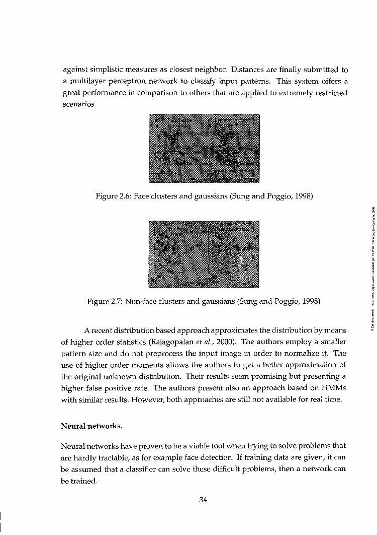
against simplistic measures as closest neighbor. Distances are finally submitted to

a multilayer perceptron network to classify input patterns. This system offers a

great performance in comparison to others that are applied to extremely restricted

scenarios.

xS '.•Míi'.nz.t xJ/•rp"i»«5a*v.': Jí l ..''7.t r ju i (iv.ssm -¡•!f•" .•

Figure 2.6: Face clusters and gaussians (Sung and Poggio, 1998)

i L}:j';:;<'rii:i i •JKSZIV.I'1J.--¡IS 1 •jKsziv.i'iJ.-ms

-f',.' > ; .1 < ; ^ ^ - . .

Figure 2.7: Non-face clusters and gaussians (Sung and Poggio, 1998)

A recent distribution based approach approximates the distribution by means

of higher order statistics (Rajagopalan et al, 2000). The authors employ a smaller

pattern size and do not preprocess the input image in order to normalize it. The

use of higher order moments allows the authors to get a better approximation of

the original unknown distribution. Their results seem promising but presenting a

higher false positive rate. The authors present also an approach based on HMMs

with similar results. However, both approaches are still not available for real time.

Neural networks.

Neural networks have proven to be a viable tool when trying to solve problems that

are hardly tractable, as for example face detection. If training data are given, it can

be assumed that a classifier can solve these difficult problems, then a network can

be trained.

34

Among those systems that have made use of neural networks, there is an in-

teresting one that can be introduced briefly (Rowley, 1999fc). This system has even

been integrated in an autonomous robotic system known as Minerva (Thrun et al.,

1998) and more recently an automatic doorman (Shuktandar and Stockton, 2001).

The work presented in (Rowley, 1999^), and other previous papers by the same au-

thor, uses a multilayer neural network trained with múltiple prototypes at different

scales, considering faces in almost upright position, but also non-face appearance.

Results seem to improve those achieved by (Sung and Poggio, 1998), being robust

enough to be tested interactively through internet (Rowley, 1999fl). The system as-

sumes a range of working sizes (starting at 20x20) as it performs a multiscale search

on the image. The system allows the configuration of its tolerance for lateral views.

A drawback is the fact that the process is computationally expensive and some op-

timization would be desirable to reduce the processing time. The author assures to

reach results in 2 — 4 seconds when improving implementation.

The work presented in (Han et al., 2000), applies a back propagation network

after a preprocessing phase based on morphology operators. This step allows the

system to reduce the potential face regions, however the system needs almost 18

seconds to process a 512 x 339 image using a SPARC 20 SUN workstation.

More recent works applied neural networks considering different head orien-

tations. In (Féraud et al, 2001) different filters and a fast search schema are applied

to avoid many candidates from the input image, thus the computational cost is re-

duced, achieving processing time of 0.3 seconds on a 333 MHz Alpha. Motion, color

and a perceptron are used to reduce the image window domain, which are indeed

part of the second family of techniques. Finally a model is built based on a neural

network that makes use of Principal Components Analysis reconstruction error and

a cluster distance.

Support Vector Machines.

Recently, Support Vector Machines (SVMs) have been applied to this problem (Os-

ima et al, 1997; Heisele et al, 2000; Ho, 2001). For those interested in pattem match-

ing framework, a detailed introduction can be found in (Burges, 1998).

SVMs can be considered a new method for training a classifier and have

proven their generalization in different tasks (Guyon, 1999). Most methods try to

minimize training error, however SVMs tries to minimize an upper bound of the

35

(a) í »

Figure 2.8: a) Hyperplane with small margin, b) hyperplane with larger margin. Extracted from (Osuna et al, 1997)

expected generalized error, making use of a principie called structural risk mini-

mization. For linearly separable case, SVMs provide an optimal hyperplane that

separates training pattems while minimizing the expected error of the unseen pat-

tems. That hyperplane maximizes the distance addition, known as margin, to posi-

tive and negative training pattems. An additional parameter is introduced to weight

misclassification cost. For non linear problems, training pattems are mapped into a

high dimensión space using a kemel function. More commonly used functions are

polynomials, exponentials and sigmoids. The problem is expected to have a linear

solution in that space. The first system presented (Osuna et al., 1997) ran 30 times

fáster and had slightly lower error rates than (Sung and Poggio, 1998). However, as

commented in (Yang et al, 2000fl), the use of SVMs has not been tested over a large

test set.

These works are limited to almost frontal views. Heisele (Heisele et al, 2000)

presented two different schemas for still gray level face detection. The first one

detects the face as a whole and the second detects its components separately. The

latter approach proved to be more robust in case of slight orientation changes in

depth. SVMs have also been tested with a multi view problem. In (Kwong and

Gong, 1999) the authors investigated the possibility of performing multi-view face

detection. This work concludes that no single SVM can learn an unique model for

all views, instead they use a classifier to select a view and later another to perform

the face/non-face classification.

Information Theory.

Another focus taken into account, is the contextual constraint, commonly in terms

of cióse neighborhood pixels (Yang et al, 2002). Mutual influences can be charac-

36

terized using Markov random fields (MRF). Thus, since the class probabilities are

dependent on their neighbors, the image is modelled as a MRF. The KuUback rel-

ative information gives a class separation measure which has proven bounds on

classification errors. Therefore, the Markov process that maximizes the information

discrimination between the face and non-face classes can be found. This procedure

leads to feature classes which are better for classification. The KuUback relative in

formation is directly related to other principies such as máximum likelihood, Shan-

non's mutual information, and mínimum description length. The measure is used to

find the most informative pixels (MIP), which from a pattem recognition perspective

should maximize the class separation. Lew (Lew and Huijsmans, 1996) presents a

face detector based on the KuUback measure of relative information. The algorithm

was tested on 4 test databases from 3 different universities (CMU, MIT, Leiden). The

results were found to be comparable to other well known methods. These authors

offer a demo that unfortunately runs only in SGI workstations. This approach is

also employed by (Colmenarez et al., 1998) to maximize information discrimination

between face and non-face classes.

Principal Component and Independent Component Analysis.

The use of principal component analysis (PCA) for representing faces in a lower

dimensión space was originally described in (Sirovich and Kirby, 1987; Kirby and

Sirovich, 1990). Lat3r their results were used for face recognition and detection (Tiirk

and Pentland, 1991). The projection of a non-face on that face space would not be

cióse to face projections. The distance can give afaceness measure (Turk and Pent-

land, 1991; Pentland et al, 1994) which is equivalent to a matching with eigenfaces

in that reduced space.

Another approach uses the reconstruction error (Hjelmás et al, 1998; Hjelmas

and Farup, 2001; K. Talmi, 1998), which can be computed transforming an input

image to the low dimensión space for later reconstructing and calculating the error

with the original image. This space is only valid for representing faces, if something

different from a face is projected to the face space, the reconstruction will have a

high error.

PCA reduces the dimensión of input data space, discarding low eigenvalues.

PCA does not pay attention to higher order moments of three or more image pixels.

For that reason some authors have used Independent Component Analysis for con-

sidering those relationships. ICA is an unsupervised learning algorithm that uses

37

the principie of optimal information transfer. In (Kim et al, 2001) the bootstrapping

ICA is used, to avoid a large set of learning patterns.

Winnow learning procedure.

An approach based on a sparse network of linear fimctions over a feature space is

the SNoW learning architecture (Yang et al, 2000&). This system uses the Winnow

update rule. This feature space can be incrementally leamed and is designed for

problems with a great number of features. Results described in that paper present,

according to their authors, the best overall performance considering rate of correctly

and false positives detected compared with Rowley (Rowley et ai, 1998), Osuna

(Osuna et al, 1997) and others.

Boosting.

The AdaBoost learning algorithm can be used to boost the classification perfor

mance of a simple learning algorithm. In the boosting language the simple learning

algorithm is called a weak learner. This is carried out by combining a coUection of

weak classification functions to form a stronger classifier.

A reminiscent of Haar basis function is used for a general object detection

system (Viola and Jones, 2001Í'). This system employs rectangle features that can

be calculated using an intermedíate representation called integral image. At a point

(x, y), of an image i, its integral image contains the sum of all pixels above and to

the left of the point, inclusive, see Figure 2.9:

ti{x,y)= Yl ^(<y') (2.1) x'<x,y'<y

Using that representation, any rectangular sum can be accomplished in four

references. Given a rectangle D defined by a comer point {xr,yr) and dimensions

{w, h). The sum within D is equal to ii{xr + w,yr + h) — ii{xr + w, y^) — ii{xr, yr +

h) + n{xr,yr)-

Two-rectangle features subtract the sum of pixels within two rectangular re-

gions, three-rectangular relate three rectangles and so on. The benefits of this prim-

itive feature is that once the integral image is computed, it can be evaluated at any

38

scale and location in a few operations in a constant time. Each rectangle feature de

fines a classifier. However, the number of rectangular features on an image is much

larger than the number of pixels, so a selection process is needed.

To select a very small number of those simple classifiers that can classify effec-

tively, the authors used the AdaBoost leaming algorithm. Adaboost combines weak

classifiers to get a strong one. Adaboost works iteratively, re-weighting the training

samples after each iteration to emphasize those which were incorrectly classified by

the previous classifier. In (Schapire et al, 1997), it is proved that the training er

ror of the strong classifier approaches zero exponentially in the number of rounds.

The authors used AdaBoost as a greedy feature selection process. After each round

they sorted the weak classifiers according to their error, getting a final sorted list of

best classifiers that depend on a single feature. This allowed to select a small set of

features, reducing the overall computational requirements of the system.

..

(x,y)

Figure 2.9: Integral image at point (x, y) is the sum of all points contained in the dark rectangle (extracted from (Viola and Jones, 2001 i»)).

AdaBoost selected a two-rectangle feature that computes the difference be-

tween eyes área and cheeks, and a three-rectangle feature that compares the inten-

sities of eye regions and the bridge of the nose. Finally, some classifiers are applied

in cascade. First, the system applies the two based filter specialized in minimiztng

false negative rate. Later, it is applied again but training the filter with samples that

passed the previous filter, thus deeper classifiers have correspondingly higher posi-

tive rates. The resulting face detector is valid for vertical and frontal faces processing

a 320 X 240 image at 15 fps.

In (Li et al, 2Q02a; Li et al, 2002b), an improved approach known as FloatBoost

39

is described. This approach is applied again to the integral image but with different

low level features and a pyramidal schema for applying in real time for múltiple

poses.

Linear subspaces.

The work presented in (Yang et al, 2000fl), described a couple of approaches for

representing face and non face spaces. These approaches were based on a mixture

of linear subspaces. One approach used a mixture of factor analyzers for cluster-

ing, performing a local dimensionality reduction on each of them. The parameters

of the mixture are estimated using an EM algorithm. The second approach uses

Kohonen's self- organizing map for clustering and Fisher Liner Discriminant (FLD)

to find the optimal projection for pattem classification, modeling each class using a

Gaussian estimated by ML. An extensive training set was used providing similar re-

sults while reducing false detections, against to well known accurate face detectors

(Sung and Poggio, 1998; Rowley et al, 1998). Different scales are analyzed scaling

the image. They always search a 20 x 20 pattem. These authors pointed out that

using techniques that perform better projection than PCA, the classification results

improve.

Wavelet transíorm.

A general framework for 3D object detection without pose restriction is presented

in (Schneiderman and Kanade, 2000). For each object the authors use a two step

strategy. First, they apply a detector specialized on the orientation, for later applying

a detector inside that orientation. For faces they use just a frontal and a profile

view. As they consider not known the shape of the distribution, flexible models are

used to accommodate a wide range of sfructures. They use histograms based on

visual attributes that are sampled from the wavelet transform. Different attribute

probabilities are combined using a product. Face and non-face samples are taken

and combined using bootstrapping for the selection of samples cióse to the class

boundaries. Results are similar to those achieved by (Rowley et al, 1998).

Another work that uses the wavelet transform is described in (García and

Tziritas, 1999). After a candidate regions selection by means of color, the multiscale

decomposition wavelet analysis is used. Results over an own and not large set are

compared with those achieved in (Rowley et al, 1998), which shows light improve-

40

ments on large sized faces, and a considerable improvement in speed.

2.1.1.2 Knowledge based (Explicit) approaches

Those techniques described in the previous section perform an exhaustive search in

the whole image for restricted poses, orientations and sizes, wasting time and pro-

cessing effort, which is really necessary when real-time performance is mandatory.

This search needs a great computational effort, affecting seriously the performance

of the system as different scales, orientations and poses mustbe chccked. Brute forcé

face detectors developers have pointed out the fact that some cues could be used for

increasing performance (Rowley et al., 1998). For that reason, some recent methods

apply cascade filters to reduce this computational cost (Li et al., 2002b). The point of

view used by the second family of face detection techniques try to use other features

to reduce the cost. Color, contour and motion are examples of cues that might help

to reduce the search área, and henee the computational effort.

Face contours.

Many works have paid attention to the elliptical shape of the face (Jacquin and Eleft-

heriadis, 1995; Sobottka and Pitas, 1996), which is true for almost frontal faces, los-

ing that feature when the head orientation changes. For that purpose, in (Yow and

CipoUa, 1998) the face contour is modelled considering two ellipse quarters, cen-

tered between the eyes, but at the same time managing that one hemiface could be

more visible.

Other works do not work with that face shape feature. An edge based ap-

proach (Froba and Küblbeck, 2001) uses geometric models getting a rate of 12 fps

or a PII500 MHz. For edge processing the Sobel operator is corr<monly used, which

convolves the images with two masks, horizontal and vertical filtering (M^ and My)

Cy{x,y)^My*I{x,y)

Later the magnitude and direction can be achieved

41

S{x,y) = ^C¡{x,y) + C^{x,y)

0(x,y) = a r c t a n ( ^ ) + f (2.3)

Applying a threshold for avoiding noise, gets ST- The edge information is

rewritten in a vector and compared with a face model built by hand. To consider

different resolutions a pyramid is used for edge resolution. A similar approach for

gray images (Maio and Maltoni, 2000), uses a Hough Transform for detecting the el-

liptical face in a ellipse fitting schema combined with a témplate matching approach,

but without offering the possibility for different resolutions.

Instead of using a simplistic ellipse, in (Jesorsky et al, 2001) the Hausdorff

distance (HD) restricted two 2D is used. This distance represents a metric between

two set of points. Given two finite sets, A = ai,...,am and B = 6i, ...,6„, HD is

defined as:

H{A,B) = max{h{A,B),h{B,A)), where h(A,B) = meixmm\\a - b\\ (2.4)

This is the directed Hausdorff distance from set Ato B. In. image processing

applications, a different measure is used, the modified Hausdorff distance (MHD)

(Dubuisson and A.K.Jain, 1994).This versión takes the average of siagle point dis-

tances, decreasing the influence of outliers.

h^odiAB) =---^xmn\\a~b\\ (2.5) ' ' aeA

The system, starts calculating an edge image, where a transformation that

minimizes the HD to a 2D face model is searched. Latei, a fine search is performed

using a model of the eye área. Selecting the model is a main aspect of this method,

a more recent work improved the model selection by means of genetic algorithms

(Kirchberg et al, 2002).

Some works make use of color vector gradient to get an edge image less sen-

sitive to noise than the scalar gradient computed from each channel or from gray

level image (Terrillon et al, 2002). The color vector gradient is computed as foUows:

42

IVC|| = W - (^g:cx + Qyy + ^ÍQXX - Qyyf + Wxy) (2.6)

being

9xx — \Qrc) + (ax j + i ax /

9yy = \J¡) + ( 9¡7J + ( a j (2.7)

Facial Features.

Facial features are the máin characteristics of faces. Their geometry and their ap-

pearance can be used to detect faces. Some works are based on local descriptors

of those features observing their contours, their geometric relations, or computing

on these salient potnts Gabor filters or Gaussian mixtures (Vogelhuber and Schmid,

2000).

Feature contours were used in (Yow and CipoUa, 1996) where a face model

based on facial features edges is considered. Facial features are grouped by loca-

tion, and different combinations are considered as some of those features could be

hidden for certain viewpotnts, see Figure 2.10. After prefiltering the image for se-

lecting pornts of interest, edges aroimd them were considered to match the model.

Later, different facial features are grouped together to test if they can fit the face

model. Ftnally, a Bayesian network is applied to survivors sets, to test their overall

likelihood.

— —

Facs

= =

Topl>l-0

— — _ _

ttottoinFlíG

=

zz

Lotwro

=

Riglrtl'l't;

—

Hpairl ItpiLÍr2 Vpairl Vpair2 Vpair^

Figure 2.10: Partial Face Groups (PFG) considered in (Yow and CipoUa, 1996), and their división in vertical and horizontal pairs.

43

Spatial constraints are powerful to increase detection rate (Vogelhuber and

Schmid, 2000). Their statistical analysis can benefit the overall system as geometric

distribution can be used to check facial features positions. In (Sahbi and Boujemaa,

2002) a Gaussian mixture is used for that purpose, a ML rule decides if the set is

accepted.

Face and facial features contours and texture are used in (Cootes and Taylor,

2000) to model a face. The model is built based on a set of labelled examples. A

new image is examined finding the best model that match the image data. The

authors describe two approaches: 1) Active Shape Model (ASM), which manipulates

a model to find structures location on the image, and 2) Active Appearance Model

(AAM), which is able to synthesize new images of the object of interest. It considera

a statistical model of shape to represent the objects of interest.

Figure 2.11: Shape Model example (Cootes and Taylor, 2000).

The authors extended the idea of Active Contour Models (Kass et al, 1988), or

snakes commonly used for tracking, imposing a shape model. The shape model is

built by labelling tateresting points in the training set, see Figure 2.11. After aligning

the samples, they form a distribution. The model can be parameterized in order to

créate new forms, but first the authors reduce the dimensionality using PCA for

computing the main axis of the distribution.

The appearance model integrates also texture. First the example image is

warped to fit the mean shape, see Figure 2.12. Intensity information forms a dis

tribution where the authors apply PCA again, to get the main directions in gray

variation.

44

Later, given a rough starting approximation, an instance of the model can be

fit to an image, applying multiresolution to improve efficiency. Finally, the appear-

ance model can be adjusted. Using ASM alone is faster, but AAM provide a better

fit to input image.

Shape Free Patch

Figure 2.12: Active Shape Model example (Cootes and Taylor, 2000).

Active appearance m,odels ha ve been used by different authors. A 3D face

model, CANDIDE-3 model, was used for this purpose in (Ahlberg, 2001), using

dedicated hardware to get real-time performance. These approaches provide pow-

erful tools to manage pose variation.

Another approach combinrng texture and geometry is described in (Burl et al,

1998). This paper describes a general framework to be applied for object recognition.

Considering a model composed by A' parts with a location, the authors describe

an optimal detector based on the likelíhood ratio p{x\F)/p{x\F), but rewriting it to

assume the different parts that form the object, taking into account both the texture

and position of them. Later, they present an invariant approximation to manage

translation, rotation and scaling. Some restricted experiments present promising

results.

Motion Detection.

If an environment with a static camera is considered, motion detection can be per-

formed in order to detect a face (Hjelmás et al, 1998). This system assumes that if

there is a large moving object in the image, there may be a human present, situa-

45

tion that happens in videoconference applications. According to these authors, four

steps are needed:

1. Frame dijference: The difference between the current frame in the video se-

quence and the previous is calculated.

2. Threshold: Those pixels with a difference greater than a threshold are selected,

creating a binary output image.

3. Noise removal: Isolated motion áreas are considered noise and removed.

4. Adding moving pixels: Moving pixels are counted on each line. If there are three

consecutive lines with more than fifteen moving pixels, it is considered that

there is an object, not just single pixels with movement. Using the information

about the number of moving pixels on each line, a point in the middle of the

upper moving object is calculated. Geometric restrictions give a position for

the center.

This processing provides the location of a potential face, where a face appear-

ance test mustbe applied. For example in this work, and others (Hjelmas and Farup,

2001; K. Talmi, 1998), the face space is defined based on eigenvectors with a number

of samples, mean subtracted. A new image is projected into face space, then us

ing the first principal components the image is reconstructed and the r^-constructi.on

error calculated, see also section 2.1.1.1. This error is interpreted as a measure for

face/non-face classification.

Motion is combined also in (Bala et al, 1997). A background reference image

is captured before the user sits in front of the camera. The user is easily located de-

tecting the differences between the current image and the reference image. The ref

erence image must be updated during the entire process by taking changes within

the background región into account. Those áreas classified both as skin and fore-

ground are registered as facial regions. The segmentation result is further improved

by applying non-linear filters, e.g. dilation and erosión, in order to fiU holes in large

connected regions and to remo ve small regions.

A whole body person tracking systems, as the one described in (Grana et al.,

1998), makes use of the motion image for later applying a signature approach, for

roughly localizing the head área. Later, a color based technique is used to detect the

face within that área.

46

• Color. - • — - - -

Color is a perceptual phenomenon that is related to the spectral characteristics of

electro-magnetic radiation in the visible wavelengths reaching the retina (Yang et al,

1998Í'). Skin color is caused by two pigments: melanin and hemoglobin (Tsumura

et al, 1999).

As pointed out in (Yang and Huang, 1994; Rowley, 1999fc) color Information^

if available, improves performance. The authors refer to color Information as a tool

that may be used to optimize the algorithm by means of restricting the search área.

Color is calculated easily and fast making it siiitablc for real time systems

providing invariance also for scale, orientation and partial occlusions (Raja et al,

1998). Thus, color pro vides a tool for an experimental set without special hardware

requirements. For that reason, several methods of face detection are based on skin

color. Color is sometimes used in combination with other cues like edges, or making

use of heuristics to improve performance using not only local operations based on

pixels but also geometric information or multiscale segmentation (Yang and Ahuja,

1998). When color is integrated, the system designer have to consider: 1) the schema

used for representing color, i.e. the color space representation, 2) the method used

for modellrng and search for a new image, and 3) the color evolution in time.

A

I

D

»•! .t,

•i;,( «f-'-t.,- . i - i .»-«

*» *.' /

Figure 2.13: Frame taken under natural light. Average normalized red and green valúes recovered for rectangles taken in those zones: A(0.311,0.328), 6(0.307,0.337), C(0.329,0.338) and D(0.318,0.326).

47

r\

' C

Figure 2.14: Frame taken under artificial light. Average norrnalized red and green valúes recovered for rectangles taken in those zones: A(0.241,0.335), 5(0.24,0.334), C(0.239,0.334) and 0(0.273,0.316). .. ^

Color Space Representations

Commonly surface color can be described using certain valúes that represent color

in a color space representation. To start with, the color space used in (Wong et al,

1995) serves as a good example of a simple approach. This paper does not use

color for face detection but for person detection. It is based on a normalizea space

obtained from the RGB image, where a rectangular área is defined of interest. Then,

it is straightforward to genérate a binary image that indicates for each pixel whether

its RGB valué is included on that selected área of the color space. It is clearly a

primitive approach that makes use of a fixed threshold. This approach would evolve

making use of probability for segmenting áreas as well as multiscale segmentation

where neighborhood is considered, avoiding light influence.

Many color spaces do not have a direct relation between differences in color

perception and differences in color representation. This means that a perceptually

different color can be located cióse in color space representation and viceversa. RGB

is a color space that has this lack. For that reason, perceptually uniform color sys-

tems have been defined and have already been used for skin detection (Cai and

Goshtasby, 1999; Wu et al, 1999fl; Chen et al, 1999). The main feature is that two

colors perceived with an equal distance by humans would project an equal distance

using this representation. In (Cai and Goshtasby, 1999), the components without

48

intensity/luminance influence of a CIEL*a*b* space (a and b) are used. This color

space was defined to represent the entire visual gamut with perceptual linearity.

The system provides a gray output image where each pixel represents with a gray

level its probability of belonging to skin color class, for details see Section C.2.

Another common color representation that has provided good results even

under wide lighting variations is normalized color coordinates (NCC), also known

as red and green normalized (Wren et al, 1997; Oliver and Pentland, 2000; Bala

et al, 1997; Stillman et al, 1998b; Oliver, 2000; Ho, 2001; Terrillon et al, 2002; Soriano

et al, 2000b). This representation uses color chromatic Information, i.e., (r„,^„) =

(R+B+G' R+B+G) (** avoid a nuil denominator in (Zarit, 1999) it is added 1).

A Hue-Saturation, HS, model is employed in (Mckenna et al, 1998). lUumi-

nation influence is again eliminated as this is a chromatic space color representation.

A model of a single person is used with success with other races. However, it was

necessary to use at least two color models, one for interior lighting and one for ex

terior natural daylight.

HSV space, see section C.l for details, is used in (Jordao et al, 1999; Bradski,

1998), this color space has received a large support from numerous works, agarnst

other chromatic representations such as (f„, „).

An application presented in (Forsyth and M.M.Fleck, 1999), uses color to de-

tect nude images in internet as a way to perform a filter for web surfers, for example

láds. The RGB image is transformed to the log-opponent / , R^ and By.

In (Birchfield, 1998), the color space used is B - G, G - R and R + G + B,

where the first two components represent chrominance while the last gives lumi-

nance Information (Swain and Ballard, 1991).

However, trying to model a general color for skin is complex, specially if dif-

ferent cameras and lighting conditions must be dealt. Thus some works prefers an

user-specific color model instead to an user-independent color model (Oliver and

Pentland, 1997; Bala et al, 1997). In (Bala et al, 1997) an user-specific color model is

used to track a face. An initialization phase is necessary to determine the individual

skin color distribution, extracting image regions with high probability of face color.

The universe of color spaces is larger, but the intention of this document is

not to bore the reader with every approach.

49

Color Space Comparisons

Different authors have performed some kind of comparison among different color

spaces applied to the skin color detection problem. These authors have given main

attention to chromaticity color spaces, as they are more suited for changes in illumi-

nation.

A t5^ical and extended chromaticity color space is NGC or (r„, 5„). Different

works agree considering that this space is not the best for skin detection purposes

while others conclude the opposite. The work described in (Bradski, 1998; Jordao

eí al., 1999), uses HSV, as the authors have found in their experiments that NCC

is more sensitive to lighting changes, as saturation is not separated. Another work

considers that HSV is more suited than NCC for prediction of color distribution

evolution (Sigal et al, 2000). However, this space has a costly conversión from stan

dard RGB sources that is more expensive than {fn,gn) (Sigal et al, 2000).

An exhaustive analysis of five color spaces {HSV, NCC, YGrCb, FleckHS

and CIELa*b*) is presented in (Zarit, 1999; Zarit et al, 1999). Skin color detection

is performed using a Lookup Table (LT) and a Bayesian approach. For the first

one, best results are obtained for HSV and Fleck HS. The Bayesian approach was

tested using Máximum Likelihood (ML) and Máximum a Posteriori (MAP) taking a

priori probabilities from trainrng images. The ML approach worked better than the

MAP approach (perhaps due to a priori probabilities arsumption). Adding ? torture

test to ML approach which consisted in eliminating áreas with high variances, the

system outperformed LT. Results are expressed in terms of percentage of correctly

detected pixels, percentage of non skin error and percentage of skin error pixels.

Tuning thresholds to get a high correctly detected pixels percentage yields also a

increase of error percentages. Low threshold, provokes marking more pixels as skin

that should be.

A subset, RGB, HSV, and CIELa*b*, is examined in (Herodotou et al, 1999)

achieving similar results. The authors analyze the distribution for different races

getttng light differences.

Another comparison is due to (Terrillon and Akamatsu, 2000). Several chro-

matic spaces were tested observing that TSL provided the best performance, while

{rn, Qn) was considered acceptable and better than others spaces such as HSV, YES,

different GIEs, etc., see section C.4 for transformation details. This study was taken

into account in (Hsu and Abdel-Mottsleb, 2002) where the image is corrected for

50

white, using later LCrCb-

A comparison among HSV and YCt,Cr is presented in (García and Tziritas,

1999). In that work, it is pointed out that even when for the second color space the

skin cluster seems to be more compact, the bounding planes for the first one are

more easily adjusted, see section C.3 for transformation details.

The authors of (Bergasa et al, 2000) assure to have accomplished a study of

human color skin distribution in different color spaces (RGB, {fn,gn)f HSI, SCT

and YQQ) concluding that the best space is (f„, „).

These comparisons do not conclude that NGC is the best color space for that

problem, but it is always among the best ones. There is no a general agreement

selecting an altemative, as some of them select one color space while others select

another. These differences among comparisons seem to proof that the samples are

sometimes noisy. Perhaps the training sets were not built (built commonly by hand,

presenting problems to select a pixel as skin or non skin) with the same criteria,

therefore results do not match.

Methods for skin detection/Modeling skin color

Any literature reference assumes that skin colors form a cluster in a color space.

However, some experiments prove that this cluster compactness varies among color

spaces. And even more, bad news are that skin and non-skin clusters are never

completely separated.

Modelling skin color and the method used to search that model are common

topics. Most approaches to segment skin color can be grouped into two main cate-

gories: 1) pixel based, 2) area-based. However, other families can be distinguished

(Herodotou et al., 1999). To date there are approaches that model the color as a

threshold (Wong et al., 1995), as a threshold with a probability function (Cai and

Goshtasby, 1999), quantizing color according to the set of dominant colors (García

and Tziritas, 1999), or as in (Feyrer and Zell, 1999), skin color is modelled in terms

of a look-up table or histograms.

Other authors conclude that under certain lighting conditions, the skin-color

distribution of an individual can be characterized by a Gaussian distribution (Yang

et al., 1998^). The authors carried out this conclusión after performing Goodness-

of-fit tests. Differences among humans are much more in brightness than color,

this means that skin-colors of different people differ mainly in intensities (Yang and

51

Waibel, 1996). For a set of subjects of different races, Ihe skin-color distribution

can be characterized by a multivariate normal distribution in the normalized color

space.

This was not the only approach based on gaussians distributions. There

are other approaches that fít skin color to gaussian distributions (Yang and Ahuja,

1998; Stillman et al., 1998&) simples or mixtures (Raja et al, 1998; Xu and Sugimoto,

1998; Yang and Ahuja, 1999), or radial basis fvinctions (RBF). Gaussians are achieved

from many samples that are studied by statistical algorithms such as Expectation-

Maximization (EM) (Redner and Walker, 1984; Bilmes, 1998; Jebara and Pentland,

1996), or training RBF's by means of neural networks. But in any case, commonly

there is a need to use at least two different models, indoor and outdoor (Mckenna

et al, 1998).

Some works argued that skin color samples taken by hand are not analo-

gous to a normal distribution or to any geometric shape, and thus a look-up table

or histogram provides a better description for skin color (Feyrer and Zell, 1999). In

(Jones and Rehg, 1998), the model described uses almost 1 billion pixels taken from

web images unconstrarned. Comparing histogram and mixture models, the first

approach got better results achieving a rate of 80% of success with a 8.5% of false

positives. The histogram model was constructed from RGB space. Another lookup

table method is described in (Zarit et al, 1999). Each training sample will be used

to increment its correspondent cell on a two dimensional histogram. Each cell rep-

resents the number of pixels w ith a particular range of color pairs. At the end, all

the cells are divided by the maximal valué yielding to a histogram that reflect the

likelihood of a color. Typically the range is divided in bins, in this work 64 x 64 and

128 X 128 were used.

An extensión of this work is described in (Sigal et al, 2000), adapting color

distribution over time for better performance. It is assumed again that the cluster of

skin color is well localized in color space, but it is pointed out that no single gaussian

can represent ^bat cluster. Thus, the extensión, to mixture gaussians is needed, but

as soon as more mixtures are needed, the real time constraint is not feasible. On

the other side, histograms are evaluated trivially regardless the complexity of the

distribution. However, histograms are not good for representing sparse data where

only a fraction of the samples is available. Interpolation or gaussian filters solve this

drawback.

A polyhedron in HSV space is defined in (Herodotou et al, 1999). Their

52

boundaries are conditionally defined according to saturation, as with low saturation

the hue is unreliable. A second polyhedron is defined to adapt the transition of the

first one. Later, some shape tests (valid for restricted scenarios) confirm the blob

selected.

Problems

Many studies have located the skin color variance in a localized área of any selected

color space, indeed people variation differ less in color than in brightness (Bala et al.,

1997). Thus, human skin-color distribution is clustered in chromatic color space and

characterized by a multivariate normal distribution (Yang and Ahuja, 1998). Chro-

maticity is not affected by identity and race, differences among people are reduced

by intensity normalization. Therefore, color seems to be easily applied.

But as it is well known, color is not robust under any circumstance. Color per-

ception varíes substantially for different environments. Specially when the scenery

is not under control due to varying lighting conditions (Storring et al., 1999) and

light source properties (Storring et al., 2001). An example is shown in Figures 2.13

and 2.14. These images were taken with different illumination. Selecting áreas on

each zone, the average valúes for the read and green normalizad components are

obtained. Enlarging the color space área to detect skin in both images will produce

lots of vmcorrect skin pixels detections.

In the foUowing some problems that appears when using color are briefly

described. Any visión system (Finlayson, 1995) needs a constant perception of the

world. Different light sources offer different spectral properties, producing differ

ent reflection effects over object surfaces. Obviously, perception is altered by these

effects. Skin color is also affected by light variations of the same light source, e.g.,

daylight. Color constancy is suggested as a method for solving this problem. The

ability of identifying a surface as having the same color under different viewing

conditions is known as color constancy. Humans have such ability, but the mech-

anism is still unclear. Thus, color constancy algorithms (Finlayson, 1995; Bamard

et al., 1997) try to get a new image corrected, from an input image imder an un-

known illumination. The new image would express its colors under a canonical

illumination independent from scenery illumination. In (Funt et al., 1998) different

color constancy algorithms are tested to use them in color based recognition, using

histogram matching approach (Swarn and Ballard, 1991), also known as color index-

ing. This approach fails when ambient lighting of the object to be recognized differs

53

from the one used for building the model (training). That paper tried to answer the

question if color constancy algorithms are effective or not providing illumination

independent color descriptors. The algorithms tested were greyworld, white-patch

retinex, neural network, 2D gamut-constraint and 3D gamut constraint. Results

prove that color constancy improves color indexing but they did not perform as

well as expected. Therefore, color constancy algorithms have still lot of work to do.

Recent works on face detection try to be conscious of color constancy prob-

lem for skin classification, in order to filter input image before applying the skin

color detection procedure (Storring et al, 2000; Storring et al, 2001). Skin color can

be modelled in terms of a reflectance model (Storring et al., 1999) but that is pos-

sible only if knowledge about the camera reflectance model and the spectrum of

light source is available. Skin color appearance depends on brightness and the color

temperature of the light source. On one hand, bright is avoided using a chromatic

color space (Yang and Waibel, 1996; Mckenna et al, 1998). On the other hand, illu

mination source influence has been rarely studied even when its influence is notori-

ous. Light source properties can be deduced from the image as skin properties are

known. Highlights provide Information for this purpose. Nose shape is relatively

good for highlights (Storring et al, 2001), thus they are used for recovering light

properties. Implementing the estimation from highlight should be possible, also in

real time, since it would be sufficient to do this once or twice a second. The problem

is more that there are not always highlights on the nose. The authors used a rather

good 3CCD camera in that paper. Also mixing different light source» vvould forcé

a system to search in color space intersection of áreas defined by the source alone

(Storring et al, 2001).

In (Storring et al, 1999) the term skin locus is used to refer the área, that under

different lighting conditions, skin color occupies in NGC. Soriano applies skin locus

concept being able to adapt the skin color model, under real conditions, for next

frame search using back projection (Soriano et al, 2000fc; Soriano et al, 2000fl). The

system does not assumes the form of skin color distribution. Instead they use the

actual skin histogram as a non parametric skin color model and employ histogram

backprojection (Swatn and Ballard, 1991) to label skin pixel candidates. Skin locus

must be first determined for the camera used, see Figure 2.15. The system needs an

initialization step to lócate skin color within skin locus. Later, it assumes that skin

color shifts due to changing illumination conditions but only inside that área. To

adapt, the histogram is updated with pixels belonging to the skin locus and detected

in the actual face bounding box. Thus, a chromaticity-based constraint is used to

54

0.8

0.6

0.4

0.2 ••

0,2 0,6 0,8

Figure 2.15: Nogatech Camera Skin Locus (Soriano et al, 2000fl), considering NCC color space. The skin locus is modelled using two intersecting quadratic functions.

exelude those pixels which are not skin. This restriction is used to créate a ratio

histogram penalizing those colors contained in the background or which are not

part of the model. The paper presents results using their adaptation schema and a

fixed one with interesting results.

Different illumrnation conditions, cameras, and skin tonalities are used in

(Martinkauppi et al, 2001) to test the performance of different color spaces. If the

skin locus in a color space occupies a contiguous región and at the same time shows

very good overlap within skin groups, then that color space is potentially useful

for adaptive skin color-based tracking. Results indícate that skin locus is a good

tool for tolerating illumination changes providing a good overlap among different

tonalities, but must be modelled for each camera.

Color processing presents interesting features for real-time systems, but it

has still open problems such as color constancy. This lack of robustness seems to

be responsible of the large number of altemative approaches in the literature. Ap-

proachcs that work well under certain conditions.

Color evolution

The color constancy problem and its variability along time have been already a topic

addressed by many researchers (Raja et al, 1998; Bergasa et al, 2000). As described

above, the skin-color distribution cluster in a small región in color space, however

55

the parameters of this distribution differ for difieren! lighting conditions (Yang and

Waibel 1996).

Environment changes can be considered under different points of view: tol-

eration and adaptation. In this section, the techniques presented focus the problem

differently, they try to adapt skin color model to cope color detection under uncon-

strained conditions instead of recovering colors.

The experiments presented in (Yang and Waibel, 1996) show that a change in

lighting conditions does not affect the shape of the distribution but there is a shift in

the color histogram.

Both (Yang and Waibel, 1996) and (Hunke and Weibel, 1994) combine color

and motion for designing a real time system. The first paper models skin color as a

multivariate normal distribution which is defined initially and evolves dynamically.

This evolution can affect seriously the color tracked. This adaptation to environ

ment changes is considered also in (Raja et al., 1998). Color evolves, while motion

provides cues about where the target is, thus provides color evolution trace. Color

blob parameters are updated based on an Expectation Maximization (EM) approach

in (Oliver and Pentland, 2000).

Kampmann (Kampmann, 1998) supposes that eyes and mouth have been pre-

viously detected for later searching color samples under the eyes. If the system is

able to detect a face, this idea could help defining color shift according to illumina-

Lion changes.

In (Sigal et al, 2000), where histograms are used, it is assumed that skin-color

distribution evolves as a whole by means of affine transformations. A dynamic mo

tion model is defined and a second order Markov model predicts the evolution over

time. The algorithm performs better than the static histogram approach, but there

is a dependency on the initialization phase. The algorithm works better growing

regions, thus oversegmented initial región would affect negatively the system. The

authors propose an integration of constraints based on face knowledge.

Segmentation and a color distribution are used in (Sahbi and Boujemaa, 2002)

to adapt color model. An off-line coarse neural network for skin color is adapted to

current image using a probabilistic framework.

The work presented in (Bergasa et al., 2000), selects in an unsupervised way

an initial location for the skin color gaussian distribution based on the pixel concen-

trations in the histogram. These concentrations are associated to the main colors in

56

the image, among which is the skin color. Later color cluster centers are adjusted

using a competitive leaming algorithm based on Euclidean distance proposed by

Kohonen. The following frames are processed estimating the skin color distribution

parameters and the adaptive threshold. This approach is more economic than those

based on EM algorithm providing similar results, and works unsupervised in con-

trast with (Yang and Waibel, 1996). The only problem pointed out is related with

the presence of a backgroxmd color with similar chromaticity to the skin and whose

blob is connected.

The coexistence of different models for different contexts is considered in

(Kruppa et al, 2001). The main aspect is to realize which model is appropriate for

each circumstance. The KuUback divergence is used to define a measure.

Combination/Heuristics

Several methods of face detection are commonly based on skin color detected alone

Qebara and Pentland, 1996; Oliver and Pentland, 1997; Raja et al, 1998; Yang and

Waibel, 1996; Jordao et al, 1999). However, some authors consider coherently fhat

color Information alone is not sufficient for face segmentation (Bala et al, 1997; Gar

cía and Tziritas, 1999), since the background may also contain skin colored objects

that could be considered part of the facial región. Thus, color is sometimes com-

bined with other cues for achieving a better performance. The use of heuristics im-

proves performance due to do not use only local operations based on pixels (Yang

and Ahuja, 1998).

In (Bala et al, 1997) the combination with motion allows the system to reject

certain áreas. Motion is also used in (Takaya and Choi, 2001), where color filtering

is applied only after subtracting consecutive frames, reducing the presence of false

detection. These motion blocks allow the definition of those thresholds needed for

color filtering. In (Hilti et al, 2001), considering persons standing in front of the

camera, the motion history image is combined with color Lo adapt the skin color

model.

in (Oliver and Pentland, 2000), the term blob feature is described. A blob is

characterized by color, texture, motion, shape, etc. In this work a blob is described

analogously to (Wren et al, 1997) using position and color. In (Bala et al, 1997; García

and Tziritas, 1999), color is combined with a texture analysis based on wavelets.

Some combinations are based on the use of geometric Information or mul-

57

tiscale segmentation (Yang and Ahuja, 1998; Forsyth and M.M.Fleck, 1999; García

and Tziritas, 1999) over blob image. This blob image can be a likely image (Yang

and Ahuja, 1998; Cai and Goshtasby, 1999) or just a binary image (Forsyth and

M.M.Fleck, 1999) where pixel regions can be joined to get a final blob that fits a

face shape (Forsyth and M.M.Fleck, 1999; Cai and Goshtasby, 1999; Feyrer and Zell,

1999), i.e., an elliptical blob. A likelihood image is achieved after assigning a proba-

bility to each pixel región.

In (Birchfield, 1998) color information is combined with a gradient measure

of the image at an estimated position for the face, gradient is fitted with an ellipse

as that is the shape expected. Dependency on gradient magnitude makes the head

tracker too sensible for cluttered environments.

Recently in (Wu et al, 1999fl; Chen et al, 1999), color has been used not just

for detecting the face but also the hair, as a cue for determining the three dimen

sional head pose attending to its relative blob position. After building a likelihood

function for skin and hair, it is possible to guess a head orientation based on the

relation among both blobs after performing a fuzzy pattem matching. Certainly, the

hair seems to be more difficult to isolate in color space, and thus luminance is also

considered in the process. The speed is better than neural networks approaches, and

the performance according to the authors ia not bad. However, they do not perform

any analysis of the facial features.

. Other approaches intégrate color and edges (Sobottka and Pitas, 1998). Kamp-

mann (Kampmann, 1998) combines different cues to sepárate head components, de-

tected eyes and mouth, and combines face contour with color definition, taking the

área under the eyes, to segment hair, face, ears and neck.

In (Darrell et al., 1998) robustness is achieved thanks to the combination of

stereo, color, and face detection modules. Real-time stereo processing is used to

isolate users from other objects and people in the backgroimd. Skin color classifica-

tion identifies and tracks likely body parts within the silhouette of the user. A face

pattern is used to localize the face within the identified body parts.

In (García Mateos and Vicente Chicote, 2001) a Hue-Intensity-Texture map

is generated for detecting face candidates. Each image plañe consists of a bina-

rised image achieved using thresholds, which are established based on histograms.

Later, vertical and horizontal projections are used to detect facial features, but no

further test is performed. Some experimental results are presented and compared

with those presented in (Rowley et al., 1998), unfortunately no comment is added

58

about the use of the same methods on the same set of images.

Edge image is subtracted from skin color image in (Terrillon et al., 2002).

Later, only major blobs are considered, computing their moments (Terrillon et al,

1998) that are filtered using a neural network.

2.1.1.3 Face Detection Benchmark

Not many years ago. Lew pointed out that there were no comprehensive perfor

mance comparisons between different face detectors (Lew and Huijsmans, 1996).

Certarnly, new papers present comparisons among the new approach described and

with well known methods using their own or known face images data sets. Re

cent face detection surveys analyze and compare different methods using different

known data sets (Hjelmas and Farup, 2001; Yang et al, 2002). In the foUowing, the

reader is guided through the data sets available and the criteria attended to estímate

the quality of a face detector.

1. Data sets

Face processing techniques need common ground data where different ap-

proaches can be compared. Main face processing efforts have focused up to

now in face recognition techniques, for that reason most face databases were

created for this purpose. This fact is reflected in the data sets described briefly

on Table 2.1. Most of them contain just one face per image (except CMU data

set), so a face detector could not be able to tackle the problem of detectrng

múltiple faces on an image. Also, these sets were conceived for brute forcé

face detectors as are a coUection of still images and mug shots. These data sets

(extracted from (Yang et al, 2002), the Face Detection Homepage (Frischholz,

1999) and other net sources) are indexed in Table 2.1.

Features of these data sets are different, according to background characteris-

tics, lighting conditions, number of people, etc. According to Face Detection

Homepage (Frischholz, 1999), specifically for face detection purposes were cre

ated: CMU, BIOID, AR, Essex Univ., Oulu Univ., Extended M2VTS and JAFFE

data sets.

Face detection methods do not pay commonly attention to temporal coherence

as they do not exploit Information enclosed rn a video stream. However, some

resources are available for being used as test, even when they are more focused

59

Source and Location MIT Datábase

ftp://whitechapel.media.mitedu/ pub/images/

Weizmann Institute Datábase

ftp://ftp.wisdom.weizmann-ac.il/ pub/FaceBase/

Univ. of Stirling Datábase

http; / /pics.psy ch.stir.ac.uk/

FERET Datábase (PhiUips et al. 1999)

. - . http://www.itl.nist.gov/ iad/humanid / feret/

UMIST Datábase

http://images.ee.umist.ac.uk/ danny/da tabase.html Univ. of Bem Datábase

ftp://iamftp.unibe.ch/pub/Images/FaceImages

Yale Datábase

http: / /cvc.yale.edu /projects/yalefaces/yalefaces.html

The AR Face Datábase

http://rvll.ecn.purdue.edu/ %7Ealeix/aleix_face_DB.html

AT&T Datábase {Graham and AUinson, 1998)

http://wv/w.uk.research.att.com/ facedatabase.html Harvard Datábase

ftp://ftp.hrl.harvard.edu/ pub/faces

CMU Datábase (Rowley et al, 1998)

http://vasc.ri.cmu.edu/ idb/html/face/index.html

The CMU Pose, Illumination and Expression Datábase (Sim et al. 20ni>

http://www.ri.cmu.edu/ search for PIE Datábase

BioID Face Datábase Qesorsky et al, 2001)

http://www.bioid.com/technology/facedatabase.html different test persons. Set eye positions are included.

The extended M2VTS Datábase

http://www.ee.surrey.ac.uk/ Research/VSSP/xm2vtsdb/

University of Oulu Face Datábase (Soriano et al, 2000b)

http: / / www.ee.oulu.fi/ research / imag / color/pbfd.html Essex University Face Datábase

http://cswww.essex.ac.uk/ allfaces/Índex .html

Ja^-anese Female Facial Expression (JAFFE) Datábase

http:/ / www.mic.atr.co.jp/ mlyons/jaffe.html

Comments Faces of 16 people,

27 of each person under various conditions of illumination, scale,

and head orientatíon. Includes variations due to

changes in viewpoint (mainly horizontal), illumination (only horizontal), and three different expressions.

Scatter set of images.

Under request.

Consists of 564 gray level images

of 20 people

Contains 165 grayscale images in GIF format of IS individuáis. There are 11 images per subject

Created at CVC, it contains over 4,000 color images

corresponding to 126 people's faces (70 men and 56 women)

Ten different gray level images of each of 40 distinct subjects

The data set consists of 1521 gray level images. Each one shows the frontal

view of a face of one out of 23

Not free. Contams tour recordings (speaking and rotating) of 295 subjects

taken over a period of four months including high quality color images.

Not free. 111 different faces each in

16 different camera calibration and illumination condition.

24bit color JPEG of 395 individuáis.

20 images per individual Con*=íins 213 images of 7 fT-ial

expressions (6 basic facial expressions + 1 neutral) posed by 10 Japanese female models.

Table 2.1: Still image resources for facial analysis

60

ftp://whitechapel.media.mitedu/

ftp://ftp.wisdom.weizmann-ac.il/

ch.stir.ac.uk/

http://www.itl.nist.gov/

http://images.ee.umist.ac.uk/

ftp://iamftp.unibe.ch/pub/Images/FaceImages

http://rvll.ecn.purdue.edu/

http://wv/w.uk.research.att.com/

ftp://ftp.hrl.harvard.edu/

http://vasc.ri.cmu.edu/

http://www.ri.cmu.edu/

http://www.bioid.com/technology/facedatabase.html

http://www.ee.surrey.ac.uk/

http://www.ee.oulu.fi/

http://cswww.essex.ac.uk/

http://www.mic.atr.co.jp/

JUDYBATS

Figure 2.16: Sample of CMU datábase (Rowley et al, 1998).

Source and Location Boston University Head Tracking

Datábase (Cascia and Sclaroff, 2000) http://www.cs.bii.edu/groups/icv/HeadTracking

The extended M2VTS Datábase

http://www.ee.surrey.ac.uk/Research/VSSP/xm2vtsdb/ CMU Facial Expression Datábase

(Cohn í'f al. 1999; Lien el al. 2000; Kanade el al. 2000) http://www.cs.cmu.edu/

Boston Univ. Color Tracking Datábase {Sigal et ai, 2000)

http://www.cs.bu.edu/groups/ivc/ColorTracking/

Comments

Expensive. Contains four recordings {speaking and rotating) Contains aroiind 2000

gray levéis image seqiiences

Contains sequences in SGI movie format

Table 2.2: Sequences resources for facial analysis

to head tracking purposes, video codrng^ and face expression recognition, see

Table 2.2.

2. Performance evaluation

Only recent papers such as (Rowley et al, 1998; Yang et al, 2002; Hjelmas and

Low, 2001) pay some effort trying to compare different face detection methods.

Face detector systems are featured in terms of false positive and false negative

percentage: - -'^^

A false positive, is basically a wrong detection. A sample is uncorrectly con-

sidered as a face.

A false negative, is a missed detection. It is a sample considered as non-face

when it should be considered as a face.

^Some known sequences are used for Video Coding: Claire, Miss America, Akiyo, Salesman, etc.

61

http://www.cs.bii.edu/groups/icv/HeadTracking

http://www.ee.surrey.ac.uk/Research/VSSP/xm2vtsdb/

http://www.cs.cmu.edu/

http://www.cs.bu.edu/groups/ivc/ColorTracking/

Face detection method developers present results about detection rate. This

valué reflects the ratio between faces detected automatically and those by hand,

which is also subjective in terms of defining what is a face: human, animal,

drawing (see Figure 3.12 and 3.13), and what is a false detection.

Certainly up to now, it has not been easy to test different methods on the same

data set. Difficulties about software reusability and the tuning parameters

used for each implementation are notorious. A face can appear at different

sizes and orientations in an image, and different methods may not search for

the same range. Wider ranges can provoke higher detection rates but also

higher false detection rates.

Each face detector system has parameters to adjust its performance to the prob-

lem. It is not enough to observe the percentage of correct detections, as a sys

tem with also a high percentage of false positives, should be discarded. A

Receiver Operating Characteristic (ROC) curve helps in the comparison, plot-

ting on one axis the probability of detection, and on the other the probability

of false alarms or false positive, see Figure 2.17, This curve shows the trade off

between both probabilities, thus the system power.

RCC eurv» tor K!» faatunj

Figure 2.17: Receiver Operating Characteristic (ROC) example curve extracted from (Viola and Jones, 2001fc).

Some other elements should be taken into account (Hjelmas and Low, 2001).

Determining the best match is variable along the different systems, which one

is the correct location? Also, the learning and execution time which is com-

monly ignored in many papers centered in the detection rate. It is clear that

a system for real use should pay attention to these parameters as well. In any

62

case, the criteria to establish a good video stream face detector has yet not been

defined.

These authors mention also the need of a large universal set to avoid good

performance with restricted training and test sets. From these lines we ask

also for a large set of sequences for real-time tests.

2.1.2 Facial features detection

Once a candidate has been confirmed by the system as a face, a normalization pro-

cess transforms properly the image to a known format suitable for further facial

analysis techniques. Even when the problem could be restricted to frontal images,

tliere could be bidimensional rotation (roU) or scale transformations that would af-

fect the system (Reisfeld and Yeshurun, 1998). This procedure would adjust the face

image to a standard size. Also hair and background should be eliminated as they

can change and affect human appearance (Moghaddam and Pentland, 1997). This

reStriction, the use of á standard pose, is not taken capriciously as a pose modifi-

cation can affect seriously system performance. This transformation would allow

to avoid differences that are not due to the individuáis but the image taken. Train

ing images will suffer this normalization process that will be performed later to any

new face processed by the system (Wong et al, 1995; Reisfeld and Yeshurun, 1998)

in order to reduce characterization space dimensionality. Also, in order to reduce

differences among faces, faces should also be transformed to a standard rntensity

range, as an intensity offset can only introduce differences in the system. Some

works have also given attention to an expression normalization of the individual

(Lanitis et al, 1997; Reisfeld, 1994). This process is performed in a similar way to

normalization, however it requires a greater amount of singular/fiducial points.

The normalization process is performed by means of facial features. These

features are elements, sometimes referred as fiducial points, that characterize a face:

eyes, mouth, nose, eyebrows, cheeks and ears. For determinrng the transformation

to get an image scaled to the standard size, those key points on the faces should be

located, as their position define the transformation to apply. For example, the fact

that the eyes are symmetrically positioned with a fixed separation provides a way

to normalize the size and orientation of the head. Also, if these key points were

not detected the system will consider that the candidate window or image does not

contain a face. Thus, facial features detection can be used as another verification test

63

for the face hypothesis. In the foUowing, different techniques for features detection

and the normalization process will be described.

2.1.2.1 Facial Features detection approaches

In several works, as for example (Rowley, 1999b; Cohn et al, 1999), different facial

features that are considered important are marked by hand. This method allows a

better, more exhaustive and more precise information specification. This exhaustive

feature detection has a great influence for activities such as recognition and facial

gestures interpretation.

Automatic facial feature detection techniques have been treated extensively

adopting different schemas: using static templates (Wong et al., 1995; Mirhosseini

and Yan, 1998), snakes (Lanitis et al, 1997; Yuille et al, 1992), eigenvectors (Pentland

et al, 1994), gray mínima (Feyrer and Zell, 1999), symmetry operators (Reisfeld and

Yeshurun, 1998; Jebara and Pentland, 1996), depth information achieved thanks to

a pair of stereo view (Galicia, 1994), with projections (Brunelli and Poggio, 1993;

Sobottka and Pitas, 1996; Sahbi and Boujemaa, 2002), morphological operators (Jor-

dao et al, 1999; Tistarelli and Grosso, 2000; Han et al, 2000), Gabor filters (Smeraldi

et al, 2000), neural networks (Takács and Wechsler, 1994), neural networks with

adapted mask (D.O.Gorodnichy et al, 1997), SVMs (Huang et al, 1998), active illu-

mination for finding pupils (Morimoto and Flickner, 2000; Davis and Vaks, 2001), or

even manually (Sniith et al, 2001).

In (O'Toole et al, 1996; CipoUa and Pentland, 1998) different systems that

make use of facial features detection technique are described. In the following, some

of these facial features detection techniques are described in more detall.

1. Symmetry operator:

Human facial features offer a symmetric appearance. For example, human

eyes are rounded by an elliptical shape. In (Reisfeld, 1994), the use of a sym

metry operator is considered in order to lócate interesting elements on the face

without an a priori knowledge about their shape. This operator presents a

high computational cost that can be reduced using some heuristics in order to

execute cióse to real-time. This technique detects edges using local operators,

for later computing a symmetry image where each pixel represents a symme

try measure of a defined range of its neighborhood. Those with high valúes

correspond to points located in symmetric áreas, see Figure 2.18. Some of the

64

experiments presented in (Reisfeld, 1994) show promising results in order to

detect some facial features.

Figure 2.18: Symmetry maximal sample

2. Hough Transform:

Iris geometry is circular. In (K. Talmi, 1998; Matsumoto and Zelinsky, 2000) the

circular Hough Transform is used to detect the center of the iris. The process

is executed on a small región taking around 10 milliseconds.

3. Principal Component Analysis:

Evolving from templates approaches (Wong et al, 1995; Mirhosseini and Yan,

1998), different authors have used principal component analysis for facial fea

tures detection purpose (Pentland et al., 1994). In (Herpers et al., 1999a) the au

thors employed eigeneyes, after scaling the blob properly, to search in specific

áreas of the blob considered as face candidate. Also in (Hjelmás and Wrold-

sen, 1999), the system makes use of a small training set of eyes to detect those

features in new images.

A recent work (Antonszczyszjm et al, 2000) describes a tracking performed in

real-time for head-and-shoulders video sequences that offer pan, rotation and

light zoom with kind results. The tracking process is based on an eigenvec-

tors schema for each feature, using for each sequence the first M trames for

training.

Results achieved in (Bartlett and Sejnowski, 1997) using Independent Compo

nent Analysis (ICA) for representing faces, arguing that PCA lose important

information contained in higher order statistics of facial images. These results

have supported the selection of components for facial features detection once

the face has been detected (Takaya and Choi, 2001).

65

4. IDFüters:

Techniques based on 2D filters ha ve been used to extract images fea tures. The

Gabor filter is an example of those filters that has been applied (sometimes as

preprocessing step) with successful results for feature detection on face sets

(B.S.Manjunath et al, 1992; Wiskott et al, 1999; Hjelmás, 2000; Smeraldi et al,

2000; Dubuisson et al, 2001).

In (Feris et al, 2002), a hierarchical approach that works coarse to fine is de-

scribed. This approach is based on Gabor wavelet networks that make use of

less filters to approximate the structure.

5. Active lUumination:

In (Morimoto and Flickner, 2000; Kapoor and Picard, 2001; Haro et al, 2000:

Davis and Vaks, 2001; Ji, 2002) inexpensive active pupil detection systems are

presented. In (Morimoto and Flickner, 2000) two IR iight sources mounted

on a pan-tjlt unit are used to illuminate the scene. Uncommon eye retro-

reflective property, make their search very simple. The combination of pupil

candidates with geometric knowledge, and temporal coherence with previovis

trames help the search process.

Commonly, features are detected/located after detecting the face as face ge-

ometry restrict the possible locations for facial features. However, the liter-

ature offers approaches that first detect eyes. One of these techniques is ae-

scribed in (Haro et al, 2000), this is another inexpensive real time approach

based on infrared lighting. The system is based on two concentric IR LEDs

that are switched on and off alternatively. For a single frame, two interlaced

images are generated, whose thresholded difference image would offer a set

of candidates. The set of candidates would be matched with an appearance

based model described using probabilistic PCA. Later, eyes are tracked using

Kalman filters as in (Oliver and Pentland, 2000).

6. Morphological operators:

A morphological filter is applied to enhance the spatial frequency of eyes, nose

and mouth but after an estimation of face candidate location using skin color

(Jordao et al, 1999). The approach tolerates well pose changes, glasses, etc.

The computed image is given hy G = h * It, where /i is a low pass filter, and It

is the result of applying gray-scale morphological open and alose operators:

66

k = \I - open{I)\ + |/ - close{I)\ (2.8)

The first part enhances peaks and the second valleys. The computation is la-

belled as fast, but iinfortunately the system speed is not precisely commented

in that paper.

Another approach selects eye candidates based on morphology-based prepro-

cessing (Han et al, 2000). A combination of closing, clipped different, thresh-

olding and OR allows the authors to select eye-analogue pixels which are later

tested in terms of geometry and appearance restrictions. Their algorithm pro-

cessed a 512 x 339 image in less than 18 seconds.

7. Color:

Color has also been used to detect facial features. In (Betke et al., 2000), color

is used to detect the white visible portion of the eyeball, the sclera. The algo-

rithms proceeds first detecting skin áreas, and tracks the área which is large

enough to be a face. Later, when the blob covers two thirds of the image, the

left and right scleras are searched, weighting a function that combines skin

and sclera color. The procedure performs in near real-time, achieving a rate of

5-14 fps ustng 450Mhz dual processor.

In (Hsu and Abdel-Mottsleb, 2002), a combination of color maps is used for

eyes and mouth. Eyes have high C^ and low C^ valúes around them while

containing dark and bright pixels. These features can be taken into account

usrng morphological operators. Combining both maps and the mask where

skin color locales, eyes are detected. For the mouth itis observed that C^ valúes

are greater than Cj,.

8. Iris detector:

Among facial features, eyes are a main element aim of several systems. The

human iris has some features that have benefit the use of operators for their de-

tection, as for example the adaptation of Hough transform mentioned above.

However in (Daugman, 1993), an specific operator is designed for locating the

iris, for later analyzing their elements. This operator is based on the gray level

gradient along iris border. For an image, the combination for a radius, r, in a

point, (xo, yo) is searched.

67

max = r,xo,yo 9^ Jr,xo,yo 27rr

(2.9)

Gcr(r) is a gaussian that determines the size of iris searched. The occlusion

debt to eyelids is normally avoided integrating only the two opposite 90° left

and right cones. A discrete implementation interchanges convolution and dif-

ferentiation.

max„Ar,xo,yo = | ¿f EfeíCC-ríín - k)Ar) - G^((n - k - a)Ar))

J2^I{{kArcos{mAe) + xo),{kArsm{mAe) + yo))}\

9. Gray levéis:

For real time purposes, some heuristics can be applied to speed up the proce-

dure as for example computing in restricted áreas or make use of less inten-

sive techniques in order to get a fast measure. A simple idea, used in (Yang

and Waibel, 1996; Stiefelhagen et al, 1997; Feyrer and Zell, 1999; Toyama, 1998)

for eye detection consists on searching for gray mínima, see 2.19. Caucasians

individuáis considered rn these works were correctly detected in most cases.

Interferences produced by glasses could be avoided making use of face geom-

etry knowledge and temporal coherence. Also in (Xu and Sugimoto, 1998),

dark regions are considered as facial features regions if they fill certain geo-

metric restrictions. The work (Stiefelhagen et al., 1997) performs a iterative

thresholding to adapt to lighting conditions after detecting the skin blob.

Sobottka and Pitas (Sobottka and Pitas, 1998) perform a more refined gray

level search. Once the face has been oriented according to the ellipse fitted, an

integral projection along y axis, see Equation 2.11, is computed. On each row,

the sum for a x range is calculated, later mínima search is performed. In Figure

2.20, gray mínima correspond to eyebrows, eyes, nostrils, mouth and chin (in

fhis example also there is a gray máxima for the nose tip). The search range

for this Figure is different for the half top of the face, eyebrow^s and eyes, and

the lower half of the face (nostrils and mouth). Later, the x integral projection

is examíned to build candidates as gray mínima can vary on those features.

Always the ellipse returned should have a large enough number of skín color

pixels (Betke et al, 2000).

68

it <-. , . ^_f^

Figure 2.19: Peaks and valleys on a face.

Figure 2.20: Projection sample.

(2.11)

10. Blink detection:

A blink detection module is used for initialization and recovery of a face tracker

in (Bala et al, 1997; Crowley and Berard, 1997; Vieux et al, 1999). Face appear-

ance changes, but a human must periodically blink synchronically both eyes to

keep them moist. However, blinking is not frequent enough to be used in real

time. The first work uses blinking for detecting eyes in an initialization step,

69

using that view as a temporal pattem. In the work described in the last two

references, face tracking is used by means of cross-correlation (failing when

face tums) and color histograms. Detecting later the blink on that área.

These references analyze the luminance differences in successive video im

ages. The resulting difference image contains generally a small botmdary re

gión around the outside of the head. If the eyes were closed in one of the

two images, there are also two small roundish regions over the eyes where the

difference is significant.

The difference image is thresholded, and a connected components algorithm is

then executed. A bounding box is computed for each connected component. A

candidate for an eye must have a bounding box within a particular horizontal

and vertical size. As it is a symmetric movement, two candidates must be

detected with a horizontal separation of a certain range of sizes, and a little

vertical difference in the vertical separation. When this configuration of two

small bounding boxes is detected, a pair of blinking eyes is hypothesized. The

position in the image is determined from the center of the line between the

bounding boxes. The distance to the face is estimated from the separation.

11. Deformable témplales:

Many eye feature extractors are based on the original method by Yuille (Yuille

et al., 1992) and recent extensions such as Active Shape Models (Cootes and

Taylor, 2000). Its main drawback is the high cost in time. Some works have

made use of eigen-points (Covell and Bregler, 1996), paying attention to dif-

ferent feature states, e.g., two states for the eye (Tian et al, 2000fl) and three

for the mouth (Tian et al., 2000^) using Pitt-CMU Facial Expression AU Coded

Datábase (Cohn et al, 1999). The first one, after an initial eye detection tracks

the eye, observing that when the iris is not detected, the eye is closed. Tem-

plates are different for each state. This system makes use of images where the

face cover an área around 220x300 pixels, i.e., high resolution images.

In (Ahlberg, 1999fc), a deformable graph whose elements can correspond to an

edge or a statistical témplate is used. The optimal deformation is computed

using the Viterbi algorithm.

In (Feng and Yuen, 2000) different cues are combined. First, a face is roughly

detected using a face detector, then a snake is adjusted to face boundary, for

restricting a possible location for eyes. On this location, the system combines

70

the dark appearance of eyes, the direction of lines joining eyes (analyzing edge

image, two main axes are clear), and the variance filter (Feng and Yuen, 1998).

2.1.2.2 Automatic Normalization based on facial features

At this point, the system has selected an image área where certain points have been

considered as potential facial features by means of a facial features detector. Once

these potential mouth, nose and eyes have been located, if the intereye distance is

different to the standard size considered the system proceeds warping the input

image. At this point two different approaches can be considered. One that just

performs translating and scaling after detecting both eyes ín a similar way to (Han

cock and Bruce, 1997; Hancock and Bruce, 1998). The second works using a shape-

free approach (Costen et al, 1996; Lanitis et al, 1997; Cootes and Taylor, 2000) that

morphes to a standard position using some feature points, leaving only gray and

not shape differences. For example in (Reisfeld and Yeshurun, 1998; Tistarelli and

Grosso, 2000), a transformation based on three points, both eyes and mouth, is used.

The shape-free utility will be commented in section 2.2.1.1.

2.1.3 Real Time Detection

Previous sections described different techniques used for face and facial features de

tection. Most of them were not conceived as a real-time detector for video streams,

but for still images (Morimoto and Flickner, 2000). No real-time restriction was de-

fined for such purpose. Nowadays, the community is not interested only in robust

face detection, but in robust real time face detection. Real-time systems are a re-

quirement in the challenge to intégrate these tasks in humans common life. This

section reviews those systems that have paid attention to real-time requirements.

As mentioned in previous sections, color provides a tool for approaching to

real-time systems. Color Information has been used in (Yang and Waibel, 1996;

Oliver and Pentland, 1997) to track face áreas using sometimes the info to control an

active camera (Oliver and Pentiand, 1997; Birchfield, 1998; Hernández et al, 1999).

Cascia and Sclaroff (Cascia and Sclaroff, 2000) developed a 3D head tracker

that exhibits a robust performance under different illumination conditions. The

main idea is to overeóme limitations of planar trackers by means of a texture-based

3D model. The head is approximated by a cylinder. After an initialization step by

71

a 2D tracker, a reference texture is defined, and a set of warping templates are used

for tracking. The experiments presented cover a large set of sequences including

illumination changes, taken into account the use of eigenimages for illumination.

This system is able to track fast, 15Hz on a SGI02, and accurately.

An adaptation of the mean shift algorithm is used by Bradski (Bradski, 1998)

to deal with dynamically changing color probability distributions. This new algo

rithm, known as CAMSHIFT, adapts an initial color definition window based on

gradient to track a face in real time, detecting x, y and z based on scale and roU. The

initial samples are used to build an histogram that will be used as a model to give

probabilities to each pixel. The initial distribution defines also a window that is later

used as an estimation for the location of the face in the next frame. A slightly larger

área is used in next frame to calcúlate color probability distribution. The Mean Shift

algorithm analyzes distribution gradients to recenter the window. This technique is

designed as a fast and robust approach which is not an end aim of a system but an

ability for interactive systems. Interesting applications are described to make use of

no-hands games. This approach does not pay attention to fílter out neck and other

skin áreas connected with the face. An implementation is included in the OpenCV

library (Intel, 2001).

An interesting work by Sobottka and Pitas (Sobottka and Pitas, 1998) com

bines color and snakes for face detection. Those skin regions that have an oval shape

are considered faces and facial features are then searched using gray level criteria

over the projection a set of features candidates is selected. In this work no atten

tion is given to neck, hair style and etc. The candidates must fulfill some geometric

restrictions to be accepted. This procedure serves as an initialization step for obtain-

ing an appearance of each feature for later tracking them. These pattems and their

updates must held the gray minima criteria. The system does not apply any further

test for appearance with previously leamed models to avoid false positives (Haro

et al., 2000). Neither non-frontal views are considered among their experiments. No

color segmentation problem is reported, but some problems are commented about

glasses, beards and hair styles for features detection.

A foveated image is used in (Scassellati, 1998) with the benefit of real time

processing. An adaptation of the ratio témplate presented in (Sinha, 1996) is used

defining gray regions and relations among them. This structure allows the system

to get a foveated image of eye área, as eye location is contained in the model. The

use of templates restricts the robustness for rotations.

71

Toyama (Toyama, 1998) describes a hand-free mouse that is directed using

the nose with evident applications for handicapped users. The main advantage of

this system is clearly the no need of expensive hardware. This system makes use of

a framework called Incremental Focus of Attention (Toyama and Hager, 1999). This

tracking tool is based on múltiple cues: color, templates and dark features. These

cues cooperate providing robustness under normal visual conditions, at a rate of

30Hz. It performs rapid recovery from tracking failure. Each tracking algorithm,

integrated in a layered architecture, helps to reduce search space, e.g., color will re

duce the search to áreas skin-colored. Features position and appearance are updated

according to observation, their position provides a 6-DOF pose, used for cursor con

trol.

This real-time 3D face tracker presents evident applications to animation,

video teleconferencing, speechreading, and accessibility. In spite of advances in

hardware and efficient visión algorithms, robust face tracking remains elusive for

all of the reasons which make computer visión difficult: variations in illumination,

pose, expression, and visibility complícate the tracking process, especially under

real-time constraints.

An application of Toyama's tracking ideas, has been recently reported for a

videoconference scenario called GazeMaster (Gemmell et al, 2000). Videoconfer-

encing systems ha ve the lack of gaze awareness and sense of spatíal relationship.

In this system, nostrils are tracked and their appearance let the system to suppose

a 3D pose (Zitnick et al, 1999). Eyes were tracked using Toyama's system (Toyama

and Hager, 1999) or by means of active contours (Kang et al, 1999). Tracking info is

transmitted with the video stream. The objective of the system is to créate a real-time

software based environment for teleconferencing were the faces could be processed

to get eyes contact for people using the system. Receivers take the tracking informa-

tion corresponding to the video and graphically place the head and eyes in a virtual

3D space such that gaze awareness and a sense of space are provided.

Another application for interaction purposes is described in (Gips et al, 2000).

There, preliminary results of an interaction device for people with disabilities is

presented. This system tracks a feature on a person's face after an initialization

process, where a face feature is selected (15x15 square subimage). Thirty times per

second calculates a new position for that window. The feature tracked acts as the

mouse, generatíng double clicks based on dwell time, i.e., when the user keeps the

mouse pointer around an object.

73

In (Matsumoto and Zelinsky, 2000), a real-time stereo face tracking and gaze

detection system is described. This system makes use of two cameras and a im-

age processing board, with a performance of 30 fps for face tracking and 15 fps for

both face tracking and gaze detection. The wheelchair system presented employs

this intuitive rnterface, making use of head and gaze motions of a user. The user

needs only to look where he/she want to go, and can start and stop by nodding and

shaking his/her head.

Gaze is not the only feature tracked for pointing purposes, in (Gorodnichy

et al, 2002) some applications are described for a real-time nose tracker, with great

applications for disable people. The authors consider just one facial feature to avoid

unwanted jitter, and analyze the intensity profile of the nose under a lambertian

reflectance model. The nose is tracked while the difference is not too high, situation

in which it will be searched again in the whole image. A similar idea to (Kapoor and

Picard, 2001) combining tracking and detection.

The Perceptual Window (Crowley et al, 2000) interprets head movements in

order to scroU coarsely a document window, avoiding eyes saccades that would give

the cursor an unnatural motion. This idea is said to outperform the use of scroUbars.

SAVI, a Stereo Active Vision Interface, described in (Herpers et al., 1999fl; Her-

pers et al, 1999&), was designed to detect frontal faces in real environments, tntegrat-

ing explicitly knowledge about the object to track, i.e., the face. The system searches

first skin color áreas, to later focus on the most salient blob. Typical facial features

must be detected in that área to confirm that a face is present. If the blob is classified

as face, then a hand blob is searched next to the face for later performing a gesture

interpretation.

Another real-time face detection system, Rits Eye, is described in (Xu and

Sugimoto, 1998). Again faces are first selected by means of skin color. This system

was developed attending to East Asians as their hair, eye and eyebrows common

characteristics is that they are black. Combining skin color detection and black áreas

detected within skin regions, those coherent áreas for facial features are selected.

Once región configuration is considered correct, the system does not perform any

further test, circumstance that increases the number of false detections.

CoUobert (CoUobert et al, 1996) presents LISTEN. This system tracks moving

regions of skin color coupled with a neural network based face detector with a low

false aiarm rate, to lócate and track faces. Acoustical information is combined to

coUect audio Information about the person being tracked with a microphone array.

74

Visual and acoustical information from the speaker face are thus combined in real

time.

A recent paper (Maio and Maltoni, 2000) that works with gray images due to

the great domain where they are used as cheap hardware, presents a schema that

reaches a rate of 13 fps, and is based on a ellipse fittrng schema combined with a

témplate matching approach. Using some ideas achieves such a performance.

Kampmann (Kampmann, 1998) focuses the problem in order to get low trans-

missions information rates for videophone purposes. Using the technique for de-

tecting eyes and mouth, described in (Kampmann and Ostermann, 1997), adjusts

later a témplate to chin and cheeks (Kampmann, 1997). Finally, the system segments

the head into hair, neck, face and ears, adapting a three dimensional face model such

as Candide (Kampmann and Farhoud, 1997). Some experiments are presented for

Claire, Miss America and Akiyo videophone sequences. In (Kampmann, 1998), it is

mentioned that no results from previous frames are used for segmenting and local-

izing in current image. In these works, focused mainly in video coding, no data are

given about time needs for processing.

In (Bala et al., 1997) an user-specific color model is used to track faces and

for gaze detection. After an initialization process to determine the eye models us

ing a blrnk detector, the tracking process is automatic with near-constant lighting

conditions. Working on a SGI 02, a rate of 25 fps is achieved. The initialization pro

cess takes place each time an user sits in front of the camera, or when illumination

changes drastically.

In (Mckenna et al., 1998), a system is mentioned that makes use of the gaus-

sian mixture model to model skin color. This approach is able to adapt to color

changes. The color-based tracking system was implemented on a 200MHz Pentium

PC equipped with a Matrox Meteor frame grabber and a Sony EVI-D31 active cam

era. Tracking was performed at approximately 15 fps. Some problems are inevitably

caused by large changes in the spectral composition of scene illumination. At least

two color models were needed, one for interior lighting and one for exterior natural

daylight.

In (Darrell et al., 1998), an approach to real-time múltiple person tracking in

crowded environments using multi-modal integration is presented. Robustness is

achieved thanks to the combination of stereo, color, and face detection modules.

Real-time stereo processing is used to isolate users from other objects and people

in the background. Skin color classification identifies and tracks likely body parts

75

within the silhouette of an user. A face pattern is used to localize the face within

the identified body parts. The system tracks over several temporal scales: short

term (user stays within the field of view), médium term (user exits/reenters within

minutes), and long term (user returns after hours or days). Short term tracking is

performed using simple región position and size correspondences, while médium

and long term tracking are based on statistics of user appearance.

The system described in (Jesorsky et al, 2001) performs under a Pili 850 MHz

at 30ms., with standard webcam video streams applying the Hausdorff distance to

the edge image.

Deformable templates or snakes (Kass et al, 1988) are commonly used for

tracking. However, this technique is time consuming and requires a good initial

estimation. In (Feng and Yuen, 2000), the initial estimation is provided by a face

detector.

2.2 Post-face detection applications

As it was already mentioned, faces are a great source of Information for social re-

lations and ínteraction (Bruce and Young, 1998). Faces provide signáis that can im-

prove or matize communication: identify a person, express the emotions of the per-

son, or just describe some features as for example gender. Face and facial features

detection approaches described in previous sections can provide facial data for fur-

ther facial analysis. This section focus on a couple of points of view according to

which applications based on facial data can be designed.

In the foUowing, different applications are described once the face has been

detected and normalized to a standard pose and size. First, the focus is given to

the static information that can be extracted from a single image. Later, the section

describes also the dynamic information that can be extracted using temporal cues,

related mainly with gestures and facial expressions.

2.2.1 Static face description. The problem

Selected the face as input data, which is the information interesting to extract from a

single face image? In this section, the focus is subject characterization using frontal

facial views. Trying to characterize him/her, means that the system would try to

76

identify some details such as: identity, gender, age, whether he/she is wearing

glasses or not, or a moustache and/or a beard, etc. This section is divided in two

groups. On one hand, techniques related to recognition or identification, on the

other hand techniques that extract other characteristics from the face. Except iden-

tity, all these elements are interesting for a system that works in environments were

persons are not necessarily known, as for example museum visitors.

2.2.1.1 Face recognition. Face authentication.

Recognition is a fundamental ability of any visual system. It describes the process

of labelling an object as belonging to a certain object class. For human faces among

other objects, the interest is not only to recognize an image as a member of the face

class, but also it is interesting to know if that face belongs to a known person. The

commtmity refer to that problem commonly as recognition but the right term seems

to be Identification (Samarla and Fallside, 1993).

Humans are able to recognize others in a wide domain of circumstances.

However, there are some situations in which the human system seems to behave

poorly. An evidence refers to the specialization that a subject can suffer with the

constant perception of his/her race, or better the people in his/her environment.

With respect to Identification, there are many evidences denoting that most people

fínd difficulties recognizing faces of people of other races (Bruce and Young, 1998).

According to this, people bom and living in Europe would pay more attention to

hair and its color while people bom and living in Japan would not consider the hair

as a Identification cue, due to the fact that it is quite homogeneous in that coun-

try. This behavior seems to be similar among different races, i.e., other races have

difficulties in recognizing us too. This is commonly known as the other race ejfect.

Also, as described by Yoting (Young, 1998) face recognition psychological

experiments with humans suggest that surface pigmentation is important for face

recognition. For humans, láser generated 3D head models without pigmentation

are not easily matched with face photographs. Humans need also more than edges

for recognition, some regions help for that purpose (Young, 1998).

In any case, the human system is considered the best recognizer system be-

having robustly agarnst many situations. Many studies have been elaborated in

order to try to understand this ability, however there is no general agreement. Dif

ferent questions are still producing discussions (Chellappa et al, 1995; Bruce and

77

Young, 1998) as for example the foUowings:

Do humans recognize globally or by some individual features? Evidence seems to

confirm that humans are able to identify a face as a whole, being able to recog

nize even when an occlusion occurs. However, in some cases where a feature

is salient, the human system focus on it and is able to recognize it, e.g. Charles

of England ears.

Are there dedicated neurons? The question is to study whether the process is sim

ilar to other recognition tasks. This is an interesting question related to the

structure that the human brain uses for recognizing faces. Some facts ha ve

been considered to argüe about this topic: 1) The easiness of recognition for fa

miliar faces (Bruce and Young, 1998), 2) The easy recognition of upright faces,

see Figure 2.21, and 3) the experience acquired with the prosopagnosia illness

(Bruce and Young, 1998; Young, 1998). As commented in section 2.1, these

arguments have been interpreted differently by some authors.

It is clear that there are still different open questions that are related with

perception and psychology. Their answers could be interesting in order to know a

little bit more about the human visión system, providing also some hints for trytng

to get robust automatic systems. Animáis could also be an interesting source.

People recognition is not a trivial task. Humans make use of many different

cues for this purpose. As mentioned in (Bruce and Young, 1998), psychological

experiments confirm common sense evidence: humans do not use only the face.

These experiments prove that the face is a main source for recognition, whereas

other cues provide enough information for recognition but their discrimination is

lower. There are different information sources with different levéis of confidence,

based on each personal perceptive experience. For example, humans are able to

recognize someone just listening his/her voice, just observing his/her movements,

clothes, environment, gait, etc. A curious example of an automatic system that does

not use the face for recognition is described in (Orr and Abowd, 1998). In that work,

the distribution of the strength performed on the floor is used for identifying people.

As a summary, it is clear that faces seem to be the best tool for doing recog

nition/authentication as humans do everyday (Tistarelli and Grosso, 2000). This

fact has been already observed by the community, in the survey developed at the

beginning of the 90's (Samal and lyengar, 1992) the face was selected as the main

discriminant element for most automatic systems designed for recognition.

78

Nowadays, many automatic recognition systems try to exploit face informa-

tion. This section will consider recognition systems based on faces. Of course, in

the literature there are developraents of multimodal systems based on different el-

ements. For example a multimodal system based on face, voice and lip movement

recognition has been described for recognition purposes (Frischholz and Dieckmann,

2000).

However, a recognition system based only on faces or any of these cues is still

far from being reliable for critical activities such as restricted access. In these days,

conventional methods of identification based on ID cards or password knowledge

are not completely secure.

"A biometric system is a pattern recognition system that establishes

the authenticity of a specific physiological or behavioral characteristic

possessed by an user". (Pankanti et al, 2000)

Biometrics is becoming an available altemative for identification. Today bio-

metrics focus on different sources for a more secure and efficient recognition. The

features used by current biometric systems are mainly fingerprint and iris recogni

tion.

When referring to automatic recognition systems, the attention must be given

to reviews of the 90's (Chellappa et al, 1995; Fromherz et al, 1997; Samal and lyen-

gar, 1992; Valentín et al, 199áb). In these works, there are references dated back in the

early 70's. But searching about the extraction of features that characterize humans,

according to (Samal and lyengar, 1992) already in the XIX century some references

appeared.

These surveys or any facial recognition paper describe different application

domains among others for people recognition:

• Surveillance.

• Recognition of a missing children after some years. In (Bruce and Young,

1998), some stories are described pointing out that even for humans it is im-

possible to be sure as in the Ivan the Terrible case.

• Interaction applications as we are interested in non dangerous/critical tasks in terms of the effect that an error can produce.

79

Face representation:

As described above, this section focuses on the face as the source information for

identity and description. Face richness is evident in human activities (Bruce and

Young, 1998). A similar structure to (Mariani, 2000) can be adopted, rn that work it

is considered that a face recognition system requires:

1. A representation of a face.

2. A recognition algorithm.

It should be clear that for recognition purposes, experience is needed, i.e., a

learning phase is necessary. Any procedure presented in the foUowing makes use

of a training or learning set that would define a cluster in a representation space.

AU these systems achieve a representation as established in (Samal and lyengar,

1992) in a feature space transformed from the face image space. In this transformed

feature space, where it is supposed that no representative information is lost, a com-

parison can be performed with those faces learned in the training phase. Once a

coding of the training set representation has been achieved, a classification criteria

or similarity measure is defined: closest neighbor using euclidean or Mahalanobis

distance, gaussians or neural networks, etc. (Brunelli and Poggio, 1992; Reisfeld and

Yeshurun, 1.998; Wong et al, 1995). Later, new images, faces in this cace, could be

submitted to the system in order to recover a label as a result of the classification

process.

Indeed, these are two different problems that can share the techniques used.

The first one is associated to recognition from a datábase without a priori knowledge

of the person identity. The second problem is related to verifícation or authentica-

tion of an identity given for a subject.

Distinctiveness:

Different studies have put attention to determine which are those facial features that

are more discriminant for recognition. Common sense tells that the elements that

provide more information are basically nose, eyes, mouth and eyebrows. Some ex-

periments have been designed in this direction, confirming it (Hjelmás and Wrold-

sen, 1999; P.Kalocsai et al, 2000; Rajapakse and Guo, 2001).

80

Figure 2.21: Can you recognize them?

Distinctiveness and familiarity are analyzed in (Hancock and Bruce, 1995).

In that work some experiments were performed to observe the first term, i.e., to

characterize faces that are easy to remember. These experiments also produced a

coUateral effect: some faces tended to be accepted as seen although they were not

presented in the training set. Those faces are familiar, they are considered known

even when they are not.

Another aspect, attractiveness, has been also discussed. For example in (Chel-

lappa et al., 1995), it is said that more attractive faces are easier recognized as they

would be more distinct, later would be recognized less attractive faces and finally in-

between faces. Other works as those presented in (Bruce and Young, 1998; Schmid-

huber, 1998; O'Toole et al., 1999) conclude that there is an evidence of a relation

among attractiveness and averageness. The theory of minimum description length

is recovered:

"Among several patterns classified as "comparable" by some subjec-

tive observer, the subjectively most beautiful is the one with the simplest

(shortest) description, given the observer's particular method for encod-

ing and memorizing it." (Schmidhuber, 1998)

Certatnly, the code employed by humans for face-encoding is not known.

However, according to this theory, these faces closer (their features) to the average

(according to race, age,...) will need a shorter representation. These faces, among a

81

set of faces with similar attractiveness rate, wül be normally selected as more attrac-

tive. According to these authors, distinctiveness is also influenced by the similarity

to the average face, as a face far from the average would be easily recognized.

If we are worried about these arguments, in (O'Toole et al, 1996) a work by

Kowner is referred where it is commented that symmetry is less attractive in eider

faces. An even more, for our tranquility, these authors comment that averageness is

just an element of attractiveness, but not the optimal element (O'Toole et al., 1999).

Face recognition approaches:

Before gotng further, it must be reminded that most techniques used for face recog

nition suppose that the face has been located, aligned and scaled to a standard size.

Among the different techniques applied, they can be sepárate as foUows (Samal and

lyengar, 1992; Valentiii et al, 1994b; de Vel and Aeberhand, 1999)^:

• On the one hand, those that make use of geometrical relations among the

structural facial features (i.e. eyes, nose, fiducial points, etc.) (Kanade, 1973;

Brunelli and Poggio, 1993; Cox et al, 1996; Lawrence et al, 1997; Takács and

Wechsler, 1994), also known as non connectionist.

• On the other hand, those that are based on representations taken directly from

the image. These approaches make use of some kind of space transformation

that gets a dimensionality reduction avoiding redundancy in such a large di

mensional space. These are connectionist approaches where both Information

based on features detail and information based on the global confíguration are

used, i.e. feature relations (Chellappa et al, 1995; Valentín et al, 1994b).

Recently (Fromherz et al, 1997) has presented a classification according to the

sort of images where the techniques can be applied to: frontal, profíles or allowing

different view transformations. This pornt of view is related with techniques evolu-

tion. Another rough classification (García et al, 2000) distinguishes among methods

based on geometrical features matchrng and témplate matching. In this work, the

first classification has been chosen as it is the most extended in the literature. In the

foUowing, the approaches attending to that classification will be briefly described.

^Face recognition internet resources can be found at (Kruizinga, 1998).

82

Feature based approaches.

In this section, those references (Abdi et al, 1995; Abdi et al, 1997) that make use of

high level features based on facial geometry are focused.

1. Geometrical representations

Early schemes for face recognition as in (Kaya and Kobayashi, 1972) made use

of geometrical representations based on some facial features that were com-

monly chosen by hand. These subjects were looking at the camera with sim

ilar illumination. Euclidean distance was used to establish the similarity of

a new image to training faces. It was also suggested that for identifying A'

individuáis, log2N facial parameters were needed. Another primigenius work

(Kanade, 1973) (with Goldstein see (Cox et al, 1996)), was also based on a wide

set of geometric facial features and the relation among them. This work also

included an evaluation of the importance of the different features, and pointed

out the relevance of an automatic extraction and the decisión process.

2. Témplales

A work analogous to (Kanade, 1973) but offering better performance is pre-

sented in (Brunelli and Poggio, 1993). In that paper, a témplate based method

is also described for comparison purposes. This work detected automatically

facial features using integral projections. Later, both approaches are compared.

The geometric approach makes use of features such as wide and nose height,

mouth position and chick shape (chin), providing a performance of aroimd

90%. On the other hand, the témplate approach achieved 100%. In these exper-

iments, lighting conditions were similar, and pose restrictions notorious. The

authors used different approaches for computing the similarity measure. In

(Brunelli and Poggio, 1992) they used a network HBF (Hyper Basis Function,

generalization of RBF (Abdi et al, 1995)) for gender classification. However, in

(Brunelli and Poggio, 1993), they based the similarity measure on a Bayesian

criterium for person identity.

Témplate approaches are commonly used with restricted illumination condi

tions. As these approaches are not robust enough for wider domains of illu

mination and pose, they seem to be proper for huge datábase treatment where

subjects are positioned in a standard position and taking care of illumination

as can occur with pólice databases (Lawrence et al, 1997).

83

3. Graph Matching

Another geometric approach is called graph matching (Wiskott et al, 1999).

Although in (de Vel and Aeberhand, 1999), this approach is considered among

those techniques based on the image, in the present document it has been ob

servad that the main information used is geometrical. That information is used

for building a graph that relates an important number of facial features. This

family offers a great recognition rate considering also variations in scale, size,

orientation and even when partial occlusion is present. Instead of using pixels,

this approach performs a processing using wavelets or Gabor filters, see (Chel-

lappa et al., 1995), producing the so-called jets. As a drawback, it is known that

rnitializing the system requires to identify by hand the first graphs integrated

in the system, being next graphs obtained automatically. However, the main

disadvantage is the need of computation as pointed out in (Wiskott et al., 1999)

where using a SPARC station the system needed 30 seconds for extracting the

graph. On the other hand, this work criticizes the necessity of alignment, other

techniques such as Principal Components Analysis (PCA is described below

in image based approaches section), and its weak performance for occlusions.

The authors also comment that their results are very similar to shape-free PCA

if faces are taken for the same point of view, i.e. using only frontal faces.

That work also presented a comparison for rotations with positive results. It

was also pointed out that distinctiveness is not uniform across the face, i.e.,

some points are more discriminant than others. As described in (P.Kalocsai

et al., 2000), the graph matching method is extended in order to analyze the

contribution of each jet. Testing different groups some results are presented

offering an evidence of the diverse influence. Taking into account this con-

sideration some recognition experiments were performed providing better re

sults. As a curiosity, a different distinctiveness schema is presented for differ

ent races as an evidence for the other race ejfect. In this work similarity measures

obtained with the graph matching technique are compared with those that re-

sult from human experiments. Results that are similar to (Hancock and Bruce,

1997), thus graph matching seems provide similar results to those achieved

with humans in terms of similarity, distinction, etc.

4. Feature transformations

As commented in (Takács and Wechsler, 1994; Cox et al, 1996), témplate based

techniques are only effective when the image to recognize and the training

84

image share the same scale, orientation and light conditions. In this work, the

technique described is based on 35 features manually marked, but does not

use an euclidean metrics.

An advantage of this kind of representation is the rnvariance to scale varia-

tions. On the other hand, exhaustive feature extraction is a hard task which

is facilitated working with profile views (Cox et al, 1996). It is notorious that

this kind of systems requires an exact localization of the different facial fea

tures. For that reason, in many papers, this process is performed by hand

frequently, or needs a great calculation capacity for integrating a fine feature

detector and the selections of relevant features, which are indeed interestíng

problems (Abdi et al, 1995).

As it was described in Section 2.1, some approaches use Gabor wavelets, to

represent salient features on the face. In (B.S.Manjunath et al., 1992), this tech

nique is used to select features that feed a graph matching classifier.

An approach based on wavelets is described in (García et al., 2000). In a first

step it detects features in an approximative manner for later computing some

coefficients on each interest área using wavelets. Some results are presented

for FERET and FACES databases. This approach provides similar performance

to PCA using less resources and without being necessary a previous normal-

ization step. However, it is still unable to manage non frontal images.

In (Hjelmás and Wroldsen, 1999), an image based approach is described but

centered on facial features, i.e., this system recognizes just using the eyes. The

encoding is performed both using Gabor filters and PCA, with similar results

and comparable to techniques that make use of the whole image.

Another technique based on Gabor filters is described in (Rajapakse and Guo,

2001). There, nine features are tracked and represented using the Gabor Wavelet

representation. In this work, the major semantics of eyes and mouth área is

commented, results coherent with many other works as for example (Hjelmás

and Wroldsen, 1999).

5. Deformable templates

Another focus, evolves from the work by Yuille (Yuille et al, 1992). The use

of snakes has been present in face recognition literature (Lanitis et al, 1997;

G.J.Edwards et al, 1998; Cootes and Taylor, 2000). This work tries an unique

schema that treats all the activities for representation, coding and facial inter-

85

pretation. For that purpose, it combines different cues: 1) a shape model based

on snakes, 2) an intensity shape-free model where intensity image is normal-

ized to the average size after adjusting to an snake, and 3) a local intensity

model for some characteristical points. Each model presents some parame-

ters, which allow the model transformation from the average. Cues combina-

tion provided a better performance, but among the different cues, the intensity

model was the best discriminant.

6. 3D tnodels

Robustness for pose is today one of the major problems (Gross et al, 2001),

and that is a main reason to introduce 3D models. This paper compares dif

ferent techniques (PCA, Faceit) with pose, lighting, expression, occlusion and

gender changes, observing that pose changes are still presenting several prob

lems. The problem of recognizing an object under different poses but wifh

few training samples has been faced in works like (Edelman and Duvdevani-

Bar, 199), where trajectories in viewspace for achieving a generalization for

pose and expression. In (Blanz et al, 2002) the image is adjusted to a 3D Head

Morphable Model. The parameters used to fit the image with the model are

employed as an Identification criteria with interésting results.

If camera intrinsic and extrinsic parameters are known, eigen-light fields (Gross

et al, 2002) can be computed to render the face in a new pose according to

poses contained in the gallery or training set. The approach is compared to

commercial and well known techniques with better results in pose change sit-

uations.

Getting these features was already described in Face Detection chapter. It

can be reminded that there are two main approaches: 1) Detecting the face, process

that defines the área for searching the features using facial structure knowledge and

its symmetry (Brunelli and Poggio, 1993), or 2) searching directly for the features.

Facial features can be selected automatically and not according to those elements

that humans consider as features in a face. An automatic selection of salient points

is performed in (Mariani, 2000) from training set. Those images that correspond

to the same individual are normalized, setting the eyes in a fixed position. Each

image is processed to find salient points, using a córner detector, around eyes, nose

and mouth. Those salient points are searched on the other samples for the same

individual. Each point is weighted, and those salient points are used for matching

with new faces.

86

Image based approaches.

In recent years, face representations have been computed directly from the intensity

valúes of the image (Rao and Ballard, 1995). However, it has been pointed out that

these representations based on intensity images offer a weak representation when

subjects are under illumination changes (Adini et al., 1997). This means that two

representations for the same individual but under different lighting conditions are

not necessarily closer in the classification space. Even when color is used as a cue

for face localization, no recognition technique makes use of that Information, as it

seems to be redundant (Bruce and Yoxmg, 1998). In any case, this focus for face

recognition has been very active in recent years.

If it was considered to work in the image space, its dimensionality would be

equal to the number of pixels which is indeed an extremely high dimensional space.

Some approaches have worked in this space using correlation with the training im

ages (Samal and lyengar, 1992). This technique is equivalent to témplate matching,

as presented (Brunelli and Poggio, 1993), and offers typical problems due to the fact

that the scenery is strongly restricted both in pose and illumination. In those scener-

ies where the illumination is not restricted, i.e., the environment is dynamic, this

approach is untractable.

Evolution arrived to this family of techniques thanks to the apparition of

transformations that allowed, almost without Information lost, a dimensionality

reduction. For exainple, the Karhunen-Loeve transform (KL) (Turk and Pentland,

1991; Pentland et al, 1994; BeUiumeur et al, 1997), or the integration of different

neural networks schemes (Valentín et al, 1994&). Dimensionality reduction allows

a faster Identification process and facilitates the treatment. In the foUowing, those

techniques presented use always the gray information for achieving a representa

tion for the faces. Remember that all these techniques suppose that a reduced di

mensionality space exists where different classes are linearly separable.

1. Eigenfaces

As it was already mentioned, working with intensity images leads us to a high

dimensionality space. A fírst option could be to work with the image as a

vector where each pixel represents a dimensión. It is clear that there is high

redundancy included in this coding and the weakness of a representation that

does not consider illumination variations. For those reasons, it was necessary

to search ways for encoding facial information extracted from the image. Not

87

avoiding a representation based on pixels (Abdi et al, 1995) it is natural to

search for a schema that reduces space dimensión for decreasing redundancy

at the same time that conveys the identification process to a space of lower

dimensión. That is the idea, the problem is getting a lower dimensional repre

sentation without losing Information. From this representation it must be pos-

sible to recover the original image. At the end of the 80's, in the work (Kirby

and Sirovich, 1990) (KL transform was used for image compression at the be-

ginning of the 70's by Wintz), a representation was proposed that meets these

demands using the KL transformation, which is an optimal linear method for

reducing redundancy (Rao and Ballard, 1995). This technique is commonly

labelled as (Kirby and Sirovich, 1990) Principal Component Analysis (PCA).

PCA chooses the dimensión reduction that maximizes the scatter of the pro-

jected samples in this space.

The procedure is equivalent to calcúlate eigenvectors of the covariance matrix

of the trainrng images. This action is done decomposing the covariance ma

trix into an ortogonal matrix that contains eigenvectors and a diagonal matrix.

Eigenvectors are used as ortogonal features sorted by its variance (Abdi et al,

1997). In (Turk and Pentland, 1991) this space is used as a new work space for

classifying the individual identity.

The process starts with a n-dimensional leaming set, Xk, its linear projection

on a m-dimensional space (m < n) is expressed as:

Vk = W^Xk (2.12)

Applying a transformation matrix, W, to the scatter matrix of the training

set, ST, the scatter matrix of the samples transformed (reduced space), yk, is

achieved. The PCA technique maximizes the determinant of the matrix of the

projected samples, that is, chooses those components that are more relevant,

those that give more information, those that better express the main change

directions of the trainrng set. It can be formalized as foUows:

Wopt = arg max|VF^5rVF| = [wiW2...Wm] (2.13) w

Where Wk are the n-dimensional eigenvectors associated to the highest m eigen-

88

, — . - - • . / . , '—•^ fpm>'^ ¿r^. "-^-^ r ^ - 7 • - - • -1 f - , í.-.»"^

1/ I . . 1 - t <i . a. • -.

L"' /: '"i- J "j.^ í:^ L." - :L'" -. ': ;:¿3 ^. i "^'^1 ' • 't^¿ . , . . - . . - — , - . .. ^ - p r - — . ' •; ' - . - • ; , --' f — .

- • • ' . • • • • . - • . ' Z^J ' ¿ j • • . 1 I - ' • • . . ; k Í : - I

- - • ' - i v ! . '* ' • ; - , 1 . ; ••} -.•" ••' • • i ' T • i -.". ' . - 5 ' i.Vj.'! ^ r : . ; , - , . • ' i ' ._- í [.:!• i ; ; - j

•:•'•": :. ;• . : \ ' • . . • ' • • . ! • . i • ' ;

Lií^í:.:

^ . .' " . ! . .• ! i"_ - ,'' ^ " -'J

^ •; Klí í . V , ' . J - . ^ I I

* _ - < . I - 1 - , ! t - I j . - : • . • • ; • • . . - • 1. : . . . - ( : : • j ' ¡

Figure 2.22: Sample eigenfaces, sorted by eigenvalue.

valúes.

If this representation is applied to a face set, eigenvectors will have the same

dimensión as the original face images. Drawing the eigenvectorr in a similar

way to the faces, the reason due to the technique is known as eigenfaces is

discovered. Eigenvectors appearance is similar to facial appearance, see Figure

2.22.

This technique, presented in 1991 (Turk and Pentland, 1991), has obtained

good results and it is a classical reference in face recognition literature. How-

ever, some experiments reflect that its performance is valid only for face sets

where expression variation, position and lighting conditions are minimal. As

it is referred in (Adini et al., 1997), PCA based methods are quite similar to

correlation. This means that they are rarely affected by expression but sub-

stantially by point of view and lighting condition.

Improvements presented in (Pentland et al., 1994), tackle the problem for múl

tiple view sets. This approach made use of a different eigenvector set for each

viewpoint and a distance frotn space measure for determining whether a face

belongs to a view or not. Their results were even better for the FERET test

89

set, that includes more than a thousand individuáis. The technique has been

improved in order to get better results for those test to which it was applied,

for example in (Moghaddanv et al, 1999) a probabilistic matching described in

(Moghaddam and Pentland, 1997) is used combining the knowledge of inter

and intraclass differences. This approach, known as PPCA, provided better

results for the FERET datábase.

The PCA approach and its variants have been extensively used by the face

recognition community. Its space dimensión reduction property has been in-

tegrated for approaches with different sources. For example, log-polar images

are used in (Tistarelli and Grosso, 2000). Attending to the fact that distinctive-

ness is not uniform across the face, discriminant áreas such as eyes and mouth

are taken as centers for those transformations. Computing PCA with this in-

formation, only a short amount of Information for the problem of person au-

thentication. This fact is useful when the information should be contained for

example on a smart card. In (Mckenna et al, 1998), the system described trains

training using PCA for faces under different poses obtaintng a pose classifier.

Results seem to improve if a Gabor filter is used for processing. The approach

presented in (Rao and Ballard, 1995) makes use of the PCA schema but uses

a fixed set of basis functions that are tolerant to minor changes in facial ex-

pression. This avoids recomputing the representations each time a new face

is added. Basis function are obtained observing natural images, where it is

discovered that there is a relation among eigenvectors ar.d different oriented

derivative-of-gaussian operators.

Once a representation in a reduced dimensión space is obtained, there are dif

ferent options for classification. Classification can be performed with a simple

scheme such as closest neighbor, or training a neural network with those repre

sentations as in (Abdi et al, 1995; Abdi et al, 1997). This approach seems to be

efficient confirming the semantic relevance of this representation. In (Mckenna

et al, 1998) mixtured gaussians are used both for identity and color modeling,

as explained in (Raja et al, 1998). Another approach is presented in (Yang and

Ahuja, 1999), but Gaussians are used for describing each class to identify. This

work is interesting as it integrates recognition in a tracking system.

The definition of this transformation gives a number of eigenvectors that is

equal to the number of training faces. For that reason some studies try to

select a certain number of eigenvectors attending to some criteria. They are

originally sorted by their eigenvalue magnitude, being those with more infor-

90

mation those with higher variation which evidences that those with greater

eigenvalues should be included as important. It is common to find different

approaches that for classification purposes make use of a certain number of

eigenfaces, sorting them by their eigenvalue, for example in (Donato et al.,

1999) the system uses 30. On the other hand in (Abdi et al, 1995), the mean-

ing of the different eigenvalues is studied concluding that those with lower

eigenvalue have greater discriminant content while those with higher eigen

values are useful for distinguishing for example gender. Also (Abdi et al., 1995)

and (Chellappa et al, 1995) share the opinión of using first eigenfaces (low fre-

quencies) for gender classification while those with higher eigenvalues seems

to be better for Identification. Other authors give more semantics to specific

eigenfaces, for example, in (Valentín et al., 1994fl) it is commented that varying

the second eigenface seems to affect the female aspect of the face. In (Abdi

et al., 1995), it is pointed out that adding more eigenfaces helps classification

of training faces but not new faces, i.e., it improves memory which means

that for gender classification those eigenvalues are not necessary. In (Hancock

and Bruce, 1995) distinctiveness seems to be more associated to low dimensión

components in a PCA representation while familiarity seem to relate to fine,

i.e. higher dimensional components.

Commonly appears a sensation of absence of semantics intuition in these rep-

resentations based on transformations such as KL. Some works have argued

about the usefukíess and meaning of these representations. For example in

(Abdi et al, 1995; Abdi et al, 1997), the authors study the benefit that these

intermediary representations based on pixels offer. This study checks results

after applying the reduction schema, applying later a classifier. In (Abdi et al,

1995) different approaches are used to get gender while in (Abdi et al, 1997) it

is proposed to apply the technique on data with greater perceptual Informa

tion such as Gabor filters or wavelets instead of applying it directly on pixels.

In (Craw, 1999) similarity relations obtained in the transformed space are re-

lated with those obtained from humans, the author seems to be optimistic in

relation with the high correlation among both sources. Using a feature selec-

tion measure, as for example GD (Lorenzo et al, 1998), it could be analyzed a

way for using the same representation but providing semantics for different

eigenfaces based on an Information criteria and the problem to solve.

2. Fisherfaces

91

There are not many works referred to study which eigenfaces are better for an

specific classifícation problem. No semantics is extracted from that represen-

tation. However, the use of neural networks with the reduced representation,

would implicitly select them. Recently some authors (Moghaddam et ai, 1999;

Lawrence et al., 1997) have referred to a work (Cui et al., 1995; Swets and Weng,

1996) that makes use of the linear Fisher Discriminant for recognizing hand

gestures.

From this focus, a similar technique to (Pentland et al., 1994) is described in

(Belhumeur et al, 1997). The authors conclude from their results that their

approach, known as fisherfaces, evidences better performance than eigexifaeet».

This improvement seems to be notorious when light conditions are important,

that is, when they are not homogeneous or there are large lighting variations.

In an imrestricted scenery a person is moving so it is normal that light changes.

Eigenfaces do not pay attention to intraclass information provided with the

training set. Indeed no information about the classification problem is consid-

ered while calculating eigenfaces that studies only the interclass scatter matrix.

The representation for a training set will be identical if the problem is gender

classification or person recognition. However, each problem will need to mod-

ify the classification rules. This fact proves that the method does not realize

that light provokes a great variation, variation that should not be considered

rn the classification problem. The fisherfaces method introduces in the train-

ing step the class information, i.e., for each problem a new training needs to be

performed. According to this arguments in (Belhumeur et al., 1997), a specific

linear method is used, Fisher Linear Discriminant (FLD) (Duda, 1973), for that

purpose. This method selects W trying to maximize the ratio among interclass

scatter, 5B , with the intraclass scatter, Sw This work is analogous to (Cui et al,

1995; Swets and Weng, 1996), where the discriminant is labelled as MDF.

For two classes, using FLD the best line is achieved, see Figure 2.23, where the

projected samples are separated but at the same time same class samples are

located as cióse as possible according to the criteria mentioned above, i.e., the

best ratio among both scattered. These matrices are deftned as

(2.14)

92

-• V

' ,'

-f ^ -

' PCA : * • /

- » ' 4

+ >" • :

• • • • ^ ^ - • . • • . . ; • • • _ ^ ^ -

: S E • ^

^ :

Figure 2.23: A comparison of PCA and FLD extracted from (Belhumeur et al., 1997).

Where c is the class number, N^ is the sample number of class i, [i is the aver-

age of the samples and /x¿ the average for class i. According to this definition

maximizing the ratio:

y^apt = arg max = \wxW2...Wm\ (2.15)

Equation 2.15 is valid whenever 5 ^ is not singular, and also should be known

that at least exist c — 1 eigenvalues not nuil, being -" the number of classes. To

avoid this singularity problem, a first dimensional reduction to space N — c

using PCA is performed. This valué is the máximum range of Sw

The procedure has two stages:

(a) ST eigenvectors are obtained.

Wpca = arg max^ liy^^rt^l

Wfid = arg max. 'fld

^It

(2.16)

Knowing XX'^ is equivalent to know the scattered matrix, where X corre-

sponds to the learning set. As generally image space dimensión is much

greater than N, for simplicity X^X eigenvectors are calculated and the

relation among both eigenvectors set is used:

93

X = PAQ'^ (2.17)

Where P and Q are the XX^ and X'^X eigenvectors matrix respectively,

and A is the diagonal matrix that contains the XX'^ eigenvalues square

roots which are equal to X'^X eigenvalues. Once A and Q have been

obtained, calculating P is straightforward.

(b) On the second stage, it is solved SBWÍ = IÍSWWÍ, or which is equivalent,

S^SBWÍ eigenvectors are calculated. At this point W^pt can be computed.

As it was mentioned above, the results presented in (Belhumeur et al, 1997)

evidence a better performance than eigenfaces as described in (Turk and Pent-

land, 1991), for a test set where there are important variations on light intensity.

The authors comment also that not using the first eigenfaces improves system

performance as those eigenfaces endose a great information about light varia-

tion. These results were achieved for the test set designed by the authors.

As fisherfaces provides a reduced space that has a lower dimensión than with

eigenfaces, the Identification process is faster but the training process is heav-

ily expensive as there is a need to perform matrix operations where the matrix

have a dimensión of number of pixels by number of pixels.

3. Independent Component Analysis

Other works as for example (Donato et al., 1999) did not obtain similar results

to (Belhumeur et al., 1997) using another test set. Even more, in this paper

some results prove that system performance decreases both using fisherfaces

or avoiding the first eigenfaces. In this work, the fisherfaces representation

was used for characterizing facial actions but even when fisherfaces provided

a compact representation and good results with training set, their results were

poor for new individuáis.

The authors referred to the fact that the dimensionality is extremely low, and

perhaps the supposition of a linear discriminant for that dimensión is not pos-

sible. That could be an explanation for the evidence that FLD works fine only

with individuáis already included in the training set. This work introduced as

a solution Independent Component Analysis (ICA), an extensión to PCA.

94

r —-^-.' h -

*,. .^tí

Figure 2.24: PCAICA samples

Independent Component Analysis (ICA) has been used in the signal process-

ing domain. ICA has been used successfuUy applied to encephalography data

analysis (EEG) o magnetic encephalography (MEG) (Vigário, 1997; Vigário

et al., 1998; Makeig et al, 1998), detecting hidden factors in economical data

(Kiviluoto and Orja, 1998; Back and Weigend, 1998) and face recognition. Its

simplest form is used to sepárate A statistically independent inputs, which

have been linearly combined in N output channels (Bell and Sejnowski, 1995;

et al., 2000), without any further knowledge about their distribution. This

problem is also known as blind separation. An introduction is available in

(Hyvárinen and Orja, 1999; et a l , 2000).

This technique searches for a transformation from input data ustng a base with

reduced statistical dependence. For that reason it is considered a generaliza-

tion of PCA. PCA searches a representation based on non correlated variables,

while ICA provides a representation based on statistically independent vari

ables. In Figure 2.24, the difference among both bases can be observed. In that

Figure, ICA seems to contain a better localization on each component. In the

face context, a comparative is presented in (Liu and Wechsler, 1999), where

ICA pro vides better results.

A main detall is that ICA does not provide coefficients sorted like PCA. There-

fore, a criterium must be established to select them. In (Bartlett and Sejnowski,

1997) the best results are obtained sorting with an interclass-intraclass relation

95

for each coefficient r = SÍ ÍJÍÍSSIL where atetween — Y'.Á^i — ^Y is the variance of

class j , and ayjuhin = Ylj 12ii^ij ~ ^T is the sum of variances within each class.

Some authors have studied the importance of different components in the re-

duced space. For example in (Liu and Wechsler, 2000) the training set is pro-

jected to PCA or ICA and in these spaces Evolutionary Pursuit is applied to

select those interesting for face recognition.

The computational cost for the ICA approach is high in comparison to PCA as

some high dimensionality matrix calculations are necessary.

4. Support Vector Machines (SVM)

Previously, it was commented an application of SVMs to face detection in a

reduced set. This technique is based on structural risk minimization, which is

the expected error valué for the test set. The risk is represented as R{a), where

a refers to trained machine parameters. If I is the number of training pattems

and O < T] < 1, then, with likelihood 1 — 77 it is maintained the foUowing

boundary for expected risk (Vapnik, 1995):

bcing Remp{,o¡) the empirical risk, which corresponds the average error of train

ing set, and h the VC dimensión (Vapnik Chervonenkis). SVMs try to minimize

the second term from Equation 2.18, for a fixed empirical risk.

In (Vapnik, 1995), the schema of SVMs as classifiers is presented. SVMs al-

low to represent classes as a set of points in a higher dimensional space where

the class botmdaries can be expressed as hyperplanes. For the linearly sepa

rable situation, SVMs provide the optimal hyperplane that sepárate training

pattems. This hyperplane maximizes the sum of distance, known as margin,

see Figure 2.8, to positive and negative pattems. To weight the cost of a wrong

classification, an additional parameter is tntroduced. For the non linear case,

training patterns are mapped in a higher dimensional space using a kernel

function. In that space, the decisión boundary is linear. Typical functions used

are polynomials, exponentials and sigmoids.

Recognition schemes can be found in (Hearst, 1998; Phillips, 1999; Déniz et al,

20G1ÍJ) and also in (Scholkopf et al., 1996) is found a comparison.

96

Experiments using PCA along with SVMs seem to provide similar perfor

mance to ICA classification. Some comparisons have been performed repre-

senting faces using both ICA and PCA, performing classification using SVMs.

Results provide similar recognition rates for both representations, being the

use of the classifier the parameter that improves them (Déniz et al., 2001&).

5. Neural networks

Already in (Turk and Pentland, 1991), a representation analogous to eigenfaces

described makes use of a neural network. More recent works such as (Reisfeld,

1994; Reisfeld and Yeshurun, 1998; Wong et al, 1995), make use of a neural net

over a reduced individuáis set. The first work uses a net with two stages, the

first one extracts features from input image, i.e., reduces the dimensionality of

work space. For that purpose, the system uses a three layer back propagation

(BP) trained to produce as output the rnput image while the intermediate layer

that has a lower dimensión is used as input for classifier. The classifier has

two layers, distinguishing from the features map among the six individuáis

considered.

The second work makes use of just one net after performing a face normal-

ization locating eyes and mouth on standard positions. This work comments

that using gradient improves performance. The test set has 16 individuáis ex-

tracted from the MIT face datábase (Turk and Pentland, 1991).

After describing briefly these two approaches it should be considered that two

different architectures can be considered for a neural network approach. One

focus uses one net that classifies everything, it means that it needs to be trained

completely for each new addition to the system. Another focus uses a net for

each individual, taking the one with highest likelíhood as the selection criteria.

This architecture reduces the cost of addition of new faces to the system.

Neural nets can also be used for classifytng after performing a dimensión re-

duction with other technique, for example in (Abdi et al, 1995; Abdi et al, 1997)

after using PCA a net classifies providing better results than original approach

(Turk and Pentland, 1991).

A more powerful schema is presented in (Lawrence et al, 1997) based on au-

toorganizative maps and convolution nets.

6. Hidden Markov Models (HMMs)

97

A seminal approach for face identification using ID HMMs (Samaría, 1993) re-

vealed the potential of this representation. The sampling technique, described

in Figure 2.25, converts an image into a sequence of column vectors. Assum-

ing a predictable order for the face features, a simple HMM is designed, and

can be used to detect similar áreas on an image.

1 forehead

5 chin

Figiire 2.25: Sample technique to extract from a 2D image for using ID HMMs (Samarla, 1993).

Hidden Markov Models (HMMs) are presented as an statistical approach based

on data that has been used for more than 30 years to model speech signal

(Huang et al., 1990; Ghahramani, 2001). A Markov process can be represented

as a State machine where transitions have a certain probability, at each step a

transition depends on a transition probability matrix. HMMs make use of a

Markov process, but each state output is associated with a probability func-

tion and not with a deterministic event. Those probabilities forcé that the

States are hidden for the observen That is the reason why HMMs are used

to model statistical features of real situation that reflects a probabilistic behav-

ior on the observations obtained. The state sequence is hidden and can only

be observed through a series of stochastic processes, fact that happens with

an HMMs. Each state is characterized by a probability distribution that can

be continuous or discrete. This similarity HMMs can be used for modelling

real situations where states are hidden as for example in (Eickeler et al., 1999)

HMMs are used for recognition tasks. The system assures a latency under 1

second with great performance.

7. Other approaches

Different techniques which are not easily classified in previous groups are

briefly described here. One of them is presented in (de Vel and Aeberhand,

98

1999) where a general and cióse to real-time recognition schema that allows

for pose changes is described. It assumes that the face has already been lo-

cated and models different identities tracing a set of lines generated randomly

in the face área. A new face is modelled using these random lines and using a

measure that compares gray levéis searches in the training set for a face with

similar lines. It is simple but does not manage occlusions by the moment.

In (Takács, 1998), a similarity measure based on a variation of the Hausdorff

distance of the image edges is proposed. This measure improves performance

with light changes. They use their own techniques for morphing the images.

Commercial products such as Faceit (Corporation, 1999) after detecting using

color modelled with gaussians (Stillman et al, 1998fl).

Training

As mentioned above, all these techniques work in a supervised schema, therefore a

training set is necessary. This means that they make use of experience in order to

recognize new views of persons or features.

It should be clear that the background adds interferences when present in

the face image. Thus, the background should be extracted both in training and test

images. This means that, on every potential image that could include a facial view,

it should be confirmed that there is a face, and the face should be adjusted to a

standard pose, size and gray range. That means that at this point a frontal facial

view of a subject face is available, see Figure 2.26.

Training sets are commonly not very large, for that reason many authors get

a bigger training sets by lightly rotating and translatrng those samples contained in

the original set (Rowley, 1999fc; Jain et al, 2000), see Figure 2.27.

The transformation applied to normalize the face can be reduced to a scale

analogous in both dimensions. Also, the system can consider shape-free philosophy,

where shape is eliminated in the normaHzation transformation. Thus, training and

test sets will contain only gray difference. Experiments with humans evidence that

gray levéis provide more Information for recognition than shape. The shape-free ap-

proach can be designed based on three points a triangle formed by eyes and mouth

(Reisfeld and Yeshurun, 1998; Tistarelli and Grosso, 2000), or morphing based on a

larger set of feature points (Costen et al, 1996; Lanitis et al, 1997).

Different works have argued the benefits of the shape-free approach (Costen

99

et al, 1996; Lanitis et al, 1997). In (Hancock and Bruce, 1998), a comparison among

a shape-free PCA (Turk and Pentland, 1991) and graph matching (Wiskott et al,

1999) is performed. These authors compared, in a previous work, different PCA ap-

proaches using images without performing a morphing (Hancock and Bruce, 1997).

The results were better for shape-free approaches. Recently in (Martínez, 2002), the

system described enhances for frontal faces the recognition rate using PPCA, and

shape-free images. In that work, an analysis of errors for facial features localization

is also described. This error is modelled, after ground data achievement, and used

by a system that focus on frontal faces presenting better performance.

Mulli.>ícala

J Stmla | -

FratutB Seareh

' [ f f a ip I »>[ Masfcl-

Figure 2.26: Process used for aligntng faces extracted from (Moghaddam et al, 1996).

Most recognition systems are not using a training set that takes into account

the pose (Talukder and Casasent, 1998; Darrell et al, 1996), they work only with

frontal faces. However, different approaches have addressed that problem. In (Pent

land et al, 1994), different eigenface sets are used to treat each view, applying a dis-

tance measure it is determined the view to process. Another approach is presented

in (Valentín and Abdi, 1996) where only one set is used but the training set includes

faces in different positions. The closest neighbor is not used and performance is

lower than other schemes but they defend this approach as identity is dissociated

from orientation as no previous knowledge is needed. In (de Verdiére and Crowley,

1999) surfaces for representing views are used.

Integration on Computer Vision Systems

The face recognition literature offers different techniques which work with gray im

ages and which until recently, have rarely been integrated in a Vision System (Wong

et al, 1995; Mckenna et al, 1998; Shuktandar and Stockton, 2001).

100

1 ^ « " ^ ^ , ^ ^ í e i p i i i ^ ^ r i ^ & : ^ .., ^k J . -T? |k H ii;,,¿^'.Í| |-* ,JÍ f1 -•

Origmal Rotate5deg Rotate-5deg Mdiror Rotat S deg R o ^ ' - Í ^ s

Figure 2.27: Example of face images variations created from a single one, extracted from (Sung and Poggio, 1994).

In (Wong et al, 1995) as was described in previous chapter, a robotic system

foUows a person detecting his T-shirt color. Finally, the robot uses a neural net-

work for recognition. A people tracking system that integrates a recognizer based

on eigenfaces is described in (Mckenna et al, 1998). A recent application consists in

an automatic doorman as described in (Shuktandar and Stockton, 2001). This sys

tem provides a signal to the person inside the building who is somehow related to

the visitor. With this signal that person can valídate the system interactively. This

supervisión improves system performance. The system uses memory searching in

a low level resolution space of frontal faces.

2.2.1.2 Other facial features

Gender is an attribute v^hich is easily distinguished by humans with a high perfor

mance. Obviously, humans make use of other cues as gait, hair, voice, etc., for that

purpose (Bruce and Young, 1998). The litera ture offers different automatic systems

that have tackled the problem. The first reference is described in (Brunelli and Pog

gio, 1992). This system used a HBF network (Hyper Basis Function generalization

de RBF (Abdi et al, 1995)), for classification. Recently, in (Moghaddam and Yang,

2000), a system based on SVMs is presented for gender classification. The system

is tested using high and low resolution images. Their results presented a low vari-

ation in its success rate, while parallel humans experiments reported a notorious

decrease when low resolution images were used. It should also be noticed that test

images where processed to avoid background and hair influence, which affects hu

mans. The same authors tested in another work (Moghaddam and Yang, 2002) low

resolution images, 12 x 21, for gender classification using different approaches. The

best results were achieved using SVMs, foUowed by RBFs .

Race and gender are analyzed in (Lyons et al, 1999), by means of a Gabor

wavelet representation on selected points defined by a automatically generated grid.

101

The use of this representation improved the performance.

In (Maciel and Costeira, 1999) a system prototype generates a synthetic hu

man face based on holistic descriptions. Separating shape and texture and decom-

posing using PCA they are able to synthesize a face with proper deformations.

Other studies have worked with faces from a different point of view. For

example analyzing the features position and their relation with age (O'Toole et al,

1996), or its attractiveness (O'Toole et al, 1999) as perceived by humans. In (O'Toole

et al, 1996) caricaturing techniques are applied over images that have been previ-

ously processed to fit a 3D facial model. When the position of different features was

exaggerated, in relation with the average face, it was observed that the person was

perceived as an elderly person, but at the same time, more distinct.

Age has also been studied, but as far as we now without many approaches.

We can refer to (Kwon and da Vitoria Lobo, 1999) where age classification is per-

formed distinguishing three groups, using head dimensions which are are different

in children and adults, and snakes for detecting wrinkles.

Attractiveness and age are subjective features, but there are other features

that can be applied in certatn interactive environments where recognition has not

such a big importance. For example, for a robot that could be a museum guide,

face recognition is certainly untractable as it is likely that the first meeting among

the robot and its visitors. Perhaps, the system could have a short term memory for

the interaction that could be combined with a long term memory for reccgnizing

museum workers for example. As pointed out by (Thrun et al, 1998), short term

interactions are the most interesting in these environments, where interaction will

rarely last more than a few minutes. It can be more interesting to train the system for

being able to characterize in some sense an unknown face that belongs to a person

that is interacting with the system. For example, it could be useful for interaction

purposes to determine hair color, eyes color, whether the person wears glasses Qing

and Mariani, 2000), wether he has a beard, a moustache, its gender, etc. Complicity

would be much higher for the person who is interacting with a machine that realizes

some of his/her features. It could be interesting applying the schemes mentioned

in this chapter but other techniques can also be integrated. However, the literature

does not provide many references about these applications.

102

2.2.1.3 Performance analysis

These systems work reliable in restricted scenarios. A common drawback is the

short domain dimensionality that the different techniques have offered, i.e., the face

datábase is commonly reduced. However, some competitions have been performed

using large data sets. Perhaps, the best known test has been performed with the

FERET datábase (Phillips et al, 1999). This set contains more than a thousand im

ages, but with few samples per subject. There is a protocol for algorithm tests, that

divides the faces in two sets: target and query. Some reports have been published

including commercial systems (Rizvi et al, 1998; Phillips et al, 1999; Phillips et al,

2000).

Some standard measures (Rajapakse and Guo, 2001) are used to evalúate the

performance of face recognition systems:

• FAR or False acceptance rate.

• FRR or False rejection rate.

• EER or Equal error rate: For the comparison with existing algorithms.

Fusión of techniques or hybrid schemas have also been presented in (Gutta

et al, 1995; Pentland and Choudhury, 2000). Combining several classification tech

niques could improve performance. Bootstrapping (Freund and Schapire, 1999: Jain

et al, 2000) takes care of those samples that overlap between the class conditional

densities while training. Voting can give a combination criteria when using different

classification techniques.

2.2.2 Dynamic face description: Gestures and Expressions

The face, or its features can be used for different aims in HCl. For example, mouth

opfening is used in (Lyons and Tetsutani, 2001) to control guitar effects: opening the

mouth increases the non linearity of an audio amplifier. Therefore, the possibilities

depend on human imagination once there is a system that detects and tracks facial

features. Head and face gestures include (Turk, 2001):

• Nod and shake.

• Direction of gaze.

103

• Raising eyebrows.

• Mouth opening.

• Flaring nostrils.

• Winking.

• Looks.

2.2.2.1 Facial Expressions

The idea of the existence of a prototypic facial expressions set that is universal and

corresponds to basic human emotions is not new (Ekman and Friesen, 1976). Even

when this is the common approach to explain facial expressions, there are different

points of view to consider (Lisetti and Schiano, 2000).

1. The Emotion View

This is the common focus, mostly considered by researchers since Darwin.

This approach correlates movements of the face with emotional states. Thus,

it is considered that emotion explains facial movements. Two kinds of expres

sions are described: those innate reflex to emotional states, and those socially

leamed, e.g. polite smile. In this framework, six universal expressions are

identified: surprise, fear, anger, disgust, sadness and happiness (Ekman and

Friesen, 1975). However, it is curious to discover that there are not terms for

all these prototypical emotions in every language (Lisetti and Schiano, 2000).

2. The Behavioral Ecology View

It considers facial expressions as a modality for communication. There are no

fundamental emotion ñor expression, instead the face displays intention. The

actual form of display may depend on communicator and context. This means

that the same expression can reflect different meanings in different contexts.

3. The Emotional Activator View

More recently, facial expression has been considered as an emotional activator.

This focus suggests that voluntarily smiling, it is possible to genérate some

of the physiological change which occurs while positive affect arises. Facial

expressions could affect and change brain blood temperature which produces

104

hedonic sensations, such as those offered by Yoga, Meditation, etc. Therefore,

under this focus, facial expressions can produce emotional states.

2.2.2.2 Facial Expression Representation

Expressions can be represented by means of the Facial Action Coding System (FACS).

This tool is used by psychologists to code facial expressions, not emotion, from static

pictures (Lien et al., 2000). The code contains "the smallest discriminable changes in

facial expression" (Lien et al, 2000). FACS is descriptive, there are no labels and

has the lack of temporal and detailed spatial information. Observations of FACS

combinations produce more than 7000 possibilities (Ekman and Friesen, 1978). This

coding process is currently performed manually (Smith et al., 2001), but some Sys

tems have tried to automatize this process with promising results in comparison to

manual codification (Cohn et al., 1999).

The Maximally Discriminative Facial Movement Coding System (MAX) (Izard,

1980), codes facial movement in terms of preconceived categories of emotion (Cohn

et al, 1999).

This focus has directed research on facial expression analysis to recognize

some prototypical expressions. However, prototypical representations are infre-

quent in daily life (li Tian et al, 2001; Lien et al, 2000; Kanade et al, 2000; Kapoor,

2002). Some facial expression databases store prototypical expressions and video

streams where the change is visualized. This databases are commonly created in

a lab, requesting different people to show an expression. However, there are dif-

ferences among spontaneous and deliberated facial expressions (Yacoob and Davis,

1994; Kanade et al, 2000), it seems that different motors are involved, and even more,

there are difference among the final expression. This fact can affect any recognizer.

Also, some subtle expressions play a main role in communication, and also, some

emotions have no prototypical expression. Thus, it is necessary to recognize more

than prototypical expressions to be emotionally intelligent.

2.2.2.3 Gestures and expression analysis

Motion

Expressions and gestures analysis require motion analysis. Some approaches basi-cally analyze facial features changes, but also some of them intégrate models based

105

orv physical properties that also consider facial muscles. It should be considered the

transition among different expressions. Even when there are different theories, tran-

sitions among states will need to pass through a neutral face, but expressions lying

cióse will not need a transition to the neutral face (Lisetti and Schiano, 2000).

The points to analyze are initially provided by a face localization system or

manually marked in the first frame (Smith et al., 2001; Cohn et al., 1999; Lien et al.,

2000). They can be observed without transformation or by means of Gabor filters

computed on those selected locations (Lyons et al., 1999). An interesting observation

of which points are more relevant is carried out with the logical main importance

for mouth, eyes, eyebrows and chin points (Lyons et al., 1999).

Edges associated to facial features (eyes, mouth, etc.) are used in (Yacoob

and Davis, 1994). The system described in (Black and Yacoob, 1997) uses local para-

metric models of image motion to track and recognize rigid (of the whole face) and

non-rigid (of the facial features) facial motions. These models provide a concise

description.

In (Terzopoulos and Waters, 1993) a model for synthesiztng and analyzing is

deftned using a physical model of the muscles of the face. A geometric and phys

ical (muscle) predeftned model describing the facial structure is used in (Essa and

Pentland, 1997).

Optical flow and tracking are the most common techniques used to observe

motion. An initial method based on optical flow (Mase and Pentland, 1991) pro

vided usefulness to observe facial motion. In (Yacoob and Davis, 1994) optical flow

based on correlation filtering and image gradient are used, starting with interest

ing área regions selected for the first frame. In (Rosenblum et al., 1996), the authors

define a motion based description of facial actions, using a radial basis function net-

work to leam correlations between facial features motion and emotions. Optical

flow is used in (Black and Yacoob, 1997) to recover head motion and relative motion

of its features. In (Essa and Pentland, 1997), it is used coupled with the predefined

model describing the facial structure. Instead of using FACS, a probabilistic repre-

sentation is employed to characterize facial motion and muscle activation known

as FACS+. Mapping 2D motion observations onto a physics-based dynamic model.

Tracking is less computer intensive than optical flow, thus it has been used by some

systems (Lien et al, 2000). Also snakes are used to track ravines extended local mín

ima on their experiments in (Terzopoulos and Waters, 1993).

106

Representation in time

Motion is a change in time. Gestures need a consideration of temporal context (Dar-

rell and Pentland, 1993), therefore timing is essential for recognizing emotions. Ob-

servations define three phases in facial actions: application, reléase and relaxation

(Essa and Pentland, 1997) or beginning, apex and ending (Yacoob and Da vis, 1994).

Different approaches are valid for analyzing temporal variation. In (Wu et al,

1998) analyzes the series of head pose parameters and compare them with learning

series. HMMs model timing, for that reason some recent approaches make use of

HMMs. A very early application is presented by (Yamato etal, 1992), where discrete

HMMs are used to recognize sequences of tennis strokes. HMMs have also been

used in Computer Graphics for movement generation (Matthew and Hertzman,

2000), or in combination with face recognition for auditory Identification (Choud-

hury et al, 1999) and for hand gestures (Stamer, 1995; Stamer et al, 1998; Lee and

Kim, 1999). In (Oliver and Pentland, 1997; Oliver and Pentland, 2000) lips are

tracked and expressions recognized. Gaze is interpreted in (Stiefelhagen et al, 1999)

using HMMs. In (Schwerdt et al, 2000) faces detected are normalized and projected

to eigenspace, a facial expression is then modelled as a trajectory in that space.

Noise, related to facial features detection, affects seriously system performance.

As mentioned above, spontaneous expression is a lack contained in databases.

Also that affects the techniques used for recognition such as HMMs which is affected

by timing.

However, some approaches just analyze facial features positions. The tem

poral analysis of ravines allowed to select fiducial points, i.e., the non rigid shape,

on each feature (Terzopoulos and Waters, 1993). In other works such as (Cohn et al,

1999) an analysis based on a comparison of a posterior! probabilities is performed.

In (Zhang, 1999), salient points positions are later classified using a two layer per-

ceptron.

2.2.2.4 Gestures and expressions analyzed in the literature

Head gestures

The focus can be given to major head gestures, like nods (yes) and head shaking (no).

In (Kawato and Ohya, 2000) a point between the eyes is detected and tracked. They

observe that nodding and head-shaking are very similar movements, except that

107

nodding appears in the y movement, while head-shakiiig appears in the x move-

ment. Tracking between the eyes seems more robust, for gestures like shaking and

nodding (Kawato and Tetsutani, 2000).

In (Hong et al., 2000), the authors describe a real-time system that recognizes

gestures performed by a combination of head and hands. Real-time restriction sup-

ports the use of Finite State Machine (FSM) recognizer due to its computational ef-

ficiency instead of using HMMs. Another simple model is used in (Davis and Vaks,

2001). Each gesture is codified by a single FSM. Segmentation and alignment are

necessary first for coding and later for recognizing. HMMs need a predefinition of

the number of states and structure.

In (Kapoor and Picard, 2001) HMMs are used to model head gestures along

time, building a system that is able to detect head nods and shakes just tracking

eye positions. The use of a statistical pattem matching approach presented some

benefits in contrast to a rule based approach. For testing, they recorded sequences

while asking questions to users instead of simulating the movements.

No hands pointer has been recently focused on the literature. Different ap-

proaches have focused the problem of using facial features as pointers (Gips et al.,

2000; Matsumoto and Zelinsky 2000; Gorodnichy, 2001).

Facial expressions

These approaches concéntrate on detailed expressions of each feature. This ap

proach is motivated by Ekman's codification: facial actions are the phonemes to

detect. Commonly, it needs a huge detection of facial points in order to elabórate an

exhaustive description of different facial features, which normally make use of high

resolution face images, e.g. face covers 220 x 300 in (Tian et al., 2000fl). An initial

work (Yuille et al., 1992) used deformable templates to track eyes. This work had the

lack of time consume, however it is a focus which has been taken as inspiration for

other Systems (Tian et al., 2000fl). In this work, a multistate témplate of a previously

detected feature is also considered and later tracked. The feature changes rn two

States model for eye in a similar manner to three for lips in (li Tian et al., 2001). The

parameters are introduced to a neural network to recognize the expression. Works

such as (Kapoor, 2002) perform this analysis. This procedure is carried outby means

of eigen-points. A combination of gray appearance and feature points position from

a training set is modelled, to later being able to determine the new feature point

108

positions given roughly estimated new image of the same feature combined with

a Bayesian estimation. It is a simplification of the process used in (Covell and Bre-

gler, 1996). This exhaustive features analysis f orces a manual detection of fea tures

to track in the first frame (Smith et al, 2001; Cohn et al, 1999)

Different representations are compared by (Donato et al, 1999): PCA, ICA,

neural networks, optical flow, local feature and Gabor representation. ICA and Ga-

bor provide better results. (Kapoor, 2002) uses SVM with a 63% rate. The system

described in (Lien et al, 2000) compares HMMs against a discriminant classifier, af-

ter aligning features, with better results for the first. Uses an HMM for the lower

part and another for the upper. - -

In (Smith et al, 2001) the co-articulation problem is considered, i.e., a facial

action can look different when produced in combination with other actions (facial

actions combination can affect the result). In speech, this problem is addressed ex-

tending the unit of analysis, therefore including context. For that aim they use a

neural network with an analog behavior to HMMs. Dynamics provide lots of Infor

mation.

109

Chapter 3

A Framework for Face Detection

IN a general sense, Computer Vision Systems (CVSs) perform complex dynamic

processing. The images impinging on the retina are seldom comprised of a se-

quence or unrelated static signáis but rather, reflect measurements of a coherent

stream of events occurring in the environment (Edelman, 1999). The regularity in

the structure of the visual input stream stems primarily from the constraints im-

posed on event outcomes by various physical laws of nature in conjimction with the

observer's own cholees of actions on the immedia te environment (Rao and Georgeff,

1995).

As it was mentioned in the introduction, the main goal of this thesis is to

develop a moaule that can be used in different general CVS applications. Among

the different possibilities of objects to treat, in this work, the face is considered as

the singular object of study. This module should be able to perform some tasks that

can relay on some basic abilities: to detect, track and describe in some terms the face

of a person that could interact with the system.

Indeed, face detection is a main, but not simple, problem in many current

Computer visión application contexts. A fast face detector is a critical component in

many cases, being a great challenge that offers a huge world of possibilities. One

of those contexts is computer human observation and interaction (HCl), as has been

mentioned previously. There are many examples, including: user interfaces that can

detect the presence and number of users, teleconference systems that can automat-

ically devote additional bandwidth to participant faces, or video security systems

that can record facial images of individuáis after unauthorized entry.

During the past years, many face detection approaches have been proposed

111

based on different paradigms and approaches (Hjelmas and Low, 2001; Yang et al,

2002), as presented in Chapter 2. A major challenge is introduced when research is

focused on obtaining fast and robust face detection solutions, i.e., real-time detection

with good performance in continuous operation. The goal of this work is to obtain

a reliable and efficient solution for HCI applications.

The module proposed will be in charge of performing observations of the

outer world. This module considers only visual data and focuses on detecting, fix-

ating and tracking faces, and also extracting and describing certain features.

Formally, given an arbitrary image at time t, / (x , t), where x e N'^, the stan

dard face detection problem can be defined as follows:

"To determine any face (if any) in the image returning the location

and extent of each." (Hjelmas and Low, 2001; Yang et al, 2002)

The problem tackled here is in some sense different as faces are not detected

just in a single image but in a stream, feature that present some interesting aspects to

be considered. The problem of face detection over a video stream can also be posed

as a State estimation problem, analogously to the tracking problem in the sense of

Hager (Hager, 2001), as follows:

1. Given a target T corresponding to the appearance, in any Tv^y, of a certain

visual object to be detected (in this case a face).

2. A video stream of subsequent images /(x, í); í = 1,2,...

Then, the goal of the face detection process can be considered as a state esti

mation over the video stream. The state at time t corresponds to the presence or not

of target T, therefore, the goal is to estímate the presence of target in current image

and to supply a window containing the instance of it.

The estimation process consist in solving, the mapping A of an image for each

t from image space, $, to the set of possible states ü = {T, T} and in the case of state

T, the extraction of Windows which contain elements of the face subspace.

A : $ ^ O (3.1)

112

Face detection can be considered an ill-structured problem in the sense of

Simón (Simón, 1973; Simón, 1996), meaning that this problem lacks at least one of

the foUowing fea tures:

1. There is a definite criterion for testing solutions.

2. There is a problem space that contains the knowledge required to solve the

problem (i.e., representation of states and operators) and that can tnclude any

newly acquired knowledge about the problem.

3. AU the processes for solving the problem can be performed in a reasonable

time.

In order to define a well-structured problem, it is necessary to impose addi-

tional restrictions. For features 1 and 2, an opportunistic approach is used based on

the use of explicit and implicit knowledge, and for feature 3, a classification scheme

. is employed based on a cascade of classifiers which can be computed attending to

the real time video stream restrictions.

To define more precisely the problem, it can be formally decomposed as two

steps action:

1. Candidate Selection: The process to track, fix and detect the possible image

zones that can correspond to target áreas, in order to be classified. The main

function of candidate selection is to extract visual cues and to propose hypoth-

esis to be confirmed/rejected by the foUowing processes.

2. Confirmation:

(a) Classification: The first step can simply be expressed as the process which

assign any input window, w, provided by the Candidate Selection step, as

a member of one of two disjunct sets: the face setw e F and the non-face

setw ^ F orw e F. Where F n F = (p (Féraud, 1997) and F U F = f/,

berng U the set of all possible Windows in the input video stream. Image

Windows, w, are defined as in Figure 3.1.

W = ( X Í 7 ¿ , X L Í J ) (3.2)

113

Figure 3.1: Window definition

Thus, the application of the face detector module over an image would

return an empty set or a set of windows (that can be also of cardinality

1) containing an image, which match with target T (in this case a face, i.e.

A(/(x, í)) = {«;„ ^ = 0,1..., n; ZL-, G F} (3.3)

(b) Extraction: Those windows classified as face containers, are extracted ac-

cording to the foUowing window definition:

A(/(x,í)) = {wi = {yiuL,^LR),i = 0,l...,n;w^ e F} (3.4)

f(x,t) A

{w(x,t), i=0,1,...n}

Figure 3.2: Detection function

As a summary, input data received by face detection function consist of a

rectangular window extracted from the image /(x, t). This image may contain none

or any number of faces (state T), which are described by means of a rectangular

114

window Wi. It is obvious that each candidate área must be extracted from the back-

ground, and confirmed or rejected based on a set of features that characterize a face.

In the context adopted for this thesis, any detected face must be almost frontal and

their major elements: mouth, eyes and nose, will also be roughly detected. As it is

exaggerated in Figure 3.3, background affects face classification. Unrestricted back-

ground scenes should be correctly classified by a reliable face detector system.

Figure 3.3: How many faces can you see? Nine?

3.1 Classification

This document tries to verify if it is possible to build a face detector module. A,

robust and comparable to other systems, just making use of a concatenation of clas-

sifiers based on a hypothesis verification schema. That is exactly the idea behind

115

this work, to develop a fast and robust face detector valid for being used for further

facial processing.

Classification is the nuclear process in face detection. There are múltiple pos-

sible Solutions, that roughly speaking can be sorted in two groups, see Figure 3.4:

b)

Figure 3.4: a) Individual and b) múltiple classifier.

1. Individual classifier: The classification function, i.e. the decisión regarding the

class of classifier input data, is performed using a simple expert unit.

2. Múltiple classifiers: When a pattem classification problem is too complex to

be solved by a single (advanced) classifier, the problem may be splitted into

subproblems in a divide and conquer fashion. So, they can be solved one

per time by tuning (or in general, training) simpler base classifiers on subsets

or variations of the problem. In the next stage, see Figure 3.4b, these base

classifiers are combined (Pekalska et al., 2002).

Face detection problem, so complex due to the nature of input data and to the

characteristics and variability of the visual object to be detected, is a good candidate

problem to solve with an approach based on múltiple classifiers.

Different combrnation schemas can be considered for classifiers as, see Figure

3.5:

1. Classifier fusión: Individual classifiers are applied to the same input, to achieve

a form of consensus.

2. Classifier cooperation: Individual classifiers are influenced by other individual

classifiers, which take different inputs.

116

o

\y A

< ^

j .

^ A K

a) b) b)

Figure 3.5: a) Fusión, b) Cooperative and c) Hierarchy. classifier.

3. Hierarchical classification: The output of certain classifiers decides the rnput

to other classifiers.

Several strategies are possible for constructing combiners (Pekalska et al,

2002; L.Lam, 2000). Base classifiers are different by nature since they deal with dif-

ferent subproblems or opérate on different variations of the original problem. It is

not interesting to use classifiers that perform almost identically instead havrng sig-

nificantly different base classifiers in a coUection is important, since this gives raise

to essentially different solutions. If they differ somewhat, as a result of estimation

errors averaging their outputs maybe worthwhile. If they differ considerably, e.g.

by approachrng the problem in independent ways, the product of their estimated

posterior probabilities may be a good combination rule (Kittler et al, 1998). Other

rules, like minimum, median or majority voting behave in a similar way. The con-

cept of diversity is, thereby crucial (Kuncheva and Whitaker, 2002), there are several

ways to describe the diversity, usually producing a single number attributed to the

whole coUection of base classifiers.

A basic problem in classifier combination is the relationship between base

classifiers. If some are, by accident, identical and others very different, what is

then the rationale of choosing particular combining rules? The outcomes of these

combination rules depend on the distribution of base classifiers but there is often

no ground for the existence of such a distribution. Other rules, like máximum or

minimum, are sensitive to outliers. Moreover, most fixed rules heavily rely on well

established outputs, in particular their suitable scaling.

One way to solve the above drawbacks is to use a trained output combiner.

If the combiner is trained on a larger set most of the above problems are overeóme.

117

Nevertheless, many architectures remain possible with different output combiners.

A disadvantage of a trained combiner is, however, that it treats the outputs of base

classifiers as features. Their original nature of distances or posterior probabilities is

not preserved. Consequently, trained output combiners need a sufficiently large set

of training examples to compénsate this loss of information.

Voting is the most common method used to combine classifiers. As pointed

out by Ali and Panzani (Ali and Pazzani, 1996), this strategy is motivated by the

Bayesian Leaming Theory, which stipulates that, in order to maximize the predic-

tive accuracy, instead of using just a single learning model, one should ideally use

ali models in the hypothesis space. Several variants of the voting method can be

found in the machine leaming literature. From uniform voting where the opinión of

each base classifiers contributes to the final classification with the same strength, to

weighted voting, where each base classifier has a weight according to the posterior

probability of that hypothesis given by the training data, that weight could change

over time, and strengthens the classification given by the classifier.

Another approach to combine classifiers consist of generating múltiple mod

els. Several learning methods appear in the literature. Gama (Gama and Brazdil,

2000) analyzes them through Bias-Variance analysis (Kohavi and Wolpert, 1996):

methods that, mainly reduce variance, like Bagging (Breiman, 1998) and Boosting

(Freund and Schapire, 1996), and methods that mainly reduce bias, like Stacked

Generalization (Wolpert, 1992) and Meta-Leaming (Chan and Stolfo, 1995).

The literature related to classifier combination is wide. There are another

possible groups of methods not related previously. Without any intention to include

a complete list, some methods are:

1. Decisión theoretic approach: By direct application of Bayes rule by decompo-

sition under simplifying assumptions.

2. Evidence combination approach: Where aggregate evidence is obtained for

beliefs using Dempster-Shafer theory.

3. Regression model: With parametric estimation by máximum likelihood or

least mean square.

4. Neural Networks:By using multilayer perceptron or another network topolo-

gies to leam combination rules.

5. Others: As decisión trees, fuzzy integral, etc.

118

3.2 Cascade Classifícation

The robustness of a combined classifier resides in the combination of individual

robust (at least in subspaces of complete input space) classifiers. But, in general,

to obtain a robust combination it is necessary to perform computations of a certain

complexity. The computational constraints imposed by real time response introduce

strong restrictions in the nature of individual classifiers.

In order to avoid the main problem related with classifier complexity, an ap-

proach is used based on these tvvo ideas: - . . .

1) The use of low computational but not necessarily too strong classifiers.

2) The use of a form of hierarchical classifier combination, usrng cues to ex-

tract evidence to confirm/reject hypothesis in a degenerated tree or cascade.

The proposed architecture for combination of classifiers foUows (Viola and

Jones, 2001&) and is sketched in Figure 3.6, however there is a difference in rela-

tion to that work where the classifiers are based on rectangle features, in this model

the different nature of the classifiers used is assumed and promoted. Initially, evi

dence about the presence of a face in the image is obtained and the face hypothesis

is launched for áreas of high evidence. A first classifier module confirms/rejects

the initial hypothesis. If it is not confirmed, the initial hypothesis is immediately

rejected and tho classifier chain is broken, directing the system towards other evi-

dences detected in current image or to the detection of new evidences. If, in another

case the hypothesis is confirmed, the foUowing module in the cascade is launched

in the same way. This process, for an initial hypothesis consecutively confirmed by

all modules, is finished when the last module confirms also the face hypothesis. In

this case, the combined classifier output is a face positive detection.

The cascade design process is driven from a set of detection and performance

goals, as are described in (Viola and Jones, 2001Í'). The number of cascade stages and

the complexity of each stage must be sufficient to achieve similar detection perfor

mance while minimizing computation. So, given a false positive rate /¿ for classifier

module /, the false positive rate FP of the cascade is:

K

^ ^ = 11/^ (3.5) í = i

119

M

*g->®- BH

't>

' LAJ

« T - cs|-

ÍRl

D Mi

F

El

* M I

F

^ . . ^

•;

h

F F

'

Figvire 3.6: T means tracking and CS Candidate Selpction, D are data. Mi is the i-th module, C¿ the i-th classifier, Ei the i-th evidence, A accept, R Reject, F/F face/nonface, di the i-th evidence computation and $ the video stream.

Where K is the number of classifiers. Similarly the detection rate D for the

cascade given the detection rate of i module di is:

K

D^J{di (3.6)

These expressions show that cascade combination is capable to obtain good

classification rates and very low false positive rates if the detection rate of individual

classifiers is good, cióse to 1, but the false positive rate of them is not so good, not

cióse to 0. Figure 3.7 shows the curve shape given different K valúes for FP and

D, which is identical for both. For example, for K = 10 and a false positive rate of

individual classifiers of 0.3, the resulting false positive rate is reduced to 6 x 10~^.

This classifier combination scheme can be considered as a kind of pattem

rejection or rejecter, in the sense given by (Baker and Nayar, 1996), and can be in-

terpreted in an analogy with fluid filtering in a filtering cascade. In this case, each

filtering stage rejects a fraction of impurity. The more stages with a rejection rate,

the more puré fluid is obtained at the output.

At this point a question is posted: how to select the individual classifier mod

ules? Certainly, there are different options. In this document, an opportunistic cri-

teria is employed to extract cues and to use, in a convenient fashion, explicit and

implicit knowledge to restrict the solutions to a solutions space fraction which can

120

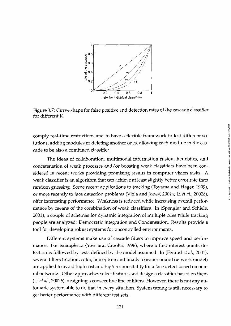
0.8

SO.6

•5 0-4

"5 0.2

K#1

/ _ , _ ^ : - . ; ^ ^ • r - " '

' K M /

/ //I

/1 • / / /

/ / / / / / /

K=4

0.2 0.4 0.6 0.8 1 rate for individual classiflers

Figure 3.7: Curve shape for false positive and detection rates of Ihe cascade classifier for different K.

comply real-time restrictions and to have a flexible framework to test different so-

lutions, adding modules or deleting another ones, allowing each module in the cas-

cade to be also a combined classifier.

The ideas of coUaboration, multimodal Information fusión, heuristics, and

concatenation of weak processes and/or boosting weak classifiers have been con

siderad in recent works providing promising results in computer visión tasks. A

weak classifier is an algorithm that can achieve at least slightly better error rate than

random guessing. Some recent applications to tracking (Toyama and Hager, 1999),

or more recently to face detection problems (Viola and Jones, 200ÍÍÍ; Li ét al., 2002b),

offer interesting performance. Weakness is reduced while increasing overall perfor

mance by means of the combination of weak classiflers. In (Spengler and Schiele,

2001), a couple of schemas for dynamic integration of múltiple cues while tracking

people are analyzed: Democratic integration and Condensation. Results provide a

tool for developing robust systems for uncontroUed environments.

Different systems make use of cascade fllters to improve speed and perfor

mance. For example in (Yow and CipoUa, 1996), where a first interest points de

tection is foUowed by tests defined by the model assumed. hi (Féraud et al., 2001),

several fllters (motion, color, perceptron and finally a proper neural network model)

are applied to avoid high cost and high responsibility for a face detect based on neu

ral networks. Other approaches select features and design a classifier based on them

(Li et al., 2002b), designing a consecutive Une of fllters. However, there is not any au-

tomatic system able to do that in every situation. System tuning is still necessary to

get better performance with different test sets.

121

3.3 Cues for Face Detection

Robust face detection is a difficult challenge. It should be noticed that trying to build

a system as robust as possible, i.e., detecting any possible facial pose at any size and

under any condition (as the human system does), seems to be an extremely difficult

problem. As an example, a surveillance system can not expect that people show

their faces clearly. For that system face appearance changes are not only derived

from lighting and expression but also due to changes in head pose. Such a system

must work continuously and should keep on looking at the person until he or she

offers a good opporttinity for the system to get a frontal view.

This problem is just a figure-ground segmentation problem (Nordlund, 1998).

In that work, the focus adopted made use of a combination of different cues to im-

prove the overall performance. The cues used in that work were contouring, cluster-

ing features of objects, grouptng by similarity, binocular disparities (when different

cameras are available), motion and tracking. This experience can be considered.

The face detection problem must be observed. What is the appearance of a

face? Which cues can be used? In Figure 3.8 a color image can be observed accom-

panied by its gray level transformation, two different pixelations of the image, a

contour image and finally a thresholded results. Some information can be extracted

from these images:

• Pixelations and binarization show that for caucasiana, facial features are darl;

áreas inside a face.

• The contour image points out that these áreas have greater variability com

pared with the rest of the face.

• The face contour can be approximated by an ellipse.

These observations can be used to extract and draw a naive model prototype

of a face, see Figures 3.9 and 3.10.

3.3.1 Spatial and Temporal coherence

3.3.1.1 Spatial coherence

The simple face model can be studied intuitively, see Figures 3.9 and 3.10, observing

that there are some spatial relations satisfied by facial features. Many face detection

122

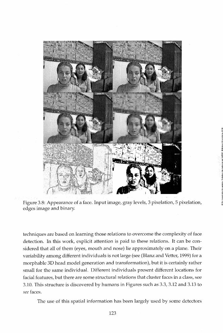
; ^ ^ V ui%.^f w % ^

Figure 3.8: Appearance of a face. Input image, gray levéis, 3 pixelation, 5 pixelation, edges image and binary.

techniques are based on leaming those relations to overeóme the complexity of face

detection. In this work, explicit attention is paid to these relations. It can be con-

sidered that all of them (eyes, mouth and nose) lie approximately on a plañe. Their

variability among different individuáis is not large (see (Blanz and Vetter, 1999) for a

morphable 3D head model generation and transformation), but it is certainly rather

small for the same individual. Different individuáis present different locations for

facial features, but there are some structural relations that cluster faces in a class, see

3.10. This structure is discovered by humans in Figures such as 3.3, 3.12 and 3.13 to

see faces.

The use of this spatial Information has been largely used by some detectors

123

Figure 3.9: Face prototype

L A (\-! ' • ' » # » ' - ^

" • ' - - . .

Figure 3.10: Relevant aspects of a face.

based on facial features. For example, the average position estimated with normal

distributions is used in (Schwerdt et al., 2000) to avoid uncorrect skin color blobs.

Facial features relations ha ve been used as heuristics. Artists use the aspect-ratio of

human faces considering this golden ratio (Stillman et al., 1998fl):

facejkeight 1 + Vs face_width 2

(3.7)

But already Renaissance artists, as Albert Dürer or Leonardo da Vinci, worked

over human proportions. Da Vinci exposed in his Trattato della pittura (da Vinci,

1976) his mathematical point of view for focusing painting.

"Let no man who is not a Mathematician read the elements of my

work." (da Vinci, 1976)

In his work, da Vinci described anatomic relations that should be observed in

124

^GAfí

order to paint a person. Among these relations, there is a set dedicated to the human

head:

312

[...] The space between the eyes is equal to the width of an eye.

320

The distance between the centers of the pupils of the eyes is 1/3 of the face. The space between the cúter corners of the eyes, that is where the eye ends in the eye socket which contains it, thus the outer corners, is half the tace, (da Vinci, 1976) . -^ ; - > , . > . . > .

-^¡-^ -mil

I*/' ^„.J,-í*-'-=.»l-,*-?='f1 '-... , •, , , . ,

Figure 3.11: Leonardo drawing sample

Research of facial landmarks and relations among them is a subject of face an-

thropometry (Farkas, 1994). Farkas listed 47 landmark sites that could potentially be

employed in forensic anthropometric photocomparison. His book is a compendium

of measurement techniques with extensive normative data.

The knowledge of this distribution of facial features has been used to con-

strain the área to search. This knowledge is extracted from the structure observed in

faces of different individuáis. In a similar way to other works (Herpers et al, 1999 ))

where distances are related with eye size. Once an eye have been detected, the ap-

pearance of that facial feature detected can be used for this individual. Therefore,

the system can search when there is no a recent detection, and track in any other

case.

125

Figure 3.12: Gala Nude Watching the Sea which, at a distance of 20 meters, Turns into the Portrait of Abraham Lincoln (Hommage to Rothko). (Dalí, 1976)

The positions of the facial features detected and the facial structure model

knowledge have been used to design strategies for estimating head position. The lit-

erature refers to roll, yaw and pitch extraction. Roll (angle resulting of rotation about

optical axis) is easy determined considering pupil position (Ji, 2002; Horprasert et al.,

1996; Horprasert et al., 1997) or computing the second moments, i.e., the 2D orien-

tation of the probability distribution head parameters (Bradski, 1998). Horprasert

(Horprasert et al., 1997) uses eye corners and a perspective model to compute yaw,

under the assumption they all lie on a line. This author calculates also pitch con

sidering a standard size for nasal bridge. Given roll, and knowing that pupils are

symmetrical, in (Birchfield, 1998) the ellipse can be computed, thus the head pose.

Other works combine Information extracted from other cues, in (Wu et al., 1998) skin

and hair color blobs are combined to deduce head orientation.

3.3.1.2 Temporal coherence

In this work, the use of spatial-temporal coherence is considered fundamental. Face

specific knowledge will bring benefits to a system designed for face detection.

It is observed that face structure has a coherent spatial distribution. This

structure is not only conformed by any face but also it is kept in time, and as it

is known an object tends to conserve its previous state, thus there is a permanence

126

a^^T'^'^-T^^fB '-mrM

Figure 3.13: Self-portrait. César Manrique 1975

of certain features or eleraents during a period of time. This fact points out that it

is useful to search the face in temporally coherent positions according to previous

detections.

It is known that faces change along time, these changes can be separated in

rigid and non-rigid motions. There are some rigid movements due to a head change,

i.e., the head is moved or rotated, affecting the whole face structure. However, rigid

movements do not affect face structure or facial features relative positions. But there

are also non rigid movements that affect facial elements. Face muscles allow chang-

ing position and shape of these elements within a certain range.

Most of face detection techniques described in the literature, see chapter 2,

tackle the problem considering just still images (Hjelmas and Low, 2001; Yang et al,

2002), see Figure 3.15. No real-time restriction was defined for such purpose. Nowa-

days, robust face detection is not the only feature expected, instead robust real time

face detection is needed. Today technology provides the community new possibili-

ties of input data integration using cheap hardware with tncreasing performance.

Thus, applying these techniques to a sequence would limit its action to a

127

/ '^-zz^ • \

/ C3 ^ C^ \

\ t „:^ ....... I

\ ^ j m

Figure 3.14: Ideal facial proportions

Figure 3.15: Traditional Automatic Face Detector

repeated execution of the module without attending to the explicit relationship ex-

pressed by a sequence that exists between consecutiva trames, see Figure 3.16. When-

ever a video stream is processed, these approaches just processes new trames with

out integrating any information obtained from previous processing.

Figure 3.16: Traditional Automatic Face Detector applied to a sequence

Rarely, the temporal dimensión is considered, although temporal context is

a basic element for diverse topics of facial analysis as happens with facial gestures

(Darrell and Pentland, 1993). Typically face detection works are concentred in de-

tection or tracking without paying attention to face changes over time. There is no

sense avoiding information provided by the inputs, see Figure 3.17.

This concept is integrated in recent systems. In (Mikolajczyk et al., 2001),

128

the system considers temporal information. Its initial detector is based on (Schnei-

derman and Kanade, 2000), then the system propagates detection information over

time using Condensation (allows representing non-Gaussian densities). Previous

face/facial detection information has also been taken into account for head gestures

analysis (Kapoor and Picard, 2001) or by the coding community (Ahlberg, 2001).

The original Equation 3.3 is modified to take into account the information

provided by previous frame.

f{^,t)^FD[f{^,t)/FD{x,t-r)] (3.8)

where FD [/(x, t)/FD{x, t — r)] means the face detection applied to the im-

age taken at time t, using the results of face detection to the image image taken at

time ¿ — T. , ,

Face Detector é - > -

MÉXifiii*

Figure 3.17: Automatic Face Detector Adapted to a Sequence

In Figure 3.18 different trames, 320 x 240 pixels, from a sequence can be ob-

served. After 50 frames, eyes have not been moved considerably in this example,

thus temporal coherence could be used as another input for providing robustness to

the system. The positions of right eye for the whole sequence are plotted in Figure

3.19. Right eye absolute positions of consecutive frames (some of them extracted in

Figure 3.18) are linked by a straight segment. It is observed that the position gap be-

tween consecutive frames is rarely greater than 20 pixels, even when the x position

for a certain frame could be around 150 and O for another (not consecutive). This

proves the fact that in many situations the proximity of eye positions in consecu

tive frames and the temporal relation of head movement an features position can be

used for improving the system. It is evident that for this face size, there is a high

likelihood of ftndtng the last detected eye not further than 20 pixels, feature that can

be used to reduce the search process cost.

129

Figure 3.18: Frames 0,1,11,19, 26, 36, 41, 47, 50.

Therefore, the face detection process is applied to a sequence, S, which is

composed oí a consecutive, in time, sort of images, also known as frames ^ acb of

them acquired at time U.

S = {f{x,U);i = 0,...,N;U<U+,} (3.9)

At time t, our aim is to detect faces using an approach based on facial fea-

tures. On each image, different evidences are searched. These evidences represent

a different stages in the procedure, i. e., an evidence could represent eye candidatos

but also whole face candidates. Each evidence reportad is described in terms of

the feature that could be, fidi, according to parameters, p (location, size, ...), and a

certainty valué, c.

< fidi{t);{ci{t;k),pi{t;k)) > (3.10)

130

If different evidences correspond to the same feature at time í, e.g., there

could be different nose candidates at time t. Each one is identified by k.

20 40 60 80 100 120 140

Figure 3.19: Movement of right eye in a 450 trames sequence. Some extracted frames are presented in Figure 3.18.

3.4 Summary

As a summary, this thesis tackle the problem of frontal face detection and facial

features localization. This chapter serves to establish the different aspects to be con-

sidered in that challenge: Combination of knowledge based cues and temporal and

spatial coherence of face elements and appearance.

The face detector module will make use of these ideas. This module will

extract different features from an image. A simple example of these features that are

described according to Equation 3.10, for a face detector base on color, could be as

foUows:

Skin color blob: Described in terms of:

Position: Position of the rectangular área containrng the face candidate.

131

Dimensions: Dimensions of the rectangular área containing the face candi-

date.

Orientation: Estimated orientation, in order to evalúate the difference with

vertical alignment.

Eye: Different potential eyes are considered, parameterized by their positions.

Nose: Each candidate is parameterized by its position in the image.

Mouth: Different potential mouths are considered, parameterized by their posi

tions and área.

Face: Only if previous evidences are reliable, a face is described in terms of its

position and elements.

The probability of detection can be propagated over time. That probability

should be considered not just for the face but also for the intermedíate aims (with

different level of abstraction) achieved in the process: skin área, facial element, face,

etc.

132

Chapter 4

ENCARA: Description, Implementation and Empirical Evaluation

THE previous chapter describes the framework for the face detection solution

proposed in this thesis. In Chapter 2, it was commented that face detection

systems described in the literature can be classified along different dimensions. One

of them is the related to how these systems use the knowledge: implicitly or explic-

itly. The first focuses on leaming a classifier from a training samples set, providing

robust detection fOx restricted scales and orientations at low rate. Learning based de-

tectors have the advantage of extracting automatically the structure from samples.

These techniques perform with brute forcé without attending to some evidences or

stimuli that could launch the face processing modules, similarly to the way some

authors consider that the human system works (Young, 1998). On the other hand,

the second group exploits the explicit knowledge of structural and appearance face

characteristics that could be provided from human experience, offering fast process

ing for restricted scenarios.

The implementation presented in this chapter is conditioned by the need of

getting a real-time system with standard general purpose hardware. A fast and

robust approach is needed that must also consider the localization of facial features.

These restrictions have conditioned the techniques used for this purpose. When

fast processing is needed, the literature focuses on the use of specific knowledge

about face elements, i.e. explicit knowledge based approaches. However, recent

developments using implicit knowledge (Viola and Jones, 2001&; Li et al, 2002fc),

133

have achieved impressive results reducing system latency but performing yet the

exhaustiva search over the whole image.

ENCARA will merge both orientations, in order to make use opportunisti-

cally of their advantages; selecting candidates using explicit knowledge for later

applying a fast implicit knowledge based approach.

Invariant features such as the skin color range and the explicit knowledge

about facial features location and appearance, as shown in the previous chapter, can

be used to design a face model. The process is speeded up thanks to this knowl

edge. The face detector will consider spatial and temporal coherence, using differ-

ent cues as a powerful strategy for getting a more robust system. The foiiowing

section describes ENCARA, an implementation carried out using these ideas and

restrictions.

4.1 ENCARA Solutions: A General View

Some facts have been considered during the development of the face detection sys

tem, i.e. ENCARA. The main features can be summarized as foUows:

1. ENCARA makes use only of visual information provided by a single camera,

therefore, no stereo information is available.

2. ENCARA does not need high quality acquisition devices ñor high perfor

mance special purpose hardware. Its performance must be good enough using

standard webcams and general purpose computers.

3. ENCARA is designed to detect frontal faces in video streams, attending speed

requirements. Thus, ENCARA must be as robust as possible in limited time

slices for real-time operation in HCI environments.

4. ENCARA makes use of both explicit and implicit knowledge. The knowledge

codifies the expert response to the question: What is a frontal face? In this

work, it is considered that a face can be defíned by the presence of múltiple

features, relations and conditions, which are opportunistically coUected and

codified by ENCARA.

5. ENCARA works in an opportunistic way making use not only of spatial co

herence but also of temporal information.

134

6. The solution does not pretend to be reliable in critical environments where it

is not allowed a misclassification (i.e. security systems). For those purposes,

other biometric techniques present better performance (Pankanti et al, 2000).

ENCARA is developed for providing fast performance in interaction environ

ments where occasional failures in recognizing frontal faces are not critical.

7. Finally, ENCARA is designed in an open, incremental and modular fashion in

order to facilítate the integration of new modules or the modification or sub-

stitution of the existing ones. This feature allows the system to add potential

improvements and to be easily modifiable for development, integration and

test of fu ture versions.

The ENCARA operation is roughly as foUows. The process launches an ini-

tial face hypothesis for selected image áreas. These áreas present some kind of evi-

dence that make them valid to assume that hypothesis. Later, the problem is tackled

making use of múltiple simple techniques applied opporttinistically in a cascade ap-

proach in order to confirm/reject the initial frontal face hypothesis. In the first case,

the module results are passed to the foUowing module. In the second, the candi-

date área is rejected. At present time, this implementation considers only bivalued

certainty degrees for each module output: O and 1. Those techniques are combined

and coordrnated with temporal information extracted from the video stream to im-

prove performance. They are based on contextual knowledge about face geometry,

appearance and temporal coherence.

ENCARA is briefly described in terms of the foUowing main modules, see

Figure 4.1, organized as a cascade of hypothesis confirmation/rejection schema:

MO.- Tracking: If there is a recent detection, next frame is analyzed first searching

for facial elements detected in previous frame.

MI.- Face Candidate Selection: Any technique applied for this purpose would se-

lect rectangular áreas in the image, where it could be a face. For example, in

Figure 4.2 a skin color detector would select as candidates two major áreas.

M2.- Facial Features Detection: Frontal faces, our aim, would verify some restric-

tions for several salient facial features. In those candidates áreas selected by

MI module, the system would search for a first frontal detection based on fa

cial features and its restrictions: geometric rnterrelations and facial features

appearance. This approach would first search potential eyes in selected áreas.

135

ENCARA

Figure 4.1: ENCARA main modules

After the first detection of an user, the detection process will be adapted to

user dimensions as a consequence of temporal coherence enforcement.

M3.- Normalization: In any case, the development of a general system capable of

detecting faces at different scales must include a size normalization process

in order to allow for a posterior face analysis and recognition reducing the

problem dimensionality.

M4.- Pattem Matching Confirmation: A final confirmation step of the resulting nor

malizad image is necessary to reduce the number of false positives. This step

is based on an implicit knowledge technique.

For each module the literature offers many valid techniques but in this im-

plementation, the emphasis has been placed on achieving a system capable of pro-

136

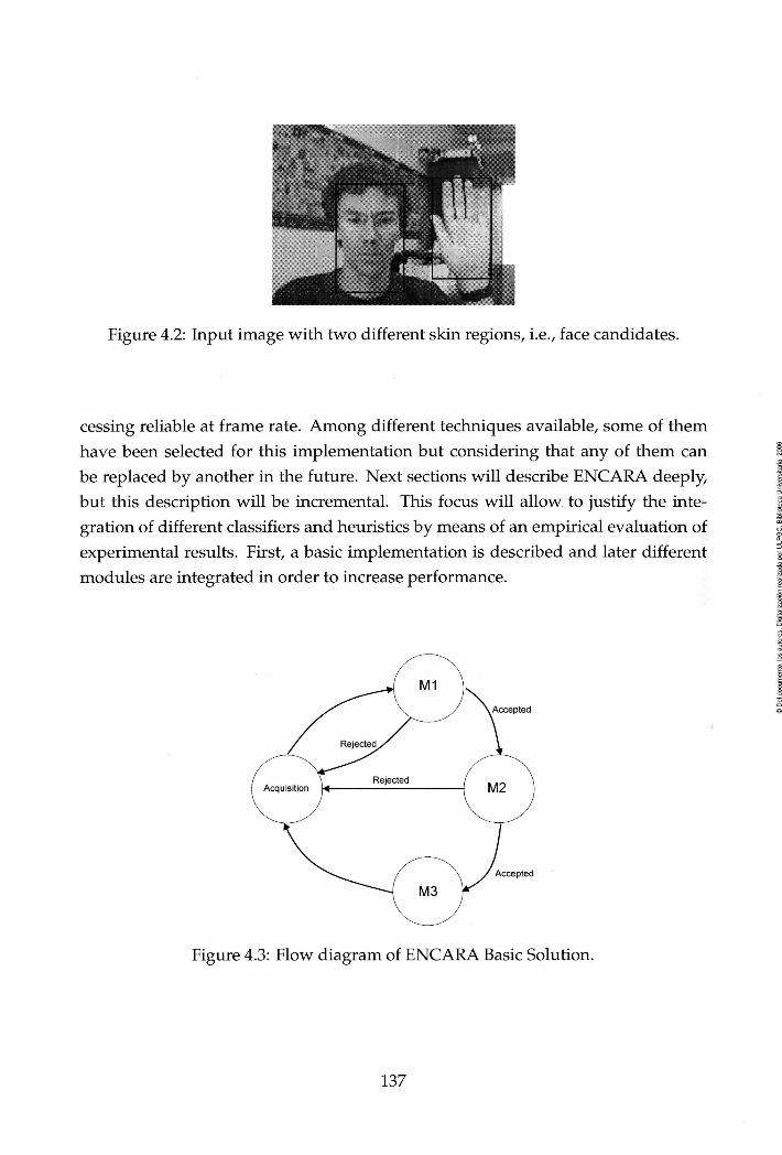
Figure 4.2: Input image with two different skin regions, i.e., face candidates.

cessing reliable at frame rate. Among different techniques available, some of them

have been selected for this implementation but considering that any of them can

be replaced by another rn the future. Next sections will describe ENCARA deeply,

but this description will be incremental. This focus will allow to justify the inte-

gration of different classifiers and heuristics by means of an empirical evaluation of

experimental results. First, a basic implementation is described and later different

modules are integrated in order to increase performance.

\ / Accepted

Figure 4.3: Flow diagram of ENCARA Basic Solution.

137

4.1.1 The Basic Solution

4.1.1.1 Techniques integrated

ENCARA basic implementation considers that for a typical frontal face standing

in its normal vertical position, the position of any facial feature can be restricted,

i.e. certain facial features have known relative positions. For example, eyes must

be located symmetrically in the upper half of the face, see Figure 3.9. Any face

candidate will have to verify that restriction in order to be accepted as a frontal

face. If the eyes are missing or mislocated for a candidate, ENCARA will refuse the

candidate.

In Figure 4.3, ENCARA basic solution main modules flow diagram are pre

sentad. It must be observed that there is no integration of modules MO and M4

in this implementation, i.e., there are no Tracking ñor Pattern Matching Confirmation

steps. These modules will be integrated and analyzed later.

Before describing the ENCARA basic solution, it is necessary to distinguish

different kinds of processes. The foUowing categories of processes are defined:

1. Transformation processes: Oriented to produce output data which are ob-

tained as modifications of input data. They include elimination of noise or

irrelevant data that can provoke confusión.

2. Feature extraction: To genérate features to be evaluated in next categories for

hypothesis launch.

3. Launching of hypothesis: Processes which, after an evaluation, launch a hy

pothesis that must to be confirmed/refused by future processes.

4. Verification of hypothesis: Those in charge of comfirming/rejecting a hypoth

esis. They correspond to classical classifiers.

The ideas adopted by this solution can be summarized roughly as foUows. In

ENCARA, as it is described in detail below, the Face Candidate Selection module, see

Figure 4.1, builds up on detecting skin-like color áreas. Frontal faces fit an elliptical

shape, whose long and short axis correspond to face height and width respectively.

Therefore, fitting an ellipse to a skin color blob will allow the system to estímate

its orientation. This Information is used to reorient the blob to fit a vertical pose in

order to search salient features in the face candidate.

138

Salient facial features considered are eyes, nose, mouth and eyebrows. EN

CARA basic solution searches facial features inside skin color regions, to verify

whether a frontal face is present. This solution has been used by different authors,

as for example in SAVI (Herpers et al, 1999fc), or redefined as a search for non skin

color áreas inside the blob (Cai and Goshtasby 1999). Analyzing caucasians indi

viduáis, those features, for a frontal face, present an invariant feature as they are

basically seen as darker áreas in the face región, see Figure 3.9.

The specific technique used by ENCARA for detectrng dark áreas, i.e., for

the first Facial Features Detection, has already been used by other systems for fea

ture detection. Logically, to search for dark áreas, it takes into account gray level

information (Sobottka and Pitas, 1998; Toyama, 1998; Feyrer and Zell, 1999). In this

work, facial features will be detected using gray mínima search. If facial features de-

tected are properly positioned for a prototypical frontal face, then the facial features

configuration is accepted by ENCARA. A final Normalization module is applied to

transform the candidate to a standard size using standard warping techniques (Wol-

berg, 1990).

4.1.1.2 ENCARA Basic Solution Processes

The basic solution includes modules MI, M2 and M3. The processes for this solution

are detailed as foUows:

1. Face Candidate Selection (MI): The foUowing steps are carried out to select áreas of rnterest:

(a) Input Image Transformation: As explained below, Normalized red and green

(^n,3n) color space (Wren et al, 1997) has been chosen as working color

space. Input image / (x, t) is a RGB color image, so it is transformed to

both normalized red and green /iv(x, í) (Equation 4.1), and to illumina-

tion //(x, t) color spaces.

r„. = 9n — R+G+B

(b) Color Blob Detection: Once the normalized red and green image, /jv(x, t),

has been calculated, a simple schema based on a rectangular discrimi-

139

nation área on that color space is employed for skin color classification.

The definition of this rectangular área in the normalized red and green

color space requires only setting the upper and lower thresholds for both

dimensions. Finally, a dilation is applied to the blob image using a 3 x 3

rectangular kernel or structuring element, /B(X, t). The kernel determines

the behavior of the morphological operation. The dilation kernel is trans-

lated over the image returning a foreground pixel whenever the intersec-

tion of image and kernel is not empty, an example is presented in Figure

4.4. In the resulting image, see Figure 4.5, only major components will

be processed, until one is considered a frontal face or there are not more

major blobs to analyze. This means that ENCARA detects up to one face

in each image.

Dilation kernel

1 1 1 1 I 1

Image ^ Dilatad image

Figure 4.4: Dilation example.

Sccure and stable color detection is a hard problem. The grcat vrrict^'

of color spaces for detection seems to prove the difficulties of achiev-

ing a general method for color detection using just a simple approach.

Notwithstanding with those problems, color is a powerful cue and some

color spaces have been examined in order to check which one offers the

best overall performance in this environment.

Figure 4.5: Input image and skin color blob detected.

Using a feature selection approach (Lorenzo et al, 1998) based on Infor

mation Theory, the color space that seems to get better skin discrimination

140

performance was selected. Along with that study, different color spaces

were studied for a set of sequences. In this experiment, 29992 color sam-

ples were used, corresponding 15634 to non skin samples and the rest

to skin samples. Different color spaces were selected considering their

fast computation and their perceptual features. Color spaces considered

were:

i. RGB: The common color space used by displays and cameras, which

is not perceptually linear.

ii. YUV: A chromaticity color space.

iii. Normalized red and green or NCC: {fn-, Qn), as presented in (Wren et al.,

1997; Oliver, 2000).

iv. A Perceptual Uniform Color System by Farnsworth: (YfUfVf), as de-

scribed in (Wu et al., 1999fl). Where the color transformation is based

first in a transformation from RGB to CIE'sXYZ color system:

X = 0.619Í? + 0.177G + 0.204fí

Y = 0.299Í? + 0.586^ + 0.115B

Z = O.OOOi? + 0.056G + 0.944B

(4.2)

A non linear transformation converts to Farnsworth UCS or CIE'sxy.

(4.3)

V. hhh: Calculattng / i R+G+B , I2 = R — B, I3 = G R+B 2

Figure 4.6: Skin color detection sample using skin color definition A.

141

Figure 4.7: Skin color detection sample using skin color definition B.

Color component yn

h V

'-^ F arnsworth

fn

h u

'Farnsworth

B h Y

^ Farnsworth

G R

GD valué 3.72 5.42 758 8.57 9.14 9.80 10.87 11.45 13.78 14.44 14.57 14.66 14.75 15.30

Table 4.1: Results of color components discrimination test.

The GD measure, see appendix A and (Lorenzo et al, 1998) for more de-

tails, provides features sorted according to its relevance degree in rela-

tion to the classification problem considered. Table 4.1, shows the results

for this color discrimination problem where the different components are

listed according to the GD measure, being in the first rows those more

discriminant. According to these results normalized red and green color

space, {fn,gn), was selected as the most discriminant color space among

those considered.

On this color space, the skin color model has been defined by specify-

ing rectangular áreas in that space. The definition of the rectangular área

for skin color detection has been done empirically. Selecting rectangular

áreas in face áreas of the image retumed average valúes for both com

ponents, see Figures 2.13 and 2.14. As can be observad for these images.

142

Figure 4.8: Skin color detection sample using skin color definition A.

Figure 4.9: Skin color detection sample using skin color definition B.

the range is not completely coincident in them. As it was mentioned in

section 2.1.1.2, the skin-color distribution cluster corresponds to a small

región in color space. However, the parameters of this distribution dif-

fer for different lighting conditions (Yang and Waibel, 1996) This is the

reason for the differences observed for skin color in these images.

Defining a large rectangle área to cope the whole range observed on both

sample images, will lead to a skin color detector too sensitive. lUumina-

tion condition changes can not be tackled by this simple skin color detec

tor. However, if a rectangle área is defrned for each image. Figures 2.13

and 2.14, each rectangle works well for the whole video stream where the

iraage was extracted.

For the experiments presented in this chapter, where different sequences

have been considered, acquired with different people at different dates

and with different light conditions, these two rectangles seem to be good

enough to ftnd one of them as valid to model roughly the skin color for

each video stream. This means that two different definitions, A and B, of

the roughly rectangle were necessary for the experiments. In an a poste-

riori analysis, set A is defined as f„ G (0.295,0.338) and ^„ G (0.30,0.34)

143

and set B as f„ e (0.24,0.305) and ^„ e (0.30,0.34). Set A seems to be

associated for those sequences acquired with high sun illumination in-

fluence. Notice that set A contains white (0.33,0.33) and the differences

between both sets are mainly in normalized red component. Figures 4.6,

4.7, 4.8 and 4.9 exemplify the action of each set on two different images.

This approach provides acceptable results within the context of this im-

plementation.

Future work will necessarily pay attention to increase color detection per

formance and adaptability. Environment changes can be considered un-

der different points of view: toleration and adaptation. As mentioned

above, during experiments, it was observed that the location of these ár

eas depends on the camera used and the time of the day, in other words,

on illumination. As skin color localization depends on lighting condi-

tions, better techniques should be used to provide reliable results in dif

ferent environments, but it is certarnly out of the scope described in this

document. It must also be observed that ENCARA processes along time,

so temporal coherence can improve skin color detection. Temporal co-

herence can be considered not only for blob geometry, blob orientation,

position and dimensions, but also for color evolution. As faces are taken

constantly, the skin color blob Information from current frame can be used

to valídate the next one.

2. Facial Features Detection (M2): ENCARA searches facial features in the candi-

date áreas, see Figure 4.10 for a graphical overview of processes performed in

this module.

(a) Ellipse Approximation: Major blobs, over 800 pixels, detected as skin in the

input image are fitted to a general ellipse using the technique described

in (Sobottka and Pitas, 1998). Taking N blob points (x, y) the foUowing

mornents are computed:

E N 1 ^

EN 1 y

xy = X^f X • y (4.4)

E N

yy = L.i y-y

144

Accepted

Figure 4.10: Flow diagram of ENCARA Basic Solution M2 module.

Blob moments allow to compute the ellipse that best fits the blob as fol-

lows:

Xr_ — TV

O = ^ arctan

Ve — N

2{xy xc-yc 1 N )

(4.5)

The ellipse approximation procedure retums the área, orientation and

axis lengths of the ellipse (J^axis arid Saxi^ in pixel units, see Figures 4.11

and 4.12. Alternatives solutions described in the literature to compute ori

entation without color are mainly based on contours. In (Feng and Yuen,

2000) a face detection method is used to get a rough estimation where

contours are calculated, for later applying PCA to get two principal axes

which correspond to head up and line joining eyes.

(b) Ellipse Filters: Before going further, some face candidates are rejected based

on the dimensions of the detected ellipse using the foUowing geometric

filters:

1) Those ellipses considered too big, with an axis bigger than image di-

145

s„ 7\ \ (Xc,y,:) / \ (XcVc)

Figure 4.11: EUipse parameters.

Figure 4.12: Input image and skin color blob detected.

mensions, and also those too small with Saxis under 15 pixels.

2) Those ellipses whose vertical axis is not the largest one, because faces

are expected almost in upright position.

3) Those with unexpected shape, laxis should have a valué between 1.1

and 2.9 times Saxis- That relation depends on the lighting and kind of

clothes the subject wears because of the neck can be added to the face

blob or not.

Temporal coherence provided by the video stream analysis is exploited by

the system to reject an ellipse whose orientation shows an abrupt change

in relation to a previous coherent orientation in the video stream. Also,

if there was a recent detection, those blobs with an área over a mínimum

size contained in the área covered by the previous detected frontal face

blob rectangle, are fused.

In future work, small ellipses could be zoomed using Active Control ca-

pabilities, if there is no other candidate área of interest. Applying hallu-

cinating faces techniques (Liu et al., 2001), a high-resolution image could

be inferred from low-resolution ones.

(c) Rotation: As people are generally standing in an upright position in desk-

top scenarios, this implementation considers that faces would never be

146

Figure 4.13: Blob rotation example.

inverted. For this problem, it has been considered that a face can be ro-

tated from its vertical position no more than 90 degrees, i.e., the hair is

always over the chin, or exceptionally at the same level. As a curiosity,

it is known the fact that humans present a lower performance rate recog-

nizing inverted faces (Bruce and Young, 1998), see Figure 2.21.

Figure 4.14: Input image and rotated image. Each image needs to define its coordi-nate system.

As exposed above, ellipse calculation provides an orientation for the blob

that contains the face candidate. The orientation obtained is employed

for rotating (Wolberg, 1990) the source image in order to get a face image

where both eyes should lie in a horizontal line, see Figure 4.13. The qual-

ity of the match provided by the ellipse detection and fitting procedure,

i.e., the skin color detection approach, is important because a good ori

entation estimation provides a good initialization for searching the facial

features.

In the following, two different coordínate systems will be used for input

image. The original coordínate system and the transformed coordinated

system. During the search process, input image could suffer transforma-

tions, as for example the rotation defined by the skin color blob, see Figure

4.14. Any operation with any of those images requires the knowledge of

their particular coordínate system.

147

\

i =^ / Narrowestrow Widest row \ ":- W .Ir

I Skin detection *—

Figure 4.15: Neck elimination.

(d) Neck Elimination: As mentioned above, the quality of ellipse fitting mecha-

nism is critical for the procedure. Clothes and hair styles affect the shape

of the blob. If all these pixels that are not face such as neck, shoulder

and decoUetage are not avoided, the rest of the process will be influenced

by a bad estimation of the face área. This blob shape uncertainty will

affect later the determination of possible position for facial features, thus,

it would be necessary to search in a broader área with higher risks of tnis-

selection.

This is not a new idea, Kampmann uses chin contour to sepárate face from

neck for coding of video streams purposes (Kampmann, 1998). Before

performing that action a contour is adjusted to chin and cheeks (Kamp

mann, 1997). This adjustment makes use of geometric constraints related

to previously detected mouth and eyes (Kampmann and Ostermann, 1997),

and a cost function based on the high valúes of the gradient image. Other

approaches observe that under certain light conditions a hole appears un-

der the chin. This fact is used as a neck evidence in (Takaya and Choi,

2001). This approach fixes upper boundary and allows lower boundary

to grow up to a certain limit according to face dimensions.

As ENCARA does not make use of contours, for eliminating the neck the

system takes into account a range of possible ratios among the long and

short axis of a face blob. The search is refined in this range for the current

subject. First, it is considered that most people present a narrower row

in skin blob at neck level, see Figure 4.15. Thus, starting from the ellipse

center, the blob widest row is searched. Finally, the narrowest blob row

that should be upper to the widest row is located.

These rows are used heuristically to select the cropping row for the skin

color blob. This row is selected as r = {widest x 0.7 + narrowest x 0.3).

That valué is accepted only if it is inside a range: {center—laxis)+^ x Saxis <

rs < {center — I axis) + 4 x Saxis- This helps refusing naked shoulders,

148

Figure 4.16: Example of resulting blob after neck elimination.

etc. Finally a new ellipse is approximated to the cropped blob, see Figure

4.16, and the image is rotated using the same procedure explained in the

previous steps.

Figure 4.17: Integral projections considering the whole face.

(e) Integral Projections: Skin color detection provides an estimation of face

orientation. Using that Information the system will search for gray mín

ima in specific áreas where facial features should be if the blob detected

was a frontal face. The basic solution just searches for eyes that will also

provide a valid estimation of face size.

At this point, the candidate has been rotated and cropped. Therefore,

if the candidate is a frontal face, the explicit knowledge will fix an área

where eyes in a frontal face must be. If this search área is not well de-

fined, partially due to the lack of stability of the color detection tech-

nique, the face will not be well delimited and therefore will be the fa

cial features search áreas. First, it was mentioned that facial features will

149

Figure 4.18: Zone computed for projections.

be located by means of gray information as they appear darker within

the face área. But if the search área for a facial feature is not correctly

estimated, the system can easily select loncorrectly for example an eye-

brow, instead of an eye, as the darkest point. This effect can be reduced

if search áreas for eyes location are bounded integrating also gray pro

jections as in (Sobottka and Pitas, 1998). This idea is showed in Fig

ure 4.17, in the image large horizontal lines represent minima projec-

tion in upper half face, while short horizontal lines represent minima

(and a máxima that corresponds to the nose tip) in lower half face. To

bound eyes search áreas, the projection in the upper part of the rotated

gray image is computed. The range of computed rows is related to blob

dimensions y^in = centery - 0.4 x laxis and ymax = centery + Saxis or

ymax = {previousJeft_eyey+previous_righi-_eyf>-y)/?.->-OA^ «a:.¿s depend-

rng whether there was a recent detection or not (<1.5 secs.), see Figure

4.18.

Verprojiy) = "^ I{x,y) (4.6) X=Xl

The nose bridge is avoided reducing the influence of glasses. For the right

eye, left in the image, the columns analyzed cover from xi = centerx —

0.7 X Saxis to X2 = centeTx — 0.25 x Saxis- For the left eye, right in the image,

from xi = centeTx + 0.25 x Saxis to X2 = centerx + 0.7 x Saxis- A smoothing

filter is applied before searchrng for minima for those y considered. Some

authors itérate the smoothing process for a better detection of minima

(Sahbi and Boujemaa, 2000). After the smoothing process, the system

searches minima. A mínimum is refused if it is too cióse to another deeper

150

Figure 4.19: Integral projections on eyes área considering hemifaces.

minimum. The distance threshold is defined by blob dimensions {saxis/8).

Finally, the two raain minima which are not further than Saxis/'^ rows are

selected and used to bound eye search minima.

A variation is applied to this process. It is known that unless there is an

uniform illumination over the whole face, there are some differences be-

tween both face sides (Mariani, 2001). This fact affects the skin color step,

and consequently some errors can be propagated to ellipse orientation. In

Figure 4.19, it is observed that the face after rotation has not both eyes ly-

ing in a horizontal line. Integral projections can help correcting this fact.

Therefore, ENCARA computes different integral projections for each face

side. As can be seen in that Figure, the projections for eyebrows and eyes

* are better loca ted for this example. - • - . i

(f) Eyes Detection: Once the neck has been eliminated, the ellipse is well fitted

to the face. As faces present geometric relations for features positions, the

system searches for an eye pair that has a coherent position for a frontal

face, see Figure 4.20. The fastest and simplest heuristic is used to detect

eyes, each eye is searched as the gray minimum in each área. The decisión

to search initially for eyes is due to the fact that eyes are relatively salient

and stable features in a face, in comparison to mouth and nostrils (Han

et al, 2000).

Integral projections, computed in previous step, are integrated with these

Windows, each hemiface produced a projection result. Previous step ob-

tatned two minima in the upper half face. The upper minimum corre-

spond to eyebrows, thus the upper y boundary of each search área is ad-

justed to avoid eyebrows. The lower minimum corresponds to the eye

área, thus the eye search área must contain it, see Figure 4.21 for an ex-

151

Long 3KG

Figure 4.20: Search área according to skin color blob.

ampie.

Figure 4.21: Integral projection test. Comparing the integration of projections for locating eyes search windows. The left image does not make use of projections and the eye search área contains eyebrows, while the right image avoids eyebrows bounding the search área with projections.

(g) Too Cióse Eyes Test: If eyes detected using gray mínima are too cióse in

relation to ellipse dimensions, the closest to ellipse center is refused. The

width of the search área is modified avoiding the subarea where it was

detected previously, see Figure 4.22 for an example. The too cióse eyes test

is useful as it must be noticed that the only reason to consider an eye has

been detected is that it is a gray minima. This test helps when the person

wears glasses because the glasses elements could be darker. This test is

applied only once.

(h) Geometric tests for eyes: Some tests are applied to gray level detected eyes:

i. Intereye distance test: Eyes should be at a certain distance coherent

with ellipse dimensión. This distance should be greater than a valué

defined by ellipse dimensions, Saxis x 0.75, and lower than another

ratio according to ellipse dimensions, Saxis x 1.5. Eyes distance must

also be within a range (15 — 90), that defines the face dimensions

152

Figure 4.22: Too cióse eyes test. Bottom image presents the reduced search área for left eye, in the image, after the first search failed the too cióse eyes test.

accepted by ENCARA.

ii. Horizontal test: As mentioned above, resulting eye candidates in trans-

formed image should He almost in a horizontal lina if the ellipse ori-

entation was correctly estimated. Using a threshold adapted to el

lipse dimensions, Saxís/6.0 + 0.5, candidate eyes that are too far from

a horizontal line are refused. For eyes that are almost horizontal but

not completely, the image is rotated one more time, to forcé eyes de-

tected to lie on the same row.

iii. Lateral eye position test: Eyes positions could provide a clue of a lateral

view. Face position is considered lateral if the distance from eyes to

the closest border of the ellipse differs considerably.

The geometric step is commonly used in different works to reduce an ini-

tial set of eye candidates. In (Han et al, 2000), the possible combinations

of the eye-analogue segments are reduced by means of geometric restric-

tions.

3. Normalization (M3): A candidate set that verifies all the previous requirements

is scaled and translated to fit a standard position and size. The relation among

X coordinates of the predefined normalized positions for eyes and detected

eyes, extracted from rotated input image, see right image in Figure 4.23, de-

153

Eyes detected

Eyesat normaüzed postions

Figure 4.23: Input and normaüzed masked image.

fines the scale operation to be applied to the transformed gray image. Once

the selected image has been cropped, it is scaled to fit standard size, 59 x 65.

Finally this normalized image is masked using an ellipse defined by means of

normaüzed eye positions.

TflQjSK Sdxis

mask I,

(N ormalized_leftx — N armalizedjrightx)

axis — i- iJ i X Tn(lSrC_SQ^xis ,2 _ '

(4.7)

mask_Sa + y

mask la

Por candidates áreas that have reached this point, the system determines that

they are frontal faces. Thus, some actions are taken:

(a) Between eyes location: According to eyes position, the middle position be-

tween them is computed, see Figure 4.24.

(b) Mouth detection: Once eyes have been detected, the mouth, a dark área, is

searched down the eyes une according to intereyes distance (Yang et al.,

1998fl). On that horizontal área, the system detects approximately both

mouth borders. Later, rotating 90° the vector that joins an eye with the

middle position between both eyes, the direction to find the center of the

mouth is obtained, see Figure 4.25 left. Using the vector joining the po

sition located between the eyes, and a mouth border, the center of the

mouth is estimated, see Figure 4.25 middle and right. The located mouth

154

Inb tween

/ / _ \ / O Í D • '^jt^ \ í i

Figure 4.24: Determination of position between eyes.

position is accepted only if it fits the prototypical distance of the face from

the eyes line. This prototypical distance is modelled by a distribution

which has been computed using manually marked data for 1500 frontal

face images. On those images, the distance between the eyes has been

normalized, for later computing a distance from the position between the

eyes to the mouth. The distances coUected allowed to define the distribu

tion represented in Figure 4.26.

/ " ~ ^ " \ / " ' ^ ~ " " \ / " ~ " " \

VI ^A- / c ^ ' ,T ^ ^ M / ^ - ^ / q -*-* *.

1.

/ \ "^—^ / \ '^-^'^^ / \ /

V y y y y y Figure 4.25: Determination of mouth center position.

(c) Nose detection: Between eyes and mouth, ENCARA searches for another

dark área using gray valúes for detecting nostrils. Upper, but cióse, from

nostrils the brightest point found is selected as the nose. No verification

is considered for this feature currently (Yang et al, 1998fl).

4.1.2 Experimental Evaluation: Environment, Data Sets and Exper

imental Setup

There are datasets for testing face detection algorithms, however the variety of

variations possible in video streams are not contained in any free dataset.

155

Figure 4.26: Average position for eyes and mouth centén

- . C * '

• • « V T -

m-• - • i

#

Figure 4.27: Áreas for searching mouth and nose.

In order to carry out empirical evaluations of the system, different video

streams were acquired and recorded using a standard webcam. These sequences,

labelled Sl-Sll, were acquired on different days without special illumination re-

strictions, see Figure 4.28. Therefore, some were taken with natural (therefore, vari

able) and others with artificial illumination. The sequences of 7 different subjects

cover different gender, face sizes and hair styles. They were taken at 15 Hz. dur-

ing 30 seconds, i.e., each sequence contains 450 trames of 320 x 240 pixels. Ground

data were manually marked for each frame in all sequences for eyes and mouth

center in any pose. This gives 11 x 450 = 4950 images manually marked. All the

frames contain one individual excepting sequence S5 where there are two individu

áis. Therefore, there is a face in each frame but not always frontal.

Sequences SI and S2 correspond to the same subject but acquired in different

days. This subject moved almost continuously his face presenting scale and out of

plañe orientation changes, consequently these sequences present less frontal faces

156

Figure 4.28: First frame extracted from each sequence, labelled Sl-Sll, used for ex-periments.

than other sequences as for example S3 and S4. Sequences S3 and S4, correspond

respectively to a female and a male individual. These sequences are different rn the

sense that they change less, i.e., in sequence S4 the user just looks at the camera,

while in sequence S3 there are only orientation changes when the individual looks

at one side during her conversation. Sequences S5 and Sil have the particularity

of containing smaller faces acquired with artificial illumination containing female

individuáis that perform orientation and expression changes. Sequences S6-S9 cor

respond to the same subject but were taken with different hair style and illumination

conditions. Sequence SIO contains a subject that performs initial out of plañe rota-

tions for later keeping his face frontal.

ENCARA performance is compared both with humans and a face detector

system. On one hand, the system is compared with manually marked or ground

data providing a measure of facial features location accuracy in terms of human

precisión. Known the actual distance between eyes, as they have been manually

157

marked, the eyes location error can be easily computed.

On the other hand, an excellent and known automatic face detector (Rowley

et al, 1998), thanks to the binary files provided for testing and comparison by Dr.

H. Rowley, has been applied on these images to give an idea of ENCARA relative

advantages and disadvantages. This well-known face detector is able to provide an

estimation of eye location under certain circumstances. Thus, for each face detected

Rowley's detector does not lócate its eyes which is a difference with ENCARA. EN

CARA, according to its aforementioned design objectives, searches for eyes to con-

firm that there is a face present, i.e., whenever ENCARA detects a face, the eye

location is supplied.

To analyze the location accuracy of face and eyes separately, two different

criteria will be used to determine if a face has been correctly detected and if its eyes

ha ve been correctly located f oUowing f eature 1 of well structured problem according

to (Simón, 1973; Simón, 1996). These criteria are defined as foUows:

Criterium 1. A face is considered correctly detected, if both eyes and the mouth are con-

tained in the rectangle retumed by the face detector. This intuitive condition

has been extended tn (Rowley et al, 1998), in order to establish that the cen-

ter of the rectangle and its size must be within a range in relation to ground

data. However, in this work, as ENCARA assigns the size according to eyes

detected, the extensión has not been considered.

Criterium 2. The eyes of a face detected are considered correctly detected if for both eyes the

distance to manually marked eyes is lower than a threshold that depends on

the actual distance between the eyes, ground_data_inter_eyes_distance/8. This

threshold is more restrictive than the one presented in (Jesorsky et al, 2001)

where the threshold established is twice the one presented here. The same

authors confirm in (Kirchberg et al, 2002), that their threshold is reasonable for

face recognition. They reported an 80% detection success using that threshold

with XM2VTS data set (of Surrey, 2000).

According to these criteria, a face could be correctly detected while its eyes

could be uncorrectly located.

The results achieved with Rowley's face detector are provided in Figure 4.29

(detailed results in appendix Tables D.l and D.2). In this Figure, the x axis represents

each sequence, the left y axis represents the detection rate according to the number of

158

frames contained in the sequence, i.e. 450, while the right y axis shows the average

processing time. For each sequence processed, four bars represent the technique

performance. From left to right: 1) rate of detected faces, 2) rate of correct detected

faces according to Criterium 1, 3) rate of correct detected eye pairs according to

Criterium 2, and 4) rate of correct detected eye pairs according to Jesorsky's test

(Jesorsky et al., 2001). Finally the polyline plotted indicates the average processing

time in milliseconds using the standard dock C function in a FUI IGHz.

Observing the quality of this solution, except for sequence S4 that retums a

42%, this algorithm provides a detection rate for these sequences over 72% corre-

sponding to correct face detections according to Criterium 1 over 97%. It must be

observed that this detector is designed to detect frontal and profile views. The av

erage time corresponds to the total time needed to compute the whole sequence di-

vided by the number of frames, i.e., 450. Unfortunately, observing the average time,

it is evident that a system that requires frame rate face detection can not use today

this algorithm as this face detector will be able to provide data for face processing at

1.07-1.64 Hz.

S5 S6 S7 Sequences

Figure 4.29: Rowley's technique summary results.

As it was mentioned, Rowley's face detector is not able to provide an es-

timation of eyes position for every face detected. In the experiments with these

sequences, it has been observed that the eye detector is not so robust as the face

detector. It is affected by pose, thus it works mainly with frontal faces which are

vertical. In Figure 4.29 third and fourth bars, Rowley's eye location results are com

pared with ground data manually marked. As it was explained above, the eyes are

uncorrectly detected if Criterium 2 is not passed. In this Figure, there is a notorious

difference for some sequences between the amount of faces detected and the num

ber of eyes located, this is mainly due to the fact that Rowley's face detector does

not detect eyes for each detected face.

159

From Figure 4.29 and detailed appendix Table D.2, it is observed that the

average error, when Rowley's technique returned eye positions, is rather small. This

eye detector provide low false positive rate but the rate of false negatives is higher.

Error on both eyes are rarely produced, though location errors for one eye are more

common. These errors are produced generally due to eyebrows or eye corners are

confused with eyes. See for example Figure 4.30, in that image the eyes of the left

face are closed. However, Rowley's technique returns an estimation for left eye,

which for this frame has been confused with the eyebrow.

Figure 4.30: Eye detection error example using Rowley's technique, only one eye location was returned, and it was uncorrectly located.

ti.v ^. ir:r^^-.s ' t . *'•

4.1.3 Experimental Evaluation of the Basic Solution

ENCARA basic solution has been described above. In this section, its performance

is evaluated and analyzed, pointing out the results of different tests integrated and

discussing its good and bad points. The implementation has been developed using

Microsoft Visual C/C++ and OpenCV (Intel, 2001).

Figures 4.31 and 4.32 present results for the different sequences applying dif

ferent variants that have been applied to each video stream (detailed results rn ap

pendix Tablea D.3 and D.4). The variants are defined in relation to the inclusión or

not of different tests. Those tests analyzed in this section according to their signifi-

cance are:

1. too cióse eyes test that corresponds to Too Cióse Eyes Adjustment process, ex-

emplified in Figure 4.22 and

160

Too cióse eyes test

No Yes Yes No

Integral Projection used

No No Yes Yes

Variant label Basl Bas2 Bas3 Bas4

Table 4.2: Summary of variants for ENCARA basic solution. Each variant indicates whether a test is included. These labels are used in Figures 4.31 and 4.32.

2. integral projection test that reflects if integral projections are used to decide eye

search Windows, see Figure 4.21.

For legibility, basic solution variants presented in Figures 4.31 and 4.32, are

labelled according to Table 4.2.

For each ENCARA Basic Solution variant four bars are plotted for each se-

quence, from left to right the first bar shows the face detection rate for the sequence,

the second represents the correct face detection rate according to Criterium 1. The

third and fourth indícate the correct eye pair detection rate if Criterium 2 or Jesos-

rky's is assumed. The polyline refers to the average processing time in milliseconds

labelled in right y axis (observe that the range plotted is one tenth the one plotted in

Figure 4.29).

The first detall to be observed is the average time processing which goes from.

37 — 68 msecs using a Pili IGhz.. These differences are related with the blob size,

simply faces in sequences S5 and Sil are smaller, see Figure 4.28. In any case, the

system provides data at 14.7 - 27 Hz, this means that it works faster than Rowley's

technique at least 9 times in the worst case, see Figure 4.29.

However, the rate of detected faces is not so good as Rowley's technique

results. Certainly, the rate of face detections can not be homogeneous among the

sequences, as each sequence is different in the sense that each individual played

differently with the camera. For example, in S4 the subject looked at the camera

always without orientation changes, but in Sl-2 the subject laughed and moved his

head constantly. But in any case, these rates are far from those achieved with Row

ley's technique as shown in Figure 4.29. This means that ENCARA basic solution

presents a high rate of false negatives, i.e. faces not detected.

On the other hand, the rate of false positives, i.e. the number of vmcorrect

detections is not high which is an interesting feature for the cascade model used. The

161

rate of correctly detected faces is in general higher than 88% excepting sequences S2

and S6. For sequence S2, it is evident that the system took as a face something that

it is not a face, see Figure 4.33.

I 0.5

i

á 0.5

Q

•E0.5

I

S1

lílnl 1

M i Face deí. üFtw ^ ^ Cerre-cí FBC« de* ^ ^ Cormct ey»5 íiet HJJI Correct e y ^ íí«t. Je«crs*iy

M ni • • „ . Bas1 Bas2 Bas3

S3 Bas4

am Bas1 Bas2 Bas3 S5

Bas4

100

Bas2 Bas3 Variant

SI g 0.5

^

Bas1 Bas2 Bas3 S4

Bas4

100

Bas1 Bas2 Bas3 S6

Bas4

100

ID a>

S. ¿0 .5 m o fe íi < Q

Bas1 tac

100

E

IBOI Bas2 Bas2

Variant BJS4

100

ii>

E

I 100

E

Figure 4.31: Results summary using Basic Solution for sequences S1-S6.

Eye location errors are neither homogeneous. In some sequences the error

rate is large but the distances are not large as for example sequences SI, S8, SIO and

Sil . In others, not only the error rate is really large but also the distance error which

is due to an uncorrect eye or blob selection, sequences S2 and S6. See for example

Figure 4.33, there the biggest blob was not accepted, but another blob which indeed

is not skin was considered coherent as after rotating there were gray minima lying in

a horizontal line. The detected facial features are plotted as circles in the input image.

On the other hand, in some sequences as for example in S3, S7 and some variants for

S4, there is a large number of correct detections, accompanied by a small number of

errors.

162

S7

áO.5

11 IIJ I

100

.i £ i 1 0.5 te i j < o

n

S8

llnl i i r 1III

100

I 8, ^

Basl Bas2 Bas3 Variant

Bas4

Figure 4.32: Results summary using Basic Solution for sequences S7-S11.

Considering the rate of correct eye pairs detections, it can be observed that

the variant Bas3 behaves more homogeneously among the different sequences. This

variant reduced slightly in comparison with other variants the rate of correct eye

pairs located for some sequences in comparison with Basl and Bas2: S2, S3 and Si l .

But improves this rate slightly for SI, S5, S7 and S9 and clearly for S4, S6, S8 and

SIO. In comparison with variant Bas4, there are minor variations but it must be

observed that variant Bas4 has in general lower face detection rate, which is evident

for sequences SI, S7, S8 and S9. These results support the use of variant Bas3 which

integra tes both tests analyzed.

It is noticed that the tests did not influence equally to all the sequences. For

example, sequences S4 and SIO improved significantly the ratio when integral pro-

jections are integrated, Bas3 and Basé. This is due to the hair style, both subjects have

a bigger forehead, thus only attending to color the system localizes the eye window

search área upper than the right position.

163

Figure 4.33: Example of false detection using the basic solution

The too clase eyes test is useful as the only reason to consider that an eye has

been detected is that it is a gray minima, thus this test avoids choosing dark points

that are too cióse in relation to blob dimensions. This test provides another opportu-

nity before rejecting a blob, as the first pair of eye candidates would not be accepted

by geometrical tests. It can be observed that this test increases the number of detec-

tions considered by the system but the number of false detections too.

These results prove the benefits of both tests without increasing the average

processing time. The average processing time allows ENCARA to produce face data

at 18-27 Hz. But face detection results are far from those achieved with Rowley's

technique, see Figure 4.29, and the large number of uncorrect detections for some

sequences, make the system not trustful though fast.

As a summary, the ENCARA basic solution presents a high false negative

rate, but the rafe of false positives for face detection is in general small. However,

there are contexts that produce high errors rafes as for sequence S2. Among the

different variants, the variant Bas3 seems to provide the most stable behavior im-

proving in general the face and eye correct detection rafes.

4.1.4 Appearance/Texture integration: Pattern matching confírma-

tion

4.1.4.1 Introduction

The basic solution produces a relative high number of false positive errors for some

situations, see for example sequence S2. Using that solution, getting a couple of

164

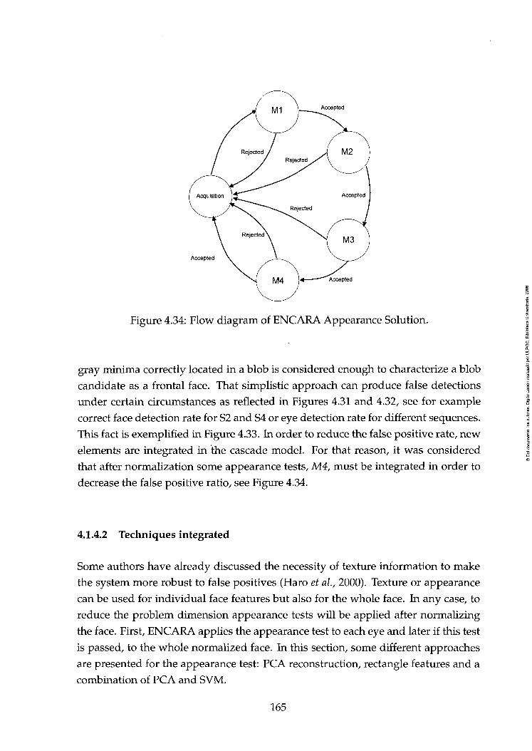
Accepted

Accepted

Acxepted

Figure 4.34: Flow diagram of ENCARA Appearance Solution.

gray minima correctly located in a blob is considered enough to characterize a blob

candidate as a frontal face. That simplistic approach can produce false detections

under certain circumstances as reflected in Figures 4.31 and 4.32, see for example

correct face detection rate for S2 and S4 or eye detection rate for different sequences.

This fact is exemplified in Figure 4.33. In order to reduce the false positive rate, new

elements are integrated in the cascade model. For that reason, it was considered

that after normalization some appearance tests, M4, must be integrated in order to

decrease the false positive ratio, see Figure 4.34.


Some authors have already discussed the necessity of texture information to make

the system more robust to false positives (Haro et al, 2000). Texture or appearance

can be used for individual face features but also for the whole face. In any case, to

reduce the problem dimensión appearance tests will be applied after normalizing

the face. First, ENCARA applies the appearance test to each eye and later if this test

is passed, to the whole normalized face. In this section, some different approaches

are presented for the appearance test: PCA reconstruction, rectangle features and a

combination of PCA and SVM.

165

4.1.4.3 PCA reconstruction error

PCA obtained from a target training set, faces, eyes or whatever, can be used to re

duce dimensionality of target images (Kirby and Sirovich, 1990). Projecting a new

target image using these eigentarget space produces a new code for the image with-

out losing information, i.e., the original image can be reconstructed using the inverse

transform. This fact can be used to prove whether an image is similar to a reference

or target image. The analytical process is described as foUows.

Defining a target image of size width x height, fi, as an element of a target set

F oí n elements, the average target:

1 " f =-T.fi (4.8)

1 = 1

The average target image, / , is subtracted to each target image contained in

the training set that yields:

4>^ = {fi - / ) (4.9)

This matrix is taken as a vector, and a matrix is created with all training tar-

gets D = [0i02---0n]- Getting a square matrix C = DD^, the eigenvectors of C, Ci, is a

set of n orthonormal vector that better describe the distribution. These vectors will

let to obtain the low dimensión space.

Unfortunately, the matrix C is width x height by width x height, becoming

untractable. Instead, the problem can be tackled using a n by n matrix problem. Let

he L = DW and /j its eigenvectors. For each Q a combination of the target images

can be fotind:

= 5^¿ifc0¿, i = l,--.,n (4.10) fe=i

Those Ci are the principal components of D. If these vectors were converted

to matrices, the eigentargets of the training set used would be visible.

166

-T.fi

Projecting a new frame cf), that results of subtracting the average image to the

input image / , and selecting a number of principal components p. The coniponents

that represent that target in the low dimensión space are:

Wk = c\(l), k = l , . . . ,p (4.11)

Reconstructing this original image using just its p principal components, a

reconstructed image is obtained:

p

0r = ^ WkCk (4.12) fc=l

The reconstruction error e = ||0 — 0 11 is a measure of how typical target is 0,

and it is applicable for target/non-target classification.

Once the reconstruction error is defined, a classification criteria is needed.

One approach it to define an empirical threshold based on a test set, whilst another

approach can be based on the elaboration of a training set containing positiva and

negative samples. The reconstruction error of both sets is normally considered to

ha ve a normal distribution. For example for the face samples, their conditional den-

sity is aefíned as:

1 / {x—x)^ ^

p{x\F) = —=e'\^^) (4.13) ayz-K

Later a new sample, x, could be associated to face set F if the likelihood ratio

was greater than 1:

Ir = ^ ^ ) - y 4.14 p{x\F)

This approach is feasible if both a priori probabilities, p{F) and p{F) are equal.

However, this seems to be not the case, as the non face class seems to be too sparse.

Likely, the non face set will not be complete enough to represent non face appear-

167

anee. Instead, the posterior probability should be used but only if a priori probabil-

ities were known.

(F\ ^ ^ P{x\F)p{F) ^^ '"" p{x\F)p{F)+p{x\F)p{F) ^ • '

The difficulties achieved to model the non-face class have lead to use the

empirical threshold for the experiments when PCA reconstruction errors was em-

ployed.

Search wintíovif

Jeítay

; » * « "i : '-2 ^ y

21

Seaícti wsRdow

V

" • •

-f,

Searc^ window

' «• ,

-

1 y

/

Searcíi window

deltax * , ;

3y

¥ 1

a

1 y

Figure 4.35: Rectangle features applied over integral image (see Figure 2.9) as de-fined in (Li eí fl/., 2002??).

4.1.4.4 Rectangle features

PCA reconstruction error is a valid technique, but unfortunalely this technique does

not use any model of non-face or non-eye appearance, which makes difficult to

model cluster borders. For that reason, other approaches available in the literature

for face detection have been studied. Recently, different systems have made use of a

classifier based on rectangle features, see Figure 4.35, with promising results (Viola

and Jones, 2001fc; Li et al, 2002&; Viola and Jones, 2002).

Building the distribution.

These operators are fast and easily computed from the integral image, see Figure

2.9. The integral image is defined as foUows: At a point (x,y), of an image i, its

integral image contains the sum of pixels above and left of the point, see Equation

2.1.

Once the integral image has been computed, any rectangular sum can be ac-

complished in four references. There are different implementations for these oper-

168

ators. Two examples in the literature are described in (Viola and Jones, 2001b) and

(Li et al, 2002íb). The second uses non syrrtmetrical operators as the authors develop

a face detector robust for out of plañe rotations. The features used by the latter are

shown in Figure 4.35, where four different configurations are presented. For each

configuration the rectangles are parametrically shifted over the integral image. For

example, the configuration shown on the left is computed based on two rectangles.

The valué of each rectangle is multiplied by the integer shown inside. Given a rect-

angle D defined by a córner point and dimensions, the sum within D is equal to the

sum of left upper and right bottom comers less the sum of the left bottom and fight

upper comers.

A huge set of rectangle features configurations are computed on a set of pos-

itives, a, and negatives, b, samples {xi,yi),{x2,y2), •••, {XN^VN)- The answer of the

system provides a biclass valué, i.e., y¿ e {+1, —1}. Using these samples, a weak

classifier could be designed with the assumption of a normal distribution function

for each set: positive and negative. According to (Forsyth and Ponce, 2001) the

probability density function for a single random variable can be defined as foUows:

1 ( {x — x)^

P{x; /., a) = — = e " V ^ ^ y (4.16)

Where the mean, ¡j,, and the standard deviation, a are defined according to

the training samples:

^2 ^ JllA^i-sr ^ (417) ^

In (Li et al, 2002b), the weak classifier is defined as

This classifier corresponds to a máximum likelihood estimation (ML). The

same a priori probability is supposed for both sets. If both a priori probabilities

169

were known (for example from training data, whicl'i is iiideed non objective) thc

máximum a posteriori estimation (MAP) could be employed:

P{y = +l/x) P{y = x¡ + l)P{+l) P[y = -l/x) P{y = x/-l)P{-l)

(4.19)

nn

Figure 4.36: Rectangle feature configuration for the best weak classifíer for face svX for 20x20 images of faces as the sample on the left.

Figure 4.37: Rectangle feature configuration for the best weak classifier for right eye set (built with 11x11 images).

Rectangle f eatures selection

According to rectangle features definition described in previous section, for a prob-

lem where an image is classified, there are thousands rectangle features configura-

tions. Of course, all of them combined with a voting schema could be used, but the

time required for computing a single classification would be excessive.

After building a training with positive and negative samples. A search is

performed to detect which are the best rectangle features for the problem using the

criteria of a reduced false positive and negative rafe. Figures 4.36, 4.37 and 4.38

170

present the best operator configuration for face, right and left eye respectively. For

each weak classifier a fast criteria based on the gaussians for both sets is easily de-

veloped. As it is seen in Figure 4.39, a threshold is easily defined based on the

probabilities of both gaussians. Later, using the best 25 rectangle features, a voting

approach can be used to classify. Reducing the number of classifiers leads to a time

cost reduction.

SÍ**"*'*!

Figure 4.38: Rectangle feature configuration for the best weak classifier for left eye set for 11x11 images of faces as the sample on the left.

Figure 4.39: First weak classifier, based on rectangle features, selected for right eye. Red means positive gaussian, while blue means negative.

4,1.4.5 PCA+SVM

The use of rectangle features is supported by its low computational time. In (Viola

and Jones, 2002), different classifiers are combined in a cascade approach to ana-

lyze exhaustively the whole image. The authors define a classifier with a low false

negative rate. However, the approach proposed in this document does not perform

an exhaustive search over the whole image, therefore ENCARA can assume a the

171

cost of selecting a classifier that balance complexity and training error (Cortes and

Vapnik, 1995; Vapnik, 1995).

The approach based on PCA reconstruction error uses a threshold to distin-

guish among face and non-face appearance after recovering the test image. The PCA

projection representation can also be usad to give a measure of faceness (Pentland

et al, 1994), the training set would define a model in PCA space that is used for

decisión by means of a Nearest Neighbor Classification (NNC) schema. NNC can

present difficulties that are avoided introducing a more powerful classifier such as

Support Vector Machines (SVMs).

The reader is referred to (Burges, 1998) for a more detailed introduction and

to (Guyon, 1999) for a list of applications of SVMs. SVMs are based on structural

risk minimization, which is the expectation of the test error for the trained machine.

This risk is represented as R{a), a being the parameters of the trained machine. Let

/ be the number of training patterns and O < 77 < 1. Then, with probability 1 — 77 the

foUowing bound on the expected risk holds (Vapnik, 1995):

Ri.)<R„,ic)^^'^Mm±}t±íím (4.20)

Remp{(^) being the empirical risk, which is the mean error on the training set,

and h is the VC dimensión. SVMs try to mJnimize the second term of (4,20), for a

fixed empirical risk.

For the linearly separable case, SVMs provide the optimal hyperplane that

separates the training patterns. The optimal hyperplane maximizes the sum of the

distances to the closest positive and negative training patterns. This sum is called

margin. In order to weight the cost of missclassification an additional parameter is

introduced. For the non-linear case, the training patterns are mapped onto a high-

dimensional space using a kernel function. In this space the decisión boundary is

linear. The most commonly used kernel functions are polynomials, exponential and

sigm.oidal ftmctions.

The integration of SVM in ENCARA has been performed by means of LIB-

SVM library (Chang and Lin, 2001).

172

4.1.4.6 ENCARA Appearance Solution Processes

The ENCARA basic solution modifications are introduced after normalizing the can-

didate, adding the Pattern Matching Confirmation (M4) module, see Figure 4.34, as

foUows:

1. Eye appearance test: Once a face is normalized, a certain área (11 x 11) around

both eyes is selected to test its appearance using the PCA reconstruction error

(Hjelmas and Farup, 2001), the rectangle feature based or the PCA+SVM based

test. For each eye, left and right, a specific trainrng set was used.

2. Face appearance test: If the previous eye appearance test is passed, a final ap

pearance test is applied to the whole normalized image. The techniques used

are again based on PCA reconstruction error, the rectangle feature based or the

PCA+SVM based.

a

Figure 4.40: Face sample extraction for facial appearance training set.

4.1.5 Experimental Evaluation of the Appearance Solution

Figures 4.41-4.44 (detailed results in appendix Tables D.5-D.11) present some results

for different video streams for the evaluation of the ENCARA appearance solution.

The criteria used to analyze the basic solution are again assumed to consider when

there is a correct detection according to ground data.

Previous section described different techniques that have been used to test

eye and face appearance. These tables endose a comparison of using no appearance

test, PCA reconstruction error technique, rectangle features based using a simple

voting schema or PCA+SVM. For PCA reconstruction error an empirical threshold

was determtned for experiments. The rectangle features based and the PCA+SVM

173

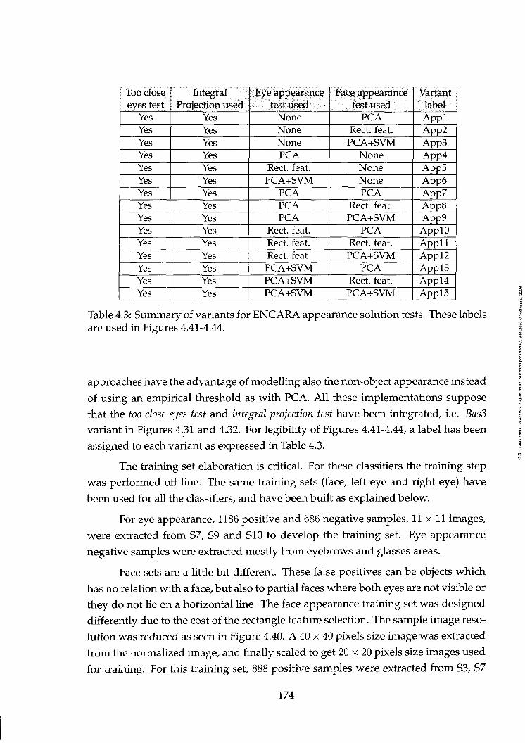
Too cióse eyes test

Yes Yes Yes Yes Yes Yes Yes Yes Yes Yes Yes Yes Yes Yes Yes

Integral Projection used

Yes Yes Yes Yes Yes Yes Yes Yes Yes Yes Yes Yes Yes Yes Yes

Eye appearance test used

None None None PCA

Rect. feat. PCA+SVM

PCA PCA PCA

Rect. feat. Rect. feat. Rect. feat.

PCA+SVM PCA+SVM PCA+SVM

Face appearance test used

PCA Rect. feat. PCA+SVM

None None None PCA

Rect. feat. PCA+SVM

PCA Eect. feat.

PCA+SVM PCA

Rect. feat. PCA+SVM

Variant label Appl App2 App3 App4 App5 App6 App7 App8 App9 ApplO Appll Appl2 Appl3 Appl4 Appl5

Table 4.3: Summary of variants for ENCARA appearance solution tests. These labels are used in Figures 4.41-4.44.

approaches have the advantage of modelling also the non-object appearance instead

of using an empirical threshold as with PCA. AU these implementations suppose

that the too cióse eyes test and integral projection test have been integrated, i.e. Bas3

variant in Figures 4.31 and 4.32. For legibility of Figures 4.41-4.44, a label has been

assigned to each variant as expressed in Table 4.3.

The training set elaboration is critical. For these classifiers the training step

was performed off-line. The same training sets (face, left eye and right eye) have

been used for all the classifiers, and have been built as explained below.

For eye appearance, 1186 positive and 686 negative samples, 11x11 images,

were extracted from S7, S9 and SI O to develop the training set. Eye appearance

negative samples were extracted mostly from eyebrows and glasses áreas.

Face sets are a little bit different. These false positives can be objects which

has no relation with a face, but also to partial faces where both eyes are not visible or

they do not lie on a horizontal line. The face appearance training set was designed

differently due to the cost of the rectangle feature selection. The sample image reso-

lution was reduced as seen in Figure 4.40. A 40 x 40 pixels size image was extracted

from the normalized image, and finally scaled to get 20 x 20 pixels size images used

for training. For this training set, 888 positive samples were extracted from S3, S7

174

and SIO. Negative samples were extracted from false detections achieved during

basic solution experiments obtaining 135 samples.

Observing face detection results in Figures 4.41-4.44, and comparing with

those in Figures 4.31-4.32, it is first observed that those sequences that produced

a low correct face detection rate using ENCARA basic solution, i.e. sequences S2

and S6, have rncreased notoriously the face detection rate. Even more for all the se

quences, if both appearance tests are included, and the rectangle feature based test

is not used for testing eye appearance (variants App7-App9 and Appl3-Appl5), the

correctly detected face rate is over 93%. Also the rates of detected faces have in-

creased in relation to the basic solution, but they are still lower than those provided

by Rowley's technique except for sequence S4. For those selected variants the detec

tion rate is over 40% for S3, S4 and S7, over 50% for S9 and SIO, and over 70% for S4.

Curiously for this sequence, Rowley's algorithm provide only a 42% face detection

rate.

The eye pairs location error is also reduced introducing the eye appearance

test, the rntroduction of both tests reduce the average distance error for eye loca

tion (see for detailed results appendix Tables 4.31). If those variants that provide a

higher face detection rate (App7-App9 and Appl3-Appl5) are analyzed in terms of

eye pairs correctly location rate, usrng the strict Criterium 2, the rate is over 90%

for sequences S4, S6, S7, S8, S9 and SIO, and over 70% for the rest except variant

Appl3 for sequence SI. This means that ENCARA appearance solution pro vides

a high correct eye pairs location rate. The error produced by those uncorrect eye

pairs detection can be also analyzed (more details in Tables D.8-D.11). As can be

seen those rates are really small considering the strictness of the criteria used. The

actual distances of those eye location errors are also small for variants that intégrate

both appearance tests. However, some evident false positive detections are present

for example with sequence S6 using variant ApplS. This false positive should be

integrated in both the non-eye and the non-face appearance training sets.

Among the different variants, those more interesting must behave homoge-

nously for all the sequences, producing a high number of correct face detected and

eyes located in relation to the amount of frontal faces that the system retums. It is

observed that different variants retum no detection for sequence S2 and S4. Observ

ing these variants, ApplO, Appll and AppU, the common feature is that rectangle

features based test are used for eye appearance. The training set for eye appear

ance was built with samples extracted from sequences S7, S9 and SIO. These results

175

S1

¿0.5 u £ D

O

n I I r

App5 App10

— I 1 I

WK f ftc« íW — time ^ Cottifct fíKs^M

l l i m m i l • - lí l IM ilnl inni .^ .^. ^. M íM m

100

O)

> <

App15 O

App5 App10 App15 Variant

Figure 4.41: Results summary using Appearance Solution for sequences S1-S3.

seem to prove that the training set must be increased in order to take into account

larger differences in eye appearances. The effect produced for eye appearance when

rectangle features are used is not observed for testing the whole face appearance.

This fací makes ENCARA to prefer PCA reconstruction error or PCA+SVM instead

of rectangle features based for testing eye appearance, i.e. variants App7-App9 and

Appl3-Appl5.

If the eye pairs correctly located rate is observed for those selected vari

ants, the use of the PCA error reconstruction for testing face appearance among

those variants never produces the best rate being clearly lower for sequence S2 and

sUghtly for sequences SI, S3, S4, S6, S8 and Sil . This fact reduces the group of se

lected variants to only four: App8-App9 and Appl4-Appl5. Among those there is

no a clear best performance. Hov^ever, if processing time is considered, even when

there is no a general increase in time cost, it is observed that variant Appl5 performs

slower for some sequences: S3 and S4.

176

áO.5

a

App5 S5

App10

Ibl I H Ifci lili -^. App5 App6

• i in l U n í ^ - , App10

S6

App15

~r ~r - tm5« I Fac« áet.

i Cofrect Face ijeí I Coítecí eyei det P Corred eye-s rfet Jesof^Jty

•nii iriii imi

100

f App15

O

100

E

¡a

App5 App6 ApplO Variant

App15


4.1.6 Integrat ion of Similari ty wi th Previous Detection


Up to now, the implementation makes no use of information provided by previous

frames, i.e. the system has no memory and every new frame supposes a complete

new search. However, it is likely that eyes would be in similar position and with

similar appearance in next frame. That information could allow to reduce and ease

the computation for a frame that is similar to the previous. In this section, the in

tegration of previously detected facial features tracking by means of images tem-

plates is described. The system's diagram introduces a new module Tracking (MO)

in charge of searching in the new frame facial patterns recently detected, see Figure

4.45. On the other modules, there will be minor modifications.

The importance of temporal coherence has been aiready mentioned. As can

177

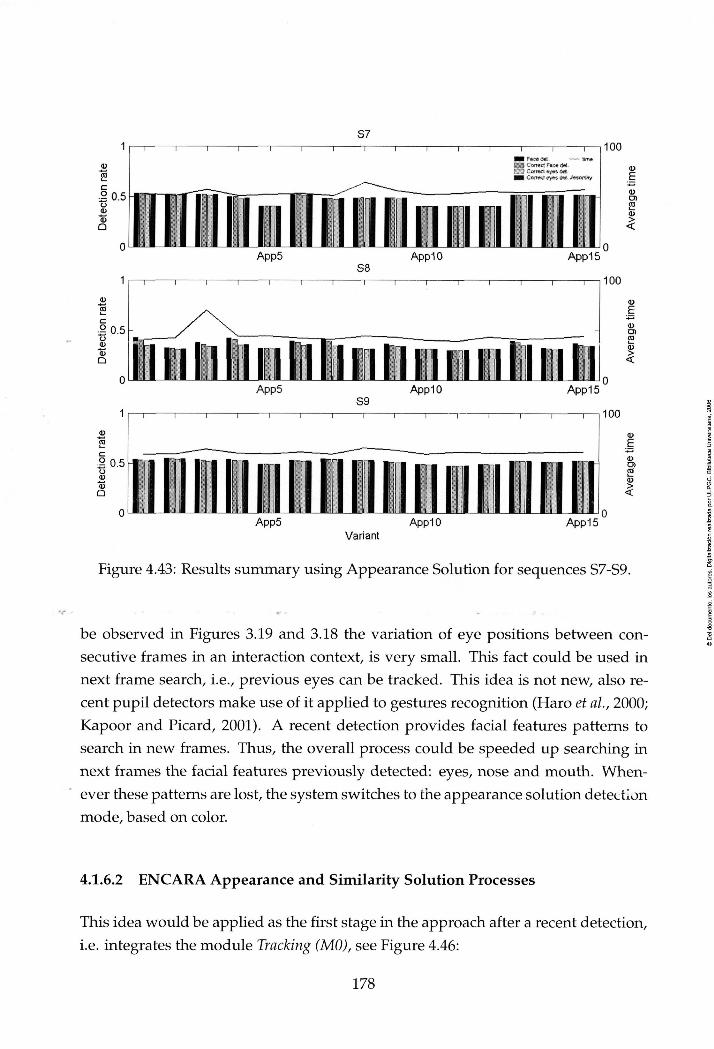
áO.5

D

App5 S8

App10 App15

áO.5 o

n 1 1 1 1 1 1 r

ílIIIIIi

100

O) <n

> <

100

J

} App5 ApplO App15

Variant


be observed in Figures 3.19 and 3.18 the variation of eye positions between con-

secutive frames in an interaction context, is very small. This fact could be used in

next frame search, i.e., previous eyes can be tracked. This idea is not new, also re

cent pupil detectors make use of it applied to gestures recognition (Haro et al, 2000;

Kapoor and Picard, 2001). A recent detection pro vides facial features patterns to

search in new frames. Thus, the overall process could be speeded up searching in

next frames the facial features previously detected: eyes, nose and mouth. When-

ever these patterns are lost, the system switches to the appearance solution detection

mode, based on color.

4.1.6.2 ENCARA Appearance and Similarity Solution Processes

This idea would be applied as the first stage in the approach after a recent detection,

i.e. integrales the module Tracking (MO), see Figure 4.46:

178

.2 0.5

i

.2 0.5

i

n 1 r

S10 T 1 1 r 100

i !

App5 S11

App10 App15

1 1 1 r

Iflnl •rini l l n l IFlnl inni JIU lOal App5

Variant

llnl irní lili I o App10 App15

100

E

I Figure 4.44: Results summary using Appearance Solution for sequences SlO-Sll.

1. Last eye and mouth search: ENCARA processes a video stream, thus before pro-

cessing a new frame, last frame results can be used. Last patterns detected are

searched in new frames, providing another pair set of potential eyes, added

to the pair provided by the color blob, see Figure 4.49. This pair will be re-

ferred as similarity -pair set. This test searches first previously detected eyes in

current frame instead of using the eye localization method based on color ern-

ployed in the general case. The search área is a window centered in previous

position detected with a dimensión of 0.6 x ínter_eyes_distance. According to

differences among consecutive frames and intereye distance for that sequence.

Figure 4.47, those dimensions could manage a general test.

The pattem search process proceeds as foUows:

(a) Compute image differences. Sliding the pattem searched over the search are,

a difference image, see Figure 4.48 is computed according to the same

operation:

I{x, y) = E í l T Ei=o^ \image{x + i,y + j)- pattern{i,j)\ H = Tmn\/x^y/0<x<sizex,0<y<sizey\^\X,yjj

(4.21)

179

Accepted Accepted

Figure 4.45: Flow diagram of ENCARA Similarity Solution.

(b) Localizefirst and second minima. The first and second minima are searched

int the image of differences, E{ta) and E{tb).

(c) Tracking by comparison. The process is controUed by two limits related with

the minimum difference, a lower, Emin, and an upper, E^ax/ thresholds.

These are the update and the lost thresholds respectively. If E(t„) < Emin

the current pattem remains unchanged. If E{ta) > Emin and E(ta) <

Emaxf the appearance of the pattem has changed and its update is neces-

sary. If E{ta) > Emax, the pattern is considered lost.

These thresholds are defíned dynamically. The update threshold is up-

dated in relation with the second minimum found on the search window.

This threshold must be lower than second rrdnimum, Emin < E{tb), to

avoid a matching with a similar pattem in the context área, more details

ir. (Guerra Artal, 2002). The lost threshold is adjusted according to the

difference among the first and the second minimum. A sudden low dif-

ference between them will be interpreted as a pattern lost.

Some authors have introduced a predictive filter, i.e. a Kalman filter, to sup-

port this tracking mode (Haro et al, 2000), but head movement is quite jerky

for such filter as pointed out by (Kapoor and Picard, 2001). For that reason no

predictive filter has been integrated in this implementation.

180

Figure 4.46: Flow diagram of ENCARA MO module.

There are different altematives in the literature for general purpose tracking.

A facial feature based approach tracks features by means of color correlation

in (Horprasert et al, 1997). The difference between témplate and the image is

considered:

M = E : T E ; L 7 m a x ( | i ? ^ , , - R,J, |GT., - GrJ, |Br., - BjJ) (4.22)

2. Test with previous detection: If in a recent frame (<1 sec.) a frontal face was

detected, a temporal coherence test is performed. When the positions detected,

i.e. retumed by the pattern search process, are similar to the one in previous

frame, ENCARA performs a rotation to lócate both eyes horizontally. Later,

the normalization is done and finally the appearance test is applied for eyes

and face.

3. Majority test: If the test with previous is not passed, an extra test is performed

observing if most pattems corresponding to facial features (both eyes, middle

eye position, nose, and mouth corners) have not been lost and are located cióse

to previous position. In that case, it is considered that the face has been located.

4. Analysis of similarity test results: The results retumed by previous similarity

tests provoke certain actions:

(a) If similarity test is passed: First the candidate is considered frontal. Later,

181

Wf,: f Y'í w * í ti\/^Mi''i-¿^^í'í/'r

'JIM , w " í f I

Figure 4.47: Upper plots represent the differences for eye position in a sequence for X and y respectively, bottom plot shows the inter eye distance for the secuence.

eye patterns are analyzed in order to reduce location problems. Gray

mínima does not correspond always with pupil, see Figure 4.50, this cir-

cumstance and the search and matching of a previous pattern can affect

pattem consistency. In order to minimize the possible pattern shift, eye

patterns are adjusted using a d)n:\amic threshold. This threshold is used

to perform a binarization of pattern image, where the major dark blob is

analyzed. The threshold is increased or decreased until the major dark

blob inside the pattem has an área corresponding to a circle whose radius

(r) must be one tenfh of the inter-eye distance, r = inter_eye_distance/10,

thus the área should be approximately TT X r^, see Figure 4.51. The center

of this blob is used as the new best position for each eye pattem.

(b) If similarity test is not passed: The system behaves as described in the previ

ous section, i.e. searching based on color. FJowever, a slight modification

is introduced. The appearance solution eyes detection step, enclosed in

M2, searches for gray mínima in a search área defined by skín color blob

and integral projections. However, at this point, even if the similarity test

was not passed, the Information got from previous frame can be used.

Thus the system can submit three eye pairs, and even combine them:

i. Gray mínima pair searched in áreas defined by color,

ii. Similarity pair set searched in áreas defined by recent detection.

182

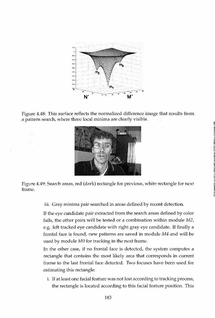
Figure 4.48: This surface reflects the normalized difference image that results from a pattern search, where three local minima are clearly visible.

Figure 4.49: Search áreas, red (dark) rectangle for previous, white rectangle for next frame.

iii. Gray minima pair searched in áreas defined by recent detection.

If the eye candidate pair extracted from the search áreas defined by color

fails, the other pairs will be tested or a combination within module M2,

e.g. left tracked eye candidate with right gray eye candidate. If finally a

frontal face is found, new pattems are saved in module M4 and will be

used by module MO for tracking in the next frame.

In the other case, if no frontal face is detected, the system computes a

rectangle that contains the most likely área that corresponds in current

frame to the last frontal face detected. Two focuses have been used for

estimating this rectangle:

i. If at least one facial feature was not lost according to tracking process,

the rectangle is located according to this facial feature position. This

183

" ' • ' • t . • . • ' 'M

• Figure 4.50: Example of an eye whose pupil is not the gray minimum.

Figure 4.51: Examples of eye pattern adjustment.

rectangle can be used with high likelihood to estímate the position of

the face,

ii. If no facial feature could be tracked and there is a skin blob big and

cióse enough to be considered, the this rectangle is associated to that

blob center.

4.1.7 Experimental Evaluation of Similarity and Appearance Solu-

tion

Figures 4.53-4.58 (detailed results in appendix Tables D.12- D.33) present some re-

sults for different sequences. These implementations intégrate the foUowing tests:

too cióse eyes test, integral projection test and appearance test. The variant labels are de-

scribed in Table 4.4. These variants are defined by the appearance test used, the use

of tracking, the adjustment of eye patterns, the use of múltiple candidates and the

integration of the majority test as explained above.

It must be noticed that an uncorrect detection can be dramatic for system re

sults, as the similarity tests will trust in last detection. A bad detection will make

the system to track something that is not a face, thus appearance tests are very im-

portant.

184

Eye test applied

PCA PCA PCA



PCA PCA PCA

Rect. feat. Rect. feat. Rect. feat. PCA+SVM PCA+SVM PCA+SVM

PCA PCA PCA



PCA PCA PCA



Face test applied

PCA Rect. feat.

PCA+SVM PCA

Rect. feat. PCA+SVM

PCA Rect. feat.

PCA+SVM PCA

Rect. feat. PCA+SVM

PCA Rect. feat.

PCA+SVM PCA

Rect. feat. PCA+SVM

PCA Rect. feat.

PCA+SVM PCA

Rect. feat. PCA+SVM

PCA Rect. feat. PCA+SVM

PCA Rect. feat.

PCA+SVM PCA

Rect. feat. PCA+SVM

PCA Rect. feat.

PCA+SVM

Uses tracking

Yes Yes Yes Yes Yes Yes Yes Yes Yes Yes Yes Yes Yes Yes Yes Yes Yes Yes Yes Yes Yes Yes Yes Yes Yes Yes Yes Yes Yes Yes Yes Yes Yes Yes Yes Yes

Adjust eye pattern

No No No No No No No No No Yes Yes Yes Yes Yes Yes Yes Yes Yes Yes Yes Yes Yes Yes Yes Yes Yes Yes Yes Yes Yes Yes Yes Yes Yes Yes Yes

Múltiple candidates

No No No No No No No No No No No No No No No No No No Yes Yes Yes Yes Yes Yes Yes Yes Yes Yes Yes Yes Yes Yes Yes Yes Yes Yes

Majority test Yes Yes Yes Yes Yes Yes Yes Yes Yes Yes Yes Yes Yes Yes Yes Yes Yes Yes Yes Yes Yes Yes Yes Yes Yes Yes Yes Yes Yes Yes Yes Yes Yes Yes Yes Yes

Variant label Siml Sim2 Sim3 Sim4 Sim5 Simó Sim7 Sim8 Sim9 Simio Simll Siml2 Siml3 Siml4 Siml5 Simio Siml7 Siml8 Siml9 Sim20 Sim21 Sim22 Sim.23 Sim24 Sim25 Sim26 Sim27 Sim28 Sim29 SimSO SimSl Sim32 Sim33 Sim34 Sim35 Sim36

Table 4.4: Summary of variants of ENCARA appearance and similarity solution (the too cióse eyes test and integral projection test are integrated) plus appearance and similarity tests. These labels are used in Figures 4.53- 4.58.

185

Figure 4.52: Candidate áreas for searching: On the right using previous detected position; on the left using color

First, it must be observed that the integration of similarity reduces signif-

icantly the processing time for some sequences while increasing significantly the

rate of detected faces. For sequence S3 using variant Sim28 ENCARA processes at

45 Hz. which means 42 times faster than Rowley's technique. This fact is similar for

other sequences using the same variant. That happens due to the facial features are

easily tracked in those sequences as the user does not perform large pose changos.

Those variants listed at the begrnning of the Table 4.4 intégrate less similarity

elements that those listed at the end. Those referred similarity elements are: the

use of tracking, the adjustment of eye patterns, the use of múltiple candidates and

the integration of the majority test. Each of these four elements is integrated in

ENCARA in that order. The resulting similarity configuration is tested using the

nine combinations of appearance tests for eyes and face. If correct detection rates

are greater for the bst variants mean that thos<^ elements integrated a -e usefu^ ^or

improving ENCARA performance.

Observing the Figures and comparing each group of nine variants with the

foUowing group of nine variants group, a general improvement of face detection

rate is observed. Only the second group that corresponds to the eye pattern adjust

ment while tracking, presents in a reduction for some sequences (SI, S9 and Sil)

of this behavior in terms of face detection rate. But on the other hand, the integra

tion of this technique improves for all the sequences the eye detection rate reducing

consequently the error rate for eyes location.

A deeper analysis referred to sequence SI provides some observations that

can be later analyzed for the rest of sequences. Figure 4.53 (detailed results in ap-

pendix Tables D.12 and D.13) shows results for that sequence. Observing the first bar

to check the detected faces rate, some variants are clearly poor: Simi-Sim?, Siml3-

Siml5, Sim22-Sim24 and Sim31-Sim33. The common feature among those variants is

that they all make use of rectangle features based test for eye appearance. It must

186

be reminded that this test produced singular results for sequences S2 and S4 using

ENCARA appearance solution, see section 4.1.5. The rectangle features test seems to

be too restrictiva for eye appearance detection across different sequences. This par

ticular behavior of rectangle features based test for eye appearance is reproduced

also for sequences S2-S5. For the rest of sequences S6-S11, those variants are not

clearly inferior than those that intégrate just one similarity element and make use of

PCA reconstruction error (Siml-SimS, SimlO-Simll, Siml9-Sim21 and Sim28-Sim30)

or PCA+SVM {Sim8-Sim9, Siml6-Siml8, Sim25-Sim27 and Sim34-Sim36) for eye ap

pearance. Even more, those based on rectangle features provide better rates for ini-

tial variants that use PCA+SVM for eye appearance but are in general overpassed

by those that intégrate more elements.

These considerations reduce the variants that seem to be more stable and

henee rnteresting, to those that intégrate all the elements introduced by the EN

CARA appearance and similarity solution except those that use the rectangle fea

tures based test for eye appearance: Sim28-Sim30 and Sim34-Sim36.

If those variants are compared among them, it is observed that the use of

PCA reconstruction error for face appearance, i.e. Sim28 and Sim34, produces lower

correct eye detection rate for some sequences: Sim34 for SI, Sim28 for S3, S6, S9,

and both for S2, S4, S5, S8. This observation was already considered for ENCARA

appearance solution results, see Section 4.1.5, this seems to prove the importance of

modelling non-face appearance.

Therefore, the selected group of variants is reduced to those that integrates

all similarity solution elements, and perform eye appearance test by means of PCA

or PCA+SVM, and face appearance tests by means of rectangle features based or

PCA+SVM. The differences among these variants in terms of detection rates are

harder to extract. In terms of face detection rate Sim29 provides the best rate for

SI, S9, Sim30 for S2-S4 and Si l , Sim35 for S5-S6 and Sim36 for S7, S8 and SIO. In

terms of correct eye location rate, Sim35-Sim36 produce slightly better rate for SI,

S4 and SIO while Sim35-Sim36 for S3, S5 and S8. For the rest of the sequences the

differences are minimal. These results difficult to select a single variant as the best

one in terms of detection rates. This group is selected and their behavior must be

compared using greater appearance training sets. The only major difference among

those selected variants, is that average processing time is always 10 — 30 msecs.

slower if PCA+SVM test is used for eye appearance. In general variants that use

PCA reconstruction error for testing eye appearance are faster than the others.

187

0.8

2 0.6

•5 0.4

0.2

S1

I Face deí - time i CofTect Face det 3 Corred eyeí deí. I Correct eyes det Jesorsity -

100

Sim5 Simio Sim15 S¡m20 S¡m25 Sim30 Sim35

100

Figure 4.53: Results summary using Appearance and Similarity Solution for se-quences S1-S2.

4.2 Summary

Accordmg to the description of the different ENCARA solutions, the best perfor

mance in terms of face and eye pairs detection rate is achieved by some selected

variants that belong to the ENCARA appearance and similarity solution. These se

lected variants are distinguished by the addition to the Basic Solution of appearance

tests for face and both eyes and the integration of similarity elements as described

in previous sections. These variants are configured as described in Table 4.4.

Figures 4.59 and 4.60 (detailed results in appendix Table D.34) show a com-

parison between those selected ENCARA variants, i.e. Sim29-Sim30 and Sim35-

SitnSó, and Rowley's technique in terms of face detection rate and average process-

188

S3

0.8

S 0.6 o t3 S 0.4 Q

0.2 F ate del. lima Cor-ect Faca det,

. Corftct eyes det. • H Cor'ect eyes det. Jesorsity « • • 1 1 « a msa • ! • • » • Mij

100

Sim5 Simio Sim15 Sim20 Sim25 SimSO Sim35

S4 100

S0.6

gO.4

0.2

\

Sim5 Simio Sim15 Sim20 Variant

Sim25 Sim30 Sim35


ing time. Figure 4.59 compares the face detection rate (upper) and the correct face

detection rate among Rowley's technique and the different variants. Instead 4.60

plots upper the correct eye detection rate according to Criterium 2 and bottom ac-

cording to Jesorsky's criterium.

The face detection rate using ENCARA is not homogeneous with each se-

quence, particularly these rates are low for sequences SI, S2, S5 and Sil .

For sequences SI and S2, the ENCARA variants do not provide a perfor

mance similar to Rowley's. This fact can be justified by the absence of this subject

eyes in the training eye appearance set which are also almost closed in many trames

(remember that eye appearance training set has been built with a small group of

samples extracted from sequences S7, S9 and SIO), but also to the continuous pose

189

0.8

S 0.6

S5

Sim5 Simio Sim15 Sim20 Sim25

• t ime • Face det. M Correct Face det. í j Correct eyes det. • Correct eyes det. Jesorsi^y ~

Sim30 Sim35

100

100

SimS Simio SimlS Sim20 Variant

Sim25 Sim30 Sim35


change of the user. Sequence S3 provides similar face detection rate with both al-

gorithms. The static behavior in sequence S4 is visible in the high success results

achieved with ENCARA variant in contrast to Rowley's technique performance.

Sequences S5 and Si l produce lower face detection rafes using ENCARA, which

could be explained commenting that the faces contained in these sequences are

smaller than the models used to test their appearance. Positive eye and face pat-

tems were learned from samples extracted from S7, S9 and SIO, for that reason these

sequences, present high rafes using ENCARA. Sequences S6 and S8 present results

for sequences where the individual plays some gestures (yes, no, look right, up,

etc.), however the rates are not far from those achieved using Rowley's technique.

According to these Figures, ENCARA performs using variant SimSO for the

worst case, SIO, 16.5 times and in the best case, S4, 39.8 faster than Rowley's tech-

190

Sim5 Simio Sim15 Sim20 Sim25 Sim30 Sim35

100

5

S8

0.8

Face det time Cotrect Face det. Corred eyes det. Corred eyes det. Jesorsity

SinnS Simio Sim15 Sim20 Variant

Sim25 S¡m30 Sim35

100


ñique. Calculating the average excluding the best and the worst times gives and

average of 22 times faster than Rowley's technique. This performance is accompa-

nied by a correct eye pairs location rate according to Jesorsky's criterium greater

than 97.5% (except for S5 which is 89.7%). This rate is always better than the one

provided by Rowley's technique, this fact can be explained due to this technique

does not provide eye detections for every face detected. However, the face detec-

tion rate is worst for that ENCARA variant except for S3, S4 and S7. In the worst

case ENCARA detects only 58% of those faces detected using Rowley's technique.

However, the average excluding the best and the worst performances is 83.4%.

In Figure 4.60 (details in appendix Table D.35) the eye detection error for

both techniques is analyzed considering not Jesorsky's criterium but the exigent

Criterium 2. As can be observed in these Figures, the rafes of eye detection errors

191

Sim5 Simio Sim15 Sim20 Sim25 Sim30 Sim35

100

S10

Sim35

100


using both techniques are small. It can be observad a greater rate for ENCARA, but

it must be reminded that in most cases ENCARA provides an eye pair for every

face detectad. Also the average distances of those errors are minimal. Eye location

errors are more evident for S5 and Sil , sequences that contain smaller faces, i.e., the

threshold to consider an eye location error is smaller.

Previous Figures reflect a performance for ENCARA that detects an average

of 84% of the faces detected using Rowley's technique but 22 times faster using stan

dard acquisition and processing hardware. ENCARA provides also the added valué

of detecting facial features for each detected face.

ENCARA provides a rectangle as a bounding box of the detected face. Ob-

serving the system working live, it happens sometimes that the face changes and

192

S11

Sim5 Simio Sinn15 Sim20 Variant

Sim25 Sim30 Sim35

Figure 4.58: Results summary using Appearance and Similarity Solution for se-quence Si l .

ENCARA is not able to track every facial elements ñor find again the face in that

frame. In that situation, if it was a recent detection and at least one face feature was

not lost, ENCARA provides a likely face location rectangle. The use of temporal

coherence in this way allows ENCARA to track the face even when there is a sud-

den out of plañe rotation, or the user blinks, etc. For these trames ENCARA does

not provide in current versión a location for facial features. Figure 4.61 (details in

Table D.36) compares face detection rate results if these rectangles are considered

as f:ice detcctions, the top imagc plots the face detection rate and the bottom im-

age the correct face detection rate. The variants labels are modified adding PosRect

to each ENCARA variant analyzed in this summary. For comparison purpose, the

face detection rates using ENCARA PosRect variants and Rowley's technique are

provided.

As it is observed, the face detection rate increases significatively becoming

similar or better to that provided by Rowley's algorithm. This rate keeps an excel-

lent correct face detection rate which for variant SimSOPosRect is always over 93.5%.

It must be considered that this rate considers as correct detections those faces whose

both eyes and mouth are contained in the rectangle provided by ENCARA, so an

error does not mean that no one facial feature is contained in that rectangle.

These face detection rate increasing results can be summarized pointing out

that ENCARA performs an average of 22 times faster than Rowley's, detecting an

average (for Sim30PosRect and excluding best and worst case) of 95.2% of the faces

detected by Rowley's algorithm.

193

Face Detection ENCARA vs Rawle^s

SI S2 S3 S4 S5 S6 S7 S8 S9 S10 S11

Corred Face Detection ENCARA vs Rowleys

S1 S2 S3 S4 S5 S6 S7 S8 S9 S10 S11

I ENCARA SniSa • S ENCARA Sim30 í ENCARA Sim35 9 ENCARA Sim36

Figure 4.59: Results summary for face detection rate comparing ENCARA variants Sim29-Sim30 and Sim35-Sim36 with Rowley's technique.

The final ENCARA Appearance and Similarity Solution algorithm can be

summarized as presenteJ In Algorithm 1.

4.3 Applications experiments. Interaction experiences

in our laboratory

This Section presents different experiences carried out in our lab related with pos-

sible applications of ENCARA face detection solution. The intention of applying

ENCARA to different scenarios is to show the ubiquity of the system. The expe

riences described in this section have been chosen based on the utility that their

abilities can offer to a PUI (Perceptual User Interface) system. First, the architec-

ture for a PUI system is described and later some results are described related with

recognition and interaction.

194

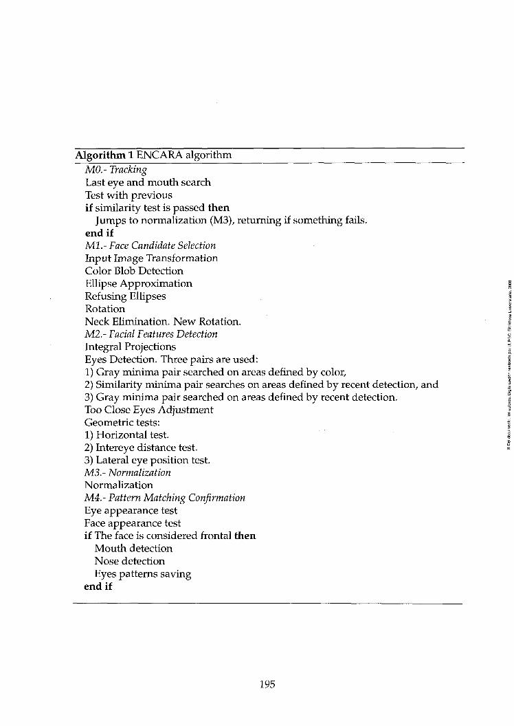
Algorithm 1 ENCARA algorithm

MO.- Tracking Last eye and mouth search Test with previous if similarity test is passed then

Jumps to normalization (M3), returning if something fails. end if MI.- Face Candidate Selection Input Image Transformation Color Blob Detection EUipse Approximation Refusing EUipses Rotation Neck Elimination. New Rotation. M2.- Facial Features Detection Integral Projections Eyes Detection. Three pairs are used: 1) Gray minima pair searched on áreas defined by color, 2) Similarity minima pair searches on áreas defined by recent detection, and 3) Gray minima pair searched on áreas defined by recent detection. Too Cióse Eyes Adjustment Geometric tests: 1) Horizontal test. 2) Intereye distance test. 3) Lateral eye position test. M3.- Normalization Normalization M4.- Pattern Matching Confirmation Eye appearance test Face appearance test if The face is considered frontal then

Mouth detection Nose detection Eyes pattems saving

endif

195

1

0.8

2 0.6 c o S 0.4 Q

0.2

Correct Eye Pairs Detection ENCARA vs Rowleys

S9 SI O

Correct Eye Pairs Detection ENCARA vs Rowley's (Jesorslíy)

• n ENCASA am29 SrfiSO L_J CNCARA Sm30 [ ; ENCARA, Slm35 mu ENCARA Sln3C

Figure 4.60: Results summary for eye detection rate comparrng ENCARA variants Sim29-Sim30 and Sim35-Sim36 with Rowley's technique.

4.3.1 Designing a PUI system

Last years have revealed Education and Entertainment as promising, tnougii de-

manding, application scenarios for robotics with a great scientific, economic and

social potential (Doi, 1999). The interest raised by commercial products like Sony's

Aibo or the attention given by the media to projects such as Rhino (Burgard et al,

1998), Sage (Nourbakhsh et al, 1999), Kismet (Breazeal and Scassellati, 1999), Minerva

(Thrun et al, 1998) and eldi (Cabrera Gámez et al, 2000) demónstrate the fascination

of the general public for these new fashion robotic pets.

In this scenario, sometimes recognition has no sense as museum visitors mav

be visiting the museum for the first time. In these conditions, it is more interesting to

interpret user gestures or to perform different transformation to visitors faces. These

transformations would be addressed to avoid outliers, elements as beards, glasses

(Pujol et al, 2001). Outliers elimination could also be used to produce socially correct

images (Crowley et al, 2000), caricaturizing (Darrell et al, 1998), protecting person

privacy (Crowley et al, 2000) (reconstructing a face with another person PC A set),

change his/her hair color, reproduce the person face changing his/her mouth say-

196

Face Detection ENCARA PosRect vs Rowle/s

SI S2 S3 S4 S5 S6 S7 SS S9

Corred Face Detection ENCARA PosRect vs RDwIe^s

S10 Sil

S1 S2 S3 S4 S5 S6 S7 S8 S9 S10 S11

Figure 4.61: Results summary comparing ENCARA variants considering Possible Rectangle as Face Detection with Rowley's technique.

ing a sentence that his/her has never said (Bregler et al., 1997; Brand, 1999), learnrng

motion pattems (Matthew and Hertzman, 2000), etc.

4.3.1.1 Casimiro

Among the projects currently being developed in our lab, the project entitled as

Casimiro treats the conception and development of a humanoid face with some ca-

pabihties of intelligent behavior. According to (Brooks, 1990) Artificial Intelligence

(AI), had on those days two main approaches for developing intelligent systems:

classical AI or GOFAI (Good Oíd Fashioned AI) and nouvelle AI.

The first approach considered that intelligence was possible in a system of

symbols. An intelligent behavior was possible under this focus by means of the

combination of different symbol-producer modules. Under this focus, symbols rep-

resent entities of the world, but there is a lack of connection between perception and

symbols. This fact is evidenced due to a different representation is necessary for

each different task which made classical AI to reach a closed road. This approach

197

Auditory/ visual data

Motors/ voice actioiíis,

• • 1™». Bkítm U

-i

J

¡ i-

! > •

-

Memo '

Míní

tíwdtííe ";

Supervisor

, • Figure 4.62: System description

tried to solve the whole problem.

In the second approach, again a system is decomposed in modules, but mod

ules are connected with the physical world, avoiding symbolic representation. Each

module has its own behavior and the combination of them generates more complex

behaviors. Sensing the environment, the system can get the information necessary

to survive in its ecological niche. The use of a behavior language allows the acti-

vation or deactivation of those modules providing the expected djmamism to the

system behavior. In (Brooks, 1990), the subsumption architecture is employed for

that purpose. This solution fails in many contexts but works successfully in others.

The failure of this solution in different contexts does not mean that the designed sys

tem has not an intelligent behavior. As expressed by Brooks in Elephants don't play

chess (Brooks, 1990), it can not be said that elephants have no intelligence, as they

survive and adapt to their environment but are not well suited to others. Minsky

(Minsky 1986) theorized that not only this AI conception will be the basis of com-

puter intelligence, but it is also an explanation of how human intelligence w^orks.

FoUowing this idea, the system has been conceived as a set of closely coop-

erating modules that have their own behavior. A major system decomposition has

been performed attending to tasks carried out by different modules. Thus, the sys

tem is made up of five major modules, see Figure 4.62: MPer, Meff, MconBeh, MInt

and MEmo. Certainly this is just a tentative system design, howeve" t is not the

focus of this work to present a detailed and finished definition of the system. Here,

the system design is described from a functional point of view, remarking that the

challenge of the work described in this document focus on a capability of one of

those major modules.

MPer: This module integrales all the activities related to modes/perceptions con-

sidered by the system: visual and auditory. The submodule devoted to the

198

visual perception is conceived according to the paradigm of active perception

(Bajcsy, 1988) and realizes visual attention tasks and sensorial abstraction. It

takes as input the visual data as well as outputs from MConBeh modules like

control commands. Results achieved by any of the abilities included in this

module, produces visual abstraction that is sent to the MConBeh module. The

visual attention tasks are devoted to detect and track objects and the sensorial

abstraction includes activities for face, posture or gesture recognition. Audi-

tory perceptions are processed by a submodule which is also included into

MPer. The auditory submodule, similar to the visual submodule, includes at

tention and recognition tasks. This submodule can detect the orientation of a

sound source to direct the visual attention. It should also be able to sepárate

different sound sources to provide the input to voice recognition tasks.

MEff: The effector activities are associated with the MEff modules, both motor

and sound/voice actions. Motor actions control the gestures and the reactive

response of the system to what the system perceives via the MPer module,

specifically the actions related to head and eyes. Also MEff module must de-

code gestures associated to the behavior selected by the MConBeh module into

motor actions to get the desired face expression (Breazeal and Scassellati, 1999;

Thrun et al, 1998).

MConBeh: The core of the perceptual-effector system which is in charge of the

generation of the conductual sequences. Interaction actions can run for sec-

onds or hours. Thus, this module should be in charge of considering conduc

tual timing, as pointed out in (Thorisson, 1996) where the Human Multimodal

Communication is divided in three levéis with respect to time:

• Encounter: Includes the whole interaction, action take place at lowest

rate.

• Tum: When people communicate, they take tums. This organizes Infor

mation exchange.

• Feedback: Paraverbals (mhmm, aha) and gestures (nod), can act as an ex

tra charmel during interaction, indicating attention, or dislike, fear while

the other interactor communicates.

This module is based on Behavior Activation Networks (Maes, 1989), which

allow to define relations between behaviors and their activation variables as

199

STRIPS-like rules. It also solves the behavior transition problem and gives a

simple and complete solution to the action selection problem.

MInt: This module serves as interface with the extern system or with an exter-

nal supervisor. If this system is embedded into another system, like a service

robot, this module will be the interface with it.

Memo: Activity selection is a problem that any autonomous system must sol ve

(Cañamero, 2000). A possible AI solution is to design the selection mechanism

based on reactive behaviors, responsive to external stimuli (Brooks, 1986), or a

repertoire of consummatory and appetitive behaviors which are guided by

internal needs and motivations (Maes, 1991). The seminal work of Dama-

sio (Damasio, 1994) introduces the idea that the human intelligence relies on

emotions in aspects like those related with the decisión making activity in dy-

namic and complex environments. The mind is not a phenomenon of the brain

alone, but derives from the entire organism as a whole. Damasio formulates

the somatic-marker hypothesis: a special class of feelings, acquired by experi-

ence, that express predicted future outcomes of known situations and help the

mind make decisions. Emotions are the brain's interpretation of reactions to

changes in the world.

Focusing on automatic systems. Cañamero (Cañamero, 1997) adopts the point

of view of considering a creature as a society of agents, understanding an

agent as a function that maps percepts into actions. The ccmbination of sim

ple agents under Minsky's conception (Minsky, 1986), i.e., a large number of

mindless agents can work together in a society to créate an intelligent society

of mind.

Changing behavior and goal priorities adapted to the situation can be car-

ried out using simple emotions (Cañamero, 2000). Their integration accordtng

to this author will benefit by providing fast reactions, solving múltiple goals

cholee and signaltng relevant issues to others. Behavior selection is carried

out by a motivational system that focus on arousal and satiation (Cañamero,

1997). Perceptive, attentional and motivational states modify the intensity and

execution of the selected behavior.

For a natural and human-like interaction with humans, HCI needs adaptation.

Emotions are used in social interactions as mechanisms for communication

and negotiation, emerging from an interaction among individuáis (Cañamero,

1999). Emotional mechanisms have a direct feedback on system behavior,

200

Figure 4.63: Casimiro

i.e., are essential for adaptation. Thus, the inclusión of an Emotional Mod

ule, whose aim would be to act on the preconditions of the MConBeh module

to tune them (Picard, 1997; Cañamero, 1997), would yield as a result a human

behavior rather than a puré rational behavior guided only by perceptions from

the environment. ,

4.3.2 Recognition in our lab

According to previous sections, a face detector such as ENCARA will provide facial

frontal views which have been normalized using a standard position for eyes. This

normalization process is performed thanks to the facial features detection that deter

mine precisely the face scale. Normalizing the image allows also cropping the input

image in order to avoid background and hair. It is known that the performance of

face recognition techniques based on image data is reduced when this normalization

process is not accomplished.

4.3.2.1 Recognition experiments

Using the sequences described above, different recognition experiments have been

carried out to check the usefulness and validity of data provided by ENCARA as

face detector. Seven different subjects were in these sequences, one on each, that will

be in the foUowing referred as A-G. The training process is performed off-line. The

training set is built using images for each subject that are extracted automatically by

201

overall performance of this approach is better, in this experiment, using PCA+SVM.

Identity Recognition using PCA+SVM Gender Recognition using PCA+SVM

S2 S4 S6 38 S10 Sequences

S2 S4 S6 S8 S10 Sequences

Figure 4.65: Identity and gender recognition results using PCA-i-SVíví.

An observation that must be reminded is that ENCARA processes a video

stream. Therefore, it is not logic to experience suddenly an identity or gender

change. Humans assume that a person behind is still the same person that they

saw a minute before. However, most techniques presented in the previous survey,

are applied to a single image. For confirming the identification of a person, tempo

ral coherence on the results associated with a blob is needed. Assuming temporal

coherence for recognition will forcé to avoid instant changes of identity (Howell and

Buxton, 1996). Therefore, temporal coherence can be integrated in recognition. Ac-

cording to (Déniz et al, 2001fl; Déniz et al., 2002) if a classifier outperforms over a

O.ñ success rate, the classification performed for frame i can be related to previous

frame once a wrndow dimensión is defined. According to this work, among the best

criteria for classification is the majority. Only the gender classifier pro vides a rate

over 0.5 for all the sequences. Processing the sequences using this temporal coher

ence for gender identification the results are presented in Figure 4.66, being clearly

better, performing over 0.93 for all the sequences.

Gender Recognjüon Comparison

Figure 4.66: Gender recognition results comparison.

As recognition is a fast task, combining different classification approaches

204

interesting applications. Detecting these parameters in short term offers Commu

nications skills that help humans to feel comfortable interacting with machines (as

long as the system does not make a wrong age suggestion).

FoUowing this idea, this reduced training set was used also for performing a

gender classification. In the right bar graph of Figure 4.64, the results are presented.

It is notorious the failure for sequence Sil , used to extract training samples, but

presents better performance than the identity recognizer for sequences not used to

extract sample trames excepting S5.

These results seem promising as the classifier used is simple, and the training

set too. The problems that simple PC A presents with illumination coñdition changes

are also pro ved. Worst results are given by sequences with smaller faces such S5 and

Sil . Perhaps artificial illumination has played also a role in this process. But also

with S8 that seems to have a distractor confusing many trames with other subject. In

summary, this simple approach could be used for a day session, taking the training

samples for later recognition without major illumination changes. PC A is f ast, also

its training, thus, this approach is feasible for a demo session. This means that an

interaction session can be started with the training phase and later will perform

quite robust. As a summary, this classifier is not valid for different conditions, or

further training is needed. However, the validity of ENCARA as data provider has

been proved.

Before going further, another point of view can be adopted. The representa-

tion space and the classification criteria have been selected for simplicity and avail-

ability. PCA has been criticized due to its semantics absence, recent developments

use local representations as for example ICA (Bartlett and Sejnowski, 1997) to get a

better representation approach. However, the work described in (Déniz et al, 2001^)

proved that using any of both different representation spaces, PCA or ICA, and

a powerful classification criteria instead of NNC such as SVMs, reported similar

recognition rates. Thus, this work concluded that the classification criteria selection

was more critical than the representation used. Accordmg to these results, the ex-

periments have been carried out using SVMs (by means of LIBSVM library (Chang

and Lin, 2001)) as classification criteria. Results as presented for identity and gender

in Figure 4.65, being in general better even also for those sequences not used to ex

tract training samples. The gender classifier using PCA+SVM performs always o ver

0.75 while the identity classifier performs for sequences used for training over 0.7

while only over 0.3 for sequences acquired with different conditions. In any case the

203

overall performance of this approach is better, in this experiment, using PCA+SVM.

Identity Recognition using PCA+SVM Gender Recognition using PCA+SVM

S4 86 S8 310 Sequences

S2 S4 S6 S8 S10 Sequences

Figure 4.65: Identity and gender recognition results using PCAi-SVM.

An observation that must be reminded is that ENCARA processes a video

stream. Therefore, it is not logic to experience suddenly an identity or gender

change. Humans assume that a person behind is still the same person that they

saw a minute before. However, most techniques presented in the previous survey

are applied to a single image. For confirming the identification of a person, tempo

ral coherence on the results associated with a blob is needed. Assuming temporal

coherence for recognition will forcé to avoid instant changes of identity (Howell and

Buxton, 1996). Therefore, temporal coherence can be integrated in recognition. Ac-

cording to (Déniz et al, 2001fl; Déniz et al, 2002) if a classifier outperforms over a

0.5 success rate, the classifícation performed for frame i can be related to previous

frame once a window dimensión is deftned. According to this work, among the best

criteria for classifícation is the majority. Only the gender classifier provides a rate

over 0.5 for all the sequences. Processing the sequences using this temporal coher

ence for gender identification the results are presented in Figure 4.66, being clearly

better, performing over 0.93 for all the sequences.

Gender Recognihon Companson

PCA*NNC C~J PCA-

" PCA-

.*NNC I ,'SVM I L*SyM MWTKtJ ¡ S9 S10 S11

Figure 4.66: Gender recognition results comparison.

As recognition is a fast task, combining different classifícation approaches

204

and heuristics could also be considered. For example, in these experiments PCA+SVM

provides a high success rate for gender, thus the identity recovered could be re-

stricted to be coherent with the gender. In any case, this section pretended to ex-

emplify the possibilities of the face detection data provided by ENCARA, exactly

for face recognition, process for which the accuracy is necessary for getting better

performance.

4.3.3 Gestures: preliminary results

4.3.3.1 Facial features motion analysis

Facial features motions provide hints about head movements. For this analysis

ground data has been used to extract that knowledge. In Figure 4.67, it is observed

that they ha ve similar shapes. However, computing their differences this fact is cor-

rectly determinad. The intereye difference changes more than %10. This fact could

be explained if the face goes further or if there is an out of plañe rotation, i.e., the

face looks to one side.

350 400 450

íí 1 1

. A

\

f

ñ o 50 100 1 JO 200 250

i /ktJ

400 450

í / i

IDO l i o 200 250 300

Figure 4.67: For a sequence of 450 trames (x axis), upper plots represent the x valué of left and right iris (y axis), bottom plots represent the y valué of left and right iris.

This fact can be easily seen zoomtng one of those áreas and observing the

205

corresponding sequence frame, see Figure 4.68. If the face was going further, the

distance to the mouth should also be smaller.

The y behavior can see observed in Figure 4.67 the movement pattern has

ranges of similarities but also ranges of opposite (see the peaks at the beginning of

both).

The difference is plotted rn Figure 4.68. It is clear that in some situations,

both eyes go together up or down, but in others, one moves up while the other goes

down. This behavior corresponds to a roll movement, as can be seen in Figure 4.68.

j i ^

I ; if Vi '.'

70 so so 100

í'

• i f

i

—-ií ' •

j-

*

'

V ^ : «M

Figure 4.68: For a sequence of 450 trames, upper left graph plots differences among X valúes of both eyes, while upper right plot is a zoom from 50 to 135 frame (x axis). Bottom left curve plots differences among y valúes of both eyes, right zooming from O to 135 frame.

As ENCARA is specialized in frontal face detection, it will generally fail de-

tecting faces with out of plañe rotations but will be useful to detect roll. The ex-

traction of head pose requires further considerations of subject evolution in order to

realize when the subject turns.

206

4.3.3,2 Using the face as a pointer

The previous section pays only attention to extracting the head pose. That knowl-

edge is useful to realize of movements such as nods and shakes. However, the ges-

tures domain of the head is small. Instead, it could be considered the fact of making

use of the face as a pointer. This focus has great interest in the development of

interfaces for handicapped users.

A couple of sample applications have been developed making use of data

provided by ENCARA. In order to improve continuity the ENCARA variant used

was Sim29PosRect that consider also the information provided by the possible rect-

angle containing a face after a recent detection.

The first appHcation makes use of a blackboard where the user draws charac-

ters. A pause in the drawing process is considered by ENCARA as an rndicator of

character written. Each written character is added to the book only if its dimensions

are big enough. The resultrng legibility of the characters is really poor. The use of

the face as a brush m absolute coordinates has proven to be tedious and uncomfort-

able. Indeed this system will require later a character recognition module to make

the Computer to understand user commands.

Another focus considers the use of a virtual keyboard to introduce user char

acters. As a demonstration, a simple one digit calculator has been developed as pre-

sented in Figure 4.69. The control of this numeric keyboard is simplified by means

of relative movement avoiding the user to make an absolute movement to select

a key Instead, the user can manage the pointer as if the face was a joystick, i.e.,

with relative movements in relation to a zero position calibrated initially. The use of

relative movement eases significantly the use of the pointer.

Of course this example is certainly simple but the objective was just to present

possible applications of face detection data. This keyboard could be designed in a

predictive fashion similar to mobile telephones to ease character introduction.

This use of the no hands mouse assumes that an object is considered of inter

est in the pointer keeps its position on that object. That is not generally the case, as

for example the normal use of the mouse leaves frequently the mouse static. For that

reason, it was considered a possibility of performing some kind of facial action that

could be easily recognized and therefore associated to typical direct manipulation

actions as for example clicking the mouse.

The system was trained for 4 different facial expressions for a subject: neu-

207

Figure 4.69: Example use of the face tracker to command a simple calculator.

^ mmi

'-' '•> • *"' "• Figure 4.70: Expression samples used for IraiiiiiLg. *•'•'*

tral, sraile, surprise and sad. Around 20 samples were extracted at different mo-

ments of the day to intégrate some variation due to light conditions in the trainrng

set, see some samples in Figure 4.70. To recognize the facial expression, the same

approaches used for recognition were employed, i.e., PCA+NNC and PCA+SVM.

The relative movement of the face in relation to a zero position defined inter-

actively, direct pointer motion. A smile expression detected for more than three con-

secutive trames was interpreted as a left mouse button event. This simple scheme

allowed to manage windows using just the face.

208

Chapter 5

Conclusions and Future Work

T HE work described in this document can be summarized in the foUowing con

clusions:

a) Face detection probletn study. State ofthe Art:

Some of the lines of work being developed at our research group, are related

with the interaction abilities that a computer must have in order to carry out

natural interaction with humans. One of the main information sources in hu

man interaction is the face. Therefore, an automatic system which tries to in-

teract naturally must be able to detect and analyze human faces.

A new work line has becn opened in our lab, being the first objective to per-

form a vast literature search to known the state of the art in topics such as

HCI, PUI, face detection, face recognition and facial gestures recognition. The

results of this serious study is presented in chapters 1 and 2.

b) New Solution:

A nev/ solution to develop a real-time facial detector using standard hardw^are

has been proposed. A cascade solution based on weak and low cost classifiers

of any nature is designed and discussed in Chapter 3.

Based on this structure, a real-time face detector has been designed, developed

and tested. The system developed presents the foUowing fea tures:

i) Main features:

• The resulting system, integrates and coordinates diff erent techniques,

heuristics and common sense ideas adapted from the literature, or

conceived during the development.

209

• The system is based on a hypothesis verification/rejection schema

applied opportunistically in cascade, making use of spatial and tem

poral coherence.

• The system uses implicit and explicit knowledge.

• The current system implementation presents promising results in desk-

top scenarios providing frontal face detection and facial features lo-

calization data valid to be used by face processing techniques.

• The system has been designed in a modular fashion to be updated,

modified and improved according to ideas and/or techniques that

could be integrated. The system is able to recover from failures.

ii) Real-Time behavior:

The main purpose established in the requirements of the system, was real

time face detection. This goal has influenced the vvhole development of

the system.

Different techniques ha ve been adopted to carry oxú that need. The use of

tracking for previously detected facial features similarly to (Sobottka and

Pitas, 1998), the integration of appearance by means of PCA reconstruc-

tion error (Hjelmás et al., 1998), rectangle features (Viola and Jones, 2001fl;

Li et al., 2002ii) or a PCA+SVM classifier, the combination of simple tests

to improve performance and the use of temporal coherence.

For the sequences analyzed, a comparison has been performed using EN

CARA and the face detector described in (Rowley et al, 1998).

As a summary, the final experiments present a rafe of 20-25 Hz (variant

SimSOPosRect) for the sizes used in the experiments using a Pili IGhz,

which represents 12 — 25 times fáster than Rowley's technique for the

same sequences detecting 95% as average rate of those faces detected by

Rowley's technique.

Therefore, it has been proven empirically that the solution proposed fits

the real-time requirements established durrng design stage.

iii) Use of Knowledge:

The use of explicit and implicit knowledge sources allows ENCARA to

make use of their advantages: reactivity provided by explicit knowledge

and robustness against false positives provided by implicit knowledge

based techniques.

iv) Temporal coherence

210

Until now, the face detection literature has not widely exploited the use

of previous detection information for video streams. Most works try to

detect on each frame as it was the first one, i.e., in a still image detection

fashion.

In this document, their use has proven to be useful in two senses: 1) al-

lows to improve the performance of a weak face detector, and 2) reduces

the processing cost.

c) Experimental Evaluation:

A main effort has been focused in experimental evaluation acquiring a set of

video streams to carry out the analysis. ENCARA has been developed pay-

ing attention to modularity allowing to configure the different modules to be

used for each expériments. A configuration file allows to execute different

ENCARA variants.

ENCARA fulfills the real-time restriction with a faster detection time than

Rowley's technique, and its detection rafes are rn average lightly lower than

those provided by Rowley's technique, though rn some situations they are

competitive. This fact is reasonable as Rowley's technique was designed to

detect faces in still images while ENCARA exploits information contained in

video streams.

However, in continuous function for HCI, the main aspect for face detection

should not be the detection rafe for individual images but to provide a good

enough rate to allow HCI applications work properly. This has been demon-

strated empirically with the sample applications developed for ENCARA, mak-

ing use of different variants according to the specific application.

d) Applications of ENCARA:

The usefuLness of the data provided by ENCARA has been tested by means of

a known techniques for face recognition: PCA+NNC and PCA+SVM. The face

recognition technique has been easily integrated providing results according

to its typical performance.

These results allow to see the advantages of the proposed solution, ENCARA,

as a valid ubiquitous, versatile, modifiable and autonomous system that can

be easily integrated by higher Computer Vision Applications.

211

5.1 Future Work

The development of a real time robust face detector system. is a challenging task.

There are many different aspects that can be revised to improve ENCARA perfor

mance. Some of them are presented in this section.

a) Robust Candidate Selection:

Future work will necessarily pay more attention to increase candidate selection

performance and adaptability. Current implementation performs this stage by

means of color detection.

Color is a main cue for several practical visión systems due to the quantity

and quality of the Information provided. But color presents some weak points

in relation to environment changes which can be considered under different

pojnts of view: toleration and adaptation. An interesting option could be

to perform a study of those solutions that are more robust to environment

changes. This fact would allow to use the system not only for HCI applica-

tions, but also would improve the success rate of face detection. Also, it will

be very interesting to intégrate and combine other visual inputs in the candi

date selection process as for example motion, depth, texture, context, etc. that

would likely increase the system reliability (Kruppa et al, 2001).

b) Classification Improvetnent: Increastng robustness employing ¡he foUowir.g Ideas:

1) Increasing the efficiency of individual classifiers, and 2) introducing new el-

ements which provide new explicit/implicit knowledge as a way to increase

performance.

c) Training sets and dassifiers:

i) Training sets:

The implicit knowledge based techniques have been tested without mak-

ing use of a massive training set. Using only 3 different sequences for

training, the whole set of 11 has been tested without finding big prob-

lems. However, it has been observed that these training sets does not

cover the whole face and eye appearances. This fact is visible when using

rectangle features for testing eye appearance. For sequences S2 and S4,

the eyes are not accepted. This seems to prove the necessity of developing

a wider appearance training set to cover a greater domain of individuáis.

212

This sets should include including positive and negative samples. The set

can be artificially increased transforming the samples already contained

as in (Sung and Poggio, 1998; Rowley et al, 1998), but also need to join

more original samples. Por example, in (Rowley et al, 1998) the system

is developed with 16000 positive and 9000 negative samples. Our sets

are reduced but the results are promising enough to consider that a great

training set will provide even better performance.

ii) Selection of samples and dassifiers:

Another aspect to observe if a classification schema is used based on dif-

ferent dassifiers, is that a more adequate approach likc boosíing, see Sec-

tion B, can improve results. This focus can be used both to study the best

dassifiers combination and to select those training samples which are not

redundant in the training set, i.e., those that define the cluster borders.

ii) Multi view models:

It must be observed also that the appearance of eyes and faces is variable.

For example, in sequence S4 the detection rate using ENCARA is quite

high, however, it happens that the subject blink produces a pattem lost

and the eye candidates do not pass the eye appearance test. It is evident

that a cióse eye has an appearance very different to an open eye. It would

be very interesting to make use of different appearance models for the

facial elements. For example rn (Tian et al, 2000fl) two different models

are used for the eye depending on whether it is open or not.

d) Multi face detector

Current ENCARA implementation retums when it finds a blob with a valid

frontal face. It is likely that in desktop scenarios the biggest face is the one

interesting for the interaction process, but a multi face ability will allow more

applications to the system.

Also, small blobs could be zoomed using Active Vision system capabilities,

when there is no other área of interest. Applying hallucinating faces tech-

niques (Liu et al, 2001), a high-resolution image could be inferred and there-

fore, processed.

e) Unrestricted face detector

ENCARA has been designed as a frontal face detector. Currently, ENCARA

can not manage out of plañe rotations, i.e. lateral or back views. The system

213

just tries to wait opportunistically until a new frontal face is present.

An interesting future work is that ENCARA were able to manage orientation

changes like those mentioned, its possibilities of applications would be im-

proved significantly. We consider that this feature could be achieved making

use of the ideas employed in this document but extended.

f) Uncertainty management:

It will be interesting to investigate the use of certainty factors in the process

to accept/reject faces in order to use an uncertainty management schema in

the classification cascade and the temporal coherence. This goal must fit the

real-time restriction.

g) Applications

Several different applications are valid to make use of facial data. Two simple

demo applications presented proved the usefulness of face detection data to

control a pointer. The study and analysis of interfaces making use of this data

is a valid field of expansión once the face detector provided is reliable enough

in certain scenarios.

Among those possibilities, interfaces for handicapped users or Information

points constitute an interesting field of work. But also this data can be used

to extract a model from a given sequence, e.g. an challenging problem would

L\: to select the best representation for an individual given a sc.:jUence and the

ability to update the model for a known individual.

214

Capítulo 6

Resumen extendido

6.1. Introducción

6.1.1. Interacción Hombre Máquina

LA sociedad actual se caracteriza por una incremental y notoria integración de

los ordenadores en la vida cotidiana tanto en el contexto social como en el

individual. A pesar de ello, no todo el mundo contempla esta circunstancia de la

misma forma. Cada vez que una persona descubre mi actividad profesional son dos

opiniones muy diferentes las expresadas:

1. Adoro los ordenadores (la tecnología),

2. Odio los ordenadores (la tecnología).

¿Cómo es posible esta diferencia? ¿Qué hace que los ordenadores no sean

completamente aceptados sino incluso rechazados? ¿No existen los ordenadores pa

ra facilitar tareas desagradables? ¿Crean los ordenadores tareas desagradables? Este

sentimiento lo han expresado distintos autores:

"... si el papel de la tecnología es servir a la gente, ¿por qué el usuario

no especializado debe emplear tanto tiempo en hacer que la tecnología

haga su trabajo?" (Picard, 2001)

"El problema de xma interfaz es justamente que existe una interfaz.

Las interfaces ocupan el camino. No quiero gastar mi energía en la inter

faz. Quiero enfocar mi energía en el trabajo." (Norman, 1990)

215

Esta situación sucede debido a que las personas deben interactuar con los

ordenadores, existe una interacción entre dos entidades no relacionadas. ¿Qué sig

nifica exactamente interacción?

"Refleja las propiedades físicas de los interactores, las funciones a rea

lizar, y el balance de poder y control." (Laurel, 1990)

Desde un punto de vista tecnológico, una interacción es una acción recíproca

entre entidades, interactores, que tienen una superficie de contacto conocida como

interfaz. En este contexto, las entidades son los humanos y las máquinas (ordenado

res). Una interfaz:

"... comprende el lugar donde la persona y el sistema se encuentran.

Es el punto de contacto, el límite y el puente entre el contexto y el lector."

(Gould, 1995)

Como mencionamos anteriormente, ocurre que en ocasiones estas máquinas

diseñadas para ayudar a los humanos, provocan rechazo o estrés. Este hecho se debe

a que la interacción hombre máquina se basa actualmente en el uso de dispositivos

que no son naturales para los humanos. Esta situación establece diferencias entre

los humanos dado que algunos no están habituados a tratar con los ordenadores,

y consecuentemente no entienden su m^odo de funcionamiento (analfabetismo fun

cional).

Dadas estas dificultades, el diseño de interfaces ha recibido gran atención ya

que afecta al éxito del producto. Donald A. Norman (Norman, 1990) resume cuatro

principios básicos para el buen diseño de interfaces:

1. Visibilidad: Buena visibilidad significa que un usuario puede mirar a un dis

positivo y ver las distintas posibilidades de acción.

2. Modelo conceptual: Un buen modelo conceptual es aquel que ofrece consis

tencia en la presentación de operaciones y su imagen en el sistema.

3. Mapeo: Si el usuario puede determinar fácilmente la relación entre acciones y

resultados, y control y efectos, significa que el diseño tiene un buen sistema de

mapeo.

4. Realimentación: Recibir realimentación de las acciones del usuario.

216

Desafortunadamente, incluso hoy, el acceso a estas herramientas de interac

ción requiere aprendizaje y entrenamiento, debido a que los usuarios deben adap

tarse al sistema en lugar de ser los ordenadores quienes se adaptan a los humanos

(Lisetti y Schiano, 2000). Es obvio que esta etapa de aprendizaje no es nueva para

un ser humano. Los humanos tenemos que aprender a utilizar todo: una bicicleta,

una lavadora, un coche, un horno, una cafetera, etc. Cualquier dispositivo requiere

ima interfaz, y cualquier interfaz requiere un proceso de aprendizaje. El proceso de

aprendizaje se apoya en convenciones sociales creando modelos conceptuales so

bre el funcionamiento de las cosas. Este modelo nos permite reconocer y utilizar un

nuevo objeto, p.e., una nueva bicicleta. Un procedimiento sencillo de aprendizaje

equivale a facilidad de uso.

Los ordenadores pueden considerarse como otro tipo de dispositivos, si bien

existe una diferencia entre los ordenadores y los objetos cotidianos (bicicleta, silla,

etc.). Los ordenadores tienen capacidades de procesamiento que les permiten ciertos

niveles de adaptación. Por ello, un ordenador puede incrementar sus capacidades

mientras que una bicicleta no. ¿Pueden los ordenadores hacer uso de la misma in

terfaz aunque evolucionen sus funciones? o ¿tendrán los usuarios que aprender una

nueva acción de interacción para acceder a esas nuevas capacidades?

Los objetos cotidianos están cambiado al integrar unidades de procesamien

to, es por ello que los hábitos de interacción con estos objetos están modificándose.

Aparecen nuevas funcionalidades para estos objetos al mismo tiempo que sus ma

nuales de instrucción se hacen más complejos. Una receta de diseño es que las cosas

sencillas que se acomodan a modelos conceptuales conocidos no necesitan más ex

plicación.

¿Qué espera un usuario? Simplicidad, la mejor interfaz es la ausencia de la

misma (van Dam, 1997). Los nuevos sistemas serán más complicados de usar que

los actuales, por lo que el diseño de la interfaz afectará a su éxito (Pentland, 2000fc).

Una interfaz es básicamente un intermediario entre el usuario y el sistema. Am

bas entidades alcanzan un punto de encuentro donde tiene lugar el intercambio

(Thorisson, 1996). En la actualidad este punto de encuentro se habilita por medio

de la interacción explícita (Schmidt, 2000), el usuario realiza un comando explícito

al sistema esperando una acción de éste en consecuencia. Este comando explícito

se aprende y afecta a la complejidad de un sistema con gran funcionalidad. Antes

de continuar es conveniente recordar los marcos actuales y pasados de interacción

hombre máquina.

217

Desde su comienzo, la evolución de las herramientas de interacción hombre

máquina ha sido larga y no trivial (Negroponte, 1995). Los modelos de interacción

adoptan una metáfora para permitir al usuario concebir el entorno de interacción de

forma más familiar. En los inicios, años 40-60, los ordenadores eran un arte oscuro,

se programaban por medio de interruptores y tarjetas perforadas, obteniendo los

resultados a través de diodos. En este contexto, no existía metáfora o simplemente

se hablaba de la tostadora (Thorisson, 1996). El teclado aparece en los años 60-70

introduciendo la metáfora de la máquina de escribir. Los 80 se caracterizan por el

salto hacia la informática amigable, aparecen las interfaces gráficas de usuario (IGU)

y la metáfora de escritorio. En 1980 Xerox lanza Star (Buxton, 2001) el primer sistema

comercial con esta metáfora.

Las IGU asumen los principios de manipulación directa de Shneiderman (Sh-

neiderman, 1982):

• Visibilidad de los objetos de interés.

• Presentación inmediata del resultado de una acciíSn.

• Vuelta atrás para todas las acciones.

• Sustitución de comandos por acciones de "señalar y seleccionar".

La facilidad de uso y aprendizaje o amigabilidad de un sistema era vm - a

riable directamente relacionada con el éxito de una interfaz, es decir, de una apli

cación. Bajo este paradigma, el objetivo es diseñar entornos donde el usuario tenga

vina imagen clara de la situación y sienta el control (Maes y Shneiderman, 1997). Las

IGU proporcionaban un entorno común independiente de la plataforma, integrando

el uso de un nuevo dispositivo, el ratón. Este hecho fue expresado: "Nadie lee ya un

manual" (van Dam, 1997).

Esta metáfora evoluciona posteriormente en los 90 hacia la metáfora inmer-

siva (Cohén et al., 1999) donde el usuario se percibe e integra en un escenario por

medio de dispositivos como los guantes de datos o los cascos de realidad virtual

(CruzÑeira et al., 1992). Sin embargo, aún tienen poco uso comercial.

Diferentes autores han señalado deficiencias de las IGU, también conocidas

como VIRP (ventanas, iconos, ratón, puntero). Por ejemplo, en (Thorisson, 1996; van

Dam, 1997; Maes y Shneiderman, 1997; Turk, 1998fl) los autores destacan la pasivi

dad de estas interfaces a la espera de la entrada, en lugar de observar y actuar. La

218

interacción proporcionada por las IGU es monocanal, no hay realimentación, no se

utiliza la voz, el oído, ni el tacto. Los ordenadores están aislados (Pentland, 2000^).

"... Las IGU basadas en el teclado y el ratón son perfectas sólo para

criaturas con un solo ojo, uno o más dedos monoarticulados, y ningún

otro órgano sensorial." (van Dam, 1997)

Estos autores promueven el uso de elementos adicionales a las interfaces

de manipulación directa. Apoyan la introducción de los agentes de software, que

actuarían cuando ciertas capacidades fueran necesarias (Tliorisson, 1996; Oviatt,

1999), como ojos u oídos extra siendo responsables de ciertas tareas que los usuarios

delegarían en ellos. La principal razón argumentada se basa en la creciente comple

jidad de las grandes aplicaciones, donde los usuarios tienden a utilizar los acelera

dores en lugar del puntero. Aplicaciones que se extienden cada día más: uso más

complejo para usuarios menos especializados.

6.1.2. Interacción perceptiva de usuario

Las IGU han dominado durante las últimas dos décadas sin que la ley de

Moore haya tenido efecto en la interacción hombre máquina.

"Siendo alguien del campo del diseño de sistemas informáticos, he

de confesar que me surgen dos sentimientos diferentes en relación a la

tecnología. Uno es el sentimiento de excitación por sus potenciales be

neficios. El otro es de frustación, por el estado en el que se encuentra."

(Buxton, 2001)

Dos décadas han provocado grandes cambios en tamaño, potencia, coste e

interconectividad de los ordenadores mientras que los mecanismos de interacción

son básicamente los mismos. Talla única para todos.

Dispositivos actuales como el ratón, el teclado o el monitor no son más que

poducto de la tecnología actual. Este hecho lo ilustra (Quek, 1995) citando la película

Star Trek IV: Misión Salvar la Tierra. Uno de los personajes, Scotty, en un viaje desde

el siglo XXIII a nuestros días intenta utilizar el ratón como un micrófono. Nuevos

dispositivos cambiarán la interacción hombre máquina.

219

La interacción hombre máquina debe ofrecer un modo de recuperar la infor

mación almacenada. Hoy día la publicación está más desarrollada que el acceso, que

no ha evolucionado en los últimos quince años. La gran desventaja de los procedi

mientos actuales es la necesidad de aprender a utilizar los dispositivos. La interac

ción se centra en ellos y no en los usuarios. El punto de vista centrado en el usuario

requiere percepción multimodal y control (Raisamo, 1999).

Los ordenadores presentados en antiguas películas de ciencia ficción tenían

capacidades de comprensión que aún no están disponibles en los ordenadores ac

tuales. Como señala (Picard, 2001), HAL en la película de Kubrick 2001: Odisea en

el espacio, disponía de habilidades perceptivas y emocionales diseñadas para facili

tar la comunicación con los personajes humanos, como el tripulante Dave Bowman

comenta:

"Bien, él [HAL] actúa como si tuviera emociones propias. Es obvio

que está programado así para hacernos más fácil hablar con él..."

Una nueva revolución en esta línea, similar a la producida por las IGU, debe

aprovechar la evolución del hardware. El uso del ordenador cambia actualmente ha

cia entornos ubicuos (Turk, 1998fl). Conceptos donde las IGU no pueden mantener

todo tipo de interacción. El éxito del proceso de búsqueda del punto de encuen

tro (Thorisson, 1996) depende, para estos nuevos contextos, de los mecanismos de

comunicación multimodal.

La multimodalidad ha sido asumida en la ficción: C3PO en La Guerra de las

Galaxias, Robbie El Robot en Planeta Prohibido, etc. (Thorisson, 1996). Sin embargo, sólo

recientemente ha atraído la atención de los investigadores en técnicas post-VIRP: en

tornos gráficos 3D, realidad virtual o aumentada (van Dam, 1997). La combinación

de voz y gestos ha provocado un significativo incremento en velocidad y robustez

sobre las IGU y las interfaces basadas en voz. Todas estas técnicas requieren una

interacción expresiva potente, flexible y eficiente con facilidad de aprendizaje y uso

(Oviatt y WahLter, 1997; Turk, 1998fl).

Raisamo da una definición intuitiva al definir una interfaz multimodal como

un sistema que acepta distintas entradas que se combinan de un modo significativo (Rai

samo, 1999). Las interfaces multimodales requieren el bucle de realimentación del

usuario y a la inversa para aportar sus beneficios (Thorisson, 1996).

En un sistema multimodal el usuario interactúa con distintas modalidades

como pueden ser la voz, los gestos, la mirada, dispositivos, etc. La interacción multi-

220

modal modela el estudio de los mecanismos que la integran para mejorar el proceso

de comunicación hombre máquina.

Algunas de las características de un sistema multímodal pueden encontrarse

en la realidad virtual (RV) (Raisamo, 1999), como el uso de entradas paralelas, si

bien la diferencia es clara dado que la RV aborda el problema de ilusiones inmersi-

vas mientras que las interfaces multimodales buscan mejorar la interacción hombre

máquina.

Las ventajas de las interfaces multimodales (Thorisson, 1996; van Dam, 1997;

Turk, 1998fl; Raisamo, 1999) son:

• Naturalidad: Los humanos estamos habituados a interactuar de forma multi-

modal.

• Eficiencia; Cada modalidad puede aplicarse a su dominio.

• Redundancia: La multimodalidad aumenta la redundancia reduciendo errores.

• Exactitud: Una modalidad menor puede incrementar la exactitud de otra ma

yor.

• Sinergia: La colaboración beneficia a todos los canales. •

Las interfaces multimodales integran diferentes canales que desde el punto

de vista del usuario son canales de percepción y de control. Por ello un ordenador

debe percibir a una persona de forma no invasiva con el objetivo de obtener una

interacción natural. Justamente lo que los humanos utilizan en su entorno: percep

ción con habilidades sociales y convenciones adquiridas (Turk, 1998fl). La robustez

de la comunicación social se basa en el uso de diversos modos (expresiones faciales,

distintos tipos de gestos, entonación, palabras, lenguaje corporal, etc.), que se com

binan y alternan de forma dinámica (Thorisson, 1994). En este sentido, las capacida

des perceptivas proporcionan una metáfora invisible donde la interacción implícita

se integra. El usuario hace uso de ello sin coste, creándose un puente entre lo físico

y los bits (Negroponte, 1995; Crowley et al., 2000).

"La interacción hombre máquina implícita es una acción realizada

por el usuario cuyo objetivo primario no es interactuar con un sistema

computerizado, pero que dicho sistema entiende como entrada." (Sch-

midt, 2000)

221

Las interfaces perceptivas de usuario (IPU) contemplan estas capacidades pa

ra sentir, percibir y razonar. Según M. Turk: "Los ordenadores actuales son mudos,

sordos y ciegos" (Turk, 1998a). Hacer uso de un modelo natural de interacción para

los humanos implica utilizar las entradas usadas por estos: visual, auditiva, táctil,

olfativa, gustativa y vestibular (Raisamo, 1999). Algunas de las ventajas de las IPU

(Turk, 1998fl):

• Reducen la dependencia de proximidad exigida por el ratón y el teclado.

• Evitan el modelo de las IGU basadas en comandos y respuestas, acercándose

a un modelo más natural de diálogo.

• El uso de habilidades sociales facilita el aprendizaje.

• Está centrada en el usuario.

• Sensores transparentes.

• Rango más amplio de usuarios y tareas.

¿Pueden las IPU proporcionar un marco independiente de la plataforma de

modo similar a las IGU? (Turk, 1998fl) Queda mucho por hacer en las tareas de in

teracción explícita. Antes debemos desarrollar sistemas que permitan interactuar

utilizdítdo visión, audio y otras entradas para aceptar comandos o p±cdfccir el coin-

portamiento humano y asistirlo.

Estos sistemas se consideran hoy día parte de la próxima generación de or

denadores (Pentland, 2000fl), donde los ordenadors estarán en casa no sólo sobre

tma mesa. Esta nueva tendencia de interfaces no invasivas basadas en comunica

ción natural y el uso de artefactos informativos se desarrolla utilizando capacidades

perceptivas similares a los humanos (Pentland y Choudhury, 2000) unido a arqui

tecturas software y hardware integradas en los objetos. Como enuncia la iniciativa

Ordenador Desaparecido (Disappearing Computer):

"La misión de la iniciativa es analizar la forma en la que la tecnolo

gía de la información puede difundirse en los objetos y configuraciones

cotidianas, y comprobar el modo en que esto puede desarrollar nuevas

formas de apoyo y mejora de la vida de las personas más allá de lo que

es posible con el ordenador hoy día." (EU-fimded, 2000)

222

Las IPU han utilizado principalmente la visión y el audio como entradas per

ceptivas. Los datos recibidos pueden tener contenido sobre control o presencial. El

primero se relaciona con la interacción explícita, donde se realiza una comunicación

explícita con el ordenador. El segundo proporciona información al sistema sin un

intento explícito de proporcionársela, lo cual es básicamente interacción implícita.

A continuación, se describen algunos aspectos de la interacción humana finalizando

con un análisis de la Visión por Computador.

6.1.2.1. Interacción Humana / Interacción Cara a Cara

Los seres humanos son sociables por naturaleza y utilizan sus capacidades

sensoriales y motoras para comunicarse con su entorno. Los humanos se comunican

no sólo con palabras sino también con sonidos y gestos. Los gestos son importantes

en la comunicación humana (McNeill, 1992). La comunicación del cuerpo, los ges

tos y la expresión facial se utilizan de forma simultánea a los sonidos producidos

por nuestras cuerdas vocales. Estas fuentes se utilizan también ante la ausencia de

sonido.

Son habilidades naturales no desconocidas para los humanos, aunque existan

distintos vocabularios en diferentes culturas. En (Bruce y Young, 1998), se describe un

experimento donde una secuencia de vídeo de una persona hablando, no se corres

ponde con el sonido. La comprensión es sensiblemente menor comparada al caso

en el que ambas entradas (sonido e imagen) se coordinan. Como expresa McNeill

(McNeill, 1992):

"Durante la conversación natural humana, los gestos y el habla ac

túan juntos como un todo coexpresivo, proporcionando el acceso de un

interlocutor al contenido semántico del acto del habla. La evidencia psi-

colinguística ha establecido la naturaleza complementaria del aspecto

verbal y no verbal de la expresión humana."

La tesis del autor se resume: los gestos forman una parte integral del lenguaje tanto

como las palabras y frases - los gestos y el lenguaje forman un único sistema. El lenguaje es

más que palabras (McNeill, 1992).

Los gestos tienen funciones diferentes y una clasificación a partir de (Rimé y

Schiaratura, 1991; McNeill, 1992; Turk, 2001):

223

• Gestos Simbólicos: Son gestos que tienen un significado único dentro de una

cultura. El gesto OK es un ejemplo, así como cualquier lenguaje de signos.

• Gestos Deícticos: Son los gestos más utilizados en interacción hombre máqui

na, utilizados para señalar. Pueden utilizarse para dirigir la atención del audi

torio sobre eventos u objetos específicos del entorno, o para dar comandos.

• Gestos Icónicos: Estos gestos se utilizan para dar información de tamaño, for

ma o la orientación del objeto de discurso. Son los gestos que utiliza alguien

que dice "El pato camina así", mientras da unos pasos asemejando los movi

mientos del pato.

• Gestos Pantomímicos: Son aquellos que típicamente se emplean para mostrar

el movimiento de un objeto en las manos del hablante. Cuando alguien dice

"Muevo la piedra a la izquierda", utiliza un gesto de este tipo.

• Gestos de Ritmo: La mano se mueve arriba y abajo con el ritmo del discurso.

• Gestos Cohesivos: Son variaciones de los icónicos, pantomímicos o deícticos

utilizadas para enlazar porciones temáticamente relacionadas pero temporal

mente separadas del discurso.

Sólo los simbólicos pueden interpretarse sin información contextual adicio

nal. El contexto lo proporciona secuencialmente otro gesto, acción o la entrada ha

blada. Los gestos pueden categorizarse también por su rekción con el discurso ha

blado (Buxton et al., 2002):

• Gestos que evocan un referente del discurso: Simbólico, Deíctico.

• Gestos que ilustran el referente del discurso: Icónico, Pantomímico.

• Gestos que relacionan el proceso conversacional: Ritmo, Cohesivo.

Es evidente que la información visual (además de la acústica) mejora la co

municación humana y la hace más natural, más relajada. Diversos experimentos han

probado la tendencia de los humanos a interactuar de forma social con las máqui

nas (Picard, 2001; Turk, 1998fl). ¿Puede un ordenador hacer uso de esta información?

Si la interacción hombre máquina pudiese aproximarse a la comunicación humana,

el acceso a estos dispositivos artificiales sería más amplio y más fácil. Esta orienta

ción convierte la interfaz hombre máquina en no invasiva, natural, confortable y no

extraña para los humanos (Pentland, 2000fl; Pentland y Choudhury, 2000).

224

6.1.2.2. Visión por Computador

En el marco IPU, donde la percepción es necesaria, las capacidades de la Vi

sión por Computador entre otras, puede jugar un papel preponderante. Se requieren

ordenadores que puedan reconocer situaciones y responder adecuadamente.

La Visión por Computador ha evolucionado en los últimos años y actualmen

te ciertas tareas pueden utilizarse en aplicaciones de interacción hombre máquina

(Pentland, 2000fl): asistentes para discapacitados, realidad aumentada (Yang et al.,

1999; Schiele et al., 2001), entretenimiento interactivo, entornos virtuales, quioscos

inteligentes. Básicamente la Visión Artificial proporciona detección, identificación y

seguimiento (Crowley et al., 2000).

Hay un vacío aún entre estos sistemas y las máquinas que ven (Crowley et al.,

2000). La falta de robustez de los sistemas actuales de reconocimiento facial ante

distintas condiciones se asocia con el uso de un solo canal de información para llevar

a cabo el proceso, las aplicaciones multimodales (Bett et al., 2000), donde se fusionan

diferentes modalidades es fundamental para este reto: cara, voz, apariencia de color,

gestos, etc. Este tipo de interacción será robusto a corto plazo.

Centrándonos en las posibilidades de un sistema de visión, pueden destacar

se las siguientes: identificación de personas, detección de la posición de personas

(Schiele et al., 2001) y la interpretación de gestos. En este marco, utilizando visión,

distintas tareas destacan como básicas para im sistema de interacción hombre má

quina.

Descripción y comunicación con el cuerpo/mano.

En contraste a la rica clasificación de gestos producidos por los humanos, los

sistemas de interacción están prácticamente ausentes de gestos. Incluso el sistema

más avanzado únicamente integra gestos simbólicos o deícticos (Buxton et al., 2002).

En el trabajo de (Quek et al., 2001), se presenta una descripción de los trabajos reali

zados por la comtmidad especializada, que ha enfocado sus esfuerzos en dos tipos

principales de gestos:

Manipulativos/deícticos: El objetivo es controlar ima entidad a través de movi

mientos de la mano y el brazo sobre la entidad manipulada. Son los gestos

utilizados ya por Bolt (Bolt, 1980), y posteriormente adoptados en diversas ta

reas de interacción (Quek et al., 2001).

225

Semafóricos/simbólicos: Se basan en un diccionario estático o dinámico de ges

tos de brazos y manos. La tarea consiste en reconocer a partir de xm dominio

predefinido de gestos. Los estáticos se analizan con técnicas como el análisis

de componentes principales. Los dinámicos se han analizado principalmente

utilizando Modelos de Markov Ocultos (MMO)(Ghahramani, 2001).

Sin embargo, como indica Pavlovic en su revisión de reconocimiento de ges

tos manuales (Pavlovic et al., 1997), actualmente las interfaces de conversación ges-

tual están en su infancia, diversas aplicaciones se describen en (CipoUa y Pentland,

1998).

Presencia de personas

El conocimiento de la presencia de una persona puede utilizarse por ejemplo

cuando una persona duerme (posición horizontal sin ruido), para evitar llamadas

de teléfono, apagando la televisión y las luces. La Visión por Ordenador puede pro

porcionar información presencial, pero para ciertas tareas otros dispositivos propor

cionan mejores soluciones.

Artefactos cotidianos se transforman en artefactos digitales (Beigl et al., 2001),

convirtiéndose en dispositivos capaces de sentir el entorno (Schmidt, 2000), como

por ejemplo MediaCups (Gellersen et al., 1999; Beigl et al., 2001). Estas copas utilizan

un sensor de aceleración y otro de temperatura, siendo capaces de conocer su estada,

caliente, fría, en movimiento. Comunicando esta información a un servidor, puede

dar información sobre los usuarios del grupo (cada uno con su copa).

Estos asistentes activos pueden diseñarse para hacer uso de la presencia de

las personas y los objetos ayudándonos a estar organizados. Dispondrán de infor

mación personal para satisfacer las necesidades personales. La presencia cada vez

más cotidiana de unidades de procesamiento en nuestro entorno puede coordinarse

para adaptarse a los humanos con los que interactúan.

"El camino hacia la computación ubicua hace aparecer artefactos in

teligentes que son objetos cotidianos aumentados con tecnología de la in

formación. Estos artefactos mantendrán su uso y aspecto original mien

tras que la computación le proporcionará valor añadido. En particular,

el valor añadido esperado será significativo en la interconexión de estos

aparatos." (Holmquist et al., 2001)

226

Descripción de la cabeza

1. Mirada. La mirada juega vin papel principal en la interacción humana. Los hu

manos miran en la dirección de aquello a lo que escuchan, y son buenos es

timadores de la dirección de mirada de los demás (Thorisson, 1996). Por ello,

detectar la mirada en tiempo real juega un papel fundamental en sistemas in

teractivos (Yang et al., 1998; Breazeal y Scassellati, 1999; Wu et al., 1999). La

mirada indica intención, emoción, actividad y punto de interés. Información

que puede extraerse de la pose de la cabeza y la orientación de los ojos. Apli

caciones actuales utilizan principalmente el aspecto de punto de interés, utili

zando la mirada como el puntero tradicional. Diversos sistemas han utilizado

para ello la mirada o la orientación de la nariz (Gemmell et al., 2000; Gips et al.,

2000; Matsumoto y Zelinsky, 2000; Gorodnichy, 2001), otros han buscado ese

punto de interés pero no relacionado con la pantalla (Stiefelhagen et al., 1999).

Por medio de MMO el usuario controla una interfaz basada en ventanas o una

silla de ruedas.

2. Descripción y expresión facial. Anteriormente se indicó la importancia de los ges

tos en el proceso de interacción. La cara proporciona información sobre la iden

tidad de un individuo, pero también permite describir a un individuo desco

nocido: género, edad, raza, expresión, etc. Los gestos faciales han mostrado

su utilidad para mostrar afecto, directamente relacionado con la emoción. La

emoción es esencial en la inteligencia social, por ello, en térrriinds de interac

ción, el interés por reconocer dichos gestos es obvio.

Computación afectiva.

Debe considerarse que la interacción tiene dos direcciones, desde el ser hu

mano hacia el ordenador y viceversa. Mucho esfuerzo se ha realizado en el sentido

humano ordenador, pero poca atención se ha dado al sentido inverso, es decir, es

tudiar la forma en la que el ordenador presenta la información y da realimentación

al usuario con un comportamiento social. La antropomorfización provoca que los

humanos atribuyan a los ordenadores capacidades de habla y reconocimiento co

mo si fueran humanos (Thorisson, 1996; Domínguez-Brito et al., 2001). El desarrollo

reciente de mascotas (Burgard et al., 1998; Breazeal y Scassellati, 1999; Thrun et al.,

1998; Nourbakhsh et al., 1999; Cabrera Gámez et al., 2000) y humanoides como Cog

(Brooks et al., 1999) o ASIMO (Honda, 2002) hace uso de estas habiUdades de inter-

227

acción.

Como decíamos, el análisis de la expresión facial proporciona indicadores

del estado emocional del usuario. La computación afectiva (Picard, 1997), considera

ambas direcciones:

"(...) la habilidad de reconocer y responder inteligentemente a la emo

ción, la habilidad de expresar (o no) emociones apropiadas, y la habi

lidad de manejarlas. La última incluye las emociones de los otros y la

propia." (Picard, 2001)

Las habilidades emotivas de HAL facilitaba las cosas. HAL era capaz de de

tectar la expresión tanto de forma visual como a través del timbre vocal. El gran

reto es la percepción precisa de la información emocional (Picard, 2001). En (Lisetti

y Schiano, 2000), se considera que los sistemas actuales tienen capacidad de proce

samiento para: percibir el afecto de forma multimodal, generar afecto, expresarlo e

interpretarlo.

6.1.3. Objetivos

IPU (Turk, 1998&) es el paradigma que explora las técnicas utilizadas por los

humanos para interactuar entre ellos y con su entorno. Estas técnicas pucdein hacer

uso de las capacidades humanas para modelar la interacción hombre máquina. Esta

interacción debe ser multimodal porque es la forma más natural de interactuar con

los ordenadores. Los ordenadores pueden actualmente hacer uso de datos visuales,

auditivos y cinéticos (Lisetti y Schiano, 2000).

Entre estas modalidades, el trabajo de este documento se centra en la percep

ción visual. El objetivo de la Visión por Ordenador es la comprensión de la imagen.

Esto significa no sólo obtener su estructura sino interpretarla. Esta tarea ha mostra

do ser más compleja con objetos naturales como las caras que con objetos artificiales

(Cootes y Taylor, 2000). Las aplicaciones reales, las necesitadas para la interacción

hombre máquina incluyen este tipo de objetos.

Este trabajo, no describe una solución completa al problema de la Visión por

Computador. En su lugar, se definen algunas capacidades o módulos especializados

que proporcionan resultados a partir de los estímulos recibidos. Este documento

asume la concepción realizada en (Minsky, 1986), según la cual, la combinación de

228

un gran número de resolvedores especializados de tareas (agentes) pueden cooperar

creando una sociedad inteligente.

Como se ha expuesto en esta sección, una de las tareas esenciales que la Vi

sión por Computador puede afrontar en el contexto de la interacción hombre má

quina, es el análisis facial. Propósito para el cual, la detección de caras es necesario.

Por ello, nuestro principal objetivo es diseñar un marco donde realizar este análisis.

Este marco se utilizará para desarrollar un prototipo que proporcione una solución

parcial al problema de detección facial en tiempo real. Esta tarea específica hará uso

únicamente de técnicas de visión por computador para llevar a cabo el proceso de

detección y seguimiento de una cara y /o sus elementos, siendo rápida y válida en

un largo rango de circunstancias con hardware estándar. Los datos proporcionados

por este detector facial podrán ser utilizados por otras tareas para llevar a cabo ac

ciones del sistema en un hipotético proceso de interacción.

6.2. Detección de la Cara y Aplicaciones

LA cara humana ha sido objeto de análisis durante siglos, nos dice quien es una

persona o nos ayuda a distinguir características de esa persona útiles para la

interacción social: género, edad, expresión, etc. Según (Young, 1998), a pesar de es

ta atracción. r.l comienzo de los 80 con el trabajo de Goldstein se comprobó que el

interés de la comunidad científica había sido escaso. Tras Charles Darv/in que ha

bía analizado el problema de la extracción de información de las caras al final del

siglo XIX (Darv^in y Ekman (Editor), 1998; Young, 1998), pocos trabajos aparecieron

posteriormente.

Darwin fue el primero en demostrar la universalidad de las expresiones y su

continuidad en hombres y animales, reconociendo su deuda con C. B. Duchenne du

Boulogne (Duchenne de Boulogne, 1862), neurofisiólogo pionero así como innova

dor fotógrafo. En su libro, sus impresionantes fotografías y comentarios proporcio

naron a los investigadores fundamentos para la experimentación en la percepción

del afecto en la cara humana. El autor utilizaba electrodos para analizar las expresio

nes faciales, su principal sujeto, "The Oíd Man", tenía prácticamente anestesia facial

total, ideal para estos desagradables y dolorosos electrodos.

En otro contexto, Francoise Delsarte (Bruce et al., 2001), desarrollaba en el

mismo siglo un código de expresiones para permitir a los actores sugerir emocio-

229

nes. Quizás la influencia de Darwin y la complejidad del problema fueron decisivas

para evitar que los investigadores tocaran el tema hasta los años 70, donde nota

bles excepciones como el estudio de las expresiones faciales (Ekman, 1973; Russell

et al., 1997) y los primeros trabajos de reconocimiento facial vieron la luz (Kaya y

Kobayashi, 1972; Kanade, 1973).

Sir Galton llevó a cabo distintas experiencias con retratos en el siglo XIX

(1878)(Young, 1998). Su trabajo consistía en alinear fotografías utilizando la zona

ocular, de esta forma la combinación de retratos pintados por distintos artistas de

personalidades producía una apariencia más realista al eliminar el estilo personal

de cada pintor. Otra idea de Galton fue la posibilidad de obtener un rostro prototi

po de un criminal con el objetivo de preveer aquellas personas con dicha tendencia

simplemente observado su cara. Por suerte, esta idea está fuera de lugar en nuestros

días.

¿Qué tipo de información puede observarse y extraerse por un sistema de

percepción facial? Goldstein (Young, 1998) en su revisión en 1983 planteó diversas

cuestiones abiertas sobre la información que podría extraerse, o no, de la cara hu

mana.

• ¿Está la expresión facial de las emociones determinada de forma innata, de

forma que para cada emoción existe un comportamiento facial común para

todas^las personas?

• ¿Se identifican las expresiones faciales correctamente entre distintas culturas?

• ¿Qué relaciona las expresiones faciales en perros, monos y humanos?

• ¿Identifica una cara la inteligencia de una persona, su etnia o su grado de ho

nestidad?

• ¿Son las caras estímulos más atractivos de forma innata que otros para los

bebés?

• ¿Qué papel juega el atractivo en la percepción y la memoria facial?

• ¿Son las caras más o menos memorizables que otros elementos?

• ¿Se almacenan de forma similar las caras extrañas/extranjeras que las nati

vas/comunes?

230

La percepción facial es un campo activo en Psicología, donde aún existen

numerosas cuestiones por responder. Los humanos somos muy eficaces localizando,

reconociendo e identificando caras, sin embargo no hay ningún sistema automático

capaz de resolver el problema de forma comparable.

Esta sección trata el tema de la detección facial y sus aplicaciones. Presenta

mos una breve revisión de la literatura sobre el tema para finalizar con dos aplica

ciones sobre el resultado de los datos de la detección: análisis de imágenes estáticas

y de secuencias.

6.2.1. Detección Facial

La detección de caras es un preproceso necesario para cualquier sistema de

reconocimiento facial (Chellappa et al., 1995; Yang et al., 2002; Hjelmas y Low, 2001)

o de análisis de la expresión facial (Ekman y Friesen, 1978; Ekman y Rosenberg, 1998;

Oliver y Pentland, 2000; Donato et al., 1999). Sin embargo, ha sido un problema poco

tratado, o considerado menor dentro de los sistemas categóricos: reconocimiento y

análisis de expresiones. Tal es así que distintos sistemas de reconocimiento asumen

que la cara ha sido ya detectada antes de realizar la comparación con los modelos

aprendidos (Samal y lyengar, 1992; CheUappa et al., 1995). Este hecho se evidencia

dado que las revisiones del tema son recientes en la comunidad de Visión por Com-

putadcr (Hjelmas y Low, 2001; Yang et al., 2002), a pesar de existir distintos métodos

desde años atrás. Por ejemplo, ya la aproximación presentada en (Govindaraju et al.,

1989), detectaba caras en fotografías conocidos previamente el tamaño aproximado

y el número de caras. Anteriormente a estas revisiones en (Chellappa et al., 1995), se

describen distintos métodos dentro del marco de reconocimiento de caras.

¿Cómo sabemos los humanos que estamos ante una cara?

Ciertamente esta habilidad no ha sido completamente explicada, y hoy día

coexisten distintas teorías. Por ejemplo, distintos experimentos muestran la eviden

cia de una mayor atención de los bebés a las imágenes similares a caras. Según esta

observación, algunos autores consideran que los humanos tendrían un conocimien

to a priori o un detector facial innato que les ayuda a ser amado por sus padres dado que

ellos mismos se sienten reconocidos por el bebé cuando éste les mira. Quizás sería una ra

zón de evolución la que facilita que los bebés que prestan más atención a sus padres

reciban mejor cuidado (Bruce y Young, 1998). Es obvio que este concepto de cono

cimiento innato no está aceptado por otros psicólogos. En estos trabajos las caras

231

se consideran como especiales y únicas, pero los recién nacidos presentan habilida

des similares para atender por ejemplo a los movimientos de dedo (Young, 1998).

Los autores contrarios a este planteamiento argumentan que las caras son un ele

mento principal en el universo perceptivo de un bebé dado que son muy amplias

las posibilidades de aprender el modelo facial. En (Gauthier et al., 1999; Gauthier y

Logothetis, 1999) se revisan distintos aspectos de los pacientes que padecen proso-

pagnosia.

Estos pacientes forman la mayor evidencia para los defensores de la especifi-

dad de la cara. Esta enfermedad provoca que los enfermos pierdan la habilidad de

reconocer a otra persona por su cara, en su lugar lo hacen por la voz, ropas, pelo, etc.

Este efecto ocurre incluso a pesar de saber que están viendo una cara e identificar

sus elementos individuales (Sacks, 1985; Gauthier et al., 1999).

Los autores que defienden la no especifidad de la cara critican las técnicas uti

lizadas en los experimentos, así como la presión que sufren los pacientes durante los

experimentos con caras. Dada la ausencia de pacientes con prosopagnosia pura, las

conclusiones no están correctamente fundadas. Neuroimágenes recientes presentan

activación de la zona facial del cerebro al categorizar objetos que no son cara. Según

esto no existiría ima disasociación entre reconocimiento de caras y de objetos, y con

siguientemente sería excesivo suponer la existencia de un detector de caras innato.

Es claro que la detección de caras no es un problema sencillo, pero su solución

presenta múltiples aplicaciones. Todo el procedimiento debe realizarse de forma

robusta para cambios de iluminación, escala y orientación del sujeto. Elaborar un

sistema capaz de detectar en cualquier circunstancia se presenta como muy duro,

siendo la robustez un aspecto fundamental a cuidar en cualquier sistema.

El problema puede considerarse como un problema de reconocimiento de objetos,

con la característica especial de que las caras no son objetos rígidos por lo que la

variabilidad dentro de la clase es amplia. El problema de detección de caras, consiste

en localizar cualquier (si existe) cara en una imagen devolviendo su posición y extensión

(Hjelmas y Low, 2001; Yang et a l , 2002).

6.2.1.1. Aproximaciones de Detección de Caras

Diversas aproximaciones se han propuesto para resolver el problema de la

detección de caras, antes de comentarlas es interesante clarificar los distintos pro-

232

blemas relacionados que aparecen en la literatura. Se distinguen los siguientes pro

blemas en (Yang et al., 2002):

1. Localización facial: Simplemente busca una cara en la imagen.

2. Detección de elementos faciales: Asume la presencia de una cara en la imagen

localizando sus elementos característicos.

3. Reconocimiento facial o Identificación: Compara una imagen de entrada con

un conjunto de entrenamiento.

4. Autentificación/Validación: Trata el problema de verificar si tmá persona es

quien dice ser.

5. Seguimiento facial: Sigue una cara en movimiento.

6. Reconocimiento de expresiones faciales: Identifica la expresión humana.

Los métodos de detección facial pueden clasificarse en función de distintos

criterios, ocurriendo que algunos solapan distintas categorías. El enfoque adoptado

en (Hjelmas y Low, 2001) se basa en el hecho de si la técnica se basa en toda la cara

o en sus elementos.

• Basadas en elementos: Estas aproximaciones detectan primeros los elementos

faciales para luego confirmar que la relación entre los mismos encaja con la

restricción de una cara.

• Basadas en la cara: Estas técnicas detectan la cara por sí misma y no en base a

sus elementos. La información relativa a los elementos faciales está implícita

en la representación de la cara.

Otro esquema de clasificación establece las categorías en base a la informa

ción proporcionada (Yang et al., 2002):

• Basadas en conocimiento: El conocimiento humano sobre las caras se codifica

utilizando ciertas reglas, generalmente sobre las relaciones de los elementos

faciales.

• Características invariantes: Se basa en características faciales que existen en

cualquier condición.

233

• Encaje de patrones: Compara vin patrón modelo con la imagen.

• Basado en apariencia: Los modelos se aprenden a partir de un conjunto de

entrenamiento buscando representar su variablididad.

La primera pareja de categorías utilizan conocimiento explícito sobre la cara,

dado que el conocimiento facial y las características invariantes utilizan conocimien

to explícito no aprendido por el sistema. Las últimas dos categorías son claramente

separables, al utilizar la tercera un patrón aportado por el diseñador, y la cuarta

aprende el modelo a partir de un conjunto ejemplo. En nuestra opinión, las técni

cas de detección facial deben considerarse según el modo en que la información se

proporciona al sistema. Sin embargo, la mayoría de las aproximaciones combinan

distintas técnicas para obtener un mejor y más robusto rendimiento. Las técnicas se

clasifican en dos grandes familias:

Basadas en patrones: Abordan en problema desde un punto de vista de recono

cimiento patrones (Heisele et al., 2000), donde el sistema de detección aprende

la estructura del objeto a detectar. Son las aproximaciones más generales, que

abordan el problema sin restricciones, aplicadas a imágenes indistintamente

en color o niveles de grises (Sung y Poggio, 1998; Rowley, 1999; Yang et al.,

2000; Osuna et al., 1997; Ho, 2001; Heisele et a l , 2000; Yang et a l , 2002; Viola

y Jones, 2001fl; Lew y Huijsmans, 1996; Hjelmas y Farup, 2001; K. Talmi, 199b;

Mariani, 2001; Li et al., 2002):

• Plantillas.

• Representaciones basadas en la distribución.

• Máquinas de Soporte Vectorial.

• Teoría de la información.

• Análisis de Componentes Principales e Independientes.

• Procedimiento de aprendizaje de Winnow.

• Métodos de refuerzo.

• Subespacios lineales.

• Transformada Wavelet.

234

• Basadas en conocimiento explícito: Las técnicas implícitas realizan una bús

queda exhaustiva para poses, orientaciones y tamaños restringidos. Esta bús

queda requiere un gran coste computacional, afectando seriamente a la efi

ciencia del sistema ya que deben comprobarse distintas escalas, orientaciones

y poses, perdiendo un tiempo precioso si se requiere tiempo real. Los desarro-

Uadores de detectores de fuerza bruta han señalado el hecho de que ciertos ele

mentos pueden utilizarse para aumentar la eficiencia (Rowley et al., 1998). Por

esa razón, otro punto de vista utiliza otras características para reducir el coste.

El color, los contomos y el movimiento son ejemplos de elementos que pueden

ayudar a reducir el área de búsqueda y consecuentemente el coste de cómputo.

Explota y combina el conocimiento de características invariantes de las caras,

tales como el color, movimiento, relaciones entre elementos, geometría, textu

ra, etc. Este tipo de técnicas podrían facilitar el proceso de las expuestas en el

grupo anterior (Hjelmás et al., 1998; Mckenna et al., 1998; Jesorsky et al., 2001;

Jordao et al., 1999; Darrell et al., 1998; Raja et al., 1998; Oliver y Pentland, 1997;

Yang y Waibel, 1996; Jebara y Pentland, 1996; Sobottka y Pitas, 1998). Los es

tudios sobre la habilidad humana de percepción facial sugieren que algunos

módulos responsables del procesamiento facial se activan después de recibir

ciertos estímulos (Young, 1998), idea que parece estar cerca a esta segunda fa

milia.

• Contornos.

• Características faciales.

• Detección de movimiento.

• Color.

• Combinación/Heurísticas

Ninguna de estas técnicas resuelve el problema completo, es decir, ninguna

de ellas funciona en tiempo real de forma robusta para diferentes condiciones de

iluminación, escala, y orientaciones. Las aproximaciones actuales presentan resul

tados prometedores en entornos controlados estando el problema completo aún no

resuelto.

Una de las mayores restricciones de estos sistemas es que la pose está restrin

gida. La mayoría de los sistemas detectan caras frontales o prácticamente frontales

a diferentes escalas y con pequeños cambios de orientación, los detectores que tra

tan las rotaciones fuera del plano son escasos en la literatura. Sin embargo existen

235

ciertas aproximaciones que utilizan información tridimensional (Kampmann y Far-

houd, 1997; Talukder y Casasent, 1998; Darrell et al., 1996; Cascia y Sclaroff, 2000;

Ho, 2001), o como en (Blanz y Vetter, 1999) donde se describe vm método para ajus-

tar un modelo 3D ajustable a una imagen por medio de principios de Gráficos por

Ordenador.

Muchas de las aproximaciones existentes se han desarrollado para imágenes

estáticas sin dar atención a los requerimientos de velocidad ni considerando que la

información obtenida de la imagen anterior puede ser útil en la imagen actual.

6.2.2. Detección de Elementos Faciales

Una vez que el sistema ha confirmado a un candidato como una cara, un

proceso de normalización transforma correctamente la imagen a un formato cono

cido y válido para aplicar posteriores técnicas de análisis facial. Este procedimiento

ajustaría la imagen a un tamaño estándar. También el pelo y el fondo deberían ser

eliminados dado que pueden afectar la apariencia (Moghaddam y Pentland, 1997).

Esta restricción, el empleo de un tamaño y pose estándar, no se toma de forma capri

chosa ya que una modificación de la pose puede afectar seriamente al rendimiento

del sistema. Esta transformación permitiría evitar las diferencias no debidas a los

sujetos sino a la imagen. Las imágenes de entrenamiento sufrirán este proceso de

norrhalización que será realizado más tarde a cualquier cara procesada por el siste

ma (Wong et al., 1995; Reisfeld y Yeshurun, 1998) para reducir la dimensionalidad

del espacio de caracterización. Para reducir diferencias, las caras deben transfor

marse también a un rango común de intensidad, dado que un desplazamiento sólo

puede introducir diferencias en el sistema. Algunos trabajos incluyen una norma

lización de la expresión del individuo como en (Lanitis et al., 1997; Reisfeld, 1994).

Este proceso se realiza de modo similar a la normalización, sin embargo requiere

una mayor cantidad de puntos singulares/fiduciarios.

El proceso de normalización se realiza utilizando las características faciales.

Estas características son elementos, a veces denominados puntos fiduciarios, que

caracterizan una cara: ojos, boca, nariz, cejas, mejillas y orejas. Para determinar la

transformación a aplicar, estos puntos claves deben localizarse, dado que su posi

ción sobre la imagen definirá la transformación. Por ejemplo, el hecho que los ojos

estén simétricamente colocados con una separación fija proporciona un modo de

normalizar el tamaño y la orientación de la cabeza. Además si estos puntos claves

236

no se detectan, el sistema consideraría que la ventana candidato o la imagen no con

tiene una cara. Por ello, la detección de los elementos faciales puede utilizarse como

otra prueba de verificación para la hipótesis de cara. A continuación se describen

distintas técnicas para la detección de elementos y el proceso de normalización.

6.2.2.1. Aproximaciones para la detección de elementos faciales

En varios trabajos, como por ejemplo (Rowley, 1999; Cohn et al., 1999), los ele

mentos faciales considerados importantes se marcan manualmente. De esta forma

se especifica la información de forma exhaustiva y precisa. La detección exhaustiva

resulta muy interesante para actividades tales como el reconocimiento y la interpre

tación de gestos faciales.

Las técnicas automáticas de detección de elementos faciales han sido tratadas

extensivamente, adoptando diferentes esquemas. Utilizando plantillas (Wong et al.,

1995; Mirhosseini y Yan, 1998), contomos activos (Lanitis et al., 1997; Yuille et al.,

1992), componentes principales (Pentland et al., 1994), mínimos de grises (Feyrer y

Zell, 1999), aplicando técnicas como operadores de simetría (Reisfeld y Yeshurun,

1998; Jebara y Pentland, 1996), usando la información de profundidad obtenida con

un par estéreo (Galicia, 1994), con proyecciones (Brunelli y Poggio, 1993; Sobottka

y Pitas, 1996; Sahbi y Boujemaa, 2002), operadores morfológicos (Jordao et al., 1999;

Tistarelli y Grosso, 2000; Han et al., 2000), o filtros de Gabor (Smeraldi et al., 2000),

el tratamiento preliminar basado en redes neuronales (Takács y Wechsler, 1994), ba

sado en Máquinas de soporte vectorial (Huang et al., 1998), o usando la iluminación

activa para el detectar la pupila (Morimoto y Flickner, 2000; Davis y Vaks, 2001), o

incluso a mano (Smith et al., 2001).

En (O'Toole et al., 1996; CipoUa y Pentland, 1998) se describen los distintos

sistemas que emplean una u otra técnica de detección de elementos faciales.

6.2.2.2. Ncrmalización automática basada en elementos faciales

En este punto, el sistema ha seleccionado un área de la imagen donde cier

tos puntos se han escogido como elementos faciales potenciales mediante vin detec

tor. Una vez detectados, el sistema ajusta la imagen si la distancia entre los ojos es

diferente al tamaño estándar considerado. Dos aproximaciones pueden considerar

se. 1) Aquella que realiza una traslación y escalado tras detectar ambos ojos (Han

cock y Bruce, 1997; Hancock y Bruce, 1998). 2) Otros trabajos usan una aproximación

237

libre de forma (Costen et a l , 1996; Lanitis et al., 1997; Cootes y Taylor, 2000) y trans

forman a ciertas posiciones diversos puntos detectados sobre la cara, dejando tan

solo las diferencias de grises y no de forma en la imagen resultante. Por ejemplo en

(Reisfeld y Yeshurun, 1998; Tistarelli y Grosso, 2000), se utiliza una transformación

basada en tres puntos, ambos ojos y la boca.

6.2.3. Aplicaciones de la Detección Facial

Como hemos mencionado, las caras son una gran fuente de información ya

sea paia relaciones sociales como para interacción (Bruce y Young, 1998). Las caras

proporcionan señales que pueden mejorar o matizar la comunicación: identifican

a una persona, expresan las emociones de la persona, o simplemente describen al

gunos rasgos como por ejemplo el género. Las aproximaciones de detección cara

y elementos faciales descritas en secciones anteriores proporcionan datos faciales

válidos para el posterior análisis. Esta sección describe dos enfoques de utilización

de los datos faciales para posibles aplicaciones. Primero, se atiende a la informa

ción estática que puede ser extraída de una imagen individual. Más tarde, la sección

describe también la información dinámica que puede ser extraída usando señales

temporales, relacionada principalmente con gestos y expresiones faciales.

6.2.3.1. Descripción de la cara estática. El problema

¿Qué información es interesante extraer de una simple imagen facial? Esta

sección, atiende a la caracterización del sujeto a partir de vistas frontales. La tentati

va de caracterizar al usuario, quiere decir que el sistema intentaría identificar algu

nos detalles como: la identidad, el género, la edad, si lleva gafas o no, o un bigote

y /o ima barba, etc. Esta sección se divide en dos: Por un lado, técnicas relacionadas

al reconocimiento o la identificación, por otra parte las técnicas que extraen otras

características de la cara.

Reconocimiento facial.

El reconocimiento es una capacidad fimdamental de cualquier sistema visual.

Describe el proceso de etiquetado de un objeto como perteneciente a una cierta clase

de objetos. Para las caras humanas, el interés no es sólo reconocer una imagen como

miembro de la clase cara, sino también es interesante saber si esa cara pertenece a

238

una persona conocida. La comunidad se refiere a este problema comúnmente como

reconocimiento pero el término correcto debe ser identificación (Samarla y Fallside,

1993).

Los humanos son capaces de reconocer en un amplio dominio de circunstan

cias. Sin embargo, hay situaciones en las que el sistema humano parece comportarse

peor. Un ejemplo se refiere a la especialización que un sujeto puede sufrir con la per

cepción constante de su raza, o mejor a la gente en su ambiente. En lo que concierne

a la identificación, hay muchas evidencias (Bruce y Young, 1998) indicando que la

mayoría de la gente encuentra dificultades para reconocer las caras de la gente de

otras rcizas. Según esto, la gente en Europa prestaría más atención al pelo y su color

mientras la gente en Japón no consideraría el pelo como una señal de identificación,

debido al hecho de su homogeneidad en aquel país. Este comportamiento parece

ser similar en otras razas, es decir, otras razas tienen dificultades para reconocer oc

cidentales. Habitualmente se conoce a este hecho como efecto de otra raza.

En cualquier caso, el sistema humano es el sistema de reconocimiento que se

comporta de forma más robusta ante muchas situaciones. Muchos estudios han sido

elaborados para intentar entender esta capacidad, sin embargo no hay un acuerdo

general. Distintas cuestiones todavía producen discusiones (Chellappa et al., 1995;

Bruce y Young, 1998) como por ejemplo:

¿Los humanos reconocen de forma global o por rasgos individuales? La evidencia

parece confirmar que los humanos son capaces de identificar una cara de for

ma global, siendo capaces de reconocer aún cuando ocurre una oclusión. Sin

embargo, en algiinos casos donde un elemento es muy destacado, el sistema

humano lo enfatiza y es capaz de reconocerlo, p.e. las orejas de Carlos de In

glaterra.

¿Existen neuronas dedicadas? La pregunta estudia si el proceso es similar a otras

tareas de reconocimiento. Es esta una cuestión interesante relacionada con la

que utiliza el cerebro humano para el reconocimimento. Algunos hechos se

han analizado en relación a este asunto: 1) la facilidad de reconocimiento para

caras familiares (Bruce y Young, 1998), 2) el reconocimiento fácil de las caras

boca arriba, y 3) la experiencia adquirida con la enfermedad prosopagnosia

(Bruce y Young, 1998; Young, 1998). Como se comenta en la sección 6.2.1, estos

argumentos han sido interpretados de manera diferente por algunos autores.

Es obvio que quedan ciertos flecos por resolver relacionados con la percep-

239

ción y la psicología. Las respuestas podrían ser interesantes para conocer un poco

mejor el sistema de visión humano, proporcionando a la vez pistas para la tentativa

de conseguir sistemas automáticos robustos.

El reconocimiento de personas no es una tarea trivial, los humanos emplean

distintas fuentes para este propósito. Como se menciona en (Bruce y Young, 1998),

los experimentos psicológicos confirman la evidencia del sentido común: los huma

nos no utilizan sólo la cara. Estos experimentos demuestran que la cara es una fuente

principal para el reconocimiento, mientras que otras señales proporcionan bastante

información para el reconocimiento pero su discriminación es inferior. Las distintas

fuentes presentan distintos niveles de confianza, basados en la propia experiencia

personal. Por ejemplo, los humanos son capaces de reconocer a alguien solamente

escuchando su voz, observando sus movimientos, su ropa, el modo de caminar, etc.

Un curioso ejemplo de un sistema automático que no emplea la cara para el recono

cimiento se describe en (Orr y Abowd, 1998). En este trabajo, la distribución de la

fuerza realizada en el suelo se utiliza para identificar personas.

Como resumen, es claro que las caras parecen ser la mejor herramienta para

el reconocimiento como la gente hace cada día (Tistarelli y Grosso, 2000). Este hecho

ya ha sido observado por la comunidad científica, en la revisión desarrollada a prin

cipios de los años 90 (Samal y lyengar, 1992) la cara se selecciona como el principal

elemento discriminante para la mayoría de los sistemas automáticos diseñados para

el reconocimiento.

Hoy día, muchos sistemas automáticos de reconocimiento intentan explotar

la información facial. Desde luego, la literatura ofrece sistemas multimodales basa

dos en distintos elementos como por ejemplo, un sistema multimodal de reconoci

miento basado en la cara, la voz y el movimiento del labio (Frischholz y Dieckmann,

2000).

Sin embargo, un sistema de reconocimiento basado sólo en caras o cualquiera

de estas fuentes está todavía lejos de ser fiable para actividades críticas como el ac

ceso restringido. Si bien es un esquema válido para aplicaciones donde un error no

es crítico. Para los entornos donde no se permiten errores, la biométrica se ha con

vertido en una alternativa disponible. Hoy, la biométrica emplea distintas fuentes

para un reconocimiento más seguro y eficiente. Las caracteríticas utilizadas por los

sistemas actuales son principalmente el iris y la huella digital.

Al referirse a sistemas de reconocimiento automáticos, deben atenderse a las

revisiones de los años 90 (Chellappa et al., 1995; Froiiú\erz et al., 1997; Samal y lyen-

240

gar, 1992; Valentín et al., 1994). En estos trabajos, hay referencias que se remontan a

los años 70. Pero buscando sobre la extracción de los elementos que caracterizan a

los humanos, según (Samal y lyengar, 1992) ya en el siglo XIX aparecieron algunas

referencias.

Para aplicar el reconocimiento facial, puede adoptarse ima estructura similar

a (Mariani, 2000), donde se considera que un sistema de reconocimiento de cara

requiere:

1. Una representación de una cara.

2. Un algoritmo de reconocimiento.

Para el objetivo de reconocimiento, la experiencia es necesaria, es decir, una

fase que aprendizaje. Cualquier procedimiento hace uso de un entrenamiento que

define las distintas clases en un espacio de representación. Todos estos sistemas al

canzan una representación en un espacio de características transformado a partir del

espacio de imagen de caras (Samal y lyengar, 1992). En este espacio transformado,

donde se supone que no se pierde información, puede realizarse una comparación

con aquellas caras aprendidas en la fase de entrenamiento. Una vez que una codi

ficación del conjunto de entrenamiento se obtiene, se define un criterio de clasifi

cación o la medida de semejanza: el vecino más cercano, la distancia euclídea o de

Mahalanobís, gaussianas o redes neuronales, etc. (Brunellí v Poggio, 1992; Reisfeld y

Yeshurun, 1998; Wong et al., 1995). Más tarde, nuevas imágenes pueden clasificarse

por el sistema recuperando una etiqueta.

La mayor parte de las técnicas usadas para el reconocimiento suponen que

la cara ha sido localizada, alineada y escalada a un tamaño estándar. Es obvio que

el fondo añade interferencias si está presente en la imagen de entrenamiento. Por

ello debería eliminarse durante el proceso de normalización tanto en las imágenes

de entrenamiento como en las de test.

Los conjuntos de entrenamiento no son habitualmente muy grandes, por eso

muchos autores consiguen aumentar sus conjuntos de entrenamiento realizando pe

queñas transformaciones sobre las muestras disponibles (Rowley, 1999; Jain et al.,

2000).

La transformación aplicada para normalizar la cara puede ser reducida a una

escala análoga en ambas dimensiones, o el sistema puede considerar la filosofía libre

de forma, donde la forma se elimina durante la transformación de normalización.

241

De esta forma, los conjuntos de entrenamiento y de test contienen sólo la diferen

cia de grises. Los experimentos con humanos evidencian que los niveles de grises

proporcionan más información para el reconocimiento que la forma.

La mayor parte de los sistemas de reconocimiento no usan conjuntos de en

trenamiento que tienen en cuenta la pose (Talukder y Casasent, 1998; Darrell et al.,

1996), trabajan sólo con caras frontales. Sin embargo, distintas aproximaciones han

tratado este problema. En (Pentland et al., 1994) se emplean distintos conjuntos de

caras principales para cada vista, aplicando una medida de distancia para determi

nar la pertenencia a una de estas vistas. Otra aproximación se presenta en (Valentín

y Abdi, 1996) donde se emplea un solo conjunto que incluye caras en poses diversas.

El rendimiento es inferior a otros esquemas pero los autores defienden esta aproxi

mación dado que la identidad está disociada de la orientación.

Las diferentes técnicas aplicadas, pueden clasificarse como sigue (Samal y

lyengar, 1992; Valentín et al., 1994; de Vel y Aeberhand, 1999):

• Por un lado, las que aprovechan relaciones geométricas entre los rasgos facia

les (ojos, nariz, puntos fiduciarios, etc.) (Kanade, 1973; Brunelli y Poggio, 1993;

Cox et al , 1996; Lawrence et al., 1997; Takács y Wechsler, 1994).

• Representaciones geométricas

• Plantillas

• Encaje de grafos

• Transformaciones de características

• Plantillas deformables

• Modelos 3D

• Por otra parte, las basadas en representaciones tomadas directamente de la

imagen. Estas aproximaciones realizan alguna transformación espacial que

consigue una reducción de dimensionalidad para la evitar la redundancia en

un espacio de tan gran dimensión. Son aproximaciones que emplean informa

ción basada en los elementos y en la configuración global (Chellappa et al.,

1995; Valentín et a l , 1994).

• Caras principales

• Caras de Fisher (Fisherfaces)

242

• Análisis de Componentes Independentes

• Máquinas de Soporte Vectorial (MSV)

• Redes neuronales

• Modelos de Markov Ocultos (MMO)

Otras características faciales

El género es un atributo que fácilmente lo distinguen los seres humanos con

gran eficacia. Obviamente, los humanos aprovechan otras señales como el modo de

caminar, el pelo, la voz, etc. (Bruce y Young, 1998). La literatura ofrece diferentes sis

temas automáticos que han abordado el problema. La primera referencia se describe

en (Brunelli y Poggio, 1992), recientemente, en (Moghaddam y Yang, 2000), se pre

senta un sistema basado en Máquinas de Soporte Vectorial para la clasificación de

género. El sistema se prueba usando imágenes de resolución altas y bajas (imágenes

sin fondo ni pelo). Sus resultados presentaron poca variación baja en su porcentaje

de éxito, mientras los experimentos con humanos relataron una disminución notoria

cuando se emplearon las imágenes de resolución baja. Los mismos autores compa

ran en otro trabajo (Moghaddam y Yang, 2002) imágenes de resolución bajas, 12x21,

la clasificación de género con distintas aproximaciones, obteniendo los mejores re

sultados con MSV, seguido de las Funciones de Base Radial (FBR).

La raza y el género se analizan en (Lyons et al., 1999), mediante tma represen

tación de wavelet de Gabor sobre puntos seleccionados automáticamente con una

rejilla. El empleo de esta representación mejoró el rendimiento.

Otros estudios han trabajado con caras desde un punto de vista diferente. Por

ejemplo analizando la posición de los elementos faciales y su relación con la edad

(O'Toole et al., 1996), o su atractivo percibido por los humanos (O'Toole et al., 1999).

En (O'Toole et al., 1996), se aplican técnicas de caricaturización sobre las imágenes

que antes han sido procesados para encajar un modelo facial de 3D. Cuando la po

sición de los rasgos se exagera, en relación con la cara media, la persona se percibe

como una persona más anciana, a la vez que más distinguible.

La edad también ha sido estudiada, podemos referirnos a (Kwon y da Vito

ria Lobo, 1999) donde la clasificación de edad se realiza distinguiendo tres grupos,

usando las dimensiones de la cabeza (son diferentes en niños y adultos) y contomos

activos para la detección de arrugas.

243

El atractivo y la edad son características subjetivas, pero hay otros elemen

tos que pueden aplicarse en ciertos ambientes interactivos donde el reconocimiento

no tiene una importancia tan grande. Por ejemplo, para un robot que actúa como

guía de museo, el reconocimiento de caras es seguramente inmanejable dado que

es sumamente probable que sea el primer encuentro entre el robot y sus visitan

tes. Quizás, el sistema podría tener una memoria de corto plazo para la interacción,

combinada con una memoria de largo plazo para reconocer a trabajadores de museo.

Como se señala en (Thrun et al., 1998), las interacciones a corto plazo son las más in

teresantes en estos ambientes, donde la interacción raras veces durará más de unos

minutos. Puede ser más interesante dotar al sistema de la capacidad de caracterizar

en algún sentido una cara desconocida que pertenece a una persona que interactúa

con él. Por ejemplo, esto podría ser útil determinar el color del pelo, de los ojos, si

lleva gafas Qing y Mariani, 2000), bigote, barba, su género, etc. La complicidad se

ría mucho mayor para la persona que interactúa con una máquina que detecta sus

rasgos. La literatura no proporciona muchas referencias sobre estas aplicaciones.

6.2.3.2. Descripción de la cara en movimiento: Gestos y Expresiones

La cara, o sus rasgos puede utilizarse para objetivos distintos en interacción

hombre máquina. Por ejemplo, la apertura de boca se interpreta en (Lyons y Tetsu-

tani, 2001) para controlar los efectos de guitarra; la apertura de la boca aumenta la

no linealidad de un amplificador de audio. Las posibilidades dependen da la iiitagi-

nación humana una vez que un sistema sea capaz de detectar y seguir los elementos

faciales. Los gestos de la cabeza y la cara incluyen (Turk, 2001):

• Afirmaciones y negaciones.

• Dirección de la mirada.

• Alzado de cejas.

• Apertura de la boca.

• Apertura de las fosas nasales.

• Guiño.

• Miradas.

244

Expresiones faciales

La idea de la existencia de un conjunto de expresiones faciales prototipo uni

versales que corresponde a emociones básicas humanas no es nueva (Ekman y Frie

sen, 1976). Incluso siendo esta la aproximación habitual, hay puntos de vista dife

rentes (Lisetti y Schiano, 2000).

1. Emocional

Es el enfoque habitual, considerado desde Darwin. Esta aproximación correla

ciona los movimientos de la cara con estados emocionales. Según esto, la emo

ción explica los movimientos faciales. Se describen dos clases de expresiones:

las innatas que reflejan estados emocionales, y las aprendidas socialmente, p.e.

sonrisa cortés. En este marco, se identifican seis expresiones universales: sor

presa, miedo, cólera, repugnancia, tristeza y felicidad (Ekman y Friesen, 1975).

Sin embargo, es curioso descubrir que no existen términos para todas ellas en

todas las lenguas (Lisetti y Schiano, 2000).

2. Conductual

Considera las expresiones faciales corao una modalidad de la comunicación.

No existe ninguna emoción ni expresión fundamental, la cara muestra la inten

ción. Lo que la cara muestra puede depender del comtmicador y del contexto.

Esto quiere decir que la misma expresión puede reflejar significados diferentes

en contextos distintos.

3. Activadora Emocional

Más recientemente, la expresión de la cara ha sido considerada como tm acti

vador emocional. Este enfoque sugiere que provocando voluntariamente la son

risa, puede generar algo del cambio fisiológico que ocurre cuando un senti

miento positivo surge. Las expresiones de la cara podrían afectar y cambiar la

temperatura de la sangre en el cerebro, produciendo sensaciones placenteras,

como las que ofrecidos por el Yoga, la meditación, etc. Según este punto de

vista, las expresiones faciales pueden producir estados emocionales.

Representación de las expresiones faciales

Las expresiones pueden representarse mediante el Sistema de Codificación

de Acción Facial (SCAF). Este instrumento lo utilizan los psicólogos para codificar

245

expresiones faciales, no la emoción, a partir de imágenes estáticas (Lien et al., 2000).

El código contiene "el menor cambio discriminable de expresión facial" (Lien et al.,

2000). SCAF es descriptivo, no hay etiquetas y tiene las carencia de la información

temporal y la información espacial detallada. Las observaciones de combinaciones

SCAF producen más de 7000 posibilidades (Ekman y Friesen, 1978). Este proceso de

codificación actualmente se realiza a mano (Smith et al., 2001), pero algunos sistemas

han intentado automatizar este proceso con resultados prometedores comparados

con la codificación manual (Cohn et al., 1999).

El Sistema de Codificación de Movimiento Facial Discriminatorio Máximo

(MAX) (Izard, 1980), cifra el movimiento facial en función de las categorías precon

cebidas de emoción (Cohn et al., 1999).

Este enfoque ha dirigido la investigación sobre el análisis de expresión facial

al reconocimiento de expresiones prototipo. Sin embargo, las expresiones prototipo

son escasas en la vida diaria (li Tian et al., 2001; Lien et al., 2000; Kanade et al., 2000;

Kapoor, 2002). Algunas bases de datos de expresión facial contienen expresiones

prototipo y secuencias de vídeo donde se aprecia la transformación. Estas bases se

crean habitualmente en un laboratorio, solicitando a los sujetos que muestren una

expresión. Sin embargo, hay diferencias entre las expresiones faciales espontáneas y

las deliberadas (Yacoob y Davis, 1994; Kanade et al., 2000), parece que se implican

motores diferentes y que hay diferencia en la expresión final. Este hecho puede afec

tar a cualquier reconocedor. También, ocurre que ciertas expresiones sutiles juegan

un papel principal en la comunicación, o que algunas emociones no tienen ningu

na expresión prototipo. Por ello, para ser emocionalmente inteligente es necesario

reconocer más expresiones que las prototipo.

Gestos y análisis de expresiones

El análisis de expresiones y gestos requiere el análisis del movimiento. Algu

nas técnicas simplemente analizan los cambios de los elemenios faciales, mientras

otras incluyen modelos basados en propiedades físicas que llegan a considerar la

musculatura facial.

Debe considerarse también la transición entre distintas expresiones, si bien

existen diferentes teorías, las transiciones necesitan pasar por un estado neutro a

menos que sean expresiones muy próximas (Lisetti y Schiano, 2000).

Los puntos a observar, los proporciona un detector facial o a mano en la pri-

246

mera imagen (Smith et al., 2001; Cohn et al., 1999; Lien et al., 2000). Un estudio sobre

los puntos más significativos llega a la conclusión de la mayor relevancia de la boca,

ojos, cejas y barbilla (Lyons et al., 1999).

El flujo óptico y el seguimiento son las técnicas más comunes para observar

el movimiento. Un método basado en flujo óptico (Mase y Pentland, 1991) seña

la la utilidad del análisis del movimiento facial. En (Yacoob y Davis, 1994) el flujo

óptico basado en correlación y el gradiente se emplea sobre las zonas de interés se

leccionadas para la primera imagen. En (Rosenblum et al., 1996), los autores definen

la descripción de acciones faciales basada en movimiento, usando una red de FBR

para modelar los movimientos correspondientes a una emoción. El flujo óptico se

emplea en (Black y Yacoob, 1997) para recuperar el movimiento de la cabeza y el

movimiento relativo de sus rasgos. En (Essa y Pentland, 1997), se acopla con el mo

delo predefinido que describe la estructura facial. En vez de utilizar SCAF, se emplea

una representación probabilística para caracterizar el movimiento facial y la activa

ción de músculo conocida como SCAF+, relacionando el movimiento bidimensional

con el modelo dinámico. El seguimiento es menos costoso que el flujo óptico, por lo

que lo han utilizado algunos sistemas (Lien et al., 2000). También los contornos ac

tivos se emplean para seguir valles de la imagen de grises en los experimentos de

(Terzopoulos y Waters, 1993).

El movimiento es un cambio en el tiempo, los gestos requieren una consi

deración en un contexto temporal (Darrell y Pentland, 1993), luego el tiempo es

fundamental para reconocer emociones. Las observaciones definen tres fases en las

acciones faciales: aplicación, liberación y relajación (Essa y Pentland, 1997).

Diversas aproximaciones son válidas para el análisis de la variación tempo

ral. En (Wu et al., 1998) se analiza la serie de parámetros de pose de la cabeza y

se compara con la serie aprendida. Un MMO modela el tiempo, por eso algunas

aproximaciones recientes los emplean para modelar los gestos.

Como se menciona anteriormente, la expresión espontánea es una carencia

de las bases de entrenamiento. Esto afecta a técnicas como MMO donde la tempora

lidad es muy importante.

Sin embargo, algunas aproximaciones solamente analizan posiciones de ras

gos faciales. El análisis temporal de valles permite seleccionar puntos fiduciarios,

esto es, sobre cada elemento facial (Terzopoulos y Waters, 1993). En otros trabajos

como (Cohn et al., 1999) se realiza un análisis basado en una comparación de pro

babilidades a posteriori. En (Zhang, 1999), las posiciones de puntos relevantes se

247

clasifican con un perceptrón de dos capas.

Gestos y expresiones analizadas en la literatura

Un primer punto de vista atiende a los gestos de la cabeza, como cabezadas

(sí) y sacudidas (no) (Kawato y Ohya, 2000; Kapoor y Picard, 2001). El uso de pun

teros sin manos ha sido recientemente enfocado en la literatura. Distintas aproxima

ciones utilizan los rasgos faciales como indicadores (Gips et al., 2000; Matsumoto y

Zelinsky 2000; Gorodnichy, 2001).

Otro punto de vista analiza detalladamente las expiesiones de cada elemento

facial. Esta aproximación está motivada por la codificación de Ekman: las acciones

faciales son los fonemas a detectar. Habitualmente esta acción requiere detectar una

enorme cantidad de puntos faciales para elaborar una descripción exhaustiva de los

distintos elementos faciales, por lo que normalmente se emplean imágenes faciales

de alta resolución, por ejemplo 220 x 300 en (Tian et al., 2000). Distiatas represen

taciones se comparan en (Donato et al., 1999): PCA, ICA, redes neuronales, flujo

óptico, características locales y Gabor. Las basadas en ICA y Gabor proporcionan

los mejores resultados. (Kapoor, 2002) utiliza MSV con un ratio del 63 %.

En (Smith et al., 2001) se considera el problema de co-articulación, es decir,

una acción facial puede parecer diferente cuando se produce combinada con otras

acciones (la combinación de acciones faciales puede afectar el resultado). Con el

habla, este problema se contempla extendiendo la unidad de análisis, por lo tanto

incluyendo el contexto. Para dicho objetivo utilizan usan una red neuronal con un

comportamiento análogo a MMO. La dinámica proporciona mucha de la informa

ción.

6.3. Un Marco para la Detección Facial

6.3.1. Detección de Cara

El módulo propuesto será responsable de las observaciones del mundo exter

no. Este módulo considerará sólo datos visuales y podrá ser utilizado por cualquier

Sistema de Visión por Computador. Entre las distintas posibilidades de objetos a

tratar, en este trabajo la cara se considera como un objeto singular con muchas rela

ciones interesantes con HCI.

248

La detección automática de la cara no es un problema simple, pero ciertamen

te representa un gran desafío que ofrece un mundo enorme de aplicaciones. Consi

derando una imagen arbitraria en el instante t, f{x, t), donde x € N"^, el problema

de detección de cara puede definirse:

"Determinar cualquier cara (si existe alguna) en la imagen devolvien

do la posición y extensión de cada una." (Hjelmas y Low, 2001; Yang

et al., 2002)

El problema abordado en este documento es en cierto modo diferente dado

que la cara no se detecta en una imagen única sino en una secuencia de imágenes,

aspecto que presenta interesantes elementos.

El problema de detección de cara puede verse como una fim^ción que trans

forma del espacio de imagen, $, al dominio de ventanas que contienen una cara

frontal, Q..

A : $ ^ n (6.1)

El problema puede descomponerse formalmente en dos acciones:

1. Detección de candidatos Lleva a cabo el proceso de detectar, fijar y seguir aque

llas posibles zonas que pueden contener una cara. Estas zonas serán confirma

das o rechazadas en el segundo paso.

2. Confirmación

a) Clasificación: El primer paso se expresa como una clasificación de cual

quier ventana de entrada, w, como miembro de uno de dos conjuntos

disjuntos:

1) el conjunto cara w G F,

2) el conjunto no cara w ^ F orw e F,

donde Fr\F = cf) (Féraud, 1997). Las ventanas w se toman del universo de

todas las posibles ventanas contenidas en la imagen de entrada definidas

como:

249

w = (xí/ i,X£i?) (6.2)

b) Extracción: Aquellas ventanas clasificadas como contenedoras de caras

frontales (su hubiera alguna), se extraen según la definición de ventana:

A(/(x,¿)) = {wi ~ ÍXUL,^LR),Í = 0,1-,n;wi G F} (6.3)

Si se aplica a una secuencia, las ventanas pueden seguirse en las imágenes

sucesivas.

f{x,t) •A

{w,(x,t), i=0,1,...n}

V...: ^ .:.^J Figura 6.1: Función de detección.

Como sumario, los datos de entrada recibidos por la función de detección de

cara consisten en una ventana rectangular extraída de la imagen /(f, t). Esta imagen

puede contener ninguna o cualquier número de caras, que se describen mediante

tma ventana rectangular Wi. Todo el dominio de ventanas de la imagen de entrada

se procesa. Es obvio que cada área candidata debe extraerse del fondo, y confirmada

o rechazada en función a las características que caracterizan una cara. En el contexto

adoptado para en este documento, la cara detectada debe ser casi frontal y sus ele

mentos principales: la boca, los ojos y la nariz, deben ser localizados. El fondo afecta

la clasificación de cara. Escenas sin restricción de fondo deben ser correctamente

clasificadas por un sistema fiable.

El objetivo es construir un módulo de detector de caras. A, rápido, robusto

y comparable con otros sistemas, empleando el encadenamiento de clasificadores

basados en esquema de hipótesis/verificación. Las secciones siguientes describen

distintos elementos empleados para abordar el problema.

250

6.3.1.1. Elementos para Detección Facial

Clasificación

La clasificación es un punto fundamental en el problema de detección facial,

existiendo distintas alternativas distinguibles en dos grupos principales:

1. Individual: La función de clasificación utiliza una unidad experta.

2. Múltiple: Para problemas complejos, es buena aproximación realizar una divi

sión en subproblemas que pueda cada uno resolverse con clasificadores sim

ples, realizándose finalmente la combinación de los mismos (Pekalska et al.,

2002) con esquemas jerárquicos, de fusión, o cooperativos.

La detección de cara robusta es un desafío difícil. Debe observarse que cons

truir im sistema tan robusto como sea posible, es decir, detectar una cara en cual

quier pose, tamaño y en cualquier condición (como hace el sisterna humano), parece

ser un problema sumamente difícil. Por ejemplo, un sistema de vigilancia no pue

de esperar que la gente muestre su cara claramente. Para este sistema los cambios

de aspecto no son sólo debidos a la luz y la expresión, sino también a la pose de la

cabeza. Tal sistema debe trabajar continuamente esperando una oportunidad buena

para el sistema de conseguir una vista frontal.

Este problema es un problema de segmentación de figura-fondo (Nordlund,

1998). En dicho trabajo, el autor aprovecha una combinación de distintas fuentes

para mejorar el funcionamiento global. Las señales usadas eran contornos, agru-

pamiento de características de objetos, agrupándose por semejanza, disparidades

binoculares, movimiento y seguimiento. La experiencia en el uso de combinaciones

de técnicas debe tomarse en consideración.

La integración de diversas fuentes ha sido considerada en trabajos recientes.

Por ejemplo en (Spengler y Schiele, 2001), se analiza una pareja de esquemas para la

integración dinámica de señales múltiples al seguir personas: integración democrá

tica y condensación. Los resultados proporcionan un instrumento para el desarrollo

de sistemas robustos para ambientes no controlados.

Las ideas de colaboración, la fusión multimodal de la información, las heurís

ticas, y el encadenamiento de procesos débiles y el refuerzo de clasificadores presen

tan prometedores resultados para tareas de visión por computador. Algunos usos

251

^ - - ^ ^ 1 ^

Figura 6.2: Apariencia de una cara. Imagen de entrada, niveles de grises, pixelado 3, pixelado 5, contornos e imagen de dos niveles.

recientes para seguimiento (Toyama y Hager, 1999), o más recientemente para de

tección de caras (Viola y Jones, 2001fl; Li et al., 2002), muestran sus posibilidades.

La debilidad se reduce aumentando el rendimiento global mediante la combinación

de clasificadores débiles. En el presente documento, la hipótesis es que la robustez

puede alcanzarse mediante el encadenamiento de procesos débiles.

Distintos sistemas emplean filtros en cascada para mejorar la velocidad y el

funcionamiento. Por ejemplo en (Yow y CipoUa, 1996), donde una primera detección

de puntos de interés es seguida por pruebas definidas por el modelo asumido. En

(Féraud et al., 2001), varios filtros (movimiento, color, perceptrón y finalmente un

modelo de red neuronal) se aplica para evitar el alto coste alto y la responsabilidad

252

de un detector de caras basado en redes neuronales. Otras aproximaciones seleccio

nan características y diseñan un clasificador basado en ellas (Li et al., 2002), diseñan

do una línea consecutiva de filtros. Sin embargo, no hay ningún sistema automático

capaz de resolver el problema en cualquier situación. El ajuste del sistema es nece

sario para conseguir el mejor funcionamiento con conjuntos diferentes de prueba.

Distancia interocuiar ^ - -^ \

Figura 6.3: Prototipo facial.

¿Cuál es el aspecto de una cara? En la Figura 6.2, puede contemplarse una

imagen en color acompañada por su transformación a nivel gris, dos pixelados

diferentes de la imagen, una imagen de contomos y finalmente un resultados de

umbralizado. Cierta información puede ser extraída de estas imágenes:

• Los pixelados y el umbralizado muestran que para los caucásicos, los elemen

tos faciales se corresponden con zonas oscuras dentro de la cara.

• La imagen de contomos indica que estas zonas tienen mayor variabilidad en

comparación al resto de la cara.

• El contomo de la cara puede aproximarse con una elipse.

Estas observaciones pueden utilizarse para diseñar un ingenuo modelo pro

totipo, ver Figura 6.3.

Coherencia espacial y temporal

Coherencia espacial

El modelo de cara simple puede ser estudiado de forma intuitiva, ver la Fi

gura 6.3, observando que hay algunas relaciones espaciales satisfechas por los ele

mentos faciales. Muchas técnicas de detección de cara se basan en el estudio de estas

253

relaciones para vencer la complejidad del problema. En este trabajo, se atiende a es

tas relaciones. Por ello puede ser considerado que todos los elementos (ojos, la boca

y la nariz) están aproximadamente sobre un plano. Su variabilidad entre distintos

individuos no es grande (ver (Blanz y Vetter, 1999) para una generación 3D de la

cabeza y sus transformaciones), pero seguramente bastante menor para el mismo

individuo. Individuos diferentes presentan posiciones diferentes para rasgos facia

les, pero hay algunas relaciones estructurales que agrupan a las caras en una clase.

El empleo de esta información espacial es frecuente en distintos detectores

faciales. Por ejemplo, la posición media estimada con distribuciones normales se

emplea en (Schwerdt et al., 2000) para evitar zonas de color piel incorrectas. Las

relaciones de rasgos faciales se utilizan como heurísticas. Los artistas usan la pro

porción de aspecto de las caras humanas denominada proporción dorada (Stillman

et al , 1998):

altura_f acial 1 + Vb -^— (6-4) anchura_f acial

Pero ya artistas Renacentistas, como Albert Dürer o Leonardo da Vinci, tra

bajaron sobre las dimensiones humanas. Da Vinci expuso en su Trattato della pittura

(da Vinci, 1976) su punto de vista matemático para el enfoque de la pintura.

No lea mis principios quien no sea matemático, (da Vinci, 1976)

Con su trabajo, da Vinci describe las relaciones anatómicas que deben obser

vase para pintar a una persona. Entre estas relaciones, hay un conjunto dedicado a

la cabeza humana:

312

Tanto es el espacio que hay entre los ojos como el tamaño de un ojo.

320

El espacio comprendido entre los centros de las pupilas de los ojos es

la tercera parte del rostro.

El espacio comprendido entre los rabillos de los ojos, esto es, allí don

de el ojo limita con la cuenca que lo contiene, equivale a la mitad del

rostro.

254

* - •• • La investigación sobre marcas faciales y las relaciones entre ellos es materia

de la antropometría (Farkas, 1994). Farkas lista 47 marcas que potencialmente po

drían emplearse para fotocomparación forense antropométrica. Su libro es un com

pendio de técnicas de medida con datos normativos extensos.

El conocimiento de la distribución de los rasgos faciales se ha utilizado para

restringir el área donde buscarlas. Este conocimiento se extrae de la estructura ob

servada en las caras de individuos diferentes. De un modo similar a otros trabajos

(Herpers et al., 1999) donde las distancias se relacionadas con el tamaño de ojo. Una

vez que un ojo ha sido detectado, el aspecto de ese elemento facial detectado puede

utilizarse para ese individuo. Por lo tanto, el sistema puede buscar cuando no hay

ninguna detección reciente, y seguir en otro caso.

Figura 6.4: Autorretrato. César Manrique 1975.

Las posiciones de los elementos faciales detectados y el conocimiento del mo

delo de estructura facial se han utilizado para diseñar estrategias para la estimación

de la pose de la cabeza. La orientación con respecto al eje óptico se determina de

forma sencilla por la posición de las pupilas (Ji, 2002; Horprasert et al., 1996; Hor-

prasert et al., 1997) o calculando los momentos de segundo orden (Bradski, 1998).

255

Horprasert (Horprasert et al., 1997) utiliza las esquinas de los ojos y un modelo de la

perspectiva para calcular la rotación con respecto al eje vertical, asumiendo que es

tos puntos caen sobre una línea. Este autor calcula también el cabeceo considerando

un tamaño estándar para el puente nasal. Otros trabajos combinan la información

extraída de otras señales, en (Wu et al., 1998) tras detectar las zonas de piel y pelo se

deduce la orientación de la cabeza.

Coherencia temporal

Este documento considera fundamental el uso de la coherencia temporal.

Unida al conocimiento específico de la estructura facial reportará beneficios a tm

sistema diseñado para la detección de caras.

La estructura facial tiene una coherencia espacial. Esta estructura no sólo ca

racteriza a cada cara, sino que también se mantiene en el tiempo, y dado que un

objeto tiende a conservar su estado anterior, ocurre que existe ima permanencia de

ciertos rasgos o elementos durante un período de tiempo. Este hecho indica que es

útü buscar la cara en posiciones temporalmente coherentes a las detecciones ante

riores.

Se sabe que las caras cambian a lo largo del tiempo, estos cambios pueden ser

separados en movimientos rígidos y no rígidos. Hay movimientos rígidos debido

a un cambio de la cabeza. Son movimientos que no afectan a la estructura de la

cara o las posiciones relativas de sus elementos. Pero hay también movimientos no

rígidos que afectan a los elementos faciales. Los músculos de cara permiten cambiar

la posición y la forma de estos elementos dentro de un cierto rango.

La mayoría de las técnicas de detección de cara descritas en la literatura abor

dan el problema que considerando imágenes únicas (Hjelmas y Low, 2001; Yang

et al., 2002), ver la Figura 6.5. Ninguna restricción sobre el tiempo real se define para

tal objetivo. Hoy la tecnología proporciona nuevas posibilidades de integración de

datos de entrada con hardware estándar que permiten mejorar el rendimiento.

Aplicando estas técnicas a una secuencia limitaría su acción a una ejecución

repetida del módulo sin asistir a la relación explícita que existen en una secuencia

entre las imágenes consecutivas, ver la Figura 6.6. Siempre que una se procesa una

secuencia de vídeo, estas aproximaciones procesan las imágenes nuevas sin integrar

cualquier información obtenida del tratamiento anterior.

Raras veces, se considera la dimensión temporal, aunque el contexto tempo-

256

Figura 6.5: Detector facial traditional.

mw »- Detector Facia

Figura 6.6: Detector facial tradicional aplicado a una secuencia.

ral sea un elemento básico de algunos aspectos del análisis facial como los gestos

faciales (Darrell y Pentland, 1993). Típicamente los trabajos de detección de cara se

centran en la detección o sin prestar al cambio de la cara en el tiempo No hay nin

gún sentido en evitar la información proporcionada por las entradas, ver la Figura

6.7.

Este concepto se integra en sistemas recientes, en (Mikolajczyk et al., 2001),

el sistema considera la información temporal. El sistema propaga la información de

detección con el tiempo por medio usando Condensación. Su detector inicial se basa

en (Schneiderman y Kanade, 2000). La información de detección de la cara anterior

se tiene en cuenta para el análisis de gestos de la cabeza (Kapoor y Picard, 2001) o

por la comunidad de codificación (Ahlberg, 2001).

La Ecuación original 6.3 se modifica para tener en cuenta la información pro

porcionada por la imagen anterior.

/ ( x , í ) ^ F D [ / ( x , í ) / F D ( x , í - r ) ] (6.5)

En la Figura 6.8 se muestran distintas imágenes, 320 x240 pixeles, de una

secuencia. Después de las primeras 50 imágenes, los ojos no se han sido movidos

excesivamente en este ejemplo, la coherencia así temporal podría utilizarse como

otra entrada para la robustez del sistema. En muchas situaciones la proximidad de

las posiciones de los ojos en imágenes consecutivas y la relación temporal del movi-

257

* Detector Facial |

Figura 6.7: Detector facial aplicado a una secuencia.

miento de la cabeza y las posiciones de los elementos pueden utilizarse para mejorar

el sistema.

Figura 6.8: Imágenes O, 2,11,19, 26, 36, 41, 47, 50.

Por ello, el proceso de detección se aplica a una secuencia, S, compuesta por

imágenes consecutivas en el tiempo, cada una adquirida en el instante U.

S = {f{^,U);i = 0,...,N;U<U+,} (6.6)

258

En el instante t, nuestro objetivo es detectar caras utilizando una aproxima

ción basada en rasgos faciales. Sobre cada imagen, se buscan distintas evidencias.

Estas evidencias representan distintas etapas diferentes en el procedimiento, es de

cir, una evidencia podría representar a candidatos de ojo, pero también un candida

to a cara. Cada evidencia se describe en términos de la característica que podría ser,

fidi, sus parámetros, p (la posición, el tamaño...), y un valor de certeza, c.

<fidi{ty,{ciit;k),p,it;k))> (6.7)

Si distintas evidencias correspondieran a la misma característica en el instante

t, es decir, si por ejemplo si hubiera varios candidatos a ser ojo derecho. Cada uno

se identifica por el índice k.

Como resumen, este documento tesis aborda el problema de detección de ca

ras frontales y la localización de sus rasgos faciales. Esta sección sirve para establecer

los aspectos diferentes que serán considerados en este propósito: la combinación de

conocimiento basado en varias fuentes y la coherencia temporal y espacial de los

elementos de cara y su aspecto.

El módulo de detector de cara aprovechará estas ideas. Este módulo extraerá

características diferentes de una imagen. La probabilidad de detección puede pro

pagarse con el tiempo. Esa probabilidad no será considerada sólo para la cara, sino

también para sus objetivos intermedios alcanzados en el proceso: el área de la piel,

elemento facial, cara, etc.

6.4. ENCARA: Descripción, Puesta en Práctica y Evaluación

Experimental

La sección anterior describe el marco para la solución de detección de cara

propuesta en este documento. En la sección 6.2, se comenta que los sistemas de de

tección de cara descritos en la literatura pueden clasificarse según distintos criterios.

Uno de ellos se relaciona con la forma en que estos sistemas usan el conocimiento:

implícita o explícitamente. Los primeros enfocan el aprendizaje de vm clasificador

a partir de unas muestras de entrenamiento, proporcionando la detección robusta

para escalas y orientaciones restringidas pero a baja frecuencia. El aprendizaje de

259

detectores tiene como ventaja la extracción automática de la estructura a partir de

las muestras. Estas técnicas utilizan la fuerza bruta sin apoyarse en evidencias o

estímulos que podrían lanzar el módulo de procesamiento facial. Por otra parte, el

segundo grupo explota el conocimiento explícito estructural y las características de

aspecto de la cara que proporciona la experiencia humana, ofreciendo procesamien

to rápido en entornos restringidos.

La puesta en práctica presentada en esta sección se condiciona a la necesidad

de conseguir un sistema de tiempo real con soporte físico estándar de propósito ge

neral. Se necesita una aproximación rápida y robusta que también debe considerar

la localización de Ios-rasgos faciales. Estas restricciones han condicionado las téc

nicas utilizadas para este propósito. Al requerir procesamiento rápido, la literatura

enfoca el empleo de conocimiento específico sobre elementos de cara, es decir, las

aproximaciones basadas en conocimiento explícito. Sin embargo, recientes desarro

llos que usan el conocimiento implícito (Viola y Jones, 2001íi; Li et al., 2002), han

alcanzado resultados impresionantes reduciendo la latencia, pero realizando aún la

búsqueda exhaustiva sobre toda la imagen.

En este documento se combinan ambas orientaciones, para aprovechar de

una manera oportunista sus ventajas; seleccionar candidatos utilizando conocimien

to explícito para aplicar posteriormente una aproximación rápida basada en conoci

miento implícito.

La§j:aracterísticas invariantes como el color de la piel y el conocimiento ex

plícito sobre la posición de elementos faciales y el aspecto pueden, como se muestra

en la sección anterior, utilizarse para diseñar un modelo de cara. El detector facial

considerará la coherencia espacial y temporal, usando distintas fuentes como una

estrategia potente para conseguir un sistema más robusto. La siguiente sección des

cribe ENCARA, tma realización de estas ideas y restricciones.

6.4.1. ENCARA: Vista General

Algunos hechos asumidos durante el desarrollo de ENCARA, se resumen

como sigue:

1. ENCARA emplea sólo información visual proporcionada por una única cáma

ra, por lo tanto, no hay información estéreo disponible.

2. ENCARA no requiere dispositivos de adquisición de alta calidad, ni hardwa-

260

re de alto rendimiento. Su funcionamiento debe ser aceptable utilizando una

webcam estándar.

3. ENCARA está diseñado para detectar caras frontales en secuencias de vídeo,

cumpliendo las exigencias de velocidad para permitir la operación en tiempo

real en ambientes de interacción hombre máquina.

4. ENCARA emplea el conocimiento explícito e implícito.

5. El sistema trabaja de un modo oportunista para aprovechar no sólo la cohe

rencia espacial, sino también Is información temporal. - . - . .-

6. La solución no pretende ser fiable en ambientes críticos donde se acepta un

error (sistemas de seguridad). Para estos objetivos, las técnicas biométricas

presentan mejor fvmcionan\iento (Pankanti et al., 2000).

7. Finalmente, el sistema se diseña de un modo abierto, incremental y modular

para la facilitar la integración de nuevos módulos y /o modificar los existen

tes. Esta característica permite al sistema añadir mejoras potenciales y ser fá

cilmente modificable para desarrollar, integrar y probar futuras versiones

ENCARA funciona someramente como sigue. Para comenzar, el proceso lan

za una hipótesis inicial sobre la existencia de una cara en áreas seleccionadas en la

imagen. Estas áreas presentan alguna evidencia que las hace válidas para asumir

esta hipótesis. Posteriormente, se aborda el problema empleando múltiples técnicas

simples aplicadas de una manera oportunista en una aproximación en cascada para

confirmar/rechazar la hipótesis inicial de cara frontal. En el primer caso, los resulta

dos de un módulo se pasan al módulo siguiente. En el segundo, el área candidato se

rechaza. Las técnicas se combinan y coordinan con la información temporal extraída

de la secuencia de vídeo para mejorar el funcionamiento. Se basan en conocimiento

contexLual sobre la geometría de la cara, el aspecto y la coherencia temporal.

ENCARA se describe brevemente con los siguientes módulos principales, ver

Figura 6.10, organizados como un esquema en cascada de confirmación/refutación

de hipótesis:

MO.-Seguimiento: Si hay una detección reciente, la próxima imagen se comienza a

analizar buscando los elementos faciales detectados en la imagen anterior.

261

Kr^^.

Figura 6.9: Imagen de entrada con dos zonas de piel, es decir, candidatos.

Ml.-Selección de Candidatos: Cualquier técnica aplicada con este objetivo selec

cionará, según algún criterio, áreas rectangulares en la imagen que pueden

contener una cara. Por ejemplo, en la Figura 6.9 un detector de color de piel

seleccionaría como candidatos dos áreas.

M2.-Detección de Elementos Faciales: Las caras frontales, nuestro objetivo, cum

plen algunas restricciones para la situación de sus elementos faciales principa

les. En aquellas zonas candidatas seleccionadas por el módulo MI, el sistema

buscará una primera detección frontal basada en los elementos faciales y sus

restricciones: interrelaciones geométricas y aspecto. Esta aproximación bus

cará ojos potenciales en áreas seleccionadas. Tras la primera detección de un

usuario, el proceso se adapta a las dimensiones del usuario como consecuencia

del refuerzo de la coherencia temporal.

M3.-Normalización: En cualquier caso, el desarrollo de un sistema general capaz

de descubrir caras a escalas diferentes debe incluir un proceso de normaliza

ción para permitir un análisis facial posterior reduciendo la dimensionalidad

del problema.

M4.-Encaje de Patrones: La imagen resultante normalizada requiere una confirma

ción final basada en una técnica de conocimiento implícita.

Para cada módulo, la literatura ofrece distintas técnicas válidas, pero dado el

énfasis puesto en alcanzar de un sistema capaz de procesar en tiempo real. Entre

las técnicas disponibles, han sido seleccionadas algunas que cumplen esta demanda

pero considerando que cada una de ellas puede ser substituida por otra en el futuro.

Las siguientes secciones describen ENCARA en profundidad.

262

ENCARA

Figura 6.10: Principales módulos de ENCARA

6.4.1.1. ENCARA

La concepción básica considera que para una cara frontal típica en su posi

ción vertical habitual, la posición de cualquier elemento facial puede estimarse, es

decir su posición es aproximadamente conocida. Por ejemplo, los ojos deben estar

localizados simétricamente en la mitad superior de la cara, ver la Figura 6.3. Cual

quier candidato tiene que verificar esta restricción para ser aceptado como una cara

frontal. Si los ojos no se localizan en estas posiciones, ENCARA rechazará al candi

dato.

El proceso se desarrolla lanzando el módulo Selección de Candidatos, ver Fi

gura 6.10, el cual detecta zonas que tienen un color parecido a la piel humana. Las

caras frontales tienen una forma elíptica, correspondiendo su eje largo y corto a la

263

altura y anchura respectivamente. Por lo tanto, encajando una elipse en una de las

zonas seleccionadas como piel el sistema podrá estimar su orientación. Esta infor

mación se emplea para reorientar la zona a una pose vertical adecuada para buscar

los elementos faciales.

Los elementos faciales considerados son los ojos, la nariz y la boca. La solu

ción básica busca estos elementos en la zona de color para verificar si ima cara fron

tal está presente. Esta aproximación ha sido empleada por distintos autores, como

por ejemplo en SAVI (Herpers et al., 1999), o redefinido como una búsqueda de islas

que no corresponden al color piel dentro de la zona de piel (Cai y Goshtasby, 1999).

Analizando individuos caucásicos, estos elementos para una cara frontal presentan

un rasgo invariante al verse como áreas más oscuras al resto de la cara, ver la Figura

6.3. La técnica específica utilizada por ENCARA para detectar estas áreas oscuras,

esto es, para la primera Detección de Elementos Faciales, ya ha sido usada por otros

sistemas. Lógicamente, para buscar áreas oscuras, se tiene en cuenta la información

del nivel de gris (Sobottka y Pitas, 1998; Toyama, 1998; Feyrer y Zell, 1999). En es

te trabajo, los elementos faciales se detecten buscando los mínimos de gris. Si los

elementos faciales detectados están colocados correctamente para una cara frontal

prototipo, una Normalización final ajusta el candidato al tamaño estándar.

Esta aproximación tal y como ha sido descrita en los párrafos anteriores pue

de producir im alto número de falsos positivos. Con esa solución, encontrar una

pareja de mínimos de gris correctamente localizados en una zona de color similar

a la piel, se considera como razón suficiente para caracterizar la zona de la imagen

como una cara frontal. Por ello, se considera la integración en el proceso de algu

nas pruebas relativas al aspecto para disminuir la proporción de falsos positivos

mediante la integración del módulo Encaje de Patrones (M4).

Algunos autores ya han hablado de la necesidad de la información de textura

para hacer el sistema más robusto en relación a los falsos positivos (Haro et al., 2000).

La textura o el aspecto pueden utilizarse tanto para rasgos individuales de la cara,

pero también para la cara completa. En cualquier caso, para reducir la dimensión

del problema, estas pruebas de aspecto se aplican después de la normalización de la

cara. Primero, ENCARA aplica el test de apariencia a los ojos y más tarde si se supe

ra esta prueba, a toda la cara normalizada. Han sido varios los esquemas estudiados

para realizar el test de apariencia: Error de reconstrucción con PCA, características

rectangulares sobre la imagen y un clasificador basado en PCA y Máquinas de So

porte Vectorial (MSV).

264

Hasta este pimto ENCARA no utiliza la información de detección disponible

de las imágenes anteriores de la secuencia, el sistema no tiene memoria y cada nueva

imagen supone una búsqueda completa nueva. Sin embargo, es altamente probable

que los ojos estén en una posición y con aspecto similar en la siguiente imagen. Esa

información puede permitir reducir y aliviar el cómputo para una imagen similar

a la anterior. Por ello se introduce un módulo nuevo Seguimiento (MO) responsable

de buscar en la imagen nueva el modelo facial recientemente detectado. Sobre los

demás módulos, se realizan modificaciones menores. Una detección reciente pro

porciona el patrón del elemento facial para seguir el las próximas imágenes. Así, el

proceso global puede acelararse buscando en las imágenes siguientes los rasgos fa

ciales antes detectados: ojos, nariz y boca. Si los patrones no se localizan, el sistema

cambia a la solución de apariencia basada en el color.

Procesos

Los procesos de ENCARA se describen como sigue:

1. Seguimiento (MO):

a) Búsqueda de los últimos ojos y boca detectados: ENCARA procesa una se

cuencia de vídeo, utilizando los resultados de la última imagen. El último

modelo detectado se busca en las nuevas imágenes, proporcionando otro

conjunto potencial de par de ojos, adicional al par proporcionado por el

color. Este par se referirá como el par de semejanza. El área de búsqueda es

una ventana centrada en la posición detectada anterior.

El proceso de búsqueda del patrón actúa como sigue:

1) Calcula la imagen de diferencias. Barriendo el patrón sobre la zona de

búsqueda se calcula tina imagen de diferencias como sigue:

I{x^ y) = E!=™'' E j l T \imagen{x + i,y + j)- patrón{i, j)\

K = 'mmyx,y/0<x<tamx,0<y<ta7ny[-l{^,y))

2) Localiza el primer y el segundo mínimo. El primer y segundo mínimo se

buscan en la imagen de diferencias, E{ta) y E{tb).

3) Seguimiento por comparación. El proceso se controla con dos límites

relacionados con la diferencia mínima, un umbral inferior, Emin/ J

265

uno superior, Emax- Estos son el umbral de actualización y de pérdi

da respectivamente. Si E{ta) < Emin el patrón permanece inalterado.

Si E{ta) > Emin J E{ta) < Emax, el aspecto del modelo ha cambiado y

su actualización es necesaria. Si E{ta} > Emax, el patrón se considera

perdido.

Estos umbrales se definen dinámicamente. El umbral de actualiza

ción se modifica en relación con el segundo mínimo encontrado en

la ventana de búsqueda. Este umbral debe ser siempre inferior al se

gundo mínimo, para evitar una falsa correspondencia con un patrón

similar en el área de contexto, más detalles en (Guerra Artal, 2002).

El umbral de pérdida se ajusta según la diferencia entre el primero y

el segundo mínimo. Una repentina pequeña diferencia entre ambos

será un indicio de la pérdida.

h) Prueba con la detección anterior: Si en una imagen reciente (<1 seg.) ha sido

detectada una cara frontal, se realiza una prueba de coherencia tempo

ral. Si las posiciones detectadas devueltas por el proceso de búsqueda de

patrones, son similares a las de la imagen anterior, ENCARA realiza una

rotación para localizar ambos ojos horizontalmente, luego la normaliza

ción y finalmente realiza el test de apariencia para los ojos y la cara.

c) Test de mayoría: Si la prueba anterior no se supera, pero la mayor parte

de los patrones que se corresponden con rasgos faciales (ambos ojos, la

media posición de ojo, la nariz, y esquinas de boca) no se han perdido

durante el seguimiento y se han localizado próximos a la posición ante

rior. Se considera que la cara ha sido localizada.

d) Análisis de los resultados de semejanza: los resultados de los test de semejan

za provocan ciertas acciones:

1) Si la prueba de semejanza se supera: Primero el candidato se considera

frontal, actualizándose los modelos de los elementos faciales que se

utilizan durante el seguimiento.

2) Si la prueba de semejanza no se supera: El sistema busca los ojos basado

en color. Pero antes calcula un rectángulo que contiene el área pro

bable que corresponde en la imagen actual a la última cara frontal

detectada. Dos enfoques se utilizan para la estimación de este rectán

gulo:

i. Si al menos un elemento facial no se ha perdido según el proceso

266

• - '" • de seguimiento, el rectángulo se localiza según la posición de este

elemento. Este rectángulo puede utilizarse con alta probabilidad

para estimar la posición de la cara.

ii. Si ningún elemento facial pudiera seguirse se asociará a una zona

de color similar y próxima a la última cara detectada, el rectángu

lo se asocia al centro de la misma.

Selección de Candidatos (MI): Para el caso en que no se verifique el test de co

herencia con la última detección, se llevan a cabo los siguientes pasos para

seleccionar zonas de interés:

a) Transformación de la Imagen de Entrada: La imagen de entrada / (x, t) es

una imagen en color RGB. Como se explica posteriormente, el espacio de

color rojo-verde normalizado {f^gn) (Wren et al., 1997) ha sido escogido

como el espacio de color de trabajo. La imagen de entrada se transforma

a este espacio /7v(x, t) (Ecuación 6.9), y al de iluminación /j (x, t).

^+g+^ (6.9) R+G+B

h) Detección del color: Una vez la imagen rojo y verde normalizado, /Ar(x, t),

se ha calculado, se emplea un esquema simple basado en la definición de

un área de discriminación rectangular sobre este espacio para la clasificar

el color piel. La definición de esta zona rectangular en el espacio de color

rojo-verde normalizado, sólo requiere el ajuste de los umbrales superiores

e inferiores para ambas dimensiones. Finalmente, se aplica una dilatación

a la imagen identificando las zonas de color piel. Sobre la imagen resul

tante, ver Figura 6.11, sólo se presta atención a las componentes de mayor

tamaño, hasta que una de ellas verifique la hipótesis de cara frontal.

Figura 6.11: Imagen de entrada y zonas de color piel detectadas.

267

Componente de color 9n h V

'-' Farnsworth

fn h u

^Farnsworth

B h Y

^Farnsworth

G R

Valor GD 3.72 5.42 7.58 8.57 9.14 9.80 10.87 11.45 13.78 UA4 14.57 14.66 14.75 15.30

Cuadro 6.1: Resultados del test sobre las componentes discriminantes.

La detección fiable del color es un problema difícil. La gran variedad de

espacios en color utilizados para la detección parece demostrar las difi

cultades para obtener un método general para la detección del color piel

con una aproximación simple. No obstante, el color es una fuente podero

sa y por ello se han examinado algunos espacios de color para comprobar

cual ofrece el mejor fimcionamiento global.

El espacio de color seleccionado ha sido escogido utilizando una técnica

de selección de características (Lorenzo et al., 1998) basada en Teoría de

la Información. Con este estudio, diferentes espacios de color han sido

estudiados para un conjunto de secuencias, eligiendo aquel que ofrece

mejor rendimiento para la discriminación. La medida de GD (Lorenzo

et al., 1998) proporciona las características ordenadas según su grado de

importancia en relación con el problema de clasificación considerado. La

Tabla 6.1, muestra los resultados para este problema de discriminación

listando las distintas componentes según la medida GD, correspondiendo

las primeras filas con aquellas más discriminantes. Según estos resultados

el espacio rojo-verde normalizado, (r„, „), ha sido seleccionado como el

de color con mejores características para la discriminación del color piel

entre los espacios seleccionados.

La definición del área rectangular en este espacio de color para la detec

ción de color de la piel se ha realizado de forma empírica, seleccionando

áreas rectangulares sobre áreas faciales y observando los valores prome-

268

dios devueltos para ambas componentes.

3. Detección de Elementos Faciales (M2): ENCARA busca los elementos faciales en

las zonas candidato.

a) Ajuste a elipse: Las zonas de color mayores, con más de 800 pixels, se ajus

tan a una elipse empleando la técnica descrita en (Sobottka y Pitas, 1998).

El procedimiento de ajuste a elipse devuelve el área, la orientación y las

longitudes de los ejes de la elipse (leje y •Seje) en pixels.

b) Filtro de elipses: Antes de continuar, algunos candidatos se rechazan en

función de las dimensiones de la elipse:

1) Aquellas elipses consideradas demasiado grandes, con un eje mayor

que las dimensiones de la imagen, y también las consideradas dema

siado pequeñas con Seje por debajo de 15 pixels.

2) Aquellas elipses el cuyo eje vertical no es el mayor, dado que se espe

ran caras casi en posición vertical.

3) Las que tienen una forma inesperada, ¿eje debe tener un valor entre

1,1 y 2,9 veces Sgje.

La coherencia temporal proporcionada por el análisis de la secuencia de

vídeo es explotada por el sistema para rechazar una elipse cuya orienta

ción muestra un cambio abrupto en relación con una orientación cohe

rente aiiterior en la secuencia de vídeo. También, si hubo una detección

reciente, las zonas contenidas en el área cubierta por el rectángulo de la

cara previamente detectada se funden.

c) Rotación: Como la gente generalmente está en una posición vertical en

entornos de escritorio, este trabajo considera que las caras nunca estarán

invertidas. Por ello se ha considerado que una cara puede ser rotada de su

posición vertical no más que 90°, es decir, el pelo siempre sobre la barbilla,

o excepcionalmente en el mismo nivel.

El cálculo de elipse proporciona una orientación para la zona de color

que contiene al candidato. La orientación obtenida se emplea para rotar

la imagen (Wolberg, 1990) y obtener una imagen de cara donde ambos

ojos deberían estar sobre una línea horizontal, ver Figura 6.12. La calidad

del proceso de ajuste a elipse es importante porque una buena estimación

de la orientación permitirá estimar de forma precisa y correcta la zona

donde buscar los elementos faciales.

269

Figura 6.12: Ejemplo de rotación de zona de color.

d) Eliminación del cuello: La calidad del ajuste a elipse es crítica para el pro

cedimiento. La ropa y los estilos de peinado afectan a la forma de la zona

de color. Si todos los pixels que no pertenecen a la cara como el cuello,

el hombro y el escote no se eliminan, el resto del proceso se verá influen

ciado por una mala estimación del área facial. Esta incertidumbre afectará

posteriormente a la determinación de la posible posición para los elemen

tos faciales, por lo que sería necesario buscar en un área más amplia con

riesgos más altos de error.

Como ENCARA no utiliza contornos, para eliminar el cuello el sistema

tiene un rango proporciones posibles entre el eje largo y corto de la elip

se. Sobre este rango, la btisqueda se refina para el sujeto actual. Primero,

se considera que la mayoría de la gente presenta un estrechamiento a la

altura del cuello, ver la Figura 6.13. Así, comenzando desde el centro de

la elipse, se localiza la fila más ancha, y finalmente la más estrecha que

debería localizarse por encima de la más ancha.

/

Fila más estrecha Fila más ancha \ .r:~> L

Det. pie!

Figura 6.13: Eliminación del cuello.

e) Proyecciones Integrales: La detección del color piel proporciona una esti

mación de la orientación de la cara. Usando esta información el sistema

busca los mínimos de grises en áreas específicas donde los elementos fa

ciales deben estar para una cara frontal. La solución básica simplemente

270

busca los ojos. *«> - , .

En este punto, la zona candidato ha sido recortada y rotada. Por lo tan

to, si el candidato es una cara frontal, el conocimiento explícito fijará un

área donde los ojos para una cara frontal deben localizarse. Si esta zona

de búsqueda no está bien definida, debido a la carencia de estabilidad de

la técnica de detección de color, la cara no estará bien delimitada y por

lo tanto tampoco las áreas de búsqueda de rasgos faciales. Anterirmente

se mencionaba que los elementos faciales se localizan mediante la infor

mación de grises dado que aparecen más oscuros dentro del área de la

cara. Pero si el área de búsqueda para un elemento facial no se estima

correctamente, el sistema puede fácilmente seleccionar incorrectamente

por ejemplo una ceja, en lugar de un ojo, como el punto más oscuro. Este

efecto puede reducirse si las áreas de búsqueda para la posición de ojos

se ajustan integrando también las proyecciones de grises como en (So-

bottka y Pitas, 1998). Esta idea se muestra en la Figura 6.14, en la imagen

las líneas horizontales largas representan la proyección de mínimos en la

mitad superior de la cara, mientras que las líneas horizontales más cortas

representan mínimos (y un máximo que se corresponde a la nariz) en la

mitad inferior de la cara.

•-, .•*•';•>•—• T - j — • v j k ^ —

.^%v.-:-s.. . . • , 1

"-* ,

y

•L Figura 6.14: Proyecciones integrales considerando toda la cara.

Una variación se aplica a este proceso al conocer que a no ser que haya

una iluminación uniforme sobre toda la cara, existen diferencias entre am

bos lados de cara (Mariani, 2001). Este hecho afecta a la detección de color

de la piel, y por consiguiente puede propagar algunos errores al ajuste de

la elipse. En la Figura 6.15, se observa que la cara después de la rotación

271

no tiene ambos ojos perfectamente horizontales. Las proyecciones inte

grales pueden ayudar a la corrección de este hecho. Para ello ENCARA

calcula proyecciones integrales separadas para cada lado de cara. Como

puede ver en esa Figura, las proyecciones para cejas y los ojos se localizan

de forma más precisa para este ejemplo.

Figura 6.15: Proyecciones integrales sobre la zona de los ojos considerando la cara dividida en dos lados.

/ ) Detección de los ojos: Una vez que el cuello ha sido eliminado, la elipse se

ajusta correctamente a la cara. Como las caras presentan relaciones geo

métricas para las posiciones de sus elementos, el sistema busca en una

zona precisa im par de ojos que tenga una posición coherente para una

cara frontal. La heurística más rápida y simple consiste en localizar el gris

mínimo en cada zona. La decisión de buscar los ojos se debe al hecho que

los ojos son rasgos relativamente destacados a la vez que estables sobre

una cara, en comparación con la boca y las fosas nasales (Han et al., 2000).

g) Test de ojos demasiado cercanos: Si los ojos detectados están muy cerca en

relación con las dimensiones de elipse, el más cercano al centro de elipse

se rechaza. La x del área de búsqueda se modifica evitando el subárea

donde se detectó el mínimo. Este test es útil dado que la única razón de

considerar un ojo candidato es que sea un mínimo de gris. Esta prueba

ayuda cuando la persona lleva gafas porque los elementos de las mismas

podrían ser más oscuros. Esta prueba se aplica sólo una vez.

h) Test geométricos: Los ojos detectados deben verificar una serie de restric

ciones:

1) Distancia entre los ojos: Los ojos deben estar a una cierta distancia

272

coherente con la dimensión de la elipse. Esta distancia debe ser ma

yor que un valor definido por las dimensiones de elipse, Seje x 0,75

y menor que otra proporción según dimensiones de elipse Sgje x 1,5.

La distancia entre los ojos también debe estar dentro de un rango

(15 — 90), que define las dimensiones de cara aceptadas por ENCA

RA.

2) Prueba horizontal: Los ojos detectados en la imagen transformada de

ben estar sobre una línea horizontal si la orientación de elipse fue

estimada correctamente. Empleando un umbral adaptado a las di

mensiones de elipse, Seje/6,0 + 0,5 , los candidatos demasiado lejanos

una línea horizontal se rechazan. Para los ojos que son casi horizon

tales, pero no completamente, la imagen se rota de nuevo, obligando

a los ojos detectados a estar sobre vina línea.

3) Prueba de posición de ojo lateral: Las posiciones de los ojos pueden pro

porcionar indicios sobre una pose lateral de la cara. La posición de

cara es considerada lateral si la distancia al borde más próximo de la

elipse difiere para ambos ojos considerablemente

En este punto, aunque la prueba de semejanza no ha sido pasada, la infor

mación conseguida en la imagen anterior puede utilizarse. Así el sistema

utiliza tres posibles pares oculares y los combina:

• El par localizado en las ventanas definidas por el color.

• El par de semejanza definido por el proceso de seguimiento.

• El par de mínimos de gris localizados en las ventanas utilizadas para

realizar el seguimiento.

Si el par extraído de las áreas de búsqueda definidas por el color no supe

ra las siguientes verificaciones relativas a la apariencia, se chequean los

otros pares o una combinación de ellos, p.e. el ojo izquierdo obtenido por

seguimiento y el derecho obtenido con el gris en la ventana definida por

el color.

4. Normalización (M3}: Un candidato que verifica todas las exigencias anteriores

se traslada y escala para encajarlo a una posición estándar. La relación entre

las coordenadas x de las posiciones predefinidas normalizadas para los ojos

y las de los ojos detectados en la imagen de entrada, ver la imagen derecha

en la Figura 6.16, define la operación de escala a aplicar a la imagen de gris

273

transformada. Una vez que la imagen seleccionada ha sido ajustada al tamaño

predefinido, 59 x 65, se aplica una máscara usando una elipse definida me

diante las posiciones de ojo normalizadas.

mascara s eje {Normalizado_izquierdox ~Normalizado_derechox)

TJ5 máscara_leje = 1,37 x máscara_Sf,je

= 1 mascara s.

j a e mascar a_lc.

(6.10)

Ojos detectados

t *

T

Ojos en posiciones normalizadas

i..- . - Figura 6.16: Imagen de entrada y normalizada. *:> : ,Í .;.-*

5. Encaje de Patrones (M4):

a) Test de aspecto de ojo: Tras normalizar la cara, se selecciona una cierta área

(11 X 11) alrededor de ambos ojos para verificar su aspecto mediante el

error de reconstrucción PC A (Hjelmas y Farup, 2001), las características

rectangulares o PCA+MSV. Para cada ojo, izquierdo y derecho, se emplea

un conjunto específico.

b) Test de aspecto de cara: Si se verifica la apariencia de ojo, se realiza un test

final para comprobar el aspecto de la imagen normalizada completa, uti

lizando una de las técnicas mencionadas.

Un candidato que alcanza este punto es considerado como cara frontal por el

sistema. Por ello se toman ciertas acciones:

274

a) Localización entre ojos: En base a los ojos detectados se calcula la posición

intermedia.

b) Detección de la boca: Una vez que los ojos han sido detectados, se busca

la boca, de nuevo un área oscura, por debajo de los ojos a una distancia

relacionada con la separación entre los ojos (Yang et al., 1998). Sobre esta

zona horizontal, el sistema detecta aproximadamente las dos esquinas de

la boca. Posteriormente, se aproxima el centro de la boca.

c) Detección de la Nariz: Entre ojos y la boca, ENCARA busca otra zona os

cura que corresponde a la nariz. Cercana a ésta pero superior el sistema

localiza el punto más brillante y lo considera como la punta de la nariz.

6.4.1.2. Evaluación experimental: Entorno, Conjuntos de Datos

Existen distintos conjuntos de test para comprobar la bondad de los algorit

mos de detección de caras, sin embargo la variedad existente en una secuencia de

vídeo no está contenida en ningún conjunto gratuito.

Para realizar las evaluaciones empíricas del sistema, se han adquirido dis

tintas secuencias de vídeo con una webcam estándar. Estas secuencias, etiquetadas

Sl-Sll, se han adquirido en días diferentes sin restricciones de iluminación especia

les, ver la Figura 6.17. Las secuencias de 7 sujetos diferentes cubren distinto género,

tamaño de cara y estilo de peinado. Las secuencias se han tomado a 15 Hz. durante

30 segundos, por lo que cada secuencia contiene 450 imágenes de 320 x 240 pixels.

Los datos de verificación se han marcado a mano para cada imagen en todas las se

cuencias para los ojos y el centro de boca. Con lo que se disponen de 11 x 450 = 4950

imágenes marcadas a mano. Todas las imágenes contienen un individuo excepto

la secuencia S5 que contiene dos. Por lo tanto hay al menos una cara en todas las

imágenes pero no siempre frontal.

El funcionamiento de ENCARA se compara con humanos y con tm sistema

de detector de cara. Por un lado, el sistema se compara los datos marcados a mano

que proporciona una medida de exactitud en la localización de los elementos facia

les. Conocida la distancia real entre los ojos el error de posición de los ojos puede

calcularse fácilmente.

Por otro lado se utiliza un excelente y conocido detector de caras (Rov/ley

et al., 1998), gracias a los ejecutables proporcionados por el Dr. H. Rowley. Este aná

lisis sobre las imágenes permite dar una idea de las posibilidades de ENCARA. Este

275

Figura 6.17: Primera imagen de cada secuencia empleada para los experimentos, etiquetadas Sl-Sll.

detector de cara es capaz de proporcionar una estimación de la posición de los ojos

en ciertas circunstancias. Esto quiere decir que no siempre el detector de Rowley lo

caliza los ojos para una cara detectada lo cual es una diferencia con ENCARA. EN

CARA, según sus objetivos de diseño ya mencionados, busca los ojos para confirmar

que hay una cara, es decir, ENCARA siempre que detecta una cara proporciona la

posición de los ojos.

Para analizar la exactitud de localización de cara y ojos separadamente, dos

criterios diferentes se emplean para determinar por un lado si una cara ha sido

correctamente detectada, y por otro si los ojos han sido correctamente localizados.

Los criterios definidos son los siguientes:

1. Una cara se considera correctamente detectada, si ambos ojos y la boca están

contenidos en el rectángulo devuelto por el detector de cara. Esta condición

intuitiva ha sido ampliada en (Rowley et a l , 1998), para establecer que el cen

tro del rectángulo y su tamaño debe estar dentro de una rango en relación con

276

los datos reales. Sin embargo, dado que ENCARA asigna el tamaño según ojos

detectados, la extensión no ha sido considerada.

2. Los ojos de una cara detectada se consideran correctos si para ambos ojos la

distancia con respecto a los ojos marcados a mano es inferior a un umbral que

depende de la distancia real entre los ojos, distancia_inter_ocular_manual/8.

Este umbral es más restrictivo que el presentado en (Jesorsky et al., 2001) don

de el umbral establecido es dos veces el presentado aquí. Los mismos autores

confirman en (Kirchberg et al., 2002), que su umbral es aceptable para reco

nocimiento facial. Comentan un éxito de detección del 80 % con el conjunto

XM2VTS.

Según estos criterios una cara puede detectarse correctamente mientras que

sus ojos pueden ser localizados incorrectamente.

6.4.2. Sumario

Según la descripción de las diferentes soluciones de ENCARA, el mejor ren

dimiento en términos del ratio de correcta detección de la cara y los pares oculares

es alcanzado por algunas variantes seleccionadas. Estas variantes seleccionadas se

distinguen por la adición a la Solución Básica de las pruebas de apariencia para la

cara y ambos ojos y la integración de elementos de semejanza como se describe en

las secciones anteriores. Estas variantes se configuran como se describen en la Tabla

6.2.

Las Figuras 6.18 y 6.19 muestran una comparativa entre las variantes selec

cionadas de ENCARA, es decir Sim29-Sim30 y Sim35-Sim36, y la técnica de Rowley

en término del ratio de detección de cara y el promedio de tiempo de proceso.

Como ha sido comentado, el detector de Rowley no es capaz de proveer una

localización para los ojos con cada cara detectada. En los experimentos con estas

secuencias, se observa que el detector de ojo produce un ratio de detección bastante

menor en general al ratio de detecciones faciales correctas. Este detector no es tan

robusto como el detector de cara, al verse afectado por la pose, funciona principal

mente con las caras frontales verticales.

Para las secuencias SI y S2, las variantes de ENCARA no proporcionan un

rendimiento similar a la técnica de Rowley. Este hecho puede justificarse por la

ausencia de los ojos de este sujeto en el reducido conjunto de entrenamiento de

277

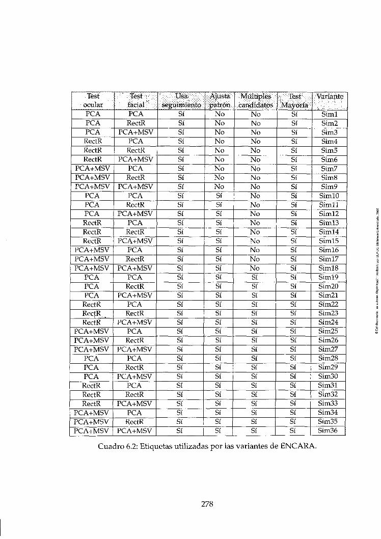
Test ocular PCA PCA PCA RectR RectR RectR

PCA+MSV PCA+MSV PCA+MSV

PCA PCA PCA

RectR RectR RectR


PCA PCA PCA

RectR RectR RectR


PCA PCA PCA RectR RectR RectR


Test facial PCA RectR

PCA+MSV PCA

RectR PCA+MSV

PCA RectR

PCA+MSV PCA

RectR PCA+MSV

PCA RectR

PCA+MSV PCA RectR

PCA+MSV PCA RectR

PCA+MSV PCA RectR

PCA+MSV PCA RectR

PCA+MSV PCA RectR

PCA+MSV PCA RectR

PCA+MSV PCA RectR

PCA+MSV

Usa seguimiento

Sí Sí Sí Sí Sí Sí Sí Sí Sí Sí Sí Sí Sí Sí Sí Sí Sí Sí Sí Sí Sí Sí Sí Sí Sí Sí Sí Sí Sí Sí Sí Sí Sí Sí Sí Sí

Ajusta patrón

No No No No No No No No No Sí Sí Sí Sí Sí Sí Sí Sí Sí Sí Sí Sí Sí Sí Sí Sí Sí Sí Sí Sí Sí Sí Sí Sí Sí Sí Sí

Múltiples candidatos

No No No No No No No No No No No No No No No No No No Sí Sí Sí Sí Sí Sí Sí Sí Sí Sí Sí Sí Sí Sí Sí Sí Sí Sí

Test Mayoría

Sí Sí Sí Sí Sí Sí Sí Sí Sí Sí Sí Sí Sí Sí Sí Sí Sí Sí Sí Sí Sí Sí Sí Sí Sí Sí Sí Sí Sí Sí Sí Sí Sí Sí Sí Sí

Variante

Siml Sim2 Sim3 Sim4 Sim5 Simó Sim7 Sim8 Sim9 Simio Simll Siml2 Siml3 Siml4 Siml 5 Simio Siml7 Siml8 Siml9 Sim20 Sim21 Sim22 Sim23 Sim24 Sim25 Sim26 Sim27 Sim28 Sim29 SimSO SimSl Sim32 Sim33 Sim34 Sim35 Sim36

Cuadro 6.2: Etiquetas utilizadas por las variantes de ENCARA.

278

la apariencia ocular (el conjunto de la apariencia ocular ha sido construido con un

pequeño grupo de muestras extraídas de secuencias S7, S9 y SIO). La secuencia S3

proporciona el ratio de caras detectadas similar con ambos algoritmos. El compor

tamiento estático en la secuencia S4 es visible en los resultados de éxito altos alcan

zados con la variante ENCARA en contraste con el pobre rendimiento de la técnica

de Rowley. Las secuencias S5 y Sil obtienen menores ratios de detección de cara

usando ENCARA, que podría ser explicado comentando que las caras contenidas

en estas secuencias son más pequeñas aún que el modelo usado para verificar su

apariencia. Los patrones positivos para el ojo y la cara de aprendizaje se han toma

do de muestras extraídas de S7, S9 y SIO, por esa razón estas secuencias presentan

elevados ratios utilizand ENCARA. Las secuencias S6 y S8 muestran los resultados

para secuencias en las que el sujeto realiza distintos gestos (sí, no, mirar a la derecha,

arriba, etc.), sin embargo los ratios no son excesivamente inferiores a los alcanzados

con la técnica de Rowley.

Según estas Figuras, ENCARA produce resultados tomando por ejemplo la

variante Sim30 para el peor caso, SIO, 16,5 veces y para el mejor caso, S4, 39,8 más

rápido que la técnica de Rowley. El cálculo del promedio excluyendo la mejor y la

peor concluye que ENCARA es 22 veces más rápido que la técnica de Rowley. Este

rendimiento está acompañado por un ratio de correcta localización del par ocular

según el criterio de Jesorsky mayor que 97,5 % (excepto con S5 que es 89,7 %). Este

ratio es siempre mejor que el proporcionado por la técnica de Rowley, este hecho

puede explicarse debido a esta técnica no proporciona detecciones de ojo para cada

cara detectada. Sin embargo, el ratio de detección de cara es peor para esta variante

de ENCARA excepto para S3, S4 y S7. En el peor caso ENCARA detecta sólo el

58 % de las caras detectadas usando la técnica de Rowley. Sin embargo, el promedio

excluyendo el mejor y el peor funcionamiento es del 83,4 %.

En la Figura 6.19 el error de detección de ojo para ambas técnicas se anali

za considerando no el criterio de Jesorsky, sino el exigente criterio 2. Como puede

observarse en estas Tablas, el ratio de errores de detección de ojo es pequeño con

ambas técnicas. Puede observarse que es mayor para ENCARA, pero se debe recor

dar que en la mayoría de los casos ENCARA proporciona más pares oculares para la

secuencia. También las distancias medias de los errores son mínimas. Los errores de

posición de ojo son más evidents para S5 y Sil , las secuencias que contienen caras

más pequeñas, para las que, el umbral para considerar un error de posición del ojo

es menor.

279

Comparativa Detección facial

S3 S4 S5 S6 S7 S8 S9 S10 S11

Comparativa Caras Detectadas Correctas

S1 S2 S3 S4 S5 S6 S7 S8 S3 S10 vS 11

« M SNCAHa [íkn.''Ji

Figura 6.18: Sumario de resultados para el ratio de detección facial comparando las variantes Sim29-Sim30 y Sim35-Sim36 de ENCARA con la técnica de Rowley.

Como resumen, las Tablas anteriores reflejan un rendimiento para ENCARA

que detecta un promedio de 84 % de las caras detectadas usando la técnica de Row

ley, pero 22 veces más rápido utilizando medios de adquisición y procesamiento

estándar. ENCARA proporciona también el valor adicional de detectar rasgos facia

les para cada cara detectada.

ENCARA proporciona un rectángulo que corresponde a una caja límite de la

cara detectada. Observando el sistema en vivo, ocurre en ocasiones que la cara cam

bia y ENCARA no es capaz de seguir todos los elementos faciales, ni de reencontrar

de nuevo la cara. En esta situación, si hubiera una detección reciente y al menos

un rasgo de cara no ha sido perdido, ENCARA proporciona un rectángulo de po

sición de cara probable. El empleo de coherencia temporal de este modo permite a

ENCARA seguir la cara aún cuando hubiera un cambio repentino, o simplemente

el parpadeo del usuario, etc. Para estas imágenes ENCARA no proporciona en la

versión actual una posición para los elementos faciales. La Figura 6.20 compara los

ratios de detección de cara si estos rectángulos son considerados como detecciones

de cara. Las etiquetas de variantes son modificadas añadiendo PosRect a cada va

riante de ENCARA analizada. Con el propósito de comparación, se proporcionan

280

Comparativa Ojos Detectados Correctos

S8 S9 S10 S11

Comparativa Ojos Detectados Correctos (Jesorsky)

^ ENCARA atnSt) Í¿;'J ENCARA S * T ^ — • • - - - - ¡ A S t m a e

Figura 6.19: Sumario de resultados para el ratio de detección ocular comparando las variantes Sim29-Sim30 y Sim35-Sim36 de ENCARA con la técnica de Rowley.

los ratios de detección de cara que con las variantes de ENCARA y la técnica de

Rowley.

Como se observa, los incrementos en el ratio de detección de cara son signifi

cativos llegando a hacerse similares o mejores a los proporcionados por el algoritmo

de Rowley. Este ratio mantiene un excelente ratio de detección de caras correctas

que para la variante SimSOPosRect es siempre superior al 93,5 %. Debe considerarse

que este ratio considera como detecciones correctas aquellas caras cuyos ojos y boca

están contenidos en el rectángulo proporcionado por ENCARA, luego un error no

significa necesariamente que se identifique como cara algo absolutamente diferente

a una cara.

Este incremento en el ratio de detección de cara puede resumirse indicando

que ENCARA realiza su procesamiento 22 veces más rápido que la técnica de Row

ley, detectando un promedio (para SimSOPosRect y excluyendo el mejor y el peor

caso) del 95,2 % de las caras detectadas por el algoritmo de Rowley.

281

Comparativa Detección Facial

c

0.8

i" o 0.4

^ i ENCARA Sim23PosRect • • ENCARA SifflSOPosRecl ^ ENCARA Sim35PosRect • « E N C A R A SmSePosRecí

31 32 33 34 35 S6 37 38

Comparativa Detección Facial Correcta

f l

Figura 6.20: Sumario de resultados comparando el ratio de detección facial de las variantes seleccionadas de ENCARA incorporando el rectángulo posible con la técnica de Rowley. .

6.4.3. Experimentos de Aplicación. Experiencias de Interacción en

nuestro laboratorio

Esta Sección presenta diferentes experiencias realizadas en nuestro laborato

rio relacionadas con las aplicaciones posibles a partir de los datos de detección de

cara. La intención de aplicar ENCARA en entornos diferentes tiene como objetivo

mostrar la ubicuidad del sistema. Las experiencias descritas en esta sección han si

do escogidas según la utilidad que las capacidades del sistema pueden ofrecer a una

IPU.

6.4.3.1. Experimentos de reconocimiento *•'* .*

Según las secciones anteriores, un detector de caras como ENCARA propor

ciona las vistas faciales normalizadas frontales. El proceso de normalización se rea

liza gracias a la detección de rasgos faciales que determinan con precisión la escala

de cara. La normalización de la imagen permite también eliminar de la imagen de

entrada el fondo y el pelo. Aspecto interesante dado que el rendimiento de técni

cas de reconocimiento de cara basadas en datos de imagen se reduce cuando este

282

proceso de normalización no se logra.

Se han realizado distintos experimentos de reconocimiento con el objeto de

comprobar la validez y utilidad de los datos proporcionados por ENCARA como

detector de cara. Siete sujetos diferentes aparecen en estas secuencias, que referire

mos como A-G. El conjunto de entrenamiento se elabora utilizando imágenes que se

extraen automáticamente por ENCARA de las siguientes secuencias: S2, S3, S4, S5,

S7, SIO y Si l . Entre aquellas imágenes normalizadas proporcionadas por ENCARA,

para cada sujeto se han seleccionado dos al azar entre las primeras diez detecciones.

La variante ENCARA utilizada ha sido Sim29, ver la Tabla 6.2 para la leyenda de

etiqueta de la variante.

Como se expone en la sección 6.2, las técnicas de reconocimiento requieren

un espacio de representación diferente al espacio imagen con el objeto de reducir

la dimensión. Para estos experimentos, se ha utilizado la representación PCA están

dar (Turk y Pentland, 1991). Una vez que la aproximación de representación ha sido

escogida, la decisión siguiente consiste en escoger el clasificador. Existen variadas

posibilidades para propósitos de clasificación una vez que la cara ha sido proyectada

a este espacio de representación de dimensión reducida. Para comenzar hemos se

leccionado el clasificador vecino cercano (CVC). En la Figura 6.21, se presentan los

resultados para las once secuencias. Aquellas secuencias utilizadas para construir

(con sólo dos imágenes) el conjunto de entrenamiento proporcionan claramente me

jores resultados. Debe notarse que las secuencias para el mismo sujeto no han sido

nunca adquiridas el mismo día. Por ello las condiciones de iluminación usadas son

diferentes para adquirir las secuencias para el mismo individuo, ver la Figura 6.17.

En estas condiciones PCA+CVC reduce su rendimiento como indica (BeUiumeur

et al., 1997).

Un uso que podría ser de interés y parece ser no común al no existir muchas

referencias (excepto para el género), podría integrar en un sistema lUP la capacidad

de proporcionar ima descripción de la persona que interactúa con el robot. Algunos

aproximaciones trat=>n la identidad y el género, pero no intentan caracterizar a un

individuo en términos de: rubio, con gafas, bigote, sin barba y 30 años. En un museo,

conocer la identidad en la mayor parte de casos no tiene ningún sentido, por contra

esta clase de interacción rápida puede tener usos interesantes. El descubrimiento de

estos parámetros a corto plazo ofrece habilidades de comunicaciones que ayudaa a

sentir la interacción con máquinas cómoda (mientras no se equivoque con la edad o

el género).

283

Con esta filosofía se ha aplicado con estos sujetos un experimento de clasifica

ción de género tomando de las mismas secuencias 9 muestras para cada género. En

la Figura 6.21, el gráfico de la derecha presenta los resultados. Es notorio el fracaso

para la secuencia Sil , usada además para extraer muestras de entrenamiento.

Reconocimiento de identidad con PCA+CVC Reconocimiento de Género con PCA+CVC

S2 S4 S6 S8 S10 Secuencias

S4 S6 S8 Secuencias

Figura 6.21: Resultados de clasificación identidad y género empleando PCA+CVC.

Estos resultados parecen prometedores dado que el clasificador utilizado es

muy simple y el conjunto de entrenamiento reducido. El uso de PCA presenta el

problema de sensibilidad a los cambios de las condiciones de iluminación. Las se

cuencias dan los peores resultados con caras más pequeñas e iluminadas artificial

mente, S5 y Sil . Pero por ejemplo también con S8 parece tener un distractor que

confunde muchos imágenes con otro sujeto. En resumen, el clasificador no es válido

para distintas condiciones, por ello esta aproximación simple podría utilizarse en

una sesión, tomando las muestras que se entrenan para el reconocimiento posterior

sin cambios de iluminación notables. Sin embargo, la validez de ENCARA como

proveedor de datos ha sido demostrada.

Antes de continuar, podemos brevemente adoptar otro punto de vista. El es

pacio de representación y los criterios de clasificación han sido seleccionados por

la simplicidad y la disponibilidad. PCA ha sido criticada debido a su ausencia de

semántica, siendo en desarrollos recientes utilizadas representaciones locales alter

nativas como puede ser ICA (Bartlett y Sejnowski, 1997) para conseguir un mejor

aproximación de representación. Sin embargo, el trabajo descrito en (Déniz et al.,

2001fl) demostró que utilizando dos espacios de representaciones diferentes, PCA o

ICA, y un criterio de clasificación poderoso como MSV en lugar de CVC, los ratios de

reconocimiento eran similares. Así, este trabajo concluyó que la selección de criterios

de clasificación es más crítica que la representación usada. Según esto, se ha reali

zado otra tanda de experimentos empleando MSV (mediante la biblioteca LIBMSV

(Chang y Lin, 2001)) como criterio de clasificación. Los resultados presentados en

284

la Figura 6.22, son en general mejores incluso para las secuencias no utilizadas para

extraer las muestras de entrenamiento.

Reconocimiento de Identidad con PCA+MSV

S4 S6 S8 Secuencias

Reconocimiento de Género con PCA+MSV 1

S4 S6 S8 Secuencias

Figura 6.22: Resultados recnocimiento idenidad y género empleando PCA+MSV.

El clasificador de género que emplea PCA+MSV clasifica correctamente para

más de 0,75 mientras el clasificador de identidad clasifica correctamenta para las

secuencias utilizadas para extraer muestras de entrenamiento por encima del 0,7 y

sólo por encima del 0,3 para el resto. En cualquier caso el mejor funcionamiento total

de esta aproximación es, en este experimento, utilizando PCA+MSV.

Una observación es que ENCARA trata una secuencia de vídeo. Por lo tanto,

no es lógico experimentar un cambio repentino en la identidad o el género. Para

confirmar la identificación de una persona, puede introducirse la coherencia tem

poral. Esta hecho evitará los cambios inmediatos de identidad (Howell y Buxton,

1996). Según (Déniz et al., 2001fo; Déniz et al., 2002) si un clasificador supera el 0,5

de ratio de éxito, la clasificación realizada para la imagen i puede ser relacionada

con la imagen anterior una vez que se define una dimensión de ventana temporal.

Según este trabajo, entre los criterios para la clasificación uno de los mejores es la

mayoría. Sólo el clasificador de género proporciona un ratio mayor de 0,5 para to

das las secuencias. Si procesamos las secuencias con la coherencia temporal para la

clasificación de género se obtienen los resultados mostrados en la Figura 6.23, que

son claramente mejores clasificando correctamente todas las secuencias por encima

del 0,93.

285

Comparativa Reconocimiento Oe Género

i 0 6

0.4

I 0.2

<^ O E ', A * c V C

^Ca<WSV ^CAt -ySVMemo 1

S6 S7 Secuencias

Figura 6.23: Comparativa resultados de reconocimiento de género.

6.4,3.2. Gestos: resultados preliminares

Uso de la cara como puntero

El dominio de gestos de la cabeza interpretables como comandos es pequeño.

En cambio, puede aprovecharse la cara como un indicador, enfoque que tiene gran

interés para e' desarrollo de interfaces para discapacitados.

Se han llevado a cabo algunas aplicaciones simples desarrolladas aprove

chando los datos faciales proporcionados por ENCARA. Para mejorar la continui

dad, la variante ENCARA usada es Sim29PosRect que considera también la informa

ción proporcionada por el rectángulo probable tras una detección reciente.

La primera utiliza una pizarra donde el usuario dibuja caracteres. Una pausa

en el proceso de dibujo se considera por parte del sistema como un indicador ue

carácter escrito. Cada carácter escrito se agrega al libro sólo si sus dimensiones son

lo bastante grandes. Un resultado de la muestra se presenta en la Figura 6.24. Co

mo se puede ver, la legibilidad de los caracteres es realmente pobre. El empleo de

la cara como un pincel en coordenadas absolutas ha resultado ser tedioso e incómo

do. Además el sistema requeriría posteriormente un módulo de reconocimiento de

caracteres para que la computadora pueda entender órdenes del usuario.

Otro enfoque más práctico considera el empleo de un teclado virtual que pre

senta los caracteres al usuario. Como demostración, se presenta una calculadora

simple que permite operaciones de un dígito, ver Figura 6.25. El control de este

teclado numérico se simplifica mediante el movimiento relativo que evita al usua

rio para hacer un movimiento absoluto seleccionar una tecla. En cambio, el usuario

puede manejar el indicador como si la cara fuera una palanca de mando, es decir,

con movimientos relativos en relación con una posición cero calibrada al inicio. El

empleo de movimiento relativo alivia considerablemente el empleo del indicador.

286

Figura 6.24: Ejemplo de uso como pincel.

Un último ejemplo hace uso del movimiento relativo indicado por la cara pa

ra mover el ratón del sistema. Dado que mover el ratón no tiene excesiva utilidad

si no puede realizarse una acción de selección, se emplea un esquema basado en

PCA y MSV para reconocer un reducido dominio de expresiones faciales de un in

dividuo, ver Figura 6.26. De esta forma el usuario al mantener la expresión sonrisa

realiza, sin tocar el ratón, la acción de selección.

Figura 6.25: Ejemplo de uso de ENCARA para interactuar con una calculadora.

287

Figura 6.26: Muestras ejemplos del conjunto de entrenamiento de expresiones de un individuo.

6.5. Conclusiones

El trabajo descrito en este documento puede ser resumido en las conclusiones

siguientes

a) El problema de la detección facial:

Una de las líneas de trabajo del grupo de investigación se relaciona con capa

cidades que un ordenador debe poseer para realizar la interacción natural con

la gente. Una de las fuentes principales de la información en la interacción hu

mana es la cara. Por lo tanto, un sistema automático que intenta de interactuar

naturalmente debe ser capaz de descubrir y analizar caras humanas.

Para realizar este trabajo considerando el estado actm\ ha sido necesario reali

zar una búsqueda amplia de la literatura en temas como HCI, lUP, la detección

de cara, el reconocimiento de cara y el reconocimiento de gestos faciales. Un

estudio serio de la literatura disponible ha sido desarrollado, tras la apertura

de una nueva línea de trabajo en el laboratorio.

b) Marco:

Se ha propuesto un marco para desarrollar un detector facial en tiempo real

facial que emplea hardware estándar. Se diseña una solución en cascada ba

sada en clasificadores débiles. La solución adoptada presenta las siguientes

características:

a) Principales características:

El sistema se basa en un esquema de verificación/rechazo de hipótesis

aplicado de una manera oportunista en cascada aprovechando la cohe

rencia espacial y temporal.

288

El sistema proporciona resultados prometedores en entornos de escritorio

proporcionando la detección de caras frontales y datos de localización de

los rasgos faciales.

El sistema ha sido diseñado para ser puesto al día y mejorado según ideas

y técnicas que podrían ser integradas.

b) Tiempo real:

El objetivo principal establecido en las exigencias del sistema, era el pro

cesamiento en tiempo real. Los experimentos finales presentan un ratio de

20-25 Hz. Para los tamaños usados en los experimentos que usan un Pili

IGhz, que representa 12 — 25 veces más rápido que la técnica de Rowley

para las mismas secuencias, detectando el 95 % de aquellas caras descu

biertas por la técnica de Rowley.

c) Liso del conocimiento:

El empleo de ambas fuentes de conocimiento permite a ENCARA apro

vechar sus ventajas: la reactividad proporcionada por el conocimiento ex

plícito y la robustez contra falsos positivos proporcionada por el conoci

miento implícito.

d) Coherencia temporal

La literatura de detección de cara no aprecia el empleo de información

de detección anterior para secuencias de vídeo. La mayor parte trabajos

intentan descubrir sobre cada imagen como si fuese la primera.

En este documento, su empleo ha resultado ser útil en dos sentidos: 1)

permite a un detector de cara que es débil mejorar su funcionamiento y

2) reduce el coste de tratamiento.

c) Evaluación experimental:

ENCARA cumple la restricción en tiempo real, sin embargo sus ratios de de

tección son ligeramente menores que las proporcionadas por la técnica de

Rowley, aunque en algunas situaciones sean competitivas.

Sin embargo, en el funcionamiento continuo para HCI, el aspecto principal

para la detección de cara no debería ser el ratio de detección para imágenes

individuales, sino un buen ratio para permitir a una aplicación HCI funcionar

correctamente. Esto ha sido demostrado empíricamente con las aplicaciones

ejemplo desarrollados para ENCARA.

289

La utilidad de los datos proporcionados por ENCARA, ha sido probada me

diante técnicas conocidas de reconocimiento de caras: PCA+NNC y PCA+MSV.

La integración resulta sencilla proporcionando resultados según su funciona

miento típico en tiempo real.

Esto permite ver a ENCARA como un sistema válido, ubicuo, versátil, flexible

y autónomo que fácilmente puede ser integrado por otros sistemas.

6.6. Trabajo Futuro

El desarrollo de un sistema detector de caras robusto en tiempo real es una

tarea difícil. Diversos aspectos diferentes pueden afrontarse para mejorar el funcio

namiento ENCARA. Algunos se presentan en esta sección.

a) Selección de cancidatos robusta:

El trabajo futuro necesariamente prestará atención a mejorar el funcionamien

to de la detección de color y su adaptabilidad. Los cambios de ambiente pue

den ser considerados bajo puntos de vista diferentes: tolerancia y adaptación.

El color es una señal principal para varios sistemas de visión prácticos debi

do a la cantidad y la calidad de la información proporcionada. Pero el color

presenta algunos puntos débiles en relación con cambios de ambiente. Una

opción interesante podría ser para realizar un estudio de aquellas soluciones

que son más robustas a cambios de ambiente. Este hecho permitiría usar el sis

tema no sólo para HCI, pero también mejoraría el ratio de éxito. También, será

muy interesante integrar otras entradas visuales en el candidato el proceso de

selección en cuanto al movimiento de ejemplo, la profundidad, la textura, el

contexto, etc. Esto probablemente aumentaría la fiabilidad.

b) Mejora de la clasificación:

Imcrementar la robustez por medio de : 1) Mejorar la eficiencia de los clasifica

dores individuales. 2) Introducir nuevos elementos de conocimiento implícito

y explícito para mejorar el rendimiento global.

c) Conjuntos de entrenamiento y clasificadores:

El conocimiento implícito se ha utilizado sin emplear conjuntos amplios de

entrenamiento. Usando sólo 3 secuencias diferentes para el entrenamiento, se

290

ha analizado el conjunto completo sin encontrar grandes problemas. Sin em

bargo, se observa que estos conjuntos de entrenamiento no cubren la completa

apariencia de los elementos modelados. Este hecho se muestra patente al em

plear las características rectangulares para modelar la apariencia de los ojos,

argumento que parece demostrar la necesidad de desarrollar un conjunto de

entrenamiento que contenga im dominio más grande de individuos. Además

el conjvinto puede aumentarse artificialmente transformando las muestras ya

contenidas como en (Sung y Poggio, 1998; Rowley et al., 1998). Tengamos en

cuenta que en (Rowley et al., 1998) se emplean 16000 muestras positivas por

6000 negativas.

También debe tenerse en cuenta que el aspecto de ojos y caras es variable. Por

ejemplo, en la secuencia S4 el ratio de detección con ENCARA es bastante alto,

sin embargo, cuando el sujeto parpadea se pierde en general el modelo. Real

mente el modelo de la apariencia de ojos no contiene ojos cerrados. Es evidente

que un ojo cerrado tiene un aspecto muy diferente a un ojo abierto. Sería muy

interesante aprovechar el modelo de aspecto diferente para los elementos fa

ciales. Por ejemplo en (Tian et al., 2000) dos modelos diferentes se emplean

para el ojo según si está abierto o no.

d) Detector no restringido

Actualmente ENCARA detecta sólo caras casi frontales. Para procesos de in

teracción es interesante detectar también la cara en múltiples vistas, así com.o

múltiples caras en una secuencia.

e) Incertidumhre:

Será interesante investigar en el empleo de factor de certeza en el proceso de

confirmación/rechazo de caras para usar un esquema de incertidumhre en la

clasificación en cascada y la coherencia temporal.

g) Aplicaciones

Se han presentado algunas aplicaciones simples de demostración, mostrando

la utilidad de los datos de detección de cara para controlar un puntero, recono

cer identidad y expresiones. El estudio y el análisis de interfaces para distintos

entornos que aprovechan los datos faciales representan un campo interesante

y válido.

291

Appendix A

GD Measure

The measure is based on Information Theory, before introducing the measure itself,

a review of some previous concepts of the Information Theory is included. The

different concepts will refer to the attributes and the class because they can be con-

sidered as random variables and so the concepts can be defined on them.

LetH{Xi) theentropyof attributeX, withvalúes {x],...,x^}, withdefinition:

if(X,) = - j ; F ( x f ) l o g P ( x f ) (A.1) ¿ = 1

where -P(xf) is the probability that valué x^ occurs. According to the expression, the

entropy measures the average of uncertainty of the attribute and it is non negative

(Cover and Thomas, 1991). In the same way that the entropy of an attribute was

defined, the entropy of the class Y can be define.

When one attribute is known, the amount of uncertainty of the class is de-

creased. A measure that reveáis the Information given by an attribute Xi o ver a

class Y is the mutual rnformation, / ( X J ; Y). The expression of the mutual Informa

tion is:

k j

In Equation A.2, H{Y/Xi) represents the entropy of Y when Xi is known.

293

This entropy is called conditional entropy and it is non negative and less or equal

to H(Y) (Cover and Thomas, 1991), so the mutual information is greater or equal to

zero and comtnutative.

From the joint entropy of an attribute and the class H{Xi, Y) and from the

mutual information I{XÍ; Y), the entropy distance (MacKay, 1997) is defined as:

d{XuY) = H{X„Y) - I{XúY) (A.3)

The entropy distance measures the information that the attribute ví¿ gives

about a class. Because, the more information the attribute gives, the greater the

mutual information is and therefore the smaller the distance is.

A.l Mantaras Distance

A measure that is conceptually very cióse to the GD measure is the Mantaras dis

tance proposed by López de Mantaras (López de Mantaras, 1991).

The Mantaras distance is a distance measure between two partitions to select

the attributes associated with the nodes of a decisión tree. In each node, it is chosen

the attribute that produces the partition closest to the correct partition of the samples

subset tn the examples.

The Mantaras distance has the foUowrng expression:

dLMiPA, PB) = H{PA/PB) + H{PB/PA) (A.4)

Where H{PA/PB) arid H{PB/PA) correspond to the entropy in each partition

when the another is known. It is possible to demónstrate the following properties

(López de Mantaras, 1991):

1. dLuiPA, PB) > O and equal iff PA = PB

2. diMiPAiPs) = diM{PB,PA)

3. dLM{PA, PB) + dLM{PB, Pe) > ¿LMÍÍ^A, PC)

294

If the references to partitions are changed by attributes and class in the defi-

nition of the Mantaras distance, the foUowing expression for the Mantaras distance

is achieved:

dLM{Xi, Y) = H{X,/Y) + H{Y/X,) (A.5)

and using Equation A.2 and the relation

H{Y/Xi) = HiY,Xi)-H{Xi) (A.6)

Equation A.5 can be transformed in

CILMÍXÍ, Y) = HiXi, Y) - I{Xú Y) = diXi,Y) (A.7)

which corresponds to the expression of the entropy distance and shows that the

entropy distance is a metric distance function.

A.2 GD Measure Defínition

The use of the Gain Ratio and the Mantaras distance (López de Mantaras, 1991) as

feature selection measure has the drawback of operating over isolated attributes.

Therefore, these methods do not detect the possible dependencies that there could

be between attributes. A manner to gather the interdependencies between attributes

is to compute the mutual information for each pair of attributes I{XÍ; XJ). These in

terdependencies of attributes can be represented with the aid of the Transinformation

Matrix T, a square matrix of dimensión n (number of attributes) where each element

tij oí the matrix is the mutual information between attributes i-th and j-th.

295

Some properties hold for this matrix whose demonstrations can be found iii (Lorenzo,

2001).

1- ti,i > ti,j> i,j = l..-n and i ^ j

2. tij > O, z, j = 1.. .n

Proposition A.l, Given an attribute set {Xi,X2,.. . ,Xn} and its associated transinfor-

mation matrix T, iffor any row i it is established that

-^ 3 • î,i — 'î,j

Then the attribute Xj is redundant with résped to Xi and it can he removed from the

set witiiout any information lost.

Proof. >From the definition of the transinformation matrix and the expression A.2

of the mutual information:

Uj, = I(Xi,Xi) = H{Xi) - HiXi/X,) = H{Xi

Uj = I{X,,Xj) = H{Xi) - H{X/X,)

oO, 11 Viî — tij

I{Xi- Xi) = I{Xf, Xj) ^ H{Xi) = H{X,) - H{Xi/Xj) => H{Xi/Xj) = O (A.8)

H{Xi/Xj) = O means that the knowledge of Xj decreases to zero the uncertainty of

Xi, and therefore attribute Xj holds the whole information over Xi and one of them

can be removed without any information lost. D

Once the transinformation matrix has been defined, it is necessary to find an

expression for the GD measure that includes the transinformation matrix and the

distance A.3. This expression must be defrned in such a way that subsets of at-

tributes with high dependencies between attributes yield lower valúes than other

296

ones without these high dependencies. A solution comes from the analogy to sig-

nificance level between the transinformation matrix and the covariance matrix (E)

of two random variables. This analogy can be established because both matrices

measure interrelation between variables. In the Mahalanobis distance (Duda, 1973),

the covariance matrix is utilized to correct the effects of cross covariances between

two components of a random variable. The expression of the Mahalanobis distance

(Duda, 1973) between two samples (X,Y) of a random variable is:

dMahalanobisiX, Y) = {X - YY^-^X - Y) ( A . 9 )

where dMahaianobis{X,Y) corresponds to the Euclidean distance if S is the identity

matrix.

Therefore the GD measure can be defined in a similar way to the Mahalanobis

distance, using the transinformation matrix instead of the covariance matrix and the

distance A.3 instead of the Euclidean distance. The GD measure dcoiX, Y) between

the set of attributes X and the class Y is expressed as:

daniX, Y) = D{X, YfT-'DiX, Y) (A.IO)

where D{X, Y) = [dLM{Xi,Y),..., diM^Xn, Y)Y is a vector whose i-th ele-

ment is the Mantaras distance (equivalent to the entropy distance) between the at-

tribute X, and the class, and T is the transinformation matrix of the set of attributes

X.

>From the Equation A.3 it can be observed that the elements of the D(X,Y)

vector are smaller as the inf ormation that the attribute gives about the class is greater.

Given a set of attributes and the associated transinformation matrix, the GD

measure fulfiUs the foUowrng properties:

1. dGD{X, Y) > O, VX, Y and daoiX, X) = O

2. dGD{X, Y) = doDiY, X), VX, Y

The demonstration of the two previous properties is trivial if the properties of the

Mantaras distance and the properties of the transinformation matrix are taken into

account. The triangle inequality property has not been demonstrated for the GD

297

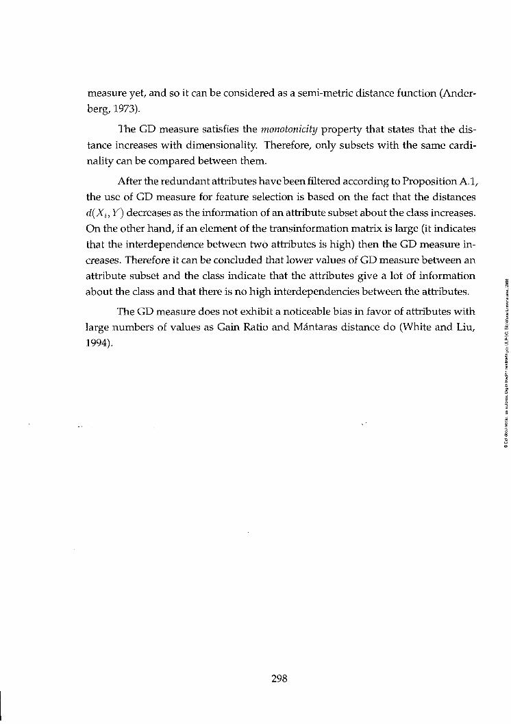
measure yet, and so it can be considered as a semi-metric distance function (Ander-

berg, 1973).

The GD measure satisfies the monotonicity property that states that the dis

tance increases with dimensionality. Therefore, only subsets with the same cardi-

nality can be compared between them.

After the redundant attributes have been filtered according to Proposition A.l,

the use of GD measure for feature selection is based on the fact that the distances

d{Xi,Y) decreases as the information of an attribute subset about the class increases.

On the other hand, if an element of the transinformation matrix is large (it indicates

that the interdependence between two attributes is high) then the GD measure in

creases. Therefore it can be concluded that lower valúes of GD measure between an

attribute subset and the class indicate that the attributes give a lot of information

about the class and that there is no high interdependencies between the attributes.

The GD measure does not exhibit a noticeable bias in favor of attributes with

large numbers of valúes as Gain Ratio and Mantaras distance do (White and Liu,

1994).

298

Appendix B

Boosting

The classifier, see Equation 4.18 based on rectangle features, can be considered a

weak classifier, see (Schapire and Singer, 1999; Friedman et al, 1998), which is valid

for being adapted for boosting leaming. Boosting has been used in the literature to

design a weighted majority vote (Viola and Jones, 2001??) instead oí a simple voting

mechanism. Large weights are assigned to good classification functions and smaller

weights to poor functions. This approach can be integrated in the system both in

order to select features but also to select training samples if the set is very large.

AdaBoost, see Algorithm 2, is an aggressive mechanism for selecting a small

set of good classification functions (or good features) which nevertheless have sig-

nificant variety. Eacn feature defines a weak leamer, that can have the form as Equa

tion 4.18, defining an optimal threshold. In practice no single feature can perform

the classification task with low error. Different authors have used this focus re-

cently in face detection context. AdaBoost is used in (Viola and Jones, 2001b) to se

lect among a huge set of rectangle features those that better fit in a cascade schema

that produces high detection rates for frontal faces at different scales and locations

at 15fps. AdaBoost performs a sequential search that assumes monotonicity, this

means that adding a new classifier does not decrease system performance. If that

circumstance is violated the process is broken. For that reason in (Li et al, 20Ü2&),

the authors introduce FloatBoost a searching mechanism that allows backtracking

steps when monotonicity is not verified. They applied this approach to develop a

real time (5fps) algorithm that performs realtime multiview face detection. More re-

cently in (Viola and Jones, 2002), modify their AdaBoost search, presented in (Viola

and Jones, 2001b), to avoid focusing on reducing the classification error but the false

negative percentage in order to reduce the number of faces not detected.

299

AU these algorithms sort the features/classifiers according to their errors in

an iterative fashion. This selection allows to design a strong classifier based on those

best weak classifiers selected. In order to select a small number.

Algorithm 2 Adaboost algorithm

Given a set of positive an negative samples {xi,yi),{x2,y2), •••,{xN,yN), and a number of classifiers M. f or For each sample positive sample do

end for for each sample negative sample do

end for for each classifier j = 1, ...M do

Compute hm according to

hm{x) = - log -f- / , ^_, B.l

Compute new weights for each sample

w^ = íüf-ie-(^''''"(^'^) (B.2)

end for

300

Appendix C

Color Spaces

C.l HSV

Transforming RGB to get HSV extracted from (Jordao et al., 1999)

H = arceos • ^

g ^ l _ omm{R,G,B) (Ql) R-\-G-\-B

^/{R-G)^+{R-B){G-B) I _ omm{R,G,B) *• " R+G+B

V = 0.299Í? + 0.587G + 0.114fí

Another transformation is given in (Herodotou et al, 1999)

rr H{R-G) + {R-B))

Hi = arceos ^j— == =—= ^(R-G)'i+{R-B){G-B)

H = Hi if B <G, H = 360-Hi if B> G, (C-2) C _ ma.x{R,G,B)-mm{R,G,B) ^ ~ ma.x{R,G,B)

Y _ max(_R,G,B) ^ ~ 255

An altérnate, labelled as Fleck HS is described in (Zarit, 1999). First RGB are

transformed to log-opponent:

301

L{x) = 105 log(a; + 1 + n)

/ = L{G)

Rg = L{R))) - L{G) B^ = L{B) - Moy^

(C.3)

n is a randoin number in the range [0,1). Fmally hue and saturation are com-

puted:

H = arctan(i?g, By) (C.4)

C.2 CÍE L*a*6*

Ilie transformation, as exposed in (Zarit, 1999), converts first RGB valúes in the

range [0,1] are gamma corrected:

if R,B,G> 0.18

^709 - in:Ó99~J

<^709 - ( ,n :o9Fj

^709 - 1^:099-;

if R,B,G <0.1S

ho9 ^709 - 0:45

^709 - 045

-B709 — B

0.45

(C.5)

The gamma-corrected RGB is converted to XYZ (D65):

/ 0.412453 0.357580 0.189423

0.212671 0.715169 0.072169

\ 0.019334 0.119193 0.950227

(C.6)

302

And finally to CIEL*a*b*

L* = 116 {\y - 16, si (^) > 0.008856

L* = 903.3 {\) , si {\) < 0.008856

«* = 500[/(^)-/(^)] 6* = 200[/(^)-/(^)]

f[t) = t,t> 0.008856

f{t) = 7.787Í + Y^, t < 0.008856

Different formulae are extracted from different sources. In (Jack, 1996) it is used:

Y = (0.257Í?) + (0.504G) + (0.098S) + 16

Cr = (0.439Í?) - (0.368G) - (0.071fí) + 128 (C.8)

Cb = -(0.148Í?) - (0.291G) + (0.4395) + 128

On the other hand, in (Zarit, 1999) it is presented CCIR 601-2 YCrCb as follows

Y = (0.299Í?) + (0.587G') + (0.1145)

Cr = R-Y (C.9)

Cb = B-Y

C.4 TSL

TSL color space is defined in that work as

303

arctan(r7fií')/27r + 1/4, g' > O

T = -j arctan(rV^')/27r + 3/4, p' < O

O, ^' = O

L = 0.299Í2 + 0.587G + 0.114B

(CIO)

where r' = f — 1/3 and g' = g — 1/3.

C.5 YUV source

If the system works with YUV images a previous conversión to RGB is needed,

extracted from Qack, 1996)

R = 1.164(y - 16) + 1.596(1^ - 128)

G = 1.164(y - 16) - 0.813(y - 128) - 0.391(C/ - 128)

B = 1.164(y - 16) + 2.018(F - 128)

(C.ll)

304

Appendix D

Experimental Evaluation Detailed

Results

This appendix presents detailed the results summarized in Chapter 4.

D.l Rowley's Technique Results

The results achieved using Rowley's technique are presented in Tables D.l and D.2.

In Table D.l, the first column reflects the sequence label. The second presents the

rate of detected faces by the system. The third provides the rate of correct detected

faces, and the last column indicates the average image processing time.

Table D.2 presents eye detection results. The first two columns are similar

to Table D.l. The third indicates the rate of eyes located according to the number

of faces detected, as the system can retum the location of only ene eye, this column

indicates: rate of eye pairs located/rate of left eyes located/rate of right eyes located.

The fourth presents the average error for eye detection. The fifth, sixth, and seventh

indícate the rate of errors detected for eye location, according to Criterium 2, and the

average eye location error if the error appear for both, left or right eye respectively.

For example, in the first sequence the system detected a rate of 0.817 which

corresponds to 368 from 450 frames. However, the system retumed an eye pair

location for only 0.309 rate of faces detected (114 of those 368 detections). From

these eye pair location a rate of 0.938 were correct according to Criterium 2 and 1.0

according to the criterium used in (Jesorsky et al, 2001). The low rate for eye pairs

detection is due to that the system retumed a position for both eyes only for 114

305

Seq

SI S2 S3 S4 S5 S6 S7 S8 S9 SIO Si l

Faces deíécted

0.817 0.724 0.917 0.426 0.744 0.913 0.802 0.96 0.997 0.948 0.844

F^ces córíectiy detected

1.0 1.0

0.968 0.974 0.988 0.99 1.0

0.99 1.0 1.0 1.0

Áverageprac,,^ time 727 929 929 837 734 900 769 707 649 610 695

Table D.l: Results of face detection using Rowley's face detector (Rowley et al, 1998).

Seq

bl S2 S3 S4 S5 S6 S7 S8 S9 SIO SU

" Faces detected

0.817 0.724 0.917 0.426 0.744 0.913 0.802 0.96 0.997 0.948 0.844

"• •* Eyesíptatéd

•0.309/U.6/II.445 0.625/0.812/0.788 0.917/0.973/0.927 9.979/0.989/0.989 0.685/0.85/0.761

0.944/0.951/0.987 0.822/0.842/0.952 0.583/0.738/0.659 0.91/0.937/0.928

0.796/0.854/0.887 0.91/0.973/0.918

Ey^paixS f conecíly located •

0.77 (0.82) 0.938 (1.0) 0.97 (0.985) 0,984 (1.0)

0.965 (0.991) 0.984 (0.994) 0.983 (0.993) 0.96 (0.996) 0.953 (0.982) 0.964 (0.985) 0.965 (0.994)

iáveragé'eye ' .: . Ibcation error

L(l,l) R(i,l) L(l,l) R(1,0) L(0,0) R(1,0) L(1,0) R(0,0) L(0,0) R(0,1) L(1,0) R(0,0) L(1,0) R(1,0) L(1,0) R(2,0) L(1,0) R(l,l) L(l,l) R(l,l) L(1,0) R(0,0)

Botheyésv."" * ••• é r r ó r S • • •'•

u 0 0 0 0 0 0 0

0.005 L(8,0),R(1,12) 0 0

téf teye ' : errürs •'?

U.022 (4,2) 0.026 (4,6) 0.001 (5,1)

0 0.017 (2,5) 0.01 (4,6)

• • - /

0.072 (4,5) 0.04 (3,8) 0.027 (4,6) 0.011 (3,5)

:--Ríght'eyé^ ••errors fc. 0.103 (3,5) 0.07 (3,5)

0 0.015 (6,1) 0.047 (3,3) 0005 (6,2) 011 (8,0) 0.024 (6,4) 0.002 (3,11) 0.018 (7,5) 0.04 (3,4)

Table D.2- Comparison of results of face and eye detection using Rowley's face detector (Rowley et al, 1998) and manually marked.

frames. The sixth column refers to the average error for eyes detected. The other

columns reflect the average error, for example the last column indicates the average

error if it was produced only for the right eye: 0.103 is the rate of errors detected

using the Criterium 2, for 0.445 * 450 = 164 right eyes located, and (3,5) i» the

average error distance for those eye detection errors.

D.2 Basic Solution Results

This section describes the results for ENCARA basic solution. In Table D.3, each

row contained reflects the face detection results of processing a video stream. The

first column identifies the sequence while the second describes the ENCARA vari-

ant used. The third column presents the rate of frontal detected faces by the system,

it correspond to facesjdetected/frames_numher. The fourth reflects the ratio of de

tected faces that were correctly detected according to Criterium 1, it corresponds

to faces_correctly_detected/faces_detected. The fifth presents the rate of eye pairs

correctly located according to ground data using Criterium 2 that corresponds to

pairs_correctly_detected/facesjdetected (in brackets according to the criterium used

306

Séq,

SI SI SI SI S2 S2 S2 S2 S3 S3 S3 S3 S4 S4 S4 S4 55 S5 S5 S5 S6 S6 S6 S6 S7 S7 S7 S7 S8 S8 S8 S8 S9 S9 S9 S9 SIO SIO SIO SIO

sn Sil s i l Sil

Váriañt

Basl Bas2 Bas3 Bas4 Basl Bas2 Basa Bas4 Basl Bas2 Bas3 Bas4 Basl Bas2 Bas3 Bas4 Basl Bas2 Bas3 Bas4 Basl Bas2 Bas3 Bas4 Basl Bas2 Bas3 Bas4 Basl Bas2 Bas3 Bas4 Basl Bas2 Bas3 Bas4 Basl Bas2 Bas3 Bas4 Basl Bas2 Bas3 Bas4

Faces detected

0.202 0.331 0.309 0.126 0.260 0.193 0.160 0.111 0.460 0.506 0.517 0.469 0.571 0.551 0.744 0.731 0.213 0.233 0.211 0.191 0.151 0.166 0.117 0.091 0.351 0.557 0.553 0.337 0.273 0.340 0.420 0.249 0.424 0.540 0.557 0.384 0.460 0.482 0.593 0.524 0.369 0.391 0.213 0.191

Faces crntétüy detectéd

0.956 0.959 0.964 0.947 0.820 0.551 0.430 0.120 0.990 0.991

1.0 1.0

0.929 0.947

1.0 1.0 1.0 1.0 1.0 1.0

0.441 0.440 0.566 0.609 0.981

1.0 1.0

0.980 0.935 0.928 0.942 0.875 0.926 0.971 0.980 0.994 0.961 0.958 0.977 0.991 0.987 0.982 0.885 0.883

EyéSCOrreGliy located

0.373 (0.692) 0.402 (0.745) 0.489 (0.691) 0.350 (0.474) 0.581 (0.675) 0.367 (0.448) 0.236 (0.278) 0.080 (0.120) 0.806 (0.942) 0.758 (0.925) 0.789 (0.983) 0.824 (0.981) 0.007 (0.171)

0 (0.169) 0.973 (1.0) 0.975 (1.0)

0.364 (0.833) 0.390 (0.819) 0.494 (0.926) 0.465 (0.942) 0.132 (0.25) 0.173 (0.32) 0.566 (0.566) 0.609 (0.61) 0.911 (0.943) 0.936 (0.96) 0.939 (0.96) 0.914 (0.941) 0.325 (0.585) 0.366 (0.595) 0.804 (0.825) 0.776 (0.786) 0.916 (0.916) 0.962 (0.936) 0.956 (0.972) 0.988 (0.988) 0.512 (0.58) 0.525 (0.604) 0.883 (0.933) 0.898 (0.945) 0.493 (0.88) 0.505 (0.881) 0.489 (0.781) 0.488 (0.802)

Avéíage time

54 50 48 49 54 53 54 54 48 47 46 46 48 48 44 44 39 37 37 37 51 51 52 52 50 50 52 50 41 44 42 40 68 60 57 60 61 61 58 58 46 40 42 42

Table D.3: Results obtained with basic solution and variants.

in (Jesorsky et al, 2001)). The sixth provides the average processing time per im-

age, it must be noticed that all the images are processed similarly, it corresponds to

totaljtime/ frames_number.

Table D.4 correspond to eye location errors. The first three columns coin

cide with Table D.3. The fourth shows the average eye location error, computed

as euclidean distance, for all the faces detected by the system, it corresponds to

correct_eye_detections/faces_detected. The foUowing columns present the rate of

trames with error locating eyes according to Criterium 2, and the average error if the

error was for both eyes, left or right respectively, therefore, the valué corresponds to

error _distance / faces_detected.

307

Seq.

SI SI SI SI S2 S2 S2 S2 S3 S3 S3 S3 S4 S4 S4 S4 S5 S5 S5 S5 S6 S6 S6 S6 S7 S7 S7 S7 S8 S8 S8 S8 S9 S9 S9 S9 SIO SIO SIO SIO SU Si l Si l Si l

Varianí

Basl Bas2 Bas3 Bas4 Basl Bas2 Bas3 Bas4 Basl Bas2 Bas3 Bas4 Basl Bas2 Bas3 Bas4 Basl Bas2 Bas3 Bas4 Basl Bas2 Bas3 Bas4 Basl Bas2 Bas3 Bas4 Basl Bas2 Bas3 Bas4 Basl Bas2 Bas3 Bas4 Basl Bas2 Bas3 Bas4 Basl Bas2 Bas3 Bas4

Faces detected

0.20 0.33 0.3C8 0.126 0.26 0.193 0.16 0.111 0.46

0.506 0.517 C.46S 0.571 0.551 0.744 0.731 0.213 0.233 0.211 0.191 0.151 0.166 0.117 0.091 0.351 0.557 0.553 0.337 0.273 0.340 0.420 0.248 0.424 0.540 0.557 0.384 0.460 0.482 0.593 0.524 0.368 0.391 0.213 0.191

EyelOGaliOfl erttírs

L(5,3) R(5,2) L(4,3) R(4,2) L(4,l) R(6,l) L(7,l) R(8,l)

L(24,16) R(23,18) L(60,42) R(53,46) L(79,55) R(71,61)

L(124,84) R(110,93) L(2,l) R(3,l) L(2,l) R(3,l) L(2,l) R(3,l) L(2,l) R(3,l)

L(6,14)R(2,11) L(7,15) R(3,12) L(2,0) R(l,l) L(2,0) R(l,l) L(2,l) R(3,l) L(2,2) R(3,l) L(2,l) R(2,l) L(2,l) R(3,l)

L(72,39) R(59,44) L(70,37) R(59,43) L(67,34) R(58,38) L(53,28) R(46,31)

L(3,l) R(2,l) L(2,l) R(2,l) L(2,l) R(2,l) L(3,l) R(2,l) L(2,2) R(4,5) L(2,2) R(5,5) L(3,l) R(4,l) L(2,1)R(4,1)

L(13,1)R(11,1) L(5,l) R(5,l) L(4,1)R(3,1) L(3,0) R(2,l) L(3,8) R(3,6) L(3,7) R(4,5) L(3,2) R(2,l) L(3,2) R(2,l) L(2,l) R(3,l) L(2,l) R(3,l) L(3,5) R(4,6) L(3,6) R(4,6)

Botíieyes errofs

0.39 L(9,4),R(10,3) 0.322 L(7,4),R(9,3)

0.345 L(10,1),R(12,1) 0.491 L(11,1),R(14Í)

0.324 L(71,50),R(68p4) 0.54 L(109,77),R(97,B5) 0.708 L(111,78),R(99,86) 0.88 L(140,96),R(125,106)

0.038 L(5,16),R(4,12) 0.057 L(6,14),R(5,11) 0.0O8 L(8,1),R(7,2) 0.009 L(8,1),R(7,2)

0.992 L(6,14),R(2,11) 0.995 L(7,15),R(3,12) 0.005 L(6,1),R(8,4) 0.006 L(6,1),R(8,4) 0.427 L(4,2),R(5,2) 0.409 L(4,2),R(5,2) 0.337 L(5,1),R(5,1) 0.349 L{5,0),R(5,1)

0.75 L(95,52),R(78,57) 0.626 L(111,59),R(93,66) 0.433 L(153,77),R(132,87) 0.390 L(134,71),R(117,78)

0.044 L(18,2),R(16,1) 0.023 L(15,1),R(15,1) 0.024 L(15,1),R(1S,1) 0.046 L(18,2),R(16,1)

0.276 L(4,7),R(8,7) 0.274 L(5,6),R(9,6)

0.100 L(11,2),R(18Í) 0.071 L(10,2),R(163)

0.073 L(151,5),R(125,11) 0.028 L(116,12),R(96,15) 0.019 L(96,17),R(81,19)

0.005 L(1S03),R(124,12) 0.338 L(4,17),R(4,14) 0.317 L(S,16),R(9,12) 0.041 L(29,15),R(9Í) 0.046 L(29,15),R(9^) 0.222 L(5,2),R(5,4) 0.25 L(4,3),R(5,4)

0.322 L(5,15),R(7,16) 0.313 L(6,17),R(7,18)

Leít eye errors

0.03 (6,2) 0.05 (6,1) 0.086 (6,1) 0.052 (3,2) 0.094 (5,0) 0.069 (5,0) 0.041 (5,0) 0.04 (7,1) 0.12S (8,1) 0.131 (7,1) 0.120 (7,1) 0.113 (8,1)

0 (0,0) 0 (0,0)

0.009 (7,1) 0.006 (7,2) 0.062(4,1) 0.057(4,1) 0.042 (5,1) 0.069 (5,1) 0.117(4,6) 0.173 (5,6)

0 (0,0) 0 (0,0) 0 (0,0)

0.007(19,1) 0.008 (19,1)

0 (0,0) 0.382 (4,8) 0.359 (4,8)

0.058 (10,3) 0.116 (12,2)

0 (0,0) 0 (0,0)

0.008 (8,0) 0 (0,0) 0 (0,0) 0 (0,0)

0.026 (16,0) 0.008 (15,1) 0.168 (6,1) 0.142 (5,1) 0.104 (5,1) 0.104 (5,1)

Righteyé enürs y;

0.197 (4,5) 0.228 (2,6) 0.079 (4,2) 0.105 (6,2)

(0,0) 0.022 (10,9) 0.014 (10,2)

0 (0,0) 0.029 (7,0) 0.052 (8,3) 0.081 (7,1) 0.052 (7,1)

0 (0,0) 0.004(0,11) 0.012 (8,0) 0.012 (9,0) 0.145 (3,4) 0.143 (3,4) 0.126 (3,3) 0.116 (3,3)

0 (0,0) 0.026 (2,9)

0 (0,0) 0 (0,0)

0.044 (11,1) 0.032(11,1) 0.028 (12,1) 0.039 (12,1) 0.016 (16,1)

0 (0,0) 0.037 (13,0) 0.035 (11,0) 0.010 (17,5) 0.008 (17,5) 0.015 (13,2) 0.005 (20,4) 0.149 (3,9) 0.156 (4,9) 0.048 (7,2) 0.046 (8,2) 0.114 (5,1) 0.102 (5,1) 0.083 (4,1) 0.093 (4,1)

Table D.4: Eyes location error summary for basic solution and variations, if too cióse eyes test and integral projection test are used.

308

- ^ SI SI SI SI SI SI SI SI SI SI SI SI SI SI SI S2 S2 S2 S2 S2 S2 S2 S2 S2 S2 S2 S2 S2 S2 S2 S3 S3 S3 S3 S3 S3 S3 S3 S3 S3 S3 S3 S3 S3 S3 S4 54 S4 S4 S4 S4 S4 S4 S4 S4 S4 S4 S4 S4 S4

label Appl App2 App3 App4 App5 App6 App7 App8 App9 ApplO Appll Apgl2 Appl3 Appl4 Appl5 Appl App2 App3 App4 App5 App6 App7 App8 App9 ApplO Appll Appl2 Appl3 Appl4 Appl5 Appl App2 App3 App4 App5 App6 App7 App8 App9 ApplO Appl l Appl2 Appl3 Appl4 Appl 5 Appl App2 App3 App4 App5 App6 App7 App8 App9 ApplO Appl l Appl2 Appl3 Appl4 ApplS

Faces delectéd-"

0.244 0.206 0.173 0.224 0.062 0.260 0.186 0.202 0.169 0.057 0.042 0.042 0.226 0.188 0.160 0.337 0.237 0.271 0.326

-0.169 0.320 0.237 0.271

---

0.308 0.217 0.256 0.520 0.400 0.520 0.520 0.071 0.526 0.522 0.402 0.524 0.071 0.066 0.071 0.526 0.402 0.526 0.744 0.724 0.740 0.744

-0.744 0.744 0.724 0.742

---

0.7444 0.724 0.740

;,.Faces «nscüy • , ' áeteeíeíí

0.981 1.0

0.987 0.960

1.0 0.974 0.976

1.0 0.986

1.0 1.0 1.0

0.980 1.0

0.986 1.0

0.990 1.0

0.952

-0.69 1.0

0.99O 1.0

. ---

1.0 . 1.0

1.0 1.0 1.0 1.0 1.0 1.0 1.0 1.0 1.0 1.0 1.0 1.0 1.0 1.0 1.0 1.0 1.0 1.0 1.0 1.0

-1.0 1.0 1.0 1.0

---

1.0 1.0 1,0

SyescoHectly located "'•

0.554 (0.745) 0.741 (0.978) 0.756 (0.974) 0.653 (0.901) 0.571 (0.786) 0.547 (0.726) 0.714 (0.964) 0.736 (0.978) 0.750 (0.974) 0.615 (0.769) 0.842 (1.0) 0.842 (1.0)

0.598 (0.76S) 0.811 (1.0)

0.819 (0.986) . 0.710 (0.882)

0.934 (0.991) 0.852 (1.0)

0.700 (0.884)

. 0.460 (0.553) 0.75Q (0.917) 0.934 (0.991) 0.852 (1.0)

-.--

0.733 (0.892) 0.959 (1.0) 0.869 (1.0)

0.790 (0.983) 0.861 (0.978) 0.790 (0.983) 0.786 (0.983) 0.812 (0.969) 0.789 (0.983) 0.791 (0.983) 0.856 (0.978) 0.788 (0.983) 0.812 (0.969) 0.800 (0.967) 0.812 (0.969) 0.789 (0.983) 0.856 (0.978) 0.789 (0.983) 0.973 (1.0) 0.990 (1.0) 0.978 (1.0) 0.973 (1.0)

-0.973 (1.0) 0.973 (1.0) 0.990 (1.0) 0.979 (1.0)

---

0.973 (1.0) 0.990(1.0) 0.978 (1.0)

Average-' • • • • • t i m e

50 51 53 50 51 50 51 56 53 52 52 54 49 52 53 52 53 54 50 56 54 48 54 54 56 56 57 51 55 54 47 46 51 47 47 49 85 53 53 46 47 60 49 48 89 44 44 47 44 47 46 48 45 48 47 47 47 46 48 56

Table D.5: Results obtained integrating appearance tests for sequences S1-S4. Time measures in msecs. are obtained using standard C/C++ command dock.

309

:' Seq.

S5 S5 S5 S5 S5 S5 S5 S5 SS S5 S5 S5 S5 S5 S5 S6 S6 S6 S6 S6 S6 S6 S6 S6 S6 S6 S6 S6 S6 S6 S7 S7 S7 S7 S7 S7 S7 S7 S7 S7 S7 S7 S7 S7 S7 S8 S8 S8 S8 S8 S8 S8 S8 S8 S8 S8 S8 S8 S8 S8

• Vaiimt: •' label Appl App2 App3 App4 App5 App6 App7 App8 App9 ApplO Appl l Appl2 Appl3 Appl4 ApplS Appl AppZ App3 App4 AppS App6 App7 AppS App9 ApplO Appll Appl2 Appl3 Appl4 ApplS Appl App2 App3 App4 AppS App6 App7 AppS App9 ApplO Appl l Appl2 Appl3 Appl4 ApplS Appl App2 App3 App4 AppS App6 App7 AppS App9

ApplO Appll Appl2 Appl3 Appl4 ApplS

FacKS deléctfid

0.142 0.140 0.116 0.111 0.022 0.206 0.100 0.076 0.086 0.017 0.022 0.022 0.133 0.142 0.106 0.213 0.197 0.211 0.149 0.164 0.137 0.204 0.197 0.202 0.164 0.153 0.164 0.213 0.197 0.211 0.S36 0.526 0.524 0.497 0.406 0.517 0.484 0.489 0.489 0.406 0.406 0.406 0.517 0.517 0.517 0.429 0.324 0.382 0.424 0.317 0.393 0.409 0.324 0.366 0.316 0.302 0.316 0.393 0.324 0.369

Faces íóáectly detéeteá

1.0 1.0 1.0 1.0

0.800 1.0 1.0

0.970 0.948

1.0 O.SOO 0.800

1.0 1.0 1.0

0.937

1.0 0.957

0.716

1.0 0.774

0.978

1.0 1.0 1.0 1.0 1.0

0.937

1.0 0.957

1.0 1.0 1.0 1.0 1.0 1.0 1.0 1.0 1.0 1.0 1.0 1.0 1.0 1.0 1.0

0.943

0.993 0.936 0.963

1.0 0.960 0.961

0.993 0.9S7

1.0 1.0 1.0

0.960 0.993 0.957

Myescostteüy V locat«d 0.656 (0.906) 0.603 (0.968) 0.730 (0.923) 0.780 (0.88) 0.800 (0.8)

0.494 (0.957) 0.800 (0.867) 0882 (0.971) 0.769 (0.846)

1.0 (1.0) 0.800 (0.8) 0.800 (0.8)

0.700 (0.967) 0.593 (0.969) 0.791 (1.0)

0.937 (0.938) 1.0 (1.0)

0.957 (0.958) 0.716 (0.716)

1.0 (1.0) 0.774 (0.774) 0.978 (0.978)

1.0 (1.0) 1.0(1.0) 1.0 (1.0) 1.0 (1.0) 1.0 (1.0)

0.937 (0.938) 1.0 (1.0)

0.957 (0.958) 0.970 (0.992) 0.978 (1.0) 0.983(1.0)

0.964 (0.982) 1.0 (1.0)

0.991 (1.0) 0.9S1 (1.0) 0.981 (1.0) 0.981 (1.0)

1.0 (1.0) 1.0 (1.0) 1.0 (1.0)

0.991 (1.0) 0.991 (1.0) 0.991 (1.0)

0.813 (0.834) 0.958 (0.966) 0.8S3 (0.89) 0.832 (0.853) 0.993 (1.0) 0.887 (0.91) 0.842 (0.864) 0.958 (0.966) 0.927 (0.933) 0.992 (1.0) 0.992 (1.0) 0.992 (1.0) 0.887 (0.91)

0958 (0.966) 0.927 (0.934)

Averagf

38 37 39 36 36 37 38 43 43 37 39 37 37 40 40 SI 52 53 52 52 53 52 S3 55 55 55 54 53 53 53 53 51 57 51 52 53 51 64 56 52 53 55 54 55 57 41 42 70 44 44 42 41 44 43 40 39 43 41 42 44

Table D.6: Results obtained integrating appearance tests for sequences S5-S8. Time measures in msecs. are obtained usiag standard C/C++ command dock.

310

Seq.

S9 S9 S9 S9 S9 S9 S9 S9 S9 S9 S9 S9 S9 S9 S9

SIO SIO SIO SIO SIO SIO SIO SIO SIO SIO SIO SIO SIO SIO SIO Sil Si l Si l S i l sil sil sil s i l s i l s u sil s u s u si l s u

.¥aríánt •Mxl i Appl App2 App3 App4 App5 App6 App7 App8 App9 ApplO AppU Appl2 Appl3 Appl4 ApplS Appl App2 App3 App4 App5 App6 App7 App8 App9 ApplO AppU Appl2 Appl3 Appl4 ApplS Appl App2 App3 App4 App5 App6 App7 App8 App9 ApplO AppU Appl2 Appl3 Appl4 ApplS

Faces . tíeféeted

0.542 0.549 0.537 0.542 0.491 0.529 0.544 0.531 0.520 0.491 0.476 0.491 0.526 0.516 0.526 0.555 0.506 0.555 0.571 0.457 0.S53 0.555 0.504 0.5S5 0.451 0.408 0.446 0.5S3 0.S04 0.553 0.124 0.077 0.115 0.104 0.086 0.197 0.091 0.042 0.077 0.066 0.040 0.060 0.120 0.086 O.IU

Faces cor*ectly detected'

0.987 1.0

0.983 0.979

10 0.995 0.995

1.0 0.982

1.0 1.0 1.0 1.0 1.0 1.0 1.0 1.0

0.992 1.0

0.990 1.0 1.0 1.0 1.0 1.0 1.0 1.0 1.0 1.0 1.0 1.0

0.942 1.0

0 936 0.923 0.921

1.0 1.0 1.0 1.0

0.888 1.0 1.0

0.948 1.0

Eyísseóiíectiy'

0.971 (0.988) 0.983 (0.992) 0.966 (0.983) 0.971 (0.98) 0.990 (1.0)

0.987 (0.996) 0.987(0.996)

1.0(1.0) 0.974 (0.983) 0.990 (1.0)

1.0 (1.0) 0.990 (1.0) 0.991 (1.0) 0.991 (1.0) 0.991 (1.0) 0.944 (1.0)

0.934 (0.996) 0.940 (0.992) 0.918 (0.973) 0.932 (0.99) 0.943 (1.0) 0.944 (1.0)

0.933 (0.996) 0.944 (1.0) 0.940 (1.0) 0.934 (1.0) 0.940 (1.0) 0.943 (1.0) 0.938 (1.0) 0.943 (1.0)

0.696 (0.857) 0.771 (0.914) 0.788 (0.962) 0.659 (0.809) 0.769 (0.923) 0.S16 (0.843) 0.756 (0.902) 0.894 (1.0)

0.800 (0.943) 0.966 (1.0)

0.833 (0.889) 0.962 (1.0)

0.722 (0.889) 0.769 (0.923) 0.820(1.0)

Averagé "' ' ame

59 59 64 60 59 61 59 65 63 59 61 60 60 61 61 58 59 64 57 58 61 59 76 62 60 61 63 63 60 64 44 43 43 41 40 41 41 41 SI 40 42 46 43 43 44

Table D.7: Results obtained integrating appearance tests for sequences S9-S11. Time measures in msecs. are obtained using standard C/C++ command clock.

311

Seq,

SI SI SI SI SI SI SI SI SI SI SI SI SI SI SI S2 S2 S2 S2 S2 S2 S2 S2 S2 S2 S2 S2 S2 S2 S2 S3 S3 S3 S3 S3 S3 S3 S3 S3 S3 S3 S3 S3 S3 S3

Variimí.

Appl App2 App3 App4 AppS App6 App7 AppS App9 ApplO Appll Appl2 Appl3 Appl4 ApplS Appl App2 AppS App4 AppS App6 App7 AppS App9

ApplO Appll Appl2 Appl3 Appl4 ApplS Appl AppZ App3 App4 AppS App6 App7 AppS App9 ApplO Appll Appl2 Appl3 Appl4 ApplS

Faces detecíed

0.244 0.206 0.173 0.224 0.062 0.260 0.186 0.202 0.169 0.057 0.042 0.042 0.226 0.188 0.160 0.337 0.237 0.271 0.326

-0.169 0.320 0.237 0.271

---

0.308 0.217 0.2S6 0.S20 0.400 0.520 0.520 0.071 0.526 0.S22 0.402 0.S24 0.071 0.066 0.071 0.S26 0.402 0.S26

l y e lócatídn •:• eaars-.

L(3,0) R(4,l) L(2,0) R(2,l) L(2,l) R(2,l) L(4,l) R(4,l) L(2,0) R(4,l) L(3,0) R(S,1) L(2,l) R(3,l) L(2,0) R(2,l) L(2,l) R(2,l) L(2,0) R(4,l) L(1,0) R(2,l) L(1,0) R(2,l) L(3,0) R(4,l) L(2,0) R(2,0) L(2,0) R(2,l) L(2,0) R(3,0) L(1,0) R(2,0) L(1,0) R(2,0) L(7,S) R(7,5)

-L(42,29) R(38,33)

L(2,0) R(3,0) L(1,0) R(2,0) L(1,0) R(2,ü)

---

L(2,0) R(3,0) L(1,0) R(1,0) L(1,0) R(2,0) L(2,l) R(3,l) L(2,l) R(2,l) L(2,l) R(3,l) L(2,l) R(3,l) L(2,l) R(2,l) L(2,l) R(3,l) L(2,l) R(3.1) L(2,l) R(2,l) L(2,l) R(3,l) L(2,l) R(2,l) L(2,l) R(2,l) L(2,l) R(2,l) L(2,l) R(3,l) L(2,l) R(2,l) L(2,l) R(3,l)

:^' Eotheyes *• etrois..

0.290 L(6,0),R(10,2) 0.064 L(6,0),R(6,2)

O.OSl L(8,1),R(12,3) 0.138 L(16,2),R(16,1) O.ZSO L(S,0),R(11,1) 0.282 L(8,1),R(12,2) 0.071 L(8,1),R(1S,3) 0.065 L(6,0),R(6,2)

0.052 L(S,1),R(12,3) 0.269 L(5,0),R(11,1)

0 L(0,0),R(0,0) 0 L(0,0),R(0,0)

0.2S4 L(6,0),R(11,2) 0.011 L(7,0),R(5,1)

0.013 L(15,5),R(37,4) 0.125 L(7,0),R(10,1)

0.009 L(44,S),R(33,9) 0 L(0,0),R(0,0)

0.170 L(35,27),R(31,30)

-0.434 L(95,67),R(85,75)

0.097 L(7,1),R(11,1) 0.009 L(44,S),R(33,9)

0 L(0,0),R(0,0)

---

0.122 L(7,1),R(10,1) 0 L(0,0),R(0,0) 0 L(0,0),R(0,0)

0.008 L(S,1),R(7,2) 0 L(0,0),R(0,0)

0.008 L(8,1),R(7,2) 0.U08 L(o,l),R(7,2i

0 L(0,0),R(0,0) 0.008 L(8,1),R(7,2) 0.008 L(8,1),R(7,2)

0 L(0,0),R(0,0) 0.008 L(8,1),R(7,2)

0 L(0,0),R(0,0) 0 L(0,0),R(0,0) 0 L(0,0),R(0,0)

0.008 L(8,1),R(7,2) 0 L(0,0),R(0,0)

0.008 L(8,1),R(7,2)

Léfteye .•.;.«mts 0.063 (S,l) 0.0S6 (5,1) 0.076 (S,l) 0.099 (5,1) 0.178 (5,1) 0.102 (6,1) 0.09S (5,1) 0.087 (5,1) 0.078 (5,1) 0.115 (4,2) 0.157 (4,2) 0.157 (4,2) 0.078 (5,1) 0.094 (5,1) 0.083 (5,1) 0.118 (6,0) 0.056 (6,0) 0.122 (5,0) 0.088 (5,0)

0.105 (7,1) 0.104 (5,0) 0.056 (6,0) 0.122 (5,0)

--

O.llS (6,0) 0.040 (6,0) 0.113(5,0) 0.119 (7,1) 0.100(8,1) 0.119 (7,1) U.1/3 (7,1) 0.125 (7,2) 0.122 (7,1) 0.119 (7,1) 0.104 (8,1) 0.122 (7,1) 0.125 (7,2) 0.133 (7,2) 0.125 (7,2) 0.122 (7,1) 0.104 (8,1) 0.122 (7,1)

Rightcye-. ertOíS V 0.090 (4,3) 0.107 (4,2) 0.115 (3,3) 0.108 (4,2)

0 (0,0) 0.068 (5,0) 0.119 (4,3) 0.109 (4,2) 0.118 (3,3)

0 (0,0) 0 (0,0) 0 (0,0)

0.068 (5,0) 0.082 (5,0) 0.083 (5,1) 0.046 (6,2)

0 (0,0) 0.024 (5,1) 0.040 (6,2)

-0 (0,0)

0.048 (6,2) 0 (0,0)

0.024 (S.l)

---

0.028 (5,3) 0(0,0)

0.017 (5,2) 0.081 (7,1) 0.039 (6,1) 0.081 (7,1) U.wi (/,;) 0.062 (5,1) 0.080 (7,1) 0.080 (7,1) 0.038 (6,1) 0.080 (7,1) 0.062 (5,1) 0.066 (5,1) 0.062 (S,l) 0.080 (7,1) 0.038 (6,1) 0.080 (7,1)

Table D.8: Eyes location error summary integrating appearance tests for sequences S1-S3.

312

Seq-

S4 S4 S4 S4 S4 S4 S4 S4 S4 S4 S4 S4 S4 S4 S4 S5 S5 S5 S5 S5 S5 S5 S5 S5 S5 S5 S5 S5 S5 S5 S6 S6 S6 S6 S6 Sé S6 S6 S6 S6 S6 S6 S6 S6 S6

Variant

Appl App2 App3 App4 App5 App6 App7 App8 App9

ApplO Appl l Appl2 Appl3 Appl4 Appl5 Appl App2 App3 App4 App5 App6 App7 App8 App9 ApplO Appl l Appl2 Appl3 Appl4 Appl5 Appl App2 App3 App4 App5 Appó App7 App8 App9 ApplO Appll Appl2 Appl3 Appl4 Appl5

Pactó • detwted

0.744 0.724 0.740 0.744

-0.744 0.744 0.724 0.742

---

0.744 0.724 0.740 0.142 0.140 0.116 0.111 0.022 0.206 0.100 0.076 0.086 0.017 0.022 0.022 0.133 0.142 0.106 0.213 0.197 0.211 0.149 0.164 0.137 0.204 0.197 0.202 0.164 0.153 0.164 0.213 0.197 0.211

Eye locaüofi efKJrS

L(2,0) R(l,l) L(2,0) R(1,0) L(2,0) R(1,0) L(2,0) R(l,l)

-L(2,0) R(l,l) L(2,0) R(l,l) L(2,0) R(1,0) L(2,0) R(1,0)

---

L(2,0)R(1,1) L(2,0) R(1,0) L(2,0) R(1,0) L(2,l) R(2,l) L(2,0) R(2,l) L(l,l) R(1,0) L(l,l) R(l,l)

L(15,l) R(14,0) L(2,l) R(3,l) L(1,1)R(1,1) L(3,l) R(2,l) L(5,2) R(4,l) L(0,0) R(0,0)

L(15,l) R(14,0) L(15,l) R(14,0) L(2,l) R(2,l) L(2,0) R(2,l) L(l,l) R(l,l) L(4,2) R(4,2) L(1,0) R(l,l) L(1,0) R(l,l)

L(40,2M) R(34,23)

L(1,0) R(1,0) L(35,18) R(30,20)

L(4,2) R(4,2) L(1,0) R(l,l) L(l,ü) R(l,l) L(1,0) R(1,0) L(1,0) R(1,0) L(1,0) R(1,0) L(4,2) R(4,2) L(1,0) R(l,l) L(1,0) R(l,l)

Bothej*!-.-errorS

0.005 L(6,1),R(8,4) 0 L(0,0),R(0,0) 0 L(0,0),R(0,0)

0.005 L(6,1),R(8,4)

0.005 L(6,1),R(8,4) 0.005 L(6,1),R(8,4)

0 L(0,0),R(0,0) 0 L(0,0),R(0,0)

---

0.005 L(6,1),R(8,4) 0 L(0,0),R(0,0)

• •' 0 L(0,0),R(0,0) 0.218 L(4,1),R(5,2) 0.222 L(5,0),R(5,1) 0.096 L(6,0),R(5,1) 0.060 L(2,3),R(5,4)

0.200 L(74,6),R(67,0) 0.365 L(5,1),R(5,1) 0.066 L(2,3),R(5,4)

0.029 L(74,6),R(67,0) 0.076 L(51,4),R(46,0)

0 L(0,0),R(0,0) 0.200 L(74,6),R(67,0) 0.200 L(74,6),R(67,0) 0.233 L(4,1),R(5^) 0.218 L(5,0),R(5,1) 0.104 L(6,0),R(5,1)

0.020 L(150,78),R(131,82) 0 L(0,0),R(0,0) 0 L(0,0),R(0,0)

0.283 L(137,71),K(il^,dO) 0 L(0,0),R(0,0)

0.225 L(149,77),R(129,85) 0.021 L(150,78),R(131,82)

0 L(0,0),R(0,0) 0 L(0,0),R(0,0) 0 L(0,0),R(0,0) 0 L(0,0),R(0,0) 0 L(0,0),R(0,0)

0.020 L(150,78),R(131,82) 0 L(0,0),R(0,0) 0 L(0,0),R(0,0)

íl;íeftcye teore

0.008 (7,1) 0.003 (8,1) 0.009 (7,1) 0.0085 (7,1)

0.008 (7,1) 0.008 (7,1) 0.003 (8,1) 0.008 (7,1)

---

0.008 (7,1) 0.003 (8,1) 0.009 (7,1)

0 (0,0) 0.031 (5,1)

0 (0,0) 0 (0,0) 0 (0,0)

0.053 (4,1) 0 (0,0) 0 (0,0) 0 (0,0) 0 (0,0) 0 (0,0) 0 (0,0) 0 (0,0)

0.031 (5,1) 0 (0,0)

0.041 (13,3) 0 (0,0)

0.042 (13,3) « v0,ü) 0 (0,0) 0 (0,0) 0 (0,0) 0 (0,0) 0 (0,0) 0 (0,0) 0 (0,0) 0 (0,0)

0.041 (13,3) 0 (0,0)

0.042 (13,3)

ViKshteye

0.011 (8,0) 0.006 (8,1) 0.012 (8,0) 0.011 (8,0)

0.011 (8,0) 0.011 (8,0) 0.006 (8,1) 0.011 (8,0)

---

0.011 (8,0) 0.006 (8,1) 0.012 (8,0) 0.125 (3,4) 0.142 (5,0) 0.173 (3,4) 0.160 (3,4)

0 (0,0) 0.086 (4,0) 0.133 (3,5) 0.088 (4,0) 0.154 (3,5)

0 (0,0) 0 (0,0) 0 (0,0)

0.066 (5,0) 0.156 (5,0) 0.104 (5,1)

0 (0,0) 0 (0,0) 0 (0,0) T (0,0) 0 (0,0) 0 (0,0) 0 (0,0) 0 (0,0) 0 (0,0) 0 (0,0) 0 (0,0) 0 (0,0) 0 (0,0) 0 (0,0) 0 (0,0)

Table D.9: Eyes location error summary integrating appearance tests for sequences S4-S6.

313

S*q.

S7 S7 S7 S7 S7 S7 S7 S7 S7 S7 S7 S7 S7 S7 S7 S8 S8 S8 S8 S8 S8 S8 S8 S8 S8 S8 S8 S8 S8 S8 S9 S9 S9 S9 S9 S9 S9 S9 S9 S9 S9 S9 S9 S9 S9

.^:yanant

Appl App2 App3 App4 App5 App6 App7 App8 App9 ApplO Appll Appl2 Appl3 Appl4 ApplS Appl App2 App3 App4 App5 App6 App7 App8 App9 ApplO

j ^ p l l Appl2 Appl3 Appl4 Appl5 Appl App2 App3 App4 App5 App6 App7 App8 App9 ApplO Appll Appl2 Appl3 Appl4 Appi5

• ítácís i- deteíled

0.536 0.526 0.524 0.497 0.406 0.517 0.484 0.489 0.489 0.406 0.406 0.406 0.517 0.517 0.517 0.429 0.324 0.382 0.424 0.317 0.393 0.409 0.324 0.366 0.316 0.302 0.316 0.393 0.324 0.369 0.542 0.549 0.537 ly.542 0.491 0.529 0.544 0.531 0.520 0.491 0.476 0.491 0.526 0.516 0.526

erfóES L(2,l) R(2,l) L(2,l) R(2,l) L(2,l) R(2,l) L(2,l) R(2,l) L(1,1)R(2,1) L(l,l) R(2,l) L(2,l) R(l,l) L(2,l) R(l,l) L(2,l) R(l,l) L(1,1)R(2,1) L(1,1)R(2,1) L(1,1)R(2,1) L(1,1)R(2,1) L(1,1)R(2,1) L(1,1)R(2,1) L(2,l) R(3,l) L(2,l) R(l,l) L(2,l) R(2,l) L(3,l) R(3,l) L(1,1)R(1,1) L(2,l) R(2,l) L(3,l) R(3,l) L(2,l) R(l,l) L(2,l) R(2,l) L(l,l) R(l,l) L(l,l) R(l,l) L(l,l) R(l,l) L(2,l) R(2,l) L(2,1)R(1,1) L(2,l) R(2,l) L(4,ü) R(4,l) L(2,0) R(2,l) L(5,0) R(4,l) L(4,l) R(3,l) L(2,0) R(2,l) L(2,l) R(2,l) L(3,0) R(2,l) L(2,0) R(2,l) L(5,0) R(4,l) L(2,0) R(2,l) L(2,0) R(2,l) L(2,0) R(2,l) L(2,0) R(2,l) L(2,0) R(2,l) L(2,0) R(2,l)

:;( éírots 0.008 L(15,0),R(24,1)

0 L(0,0),R(0,0) 0 L(0,0),R(0,0) 0 L(0,0),R(0,0) 0 L(0,0),R(0,0) 0 L(0,0),R(0,0) 0 L(0,0),R(0,0) 0 L(0,0),R(0,0) 0 L(0,0),R(0,0) 0 L(O,0),R(0,O) 0 L(O,0),R(O,O) 0 L(0,0),R(0,0) 0 L(0,0),R(0,0) 0 L(0,0),R(0,0) 0 L(0,0),R(0,0)

0.088 L(10,1),R(18,2) 0 L(0,0),R(0,0)

0.017 L(15,4),R(16,6) 0.089 L(10.1),R(18,2)

0 L(0,0),R(0,0) 0.045 L(12.2),R(18,2) 0.092 L(10,1),R(18,2)

0 L(0,0),R(0,0) 0.018 L(15,4),R(16,6)

0 L(0,0),R(0,0) 0 L(0,0),R(0,0) 0 L(O,O),R(0,0)

0.045 L(12,2),R(18,2) 0 L(0,0),R(0,0)

0.018 L(15,4),R(16,6) 0.012 L(165,1),R(136,4)

0 L(0,0),R(0,0) 0.016 L(160,3),R(134,6) 0.020 L(96,17),R(61,19)

0 L(0,0),R(0,0) 0.004 L(1,42),R(6,36)

0.0O4 L(155,3),R(128,8) 0 L(0,0),R(0,0)

0.017 L(160,3),R(134,6) 0 L(0,0),R(0,0) 0 L(0,0),R(0,0) 0 L(0,O),R(0,0) 0 L(O,O),R(O,0) 0 L(0,0),R(0,0)

{^\ ertOíS 0 (0,0) 0 (0,0) 0 (0,0)

0.008 (19,1) 0 (0,0) 0 (0,0) 0 (0,0) 0 (0,0) 0 (0,0) 0 (0,0) 0 (0,0) 0 (0,0) 0 (0,0) 0 (0,0) 0 (0,0)

0.062 (9,4) 0.013 (7,7)

0.058 (11,4) 0.041 (5,6)

0 (0,0) 0.039 (8,4) 0.027 (6,4) 0.013 (7,7) 0.012 (6,8)

0 (0,0) 0 (0,0) 0 (0,0)

0.039 (8,4) 0.013 (7,7) 0.024 (10,5) 0.008 (8,0)

0 (0,0) 0.008 (8,0) O.u'üS ,t,,0) 0.0Q9 (8,0)

0 (0,0) 0.008 (8,0)

0 (0,0) 0.0O8 (8,0) 0.009 (8,0)

0 (0,0) 0.009 (8,0)

0 (0,0) 0 (0,0)

0 L(0,0),R(0,0) 1 0 (0,0)

eimts 0.020 (9,1) 0.021 (9,1) 0.016 (9,0) 0.026 (12,1)

0 (0,0) 0.008 (7,0) 0.018 (9,0) 0.018 (9,0) 0.018 (9,0)

0 (0,0) 0 (0,0) 0 (0,0)

0.008 (7,0) 0.008 (7,0) 0.008 (7,0) 0.036 (13,0) 0,027 (12,1) 0,040 (13,0) 0.036 (13,0) 0.006 (6,0) 0.028 (13,0) 0.038 (13,0) 0.027 (12,1) 0.042 (13,0) 0.007 (6,0) 0.007 (6,0) 0.007 (6,0) 0.028 (13,0) 0,027 (12,1) 0.030 (13,0) 0.008 (7,1) 0.016 (13,2) 0.008 (7,1)

0 (0,0) 0 (0,0)

0.008 (7,1) 0 (0,0) 0 (0,0) 0 (0,0) 0 (0,0) 0 (0,0) 0 (0,0)

0.008 (7,1) 0.0O8 (7,1) 0.008 (7,1)

Table D.IO: Eyes location error summary integrating appearance tests for sequences S7-S9.

314

Seq.-

SIO SIO

cSlO SIO SIO SIO SIO SIO SIO SIO SIO SIO SIO SIO SIO s i l s i l s i l s i l s i l s i l s i l s i l s i l s i l s i l s i l s i l s i l s i l

Variant

Appl App2 App3 App4 App5 App6 App7 App8 App9 ApplO Appl l Appl2 ApplS Appl4 Appl5 Appl App2 App3 App4 App5 App6 App7 AppS App9 ApplO Appl l Appl2 Appl3 Appl4 Appl5

Faces detectéd

0.555 0.506 0.555 0.571 0.457 0.553 0.555 0.504 0.555 0.4S1 0.409 0.446 0.553 0.504 0.553 0.124 0.077 0.116 0.104 0.086 0.197 0.091 0.042 0.077 0.066 0.040 0.060 0.120 0.086 0.111

Eye íocatiojá

L(2,l) R(2,l) L(2,l) R(2,l) L(2,l) R(2,l) L(3,2) R(2,l) L(2,l) R(2,l) L(2,l) R(2,l) L(2,l) R(2,l) L(2,l) R(2,l) L(2,l) R(2,l) L(2,l) R(2,l) L(2,l) R(2,l) L(2,l) R(2,l) L(2,l) R(2,l) L(2,l) R(2,l) L(2,l) R(2,l) L(2,l) R(2,l) L(3,6) R(2,5) L(2,l) R{U) L(4,4) R(5,4) L(2,5) R(3,6) L(3,4) R(3,4) L(2,l) R(2,l) L(l,l) R(l,l) L(2,l) R(2,l) L(1,0) R(2,l)

L(4,10) R(3,10) L(1,0) R(l,l) L(2,l) R(2,l) L(3,5) R(2,5) L(2,1)R(1,1)

Botheyes •, érrOis

0 L(0,0),R(0,0) 0.004 L(31,18),R(21,1)

0 L(0,0),R(0,0) 0.027 L(27,21),R(8,12)

0 L(0,0),R(0,O) 0 L(0,0),R(0,0) 0 L(0,0),R(0,0)

0.004 L(31,18),R(21,1) 0 L(0,0),R(0,0) 0 L(O,0),R(0,0) 0 L(0,0),R(0,0) 0 L(0,0),R(0,0) 0 L(0,0),R(O,O) 0 L(0,0),R(0,0) 0 L(0,0),R(O,0)

0.196 L(5,1),R(6,3) 0.057 L(28,87),R(20,82)

0.038 L(5,2),R(4,7) 0.191 L(15,17),R(18,21) 0.076 L(20,68),R(14,64) 0,258 L(6,15),R(6,15) 0.121 L(S,0),R(5,5)

0 L(0,0),R(0,0) 0.057 L(5,2),R(4,7)

0 L(0,O),R(0,0) 0.111 L(28,87),R(20,82)

0 L(O,0),R(0,0) 0.166 L(5,0),R(7,2)

0.051 L(28,87),R(20,82) 0 L(0,0),R(0,O)

te f teyt ecrors 0 (0,0) 0 (0,0)

0.008 (17,0) 0 (0,0)

0.009 (17,1) 0 (0,0) 0 (0,0) 0 (0,0) 0 (0,0) 0 (0,0) 0 (0,0) 0 (0,0) 0 (0,0) 0 (0,0) 0 (0,0)

0.035 (5,1) 0.028571 (3,2)

0.019 (3,2) 0.021 (6,1) 0.154 (4,2) 0.134 (5,2)

0 (0,0) 0 (0,0) 0 (0,0)

0.033 (3,2) 0.056 (3,2) 0.037 (3,2) 0.037 (5,1) 0.025 (3,2) 0.020 (3,2)

. M^i éyé. • •errors-0.056 (7,2) 0.061 (7,2) 0.052 (7,2) 0.054 (7,2) 0.058 (7,3) 0.056 (7,2) 0.056 (7,2) 0.061 (7,2) 0.056 (7,2) 0.059 (7,3) 0.065 (7,3) 0.059 (7,3) 0.056 (7,2) 0.061 (7,2) 0.056 (7,2) 0.071 (4,1) 0.142 (4,3) 0.154 (3,2)

0.127660 (3,1) 0 (0,0)

0.089 (4,1) 0.121 (4,2) 0.105 (3,2) 0.142 (3,2)

0 (0,0) 0 (0,0) 0 (0,0)

0.074 (4,1) 0.154 (4,2) 0.160 (3,2)

Table D.ll: Eyes location error summary integrating appearance tests for sequences SlO-Sll.

D.3 Appearance Solution Results

Tables D.5-D.7 present results for different video streams for the evaluation of the

ENCARA appearance solution. Columns meaning is similar to Basic Solution re

sults.

The error produced for eye pairs location can be analyzed in Tables D.8-D.11.

D.4 Appearance and Similarity Solution Results

Tables D.12- D.33 present results for different sequences using the ENCARA solu

tion that integrates appearance and similarity. Columns meaning is similar to Basic

Solution results.

315

Seíj: ,

SI SI SI SI SI SI SI SI SI SI SI SI SI SI SI SI SI SI SI SI SI SI SI SI SI SI SI SI SI SI SI SI SI SI SI SI

VSriant Wse! Siml Sim2 Sim3 Siin4 Sim5 Simó Sim7 Sim8 Sim9 Simio Símil Siml2 Siml3 Siml4 Siml5 Siml6 Siml7 SimlS Siml9 Sim20 Sim21 Sim22 Sim23 Sim24 Sim25 Sim26 Sim27 Sim28 Sim29 Sim30 Sim31 Sim32 Sim33 Sim34 S¡m35 Sim36

0.493 0.477 0.502 0.151 0.111 0.111 0.297 0.262 0.246 0.422 0.442 0.413 0.133 0.120 0.117 0.286 0.224 0.217 0.548 0.548 0.542 0.157 0.168 0.177 0.455 0.464 0.466 0.566 0.577 0.568 0.144 0.217 0.217 0.500 0.497 0.504

FáíesCMiBcUy MetectM

0.995 1.0 1.0 1.0 1.0 1.0

0.992 1.0 1.0 1.0 1.0 1.0 1.0 1.0 1.0

0.992 1.0 1.0 1.0 1.0 1.0 1.0 1.0 1.0

0.995 0.995

1.0 1.0 1.0 1.0 1.0 1.0 1.0

0.969 0.995

1.0

ByeS correctly: :: Jocaled •"'

0.567 (0.937) 0.665116 (0.986) 0.668142 (0.987) 0.764706 (0.868)

0.880 (1.0) 0.880 (1.0)

0.582 (0.739) 0.830(1.0) 0.837 (1.0)

0.773 (0.984) 0.829 (0.98) 0.828 (0.989) 0.783 (0.967) 0.926 (1.0) 0.887 (1.0)

0.589 (0.721) 0.851 (1.0) 0.857(1.0)

0.744 (0.964) 0.809 (0.98)

0.745 (0.984) 0.718 (0.887) 0.907(1.0) 0.862 (1.0)

0.624 (0.785) 0.885 (0.995) 0.814 (0.986) 0.729 (0.965) 0.788 (0.985) 0.718 (0.977) 0.661 (0.785) 0.908 (1.0) 0.908 (1.0)

0.671 (0.831) 0.879 (0.996) 0.806(1.0)

Averagé time •:*: 37 40 41 51 51 57 57 56 60 39 39 43 50 50 51 53 56 58 35 37 40 57 52 52 55 56 60 40 41 "43" 55 66 59 59 60 63

Table D.12: Results obtained integrating tracking for sequence SI. Time measures in msecs. are obtained using standard C command clock.

316

Variant

Siml Sim2 Sim3 Sim4 Sim5 Sim6 Siin7 Sim8 Sim9 Simio Simll Siml2 Siml3 Siml4 Siml5 Siml6 Siml7 SimlS Siml9 Sim20 SimZl S¡m22 Sim23 Sim24 Sim25 Siin26 Sim27 Slm28 Sim29 SimaO Sim31 S¡m32 Sim33 Sim34 Sini35 Sim36

Faces detecled

0.49 0.47 0.50 0.15 0.11 0.11 0.29 0.26 0.24 0.42 0.44 0.41 0.13 0.12 0.11 0.28 0.22 0.21 0.55 0.55 0.54 0.15 0.17 0.17 0.45 0.46 0.46 0.56 0.57 0.57 0.14 0.21 0.21 0.50 0.49 0.50

Hye locaüon errors

L(3,l) R(2,l) L(2,l) R(2,l) L(2,l) R(2,l) L(2,0) R(3,l) L(1,0) R(l,l) L(1,0) R(U) L(3,0) R(4,l) L(2,0) R(2,l) L(2,0) R(2,l) L(2,l) R(2,l) L(1,0) R(2,0) L(l,l) R(2,0) L(2,0) R(2,0) L(1,0) R(1,0) L(1,0) R(1,0) L(3,0) R(4,l) L(1,0) R(2,0) L(1,0) R(2,l) L(2,l) R(2,l) L(1,1)R(2,1) L(1,1)R(2,1) L(2,0) R(2,l) L(1,0) R(1,0) L(1,0) R(1,0) L(2,0) R(4,l) L(1,0) R(2,0) L(l,l) R(2,l) L(2,l) R(2,l) L(l,l) R(2,l) L(l,l) R(2,l) L(2,0) R(3,l) L(1,0) R(1,0) L(1,0) R(1,0) L(2,0) R(3,l) L(1,0) R(2,l) L(1,0) R(2,l)

BoUleyes BTXOtS

0.11 L(7;2),R(5,3) 0.05 L(3,3),R(5,3) 0.05 L(7,0),R(4,2) 0.13 L(5,0),R(11,1)

0 L(0,0),R(0,0) 0 L(0,0),R(0,0)

0.28 L(6,0),R(10,2) 0.01 L(7,0),R(6,2) 0.02 L(7,0),R(6,2) 0.1 L(2,6),R(4,3) 0.04 L(43),R(5,3) 0.04 L(2^),R(5,1) 0.08 L(5,1),R(7,1)

0 L(0,0),R(0,0) 0 L(0,0),R(0,0)

0.29 L(6,0),R(10,2) 0 L(0,0),R(0,0) 0 L(0,0),R(0,0)

0.11 L{3,6),R(4,2) 0.03 L(3,4),R(4,3) 0.06 L(4^),R(4,3) 0.14 L(5,1),R(9,1)

0 L(0,0),R(0,0) 0 L(0,0),R(0,0)

0.23 L(6,0),R(10,2) 0.004 L(24,5),R(15,5)

0.02 L(7,6),R(6,2) 0.12 L(3,6),R(4^) 0.06 L(2,6),R(5,2) 0.08 L(4^),R(5,2) 0.17 L(5,1),R(10,1)

0 L(0,0),R(0,0) 0 L(0,0),R(0,0)

0.15 L(6,1),R(9,2) 0.01 L(10,5),R(7,5) 0.03 L(6,3),R(5,2)

lefteye errors

0.15 (4,2) 0.15 (4,2) 0.19 (5,1) 0.09 (4,2) 0.10 (5,2) 0.10 (5,2) 0.07 (5,1) 0.09 (5,1) 0.08 (5,1) 0.05 (5,1) 0.05 (5,1) 0.05 (5,1) 0.05 (4,2) 0.05 (4,2) 0.094 (4,2) 0.07 (5,1) 0.1 (5,1)

0.09 (5,1) 0.05 (4,1) 0.07 (4,2) 0.06 (5,1) 0.1 (6,2) 0.08 (4,1) 0.12 (5,1) 0.11 (5,2) 0.057 (5,1) 0.07 (4,2) 0.05 (4,2) 0.07 (5,2) 0.09 (5,2) 0.17 (7,1) 0.08 (4,1) 0.08 (4,1) 0.12 (8,1) 0.05 (5,2) 0.08 (4,2)

Ríghteye errors

0.171 (5,2) 0.130 (5,2) 0.092 (4,2) 0.014 (5,1) 0.020 (5,1) 0.020 (5,1) 0.059 (5,1) 0.059 (5,1) 0.063 (5,1) 0.073 (4,5) 0.075 (4,3) 0.080 (3,3) 0.083 (5,1) 0.018 (4,1) 0.018 (4,1) 0.046 (5,1) 0.049 (5,1) 0.051 (5,1) 0.085 (5,6) 0.085 (4,5) 0.131 (3,6) 0.042 (4,1) 0.013 (4,1) 0.012 (4,1) 0.039 (5,1) 0.052 (4,2) 0.09 (4,3) 0.09 (4,6) 0.08 (3,5)

0.101 (3,5) 0 (0,0)

0.01 (4,1) 0.01 (4,1) 0.06 (4,2) 0.05 (4,2) 0.08 (4,2)

Table D.13: Eyes location error summary integrating appearance tests and tracking for sequence SI.

317

> iSéq

S2 S2 S2 S2 S2 S2 S2 S2 S2 S2 S2 S2 S2 S2 S2 S2 S2 S2 S2 S2 S2 S2 S2 S2 S2 S2 S2 S2 S2 S2 S2 S2 S2 S2 S2 S2

VanáJtt

Siml Sim2 Sim3 Sim4 Sim5 Sim6 S¡m7 SimS Sim9 Simio Simll Siml2 Siml3 Siml4 SimlS Siml6 Siml7 Siml8 Siml9 Sim20 Sim21 Sim22 Sim23 Sim24 Sim25 Sim26 Sim27 Sim28 Sim29 Sim30 Sim31 Sim32 Sim33 Sim34 Sim35 Sim36

Faces delected

0.497 0.376 0.471

---

0.371 0.242 0.320 0.504 0.353 0.486

---

0.346 0.213 0.296 0.56 0.433 0.509

---0.5H1

0.366 0.453 0.573 0.440 0.531

---

0.615 0.422 0.493

Facéscorretítly . deíécted •"•••'•

1.0 0.988

1.0

---

1.0 1.0 1.0 1.0

0.993 1.0

' '

1.0 1.0 1.0 1.0 1.0 1.0

---0.982

0.987 0.995

1.0 0.995

1.0

-' '

0.978 1.0 1.0

.ilíScaled'"? 0.803 (0.924) 0.929 (0.988) 0.910 (1.0)

---

0742 (0.874) 0.963 (1.0) 0.896(1.0)

0.784 (0.987) 0.924 (0.994) 0.776 (1.0)

--

0.730 (0.872) 0.958 (1.0) 0.887 (1.0)

0730 (0.952) 0.928 (1.0) 0.773 (1.0)

---0674 (0.835)

0.933 (0.988) 0.853 (0.99) 0.724 (0.934) 0.843 (0.955) 0.761 (0.975)

---

0.574 (0.794) 0.863 (1.0)

0815 (0.991)

% Averige : time.:

37 48 48 54 58 59 60 60 62 38 45 42 59 58 57 58 60 62 38 43 43 62 58 59 60 61 64 41 49 46 56 57 58 58 60 60

Table D.14: Results obtairved integrating tracking for sequence S2. Time measures in msecs. are obtained using standard C command clock.

318

Variant

Siml Sim2 SimS Siin4 Sim5 Simó Sim7 Sim8 Sim9 Simio Simll Siml2 Siml3 Siml4 SímlS Siml 6 Siml7 SimlS Siml9 Sim20 Sim21 Sim22 Sim23 Sim24 Siin25 Sim26 Sim27 Sim28 Sim29 Sim30 Sim31 Siin32 Sim33 Sim34 Sim35 Sim36

Paces detected

0.497 0.37 0.471

---

0.37 0.242 0.320 0.50 0.353 0.49

---

0.34 0.21 0.295 0.560 0.433 0.508

---

0.511 0.366 0.453 0.573 0.440 0.531

---

0.615 0.422 0.493

Eye locatíoíi errors

L(2,l) R(2,0) L(2,1)R(1,1) L(l,l) R(2,0)

---

L(2,l) R(3,l) L(1,0) R(l,l) L(1,0) R(l,ü) L(1,0) R(2,0) L(1,0) R(2,0) L(l,l) R(2,0)

---

L(2,0) R(3,l) L(1,0) R(1,0) L(1,0) R(2,0) L(l,l) R(2,0) L(l,l) R(1,0) L(l,l) R(2,0)

---

L(3,l) R(3,l) L{1,0) R(2,0) L(1,0) R(2,0) L(2,l) R(2,0) L(l,l) R(2,0) L(l,l) R(2,0)

---

L(3,l) R(4,l) L(1,0) R(2,0) L(l,l) R(2,0)

Both eyes errors

0.093 H7,1),R(10,1) 0011L(44,5),R(32,9) 0.004 L(4,2),R(5,1)

---

0.14 L(7,1),R(10,2) 0 L(0,0),R(0,0) 0 L(0,0),R(0,0)

0.04 L(6,1),R(7,1) 0.01 L(24,3),R(18,5) 0.08 L(1,6),R(S,1)

---

0.14 L(7,1),R(10,2) 0 L(0,0),R(0,0) 0 L(0,0),R(0,0)

0.035 L(5,2),R(8,1) 0.005 L(4,2),R(4,2) 0.074 L(1,6),R(5,1)

---

0152 L(10,3),R(10,2) O024 L(14,1),R(13,1) 0.009 L(14^),R(14,1) 0.046 L(5,2),R(7,1)

0.015 L(18,5),R(13,3) 0.016 L(5,0),R(5,1)

---

0.227 L(10,3),R(8,4) 0.005 L(4,2),R(4,2) 0.009 L(5,2),R(5,1)

iefteye errors

0.075 (5,u; 0.03 (5,0) 0.08 (5,0)

---

0.09 (6,0) 0.04 (6,0) 0.09 (5,0) 0.13 (5,0) 0.05 (5,0) 0.08 (5,1)

---

0.102 (6,0) 0.04 (6,0) 0.097 (5,0) 0.154 (5,1) 0.046 (5,1) 0.082 (5,1)

---

0.139 (7,1) 0.042 (5,1) 0.122 (5,1) 0.143 (6,1) 0.075 (5,0) 0.188 (6,1)

---

0.126 (6,2) 0.121 (5,0) 0.157 (6,0)

Righíeye errors

U u26 (5,3) 0.03 (5.1) 0.004 (5,0)

---

0.02 (5,3) 0 (0,0)

0.013 (5,2) 0.04 (5,2) 0.01 (2,4) 006 (2,4)

---

0.025 (5,3) 0 (0,0)

0.015 (5,2) 0.079 (6,3) 0.020 (2,5) 0.069 (2,5)

---

0.034 (7,5) 0 (0,0)

0.014 (6,2) 0.085(6,4) 0.065 (3,7) 0.033 (4,4)

---

0.072 (4,4) 0.010 (3,4) 0.018 (5,2)

Table D.15: Eyes location error summary integrating appearance tests and tracking for sequence S2.

319

Seq


Varíáñt tabel Siml Sím2 Sim3 Sim4 Siin5 Simó Sim7 Sim8 Sim9

Simio Simll Siml2 Siml3 Siml4 Siml5 Simio Siml7 SimlS Siml9 Sim20 Sim21 Sim22 Sim23 Sim24 Sim25 Sim26 Sim27 Sim28 Sim29 Sim30 Sim31 Sim32 Sim33 Sim34 Sim35 Sini36

detecteíl 0.868 0.76 0.884 0.164 0.133 0.156 0.569 0.420 0.571 0.902

• 0.717. 0.896 0.156 0.126 0.156 0.56 0.417 0.553 0.920 0.783 0.911 0.329 0.3

0.316 0.833 0.717 0.829 0.906 0.811 0.922 0.384 0.320 0.346 0.871 0.786 0.871

1.0 1.0 l io 1.0 1.0 1.0 1.0 1.0 1.0 1.0 1.0 1.0 1.0 1.0 1.0 1.0 1.0 1.0 1.0 1.0 1.0 1.0 1.0 1.0 1.0 1.0 1.0 1.0 1.0 1.0 1.0 1.0 1.0 1.0 1.0 1.0

locafed 0.757(1.0)

0.842 (0.991) 0.776(1.0) 0.851 (1.0) 0.933 (1.0)

0.9 (1.0) 0.769 (0.988) 0.809 (0.984) 0.770 (0.988) 0.911 (0.995) 0.916 (0.997) 0.910 (0.995) 0.957(1.0) 0.947(1.0) 0.957(1.0)

0.762 (0.988) 0.808 (0.984) 0.767 (0.988) 0.903 (0.994) 0.927 (0.994) 0.902 (0.995) 0.986 (1.0) 0.866 (1.0) 0.985 (1.0)

0.752 (0.981) 0.746 (0.981) 0.756 (0.981) 0.835 (0.90) 0.920 (0.995) 0.944 (0.994) 0.930 (0.988) 0.916 (0.986) 0.923 (0.987) 0.862 (0.987) 0.89 (0.986) 0.862 (0.987)

Ayerágé-. tinte

19 24 22 46 48 47 55 54 61 18 29 23 46 63 49 55 66 61 18 37 23 47 51 47 59 58 66 22 31 26 46 49 51 52 54 57

Table D.16: Results obtained integrating tracking for sequence S3. Time measures in msecs. are obtained usrng standard C command clock.

320

VariaíÉt

Siml Sim2 Sim3 Sim4 Sim5 Simó Sim7 Sim8 Sim9 Simio Simll Siml2 Siml3 Siml4 Siml5 Siml6 Siml7 SimlS Siml9 Sim20 Sim21 Sim22 Sim23 Sim24 Sim25 Sim26 Sim27 Sim28 Sim29 Sim30 Sim31 Sim32 Sim33 Sim34 Siin35 Sim36

fsíss dfétg¿ted

0.868 0.760 0.884 0.164 0.133 0.155 0.568 0.420 0.571 0.902 0.717 0.896 0.156 0.126 0.156 0.56 0.417 0.553 0.920 0.783 0.911 0.329 0.3

0.316 0.833 0.717 0.829 0.906 0.811 0.922 0.384 0.320 0.346 0.871 0.786 0.871

• erross L(2,l) R(3,0) L(2,l) R(3,0) L(2,l) R(3,0) L(2,0) R(2,0) L(2,l) R(1,0) L(2,0) R(2,0) L(2,l) R(3,l) L(2,l) R(3,l) L(2,l) R(3,l) L(2,0) R(1,0) L(1,0) R(2,0) L(2,0) R(2,0) L(2,l) R(1,0) L(2,l) R(1,0) L(2,l) R(1,0) L(2,l) R(3,l) L(2,l) R(3,l) L(2,l) R(3,l) L(2,0) R(1,0) L(2,0) R(2,0) L(2,0) R(2,0) L(2,0) R(1,0) L(3,l) R(1,0) L(2,0) R(1,0) L(2,0) R(3,l) L(2,l) R(3,l) L(2,l) R(3,l) L(2,0) R(1,0) L(1,0) R(2,0) L(2,0) R(1,0) L(2,0) R(1,0) L(2,l) R(1,0) L(2,0) R(1,0) L{2,0) R(2,0) L(1,0) R(2,0) L(2,0) R(2,l)

Botheyes erroís

0 007L(8,1),R(7,1) 0 L(0,0),R(0,0)

0.007 L(8,1),R(7,1) 0 L(0,O),R(O,O) 0 L(O,O),R(0,O) 0 L(0,0),R(0,0)

0.007 L(8,1),R(7,2) 0 L(0,0),R(0,0)

0.007 L(8,1),R(7,2) 0.007L(7,1),R(8,2)

OL(0,0),R(0,0) 0.007 L(7,1),R(8,2)

0 L(0,0),R(0,0) 0 L(0,0),R(0,0) 0 L(O,O),R(0,0)

0.007 L(8,1),R(7,2) 0 L(0,0),R(0,0)

0.008 L(8,1),R(7,2) 0.007 L(7,1),R(8,2)

0.002 L(7,1),R(10,2) 0.007 L(7,1),R(8,2)

0 L(0,0),R(0,0) 0 L(0,0),R(0,O) 0 L(0,0),R(0,0)

0.005 L(8,1),R(7,2) 0 L(0,0),R(0,0)

0.005 L(8,1),R(7,2) 0.007 L(8,1),R(8,0)

0.002 L(7,1),R(10,2) 0.002 L(7,1),R(10,2)

0L(O,0),R(0,0) 0 L(0,0),R(0,0) 0 L(0,0),R(0,O)

0.002 L(7,1),R(10,2) 0.002 L(7,1),R(10,2) 0.002 L(7,1),R(10,2)

Léfteye errors

0.168 (7,U) 0.137 (8,0) 0.150 (7,0) 0.108 (7,1) 0.033 (6,1) 0.071 (7,1) 0.156 (7,1) 0.164 (8,1) 0.155 (8,1) 0.036 (7,0) 0.061 (8,1) 0.037 (7,0) 0.028 (6,1) 0.035 (6,1) 0.028 (6,1) 0.162 (7,1) 0.164 (8,1) 0.156 (8,1) 0.028 (8,0)

0.0615 (8,1) 0.029 (8,0) 0.006 (5,1) 0.007 (5,1) 0.007 (5,1) 0.157 (8,1) 0.157 (8,1) 0.152 (8,1) 0.041 (8,1) 0.063 (8,0) 0.016 (7,1) 0.063 (8,1) 0.076 (8,1) 0.070 (8,1) 0.094 (7,1) 0.081 (8,1) 0.094 (7,1)

Rigítíeye enors

0.U66 (6,1) 0.020 (6,1) 0.065 (6,1) 0.040 (5,1) 0.033 (5,2) 0.028 (5,2) 0.066 (7,1) 0.026 (5,1) 0.066 (7,1) 0.044 (7,1) 0.021 (6,1) 0.044 (7,1) 0.014 (5,2) 0.017 (5,2) 0.014 (5,2) 0.067 (7,1) 0.026 (5,1) 0.068 (7,1) 0.060 (7,1) 0.008 (7,1) 0.060 (7,1) 0.006 (5,2) 0.125 (5,2) 0.007 (5,2) 0.085 (7,0) 0.095 (6,0) 0.085 (7,0) 0.115 (7,0) 0.013 (7,1) 0.036 (7,1) 0.005 (5,2) 0.006 (5,2) 0.0O6 (5,2) 0.040 (7,1) 0.025 (6,1) 0.040 (7,1)


321

Seq .•

S4-S4 S4 S4 S4 S4 S4 S4 S4 S4 S4 S4 S4 S4 S4 S4 S4 S4 S4 S4 S4 S4 S4 S4 S4 S4 S4 S4 S4 SÍ S4 S4 S4 S4 S4 S4

- Variant " t a b e l

Siml Sim2 Sim3 Sim4 Sím5 Sim6 Sim7 SimS S¡m9 Simio Simll Siml2 Siml3 Siml4 Siml5 Siml6 Siml7 Siml8 Siml9 Sim20 Sim21 Sim22 Sim23 Sim24 Sim25 Sim26 Sim27 Sim28 Sim29 Sim30 Sim31 Sim32 Sim33 Sim34 Sim35 Sim36

Faces " detected

0.94U 0.920 0.920

---

0.76 0.740 0.755 0.931 0.913 0.917

---

0.747 0.736 0.748 0.960 0.880 0.886

---

0.933 0.917 0.928 0.966 0.956 0.960

---

0.933 0.937 0.944

Faces con^ñj^ ÜitéCted

1.0 1.0 1.0

---

1.0 1.0 1.0 1.0 1.0 1.0

---

1.0 1.0 1.0 1.0

0.997 0.997

--

1.0 1.0 1.0 1.0 1.0 1.0

---

l i o 1.0 1.0

^ EyéS corjéctly" loéated ^

0.886 (0.981) 0.901 (0.99) 0.905 (0.99)

---

0.968 (1.0) 0.985 (1.0) 0.973 (1.0)

0.778 (0.952) 0.971 (0.99) 0.910 (0.99)

-0.967(1.0) 0.984 (1.0) 0.973 (1.0)

0.754 (0.942) 0.957 (0.975) 0.909 (0.975)

---

0.947(1.0) 0.973 (1.0) 0.959 (1.0)

0.797 (0.901) 0.911 (0.991) 0.914 (0.986)

---

0.926 (0.99) 0941 (0.991) 0.962 (0.991)

Avéíage ' " tínit?''

15 20 29 56 55 54 62 60 66 16 19 22 54 55 54 63 60 67 16 21 25 55 54 52 59 60 65 17 20 21 50 50 52 50 53 55

Table D.18: Results obtained integrating tracking for sequence S4. Time measures in msecs. are obtained using standard C comniand clock.

322

Vaxlánt

Siml Sim2 Sim3 Sim4 Sim5 Sím6 Sim7 Sim8 Sim9 Simio Simll Siml2 Siml 3 Siml4 Siml 5 Siml6 Siml7 SimlS S¡ml9 Sim20 Sim21 Sim22 Sim23 Sim24 Sim25 Sim26 Sim27 Sim28 Sim29 SimSO SimSl Sim32 Sim33 Sim34 Sim35 Sim36

.Faces déiected

0.940 0.920 0,920

---

0.76 0.740 0.755 0.931 0.913 0.917

---

0.746 0.736 0.748 0.960 0.880 0.886

--

0.933 0.917 0.929 0.966 0.956 0.960

---

0.933 0.937 0.944

giípticatien •:ecrors

H2,ü) R(1,0) L(2,0) R(l,l) L(2,0) R(1,0)

---

L(2,0) R(l,l) L(2,0) R(l,l) L(2,0) R(l,l) L(2,1)R(1,1) L(1,0) R(0,0) L(1,0) R(1,0)

---

L(2,0) R(l,l) L(2,0) R(l,l) L(2,0) R(l,l) L(2,l) R(l,l) L(l,l) R(0,0) L(1,0) R(1,0)

---

L(2,0) R(l,l) L(2,0) R(l,l) L(2,0) R(1,0) L(l,a) R(l,2) L(1,0) R(l,l) L(1,U) R(1,0)

---

L(1,0) R(l,l) L(1,0) R(l,l) L(1,0) R(1,0)

Bbtheyes extóxs

0.021 L(8,6),R(8,3) ' ' 0 L(0,0),R(0,0) 0 L(0,0),R(0,0)

---

0.005 L(6,1),R(8,4) 0 L(O,0),R(0,0) 0 L(O,0),R(0,0)

0.043 L(8,11),R(7,5) 0 L(O,0),R(0,0) 0 L(0,0),R(0,0)

---

0.005 L(6,1),R(8,4) 0 L(O,0),R(0,0) 0 L(0,0),R(0,0)

0.037 L(8,12),R(7,6) 0 L(0,0),R(0,0) 0 L(0,0),R(0,0)

---

0.004 L(6,1),R(8,4) 0 L(0,0),R(0,0) 0 L(0,0),R(0,0)

0.018 L(9,8),R(8,6) 0.009 L(9,13),R(10,2) 0.009 L(9,13),K(10,2)

---

0.011 L(9,10),R(9,2) 0,009 L(10,12),R(10^) 0,009 L(10,12),R(10,2)

lefteyé érr^rs

•0,00/ [S,í) 0,002 (8,1) 0,002 (8,1)

---

0,008 (7,1) 0,003 (8,1) 0,008 (7,1) 0,069 (7,4) 0,002 (8,1) 0,058 (7,5)

---

0,008 (7,1) 0,003 (8,1) 0,008 (7,1) 0,064 (7,4) 0,005 (9,2) 0,045 (9,2)

---

0,016 (5,2) 0,009 (6,1) 0,014 (6,1) 0,172 (6,8) 0,065 (4,6) 03343 (9,J)

---

0,033 (3,7) 0,033 (3,8) 0,009 (4,7)

; errois' u,u89 (6,1) 0,096 (6,1) 0,091 (6,1)

---

0,017 (8,0) 0,012 (8,0) 0,017 (8,0) 0,109 (8,0) 0026 (7,5) O031 (7,4)

---

0017 (8,0) O012 (8,0) O017 (8,0) 0143 (8,1) O037 (5,8), 0045 (6,6)

---

O030 (8,0) 0016 (8,0) 0026 (8,0) OOll (8,0) 0,013 (6,2) 0,032 (5,5)

---

0,028 (7,0) 0,016 (8,0) 0,018 (8,0)


323

v.Se?


Vartant

Siml Sim2 Sim3 Sim4 Sím5 Simó Sim7 SimS Sim9 Simio Simll Siml2 Siml3 S¡ml4 SimlS Siml6 Siml7 SimlS Siml9 Sim20 S¡m21 Sim22 Sim23 S¡m24 Sim25 Sim26 Sim27 Sim28 Sim29 SimSO Sim31 Sim32 Sim33 Sim34 Sim35 Sim36

detecietJ 0.371 0.306 0.342 0.024 0.029 0.029 0.176 0.157 0.142 0.373 0.180 0.324 0.056 0.022 0.060 0.151 0.136 0.120 0.493 0.304 0.413 0.111 0.026 0.116 0.471 0.389 0.431 0.516 0.377 0.433 0.209 0.160 0.217 0.569 0.473 0.457

•!, Facéjcoixectly ; défected

1.0 0.978 0.980

1.0 0.846 0.846 1.0 1.0 1.0

0.970 0.963 0.979

1.0 0.800 0.926

1.0 1.0 1.0 1.0 1.0 1.0 1.0

0.833 0.961

1.0 1.0 1.0

0.978 0.935

1.0 1.0

0.972 0.979

1.0 0.99 0.976

: Eye||:pri«ctly ' íocafS .

0.137 (0.952) 0.507 (0.978) 0.837 (0.968)

1.0 (1.0) 0.846 (0.846) 0.846 (0.846) 0.721 (0.975) 0.718 (0.958) 0.781 (0.984) 0.428 (0.679) 0.741 (0.963) 0.732 (0.966)

1.0 (1.0) 0.800 (0.8)

0.926 (0.926) 0.691 (0.971) 0.721 (0.967) 0.777 (0.981) 0.536 (0.887) 0.803 (1.0)

0.822 (0.989) 1.0 (1.0)

0.833 (0.833) 0.961 (0.962) 0.632 (0.976) 0.891 (0.994) 0.783 (0.995) 0.314 (0.647) 0.759 (0.935) 0.579 (0.897) 0.936 (1.0)

0.972 (0.972) 0.979 (0.98) 0.484 (0.983) 0.699 (0.972) 0.480 (0.801)

' •"t ime"" ' 31 39 48 50 42 45 45 42 47 31 37 33 41 42 41 43 43 46 30 38 35 46 43 42 43 54 50 33 41 38 43 44 45 50 51 55

Table D.20: Results obtained integrating tracking for sequences S5. Time measures in msecs. are obtained using standard C command dock.

324

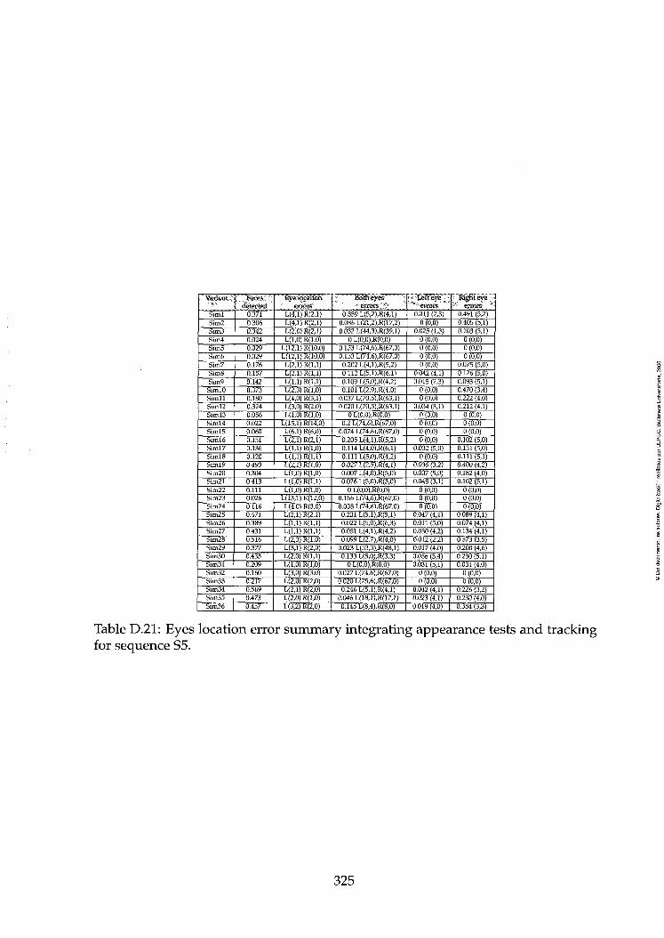
Variant

Siml Siin2 Sim3 Sim4 Sím5 Simó Sim7 Sim8 Sini9 Simio Simll Siml2 Siml3 Siml4 Siml5 Siml6 Siml7 SimlS Siml9 Sim20 Sim21 Sim22 Sim23 Sim24 Sim25 Sim26 Sim27 SimlS Sim29 Sim30 Sim31 Sim32 Sim33 Sim34 Sim35 Sim36

Faces detecíed

0.371 0.306 0.342 0.024 0.029 0.029 0.176 0.157 0.142 0.373 0.180 0.324 0.056 0.022 0.060 0.151 0.136 0.120 0.493 0.304 0.413 0.111 0.026 0.116 0.471 0.389 0.431 0.516 0.377 0.433 0.209 0.160 0.217 0.569 0.473 0.457

Eye íocatioíi ernsrs

L(4,l) R(2,l) L(4,l) R(2,l) L(2,0) R(2,l) L(1,0) R(1,0)

L(12,l) R(10,0) L(12,l) R(10,0) L(2,l) R(l,l) L(2,1)R(1,1) L(l,l) R(l,l) L(2,3) R(1,0) L(4,0) R(3,l) L(3,0) R(2,0) L{1,0) R(1,0)

L(15,l) R(14,0) L(6,l) R(6,0) L(2,l) R(2,l) L(l,l) R(1,0) L(l,l) R(l,l) L(2,l) R(1,0) L(1,0) R(1,0) L(1,0) R(l,l) L(1,0) R(1,0)

L(13,l) R(12,0) L(4,0) R(3,0) L(2,l) R(2,l) m , l ) R(l,l) L(l,l) R(l,l) L(Z,3) R(1,0) L(3,l) R(2,0) L(2,0) R(l,l) L(1,0) R(1,0) L(3,0) R(3,0) L(2,0) R{2,0) L(2,l) R(2,0) L(2,0) R(1,0) L(3,2) R(2,0)

Botheyes errors

0.359 L(5,2),R(4,1) 0.086 L(21,2),R(17,2) 0.032 L(44,3),R(39,1)

0 L(0,0),R(0,0) 0.153 L(74,6),R(67,0) 0.153 L(74,6),R(67,0) 0.202 L(4,1),R(5,2) 0.112 L(S,1),R(6,1) 0.109 L(5,0),R(4,2) 0.101 L(2,9),R(4,0)

0.037 L(70,5),R(63,1) 0.020 L(70,5),R(63,1)

0 L(0,O),R(0,O) 0.2 L(74,6),R(67,0)

0.074 L(74,6),R(67,0) 0.205 L(4,1),R(5,2) 0.114 L(4,0),R(6,1) 0.111 L(5,0),R(4,2) 0.027 L(2,5),R(4,1) 0.007 L(4,0),R(5,0) 0.026 L(5,0),R(3,0)

0 L(0,0),R(0,0) 0.166 L(74,6),R(67,0) 0.038 L(74,6),R(67,0) 0.231 L(5,1),R(5,1) 0.022 L(5,0),R(6,3) 0.051 L(4,1),R(4,2) 0.099 L(2,7),R(4,0)

0.023 L(53,3),R(48,1) 0.133 L(5,0),R(3,3)

0 L(0,O),R(0,0) 0.027 L(74,6),R(67,0) 0.020 L(7S,6),R(67,0) 0.246 L(5,1),R(4,1)

0.046 L(18,1),R(17,1) 0.145 L(8,4),R(8,0)

LefteyB eiTOrs

0.011 (2,3) 0 (0,0)

0025 (1,3) 0 (0,0) 0 (0,0) 0 (0,0) 0 (0,0)

O042 (4,1) 0.015 (2,3)

0 (0,0) 0 (0,0)

0.034 (3,1) 0 (0,0) 0 (0,0) 0 (0,0) 0 (0,0)

0.032 (5,0) 0 (0,0)

0.036 (3,2) 0.007 (5,0) 0.048 (3,1)

0 (0,0) 0 (0,0) 0 (0,0)

0047 (4,1) aOll (5,0) O030 (4,2) 0.012 (2,2) 0.017 (4,0) 0.056 (3,4) 0.031 (5,1)

0 (0,0) 0 (0,0)

0.042 (4,1) 0.023 (4,1) 0.019 (4,0)

Eighl eye eiTors

0.491 (5,2) 0.405 (5,1) 0.103 (5,1)

0 (0,0) 0 (0,0) 0 (0,0)

0.075 (5,0) 0.126 (5,0) 0.093 (5,1) 0.470 (3,4) 0.222 (4,0) 0.212 (4,1)

0 (0,0) 0 (0,0) 0 (0,0)

0.102 (5,0) 0.131 (5,0) 0.111 (5,1) 0.400 (4,2) 0.182 (4,0) 0.102 (5,1)

0 (0,0) 0 (0,0) 0 (0,0)

0.089 (4,1) 0.074 (4,1) 0.134 (4,1) 0.573 (3,5) 0.200 (4,6) 0.230 (5,1) 0.031 (4,0)

0 (0,0) 0 (0,0)

0.226 (3,2) 0.230 (4,0) 0.354 (3,3)


325

Seq

S6 S6 S6 S6 S6 S6 S6 S6 S6 S6 S6 S6 S6 S6 S6 S6 S6 S6 S6 S6 S6 S6 S6 S6 S6 S6 S6 S6 S6 S6 S6 S6 S6 S6 Sí S6

Variant label Siml Sim2 Sim3 Sím4 Sim5 Simó Sim7 Sim8 Sim9 Simio Simll Siml2 Siml3 Siml4 Siml5 Simie Siml7 SimJS Siml9 Sim20 Sim21 Sim22 Sim23 Sim24 Sim25 Sim26 Sim27 Sim28 Sim29 Sim30 Sim31 Sim32 Sim33 Sim34 Sim35 Sim36

Faces detected

0.676 0.657 0.664 0.691 0.633 0.553 0.306 0.286 0.284 0.664 0.662 0.613 0.460 0,436 0.457 0.246 0.257 0.262 0.817 0.764 0.791 0.617 0.56

0.564 0.546 0.731 0.656 0.817 0.820 0.791 0.717 0.713 0.717 0.826 0.824 0.813

Faces correctíy deiected

0.98 1.0 1.0 1.0 1.0 1.0

0.913 1.0 1,0

0.98 1.0 1.0 1.0 1.0 1.0

0.982 1.0 1.0 1.0 1.0 1.0

0.993 1.0 1.0

0.928 1.0

0.939 1.0 1.0 1.0 1.0 1.0 1.0

0.957 1.0

0.973

Eyes coriectíy located

0.947 (0.98) 0.969 (1.0) 0.966 (1.0)

0.836 (0.891) 0.975 (1.0) 0.992 (1.0)

0.898 (0.913) 0.984 (1.0) 0.984 (1.0)

0.923 (0.970) 0.949 (0.997) 0.938 (0.989)

1,0 (1.0) 1,0 (1.0) 1,0 (1,0)

0,982 (0,982) 1,0(1,0) 1,0 (1,0)

0,921 (0,948) 0,988(1,0) 0,958 (0,98)

0,993 (0,993) 1,0 (1,0) 1,0 (1,0)

0.88 (0.914) 0.985 (1.0)

0.891 (0.925) 0.894 (0.959) 0.943 (0.997) 0.949 (1.0)

0.941 (0.985) 0.947 (0.984) 0.941 (0.985) 0.93 (0.941) 0.927 (0.989) 0.945 (0.951)

Average time 27 33 45 26 31 35 57 57 63 30 29 32 39 39 44 80 58 62 23 26 27 39 40 41 59 71 66 26 35 28" 33 34 37 46 45 49

Table D.22: Results obtained integrating tracking for sequences S6. Time measures in msecs. are obtained using standard C command clock.

326

VManí ,

Siml Sim2 Sim3 Sim4 Sim5 Sim6 Sim7 Sim8 Sim9 Simio Simll Siml2 Siml3 Siml4 Siml5 Simio Siml7 SimlS Siml9 Sim20 Sim21 Sim22 Sim23 Sim24 Sim25 Sim26 Sim27 Sim28 Sim29 Sim30 Sim31 Sim32 Sim33 Sim34 Sim35 Sim36

Facéá

0.676 0.657 0.664 0.691 0.633 0.553 0.306 0.286 0.284 0.664 0.662 0.613 0.460 0.436 0.457 0.246 0.257 0.262 0.817 0.764 0.791 0.617 0.56 0.564 0.646 0.731 0.656 0.817 0.820 0.791 0.717 0.713 0.717 0.826 0.824 0.813

: ByelíjcaHon

L(4,2) R(3,2) L(1,0) R(l,l) L(l,l) R(l,l) L(l,l) R(2,l) L(l,l) R(l,l) L(1,0) R(l,l) L(1,0) R(2,l) L(1,0) R(1,0) L(1,0) R(l,l) L(4,l) R(3,l) L(1,0) R(1,0) L(1,0)R(1,1) L(1,0) R(0,0) L(1,0) R(0,0) L(1,0) R(0,0) L(4,2) R(3,2) L(1,0) R(1,0) L(1,0) R(1,0) L(l,l) R(l,l) L(1,0) R(1,0) L(1,0) R(1,0) L(1,0) R(1,0) L(1,0) R(0,0) L(1,0) R(0,0) L(1,0) R(2,l) L(1,0) R(1,0) L(1,0) R(2,l) L(l,l) R(1,0) L(1,0) R(1,0) L(1,0) R(1,0) L(1,0) R(l,l) L(1,0) R(l,l) L(1,0) R(l,l) L(1,0) R(1,0) L(1,0) R(1,0) L(1,0) R(1,0)

Botheyes : • errare

0.036 L(82¿0),R(69,19) 0.016 L(6,1),R(6,4) 0.016 L(6,1),R(6,4) 0.003 L(5,3),R(10,1)

0 L(0,0),R(0,0) 0 L(0,0),R(0,0) 0 L(0,0),R(0,0) 0 L(0,0),R(0,0) 0 L(0,0),R(0,0)

0.026 L(112,30),R(96,24) 0.006 L(5,2),R(6,2) 0.007 L(5,2),R(6,2)

0 L(0,0),R(0,0) 0 L(0,0),R(0,0) 0 L(0,0),R(0,0)

0.02 L(150,78),R(131,82) 0 L(0,0),R(0,0) 0 L(0,0),R(0,0)

0.035 L(4,11),R(10,3) 0.002 L(6,0),R(8,5) 0.002 L(6,0),R(8,5)

0.007 L(25,3),R(26,1) 0 L(0,0),R(0,0) 0 L(0,0),R(0,0)

0.010 L(25,3),R(30,1) 0 L(0,0),R(0,0) 0 L(0,0),R(0,0)

0.043 L(4,10),R(10,4) 0.008 L(7,1),R(4,8) 0.005 L(8,1),R(4,8)

0 L(0,0),R(0,0) 0 L(0,0),R(0,0) 0 L(0,0),R(0,0)

0.005 L(6,1),R(12,1) 0.002 L(7,5),R(8,5)

0 L(0,0),R(0,0)

eríórS". x 0.013 (2,4) 0.013 (2,4) 0.013 (2,4) 0.138 (10,1) 0.007 (9,1) 0.008 (9,1) 0.086 (14,3)

0 (0,0) 0 (0,0)

0.050 (5,8) 0.043 (5,8) 0.054 (5,8)

0 (0,0) 0 (0,0) 0 (0,0) 0 (0,0) 0 (0,0) 0 (0,0)

0.032 (4,7) 0.008 (5,4) 0.033 (4,7)

0 (0,0) 0 (0,0) 0 (0,0)

0.109 (9,3) 0.015 (6,0) 0.108 (9,3) 0.043 (4,4) 0.046 (5,5) 0.039 (4,5) 0.058 (5,7) 0.052 (5,8) 0.058 (5,7)

0.064 (11,2) 0.029 (4,7) 0.054 (11,3)

Kghteye y,, érrers

0.003 (4,4) 0 (0,0)

0.003 (4,4) 0.022 (4,4) 0.017 (4,3)

0 (0,0) 0.014 (5,3) 0.015 (5,3) O.OIS (5,3)

0 (0,0) 0 (0,0) 0 (0,0) 0 (0,0) 0 (0,0) 0 (0,0) 0 (0,0) 0 (0,0) 0 (0,0)

0.010 (2,9) 0 (0,0)

0.005 (1,11) 0 (0,0) 0 (0,0) 0 (0,0) 0 (0,0) 0 (0,0) 0 (0,0)

0.019 (2,9) 0.002 (6,0) 0.005 (6,2)

0 (0,0) 0 (0,0) 0 (0,0) 0 (0,0)

0.040 (5,2) 0 (0,0)


327

Seqíi-


f. Variant ,, label

Siml Sim2 Sim3 Sim4 SimS Simó Sim7 Sim8 Sim9

Simio Simll SimlZ Siml3 Siml4 Siml5 Simio Siml7 SimlS Siml9 Sim20 Sim21 Sim22 Sim23 Sim24 Sim25 Sim26 Sim27 Siin28 Sim29 SimBO Sim31 Slm32 Sim33 Sim34 Sim35 Sim36

Facé$ det€G%d

0.871 0.871 0.871 0.782 0.786 0.786 0.516 0.596 0.540 0.766 0.775 0.775 0.746 0.746 0.746 0.511 0.564 0.520 0.853 0.893 0.873 0.868 0.844 0.844 0.797 0.857 0.804 0.904 0.902 0.877 0.783 0.848 0.856 0.897 0.900 0.906

K; FafSiS'éorrectl)' , défecteí

1.0 1.0 1.0 1.0 1.0 1.0 1.0 1.0

0.992 1.0 1,0 1.0 1.0 1.0 1.0 1.0 1.0

0.996 0.997

1.0 1.0 1.0 1.0 1.0 1.0 1.0 1.0 1.0 1.0

0.992 1.0 1.0 1.0 1.0 1.0

0.99

ideaied 1.0 (1.0) 1.0 (1.0) 1.0 (1.0) 1.0 (1.0) 1.0 (1.0) 1.0 (1.0)

0.991 (1.0) 0.992 (1,0)

0.983 (0.992) 1.0(1.0) 1.0(1.0) 1.0 (1.0) 1.0(1.0) 1.0 (1.0) 1.0 (1.0)

0.991 (1.0) 0.992 (1.0)

0.987 (0.996) 0.987 (0.992)

1.0 (1.0) 0.995(1.0) 1.0 (1.0) 1.0 (1.0) 1.0(1.0)

0.994 (1.0) 0.995 (1.0) 0.994 (1,0)

0.983 (0.983) 1.0 (1.0)

0.992 (0.992) 0.994 (1,0)

1.0 (1.0) 1.0 (1.0) 1.0 (1.0) 1.0 (1.0)

0.99 (0.99)

^Average 4iine...

21 24 44 25 25 29 61 60 66 27 28 30 27 28 31 62 61 70 23 25 29 31 33 36 64 64 70 29 30 34 35 33 37 51 51 57

Table D.24: Results obtained integrating tracking for sequence S7. Time measures in msecs. are obtained using standard C command clock.

328

¥,aiiant;..

Siml Sim2 Sim3 Sim4 Sim5 Sim6 Sim7 Sim8 Sim9 Simio Simll Siml2 Siml3 Sijnl4 Siml5 Siml6 Siinl7 Siml8 Siml9 Sim20 Sim21 Sim22 Siin23 Sim24 Sim25 Slm26 Sim27 Sim28 Sim29 Sim30 Sim31 Slm32 Sim33 Sim34 Sim35 Sim36

;, Faces '•'detected

0.871 0.871 0.871 0.782 0.786 0.786 0.516 0.596 0.540 0.766 0.775 0.775 0.746 0.746 0.746 0.511 0.564 0.520 0.853 0.893 0.873 0.868 0.844 0.844 0.797 0.857 0.804 0.904 0.902

0.877) 0.783 0.848 0.856 0.897 0.900 0.906

/•Byelocition enóEs

L(2,l) R(2,l) L(2,l) R(2,l) L(2,l) R(2,l) L(2,l) R(2,l) L(2,0) R(2,l) L(2,0) R(2,l) L(l,l) R(l,l) L(2,l) R(l,l) L(2,l) R(2,l) L(1,0) R(1,0) L(1,0) R(1,0) L(1,0) R(1,0) L(l,l) R(1,0) L(l,l) R(1,0) L(l,l) R(l.O) L(2,1)R(1,1) L(2,1)R(1,1) L(2,l) R(2,l) L(l,l) R(l.O) L(l,l) R(1,0) L(l,l) R(1,0) L(1,0) R(1,0) L(1,0) R(1,0) L(1,0) R(1,0) L(U)R(1,1) L(1,1)R(1,1) L(1,1)R(1,1) L(2,0) R(1,0) L(1.0)R(0,0) L(1,0) R(1,0) L(2,l) R(0,0) L(2,l) R(0,0) L(l,l) R(0,0) L(1,0) R(1,0) L(1,0) R(1,0) L(2,1)R(1,1)

Botheyes errocs

0 L(0,ü),R(0,0) 0 L(0,0),R(0,O) 0 L(0,0),R(0,0) 0 L(ü,0),R(0,0) OL(0,0),R(0,0) OL(Ü,0),R(0,0) OL(0,0),R(0,0) OL(0,0),R(0,0)

0.008 L(46,5),R(35,5) OL(0,0),R(0,0) OL(0,0),R(0,0) OL(0,0),R(0,0) OL(0,0),R(0,0) 0 L(0,0),R(0,0) 0L(0,O),R(O,0) OL(0,0),R(0,0) OL(0,0),R(0,0)

0.004 L(46^),R(35,5) 0 L(0,O),R(O,0) 0 L(0,0),R(0,0) 0 L(0,O),R(O,0) 0 L(0,0),R(0,0) OL(0,0),R(0,0) 0 L(0,O),R(O,0) 0 L(0,0),R(0,0) 0 L(0,0),R(0,0) 0 L(0,0),R(0,0)

0.017 L(14,1),R(21,0) 0 L(0,0),R{0,0) 0 L(0,0),R(0,0) 0 L(0,0),R(0,0) 0 L(0,0),R(0,a) 0 L(0,0),R(0,0) 0 L(0,0),R(0,0) 0 L(0,0),R(0,0)

0.009 L(45^),R(34,4)

Lef t eye ertots 0 (0,0) 0 (0,0) 0 (0,0) 0 (0,0) 0 (0,0) 0 (0,0) 0 (0,0) 0 (0,0) 0 (0,0) 0 (0,0) 0 (0,0) 0 (0,0) 0 (0,0) 0 (0,0) 0 (0,0) 0 (0,0) 0 (0,0) 0 (0,0) 0 (0,0) 0 (0,0) 0 (0,0) 0 (0,0) 0 (0,0) 0 (0,0) 0 (0,0) 0 (0,0) 0 (0,0) 0 (0,0) 0 (0,0) 0 (0,0)

0.005 (6,0) 0 (0,0) 0 (0,0) 0 (0,0) 0 (0,0) 0 (0,0)

Righteye ercors 0 (0,0) 0 (0,0) 0 (0,0) 0 (0,0) 0 (0,0) 0 (0,0)

0.008 (7,0) 0.007 (7,0) 0.008 (7,0)

0 (0,0) 0 (0,0) 0 (0,0) 0 (0,0) 0 (0,0) 0 (0,0)

0.008 (7,0) 0.007 (7,0) 0.008 (7,0) 0.013 (10,0)

0 (0,0) 0.005 (7,0)

0 (0,0) 0 (0,0) 0 (0,0)

0.005 (7,0) 0.005 (7,0) 0.005 (7,0)

0 (0,0) 0 (0,0)

O.üo) (14,1) 0 (0,0) 0 (0,0) 0 (0,0) 0 (0,0) 0 (0,0) 0 (0,0)


329

^>S^q'

S8 S8 S8 S8 S8 S8

• S8 S8 S8 S8 S8 S8 S8 S8 S8 S8 S8 S8 S8 S8 S8 S8 S8 S8 S8 S8 S8 S8 S8, S8 S8 S8 S8 S8 S8 S8

Variant label Sin\l Sim2 Sim3 Siin4 Sim5 Simó Sim7 Sim8 Sim9 Simio Simll Siml2 Siml3 Siml4 SimlS Siml6 Siml7 SimlS Siml9 Sim20 Sim21 Sim22 Sim23 Sim24 Sim25 Sim26 Sim27 SimlS Sim29 Sim30 Sim31 Sim32 Sim33 Sim34 Sijn35 Sim36

faces detecifed

0.716 0.611 0.709 0.653 0.588 0.649 0.442 0.360 0.409 0.713 0.656 0,676 0.644 0.611 0.644 0.437 0.362 0.411 0.746 0.697 0.786 0.726 0.702 0.731 0.700 0.624 0.617 0.782 0.686 0.748 0.731 0.688 0.753 0.751 0.744 0.755

Fae$s cd#éGííy detected

0.9S4 1.0

0.969 1.0 1.0 1.0

0.97 0.994 0.967 0.9S4

1.0 0.9S4

1.0 1.0 1.0

0.97 0.994 0.968 0.985

1.0 0.952

1.0 1.0 1.0

0.971 0.996 0.986 0.983

1.0 1.0 1.0 1.0 1.0

0.964 1.0

0.991

iicatcd'" 0.tit)3 (0.929) 0.927(1.0)

0.899 (0.962) 0.973 (1.0) 0.992 (1.0) 0.976 (1.0) 0.89 (0.935) 0.938 (0.981) 0.S97 (0.94) 0.875 (0.903) 0.936 (0.983) 0911 (0.954) 0.969 (1.0) 0.949 (1.0) 0.969 (1.0)

0.898 (0.934) 0.945 (0.982) 0.908 (0.941) 0.866 (0.929) 0.965(1.0)

0.879 (0.901) 0.976 (1.0) 0.949 (1.0) 0.982 (1.0)

0.905 (0.943) 0.932 (0.972) 0.924 (0.964) 0.866 (0.912) 0.955 (1.0) ,

0.947 (0.988) 0.948 (1.0) 0.958 (1.0)

0.923 (0.979) 0.87 (0.935) 0.910 (0.973) 0.894 (0.962)

^::.Avérage ^ i<Minfé J

¿ i

35 30 25 28 28 51 48 54 23 26 34 26 27 30 51 49 54 24 26 27 25 26 28 53 52 59 31 33 35 33 34 36 52 50 57


330

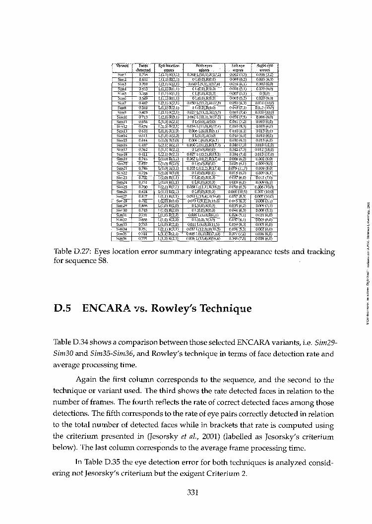
Variant

Siml Sim2 Sim3 Sim4 Sim5 Sim6 Sim7 SimS Sim9 Simio Simll Siml2 Siml3 Siml4 Siml5 Simio Siml7 SimlS Siml9 Sim20 Sim21 Sim22 Sim23 Sim24 Sim25 Sim26 Sim27 Sim28 S¡m29 Sim30 Sim31 Sim32 Sim33 Sim34 Sim35 Sim36

Faces detecten

0.716 0.611 0.709 0.653 0.588 0.649 0.442 0.360 0.409 0.713 0.656 0.676 0.644 0.611 0.644 0.437 0.362 0.411 0.746 0.697 0.786 0.726 0.702 0.731 0.700 0.624 0.617 0.782 0.686 0.748 0.731 0.688 0.753 0.751 0.744 0.755

Byé iocatíon errois

L(2,l) R(3,l) L(l,l) R(2,l) L(2,l) R(2,l) L(1,1)R(1,1) L(1,1)R(1,1) L(l,l) R(l,l) L(2,l) R(2,l) L(l,l) R(2,l) L(2,l) R(2,l) L(2,0) R(3,l) L(1,0) R(2,l) L(1,0) R(2,l) L(1,0) R(1,0) L(1,0) R(2,0) L(1,0) R(1,0) L(2,l) R(2,l) L(l,l) R(2,l) L(2,l) R(2,l) L(1,0) R(3,l) L(1,0) R(2,0) L(1,0) R(3,l) L(1,0) R(1,0) L(1,0) R(l,l) L(1,0) R(l,l) L(2,l) R(2,l) L(l,l) R(2,l) L(1,1)R(2,1) L(2,0) R(3,0) L(1,0) R(2,0) L(1,0) R(2,0) L(1,0) R(2,0) L(1,0) R(2,0) L(1,0) R(2,0) L(2,l) R(2,l) L(l,l) R(2,l) L(1,0) R(2,l)

Botheyes

0.068 L(10,1),R(17,2) 0 L(0,0),R(0,0)

0.040 L(9,1),R(17,4) 0 L(0,O),R(0,O) 0 L(0,O),R(0,0) OL(0,0),R(0,0)

0.050 L(11,2),R(17,3) 0 L(0,0),R(0,0)

0.027 L(13,2),R(15,5) 0.062 L(10,1),R(17,3)

0 L(0,0),R(0,0) 0.016 L(11,0),R(17,4) 0.006 L(6,0),R(6,1)

0 L(0,0),R(0,0) 0.006 L(6,0),R(6,1)

0.050 L(11,2),R(17,3) 0 L(O,O),R(0,0)

0.027 L(13,2),R(15,5) 0.062 L(ia,2),R(17,3)

0 L(0,0),R(0,0) 0.033 L(12,2),R(17,4)

0 L(0,0),R(0,0) 0 L(O,O),R(0,O) OL(0,0),R(0,0)

0.038 L(11,1),R(18,2) 0 L(0,0),R(0,0)

O.OIO L(15,4),R(16,6) 0.079 L(9,1),R(18,3)

0 L(0,0),R(0,0) 0 L(0,0),R(0,0)

0.006 L(6,0),R(6,1) OL(0,0),R(0,0)

0.011 L(6,0),R(11,5) 0.032 L(12,3),R(18,3) 0.005 L(6,1),R(17,10) 0.008 L(15,4),R(16,6)

\eít eye érrOiS

0.062 (5,3) 0.069 (6,2) 0.056 (6,1) 0.006 (5,1) 0.007 (5,1) 0.003 (5,2) 0.050 (6,3) 0.049 (7,3) 0.065 (7,4) 0.056 (7,5) 0.061 (7,2) 0.069 (8,3) 0.010 (6,1) 0.040 (6,0) 0.010 (6,1) 0.040 (7,3) 0.042 (7,3) 0.054 (7,4) 0.068 (6,2) 0.025 (6,1) 0.079 (11,7) 0.015 (6,2) 0.037 (6,0) 0.009 (6,0) 0.050 (6,3) 0.060 (10,5) 0.057 (8,3) 0.045 (6,3) 0.035 (6,2) 0.044 (6,3) 0.024 (5,1) 0.032 (6,1) 0.059 (8,3) 0.094 (5,3) 0.077 (7,2) 0.088 (7,3)

Right eye erroxs

0.006 (3,2) 0.003 (6,0) 0.003 (6,0) 0.020 (6,0)

0 (0,0) 0.020 (6,0)

0.010 (10,0) 0.012 (10,0) 0.010 (10,0) 0.006 (6,0) 0.003 (6,0) 0.003 (6,0) 0.013 (6,0) 0.010 (8,0) 0.013 (6,0) 0.010 (10,0) 0.012 (10,0) 0.010 (10,0) 0.002 (6,0) 0.009 (8,0) 0.008 (8,0) 0.009 (6,1) 0.012 (7,0) 0.009 (6,1) 0.006 (10,0) 0.007 (10,0) 0.007 (10,0) 0.008 (5,1) 0.009 (5,1) 0.008 (5,1) 0.021 (6,0) 0.009 (8,0) 0.005 (6,0) 0.002 (6,0) 0.006 (6,0) 0.008 (6,0)

Table D.27: Eyes location error summary integratixig appearance tests and tracking for sequence S8.

D.5 ENCARA vs. Rowley's Technique

Table D.34 shows a comparisonbetween those selected ENCARA variants, i.e. Sim29-

Sim30 and Sim35-Sim36, and Rowley's technique in terms of face detection rate and

average processing time.

Again the first column corresponds to the sequence, and the second to the

technique or variant used. The third shows the rate detected faces in relation to the

number of frames. The fourth reflects the rate of correct detected faces among those

detections. The fifth corresponds to the rate of eye pairs correctly detected in relation

to the total number of detected faces while in brackets that rate is computed using

the criterium presented in (Jesorsky et al, 2001) (labelled as Jesorsky's criterium

below). The last column corresponds to the average frame processing time.

In Table D.35 the eye detection error for both techniques is analyzed consid-

ering not Jesorsky's criterium but the exigent Criterium 2.

331

•Seq


Variant ¡:' label

Síml Sim2 Sim3 Sim4 Sim5 Simó Sim7 SimS Sim9 Simio Simll Siml2 Siml3 Siml4 Siml5 Svml6 Siml7 SimlS Siml9 Sim20 Simll Sim22 Sim23 Sim24 Sim25 Sim26 Sim27 S¡m28 Sim29 SimSO Sim31 Sim32 Sim33 Sim34 Simas Sim36

• Faiíes'" detecíed

0.893 0.806 0.816 0.782 0.782 0.782 0.56

0.546 0.56 0.755 0.777 0.755 0.804 0.773 0.8O4 0.555 0.546 0.555 0.888 0.864 0.868 0.868 0.864 0.871 0.853 0.848 0.853 0.904 0.922 0.922 0.929 0.924 0.929 0.873 0.862 0.884

Faces-cqrrectly . dtfeíéd*'

0.440 1.0 1.0 1.0 1.0 1.0 1.0 1.0 1.0

0.867 1.0

0.988 1.0 1.0 1.0 1.0 1.0 1.0 1.0 1.0 1.0 1.0 1.0 1.0 1.0 1.0 1.0

0.816 1.0 1.0 1.0 1.0 1.0 1.0 1.0 1.0

íocaíed 0.440 (0.44)

1.0 (1.0) 1.0 (1.0) 1.0 (1.0) 1.0 (1.0) 1.0 (1.0)

0.992 (1.0) 0.991 (1.0) 0.992 (1.0)

0.867 (0.868) 1.0(1.0)

0.988 (0.988) 1.0 (1.0) 1.0 (1.0) 1.0 (1.0)

0.992(1.0) 0.992(1.0) 0.992 (1.0)

1.0 (1.0) 1.0(1.0) 1.0 (1.0)

0.997(1.0) 0.997 (1.0) 0.997(1.0) 0.987(1.0) 0.987(1.0) 0.987(1.0)

0.816 (0.816) 0.986(1.0) 0.986 (1.0)

1.0 (1.0) 1.0 (1.0) 1.0 (1.0)

0.98 (0.987) 0.974 (0.982) 0.98 (0.987)

Averáge

22 37 45 29 30 31 68 69 74 32 30 37 27 29 .... ^ 68 71 75 25 28 32 29 34 34 68 68 77 33 28 31 27 27 30 57 63 68


332

Variant

Siml Sim2 Sim3 Siin4 Sim5 Simó Sim7 Sim8 Sim9 Simio Simll Siml2 SimX3 Siml4 Siml5 Siml6 Siml7 Siml8 Siml9 Sim20 SimZl Sim22 Sim23 Sim24 Sim25 Sim26 Sim27 Sim28 Sim29 Simao Simal Sima2 Sim33 Sim34 Sim35 Siin36

Faces detected

Ü.893 0.806 0.816 0.782 0.782 0.782 0.56 0.546 0.56 0.755 0.7/7 0.755 0.804 0.773 0.804 0.555 0.546 0.555 0.888 0.B64 0.868 0.868 0.864 0.871 0.853 0.848 0.853 0.904 0.922 0.922 0.929 0.924 0.929 0.873 0.862 0.884

Eye íocatkai errors

L(92,2) R(78,5) L(2,l) R(2,l) L(2,l) R(2,l) L(2,l) R(2,0) L(2,l) R(2,0) L(2,l) R(2,0) L(2,0) R(2,l) L(2,0) R(2,l) L(2,0) R(2,l)

L(23,0) R(19,l) L(1,0) R(1,0) L(3,0) R(2,0) L(1,0) R(1,0) L(1,0) R(1,0) L(1,0) R(1,0) L(2,0) R(2,l) L(2,0) R(2,l) L(2,0) R(2,l) L(1,0) R(1,0) L(1,0) R(1,0) L(1,0) R(1,0) L(1,0) R(1,0) L(1,0) R(1,0) L(1,0) R(1,0) L(2,0) R(2,l) L(2,0) R(2,l) L(2,0) R(2,l)

L(30,l) R(26,l) L(1,0) R(0,0) L(1,0) R(0,0) L(1,0) R(0,0) L(1,0) R(0,0) L(1,0) R(0,0) L(1,0) R(1,0) L(1,0) R(2,l) L(1,0) R(2,0)

Botheyes enx>rs

056L(164,4),R(138,8) 0 L(0,0),R(0,0) 0 L(0,0),R(0,0) 0 L(0,0),R(0,0) 0 L(0,O),R(0,O) 0 L(0,0),R(0,0) 0 L(0,0),R(0,0) 0 L(0,0),R(0,0) 0 L(0,0),R(0,0)

0.13 L(165,1),R(139,3) 0 L(0,0),R(0,0)

0.01 L(161,2),R(134,6) 0 L(0,0),R(0,0) 0 L(0,0),R(0,0) 0 L(0,0),R(0,0) 0 L(0,0),R(0,0) 0 L(0,0),R(0,0) 0 L(0,0),R(0,0) 0 L(0,0),R(0,0) 0 L(0,0),R(0,0) 0 L(0,0),R(0,0) 0 L(0,0),R(0,0) 0 L(0,0),R(O,0) 0 L(0,0),R(0,0) 0 L(0,0),R(O,0) 0 L(0,0),R(0,0) 0 L(0,0),R(0,0)

018 L(158,6),R(139,5) 0 L(0,0),R{0,0) 0 L(0,0),R(ü,0) 0 L(0,0),R(0,0) 0 L(0,0),R(0,0) 0 L(0,0),R(0,0) 0 L(0,0),R(0,0) 0 L(0,0),R(0,0) 0 L(0,0),R(0,0)

Leít eye exroíS 0 (0,0) 0 (0,0) 0 (0,0) 0 (0,0) 0 (0,0) 0 (0,0) 0 (0,0) 0 (0,0) 0 (0,0) 0 (0,0) 0 (0,0) 0 (0,0) 0 (0,0) 0 (0,0) 0 (0,0) 0 (0,0) 0 (0,0) 0 (0,0) 0 (0,0) 0 (0,0) 0 (0,0) 0 (0,0) 0 (0,0) 0 (0,0) 0 (0,0) 0 (0,0) 0 (0,0) 0 (0,0)

0.009 (6,1) 0.009 (6,1)

0 (0,0) 0 (0,0) 0 (0,0)

O02 (15,8) 0.02 (19,14) 0.02 (15,8)

Eightesfe errors .-0 (ü,uj 0 (0,0) 0 (0,0) 0 (0,0) 0 (0,0) 0 (0,0)

0.007 (7,1) 0.008 (7,1) 0.007 (7,1)

0 (0,0) 0 (0,0) 0 (0,0) 0 (0,0) 0 (0,0) 0 (0,0)

0.008 (7,1) 0.008 (7,1) 0.008 (7,1)

0 (0,0) 0 (0,0) 0 (0,0)

0.002 (6,2) 0.002 (6,2) 0.002 (6,2) 0.013 (6,1) 0.013 (6,1) 0.013 (6,1)

0 (0,0) 0.004 (6,1) 0.004 (6,1)

0 (0,0) 0 (0,0) 0 (0,0)

0.002 (3,5) 0.002 (3,5) 0.002 (3,5)


333

•Séciíj

SIO SIO SIO SIO SIO SIO SIO SIO SIO SIO SIO SIO SIO SIO SIO SIO SIO SIO SIO SIO SIO SIO SIO SIO SIO SIO SIO SIO SIO SIO SIO SIO SIO SIO SIO SIO

yariaut

Siml Sim2 Sim3 Sim4 Sim5 Simó Sim7 Sim8 Sim9

Simio Simll Siml2 Siml3 Siml4 SimlS Simio Síml7 SimlS Siml9 Sim20 Sim21 Sim22 Sim23 Sim24 Sim25 Siln26 Sim27 Sim28 Sim29 Sim30 Sim31 Sim32 Sim33 Sim34 Sím35

Faces' ^

0.746 0.704 0.76 0.644 0.620 0.635 0.588 0.542 0.584 0.724 0.697 0.72 0.682 0.673 0.682 0.586 0.542 0.582 0.829 0.775 0.783 0.748 0.731 0.76 0.777 0.72 0.757 0.788 0.804 0.768 0.751 0.748 0.737 0.809 0.802

Sim36 0.816

;Ftóescíarré£tly..

1.0 0.997

1.0 1.0 1.0 1.0 1.0 1.0 1.0 1.0 1.0 1.0 1.0 1.0 1.0 1.0 1.0 1.0 1.0

0.966 0.989

1.0 1.0 1.0

0.997 0.997 0.994

1.0 0.994

1.0 1.0 1.0 1.0 1.0

0.992 1.0

Eyss corrécüy

0.747 (0.985) 0.823 (0.965) 0.754 (0.991) 0.945 (1.0) 0.932 (1.0) 0.944 (1.0) 0.94 (1.0) 0.934 (1.0) 0.939 (1.0) 0.954 (1.0)

0.942 (0.984) 0.954 (1.0) 0.948 (1.0) 0.937 (1.0) 0.948 (1.0) 0.94 (1.0) 0.934 (1.0) 0.939 (1.0) 0.944 (1.0)

0.897 (0.946) 0.93 (0.989) 0.935 (1.0) 0.939 (1.0) 0.936 (1.0)

0.929 (0.997) 0.910 (0.997)

0.944282 (0.994) 0.879 (0.994) 0.870 (0.975) 0.873 (1.0) 0.888 (1.0) 0.887 (1.0) 0.886 (1.0)

0.962 (0.989) 0.950 (0.989)

Ayeragé.^:

30 34 32 36 39 40 69 69 71 31 34 35 35 36 39 70 72 76 28 33 34 35 36 37 68 67 76 33 35 37 37 36 42 59 58

0.962 (1.0) 1 64

Table D.30: Results obtained integrating tracking for sequence SIO. Time measures in msecs. are obtained using standard C command clock.

334

Va4ánt

Siml Sim2 SimS Sim4 SiinS Simó Sim7 Sim8 Sim9 Simio Simll Siml2 Siml3 Siml4 Siml5 Siml6 Siml7 Siml8 Siml9 Sim20 Sim21 Sim22 Sim23 Sim24 Sim25 Sim26 Sim27 Sim28 Sim29 Sim30 Sim31 Sim32 Sim33 Sim34 Sim35 Sim36

detectad : U.746 0.704 0.76 0.644 0.620 0.635 0.588 0.542 0.584 0.724 0.697 0.72 0.682 0.673 0.682 0.586 0.542 0.582 0.829 0.775 0.783 0.748 0.731 0.76 0.777 0.72 0.757 0.788 0.804 0.768 0.751 0.748 0.737 0.809 0.802 0.816

: Eye íocatííai •,;, errors ••

H3,l) R(2,l) L(3,2)R(2,1) L(3,l) R(2,l) L(2,l) R(2,l) L(2,l) R(2,l) L(2,l) R(2,l) L(2,l) R(2,l) L(2,l) R(2,l)

• L(2,l) R(2,l) L(1,1)R(1,1) L(1,1)R(2,1) L(1,1)R(1,1) L(1,1)R(1,1) L(1,1)R(1,1) L(1,1)R(U) L(2,l) R(2,l) L(2,l) R(2,l) L(2,l) R(2,l) L(1,1)R(1,1) L(2,l) R(2,l) L(1,1)R(1,1) L{1,1) R(U) L(l,l) R(l,l) L(1,1)R(U) L(2,l) R(2,l) L(2,l) R(l,l) L(2,l) R(2,l) L(2,1)R(1,1) L(2,l) R(2,0) L(2,1)R(1,1) L(2,l) R(1,0) L(2,l) R(1,0) L(2,l) R(1,0) L(1,1)R(1,1) L(1,1)R(U) L(1,1)R(U)

Botheyes errors

0 L(0,0),R(0,0) - 0.02S L(28,14),R(22,1)

0 L(0,0),R(0,0) 0 L(0,0),R(0,0) 0 L(0,0),R(0,0) 0 L(0,0),R(0,0)

• OL(0,0),R(0,0) - 0 L(O,0),R(0,O)

0 L(0,0),R(0,0) OL(0,0),R(0,0)

0.015 L(30,16),R(21,1) OL(0,0),R(0,0) 0L(0,0),R(0,0) OL(0,0),R(0,0) OL(0,0),R(0,0) 0 L(0,0),R(0,0) 0 L(0,0),R(0,0) OL(0,0),R(0,0) 0 L(0,0),R(0,0)

0.014 L(30,16),R(21,1) 0 L(0,0),R(0,0) 0 L(0,0),R(0,0) 0 L(0,0),R(0,0) 0 L(0,0),R(0,0) 0 L(0,0),R(0,0) 0 L(0,0),R(0,0) 0 L(0,0),R(0,0) 0 L(0,0),R(0,0)

0.024 L(26,11),R(22,0) 0 L(0,0),R(0,0) OL(0,0),R(0,0) OL(0,0),R(0,0) OL(0,0),R(0,0) 0 L(0,0),R(0,0) 0 L(0,0),R(0,0) 0 L(0,0),R(0,0)

Lefteye errors 0 (0,0) 0 (0,0)

0.002 (7,4) 0 (0,0)

0.010 (5,2) 0 (0,0) 0 (0,0) 0 (0,0) 0 (0,0)

0.003 (7,4) 0 (0,0)

0.003 (7,4) 0 (0,0) 0 (0,0) 0 (0,0) 0 (0,0) 0 (0,0) 0 (0,0)

0.002 (6,2) 0 (0,0)

0.002 (6,2) 0.002 (6,2)

0 (0,0) 0.002 (6,2)

0 (0,0) 0.003 (6,2) 0.002 (6,2) 0.002 (6,2)

0 (0,0) 0 (0,0)

0.002 (6,2) 0.002 (6,2) 0.003 (6,2)

0 (0,0) 0 (0,0) 0 (0,0)

Righteye errors

0.ij2 {7,i) 0.151 (6,4) 0.242 (7,2) 0.055 (7,2) 0.057 (7,2) 0.055 (7,2) 0.060 (8,2) 0.065 (8,2) 0.060 (8,2) 0.042 (7,2) 0.041 (7,3) 0.043 (7,2) 0.052 (7,2) 0.062 (7,3) 0.052 (7,2) 0.060 (8,2) 0.065 (8,2) 0.051 (8,2) 0.053 (7,2) 0.088 (10,3) 0.067 (8,2) 0.062 (7,2) 0050 (7,2) 0061 (7,2) 0071 (8,2) 0.086 (7,2) 0.052 (8,2) 0.118 (7,2) 0.104 (7,2) 0.127(7,2) 0.109 (7,2) 0.109 (7,2) 0.111 (7,2) 0.038 (9,2) 0.049 (8,2) 0.038 (7,2)

Table D.31: Eyes location error summary integrating appearance tests and tracking for sequence SIO.

335

Seq

S i l Sil Sil s i l s i l s i l s i l s i l s i l s i l s i l s i l s i l s i l s i l s i l s i l s i l s i l s i l s i l s i l s i l s i l s i l s i l s i l s i l s i l s i l s i l s i l s i l s i l s i l s i l

í Vanaíit label • Siml Siin2 Sim3 Sim4 Sim5 Sim6 Sim7 Sim8 Sim9

Simio Simll Siml2 Siml3 Siml4 SimlS Simio Siml7 SimlS Siml9 Sim20 Sim21 Sim22 Sim23 Sim24 Sim25 Sim26 Sim27 Sim28 Sim29 Sim30 Sim31 Sim32 Sim33 Sim34 Sim35 Sim36

de&tefl 0.382 0.204 0.331 0.246 0.153 0.242 0.137 0.096 0.116 0.313 0.126 0.253 0.216 0.164 0.193 0.133 0.093 0.117 0.480 0.188 0.462 0.3

0.217 0.302 0.526 0.344 0.544 0.553 0.251 0.533 0.433 0.264 0.393 0.620 0.393 0.513

deteéted :<k > 1.0 1.0 1.0 1.0

0.942 1.0 1.0

0.953 1.0 1.0 1.0 1.0 1.0

0.973 1.0 1.0

0.952 1.0 1.0

0.965 1.0 1.0 1.0 1.0 1.0

0.961 1.0 1.0

0.973 1.0 1.0

0.983 1.0 1.0

0.977 1.0

tS' locafed 0.535 (0.83/) 0.891 (1.0)

0.483 (0.987) 0.973 (1.0)

0.942 (0.942) 0.972 (1.0)

0.726 (0.919) 0.767 (0.93) 0.827 (1.0) 0.759(1.0) 0.947(1.0)

0.807 (0.877) 0.959 (1.0)

0.959 (0.973) 0.931 (1.0) 0.716 (0.9)

0.81 (0.929) 0.B49 (1.0)

0.7083 (0.801) 0.929 (0.965) 0.928 (1.0) 0.94 (1.0) 0.98 (1.0) 0.831 (1.0)

0.793 (0.958) 0.884 (0.955) 0.927 (1.0)

0.795 (0.896) 0.726 (0.867) 0.812 (0.975) 0.918 (1.0)

0.958 (0.983) 0.949 (1.0)

0.810 (0.993) 0.802 (0.955) 0.822 (0.965)

toe.. í 33 51 54 40 44 44 50 48 51 36 44 40 40 41 43 49 49 52 32 47 38 41 41 43 48 52 56 31 49 38 41 52 46 51 54 54

Table D.32: Results obtained integrating tracking for sequence Sil . Time measures in msecs. are obtained using standard C command clock.

336

V«Sanl v

Siml Sim2 S¡m3 Sim4 Sim5 Simó Sim7 Sim8 Sim9 Simio Simll Siml2 Siml3 Siml4 Siml5 Simio Siml7 SimlS Siml9 Sim20 Sim21 Sim22 Sim23 Sim24 Sim25 Sim26 Sim27 Sim28 Sim29 SimSO SimSl Sim32 Sim33 Sim34 Sim35 Sim36

FacéS:-detectad

0.382 0.204 0.331 0.246 0.153 0.242 0.137 0.096 0.116 0.313 0.126 0.253 0.216 0.164 0.193 0.133 0.093 0.117 0.480 0.188 0.462 0.3

0.217 0.302 0.526 0.344 0.544 0.553 0.251 0.533 0.433 0.264 0.393 0.620 0.393 0.513

Eye locatícffi éirors

L(2,2) R(2,l) L(2,0) R(l,l) L(4,0) R(l,2) L(1,0) R(l,l) L(3,5) R(2,6) L(1,0) R(l,l) L(2,l) R(3,l) L(3,5) R(2,4) L(2,l) R(l,l) L(1,0) R(2,l) L(l,l) R(2,0) L(l,l) R(2,0) L(1,0) R(2,l) L(2,2) R(2,3) L(1,0) R(2,l) L(2,l) R(3,l) L(3,5) R(2,4) L(2,1)R(1,1) L(0,2) R(2,0) L(1,0) R(3,l) L(1,0) R(2,0) L(1,0) R(2,0) L(1,0) R(2,0) L(1,0) R(2,0) L(1,0) R(2,l) L(2,3) R(2,3) L(1,0) R(1,0) L(0,1) R(2,0) L(l,l) R(3,l) L(0,1) R(2,0) L(1,0) R(2,0) L(l,l) R(2,2) L(1,0) R(2,0) L(1,0) R(2,0) L(l,2) R(2,2) L(1,1)R(2,1)

• Bot í íéps

0.011 L(6,3),R(2,4) 0 L(0,0),R(0,0)

0.174 L(5,1),R(2,4) 0 L(0,0),R(0,0)

0.057 L(28,87),R(20,82) 0 L(0,0),R(0,0)

0.129 L(5,1),R(7,2) 0.046 L(28,87),R(20,82)

0 L(0,0),R(0,0) 0 L(0,0),R(0,0) 0 L(0,0),R(0,0)

0.017 L(5,2),R(4,7) 0 L(0,0),R(0,0)

0.027 L(28,87),R(19,80) 0 L(0,0),R(0,0)

0.150 L(5,0),R(7,2) 0.047 L(28,87),R(20,82)

0 L(0,0),R(0,0) 0.037 L(1,9),R(4,1)

0.035 L(18,1),R(38,1) 0 L(0,0),R(0,0) 0 L(0,0),R(0,0) 0 L(0,0),R(0,0) 0 L(0,0),R(0,0)

0.029 L(5,1),R(7,4) 0.045 L(18,61),R(13,57)

0 L(0,0),R(0,0) 0.016 L(0,10),R(4,1)

0.026 L(18,1),R(38,1) 0.012 L(1,8),R(4,0)

0.0106 L(4,0),R(3,4) 0.016 L(28,87),R(19,80)

0 L(0,0),R(0,0) 0.007 L(4,2),R(7,1)

0.022 L(30,83),R(19,79) 0.004 L(0,10),R(3,3)

Lefteye etrors

0.087 (4,1) 0.021 (1,4) 0.013 (3,3) 0.027 (3,3)

0 (0,0) 0.027 (3,3) 0.096 (5,1) 0.023 (3,2) 0.019 (3,2) 0.234 (4,1)

0 (0,0) 0.052 (3,1) 0.041 (3,1) 0.013 (3,2) 0.068 (3,1) 0.066 (5,1) 0.023 (3,2) 0.018 (3,2) 0.083 (3,0)

0 (0,0) 0.048 (3,1) 0.059 (3,1) 0.020 (3,1) 0.154 (3,0) 0.156 (4,2) 0.019 (3,2) 0.061 (4,1) 0.092 (3,0) 0.115 (4,1) 0.162 (4,0) 0.071 (3,0) 0.025 (4,0) 0.050 (3,1) 0.164 (4,0) 0.118(4,1) 0.099 (3,1)

Rightéye eiTOrs

0.366 (3,4) 0.086 (5,0) 0.328 (5,1)

0 (0,0) 0 (0,0) 0 (0,0)

0.048 (4,2) 0.162 (4,2) 0.154 (4,1) 0.007 (6,1) 0.052 (4,1) 0.122 (2,8)

0 (0,0) 0 (0,0) 0 (0,0)

0.066 (3,2) 0.119 (4,3) 0.132 (4,1) 0.171 (1,9) 0.035 (4,1) 0.024 (3,2)

0 (0,0) 0 (0,0)

0.014 (4,1) 0.021 (4,2) 0.051 (1,5) 0.012 (1,4) 0.096 (1,9) 0.132 (1,8) 0.U12 (1,9)

0 (0,0) 0 (0,0) 0 (0,0)

0.017 (3,1) 0.056 (3,3) 0.073 (2,5)

Table D.33: Eyes location error summary integrating appearance tests and tracking for sequenceSll.

337

Seq

SI

SI

SI SI

: SI S2 S2

S2

S2 c-j •

53

S3 S3

S3 ,-•83

S4 S4

S4 S4

S4 S5

S5 S5

55 85 ;;. S6

56

S6 56

S6 57

57 57

S7

S7--58

S8

S8 SS

; . S8 59 S9

59 59

• S9 ' SIO

SIO 510 510

SIB Si l

Sil 511

Sil

...Sllií

Techoií ue «sed'

E N C A R A 5im29 E N C A R A Sim30

E N C A R A Sim35

E N C A R A 5 im36

-. Rowléy's ENCARA 5im29 ENCARA 5im30

ENCARA SimSS

ENCARA S¡m36

Rpwíey's ENCARA Sim29

ENCARA Sim30 ENCARA Sim35

ENCARA 5im36 RDwle/s

ENCARA Sim29 ENCARA 5im30


Rowley's ENCARA 5im29


ENCARA Sim36

Rowley's ENCARA Sim29

ENCARA 5im30


Rowley's ENCARA Sim29


ENCARA Sim36

Rowley's E N C A R A Sim29

E N C A R A Sim30 E N C A R A Sim35

E N C A R A Sim36

'-Rbwlet 's E N C A R A Sim29

E N C A R A 5 im30 E N C A R A SimSS E N C A R A 5 im36

• ' .Rowley ' s E N C A R A 5 im29 E N C A R A Sim30 E N C A R A Sim35 E N C A R A 5 im36

:jv R o w l e y ' s ' •. E N C A R A Sim29

E N C A R A Sim30 E N C A R A Sim35

E N C A R A 5im36

4,, Rowley's.;,,

Fases Mema

0.577

0.568 0.497

0.504

^ -8.817 .;„ 0.440

0.531 0.422

0.493

a.724 0.811 0.922

0.786 0.871

' O.»?.-0.956

0.960 0.937 0.944

0.426 0.377

0.433

0.473 0.457

• 0.744 y-

0.820

0.791 0.824

0.813

• 0.913 0.902 0.877

0.900 0.906

' Ó.802 0.686

0.748 0.744

0.755

?•: . 0 . % •• 0.922 0.922

0.862 0.884

: 0.997 0.804

0.768 0.802 0.816

• OMSl 0.251 0.533 0.393

0.513

Msm.

Mátestoaectiy :i;detected

1.0

1.0

0.995 1.0

-i-1.0

0.995 1.0

1.0

1.0

%0 1.0

1.0 1.0

1.0 •yy 0.9m

1.0 1.0

1.0 1.0

0.974 0.935

1.0 0.99

0.976

Di988 : • 1.0

1.0

1.0 0.973

.¡0.99 1.0

0.992

1.0 0.99

•« i . 0 1.0

1.0

1.0 0.991

• '.,;(>.991

1.0 1.0

1.0 1.0

•:ÍÍ>V.1.0

0.994

1.0 0.992

1.0 : * • - 1 . 0 .

0.973

1.0 0.977

1.0

;*... i.o;; ,

Eye pátf; cotrecüy localed

0.788 (0.985) 0.718 (0.977)

0.879 (0.996) 0.806 (1.0)

0.29 (0 ,312) .> 0.843 (0.955)

0.761 (0.975)

0.863 (1.0) 0.815 (0.991)

o.imm.mí} 0.920 (0.995) 0.944 (0.994)

0.89 (0.986) 0.862 (0.987)

.; 0.» (0.918) » 0.911 (0.991)

0.914 (0.986) 0.941 (0.991)

0.962 (0.991)

0.944 <a9S9) 0 759 (0.935) 0.579 ;0.897)

0.699 (0.972)

0.480 (u.801)

0.663 iOMT) • • 0.943 (0.997)

0.9.-:.9 -1.0)

0.927 (0.989) 0.945 (0.951)

0:929 (0.944) 1.0 (1.0)

0.992 (0.992)

1.0 (1.0) 0.99 (0.99)

0 .809 (0 .842 ) ' 0.955 (1.0)

0.947 (0.988) 0.910 (0.973)

o.c;j(: ^.a) 0SS9 (9583).;.

0.986 (1.0) 0.986 (1.0)

0.974 (0.982) 0.98 (0.987) 0.869(0,911);, 0.870 (0.975)

0.873 (1.0) 0.9S0 (0.989) 0.962 (1.0)

0.768 (0;796) 0.726 (0.867)

0.812 (0.975) 0.802 (0.955) 0.822 (0.965)

Average t i m e • :'• 41

43 60

63 727

49

46 60

60 9 2 9 .

31

26 54

57 929 20 21

53 55

837 41

38 51

55

- 734 35

28

45 49

•: 707 30

34 51

57 , - 7 6 9 • ••

33

35

50

'"' 707 / > :

28 31

63 68

6 4 9 .,••:-, 35

37 58 64

,,x.610i|!í. 49

38 54 54

.....0.87?(0.911) ;• 69S .,,

Table D.34: Comparison ENCARA vs. Rowley's in térras of detection rate and average time for sequences Sl-Sll.

338

Seq

SI SI SI SI SI S2 S2 S2 S2 S2 S3 S3 S3 S3 S3 S4 S4 S4 S4 S4 S5 S5 S5 S5

m-:-S6 S6 S6 S6 S6 S7 S7 S7 S7 S^ S8 S8 S8 S8-S8 S9 S9 S9 S9 S9 SIO SIO SIO SIO SIO Si l S i l Si l Si l SU -i

Vaiiam «sed

Sim29 Sim30 Sim35 Sim36

Sowley's Sim29 Sim30 Sim35 Sim36

^ Hfiw'ey'9 Sim29 Slm30 Sim35 Sim36

:•: •Rowley's Sim29 Sim30 Sim35 Sim36

Rowley's Sim29 Sim30 Sim35 Sim36

Kowlty's,, Sim29 Sim30 Sim35 Sim36


lídWléy's Sim29 S¡m30 Sim35 j i i i . j u

S-awley*^ Sim29 Sim30 Sim35 Sím36

:: •RííWley's Sim29 Sim30 Sim35 Sim36


Rowley's

Faces deiected

0.57 0.57 0.49 050

0.817 0 440 0 531 0.422 0.493 «724 0.811 0.922 0.786 0.871 0.917 0.956 0.960 0.937 0.944 0.426 0.377 0.433 0.473 0.457

. 074*. 0.820 0.791 0.824 0.813 0.913 0.902

0.877) 0,900 0.906 0,802 0.686 0.748 0.744 0.755 0.96 0.922 0.922 0.862 0.884 0.997 .. .• 0,804 0,768 0.802 0.816 0.948 0.251 0.533 0.393 0.513 0.844 -..

Eyelocatíon errois

L(l,l) R(2,l) L(l,l) R(2,l) L(1,0) R(2,l) L(1,0) R(2,l) L(1,1)R(1,1) L(l,l) R(2,0) L(l,l) R(2,0) L(1,0) R(2,0) L(l,l) R(2,0) 1,(1,1) RÍW) L(1,0) R(2,0) L(2,0) R(1,0) L(1,0) R(2,0) L(2,0) R(2,l) L(0,0}K(1J5) L(1,0) R(l,l) L(1,0) R(1,0) L(1,0) R(l,l) L(1,0) R(1,0) t(lí>R(0,0) L(3,l) R(2,0) L(2,0) R(l,l) L(2,0) R(1,0) U3,2) R(2,0) 1,(0,0) R(0,1) L(1,0) R(1,0) L(1,0) R(1,0) L(1,0) R(1,0) L(1,0) R(1,0) L(1,0) R(0,0) L(1,0) R(0,0) L(1,0) R(1,0) L(1,0) R(1,0) L(2,l) R(l,l)

uwimm L(1,0) R(2,0) L(1,0) R(2,0) L(l,l) R(2,l) L(l,u, R(2,l) L(141)»(2,0) L(1,0) R(0,0) L(1,0) R(0,0) L(1,0) R(2,l) L(1,0) R(2,0)

• L(1,0JR{I,1) L(2,l) R(2,0) L(2,l) R(l,l) L(1,1)R(1,1) L(1,1)R(1,1) L{1,1) R(1,X) L(l,l) R(3,l) L(0,1) R(2,0) L(l,2) R(2,2) L(l,l) R(2,l)

mmmm:

Botheyes errors

0.06 L(2,6),R(5,2) 0.08 L(4,5),R(5,2) 0.01 L(10,5),R(7,5) 0 03 L(6,3),R(5,2)

0 0 015L(18,5),R(13,3)

0 016 L(5,0),R(S,1) 0.005 L(4,2),R(4,2) 0.009 L(5,2),R(5,1)

• O - ••=

0.002 L(7,1),R(10,2) 0.002 L(7,1),R(10,2) 0.002 L(7,1),R(10,2) 0.002 L(7,1),R(10,2)

0 ,-;: 0.009 L(9,13),R(10,2) 0.009 L(9,13),R(10,2)

0.009 L(10,12),R(10,2) 0.009 L(10,12),R(10,2)

• :' 0 .V,: 0.023 L(53,3),R(48,1) 0.133 L(5,0),R(3,3)

0.046 L(18,1),R(17,1) 0.145 L(8,4),R(8,0)

• ¿ : , 0 0.008 L(7,1),R(4,8) 0.005 L(8,1),R(4,8) 0.002 L(7,5),R(8,5)

0 O-;/™"' 0 0 0

0.009 L(45,5),R(34,4) .•• 0 . . - é i ;

0 0

0.005 L(6,1),R(17,10) 0.008 L(15,4),R(16,o;

0 0 0 0 0

0.064 L{8,0),R{1,12)) 0.024 L(26,11),R(22,0)

0 0 0

-i-;-<::.íff 0.026 L(18,1),R(38,1) 0.012 L(1,8),R(4,0)

0.022 L(30,83),R(19,79) 0.004 L(0,10),R(3,3)

0 " : :.

tefi eye erro»

0.07 (5,2) 0.09 (5,2) 0.05 (5,2) 0 08 (4,2)

omnsx) 0 075 (5,0) 0 188 (6,1) 0.121 (5,0) 0.157 (6,0)

nmvraay 0.063 (8,0) 0.016 (7,1) 0.081 (8,1) 0.094 (7,1) 0.017(5,1)1.,: 0.065 (4,6) 0.043 (9,3) 0.033 (3,8) 0.009 (4,7)

Si: . 0 0.017 (4,0) 0.056 (3,4) 0.023 (4,1) 0.019 (4,0) 0.015 (2,g), 0.046 (5,5) 0.039 (4,5) 0.029 (4,7) 0.054 (11,3) 0.01 (4,6)

0 0 0 0

• SáB.(33) 0.035 (6,2) 0.044 (6,3) 0.077 (7,2) 0.088 (.',3) 0.053 {4A> 0.009 (6,1) 0.009 (6,1) 0.02 (19,14) 0.02 (15,8) 0.038(33)

0 0 0 0

0.023(4,6);,, 0,115 (4,1) 0,162 (4,0) 0,118 (4,1) 0,099 (3,1)

. OMl (33)

Righteye erFors

0.08 (3,5) 0.101 (3,5) 0.05 (4,2) 0 08 (4,2)

0 046(3,5) 0 065 (3,7) 0 033 (4,4) 0.010 (3,4) 0.018 (5,2)

^ 0,OSS{3,5)* 0,013 (7,1) 0,036 (7,1) 0,025 (6,1) 0.040 (7,1)

0 ' 0.013 (6,2) 0.032 (5,5) 0.016 (8,0) 0.018 (8,0) 0.0ISi{6,l¡ 0,200 (4,6) 0,230 (5,1) 0,230 (4,0) 0,354 (3,3)

,: 0;036(3a) 0,002 (6,0) 0,005 (6,2) 0,040 (5,2)

0 O.P0S (6,2)

0 0,007 (14,1)

0 0

O,01j,{8,0) 0,009 (5,1) 0,008 (5,1) 0,006 (6,0) C,008 (6,0) 0.016(6,4) 0,004 (6,1) 0,004 (6,1) 0,002 (3,5) 0,002 (3,5)

3^(417) ( a n ) 0,104 (7,2) 0,127 (7,2) 0,049 (8,2) 0,038 (7,2) 0,016(7,5) 0,132 (1,8) 0,012 (1,9) 0,056 (3,3) 0,073 (2,5)

,0,037(3,4)

Table D.35: Compariscn ENCARA vs. Rowley's in terms of eye detection errors for sequences SI-Sil.

339

Seq

SI SI SI SI SI-S2 S2 S2 S2

:'S2-^ S3 S3 S3 S3

S S4 S4 S4 S4 Si S5 S5 S5 S5

Sí-Sé S6 S6 S6

S6 S7 S7 S7 57 S7 SS S8 38

•SS S8 S9 S9 S9 S9

•*:S9 SIO SIO SIO SIO SIO

su SU

su SU

su

Techniqíié u9ed .

ENCARA Sim29PosRect ENCARA SimSOPosRect ENCARA Sim35PosRect ENCARA Sim36PosRecl '•\. .Rowhy's

ENCARA Sim29PosRect ENCARA Sim30PosRect ENCARA Sim35PosRecl ENCARA Sim36PosRect

Rówley's ENCARA Sim29PosRect ENCARA Sim30PosRect ENCARA Sim35PosRecl ENCARA Sim36PosRecl

Rawlefi -ENCARA Sim29PosRecl ENCARA SimSOPosRecl ENCARA Sim35PosRect ENCARA Sim36PosRecl

Rowley'S ENCARA Sim29PosRect ENCARA SimSOPosRecl ENCARA Sim35Po5Recl ENCARA Sim36PosRect

Rottrfey's í ,; ENCARA Sim29PD5Rect ENCARA SimSOPosRecl ENCARA Sim35P05Recl ENCARA Sim36PosRect

Rowley'S ENCARA Sim29PosRecl ENCARA Sim30PosRect ENCARA Sim35PosRect ENCARA Sim36PosRect

Rowley'S ENCARA Sim29PosRect ENCARA Sim30PosRect ENCARA S¡m35PosRecl ENCARA Sim36PosRect

••Rowley'á -••• • ENCARA Sim29PosRect ENCARA Sim30PosRect ENCARA Sim36PosRecl ENCARA Sim36PosRect

'/;:-• "• RowJey'9 • ^'^^ ENCARA Sim29PosRecl ENCARA SimSOPosRecl ENCARA Sim35PosRecl ENCARA Sim36PosRecl

Rowley'S ENCARA Sim29PosRecl ENCARA SimSOPosRecl ENCARA SimSSPosRecl ENCARA SimSOPosRecl

Rowley'S •

Fáties-detected-

0.713 0.709 0.682 0.662 ftSK. 0.646 0.724 0.722 Ü.664

o-m- • 0.922 0.98 0.929 0.978

' 0.9X7 1.0 1.0

0.998 1.0

Bí4Iff 0.618 0.627 0.8

0.742 0.744 0.978 0.873 0.924 0.92

0.913 0.978 0.949 0.958 Ü.978 0.802 i 0.869 0.94 0.918 0.942

, . , « 6 •: 1.0 1.0

0.996 1.0

0:997 0.953 0.8S6 0.916 0.92

0.948 • 0.531 0.691 0.684 0.68

0.844

Faces corréctlyr detected'

0.981 0.987 0.974 0.97

» -0.928 0.936 0.951 0.923

1,0 ^ •• 1.0 1.0 1.0 1.0

0.968 1.0 1.0 1.0 1.0

0.9W-: ••-!• 0.917 0.957 0.964 0.916 0.988 " 0.981 0.995

1.0 0.971 0.99 • 0.998 0.981

1.0 0.98 1.0 1.0

0.976 0.983 0.972

.¿í:., 0.991...,. , 0.998 0.998

1.0 1.0 1.0

0.972 1.0

0.992 1.0

:.o 0.904 0.984 0.945

1.0 1.0

Ayérage timje¿, 41 43 60 63

!í : . 7 2 7 - Í ; ;

49 46 60 60

•92? 31 26 54 57 929 20 21 53 55

••837 • 41 38 51 55

;734 35 28 45 49 900 30 34 51 57 769 33 35 50 57

W 28 31 63 68

&» 35 37 58 64

610 49 38 54 54 695

Table D.36: Comparison ENCARA vs. Rowley's in terms of detection rate and aver-age time for sequences Sl-Sll.

340

Seq.

SI S2 S3 S4 S5 S6 S7 S8 S9 SIO SU

Subject

Subject A Subject A Subject B Subject C Subject D Subject E Subject E Subject E Subject E Subject F Subject G

Faces detected

224 207 343 435 157 357 393 316 412 351 179

Faces correctly recognized

19 142 325 435 89 28

391 11

327 346 141

Faces uiicorrectly recognized

B(13), C(140), F(45), G(7) B(2), C(63) A(16),C(2)

-A(12), B(20), C(18), G(18)

B(28), C(143), F(158) F(2)

B(253), C(13), F(39) F(85)

E(2),G(3) A(34), C(3), D(l)

Table D.37: Results of recognition experiments using PCA for representation and NNC for classification.

D.6 Recognition Results

Table D.37 shows identity recognition results for the eleven sequences. First col-

umn presents the sequence, the second reflects the label associated to the individual

contained in the sequence. The third presents the number of detected faces, while

the fourth indicates the number of correct recognized faces, providing in the last

column the uncorrect recognition labels.

In Tabla D.38, the results are presented for gender classification.

Results using PCA and SVM for classsification are presented in Tables D.39

and D.40, being in general better even also for those sequences not used to extract

training samples.

A comparison among both schemas is presented in Table D.41.

Processing the sequences using this temporal coherence for gender Identifi

cation the results are presented in Table D.42, being clearly better, performing over

0.93 for all the sequences. •

341

Seq.

SI S2 S3 S4 S5 S6 S7 S8 S9 SIO Sil

Subject

Subject A (male) Subject A (male)

Subject B (female) Subject C (male)

Subject D (female) Subject E (male) Subject E (male) Subject E (male) Subject E (male) Subject F (male) Subject G (male)

Faces detected

224 207 343 435 157 357 393 316 412 351 179


209 204 304 435 118 221 393 76

412 351 35

Faces uncorrcctly recognized

15 3 39 -

39 136

-240

--

144

Table D.38: Results of gender recognition experiments using PCA for representation and NNC for classification.

Seq.


Subject

Subject A Subject A Subject B Subject C Subject D Subject E Subject E Subject E Subject E Subject F Subject G

Faces detected

224 207 343 435 157 357 393 316 412 351 179


71 157 343 430 103 146 391 130 263 339 133

Faces uncorrectly recognized

C(25), D(24), E(6), F(59), G(39) B(3), C(39)

-A(5)

A(ll), B(14), C(14), F(l), G(14) A(109), C(66), F(36)

F(2) B(132),C(5),G(1)

F(150) E(9), G(3)

A(5),B(2),C(23),D(3)

Table D.39: Results of recognition experiments using PCA for representation and SVM for classification.

342

Seq. /


Subject

Subject A (male) Subject A (male)

Subject B (female) Subject C (male)

Subject D (female) Subject E (male) Subject E (male) Subject E (male) Subject E (male) Subject F (male) Subject G (male)

Faces detected

224 207 343 435 157 357 393 316 412 351 179


203 181 343 435 155 357 393 245 412 351 141

Faces uncorrectly recognized

21 18 --2 --

•49 --

28

Table D.40: Results of gender recognition experiments using PCA for representation and SVM for classification.

Seq.

SI S2 S3 S4 S5 S6 S7 S8 S9 SIO Sil

Faces detected

224 207 343 435 157 357 393 316 412 351 179

PCA+NNC Id rate

0.08 0.68 0.92

1 0.56 0.09 0.99 0.03 0.79 0.98 0.78

Gender rate 0.93 0.98 0.88

1 0.75 0.61

1 0.24

1 1

0.19

PCA+SVMs Id rate

0.31 0.75

1 0.98 0.65 0.4

0.99 0.41 0.63 0.96 0.74

Gender rate 0.9 0.87

1 1

0.98 1 1

0.77 1 1

0.78

Table D.41: Results comparison PCA+NNC and PCA+SVM for identity and gender.

343

Seq.

SI S2 S3 S4 S5 S6 S7 S8 S9 SIO 511

Faces detected

224 207 343 435 157 357 393 316 412 351

.-179 .

PCA+NNC Gender rate

0.93 0.98 0.88

1 0.75 0.61

1 0.24

1 1

0.19

PCA+SVM Gender rate

0.9 0.87

1 1

0.98 1 1

0.77 1 1

0.78

PCA+SVM+memo ; Gender rate

0.93 0.95

1 1

0.96 1 1 1 1

0.99 }

Table D.42: Results PCA+SVM for gender using temporal coherence.

344

Bibliography

H. Abdi et al. More about the difference between men and women: evidence from linear neural network and the principal component approach. Perception, vol. 24,1995.

H. Abdi et al.. Eigenfeatures as intermedíate level representations: The case for PC A models. Brain and Behaviouml Sciences, December 1997.

Y. Adini et al.. Face Recognition: The problem of Compensating for Changes in Illumination Direction. IEEE Trans. on PAMI, vol. 19(7), 721-732,1997.

J. Ahlberg. Extraction and Coding ofFace Model Parameters. Licentiate thesis no. 747, Dept. of Electrical Engineertng, Linkoping University, Sweden, March 1999fl.

J. Ahlberg. Facial Feature Extraction using Eigenspaces and Deformable Graphs. In International Workshop on Synthetic/Natural Hyhrid Coding and 3-D Imaging (mSNHC3DI), Santorini, Greece, pp. 63-67, September 1999&.

J. Ahlberg. Real-Time Facial Feature Tracking using an Active Model with Fast Im-age VVarping. In International Workshop on Very Low Bitirde Video (VLBV), Athens, Greece, pp. 39^3 , October 2001.

K. Ali and M. Pazzani. Error reduction through leaming múltiple descriptions. Machine Learning, vol. 24(1), 1996.

M. R. Anderberg. Cluster Analysis for Applications. Academic Press Inc., New York, 1973.

P. Antonszczyszyn et al. Facial Motion Analysis for Content-based Video Coding. Real-Time Imaging, vol. 6,3-16, 2000.

A. Back and A. Weigend. A first Application of Independent Component Analysis to extracting Structure from Stock Retums. Int. Journal on Neural Systems, vol. 4(8), 473^84,1998.

R. Bajcsy. Active Perception. In Proc. ofthe IEEE, Special issue on Computer Vision, vol. 76(8), pp. 996-1005, August 1988.

S. Baker and S. Nayar. Pattern Rejection. In Proceedings ofthe 1996 IEEE Conference on Computer Vision and Pattern Recognition, pp. 544-549, Jxme 1996.

345

L.-P. Bala et al. Automatic Detection and Tracking of Faces and Facial Features in Video. In Picture Coding Symposium, 1997.

K. Barnard et al. Color Constancy for Scenes with Varying lUumination. Computer Vision and Image Understanding, vol. 65(2), 311-321,1997.

M. Bartlett and T. Sejnowski. Independent Component of Face Images: a Represen-tation for Face Recognition. In Procs. of the Annual Joint Symposium on Neural Computation,Pasadena, CA, May 1997.

M. Beigl et al. MediaCups: Experience with Design and Use of Computer-Augmented Everyday Artefacts. Computer Networks, Special Issue on Pervasive Computing, vol. 35, March 2001.

R BeUiumeur et al. Eigenfaces vs. fisherfaces: Recognition using class specific linear projection. IEEE Trans. on PAMI, vol. 19(7), 711-720,1997.

A. Bell and T. Sejnowski. An Information Maximization Approach to Blind Separa-tion and Blind Deconvolution. Neural Computation, vol. 7,1129-1159,1995.

L. Bergasa et al. Unsupervised and adaptive Gaussian skia-color model. Image and Vision Computing, vol. 18, 2000.

J. Bers. Direction Animated Creatures through Gesture and Speech. Master's thesis. Media Arts and Sciences, MIT, Media Laboratory, 1995.

M. Betke et al. Active Detection of Eye Scleras in Real Time. In Proa, of the IEEE CVPR Workshop on HUman Modeling, Analysis and Synthesis, 2000.

M. Bett et al. Multimodal Meeting Tracker. In Proc. RIAO, April 2000.

J. A. Bilmes. A Gentle Tutorial of the EM Algorithm and its Application to Paranaeter Estimation for Gaussian Mixture and Hidden Markov Model. Tech. Rep. TR-97-021, International Computer Science Institute, April 1998.

S. Birchfield. EUiptical Head Tracking Using Intensity Gradients and Color His-tograms. In Proc. IEEE Conf on CVPR, 1998.

M. Black and Y. Yacoob. Recognizing facial expressions in image sequences using local parameterized models of image motion. Int. Journal of Computer Vision, vol. 25(1), 23^8,1997.

V. Blanz and T. Vetter. A Morphable Model for the Synthesis of 3D Faces. In Proceed-ings ofthe SIGGRAPH Conference, 1999.

V. Blanz et al. Face Identification across different Poses and lUumination with a 3D Morphable Model. In Proceedings of the IEEE International Conference on Automatic Pace and Gesture Recognition, May 2002.

346

A. F. Bobick et al. The KidsRoom: A Perceptually-Based Interactive and Immersive Story Environment. Presence: Teleoperators and Virtual Environments, vol. 8(4), 367-391, August 1998.

R. A. Bolt. "Put-That-There": Voice and gesture at the graphics interface. Computer Graphics (SIGGRAPH '80 Proceedings), vol. 14(3), 262-270, July 1980.

R. A. Bolt. The Human Interface: Where People and Computers Meet. Lifetime Learning Publications, Belmont, CA, 1984.

R. A. Bolt and E. Herranz. Two-handed gesture in multi-modal natural dialog. In ACM UIST '92 Symposium on User Interface Software and Technology, pp. 7-14. ACM Press, San Mateo, California, 1992.

R. Bonasso et al. Recognizing and Interpreting Gestures within the Context of an Intelligent Robot Control Architecture. Tech, rep.. Métrica Inc. Robotics and Automation Group, NASA Johnson Space Center, 1995.

G. Bradski. Computer Vision Face Tracking for Use in a Perceptual User Interface. Intel Technology Journal, 1998.

M. Brand. Voice Pupperty. In Proc. of SIGGRAPH, 1999.

C. Breazeal and B. Scassellati. How to build robots that make friends and influence people. In lEEE/RSJ International Confer-ence on Intelligent Robots and Systems (IROS). Korea, 1999. URL http: //vivjw. ai .mit .edu/projects/humanoid-robotics-group/kismet/.

C. Bregler et al. Video Rewrite: Driving Visual Speech with Audio. In Proc. of SIGGRAPH, 1997.

L. Breiman. Arcing Classifiers. The Annals of Statistics, vol. 26(3), 801-849, March 1998.

R. A. Brooks. A robust layered control system for a mobile robot. IEEE }. Robotics and Automation, vol. 2(1), 14-23,1986.

R. A. Brooks. Elephant's Don't Play Chess. Robotics and Autonomous Systems, vol. 6, 3-15,1990.

R. A. Brooks et al. The Cog Project: Building a Humanoid Project. C.Nehaniv (ed.): Computation for Metaphors, Analogy and Agents, LNCS, vol. 1562,52-87,1999.

A. Bruce et al. The Role of Expressiveness and Attention in Human-Robot Interac-tion. In AAAI Fall Symposium, 2001.

V. Bruce and A. Young. The eye ofthe beholder. Oxford University Press, 1998.

R. Brunelli and T. Poggio. HyperBF Networks for Gender Classification. In Proceedings ofthe DARPA Image Understanding Workshop, pp. 311-314,1992.

347

R. Brxinelli and T. Poggio. Face Recognition: Features versus Templates. IEEE Trans. on Pattern Analysis and Machine Intelligence, vol. 15(10), 1042-1052,1993.

B.S.Manjunath et al. A Feature Based Approach to Face Recognition. In Proceedings ofthe IEEE Conference on Computer Vision and Pattern Recognition, June 1992.

J. Bulwer. Philocopus, or the Deafand Dumbe Mans Friend. Humphrey and Moseley, London, 1648.

W. Burgard et al. Experiences with an interactive Mu-seum Tour-Guide Robot. Artificial Intelligence, 1998. URL h t t p : //www. i n f o r m a t i k . u n i - b o n n . d e / ~ r h i n o / .

C. Burges. A Tutorial on Support Vector Machines for Pattern Recognition. Data Mining and Knowledge Discovery, vol. 2(2), 121-167,1998.

M. C. Burl et al. A probabilistic approach to object recognition using local photome-try and global geometry. Lecture Notes in Computer Science, vol. 1407, 628-, 1998. URL c i t e s e e r . n j . n e c . c o m / b u r l 9 8 p r o b a b i l i s t i c . h t m l .

W. Buxton. The Invisible Future: The seamless integration of technology in everyday Ufe., chap. Less is More (More or Less), pp. 145-179. R Dennlng (Ed.), McGraw Hill, New York, 2001. URL h t t p : / / w w w . b i l l b u x t o n . com/LessIsMore .h tml .

W. Buxton et al. Human Input to Computer Systems: Theories, Techniques and Technology, 2002. URL h t t p : / / w w w . b i l l b u x t o n . c o m / i n p u t M a n u s c r i p t . h t m l . Work on progress.

D. Cañamero. Modelling motivations and emotions as a basis for intelligent behav-ior. In Fracs. ofAgents'97, pp. 25-32. ACM, 1997.

D. Cañamero. What Emotions are Necessary for HCI? HCI (1) 1999:. In Procs. of HCI: Ergonomics and User Interfaces, vol. 1, pp. 838-842. Lawrence Erlbaum Associates, 1999.

D. Cañamero. Designing Emotions for Activity Selection. Tech. Rep. DAIMIPB 545, LEGO LAb, University of Aarbus, DK-8200 Árbus N, Denmark, 2000.

J. Cabrera Gámez et al. Experiences with a Museum Robot. In Workshop on Edutain-ment, St. Augustin, (Bonn), September 2000.

J. Cai and A. Goshtasby. Detecting Human Faces in Color Images. Image and Vision Computing, vol. 18,1999.

D. J. Cannon. Point-And-Direct Telerobotics: Object Level Strategic Supervisor^ Control in Unstructured Interactive Human-Machine System Environments. Ph.D. thesis, Stanford Mechanical Engineering, June 1992.

348

http://www.billbuxton

http://www.billbuxton.com/inputManuscript.html

M. L. Cascia and S. Sclaroff. Fast, Reliable Head Tracking under Varying lUumina-tion: An Approach Based on Registration of Texture-Mapped 3D Models. IEEE Trans. on Pattern Analysis and Machine Intelligence, vol. 22(4), 322-336, April 2000.

J. Cassell et al. Animated conversation: rule-based generation of facial ex-pression, gesture & spoken intonation for múltiple conversational agents. Computer Graphics, vol. 28(Annual Conference Series), 413-420, 1994. URL citeseer.nj.nec.com/casse1194animated.html.

P. Chan and S. Stolfo. Leaming arbiter and combiner trees from partitioned data for scaling machine learning. In Proceedings KDD), 1995.

C.-C. Chang and C.-J. Lin. LIBSVM: a libraryfor support vector machines, 2001. Software available at h t t p : //www. c s i e . n t u . e d u . tw /~c j l i n / l i b s v m .

R. Chellappa et al.. Human and machine recognition of faces: A survey. Proceedings IEEE, vol. 83(5), 705-740,1995.

Q. Chen et al. 3D Head Pose Estimation using Color Information. Proceedings IEEE, 1999.

T. Choudhury et al. Multimodal Person Recognition using Unsconstrained Audio and Video. In Proceedings of the Second Conference on Audio- and Video-based Bio-metric Person Authentication, 1999.

CipoUa and A. Pentland. Computer Vision for Human-Machine Interaction. Cambridge University Press, 1998.

C. Codella ei al. Interactive simulation in a multi-person virtual world. In ACM Conference on Human factors in Computing Systems, pp. 329-334,1992.

P. Cohén et al. Quickset: Multimodal interface for distributed applications. In Proceedings of the Fifth ACM International Multimedia Conference, pp. 31-40. ACM Press, 1997.

P. R. Cohén et al. ShopTalk: an tntegrated interface for decisión support in manu-facturing. In Working Notes of the AAAI Spring Symposium Series, AI in Manufac-turing, pp. 11-15, March 1989.

P. R. Cohén et al. Multimodal interaction for 2D and 3D Environments. IEEE Computer Graphics and Applications, pp. 10-13,1999.

J. F. Cohn et al. Automated Face Analysis by Feature Point Tracking Has High Concurrent Validity with Manual FACS Coding. Psychophysiology, 1999.

M. CoUobert et al. LISTEN: A System for Locating and Tracking Individual Speak-ers. In Proceedings ofthe 2nd International Conference on Automatic Face and Gesture Recognition, 1996.

349

ntu.edu

A. Colmenarez et al. Detection and Tracking of Faces and Facial Fea tures. In Proc. International Conference on Image Processing'99, Kobe, Japan, 1998.

T. Cootes and C. Taylor. Statistical Models of Appearance for Computer Vision, Uni-versity of Manchester. Draft report, Wolfson Image Analysis Unit, University of Manchester, December 2000. URL h t t p -. / /www. wiau . man . a c . u k .

V. Corporation. Faceit Developer BCit Versión 2.0. url, 1999. URL www.visionics.com.

C. Cortes and V. Vapnik. Support Vector Networks. Machine Learning, (20), 1995.

N. Costen et al. Automatic Face Recognition: What Representation? Proc. ECCV, 1996.

M. Covell and C. Bregler. Eigen-points: Control-point Location using Principal Component Analyses. In Proceedings ofthe second International Conference on Automatic Face and Gesture Recognition, Killington VT, USA. IEEE, Oct 14-16 1996.

T. M. Cover and J. A. Thon\as. Elements of Information Theory. John Wiley & Sons Inc., 1991.

I. J. Cox et al. Feature-Based Face Recognition Using Mixture-Distance. Proc. CVPR, 1996.

I. Craw. How should we represent faces for automatic recognition? IEEE Trans. on Pattern Analysis and Machine Intelligence, vol. 21,1999.

J. Crowley and F. Berard. Multi-Modal Tracking of Faces for Video Communications. Proc. IEEE Conf. on Comput. Vision Patt. Recog, June 1997.

J. Crowley et al. Things that see. Communications ofthe ACM, vol. 43(3), March 2000.

C. Cruz Neira et al. The CAVE: Audio Visual Experience Automatic Virtual Envi-ronment. Communications ofthe ACM, vol. 35(6), 65-72, June 1992.

Y. Cui et al. Learning Based Hand Sign Recognition using SHOSLIF-M. Intl Conf. on Computer Vision, 1995.

L. da Vinci. Tratado de la pintura. Edic. preparada por Ángel González García, 1976.

S. Dalí. ' Fundado Gala-Salvador Dalí, 1976. URL http://www.salvador-dali.org/eng/indexl.htm.

A. R. Damasio. Descartes' Error: Emotion, Reason and the Human Brain. Picador, 1994.

T. Darrell and A. Pentland. Recognition of Space-Time Gestures using a Distributed Representation. Tech. Rep. TR197, Massachussets Institute of Technology, 1993.

T. Darrell et al. Active Face Tracking and pose Estimation in an Interactive Room. CVPR'96,1996.

350

ac.uk

http://www.visionics.com

http://www.salvador-dali.org/eng/indexl.htm

T. Darrell et al. Integrated person tracking using stereo, color and pattem detectíon. Tech. Rep. TR-1998-021, Interval Research Corp., 1998.

C. Darwin and R Ekman (Editor). The Expression ofthe Emotions in Man and Animáis. Oxford University Press, 3rd ed., 1998.

J. G. Daugman. High Confidence Visual Recognition of Persons by atest of Sta-tistical Independence. IEEE Trans. on Pattem Analysis and Machine Intelligence, vol. 15(11), November 1993.

J. W. Davis and A. F. Bobick. Virtual PAT: A Virtual Personal Aerobics Trainer. In Perceptive User Interface, 1998.

J. W. Davis and S. Vaks. A Perceptual User Interface for Recognizing Head Gesture Acknowledgements. In Perceptive User Interface, Orlando, Florida, USA, 2001.

O. de Vel and S. Aeberhand. Line-Based Face Recognition under Varying Pose. IEEE Trans. on Pattern Analysis and Machine Intelligence, vol. 21(10), October 1999.

V. C. de Verdiére and J. Crowley. A Prediction-Verification Strategy for Object Recognition using Local Appearance. Proc. ICCV'99, Kerkyra, Greece, 1999.

O. Déniz et al. El método IRDB: Aprendizaje incremental para el reconocimiento de caras. In IX Conferencia de la Asociación Española para la Inteligencia Artificial, Gijón, pp. 59-64, November 2001a.

O. Déniz et al. Face Recognition Using Independent Component Analysis and Sup-port Vector Machines. In Procs. ofthe Third International Conference on Audio- and Video-Based Person Authentication, Halmstad, Sweden. Lecture Notes in Computer Science 2091, pp. 59-64, 2001b.

O. Déniz et al. An incremental learning algorithm for face recognition. In Post-ECCV Workshop on Biometric Authentication, Copenhagen, Denmark, June 2002.

D.O.Gorodnichy et al. Adaptive Logic Networks for Facial Feature Detection. Lee-tures Notes in Computer Science, vol. 1311,332-339,1997.

T. Doi. citation. excerpt from Computists' Weekly, AI Brief section in Intelligent Systems, December 1999.

A. C. Domínguez-Brito et al. Eldi: An Agent Based Museum Robot. In Ser-viceRob'2001, European Workshop on Service and Humanoid Robots, Santorini, Greece, June 24-28 2001.

G. Donato et al. Classifying Facial Actions. IEEE Trans. on Pattern Analysis and Machine Intelligence, vol. 21(10), October 1999.

E. Dubois and L. Nigay. Augmented Reality: Which Augmentation for which Re-ality? In Proceeding of Designing Augmented Reality Environments (DARÉ), pp. 165-166, 2000.

351

S. Dubuisson and A.K.Jain. A modified Hausdorff distance for object matching. In International Conference on Pattern Recognition, 1994.

S. Dubuisson et al. Automatic Facial Feature Extraction and Facial Expression Recognition. In Procs. of the Third International Conference on Audio- and Video-Based Person Authentication. Lecture Notes in Computer Science 2091, pp. 121-126, 2001.

C.-B. Duchenne de Boulogne. The Mechanism of Human Facial Expression Paris: fules Renard. Cambridge Univ Press, edited and translated by r. andrew cuthbertson ed., 1862.

H. Duda. Pattern Classification and Scene Analysis. Wiley Interscience, 1973.

S. Edelman. Representation and Recognition in Vision. The MIT Press, Cambridge, MA, USA, 1999.

S. Edelman and S. Duvdevani-Bar. Similarity-based viewspace interpolation and the categorization of 3D objects. In Proa. Edinburgh Workshop on Similarity and Categorization, pp. 75-81, November 199.

S. Eickeler et al. High Quality Face Recognition in JPEG Compressed Images. Tech, rep., Gerhard-Mercator-University Duisburg, Germany, 1999.

P. Ekman. Darwin and Facial Expression: A Century of Research in Review. Academic Press, 1973.

P. Ekman and W. Friesen. Unmasking the Face: A Cuide to Recognizing Emotionsfrom Facial Expressions. Prentice Hall, 1975.

• , ff " • , ^ ; • .

P. Ekman and W. Friesen. Pictures of Facial Affect. Consulting Psychologist, Palo Alto, CA, 1976.

P. Ekman and W. Friesen. Facial Action Codtng System: A Technique for the Mea-surement of Facial Movement. Consulting Psychologists Press, 1978.

P. Ekman and E. Rosenberg. What the Face Reveáis : Basic and Applied Studies ofSpon-taneous Expression Using the Facial Action Coding System (Facs). Series in Affective Science. Oxford University Press, 1998.

I. Essa and A. Pentland. Coding, Analysis, Interpretation, and Recognition of Facial Expressions. IEEE Trans. on Pattern Analysis and Machine Intelligence, vol. 19(7), 1997. URL c i t e s e e r .n j . n e c . c o m / e s s a 9 5 c o d i n g . h t m l .

I. A. Essa and A. P. Pentland. Coding, Analysis, Interpretation and Recognition of Facial Expressions. Tech. Rep. TR 325, M.I.T. Media lavoratory Perceptual Computing Section, April 1995.

S. M. et al. Frequently Asked Questions about ICA applied to EEG and MEG data. www.cnl.salk.edu/~scott/icafaq.html, December 2000.

352

nec.com/essa95coding.html

http://www.cnl.salk.edu/~scott/icafaq.html

EU-funded. The Disappearing Computer, 2000. URL http://www.disappearing-computer.net/.

L. Farkas. Anthropometry ofHead and Face. Raven Press, 1994.

G. C. Feng and R C. Yuen. Variance projection function and its application to eye detectíon for human face recognition. Pattern Recognition Letters, vol. 19(9), 899-906, February 1998.

G. C. Feng and F. C. Yuen. Multi cues eye detection on gray intensity image. Pattern Recognition, February 2000.

R. S. Feris et al. Hierarquical Wavelet Networks for Facial Feature LocaHzation. In Workshop on Automatic Face and Gesture Recognition, 2002.

S. Feyrer and A. Zell. Detection, Tracking and Pursuit of Humans with Autonomous Mobile Robot. In Proc. of International Conference on Intelligent Robots and Systems, Kyongju, Korea, pp. 864-869,1999.

G. D. Finlayson. Coefficient Color Constancy. Ph.D. thesis, Simón Fraser University, Aprill995.

D. Forsyth and M.M.Fleck. Automatic Detection of Human Nudes. Int. Journal of Computer Vision, vol. 32(1), 1999.

D. Forsyth and J. Ponce. Computer Vision: A Modern Approach. Prentice Hall, 2001.

R. Féraud. PCA, Neural Networks and Estimation for Face Detection. In In Face Recognition: From Theory to Applications. Sprrnger Verlag, 1997.

R. Féraud et al.. A Fast and Accurate Face Detector Based on Neural Networks. IEEE Trans. on Pattern Analysis and Machine Intelligence, vol. 23(1), January 2001.

B. Froba and C. Küblbeck. Real-Time Face Detection Using Edge-Orientation Match-ing. In Procs. ofthe Third International Conference on Audio- and Video-Based Person Authentication. Eecture Notes in Computer Science 2091, pp. 78-83, 2001.

Y. Freund and R. E. Schapire. Experiments with a new boosting algorithm. In Machine Eearning, Procs. ofthe 13th Int. Conf, 1996.

Y. Freimd and R. E. Schapire. A Short Introduction to Boosting. Journal ofjapanese Societyfor Artificial Intelligence, vol. 14(5), 771-780, September 1999.

J. Friedman et al. Additive Logistic Regression: a Statistical View of Boosting. Tech, rep., Department of Statistics, Sequoia Hall Stanford University, 1998.

R. W. Frischholz. Face Detection Home Page, 1999. URL http://home.t-online.de/home/Robert.Frischholz/face.htm.

R. W. Frischholz and U. Dieckmann. BioID: A multimodal Biometric Identification System. IEEE Computer, vol. 33(2), February 2000.

353

http://www.disappearing-computer.net/

http://home.t-online.de/home/Robert.Frischholz/face.htm

T. Fromlierz et al.. A Survey of Face Recognition. Tr, University of Zurich, 1997.

M. Fukumoto et al. Finger-pointer: pointing interface by image processing. Computer Graphics, vol. 18(5), 633-642,1994.

B. Funt et al. Is Machine Colour Constancy Good Enough? In European Conference on Computer Vision, pp. 445^59,1998.

G. Galicia. Recoven/ of Human Facial Structure and Features using Uncalibrated Cameras. Master's thesis, Univ. Of California, Berkeley, 1994.

J. Gama and P. Brazdil. Cascade generalization. Machine Learning, vol. 43(3), 315-343, 2000.

C. García and G. Tziritas. Face Detecttion using Quantized Skin Color Regions Merging and Wavelet Packet Analysis. Image and Vision Computing, vol. 1(3), 264-277,1999.

C. García et al. Wavelet packet analysis for face recognition. Image and Vision Computing, vol. 18, 289-297, 2000.

G. García Mateos and C. Vicente Chicote. A Unified Approach to Face Detection, Segmentation and Location Using HIT Maps. In Symposium Nacional de Reconocimiento de Formas y Análisis de Imágenes, Benicasim, Castellón, May 2001.

I. Gauthier and N. K. Logothetis. Is Face Recognition not so unique after all? Cogni-tive Neuropsychology, 1999.

I. Gauthier et al. Can Face Recognition really be dicsociatcd from Cbjcct Recogri-tion? Journal ofCognitive Neuroscience, vol. 11(4), 349-370,1999.

H.-W. Gellersen et al. The MediaCup: Awareness technology embedded in an Ev-eryday Object. In Ist International Symposium on Handheld and Ubiquitous Computing, 1999.

H.-W. Gellersen et al. Multi-Sensor Context Awareness in Mobile Devices and Smart Artefacts. Mobile Networks and Applications, vol. 6(5), September 2001.

J. Gemmell et al. Gaze Awareness for Videoconferencing: A Software Approach. IEEE Multimedia, vol. 7(4), October-December 2000.

Z. Ghahramani. An Introduction to Hidden Markov Models and Bayesian Networks. International Journal of Pattern Recognition and Artificial Intelligence, vol. 15(1), 9^2 , 2001.

J. Gips et al. The Camera Mouse: Perliminary Investigation of Automated Visual Tracking for Computer Access. In Proc. ofthe Rehabilitation Engineering and As-sistive Technology Society ofNorth America Annual Conf. (RESNA), July 2000.

354

G.J.Edwards et al. Statistical models of face images - improving specifity. Image and Vision Computing, vol. 16,1998.

D. Gorodnichy. NouseTM - Use Your Nose as a Joystick or a Mouse!, 2001. URL http://www.cv.iit.nrc.ca/research/Nouse/.

D. O. Gorodnichy et al. Affordable 2D and 3D Hands-free User Interfaces With USB Cameras. In Proc. Intern. Conf. on Vision Interface. Calgary, May 27-29 2002.

E. J. Gould. Empowering the Audience: The Interface as a Communications Médium. Interactivity, pp. 86-88, Sept./Oct. 1995.

V. Govindaraju et al. Locating human face rn newspaper photographs. In Proc. Computer Vision and Pattern Recognition, pp. 549-554. San Diego, Californiah, Jun 1989.

M. Grana et al. Fast Face localization for mobile robots: signature analysis and color processing. In Procs. ofSPIE Conference on Intelligent Robots and Computer Vision XVII. Algorithms, Techniques and Active Vision, November 1998.

D. B. Graham and N. M. AUinson. Characterizing Virtual Eigensignatures for General Purpose Face Recognition. Pace Recognition: From Theory to Applications , NATO ASI Series F, Computer and Systems Sciences. H. Wechsler, P. J. Phillips, V. Bruce, F. Fogelman-Soulie and T. S. Huang (eds), vol. 163, 446-456,1998.

R. Gross et al. Quo Vadis Face Recognition? In Third Workshop on Empirical Evalua-tion Methods in Computer Vision, December 2001.

R. Gross et al. Eigen Light-Fields and Face Recognition Across Pose. InProceedings of the IEEE International Conference on Automatic Face and Gesture Recognition, May 2002.

C. Guerra Artal. Contribuciones al seguimiento visual precategórico. Ph.D. thesis. Universidad de Las Palmas de Gran Canaria, Diciembre 2002.

S. Gutta et al. Benchmark Studies on Face Recognition. Proc. Int. Workshop on Automatic Face and Recognition, Zurich, Switzerland, 1995.

I. Guyon. SVM application list, 1999. URL h t t p : //www. i - l o p i n e t . c o m / i s a b e l l e / F r o j e c t s / S V M / a p p l i s t .h tml .

G. Hager. A Brief Reading Guide to Dynamic Vision. http://www.cs.jhu.edu/~hager/tutorial/, January 2001.

C.-C. Han et al. Fast Face Detection on via Morphology-based Pre-processing. Pattern Recognition, vol. 33,1701-1712, 2000.

P. J. Hancock and A. M. B. V. Bruce. Preprocessing images of faces: Correlations with human perceptions of distinctiveness and familiarity. In IEEE, 1995.

355

http://www.cv.iit.nrc.ca/research/Nouse/

http://www.cs.jhu.edu/~hager/tutorial/

P. J. Hancock and V. Bruce. Testing Principal Component Representations for faces. Tr, England, 1997.

P. J. Hancock and V. Bruce. A Comparison of two Computer-based Face Identification Systems with Human Perception of Faces. Vision Research, 1998.

I. Haritaoglu et al. W^: Real-Time Surveillance of People and Their Activities. IEEE Transactions on Paüern Analysis and Machine Intelligence, vol. 22(8), 809-830, Au-gust 2000.

A. Haro et al. Detecting and Tracking Eyes by using their Physiological Properties, Dynamics and Appearance. In Proc. ofthe Computer Vision and Pattern Recogni-tion Conference, 2000.

M. Hearst. Support Vector Machines. IEEE Intelligent Systems, August 1998.

B. Heisele et al. Face Detection in Still Gray Images. AI 1687, Massachussetts Insti-tute of Technology May 2000.

F. Hernández et al. DESEO: An Active Vision System for Detection, Tracking and Recognition. In Lectures Notes in Computer Science, International Conference on Vision Systems (ICVS'99) (editad by H. I. Christensen), vol. 1542, pp. 379-391, 1999.

N. Herodotou et al. Automatic location and tracking of the facial región in color video sequences. Signal Processing: Image Communications, vol. 14,359-388,1999.

R. Herpers et al. An Active Stereo Vision System for Recognition of Faces and Re-lated Hand Gestares. In Second Int. Conference on Audio- and Video-based Bio-metric Person Authentication, Washington, D.C., U.S.A., pp. 217-223,1999fl. URL http://www.es.toronto.edu/ herpers/projects.html.

R. Herpers et al. Detection and Tracking of Faces in Real Environ-ments. In Proc. Int. Workshop on Recognition Analysis and Tracking of Faces and Gestures in Real-Time Systems, September 1999b. URL http://www.es.toronto.edu/ herpers/proj ects.html.

A. Hilti et al. Narrative-Ievel visual interpretation of human motion for human-robot interaction. In Proceedings oflROS, November 2001.

E. Hjelmas and I. Farup. Experimental Comparison of Face/Non-Face Classifiers. In Procs. of the Third International Conference on Audio- and Video-Based Person Authentication. Lecture Notes in Computer Science 2091, 2001.

E. Hjelmas and B. K. Low. Face Detection: A Survey. Computer Vision and Image Understanding, vol. 83(3), 2001.

E. Hjelmas. Feature-Based Face Recognition. In Proceedings of the Norwegian Image Processing and Pattern Recognition Conference, 2000.

356

http://www.es.toronto.edu/

http://www.es.toronto.edu/

E. Hjelmás and J. Wroldsen. Recognizing Faces from the Eyes Only. In In Proceedings ofthe llth Scandinavian Conference on Image Analysis, 1999.

E. Hjelmás et al. Detection and Localization of Human Faces in the ICI System: A First Attempt. Tech. Rep. 6, Gj0vik CoUege, 1998.

P. Ho. Rotation Invariant Real-time Face Detection and Recognition System. Tech, rep., Massachusetts Institute of Technology - Artificial Intelligence Laboratory 2001.

L. E. Holmquist et al. Smart-Its Friends: A Technique for Users to Easily Establish Connections between Smart Artefacts. In UBICOMP, September 2001.

Honda. Honda Technology ASIMO. www, 2002. URL h t tp : / /wor ld .honda .com/ASIMO.

R Hong et al. Gesture Modeling and Recognition using Finite State Machines. In Proc. ofIEEE Conference on Face and Gesture Recognition, Grenoble, France, 2000.

T. Horprasert et al. Computing 3-D Head Orientation from a Monocular Image Sequence. In Proc. Int'l Conf. Automatic Face and Gesture Recognition, Killington, Vermont, USA, pp. 242-247, October 1996.

T. Horprasert et al. An anthropometric shape model for estimating head orientation. In Proceedings ofSrd International Workshop on Visual Form, Capri, Italy, May 1997.

A. J. How^ell and H. Buxton. Towards Unconstrained Face Recognition from Image Sequences. Tech. Rep. CSRP 430, University of Sussex, August 1996.

R.-L. Hsu and M. Abdel-Mottsleb. Face Detection in Color Images. In Proceedings of thefourth IEEE International Conference on Automatic Face and Gesture Recognition (FG 2000), May 2002.

J. Huang et al. Pose Discrimination and Eye Detection Using Support Vector Machines. In Proc. NATO-ASI on Face Recognition: From Theory to Applications, pp. 348-377. Wechsler, H., Phillips, R J., Bruce, V., Huang, T., and Fogelman, R Soulie (eds.), Springer Verlag, 1998.

X. Huang et al. Hidden Markov Modelsfor Speech Recognition. Edinburgh University Press, 1990.

M. Hunke and A. Weibel. Face Locating and Trackrng for Human-Computer In-teraction. Proc. Asilomar Conf. ob Sugnals, Systems and Computers, Monterey, CA, 1994.

A. Hyvárinen and E. Orja. Independent Component Analysis: A Tutorial. www.cis.hut.fi/~aapo/papers/IJCNN99_tutorialweb/, 1999.

Intel. Intel Open Source Computer Vision Library, b2.1. www.intel.com/research/mrl/research/opencv, 2001.

357

http://world.honda.com/ASIMO

http://www.cis.hut.fi/~aapo/papers/IJCNN99_tutorialweb/

http://www.intel.com/research/mrl/research/opencv

C. E. Izard. The maximally discriminative facial movement coding system (MAX), 1980. Available from Instructional Resource Center, University of Delaware, Newark, Delaware.

K. Jack. Video Demystified. LLH Technology Publishing, 3rd ed., 1996.

A. Jacquin and A. Eleftheriadis. Automatic location tracking of faces and facial features in video sequences. In Proc. International Workshop on Automatic Face and Gesture Recognition, Zurich, Switzerland, 1995.

A. K. Jarn et al. Statistical Pattern Recognition: A Review. IEEE Transsactions on Pattern Analysis and Machine Intelligence, vol. 22(1), 4-37, January 2000.

T. S. Jebara and A. Pentland. Parametrized Structure from Motion for 3D Adaptive Feedback Tracking of Faces. Proc CVPR'96,1996.

T. S. Jebara and A. Pentland. Action Reaction Leaming: Analysis and Synthesis of Human Behaviour. Proc CVPR'98,1998.

O. Jesorsky et al. Robust Face Detection Using the Hausdorff Distance. Lecture Notes in Computer Science. Procs. of the Third International Conference on Audio-and Video-Based Person Authentication, vol. 2091, 90-95, 2001.

Q. Ji. 3D Face pose estimation and tracking from a monocular camera. Image and Vision Computing, vol. 20, 499-511, 2002.

Z. Jing and R. Mariani. Glasses Detection and Extraction by Deformable Contour. In International Conference on Pattern Recognition, 2000.

M. J. Jones and J. M. Rehg. Statistical Color Models with Application to Skin Detection. Technical Report Series CRL 98/11, Cambridge Research Laboratory, December 1998.

L. Jordao et al. Active Face and Feature Tracking. In Procs. of the lOth International Conference on Image Analysis and Processing, September 1999.

J. L. K. Talmi. Eye and Gaze Tracking for Visually ControUed Interactive Stereo-scopic Displays. Image Communication, 1998.

M. Kampmann. Estimation of the Chin and Cheek Contours for Precise Model Adaptation. In Proc. International Conference on Image Processing 1997,1997.

M. Kampmann. Segmentation of a Head into Face, Ears, Neck and Hair for Knowledge-Based Analysis-Synthesis Coding of Videophone Sequences. In Proc. International Conference on Image Processing 1998,1998.

M. Kampmann and R. Farhoud. Precise Face Model Adaptation for Semantic Coding of Videophone Sequences. In Proc. Precise Coding Symposium 1997,1997.

358

M. Kampmann and J. Ostermann. Automatic Adaptation of a Face Model in a Lay-ered Coder with an Object-Based Analysis-Synthesis Layer and a Knowledge-Based Layer. Signal Processing: Image Communications, vol. 9(3), 201-220, March 1997.

T. Kanade. Picture Processing by Computer Complex and Recognition of Human Faces. Tr, Dept. of Information Sciences, Kyoto Univ, 1973.

T. Kanade et al.. Comprehensive Datábase for Facial Expression Analysis. In Pro-ceedings of the Fourth IEEE International Conference on Automatic Face and Gesture Recognition, pp. 46-53, March 2000.

T. Kang et al. A Warp-Based Feature Tracker. MSR MSR-TR-99-80, Microsoft Reser-ach, Microsoft Corporation, One Microsoft Way, Redmond, WA 98052, October 1999.

A. Kapoor. Automatic Facial Action Analysis. Master's thesis, MIT Media Lab, June 2002.

A. Kapoor and R. Picard. A Real-Time Head Nod and Shake Detector. In Workshop on Perceptive Unser Interfaces, November 2001.

M. Kass et al. Snakes: Active Contour Models. International Journal of Computer Vision, pp. 321-331,1988.

S. Kawato and J. Ohya. Real-Time Detection of Nodding and Head-Shaking by Directly Detecting and Tracking the "Between-Eyes". In Proceedings ofthe Fourth IEEE International Conference on Automatic Face and Gesture Recognition, March 2000.

S. Kawato and N. Tetsutani. Detection and Tracking of Eyes for Gaze-camera Control. In Proceedings of Vision Interface, 2000.

Y. Kaya and K. Kobayashi. A Basic Study on Human Face Recognition. Frontiers of Pattem Recognition, New York. Academic Press, 1972.

C. D. Kidd et al.. The Aware Home: A Living Laboratory for Ubiquitous Computing Research. Georgia Institute of Technology, vol. 12(1), July 1999.

T. Kim et al.. Face Detection using Consecutive Bootstrapping ICA. In International Symposium on Communications, 2001.

Y. Kirby and L. Sirovich. Application of the Karhunen-Loéve Procedure for the Char-tacterization of Human Faces. IEEE Trans. on Pattem Analysis and Machine Intel-ligence, vol. 12(1), July 1990.

K. J. Kirchberg et al. Genetic Model Optimization for Hausdorff Distance-Based Face Localization. Lecture Notes in Computer Science. Biometric Authentication Person Authentication, vol. 2359,103-111, 2002.

359

J. Kittler et al. On combining classifiers. IEEE Trans. on PAMI, vol. 20(3), 226-239, 1998.

K. Kiviluoto and E. Orja. Independent Component Analysis for Parallel Financial Time Series. In Proc. ICONIP'98, vol. 2, pp. 895-898,1998.

R. Kohavi and D. Wolpert. Bias plus variance decomposition for zero-one loss func-tion. ]n Machine Learning, Procs. ofthe 13th Int. Conf., 1996.

D. Koons et al. Intelligent Multimedia Interfaces, chap. Integratrng simultaneous input from speech, gaze and hand gestures, pp. 257-276. M. Maybury (Ed.), MIT Press, Menlo Park, CA, 1993.

P. BCruizinga. Face Recognition Home Page, 1998. URL http://www.es.rug.nl/ peterkr/FACE/face.html.

H. Kruppa et al. Context-Driven Model Switching for Visual Tracking. In 9th International Symposium on Intelligent Robotic Systems, Toulouse, France, July 2001.

L. Kuncheva and C. Whitaker. Measures of diversity in classifier ensembles, 2002. Submitted.

Y. H. Kwop and N. da Vitoria Lobo. Age Classification from Facial Images. Computer Vision and Image Understanding, vol. 74(1), April 1999.

J. N. S. Kwong and S. Gong. Learning Support Vector Machines for A Multi-View Face Model. In British Machine and Vision Conference (BMVC), Nottingham, Eng-land, 1999.

A. Lanitis et al. Automatic mterpretation and Coding oí Face Image Using Flexible Models. IEEE Trans. on Pattern Analysis and Machine Intelligence, vol. 19(7), July 1997.

B. e. Laurel. Art of Human-Computer Interface Design. Addison-Wesley Pub. Co., 1990.

S. Lawrence et al. Face Recognition: A Convolutional Neural Network Approach. IEEE Trans. on Neural Networks, vol. 8(1), 1997.

H.-K. Lee and J. H. Kim. An HMM-based Threshold Model Approach for Gesture Recognition. IEEE Trans. on Pattern Analysis and Machine Intelligence, vol. 21(10), October 1999.

M. S. Lew and N. Huijsmans. Information Theory and Face Detection. In Proceedings ofthe International Conference on Pattern Recognition, Vienna, Austria, pp. 601-605, August 25-30 1996.

S. Li et al. Learning to Detect Multi-View Faces in Real-Time. In Proceedings ofThe 2nd International Conference on Development and Learning, Washington DC, June 2002fl.

360

http://www.es.rug.nl/

S. Z. Li et al. Statistical Leaming of Multi-View Face Detection. In European Confer-ence Computer Vision, 2002&.

Y. li Tian et al. Recognizing Action Units for Facial Expression Analysis. IEEE Trans. on Pattern Analysis and Machine Intelligence, vol. 23(2), February 2001.

J. J.-J. Lien et al. Detection, Tracking and Classification of subtle Changes in Facial Expression. Journal ofRobotics and Autonomous Systems, vol. 31,131-146, 2000.

C. L. Lisetti and D. J. Schiano. Automatic Facial Expression Interpretation: Where Human-Computer Interaction, Artificial Intelligence and Cognitive Science In-tersect. Pragmatics and Cognition (Special Issue on Facial Information Processing: A Multidisciplinary Perspective, vol. 8(1), 185-235,2000.

C. Liu and H. Wechsler. Comparative Assesment of Independent Component Analysis for Face Recognition. In Second Int. Conf. on Audio and Video-based Biometric Person Auihentication, March 1999.

C. Liu and H. Wechsler. Evolutionary Pürsuit and Its Application to Face Recognition. IEEE Transactions on Pattern Analysis and Machine Intelligence, vol. 22(6), 570-581, June 2000.

C. Liu et al. A Two-Step Approach to Hallucinating Faces: Global Pararnetric Model and Local Nonparametric Model. In Computer Vision and Pattern Recognition, 2001.

L.Lam. Classifier combinations: implementation and theoretical issues. Lecture Notes in Computer Science, vol. 1857, 78-86, 2000.

R. T-ópez de Mantaras. A Distance-based Attribute Selpction Measure for Decisión Tree Induction. Machine Leaming, vol. 6, 81-92,1991.

J. Lorenzo. Selección de Atributos en Aprendizaje Automático basada en Teoría de la Información. Ph.D. thesis, Univ. De Las Palmas de Gran Canaria, 2001.

J. Lorenzo et al. GD: A Measure Based on Information Theory for Attribute Se-lection. In Proceedings of the 6th Ibero-American Conference on AI on Progress in Artificial Intelligence (IBERAMIA-98 (edited by H. Coelho), vol. 1484 of LNAI, pp. 124-135. Springer, Berlin, Oct. 5-9 1998.

M. J. Lyons and N. Tetsutani. Facing the Music. A Facial Action ControUed Musical Interface. In Proceedings of CHI. Conference on Human Factors in Computing Systems, 2001.

M. J. Lyons et al. Automatic Classification of Single Facial Images. IEEE Transactions on Pattern Analysis and Machine Intelligence, vol. 21(12), 1357-1362, December 1999.

J. Maciel and J. Costeira. Holistic Synthesis of Human Face Images. In Proceedings of IEEE ICASSP 99, Phoenix, Arizona, USA, September 1999.

361

D. J. MacKay. Information Theory, Inference and Learning Algorithms, 1997. http://wol.ra.phy.cam.ac.uk/mackay/itprnn/book.ps.gz.

P. Maes. How to do the right thing. Connection Science Journal, vol. 1(3), 291-323, 1989.

P. Maes. A bottom-up mechanism for behavior selection in an artificial creature. In From Animáis to Animáis: Proceesings of the First International Conference on Simulation and Adaptive Behavior, pp. 478-485. In Meyer, J.-A. and Wilson, S., (Eds.) MIT Press, Cambridge, MA, November 1991.

P. Maes and B. Shneiderman. Direct Manipulation vs. Interface Agents: a Debate. Interactions, vol. 4(6), Nov-Dec 1997.

P. Maes et al. The ALIVE System: Wireless, FuU-Body Interaction with Autonomous Agents. Special Issue on Multimedia and Multisensory Virtual Worlds, ACM Multimedia Systems, Spring 1996.

D. Maio and D. Maltoni. Real-time face location on gray-scale static images. Pattern Recognition, vol. 33,1525-1539, 2000.

S, Makeig et al. Independent Component Analysis for Electroencephalographic Data. Advances in Neural Information Processing Systems, vol. 8,145-151,1998.

R. Mariani. Face Learning using a Sequence of Images. International Journal of Pattern Recognition and Artificial Intelligence, vol. 14(5), 631-648, 2000.

R. Mariani. A Face Location Algorithm Robust to Complex Lighting Conditions. In Procs. of the Third International Conference on Audio- and Video-Based Person Authentication, Halmstad, Sxveden. Lecture Notes in Computer Science 2091, pp. 115-120, 2001.

B. Martinkauppi et al. Behavior of skin color under varying illumination seen by different cameras at different color spaces. In Proc. SPIE Vol. 4301 Machine Vision in Industrial Inspection IX, pp. 102-113. San José, CA, USA, January 2001.

A. M. Martínez. Recognizing Imprecisely Localized, Partially Occluded and Expres-sion Variant Faces from a Single Sample per Class. IEEE Transactions on Pattern Analysis and Machine Intelligence, June 2002.

K. Mase and A. Pentland. Automatic Lipreading by Optical. In Flow A.nalysis, Systems and Computers in Jopan, 1991.

Y. Matsumoto and A. Zelinsky. An Algorithm for Real-Time Stereo Vision Imple-mentation of Head Pose and Gaze Direction Measurement. In áth IEEE International Conference on Automatic Face and Gesture Recognition, pp. 499-505, March 2000.

Matthew and A. Hertzman. Style Machines. In Proceedings of SIGGRAPH, pp. 183-192, July 2000.

362

http://wol.ra.phy.cam.ac.uk/mackay/itprnn/book.ps.gz

S. Mckenna et al. Modelling Facial Colour and Identity with Gaussian Mixtures. Pattern Recognition, vol. 31(12), 1998.

D. McNeill. Hand and Mind: What Gestures Reveal about Thought. University of Chicago Press, 1992.

F. Michahelles and M. Samulowitz. Smart CAPs for Smart Its - Context Detection for Mobile Users. In Workshop on Huhman Computer Interadion with Mobile Devices (Mobile HCI), September 2001.

K. Mikolajczyk et al. Face Detection in a video sequence - a temporal approach. In Computer Vision and Pattern Recognition), 2001.

M. Mrnsky. The Society ofMind. Simón and Schuster, New York, 1986.

A. R. Mirhosseini and H. Yan. Human Face Image Recognition: An Evidence Ag-gregation Approach. Computer Vision and Image Understanding, vol. 71(2), 1998.

B. Moghaddam and A. Pentland. Probabilistic Visual Leaming for Object Represen-tation. IEEE Trans. on Pattern Analysis and Machine Intelligence, vol. 19(7), 1997.

B. Moghaddam and M.-H. Yang. Gender Classification with Support Vector Machines. In Proceedings ofthefourth IEEE International Conference on Automatic Face and Gesture Recognition (FG 2000), March 2000.

B. Moghaddam and M.-H. Yang. Leaming Gender with Support Faces. In Proceedings ofthefourth IEEE International Conference on Automatic Face and Gesture Recognition (FG 2000), May 2002.

B. Moghaddam et al. A Bayesian Similarity Measure for Direct Image Matching. In Proceedings ofthe Int. Conf. on Pattern Recognition. Vienna, Austria, August 1996.

B. Moghaddam et al. Advances in Neural Information Processing Systems 11. MIT Press, 1999. Chapter Bayesian Modeling of Facial Similarity.

C. H. Morimoto and M. Flickner. Real Time Múltiple Face Detection using Active lUumination. In 4th IEEE International Conference on Automatic Face and Gesture Recognition, March 2000.

J. Neal and S. S.C. Intelligent User Interfaces, chap. Intelligent Multimedia Interídce Technology, pp. 11^3. ACM Press, 1991.

N. Negroponte. being digital. Vintage Books, 1995.

P. Nordlund. Figure-Ground Segmentation Using Múltiple Cues. Ph.D. thesis, Stock-holms Universitet, Department of Numerical Analysis and Computing Science, Computational Vision and Active Perception Laboratory (CVAP), May 1998.

D. A. Norman. The Design ofEveryday Things. New York: Doubleday, 1990.

363

I. R. Nourbakhsh et al. An Affective Mobile Robot Educator with a FuU-time Job. Artificial Intelligence, vol. 114, 95-124, October 1999. URL h t t p : //www. es . cmu. e d u / ~ i l l a h / S A G E / i n d e x . h t m l .

U. of Surrey. The extended M2VTS Datábase. http://www.ee.surrey.ac.uk/Research/VSSP/xm2vtsdb/, 2000.

N. Oliver and A. Pentland. LAFTER: Lips and Face Real Time Tracker with Facial Expression Recognition. Proc. ofCVPR'97,1997.

N. Oliver and A. Pentland. LAFTER: a real-time face and lips tracker with facial expression recognition. Pattern Recognition, vol. 33, 1369, 2000. URL citeseer.nj.nec.com/46 5572.html.

N. M. Oliver. Toxvards Perceptual Intelligence: Statistical Modeling of Human Individual and Interactive Behaviors. Ph.D. thesis, MIT, June 2000.

R. J. Orr and G. D. Abowd. The Smart Floor: A Mechanism for Natural User Identification and Tracking. Tech, rep., Georgia Institute of Technology, 1998.

E. Osuna et al. Trainrng Support Vector Machines: An Aplication to Face Detection. Proc. ofCVPR'97,1997.

A. O'Toole et al. 3D shape and 2D surface textures of human faces:the role of 'aver-ages' in attractiveness and age. Image Vision Computing, vol. 18, 9-19,1999.

A. J. O'Toole et al. As we get older, do we get more distinct? Tech. Rep. TR 49, Max-Planck-Institut für biologische Kybernetik, 1996.

S. Oviatt. Ten Myths of Multimodal Interaction. Communications of the ACM, vol. 42(11), November 1999.

S. Oviatt and W. e. Wahlster. Human-Computer Interaction, vol. 12 of Multimodal In-terfaces. Lawrence Erlbaum Associates, 1997.

S. Pankanti et al. Biometrics: The Future of Identification. IEEE Computer, vol. 33(2), February 2000.

V. I. Pavlovic et al. Visual Interpretation of Hand Gestures for Human-Computer Intera'^tion: A Review. ÍEEE Trans. on Pattern Analysis and Maehi-^e Intelligence, vol. 19(7), 1997.

E. Pekalska et al. A discussion on the classifier projection space for classifier com-bining. f. Roli, J. Kittler (eds.). Múltiple Classifier Systems, Proceedings Third International Workshop MC. Lecture Notes in Computer Science, vol. 2364,137-148, June 2002.

A. Pentland. Looking at People: Sensing for Ubiquitous and Wearable Computing. IEEE Trans. on Pattern Analysis and Machine Intelligence, January 2000fl.

364

http://www.ee.surrey.ac.uk/Research/VSSP/xm2vtsdb/

A. Pentland. Perceptual Intelligence. Communications of the ACM, pp. 35-44, March 2000Í7.

A. Pentland and T. Choudhury. Face Recognition for Smart Environments. Computer, February 2000.

A. Pentland et al. View Based and Modular Eigenspaces for Face Recognition. In Proc. IEEE Conference on CVPR'94,1994.

P. J. Phillips. Support Vector Machines Applied to Face Recognition. TR 6241, NIS-TIR, 1999.

P. J. Phillips et al. The FERET Evaluation Methodology for Face Recognition Algo-rithms. TR 6264, NISTIR, January 1999.

P. J. Phillips et al. An Introduction to Evaluating Biometric Systems. IEEE Computer, vol. 33(2), February 2000.

R. Picard. Building HAL: Computers that sense, recognize and respond to human emotion. In Human Vision and Electronic Imaging VI, part of SPIE Photonics West, 2001.

R. W. Picard. AJfective Computing. MIT Press, 1997.

P.Kalocsai et al. Face Recognition by Statistical Analysis of Feature Detectors. Image and Vision Computing, vol. 18, 273-278, 2000.

A. Pujol et al. On the suitability of pixel-outlier removal in face recognition. In Sympcsium Nacional de Reconocimiento de Formas y Análisis de Imágenes, Benicasim, Castellón, May 2001.

F. Quek et al. Gesture and Specch Multimodal Conversational Interaction. VISLab 01-01, VISLAB, 2001. Submitted to ACM Transactions on Computer-Human Interaction.

F. K. Quek. Eyes in the Interface. International Journal of Image and Vision Computing, vol. 12(6), 511-525, August 1995. Also VISLab-95-03.

R. Raisamo. Multimodal Human-Computer Interaction: a constructive and empirical study. Ph.D. thesis, University of Tampere, Department of Computer and Information Sciences, TAUCHI Unit, Pinninkatu 53B, FIN-33014 University of Tampere, Finland, 1999.

Y. Raja et al. Tracking and Segmentrng People in Varying Lightrng Conditions using Colour. Proc. ofFG, 1998.

A. Rajagopalan et al. Locating Human Faces in Cluttered Scene. Graphical Models, vol. 62, 323-342, 2000.

365

M. Rajapakse and Y. Guo. Múltiple Landmark Feature Point Mapping for Robust Face Recognition. In Procs. of the Third International Conference on Audio- and Video-Based Person Authentication, Halmstad, Sweden. Lecture Notes in Computer Science 2091, pp. 96-101, 2001.

R. Rao and M. P. Georgeff. Dynamic Appearance-Based Recognition. In Proceedings of Computer Vision and Pattern Recognition, pp. 540-546,1995.

R. P. Rao and D. H. Ballard. Natural Basis Functions and Topographic Menvory for Face Recognition. IJCAl, pp. 10-19,1995.

R. A. Redner and H. F. Walker. Mixture Densities, Máximum Likelihood and the EM Algorithm. SIAM Reviezu, vol. 26(2), 195-239,1984.

D. Reisfeld. Generalized Symmetry Transforme: Attentional Mechanisms and Face Recognition. Ph.D. thesis, Univ. of Tel.Aviv, 1994.

D. Reisfeld and Y. Yeshurun. Preprocessing of Face Images: Detection of Features and Pose Normalization. Computer Vision and Image Understanding, vol. 71(3), September 1998.

B. Rimé and L. Schiaratura. Fundamentáis of Nonverbal Behaviour, chap. Gesture and Speech, pp. 239-281. In R.S. Feldman & B. Rime (eds). Cambridge University Press, 1991.

S. A. Rizvi et al. The FERET Verification Testing Protocol for Face Recognition Al-gorithms. TR 6281, NISTIR, October 1998.

M. Rosenblum et al. Human Emotion Recognition froni Motion Using a Radial Basis Function Network Architecture. ÍEEE Trans. on NN, vol. 7(5), 1121-1138,1996.

H. A. Rowley. Face Detector Algorithm Demonstration, 1999a. URL http://vasc.ri.cmu.edu/cgi-bin/demos/findface.cgi.

H. A. Rowley. Neural Network-Based Face Detection. Ph.D. thesis, Carnegie Mellon University, May 1999fc.

H. A. Rowley et al. Neural Network-Based Face Detection. IEEE Trans. on Pattern Analysis and Machine Intelligence, vol. 20(1), 23-38,1998.

J. A. Russell et al. The Psychology of Facial Expression (Studies in Emotion and Social Interaction). Cambridge Univ Press, 1997.

O. Sacks. The Man Who Mistook His Wifefor a Hat. Picador, 1985.

H. Sahbi and N. Boujemaa. Accurate Face Detection Based on Coarse Segmentation and Fine Skin Color Adaption. In Proc International Conference on Image Processing, 2000.

366

http://vasc.ri.cmu.edu/cgi-bin/demos/findface.cgi

H. Sahbi and N. Boujemaa. Coarse to Fine Face Detection Based on Skin Color Adaption. Lecture Notes in Computer Science. Biometric Authentication Person Au-thentication, vol. 2359,112-120, 2002.

A. Samal and P. A. lyengar. Automatic Recognition and Analysis of Human Faces and Facial Expressions: A Survey. Pattern Recognition, vol. 25(1), 1992.

F. Samarla. Face Segmentation for Identification using Hidden Markov Models. Tech. Rep. tr93-3, Cambridge University, 1993.

F. Samaría and F. Fallside. Automated Face Identification using Hidden Markov Models. Tech. Rep. tr93-2, Cambridge University, 1993.

B. Scassellati. Eye Findrng via Face Detection for a Foveated, Active Vision System. AI Memo 1628, MIT Artificial Intelligence Lab, Cambridge, MA, 02139, USA, March 1998.

R. E. Schapire and Y. Singer. Improved Boosting Algorithms Using Confidence-rated Predictíons. Machine Learning, vol. 37(3), 297-336,1999.

R. E. Schapire et al. Boosting the margin: A new explanation for the effectiveness of voting methods. In Proceedings of the Fourteenth International Conference on Machine Learning, 1997.

B. Schiele and S. Antifakos. Beyond Position Awareness. In Proceedings ofthe Work-shop on Location Modeling UBICOMP, September 2001.

B. Schiele et al. Sensory Augmented Computing: Wearing the Museum's Cuide. IEEE Micro, May/June 2001.

B. Scholkopf et al. Comparing Support Vector Machines with Gaussian Kemels to Radial Basis Function Classifiers. Tech. Rep. AI Memo no. 1599, MIT, December 1996.

J. Schmidhuber. Facial Beauty and Fractal Geometry Tech. Rep. IDSIA-28-98, IDSIA, Corso Elvezia 36, 6900 Lugano, Switzerland, June 1998.

A. Schmidt. Implicit Human Computer Interaction Through Context. Personal Technologies, vol. 4(2&3), 191-199, June 2000.

A. Schmidt and K. van Laerhoven. How to Build Smart Appliances. IEEE Personal Communications, vol. 8(4), 66-71, August 2001.

H. Schneiderman and T. Kanade. A Statistical Method for 3D Object detection Applied to Faces and Cars. In IEEE Conference on Computer Vision and Pattern Recognition, 2000.

K. Schwerdt et al. Visual Recognition of Emotional States. In ICMI, 2000.

367

B. Shneiderman. The future of interactive systems and the emergence of direct ma-nipulation. Behavior and Information Technology, vol. 1(3), 237-256,1982.

R. Shuktandar and R. Stockton. Argus: The digital doorman. IEEE Intelligent Systems and their Applications, vol. 16(2), 14-19, 2001.

L. Sigal et al. Estimation and Prediction of Evolving Color Distributions for Skin Segmentation under Varying lUumination. In Proceedings ofthe IEEE Conference on Computer Vision and Pattern Recognition (CVPR 2000), 2000.

T. Sim et al. The CMU Pose, lUumination, and Expression (PIE) Datábase of Human Faces. Tech. Rep. CMU-RI-TR-01-02, Robotics Institute, Carnegie Mellon University, January 2001.

H. A. Simón. The structure of ill-structured problems. Artificial Intelligence, vol. 4(3), 181-201,1973.

H. A. Simón. The Sciences of the Artificial. The MIT Press, Cambridge, MA, USA, 1996.

P. Sinha. Perceiving and recognizing three-dimensional forms. Ph.D. thesis, Massachus-sets Institute of Technology, 1996.

L. Sirovich and M. Bdrby. Low-dimensional procedure for the characterization of human faces. Journal ofthe Optical Society of America, vol. 4, 519-524,1987.

F. Smeraldi et al. Saccadic search with Gabor features applied to eye detection and real-time head tracking. Image and Vision Computing, vol. 18, 2000.

E. Smith et al. Computer Recognition of Facial Actions: A study of co-articulation effects. In Proceedings ofthe 8th Symposium on Neural Computation, 2001.

K. Sobottka and I. Pitas. Extraction of facial regions and features using color and shape information, 1996.

K. Sobottka and I. Pitas. A novel method for automatic face segmentation, face fea-ture extraction and tracking. Signal Processing: Image Communication, vol. 12(3), 1998.

M. Soriano et al. Skin detection in video under changing lUumination conditions. In Intl. Conference on Pattern Recognition, Barcelona, Spain, 3-8 September 2000fl.

M. Soriano et al. Using the Skin Locus to cope with Changing lUumination Conditions in Color-Based Face Tracking. In Proc. Nordic Signal Processing Symposium (NORSIG2000), Kolmárden, Sweden, pp. 383-386, June 13-15 2000fc.

M. Spengler and B. Schiele. Towards Robust Multi-Cue Integration fro Visual Tracking. In ICVS, pp. 93-106,2001.

368

I. Starker and R. A. Bolt. A gaze-responsive self-disclosing display. In Proc. CHI, pp. 3-9. ACM, 1990.

T. Stamer. Visual recognition of american sign language using Hid-den Markov Models. Master's thesis, Program in Media Arts & Sciences, MIT Media Laboratory, February 1995. URL http://www-white.media.mit.edu/vismod/people/publications. Also Media Lab VISMOD TR 316.

T. Stamer et al. Real-Time American Sign Language Recognition Using Desk and Wearable Computer Based Video. Perceptual Computing TR466, MIT Media Laboratory, The Media Laboratory, Massachusetts Institute of Technology, 20 Ames Street, Cambridge MA 02139,1996.

T. Stamer et al. Real-Time American Sign Language Recognition Using Desk and Wearable Computer Based Video. IEEE Trans. on Pat-tern Analysis and Machine Intelligence, vol. 20(12), December 1998. URL http://citeseer.nj.nec.com/starner98realtime.html.

R. Stiefelhagen et al. Tracking Eyes and Monitoring Eye Gaze. In Workshop on Perceptual User Interfaces, 1997.

R. Stiefelhagen et al. From Gaze to Focus of Attention. In Proceedings of third International Conference on Visual Information Systems, VISUAL99. Lecture Notes in Computer Science. Vol 1614, pp. 761-768, June 1999.

S. Stillman et al. A System for Tracking and recognizing Múltiple People with Múltiple Cameras. GIT GVIU-98-25, Georgia Institute of Technology, August 1998fl.

S. Stillman et al. Tracking Múltiple People with Múltiple Cameras. In PUL San Francisco, CA, November 1998fc.

M. Storring et al. Skin Colour Detection under Changing Lighting Conditions. In 7th Symposium on Intelligent Robotics Systems, July 1999.

M. Storring et al. Estimation of the lUuminant Colour from Human Skin Colour. In 4th IEEE International Conference on Automatic Face and Gesture Recognition, pp. 64-69, March 2000.

M. Storring et al. Physics-based modelling of human skin colour under mixed illu-minants. Robotics and Autonomous Systems, 2001.

K.-K. Sung and T. Poggio. Example-based Learning for View-based Human Face Detection. Tech. Rep. AI Memo no. 1521, MIT, December 1994.

K.-K. Sung and T. Poggio. Example-based Learning for View-based Human Face Detection. IEEE Trans. on Pattern Analysis and Machine Intelligence, vol. 20(1), January 1998.

369

http://www-white.media.mit.edu/vismod/people/publications

http://citeseer.nj.nec.com/starner98realtime.html

M. J. Swain and D. H. Ballard. Color Indexing. International Journal on Computer Vision, vol. 7(1), 11-32,1991.

D. L. Swets and J. J. Weng. Using Discriminant Eigenfeatures for Image Retrieval. IEEE Trans. on Pattern Analysis and Machine Intelligence, October 1996.

K. Takaya and K.-Y. Choi. Detection of Facial Components in a Video Sequence by Independent Component Analysis. In International Conference on Independent Component Analysis and Blind Signal Separation, December 2001.

B. Takács. Comparing Face Images Using the Modified Hausdorff Distance. Pattern Recognition, vol. 31(12), 1998.

6. Takács and H. Wechsler. Locating Facial Features Using SOFM. International Conference on Pattern Recognition, October, 1994.

A. Talukder and D. Casasent. Pose Estimation and Transformation of Faces. Tech, rep., Carnegie Mellon University, 1998.

J. -C. Terrillon and S. Akamatsu. Comparative Performance of Difference Chromi-nance Spaces for Color Segmentation and Detection of Human Faces in Com-plex Scene Images. In Proc. of the 4th International Conference on Automatic Pace and Gesture Recognition, 2000.

J.-C. Terrillon et al.. Automatic Detection of Human Faces in Natural Scene Images by Use of a Skin Color Model and of Invariant Moments. In Proc. of the 4th International Conference on Automatic Face and Gesture Recognition, 1998.

J.-C. Terrillon et al.. Robust Face Detection and Japanese Sign Language Hand Posture Recognition for Human-Coomputer Interaction in an "Intelligent" Koom. In Visual Interface, 2002.

D. Terzopoulos and K. Waters. Analysis and synthesis of facial images using phys-ical and anatomical models. IEEE Transactions on Pattern Analysis and Machine Intelligence,, vol. 15(6), 569-579., 1993.

K. R. Thorisson. Communicative Humanoids. A Computational Model of Psychosocial Dialogue Skills. Ph.D. thesis, Massachussets Institute of Technology, 1996.

K. R. Thorisson. Face-to-Face Communication with Computer Agents. In /• AAJ Spring Symposium on Believdble Agents, pp. 86-90, March 1994.

S. Thrun et al. MINERVA: A Second-Generation Museum Tour-Guide Robot. Tech, rep., Carnegie Mellon University, 1998. URL h t t p : //www. es . cmu. e d u / ~ m i n e r v a / .

Y. Tian et al. Dual-state Parametric Eye Tracktng. In Proceedings of the 4th IEEE International Conference on Automatic Face andGesture Recognition, pp. 110-115, March 2000fl.

370

Y. Tian et al. Robust Lip Tracking by Combining Shape, Color and Motion. In Proceedings ofthe 4th Asian Conference on Computer Vision, January 2000&.

M. Tistarelli and E. Grosso. Active vision-based face authentication. Image and Vision Computing, vol. 18, 2000.

K. Toyama. 'Look, Ma - No Hands!' Hands-Free Cursor Control with Real-Time 3D Face Tracking. In In Proc. Workshop on Perceptual User Interfaces (PUr98), November 1998.

K. Toyama and G. Hager. Incremental Focus of Attention for Robust Vision-Baséd Tracking. Internationaljournal Cognitive Vision, 1999.

N. Tsumura et al.. Independent-Component Analysis of Skin Color Image. Journal Optical Society of America, vol. 16(9), September 1999.

M. Turk. Moving fromgui to pui. In Symposium on Intelligent Information Media, 1998fl. '/ ;

M. Turk. Proc. ofthe Workshop on Perceptual User Interfaces, 1998b.

M. Turk. Gesture Recognition, Lawrence Erlbaum Associates, Inc., 2001,

M. Turk and A. Pentland. Eigenfaces for recognition. /. Cognitive Neuroscience, vol. 3(1), 71-86,1991.

D. Valentín and H. Abdi. Can a Linear Autoassociator Recognize Faces From New Orientations? f.Opt.Soc.Am.A, vol. 13,1996.

D. Valentín et al.. Categorization and Identification of human faces images by neu-ral networks: A review of the linear autoassociative and principal components analysis. Biological Systems, vol. 2(3), 413^29,1994a.

D. Valentín et al. Connectionist Models of Face Processing: A Survey. Pattern Recognition, vol. 27(9), 1994&.

A. van Dam. Post-WIMP User Interfaces. Communications of the ACM, vol. 40(2), 229-235,1997.

V. Vapnik. The nature of statistical learning theory. Springer, New York, 1995.

W. E. Vieux et al. Face Tracking and Coding for Video Compression. In Proc. of International Conference on Vision Systems, January 1999.

R. Vigário. Extraction of Ocular Artifacts from EEG usíng Independent Component Analysis. Electroenceph. clin. Neurophisiol, vol. 103(3), 395-404,1997.

R. Vigário et al. Independent Component Analysis for Identification of Artifacts in Magnetoencephalographic Recordíng. ADvances in Neural Information Processing Systems., vol. 10, 229-235,1998.

371

P. Viola and M. J. Jones. Rapid Object Detection using a Boosted Cascade of Simple Features. In Computer Vision and Pattern Recognition, 2001fl.

P. Viola and M. J. Jones. Robust Real-time Object Detection. Technical Report Series CRL 2001/01, Cambridge Research Laboratory, February 2001b.

P. Viola and M. J. Jones. Fast and Robust Classification using Asymmetric AdaBoost and a Detector Cascade. In Neural Information Processing Systems, December 2002.

M. Vo and C. Wood. Building an application framework for speecb. and pen in-put integration in multimodal learning interfaces. In International Conference on Acoustics, Speech and Signal Processing, 1996.

V. VogeLHuber and C. Schmid. Face Detection bases on Generic Local Descriptors andSpatial Constraints. In International Conference on Pattern Recognition, 2000.

S, Waldherr et al. A Gesture Based Interface for Human-Robot Iriteraction. A.u-tonomous Robots, vql 9,151-173, Octoher 2000.

J. VVang. Integratiorí of eye-gaze, voice and manual response in multimodal usei: ititfcfface. In Proceeding of the IEEE International Conference on Systems, Man and Cyhernetics, pp. 3338-3942,1995. • . •

A. P. White and W. Z. Liu. Bias in Information-Based Measures in Decisión Tree Induction. Machine Learning, vol. 15, 321-329,1994.

L. Wiskott et al.. Intelligence Biometric Techniques in Fingerprint and Face Recogni-tioniChapter Face Recognition by Elastic Bunch Graph Matching ) . CRC Press, 1999.

G. Wolberg. Digital Image Warping. IEEE Computer Society Press Monograph, 1990.

D. Wolpert. Stacked Generalization. In Neural Networks, vol. 5,1992.

C. Wong et al. A Mobile Robot that Recognizes People. IEEE International Conference on Tools and Artificial intelligence, 1995.

C. Wren et al. Pfinder: Real-Time Tracking of the Human Body. IEEE Trans. on Pattern Analysis and Machine Intelligence, vol. 19(7), July 1997.

H. Wu et al. Spotting Recognition of Head gestures from Color Images Series. In láth Int. Conf. on Pattern Recognition, Brisbane, Australia, vol. I, pp. 83-85, August 1998.

H. Wu et al. Face Detection From Color Images Using a Fuzzy Pattern Matching Method. IEEE Trans. on Pattern Analysis and Machine Intelligence, vol. 21(6), June 1999fl.

L. Wu et al. Multimodal Integration - A Statistical View. IEEE Trans. on Multimedia, vol. 1(4), December 1999b.

372

G. Xu and T. Sugimoto. Rits Eyes: A Software-Based System for Realtime Face Detection and Tracking Using Pan-Tilt-Zoom ControUable Camera. In In Proc. ICPR'98,1998.

Y. Yacoob and L. Davis. Recognizing Facial Expressions. In The Second Workshop on Visual Form, pp. 584-593. Capri, Italy May 1994.

J. Yamato et al.. Recognizing human action in time-sequential images using hidden markov model. In Proc. Conf on Computer Vision and Pattern Recognition, pp. 379-385. Champaign, IL, USA, 1992.

G. Yang and T. S. Huang. Human Face Detection in complex background. Pattern Recognition, vol. 27(1), 53-63,1994.

J. Yang and A. Waibel. A Real-Time Face Ti-acker. In Proceeding of Workshop on Applications of Computer Vision, WACV'96, Sarasota, FL, pp. 142-147,1996.

J. Yang et al. Real-time Face and Facial Feature Tracking and Applications. In Proc. Auditory-Visual Speech Processing Ú4VSP,', 1998a.

J. Yang et al. Skin-Color Modeling and Adaptation. In Proc. of ACCV, vol. II, pp.: 687-694,1998b.

J. Yang et al. Smart Sight: A Tourist Assistant System. In Proc. third International. Symposium on Wearable Computers (ISWC), October 1999.

M.-H. Yang and N. Ahuja. Detecting Human Faces in Color Images. Proc. Int. Conf. on Image Processing, 1998.

M.-H. Yang and N. Ahuja. Gaussian Mixture Model for Human Skin Color and Its Applications in Image and Video Databases. SPIE'99,1999.

M.-H. Yang et al. Face Detection using Mixtures of Linear Subspaces. In Proc. ofthe 4th International Conference on Automatic Face and Gesture Recognition, 2000fl.

M.-H. Yang et al. A SNoW-Based Face Detector. Neural Information Processing Systems 12 (NIPS 12). S. A. Solía, T.K. Leen and K.-R. Muller (eds), pp. 855-861,2000&.

M.-H. Yang et al. Detecting Faces in Images: A Survey. Transactions on Pattern Analysis and Machine Intelligence, vol. 24(1), 34-58,2002.

A. W. Young. Face and Mind. Oxford Cognitive Science Series. Oxford University Press, 1998.

K. C. Yow and R. CipoUa. Feature-Based Human Face Detection. Tech. Rep. CUED/INFENG/TR 249, University of Cambridge, Department of Engineer-ing, August 1996.

K. C. Yow and R. CipoUa. Enhacing Human Face Detection using Motion and Active Contours. In Proc. of 3rd Asian Conference on Computer Vision, pp. 515-522, January 1998.

373

A. L. Yuille et al. Feature Extraction from Faces using Deformable Templates. International Journal of Computer Vision, vol. 8(2), 1992.

B. D. Zarit. Skin Detection in Video Images. Master's thesis, University of Illinois, 1999.

B. D. Zarit et al. Comparison of Five Color Models in Skin Pixel Classification. In Proc. of ICCV'99 International Workshop on Recognition, Analysis and Tracking of Faces and Gestures in Real-Time Systems, RATFG-RTS, Corfú, Greece, pp. 58-63, 1999.

Z. Zhang. Feature-based facial expréssión recognition: Sensitivity analysis and ex-periments with a multilayer perceptron. International Journal ofPattern Recognition and Artificial Intelligence, voL 13(6), 893-911,1999.

C. L. Zitnick et al. Manipulation of Video Eye Gaze and Head Orientation for Video Conferencing. Technical Report MSR-TR-99-46, Microsoft Research, June 1999

^ : v ^ ' - ' ^

- ^ t ^ © ^ '

374

Sobre la Detección en Tiempo Real de Caras en Secuencias ...

Documents

Transcript of Sobre la Detección en Tiempo Real de Caras en Secuencias ...