SMURFS - Release 1.1.6 Marco Müllner

SMURFSRelease 1.1.6

Marco Müllner

Apr 27, 2020

GETTING STARTED

1 About SMURFS 3

2 Installation and requirements 5

3 Quickstart 7

4 Interactive Mode 11

5 Standalone settings 13

6 Internals 17

7 Downloading and reducing data 23

8 smurfs.Smurfs 25

9 smurfs.FFinder 29

10 smurfs.Frequency 31

11 smurfs.Periodogram 33

12 Other functions 35

13 Downloading data 37

14 Plotting things 55

15 Looking at the full frame images of SC data 63

16 Index and search function 79

Index 81

i

SMURFS, Release 1.1.6

SMURFS provides a fully automated way to extract frequencies from timeseries data sets. It provides various in-terfaces, from a standalone command line tool, to jupyter and python integrations and computes possible frequencycombinations, directly downloads and reduces (if necessary) data of TESS/Kepler/K2 observations and much muchmore.

You can use SMURFS both integrated in your code, as well as a stand-alone product in the terminal. After checkinginstallation page, you can take a look at the quickstart page, which gives you the easiest possible example on how touse SMURFS. For more detail on the usage as a stand-alone product, standalone settings page. For more informationon what SMURFS is all about, check the About SMURFS page. SMURFS also gives you an interactive mod to workwith SMURFS. Its basic usage is described in the Interactive Mode page.

After this, you might be interested on how SMURFS actually works. A good starting point is the Internals page, whichshows you how SMURFS gets to its result. It should also give you a basic idea on the different classes. The mostimportant ones are described in the various class documentation pages, which documents all the different classes. Ifyou are interested on how SMURFS downloads data sets and reduces them, check the downloads page.

SMURFS also allows you for vastly more advanced usage of its internals. The advanced examples page shows yousome of those in jupyter notebooks. However, you can apply the same procedures in the interactive mode.

GETTING STARTED 1


2 GETTING STARTED

CHAPTER

ONE

ABOUT SMURFS

1.1 Functionality

At its heart, SMURFS is a tool designed to extract significant frequencies from a time series in a fully automated way.SMURFS can be very easy to use, and give you quick insight into the data. It is also designed to be as configurable asone wants it to be, and it is possible to drill down to the individual frequencies.

In its simplest form, one only needs to provide a name of a star that is observed by the missions supported by SMURFS(e.g. TESS, Kepler, K2), the minimum Signal to Noise Ratio (SNR, being the ratio of the signals amplitude and themean of the surrounding area in the amplitude spectrum) and the window size (defining the area around the peak,which SMURFS considers as a proxy for noise).

But what if i want to do a deeper analysis? SMURFS has you covered there as well and has loads of configurabilityand settings, allowing you to take a deeper look. For example, SMURFS can download/extract different data products,with different amount or reduction applied. You can specify, how the frequencies are fitted to the data, you can look atspecific frequency ranges, you can fold and flatten your light curves and much more.

To get you started, you should first check the installation page, to make sure you have all prerequisites installed.Afterwards, take a look at the quickstart page, giving you a first easy example. Afterwards, feel free to roam thisdocumentation and check out the different possibilities you have with SMURFS.

1.2 References and links

Of course, SMURFS wasn’t built in a vacuum. Check out these amazing packages on which SMURFS is built on:

• Lightkurve: Lightkurve is the heart and soul of all time series/periodogram objects in SMURFS. Therefore youcan use the whole Lightkurve API on these types of objects (for example: Smurfs.lc, Smurfs.pdg). Here is a linkto the API for LightCurve objects for example.

• Eleanor: Eleanor is a python package, that allows for extraction of long cadence light curves from TESS FFIs.

3

https://docs.lightkurve.org/

https://docs.lightkurve.org/api/lightkurve.lightcurve.LightCurve.html#lightkurve.lightcurve.LightCurve

https://github.com/afeinstein20/eleanor


4 Chapter 1. About SMURFS

CHAPTER

TWO

INSTALLATION AND REQUIREMENTS

2.1 Requirements

SMURFS is available through pip on all python versions >= 3.5. Before you can install it, make sure that you havepip, python, and most importantly cmake. If you don’t have these installed, use your favourite package manager toinstall them.

2.2 Installation

First off, create a virtual environment

cd /Path/python3 -m venv venv/source venv/bin/activate

Install smurfs through pip

pip install smurfs

5


6 Chapter 2. Installation and requirements

CHAPTER

THREE

QUICKSTART

Usually if we want to take a look at the time series of a given star, we want to take a look at its amplitude spectrumand time series and extract the significant frequencies from it. Depending on the object, this can be a quite involvedprocess, starting with getting the data products, computing the amplitude spectrum and running it through some manualtool that extracts frequencies for us. SMURFS makes this process really simple, and takes care of all of those steps.

Lets say we want to take a look at the namesake of Delta Scuti pulsators, Gamma Doradus. Assuming you have avirtual environment activated that contains a SMURF installation. To analyse Gamma Doradus, we can then simplycall

smurfs "Gamma Doradus" 4 2

The three parameter in this call are the absolute minimum you need to provide for SMURFS. Lets go through them:

• First parameter: The first parameter in a smurfs call represents the object, name or file containing the timeseries. For example, if you would have a file called light_curve.txt in your path, you can simply provide thefile name as the parameter. However, if you provide a name, like in the example above, SMURFS will down-load/extract the light curve for you.

• Second parameter: The second parameter represents the lower bound of the Signal to Noise Ratio (SNR).SMURFS understands the SNR as the ratio between the amplitude of an individual frequency and its surroundingbackground noise. More on that below.

• Third parameter: Lastly, the third parameter represents the window size considered by SMURF when com-puting the SNR of any given frequency. Again, more on this parameter below.

So now that you have your analysis running, you should find the following output in your terminal:

7


SMURFS now generated a result path for this star. It takes the name given as the first parameter (or the filenamewithout the file ending) and creates a folder containing all necessary results. This is its file structure:

- Gamma_Doradus- data

- combinations.csv- result.csv- LC_residual.txt- LC.txt- PS_residual.txt- PS.txt

- plots- LC_residual.pdf- LC.pdf- PS_residual.pdf- PS_result.pdf- PS.pdf

Additionally, it creates a Validation page if you extracted a target from TESS FFIs (also more on that later). now, whatis in these files?

• data - plots folders: The names of theses folders should be self explanatory. data contains text files with theresults, and plots some relevant plots about the analysis.

• combinations.csv: For every run SMURFS performs, it automatically computes possible combination frequen-cies, that might not be real signal in the time series. This file contains these combinations. You can simply loadit in python using pandas.read_csv if you want to do something with it further

• result.csv: The results file contains a myriad of information about the SMURFS run. It first gives you thesettings with which SMURFS ran. Next, it shows you some statistics, like Duty cycle, Nyquist frequency andottal number of found frequencies. Lastly, it lists all significant frequencies found by SMURFS. Due to the

8 Chapter 3. Quickstart


fact that this file is actually a combination of three csv files, it isn’t very straight forward to load this file again.SMURFS provides a function for that though. If you call _Smurfs.load_results(path)_, it will load this file andreturn three pandas objects. Amplitudes are always given in magnitudes

• LC and PS files: LC and PS files represent the computed periodogram and used light curve (after sigma clip-ping), with which SMURFS ran. The residual files show you the light curve and periodogram after all foundfrequencies have been removed from the initial data set.

• pdf files: Again, these are pretty much self explanatory. They show you plots of the result, the residual and theinitial data set.

In its simplest form, this is it for SMURFS. You can now go on and do cool science with those results. If you areinterested in all possible parameters, when using SMURFS as a stand alone product, check the standalone settingspage. You can also take a look at the various examples, that are provided with this documentation. Alternatively, ifyou want to embed SMURFS in your code, you should check the API page, as well as the examples for such use cases.You can also take a look at the internals page, to give you an idea how SMURFS actually performs its task.

9


10 Chapter 3. Quickstart

CHAPTER

FOUR

INTERACTIVE MODE

One of the core features of SMURFS is the ability to actually interact with the result of a SMURFS run. It thereforehas something called an interactive mode. To activate it, you have the positional argument –interactive, or -i.

smurfs "Gamma Doradus" 4 2 -i

If a run is then completed, SMURFS will start an IPython shell. IPython has a couple of advantages to a normal Pythonshell:

• Object introspection and a powerful autocompleter

• An input history and search

• magic commands, similar to jupyter

and much more. Check the IPython documentation, if you are interested in more details.

After the shell is started, you get prompted by the following message:

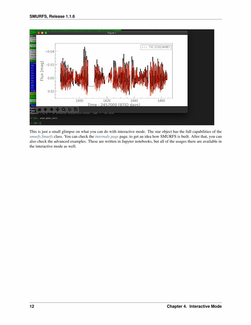
To interact with the SMURFS object, you can use the star object. Using this object you can do a myriad of things.For example, you can open an interactive plot of the light curve, by calling

star.plot_lc()

resulting in the following output:

11

https://ipython.org/


This is just a small glimpse on what you can do with interactive mode. The star object has the full capabilities of thesmurfs.Smurfs class. You can check the internals page page, to get an idea how SMURFS is built. After that, you canalso check the advanced examples. These are written in Jupyter notebooks, but all of the usages there are available inthe interactive mode as well.

12 Chapter 4. Interactive Mode

CHAPTER

FIVE

STANDALONE SETTINGS

You have now completed the Quickstart example. But what options are available to run SMURFS? Below you canfind a full list of settings available through the terminal. If you are interested in some examples, you can take a look atthose as well. Mandatory parameters are noted as such, the optional ones give you the default as well. Call smurfs -hto show a help message, explaining all parameters.

Positional arguments are required for every run of SMURFS. Named parameters can be used as explained below

usage: smurfs [-h] [-fr FREQUENCYRANGE] [-ssa] [-sc] [-ef EXTENDFREQUENCIES][-fd FREQUENCYDETECTION] [-imf {all,end,none}][-fm {scipy,lmfit}] [-ft {PDCSAP,SAP,PSF}] [-pca] [-psf] [-so][-sp SAVEPATH] [-i] [-m {Kepler,TESS,K2}] [-cl SIGMACLIP][-it ITERS] [-ac] [--version]target snr windowSize

5.1 Positional Arguments

target This parameter represents the target analyzed by SMURFS. This parameter israther vague, to give you the maximum amount of flexibility. Either you canprovide any name of a star (resolvable through Simbad) that has been observedby TESS/Kepler/K2. You can also provide a filename through this parameter.

If you choose to do the the first, the code prioritizes TESS over all other mis-sions (if you don’t provide the mission parameter), and SC over LC observations.It then checks MAST if there are SC observations from TESS for this star. Ifthere are, it uses lightkurve.search_lightcurvefile to download those. If there arenone, it checks if there are LC observations from TESS and uses Eleanor to ex-tract the light curves from the FFIs. If there are None, it searches all other mis-sions for light kurves of this object.If you choose another mission, it will calllightkurve.search_lightcurvefile for this specific mission.

If you choose to provide a file through this parameter, make sure that you followthese conventions:

• The file must be an ASCII file

• The first column must contain the time stamps

• The second column must contain the flux

• If a third column exists, SMURFS will assume that these are the uncertain-ties in the flux.

SMURFS will take the file as is and won’t apply any corrections to it, if youdon’t use the apply_corrections flag. It then assumes that the flux values are in

13


magnitude and varying around 0, that the time stamps are in days and that thedata set is properly reduced.

snr This parameter represents the lower bound signal to noise ratio any frequencymust have. SMURFS computes the SNR by taking the amplitude of an individualfrequency (as defined by the amplitude in the frequency spectrum). Next, it ap-plies half of the window size to either side of the frequency, starting by the nextadjacent minima, and takes the mean of this window as the noise surrounding thefrequency. The ratio of these two values is the resulting SNR for an individualfrequency. By default, SMURFS stops its run when the first frequency less thanthis value has been found

windowSize The window size used to get the SNR for a given frequency. SMURFS definesthe window as half of the given value on each side of the peak in the periodogram,starting from the first minima next to the peak.

5.2 Named Arguments

-fr, --frequencyRange Setting this parameter, allows you to restrict the analysis of a time series to agiven range in the frequency spectrum. This might be useful, if yo have a lot ofhigh amplitude noise in another part of the spectrum, than the one you might beinterested in. Provide the parameter in the form 0,100.

Default: “None,None”

-ssa, --skipSimilarFrequencies Ignores regions where SMURFS finds multiple frequencies within asmall range. This can happen due to insufficient fits or signals that are hard to fit.

Default: False

-sc, --skipCutoff By default, SMURFS stops the extraction of frequencies if it finds 10 frequenciesin a rowthat have a standard deviation of <0.05, as it assumes it can’t work itselfout of this region. You can override this behaviour by setting this flag. Be aware,that this might lead to unknown behaviour. Usually, instead of setting this flag, itis better to set the -ssa flag

Default: False

-ef, --extendFrequencies Extends the analysis by n frequencies. By default, SMURFS stops when itfinds the first insignificant frequency. Setting this parameter requires SMURFSto find n insignificant frequencies in a row.

Default: 0

-fd, --frequencyDetection If this value is set, a found frequency is compared to the original peri-odogramm. If the ratio between the amplitude of the found frequency and themaximum in the range of the found frequency on the original periodogram islower than the set value, it will ignore this frequency range going forward.

-imf, --improveFitMode Possible choices: all, end, none

This parameter defines the way SMURFS uses a Period04 like improvement offrequencies. You can set the following modes:

• all: Tries to refit all found frequencies after every frequeny that is found.This is the usual behaviour of Period04 and the default setting.

• end: Improves the frequencies after SMURFS would stop its run

14 Chapter 5. Standalone settings


• none: Disables the improve frequencies setting. This can be useful if youfind a lot of frequencies and the run would take an unnecessary amount oftime

Default: “all”

-fm, --fitMethod Possible choices: scipy, lmfit

SMURFS implements two different fitting libraries: Either it uses scipy(scipy.optimize.curve_fit) or lmfit (lmfit Model fit). Choosing one over the othermight lead to different results, so if you have find an unexpected result, try toswitch the fitting mode.

Default: “lmfit”

-ft, --fluxType Possible choices: PDCSAP, SAP, PSF

The TESS mission gives its end users different data products to choose, if youdownload them directly from MAST. You can pass the type of data product youlike using this parameter. For the SC data, where the light curve is preprocessedby SPOC, you can choosetwo different products:

• SAP flux: SAP is the simple aperture photometry flux (resulting light curveis the flux after summing the calibrated pixels within the TESS optimalaperture)

• PDCSAP flux: PDCSAP is the Pre-search Data conditioned Simple aperturephotometry, which is corrected using co-trending basis vectors.

By default we use the PDCSAP flux, but you can also choose another one if youlike.

If your target is only observed in LC mode, SMURFS also provides these twomodes (these have a slightly different meaning, their result is however equivalentto the SC SAP and PDSCAP fluxes, see the Eleanor documentation). However, inLC mode you have also the PSF flux type, which models a point spread functionfor a given star. The validation page generated when SMURFS extracts a targetfrom a FFI always shows the SAP and the chosen flux to compare. You mightwant to try different settings, depending on your use case

Default: “PDCSAP”

-pca, --do_pca Activates the PCA analysis (aperture × TPF + background subtraction + cotrend-ing basis vectors). This doesn’t change the data you are trying to analyze, butshows the PDSCAP flux in the validation page. Only applicable when using LCdata.

Default: False

-psf, --do_psf Activates the PSF analysis. This adds point spread function modelling to theextraction of light curves from FFIs. This doesn’t change the data you are tryingto analyze, but shows the PSF flux in the validation page. Only applicable whenusing LC data.

Default: False

-so, --storeObject If this flag is set, the SMURFS object is stored in the results. You can later usethis object to load the _result into a python file using ‘Smurfs.from_path’. Allowsyou to easily access all convenience functions from SMURFS.

Default: False

5.2. Named Arguments 15


-sp, --savePath Allows you to set the save path of the analysis. By default it will save it in thesame folder, where the module was called.

Default: “.”

-i, --interactive Using this flag will automatically start an iPython shell. This allows for directinteraction with the result using the ‘star’ object. You can then access all conve-nience functions directly (like plotting, the FrequencyFinder object, etc).

Default: False

-m, --mission Possible choices: Kepler, TESS, K2

Three different missions are available: Kepler,TESS,K2. You can choose themission by setting this value. By default, only TESS missions are considered

Default: “TESS”

-cl, --sigmaClip Sets the sigma for the sigma clipping. Default is 4.

Default: 4

-it, --iters Sets the iterations for the sigma clipping. Default is 1.

Default: 1

-ac, --apply_corrections If this flag is set, correction (sigma clipping, conversion to magnitude) areapplied to files. Make sure that your flux is in electron counts if you use this flag.

Default: False

--version Shows version of SMURFS

16 Chapter 5. Standalone settings

CHAPTER

SIX

INTERNALS

To understand the internals of SMURF, lets first consider this rough schematic on the run taken in the quickstart page.

17


Very generally, what SMURFS does is the following procedure:

18 Chapter 6. Internals


1) Create a smurfs.Smurfs() object according to the settings provided through the constructor or through thecommand line

2) Call smurfs.Smurfs.run(). This in turn creates a smurfs.FFinder() object, stored in the smurfs.Smurfs.ff() property.

3) smurfs.Smurfs.run() calls smurfs.FFinder.run(), which iteratively tries to find all significantfrequencies in the data.

4) This iterative run creates a smurfs.Frequency() object for each frequency it finds.

5) After it finds the first insignificant frequency (insignificant defined through the set SNR and window size) orafter n insignificant (if the extend_frequencies parameter is set) it stops the run and saves the data

There are a lot of different settings you can set that slightly change this behaviour one way or the other, but in principleit stays this way. While the individual pages on the classes give you a lot more insight on the each of them, we wantto give an overview here over the individual classes.

6.1 smurfs.Smurfs()

This is the base class, which is the prime interface to all things SMURFS. If you want to incorporate SMURFS intoyour own code, you want to follow this procedure (this is what SMURFS does internally also when using it as astandalone tool):

1) Instantiate smurfs.Smurfs() through the constructor and pass the appropiate parameters. Use the file parameterif you want to provide a file, use the time and flux parameter if you want to provide these things directly as arrays oruse the target_name parameter if you want to provide the name of the target.

2) Call smurfs.Smurfs.run() to start the analysis. Provide the parameters according to its documentation.

3) Call smurfs.Smurfs.save() to save the data to the path of your choosing.

This will store the result as described in quickstart page. After you completed step 2, you will also have direct accessto the smurfs.Smurfs.result() property. This property, at its heart, is a simple pandas object. It contains allthe individual smurfs.Frequency() objects and you can access each individual one through iloc. Assuming yourSMURFS object is called star, you can access it like this:

In [1]: star.resultOut[1]:

f_obj frequency→˓ amp phase snr res_noise significantf_nr0 <smurfs._smurfs.frequency_finder.Frequency obj... 1.363741+/-0.000004 0.→˓01033+/-0.00008 0.3267+/-0.0012 14.621918 -0.000890 True1 <smurfs._smurfs.frequency_finder.Frequency obj... 1.321203+/-0.000004 0.→˓01025+/-0.00008 1.2294+/-0.0012 17.646618 -0.000841 True2 <smurfs._smurfs.frequency_finder.Frequency obj... 1.470777+/-0.000015 0.→˓00281+/-0.00008 0.965+/-0.004 7.578344 -0.000855 True3 <smurfs._smurfs.frequency_finder.Frequency obj... 1.878144+/-0.000017 0.→˓00241+/-0.00008 0.517+/-0.005 6.717144 -0.000854 True4 <smurfs._smurfs.frequency_finder.Frequency obj... 1.385307+/-0.000018 0.→˓00223+/-0.00008 0.175+/-0.005 7.318523 -0.000865 True5 <smurfs._smurfs.frequency_finder.Frequency obj... 0.316642+/-0.000020 0.→˓00203+/-0.00008 0.254+/-0.006 5.597835 -0.000865 True6 <smurfs._smurfs.frequency_finder.Frequency obj... 1.417226+/-0.000023 0.→˓00181+/-0.00008 0.384+/-0.007 6.523381 -0.000859 True7 <smurfs._smurfs.frequency_finder.Frequency obj... 2.742524+/-0.000023 0.→˓00178+/-0.00008 0.943+/-0.007 9.558567 -0.000859 True

(continues on next page)

6.1. smurfs.Smurfs() 19

https://pandas.pydata.org/


(continued from previous page)

8 <smurfs._smurfs.frequency_finder.Frequency obj... 0.112357+/-0.000025 0.→˓00163+/-0.00008 0.023+/-0.007 5.270446 -0.000856 True9 <smurfs._smurfs.frequency_finder.Frequency obj... 1.237200+/-0.000029 0.→˓00139+/-0.00008 0.091+/-0.009 5.176608 -0.000856 True10 <smurfs._smurfs.frequency_finder.Frequency obj... 1.68152+/-0.00004 0.→˓00112+/-0.00008 0.166+/-0.011 4.585938 -0.000860 True

You can access each indivdual frequency through pandas iloc method, and the individual values through their names.For example, you can access the frequency object like this:

In [2]: star.result.iloc[0]Out[2]:f_obj <smurfs._smurfs.frequency_finder.Frequency obj...frequency 1.363741+/-0.000004amp 0.01033+/-0.00008phase 0.3267+/-0.0012snr 14.6219res_noise -0.000889747significant TrueName: 0, dtype: object

In [3]: star.result.iloc[0].f_objOut[3]: <smurfs._smurfs.frequency_finder.Frequency at 0x12c0536a0>

This way you can access the full interface of the smurfs.Frequency() class.

You can also access the linked smurfs.FFinder() object through the smurfs.Smurfs.ff() property:

In [4]: star.ffOut[4]: <smurfs._smurfs.frequency_finder.FFinder at 0x12c074e48>

The smurfs.Smurfs() object also gives you some statistics about each run. You can access those through thesmurfs.Smurfs.statistics() property:

In [5]: star.statisticsOut[5]:

Duty cycle Nyquist frequency Total number of found frequencies0 0.844463 360.001476 11

Reading results works through the smurfs.Smurfs.load_results() method:

In [6]: Smurfs.load_results("Gamma_Doradus/data/result.csv")Out[6]:( Unnamed: 0 Signal to Noise Ratio Window size ... Skip similar frequency→˓regions Chancel run after 10 similar frequencies Ignore unsignificant frequencies→˓number0 0 4.0 2.0 ...→˓False True→˓ 0

[1 rows x 8 columns],Unnamed: 0 Duty cycle Nyquist frequency Total number of found frequencies

0 0 0.844463 360.001476 11,f_nr frequency amp phase snr res_

→˓noise significant0 0 1.363741+/-0.000004 0.01033+/-0.00008 0.3267+/-0.0012 14.621918 -0.→˓000890 True





1 1 1.321203+/-0.000004 0.01025+/-0.00008 1.2294+/-0.0012 17.646618 -0.→˓000841 True2 2 1.470777+/-0.000015 0.00281+/-0.00008 0.965+/-0.004 7.578344 -0.→˓000855 True3 3 1.878144+/-0.000017 0.00241+/-0.00008 0.517+/-0.005 6.717144 -0.→˓000854 True4 4 1.385307+/-0.000018 0.00223+/-0.00008 0.175+/-0.005 7.318523 -0.→˓000865 True5 5 0.316642+/-0.000020 0.00203+/-0.00008 0.254+/-0.006 5.597835 -0.→˓000865 True6 6 1.417226+/-0.000023 0.00181+/-0.00008 0.384+/-0.007 6.523381 -0.→˓000859 True7 7 2.742524+/-0.000023 0.00178+/-0.00008 0.943+/-0.007 9.558567 -0.→˓000859 True8 8 0.112357+/-0.000025 0.00163+/-0.00008 0.023+/-0.007 5.270446 -0.→˓000856 True9 9 1.237200+/-0.000029 0.00139+/-0.00008 0.091+/-0.009 5.176608 -0.→˓000856 True10 10 1.68152+/-0.00004 0.00112+/-0.00008 0.166+/-0.011 4.585938 -0.→˓000860 True)

This returns two pandas DataFrames, the first containing the statistics, the second containing the actual results. Theseof course don’t include the smurfs.Frequency() objects, as this is only a text file. You can however load a fullsmurfs object (if you saved it through setting store_obj=True or by setting the -so flag when using the standaloneversion.

In [7]: star = Smurfs.from_path("Gamma_Doradus")

In [8]: starOut[8]: <smurfs._smurfs.smurfs.Smurfs at 0x13562aa20>

In [9]: star.resultOut[9]:

f_obj frequency→˓ amp phase snr res_noise significantf_nr0 <smurfs._smurfs.frequency_finder.Frequency obj... 1.363741+/-0.000004 0.→˓01033+/-0.00008 0.3267+/-0.0012 14.621918 -0.000890 True1 <smurfs._smurfs.frequency_finder.Frequency obj... 1.321203+/-0.000004 0.→˓01025+/-0.00008 1.2294+/-0.0012 17.646618 -0.000841 True2 <smurfs._smurfs.frequency_finder.Frequency obj... 1.470777+/-0.000015 0.→˓00281+/-0.00008 0.965+/-0.004 7.578344 -0.000855 True3 <smurfs._smurfs.frequency_finder.Frequency obj... 1.878144+/-0.000017 0.→˓00241+/-0.00008 0.517+/-0.005 6.717144 -0.000854 True4 <smurfs._smurfs.frequency_finder.Frequency obj... 1.385307+/-0.000018 0.→˓00223+/-0.00008 0.175+/-0.005 7.318523 -0.000865 True5 <smurfs._smurfs.frequency_finder.Frequency obj... 0.316642+/-0.000020 0.→˓00203+/-0.00008 0.254+/-0.006 5.597835 -0.000865 True6 <smurfs._smurfs.frequency_finder.Frequency obj... 1.417226+/-0.000023 0.→˓00181+/-0.00008 0.384+/-0.007 6.523381 -0.000859 True7 <smurfs._smurfs.frequency_finder.Frequency obj... 2.742524+/-0.000023 0.→˓00178+/-0.00008 0.943+/-0.007 9.558567 -0.000859 True8 <smurfs._smurfs.frequency_finder.Frequency obj... 0.112357+/-0.000025 0.→˓00163+/-0.00008 0.023+/-0.007 5.270446 -0.000856 True9 <smurfs._smurfs.frequency_finder.Frequency obj... 1.237200+/-0.000029 0.→˓00139+/-0.00008 0.091+/-0.009 5.176608 -0.000856 True


6.1. smurfs.Smurfs() 21



10 <smurfs._smurfs.frequency_finder.Frequency obj... 1.68152+/-0.00004 0.→˓00112+/-0.00008 0.166+/-0.011 4.585938 -0.000860 True

Be aware that these objects take up a lot of disk space, especially for targets with many significant frequencies.

6.2 smurfs.FFinder()

The FFinder object contains the actual logic for the frequency analysis. As describe above, it iteratively runs throughthe significant frequencies. The method that is used here is the smurfs.FFinder.run() and performs the analysisaccording to its settings. This is mostly an internal class and not much use outside of SMURFS. You can check theindividual methods through its documentation.

6.3 smurfs.Frequency()

This class represents each individual frequency. It contains all settings and results for each frequency. The process onhow the result is found is the following:

1) The object is built through the constructor by passing the light curve, snr and window size. It computes thecorresponding smurfs.Periodogram() object

2) Using the frequency with the maximum amplitude in the periodogram, it then computes the boundaries of thepeak, by finding the corresponding next two minima to the left and right of the peak

3) You can then

The most important ones are:

• smurfs.Frequency.lc(): Gives you the LightCurve object that the frequency uses for the analysis.

• smurfs.Frequency.amp(): Returns the amplitude of the frequency.

• smurfs.Frequency.f(): Returns the frequency.

• smurfs.Frequency.phase(): Returns the phase of the frequency.

• smurfs.Frequency.snr(): Returns the SNR of the frequency.


https://docs.lightkurve.org/api/lightkurve.lightcurve.LightCurve.html#lightkurve.lightcurve.LightCurve

CHAPTER

SEVEN

DOWNLOADING AND REDUCING DATA

7.1 SC data

SMURFS provides various ways to access online data. The following missions are supported and can be accessedthrough SMURFS:

• TESS

• Kepler

• K2

You can provide these missions either through the class interface of SMURFS, or as a setting in the standalone versionof SMURFS. In many cases, the download of data is facilitated through lightkurve , giving you access to SC data.

SMURFS automatically removes data points with bad quality flags and nans in the flux. In general,lightkurve.search_lightcurvefile provides the data in electron counts, which SMURFS converts into magnitude. Fur-ther, it normalizes the light curve around zero by removing the median in the data and applies sigma clipping (sigma=4,iters=1) by default. You can change this behaviour through the appropriate settings in the standalone version, or bysetting the parameters in the smurfs.Smurfs() class.

7.2 LC data download

Seeing as the vast majority of targets in TESS are observed in the LC mode, SMURFS also provides a very simpleway to access these targets. It makes heavy use of the eleanor pipeline.

If you provide a target that has been observed in TESSs LC mode, SMURFS will automatically try to resolve it throughMAST. It then will download a cutout around the target using the TessCut service. We then extract the lightcurve byusing Eleanor. It automatically tries to find the best aperture around the target, by checking apertures that have shownto work well with Kepler data. From there, the systematics are removed from the light curve, and if the PSA flag isset (which is on by default), it applies co-trending basis vectors to further improve the data. SMURFS also provides avalidation page for each LC target, showing you how the extraction worked.

23

https://docs.lightkurve.org/api/lightkurve.search.search_lightcurvefile.html?highlight=search_lightcurvefile

https://github.com/afeinstein20/eleanor

https://mast.stsci.edu/tesscut/


7.3 Using internal functions

While the interface of SMURFS is designed to be as convenient as possible, you can also choose to use the in-ternal functions to download data and load files. To make the code do the work, you can simply use smurfs.preprocess.tess.download_lc(). It has a very similar interface to the normal smurfs.Smurfs() class.

If you are interested only in the LC data of a given target (seeing as SMURFS always uses SC data if available), youcan also use the smurfs.preprocess.tess.cut_ffi() function. You need the TIC id of the target to run thisfunction. If you don’t have it, you can get it using this simple snippet:

from astroquery.mast import Catalogs

Catalogs.query_object(target_name,catalog='TIC',radius=0.003)[0]['ID']

If you are interested in the different observations that exist in MAST for a given target, you can use

from astroquery.mast import Observations

Observations.query_criteria(objectname=target_name, radius=str(0 * u.deg), project=→˓'TESS',

obs_collection='TESS')

24 Chapter 7. Downloading and reducing data

CHAPTER

EIGHT

SMURFS.SMURFS

class Smurfs(file=None, time=None, flux=None, target_name=None, flux_type='PDCSAP', label=None,quiet_flag=False, mission='TESS', sigma_clip=4, iters=1, do_pca=False, do_psf=False,apply_file_correction=False)

The Smurfs class is the main way to start your frequency analysis. The workflow for a generic problem is thefollowing:

1) Instantiate the Smurfs class, by providing the light curve through one of different methods.

2) Call ‘run’, by providing at least the signal to noise ratio and window size of the analysis.

3) Either save the analysis using ‘save’ or get the result from the class and continue your analysis.

After ‘run’ has finished, you can access the results through various channels:

• Use the ‘ff’ property (returns the ‘FFinder’ instance, where the analysis happens)

• Use the ‘result’ property

The class also has other interesting properties like ‘combinations’ (calculates all possible combinations forthe frequencies from the results, uses [pyfcomb](https://github.com/MarcoMuellner/pyfcomb) ), ‘nyquist’ ( thenyquist frequency of the provided data) and more.

You can also plot the results using the ‘plot_lc’ or ‘plot_pdg’ methods.

You can provide a light curve through three different methods:

1) Set target_name: Can be any star that has been observed by the TESS or Kepler mission. You can provideany TIC or KIC ID (including KIC/TIC) or any name resolvable by Simbad.

2) Set time and flux

3) Set file: Needs to be an ASCII file containing time and flux

Either can be used. 1) and 2) will be automatically sigma clipped and converted to magnitude.

Parameters

• file – ASCII file containing time and flux

• time – time column of the light curve

• flux – flux column of the light curve

• target_name – Name of the target, resolvable by Simbad or either KIC/TIC ID

• flux_type – If you supply a target name that has been observed by TESS SC mode, youcan choose either ‘PCDSAP’ or ‘SAP’ flux for that target.

• label – Optional label for the star. Results will be saved under this name

• quiet_flag – Quiets Smurfs (no more print message will be piped to stdout)

25

https://github.com/MarcoMuellner/pyfcomb


property combinationsGives a pandas dataframe of all possible combinations for the frequencies from result. It consists of thefollowing columns in this order:

• Name: Name of the frequency

• ID: Frequency ID (order in which it was removed from the light curve)

• Frequency: The frequency for which combinations where searched.

• Amplitude: Amplitude of the frequency

• Solution: Best solution for this frequency

• Residual: Residual for the best solution

• Independent: Flag if the frequency is independent according to the solver

• Other_solutions: All other possible solutions for this frequency

Will be populated after run was called.

property resultGives a pandas dataframe of the result from smurfs. It consists of the following columns in this order:

• f_obj: Frequency object, that represents a given frequency

• frequency

• amp

• phase

• snr

• res_noise: Residual noise

• significant: Flag that shows if a frequency is significant or not

property ffReturns the FrequencyFinder object.

property settingsReturns a dataframe consising of the settings used in the analysis.

property statisticsReturns a dataframe consisting of various statistics of the run.

property obs_lengthReturns the length of the data set.

property nyquistReturns the nyquist frequency

property duty_cycleShows the duty cycle of the light curve

property periodogramReturns a Periodogram object of the light curve.

property spectral_windowComputes the spectral window of a given dataset by transforming the light curve with constant flux.

fold(period, t0=None, transit_midpoint=None)Returns a folded light curve. Signature equivalent to lightkurve.LightCurve.fold.

26 Chapter 8. smurfs.Smurfs


flatten(window_length=101, polyorder=2, return_trend=False, break_tolerance=5, niters=3,sigma=3, mask=None, **kwargs)

Flattens the light curve by applying a Savitzky Golay filter. Signature equivalent tolightkurve.LightCurve.flatten.

run(snr=4, window_size=2, f_min=None, f_max=None, skip_similar=False, similar_chancel=True, ex-tend_frequencies=0, improve_fit=True, mode='lmfit', frequency_detection=None)Starts the frequency analysis by instantiating a FrequencyFinder object and running it. After finishing therun, combinations are computed. See FrequencyFinder.run for an explanation of the algorithm.

Parameters

• snr (float) – Signal to noise ratio, that provides a lower end of the analysis.

• window_size (float) – Window size, with which the SNR is computed.

• f_min (Optional[float]) – Minimum frequency that is considered in the analysis.

• f_max (Optional[float]) – Maximum frequency that is considered in the analysis.

• skip_similar (bool) – Flag that skips a certain range if too many similar frequenciesin this range are found in a row.

• similar_chancel – Flat that chancels the run after 10 frequencies found that are toosimilar.

• extend_frequencies (int) – Extends the analysis by this number of insignificantfrequencies.

• improve_fit – If this flag is set, all combined frequencies are re-fitted after every newfrequency was found

• mode – Fitting mode. You can choose between ‘scipy’ and ‘lmfit’

• frequency_detection – If this value is not None and the ratio between the amplitudeof the found frequency and the amplitude of the frequency in the original spectrum exceedsthis value, this frequency is ignored.

improve_result()Fits the combined found frequencies to the original light curve, hence improving the fit of the total model.

plot_lc(show=False, result=None, **kwargs)Plots the light curve. If a result is already computed, it also plots the resulting model

Parameters

• show – if this is set, pyplot.show() is called

• kwargs – kwargs for lightkurve.LightCurve.scatter

plot_pdg(show=False, plot_insignificant=False, **kwargs)Plots the periodogram. If the result is already computed, it will mark the found frequencies in the peri-odogram.

Parameters

• show – if this is set, pyplot.show() is called

• plot_insignificant – Flag, if set, insignififcant frequencies are marked in the pe-rioodogram

• kwargs – kwargs for lightkurve.Periodogram.plot

Returns

27


save(path, store_obj=False)Saves the result of the analysis to a given folder.

Parameters

• path (str) – Path where the result is stored

• store_obj – If this is set, the Smurfs object is stored, and can be later reloaded.

static from_path(path)Loads a smurfs object from path. You need to have set the store_obj flag in save, for this object to besaved.

static load_results(path)Loads the pandas dataframes from the results file :type path: str :param path: exact path of the resultsfile :return: 3 pandas dataframes, settings, statistics and results

28 Chapter 8. smurfs.Smurfs

CHAPTER

NINE

SMURFS.FFINDER

class FFinder(smurfs, f_min=None, f_max=None)The FFinder object computes all frequencies according to the input parameters. After instantiating this object,use the run method to start the computation of frequencies.

Parameters

• smurfs – Smurfs object

• f_min (Optional[float]) – Lower bound frequency that is considered

• f_max (Optional[float]) – Upper bound frequency that is considered

run(snr=4, window_size=2, skip_similar=False, similar_chancel=True, extend_frequencies=0, im-prove_fit=True, mode='lmfit', frequency_detection=None)Starts the frequency extraction from a light curve. In general, it always uses the frequency of maximumpower and removes it from the light curve. In general, this process is repeated until we reach a frequencythat has a SNR below the lower SNR bound. It is possible to extend this process, by setting the ex-tend_frequencies parameter. It then stops after extend_frequencies insignificant frequencies are found. Ifsimilar_chancel is set, the process also stops after 10 frequencies with a standard deviation of 0.05 werefound in a row.

Parameters

• snr (float) – Lower bound Signal to noise ratio

• window_size (float) – Window size, to compute the SNR

• skip_similar (bool) – If this is set and 10 frequencies with a standard deviation of0.05 were found in a row, that region will be ignored for all further analysis.

• similar_chancel – If this is set and skip_similar is False, the run chancels after 10frequencies with a standard deviation of 0.05 were found in a row.

• extend_frequencies (int) – Defines the number of insignificant frequencies, theanalysis extends to.

• improve_fit – If this is set, the combination of frequencies are fitted to the data set toimprove the parameters

• mode – Fitting mode. Can be either ‘lmfit’ or ‘scipy’

• frequency_detection – If this value is not None and the ratio between the amplitudeof the found frequency and the amplitude of the frequency in the original spectrum exceedsthis value, this frequency is ignored.

Return type DataFrame

Returns Pandas dataframe, consisting of the results for the analysis. Consists of a Frequencyobject, frequency, amplitude, phase, snr, residual noise and a significance flag.

29


plot(ax=None, show=False, plot_insignificant=False, **kwargs)Plots the periodogram of the data set, including the found frequencies.

Parameters

• ax (Optional[Axes]) – Axes object

• show – Show flag, if True, pylab.show is called

• plot_insignificant – If True, insignificant frequencies are shown

• kwargs – kwargs for Periodogram.plot

improve_result()Improves the result by fitting the combined result to the original light curve

Return type DataFrame

30 Chapter 9. smurfs.FFinder

CHAPTER

TEN

SMURFS.FREQUENCY

class Frequency(time, flux, window_size, snr, flux_err=None, f_min=None, f_max=None,rm_ranges=None)

The Frequency class represents a single frequency of a given data set. It takes the frequency of maximum poweras the guess for pre-whitening. It also computes the Signal to noise ratio of that frequency. After instantiatingthis class, you can call pre-whiten, which tries to fit the frequency to the light curve, and returns the residualbetween the original light curve and the model of the frequency.

Parameters

• time (ndarray) – Time axis

• flux (ndarray) – Flux axis

• window_size (float) – Window size, used to compute the SNR

• snr (float) – Lower end signal to noise ratio, defines if a frequency is marked as signifi-cant

• flux_err (Optional[ndarray]) – Error in the flux

• f_min (Optional[float]) – Lower end of the frequency range considered. If None, ituses 0

• f_max (Optional[float]) – Upper end of the frequency range considered. If None, ituses the Nyquist frequency

• rm_ranges (Optional[List[Tuple[float]]]) – Ranges of frequencies, that shouldbe ignored (List of tuples, that contain a f_min -> f_max range. These areas are ignored)

property ampReturns the amplitude of the found frequency (in mag)

Return type Union[float, Variable]

property fReturns the frequency of the found frequency (in c/d)


property phaseReturns the phase of the found frequency (between 0 and 1)


property significantReturns the significance of the frequency. True –> significant, False –> insignificant

Return type bool

31


property labelReturns the label of the found frequency

Return type str

property lcRepresents the light curve on which the analysis is performed

Return type LightCurve

property snrComputes the signal to noise ratio of a given frequency. It considers the area from the first minima beforethe peak until window halfed, as well as the area from the first minima after the peak until window halfed.

Return type float

Returns Signal to noise ratio of the peak

scipy_fit()Performs a scipy fit on the light curve of the object. Limits are 50% up and down from the initial guess.Computes uncertainties using the provided covariance matrix from curve_fit.

Return type Tuple[Variable, Variable, Variable, Tuple[float, float,float]]

Returns values for amplitude,frequency, phase (in this order) including their uncertainties, aswell as the param object

lmfit_fit()Uses lmfit to perform the sin fit on the light curve. We first fit all three free parameters, and then vary thephase parameter, to get a more accurate value for it. Uncertainties are computed according to Montgomery& O’Donoghue (1999).

Return type Tuple[Variable, Variable, Variable, List[float]]

Returns values for amplitude,frequency, phase (in this order) including their uncertainties, aswell as the param object

pre_whiten(mode='lmfit')‘Pre whitens’ a given light curve. As an estimate, the method always uses the frequency with maximumpower. It then performs the fit according to the mode parameter, and returns a Lightcurve object with thereduced light curve

:param mode:’scipy’ or ‘lmfit’ :rtype: LightCurve :return: Pre-whitened lightcurve object

plot(ax=None, show=False, use_guess=False)Plots the periodogramm. If a fit was already performed, it uses the fit _result by default. This can beoverwritten by setting use_guess to True

Parameters

• ax (Optional[Axes]) – Axis object

• show – Shows the plot

• use_guess – Uses the guess

Return type Optional[Axes]

Returns Axis object if plot was not shown

find_adjacent_minima()Finds the adjacent minima to the guessed frequency, and sets them within the class.

32 Chapter 10. smurfs.Frequency

CHAPTER

ELEVEN

SMURFS.PERIODOGRAM

class Periodogram(frequency, power, nyquist=None, targetid=None, default_view='frequency',meta={})

Custom Periodogram class, fit to the needs of smurfs. Mirrors the behaviour of the Lightkurve Periodogramclass, and is derived from it. See https://docs.lightkurve.org/api/lightkurve.periodogram.Periodogram.html#lightkurve.periodogram.Periodogram for documentation on the constructor parameters.

This class differs from the Lightkurve Periodogram class through two aspects: 1) It adds a different staticmethod, that converts a Lightcurve object into a periodogram. 2) The plotting and saving of data has beenadapted to fit the needs of smurfs

static from_lightcurve(lc, f_min=None, f_max=None, remove_ranges=None, sam-ples_per_peak=10)

Computes a periodogram from a Lightcurve object and normalizes it according to Parcivals theorem. Itthen reflects the physical values in the Light curve and has the same units. It then returns a Periodogramobject.

It also has a possibility to remove certain ranges from the periodogram. :type lc: LightCurve :paramlc: Lightcurve object :param f_min: Lower range for the periodogram :param f_max: Upper range for theperiodogram :type remove_ranges: Optional[List[Tuple[float]]] :param remove_ranges: List oftuples, that represent areas in the periodogram that are ignored. These are removed from the periodogram:param samples_per_peak: number of samples per peak :return: Periodogram object

plot(scale='linear', ax=None, xlabel=None, ylabel=None, title='', style='lightkurve', view=None,unit=None, color='k', **kwargs)

Plots the periodogram. Same call signature as lightkurve.periodogram.Periodogram.

to_csv(file)Stores the periodogram into a file. :param file: File object

33

https://docs.lightkurve.org/api/lightkurve.periodogram.Periodogram.html#lightkurve.periodogram.Periodogram

https://docs.lightkurve.org/api/lightkurve.periodogram.Periodogram.html#lightkurve.periodogram.Periodogram


34 Chapter 11. smurfs.Periodogram

CHAPTER

TWELVE

OTHER FUNCTIONS

12.1 Data Download

download_lc(target_name, flux_type='PDCSAP', mission='TESS', sigma_clip=4, iters=1, do_pca=False,do_psf=False)

Downloads a light curve using the TESS mission. If the star has been observed in the SC mode, it will downloadthe original light curve from MAST. You can also choose the flux type you want to use.

If it wasn’t observed in SC mode, it will try to extract a light curve from the FFIs if the target has been observedby TESS.

You can also download light curves of stars that are observed by the K2 or Kepler mission, by setting the missionparameter.

Parameters

• target_name (str) – Name of the target. You can either provide the TIC ID (TIC . . . ),Kepler ID (KIC . . . ), K2 ID(EPIC . . . ) or a name that is resolvable by Simbad.

• flux_type – Type of flux in the SC mode. Can be either PDCSAP or SAP or PSF forlong cadence data

• mission (str) – Mission from which the light curves are extracted. By default TESSonly is used. You can consider all missions by passing ‘all’ (TESS, Kepler, K2)

• sigma_clip – Sigma clip parameter. Defines the number of standard deviations that areclipped.

• iters – Iterations for the sigma clipping

Return type Tuple[LightCurve, Optional[List[Figure]]]

Returns lightkurve.LightCurve object and validation page if extracted from FFI

combine_light_curves(target_list, sigma_clip=4, iters=1)


cut_ffi(tic_id, clip=4, iter=1, do_pca=False, do_psf=False, flux_type='PDCSAP')Extracts light curves from FFIs using TESScut and Eleanor. This function automatically combines all availablesectors for a given target.

Parameters

• tic_id (int) – TIC ID of the target

• clip (float) – Sigma clip range of the target.

• iter (int) – Iterations of the sigma clipping

35


• do_pca (bool) – Perform pca analysis with eleanor

• do_psf (bool) – Perform psf analysis with eleanor

• flux_type – Flux type that is returned. Choose between ‘PDCSAP’,’SAP’,’PSF’

Return type Tuple[LightCurve, List[Figure]]

Returns Lightcurve

mag(lc)Converts and normalizes a LighCurve object to magnitudes.

Parameters lc (LightCurve) – lightcurve object


Returns reduced light curve object

load_file(file, clip=4, it=1, apply_file_correction=False)Loads and normalizes target content :type file: str :param file: Name of target including path :rtype:LightCurve :return: LightCurve object

12.2 Miscellaneous

m_od_uncertainty(lc, a)Computes uncertainty for a given light curve according to Montgomery & O’Donoghue (1999).

Parameters

• lc (LightCurve) – smurfs.Lightcurve() object

• a (float) – amplitude of the frequency

Return type Tuple

Returns A tuple of uncertainties in this order: Amplitude, frequency, phase

mprint(text, type)

ctext(text, type)

Return type str

class cd(newPath)Directory changer. can change the directory using the ‘with’ keyword, and returns to the previous path afterleaving intendation. Example:

with cd(“some/path/to/go”): # changing dir foo() . . . bar()

#back to old dir

36 Chapter 12. Other functions

CHAPTER

THIRTEEN

DOWNLOADING DATA

One of the core features in SMURFS is the downloading of data from MAST directly. To download these light curves,simply instantiate a smurfs object. Lets download the TESS observations for our favourite Delta Scuti pulsator: BetaPictoris

[1]: from smurfs import Smurfs

[2]: star = Smurfs(target_name="Beta Pictoris")

Searching processed light curves for Beta Pictoris on mission(s) TESS ...Resolving Beta Pictoris to TIC using MAST ...TIC ID for Beta Pictoris: TIC 270577175Short cadence observations available for Beta Pictoris. Downloading ...Found processed light curve for Beta Pictoris!Using TESS observations! Combining sectors ...Total observation length: 105.18 days.Duty cycle for Beta Pictoris: 86.02%

[3]: star.plot_lc()

But using the most common name alone isn’t the only thing we can use here. We can also use the Gaia ID for example:

[4]: star = Smurfs(target_name="Gaia DR2 4792774797545105664")

37


Searching processed light curves for Gaia DR2 4792774797545105664 on mission(s) TESS ...Resolving Gaia DR2 4792774797545105664 to TIC using MAST ...TIC ID for Gaia DR2 4792774797545105664: TIC 270577175Short cadence observations available for Gaia DR2 4792774797545105664. Downloading ...Found processed light curve for Gaia DR2 4792774797545105664!Using TESS observations! Combining sectors ...Total observation length: 105.18 days.Duty cycle for Gaia DR2 4792774797545105664: 86.02%

[5]: star.plot_lc()

As we can see, both stars are the same, as their TIC IDs are the same.

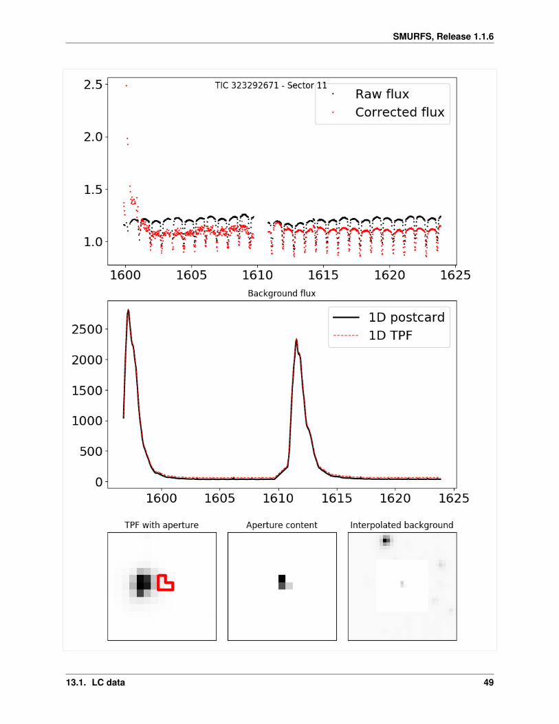
13.1 LC data

But downloading SC data from TESS is easy. We can also download LC data for TESS targets. Lets consider the starET Cha

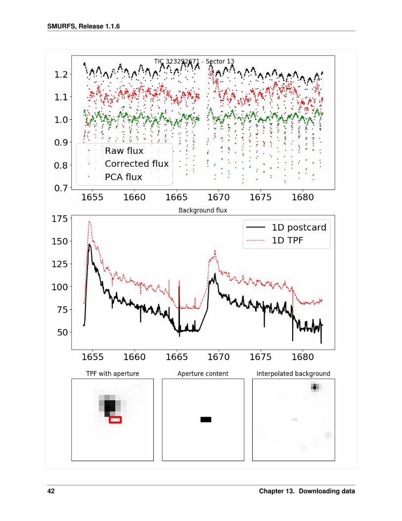
[6]: star = Smurfs(target_name='ET Cha')

Searching processed light curves for ET Cha on mission(s) TESS ...Resolving ET Cha to TIC using MAST ...TIC ID for ET Cha: TIC 323292671No short cadence data available for ET Cha, extracting from FFI ...Extracting light curves from FFIs, this may take a bit ...Found star in Sector(s) 11 12 13

Extracted light curve for TIC 323292671!Total observation length: 82.48 days.Duty cycle for ET Cha: 92.88%

38 Chapter 13. Downloading data


13.1. LC data 39


13.1. LC data 41


As you can see above, if you provide a LC target, SMURFS will automatically generate a validation page for itsreduction. At the top, you can see the combination of all three sectors, representing the first page in the pdf. The otherpages consist of the individual sectors and their reductions. You can see the individual fluxes. By default it alwaysuses the PCA flux. It also shows you the Background flux of the CCD in the plot below that and the aperture as wellas the FFI below that.

But which flux is the best? You can pass the pca and psf flag, to show you all the different fluxes available through theEleanor pipeline.

[7]: star = Smurfs(target_name='ET Cha',do_pca=True,do_psf=True)


WARNING:tensorflow:From /Users/marco/Documents/Dev/science/smurf/venv/lib/python3.6/→˓site-packages/eleanor_mamu-1.0.2-py3.6.egg/eleanor/targetdata.py:826: The name tf.→˓logging.set_verbosity is deprecated. Please use tf.compat.v1.logging.set_verbosity→˓instead.

WARNING:tensorflow:From /Users/marco/Documents/Dev/science/smurf/venv/lib/python3.6/→˓site-packages/eleanor_mamu-1.0.2-py3.6.egg/eleanor/targetdata.py:826: The name tf.→˓logging.ERROR is deprecated. Please use tf.compat.v1.logging.ERROR instead.

100%|| 1248/1248 [00:12<00:00, 99.27it/s]

100%|| 1289/1289 [00:12<00:00, 106.55it/s]

100%|| 1320/1320 [00:12<00:00, 102.56it/s]


13.1. LC data 43


13.1. LC data 45


13.1. LC data 47


All available fluxes are now visible in the Validation page. The PCA flux seems to be the best for this target, which isthe default flux used. If we would want to use any other, we could pass the flux_type parameter.

[8]: star = Smurfs(target_name='ET Cha', flux_type='SAP')





13.1. LC data 49


13.1. LC data 51


13.2 Other misssions

We can also use other missions if we like. Lets have a look at the Star Kepler-10 from the Kepler mission:

[9]: star = Smurfs(target_name='Kepler-10', mission='Kepler')

Searching processed light curves for Kepler-10 on mission(s) Kepler ...Found processed light curve for Kepler-10!Using Kepler observations! Combining sectors ...Total observation length: 1470.46 days.Duty cycle for Kepler-10: 75.40%

[10]: star.plot_lc()

The default is however TESS. So if we don’t provide the mission parameter, SMURFS will download the SC data.

[11]: star = Smurfs(target_name='Kepler-10')

Searching processed light curves for Kepler-10 on mission(s) TESS ...Resolving Kepler-10 to TIC using MAST ...TIC ID for Kepler-10: TIC 377780790Short cadence observations available for Kepler-10. Downloading ...Found processed light curve for Kepler-10!Using TESS observations! Combining sectors ...Total observation length: 26.85 days.Duty cycle for Kepler-10: 96.44%




[ ]:

13.2. Other misssions 53

CHAPTER

FOURTEEN

PLOTTING THINGS

SMURFS implements quite a lot of different plotting mechanisms. So lets have a look at the different ways you canplot things with SMURFS. Lets first get some data and analyze it:


[2]: star = Smurfs(target_name='Gamma Doradus')

Searching processed light curves for Gamma Doradus on mission(s) TESS ...Resolving Gamma Doradus to TIC using MAST ...TIC ID for Gamma Doradus: TIC 219234987Short cadence observations available for Gamma Doradus. Downloading ...

Warning: 31% (6168/19692) of the cadences will be ignored due to the quality mask→˓(quality_bitmask=175).

Found processed light curve for Gamma Doradus!Using TESS observations! Combining sectors ...Total observation length: 78.32 days.Duty cycle for Gamma Doradus: 84.45%

[3]: star.run(snr=4,window_size=2)

Periodogramm from 0.0 1 / d to 360.0 1 / dStarting frequency extraction.Skip similar: DeactivatedChancel after 10 similar: ActivatedWindow size: 2Number of extended frequencies: 0Nyquist frequency: 360.0 1 / dList of frequencies, amplitudes, phases, S/NF0 1.363601+/-0.000004 1 / d 0.01056+/-0.00008 mag 0.5105+/-0.0011 14.621917538996478F1 1.3214676+/-0.0000031 1 / d 0.01011+/-0.00006 mag 0.8538+/-0.0009 17.646618113213755F2 1.470851+/-0.000007 1 / d 0.002806+/-0.000035 mag 0.8600+/-0.0020 7.578344472336695F3 1.878144+/-0.000007 1 / d 0.002413+/-0.000032 mag 0.5167+/-0.0021 6.717143847007492F4 1.385307+/-0.000007 1 / d 0.002228+/-0.000030 mag 0.1748+/-0.0022 7.318522855378772F5 0.316642+/-0.000008 1 / d 0.002030+/-0.000028 mag 0.2544+/-0.0022 5.597834999218046F6 1.417226+/-0.000008 1 / d 0.001813+/-0.000027 mag 0.3842+/-0.0024 6.523381016995975F7 2.742524+/-0.000008 1 / d 0.001779+/-0.000026 mag 0.9427+/-0.0023 9.558566515908968F8 0.112357+/-0.000008 1 / d 0.001629+/-0.000024 mag 0.0235+/-0.0024 5.27044577952894F9 1.237200+/-0.000009 1 / d 0.001393+/-0.000023 mag 0.0913+/-0.0026 5.176607940138036F10 1.681520+/-0.000011 1 / d 0.001115+/-0.000022 mag 0.1662+/-0.0032 4.585937811798608Stopping extraction after 11 frequencies.Total frequencies: 11Gamma Doradus Analysis done!

55


14.1 Plotting the light curve

Now, if you want to plot the light curve, you can call the plot_lc method

[4]: star.plot_lc()

In black you can see the data set, in red the model.

In the backend, SMURFS uses the lightkurve.LightCurve.plot method to plot the light curve. You have access to allthe parameters for these objects. We can make use of this if we want to plot the light curve without the model:

[5]: star.lc.scatter()

[5]: <matplotlib.axes._subplots.AxesSubplot at 0x1319cb5c0>

56 Chapter 14. Plotting things


14.2 Plotting periodograms

What is true for the LightCurve objects, is also true for the periodogram. To plot the periodogram, including thesignificant frequencies, you can use the plot_pdg function

[6]: star.plot_pdg()

This of course restricts us to the range where significant frequencies have been found. If we want the whole peri-odogram, we can use the pdg property

[7]: star.pdg.plot()

[7]: <matplotlib.axes._subplots.AxesSubplot at 0x13246d518>

14.2. Plotting periodograms 57


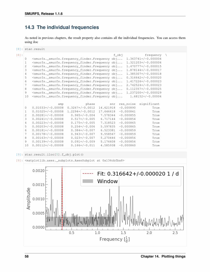
14.3 The individual frequencies

As noted in previous chapters, the result property also contains all the individual frequencies. You can access themusing iloc

[8]: star.result

[8]: f_obj frequency \0 <smurfs._smurfs.frequency_finder.Frequency obj... 1.363741+/-0.0000041 <smurfs._smurfs.frequency_finder.Frequency obj... 1.321203+/-0.0000042 <smurfs._smurfs.frequency_finder.Frequency obj... 1.470777+/-0.0000153 <smurfs._smurfs.frequency_finder.Frequency obj... 1.878144+/-0.0000174 <smurfs._smurfs.frequency_finder.Frequency obj... 1.385307+/-0.0000185 <smurfs._smurfs.frequency_finder.Frequency obj... 0.316642+/-0.0000206 <smurfs._smurfs.frequency_finder.Frequency obj... 1.417226+/-0.0000237 <smurfs._smurfs.frequency_finder.Frequency obj... 2.742524+/-0.0000238 <smurfs._smurfs.frequency_finder.Frequency obj... 0.112357+/-0.0000259 <smurfs._smurfs.frequency_finder.Frequency obj... 1.237200+/-0.00002910 <smurfs._smurfs.frequency_finder.Frequency obj... 1.68152+/-0.00004

amp phase snr res_noise significant0 0.01033+/-0.00008 0.3267+/-0.0012 14.621918 -0.000890 True1 0.01025+/-0.00008 1.2294+/-0.0012 17.646618 -0.000841 True2 0.00281+/-0.00008 0.965+/-0.004 7.578344 -0.000855 True3 0.00241+/-0.00008 0.517+/-0.005 6.717144 -0.000854 True4 0.00223+/-0.00008 0.175+/-0.005 7.318523 -0.000865 True5 0.00203+/-0.00008 0.254+/-0.006 5.597835 -0.000865 True6 0.00181+/-0.00008 0.384+/-0.007 6.523381 -0.000859 True7 0.00178+/-0.00008 0.943+/-0.007 9.558567 -0.000859 True8 0.00163+/-0.00008 0.023+/-0.007 5.270446 -0.000856 True9 0.00139+/-0.00008 0.091+/-0.009 5.176608 -0.000856 True10 0.00112+/-0.00008 0.166+/-0.011 4.585938 -0.000860 True

[9]: star.result.iloc[5].f_obj.plot()

[9]: <matplotlib.axes._subplots.AxesSubplot at 0x136cbfba8>



To plot the corresponding light curve, we can access them through the corresponding property

[10]: star.result.iloc[5].f_obj.lc.scatter()

[10]: <matplotlib.axes._subplots.AxesSubplot at 0x136cec278>

We can also take a look at the whole periodogram

[11]: star.result.iloc[5].f_obj.pdg.plot()

[11]: <matplotlib.axes._subplots.AxesSubplot at 0x130aaf6a0>

We can also plot as many as we like here. For example the first three:

[12]: star.result.iloc[0].f_obj.plot()


14.3. The individual frequencies 59



star.result.iloc[1].f_obj.plot()star.result.iloc[2].f_obj.plot()

[12]: <matplotlib.axes._subplots.AxesSubplot at 0x12fe0d550>



14.4 Plotting only part of the model

We might also be interested to only plot part of the model. For this, we copy the result from the smurfs object andrestrict ourselves to the interesting frequencies:

[14]: model = star.result.iloc[[0,2,5]]

[15]: model

[15]: f_obj frequency \0 <smurfs._smurfs.frequency_finder.Frequency obj... 1.363741+/-0.0000042 <smurfs._smurfs.frequency_finder.Frequency obj... 1.470777+/-0.0000155 <smurfs._smurfs.frequency_finder.Frequency obj... 0.316642+/-0.000020

amp phase snr res_noise significant0 0.01033+/-0.00008 0.3267+/-0.0012 14.621918 -0.000890 True2 0.00281+/-0.00008 0.965+/-0.004 7.578344 -0.000855 True5 0.00203+/-0.00008 0.254+/-0.006 5.597835 -0.000865 True

[18]: star.plot_lc(result=model)

14.4. Plotting only part of the model 61



You can of course use any filtering you like with pandas.

[ ]:


CHAPTER

FIFTEEN

LOOKING AT THE FULL FRAME IMAGES OF SC DATA

Sometimes it might be useful to take a look at the FFI and the LC time series of data for which short cadence isavailable. By default, SMURFS uses the SC data, but using some internal functions, we can still take a look at the FFI


Lets consider Beta Pictoris. It has 4 sectors of SC available at this point.

[2]: star = Smurfs(target_name="Beta Pictoris")

Searching processed light curves for Beta Pictoris on mission(s) TESS ...Resolving Beta Pictoris to TIC using MAST ...TIC ID for Beta Pictoris: TIC 270577175Short cadence observations available for Beta Pictoris. Downloading ...Found processed light curve for Beta Pictoris!Using TESS observations! Combining sectors ...Total observation length: 105.18 days.Duty cycle for Beta Pictoris: 86.02%

[3]: star.plot_lc()

But how does the FFI and the surrounding look like? For this, we’ll use what Smurfs internally: the cut_ffi function.For this function to work, we need the TIC number. We can either take a look at the output above, or use astroquery tofind the TIC ID

63


[5]: from astroquery.mast import Catalogs

[9]: tic_id = int(Catalogs.query_object("Beta Pictoris",catalog='TIC',radius=0.003)[0]['ID→˓'])tic_id

[9]: 270577175

Now lets feed this into smurfs

[4]: from smurfs.preprocess.tess import cut_ffi

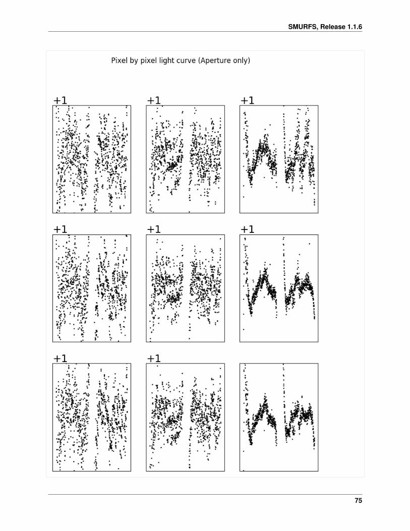
[10]: lc,fig = cut_ffi(tic_id=tic_id)

Found star in Sector(s) 4 5 6 7Inflating...This is the first light curve you have made for this sector. Getting eleanor metadata products for Sector 4...This will only take a minute, and only needs to be done once. Any other light curves you make in this sector will be faster.Target AcquiredCadences CalculatedQuality Flags AssuredCBVs MadeSuccess! Sector 4 now available.Inflating...Inflating...This is the first light curve you have made for this sector. Getting eleanor metadata products for Sector 5...This will only take a minute, and only needs to be done once. Any other light curves you make in this sector will be faster.Target AcquiredCadences CalculatedQuality Flags AssuredCBVs MadeSuccess! Sector 5 now available.Inflating...Inflating...Inflating...This is the first light curve you have made for this sector. Getting eleanor metadata products for Sector 7...This will only take a minute, and only needs to be done once. Any other light curves you make in this sector will be faster.Target AcquiredCadences CalculatedQuality Flags AssuredCBVs MadeSuccess! Sector 7 now available.Inflating...

Extracted light curve for TIC 270577175!

64 Chapter 15. Looking at the full frame images of SC data


65


67


69


71


73


75


[ ]:

77

CHAPTER

SIXTEEN

INDEX AND SEARCH FUNCTION

genindex

search

79


80 Chapter 16. Index and search function

INDEX

Aamp() (Frequency property), 31

Ccd (class in smurfs.support.support), 36combinations() (Smurfs property), 25combine_light_curves() (in module

smurfs.preprocess.tess), 35ctext() (in module smurfs.support.mprint), 36cut_ffi() (in module smurfs.preprocess.tess), 35

Ddownload_lc() (in module smurfs.preprocess.tess),

35duty_cycle() (Smurfs property), 26

Ff() (Frequency property), 31ff() (Smurfs property), 26FFinder (class in smurfs), 29find_adjacent_minima() (Frequency method), 32flatten() (Smurfs method), 26fold() (Smurfs method), 26Frequency (class in smurfs), 31from_lightcurve() (Periodogram static method),

33from_path() (Smurfs static method), 28

Iimprove_result() (FFinder method), 30improve_result() (Smurfs method), 27

Llabel() (Frequency property), 31lc() (Frequency property), 32lmfit_fit() (Frequency method), 32load_file() (in module smurfs.preprocess.file), 36load_results() (Smurfs static method), 28

Mm_od_uncertainty() (in module

smurfs._smurfs.frequency_finder), 36

mag() (in module smurfs.preprocess.tess), 36mprint() (in module smurfs.support.mprint), 36

Nnyquist() (Smurfs property), 26

Oobs_length() (Smurfs property), 26

PPeriodogram (class in smurfs), 33periodogram() (Smurfs property), 26phase() (Frequency property), 31plot() (FFinder method), 29plot() (Frequency method), 32plot() (Periodogram method), 33plot_lc() (Smurfs method), 27plot_pdg() (Smurfs method), 27pre_whiten() (Frequency method), 32

Rresult() (Smurfs property), 26run() (FFinder method), 29run() (Smurfs method), 27

Ssave() (Smurfs method), 27scipy_fit() (Frequency method), 32settings() (Smurfs property), 26significant() (Frequency property), 31Smurfs (class in smurfs), 25snr() (Frequency property), 32spectral_window() (Smurfs property), 26statistics() (Smurfs property), 26

Tto_csv() (Periodogram method), 33

81

SMURFS - Release 1.1.6 Marco Müllner

Documents

Transcript of SMURFS - Release 1.1.6 Marco Müllner