SM

AR

T G

RID

Section 1:

Electric Vehicles

This paper has been accepted for poster at the APEC 2012 Conference, Orlando, FL, Feb. 5-9, 2012

Investigation of the Topology and Control for A 4800-V Grid-

Connected Electrical Vehicle Charging Station with STACOM-APF

Functions Using A Bi-directional, Multi-level, Cascaded Converter

Abstract— This paper presents a new design for an ultra-fast,

public electric vehicle (EV) charging station. Because of the

multi-megawatt nature of such a station, the design is aimed at

being appropriate for a medium voltage (MV) connection.

Through the proper choice of a multi-level topology and

staircase modulation, it is able to operate efficiently and provide

galvanic isolation without the use of a large transformer. As a

further benefit for this application, it is able to provide reactive,

harmonic, and unbalanced load compensation. Simulation

results are provided in Simulink to verify the effectiveness of the staircase modulation and capabilities of the topology.

I. INTRODUCTION

In comparison to conventional road vehicles, electric

vehicles (EVs) suffer from a limited range and long (>15

min.) charging times. It has been suggested [1] that the

existence of public, ultrafast (≤3 min.) charging stations will

address this issue to some extent. However, such stations have numerous challenges to overcome. For reasons of cost

and multi-megawatt power levels, one challenge is to

interface directly with distribution-level voltages (MV) while

drawing an acceptable harmonic profile. For reasons of

footprint and safety, a second challenge is to do this without a

conventional (50/60 Hz) transformer while providing

galvanic isolation for safety reasons. A final challenge is to

address the negative impact that such stations are predicted to

have on the electrical grid [1].

In addition to these challenges, there is a strong

preference from utilities and investors to invest in new infrastructure and technology when it can provide multiple

services or benefits in addition to its primary purpose.

Because a charging station does not always operate at full

power, this translates into several MVA of capacity that could

be utilized (e.g., to provide reactive power support).

Therefore, we have identified the following goals in addition

to challenges discussed above: (1) the ability to compensate

existing reactive, harmonic, and negative-sequence currents

on the distribution system; (2) the ability to provide

additional reactive support; and (3) the ability to provide load

leveling (with the incorporation of a large battery or some

other form of energy storage).

Existing topologies (for example, [1-7]) do not address all of these issues. In this paper, we present a modular design based on the isolated, DC-DC cell in [8]. These cells are connected and controlled in such a way to act as a MV, cascaded, multi-level inverter. Through an appropriate control and modulation scheme (described herein), our unique topology can draw arbitrary waveforms from the grid. This allows it to have STATCOM/APF and load-leveling capabilities to meet the goals above and to address its cost (both in capital expense and in negative impact on the grid). In addition, it draws current with an acceptable harmonic profile, is modular, provides galvanic isolation from the MV (4.8 kVrms, phase-phase or 3.92 kV) grid, and has a small footprint due to the absence of a 50/60 Hz transformer.

II. TOPOLOGY

A. Ultrafast Topology

We determined that the charging station (Fig. 1) should

have a power rating of 2.4 MW (6 EVs, up to 400 kW each).

In addition, we determined that the station should have an

apparent power rating of 6 MVA to provide active and

reactive power for grid support purposes. To achieve this

MVA capacity and to achieve the current slew rate necessary

for APF functionality, we determined that each phase should

be able to produce +-4800 V and that the inductor L of each

phase should be equal to 1 mH. To minimize the charging station's impact on the grid

during peak loading, we propose using a large battery or other

form of energy storage for the common DC-link. This will

enable EV charging without drawing power from the grid

during those times. Because the topology is bi-directional, the

battery can also be used to supply the grid during when the

marginal cost of generation is very high.

This work has been supported, in part, by a grant from CPS Energy, San

Antonio, TX through Texas Sustainable Energy Research Institute,

University of Texas, San Antonio.

Russell Crosier, Shuo Wang and Mo Jamshidi

Power Electronics and Electrical Power Research Laboratory

Electrical and Computer Engineering Department

University of Texas at San Antonio

San Antonio, TX 78249

This paper has been accepted for poster at the APEC 2012 Conference, Orlando, FL, Feb. 5-9, 2012

4800 V

Grid vgrid,b

vgrid,a

vgrid,c

EV1 DC/DC

EV2

EVN

Battery

(Common DC-

Link)

Phase A

Multi-

Level

Inverter

Phase B

Multi-

Level

Inverter

Phase C

Multi-

Level

Inverter

+ -vg,n

Reactive,

Harmonic,

Unbalanced

Load

iext,b

iext,a

iL,a iL,b iL,cL L L HBIsolated

DC/DC #1

HB

HB

Cascaded, Multi-level

Inverter in each Phase

(a)

DC/DC

DC/DC

Isolated

DC/DC #2

Isolated

DC/DC #12

(b)

iext,c

g n

Figure 1: Layout of charging station with grid and load to be compensated (a) and the makeup of the multi-level inverter in each phase (b).

To have non-visible rules on your frame, use the MSWord “Format” pull-down menu, select Text Box > Colors and Lines to choose No Fill and No Line.

Our topology is u nique in that power flows through a

common DC-link (see Fig. 1a) without the use of a bulky

transformer. We have selected the cascaded H-bridge (HB),

multilevel inverter of Fig. 1b as one of the best practical

alternative to using a large transformer (SiC devices promise

to fulfill this task with two-level inverters and enhanced

efficiency in the future [9]). In particular we use 12, cascaded HBs per phase, each with a floating, 400V DC-link. Whether

or not Si-C is used in future implementations to enhance the

efficiency of our topology, multilevel modulation of the

output voltage is optimal for this particular application

because, as detailed in section V, it has vastly superior

harmonic performance.

Finally, because of the modularity inherent in Fig. 1B, our

topology is easily adapted to other voltages (say 7.2 or 13.8

kV). Alternatively, the HBs in Fig. 1B can be designed with

higher DC-link voltages. The choice between these two

alternatives depends on whether improving efficiency or harmonic performance is a priority.

B. Isolated, Bi-directional, DC-DC Converters and the

Common DC-Link

As mentioned above, in our topology all power flows

through the common DC-link. Key to this are the isolated, bi-

directional, DC-DC converters shown in Fig. 1b. By virtue of

the isolation, the DC-links in Fig. 1b can be stacked by the

HBs while still being able to transfer energy to and from the

common DC-link. [8] discusses a zero-voltage-switching

(ZVS) converter that is a possible candidate for this

application. As this paper focuses on the control of the output current and the necessary modulation of the HBs to achieve

that, readers interested in the design and control of the

isolated converters are directed to [8].

However, it is worth analyzing the benefit of a common DC-link. The total, instantaneous power drawn by a 3-phase load is constant in time for balanced, sinusoidal conditions.

Therefore, when drawing/ supplying positive sequence current from/to the grid, our topology results in no low frequency power circulation in the battery (as shown in the simulation results). In theory, there are some other topologies that can draw a balanced, 3-phase power from MV levels and transfer it to a single DC load. However, they are unsuitable for this application because they either cannot function as a charging station [9], use a large transformer [1-3], draw unacceptable harmonics [4], have excessive capacitance requirements [1,3,5], do not provide galvanic isolation ([6] and [10]). Additionally, because the isolated, DC-DC converters are bidirectional and energy can be freely transferred between phases, our topology can correct any load imbalance upstream of it (as shown it Fig. 1a).

Figure 2: Overall control diagram showing how the reference current and

then inverter reference voltage are determined.

III. REFERENCE CURRENT IDENTIFICATION

As shown in Fig. 2, the overall control process consists of

two main steps which are the reference current identification

(determining what current to draw from the grid) and the

inverter voltage reference identification (the voltage

necessary to control iLa, iLb, and iLc in Fig. 1 so they follow

Observed

Grid

Voltage

Pref

Observed

External

Load Current

Qref

Compensation

Current

Identification

Reactive

Current

Identification

Active Current

Identification

Inductor (output)

Current

Controller

Inductor

Current

Feedback

Reference Current Identification

Inverter

Reference

Voltage

Identification

+

+

iref,act

iref,ractiext,comp

iref iL

Inverter Reference

Voltage

+

This paper has been accepted for poster at the APEC 2012 Conference, Orlando, FL, Feb. 5-9, 2012

the reference current). In this section, we develop a reference

current identification scheme to achieve the following tasks:

draw the appropriate amount of power to charge the EVs,

charge/discharge the battery as commanded to provide grid support, provide APF/STATCOM compensation of the

external load in Fig. 1a, and supply reactive power (in

addition to that supplied by the STATCOM functionality)

when commanded.

The first two tasks both require active power. Therefore, the first component of the inductor reference current is the active reference current and is a function of the reference power, Pref. We use the following equation which, according to [14], calculates the active, positive sequence current necessary to draw Pref:

grid

T

refgrid

activeref

grid

P

vv

vi

,

where vgrid is the observed, three-phase, grid voltage column,

vgrid Tvgrid is the dot product of the grid voltage with itself, and

bold is used to indicate a three phase column vector. Pref is a

function of the power demanded by the EVs and the power

commanded to charge/discharge the battery. However, it is

determined by a feedback controller and, so, is discussed in

section IV.B.

Next we write the reference current to provide STATCOM/APF functionality. First, need to determine the component of the load current that we don’t want to compensate. To do this, we adapt (1) to yield the active, positive-sequence current of the external load:

grid

T

extestgrid

activeext

grid

P

vv

vi

,

,

where Pest,ext is the estimated, active power of the external

load and is given by (6) and, again, bold indicates a three

phase column vector.

Because the remaining components of the load current are what we wish to compensate, we write the compensation current reference as

ext

grid

T

extestgrid

activeextextcompref

grid

Pi

vv

viii

,

,,

where iext is the observed, external load current and the

negative sign outside of the parentheses is due to the direction of the inductor current in Fig. 1a.

The final component of the reference current, is the component necessary to provide reactive support to the grid (in addition to reactive power supplied by compensating the external load). This is often desirable because supplying a net amount reactive power to the grid can help boost the voltage

at a load bus. In order for the incoming inductor current to supply reactive power to the grid, the current needs to lead the grid voltage by 90˚. Therefore, (1) can be modified to give the equation for reactive current reference:

grid

T

grid

reflinegrid

reacref

Qft

vv

vi

))4/(3(,

where Qref is the reference command to supply reactive power to the grid and fline is line frequency. Because Qref results in a balanced reactive power being supplied, this function does impose any extra requirements on or incur any losses in the battery.

Now that we have (1-3), we can combine them to form the equation for the total reference current of the inductors:

ext

grid

T

reflinegridestextrefgrid

comprefreacrefactrefref

grid

QftPPi

vv

vv

iiii

))4/(3()( ,

,,,

where Pest,ext is given by (6) and line frequency is 60Hz.

We discuss the determination of Pest,ext last because it has a strong effect on APF/STATCOM performance. Various algorithms exist for this purpose with various trade-offs. We use the method developed in [11] which has an excellent trade-off between rapid transient response and robustness. It is also very simple:

dtPt

text

T

extest grid )(120

.sec 1

120/.sec, iv ,

where vgridTiext is dot product of the grid voltage and the

external load current, and the integral is implemented with a

moving average filter over the most recent half-cycle.

IV. CONTROL AND MODELING

A. Inductor Current Control

In order for the inductor current, iL, in Fig. 1a to follow the reference current, iref, in equation (1), the correct voltage needs to applied to those inductors, and thus the correct inverter voltage v must be synthesized for each phase. Again, bold variables indicate a three-phase vector. To begin, we write the basic equation for the inductor current:

),(d

d1,

vvi

gngrid

abcLvL

t

where vgrid is the three phase grid voltage, v is the three phase

inverter voltage, and vgn is the common mode voltage

between the grid ground and the floating inverter neutral.

Since there is no neutral current, we do not desire there to be any neutral component in the reference current. Therefore, there will no neutral component in di/dt. With this assumption, we can drop the ground to neutral voltage:

This paper has been accepted for poster at the APEC 2012 Conference, Orlando, FL, Feb. 5-9, 2012

),vv(Ltd

idgrid

1L (8)

We are now going to approximate di/dt as being constant in the next Ts seconds (Ts is sampling time period or the dead-beat delay time in dead beat control and is set to 1/2880 or .000347 sec. as described at the end of section V). Therefore, we write:

),(1vv

I

grid

s

L LT

Now we assume that we want iL to be iref at the end of this period. Therefore, ΔiL=iref-iL. Substituting this expression into (4) yields:

),(1vv

ii

grid

s

LrefL

T

and isolating v yields

s

Lref

gridT

Lii

vv

(*)

*

Equation (6) is the is inverter voltage necessary to make

ΔiL=iref-iL. That is, iL will equal iref at the end of each Ts

interval. Whenever a discrete-time controller is used to make a first-order system (as ours is) have zero error after one

switching cycle, it known as deadbeat control (although this

definition can be modified for nth order systems). However, as

we are using a natural form of modulation (Section V), the

controller runs in continuous time and, strictly speaking, is

not deadbeat.

Notice that there are “(*)” operators in (6). This is because we need to modify the expression for v. As discussed in section V, to prevent multiple switching, we need to add a smoothing filter to the expression for v. This expression is given by:

*

2

*

)(1053.097

053.

)()()(

ssse

s

ssCs smooth

V

VV

where Csmooth(s) has unity gain at its resonance frequency of 60 Hz and a Q of 1/20.

In addition to Csmooth(s), we need to compensate iref so that the resulting iL will not have a steady-state, phase error at 60 Hz due to the delay of Ts. Therefore, we compensate iref with a lead compensator:

)(534

266413.1)()()( * s

s

sssCs refrefleadref III

where Clead(s) has unity gain and a phase lead of 19.6° at 60

Hz and minimal effect on other frequencies.

Combining (6), (7), and (8) yields the final equation for the inverter voltage:

s

Lref

grid

2

T

)s(I)s(I534s

266s413.1

L)s(V.

1s053.s09e7

s053.)s(V

When this equation and L = 1 mH are used, the inductor current has the per-phase transfer function of

053.s5e84.1s9e44.2

075.

534s

266s

)s(I

)s(I

2

ref,L

phase,L

B. Battery Power Flow Control Loop and System Model

Under normal circumstances, the power demanded by the charging EVs (hereafter refered to as Pdem,EV) should be matched by power flowing from the grid, through the multi-level inverters to the DC-link (hereafter called Pret). However, because ultra-fast vehicle charging presents a very transient load (especially if pulse-and-burp methods [12] are employed), we use an integral controller to soften the transients presented to the grid. In addition, integral control ensures that Pret is exactly equal to Pdev,EV. To achieve this we have

)()(10

)( ,

(*) sPsPs

sP retEVdemref

where the integral gain of 10 is chosen to yield dominant pole

in (20).

Equation (16) contains “(*)” because it needs modification. It does not allow the common DC-link’s battery to be discharged (for grid support) or charged back up. Instead, it ensures that, at steady state, the returned power will exactly match the power consumed by the EVs. Therefore, we modify the integrand of (16) to allow the returned power to be different from the power consumed by the EVs if desired:

)()()(10

)( pp,, sPsPsPs

sP retsurefEVdemref

where Pref,supp is the reference power for grid support. When

Pref,supp is negative, then the steady state value of Pret will be

greater than Pdem,EV. This discrepancy will flow into the

battery causing the battery to be charged. Vice versa, when

Pref,supp is positive, the battery will discharge providing grid support.

This paper has been accepted for poster at the APEC 2012 Conference, Orlando, FL, Feb. 5-9, 2012

Figure 3: (a) Response of power consumed by station (gray) in response to step changes in EV charging power (solid) and grid support (dashed) according to equation (21) and (b) response of power supplied by battery.

0 0.05 0.1 0.15 0.2 0.25 0.30

5

0 0.05 0.1 0.15 0.2 0.25 0.3

-2

0

2

4

(a)

(sec)

Pow

er

[MW

]

(b)

Time (sec)

Pow

er

[MW

]

0 0.05 0.1 0.15 0.2 0.25 0.30

5

0 0.05 0.1 0.15 0.2 0.25 0.3

-2

0

2

4

(a)

(sec)

Pow

er

[MW

]

(b)

Time (sec)

Pow

er

[MW

]

P to Battery

EV Demand

Grid Support

0 0.05 0.1 0.15 0.2 0.25 0.30

5

0 0.05 0.1 0.15 0.2 0.25 0.3

-2

0

2

4

(a)

(sec)

Pow

er

[MW

]

(b)

Time (sec)

Pow

er

[MW

]

P to Battery

EV Demand

Grid Support

0 0.05 0.1 0.15 0.2 0.25 0.30

1

2

3

4

Step Response

Time (sec)

Ampli

tude

Because the relationship between Pref and iL is time-varying (1) and complicated (15), it is reasonable to first investigate the open-loop response of the system before further investigating the closed-loop performance. Therefore, equation below is based on open-loop simulation results. We used the same model described in the Simulation section except that we manually drove Pref instead of using (17) to close the loop. Based on the open-loop step response of the observed P, we found the following pseudo-delay to be very accurate:

1102

1102

)(

)(

ssP

sP

ref

where P(s) is the actual resulting power drawn from the grid

and the pole of P(s)/Pref(s) at s= -1102 corresponds to a time

constant of 0.91 ms (i.e., it approximates a delay of 0.91ms).

To model the losses of the cascaded HBs and isolated converters (it is assumed that the dynamics of the isolated converters are fast enough so power flowing into them from the grid instantaneously appears at the battery), we assume a 97% efficiency [8]:

)(1102

1102

)(

)(s

ssP

sP

ref

ret

where α(t) is 97% or 1/97% depending on the direction of

power flow. This reciprocation happens because the bi-

directional capability of the topology. When power flows from the DC-link to the grid, then P (the grid power) is 97%

of Pret. However, when power flows the other direction Pret is

97% of P.

We can now substitute this equation into (17) and rearrange to yield

)(110201102

)1102(10

)()(

)(

2

upp,, sss

s

sPsP

sP

srefEVdem

ref

which, because 1 ≈ α(t) ≈ α(s), has a dominant pole at -10 rad./sec.

Because of the very dominant pole at -10 rad./sec., we can accurately model the power flow with the following approximations:

10s

10

)s(P)s(P

)s(P

)s(

1

10s

10

)s(P)s(P

)s(P

supp,refEV,dem

ret

supp,refEV,dem

Fig. 3a shows the response of the power absorbed from the grid to a 2.4 MW step in Pdem,EV and a -5 MW step in Pref,supp. Likewise, Fig. 3b shows the step-response of the power supplied by the battery based on (21). Comparing Fig. 3 to Fig. 10 in the simulation section shows that (21) is indeed an accurate approximation.

C. Controller Limitations

In subsection A, we had to place some restrictions on (11)

to arrive at (14). As discussed in more detail in the next

section, this is because we are using a natural method to

modulate the inverters and the reference voltage given by

(11) contains frequency components near the switching

frequency. Therefore, there is no guarantee that the average

output voltage will equal the average reference voltage over a

fixed interval Ts (the dead-beat delay time in (11)). This is

especially apparent in Fig. 4 between t=45 ms and 47 ms.

These limitations, however, are not a fundamental

limitation of our topology. Equation (11) could be used if a

modulation method existed that could guarantee the average

inverter output voltage is equal to a reference value over

fixed, discrete-time intervals. Such a method, known as

multi-level, space vector PWM (SVPWM) is the subject of

Ch. 12 of [7]. While its implementation is far more complex

than the staircase modulation we use in section V, the end

result is very similar. Essentially, the only difference is that

the edges of the output voltage in Fig. 4 timed to achieve a

given average value. The rising and falling still happens in

the same sequence.

To fully optimize the operation of the topology, we recommend the use of multi-level, SVPWM and synchronous, DQ-based, dead-beat controller. This will allow the bandwidth of dead-beat control to be achieved, without having a phase delay for the 60 Hz component [13] and without having to sacrifice the advantages of multi-level modulation discussed in the next section.

This paper has been accepted for poster at the APEC 2012 Conference, Orlando, FL, Feb. 5-9, 2012

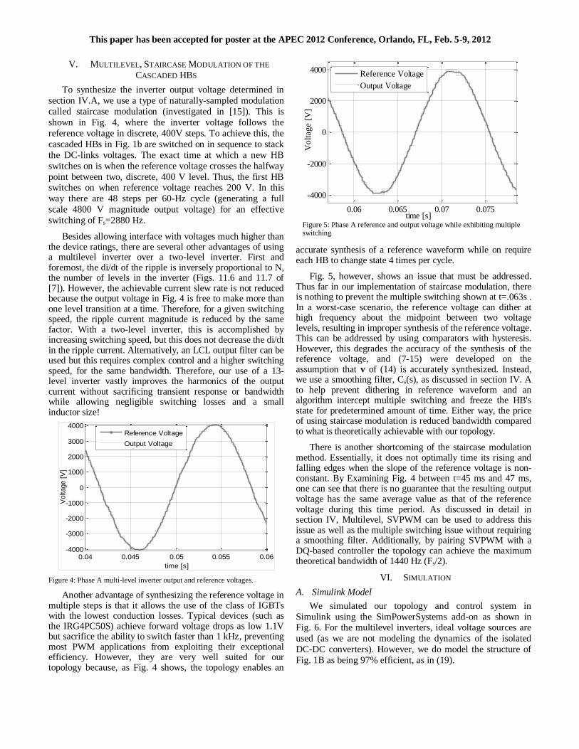
Figure 5: Phase A reference and output voltage while exhibiting multiple switching

0.06 0.065 0.07 0.075

-4000

-2000

0

2000

4000

time [s]

Vo

ltag

e [

V]

Reference Voltage

Output Voltage

V. MULTILEVEL, STAIRCASE MODULATION OF THE

CASCADED HBS

To synthesize the inverter output voltage determined in

section IV.A, we use a type of naturally-sampled modulation

called staircase modulation (investigated in [15]). This is

shown in Fig. 4, where the inverter voltage follows the

reference voltage in discrete, 400V steps. To achieve this, the

cascaded HBs in Fig. 1b are switched on in sequence to stack

the DC-links voltages. The exact time at which a new HB

switches on is when the reference voltage crosses the halfway

point between two, discrete, 400 V level. Thus, the first HB switches on when reference voltage reaches 200 V. In this

way there are 48 steps per 60-Hz cycle (generating a full

scale 4800 V magnitude output voltage) for an effective

switching of Fs=2880 Hz.

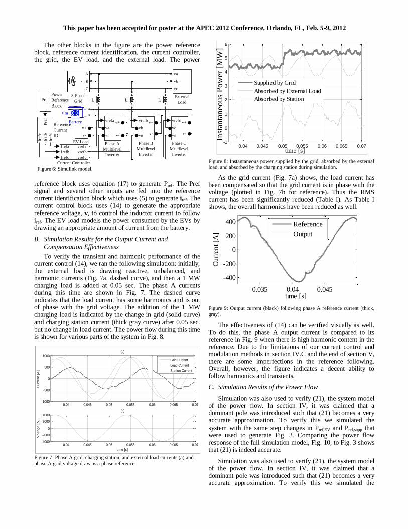
Besides allowing interface with voltages much higher than the device ratings, there are several other advantages of using a multilevel inverter over a two-level inverter. First and foremost, the di/dt of the ripple is inversely proportional to N, the number of levels in the inverter (Figs. 11.6 and 11.7 of [7]). However, the achievable current slew rate is not reduced because the output voltage in Fig. 4 is free to make more than one level transition at a time. Therefore, for a given switching speed, the ripple current magnitude is reduced by the same factor. With a two-level inverter, this is accomplished by increasing switching speed, but this does not decrease the di/dt in the ripple current. Alternatively, an LCL output filter can be used but this requires complex control and a higher switching speed, for the same bandwidth. Therefore, our use of a 13-level inverter vastly improves the harmonics of the output current without sacrificing transient response or bandwidth while allowing negligible switching losses and a small inductor size!

Figure 4: Phase A multi-level inverter output and reference voltages.

Another advantage of synthesizing the reference voltage in multiple steps is that it allows the use of the class of IGBTs with the lowest conduction losses. Typical devices (such as the IRG4PC50S) achieve forward voltage drops as low 1.1V but sacrifice the ability to switch faster than 1 kHz, preventing most PWM applications from exploiting their exceptional efficiency. However, they are very well suited for our topology because, as Fig. 4 shows, the topology enables an

accurate synthesis of a reference waveform while on require each HB to change state 4 times per cycle.

Fig. 5, however, shows an issue that must be addressed. Thus far in our implementation of staircase modulation, there is nothing to prevent the multiple switching shown at t=.063s . In a worst-case scenario, the reference voltage can dither at high frequency about the midpoint between two voltage levels, resulting in improper synthesis of the reference voltage. This can be addressed by using comparators with hysteresis. However, this degrades the accuracy of the synthesis of the reference voltage, and (7-15) were developed on the assumption that v of (14) is accurately synthesized. Instead, we use a smoothing filter, Cs(s), as discussed in section IV. A to help prevent dithering in reference waveform and an algorithm intercept multiple switching and freeze the HB's state for predetermined amount of time. Either way, the price of using staircase modulation is reduced bandwidth compared to what is theoretically achievable with our topology.

There is another shortcoming of the staircase modulation method. Essentially, it does not optimally time its rising and falling edges when the slope of the reference voltage is non-constant. By Examining Fig. 4 between t=45 ms and 47 ms, one can see that there is no guarantee that the resulting output voltage has the same average value as that of the reference voltage during this time period. As discussed in detail in section IV, Multilevel, SVPWM can be used to address this issue as well as the multiple switching issue without requiring a smoothing filter. Additionally, by pairing SVPWM with a DQ-based controller the topology can achieve the maximum theoretical bandwidth of 1440 Hz (Fs/2).

VI. SIMULATION

A. Simulink Model

We simulated our topology and control system in

Simulink using the SimPowerSystems add-on as shown in Fig. 6. For the multilevel inverters, ideal voltage sources are

used (as we are not modeling the dynamics of the isolated

DC-DC converters). However, we do model the structure of

Fig. 1B as being 97% efficient, as in (19).

0.04 0.045 0.05 0.055 0.06-4000

-3000

-2000

-1000

0

1000

2000

3000

4000

time [s]

Voltage [

V]

Reference Voltage

Output Voltage

This paper has been accepted for poster at the APEC 2012 Conference, Orlando, FL, Feb. 5-9, 2012

Figure 6: Simulink model.

Pre

f

Iref

c

Iref

b

Iref

a

Reference

Current

ID

Pref

Power

Reference

Block

vrefc

vc

vn

v+

v-

Phase C

Multilevel

Inverter

vrefb

vb

vn

v+

v-

Phase B

Multilevel

Inverter

vrefa

va

vn

v+

v-

Phase A

Multilevel

Inverter

L

va

vb

vc

External

Load

v+

v-

EV LoadIrefa

Irefb

Irefc

vrefa

vrefb

vrefc

Current Controller

+

_m

Battery

A

B

C

3-Phase

Grid L L

Figure 7: Phase A grid, charging station, and external load currents (a) and

phase A grid voltage draw as a phase reference.

0.04 0.045 0.05 0.055 0.06 0.065 0.07-4000

-2000

0

2000

4000

time [s]

Voltage [

V]

(b)

0.04 0.045 0.05 0.055 0.06 0.065 0.07-1000

-500

0

500

1000

Curr

ent

[A]

(a)

Grid Current

Load Current

Station Current

The other blocks in the figure are the power reference block, reference current identification, the current controller, the grid, the EV load, and the external load. The power

reference block uses equation (17) to generate Pref. The Pref signal and several other inputs are fed into the reference current identification block which uses (5) to generate iref. The current control block uses (14) to generate the appropriate reference voltage, v, to control the inductor current to follow iref. The EV load models the power consumed by the EVs by drawing an appropriate amount of current from the battery.

B. Simulation Results for the Output Current and

Compensation Effectiveness

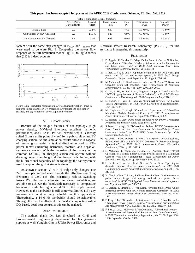
To verify the transient and harmonic performance of the current control (14), we ran the following simulation: initially, the external load is drawing reactive, unbalanced, and harmonic currents (Fig. 7a, dashed curve), and then a 1 MW charging load is added at 0.05 sec. The phase A currents during this time are shown in Fig. 7. The dashed curve indicates that the load current has some harmonics and is out of phase with the grid voltage. The addition of the 1 MW charging load is indicated by the change in grid (solid curve) and charging station current (thick gray curve) after 0.05 sec. but no change in load current. The power flow during this time is shown for various parts of the system in Fig. 8.

Figure 8: Instantaneous power supplied by the grid, absorbed by the external load, and absorbed by the charging station during simulation.

As the grid current (Fig. 7a) shows, the load current has been compensated so that the grid current is in phase with the voltage (plotted in Fig. 7b for reference). Thus the RMS current has been significantly reduced (Table I). As Table I shows, the overall harmonics have been reduced as well.

Figure 9: Output current (black) following phase A reference current (thick, gray).

The effectiveness of (14) can be verified visually as well. To do this, the phase A output current is compared to its reference in Fig. 9 when there is high harmonic content in the reference. Due to the limitations of our current control and modulation methods in section IV.C and the end of section V, there are some imperfections in the reference following. Overall, however, the figure indicates a decent ability to follow harmonics and transients.

C. Simulation Results of the Power Flow

Simulation was also used to verify (21), the system model of the power flow. In section IV, it was claimed that a dominant pole was introduced such that (21) becomes a very accurate approximation. To verify this we simulated the system with the same step changes in Pref,EV and Pref,supp that were used to generate Fig. 3. Comparing the power flow response of the full simulation model, Fig. 10, to Fig. 3 shows that (21) is indeed accurate.

Simulation was also used to verify (21), the system model of the power flow. In section IV, it was claimed that a dominant pole was introduced such that (21) becomes a very accurate approximation. To verify this we simulated the

0.04 0.045 0.05 0.055 0.06 0.065 0.07-1

0

1

2

3

4

5

6

time [s]

Inst

anta

neo

us

Po

wer

[M

W]

Supplied by Grid

Absorbed by External Load

Absorbed by Station

0.035 0.04 0.045

-400

-200

0

200

400C

urr

en

t [A

]

time [s]

Reference

Output

This paper has been accepted for poster at the APEC 2012 Conference, Orlando, FL, Feb. 5-9, 2012

Table I: Simulation Results Summary

Active Phase

Current (RMS)

Current

THD

Phase Current

RMS

Total

PF

Total Apparent

Power

Total Active

Power

External Load 523 2.76% 680 77% 5.6 MVA 4.3 MW

Grid Current w/o EV Charging 523 2.19 % 523 >99% 4.3 MVA 4.3 MW

Grid Current with EV Charging 648 1.2% 648 >99% 5.3 MVA 5.3 MW

system with the same step changes in Pref,EV and Pref,supp that were used to generate Fig. 3. Comparing the power flow response of the full simulation model, Fig. 10, to Fig. 3 shows that (21) is indeed accurate.

Figure 10: (a) Simulated response of power consumed by station (gray) in

response to step changes in EV charging power (solid) and grid support (dashed) and (b) response of power supplied by battery.

VII. CONCLUSIONS

Because of the unique features of our topology (high power density, MV-level interface, excellent harmonic performance, and STATCOM/APF capabilities) it is ideally suited (from a utility point of view) for a public, ultra-fast, EV charging station. As the simulation results show it is capable of removing correcting a typical distribution load to 99% power factor (including harmonic, reactive, and negative-sequence currents). With the inclusion of the battery as the common DC-link, the charging station can operate without drawing power from the grid during heavy loads. In fact, with the bi-directional capability of the topology, the battery can be used to support the grid at strategic times.

As shown in section V, each H-bridge only changes state 240 times per second even though the effective switching frequency is 2880 Hz. This drastically reduces switching losses. With the use of staircase, multi-level modulation, we are able to achieve the bandwidth necessary to compensate harmonics while having small di/dt in the ripple current. However, as the bandwidth is still somewhat limited (15), any improvement in it is very valuable in this application. Theoretically, a 1440 Hz bandwidth should be achievable. Through the use of multi-level, SVPWM in conjunction with a DQ-based, dead-beat controller this can be realized.

ACKNOWLEDGMENT

The authors thank Dr. Les Shepherd in Civil and Environmental Engineering department for his generous support as well Yongbin Chu in UTSA Power Electronics and

Electrical Power Research Laboratory (PEEPRL) for his assistance in preparing this manuscript.

REFERENCES

[1] D. Aggeler, F. Canales, H. Zelaya-De La Parra, A. Coccia, N. Butcher,

O. Apeldoorn, “Ultra-fast DC-charge infrastructures for EV-mobility and future smart grids”, in IEEE 2010 Innovative Smart Grid

Technologies Conference Europe, 2010, pp.1-8.

[2] S. Bai, D. Yu, S. Lukic, “Optimum design of an EV/PHEV charging station with DC bus and storage system”, in IEEE 2010 Energy

Conversion Congress and Exposition, 2010, pp. 1178-1184.

[3] M. Malinowski, K. Gopakumar, J. Rodriguez, M. Perez, “A Survey on Cascaded Multilevel Inverters, IEEE Transactions of Industrial

Electronics, vol. 57, no. 7, pp. 2197-2206, July 2010.

[4] C. Liu, S. Ho, W. Fu, S. Hai, Magnetic Design of Transformers for 20kW Charging Stations of Electrical Vehicles”, in 2010 14th Biennial

Conference on Electromagnetic Field Computation, May 2010, p. 1.

[5] L. Tolbert, F. Peng, T. Habetler, “Multilevel Inverters for Electric Vehicle Applications”, in 1998 Power Electronics in Transportation,

1998, pp. 79-84.

[6] M. Hagiwara, H. Akagi, “Control and Experiment of Pulsewidth-

Modulated Modular Multilevel Converters”, IEEE Transactions on Power Electronics, vol. 24, no. 7, pp. 1737-1746, July 2009.

[7] D. Holmes, T. Lipo, Pulse Width Modulation for Power Converters:

Principles and Practice, Wiley-IEEE Press, 2003.

[8] S. Inoue, H. Akagi, “A Bi-Directional Isolated DC/DC Converter as a Core Circuit of the Next-Generation Medium-Voltage Power

Conversion System”, in IEEE 2006 Power Electronics Specialists Conference, 2006, pp. 1-7.

[9] G. Ortiz, J. Biela, D. Bortis, J. Kolar, “1 Megawatt, 20 kHz, Isolated,

Bidirectional 12kV to 1.2kV DC-DC Converter for Renewable Energy Applications”, in IEEE 2010 International Power Electronics

Conference, 2010, pp. 3212-3219.

[10] L. Maharjan, T. Yamagishi, H. Akagi, J. Asakura, “Fault-Tolerant Operation of a Battery-Energy-Storage System Based on a Multilevel

Cascade With Star Configuration”, IEEE Transactions on Power Eletronics, vol. 25, no. 9, pp. 2386-2396, Sept. 2010.

[11] L. da Silva, L. de Lacerda de Oliveira, V. da Silva, “Speeding-up

dynamic response of active power conditioners”, in IEEE 2003 Canadian Conference Electrical and Computer Engineering, 2003, pp.

347-350.

[12] Y. Chu, R. Chen, T. Liang, S. Changchien, J. Chen, “Positive/negative

pulse battery charger with energy feedback and power factor correction”, in IEEE 2005 Applied Power Electronics and Conference

and Exposition, 2005, pp. 986-990.

[13] T. Saigusa, K. Imamura, T. Yokoyama, “100kHz Single Phase Utility Interactive Inverter with FPGA based Hardware Controller”, in IEEE

2010 International Power Electronics Conference, 2010, pp. 1457-1462.

[14] F. Peng, J. Lai, “Generalized Instantaneous Reactive Power Theory for

Three-phase Power Systems”, in IEEE Transactions on Instrumentation and Measurement, VOL. 45, NO. 1, pp. 293-297, February 1996.

[15] F. Peng, J. Lai, J. Mckeever, J. VanCoevering, “A Multilevel Voltage-

Source Inverter with Separate DC Sources for Static VAr Generation”, in IEEE Transactions on Industry Applications, Vol 32, No 5, pp.1130-

1138, September/October 1996.

0.05 0.1 0.15 0.2 0.25 0.3

-2

0

2

4

6(a)

(b)

Pow

er

Flo

w (

MW

)

0.05 0.1 0.15 0.2 0.25 0.30

1

2

3

4

5

time (s)

Pow

er

Flo

w (

MW

)

Single-stage Isolated Bi-directional Converter

Topology using High Frequency AC link for

Charging and V2G Applications of PHEV

Shesh Narayan Vaishnav and H. Krishnaswami, Member, IEEE,

Department of Electrical and Computer Engineering

The University of Texas at San Antonio

San Antonio, Texas, USA

E-mail: sheshvaishnav@yahoo.co.in and Hariharan.Krishnaswami@utsa.edu

Abstract—In this paper, an isolated bi-directional ac/dc con-verter with a single power conversion stage is proposed for bothcharging and Vehicle-to-Grid (V2G) applications of PHEV. Theconverter consists of two active bridges connected through a se-ries resonant tank and a high-frequency transformer. Steady-stateanalysis is presented for the proposed phase-shift modulationtechnique between active bridges, to control the bi-directionalpower flow in the converter. Simulation results are presented toaugment the analysis. The proposed converter has the advantagesof minimal power conversion stages, high switching frequencyoperation and low switching losses.

I. INTRODUCTION

Plug-in Hybrid Electric Vehicles (PHEV) are expected to

capture significant market share of automobiles in next 10

years [1]. PHEV batteries will be charged from the power

grid and hence, utilities nationwide have started exploring the

effects of PHEVs on distribution infrastructure. Furthermore,

a fleet of PHEV can act as a distributed energy storage for

utilities to use under peak load condition, termed as Vehicle-to-

Grid (V2G) functionality. A review of the V2G functionalities

and the power electronics configurations associated with such

vehicles is given in [2]. Hence, the bi-directional charger either

on-board or off-board forms an important unit in PHEV. In

this paper, a high-frequency ac link based power electronic

topology is proposed for bi-directional charging applications.

Existing bi-directional chargers proposed in literature [3],

[4], [5] use two stages of power conversion, an ac-dc converter

and a dc-dc converter, both bi-directional in power flow.

Several topologies for the ac-dc and dc-dc conversion stages

are discussed in [3]. Two dc-dc converters are discussed, a dual

active bridge high power converter [6] and the integrated buck-

boost dc-dc converter [7]. A bi-directional battery charger for

residential applications is discussed in [5] with an improved

control method for V2G operating mode. Reactive power

compensation, which is one of the V2G functionalities, is

demonstrated in [4] with a bi-directional ac-dc front end con-

verter. With two stages of power conversion, the intermediate

link is mostly dc. Such two stage power conversion will lead to

This project was partially funded by CPSEnergy through its StrategicResearch Alliance with The University of Texas at San Antonio.

increased part count, size and weight, which are major design

challenges for on-board or external level 1 or level 2 chargers.

To address these challenges, a single-stage power converter is

proposed in this paper.

The proposed converter is shown in Fig. 1. It consists of

two active bridges with an intermediate high frequency ac link.

A series resonant tank is used as the impedance at the high

frequency link. The high frequency transformer is used both

for isolation and voltage conversion. Traditionally, resonant

converters are controlled using frequency or Pulse Width

Modulation (PWM) in only one bridge and is uni-directional

due to the presence of a diode bridge at the load side. In

this paper, a phase-shift modulation technique is proposed

which controls the phase-shift between input and output-side

active bridges at constant switching frequency. This proposed

technique naturally allows bi-directional power flow and uses

the principle of power flow in a dual active bridge converter

[6]. A three-port dc-dc-dc converter using similar principle is

explained in [8]. The proposed modulation technique in this

paper allows for direct dc-ac or ac-dc conversion determined

by power flow direction.

The advantages of the proposed converter are: (1) Single-

stage conversion with high frequency ac link reduces compo-

nent count and increases power density and (2) Soft-switching

operation achieved due to the presence of resonant tank,

reduces switching losses and increases efficiency. Analysis of

the proposed converter is presented in the following section.

II. ANALYSIS

The converter shown in Fig. 1 has a series resonant cir-

cuit with inductance L and capacitance C. It switches at a

frequency Fs which is above resonant frequency Fr formed

by the series resonant tank. The input voltage vin(t) =Vin sin (2πFot) from grid, is connected to the active bridge

through an input filter which filters the current ripple at

switching frequency. The PHEV battery is connected at the

output of the load-side active bridge. The input-side active

bridge switches operate in four-quadrant mode, i.e., each

switch uses two Mosfets connected back-back as shown in

Fig. 1. Vb is the battery voltage at the output side, Fs is

−

++

−

S3

iin

vin

S1

S1 S1

iL

S1

vhf

C L

Series ResonantTank

Phase Shift φ

1 : nib

VbCi

vs

S3S2

S2

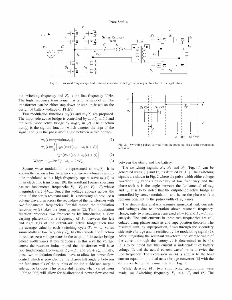
Fig. 1. Proposed Single-stage bi-directional converter with high frequency ac link for PHEV application

the switching frequency and Fo is the line frequency 60Hz.

The high frequency transformer has a turns ratio of n. The

transformer can be either step-down or step-up based on the

design of battery voltage of PHEV.

Two modulation functions m1(t) and m2(t) are proposed.

The input-side active bridge is controlled by m1(t) in (1) and

the output-side active bridge by m2(t) in (2). The function

sgn(.) is the signum function which denotes the sign of the

signal and φ is the phase-shift angle between active bridges.

m1(t)=sgn(sin(ωst)) (1)

m2(t)=1

2

[

sgn(cos((ωs − ωo)t + φ))

− sgn(cos((ωs + ωo)t) + φ)]

(2)

Where ωs=2πFs; ωo = 2πFo (3)

Square wave modulation is represented as m1(t). It is

known that when a low frequency voltage waveform is ampli-

tude modulated with a high frequency square wave m1(t) as

in an electronic transformer [9], the resultant Fourier spectrum

has two fundamental frequencies Fs −Fo and Fs +Fo whose

magnitudes are 2πVin. Since this voltage appears across the

input of the series resonant tank, it is necessary to produce a

voltage waveform across the secondary of the transformer with

two fundamental frequencies. For this reason, the modulation

function m2(t) takes the form given in (2). This modulation

function produces two frequencies by introducing a slow

varying phase-shift at a frequency of Fo between the left

and right legs of the output-side active bridge such that

the average value in each switching cycle Ts = 1Fs

varies

sinusoidally at low frequency Fo. In other words, the function

introduces zero voltage states in the output of the active bridge

whose width varies at low frequency. In this way, the voltage

across the resonant inductor and the transformer will have

two fundamental frequencies Fs − Fo and Fs + Fo. Finally,

these two modulation functions have to allow for power flow

control which is provided by the phase-shift angle φ between

the fundamentals of the outputs of the input-side and output-

side active bridges. This phase-shift angle, when varied from

−90o to 90o, will allow for bi-directional power flow control

S2 ON

S1

t

φ

vs

S3 ON

S2 OFF S3 OFF

Ts

2

t

Vb

Fig. 2. Switching pulses derived from the proposed phase-shift modulationtechnique

between the utility and the battery.

The switching signals S1, S2 and S3 (Fig. 1) can be

generated using (1) and (2) as detailed in [10]. The switching

signals are shown in Fig. 2 where the pulse-width ofthe voltage

waveform vs varies sinusoidally at low frequency and the

phase-shift φ is the angle between the fundamental of vhf

and vs. It is to be noted that the output-side active bridge is

controlled by center modulation and hence the phase-shift φ

remains constant as the pulse-width of vs varies.

The steady-state analysis assumes sinusoidal tank currents

and voltages due to operation above resonant frequency.

Hence, only two frequencies are used Fs−Fo and Fs +Fo for

analysis. The tank currents in these two frequencies are cal-

culated using phasor analysis and superposition theorem. The

resultant sum, by superposition, flows through the secondary

side active bridge and is rectified by the modulating signal (2).

After integrating the resultant waveform, the average value of

the current through the battery Ib is determined to be (4).

It is to be noted that this current is independent of battery

voltage Vb and the actual current waveform is at twice the

line frequency. The expression in (4) is similar to the load

current equation in a dual active bridge converter [6] with the

difference being the resonant tank in Fig. 1.

While deriving (4), two simplifying assumptions were

made: (a) Switching frequency Fs >> Fo and (b) The

10

-200

0

200

0

i in

vin

i b

16.67 25time(ms)

33.33

40

-10

0

Fig. 3. Input voltage in volts vin(t), filtered input current iin(t) and batterycurrent ib(t) in Amperes for power flow from AC input to battery

impedance of the resonant tank at Fs + Fo and Fs − Fo are

equal.

Ib =4

π2

Vin

nZ(F −1F

)sin φ (4)

where Z =

√

L

C; F =

Fs

Fr

; Fr =1

2π√

LC(5)

III. SIMULATION RESULTS

A charger with power level of Po = 650W is used for

simulation purposes in order to verify the analysis results. The

input ac voltage is chosen to be Vin(rms) = 120V and the

battery voltage Vb is chosen to be 36V . The battery voltage

is assumed fairly constant during the simulation time, since

the battery charging current is independent of battery voltage.

The switching frequency is chosen as Fs = 100kHz close to

and 1.1 times above resonant frequency. The value of turns

ratio is chosen such that the overall voltage conversion ratio

is unity [8] i.e., nVin

Vb

= 1. With the required value of Ib

and the maximum value of phase-shift angle, the value of

the characteristic impedance Z can be calculated using (4).

The values of the resonant inductor and capacitor can then be

calculated from (5).

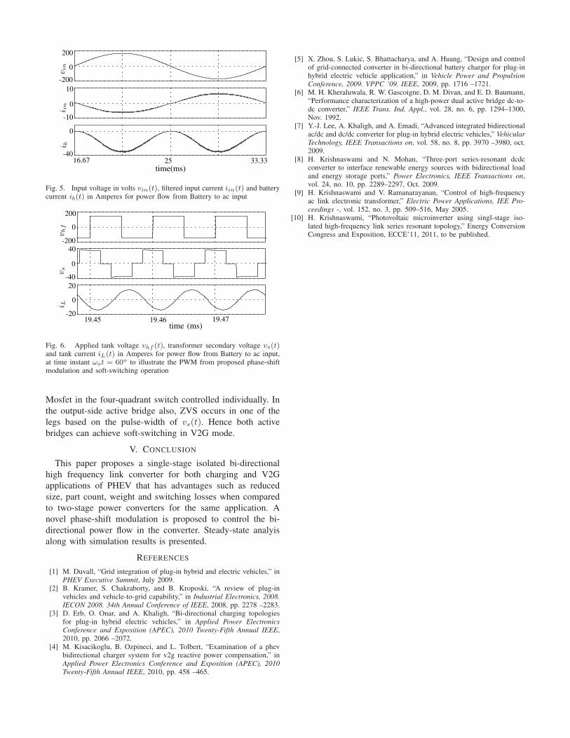
The results of the battery current along with input voltage

and input current are shown in Fig. 3 for the specified power

level and a phase-shift of φ = 90o. It can be observed that

battery current waveform is at twice the line frequency and

its average value matches (4). The high frequency ripple in

input current is filtered by Ci. The input current is normally

in phase with the input voltage for this type of modulation

scheme.

The tank current and the applied tank voltage vhf (t) for

few switching cycles are shown in Fig. 4. The phase-shift φ

between the waveforms of vhf (t) and vs(t) can be observed to

be 90o from Fig. 4 shown for three switching cycles around

ωot = 60o. The pulse-width of the waveform vs(t) varies

sinusoidally such that its fundamental has two frequencies

Fs + Fo and Fs − Fo. Due to the resonant nature of the

circuit, soft-switching operation is possible in both the active

bridges. Tank current iL(t) lags the applied voltage vhf (t)

0

20

-40

0

40

-200

0

200

i Lv

sv

hf

time(ms)19.45 19.46 19.47

-20

Fig. 4. Applied tank voltage vhf (t), transformer secondary voltage vs(t)and tank current iL(t) in Amperes for power flow from AC input to batteryat time instant ωot = 60o to illustrate the PWM from proposed phase-shiftmodulation and soft-switching operation

from input-side bridge as seen in Fig. 4. Since the current

drawn from utility is in phase with the voltage, only one

Mosfet can be switched in the four-quadrant switch enabling

Zero Voltage Switching (ZVS) in all eight switches in the input

side active bridge. This eliminates the commutation problem

in four-quadrant switches. Although it adds drive circuitry to

control each individual Mosfet in a four-quadrant switch, the

efficiency gain is significant.

ZVS operation is possible in the battery side active bridge

only when the the voltage conversion ratio is unity. The

condition for ZVS is that this tank current lead the transformer

secondary voltage vs(t) from the output-side active bridge

based on current direction defined in Fig. 1. This lagging angle

can be observed from Fig. 4 proving that ZVS is possible in

secondary-side switches also. But, the voltage waveform vs

has zero voltage states and hence, when the pulse-width of

vs(t) is lower than the phase-shift, ZVS is lost in one of the

legs.

IV. BI-DIRECTIONAL POWER FLOW

Power flow from PHEV to utility is needed for V2G

applications. This paper considers only real power flow into

the grid with its application of peak load reduction. In the

proposed converter, if the phase-shift is made negative, the

power flows from the battery to the grid. Considering this

mode, the average value of the current into utility can be

derived using the same phasor analysis as in Section 2 and

is given in (6). This result is equivalent to the one presented

in [10] for photovoltaic inverter application.

iin(t) =8

π2

Vb sin φ

nZ(F −1F

)sin (2πFot) (6)

Simulation results of the input current and battery current

are shown in Fig. 5 to illustrate the bi-directional capability

of the proposed converter. The average of the battery current

is negative as seen in Fig. 5. The difference in phase-shifts

between Fig. 3 and Fig. 4 can be seen. It is observed from Fig.

6 that the tank current still lags the applied voltage vhf (t) and

hence ZVS is possible in the input-side active bridge with each

16.67-40

0

-10

0

10

-200

0

200

25 33.33time(ms)

i bi i

nv

in

Fig. 5. Input voltage in volts vin(t), filtered input current iin(t) and batterycurrent ib(t) in Amperes for power flow from Battery to ac input

vs

vh

fi L

time (ms)

-20

0

20

-40

0

40-200

0

200

19.45 19.46 19.47

Fig. 6. Applied tank voltage vhf (t), transformer secondary voltage vs(t)and tank current iL(t) in Amperes for power flow from Battery to ac input,at time instant ωot = 60o to illustrate the PWM from proposed phase-shiftmodulation and soft-switching operation

Mosfet in the four-quadrant switch controlled individually. In

the output-side active bridge also, ZVS occurs in one of the

legs based on the pulse-width of vs(t). Hence both active

bridges can achieve soft-switching in V2G mode.

V. CONCLUSION

This paper proposes a single-stage isolated bi-directional

high frequency link converter for both charging and V2G

applications of PHEV that has advantages such as reduced

size, part count, weight and switching losses when compared

to two-stage power converters for the same application. A

novel phase-shift modulation is proposed to control the bi-

directional power flow in the converter. Steady-state analyis

along with simulation results is presented.

REFERENCES

[1] M. Duvall, “Grid integration of plug-in hybrid and electric vehicles,” inPHEV Executive Summit, July 2009.

[2] B. Kramer, S. Chakraborty, and B. Kroposki, “A review of plug-invehicles and vehicle-to-grid capability,” in Industrial Electronics, 2008.

IECON 2008. 34th Annual Conference of IEEE, 2008, pp. 2278 –2283.[3] D. Erb, O. Onar, and A. Khaligh, “Bi-directional charging topologies

for plug-in hybrid electric vehicles,” in Applied Power Electronics

Conference and Exposition (APEC), 2010 Twenty-Fifth Annual IEEE,2010, pp. 2066 –2072.

[4] M. Kisacikoglu, B. Ozpineci, and L. Tolbert, “Examination of a phevbidirectional charger system for v2g reactive power compensation,” inApplied Power Electronics Conference and Exposition (APEC), 2010

Twenty-Fifth Annual IEEE, 2010, pp. 458 –465.

[5] X. Zhou, S. Lukic, S. Bhattacharya, and A. Huang, “Design and controlof grid-connected converter in bi-directional battery charger for plug-inhybrid electric vehicle application,” in Vehicle Power and Propulsion

Conference, 2009. VPPC ’09. IEEE, 2009, pp. 1716 –1721.[6] M. H. Kheraluwala, R. W. Gascoigne, D. M. Divan, and E. D. Baumann,

“Performance characterization of a high-power dual active bridge dc-to-dc converter,” IEEE Trans. Ind. Appl., vol. 28, no. 6, pp. 1294–1300,Nov. 1992.

[7] Y.-J. Lee, A. Khaligh, and A. Emadi, “Advanced integrated bidirectionalac/dc and dc/dc converter for plug-in hybrid electric vehicles,” Vehicular

Technology, IEEE Transactions on, vol. 58, no. 8, pp. 3970 –3980, oct.2009.

[8] H. Krishnaswami and N. Mohan, “Three-port series-resonant dcdcconverter to interface renewable energy sources with bidirectional loadand energy storage ports,” Power Electronics, IEEE Transactions on,vol. 24, no. 10, pp. 2289–2297, Oct. 2009.

[9] H. Krishnaswami and V. Ramanarayanan, “Control of high-frequencyac link electronic transformer,” Electric Power Applications, IEE Pro-

ceedings -, vol. 152, no. 3, pp. 509–516, May 2005.[10] H. Krishnaswami, “Photovoltaic microinverter using singl-stage iso-

lated high-frequency link series resonant topology,” Energy ConversionCongress and Exposition, ECCE’11, 2011, to be published.

Section 2:

Microgrids

1

Abstract— In this paper, a Fuzzy-Logic based control

framework is proposed for Battery Management in Micro-

Grid System. The Micro-Grid system operates

synchronously with the main grid and also has the ability

to operate independently from the power grid. Distributed

renewable energy generators including solar, wind, and

batteries supply power to the consumer in the Micro-Grid

network. The goal is to control the amount of power given

to the storage system in order to minimize a cost function

based on payment/profit and distribution loss through

reasonable decision making using predefined profiles of

system variables such as Load Demand, Electricity Price,

and Renewable Generation.

Simulation results are presented and discussed. The

proposed intelligent control system turns out to be capable

of achieving effective energy management.

Index Terms—Micro-Grid, Control, Power Flow, Fuzzy-Logic,

Load Demand.

I. INTRODUCTION

Micro-Grid is can be referred to as a small scale grid that is

designed to provide power for small communities. A Micro-

Grid is an aggregation of multiple distributed generators

(DGs) such as renewable energy sources, conventional

generators, and energy storage systems which work together

as a power supply network in order to provide both electric

power and thermal energy for small communities which may

vary from one common building to a smart house or even a set

of loads consisting of a mixture of different structures such as

buildings, factories, etc. Typically, a Micro-Grid operates in

parallel with the main grid. However, there are cases in which

a Micro-Grid operates in islanded mode, or in a disconnected

state [1]. In this article, in addition to both of the states already

mentioned, a third state is assumed for operation of Micro-

Grid in which excess power in the Micro-Grid is delivered to

the main grid, i.e. the excess power is sold to the grid.

II. SYSTEM MODEL

A three bus system is used to model the Micro-Grid network

for simulations in this article. One of the busses in the

distributed generation system model is assumed to serve the

renewable generators which include either solar farm, wind

farm, or any other renewable generation units. Another bus is

assumed to be working as the grid (utility) bus which will

provide the complement part of the power demand that

renewable generation system cannot afford to the load. The

third bus will be the specific load to which the demanded

power is to be provided. This load can be anything from a

common building or a smart house, to even a group of plants

and factories or a mixture of all of them. Figure 1 shows an

overall Micro-Grid schematic including Renewable Electricity

Generators and Storage Unit, Utility, and Typical Load.

Figure 1 Micro-Grid Schematic

There are two scenarios assumed for simulation in this article,

scenario 1 deals with a Micro-Grid which includes the

renewable generation unit without any battery storage unit.

Therefore there will not be any approaches required for

controlling the battery storage system in this scenario. The

second scenario deals with the same Micro-Grid system as

mentioned in scenario 1 but with the battery storage unit

considered to be connected to the same bus as the renewable

generators. These two scenarios will be described in more

detail in the next section “Problem Statement”. The

characteristics of busses in each of the two scenarios are as

follows:

Scenario 1:

Bus1 is of type PQ and is used as the renewable

generation unit's bus

Bus2 is of type Slack (reference) and is used as the

Utility (grid) bus

Bus3 is of type PV and is used as the Load bus

Fuzzy-Logic Based Control for Battery

Management in Micro-Grid

Yashar Sahraei Manjili, Student Member IEEE, Amir Rajaee, Student Member IEEE

Brian Kelley, Senior Member IEEE, Mo Jamshidi Fellow IEEE

2

Scenario 2:

Bus1 is of type PQ and is used as the bus for renewable

generation unit and the Battery storage unit

Bus2 is of type Slack (reference) and is used as the

Utility (grid) bus

Bus3 is of type PV and is used as the Load bus

III. PROBLEM STATEMENT

Important point on this first idea is that we have assumed the

time-varying pricing for electricity. The update duration of

pricing is assumed to be 15 mins, which means that the price

per killowatt-hour of electricity consumed by the customers of

the load region is updated every 15 minutes, and there will be

a cost function determined by us as:

(1)

where the electricity price is determined by the CPS energy

every 15 minutes for the next 15 minute period. is the

amount of power transferred to/from the Grid during each 15

minute period. If power is received from the Grid will

be positive, and if power is delivered to the grid in case of

excess power generation by the renewable generation system

will appear in the equations with a negative sign.

is the amount of distribution loss which will occur on the

branches we have between these three Busses in the Micro-

Grid system during each 15 minute period. Depending on

whether the load is getting how much of its demanded power

from renewable generation system and how much from the

Grid, and also depending on whether the renewable generation

system is producing excess power and is selling the excess

power to the Grid, this power Loss will vary.

The simulation is done on the Micro-Grid system considering

two scenarios. In the following the summary of the two

scenarios is given:

Scenario 1: Analysis of the Micro-Grid system profits and

costs under time-varying electricity pricing policy; in this

scenario, the simulation, analysis and study will be done

Micro-Grid which includes the renewable generation unit

without any battery storage unit. Therefore there will not be

any approaches required for controlling the battery storage

system in this scenario.

Scenario 2: Fuzzy Control of the Micro-Grid system

under time-varying electricity pricing policy; the cost function

assumed in this scenario is the same as the cost function

described in the scenario 1. The main difference here is that

the storage system exists in the network and will appear to be

on the same bus with the renewable generation unit.

The power flow calculation in the Micro-Grid is the key to

simulate the whole system. There are a number of well-known

methods for calculation of power flow in the distributed

generation network [2]. There are four different types of

busses considered in a distributed generation network, the

characteristics of which will be calculated in power flow

algorithms. These four types include PQ, PV, Slack, and

isolated [3,4].

IV. FUZZY CONTROL APPROACH

The control strategy implemented in this paper is to use the

Fuzzy Logic [5] approach for controlling the power flow

to/from the battery storage unit in order to minimize the cost

function introduced in previous section “Problem Statement”.

The three input variables to the fuzzy inference engine are

Price, Renewable Generation, and Load Demand.

The numerical values for these three input variables are

normalized to the [0 1] interval, and then are Fuzzified using

three fuzzy sets defined as Low, Medium, and High. The input

variables after fuzzification will be fed to a fuzzy inference

engine where the rule-base is applied to the input-output

variables and the output will be determined by human

reasoning. There is only one output variable which determines

the amount of power to be stored in the battery, or to be drawn

from battery. Output variable fuzzy set is assumed to have five

membership functions called Negative Large (NL), Negative

Small (NS), Zero (Z), Positive Small (PS), and Positive Large

(PL). The power drawn from the batteries can be used to

provide the load in order to complement the renewable

generation power for providing the load's demand, can be sold

to the Grid, or can be partially used for both reasons [6]. The

role of fuzzy inference engine is critically important for

obtaining satisfactory results. For example, if the Price is Low,

the Renewable Generation is High, and the Load Demand is

Medium, then, the amount of Power to Battery storage system

should be Positive-Large, even if this requires the system to

get power from grid and store it in the battery storage unit,

because the main point here is that Price is low, which means

that by storing the energy in the batteries during low price

times, the system will have enough stored energy in order to

sell to the Grid during high-price periods. Even under cases of

High Load demand this will be a good strategy. Therefore,

having feasible rules predefined for the fuzzy system will help

to minimize the cost function drastically. The proposed

approach may sometimes result in making the cost function

value negative, which means that the system is even making

some profit out of this control approach instead of paying to

the utility.

Figure 2 Three Bus Model for Micro-Grid

3

V. SIMULATION RESULTS & DISCUSSIONS

The simulation is done on the three bus system for power flow

calculation. The Gauss-Seidel algorithm is implemented using

Matlab for power flow calculation. Some typical data are

generated for dynamic Load Demand and Renewable

Generation rate.

The power demand of the Load on bus 3 (Smart House) is

supplied by two generators on buses 1 and 2. Bus 1 includes

solar panel and storage and bus 2 is slack which is connected

to utility as shown in figure 2.

Figure 3 Profiles of Price, Renewable Generation, and the Load

during a typical day for each 15min period

The numerical values of the data profile for the three input

variables to the fuzzy inference engine are shown in figure 3.

These variables include electricity price, renewable generation

rate, and load demand. The data is generated typically for

simulation purposes only with regard to the fact that the peak

electricity consumption duration of the whole region of

interest is around 8:30 pm where the price gets to its peak

value. The simulation results for scenario 1 are represented in

figures 4 to 6.

As it can be inferred from figure 4, the value of reactive power

for bus 1 is constantly zero which corresponds to the

assumption that the renewable generators do not provide

reactive energy. Figure 5 shows that the active power is taken

from the Utility during first half of the day time, and during

the most of the second half of the day the active power is

being delivered to the grid. Load is evidently consuming

active power regarding the blue curve represented in figure 6.

Figure 4 The Power Flow of Bus 1 including Solar Panel in a

typical day for each 15min period

Figure 5 The Power Flow of Bus 2 connected to utility in a typical

day for each 15min period

Figure 6 The Power Flow of Bus 3 including Load in a typical

day for each 15min period

4

Output of the fuzzy inference engine which represents the

power rate given to battery is shown in figure 7. Whenever the

value of this variable is positive it means that power is

delivered to the storage unit and if the power is drawn from

the storage unit, the value will be negative.

Figure 7 The normalized Value of Power given to Storage

obtained by Fuzzy Inference Engine

Simulation results for scenario 2 which includes storage on

bus 2 are represented in figures 8 to 10.

As one can infer from figure 8, the value of reactive power for

bus 1 is again constantly zero – the same as it was in scenario

1 - which corresponds to the assumption that the renewable

generators do not provide reactive energy. Figure 9 shows that

the active power is taken from the utility during first half of

the day time, and during the most of the second half of day the

active power is being sold to the grid. The point is that the first

part of the active power diagram is raised dramatically due to

fuzzy decision making which means that the system is

absorbing more active power from the grid during low-price

hours and stores the power in the storage unit. Also, the

second part of the active power diagram has fallen more in

comparison to the same section of figure 5 which denotes on

increase in the amount of power drawn from storage unit and

using this power for partially charging the load and also

selling the excess power to the grid during high-price hours.

This strategy results in minimization of cost function or in

other words maximizes the profit function. As shown in figure

10, load (smart house) is consuming active power.

Remembering that the pricing periods are assumed to be 15

minute periods and one day is 24 hours overally there will be

96 periods of pricing during one day period. The summation

of payment/profit and the loss during each of the periods will

give us the overall value of cost function for one day. The

process can be extended to one week, one month, one year etc.

Figure 8 The Power Flow of Bus 1 including Solar Panel in a

typical day for each 15min period with storage on bus 2

Figure 9 The Power Flow of Bus 2 connected to utility in a typical

day for each 15min period with the Storage on bus 2

Figure 10 The Power Flow of Bus 3 including Load (Smart

House) in a typical day for each 15min period with storage on

bus 2

5

In table 1, total values of distribution loss, payment/profit, and

the cost function on one typical day for the two scenarios

mentioned in section III are summarized. It must be mentioned

that the values in the table are dimension-less, and they can be

regarded as the costs or the prices that the end-user should pay

to the utility because of regular operation of Micro-Grid, or

earns due to improved operation and control of the Micro-

Grid.

Table 1. The simulation results for Loss, Payment, and Cost

Loss Payment Cost

Scenario 1 0.1286 2.3433 2.4719

Scenario 2 6.3430 -11.8192 -5.4761

The Cost is equal to summation of Payment and Loss.

Payment is simply the overall summation of power from/to

grid multiplied by the relevant price for all 15 min periods,

and the overall summation of multiplication of the price and

consumed power on distribution branches for all 15 min

periods is defined as Loss for one typical day. With no loss of

generality, it is assumed that the active and reactive power

have the same price.

VI. CONCLUSION

The proposed Fuzzy-Logic based control method is applied

for Battery Management in Micro-Grid System. In the micro-

grid system three buses are considered as renewable generator

and Storage, utility, and load (smart house). The goal was to

minimize the cost function which is based on distribution loss

and payment/profit. The Micro-Grid was simulated under first

scenario 1 without any storage units involved. Simulation

results obtained for the same Micro-Grid under scenario 2

where the storage system is included with the Fuzzy controller

show that scenario 2 outperforms the first scenario where no

storage system with fuzzy controller is incorporated.

Therefore, using fuzzy controller it is possible to reduce the

cost of the Micro-Grid system, and even let the customers

make profit from selling the excess power to the utility.

REFERENCES

[1] Cho, C.; Jeon, J.; Kim, J.; Kwon, S.; Park, K.; Kim, S., „Active

Synchronizing Control of a Microgrid‟ IEEE Transactions on Power

Electronics, issue 99, PP, 2011

[2] N. L. Srinivasa Rao, G. Govinda Rao, B. Ragunath, “Power Flow Studies Of The Regional Grid With Inter State Tie-Line Constraints”

IEEE Conference on Power Quality, pp. 165-171, 2002.

[3] R. D. Zimmerman, C. E. Murillo-Sánchez, and R. J. Thomas, "MATPOWER's Extensible Optimal Power Flow

Architecture," Power and Energy Society General Meeting, 2009 IEEE,

pp. 1-7, July 26-30 2009. [4] R. D. Zimmerman, C. E. Murillo-Sánchez, and R. J.

Thomas, "MATPOWER Steady-State Operations, Planning and Analysis Tools for Power Systems Research and Education," Power

Systems, IEEE Transactions on, vol. 26, no. 1, pp. 12-19, Feb. 2011.

[5] Chang, Sheldon S. L. ; Zadeh, Lofti A. ; “On Fuzzy Mapping and Control”, IEEE Transactions on Systems, Man and Cybernetics, pp. 30-

34, 1972.

[6] Zhu Wang, Rui Yang and Lingfeng Wang,” Intelligent Multi-agent Control for Integrated Building and Micro-grid Systems” IEEE

PES Innovative Smart Grid Technologies (ISGT), pp.1-7, 2011.

Fuzzy Control of Electricity Storage Unit for Energy Management of Micro-Grids1

Yashar Sahraei Manjili*†, Amir Rajaee*, Mohammad Jamshidi*, Brian T. Kelley* *Department of Electrical and Computer Engineering

University of Texas at San Antonio San Antonio, TX

†sca102@my.utsa.edu

Abstract— A Fuzzy Logic-based framework is proposed for control of Battery Storage Unit in Micro-Grid Systems to achieve Efficient Energy Management. Typically, a Micro-Grid system operates synchronously with the main grid and also has the ability to operate independently from the main power grid in an islanded mode. Distributed renewable energy generators including solar, wind in association with batteries and main grid supply power to the consumer in the Micro-Grid network. The goal here is to control the amount of power delivered to/taken from the storage unit in order to improve a cost function, defined based on summation of payment required for purchasing power from main grid or profit obtained by selling power to the main grid and distribution power loss, through reasonable decision making using predetermined human reasoning-based fuzzy rules. Profiles of system variables such as Consumer’s Load Demand, Electricity Price Rate, and Renewable Electricity Generation Rate are assumed arbitrarily for obtaining general results. Measures of payment/profit will be extracted to compute amounts of cost and balance for the network which represent benefits of using Fuzzy logic for Storage Unit control with and without considering storage unit capacity limits. Simulation results are presented and discussed.

Keywords- Micro-Grid Network, Intelligent Control, Power Flow Analysis, Fuzzy-Logic, Load Demand, Variable Electricity Price Rate.

I. INTRODUCTION Micro-Grid is a small-scale grid that is designed to provide

power for local communities. A Micro-Grid is an aggregation of multiple distributed generators (DGs) such as renewable energy sources, conventional generators, in association with energy storage units which work together as a power supply network in order to provide both electric power and thermal energy for small communities which may vary from one common building to a smart house or even a set of complicated loads consisting of a mixture of different structures such as buildings, factories, etc [1]. Typically, a Micro-Grid operates synchronously in parallel with the main grid. However, there are cases in which a Micro-Grid operates in islanded mode, or in a disconnected state [2]. In this article we assume that when the Micro-grid is connected to the main grid and is working synchronously with it, the flow of electric power can be either from the main grid to the Micro-grid or vice-versa. If the flow

of electric power is from the main grid towards Micro-grid it means that the Micro-grid is consuming the main grid’s energy for each KiloWatt-Hour of which the consumer, here Micro-grid, must pay to the Grid. This borrowed power can be either sent to local load to be consumed or can be stored in battery for future use. But, in case the flow of power is from the Micro-Grid towards the main grid, this means that Micro-Grid is delivering power to the main grid. In other words, the excess power generated currently by the renewable electricity generators or stored previously in the batteries is being sold to the main grid, and the Micro-Grid, or in general the consumer, is making profit by selling energy to the main grid. Without loss of generality, we have assumed that the price rate for buying energy from the main grid is equal to the electricity price rate which is sold to the grid. The excess power can be sold to the grid whenever the storage unit or load don’t need that power or whenever it is more beneficial to sell power to grid than to use it for supplying the load. However, in this article the main goal is to have the load completely supplied by the required power demand at all conditions. Authors have previously simulated the Micro-Grid assuming no maximum and minimum limit for the amount of energy stored in the battery unit [1]. In this article, storage unit’s limits on maximum and minimum amount of stored energy are considered and the results are compared to the results of the previous work.

II. SYSTEM MODEL The model used for simulation of the Micro-grid network

is a three-bus system. One of the busses in the distributed generation model is assumed to serve the renewable generators which include either solar farm, wind farm, or any other renewable generation units either in association with battery storage unit or without storage. Another bus is assumed to be there as the grid (utility) bus which will provide the complement part of the power demanded by the local load that renewable electricity generation system cannot afford. The third bus will be the specific load to which the demanded power is to be provided. This load can be anything from a common building or a smart house, to even a group of plants and factories or a mixture of all of them. Figure 1 shows an

1This work is partially funded by CPS Energy through Texas Sustainable Energy Research Institute at the University of Texas at San Antonio.

overall Micro-Grid schematic including Renewable Electricity Generators and Storage Unit, Utility, and Local Load.

III. SYSTEM MODEL

There are three scenarios defined for simulation in this article; scenario 1 deals with a Micro-Grid which includes the renewable electricity generators without any battery storage unit. Therefore there will not be any approaches required for controlling the battery storage system in this scenario. The second scenario deals with the same Micro-Grid system as mentioned in scenario one but after the battery storage unit is connected to the same bus with the renewable generators. Also, the fuzzy approach is applied in this scenario for energy management through battery unit control. The point in this scenario is that the battery storage is assumed to be an ideal battery without any maximum or minimum limits on stored energy, i.e. infinite battery capacity. In the third scenario which is the last one, the Micro-Grid is assumed to have everything mentioned in scenario two plus the fact that maximum and minimum limits of stored energy are taken into account for storage unit and are assumed to be 85% and 15% of the nominal maximum storable energy respectively. These three scenarios will be described in more detail in section III.

A. Characteristics of Buses in Scenario 1 The three buses in the model of Micro-Grid Network

simulated in this article have the following characteristics in the first scenario:

• Bus 1 is of type PQ and is used as the renewable electricity generation unit's bus.

• Bus 2 is of type Slack (reference) and is used as the Utility (grid) bus.

• Bus 3 is of type PV and is used as the Local Load bus.

B. Characteristics of Buses in Scenario 2 The characteristics of the three buses in the Micro-Grid

Network model simulated in this article are as follows in the second scenario:

• Bus 1 is a PQ bus and is used as the bus for renewable generation unit and infinite-capacity battery storage.

• Bus 2 will be the Slack (reference) bus and is used as the Utility (grid) bus.

• Bus 3 is of type PV and is used as the Local Load bus.

C. Characteristics of Buses in Scenario 3 Bus characteristics of the three buses in the Micro-Grid

Network model simulated in this article are as follows in the third, i.e. last, scenario:

• Bus 1 is a PQ bus and is used as the bus for renewable generation unit and finite-capacity battery storage unit.

• Bus 2 will be the Slack (reference) bus and is used as the Utility (grid) bus.

• Bus 3 is of type PV and is used as the Local Load bus.

This must be noted that battery units are assumed to be ideal batteries, i.e. no dynamic transient of change in the amount of stored energy in batteries are assumed, i.e. the amount of stored energy in the batteries is assumed to be changing as a pure ramp by time in both ascending and descending direction.

III. PROBLEM STATEMENT The important point which lies behind the idea of this

article is that we have assumed the real-time pricing for electricity. The update duration of pricing is assumed to be 15 minutes, which means that the price per KiloWatt-Hour of electricity consumed by the customers of the load region is updated every 15 minutes. This means that the money consumers need to pay to the utility for the same amount of energy used during different time-intervals might be different. Therefore, a function is required to be defined which takes into account the difference between amount of power given to the utility by the Micro-Grid, and the amount of power taken from the utility by the Micro-Grid. The Equation 1 represents this cost function:

𝐶𝑜𝑠𝑡 = ∑ (Pr(𝑡) . (𝑆𝑈(𝑡) + 𝑆𝐿(𝑡)))𝑇𝑡=1 (1)

where the electricity price Pr(𝑡) is determined by the CPS energy every 15 minutes for the next 15 minute period. is the amount of power transferred to/from the Grid during each 15 minute period. If power is received from the Grid

will be positive, and if power is delivered to the grid in case of excess power generation by the renewable generation system will appear in the equations with a negative sign.

is the amount of distribution loss which will occur on the branches we have between these three buses in the Micro-Grid system during each 15 minute period. Depending on whether the load is getting how much of its demanded power from renewable generation system and how much from the Grid, and also depending on whether the renewable generation system is producing excess power and is selling the excess power to the Grid, this power Loss will vary.

Figure 1 Micro-Grid Network Schematic

Figure 2 represents the three-bus model used for simulation of the Micro-Grid in different scenarios along with the branch impedances and the types of buses. Simulation is done on the Micro-Grid system considering three scenarios. In the following the summary of these scenarios is given:

A. Scenario 1 Analysis of the Micro-Grid system profits and costs

under real-time electricity pricing policy; in this scenario the simulation, analysis and study will be done on a Micro-Grid model which includes the renewable generation unit without any battery storage unit. Therefore there will not be any approaches required for controlling the battery storage system.

B. Scenario 2 Fuzzy Control of the Micro-Grid system under real-time

electricity pricing policy; the cost function assumed in this scenario is the same as the cost function used in the scenario 1. The main difference here is that the storage unit exists in the network and will appear to be on the same bus with the renewable electricity generation unit. The storage unit in this scenario is assumed to be ideal with infinite capacity.

C. Scenario 3 Fuzzy Control of the Micro-Grid system under real-time

electricity pricing policy; the cost function assumed in this scenario is the same as the cost function described in the two scenarios 1 and 2. In this scenario also the storage unit exists in the network on the same bus with the renewable generation unit. The critical difference between this scenario and scenario 2 is that the storage unit in this scenario is assumed to be an ideal battery with finite capacity. Therefore, the maximum and minimum amounts of energy stored in the batteries are finite values and serve as boundaries which cannot be exceeded.

The power flow calculation and analysis in the Micro-Grid is the key to simulate the whole system. There are a number of well-known methods for calculation of power flow in the distributed generation network [3]. There are four different types of busses considered in a distributed generation network, the characteristics of which will be calculated in power flow

algorithms. These four types include PQ, PV, Slack, and isolated [4, 5].

IV. FUZZY CONTROL APPROACH The control strategy implemented in this paper is to use

Fuzzy Logic [6] for controlling the power flow to/from the battery storage unit in order to improve the value of the cost function introduced in section III. The three input variables to the fuzzy inference engine are Electricity Price, Renewable Generation Rate, and Load Demand. The Fuzzy inference engine serves as the controller which determines a measure of the amount of power that must be sent to/taken from the battery unit during the next time interval, i.e. 15 minute period, based on the current values of its three inputs.

The fuzzy membership functions for the three inputs price, load demand, and renewable generation rate, and also for the output variable which determines the amount of power transaction with the storage unit are shown in figure 3.

The numerical values for these three input variables are normalized to the [0 1] interval, and then are Fuzzified using three fuzzy sets defined as Low (L), Medium (M), and High (H) as can be seen in figure 3a. The input variables after fuzzification will be fed to a fuzzy inference engine where the rule-base is applied to the input-output variables and the output will be determined by human reasoning. There is only one output variable from the fuzzy controller. This variable determines the amount of power to be stored in the battery, or to be drawn out from battery in each 15 minute interval. As represented in figure 3b, output variable fuzzy set is assumed to have five membership functions called Negative Large (NL), Negative Small (NS), Zero (Z), Positive Small (PS), and Positive Large (PL). The power drawn from the batteries can be used to complement the renewable electricity generation unit’s power for providing the load's demand, can be sold to the Grid, or can be partially used for both reasons [7]. The role of fuzzy inference engine is critically important for obtaining

(a)

(b)

Figure 3 Fuzzy Membership functions for input and output variables of the Fuzzy Controller; (a) inputs (b) output

Figure 2 Three Bus Model for Micro-Grid

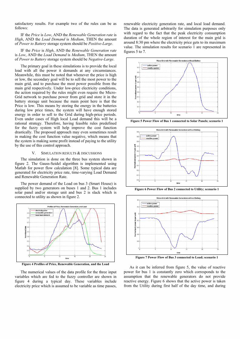
satisfactory results. For example two of the rules can be as follows:

IF the Price is Low, AND the Renewable Generation rate is High, AND the Load Demand is Medium, THEN the amount of Power to Battery storage system should be Positive-Large.

IF the Price is High, AND the Renewable Generation rate is Low, AND the Load Demand is Medium, THEN the amount of Power to Battery storage system should be Negative-Large.

The primary goal in these simulations is to provide the local load with all the power it demands at any circumstances. Meanwhile, this must be noted that whenever the price is high or low, the secondary goal will be to sell the most power to the main grid, and to purchase the most power possible from the main grid respectively. Under low-price electricity conditions, the action required by the rules might even require the Micro-Grid network to purchase power from grid and store it in the battery storage unit because the main point here is that the Price is low. This means by storing the energy in the batteries during low price times, the system will have enough stored energy in order to sell to the Grid during high-price periods. Even under cases of High local Load demand this will be a rational strategy. Therefore, having feasible rules predefined for the fuzzy system will help improve the cost function drastically. The proposed approach may even sometimes result in making the cost function value negative, which means that the system is making some profit instead of paying to the utility by the use of this control approach.

V. SIMULATION RESULTS & DISCUSSIONS The simulation is done on the three bus system shown in

figure 2. The Gauss-Seidel algorithm is implemented using Matlab for power flow calculation [8]. Some typical data are generated for electricity price rate, time-varying Load Demand and Renewable Generation Rate.

The power demand of the Load on bus 3 (Smart House) is supplied by two generators on buses 1 and 2. Bus 1 includes solar panel and/or storage unit and bus 2 is slack which is connected to utility as shown in figure 2.

The numerical values of the data profile for the three input variables which are fed to the fuzzy controller are shown in figure 4 during a typical day. These variables include electricity price which is assumed to be variable as time passes,

renewable electricity generation rate, and local load demand. The data is generated arbitrarily for simulation purposes only with regard to the fact that the peak electricity consumption duration of the whole region of interest for the main grid is around 8:30 pm where the electricity price gets to its maximum value. The simulation results for scenario 1 are represented in figures 5 to 7.

As it can be inferred from figure 5, the value of reactive power for bus 1 is constantly zero which corresponds to the assumption that the renewable generators do not provide reactive energy. Figure 6 shows that the active power is taken from the Utility during first half of the day time, and during

Figure 4 Profiles of Price, Renewable Generation, and the Load

Figure 5 Power Flow of Bus 1 connected to Solar Panels; scenario 1

Figure 6 Power Flow of Bus 2 connected to Utility; scenario 1

Figure 7 Power Flow of Bus 3 connected to Load; scenario 1

most of the second half of the day the active power is being delivered to the grid. Load is evidently consuming active power regarding the blue curve represented in figure 7.

Simulation results for scenario 2 which associates ideal storage with infinite capacity to the renewable electricity generators on bus 2 are represented in figures 8 and 9.

.

Figure 8 parts a and b are matched to each other and this clearly shows that any value decided by the Fuzzy Controller for the power to be given to Battery or to be taken from it can be practical since battery unit assumed in scenario 2 is of infinite capacity. Figure 9 shows that active power is taken from the utility during first half of the day, and in the second half of day the active power is mostly being sold to the grid which can be deduced by the negative value of the blue curve in figure 9. The point is that the first part of the active power diagram is raised dramatically due to fuzzy decision making which means that the system is absorbing more active power from the grid during low-price hours and stores the power in the storage unit. Also, the second part of the active power diagram has fallen more in comparison to the same section of figure 6 which denotes on increase in the amount of power drawn from storage unit and using this power for partially charging the load and also selling the excess power to the grid

during high-price hours. This strategy results in reduction of cost function value or in other words increases the profit.

Remembering that the pricing periods are assumed to be 15 minute periods and one day is 24 hours overally there will be 96 periods of pricing during one day period. The summation of payment/profit and the loss during each of the periods will give us the overall value of cost function for one day. The process can be extended to one week, one month, one year etc.

Output of the fuzzy inference engine which represents the power rate given to battery is shown in figure 11. Whenever the value of this variable is positive it means that power is delivered to the storage unit and if the power is drawn from the storage unit, the value will be negative.

Simulation results for scenario 3 in which ideal finite-capacity storage is added on bus 2 in Micro-Grid network are represented in figures 10 to 12.

Figure 10 parts a and b are not matched to each other and this shows the fact that the values decided by the Fuzzy Controller for the power to be given to Battery or be taken from it might not be practical since battery unit assumed in scenario 3 is of finite capacity and the maximum and minimum limits of stored energy should be taken into account.

Figure 10 Output of the Fuzzy Controller; scenario 3; (a) Theoretically decided (b) Practically allowed

Figure 11 Measure of Energy stored in Battery; scenario 3

Figure 8 Output of the Fuzzy Controller, i.e. measure of the amount of

power given to/taken from storage unit; scenario 2; (a) Theoretically decided (b) Practically allowed

Figure 9 Power Flow of Bus 2 connected to Utility; scenario 2

The Center of Gravity, i.e. Centroid, defuzzification method is used for computing the crisp values of the output variable from the union of the Fuzzy rules. The formula used for defuzzification is shown in Eq. 2

𝑦𝑐𝑟𝑖𝑠𝑝 =∑ (𝑚𝑎𝑥j (𝜇𝑖)×𝑦𝑖)𝑛𝑖=1∑ 𝑚𝑎𝑥j (𝜇𝑖)𝑛𝑖=1

(2)

Where 𝑦𝑐𝑟𝑖𝑠𝑝 stands for crisp value of output variable. i

changes between 1 and n, and refers to the number of discrete point at which the calculation is being done. j changes between 1 and the number of membership functions of output variable which in this case is 5, and represents the number of membership function curve for which we are getting the membership value of ith point in the universe of discourse of the output variable. Therefore, 𝑚𝑎𝑥j(𝜇𝑖) represents the final membership value of the ith point in the universe of discourse of output, i.e. 𝑦𝑖 . Equation 3 shows the relation between Balance, Distribution Loss and the overall Cost of Electricity.

𝐵𝑎𝑙𝑎𝑛𝑐𝑒 = 𝐿𝑜𝑠𝑠 + 𝐶𝑜𝑠𝑡 (3)

In table 1, total values of distribution loss, cost, and balance on one typical day for the three scenarios mentioned in section III are summarized. It must be noted that the values in the table are unit-less, and they can be regarded as measures for payment that the end-user should make to the utility because of regular operation of Micro-Grid, or profits earned due to improved operation and control of the Micro-Grid.

Table 1. Simulation results for Loss, Cost and Balance Loss Cost Balance

Scenario 1 0.1339 1.2294 1.3632 Scenario 2 6.6039 -17.6716 -11.0677 Scenario 3 6.6039 -13.3021 -6.6982

Cost is simply the overall summation of power from/to grid multiplied by the relevant price for all 15 min periods. The overall summation of multiplication of the price and wasted power on distribution branches for all 15 min periods is defined as Loss. With no loss of generality, it is assumed that the reactive power has one tenth the value of active power.

We can see that scenario 2 will provide the consumer with the most possible profit on balance and this is because of the fact that the battery unit used in scenario 2 is assumed to be of infinite capacity. Therefore there will be chance for utmost storage of power in the battery whenever required and the battery can provide that stored power completely to the Micro-Grid for appropriate usage any time. This is not a practical case though. In scenario 3 which is the practical case compared to the second scenario, battery storage unit is assumed to be of limited capacity and therefore, maximum and minimum limits of the stored energy in the battery might prevent the control system to apply the decided action on the storage unit thoroughly. This might cause a drop in the benefits that consumer will obtain using this approach as it can be seen by comparing the values of Balance for the two scenarios 2 and 3. However, by improvements in the battery production technologies this issue can be solved to good extents.

VI. CONCLUSION The proposed Fuzzy-Logic based control method is

applied for Battery Management in Micro-Grid Systems. In the micro-grid system three buses are considered as renewable generator and storage, utility, and load (smart house). The goal was to reduce the balance which is based on distribution loss and cost. The Micro-Grid was simulated under three scenarios. Simulation results obtained for Micro-Grid under scenario 2 where the ideal infinite-capacity storage is involved with the Fuzzy controller outperform the other two scenarios. However this is not practical. In third scenario, ideal limited-capacity storage was involved and the results were satisfactory. Therefore, using fuzzy controller it is possible to reduce the cost of the Micro-Grid system, and even let the customers make profit from selling the excess power to the utility.

REFERENCES [1] Y. S. Manjili; A. Rajaee; B. Kelley; M. Jamshidi, “Fuzzy Control of

Storage Unit for Energy Management in Micro-Grids” University of Texas at San Antonio College Of Science Conference, UTSA-COS 2011 (Best paper award winner)

[2] C. Cho; J. Jeon; J. Kim; S. Kwon; K. Park.; S. Kim, “Active Synchronizing Control of a Microgrid” IEEE Transactions on Power Electronics, issue 99, pp., 2011

[3] N. L. Srinivasa Rao; G. Govinda Rao; B. Ragunath, “Power Flow Studies Of The Regional Grid With Inter State Tie-Line Constraints” IEEE Conference on Power Quality, pp. 165-171, 2002.

[4] R.D. Zimmerman; C.E. Murillo-Sánchez; R.J. Thomas, “MATPOWER's Extensible Optimal Power Flow Architecture” IEEE Power and Energy Society General Meeting, pp. 1-7, July 26-30 2009.

[5] R.D. Zimmerman; C.E. Murillo-Sánchez; R.J. Thomas, “MATPOWER Steady-State Operations, Planning and Analysis Tools for Power Systems Research and Education” IEEE Transactions on Power Systems, vol. 26, no. 1, pp. 12-19, Feb. 2011.

[6] S. L. Chang; L. A. Zadeh, “On Fuzzy Mapping and Control”, IEEE Transactions on Systems, Man and Cybernetics, pp. 30-34, 1972.

[7] Z. Wang; R. Yang; L. Wang, “Intelligent Multi-agent Control for Integrated Building and Micro-grid Systems” IEEE PES Innovative Smart Grid Technologies (ISGT), pp.1-7, 2011.

[8] G.M. Gilbert; D.E. Bouchard; A.Y. Chikhani, “A Comparison Of Load Flow Analysis Using Distflow, Gauss-Seidel, And Optimal Load Flow Algorithms” IEEE Canadian Conf. on Elec. and Comp. Eng, 1998

Figure 12 Power Flow of Bus 2 connected to Utility; scenario 3

Cognitive Radio Capacity Analysis for Smart Grid

Networks

Abstract— In this paper a framework is presented based on

4G Cognitive Radio (CR) network capable of

communicating with high numbers of geographically

dispersed smart meters for command and control feature

concurrently with private cellular network. Our approach

uses pervasive smart grid systems (i.e. cloud data centers)

as the central communication and optimization

infrastructure supporting metropolitan area based smart

meter infrastructure. In this paper, we investigate the

performance of various scheduling algorithms in context

with CR units to provide a satisfactory tradeoff between

maximizing the system capacity, achieving fairness among

cognitive users. We lay as a framework evaluation 3GPP

LTE system model simulations. Our system level simulation

results show that the 4G CR network model meets the

smart grid protocols requirements for a multi-user CR

network of Smart meters.

Keywords-4G Cognitive radio networks, cloud data center,

scheduling algorithms, and smart meters

I. INTRODUCTION

The smart grid of the future is generally perceived to be an intelligent energy delivery system that supports plug-and-play integration of power, information, and security services. [1]. We consider the future smart grid as leveraging Information and Communications Technology (ICT) facilitated by the smart meter (also named as Advance Infrastructure Metering (AMI)) information networks. The smart meter enables the flow of real-time information within the power utility, between the power utility and its customers. It also provides customers and utilities the technology to optimize their energy consumption in participating in closed loop demand response; moreover, these services allow convergence of high penetrations of renewable energy components into grid and third party energy management applications for demand optimization. It is essential for AMI to be networked since it enables system wide sensing, utility and customer linkages, and future self healing capability.

Communication network infrastructures represent a very large capital expense. Much of this expenditure is due to the high prices of purchasing licensed bands either from the FCC auction process or from existing licensed band owners. We therefore analyze a novel, low cost framework based on 4G cognitive radio smart meter networks enabling command and control, demand optimization and other features. Research on CR has evolved from SDR (see [2-3]) with an objective of

efficient utilization of radio spectrum. In this paper, we analyze CR in the context of smart energy systems. Although there have been significant advances and improvements in CR hardware, algorithms, and protocols, less attention has been given to developing ubiquitous and pervasive metropolitan scale CR networks, particularly with respect to smart grid information networking[4]. A metropolitan infrastructure based CR networks is shown in Fig. 1. In this context, there are major challenges to overcome such as Secondary Users (SU) should sense the spectrum and timely model the behavior of the Primary Users (PU). The other issue is how the SUs manage the available spectrum resources and share the resources among the SUs to satisfy the smart grid protocol requirements and meeting the interference constraints suggested by the FCC Spectrum Policy Task.

In such a system, our objective for SUs (i.e. AMI) is to

efficiently transmit their delay sensitive traffic over the network

and meet the QoS requirements of the smart grid protocol. In

this paper, we investigate different scheduling polices that

maximize the downlink sum throughput in the given area and

achieving fairness among the SUs. We present an opportunistic

scheduling policy that exploits both maximizing the downlink

sum throughput and fairness under time-varying channel

conditions for multi-user CR network in a metropolitan based

environment.

Several authors have defined aspects of AMI networking in

smart grids. Mesh, Ethernet and cellular AMI network topology

for smart grid has been proposed. In [5] the authors propose

mesh networks of Zigbee based transmission architecture.

Challenging issue with line of sight requirements in Zigbee is

the limit of single-hop range to hundreds of feet. Inefficiencies

arise when transmission distances featured by the protocols in

the entire metropolitan area for AMI networking. In [6], the

authors discuss communication infrastructure based on Ethernet

(LAN and WAN). The approach will support automated meter

readings and customer home appliance connections. However,

wireline systems are not always available. Customer

subscription to service must occur and wired system can be

challenging to rapidly redeploy, particularly in swiftly

enveloping emergencies.

The authors in [7] describe a framework for RF mesh

networking interfaced with high speed WiMAX access

networks. In [8], overview of architecture, hardware platform,

is reported to enable CR for smart grid communications.

However, to our knowledge anywhere in the literature a

complete multi-user capacity analysis using CR network in

Amir Rajaee, KranthiManoj Nagothu, Brian Kelley Senior Member IEEE,

Electrical and Computer Engineering, The University of Texas at San Antonio, TX, USA

context with smart grid has been yet reported. Our work

discusses the CR network infrastructure architecture from 4G

perspective. We also present multi-user performance analysis

of various scheduling algorithms in context with AMI units

considering the delay occurred due to offloading the processes

to cloud in our architecture.

The rest of the paper is organized as follows. Section II

overviews the 4G CR system architecture in brief. In section III

we present overall 4G CR system model detailing the sensing

model and different scheduling polices and their properties.

Section IV discusses the performance of the different

scheduling algorithms with system level simulations and

concludes this paper.

II. 4g Cognitive radio framework

A. 4G cognitive radio system architecture

We presume a LTE network as a CR LTE network (4G CR),

if the LTE work is adopted the CR techniques. We consider a

cloud data center infrastructure based CR network coexisting

with PU network shown in Fig.1. The coverage of both the CR

base station and PU network base station are similar. As

depicted in the Fig. 1 at the center of the each cell, there is

base-station which is shared as e Node-B for PUs and as

antenna for SUs. The PU base-station only serves to PUs as it

lacks the CR protocols capabilities to support SUs. However, it

may consider supporting certain features in order to

communicate with SUs.

A CR system does not own a license band to operate in a

desired band. Hence, the spectrum access is allowed only in an

opportunistic manner. The licensed user of the frequency band

is always given priority access to the shared channel (time-

frequency resource). Due to their priority in spectrum access,

the operations of PUs are always 1st in the transmission queue

so as to not be affected by unlicensed users All the SUs have

the same right to access the spectrum; SUs should compete

with each other for the same unlicensed band. Thus,

sophisticated spectrum sharing methods among SUs are

required in this architecture. If multiple SUs network operators

reside in the same unlicensed band, fair spectrum sharing

among these networks is also required and different scheduling

algorithms are discussed in detail in section III.

Placement of a Cognitive Radio Antenna on the BTS tower

may occur in tandem with deployment of the cellular provider

antenna. The CR senses the spectral environment over a wide

frequency band, particularly the spectrum in the cell region. It

identifies the unused bands in the spectrum. These bands could

be owned by cellular companies or license television band

owners, but are not limited to these bands or to licensed bands.

Sensed information using the CR is relayed to cloud data

center. In principle, eNode-B which terminates the air interface

protocol and first point of contact for PU is located at the

primary user base-station. However, in proposed architecture

all the cognitive radio service, waveform service, protocols

service, security service, scheduling and control services are

displaced into cloud data center. The CR services indentify

unused frequency bands, the relevant cognitive services

residing in the cloud data center generates a clear to send (CTS)

signal.

Fig. 1. 4G CR network system architecture: Scenario of multiple AMI meters

serviced by cognitive radio network infrastructure enabled by cloud center

coexisting with private cellular network The CTS is sent back to the AMI meters through the

feedback channel via base station. Eventually, the CR antenna

relays CTS signals to every AMI in the cell region for uplink

transmission.

1) Pervasive smart grid systems

The energy services of the future can be privately contracted

services or public services. The cloud center enables

convenient, on-demand network access to a shared pool of

configurable, computing resources (e.g., networks, servers,

storage, applications, and services) that can be rapidly

provisioned and released with minimal management effort.

There are different cloud computing platform classifications.

Standard architectures includes Abi (or Abiquo), Nimbus Open

Nebula, Azure (Microsoft), Google (App Engine), Blue (IBM)

and Mosso (Rackspace). Fig.1. depicts the model for a cloud

data center architecture optimized for based smart grids. Our

Wireless Cloud Data (WCD) model is organized into four

principle layers: application layer, platform layer, CR

communication and networking layer and infrastructure layer.

The first two layers are akin to existing cloud architectures.

However, the lower two layers are augmented to enable the CR

networking and wireless services. CR communication and

networking layer provides services such as cognitive radio

services, waveform services, Radio Link Control (RLC), and

Medium Access Control (MAC) services. CR services, which

provide spectrum management and spectrum sensing, are

discussed in detail in section III. The infrastructure layer

facilitates the effective integration of computing resources,

storage, networks to deploy applications and operating systems.

We augment our cloud infrastructure microprocessor racks with

FPGA boards targeted to processing high computation rate

processes typically associate with CR services, communication

waveform signal processing and coding.

III. CR SYSTEM MODEL

In the paper system model 4G cellular network is considered

with Nsu secondary users sharing the spectrum simultaneously

PUBS

(eNode-B) PU

PU

PU

PU PU

Primary user radio network

BS / e Node -B

Cognitive user

(i.e. AMI(A-SU)) radio network with

cloud infrastructure

A-SU

A-SU

A-SU

PU

PU

CR: Cognitive radio

SU: Secondary user

PU: Primary user

PUBS: PU Base station

CTS: clear to send

Wireless cloud data

center

PDN

GWHSSMME

Serving

GW

SGSN

PCRF UTRANGERAN

Packet data

network

S1

S1-MME

S6a

S1-U

Rx

SGi

GXS12

S4

S3

S11S5

S1

PU

Back Haul

NetworkCTS CTS

CTS

•

Application

Radio servers

Radio services

Servers, storage, networking

Platform

Communication, Networking

InfrastructureCR boards

Cognitive radio

Radio

boards

Demand response

management services

Energy manager

servicesOther services

CR

services e Node-BRadio interface

protocols

Wireless networking

with Npu primary users. It is presumed in the context that the

secondary users (i.e. AMI meters) are fixed in sense of

geographical location and yields to fixed first and second

statistical moments of SINR.

A. Spectrum Sensing

The spectrum sensing is one of the main layer task for CR

system to obtain the spectrum usage information and the

presence of PUs. Spectrum detection is based on the detection

of the signal from PU through the observation of cognitive

radio network.

The sensing methods can be categorized in three methods: i)

Energy Detection, ii) Matched Filter, and iii) Feature Detection.

The spectrum sensing method considered for this paper is

Energy Detection. Since, it is particularly suitable for

multiband sensing because of its low computational and

implementation complexities [9-10]. We presume using OFDM

modulation with M sub carriers with bandwidth W. In this

paper we premised the IEEE 802.22 as it has developed air

interface for opportunistic SU access to the TV spectrum in

which PUs change slowly [11].

The timing model for spectrum sensing is shown in Fig.

2.a and spectrum mobility model for SUs is depicted in Fig.

2.b. The required time for channel estimation, spectrum sensing

and sharing is indicated by . According to the [12] the given

channel estimation delay is for WCDMA/HSDPA, so the

scaled delay for a shorter sub-frame length in UTRAN LTE is

considered for this paper. For each Resource Block (RB), there

are 7 frames in time frame and 12 subcarriers and each square

in Fig .2.b is called Resource Element (RE). For example, in

Fig. 2.b, RE (10, 7) means that the frequency carrier at frame 7

and subcarrier 10 is occupied by primary user 3. At each time,

idle resource elements will be detected and allocated to SUs.

Once a PU requests the subcarrier occupied by the active SU,

SU has to leave the spectrum and try to find another idle

resource element to continue transmission. In Fig. 2.a. T is time

length of each frame and K is number of frames. The idle RB

or hole is a band can be used by SU without interfering with

PU. Supposed that received signal at SUs sampled at fs over ith

sub channel where values of discretized samples at ,

which is in our framework. In discrete form, when

the primary user is active, we define two hypotheses as follow:

(1)

That is the subchannel gain between PU transmitter and SU

receiver with variance . The signal transmitted,

, by PU is assumed to be independent and identically

distributed (i.i.d), , and , the noise, is circularly

symmetric complex Gaussian (CSCG) noise.

B. Energy Detection

In order to detect the RF energy in the certain subcarrier for a given PU, the CR service residing in the WCD samples on-the-air signal constructs the following test statistics as the

observed energy summation within N samples to decide on the presence of the active users in targeted subcarrier [13].

(2)

Fig. 2. a)Timing Model, b)Resource Block & Dynamic Resource Management

is number of samples transmitted on duration which is

equal to . The PDF of is Central Chi Square

distribution with degrees of freedom, , for when no

PU exists and on Central Chi Square distribution with

degrees of freedom and non-centrality parameter ,

, for the state that PU exists. So:

(3)

where the signal to noise ratio (SNR) is depicted by

, denotes the gamma function, is the

first kind modified Bessel function of degree .

Two performance parameters for spectrum sensing are probability of detection, , and probability of false alarm, ,

which is probability of when the frequency is unoccupied but we get alarm that the frequency is used. Hence, Higher

protects PU from interfering with SUs and smaller causes

better band usage efficiency. To calculate probability of detection [14]:

(4)

where is threshold and is denoted sensing time for ith

subchannel.

(5)

Now the probability of missed detection can be defined as:

(6)

we have following equations for probability of false alarm,

Frame 1 Frame 2 Frame K

Sensing

Time

Data Transmission

Time Duration

Frequency

Time Frame

Channel

Estimation Time

b)a)

P12 P12 P12

P11 P11 P11 P11

P10 P10 P10 P10 P10

P9 P9 P9 P9 P9

P8P8P8

P7 P7 P7 P7

P6 P6 P6 P6

P5 P5 P5P5 P5

P4P4P4

P3 P3 P3 P3

P4

P2P2P2P2P2

P1 P1 P1

P8P8

S2 S2

S2

S1 S1 S1

0

0

S3

0

S3 S3

S3 S3 S3S3

0 0

S2 S2 S2

0

0

S1S1S1S1

P6

S2

P3

P8

0

0

Frequency

Time Frame

1 2

12

11

10

9

8

76543

2

3

4

5

6

7

RE(10,7)

15 KHz

1ms

1

S>>SU, P>>PU, 0>>Idle

Resource

Block

Subcarrier 4

(7)

(8)

Usually to evaluate the performance of energy detection, the

goal is to minimize for a target or to maximize for a

target . At first we assume is our target

probability of detection ,

(9)

(10)

is the probability of false alarm regard

to target , and is the inverse of complementary error

function. For a target we have:

(11)

(12)

is the probability of detection when

is targeted. As a result, in this part, probability of false

alarm and detection based on and ,

respectively, are calculated.

C. Primary User Activity Model

In this section, we present a model for primary users’

activities which is directly proportional to CR network

performance. In our Markov chains model, we consider two

states (Busy by PU and Idle) for each subcarrier. Since each

user arrival is independent, each transition follows the Poisson

arrival process. Thus, the length of Busy and Idle periods are

exponentially distributed. The Poisson distribution is

considered in the modelling with arrival rate, α, and departure

rate, β, and in simulation, the average existing users is assumed

such that %80 of total spectrums are loaded by primary users in

average.

(13)

as a result, the existing users in a cell is equivalent to total

existing users on previous time period added to arrival rate at

current time and subtracted by current departure time as

mentioned in equation (13). The transition probabilities are

pTand q

T as illustrated in Fig. 3 and the calculated steady

probabilities are depicted below [15]:

, (14)

Eq. (14) is applied to analyze the model for identifying subcarriers states (i.e. busy or idle).

D. Optimum Sensing Time

The throughput of SU is calculated as follows [16],

(15)

where W is bandwidth, is the power of transmitter SU

and is the noise power and is the gain channel

between ith SU’s transmitter and receiver with variance

.

Considering probabilities for different states gives us achievable throughput, , calculated by,

(16)

where is the probability of absence of

PU when we detect correctly. is the entire data

transmission. Following equations can be derived,

(17)

(18)

Thus, there is a between 0 and T that gives us maximum

. The Fig. 4 shows the optimum sensing time based on

equation (16). By Fig. 4, it can be denoted that the optimum sensing time in regard to technology limits and optimum sensing time is approximated between 3ns and 1µs.

Fig. 3. Markov Chains Model Fig. 4. Optimum Sensing Time

E. Scheduling algorithms for CR users

We consider the downlink of Nsu secondary users are

serviced by a base station within a cell. The base station

allocates RE(i,j) among the Nsu SUs. At each frame multiple

REs can be assigned to a single user, although each RE can be

allocated to only one SU.

We assume that channel conditions vary across the

subcarriers as well as secondary users. The channel conditions

typically depend on the channel frequency, so they may be

different for different channels. We presume typical urban area

model. Moreover, scheduling of SUs also depend on the user

location and the time frame. However, in our context the AMI

meters are geographical stationary leading to constant SINR

values.

In order to make optimal multi user scheduling decision and

achieve high gain from multiplexing, the scheduler needs

accurate channel quality indicator (CQI). Accuracy of CQI

prediction depends on error in measuring the channel from the

pilot and delays in the feeding back the information to the case-

station. Feedback delay can be reduced by shrinking the size of

the scheduling frame time. However, due to reduction of frame

time the feedback request rate in uplink increases and

eventually increasing the system overhead.

We define the peak downlink multiuser capacity for

orthogonal OFDM signaling and note that it cannot exceed the

Shannon capacity :

100

101

102

103

104

0

0.5

1

1.5

2x 10

7

Time (ns)

Am

plitu

de

10 ns: OptimumSensing Time

Busy Idle

(19)

In real deployments, we can develop a modified Shannon

capacity formula by replacing the cell bandwidth, with an

effective bandwidth and [17] which accounts for G-

factor dependencies and protocol control, pilot, and cyclic

prefix overheads. Closely related to the SINR is the G-factor,

which accounts for the geometric dependencies of cell layouts

and dictates the statistics of the downlink capacity. The G-

factor is the average own cell power to the other cell-power

plus noise ratio when considering uniform spatial distributions

of transceivers within a cell.

In addition, we can define a normalized effective signal to

noise ratio, , adjust SNR for both interference, G-factor

statistics, and LTE implementation parameters. Defining the

modified Shannon spectral efficiency for PU as

(20)

We also define capacity of secondary user in presence of loss,

(21)

ρ is detection probability parameter and calculated by addition

of false alarm detection probability (Pf) and detection

probability (Pd). δ is primary user spectrum usage and we

presume a average of 80% loading. β is a correction factor

which nominally should be equal to one and it is discussed

more detailed in. η is the spectrum sensing efficiency. The

scheduler decides which SU to transmit the information at each

time frames, based on the request rates the base station.

Scheduling the user with the instantaneously best link

conditions is often referred as max rate scheduling. The max

rate can be expressed as for ith user.

Proportional fair (PF) scheduler is designed to meet the

challenges of delay and fairness constraints while harnessing

multi user diversity. PF scheduler tracks the average

throughput, Tk[nTs], for each SU delivered in the past over

sliding window of size tc . In the time frame [τ], the base station

receives rates Rk[nTs], k=1...Nsu from all the active SUs and

scheduler basically schedules the SU with highest PF metric

value, γ that is defined as .

The average throughputs Tk[nTs] are updated using an

exponentially weighted low pass-filter :

(22)

Based on the Eq. (21) and (22) we can write as the following

(23)

Opportunistic Scheduling (OS) is an approach to deal with both

fairness among users and maximizing the capacity rate. In max

rate algorithm the user with highest request rate implies giving

all the system resources to particular users, yields to highly

unfair scheme to all other users. However, in PF the users

compete for resources not directly based on the requested rates

but based on the rates normalized by their respective average

throughputs also defined as PF metric value. The downside of

the PF approach is sacrificing over all throughputs. Thus OS

algorithm schedules subcarriers sc1,1 to sci,j to the best

secondary user based on two step criteria. First, the user who

has the maximum PF metric value, γ, is selected. Second, the

selected SU requested rate should be greater than the mean of

all the secondary users requested rate, , to be scheduled

as follow,

(24)

As a result, unlike PF scheduling, the users having low

throughput but high PF metric, γ, that had been chosen to

access frequency will have lower priority than users with

enough PF metric and higher throughput.

Algorithm: Opportunistic scheduling

1) for n=1 to NT (simulation time)

2)Update SU profile, Update γ

3)Let S be the set of secondary users

4)Let RE(i,j) where i=1 to M subcarriers and j=1 to K be the

total time frames.

5)for i=1 to M, for j=1to K

6)Select the secondary user l ϵ S with highest γ(l)

7)If

8) Update the SU profile with S=S-l

9)Allocate RE(i,j) to lth secondary user from S

10)Else

11)Update the SU profile with S=S-l

12)End if, End for j, i, n

IV. ANALYSIS & SIMULATION RESULTS

To evaluate the performance of CR system model, system level simulations have been conducted based on 3GPP LTE system model. Table [see 15] shows the simulation parameters used for the simulations. We analyze the performance of the scheduling in terms of throughput and fairness. We first evaluate the system throughput for algorithms with varying the primary user loading within a cell. In this case, the primary user average loading is around 80% and total number of users is 500 in a cell. Over the period of time that spectrum sensing reports the number of idle resource blocks, scheduler allocates the idle REs with SUs. The Fig. 5 illustrates average capacity for three aforementioned algorithms.

Max-rate results in highest average capacity among three algorithms are followed by opportunistic and fairness algorithms. The results seem to match our expectations, since the goal of the Max-rate capacity is the user with highest request rate implies giving all the system resources to particular users. In proportional fair algorithm the users compete for resources not directly based on the requested rates but based on the rates normalized by their respective average throughputs, PF metrics. By this approach PF sacrifices the overall throughput while, achieving higher number of SUs scheduled. In OS the users having low request rate but high PF metric, γ, will have less chance to be scheduled. OS objective is to achieve higher average capacity compared to PF, while achieving decent fairness among the SUs.

Fig. 6.a and 6.b show the average number of users scheduled per one Transmission Time Interval (TTI) when 75 SUs are

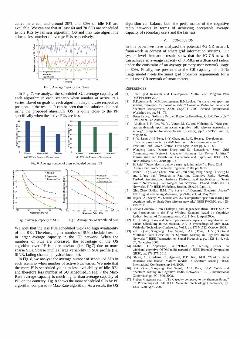
active in a cell and around 20% and 30% of idle RE are available. We can see that at least 60 and 70 SUs are scheduled to idle REs by fairness algorithm. OS and max rate algorithms allocate less number of average SUs respectively.

Fig. 5 Average Capacity over Time

In Fig. 7, we analyze the scheduled SUs average capacity of each algorithm in each scenario when number of active PUs varies. Based on goals of each algorithm they indicate respective positions in the results. It can be seen that the solution obtained using the proposed algorithm (OS) is quite close to the PF specifically when the active PUs are less.

Fig. 6. Average number of users scheduled per one TTI

Fig. 7 Average capacity of SUs Fig. 8 Average No. of scheduled SUs

We note that the less PUs scheduled yields to high availability of idle REs. Therefore, higher number of SUs scheduled results in larger average capacity in the CR network. When the numbers of PUs are increased, the advantage of the OS algorithm over PF is more obvious (i.e. Fig.7) due to more sparse SUs. Sparse implies large variability in SUs profile (i.e. SINR, fading channel, physical location).

In Fig. 8, we analyze the average number of scheduled SUs in each scenario when number of active PUs varies. We note that the more PUs scheduled yields to less availability of idle REs and therefore less number of SU scheduled.In Fig. 7 the Max-Rate average capacity is much higher than average capacity of PF; on the contrary, Fig. 8 shows the more scheduled SUs by PF algorithm compared to Max-Rate algorithm. As a result, the OS

algorithm can balance both the performance of the cognitive radio networks in terms of achieving acceptable average capacity of secondary users and the fairness.

V. CONCLUSION

In this paper, we have analyzed the potential 4G CR network

framework in context of smart grid information systems. Our

system level simulation results show that the 4G CR network

can achieve an average capacity of 3.5Mbs in a 3Km cell radius

under the constraint of an average primary user network usage

of 80%. Finally, we present that the CR capacity of a 20%

usage model meets the smart grid protocols requirements for a

multi-user CR network of smart meters.

REFERENCES

[1] Smart grid Research and Development Multi- Year Program Plan (MYPP) 2010-2014.

[2] D.D.Ariananda, M.K.Lakshmanan, H.Nikookar, ―A survey on spectrum

sensing techniques for cognitive radio,‖ Cognitive Radio and Advanced

Spectrum Management, 2009. CogART 2009. Second International

Workshop on, pp. 74 – 79.

[3] Brian Kelley, ―Software Defined Radio for Broadband OFDM Protocols,‖ SMC 2009, San Antonio.

[4] Akyildiz, I. F., Lee, W.-Y., Vuran, M. C., and Mohanty, S, ―Next gen-

eration dynamic spectrum access cognitive radio wireless networks: a survey," Computer Networks Journal (Elsevier), pp.2127-2159, vol. 50,

May 2006.

[5] S.-W. Luan, J.-H. Teng, S.-Y. Chan, and L.-C. Hwang, ―Development of a smart power meter for AMI based on zigbee communication,‖ in

Proc. Int. Conf. Power Electron. Drive Syst., 2009, pp. 661–665.

[6] Wenpeng Luan, Duncan Sharp and Sol Lancashire,‖ Smart Grid Communication Network Capacity Planning for Power Utilities,‖

Transmission and Distribution Conference and Exposition, IEEE PES,

New Orleans, USA, 2010, pp. 1-4. [7] B. Reid, ―Oncor electric delivery smart grid initiative,‖ in Proc. 62nd

Annu. Conf. Protective Relay Engineers, 2009, pp. 8–15.

[8] Robert C. Qiu, Zhe Chen , Nan Guo , Yu Song, Peng Zhang, Husheng Li and Lifeng Lai,‖ Towards A Real-time Cognitive Radio Network

Testbed: Architecture, Hardware Platform, and Application to Smart

Grid,‖ Networking Technologies for Software Defined Radio (SDR) Networks, Fifth IEEE Workshop, Boston, USA,2010,pp.1-6.

[9] Qing Zhao ; Sadler, B.M. ; ―A Survey of Dynamic Spectrum Access‖

IEEE Signal Processing Magazine, pp.79-89, vol. 24, May 2007. [10] Rajaee, A., Saedy, M., Sahebalam, A., "Competitive spectrum sharing for

cognitive radio on Scale-Free wireless networks" IEEE IWCMC, pp. 455-459, 2011.

[11] Carlos Cordeiro, Kiran Challapali, and Dagnachew Birru,‖ IEEE 802.22:

An Introduction to the First Wireless Standard based on Cognitive Radios‖ Journal of Communications, Vol. 1, No. 1, April 2006.

[12] T.E Kolding. ―Link and System performance aspects of Proportional Fair

Packet Scheduling in WCMS/HSDPA‖, In Proceedings of 58th IEEE Vehicular Technology Conference, Vol.3, pp. 1717-1722, October 2008.

[13] Zhi Quan ; Shuguang Cui ; Sayed, A.H. ; Poor, H.V. ; ―Optimal

Multiband Joint Detection for Spectrum Sensing in Cognitive Radio Networks ‖ IEEE Transaction on Signal Processing, pp. 1128-1140, vol.

57, November 2008.

[14] Khalid, L. ; Anpalagan, A. ; ―Effect of sensing errors on wideband cognitive OFDM radio networks‖ IEEE Biennial Symposium

QBSC, pp. 273-277, 2010.

[15] Ghosh, C. ; Cordeiro, C. ; Agrawal, D.P. ; Rao, M.B. ; ―Markov chain existence and Hidden Markov models in spectrum sensing‖ IEEE

International Conference, pp.1-6, 2009.

[16] Zhi Quan ; Shuguang Cui ; Sayed, A.H. ; Poor, H.V. ; ―Wideband Spectrum sensing in Cognitive Radio Networks ‖ IEEE International

Conference, pp. 901-906, 2008.

[17] Preben Mogensen et,al. ―LTE Capacity compared to the Shannon Bound‖ ,In Proceedings of 65th IEEE Vehicular Technology Conference, pp.

1234-1238,April, 2007.

10 20 30 40 50 60 70 80

2

2.5

3

3.5

4

4.5

5

Time(ms)

Av

era

ge

cap

aci

ty o

f S

Us

(Mb

/s)

Proportional Fairness

Max-Rate

Opportunistic

Fairness Oppurtunistic Max-Rate0

10

20

30

40

50

60

Av

g S

Us

Sce

hd

ule

d p

er T

TI

Fairness Opportunistic Max-Rate0

10

20

30

40

50

60

70

Avg S

Us

Sce

hd

ule

d p

er T

TI

(a) 20% idle Resource Element case (b) 30% idle Resource Element case

150 200 250 300 3502

2.5

3

3.5

4

4.5

5

5.5

Number of Active PUs

Av

era

ge C

ap

acit

y o

f S

erv

iced

SU

s (

Mb

ps)

Max-Rate

Opportunistic

Proportional Fair

160 180 200 220 240 260 280 300 320 34040

45

50

55

60

65

70

75

Number of Active PUs

Nu

mb

er o

f S

erv

iced

SU

s

Max-Rate

Opportunistic

Proportional Fair

COGNITIVE RADIO NETWORKS:

SYSTEM OPTIMIZATION AND SMART GRID

APPLICATIONS

by

AMIR RAJAEE, B.S.

THESIS

Presented to the Graduate Faculty of

The University of Texas at San Antonio

In partial Fulfillment

Of the Requirements

For the Degree of

MASTER OF SCIENCE IN ELECTRICAL ENGINEERING

THE UNIVERSITY OF TEXAS AT SAN ANTONIO

College of Engineering

Department of Electrical Engineering

July 2012

1

I am extremely thankful to my supervisor Dr. Mo Jamshidi for his outstanding pedagogy,

valuable advice and consistent support during preparation of this research project. I hope he

will be proud of me throughout future successful challenges in my career. I also express my

gratitude and special thanks to my supervisor Dr. Brian Kelley for his support, patience, and

encouragement throughout my graduate studies. It is not often that one finds an advisor and

colleague that always finds the time for listening to the little problems and roadblocks that

unavoidably crop up in the course of performing research. His technical and editorial advice

was essential to the completion of this dissertation and has taught me innumerable lessons

and insights on the workings of academic research in general.

July 2012

2

CHAPTER I. INTRODUCTION .................................................................................................. 8

CHAPTER II. COGNITIVE RADIO ............................................................................................ 12

APPLICATIONS OF COGNITIVE RADIO .................................................................................................. 12 A. TV White Spaces ......................................................................................................... 12 B. Cellular Networks ........................................................................................................ 13 C. Military Usage............................................................................................................. 13

COGNITIVE RADIO NETWORK ARCHITECTURE ...................................................................................... 13 NETWORK COMPONENTS ................................................................................................................ 14 SPECTRUM MANAGEMENT FRAMEWORK ............................................................................................ 16 SPECTRUM SENSING ....................................................................................................................... 17

A. Spectrum Sensing Challenges ..................................................................................... 20 SPECTRUM DECISION ...................................................................................................................... 22

A. Channel Characteristics In Cognitive Radio Networks ...................................................... 22 B. Decision Procedure ..................................................................................................... 23 C. Spectrum Decision Challenges .................................................................................... 24

SPECTRUM SHARING ....................................................................................................................... 25 A. Spectrum Sharing Challenges ..................................................................................... 27

SPECTRUM MOBILITY ...................................................................................................................... 28 B. Spectrum Mobility Challenges .................................................................................... 29

CHAPTER III. PROPOSED SPECTRUM DECISION AND SPECTRUM SHARING ALGORITHM ... 30

INTRODUCTION .............................................................................................................................. 30 NETWORK TOPOLOGY ..................................................................................................................... 31

A. Random Topology ............................................................................................................ 32 B. Scale-Free Topology ......................................................................................................... 32

SPECTRUM SENSING ....................................................................................................................... 33 A. Energy Detection .............................................................................................................. 35

QUEUED MARKOV CHAIN MODEL FOR SPECTRUM ANALYSIS-ACCESS ...................................................... 38 MAX-RATE SPECTRUM SHARING ....................................................................................................... 41

A. Cognitive Parameters.................................................................................................. 43 B. Merit Function ............................................................................................................ 44 C. Channel Indexing Function .......................................................................................... 44 D. Competitive Indexing Algorithm ................................................................................. 45

SHARING INCORPORATED IN MARKOV CHAIN MODEL ............................................................................ 47 SIMULATION ................................................................................................................................. 48

A. Simulation Results For Sensing ................................................................................... 48 B. Simulation Results For Sharing ................................................................................... 50

CONCLUSION ................................................................................................................................. 53

CHAPTER IV. COGNITIVE RADIO IN SMART GRID .............................................................. 54

THROUGHPUT ANALYSIS ON COGNITIVE RADIO NETWORKS FOR AMI METERS IN SMART GRID ..................... 54 INTRODUCTION .............................................................................................................................. 54 4G COGNITIVE RADIO FRAMEWORK .................................................................................................. 56

A. 4G Cognitive Radio System Architecture ..................................................................... 56 B. Pervasive Smart Grid Systems ..................................................................................... 57

CR SYSTEM MODEL ........................................................................................................................ 58 A. Primary User Activity Model ....................................................................................... 59 B. Optimum Sensing Time ............................................................................................... 60

SCHEDULING ALGORITHMS FOR CR USERS ........................................................................................... 61 ANALYSIS & SIMULATION RESULTS .................................................................................................... 63 CONCLUSION ................................................................................................................................. 65

CHAPTER V. INTERFERENCE AWARE SCHEDULING FOR MAXIMUM CHANNEL REUSE AND MAX-CAPACITY IN SMART METER NETWORKS ........................................................................ 66

3

CONTRIBUTIONS OF THIS THESIS ON INTERFERENCE AWARE SCHEDULING ................................................. 66 SYSTEM MODEL ............................................................................................................................. 67 INTERFERENCE –AWARE SCHEDULING ALGORITHM ............................................................................... 69 INTERFERENCE MODEL FOR SISO ...................................................................................................... 72 INTERFERENCE MODEL FOR BEAMFORMING ........................................................................................ 74 SIMULATIONS AND RESULTS ............................................................................................................. 74 CONCLUSION ................................................................................................................................. 78

CHAPTER VI. SMART GRID AND OPTIMIZATION ............................................................... 80

FUZZY CONTROL OF ELECTRICITY STORAGE UNIT FOR ENERGY MANAGEMENT OF MICRO-GRIDS ................... 80 INTRODUCTION .............................................................................................................................. 80 SYSTEM MODEL ............................................................................................................................. 81

A. Characteristics of Buses in Scenario 1 ......................................................................... 83 B. Characteristics of Buses in Scenario 2 ......................................................................... 83 C. Characteristics of Buses in Scenario 3 ......................................................................... 84

PROBLEM STATEMENT .................................................................................................................... 84 A. Scenario 1 ................................................................................................................... 86 B. Scenario 2 ................................................................................................................... 86 C. Scenario 3 ................................................................................................................... 86

FUZZY CONTROL APPROACH ............................................................................................................. 87 SIMULATION RESULTS & DISCUSSIONS ................................................................................................ 89 CONCLUSION ................................................................................................................................. 96

CHAPTER VII. PARTICLE SWARM OPTIMIZATION ............................................................... 97

SIMULATIONS FOR PSO ................................................................................................................... 99

CHAPTER VIII. CONCLUSION ............................................................................................. 104

CHAPTER IX. REFERENCES ............................................................................................... 107

4

Table of Figures

FIGURE 1 AVAILABLE CHUNKS OF SPECTRUM (WHITE SQUARES) ARE DETECTED IN FREQUENCY AND TIME AND CAN BE

AGGREGATED FOR OPPORTUNISTIC USE ............................................................................................ 9 FIGURE 2 COGNITIVE OPERATIONS NEEDED FOR AN OPTIMAL DECISION ............................................................ 9 FIGURE 3 COGNITIVE RADIO NETWORK ARCHITECTURE. .............................................................................. 14 FIGURE 4 SCALE-FREE NETWORK FORMATION WITH POWER-LAW DEGREE DISTRIBUTION ................................... 33 FIGURE 5 A)TIMING MODEL, B)RESOURCE BLOCK & DYNAMIC RESOURCE MANAGEMENT ............................... 35 FIGURE 6 WIDE SPECTRUM SENSING MODEL ............................................................................................. 38 FIGURE 7 QUEUED MARKOV CHAIN STATE MACHINE WITHOUT SHARING ...................................................... 39 FIGURE 8 SCALE FREE INFRASTRUCTURE AND ITS UL AND DL SPECTRUM RESOURCE MODEL ............................... 43 FIGURE 9 QUEUED MARKOV CHAIN STATE MACHINE WITH SHARING ............................................................ 48 FIGURE 10 STATE PROBABILITIES USING COMPETITIVE SHARING FOR DIFFERENT NUMBER OF USERS ..................... 49 FIGURE 11 STATE PROBABILITIES USING COMPETITIVE AND UNIFORM SHARING N=3......................................... 50 FIGURE 12 LOAD AND NET REQUEST IN CLUSTER A ................................................................................... 51 FIGURE 13 LOAD WITH DIFFERENT TRAFFIC IN CLUSTER A ........................................................................... 51 FIGURE 14 CAPACITY IMPROVEMENT IN CLUSTER A ................................................................................... 52 FIGURE 15 CAPACITY IMPROVEMENT IN CLUSTER A ................................................................................... 52 FIGURE 16 CAPACITY IMPROVEMENT FOR SCALE-FREE NETWORK ................................................................ 52 FIGURE 17 4G CR NETWORK SYSTEM ARCHITECTURE: SCENARIO OF MULTIPLE AMI METERS SERVICED BY COGNITIVE

RADIO NETWORK INFRASTRUCTURE ENABLED BY CLOUD CENTER COEXISTING WITH PRIVATE CELLULAR

NETWORK ................................................................................................................................ 57 FIGURE 18 MARKOV CHAINS MODEL; OPTIMUM SENSING TIME ................................................................ 59 FIGURE 19 AVERAGE CAPACITY OVER TIME .............................................................................................. 63 FIGURE 20 MAX-RATE AVERAGE CAPACITY .............................................................................................. 64 FIGURE 21 AVERAGE NO. OF SCHEDULED SUS.......................................................................................... 64 FIGURE 22 SISO SYSTEM MODEL DEPICTED WITH COORDINATED AND UNCOORDINATED INTERFERENCE ............... 67 FIGURE 23 MECHANISM OF OUR REUSE MODEL ....................................................................................... 68 FIGURE 24 INTERFERENCE-AWARE SCHEDULER (IAS) ALGORITHM FOR PRE REUSE .......................................... 69 FIGURE 25 MIMO SYSTEM MODEL WITH COORDINATED AND UNCOORDINATED INTERFERENCE ......................... 73 FIGURE 26 TOTAL CAPACITY OF A-SU IN THE CASES OF NO IAS, IAS-SISO AND IAS-BF ................................... 76 FIGURE 27 TOTAL CAPACITY OF A-SU IN THE CASES OF NO IAS, IAS-SISO AND IAS-BF ................................... 76 FIGURE 28 RELATION BETWEEN INTERFERENCE GENERATED BY REUSE AND TOTAL CAPACITY OF SCHEDULED A-SU IN

THE CASES OF IAS-SISO AND IAS-BF ............................................................................................ 78 FIGURE 29 NUMBER OF REUSE FOR EVERY SCHEDULED A-SUS IN ONE INSTANCE............................................. 79 FIGURE 30 TOTAL NUMBER OF REUSES OVER ENTIRE BW IN CASES OF IAS-SISO AND IAS-BF. .......................... 79 FIGURE 31 BASIC GRID SYSTEM MODEL .................................................................................................. 82 FIGURE 32 THREE BUS MODEL FOR MICRO-GRID ..................................................................................... 85 FIGURE 33 FUZZY MEMBERSHIP FUNCTIONS FOR INPUT AND OUTPUT VARIABLES OF THE FUZZY CONTROLLER; ...... 88 FIGURE 34 PROFILES OF PRICE, RENEWABLE GENERATION, AND THE LOAD .................................................... 90 FIGURE 35 POWER FLOW OF BUS 1 CONNECTED TO SOLAR PANELS; SCENARIO 1 ............................................ 90 FIGURE 36 POWER FLOW OF BUS 2 CONNECTED TO UTILITY; SCENARIO 1...................................................... 90 FIGURE 37 POWER FLOW OF BUS 3 CONNECTED TO LOAD; SCENARIO 1 ........................................................ 91 FIGURE 38 OUTPUT OF THE FUZZY CONTROLLER, I.E. MEASURE OF THE AMOUNT OF POWER GIVEN TO/TAKEN FROM

STORAGE UNIT; SCENARIO 2; ....................................................................................................... 92 FIGURE 39 POWER FLOW OF BUS 2 CONNECTED TO UTILITY; SCENARIO 2...................................................... 92 FIGURE 40 OUTPUT OF THE FUZZY CONTROLLER; SCENARIO 3; .................................................................... 93 FIGURE 41 MEASURE OF ENERGY STORED IN BATTERY; SCENARIO 3 ............................................................. 94 FIGURE 42 POWER FLOW OF BUS 2 CONNECTED TO UTILITY; SCENARIO 3...................................................... 94 FIGURE 43 MICRO GRID CONTROL BY PSO WITH LOAD, RE, AND PRICE PROFILE ............................................ 99 FIGURE 44 POWER FROM BATTERY ......................................................................................................... 99 FIGURE 45 ALL PROFILES AND BATTERY BEHAVIOR THROUGH PSO UTILIZATION ............................................. 100

5

FIGURE 46 THE RE POWER, PRICE, AND LOAD PROFILE WHEN RE POWER IS NOT SUFFICIENT FOR GIVEN LOAD ..... 101 FIGURE 47 BATTERY CHARGING AND DISCHARGING STATES ....................................................................... 101 FIGURE 48 GRID POWER, PRICE, COST FUNCTION, AND POWER FROM RE ................................................... 102 FIGURE 49 BATTERY POWER, INPUT PROFILES AND GRID POWER ............................................................... 103

6

This thesis presents the Cognitive Radio framework for wireless networks. The proposed

Cognitive Radio framework is a complete model for Cognitive Radio that describes the

decision and sharing procedures in wireless networks by introducing Queued Markov Chain

method.

Queued Markov Chain method is capable of considering waiting time and is very well

generalized for unlimited number of secondary users. It includes the sharing aspect of

Cognitive Radio.

The proposed approach in this thesis uses pervasive smart grid systems (i.e. cloud data

centers) as the central communication and optimization infrastructure supporting

metropolitan area based smart meter infrastructure. In this thesis, we investigate the

performance of various scheduling algorithms in context with CR units to provide a

satisfactory tradeoff between maximizing the system capacity, achieving fairness among

cognitive users.

This thesis also addresses improvements in the multiuser capacity in unplanned networks

with high levels of co-channel interference. For this, a novel opportunistic interference

aware scheduling protocol ideally suited for maximum channel reuse in unplanned networks.

In this thesis, we analyze the application of SISO and MIMO interference aware scheduling

to maximize the capacity and number of scheduled smart meters.

Moreover, a Fuzzy Logic-based framework and Particle Swarm Optimization are proposed

for control of Battery Storage Unit in Micro-Grid Systems to achieve Efficient Energy

Management. Typically, a Micro-Grid system operates synchronously with the main grid

and also has the ability to operate independently from the main power grid in an islanded

7

mode. The goal here is to control the amount of power delivered to/taken from the storage

unit in order to improve a cost function, defined based on summation of payment required

for purchasing power from main grid or profit obtained by selling power to the main grid

and distribution power loss.

KEYWORDS

Queued Markov Chain, Cognitive Radio, Spectrum Sensing, Spectrum Decision, Spectrum

Sharing, Ad Hoc, Scale-Free, Random Networks, 4G, Cloud Data Center, Scheduling

Algorithms, Smart Meters, Micro-Grid Network, Power Flow Analysis, Fuzzy-Logic, Load

Demand, Particle Swarm Optimization.

8

Chapter I. INTRODUCTION

Current wireless networks are identified by an inactive spectrum allocation policy, where

governmental agencies assign wireless spectrum to licensed users on a long-term basis for

large geographical regions. Recently, because of the increase in spectrum demand, this

policy faces spectrum scarcity in particular spectrum bands [1].

Most of the spectrum that is interesting to operators has already been exclusively assigned.

This is particularly true for spectrum below 3 GHz, which can be used for providing mobile

services and indoor coverage. This means that it is difficult for new operators to get access

to spectrum and for existing operators to get access to more spectrums to meet an ever

increasing demand for capacity [2].

In contrast, a large portion of the assigned spectrum is used periodically, leading to

underutilization of a significant amount of spectrum. Hence, dynamic spectrum access

techniques were recently proposed to solve these spectrum inefficiency problems[1].

One of the ways to achieve a more efficient utilization of spectrum is Cognitive Radio (CR),

which relies on the opportunistic use of frequency holes. A number of rule bodies are

promoting a more liberalized use of spectrum that would also encompass a more dynamic

9

usage. This trend is also reflected in several standardization forums that develop methods

enabling a more flexible and highly dynamic spectrum usage[2].

Figure 1 Available chunks of spectrum (white squares) are detected in frequency and time and can be

aggregated for opportunistic use

Figure 2 Cognitive operations needed for an optimal decision

0

1 1 1 1 1 1

1 1 1 1

0

0

0 0 0

0 0 0

0

0

2 2 2 2 2 2

2 2 2 2

2 2 2

2

frequency

time

Channel in use by another secondary user :1 Channel available to cognitive radio user : 0

Channel in use by another primary user:2

power

time

Spectrum hole

frequencySpectrum in

use

Spectrum

management

(a)

(b)

Localization Info

Policies

Sensing Data

PoliciesCommunication Needs

CommunicationCapabilities and

Constraints

Decision on adaptionof transmission

parameters

10

This combination of a large unsatisfied demand for spectrum and the current poor spectrum

utilization is unacceptable from a regulatory and political point of view. It indicates that

there is a potential for offering the public better and cheaper wireless telecommunication

services. Not utilized spectrum can be used by a new operator to offer services competing

with existing services to enhance the competition in the market and hence reduce prices. Or

it can be used by new operators to offer new types of services or by existing operators to

enhance their existing services [2].

Cognitive Radio (CR) has been proposed as a way to increase the availability of spectrum

resources. It is a system utilizing spectrum holes in licensed bands in an opportunistic

manner. In order to implement this feature, a CR system functions along three basic steps

further illustrated in Figure 1: 1 Detection of available spectrum from primary, licensed

users; 2 Usage of this spectrum as secondary user; 3 Exit as quickly as possible if primary

usage resumes [2].

A Cognitive Radio system is an ‘intelligent’ radio system that takes into account its

knowledge about its environment and its communication needs and adapts its wireless

transmissions in an optimal manner as illustrated in Figure 2[2].

The key enabling technology of dynamic spectrum access techniques is cognitive radio (CR)

technology, which provides the capability to share the wireless channel with licensed users

in an opportunistic manner. CR networks are envisioned to provide high bandwidth to

mobile users via heterogeneous wireless architectures and dynamic spectrum access

techniques. This goal can be realized only through dynamic and efficient spectrum

management techniques. CR networks, however, impose unique challenges due to the high

fluctuation in the available spectrum, as well as the diverse quality of service (QoS)

11

requirements of various applications. In order to address these challenges, each CR user in

the CR network must[1]:

• Determine which portions of the spectrum are available

• Select the best available channel

• Coordinate access to this channel with other users

• Vacate the channel when a licensed user is detected [3]

These capabilities can be realized through spectrum management functions that address four

main challenges: spectrum sensing, spectrum decision, spectrum sharing, and spectrum

mobility. This article presents a definition, the functions, and the current research challenges

of spectrum management in CR networks. [1].

12

Chapter II. COGNITIVE RADIO

Applications of Cognitive Radio

The development of spectrum sensing and spectrum sharing techniques enable the

applications of CR in many areas. In this section, we introduce some of them.

A. TV White Spaces

The main regulatory agencies for the unlicensed use of TV white spaces are the FCC in the

United States, the Office of Communications in the United Kingdom, and the Electronic

Communications Committee (ECC) of the conference of European Post and

Telecommunications in Europe. After many years of effort in this area, FCC released the

final rules for using the TV white space in September 2010 [4], which led to the culmination

of this field. Meanwhile, other agencies have been also getting progress [5]. This is based on

the idea of having an accessible database (centralize-fashion) of free TV bands, otherwise

called TV white space, or to sense and obtain SHs (distributed-fashion) within TV bands to

utilize for SUs communication.

13

B. Cellular Networks

The applications of CR in cellular networks are emerging in recent years. To overcome the

indoor coverage problem and adapt to traffic growth, the concept of small cells, such as

femtocells, has been proposed in 3GPP LTE-Advanced (LTE-A)[6] and IEEE 802.16m [7],

and companies like PicoChip driving femtocell revolution.. The femtocell unit has the

function of the typical BS (eNodeB in LTE). However, the self-deployment property of the

femtocells makes the centralized interference management impractical.

C. Military Usage

CR is a must-have technique for military usage. With CR, the users can recognize the

enemies’ communications and protect their own. Moreover, the users can search for more

transmission opportunities. The US department of defense (DoD) has already established

programs such as SPEAK easy radio system and next Generation (XG) to exploit the

benefits of CR techniques [3].

Cognitive Radio Network Architecture

A comprehensive description of the CR network architecture is essential for the

development of communication protocols that address the dynamic spectrum challenges.

The CR network architecture is presented in this section.

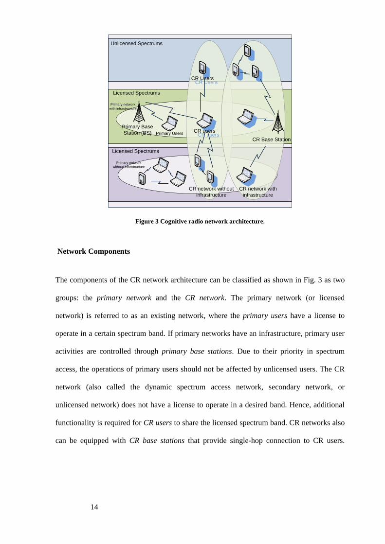
14

Figure 3 Cognitive radio network architecture.

Network Components

The components of the CR network architecture can be classified as shown in Fig. 3 as two

groups: the primary network and the CR network. The primary network (or licensed

network) is referred to as an existing network, where the primary users have a license to

operate in a certain spectrum band. If primary networks have an infrastructure, primary user

activities are controlled through primary base stations. Due to their priority in spectrum

access, the operations of primary users should not be affected by unlicensed users. The CR

network (also called the dynamic spectrum access network, secondary network, or

unlicensed network) does not have a license to operate in a desired band. Hence, additional

functionality is required for CR users to share the licensed spectrum band. CR networks also

can be equipped with CR base stations that provide single-hop connection to CR users.

Unlicensed Spectrums

Licensed Spectrums

Licensed Spectrums

CR UsersCR Users

CR usersCR users

Primary Users

CR network without

infrastructure

CR network with

infrastructure

CR Base Station

Primary Base

Station (BS)

Primary network

with infrastructure

Primary network

without infrastructure

15

Finally, CR networks may include spectrum brokers that play a role in distributing the

spectrum resources among different CR networks [1].

CR users are capable of accessing both the licensed portions of the spectrum used by

primary users and the unlicensed portions of the spectrum through wideband access

technology. Consequently, the operation types for CR networks can be classified as licensed

band operation and unlicensed band operation.

• Licensed band operation: The licensed band is primarily used by the primary network.

Hence, CR networks are focused mainly on the detection of primary users in this case. The

channel capacity depends on the interference at nearby primary users. Furthermore, if

primary users appear in the spectrum band occupied by CR users, CR users should vacate

that spectrum band and move to available spectrum immediately [1].

• Unlicensed band operation: In the absence of primary users, CR users have the same right

to access the spectrum. Hence, sophisticated spectrum sharing methods are required for CR

users to compete for the unlicensed band [1].

As shown in Fig. 3, the CR users have the opportunity to perform three different access

types:

• CR network access: CR users can access their own CR base station, on both licensed and

unlicensed spectrum bands. Because all interactions occur inside the CR network, their

spectrum sharing policy can be independent of that of the primary network.

• CR ad hoc access: CR users can communicate with other CR users through an ad hoc

connection on both licensed and unlicensed spectrum bands.

• Primary network access: CR users can also access the primary base station through the

licensed band. Unlike for other access types, CR users require an adaptive medium access

control (MAC) protocol, which enables roaming over multiple primary networks with

16

different access technologies. According to the CR architecture shown in Fig. 3, various

functionalities are required to support spectrum management in CR networks. An overview

of the spectrum management framework and its components is provided next[1].

Spectrum Management Framework

CR networks impose unique challenges due to their coexistence with primary networks as

well as diverse QoS requirements. Thus, new spectrum management functions are required

for CR networks with the following critical design challenges:

• Interference avoidance: CR networks should avoid interference with primary networks.

• QoS awareness: To decide on an appropriate spectrum band, CR networks should support

QoS-aware communication, considering the dynamic and heterogeneous spectrum

environment.

• Seamless communication: CR networks should provide seamless communication

regardless of the appearance of primary users. To address these challenges, we provide a

directory for different functionalities required for spectrum management in CR networks.

The spectrum management process consists of four major steps:

• Spectrum sensing: A CR user can allocate only an unused portion of the spectrum.

Therefore, a CR user should monitor the available spectrum bands, capture their

information, and then detect spectrum holes.

• Spectrum decision: Based on the spectrum availability, CR users can allocate a channel.

This allocation not only depends on spectrum availability, but is also determined based on

internal (and possibly external) policies.

17

• Spectrum sharing: Because there may be multiple CR users trying to access the spectrum,

CR network access should be coordinated to prevent multiple users colliding in overlapping

portions of the spectrum.

• Spectrum mobility: CR users are regarded as visitors to the spectrum. Hence, if the specific

portion of the spectrum in use is required by a primary user, the communication must be

continued in another vacant portion of the spectrum. The spectrum management framework

for CR network communication is illustrated in Fig.3. It is evident from the significant

number of interactions that the spectrum management functions require a cross-layer design

approach. In the following sections we discuss the four main spectrum management

functions[1].

Spectrum Sensing

Cognitive radio (CR) can successfully deal with the growing demand and scarcity of the

wireless spectrum. To increase the spectrum usage, CR technology allows unlicensed users

to access licensed spectrum bands. Since licensed users have priorities to use the bands, the

unlicensed users need to continuously monitor the licensed users’ activities to avoid

interference and collisions. How to obtain reliable results of the licensed users’ activities is

the main task for spectrum sensing. Based on the sensing results, the unlicensed users should

adapt their transmit powers and access strategies to protect the licensed communications.

The requirement naturally presents challenges to the implementation of CR.

In practice, the unlicensed users, also called secondary users (SUs), need to continuously

monitor the activities of the licensed users, also called primary users (PUs), to find the

spectrum holes (SHs), which is defined as the spectrum bands that can be used by the SUs

18

without interfering with the PUs. This procedure is called spectrum sensing [8], [9]. There

are two types of SHs, namely temporal and spatial SHs [8], respectively. A temporal SH

appears when there is no PU transmission during a certain time period and the SUs can use

the spectrum for transmission. A spatial SH appears when the PU transmission is within an

area and the SUs can use the spectrum outside that area.

This can be accomplished through a real-time wideband sensing capability to detect weak

primary signals in a wide spectrum range. Generally, spectrum sensing techniques can be

classified into three groups: primary transmitter detection, primary receiver detection, and

interference temperature management as described in the following[1].

Transmitter detection is based on the detection of a weak signal from a primary transmitter

through the local observations of CR users. Three schemes are generally used for transmitter

detection: matched filter detection, energy detection, and feature detection[10]:

• Matched filter detection: When the information of the primary user signal is known to the

CR user, the optimal detector in stationary Gaussian noise is the matched filter. However,

the matched filter requires a priori knowledge of the characteristics of the primary user

signal.

• Energy detection: If the receiver cannot gather sufficient information about the primary

user signal, the optimal detector is an energy detector. However, the performance of the

energy detector is susceptible to uncertainty in noise power. Also, energy detectors often

generate false alarms triggered by unintended signals because they cannot differentiate

signal types.

• Feature detection: In general, modulated signals are characterized by built-in periodicity or

cyclostationarity. This feature can be detected by analyzing a spectral correlation function.

The main advantage of feature detection is its robustness to uncertainty in noise power.

19

However, it is computationally complex and requires significantly long observation times.

Due to the lack of interactions between primary users and CR users, transmitter detection

techniques rely only on weak signals from the primary transmitters. Hence, transmitter

detection techniques alone cannot avoid interference to primary receivers because of the lack

of primary receiver information as depicted in Fig. 4a. Moreover, transmitter detection

models cannot prevent the hidden terminal problem. A CR user (transmitter) can have a

good line of sight to a CR receiver but may not be able to detect the primary transmitter due

to shadowing. Therefore, sensing information from other users is required for more accurate

primary transmitter detection — referred to as cooperative detection.

Cooperative detection is theoretically more accurate because the uncertainty in a single

user’s detection can be minimized through collaboration. Moreover, multipath fading and

shadowing effects can be mitigated so that the detection probability is improved in a heavily

shadowed environment. However, cooperative approaches cause adverse effects on resource

constrained networks due to the overhead traffic required for cooperation[1].

There are several other spectrum sensing techniques, such as eigenvalue-based and moment-

based detectors. Eigenvalue-based detector: In the multiple-antenna system, eigenvalue-

based detection can be used for spectrum sensing [11],[12]. In [11], maximum-minimum

eigenvalue (MME) and energy with minimum eigenvalue detectors have been proposed,

which can simultaneously achieve both high probability of detection and low probability of

false-alarm without requiring information of the PU transmitter signals and noise power. In

most of the existing eigenvalue-based methods, the expression for the decision threshold and

the probabilities of detection and false-alarm are calculated based on the asymptotical

distributions of eigenvalues. To address this issue, the exact decision threshold for the

probability of false-alarm for the MME detector with finite numbers of cooperative SUs and

20

samples has been derived in [12], which leads to our next section on cooperative spectrum

sensing (CSS). Moment-based detector: When accurate noise variance and PU transmitter

signal power are unknown, blind moment-based spectrum sensing algorithms can be

applied[13]. Unknown parameters are first estimated by exploiting the constellation of the

PU transmitter signal. When the SU does not know the PU transmitter signal constellation, a

robust approach that approximates a finite quadrature amplitude modulation (QAM)

constellation by a continuous uniform distribution has been developed [13].

A. Spectrum Sensing Challenges

There exist several open research challenges that must be investigated for the development

of spectrum sensing techniques:

• Interference temperature measurement: Due to the lack of interactions between primary

networks and CR networks, generally a CR user cannot be aware of the precise locations of

the primary receivers. Thus, new techniques are required to measure or estimate the

interference temperature at nearby primary receivers.

• Spectrum sensing in multi-user networks: The multi-user environment, consisting of

multiple CR users and primary users, makes it more difficult to sense spectrum holes and

estimate interference. Hence, spectrum sensing functions should be developed considering

the multi-user environment.

• Spectrum-efficient sensing: Sensing cannot be performed while transmitting packets.

Hence, CR users should stop transmitting while sensing, which decreases spectrum

efficiency. For this reason, balancing spectrum efficiency and sensing accuracy is an

important issue. Moreover, because sensing time directly affects transmission performance,

21

novel spectrum sensing algorithms must be developed such that the sensing time is

minimized within a given sensing accuracy [1].

Wideband sensing: Wideband sensing faces technique challenges and there is limited

work on it. The main challenge stems from the high data rate radio-front (RF) end

requirement to sense the whole band, with the additional constraint that deployed CR

systems (like mobile phones) will be limited in data processing rates. To achieve reliable

results, the sample rate should be above the Nyquist rate if conventional estimation methods

are used, which is a challenging task. Alternatively, the RF end can use a sequence of

narrowband bandpass filters to sense one narrow frequency band at a time [14]. However, a

large number of RF components are needed for the whole band. For more effective SU

network, a multiband sensing-time-adaptive joint detection framework has been proposed in

[15], [16], which adaptively senses multiple narrowband channels jointly to maximize the

achievable opportunistic throughput of the SU network while keeping the interference with

the PU network bounded to a reasonably low level. Based on energy detector for

narrowband sensing, the sensing time and detection thresholds for each narrowband detector

are optimized jointly, which is different from the previous multiband joint detection

framework in [17].

Synchronization: Besides the synchronization problem for quiet sensing period, spectrum

synchronization before the data transmission for non-contiguous OFDM based systems is

also a challenge. To address this challenge, a scheme has been proposed in [18] to use the

received training symbols to calculate a posterior probability of each subband’s being active

without the information of out-of-band spectrum synchronization. The proposed hard-

decision-based detection (HDD) utilizes a set of adjacent subbands while the soft-decision-

22

based detection (SDD) uses all the subbands for detection. Both HDD and SDD schemes

provide satisfactory performance while SDD performs better.

Spectrum Decision

CR networks require the capability to decide which spectrum is the best spectrum band

among the available bands according to the QoS requirements of the applications. This

notion is called spectrum decision and constitutes a rather important but as yet unexplored

topic in CR networks. Spectrum decision is closely related to the channel characteristics and

operations of primary users. Furthermore, spectrum decision is affected by the activities of

other CR users in the network. Spectrum decision usually consists of two steps: first, each

spectrum band is characterized, based on not only local observations of CR users but also

statistical information of primary networks. Then, based on this characterization, the most

appropriate spectrum band can be chosen. In the following we investigate the channel

characteristics, decision procedures, and research challenges in CR networks [1].

A. Channel Characteristics In Cognitive Radio Networks

Because available spectrum holes show different characteristics that vary over time, each

spectrum hole should be characterized considering both the time-varying radio environment

and spectrum parameters, such as operating frequency and bandwidth. Hence, it is essential

to define parameters that can represent a particular spectrum band as follows:

• Interference: From the amount of interference at the primary receiver, the permissible

power of a CR user can be derived, which is used for the estimation of channel capacity.

23

• Path loss: The path loss is closely related to distance and frequency. As the operating

frequency increases, the path loss increases, which results in a decrease in the transmission

range. If transmission power is increased to compensate for the increased path loss,

interference at other users may increase.

• Wireless link errors: Depending on the modulation scheme and the interference level of the

spectrum band, the error rate of the channel changes.

• Link layer delay: To address different path loss, wireless link error, and interference,

different types of link layer protocols are required at different spectrum bands. This results

in different link layer delays. It is desirable to identify the spectrum bands that combine all

the characterization parameters described previously for accurate spectrum decision.

However, a complete analysis and modeling of spectrum in CR networks has not been

developed yet [1].

B. Decision Procedure

After the available spectrum bands are characterized, the most appropriate spectrum band

should be selected, considering the QoS requirements and spectrum characteristics.

Accordingly, the transmission mode and bandwidth for the transmission can be

reconfigured. To describe the dynamic nature of CR networks, a new metric — primary user

activity — is proposed[19], which is defined as the probability of a primary user appearance

during CR user transmission. Because there is no guarantee that a spectrum band will be

available during the entire communication of a CR user, it is important to consider how

often the primary user appears on the spectrum band.

24

However, because of the operation of primary networks, CR users cannot obtain a reliable

communication channel for a long time period. Moreover, CR users may not detect any

single spectrum band to meet the user’s requirements. Therefore, multiple noncontiguous

spectrum bands can be simultaneously used for transmission in CR networks. This method

can create a signal that is not only capable of high data throughput, but is also immune to

interference and primary user activity. Even if spectrum handoff occurs in one of the current

spectrum bands, the rest of the spectrum bands will maintain current transmissions[1].

C. Spectrum Decision Challenges

In the development of the spectrum decision function, several challenges still remain

unsolved:

• Decision model: Spectrum capacity estimation using signal-to-noise ratio (SNR) is not

sufficient to characterize the spectrum band in CR networks. Also, applications require

different QoS requirements. Thus, design of application- and spectrum-adaptive spectrum

decision models is still an open issue.

• Cooperation with reconfiguration: CR techniques enable transmission parameters to be

reconfigured for optimal operation in a certain spectrum band. For example, even if SNR is

changed, bit rate and bit error rate (BER) can be maintained by exploiting adaptive

modulation instead of spectrum decision. Hence, a cooperative framework with

reconfiguration is required in spectrum decision.

• Spectrum decision over heterogeneous spectrum bands: Currently, certain spectrum bands

are assigned to different purposes, whereas some bands remain unlicensed. Thus, a CR

network should support spectrum decision operations on both the licensed and unlicensed

bands[1].

25

Spectrum Sharing

The shared nature of the wireless channel requires the coordination of transmission attempts

between CR users. In this respect, spectrum sharing should include much of the functionality

of a MAC protocol. Moreover, the unique characteristics of CRs, such as the coexistence of

CR users with licensed users and the wide range of available spectrum, incur substantially

different challenges for spectrum sharing in CR networks. The existing work in spectrum

sharing aims to address these challenges and can be classified by four aspects: the

architecture, spectrum allocation behavior, spectrum access technique, and scope.

The first classification is based on the architecture, which can be centralized or distributed:

• Centralized spectrum sharing: The spectrum allocation and access procedures are

controlled by a central entity. Moreover, a distributed sensing procedure can be used such

that measurements of the spectrum allocation are forwarded to the central entity, and a

spectrum allocation map is constructed. Furthermore, the central entity can lease spectrum to

users in a limited geographical region for a specific amount of time. In addition to

competition for the spectrum, competition for users can also be considered through a central

spectrum policy server [20].

• Distributed spectrum sharing: Spectrum allocation and access are based on local (or

possibly global) policies that are performed by each node distributively [21]. Distributed

solutions also are used between different networks such that a base station (BS) competes

with its interferer BSs according to the QoS requirements of its users to allocate a portion of

the spectrum. The recent work on comparison of centralized and distributed solutions reveals

26

that distributed solutions generally closely follow the centralized solutions, but at the cost of

message exchanges between nodes. The second classification is based on allocation

behavior, where spectrum access can be cooperative or noncooperative.

• Cooperative spectrum sharing: Cooperative (or collaborative) solutions exploit the

interference measurements of each node such that the effect of the communication of one

node on other nodes is considered. A common technique used in these schemes is forming

clusters to share interference information locally. This localized operation provides an

effective balance between a fully centralized and a distributed scheme.

• Non-cooperative spectrum sharing: Only a single node is considered in non-cooperative

(or non-collaborative, selfish) solutions [22]. Because interference in other CR nodes is not

considered, non-cooperative solutions may result in reduced spectrum utilization. However,

these solutions do not require frequent message exchanges between neighbors as in

cooperative solutions. Cooperative approaches generally outperform noncooperative

approaches, as well as closely approximating the global optimum. Moreover, cooperative

techniques result in a certain degree of fairness, as well as improved throughput. On the

other hand, the performance degradation of non-cooperative approaches are generally offset

by the significantly low information exchange and hence, energy consumption. The third

classification for spectrum sharing in CR networks is based on the access technology [23]:

• Overlay spectrum sharing: Nodes access the network using a portion of the spectrum that

has not been used by licensed users. This minimizes interference to the primary network.

• Underlay spectrum sharing: The spread spectrum techniques are exploited such that the

transmission of a CR node is regarded as noise by licensed users. Underlay techniques can

utilize higher bandwidth at the cost of a slight increase in complexity. Considering this

trade-off, hybrid techniques can be considered for the spectrum access technology for CR

27

networks. Finally, spectrum sharing techniques are generally focused on two types of

solutions: spectrum sharing inside a CR network (intranetwork spectrum sharing) and

among multiple coexisting CR networks (internetwork spectrum sharing), as explained in

the following:

• Intranetwork spectrum sharing: These solutions focus on spectrum allocation between the

entities of a CR network. Accordingly, the users of a CR network try to access the available

spectrum without causing interference to the primary users. Intranetwork spectrum sharing

poses unique challenges that have not been considered previously in wireless

communication systems.

• Internetwork spectrum sharing: The CR architecture enables multiple systems to be

deployed in overlapping locations and spectrum.

A. Spectrum Sharing Challenges

There are many open research issues for the realization of efficient and seamless open

spectrum operation in CR networks, such as:

• Common control channel: A common control channel (CCC) facilitates many spectrum

sharing functionalities. However, because a channel must be vacated when a primary user

chooses a channel, implementation of a fixed CCC is infeasible. Moreover, in CR networks

a channel common to all users is highly dependent on topology and varies over time[24].

Consequently, either CCC mitigation techniques must be devised or local CCCs must be

exploited for clusters of nodes.

• Dynamic radio range: Due to the interdependency between radio range and operating

frequency, the neighbors of a node may change as the operating frequency changes. So far,

28

there is no work addressing this important challenge in CR networks, and we advocate

frequency-aware spectrum sharing techniques.

• Spectrum unit: Almost all spectrum decision and sharing techniques consider a channel as

the basic spectrum unit. Hence, the definition of a channel as a spectrum unit is crucial in

developing algorithms.

• Location information: An important assumption in the existing work is that secondary

users know the location and transmit power of primary users so that interference calculations

can be performed easily. However, such an assumption may not always be valid in CR

networks.

Spectrum Mobility

The fourth step of spectrum management, as explained earlier, is spectrum mobility

management. After a CR captures the best available spectrum, primary user activity on the

selected spectrum may necessitate that the user change its operating spectrum band(s), which

is referred to as spectrum mobility. Spectrum mobility gives rise to a new type of handoff in

CR networks, spectrum handoff. Protocols for different layers of the network stack must

adapt to the channel parameters of the operating frequency. Moreover, they should be

transparent to spectrum handoff and the associated latency. Each time a CR user changes its

frequency of operation, the network protocols may require modifications to the operation

parameters. The purpose of the spectrum mobility management in CR networks is to ensure

smooth and fast transition leading to minimum performance degradation during a spectrum

handoff. An important requirement of mobility management protocols is information about

29

the duration of a spectrum handoff. This information can be provided by the sensing

algorithm. After the latency information is available, the ongoing communications can be

preserved with only minimum performance degradation. The intrinsic characteristics of a

CR network give rise to two novel concepts: spectrum mobility and spectrum handoff. So

far, there is no research effort to address the problems of spectrum handoff. Although the

mobility-based handoff mechanisms that have been investigated in cellular networks may

lay the groundwork in this area, there are still open research topics to be investigated[1].

A. Spectrum Mobility Challenges

The following are the open research issues for efficient spectrum mobility in CR networks:

• Spectrum mobility in the time domain: CR networks adapt to the wireless spectrum based

on the available bands. Because these available channels change over time, enabling QoS in

this environment is challenging.

• Spectrum mobility in space: The available bands also change as a user moves from one

place to another. Hence, continuous allocation of spectrum is a major challenge [1].

30

Chapter III. PROPOSED SPECTRUM DECISION AND

SPECTRUM SHARING ALGORITHM

Introduction

In current communication networks, the average spectrum utilization is between 15% to

85%. Cognitive Radio (CR) is a solution to increase the spectrum utilization and ultimately

the network capacity leading to generating new revenue streams with higher quality of

service. With increasing demand for higher capacity in wireless networks due to the rapid

growth of new applications such as multimedia, the network resources such as spectrum

should be used more efficiently to fulfill the need for both quantity and quality of service.

This implies an optimum resource management [25],[26]. Spectrum is one of the most

challenging network resources which needs to be carefully consumed. Cognitive Radio

Networks (CRN) are supposed to efficiently use idle portions of the spectrum (resource

grid). There are many techniques to sense the idle spectrum channels and manage them to

increase the networks efficiency.

The works done in spectrum sharing has faced some challenges and can be categorized as

centralized spectrum sharing vs. distributed spectrum sharing, and cooperative spectrum

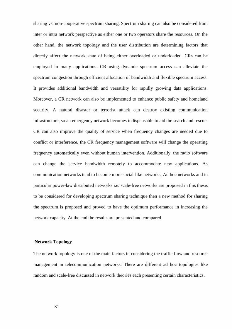
31

sharing vs. non-cooperative spectrum sharing. Spectrum sharing can also be considered from

inter or intra network perspective as either one or two operators share the resources. On the

other hand, the network topology and the user distribution are determining factors that

directly affect the network state of being either overloaded or underloaded. CRs can be

employed in many applications. CR using dynamic spectrum access can alleviate the

spectrum congestion through efficient allocation of bandwidth and flexible spectrum access.

It provides additional bandwidth and versatility for rapidly growing data applications.

Moreover, a CR network can also be implemented to enhance public safety and homeland

security. A natural disaster or terrorist attack can destroy existing communication

infrastructure, so an emergency network becomes indispensable to aid the search and rescue.

CR can also improve the quality of service when frequency changes are needed due to

conflict or interference, the CR frequency management software will change the operating

frequency automatically even without human intervention. Additionally, the radio software

can change the service bandwidth remotely to accommodate new applications. As

communication networks tend to become more social-like networks, Ad hoc networks and in

particular power-law distributed networks i.e. scale-free networks are proposed in this thesis

to be considered for developing spectrum sharing technique then a new method for sharing

the spectrum is proposed and proved to have the optimum performance in increasing the

network capacity. At the end the results are presented and compared.

Network Topology

The network topology is one of the main factors in considering the traffic flow and resource

management in telecommunication networks. There are different ad hoc topologies like

random and scale-free discussed in network theories each presenting certain characteristics.

32

A. Random Topology

There are classes of networks where the nodes are attached to the network in a random way

meaning that the number of connections of nodes has a normal distribution. The degree

(number of links to the node) distribution of nodes in such networks is a Gaussian type

distribution.

B. Scale-Free Topology

In 1999, A. L. Barabasi, and R. Albert (BA) proposed a scale-free network model based on a

mechanism of growth with preferential attachment characterized with power-law distribution

of the nodes degree [27]. Scale-free networks are robust to random attacks (node removal)

and very well describe the nature of real world networks where there are always few nodes

with much higher degree called hubs. Each new node enters the network initially with ability

to have m links to existing nodes. The probability to connect to an existing node is

dependent on the degree of that node meaning that the new node gets connected most

probably to nodes with higher degree. The degree distribution for this model is a power-law

distribution. The probability of a node to have a degree di is given by

i iP d d (1)

where .

33

i x

rx

Figure 4 scale-free network formation with power-law degree distribution

The distribution tail shows the nodes with highest degree called hubs. Here we use scale-free

properties to better sense network traffic and manage the resources. Since hubs have the

highest degrees amongst the nodes and because of their many connections, they have big

impact on overall behavior of the network [27]. Consider a cluster of having N0 nodes and

some newcomers tends to attach to this network. The newcomer starts to scan its

neighborhood in a radius of rx which is determined by minimum satisfactory bitrate. There

will be some existing nodes within rx from which only one node is selected to be connected

based on scale-free algorithm and that is the node with highest degree and of course the one

with the best link quality as in Figure 4.

Spectrum Sensing

The spectrum sensing is one of the main layer tasks for CR system to obtain the spectrum

usage information and the presence of PUs. Spectrum detection is based on the detection of

the signal from PU through the observation of cognitive radio network.

The sensing methods can be categorized in three methods: i) Energy Detection, ii) Matched

Filter, and iii) Feature Detection. The spectrum sensing method considered for this thesis is

34

Energy Detection. Since, it is particularly suitable for multiband sensing because of its low

computational and implementation complexities. We presume using OFDM modulation with

M sub carriers with bandwidth W. In this thesis we premised the IEEE 802.22 as it has

developed air interface for opportunistic SU access to the TV spectrum in which PUs change

slowly [28].

The timing model for spectrum sensing is shown in Fig. 2.a and spectrum mobility model for

SUs is depicted in Fig. 2.b. The required time for channel estimation, spectrum sensing and

sharing is indicated by . According to the [29] the given channel estimation delay is for

WCDMA/HSDPA, so the scaled delay for a shorter sub-frame length in UTRAN LTE is

considered for this thesis. For each Resource Block (RB), there are 7 frames in time frame

and 12 subcarriers and each square in Fig .5.b is called Resource Element (RE In Fig. 5.a. T

is time length of each frame and K is number of frames. Supposed that received signal at

SUs sampled at fs over ith sub channel where values of discretized samples at ,

which is in our framework. In discrete form, when the primary user is active, we

define two hypotheses as follow:

1,

0,

( ) ( ) ( ) ,

( ) ( ) ,

i i i i i

i i i

y n h x n u n

y n u n

(2)

That is the subchannel gain between PU transmitter and SU receiver with variance

. The signal transmitted, , by PU is assumed to be independent and identically

distributed (i.i.d), , and , the noise, is circularly symmetric complex Gaussian

(CSCG) noise.

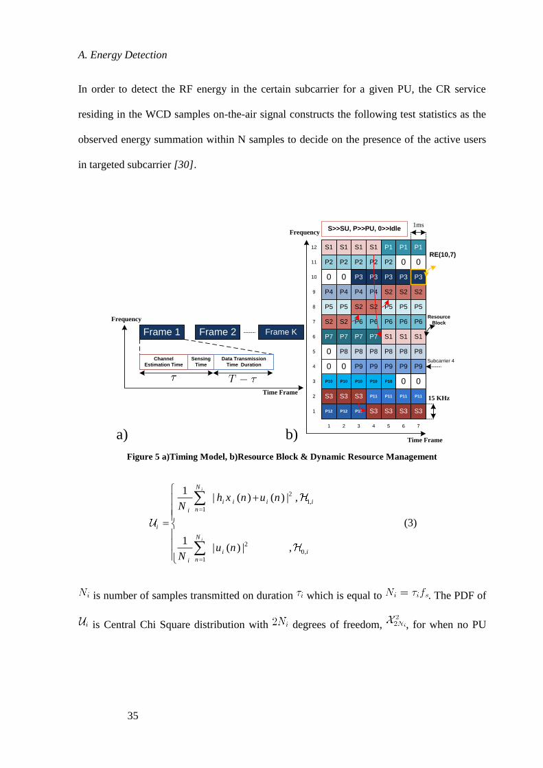
35

A. Energy Detection

In order to detect the RF energy in the certain subcarrier for a given PU, the CR service

residing in the WCD samples on-the-air signal constructs the following test statistics as the

observed energy summation within N samples to decide on the presence of the active users

in targeted subcarrier [30].

Figure 5 a)Timing Model, b)Resource Block & Dynamic Resource Management

2

1,

1

2

0,

1

1| ( ) ( ) | ,

1| ( ) | ,

i

i

N

i i i i

ni

i

N

i i

ni

h x n u nN

u nN

(3)

is number of samples transmitted on duration which is equal to . The PDF of

is Central Chi Square distribution with degrees of freedom, , for when no PU

Frame 1 Frame 2 Frame K

Sensing

Time

Data Transmission

Time Duration

Frequency

Time Frame

Channel

Estimation Time

b)a)

P12 P12 P12

P11 P11 P11 P11

P10 P10 P10 P10 P10

P9 P9 P9 P9 P9

P8P8P8

P7 P7 P7 P7

P6 P6 P6 P6

P5 P5 P5P5 P5

P4P4P4

P3 P3 P3 P3

P4

P2P2P2P2P2

P1 P1 P1

P8P8

S2 S2

S2

S1 S1 S1

0

0

S3

0

S3 S3

S3 S3 S3S3

0 0

S2 S2 S2

0

0

S1S1S1S1

P6

S2

P3

P8

0

0

Frequency

Time Frame

1 2

12

11

10

9

8

76543

2

3

4

5

6

7

RE(10,7)

15 KHz

1ms

1

S>>SU, P>>PU, 0>>Idle

Resource

Block

Subcarrier 4

36

exists and on Central Chi Square distribution with degrees of freedom and non-

centrality parameter , , for the state that PU exists. So:

,1

,0

12 22 ,1 1,2

21,02 2 2

2 1 ,0 0,

1,

2 ( )

( )1

(2 ) ( ) ( 2 ) ,2 2

i

i

i i

i i ii

i i

N

N i iN

i

i Ni

N i N i i i

i

eN

e I

(4)

where the signal to noise ratio (SNR) is depicted by , denotes the gamma

function, is the first kind modified Bessel function of degree .

Two performance parameters for spectrum sensing are probability of detection, , and

probability of false alarm, , which is probability of when the frequency is unoccupied but

we get alarm that the frequency is used. Hence, Higher protects PU from interfering with

SUs and smaller causes better band usage efficiency. To calculate probability of

detection [31]:

, 1 1( , , ) ( | ) ( )i

d i i i i i iP Pr p x dx

(5)

where is threshold and is denoted sensing time for ith subchannel.

2

, 2 2( , , ) (

|( | | 1 )

2 1|)

i

i sid i i i i i i

u i i

fP h

h

(6)

Now the probability of missed detection can be defined as:

, ,( , , ) 1 ( , , )m i i i i d i i i iP P (7)

We have following equations for probability of false alarm,

37

, 0 0( , ) ( | ) ( )i

f i i i i iP Pr p x dx

(8)

, 2( , ) (( 1) )

i

if i i i i s

u

P f

(9)

Usually to evaluate the performance of energy detection, the goal is to minimize for a

target or to maximize for a target . At first we assume is our target

probability of detection,

1

, , 2 2

, ,

2

|

|

( )( ) ( 1)

2

|

|

i

d i target

i d i terget i i h

i s

i i

PP h

f

h

(10)

1 2 2

, , , , ,( ( ) | |, ) ( ( ) 2 |1 )|f i i d i terget i d i terget i i i i i sP P P h h f (11)

is the probability of false alarm regard to target , and is the

inverse of complementary error function. For a target we have:

1

, , 2

, ,

( )( ) ( 1)

i

d i target

i f i terget h

i s

PP

f

(12)

1 2

, ,

, , ,2

|( )( ( ),

|) ( )

2 1

|

|

f i terget i i i s

d i i f i terget i

i i

P h fP P

h

(13)

is the probability of detection when is targeted. As a result, in this

part, probability of false alarm and detection based on and , respectively,

are calculated. The proposed wide spectrum sensing by energy detection can be shown in

figure 6.

38

Figure 6 wide spectrum sensing model

Queued Markov Chain Model For Spectrum Analysis-Access

In this section, we consider group of secondary users that tend to access idle licensed

spectrum portions in an opportunistic way. The process of sensing and decision making on

the spectrum allocation is analyzed with a Markov Chain Process with a queue state in

which, primary user has the spectrum and secondary users are waiting to access once it is

released by primary user. This model is for one subcarrier and can be generalized for a

resource block with multiple subcarriers.

The primary user PU is licensed to operate in the spectrum. The PU traffic is modeled as

Poisson random process with arrival rate λp and departure rate μp. The secondary users are

indexed by i (i=1,2,…,N) and modeled with Poisson random process as well; the arrival rate

of SU is λi and departure rate is μi. All users are connected to Cognitive Radio (CR) Control

Unit (CU) that controls CR network. To avoid interference with Primary Users (PU), once

the PU starts using the subchannel, CU forces the Secondary Users (SU) to leave and if SUs

still need to access the subchannel, CU puts them in Queue State (Sq) to find another band

or wait for PU to release the subchannel. Here we assume that spectrum band is not allowed

to be shared with two or more users concurrently [32], [33], [34].

Frequency

selector

system Sampling

Frequency

selector

system

Average

Average

Sampling

CR

Recevier

Transmitted

PU

39

S0

S1

S2

SN

SPU

Sq

Figure 7 Queued Markov Chain State Machine without sharing

(N+3)-state Markov Chain State Machine is illustrated in Figure 2, where state S0 means

that the spectrum band is idle. Without the loss of generality, the probability of transition

from S0 to Si (i=1,2,…,N) is proportional to λi’s. S0 is the state when the subchannel is idle.

Inversely, the transition probability from Si to S0 is μi. If SU’s are operating in subchannel,

and PU shows up, SU’s have to leave the subchannel. The probability of Si to SPU is

proportional to arrival rate of primary user. If PU is active in the subchannel by itself i.e.

SPU, the transition probability from SPU to Sq is proportional to summation of SU’s arrival

rates, , because when they request to access, due to PU’s priority, they

will be forced to be put in queue. In Sq state, as soon as PU leaves the subchannel, the user

state changes to either of Si whose total probabilities are proportional to departure rate of PU

that are considered ai.

The set of equations based on above Markov Chain Model is as follow:

0ΠH (14)

0 1 2 1N Q P (15)

40

where H is the matrix that characterizes the transition state of the Markov chain, and Π =

[Π0, Π1, Π2,…, ΠN, ΠQ, ΠP] is the state probability vector for

respectively.

The H matrix of our model is as follow:

0 1

1 2 1

1 1

1 1

1 2 1 2

, , , , , .

( ) 0

( ) 0 0

0 ( ) 0

0 ( ) 0

0 0 ( )

N Q P

N p N p

p p

N N p p

N N

p N N p

a a a a

0

(16)

So the set of equations from (16) will be:

With which all entries will be calculated with known entries of H. With more complex

systems, computer aided solution is required to above set of equations. This has been done

for specific H in simulation section.

41

Max-Rate Spectrum Sharing

In communication networks, there are always unused resources due to mismanagement or

the traffic usage pattern. However, it is possible to share the inactive resources between

different portions of the network and in some cases share them with other service providers.

Therefore, implementing spectrum sharing would highly improve the spectrum utilization

efficiency and reduce the request blocking rate (Grade of Service). We assume that the

network topology is mainly scale free which has ad hoc properties plus that nodes are

preferentially distributed mostly around hubs; different portions of the network are then

categorized as clusters which have access to certain part of the resources. In this thesis we

deal with a case where clusters are overloaded and needs extra resources for providing

acceptable quality of service. Figure 8 shows the infrastructure of scale free inter-network

interaction. Each cluster is defined with a cluster hub and a range of operation. Clusters A,

B, and C each of NA, NB, and NC active users are initially planned to operate in separate

allocated resource blocks (AU, AD), (BU, BD), and (CU, CD), respectively as in Figure 8.

Index U represents the uplink and D is for downlink communications. If a new user attaches

to cluster A and all of the resources in resource block A are busy, the hub node in cluster A

i.e. HA, tries to see if there is available idle resources in neighboring clusters. The resource

elements in this portion are in the form of REU and RED. For instance, REU(i,j) represents

the resource element for uplink at ith subcarrier and jth time slot. Now consider a new user

willing to attach to cluster A by sending a request to the cluster hub, HA. We presume at the

time of request all of the resources of cluster A are occupied. The new user is not blocked at

this stage like conventional communication networks. Instead, HA starts to sense and search

for potential available resources in neighboring clusters like B, and C. if the resource is

available in either neighboring clusters for more than a limited period of time, it will be

42

granted to cluster A and finally allocated to the new user. There is a process to consider

associated criteria for releasing and granting the resources from other clusters to requesting

clusters. In real world applications the hubs in clusters are distinguished mainly with their

degree which is the number of active links either terminated to or originated from these hub

nodes. Hubs are basically supposed to have access to as many resources as the number of

active links connected to them. This leads to initially interrogating the more populated

clusters as opposed to handshaking with less important (lower degree) nodes. The degree of

the nodes is then considered in evaluating the merit for a specific hub. The Merit function

determines the merit value for each requesting node given a certain set of available resources

in granting cluster. One of the main factors in merit function is that the idle resources in

neighboring clusters are not idle for unlimited time. As opposed, based on the number of

active users in granting clusters, there is an average number of requests coming from user

side which leads to always updating a request queue. This queue will be monitored at the

time of releasing the idle resource to make sure that there is no potential demand from local

cluster for the idle resource.

43

Cluster A

Cluster B

Cluster C

Figure 8 Scale free infrastructure and its UL and DL spectrum resource model

A. Cognitive Parameters

The hubs are presumed to be Cognitive Enabled in order to be able to sense unoccupied

channels. A channel is said to be unoccupied if the instantaneous radio frequency (RF)

energy (plus noise) in this channel, is less than the certain interference limit. The probability

that the channel is available for a period of time is greater than a threshold pth, These

measures can be evaluated by the CR node through monitoring the traffic pattern. The

Interference is measured using Carrier to Interference ratio for each subcarrier. The

probability of a channel to be available for a certain period of time is predicted by looking

up the traffic profiles both in real time and the traffic history. Because the network has a

scale-free topology, the requesting users/nodes are characterized with their degree. di is the

degree of ith node in a cluster. The degree information of the nodes is also communicated

along with the request or obtained from network statistics. Nodes with higher degree have

higher priority. This information is known in the local cluster and there is no need for global

information broadcast [35],[36].

Another criterion for granting the network resources to requesting users is the Costumer

Classification (Qi). Each of these new users has a specific service profile with different QoS

44

like gold, silver and bronze. When a resource is reported to be available, it’s now time to see

which users of what level of quality (priority) have requested the resource. There are users

with different subscription profiles which enables the decision making process directed

based on the required QoS from user side. Another level of priority is also defined for

emergency and security cases which dominate all incoming requests.

Signal to Noise Ratio (SNR) is important parameter that is considered for the users. Finally,

the interrogated CR node from neighboring cluster reports the available channels with a set

of information , p to the overloaded cluster. At the requesting cluster, di, Qi are used to

classify the users for granting borrowed resources.

B. Merit Function

For the reported available resources to be granted to requesting users/nodes in a fairly

optimum way there needs to be a function that considers the Cognitive Parameters to

calculate the merit for users/nodes.

C. Channel Indexing Function

Let R denote the set of available resources reported by the CR node. (Hub node in

neighboring cluster(s)). The Channel Indexing Function (CIF) is meant for indexing the

elements in R based on received Cognitive Parameters Where

for every available channel. Then CIF operates on R to generate

( ) R χ (17)

is the output of Channel Indexing Function, , which consists of sorted

performance indices for all available channels. U is the list of cognitive parameters collected

45

from requesting users/nodes from requesting clusters. where

. Then the Merit Function is applied to calculate the merit value for

requesting users.

( ) U M (18)

where M is the set of merit values for all requesting users i.e. . and

are CIF and Merit functions operating on each resource and user respectively and can be

defined as:

( )i p i I i

Cp

I (19)

i D i Q i S id Q SNR (20)

All parameters are set according to technical and commercial constraints. We define the

SNR for target node i as the summation of uplink (UL) and downlink (DL) SNRs.

2 2

/ /UL DL x i i xi i i

x x

P N P NSNR SNR SNR

r r (21)

Px and Pi represent the transmit power of the newcomer node x and target node i,

respectively. Nx and Ni are the noise power at newcomer and target node receivers.

D. Competitive Indexing Algorithm

M and are matched against each other to grant the best performing channel to the

users/nodes with highest merit values because the users with higher value are those who

require better quality of service and are in urgent need of resources to either use them or

distribute them amongst their neighbors. Then the second best resource is granted to the

46

second user with highest merit. This process goes on until either there is no request from

overloaded cluster or comes a new request from the local cluster which leads to filling up the

request queue in the local cluster[37].

Cluster A sends its request to the neighboring clusters. Matrix is a set of performance

indices for all available resources (channels) in neighboring clusters where is the

performance index for ith available resource element which is a function of cognitive

parameters for ith subcarrier like interference and availability probability and other potential

cognitive parameters that can be defined/measured as well.

and are determined based on network statistics, measurements, topology and operators

commercial strategies. Based on the proposed competitive algorithm for granting available

resources, and M are sorted in descendingly and the winning channel which is the top

indexed one in is granted to the user with highest merit value at the top of M. this process

goes on until all the demands from cluster A(or all requesting clusters) are supplied. This

algorithm gives optimum performance in terms of the increased capacity in the network

compared to uniform allocation of resources (without indexing) in response to incoming

request.

To evaluate the performance for different algorithms, We define a resource sharing

performance index, , which is maximized based on rearrangement inequality for

proposed competitive indexing algorithm. Since and M are sorted, we can write:

1 2 1 2;,.., ,..,L Lx x x m m m (22)

Let and be any arbitrary permutation of and M. The rearrangement

inequality states that for sorted matrices and M :

47

1 1

( ) ( )L L

i i k i l i

i i

x m x m

(23)

1 1

( ) ( )L L

opt i i k i l i rand

i i

x m x m

(24)

is the performance index of the proposed competitive algorithm. can be defined as

different known parameters like total increased capacity if and M are defined

appropriately.

Sharing incorporated in Markov chain model

Now, we put sharing part in our Markov Chain Model as shown in Figure 7. Because of each

futures the SU’s have, their chance to get spectrum from Sq is different based on our specific

sharing policy shown by ai’s. Based on different policies we considered for allocating the

spectrum with SU’s, the ai’s will be different. For example, in Scale-Free Ad Hoc networks,

degree is an important feature we can consider for SU that user with greater degree has more

priority to get access. In our simulation, we assumed different traffic for each SU. The

arrival rates is the same and departure rates are different. The first user has more priority

than others in our simulation and the departure rates descending from first to last SU. So, the

chance of first user is more than others, because of its less departure rate and its higher

priority, and for second user is more than third user, only because of its less departure rate,

and so on. As we see, if we increase the number of users, Pq(probability of being in queue) is

decreasing and PPU (the probability that only the primary user requested to access)

decreasing. At the End, we compared the probability of SU’s when number of users is 3. The

only difference will be in Pi’s that in sharing method, the chance of user with priority is

more (user 1) and the difference between other users is because of their different traffics.

48

S0

S1

S2

SN

SPU

Sq

Figure 9 Queued Markov Chain State Machine with sharing

Here .

In this model, imperfect spectrum sensing consisting of false alarm, and miss-detection,

is also considered. If the idle channel is reported as busy, the current state does not

change. So is multiplied by arrival rates. In addition, when a channel is busy but

reported as idle, the state Sq will not be allowed to go to Si’s. As a result, is

considered as a transition probability.

Simulation

A. Simulation Results For Sensing

SU with greater degree has more priority to get access to subchannel. In our simulation, we

assumed different traffic models i.e. for each SU. We simulated a scenario with 2,3,4 and

5 secondary users and one primary user over one subchannel. .

The rest of parameters are assigned as in Table 1.

Table 1 Simulation traffic parameters

No.

1 2 2

2 4 0.5

3 6 0.5

4 8 0.5

5 10 0.5

49

The first user is assumed to have higher degree in our scale-free model resulting in having

greater parameter , which means it will have better chance than other users in the queue.

The departure rates are assigned to SU’s descendingly. Therefore, the probability of S1,

will be greater than other secondary users because of its less departure rate and higher

priority. also , the probability of S2 is more that others’ since its departure rate is smaller

than others’ and so on. As we see in Figure 10, if we increase the number of secondary

users, (probability of SQ) is increasing and (the probability of SPU) is decreasing. At

the End, we compared the probability of SU’s when number of SU’s is 3. The only

difference between results with uniform sharing ( all users have equal allocation chance) and

competitive sharing (users are prioritized) will be in (j=1,2,…,N). in our simulation we

assumed only first SU has higher priority in competitive sharing. As shown in Figure 11,

in competitive sharing is greater than in uniform sharing.

Figure 10 state probabilities using competitive sharing for different number of users

0

0.05

0.1

0.15

0.2

0.25

0.3

2 3 4 5

𝝥0

𝝥1

𝝥2

𝝥3

𝝥4

𝝥5

𝝥Q

𝝥P

50

Figure 11 state probabilities using competitive and uniform sharing N=3

B. Simulation Results For Sharing

The network structure used in the simulation is a scale-free topology with N= 100 nodes and

three hubs each of 19 , 17, and 15 links. The average degree of nodes in this network is 3.7

meaning that each user is in average connected to about 4 nodes. There are 3 clusters

centered around aforementioned hubs called cluster A, B, and C respectively. Each cluster

uses a typical OFDM (3GPP compliant) resource block of 12 subcarriers in 7 time slots for

Uplink and another 7 time slots for Downlinks resulting total 84 resource elements. At each

time instance, there are Ki incoming nodes to cluster A and Ko nodes leave this cluster

drawn from Poisson distribution. Without spectrum sharing based on the distribution of the

requests coming from the users side, cluster A may get overloaded. The capacity and load

measures are simulated for cluster A without having the chance to borrow resources from

neighboring clusters; Figure 9 demonstrates the performance of Uniform Indexing and

Competitive Indexing. Our method in Spectrum Sharing outperforms the Uniform Indexing.

0

0.05

0.1

0.15

0.2

0.25

0.3

uniform sharing competitive sharing

𝝥0

𝝥1

𝝥2

𝝥3

𝝥Q

𝝥P

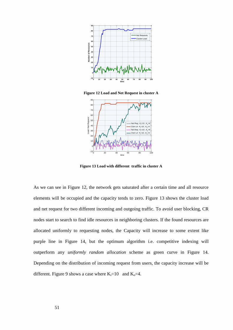
51

Figure 12 Load and Net Request in cluster A

Figure 13 Load with different traffic in cluster A

As we can see in Figure 12, the network gets saturated after a certain time and all resource

elements will be occupied and the capacity tends to zero. Figure 13 shows the cluster load

and net request for two different incoming and outgoing traffic. To avoid user blocking, CR

nodes start to search to find idle resources in neighboring clusters. If the found resources are

allocated uniformly to requesting nodes, the Capacity will increase to some extent like

purple line in Figure 14, but the optimum algorithm i.e. competitive indexing will

outperform any uniformly random allocation scheme as green curve in Figure 14.

Depending on the distribution of incoming request from users, the capacity increase will be

different. Figure 9 shows a case where Ki=10 and Ko=4.

0 10 20 30 40 50 60 70 80 90 100-10

0

10

20

30

40

50

60

70

80

90

time

Nu

mb

er

of

Res

ou

rces

Net Requests

Cluster Load

0 20 40 60 80 100-10

0

10

20

30

40

50

60

70

80

90

time

Lo

ad

/ N

et R

eq

ue

st

Net Req: Ki=10 , K

o=4

Clstr Ld : Ki=10 , K

o=4

Net Req: Ki=10 , K

o=9

Clstr Ld : Ki=10 , K

o=9

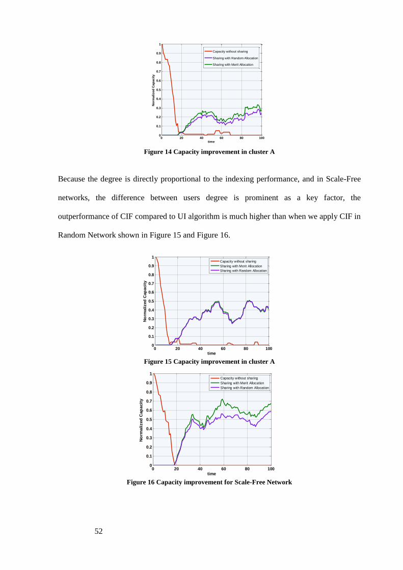
52

Figure 14 Capacity improvement in cluster A

Because the degree is directly proportional to the indexing performance, and in Scale-Free

networks, the difference between users degree is prominent as a key factor, the

outperformance of CIF compared to UI algorithm is much higher than when we apply CIF in

Random Network shown in Figure 15 and Figure 16.

Figure 15 Capacity improvement in cluster A

Figure 16 Capacity improvement for Scale-Free Network

0 20 40 60 80 1000

0.1

0.2

0.3

0.4

0.5

0.6

0.7

0.8

0.9

1

time

No

rmalized

Cap

acit

y

Capacity without sharing

Sharing with Random Allocation

Sharing with Merit Allocation

0 20 40 60 80 1000

0.1

0.2

0.3

0.4

0.5

0.6

0.7

0.8

0.9

1

time

No

rma

lized

Cap

acit

y

Capacity without sharing

Sharing with Merit Allocation

Sharing with Random Allocation

0 20 40 60 80 1000

0.1

0.2

0.3

0.4

0.5

0.6

0.7

0.8

0.9

1

time

No

rma

lized

Cap

acit

y

Capacity without sharing

Sharing with Merit Allocation

Sharing with Random Allocation

53

Conclusion

In this thesis, we presented the Cognitive Radio framework for wireless Ad Hoc networks.

The complete model describes the sensing and sharing procedures in wireless networks in

general but the simulation results are for random and scale-free topologies. We introduced

Queued Markov Chain method in spectrum sensing and Competitive Indexing Algorithm in

spectrum sharing part. We demonstrate that our proposed Competitive Indexing Algorithm

outperforms the Uniform Indexing Algorithm.

54

Chapter IV. COGNITIVE RADIO IN SMART GRID

Throughput Analysis on Cognitive Radio Networks for AMI Meters in Smart Grid

Introduction

We consider the future smart grid as leveraging Information and Communications

Technology (ICT) facilitated by the smart meter (also named as Advance Infrastructure

Metering (AMI)) information networks. The smart meter enables the flow of real-time

information within the power utility, between the power utility and its customers. It is

essential for AMI to be networked since it enables system wide sensing, utility and customer

linkages, and future self healing capability.

Communication network infrastructures represent a very large capital expense. Research on

CR has evolved from SDR (see [38],[39] ) with an objective of efficient utilization of radio

spectrum. In this thesis, we analyze CR in the context of smart energy systems. Although

there have been significant advances and improvements in CR hardware, algorithms, and

protocols, less attention has been given to developing ubiquitous and pervasive metropolitan

55

scale CR networks, particularly with respect to smart grid information networking [3]. A

metropolitan infrastructure based CR networks is shown in Fig. 1. In this context, there are

major challenges to overcome such as Secondary Users (SU) should sense the spectrum and

timely model the behavior of the Primary Users (PU). The other issue is how the SUs

manage the available spectrum resources and share the resources among the SUs to satisfy

the smart grid protocol requirements and meeting the interference constraints suggested by

the FCC Spectrum Policy Task.

In such a system, our objective for SUs (i.e. AMI) is to efficiently transmit their delay

sensitive traffic over the network and meet the QoS requirements of the smart grid protocol.

In this thesis, we investigate different scheduling polices that maximize the downlink sum

throughput in the given area and achieving fairness among the SUs. We present an

opportunistic scheduling policy that exploits both maximizing the downlink sum throughput

and fairness under time-varying channel conditions for multi-user CR network in a

metropolitan based environment.

Several authors have defined aspects of AMI networking in smart grids. Mesh, Ethernet and

cellular AMI network topology for smart grid has been proposed. In [40] the authors propose

mesh networks of Zigbee based transmission architecture. In [41], the authors discuss

communication infrastructure based on Ethernet (LAN and WAN). The approach will

support automated meter readings and customer home appliance connections. However,

wireline systems are not always available. Customer subscription to service must occur and

wired system can be challenging to rapidly redeploy, particularly in swiftly enveloping

emergencies.

The authors in [42] describe a framework for RF mesh networking interfaced with high

speed WiMAX access networks. In [43], overview of architecture, hardware platform, is

56

reported to enable CR for smart grid communications. Our work discusses the CR network

infrastructure architecture from 4G perspective. We also present multi-user performance

analysis of various scheduling algorithms in context with AMI units considering the delay

occurred due to offloading the processes to cloud in our architecture.

4G Cognitive Radio Framework

A. 4G Cognitive Radio System Architecture

We presume a LTE network as a CR LTE network (4G CR), if the LTE work is adopted the

CR techniques. We consider a cloud data center infrastructure based CR network coexisting

with PU network shown in Fig.17. The coverage of both the CR base station and PU

network base station are similar. As depicted in the Fig. 1 at the center of the each cell, there

is base-station which is shared as e Node-B for PUs and as antenna for SUs. The PU base-

station only serves to PUs as it lacks the CR protocols capabilities to support SUs. However,

it may consider supporting certain features in order to communicate with SUs.

Placement of a Cognitive Radio Antenna on the BTS tower may occur in tandem with

deployment of the cellular provider antenna. The CR senses the spectral environment over a

wide frequency band, particularly the spectrum in the cell region. It identifies the unused

bands in the spectrum. These bands could be owned by cellular companies or license

television band owners, but are not limited to these bands or to licensed bands. Sensed

information using the CR is relayed to cloud data center. In principle, eNode-B which

terminates the air interface protocol and first point of contact for PU is located at the primary

user base-station. However, in proposed architecture all the cognitive radio service,

waveform service, protocols service, security service, scheduling and control services are

57

displaced into cloud data center. The CR services indentify unused frequency bands, the

relevant cognitive services residing in the cloud data center generates a clear to send (CTS)

signal.

Figure 17 4G CR network system architecture: Scenario of multiple AMI meters serviced by cognitive

radio network infrastructure enabled by cloud center coexisting with private cellular network

The CTS is sent back to the AMI meters through the feedback channel via base station.

Eventually, the CR antenna relays CTS signals to every AMI in the cell region for uplink

transmission.

B. Pervasive Smart Grid Systems

The energy services of the future can be privately contracted services or public services. The

cloud center enables convenient, on-demand network access to a shared pool of

configurable, computing resources (e.g., networks, servers, storage, applications, and

services) that can be rapidly provisioned and released with minimal management effort.

There are different cloud computing platform classifications. Standard architectures includes

Abi (or Abiquo), Nimbus Open Nebula, Azure (Microsoft), Google (App Engine), Blue

58

(IBM) and Mosso (Rackspace). Fig.17. depicts the model for a cloud data center

architecture optimized for based smart grids. Our Wireless Cloud Data (WCD) model is

organized into four principle layers: application layer, platform layer, CR communication

and networking layer and infrastructure layer. The first two layers are akin to existing cloud

architectures. However, the lower two layers are augmented to enable the CR networking

and wireless services. CR communication and networking layer provides services such as

cognitive radio services, waveform services, Radio Link Control (RLC), and Medium

Access Control (MAC) services. CR services, which provide spectrum management and

spectrum sensing, are discussed in detail in section III. The infrastructure layer facilitates the

effective integration of computing resources, storage, networks to deploy applications and

operating systems. We augment our cloud infrastructure microprocessor racks with FPGA

boards targeted to processing high computation rate processes typically associate with CR

services, communication waveform signal processing and coding.

CR System Model

In the thesis system model 4G cellular network is considered with Nsu secondary users

sharing the spectrum simultaneously with Npu primary users. It is presumed in the context

that the secondary users (i.e. AMI meters) are fixed in sense of geographical location and

yields to fixed first and second statistical moments of SINR.

59

Figure 18 Markov Chains Model; Optimum Sensing Time

A. Primary User Activity Model

In this section, we present a model for primary users’ activities which is directly

proportional to CR network performance. In our Markov chains model, we consider two

states (Busy by PU and Idle) for each subcarrier. The Poisson distribution is considered in

the modeling with arrival rate, α, and departure rate, β:

( ) ( ( 1)) ( ) ( )tot s tot s s sN nT N n T nT nT (25)

as a result, the existing users in a cell is equivalent to total existing users on previous time

period added to arrival rate at current time and subtracted by current departure time as

mentioned in equation (25). The transition probabilities are pTand q

T as illustrated in Fig. 18

and the calculated steady probabilities are depicted below [34]:

, ,,T T

i BUSY i IdleT T T T

p qP P

p q p q

(26)

Eq. (26) is applied to analyze the model for identifying subcarriers states (i.e. busy or idle).

100

101

102

103

104

0

0.5

1

1.5

2x 10

7

Time (ns)

Am

plitu

de

10 ns: OptimumSensing Time

Busy Idle

60

B. Optimum Sensing Time

The throughput of SU is calculated as follows [17],

2

, ,

2

0

log (1| |

)i SU i SU

i

P hC W (27)

where W is bandwidth, is the power of transmitter SU and is the noise power and

is the gain channel between ith SU’s transmitter and receiver with variance

.

Considering probabilities for different states gives us achievable throughput, ,

calculated by,

, ,( ) (1 )(1 )ii i f i i Idle iR P P C

T

(28)

where is the probability of absence of PU when we detect correctly.

is the entire data transmission. Following equations can be derived,

0

( )lim 0i

i i

i

d R

d

(29)

( )lim 0i

i i

Ti

d R

d

(30)

Thus, there is a between 0 and T that gives us maximum . The Fig. 18 shows the

optimum sensing time based on equation (28). By Fig. 18, it can be denoted that the

optimum sensing time in regard to technology limits and optimum sensing time is

approximated between 3ns and 1µs.

61

Scheduling algorithms for CR users

We consider the downlink of Nsu secondary users are serviced by a base station within a cell.

The base station allocates RE(i,j) among the Nsu SUs. At each frame multiple REs can be

assigned to a single user, although each RE can be allocated to only one SU.

We assume that channel conditions vary across the subcarriers as well as secondary users.

The channel conditions typically depend on the channel frequency, so they may be different

for different channels. We presume typical urban area model. Moreover, scheduling of SUs

also depend on the user location and the time frame. However, in our context the AMI

meters are geographical stationary leading to constant SINR values. We also define capacity

of secondary user in presence of loss,

2

2

| |

(1 )(1 ) . . . (1 )eff

SINR eff

h S

N IC W log dtSNR

(31)

ρ is detection probability parameter and calculated by addition of false alarm detection

probability (Pf) and detection probability (Pd). δ is primary user spectrum usage and we

presume a average of 80% loading. β is a correction factor which nominally should be equal

to one and it is discussed more detailed in. η is the spectrum sensing efficiency. The

scheduler decides which SU to transmit the information at each time frames, based on the

request rates the base station.

Scheduling the user with the instantaneously best link conditions is often referred as max rate

scheduling. The max rate can be expressed as for ith

user.

Proportional fair (PF) scheduler is designed to meet the challenges of delay and fairness

constraints while harnessing multi user diversity. PF scheduler tracks the average

throughput, Tk[nTs], for each SU delivered in the past over sliding window of size tc . In the

time frame [τ], the base station receives rates Rk[nTs], k=1...Nsu from all the active SUs and

62

scheduler basically schedules the SU with highest PF metric value, γ that is defined as

.

The average throughputs Tk[nTs] are updated using an exponentially weighted low pass-

filter :

1 1(1 [ ] ( ) [ ]

[ 1]1

(1 [ ]

k s k s

c c

k s

k s

c

T nT T nT kt t

T nT

T nT kt

(32)

Based on the Eq. (31) and (32) we can write as the following 2

2

| |

(1 )(1 ) . . . (1 )

[ ]

eff

SINR eff

k s

h S

N IC W log dtSNR

T nT

(33)

As a result, unlike PF scheduling, the users having low throughput but high PF metric, γ, that

had been chosen to access frequency will have lower priority than users with enough PF

metric and higher throughput.

Algorithm: Opportunistic scheduling

1) for n=1 to NT (simulation time)

2)Update SU profile, Update γ

3)Let S be the set of secondary users

4)Let RE(i,j) where i=1 to M subcarriers and j=1 to K be the total time frames.

5)for i=1 to M, for j=1to K

6)Select the secondary user l ϵ S with highest γ(l)

7)If

8) Update the SU profile with S=S-l

9)Allocate RE(i,j) to lth secondary user from S

10)Else

11)Update the SU profile with S=S-l

12)End if, End for j, i, n

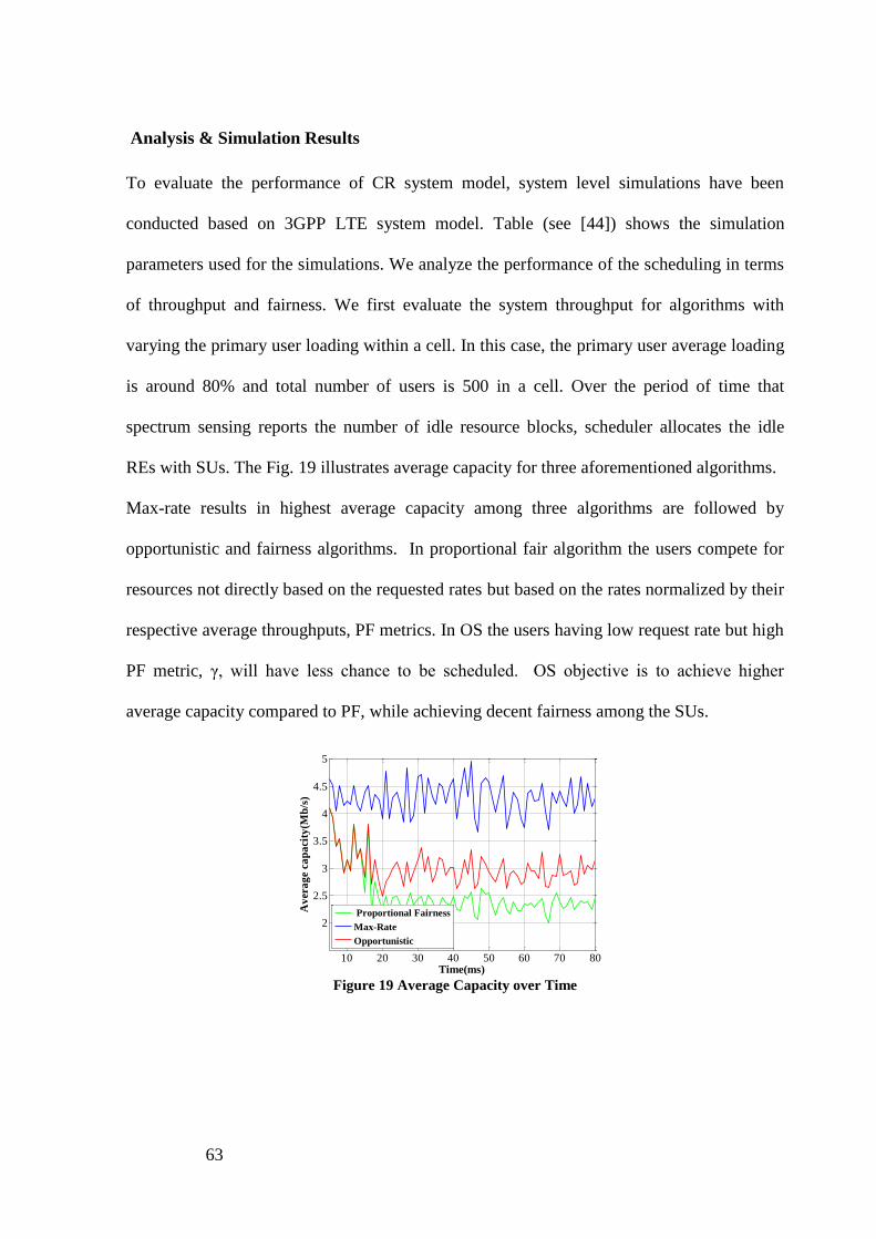
63

Analysis & Simulation Results

To evaluate the performance of CR system model, system level simulations have been

conducted based on 3GPP LTE system model. Table (see [44]) shows the simulation

parameters used for the simulations. We analyze the performance of the scheduling in terms

of throughput and fairness. We first evaluate the system throughput for algorithms with

varying the primary user loading within a cell. In this case, the primary user average loading

is around 80% and total number of users is 500 in a cell. Over the period of time that

spectrum sensing reports the number of idle resource blocks, scheduler allocates the idle

REs with SUs. The Fig. 19 illustrates average capacity for three aforementioned algorithms.

Max-rate results in highest average capacity among three algorithms are followed by

opportunistic and fairness algorithms. In proportional fair algorithm the users compete for

resources not directly based on the requested rates but based on the rates normalized by their

respective average throughputs, PF metrics. In OS the users having low request rate but high

PF metric, γ, will have less chance to be scheduled. OS objective is to achieve higher

average capacity compared to PF, while achieving decent fairness among the SUs.

Figure 19 Average Capacity over Time

10 20 30 40 50 60 70 80

2

2.5

3

3.5

4

4.5

5

Time(ms)

Av

era

ge

cap

aci

ty(M

b/s

)

Proportional Fairness

Max-Rate

Opportunistic

64

In Fig. 20, we analyze the scheduled SUs average capacity of each algorithm in each

scenario when number of active PUs varies. Based on goals of each algorithm they indicate

respective positions in the results. It can be seen that the solution obtained using the

proposed algorithm (OS) is quite close to the PF specifically when the active PUs are less.

Figure 20 Max-Rate average capacity

Figure 21 Average No. of scheduled SUs

We note that the less PUs scheduled yields to high availability of idle REs. Therefore, higher

number of SUs scheduled results in larger average capacity in the CR network. When the

numbers of PUs are increased, the advantage of the OS algorithm over PF is more obvious

(i.e. Fig.20) due to more sparse SUs. Sparse implies large variability in SUs profile (i.e.

SINR, fading channel, physical location).

150 200 250 300 3502

2.5

3

3.5

4

4.5

5

5.5

Number of Active PUs

Av

era

ge C

ap

acit

y o

f S

erv

iced

SU

s (M

bp

s)

Max-Rate

Opportunistic

Proportional Fair

150 200 250 300 35040

45

50

55

60

65

70

75

Number of Active PUs

Nu

mb

er o

f S

erv

iced

SU

s

Max-Rate

Opportunistic

Proportional Fair

65

In Fig. 21, we analyze the average number of scheduled SUs in each scenario when number

of active PUs varies. We note that the more PUs scheduled yields to less availability of idle

REs and therefore less number of SU scheduled.

In Fig. 21 the Max-Rate average capacity is much higher than average capacity of PF; on the

contrary, Fig. 22 shows the more scheduled SUs by PF algorithm compared to Max-Rate

algorithm. As a result, the OS algorithm can balance both the performance of the cognitive

radio networks in terms of achieving acceptable average capacity of secondary users and the

fairness.

Conclusion

In this thesis, we have analyzed the potential 4G CR network framework in context of smart

grid information systems. Our system level simulation results show that the 4G CR network

can achieve an average capacity of 3.5Mbs in a 3Km cell radius under the constraint of an

average primary user network usage of 80%. Finally, we present that the CR capacity of a

20% usage model meets the smart grid protocols requirements for a multi-user CR network of

smart meters.

66

Chapter V. Interference Aware Scheduling for Maximum Channel

Reuse and Max-Capacity in Smart Meter Networks

Contributions of This Thesis on Interference Aware Scheduling

In this thesis, we develop a novel opportunistic interference–aware scheme based on maximum

channel reuse in unplanned networks. The framework adopts the IEEE 802.22 for CR. Our

model of channel reuse implies simultaneous use of intra cell physical resource elements (PRE)

leading to dynamic co-channel interference on a per-PRE basis. We analyze the application of

SISO and MIMO interference aware scheduling. The proposed scheduling scheme eliminates idle

time-slots under the joint constraint of maximum interference and maximum capacity. We

demonstrate that this approach substantially increases capacity gains for MIMO systems in

multi-cell environments compared to conventional scheduling schemes discussed previously.

Another distinguishing aspect of this thesis is that we analyze the smart meter network in a

manner that jointly satisfies both the DOE smart grid communication protocol in terms of capacity [45]

and the IEEE 802.22 protocol satisfying the FCC CR requirements.

67

System Model

Fig. 22 illustrates the system model under consideration in this thesis. As shown in Fig. 22, the

system utilizes the CR scheme of IEEE802.22 WRAN. The TV antenna indicates service for

PUs in the CR protocol. In addition, AMI is denoted as SU. The SU electronic component is

alternatively named as consumer premise equipment (CPE) indicates in the CR protocol [46].

Since the 802.22 WRAN specifies a fixed point-to-multipoint wireless air interface, CR base

station (BS) can manage its own cell and all associated AMIs as shown in Fig. 22. In

IEEE802.22 WRAN, multiple cells are overlapped which results in uncoordinated interference

from other cells as shown in Fig. 22.

Figure 22 SISO system model depicted with coordinated and uncoordinated interference

Radio resource management in our IEEE 802.22 based CR network model involves three

dimensions: frequency, time and space. Physical resource element (PRE) spans in both

frequency and time dimensions. We presume a scheduler coordinating the usage of PREs in

adjacent cells by opportunistically leveraging multi-user AMI frequency, time and spatial

diversity. It also ensures that PRE may be simultaneously assigned to more than one A-SU

Coordinated

interference

Unscheduled A-SU

Scheduled A-SU

TV TX

CR BS

Uncoordinated

interference

TV TXCR BS TV BS

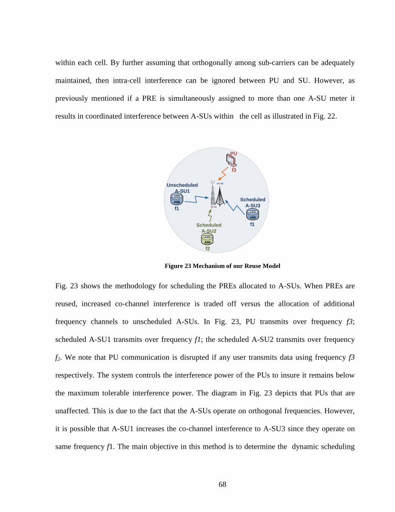
68

within each cell. By further assuming that orthogonally among sub-carriers can be adequately

maintained, then intra-cell interference can be ignored between PU and SU. However, as

previously mentioned if a PRE is simultaneously assigned to more than one A-SU meter it

results in coordinated interference between A-SUs within the cell as illustrated in Fig. 22.

Figure 23 Mechanism of our Reuse Model

Fig. 23 shows the methodology for scheduling the PREs allocated to A-SUs. When PREs are

reused, increased co-channel interference is traded off versus the allocation of additional

frequency channels to unscheduled A-SUs. In Fig. 23, PU transmits over frequency f3;

scheduled A-SU1 transmits over frequency f1; the scheduled A-SU2 transmits over frequency

f2. We note that PU communication is disrupted if any user transmits data using frequency f3

respectively. The system controls the interference power of the PUs to insure it remains below

the maximum tolerable interference power. The diagram in Fig. 23 depicts that PUs that are

unaffected. This is due to the fact that the A-SUs operate on orthogonal frequencies. However,

it is possible that A-SU1 increases the co-channel interference to A-SU3 since they operate on

same frequency f1. The main objective in this method is to determine the dynamic scheduling

f1

f1

f3

0.000

AMI

0.000

AMI

0.000

AMI

f2

Unscheduled

A-SU1

Scheduled

A-SU3

PU

Scheduled

A-SU2

TV TX

CR BS

69

of PREs that maximizes channel reuse among A-SUs and maximized multi-user capacity

considering both interference and noise of existing A-SU in that particular PRE.

Figure 24 Interference-Aware scheduler (IAS) algorithm for PRE reuse

Interference –Aware Scheduling Algorithm

We presume the initial scheduling is performed on secondary users based on max rate algorithm

(MRA) [47] . is showing set of indices of all A-SUs within the cell as follow,

1.

2.

1 2[ , ,..., ]NSU su su su

1 2[ , ,..., ],s sNSU su su su1 2[ , ,..., ]us usNSU su su su

3. sort based on SINR and channel in ascending order in usSU sortusSU

4. choose the with maximum SINR and channel

5. calculate the for ( ) ( ), sorts usSU j SU i

I

( )usSU i

1,2,..., sj N

6. pick the that have min interference with ( )sSU j ( )sortusSU i

7. :recalculate the capacity of ( )( )

and sortsus SU jSU i

C C

8. ' ' '( )( )sort

sus SU jSU iC C C

9. If and '

( )sSU jC C '

thI I

10. allow reuse the spectrum of ( )sort

usSU i ( )sSU j

YES

11. update the scheduling profile:

( ) and ( )sort sort

us uss usSU SU i SU SU i

EXIT

12. update as follow:

( )sort

ususSU SU i

NO

' '( )( )

,sortsus SU jSU i

C C

is empty?usSU

is empty?usSU

YES

YES

EXIT

NO

NO

SU

70

1 2[ , ,..., ]NSU su su su (34)

where N is total number of A-SUs. sSU is defined as the initial scheduled users through max–

rate and usSU are unscheduled users.

sSU and usSU are sub set of SU ,

s usSU SU SU (35)

Furthermore, the vector of fading coefficients for the channels between the SUs and CBS is

1[ ( ),..., ( )]( )CBS

SU NH h nT h nTnT (36)

Fig. 3 depicts the proposed interference aware scheduling (IAS) algorithm. The scheduler

selects active unscheduled users with data to send. We sort the usSU by SINR and channel

coefficients in ascending order represented as sort

usSU . The ascending order ensures that A-SUs

with high SINR are available for exploiting interference introduced by reusing the PRE. We

choose unscheduled A-SU ( ), 1.. sort

us usSU i i N from sort

usSU with maximum SINR and higher

channel coefficients as represented in step 4 in Fig. 24. We calculate the co-channel interference

between ( )sort

usSU i and ( ), 1.. s SSU j j N . Wheres

N and us

N are total number of scheduled and

unscheduled A-SUs respectively. Choose the ( )s

SU j with minimum co-channel interference with

respect to ( )sort

usSU i . Co-channel interference ( ), ( )sort

s usSU j SU iI I is evaluated in the later part of the

section. In step 7, we recalculate the capacity of ( )s

SU j and sort

usSU based on updated interference

I in step 5.

If each A-SU, i, is serviced on a channel, the multiuser capacity for orthogonal OFDM signaling

is given below and notes that it cannot exceed the Shannon capacity given in [47],

2

2W log 1 ( )SINR

i ii iC h nT (37)

71

In real-world deployments, we can develop a modified Shannon capacity formula, by replacing

the cell bandwidth, with an effective bandwidth and effW [47] which accounts for G-

factor dependencies and protocol control, pilot, and cyclic prefix overheads. Closely related to

the SINR is the G-factor, which accounts for the geometric dependencies of cell layouts and

dictates the statistics of the downlink capacity. The G-factor is the average own cell power to

the other cell-power plus noise ratio when considering uniform spatial distributions of

transceivers within a cell.

In addition, we can define a normalized effective signal to noise ratio, SINReff adjust SNR for

both interference, G-factor and statistics. Defining the modified Shannon spectral efficiency for

PU, as we therefore define the modified A-SU capacity in

2

2

(

(1 )

)SINR

.log

ef

i i

f

iieff

h n

N I

SN

T

C WR

(38)

whereiSINR is the signal to interference plus noise power ratio for i

th A-SU. Therefore

iSINR

can be expresses as

2 2

ir

i

N I

PSINR

(39)

where ir

P , 2

N , and 2

I denote the received signal power from ith

A-SU, the noise power, and the

self-interference power at the CBS in the cell.

Using equation 5 we calculate capacity of ( )sSU j and ( )sort

usSU i as labeled as ( )sSU j

C and ( )sort

usSU iC .

( )sSU j

C < ( )sSU j

C , is due to effect of increase in interference caused due to PRE reuse. The

objective of the IAS algorithm is to reuse the PRE and improve the capacity while optimally

exploiting the interference variations occurred. This necessity to verify,

72

( )( )

sortsus

SU jSU iC C C (40)

( )sSU jC C (41)

However, the other critical factor to be taken in consideration is maximum tolerable interference

thI . We need to check the co-channel interference ( ), ( )sort

s usSU j SU iI I observed should be always less

than thI in order satisfy QoS factor and FCC requirements.

thI I (42)

In step 9, we check the conditions stated in (41) and (42). If conditions are satisfied scheduler

allows ( )sort

usSU i reusing the same PREs of ( )sSU i and updates the usSU and sSU shown in step 11

and iterates the process until all usSU are empty. If the conditions are not satisfies, we updated

the usSU as seen in step 12 and we iterates the process to step 3.

Interference Model for SISO

The OFDM transmission system with MIMO model for an A-SU as a function of sub carrier K

is given by,

T Rn n

(k) = (k) (k) + (k) + (K)

Y H X N I (43)

In (43), is the received signal on the kth

subcarrier in CR base station.

is the channel coefficients. In SISO, nT=1 and nR=1;

denotes vector of transmit data at kth

subcarrier in CRBS from the

transmitted OFDM signal in uplink model.

1[ [ ],..., [ ]]TN(k)= Y k Y kY

1[ [ ],..., [ ]]TNT Rn n (k)= H k H kH

1[ [ ],..., [ ]]TN(k)= X k X kX

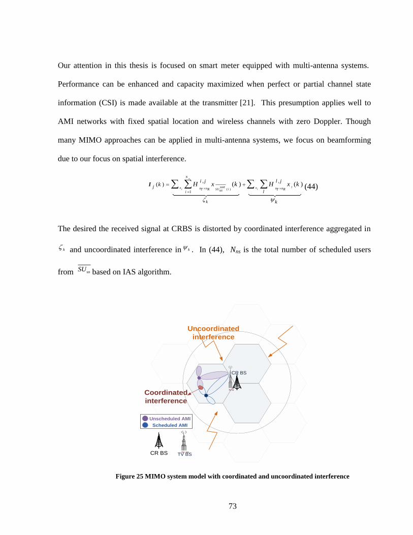
73

Our attention in this thesis is focused on smart meter equipped with multi-antenna systems.

Performance can be enhanced and capacity maximized when perfect or partial channel state

information (CSI) is made available at the transmitter [21]. This presumption applies well to

AMI networks with fixed spatial location and wireless channels with zero Doppler. Though

many MIMO approaches can be applied in multi-antenna systems, we focus on beamforming

due to our focus on spatial interference.

( )1

, ,( ) ( ) ( )

ns

T T

N

ln nSU i

sortn n n nT R T Rusi

k

jl

i j l j

k

k H x k H x k

I (44)

The desired the received signal at CRBS is distorted by coordinated interference aggregated in

and uncoordinated interference in . In (44), Nns is the total number of scheduled users

from based on IAS algorithm.

Figure 25 MIMO system model with coordinated and uncoordinated interference

k k

usSU

Unscheduled AMI

Scheduled AMI

TV TX

CR BS

Uncoordinated

interference

TV TXCR BS

Coordinated

interference

TV BS

74

Interference Model for Beamforming

The multi-antenna system offers well known motivations compared to conventional wireless

communication systems. Our attention in this thesis is focused on smart meter equipped with

multi-antenna systems. Performance can be enhanced and capacity maximized when perfect or

partial channel state information (CSI) is made available at the transmitter [21]. This

presumption applies well to AMI networks with fixed spatial location and wireless channels

with zero Doppler. Though many MIMO approaches can be applied in multi-antenna systems,

we focus on beamforming due to our focus on spatial interference.

Simulations and results

Numerical results exhibit the effectiveness of the proposed interference-aware scheduler for the

SSIO and beamforming approach to smart meters. In this simulation, we follow the IEEE

WRAN standard [46] as OFDM parameters.

Table 2 THE OFDM PARAMETERS FOR IEEE802.22 WRAN

Channel bandwidth (MHz) 6

Number (N) of subcarriers for FFT 2048

Number of data subcarriers for FFT 1440

Number of pilot subcarriers for FFT 240

Subcarrier spacing (KHz): PRE BW 3.348

Modulation QPSK

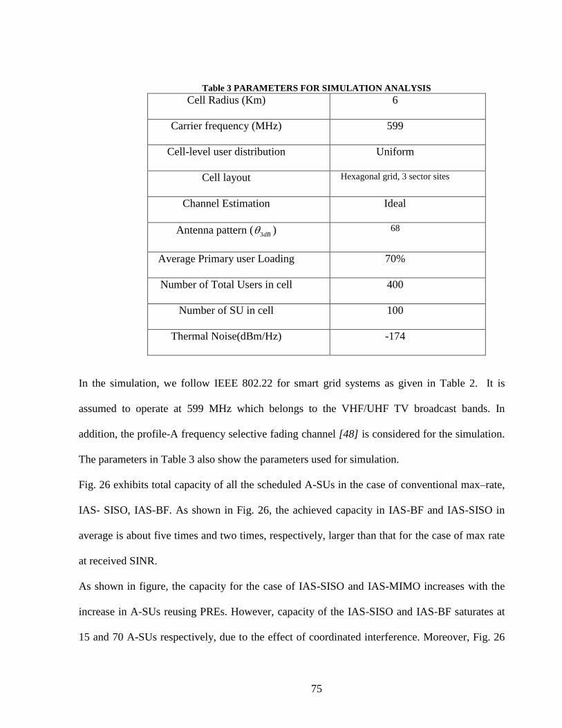
75

Table 3 PARAMETERS FOR SIMULATION ANALYSIS

Cell Radius (Km) 6

Carrier frequency (MHz) 599

Cell-level user distribution Uniform

Cell layout Hexagonal grid, 3 sector sites

Channel Estimation Ideal

Antenna pattern ( ) 68

Average Primary user Loading 70%

Number of Total Users in cell 400

Number of SU in cell 100

Thermal Noise(dBm/Hz) -174

In the simulation, we follow IEEE 802.22 for smart grid systems as given in Table 2. It is

assumed to operate at 599 MHz which belongs to the VHF/UHF TV broadcast bands. In

addition, the profile-A frequency selective fading channel [48] is considered for the simulation.

The parameters in Table 3 also show the parameters used for simulation.

Fig. 26 exhibits total capacity of all the scheduled A-SUs in the case of conventional max–rate,

IAS- SISO, IAS-BF. As shown in Fig. 26, the achieved capacity in IAS-BF and IAS-SISO in

average is about five times and two times, respectively, larger than that for the case of max rate

at received SINR.

As shown in figure, the capacity for the case of IAS-SISO and IAS-MIMO increases with the

increase in A-SUs reusing PREs. However, capacity of the IAS-SISO and IAS-BF saturates at

15 and 70 A-SUs respectively, due to the effect of coordinated interference. Moreover, Fig. 26

3dB

76

shows that the average capacity for each scheduled A-SU satisfies the DOE smart grid

communication protocol average capacity requirements[45].

Figure 26 Total capacity of A-SU in the cases of no IAS, IAS-SISO and IAS-BF

Figure 27 Total capacity of A-SU in the cases of no IAS, IAS-SISO and IAS-BF

Fig. 27 illustrates the interference and number of reuses for one of A-SUs scheduled (with index

22). As it shown in figure, after third reuse for SISO, if we add one more unscheduled A-SU

with minimum interference in order to reuse the PRE, interference exceeds the threshold. This is

because of high interference caused by SISO. To satisfy the condition in step 9 in Fig. 24, the

0 10 20 30 40 50 60 700

1

2

3

4

5

6

7

8

9

10

11

12

13

14

Number of scheduled A-SU

Cap

acit

y(M

bp

s)

SISO

Beamforming 4x4

Max rate

1 1.5 2 2.5 3 3.5 4 4.5 5 5.5 60

0.5

1

1.5

2

2.5

3

3.5

4

4.5

5x 10

-13

Number of reuse

Inte

rfere

nce

22th scheduled SU-SISO

22th scheduled SU-MIMO

77

reusing is ended at 3. On the other hand, because of less interference due to side lobes in

beamforming, we are able to reuse more unscheduled A-SUs till we have total interference close

to in that PRE. As a result, in Fig. 26, we have greater interference for beamforming

compared to SISO, because in beamforming, the interference is closer to than in SISO for all

PREs. That is, we are taking advantage of all possible interference that can be tolerated by A-

SUs.

Fig. 28 illustrates the comparison of total capacity for IAS-SISO and IAS-BF. As exhibited in

Fig. 28, the proposed IAS-BF achieves greater capacity than IAS-SISO at the same interference.

Moreover, capacity of the IAS-SISO and IAS-BF saturates due to the effect of coordinated

interference. Although, the IAS-BF shows higher interference compared to IAS-SISO, the

interference in all PREs caused by IAS-BF is still within .

Fig. 29 illustrates the number of reuse for each scheduled A-SU. As depicted in Fig. 29a, 22 A-

SUs have been scheduled by max rate algorithm. Regard to two conditions in step 9 in Fig.24,

PREs of A-SU with indices 2, 6, 7, 13, 15 and 22are reused.

Based on Fig 29, reuse of each scheduled A-SU’s PREs in IAS-BF is always more than reuse in

IAS-SISO. Since the interference in other A-SUs exceeds the threshold, no reuse occurred.

In Fig. 30, the total number of reuse in IAS-SISO and IAS-BF SUs bandwidth is depicted. The

figure shows that the total number in IAS-BF is always more than IAS-SISO. This is due to less

interference caused by IAS-BF.

thI

thI

thI

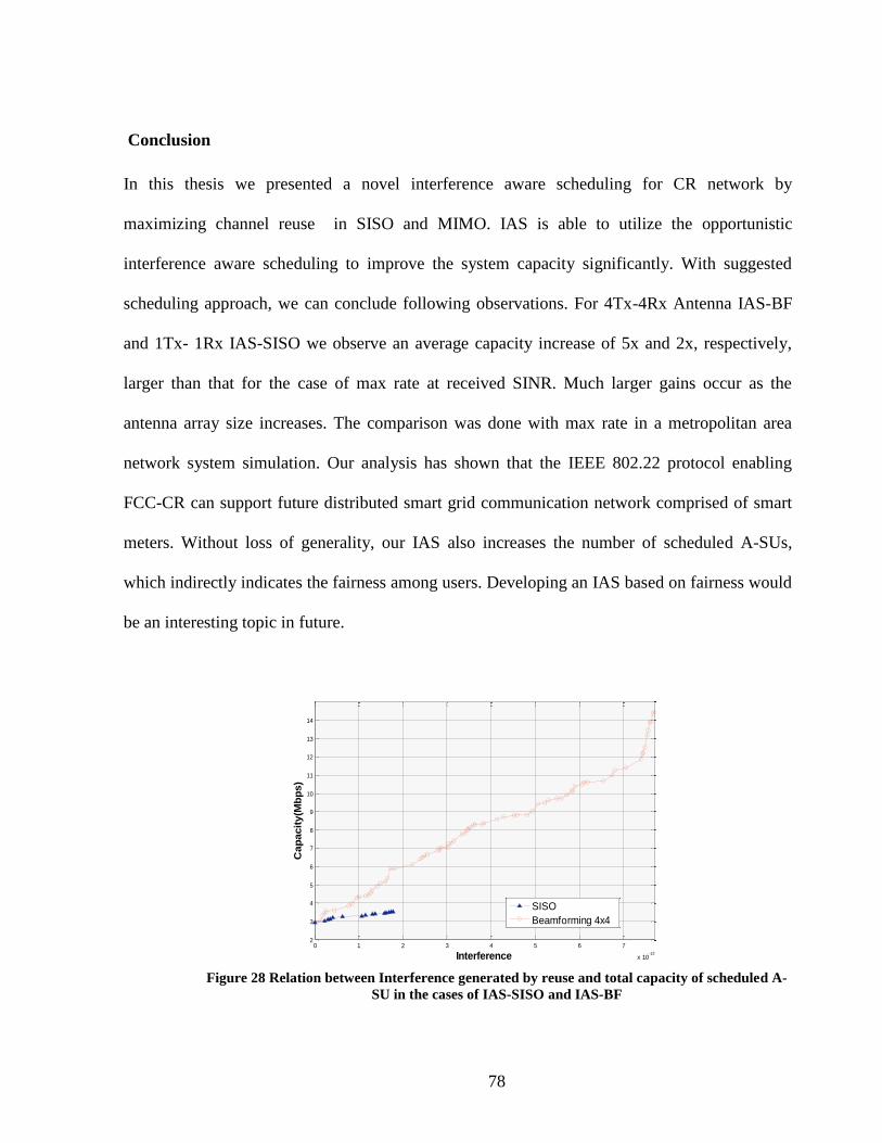
78

Conclusion

In this thesis we presented a novel interference aware scheduling for CR network by

maximizing channel reuse in SISO and MIMO. IAS is able to utilize the opportunistic

interference aware scheduling to improve the system capacity significantly. With suggested

scheduling approach, we can conclude following observations. For 4Tx-4Rx Antenna IAS-BF

and 1Tx- 1Rx IAS-SISO we observe an average capacity increase of 5x and 2x, respectively,

larger than that for the case of max rate at received SINR. Much larger gains occur as the

antenna array size increases. The comparison was done with max rate in a metropolitan area

network system simulation. Our analysis has shown that the IEEE 802.22 protocol enabling

FCC-CR can support future distributed smart grid communication network comprised of smart

meters. Without loss of generality, our IAS also increases the number of scheduled A-SUs,

which indirectly indicates the fairness among users. Developing an IAS based on fairness would

be an interesting topic in future.

Figure 28 Relation between Interference generated by reuse and total capacity of scheduled A-

SU in the cases of IAS-SISO and IAS-BF

0 1 2 3 4 5 6 7

x 10-12

2

3

4

5

6

7

8

9

10

11

12

13

14

Interference

Cap

acit

y(M

bp

s)

SISO

Beamforming 4x4

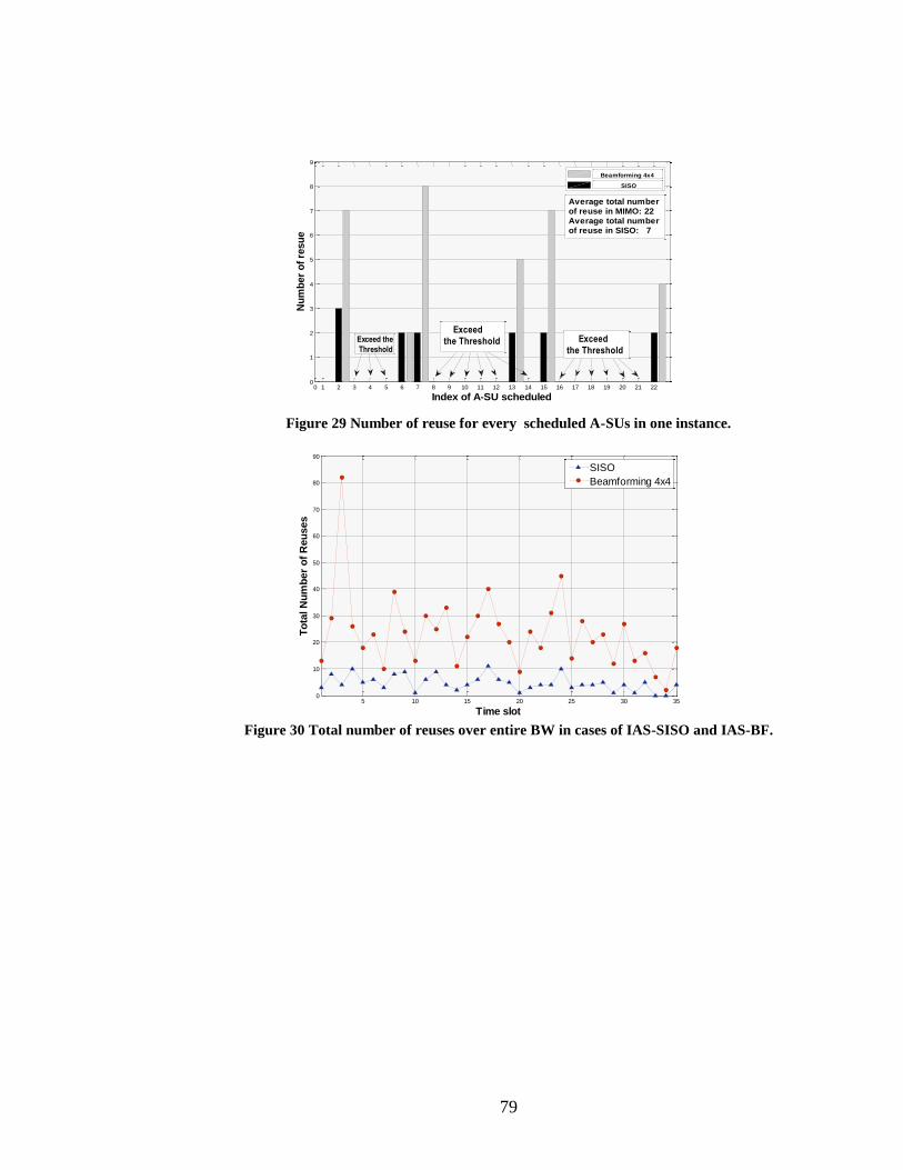
79

Figure 29 Number of reuse for every scheduled A-SUs in one instance.

Figure 30 Total number of reuses over entire BW in cases of IAS-SISO and IAS-BF.

0 1 2 3 4 5 6 7 8 9 10 11 12 13 14 15 16 17 18 19 20 21 220

1

2

3

4

5

6

7

8

9

Index of A-SU scheduled

Nu

mb

er

of

resu

e

Exceed the

Threshold

Average total numberof reuse in MIMO: 22Average total numberof reuse in SISO: 7

SISO

Beamforming 4x4

Exceed

the Threshold Exceed

the Threshold

5 10 15 20 25 30 350

10

20

30

40

50

60

70

80

90

Time slot

To

tal N

um

ber

of

Reu

ses

SISO

Beamforming 4x4

80

Chapter VI. Smart Grid and Optimization

Fuzzy Control of Electricity Storage Unit for Energy Management of Micro-Grids

Introduction

This work is partially funded by CPS Energy through Texas Sustainable Energy Research

Institute at the University of Texas at San Antonio.

Micro-Grid is a small-scale grid that is designed to provide power for local communities. A

Micro-Grid is an aggregation of multiple distributed generators (DGs) such as renewable energy

sources, conventional generators, in association with energy storage units which work together

as a power supply network in order to provide both electric power and thermal energy for small

communities which may vary from one common building to a smart house or even a set of

complicated loads consisting of a mixture of different structures such as buildings, factories, etc

[49]. Typically, a Micro-Grid operates synchronously in parallel with the main grid. However,

there are cases in which a Micro-Grid operates in islanded mode, or in a disconnected state [50].

In this article we assume that when the Micro-grid is connected to the main grid and is working

81

synchronously with it, the flow of electric power can be either from the main grid to the Micro-

grid or vice-versa. If the flow of electric power is from the main grid towards Micro-grid it

means that the Micro-grid is consuming the main grid’s energy for each KiloWatt-Hour of

which the consumer, here Micro-grid, must pay to the Grid. This borrowed power can be either

sent to local load to be consumed or can be stored in battery for future use. But, in case the flow

of power is from the Micro-Grid towards the main grid, this means that Micro-Grid is delivering

power to the main grid. In other words, the excess power generated currently by the renewable

electricity generators or stored previously in the batteries is being sold to the main grid, and the

Micro-Grid, or in general the consumer, is making profit by selling energy to the main grid.

Without loss of generality, we have assumed that the price rate for buying energy from the main

grid is equal to the electricity price rate which is sold to the grid. The excess power can be sold

to the grid whenever the storage unit or load don’t need that power or whenever it is more

beneficial to sell power to grid than to use it for supplying the load. However, in this article the

main goal is to have the load completely supplied by the required power demand at all

conditions. Authors have previously simulated the Micro-Grid assuming no maximum and

minimum limit for the amount of energy stored in the battery unit [49]. In this article, storage

unit’s limits on maximum and minimum amount of stored energy are considered and the results

are compared to the results of the previous work.

System Model

The model used for simulation of the Micro-grid network is a three-bus system. One of the

busses in the distributed generation model is assumed to serve the renewable generators which

include either solar farm, wind farm, or any other renewable generation units either in

82

association with battery storage unit or without storage. Another bus is assumed to be there as

the grid (utility) bus which will provide the complement part of the power demanded by the

local load that renewable electricity generation system cannot afford. The third bus will be the

specific load to which the demanded power is to be provided. This load can be anything from a

common building or a smart house, to even a group of plants and factories or a mixture of all of

them. Figure 31 shows an overall Micro-Grid schematic including Renewable Electricity

Generators and Storage Unit, Utility, and Local Load.

Figure 31 Basic Grid System Model

There are three scenarios defined for simulation in this article; scenario 1 deals with a Micro-

Grid which includes the renewable electricity generators without any battery storage unit.

Therefore there will not be any approaches required for controlling the battery storage system in

this scenario. The second scenario deals with the same Micro-Grid system as mentioned in

scenario one but after the battery storage unit is connected to the same bus with the renewable

generators. Also, the fuzzy approach is applied in this scenario for energy management through

battery unit control. The point in this scenario is that the battery storage is assumed to be an

PowerlinesStorage Unit

Renewable

Generators

Utility

Local load

83

ideal battery without any maximum or minimum limits on stored energy, i.e. infinite battery

capacity. In the third scenario which is the last one, the Micro-Grid is assumed to have

everything mentioned in scenario two plus the fact that maximum and minimum limits of stored

energy are taken into account for storage unit and are assumed to be 85% and 15% of the

nominal maximum storable energy respectively.

A. Characteristics of Buses in Scenario 1

The three buses in the model of Micro-Grid Network simulated in this article have the following

characteristics in the first scenario:

Bus 1 is of type PQ and is used as the renewable electricity generation unit's bus.

Bus 2 is of type Slack (reference) and is used as the Utility (grid) bus.

Bus 3 is of type PV and is used as the Local Load bus.

B. Characteristics of Buses in Scenario 2

The characteristics of the three buses in the Micro-Grid Network model simulated in this article

are as follows in the second scenario:

Bus 1 is a PQ bus and is used as the bus for renewable generation unit and infinite-capacity

battery storage.

Bus 2 will be the Slack (reference) bus and is used as the Utility (grid) bus.

Bus 3 is of type PV and is used as the Local Load bus.

84

C. Characteristics of Buses in Scenario 3

Bus characteristics of the three buses in the Micro-Grid Network model simulated in this article

are as follows in the third, i.e. last, scenario:

Bus 1 is a PQ bus and is used as the bus for renewable generation unit and finite-capacity

battery storage unit.

Bus 2 will be the Slack (reference) bus and is used as the Utility (grid) bus.

Bus 3 is of type PV and is used as the Local Load bus.

This must be noted that battery units are assumed to be ideal batteries, i.e. no dynamic transient

of change in the amount of stored energy in batteries are assumed, i.e. the amount of stored

energy in the batteries is assumed to be changing as a pure ramp by time in both ascending and

descending direction.

Problem Statement

The important point which lies behind the idea of this article is that we have assumed the real-

time pricing for electricity. The update duration of pricing is assumed to be 15 minutes, which

means that the price per KiloWatt-Hour of electricity consumed by the customers of the load

region is updated every 15 minutes. This means that the money consumers need to pay to the

utility for the same amount of energy used during different time-intervals might be different.

Therefore, a function is required to be defined which takes into account the difference between

amount of power given to the utility by the Micro-Grid, and the amount of power taken from the

utility by the Micro-Grid. The Equation 1 represents this cost function:

85

1

Pr .( ( ))T

U L

t

Cost t S t S t

(45)

where the electricity price is determined by the CPS energy every 15 minutes for the next

15 minute period. is the amount of power transferred to/from the Grid during each 15

minute period. If power is received from the Grid will be positive, and if power is

delivered to the grid in case of excess power generation by the renewable generation system

will appear in the equations with a negative sign. is the amount of distribution loss

which will occur on the branches we have between these three buses in the Micro-Grid system

during each 15 minute period. Depending on whether the load is getting how much of its

demanded power from renewable generation system and how much from the Grid, and also

depending on whether the renewable generation system is producing excess power and is selling

the excess power to the Grid, this power Loss will vary.

Figure 32 Three Bus Model for Micro-Grid

Figure 32 represents the three-bus model used for simulation of the Micro-Grid in different

scenarios along with the branch impedances and the types of buses. Simulation is done on the

86

Micro-Grid system considering three scenarios. In the following the summary of these scenarios

is given:

A. Scenario 1

Analysis of the Micro-Grid system profits and costs under real-time electricity pricing policy; in

this scenario the simulation, analysis and study will be done on a Micro-Grid model which

includes the renewable generation unit without any battery storage unit. Therefore there will not

be any approaches required for controlling the battery storage system.

B. Scenario 2

Fuzzy Control of the Micro-Grid system under real-time electricity pricing policy; the cost

function assumed in this scenario is the same as the cost function used in the scenario 1. The

main difference here is that the storage unit exists in the network and will appear to be on the

same bus with the renewable electricity generation unit. The storage unit in this scenario is

assumed to be ideal with infinite capacity.

C. Scenario 3

Fuzzy Control of the Micro-Grid system under real-time electricity pricing policy; the cost

function assumed in this scenario is the same as the cost function described in the two scenarios

1 and 2. In this scenario also the storage unit exists in the network on the same bus with the

renewable generation unit. The critical difference between this scenario and scenario 2 is that

the storage unit in this scenario is assumed to be an ideal battery with finite capacity. Therefore,

87

the maximum and minimum amounts of energy stored in the batteries are finite values and serve

as boundaries which cannot be exceeded.

The power flow calculation and analysis in the Micro-Grid is the key to simulate the whole

system. There are a number of well-known methods for calculation of power flow in the

distributed generation network. There are four different types of busses considered in a

distributed generation network, the characteristics of which will be calculated in power flow

algorithms. These four types include PQ, PV, Slack, and isolated.

Fuzzy Control Approach

The control strategy implemented in this thesis is to use Fuzzy Logic for controlling the power

flow to/from the battery storage unit in order to improve the value of the cost function

introduced in section III. The three input variables to the fuzzy inference engine are Electricity

Price, Renewable Generation Rate, and Load Demand. The Fuzzy inference engine serves as the

controller which determines a measure of the amount of power that must be sent to/taken from

the battery unit during the next time interval, i.e. 15 minute period, based on the current values

of its three inputs.

The fuzzy membership functions for the three inputs price, load demand, and renewable

generation rate, and also for the output variable which determines the amount of power

transaction with the storage unit are shown in figure 33.

88

(a)

(b)

Figure 33 Fuzzy Membership functions for input and output variables of the Fuzzy Controller;

(a) inputs (b) output

The numerical values for these three input variables are normalized to the [0 1] interval, and

then are Fuzzified using three fuzzy sets defined as Low (L), Medium (M), and High (H) as can

be seen in figure 3a. The input variables after fuzzification will be fed to a fuzzy inference

engine where the rule-base is applied to the input-output variables and the output will be

determined by human reasoning. There is only one output variable from the fuzzy controller.

This variable determines the amount of power to be stored in the battery, or to be drawn out

from battery in each 15 minute interval. As represented in figure 3b, output variable fuzzy set is

assumed to have five membership functions called Negative Large (NL), Negative Small (NS),

Zero (Z), Positive Small (PS), and Positive Large (PL). The power drawn from the batteries can

be used to complement the renewable electricity generation unit’s power for providing the

load's demand, can be sold to the Grid, or can be partially used for both reasons. The role of

fuzzy inference engine is critically important for obtaining satisfactory results. For example two

of the rules can be as follows:

89

IF the Price is Low, AND the Renewable Generation rate is High, AND the Load Demand is

Medium, THEN the amount of Power to Battery storage system should be Positive-Large.

IF the Price is High, AND the Renewable Generation rate is Low, AND the Load Demand is

Medium, THEN the amount of Power to Battery storage system should be Negative-Large.

The primary goal in these simulations is to provide the local load with all the power it demands

at any circumstances. Meanwhile, this must be noted that whenever the price is high or low, the

secondary goal will be to sell the most power to the main grid, and to purchase the most power

possible from the main grid respectively. Under low-price electricity conditions, the action

required by the rules might even require the Micro-Grid network to purchase power from grid

and store it in the battery storage unit because the main point here is that the Price is low. This

means by storing the energy in the batteries during low price times, the system will have enough

stored energy in order to sell to the Grid during high-price periods. Even under cases of High

local Load demand this will be a rational strategy. Therefore, having feasible rules predefined

for the fuzzy system will help improve the cost function drastically. The proposed approach

may even sometimes result in making the cost function value negative, which means that the

system is making some profit instead of paying to the utility by the use of this control approach.

Simulation results & discussions

The simulation is done on the three bus system shown in figure 32. The Gauss-Seidel algorithm

is implemented using Matlab for power flow calculation. Some typical data are generated for

electricity price rate, time-varying Load Demand and Renewable Generation Rate. The power

demand of the Load on bus 3 (Smart House) is supplied by two generators on buses 1 and 2.

90

Bus 1 includes solar panel and/or storage unit and bus 2 is slack which is connected to utility as

shown in figure 2.

Figure 34 Profiles of Price, Renewable Generation, and the Load

Figure 35 Power Flow of Bus 1 connected to Solar Panels; scenario 1

Figure 36 Power Flow of Bus 2 connected to Utility; scenario 1

91

Figure 37 Power Flow of Bus 3 connected to Load; scenario 1

The numerical values of the data profile for the three input variables which are fed to the fuzzy

controller are shown in figure 34 during a typical day. These variables include electricity price

which is assumed to be variable as time passes, renewable electricity generation rate, and local

load demand. The data is generated arbitrarily for simulation purposes only with regard to the

fact that the peak electricity consumption duration of the whole region of interest for the main

grid is around 8:30 pm where the electricity price gets to its maximum value. The simulation

results for scenario 1 are represented in figures 35 to 37.

As it can be inferred from figure 35, the value of reactive power for bus 1 is constantly zero

which corresponds to the assumption that the renewable generators do not provide reactive

energy. Figure 6 shows that the active power is taken from the Utility during first half of the day

time, and during most of the second half of the day the active power is being delivered to the

grid. Load is evidently consuming active power regarding the blue curve represented in figure

37.

Simulation results for scenario 2 which associates ideal storage with infinite capacity to the

renewable electricity generators on bus 2 are represented in figures 38 and 39.

92

Figure 38 Output of the Fuzzy Controller, i.e. measure of the amount of power given to/taken

from storage unit; scenario 2;

Figure 39 Power Flow of Bus 2 connected to Utility; scenario 2

Figure 38 parts a and b are matched to each other and this clearly shows that any value decided

by the Fuzzy Controller for the power to be given to Battery or to be taken from it can be

practical since battery unit assumed in scenario 2 is of infinite capacity. Figure 39 shows that

active power is taken from the utility during first half of the day, and in the second half of day

the active power is mostly being sold to the grid which can be deduced by the negative value of

the blue curve in figure 39. The point is that the first part of the active power diagram is raised

dramatically due to fuzzy decision making which means that the system is absorbing more

active power from the grid during low-price hours and stores the power in the storage unit.

Also, the second part of the active power diagram has fallen more in comparison to the same

93

section of figure 36 which denotes on increase in the amount of power drawn from storage unit

and using this power for partially charging the load and also selling the excess power to the grid

during high-price hours. This strategy results in reduction of cost function value or in other

words increases the profit.

Remembering that the pricing periods are assumed to be 15 minute periods and one day is 24

hours overally there will be 96 periods of pricing during one day period. The summation of

payment/profit and the loss during each of the periods will give us the overall value of cost

function for one day. The process can be extended to one week, one month, one year etc.

Output of the fuzzy inference engine which represents the power rate given to battery is shown

in figure 41. Whenever the value of this variable is positive it means that power is delivered to

the storage unit and if the power is drawn from the storage unit, the value will be negative.

Simulation results for scenario 3 in which ideal finite-capacity storage is added on bus 2 in

Micro-Grid network are represented in figures 40 to 42.

Figure 40 Output of the Fuzzy Controller; scenario 3;

Figure 40 parts a and b are not matched to each other and this shows the fact that the values

decided by the Fuzzy Controller for the power to be given to Battery or be taken from it might

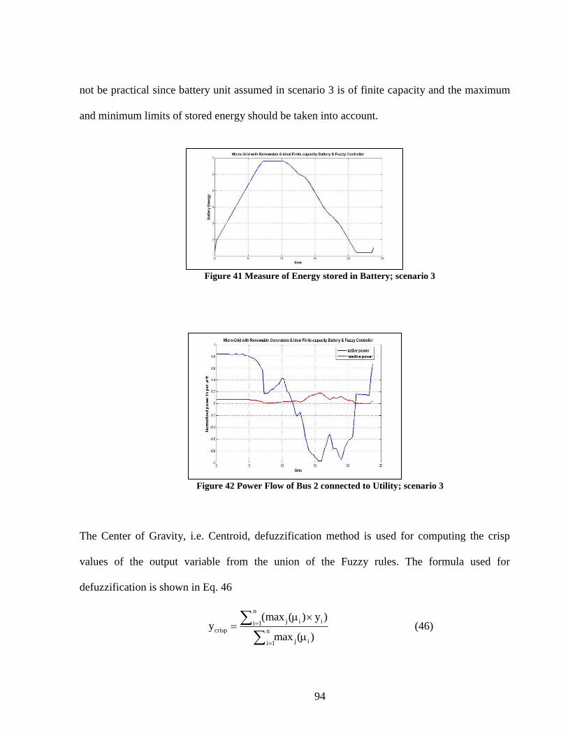
94

not be practical since battery unit assumed in scenario 3 is of finite capacity and the maximum

and minimum limits of stored energy should be taken into account.

Figure 41 Measure of Energy stored in Battery; scenario 3

Figure 42 Power Flow of Bus 2 connected to Utility; scenario 3

The Center of Gravity, i.e. Centroid, defuzzification method is used for computing the crisp

values of the output variable from the union of the Fuzzy rules. The formula used for

defuzzification is shown in Eq. 46

n

j i ii 1crisp n

j ii 1

(max ( ) y )y

max ( )

(46)

95

where stands for crisp value of output variable. i changes between 1 and n, and refers to

the number of discrete point at which the calculation is being done. j changes between 1 and the

number of membership functions of output variable which in this case is , and represents the

number of membership function curve for which we are getting the membership value of ith

point in the universe of discourse of the output variable. Therefore, represents the

final membership value of the ith

point in the universe of discourse of output, i.e. . Equation

47 shows the relation between Balance, Distribution Loss and the overall Cost of Electricity.

Balance Loss Cost (47)

In table 4, total values of distribution loss, cost, and balance on one typical day for the three

scenarios mentioned in section III are summarized. It must be noted that the values in the table

are unit-less, and they can be regarded as measures for payment that the end-user should make

to the utility because of regular operation of Micro-Grid, or profits earned due to improved

operation and control of the Micro-Grid.

Table 4 Simulation results for Loss, Cost, and Balance

Loss Cost Balance

Scenario

1

0.1339 1.2294 1.3632

Scenario

2

6.6039 -17.6716 -11.0677

Scenario

3

6.6039 -13.3021 -6.6982

Cost is simply the overall summation of power from/to grid multiplied by the relevant price for

all 15 min periods. The overall summation of multiplication of the price and wasted power on

distribution branches for all 15 min periods is defined as Loss. With no loss of generality, it is

assumed that the reactive power has one tenth the value of active power.

96

We can see that scenario 2 will provide the consumer with the most possible profit on balance

and this is because of the fact that the battery unit used in scenario 2 is assumed to be of infinite

capacity. Therefore there will be chance for utmost storage of power in the battery whenever

required and the battery can provide that stored power completely to the Micro-Grid for

appropriate usage any time. This is not a practical case though. In scenario 3 which is the

practical case compared to the second scenario, battery storage unit is assumed to be of limited

capacity and therefore, maximum and minimum limits of the stored energy in the battery might

prevent the control system to apply the decided action on the storage unit thoroughly. This

might cause a drop in the benefits that consumer will obtain using this approach as it can be

seen by comparing the values of Balance for the two scenarios 2 and 3. However, by

improvements in the battery production technologies this issue can be solved to good extents.

Conclusion

The proposed Fuzzy-Logic based control method is applied for Battery Management in Micro-

Grid Systems. In the micro-grid system three buses are considered as renewable generator and

storage, utility, and load (smart house). The goal was to reduce the balance which is based on

distribution loss and cost. The Micro-Grid was simulated under three scenarios. Simulation

results obtained for Micro-Grid under scenario 2 where the ideal infinite-capacity storage is

involved with the Fuzzy controller outperform the other two scenarios. However this is not

practical. In third scenario, ideal limited-capacity storage was involved and the results were

satisfactory. Therefore, using fuzzy controller it is possible to reduce the cost of the Micro-Grid

system, and even let the customers make profit from selling the excess power to the utility.

97

Chapter VII. Particle Swarm Optimization

Particle swarm optimization (PSO) is inspired by social behavior of bird flocking or fish

schooling, originally introduced by Eberhart and Kennedy [51] PSO is suitable for optimization

problems that are relatively irregular, noisy, or dynamic Each particle updates its position based

on the following factors: its best solution (Pbest), a best solution of swarm (gbest), and a best

solution of its neighbors (nbest).

Pbest is the best position that each particle found by the pervious iterations. Each particle has a

special Pbest. gbest is the best position that all of particles found by pervious iterations. gbest is

same for all of particles. We can consider some neighbors for each particle. nbest is the best

position that all of neighbors of each particle found by pervious iterations. Each particle has a

special nbest.

There are several means to initialize positions of particles. One of them used in this thesis is

random initialization. In random initialization, particles are placed in random positions in the

space. The update equation of positions is:

98

0 1 1 2 2 3 3V c X c r pbest X c r gbest X c r nbest X (48)

X X V (49)

Where and are constants and and are random numbers between 0 and 1.

Also, is velocity of each particle. In this study, we consider and

(which these amounts show the best results rather than other amounts). As mentioned

before, the problem is to maximize comfort function under certain conditions. For doing this, p

particles with random positions are produced. Then, their fitness (comfort function) is

calculated and pbest and gbest are obtained .

The velocity of particles is obtained and their positions are updated. This procedure is continued

iteratively until a stopping condition is satisfied. Our stopping condition is that the number of

iteration reaches a maximum or the increase of the fitness (comfort function) is smaller than a

given threshold ( denotes the iteration number):

k k 1gbest gbest (50)

In this study, the first one is chosen because the second one may be trapped in a local optimum.

Here, X or each particle is considered as the amount of power to be delivered or taken.

Comfort Function applied for Our Specific 3-bus Micro Gird Model:

2

1( ) .( ( ) ( ). (1, )) (. ).(| | | |).2

Grid totalcomfort p e price t sin t x p price t V Loss

(51)

99

Simulations for PSO

Figure 43 illustrates when PSO is applied for given Load, RE, and Price profile. As it shown in

Figure 43, the power coming out from RE bus is completely satisfy required load and once the

price in at peak and less load is needed, it consumes more power from RE to minimize cost.

Figure 43 Micro Grid Control by PSO with Load, RE, and Price profile

Figure 44 Power from battery

4 8 12 16 20 30-0.2

0

0.2

0.4

0.6

0.8

1

1.2

1.4

1.6

Hours

Po

wer

RE power

RE Bus power

Grid

Loss

Load

Price

0 4 8 12 16 20-0.2

-0.1

0

0.1

0.2

0.3

0.4

0.5

Hours

Po

wer

Battery Power Flow

100

As shown in Figure 44, PSO makes battery to charge when electricity is low (0-8 hours) and

discharge when price is high (8-16). Also, the stored battery in low price period is consumed for

required load when price is high. This figure verifies the perfect and intelligent performance of

PSO for this kind of model that every input parameter is stochastic and hard to assign fuzzy

logic rules and useless to use deterministic optimization methods.

Figure 45 all profiles and battery behavior through PSO utilization

The results shown in figures (43-45) were for when the sufficient renewable energy exists.

Following results will be showing for when the renewable energy is not enough.

Powerlines

Storage Unit

Renewable

Generators

Utility

Local load

0 4 8 12 16 20-0.2

-0.1

0

0.1

0.2

0.3

0.4

0.5

Hours

Po

wer

Battery Power Flow

4 8 12 16 20 30-0.2

0

0.2

0.4

0.6

0.8

1

1.2

1.4

1.6

Hours

Po

wer

RE power

RE Bus power

Grid

Loss

Load

Price

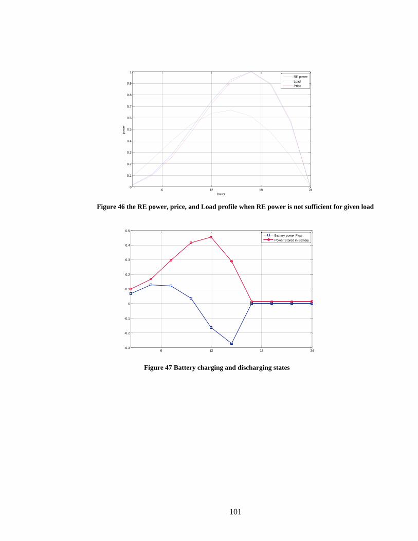
101

Figure 46 the RE power, price, and Load profile when RE power is not sufficient for given load

Figure 47 Battery charging and discharging states

6 12 18 240

0.1

0.2

0.3

0.4

0.5

0.6

0.7

0.8

0.9

1

hours

pow

er

RE power

Load

Price

6 12 18 24-0.3

-0.2

-0.1

0

0.1

0.2

0.3

0.4

0.5

Battery power Flow

Power Stored in Battery

102

Figure 48 Grid Power, Price, Cost Function, and power from RE

As depicted in figure 46, there is no ample renewable energy for needed load. Figure 47 shows

that battery stores low price power as much as possible for high price power priod. As shown in

48, at hour 18, when the price has its maximum value, the battery does not let grid power to be

increased and decrease the grid power as much as possible. Based upon results shown in figures

43-48, the PSO performs acceptable for Micro Grid model that has stochastic parameters.

6 12 18 24-0.4

-0.2

0

0.2

0.4

0.6

0.8

1

1.2

1.4

1.6

hours

pow

er

Power from RenBus

Grid Power

Loss

Cost Func

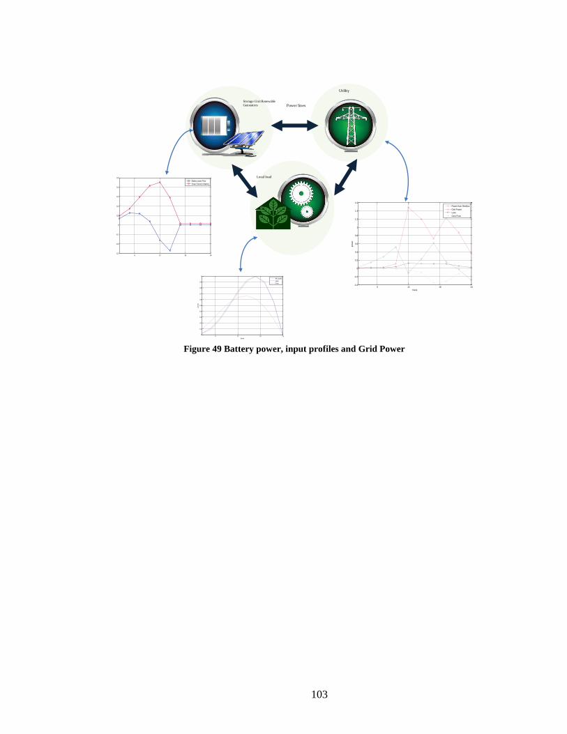
103

Figure 49 Battery power, input profiles and Grid Power

Power linesStorage Unit Renewable

Generators

Utility

Local load

6 12 18 240

0.1

0.2

0.3

0.4

0.5

0.6

0.7

0.8

0.9

1

hours

pow

er

RE power

Load

Price

6 12 18 24-0.4

-0.2

0

0.2

0.4

0.6

0.8

1

1.2

1.4

1.6

hours

pow

er

Power from RenBus

Grid Power

Loss

Cost Func

6 12 18 24-0.3

-0.2

-0.1

0

0.1

0.2

0.3

0.4

0.5

Battery power Flow

Power Stored in Battery

104

Chapter VIII. CONCLUSION

This thesis, presents the Cognitive Radio framework for wireless Ad Hoc networks. The

proposed Cognitive Radio framework is a complete model for Cognitive Radio that describes

the sensing and sharing procedures in wireless networks by introducing Queued Markov Chain

method in spectrum sensing and Competitive Indexing Algorithm in spectrum sharing part.

Queued Markov Chain method is capable of considering waiting time and is very well

generalized for unlimited number of secondary users. It includes the sharing aspect of Cognitive

Radio. Power-law distribution of node degree in scale-free networks is important for

considering the traffic distribution and resource management thus we consider the effect of the

topology on sensing and sharing performances. We demonstrate that CIF outperforms Uniform

Indexing (UI) algorithm in Scale-Free networks while in Random networks UI performs as well

as CIF.

Also, in this thesis, a framework is presented based on 4G Cognitive Radio (CR) network

capable of communicating with high numbers of geographically dispersed smart meters for

command and control feature concurrently with private cellular network. Our approach uses

pervasive smart grid systems (i.e. cloud data centers) as the central communication and

optimization infrastructure supporting metropolitan area based smart meter infrastructure. In

this thesis, we investigate the performance of various scheduling algorithms in context with CR

105

units to provide a satisfactory tradeoff between maximizing the system capacity, achieving

fairness among cognitive users. We lay as a framework evaluation 3GPP LTE system model

simulations. Our system level simulation results show that the 4G CR network model meets the

smart grid protocols requirements for a multi-user CR network of Smart meters.

This thesis addresses improvements in the multiuser capacity in unplanned networks with high

levels of co-channel interference. We view this as the likely system scenario for future

cognitive radio (CR) networks. For this reason, this thesis presents a novel opportunistic

interference aware scheduling protocol ideally suited for maximum channel reuse in unplanned

networks. We present results for maximum capacity CR networks, many of which may be based

upon the future IEEE 802.22 standard. In addition, we show that the IEEE 802.22 protocol

enabling Federal Communication Commission (FCC)-CR can support future distributed smart

grid communication network comprised of smart meters. We analyze the application of SISO

and MIMO interference aware scheduling to maximize the capacity and number of scheduled

smart meters. We present simulation results that show significant improvement in the total

capacity and number of scheduled smart meters in comparison to traditional scheduling

schemes. Finally, we show that our system meets the DOE smart grid communication protocol

requirements in terms of capacity.

Moreover, a Fuzzy Logic-based framework is proposed for control of Battery Storage Unit in

Micro-Grid Systems to achieve Efficient Energy Management. Typically, a Micro-Grid system

operates synchronously with the main grid and also has the ability to operate independently

from the main power grid in an islanded mode. Distributed renewable energy generators

including solar, wind in association with batteries and main grid supply power to the consumer

in the Micro-Grid network. The goal here is to control the amount of power delivered to/taken

106

from the storage unit in order to improve a cost function, defined based on summation of

payment required for purchasing power from main grid or profit obtained by selling power to

the main grid and distribution power loss, through reasonable decision making using

predetermined human reasoning-based fuzzy rules. Profiles of system variables such as

Consumer’s Load Demand, Electricity Price Rate, and Renewable Electricity Generation Rate

are assumed arbitrarily for obtaining general results. Measures of payment/profit will be

extracted to compute amounts of cost and balance for the network which represents benefits of

using Fuzzy logic for Storage Unit control with and without considering storage unit capacity

limits. Simulation results are presented and discussed.

107

Chapter IX. References

[1] Ian F. Akyildiz, Won-Yeol Lee, Mehmet C. Vuran, and Shantidev Mohanty, "A

Survey on Spectrum Management in," IEEE Communications Magazine, April

2008.

[2] Isabelle Tardy,Ole Grondalen, "Which Regulation for Cognitive Radio?An

Operator’s Perspective," Telektronikk, 2010.

[3] I. F. A. e. al, "NeXt Generation/Dynamic Spectrum Access/Cognitive Radio

Wireless Networks: A Survey," Comp. Networks J, pp. 2127-2159, 2006.

[4] FCC, "Unlicensed Operations in the TV Broadcast Bands, Second

Memorandum Opinion and Order,," 2010.

[5] J. Wang, M. Shosh, and K. Challapali, "Emerging cognitive radio applications:

a survey," IEEE Commun. Mag, vol. 49, p. pp. 74–81, mar 2011.

[6] 3. S. T. 36.321, "Technical Specification Group Radio Access Network;

Evolved Universal Terrestrial Radio Access; Medium Access Control," 2010.

[7] I. S. 802.16m, "System Description Document," 2009.

[8] J. Ma, G. Y. Li, and B. H. Juang, "Signal processing in cognitive radio," Proc.

IEEE, p. pp. 805–823, 2010..

[9] S. Haykin, D. J. Thomson, and J. H. Reed, "Spectrum sensing for cognitive

radio," Proc. IEEE, p. 849–877, 2010.

[10] D. Cabric, S. M. Mishra, and R. W. Brodersen, "Implementation Issues in

Spectrum Sensing for Cognitive Radios," p. 772–76, 2004.

[11] Y. Zeng and Y.-C. Liang, "Eigenvalue-based spectrum sensing algorithms for

cognitive radio," IEEE Trans. Commun, p. 1784–1793, 2009.

[12] A. Kortun, T. Ratnarajah, Sellathurai, C. M., Zhong, and C. B. Papadias, "On

the performance of eigenvalue-based cooperative spectrum sensing for

cognitive radio," IEEE J. Sel. Topics Signal Process, p. 49–55, 2011.

[13] T. Cui, J. Tang, F. Gao, and C. Tellambura, "Moment-based parameter

estimation and blind spectrum sensing for quadrature amplitude modulation,"

IEEE Trans. Commun, p. 613–623, 2011.

[14] A. Sahai and D. Cabric, "A tutorial on spectrum sensing: Fundamental limits

108

and practical challenges," Int. Symp. on New Frontier in Dynamic Spectrum

Access Networks (DySPAN), 2005.

[15] P. P. Hoseini and N. C. Beaulieu, "An optimal algorithm for wideband spectrum

sensing in cognitive radio systems," Proc. IEEE Int. Conf. Commun. (ICC),, pp.

1-6, 2010.

[16] P. Paysarvi-Hoseini and N. C. Beaulieu, "Optimal wideband spectrum sensing

framework for cognitive radio systems," IEEE Trans. Signal Process, p. 1170–

1182, 2011.

[17] Z. Quan, S. Cui, A. H. Sayed, and H. V. Poor, "Optimal multiband joint

detection for spectrum sensing in cognitive radio networks," IEEE Trans. Signal

Process, p. 1128–1140, 2009.

[18] D. Qu, J. Ding, T. Jiang, and X. Sun, "Detection of non-contiguous OFDM

symbols for cognitive radio systems without out-of-band spectrum

synchronization," IEEE Trans. Wireless Commun, p. 693–701, 2011.

[19] S. Krishnamurthy et al.,, "Control Channel Based MAC Layer Configuration,

Routing and Situation Awareness for Cognitive Radio Networks," Proc. IEEE

MILCOM, p. 455–60, 2005.

[20] O. Ileri, D. Samardzija, and N. B. Mandayam, "Demand Responsive Pricing and

Competitive Spectrum Allocation via Spectrum Server," Proc. IEEE DySPAN,

p. 194–202, 2005.

[21] Q. Zhao et al., "Decentralized Cognitive MAC for Opportunistic Spectrum

Access in Ad Hoc Networks: A POMDP Framework," IEEE JSAC, pp. 589-99,

2007.

[22] H. Zheng and L. Cao, "Device-centric Spectrum Management," Proc. IEEE

DySPAN, pp. 56-65, 2005.

[23] R. Menon, R. M. Buehrer, and J. H. Reed, "Outage Probability Based

Comparison of Underlay and Overlay Spectrum Sharing Techniques," Proc.

IEEE DySPAN, pp. 101-9, 2005.

[24] J. Zhao, H. Zheng, and G.-H. Yang, "Distributed Coordination in Dynamic

Spectrum Allocation Networks," Proc. IEEE DySPAN, p. 259–68, 2005.

[25] Pengbo Si ; Enchang Sun ; Ruizhe Yang ; Yanhua Zhang ;, "Cooperative and

distributed spectrum sharing in dynamic spectrum pooling networks," Wireless

and Optical Communications Conference (WOCC), pp. 1-5, 2010.

[26] Toroujeni, S.M.M. ; Sadough, S.M.-S. ; Ghorashi, S.A., "Time-frequency

spectrum leasing for OFDM-based Dynamic Spectrum Sharing systems,"

Wireless Advanced (WiAD), pp. 1-5, 2010.

[27] A.L. Barabasi,R. Albert, "Emergence of scaling in random networks," Science,

vol. 286, pp. 509-512, 1999.

[28] Carlos Cordeiro, Kiran Challapali, and Dagnachew Birru, "IEEE 802.22: An

Introduction to the First Wireless Standard based on Cognitive Radios," Journal

of Communications, vol. 1, 2006.

[29] T. Kolding., "Link and System performance aspects of Proportional Fair Packet

Scheduling in WCMS/HSDPA," In Proceedings of 58th IEEE Vehicular

109

Technology Conference, vol. 3, pp. 1717-1722, 2008.

[30] Zhi Quan ; Shuguang Cui ; Sayed, A.H. ; Poor, H.V. , "Optimal Multiband Joint

Detection for Spectrum Sensing in Cognitive Radio Networks," IEEE

Transaction on Signal Processing, vol. 57, pp. 1128-1140, 2008.

[31] Khalid, L. ; Anpalagan, A., "Effect of sensing errors on wideband cognitive

OFDM radio networks," IEEE Biennial Symposium QBSC, pp. 273-277, 2010.

[32] Ying-Chang Liang ; Yonghong Zeng ; Peh, E.C.Y. ; Anh Tuan Hoang,

"Snesing-Throughput Tradeoff for Cognitive Radio Networks," IEEE

Transactions On Wireless Communications, vol. 7, 2008.

[33] Yanjun Yao ; Zhiyong Feng ; Dan Miao , "Markov-based Optimal Access

Probability for Dynamic Spectrum Access in Cognitive Radio Networks,"

Vehicular Technology Conference (VTC 2010-Spring, 2010.

[34] Ghosh, C. ; Cordeiro, C. ; Agrawal, D.P. ; Rao, M.B. , "Markov Chain

Existence and Hidden Markov Models in Spectrum Sensing," IEEE

International Conference on Pervasive Computing and Communications, 2009.

[35] Akyildiz, I.F. ; Won-Yeol Lee ; Vuran, M.C. ; Mohanty, S., "A survey on

spectrum management in cognitive radio networks," Communications

Magazine, IEEE, vol. 46, pp. 40-48, 2010.

[36] Pengbo Si ; Hong Ji ; Yu, F.R. ; Leung, V.C.M., "Optimal Cooperative

Internetwork Spectrum Sharing for Cognitive Radio Systems With Spectrum

Pooling," Vehicular Technology, IEEE Transactions on, vol. 59, pp. 1760-1768,

2010.

[37] Amir Rajaee, Mahdy Saedy, Asadallah Sahebalam, "Competitive Spectrum

Sharing for Cognitive Radio on Scal-Free Wireless Networks," IEEE IWCMC

Istanbul, 2010.

[38] D.D.Ariananda, M.K.Lakshmanan, H.Nikookar, "A survey on spectrum sensing

techniques for cognitive radio;Cognitive Radio and Advanced Spectrum

Management," Second International Workshop on, pp. 74-79.

[39] B. Kelley, "Software Defined Radio for Broadband OFDM Protocols," SMC,

2009.

[40] S.-W. Luan, J.-H. Teng, S.-Y. Chan, and L.-C. Hwang, "Development of a

smart power meter for AMI based on zigbee communication," Proc. Int. Conf.

Power Electron, pp. 661-665, 2009.

[41] Wenpeng Luan, Duncan Sharp and Sol Lancashire, "Smart Grid

Communication Network Capacity Planning for Power Utilities," IEEE PES

Transmission and Distribution Conference and Exposition, pp. 1-4, 2010.

[42] B. Reid, "Oncor electric delivery smart grid initiative," in Proc. 62nd Annu.

Conf. Protective Relay Engineers, pp. 8-15, 2009.

[43] Robert C. Qiu, Zhe Chen , Nan Guo , Yu Song, Peng Zhang, Husheng Li and

Lifeng Lai, "Towards A Real-time Cognitive Radio Network Testbed:

Architecture, Hardware Platform, and Application to Smart Grid," Networking

Technologies for Software Defined Radio (SDR) Networks, Fifth IEEE

Workshop, Boston, pp. 1-6, 2010.

110

[44] Preben Mogensen et,al., "LTE Capacity compared to the Shannon Bound," In

Proceedings of 65th IEEE Vehicular Technology Conference, pp. 1234-1238,

2007.

[45] Department of Energy, "Communications Requirements of Smart Grid

Technology”," 2010.

[46] Chawla, K., Xiaoxin Qiu, "Throughput performance of adaptive modulation in

cellular systems," IEEE , Int. Conf. Universal Personal Communiations,

Florence, 1998.

[47] "LTE Capacity Compared to the Shannon Bound," IEEE 65th Vehicular

Technology Conference, Dublin, pp. 1234-1238, 2007.

[48] IEEE802.22-05/0055r7, "WRAN Channel Modeling," 2005.

[49] Y. S. Manjili; A. Rajaee; B. Kelley; M. Jamshidi, "Fuzzy Control of Storage

Unit for Energy Management in Micro-Grids," University of Texas at San

Antonio College Of Science Conference, UTSA-COS, 2011.

[50] C. Cho; J. Jeon; J. Kim; S. Kwon; K. Park.; S. Kim, "Active Synchronizing

Control of a Microgrid," IEEE Transactions on Power Electronics, no. 99,

2011.

[51] J. Kennedy, R.C. Eberhart., "Particle Swarm Optimization," In Proc .of the

IEEE Int Conf. Neural Networks, 1995.

Section 3:

Photovoltaics

Abstract — The rapid growing interests in renewable energy, such

as solar energy, outweigh the benefit of distributed grids in current grid networks. Innovative topologies for renewable energy conversion systems that integrate with electric grids and energy storage systems are being proposed, each with limited modes of operation for the various needs in smart grid applications. In this paper, we propose a modified version of a multi-source converter,

which uses a small number of elements to accomplish each task of multi-mode operation in a smart-grid. The proposed approach is verified by simulations in MATLAB. We found that by introducing an additional switch in the converter’s output allows the reverse flow of current, enabling current to charge a battery from the grid while maintaining the integrity of the former modes of operation.

Index Terms—Battery Storage, Bi-directional Converters, Micro-

grid, Multi-Mode Converters, Renewable Energy, Smart-grid

I. INTRODUCTION

raditional fossil fuel power plants are built away from

cities due to the air pollution they produce. Despite their

steady performance, the amount of energy lost in

transmission lines can be significant. This energy loss can be

reduced by distributing power plants inside the city. On the

other hand, with increasing the load demands, these

distributed generation systems can help diminish the need for new fossil power plants. Renewable energy sources, such as

solar arrays, are known for their clean source of energy, and

their power plants are rapidly being built on the vicinity of

cities and within the cities themselves. This paradigm shift is

becoming apparent in the U.S., as renewable energy electricity

generation is projected to increase from 462 billion kilowatt-

hours in 2010 to 469 billion kilowatt-hours in 2015[1]. Many

countries are promoting their plans to multiply their solar

energy generation plants by facilitating the procurement of

solar plants and offering incentives. To date, the U.S. has nine

of the thirteen biggest photovoltaic solar projects in the world [2].

As renewable energies become more readily available in the

residential sector, DC devices in residences can be supplied

energy from the DC bus of a microgrid. There are advantages

in utilizing a DC bus source as opposed to the synthesized AC

source for these devices. Even though current AC/DC

converters offer huge amounts of power savings thanks to the

advances in power electronic conversion systems, it is still

1 This project was partially funded by CPS Energy through its Strategic

Research Alliance with The University of Texas at San Antonio, San Antonio,

TX, USA.

more reliable and efficient to utilize the DC bus due to the reduced amount of components in comparison to AC-DC

converters.

Solar energy is a well known and favorable type of

renewable energy source, which generates DC power.

However, solar, wind, and other types of renewable energies

are inherently intermittent in nature, meaning they cannot

supply the load demand continuously. To provide a more

rigid flow of electricity, solar energy is integrated with utility

grid with energy storage systems and other available

renewable energy sources such as wind energy. Hybrid

energy systems are capable of providing better power quality and reliability and can improve the system performance. As

an example, wind and solar energy are somewhat

complementary on a daily or seasonal basis [3-4]. Having an

energy storage system may stabilize the energy generated

from renewable sources, specifically during sporadic climate

changes that can affect the output of renewable energy sources

dramatically, and thus increasing the reliability of the DC bus.

In this paper, we propose an amendment to an existing

topology, which may serve to regulate DC voltage into an

inverter or a DC bus and charge/discharge a battery storage

system. The hybrid system in this paper is combination of

photovoltaic, energy storage system and the utility grid. Bi-directionality of converter provides a good power exchange

among sources, load and DC-voltage bus. This concept is

This paper has been submitted to World Automation Congress, Puerto Vallarta, Mexico, June 24-28, 2012.

Bi-Directional Multi-Mode Grid tied Converter

for Solar Energy Conversion Systems1 Elmira Mohyedinbonab, Student Member, IEEE, Emiliano Morales, Member, IEEE,

Hariharan Krishnaswami, Member, IEEE, Mo Jamshidi, Fellow IEEE.

T

Fig. 1. The smart-grid functionality allows the battery to be charged from the

grid.

(a) (b)

Fig. 2. (a) Original method. (b) Proposed method which places the original

diode besides the inductor and places a four quadrant operating MOSFET

in its place.

illustrated in Fig.1.

II. CONVENTIONAL STRUCTURE OF THE MULTI-MODE SINGLE

LEG CONVERTER.

In paper [5], a novel method is proposed that utilized only

two switches (single leg), one diode, and two inductors to

implement different converter modes in the bi-direction

operation of DC/DC converters. This was an improvement to

the conventional boost and bi-directional DC/DC converters

by removing a switching element from the converter, while

still offering the same functionalities and modes. In [5], the

battery is charged in only one mode of operation. Generated

voltage can boost up/down and charge/discharge the battery at

the same time a DC voltage is being supplied to the output of

the circuit.

However, the methods on [5] allowed the battery to be

charged from the renewable source only, and not from the

grid. In this paper, the switch is re-introduced and the

configuration was changed for the benefit of an additional

mode. In this additional mode, the battery can be charged

from the grid when the renewable source is absent or not

sufficient to supply power to the battery. Despite the re-

configuration of the single leg converter, the four former

proposed modes of operation worked.

The placement of the switch to the proposed converter does

not introduce any new switching losses during the original

four modes, for the primary purpose of the switch is to act as a

gate that allows current from the output into the battery, and as

a diode for voltage boost operations (See fig. 2). In these four

modes, the properties of the MOSFET allow the switch to

behave like a diode when no pulse is felt at the gate.

The converter in [5] was limited in interactions between the

renewable energy source and the battery, load, or both. By

taking advantage of the bi-directionality capability of

inverters, the excess grid power can be rectified by the inverter

and stored in the battery. This proposed configuration allows

more interaction among the renewable energy source and grid,

including the battery. This useful feature is capable of storing

excess power from grid and renewable energy power in the

battery when the load demand drops, and may serve as smart

grid function that helps regulate the utility grid.

This paper is structured as follows. In the first section, the

four modes in [5] are re-tested with new configuration, and

briefly describe each mode of operation. That same section

will introduce and cover the new mode and derives its

corresponding equations. The second section will cover the

controller design and explain how to find the desired duty

cycles for the MOSFET switches. In the final section, we will

present our simulation results from MATLAB’s Simulink

followed by a conclusion, which presents the limitations of

this configuration and future endeavors.

III. PROPOSED METHOD FOR THE INTERACTION BETWEEN

RENEWABLE ENERGY SOURCE, BATTERY, AND GRID

The schematic for proposed configuration is shown on fig.

2. As seen on this figure, the diode is replaced with a bi-

directional MOSFET and placed in series with , which will

become essential to block the current from flowing into the

PV source in the proposed mode of operation. The four

original modes are the Main Boost Mode, the Boost-Buck

Mode, the Boost-Boost Mode, the Battery Boost Mode, and

the Reverse Buck Mode. In the Main Boost mode, the single

leg converter increases the voltage that is supplied to the

inverter. In the Boost-Buck mode, energy is stored in the

battery while voltage is supplied to the inverter or DC bus simultaneously. During high load demands, the Boost-Boost

mode can supply the inverter with energy from the PV source

and the battery simultaneously. And during cloud cover,

energy can be supplied to the inverter from the battery in

Battery-Boost mode.

In cases in which grid peak shaving is desired, the battery

can be charged from the grid. The grid alone can supply the

current to the battery through a buck operation in the Reverse

Buck Mode. Times in which is critical to charge the battery

from the grid include peak shaving during inclement weather

or nights, when PV source cannot provide sufficient current to

charge the battery, when the load demand drops, or to store energy during times when grid energy costs are low.

A. Main Boost Mode

In this mode, and have the same duty ratio.

Together, both switches form a boost converter that boosts the

PV input voltage. During this mode, behaves as a diode

by sending zero to its gate. The basic input to output principle

of boost converters applies to this mode, where:

a. Main Boost Mode

b. Boost-Buck Mode

c. Boost-Boost Mode

d. Battery Boost Mode

Fig. 3. The original four modes of operation still operate under the same principle as before.

(1)

In which,

(2)

B. Boost Buck Mode

For this mode, the duty ratio of is longer than .

This way, the PV voltage is boosted during the time both

and are “ON”. During the time remains “ON” and

turns “OFF”, the PV supplies energy to the load and

charges the battery. In this mode, behaves as a diode. To

determine the output of the boost converter for this mode, the

equations become:

(3)

In which,

(4)

To charge the battery, the equations become:

(5)

Where,

(6)

C. Boost-Boost Mode

Here, we have the opposite case from the Boost-Buck

mode, in which the duty ratio of is longer than ’s.

This allows the battery to discharge energy to the inverter

when the PV energy generation is not sufficient. During this

mode, behaves as a diode. This mode boosts the input

voltage while discharging the battery to supply the load. The

equations for this mode are:

(7)

In which,

(8)

And

(9)

In which,

(10)

D. Battery Boost Mode

The Battery Boost mode is useful in the case of input fault

such as cloud cover, or damaged modules, etc. Since our

modification to the converter, the state for is no longer

relevant while acts as a diode. In this mode, the battery

supplies the inverter with energy via the mathematical

equations (11) and (12).

(11)

In which the duty ratio of is,

(12)

E. Reverse Buck Mode

The Reverse Buck Mode (RBM) benefits from the

switch and makes use of the bi-directionality of the

interconnected inverter. This is accomplished by either sending no pulses to the MOSFETs of the universal bridge, in

essence converting the universal bridge into a full bridge

rectifier (see Fig.4.), or by controlling the individual MOSFET

switching cycles to achieve a desired DC voltage.

Subsequently, this system converts the AC grid voltage into

DC for battery charging. In this mode, we made “OFF”,

“ON”, and “OFF”. In this way, the battery is

charged from the rectified grid voltage by varying the duty of

. When the is “ON”, is transferred to the

battery and the inductor current increases. This is

mathematically expressed as:

(13)

Where, is the inductor ripple current. When is

“OFF”, then inductor current in decreases in the rest of the

period . This is expressed as

(14)

By equating (13) and (14), we derived the RBM input to

output relation.

(15)

IV. CONTROL SCHEME

A control scheme was designed for proposed Reverse Buck

Mode. This scheme consisted of a Lag compensator

(Proportional-plus-integral controller) which increases the

low-frequency loop gain, such that the output is better

Fig. 5. Reverse Buck Mode charges the battery when is “ON” and when

no renewable power source is available.

Fig. 4. A three phase full bridge inverter can act as a diode bridge rectifier in reverse when no signals are sent to the gates.

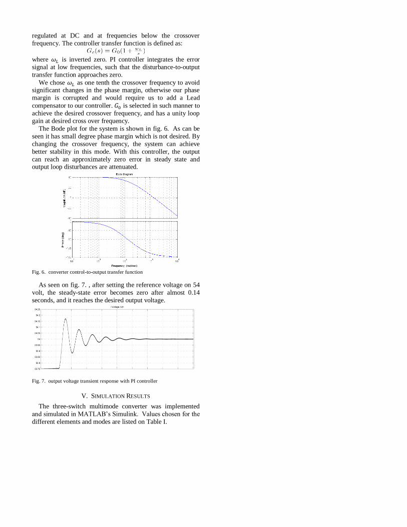
regulated at DC and at frequencies below the crossover

frequency. The controller transfer function is defined as:

where is inverted zero. PI controller integrates the error

signal at low frequencies, such that the disturbance-to-output

transfer function approaches zero.

We chose as one tenth the crossover frequency to avoid significant changes in the phase margin, otherwise our phase

margin is corrupted and would require us to add a Lead

compensator to our controller. is selected in such manner to

achieve the desired crossover frequency, and has a unity loop

gain at desired cross over frequency.

The Bode plot for the system is shown in fig. 6. As can be

seen it has small degree phase margin which is not desired. By

changing the crossover frequency, the system can achieve

better stability in this mode. With this controller, the output

can reach an approximately zero error in steady state and output loop disturbances are attenuated.

Fig. 6. converter control-to-output transfer function

As seen on fig. 7. , after setting the reference voltage on 54

volt, the steady-state error becomes zero after almost 0.14

seconds, and it reaches the desired output voltage.

Fig. 7. output voltage transient response with PI controller

V. SIMULATION RESULTS

The three-switch multimode converter was implemented

and simulated in MATLAB’s Simulink. Values chosen for the

different elements and modes are listed on Table I.

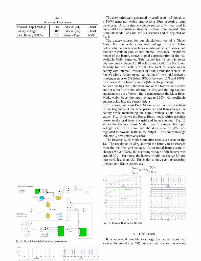
The duty ratios were generated by sending control signals to

a PWM generator which employed a repeating ramp

waveform. Also, a similar voltage source to was used in

our model to simulate an ideal rectification from the grid. The

Simulink model was run for 0.4 seconds and is depicted on fig. 8.

The battery chosen for our simulations was of a Nickel

Metal Hydride with a nominal voltage of 50V. Other

noteworthy parameters includes number of cells in series, and

number of cells in parallel and Internal Resistance. Nonlinear

model of the battery shows a good approxiamtion of the real

available NMH batteries. This battery has 42 cells in series

with nominal voltage of 1.18 volt for each cell. The Maximum

capacity for each cell is 7 AH. The total resistance of the

battery with Internal Resistance of 0.002 Ohms for each cell is

0.0084 Ohms. Experimental validation of the model shown a maximum error of 5% (when SOC is between 10% and 100%)

for chare and dischare dynamics.[Matlab help. menu].

As seen on figs 9-12, the behavior of the former four modes

are not altered with the addition of and the input/output

equations are not affected. fig. 9 demonstrates the Main Boost

Mode, which boost the input voltage to with negligible

current going into the battery ( ).

fig. 10 shows the Boost Buck Mode, which boosts the voltage

in the beginning of the time period and then charges the battery while maintaining the output voltage at its nominal

value. Fig. 11 shows the Boost-Boost mode, which provides

power to the grid from the grid and input sources. Fig. 12

shows the Battery Boost Mode. For this mode, the input

voltage was set to zero, and the duty ratio of was

regulated to provide in the output. The current through

inductor was effectively zero.

The Reverse Buck Mode simulation results are seen on fig.

13. The regulation of allowed the battery to be charged

from the rectified grid voltage. At an initial battery state of

charge (SOC) of 50%, the operating voltage of the battery was

around 50V. Therefore, the battery would not charge for any

duty cycle less than 0.5. This is due to duty cycle relationship

of equation (15), expressed as:

VI. DISCUSSION

It is somewhat possible to charge the battery from two

sources by modifying into a four quadrant operating

Fig. 13. Reverse Buck Mode Results.

Fig. 8. Simulink model of multi-mode converter.

Nominal Output Voltage 160V Inductor (L1) 0.8mH

Battery Voltage 50V Inductor (L2) 0.6mH

Initial Battery SOC% 0.5 Battery Type NMH

Simulation Parameters

Table I

switch (that is a MOSFET configuration that allows for the

positive and negative exchange of voltage and current through

it). The four quadrant operating MOSFET is illustrated on fig.

14a. The four quadrant flexibility was used to preclude any

current from flowing into each of the respective sources, and

solely supply current to the battery. This mode is desired,

since it could increase savings by storing the energy when the

electric rate is low, and utilizing it when it is high in the

following day(s).

In this mode, remains “ON” for the entire period while

is “OFF”, and becomes “ON” for seconds. In

this mode, may cycle “ON” for seconds during the

remaining period (See Fig. 14b). Consequently,

during the the PV charges the inductor, which is the

amount of energy that will be pushed into the battery when

turns “OFF”. During this period of time, the grid

remains disconnected from the battery. When turns

“ON”, the grid supplies energy to the battery for the remaining

duration of time. It is during this period of time that both the

PV and the grid should charge the battery.

Formulas for two scenarios under this mode were derived.

In the first scenario in which both and are “ON”, the

ripple current of both inductors is calculated as follow:

(16)

And,

(17)

During the time that turns “ON” and is “OFF”, the

ripple current of both inductors are mathematically described

by:

(18)

and,

(19)

However, unlike the previous method, (16) and (18) cannot be

equated with (17) and (19) to find the input/output

relationships. This may be due to the inequality of inductor

currents during the short time gap which

and are both “OFF”. Due to this characteristic, the

input/output equations cannot be derived precisely.

VII. CONCLUSIONS

This paper proposed an additional switching element to an

existing method at the expense of adding a valuable capability.

The goal was to add smart grid functionalities to this novel

application with the introduction of minimal switching

elements that ultimately reduce power electronics costs of

renewable energy systems. The proposed configuration

introduced more interaction between the grid and the energy

storage system and while maintaining low switching losses

compared to conventional boost and bi-directional DC/DC

converters. While it was only possible to charge the battery

from the grid with this configuration, charging the battery

from both the PV source and the grid simultaneously present

several challenges.

It is of active interest to introduce the ability to charge the

battery from both sources simultaneously to enhance the

feasibility of this topology as an economical and complete

smart grid system. Topologies such as those in [6], or time

shared basis flyback converters present viable approaches to

this task.

VIII. REFERENCES

[1] M. Barnes, J. Kondoh, H. Asano, J. Oyarzabal, G. Ventakaramanan,

R. Lasseter, N. Hatziargyriou, and T. Green. “Real-world microgrids

- an overview,” in IEEE International Conference on System of

Systems Engineering (SoSE’07), Apr. 2007, pp. 1-8.

[2] L. Zhang, T. Wu, Y. Xing, K. Sun, and J. M. Gurrero

“Power Control of DC Microgrid Using DC Bus Signaling,”

APEC'11 , 2011, pp. 1926-1932.

[3] Available: www.smartgridresearch.org.

[4] Nehrir, M.H.; Wang, C.; Strunz, K.; Aki, H.; Ramakumar, R.; Bing, J.;

Miao, Z.; Salameh, Z.; , "A Review of Hybrid Renewable/Alternative Energy

Systems for Electric Power Generation: Configurations, Control, and

Applications," Sustainable Energy, IEEE Transactions on , vol.2, no.4,

pp.392-403, Oct. 2011.

[5] Taesik Park; Taehyung Kim; , "Novel multi-mode single leg converter for

renewable energy conversion systems," Industrial Technology (ICIT),

2011 IEEE International Conference on , vol., no., pp.198-203,14-16

March 2011

[6] Kwang-Hwa Liu, F.C. Lee, “Topological constraints on basic PWM

converters”, PESC 1988, pp164-172

[7] N. Mohan, “Designing Feedback Controllers in Switch Mode DC Power

Supplies,” First Course in Power Electronics, 2009 ed. Minneapolis,

MNPERE, 2009, ch. 4, pp. (4-1)-(4-6)

[8] R. W. Erickson and D. Maksimovic, “Controller Design,” Fundamentals

of Power Electronics, 2nd

ed. Boulder, 2001, ch. 9, pp. 331-369

(a) (b)

Fig.14. (a) Four Quadrant Bi-Directional Switch. (b)The basic order of

switching operation to charge the battery from energy of the PV source and the rectified grid voltage simultaneously.

Photovoltaic Microinverter using Single-stage

Isolated High-frequency link Series Resonant

Topology

Hariharan Krishnaswami, Member, IEEE,

Department of Electrical and Computer Engineering

The University of Texas at San Antonio

San Antonio, Texas, USA

E-mail: Hariharan.Krishnaswami@utsa.edu

Abstract— In this paper, PhotoVoltaic (PV) microinverter usinga single-stage high-frequency ac link series resonant topology isproposed. The inverter has two active bridges, one at the front-end of PV module and the other at the output or utility side.The active bridges are interfaced through a series resonant tankand a high frequency transformer. A novel phase-shift modulationtechnique to regulate the current into utility is proposed. Steady-state analysis using sinusoidal approximation is presented todetermine the magnitude of output current into utility. Soft-switching operation is ensured in all switches in the converterdue to resonant nature of the circuit. The inverter has advantagesof minimal power conversion stages, high-switching frequencyoperation and low switching losses and hence ideally suited forlow power module integrated applications.

I. INTRODUCTION

Microinverters, also known as AC modules or Module

Integrated Converters (MIC), have been shown to have high

energy yield in Photovoltaic (PV) generation system due to

inverters for each individual PV module [1]. The plug and play

feature of MIC is especially useful for low power residential

applications. Several topologies of MIC have been proposed

in literature [2], [3], [4], [5] which use high-frequency link

based power conversion instead of traditional dc link based

systems. In [2], a MIC is proposed which uses impedance-

admittance conversion theory to supply current into the utility.

In [3] a push-pull based dc-ac inverter with high frequency

link is proposed. It has a matrix converter with four-quadrant

switches at the secondary of the transformer. A flyback-based

inverter is proposed in [4] with an unique power decoupling

circuit at the output of the PV module. A full-bridge based

high-frequency link inverter is proposed in [5] with lowered

switching frequency of the matrix converter.

The principle of power conversion in most of these topolo-

gies is through an high frequency converter followed by a

matrix converter. But leakage inductance of the transformer is

a non-ideality and it creates high voltages across the output

side converter switches, whenever current changes direction

in one switching cycle. This causes severe voltage stress on

the devices and reduces reliability. Having the inductance at

This project was partially funded by CPSEnergy through its StrategicResearch Alliance with The University of Texas at San Antonio.

the high frequency link and creating a high frequency current

source which will then be rectified and fed to the utility as in

[2], [6] can reduce the voltage stresses and also contribute to

increased efficiency of power conversion.

In this paper a series resonant tank circuit is used at the

high frequency link. The proposed converter consists of two

active bridges, a high frequency transformer and a series

resonant tank as shown in Fig. 1. The active bridges switch at

constant switching frequency above resonant frequency. Phase-

shift modulation technique between active bridges is proposed

to control the current being fed to the utility as opposed to

variable frequency and cycloconverter operation in [6]. The

proposed principle of power conversion is similar to the dc-

dc dual active bridge high power converter [7]. This principle

is extended to dc-ac conversion for microinverter application

with inductance replaced by a series resonant tank circuit

in this paper. Four-quadrant full-bridge converter is used as

the output side converter. In summary, the advantages of the

proposed converter are,

• Reduced component count due to single conversion stage

• Reduced switching losses due to soft-switching operation

in all the semiconductor switches

• Reduced size due to high switching frequency capability

of the resonant nature of the circuit

• No adverse effect of voltage stresses on devices due to

leakage inductance since it forms part of resonant circuit.

II. PROPOSED PHASE-SHIFT MODULATION

The converter shown in Fig. 1 operates above resonant

frequency fr formed by the series resonant tank inductance

L and capacitance C. The output of the solar module Vin

is connected to the active bridge through a large capacitor

which filters the current ripple at twice the line frequency. The

active bridge at the output-side of the converter is connected

to the load or the grid through a capacitive filter for filtering

the switching frequency component of the output current. The

input-side active bridge is modulated using the function m1(t)in (1) and the output side active bridge is modulated using

m2(t) in (2). The function sgn(.) is the signum function

which denotes the sign of the signal. In the equations, φ is

+

−

+

−

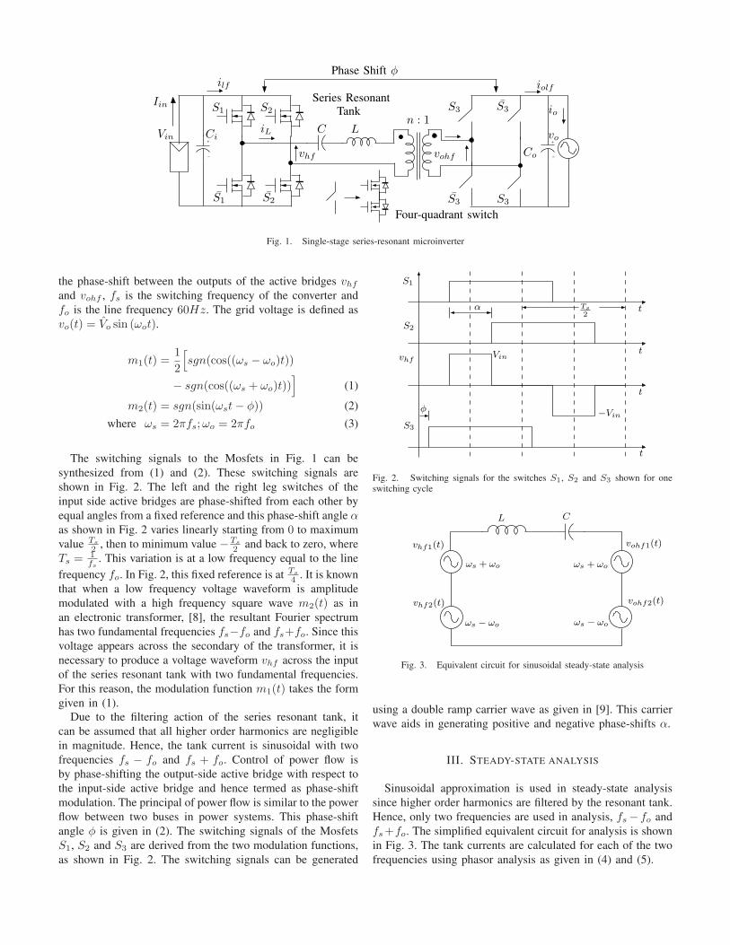
Vin

ilf

iL C L

Series ResonantTank

Phase Shift φ

iolf

vo

Covhf

Ci

vohf

n : 1

S2S1

S3 S3

S3 S3

Iin S1 S2 io

Four-quadrant switch

Fig. 1. Single-stage series-resonant microinverter

the phase-shift between the outputs of the active bridges vhf

and vohf , fs is the switching frequency of the converter and

fo is the line frequency 60Hz. The grid voltage is defined as

vo(t) = Vo sin (ωot).

m1(t) =1

2

[

sgn(cos((ωs − ωo)t))

− sgn(cos((ωs + ωo)t))]

(1)

m2(t) = sgn(sin(ωst − φ)) (2)

where ωs = 2πfs;ωo = 2πfo (3)

The switching signals to the Mosfets in Fig. 1 can be

synthesized from (1) and (2). These switching signals are

shown in Fig. 2. The left and the right leg switches of the

input side active bridges are phase-shifted from each other by

equal angles from a fixed reference and this phase-shift angle α

as shown in Fig. 2 varies linearly starting from 0 to maximum

value Ts

2 , then to minimum value −Ts

2 and back to zero, where

Ts = 1fs

. This variation is at a low frequency equal to the line

frequency fo. In Fig. 2, this fixed reference is at Ts

4 . It is known

that when a low frequency voltage waveform is amplitude

modulated with a high frequency square wave m2(t) as in

an electronic transformer, [8], the resultant Fourier spectrum

has two fundamental frequencies fs−fo and fs+fo. Since this

voltage appears across the secondary of the transformer, it is

necessary to produce a voltage waveform vhf across the input

of the series resonant tank with two fundamental frequencies.

For this reason, the modulation function m1(t) takes the form

given in (1).

Due to the filtering action of the series resonant tank, it

can be assumed that all higher order harmonics are negligible

in magnitude. Hence, the tank current is sinusoidal with two

frequencies fs − fo and fs + fo. Control of power flow is

by phase-shifting the output-side active bridge with respect to

the input-side active bridge and hence termed as phase-shift

modulation. The principal of power flow is similar to the power

flow between two buses in power systems. This phase-shift

angle φ is given in (2). The switching signals of the Mosfets

S1, S2 and S3 are derived from the two modulation functions,

as shown in Fig. 2. The switching signals can be generated

φ

S1

S2

S3

α

Vin

Ts

2t

t

t

−Vin

t

vhf

Fig. 2. Switching signals for the switches S1, S2 and S3 shown for oneswitching cycle

ωs − ωo

vhf1(t)

ωs + ωo

ωs − ωo

vhf2(t)

L C

vohf1(t)

ωs + ωo

vohf2(t)

Fig. 3. Equivalent circuit for sinusoidal steady-state analysis

using a double ramp carrier wave as given in [9]. This carrier

wave aids in generating positive and negative phase-shifts α.

III. STEADY-STATE ANALYSIS

Sinusoidal approximation is used in steady-state analysis

since higher order harmonics are filtered by the resonant tank.

Hence, only two frequencies are used in analysis, fs − fo and

fs +fo. The simplified equivalent circuit for analysis is shown

in Fig. 3. The tank currents are calculated for each of the two

frequencies using phasor analysis as given in (4) and (5).

IL1

6 θ1 =2πVin

6 0 − 2πVo

6 φ

j(ωs − ωo)L + 1j(ωs−ωo)C

(4)

IL2

6 θ2 =2πVin

6 0 − 2πVo

6 φ

j(ωs + ωo)L + 1j(ωs+ωo)C

(5)

The fundamental of vohf calculated from Fourier series

leads to the constants 2π

in the equations. The inductor current

is converted to a low frequency fo by the output side bridge

through the modulation function m2(t). The average current

in one switching cycle Ts can be calculated by integrating

the current between the limits φ and π + φ. The integration

for the inductor current with frequency ωs − ωo is shown in

(6). Similar integration applies for the inductor current with

frequency ωs + ωo.

IL1=

1

π

∫ π+φ

φ

IL1sin((ωs − ωo)t − θ1)d(ωst) (6)

The following two assumptions are used since fs ≫ fo:

• The average value of the output current remains constant

in one switching cycle and

• The impedance of the resonant tank remains same for

variations in frequency from fs − fo to fs + fo and the

impedance at switching frequency is used for analysis.

With the application of the above two assumptions and

simplifying the equations, the resultant average output current

io(t) is given in (7). The output current is sinusoidal with the

direction of the current indicated in Fig. 1. The current is in

phase with utility voltage and hence power is fed back to the

utility at unity power factor. The transformer turns ratio n is

included in the equation.

io(t) =8

π2

nVin sin φ

Z(F − 1F

)sin(ωot) (7)

where Z =

√

L

C; F =

ωs

ωr

; ωr = 2πfr =1

√LC

(8)

The analysis equations are converted to per unit representa-

tion by choosing the output power as Pbase and the line voltage

rms as Vbase. This conversion helps in designing the system for

varied power and input voltage levels. The variable d termed as

voltage conversion ratio is defined in (9). Dividing (7) by the

base current, the resultant normalized output current is given

in (10). In Section IV, a design procedure is discussed.

d =Vin

nVo(rms)

√2

(9)

io,pu(t) =d sin φ

Q(F − 1F

)sin(ωot) (10)

where Q =Z

8π2 n2Rbase

; Rbase =V 2

base

Pbase

(11)

TABLE ISERIES RESONANT DC-AC CONVERTER PARAMETERS

Converter Parameter Value

Resonant Inductor L 10.68µH

Resonant Capacitor C 0.3µF

Input voltage Vin 29.1V

Line voltage rms Vo(rms) 120V

Maximum power output Pbase 225W

Turns ratio n 0.17

Quality factor Q 4.0

IV. DESIGN

The design of the converter is based on the per unit equa-

tions in Section III. For the series resonant circuit, the quality

factor is chosen as 4.0 or higher for validity of sinusoidal

approximation. The ratio of switching frequency to resonant

frequency is chosen as F = 1.1, to enable soft-switching

operation. The voltage conversion ratio is chosen as d = 1.0to enable wider range of soft-switching operation as in [7],

[10]. With these chosen values, the value of phase-shift can

be calculated from the required per unit current into the grid.

As an example, a 225W solar module from BP solar is

chosen and the maximum power point (MPPT) mentioned

in the datasheet Vmax = 29.1V and Imax = 7.7A is used

for simulation, although in real systems, MPPT can change

based on sun’s irradiance. MPPT can be implemented in this

converter by appropriately varying the phase-shift angle φ.

Since this converter is single-phase utility interactive, the grid

voltage used in the simulation is 120V rms at a frequency

of 60Hz. The switching frequency fs is chosen as 100kHz.

The converter parameters are calculated using (8) and (11).

The values used in the converter simulation are summarized

in Table I.

The converter can be represented using two state equations,

with the inductor current and the capacitor voltage being the

state variables. The input voltage Vin and the grid voltage

vo(t) can be considered as ideal voltage sources. The state

equations are given in (12-13).

iL =Vin

Lm1(t) −

1

LvC −

n

Lvo(t)m2(t) (12)

vC =1

CiL (13)

These equations are simulated in Simulink and the ideal

waveforms of the applied voltage across the tank vhf , the

transformer voltage vohf and the unfiltered output current iolf

are shown in Fig. 4 for one switching cycle Ts. In this figure,

two instants are shown, which are the positive and negative

peak of the grid voltage. The values used in this simulation is

given in Table I.

V. SOFT-SWITCHING OPERATION

One of the advantages of operating the series resonant

converter above resonant frequency is soft-switching. The

0.1873 0.18732−40

0

40Tank

voltage

vh

f

time in seconds

0.1873 0.18732−200

0

200

Tra

nsform

er

voltage

vo

hf

time in seconds

0.1873 0.18732−10

0

10

Outp

ut

curr

ent

i olf

time in seconds

0.1956 0.19562−40

0

40

Tank

voltage

vh

f

time in seconds

0.1956 0.19562−200

0

200

Tra

nsform

er

voltage

vo

hf

time in seconds

0.1956 0.19562−10

0

10

Outp

ut

curr

ent

i olf

time in seconds

Fig. 4. Ideal waveforms of applied tank voltage vhf , transformer voltagevohf and unfiltered output current iolf for two switching cycles at twoinstants, positive and negative peak in line voltage

tank current always lags the applied tank voltage and hence

Zero Voltage Switching (ZVS) in all switches in input-side

converter. But, the tank voltage is not a square-wave as it has

zero voltage states, as shown in Fig. 2. Hence, for low values

of α, one of the legs loses ZVS operation.

Based on the current direction shown in Fig. 1, the condition

for soft-switching operation in the output-side active bridge is

the transformer secondary current leading the voltage across

the transformer. As long as the voltage conversion ratio is

unity, soft-switching operation is possible in the output-side

converter also. The active bridge at the output-side uses four-

quadrant switches. In order to achieve soft-switching, one of

the two Mosfets in a four-quadrant switch is always kept ON

based on the polarity of the line voltage. This ensures that the

other switch performs ZVS, based on the condition that the

transformer secondary current leads vohf . Simulation results

are given in the following section to prove soft-switching

operation.

VI. SIMULATION RESULTS

In this section, the simulation results from Saber c© are

presented using the converter values summarized in Table I.

Simulation results of the tank current in one switching cycle

along with the applied tank voltage is shown in Fig. 5 for a

(A

)

−10.0

0.0

10.0

t(s)

4.105m 4.11m 4.115m 4.12m

(V

)

−200.0

0.0

200.0

(A

)

−40.0

0.0

40.0

(V

)

−40.0

0.0

40.0

(A) : t(s)

iolf

(V) : t(s)

vohf

(A) : t(s)

iL

(V) : t(s)

vhf

Fig. 5. Simulation results of tank current iL(t), applied tank voltage vhf (t),transformer voltage vohf (t) and unfiltered output current iolf (t) shown fortwo switching cycles around the positive maximum of line voltage vo(t)

phase-shift angle of α = 50o. The time instant during which

the line voltage vo(t) is at its positive maximum is chosen for

this plot. Due to the lagging nature of the current as observed

from Fig. 5, soft-switching operation in the input-side bridge

is ensured. The tank current leads the voltage across the

transformer which ensures ZVS in output-side bridge. This

is made possible by switching only one of the Mosfets in the

four-quadrant switch shown in Fig. 1 according to polarity

of line voltage and the other switch is ON continuously. The

waveforms are repeated in Fig. 6 for the time instant at which

the line voltage is at its minimum. It can be observed that

soft-switching operation is ensured in this case also.

The filtered output current along with the line voltage is

shown in Fig. 7. It is observed that line voltage and line current

in the direction indicated in Fig. 1 are in phase and hence

power is being fed to the utility. The analysis results match

with the simulation results with an error of < 5% due to

the sinusoidal approximation. The input current has a second

harmonic component of the line frequency. The capacitor Ci

at the input can be designed to filter this harmonic component.

The tank current and its Fourier spectrum are shown in Fig.

8 which confirms the analysis assumption.

The converter efficiency is improved due to reduction in

switching losses achieved by ZVS. Due to the use of two

(A

)

−10.0

0.0

10.0

t(s)

12.405m 12.41m 12.415m 12.42m

(V

)

−200.0

0.0

200.0

(A

)

−40.0

0.0

40.0

(V

)

−40.0

0.0

40.0

(A) : t(s)

iolf

(V) : t(s)

vohf

(A) : t(s)

iL

(V) : t(s)

vhf

Fig. 6. Simulation results of tank current iL(t), applied tank voltage vhf (t),transformer voltage vohf (t) and unfiltered output current iolf (t) shown fortwo switching cycles around the negative maximum of line voltage vo(t)

t(s)

16.7m 33.4m

(A

)

−3.0

0.0

3.0

(V

)

−200.0

0.0

200.0

(A) : t(s)

io

(V) : t(s)

vo

Fig. 7. Line voltage vo(t) and current io(t) for two 60Hz cycles

semiconductor switches to realize a four-quadrant switch in

the output-side converter, one of which is continuously ON

based on grid voltage, the conduction losses can increase

two-fold. But, since the switches are at the high voltage

f(Hz)

10.0 100.0 1.0k 10.0k 100.0k 1meg

(A

)

0.0

5.0

10.0

15.0

t(s)

33.4m

(A

)

−40.0

−20.0

0.0

20.0

40.0

(A) : f(Hz)

iL Spectrum

(A) : t(s)

iL

Fig. 8. Tank current iL(t) and its Fourier spectrum

side < 200V and the currents are lower, it is possible to

design the converter such that the effect of conduction losses

on efficiency is minimal. The effect of increased cost of

the converter due to addition of four-quadrant semiconductor

switches in the output side converter is minimized by reduction

in overall component count due to the use of single-stage

power conversion as compared to the conventional two-stage

dc-dc and dc-ac conversion.

VII. CONCLUSION

In this paper, a single-stage series resonant based photo-

voltaic microinverter is proposed. A novel phase-shift mod-

ulation technique to control the current into the grid is

proposed along with steady-state analysis using sinusoidal

approximation. Soft-switching operation is achieved in all the

semiconductor switches. Simulation results are presented to

verify the analysis. Experimental results under closed loop

operation is part of further research in this project.

REFERENCES

[1] Q. Li and P. Wolfs, “A review of the single phase photovoltaic moduleintegrated converter topologies with three different dc link configura-tions,” Power Electronics, IEEE Transactions on, vol. 23, no. 3, pp.1320–1333, May 2008.

[2] S. Yatsuki, K. Wada, T. Shimizu, H. Takagi, and M. Ito, “A novelac photovoltaic module system based on the impedance-admittanceconversion theory,” in Power Electronics Specialists Conference, 2001.

PESC. 2001 IEEE 32nd Annual, vol. 4, 2001, pp. 2191–2196 vol. 4.

[3] K. de Souza, M. de Castro, and F. Antunes, “A dc/ac converter for single-phase grid-connected photovoltaic systems,” in IECON 02 [Industrial

Electronics Society, IEEE 2002 28th Annual Conference of the], vol. 4,Nov. 2002, pp. 3268–3273 vol.4.

[4] T. Shimizu, K. Wada, and N. Nakamura, “Flyback-type single-phaseutility interactive inverter with power pulsation decoupling on the dcinput for an ac photovoltaic module system,” Power Electronics, IEEE

Transactions on, vol. 21, no. 5, pp. 1264–1272, Sept. 2006.

[5] S. Deng, H. Mao, J. Mazumdar, I. Batarseh, and K. Islam, “A new con-trol scheme for high-frequency link inverter design,” in Applied Power

Electronics Conference and Exposition, 2003. APEC ’03. Eighteenth

Annual IEEE, vol. 1, Feb. 2003, pp. 512–517 vol.1.

[6] A. Trubitsyn, B. Pierquet, A. Hayman, G. Gamache, C. Sullivan, andD. Perreault, “High-efficiency inverter for photovoltaic applications,” inEnergy Conversion Congress and Exposition (ECCE), 2010 IEEE, 2010,pp. 2803 –2810.

[7] M. H. Kheraluwala, R. W. Gascoigne, D. M. Divan, and E. D. Baumann,“Performance characterization of a high-power dual active bridge dc-to-dc converter,” IEEE Trans. Ind. Appl., vol. 28, no. 6, pp. 1294–1300,Nov. 1992.

[8] M. Kang, P. Enjeti, and I. Pitel, “Analysis and design of electronictransformers for electric power distribution system,” Power Electronics,

IEEE Transactions on, vol. 14, no. 6, pp. 1133–1141, Nov 1999.[9] H. Krishnaswami and V. Ramanarayanan, “Control of high-frequency

ac link electronic transformer,” Electric Power Applications, IEE Pro-

ceedings -, vol. 152, no. 3, pp. 509–516, May 2005.[10] H. Krishnaswami and N. Mohan, “Three-port series-resonant dcdc

converter to interface renewable energy sources with bidirectional loadand energy storage ports,” Power Electronics, IEEE Transactions on,vol. 24, no. 10, pp. 2289–2297, Oct. 2009.

VOLTAGE REGULATION AND REACTIVE POWER SUPPORT VIA

PHOTOVOLTAIC INVERTERS AS A SMART GRID

APPLICATION

by

EMILIANO MORALES, B.A.

THESIS

Presented to the Graduate Faculty of

The University of Texas at San Antonio

In Partial Fulfillment

Of the Requirements

For the Degree of

MASTER OF SCIENCE IN ELECTRICAL ENGINEERING

THE UNIVERSITY OF TEXAS AT SAN ANTONIO

College of Engineering

Department of Electrical and Computer Engineering

December 2011

All rights reserved

INFORMATION TO ALL USERSThe quality of this reproduction is dependent on the quality of the copy submitted.

In the unlikely event that the author did not send a complete manuscriptand there are missing pages, these will be noted. Also, if material had to be removed,

a note will indicate the deletion.

All rights reserved. This edition of the work is protected againstunauthorized copying under Title 17, United States Code.

ProQuest LLC.789 East Eisenhower Parkway

P.O. Box 1346Ann Arbor, MI 48106 - 1346

UMI 1503380

Copyright 2011 by ProQuest LLC.

UMI Number: 1503380

iv

ACKNOWLEDGEMENTS

Thanks go to Dr. Hariharan Krishnaswami, and all past UTSA professors for their

support and instruction. Gratitude is also extended to Mr. Richard Fryer, for shifting my

research focus to the renewable energy field and placing my education first. And most

importantly, thanks to all family and friends in support of my education.

Finally, a special thanks to Elmira, for her support in the multi-mode converter and for

inspiring me to complete this Thesis.

December 2011

v

VOLTAGE REGULATION AND REACTIVE POWER SUPPORT VIA

PHOTOVOLTAIC INVERTERS AS A SMART GRID

APPLICATION

Emiliano Morales, M.S. The University of Texas at San Antonio, 2011

Supervising Professor: Hariharan Krishnaswami, Ph.D.

According to the U.S. Department of Energy, there has been a rise in reactive loads in the

last 20 years; reactive loads from electronic devices have risen by 40% since 1980, and are

anticipated to increase by 60% by 2015. To alleviate some of the burden, the continual increase

of interconnected photovoltaic (PV) inverters to grids can beneficially be employed to provide

reactive power (VAR) support. Current IEEE standards preclude the active regulation of voltage

by PV inverters, eliminating the possibility of providing VAR support. As these standards are

anticipated to be amended, the study of VAR support by PV inverters and other renewable

resources has become an active area of research.

This Thesis is supported by two years of academic and one year of graduate research.

Throughout the research, it was found that a PV inveter can be broken down into two main

sections, the DC side (input control) and the AC side (output control). For the output side of the

inverter, reactive power control by the use of the Synchronous Reference Frame Control method

will be demonstrated, a method introduced first in [18] and employed in multiple papers. This

Thesis demonstrates that the control of reactive power can be achieved by this method using the

Specification of Smart Inverter Interactions with Electric Grids using International Electotechnic

Commission 61850 report [19]. It was also found that this was possible under response times a

little over a 60 Hz cycle.

vi

The second part of this Thesis showcases a demonstration of a converter capable of

providing multiple operation modes to the input side control of an inverter, thus eliminating the

need of multiple DC-DC converters. It is demonstrated that the proposed converter

configuration can provide DC boosting actions, discharging, and charging to integrated battery

storage systems. The energy storage system proves to be an essential medium to absorb and

inject reactive power actively. Simulation models for both aspects of PV inverters as VAR

supporters were conducted using MATLAB’s Simulink. Plots that demonstrate the feasibility of

this approach were also provided using MATLAB.

vii

TABLE OF CONTENTS

Acknowledgements ........................................................................................................................ iv

Abstract ............................................................................................................................................v

List of Tables ............................................................................................................................... vii

List of Figures .............................................................................................................................. viii

Chapter One: Introduction ...............................................................................................................1

1.1 PV Systems ..............................................................................................................1

1.2 PV Inverter Standards ..............................................................................................3

1.3 Smart Grid ................................................................................................................4

1.4 Smart Grid Functionalities .......................................................................................5

1.5 Literature Survey of VAR Support on Smart Grids.................................................6

1.5.1 Integral Method ..............................................................................................8

1.5.2 LinDistFlow Analysis ......................................................................................9

1.5.3 PV Inverter as UPS .......................................................................................10

1.5.4 Bus Linked Micro-Grid .................................................................................11

1.5.5 Other Literature ............................................................................................11

1.6 Contributions of this Thesis ...................................................................................12

1.7 Organization of this Thesis ....................................................................................13

1.8 Conclusion .............................................................................................................14

Chapter Two: Demonstration of Q Control ...................................................................................15

2.1 Modulation Techniques .........................................................................................16

2.1.1 Space Vector Modulation ..............................................................................16

2.2 Stationary Reference Frame Control .....................................................................18

viii

2.2.1 The Transform .........................................................................................18

2.2.2 Control of Power Flow under Stationary Reference Frame Control ...........19

2.3 Synchronous Reference Frame Control .................................................................20

2.3.1 The dq Transform ..........................................................................................20

2.3.2 Control of Power Flow under Synchronous Reference Frame Control .......21

2.4 Transfer Functions .................................................................................................22

Chapter Three: Simulation Results and Findings of the Q Control Model ....................................23

3.1 Space Vector Modulation Setup ............................................................................23

3.1 Space Vector Modulation Simulation Results .......................................................25

3.3 Synchronous Reference Frame Controller Setup ...................................................26

3.3.1 Controller Designs ........................................................................................26

3.3.2 Block Models .................................................................................................27

3.3.3 R-L Line Impedance Model ...........................................................................28

3.4 Synchronous Reference Frame Controller Simulation Results .............................29

3.4.1 Normal Energy Conservation Mode .............................................................30

3.4.2 Maximum VAR Support Mode ......................................................................33

3.4.3 Fixed VAR Mode ...........................................................................................33

3.4.4 Passive Mode ................................................................................................33

3.5 Other Findings .......................................................................................................34

Chapter Four: Multi-Mode Converter for Input Side Inverter .......................................................37

4.1 Conventional Battery Storage Methods .................................................................37

Chapter Five: Simulation Results and Findings of the Multi-Mode Converter .............................39

5.1 Multi Mode Converter Setup .................................................................................39

ix

5.2 Multi Mode Converter Results...............................................................................40

5.2.1 Main Boost Mode Results .............................................................................41

5.2.2 Boost Buck Mode Results ..............................................................................41

5.2.3 Boost Boost Mode Results .............................................................................43

5.2.4 Battery Boost Mode Results ..........................................................................45

5.2.5 Reverse Buck Mode Results ..........................................................................46

5.3 Other Findings .......................................................................................................47

Conclusion .....................................................................................................................................50

Bibliography ..................................................................................................................................51

Vita

x

LIST OF TABLES

Table 1 Major PV System Components .............................................................................2

Table 2 Space Vector Modulation Parameters .................................................................24

Table 3 Synchronous Reference Frame Control Parameters ...........................................26

Table 4 Reactive Power Measurement Results ................................................................35

Table 5 Multi-Mode Converter Parameters .....................................................................40

xi

LIST OF FIGURES

Fig. 1 Projections for Renewables ...................................................................................1

Fig. 2 Basic Setup of a PV System..................................................................................2

Fig. 3 Four Quadrants of Operation ................................................................................6

Fig. 4 Phasor Diagrams ...................................................................................................7

Fig. 5 Control Structure for Integral Method ..................................................................8

Fig. 6 Power Regulator for Integral Method ...................................................................9

Fig. 7 Diagram of Sample Radial Network .....................................................................9

Fig. 8 Hybrid DC Micro-grid ........................................................................................11

Fig. 9 Breakdown of PV Inverter ..................................................................................12

Fig. 10 Typical Setup of a 3-Phase Inverter Without Energy Storage ............................15

Fig. 11 Space Vector Modulation ...................................................................................17

Fig. 12 Representation of a 3-Phase System as a Rotating Vector .................................18

Fig. 13 The and Components of Voltage and Current Vectors ................................19

Fig. 14 Stationary Reference Frame Control Structure ...................................................20

Fig. 15 The d and q axes in the Plane ........................................................................21

Fig. 16 Synchronous Reference Frame Control Structure ..............................................22

Fig. 17 Space Vector Modulation Simulink Model Setup ..............................................24

Fig. 18 Space Vector Modulation Simulink Model ........................................................25

Fig. 19 SVM Simulink Model Results ............................................................................26

Fig. 20 PI Controller Response Times ............................................................................27

Fig. 21 Line Impedance Model .......................................................................................28

Fig. 22 Synchronous Rotating Reference Frame Control Simulink Model ....................29

Fig. 23 PV1: Normal Energy Conservation Mode Array Sample...................................30

xii

Fig. 24 Normal Energy Conservation Mode Simulation Results ....................................31

Fig. 25 PV2: Maximum VAR Support Mode Array Sample ..........................................32

Fig. 26 Maximum VAR Support Mode Simulation Results ...........................................32

Fig. 27 PV3: Fixed VAR Mode Array Sample ...............................................................32

Fig. 28 Fixed VAR Mode Simulation Results ................................................................33

Fig. 29 Passive Mode Simulation Results .......................................................................34

Fig. 30 Phase Shift Simulation Results ...........................................................................36

Fig. 31 Conventional Methods to Implement Energy Storage Systems .........................37

Fig. 32 Novel Method to Implement Energy Storage Systems .......................................38

Fig. 33 Multi-Mode Converter ........................................................................................38

Fig. 34 Simulink Model of Multi-Mode Converter.........................................................39

Fig. 35 Main Boost Mode Power Flow ...........................................................................41

Fig. 36 Main Boost Mode Results ...................................................................................42

Fig. 37 Boost Buck Mode Power Flow ...........................................................................42

Fig. 38 Boost Buck Mode Results ...................................................................................43

Fig. 39 Boost Boost Mode Power Flow ..........................................................................43

Fig. 40 Boost Boost Mode Results ..................................................................................44

Fig. 41 Battery Boost Mode Power Flow ........................................................................45

Fig. 42 Battery Boost Mode Results ...............................................................................45

Fig. 43 Reverse Buck Mode Power Flow .......................................................................46

Fig. 44 Reverse Buck Mode Results ...............................................................................47

Fig. 45 Four Quadrant Bi-Directional Switch .................................................................48

1

CHAPTER ONE: INTRODUCTION

This chapter provides the underlying framework and basis for this Thesis. It sets the tone

by briefly introducing solar power projections, their basic setup, and the role of the inverter

under current codes and standards. This chapter also contains a broad definition of smart grids,

the functionalities possible under photovoltaic (PV) inverters, and followed by a summary on

current literature. Finally, this chapter provides a summary on the contributions of this Thesis,

followed by an outline of the organization of this document and a conclusion.

1.1 PV Systems

There are many factors to consider that are causing the ongoing increase in renewable

energy penetration, such as solar, to electric grids. Major factors include rising oil and electricity

costs, oil independence, and financial factors such as Federal and State incentives, utility rebates,

renewable energy credits (RECs), and the continual drop in panel and system costs. As the

overall consumption of energy continues to increase, coal plants continue to be the largest source

of energy generation. Coal plant’s total contribution is projected to fall from 45% to 43% in

2035 due to the increase in renewable energy contributions, according to projections statistics

Renewable Electricity Generation (Billion Primary Energy Use (Quadrillion Btu)

kW per Year)

Fig. 1 Projections for renewables. Source. *Courtesy: [1]

2

presented by the 2011 energy outlook report by U.S. Energy Information Administration [1].

Therefore, addressing integration issues that may arise as the penetration of Photovoltaic (PV)

systems gradually increase are of paramount importance.

The basic setup of a PV system begins with PV panels, which use light from the sun to

produce energy, a process known as the photoelectric effect. Panels are connected in series

(strings) and parallel to form arrays that can generate DC power from a few kilo-Watts to Mega-

Watt scale farms. Arrays are, in turn, connected to a DC/AC converter, most commonly referred

to as an inverter. The job of the inverter goes beyond converting direct current to alternating

current, but is also responsible for operating the panels at the max power point and providing

voltage and frequency ride-through for abnormal transients. The inverter is then connected to

the point of common coupling (PCC) via a transformer, etc. Table 1 summarizes the major

components and the common types of solar panels, racking methods, BOS, and interconnection

methods.

Fig. 2 Basic setup of a PV system consists of panel strings, balance of systems (BOS), and DC to

AC inverters.

Table 1 Major PV System Components.

3

1.2 PV Inverter Standards

The role of the inverter, and emphasis of this Thesis, is delineated by codes and standards

which are constantly being amended, namely:

• UL 1741: Inverters, Converters, Controllers, and Interconnection System Equipment for

Use With Distributed Energy Resources

• IEEE 519: Recommended Practices and Requirements for Harmonic Control in Electrical

Power Systems

• IEEE 929: Recommended Practice for Utility Interface of Photovoltaic Systems

• IEEE 1262: Recommended Practice for Qualification of Photovoltaic Modules

• IEEE 1374: Guide for Terrestrial Photovoltaic Power System Safety

• IEEE 1547: Standard for Interconnecting Distributed Resources with Electric Power

Systems

These standards also provide definitions and testing procedures that ensure PV systems are

interconnected in accordance with specifications. Stipulations relevant to the operation of PV

inverters covered in these standards include the response times for abnormal voltage transients

that range 50-137% of the voltage at the PCC, response times for abnormal frequencies outside

the ranges of 59.3-60.5 Hertz, and the total harmonic current distortion less than 5.0%

requirement. Stipulations pertaining to this document include the requirement for a power factor

(PF) less than 0.85 (leading or lagging) at 10% rated capacity; otherwise, the inverter should

operate close to a unity PF. It is also explicitly stated in standard IEEE 1547 that the inverter

cannot actively regulate voltage, a requirement anticipated to be amended to allow the future role

of inverters as integral components of the smart grid.

4

1.3 Smart Grid

To ensure the stability and reliability of the current and aging, electric transmission and

distribution (T&D) grids, a paradigm shift to a “smart grid” is in need. While most are

considering this a challenging shift, a smart grid is essential to answer the reliability concerns of

rising intermittent renewable penetration to grids and the increase of plug-in hybrid electric

vehicles (PHEVs) on residences. As it stands, power grids today provide protection and central

control through Supervisory Control and Data Acquisition (SCADA) systems, which may be too

slow and limited to deal with the eminent increases.

The challenges that arise due to the growing high penetration of solar PV systems are

many. Typically, sites suitable for 100+ MW solar farms are far from transmission lines and

electrical stations, which call for the need of standard communication protocols between

subsystems to provide automation, reduce human intervention, and troubleshoot/diagnose/heal.

Another challenge of current interest is the lack of research in the new power flow patterns

introduced by solar systems. Collaborative research, such as the CPSEnergy, South west

Research Institute (SWRI), and the University of Texas at San Antonio (UTSA) Blue Wing

Research are being initiated to study these new patterns produced by high penetration of solar

farms and their impact to existing grids. The fast ramping caused by the inherent intermittent

nature of solar systems is also a challenge of high interest. Current challenges that address these

issues are continually being proposed, including power electronic topologies and algorithms for

storage systems.

In broad terms, a smart grid is the upgrade of current grids to be able to respond to these

challenges intelligently, through the use of networks and automation.

5

1.4 Smart Grid Functionalities

There are many different kinds of functionalities and services that can be automated for

smart grids. The list of services can be as extensive as to include forty services, however six

main functionalities for smart grids have been identified by the Oak Ridge National Laboratory

[5], including loss compensation, scheduling & dispatch, load following, operating reserves,

energy imbalance, and voltage control. Those that can be addressed by PV inverters will be

discussed below.

Scheduling and dispatch have been bundled in the same category since they can be

coordinated by the individual independent system operators (ISOs). Scheduling is the planning

for anticipated energy load demands. Schedules can be done in terms of days/hours/minutes, and

can be performed by programming PV inverters to respond to anticipated loads by making the

necessary accommodations by charging and discharging storage systems at the appropriate times.

In turn, dispatch is the real time control of energy resources to meet load demands. Again, to the

limitation of the energy storage system’s response times, the PV inverter can provide or curtail

power in real time when in need.

Load following is also a service that can be provided by PV inverters. Inverters have the

power electronic capability of regulating frequency and curtailing power during rapid load drops

by storing excess power into its storage device. This differs from scheduling and dispatch by not

being coordinated by the ISO. This function can mitigate the effect of fast power ramping

caused by intermittent distributed resources such as other wind or solar systems.

Operating reserves is the supply-side of load following; in other words, they go hand-in-

hand. PV systems can be made to interface with the different types of storage systems available,

such as electrochemical batteries (lithium ion, sodium sulfur (NaS), lead acid, fuel cells, nickel

6

Fig. 3 Four possible quadrants of

operation of PV inverters.

cadmium, etc.), flow batteries, flywheels, compressed air systems, hydro, thermal storage etc.

Each storage systems have different characteristics, and the biggest challenge continues to be

their cost.

Energy imbalance is introduced to correct the unavoidable imbalance between actual and

scheduled flows. The Federal Energy Regulatory Commission recommends a dead-band of

1.5%, which again, can be accomplished by a PV inverter interfaced with a battery storage

system.

In basic theory, reactive power control can be

achieved by regulating voltage. Dynamic control of real

and reactive power, as a smart-grid functionality, is the

emphasis of this Thesis. Current codes and standards

prohibit the active regulation of voltage. However, a PV

inverter in conjunction with a storage system can supply

and absorb both real and reactive power, as depicted on

Figure 3. Reactive power control by PV inverters is an

active area of research and many methods are continually being proposed as of today. Many of

the methods introduced vary in complexity, capability, and cost. One of the main contributions

by this Thesis will be to model the feasibility of having PV inverters provide reactive power

support.

1.5 Literature Survey of VAR Support on Smart Grids

There are many papers that present different ideas and methods to control voltage so that

inverters can provide volt-ampere reactive (VAR) support. The basic principle to inject and/or

7

absorb VARs by regulating voltage is by manipulating the magnitude and phase of the

interconnected inverter’s voltage. Explained thoroughly in [6]-[8], a common application in

which an inverter is connected to the grid is presented in Figure 4. The top-right phasor diagram

illustrates the operation of an inverter under unity power factor, where the converter’s current is

in phase with the grid voltage; when the converter voltage matches the grid voltage, the voltage

across the inductor becomes zero.

As seen on the figure, in order for the inverter to supply or absorb reactive power, must be

able to change its phase and magnitude. Thereby, equations for and can be derived from

the conventional equations in terms of and phase .

= (1.1)

= (1.2)

= (1.3)

Fig. 4 Phasor diagrams of the operation modes of current inverters,

inverters supplying VARs and inverters absorbing VARs.

8

Where (1.2) corresponds to the reactive power injected to the grid and (3) represents the

reactive power absorbed. It must be noted that direct calculation of and via (1.1) through

(1.3) is impractical, due primarily to the fact that both equations are nonlinear and difficult to

solve in real time. Therefore, methods that manipulate phase and voltage magnitudes have been

explored and will be briefly described next.

1.5.1 Integral Method

This conventional method is presented in [9] and is a feedback loop based method that

solves for the desired !"# and !"# as illustrated in Figure 5.

Based on the analysis performed in [9], partial derivatives of power equations (1.1)-(1.3) show

that is sensitive to the phase and is sensitive to changes in the output converter voltage

. This fact makes it possible to control and independently. If the grid’s voltage is kept

as the reference for the converter phase angle, then the desired phase and voltage magnitudes can

be solved by:

!"# = $%&'(!"# ) * + ,-./ + 0 (1.4)

!"# = $&1(!"# ) *./ + 0 (1.5)

Which may be graphically represented as shown in Figure 6.

Fig. 5 Control structure for integral method.

9

1.5.2 LinDistFlow Analysis

Paper [10] performs a large scale analysis of PV inverters as reactive power

compensators in smart grids. To compute voltages and power flow, the authors introduce a set of

equations called the LinDistFlow equations, namely:

234 = 2 ) 523467 + 5234687 (1.6)

234 = 2 ) 923467 + 9234687 (1.7)

Where : is the :;< inverter at node :, the 6=7 superscript denotes the power consumed, and the

6>7 superscript denotes the power generated at that node.

Fig. 6 Power regulator for integral method.

Fig. 7 Diagram of a sample radial network.

10

Equations (1.6)-(1.7) represent the power calculations at node : + 1 seen on Figure 7, where

2 + 2 = 52 + 92 = 65267 ) 526877 + 69267 ) 926877 (1.8)

In (1.8), 92687 is the reactive power generated by the individual inverter at that node. In this

analysis, reactive power was only achievable for nodes where PV inverters operated. The

allowable reactive power generation on this paper was limited by:

?9687? ≤ ABC ) 5687C 61.97Equation (1.9) can be graphically represented by phasors inscribed in a circle with radius B,

similar to Figure 3. The analysis was modeled with parameters typical in distribution systems

where 0 = 7.2G, 250 nodes with 50% of them with PV inverters at a capacity of 2.2GH.

1.5.3 PV Inverters as UPS

In [11], titled “A Control Algorithm of Power Converters in Smart-Grids for Providing

Uninterruptible Ancillary Services”, the authors present a method that device a control strategy

to regulate both real and reactive power, providing reactive power compensation even when solar

output is negligible. The PV source modeled in their simulation was mathematically represented

according to the following relationship:

I' = J KL> MNOP QO3NRNR ) S' ' T 61.107This enabled the simulation to mimic i-v curves comparable to monocrystalline PV panels.

Their control scheme included strategies that modeled MPPT, phase lock loop (PLL) functions to

lock into the interconnected phase, and power flow control via the synchronous rotating frame.

The synchronous rotating frame was employed in a manner such that the required current and

outputs were derived from the desire !"# and !"#.

11

1.5.4 Bus Linked Micro-Grid

One of the benefits of smart grids is its ability to improve reliability by providing power

to critical loads (such as hospitals or military bases) through the innovation of micro-grids.

Micro-grids can be comprised of distributed energy resources (DER) such as wind and solar. In

[12], the authors propose a strategy that includes a wind turbine, a solar array, and a battery

storage system in parallel to a super-capacitor in a single DC bus, and utilizes a synchronous

rotating frame to regulate voltage during island modes. See Figure 8.

1.5.5 Other Literature

Methods such as [13] and [14] make use of look-up tables and direct power control

(DPC) methods to actively regulate voltage. Method [14] is an enhanced modification of its

predecessor, in which it proposes the use of sliding mode control schemes to generate a converter

output voltage reference as an input to a space vector modulation (SVM) module. This directly

addresses the issues with its former method.

Other methods, such as [15], estimate the required reactive current by making current

measurements based on the inherent orthogonality of the trigonometric system.

Fig. 8 Hybrid DC Micro-grid.

12

1.6 Contributions of this Thesis

Current standards preclude the active regulation of voltage by PV inverters, compelling

inverters to supply active, more commonly referred to as real, power only. As more real power

is integrated to grids, a larger amount of reactive power has to be injected/absorbed by utility

substations. Substations have to be able to meet the demand that is offset by the real power

injected by PV systems. Measures to inject and/or absorb reactive power today include

synchronous generators, which are typically localized and have a limited effect on a distribution

system. Other methods include the use of capacitor banks in which reactive power is supplied by

controlling switches to the capacitors. Placement of capacitor banks in these scenarios are of

critical importance and in most cases, challenging to implement. Other methods include On-

Load Tap Charging (OLTC) transformers and Static VAR Compensators (SVCs). However

reverse power flow under high penetration of PV sources can lead to increases in voltages at the

feeder end, which OLTC transformers and SVCs cannot correct. Given the eminent rise in

renewable energy penetration to grids, standards are anticipated to change and allow reactive

power compensation to relieve some of the burden off substations and feeders.

A PV inverter can be broken down into two major sections of control, an input and output

side; see Figure 9.

Fig. 9 Breakdown of a PV inverter.

13

The input side’s primary tasks focus on regulating the DC voltage from the DC link (with the use

of DC-DC boost converter actions) to achieve max power point tracking (MPPT). The input

DC-DC boost converter action performed by the input side also serves as an isolation point

between the DC link capacitor and the universal bridge DC-AC converter. As outlined in [16],

the output side of a PV inverter can provide control of active power generated to the grid, control

of reactive power between the inverter and the grid, control of DC-link voltage, power quality of

injected power and filtering, grid synchronization, and isolation between the universal bridge

converter and the grid.

The two main contributions by this Thesis are supported by 2 years of academic, and 1

year of graduate research for each of the two major sections identified in Figure 9. For the

output side of the inverter, the main focus of this Thesis will be the demonstration of reactive

power control by PV inverters with the use of synchronous reference frame control methods,

introduced first in [18] and used in [11], [12], [16], and [17]. It will be demonstrated that control

of power can be achieved using the Specifications for Smart Inverter Interactions with Electric

Grids using International Electrotechnical Commission 61850 report [19]. As an addendum to

this Thesis, the second part will showcase the demonstration of a circuit capable of charging and

discharging a battery storage system at the input side of Figure 9. It will be demonstrated that

the input side can provide DC boosting actions, charging, and discharging capabilities using the

DC bus, with minimal switching elements.

1.7 Organization of this Thesis

This document has been organized into five chapters and a conclusion. Chapter Two

briefly introduces the dq-method and its role in the synchronous reference frame control strategy

14

to control active and reactive power injected by the inverter to the grid. Chapter Three will use

the synchronous frame model and apply the specifications and guidelines found in Electric

Power Research Institute’s (EPRI’s) report [19]. Chapter Four will demonstrate an addendum to

a bi-directional multi-mode converter in the input side of the inverter that is able to provide the

actions of a typical DC-DC input side converter and charge/discharge a battery in the same bus.

Chapter Five will convey the simulation results of the addendum to the multi-mode converter

and report findings. Finally, a recap of chapters One through Five will bridge all the gaps in the

Conclusion, aiming at defending this Thesis as a holistic approach that tests the feasibility of a

PV inverter that implements smart grid functionalities by regulating voltage.

1.8 Conclusion

This Chapter provided the underlying framework and basis for this Thesis. It introduced

PV market trends and projections, followed by a breakdown of the basic setup of PV systems

and its major components. It states the problem that is anticipated to occur if current codes and

standards are not amended. This Chapter introduced the main six out of dozens of smart grid

services and functionalities, and a literature survey on the different proposed methods that

implement them. This Chapter included a section that explained the major contributions by this

Thesis followed by a description of the organization of this document.

15

CHAPTER TWO: DEMONSTRATION OF P-Q CONTROL

PV arrays produce direct current (DC) power, which is injected to the input side of an

inverter though a DC-DC converter. Common DC-DC converters used are Boost Converters,

comprised of a switch (such as MOSFETs), inductor, and a diode, as shown on Figure 10.

The input side control sends signals to the Boost Converter, which is in charge of boosting

voltage to the Full-Bridge DC-AC Converter. This enables the Boost Converter to generate the

optimal operating voltage, known as MPPT. Boost Converters are commonly employed to

discharge battery systems as well. It will be demonstrated in Chapter Four and Five that a few

modifications and new algorithms to the input side Boost Converter can simultaneously

charge/discharge the battery in the same DC bus. DC-link capacitors are placed in between both

converter stages. Capacitors are known to provide a short circuit path to AC changes in DC

buses, making them a suitable choice for a filter.

Full-Bridge Converters are the most common choice of output side control, able to

synthesize DC from a DC source to 3-phase alternating current (AC) voltages. The output side

control sends signals to the Full Bridge Converter, which can effectively manipulate the output

voltage magnitude and phase, which is the focus of this Chapter. The output is then stepped

up/down by a transformer, which is then filtered before being connected to the grid.

Fig. 10 Typical setup of a 3-phase PV inverter (without energy storage).

16

This Chapter will begin with the research on several different kinds of modulation

techniques, to achieve AC waveforms at the output of PV inverters. Two techniques that use

transformations to facilitate the regulation of voltage will be presented, followed by the transfer

function derivation of an inverter.

2.1 Modulation Techniques

Obsolete now, the past technique to achieve sinusoidal waveforms was through line

commutation, which matched the interconnected grid waveform. Now, most inverters use pulse

width modulation (PWM) to generate switching signals for the gates at the full bridge inverter.

The first use of digital modulation was Sine-PWM, which its line-to-line output voltage

waveform is limited by:

VWXY = √[C Q (2.1)

A full bridge converter can be fully exploited with the use of space vectors, which will be

presented next.

2.1.1 Space Vector Modulation

Space vector modulation (SVM) is one of the most efficient techniques to perform pulse

width modulation (PWM), which is 13.4% more efficient than the conventional Sine-PWM

mentioned. Figure 11 demonstrates the eight vectors possible under a full bridge inverter

topology. Each of the eight possible switching configurations form eight vectors, two of which

are zero vectors and can be used beneficially during modulation. The eight vectors form six

different sections which may be represented in phasors, where the resultant vector across any of

the six sections, I\, is represented in (2.2).

17

I\ = I]^20 + I_^2a + I^2ba (2.2)

By varying each of the vectors for different duty ratios in a time period c, the vector I can

rotate. Representing each voltage output in terms of duty ratio I] = .]d, (2.2) may be

written as:

I = d e.]^20 + ._^2a + .^2ba f (2.3)

Therefore, in order to synthesize a vector in between g\400 and g\440, each vector has to be varied

for different time durations, such that on “average”, a vector in-between them can be achieved.

The zero vectors can be used to an advantage, since the sum of all duty ratios must equal zero in

Fig. 11 Space Vector Modulation.

18

order to synthesize any space vector I\. Countless

methods that determine the appropriate duty ratio values

have been introduced, with each choice in algorithm

typically resulting in a compromise between harmonics and

switching losses.

2.2 Stationary Reference Frame Control

2.2.1 The hi Transform

Advantages in utilizing a transformation to reduce the complexity of representing a three

phase system as a whole are without question. The transformation can fulfill a similar

advantage. It can reduce a three-phase mathematical model to 2 manageable dimensions, and

permits the vectorial rotation needed for SVM. Using a synchronized vectorial rotation of ,/ will lead to an analysis in DC components when the rotation effects are withdrawn.

In form, a three phase system jk is represented by two rotating vectors. There are

several methods to accomplish this transformation. One of the methods to accomplish this is by

performing the matrix multiplication (2.4) to the magnitude of the three phases:

lmnmol = pC[ q1 )1 2r )1 2r0 √2 3r )√2 3r q m\]_ (2.4)

Where the magnitude of the three phase voltages is m\]_ = |m] m_ m|J. The resulting

transform can thereby represent a three-phase system into a two element vector of components

mn and mo. Vectors mn and mo can then be conveniently plotted on the same axes presented on

Figure11, see Figure 12. To obtain the inverse transformation, equation (2.5) is used.

Fig. 12 Representation of 3-phase

system as a rotating vector.

19

um]m_m u = pC[ v1 0)1 2⁄ √3 2⁄)1 2⁄ )√3 2⁄ v lmnmol (2.5)

2.2.2 Control of Power Flow under Stationary Reference

Frame Control

Computing the instantaneous power flow from a three-phase source by conventional

methods, (2.6), can prove to be a cumbersome method to regulate active and reactive power

injection.

= I]] + I__ + I (2.6)

However, power can beneficially be calculated and controlled in the -plane, by taking

advantage of the vectorial characteristics of voltage and current in the plane. It is evident to see

that the current component in phase with the voltage is the real power, while the current

orthogonal to voltage is the reactive component seen on Figure 13. This fact opens a new

interpretation of active and reactive power in the -plane as (2.7) and (2.8), where x is the

angle between voltage and current.

no = [C |I||| cos6x7 (2.7)

no = [C |I||| sin6x7 (2.8)

The active and reactive power equations (2.7) and (2.8) can also be expressed in terms of and

vector components, by noting that (2.7) is the dot product between the current and voltage

vectors while (2.8) is the cross product of the vectors shown on Figure 13. Equations (2.7) and

(2.8) can be then re-written as (2.9) and (2.10) respectively.

no = [C (Inn + Ioo* (2.9)

Fig. 13 The and components

of voltage and current vectors.

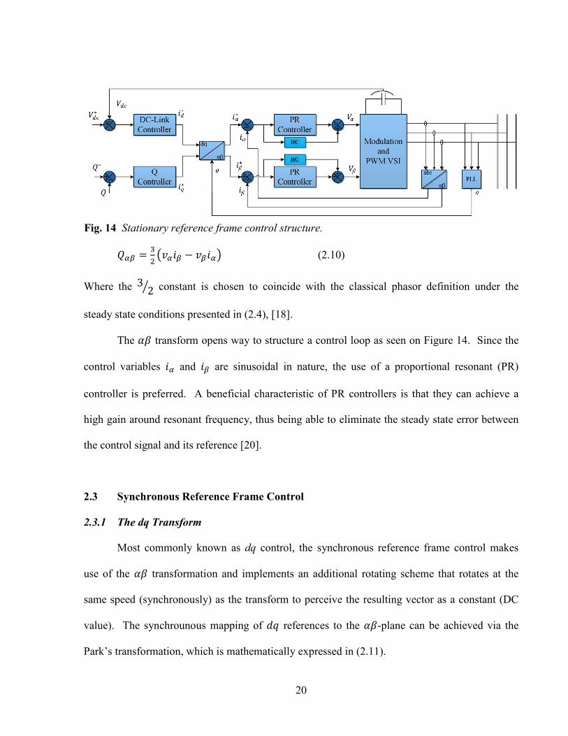
20

no = [C (Ino ) Ion* (2.10)

Where the 3 2r constant is chosen to coincide with the classical phasor definition under the

steady state conditions presented in (2.4), [18].

The transform opens way to structure a control loop as seen on Figure 14. Since the

control variables n and o are sinusoidal in nature, the use of a proportional resonant (PR)

controller is preferred. A beneficial characteristic of PR controllers is that they can achieve a

high gain around resonant frequency, thus being able to eliminate the steady state error between

the control signal and its reference [20].

2.3 Synchronous Reference Frame Control

2.3.1 The dq Transform

Most commonly known as dq control, the synchronous reference frame control makes

use of the transformation and implements an additional rotating scheme that rotates at the

same speed (synchronously) as the transform to perceive the resulting vector as a constant (DC

value). The synchrounous mapping of .9 references to the -plane can be achieved via the

Park’s transformation, which is mathematically expressed in (2.11).

Fig. 14 Stationary reference frame control structure.

21

lmdm1l = l =Lx x)x =Lxl lmnmol (2.11)

With Park’s transformation, the former m\no is multiplied

by sinusoids with an angular speed equal to x = ,/. By

matching the speed of the rotating vector with the speed of

the grid, the vector m\no will appear not to be moving at all

in the .9 axes. Conversely, the inverse of a Park’s transformation is accomplished by (2.12).

lmnmol = l=Lx )xx =Lx l lmdm1l (2.12)

Another benefit of dq frames is the fact that they can be represented using complex phasorial

representation of vectors, which is a simplified way of expressing a three phase system.

m\d1 = m\no^ 2~ (2.13)

2.3.2 Control of Power Flow under Synchronous Reference Frame Control

To simplify the power derivations in the dq frame, the voltage vector can be made to rest

on the d-axis. When the voltage vector is aligned with the d-axis, the current component in d is

the real current power, while the current component orthogonal to the voltage vector is the

reactive current, as seen on Figure 15. Power derivation in dq becomes simpler:

= [C |I|d (2.14)

= [C |I|1 (2.15)

The DC characteristics of the synchronous reference frame controllers are beneficial to PI

controllers, since they can guarantee zero tracking error on constant signals [16]. The

synchronous reference frame control scheme is shown on Figure 16. As seen on Figure 16, the

voltage of the grid is placed as reference for the phase .

Fig. 15 The . and 9 axes in the plane.

22

2.4 Transfer Functions

Using the conventions in Figure 16, it is verifiable that the transfer function for voltage

source inverters is expressed as (2.16).

dd; ]_ = ) ]_ + 4 I,]_ (2.16)

Where I is the voltage across the inductors. By applying the -transform (2.4), the resulting

equivalent circuit equation becomes (2.17).

dd; ]_ = ) no + 4 n ) 8!Qd,no ) 8!Qd,o (2.17)

Equation (2.17) coincides with the control structure presented in Figure 14. In order to solve for

the state equations in the dq plane, equation (2.12) can be applied to (2.17). The final result is

(2.18).

dd; d1 = )/k ,), )/ d1 + 4 ^d ) |I|^1 (2.18)

Equation (2.18) shows that d and q are not independent from each other, therefore a de-coupling

cross-coupling is introduced in Figure 16. After applying de-coupler’s, the voltage vectors d and

q can be controlled independently, and the final state equation becomes (2.19).

dd; d1 = )/ 00 )/ d1 + lm4mCl 62.197

Fig. 16 Synchronous reference frame control structure.

23

CHAPTER THREE: SIMULATION RESULTS AND FINDINGS OF THE Q CONTROL

METHOD

This chapter begins by explaining the setups for the SVM simulation model and the

synchronous rotating frame model, followed by their respective results and findings.

3.1 Space Vector Modulation Setup

Space vector modulation is one of the most efficient techniques to perform PWM, which

is 13.4% more efficient than conventional Sine-PWM techniques. Figure 11 demonstrated eight

of the vectors possible under a full bridge topology, with each switching configurations forming

the eight vectors and two resulting in zero vectors. The six non-zero vectors form six different

sections. Mathematically, these vectors may be represented in phasors, where the resultant

vector, I\ can be represented as in (3.1).

I\ = I]^2~X + I_^2~ + I^2~ (3.1)

By varying each of the vectors for different duty ratios in a time period c, the rotating vector I, can be represented in terms of duty ratio, (3.2). As seen on Figure 11, each voltage vector varies

by one bit, in which it becomes the task of a SVM PWM generator’s task to solve for the

duration of each bit, m, , and for the given time period c. I∠x = d%.^2~Y + .^2~ + .^2~- (3.2)

Where x is the current vector location.

Countless methods to determine the duty ratios have been proposed. With recent

increasing improvements in computation power, the ability to solve for complex equations in

fewer clock cycles has become an advantageous approach to solve for the duty ratios. As

24

conducted by this research, it is possible to solve for the duty ratios faster than the sampling

frequency c. By noting that the .^2~ component in (3.2) is zero, (3.2) can be broken down

into its real and imaginary components, (3.3-3.4).

I cos6x7 = .d cos6x7 + .d cos(x* (3.3)

I sin6x7 = .d sin6x7 + .d cos(x* (3.4)

1 = . + . + . (3.5)

Where (3.5) is used to solve for the third unknown, .. Results were as follow:

. = 4C 6~7 (~* (~* 6~7 6~Y7 (~* (~* 6~Y7 (3.6)

. = 4C 6~7 6~Y7 6~Y7 6~7 6~Y7 (~* (~* 6~Y7 (3.7)

. = 1 + 6766~Y7 6~773 6~766~Y736~77C6(~* 6~Y7 6~Y7 (~*7 (3.8)

Figure 17 is a graphical representation of the setup for the model. A three phase

reference signal was given to a m-file function that determines the location of the vector,

outputting the current locations to another m-file. The “solver” block then transfers the results to

a “section selector” block, which translates the input to duty ratios for the full bridge inverter.

The model was connected to a 3-phase load with parameters shown on Table 2.

Vd 240 V Sampling Frequency 100 kHz

V phase to phase 240 V Grid Frequency 60 Hz

Inductor 1.5 mH Phase angle of 'a' 90˚

Table 2

Fig. 17 Space vector modulation Simulink model setup.

25

3.2 Space Vector Modulation Simulation Results

The MATLAB Simulink model is seen on Figure 18, which is based on the approach

presented on Figure 17. Simulink’s PowerSim blocks were used to model inductors, load, and

the switches of the full bridge inverter. A ramp signal was used to generate duty cycles with a

sampling frequency of 100 kHz. Figure 19 probes two locations in the model. The image to the

left plots ., ., and ., which their sum is seen to be equal to zero. These signals were sent to

a duty ratio generator, which selected the appropriate block based on the location of the rotating

vector. The image to the right probes the output voltage, which verifies a line to line voltage of

240 and a 90° phase shift. This minor demonstration shows that it is possible to manipulate

the voltage magnitude and phase by the direct calculation of (3.6), (3.7), and (3.8).

Fig. 18 Space vector modulation Simulink model.

26

3.3 Synchronous Reference Frame Controller Setup

Essentially, the setup for the synchronous reference frame controller was a derivation of

Figure 16 and the design was based on transfer function (2.19). This was accomplished using

MATLAB’s Simulink, a proven tool for modeling, simulating, and analysis of dynamic systems.

Parameters for the simulation are listed on Table 3.

3.3.1 Controller Designs

The approach taken was designing the inner PI controllers first. This required the desired

voltage vectors ingoing the inverter, ^d and ^1, to be controlled independently. Both vectors

could be represented mathematically by (3.9) and (3.10).

^d = (m4 ) ,1* + |I| (3.9)

^1 = 6mC ) ,d7 (3.10)

Where m4 and mC are the PI controller error equations represented by (3.11) and (3.12).

Simulation Step Size 10 µs System Frequency 60 Hz

Simulation Error Tolerance 1 ms Apparent Power 1.5 kVA

Simulation Run Time 1 s Load Inductor 1.5 mH

Nominal Grid Voltage 120 V Load Resistor 0.1 Ω

Table 3

Fig. 19 SVM Simulink model results.

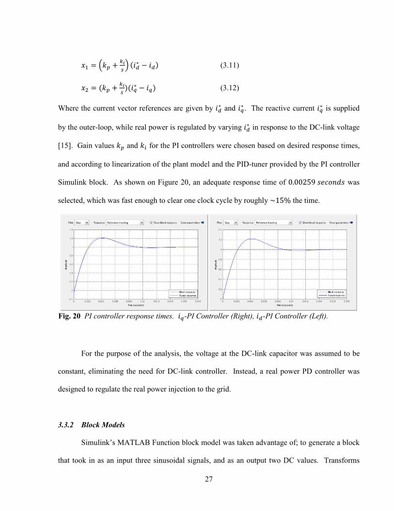
27

m4 = MG' + T 6d∗ ) d7 (3.11)

mC = 6G' + 761∗ ) 17 (3.12)

Where the current vector references are given by d∗ and 1∗ . The reactive current 1∗ is supplied

by the outer-loop, while real power is regulated by varying d∗ in response to the DC-link voltage

[15]. Gain values G' and GQ for the PI controllers were chosen based on desired response times,

and according to linearization of the plant model and the PID-tuner provided by the PI controller

Simulink block. As shown on Figure 20, an adequate response time of 0.00259^=L. was

selected, which was fast enough to clear one clock cycle by roughly ~15% the time.

For the purpose of the analysis, the voltage at the DC-link capacitor was assumed to be

constant, eliminating the need for DC-link controller. Instead, a real power PD controller was

designed to regulate the real power injection to the grid.

3.3.2 Block Models

Simulink’s MATLAB Function block model was taken advantage of; to generate a block

that took in as an input three sinusoidal signals, and as an output two DC values. Transforms

Fig. 20 PI controller response times. 1-PI Controller (Right), d-PI Controller (Left).

28

(2.4) and (2.11) were used to generate two 2-stage = → → .9 blocks, one for current and

another for the grid voltage. The grid voltage transform block was strategically aligned along the

. ) m by ensuring the three grid voltage signals were synchronized directly with the

transform. Conversely, to model a three phase voltage source inverter (VSI), MATLAB code for

a .9 → = was generated utilizing the inverse transform relations (2.5) and (2.12).

3.3.3 R-L Line Impedance Model

To model typical line impedances, parameters from Table 3 three were used to simulate

the behavior of a PV inverter connected to the grid. The model was based on the mathematical

premise of the voltage across the line, given by (3.13).

IQ" = MdQd;T + 6/7 (3.13)

Where the line current can be solved for as (3.14) and graphically depicted on Figure 21.

6/7 = 4 $6IQ" ) 7./ (3.14)

The voltage across the line, IQ", was found by computing the difference between the grid

voltage and the inverter’s voltage, as seen on figure 21.

Fig. 21 Line impedance model.

29

3.4 Synchronous Reference Frame Controller Simulation Results

The final Simulink model used for the demonstration and analysis of VAR control is

depicted in Figure 22. The specification report for future smart inverters by the Electric Power

Research Institute [19] contained suggestions for the possible future role of smart inverters.

According to the U.S. Department of Energy, there has been a rise in reactive load in the last 20

years. Reactive loads from electronic devices have risen by 40% since 1980, and are anticipated

to increase by 60% by 2015. Therefore, to relieve the anticipate stress, utilities will someday be

able to use the reactive power support by the countless integrated smart inverters. There are

several challenges that may arise if the request by the utility is not coordinated properly. For

example, sending requests to many inverters of different sizes may be complex and

communication traffic may cause delays which may lead to further issues. Other considerations

to be taken include the precedence of user/owner control. EPRI’s report [19] suggests that the

Fig. 22 Synchronous Rotating Reference Frame Control Simulink Model

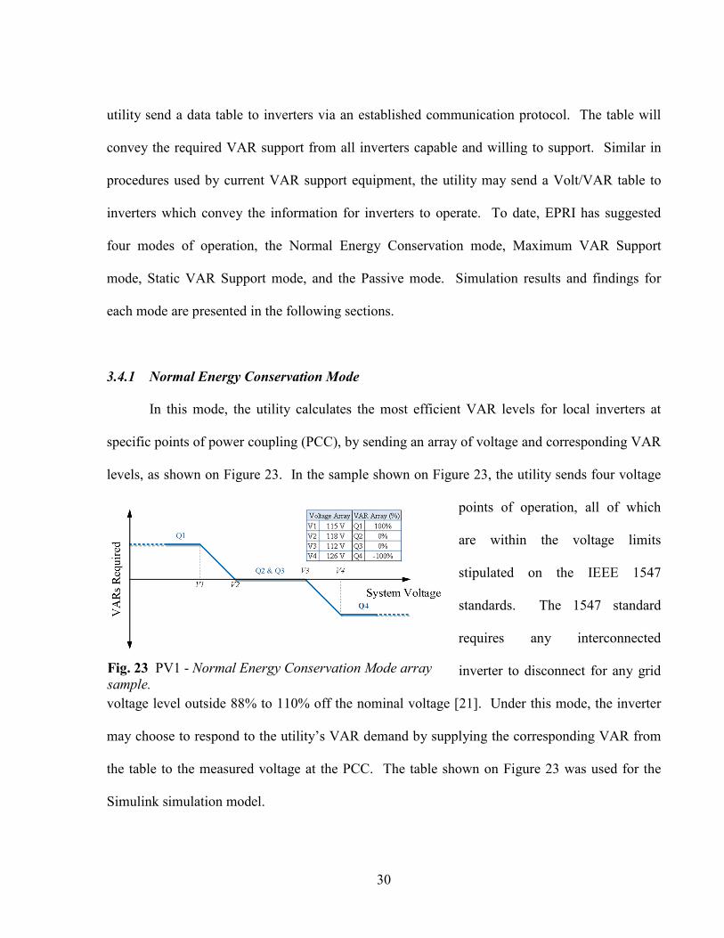
30

utility send a data table to inverters via an established communication protocol. The table will

convey the required VAR support from all inverters capable and willing to support. Similar in

procedures used by current VAR support equipment, the utility may send a Volt/VAR table to

inverters which convey the information for inverters to operate. To date, EPRI has suggested

four modes of operation, the Normal Energy Conservation mode, Maximum VAR Support

mode, Static VAR Support mode, and the Passive mode. Simulation results and findings for

each mode are presented in the following sections.

3.4.1 Normal Energy Conservation Mode

In this mode, the utility calculates the most efficient VAR levels for local inverters at

specific points of power coupling (PCC), by sending an array of voltage and corresponding VAR

levels, as shown on Figure 23. In the sample shown on Figure 23, the utility sends four voltage

points of operation, all of which

are within the voltage limits

stipulated on the IEEE 1547

standards. The 1547 standard

requires any interconnected

inverter to disconnect for any grid

voltage level outside 88% to 110% off the nominal voltage [21]. Under this mode, the inverter

may choose to respond to the utility’s VAR demand by supplying the corresponding VAR from

the table to the measured voltage at the PCC. The table shown on Figure 23 was used for the

Simulink simulation model.

Fig. 23 PV1 - Normal Energy Conservation Mode array

sample.

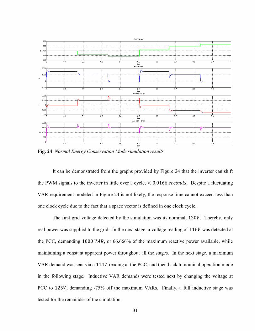
31

It can be demonstrated from the graphs provided by Figure 24 that the inverter can shift

the PWM signals to the inverter in little over a cycle, 0.0166^=L.. Despite a fluctuating

VAR requirement modeled in Figure 24 is not likely, the response time cannot exceed less than

one clock cycle due to the fact that a space vector is defined in one clock cycle.

The first grid voltage detected by the simulation was its nominal, 120. Thereby, only

real power was supplied to the grid. In the next stage, a voltage reading of 116 was detected at

the PCC, demanding 1000H, or 66.666% of the maximum reactive power available, while

maintaining a constant apparent power throughout all the stages. In the next stage, a maximum

VAR demand was sent via a 114 reading at the PCC, and then back to nominal operation mode

in the following stage. Inductive VAR demands were tested next by changing the voltage at

PCC to 125, demanding -75% off the maximum VARs. Finally, a full inductive stage was

tested for the remainder of the simulation.

Fig. 24 Normal Energy Conservation Mode simulation results.

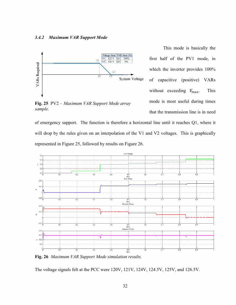
32

3.4.2 Maximum VAR Support Mode

This mode is basically the

first half of the PV1 mode, in

which the inverter provides 100%

of capacitive (positive) VARs

without exceeding ¢]. This

mode is most useful during times

that the transmission line is in need

of emergency support. The function is therefore a horizontal line until it reaches Q1, where it

will drop by the rules given on an interpolation of the V1 and V2 voltages. This is graphically

represented in Figure 25, followed by results on Figure 26.

The voltage signals felt at the PCC were 120V, 121V, 124V, 124.5V, 125V, and 126.5V.

Fig. 26 Maximum VAR Support Mode simulation results.

Fig. 25 PV2 – Maximum VAR Support Mode array

sample.

33

3.4.3 Fixed VAR Mode

For this mode, inverters

inject a constant VAR level,

regardless of voltage reading at

PCC. The main objective of this

mode is to free the inverter of

controller requirements. This way,

a centralized, more intelligent controller will send fixed VAR requirements, managing the

regulation of VARs injected to the grid.

3.4.4 Passive Mode

This final mode is similar to the Fixed VAR Mode, except instead of providing constant

VARs, it provides constant real power. The results for this mode are shown on Figure 29.

Fig. 28 Fixed VAR Mode simulation results.

Fig. 27 PV3 – Fixed VAR Mode array sample.

34

The same voltage sequence as those of Figure 28 was sent: 115V, 118V, 120V, 122V, 124V, and

126V.

3.5 Other Findings

Due to the sudden voltage changes detected on the PCC, small perturbations that adjust to

these changes can be seen on the active and reactive power graphs of Figure 28 and Figure 29. It

should be noted that these perturbations are also less than a clock cycle, measuring

0.0176^=L., for example.

The validity of the simulation model was tested via power equations (1.1), (1.2), (3.14),

and (3.15) versus the method utilized in the simulation, the multiplication of dq vectors (3.17).

= I]]cos6x7 + I__ =L6x7 + I =L6x7 (3.14)

= I]] 6x7 + I__ 6x7 + I 6x7 (3.15)

Fig. 29 Passive Mode simulation results.

35

B = (^d + :^1*(d + :1* (3.17)

Where

= ^dd ) ^11 (3.18)

= ^d1 + ^1d (3.19)

Table 4 shows the results under PV1 Energy Conservation Mode, for a voltage at PCC of

116V. Under that situation, and using equations (3.18) and (3.19), real power required becomes

1118 Watts while the total reactive power needed becomes 1000 VAR. However, as seen by

results on Table 4, using (1.1) and (1.2) to solve for active and reactive power is not as precise,

due to the small shift between grid and inverter voltages, . The arrays stored in the simulation

were accurate to the 1000th

decimal, giving a change in phase of 0.0001 seconds, not enough

digits to accurately derive the actual shift. Using equations (3.14) and (3.15) yielded more

formidable results, due to the larger discrepancy between the voltage and current phase shift.

However, the same issue arose with the 1000th

decimal limitation, with a 0.0021 second phase

Measurement Value Eqn. no. Equation Results

0.791681 rads

45.36˚

0.033929 rads

1.944˚

82.024V 1466.78 VA

83.971V (3.14) 1067.31 W

5.9545A (3.15) 1053.98 VAR

1500.01 VA

1220.6 W

813.375 VAR

Table 4

(1.1)

(1.2)

]6S£7^]6S£7I]6S£7

= I]^]j sin67 = I]^] cos ) I]CjB = 1.1 C+ 1.2 C

= I]] sin x + I__ sin x + I sin x = I]] co x + I__ cos x + I cos x

x

B = 3.14 C+ 3.15 C

8!Qd = 116, = 1118¥, = 1000H, B = 1500H

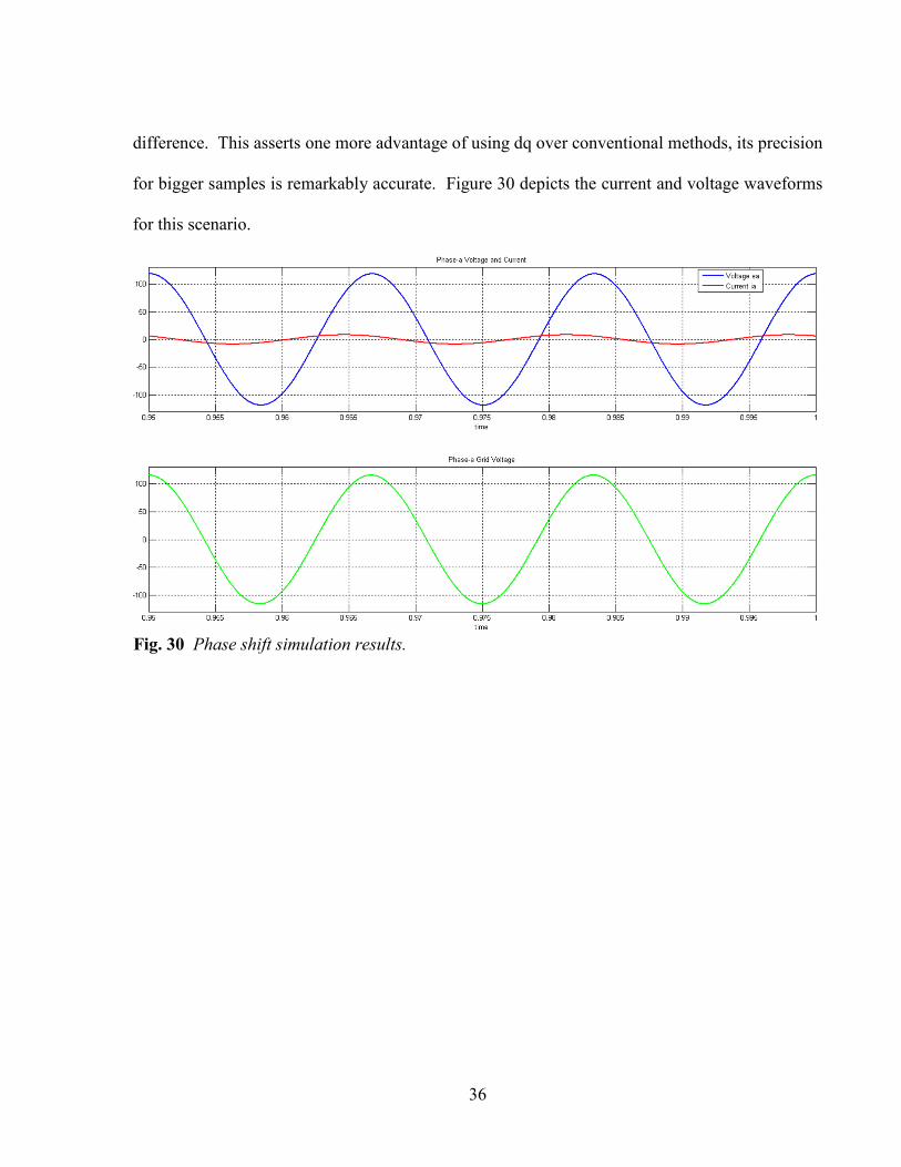
36

difference. This asserts one more advantage of using dq over conventional methods, its precision

for bigger samples is remarkably accurate. Figure 30 depicts the current and voltage waveforms

for this scenario.

Fig. 30 Phase shift simulation results.

37

CHAPTER FOUR: MULTI-MODE CONVERTER FOR INPUT SIDE OF INVERTERS

This chapter deals with the input side controller that interfaces battery storage systems

with PV arrays, as presented on Figure 9. As more and more intermittent sources are integrated

into grids, the need for stability via the use of energy storage systems becomes imperative. One

of the main challenges of energy storage systems is their cost, reducing the payback of PV

systems. While different technologies and research on different chemical batteries are reducing

the costs of storage systems, input side power electronics components can also be reduced to

lower costs of storage systems. Another most important advantage of implementing energy

storage systems to PV systems is the fact that it allows for the inverter to operate in all four

quadrants of power flow, presented previously on Figure 3.

4.1 Conventional Battery Storage Methods

Typically, battery storage systems are integrated to PV systems as seen on Figure 31.

Configurations consist of DC-DC boost converters to optimize the input for max power delivery.

The boosted voltage is then supplied to inverters which are in turn connected to the grid. Both

configurations offer different levels of control, with more control with increased components.

The configuration on the right of Figure 31 has fewer components, but suffers from control

Fig. 31 Conventional methods to implement energy storage systems.

38

freedoms offered by its counterpart on the

left. A novel method, introduced in [22],

allows for the use of a single input side

converter, which can operate in boost and

buck modes to charge and discharge the

battery while providing MPPT

simultaneously. This is done by utilizing two switches, one diode, and two inductors, as seen on

the left circuit of Figure 33.

However, despite its advantages, the multimode converter on [22] was limited to charging the

battery from the PV system, and not from power flowing from the grid into the inverter. With

the use of a bidirectional switch in place of the diode, and PWM to that switch (B¥ from Figure

33), it becomes possible to charge the battery from the grid as well. This feature allows the

battery storage system to absorb real and reactive power from the grid, allowing it to operate in

all four quadrants presented on Figure 3. The diode is placed next to the input bus, to prevent the

flow of current into PV panels, and avoid damage to them. The new topology is able to operate

in all four mode originally presented in [22], as well the additional mode aforementioned.

Fig. 33 Multi-Mode Converters.

Fig. 32 Novel method to implement energy storage

systems.

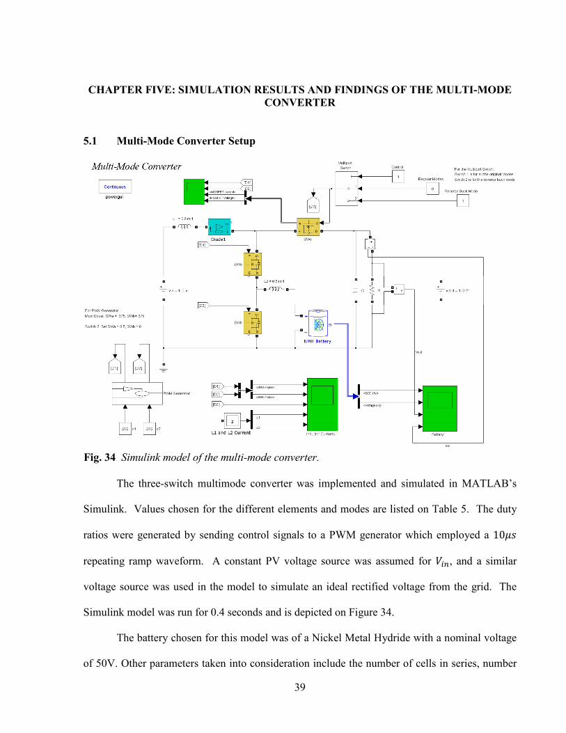
39

CHAPTER FIVE: SIMULATION RESULTS AND FINDINGS OF THE MULTI-MODE

CONVERTER

5.1 Multi-Mode Converter Setup

The three-switch multimode converter was implemented and simulated in MATLAB’s

Simulink. Values chosen for the different elements and modes are listed on Table 5. The duty

ratios were generated by sending control signals to a PWM generator which employed a 10¦ repeating ramp waveform. A constant PV voltage source was assumed for Q, and a similar

voltage source was used in the model to simulate an ideal rectified voltage from the grid. The

Simulink model was run for 0.4 seconds and is depicted on Figure 34.

The battery chosen for this model was of a Nickel Metal Hydride with a nominal voltage

of 50V. Other parameters taken into consideration include the number of cells in series, number

Fig. 34 Simulink model of the multi-mode converter.

40

of cells in parallel, and the internal resistance. The nonlinear model of the battery showed a

good approximation of real available NMH batteries in the market. The battery had 42 cells in

series with nominal voltage of 1.18 volt for each cell with a maximum capacity of 7 AH for each

cell. The total resistance of the battery was 0.0084 Ohms, with an internal resistance of 0.002

Ohms for each cell. Experimental validation of the model showed a maximum error of 5%

(when SOC is between 10% and 100%) for charge and discharge dynamics.

5.2 Multi-Mode Converter Results

As seen on the circuit to the right in Figure 33, the diode is replaced with a bi-directional

MOSFET and placed in series with 4, which will become essential to block the current from

flowing into the PV source in the additional mode of operation. The four original modes are the

Main Boost Mode, the Boost-Buck Mode, the Boost-Boost Mode, the Battery Boost Mode, and

the Reverse Buck Mode. In the Main Boost mode, the single leg converter increases the voltage

that is supplied to the inverter. In the Boost-Buck mode, energy is stored in the battery while

voltage is supplied to the inverter or DC bus simultaneously. During high load demands, the

Boost-Boost mode can supply the inverter with energy from the PV source and the battery

simultaneously. And during cloud cover, energy can be supplied to the inverter from the battery

in Battery-Boost mode.

In cases in which grid peak shaving is desired, the battery can be charged from the grid.

The grid alone can supply the current to the battery through a buck operation. This new mode

Nominal Output Voltage 160 V Inductor (L1) 0.8mH

Battery Voltage 50 V Inductor (L2) 0.6mH

Initial Battery SOC% 0.5 Battery Type NMH

Simulation Parameters

Table 5

41

was dubbed the Reverse Buck Mode. Times in which is critical to charge the battery from the

grid include peak shaving during inclement weather or nights, when PV source cannot provide

sufficient current to charge the battery, when the load demand drops, or to store energy during

times when grid energy costs are low.

5.2.1 Main Boost Mode Results

In this mode, B¥] and B¥_ have the same duty ratio. Together, both switches form a

boost converter that boosts the PV input voltage. During this mode, B¥ behaves as a diode by

sending zero to its gate. The basic input to output principle of boost converters applies to this

mode, as described in (5.1). Solving for the duty ratio, this mode yields (5.2).

§; = 4 ¨ (5.1)

© = JJ (5.2)

The results for this mode are seen on Figure 36, where a duty ratio of 0.375 was sent to

both switches, while B¥ remained off, acting as a diode.

5.2.2 Boost Buck Mode Results

For this mode, the duty ratio of B¥] is longer than B¥_. This way, the PV voltages are

boosted during the time both B¥] and B¥_ are “ON”. During the time B¥] remains “ON” and

Fig. 35 Main Boost Mode power flow.

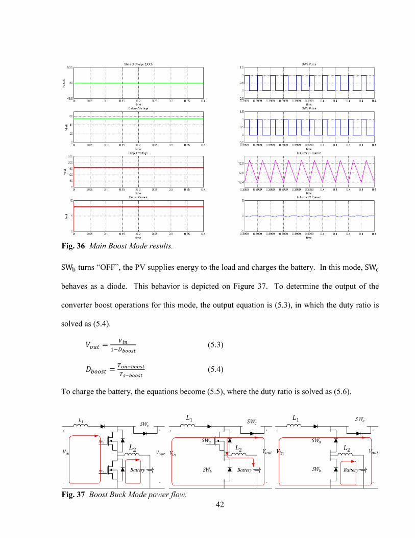
42

SW¬ turns “OFF”, the PV supplies energy to the load and charges the battery. In this mode, SW behaves as a diode. This behavior is depicted on Figure 37. To determine the output of the

converter boost operations for this mode, the output equation is (5.3), in which the duty ratio is

solved as (5.4).

§; = 4 ¨­ (5.3)

©_; = J®­J®­ (5.4)

To charge the battery, the equations become (5.5), where the duty ratio is solved as (5.6).

Fig. 36 Main Boost Mode results.

Fig. 37 Boost Buck Mode power flow.

43

_];; = ©_§Q (5.5)

©_§ = J®¯°J®­ (5.6)

5.2.3 Boost Boost Mode Results

In this mode, the opposite case from the Boost-Buck mode is the case, in which the duty

ratio of B¥_ is longer than B¥]’s. This allows the battery to discharge energy to the inverter

when the PV energy generation is not sufficient. During this mode, B¥ behaves as a diode.

Fig. 38 Boost Buck Mode results.

Fig. 39 Boost Boost Mode power flow.

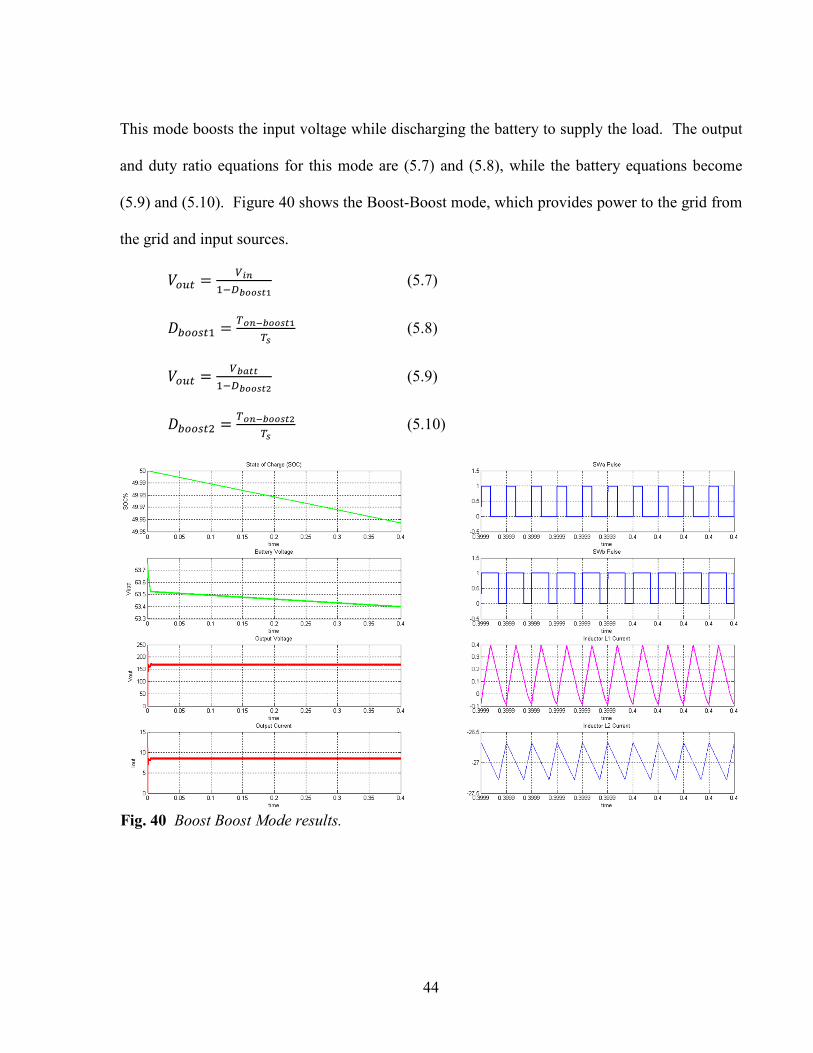
44

This mode boosts the input voltage while discharging the battery to supply the load. The output

and duty ratio equations for this mode are (5.7) and (5.8), while the battery equations become

(5.9) and (5.10). Figure 40 shows the Boost-Boost mode, which provides power to the grid from

the grid and input sources.

§; = 4 ¨­± (5.7)

©_;4 = J®­±J (5.8)

§; = X­­4 ¨­ (5.9)

©_;C = J®­J (5.10)

Fig. 40 Boost Boost Mode results.

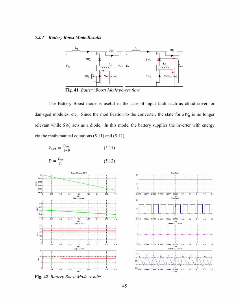
45

5.2.4 Battery Boost Mode Results

The Battery Boost mode is useful in the case of input fault such as cloud cover, or

damaged modules, etc. Since the modification to the converter, the state for B¥] is no longer

relevant while B¥ acts as a diode. In this mode, the battery supplies the inverter with energy

via the mathematical equations (5.11) and (5.12).

§; = X­­4 ¨ (5.11)

© = JJ (5.12)

Fig. 41 Battery Boost Mode power flow.

Fig. 42 Battery Boost Mode results.

46

5.2.5 Reverse Buck Mode Results

The Reverse Buck Mode benefits from the B¥ switch and makes use of the bi-

directionality of the interconnected inverter. This is accomplished by either sending no pulses to

the MOSFETs of the universal bridge, in essence converting the universal bridge into a full

bridge rectifier, or by controlling the individual MOSFET switching cycles to achieve a desired

DC voltage. Subsequently, this system converts the AC grid voltage into DC for battery

charging. In this mode, B¥4 is “OFF”, B¥C is “ON”, and B¥_ is “OFF”. In this way, the

battery is charged from the rectified grid voltage by varying the duty of B¥]. When the B¥] is

“ON”, !"; is transferred to the battery and the inductor current ²4 increases. This is

mathematically expressed as (5.13).

Δ²C = µ­ X­­ ©c (5.13)

Where, Δ²C is the inductor ripple current. When B¥] is “OFF”, then inductor current in C

decreases in the rest of the period ck. This is expressed as (5.14).

Δ²C = X­­ 61 ) ©7c (5.14)

By equating (5.13) and (5.14), the input to output relation is derived as (5.15).

V¬·¸¸ = ©!"; (5.15)

Fig. 43 Reverse Buck Mode power flow.

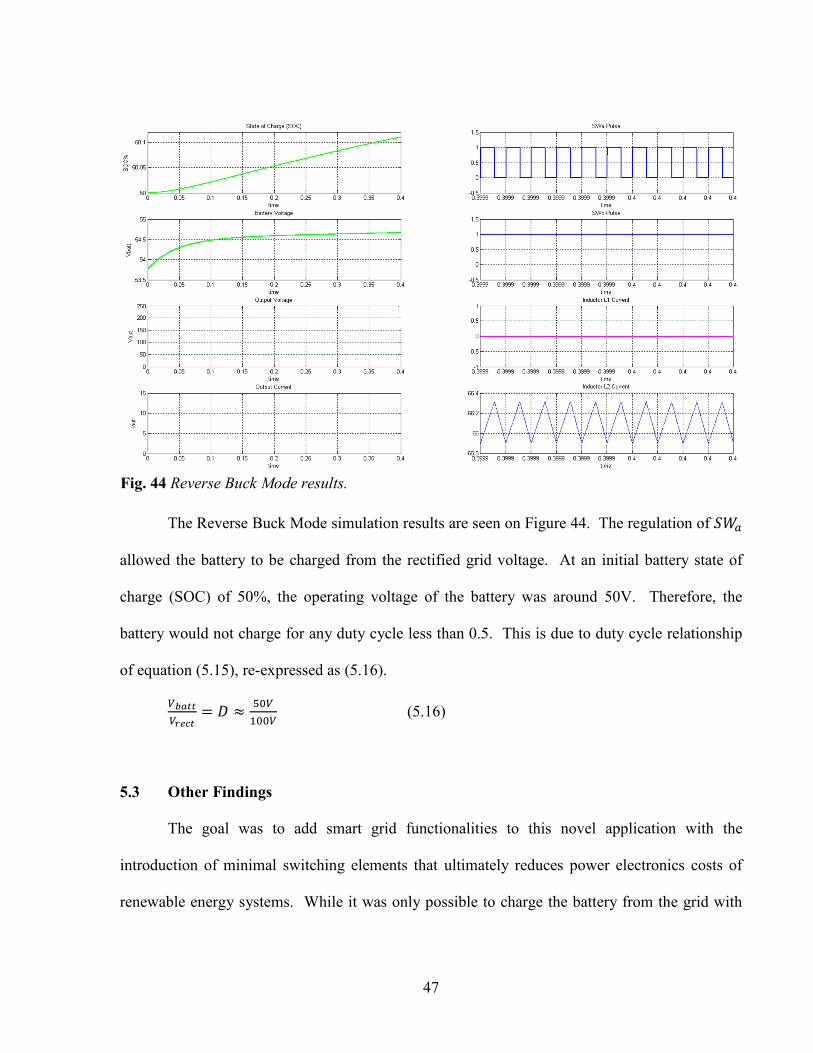
47

The Reverse Buck Mode simulation results are seen on Figure 44. The regulation of B¥]

allowed the battery to be charged from the rectified grid voltage. At an initial battery state of

charge (SOC) of 50%, the operating voltage of the battery was around 50V. Therefore, the

battery would not charge for any duty cycle less than 0.5. This is due to duty cycle relationship

of equation (5.15), re-expressed as (5.16).

X­­ µ­ = © ¹ º0400 (5.16)

5.3 Other Findings

The goal was to add smart grid functionalities to this novel application with the

introduction of minimal switching elements that ultimately reduces power electronics costs of

renewable energy systems. While it was only possible to charge the battery from the grid with

Fig. 44 Reverse Buck Mode results.

48

this configuration, charging the battery from both the PV source and the grid simultaneously

present several challenges.

It is somewhat possible to charge the battery from two sources by modifying B¥ into a

four quadrant operating switch (that is a MOSFET configuration that allows for the positive and

negative exchange of voltage and current through it). The four-quadrant operating MOSFET is

illustrated on Figure 45. The four-quadrant flexibility was used to preclude any current from

flowing into each of the respective sources, and solely supply current to the battery. This mode

is desired, for it could increase savings by storing the energy when the electric rate is low, and

utilizing it when it is high in the following day(s).

In this mode, B¥] remains “ON”

for the entire period while B¥4 is “OFF”,

and B¥_ becomes “ON” for ._c seconds.

B¥C may cycle “ON” for .c seconds

during the remaining period 61 ) ._7c (See Fig. 45). Consequently, during the ._c the PV charges the 4 inductor, which is the

amount of energy that will be pushed into the battery when B¥_ turns “OFF”. During this

period of time, the grid remains disconnected from the battery. When B¥C turns “ON”, the grid

supplies energy to the battery for the remaining duration of time. It is during this period of time

that both the PV and the grid should charge the battery. In the first scenario in which both B¥]

and B¥_ are “ON”, the ripple current of both inductors is calculated as (5.17) and (5.18).

Δ²C = X­dJ (5.17)

Δ²4 = dJ± (5.18)

Fig.45 Four Quadrant Bi-Directional Switch and

The basic order of switching operation.

49

During the time that B¥C turns “ON” and B¥_ is “OFF”, the ripple current of both inductors are

mathematically described by (5.19) and (5.20).

Δ²C» = µ­ X­­ .c (5.19)

Δ²4» = µ­± .ck (5.20)

However, unlike the previous method, equations (16) and (18) cannot be equated with (17) and

(19) to find the input/output relationships. This is due to the inequality of inductor currents

64.C7 during the short time gap which B¥_ and B¥C are both “OFF”. Due to this

characteristic, the input/output equations cannot be derived precisely.

50

CONCLUSION

Two major aspects of a PV inverter were modeled and simulated in MATLAB.

Parameters were chosen consistently, to study the holistic feasibility of the dq-method, space

vector modulation, and the proposed multi-mode converter. For the input side of the inverter, an

existing multi-mode converter was improved by allowing additional interaction between the grid

and interconnected PV systems. It was shown that the addition of an extra switch, in conjunction

with a pulse width modulation scheme, were sufficient to charge an integrated battery from the

grid. For the output side of the inverter, the synthesis of AC waveforms was demonstrated by

using direct calculations of the SVM equations for high sampling frequencies. It was also

demonstrated that the control of reactive power can be achieve using the Specifications for Smart

Inverter Interactions with Electric Grids using IEC 6185 report with the synchronous reference

frame, or dq, method.

51

BIBLIOGRAPHY

[1] U.S. Energy Information Administration. (2011, April). Annual Energy Outlook 2011 with

Projections to 2035. [On-line]. Available: www.eia.gov/forecasts/aeo/ [Oct 2011].

[2] "IEEE Recommended Practices and Requirements for Harmonic Control in Electrical Power

Systems," IEEE Std 519-1992 , vol., no., pp.0_1, 1993

[3] "IEEE Recommended Practice for Utility Interface of Photovoltaic (PV) Systems," IEEE Std

929-2000 , vol., no., pp.i, 2000

[4] Ipakchi, A.; Albuyeh, F.; , "Grid of the future," Power and Energy Magazine, IEEE , vol.7,

no.2, pp.52-62, March-April 2009

[5] E. Hirst and B. Kirby, “Electric-Power Ancillary Services”, ORNL/CON-426, Oak Ridge

National Laboratory, Oak Ridge, TN, January 1996.

[6] N. Mohan, T. Underland, and W. Robbins, “Power electronics converters, applications, and

design”, Wiley, 3rd

ed., 2003

[7] A. Keyhani, M. N. Marwalli, and M. Dai, “Power flow control of a single distributed

generation unit,” in Integration of Green and Renewable Energy in Electric Power Systems, New

Jersey: Wiley, 2010, ch. 6, pp 179-202.

[8] N. Mohan, “First Course on Power Electronics”, Minneapolis: MNPERE, 2009,

[9] A. Keyhani, M. N. Marwalli, and M. Dai, “Power flow control of a single distributed

generation unit,” in Integration of Green and Renewable Energy in Electric Power Systems, New

Jersey: Wiley, 2010, ch. 6, pp 179-202.

[10] Turitsyn, K.; Sulc, P.; Backhaus, S.; Chertkov, M.; , "Options for Control of Reactive

Power by Distributed Photovoltaic Generators," Proceedings of the IEEE , vol.99, no.6, pp.1063-

1073, June 2011

[11] Piegari, L.; Tricoli, P.; , "A control algorithm of power converters in smart-grids for

providing uninterruptible ancillary services," Harmonics and Quality of Power (ICHQP), 2010

14th International Conference on , vol., no., pp.1-7, 26-29 Sept. 2010.

[12] Bo, Dong; Li, Yongdong; Zheng, Zedong; , "Energy management of hybrid DC and AC

bus linked microgrid," Power Electronics for Distributed Generation Systems (PEDG), 2010 2nd

IEEE International Symposium on , vol., no., pp.713-716, 16-18 June 2010

[13] T. Noguchi, H. Tomiki, S. Kondo, and I. Takahashi, “Direct power control of PWM

converter without power-source voltage sensors” IEEE Trans. Ind. Appl., vol. 34, no. 3, pp.473-

479, May/Jun. 1998.

52

[14] J. Hu; L. Shang; Y. He; Zhu, Z.Z.; , "Direct Active and Reactive Power Regulation of Grid-

Connected DC/AC Converters Using Sliding Mode Control Approach," Power Electronics,

IEEE Transactions on , vol.26, no.1, pp.210-222, Jan. 2011

[15] J. Gong; J. Lu; D. Xie; Y. Zhang; , "A new-style dynamic var compensation control

strategy," Electric Utility Deregulation and Restructuring and Power Technologies, 2008. DRPT

2008. Third International Conference on , vol., no., pp.1625-1630, 6-9 April 2008

[16] Blaabjerg, F.; Teodorescu, R.; Liserre, M.; Timbus, A.V.; , "Overview of Control and Grid

Synchronization for Distributed Power Generation Systems,"Industrial Electronics, IEEE

Transactions on, vol.53, no.5, pp.1398-1409, Oct. 2006

[17] S. Buso and P. Mattavelli. “Extension to Three Phase Inverters” in Digital Control in

Power Electronics, USA: Morgan & Claypool Publishers, 2006, pp.81-107

[18] Schauder, C.; Mehta, H.; , "Vector analysis and control of advanced static VAr

compensators," Generation, Transmission and Distribution, IEE Proceedings C , vol.140, no.4,

pp.299-306, Jul 1993

[19] Specifications for Smart Inverter Interactions with Electric Grids using International

Electrotechnical Commission 61850 report

[20] R. Teodorescu and F. Blaabjerg, “Proportional-resonant controllers. A new breed of

controllers suitable for grid-connected voltage-source converters,” in Proc. OPTIM, 2004, vol. 3,

pp. 9–14

[21] “IEEE Standard Conformance Test Procedures for Equipment Interconnecting Distributed

Resources With Electric Power Systems,” IEEE Std 1547.1-2005 , vol., no., pp.0_1-54, 2005

[22] Taesik Park; Taehyung Kim; , "Novel multi-mode single leg converter for renewable

energy conversion systems," Industrial Technology (ICIT), 2011 IEEE International Conference

on , vol., no., pp.198-203,14-16 March 2011

VITA

Emiliano Morales was born and raised in the border town of Eagle Pass, Texas. He is the first

male of his extended family to graduate from a University with a Master’s degree. His Bachelor

degree was in Electrical Engineering and concentrated in computer engineering. His Master’s

research focused primarily on the renewable energy field. His future plans include becoming

part of the Navy as an active duty Officer, continue his education, and traveling the world in

humanitarian missions.

Section 4:

Advance Metering Infrastructure and Communications

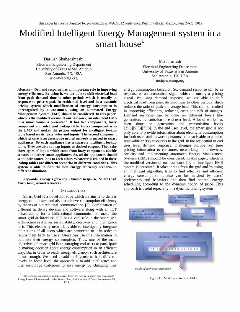
This paper has been submitted for presentation at WAC2012 conference, Puerto Vallarta, Mexico, June 24-28, 2012

Modified Intelligent Energy Management system in a

smart house1

Dariush Shahgoshtasbi

Electrical Engineering Department

University of Texas at San Antonio

San Antonio, TX, USA

isjd@wacong.org

Mo Jamshidi

Electrical Engineering Department

University of Texas at San Antonio

San Antonio, TX, USA

moj@wacong.org

Abstract— Demand response has an important role in improving

energy efficiency. By using it, we are able to shift electrical load

from peak demand time to other periods which is usually in

response to price signal. In residential level and in a dynamic

pricing system which modification of energy consumption is

unrecognized by a consumer, using an automated Energy

Management System (EMS) should be considered. In this paper,

which is the modified version of our last work, an intelligent EMS

in a smart house is presented1. It has two components, fuzzy

component and intelligent lookup table. Fuzzy component is in

the EMS and makes the proper output for intelligent lookup

table based on its fuzzy rules and inputs. The second component

which its core is an associative neural network is moved to smart

appliances. So each appliance has a separate intelligent lookup

table. They are able to map inputs to desired outputs. They take

three types of inputs which come from fuzzy component, outside

sensors and other smart appliances. So, all the appliances should

send their control bits to each other. Whatever is trained in these

lookup tables are different scenarios in different conditions. This

system is able to find the best energy efficiency scenario in different situations.

Keywords- Energy Efficiency, Demand Response, Smart Grid,

Fuzzy logic, Neural Networks.

I. INTRODUCTION

Smart Grid is a novel initiative which its aim is to deliver energy to the users and also to achieve consumption efficiency by means of bidirectional communication [2]. Combination of different hardware devices and software along with an ICT infrastructure for a bidirectional communication make the smart grid architecture. ICT has a vital rule in the smart grid architecture as it gives sustainability, creativity and intelligence to it. This electricity network is able to intelligently integrate the actions of all users which are connected to it in order to return them back to users. Users can use this information to optimize their energy consumption. Thus, one of the main objectives of smart grid is encouraging end users to participate in making decision about energy consumption in an efficient way. But in order to reach energy efficiency, such architecture is not enough. We need to add intelligence to it in different levels. In home level, the approach is to add intelligence and then encourage customers to save energy by changing their

1 This work was supported, in part, by a grant from CPS Energy through Texas Sustainable

Energy Research Institute and Lutcher Brown Chair, the University of Texas, San Antonio, TX,

USA.

energy consumption behavior. So, demand response can be in response to an economical signal which is mostly a pricing signal. By using demand response, we are able to shift electrical load from peak demand time to other periods which reduces the ratio of peak to average load. This can be resulted in improving efficiency, reducing costs and risk of outages. Demand response can be done on different levels like generation, transmission or end user level. A lot of works has been done on generation and transmission levels [2][3][5][6][7][8]. In the end user level, the smart grid is not only able to provide information about electricity consumption for both users and network operators, but also is able to connect renewable energy resources to the grid. In the residential or end user level demand response, challenges include real time pricing information to consumer, networking home devices, security and implementing automated Energy Management Systems (EMS) should be considered. In this paper, which is the modified version of our last work [1], an intelligent EMS system is presented. It takes inputs from the grid and by using an intelligent algorithm, tries to find effective and efficient energy consumption. It also can be matched by users’ preferences and behaviors and then find optimal energy scheduling according to the dynamic notion of price. This approach is useful especially in a dynamic pricing system

Figure 1. Modified automated EMS

Figure 2. Smart appliances connection.

which modification of energy consumption is unrecognized by and renewable resources or can be human behavior and a consumer. The suggested system has two components as it is shown in Figure 1. The first component is a fuzzy system which its inputs can be external events like price signal, environment condition data preferences. This component which is inside the EMS has some fuzzy rules along with their membership functions which make appropriate output for the second component which is intelligent lookup table. The reason of using Fuzzy component is to get real time changeable external information and find the best system situation based on the fuzzy rules and then by using centralized defuzzification get a unique number in the output range. The second and the main component is intelligent lookup table which is moved to smart appliances. So each appliance has a separate intelligent lookup table. The reason of doing that is to have a very simple structure of neural network which will be resulted in fewer scenarios in each appliance. In this situation all of the appliances should send some control bits to each other. Therefore, they should be connected to each other as it is shown in Figure 2. The Intelligent lookup table is made by using a new topology of neural network [4]. The output part of this topology is modified. By using this modification which will be explained in section III, we are able to connect more inputs to the neural network. The first reason of using this type of neural network is that its structure is crystal type and can be easily extended for more inputs and the second reason is that it is able to act as an associative memory to map inputs to desired outputs. This paper is organized as follows. In Section II, the fuzzy component of the system is explained. In section III, the structure of the intelligent lookup table, its training and functionality are described and in section IV, the simulation of the suggested approach is shown.

II. FUZZY LOGIC COMPONENT

This component has 5 types of inputs. The first one is price signal which comes from the smart meter, the second one is battery storage situation, and the rest are environment condition

data like humidity, temperature and solar as their membership functions are depicted in Figure 3. These inputs are divided into two categories. Price signal, battery storage and solar inputs are in the first category which makes a unique and appropriate input for the intelligent lookup table. The output of this category has 7 membership functions which gives us the energy consumption situation in the gird. These 7 fuzzy sets are Neutral-, Neutral+, Normal, High-, High+, Peak- and Peak+ which are selected based on the fuzzy rules and mapping of input values to their appropriate membership functions. Finally the resulting set is defuzzified by Centriod defuzzification technique and gets a single number as (1).

Where x* is the defuzzified output, µi(x) is the aggregated membership function and x is the output variable. This number is rounded and its binary value goes to the intelligent lookup table. The second category of this component which contains environment condition data makes some input control signals to the second component which will be explained in the next section. The fuzzy rules and membership function values are set based on our knowledge from the grid and the environment. These values can be changed by human behavior and preferences. The behavior and preferences are logged and if there are any changes in them (like A/C setting), the system just modifies the initial membership values.

III. INTELLIGENT LOOKUP TABLE COMPONENT

A. Structure

The main part of this system has a crystal structure with cells as shown in Figure 4-a. As it can be seen, each cell

is constructed of two middle neurons and four side neurons

such that the two upper ones have fixed weights and the two

lower ones have trainable weights. The two upper neurons and

also the middle neurons have linear function and the two lower

ones have a sigmoid function as (2).

The neurons of this layer receive their binary inputs

from the previous layer. Figure 4-a can be summarized as

Figure 4-b. For each cell we have:

(3)

Where n is the input cell number. In Figure 4-a, if , which is the complement of , gets value 1, the first and the forth neuron will fire whereas if it gets 0, the second and third neurons do so. In the training step, only active neurons are trained. The characteristic of the lower neurons is that the increasing and decreasing rate of the weight changes are not equivalent during the training step as will be explain in section III.B. In each cell, there are only two active neurons at a time and the output of that cell enters as input to the succeeding cell. If each input consists of n bits, cells would be connected as a chain up to the input. The only remaining input is n

where the output of the chained string is connected to

of this

Figure 3. Fuzzy membership functions for the fuzzy component. (a): Category 1. (b): Category 2.

input cell. We call this layer the parallel layer as its cells are parallel to each other. In this layer, only one cell of input n is selected. With this selection, we reach our desired memory cell.

For networks with more than one output,

of input cell n are

added to the parallel layer for each output. These added cells are only used for adjustment of all outputs except the first one. They have no influence on the adjustment of other weights. On the other word, the weights of the network are adjusted only by the first output and the other outputs are adjusted by the weights of added input cells in the parallel layer [4]. Figure 5 shows this structure for an example network with 3 inputs and 2 outputs. The problem of using this type of network is when we have a lot of inputs, the number of cells in parallel layer increase dramatically. On the other hand, we increase the capacity of associative memory, but most of the cells in parallel layer will be never used. In order to solve the problem, instead

of having

cell in parallel layer, we consider m cells and by

using a mapping table, each used output is mapped to one of these m considered cells. In order to make an intelligent lookup table by the suggested neural network, we create feedbacks from outputs of the network to its inputs as it is depicted in Figure 6. This makes a sequential system with memory. In this situation, next outputs will be made based on the present inputs and feedback outputs. As it was mentioned earlier, the system has three types of inputs; the first type comes directly from the fuzzy component and is a unique value which shows energy consumption situation in the grid. This input is connected to n first inputs of neural networks and implies the network which scenario should be started. The second type of inputs is some control bits which come either from fuzzy component or some outside sensors and the last type are feedback outputs. All of

Figure 4. One cell of the network in the associative memory layer (a): Original Shape , (b): The summary of part a.

the inputs together based on their conditions make different

scenarios for the intelligent lookup table. Control bits can

show for example water heater, air conditioner, refrigerator

and other appliances situation in the smart house. Also they

can be battery storage and solar situation which come from the

fuzzy component. This intelligent lookup table should be

trained based on the different inputs and control bits.

B. Learning

The algorithm of network training is a way to decode

the problem to be solved [9]. The learning of this network is

supervised. The single layer perceptron learning rule is used to

train this network [10]:

(4)

Where W is the weight, j is the input cell number, is

the input of that cell, is the output of the network and

is the desired output. The important point is that

using the learning rule of single layer perceptron for this multi-layer network makes learning easy. The way of using

this rule is presented here. As mentioned earlier, only active

neurons are trained and in each cell there is only one lower

active neuron at a time. So the Eq. (4) can be rewritten as:

(5)

In each layer, the values which have been used for the stabilization of weights are smaller when weights increase

than when they decrease. This always makes weights

decreasing values larger than weights increasing values. These

increasing and decreasing values are reduced in subsequent

layers. The reason is that in binary numbers, the bit toggle frequency is halved when we move from LSB bits toward

MSB bits. Since the inputs of the suggested network are

binary, considering as mentioned, will cause the changes of weights to become slower in subsequent layers. On the other

words, weights change with lower frequency for 2n sequential

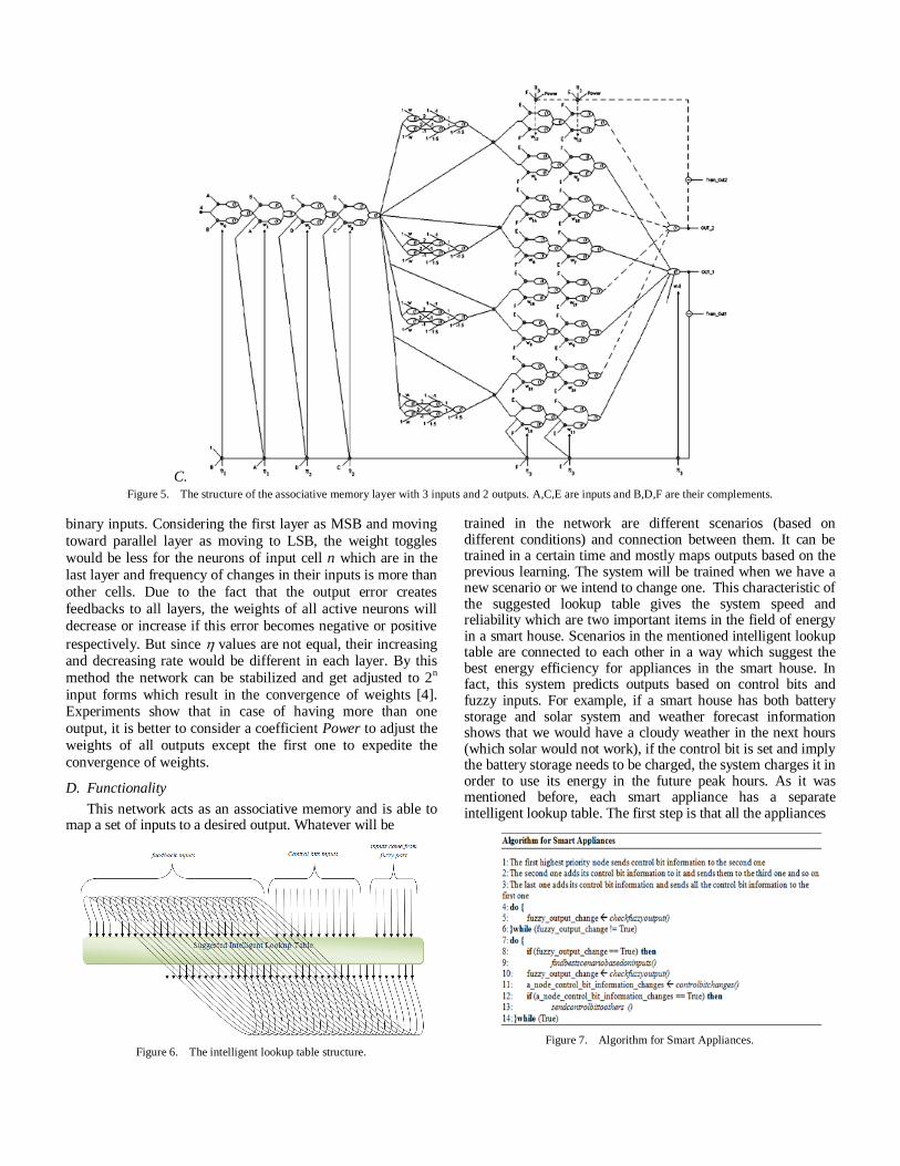
C. Figure 5. The structure of the associative memory layer with 3 inputs and 2 outputs. A,C,E are inputs and B,D,F are their complements.

binary inputs. Considering the first layer as MSB and moving

toward parallel layer as moving to LSB, the weight toggles

would be less for the neurons of input cell n which are in the

last layer and frequency of changes in their inputs is more than

other cells. Due to the fact that the output error creates

feedbacks to all layers, the weights of all active neurons will

decrease or increase if this error becomes negative or positive

respectively. But since values are not equal, their increasing and decreasing rate would be different in each layer. By this

method the network can be stabilized and get adjusted to 2n

input forms which result in the convergence of weights [4]. Experiments show that in case of having more than one

output, it is better to consider a coefficient Power to adjust the

weights of all outputs except the first one to expedite the

convergence of weights.

D. Functionality

This network acts as an associative memory and is able to map a set of inputs to a desired output. Whatever will be

Figure 6. The intelligent lookup table structure.

trained in the network are different scenarios (based on different conditions) and connection between them. It can be trained in a certain time and mostly maps outputs based on the previous learning. The system will be trained when we have a new scenario or we intend to change one. This characteristic of the suggested lookup table gives the system speed and reliability which are two important items in the field of energy in a smart house. Scenarios in the mentioned intelligent lookup table are connected to each other in a way which suggest the best energy efficiency for appliances in the smart house. In fact, this system predicts outputs based on control bits and fuzzy inputs. For example, if a smart house has both battery storage and solar system and weather forecast information shows that we would have a cloudy weather in the next hours (which solar would not work), if the control bit is set and imply the battery storage needs to be charged, the system charges it in order to use its energy in the future peak hours. As it was mentioned before, each smart appliance has a separate intelligent lookup table. The first step is that all the appliances

Figure 7. Algorithm for Smart Appliances.

should send their control bits to each other. We consider priority for our appliances. The priority can be in the plug which the appliances is connected to. The highest priority appliance sends its control bit information to the second one. It is clear that if the second one is turned off or is not plugged in, the third one will be considered as the second one. The second one adds its control bit information to it and sends them to the third one. This process continues to reach the last one. The last one adds its control bit information and sends all the control bit information to the first one. Therefore, all the appliances have all the control bits. After that all the intelligent lookup tables are waiting for inputs from Fuzzy component. When they

receive it, each intelligent lookup table tries to find the best scenario for its appliances based on the inputs and whatever they have been trained. This algorithm is shown in Figure 7. We just have n Scenarios which the connections between them in different situations are trained in the network.

IV. SIMULATION

For simulation of the mentioned system, we consider a smart house with water heater, air conditioner, light, solar panel, battery storage, refrigerator, freezer, dishwasher, washer and dryer. The fuzzy component of the simulation has 5 types of inputs along with membership functions as they are shown in Figure 3. In the first category, we have 15 fuzzy rules which make proper inputs for the intelligent lookup table. These fuzzy rules are shown in Figure 8. An associative memory with 38 inputs and 18 outputs is designed. Totally 4096 cells are considered for its parallel layer. The outputs of the fuzzy component enter the first six inputs of the network. We consider 12 control bits which enter the network as next inputs. These control bits are for solar, battery storage and home appliances situations. The rest inputs come from feedback

TABLE I. SEVENTEEN DEFINED SCENARIOS FOR ENERGY EFFICIENCY IN

A SMART HOUSE

No. Scenario

1 Charge battery by grid

2 Charge battery by solar

3 Turn on water heater

4 Turn on air conditioner

5 Turn on dishwasher if programmed on

6 Turn on washer if programmed on

7 Turn on dryer if programmed on

8 Give portion of energy to dishwasher if

programmed on

9 Give portion of energy to washer if programmed

on

10 Give portion of energy to dyer if programmed on

11 Give portion of energy to refrigerator if needed

(on)

12 Give portion of energy to freezer if needed (on)

13 Turn off dishwasher

14 Turn off washer

15 Turn off dryer

16 Get energy from battery storage

17 Turn on light controller

Figure 8. Fuzzy rules for the intelligent Energy Management System

outputs. Seventeen different scenarios are defined and based on different conditions; proper scenarios are trained to each neural network. These scenarios are shown in Table 1. The weight changes are shown in Figure 9. As shown in this figure, the weights stabilize after 25 samples which shows that this kind of connection between neurons results in weight convergence to the desired output. The figure also shows that the weight changes in cells toward parallel layer are reduced which indicates the stabilization of the network. Figure 10 and 11 show the weight changes for two lower trainable weights in parallel layer for all of the training situations. They show that weight changes are limited and also for all of the outputs are very close to each other. For the simulation result, the mentioned house is simulated in GridLAB-D software and the results of real power with and without using the intelligent EMS during one day (24 hours) are compared. As it is shown in Figure 12, by applying the intelligent EMS in the house, the energy consumption is moved from peak hour to non-peak hour by the system.

Figure 9. The value of weight changes for simulation of system with 38 inputs and 18 outputs.

Figure 10. Weight changes for the first lower trainable weight in parallel layer

for all of the training situations.

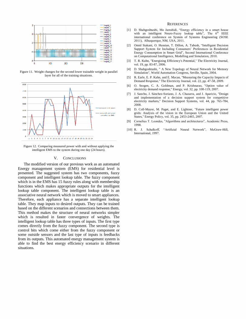
Figure 11. Weight changes for the second lower trainable weight in parallel

layer for all of the training situations.

Figure 12. Comparing measured power with and without applying the

intelligent EMS to the system during one day (24 hours).

V. CONCLUSIONS

The modified version of our previous work as an automated Energy management system (EMS) for residential level is presented. The suggested system has two components, fuzzy component and intelligent lookup table. The fuzzy component which is in the EMS has 15 fuzzy rules along with membership functions which makes appropriate outputs for the intelligent lookup table component. The intelligent lookup table is an associative neural network which is moved to smart appliances. Therefore, each appliance has a separate intelligent lookup table. They map inputs to desired outputs. They can be trained based on the different scenarios and connections between them. This method makes the structure of neural networks simpler which is resulted in faster convergence of weights. The intelligent lookup table has three types of inputs. The first type comes directly from the fuzzy component. The second type is control bits which come either from the fuzzy component or some outside sensors and the last type of inputs is feedbacks from its outputs. This automated energy management system is able to find the best energy efficiency scenario in different situations.

REFERENCES

[1] D. Shahgoshtasbi, Mo Jamshidi, “Energy efficiency in a smart house with an intelligent Neuro-Fuzzy lookup table”, The 6

th IEEE

international conference on System of Systems Engineering (SOSE 2011), Albuquerque, NM, USA, 2011.

[2] Omid Siakani, O. Hussian, T. Dillon, A. Tabesh, “Intelligent Decision Support System for Including Consumers’ Preferences in Residential

Energy Consumption in Smart Grid”, Second International Conference on Computational Intelligence, Modelling and Simulation, 2010.

[3] T. R. Kuhn, "Energizing Efficiency's Potential," The Electricity Journal,

vol. 19, pp. 83-87, 2006.

[4] D. Shahgoshtasbi, " A New Topology of Neural Network for Memory Simulation", World Automation Congress, Seville, Spain, 2004.

[5] R. Earle, E. P. Kahn, and E. Macan, "Measuring the Capacity Impacts of

Demand Response," The Electricity Journal, vol. 22, pp. 47-58, 2009.

[6] O. Sezgen, C. A. Goldman, and P. Krishnarao, "Option value of electricity demand response," Energy, vol. 32, pp. 108-119, 2007.

[7] J. Sancho, J. Sánchez-Soriano, J. A. Chazarra, and J. Aparicio, "Design

and implementation of a decision support system for competitive electricity markets," Decision Support Systems, vol. 44, pp. 765-784,

2008.

[8] D. Coll-Mayor, M. Paget, and E. Lightner, "Future intelligent power

grids: Analysis of the vision in the European Union and the United States," Energy Policy, vol. 35, pp. 2453-2465, 2007.

[9] Cornelius T. Leondes, ”Algorithms and architectures”, Academic Press,

1998.

[10] R. J. Schalkoff, “Artificial Neural Network”, McGraw-Hill, International, 1997.

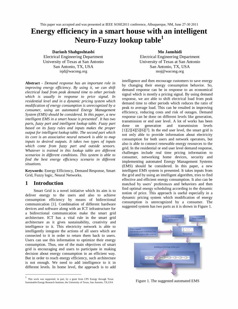
This paper was accepted and was presented at IEEE SOSE2011 conference, Albuquerque, NM, June 27-30 2011

Energy efficiency in a smart house with an intelligent

Neuro-Fuzzy lookup table1

Dariush Shahgoshtasbi

Electrical Engineering Department

University of Texas at San Antonio

San Antonio, TX, USA isjd@wacong.org

Mo Jamshidi

Electrical Engineering Department

University of Texas at San Antonio

San Antonio, TX, USA moj@wacong.org

Abstract - Demand response has an important role in

improving energy efficiency. By using it, we can shift

electrical load from peak demand time to other periods

which is usually in response to price signal. In

residential level and in a dynamic pricing system which modification of energy consumption is unrecognized by a

consumer, using an automated Energy Management

System (EMS) should be considered. In this paper, a new

intelligent EMS in a smart house is presented1. It has two

parts, fuzzy part and intelligent lookup table. Fuzzy part

based on its fuzzy rules and inputs makes the proper

output for intelligent lookup table. The second part which

its core is an associative neural network is able to map

inputs to desired outputs. It takes two types of inputs

which come from fuzzy part and outside sensors.

Whatever is trained in this lookup table are different

scenarios in different conditions. This system is able to find the best energy efficiency scenario in different

situations.

Keywords: Energy Efficiency, Demand Response, Smart

Grid, Fuzzy logic, Neural Networks.

1 Introduction

Smart Grid is a novel initiative which its aim is to

deliver energy to the users and also to achieve

consumption efficiency by means of bidirectional

communication [1]. Combination of different hardware

devices and software along with an ICT infrastructure for

a bidirectional communication make the smart grid

architecture. ICT has a vital rule in the smart grid

architecture as it gives sustainability, creativity and intelligence to it. This electricity network is able to

intelligently integrate the actions of all users which are

connected to it in order to return them back to users.

Users can use this information to optimize their energy

consumption. Thus, one of the main objectives of smart

grid is encouraging end users to participate in making

decision about energy consumption in an efficient way.

But in order to reach energy efficiency, such architecture

is not enough. We need to add intelligence to it in

different levels. In home level, the approach is to add

1 This work was supported, in part, by a grant from CPS Energy through Texas

Sustainable Energy Research Institute, the University of Texas, San Antonio, TX,USA

intelligence and then encourage customers to save energy

by changing their energy consumption behavior. So,

demand response can be in response to an economical

signal which is mostly a pricing signal. By using demand

response, we are able to shift electrical load from peak demand time to other periods which reduces the ratio of

peak to average load. This can be resulted in improving

efficiency, reducing costs and risk of outages. Demand

response can be done on different levels like generation,

transmission or end user level. A lot of works has been

done on generation and transmission levels

[1][2][4][5][6][7]. In the end user level, the smart grid is

not only able to provide information about electricity

consumption for both users and network operators, but

also is able to connect renewable energy resources to the

grid. In the residential or end user level demand response,

challenges include real time pricing information to consumer, networking home devices, security and

implementing automated Energy Management Systems

(EMS) should be considered. In this paper, a new

intelligent EMS system is presented. It takes inputs from

the grid and by using an intelligent algorithm, tries to find

effective and efficient energy consumption. It also can be

matched by users’ preferences and behaviors and then

find optimal energy scheduling according to the dynamic

notion of price. This approach is useful especially in a

dynamic pricing system which modification of energy

consumption is unrecognized by a consumer. The suggested system has two parts as it is shown in Figure 1.

Figure 1. The suggested automated EMS

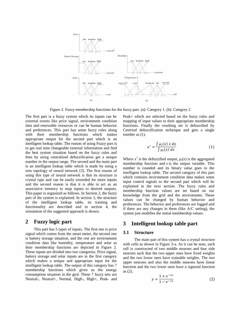
Figure 2. Fuzzy membership functions for the fuzzy part. (a): Category 1. (b): Category 2

The first part is a fuzzy system which its inputs can be

external events like price signal, environment condition

data and renewable resources or can be human behavior

and preferences. This part has some fuzzy rules along with their membership functions which makes

appropriate output for the second part which is an

intelligent lookup table. The reason of using Fuzzy part is

to get real time changeable external information and find

the best system situation based on the fuzzy rules and

then by using centralized defuzzification get a unique

number in the output range. The second and the main part

is an intelligent lookup table which is made by using a

new topology of neural network [3]. The first reason of

using this type of neural network is that its structure is

crystal type and can be easily extended for more inputs

and the second reason is that it is able to act as an associative memory to map inputs to desired outputs.

This paper is organized as follows. In Section 2, the fuzzy

part of the system is explained. In section 3, the structure

of the intelligent lookup table, its training and

functionality are described and in section 4, the

simulation of the suggested approach is shown.

2 Fuzzy logic part

This part has 5 types of inputs. The first one is price

signal which comes from the smart meter, the second one

is battery storage situation, and the rest are environment

condition data like humidity, temperature and solar as

their membership functions are depicted in Figure 2.

These inputs are divided into two categories. Price signal, battery storage and solar inputs are in the first category

which makes a unique and appropriate input for the

intelligent lookup table. The output of this category has 7

membership functions which gives us the energy

consumption situation in the gird. These 7 fuzzy sets are

Neutral-, Neutral+, Normal, High-, High+, Peak- and

Peak+ which are selected based on the fuzzy rules and

mapping of input values to their appropriate membership

functions. Finally the resulting set is defuzzified by

Centriod defuzzification technique and gets a single number as (1).

Where x* is the defuzzified output, µi(x) is the aggregated

membership function and x is the output variable. This

number is rounded and its binary value goes to the

intelligent lookup table. The second category of this part

which contains environment condition data makes some

input control signals to the second part which will be

explained in the next section. The fuzzy rules and

membership function values are set based on our

knowledge from the grid and the environment. These

values can be changed by human behavior and preferences. The behavior and preferences are logged and

if there are any changes in them (like A/C setting), the

system just modifies the initial membership values.

3 Intelligent lookup table part

3.1 Structure

The main part of this system has a crystal structure

with cells as shown in Figure 3-a. As it can be seen, each

cell is constructed of two middle neurons and four side

neurons such that the two upper ones have fixed weights

and the two lower ones have trainable weights. The two

upper neurons and also the middle neurons have linear

function and the two lower ones have a sigmoid function

as (2).

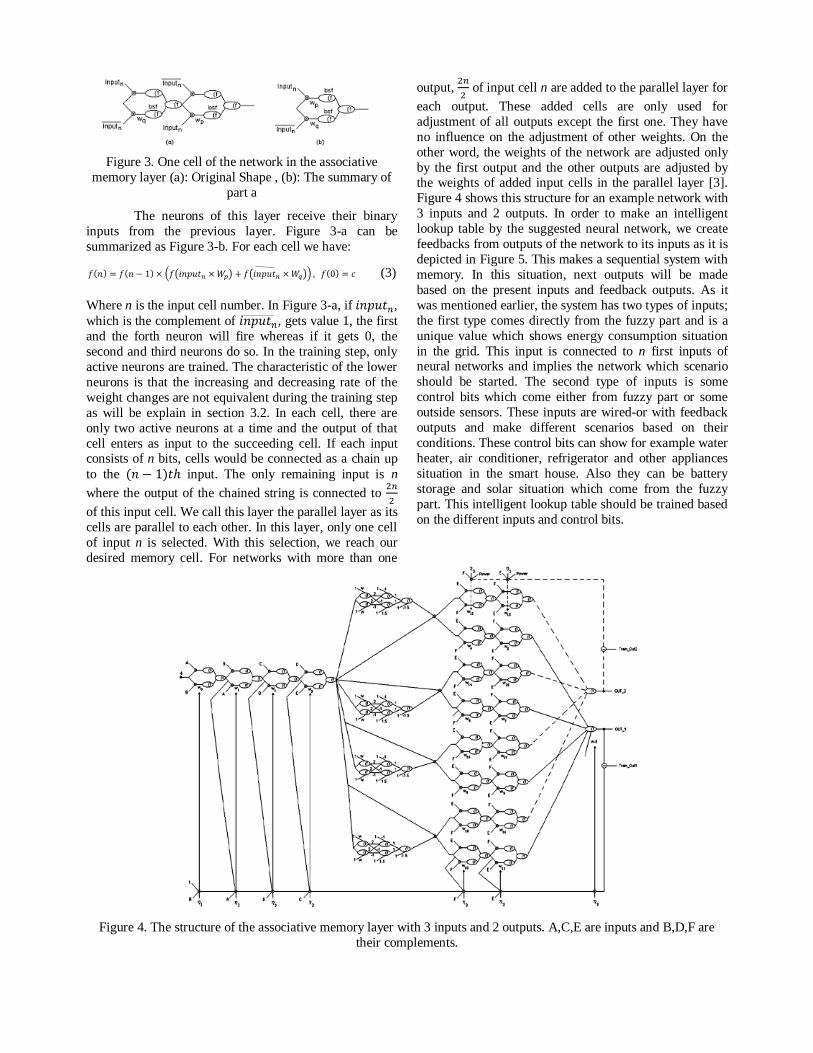
Figure 3. One cell of the network in the associative

memory layer (a): Original Shape , (b): The summary of

part a

The neurons of this layer receive their binary

inputs from the previous layer. Figure 3-a can be

summarized as Figure 3-b. For each cell we have:

(3)

Where n is the input cell number. In Figure 3-a, if ,

which is the complement of , gets value 1, the first

and the forth neuron will fire whereas if it gets 0, the

second and third neurons do so. In the training step, only

active neurons are trained. The characteristic of the lower

neurons is that the increasing and decreasing rate of the

weight changes are not equivalent during the training step

as will be explain in section 3.2. In each cell, there are

only two active neurons at a time and the output of that

cell enters as input to the succeeding cell. If each input consists of n bits, cells would be connected as a chain up

to the input. The only remaining input is n

where the output of the chained string is connected to

of this input cell. We call this layer the parallel layer as its

cells are parallel to each other. In this layer, only one cell

of input n is selected. With this selection, we reach our

desired memory cell. For networks with more than one

output,

of input cell n are added to the parallel layer for

each output. These added cells are only used for

adjustment of all outputs except the first one. They have

no influence on the adjustment of other weights. On the

other word, the weights of the network are adjusted only

by the first output and the other outputs are adjusted by the weights of added input cells in the parallel layer [3].

Figure 4 shows this structure for an example network with

3 inputs and 2 outputs. In order to make an intelligent

lookup table by the suggested neural network, we create

feedbacks from outputs of the network to its inputs as it is

depicted in Figure 5. This makes a sequential system with

memory. In this situation, next outputs will be made

based on the present inputs and feedback outputs. As it

was mentioned earlier, the system has two types of inputs;

the first type comes directly from the fuzzy part and is a

unique value which shows energy consumption situation

in the grid. This input is connected to n first inputs of neural networks and implies the network which scenario

should be started. The second type of inputs is some

control bits which come either from fuzzy part or some

outside sensors. These inputs are wired-or with feedback

outputs and make different scenarios based on their

conditions. These control bits can show for example water

heater, air conditioner, refrigerator and other appliances

situation in the smart house. Also they can be battery

storage and solar situation which come from the fuzzy

part. This intelligent lookup table should be trained based

on the different inputs and control bits.

Figure 4. The structure of the associative memory layer with 3 inputs and 2 outputs. A,C,E are inputs and B,D,F are

their complements.

3.2 Learning

The algorithm of network training is a way to

decode the problem to be solved [8]. The learning of this

network is supervised. The single layer perceptron

learning rule is used to train this network [9]:

(4)

Where j is the input cell number, is the input of

that cell, is the output of the network and is

the desired output. The important point is that using the learning rule of single layer perceptron for this multi-layer

network makes learning easy. The way of using this rule

is presented here. As mentioned earlier, only active

neurons are trained and in each cell there is only one

lower active neuron at a time. So the Eq. (4) can be

rewritten as:

(5)

In each layer, the values which have been used for the stabilization of weights are smaller when weights

increase than when they decrease. This always makes

weights decreasing values larger than weights increasing values. These increasing and decreasing values are

reduced in subsequent layers. The reason is that in binary

numbers, the bit toggle frequency is halved when we

move from LSB bits toward MSB bits. Since the inputs of

the suggested network are binary, considering as mentioned, will cause the changes of weights to become

slower in subsequent layers. On the other words, weights

change with lower frequency for 2n sequential binary

inputs. Considering the first layer as MSB and moving

toward parallel layer as moving to LSB, the weight

toggles would be less for the neurons of input cell n

which are in the last layer and frequency of changes in

their inputs is more than other cells. Due to the fact that the output error creates feedbacks to all layers, the

weights of all active neurons will decrease or increase if

this error becomes negative or positive respectively. But

Figure 5. The intelligent lookup table structure

since values are not equal, their increasing and decreasing rate would be different in each layer. By this

method the network can be stabilized and get adjusted to

2n input forms which result in the convergence of weights

[3]. Experiments show that in case of having more than

one output, it is better to consider a coefficient Power to

adjust the weights of all outputs except the first one to

expedite the convergence of weights.

3.3 Functionality

This network acts as an associative memory and is

able to map a set of inputs to a desired output. Whatever

will be trained in the network are different scenarios

(based on different conditions) and connection between

them. It can be trained in a certain time and mostly maps

outputs based on the previous learning. The system will

be trained when we have a new scenario or we intend to

change one. This characteristic of the suggested lookup

table gives the system speed and reliability which are two

important items in the field of energy in a smart house. Scenarios in the mentioned intelligent lookup table are

connected to each other in a way which suggest the best

energy efficiency for appliances in the smart house. In

fact, this system predicts outputs based on control bits

and fuzzy inputs. For example, if a smart house has both

battery storage and solar system and weather forecast

information shows that we would have a cloudy weather

in the next hours (which solar would not work), if the

control bit is set and imply the battery storage needs to be

charged, the system charges it in order to use its energy in

Table 1: Seventeen defined scenarios for energy

efficiency in a smart house

No. Scenario

1 Charge battery by grid

2 Charge battery by solar

3 Turn on water heater

4 Turn on air conditioner

5 Turn on dishwasher if programmed on

6 Turn on washer if programmed on

7 Turn on dryer if programmed on

8 Give portion of energy to dishwasher if

programmed on

9 Give portion of energy to washer if programmed

on

10 Give portion of energy to dyer if programmed on

11 Give portion of energy to refrigerator if needed

(on)

12 Give portion of energy to freezer if needed (on)

13 Turn off dishwasher

14 Turn off washer

15 Turn off dryer

16 Get energy from battery storage

17 Turn on light controller

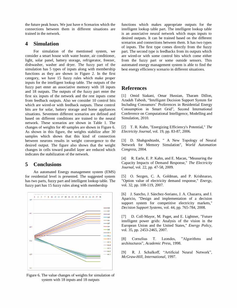
the future peak hours. We just have n Scenarios which the

connections between them in different situations are

trained in the network.

4 Simulation

For simulation of the mentioned system, we

consider a smart house with water heater, air conditioner,

light, solar panel, battery storage, refrigerator, freezer,

dishwasher, washer and dryer. The fuzzy part of the simulation has 5 types of inputs along with membership

functions as they are shown in Figure 2. In the first

category, we have 15 fuzzy rules which make proper

inputs for the intelligent lookup table. The outputs of the

fuzzy part enter an associative memory with 18 inputs

and 18 outputs. The outputs of the fuzzy part enter the

first six inputs of the network and the rest inputs come

from feedback outputs. Also we consider 10 control bits

which are wired-or with feedback outputs. These control

bits are for solar, battery storage and home appliances

situations. Seventeen different scenarios are defined and

based on different conditions are trained to the neural network. These scenarios are shown in Table 1. The

changes of weights for 40 samples are shown in Figure 6.

As shown in this figure, the weights stabilize after 30

samples which shows that this kind of connection

between neurons results in weight convergence to the

desired output. The figure also shows that the weight

changes in cells toward parallel layer are reduced which

indicates the stabilization of the network.

5 Conclusions

An automated Energy management system (EMS)

for residential level is presented. The suggested system

has two parts, fuzzy part and intelligent lookup table. The

fuzzy part has 15 fuzzy rules along with membership

Figure 6. The value changes of weights for simulation of

system with 18 inputs and 18 outputs

functions which makes appropriate outputs for the

intelligent lookup table part. The intelligent lookup table

is an associative neural network which maps inputs to

desired outputs. It can be trained based on the different

scenarios and connections between them. It has two types

of inputs. The first type comes directly from the fuzzy part. The second type is feedbacks from its outputs which

are wired-or with some control bits which come either

from the fuzzy part or some outside sensors. This

automated energy management system is able to find the

best energy efficiency scenario in different situations.

References

[1] Omid Siakani, Omar Hussian, Tharam Dillon,

Azadeh Tabesh, “Intelligent Decision Support System for

Including Consumers’ Preferences in Residential Energy

Consumption in Smart Grid”, Second International

Conference on Computational Intelligence, Modelling and

Simulation, 2010.

[2] T. R. Kuhn, "Energizing Efficiency's Potential," The Electricity Journal, vol. 19, pp. 83-87, 2006.

[3] D. Shahgoshtasbi, " A New Topology of Neural

Network for Memory Simulation", World Automation

Congress, 2004.

[4] R. Earle, E. P. Kahn, and E. Macan, "Measuring the

Capacity Impacts of Demand Response," The Electricity

Journal, vol. 22, pp. 47-58, 2009.

[5] O. Sezgen, C. A. Goldman, and P. Krishnarao,

"Option value of electricity demand response," Energy, vol. 32, pp. 108-119, 2007.

[6] J. Sancho, J. Sánchez-Soriano, J. A. Chazarra, and J.

Aparicio, "Design and implementation of a decision

support system for competitive electricity markets,"

Decision Support Systems, vol. 44, pp. 765-784, 2008.

[7] D. Coll-Mayor, M. Paget, and E. Lightner, "Future

intelligent power grids: Analysis of the vision in the

European Union and the United States," Energy Policy,

vol. 35, pp. 2453-2465, 2007.

[8] Cornelius T. Leondes, ”Algorithms and

architectures”, Academic Press, 1998.

[9] R. J. Schalkoff, “Artificial Neural Network”,

McGraw-Hill, International, 1997.

1

Fail-Safe Decentralized Architectures forAdvanced Metering Infrastructure

Sai Krishna Narra and Ram KrishnanDept. of Electrical and Computer Engineering

University of Texas at San AntonioEmail: hrl334@my.utsa.edu and Ram.Krishnan@utsa.edu

Abstract—Advanced Metering Infrastructure (AMI) is a keycomponent of smart grid. Current AMI solutions employ amesh network of routers, collectors and potentially hundreds ofthousands of smart meters. Typically, a command center (headend) manages this whole infrastructure. This type of securitysolution suffers from a single point of failure, since in mostcurrent deployments, a single instance of the command centermanages the whole network. Specifically compromise of thecommand center (or any of its instances) implies compromiseof the whole network—allowing one to arbitrarily control allthe smart meters. In this paper, we propose a decentralizedarchitecture with multiple head ends each of which is responsiblefor different domain of meters with some overlap of managementamongst various head ends. The benefit of this architecture is thatif there is a compromise of one head end only a subset of meterswill be affected and the rest of the system can continue to operatenormally. We also discuss various classes of such architectureswith varying security properties and analyze them in detail.

Index Terms—Decentralized Architecture, Security Analysis,Key management.

I. INTRODUCTION

AMI (Advanced Metering Infrastructure) offers useful fea-tures like remote control of meters and two-way communica-tion. AMI is majorly influenced by the use of smart meterswhich record the consumption of energy more frequentlythan the traditional meters and transmit that information toa central controlling center. Remote management of the smartmeters in AMI is made possible by routers and collectorsthat facilitate hop by hop data transfer. Furthermore, the smartmeter themselves act as mesh network. This is illustrated infigure 1.

A major issue in current deployments is that there istypically one logical command center that manages the wholenetwork of meters, collectors and routers. This suffers fromthe problem of single point of failure. That, compromise ofthe command center compromises the whole network. In thispaper, we develop a framework of decentralized architecturesfor the AMI with multiple command centers with different,yet overlapping, management responsibilities, so that if one iscompromised, it minimizes the number of meters that wouldbe affected. We specify a formal graph based model that can beused for analyzing the extent of damage in case of compromiseof a node in the AMI network. We identify three classes ofdecentralized architectures with different cryptographic keysharing patterns. We analyze and compare the robustness of

Fig. 1. High level architecture of an AMI: The meters are connected in a meshnetwork. Meters M1 and M4 transmit data directly to the router R23. Othermeters may transfer data to routers using multiple hops. Collectors aggregatedata from routers and perform encoding/decoding and pre-processing beforetransmitting them to the Command Center.

these classes with respect to security in case of different kindsof compromise.

II. DECENTRALIZED AMI MODEL

In a decentralized AMI network, there are multiple headends that manage various smart meters. For the purposes ofthis paper, we assume that each smart meter owns a uniquekey, KU, that is shared with one or more head ends. Similarly,each head end owns a network key, KN, that is sharedwith the meters that it would manage. With the knowledgeof these keys, the meters and the head ends can achievemutual authentication and confidentiality and integrity of data

2

Fig. 2. Example Figure:A1 can be a single node or a domain comprising ofmultiple Smart meter nodes. Then each node in a domain will have its ownKU ,KN1,KN2

exchanged between them. (See [1] for example.)

A. Components of the Model

In this section, we develop a graph based model fordecentralized AMI and formally define various requirementsof this model. Later, we analyze specific classes of this model.

Definition 1 (Decentralized AMI system (dAMI-system))A Decentralized AMI system (dAMI-system) is a directedgraph G(V,E) where V is a set of vertices in the graph and Eis the set of edges that connect different vertices in V.

Definition 2 (Node) A node in a dAMI-system is represents aunique end point entity.

There are two different types of nodes present in the dAMI-system: Type-S and Type-H. Type-S nodes represent smartmeters and are denoted using single circles in figures andType-H nodes represent head ends and are denoted usingdouble circles.

Note that we are only interested in modeling the smartmeters and the head ends for security analysis. Specifically,devices like routers and collectors (see figure 1) are solelypart of the communication infrastructure of the AMI and arenot directly relevant to our study in this paper. We assumethe existence of such a communication infrastructure thatfacilitates data transfer from one node to another in our model.

Definition 3 (Edge) An edge represents sharing of key(s)from the source node to the destination node. Nodes are onlyallowed to share the key(s) that it owns.

An edge represents key sharing in a Decentralized AMIsystem. Every Type-S node owns its unique key KU. Similarly,every Type-H node owns its network key KN. Figure 2illustrates an example dAMI-system with 3 Type-S nodes and

3 Types-H nodes. This is a dAMI-system G(V,E) where:

V =S1A, S1B , S1C , HA, HB , HCE =(S1A, HA), (HA, S1A), (S1B , HB), (HB , S1B), (S1C , HC),

(HC , S1C), (S1C , HB), (HB , S1C), (S1A, HB), (HB , S1A),

(S1B , HA), (HA, HB), (HB , HA)As seen, each node in the graph has knowledge of a number

of keys in addition to the key it owns. A key owned by a nodeis indicated in bold font. The key configuration at variousnodes is a result of key sharing facilitated by the edges. Inthe figure, for clarity, if two nodes mutually share their keysthen they are represented by a single bidirectional edge. Recallthat edges only represent key sharing and do not speak to thecommunication infrastructure.

Consider the node S1A int he figure. KU1 is S1A’s originalkey (bold font). KN1 and KN2 are the original keys of HA

and HB respectively. Since there is an incoming edge into S1A

from both HA and HB , their original keys KN1 and KN2 areavailble at S1A. Similarly, consider the node HB . KN2 is thekey owned by HB . Due to the incoming edges from S1A andS1B , it obtains KU1 and KU2. Further, due to an incomingedge from HA, it also obtains KN1.

Next, we introduce the concept of a domain that allows usto assign ownership of a set of smart meters to a specific headend.Definition 4 (DOMAIN) The domain of a H-Type node is acollection of Type-S nodes with which an edge exists.

There are two types of domains: primary and secondary.A Type-S node’s primary Type-H node is that node withwhich there is a bidirectional edge. That is, the Type-S nodemutually shares keys with that Type-H node. A Type-S node’ssecondary Type-H node is that node with there need not be abidirectional node. In figure 2, the primary domain of S1C isHC and its secondary domain is HB . The naming conventionallows one to identify the primary and secondary domainsof a Type-S node. (The letter subscript in the Type-S nodeidentifies the primary domain.) Note that a bidirectional edgeis not prohibited between a Type-S node and its secondarydomain head end. For example, S1A mutually shares keys withits secondary domain HB . In general, the secondary domainType-H nodes act as a backup head end for any given smartmeter. Partial sharing with the backup head end allows forthe dAMI-system to have reduced risk while ensuring partialoperation in case of compromise of the primary head end.

B. Required Properties of the dAMI-system

We define 3 core rules that are required all dAMI-systems.1) In a dAMI-system, every edge that connects a Type-S

node with its primary domain Type-H node should bebidirectional.

2) A dAMI-system should contain both types of nodes.3) Each S-Type node should share an edge with at least

two H-Type nodes.4) Edges are not allowed between two S-Type nodes.

Note that these rules are consistent with many of the currentindustry solutions for AMI.

3

TABLE ISECURITY STATUS OF VARIOUS CLASSES UNDER DIFFERENT COMPROMISE SCENARIOS

Compromisetype

Affected edge(s) Status of CIAu on affected edges

CLASS-A CLASS- B CLASS- C

Compromiseof Type-Snode key

The one connecting that Type-S nodewith its primary Type-H node

Only Integrity of messagesis protected. CAu is lostsince KU is lost.

Only Integrity of messagesis protected. CAu is lostsince KU is lost.

Only Integrity of messagesis protected. CAu is lostsince KU is lost.

The one connecting that Type-S nodewith its secondary Type-H node

Only Integrity of messagesis protected. CAu is lostsince KU is lost.

CIAu is lost becasue onlyKU is shared and not KN .

Only Integrity of messagesis protected. CAu is lostsince KU is lost.

Compromiseof Type-Snode

The one connecting that Type-S nodewith its primary Type-H node

CIAu is lost because bothKU and secondary Type-Hnodes KN is lost.

CIAu is lost because bothKU and secondary Type-Hnodes KN is lost.

CIAu is lost because bothKU and secondary Type-Hnodes KN is lost.

(all keysstored at thatnode com-promised)

The one connecting the compromisedType-S node with its secondary Type-H node

CIAu is lost because bothKU and secondary Type-Hnodes KN is lost.

CIAu is lost because bothKU is lost.

CIAu is lost because bothKU and primary Type-Hnodes KN is lost.

Those edges that connect other Type-S nodes in the same domain as thecompromised node with the primaryType-H node

C- is preserved and Type-H node can authenticate S-type nodes.

C- is preserved and Type-H node can authenticate S-type nodes.

C- is preserved and Type-H node can authenticate S-type nodes.

Those edges that connect other Type-S nodes in the same domain as thecompromised node with the secondaryType-H node of the compromised node.

C- is preserved and Type-H node can authenticate S-type nodes.

C- is preserved and Type-H node can authenticate S-type nodes.

C- is preserved and Ty‘pe-H node can authenticate S-type nodes.

Those edges that connect other Type-Snodes in the same domain as the com-promised node with secondary Type-Hnodes that are not the same as that ofthe compromised node.

CIAu is achieved C- is preserved and Type-H node can authenticate S-type nodes

CI- is preserved and Type-H node can authenticate S-type nodes.

Compromiseof a Type-Hnode’s key

Those edges between the compromisedType-H node and Type-S nodes forwhich the compromised node is theprimary.

C- is preserved and Type-H node can authenticate S-type nodes.

C- is preserved and Type-Hnode can authenticate Type-S nodes.

C- is preserved and Type-Hnode can authenticate Type-S nodes .

Those edges between the compromisedType-H node and Type-S nodes forwhich the compromised node is thesecondary.

C- is preserved and Type-H node can authenticate S-type nodes.

C- is preserved and Type-H node can authenticate S-type nodes .

CI- is preserved and Type-H node can authenticate S-type nodes.

Those edges that connect Type-S nodesfor which the compromised node isprimary with their respective secondaryType-H nodes.

CIAu is preserved C- is preserved and Type-Hnode can authenticate Type-S nodes.

C- is preserved and Type-Hnode can authenticate Type-S nodes.

Compromiseof a Type-Hnode

Those edges that connect the compro-mised Type-H node with Type-S nodesin the same domain.

CIAu is lost since both KU

and KN are compromisedCIAu is lost since both KU

and KN are compromised.CIAu is lost since both KU

and KN are compromised.

(all keysstored at thatnode com-promised.)

Those edges that connect the compro-mised Type-H node with Type-S nodesfor which the compromised node actsas secondary.

CIAu is lost since both KU

and KN are compromised.CIAu is lost since KU iscompromised and KN isabsent.

CIAu is lost since both KU

of secondary andKN ofprimary Type-H node of thesecondary Type-S domianare compromised.

Those edges that connect the Type-S nodes for which the compromisednode is primary with their respectivesecondary Type-H nodes.

Integrity is preserved be-cause KN is not compro-mised.

CIAu is lost since both KU

and KN are compromised.CIAu is lost since both KU

and KN are compromised.

Those edges that connect the Type-S nodes for which the compromisednode is secondary with their respectiveprimary Type-H nodes.

Integrity is preserved be-cause KN is not compro-mised.

Integrity is preserved be-cause KN is not compro-mised.

CIAu is lost since both KU

and KN are compromised.

4

C. Reachability in dAMI-system

We use the term reachability to specify whether anedge between two nodes in the dAMI-system facilitatesauthentication, confidentiality and/or integrity.

Definition 5 (C-Reachability/Confidentiality Reachability:)A node X is C-Reachable from a node Y if data can beconfidentially exchanged between nodes X and Y.

Given a graph G(V,E), confidentiality of data exchangedbetween an S-Type node P and an H-Type node Q is achievedif an edge (P,Q) exists in E. This is because such an edgewould imply that P’s unique key is shared with Q. Forexample, in figure 2, the edge from S1A to HA indicatesthat KU1 is shared between those nodes. This allows forconfidential exchange of data between them.

Definition 6 (I-Reachability/Integrity Reachability:) A nodeX is I-Reachable from a node Y if integrity of data exchangedbetween X and Y can be achieved.

Given a graph G(V,E), integrity of data exchanged betweenan S-Type node P and an H-Type node Q is achieved if anedge (Q,P) exists in E. This is because such an edge wouldimply that Q’s network key is shared with P. For example,in figure 2, the edge from HA to S1A indicates that KN1 isshared between those nodes. This means that integrity of dataexchanged between them can be achieved.

Definition 7 (Au-Reachability/Authentication Reachabil-ity:) A node X is Au-Reachable from a node Y if messagesfrom Y can be authenticated by X.

Given a graph G(V,E), authentication of messages betweenan S-Type node and an H-type node is achieved if edges(P,Q) and (Q,P) exists in E. That is, if any two nodes haveC and I-Reachability, then they also have Au-Reachability.This is because authentication of messages from a node P toQ (where P and Q are of different types) is achieved basedon the unique key of the S-Type node and the network key ofthe H-Type node. For example, in figure 2, the bidirectionaledge between S1A and HA indicate that the two nodes canmutually authenticate each other’s messages.

III. CLASSES OF DAMI-SYSTEM

In this section, we discuss 3 different classes of dAMI-systems. These classes specify rules in addition to the corerules defined in section II-B. For each class, a number ofdAMI-systems may be developed based on these rules. Weanalyze the security properties of each class of systems insituations of compromise.

A. Class-A dAMI-Systems

Class-A systems are developed based on the following rules:1) Only bidirectional edges are allowed.2) Edges between H-Type nodes are not allowed.

B. Class-B dAMI-Systems

Class-B systems are developed based on the following rules:1) Between Type-S nodes and their secondary Type-H

nodes, only unidirectional edges originating from theType-S nodes are allowed.

2) Edges between H-Type nodes are not allowed.

C. Class-C dAMI-Systems

1) Only unidirectional edges are allowed.2) For every edge that connects a Type-S node with its

secondary Type-H node, another edge should originatefrom the Type-S node’s primary Type-H node and endat that secondary Type-H node.

IV. COMPARISION TABLE

Table I presents our final analysis of how class A, B andC systems compare under different compromise scenarios. Incolumn 1, we consider two high-level compromise scenarios:1. compromise at the smart meter level and 2. compromise atthe head end level. In each of these two levels, a single keyin that node may be compromised or the whole node may becompromised (leading to compromise of all the keys stored inthat node). In column 2, we identify the edges that are affectedby the specific compromise scenario in column 1. In column3, we specify how CIAu-Reachability on the edges identifiedin column 2 is affected for class A, B and C systems.

V. CONTRIBUTIONS OF THIS PAPER

• We have specified a formal graph based model for design-ing decentralized architectures for Advanced MeteringInstrastructure.

• We have specified properties of 3 different classes ofsystems and shown that systems in the same class havethe same set of security properties. This is a highly usefulanalysis for a security architect designing a decentralizedAMI system as the classes provide various key sharingchoices.

REFERENCES

[1] S. Fuloria, R. Anderson, F. Alvarez, and K. McGrath. Key managementfor substations: Symmetric keys, public keys or no keys? In PowerSystems Conference and Exposition (PSCE), 2011 IEEE/PES, pages 1–6, march 2011.

This paper has been submitted to IEEE Journal on Selected Areas in Communications

Abstract— We present a framework and analysis of a

smart meter network that communicates over a 4G

cognitive radio (CR) channel. We view our Advanced

Metering Infrastructure (AMI) network as ideally suited

for a next generation of metropolitan area smart grid

systems. We define capacity analysis models of multi-user

AMI meter communication in the context of smart grid

networks. Our proposed 4G CR network framework is

capable of communicating with high numbers of

geographically dispersed smart meters for command and

control feature over the unused wholes within licensed 4G

cellular network bands and TV white spaces. We introduce

the foundations of a new AMI meter system model that

utilizes cloud data centers as the central communication

and optimization infrastructure supporting metropolitan

area based smart meter networks. The performance of

various scheduling algorithms for AMI is presented in the

context of the CR channel. Tradeoffs between maximizing

the system capacity and achieving fairness among

cognitive AMI users and system level capacity results for

our AMI network are presented. Detailed simulations

involving the CR transmission of secondary user packets

in the holes of a typical 4G Cellular network indicate that

our system can obtain an average capacity that meets the

smart grid communication protocol requirements.

Index Terms—4g Cognitive radio networks, cloud data center,

scheduling algorithms, and smart meters.

Manuscript received October, 1, 2011.

KranthiManoj Nagothu, Amir Rajee, Brian Kelley and Mo Jamshidi is with the University of Texas at San Antonio, San Antonio, TX 78249 USA; e-

mail: kranthimanoj@ gmail.com, amirajaee@ gmail.com, Brian.Kelley@

utsa.edu, moj@ wacong.org). This material is based upon work was supported, in part, by the Texas

Sustainable Energy Conservation office (SECO) and the U.S. Department of

Energy (DOE) under Grant RFA No. RE-AG1-2010 and has been supported, in part, by a grant from CPS Energy, San Antonio, TX through Texas

Sustainable Energy Research Institute, University of Texas, San Antonio.

I. INTRODUCTION

The smart grid of the future is generally perceived to be an

intelligent energy delivery system that supports plug-and-play

integration of power, information, and security services. The

services should be supportive of high penetrations of

renewable energy sources. It also acts as platform for

consumer and utility engagement in load management, closed

loop demand response, conversion of carbon generating power

to low carbon emitting sources, and economic security [1].

While it is essential that smart meter be networked,

communication network infrastructures represent a very large

capital expense. Much of this expenditure is due to the high

prices of purchasing licensed wireless bands either from the

Federal Communications Commission (FCC) auction process

or from existing licensed band owners. According to the FCC,

temporal and geographical variations in the utilization of the

assigned spectrum range from 15% to 85% [5]. To address this

issue in the context of spectrum availability, Cognitive Radio

(CR) is considered by the FCC as one of leading approaches to

improve the utilization and efficiency of spectrum [6]. We, therefore analyze a new low cost wireless system based on a 4G cognitive

radio AMI networks. In our context, we refer to 3GPP-LTE protocol

parameters as 4G. The smart grid AMI network we describe is

metropolitan in scale and principally independent of existing

cellular infrastructure.

A. Related work on AMI Networks

Several authors have defined aspects of AMI networking in

smart grids. Mesh, Ethernet and cellular AMI network

topology for smart grid has been proposed in [7-8]. In these

Smart Grid AMI Communication Networks and

Capacity Analysis Using 4G Cognitive Radio

Kranthi Manoj Member IEEE, Amir Rajaee Member IEEE, Brian Kelley Senior Member IEEE,

Mo Jamshidi Fellow IEEE

We anticipate that the future smart grid will leverage

Information and Communications Technology (ICT)

facilitated by sophisticated smart meter information networks.

The smart meter (often referred to as an Advanced Metering

Infrastructure (AMI)), enables the flow of real-time

information to the power utility servers and between the power

utility and its customers. It also provides customers and

utilities with the technology to optimize their energy

consumption via closed loop demand response services.

Additional battery management services are necessary to

integrate high penetrations of renewable energy components in

the grid, to support third party energy management

applications and enable dynamic optimization of distributed

power sources [2-4].

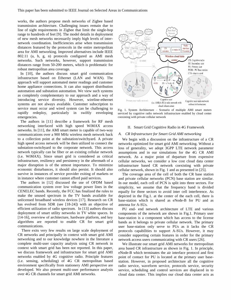
This paper has been submitted to IEEE Journal on Selected Areas in Communications

works, the authors propose mesh networks of Zigbee based

transmission architecture. Challenging issues remain due to

line of sight requirements in Zigbee that limit the single-hop

range to hundreds of feet [9]. The model details in deployment

of new mesh networks necessarily imply high levels of inter-

network coordination. Inefficiencies arise when transmission

distances featured by the protocols in the entire metropolitan

area for AMI networking. Improved alternatives include IEEE

802.11 (a, b, g, n) protocols configured as AMI mesh

networks. Such networks, however, support transmission

distances range from 50-200 meters, which is problematic for

robust metropolitan area coverage.

In [10], the authors discuss smart grid communication

infrastructure based on Ethernet (LAN and WAN). The

approach will support automated meter readings and customer

home appliance connections. It can also support distribution

automation and substation automation. We view such systems

as completely complementary to our approach and a way of

introducing service diversity. However, wireline-ethernet

systems are not always available. Customer subscription to

service must occur and wired system can be challenging to

rapidly redeploy, particularly in swiftly enveloping

emergencies.

The authors in [11] describe a framework for RF mesh

networking interfaced with high speed WiMAX access

networks. In [11], the AMI smart meter is capable of two-way

communications over a 900 MHz wireless mesh network back

to a collection point at the substation/switchyard. A private

high speed access network will be then utilized to connect the

substation-switchyard to the corporate network. This access

network typically can be fiber or an existing cellular network

(i.e. WiMAX). Since smart grid is considered as critical

infrastructure, resiliency and persistency in the aftermath of a

major disruption is of the utmost importance. To minimize

economic disturbances, it should also persist. It should also

survive in instances of service provider exiting of markets or

in instance where customer cannot afford paid services.

The authors in [12] discussed the use of OFDM based

communication system over low voltage power lines in the

CENELEC bands. Recently, the FCC has finalized the rules to

make the unused spectrum in the TV bands available for

unlicensed broadband wireless devices [17]. Research on CR

has evolved from SDR (see [18-24]) with an objective of

efficient utilization of radio spectrum. In [13] authors discuss

deployment of smart utility networks in TV white spaces. In

[14-16], overview of architecture, hardware platform, and key

algorithms are reported to enable CR for smart grid

communications.

There exits very few results on large scale deployment of

CR networks and principally in context with smart grid AMI

networking and to our knowledge nowhere in the literature a

complete multi-user capacity analysis using CR network in

context with smart grid has been not reported. In this paper,

we discuss framework and infrastructure for smart grid AMI

networks enabled by 4G cognitive radio. Principle features

(i.e. sensing, scheduling) of 4G CR metropolitan based

environment specifically from stationery AMI perspective are

developed. We also present multi-user performance analysis

over 4G CR channels for smart grid AMI networks.

II. Smart Grid Cognitive Radio in 4G Framework

A. CR Infrastructure for Smart Grid AMI networking

We begin with a discussion on the infrastructure of a CR

networks optimized for smart grid AMI networking. Without a

loss of generality, we adopt 3GPP LTE network parameter

assumptions and in our simulations for the 4G CR AMI

network. As a major point of departure from expensive

cellular networks, we consider a low cost cloud data center

infrastructure based CR network coexisting with private

cellular network, shown in Fig. 1 and as presented in [25].

The coverage area of the cell of both the CR base station

and private cellular networks (PCN) base station are similar.

In our model, each cell of PCN is split into three sectors. For

simplicity, we assume that the frequency band is divided

equally for three sectors to avoid inter cell interference. As

depicted in the Fig.1. at the center of the each cell, there is

base-station which is shared as eNode-B for PU and as

antenna for A-SUs.

PU end- end network architecture of LTE and various

components of the network are shown in Fig.1. Primary user

base-station is a component which has access to the license

bands as it belongs to private cellular network. The primary

user base-station only serve to PUs as it lacks the CR

protocols capabilities to support A-SUs. However, it may

consider supporting certain features in order for the primary

network access users communicating with CR users [26].

We illustrate our smart grid AMI networks for metropolitan

area based CR infrastructure as shown in Fig. 1. In principle,

eNode-B which terminates the air interface protocol and first

point of contact for PU is located at the primary user base-

station. However, in proposed architecture all the cognitive

radio service, waveform service, protocols service, security

service, scheduling and control services are displaced in to

cloud data center. This implies our cloud data center acts as

Fig. 1. System Architecture – Scenario of multiple AMI smart meters

serviced by cognitive radio network infrastructure enabled by cloud center

coexisting with private cellular network

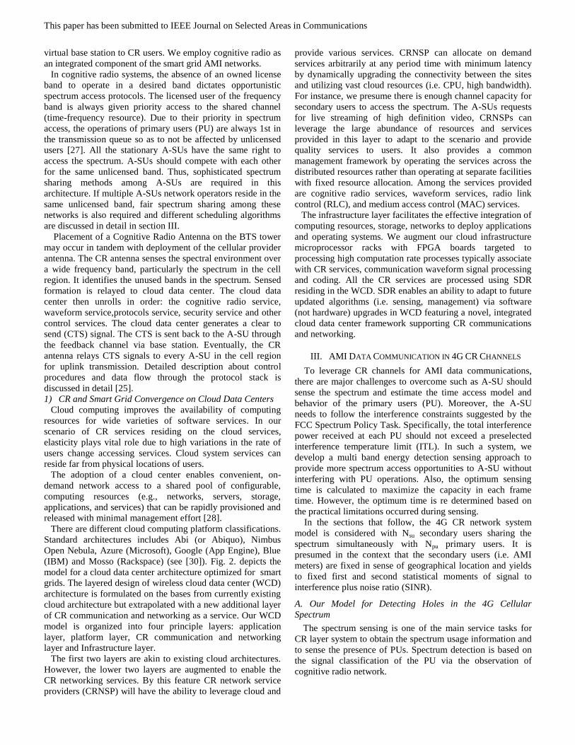
This paper has been submitted to IEEE Journal on Selected Areas in Communications

virtual base station to CR users. We employ cognitive radio as

an integrated component of the smart grid AMI networks.

In cognitive radio systems, the absence of an owned license

band to operate in a desired band dictates opportunistic

spectrum access protocols. The licensed user of the frequency

band is always given priority access to the shared channel

(time-frequency resource). Due to their priority in spectrum

access, the operations of primary users (PU) are always 1st in

the transmission queue so as to not be affected by unlicensed

users [27]. All the stationary A-SUs have the same right to

access the spectrum. A-SUs should compete with each other

for the same unlicensed band. Thus, sophisticated spectrum

sharing methods among A-SUs are required in this

architecture. If multiple A-SUs network operators reside in the

same unlicensed band, fair spectrum sharing among these

networks is also required and different scheduling algorithms

are discussed in detail in section III.

Placement of a Cognitive Radio Antenna on the BTS tower

may occur in tandem with deployment of the cellular provider

antenna. The CR antenna senses the spectral environment over

a wide frequency band, particularly the spectrum in the cell

region. It identifies the unused bands in the spectrum. Sensed

formation is relayed to cloud data center. The cloud data

center then unrolls in order: the cognitive radio service,

waveform service,protocols service, security service and other

control services. The cloud data center generates a clear to

send (CTS) signal. The CTS is sent back to the A-SU through

the feedback channel via base station. Eventually, the CR

antenna relays CTS signals to every A-SU in the cell region

for uplink transmission. Detailed description about control

procedures and data flow through the protocol stack is

discussed in detail [25].

1) CR and Smart Grid Convergence on Cloud Data Centers

Cloud computing improves the availability of computing

resources for wide varieties of software services. In our

scenario of CR services residing on the cloud services,

elasticity plays vital role due to high variations in the rate of

users change accessing services. Cloud system services can

reside far from physical locations of users.

The adoption of a cloud center enables convenient, on-

demand network access to a shared pool of configurable,

computing resources (e.g., networks, servers, storage,

applications, and services) that can be rapidly provisioned and

released with minimal management effort [28].

There are different cloud computing platform classifications.

Standard architectures includes Abi (or Abiquo), Nimbus

Open Nebula, Azure (Microsoft), Google (App Engine), Blue

(IBM) and Mosso (Rackspace) (see [30]). Fig. 2. depicts the

model for a cloud data center architecture optimized for smart

grids. The layered design of wireless cloud data center (WCD)

architecture is formulated on the bases from currently existing

cloud architecture but extrapolated with a new additional layer

of CR communication and networking as a service. Our WCD

model is organized into four principle layers: application

layer, platform layer, CR communication and networking

layer and Infrastructure layer.

The first two layers are akin to existing cloud architectures.

However, the lower two layers are augmented to enable the

CR networking services. By this feature CR network service

providers (CRNSP) will have the ability to leverage cloud and

provide various services. CRNSP can allocate on demand

services arbitrarily at any period time with minimum latency

by dynamically upgrading the connectivity between the sites

and utilizing vast cloud resources (i.e. CPU, high bandwidth).

For instance, we presume there is enough channel capacity for

secondary users to access the spectrum. The A-SUs requests

for live streaming of high definition video, CRNSPs can

leverage the large abundance of resources and services

provided in this layer to adapt to the scenario and provide

quality services to users. It also provides a common

management framework by operating the services across the

distributed resources rather than operating at separate facilities

with fixed resource allocation. Among the services provided

are cognitive radio services, waveform services, radio link

control (RLC), and medium access control (MAC) services.

The infrastructure layer facilitates the effective integration of

computing resources, storage, networks to deploy applications

and operating systems. We augment our cloud infrastructure

microprocessor racks with FPGA boards targeted to

processing high computation rate processes typically associate

with CR services, communication waveform signal processing

and coding. All the CR services are processed using SDR

residing in the WCD. SDR enables an ability to adapt to future

updated algorithms (i.e. sensing, management) via software

(not hardware) upgrades in WCD featuring a novel, integrated

cloud data center framework supporting CR communications

and networking.

III. AMI DATA COMMUNICATION IN 4G CR CHANNELS

To leverage CR channels for AMI data communications,

there are major challenges to overcome such as A-SU should

sense the spectrum and estimate the time access model and

behavior of the primary users (PU). Moreover, the A-SU

needs to follow the interference constraints suggested by the

FCC Spectrum Policy Task. Specifically, the total interference

power received at each PU should not exceed a preselected

interference temperature limit (ITL). In such a system, we

develop a multi band energy detection sensing approach to

provide more spectrum access opportunities to A-SU without

interfering with PU operations. Also, the optimum sensing

time is calculated to maximize the capacity in each frame

time. However, the optimum time is re determined based on

the practical limitations occurred during sensing.

In the sections that follow, the 4G CR network system

model is considered with Nsu secondary users sharing the

spectrum simultaneously with Npu primary users. It is

presumed in the context that the secondary users (i.e. AMI

meters) are fixed in sense of geographical location and yields

to fixed first and second statistical moments of signal to

interference plus noise ratio (SINR).

A. Our Model for Detecting Holes in the 4G Cellular

Spectrum

The spectrum sensing is one of the main service tasks for

CR layer system to obtain the spectrum usage information and

to sense the presence of PUs. Spectrum detection is based on

the signal classification of the PU via the observation of

cognitive radio network.

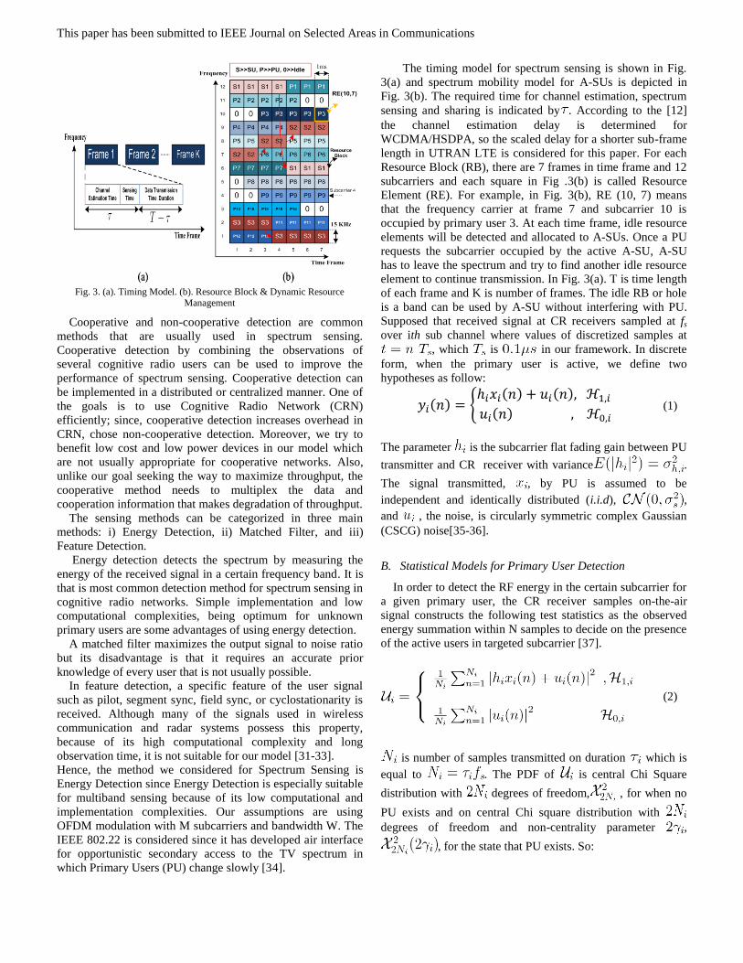
This paper has been submitted to IEEE Journal on Selected Areas in Communications

Cooperative and non-cooperative detection are common

methods that are usually used in spectrum sensing.

Cooperative detection by combining the observations of

several cognitive radio users can be used to improve the

performance of spectrum sensing. Cooperative detection can

be implemented in a distributed or centralized manner. One of

the goals is to use Cognitive Radio Network (CRN)

efficiently; since, cooperative detection increases overhead in

CRN, chose non-cooperative detection. Moreover, we try to

benefit low cost and low power devices in our model which

are not usually appropriate for cooperative networks. Also,

unlike our goal seeking the way to maximize throughput, the

cooperative method needs to multiplex the data and

cooperation information that makes degradation of throughput.

The sensing methods can be categorized in three main

methods: i) Energy Detection, ii) Matched Filter, and iii)

Feature Detection.

Energy detection detects the spectrum by measuring the

energy of the received signal in a certain frequency band. It is

that is most common detection method for spectrum sensing in

cognitive radio networks. Simple implementation and low

computational complexities, being optimum for unknown

primary users are some advantages of using energy detection.

A matched filter maximizes the output signal to noise ratio

but its disadvantage is that it requires an accurate prior

knowledge of every user that is not usually possible.

In feature detection, a specific feature of the user signal

such as pilot, segment sync, field sync, or cyclostationarity is

received. Although many of the signals used in wireless

communication and radar systems possess this property,

because of its high computational complexity and long

observation time, it is not suitable for our model [31-33].

Hence, the method we considered for Spectrum Sensing is

Energy Detection since Energy Detection is especially suitable

for multiband sensing because of its low computational and

implementation complexities. Our assumptions are using

OFDM modulation with M subcarriers and bandwidth W. The

IEEE 802.22 is considered since it has developed air interface

for opportunistic secondary access to the TV spectrum in

which Primary Users (PU) change slowly [34].

The timing model for spectrum sensing is shown in Fig.

3(a) and spectrum mobility model for A-SUs is depicted in

Fig. 3(b). The required time for channel estimation, spectrum

sensing and sharing is indicated by . According to the [12]

the channel estimation delay is determined for

WCDMA/HSDPA, so the scaled delay for a shorter sub-frame

length in UTRAN LTE is considered for this paper. For each

Resource Block (RB), there are 7 frames in time frame and 12

subcarriers and each square in Fig .3(b) is called Resource

Element (RE). For example, in Fig. 3(b), RE (10, 7) means

that the frequency carrier at frame 7 and subcarrier 10 is

occupied by primary user 3. At each time frame, idle resource

elements will be detected and allocated to A-SUs. Once a PU

requests the subcarrier occupied by the active A-SU, A-SU

has to leave the spectrum and try to find another idle resource

element to continue transmission. In Fig. 3(a). T is time length

of each frame and K is number of frames. The idle RB or hole

is a band can be used by A-SU without interfering with PU.

Supposed that received signal at CR receivers sampled at fs

over ith sub channel where values of discretized samples at

, which is in our framework. In discrete

form, when the primary user is active, we define two

hypotheses as follow:

( ) ( ) ( )

( ) (1)

The parameter is the subcarrier flat fading gain between PU

transmitter and CR receiver with variance .

The signal transmitted, , by PU is assumed to be

independent and identically distributed (i.i.d), ,

and , the noise, is circularly symmetric complex Gaussian

(CSCG) noise[35-36].

B. Statistical Models for Primary User Detection

In order to detect the RF energy in the certain subcarrier for

a given primary user, the CR receiver samples on-the-air

signal constructs the following test statistics as the observed

energy summation within N samples to decide on the presence

of the active users in targeted subcarrier [37].

(2)

is number of samples transmitted on duration which is

equal to . The PDF of is central Chi Square

distribution with degrees of freedom, , for when no

PU exists and on central Chi square distribution with

degrees of freedom and non-centrality parameter ,

, for the state that PU exists. So:

Fig. 3. (a). Timing Model. (b). Resource Block & Dynamic Resource

Management

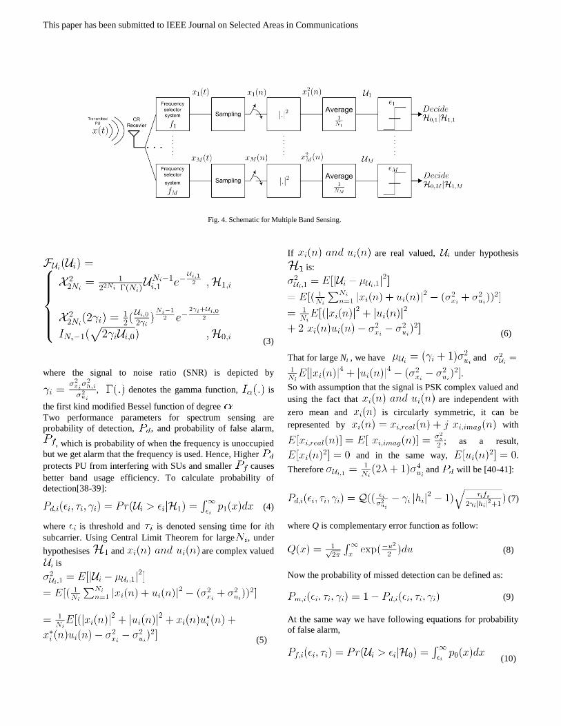
This paper has been submitted to IEEE Journal on Selected Areas in Communications

(3)

where the signal to noise ratio (SNR) is depicted by

, denotes the gamma function, is

the first kind modified Bessel function of degree

Two performance parameters for spectrum sensing are

probability of detection, , and probability of false alarm,

, which is probability of when the frequency is unoccupied

but we get alarm that the frequency is used. Hence, Higher

protects PU from interfering with SUs and smaller causes

better band usage efficiency. To calculate probability of

detection[38-39]:

(4)

where is threshold and is denoted sensing time for ith

subcarrier. Using Central Limit Theorem for large , under

hypothesises and are complex valued

is

(5)

If are real valued, under hypothesis

is:

(6)

That for large Ni , we have and

.

So with assumption that the signal is PSK complex valued and

using the fact that are independent with

zero mean and is circularly symmetric, it can be

represented by with

; as a result,

and in the same way, .

Therefore and will be [40-41]:

(7)

where Q is complementary error function as follow:

(8)

Now the probability of missed detection can be defined as:

(9)

At the same way we have following equations for probability

of false alarm,

(10)

Fig. 4. Schematic for Multiple Band Sensing.

This paper has been submitted to IEEE Journal on Selected Areas in Communications

(11)

Usually to evaluate the performance of energy detection, the

goal is to minimize for a target or to maximize .

for a target . At first we assume is our target

probability of detection and later we obtain threshold as a

function of , then substitute by in (11),

(12)

(13)

is the probability of false alarm

regard to target , and is the inverse of

complementary error function. For a target we

have:

(14)

(15)

is the probability of detection when

is targeted. As a result, in this part, probability of false

alarm and detection based on and ,

respectively, are calculated.

C. Model for Multiple Band Sensing

We present the model developed for wideband sensing as

illustrated in Fig. 4. At the first step, the primary user signal is

received by CR receiver at each subcarrier [42]. Next state is

sampling and after sampling, the test statistics of the energy

detection are obtained as the observed energy summation. At

the end, in regard to each threshold, the CR decides whether

the band is busy or idle. It is assumed that

and as

sensing time duration and the SNR for M subcarriers.

Moreover the probability of false alarm and detection for all

M subcarriers can be considered as

and . In the model, CR receiver can

search in all frequencies and detect idle frequencies. Then, CR

sends its results to scheduler and let it allocate the idle

spectrums based on different policies which are set to achieve

the goals like maximum total throughput and fairness

allocation[43].

D. Primary User Activity Model

In this section, we present a model for primary users’

activities which is directly proportional to CR network

performance. In the Markov chains model, it is considered that

two states (Busy by PU and Idle) are for each subcarrier. Since

each user arrival is independent, each transition follows the

Poisson arrival process. Thus, the length of Busy and Idle

periods are exponentially distributed (or the time that user

shall be served). The Poisson distribution is considered in the

modelling with arrival rate, α, and departure rate,β, and in

simulation, the average existing users is assumed such that

80% of total spectrums are loaded by primary users in

average.

(16)

As a result, the existing users in a cell is equivalent to total

existing users on previous time period added to arrival rate at

current time and subtracted by current departure time as

mentioned in equation (26). The transition probabilities are

pTand q

T as illustrated in Fig. 5. Hence, the probability

transition matrix, P, in this case is given by:

(17)

which results in transition rate matrix Q as:

(18)

(19)

(20)

The calculated steady probabilities are depicted below:

, (21)

Eq. (21) is applied to analyse the model for identifying

subcarriers states (i.e. busy or idle) [44-46].

E. Optimum Sensing time for A-SU in 4G CR network

The throughput of A-SU is calculated as follow while it can

access subcarrier when PU is not using that spectrum,

(22)

where W is bandwidth, is the power of transmitter CR

and is the noise power and is the gain channel

between ith CR transmitter and receiver with variance

.

Fig. 5. Markov Chains Model.

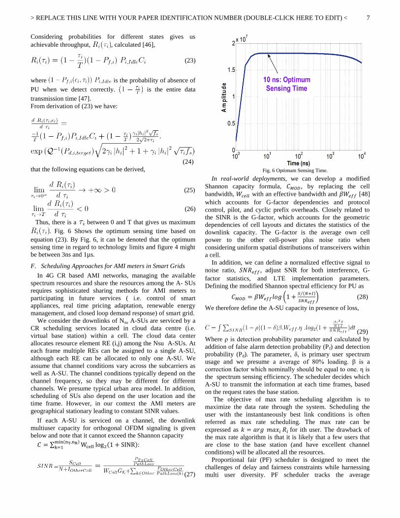
> REPLACE THIS LINE WITH YOUR PAPER IDENTIFICATION NUMBER (DOUBLE-CLICK HERE TO EDIT) <

7

Considering probabilities for different states gives us

achievable throughput, , calculated [46],

(23)

where is the probability of absence of

PU when we detect correctly.

is the entire data

transmission time [47].

From derivation of (23) we have:

(24)

that the following equations can be derived,

(25)

(26)

Thus, there is a between 0 and T that gives us maximum

. Fig. 6 Shows the optimum sensing time based on

equation (23). By Fig. 6, it can be denoted that the optimum

sensing time in regard to technology limits and figure 4 might

be between 3ns and 1µs.

F. Scheduling Approaches for AMI meters in Smart Grids

In 4G CR based AMI networks, managing the available

spectrum resources and share the resources among the A- SUs

requires sophisticated sharing methods for AMI meters to

participating in future services ( i.e. control of smart

appliances, real time pricing adaptation, renewable energy

management, and closed loop demand response) of smart grid.

We consider the downlinks of Nsu A-SUs are serviced by a

CR scheduling services located in cloud data centre (i.e.

virtual base station) within a cell. The cloud data center

allocates resource element RE (i,j) among the Nsu A-SUs. At

each frame multiple REs can be assigned to a single A-SU,

although each RE can be allocated to only one A-SU. We

assume that channel conditions vary across the subcarriers as

well as A-SU. The channel conditions typically depend on the

channel frequency, so they may be different for different

channels. We presume typical urban area model. In addition,

scheduling of SUs also depend on the user location and the

time frame. However, in our context the AMI meters are

geographical stationary leading to constant SINR values.

If each A-SU is serviced on a channel, the downlink

multiuser capacity for orthogonal OFDM signaling is given

below and note that it cannot exceed the Shannon capacity

∑ ( ) ( ) :

(27)

In real-world deployments, we can develop a modified

Shannon capacity formula, , by replacing the cell

bandwidth, with an effective bandwidth and [48]

which accounts for G-factor dependencies and protocol

control, pilot, and cyclic prefix overheads. Closely related to

the SINR is the G-factor, which accounts for the geometric

dependencies of cell layouts and dictates the statistics of the

downlink capacity. The G-factor is the average own cell

power to the other cell-power plus noise ratio when

considering uniform spatial distributions of transceivers within

a cell.

In addition, we can define a normalized effective signal to

noise ratio, , adjust SNR for both interference, G-

factor statistics, and LTE implementation parameters.

Defining the modified Shannon spectral efficiency for PU as

( ( )⁄

) (28)

We therefore define the A-SU capacity in presence of loss,

(29)

Where ρ is detection probability parameter and calculated by

addition of false alarm detection probability (Pf) and detection

probability (Pd). The parameter, δ, is primary user spectrum

usage and we presume a average of 80% loading. β is a

correction factor which nominally should be equal to one. η is

the spectrum sensing efficiency. The scheduler decides which

A-SU to transmit the information at each time frames, based

on the request rates the base station.

The objective of max rate scheduling algorithm is to

maximize the data rate through the system. Scheduling the

user with the instantaneously best link conditions is often

referred as max rate scheduling. The max rate can be

expressed as for ith user. The drawback of

the max rate algorithm is that it is likely that a few users that

are close to the base station (and have excellent channel

conditions) will be allocated all the resources.

Proportional fair (PF) scheduler is designed to meet the

challenges of delay and fairness constraints while harnessing

multi user diversity. PF scheduler tracks the average

Fig. 6 Optimum Sensing Time.

> REPLACE THIS LINE WITH YOUR PAPER IDENTIFICATION NUMBER (DOUBLE-CLICK HERE TO EDIT) <

8

throughput, Tk[nTs], for each A-SU delivered in the past over

sliding window of size tc .In the time frame [τ], the base

station receives rates Rk[nTs], k=1...Nsu from all the active A-

SUs and scheduler basically schedules the A-SU with highest

PF metric value, γ that is defined as .

The average throughputs Tk[nTs] are updated using an

exponentially weighted low pass-filter [49]:

(30)

Based on the Eq. (21) and (22) we can write as the following

(31)

Opportunistic Scheduling (OS) is an approach to deal with

both fairness among users and maximizing the capacity rate.

In max rate algorithm the user with highest request rate

implies giving all the system resources to particular users,

yields to highly unfair scheme to all other users. However, in

PF the users compete for resources not directly based on the

requested rates but based on the rates normalized by their

respective average throughputs also defined as PF metric

value. The downside of the PF approach is sacrificing over all

throughputs. Thus OS algorithm schedules subcarriers sc1,1 to

sci,j to the best secondary user based on two step criteria.

First, the user who has the maximum PF metric value, γ, is

selected. Second, the selected A-SU requested rate should be

greater than the mean of all the secondary users requested rate,

, to be scheduled as follow,

(32)

As a result, unlike PF scheduling, the users having low

throughput but high PF metric, γ, that have been chosen to

access resource elements will have lower priority than users

with enough PF metric and higher throughput.

Algorithm: Opportunistic scheduling

1) for n=1 to NT (simulation time)

2)Update A-SU profile, Update γ

3)Let S be the set of secondary users

4)Let RE(i,j) where i=1 to M subcarriers and j=1 to K be the

total time frames.

5)for i=1 to M, for j=1to K

6)Select the secondary user l ϵ S with highest γ(l)

7)If

8) Update the A-SU profile with S=S-l

9)Allocate RE(i,j) to lth secondary user from S

10)Else

11)Update the A-SU profile with S=S-l

12)End if, End for j, i, n

G. Inter-cell Interference coordination for Edge AMI meters

The performance of wireless cellular system is significantly

limited by Inter-cell Interference (ICI). The principal reason

for ICI is spatial reuse (i.e., the reuse of resource elements

such as timeslots or frequency bands) in a geographical

distance, where the signal strength is reduced due to path loss,

shadowing, and so on. In our 4G CR network, each A-SU

suffers from ICI due to frequency reuse in other cells adopted

by the primary user network frequency reuse patterns, which

lead to poor resource utilization and less spectral efficient. In

this paper we presume a frequency reuse of 2 is considered for

PU network. Researchers proposed network-level approaches

such as cooperative scheduling, multicell power control and

distributed antennas as means of reducing the interference and

improve spectral efficiency.

Ericson in [50-51] developed an uplink inter-cell

interference co-ordination/avoidance scheme for frequency

reuse. In this scheme cell users are divided in to two different

groups; cell center users and edge cell users. Only a part of the

frequency is used for cell-edge users with full power and

should be orthogonal between neighbor cells to mitigate most

of the interference. Cell-center users use the whole spectrum

with restricted power to transmit/receive, and hence there will

not too much ICI even the same frequency is used. In the case

of CR users, as we borrow the unused resource blocks and

specifically, the total interference power received at each PU

should not exceed a preselected interference temperature limit

(ITL) stated by FCC. There is not much flexibility to allocate

RBs separately for cell edge users and cell center users.

This challenge necessitates proposing a coordinated multi-

point uplink transmission scheme to improve cell-edge

performance in terms of average throughput. Fig. 7. shows

example scenario of A-SU present in the overlapping area of

both cells representing a cell edge user. Fig. 7. depicts cell

edge A-SU receives the received SINR from left BS is 10dB

and no idle hole for uplink transmission. Fig. 7. also shows

that left cell has high level of PU usage of RB. Cell edge A-

SU receives the received SINR from right BS is 16dB and has

idle hole for uplink transmission, so it performs uplink

transmission with right cell BS due to unused RB availability.

For the case2, Fig. 8. Shows if PUs moves from the range of

the left BS to right BS and now edge A-SU receives the

received SINR from left BS is 10dB and has idle hole for

uplink transmission. Cell edge A-SU also receives the

received SINR from right BS is 16dB and has idle hole for

uplink transmission, it performs uplink transmission with both

BS using coordinated multi-point uplink transmission scheme

as shown in Fig .8.

To evaluate the zero delay expected transmission time for

A-SU based on the allocated resource elements is defined as

treq for the remaining data size dt. Let Ri denote the

transmission rate of A-SUi with mi sub carriers allocated for

transmission with bandwidth BW. According to Shannon

theorem, the zero delay expected transmission time is given by

(33)

The zero delay expected transmission time for cell edge A-

SU in case 2 as follows:

(34)

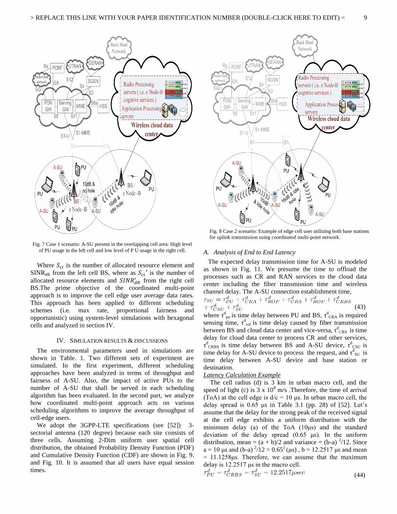
> REPLACE THIS LINE WITH YOUR PAPER IDENTIFICATION NUMBER (DOUBLE-CLICK HERE TO EDIT) <

9

Where is the number of allocated resource element and

SINRdB from the left cell BS, where as is the number of

allocated resource elements and from the right cell

BS.The prime objective of the coordinated multi-point

approach is to improve the cell edge user average data rates.

This approach has been applied to different scheduling

schemes (i.e. max rate, proportional fairness and

opportunistic) using system-level simulations with hexagonal

cells and analyzed in section IV.

IV. SIMULATION RESULTS & DISCUSSIONS

The environmental parameters used in simulations are

shown in Table. 1. Two different sets of experiment are

simulated. In the first experiment, different scheduling

approaches have been analyzed in terms of throughput and

fairness of A-SU. Also, the impact of active PUs to the

number of A-SU that shall be served in each scheduling

algorithm has been evaluated. In the second part, we analyze

how coordinated multi-point approach acts on various

scheduling algorithms to improve the average throughput of

cell-edge users.

We adopt the 3GPP-LTE specifications (see [52]) 3-

sectorial antenna (120 degree) because each site consists of

three cells. Assuming 2-Dim uniform user spatial cell

distribution, the obtained Probability Density Function (PDF)

and Cumulative Density Function (CDF) are shown in Fig. 9.

and Fig. 10. It is assumed that all users have equal session

times.

A. Analysis of End to End Latency

The expected delay transmission time for A-SU is modeled

as shown in Fig. 11. We presume the time to offload the

processes such as CR and RAN services to the cloud data

center including the fiber transmission time and wireless

channel delay. The A-SU connection establishment time,

(43)

where τdpu is time delay between PU and BS, τ

dCRA is required

sensing time, τdrof is time delay caused by fiber transmission

between BS and cloud data center and vice-versa, τd

CRS is time

delay for cloud data center to process CR and other services,

τd

CRBS is time delay between BS and A-SU device, τdCSU is

time delay for A-SU device to process the request, and τd

SU is

time delay between A-SU device and base station or

destination.

Latency Calculation Example

The cell radius (d) is 3 km in urban macro cell, and the

speed of light (c) is 3 x 108 m/s .Therefore, the time of arrival

(ToA) at the cell edge is d/c = 10 μs. In urban macro cell, the

delay spread is 0.65 μs in Table 3.1 (pp. 28) of [52]. Let’s

assume that the delay for the strong peak of the received signal

at the cell edge exhibits a uniform distribution with the

minimum delay (a) of the ToA (10μs) and the standard

deviation of the delay spread (0.65 μs). In the uniform

distribution, mean = (a + b)/2 and variance = (b-a) 2/12. Since

a = 10 μs and (b-a) 2/12 = 0.65

2 (μs) , b = 12.2517 μs and mean

= 11.1258μs. Therefore, we can assume that the maximum

delay is 12.2517 μs in the macro cell.

(44)

Fig. 7 Case 1 scenario: A-SU present in the overlapping cell area: High level

of PU usage in the left cell and low level of P U usage in the right cell.

Fig. 8 Case 2 scenario: Example of edge cell user utilizing both base stations

for uplink transmission using coordinated multi-point network.

> REPLACE THIS LINE WITH YOUR PAPER IDENTIFICATION NUMBER (DOUBLE-CLICK HERE TO EDIT) <

10

The τd

CRA and τdCRA are very minimum; therefore delay caused

by them is negligible. τdrof is the propagation delay incurred

for the signal to propagate through the medium. For a distance

of about 10km the round trip delay is app. to 100 μs. Finally,

the τdCRS the time delay for cloud data center to process CR

and other services is based on the hardware specifications of

provided the cloud infrastructure. A preliminary benchmark

analysis for various Intel processors using VTune performance

analyzer has been performed. We can tolerate the delay up to

200 μs and to satisfy the latency requirements our system

model needs minimum hardware specifications of 3.66 GHz

processor and 12M cache and other network level

requirements. Overall τSU delay is marginally reasonable to

perform cognitive functionality on to the cloud. It can be

realized due to the significant adoption of an on-demand

network access to a shared pool of configurable, computing

resources that can be rapidly provisioned and released by

cloud data center.

B. Scheduling Performance of AMI Packets on CR Networks

To evaluate the performance of transmitting AMI packets

on a CR system model, system level simulations have been

conducted based on 3GPP LTE physical layer parameter

assumptions. We first evaluate the system throughput for

algorithms with varying the primary user loading within a cell.

In this case, the primary user average loading is around 80%

and total number of users is 500 in a cell. Over the period of

time that spectrum sensing reports the number of idle resource

elements, scheduler allocates the idle REs with A-SUs. The

Fig. 12 illustrates average capacity for three aforementioned

algorithms.

Max-rate scheduling algorithm results in highest average

capacity among three algorithms, followed by opportunistic

and fairness algorithms. The results seem to match our

expectations, since the goal of the max-rate capacity is the

user with highest request rate implies giving all the system

resources to particular users. In proportional fair algorithm the

users compete for resources not directly based on the

requested rates but based on the rates normalized by their

respective average throughputs, PF metrics. By this approach

PF sacrifices the overall throughput while, achieving higher

number of A-SUs scheduled. In OS the users having low

request rate but high PF metric, γ, will have less chance to be

scheduled. OS objective is to achieve higher average capacity

compared to PF, while achieving decent fairness among the A-

SUs.

Fig. 13.a and 13.b show the average number of users

scheduled per one Transmission Time Interval (TTI) when 75

A-SUs are active in a cell and around 20% and 30% of idle RE

are available. We can see that at least 60 and 70 A-SUs are

scheduled to idle REs by fairness algorithm. OS and max rate

algorithms allocate less number of average SUs respectively.

In Fig. 14, we analyze the scheduled A-SUs average

capacity for each scheduling algorithm when number of active

PUs varies. Based on goals of each algorithm they indicate

respective positions in the results. It can be seen that the

solution obtained using the proposed algorithm (OS) is quite

close to the PF specifically when the active PUs are less.

We note that in scenario where less PU are scheduled, it

yields to high availability of idle REs. Therefore, higher

number of A-SUs scheduled results in larger average capacity

in the CR network. When the numbers of PUs are increased,

the advantage of the OS algorithm over PF is more obvious

(i.e. Fig.14) due to more sparse A-SUs. Sparse implies large

variability in A-SUs profile (i.e. SINR, fading channel,

physical location).

In Fig. 15, we analyze the average number of scheduled SUs

in each scenario when number of active PUs varies. We note

that the more PUs scheduled yields to less availability of idle

REs and therefore less number of A-SU scheduled. In Fig. 14

the Max-Rate average capacity is much higher than average

capacity of PF; on the contrary, Fig. 15 shows the more

scheduled A-SUs by PF algorithm compared to Max-Rate

algorithm. As a result, the OS algorithm can balance both the

performance of the cognitive radio networks in terms of

achieving acceptable average capacity of A-SUs and the

fairness.

C. Coordinated Multi-point Performance of AMI Edge Users

In the second experiment, we evaluate the number of cell

edge A-SUs scheduled by the scheduling schemes enabled by

Fig. 10. G-factor CDFs for the cell.

Fig. 9. PDF of SINR of all the users ( i.e. PU and A-SU) within a cell.

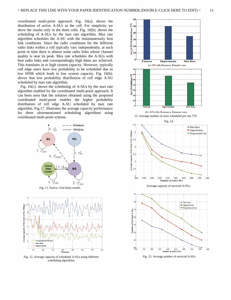
> REPLACE THIS LINE WITH YOUR PAPER IDENTIFICATION NUMBER (DOUBLE-CLICK HERE TO EDIT) <

11

coordinated multi-point approach. Fig. 16(a). shows the

distribution of active A-SUs in the cell. For simplicity we

show the results only in the three cells. Fig. 16(b). shows the

scheduling of A-SUs by the max rate algorithm. Max rate

algorithm schedules the A-SU with the instantaneously best

link conditions. Since the radio conditions for the different

radio links within a cell typically vary independently, at each

point in time there is almost some radio links whose channel

quality is near its peak. Max rate schedules the A-SUs with

best radio links and correspondingly high dates are achieved.

This translates in to high system capacity. However, typically

cell edge users have low probability to be scheduled due to

low SINR which leads to low system capacity. Fig. 16(b).

shows that low probability distribution of cell edge A-SU

scheduled by max rate algorithm.

Fig. 16(c). shows the scheduling of A-SUs by the max rate

algorithm enabled by the coordinated multi-point approach. It

can been seen that the solution obtained using the proposed

coordinated multi-point enables the higher probability

distribution of cell edge A-SU scheduled by max rate

algorithm. Fig.17. illustrates the average capacity performance

for three aforementioned scheduling algorithms using

coordinated multi-point scheme.

Fig. 11. End-to- End delay model.

Fig. 12. Average capacity of scheduled A-SUs using different

scheduling algorithms

13. Average number of users scheduled per one TTI

Fig. 15. Average number of serviced A-SUs

Fig. 14.

Average capacity of serviced A-SUs.

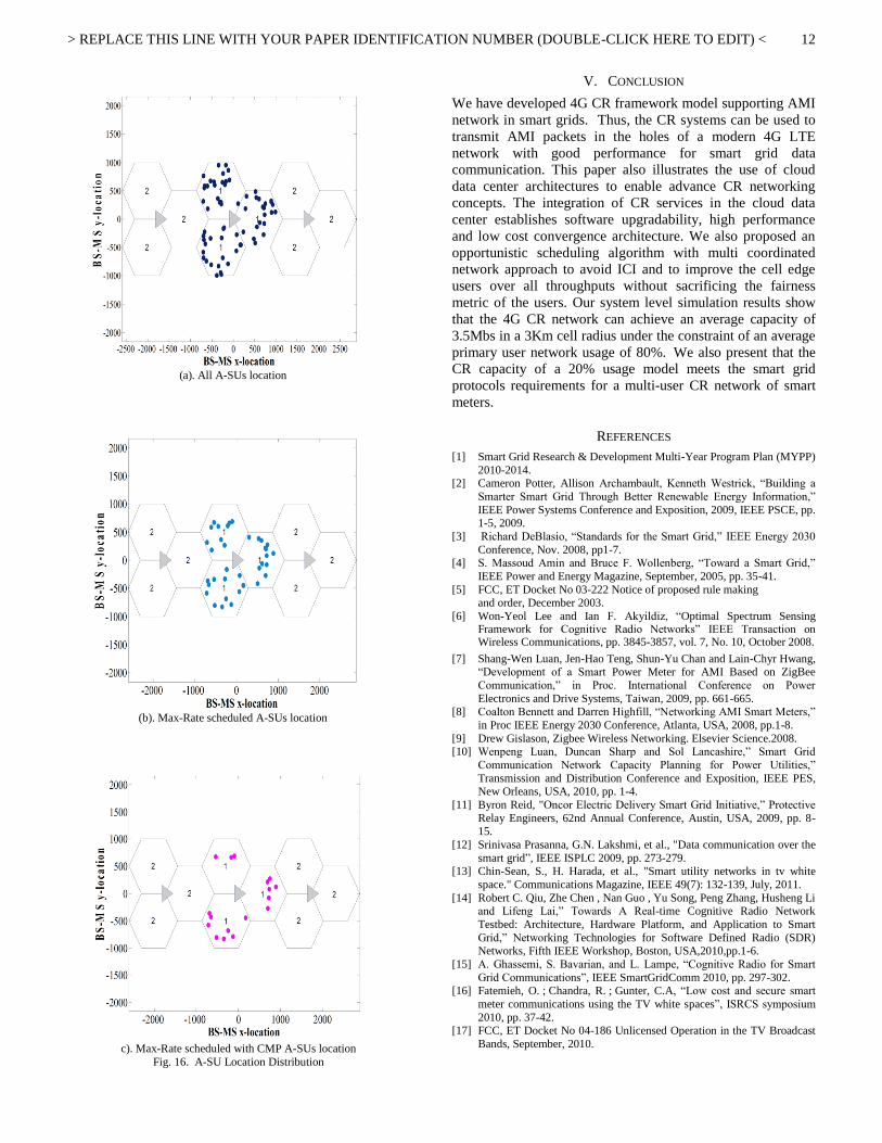
> REPLACE THIS LINE WITH YOUR PAPER IDENTIFICATION NUMBER (DOUBLE-CLICK HERE TO EDIT) <

12

V. CONCLUSION

We have developed 4G CR framework model supporting AMI

network in smart grids. Thus, the CR systems can be used to

transmit AMI packets in the holes of a modern 4G LTE

network with good performance for smart grid data

communication. This paper also illustrates the use of cloud

data center architectures to enable advance CR networking

concepts. The integration of CR services in the cloud data

center establishes software upgradability, high performance

and low cost convergence architecture. We also proposed an

opportunistic scheduling algorithm with multi coordinated

network approach to avoid ICI and to improve the cell edge

users over all throughputs without sacrificing the fairness

metric of the users. Our system level simulation results show

that the 4G CR network can achieve an average capacity of

3.5Mbs in a 3Km cell radius under the constraint of an average

primary user network usage of 80%. We also present that the

CR capacity of a 20% usage model meets the smart grid

protocols requirements for a multi-user CR network of smart

meters.

REFERENCES

[1] Smart Grid Research & Development Multi-Year Program Plan (MYPP)

2010-2014. [2] Cameron Potter, Allison Archambault, Kenneth Westrick, ―Building a

Smarter Smart Grid Through Better Renewable Energy Information,‖

IEEE Power Systems Conference and Exposition, 2009, IEEE PSCE, pp. 1-5, 2009.

[3] Richard DeBlasio, ―Standards for the Smart Grid,‖ IEEE Energy 2030

Conference, Nov. 2008, pp1-7. [4] S. Massoud Amin and Bruce F. Wollenberg, ―Toward a Smart Grid,‖

IEEE Power and Energy Magazine, September, 2005, pp. 35-41.

[5] FCC, ET Docket No 03-222 Notice of proposed rule making

and order, December 2003.

[6] Won-Yeol Lee and Ian F. Akyildiz, ―Optimal Spectrum Sensing Framework for Cognitive Radio Networks‖ IEEE Transaction on Wireless Communications, pp. 3845-3857, vol. 7, No. 10, October 2008.

[7] Shang-Wen Luan, Jen-Hao Teng, Shun-Yu Chan and Lain-Chyr Hwang, ―Development of a Smart Power Meter for AMI Based on ZigBee

Communication,‖ in Proc. International Conference on Power

Electronics and Drive Systems, Taiwan, 2009, pp. 661-665. [8] Coalton Bennett and Darren Highfill, ―Networking AMI Smart Meters,‖

in Proc IEEE Energy 2030 Conference, Atlanta, USA, 2008, pp.1-8.

[9] Drew Gislason, Zigbee Wireless Networking. Elsevier Science.2008. [10] Wenpeng Luan, Duncan Sharp and Sol Lancashire,‖ Smart Grid

Communication Network Capacity Planning for Power Utilities,‖

Transmission and Distribution Conference and Exposition, IEEE PES, New Orleans, USA, 2010, pp. 1-4.

[11] Byron Reid, "Oncor Electric Delivery Smart Grid Initiative,‖ Protective

Relay Engineers, 62nd Annual Conference, Austin, USA, 2009, pp. 8-15.

[12] Srinivasa Prasanna, G.N. Lakshmi, et al., "Data communication over the

smart grid‖, IEEE ISPLC 2009, pp. 273-279. [13] Chin-Sean, S., H. Harada, et al., "Smart utility networks in tv white

space." Communications Magazine, IEEE 49(7): 132-139, July, 2011.

[14] Robert C. Qiu, Zhe Chen , Nan Guo , Yu Song, Peng Zhang, Husheng Li and Lifeng Lai,‖ Towards A Real-time Cognitive Radio Network

Testbed: Architecture, Hardware Platform, and Application to Smart

Grid,‖ Networking Technologies for Software Defined Radio (SDR) Networks, Fifth IEEE Workshop, Boston, USA,2010,pp.1-6.

[15] A. Ghassemi, S. Bavarian, and L. Lampe, ―Cognitive Radio for Smart

Grid Communications‖, IEEE SmartGridComm 2010, pp. 297-302. [16] Fatemieh, O. ; Chandra, R. ; Gunter, C.A, ―Low cost and secure smart

meter communications using the TV white spaces‖, ISRCS symposium

2010, pp. 37-42. [17] FCC, ET Docket No 04-186 Unlicensed Operation in the TV Broadcast

Bands, September, 2010.

(a). All A-SUs location

(b). Max-Rate scheduled A-SUs location

c). Max-Rate scheduled with CMP A-SUs location

Fig. 16. A-SU Location Distribution

> REPLACE THIS LINE WITH YOUR PAPER IDENTIFICATION NUMBER (DOUBLE-CLICK HERE TO EDIT) <

13

[18] Jon M. Peha, ―Sharing Spectrum Through Spectrum Policy Reform and Cognitive Radio,‖ Proceedings of the IEEE, Vol 97, No. 4, 2009, pp. 708-719.

[19] Chittabrata Ghosh and Dharma P. Agravwal, ―Channel Assignment with Route Discovery (CARD) Using Cognitive Radio in Multi-channel Multi-radioWireless Mesh Networks‖, 2006 IEEE Conference on Software Defined Radio.

[20] Brian Kelley, ―Software Defined Radio for Broadband OFDM Protocols,‖ SMC 2009, San Antonio.

[21] Brian Kelley, Software Defined Radio for Advanced Gigabit Cellular Systems, to appear in DSP Handbook & Wireless, Networking, Radar, Sensor Array Processing, and Nonlinear Signal Processing, Chapter 22, 2009.

[22] Weifang Wang, ―Spectrum Sensing for Cognitive Radio,‖ Third International Symposium on Intelligent Information Technology Application Workshops, IEEE computer society, 2009, pp. 410-412.

[23] D.D.Ariananda, M.K.Lakshmanan, H.Nikookar, ―A survey on spectrum sensing techniques for cognitive radio,‖ Cognitive Radio and Advanced Spectrum Management, 2009. CogART 2009. Second International Workshop on, pp. 74 – 79.

[24] Akyildiz, I. F., Lee, W.-Y., Vuran, M. C., and Mohanty, S, ―Next gen-

eration dynamic spectrum access cognitive radio wireless networks: a survey," Computer Networks Journal (Elsevier), 2006.

[25] Kranthimanoj Nagothu, Brain Kelley, Mo Jamshidi and Amir Raajee,

―Persistent Net-AMI for Microgrid Infrastructure Using Cognitive Radio on Cloud Data Centers‖, accepted in IEEE system Journal, special

edition Integration of Intermittent Renewable Energy Resources into

Power grid, April 2012. [26] Minh-Viet, N. and L. Hwang Soo. "Effective Scheduling in

Infrastructure-Based Cognitive Radio Networks." Mobile Computing,

IEEE Transactions on vol. 10 No.6, pp. 853-867, 2011. [27] Qing Zhao ; Sadler, B.M. ;., ―A Survey of Dynamic Spectrum Access,‖

IEEE Sig. Proc. Mag., vol 24, no.3, pp.79-89, 2007.

[28] Shuai Zhang, Shufen Zhang, Xuebin Chen and Xiuzhen Huo,‖ Cloud Computing Research and Development Trend‖, Future Networks, ICFN

'10, Sanya, Hainan, 2010, pp. 93-97.

[29] Bhaskar Prasad Rimal, Eumi Choi and Ian Lamb, ―A Taxnomy and Survey of Cloud Computing Systems,‖ in Proc. Fifth International Joint

Conference on INC, IMS and IDC, 2009, pp. 44-51.

[30] Junjie Peng, Xuejun Zhang Zhou Lei, Bofeng Zhang, Wu Zhang and Qing Li,‖ Comparison of Several Cloud Computing Platforms,‖

Information Science and Engineering (ISISE), Dec, 2009, pp. 23-27.

[31] Qing Zhao ; Sadler, B.M. ; ―A Survey of Dynamic Spectrum Access‖ IEEE Signal Processing Magazine, pp.79-89, vol. 24, May 2007.

[32] Zhang Jingping,‖ Theoretical Analysis of Combination and Detection

for Short-Term Cooperative Sensing in Cognitive Radio Systems‖ 2nd International Conforence on Education Technology and Computer

(ICETC), vol. 2, pp. 381 -384, June 2010. [33] Akyildiz, I.F. ; Won-Yeol Lee ; Vuran, M.C. ; Mohanty, S. ; ―A survey

on spectrum management in cognitive radio networks‖ IEEE

Communications Magazine, pp. 40-48, April 2008. [34] Carlos Cordeiro, Kiran Challapali, and Dagnachew Birru,‖ IEEE

802.22: An Introduction to the First Wireless Standard based on

Cognitive Radios‖ Journal of Communications, Vol. 1, No. 1, April 2006.

[35] Digham, F. F. ; Alouini, M.-S. ; Simon, M. K. ; ―On the Energy

Detection of Unknown Signals Over Fading Channels‖ IEEE

Transactions on Communications, vol. 55, pp. 21-24, Jan 2007.

[36] Digham, F.F. ; Alouini, M.-S. ; Simon, M.K. ; ―On the energy detection

of unknown signals over fading channels‖ ICC '03. IEEE International Conference on Communications, vol. 5, pp. 3575-3579, May 2003.

[37] Zhi Quan ; Shuguang Cui ; Sayed, A.H. ; Poor, H.V. ; ―Optimal

Multiband Joint Detection for Spectrum Sensing in Cognitive Radio Networks ‖ IEEE Transaction on Signal Processing, pp. 1128-1140, vol.

57, November 2008.

[38] Feng, T. ; Wang, G. ; Culver, S. ; Gidlund, M. ; ―Collaborative Spectrum Sensing in Cognitive Radio System - Performance Analysis of Weighted

Gain Combining‖ Communication Networks and Services Research

Conference (CNSR), pp. 1-6, May 2011. [39] Zhi Quan, Shuguang Cui, and Ali H. Sayed,‖ Optimal Linear

Cooperation for Spectrum Sensing in Cognitive Radio Networks‖ IEEE

Journal Of Selected Topics In Signal Processing, Vol. 2, No. 1, February 2008.

[40] Zhaoxia Song ; Zheng Zhou ; Xuan Sun ; Zhichao Qin ; ―Cooperative

Spectrum Sensing for Multiband under Noise Uncertainty in Cognitive Radio Networks‖ IEEE International Conference ICC, pp. 1-5, 2010.

[41] Jiang Zhu ; Benxiong Huang ; Furong Wang ; Bo Zhang ; Wei

Wu ; ―AEF Analysis of Central Limit Theory Approximation in Spectrum Sensing‖ WiCom '09. 5th International Conference on

Wireless Communications, Networking and Mobile Computing, pp. 1-4,

2009. [42] Khalid, L. ; Anpalagan, A. ; ―Effect of sensing errors on

wideband cognitive OFDM radio networks‖ IEEE Biennial Symposium

QBSC, pp. 273-277, 2010. [43] Zhi Quan ; Shuguang Cui ; Sayed, A.H. ; Poor, H.V. ; ―Wideband

Spectrum sensing in Cognitive Radio Networks ‖ IEEE International

Conference, pp. 901-906, 2008. [44] Ghosh, C. ; Cordeiro, C. ; Agrawal, D.P. ; Rao, M.B. ; ―Markov chain

existence and Hidden Markov models in spectrum sensing‖ IEEE

International Conference, pp.1-6, 2009. [45] Siddhartha Chib; Edward Greenberg; ―Understanding the Metropolis-

Hastings Algorithm‖ The American Statistician, Vol. 49, No. 4. (Nov.,

1995), pp. 327-335. [46] Xiao Yu Wang, Alexander Wong, and Pin-Han Ho ―Spectrum Sensing

in Cognitive Radio Using a Markov-Chain Monte-Carlo Scheme‖ IEEE

Communications Letters, Vol. 14, No. 9, September 2010. [47] Ying-Chang Liang, Yonghong Zeng, Edward C.Y. Peh, and Anh Tuan

Hoang,―Sensing-Throughput Tradeoff for Cognitive Radio Networks‖

IEEE TRANSACTIONS ON WIRELESS COMMUNICATIONS, VOL. 7, NO. 4, APRIL 2008

[48] Preben Mogensen, et al, ―LTE Capacity compared to the Shannon Bound,‖ IEEE 65th Vehicular Technology Conference, 2007. VTC2007-

Spring. April 2007.

[49] Davis Tse and Pramod Viswanth, ―Fundamentals of Wireless Communications‖, Cambridge university press, 2005.

[50] R1-050764,‖Inter-cell Interference Handling for EUTRA‖, Ericsson,

August 28-September 2,2005 [51] R1-061374,―Downlink inter-cell interference coordination avoidance-

evaluation of frequency reuse‖, Ericsson, May, 2006.

[52] Lathaharan Somasegaran, "Channel Estimation and Prediction in UMTS LTE," Master Thesis (Aalborg University), 2007.

> REPLACE THIS LINE WITH YOUR PAPER IDENTIFICATION NUMBER (DOUBLE-CLICK HERE TO EDIT) <

14

APPENDIX

Table Parameters Value

Cell-level user distribution Uniform

Power delay profile 3gppTU

G-factor Ref [48]

Inter-Site DistanceCell 1732 Meters

Cell Layout Hexagonal Grid, 3 sector sites

Network Scheduling

Frequency Domain

Packet Scheduler

LTE-OFDM MIMO: 1Tx, 2Rx

Deployment Spectral Efficiency 1.5bits/sec/Hz [48]

Bandwidth 20MHz

RB Bandwith 180kHz

3dB Beam-width (θ3dB) 70

Maximum Attenuation (Am) 20dB

Cognitive Radio Secondary Usage 10%

Cognitive Radio Primary Load 80%

Modulation/code rate settings

Qpsk/ 0.2-0.8

16QAM/ 0.5-0.9

64QAM/ 0.5-0.9

Channel Estimation Ideal

Carrier frequency 2GHz Table 1: Network Capacity Parameters for Cognitive Radio AMI Network

This article has been accepted for inclusion in a future issue of this journal. Content is final as presented, with the exception of pagination.

IEEE SYSTEMS JOURNAL 1

Persistent Net-AMI for Microgrid InfrastructureUsing Cognitive Radio on Cloud Data Centers

Kranthimanoj Nagothu, Student Member, IEEE, Brian Kelley, Senior Member, IEEE, Mo Jamshidi, Fellow, IEEE, andAmir Rajaee, Student Member, IEEE

Abstract—We address the potential for a truly universal set ofintegrated wireless communication services, energy management,and control services for a next-generation of National Institute ofStandards and Technology microgrid standards. Our approachuses cloud computing data center as the central communicationand optimization infrastructure supporting a cognitive radionetwork of AMI meters which we label netbook advance meteringinfrastructure (Net-AMI). The Net-AMI is a novel low costinfrastructure of AMI meters that operate akin to netbookswith wireless transceiver that access to cloud data center energyservices, cognitive radio services, and wireless communicationservices. Access occurs via cognitive radios channels. We claimthat this solution solves the important problem in smart gridsystems of how to develop an extensible, persistent, smart gridinformation network with a lifespan equivalent to that of mostpower systems (20–30 years). By persistence, we imply alwaysoperable, entirely software upgradeable, and independent ofcellular networks. Our system is extensible and can easily handlethousands of variations in power systems, communication pro-tocols, control, and energy optimization protocols. We formulatenecessary link analysis and optimum scheduling of downlinkand uplink Net-AMI packets in a multiuser cognitive radioenvironment.

Index Terms—Cloud data center, cognitive radio, netbookadvance metering infrastructure (Net-AMI), smart grid, wireless.

I. Introduction

THE SMART grid of the future is generally anticipatedto consist of an intelligent energy delivery system that

supports plug-and-play integration of power, information, andsecurity services. The future smart grid should possess awide range of attributes that enable it to cope with infor-mation delivery, power flow distribution, intermittent energysources, transmission line failures, energy storage systems,command and control of national infrastructure to achievepeak efficiency. In addition, as critical infrastructure it supportscommerce and service needs. Resiliency and persistency inthe aftermath of a major disruption is of the utmost im-

Manuscript received August 5, 2010; revised January 17, 2011; acceptedMay 25, 2011. This work was supported in part by the Texas SustainableEnergy Conservation Office and the U.S. Department of Energy under GrantRFA RE-AG1-2010, and by the Lutcher Brown Chair Endowment at theUniversity of Texas System, San Antonio.

The authors are with the University of Texas, San Antonio, TX 78249 USA(e-mail: kranthimanoj@gmail.com; brian.kelley@utsa.edu; moj@wacong.org;amirajaee@gmail.com).

Color versions of one or more of the figures in this paper are availableonline at http://ieeexplore.ieee.org.

Digital Object Identifier 10.1109/JSYST.2011.2162794

portance to minimize economic disturbances. Future serviceswill involve autonomous control of smart appliances, realtime pricing adaptation, shifting grid-tied power usage to non-peak periods, renewable energy management, and closed loopdemand response [2], [3]. The services should be support-ive of high penetrations of renewable energy components.It also acts as platform for consumer engagement in loadmanagement, national energy independence, and economicsecurity [1]. In many such scenarios services, the advancedmetering infrastructure (AMI) system is a central access pointfor communication of information flows in the smart grid andmicro-grid distribution system networks.

We describe a new flexible Net-AMI infrastructure thatsupports the distributed smart grid. The Net-AMI networkin the smart grid realm can be connoted as the firmwareanalogous to the PC-Netbooks [4], but integrated to the realmNet-AMI infrastructure. In addition, in our model of the pro-cessing, public and private energy services reside in customeraccessible cloud data center containing remote servers. Thecloud offers other services such as demodulation of homearea network protocols (IEEE 802.15.4–Zigbee, Bluetooth,and Proprietary RF). Moreover, it also hosts energy managerapplications with all the optimization algorithms residing inthe cloud. It also provides microgrid energy optimization andother control services.

Net-AMI meters behave akin to a message relay and storagewith a modicum of processing capabilities and communicationand wireless interfaces. Rather than full fledged intelligentcontrol processing devices, the Net-AMI is optimized forcarrying out control tasks, accessing power system informationin buildings and home area networks, and relaying (andreceiving) data whose fundamental processing occurs in clouddata centers.

We define an ideal Net-AMI meter network attributes as:1) low cost infrastructure (due to cell tower reuse and lowfrequency band costs) that is simultaneously rapidly deploy-able and can communicate wirelessly to a metropolitan widenetwork; 2) supports a universal set of protocols, standards,including most wireless and proprietary standards; 3) an abilityto extensively adapt to future protocols via software (nothardware) upgrades; and 4) persistent power information flowsof building usage and control, especially during power linedisruption (e.g., convert to microgrid control due to hurricanes,lighting, transmission line failures). It should also persist ifa service provider exits the market, a customer lacks paid

1932-8184/$26.00 c© 2011 IEEE

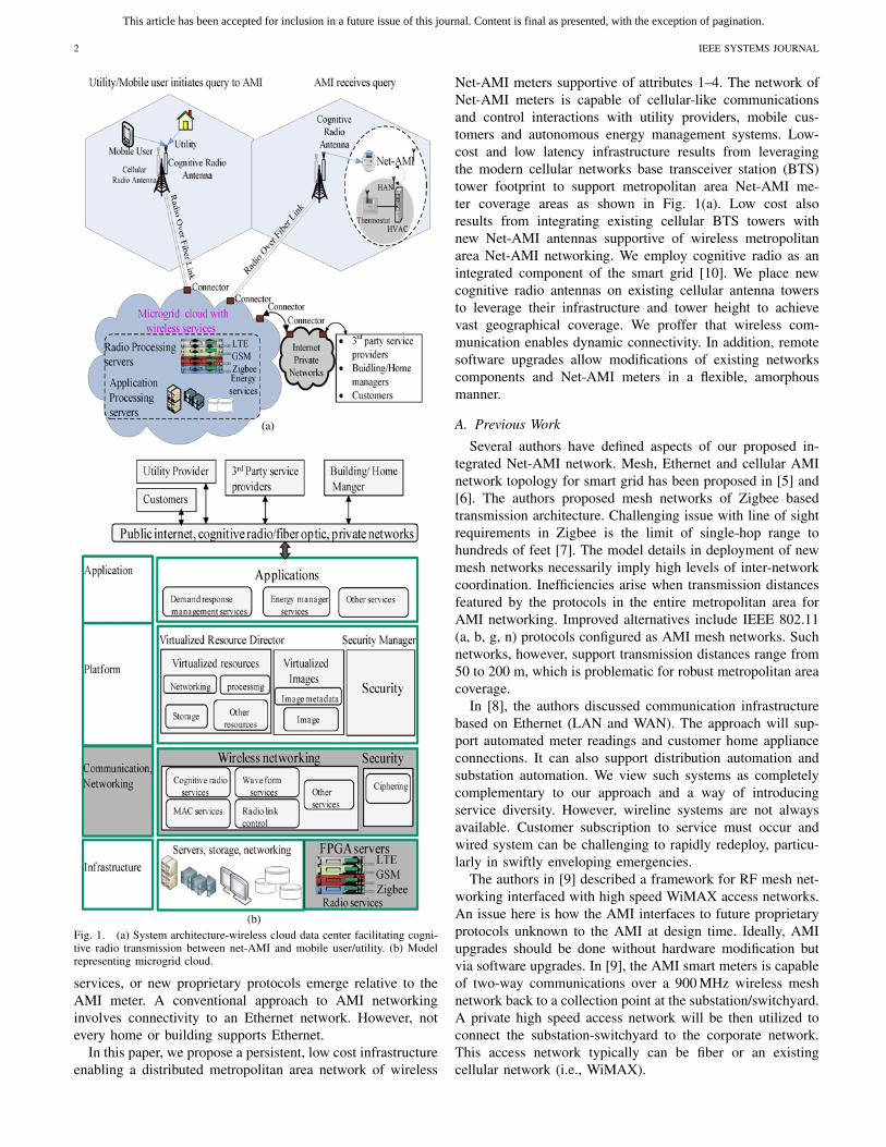
This article has been accepted for inclusion in a future issue of this journal. Content is final as presented, with the exception of pagination.

2 IEEE SYSTEMS JOURNAL

Fig. 1. (a) System architecture-wireless cloud data center facilitating cogni-tive radio transmission between net-AMI and mobile user/utility. (b) Modelrepresenting microgrid cloud.

services, or new proprietary protocols emerge relative to theAMI meter. A conventional approach to AMI networkinginvolves connectivity to an Ethernet network. However, notevery home or building supports Ethernet.

In this paper, we propose a persistent, low cost infrastructureenabling a distributed metropolitan area network of wireless

Net-AMI meters supportive of attributes 1–4. The network ofNet-AMI meters is capable of cellular-like communicationsand control interactions with utility providers, mobile cus-tomers and autonomous energy management systems. Low-cost and low latency infrastructure results from leveragingthe modern cellular networks base transceiver station (BTS)tower footprint to support metropolitan area Net-AMI me-ter coverage areas as shown in Fig. 1(a). Low cost alsoresults from integrating existing cellular BTS towers withnew Net-AMI antennas supportive of wireless metropolitanarea Net-AMI networking. We employ cognitive radio as anintegrated component of the smart grid [10]. We place newcognitive radio antennas on existing cellular antenna towersto leverage their infrastructure and tower height to achievevast geographical coverage. We proffer that wireless com-munication enables dynamic connectivity. In addition, remotesoftware upgrades allow modifications of existing networkscomponents and Net-AMI meters in a flexible, amorphousmanner.

A. Previous Work

Several authors have defined aspects of our proposed in-tegrated Net-AMI network. Mesh, Ethernet and cellular AMInetwork topology for smart grid has been proposed in [5] and[6]. The authors proposed mesh networks of Zigbee basedtransmission architecture. Challenging issue with line of sightrequirements in Zigbee is the limit of single-hop range tohundreds of feet [7]. The model details in deployment of newmesh networks necessarily imply high levels of inter-networkcoordination. Inefficiencies arise when transmission distancesfeatured by the protocols in the entire metropolitan area forAMI networking. Improved alternatives include IEEE 802.11(a, b, g, n) protocols configured as AMI mesh networks. Suchnetworks, however, support transmission distances range from50 to 200 m, which is problematic for robust metropolitan areacoverage.

In [8], the authors discussed communication infrastructurebased on Ethernet (LAN and WAN). The approach will sup-port automated meter readings and customer home applianceconnections. It can also support distribution automation andsubstation automation. We view such systems as completelycomplementary to our approach and a way of introducingservice diversity. However, wireline systems are not alwaysavailable. Customer subscription to service must occur andwired system can be challenging to rapidly redeploy, particu-larly in swiftly enveloping emergencies.

The authors in [9] described a framework for RF mesh net-working interfaced with high speed WiMAX access networks.An issue here is how the AMI interfaces to future proprietaryprotocols unknown to the AMI at design time. Ideally, AMIupgrades should be done without hardware modification butvia software upgrades. In [9], the AMI smart meters is capableof two-way communications over a 900 MHz wireless meshnetwork back to a collection point at the substation/switchyard.A private high speed access network will be then utilized toconnect the substation-switchyard to the corporate network.This access network typically can be fiber or an existingcellular network (i.e., WiMAX).

This article has been accepted for inclusion in a future issue of this journal. Content is final as presented, with the exception of pagination.

NAGOTHU et al.: PERSISTENT NET-AMI FOR MICROGRID INFRASTRUCTURE USING COGNITIVE RADIO ON CLOUD DATA CENTERS 3

The rest of this paper is organized as follows. Section IIdiscusses core concepts such as cloud data center model,cognitive radio model, radio over fiber involved in developingNet-AMI networking infrastructure system in brief. Section IIIdescribes the overview of cognitive radio Net-AMI networksystem model. This section also details procedure of AMIinformation flow through communication protocol. Moreover,a hybrid RF-Optical communication analytical model is de-veloped. Section IV details about study results on the overallsystem model and concludes this paper.

II. Core Concept Ideas Key to Persistent

Net-AMI Networking

A. Cloud Data Center System Model

The energy services of the future can be privately contractedservices or public services. The centralized energy servicesmanager resides on a cloud computing data center. The cloudcenter enables convenient, on-demand network access to ashared pool of configurable, computing resources (e.g., net-works, servers, storage, applications, and services) that can berapidly provisioned and released with minimal managementeffort [11], [12]. Cloud computing improves the availability ofcomputing resources for wide varieties of software services.For instance, it can provide self-help services without the needfor any manual interactions with service providers [13]. In ourscenario of wireless cloud services, elasticity plays vital roledue to high variations in the rate of users change accessingservices. Cloud system services can reside far from physicallocations of users.

There are different cloud computing platform classifications.Standard architectures include Abi (or Abiquo), Nimbus OpenNebula, Azure (Microsoft), Google (App Engine), Blue (IBM),and Mosso (Rackspace) (see [14]). Fig. 1(b) depicts the modelfor a cloud data center architecture optimized for microgridbased smart grids. Microgrids can act as an island with a set ofloads, energy storage, and dynamic adjustable capability whichcan be detached from grid-tied power. The layered designof microgrid architecture is formulated on the bases fromcurrently existing cloud architecture but extrapolated with anew additional layer of communication and networking as aservice. Our microgrid cloud is layered into four layers.

1) Application Layer: This layer facilitates consumersto utilize the providers’ application running on the cloudinfrastructure. Applications may vary from energy services,optimization services to music and video services. Applicationlayer is interfaced by the utility providers, customers, thirdparty energy services providers via cognitive radio, internet orprivate networks. Consider an example, where a utility updatesthe AMI meter at any location with real-time pricing abilityusing an API on the cloud. The building energy manager(i.e., energy management service provider for end user) callsa different API on the cloud to access the real time pricing toevaluate and consider necessary changes to make a beneficiarydecision. Eventually, the energy manager will send a controlsignal to net-AMI meter to allocate power flows amongintermittent renewable sources, grid-tied sources, and loadsto maintain equilibrium via demand response management

applications. When load demand is high and plant facilitiesneed additional power capacity, the energy manger sends APIrequests to all the customers registered in demand responseservice to shutter devices or reduce serviceable loads (i.e.,HVAC, lighting) according to a preplanned load prioritiza-tion scheme. These application services can be accessed byvarious partners with particular access control rights leadingto a secure system. The attribute of accessing API’s permitsinteroperability and extensibility around the cloud servicessupporting microgrids [15].

2) Platform Layer: The platform layer applications canbe created using tools, software’s provided by the cloud.Moreover, the layer attributes include a virtualization resourcedirector (VRD) and security manager. The VRD allows usersto create virtual machines and configure them with a specificoperating system, resource allocation (i.e., CPU, memory) andsoftware. However, the VRD has the ability to control andlimit resources (i.e., CPU or memory) utilized by the users[16], [17]. This layer also supports the creation of images andimage metadata.

The platform layer also dictates how security policies arecreated, managed and enforced in the cloud. It provides au-thentication, identity management mechanism to authenticateusers and services based on credentials and characteristics.Trust management and policy integration enables multipleservice providers to coexist and collaborate. It ensures thatthese features are handled securely and security breachesare effectively monitored during the interoperation process.Access controls, privacy and data management issues to bedealt with cloud. As some of the business enterprises are notcomfortable storing their customer’s data and applications onsystems that reside outside of their on-premise datacenters.However there are large communities of researchers develop-ing enhancements to existing solutions as well as creating ma-ture newer solutions to above stated security related paradigms[18]–[21]. We contend that cloud computing benefits are fullyrealized as its adoption accelerates.

3) Communication and Networking Layer: This layerconsists of services specifically designed to deliver network-ing services. By this feature AMI network service providers(ANSP) will have the ability to leverage cloud and providevarious services. ANSP can allocate on demand servicesarbitrarily at any period time with minimum latency by dy-namically upgrading the connectivity between the sites andutilizing vast cloud resources (i.e., CPU, high bandwidth). Forinstance, when there are large requests for a live streaming ofhigh definition video. The ANSPs can leverage the servicesprovided in this layer to adapt to the scenario and provide qual-ity services to users. It also provides a common managementframework by operating the services across the distributedresources rather than operating at separate facilities with fixedresource allocation. Among the services provided are cognitiveradio services, waveform services, radio link control (RLC),and medium access control (MAC) services. Cognitive radioservices, which provide spectrum management and spectrumsensing, are discussed further in Section III.

Waveform services represent error correction, modulationand demodulation for various protocols [i.e., long term evo-

This article has been accepted for inclusion in a future issue of this journal. Content is final as presented, with the exception of pagination.

4 IEEE SYSTEMS JOURNAL

lution (LTE), GSM]. The RLC services transport traffic be-tween user devices and enodeB. The MAC services providescheduling, reliability with advance transmission schemes andother services. Moreover, RLC provides ciphering (e.g., 128 bitAES) to the data. It ensures confidentiality and integrity of thesignaling data. Finally, cloud communication and networkingsolution will lead to compelling next generation cloud com-munication networking services.

4) Infrastructure Layer: The infrastructure layer facili-tates the effective integration of computing resources, storage,networks to deploy applications and operating systems. Weaugment our cloud infrastructure microprocessor racks withFPGA boards targeted to processing high computation rateprocesses typically associate with communication waveformsignal processing and coding.

B. Data Center Based Microgrids and Smartgrids

Microgrids are envisaged as crucial infrastructure with aneed for high levels of resiliency. Smart grid data in thecloud is obtained from various sources such as home areanetworks (HAN), AMI meters, transmission lines, distributionlines and vast arrays of sensor networks. Data obtained fromthese sources directly alter time-varying consumption andgeneration. Our model uses a robust, scalable data centricsystem that provides a (key, value). Data is stored in the formof key-value pairs [22]. The key can be the ID number of net-AMI meter or the time stamp. The value is the data associatedwith the key. Both the storage and retrieval is performedusing keys. Flexibility is the key attribute for data centricsystem, which enables distributed data management and leadsto horizontally scalable system. To enable redundancy, wecan configure the number of replicas of any critical datawith networked cloud centers. Moreover, as we rely on cloudcenters to deliver critical services, system outage probabilitiesmust be minimized. During network outages or environmentaldisturbances, the outage event service applications will shiftthe distribution equilibrium of the power system network viahigh speed control links to on distributed cloud resources.

In our model, we also achieve resiliency by integratingrobust cellular-like services which are independent of cellularinfrastructure and operated by utility-based network serviceproviders. Cloud computing centers are designed to be scalableand to process large varieties of software applications. Finally,thought the total power required by cloud computing systemsis not insignificant, many approaches to minimizing power in-volving adaptive prediction algorithms to achieve optimal taskallocation, minimum resource utilization, and optimum energydissipation workloads have been proposed in [23] and [24].

C. Core Cognitive Radios Model

Cognitive radio networks (CRN) for advanced Net-AMIinfrastructure enable persistent operation independent of spec-tral band license ownership arrangements. Persistence resultsfrom opportunistic barrowing of unused spectrum. TraditionalCRN include three primary components: spectrum sensing,spectrum management (decision), and spectrum sharing. Incognitive radio systems, the licensed user of the frequency

band is always given priority access to the shared channel(time-frequency resource). Due to their priority in spectrumaccess, the operations of primary users (PU) are alwaysfirst in the transmission queue so as to not be affected byunlicensed users [25], [26]. In our model of persistent Net-AMI wireless networking, the CRN is not required to havea license to operate in the desired spectrum. As a result,additional functionality is needed for CRN users to share thelicensed spectrum band. We use a logical feedback channelmodel from a cognitive radio service running on a cloud datacenter. This is relayed to a cognitive radio antenna. In this waythe Net-AMI schedules uplink transmission after the cognitiveradio antenna transmits a downlink clear to send (CTS) signal.This is discussed further in Section III. In this event, theNet-AMI transmits an uplink signal over the allocated CRNband (e.g., television band, cellular band, unlicensed band).We presume procedures similar to [10].

D. Relaying RF Signals over Fiber Optics Cables

A major principal we follow revolves around relayingduplex information between the Net-AMI and cognitive radioantenna and the cloud data center in support of the Net-AMIsystem. This is shown in Fig. 1. In this context, we incorporatethe transport of cognitive radio antennas signals, as relayedanalog signals at RF, to the cloud data center at RF via fiberoptic techniques. Such low loss, GHz broadband fiber optictechnology has been demonstrated by researchers in [27]–[31]for use in micro cellular systems and is applied here. Thetechnique is known as radio over fiber (ROF).

Traditionally a single radio over fiber can carry informationin one direction only (simplex) and we usually require twofibers for bidirectional (duplex) communication. However,advanced wavelength division multiplexing (WDM) makes itpossible to use the same fiber for duplex communication usingdifferent wavelengths [32]. WDM can be used to combineseveral wavelengths together. It can send them through a fiberoptic network, greatly increasing the use of the available fiberbandwidth and maximizing total data throughput and wirelessbandwidth.

Data centers are capable of handling enormous varieties ofservices, protocols, wireless standards, and new applications.The migration of the bulk hardware and software computationaway from the Net-AMI and cognitive radio antenna to theflexible cloud data center enables virtually limitless extensi-bility of the Net-AMI network services. The benefit of thisis that the cloud data center can process the universal setof wireless services, including wireless and Net-AMI meterservices, allowing a virtually unlimited extensibility to the Net-AMI services and infrastructure.

III. Cognitive Radio Net-AMI Network Systems

We now describe the procedure for communicating datafrom the mobile user to an in-building network controllableby the Net-AMI as shown in Fig. 1(a). This infrastructureenables true metropolitan areas wireless via Net-AMI meternetworking. In this scenario the Net-AMI meter is notformally registered with any wireless service provider. We

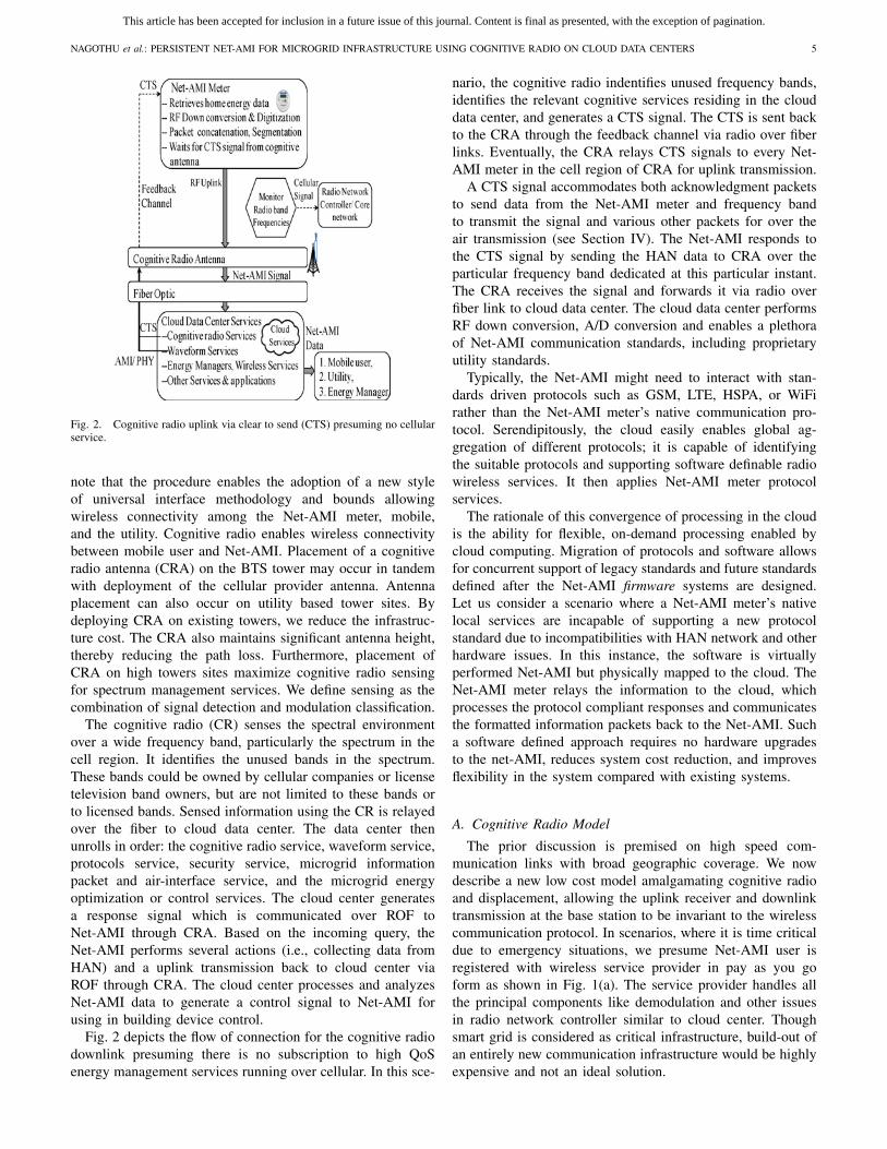
This article has been accepted for inclusion in a future issue of this journal. Content is final as presented, with the exception of pagination.

NAGOTHU et al.: PERSISTENT NET-AMI FOR MICROGRID INFRASTRUCTURE USING COGNITIVE RADIO ON CLOUD DATA CENTERS 5

Fig. 2. Cognitive radio uplink via clear to send (CTS) presuming no cellularservice.

note that the procedure enables the adoption of a new styleof universal interface methodology and bounds allowingwireless connectivity among the Net-AMI meter, mobile,and the utility. Cognitive radio enables wireless connectivitybetween mobile user and Net-AMI. Placement of a cognitiveradio antenna (CRA) on the BTS tower may occur in tandemwith deployment of the cellular provider antenna. Antennaplacement can also occur on utility based tower sites. Bydeploying CRA on existing towers, we reduce the infrastruc-ture cost. The CRA also maintains significant antenna height,thereby reducing the path loss. Furthermore, placement ofCRA on high towers sites maximize cognitive radio sensingfor spectrum management services. We define sensing as thecombination of signal detection and modulation classification.

The cognitive radio (CR) senses the spectral environmentover a wide frequency band, particularly the spectrum in thecell region. It identifies the unused bands in the spectrum.These bands could be owned by cellular companies or licensetelevision band owners, but are not limited to these bands orto licensed bands. Sensed information using the CR is relayedover the fiber to cloud data center. The data center thenunrolls in order: the cognitive radio service, waveform service,protocols service, security service, microgrid informationpacket and air-interface service, and the microgrid energyoptimization or control services. The cloud center generatesa response signal which is communicated over ROF toNet-AMI through CRA. Based on the incoming query, theNet-AMI performs several actions (i.e., collecting data fromHAN) and a uplink transmission back to cloud center viaROF through CRA. The cloud center processes and analyzesNet-AMI data to generate a control signal to Net-AMI forusing in building device control.

Fig. 2 depicts the flow of connection for the cognitive radiodownlink presuming there is no subscription to high QoSenergy management services running over cellular. In this sce-

nario, the cognitive radio indentifies unused frequency bands,identifies the relevant cognitive services residing in the clouddata center, and generates a CTS signal. The CTS is sent backto the CRA through the feedback channel via radio over fiberlinks. Eventually, the CRA relays CTS signals to every Net-AMI meter in the cell region of CRA for uplink transmission.

A CTS signal accommodates both acknowledgment packetsto send data from the Net-AMI meter and frequency bandto transmit the signal and various other packets for over theair transmission (see Section IV). The Net-AMI responds tothe CTS signal by sending the HAN data to CRA over theparticular frequency band dedicated at this particular instant.The CRA receives the signal and forwards it via radio overfiber link to cloud data center. The cloud data center performsRF down conversion, A/D conversion and enables a plethoraof Net-AMI communication standards, including proprietaryutility standards.

Typically, the Net-AMI might need to interact with stan-dards driven protocols such as GSM, LTE, HSPA, or WiFirather than the Net-AMI meter’s native communication pro-tocol. Serendipitously, the cloud easily enables global ag-gregation of different protocols; it is capable of identifyingthe suitable protocols and supporting software definable radiowireless services. It then applies Net-AMI meter protocolservices.

The rationale of this convergence of processing in the cloudis the ability for flexible, on-demand processing enabled bycloud computing. Migration of protocols and software allowsfor concurrent support of legacy standards and future standardsdefined after the Net-AMI firmware systems are designed.Let us consider a scenario where a Net-AMI meter’s nativelocal services are incapable of supporting a new protocolstandard due to incompatibilities with HAN network and otherhardware issues. In this instance, the software is virtuallyperformed Net-AMI but physically mapped to the cloud. TheNet-AMI meter relays the information to the cloud, whichprocesses the protocol compliant responses and communicatesthe formatted information packets back to the Net-AMI. Sucha software defined approach requires no hardware upgradesto the net-AMI, reduces system cost reduction, and improvesflexibility in the system compared with existing systems.

A. Cognitive Radio Model

The prior discussion is premised on high speed com-munication links with broad geographic coverage. We nowdescribe a new low cost model amalgamating cognitive radioand displacement, allowing the uplink receiver and downlinktransmission at the base station to be invariant to the wirelesscommunication protocol. In scenarios, where it is time criticaldue to emergency situations, we presume Net-AMI user isregistered with wireless service provider in pay as you goform as shown in Fig. 1(a). The service provider handles allthe principal components like demodulation and other issuesin radio network controller similar to cloud center. Thoughsmart grid is considered as critical infrastructure, build-out ofan entirely new communication infrastructure would be highlyexpensive and not an ideal solution.

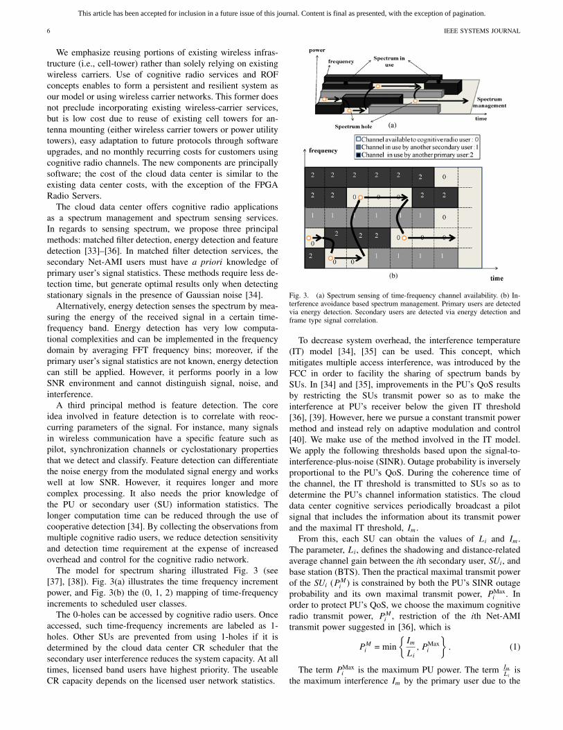
This article has been accepted for inclusion in a future issue of this journal. Content is final as presented, with the exception of pagination.

6 IEEE SYSTEMS JOURNAL

We emphasize reusing portions of existing wireless infras-tructure (i.e., cell-tower) rather than solely relying on existingwireless carriers. Use of cognitive radio services and ROFconcepts enables to form a persistent and resilient system asour model or using wireless carrier networks. This former doesnot preclude incorporating existing wireless-carrier services,but is low cost due to reuse of existing cell towers for an-tenna mounting (either wireless carrier towers or power utilitytowers), easy adaptation to future protocols through softwareupgrades, and no monthly recurring costs for customers usingcognitive radio channels. The new components are principallysoftware; the cost of the cloud data center is similar to theexisting data center costs, with the exception of the FPGARadio Servers.

The cloud data center offers cognitive radio applicationsas a spectrum management and spectrum sensing services.In regards to sensing spectrum, we propose three principalmethods: matched filter detection, energy detection and featuredetection [33]–[36]. In matched filter detection services, thesecondary Net-AMI users must have a priori knowledge ofprimary user’s signal statistics. These methods require less de-tection time, but generate optimal results only when detectingstationary signals in the presence of Gaussian noise [34].

Alternatively, energy detection senses the spectrum by mea-suring the energy of the received signal in a certain time-frequency band. Energy detection has very low computa-tional complexities and can be implemented in the frequencydomain by averaging FFT frequency bins; moreover, if theprimary user’s signal statistics are not known, energy detectioncan still be applied. However, it performs poorly in a lowSNR environment and cannot distinguish signal, noise, andinterference.

A third principal method is feature detection. The coreidea involved in feature detection is to correlate with reoc-curring parameters of the signal. For instance, many signalsin wireless communication have a specific feature such aspilot, synchronization channels or cyclostationary propertiesthat we detect and classify. Feature detection can differentiatethe noise energy from the modulated signal energy and workswell at low SNR. However, it requires longer and morecomplex processing. It also needs the prior knowledge ofthe PU or secondary user (SU) information statistics. Thelonger computation time can be reduced through the use ofcooperative detection [34]. By collecting the observations frommultiple cognitive radio users, we reduce detection sensitivityand detection time requirement at the expense of increasedoverhead and control for the cognitive radio network.

The model for spectrum sharing illustrated Fig. 3 (see[37], [38]). Fig. 3(a) illustrates the time frequency incrementpower, and Fig. 3(b) the (0, 1, 2) mapping of time-frequencyincrements to scheduled user classes.

The 0-holes can be accessed by cognitive radio users. Onceaccessed, such time-frequency increments are labeled as 1-holes. Other SUs are prevented from using 1-holes if it isdetermined by the cloud data center CR scheduler that thesecondary user interference reduces the system capacity. At alltimes, licensed band users have highest priority. The useableCR capacity depends on the licensed user network statistics.

Fig. 3. (a) Spectrum sensing of time-frequency channel availability. (b) In-terference avoidance based spectrum management. Primary users are detectedvia energy detection. Secondary users are detected via energy detection andframe type signal correlation.

To decrease system overhead, the interference temperature(IT) model [34], [35] can be used. This concept, whichmitigates multiple access interference, was introduced by theFCC in order to facility the sharing of spectrum bands bySUs. In [34] and [35], improvements in the PU’s QoS resultsby restricting the SUs transmit power so as to make theinterference at PU’s receiver below the given IT threshold[36], [39]. However, here we pursue a constant transmit powermethod and instead rely on adaptive modulation and control[40]. We make use of the method involved in the IT model.We apply the following thresholds based upon the signal-to-interference-plus-noise (SINR). Outage probability is inverselyproportional to the PU’s QoS. During the coherence time ofthe channel, the IT threshold is transmitted to SUs so as todetermine the PU’s channel information statistics. The clouddata center cognitive services periodically broadcast a pilotsignal that includes the information about its transmit powerand the maximal IT threshold, Im.

From this, each SU can obtain the values of Li and Im.The parameter, Li, defines the shadowing and distance-relatedaverage channel gain between the ith secondary user, SUi, andbase station (BTS). Then the practical maximal transmit powerof the SUi (PM

i ) is constrained by both the PU’s SINR outageprobability and its own maximal transmit power, PMax

i . Inorder to protect PU’s QoS, we choose the maximum cognitiveradio transmit power, PM

i , restriction of the ith Net-AMItransmit power suggested in [36], which is

PMi = min

Im

Li

, PMaxi

. (1)

The term PMaxi is the maximum PU power. The term Im

Liis

the maximum interference Im by the primary user due to the

This article has been accepted for inclusion in a future issue of this journal. Content is final as presented, with the exception of pagination.

NAGOTHU et al.: PERSISTENT NET-AMI FOR MICROGRID INFRASTRUCTURE USING COGNITIVE RADIO ON CLOUD DATA CENTERS 7

SU co-channel interference. The SUs compete to access theshared cognitive radio channel based on their average transmitrate, we apply the practical method max throughput algorithmwith proportional fair (PMTA-PF, see [36]). This makes ourcognitive radio cell spectrum sharing procedure “proportionalfair” with the following scheduling rule metric:

i∗ = maxi

(

RMi

Ti

)

= maxi

⎛

⎝

log2(1 + (PMi

/Li)||hi||2ni+Ip

)

Ti

⎞

⎠ . (2)

If the ith SU has interference plus noise which is ni + lp.The optimum scheduling strategy is to schedule user i* iftheir channel has the maximum rate indicated in (2) duringthe time period at time t, Ti(t). In order to achieve fairnessamong SUs, the SU who has larger transmit rate and largeraverage throughput will not be selected, due to its largeraverage throughput. The parameter, i*, is the scheduling rule,RM

i is the maximal transmit rate of SUi, Li represents thedistance-dependent channel loss (>1) and shadowing effectfrom SUi to cognitive radio base station, hi ∼ CN0, 1 modelsthe normalized Rayleigh fading. Ip and ni are the backgroundinterference plus the interference caused by SUs and ith usersbackground noise power, respectively. In [36], the methodshows an average throughput bps/Hz is not saturated untilnumber of secondary users is less than 120 in each cell andrange of throughput bits/s/Hz is about 19 kb/s to 23 kb/s.

B. System Infrastructure an Net-AMI Meter Data FlowIllustration Through the Protocol Stack

The Net-AMI meter is the major component for commu-nication of information flows in the smart grid distributionsystem networks. The Net-AMI meter needs to relay timeof use metering, power information, HAN information foroutage management, demand response, network optimization,distribution of renewable sources and controlling home orbuilding appliances. As we discussed in Section III, the Net-AMI meter may not be capable of processing HAN protocolsdue to protocol incompatibilities issues and limited process-ing capabilities. The Net-AMI meter’s principal architecturalfunction is the fast communication of data to and from thecloud center. In this section, we describe how the Net-AMImeter combines all the data from various sources and handsoff data to a cellular protocol [e.g., typically GSM, 3 GPPhigh speed packet access (HSPA), 3 GPP LTE] for over theair communication. Eventually, data is received by the cloudsystem for processing. In order to process the data in the cloudin a systematic way, the Net-AMI meter appends a packetheader to data to enable protocol identification and messagehandling.

In Fig. 4(a), we illustrate an example of the mobile deviceinitiating a control operation of in-building power system(i.e., HAN network) using the Net-AMI as relay portal. Inour discussion the cognitive spectrum management (cognitiveradio services) residing in cloud center, identifies the unusedbands and sends a CTS signal including the query by theuser to the Net-AMI meter indicating band availability. TheNet-AMI responds to query (i.e., in this case it is remote

Fig. 4. Session control procedures with data flow. (a) Session control pro-cedures. (b) Illustration of data flow through cellular protocol stack. (c) EACuplink control frame and EAC downlink control frame (indicating CTS/query).

home energy control) and retrieves home energy data fromHAN network. The Net-AMI acts a relay portal device andperforms uplink transmission to the cloud center. The cloudcenter performs a plethora of services such as waveformprocessing service, protocols service and energy managerand optimization algorithms. The energy control servicesare displaced back to Net-AMI via ROF through CRA forin-building control operation. The Net-AMI meter performsconcatenation of energy application control (EAC) header foruplink transmission as shown in Fig. 4(c). The EAC headerdetails the type of the HAN protocol (i.e., Zigbee, Zwave,Proprietary, and WiFi), the version of protocol, and the Net-AMI identifier used for source and destination identification.

The Net-AMI meter waits for the CTS signal from CRAfor uplink transmission. The CTS signal broadcasts specificinformation to Net-AMI meter, as shown in Fig. 4(c). TheEAC header in downlink details first field as frame type. TheCloud sends CTS, query or both. This field identifies as binary0 (CTS), query (1), and both (0, 1). The next field providesscheduling of time and frequency slots for data transfer withless interference of signals at CRA. If the Net-AMI is unableto perform transmission within a CTS time-out period, thesystem delays transmission until next CTS control signal. A

This article has been accepted for inclusion in a future issue of this journal. Content is final as presented, with the exception of pagination.

8 IEEE SYSTEMS JOURNAL

field indicating the type of cellular protocol (i.e., LTE, GSM,and CDMA) is included in the RF carrier frequency signalto support uplink transmission. The cloud reference time isused to account for time out scenarios based on received timeslots. Finally, a Net-AMI identifier is needed for destinationand source routing. Based on all these inputs, the Net-AMImeter bandpass modulates the signal to a specific RF carrierfrequency and performs uplink transmission.

In Fig. 4(b), without loss of generality, we illustrate dataflow through a cellular protocol stack with respect to the3 GPP-LTE protocol. The Net-AMI meter concatenates anEAC header to the data packet in the EAC layer. It insertsas information packets in the cellular protocol frame (LTE inthis example). The uplink and downlink transmission of theLTE protocol are below the EAC layer. Thus, LTE appliespacket retransmission to the occasional uncorrectable packeterrors due to fading and pathloss. This is accomplished througha highly sophisticated two-layered retransmission scheme: afast hybrid-ARQ protocol with low overhead feedback andsupport for soft combining with incremental redundancy. Thisis complemented with a highly reliable selective-repeat ARQprotocol in the MAC layer [41], [42]. A fixed bit 24 bit cyclicredundancy check (CRC) is performed on every block comingfrom above layers in physical layer. The calculation performedusing CRC is appended to every transport block in order tocheck coherence of received signal. This process ensures dataintegrity and allows cellular protocols to handle the issueswithout our intervention. Since we included the CRC in theapplication layer, retransmission of packets is done in networklayer.

C. Procedures for Cloud Control Services

The cloud center is the global aggregator of services andprotocols, from cognitive radio services to wave form servicesto energy management, to microgrid control, and many otherservices. The cloud data center is imbued with both basebandprocessor servers and general processor severs. Base bandprocessors resemble to conventional radio network controllerof the cellular service providers. Demodulation, encryption,error detection are specifically processed in baseband serversand other application oriented processes are dedicated togeneral purpose servers.

The structural components of the downlink cognitive radioservices are spectrum management and process the cognitiveradio signals from the CRA to generate a CTS signal with EACheader for downlink transmission as shown in Fig. 4(c). More-over, cloud service supports waveform services. Processes likesignal processing, error correction, baseband conversion, andother modulation techniques are designated to radio processingservers. Furthermore, radio processing servers are loaded withprotocol oriented applications (i.e., Zigbee, propriety RF, Wi-Fi, and Bluetooth) to process the requested services. It alsoprovides energy home management services. These servicesrequest the necessary data from waveform services in order tomonitor and analyze energy consumption, if this service hasbeen registered or requested by the user. Similarly, if the userhas renewable sources he can register with energy optimizationservices for optimal renewable source management. Cloud

Fig. 5. Downlink models. (a) Structural cloud downlink configuration toNet-AMI. (b) Noise model of cloud source to net-AMI receiver link withlosses, gains, signal components, and noise sources.

data center enables users to install any third party applicationsfor additional services. This empowers the whole system to beflexible and extensible.

D. Hybrid Wireless (RF)-Fiber Optic Communication Model

We now analyze the communication link consisting ofROF, wireless signaling, and noise at the transmitter side andreceiver side. We present an example Net-AMI network basedROF architecture using on external modulation for illustrationin Fig. 5(a). For downlink transmission from Cloud datacenters to Net-AMI meters the energy services signal, s(t)at power Ps−Tx is modulated to an RF band which, in turn,is converted to an RF optical light source using an externaloptical modulator. This signal is carried over the downlinkoptical fiber where the optical signal is converted back toelectrical signal using a photo detector. The Net-AMI signalis relayed to a Net-AMI meter. For uplink transmission fromNet-AMI meter to cloud center, the Net-AMI signal receivedat the cognitive radio is converted into an optical signal bymodulating a light source. It is then relayed at RF over theoptical fiber relay to the cloud data center. A photo detectordemodulates the optical signal to obtain electrical signal whichis again demodulated using RF band to process the Net-AMIsignal at the cloud data center.

The, end-to-end noise, NRx, contains both radio over fibernoise, and Nref . Due to transmission of fiber optic data to thecognitive radio base station antenna and downlink operatesfrom the base station transmitter to the wireless Net-AMImeter. Nrof noise is influenced by the linear amplifier afterthe lossy cable connecting the radio fiber optics and the basestation linear amplifier after RF up-converter. The completenoise model of Cloud Source to Net-AMI receiver link withlosses, gains, signal components, and noise sources is illus-trated in Fig. 5(b).

The optical carrier’s wavelength is usually selected to co-incide with either the 1.3 mm window, which corresponds tominimum dispersion for standard single-mode fiber. Alterna-tively, an approximately 1.55 mm window obtains minimumattenuation and is compatible with the best-performing type ofoptical amplifier. Considering a single mode fiber and radioover the fiber noise, Nrof is added at the optical receiver where

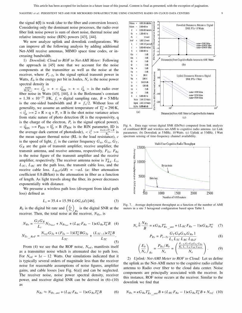
This article has been accepted for inclusion in a future issue of this journal. Content is final as presented, with the exception of pagination.

NAGOTHU et al.: PERSISTENT NET-AMI FOR MICROGRID INFRASTRUCTURE USING COGNITIVE RADIO ON CLOUD DATA CENTERS 9

the signal s(t) is weak (due to the fiber and conversion losses).Considering only the dominant noise processes, the radio overfiber link noise power is sum of short noise, thermal noise andrelative intensity noise (RIN) powers [43], [44].

We now analyze uplink and downlink configurations. Wecan improve all the following analysis by adding additionalNet-AMI receive antennas, MIMO space time codes, or in-creasing bandwidth.

1) Downlink: Cloud to ROF to Net-AMI Meter: Followingthe approach in [45] note that we account for the noisecomponents at the transmitter as well as the noise at thereceiver, where Ps−Tx is the signal optical transmit power inWatts, Eb is the energy per bit in Joules, No is the noise powerspectral density in

wattsHzNrof

=< i2sh > + < i2

RIN > + < i2th > is the radio over

fiber noise in Watts [43], [44], k is the Botlzmann’s constant= 1.38 × 10−23 J/K, fs = digital sampling rate, B = 5 MHzis the one-sided bandwidth and B = fs/2. Without loss ofgenerality, we assume an ambient temperature of T o

0 = 290 K,< i2

sh >= 2 × R × q × Ps × B is the shot noise variance arisesfrom static nature of photo detection (R is the responsivity, qis the charge of the electron, Ps is the signal optical power),< i2

RIN >= PRIN × I2D × B (PRIN is the RIN parameter, ID is

the average dark current of photodiode), < i2t >= 4×k×T o

0 ×B

RLis

the mean square thermal noise (RL is the load resistance), cis the speed of light, fc is the carrier frequency Gta, Gra, GT ,GR are the gain of transmit amplifier, receive amplifier, thetransmit antenna, and receive antenna, respectively, FTa, FRa

is the noise figure of the transmit amplifier and the receiveamplifier, respectively. The receiver antenna noise is T o

RA. Ls,LTC, LRC are the path loss, the transmit cable loss, and thereceive cable loss. LRoF (dB) = −αL (α: fiber attenuationcoefficient 0.8 dB/km) is the attenuation in fiber as a functionof length. As light travels along the fiber, its power decreasesexponentially with distance.

We presume a wireless path loss (divergent from ideal pathloss) defined as

Ls = 35.4 + 15.59 LOGe(d) [46]. (3)

Rb is the digital bit rate and(

Eb

No

)

Rxis the digital SNR at the

receiver. Then, the total noise at the receiver, NRx, is

NRx =GT GR

Ls

NTxRoF+ NRxant

+ (LRCFRa − 1)κGRaTo0 B (4)

NTx RoF =Nrof GTa + (FTa − 1)kT o

0 BGTa

LTC

+(LTC−1)κT o

0 B

LTC

.

(5)From (4) we see that the ROF noise, Nrof , manifests itself

as a transmitter noise which is attenuated due to path loss.For Nrof = 1e − 12 Watts. Our simulations indicated that itis typically several orders of magnitude less than the receivernoise for reasonable assumptions of noise figures, amplifiergains, and cable losses [see Fig. 6(a)] and can be neglected.The receiver noise, noise power spectral density, receiverpower, and receiver digital SNR can be derived in (6)–(10)as

NRx ≈ NRx−ant + (LRCFRa − 1)κGRaTo0 B (6)

Fig. 6. Data rage versus digital SNR (Eb/No) computed from link analysisof combined ROF and wireless net-AMI to cognitive radio antenna. (a) Linkparameters. (b) Downlink at 5 MHz, 10 Watts. (c) Uplink at 5 MHz, 1 Wattspectrum sensing of time-frequency channel availability.

Fig. 7. Average deployment throughput as a function of the number of AMImeters in a site 3 hexagonal configuration based upon Table I.

No=

NRx

B= κGRaT

oRx ant + (LRCFRa − 1)κGRaT

o0 (7)

PRx = Ps−Tx

GT GRGTaGRa 1

Ls LTC LRC LRoF

(8)

(

Eb

No

)

Rx

=PRx/Rb

No

=

(

Ps−TxGT GRGTa GRa

Rb Ls LTCLRCLROF

No

)

. (9)

2) Uplink: Net-AMI Meter to ROF to Cloud: Let us definethe uplink as the Net-AMI meter to the cognitive radio cellularantenna to Radio over fiber to the cloud data center. Noisecomponents are principally associated with the receiver. Inthis instance, ROF noise occurs at the receiver. Similar to thedownlink we find that

NRx = κGRaToRx antB + (LRCFRa − 1)κGRaT

o0 B + Nrof (10)

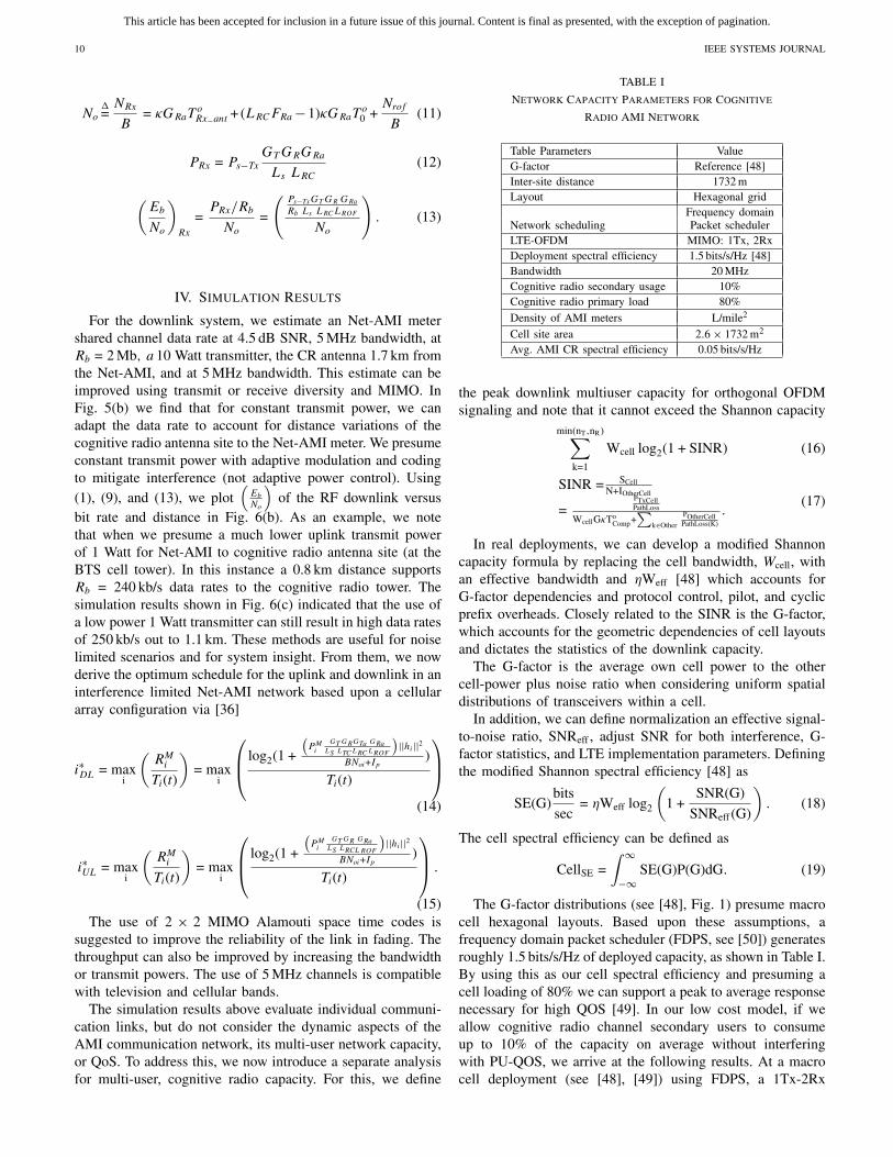
This article has been accepted for inclusion in a future issue of this journal. Content is final as presented, with the exception of pagination.

10 IEEE SYSTEMS JOURNAL

No=

NRx

B= κGRaT

oRx−ant + (LRCFRa −1)κGRaT

o0 +

Nrof

B(11)

PRx = Ps−Tx

GT GRGRa

Ls LRC

(12)

(

Eb

No

)

Rx

=PRx/Rb

No

=

(

Ps−TxGT GR GRa

Rb Ls LRCLROF

No

)

. (13)

IV. Simulation Results

For the downlink system, we estimate an Net-AMI metershared channel data rate at 4.5 dB SNR, 5 MHz bandwidth, atRb = 2 Mb, a 10 Watt transmitter, the CR antenna 1.7 km fromthe Net-AMI, and at 5 MHz bandwidth. This estimate can beimproved using transmit or receive diversity and MIMO. InFig. 5(b) we find that for constant transmit power, we canadapt the data rate to account for distance variations of thecognitive radio antenna site to the Net-AMI meter. We presumeconstant transmit power with adaptive modulation and codingto mitigate interference (not adaptive power control). Using(1), (9), and (13), we plot

(

Eb

No

)

of the RF downlink versusbit rate and distance in Fig. 6(b). As an example, we notethat when we presume a much lower uplink transmit powerof 1 Watt for Net-AMI to cognitive radio antenna site (at theBTS cell tower). In this instance a 0.8 km distance supportsRb = 240 kb/s data rates to the cognitive radio tower. Thesimulation results shown in Fig. 6(c) indicated that the use ofa low power 1 Watt transmitter can still result in high data ratesof 250 kb/s out to 1.1 km. These methods are useful for noiselimited scenarios and for system insight. From them, we nowderive the optimum schedule for the uplink and downlink in aninterference limited Net-AMI network based upon a cellulararray configuration via [36]

i∗DL = maxi

(

RMi

Ti(t)

)

= maxi

⎛

⎜

⎝

log2(1 +

(

PMi

GT GRGTa GRaLS LTCLRCLROF

)

||hi||2BNoi+Ip

)

Ti(t)

⎞

⎟

⎠

(14)

i∗UL = maxi

(

RMi

Ti(t)

)

= maxi

⎛

⎜

⎝

log2(1 +

(

PMi

GT GR GRaLS LRCLROF

)

||hi||2BNoi+Ip

)

Ti(t)

⎞

⎟

⎠.

(15)The use of 2 × 2 MIMO Alamouti space time codes is

suggested to improve the reliability of the link in fading. Thethroughput can also be improved by increasing the bandwidthor transmit powers. The use of 5 MHz channels is compatiblewith television and cellular bands.

The simulation results above evaluate individual communi-cation links, but do not consider the dynamic aspects of theAMI communication network, its multi-user network capacity,or QoS. To address this, we now introduce a separate analysisfor multi-user, cognitive radio capacity. For this, we define

TABLE I

Network Capacity Parameters for Cognitive

Radio AMI Network

Table Parameters ValueG-factor Reference [48]Inter-site distance 1732 mLayout Hexagonal grid

Frequency domainNetwork scheduling Packet schedulerLTE-OFDM MIMO: 1Tx, 2RxDeployment spectral efficiency 1.5 bits/s/Hz [48]Bandwidth 20 MHzCognitive radio secondary usage 10%Cognitive radio primary load 80%

Density of AMI meters L/mile2

Cell site area 2.6 × 1732 m2

Avg. AMI CR spectral efficiency 0.05 bits/s/Hz

the peak downlink multiuser capacity for orthogonal OFDMsignaling and note that it cannot exceed the Shannon capacity

min(nT,nR)∑

k=1

Wcell log2(1 + SINR) (16)

SINR = SCellN+IOtherCell

=PTxCellPathLoss

WcellGκToComp+

∑

k∈Other

POtherCellPathLoss(K)

.(17)

In real deployments, we can develop a modified Shannoncapacity formula by replacing the cell bandwidth, Wcell, withan effective bandwidth and ηWeff [48] which accounts forG-factor dependencies and protocol control, pilot, and cyclicprefix overheads. Closely related to the SINR is the G-factor,which accounts for the geometric dependencies of cell layoutsand dictates the statistics of the downlink capacity.

The G-factor is the average own cell power to the othercell-power plus noise ratio when considering uniform spatialdistributions of transceivers within a cell.

In addition, we can define normalization an effective signal-to-noise ratio, SNReff , adjust SNR for both interference, G-factor statistics, and LTE implementation parameters. Definingthe modified Shannon spectral efficiency [48] as

SE(G)bits

sec= ηWeff log2

(

1 +SNR(G)

SNReff (G)

)

. (18)

The cell spectral efficiency can be defined as

CellSE =∫ ∞

−∞SE(G)P(G)dG. (19)

The G-factor distributions (see [48], Fig. 1) presume macrocell hexagonal layouts. Based upon these assumptions, afrequency domain packet scheduler (FDPS, see [50]) generatesroughly 1.5 bits/s/Hz of deployed capacity, as shown in Table I.By using this as our cell spectral efficiency and presuming acell loading of 80% we can support a peak to average responsenecessary for high QOS [49]. In our low cost model, if weallow cognitive radio channel secondary users to consumeup to 10% of the capacity on average without interferingwith PU-QOS, we arrive at the following results. At a macrocell deployment (see [48], [49]) using FDPS, a 1Tx-2Rx

This article has been accepted for inclusion in a future issue of this journal. Content is final as presented, with the exception of pagination.

NAGOTHU et al.: PERSISTENT NET-AMI FOR MICROGRID INFRASTRUCTURE USING COGNITIVE RADIO ON CLOUD DATA CENTERS 11

transceiver, an AMI meter density of L AMIs per squaremile, an omni directional site with hexagonal grid layout (case3 with inter site distance of 1732 m), the 10% secondaryuser cognitive radio spectral efficiency per L-AMI meters in

bit/s/HzLAMImeter can be approximated as

CAMI ≈ 1 mile2

LAMI m× (1609 m)2/mile2

2.6×(1732 m)2 ×10% × (1.5 bits/s/Hz)

= 0.05bit/s/Hz

L-AMImeter. (20)

This supports streaming of a typical TCP/IP packet of1500 bytes every 30 s to L = 2500 smart meters in a shared20 MHz cognitive radio (secondary-user) wireless channel.The network parameter assumptions are indicated in Table I.

V. Conclusion

We developed the key equations and models supportingpersistence in Net-AMI networks. We illustrated the methodof analysis for cognitive radios, which can secure time-frequency bands for wireless communication of key powerservice applications in a manner which is invariant to cellularor other network infrastructures. Thus, the all Net-AMI meters,whether or not high QoS services are enabled, formally registerwith the utility service provider and allow a basic primitive setof utility power services. The cloud data center uploads theNet-AMI network infrastructure with legacy system protocols,proprietary protocols, and future systems protocols, therebyensuring extensible services over long time horizons. Datarates, ranges, and capacity of the cognitive radio for relativelylow 1 W uplink and 10 Watt downlink configurations revealhighly reliable data rate configurations from 1–3 km, with apossibility of trading off additional range versus data rate.

Acknowledgment

The authors would like to thank the support of the De-partment of Electrical and Computer Engineering, and theircolleagues, especially Dr. H. Krishnaswami, T. Shaneyfelt, J.Prevost, and the anonymous reviewers for their comments,which helped to improve this paper.

References

[1] Smart Grid Research and Development Multi-Year Program Plan(MYPP) 2010–2014.

[2] C. Potter, A. Archambault, and K. Westrick, “Building a smarter smartgrid through better renewable energy information,” in Proc. IEEE PSCE,Mar. 2009, pp. 1–5.

[3] R. DeBlasio, “Standards for the smart grid,” in Proc. IEEE Energy 2030Conf., Nov. 2008, pp. 1–7.

[4] S. M. Amin and B. F. Wollenberg, “Toward a smart grid,” IEEE PowerEnergy Mag., vol. 3, no. 5, pp. 35–41, Sep.–Oct. 2005.

[5] S.-W. Luan, J.-H. Teng, S.-Y. Chan, and L.-C. Hwang, “Developmentof a smart power meter for AMI based on zigbee communication,” inProc. Int. Conf. Power Electron. Drive Syst., 2009, pp. 661–665.

[6] C. Bennett and D. Highfill, “Networking AMI smart meters,” in Proc.IEEE Energy 2030 Conf., Nov. 2008, pp. 1–8.

[7] D. Gislason, Zigbee Wireless Networking. Amsterdam, The Netherlands:Elsevier Science, 2008.

[8] W. Luan, D. Sharp, and S. Lancashire, “Smart grid communicationnetwork capacity planning for power utilities,” in Proc. TransmissionDistribution Conf. Expos., 2010, pp. 1–4.

[9] B. Reid, “Oncor electric delivery smart grid initiative,” in Proc. 62ndAnnu. Conf. Protective Relay Engineers, 2009, pp. 8–15.

[10] R. C. Qiu, Z. Chen, N. Guo, Y. Song, P. Zhang, H. Li, and L.Lai, “Toward a real-time cognitive radio network testbed: Architecture,hardware platform, and application to smart grid,” in Proc. 5th IEEEWorkshop Netw. Technologies Softw. Defined Radio Netw., Jun. 2010,pp. 1–6.

[11] S. Zhang, S. Zhang, X. Chen, and X. Huo, “Cloud computing researchand development trend,” in Proc. Future Netw. ICFN, 2010, pp. 93–97.

[12] M. Naghshineh, R. Ratnaparkhi, D. Dillenberger, J. R. Doran, C. Dorai,L. Anderson, G. Pacifici, J. L. Snowdon, A. Azagury, M. VanderWiele,and Y. Wolfsthal, “IBM Research Division cloud computing initiative,”IBM J. Res. Dev., vol. 53, no. 4, pp. 1–10, Jul. 2009.

[13] B. P. Rimal, E. Choi, and I. Lamb, “A taxonomy and survey of cloudcomputing systems,” in Proc. 5th Int. Joint Conf. INC IMS IDC, 2009,pp. 44–51.

[14] J. Peng, X. Zhang, Z. Lei, B. Zhang, W. Zhang, and Q. Li, “Comparisonof several cloud computing platforms,” in Proc. ISISE, Dec. 2009, pp.23–27.

[15] Z. Wei, S. Qin, D. Jia, and Y. Yang, “Research and design of cloudarchitecture for smart home,” in Proc. ICSESS, Jul. 2010, pp. 87–92.

[16] J. Bi, Z. Zhu, R. Tian, and Q. Wang, “Dynamic provisioning modelingfor virtualized multi-tier applications in cloud data center,” in Proc. 3rdIEEE Int. Conf. Cloud Comput., Jul. 2010, pp. 370–377.

[17] A. Di Costanzo, M. D. De Assuncao, and R. Buyya, “Harnessing cloudtechnologies for a virtualized distributed computing infrastructure,”IEEE Internet Comput. J., vol. 13, no. 5, pp. 24–33, Sep.–Oct. 2009.

[18] C. Wang, Q. Wang, K. Ren, and W. Lou, “Ensuring data storage securityin cloud computing,” in Proc. IWQoS, Jul. 2009, pp. 1–9.

[19] Q. Liu, C. Weng, M. Li, and Y. Luo, “An In-VM measuring frameworkfor increasing virtual machine security in clouds,” IEEE Security PrivacyJ., vol. 8, no. 6, pp. 56–62, Nov.–Dec. 2010.

[20] E. Bertino, F. Paci, and R. Ferrini, “Privacy-preserving digital identitymanagement for cloud computing,” IEEE Comput. Soc. Data Eng. Bull.,vol. 32, pp. 1–4, Mar. 2009.

[21] Y. Zhang and J. Joshi, “Access control and trust management foremerging multidomain environments,” in Annals of Emerging Researchin Information Assurance, Security and Privacy Services, S. Upadhyayaand R. O. Rao, Eds. Bradford, U.K.: Emerald Group Publishing, 2009,pp. 421–452.

[22] G. DeCandia, “Dynamo: Amazon highly available key-value store,” inProc. 21st ACM Symp. Operating Syst. Principles, Oct. 2007, pp. 205–220.

[23] K. Nagothu, B. Kelley, J. Prevost, and M. Jamshidi, “On predictionto dynamically assign heterogeneous microprocessors to the minimumjoint power state to achieve ultralow power cloud computing,” in Proc.Asilomar Conf. Signals Syst. Comput., Nov. 2010, pp. 1269–1273.

[24] K. Nagothu, B. Kelley, J. Prevost, and M. Jamshidi, “Low energy cloudcomputing using adaptive load prediction algorithms,” in Proc. WorldAutom. Congr., 2010, pp. 1–7.

[25] I. F. Akyildiz, W.-Y. Lee, M. C. Vuran, and S. Mohanty, “A surveyon spectrum management in cognitive radio networks,” IEEE Commun.Mag., vol. 46, no. 4, pp. 40–48, Apr. 2008.

[26] Q. Zhao and B. M. Sadler, “A survey of dynamic spectrum access,”IEEE Sig. Process. Mag., vol. 24, no. 3, pp. 79–89, May 2007.

[27] E. I. Ackerman and C. H. Cox, “RF fiber-optic link performance,” IEEEMicrow. Mag., vol. 2, no. 4, pp. 50–58, Dec. 2001.

[28] H. Al-Raweshidy, Radio Over Fiber Technology for Next Generation.Norwood, MA: Arctech House, 2002, ch. 1.

[29] H. B. Kim, “Radio over fiber based network architecture,” Ph.D.dissertation, Dept. Electr. Comput. Eng., Tech. Univ. Berlin Sekr FT5Einsteinufe, Berlin, Germany, 2005.

[30] Y. Ebine, “Development of fiber-radio systems for cellular mobilecommunications,” in Proc. Int. Microw. Photonics MWP, vol. 1. 1999,pp. 249–252.

[31] H. B. Kim, M. Emmelmann, B. Rathke, and A. Wolisz, “A radioover fiber network architecture for road vehicle communication sys-tems,” in Proc. IEEE Vehicular Technol. Conf., vol. 5. Jun. 2005,pp. 2920–2924.

[32] T. Kuri, H. Toda, J. J. V. Olmos, and K. Kitayama, “Recon-figurable dense wavelength-division-multiplexing millimeter-wavebandradio-over-fiber,” J. Lightw. Technol., vol. 28, no. 16, pp. 2247–2257,2010.

[33] W. Wang, “Spectrum sensing for cognitive radio,” in Proc. 3rd Int. Symp.Intell. Inform. Technol. Applicat. Workshops, 2009, pp. 410–412.

[34] D. D. Ariananda, M. K. Lakshmanan, and H. Nikookar, “A surveyon spectrum sensing techniques for cognitive radio,” in Proc. 2nd Int.Workshop Cognitive Radio Adv. Spectrum Manage. (CogART), 2009, pp.74–79.

This article has been accepted for inclusion in a future issue of this journal. Content is final as presented, with the exception of pagination.

12 IEEE SYSTEMS JOURNAL

[35] D. Cabric, S. M. Mishra, and R. W. Brodersen, “Implementation issuesin spectrum sensing for cognitive radios,” in Proc. 38th Asilomar Conf.Signals Syst. Comput., vol. 1. Nov. 2004, pp. 772–776.

[36] J. Zhang, Z. Zhang, H. Luo, A. Huang, and R. Yin, “Uplink schedulingfor cognitive radio cellular network with primary user’s QoS protection,”in Proc. WCNC, 2010, pp. 1–5.

[37] J. M. Peha, “Sharing spectrum through spectrum policy reform andcognitive radio,” Proc. IEEE, vol. 97, no. 4, pp. 708–719, Apr. 2009.

[38] E. G. Larsson and M. Skoglund, “Cognitive radio in a frequency plannedenvironment: Some basic limits,” IEEE Trans. Wirel. Commun., vol. 7,no. 12, pp. 4800–4806, Dec. 2008.

[39] I. Sooyeol, H. Jeon, and H. Lee, “Autonomous distributed power controlfor cognitive radio networks,” in Proc. IEEE 68th VTC, Sep. 2008, pp.1–5.

[40] K. C. Beh, A. Doufexi, and S. Armour, “Performance evaluation ofhybrid ARQ schemes of 3GPP LTE OFDMA systems,” in Proc. 18thAnnu. IEEE Int. Symp. Personal Indoor Mobile Radio Commun., Sep.2007, pp. 1–5.

[41] D. Astély, E. Dahlman, A. Furuskär, Y. Jading, M. Lindström, and S.Parkvall, “LTE: The evolution of mobile broadband,” IEEE Commun.Mag., vol. 47, no. 4, pp. 44–51, Apr. 2009.

[42] A. Larmo, M. Lindström, M. Meyer, G. Pelletier, and J. Torsner, “TheLTE link-layer design,” IEEE Commun. Mag., vol. 47, no. 4, pp. 52–59,Apr. 2009.

[43] G. Keiser, Optical Fiber Communications. New York: McGraw-Hill,2000, chs. 3–6.

[44] R. Hui and M. O Sullivan, Fiber Optic Measurements Techniques.Amsterdam, The Netherlands: Elsevier/Academic Press, 2009, ch. 5.

[45] B. Sklar, Digital Communications: Fundamentals and Applications, 2nded. Englewood Cliffs, NJ: Prentice-Hall, 2009.

[46] R. Mardeni and T. S. Priya, “Optimized COST-231 Hata models forWiMAX path loss prediction in suburban and open urban environments,”Mod. Appl. Sci., vol. 4, no. 9, pp. 75–89, 2010.

[47] B. Kelley, “Software defined radio for advanced gigabit cellular systems,to appear in DSP handbook and wireless,” in Proc. Networking RadarSensor Array Process. Nonlinear Signal, 2009, ch. 22.

[48] P. E. Mogensen, W. Na, I. Z. Kovács, F. Frederiksen, A. Pokhariyal,K. I. Pedersen, T. E. Kolding, K. Hugl, and M. Kuusela, “LTE capacitycompared to the Shannon bound,” in Proc. IEEE 65th Vehicular Technol.Conf., Apr. 2007, pp. 1234–1238.

[49] A. B. Syed, “Dimensioning of LTE network description of models andtool, coverage and capacity estimation of 3GPP long term evolutionradio interface,” M.S. thesis, Dept. Elect. Eng., Helsinki Univ. Technol.,Helsinki, Finland.

[50] P. Mogensen, W. Na, I. Z. Kovacs, F. Frederiksen, A. Pokhariyal,K. I. Pedersen, K. Hugl, and M. Kuusela, “LTE capacity compared to theShannon bound,” in Proc. IEEE 65th VTC, Apr. 2007, pp. 1234–1238.

Kranthimanoj Nagothu (S’07) received theB.S.E.E. degree from Anna University, Chennai, In-dia, in 2006, and the M.S.E.E. degree from the Uni-versity of Texas, San Antonio, in 2009. Currently, heis pursuing the Ph.D. degree in electrical engineeringwith the University of Texas, San Antonio.

He is with the Autonomous Control EngineeringCenter and the Wireless Advanced Next-GenerationLaboratory as a Graduate Research Assistant. Hiscurrent research interests include communicationsand networking for smart grid systems, software

define radio, 4G cellular, sensor networks, low power cloud systems, systemof systems and underwater robotics swarms.

Mr. Nagothu received several awards including the Best Paper Award for theESB Student Conference 2007 at the University of Texas, San Antonio, and isa member of Eta Kappa Nu. He has been actively participating in organizinginternational conferences.

Brian Kelley (S’91–M’93–SM’06) received theB.S.E.E. degree from the College of Electrical En-gineering, Cornell University, Ithaca, NY, and theM.S.E.E. and Ph.D.E.E. degrees from the Depart-ment Electrical and Computer Engineering, GeorgiaInstitute of Technology, Atlanta, where he was anOffice of Naval Research Fellow and a Georgia TechPresidential Fellow.

He is currently with the Department of Electricaland Computer Engineering, University of Texas,San Antonio. After research and development efforts

with Motorola, Austin, TX, and Freescale, Austin, he joined the faculty ofthe University of Texas, San Antonio, as an Assistant Professor in communi-cations. With the University of Texas, San Antonio, he has taught numerousgraduate courses in communications. He has numerous publications and isa holder of ten U.S. patents. His current research interests include softwaredefined radio, power system communications, 4G cellular, communications,and sensor networks.

Dr. Kelley is the Chair of the San Antonio IEEE Communication and SignalProcessing Chapter, and was an Associate Editor of Computers and ElectricalEngineering, Elsevier in 2008. He is a member of Tau Beta Pi and Eta KappaNu.

Mo Jamshidi (S’66–M’71–SM’74–F’89) receivedthe B.S. degree from Oregon State University, New-port, in June 1967, and the M.S. and Ph.D. degreesin electrical engineering from the University of Illi-nois at Urbana-Champaign, Urbana, in June 1969and February 1971, respectively. He holds threeHonorary Doctorate degrees from Odlar YourduUniversity, Baku, Azerbaijan, in 1999, the Univer-sity of Waterloo, Waterloo, ON, Canada, and theTechnical University of Crete, Crete, Greece, in2004.

Currently, he is the Lutcher Brown Endowed Chaired Professor with theUniversity of Texas System, San Antonio. He also has been the FoundingDirector of the Center for Autonomous Control Engineering (ACE), Universityof New Mexico (UNM), Albuquerque, and moved the center to the Universityof Texas, San Antonio, in early 2006. He has been the Director of theInternational Consortium on System of Systems Engineering since 2006. Heis currently organizing the U.S. System of Systems Engineering Networkconsisting of many academic institutions and industries in the U.S. He is alsoRegents Professor Emeritus of ACE with UNM. In 1999, he was a NATODistinguished Professor of intelligent systems and control in Portugal. He hasbeen an advisor, an IPA, or a special government employee with NASA (10years), U.S. AFRL (9 years), and DOE (9 years) since 1984. He has over 625technical publications, including 63 books (11 textbooks) and edited volumes.Six of his books have been translated into at least one foreign language.

Dr. Jamshidi is the Founding Editor, Co-Founding Editor or Editor-in-Chiefof five journals. He is the Editor-in-Chief of the new IEEE Systems Journal

(inaugurated in 2007) and the Founding Editor-in-Chief of the IEEE Control

Systems Magazine. He is a recipient of the IEEE Centennial Medal andthe IEEE CSS Distinguished Member Award. He received the IEEE SMCSocieties Norbert Weiner Research Achievement Award in 2005 and the IEEESMC Distinguished Contribution Award in 2006. In 2006, he was awarded aDistinguished Alumni in Engineering at Oregon State University, Corvallis.In 2009, he was a Distinguished Fellow of the U.K. Royal Academy ofEngineering, Cardiff University, Cardiff, U.K., and from 2009 to 2012 heis an Honorary Professor of Deakin University, Australia. In October 2009,he served as an Advisor to the European Commission on System of SystemsEngineering. Since 2010, he has been serving on the Review Board of theU.S.–Vietnam Education Foundation of the U.S. National Research Council.From 2009 to 2010, he was a U.K. Royal Academy of Engineering Fellowwith Cardiff University. In April 2010, his research paper on robotic swarmswas chosen as the Best Paper at the IEEE Systems Conference, San Diego,CA, and in September 2010 his research papers on swarm robotics and UAVcontrol systems received the First and Second Best Paper Awards at the WACMeeting, Kobe, Japan. He is a member of the International Council on SystemsEngineering. He is a fellow of ASME, AAAS, NYAS, TWAS (DevelopingNations Science Academy), and an associate fellow of AIAA.

Amir Rajaee (S’11) received the B.S.E.E. degreefrom the Iran University of Science and Technology,Tehran, Iran, in 2010. He is currently pursuing theM.S.E.E. degree with the University of Texas, SanAntonio.

His current research interests include spectrumsensing and management in cognitive radio (ad hocand cellular networks), communications and opti-mization for smart grids, and he has worked onlocalization in speech processing.

Throughput Analysis for AMI Meters in Smart Grid

on Cognitive Radio Networks

Abstract— In this paper a framework is presented based on

4G Cognitive Radio (CR) network capable of

communicating with high numbers of geographically

dispersed smart meters for command and control feature

concurrently with private cellular network. Our approach

uses pervasive smart grid systems (i.e. cloud data centers)

as the central communication and optimization

infrastructure supporting metropolitan area based smart

meter infrastructure. In this paper, we investigate the

performance of various scheduling algorithms in context

with CR units to provide a satisfactory tradeoff between

maximizing the system capacity, achieving fairness among

cognitive users. We lay as a framework evaluation 3GPP

LTE system model simulations. Our system level simulation

results show that the 4G CR network model meets the

smart grid protocols requirements for a multi-user CR

network of Smart meters.

Keywords-4G Cognitive radio networks, cloud data center,

scheduling algorithms, and smart meters

I. INTRODUCTION

The smart grid of the future is generally perceived to be an intelligent energy delivery system that supports plug-and-play integration of power, information, and security services. [1]. We consider the future smart grid as leveraging Information and Communications Technology (ICT) facilitated by the smart meter (also named as Advance Infrastructure Metering (AMI)) information networks. The smart meter enables the flow of real-time information within the power utility, between the power utility and its customers. It also provides customers and utilities the technology to optimize their energy consumption in participating in closed loop demand response; moreover, these services allow convergence of high penetrations of renewable energy components into grid and third party energy management applications for demand optimization. It is essential for AMI to be networked since it enables system wide sensing, utility and customer linkages, and future self healing capability.

Communication network infrastructures represent a very large capital expense. Much of this expenditure is due to the high prices of purchasing licensed bands either from the FCC auction process or from existing licensed band owners. We therefore analyze a novel, low cost framework based on 4G cognitive radio smart meter networks enabling command and control, demand optimization and other features. Research on CR has evolved from SDR (see [2-3]) with an objective of efficient utilization of radio spectrum. In this paper, we analyze

CR in the context of smart energy systems. Although there have been significant advances and improvements in CR hardware, algorithms, and protocols, less attention has been given to developing ubiquitous and pervasive metropolitan scale CR networks, particularly with respect to smart grid information networking[4]. A metropolitan infrastructure based CR networks is shown in Fig. 1. In this context, there are major challenges to overcome such as Secondary Users (SU) should sense the spectrum and timely model the behavior of the Primary Users (PU). The other issue is how the SUs manage the available spectrum resources and share the resources among the SUs to satisfy the smart grid protocol requirements and meeting the interference constraints suggested by the FCC Spectrum Policy Task.

In such a system, our objective for SUs (i.e. AMI) is to

efficiently transmit their delay sensitive traffic over the network

and meet the QoS requirements of the smart grid protocol. In

this paper, we investigate different scheduling polices that

maximize the downlink sum throughput in the given area and

achieving fairness among the SUs. We present an opportunistic

scheduling policy that exploits both maximizing the downlink

sum throughput and fairness under time-varying channel

conditions for multi-user CR network in a metropolitan based

environment.

Several authors have defined aspects of AMI networking in

smart grids. Mesh, Ethernet and cellular AMI network topology

for smart grid has been proposed. In [5] the authors propose

mesh networks of Zigbee based transmission architecture.

Challenging issue with line of sight requirements in Zigbee is

the limit of single-hop range to hundreds of feet. Inefficiencies

arise when transmission distances featured by the protocols in

the entire metropolitan area for AMI networking. In [6], the

authors discuss communication infrastructure based on Ethernet

(LAN and WAN). The approach will support automated meter

readings and customer home appliance connections. However,

wireline systems are not always available. Customer

subscription to service must occur and wired system can be

challenging to rapidly redeploy, particularly in swiftly

enveloping emergencies.

The authors in [7] describe a framework for RF mesh

networking interfaced with high speed WiMAX access

networks. In [8], overview of architecture, hardware platform,

is reported to enable CR for smart grid communications.

However, to our knowledge anywhere in the literature a

complete multi-user capacity analysis using CR network in

context with smart grid has been yet reported. Our work

discusses the CR network infrastructure architecture from 4G

Amir Rajaee1, KranthiManoj Nagothu

2, Brian Kelley

3, Mo Jamshidi

4

amirajaee@gmail.com1, kranthimanoj@gmail.com

2, brian.kelley@utsa.edu

3, moj@wacong.org

4

Electrical and Computer Engineering, the University of Texas at San Antonio, TX, USA

perspective. We also present multi-user performance analysis

of various scheduling algorithms in context with AMI units

considering the delay occurred due to offloading the processes

to cloud in our architecture.

The rest of the paper is organized as follows. Section II

overviews the 4G CR system architecture in brief. In section III

we present overall 4G CR system model detailing the sensing

model and different scheduling polices and their properties.

Section IV discusses the performance of the different

scheduling algorithms with system level simulations and

concludes this paper.

II. 4g Cognitive radio framework

A. 4G cognitive radio system architecture

We presume a LTE network as a CR LTE network (4G CR),

if the LTE work is adopted the CR techniques. We consider a

cloud data center infrastructure based CR network coexisting

with PU network shown in Fig.1. The coverage of both the CR

base station and PU network base station are similar. As

depicted in the Fig. 1 at the center of the each cell, there is

base-station which is shared as e Node-B for PUs and as

antenna for SUs. The PU base-station only serves to PUs as it

lacks the CR protocols capabilities to support SUs. However, it

may consider supporting certain features in order to

communicate with SUs.

A CR system does not own a license band to operate in a

desired band. Hence, the spectrum access is allowed only in an

opportunistic manner. The licensed user of the frequency band

is always given priority access to the shared channel (time-

frequency resource). Due to their priority in spectrum access,

the operations of PUs are always 1st in the transmission queue

so as to not be affected by unlicensed users All the SUs have

the same right to access the spectrum; SUs should compete

with each other for the same unlicensed band. Thus,

sophisticated spectrum sharing methods among SUs are

required in this architecture. If multiple SUs network operators

reside in the same unlicensed band, fair spectrum sharing

among these networks is also required and different scheduling

algorithms are discussed in detail in section III.

Placement of a Cognitive Radio Antenna on the BTS tower

may occur in tandem with deployment of the cellular provider

antenna. The CR senses the spectral environment over a wide

frequency band, particularly the spectrum in the cell region. It

identifies the unused bands in the spectrum. These bands could

be owned by cellular companies or license television band

owners, but are not limited to these bands or to licensed bands.

Sensed information using the CR is relayed to cloud data

center. In principle, eNode-B which terminates the air interface

protocol and first point of contact for PU is located at the

primary user base-station. However, in proposed architecture

all the cognitive radio service, waveform service, protocols

service, security service, scheduling and control services are

displaced into cloud data center. The CR services indentify

unused frequency bands, the relevant cognitive services

residing in the cloud data center generates a clear to send (CTS)

signal.

Fig. 1. 4G CR network system architecture: Scenario of multiple AMI meters

serviced by cognitive radio network infrastructure enabled by cloud center

coexisting with private cellular network The CTS is sent back to the AMI meters through the

feedback channel via base station. Eventually, the CR antenna

relays CTS signals to every AMI in the cell region for uplink

transmission.

1) Pervasive smart grid systems

The energy services of the future can be privately contracted

services or public services. The cloud center enables

convenient, on-demand network access to a shared pool of

configurable, computing resources (e.g., networks, servers,

storage, applications, and services) that can be rapidly

provisioned and released with minimal management effort.

There are different cloud computing platform classifications.

Standard architectures includes Abi (or Abiquo), Nimbus Open

Nebula, Azure (Microsoft), Google (App Engine), Blue (IBM)

and Mosso (Rackspace). Fig.1. depicts the model for a cloud

data center architecture optimized for based smart grids. Our

Wireless Cloud Data (WCD) model is organized into four

principle layers: application layer, platform layer, CR

communication and networking layer and infrastructure layer.

The first two layers are akin to existing cloud architectures.

However, the lower two layers are augmented to enable the CR

networking and wireless services. CR communication and

networking layer provides services such as cognitive radio

services, waveform services, Radio Link Control (RLC), and

Medium Access Control (MAC) services. CR services, which

provide spectrum management and spectrum sensing, are

discussed in detail in section III. The infrastructure layer

facilitates the effective integration of computing resources,

storage, networks to deploy applications and operating systems.

We augment our cloud infrastructure microprocessor racks with

FPGA boards targeted to processing high computation rate

processes typically associate with CR services, communication

waveform signal processing and coding.

III. CR SYSTEM MODEL

In the paper system model 4G cellular network is considered

with Nsu secondary users sharing the spectrum simultaneously

with Npu primary users. It is presumed in the context that the

secondary users (i.e. AMI meters) are fixed in sense of

PUBS

(eNode-B) PU

PU

PU

PU PU

Primary user radio network

BS / e Node -B

Cognitive user

(i.e. AMI(A-SU)) radio network with

cloud infrastructure

A-SU

A-SU

A-SU

PU

PU

CR: Cognitive radio

SU: Secondary user

PU: Primary user

PUBS: PU Base station

CTS: clear to send

Wireless cloud data

center

PDN

GWHSSMME

Serving

GW

SGSN

PCRF UTRANGERAN

Packet data

network

S1

S1-MME

S6a

S1-U

Rx

SGi

GXS12

S4

S3

S11S5

S1

PU

Back Haul

NetworkCTS CTS

CTS

•

Application

Radio servers

Radio services

Servers, storage, networking

Platform

Communication, Networking

InfrastructureCR boards

Cognitive radio

Radio

boards

Demand response

management services

Energy manager

servicesOther services

CR

services e Node-BRadio interface

protocols

Wireless networking

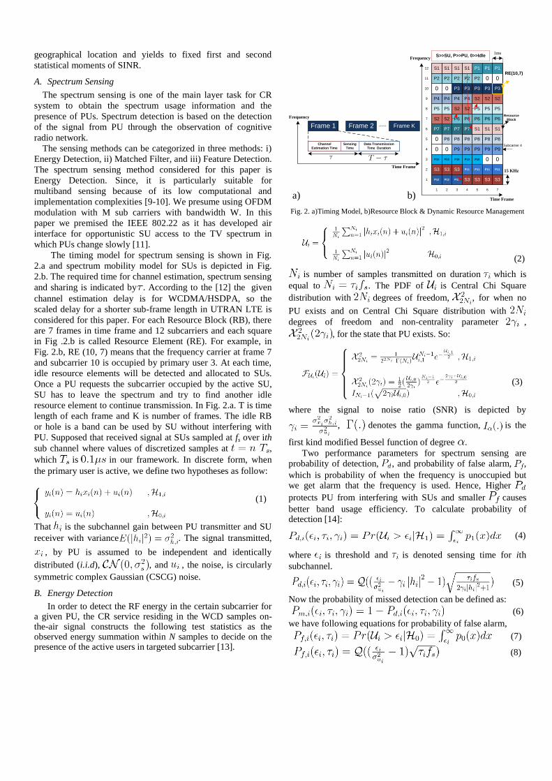
geographical location and yields to fixed first and second

statistical moments of SINR.

A. Spectrum Sensing

The spectrum sensing is one of the main layer task for CR

system to obtain the spectrum usage information and the

presence of PUs. Spectrum detection is based on the detection

of the signal from PU through the observation of cognitive

radio network.

The sensing methods can be categorized in three methods: i)

Energy Detection, ii) Matched Filter, and iii) Feature Detection.

The spectrum sensing method considered for this paper is

Energy Detection. Since, it is particularly suitable for

multiband sensing because of its low computational and

implementation complexities [9-10]. We presume using OFDM

modulation with M sub carriers with bandwidth W. In this

paper we premised the IEEE 802.22 as it has developed air

interface for opportunistic SU access to the TV spectrum in

which PUs change slowly [11].

The timing model for spectrum sensing is shown in Fig.

2.a and spectrum mobility model for SUs is depicted in Fig.

2.b. The required time for channel estimation, spectrum sensing

and sharing is indicated by . According to the [12] the given

channel estimation delay is for WCDMA/HSDPA, so the

scaled delay for a shorter sub-frame length in UTRAN LTE is

considered for this paper. For each Resource Block (RB), there

are 7 frames in time frame and 12 subcarriers and each square

in Fig .2.b is called Resource Element (RE). For example, in

Fig. 2.b, RE (10, 7) means that the frequency carrier at frame 7

and subcarrier 10 is occupied by primary user 3. At each time,

idle resource elements will be detected and allocated to SUs.

Once a PU requests the subcarrier occupied by the active SU,

SU has to leave the spectrum and try to find another idle

resource element to continue transmission. In Fig. 2.a. T is time

length of each frame and K is number of frames. The idle RB

or hole is a band can be used by SU without interfering with

PU. Supposed that received signal at SUs sampled at fs over ith

sub channel where values of discretized samples at ,

which is in our framework. In discrete form, when

the primary user is active, we define two hypotheses as follow:

(1)

That is the subchannel gain between PU transmitter and SU

receiver with variance . The signal transmitted,

, by PU is assumed to be independent and identically

distributed (i.i.d), , and , the noise, is circularly

symmetric complex Gaussian (CSCG) noise.

B. Energy Detection

In order to detect the RF energy in the certain subcarrier for a given PU, the CR service residing in the WCD samples on-the-air signal constructs the following test statistics as the observed energy summation within N samples to decide on the presence of the active users in targeted subcarrier [13].

Fig. 2. a)Timing Model, b)Resource Block & Dynamic Resource Management

(2)

is number of samples transmitted on duration which is

equal to . The PDF of is Central Chi Square

distribution with degrees of freedom, , for when no

PU exists and on Central Chi Square distribution with

degrees of freedom and non-centrality parameter ,

, for the state that PU exists. So:

(3)

where the signal to noise ratio (SNR) is depicted by

, denotes the gamma function, is the

first kind modified Bessel function of degree .

Two performance parameters for spectrum sensing are probability of detection, , and probability of false alarm, ,

which is probability of when the frequency is unoccupied but we get alarm that the frequency is used. Hence, Higher

protects PU from interfering with SUs and smaller causes

better band usage efficiency. To calculate probability of detection [14]:

(4)

where is threshold and is denoted sensing time for ith

subchannel.

(5)

Now the probability of missed detection can be defined as:

(6)

we have following equations for probability of false alarm,

(7)

(8)

Frame 1 Frame 2 Frame K

Sensing

Time

Data Transmission

Time Duration

Frequency

Time Frame

Channel

Estimation Time

b)a)

P12 P12 P12

P11 P11 P11 P11

P10 P10 P10 P10 P10

P9 P9 P9 P9 P9

P8P8P8

P7 P7 P7 P7

P6 P6 P6 P6

P5 P5 P5P5 P5

P4P4P4

P3 P3 P3 P3

P4

P2P2P2P2P2

P1 P1 P1

P8P8

S2 S2

S2

S1 S1 S1

0

0

S3

0

S3 S3

S3 S3 S3S3

0 0

S2 S2 S2

0

0

S1S1S1S1

P6

S2

P3

P8

0

0

Frequency

Time Frame

1 2

12

11

10

9

8

76543

2

3

4

5

6

7

RE(10,7)

15 KHz

1ms

1

S>>SU, P>>PU, 0>>Idle

Resource

Block

Subcarrier 4

Usually to evaluate the performance of energy detection, the

goal is to minimize for a target or to maximize for a

target . At first we assume is our target

probability of detection ,

(9)

(10)

is the probability of false alarm regard

to target , and is the inverse of complementary error

function. For a target we have:

(11)

(12)

is the probability of detection when

is targeted. As a result, in this part, probability of false

alarm and detection based on and ,

respectively, are calculated.

C. Primary User Activity Model

In this section, we present a model for primary users’

activities which is directly proportional to CR network

performance. In our Markov chains model, we consider two

states (Busy by PU and Idle) for each subcarrier. Since each

user arrival is independent, each transition follows the Poisson

arrival process. Thus, the length of Busy and Idle periods are

exponentially distributed. The Poisson distribution is

considered in the modelling with arrival rate, α, and departure

rate, β, and in simulation, the average existing users is assumed

such that %80 of total spectrums are loaded by primary users in

average.

(13)

as a result, the existing users in a cell is equivalent to total

existing users on previous time period added to arrival rate at

current time and subtracted by current departure time as

mentioned in equation (13). The transition probabilities are

pTand q

T as illustrated in Fig. 3 and the calculated steady

probabilities are depicted below [15]:

, (14)

Eq. (14) is applied to analyze the model for identifying subcarriers states (i.e. busy or idle).

D. Optimum Sensing Time

The throughput of SU is calculated as follows [16],

(15)

where W is bandwidth, is the power of transmitter SU

and is the noise power and is the gain channel

between ith SU’s transmitter and receiver with variance

.

Considering probabilities for different states gives us achievable throughput, , calculated by,

(16)

where is the probability of absence of

PU when we detect correctly. is the entire data

transmission. Following equations can be derived,

(17)

(18)

Thus, there is a between 0 and T that gives us maximum

. The Fig. 4 shows the optimum sensing time based on

equation (16). By Fig. 4, it can be denoted that the optimum sensing time in regard to technology limits and optimum sensing time is approximated between 3ns and 1µs.

Fig. 3. Markov Chains Model Fig. 4. Optimum Sensing Time

E. Scheduling algorithms for CR users

We consider the downlink of Nsu secondary users are

serviced by a base station within a cell. The base station

allocates RE(i,j) among the Nsu SUs. At each frame multiple

REs can be assigned to a single user, although each RE can be

allocated to only one SU.

We assume that channel conditions vary across the

subcarriers as well as secondary users. The channel conditions

typically depend on the channel frequency, so they may be

different for different channels. We presume typical urban area

model. Moreover, scheduling of SUs also depend on the user

location and the time frame. However, in our context the AMI

meters are geographical stationary leading to constant SINR

values.

In order to make optimal multi user scheduling decision and

achieve high gain from multiplexing, the scheduler needs

accurate channel quality indicator (CQI). Accuracy of CQI

prediction depends on error in measuring the channel from the

pilot and delays in the feeding back the information to the case-

station. Feedback delay can be reduced by shrinking the size of

the scheduling frame time. However, due to reduction of frame

time the feedback request rate in uplink increases and

eventually increasing the system overhead.

We define the peak downlink multiuser capacity for

orthogonal OFDM signaling and note that it cannot exceed the

Shannon capacity :

(19)

100

101

102

103

104

0

0.5

1

1.5

2x 10

7

Time (ns)

Am

plitu

de

10 ns: OptimumSensing Time

Busy Idle

In real deployments, we can develop a modified Shannon

capacity formula by replacing the cell bandwidth, with an

effective bandwidth and [17] which accounts for G-

factor dependencies and protocol control, pilot, and cyclic

prefix overheads. Closely related to the SINR is the G-factor,

which accounts for the geometric dependencies of cell layouts

and dictates the statistics of the downlink capacity. The G-

factor is the average own cell power to the other cell-power

plus noise ratio when considering uniform spatial distributions

of transceivers within a cell.

In addition, we can define a normalized effective signal to

noise ratio, , adjust SNR for both interference, G-factor

statistics, and LTE implementation parameters. Defining the

modified Shannon spectral efficiency for PU as

(20)

We also define capacity of secondary user in presence of loss,

(21)

ρ is detection probability parameter and calculated by addition

of false alarm detection probability (Pf) and detection

probability (Pd). δ is primary user spectrum usage and we

presume a average of 80% loading. β is a correction factor

which nominally should be equal to one and it is discussed

more detailed in. η is the spectrum sensing efficiency. The

scheduler decides which SU to transmit the information at each

time frames, based on the request rates the base station.

Scheduling the user with the instantaneously best link

conditions is often referred as max rate scheduling. The max

rate can be expressed as for ith user.

Proportional fair (PF) scheduler is designed to meet the

challenges of delay and fairness constraints while harnessing

multi user diversity. PF scheduler tracks the average

throughput, Tk[nTs], for each SU delivered in the past over

sliding window of size tc . In the time frame [τ], the base station

receives rates Rk[nTs], k=1...Nsu from all the active SUs and

scheduler basically schedules the SU with highest PF metric

value, γ that is defined as .

The average throughputs Tk[nTs] are updated using an

exponentially weighted low pass-filter :

(22)

Based on the Eq. (21) and (22) we can write as the following

(23)

Opportunistic Scheduling (OS) is an approach to deal with both

fairness among users and maximizing the capacity rate. In max

rate algorithm the user with highest request rate implies giving

all the system resources to particular users, yields to highly

unfair scheme to all other users. However, in PF the users

compete for resources not directly based on the requested rates

but based on the rates normalized by their respective average

throughputs also defined as PF metric value. The downside of

the PF approach is sacrificing over all throughputs. Thus OS

algorithm schedules subcarriers sc1,1 to sci,j to the best

secondary user based on two step criteria. First, the user who

has the maximum PF metric value, γ, is selected. Second, the

selected SU requested rate should be greater than the mean of

all the secondary users requested rate, , to be scheduled

as follow,

(24)

As a result, unlike PF scheduling, the users having low

throughput but high PF metric, γ, that had been chosen to

access frequency will have lower priority than users with

enough PF metric and higher throughput.

Algorithm: Opportunistic scheduling

1) for n=1 to NT (simulation time)

2)Update SU profile, Update γ

3)Let S be the set of secondary users

4)Let RE(i,j) where i=1 to M subcarriers and j=1 to K be the

total time frames.

5)for i=1 to M, for j=1to K

6)Select the secondary user l ϵ S with highest γ(l)

7)If

8) Update the SU profile with S=S-l

9)Allocate RE(i,j) to lth secondary user from S

10)Else

11)Update the SU profile with S=S-l

12)End if, End for j, i, n

IV. ANALYSIS & SIMULATION RESULTS

To evaluate the performance of CR system model, system level simulations have been conducted based on 3GPP LTE system model. Table [see 15] shows the simulation parameters used for the simulations. We analyze the performance of the scheduling in terms of throughput and fairness. We first evaluate the system throughput for algorithms with varying the primary user loading within a cell. In this case, the primary user average loading is around 80% and total number of users is 500 in a cell. Over the period of time that spectrum sensing reports the number of idle resource blocks, scheduler allocates the idle REs with SUs. The Fig. 5 illustrates average capacity for three aforementioned algorithms.

Max-rate results in highest average capacity among three algorithms are followed by opportunistic and fairness algorithms. The results seem to match our expectations, since the goal of the Max-rate capacity is the user with highest request rate implies giving all the system resources to particular users. In proportional fair algorithm the users compete for resources not directly based on the requested rates but based on the rates normalized by their respective average throughputs, PF metrics. By this approach PF sacrifices the overall throughput while, achieving higher number of SUs scheduled. In OS the users having low request rate but high PF metric, γ, will have less chance to be scheduled. OS objective is to achieve higher average capacity compared to PF, while achieving decent fairness among the SUs.

Fig. 6.a and 6.b show the average number of users scheduled per one Transmission Time Interval (TTI) when 75 SUs are active in a cell and around 20% and 30% of idle RE are available. We can see that at least 60 and 70 SUs are scheduled

to idle REs by fairness algorithm. OS and max rate algorithms allocate less number of average SUs respectively.

Fig. 5 Average Capacity over Time

In Fig. 7, we analyze the scheduled SUs average capacity of each algorithm in each scenario when number of active PUs varies. Based on goals of each algorithm they indicate respective positions in the results. It can be seen that the solution obtained using the proposed algorithm (OS) is quite close to the PF specifically when the active PUs are less.

Fig. 6. Average number of users scheduled per one TTI

Fig. 7 Max-Rate average capacity Fig. 8 Average No. of scheduled SUs

We note that the less PUs scheduled yields to high availability of idle REs. Therefore, higher number of SUs scheduled results in larger average capacity in the CR network. When the numbers of PUs are increased, the advantage of the OS algorithm over PF is more obvious (i.e. Fig.7) due to more sparse SUs. Sparse implies large variability in SUs profile (i.e. SINR, fading channel, physical location).

In Fig. 8, we analyze the average number of scheduled SUs in each scenario when number of active PUs varies. We note that the more PUs scheduled yields to less availability of idle REs and therefore less number of SU scheduled. In Fig. 7 the Max-Rate average capacity is much higher than average capacity of PF; on the contrary, Fig. 8 shows the more scheduled SUs by PF algorithm compared to Max-Rate algorithm. As a result, the OS algorithm can balance both the performance of the cognitive radio networks in terms of

achieving acceptable average capacity of secondary users and the fairness.

V. CONCLUSION

In this paper, we have analyzed the potential 4G CR network

framework in context of smart grid information systems. Our

system level simulation results show that the 4G CR network

can achieve an average capacity of 3.5Mbs in a 3Km cell radius

under the constraint of an average primary user network usage

of 80%. Finally, we present that the CR capacity of a 20%

usage model meets the smart grid protocols requirements for a

multi-user CR network of smart meters.

REFERENCES

[1] Smart grid Research and Development Multi- Year Program Plan (MYPP) 2010-2014.

[2] D.D.Ariananda, M.K.Lakshmanan, H.Nikookar, ―A survey on spectrum

sensing techniques for cognitive radio,‖ Cognitive Radio and Advanced Spectrum Management, 2009. CogART 2009. Second International

Workshop on, pp. 74 – 79.

[3] Brian Kelley, ―Software Defined Radio for Broadband OFDM Protocols,‖ SMC 2009, San Antonio.

[4] Akyildiz, I. F., Lee, W.-Y., Vuran, M. C., and Mohanty, S, ―Next gen-

eration dynamic spectrum access cognitive radio wireless networks: a survey," Computer Networks Journal (Elsevier), pp.2127-2159, vol. 50,

May 2006.

[5] S.-W. Luan, J.-H. Teng, S.-Y. Chan, and L.-C. Hwang, ―Development of a smart power meter for AMI based on zigbee communication,‖ in

Proc. Int. Conf. Power Electron. Drive Syst., 2009, pp. 661–665.

[6] Wenpeng Luan, Duncan Sharp and Sol Lancashire,‖ Smart Grid Communication Network Capacity Planning for Power Utilities,‖

Transmission and Distribution Conference and Exposition, IEEE PES,

New Orleans, USA, 2010, pp. 1-4. [7] B. Reid, ―Oncor electric delivery smart grid initiative,‖ in Proc. 62nd

Annu. Conf. Protective Relay Engineers, 2009, pp. 8–15.

[8] Robert C. Qiu, Zhe Chen , Nan Guo , Yu Song, Peng Zhang, Husheng Li and Lifeng Lai,‖ Towards A Real-time Cognitive Radio Network

Testbed: Architecture, Hardware Platform, and Application to Smart Grid,‖ Networking Technologies for Software Defined Radio (SDR)

Networks, Fifth IEEE Workshop, Boston, USA,2010,pp.1-6.

[9] Qing Zhao ; Sadler, B.M. ; ―A Survey of Dynamic Spectrum Access‖ IEEE Signal Processing Magazine, pp.79-89, vol. 24, May 2007.

[10] Rajaee, A., Saedy, M., Sahebalam, A., "Competitive spectrum sharing for

cognitive radio on Scale-Free wireless networks" IEEE IWCMC, pp. 455-459, 2011.

[11] Carlos Cordeiro, Kiran Challapali, and Dagnachew Birru,‖ IEEE 802.22:

An Introduction to the First Wireless Standard based on Cognitive Radios‖ Journal of Communications, Vol. 1, No. 1, April 2006.

[12] T.E Kolding. ―Link and System performance aspects of Proportional Fair

Packet Scheduling in WCMS/HSDPA‖, In Proceedings of 58th IEEE Vehicular Technology Conference, Vol.3, pp. 1717-1722, October 2008.

[13] Zhi Quan ; Shuguang Cui ; Sayed, A.H. ; Poor, H.V. ; ―Optimal

Multiband Joint Detection for Spectrum Sensing in Cognitive Radio Networks ‖ IEEE Transaction on Signal Processing, pp. 1128-1140, vol.

57, November 2008.

[14] Khalid, L. ; Anpalagan, A. ; ―Effect of sensing errors on wideband cognitive OFDM radio networks‖ IEEE Biennial Symposium

QBSC, pp. 273-277, 2010.

[15] Ghosh, C. ; Cordeiro, C. ; Agrawal, D.P. ; Rao, M.B. ; ―Markov chain

existence and Hidden Markov models in spectrum sensing‖ IEEE

International Conference, pp.1-6, 2009.

[16] Zhi Quan ; Shuguang Cui ; Sayed, A.H. ; Poor, H.V. ; ―Wideband Spectrum sensing in Cognitive Radio Networks ‖ IEEE International

Conference, pp. 901-906, 2008.

[17] Preben Mogensen et,al. ―LTE Capacity compared to the Shannon Bound‖ ,In Proceedings of 65th IEEE Vehicular Technology Conference, pp.

1234-1238,April, 2007.

10 20 30 40 50 60 70 80

2

2.5

3

3.5

4

4.5

5

Time(ms)

Ave

rage

cap

acit

y(M

b/s)

Proportional Fairness

Max-Rate

Opportunistic

Fairness Opportunistic Max-Rate0

10

20

30

40

50

60

70

Av

g u

sers

Sce

hd

ule

d p

er T

TI

Fairness Oppurtunistic Max-Rate0

10

20

30

40

50

60

Av

g u

sers

Sce

hd

ule

d p

er T

TI

(a) 20% idle Resource Element case (b) 30% idle Resource Element case

150 200 250 300 3502

2.5

3

3.5

4

4.5

5

5.5

Number of Active PUs

Av

era

ge C

ap

acit

y o

f S

erv

iced

SU

s (M

bp

s)

Max-Rate

Opportunistic

Proportional Fair

150 200 250 300 35040

45

50

55

60

65

70

75

Number of Active PUs

Nu

mb

er o

f S

erv

iced

SU

s

Max-Rate

Opportunistic

Proportional Fair

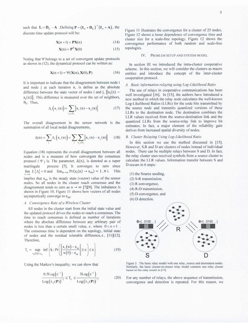
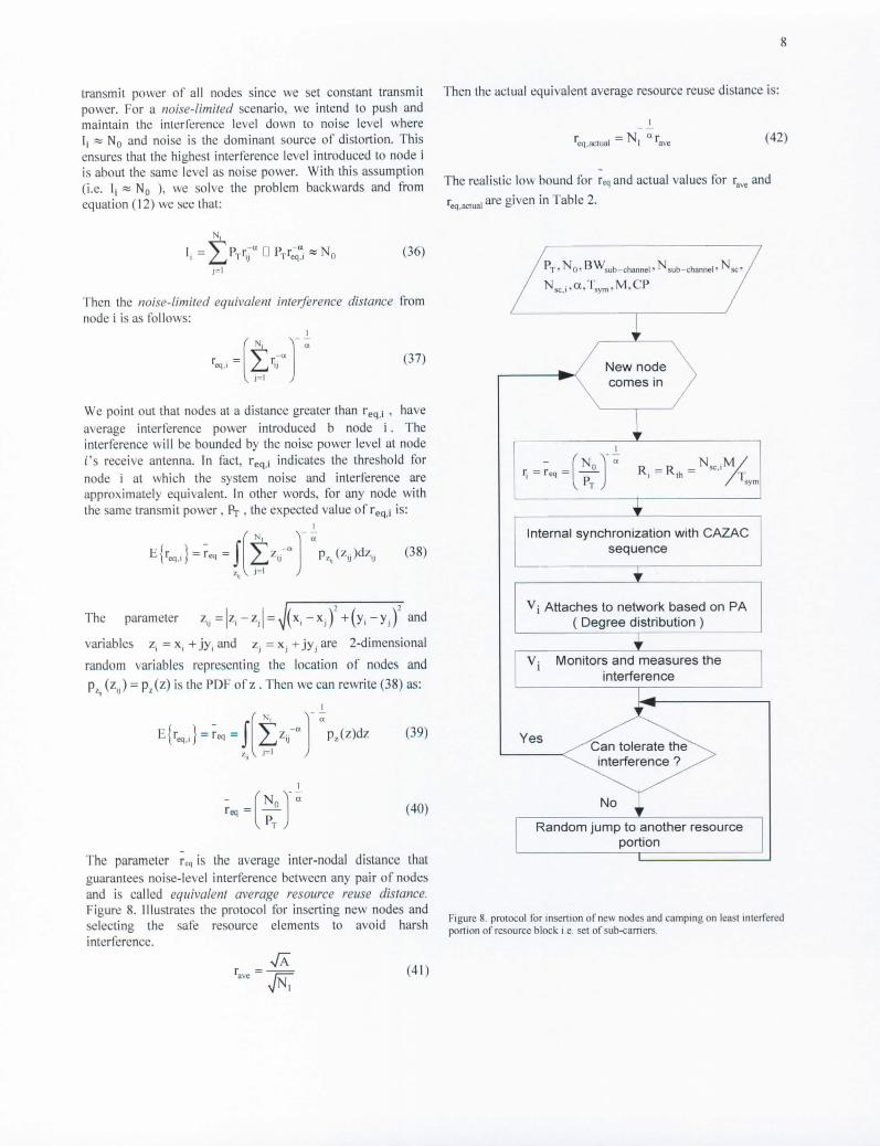
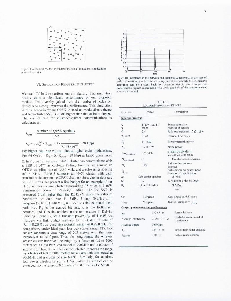
One UTSA Circle - San Antonio, TX 78249 - 210-458-7970