Working Paper no. 61

Skilled and Unskilled Wage Dynamics in Italy in the ‘90s:

Changes in the individual characteristics, institutions, trade and

technology.

Anna M. Falzoni, University of Bergamo and CESPRI - Bocconi University

Alessandra Venturini, University of Turin, IZA, CHILD

Claudia Villosio, LABORatorio R. Revelli, Collegio Carlo Alberto, R&P, Turin

July 2007

Laboratorio R. Revelli, Collegio Carlo Alberto Tel. +39 011 670.50.60 - Fax +39 011 670.50.61 Via Real Collegio, 30 - 10024 Moncalieri (TO) www.laboratoriorevelli.it - labor@laboratoriorevelli.it

LABOR is an independent research centre of the Collegio Carlo Alberto

1

Skilled and Unskilled Wage Dynamics in Italy in the ‘90s:

Changes in the individual characteristics, institutions, trade and technology.

Anna M. Falzoni, University of Bergamo and CESPRI - Bocconi University Alessandra Venturini, University of Turin, IZA, CHILD

Claudia Villosio, LABORatorio R. Revelli, Collegio Carlo Alberto, R&P, Turin

Abstract

In this paper we use individual micro data on workers combined with industry and regional data to study the wage dynamics of skilled and unskilled workers in Italy in the period 1991-1998. Being different to previous empirical studies, our data allow us to explore in a unique framework the role of many of the factors indicated in the literature as possible causes of the widening of the wage gap between skilled and unskilled workers: changes in the individual characteristics of workers, changes in the institutions of the labour market, increasing international integration and skill-biased technological progress. Our results show that international integration, both in terms of trade in goods and in terms of international labour mobility, plays a role in determining the wage dynamics of skilled (white collar) and of unskilled (blue collar) workers. In addition, in line with the research in labour economics, our findings show that the individual characteristics of workers, and the institutional variables matter more in explaining skilled and unskilled wage dynamics than differential wage one.

JEL Classification: J31, F16

Keywords: Skilled and unskilled wages, individual characteristics, labour market institutions, international trade. Preliminary version July 2007

2

1. Introduction

In the past decades wage differential has been a hotly debated issue. The widening of the wage gap

between skilled and unskilled workers experienced by the United States during the 1980s and the first half of the

1990s, raised great concern for the adverse fortunes of the less-skilled workers. The same concerns involved

continental Europe, where countries showed little changes in wage differential, but experienced robust increases

in unemployment.

A rich body of theoretical and empirical literature has investigated the causes of these trends. Large

consensus has received the hypothesis that an outward shift in relative skilled labour demand was the main

determinant of the changing conditions in the labour market. However, scholars disagree on the explanations of

such a shift, focussing alternatively on the role of international trade (i.e. Feenstra and Hanson,2001) or

skilled biased technological progress (i.e. Machin and Van Reenen, 1998) 1. Adopting a different

perspective, a number of studies have revised the leading role attributed to demand shifts, focussing on the

importance of supply and institutional factors (see for instance Acemoglu, 2003)): the increasing participation of

women in the labour force; the aging of the workers; the increase in the supply of foreign workers; the increase

in the average education level; the institutional characteristics of the wage setting, centralised or not; the strength

of Trade Unions; the firing regulation; and so on2.

To disentangle the relative importance of supply and demand factors and of institutions in explaining the

wage dynamics of skilled and unskilled workers seems particularly relevant in the case of continental Europe

where all these factors were at work during the last decades.

Among European countries, we chose to study Italy, analysing the wage dynamics of skilled and

unskilled workers in the period 1991-1998. We benefited from the availability of a dataset containing individual

micro data on workers that we combined with industry and regional data. Being different to previous empirical

studies, our data allow us to explore in a unique framework the role of many of the factors indicated in the

literature as possible causes of the widening of the wage gap between skilled and unskilled workers: changes in

the individual characteristics of workers, changes in the institutions of the labour market, increasing international

integration and skill-biased technological progress.

Italy represents an interesting case study from many perspectives, but in particular because of its

peculiar institutional features (especially in the labour market) and its pattern of international specialization. In

addition, the 1990s – the period under study - were characterised at least by two important changes which had

relevant effects on the Italian economy: specifically, the end of the nation wide wage indexation (the so-called

1 The current consensus emerging from the empirical literature is that trade plays a positive, yet relatively small, role in rising wage inequality (see for a survey, among others, Haskel (2000), Feenstra and Hanson (2001) and Crinò (2007)). As for the role of technological progress, see among others, Machin and Van Reenen (1998) and Berman et al. (1994). 2 See, among others, Dell’Aringa and Lucifora (1994), Erikson and Ichino (1995), Bertola and Rogerson (1997), Lucifora (2000), Baccaro (2000), Cappellari (2004), Cipollone (2001), Katz and Murphy (1992), Autor, Katz and Kearney (2005) and Koeniger, Leonardi and Nunziata (2007).

3

scala mobile) with the agreement signed in 1993 and the rapid export growth following the devaluation of the

Italian Lira the year before, to which we can add the increase in foreign employment, in female employment and

the ageing of the workers.

Due to its peculiar position in the international division of labour, Italy gives the opportunity to test

whether international trade plays a role in explaining the changing conditions of unskilled workers. Italy’s

position in traditional sectors and in some specialised supplier industries is very strong, while it is weak in

sectors based on economies of scale and, especially, in high tech industries, where capital and skill abundant

countries traditionally have their comparative advantages. Overall, both the observed pattern of trade and the

characteristics of the manufacturing sector seem to suggest that Italy has a comparative advantage in labour-

intensive goods, as many other emerging economies. On the one hand, these features of the pattern of production

and trade have raised growing concern regarding Italy’s vulnerability on foreign markets, when facing the

competitive pressures of products from low-wage countries. On the other hand, given this distinct pattern of

comparative advantage in low-skill, high-labour intensive productions, “Italy should be placed among those

countries whose labour force is likely to gain from the operating of the Stolper-Samuelson effect” (Faini et al.,

1999, 129).

This paper is different from the previous works which inquire into the effect of trade on the wage

dynamics in Italy in many respects. Firstly, most of the studies do not distinguish the effect of trade between

skilled and unskilled workers3. Apart from the very recent work by Matano and Naticchione (2007)4, only

Brenton and Pinna (2001) and, in a different context, Helg and Tajoli (2005), analyse the role of trade on skilled

and unskilled worker but on workers’ employment. Brenton and Pinna (2001) find that imports from low-wage

labour abundant countries influenced negatively the employment opportunities of unskilled workers in Italy in

the 1980s and in the 1990s (particularly in skill intensive sectors). Helg and Tajoli (2005) find that the increase

in the skilled-to-unskilled labour ratio in Italy is positively and significantly related to an index of international

fragmentation of production. Secondly, other studies have investigated the role of trade on skill upgrading

focussing attention only on the export activity of firms. In all these studies, the trade variable being analysed is

the firms’ export activity and, due to the nature of the data, the impact of increasing foreign competition is not

investigated (Quintieri and Rosati (1995), Ferragina and Quintieri (2000), Manasse et al. (2004)).

This paper is also different from the labour studies on the institutions or individual effect on wage

dynamics. The firsts are mainly international comparisons of countries with different institutions (Erikson and

Ichino 1995, Lucifora 2000, Bertola and Rogerson 1997), while the seconds mainly analyse only the individual

components of the wage dynamics (Cappellari, 2004, 2007).

3 See, among others, De Nardis and Malgarino (1996), Bella and Quintieri (2000), Faini et al. (1999). 4 Matano and Naticchione (2007) study the impact of international trade on wage inequality focussing on the geographical structure of trade, distinguishing the effect of trade with developed, developing and transition countries.

4

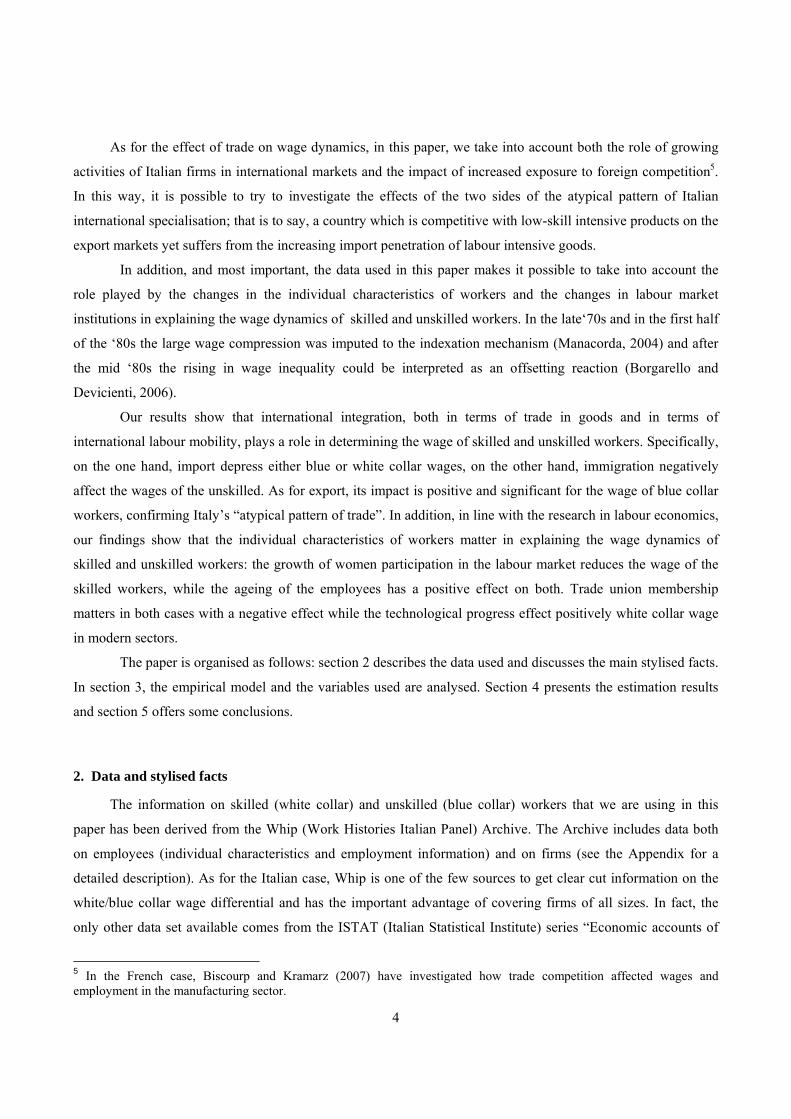
As for the effect of trade on wage dynamics, in this paper, we take into account both the role of growing

activities of Italian firms in international markets and the impact of increased exposure to foreign competition5.

In this way, it is possible to try to investigate the effects of the two sides of the atypical pattern of Italian

international specialisation; that is to say, a country which is competitive with low-skill intensive products on the

export markets yet suffers from the increasing import penetration of labour intensive goods.

In addition, and most important, the data used in this paper makes it possible to take into account the

role played by the changes in the individual characteristics of workers and the changes in labour market

institutions in explaining the wage dynamics of skilled and unskilled workers. In the late‘70s and in the first half

of the ‘80s the large wage compression was imputed to the indexation mechanism (Manacorda, 2004) and after

the mid ‘80s the rising in wage inequality could be interpreted as an offsetting reaction (Borgarello and

Devicienti, 2006).

Our results show that international integration, both in terms of trade in goods and in terms of

international labour mobility, plays a role in determining the wage of skilled and unskilled workers. Specifically,

on the one hand, import depress either blue or white collar wages, on the other hand, immigration negatively

affect the wages of the unskilled. As for export, its impact is positive and significant for the wage of blue collar

workers, confirming Italy’s “atypical pattern of trade”. In addition, in line with the research in labour economics,

our findings show that the individual characteristics of workers matter in explaining the wage dynamics of

skilled and unskilled workers: the growth of women participation in the labour market reduces the wage of the

skilled workers, while the ageing of the employees has a positive effect on both. Trade union membership

matters in both cases with a negative effect while the technological progress effect positively white collar wage

in modern sectors.

The paper is organised as follows: section 2 describes the data used and discusses the main stylised facts.

In section 3, the empirical model and the variables used are analysed. Section 4 presents the estimation results

and section 5 offers some conclusions.

2. Data and stylised facts

The information on skilled (white collar) and unskilled (blue collar) workers that we are using in this

paper has been derived from the Whip (Work Histories Italian Panel) Archive. The Archive includes data both

on employees (individual characteristics and employment information) and on firms (see the Appendix for a

detailed description). As for the Italian case, Whip is one of the few sources to get clear cut information on the

white/blue collar wage differential and has the important advantage of covering firms of all sizes. In fact, the

only other data set available comes from the ISTAT (Italian Statistical Institute) series “Economic accounts of

5 In the French case, Biscourp and Kramarz (2007) have investigated how trade competition affected wages and employment in the manufacturing sector.

5

the manufacturing firms” covering firms with more than 20 employees, thus excluding something like 30% of

total employment in Italian manufacturing industry. As in previous researches (i.e Manasse et al., 2004), in this

paper only blue collar and white collar workers are considered and used as proxies of skilled and unskilled

workers.6 White collar employees include the cadres (Quadri) and they correspond to the executive category in

other researches.

The wage variable used in our analysis is the annual wage based on the total amount of the monthly

earnings paid to the worker (basic wage, cost-of-living allowance, residual fees, overtime), plus the total amount

of the non-monthly wage (back pay, bonuses, supplements holiday pay, sick pay), expressed in thousands of

Italian lira. At a fiscal level it represents the basis on which payroll taxes are determined7.

Figure 1a shows, for the years 1991 to 1998, the blue and white collar wage trends and the wage

differential (all in logs). Both white and blue collar wages increase, with the former increasing more than the

latter. As a result, the total wage differential rises a bit after 1994 and decline in 1997 to increase again in the

subsequent period. This is not the result of a variation in the dispersion within the groups because the variance

within each group remains stable throughout the period (see Figure 1b). As Borgarello and Devicienti (2002,

2006) have shown, inequality in Italy has increased mainly during the 1985-1991 period8, while in the 1992-

1995 period it has been rather constant.

Many changes however took place during this period which could help to explain this trend. There were at

least three important transitions in the labour market. Firstly, Italy becomes a country of immigration. At the

beginning of the period foreigners were 1.5% of total employees in the manufacturing sector and reached 3% in

1996 and 4% in 1999 (see Figure 2). Secondly, women entered the labour market in large numbers; even in the

manufacturing sector they were 31% of total employed in 1991 and reached 34% in 1998. Finally, there was a

very significant aging of the labour force; the share of old workers (over 50) over the share of young workers

(aged less than 25) was only 48.5% in 1991 and reached 61.8% in 1998.

All these factors have contrasting effects on wages: immigrants are mainly blue collars and are registered

in low wage jobs, thus they tend to increase the wage differential between skilled and unskilled workers; women

are usually in high wage jobs among blue collar workers and in low wage jobs among white collar workers, thus

their growth in employment tends to reduce the wage differential. The aging of the employees in both groups

increases the wage differential. To have a clear cut idea of how important the age is for the level of wage

6 Whip includes also the category of the managers. However, managers who are registered in the Whip dataset are not representative of the entire category because most managers belong to a different social security fund. 7 An alternative would be to use the daily wage calculated as annual wage divided by the number of paid working days. The reason why the former is adopted is that paid working days could be underreported by the firms to adjust the total wage bill to the minimum wage requirements. Further, such underreporting does not seem to be distributed uniformly in the country, but it appears to be very frequent in the South and among the blue collars (Contini et al., 2000). 8 It took place when the wage indexation (scala mobile) was dismantled.

6

differentials, it is only necessary to look at Figure 3 where it can be seen that the wage differential is quite stable

for each age group and increases only through the aging of the cohort.

While the workers’ characteristics changed, the role of labour market institutions changed too. In 1993 an

important agreement was signed which brought to an end the nation wide wage indexation (the so-called scala

mobile). Thus, since then wage increases were more closely related to labour productivity and to firm profit

margin. As for trade union membership, it increased from 39% in 1991 to 40% in 1992-1993 and declined to

38% in 1996 and 36% in 1998. The fall in trade union membership in the latter period may help to explain the

increase in the wage differential, it was the result namely of white collar workers’ wages catching up. Territorial

distribution of trade union membership however shows an overall declining rate, but in Lombardy and Piedmont,

for example, the trade union rate remained quite stable and these two regions are the ones where the trade union

base is strongest. The strike pattern is again very uneven. The number of hours lost for strikes were stable at

about 9 or 10 thousand per year but fell to 2050 in 1995 and recovered just a little in 1998 (2200). In general

Lombardy is the most conflicting region, but other regions experienced peaks of conflicts in the years under

analysis. Both indicators - trade union membership and strike pattern - are expected to have a negative effect on

wage differentials: trade unions are assumed to protect the unskilled workers more and strikes are more frequent

among the blue collars. However this assumption is not always confirmed.

There are other variables which might affect the wage differential as for instance firms’ characteristics in

terms of size, industry and so on. Figure 4 shows how strong and stable the relationship between a firm’s size

and the wage differential is. But the figure also suggests that the growth of a firm’s size changes the average

wage differential.

In addition to the workers’ and firms’ characteristics and the role played by labour market institutions,

increasing international integration has been pointed out as a possible source of the widening wage gap between

skilled and unskilled workers. Under this respect, the period covered by our analysis is particularly interesting

being characterised by the growth of trade flows and the switching from a negative to a positive trade balance

following the devaluation of the Italian Lira in 1992 (Figure 5). Thus, in the Italian case, trade could be an

explanatory variable for the growth of the wage differential a year after the Lira depreciation. But of course the

possible effect of the trade variable will be different in the various sectors according to their openness.

As preliminary evidence, Figure 6 shows the industry’s degree of openness (measured as exports plus

imports over value added) and the corresponding white-blue collar wage differential. A clear relationship does

not emerge; however for a number of sectors it seems that a high degree of openness is associated to a larger

wage gap. Even more heterogeneous it seems the picture presented in Figure 7, where higher degrees of

openness at the territorial level (regions) are related to lower wage differentials. The analysis at the territorial

level is justified by the well known ‘dualistic nature’ of the Italian economy, with regions in the North

historically more developed than regions in the South. Again there is not a clear cut pattern between trade

7

openness and wage differentials between skilled and unskilled workers, thus a more specific analysis has to be

done to control these many components.

3. The empirical model

The aim of this paper is to investigate whether the wage differential between white and blue collar

workers is explained by changes in the individual characteristics of the workers, changes in the labour market

institutions and increasing international integration, both in terms of trade in goods and of labour mobility.

The dependent variable of our empirical model - the wage differential between white and blue collar

workers - cannot be computed at an individual level, but only at a unit level. Thus the analysis should be made at

a higher level of aggregation. From the discussion presented in the previous section it would appear to be

appropriate to check for both region and industry dimension. Therefore, the joint region and branch dimension

has been chosen and all the variables used in the empirical analysis have been aggregated at the corresponding

level.

3.1 Is the analysis by branch and region appropriate?

Before going on with the analysis of the wage differential by the region and branch ‘cells’, it is necessary

to investigate the changes in the white collar share of total employment so as to be sure that the subsequent

analyses of the wage differential capture the areas where the phenomenon is relevant. Using the break-up of the

share of white collar employment over total employment first used by Berman et al. (1994) and Machin (1996),

white collar growth is split up into two components. The between component which shows by how much the

change in the white collar employment share is due to shifts in employment shares between ‘units’ with different

proportions of white collar employment; and the within component which shows by how much the change in the

white collar employment share takes place within each ‘unit’9.

Table 1 shows a general growth in the white collar employment share. In particular, the growth is due for

the 78% to the within component, while the between component is very small. This means that the growth is due

to changes in the proportion of white collar workers within each ‘unit’, rather than to the reallocation of the

workforce towards ‘units’ with different skill-intensity. Moreover, also grouping the sectors according different

characteristics of interest, we find that the within ‘unit’ component is dominant both for the low and high wage

9 The decomposition is shown by the expression below where the first term represents the between component and the second term the within component:

∑∑ Δ+Δ=Δi

iwiwii

iw SSSSS

i = region and branch ‘cell’ Sw= white collars share of total employment Si= share of employment in the ‘cell’ i Swi= white collars share of employment in the ‘cell’ i A bar over a term denotes mean over time.

8

differential sectors, and for the less and more open to trade sectors. Thus, the analysis at the branch-region

dimension seems to be very appropriate.

3.2 The model, the variables and the test

For each ‘unit’ given by the joint region (r) and branch (s) of the manufacturing sector, the white collar (1)

- blue collar (2) wage differential is defined as below

δs,r,t= ln(W1 s,r,t ) - ln(W2 s,r,t) [1]

s =1,…,10 r =1,…,20 t=1,…8

The wage differential, δ s,r,t , is explained by a series of variables at the same level of aggregation but

belonging to different areas: the average characteristics of the workers (X), the structure of production (F), the

macro economic or the institutional variables (Y), the degree of openness to trade (T), and proxies for the

technological progress (K).

The baseline equation estimated in our analysis is the following:

δ s,r,t = α s,r + β X s,r,t + γF s,r,t + λY s,r,t + θ T s,r,t + ϕ K s,t + ε s,r,t [2]

With this model an attempt has been made to capture in a unique framework the role of many of the

factors indicated in the literature as possible causes of the widening of the wage gap between skilled and

unskilled workers. In addition to the more trendy trade and technological progress variables, allowance has been

made for the composition of supply. Individual characteristics and institutional factors which change the

incentives in the hiring and firing of workers are taken into account. At the same time we check for

macroeconomic variables and changes in the structure of production.

Given that we use data averaged at branch and region level, to have a representative sample, we weight all

the units by the share of employed workers in the unit on total employed workers10. This correction is particularly

important in Italy, where in the Northern part there are units which involve more workers than in the Southern

regions11.

10 This strategy provides the same result as using individual data with aggregate variables.

9

Table 2 summarizes the variables used in the empirical analysis. The individual variables, X, in equation

(2) account for all the variables by branch and region: the number of women (female); the average age of the

employed (age); and the number of foreign workers (foreigner). The variables included to check the structure of

production, F, are as well by branch and region: the share of small firms (small) 12; the share of medium-sized

firms (medium) 13; the net creation rate of new firms (net firm); the net job creation rate (job creation); and the

turnover rate (turnover) 14. The institutional and macro variables, Y, represent: the value added by branch and

region (value added); the unemployment rate by region (unemployment); the hours lost because of strikes by “3

branches” and by region (strikes); and the unionization rate by region (unionization). The trade variables, T,

measure, by branch and region, the amount of imports (imp) and of exports (exp). Proxies which can capture

technological change (K) are introduced, as a Pavitt index of technological change interacted with time dummies

or sector dummies interacted with a time trend15.

Two points we should stress about the estimates.

First of all, to eliminate the unit fixed effect α s,r the within estimator has been adopted. Thus the observations of

each unit are expressed in terms of deviations around the time mean for that unit16.

Second, given that the units have different dimension, it is likely that the variance of the residuals varies by unit

dimension, thus that the residuals are heteroschedastic. Our expectation is that residuals are smaller in larger

units. We use the Godfrey Quandt test and after ranking the observations by increasing size - either by using the

first 50 and last 50 units or the first 75 and last 75 units - we get a ratio between the first and the second group

standard error residuals of 38 and 18 respectively, much above the F value of 1.6 and 1.48 respectively. We,

thus, refuse the null hypothesis of absence of heterogeneity and to overcome this heterogeneity problem GLS

estimates have been performed17.

4. Results

11 i.e. the textile sector in Lombardia employ about 180.000 workers while the textile sector in Basilicata only 3.000, and the lack of appropriate weights will over value the relation that takes place in the Southern regions. 12 Firms with less than 20 employees. 13 Firms with employees between 20 to 100. 14 Annual inflow plus outflow of employment. 15 As suggested and adopted by Geishecker and Görg (2005). 16 Within estimates are also very appropriate for this case where the effect of the covariates is distributed upon more years and first difference estimates overstress the contemporarily annual effect. 17 Given that we weight each unit by their employment and that the GLS estimated tend to overweigh the larger units, we could incur in an over weighting problem and for that reason we have tested for the under or over weighting by regressing the residual of the regression on the unit dimension. The results show that the variable unit size is never significant in explaining the residual of the regression, reassuring about the weight given to the larger units. We thank Steiner Strom for this suggestion.

10

Table 3 shows our first results using different specifications of the empirical model discussed in the

previous section.

We start testing the hypothesis that an outward shift in relative skilled labour demand was the determinant

of increasing wage inequality and column 1 presents only trade variables, imports and exports, and proxies of

the technological progress as regressors. Which ever proxy we adopt for the technological progress, either

macro sector dummies à la Pavitt as Traditional, Specialization, High-tech and Scale Intensity18 plus an unique

trend (the specification shown in Table 3, column 1), or macro sector trends, or Pavitt dummies19 and a trend,

the trade variables keep the same sign and significance, always negative for imports and positive but non

significant for exports. Namely, exports seems to have no effect on white-blue collar differential, while imports

reduce wage differential by depressing white collar wages or by increasing blue collar ones. The proxies of the

technological change as well are always significant, with macro-sectors dummies negative and a positive trend

or positive macro-sector trends (see Table 3). Of course, additional time dummies are included to control for

macro shocks.

The specification adopted in column 2 of Table 3 introduces institutional and macro controls. As before,

the trade variables maintain the previous significance and sign and some of the technological proxies remain

significant. Among the institutional variables, the numbers of days lost for strike perform better than the Trade

Union participation and hold a negative sign as expected. Usually blue collar workers are more strike prone than

white collar ones and get wage increases afterward, then a negative effect of the number of strikes on wage

differential is expected while unexpectly the macro controls are non significant.

In column 3 of Table 3 all the variables are introduced: individuals, firms, macro, institutional, trade and

technological proxies. The results are unexpected. Among the trade variables, imports are slightly significant

with a negative sign, while exports as before are not significant and technological variables are no more

significant. Strikes, previously significant, are no more significant now, the macro controls are as before little

significant, among the individual and firm variables only the turnover rate and the female employed are relevant.

The first hold a positive sign because mobility among the white collars usually means upgrading while among

the blue collars means instability. The second, female employment, is negative because usually women are

employed in low white collar positions and in high blue collar ones. The specification of column 3 is largely

unsatisfactory, because the use of individual data seems not producing an improvement in the total control. A

possible interpretation could refer to a over-identification problem. The technological proxies are probably

18 Sectors 1 ‘Energy’, 7 ‘Food’ and 8 ‘Textiles’ are classified as Traditional; sectors 2 ‘Metals’, 3 ‘Non-metal products’, 6 ‘Vehicles’ and 9 ‘Paper and editorial products’ are classified as Scale Intensive sectors; sectors 4 ‘Chemicals’ and 5 ‘Metal products and machinery’ as High Tech; and sector 10 ‘Wood and rubber’ as Specialization. 19 Sector 1 ‘Energy’ has been given the value 1, sector 2 ‘Metals’ the value 2.94, sector 3 ‘Non-metal products’ the value 2.77, sector 4 ‘Chemicals’ the value 10, sector 5 ‘Metal products and machinery’ the value 3.42 , sector 6 ‘Vehicles’ the value 3, sector 7 ‘Food’ the value 1, sector 8 ‘Textiles’ the value 1, sector 9 ‘Paper and editorial products’ the value 3.14, sector 10 ‘Wood and rubber ‘ the value 3.

11

catching up changes of the individual and firm variables. The results remain the same if we replace the macro-

sector trends variables with macro-sectors dummies or with a simple unique time trend. The idea of putting

together individual variables and the trade variables want to combine two different approaches at the labour

market. The trade approach which imagines that firms are free to choose the more efficient workers by choosing

the component of the labour force which maximise profits, while the labour market approach stresses that there

are fixed costs to incur. Thus firms maximise their profits by keeping their employees and paying the seniority

wage increase until it does not overcome the fixed cost that they have to incur if they want to replace the old

workers with younger ones. Thus only part of the wage is affected by trade and technological changes, while

another part of the wage increase is function of the internal dynamics of the labour force. However individual

variables move slowly and probably they follow a sector trend and the two sets of variables override each other.

This is not the only explanation of the problem. An additional interpretation point out the individual

variables do not perform appropriately because they have different effects on blue and white collar wages, and

an unique measure confuses the two effects. We thus pursue these two not necessarily contradicting

interpretations.

We first analyses the effect of all the explicative variables but the proxies of the technological ones (not

reported in the table). Probably we do not have adequate measure of the technological progress and thus the

proxies used could capture many additional factors, but if we take these last off, the individual variables which

are at the branch and region level become significant but with some unusual sign. The trade variables improve

their significance, exports become significant with a positive sign and import negative.

We distinguish the individual variables into the two components white and blue in Column 4 of Table 3.

The equation performs much better and in particular it shows different and opposite sign of the coefficients for

the two groups. The macro variables remain not significant, strikes instead are again significant, while the trade

variables keep the same sign, negative for import and positive for exports, but loose some of the significance.

The technological proxies are no more significant but these results could be recalled to a different effect on blue

and white collar wage.

These results push us into the direction of splitting the wage differential into the two separate components

white and blue collar wages to better inquire into the effects of the different variables. In addition, the constant

level of wage dispersion inside the two groups skilled and unskilled presented in Table 1.b suggests to pursue

with the analysis of the wage level and not to the wage inequality.

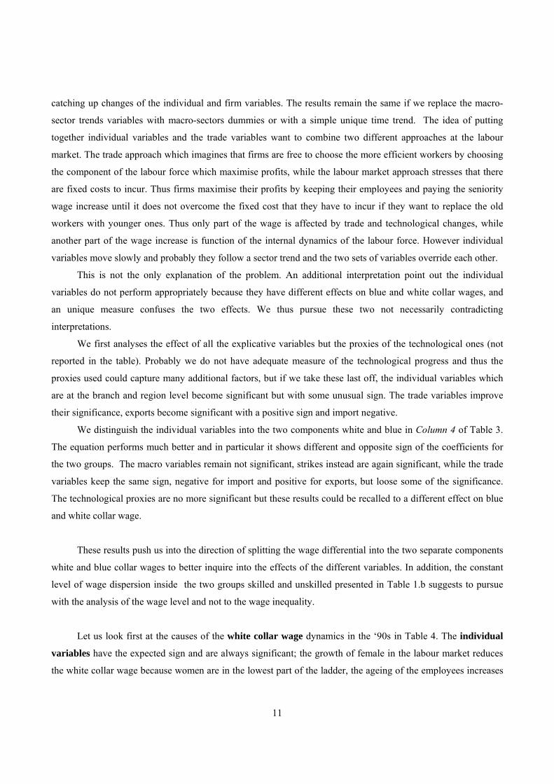
Let us look first at the causes of the white collar wage dynamics in the ‘90s in Table 4. The individual

variables have the expected sign and are always significant; the growth of female in the labour market reduces

the white collar wage because women are in the lowest part of the ladder, the ageing of the employees increases

12

the wage as tenure is an important part of white collar wage. And the increase of foreigners in employment has a

negative sign but not significant because immigrants are mainly in blue collar jobs.

As for the variables controlling for the structure of the production system, the firm size is not

significant. A series of variables, namely, net firm creation rate, job creation rate and turnover rate has been

included in our regression20. They are aimed at checking for the turbulence of the ‘unit’ and capturing sectorial

relocation, if presents in the data. As the previous section shows, the increase in white collars took place mainly

within the units, and the not significant coefficient of the variable net firm creation and the positive sign of the

variable job-creation is in line with the previous results, and confirm that high wage jobs are created within

firms. Among all these variables the turnover rate is always significant with a negative sign; a high turnover rate

reduces the wage growth as instable jobs are hold by low skilled people.

The macro variables - value added and unemployment rate – hold the expected sign, the first according

to the specification also significant; the latter, the unemployment rate, is always significant with a negative sign

which implies that the growth of unemployment has a negative effect on the growth of white collar wage.

The institutional variables - strikes and trade union membership - are both significant but with a negative

sign. If we use either one or the other the sign remain negative, and the use of only the trade union participation

rate improves the general performance of the results (value added and foreign workers improve the significance).

Let us now turn to the trade variables. Table 4 shows that exports do play a positive role in explaining

white collar wage growth, while import penetration reduces white collar wage. Thus labour immigration and

imports of good have a negative effect on white collar wage growth.

The technological proxies in the form of macro-sector trends are significant as well, stressing the

importance of the technological change. Also the time dummies are significant.

Let us go to the blue collars wage dynamics. The results in Table 5 show that the individual variables

play a role; ageing increases the wage, while the increase in the number of immigrants reduces the average

branch region wage. The growth of female in employment do not affect the average blue collar wage namely

because their growth is mainly in white collar jobs. Blue collar wage increases in medium size firm, and the new

jobs are created for high skill manual workers, while the destruction of firms increases the average wage because

marginal companies are closing (the average value of the net-firm creation is negative). The turnover rate is an

indicator of marginal or temporary positions and decreases average wage. The macro variables are both

significant with the expected sign; the growth of value added by branch and region has a positive effect on

manual wage while the growth of unemployment has a negative one with a clear trade off between wage and

employment for blue collar workers. Between the two institutional proxies, only the Trade Union registration is

20 The three variables - changes in net firm creation, job-creation and turnover rate - could be affected by the changes in trade openness and also by technology. Therefore, it was decided to check for possible endogeneity in the variables by calculating a Pearson correlation test. The Pearson correlation test shows no significant.

13

significant with a negative sign which fundamentally means that blue collars are more unionized if their sector is

a low wage one and has lower growth.

The trade variables are always significant with import playing a negative role and export a positive one.

For blue collar the negative effect of imports and foreign workers is even stronger than in the case of white

collars, however the positive effect of export is as well stronger in the blue collar wage. Blue collar wages seem

to be more sensitive to foreign economic relations.

The proxies of the technological change are significant with positive coefficients and the time dummies

as well significant but with a negative sign.

These results shed light on previous findings regarding the wage differential equation. In fact, in the wage

equations for blue and white collar workers, the individual variables, but also the firm variables, are all

significant but hold different coefficients (in some cases with contrasting signs) and in the wage differential

equation they resulted not significant. As well, the inclusion of technological proxies, which are significant and

positive in both blue collar and white collar wage equations, explains the non significance of these proxies in the

wage differential case.

5. Conclusions

In this paper we use individual micro data on workers together with industry and regional data to

understand the wage dynamics of skilled and unskilled workers in Italy in the Nineties. This period was

characterised at least by two changes which had important effects on the Italian economy: specifically, the end of

the nation wide wage indexation (the so-called scala mobile) with the agreement signed in 1993 and the rapid

export growth following the devaluation of the Italian Lira the year before, to which we can add the increase in

foreign employment, in female employment and the ageing of the workers.

Differently to previous empirical studies, our data enable us to explore within a unique framework the role

of many of the factors indicated in the literature as possible causes of the widening of the wage gap between

skilled (white collar) and unskilled (blue collar) workers: changes in workers’ individual characteristics, changes

in the institutions of the labour market, skill-biased technological progress, and increasing international

integration.

Our results show that, while the trade variables and the proxies that we used to control for the

technological change were significant in interpreting blue and white collar wage differential, the addition of the

institutional variables, of the macro ones and, even more, of the individual variables shows very little power in

explaining the wage differential. While instead all the components previously mentioned are very effective in

explaining the white and blue collar wage dynamics.

Our analysis based on separate white and blue collar wage equations points out that the international

integration, both in terms of trade in goods and in terms of international labour mobility, plays a role in

14

determining the wage of skilled and unskilled workers. On the one hand, increasing export has a positive and

significant effect on unskilled workers wage, while the increase of imports and of immigrants has a negative

effect on earnings of this group of workers. On the other hand, the import of goods affects negatively also the

wages of the skilled workers, but they don’t seem to benefit from increasing export activities. These results

support the view of Italy characterised by comparative advantages in low-skill, high-labour intensive

productions; at the same time these findings stress the negative effect, both for skilled and unskilled workers, of

the international competition through increasing import penetration. Institutional variables, better strikes than

trade unions membership, play a negative role either on the blue and white collar wage, which shows that

conflict dominates in low wage and slow growing wage sectors and regions. Sociological studies stress that the

many years dominated by the indexation mechanism seem to have weakened the Trade Unions strength and they

remain only the defender of the weaker segment of the labour force. Individual variables matter with the

expected sign: positive for age and negative for female, and the turnover rate plays a negative role on wage

growth of both types of workers, but it is much more serious for the blue ones. The proxies for the technological

change are significant in the blue and white collar equations and not in the wage differential one because the

coefficients hold similar sign, as well the time dummies, which were only occasionally significant in the

differential case.

What finally emerges from these results is that in the analysis of the wage differential the trade variables

are always consistent, while the individual variables conflict with the long term sectorial ones.

All the components instead contribute in the explanation of the white and blue collar wage dynamics, and

this provides strong support to the need of considering both supply and demand factors as determinants of wage

dynamics and the need to use less aggregate data to control both.

15

16

Data Appendix

The data set used in this paper is derived from the INPS (Italian Social Security Institute) Social Security Archives. Social security contributions (and payments to the National Health Service) are collected from firms and individual workers by INPS, which pays out retirement benefits and various wage supplements. The data used in the paper are derived from two different archives: the first (O1M) which has yearly data on individual employees filled in by the employers to certify an employee’s rights to pension benefits21; and the second (DM10M), monthly data on firms with employees filled in by the employer (payments of social security contributions)22. The former archive is organized by individual worker and year (roughly 12.5 million records per year). A worker may appear with more than one record in a given year, whenever (s)he has worked for two or more employers during the year. The latter archive, roughly 1.2 million records (firms), is updated each month, corresponding to the number of active firms with at least one employee. The archive includes all private firms in the industrial and service sectors with at least one employee; services and other activities connected with agriculture are not included. Central administration employees are entirely absent from the archive; i.e. mail services, state school teachers, the justice, the armed forces and all government agencies are not included. Whenever a firm is recorded in the archive, all its employees are observed (with the exclusion of family and self-employed workers). For each calendar year 1985-96, the Social Security forms ("moduli O1M") of employees born on the 10th of March, June, September and December of any year were selected. In this way, a sequence of random (roughly, 1:90) samples of the population of employees of private firms is formed. Each yearly sample includes approximately 100,000 workers. Using available identifiers (fiscal and social security codes), individual longitudinal data are generated for each sampled worker. The firm’s longitudinal records are then accessed for each worker in the sample and the employer’s details (code of economic activity, total number of employees) are then associated to the employee23. 21 For each employee, calendar year and employer the following data are available: - employee identification (social security number, fiscal code, date of birth, sex, etc.); - employer identification, linking the worker to the relevant firm; - place of work ("provincia"); - list of months for which wages or salaries were paid; - number of "paid" weeks and days; - date of closure of the relationship with the current employer; - yearly salary or wage subject to social security contributions; - yearly wage supplements due and paid by the employer; - occupation (apprentice, manual worker, non-manual worker, manager); - type of labour relationship (full time, part time, limited or unlimited duration); - code of contractual agreement and position in the contractual ladder. - wage supplements paid by the employer on behalf of INPS (starting from 1989). 22 Firms pay compulsory social security contributions and national health insurance on a monthly basis. Forms used for the payment specify: i firm's identifiers: social security and fiscal code, company name, address; ii economic activity (code), iii dates of registration and termination (if applicable); and, for each reference month iv number of employees to whom some salary or wage was paid by the employer; v before tax wage (or salary) bill paid by the employer; vi social security contributions paid by the employer; vii total number of days for which some wage (or salary) was paid by the employer; viii wage supplements paid by the employer on behalf on the Social Security Institute; rebates on contributions (for young and female workers, firms located in "depressed" areas, etc.). Items (iv)-(vii) are broken down into 4 occupational groups (manual and non manual workers, cadre and managers, apprentices), as well as taking account of part time and other special work contracts. 23 For each employee, employer and year, the following data are available: - the content of the employees’ archive

17

If a worker is not in the archive, and hence in the panel of employees of private firms, it means that (s)he is in a different category: self-employment, unemployment, public sector, retirement, black economy24. This is the more appropriate dataset available for the purpose of our research because those not covered by this dataset – i.e. public sectors, self employment - are not so relevant for an analysis on the effect of trade flows and technology. In addition, of this dataset we use only the section more exposed to international trade, namely the manufacturing sector. The main characteristics of the employees are shown in Table A1. Males prevail in all the dataset, but in the manufacturing sector the male group reaches about 70% of total employees, 47% are employed in firms with less than 50 employees , 72.8% are blue collars and the remainder white collar workers. Of course there are more blue collars in the manufacturing sector alone than in the dataset for the private service sector. The Textiles and the Metal products and machineries sectors are by large the most important and the North West is by large the most important area and the North alone accounts for 67% of total employees.

- the code of economic activity of the relevant firm (employer); - firm’s location, dates of enrolment and cancellation; - monthly number of employees in the firm, by occupation; - annual wage bill, by occupation. 24 There is no attrition in these archives, if we exclude updating problems, i.e. delays in the acquisition of information from the firms. It is compulsory to provide records on employees and firms to the social security administration, if the worker and the firm belong to one of the mentioned categories.

18

Table A1 - Characteristics of the Employees in the Whip panel, 1996

Gender Manufacturing Sectors Manufacturing % Female 30.75% 1 Energy 3.38% Male 69.25% 2 Metals, 2.68% Age 3 Non-metal products 5.85%

-20 1.47% 4 Chemicals 4.78%

21-25 13.41% 5 Metal products and machineries 35.12%

26-30 18.45% 6 Vehicles 5.44%31-35 17.02% 7 Food 7.81%36-40 13.50% 8 Textiles 18.07%41-45 12.24% 9 Papers and editorial products 4.59%46-50 13.33% 10 Wood and rubber 12.30%

51-60 9.98% Geographical areas

61+ 0.60% North-West 39.86%

Firm Size North-East 27.39%

1-5 8.80% Centre 17.09%6-9 7.18% South 15.67%

10-19 14.13% Skill 20-49 17.17% Blue collar 72.8% 50-99 10.69% White collar 27.2%

100-199 9.25% 200-499 10.07% 500-999 5.59% 1000 + 17.12%

19

References Acemoglu D. (2003), “Cross-Country Inequality Trends”, Economic Journal,vol.113, F121-49. Autor D., Katz L., Kearney M. (2005), “Trends in the U.S. Wage Inequality: Re-Assessing the Revisionists”, NBER W.P. 11627. Baccaro L. (2000), “Centralized Collective Bargaining and the Problem of ‘Compliance’: Lessons from the

Italian Experience”, Industrial and Labour Relations Review, vol.53, n.4, 579-601. Bella M., Quintieri B. (2000), “The effect of trade on employment of Italian industry”, Labour, vol. 14, 291-309. Berman E., Bound J., Griliches Z. (1994), “Changes in the Demand for Skilled Labor within U.S.

Manufacturing: Evidence from the Annual Survey of Manufacturers”, Quarterly Journal of Economics, vol.109, 367-397.

Bertola G., Rogerson R. (1997), “Institutions and Labor Relocation”, European Economic Review, vol.41, 1147-

71. Biscourp P., Kramarz F. (2007), “Employment, Skill Structure and International Trade: Firm-level Evidence for

France”, Journal of International Economics, vol.72, 22-51. Blau F.D., Kahn M. (1996), “International differences in male wage inequality: Institutions versus market

forces”, Journal of Political Economy, vol.104, 791-837. Borgarello A., Devicienti F. (2002), “Trends in the Italian Earnings Distribution, 1985-1996”, in: B. Contini

(ed.), Labor Mobility and Wage Dynamics in Italy, Rosenberg & Sellier, Torino. Borgarello A., Devicienti F. (2006), “L’aumento della disuguaglianza dei salari in Italia: premi salariali per le

“nuove” skill?”, Politica Economica, vol.2. Brenton P., Pinna A.M. (2001), “The declining use of unskilled labour in Italian manufacturing: Is trade to

blame?”, CEPS Working Document 178. Cappellari L. (2004), “The Dynamics and Inequality of Italian Men’s Earnings: Long-term Changes or

Transitory Fluctuations?”, The Journal of Human Resources, XXXIX (2). Cappellari L. (2007), “Earnings Mobility among Italian Low Paid Workers”, Journal of Population Economics,

vol.20. Cipollone P. (2001), "La convergenza dei salari dell'industria manifatturiera in Europa", Banca d'Italia, Temi di

discussione No.398. Contini B., Filippi M., Malpede C. (2000), "Safari tra la giungla dei salari. Nel Mezzogiorno si lavora meno?",

Lavoro e Relazioni Industriali, vol.2. Crinò R. (2007), “Offshoring, Multinationals and Labor Market: A Review of the Empirical Literature”,

CESPRI-Bocconi University W.P. No.196. Dell’Aringa C., Lucifora C. (1994), “Wage Dispersion and Unionism: Do Unions Protect Low Pay?”,

International Journal of Manpower, vol.15, 221-32.

20

De Nardis S., Malgarino (1996), “Commercio estero e occupazione in Italia: Una stima con le tavole

intersettoriali”, ICE, Rapporto sul commercio estero, Roma. Erickson C. L., Ichino A. (1995), “Wage differentials in Italy: Market Forces, Institutions, and Inflation”, in:

Freeman R., Katz L.F. (eds), Differences and Changes in the Wage Structure, Chicago University Press. Faini R., Falzoni A.M., Galeotti M., Helg R., Turrini A. (1999), "Importing jobs and exporting firms? On the

wage and employment implications of Italy's trade and foreign direct investment flows", Giornale degli Economisti e Annali di Economia, Vol. 58, No.1.

Feenstra R., Hanson G. (2001), “Global production sharing and rising inequality: a survey of trade and wages”,

NBER W.P. 8372. Ferragina A.M., Quintieri B. (2000), “Caratteristiche delle imprese esportatrici italiane. Un’analisi su dati

Mediocredito e Federmeccanica”, Technical report 14, ICE Working paper. Geishecker I., Görg H. (2005), “Do unskilled workers always lose from fragmentation?”, The North American

Journal of Economics and Finance, vol.16, 81-92. Haskel J. (2000), “Trade and labour approaches to wage inequality”, Review of International Economics, vol.8,

397-408. Helg R., Tajoli L. (2005), “Patterns of international fragmentation of production and the relative demand for

labor", The North American Journal of Economics and Finance, vol.16, 233-254. Katz L., Murphy K. (1992), “Changes in relative wages, 1963-87: Supply and Demand Factors”, Quarterly

Journal of Economics, 35-78. Koeniger W., Leonardi M., Nunziata L. (2007), “Labour Market Institutions and Wage Inequality”, Industrial

and Labor Relations Review, Vol. 60, No. 3. Lucifora C. (2000), “Wage Inequalities and Low Pay: The Role of Labour Market Institutions”, in: Gregory M.,

Salverda W., Bazen S., Labour Market Inequalities: Problems and Policies in International Perspective, Oxford University Press.

Machin S. (1996), “Wage Inequality in the UK”, Oxford Review of Economic Policy, Vol. 12, No.1. Machin S., Van Reenen J. (1998), “Technology and changes in skill structure: Evidence from seven OECD

countries”, Quarterly Journal of Economics, vol.113, 1215-44. Manacorda M. (2004), “Can the Scala Mobile Explain the Fall and Rise of Wage Inequality in Italy? A

Semiparametric Analysis 1977-1993”, Journal of Labor Economics, vol.22, n.3, 585-613. Manasse P., Stanca L., Turrini, A. (2004), “Wage Premia and Skill Upgrading in Italy: Why didn't the Hound

Bark?”, Labour Economics, 59-83. Matano A., Naticchioni P. (2007), “Trade Specialization, Wage Dynamics and Inequality”, mimeo. Moulton B.R. (1990), “An Illustration of a Pitfall in Estimating the Effects of Aggregate Variables on Micro

Units”, The Review of Economics and Statistics, 32: 334-338.

21

Quintieri B., Rosati F.C. (1995), “Employment structure, technological change and international trade: The

Italian manufacturing sector in the eighties”, in: Quintieri B. (Ed), Pattern of trade competition and trade policies, Avebury.

22

Table 1 - Change in the share of white collar employment by regions and sectors Between and Within components (1991-1998) I II

share white collars Δ share

white collars between within 1991 1998 Manufacturing 27.7% 29.0% 0.0131 0.0028 0.0103 21.5% 78.5%Manufacturing High differential * 26.9% 27.8% 0.0091 0.0044 0.0047 48.2% 51.8%Manufacturing Low differential * 30.0% 32.9% 0.0289 0.0011 0.0278 3.9% 96.1%Manufacturing Sectors more open to trade ° 32.8% 33.6% 0.0075 0.0010 0.0065

13.3% 86.7%Manufacturing Sectors less open to trade ° 22.8% 24.3% 0.0155 0.0015 0.0140

9.9% 90.1% *High differential sectors are: Chemicals, Metal products and machineries, Food, Textiles, Wood and rubber. *Low differential sectors are: Energy, Metals, Non-metal products, Vehicles, Paper and printings. °More open to trade sectors are: Metals, Chemicals, Metal products and machineries, Vehicles. °Less open to trade sectors are: Energy, Non-metal products, Food, Textiles, Paper and printings, Wood and rubber

Table 2 – The variables

Variables

Source Level of aggregation Mean value

log wage differential Panel WHIP Branch and Region 0.473log wage blue collars Panel WHIP Branch and Region 9.505log wage white collars Panel WHIP Branch and Region 9.921Female all Panel WHIP Branch and Region 10244Female blue collars Panel WHIP Branch and Region 8343Female white collars Panel WHIP Branch and Region 13947age all Panel WHIP Branch and Region 37Age blue collars Panel WHIP Branch and Region 37Age white collars Panel WHIP Branch and Region 37Foreigner Panel WHIP Branch and Region 954Small Firm archive WHIP Branch and Region 0.867Medium Firm archive WHIP Branch and Region 0.101Large Firm archive WHIP Branch and Region 0.032 net firm Firm archive WHIP Branch and Region -0.008job creation Firm archive WHIP Branch and Region -0.019turnover all Panel WHIP Branch and Region 0.567turnover blue collars Panel WHIP Branch and Region 0.644turnover white collars Panel WHIP Branch and Region 0.369value added ISTAT national accounts Branch and Region 4.406unemployment ISTAT Labour force survey Region 11.563strikes ISTAT Macro branch and region 0.301unionization Unions data Region 39.25imp ISTAT International trade accounts Branch and Region 1359exp ISTAT International trade accounts Branch and Region 1518

23

Table 3- Log Wage Differentials White and Blue Collars 1991-1998 Dep. Var.: Log wage differential by branch and region Variables Param. t Value Param. t Value Param. t Value Param. t Value 1 2 3 4 female -0.0011 -2.71

female blue 0.0018 2.18 female white -0.0018 -1.91

age 0.0015 0.46 age blue -0.0119 -5.34

age white 0.0206 12.41 foreigner -0.0011 -0.75 -0.0001 -0.03 small 0.0125 0.05 -0.1951 -0.75 medium 0.1574 0.6 -0.0755 -0.29 net firm 0.0916 1.12 0.1156 1.62 Job creation 0.0579 1.78 -0.0033 -0.11 turnover 0.0642 4.12

turnover blue 0.1808 15.85 turnover white -0.1112 -13.54 value added 0.0017 0.54 0.0030 1.14 0.0010 0.34 unemployment 0.0023 1.32 0.0014 0.77 0.0019 1.16 strikes -0.0064 -2.26 -0.0021 -0.72 -0.0056 -2.73 unionization -0.0015 -0.65 -0.0024 -1.09 0.0015 0.79 imp -0.0022 -2.73 -0.0025 -2.52 -0.0011 -1.21 -0.0012 -1.65 exp 0.0003 0.42 0.0002 0.24 -0.0011 -1.43 0.0001 0.16 t-scale intensive 0.0020 1.62 0.0010 0.71 0.0003 0.24 0.0000 0.03 t-traditional 0.0026 3.95 0.0017 1.86 0.0008 0.95 0.0011 1.11 t-specializ 0.0017 1.77 0.0010 0.79 0.0002 0.12 -0.0009 -0.82 t-hightech 0.0024 4.25 0.0018 2.03 0.0008 0.9 -0.0001 -0.08 D91 -0.0146 -2.45 -0.0048 -0.64 -0.0075 -1.09 0.0094 1.5 D92 -0.0119 -2.49 -0.0064 -0.91 -0.0011 -0.17 0.0107 1.76 D93 -0.0177 -3.72 -0.0096 -1.29 0.0010 0.14 0.0059 0.87 D94 -0.0162 -3.76 -0.0107 -1.75 -0.0040 -0.62 -0.0055 -0.99 D95 -0.0028 -0.57 -0.0038 -0.69 0.0021 0.38 -0.0074 -1.28 D96 -0.0017 -0.37 0.0021 0.38 0.0066 1.29 0.0040 0.71 D97 -0.0182 -3.04 -0.0193 -3.31 -0.0093 -1.93 -0.0116 -2.06 RsqAd 0.04 0.04 0.10 0.30 No. obs. 1372 1372 1372 1372 F-value 5.29 4.20 6.9 22.02 ▫Sectors 1 ‘Energy’, 7 ‘Food’ and 8 ‘Textiles’ are classified as Traditional; sectors 2 ‘Metals’, 3 ‘Non-metal products’, 6 ‘Vehicles’ and 9 ‘Paper and editorial products’ are classified as Scale Intensive sectors; sectors 4 ‘Chemicals’ and 5 ‘Metal products and machinery’ as High Tech; and sector 10 ‘Wood and rubber’ as Specialization.

24

Table 4 - Log Wage White 1991-1998 Dep. Var.: Log white collar wage by branch and region Without Trade Union Without Strikes Variables Param. t Value Param. t Value Param. t Value female -0.0012 -3.12 -0.0012 -3.15 -0.0013 -3.27 age 0.0181 12.67 0.0182 12.59 0.0182 12.79 foreigner -0.0016 -1.23 -0.0019 -1.39 -0.0024 -1.82 small -0.0102 -0.06 0.0055 0.03 0.0199 0.11 medium 0.0026 0.02 0.0363 0.22 0.0310 0.18 net firm 0.0112 0.21 0.0142 0.28 -0.0025 -0.05 Job creation 0.0454 2.08 0.0446 2 0.0473 2.18 turnover -0.0478 -8.25 -0.0510 -8.62 -0.0502 -8.35 value added 0.0026 1.5 0.0019 1.15 0.0035 2.07 unemployment -0.0099 -7.51 -0.0107 -8.37 -0.0106 -8.23 strikes -0.0033 -1.8 -0.0034 -1.94 unionization -0.0031 -2.12 -0.0033 -2.24 imp -0.0019 -3.94 -0.0018 -3.87 -0.0019 -4.18 exp 0.0010 1.85 0.0010 1.98 0.0014 2.94 t-scale 0.0015 1.73 0.0024 3.07 0.0016 1.76 t-trad 0.0009 1.13 0.0019 2.95 0.0010 1.27 t-specializ 0.0004 0.43 0.0012 1.33 0.0006 0.59 t-hightech 0.0017 2.76 0.0026 5.92 0.0017 2.78 D91 0.0134 2.4 0.0073 1.42 0.0141 2.43 D92 -0.0037 -0.68 -0.0109 -2.47 -0.0031 -0.57 D93 -0.0024 -0.48 -0.0110 -2.91 -0.0031 -0.64 D94 -0.0096 -1.96 -0.0158 -3.96 -0.0098 -2.04 D95 -0.0161 -4.37 -0.0202 -6.37 -0.0144 -4.12 D96 -0.0169 -4.18 -0.0193 -5 -0.0187 -4.9 D97 -0.0035 -1.05 -0.0046 -1.43 -0.0025 -0.8 RsqAd 0.64 0.63 0.78 No. obs. 1369 1369 1369 F-value 98.6 98 203

25

Table 5 - Log Wage Blue Collars 1991-1998 Dep. Var.: Log blue collar wage by branch and region Without Trade Union Without Strikes Variables Param. t Value Param. t Value Param. t Value female -0.0001 -0.22 0.00005 0.14 -0.0003 -0.89 age 0.0085 4.98 0.0090 4.78 0.0085 5.1 foreigner -0.0032 -3.04 -0.0030 -2.67 -0.0028 -2.68 small 0.0214 0.24 0.1177 0.66 -0.0097 -0.11 medium 0.2524 2.34 0.2402 1.18 0.2465 2.41 net firm -0.1731 -3.31 -0.1593 -2.84 -0.1701 -3.29 Job creation 0.1504 15.28 0.0792 10.09 0.1310 13.4 turnover -0.2050 -31.26 -0.2224 -33.58 -0.2029 -30.49 value added 0.0049 2.96 0.0041 2.21 0.0045 2.64 unemployment -0.0065 -5.61 -0.0064 -5.16 -0.0062 -5.46 strikes 0.0007 0.46 0.0015 0.84 unionization -0.0036 -2.76 -0.0043 -3.36 imp -0.0017 -2.49 -0.0022 -2.85 -0.0017 -3.32 exp 0.0027 3.62 0.0036 4.17 0.0029 4.93 t-scale 0.0041 4.69 0.0055 6.05 0.0040 4.37 t-trad 0.0008 1.36 0.0023 4.18 0.0006 1.02 t-specializ 0.0023 4.24 0.0038 8.52 0.0018 3.19 t-hightech 0.0017 2.9 0.0031 5.8 0.0013 2.16 D91 0.0097 2.13 0.0045 0.91 0.0108 2.44 D92 0.0029 0.69 -0.0082 -2.4 0.0048 1.15 D93 -0.0085 -1.68 -0.0226 -5.45 -0.0063 -1.34 D94 -0.0095 -2.65 -0.0164 -5.36 -0.0069 -1.99 D95 -0.0197 -6.03 -0.0239 -7.76 -0.0189 -5.73 D96 -0.0432 -10.09 -0.0562 -12.17 -0.0371 -9.17 D97 -0.0105 -3.11 -0.0146 -4.05 -0.0109 -3.13 RsqAd 0.62 0.60 0.59 No. obs. 1410 1410 1410 F-value 93 90 85

26

Figure 1a Blue collar wage, white collar wage and wage differential in Italy (in logs)

9.00

9.10

9.20

9.30

9.40

9.50

9.60

9.70

9.80

9.90

10.00

1991 1992 1993 1994 1995 1996 1997 19980.40

0.45

0.50

0.55

0.60

0.65

0.70

Blue collars White collars Differential (left axis)

Figure 1b Coefficient of variation of blue and white collar wage

0.40

0.45

0.50

0.55

0.60

0.65

0.70

1991 1992 1993 1994 1995 1996 1997 1998

blue collars white collars

Figure 2 Foreign employment 1991-1998

2.0% 2.1% 2.1%2.2%

2.5%

3.1%

3.4%

3.6%

100000

150000

200000

250000

300000

350000

400000

1991 1992 1993 1994 1995 1996 1997 19981.0%

1.5%

2.0%

2.5%

3.0%

3.5%

4.0%

Absolute values Share on tot. employment

27

Figure 3

Wage differential white-blue collars by age groups

1

1.1

1.2

1.3

1.4

1.5

1.6

1.7

1.8

1.9

1991 1992 1993 1994 1995 1996 1997 1998

Years

Wag

e di

ffere

ntia

l

15-30 31-40 41-50 51 +

Figure 4

Wage differential white-blue collars by firm size

1.2

1.25

1.3

1.35

1.4

1.45

1.5

1.55

1991 1992 1993 1994 1995 1996 1997 1998

Years

Wag

e di

ffere

ntia

l

1-9 10-50 50-200 200-999 1000 +

28

Figure 5

Import and Export Flows (Absolute values)

0

50000

100000

150000

200000

250000

300000

350000

400000

450000

1991 1992 1993 1994 1995 1996 1997 1998

Import Export

Figure 6 White-Blue Wage Differential

and the Degree of Trade Openness (Import+ Export over Value Added) by Industry, Average 1991 - 1998

Wood and Rubber

Papers and editorial products

Textile Food

Vehicles

Metal products and Machineries Chemical

Non metal products

Metals

Energy

0.0

0.5

1.0

1.5

2.0

2.5

3.0

3.5

0.10 0.15 0.20 0.25 0.30 0.35 0.40 0.45 0.50 0.55 0.60

White-Blue wage differential

Trad

e O

penn

ess

29

Figure 7 White-Blue Wage Differential

and the Degree of Trade Openness (Import+ Export over Value Added) by Region, Average 1991-1998

Sardegna

Sicilia

Calabria

Basilicata

PugliaCampania

Molise

Abruzzo

Lazio

Marche

Umbria

ToscanaEmilia-Romagna

Friuli-Venezia Giulia

Veneto

Trentino-Alto Adige

Liguria

Lombardia

Valle d'Aosta

Piemonte

0.00

0.20

0.40

0.60

0.80

1.00

1.20

0.35 0.40 0.45 0.50 0.55 0.60 0.65 0.70

White-Blue wage differential

Trad

e O

penn

ess