Simulations of the wind field in Athens with the nonhydrostatic mesoscale model MEMO

Environmental Software 8 (1993) 29-42

Simulations of the wind field in Athens with the nonhydrostatic mesoscale model MEMO

N. Moussiopoulos, a'b Th. Fiassak, b P. Sahm ~ & D. Berlowitg

"Laboratory of Heat Transfer and Environmental Engineering, Aristotle University Thessaloniki, GR-54006 Thessaloniki, Greece

blnstitut ffir Technische Thermodymanik, Universitat Karlsruhe, D-7500 Karlsruhe, Germany

CPaul Scherrer Institute, CH-5232 Viligen, Switzerland

ABSTRACT

MEMO is a fully vectorized nonhydrostatic mesoscale model using terrain-following coordinates.

The numerical solution is based on second-order discretization applied on a staggered grid which

is allowed to be non-equidistant in all directions. Special care is taken that conservative prop-

erties are preserved within the discrete model equations. The discrete pressure equation is solved

with a direct elliptic solver in conjunction with a generalized conjugate gradient method. Advec-

tive terms are treated with an explicit, monotonicity-preserving discretization scheme with only

small implicit diffusion. Turbulent diffusion is described using an one-equation turbulence model,

while at roughness height similarity theory is applied. An efficient scheme is applied to calculate

radiative transfer. The algebraic surface heat budget equation and an one dimensional heat con-

duction equation are solved to obtain the surface temperature over land and the soil tem-

perature. In the frame of the APSIS exercise A the model MEMO was used to simulate the

mesoscale flow in the Athens basin on May 25, 1990. Being in satisfactory agreement with obser-

vations, the results indicate that weak pressure gradients accompanied by warm advection aloft

may lead to stagnant conditions and thus to severe air pollution episodes in Athens.

Key words Mesoscale Model, Nonhydrostatic, Sea Breeze, Air Pollution Episodes

Software Availability Name: MEMO Developers: Nicolas Moussiopoulos and Thomas Flassak

Contact Address: Box 483, Aristotle University Thessalonild, GR-54006 Tbossalonild Phone:

+30 31 996011 Fax: +30 31 215800 E-mail: [email protected] Available since: 1990

Hardware required: Workstations or mainframes; full advantage of vector capab///fies Program

language: FORTRAN 77 Timing example: On a SIEMENS $600/20 vector processor (peak per-

formance 6 GFIops) at about 60 000 grid cells, 1000 seconds for an one-day s/mu/ation (computer

memory demand about 10 MBytes).

INTRODUCTION

For an efficient air pollution abatement it is essential

to understand the fundamental mechanisms of air pol-

lutant transport and transformation. These mecha-

nisms are decisively influenced by the time dependent,

spatially inhomogeneous wind field. In the last decades

much effort has been devoted to the development and

improvement of prognostic mesoscale models, i.e. mod-

els simulating the dyvamics of the planetary boundary

layer and thus to forecast mesoscale air motion I.

29

In this paper the nonhydrostatic" mesoscale model

MEMO is applied to simulate the wind field in Athens

Environmental Software 0266-9838/93/$06.00 © 1993 Elsevier Science Publishers Ltd

30 N. Moussiopoulos, Th. Flassak, P. Sahm, D. Berlowitz

on May 25, 1990 (APSIS exercise A). Already in the

past the model MEMO has been proved to be capable

of simulating the sea and land breezes in the Greater

Athens Area2 3 4. After a model description in the next

section, the case studied is outlined. Subsequently,

simulation results are presented and compared to avail-

able observations. The final section contains concluding

remarks.

M O D E L D E S C R I P T I O N

The original version of the nonhydrostatic mesoscale

model MEMO has been developed at the University of

Karlsruhe. In the last years MEMO has been increas-

ingly installed and utilized at several research insti-

tutions throughout Europe. Recently, MEMO was se-

lected as one of the core models of the EURAD Zoom-

ing Model (EZM) to be used for the refined modelling

of transport and chemical transformation of pollutants

in selected European regions in the frame of the

EUROTRAC projectS. Further development of MEMO

is currently undertaken at both the Aristotle Univer-

sity Thessaloniki and the Universitit Karlsruhe. In the

following, a complete description of MEMO is given in

brief outlines. More details can be found elsewhere 2 4.

Model eqemtions

The prognostic mesoscale model MEMO describes the

dynamics of the atmospheric boundary layer. In the

present model version air is assumed to be unsaturated.

The model solves the continuity equation, the mo-

mentum equations and several transport equations for

scalars (including the thermal energy equation and, as

options, transport equations for water vapor, the turbu-

lent kinetic energy and pollutant concentrations).

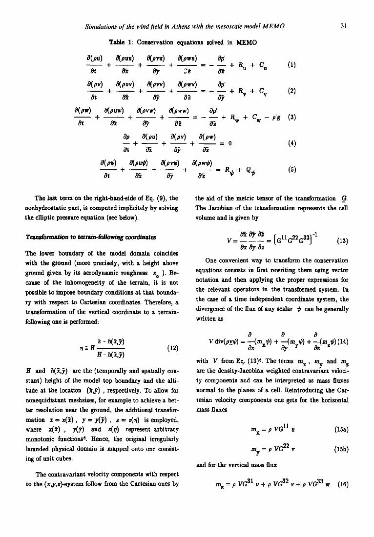
Table 1 shows the conservation equations solved in

MEMO. Yc, ~ and ~ represent Cartesian coordinates

and u , v and w are wind velocity components in

the ~ , ~ and ~ direction, respectively. 9 is any

scalar (e.g. the potential temperature 0, the turbulent

kinetic energy E ).

ponents( C = 2p.~_xX ). The source/sink terms Q¢

depend on the transported scalar quantity: For the

potential temperature this term includes anthropogenic

heat emission and the divergence of radiative fluxes, for

the turbulent kinetic energy it contains the shear and

buoyancy production rates as well as the dissipation

rate.

Following the common practice in mesoscale mod-

els, variables are split into base-state parts (denoted by

overbars) and mesoscale perturbations (primed varia-

bles). By definition, the base-state parts of the wind

velocity components are taken as zero. For the thermo-

dynamic variables the separation yields

p = + (e)

p = + (7)

(8)

In order to accelerate the convergence of the solution of

the elliptic equation for pressure (see below), it is ad-

visable to split the mesoscale pressure perturbation

into three components:

p ' = pg -I- Ph -I" Pnh (9)

By the first term on the fight-hand-side of this equa-

tion a large-scale horizontal pressure gradient in the

considered mesoscale domain may be specified. The

components of this gradient read

; _Opg=+pr.g (lO) ay

with the Coriolis parameter f = 2 [Q[ sin~b. Large-scale temperature gradients may be specified either via the lateral boundary conditions or by defining Ug and Vg

as height dependent.

The hydrostatic part, i.e. the second term on the

right-hand-side of Eq. (9), may be obtained by integra-

ting the hydrostatic equation:

0Ph ---- - p' g - - - ~o - ~ ( z ) ] g ( 1 1 )

O~

In the conservation equations, R u , R v , R w and

Re denote turbulent diffusion (see below), while C u ,

C v and C w represent volumetric Coriolis force corn-

where p follows from the ideal gas law. It should be

noted that the vertical derivative of Ph and the buoy-

ancy term in Eq. (3) cancel ont.

Simulations of the wind field in Athens with the mesoscale model MEMO 31

Table 1: Conservation equations solved in MEMO

a(p.)

at

0(91,)

at

a(pw) +

at

a(pu. ) a(p, , . ) O(pwu) ap' - - + - - + - - + - - = - - - + R u + c . (1)

a(puv) a(p~) a(p,~,) ap' + - - + - - + - - = - - - + R v + c v (2)

oy a~ oy

O(puw) O(p~) a(p.,~) ap' ~ + - - + - - = - - - + % + Cw-p'g (3)

oy 0~ 0~

ap a(p.) a(p,,) a(pw) - - + ~ + ~ + ~ = 0 (4) at ~ o~

- - + - - + - - + ~ = Re+ q~ (5) ot ~ 8y o~

The last term on the right-hand-side of Eq. (9), the

nonhydrostatic part, is computed implicitely by solving

the elliptic pressure equation (see below).

T r ~ r m a t i o , to terrai~fo//ow/~ coord/nates

The lower boundary of the model domain coincides

with the ground (more precisely, with a height above

ground given by its aerodynamic roughness z o ). Be-

cause of the inhomogeneity of the terrain, it is not

possible to impose boundary conditions at that bounda-

ry with respect to Cartesian coordinates. Therefore, a

transformation of the vertical coordinate to a terrain-

following one is performed:

_ h(~,y) - . (1~)

H - hC~,y)

H and h(~,j,) are the (temporally and spatially con-

stant) height of the model top boundary and the alti-

tude at the location (Y~,~,) , respectively. To allow for

nonequidistant meshsizes, for example to achieve a bet-

ter resolution near the ground, the additional transfor-

mation z = x(Y 0 , y = y(y) , z = z(y) is employed,

where x(Yc) , y(j,) and z07 ) represent arbitrary

monotonic functions 6. Hence, the original irregularly

bounded physical domain is mapped onto one consist-

ing of unit cubes.

The contravariant velocity components with respect

to the (x,y,z)-system follow from the Cartesian ones by

the aid of the metric tensor of the transformation •G.

The Jacobian of the transformation represents the cell

volume and is given by

0~ Oy 0~ l ~jrG11~2--3~-I V = = (13)

~OyOz

One convenient way to transform the conservation

equations consists in first rewriting them using vector

notation and then applying the proper expressions for

the relevant operators in the transformed system. In

the case of a time independent coordinate system, the

divergence of the flux of any scalar ~ can be generally

written as

0 0 a

with V from Eq. (13)e. The terms rex, my and m z

are the density-Jacobian weighted contravariant veloci-

ty components and can be interpreted as mass fluxes

normal to the planes of a cell. Reintroducing the Car-

tesian velocity components one gets for the horizontal

mass fluxes

mx = P ...~lvt~l_ u

m =pV~2v Y

and for the vertical mass flux

(15a)

(15b)

m z=pVG 31u+pVG 32v+pVG 33w (16)

32

It should be noted that the product

a n a rea .

N. Moussiopoulos, Th. Flassak, P. Sahm, D. Berlowitz

Numerical s o l u t i o a o f the equatioa s y s t e m

VG ij represents

To ensure conservativity, the discretized equations a~e

solved numerically on a staggered grid. The scalar

quantities p , p , 0 and V axe defined at the cell

center, the velocity components u , v and w at the

centers of the appropriate interface. As the variables

axe needed also at locations where they are not defined,

a suitable averaging operator is needed. In addition, a

finite difference operator has to be used. These oper-

ators take the form

~ = [~b(~+A~/2) + #b(~-A~/2)]/2 (17)

6~b - ~(~+A~/2) - ~b(~-A~/2) (18)

where ¢ stands for any of x, ¥ and z( A~ ~ 1 ).

With M = p V and the discrete form of the mass

fluxes

m x ---- G11MXu (19a)

my-- G22MYv (19b)

~ X X~Z y ,z

m z-- G31M u + G32MYv + G33M-Zw (19c)

the discrete form of continuity follows from Eqs (4)

and (14) with ~b = 1:

8 M v r = (mx) + 6y(my) + 6,(m) (20)

The discrete form of the prognostic equations (1-3)

and (5) reads

- - X

~ M u) = - A u

-~MYv) _- - A 82 v

- P ( p g + Ph + Pnh ) + R u + C u

(21a)

- Py(pg+ Ph + Pnh ) + R v + C v

(21b)

- P z ( p g + Pnh ) + R w + C w

(21c) 8 -~tM ~b) = - A~ + R~ + Q~b (21d)

~ - ( M Z . ) = - A w a t

On principle, the advective terms A u , A v , A w

and A~b can be computed using any suitable advection

scheme. In the present version of MEMO two schemes

are implemented, the scheme of SmolaxkiewiczZ and the

TVD-scheme [TVD: Total Variation Diminishing]8.

The results presented in the next section were obtained

with the TVD-scheme.

In Eqs (21a-c) P x ' P and Pz are operators

yielding the discrete Cartesian gradient components. If

applied to p , they read

,-~ l - - X , 7- Px(p)- 6x(VG11p)+ ~(VG"~p ) (22a)

%(p)-- 6y(VG22p) + 6z(VG32p y'z) (22b)

Pz(p) = 6z(VG 33p) (22c)

The temporal discretization of the prognostic equa-

tions is based on the explicit second order Adams-Bash-

forth scheme (here for the u-momentum equation):

--X

M ;i = + (23)

+~At[-Au-Px(Pg+Ph+Pnh)+Ru'l-Cu] n"

I At [-Au-Px(Pg+ Ph-l-Pnh)+ Ru+ Cu] n-1

There axe two deviations from the Adams-Bnshforth

scheme: The first refers to the implicit treatment of the

nonhydrostatic part of the mesoscaie pressure perturba-

tion Pnh • With the second order approximation pnh = (pn+hl + pnhl)/2 , the 'new' velocity u n+l is ob-

tained from the intermediate value u by aid of the

equations

--X --X

M ~ M u + A t n = Pnh ) (24) px(Pnh - n-I

MXu n+l -i- At Px(Pn h " n+1_Pnh ) n = M-Xu (25)

Ap

Equations similar to Eq. (25) axe readily obtained for the v mad the w-momentum equations:

, n+1 n - Y - M xn+l + At ry(Pnh -Pnh)= M v (26)

--Z :-x n+l p , n+l n • M~" (27) M w + At zlPnh - P n h ) =


Introduction of Eqs (25-27) into the discretized conti-

nuity equation (20) results in the diagnostic equation

for Ap, i.e. the change in the nonhydmstatic part of

the mesoscale pressure perturbation (see below). It

should be noted, that wherever densities are needed

they are replaced by corresponding values in the previ-

ous time step, i.e. pn is used instead of pn+l and n-1 n p instead of p

The second deviation from the explicit treatment is

related to the turbulent diffusion in vertical direction.

In case of an explicit treatment of this term, the stab-

ility requirement may necessitate an unacceptable a-

bridgement of the time increment. To avoid this, verti-

cal turbulent diffusion is treated using the second order

Crank-Nicolson method. By other words, Eq. (24) is re-

placed by

- x - x M u - - ~ R u , z=Mu+

(28) n-1

Pith ) - Run,z+

In this application, the Crank-Nicolson method is qua-

si-implicit, as u is used instead of u n+l . Obviously,

Eq. (28) corresponds to a three-diagonal equation sys-

tem for u which is solved at each time step using

Ganssian elimination.

The elliptic pressure equation takes the form

Unfortunately, Eq. (29) is not of this form. Therefore,

the fast direct solver is used in conjunction with a

generalized conjugate gradient method. It was proved

that the above described formulation of the elliptic

equation in terms of the pressure change Ap instead

of the pressure itself leads to a faster convergence of

the conjugate gradient method.

It is worthy of notice that Eq. (29) represents conti-

nuity expressed in terms of pressure. Thus, it corre-

sponds to the equation solved in diagnostic wind mod-

els ~o calculate the Lagrangian multiplier, if the ratio

of the Gauss precision moduli is unity t0.

Parameterizafions

The most important processes that have to be parame-

terized in a prognostic mesoscale model are turbulence

and radiative transfer. In MEMO, the former is treated

with an one-equation turbulence model, while the latter

is calculated with an efficient scheme based on the

emissivity method for longwave radiation and an italy-

licit multflayer method for shortwave radiationtt.

The diffusion terms in Eqs (1-3) and (5) may be re-

presented as the divergence of the corresponding fluxes.

In case of a statistical description of turbulence, the

turbulent diffusion terms in the u-momentum equation

and the transport equation for scalars take the form

~x{G11Px(AP)} .4. 6y{G22py(Ap)} .4.

~z{G ° Px(Ap) + =

- {Mn- Mn-1}/At 2 -4- [6x{GI1MXu} + ~{G22MYv }

~ X X~Z - - v y , z - - Z

4. 6 {G31M u .4. G32MJv .4. G33M Q}]/At

The left-hand-side of this equation represents a 25-

point operator. The procedure for solving this equation

is based on a fast direct method described elsewhere 9.

This algorithm adopts the eigenfunction expansion

method in two directions; application of Fast Fourier

Transformation and full vectorization allow an ex-

t remdy efficient solution of equations having the form

~t..r .+ ~:~;~ d ( z ) ~ .4. e(z 0~')~-£ .4. t(z)~ = S (30)

Ru = _ o pu-'n' _ _ ( 3 1 )

R~ = - O~PU--~ - o ~ p ' ~ _ o ~ p ~ ' ~ (32)

where doubly primed variables represent subgrid scale

quantities. By the aid of the common gradient assump-

tion the above correlations may be expressed in terms of the mean gradients of the transported quantities, i.e.

• - - - .4. @u J1 (33) u i - - ~ = ' g m D i j ' Dij ~0x j OxiJ

= - g ~ - - (34) ax i

Dij are the components of the deformation tensor, while K m and K@ are referred to as the eddy viscos-


ity and the eddy diffusivity for scalar ~0, respectively.

As horizontal diffusion is rather insignificant in the

cases treated with the model MEMO (i.e., at horizontal

grid spacings exceeding 1 kln), no distinction is made

betwem the eddy viscosity in the horizontal and verti-

cal directions. Moreover, K# is the same for all con-

sidered scalars. Obviously, turbulent diffusion can be

described, if K m and K# (or, alternatively, the tur-

bulent Prandtl number Pr t - Km/K ~ ) are properly determined. With the parameterization

Pr t = max [1; 1.35-0.35 ~-h(Yc,~,)] (35) z D

(typically zi) = 1000 m ), only the eddy viscosity

rein&ins to be parameterized. A significant quantity for

the latter parameterization is the 'gradient Richardson

number' Rig representing the ratio of buoyancy forces

to forces related to turbulent shear.

Rig = ~iD~ (36)

( D2/2 is the deformation of the wind field.) Ap-

parently, Rig characterizes the thermal stratification

of the atmospheric boundary layer.

In addition, a length scale (the so-called mixing

length) is needed. An appropriate length scale is given

by the expression

t = +

t and the deformation of the wind field. An appropri-

ate method to obtain such an expression is to derive it

from a simplified form of the transport equation for

E , i.e.

QE Km ~ [ 1 - P r t l . R i ~ K3m' = - L--4- = o ( 4 0 )

stating that if temporal variation, advection and turbu-

lent diffusion of E are negligible, there is a balance

between production and dissipation of E . Apparently,

one gets for K m

Km = £2 J - D ~ J 1- Pr t l .Rig (41)

Initial and boundary conditions

In the prognostic mesoscale model MEMO initializa-

tion is performed with suitable diagnostic methods: A

mass-consistent initial wind field is formulated using an

objective analysis model t0. Scalsr fidds are initialized

using appropriate interpolating techniques 4. Data need-

ed to apply the diagnostic methods may be derived

either from observations or from larger scale simula-

tions. It is likely that an improved initialization might

be achieved by applying data assimilation techniques.

Suitable boundary conditions have to be imposed

for the wind velocity components u , v , w , the

potential temperature 0 and pressure p at aft boun-

daries. At open boundaries, wave reflection and defor-

mation may be minimized by the use of so-called 'radiation conditions'IS. Therefore, at lateral boundaries

the radiation conditions

( ~ :von K/u-m~n constant) t2. In MEMO the limiting

value t ® is given by

t® = max ( 30 m , 0.00027 [Xg[/[) (38)

If a transport equation for the turbulent kinetic energy

E is solved, the eddy viscosity follows from its solu-

tion:

K m ---- c k t ~'E (39)

In case of a purely algebraic parameterization, an ana-

lytic function has to be specified relating K m to Rig,

a4, a4~ ~b s a4, s -- = - c-- + + c (42)

Ot an Ot 8n

are nsedtl, where n is the direction perpendicular to

the boundary and C the phase velocity that includes wave propagation and advection and is calculated for every variable # from known values from the interior

of the computational domain. Eq. (42) differs from the standard formulation of the radiation conditiontS by

the last two terms describing the temporal and spatial

change of the undisturbed large scale environment. Ap- parently, this information has to be specified to the


model. Without the last two terms of Eq. (42), the ra-

diation conditions merely allow disturbances to propa-

gate out through the boundary, but do not allow infor-

mation from outside to be imposed at the boundary.

According to the experience gained so far with the

model MEMO, this might result in instabilities in case

of simulations over longer time periods.

For the v,,nhydrostatic part of the mesoscale

pressure perturbation, homogeneous Nenmann bound-

ary conditions are used at lateral boundaries. With

these conditions the wind velocity component per-

pendicular to the boundary remains unaffected by the

pressure change.

At the upper boundary Neumann boundary condi-

tions are imposed for the horizontal velocity compo-

nents and the potential temperature. To ensure non-

reflectivity, a radiative condition is used for the

hydrostatic part of the mesoscale pressure perturbation

Ph at that boundary. Hence, vertically propagating

internal gravity waves are allowed to leave the compu-

tational domainlS. This condition yields the following

relation between Ph and the vertical velocity compo-

nent w :

=

Y

kx, ~ are wave numbers, ~ and

transforms of Ph and

frequency.

(43)

fv the Fourier

w and N the Brunt-V~is~l~

For the nonhydrostatic part of the mesoscale pres-

sure perturbation, homogeneous staggered Dirichlet

conditions are imposed at the upper boundary. Being

justified by the fact that nonhydrostatic effects are

negligible at large heights, this condition is necessary,

if singularity of the elliptic pressure equation is to be

avoided in view of the Nenm~nn boundary conditions

at all other boundaries.

The lower boundary coincides with the ground (or,

more precisely, a height above ground corresponding to

its aerodynamic roughness). For the nonhydrostatic

part of the mesoscale pressure perturbation, inhomo.

geneons Neumann conditions are imposed at that 'no-

flow-through' bou~,dary. All other conditions at the

lower boundary follow from the assumption that the

Monin-Obuldtov similarity theory is valid. With the

exception of water surfaces (where the temperature is

specified) the surface temperature is calculated from

the nonlinear heat balance equation

Rio - RTo + S~o - 2 o - Qs - Qo - Lo - Qa = 0 (44)

( R : longwave, S : shortwave radiative fluxes (RTo ~

To/); Qs heat flux to the soft ; Qo ' Lo : sensible and

latent heat to the atmosphere ; Qa : anthropogenic

heat flux), which is solved using a Newton iteration

technique. Radiative fluxes follow from the above men-

tioned radiation scheme tl. For the calculation of the

soil temperature, an one-dimensional heat conduction

equation for the soil is solved. The specific humidity at

the surface (needed even in the case that the transport

equation for water vapor is not included in the model)

is computed from

q = ql qs + (l-~) q2 (45)

where • is the evaporation parameter varying be-

tween 0 and 1 (water: ~ = 1 , dry soil: ~ = 0), qs is

the saturation humidity and q2 is the humidity com-

puted at the lowermost grid level above ground. In the

present model version the value of • is specified for

each grid cell and it is assumed to be constant through-

out the simulation.

MODEL APPLICATION

The APSIS Exercise A consisted in simulating the

mesoscale air motion in Athens on May 25, 1990ts.

Identical topographical and meteorological input data

were distributed to be used by all APSIS participants.

Topographical data included orography and land use

for a 72x72 km~ domain around Athens at a resolution

of i km. This domain is illustrated in Fig. 1. Meteo-

rological data consisted of vertical soundings at the

Hellenicon airport and surface wind measurements at

several stations of the routine network operated by the

Hellenic Meteorological ServicelT. The synoptic situa-

tion for the period of interest is described elsewhere 16.

Previous experience with the model MEMO showed

that in case of a stand-alone model application for

Athens a realistic representation of mesoscale flow


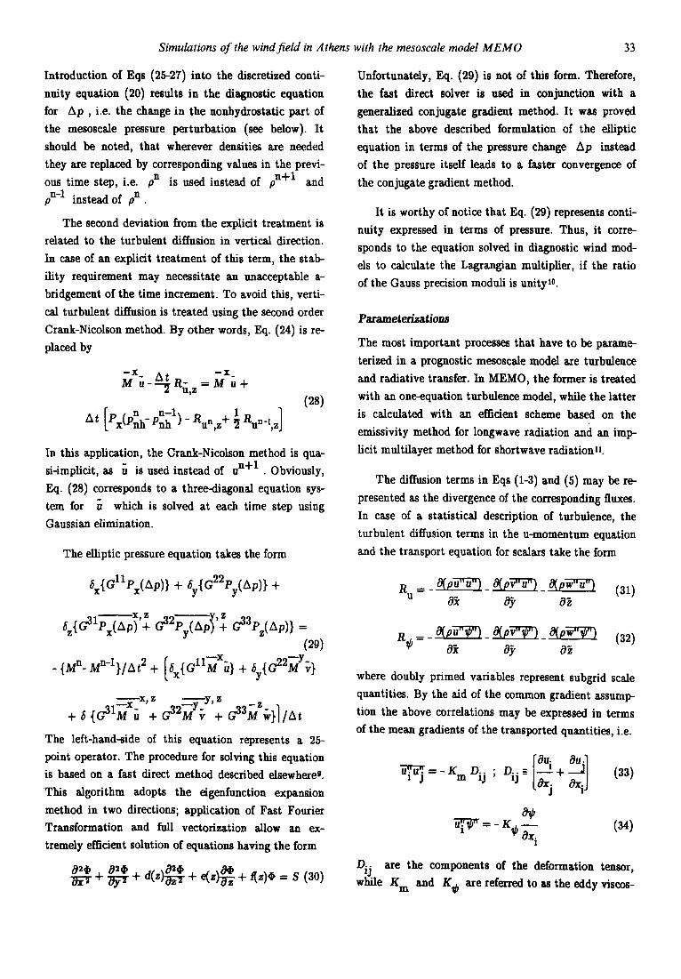
Fig. I. Computational domain for the APSIS model

intercomparison. Terrain is contoured at 100 m inter-

vais. The arrow marks the position of the cross-section,

for which results are given in Fig. 3. The dots denote

locations, for which detailed results are given in Fig. 4

(H: Hellenicon, P: Piraeus, E: Eleusis, N: National Ob-

servatory of Athens (NOA ), F: Filadelfia, T: Tatoi).

totle University Thessaloniki. These results are very

similar to those obtained on the SIEMENS $600/20

vector processor of the UniversitEt Karlsruhe and on

the VAX 9000 of the Paul Scherrer Institute.

SIMULATION RESULTS

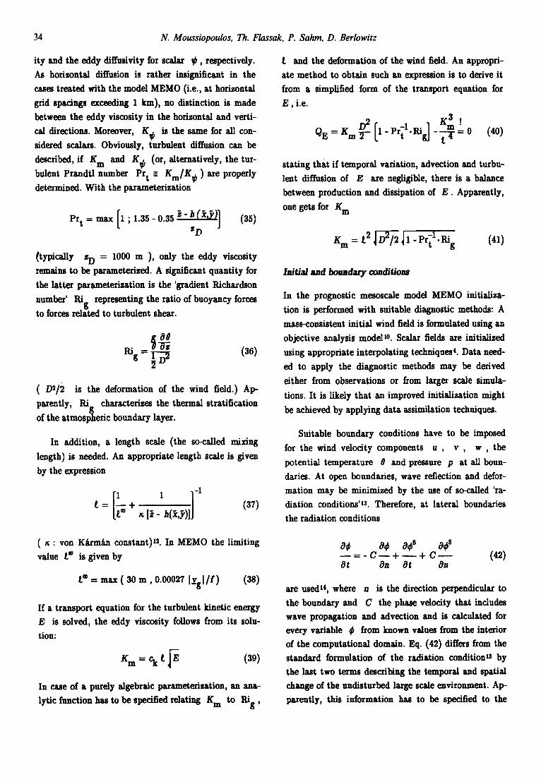
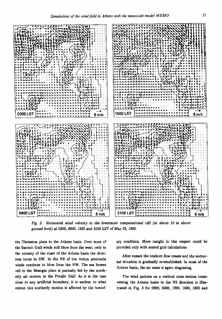
Figure 2 shows the wind field at a height of approx-

imately 10 m above ground level for 0300, 0900, 1500

and 2100 LST of May 25, 1990. For clarity, the 24 km

extension of the computational domain to the south is

omitted.

The nocturnal surface wind pattern is dominated by

moderate westerly flow over the sea and downslope

winds in the mountainous ridge to the north of the

Athens basin and the Thriasion plain. As a conse-

quence of this flow configuration, the wind velocities

above the town of Athens remain at a very low level. It

should be noted that the synoptic conditions in the

present case do not favour the development of land

breeze which was found to occur at night in case of

weaker synoptic forcings is.

circulations can only be expected, if the modelling

domain is extended to the south to obtain a reasonable

ratio of water to land masses4. Correspondingly, the

simulation with model MEMO was performed on a 72x

96x6 km 3 domain starting at 2100 LST of May 24. In

accordance with the APSIS specifications, a constant

horizontal resolution of 2 km was chosen. It should be

noted, that this resolution was found sufficient to re-

solve even small scale characteristics of the wind pat-

tern in Athens ts. In the vertical direction a non-equi-

distant grid consisting of 35 layers was used. Starting

with 20 m, the grid spacing in vertical direction in-

creased by a constant factor up to the model top at 6

kin. A constant time increment of 15 seconds was used.

Initialization was performed using the 0000 UTC verti-

cal sounding, which was also considered to be represen-

tative for the large scale situation over the entire

simulation period.

The simulation results presented in the next section

originate from calculations with MEMO on the IBM

IIISC 6000/520 workstation of the Laboratory of Heat

Transfer and Environmental Engineering of the Aris-

At 0900 LST (corresponding to 0600 UTC because

of daylight saving) the situation is very sindlar to that

of 0300 LST. Among the few noticeable deviations,

weak onshore flow develops both to the east of Mt.

Pendeli and in the Thriasion plain. Differently from the

case of a weaker synoptic forcing, the sea breeze cell in

the Mesogia plain does not form early in the morning,

obviously because of the counterbalancing influence of

the prevailing horizontal pressure gradient. Merely a

weak upslope motion is visible to the east of Mt.

Hymettus. It should be noted that a well-structured

wind from the NW is established in the NE of the

Attica peninsula. It is worthy of notice that air mass

practically stagnates over most of the Athens basin.

During the day land heating leads to significant

alterations of the wind field. Firstly, sea breeze cells

develop in the Athens basin as well as in the Thriasion

and Mesogia plains. The corresponding circulations are,

however, rather weak as a consequence of the persisting

inversion (see Fig. 5 of Moussiopoulost6). The combina-

tion of the prevailing westerly synoptic wind direction

and the sea breeze results in air mass transport from


Fig. 2. Horizontal wind velocity in the lowermost computational cell (at about 10 m above

ground level) at 0300, 0900, 1500 and 2100 LST of May 25, 1990.

the Thriasion plain to the Athens basin. Over most of

the Saronic Gulf winds still blow from the west; only in

the vicinity of the coast of the Athens basin the direc-

tion turns to SW. In the NE of the Attica peninsula

winds continue to blow from the NW. The sea breeze

cell in the Mesogia plain is partially fed by the north-

erly air motion in the Petalic Gulf. As it is the case

close to any artificial boundary, it is unclear to what

extent this northerly motion is affected by the bound-

ary condition. More insight in this respect could be

provided only with nested grid calculations.

After sunset the onshore flow ceases and the noctur-

nal situation is gradually re-established. In most of the

Athens basin, the air mass is again stagnating.

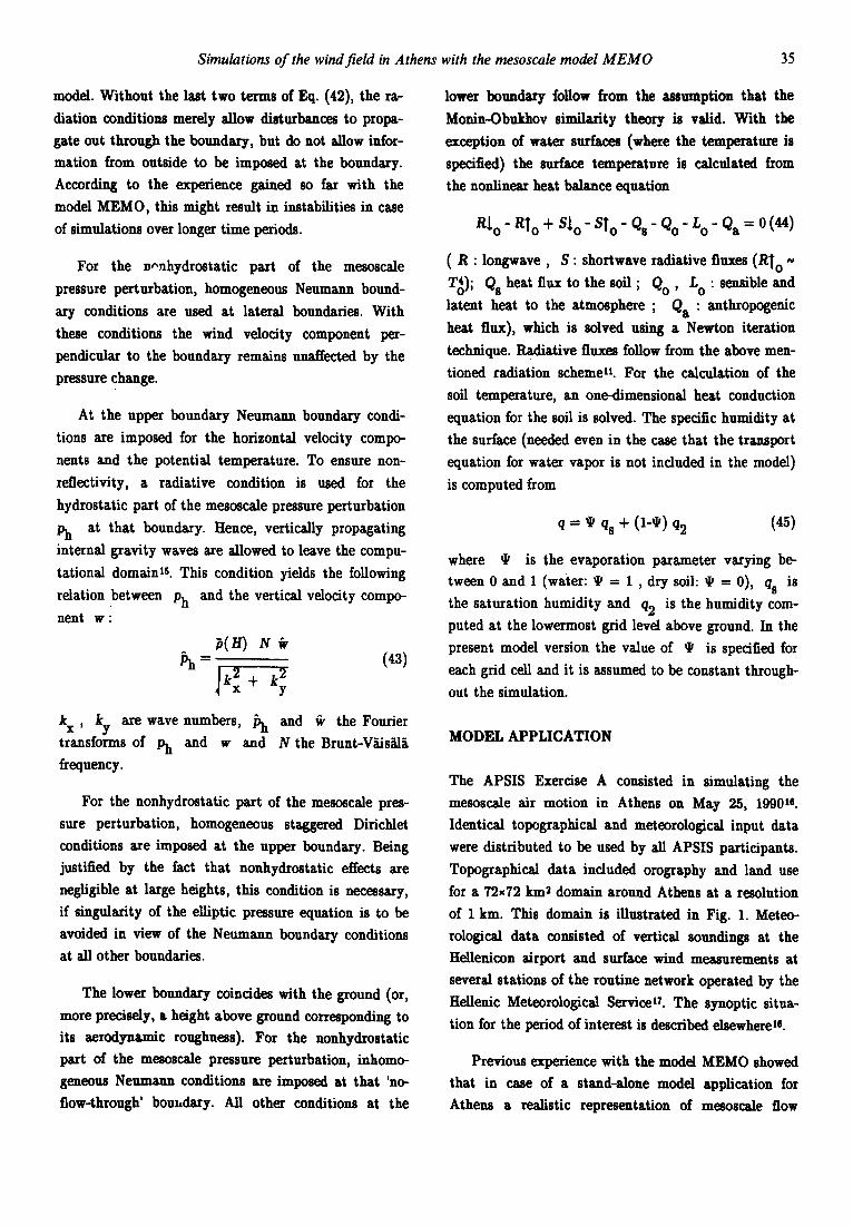
The wind pattern on a vertical cross section trans-

versing the Athens basin in the NS direction is illus-

trated in Fig. 3 for 0600, 0900, 1200, 1500, 1800 and

_ . , . . . . . j fiiT{Tit H, o,. I l l + + + + + + + + + ~ + + v 17 t , / <,--<>-<,-<>-<,-<>-<>-<,-~- <, .~= 11/ %,>/

<1. ¢1- "v'- ~:~ , ~ li,

< > - < > - ~ < , - < > - < > - ~ < , - ~ ,<,- ,,- <,- ,> . ~ t m l<i-~<i.-~ + <~ ~- + <~ ,, • • ~ ' l ? < l - - < i - - - < l - - < l - . < a - < l . . - < } - < l . . - ~ ~ ,, .o. ~ " . I i 7 i / I < l - < l - < : l - - < l - . - ~ . ~ ~ ~ ° . • ,. ~' i i !

~ i - ~ - - ~ l - < l - - ~ t - ~ . - ~ - - - <! - ~" , • " ~ .W l / I ~ - ~ ~ ~ ~ ~ ~ ~ " • ~ ~ ~ i /

i<}- <3-- <}- <}- <P <1-- <P <}- # • ." . : , I / l / I '~,- q- ,~.- ',::l.- ~,,,, '~,- '~- ',,, " • -t~ J~. ~5, /

~ O O L S T i ~ t ] t ] ~ ~ L S T • , . ~ ~ , 4 5 0 0 , , . • o ~ ~ v • '

~ _ <F_. <1_ <F_ <1_ <1__ <~_ <1_ <~- <0 - - <3- ~ "

~--- <1-- <1-- <F- <1-- < } - < } - <} - < F - . ~ " ~,

~ - ~ - ~ - ~ - ~ - ~ - ~ ~ I I F . ~ =

el-.- ~ <i-- <i- <I-- <i-- ~ <I---

o_o_+_o o_ o_ \. <l._ <3~ <l._ <:}_ <1._ <3... <}.__ <3 <} ~ :~ , ~ . ~ - - <1._ <l- <

<3__ <}._ <}_._ < ~ ~._. ~,.. ,:/._. <t.-

< ~ - ~ < ~ - < l - < l - < ~ - < ) - - < l - - ~ - ~ ~ ~ <~ ~ t ~ < l - < } - < ~ - <l-- <~- < } - < } - < t - <l" ~ ~ ~ ~ ~

< l - < i - < i . - < l - ~ = ~ '~ , • ' : . / ~ : . < l - < l . - ~ - < ~ - + <,- .> • • ; • ; - -

~ - . < l - ~ l - ~ ~ - ~ .~ • I. o " : /

. I I I i

<3-- <t-- <!-- Ii Z~

% /####~

td . - <~- < l - - 4 - - 4 - - ~ b - - ~ i - - ~ l - - < x - < l - ~ . u \\~1 Ik

I ~ - ~ - < ~ - < v - ~ - ~ - ~ - ~ - ~ ~ -, ~ • ~lill" !1 I ~ - ~ - ~ - ~ - ~ ~ ~ ~ . • , #, I I

I,q.-~l--.~-,~-.."~'..--'<~'-.~-<,. : . ' ~ .I I [ I

i i " ! O O L S T

. . . . . ~ ~ ~ ~ ~ = , i ~ t~ i b ~ ~ ~ ~ ~ ~ - ~ - ~ - ~ ~ + + .~ /# I / I

<~ ~ - < - ~ ~ ~ ~ ~ ~ • • • • ~ ! ! 1 1 I ~ ~ < t - < l - - ~ l - ~ - ~ ~ ~ ~ : l i l !111

E ' ." | t | Z I I ] l l ~ i ":'~ " l - L l ~ 2 1 0 0 L S ,

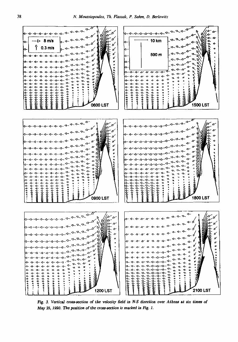
Fig. 3. Vertical cross-section of the velocity field in N-S direction over Athens at six times of

May 25, 1990. The position of the cross-section is marked in ~g. 1.


2100 LST of May 25, 1990. The precise location of the

cross-section is shown in Fig. 1. In view of the different

scaling factors in the horizontal and vertical directions,

neither the length nor the angle of the arrows conform

to wind speed and direction. To facilitate the interpre-

tation of the results shown in Fig. 3, the arrow tip sur-

face area was selected to be proportional to the magni-

tude of the corresponding wind vector.

The result at 0600 LST (which is practically iden-

tical to that at 0300 LST) confirms the occurence of

katabatic winds to the south of Mr. Parnis during the

night. Above the city of Athens a layer of stagnant air

resides, the thickness of which is of the order of 300 m.

At 0900 LST the stagnation over Athens still persists,

while at the same time the wind vector at the slopes

veers gradually upward.

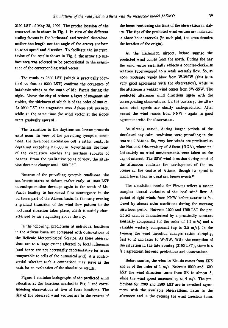
the boxes containing ~lle time of the observation in ital-

ics. The tips of the predicted wind vectors are indicated

in three hour intervals (in each plot, the cross denotes

the location of the origin).

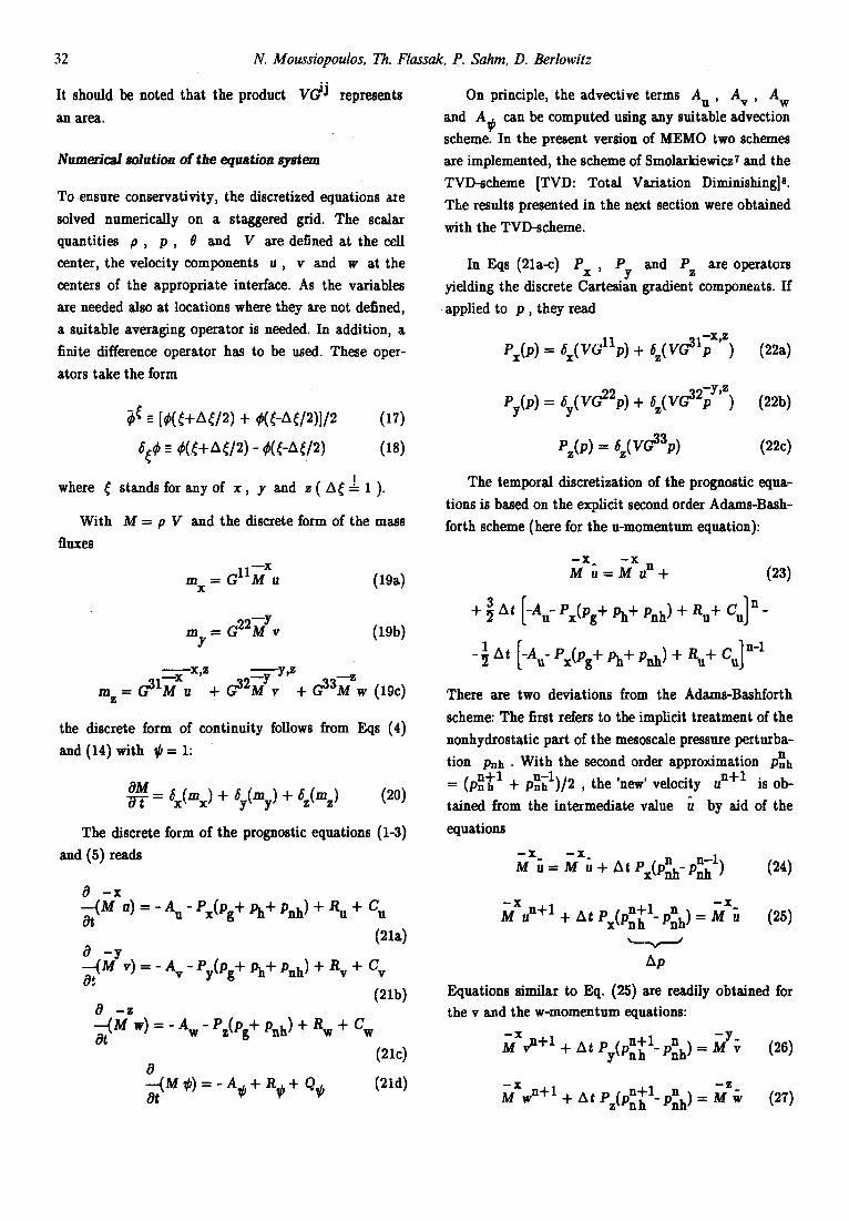
At the Hellenicon airport, before sunrise the

predicted wind comes from the north. During the day

the wind vector essentially reflects a counter-clockwise

rotation superimposed to a weak westerly flow. So, at

noon moderate winds blow from W-WSW (this is in

very good agreement with the observation), while in

the afternoon a weaker wind comes from SW-SSW. The

predicted afternoon wind directions agree with the

corresponding observations. On the contrary, the after-

noon wind speeds are clearly underpredicted. After

sunset the wind comes from NNW - again in good

agreement with the observation.

The transition to the daytime sea breeze proceeds

until noon. In view of the prevailing synoptic condi-

tions, the developed circulation cell is rather weak, its

depth not exceeding 200-300 m. Nevertheless, the front

of the circulation reaches the northern suburbs of

Athens. From the qualitative point of view, the situa-

tion does not change until 1500 LST.

Because of the prevailing synoptic conditions, the

sea breeze starts to deform rather early; at 1800 LST

downslope motion develops again to the south of Mt.

Parnis leading to horizontal flow convergence in the

northern part of the Athens basin. In the early evening

a gradual transition of the wind flow pattern to the

nocturnal situation takes place, which is mainly char-

acterized by air stagnating above the city.

In the following, predictions at individual locations

in the Athens basin are compared with observations of

the Hellenic Meteorological Service. As these observa-

tions are to a large extent affected by local influences

(and hence are not necessarily representative for areas

comparable to cells of the numerical grid), it is contro-

versial whether such a comparison may serve as the

basis for an evaluation of the simulation results.

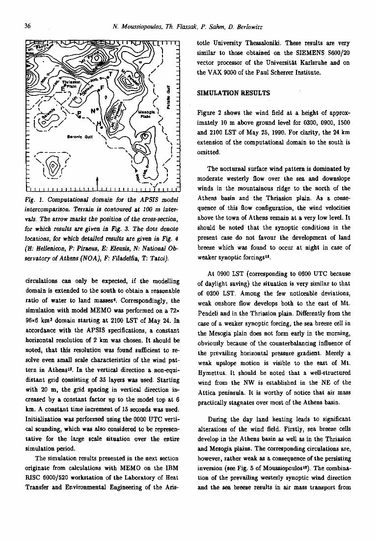
Figure 4 contains hodographs of the predicted wind

velocities at the locations marked in Fig. 1 and corre-

sponding observations at five of these locations. The

tips of the observed wind vectors are in the centres of

As already stated, during longer periods of the

simulated day calm conditions were prevailing in the

centre of Athens. So, very low winds are predicted at

the National Observatory of Athens (NOA), where un-

fortunately no wind measurements were taken on the

day of interest. The SSW wind direction during most of

the afternoon confirms the development of the sea

breeze in the centre of Athens, though its speed is

much lower than in usual sea breeze events ~s.

The simulation results for Piraeus reflect a rather

complex diurnal variation of the local wind flow. A

period of light winds from NNW before sunrise is fol-

lowed by almost calm conditions during the morning

rush hour period. Between 1000 and 1700 LST the pre-

dicted wind is characterized by a practically constant

southerly component (of the order of 1.5 m/s) and a

variable westerly component (up to 2.5 m/s). In the

evening the wind direction changes rather abruptly,

first to E and later to W-NW. With the exception of

the situation in the late evening (2100 LST), there is a

fair agreement between predictions and observations.

Before sunrise, the win~ in Eleusis comes from ESE

and is of the order of 1 m/s. Between 0900 and 1500

LST the wind direction turns from SE to almost S,

while the wind speed increases up to 4 m/s. The pre-

dictions for 1200 and 1500 LST are in excellent agree-

ment with the available observations. Later in the

afternoon and in the evening the wind direction turns


Hellenicon

18 1512~]

0

NOA

6 2

Piraeus Eleusis

15

Filadelfia Tatoi

3 0 0

1 m/s

15

~'12

Fig. 4. Hodographs of predicted surface level wind velocities at the six locations marked in Fig. 7

and ava//ab/e observations. The tips of the observed wind vectors are in the centres of the boxes

containing the time of the observation in italics. The tips of the predicted wind vectors are indi-

cated in three hour intervals (in each plot, the cross corresponds to the origin).


back to ESE, while the wind speed gradually decreases

to very low values. As there are no observations after

1800 LST, it is not possible to evaluate the late after-

noon and evening predictions of the wind in Eleusis.

The situation in Filadelfia is rather simple: Before

sunrise light easterly winds are predicted. During the

morning rush hour period practically calm conditions

prevail. Subsequently, the sea breeze develops; the cor-

responding wind directions change from S at noon to

SSW at 1500 LST, while the wind speed is of the order

of 2-3 m/s. Later in the afternoon the wind gradually

ceases. In spite of some minor deviations, especially as

the wind direction is concerned, the agreement between

predicted and observed wind velocities is fair.

The diurnal variation of the local wind flow in

Tatoi is similar to that in Filadelfia. The wind remains

light until 0900 LST, while its direction turns clockwise

from ENE to SSW. During the day stronger winds from

SSW develop, indicating that the sea breeze penetrates

up to the northern suburbs of Athens. After reaching a

maximum speed of 3.5 m/s at 1500 LST, the wind

gradually ceases. From the three available observa-

tions, one (1200 LST) is in contradiction to the pre-

dicted wind velocity, while two are in very good agree-

ment with the corresponding model results.

CONCLUDING REMARKS

The nonhydrostatic mesoscale model MEMO was used

to simulate mesoscale flow phenomena in Athens on

May 25, 1990. The results reveal several characteristics

of the wind field on the specific date:

• Moderate westerly winds over the Saronic Gulf the

whole day.

~Practically stagnant conditions in Athens until 10

a.m..

• An onset of the sea breeze in Athens around noon.

• The development of a rather weak sea breeze in the

Mesogia plain.

• A flow pattern favouring the transport of air pol-

lutants from the Thriasion plain to the Athens basin

in the afternoon.

Simulation results were compared with available

observations. Given that the latter may be affected by

local influences (and that they therefore are not neces-

sarily representative for areas comparable to cells of

the numerical grid), the agreement between prediction

and observation is very satisfactory.

The smaller the distance from the domain bound-

aries, the higher the uncertainties of the model results.

The reliability of the prediction at these locations can

only be improved if nested simulations are performed,

i.e. if the boundary conditions for the domain consider-

ed are derived from calculations on a larger domain (of

the order of 250x250 kin2).

REFERENCES

1 Pielke, R.A. Mesoscale Meteorological Modeling, Academic Press, pp. 612, 1984.

2 Mouesiopoulos, N. Msthemat~:he Modellierung mesoskall- get Ausbreitung in der Atmosphere, Fortschr.-Ber. VDI, Re'he 15, Nr. 64, pp. 307, 1989.

3 Flassak, Th. and Moussiopoulos, N. Simulation of the sea breeze in Athens with an efficient non-hydrostatic mesoscale model, in Man and His Ecosystem (Brassor, L.J. and Muider, W.C., eds), Elsevier, Vol. 3, 189-195, 1989.

4 Flassak, Th. Ein nichthydrostatisches mesoskaliges Modeli der planetaren Grensschicht, Fortschr.-Ber. VDI, Re]he 15, Nr. 74, pp. 203, 1990.

5 EUROTRAC, Annual Report 1991, Part 5, 1992. 6 Schumann, U. and Volkert, H. Three-dimensional mass-

and momentum-conslstent Helmholts-equation in terrain- following coordinates, in Notes on Numerical Fluid Mech- anics, Vol. 10 (Hackbusch, W., ed.), Vleweg, Braunschwelg, 109-131, 1984.

7 Smol~rkiewics, P.K. A fully multidhnensional positive deft- nite advection transport algorithm with small implicit diffusion, J. Comput. Phys. 54, 325-362, 1984.

8 Harten, A. On a large tlme-step high resolution scheme, Math. Comp. 46, 379-399, 1986.

9 Flassak, Th. and Monssiopoulos, N. A fully vectorised fast direct solver of the Helmholtz equation, in Applications of Supercomputers in Engineering (Brebbla, C.A. and Peters, A., eds), Elsevier, Amsterdam, 67-77, 1989.

10 Mouesiopoulos, N. and Flaesak, Th. A diagnostic wind model and its inter-actions with observations and experiments, in Computers and Experiments in Fluid Flow (Carlomagno, G.kl. and Brebbla, C.A., eds), Springer, Berlin, 239-250, 1989.

Ii Mouesiopoolos, N. An efficient scheme to calculate radiative transfer in mesoscale models, Environments] Software 2, 172-191, 1987.

12 Blackadar, A.K. The vertical distribution of wind and turbulent exchange in a neutral atmosphere, J. Geophys. Res. 67, 3095-3102, 1962.

13 Orlanskl, J. A simple boundary condition for unbounded hyperbolic flows, J. Comput. Phys. 21, 251-269, 1976.

14 Carpenter, K.M. Note on the paper 'Radiational condition for the lateral boundaries of lhnRed-~ares.numerical models' by Miller, M.J. and Thorpe, A.J. (QJ. 107, 615-628), Qu~rt. J. R. Met. Soc. 108, 717-719, 1982.


15 Klemp, J.B. and Durran, D.I~ An upper boundary condition permitting intern al gravity wave radiation in numerical mesoscule models, Mon. Weather Rev. I I I , 430-444, 1983.

16 Mouuioponlos, N. Athenian photochemical smog - Inter- comparison of simulations (APSIS), background and objec- tives, Environmental Software 8, 1993.

17 18

Sakellarid;-, G. private cornmuulc~tioa, 1992. Flasuk, Th. and Moussiopouloi, N. High resolution simulations of the sea/land breese in Athens, Greece, using the non-hydrostatic mesoscsle model MEMO, in Air Pollution Mode/llng and its Application Vol IX (van Dop, H. and Kallos, G. eds), Plenum, New York, 123-131, 1992.

Simulations of the wind field in Athens with the nonhydrostatic mesoscale model MEMO

Documents

Transcript of Simulations of the wind field in Athens with the nonhydrostatic mesoscale model MEMO