arX

iv:m

ath/

0702

668v

1 [

mat

h.A

C]

22

Feb

2007

SIMPLICIAL IDEALS, 2-LINEAR IDEALS AND ARITHMETICAL RANK

Marcel Morales

Universite de Grenoble I, Institut Fourier, UMR 5582, B.P.74,38402 Saint-Martin D’Heres Cedex,and IUFM de Lyon, 5 rue Anselme,

69317 Lyon Cedex (FRANCE)

Abstract.1 In the first part of this paper we study scrollers and linearly joined varieties.

Scrollers were introduced in [BM4], linearly joined varieties are an extenson of scroller and weredefined in [EGHP], and they proved that scrollers are defined by homogeneous ideals having a2−linear resolution. A particular class of varieties, of important interest in classical Geometry areCohen–Macaulay varieties of minimal degree, they were classified by the successive contribution ofDel Pezzo [DP], Bertini [B], and Xambo [X]. They appear naturally studying the fiber cone of of acodimension two toric ideals [GMS1], [GMS2], [BM1], [H], [HM]. Let S be a polynomial ring andI ⊂ S a homogeneous ideal defining a sequence of linearly-joined varieties.

• We compute the depthS/I, and the cohomological dimension cd(I).

• We prove that under some hypothesis that c(V) = depthS/I − 1, where c(V) is the connect-edness dimension of the algebraic set defined by I.

• We characterize sets of generators of I, and give an effective algorithm to find equations, asan application we prove that ara (I) = projdim (S/I) in the case where V is a union oflinear spaces, in particular this applies to any square free monomial ideal having a 2− linearresolution.

• In the case where V is a union of linear spaces, the ideal I, can be characterized by a tableau,which is an extension of a Ferrer (or Young) tableau.

• We introduce a new class of ideals called simplicial ideals, ideals defining linearly-joined vari-eties are a particular case of simplicial ideals. All these results are new, and extend results in[BM4], [EGHP] .

1 Introduction

Throughout this paper we will work with projective schemes X ⊂ IPr, but we adopt thealgebraic point of view, that is we consider a polynomial ring S, graded by its standardgraduation and reduced homogeneous ideals. Our motivation comes from the study of thefiber cone F (I) of a codimension two toric ideal, as it was shown in [GMS1], [GMS2],

1 first version may 2006, revised version November 2006

1

[BM1], , [H], [HM], F (I) appears to be a Cohen–Macaulay reduced ring having minimalmultiplicity. Projective algebraic sets arithmetically Cohen–Macaulay with minimal degreewere classified by the successive contribution of Del Pezzo [DP], Bertini [B], and Xambo[X], and were characterized homologically by Eisenbd-Goto [EG]. In the case of irreduciblevarieties of minimal degree, equations defining such varieties are given, but as was pointed byDe Concini-Eisenbud-Procesi [CEP]: ”the precise equations satisfied by reducible suvarietiesof minimal degree remain mysterious”, hence they ”stop short of giving a normal form for theequations of each type. In [BM2], [BM4], we tried to answer to this question by describinga set of axioms satisfyied by the ideal of any a linear union of scrolls. Some of our resultswere extended in [EGHP].

In [BM4], we have extended the notion of varieties of minimal degree to the notion ofscrollers, where the algebraic set is not assumed to be equidimensional, Eisenbud-Green-Hulek-Popescu [EGHP] have defined, more generally, the notion of linearly joined varieties,without assuming that each irreducible component is a scroll, and they prove that scrollers (Iuse here our definition) are exactly the 2− regular (in the sense of Castelnuovo-Mumford)projective reduced algebraic sets. In this paper we continue to investigated about thestructure of scrollers, in the first part of the paper we extend the characterization of theideals of scrollers given in [BM4] to the case of linearly joined varieties, as a consequencewe can compute some invariants of linearly joined varieties, as the depth, the connectdnessdimension and the arithmetical rank, as a corrolary we can give an effective algorithm todescribe equations of lnearly joined varieties, improving previuos results in [BM4], [EGHP].As an important corollary we get that for the ideal J ⊂ S of any 2− regular algebraic setwich is a union of linear spaces, the arithmetical rank of J equals the projective dimensionprojdim (S/J ). In particular this is true for square free monomial ideals having a 2− linear

resolution. Note that this results are independent on the characteristic of the field K.In the second part of this paper, we extend the notion of linearly joined varieties to a

linear-union of varieties, A reduced ideal J ⊂ S defines a linear-union of varieties, if J ⊂ Sis the intersection of primes ideals Ji = (Mi, (Qi)) for i = 1, ..., l, where (Qi) is the ideal ofsome sublinear space, satisfying the property:

J = (M1, ...,M,

s⋂

j=1

(Qi)).

We define a class of linear-union of varieties, defined by ”Simplicial ideals”, a Simplicialideal is a couple (PG, △) associated to a simplicial complex △, on a set of vertices G,and with facets G1, ..., Gs, with some properties. Recently, in her thesis work, my studentHa Minh Lam [H] has studied a class of Simplicial ideals, which variety is an intersectionof scrolls, and she has proved that they are scrollers and have a 2-linear resolution. Shealso has studied the reduction number for some class of Simplicial ideals. We apply andextends some results of the first part of the paper to Simplicial ideals. In fact the methodsdevelopped here apply to a more general setting, this is part of my work in progress.

The author thanks F. Arslan, M. Barile, Ha Minh Lam, A. Thoma , S. Yassemi, U.Walther, and Rashid and Rahim Zaare Nahandi for useful discussions.

2

2 Linearly joined varieties

Definition 1 (See [EGHP],[BM4]) An ordered sequence V1, ...,Vl ⊂ IPr of irreducible pro-jective subvarieties is linearly joined if for any i = 1, ..., l − 1 we have :

Vi+1 ∩ (V1 ∪ ... ∪ Vi) = span(Vi+1) ∩ span(V1 ∪ ... ∪ Vi)

where span(V) is the smallest linear subspace of IPr containing V.

Linearly joined varieties were defined first in [BM4], assuming that each variety Vi is a scroll(there were called scrollers), then it was extended to the general case in [EGHP].

Here we follow the algebraic point of view developed in [BM4]. Let V a K vector spaceof dimension r + 1, S = K[V], the polynomial ring corresponding to the projective spaceIPr. For any set Q ⊂ V we will denote by 〈Q〉 ⊂ V the K–vector space generated by Qand by (Q) ⊂ S the ideal generated by Q. For all m = 1, ..., l, the irreducible variety Vm isdefined by the reduced ideal Jm ⊂ S. The linear variety Lm := span(Vm) is defined by anideal generated by independent linear forms, so let Qm ⊂ V be the linear space such that(Qm) is the ideal defining Lm. We can write Jm = (Mm, (Qm)) where Mm is an ideal.

By [BM4, page 163], to show that the sequence of irreducible projective varieties V1, ...,Vl ⊂IPr is linearly joined, ( we will say that the sequence of ideals J1, ...,Jl is linearly joined),is equivalent to show that for all k = 2, ..., l :

(∗) Jk + ∩k−1i=1 Ji = (Qk) + (∩k−1

i=1 Qi).

It follows from this relation that the sequence L1, ...,Ll is also linearly joined. We denoteL = L1 ∪ ... ∪ Ll and Q := (Q1) ∩ ... ∩ (Ql) its difining ideal. The Theorem 2.1 of [BM4,page 163], can be extended to linearly joined varieties: more precisely

Definition 2 let D1 = Q1, Di :=⋂i

j=1 Qj . For all i = 2, ..., r let 〈∆i〉 be a linear spacesuch that Di−1 = Di ⊕ 〈∆i〉, and let Pi be a linear space such that Qi = Pi ⊕Di.

It follows from the definition that P1 = 0,Dl = 0, D1 ⊇ D2 ⊇ ... ⊇ Dl, is a chain ofsubvector spaces, and Di =

⊕lj=i+1〈∆j〉. From [BM4, page 163], we have that for all

i = 2, ..., r Pi ∩ Di−1 = 0, Qi + Di−1 = Di ⊕ 〈∆i〉 ⊕ PiWith the notations introduced before we have:

Theorem 1 The following conditions are equivalent:

1. the sequence of ideals J1, ...,Jl ⊂ S := K[V] is linearly joined,

2. For all i = 1, ..., l, there exist sublinear spaces Di,Pi ⊂ V, with Dl = 0,P1 = 0, andideals Mi ⊂ K[V] such that

• a) for all i = 1, ..., l, Ji = (Mi,Qi)

• b) Qi = Di ⊕ Pi

• c) D1 ⊇ D2 ⊇ ... ⊇ Dl.

• d) Mi ⊆ (Di−1) for all i = 2, ..., l.

3

• e) Mi ⊆ (Pj) for all i = 1, ..., l − 1 and j = i + 1, ..., l.

• f)⋂k−1

j=1(Qj) ⊆ (Pk,Dk−1) for all k = 2, ..., l.

Proof Though the proof developped in [BM4, page 164] applies here, I will give a shorterproof of the implication ”1. ⇒ 2.”.

The proof is by induction on l. For l = 2, Q1 = 〈∆2〉 ⊕ D2,Q2 = P2 ⊕ D2 with〈∆2〉 ∩ P2 = 0, let S = K[V], where V ⊃ 〈∆2〉 ⊕ P2 ⊕D2. The relation (*) implies that

(M1) + (M2) ⊂ (〈∆2〉 ⊕ P2 ⊕D2),

and without changing the ideals J1,J2 we can consider the ideal M1 modulo the ideal(〈∆2〉 ⊕ D2), and the ideal the ideal M2 modulo the ideal (〈∆2〉 ⊕ P2), so we get thatM1 ⊆ (D1),M2 ⊆ (P2).

Now suppose that our assertion is true for l − 1, thenFor i = 1, ..., l − 1, Qi = Q′

i ⊕Dl−1

Jl + ∩l−1i=1Ji = (Ql) + (∩l−1

i=1Qi) = (Pl ⊕Dl−1),

which implies thatM1 + M2 + ... + Ml ⊂ (Pl ⊕Dl−1),

by induction hypothesis M1,M2, ...,Ml−1 are defined modulo (Dl−1) and without changingthe ideal Jl we can consider the ideal Ml modulo the ideal (Pl), and by the same argumentsas above we get that for i = 1, ..., l − 1,Mi ⊆ (Pl), and Ml ⊆ (Dl−1).

Corollary 1 1. the sequence of ideals J1, ...,Jl ⊂ S := K[V] is linearly joined,

2. For all i = 1, ..., l, there exist sublinear spaces Qi ⊂ V, and ideals Mi ⊂ K[V] suchthat

• a) for all i = 1, ..., l, Ji = (Mi,Qi)

• b) the sequence of ideals Q1, ...,Ql ⊂ S := K[V] is linearly joined,

• c)Mi ⊆ (Qj) for all i 6= j, i, j ∈ {1, ..., l}.

Proof

1. ”1. ⇒ 2.”, is clear from the above theorem.

2. ”2. ⇒ 1.” We know from [EGHP, Prop. 3.4], that J1, ...,Jl ⊂ S := K[V] is linearlyjoined, if and only if Q1, ...,Ql ⊂ S := K[V] is linearly joined, and for all i 6= j, i, j ∈{1, ..., l} the pair Ji,Jj is linearly joined. So it will be enough to prove that i 6= j, thepair Ji,Jj is linearly joined, but Ji + Jj = (Qi) + (Qj), by hypothesis so our claimfollows.

We also have from of [BM4, page 164],

Corollary 2 For any sequence of ideals J1, ...,Jl satisfying the axioms a) to e) we have:

k⋂

j=1

Jj = (M1, ...,Mk,k⋂

j=1

(Qj))

for all k = 1, ..., l.

4

2.1 Equations of linearly-joined Hyperplane arrangements

As we have seen before if V1, ...,Vl is a sequence of linearly joined irreducible varieties inIPr, then the sequence L1, ...,Ll is also linearly joined. In this subsection we will study thissituation. We denote L = L1 ∪ ... ∪ Ll and Q := (Q1) ∩ ... ∩ (Ql) its defining ideal.

Corollary 3 (See Theorem 1) The following conditions are equivalent:

1. the sequence of ideals (Q1), ..., (Ql) is linearly joined,

2. For all i = 1, ..., l, there exist sublinear spaces Di,Pi, with Dl = 0,P1 = 0, such that

• a) Qi = Di ⊕ Pi

• b) D1 ⊇ D2 ⊇ ... ⊇ Dl.

• c)⋂k−1

j=1(Qj) ⊆ (Pk,Dk−1) for all k = 2, ..., l.

For all k = 2, ..., l the sequence L1, ...,Lk is linearly joined in the linear space spannedby L1, ...,Lk. Let Dj,k =

⊕ki=j+1〈∆i〉, Qj,k := Pj ⊕ Dj,k. So we have that for j = 1, ..., k,

Qj = Qj,k ⊕Dj,k, Qj,k is the ideal defining Lj in 〈L1, ...,Lk〉, and the sequence Q1,k, ...,Qk,k

is linearly joined. As a consequence of the above corollary we have that⋂k−1

j=1(Qj,k) ⊆ (Pk)

for all k = 2, ..., l. We can now improve the Lemma 3.1 of [BM4]:

Lemma 1 For any k = 2, ..., l,

k⋂

j=1

(Qj,k) =k⋃

j=1

(〈∆j〉 × Pj),

where (〈∆j〉 × Pj) is the ideal generated by all the products fg, with f ∈ 〈∆j〉, g ∈ Pj .

Proof The proof is by induction on k. For k = 2, Q1,2 = 〈∆2〉,Q1,2 = P2 and 〈∆2〉∩P2 = 0,and S = K[〈∆2〉 ⊕ P2]. It is clear that (〈∆2〉 × P2) ⊂ (Q1,2) ∩ (Q1,2). The other inclusionfollows working modulo (〈∆2〉 × P2) and using the fact that 〈∆2〉 ∩ P2 = 0.

Now suppose that our assertion is true for k − 1, then

k⋂

j=1

(Qj,k) = (Pk) ∩ (k−1⋃

j=1

(〈∆j〉 × Pj, 〈∆k〉),

but by the above corollary⋃k−1

j=1(〈∆j〉 × Pj) ⊂ (Pk), so⋃k

j=1(〈∆j〉 × Pj) ⊂⋂k

j=1(Qj,k),

again using the fact that 〈∆k〉 ∩ Pk = 0 we will have our statement. As a consequence ofthe Lemma we get the following characterization of equations of linearly joined hyperplanearrangements:

Proposition 1 (See Theorem 1) The following conditions are equivalent:

1. the sequence of ideals (Q1), ..., (Ql) is linearly joined,

5

2. For all i = 1, ..., l, there exist sublinear spaces 〈∆i〉,Pi, with 〈∆1〉 = 0,P1 = 0, suchthat

• a) Di :=⊕l

j=i+1 ⊕〈∆j〉

• b) Qi = Di ⊕ Pi

• c) For any k = 2, ..., l, and j < k we have

〈∆j〉 × Pj ⊂ (Pk).

Proof The above Lemma implies that for all k = 2, ..., l

k−1⋂

j=1

(Qj) = (k−1⋃

j=2

(〈∆j〉 × Pj),Dk−1) ⊂ (Pk,Dk−1).

Definition 3 (In view of the applications.) Given a sequence of linearly joined linear spaces

L1 ∪ ... ∪ Ll ⊂ IPr, we will make an extension L1 ∪ ... ∪ Ll ⊂ IP((V ⊕ V ′)∗). Let consider

a sequence of linear spaces H1, ...,Hl, such that IP((V ⊕ V ′)∗) = IP(V ∗) ⊕⊕l

i=1 Hi and set

Li = Li ⊕Hi.

Proposition 2 1. The sequence L1∪ ...∪Ll ⊂ IP((V ⊕V ′)∗) is linearly joined. Moreover

Li ∩ (L1 ∪ ... ∪ Li−1) = Li ∩ (L1 ∪ ... ∪ Li−1).

2. From the algebraic point of view, let V ′ =⊕l

i=1 Fi, such that Hi is defined by the ideal

(⊕l

j 6=i Fj), so Li is defined by the ideal (Qi) := (Qi ⊕ (⊕l

j 6=i Fj). With this notation

l⋂

i=1

(Qi) = (l

⋂

i=1

(Qi),l

⋃

i=1

Qi ×Fi).

Proof

1. For any i = 2, ..., l we have

Li ∩ (L1 ∪ ... ∪ Li−1) ⊂ Li ∩ 〈L1 ∪ ... ∪ Li−1〉

= (Li ⊕Hi) ∩ (L1 ⊕H1 ⊕ ... ⊕ Li−1 ⊕Hi−1)

⊂ Li ∩ (L1 + ... + Li−1) = Li ∩ (L1 ∪ ... ∪ Li−1)

The last two relations follows since by hypothesis IP((V ⊕ V ′)∗) = IP(V ∗)⊕⊕l

i=1 Hi,and the sequence L1, ...,Ll ⊂ IP(V ) is linearly joined.

6

2. We have the decomposition :Qi = Pi ⊕ Di,

with

Pi = Pi ⊕l

⊕

j<i

Fj , Di = Di ⊕l

⊕

j>i

Fj .

Let 〈∆i+1〉 be a linear space such that Di = Di+1 ⊕ 〈∆i+1〉, so we have that Di =

Di+1 ⊕ 〈∆i+1〉 ⊕ Fi+1, and applying the lemma1 the ideal⋂l

i=1(Qi) is generated by

l⋃

i=2

(〈∆i〉 ⊕ Fi) × (Pi ⊕l

⊕

j<i

Fj),

which is equal to:

l⋃

i=2

(〈∆i〉) × (Pi) ∪l

⋃

i=2

(〈∆i〉) × (l

⊕

j<i

Fj)l

⋃

i=2

(Fi) × (Pi)l

⋃

i=2

(Fi) × (l

⊕

j<i

Fj),

butl

⋃

i=2

(Fi) × (l

⊕

j<i

Fj) =l

⋃

i=2

(Fi) × (l

⊕

j 6=i

Fj),

andl

⋃

i=2

(〈∆i〉) × (l

⊕

j<i

Fj) =l−1⋃

i=1

(l

⊕

j>i

〈∆i〉) × (Fi) =l−1⋃

i=1

(Di) × (Fi),

so putting both computations together we get our claim.

2.2 Depth of linearly-joined varieties

We recall the following important facts :

Remark 1 1. Let S = K[G] be a ring of polynomials over a field K, on a set of vari-ables G. For any subset σ ⊂ G, with cardinal card σ, the local cohomology groupH card σ

m(K[σ]), is an S−module isomorphic to

K[σ−1]σ ≃⊕

α∈(1,...,1)+IN card σ

X−α.

It then follows that H card σm

(K[σ])−k = 0 for k < card σ, anddim (H card σ

m(K[σ])− card σ) = 1.

2. Let J ⊂ S be a reduced homogeneous ideal (for the standard grading in the polyno-mial ring) Suppose that J doesnot defines a linear space, let h = depthS/J , thenHh

m(S/J )−(h−i) 6= 0 for at least some i > 0.

7

3. For any two ideals J1,J2 ⊂ S we have the following exact sequence:

0 → S/J1 ∩ J2 → S/J1 ⊕ S/J2 → S/(J1 + J2) → 0

which gives rise to the long exact sequence:

→ Hh−1m

(S/J1+J2) → Hhm

(S/J1∩J2) → Hhm

(S/J1)⊕Hhm

(S/J2) → Hhm

(S/J1+J2) →

Lemma 2 Let X1,X2 ⊂ IPr be a linearly joined sequence of projective subchemes (havinga proper intersection). Let J1,J2 be the (reduced) ideals of definition of X1,X2, L1 =span(X1),L2 = span(X2) and (Q1), (Q2) its defining ideals. Then

depthS/J1 ∩ J2 = min{ depth S/J1, depthS/J2, dim S/(Q1 + Q2) + 1}.

Moreover since dimS/(Q1 +Q2) + 1 ≤ min{ dim S/J1, dim S/J2} we have the particularcases

1. If S/J2 is a Cohen–Macaulay ring then

depth S/J1 ∩ J2 = min{ depthS/J1, dimS/(Q1 + Q2) + 1}.

2. If boths S/J1, S/J2 are Cohen–Macaulay rings then

depth S/J1 ∩ J2 = dim S/(Q1 + Q2) + 1.

Proof We have that J1 + J2 = (Q1) + (Q2), so S/J1 + J2 is isomorphic to a polynomialring, let h = dim S/J1 +J2, and q = min{ dim S/J1, dimS/J2}, it follows that h+1 ≤ q.So the last two assertions follows from the first one.

We have the following exact sequences:

(A) 0 → H im

(S/J1 ∩ J2) → H im

(S/J1) ⊕ H im

(S/J2) →→ 0

for either i < h or i > h + 1 and

(B) 0 → Hhm

(S/J1 ∩ J2) → Hhm

(S/J1) ⊕ Hhm

(S/J2) → Hhm

(S/J1 + J2) →

→ Hh+1m

(S/J1 ∩ J2) → Hh+1m

(S/J1) ⊕ Hh+1m

(S/J2) → 0

If min{ depth S/J1, depthS/J2} < h or min{ depthS/J1, depth S/J2} > h we have that

depthS/J1 ∩ J2 = min{ depth S/J1, depthS/J2, dim S/(Q1 + Q2) + 1},

it remains to consider the case min{ depthS/J1, depth S/J2} = h, since the above sequenceis graded we have for any integer i > 0 :

0 → Hhm

(S/J1 ∩ J2)−h+i → Hhm

(S/J1)−h+i ⊕ Hhm

(S/J2)−h+i → Hhm

(S/J1 + J2)−h+i →

→ Hh+1m

(S/J1 ∩ J2)−h+i → Hh+1m

(S/J1)−h+i ⊕ Hh+1m

(S/J2)−h+i → 0

8

but since S/J1 + J2 is isomorphic to a polynomial ring of dimension h,Hh

m(S/J1 + J2)−h+i = 0, for any integer i > 0, so we get

Hhm

(S/J1 ∩ J2)−h+i ≃ Hhm

(S/J1)−h+i ⊕ Hhm

(S/J2)−h+i

Without restriction we can assume for example that h = depth S/J1, buth < min{ dim S/J1, dim S/J2}, this implies that J1 cannot define a linear space and soHh

m(S/J1)−h+i 6= 0, for at least some i > 0, wich implies Hh

m(S/J1 ∩ J2)−h+i 6= 0. So

depthS/J1 ∩ J2 = h = min{ depthS/J1, depthS/J2, dim S/(Q1 + Q2) + 1}.

Theorem 2 Let V1, ...,Vl ⊂ IPr be a linearly joined sequence of irreducible projective sub-varieties. Let V = V1 ∪ ... ∪ Vl, J the (reduced) ideal of definition of V, L = L1 ∪ ... ∪ Ll

and Q := (Q1) ∩ ... ∩ (Ql) its defining ideal. then

1. depthS/Q = mini=1,...,l−1{ dimLi+1 ∩ (L1 ∪ ... ∪ Li)} + 2.

2. depthS/J = min{ depthS/J1, ..., depthS/Jl, depth S/Q}.

3. Assume that for all i = 1, ..., l the ring S/Ji is Cohen–Macaulay, then we havedepthS/J = depthS/Q.

Proof 1. The proof is by induction on l. If l = 2, both rings S/(Q1), S/(Q2) are Cohen–Macaulay, so by the above lemma we have

depthS/Q1 ∩ Q2 = dimS/(Q1 + Q2) + 1,

and dimL1 ∩ L2 = dimS/(Q1 + Q2) − 1.Now suppose that our claim is true for l−1 and we will prove it for l. We can apply the

above lemma to the ideals⋂l−1

i=1(Qi), (Ql) so depthS/Q = min{ depthS/⋂l−1

i=1(Qi), dim S/(Ql)+

(⋂l−1

i=1 Qi)+1}, but dimLl∩(L1∪ ...∪Ll−1)+1 = dim S/(Ql)+(⋂l−1

i=1 Qi) and by inductionhypothesis

depthS/l−1⋂

i=1

(Qi) = mini=1,...,l−2

{ dimLi+1 ∩ (L1 ∪ ... ∪ Li)} + 2.

So the claim follows.2. The proof is by induction on l. The case l = 2 follows from the above lemma. Wesuppose that our claim is true for l − 1 and we will prove it for l. We can apply the abovelemma to the ideals

⋂l−1i=1(Ji), (Jl) so

depth S/J = min{ depthS/l−1⋂

i=1

(Ji), depth S/(Jl), dim S/(Jl) + (l−1⋂

i=1

Ji) + 1},

9

but (Jl) + (⋂l−1

i=1 Ji) = (Ql) + (⋂l−1

i=1 Qi), so dim S/(Jl) + (⋂l−1

i=1 Ji) = dimLl ∩ (L1 ∪ ... ∪Ll−1) + 1, and by induction hypothesis

depthS/l−1⋂

i=1

(Ji) = min{ depthS/J1, ..., depth S/Jl, depthS/l−1⋂

i=1

(Qi)}

So by using our claim 1. the claim 2. follows.The proof of the claim 3. follows by the same arguments developed in the proof of the

claim 2.

Corollary 4 Let L1 ∪ ... ∪ Ll ⊂ IPr be a sequence of linearly joined linear spaces, andconsider its extension L1 ∪ ... ∪ Ll ⊂ IP((V ⊕ V ′)∗), as defined in the Definition 3. Then

depth K[V ⊕ V ′]/l

⋂

i=1

(Qi) = depthK[V ]/l

⋂

i=1

(Qi).

From the proof of the Lemma 2 we also get:

Corollary 5 Let J1, ...,Jl ⊂ S be a sequence of ideals. Then

1. If S/J1, S/J2, S/(J1 + J2) are Cohen–Macaulay rings anddim S/(J1 + J2) < min{ dimS/J1, dimS/J2}, then

depthS/J1 ∩ J2 = dimS/(J1 + J2) + 1.

and S/J1 ∩ J2 is Cohen–Macaulay if and only if

dim S/J1 = dim S/J2 = dim S/(J1 + J2) + 1.

2. If S/J1, ..., S/Jl are Cohen–Macaulay rings of the same dimension d and for alli = 2, ..., l, S/(Ji+1 +

⋂ij=1 Jj) is a Cohen–Macaulay ring of dimension d − 1 then

S/(⋂l

j=1 Jj) is a Cohen–Macaulay ring of dimension d.

Remark 2 The proof of the Lemma 2, provides an effective way to compute local cohomol-ogy modules for linearly joined varieties, it should be interesting to study such kind of localcohomology modules.

The next result was proved in [EGHP], we give here a shorter proof.

Theorem 3 Let V1, ...,Vl ⊂ IPr be a linearly joined sequence of irreducible projective sub-varieties. Let V = V1 ∪ ... ∪ Vl, J the (reduced) ideal of definition of V, L = L1 ∪ ... ∪ Ll

and Q := (Q1) ∩ ... ∩ (Ql) its defining ideal. then

reg (J ) = max{2, reg (J1), ..., reg (Jl)}.

10

Proof For l = 2, our assertion is clear from the following exact sequence

0 → Hhm

(S/J1 ∩ J2)−h+j → Hhm

(S/J1)−h+j ⊕ Hhm

(S/J2)−h+j → Hhm

(S/J1 + J2)−h+j →

→ Hh+1m

(S/J1 ∩ J2)−h+j → Hh+1m

(S/J1)−h+j ⊕ Hh+1m

(S/J2)−h+j → 0

the general case follows by induction on l.

Example 1 Consider S = K[a, b, c, x, y, z, u] the ring of polynomials, and

J1 = (a, b, c);J2 = (y, z, a, b);J3 = (x, z − u, b, c);J4 = (x − u, y − u, a, c).

The sequence J1, ...,J4 is linearly joined:

• J1 + J2 = (y, z, a, b, c)

• J3 + J1 ∩ J2 = (a, b, c, x, z − u)

• J1 ∩J2 ∩J3 = (b, ac, az − au, ax, cz, cy), and J4 +J1 ∩J2 ∩J3 = (a, b, c, x−u, y −u)

In this case depth (S/⋂4

i=1 Ji) = 3.

2.3 Cohomological dimension

Let I ⊂ S be an ideal (in our situation S will be a graded polynomial ring). The cohomo-logical dimension cd(I) is the highest integer q such that Hq

I(S) 6= 0. In this subsectionwe compute the cohomological dimension for some sequences of linearly joined ideals.

For any two ideals J1,J2 ⊂ S we have the following exact sequence:

0 → S/J1 ∩ J2 → S/J1 ⊕ S/J2 → S/(J1 + J2) → 0

which gives rise to the long exact sequence:

→ Hh−1J1∩J2

(S) → HhJ1+J2

(S) → HhJ1

(S) ⊕ HhJ2

(S) → HhJ1∩J2

(S) → .

Theorem 4 Let V1, ...,Vl ⊂ IPr be a linearly joined sequence of irreducible projective sub-varieties. Let V = V1 ∪ ... ∪ Vl, Ji (resp. J ) the (reduced) ideal of definition of Vi (resp.V), L = L1 ∪ ... ∪ Ll and Q := (Q1) ∩ ... ∩ (Ql) its defining ideal. We assume that each Jiis a stci.

1. cd(J ) = maxi=2,...,l{ dim K(Pi + Di−1) − 1}.

2. cd(J ) = cd(Q) = projdim (S/Q).

11

Since each Ji is a stci, we have that Ji can be generated up to radical by a regular sequenceof ht(Ji) elements. Let qi := ht(Ji) then cd(Ji) = qi, also by definition of linearly joinedideals, (we use freely the notations of section 2.) for i = 2, ..., l we have (Ji) + (

⋂i−1j=1 Jj) ⊂

(Pi + Di−1), wich implies that

cd((Ji) = ht(Ji) < ht(Pi + Di−1) = dim K(Pi + Di−1) = cd(Pi + Di−1).

The same relation also implies cd((J1) = ht(J1) < cd(P2+D1). The proof is by induction:For i = 2, let h = cd(P2 + D1) we have

→ Hh−1J1∩J2

(S) → HhJ1+J2

(S) → HhJ1

(S) ⊕ HhJ2

(S) → HhJ1∩J2

(S) → .

which implies that cd(J1 ∩ J2) = cd(P2 + D1) − 1. Now by induction suppose that i ≥ 3and

cd(i−1⋂

j=1

Jj) = maxj=2,...,i−1{ dim K(Pj + Dj−1) − 1}.

Let I :=⋂i−1

j=1 Jj, we consider the exact sequence:

→ Hh−1Ji∩I

(S) → HhJi+I(S) → Hh

Ji(S) ⊕ Hh

I (S) → HhJi∩I(S) → .

where Hj+1Ji+I(S) = 0,Hj

Ji(S) = 0, for j ≥ h. This implies that

cd(i

⋂

j=1

Jj) = max{ cd((i−1⋂

j=1

Jj), dim K(Pi+Di−1)−1} = maxj=2,...,i{ dim K(Pj+Dj−1)−1}.

his completes the induction. The second assertion follows from our proof.

2.4 Connectedness dimension

Definition 4 We recall the definition of connectedness dimension for a noetherian topo-logical space T :

c(T ) = min{ dim Z : Z ⊆ T,Z is closed and T \ Z is disconnected}.

Let K be an algebraically closed field. For any ideal radical ideal I in a polynomial ring Sover K, we set c(S/I) for the connectedness dimension of the affine subvariety defined byI in Spec(S).

Let remark that if V ⊂ IPr, is a projective variety defined by a homogeneous reduced idealI ⊂ S, then c(S/I) = c(V) + 1. I this section we will use the notations and the results of[?].

Theorem 5 Let X be a topological space, A,B ⊂ X two closed subspaces having no relationof inclusion, then

12

1. c(A ∪ B) ≤ dim (A ∩ B);

2. if A ∩ B is irreducible then c(A ∪ B) ≤ c(A);

3. If B is irreducible then c(A ∪ B) ≥ min{c(A), dim (A ∩ B)};

4. If B,A ∩ B are irreducible then c(A ∪ B) = min{c(A), dim (A ∩ B)}.

Proof

1. It follows from the relation (A ∪ B) \ (A ∩ B) = (A \ (A ∩ B)) ∪ (B \ (A ∩ B)).

2. Let Z ⊂ A be a closed set such that A \Z is disconnected, it will be enough to provethat (A ∪ B) \ Z is disconnected.

Assume that (A ∪ B) \ Z is connected, by hypothesis we have that A \ Z = U1 ∪ U2,with U1, U2 non empty closed sets in A \ Z, such that U1 ∩ U2 = ∅. We have that(A∪B)\Z = U1∪U2∪B\Z, and U1, U2, B\Z are non empty closed sets in (A∪B)\Z.If U1 ∩ B \ Z = ∅ then we can write (A ∪ B) \ Z = U1 ∪ (U2 ∪ B \ Z), which provesthat (A∪B) \Z is disconnected, we get the same conclusion if U2 ∩B \Z = ∅. So wehave that U1 ∩ B \ Z 6= ∅ and U2 ∩ B \ Z 6= ∅, but we have that

(A ∩ B) \ Z = (A \ Z) ∩ (B \ Z) = (U1 ∩ B \ Z) ∩ (U2 ∩ B \ Z)

this is a contradiction since A ∩ B is irreducible, showing our claim.

3. Let Z ⊂ A ∪ B be a closed set such that A ∪B \ Z is disconnected, it will be enoughto prove that either dimZ ≥ dim (A ∩B) or dim Z ≥ c(A). By hypothesis we havethat (A ∪ B) \ Z = U1 ∪ U2, with U1, U2 non empty closed sets in (A ∪ B) \ Z, suchthat U1 ∩ U2 = ∅, this implies that A \ (A ∩ Z) = A \ Z = (U1 ∩ A) ∪ (U2 ∩ A), ifboth U1 ∩ A,U2 ∩ A are non empty, this relation implies that dimZ ≥ c(A) and weget our claim. So we can assume that either U1 ∩ A = ∅ or U2 ∩ A = ∅. On the otherhand we have that B \ Z = (U1 ∩ B) ∪ (U2 ∩ B) and by assumptions B is irreducibleso we have either U1 ∩ B = ∅ or U2 ∩ B = ∅. So we have A \ Z = Ui and B \ Z = Uj

for {i, j} = {1, 2}. These last two conditions imply that A ∩ B ⊂ Z, since A \ Z andB \ Z are disjoint, so we get that dimZ ≥ dim (A ∩ B) and our claim is proved.

4. Follows from the preceding assertions.

Theorem 6 Let X be a topological space, A1, ...,Al ⊂ X be a sequence of closed irreduciblesubspaces such that for any i = 1, ..., l − 1 the intersection Ai+1 ∩ (A1, ...,Ai) is irreduciblethen:

c(l

⋃

i=1

Ai) = mini=1,...,l−1

{ dimAi+1 ∩ (A1 ∪ ... ∪Ai)}.

In particular let V1, ...,Vl ⊂ IPr be a linearly joined sequence of irreducible projective subva-rieties, Li =< Vi > for i = 1, ..., l. Let V = V1 ∪ ... ∪ Vl, J the (reduced) ideal of definitionof V, L = L1 ∪ ... ∪ Ll and Q := (Q1) ∩ ... ∩ (Ql) its defining ideal Then

13

1. c(V) = mini=1,...,l−1

{ dimLi+1 ∩ (L1 ∪ ... ∪ Li)} = c(L).

2. c(S/J ) = c(S/Q) = depthS/Q− 1.

3. Assume that for all i = 1, ..., l, Vi is arithmetically Cohen–Macaulay then c(S/J ) =depthS/J − 1.

Proof The proof is by induction on l. For l = 2, since A1,A2 are irreducible, we havefrom the above theorem that c(A1 ∪ A2) = dimA1 ∩A2, so our claim follows.

Suppose that our claim is true for l− 1. By the claim 4. of the above theorem, we havethat c(A1 ∪ ... ∪Al) = min{c(A1 ∪ ... ∪Al−1),Al ∩ (A1 ∪ ... ∪Al−1)}. Our claim follows byusing the induction hypothesis.

The claim 1., 2. and 3. are consequences of the Theorem 2.

Remark 3 It should be interesting to study ideals I in a polynomial ring S, having theproperty c(S/I) = depth S/I − 1. Let recall that Hartshorne have introduced and studiedthe varieties connected in codimension one.

2.5 Arithmetical rank of linearly-joined linear spaces

In this section for the computation of the arithmetical rank we use the following result ofSchmitt and Vogel[S-V]:

Lemma 3 Let R be a commutative ring, with identity. Let P be a finite subset of elementsof R. Let P0, ..., Pr be subsets of P such that:

• (i)⋃r

l=0 Pl = P ;

• (ii) P0 has exactly one element;

• (iii) If p and p′′ are different elements of Pl (0 ≤ l ≤ r) there is an integer l′ with0 ≤ l′ < l and an element p′ ∈ Pl′ such that (pp′′)m ∈ (p′) for some positive integerm.

We set ql =∑

p∈Plp. Let (P ) be the ideal generated by P , then

rad (P ) = rad (q0, ..., qr).

Theorem 7 Let V be a K− vector space of dimension r + 1, S = K[V], the polynomialring graded by the standard graduation and IPr the projectif space associated to S. LetL = L1 ∪ ... ∪Ll ⊂ IPr be a linearly joined sequence of sublinear spaces, Qi ⊂ V be a linearspace defining Li, for i = 1, ..., l, and Q := (Q1) ∩ ... ∩ (Ql) the defining ideal of L. We usethe notations and results of section 4.1.

There exists an ordered subset x1, ..., xn of⋃

2≤i≤l ∆i ∪ Pi such that we can arrangethe generators of (Q1) ∩ (Q2) ∩ ... ∩ (Ql) =

⋃

2≤i≤l ∆i × Pi into a triangle having L(l) :=max2≤i≤l{ card (Pi) + card (Di−1) − 1} lines, as follows:

x1x1,0 (1)

14

x2x2,0, x1x1,1 (2)

x3x3,0, x2x2,1, x1x1,2 (3)

. . .

. . .

xjxj,0, xj−1xj−1,1, . . . x1x1,j−1 (j)

. . .

. . .

satisfying the properties:

1. For any positive integers j,m we have xj,0 = xm,0, in what follows we set xj,0 = xn

2. All the products containing xn appear in the left diagonal of the triangle.

3. All the products containing x1 appear in the right diagonal of the triangle.

4. For any xi appearing in the left diagonal, there is no holes in the right diagonal labelledi consisting of xixi,0, ..., xixi,si

and the elements of the set {xi,0, xi,1, ..., xi,si} are all

linearly independent. In what follows we will set Xi,j be the linear space spanned by{xi,0, ..., xi,j}.

5. for any m > i and k if there are two products xixi,k−i, xmxm,k−m we have :

• If xm ∈ Xi,sithen there exist some s < k such that xm ∈ Xi,s

• If xm 6∈ Xi,sithen there exist some s < k such that xm,k+1−m ∈ Xi,s.

The proof is given by induction on l, the number of irreducible components. For l = 2,take any basis P2 of P2, so we can range the elements in ∆2 × P2 in the following triangleof card (∆2) + card (P2) − 1 lines:

15

It is then clear that the theorem is true for l = 2.Suppose that the theorem is true for l − 1 ≥ 2, and we must prove it for l.The proof is constructive and gives an algorithm to find a basis of Pl and to compute

ara ((Q1) ∩ (Q2) ∩ ... ∩ (Ql)).By definition of Dl−1, we can write (Qi) = (Q′

i,Dl−1) for i = 1, ..., l − 1. By inductionhypothesis the generators of (Q′

1) ∩ (Q′2) ∩ ... ∩ (Q′

l−1) are ranged in a triangle, satisfyingthe theorem, then we will define an ordered basis Pl of Pl, and we form a new triangle byadding the quadratic elements in ∆l × Pl as a diagonal on the left or the right side of thistriangle.

As a consequence we have that if L(l − 1) is the number of lines in the triangle corre-sponding to (Q′

1) ∩ (Q′2) ∩ ... ∩ (Q′

l−1), then:

L(l) = max{ card (Pl) + card (∆l) − 1, L(l − 1) + card (∆l)}

= max2≤i≤l

{ card (Pi) + card (Di−1) − 1}.

Now let go to the proof. By induction hypothesis there exists an ordered subset x1, ..., xnof

⋃

2≤i≤l−1 ∆i ∪Pi such that we can arrange the generators of (Q′1)∩ (Q′

2)∩ ... ∩ (Q′l−1) =

⋃

2≤i≤l−1 ∆i × Pi into a triangle of L(l − 1) lines, as follows:

x1x1,0 (1)

x2x2,0, x1x1,1 (2)

x3x3,0, x2x2,1, x1x1,2 (3)

. . .

. . .

xjxj,0, xj−1xj−1,1, . . . x1x1,j−1 (j)

. . .

. . .

where xj,0 = xn satisfying the properties in the theorem.Let x ∈ ∆l = Dl−1. We consider two cases:

16

• xn 6∈ (Pl). We know that⋃

2≤i≤l−1 ∆i × Pi ⊂ (Pl), in particular for any product inthe left diagonal xixn ∈ (Pl) we have that xi ∈ (Pl). Let the set Pl a basis of Plcontaining the elements appearing in the left diagonal and multiplying xn, note thatby the point 4 of the theorem they are linearly independent.

We set xn+1 = x, and we add a left diagonal corresponding to all elements in ∆l ×Pl.Then we can range the elements in {x} × Pl ∪

⋃

2≤i≤l−1 ∆i × Pi into the triangle:

x1xn+1 (1)

x2xn+1, x1xn (2)

x3xn+1, x2xn, x1x1,1 (3)

x4xn+1, x3xn, x2x2,1, x1x1,2 (4)

. . .

. . .

xjxn+1, xj−1xn, xj−2xj−2,1, . . . x1x1,j−2 (j)

. . .

. . .

It is clear that we get the required properties in the theorem.

• Second case xn ∈ (Pl), Set x0 := x, x0,0 := xn. We define now by induction an orderedbasis of Pl, and we add a right diagonal corresponding to all elements in {x} × Pl.Then we can range the elements in {x}×Pl∪

⋃

2≤i≤l−1 ∆i×Pi in the following triangle:

x0xn (1)

x1xn, x0x0,1 (2)

x2xn, x1x1,1, x0x0,2 (3)

x3xn, x2x2,1, x1x1,2, x0x0,3 (4)

. . .

. . .

xj−1xn, xj−2xj−2,1, . . .x1x1,j−2, x0x0,j−1 (j)

. . .

. . .

Let Hs: Suppose that we have defined x0,0, ..., x0,s lineal independent elements in Pl,and there exists an integer k > s, such that for any product xlxl,j−l with l ≤ j ≤ k,we have

a) If xl ∈ Pl, then xl ∈ 〈Pl〉s, where 〈Pl〉s = 〈x0,0, ..., x0,s〉;

b) If xl 6∈ Pl then xl,j−l ∈ 〈Pl〉s.

17

We call k(s) the biggest integer k for which Hs is true.

The hypothesis H0 is clearly true.

We suppose that Hs is true. If k(s) = L(l− 1) + 1 then in order to finish the proof ofthe proposition, we complete to a basis of Pl.

So suppose that k(s) 6= L(l− 1)+1, let 1 ≤ i ≤ k(s) be the smallest integer such thatfor xixi,k(s)+1−i the statement in Hs is not true, so we have two cases:

– If xi ∈ Pl, first we show that necessarily i = k(s). Suppose that i < k(s)then k(s)− i ≥ 1, the element xixi,k(s)−i appears in the line k(s), so by inductionhypothesis xi ∈ 〈Pl〉s, in contradiction with the choice of i. In conclusion i = k(s)and xixi,k(s)+1−i = xk(s)xk(s),1. We set x0,s+1 := xk(s), so Hs+1 is verified in thiscase

– If xi 6∈ Pl, then xi,k(s)+1−i ∈ Pl, but xi,k(s)+1−i 6∈ 〈Pl〉s, we define x0,s+1 :=xi,k(s)+1−i. In order to verify Hs+1 it will be enough to proof that for any m > i,and the element xmxm,k(s)+1−m we have either xm ∈ 〈Pl〉s+1, or xm 6∈ Pl andxm,k(s)+1−m ∈ 〈Pl〉s+1. We have to consider several cases

∗ If k(s) + 1 − m = 0, then xk(s)+1,0 = x0,0, so this case is clear;

∗ if k(s)+1−m ≥ 1, then by induction hypothesis, for the product xmxl,k(s)+1−m

we have either xm ∈ Xi,k(s) or xm,k(s)+1−m ∈ Xi,k(s).If xm ∈ Xi,k(s), then for each j ≤ k(s) we have that xi,j ∈ 〈Pl〉s, it thenfollows that xm ∈ 〈Pl〉s. If xm,k(s)+1−m ∈ Xi,k(s) we have again thatxm,k(s)+1−m ∈ 〈Pl〉s. The theorem is over.

Theorem 8 In this theorem K is considered to be algebraically closed. Let L1, ...,Ll ⊂ IPr

be a linearly joined sequence of linear spaces, Let Qi be the ideal of definition of Li, andQ := (Q1) ∩ ... ∩ (Ql) then :

c(S/Q) = dim S − ara (Q) − 1.

ara (Q) = dim S − depth(S/Q).

ara (Q) = projdim (S/Q) = cd(Q).

Proof. It follows from the Theorem 6 that c(S/Q) = depth (S/Q) − 1, and from theabove theorem we have that

ara (Q) ≤ dimS − depth(S/Q) = dim S − c(S/Q) − 1,

on the other hand, by [B-S], 19.5.3

c(S/Q) ≥ dim S − ara (Q) − 1,

so we have both equalities in the claim. Recall that by the Auslander-Buchsbaum’s theoremdimS − depth(S/Q) = projdim (S/Q). The last assertion follows from the Theorem 4.

18

Example 2 Consider again the example 1. S = K[a, b, c, x, y, z, u], and

J1 = (a, b, c);J2 = (y, z, a, b);J3 = (x, z − u, b, c);J4 = (x − u, y − u, a, c).

⋂4i=1 Ji is generated by the following terms ordered in a triangle):

cb

ca ab

cy ax b(x − u)

cz a(z − u) b(y − u)

So⋂4

i=1 Ji = rad (cb, ca + ab, cy + ax + b(x − u), cz + a(z − u) + b(y − u)).

As a corollary we get the following important theorem.

Theorem 9 For any square free monomial ideal Q ⊂ S having a 2−linear resolution, wehave

ara (Q) = dim S − depth(S/Q).

Moreover computing depth(S/Q), ara (Q) and a set of generators up to radical for Q iseffective.

Let remark that Herzog-Hibi-Zheng have proved in [HHZ] that any square free monomialideal Q ⊂ S having a 2−linear resolution, has the property that any power Qk has a linearresolution. In a work in progress we are trying to extend this result to any linearly joinedhyperplane arrangements.

2.6 Linearly joined tableau, Ferrer’s tableaux.

Definition 5 Suppose that for all i = 1, ..., l, there exist subsets ∆i, Pi, with ∆1 = ∅, P1 = ∅,such that Pi ∩

⋃lj=i+1 ∆j = ∅. We will say that the elements in

⋃

2≤i≤l ∆i ×Pi are ranged ina ”linearly joined tableau” if there exists an ordered subset x1, ..., xn of

⋃

2≤i≤l ∆i ∪Pi suchthat we can arrange the elements of

⋃

2≤i≤l ∆i ×Pi into a triangle satisfying the propertiesof the Theorem 7.

We have the followig consequence:

Corollary 6 Any linearly joined sequence of hyperplane arrangements, with ideal Q ⊂S, determines a linearly joined tableau and reciprocally. Moreover projdim (S/Q) is thenumber of lines in a linearly joined tableau.

Note that a linearly joined tableau should be unique up to some operations. This is part ofa work in progress.

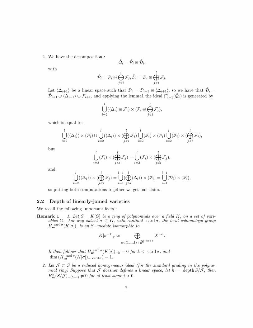
The monomial ideals associated to Ferrer’s tableaux or diagram are a particular caseof the above construction. Using the notations of the Corollary 3, we can describe a Fer-rer’ideal.

A Ferrers diagram is a way to represent partitions of a natural number N . Let N,m bea natural number. A partition of N is a sum of natural numbers: N = λ1 + λ2 + ... + λm,

19

where λ1 ≥ λ2 ≥ ... ≥ λm. A partition is described by a Young diagram which consistsof m rows, with the first row containing λ1 boxes, the second row containing λ2 boxes,etc. Each row is left-justified. Let λm+1 = 0, δ0 = 0, and δ1 be the highest integer suchthat λ1 = ... = λδ1 , and by induction we define δi+1 as the highest integer such thatλδi+1 = ... = λδi+1

, and set l such that δl−1 = m. Let n = λ1, we consider two disjoint setsof variables : {x1, x2, ..., xm}, {y1, y2, ..., yn}. For i = 0, ..., l − 2 let

∆l−i = {xδi+1, ..., xδi+1},Πi+2 = {yλm−i+1+1, ..., yλm−i

}.

and Pi+2 =i+2⋃

j=2

Πj . The Ferrer’s ideal corresponding to the Ferrer’s tableau is generated by

IF = (l

⋃

i=2

∆i × Pi).

So we have the following:

Proposition 3 Let l > 1 be a natural number and for i = 1, ..., l consider two families ofsubsets ∆i,Πi such that V =

⊕li=2(〈∆i〉 ⊕ 〈Πi〉) is a decomposition into linear spaces, and

let

Pk =k

⊕

i=2

〈Πi〉,Dk−1 =l

⊕

i=k

(〈∆i〉),

Qk = Pk⊕Dk, and (Qk) ⊂ K[V ] be the ideal generated by Qk. Then the linearly joined ideal

Q =⊕l

k=1(Qk) is a Ferrer’s ideal. Reciprocally it is immediate to see that any Ferrer’sideal is obtained in this way. Moreover Ferrer’s ideal are characterized as those linearlyjoined ideals (see Corollary 3) Q =

⊕lk=1(Qk), with Qk = Pk ⊕Dk, arrangements of linear

spaces for which we have the inclusions P2 ⊂ P3 ⊂ ...Pl and such that V = D1 ⊕ Pl.

Proof Applying the algorithm described in the proof of the Theorem 7 gives the followingtableau, we recognize a Ferrer’s tableau, reciprocally any Ferrer’s tableau gives rise to suchdecomposition.

20

As a consequence we have

Corollary 7 For any Ferrer’s ideal Iλ ⊂ S, with label λ1 ≥ λ2 ≥ ... ≥ λm

1. The minimal primary decomposition of Iλ is given inthe above proposition.

2. projdim (S/Iλ) = maxmi=1{λi + i − 1}.

3. ara (Iλ) = cd(Iλ) = projdim (S/Iλ). In fact projdim (S/Iλ) is the number ofdiagonals in a Ferrer’s tableau.

4. c(S/Iλ) =∈mi=1 {(λm − λi) + (m − i)}.

Items 1. and 2. were proved by Corso-Nagel in [CN].

2.7 Generalized trees, square free monomial ideals

Let K be a field, and let R = K[x1, ..., xn] be the ring of polynomials. Let ∆ be a simplicialcomplex of dimension d, on the vertex set V = {x1, ..., xn}. Let I∆ be the ideal of R =K[x1, ..., xn] generated by the products of those sets of variables which are not faces of ∆.The ring S = K[x1, ..., xn]/I∆ is called the Stanley-Reisner ring of ∆ over K. It holds thatdimS = d + 1. The graph associated to ∆ will be the (1-dimensional) graph G(∆) on the

vertex set V whose edges are the 1-dimensional faces of ∆, (often named the 1-skeleton of∆). Vice versa, if G is a graph on the vertex set V , we shall consider the simplicial complexassociated to G, denoted by ∆(G), whose maximal faces are all subsets F of V such thatthe complete graph on F is a subgraph of G.

Definition 6 A generalized d−tree on V is a graph defined recursively as follows:

• (a) The complete graph on a set of d + 1 elements of V , is a d− tree

21

• (b) Let G be a graph on the vertex set V . Suppose that there exists some vertex v ∈ Vsuch that:

– the restriction G′ of G to V ′ = V \ {v} is a generalized d − tree, and

– there exists a subset V ′′ ⊂ V ′ of exactly 1 ≤ j ≤ d vertices, such that therestriction of G to V ′′ is a complete graph, and

– G is the graph generated by G′ and the complete graph on V ′′ ∪ {v}.

The vertex v in the above definition will be called an extremal vertex. If always j = d in theabove definition then we say that G is a d−tree. In all this paper we will use the terminologygeneralized tree, instead of generalized d−tree.

We can quote the following theorems of Froberg [Fr]:

Theorem 10 The Stanley Reisner ring of ∆ is a Cohen-Macaulay ring of minimal degreeif and only if

• the graph G(∆) is a d−tree and

• ∆ = ∆(G(∆)).

Theorem 11 The Stanley Reisner ring of ∆ has a 2-linear resolution if and only if

• the graph G(∆) is a generalized tree and

• ∆ = ∆(G(∆)).

Let ∆ a simplicial complex as in the above theorem, in the rest of this paper we willsay that ∆ is a generalized tree.

Example 3 Let I1 be the Stanley-Reisner ideal defined by the simplicial complex:

then the generators of I1 can be ranged in the following linearly joined tableau:

fd (1)

ad, fe (2)

de, ae, fb (3)

fa (4)

22

Example 4 Let I2 be the Stanley-Reisner ideal defined by the simplicial complex:

then the generators of I2 can be ranged in the following linearly joined tableau: (1st stepadding g )

gd (0)

fd, ge (1)

ad, fe, gb (2)

de, ae, fb, ga (3)

fa, gc (4)

(2nd step adding g, h)hd (−1)

gd, he (0)

fd, ge, hb (1)

ad, fe, gb, ha (2)

de, ae, fb, ga, hc (3)

fa, gc (4)

(3th step adding g, h, i)id (−2)

hd, ie (−1)

gd, he, ib (0)

fd, ge, hb, ia (1)

ad, fe, gb, ha, ic (2)

de, ae, fb, ga, hc (3)

fa, gc (4)

23

Example 5 Let I3 be the Stanley-Reisner ideal defined by the simplicial complex:

then the generators of I3 can be ranged in the following linearly joined tableau:(4th step adding g, h, i, j)

jd (−2)

id, ji (−2)

hd, ie, jh (−1)

gd, he, ib, jg (0)

fd, ge, hb, ia, je (1)

ad, fe, gb, ha, ic, jb (2)

de, ae, fb, ga, hc, ja (3)

fa, gc, jc (4)

3 Linear-union of varieties, simplicial ideals

Definition 7 A reduced ideal J ⊂ S defines a linear-union of affine varieties, if J is theintersection of primes ideals Ji = (Mi, (Qi)) for i = 1, ..., l, where (Qi) is the ideal of somesublinear space, satisfying the property:

J = (M1, ...,M,

s⋂

j=1

(Qi)).

Definition 8 Let consider a set of variables G and a decomposition G =s

⋃

i=1

Gi into distinct

sets Gi. For any i = 1, ..., s, let Li ⊂ K[G] be a set of polynomials, such that Li ⊂ (Gi)2.

For i 6= j, we set Gi,j = Gi ∩ Gj , Li,j = Li ∩ (Gi,j), Ii,j ⊂ K[G] be the ideal generated by

24

Li,j, Ii,i ⊂ K[G] be the ideal generated by Li \ ∪j 6=iLj , We set Ii =s

∑

j=1

Ii,j, IG =s

∑

j=1

Ijand

PG = (IG,s

⋂

j=1

(G \ Gj)). We assume

• Ii is a prime ideal for any i

• For any k, l and j 6= k, l we have Ik,l ⊂ (G \ Gj).

We call PG a simplicial ideal.

We can prove our first theorem:

Theorem 12 Simplicial ideals define linear-union of varieties, more precisely : if PG is asimplicial ideal then

PG =s

⋂

j=1

(Ij , (G \ Gj)).

We prove the two inclusions:

• ” ⊂ ”: Since for k 6= j, l we have that Ij,l ⊂ (G \ Gk), it follows that IG = Ik +∑

j,l 6=k Ij,l ⊂ (Ik + (G \ Gk)), on the other hand for any k, ∩sj=1(G \ Gj) ⊂ (G \ Gk),

and so PG = (IG,∩sj=1(G \ Gj)) ⊂ ∩s

k=1(Ik, (G \ Gk),

• ” ⊃ ”: Let P ⊃ PG be a minimal associated prime of PG, then P ⊃ ∩sj=1(G \Gj) and

since (G\Gj) is a prime ideal, there exist some l such that P ⊃ (G\Gl), on the otherhand since P ⊃ PG ⊃ Il, it follows that P ⊃ (Il, G \ Gl), and (Il, G \ Gl) is a primeideal containing P by the first item. In conclusion the minimal associated primes ofP are the prime ideals (Il, G \ Gl), for l = 1, ..., s.

Secondly we compute for l = 1, ..., s, the (Il, G \Gl)-primary component of P. In factwe will prove that

P(Il,G\Gl) = (Il, G \ Gl)(Il,G\Gl),

which will imply that P is reduced and we will get our claim. Let j 6= l, since thereexist at least one element x ∈ Gl \ Gj , and Il ⊂ (Gl)

2, we get that x 6∈ (Il, G \ Gl),and (G \ Gj)(Il,G\Gl) = (1), this implies that

P(Il,G\Gl) = (IG,∩sj=1(G\Gj))(Il,G\Gl) = (IG, (G\Gl))(Il,G\Gl) = (Il, (G\Gl))(Il,G\Gl),

because Ik,j ⊂ (G \ Gl) for any j, k 6= l, and we are done.

Corollary 8

dim (R/PG) = maxl=1,...,s

{ dim (R/(Il, G \ Gl))} = maxl=1,...,s

{ dim (K[Gl]/(Il))}.

If all our ideals are homogeneous

deg(R/PG) =∑

dim (R/(Il,G\Gl))= dim (R/PG)

deg(R/(Il, G \ Gl)).

25

We illustrate the definition of simplicial ideals by the following examples. In these exampleswe can apply the methods developped above for a linearly joined sequence of ideals, in orderto compute projdim (K[G]/PG), depth (K[G]/PG), c(K[G]/PG) and cd(PG). For all ofthem K[G]/PG will be a a Cohen–Macaulay ring, by the Corollary5. We introduce somemethods in order to compute the arithmetical rank. We will use it in the next section.

Example 6 Let G1 = {d, b, c, y1, y2}, G2 = {a, b, c, y1, y2, z1, z2}, G3 = {e, a, c, z1, z2} andI1,2 be the ideal generated by the 2× 2 minors of the matrix M1, I2,3 be the ideal generatedby the 2 × 2 minors of the matrix M2, where

M1 =

(

b y1 y2

y1 y2 c

)

,M2 =

(

a z1 z2

z1 z2 c

)

we can check easily the hypothesis in the definition of a simplicial ideal. Note that I2 :=I1,2 + I2,3 is a prime ideal because it is the toric ideal of the variety parametrized by

b = s3, c = t3, a = u3, y1 = s2t, y2 = st2, z1 = u2t, z2 = ut2,

then:PG := (I1,2, I2,3, da, de, be, dz1dz2, ey1, ey2) =

(I1,2, a, e, z1, z2) ∩ (I1,2, I2,3, d, e) ∩ (I2,3, b, d, y1, y2),

and

PG =√

(I1,2, I2,3, da, de, be),

remark that z21 = az2 modI2,3, so (dz1)

2 = (da)(dz2) modI2,3, this shows that dz1 ∈√

(I1,2, I2,3, da, de, be), in the same way we can prove that dz2, ey1, ey2 ∈√

(I1,2, I2,3, da, de, be),

which proves the equality proposed.Let remark that :

ht(PG) = 6, ara(I1,2) = htI1,2) = 2, ara(I2,3) = htI2,3) = 2,

and (da, de, be) =√

(de, da + be), it then follows that PG is a stci.

Example 7 Let G = {a, b, c, d, e, f, g, h, i, l,m}, G1 = {d, b, c, f, g, l}, G2 = {a, b, c, f, g, h, i}, G3 ={e, a, c, h, i,m} and L1 be the set of 2 × 2 minors of the matrix M1, L3 be the set of 2 × 2minors of the matrix M2, where

M1 =

(

b f g lf g c d

)

,M2 =

(

a h i mh i c e

)

.

We have that I1, I3 ⊂ (G2), and we have that I2 := I1,2 + I2,3 . I1, I2, I3 are prime becausethey are toric ideals, and

PG := (I1, I3, ad, al, be, bm, de, dh, di, dm, ef, eg, el, fm, gm, hl, il, lm)

is equal to(I1, a, e,m, h, i) ∩ (I1, I3, d, e, l,m) ∩ (I3, b, d, f, g, l),

26

and projdim (K[G]/PG) = 8. On the other hand

PG =√

(I1, I3, ad, al, be, bm, de, dm, el, lm),

remark that h2 = ai modI3, so (dh)2 = (da)(di) modI3, this shows thatdh ∈

√

(I1, I3, ad, al, be, bm, de, dm, el, lm), in the same way we can prove our assertion.Let remark that :

ht(PG) = 8, ara (I1) = ht(I1) = 3, ara (I3) = ht(I3) = 3,

and (ad, al, be, bm, de, dm, el, lm) =√

(de, el + md, eb + ml + ad,mb + ld), it then followsthat ara (PG) ≤ 10. It should be interesting to improve this inequality. Note that cd(PG) =8, c(K[G]/PG) = 2.

Example 8 Let G1 = {d, b, c, f, g, l}, G2 = {a, b, c, f, g, h, i}, G3 = {e, a, c, h, i,m} and Lbe the set {h2 − ai, f2 − bg, ch − i2, cf − g2, bc − fg, ac − hi, b2d − l3, ae2 − m3}, this set isa generator of the toric ideal IT parametrized by u3 − a, s3 − b, t3 − c, v3 − d,w3 − e, s2t −f, st2 − g, tu2 − h, t2u − i, s2v − l, uw2 − m. We have that

L1 = {f2 − bg, cf − g2, bc − fg, b2d − l3},

L2 = {h2 − ai, f2 − bg, ch − i2, cf − g2, bc − fg, ac − hi},

L3 = {h2 − ai, ch − i2, ac − hi, ae2 − m3}.

The ideals I1, I2, I3, generated respectively by L1, L2, L3 are prime, because they are toric,Then we have that:

PG := (IT , da, de, dm, dh, di, be, bm, al, ef, eg, el, fm, gm, hl, il, lm)

is equal to(I1, a, e, h, i,m) ∩ (I2, d, e, l,m) ∩ (I3, b, d, f, g, l),

On the other hand

PG =√

IT , da, de, be),

remark that h2 = ah modI3, so (dh)2 = (da)(di) modI3, this shows that dh ∈√

(IT , da, de, be),in the same way we can prove that dm, di, bm, al, ef, eg, el, fm, gm, hl, il, lm ∈

√

(IT , da, de, be),which proves the equality proposed. Also we have that ara (I1) ≤ 3, ara (I3) ≤ 3, soara (IT ) ≤ 6, which implies that: 8 = ht(PG) ≤ ara (PG) ≤ ara (IT ) + 2 ≤ 8. SoPG is a set theoretically complete intersection and we can give explicitly the generators upto the radical. Note that IT is also a stci.

Now we study the Cohen–Macaulay property. In this example we have that

(I1, a, h, i, e,m) + (I2, d, l, e,m) = (f2 − bg, cf − g2, bc − fg, a, h, i, d, l, e,m)

so the quotient ring K[G]/((I1, a, h, i, e,m) + (I2, d, le,m)) ≃ K[b, c, f, g]/(f2 − bg, cf −g2, bc−fg) is Cohen–Macaulay of dimension two, this will imply that K[G]/((I1, a, h, i, e,m)∩(I2, d, le,m)) is Cohen–Macaulay of dimension three.

27

((I1, a, h, i, e,m)∩ (I2 , d, l, e,m))+(I3, b, d, f, g, l) = (h2−ai, ch− i2, ac−hi, b, d, e, f, g, l,m)

so the quotient ring K[G]/(((I1, a, h, i, e,m)∩(I2 , d, l, e,m))+(I3, b, d, f, g, l)) ≃ K[a, c, h, i]/(h2−ai, ch− i2, ac−hi) is Cohen–Macaulay of dimension two, this will imply from the Corollary5 that K[G]/(PG) is Cohen–Macaulay of dimension three.

4 Ara of some simplicial ideals

In the Definition 3 we have extended any sequence of linearly joined linear spaces. In thecase of Stanley-Reisner ideal associated to a simplicial complex we can give a more generaldefinition.

Definition 9 Let △(F ) be a simplicial complex, with set of vertices F and facets F1, ..., Fs.Let denote by I△(F ), the Stanley-Reisner ideal associated to △(F ). Let consider a family ofdisjoints sets F ′

l , 1 ≤ l ≤ s and disjoints also from F , we define new sets Gl = Fl ∪ F ′l , and

let △(G) be the simplicial complex with vertices G = ∪1≤l≤sGl and facets G1, ..., Gs. Wecall △(G) a extension of △(F ).

Let remark that in the above situation I△(G), is generated by I△(F ), and all products yzsuch that y ∈ F ′

i , y ∈ Gj \ Fi for all i 6= j. This is clear since by hypothesis, for all i 6= jand y ∈ F ′

i , z ∈ Gj \Fi the edge [y, z] is not in any facet of △(G) so the product yz belongsto I△(G), and the other generators of I△(G) have its support in F .

It follows from the Proposition 2, that if △(F ) is a generalized tree then △(G) is ageneralized tree, and depth (K[F ]/I△(F )) = depth (K[G]/I△(G)),

In the following theorem, Ii will be a toric ideal on the variables Gi, and we assumethat Ii is fully parametrized on the set Fi, that is for any y ∈ F ′

i , there exists some naturalnumber m such that ym − xFi

∈ Ii, where xFiis a monomial with support the set Fi. In

particular this implies that dimK[Gi]/Ii = card Fi, for all i. Let remark that the idealPG = (I1, ..., Is, I△(G)) fullfils the conditions to be a simplicial ideal, and it flllows thatPG =

⋂si=1(Ii, G \ Gi).

Theorem 13 Let consider as above △(H), △(G), toric ideals Ii on the variables Gi, thatare fully parametrized on the set Fi and PG = (I1, ..., Is, I△(G)). Then

1. PG = rad (∑s

i=1 Ii + I△(F )) and ara (PG) ≤∑s

i=1 ara (Ii) + ara I△(F ).

2. If △(F ) is a generalized tree and each ideal Ii is a stci then

cd(PG) = ara (PG) = card G − depth (K[F ]/I△(F )).

c(K[G]/PG) = card G − ara (PG) − 1.

3. In particular if △(F ) is a d−tree, and each ideal Ii is a stci then PG is a stci.

28

4. If △(F ) is a generalized tree, each ideal Ii is a stci, and K[Gi]/Ii is Cohen–Macaulay,then :

c(K[G]/PG) = card G − ara (PG) − 1.

cd(PG) = ara (PG) = projdim (K[G]/PG).

Proof.

1. It will be enough to prove that for all i 6= j and y ∈ F ′i , z ∈ Gj \ Fi, yz ∈

rad (I1, ..., Is, I△(F )). Since for every i, Ii,i = Ii is a simplicial toric ideal, and Fi

is a set of parameters of Ii, for every element y ∈ F ′i , there exists some natural

number m such that ym − xFi∈ Ii, where xFi

is a monomial with support Fi, letz ∈ Fj \ Fi, it follows that zxFi

∈ I△(F ), which implies that zmym ∈ (Ii, I△(F )), nowlet let z ∈ F ′

j \Fi, then there exists an integer µ such that zµ − xFj∈ Ij , where xFj

isa monomial with support Fj 6= Fi. Let remark that we can choose m = µ. We havethat

(ym − xFi)(zm − xFj

) = ymzm − ymxFj− zmxFi

+ xFixFj

,

which implies that ymzm ∈ (Ii, Ij , I△(F )). as a consequence PG = rad (∑

i Ii + I△(F )).

2. If each Ii is a stci then ara (Ii) = card (F ′i ), and if △(F ), is a generalized tree, then

also △(G), is a generalized tree, depth (K[G]/I△(G)) = depth (K[F ]/I△(F )), andara (I△(F )) = card F − depth (K[F ]/I△(F )), so

ara (PG) ≤∑

i

card (F ′i )+ card F− depth (K[F ]/I△(F )) = card G− depth (K[F ]/I△(F )) =

= card G − depth (K[G]/I△(G)) = card G − c(K[G]/PG) − 1,

since by the Theorem 6 depth (K[G]/I△(G)) = c(K[G]/I△(G)) = c(K[G]/PG), itfollows then :

ara (PG) ≤ card G − c(K[G]/PG) − 1,

orc(K[G]/PG) ≤ card G − ara (PG) − 1,

on the other hand, by [B-S], 19.5.3

c(K[G]/PG) ≥ card G − ara (PG) − 1,

so we have the equality.

3. in particular if △(F ) is a d−tree then K[F ]/I△(F ) is a Cohen–Macaulay ring, so

depth (K[F ]/I△(F )) = dim (K[F ]/I△(F )) = dim (K[G]/PG)

ara (PG) ≤ card G − dim (K[G]/PG) = ht(PG),

which implies that ara (PG) = ht(PG), and so PG is a stci.

29

4. If for every i, K[Gi]/Ii is Cohen–Macaulay, then :

depth (K[F ]/I△(F )) = depth (K[G]/I△(G)) = depth (K[G]/PG),

so our statement follows from 2.

The statements about cohomological dimension follows from the Theorem 4.

Remark 4 1. We recall that in [BMT]it was proved that any (simplicial) toric ideal Ifully parametrized is a stci if char(K) = p > 0 and almost stci if char(K) = p > 0. Sowe can apply the above theorem to find a large class of examples for which ara (PG) <projdim (K[G]/PG). This will be published later.

2. It follows from my work [M], and the work of Robbiano-Valla [RV1],[RV1] that anysimplicial toric ideal in codimension two, arithmetically Cohen–Macaulay is a stci. Sowe can apply the above theorem to this family.

3. The examples given in this paper sustend that there is a more general version of theabove Theorem, this is part of a work in progress.

4. It should be interesting to study homogeneous ideals in a polynomial ring S for which

c(S/I) = dimS − ara (I) − 1.

References

[BM1] Barile M., Morales M., On certain algebras of reduction number one, J. Algebra 206(1998), 113 – 128.

[BM2] Barile M., Morales M., On the equations defining minimal varieties, Comm. Alg.,28 (2000), 1223 – 1239.

[BM3] Barile M., Morales M., On Stanley-Reisner Rings of Reduction Number One, Ann.Sc.Nor. Sup. Pisa, Serie IV. Vol. XXIX Fasc. 3. (2000), 605 – 610.

[BM4] Barile M., Morales M., On unions of scrolls along linear spaces, Rend. Sem. Mat.Univ. Padova, 111 (2004), 161 – 178.

[B] Bertini, E. Introduzione alla geometria projettiva degli iperspazi con appendice sullecurve algebriche e loro singolarita. Pisa: E. Spoerri. (1907).

[BMT] Barile, Margherita; Morales, Marcel; Thoma, Apostolos On simplicial toric varietieswhich are set-theoretic complete intersections. J. Algebra 226, No.2, 880-892 (2000).

[B-S] Brodmann M.P. and R.Y. Sharp, Local cohomology, Cambridge studies in AdvancedMath. 60, (1998).

[CEP] De Concini, Corrado; Eisenbud, David; Procesi, Claudio Hodge algebras. Asterisque91, 87 p. (1982).

30

[DP] Del Pezzo, P. Sulle superficie di ordine n immerse nello spazio di n + 1 dimensioni.Nap. rend. XXIV. 212-216. (1885).

[EG] Eisenbud, David; Goto, Shiro Linear free resolutions and minimal multiplicity. J.Algebra 88, 89-133 (1984).

[EGHP] Eisenbud D., Green M., Hulek K., Popescu S., Restricting linear syzygies: algebraand geometry, Compos. Math. 141 (2005), no. 6, 1460–1478.

[Fr] Froberg R, On Stanley – Reisner rings, Banach Center Publ. 26, Part 2 (1990), 57 –70.

[GMS1] Gimenez, P.; Morales, M.; Simis, A. The analytic spread of the ideal of a mono-mial curve in projective 3- space. Eyssette, Frederic et al., Computational algebraicgeometry. Papers from a conference, held in Nice, France, April 21-25, 1992. Boston:Birkhauser. Prog. Math. 109, 77-90 (1993).

[GMS2] Gimenez Ph., Morales M., Simis A., The analytical spread of the ideal of codimen-sion 2 monomial varieties, Result. Math. Vol 35 (1999), 250 - 259.

[H] Ha Minh Lam, Algebre de Rees et fibre speciale PhD Thesis work, Universite J-Fourier, Grenoble, France (2006).

[HM] Ha Minh Lam, Morales M., Fiber cone of codimension 2 lattice ideals To appearComm. Alg.

[HHZ] Herzog, Jurgen; Hibi, Takayuki; Zheng, Xinxian Monomial ideals whose powers havea linear resolution. Math. Scand. 95, No.1, 23-32 (2004).

[M] Morales, Marcel Equations des varietes monomiales en codimension deux. (Equationsof monomial varieties in codimension two). J. Algebra 175, No.3, 1082-1095 (1995).

[CN] Alberto Corso, Uwe Nagel, Monomial and toric ideals associated to Ferrers graphs.math.AC/0609371.

[RV1] Robbiano, Lorenzo; Valla, Giuseppe On set-theoretic complete intersections in theprojective space. Rend. Semin. Mat. Fis. Milano 53, 333-346 (1983).

[RV2] Robbiano, Lorenzo; Valla, Giuseppe Some curves in P 3are set-theoretic completeintersections. Algebraic geometry - open problems, Proc. Conf., Ravello/Italy 1982,Lect. Notes Math. 997, 391-399 (1983).

[S-V] Schmitt, Th.; Vogel, W., Note on Set-Theoretic Intersections of Subvarieties of Pro-jective space, Math. Ann. 245 (1979), 247 - 253.

[X] Xambo, S. On projective varieties of minimal degree. Collect. Math. 32, 149 (1981).

31