SIGMOD Officers, Committees, and Awardees

SIGMOD Officers, Committees, and Awardees

Chair Vice-Chair Secretary/TreasurerDivyakantAgrawal FatmaOzcan RachelPottinger

DepartmentofComputerScience SystemsResearchGroup DepartmentofComputerScienceUCSantaBarbara Google UniversityofBritishColumbia

SantaBarbara,California Sunnyvale,California VancouverUSA USA Canada

+18058934385 +16692649238 +16048220436agrawal<at>cs.ucsb.edu Fozcan<at>google.com Rap<at>cs.ubc.ca

SIGMODExecutiveCommittee:

Divyakant Agrawal (Chair), Fatma Ozcan (Vice-chair), Rachel Pottinger (Treasurer), Juliana Freire (Previous SIGMOD Chair), K. Selçuk Candan (SIGMOD Conference Coordinator), Rada Chirkova (SIGMOD Record Editor), Chris Jermaine (ACM TODS Editor in Chief), Divesh Srivastava (2021 SIGMOD PC co-chair), Stratos Idreos (2021 SIGMOD PC co-chair), Leonid Libkin (Chair of PODS), Sihem Amer-Yahia (SIGMOD Diversity and Inclusion Coordinator), Curtis Dyreson (Information Director)

AdvisoryBoard:YannisIoannidis(Chair),PhilBernstein,SurajitChaudhuri,RakeshAgrawal,JoeHellerstein,MikeFranklin,LauraHaas,ReneeMiller,JohnWilkes,ChrisOlsten,AnHaiDoan,TamerÖzsu,GerhardWeikum,StefanoCeri,BengChinOoi,TimosSellis,SunitaSarawagi,StratosIdreos,andTimKraska

SIGMODInformationDirector: CurtisDyreson,UtahStateUniversityAssociateInformationDirectors:

HuipingCao(SIGMODRecord),GeorgiaKoutrika(Blogging),WimMartens(PODS),andSouravSBhowmick(SIGMODRecord)

SIGMODRecordEditor-in-Chief: RadaChirkova,NCStateUniversitySIGMODRecordAssociateEditors:

LyublenaAntova,MarceloArenas,ManosAthanassoulis,RenataBorovica-Gajic,VanessaBraganholo,SusanDavidson,AaronJ.Elmore,Wook-ShinHan,WimMartens,KyriakosMouratidis,DanOlteanu,TamerÖzsu,KennethRoss,PınarTözün,ImmanuelTrummer,YannisVelegrakis,MarianneWinslett,andJunYang

SIGMODConferenceCoordinator:

K.SelçukCandan,ArizonaStateUniversity

PODSExecutiveCommittee: Leonid Libkin (chair), Christoph Koch, Reinhard Pichler, Dan Suciu, Yufei Tao, Jan Van den BusscheSisterSocietyLiaisons: RaghuRamakhrishnan(SIGKDD),YannisIoannidis(EDBTEndowment),ChristianJensen(IEEETKDE)SIGMODAwardsCommittee: Sunita Sarawagi (Chair), Volker Markl, Renée Miller, H. V. Jagadish, Yanlei Diao, Stefano Ceri

SIGMOD Record, March 2022 (Vol. 51, No. 1) 1

JimGrayDoctoralDissertationAwardCommittee:Vanessa Braganholo (co-chair), Viktor Leis (co-chair), Bailu Ding, Immanuel Trummer, Joy Arulraj, Jose Faleiro, Gustavo Alonso, Wolfgang Lehner

SIGMODEdgarF.CoddInnovationsAwardForinnovativeandhighlysignificantcontributionsofenduringvaluetothedevelopment,understanding,oruseofdatabasesystemsanddatabases.Recipientsoftheawardarethefollowing:

MichaelStonebraker(1992) JimGray(1993) PhilipBernstein(1994)DavidDeWitt(1995) C.Mohan(1996) DavidMaier(1997)SergeAbiteboul(1998) HectorGarcia-Molina(1999) RakeshAgrawal(2000)RudolfBayer(2001) PatriciaSelinger(2002) DonChamberlin(2003)RonaldFagin(2004) MichaelCarey(2005) JeffreyD.Ullman(2006)JenniferWidom(2007) MosheY.Vardi(2008) MasaruKitsuregawa(2009)UmeshwarDayal(2010) SurajitChaudhuri(2011) BruceLindsay(2012)StefanoCeri(2013) MartinKersten(2014) LauraHaas(2015)GerhardWeikum(2016) GoetzGraefe(2017) RaghuRamakrishnan(2018)AnastasiaAilamaki(2019)BengChinOoi(2020)SIGMODSystemsAwardFor technical contributions that have had significant impact on the theory or practice of large-scale data management systems.

MichaelStonebrakerandLawrenceRowe(2015);MartinKersten(2016);RichardHipp(2017);JeffHammerbacher,AshishThusoo,JoydeepSenSarma;ChristopherOlston,BenjaminReed,andUtkarshSrivastava(2018);XiaofengBao,CharlieBell,MuraliBrahmadesam,JamesCorey,NealFachan,RajuGulabani,AnuragGupta,KamalGupta,JamesHamilton,AndyJassy,TengizKharatishvili,SaileshKrishnamurthy,YanLeshinsky,LonLundgren,PradeepMadhavarapu,SandorMaurice,GrantMcAlister,SamMcKelvie,RamanMittal,DebanjanSaha,SwamiSivasubramanian,StefanoStefani,andAlexVerbitski(2019);DonAnderson,KeithBostic,AlanBram,GrgBurd,MichaelCahill,RonCohen,AlexGorrod,GeorgeFeinberg,MarkHayes,CharlesLamb,LindaLee,SusanLoVerso,JohnMerrells,MikeOlson,CarolSandstrom,SteveSarette,DavidSchacter,DavidSegleau,MarioSeltzer,andMikeUbell(2020)SIGMODContributionsAwardFor significant contributions to the field of database systems through research funding, education, andprofessionalservices.Recipientsoftheawardarethefollowing:

MariaZemankova(1992) GioWiederhold(1995) YahikoKambayashi(1995)JeffreyUllman(1996) AviSilberschatz(1997) WonKim(1998)RaghuRamakrishnan(1999) MichaelCarey(2000) LauraHaas(2000)DanielRosenkrantz(2001) RichardSnodgrass(2002) MichaelLey(2003)SurajitChaudhuri(2004) HongjunLu(2005) TamerÖzsu(2006)Hans-JörgSchek(2007) KlausR.Dittrich(2008) BengChinOoi(2009)DavidLomet(2010) GerhardWeikum(2011) MarianneWinslett(2012)H.V.Jagadish(2013) Kyu-YoungWhang(2014) CurtisDyreson(2015)SamuelMadden(2016) YannisE.Ioannidis(2017) Z.MeralÖzsoyoğlu(2018)AhmedElmagarmid(2019)PhilipeBonnet(2020) JulianaFreire(2020)StratosIdreos(2020) StefanManegold(2020) IoanaManolescu(2020)DennisShasha(2020)SIGMODJimGrayDoctoralDissertationAwardSIGMODhasestablishedtheannualSIGMODJimGrayDoctoralDissertationAwardtorecognizeexcellentresearchbydoctoralcandidatesinthedatabasefield.Recipientsoftheawardarethefollowing:

§ 2006Winner:GeromeMiklau.HonorableMentions:MarceloArenasandYanleiDiao§ 2007Winner:BoonThauLoo.HonorableMentions:XifengYanandMartinTheobald

2 SIGMOD Record, March 2022 (Vol. 51, No. 1)

§ 2008Winner:ArielFuxman.HonorableMentions:CongYuandNileshDalvi§ 2009Winner:DanielAbadi.HonorableMentions:Bee-ChungChenandAshwinMachanavajjhala§ 2010Winner:ChristopherRé.HonorableMentions:SoumyadebMitraandFabianSuchanek§ 2011Winner:StratosIdreos.HonorableMentions:ToddGreenandKarlSchnaitterz§ 2012Winner:RyanJohnson.HonorableMention:BogdanAlexe§ 2013Winner:SudiptoDas,HonorableMention:HerodotosHerodotouandWenchaoZhou§ 2014Winners:AdityaParameswaranandAndyPavlo.§ 2015Winner:AlexanderThomson.HonorableMentions:MarinaDrosouandKarthikRamachandra§ 2016Winner:Paris Koutris.HonorableMentions:Pinar TozunandAlvin Cheung§ 2017Winner:PeterBailis.HonorableMention:ImmanuelTrummer§ 2018Winner:ViktorLeis.HonorableMention:LuisGalárragaandYongjooPark§ 2019Winner:JoyArulraj.HonorableMention:BasKetsman§ 2020Winner:JoseFaleiro.HonorableMention:SiluHuang§ 2021Winner:HuanchenZhang,HonorableMentions:ErfanZamanian,MaximilianSchleich,andNatacha

Crooks

AcompletelistofallSIGMODAwardsisavailableat:https://sigmod.org/sigmod-awards/

[Lastupdated:September30,2021]


Guest Editor’s Notes

WelcometotheMarch2022issueoftheACMSIGMODRecord!Thenewyearof2022beginswithaspecialissueonthe2021ACMSIGMODResearchHighlightsAwards.Theseareawardsforthedatabasecommunitytoshowcaseasetofresearchprojectsthatexemplify core database research. In particular, each of these projects addresses an importantproblem,representsadefinitivemilestoneinsolvingtheproblem,andhasthepotentialofsignifi-cant impact. These awards also aim tomake the selected works widely known in the databasecommunity,toourindustrypartners,andtothebroaderACMcommunity.TheawardscommitteeandeditorialboardincludedMarceloArenas,RadaChirkova,WimMartens,Kenneth Ross, and Jun Yang. We solicited articles fromPODS 2021, SIGMOD2021, VLDB 2021,ICDE2021,EDBT2021,andICDT2021,aswellasfromcommunitynominations.Throughacarefulreviewprocesstenarticleswerefinallyselectedas2021ResearchHighlights.Theauthorsofeacharticleworkedcloselywiththeeditorialboardtorewritethearticleintoacompact8-pageformatand improved it to appeal to thebroaddata-management community. Inaddition, each researchhighlightisaccompaniedbyaone-pagetechnicalperspectivewrittenbyanexpertonthetopicpre-sentedinthearticle.Thetechnicalperspectiveprovidesthereaderwithanoverviewoftheback-ground,themotivation,andthekeyinnovationofthefeaturedresearchhighlight,aswellasitssci-entificandpracticalsignificance.The2021researchhighlightscoverabroadsetoftopics,including(a)asignificantstepforwardforqueryoptimizationthatcombinestraditionalwisdomwithneuralnetworks(“Bao:MakingLearnedQueryOptimizationPractical”);(b)anewapproachthatmakesiteasierfordataprocessingsystemsto exploit high-speednetworks (“DFI: TheData Flow Interface forHigh-SpeedNetworks”); (c) afoundationforfuturecloudinformationsystemsthataimatbalancingperformanceandconsistency(“FoundationDB:ADistributedKeyValueStore”);(d)anewframeworkthatlearnsdeepcontextu-alizedrepresentationsonrelationalWebtables(“TURL:TableUnderstandingthroughRepresenta-tionLearning”);(e)ahighlyscalableapproachforembeddingattributednetworksonasingleserv-er(“NoPANE,NoGain:ScalingAttributedNetworkEmbeddinginaSingleServer”);(f)keyinnova-tions for bipartitematching that significantly improve the computation of the assignment costs(“BipartiteMatching:WhattodointheRealWorldWhenComputingAssignmentCostsDominatesFinding theOptimalAssignment”); (g) asystem that combines the advantagesof imperative andfunctionaldataflowsystems(“ImperativeorFunctionalControlFlowHandling:WhynottheBestofBothWorlds?”);(h)newinsightsforestimatingquantilesinstreamswithstrongtheoreticalguar-antees,whicharealreadyavailableintheApacheDatasketcheslibrary(“RelativeErrorStreamingQuantiles”); (i)characterizationsandanswers to foundationalquestionson theconsistencyprob-lemforrelationsunderbagsemantics(“StructureandComplexityofBagConsistency”);and(j)aninterestingnewconnectionbetweencountingthenumberofmodelsofaCNFformulaandthedis-tinctelementsinadatastream(“ModelCountingMeetsDistinctElementsinaDataStream”).

Onbehalf of the SIGMODRecordEditorialBoard, I hope that you enjoy reading theMarch2022issueoftheSIGMODRecord!

WimMartens

March2022


Making Learned Query Optimization Practical:A Technical Perspective

Volker MarklTechnische Universität Berlin, Germany

[email protected]

Query optimization has been a challenging problem eversince the relational data model had been proposed. The roleof the query optimizer in a database system is to compute anexecution plan for a (relational) query expression comprisedof physical operators whose implementations correspond tothe operations of the (relational) algebra. There are manydegrees of freedom for selecting a physical plan, in particulardue to the laws of associativity, commutativity, and distribu-tivity among the operators in the (relational) algebra, whichnecessitates our taking the order of operations into consider-ation. In addition, there are many alternative access pathsto a dataset and a multitude of physical implementations foroperations, such as relational joins (e.g., merge-join, nested-loop join, hash-join). Thus, when seeking to determine thebest (or even a sufficiently good) execution plan there is ahuge search space.

Query optimizers use a cost model to guide this search,which is usually a linear combination of the cardinality (i.e.,the expected size of an intermediate result that needs to becomputed when processing a query) and physical parame-ters, such as the I/O transfer cost and CPU processing cost.While the I/O transfer cost and CPU processing cost caneasily be measured, it is very hard to accurately model thesize of an intermediate result that may arise during queryprocessing, in particular after many joins, selections, or pro-jections with duplicate elimination have been applied to adata set.

Traditionally, query optimizers rely on statistics about atable and the database in conjunction with assumptions,such as the independence of predicates occurring in selec-tions, the inclusion of one data set in another data set forkey-foreign key joins, or uniformity when more informativestatistics are unavailable. When these assumptions are in-valid or the statistical information available is outdated ormissing altogether, the cardinality estimates produced bythe cost model of the query optimizer may be off, often byorders of magnitude. This in turn is the major cause forpoor execution plans and suboptimal performance duringquery processing.

This problem has been well recognized by the researchcommunity, and in the early mid-90s researchers started tolook into learning methods for specific statistical artefacts.

Permission to make digital or hard copies of all or part of this work forpersonal or classroom use is granted without fee provided that copies arenot made or distributed for profit or commercial advantage and that copiesbear this notice and the full citation on the first page. To copy otherwise, torepublish, to post on servers or to redistribute to lists, requires prior specificpermission and/or a fee.Copyright 2008 ACM 0001-0782/08/0X00 ...$5.00.

In particular, to monitor cardinalities during query execu-tion and exploit the learned information in future querycompilations. Chen and Roussopulos [2] used query resultsto learn the statistical distributions of simple predicates af-ter the execution of a query and accordingly adapt the coef-ficients via a curve-fitting function. Aboulnaga and Chaud-huri [1] introduced a query feedback loop, where the actualcardinalities monitored during execution are used to correcthistograms.

LEO [4] pioneered the concept of a learning query opti-mizer, where a feedback loop is used to determine and adjustfor discrepancies among cardinalities and other parametersof the cost model during all steps of the query executionplan. Recently, due to advances in machine learning andthe emergence of Software 2.0, these ideas have received re-newed interest. In particular, several works have proposedto use deep learning or reinforcement learning to computethe cardinalities or the entire cost model.

The Bao paper [3] is a consequent continuation of this lineof research, which can take advantage of the prior knowledgehard-coded in the cost model of existing query optimizers,while leveraging the core ideas of learned optimizers (e.g., in-corporating query feedback, learning from mistakes). BaoSskey innovations include leveraging the existing query opti-mizer, using a deep convolutional neural network to predictthe performance of queries and suggest hints, and leverag-ing Thompson sampling for plan selection. This approachallows Bao to be easily integrated and combined with ex-isting systems, while being able to adjust to changes in theworkload, data, and schema.

1. REFERENCES[1] A. Aboulnaga and S. Chaudhuri. Self-tuning

histograms: Building histograms without looking atdata. In SIGMOD, 1999.

[2] C. M. Chen and N. Roussopoulos. Adaptive selectivityestimation using query feedback. In SIGMOD, 1994.

[3] R. Marcus, P. Negi, H. Mao, N. Tatbul, M. Alizadeh,and T. Kraska. Bao: Making learned queryoptimization practical. In SIGMOD, 2021.

[4] M. Stillger, G. M. Lohman, V. Markl, and M. Kandil.Leo - db2’s learning optimizer. In VLDB, 2001.


Bao: Making Learned Query Optimization Practical

Ryan Marcus12, Parimarjan Negi1, Hongzi Mao1,Nesime Tatbul12, Mohammad Alizadeh1, Tim Kraska1

1MIT CSAIL 2Intel Labsryanmarcus, pnegi, hongzi, tatbul, alizadeh, [email protected]

ABSTRACTRecent efforts applying machine learning techniques to queryoptimization have shown few practical gains due to substan-tive training overhead, inability to adapt to changes, andpoor tail performance. Motivated by these difficulties, weintroduce Bao (the Bandit optimizer). Bao takes advantageof the wisdom built into existing query optimizers by provid-ing per-query optimization hints. Bao combines modern treeconvolutional neural networks with Thompson sampling, awell-studied reinforcement learning algorithm. As a result,Bao automatically learns from its mistakes and adapts tochanges in query workloads, data, and schema. Experimen-tally, we demonstrate that Bao can quickly learn strategiesthat improve end-to-end query execution performance, in-cluding tail latency, for several workloads containing long-running queries. In cloud environments, we show that Baocan offer both reduced costs and better performance com-pared with a commercial system.

1. INTRODUCTIONQuery optimization is the task of transforming a user-

issued declarative SQL query into an execution plan. De-spite decades of study [30], query optimization remains aunsolved problem [17]. Several works have applied machinelearning techniques to query optimization [32, 16, 19, 33,35], often showing remarkable results. We argue that noneof the techniques are yet practical, as they suffer from sev-eral fundamental problems:

1. Long training time. Most proposed machine learning tech-niques require an impractical amount of training data beforethey have a positive impact on query performance. For ex-ample, ML-powered cardinality estimators based on super-vised learning require gathering precise cardinalities fromthe underlying data, a prohibitively expensive operation inpractice (this is why we wish to estimate cardinalities in thefirst place). Reinforcement learning techniques must pro-cess thousands of queries before outperforming traditionaloptimizers, which can take on the order of days [19].

1© ACM 2021. This is a minor revision of the work published inSIGMOD ’21. ISBN 978-1-4503-8343-1, June 20–25, 2021, VirtualEvent, China. DOI: https://doi.org/10.1145/3448016.3452838


Figure 1: Disabling loop join in PostgreSQL can signifi-cantly improve (16b) or harm (24b) a particular query’s per-formance. These example queries are from the Join OrderBenchmark (JOB) [15].

2. Handling change. While performing expensive trainingoperations once may already be impractical, changes in queryworkload, data, or schema can make matters worse. Super-vised cardinality estimators must be retrained when datachanges, or risk becoming stale. Several proposed reinforce-ment learning techniques require retraining when either theworkload or the schema change [14, 20, 25, 19].

3. Tail catastrophe. Recent work has shown that learningtechniques can outperform traditional optimizers on aver-age, but often perform catastrophically (e.g., 100x regres-sion in query performance) in the tail [19, 26, 24, 9]. Thisis especially true when training data is sparse. While someapproaches offer statistical guarantees of their dominance inthe average case [35], such failures, even if rare, are unac-ceptable in many real world applications.

4. Black-box decisions. While traditional cost-based opti-mizers are already complex, understanding query optimiza-tion is even harder when black-box deep learning approachesare used. Moreover, in contrast to traditional optimizers,current learned optimizers do not provide a way for databaseadministrators to influence or understand the learned com-ponent’s query planning.

5. Integration cost. To the best of our knowledge, all previ-ous learned optimizers are still research prototypes, offeringlittle to no integration with a real DBMS. None even sup-ports all features of standard SQL, not to mention vendorspecific features. Hence, fully integrating any learned opti-mizer into a commercial or open-source database system isnot a trivial undertaking.


1.1 BaoIn [18], we introduced Bao (Bandit optimizer), the first

learned optimizer which overcomes the aforementioned prob-lems. This paper presents a short summary of Bao’s keytechniques and our experimental insights. Bao is fully inte-grated into PostgreSQL as an extension, and can be easilyinstalled without the need to recompile PostgreSQL. Thedatabase administrator (DBA) just needs to download ouropen-source module, and even has the option to selectivelyturn the learned optimizer on or off for specific queries.

The core idea behind Bao is to avoid learning an optimizerfrom scratch. Instead, we take an existing optimizer (e.g.,PostgreSQL’s optimizer) and learn when to activate (or de-activate) some of its features on a query-by-query basis. Inother words, Bao is a learned component that sits on top ofan existing query optimizer in order to enhance query opti-mization, rather than replacing or discarding the traditionalquery optimizer altogether.

For instance, on a particular query, the PostgreSQL op-timizer might under-estimate the cardinality for some joinsand wrongly select a loop join when other join algorithms(e.g., merge join, hash join) would be more effective [15].This occurs in query 16b of the Join Order Benchmark [15],and disabling loop-joins for this query yields a 3x perfor-mance improvement (see Figure 1). Yet, it would be wrongto always disable loop joins. For example, for query 24b,disabling loop joins causes the performance to degrade byalmost 50x, an arguably catastrophic regression.

At a high level, Bao tries to “correct” a traditional queryoptimizer by learning a mapping between an incoming queryand the execution strategy the query optimizer should usefor that query. We refer to these corrections – a subset ofstrategies to enable – as query hint sets. Effectively, throughthe provided hint sets, Bao limits and steers the search spaceof the traditional optimizer.

Our approach assumes a finite set of hint sets and treatseach hint set as an arm in a contextual multi-armed banditproblem. Bao learns a model that predicts which hints willlead to good performance for a particular query. When aquery arrives, our system selects a hint set, executes the re-sulting query plan, and observes a reward. Over time, Baorefines its model to more accurately predict which hint setwill most benefit an incoming query. For example, for ahighly selective query, Bao can automatically steer an opti-mizer towards a left-deep loop join plan (by restricting theoptimizer from using hash or merge joins), and to disableloop joins for less selective queries.

By formulating the problem as a contextual multi-armedbandit, Bao can take advantage of Thompson sampling, awell-studied sample-efficient algorithm [3]. Because Bao usesan underlying query optimizer, Bao can potentially adaptto new data and schema changes just as well as the un-derlying optimizer. While other learned query optimizationmethods have to relearn what traditional query optimizersalready know, Bao immediately starts learning to improvethe underlying optimizer, and is able to reduce tail latencyeven compared to traditional query optimizers. In additionto addressing the practical issues of previous learned queryoptimization systems, Bao comes with a number of desir-able features that were either lacking or hard to achieve inprevious traditional and learned optimizers:

1. Short training time. In contrast to other deep-learningapproaches, which can take days to train, Bao can outper-form traditional query optimizers with much less trainingtime (≈ 1 hour). Bao achieves this by taking full advan-tage of existing query optimization knowledge, which wasencoded by human experts into traditional optimizers avail-able in DBMSes today. Moreover, Bao can be configuredto start out using only the traditional optimizer and onlyperform training when the load of the system is low.

2. Robustness to schema, data, and workload changes. Baocan maintain performance even in the presence of workload,data, and schema changes. Bao does this by leveraging atraditional query optimizer’s cost and cardinality estimates.

3. Better tail latency. While previous learned approacheseither did not improve or did not evaluate tail performance,we show that Bao is capable of improving tail performanceby orders of magnitude with as little as 30 minutes to a fewhours of training.

4. Interpretability and easier debugging. Bao’s decisions canbe inspected using standard tools, and Bao can be enabledor disabled on a per-query basis. Thus, when a query misbe-haves, an engineer can examine the query hint chosen by Baoand the decisions made by the underlying optimizer with EX-

PLAIN. If the underlying optimizer is functioning correctly,but Bao made a poor decision, Bao can be specifically dis-abled. Alternatively, Bao can be off by default, and onlyenabled on specific queries known to have poor performancewith the underlying traditional query optimizer.

5. Low integration cost. Bao is easy to integrate into an ex-isting database and often does not even require code changes,as most database systems already expose all necessary hintsand hooks. Moreover, Bao builds on top of an existing op-timizer and can thus support every SQL feature supportedby the underlying database.

6. Extensibility. Bao can be extended by adding new queryhints over time, without retraining. Additionally, Bao’sfeature representation can be easily augmented with ad-ditional information which can be taken into account dur-ing optimization, although this does require retraining. Forexample, when Bao’s feature representation is augmentedwith information about the cache, Bao can learn how tochange query plans based on the cache state. This is a desir-able feature because reading data from cache is significantlyfaster than reading information off of disk, and it is possi-ble that the best plan for a query changes based on what iscached. While integrating such a feature into a traditionalcost-based optimizer may require significant engineering andhand-tuning, making Bao cache-aware is as simple as sur-facing a description of the cache state.

Of course, Bao also has downsides. First, one of the mostsignificant drawbacks is that query optimization time in-creases, as Bao must run the traditional query optimizerseveral times for each incoming query. A slight increasein optimization time is not an issue for problematic long-running queries, since the improved latency of the plan se-lected by Bao often greatly exceeds the additional optimiza-tion time. However, for very short running queries, increasedoptimization time can be an issue, especially if the applica-tion issues many such queries. Thus, Bao is ideally suitedto workloads that are tail-dominated (e.g., 80% of queryprocessing time is spent processing 20% of the queries) or


SQLSQLSQL

Parser

Que

ry O

ptim

izer

Hint set 1

...

TCNNReward

Predictions

Execution Engine

ExperienceTraining

User providedQuery planExternal componentBao

...

Hint set 2

Hint set 3

Figure 2: Bao system model

contain many long-running queries, although Bao’s architec-ture also allows users to easily disable Bao for such short-running queries, or enable Bao exclusively for problematiclonger-running queries. Second, by using only a limited setof hints, Bao has a restricted action space, and thus Bao isnot always able to learn the best possible query plan. De-spite this restriction, in our experiments, Bao is still able tosignificantly outperform traditional optimizers while train-ing and adjusting to change orders-of-magnitudes faster than“unrestricted” learned query optimizers, like Neo [19].

In summary, the key contributions of this paper are:

• We introduce Bao, a learned system for query opti-mization that is capable of learning how to apply queryhints on a case-by-case basis.

• For the first time, we demonstrate a learned query op-timization system that outperforms both open sourceand commercial systems in cost and latency, all whileadapting to changes in workload, data, and schema.

2. BAO ARCHITECTUREOn a high-level, Bao combines a tree convolution model [22],

a neural network operator that can recognize important pat-terns in query plan trees [19], with Thompson sampling [3],a technique for solving contextual multi-armed bandit prob-lems. This unique combination allows Bao to explore andexploit knowledge quickly. The architecture of Bao is shownin Figure 2.

Generating n query plans: When a user submits a query,Bao uses the underlying query optimizer to produce n queryplans, one for each set of hint. Many DBMSes provide a widerange of such hints. While some hints can be applied to asingle relation or predicate, Bao focuses only on query hintsthat are a boolean flag (e.g., disable loop join, force indexusage). The sets of hints available to Bao must be specifiedupfront. Note that one set of hints could be empty, that is,using the original optimizer without any restriction.

Estimating the run-time for each query plan: Afterwards,each query plan is transformed into a vector tree (a treewhere each node is a feature vector). These vector trees arefed into Bao’s value model, a tree convolutional neural net-work [22], which predicts the quality (e.g., execution time)of each plan. To reduce optimization time, each of the nquery plans can be generated and evaluated in parallel.

Selecting a query plan for execution: If we just wanted to ex-ecute the query plan with the best expected performance, wewould train a model in a standard supervised fashion andpick the query plan with the best predicted performance.However, as our value model might be wrong, we might not

always pick the optimal plan, and, as we never try alterna-tive strategies, never learn when we are wrong. To balancethe exploration of new plans with the exploitation of plansknown to be fast, we use a technique called Thompson sam-pling [3] (see Section 3). It is also possible to configure Baoto explore a specific query offline and guarantee that onlythe best plan is selected during query processing (see [18]).

After a plan is selected by Bao, it is sent to a query ex-ecution engine. Once the query execution is complete, thecombination of the selected query plan and the observedperformance is added to Bao’s experience. Periodically, thisexperience is used to retrain the predictive model, creatinga feedback loop. As a result, Bao’s predictive model im-proves, and Bao more reliable picks the best set of hints foreach query. For workloads that cannot ever afford a queryregression, this exploration can also be performed offline.

3. LEARNING FRAMEWORKHere, we discuss Bao’s learning approach. We first define

Bao’s optimization goal, and formalize it as a contextualmulti-armed bandit problem. Then, we apply Thompsonsampling, a classical technique used to solve such problems.

Bao models each hint set HSeti ∈ F in the family ofhint sets F as if it were its own query optimizer: a functionmapping a query q ∈ Q to a query plan tree t ∈ T :

HSeti : Q→ T

This function is realized by passing the query Q and theselected hint set HSeti to the underlying query optimizer.We refer to HSeti as this function for convenience. Weassume that each query plan tree t ∈ T is composed of anarbitrary number of operators drawn from a known finite set(i.e., that the trees may be arbitrarily large but all of thedistinct operator types are known ahead of time).

Bao also assumes a user-defined performance metric P ,which determines the quality of a query plan by executingit. For example, P may measure the execution time of aquery plan, or may measure the number of disk operationsperformed by the plan.

For a query q, Bao must select a hint set to use. We callthis selection function B : Q → F . Bao’s goal is to selectthe best query plan (in terms of the performance metric P )produced by a hint set. We formalize the goal as a regretminimization problem, where the regret for a query q, Rq,is defined as the difference between the performance of theplan produced with the hint set selected by Bao and theperformance of the plan produced with the ideal hint set:

Rq =(P (B(q)(q))−min

iP (HSeti(q))

)2(1)

Contextual multi-armed bandits (CMABs) The regret mini-mization problem in Equation 1 is a contextual multi-armedbandit [39] problem. An agent must maximize their reward(i.e., minimize regret) by repeatedly selecting from a fixednumber of arms. The agent first receives some contextual in-formation (context), and must then select an arm. Each timean arm is selected, the agent receives a payout. The payoutof each arm is assumed to be independent given the con-textual information. After receiving the payout, the agentreceives a new context and must select another arm. Eachtrial is considered independent.


Vectorized Tree

Tree Convolution

1x256 1x128 1x64

Fully C

o nnecte d Laye r1 x 32

Fully C

o nnecte d Laye r1 x 1

Dynam

i c Pooli ng

1 x 64LayerInput

Cost P

r ediction

Output

Figure 3: Bao prediction model architecture

For Bao, each “arm” is a hint set, and the “context” is theset of query plans produced by the underlying optimizer.Thus, our agent observes the query plans produced, choosesone of those plans, and receives a reward based on the re-sulting performance. Over time, our agent needs to improveits selection and get closer to choosing optimally (i.e., min-imize regret). Doing so involves balancing exploration andexploitation: our agent must not always select a query planrandomly (as this would not help to improve performance),nor must our agent blindly use the first query plan it encoun-ters with good performance (as this may leave significant im-provements on the table). We use Thompson sampling [3],a well-studied technique for solving bandit problems.

3.1 Tree convolutional neural networksWe next explain Bao’s predictive model, a tree convolu-

tion neural network [22, 19] responsible for estimating thequality of a query plan. Tree convolution is a compos-able and differentiable neural network operator specializedto work with tree-shaped inputs. Here, we give an intuitiveoverview of tree convolution, and refer to [19] for technicaldetails and analysis of tree convolution on plan trees.

Human experts studying query plans learn to recognizegood or bad plans by pattern matching: a pipeline of mergejoins without any intermediate sorts may perform well, whereasa merge join on top of a hash join may induce a redundantsort or hash operation. Similarly, a hash join which builds ahash table over a very large relation may incur a spill, dras-tically slowing down execution. While none of this patternsare independently enough to decide if a query plan is good orbad, they do serve as useful indicators for further analysis;in other words, the presence or absence of such a pattern is auseful feature from a learning perspective. Tree convolutionis precisely suited to recognize such patterns, and learns todo so automatically, from the data itself.

Tree convolution consists of sliding tree-shaped “filters”over a query plan tree (similar to image convolution, wherefilters are convolved with an image) to produce a trans-formed tree of the same size. These filters may look forpatterns like pairs of hash joins, or an index scan over a smallrelation. Tree convolution operators are stacked in severallayers. Later layers can learn to recognize more complexpatterns, like a long chain of merge joins or a bushy tree ofhash operators. Because of tree convolution’s natural abil-ity to represent and learn these patterns, we say that treeconvolution represents a helpful inductive bias [21] for queryoptimization: that is, the structure of the network, not justits parameters, are tuned to the underlying problem.

The architecture of Bao’s prediction model is shown inFigure 3. The query plan tree is passed through three layersof tree convolution. After the last layer of tree convolution,dynamic pooling [22] is used to flatten the tree structure intoa single vector. Then, two fully connected layers are used tomap the pooled vector to a performance prediction.

3.2 Training loopBao’s training loop closely follows a classical Thompson

sampling regime: when a query is received, Bao builds aquery plan tree for each hint set and uses the current pre-dictive model to select a plan to execute. After execution,that plan and the observed performance are added to Bao’sexperience. Periodically, Bao retrains its predictive modelby sampling model parameters (i.e., neural network weights)to balance exploration and exploitation. Practical consider-ations specific to query optimization require a few deviationsfrom the classical Thompson sampling regime, which we dis-cuss next.

In classical Thompson sampling [34], the model parame-ters θ are resampled after every selection (query). In thecontext of query optimization, this is not practical for tworeasons. First, sampling θ requires training a neural net-work, which is a time-consuming process. Second, if the sizeof the experience |E| grows unbounded as queries are pro-cessed, the time to train the neural network will also growunbounded, as the time required to perform a training epochis linear in the number of training examples.

We use two techniques from prior work [4] to solve theseissues. First, instead of resampling the model parameters(i.e., retraining the neural network) after every query, weonly resample the parameters every nth query. This obvi-ously decreases the training overhead by a factor of n byusing the same model parameters for more than one query.Second, instead of allowing |E| to grow unbounded, we onlystore the k most recent experiences in E. By tuning n andk, the user can control the tradeoff between model qualityand training overhead to their needs.

We also introduce a new optimization, specifically usefulfor query optimization. On modern cloud platforms suchas [1], GPUs can be attached and detached from a VM withper-second billing. Since training a neural network primar-ily uses the GPU, whereas query processing primarily usesthe CPU, disk, and RAM, model training and query ex-ecution can be overlapped. When new model parametersneed to be sampled, a GPU can be temporarily provisioned.Model training can then be offloaded to the GPU. Oncemodel training is complete, the new model parameters canbe swapped in for use when the next query arrives, and theGPU can be detached. Of course, users may also choose touse a machine with a dedicated GPU, or to offload modeltraining to a different machine entirely, possibly with in-creased cost and network usage.

4. RELATED WORKOne of the earliest applications of learning to query op-

timization was Leo [32], which used successive runs of thesimilar queries to adjust histogram estimators. Recent ap-proaches [16, 12, 27, 2] have learned cardinality estimationsor query costs in a supervised fashion. Unsupervised ap-proaches have also been proposed [38, 37]. While all of theseworks demonstrate improved cardinality estimation accu-racy (potentially useful in its own right), they do not pro-vide evidence that these improvements lead to better queryplans. Ortiz et al. [26] showed that certain learned cardinal-ity estimation techniques may improve mean performanceon certain datasets, but tail latency is not evaluated. Negiet al. [24] showed how prioritizing training on cardinalityestimations that have a large impact on query performancecan improve estimation models.


Size Queries WL Data Schema

IMDb 7.2 GB 5000 Dynamic Static StaticStack 100 GB 5000 Dynamic Dynamic StaticCorp 1 TB 2000 Dynamic Statica Dynamic

aThe schema change did not introduce new data, but did nor-malize a large fact table.

Table 1: Evaluation dataset sizes, query counts, and if theworkload (WL), data, and schema are static or dynamic.

[20, 14] showed that, with sufficient training, reinforce-ment learning based approaches could find plans with lowercosts (according to the PostgreSQL optimizer). [25] showedthat the internal state learned by reinforcement learning al-gorithms are strongly related to cardinality. Neo [19] showedthat deep reinforcement learning could be applied directly toquery latency, and could learn optimization strategies thatwere competitive with commercial systems after 24 hoursof training. However, none of these techniques are capableof handling changes in schema, data, or query workload,and none demonstrate improvement in tail performance.Works applying reinforcement learning to adaptive queryprocessing [35, 11, 36] have shown interesting results, but arenot applicable to existing, non-adaptive systems like Post-greSQL.

Our work is part of a recent trend in seeking to use ma-chine learning to build easy to use, adaptive, and inventivesystems, a trend more broadly known as machine program-ming [8]. In the context of data management systems, ma-chine learning techniques have been applied to a wide vari-ety of problems too numerous to list here, including indexstructures [13], data matching [7], workload forecasting [28],index selection [5], query latency prediction [6], and queryembedding / representation [31, 10].

5. EXPERIMENTSThe key question we pose in our evaluation is whether or

not Bao could have a positive, practical impact on real-worlddatabase workloads that include changes in queries, data,and/or schema. To answer this, we focus on quantifyingnot only query performance, but also on the dollar-cost ofexecuting a workload (including the training overhead intro-duced by Bao) on cloud infrastructure against PostgreSQLand a commercial database system (Section 5.2). Here, wepresent only a short summary of our experimental evalua-tion; for a complete examination, see [18].

5.1 SetupWe evaluated Bao using the datasets listed in Table 1. The

IMDb dataset is an augmentation of the Join Order Bench-mark [15]. We created a new real-world datasets and work-load called Stack, now publicly available.1 – Stack containsover 18 million questions and answers from StackExchangewebsites (e.g., StackOverflow.com) over ten years. The Corpdataset is a dashboard workload executed over one monthdonated by an anonymous corporation. The Corp datasetcontains 2000 unique queries issued by analysts. Half waythrough the month, the corporation normalized a large facttable, resulting in a significant schema change. We emu-late this schema change by introducing the normalization

1https://rm.cab/stack

after the execution of the 1000th query (queries after the1000th expect the new normalized schema). The data re-mains static.

We use a “time series split” strategy for training and test-ing Bao. Bao is always evaluated on the next, never-before-seen query qt+1. When Bao makes a decision for query qt+1,Bao is only trained on data from earlier queries. Once Baomakes a decision for query qt+1, the observed reward for thatdecision – and only that decision – is added to Bao’s expe-rience set. This strategy differs from previous evaluationsin [19, 20, 14] because Bao is never allowed to learn fromdifferent decisions about the same query. In OLAP work-loads where nearly-identical queries are frequently repeated(e.g., dashboards), this may be an overcautious procedure.

Unless noted, all experiments were performed on Google’sCloud Platform, using a N1-4 VM type and TESLA T4GPU. Cost and time measurements include query optimiza-tion, model training (including GPU), and query execution.Costs are reported as billed by Google, and include startuptimes and minimum usage thresholds. Database statisticsare fully rebuilt each time a new dataset is loaded.

We compare Bao against PostgreSQL and a commercialdatabase system (ComSys) [29]. Both systems are config-ured and tuned according to their respective documentationand best practices guide; a consultant for ComSys doublechecked our configuration through small performance tests.For both baselines, we integrated Bao into the database us-ing the original optimizer through hints. For example, weintegrated Bao into ComSys by leveraging ComSys originaloptimizer with hints and executing all queries on ComSys.

Unless otherwise noted, queries are executed sequentially.We use 48 hint sets, which each use some subset of the joinoperators hash join, merge join, loop join and some subsetof the scan operators sequential, index, index only. Fora detailed description, see [18]. We found that setting thelookback window size to k = 2000 and retraining every n =100 queries provided a good tradeoff between GPU time andquery performance.

5.2 Is Bao practical?In this first section, we evaluate if Bao is actually practical,

and evaluate Bao’s performance in a realistic warm-cachescenario; we augment each leaf node vector with cachinginformation (see [18]).

Cost and performance in the cloud Figure 4 shows the cost(left) and time required (right) to execute our three work-loads in their entirety on the Google Cloud using an N1-16VM. Bao outperforms PostgreSQL by almost 50% in costand latency across the different datasets (Figure 4a). Note,that this includes the cost of training and the cost for at-taching the GPU to the VM. Moreover, all datasets containeither workload, data, or schema changes, demonstratingBao’s adaptability to this common and important scenarios.

The performance improvement Bao makes on top of thecommercial database is still significant though not as large(Figure 4b). Across the three dataset, we see an improve-ment of around 20%, indicating that ComSys optimizer is amuch stronger baseline. Note, that the costs do not includethe licensing fees for the commercial system. In our opinion,achieving a 20% cost and performance improvement over ahighly capably query optimizer, which was developed overdecades, without requiring any code changes to the databaseitself, is a very encouraging result.


(a) Across our three evaluation datasets, Bao on the PostgreSQLengine vs. PostgreSQL optimizer on the PostgreSQL engine.

(b) Across our three evaluation datasets, Bao on the ComSysengine vs. ComSys optimizer on the ComSys engine.

Figure 4: Cost (left) and workload latency (right) for Baoand two traditional query optimizers across three differentworkloads on a N1-16 Google Cloud VM.

(a) Across four different VM types, Bao on the PostgreSQL en-gine vs. PostgreSQL optimizer on the PostgreSQL engine.

(b) Across four different VM types, Bao on the ComSys enginevs. ComSys optimizer on the ComSys engine.

Figure 5: Cost (left) and workload latency (right) for Baoand two traditional query optimizers across four differentGoogle Cloud Platform VM sizes for the IMDb workload.

N1-2 N1-4 N1-8 N1-16

Post

gre

SQ

LC

om

Sys

Figure 6: Percentile latency for queries, IMDb workload. Each column represents a VM type, from smallest to largest. Thetop row compares Bao against the PostgreSQL optimizer on the PostgreSQL engine. The bottom row compares Bao againsta commercial database system on the commercial system’s engine. Measured across the entire (dynamic) IMDb workload.

(a) VM type N1-2 (b) VM type N1-4 (c) VM type N1-8 (d) VM type N1-16

Figure 7: Number of IMDb queries processed over time for Bao and the PostgreSQL optimizer on the PostgreSQL engine.The IMDb workload contains 5000 unique queries which vary over time.


Figure 8: Absolute difference in query latency between Bao’s selected plan and PostgreSQL’s selected plan for the subset ofthe IMDb queries from the Join Order Benchmark [15] (lower is better).

Hardware type As a second experiment we varied the hard-ware type for the IMDb workload (Figure 5). For Post-greSQL (Figure 5a), the difference in both cost and perfor-mance is most significant with larger VM types (e.g., N1-16vs. N1-8), suggesting the Bao is better capable of tuningitself towards the changing hardware than PostgreSQL. Wedid re-tune PostgreSQL for each hardware platform. More-over, Bao itself benefits from larger machines as its paral-lelizes the execution of all the arms (discussed later).

Interestingly, whereas the benefits of Bao increase withlarger machine sizes for PostgreSQL, it does not for the com-mercial system (Figure 5b). This suggests that the commer-cial system is more capable of adjusting to different hard-ware types, or perhaps that the commercial system is “bydefault” tuned for larger machine types. We note that theN1-2 machine type does not meet the ComSys vendor’s rec-ommended system requirements, although it does meet thevendor’s minimum system requirements.

Tail latency analysis The previous two experiments demon-strate Bao’s ability to reduce the cost and latency of anentire workload. Since practitioners are often interested intail latency, here we examine the distribution of query la-tencies within the IMDb workload on multiple VM types.Figure 6 shows median, 95%, 99%, and 99.5% latencies foreach VM type (column) for both PostgreSQL (top row) andthe commercial system (bottom row). For each VM type,Bao drastically decreases tail latencies when compared to thePostgreSQL optimizer. For example, on an N1-8 instance,99% latency fell from 130 seconds with the PostgreSQL op-timizer to under 20 seconds with Bao. This suggests thatmost of the cost and performance gains from Bao come fromreductions at the tail of the latency distribution. Comparedwith the commercial system, Bao always reduces tail latency,although the reduction is only significant on the smaller VMtypes where resources are more scarce.

It is important to note that Bao’s improvement in taillatency (Figure 6) is primarily responsible for the overallimprovements in workload performance (Figure 4). This isbecause these tail queries are disproportionately large con-tributors to workload latency (see Section 5.1 for a quan-tification). In fact, Bao hardly improves the median queryperformance at all (< 5%). Thus, in a workload comprisedentirely of such “median” queries, performance gains fromBao could be significantly lower. We next examine the worstcase, in which the query optimizer is already making a near-optimal decision for each query. To demonstrate this, weexecuted the fastest 20% of queries from the IMDb work-load using Bao and PostgreSQL. In this setup, Bao executedthe restricted workload in 4.5m compared to PostgreSQL’s

4.2m – this 18 second regression is attributable to additionaloverhead of Bao (quantified in [18]).

Training time and convergence A major concern with anyapplication of reinforcement learning is convergence time.Figure 7 shows time vs. queries completed plots (perfor-mance curves) for each VM type while executing the IMDbworkload. In all cases, Bao has similar performance to Post-greSQL for the first 2 hours, and exceeds the performanceafterwards. Plots for the Stack and Corp datasets are simi-lar. Plots comparing Bao against the commercial system arealso similar, with slightly longer convergence times: 3 hoursto exceed the performance of the commercial optimizer.

The IMDb workload is dynamic, yet Bao adapts to changesin the query workload. This is visible in Figure 7: Bao’s per-formance curve remains straight after a short initial period,indicating that shifts in the query workload did not producea significant change in query performance.

Query regression analysis Practitioners are often concernedwith query regressions (e.g., when statistics change or a newversion of an optimizer is installed) and thus naturally ask,would Bao cause regressions? Figure 8 shows the absoluteperformance improvement for Bao and what the theoreti-cal optimal set of hints would be able to achieve (green)for each of the Join Order Benchmark (JOB) [15] queries, asubset of our IMDb workload. A negative value is a perfor-mance improvement, a positive value a regression. For thisexperiment, we trained Bao by executing the entire IMDbworkload with the JOB queries removed, and then executedeach JOB query without updating Bao’s predictive model.That is, Bao has not seen any of the JOB queries before, andthere was no predicate overlap. Of the 113 JOB queries, Baoonly incurs regressions on three, and these regressions are allunder 3 seconds. Ten queries see performance improvementsof over 20 seconds. Of course, Bao (blue) does not alwayschoose the optimal hint set (green).

6. CONCLUSION AND FUTURE WORKThis work introduced Bao, a bandit optimizer which steers

a query optimizer using reinforcement learning. Bao is ca-pable of matching the performance of commercial optimizerswith as little as one hour of training time. We have demon-strated that Bao can reduce median and tail latencies, evenin the presence of dynamic workloads, data, and schema.

In the future, we plan to investigate integrating Bao intocloud systems. With inspiring results from Microsoft [23],we believe that Bao can improve resource utilization in multi-tenant environments where disk, RAM, and CPU time arescarce resources. We additionally plan to investigate if Bao’s


predictive model can be used as a cost model in a traditionaldatabase optimizer, enabling more traditional optimizationtechniques to take advantage of machine learning.

This research is supported by Google, Intel, and Microsoftas part of the MIT Data Systems and AI Lab (DSAIL) atMIT, and NSF IIS 1900933. This research was also spon-sored by the United States Air Force Research Laboratoryand the United States Air Force Artificial Intelligence Accel-erator and was accomplished under Cooperative AgreementNumber FA8750-19-2-1000. The views and conclusions con-tained in this document are those of the authors and shouldnot be interpreted as representing the official policies, eitherexpressed or implied, of the United States Air Force or theU.S. Government. The U.S. Government is authorized toreproduce and distribute reprints for Government purposesnotwithstanding any copyright notation herein.

7. REFERENCES[1] Google Cloud Platform, https://cloud.google.com/.

[2] C. Anagnostopoulos and P. Triantafillou. Learning toaccurately COUNT with query-driven predictive analytics. In2015 IEEE International Conference on Big Data (BigData), Big Data ’15, pages 14–23, Oct. 2015.

[3] O. Chapelle and L. Li. An empirical evaluation of Thompsonsampling. In Advances in Neural Information ProcessingSystems, NIPS’11, 2011.

[4] M. Collier and H. U. Llorens. Deep Contextual Multi-armedBandits. arXiv:1807.09809 [cs, stat], July 2018.

[5] B. Ding, S. Das, R. Marcus, W. Wu, S. Chaudhuri, and V. R.Narasayya. AI Meets AI: Leveraging Query Executions toImprove Index Recommendations. In 38th ACM SpecialInterest Group in Data Management, SIGMOD ’19, 2019.

[6] J. Duggan, O. Papaemmanouil, U. Cetintemel, and E. Upfal.Contender: A Resource Modeling Approach for ConcurrentQuery Performance Prediction. In Proceedings of the 14thInternational Conference on Extending Database Technology,EDBT ’14, pages 109–120, 2014.

[7] R. C. Fernandez and S. Madden. Termite: A System forTunneling Through Heterogeneous Data. In AIDM @ SIGMOD2019, aiDM ’19, 2019.

[8] J. Gottschlich, A. Solar-Lezama, N. Tatbul, M. Carbin,M. Rinard, R. Barzilay, S. Amarasinghe, J. B. Tenenbaum, andT. Mattson. The three pillars of machine programming. InProceedings of the 2nd ACM SIGPLAN InternationalWorkshop on Machine Learning and ProgrammingLanguages, MAPL 2018, pages 69–80, Philadelphia, PA, USA,June 2018. Association for Computing Machinery.

[9] R. B. Guo and K. Daudjee. Research challenges in deepreinforcement learning-based join query optimization. InProceedings of the Third International Workshop onExploiting Artificial Intelligence Techniques for DataManagement, aiDM ’20, pages 1–6, Portland, Oregon, June2020. Association for Computing Machinery.

[10] S. Jain, B. Howe, J. Yan, and T. Cruanes. Query2Vec: AnEvaluation of NLP Techniques for Generalized WorkloadAnalytics. arXiv:1801.05613 [cs], Feb. 2018.

[11] T. Kaftan, M. Balazinska, A. Cheung, and J. Gehrke.Cuttlefish: A Lightweight Primitive for Adaptive QueryProcessing. arXiv preprint, Feb. 2018.

[12] A. Kipf, T. Kipf, B. Radke, V. Leis, P. Boncz, and A. Kemper.Learned Cardinalities: Estimating Correlated Joins with DeepLearning. In 9th Biennial Conference on Innovative DataSystems Research, CIDR ’19, 2019.

[13] T. Kraska, A. Beutel, E. H. Chi, J. Dean, and N. Polyzotis.The Case for Learned Index Structures. In Proceedings of the2018 International Conference on Management of Data,SIGMOD ’18, New York, NY, USA, 2018. ACM.

[14] S. Krishnan, Z. Yang, K. Goldberg, J. Hellerstein, andI. Stoica. Learning to Optimize Join Queries With DeepReinforcement Learning. arXiv:1808.03196 [cs], Aug. 2018.

[15] V. Leis, A. Gubichev, A. Mirchev, P. Boncz, A. Kemper, andT. Neumann. How Good Are Query Optimizers, Really?PVLDB, 9(3):204–215, 2015.

[16] H. Liu, M. Xu, Z. Yu, V. Corvinelli, and C. Zuzarte.Cardinality Estimation Using Neural Networks. In Proceedingsof the 25th Annual International Conference on Computer

Science and Software Engineering, CASCON ’15, pages 53–59,Riverton, NJ, USA, 2015. IBM Corp.

[17] G. Lohman. Is Query Optimization a ‘”Solved” Problem? InACM SIGMOD Blog, ACM Blog ’14, 2014.

[18] R. Marcus, P. Negi, H. Mao, N. Tatbul, M. Alizadeh, andT. Kraska. Bao: Making Learned Query OptimizationPractical. In Proceedings of the 2021 International Conferenceon Management of Data, SIGMOD ’21, China, June 2021.

[19] R. Marcus, P. Negi, H. Mao, C. Zhang, M. Alizadeh, T. Kraska,O. Papaemmanouil, and N. Tatbul. Neo: A Learned QueryOptimizer. PVLDB, 12(11):1705–1718, 2019.

[20] R. Marcus and O. Papaemmanouil. Deep ReinforcementLearning for Join Order Enumeration. In First InternationalWorkshop on Exploiting Artificial Intelligence Techniques forData Management, aiDM @ SIGMOD ’18, Houston, TX, 2018.

[21] T. M. Mitchell. The Need for Biases in LearningGeneralizations. Technical report, 1980.

[22] L. Mou, G. Li, L. Zhang, T. Wang, and Z. Jin. ConvolutionalNeural Networks over Tree Structures for ProgrammingLanguage Processing. In Proceedings of the Thirtieth AAAIConference on Artificial Intelligence, AAAI ’16, pages1287–1293, Phoenix, Arizona, 2016. AAAI Press.

[23] P. Negi, M. Interlandi, R. Marcus, M. Alizadeh, T. Kraska,M. Friedman, and A. Jindal. Steering Query Optimizers: APractical Take on Big Data Workloads. In Proceedings of the2021 International Conference on Management of Data,SIGMOD ’21, pages 2557–2569, Virtual Event China, June2021. ACM.

[24] P. Negi, R. Marcus, H. Mao, N. Tatbul, T. Kraska, andM. Alizadeh. Cost-Guided Cardinality Estimation: FocusWhere it Matters. In Workshop on Self-Managing Databases,SMDB @ ICDE ’20, 2020.

[25] J. Ortiz, M. Balazinska, J. Gehrke, and S. S. Keerthi. LearningState Representations for Query Optimization with DeepReinforcement Learning. In 2nd Workshop on DataManagmeent for End-to-End Machine Learning, DEEM ’18,2018.

[26] J. Ortiz, M. Balazinska, J. Gehrke, and S. S. Keerthi. AnEmpirical Analysis of Deep Learning for CardinalityEstimation. arXiv:1905.06425 [cs], Sept. 2019.

[27] Y. Park, S. Zhong, and B. Mozafari. QuickSel: QuickSelectivity Learning with Mixture Models. arXiv:1812.10568[cs], Dec. 2018.

[28] A. Pavlo, E. P. C. Jones, and S. Zdonik. On PredictiveModeling for Optimizing Transaction Execution in ParallelOLTP Systems. PVLDB, 5(2):86–96, 2011.

[29] A. G. Read. DeWitt clauses: Can we protect purchaserswithout hurting Microsoft. Rev. Litig., 25:387, 2006.

[30] P. G. Selinger, M. M. Astrahan, D. D. Chamberlin, R. A. Lorie,and T. G. Price. Access Path Selection in a RelationalDatabase Management System. In J. Mylopolous andM. Brodie, editors, SIGMOD ’79, SIGMOD ’79, pages511–522, San Francisco (CA), 1979. Morgan Kaufmann.

[31] Shrainik Jain, Jiaqi Yan, Thiery Cruanes, and Bill Howe.Database-Agnostic Workload Management. In 9th BiennialConference on Innovative Data Systems Research, CIDR ’19,2019.

[32] M. Stillger, G. M. Lohman, V. Markl, and M. Kandil. LEO -DB2’s LEarning Optimizer. In VLDB, VLDB ’01, pages 19–28,2001.

[33] J. Sun and G. Li. An end-to-end learning-based cost estimator.Proceedings of the VLDB Endowment, 13(3):307–319, Nov.2019.

[34] W. R. Thompson. On the Likelihood that One UnknownProbability Exceeds Another in View of the Evidence of TwoSamples. Biometrika, 1933.

[35] I. Trummer, S. Moseley, D. Maram, S. Jo, and J. Antonakakis.SkinnerDB: Regret-bounded Query Evaluation viaReinforcement Learning. PVLDB, 11(12):2074–2077, 2018.

[36] K. Tzoumas, T. Sellis, and C. Jensen. A ReinforcementLearning Approach for Adaptive Query Processing. TechnicalReports, June 2008.

[37] Z. Yang, A. Kamsetty, S. Luan, E. Liang, Y. Duan, X. Chen,and I. Stoica. NeuroCard: One Cardinality Estimator for AllTables. arXiv:2006.08109 [cs], June 2020.

[38] Z. Yang, E. Liang, A. Kamsetty, C. Wu, Y. Duan, X. Chen,P. Abbeel, J. M. Hellerstein, S. Krishnan, and I. Stoica. Deepunsupervised cardinality estimation. Proceedings of the VLDBEndowment, 13(3):279–292, Nov. 2019.

[39] L. Zhou. A Survey on Contextual Multi-armed Bandits.arXiv:1508.03326 [cs], Feb. 2016.


Technical perspective:DFI: The Data Flow Interface for High-Speed Networks

Gustavo AlonsoSystems Group

Computer Science DepartmentETH Zurich

[email protected]

Optimizing data movement has always been one of thekey ways to get a data processing system to perform effi-ciently. Appearing under different disguises as computersevolved over the years, the issue is today as relevant as ever.With the advent of the cloud, data movement has becomethe bottleneck to address in any data processing system.In the cloud, compute and storage are typically disaggre-gated, with a network in between. In addition, cloud systemsare scale-out, i.e., performance is obtained by parallelizingacross machines, which also involves network communica-tion. And while it is possible to use machines with largeamounts of memory, the pricing models and the virtualizednature of the cloud tends to favor clusters of smaller com-puting nodes. Nowadays, the problem of optimizing datamovement has become the problem of using the network asefficiently as possible.

Unfortunately, optimizing the network is easier said thandone. Network communication is actually computationallyquite expensive. As network bandwidth grows and the po-tential number of concurrent flows (connections) increases,the computational power required to run the network pro-tocol can be quite high. In the cloud, this problem is mademore acute by the need to support many concurrent virtualmachines on the same physical node (implying many moreconnections) and the necessity of virtualizing the network,which adds considerable overhead. Such an overhead hasled to the proliferation of smart NICs where most, if notall, of the computation related to the network protocol isoffloaded, thereby freeing the CPU from the task.

It is in this context that Remote Direct Memory Access(RDMA) plays a big role. As the name implies, RDMAenables the transfer of data directly across the memoriesof the sender and receiver with no (single-sided operations)or only minimal (two-sided operations) intervention of theCPU since the transfer is managed by the NIC. Doing soremoves many of the inefficiencies of conventional networkprotocols (involvement of the operating system which intro-duces overhead for system calls and context switches, needto copy the data from the network buffers to the operatingsystem and then to user space, need to reserve CPU capac-ity to process network packages, etc.), leading to significantlower latencies.


Unfortunately, nothing is perfect. RDMA offers only alow level interface that requires the developer to manage agreat deal of complexity. In high performance computing,this has been addressed through the development of librariessuch as MPI. However, MPI is surprisingly unsuitable forconventional applications for a wide variety of reasons (thevery restrictive computational model, poor support for mul-tithreading, etc.). Thus, it seems to make sense to developan equivalent to MPI for data processing using RDMA. Thepaper highlighted in the next section does exactly this byproposing the DFI (Data Flow Interface), a library that usesRDMA in the background to provide a declarative way tospecify data exchanges across nodes specifically tailored todata processing applications. DFI abstracts away many ofthe elements of RDMA and replaces them with data struc-tures and interfaces more suitable to data management. Forinstance, RDMA requires to register memory in advancewith the NIC so that the NIC can actually operate on thatregion of memory without CPU or OS involvement. Thisadds overhead to every exchange and is difficult to manage.In data processing, the amount of data to transfer dependson the selectivity, which varies greatly from query to query.This would imply that a large part of memory would haveto be reserved for RDMA exchanges in case a lot of datais involved even if it is not often used. Given the demandfor main memory in today’s systems, such overprovisioningwould be highly problematic. The DFI addresses this prob-lem by automatically introducing and managing ring bufferswhere data can be continuously be sent without having toregister new regions mid-way through the exchange or hav-ing to resort to overprovisioning. Similarly, using RDMAdirectly, developers need to take care of partitioning thedata across nodes and of routing the data as needed. DFItakes care of such tasks by supporting pluggable partitionoperators and also letting the developer indicate the type ofexchange to implement in a declarative manner.

The paper makes a convincing case that DFI is more suit-able for data processing than existing solutions by present-ing several use cases where DFI takes care of complex tasksthat RDMA would force the developer to manage manually.The performance numbers are impressive, showing the DFIdoes not add any significant overhead and that sometimesleads to better results as some of the complex steps requiredwhen using RDMA directly are not longer needed. With thegrowing number of systems and research relying on RDMA,DFI is a valuable contribution that opens up many possibil-ities for building systems but also by enabling research onnetwork optimizations for data processing.


DFI: The Data Flow Interface for High-Speed Networks

Lasse ThostrupTU Darmstadt

Jan Skrzypczak∗

Zuse Institute, BerlinMatthias Jasny

TU Darmstadt

Tobias ZieglerTU Darmstadt

Carsten BinnigTU Darmstadt

ABSTRACTIn this paper, we propose the Data Flow Interface (DFI)as a way to make it easier for data processing systems toexploit high-speed networks without the need to deal withthe complexity of RDMA. By lifting the level of abstraction,DFI factors out much of the complexity of network commu-nication and makes it easier for developers to declarativelyexpress how data should be efficiently routed to accomplisha given distributed data processing task. As we show inour experiments, DFI is able to support a wide variety ofdata-centric applications with high performance at a lowcomplexity for the applications.

1 IntroductionMotivation: Scale-out data processing systems are the typ-ical architecture used today by many systems to processlarge data volumes since they allow applications to increasecompute and memory capacities by simply adding furtherprocessing nodes. However, a typical bottleneck in scale-outsystems is the network which often slows down the speed ofdata processing if communication is in the critical path. Fordistributed in-memory systems this might lead to degradedperformance when adding more nodes.

However, this changed with the advent of high-speed net-works such as InfiniBand. Network bandwidth increased al-most up to the speed of main memory and latencies droppedby orders of magnitude [4], making scale-out solutions morecompetitive. However, blindly upgrading to faster networksdoes often not directly translate into performance gains, asthere is a plenitude of aspects to consider to achieve a goodperformance for distributed data processing systems.

One particular important aspect to efficiently use high-speed networks is to redesign data processing systems toleverage remote direct memory access (RDMA) as a lowoverhead communication protocol. RDMA provides kernelbypass and zero-copy making data transfers less expensive

© Owner/Author | ACM 2021. This is a minor revision ofthe work published in Proceedings of the 2021 InternationalConference on Management of Data (SIGMOD ’21), June20–25, 2021 http://dx.doi.org/10.1145/3448016.3452816∗Work done while at Zuse Institute, Berlin


than classical network stacks such as TCP/IP [9]. In recentyears, industry and academia have thus started to adaptscale-out data processing systems in order to make use ofRDMA. As a result, significant speed-ups have been shownfor a wide range of data processing systems ranging fromkey-value stores [11, 15, 17], over distributed DBMSs (forOLTP and OLAP) [4, 12, 23] to Big Data systems and Dis-tributed Machine Learning [22].

However, using RDMA is complicated because it providesonly low-level abstractions (called RDMA verbs) for dataprocessing. Hence, redesigning data processing systems forRDMA often requires significant efforts to take care of manylow-level detail choices [4, 3, 12, 25] regarding remote mem-ory and connection management as well as other decisionssuch as which RDMA verbs to use for which type of work-load.

Contribution: In this paper, we propose the Data FlowInterface (DFI) as a way to make it easier for data process-ing systems to exploit high-speed networks. Accordingly,DFI defines abstractions and interfaces suited to a broadclass of data-intensive applications, yet simple enough forpractical implementation with predictable performance andlow overhead relative to “hand-tuned”, ad hoc alternatives.In designing a high-level interface tailored to data process-ing, we adopt the approach taken by the high-performancecommunity for MPI [10] to provide a simple yet effectiveinterface for high-speed networks. However, since MPI hasbeen designed for computation-intensive workloads such aslarge-scale simulations, it comes with many design choicesthat are not optimal for data-intensive workloads [13]. Con-sequently, MPI has seen only very limited adoption for dataprocessing systems [2].

In brief, the main idea of DFI is that data movements arerepresented as flows. DFI flows are an abstraction provid-ing primitives for efficient network communication. Theseprimitives are intended to be used as a foundation for build-ing data-intensive systems and provide many benefits overMPI (e.g., thread-centricity and pipelined communication).By lifting the level of abstraction, DFI flows not only hidemuch of the low-level complexity of network communicationbut also allow developers to declaratively express how datashould be efficiently routed to accomplish a given distributeddata processing task. Moreover, DFI flows allow developersto specify optimization hints ; e.g., to maximize bandwidth-utilization or minimize network latency of transfers. By us-ing flows as the main abstraction, DFI supports a wide va-riety of data-centric applications ranging from bandwidth-sensitive distributed OLAP to more latency-sensitive work-


loads such as distributed OLTP or replication with consen-sus protocols.

Recently, the need for better interfaces to high-speed net-works has also been discussed in a vision paper [1]. We, how-ever, are the first paper that provide a concrete suggestionand a full implementation for an interface that can enable abroad class of data-centric applications to make efficient useof modern networks. Moreover, there have also been severalother attempts to build libraries for data processing overhigh-speed networks [7, 8, 5]. For example, FaRM [7] andGAM [5] provide a programming model based on a sharedaddress space which focuses on supporting latency-sensitiveworkloads (e.g., such as distributed transactions). Anotherexample is L5 [8], which target the communication betweenclients and servers to replace traditional client-centric com-munication libraries such as ODBC. Different from thoselibraries, as mentioned before, DFI flows aim to be a muchmore general abstraction that can support a broader classof data-centric applications.

In summary, this paper makes the following contributions:

• First, we present the design of DFI based on the gen-eral abstraction of flows that allow developers to declar-atively specify the communication behavior of distributedsystems by defining its topology (1:1, N:1, 1:N andN:M) as well as providing other properties for execu-tion.

• Second, we provide a first implementation of DFI1 foran InfiniBand-based networking stack and discuss howthe high-level abstractions of DFI are being mappedto the low-level implementations using RDMA.

• Third, we provide an evaluation of our DFI implemen-tation and demonstrate that DFI is able to efficientlyutilize the network but also showcase that DFI canprovide high performance for different data-centric ap-plications.

Outline: The remainder of this paper is structured as fol-lows: In Section 2, we first give an overview of two existinginterfaces, RDMA verbs and MPI. Afterwards, in Section 3we present an overview of DFI before we discuss details ofthe programming model in Section 4 as well as our imple-mentation for InfiniBand in Section 5. Finally, we concludewith our evaluation in Section 6, details on how to integrateDFI in Section 7 and a summary in Section 8.

2 Existing InterfacesIn this section we give a short overview of existing interfacesnamely the standard RDMA verbs interface native to theInfiniBand network stack and the Message Passing Interface(MPI), the de facto standard in the HPC community.

2.1 RDMA VerbsThe InfiniBand RDMA verb interface is a low-level interfaceproviding low latency and high bandwidth communication.The interface exposes one-sided verbs (write, read & atom-ics) and two-sided verbs (send & receive) which refer to theinvolvement of end-points (i.e., one-sided verbs only involvesthe CPU of the sender). The high performance of RDMA isin general achieved by the asynchronous nature of RDMA,

1https://github.com/DataManagementLab/DFI-public

making it possible to pipeline computation and communica-tion such that the CPU is not busy idling during networkcommunication. To issue RDMA verbs (one- or two-sided),the application has to register a memory region in which theRNIC can directly access memory, leaving communicationrelated memory-management a responsibility of the appli-cation. Moreover, due to the RDMA verb interface’s verylow abstraction level it provides also a huge design space.This requires applications need to carefully explore this de-sign space and to optimally make use the available low-leveloptions [8, 25, 11, 24].

2.2 Message Passing InterfaceThe Message Passing Interface (MPI) is widely used by theHPC community as a high-level abstraction for high-speednetworks, and has through many years of development reacheda mature and industrial-strength quality. It has howeverseen limited adoption in data management systems due to itssynchronization heavy block-synchronous-parallel process-ing model and poor multi-threading performance [20].

3 DFI OverviewIn this section, we first highlight the central design goals ofDFI before we discuss the flow-based programming model,as well as the high-level idea of the execution model behindflows.

3.1 Key Design PrinciplesThe aim of DFI is to provide a high-level abstraction thatprovides efficient support for a broad set of data processingsystems. In the following, we present the key design princi-ples of DFI to ideally support the needs of these systems:

(1) Pipelining: Different from MPI, which targets compute-centric applications such as distributed simulations, manydata-centric applications are often dominated by data trans-fers (i.e., data shuffling). For this reason, it is shown to becrucial that computation and communication can be over-lapped [3].

(2) Thread-centricity: Multi-threading is essential not onlyin achieving high degrees of parallelism in modern data-centric architectures but also to saturate the network asmentioned before. Hence, different from MPI, DFI shouldbe designed from ground up to enable a thread-centric exe-cution and communication model.

(3) Low-overhead synchronization: Another important as-pect that goes along with thread-centricity is that DFI aimsto provide low-overhead synchronization between sender andreceiver threads as well as between sender threads that tar-get the same receiver. By providing low-overhead synchro-nization, DFI thus should enable scalability to a high num-ber of sender and receiver threads.

(4) Declarative optimization: A last important goal is thatDFI exposes parameters as a handle for applications to de-clare what optimizations are desired. Examples of such opti-mizations are whether applications are bandwidth or latencysensitive, but also other guarantees such as global orderingof messages when data is send across flows (which is impor-tant, for example, for data replication protocols).

3.2 Flow-based Programming ModelAt the center of the abstraction are DFI’s flows. Flows en-capsulate the movement of data between end-points in a


Source 1

Target 1

Target 2

sources targets shuffle key

Flow initialization

Flow execution

DFI_Nodes n("192.168.0.1|0", ...);DFI_Schema schema("key", int,"value", int);DFI_Flow_init(name, n[0], n[1], n[2], schema, 0);

for(auto tuple : tuples) source.push(tuple);

target.consume(tuple); // 0,20target.consume(tuple); // 2,30

target.consume(tuple); // 3,20target.consume(tuple); // 7,40

Figure 1: DFI’s Programming and Execution Model. Ex-ample of flow initialization for setting up a shuffle basedflow. The flow execution exemplifies the tuple-based pushand consume primitives on DFI.

distributed application, by exposing sources and targets asdata entry and exit points on a per thread-level. This sim-ple abstraction allows applications to compose potentiallycomplex communication topologies, including both point-to-point, one-to-many, many-to-one and many-to-many com-munications between worker threads of multiple nodes. Aswe show later in this section, the flow abstraction is powerfulenough to support a wide range of data processing use-casessuch as distributed join algorithms, but also consensus pro-tocols.

In the following, we provide an example of a concretemany-to-many flow type in DFI, which is one out of multi-ple other flow types as we discuss later. The most commonmany-to-many communication in data processing systems isarguably key-based shuffling of data across multiple sourcesand targets. An example of such a shuffle flow in DFI isillustrated in Figure 1.

As we see in the example, before a flow can be used it firsthas to be initialized by specifying a unique flow name iden-tifier, location of source and target threads identified withthe node address and a thread ID in DFI Nodes, the schemaof tuples that are transferred and on which key the tuplesshould be shuffled (see upper part of Figure 1). Note, it isalso possible for applications to specify application-specificpartition functions, but as default a simple key-based hashfunction is used to partition the tuples across receivers.

To make the flow available for other nodes, its metadatais published in a central registry upon initialization (e.g.,a master node in a distributed system). For using a flow,sources and targets first need to retrieve the flow metadatafrom the central registry. The source nodes can then usea flow by pushing tuples into the flow and the target toconsume tuples out of the flow by pulling from the flow (seelower part of Figure 1).

In addition to shuffle flows between N senders and Mreceivers, DFI provides other flow types (i.e., a combinerand a replicate flow) and topologies (i.e., 1:1, N:1, 1:N andN:M) to support various data processing applications. Moredetails about the full programming model of DFI will beexplained in Section 4.

3.3 High-level Flow ExecutionKey to the execution model of DFI’s flows are the designprinciples discussed above. We achieve these design princi-ples by implementing an execution model where each thread

Flow type Communicationtopology

Flow options

Shuffle flow 1:1, N:1, 1:N, N:M Bandwidth/latencyReplicate flow 1:N, N:M Bandwidth/latency

+ ordering guaran-tees

Combiner flow N:1 Bandwidth/latency+ various aggrega-tions

Table 1: DFI flow types for a wide range of data-centricapplications. Communication topologies and flow optionsfurther allow applications to adjust the behavior of flowsbased on application requirements.

with a source or target has a private send/receive buffer thatnot only decouples sender from receiver threads but alsouses a new memory layout for remote data transfer betweensender/receiver threads with only minimal synchronizationoverhead as we discuss next.

In the following, we present the high level execution offlows by following the example of shuffling tuples shown inFigure 1. The push primitive on sources is asynchronousand returns immediately after the tuple to be transferred iscopied into the internal send buffer. This non-blocking be-havior allows applications to interleave the computation andcommunication, i.e., pipeline, and thus utilize both CPU andnetwork resources. Moreover, internally the flow executionheavily uses the available one-sided RDMA primitives toreduce the CPU involvement of the targets, and thus decou-ples the sources and targets as much as possible. To enableone-sided network communication, as mentioned before, areceive buffer must be in place in which the tuples of one ormultiple sending threads are written to. Details about thebuffer design and their low-overhead synchronization modelare discussed further in Section 5.

Once a tuple has been pushed into the flow, a routingdecision will be made by the flow based on the providedshuffling key. Depending on the chosen optimization goal(bandwidth or latency), the execution of the flow will trans-port tuples across the network. For bandwidth optimiza-tion, flows batch tuples together destined for the same targetin order to achieve a better bandwidth utilization throughlarger messages. On the other hand if a latency optimiza-tion is chosen, the flow execution will prioritize transferringthe tuple as soon as possible.

4 Programming ModelIn the following, we present a more detailed view on theprogramming model of DFI and its main abstractions bydetailing the opportunities for setting up various communi-cation flow types. In addition, the programming model willbe demonstrated through a set of concrete use cases.

4.1 DFI FlowsSo far we have only presented a concrete example of con-structing a flow for shuffling tuples between a set of sourceand target threads. However, DFI defines flows with dif-ferent characteristics to support the wide demands of dataprocessing systems. Table 1 shows the three flow types inDFI, the communication topologies supported by the corre-sponding flows, as well as their declarative flow options.

The flow abstraction also offers easy adaptability of appli-cation algorithms, since different types of flows can be triv-


ially exchanged to offer different behaviors. For instance,to change a symmetric re-partition join algorithm into afragment-and-replicate join, instead of using a shuffle flowthat routes tuples based on the join key, use a replicateflow to replicate the inner table. Performing such algorith-mic changes on typical solutions leveraging the RDMA verbinterface would infer a significant rewrite of the communi-cation relevant parts of the solution.

In the following, we discuss the different flow types andtheir potential use in data processing systems.

Shuffle Flow: The shuffle flow is a central abstraction ofDFI, where various different communication patterns androuting options can be specified. The communication pat-tern is indirectly defined by declaring the participating sourcesand targets in the flow initialization, and can therefore fol-low 1:1, N:1, 1:N and N:M communication patterns betweensending and receiving threads.

The routing of tuples from sources to targets can be de-fined in three ways in a shuffle flow: (1) The applicationspecifies the shuffle key and let DFI handle the routing.(2) A routing function can be supplied for more control,e.g., to realize different partition functions such as range-partitioning or radix hash partitioning. (3) Lastly, it is alsopossible to directly specify the node identifier of a targetthread on each push into the flow.

Replicate Flow: Another flow type that DFI provides isa so called replicate flow, which targets data processingtasks involving data duplication, such as replicated statemachines, fragment-and-replicate join operators or data du-plication for stream processing.

The performance of a naıve replication of tuples whichuses multiple RDMA operations (i.e., one for each target),will quickly become limited by the outgoing link-speed ofthe source node; e.g., a replicate flow with 1 source and 8targets, will have to divide the available network bandwidthat the source, if messages are replicated to all 8 targets onthe source node. In DFI, we instead make use of RDMAmulticast such that when enabled, messages are replicated inthe network as to prevent the outgoing link of the source(s)from becoming a bottleneck.

For some applications using replication, ordering of mes-sages plays an important role. An example of this is statemachine replication, where the correctness depends on allreplicas processing the incoming operations in the same or-der. Since many networks (including InfiniBand) do notprovide this guarantee if multiple receivers are involved [16](even not for simple networks with only one switch), repli-cate flows can be initialized to provide global ordering guar-antees, such that all targets consume tuples out of the flowin the same order.

Combiner Flow: The third flow type supported by DFI isthe combiner flow. The focus of the combiner flow is many-to-one communication patterns which is typically used in ag-gregation scenarios, such as a SQL aggregation or a param-eter server for distributed machine learning. The combinerflow supports different aggregations (e.g., SUM, COUNT,MIN, MAX) to be performed on the tuples.

Again while a naıve implementation would implement thereduction at the target node, the network can be used toaccelerate the reduction. For example, InfiniBand offers theSHARP protocol, that enables in-network aggregations for

Inner relation

worker worker worker worker

N:M Shuffle Flow (f1)

Part 1 Part 2 Part 3 Part 4 Part N...

N:M Shuffle Flow (f2)

Outer relation

Network Partition

Network Partition

Build and Probe

worker worker worker worker

while(f2_target.consume(tuple) != FLOW_END) hashTable.probe(tuple);

for(auto tuple : relation) f1_source.push(tuple);

while(f1_target.consume(tuple) != FLOW_END) hashTable.insert(tuple);

for(auto tuple : relation) f2_source.push(tuple);

Figure 2: Distributed Radix Hash Join with DFI flows. Twoshuffle flows are used to partition tuples across network, onefor each relation.

high-speed InfiniBand networks and thus could help to mit-igate when the in-bound network of the receiver becomes abottleneck.

4.2 Use CasesIn the following we present two distributed data processinguse cases and how they are realized through DFI: First, wediscuss distributed joins for OLAP where the aim is to re-duce the runtime by making efficient use of the availablenetwork bandwidth. Second, we present a distributed con-sensus use case where the performance criteria is low latencyand high message throughput.

Distributed Radix Join: The distributed radix hash join isa popular join operator due to its dominating performance[3, 2]. The idea behind the radix hash join is to partition theinput relations into such small partitions that the resultinghash tables fit into the CPU caches to reduce cache-misses.

In its original form the distributed radix join has a highlevel of complexity since multiple senders need to coordinatewhen writing to the same receivers. For example, in [3, 2],histograms of buckets are pre-computed in a first pass oneach input table to allocate private memory buffers for eachthread on the receiver node and then use coordination-freeone-sided communication in a second pass to shuffle the dataof each input table.

We argue that with DFI, the design of a distributed radixjoin is simpler while the performance is on par (and some-times even better) with the latest distributed radix join im-plementations (as will be shown in Section 6.2). To realizethe join with DFI, two bandwidth optimized shuffle flowsare used as shown in Figure 2, one for shuffling each rela-tion. Figure 2 also shows the pseudo-code how tuples canbe pushed into the flows during network partitioning, andconsumed at the target (i.e., receiver node) out of the flowsfor the relations to either build the hash table (for the innerrelation) or probe the hash table (for the outer relation).

The shuffle flows for the join are initialized with one sourceper sender thread and one target per output partition. Thatway the flow can used for achieving the desired partition fan-out. The routing of tuples to the partition-specific targets isdone on a per thread level by passing a radix hash functionto DFI as the routing function. This also leads to a reduc-tion of complexity of the DFI join compared to the origi-nal RDMA-based distributed radix join since the histogramcomputation can be omitted. Moreover, the memory man-agement of local and remote buffers is handled in DFI.


Client Client Client Client

N:1 Shuffle Flow (f1)

submitrequest

auto tuple = newRequest();f1_source.push(tuple);

while(f1_target.consume(tuple) != FLOW_END) auto tuple2 = constructProposal(tuple) f2_source.push(tuple2);

Leaderproposerequest

Replicate Flow (f2)

Follower Follower Follower

N:1 Shuffle Flow (f3)

while(f2_target.consume(tuple) != FLOW_END) appendToLog(tuple); f3_source.push(tuple.reqid, ACK);

......

Leader

vote forrequest

execute requeston vote majority

1:N Shuffle Flow (f4)

Client Client Client Client

while(f3_target.consume(tuple) != FLOW_END) votes[tuple.reqid]++; if(votes[tuple.reqid] == majority()) executeRequest(tuple); f4_source.push(tuple.reqid, ACK);

Figure 3: Leader-based consensus with DFI flows. Fourflows are used to realize consensus between replicas.

Distributed Consensus: Consensus in a distributed sys-tem describes the agreement of multiple (often asynchronous)participants on a single value, or a sequence of values, whiletolerating the presence of faulty participants. It is a funda-mental primitive in distributed computing which is needed,for example, for the reliable implementation of replicatedstate machines, leader election, or system reconfiguration.

Classical consensus protocols [14, 18] are centered arounda centralized coordinator, called leader. The leader ordersconcurrently arriving requests of participants (i.e., clients)and forwards them to a set of so called followers. The fol-lowers vote for requests that they receive from the leader.Once the leader has received a majority of votes (itself in-cluded), the leader can notify the corresponding client thatits request was agreed-upon. The high-level message flow ofa leader-based consensus implementation using DFI can bemodeled directly with the flows provided by DFI and is de-picted in Figure 3. Figure 3 additionally shows pseudo-codeof how these flows are used for the communication which weexplain in the following.

Clients initially send their vote with an N:1 shuffle flowto the leader. The replicate flow is ideal to handle the com-munication from the leader to its followers, as all followersreceive identical messages. The use of the RDMA multicastverbs built into DFI alleviates load placed on the leader com-pared to the naıve replication of messages. This is an inter-esting optimization, as the leader is typically a major bot-tleneck in consensus-based systems. Once followers receivedthe request and voted for a result, they send the outcomeback to the leader, again using a shuffle flow. In a last stepthe leader distributes the consensus-outcome to the clientusing the client IDs as the shuffle key.

An interesting optimization that DFI provides is to usethe optimization option for global ordered multicast (alsoreferred to as ordered unreliable multicast - OUM). In par-ticular, Li et al. [16] propose a single round-trip consen-sus protocol based on OUM. While this work focuses onEthernet-based systems, to our knowledge, DFI is the firstsystem that can provide these semantics in the context ofInfiniBand.

As we show in Section 6.2.2, using the ordered multicastsignificantly improves both throughput and latency com-pared to conventional consensus protocol designs using na-tive RDMA that follow more classical consensus designs.

5 Flow ImplementationIn this section, we briefly present how we realized the keydesign principles discussed in Section 3 through an imple-

Network

Target

Source 1

Source 2

RDMA Target-sidebuffer

Flow push

Flow consume

Source-sidebuffer

push (tuple) curSegment = sendRing.curSegment; curSegment.append(tuple) if (curSegment.isFull()) curSegment.setConsumable(); transferByRdmaWrite(curSegment); //async sendRing.advanceSegment();

consume (&tuples) while (!curSegment.isConsumable()) curRing = nextRing(); curSegment = curRing.curSegment; tuples = curSegment.payload; curRing.advanceSegment();

Figure 4: DFI flow implementation using ring buffers. InDFI flows, each source allocates a private target-side ringbuffer to minimize coordination overhead.

mentation of DFI. A more extensive discussion of the im-plementation along with details on the different flow imple-mentations can be found in the original publication [20].

5.1 Flow ExecutionThe key design principles listed in Section 3 impose chal-lenges for how the data transfer between the sources andtargets is realized which are pivotal for distributed data pro-cessing. In the following, we give a brief overview of the flowexecution paired with the design principles.

On a high-level, DFI uses a private send/receive bufferfor each pair of source and target threads as illustrated inFigure 4. The design of source- and target-side buffers fol-lows a ring-based design where each ring is composed ofa configurable number of segments and is allocated as oneconsecutive RDMA-enabled region in memory. The segmentitself can be sized to contain a single tuple up to a batch oftuples. Therefore, the segment size is a tuning parameterthat allows DFI to either optimize for bandwidth or latencyindependent of the tuple sizes used by the application.

One key question is how such a segmented ring designenables pipelining of tuples with low-overhead synchroniza-tion. By having private send/receive buffers for each pairof sources and targets, no synchronization or coordinationis needed between, e.g., multiple sources writing to the sametarget. As such DFI can effectively scale-out to many sourcesand targets without negatively impacting the performance.In order to achieve pipelined data transfer between buffers(i.e., a decoupling of senders and receivers), one-sided RDMAwrites are used to copy data asynchronously from sourcesto targets. This asynchronous data transfer using RDMAwrites is implemented by the transferByRdmaWrite call inFigure 4. This method also implements the synchronizationwith the target buffer to not overwrite any segments thathas not been consumed yet. The synchronization is basedon a credit approach where sources only have to synchronizewith target buffers once the credit is used up.

6 Experimental EvaluationWe now evaluate DFI by first looking at the efficiency ofDFI in terms of how well the high-level interface utilizes thenetwork compared to low-level RDMA verbs. Subsequentlywe look at two typical use cases in data processing systemsand compare the implementations to existing state-of-the-art solutions.

In all experiments we use the notation (N:M) to indicatethe number of servers involved in a flow topology. The num-


1 2 4Source threads

0 B/s

2 GiB/s

4 GiB/s

6 GiB/s

8 GiB/s

10 GiB/s

12 GiB/s

Send

erBW

64 B tuples256 B tuples1024 B tuplesMax. link speed

(a) Sender bandwidth (1:8)

16 B 64 B 256 B 1 KiB 4 KiB 16 KiB

Tuple size

2 µs4 µs6 µs8 µs

10 µs12 µs14 µs16 µs18 µs

Rou

nd-t

riptim

e DFI - N=1 targetDFI - N=4 targetsDFI - N=8 targetsib_write_lat - N=1 target

(b) Median latency (1:N)

2 3 4 5 6 7 8

Servers

0 B/s

16 GiB/s

32 GiB/s

48 GiB/s

64 GiB/s

80 GiB/s

96 GiB/s

Agg

.BW

4 source & target threads per server14 source & target threads per server

(c) Aggr. sender bandwidth (N:N)

Figure 5: Shuffle flow performance. DFI achieves max. bandwidth and low latency for various scenarios.

ber of threads per server is reported separately per experi-ment.

Evaluation Environment: All experiments were conductedon an 8 node cluster where 6 of the nodes are equipped withtwo Intel(R) Xeon(R) Gold 5120 CPUs (14 cores) and 512GB main-memory, and 2 nodes equipped with two Intel(R)Xeon(R) Gold 5220 CPUs (18 cores). Hyper-threading isdisabled for all nodes. Each node is equipped with twoMellanox ConnectX-5 MT27800 NICs (InfiniBand EDR 4xNICs, 100 Gbps), connected to one SB7890 InfiniBand switch.The operating system is Ubuntu 18.04.1 LTS, with Linux4.15.0-47 kernel on all nodes. DFI is implemented withC++17 and compiled with gcc-7.3.0.

6.1 Experiment 1: Efficiency of DFIThe first experiment shows the efficiency of DFI comparedto low-level RDMA verbs. In the following, we evaluate theshuffle flows with bandwidth and latency optimization andlastly, a scale-out experiment is presented. For an extensiveevaluation of the flows available in DFI, see full paper version[20].

Bandwidth-Optimized: Our first experiment evaluates per-formance for the shuffle flow from 1 server to 8 servers withvarying tuple sizes. Further, we vary the number of sources(threads) pushing tuples into the flow. The batch size for thebandwidth optimized version in our experiments is 8 KiB.We choose a batch size of 8 KiB as this offers a good trade-off between network bandwidth and time until the batch isfilled.

Figure 5a reports results for the bandwidth-optimized flow.As we see, in most settings we achieve the full network band-width. Only, the single-threaded scenario shows some over-head since batches must first be filled on the source sidewith individual tuples before they can be transferred to thetarget. This overhead can, however, be amortized by usingmore threads per server as shown in Figure 5a. Due to theefficient multi-threading support of DFI, we see that fromtwo source threads on, the bandwidth is limited by the speedof the outgoing link (100 Gbps / 11,64 GiB/s - red line)for tuple sizes larger than 128 B. Moreover, when using 4threads the maximal bandwidth is achieved independent oftuple sizes.

Latency-Optimized: We additionally evaluated the shuffleflow that implements latency optimizations. For measuringlatency, two shuffle flows are used to implement a requestand response pattern to measure the round-trip time be-tween two nodes. To show that DFI’s buffer design onlyadds minimal latency overhead, we compare the latency ofDFI to ib write lat2 which is a standard tool for performance

2https://github.com/linux-rdma/perftest.

testing that uses low-level verbs to implement a round-tripbetween a sender and a receiver node. For DFI, we addition-ally used a varying number of receiving servers (1, 4, and 8)to observe the effect on latency when shuffling to variousdestinations.

As we see in Figure 5b, the median latency of DFI forone full round-trip only adds minimal overhead when com-pared to ib write lat which is due to the intermediate copyto the buffer. Moreover, keep in mind that DFI providesa high-level abstraction and thus not only reduces applica-tion complexity but also provides several optimizations toapplications. This includes an efficient overlapping of com-pute and communication as well as many other optimiza-tions such as efficient replication and ordering guarantees.As we show in Section 6.2, this enables DFI to provide su-perior performance in different use cases when compared toexisting approaches that are using other interfaces (low-levelRDMA verbs or MPI).

Moreover, the advantage of DFI compared to plain RDMAis the encapsulated memory management, which allows ap-plications to use RDMA transparently without hand-tunedmemory management while still achieving optimal perfor-mance. The experiment shows that this abstraction hardlyincurs any overhead compared to ib write lat. For multipletargets the latency of DFI is only slightly higher due to theinternal routing in the shuffle flow. Multiple targets are notsupported by ib write lat though (i.e., ib write lat uses onlyone target in this experiment).

Scale-out: Since data processing systems often need to scaleout to many nodes, we conducted a scale-out experiment forthe shuffle flow, increasing the number of source and tar-get servers. Moreover, we use 14 sources and targets on allnodes which in total gives 12544 unique source/target con-nections for the maximal number of nodes used. As shownin Figure 5c, DFI scales linearly with the number of nodes(as indicated by the x-axis), effectively increasing the aggre-gated bandwidth with the link-speed of each added node.

Key Insights (Exp. 1): Our results show, that DFI flows canprovide a high-level abstraction with no or only negligibleoverhead compared to low-level RDMA verbs.

6.2 Experiment 2: Use CasesWe now evaluate DFI by implementing the two use cases wediscussed in Section 4.2.

6.2.1 Distributed JoinsDistributed joins are crucial operators in OLAP due to largeamounts of data having to be transferred across the net-work, and therefore a good candidate to evaluate bandwidth-optimized flows of DFI.


DFI radix joinMPI radix join0.0 s

0.5 s

1.0 s

1.5 s

2.0 s

2.5 s

Run

time

JoinLocal PartitionSync. Barrier

Network Shuffle & PartitionHistogram

Figure 6: Dist. radix join - 8 nodes,64 threads (DFI)/64 processes (MPI)in total. 2.56 B ▷◁ 2.56 B tuples.

MPI radix join DFI radix join DFI replicate join0.0 s

0.2 s

0.5 s

0.8 s

1.0 s

1.2 s

Run

time

JoinLocal PartitionSync. Barrier

Network ReplicationNetwork Shuffle & PartitionHistogram

Figure 7: Dist. joins - 8 nodes, 64threads (DFI)/64 processes (MPI) intotal. 2.56 M ▷◁ 2.56 B tuples.

0 500,000 1,000,000 1,500,000 2,000,000Requests per second

0 µs

5 µs

10 µs

15 µs

20 µs

25 µs

Late

ncy

DFI NOPaxos MedianDFI NOPaxos 95pctDARE 95pct

DFI Paxos 95pctDFI Paxos MedianDARE Median

Figure 8: Performance comparison ofDARE [19] with DFI-based implemen-tations of Multi-Paxos and NOPaxos.

Radix Join: We implemented a distributed radix hash joinon DFI and compared its performance to a state-of-the-artimplementation for RDMA using MPI [2]. Both implemen-tations employ the same optimizations (e.g., write-combinebuffer in partitioning phase and tuple compression). How-ever, the MPI join of [2] uses multi-process parallelism whileour join uses multi-threading instead. Figure 6 shows theaverage runtime of the two joins for all 8 nodes.

The DFI radix join achieves the best runtime mainly dueto two design choices of DFI. At first, the DFI radix joindoes not need to first compute a global histogram of thepartition buckets. The MPI radix join in [2] makes use ofone-sided MPI Put primitives. In order to achieve coordi-nation free writes, it thus has to compute exclusive writingoffsets for each partition using one additional pass. Differ-ent from this, DFI encapsulates the memory managementthrough our buffer design which makes the additional passsuperfluous.

The other reason for the runtime gap is due to the syn-chronization barrier needed in the MPI radix join after thenetwork partition phase. Here, the join algorithm needs tomake sure that all data has arrived before starting to processthe local partitioning. While the data in this experiment isuniformly distributed, some runtime variance between mul-tiple parallel workers still exists and is more pronounced inhigh-speed networks. This synchronization is not neededwith DFI, since incoming tuples can already be processedwhen they arrive in a streaming-wise fashion.

Join Adaptability: Flows in DFI offer a high-level abstrac-tion which encapsulates the data transfer of applications.As a result, it is trivial to adapt algorithms to use a dif-ferent communication pattern. To demonstrate this, weadapted our radix hash join implementation to a fragment-and-replicate join variant which uses one replicate flow thatreplicates the inner table on all nodes. Figure 7 shows theruntimes of the three different join implementations with asmaller inner table (1000× smaller than the outer table).The replication of the small inner table is comparably cheapcompared to shuffling the big outer table over the network.Overall, for this setup this helps to further reduce the overallruntime by another 20%,

6.2.2 State Machine ReplicationIn this experiment, we implemented a simple key-value storethat replicates data using a consensus protocol. For the ex-periment, we used two different consensus protocols, clas-sical Multi-Paxos [14] and NOPaxos [16]. We modeled thenormal, failure-free operation of Multi-Paxos as depicted in

Figure 3. For NOPaxos, we implemented its normal op-eration protocol, which relies on the OUM primitive thatcan be provided by DFI’s replicate flow, as well as its gapagreement protocol to detect lost messages. We compareboth implementations with DARE [19], a state-of-the-artreplicated key-value store that is based on a hand-craftedconsensus protocol and heavily relies on one-sided RDMA.

We deployed all approaches with five replicas (a leader andfour followers). Load was generated by six clients distributedacross three separate nodes. Clients submitted 64 byte sizedrequests using YCSB’s read-dominated workload [6] (95%reads and 5% writes). The results are shown in Figure 8.

The two DFI-based implementations consistently outper-form DARE in our settings in both achieved throughput andlatency. This is caused mainly by DARE’s sequential design.First, each DARE client cannot submit a new request untilit has received the result from its previous request, whichlimits its achievable throughput.

Second, DARE’s write protocol serializes requests. Whilethis limitation is mitigated by separately batching reads andwrites, a mix of both request types frequently interruptsbatches [21]. This is confirmed by DARE’s own evalua-tion [19].

Our Multi-Paxos and NOPaxos implementation exhibitnear-identical response latencies as long as they are not sat-urated. This appears counter-intuitive at first, as Multi-Paxos requires four message delays to respond to a client,whereas two messages delays suffices for NOPaxos as long asno messages are lost. However, fetching a global sequencenumber from the tuple sequencer of the ordered replicateflow incurs an additional two message delays.

For a load higher than 700k requests/s, we see benefits ofour NOPaxos over our Multi-Paxos implementation. Underthis load, the leader in Multi-Paxos becomes saturated asit has to repeatedly collect responses from a majority ofreplicas. In contrast, in NOPaxos the clients themselvescollect these responses. This alleviates the burden placedon the leader in Multi-Paxos, which leads to stable responselatencies in DFI’s NOPaxos up to even higher request ratesof almost 1.5M (95th percentile).

Key Insights (Exp. 2): In summary, DFI does not onlyachieve a better performance for distributed joins and con-sensus than state-of-the-art, but also offers an ease-of-usehigh-level abstraction to implement efficient solutions witha low code complexity.


7 Using DFIWe provide DFI as an open-source project.3 In the reposi-tory, guides can be found detailing how to set up and includeDFI, either as a git submodule or installation, along withsmall examples showing the setup and usage of DFI flows.

By open-sourcing our implementation, we hope to stimu-late not only follow-up research but also any form of contri-butions and invite any interested parties to collaborate andbuild DFI further. Additionally we hope that commercialvendors will contribute and provide a DFI implementationalso for other high-speed network stacks, similar to the col-laborative effort of MPI.

8 ConclusionsIn this paper, we presented DFI, a new data-centric interfacefor fast networks. With our implementation for InfiniBandwe have shown that DFI adds only minor overhead comparedto low-level abstractions such as RDMA verbs. Moreover,by implementing two use cases, we demonstrated that DFIcan efficiently support data-centric applications with differ-ent requirements (high-bandwidth vs. low-latency) at highperformance.

In future, we plan to integrate further useful extensionsinto DFI flows such as fault-tolerance as well as elasticity offlows to add/remove nodes at runtime. Additionally, we aimto extend DFI flows to support other compute architecturessuch as GPUs and DPUs.

9 AcknowledgmentsThis work was partially funded by the German ResearchFoundation (DFG) under the grants BI2011/1 & BI2011/2(DFG priority program 2037), the DFG Collaborative Re-search Center 1053 (MAKI) as well as gifts from Mellanoxand Huawei.

10 References

[1] G. Alonso, C. Binnig, I. Pandis, K. Salem,J. Skrzypczak, R. Stutsman, L. Thostrup, T. Wang,Z. Wang, and T. Ziegler. DPI: the data processinginterface for modern networks. In CIDR, 2019.

[2] C. Barthels et al. Distributed join algorithms onthousands of cores. PVLDB, 10(5):517–528, 2017.

[3] C. Barthels, S. Loesing, G. Alonso, and D. Kossmann.Rack-scale in-memory join processing using rdma. InSIGMOD, page 14631475, 2015.

[4] C. Binnig, A. Crotty, A. Galakatos, T. Kraska, andE. Zamanian. The end of slow networks: It’s time fora redesign. PVLDB, 9(7):528–539, 2016.

[5] Q. Cai, W. Guo, H. Zhang, D. Agrawal, G. Chen,B. C. Ooi, K. Tan, Y. M. Teo, and S. Wang. Efficientdistributed memory management with RDMA andcaching. PVLDB, 11(11):1604–1617, 2018.

[6] B. F. Cooper, A. Silberstein, E. Tam,R. Ramakrishnan, and R. Sears. Benchmarking cloudserving systems with YCSB. In SoCC, pages 143–154,2010.

[7] A. Dragojevic, D. Narayanan, M. Castro, andO. Hodson. Farm: Fast remote memory. In

3https://github.com/DataManagementLab/DFI-public

R. Mahajan and I. Stoica, editors, NSDI, pages401–414, 2014.

[8] P. Fent, A. van Renen, A. Kipf, V. Leis, T. Neumann,and A. Kemper. Low-latency communication for fastDBMS using RDMA and shared memory. In ICDE,pages 1477–1488, 2020.

[9] P. W. Frey and G. Alonso. Minimizing the hidden costof RDMA. In ICDCS, pages 553–560, 2009.

[10] W. Gropp et al. Using Advanced MPI: ModernFeatures of the Message-Passing Interface. The MITPress, 2014.

[11] A. Kalia, M. Kaminsky, and D. G. Andersen. UsingRDMA efficiently for key-value services. InSIGCOMM, pages 295–306, 2014.

[12] A. Kalia, M. Kaminsky, and D. G. Andersen. Fasst:Fast, scalable and simple distributed transactions withtwo-sided (RDMA) datagram rpcs. In OSDI, pages185–201, 2016.

[13] S. J. Kang, S. Y. Lee, and K. M. Lee. Performancecomparison of openmp, mpi, and mapreduce inpractical problems. Advances in Multimedia, 2015.

[14] L. Lamport et al. Paxos made simple. ACM SigactNews, 32(4):18–25, 2001.

[15] B. Li, Z. Ruan, W. Xiao, Y. Lu, Y. Xiong,A. Putnam, E. Chen, and L. Zhang. Kv-direct:high-performance in-memory key-value store withprogrammable NIC. In SOSP, pages 137–152, 2017.

[16] J. Li, E. Michael, N. K. Sharma, A. Szekeres, andD. R. K. Ports. Just say NO to paxos overhead:Replacing consensus with network ordering. In OSDI,pages 467–483, 2016.

[17] C. Mitchell, Y. Geng, and J. Li. Using one-sidedRDMA reads to build a fast, cpu-efficient key-valuestore. In ATC, pages 103–114, 2013.

[18] D. Ongaro and J. K. Ousterhout. In search of anunderstandable consensus algorithm. In ATC, pages305–319, 2014.

[19] M. Poke and T. Hoefler. DARE: high-performancestate machine replication on RDMA networks. InHPDC, pages 107–118, 2015.

[20] L. Thostrup, J. Skrzypczak, M. Jasny, T. Ziegler, andC. Binnig. DFI: the data flow interface for high-speednetworks. In SIGMOD, pages 1825–1837, 2021.

[21] C. Wang, J. Jiang, X. Chen, N. Yi, and H. Cui.APUS: fast and scalable paxos on RDMA. In SoCC,pages 94–107, 2017.

[22] J. Xue, Y. Miao, C. Chen, M. Wu, L. Zhang, andL. Zhou. Fast distributed deep learning over RDMA.In EuroSys, pages 44:1–44:14, 2019.

[23] E. Zamanian, J. Shun, C. Binnig, and T. Kraska.Chiller: Contention-centric transaction execution anddata partitioning for modern networks. In SIGMOD,page 511526, 2020.

[24] T. Ziegler, V. Leis, and C. Binnig. Rdmacommunciation patterns. Datenbank-Spektrum,20(3):199–210, Nov 2020.

[25] T. Ziegler, S. Tumkur Vani, C. Binnig, R. Fonseca,and T. Kraska. Designing distributed tree-based indexstructures for fast rdma-capable networks. InSIGMOD, page 741758, 2019.


Technical Perspective: FoundationDB: A DistributedUnbundled Transactional Key Value Store

Alfons KemperTechnical University of Munich

With the emergence of (geographically) distributed datamangement in cloud infrastructures the key value systemswere promoted as so-called NoSQL systems. In order toachieve maximum availability and performance these KVstores sacrificed the “holy grail” of database consistency andrelied on relaxed consistency models, such as eventual con-sistency. This was a consequence of Eric Brewer’s so-calledCAP observation (aka Theorem) [1] stating that only twoof the three desiderata of distributed systems could possi-bly be satisfied at the same time: (1) Consistency, whereevery read operation receives the most recent committedwrite, (2) Availability which nowadays typically strives forthe so-called many (e.g., seven or even nine) nines mean-ing 99.99999% up-time, (3) Partition tolerance which de-mands that the system has to remain operational even un-der severe network malfunctions. As a consequnce, NoSQLsystem designers traded consistency for higher availabilityand network fault tolerance. The relaxed replica conver-gence models were categorized by Werner Vogels [2] of Ama-zon in 2009. However, many mission critical applicationseven in cloud settings do require stronger consistency guar-antees. Eventual consistency only ensures convergence tothe same state of all replicas. FoundationDB, on the otherhand, is a scalable distributed key value store with strongconsistency guarantees. It started 10 years ago as an opensource project and is now widely used as a mission-criticalbackbone repository in cloud infrastructures, such as Ap-ple and Snowflake. In this respect FoundationDB re-unitesthe NoSQL paradigm of high availability and low latencywith the ACID (Atomicity, Consistency, Isolation, Durabil-ity) guarantees imposed by traditional database systems.This new breed of systems is therefore coined NewSQL –albeit not all offering SQL interfaces. For scalability andelasticity in cloud infrastructures FoundationDB exhibits afully disaggregated architecture consisting of a storage sys-tem (SS), a logging system (LS), and a separated transac-tion system (TS). Storage Servers are decoupled from LogServers, which maintain the “ground truth”. Storage Serverscontinuously apply log records from Log Servers in order tolag only slightly behind the transaction commit state – inproduction system measurements the authors report a lagin the order of just milliseconds only. The transaction sys-


tem employs an optimistic multi version concurrency control(MVCC) scheme with a subsequent verification phase to en-sure strict serializability. Thereby, read only transactionsare not penalized as they access versions that were commit-ted by the time they started. For this purpose a so-calledSequencer process determines the corresponding time stampthat is then observed by proxies to access the correct versionfrom storage servers. For write transactions, the Sequencerassigns the commit time stamp with which the resolvers ver-ify strict serializability by comparing the transaction’s readset (i.e., the key ranges of key value pairs that were accessedin the course of the transaction) with the write sets of trans-actions committed in the mean time. Successfully verifiedtransactions are made durable by writing their logs to mul-tiple log servers for fault tolerance. These log servers canbe replicated across distinct (geographic) regions to toleratefailures (such as power outages) within an entire region. TheFoundationDB system can be configured for synchronous aswell as asynchronous log transferral – thereby trading off be-tween safety and latency requirements. In case of a primaryserver failure the synchronous mode guarantees seamless in-stantaneous takeover by the secondary server – albeit incur-ring extra latency overhead during commit processing. Un-der asynchronous mode the primary server maintains severalsatellites within the same region which, in case of failure, cansubmit the log’s suffix that was not yet sent to the secondaryserver in a remote region. Thus, the tradeoff between per-formance/responsiveness and failure resilience is one of theforemost goals of the FoundationDB design. Correctnessand Robustness was also a key aspect in the developmentlife cycle of the FoundationDB system. In order to achievethis the team relied on simulation testing that allowed torun the distributed software code in a deterministic mannerfor error reproducibility and extensive test coverage.

To conclude, the design of FoundationDB lays the “foun-dation” for future cloud information systems that have tobalance performance and consistency requirements.

1. REFERENCES[1] Armando Fox and Eric Brewer. Harvest, Yield and

Scalable Tolerant Systems. In Proc. 7th Workshop HotTopics in Operating Systems (HotOS 99), IEEE CS,1999, pg. 174–178.

[2] Werner Vogels. Eventually consistent. Communicationsof the ACM. 52: 40–44, 2009.


FoundationDB: A Distributed Key Value Store

Jingyu Zhou*, Meng Xu*, Alexander Shraer†, Bala Namasivayam*, Alex Miller‡,Evan Tschannen‡, Steve Atherton‡, Andrew J. Beamon‡, Rusty Sears*, John Leach*,

Dave Rosenthal*, Xin Dong*, Will Wilson⋄, Ben Collins⋄, David Scherer⋄, Alec Grieser*,Young Liu†, Alvin Moore*, Bhaskar Muppana*, Xiaoge Su*, Vishesh Yadav*

*Apple Inc. ‡Snowflake Inc. † Cockroach Labs ⋄antithesis.com

ABSTRACTFoundationDB is an open source transactional key valuestore created more than ten years ago. It is one of the firstsystems to combine the flexibility and scalability of NoSQLarchitectures with the power of ACID transactions. Founda-tionDB adopts an unbundled architecture that decouples anin-memory transaction management system, a distributedstorage system, and a built-in distributed configuration sys-tem. Each sub-system can be independently provisionedand configured to achieve scalability, high-availability andfault tolerance. FoundationDB includes a deterministic sim-ulation framework, used to test every new feature under amyriad of possible faults. FoundationDB offers a minimaland carefully chosen feature set, which has enabled a rangeof disparate systems to be built as layers on top. Founda-tionDB is the underpinning of cloud infrastructure at Apple,Snowflake and other companies.

1 IntroductionMany cloud services rely on scalable, distributed storagebackends for persisting application state. Such storage sys-tems must be fault tolerant and highly available, and at thesame time provide sufficiently strong semantics and flexibledata models to enable rapid application development. Suchservices must scale to billions of users, petabytes or exabytesof stored data, and millions of requests per second.

More than a decade ago, NoSQL storage systems emergedoffering ease of application development, making it simpleto scale and operate storage systems, offering fault-toleranceand supporting a wide range of data models (instead of thetraditional rigid relational model). In order to scale, thesesystems sacrificed transactional semantics, and instead pro-vided eventual consistency, forcing application developers toreason about interleavings of updates from concurrent oper-ations.

©ACM 2022. This is a minor revision of the pa-per entitled “FoundationDB: A Distributed UnbundledTransactional Key Value Store”, published in SIGMOD’21, June 20–25, 2021, Virtual Event, China. DOI:https://doi.org/10.1145/3448016.3457559

Permission to make digital or hard copies of all or part of this work forpersonal or classroom use is granted without fee provided that copies are notmade or distributed for profit or commercial advantage and that copies bearthis notice and the full citation on the first page. Copyrights for componentsof this work owned by others than ACM must be honored. Abstracting withcredit is permitted. To copy otherwise, or republish, to post on servers or toredistribute to lists, requires prior specific permission and/or a fee. Requestpermissions from [email protected] 2022 ACM 0001-0782/08/0X00 ...$5.00.

FoundationDB (FDB) [4] was created in 2009 and getsits name from the focus on providing what we saw as thefoundational set of building blocks required to build higher-level distributed systems. It is an ordered, transactional,key-value store natively supporting multi-key strictly serial-izable transactions across its entire key-space. Unlike mostdatabases, which bundle together a storage engine, datamodel, and query language, forcing users to choose all threeor none, FDB takes a modular approach: it provides a highlyscalable, transactional storage engine with a minimal yetcarefully chosen set of features. The NoSQL model leavesapplication developers with great flexibility. Applicationscan manage data stored as simple key-value pairs, but atthe same time implement advanced features, such as consis-tent secondary indices and referential integrity checks [16].FDB defaults to strictly serializable transactions, but allowsrelaxing these semantics for applications that don’t requirethem with flexible, fine-grained controls over conflicts.

One of the reasons for its popularity and growing opensource community is FoundationDB’s focus on the “lowerhalf” of a database, leaving the rest to its “layers”—statelessapplications developed on top to provide various data mod-els and other capabilities. With this, applications that wouldtraditionally require completely different types of storagesystems, can instead all leverage FDB. Indeed, the widerange of layers that have been built on FDB in recent yearsare evidence to the usefulness of this unusual design. Forexample, the FoundationDB Record Layer [16] adds backmuch of what users expect from a relational database, andJanusGraph [8], a graph database, provides an implemen-tation as a FoundationDB layer [7]. In its newest release,CouchDB [1] (arguably the first NoSQL system) is beingre-built as a layer on top of FoundationDB.

Testing and debugging distributed systems is at least ashard as building them. Unexpected process and networkfailures, message reorderings, and other sources of non de-terminism can expose subtle bugs and implicit assumptionsthat break in reality, which are extremely difficult to repro-duce or debug. The consequences of such subtle bugs areespecially severe for database systems, which purport to of-fer perfect fidelity to an unambiguous contract. Moreover,the stateful nature of a database system means that anysuch bug can result in subtle data corruption that may notbe discovered for months. FDB took a radical approach—before building the database itself, we built a deterministicdatabase simulation framework that can simulate a networkof interacting processes and a variety of disk, process, net-work, and request-level failures and recoveries, all within a


single physical process. This rigorous testing in simulationmakes FDB extremely stable, and allows its developers tointroduce new features and releases in a rapid cadence.

FDB adopts an unbundled architecture [29] that com-prises a control plane and a data plane. The control planemanages the metadata of the cluster and uses Active DiskPaxos [15] for high availability. The data plane consists of atransaction management system, responsible for processingupdates, and a distributed storage layer serving reads; bothcan be independently scaled out. FDB achieves strict seri-alizability through a combination of optimistic concurrencycontrol (OCC) [25] and multi-version concurrency control(MVCC) [12]. One of the features distinguishing FDB fromother distributed databases is its approach to handling fail-ures. Unlike most similar systems, FDB does not rely onquorums to mask failures, but rather tries to eagerly detectand recover from them by reconfiguring the system. Thisallows us to achieve the same level of fault tolerance withsignificantly fewer resources: FDB can tolerate f failureswith only f + 1 (rather than 2f + 1) replicas.

This paper makes three primary contributions. First, wedescribe an open source distributed storage system, Founda-tionDB, combining NoSQL and ACID, used in productionat Apple, Snowflake, and other companies. Second, an in-tegrated deterministic simulation framework makes Founda-tionDB one of the most stable systems of its kind. Third, wedescribe a unique architecture and approach to transactionprocessing, fault tolerance, and high availability.

2 DesignThe main design principles of FDB are:

• Divide-and-Conquer (or separation of concerns). FDBdecouples the transaction management system (writepath) from the distributed storage (read path) andscales them independently. Within the transactionmanagement system, processes are assigned variousroles representing different aspects of transaction man-agement. Furthermore, cluster-wide orchestrating tasks,such as overload control, and load balancing are alsodivided and serviced by additional heterogeneous roles.

• Make failure a common case. For distributed systems,failure is a norm rather than an exception. To copewith failures in the transaction management system ofFDB, we handle all failures through the recovery path:the transaction system proactively shuts down when itdetects a failure. Thus, all failure handling is reducedto a single recovery operation, which becomes a com-mon and well-tested code path. To improve availabil-ity, FDB strives to minimize Mean-Time-To-Recovery(MTTR). In our production clusters, the total time isusually less than five seconds.

• Simulation testing. FDB relies on a randomized, deter-ministic simulation framework for testing the correct-ness of its distributed database. Simulation tests notonly expose deep bugs [27], but also boost developerproductivity and the code quality of FDB.

2.1 ArchitectureAn FDB cluster has a control plane for managing criticalsystem metadata and cluster-wide orchestration, and a dataplane for transaction processing and data storage, as illus-trated in Figure 1.

Log System (LS)

Data Plane

Storage System (SS)

Control Plane

…

Coordinators DataDistributor

Transaction System (TS)

LogServers

Proxies

Resolvers

Client Transaction

Get Read Version

Reads

Writes

Commit

1

3

1.13.1

3.2

3.3

ClusterController

Ratekeeper

StorageServers

2

Sequencer

Transaction RPCs

Async. data copy

Figure 1: Architecture and the transaction processing.

2.1.1 Control PlaneThe control plane is responsible for persisting critical sys-tem metadata, i.e., the configuration of transaction sys-tems, on Coordinators. These Coordinators form a Paxosgroup [15] and elect a ClusterController. The Cluster-

Controller monitors all servers in the cluster and recruitsthree processes, Sequencer (described in Section 2.1.2), Data-Distributor, and Ratekeeper, which are re-recruited if theyfail or crash. The DataDistributor is responsible for mon-itoring failures and balancing data among StorageServers.Ratekeeper provides overload protection for the cluster.

2.1.2 Data PlaneFDB targets OLTP workloads that are read-mostly, readand write a small set of keys per transaction, have low con-tention, and require scalability. FDB chooses an unbundledarchitecture [29]: a distributed transaction management sys-tem (TS) consists of a Sequencer, Proxies, and Resolvers,all of which are stateless processes. A log system (LS) storesWrite-Ahead-Log (WAL) for TS, and a separate distributedstorage system (SS) is used for storing data and servicingreads. The LS contains a set of LogServers and the SS hasa number of StorageServers. This scales well to Apple’slargest transactional workloads [16].

The Sequencer assigns a read and a commit version toeach transaction and, for historical reasons, recruits Prox-

ies, Resolvers, and LogServers. Proxies offer MVCC readversions to clients and orchestrate transaction commits. Re-solvers check for conflicts among transactions. LogServersact as replicated, sharded, distributed persistent queues,each queue storing WAL data for a StorageServer.

The SS consists of a number of StorageServers, eachstoring a set of data shards, i.e., contiguous key ranges,and serving client reads. StorageServers are the major-ity of processes in the system, and together they form adistributed B-tree. Currently, the storage engine on eachStorageServer is an enhanced version of SQLite [24].


2.1.3 Read-Write Separation and ScalingAs mentioned above, processes are assigned different roles;FDB scales by adding new processes for each role. Clientsread from sharded StorageServers, so reads scale linearlywith the number of StorageServers. Writes are scaled byadding more Proxies, Resolvers, and LogServers. Thecontrol plane’s singleton processes (e.g., ClusterControllerand Sequencer) and Coordinators are not performance bot-tlenecks; they only perform limited metadata operations.

2.1.4 BootstrappingFDB has no dependency on external coordination services.All user data and most system metadata (keys that startwith 0xFF prefix) are stored in StorageServers. The meta-data about StorageServers is persisted in LogServers, andthe LogServers configuration data is stored in all Coordi-nators. The Coordinators are a disk Paxos group; serversattempt to become the ClusterController if one does notexist. A newly elected ClusterController recruits a newSequencer, which reads the old LS configuration from theCoordinators and spawns a new TS and LS. Proxies re-cover system metadata from the old LS, including informa-tion about all StorageServers. The Sequencer waits untilthe new TS finishes recovery (Section 2.2.4), then writes thenew LS configuration to all Coordinators. The new trans-action system is then ready to accept client transactions.

2.1.5 ReconfigurationThe Sequencer process monitors the health of Proxies, Re-solvers, and LogServers. Whenever there is a failure inthe TS or LS, or the database configuration changes, theSequencer terminates. The ClusterController treats thisas a Sequencer failure and recruits a new Sequencer, whichfollows the above bootstrapping process to spawn a newTS and LS. In this way, transaction processing is dividedinto epochs, where each epoch represents a generation of thetransaction management system with its own Sequencer.

2.2 Transaction ManagementThis section describes end-to-end transaction processing andstrict serializability, then discusses logging and recovery.

2.2.1 End-to-end Transaction ProcessingAs illustrated in Figure 1, a client transaction starts by con-tacting one of the Proxies to obtain a read version (i.e.,a timestamp). The Proxy then asks the Sequencer for aread version that at least as large as all previously issuedtransaction commit versions, and sends this read versionback to the client. The client may then issue reads toStorageServers and obtain values at that specific read ver-sion. Client writes are buffered locally without contactingthe cluster and read-your-write semantics are preserved bycombining results from database look-ups with uncommittedwrites of the transaction. At commit time, the client sendsthe transaction data, including the read and write sets (i.e.,key ranges), to one of the Proxies and waits for a commitor abort response. If the transaction cannot commit, theclient may choose to restart it.

A Proxy commits a client transaction in three steps. First,it contacts the Sequencer to obtain a commit version thatis larger than any existing read versions or commit versions.The Sequencer chooses the commit version by advancing itat a rate of one million versions per second. Then, the Proxy

sends the transaction information to range-partitioned Re-

solvers, which implement FDB’s optimistic concurrencycontrol by checking for read-write conflicts. If all Resolversreturn with no conflict, the transaction can proceed to thefinal commit stage. Otherwise, the Proxy marks the trans-action as aborted. Finally, committed transactions are sentto a set of LogServers for persistence. A transaction isconsidered committed after all designated LogServers havereplied to the Proxy, which reports the committed version tothe Sequencer (to ensure that later transactions’ read ver-sions are after this commit) and then replies to the client.StorageServers continuously pull mutation logs from Log-

Servers and apply committed updates to disks.

In addition to the above read-write transactions, FDB alsosupports read-only transactions and snapshot reads. A read-only transaction in FDB is both serializable (happens at theread version) and performant (thanks to the MVCC), andthe client can commit these transactions locally without con-tacting the database. This is particularly important becausethe majority of transactions are read-only. Snapshot readsin FDB selectively relax the isolation property of a trans-action by reducing conflicts, i.e., concurrent writes will notconflict with snapshot reads.

2.2.2 Strict SerializabilityFDB implements Serializable Snapshot Isolation (SSI) bycombining OCC with MVCC. Recall that a transaction Tx

gets both its read version and commit version from the Se-

quencer, where the read version is guaranteed to be noless than any committed version when Tx starts and thecommit version is larger than any existing read or commitversions. This commit version defines a serial history fortransactions and serves as a Log Sequence Number (LSN).Because Tx observes the results of all previous committedtransactions, FDB achieves strict serializability. To ensurethere are no gaps between LSNs, the Sequencer returns theprevious commit version (i.e., previous LSN) with each com-mit version. A Proxy sends both LSN and the previous LSNto Resolvers and LogServers so that they can serially pro-cess transactions in the order of LSNs. Similarly, Storage-Servers pull log data from LogServers in increasing LSNorder.

Resolvers use a lock-free conflict detection algorithm sim-ilar to write-snapshot isolation [34], with the difference thatin FDB the commit version is chosen before conflict detec-tion. This allows FDB to efficiently batch-process both ver-sion assignments and conflict detection.

The entire key space is divided among Resolvers allowingconflict detection to be performed in parallel. A transactioncan commit only when all Resolvers admit the transaction.Otherwise, the transaction is aborted. It is possible that anaborted transaction is admitted by a subset of Resolvers,and they have already updated their history of potentiallycommitted transactions, which may cause other transactionsto conflict (i.e., a false positive). In practice, this has notbeen an issue for our production workloads, because trans-actions’ key ranges usually fall into one Resolver. Addition-ally, because the modified keys expire after the MVCC win-dow, such false positives are limited to only happen withinthe short MVCC window time (i.e., 5 seconds).

The OCC design of FDB avoids the complicated logic ofacquiring and releasing (logical) locks, which greatly simpli-fies interactions between the TS and the SS. The price is


wasted work done by aborted transactions. In our multi-tenant production workload transaction conflict rate is verylow (less than 1%) and OCC works well. If a conflict hap-pens, the client can simply restart the transaction.

2.2.3 Logging ProtocolAfter a Proxy decides to commit a transaction, it sendsa message to all LogServers: mutations are sent to Log-

Servers responsible for the modified key ranges, while otherLogServers receive an empty message body. The log mes-sage header includes both the current and previous LSNobtained from the Sequencer, as well as the largest knowncommitted version (KCV) of this Proxy. LogServers replyto the Proxy once the log data is made durable, and theProxy updates its KCV to the LSN if all replica LogServers

have replied and this LSN is larger than the current KCV.Shipping the redo log from the LS to the SS is not a part

of the commit path and is performed in the background.In FDB, StorageServers apply non-durable redo logs fromLogServers to an in-memory index. In the common case,this happens before any read versions that reflect the commitare handed out to a client. Therefore, when client read re-quests reach StorageServers, the requested version (i.e., thelatest committed data) is usually already available. If freshdata is not available to read at a StorageServer replica, theclient either waits for the data to become available or reis-sues the request at another replica [18]. If both reads timeout, the client can simply restart the transaction.

Since log data is already durable on LogServers, Storage-Servers can buffer updates in memory and persist batchesof data to disks periodically, thus improving I/O efficiency.

2.2.4 Transaction System RecoveryTraditional database systems often employ the ARIES re-covery protocol [30]. During recovery, the system processesredo log records from the last checkpoint by re-applyingthem to relevant data pages. This brings the database to aconsistent state; transactions that were in-flight during thecrash can be rolled back by executing the undo log records.

In FDB, recovery is purposely made very cheap—there isno need to apply undo log entries. This is possible becauseof a greatly simplifying design choice: redo log processingis the same as normal log forward path. In FDB, Storage-Servers pull logs from LogServers and apply them in thebackground. The recovery process starts by detecting a fail-ure and recruits a new transaction system. The new TS canaccept transactions before all the data in old LogServers isprocessed. Recovery only needs to find out the end of theredo log: At that point (as in normal forward operation)StorageServers asynchronously replay the log.

For each epoch, the Sequencer executes recovery in sev-eral steps. First, it reads the previous TS configuration fromCoordinators and locks this information to prevent anotherSequencer from recovering concurrently. Next, it recov-ers previous TS system states, including information aboutolder LogServers, stops them from accepting transactions,and recruits a new set of Proxies, Resolvers, and Log-

Servers. After previous LogServers are stopped and a newTS is recruited, the Sequencer writes the new TS informa-tion to the Coordinators. Because Proxies and Resolvers

are stateless, their recoveries have no extra work. In con-trast, LogServers save the logs of committed transactions,and we need to ensure all such transactions are durable andretrievable by StorageServers.

P1 P2 Pn

Proxies

L1 L2

LogServers

Lm

(LSNa, KCVa) (LSNb, KCVb)

…

…

Version

…

L1 KCV1 DV1

L2 KCV2 DV2

Lm KCVm DVm

PEV RV

Figure 2: An illustration of RV and PEV.

The essence of the recovery of old LogServers is to de-termine the end of redo log, i.e., a Recovery Version (RV).Rolling back undo log is essentially discarding any data afterRV in the old LogServers and StorageServers. Figure 2illustrates how RV is determined by the Sequencer. Recallthat a Proxy request to LogServers piggybacks its KCV,the maximum LSN that this Proxy has committed, alongwith the LSN of the current transaction. Each LogServer

keeps the maximum KCV received and a Durable Version(DV), which is the maximum LSN persisted by the Log-

Server (DV is ahead of KCV since it corresponds to in-flighttransactions). During a recovery, the Sequencer attemptsto stop all m old LogServers, where each response containsthe DV and KCV on that LogServer. Assume the replica-tion degree for LogServers is k. Once the Sequencer hasreceived more than m− k replies, the Sequencer knows theprevious epoch has committed transactions up to the maxi-mum of all KCVs, which becomes the previous epoch’s endversion (PEV). All data before this version has been fullyreplicated. For current epoch, its start version is PEV + 1and the Sequencer chooses the minimum of all DVs to bethe RV. Logs in the range of [PEV +1, RV ] are copied fromprevious epoch’s LogServers to the current ones, for heal-ing the replication degree in case of LogServer failures. Theoverhead of copying this range is very small because it onlycontains a few seconds’ log data.

When Sequencer accepts new transactions, the first is aspecial recovery transaction that informs StorageServers

the RV so that they can roll back any data larger than RV.The current FDB storage engine consists of an unversionedSQLite [24] B-tree and in-memory multi-versioned redo logdata. Only mutations leaving the MVCC window (i.e., com-mitted data) are written to SQLite. The rollback is sim-ply discarding in-memory multi-versioned data in Storage-

Servers. Then StorageServers pull any data larger thanversion PEV from new LogServers.

2.3 ReplicationFDB uses a combination of various replication strategies fordifferent data to tolerate f failures:

• Metadata replication. System metadata of the con-trol plane is stored on Coordinators using Active DiskPaxos [15]. As long as a quorum (i.e., majority) of Co-ordinators are live, this metadata can be recovered.

• Log replication. When a Proxy writes logs to Log-

Servers, each sharded log record is synchronously repli-cated on k = f + 1 LogServers. Only when all k havereplied with successful persistence can the Proxy sendback the commit response to the client. Failure of aLogServer results in a transaction system recovery.


• Storage replication. Every shard, i.e., a key range,is asynchronously replicated to k = f + 1 Storage-

Servers, which is called a team. A StorageServer

usually hosts a number of shards so that its data isevenly distributed across many teams. A failure ofa StorageServer triggers DataDistributor to movedata from teams containing the failed process to otherhealthy teams.

Note the storage team abstraction is more sophisticatedthan Copysets [17]. To reduce the chance of data loss due tosimultaneous failures, FDB ensures that at most one processin a replica group is placed in a fault domain, e.g., a host,rack or availability zone. Each team is guaranteed to haveat least one process live and there is no data loss if any oneof the respective fault domains remains available.

3 Simulation Testing

Figure 3: The FDB deterministic simulator.

Testing and debugging distributed systems is a challeng-ing and inefficient process. This problem is particularlyacute for FDB—any failure of its strong concurrency con-trol contract can produce almost arbitrary corruption in sys-tems layered on top. Accordingly, an ambitious approachto end-to-end testing was adopted from the beginning: thereal database software is run, together with randomized syn-thetic workloads and fault injection, in a deterministic discrete-event simulation. The harsh simulated environment quicklyprovokes bugs in the database, and determinism guaranteesthat every such bug can be reproduced and investigated.

Deterministic simulator. FDB was built from the groundup to enable this testing approach. All database code isdeterministic and multithreaded concurrency is avoided (in-stead, one database node is deployed per core). Figure 3illustrates the simulator process of FDB, where all sourcesof nondeterminism and communication are abstracted, in-cluding network, disk, time, and pseudo random numbergenerator. FDB is written in Flow [3], a novel syntactic ex-tension to C++ adding async/await-like concurrency primi-tives. Flow provides the Actor programming model [10] thatabstracts various actions of the FDB server process into anumber of actors that are scheduled by the Flow runtimelibrary. The simulator process is able to spawn multipleFDB servers that communicate with each other through asimulated network in a single discrete-event simulation.

The simulator runs multiple workloads (written in Flow)that communicate with simulated FDB servers through thesimulated network. These workloads include fault injec-tion instructions, mock applications, database configurationchanges, and internal database functionality invocations.

Test oracles. FDB uses a variety of test oracles to detectfailures in simulation. Most of the synthetic workloads haveassertions built in to verify the contracts and properties ofthe database, e.g., by checking invariants in their data thatcan only be maintained through transaction atomicity andisolation. Assertions are used throughout the code-base tocheck properties that can be verified “locally”. Propertieslike recoverability (eventual availability) can be checked byreturning the modeled hardware environment (after a set offailures sufficient to break the database’s availability) to astate in which recovery should be possible and verifying thatthe cluster eventually recovers.

Fault injection. Simulation injects machine, rack, anddata-center failures and reboots, a variety of network faults,partitions, and latency problems, disk behavior (e.g. thecorruption of unsynchronized writes when machines reboot),and randomizes event times. This variety of fault injectionboth tests the database’s resilience to specific faults and in-creases the diversity of states in simulation. Fault injectiondistributions are carefully tuned to avoid driving the systeminto a small state-space caused by an excessive fault rate.

FDB itself cooperates with the simulation in making rarestates and events more common, through a high-level faultinjection technique informally referred to as “buggification”.At many places in its code-base, the simulation is giventhe opportunity to inject some unusual (but not contract-breaking) behavior such as unnecessarily returning an errorfrom an operation that usually succeeds, or choosing an un-usual value for a tuning parameter, etc. This complementsfault injection at the network and hardware level.

Swarm testing [23] is extensively used to maximize the di-versity of simulation runs. Each run uses a random clustersize and configuration, random workloads, random fault in-jection parameters, random tuning parameters, and enablesand disables a random subset of buggification points. Wehave open-sourced the swarm testing framework for FDB [6].

Latency to bug discovery. Finding bugs quickly is impor-tant both so that they are encountered in testing before pro-duction, and for engineering productivity (since bugs foundimmediately in an individual commit can be trivially tracedto that commit). Discrete-event simulation can run arbi-trarily faster than real-time if CPU utilization within thesimulation is low, as the simulator can fast-forward clock tothe next event. Many distributed systems bugs take time toplay out, and running simulations with long stretches of lowutilization allows many more of these to be found per coresecond than in “real-world” end-to-end tests.

Additionally, randomized testing is embarrassingly paral-lel and FDB developers can and do “burst” the amount oftesting they do before major releases. Since the search spaceis effectively infinite, running more tests results in more codebeing covered and more potential bugs being found.

Limitations. Simulation cannot reliably detect performanceissues, such as an imperfect load balancing algorithm. It isalso unable to test third-party libraries or dependencies, oreven first-party code not implemented in Flow. As a conse-quence, we have largely avoided taking dependencies on ex-ternal systems. Finally, bugs in critical dependent systems,such as a filesystem or the operating system, or misunder-standings of their contract, can lead to bugs in FDB. Forexample, several bugs have resulted from the true operatingsystem contract being weaker than it was believed to be.


4 6 8 12 16 20 24Machines

102

103

104

Th

rou

ghp

ut

MB

ps

Write (100)

Write (500)

Read (100)

Read (500)

(a) Read and write through-put with 100 and 500 opera-tions per transaction.

4 6 8 12 16 20 24Machines

105

106

107

Op

erat

ion

s/s

90/10 Read-Write

(b) 90/10 Read-write.

Figure 4: Scalability test.

4 EvaluationThis section studies the scalability of FDB and providessome data on the time of reconfiguration.

4.1 Scalability TestThe experiments were conducted on a test cluster of 27 ma-chines in a single data center. Each machine has a 16-core2.5 GHz Intel Xeon CPU with hyper-threading enabled, 256GB memory, 8 SSD disks, connected via 10 Gigabit Eth-ernet. Each machine runs 14 StorageServers on 7 SSDdisks and reserves the remaining SSD for LogServer. In theexperiments, we use the same number of Proxies and Log-

Servers. The replication degrees for both LogServers andStorageServers are set to three.

We use a synthetic workload to evaluate the performanceof FDB. Specifically, there are four types of transactions:1) blind writes that update a configured number of ran-dom keys; 2) range reads that fetch a configured numberof continuous keys starting at a random key; 3) point readsthat fetch 10 random keys; and 4) point writes that fetch5 random keys and update another 5 random keys. Weuse blind writes and range reads to evaluate the write andread performance, respectively. Point reads and point writesare used together to evaluate mixed read-write performance.For instance, 90% reads and 10% writes (90/10 read-write)is constructed with 80% point reads and 20% point writestransactions. Each key is 16 bytes and the value size is uni-formly distributed between 8 and 100 bytes (averaging 54bytes). The database is pre-populated with data using thesame size distribution. In the experiments, we make surethe dataset cannot be completely cached in the memory ofStorageServers.

Figure 4 illustrates the scalability test of FDB from 4 to24 machines using 2 to 22 Proxies or LogServers. Fig-ure 4a shows that the write throughput scales from 67 to 391MBps (5.84X) for 100 operations per transaction (T100),and from 73 to 467 MBps (6.40X) for 500 operations pertransaction (T500). Note the raw write throughput is threetimes higher, because each write is replicated three timesto LogServers and StorageServers. LogServers are CPUsaturated at the maximum write throughput. Read through-put increases from 2,946 to 10,096 MBps (3.43X) for T100,and from 5055 to 21,830 MBps (4.32X) for T500, whereStorageServers are saturated. For both reads and writes,increasing the number operations in a transaction booststhroughput. However, increasing operations further (e.g. to1000) doesn’t bring significant changes. Figure 4b shows theoperations per second for 90/10 read-write traffic, which in-

103 104 105 106

Operations per second

102

104

106

108

Th

rou

ghp

ut

Bp

s

Reads

Writes

(a) Throughput.

103 104 105 106

Operations per second

100

101

102

Lat

ency

(ms)

GetReadVersion

Read

Commit

(b) Average latency.

Figure 5: Throughput and average latency for different op-eration rate on a 24-machine cluster configuration.

creases from 593k to 2,779k (4.69X). In this case, Resolversand Proxies are CPU saturated.

The above experiments study saturated performance. Fig-ure 5 illustrates the client performance on a 24-machine clus-ter with varying operation rate of 90/10 read-write load.This configuration has 2 Resolvers, 22 LogServers, 22 Prox-

ies, and 336 StorageServers. Figure 5a shows that thethroughput scales linearly with more operations per second(Ops) for both reads and writes. For latency, Figure 5bshows that when Ops is below 100k, the mean latencies re-main stable: about 0.35ms to read a key, 2ms to commit, and1ms to get a read version (GRV). Read is a single hop op-eration, thus is faster than the two-hop GRV request. Thecommit request involves multiple hops and persistence tothree LogServers, thus higher latency than reads and GRVs.When Ops exceeds 100k, all these latencies increase becauseof more queuing time. At 2m Ops, Resolvers and Proxies

are saturated. Batching helps to sustain the throughput,but commit latency spike to 368ms due to saturation.

0 2 4 6 8 10Recovery Duration (s)

0.0

0.2

0.4

0.6

0.8

1.0

CD

F

Figure 6: CDF plot for reconfiguration duration in seconds.

4.2 Reconfiguration DurationWe collected 289 reconfiguration (i.e., transaction systemrecovery) traces from our production clusters that typicallyhost hundreds of TBs data. Because of the client-facing na-ture, short reconfiguration time is critical for the high avail-ability of these clusters. Figure 6 illustrates the cumulativedistribution function (CDF) of the reconfiguration times.The median and 90-percentile are 3.08 and 5.28 seconds, re-spectively. The reason for these short recovery times is thatthey are not bounded by the data or transaction log size, andare only related to the system metadata sizes. During therecovery, read-write transactions were temporarily blockedand were retried after timeout. However, client reads werenot impacted. The causes of these reconfigurations includeautomatic failure recovery from software or hardware faults,software upgrades, database configuration changes, and themanual mitigation of production issues.


5 Lessons LearnedThis section discusses our experience and lessons of FDB.

Architecture Design. The divide-and-conquer design prin-ciple has proven to be an enabling force for flexible clouddeployment, making the database extensible as well as per-formant. First, separating the transaction system from thestorage layer enables greater flexibility in placing and scal-ing compute and storage resources independently. An addedbenefit of LogServers is that they are akin to witness repli-cas; in some of our multi-region production deployments,LogServers significantly reduce the number of Storage-

Servers (full replicas) required to achieve the same high-availability properties. Further, operators are free to placeheterogeneous roles of FDB on different server instance types,optimizing for performance and costs. Second, the decou-pling design makes it possible to extend the database func-tionality, such as our ongoing work of supporting RocksDB [21]as a drop-in replacement for the current SQLite engine. Fi-nally, many of the recent performance improvements arespecializing functionality as dedicated roles, e.g., separatingDataDistributor and Ratekeeper from Sequencer, addingstorage cache, dividing Proxies into get-read-version proxyand commit proxy. This design pattern successfully allowsnew features and capabilities to be added frequently.

Simulation Testing. Simulation testing has enabled FDBto maintain a very high development velocity with a smallteam by shortening the latency between a bug being intro-duced and a bug being found, and by allowing deterministicreproduction of issues. Adding additional logging, for in-stance, generally does not affect the deterministic orderingof events, so an exact reproduction is guaranteed. The pro-ductivity of this debugging approach is so much higher thannormal production debugging, that in the rare circumstanceswhen a bug was first found “in the wild”, the debugging pro-cess was almost always first to improve the capabilities orthe fidelity of the simulation until the issue could be repro-duced there, and only then to begin the normal debuggingprocess. Rigorous correctness testing via simulation makesFDB extremely reliable. In the past several years, Cloud-Kit [32] has deployed FDB for more than 0.5M disk yearswithout a single data corruption event.

It is hard to measure the productivity improvements stem-ming from increased confidence in the testability of the sys-tem. On numerous occasions, the FDB team executed am-bitious, ground-up rewrites of major subsystems. Withoutsimulation testing, many of these projects would have beendeemed too risky or too difficult, and not even attempted.

The success of simulation has led us to continuously pushthe boundary of what is amenable to simulation testingby eliminating dependencies and reimplementing them our-selves in Flow. For example, early versions of FDB dependedon Apache Zookeeper for coordination, which was deleted af-ter real-world fault injection found two independent bugs inZookeeper (circa 2010) and was replaced by a de novo Paxosimplementation written in Flow. No production bugs haveever been reported since.

Fast Recovery. Fast recovery is not only useful for im-proving availability, but also greatly simplifies the softwareupgrades and configuration changes and makes them faster.Traditional wisdom of upgrading a distributed system is toperform rolling upgrades so that rollback is possible whensomething goes wrong. The duration of rolling upgradescan last from hours to days. In contrast, FoundationDB

upgrades can be performed by restarting all processes atthe same time, which usually finishes within a few seconds.Because this upgrade path has been extensively tested insimulation, all upgrades in Apple’s production clusters areperformed in this way. Additionally, this upgrade path sim-plifies protocol compatibility between different versions—weonly need to make sure on-disk data is compatible. Thereis no need to ensure the compatibility of RPC protocols be-tween different software versions.

5s MVCC Window. FDB chooses a 5-second MVCC win-dow to limit the memory usage of the transaction systemand storage servers, because the multi-version data is storedin the memory of Resolvers and StorageServers, which inturn restricts transaction sizes. From our experience, this 5swindow is long enough for the majority of OLTP use cases.If a transaction exceeds the time limit, it is often the casethat the client application is doing something inefficient, e.g.,issuing reads one by one instead of parallel reads. As a re-sult, exceeding the time limit often exposes inefficiency inthe application.

For some transactions that may span more than 5s, manycan be divided into smaller transactions. For instance, thecontinuous backup process of FDB will scan through thekey space and create snapshots of key ranges. Because ofthe 5s limit, the scanning process is divided into a numberof smaller ranges so that each range can be performed within5s. In fact, this is a common pattern: one transaction createsa number of jobs and each job can be further divided orexecuted in a transaction. FDB has implemented such apattern in an abstraction called TaskBucket and the backupsystem heavily depends on it.

6 Related WorkNoSQL systems such as BigTable [14], Dynamo [19], Mon-goDB [9], Cassandra [26] do not provide ACID transactions.Google’s Percolator [31]and Omid [13] layered transactionalAPIs atop key value stores with snapshot isolation. FDBsupports strict serializable ACID transactions on a scalablekey-value store that has been used to support flexible schemaand richer queries [5, 16, 28].

Traditional bundled database systems have tight couplingof the transaction component and data component [20, 33].Unbundled database systems separate transaction compo-nent (TC) from data component (DC) [29], and typicallyadopt lock-based concurrency control. In FDB, TC is fur-ther decomposed into a number of dedicated roles and thetransaction logging is decoupled from TC. As a result, FDBchooses OCC with a deterministic transaction order.

Non-deterministic fault-injection has been widely used inthe testing of distributed systems, such as network parti-tion [11], power failures [36], storage faults [22], and Jepsentesting [2]. All of these approaches lack deterministic repro-ducibility. While model checking [27, 35] can be more ex-haustive than simulation, it can only verify the correctnessof a model rather than of the actual implementation. TheFDB deterministic simulation approach allows verificationof database invariants and other properties against the realdatabase code, together with deterministic reproducibility.

7 ConclusionsFoundationDB is a key value store designed for OLTP cloudservices. The main idea is to decouple transaction process-ing from logging and storage. Such an unbundled architec-


ture enables the separation and horizontal scaling of bothread and write handling. The transaction system combinesOCC and MVCC to ensure strict serializability. The decou-pling of logging and the determinism in transaction ordersgreatly simplify recovery, thus allowing unusually quick re-covery time and improving availability. Finally, determinis-tic and randomized simulation has ensured the correctnessof the database implementation.

8 References

[1] CouchDB. https://couchdb.apache.org/.

[2] Distributed system safety research.https://jepsen.io/.

[3] Flow. https://github.com/apple/foundationdb/tree/master/flow.

[4] FoundationDB.https://github.com/apple/foundationdb.

[5] FoundationDB Document Layer. https://github.com/FoundationDB/fdb-document-layer.

[6] FoundationDB Joshua.https://github.com/FoundationDB/fdb-joshua.

[7] Foundationdb storage adapter for janusgraph.https://github.com/JanusGraph/

janusgraph-foundationdb.

[8] Janusgraph. https://janusgraph.org/.

[9] MongoDB. https://www.mongodb.com/.

[10] G. Agha. Actors: A Model of Concurrent Computationin Distributed Systems. MIT Press, 1986.

[11] A. Alquraan, H. Takruri, M. Alfatafta, andS. Al-Kiswany. An analysis of network-partitioningfailures in cloud systems. In USENIX OSDI, 2018.

[12] P. A. Bernstein, V. Hadzilacos, and N. Goodman.Concurrency Control and Recovery in DatabaseSystems. Addison-Wesley, 1987.

[13] E. Bortnikov, E. Hillel, I. Keidar, I. Kelly, M. Morel,S. Paranjpye, F. Perez-Sorrosal, and O. Shacham.Omid, reloaded: Scalable and highly-availabletransaction processing. In USENIX FAST, 2017.

[14] F. Chang, J. Dean, S. Ghemawat, W. C. Hsieh, D. A.Wallach, M. Burrows, T. Chandra, A. Fikes, and R. E.Gruber. Bigtable: A distributed storage system forstructured data. In USENIX OSDI, 2006.

[15] G. Chockler and D. Malkhi. Active disk paxos withinfinitely many processes. In ACM PODC, 2002.

[16] C. Chrysafis, B. Collins, S. Dugas, J. Dunkelberger,M. Ehsan, S. Gray, A. Grieser, O. Herrnstadt,K. Lev-Ari, T. Lin, M. McMahon, N. Schiefer, andA. Shraer. FoundationDB Record Layer: AMulti-Tenant Structured Datastore. In ACMSIGMOD, 2019.

[17] A. Cidon, S. Rumble, R. Stutsman, S. Katti,J. Ousterhout, and M. Rosenblum. Copysets:Reducing the frequency of data loss in cloud storage.In USENIX Annual Technical Conference, 2013.

[18] J. Dean and L. A. Barroso. The tail at scale.Communications of the ACM, 56(2):74–80, Feb. 2013.

[19] G. DeCandia, D. Hastorun, M. Jampani,G. Kakulapati, A. Lakshman, A. Pilchin,S. Sivasubramanian, P. Vosshall, and W. Vogels.Dynamo: amazon’s highly available key-value store.ACM SIGOPS Operating Systems Review,

41(6):205–220, 2007.

[20] C. Diaconu, C. Freedman, E. Ismert, P.-A. Larson,P. Mittal, R. Stonecipher, N. Verma, and M. Zwilling.Hekaton: Sql server’s memory-optimized oltp engine.In ACM SIGMOD, 2013.

[21] Facebook. Rocksdb. https://rocksdb.org.

[22] A. Ganesan, R. Alagappan, A. C. Arpaci-Dusseau,and R. H. Arpaci-Dusseau. Redundancy does notimply fault tolerance: Analysis of distributed storagereactions to single errors and corruptions. In USENIXFAST, 2017.

[23] A. Groce, C. Zhang, E. Eide, Y. Chen, and J. Regehr.Swarm testing. In ACM ISSTA, 2012.

[24] R. D. Hipp. SQLite.https://www.sqlite.org/index.html, 2020.

[25] H. T. Kung and J. T. Robinson. On optimisticmethods for concurrency control. ACM Transactionson Database Systems, June 1981.

[26] A. Lakshman and P. Malik. Cassandra: structuredstorage system on a p2p network. In ACM PODC,2009.

[27] T. Leesatapornwongsa, M. Hao, P. Joshi, J. F.Lukman, and H. S. Gunawi. Samc: Semantic-awaremodel checking for fast discovery of deep bugs in cloudsystems. In USENIX OSDI, 2014.

[28] K. Lev-Ari, Y. Tian, A. Shraer, C. Douglas, H. Fu,A. Andreev, K. Beranek, S. Dugas, A. Grieser, andJ. Hemmo. Quick: a queuing system in cloudkit. InACM SIGMOD, 2021.

[29] D. Lomet, A. Fekete, G. Weikum, and M. J. Zwilling.Unbundling transaction services in the cloud. InCIDR, 2009.

[30] C. Mohan, D. Haderle, B. G. Lindsay, H. Pirahesh,and P. M. Schwarz. Aries: A transaction recoverymethod supporting fine-granularity locking and partialrollbacks using write-ahead logging. ACMTransactions on Database Systems, 1992.

[31] D. Peng and F. Dabek. Large-scale incrementalprocessing using distributed transactions andnotifications. In USENIX OSDI, 2010.

[32] A. Shraer, A. Aybes, B. Davis, C. Chrysafis,D. Browning, E. Krugler, E. Stone, H. Chandler,J. Farkas, J. Quinn, J. Ruben, M. Ford, M. McMahon,N. Williams, N. Favre-Felix, N. Sharma,O. Herrnstadt, P. Seligman, R. Pisolkar, S. Dugas,S. Gray, S. Lu, S. Harkema, V. Kravtsov, V. Hong,Y. Tian, and W. L. Yih. Cloudkit: Structured storagefor mobile applications. Proceedings of the VLDBEndowment, 11(5), Jan. 2018.

[33] S. Tu, W. Zheng, E. Kohler, B. Liskov, andS. Madden. Speedy transactions in multicorein-memory databases. In ACM SOSP, 2013.

[34] M. Yabandeh and D. Gomez Ferro. A Critique ofSnapshot Isolation. In ACM EuroSys, 2012.

[35] J. Yang, T. Chen, M. Wu, Z. Xu, X. Liu, H. Lin,M. Yang, F. Long, L. Zhang, and L. Zhou. MODIST:transparent model checking of unmodified distributedsystems. In USENIX NSDI, 2009.

[36] M. Zheng, J. Tucek, D. Huang, F. Qin, M. Lillibridge,E. S. Yang, B. W. Zhao, and S. Singh. Torturingdatabases for fun and profit. In USENIX OSDI, 2014.


Technical Perspective of TURL: Table Understandingthrough Representation Learning

Paolo [email protected]

EURECOMSeveral efforts aim at representing tabular data with neuralmodels for supporting target applications at the intersectionof natural language processing (NLP) and databases (DB) [1–3]. The goal is to extend to structured data the recent neuralarchitectures, which achieve state of the art results in NLPapplications. Language models (LMs) are usually pre-trainedwith unsupervised tasks on a large text corpus. The outputLM is then fine-tuned on a variety of downstream tasks witha small set of specific examples. This process has many ad-vantages, because the LM contains information about textualstructure and content, which are used by the target applica-tion without manually defining features.Language models that consume tables and text can en-

able solutions that go beyond the limits of traditional declar-ative specifications built around SQL, such as answeringqueries expressed in natural language [3], computationalfact-checking of textual claims [2], data integration [1], andtext generation. Indeed, there is consensus across the twocommunities of the importance of developing models for rep-resenting and “understanding” tables accurately in applica-tions that involve both structured data and natural language.Given the success of transformers in developing pre-trainedLMs, such as BERT, there are several proposals to enhancetheir architecture for representing relational tables.In this landscape, TURL stands as one of the reference

approaches with three main contributions. First, it is amongthe first solutions extending the transformer architecture toconsume structured data and text during pre-training. This iscrucial, as it allows the generation of contextual embeddings,which naturally outperform in applications the previousmethods based on static embeddings, e.g., tuples linearizedand encoded with Word2Vec [1]. Second, it shows how to

Permission to make digital or hard copies of all or part of this work forpersonal or classroom use is granted without fee provided that copies are notmade or distributed for profit or commercial advantage and that copies bearthis notice and the full citation on the first page. Copyrights for componentsof this work owned by others than ACMmust be honored. Abstracting withcredit is permitted. To copy otherwise, or republish, to post on servers or toredistribute to lists, requires prior specific permission and/or a fee. Requestpermissions from [email protected]’17, July 2017, Washington, DC, USA© 2022 Association for Computing Machinery.ACM ISBN 978-x-xxxx-xxxx-x/YY/MM. . . $15.00https://doi.org/10.1145/nnnnnnn.nnnnnnn

effectively model the structure in relational tables, with clearnotions of tuples and columns. Information expressed intables cannot be modeled without explicitly capturing suchrelationships across cell values. Third, it shows the benefits ofthe fine tuning approach with promising qualitative resultsover six traditional DB tasks. While the benefits for NLPtasks are well documented, the results over these DB targetapplications are especially important to show the potentialof the LMs with structured data.To achieve these results, the technical advancements in

TURL span across the transformer architecture. To properlymodel the structure of data in tables, the original transformeris extended and updated by modifying components at dif-ferent levels. At the embedding level, modifications includeadditional embeddings to explicitly model the table struc-ture and differentiate entity types. At the encoder level, amasked self-attention module attends to structurally relatedelements, such as elements in a row or a column, unlike thetraditional transformer where each element attends to allother elements in the sequence. Finally, in terms of training,it introduces a reconstruction task with the Masked EntityRecovery pre-training objective. The idea is to reconstructthe correct input from a corrupted one, i.e., randomly maskout entities in the table with the objective of recovering thembased on the remaining entities and the sentences associatedto the table, such as captions.Stepping back to look at the bigger picture, the meth-

ods proposed in this paper enable the generation of datastructure-aware LMs, which can be a fundamental tool topush progress in target applications using structured data.From this perspective, it is clear that TURL makes an impor-tant contribution to the general quest of bridging the gapbetween the NLP and the DB communities.

REFERENCES[1] Riccardo Cappuzzo, Paolo Papotti, and Saravanan Thirumuruganathan.

2020. Creating Embeddings of Heterogeneous Relational Datasets forData Integration Tasks. In SIGMOD.

[2] Rami Aly et al. 2021. FEVEROUS: Fact Extraction and VERificationOver Unstructured and Structured information. In NeurIPS - Datasetsand Benchmarks Track.

[3] Jonathan Herzig, Pawel Krzysztof Nowak, Thomas Mueller, FrancescoPiccinno, and Julian Eisenschlos. 2020. TaPas: Weakly Supervised TableParsing via Pre-training. In ACL. 4320–4333.


TURL: Table Understanding through RepresentationLearning

Xiang Deng∗

The Ohio State UniversityColumbus, OH

[email protected]

Huan Sun∗

The Ohio State UniversityColumbus, OH

[email protected]

Alyssa LeesGoogle Research

New York, [email protected]

You WuGoogle Research


Cong YuGoogle Research


ABSTRACTRelational tables on the Web store a vast amount of knowl-edge. Owing to the wealth of such tables, there has beentremendous progress on a variety of tasks in the area of ta-ble understanding. However, existing work generally relieson heavily-engineered task-specific features and model archi-tectures. In this paper, we present TURL, a novel frameworkthat introduces the pre-training/fine-tuning paradigm to re-lational Web tables. During pre-training, our frameworklearns deep contextualized representations on relational ta-bles in a self-supervised manner. Its universal model designwith pre-trained representations can be applied to a widerange of tasks with minimal task-specific fine-tuning.

Specifically, we propose a structure-aware Transformer en-coder to model the row-column structure, and present a newMasked Entity Recovery (MER) objective for pre-trainingto capture relational knowledge. We compiled a bench-mark consisting of 6 different tasks for table understandingand used it to systematically evaluate TURL. We show thatTURL generalizes well to all tasks and substantially outper-forms existing methods in almost all instances.

1. INTRODUCTIONRelational tables are in abundance on the Web and store

a large amount of knowledge. Each relational Web table hasits own “schema” of labeled and typed columns and essen-tially forms a small structured database [3]. Over the pastdecade, various large-scale collections of such tables havebeen aggregated [3, 4, 2, 21]. Owing to the wealth and util-ity of these tables, various tasks such as table interpretation[2, 35, 26, 36, 14] and table augmentation [8, 33, 1, 34, 3]have made tremendous progress in the past few years.

However, previous work [33, 34, 2] often relies on heavily-engineered task-specific methods such as using simple statis-tical/language features or straightforward string matching.These techniques suffer from several disadvantages. First,

∗Corresponding authors.

© Copyright is held by the owner/author(s). Publication rights licensedto the VLDB Endowment. This is a minor revision of the paper entitledTURL: Table Understanding through Representation Learning, publishedin PVLDB, Vol. 14, No. 3, 2150-8097/20/11.DOI: 10.14778/3430915.3430921..

Figure 1: An example of a relational table from Wikipedia.

simple features only capture shallow patterns and often failto handle the flexible schema and varied expressions in rela-tional tables. Second, task-specific features and model archi-tectures require a lot of effort to design and do not generalizewell across tasks.

On the other hand, the representation learning model of[9], which uses Word2Vec [24] to learn general-purpose em-bedding vectors for words and entities in tables, achievedpromising results on some table based tasks. However, [9]cannot generate contextualized representations, i.e., it doesnot consider varied use of words/entities in different con-texts and only produces a single fixed embedding vectorfor word/entity. In addition, shallow neural models likeWord2Vec have relatively limited learning capabilities, whichhinder the capture of complex semantic knowledge containedin relational tables.

We propose TURL, a novel framework for learning deepcontextualized representations on relational tables via self-supervised pre-training and task-specific fine-tuning. Re-cently, such pre-training and fine-tuning paradigms haveachieved remarkable success on unstructured text data [13].In contrast, little effort has been extended to study them onrelational tables. Our work fills this gap.

There are two main challenges in the development of TURL:(1) Relational table encoding. Existing neural network en-coders are designed for linearized sequence input and are agood fit with unstructured texts. However, data in relationaltables is organized in a semi-structured format. Moreover,a relational table contains multiple components includingtable caption, headers and cell values. The challenge is todevelop a means of modeling the row-and-column structure


as well as integrating the information from different com-ponents of the table. (2) Factual knowledge modeling. Pre-trained language models such as BERT [13] focus on model-ing the syntactic and semantic characteristics of word use innatural sentences. However, relational tables contain a vastamount of factual knowledge about entities, which cannot becaptured by existing language models directly. Effectivelymodelling such knowledge in TURL is a second challenge.

To address the first challenge, we encode information fromdifferent table components into separate input embeddingsand fuse them together. We then employ a structure-awareTransformer [28] encoder with masked self-attention. Weexplicitly model the row-and-column structure by restrain-ing each element to only aggregate information from otherstructurally related elements. To achieve this, we build avisibility matrix based on the table structure and use it asan additional mask for the self-attention layer [28]. For thesecond challenge, we learn embeddings for each entity duringpre-training, and model the relation between entities withthe assistance of the visibility matrix. We then proposea Masked Entity Recovery (MER) pre-training objective:We randomly mask out entities in a table and predict themasked entities based on other entities and the table context(e.g., caption/header). This encourages the model to learnfactual knowledge from the tables and encode it into entityembeddings. In addition, for a certain percentage of maskedentities, we utilize their entity mention as additional infor-mation to base the recovery on. This helps our model buildconnections between words and entities.

We pre-train our model on around 570K relational ta-bles from Wikipedia and fine-tune it for specific downstreamtasks. A distinguishing feature of TURL is its universal ar-chitecture across different tasks - only minimal modificationis needed to cope with each downstream task. To facilitateresearch in this direction, we compiled a benchmark thatconsists of 6 table understanding tasks, including entity link-ing, column type annotation, relation extraction, row popu-lation, cell filling and schema augmentation. Experimentalresults show that TURL substantially outperforms existingtask-specific and shallow representation learning methods [7,14, 26, 17, 33, 9].

This paper is a shortened version of our paper with thesame title that appeared in VLDB 2021 [11]. More technicaldetails and experimental results can be found in [11], as wellas in the extended version published on Arxiv [12]. Oursource code, benchmark, as well as pre-trained models areavailable online to facilitate future research.1

2. PRELIMINARYIn this work, we focus on relational Web tables and are

most interested in the factual knowledge about entities. Eachtable T is associated with the following: (1) Table captionC, which is a short text description summarizing what thetable is about. (2) Table headers H, which define the tableschema; (3) Topic entity et, which describes what the tableis about and is usually extracted from the table caption orpage title; (4) Table cells E containing entities. Each entitycell e ∈ E contains a specific object with a unique identifier.For each cell, we define the entity as e = (ee, em), where ee

is the specific entity linked to the cell and em is the entitymention (i.e., the text string).

1https://github.com/sunlab-osu/TURL

(C,H, et) is also known as table metadata and E is the ac-tual table content. We study self-supervised representationlearning on relational Web tables, defined as follows.

Definition. Given a relational Web table corpus, we aimto learn in a self-supervised manner a task-agnostic con-textualized vector representation for each token in all tablecaptions C’s and headers H’s and for each entity (i.e., allentity cells E’s and topic entities et’s).

3. RELATED WORKRepresentation Learning. The pre-training/fine-tuning para-digm has drawn tremendous attention in recent years. Ex-tensive effort has been devoted to the development of self-supervised representation learning methods for both unstruc-tured text [24, 13] and structured knowledge bases (KB) [27],which in turn can be utilized for a wide variety of down-stream tasks via fine-tuning.

Despite the success of representation learning on text andKB, few works have thoroughly explored representation learn-ing on tables. Pre-trained language models are directlyadopted in [22] for entity matching. Two recent papers fromthe NLP community [16, 31] study pre-training on Web ta-bles to assist in semantic parsing or question answering taskson tables. In this work, we introduce TURL, a new method-ology for learning deep contextualized representations for re-lational Web tables that preserve both semantic and knowl-edge information. In addition, we conduct comprehensiveexperiments on a much wider range of table-related tasks.Table Understanding. In general, there are two types oftable understanding tasks: table interpretation and tableaugmentation. Table interpretation aims to uncover the se-mantic attributes of the data contained in relational tables,and transform this information into machine understandableknowledge. This task is usually accomplished with help fromexisting KBs. In turn, the extracted knowledge can be usedfor KB construction and population. There are three maintasks for table interpretation: entity linking [2, 26, 14], col-umn type annotation [6, 17] and relation extraction [26, 36].Table augmentation seeks to offer intelligent assistance tothe user when composing tables by expanding a seed querytable with additional data. Specifically, for relational tablesthis can be divided into three sub-tasks: row population [8,33], cell filling [1, 34] and schema augmentation [3, 33].

Several benchmarks have been proposed for both table in-terpretation [21, 23, 14, 19] and table augmentation [33, 34]over the last decade. Although these benchmarks have beenused in various recent studies, they still suffer from a fewshortcomings: (1) They are typically small sets of sampledtables with limited annotations. (2) SemTab 2019 [19] con-tains a large number of instances; however, most of them areautomatically generated and lack metadata/context of theWeb tables. In this work, we compile a larger benchmarkcovering both table interpretation and table augmentationtasks. We also use some of these existing datasets for morecomprehensive evaluation. By leveraging large-scale rela-tional tables on Wikipedia and a curated KB, we ensureboth the size and quality of our dataset.

4. METHODOLOGYIn this section, we introduce our TURL framework for

self-supervised representation learning on relational tables.Figure 3 presents an overview of TURL which consists of


Figure 2: Illustration of the model input-output. The input table is first transformed into a sequence of tokens and entity cells,and masked for pre-training as described in Section 4.3. We then get contextualized representations for the table and use themfor pre-training. Here [15th] (which means 15th National Film Awards), [Satyajit], ... are linked entity cells.

Figure 3: Overview of our TURL framework.

three modules: (1) An embedding layer to convert differ-ent components of an input table into input embeddings,(2) N stacked structure-aware Transformer [28] encoders tocapture the textual information and relational knowledge,and (3) a final projection layer for pre-training objectives.Figure 2 shows an input-output example.

4.1 Embedding LayerGiven a table T=(C,H,E, et), we first linearize the input

into a sequence of tokens and entity cells by concatenatingthe metadata and scanning the content row by row. Theembedding layer then converts each token in C and H andeach entity in E and et into an embedding representation.Input token representation. For each token w, its vectorrepresentation is obtained as follows:

xt = w + t + p. (1)

Here w is the word embedding vector, t is called the typeembedding vector and aims to differentiate whether tokenw is in the table caption or a header, and p is the positionembedding vector that provides relative position informationfor a token within the caption or a header.Input entity representation. For each entity cell e = (ee, em)(same for topic entity et), we fuse the information from thelinked entity ee and entity mention em together, and use anadditional type embedding vector te to differentiate threetypes of entity cells (i.e., subject/object/topic). Specifically,we calculate the input entity representation xe as:

xe = LINEAR([ee; em]) + te; (2)

em = MEAN(w1,w2, . . . ,wj , . . .). (3)

Here ee is the entity embedding learned during pre-training.To represent entity mention em, we use its average word em-bedding wj ’s. LINEAR is a linear layer to fuse ee and em.

Figure 4: Graphical illustration of masked self-attention byour visibility matrix. Each token/entity in a table can onlyattend to its directly connected neighbors (shown as edgeshere, Mi,j = 1 only if two elements are connected).

A sequence of token and entity representations (xt’s andxe’s) are then fed into the structure-aware Transformer en-coder to produce contextualized representations.

4.2 Structure-aware Transformer EncoderWe choose Transformer [28] as our base encoder block,

which is composed of a multi-head self-attention layer fol-lowed by a fully connected layer. Transformer has beenwidely used in pre-trained language models [13, 25]. How-ever, Transformer is originally designed for unstructuredtext sequences and cannot model the row-column structure,which is important for interpreting relational tables. Wepropose a visibility matrix M to model such structure infor-mation in a relational table.

Our visibility matrix acts as an attention mask so thateach token (or entity) can only aggregate information fromother structurally related tokens/entities during the self-attention calculation [28]. M is a symmetric binary matrixwith Mi,j = 1 if and only if elementj is visible to elementi.The element here can be a token in the caption or header, oran entity in a table cell. Specifically, we define M as follows:

• If elementi is the topic entity or a token in table cap-tion, ∀j,Mi,j = 1. Table caption and topic entity arevisible to all components of the table.

• If elementi is a token or an entity in the table andelementj is a token or an entity in the same row orcolumn, Mi,j = 1. Entities and text content in thesame row or the same column are visible to each other.

4.3 Pre-training ObjectiveIn order to pre-train our model on an unlabeled table cor-

pus, we adopt the Masked Language Model (MLM) objec-


tive from BERT to learn representations for tokens in tablemetadata and propose a Masked Entity Recovery (MER)objective to learn entity cell representations.Masked Language Model. We adopt the same MLM objec-tive as BERT, which trains the model to capture the lexi-cal, semantic and contextual information described by tablemetadata. Given an input token sequence including tablecaption and table headers, we simply mask some percent-age of the tokens at random, and then predict these maskedtokens. We adopt the same percentage settings as BERT.The data processor selects 20% of the token positions atrandom. For a selected position, (1) 80% of the time wereplace it with a special [MASK] token, (2) 10% of the timewe replace it with another random token, and (3) 10% ofthe time we keep it unchanged.

Given a token position selected for MLM with representa-tion ht output by our encoder, the probability of predictingits original token w ∈ W is then calculated as:

P (w) =exp

(LINEAR(ht) ·w

)∑

wk∈W exp (LINEAR(ht) ·wk). (4)

Masked Entity Recovery. We propose a novel Masked EntityRecovery (MER) objective to help the model capture thefactual knowledge embedded in the table content as well asthe associations between table metadata and table content.Essentially, we mask a certain percentage of input entitycells and then recover the linked entity based on surroundingentity cells and table metadata. This requires the model toinfer the relation between entities from table metadata andto encode the knowledge in entity embeddings.

We also take advantage of entity mentions. Specifically,as shown in Eqn. 2, the input entity representation has twoparts: the embedding ee and the mention representation em.For some percentage of masked entity cells, we only maskee, and as such the model receives additional entity mentioninformation to help form predictions. This assists the modelin building a connection between entity embeddings and en-tity mentions, and helps downstream tasks where only celltexts are available.

Specifically, the data processor first chooses 60% of en-tity cells at random. Here we adopt a higher masking ratiofor MER compared with MLM, because oftentimes in down-stream tasks, none or few entities are given. For one chosenentity cell, (1) 10% of the time we keep both em and ee

unchanged, (2) 63% (i.e., 70% of the left 90%) of the timewe mask both em and ee, (3) 27% of the time we keep em

unchanged and mask ee (among which we replace ee withembedding of a random entity to inject noise in 10% of thetime). In both MLM and MER, we keep a certain portionof the selected positions unchanged so that the model cangenerate good representations for non-masked tokens/cells.

Given an entity cell selected for MER with a contexutal-ized representation he output by our encoder, the probabil-ity of predicting entity e ∈ E is then calculated as follows:

P (e) =exp (LINEAR(he) · ee)∑

ek∈E exp (LINEAR(he) · eek)

. (5)

In reality, considering the entity vocabulary E is quite large,we only use the above equation to rank entities from a givencandidate set. For efficient training, we construct the can-didate set with (1) entities in the current table, (2) entitiesthat have co-occurred with those in the current table, and(3) randomly sampled negative entities.

We use cross-entropy loss for both MLM and MER objec-tives and the final pre-training loss is given as follows:

loss =∑

log (P (w)) +∑

log (P (e)), (6)

where the sums are over all tokens and entity cells selectedin MLM and MER respectively.Pre-training details. In this work, we leverage a pre-trainedTinyBERT [18] model to initialize our structure-aware Trans-former encoder. We use the Adam [20] optimizer with a lin-early decreasing learning rate. The initial learning rate is1e-4 and we pre-train the model for 80 epochs.

4.4 Pre-training Dataset ConstructionWe construct the pre-training data based on the Wik-

iTable corpus [2] which contains around 1.65M tables ex-tracted from Wikipedia pages. We process and extract rela-tional tables from the corpus, which are further partitionedinto the pre-training and held-out validation/test sets.Pre-processing. For each table, we concatenate the page ti-tle and section title with the table caption to obtain a morecomprehensive description. For each cell, we leverage hyper-links to Wikipedia pages in it to normalize different entitymentions corresponding to the same entity. To identify rela-tional tables, we first locate entity columns that contain atleast one linked cell and have meaningful headers (i.e., notnote, digit numbers, etc.). We then identify relational tablesby finding tables that have a subject column. We employa simple heuristic for subject column detection: the subjectcolumn must be located in the first two columns of the tableand contain unique entities. We further filter out tables con-taining less than three entities or more than twenty columns.With this process, we obtain 670,171 relational tables.Data partitioning. We further select a high quality subsetof the relational tables for evaluation: From tables thathave (1) more than four linked entities in the subject col-umn, (2) at least three entity columns including the sub-ject column, and (3) more than half of the cells in entitycolumns are linked. We randomly select 10000 to form aheld-out set, and partition it into validation/test sets viaa rough 1:1 ratio for model evaluation. All relational ta-bles not in the evaluation set are used for pre-training. Insum, we have 570171 / 5036 / 4964 tables respectively forpre-training/validation/test sets.

Most tables in our pre-training dataset have moderatesize, with an average of 13 rows and 2 entity columns. Weuse the token vocabulary from BERT [13], and construct theentity vocabulary based on entities that appear more thanonce in the pre-training table corpus (926,135 entities).

5. EXPERIMENTSTo systematically evaluate our pre-trained framework as

well as facilitate research, we compile a table understandingbenchmark consisting of 6 widely studied tasks covering ta-ble interpretation and table augmentation. Our pre-trainedframework is general and can be applied to all the tasks withminimal task-specific fine-tuning.

5.1 Entity LinkingDefinition. Given a table T and a knowledge base KB,

entity linking aims to link each potential mention in cells ofT to its referent entity e ∈ KB. Here we consider KB asstructured databases that store descriptions and relations ofentities in structured formats such as RDF triples.


Table 1: An overview of our benchmark tasks and strategiesto fine-tune TURL.

Task Finetune StrategyT

able

Inte

rpre

tati

on

Table

Augm

enta

tion

Fine-tuning TURL. For entity linking, we first generate can-didate entities using the Wikidata Lookup service. We thenrank them by their matching scores with the target cell. Weobtain a contextualized representation he for each cell withits cell text (i.e., entity mention em in Eqn. 2) and tablemetadata. To represent each candidate entity, we utilize thename, description and type information from a KB. Specif-ically, for a KB entity e, given its name N and descriptionD (both are a sequence of words) and types T , we get itsrepresentation ekb as follows:

ekb = [MEANw∈N (w) , MEANw∈D (w) , MEANt∈T (t)]. (7)

Here, w is the embedding for word w, and t is the embed-ding for entity type t. We then calculate a matching scorebetween ekb and he similarly as Eqn. 5. We do not usethe entity embeddings pre-trained by our model here, as thegoal is to link mentions to entities in a target KB, not nec-essarily those appear in our pre-training table corpus. Themodel is fine-tuned with a cross-entropy loss.Datasets and baselines. We test with three datasets: (1)The Wikipedia gold standards (WikiGS) dataset [14], (2)our own test set from the held-out test tables mentioned inSection 4.4, (3) the T2D dataset [21] with Web tables fromwebsites other than Wikipedia. We use names and descrip-tions returned by Wikidata Lookup, and entity types fromDBpedia. We compare against the most recent methods fortable entity linking T2K [26], Hybrid II [14], as well as theoff-the-shelf Wikidata Lookup service.Results. Results are shown in Table 2. Our model getsthe best F1 score and substantially improves precision onWikiGS and our own test set. The disambiguation accuracyon WikiGS is 89.62% (predict the correct entity if it is inthe candidate set). A more advanced candidate generationmodule can help achieve better results in the future. Onthe T2D dataset, all models perform much better than on

Table 2: Model evaluation on entity linking. We use the sameTURL + fine-tuning model for all three datasets.

MethodWikiGS Our Test Set T2D

F1 P R F1 P R F1 P RT2K [26] 34 70 22 - - - 82 90 76Hybrid II [14] 64 69 60 - - - 83 85 81Wikidata Lookup 57 67 49 62 62 60 80 86 75TURL + fine-tuning 67 79 58 68 71 66 78 83 73

+ reweighting - - - - - - 82 88 77

Table 3: Model evaluation on column type annotation.Method F1 P RSherlock (only entity mention) [17] 78.47 88.40 70.55TURL + fine-tuning (only entity mention) 88.86 90.54 87.23TURL + fine-tuning 94.75 94.95 94.56

w/o table metadata 93.77 94.80 92.76only table metadata 90.24 89.91 90.58

the two Wikipedia datasets, mainly because of its smallersize and limited types of entities. The Wikidata Lookupbaseline achieved high performance, and re-ranking usingour model does not further improve. However, we adoptsimple reweighting2 to take into account the original resultreturned by Wikidata Lookup, which brings the F1 scoreto 0.82. This demonstrates the potential of using featuressuch as entity popularity (used in Wikidata Lookup) andensembling strong base models.

5.2 Column Type AnnotationDefinition. Given a table T and a set of semantic typesL, column type annotation refers to the task of annotatinga column in T with l ∈ L so that all entities in the columnhave type l. Note that a column can have multiple types.

Earlier work [26, 36] often coupled column type annota-tion with entity linking. More recently, [6, 7, 17] have stud-ied column type annotation based on cell texts only. Herewe adopt a similar setting, i.e., use the available informationin a given table directly for column type annotation withoutperforming entity linking first.Fine-tuning TURL. We calculate the probability of predict-ing type l given column hc as follows:

hc = [MEAN(hti, . . .

); MEAN

(hej , . . .

)]; (8)

P (l) = Sigmoid (hcWl + bl) . (9)

Here hti’s are representations of tokens in the column header,

hej ’s are representations of entity cells in the column. We

optimize the model with binary cross-entropy loss.Datasets and baselines. We refer to Freebase [15] to ob-tain semantic types L. For each column, we use the com-mon types of its entities in Freebase as annotations. Wefurther filter columns with less than three linked entitiesand keep only the most representative types. In the end,we get a total number of 255 types, 628,254 columns from397,098 tables for training, 13,025 (13,391) columns from4,764 (4,844) tables for testing (validation). We also testour model on two existing small-scale datasets, T2D-Te andEfthymiou [7]. Follow the setting in [7], we use 70% of T2Das training data (250 columns). We compare our resultswith Sherlock [17] and HNN + P2Vec [7].

2We simply reweight the score of the top-1 prediction byour model with a factor of 0.8 and compare it with the top-1 prediction returned by Wikidata Lookup. The higher oneis chosen as final prediction.


Table 4: Accuracy on T2D-Te and Efthymiou for column typeannotation.

Method T2D-Te EfthymiouHNN + P2Vec (entity mention + KB) [7] 0.966 0.650TURL + fine-tuning (only entity mention) 0.940 0.516

+ table metadata 0.962 0.746

Table 5: Model evaluation on relation extraction.Method F1 P RBERT-based 90.94 91.18 90.69TURL + fine-tuning (only table metadata) 92.13 91.17 93.12TURL + fine-tuning 94.91 94.57 95.25

w/o table metadata 93.85 93.78 93.91

Results. Results are shown in Table 3. Our model sub-stantially outperforms the baselines. Further analysis forseveral types shows that although all methods work wellfor coarse-grained types like person, using table metadatagreatly improves the results for fine-grained types like actor

and pro_athlete. This indicates the importance of tablecontext for predicting fine-grained column types. Resultson T2D-Te and Efthymiou are summarized in Table 4. Wecan see that without using KB information, our model withentity mention and table metadata still outperforms or ison par with the baseline. However, when using only entitymention, our model does not perform as well as the baseline,especially when generalizing to Efthymiou. This is because:(1) Our model is pretrained with table metadata and entityembedding. Removing both creates a big mismatch betweenpretraining and fine-tuning. (2) With only 250 training in-stances, it is easy for deep models to overfit.

5.3 Relation ExtractionDefinition. Given a table T and a set of relationsR in KB.

For a subject-object column pair in T , we aim to annotateit with r ∈ R so that r holds between all entity pairs in thecolumns.

Most existing work [26, 36] infers relations between columnsbased on entity linking results. However, such methods relyon entity linking performance and suffer from KB incom-pleteness. Here we aim to conduct relation extraction with-out explicitly linking table cells to entities. This is importantas it allows the extraction of new knowledge from Web tablesfor tasks like knowledge base population.Fine-tuning TURL. We use similar model architecture as col-umn type annotation as follows.

P (r) = Sigmoid ([hc;hc′ ]Wr + br) . (10)

Here hc,hc′ are aggregated column representations obtainedsame as Eqn. 8. We optimize with binary cross-entropy loss.Datasets and baselines. We prepare datasets for relation ex-traction in a similar way as column type annotation. Specif-ically, we obtain relations R from Freebase. For each tablein our corpus, we pair its subject column with each of itsobject columns, and annotate the column pair with rela-tions shared by more than half of the entity pairs in thecolumns. Finally, we obtain a total number of 121 relations,62,954 column pairs from 52,943 tables for training, and2072 (2,175) column pairs from 1467 (1,560) tables for test-ing (validation). We compare our model with a text basedrelation extraction model [37]. Here we adapt the setting bytreating the concatenated table metadata as a sentence, andthe headers of the two columns as entity mentions. We alsoimplement an entity linking based system using our entity

Table 6: Relation extraction results of an entity linking basedsystem, under different agreement ratio thresholds.

Min Ag. Ratio F1 P R0 68.73 60.33 79.85

0.4 82.10 94.65 72.500.7 63.10 99.37 46.23

Table 7: Model evaluation on row population. Recall is thesame for all methods because they share the same candidategeneration module.

# seed 0 1Method MAP Recall MAP RecallEntiTables [33] 17.90 63.30 42.31 78.13Table2Vec [9] - 63.30 20.86 78.13TURL + fine-tuning 40.92 63.30 48.31 78.13

linking model described in Section 5.1, and predict a rela-tion if it holds between a minimum portion of linked entitypairs in KB.Results. From the main results in Table 5, we can see thatour model outperforms the BERT-based baseline under allsettings. Moreover, we notice that our model convergesmuch faster in comparison to the BERT-based baseline dur-ing training, demonstrating that our model learns a betterinitialization through pre-training. Results for the entitylinking based system are summarized in Table 6. We cansee that it can achieve high precision, but suffers from lowrecall: The upper-bound of recall is only 79.85%, achievedat an agreement ratio of 0 (i.e., taking all relations that existbetween the linked entity pairs as positive). As seen fromTable 5 and 6, our model also substantially outperforms thesystem based on a strong entity linker.

5.4 Row PopulationDefinition. Given a partial table T , and an optional set of

seed subject entities, row population aims to retrieve moreentities to fill the subject column.

Fine-tuning TURL. We first generate candidate entities fol-low [33], which formulates a search query using either thetable caption or seed entities and then retrieves tables viathe BM25 retrieval algorithm. Subject entities in those re-trieved tables will be candidates for row population. Wethen append the [MASK] token to the input, and use thehidden representation he of [MASK] to rank these candi-dates as shown in Table 1. We fine-tune our model withmulti-label soft margin loss.Datasets and baselines. We use tables in our pre-training setthat have more than 3 subject entities for fine-tuning TURLand developing baseline models, and use tables in our held-out set with more than 5 subject entities for evaluation. Intotal, we obtain 432,660 tables for fine-tuning with 10 sub-ject entities on average, and 4,132 (4,205) tables for testing(validation) with 16 (15) subject entities on average. Weadopt models from [33] and [9] as baselines.Results. We experiment both with and without seed entity.As shown in Table 7, our method outperforms all baselines.In particular, previous methods rely on entity similarity andare not applicable or have poor results when there is no seedentity available. Our method achieves a decent performanceeven without any seed entity, which demonstrates the effec-tiveness of TURL for generating contextualized representa-tions based on both table metadata and content.


Table 8: Precision @ K on cell filling.Method P @ 1 P @ 3 P @ 5 P @ 10Exact 51.36 70.10 76.80 84.93H2H 51.90 70.95 77.33 85.44H2V 52.23 70.82 77.35 85.58TURL 54.80 76.58 83.66 90.98

Table 9: Mean Average Precision on schema augmentation.

Method#seed column labels

0 1kNN 80.16 82.01TURL + fine-tuning 81.94 77.55

5.5 Cell FillingDefinition. Given a partial table T with the subject col-

umn filled and an object column header, cell filling aims topredict the object entity for each subject entity.

Fine-tuning TURL. Since cell filling is very similar to theMER pre-training task, we do not fine-tune the model, anddirectly use [MASK] to select from candidate entities sameas MER (Eqn. 5). We use the same candidate generationmodule for TURL and baselines, which we describe in thenext section.Datasets and baselines. To evaluate different methods onthis task, we use the held-out test tables in our pre-trainingphase and extract from them those subject-object columnpairs that have at least three valid entity pairs. Finally weobtain 9,075 column pairs for evaluation. We adopt [34] asour base model. It has two main components, candidatevalue finding and value ranking. The same candidate valuefinding module is used for all methods: Given a subjectentity e and object header h for the to-be-filled cells, we findall entities that appear in the same row with e in our pre-training table corpus, and only keep entities whose sourceheader h′ is related to h. Here we use the formula from [34]to measure the relevance of two headers P (h′|h),

P (h′|h) =n(h′, h)∑h′′ n(h′′, h)

. (11)

Here n(h′, h) is the number of table pairs in the table corpusthat contain the same entity for a given subject entity incolumns h′ and h. We can then get the probability of thecandidate entity e belongs to the cell P (e|h) as follows:

P (e|h) = MAX(sim(h′, h)

). (12)

Here h′’s are the source headers associated with the can-didate entity in the pre-training table corpus. sim(h′, h) isthe similarity between h′ and h. We develop three baselinemethods for sim(h′, h): (1) Exact: predict the entity withexact matched header, (2) H2H: use the P (h′|h) describedabove. (3) H2V: similar to [9], we train header embeddingswith Word2Vec on the table corpus. We then measure thesimilarity between headers using cosine similarity.Results. We use the same candidate value finding modulefor all methods, which obtains 61.45% recall with an averageof 86 candidates. For value ranking, we only consider thosetest instances with the target object entity in the candidateset and evaluate them under Precision@K (or, P@K). FromTable 8 we can see that: (1) Simple Exact match achievesdecent performance, and using H2H or H2V only sightly im-proves the results. (2) Even though our model directly ranksthe candidate entities without explicitly using their source

table information, it outperforms other methods. This indi-cates that our model already encodes the factual knowledgein tables into entity embeddings through pre-training.

5.6 Schema AugmentationDefinition. Given a partial table T , which has a caption

and zero or a few seed headers, and a header vocabulary H,schema augmentation aims to recommend a ranked list ofheaders h ∈ H to add to T .

Fine-tuning TURL. We concatenate the table caption, seedheaders and a [MASK] token as input to our model. Theoutput for [MASK] is then used to predict the headers ina given header vocabulary H. We fine-tune our model usebinary cross-entropy loss.Datasets and baselines. We collect H from the pre-trainingtable corpus. We normalize the headers using simple rules,only keep those that appear in at least 10 different tables,and finally obtain 5652 unique headers, with 316,858 train-ing tables and 4,646 (4,708) test (validation) tables. Weadopt the method in [33] (kNN) which searches our pre-training table corpus for related tables, and use headers inthose related tables for augmentation.Results. From Table 9, we observe that both kNN baselineand our model achieve good performance. Our model worksbetter when no seed header is available, but does not per-form as well when there is one seed header. Further analysisshows that: One major reason why kNN works well is thatthere exist tables in the pre-training table corpus that arevery similar to the query table and have almost the sametable schema. On the other hand, our model oftentimessuggests plausible, semantically related headers, but missesthe ground-truth headers.

6. CONCLUSION AND FUTURE WORKWe present TURL, a novel framework for learning deep

contextualized representations on relational Web tables viaself-supervised pre-training and task-specific fine-tuning. Wepropose a structure-aware Transformer encoder to model therow-column structure, and a new Masked Entity Recoveryobjective to capture the relational knowledge in tables. Tofacilitate research in this direction, we compile a new bench-mark that consists of 6 different tasks for table understand-ing and conduct comprehensive experiments.

This paper, for the first time to our knowledge, studiesthe application of the pre-training/fine-tuning paradigm onrelational table understanding. Although we mainly focuson relational Web tables, our techniques could be extendedto other (semi-)structured data formats, such as databasetables, SpreadSheets, JSON etc. In this work, we examinethe utility of our approach for table interpretation and tableaugmentation. Some recent work also researches the poten-tial of the pre-training/fine-tuning paradigm on other taskssuch as table searching [29], table to text generation [30] andbuilding natural language interfaces [10, 32]. More broadly,we believe that developing more advanced machine learningtechniques to understand (semi-)structured data could ben-efit all stages of data management, from data preparationto data query and analysis. We hope our work could inspiremore future work along that direction.

Acknowledgments: Authors at the Ohio State Universitywere sponsored in part by Google Faculty Award, the ArmyResearch Office under cooperative agreements W911NF-17-


1-0412, NSF Grant IIS1815674, NSF OAC-2112606, NSFCAREER #1942980, Fujitsu gift grant, and Ohio Super-computer Center [5]. The views and conclusions containedherein are those of the authors and should not be interpretedas representing the official policies, either expressed or im-plied, of the Army Research Office or the U.S. Government.The U.S. Government is authorized to reproduce and dis-tribute reprints for Government purposes notwithstandingany copyright notice herein.

7. REFERENCES[1] A. Ahmadov, M. Thiele, J. Eberius, W. Lehner, and

R. Wrembel. Towards a hybrid imputation approachusing web tables. In BDC, 2015.

[2] C. S. Bhagavatula, T. Noraset, and D. Downey. Tabel:Entity linking in web tables. In ISWC, 2015.

[3] M. J. Cafarella, A. Halevy, D. Z. Wang, E. Wu, andY. Zhang. Webtables: exploring the power of tables onthe web. VLDB, 2008.

[4] M. J. Cafarella, A. Y. Halevy, Y. Zhang, D. Z. Wang,and E. Wu. Uncovering the relational web. In WebDB,2008.

[5] O. S. Center. Ohio supercomputer center, 1987.

[6] J. Chen, E. Jimenez-Ruiz, I. Horrocks, and C. A.Sutton. Colnet: Embedding the semantics of webtables for column type prediction. In AAAI, 2018.

[7] J. Chen, E. Jimenez-Ruiz, I. Horrocks, and C. A.Sutton. Learning semantic annotations for tabulardata. In IJCAI, 2019.

[8] A. Das Sarma, L. Fang, N. Gupta, A. Halevy, H. Lee,F. Wu, R. Xin, and C. Yu. Finding related tables. InSIGMOD, 2012.

[9] L. M. Deng, S. Zhang, and K. Balog. Table2vec:Neural word and entity embeddings for tablepopulation and retrieval. In SIGIR, 2019.

[10] X. Deng, A. Hassan, C. Meek, O. Polozov, H. Sun,and M. Richardson. Structure-grounded pretrainingfor text-to-sql. In NAACL, 2021.

[11] X. Deng, H. Sun, A. Lees, Y. Wu, and C. Yu. Turl:Table understanding through representation learning.VLDB, 2020.

[12] X. Deng, H. Sun, A. Lees, Y. Wu, and C. Yu. Turl:Table understanding through representation learning.https://arxiv.org/abs/2006.14806, 2020.

[13] J. Devlin, M.-W. Chang, K. Lee, and K. Toutanova.Bert: Pre-training of deep bidirectional transformersfor language understanding. In NAACL-HLT, 2019.

[14] V. Efthymiou, O. Hassanzadeh, M. Rodriguez-Muro,and V. Christophides. Matching web tables withknowledge base entities: From entity lookups to entityembeddings. In ISWC, 2017.

[15] Google. Freebase data dumps.https://developers.google.com/freebase/data.

[16] J. Herzig, P. Nowak, T. Muller, F. Piccinno, and J. M.Eisenschlos. Tapas: Weakly supervised table parsingvia pre-training. In ACL, 2020.

[17] M. Hulsebos, K. Z. Hu, M. Bakker, E. Zgraggen,A. Satyanarayan, T. Kraska, cCaugatay Demiralp,and C. A. Hidalgo. Sherlock: A deep learningapproach to semantic data type detection. KDD, 2019.

[18] X. Jiao, Y. Yin, L. Shang, X. Jiang, X. Chen, L. Li,

F. Wang, and Q. Liu. Tinybert: Distilling bert fornatural language understanding. ArXiv, 2019.

[19] E. Jimenez-Ruiz, O. Hassanzadeh, V. Efthymiou,J. Chen, and K. Srinivas. Semtab 2019: Resources tobenchmark tabular data to knowledge graph matchingsystems. In ESWC, 2020.

[20] D. P. Kingma and J. Ba. Adam: A method forstochastic optimization. ArXiv, 2015.

[21] O. Lehmberg, D. Ritze, R. Meusel, and C. Bizer. Alarge public corpus of web tables containing time andcontext metadata. In WWW, 2016.

[22] Y. Li, J. Li, Y. Suhara, A. Doan, and W.-C. Tan.Deep entity matching with pre-trained languagemodels. ArXiv, 2020.

[23] G. Limaye, S. Sarawagi, and S. Chakrabarti.Annotating and searching web tables using entities,types and relationships. In VLDB, 2010.

[24] T. Mikolov, I. Sutskever, K. Chen, G. S. Corrado, andJ. Dean. Distributed representations of words andphrases and their compositionality. In NeurIPS, 2013.

[25] A. Radford, J. Wu, R. Child, D. Luan, D. Amodei,and I. Sutskever. Language models are unsupervisedmultitask learners. 2019.

[26] D. Ritze, O. Lehmberg, and C. Bizer. Matching htmltables to dbpedia. In WIMS, 2015.

[27] Q. shan Wang, Z. Mao, B. Wang, and L. Guo.Knowledge graph embedding: A survey of approachesand applications. TKDE, 2017.

[28] A. Vaswani, N. Shazeer, N. Parmar, J. Uszkoreit,L. Jones, A. N. Gomez, L. Kaiser, and I. Polosukhin.Attention is all you need. In NeurIPS, 2017.

[29] F. Wang, K. Sun, M. Chen, J. Pujara, and P. Szekely.Retrieving complex tables with multi-granular graphrepresentation learning. SIGIR, 2021.

[30] T. Xie, C. H. Wu, P. Shi, R. Zhong, T. Scholak,M. Yasunaga, C.-S. Wu, M. Zhong, P. Yin, S. I. Wang,V. Zhong, B. Wang, C. Li, C. Boyle, A. Ni, Z. Yao,D. Radev, C. Xiong, L. Kong, R. Zhang, N. A. Smith,L. Zettlemoyer, and T. Yu. Unifiedskg: Unifying andmulti-tasking structured knowledge grounding withtext-to-text language models. ArXiv, 2022.

[31] P. Yin, G. Neubig, W. tau Yih, and S. Riedel.Pretraining for joint understanding of textual andtabular data. In ACL, 2020.

[32] T. Yu, C.-S. Wu, X. V. Lin, Y. C. Tan, X. Yang,D. Radev, C. Xiong, et al. Grappa:Grammar-augmented pre-training for table semanticparsing. In ICLR, 2020.

[33] S. Zhang and K. Balog. Entitables: Smart assistancefor entity-focused tables. In SIGIR, 2017.

[34] S. Zhang and K. Balog. Auto-completion for data cellsin relational tables. In CIKM, 2019.

[35] S. Zhang and K. Balog. Web table extraction,retrieval, and augmentation: A survey. TIST, 2020.

[36] Z. Zhang. Effective and efficient semantic tableinterpretation using tableminer+. Semantic Web,2017.

[37] Z. Zhang, X. Han, Z. Liu, X. Jiang, M. Sun, andQ. Liu. Ernie: Enhanced language representation withinformative entities. In ACL, 2019.


Technical Perspective – No PANE, No Gain:Scaling Attributed Network Embedding in a Single Server

Aidan HoganDCC, Universidad de Chile & IMFD

[email protected]

The machine learning community has traditionally been proactivein developing techniques for diverse types of data, such as text,audio, images, videos, time series, and, of course, matrices, tensors,etc. “But what about graphs?” some of us graph enthusiasts mayhave asked ourselves, dejectedly, before transforming our beautifulgraph into a brutalistic table of numbers that bore little resemblanceto its parent, nor the phenomena it represented, but could at leastbe shovelled into the machine learning frameworks of the time.

Thankfully those days are coming to an end.The area of graph representation learning [1] has enjoyed growing

momentum, spurred on not only by graph enthusiasts, but alsoby applications relating to transport networks, social networks,biological networks, and more recently, knowledge graphs. Withinthe area, we find a fork in the road. To the left, we find researchersdeveloping novel learning frameworks over the topology of thegraph itself, à la graph neural networks. Veering right, we find workson various forms of graph or network embeddings that transformelements of the graph into vectors, matrices, etc., that can be fedinto the more traditional machine learning frameworks used fordownstream tasks, but now in a principled and elegant way that ismore respectful to the original graph and what it represents.

We can find two common limitations, however, when networkembedding techniques are applied in real-world scenarios. First,they may struggle to cope with large graphs (let’s say in the orderof billions of edges). Second, in order to learn representations ofmore complex graph data, we often need to learn representationsfor features like edge direction, edge labels, node attributes, etc.

The paper “No PANE, No Gain: Scaling Attributed Network Em-bedding in a Single Server” by Yang et al. [2] addresses these twokey issues of scalability and handling complex features in the con-text of network embeddings. The model they adopt is that of anattributed network, which features directed edges, where nodes canadditionally be associated with weighted attributes. This approachthus narrows the gap between network embedding techniques thattypically address undirected graphs and graph models popular inpractice with features like directed edges and node attributes. Anattributed network could be used to model, for example, a cita-tion graph, where nodes represent edges, directed edges indicatecitations, and attributes indicate (weighted) topics for each paper.

The stated goal of the paper is then to learn vector representa-tions of nodes within an attributed network that capture “node–attribute affinities”, i.e., attributes reachable from a node throughzero or more hops in the graph. Both forward and backward affini-ties are considered. This can capture, for example, what affinities apaper (a node) has with which topics (attributes) based not only onits own topics, but also those of the papers it cites, and the paperthey cite, etc., (forward affinities); as well as the topics of the pa-pers that cite it, and the papers they are cited by, etc. (backwards

affinities). These affinities are captured through forward and back-ward random walks (with restart) that explore neighbours in bothdirections with a given stop probability at each step, recording arandom attribute of the node where the walk stops. Two vectors –for forwards and backwards affinity – are then learnt for each node,and one vector is learnt for each attribute, such that the dot productof a given forward-affinity node vector and a given attribute vec-tor approximate the corresponding affinity seen through randomwalks; the same is applied for backwards affinity.

The pressing challenge now is to train vectors at large scale,where it is computationally challenging, for example, to jointly op-timise both forwards and backwards affinities together. The paperthus proposes two novelties to address this issue. The first is toapproximate both forward and backward affinities by replacingthe random walks with a fixed number of iterations of a powermethod-style algorithm to approximate the target affinities in bothdirections. The second is to propose an efficient method for com-puting the necessary embeddings that first applies a matrix factor-ization of the forward and backward affinity matrices producedby the previous step in order to approximate the correspondingembeddings separately, and using these embeddings to initialisea cyclic coordinate descent method, which then jointly optimisesthe embeddings according to both forward and backward affinities.Finally, the authors show how the proposed algorithm, which theycall PANE, can be effectively parallelised over multiple cores.

Experiments compare PANE with a wide range of baselines ona wide range of graphs, for a variety of downstream tasks, includ-ing attribute inference (predicting the attributes of a node), linkprediction (predicting which node a give node links to), and nodeclassification (predicting a label for a node). PANE is shown tolargely outperform the competitors in terms not only of qualitymetrics (such as average precision), but also in terms of scale andperformance, with only one other competitor able to cope with thelargest graph considered: the Microsoft Academic Graph, with 59million nodes, 2 thousand attributes, and close to a billion edges.

The paper thus advances the state of the art in a number ofways that should please the average graph enthusiast, showingnot only how node attributes can be taken into account whenlearning embeddings, but also how such an approach can be madeto scale by using approximations, clever initialisation techniques,and parallelism. A pressing question for the future then: how couldthese techniques be adapted to support attributes and edge labels?

REFERENCES[1] William L. Hamilton. 2020. Graph Representation Learning. Morgan & Claypool

Publishers. https://doi.org/10.2200/S01045ED1V01Y202009AIM046[2] Renchi Yang, Jieming Shi, Xiaokui Xiao, Yin Yang, Juncheng Liu, and Sourav S.

Bhowmick. 2020. Scaling Attributed Network Embedding to Massive Graphs. Proc.VLDB Endow. 14, 1 (2020), 37–49. https://doi.org/10.14778/3421424.3421430


No PANE, No Gain: Scaling Attributed Network Embeddingin a Single Server

Renchi Yang∗

National University of [email protected]

Jieming ShiHong Kong Polytechnic

[email protected]

Xiaokui XiaoNational University of

[email protected]

Yin YangHamad bin Khalifa University

[email protected]

Sourav S. BhowmickNanyang Technological

[email protected]

Juncheng LiuNational University of

[email protected]

ABSTRACTGiven a graph G where each node is associated with a set ofattributes, attributed network embedding (ANE) maps eachnode v ∈ G to a compact vector Xv, which can be usedin downstream machine learning tasks in a variety of ap-plications. Existing ANE solutions do not scale to massivegraphs due to prohibitive computation costs or generation oflow-quality embeddings. This paper proposes PANE, an effec-tive and scalable approach to ANE computation for massivegraphs in a single server that achieves state-of-the-art resultquality on multiple benchmark datasets for two common pre-diction tasks: link prediction and node classification. Un-der the hood, PANE takes inspiration from well-establisheddata management techniques to scale up ANE in a singleserver. Specifically, it exploits a carefully formulated prob-lem based on a novel random walk model, a highly efficientsolver, and non-trivial parallelization by utilizing modernmulti-core CPUs. Extensive experiments demonstrate thatPANE consistently outperforms all existing methods in termsof result quality, while being orders of magnitude faster.

1. INTRODUCTIONGraphs (a.k.a networks) are ubiquitous nowadays in many

application domains such as biology, social sciences, chem-istry, and finance. A recent survey [12] revealed that scala-bility and faster graph analytics or machine learning (ML)algorithms are considered as some of the top challenges forgraph processing. Although considerable efforts have beeninvested toward these goals in academia and industry, theseissues remain tenaciously challenging to address due to highcomputational complexity of iterative or combinatorial graphalgorithms, low parallelizability due to tight coupling be-tween nodes and edges, and difficulty to leverage traditionalgraph representation (e.g., adjancency matrix) for ML prob-

∗Work done when the first author was a doctoral student at the

Nanyang Technological University, Singapore.

© Copyright is held by the owner/author(s). Publication rights licensedto the VLDB Endowment. This is a minor revision of the paper entitledScaling Attributed Network Embedding to Massive Graphs, published inPVLDB, Vol. 14, No. 1, 37–49, 2150-8097.DOI: https://doi.org/10.14778/3421424.3421430 .

lems [5]. In particular, many ML techniques typically as-sume independent real-valued input vectors and outputs inorder to learn a latent function that maps each input toan output. Unfortunately, nodes in any network data arecoupled through their edges, making it challenging for us-ing traditional network representations in ML techniques.Although in principle we can represent the nodes as theircorresponding row vectors in the adjacency matrix of thenetwork, the dimensionalilty of such simplistic representa-tion can be prohibitively large, rendering them impractical.

Network Embedding. Network embedding [5] aims to ad-dress the aforementioned challenges of traditional networkrepresentations by learning low-dimensional, fixed-length vec-tor representations of network nodes such that the similarityin the embedding space reflects the similarity in the network.Specifically, in the original network, relationships betweennodes are captured by edges or other higher-order topolog-ical measures. In the embedding space, these relationshipsare captured by distances between nodes in the vector spaceand the topological properties of the nodes are encoded bytheir corresponding embedding vectors. Since each node isrepresented by a vector encapsulating information of inter-est, many iterative or combinatorial graph problems can bereframed as computing mapping functions and operationson the embedding vectors, paving the way for more effi-cient or scalable solutions. Furthermore, the learned em-bedding space enables various network inference tasks suchas link prediction, node label inference, and finding “im-portant” nodes. For example, we can input two real-valuedvectors representing a pair of nodes to a machine learning al-gorithm to predict the existence of a link between them (i.e.,a binary classification problem where the output label of 0or 1 represents absence or presence of a link, respectively).Observe that the learned embeddings for all these tasks arerealizable without demanding expensive feature engineeringby domain experts. All these opportunities have led to theproposal of a cornucopia of techniques in the literature fornetwork embedding and their usage in a wide variety of ap-plications [5].

Attributed Network Embedding. The majority of existingnetwork embedding techniques, however, exploit only thetopological connections when learning node representations.In practice, however, real-world networks often are attributed


networks where nodes are associated with attribute-valuepairs that capture important information about them. Tech-niques that are oblivious to such rich information associatedwith nodes often tend to learn poorer quality node represen-tations, adversely impacting downstream ML tasks [14]. Forexample, consider a pair of users, u1 and u2, in a social net-work who are in topologically close proximity. Assume thatu1 is interested in the game of cricket whereas u2’s inter-est lies in canoeing. Ignoring such attribute information ofu1 and u2 by simply considering only their neighborhoods’structural features may lead to an inferior-quality vectorspace representation of them. As an aftermath, a link maybe predicted between u1 and u2 due to their topological sim-ilarity although they are individuals with highly dissimilartaste. Furthermore, the information associated with nodeattributes are even more useful in sparse scale-free networkswhere such information can complement scant topologicalinformation for learning superior embedding vectors.

Attributed network embedding (ANE) [14] aims to mapboth topological and attribute information surrounding anode to an embedding vector to facilitate superior networkinference tasks. At first glance, it may seem that we cantreat topology and attributes as separate features to addressthe ANE problem. Unfortunately, doing so loses the impor-tant information of node-attribute affinity [9], i.e., attributesthat can be reached by a node through one or more hopsalong the edges in the network. Hence, the key challenge toaddress the ANE problem is to devise efficient and scalableways to integrate these information for network embedding.

Research Challenges and Gap in ANE. Effective ANE com-putation is a highly challenging task, especially for massivegraphs. In particular, each node v in a network G could beassociated with a large number of attributes, adding up tothe number of dimensions. Furthermore, each attribute of vcould influence not only v’s own embedding, but also thoseof v’s neighbors, neighbors’ neighbors, and far-reaching con-nections via multiple hops along the edges in G.

Existing ANE solutions can be broadly classified into twocategories, factorization-based and auto-encoder-based ap-proaches. Unfortunately, these solutions are prohibitivelyexpensive and largely fail on massive networks. Factorization-based methods [14–16] are based on the idea of reducing ann× n matrix, where n is the number of nodes in G, into itssmaller constituent parts so that embeddings can be discov-ered from the latter. In order to realize this, the n× n ma-trix often needs to be explicitly constructed and factorized.For a graph with 50 million nodes, storing such a matrixof double-precision values would require over 20 petabytesof memory, which is clearly infeasible. On the other hand,auto-encoder-based strategies [8, 9, 11] employ deep neuralnetworks to extract higher-order features from nodes’ con-nections and attributes. For a large dataset, training sucha neural network incurs vast computational costs. In ad-dition, the training process is usually done on GPUs withlimited graphics memory. Consequently, for massive graphs,currently the only option is to compute ANE leveraging alarge cluster, which is rather expensive, and has a significantenvironmental impact.

In addition, many existing ANE solutions are designed forundirected graphs. In reality, directed networks are com-mon; as we shall see later, these methods yield suboptimalresult quality on directed networks.

Gain with PANE. In this paper, we provide an affirmativeanswer to the following question of significance: Can we ef-ficiently compute effective ANE embeddings on a massive,attributed, directed graph on a single server? To this end,we present PANE, a novel solution that significantly advancesthe state of the art in ANE computation. The key ideabehind our solution is to devise techniques inspired by es-tablished ideas used in data management to speed up andscale ANE operations. Specifically, PANE formulates ANEas an optimization problem with the objective of approx-imating normalized multi-hop node-attribute affinity usingnode-attribute co-projections [9], guided by a shifted pair-wise mutual information (SPMI) metric. The affinity be-tween a given node-attribute pair is defined via a novelrandom walk model with a flexible neighborhood samplingstrategy specifically adapted to attributed networks. Fur-ther, we incorporate edge direction information by definingseparate forward and backward affinity, embeddings, andSPMI metrics. Solving this optimization problem is stillimmensely expensive with off-the-shelf algorithms, as it in-volves the joint factorization of two O(n · d)-sized matrices,where n and d are the numbers of nodes and attributes inthe input data, respectively. Thus, PANE includes a novelsolver with a key module that seeds the optimizer through ahighly effective greedy algorithm, which drastically reducesthe number of iterations till convergence. Finally, we de-vise database-inspired non-trivial parallelization of the PANE

algorithm by utilizing modern multi-core CPUs judiciouslywithout significantly compromising result quality.

Extensive experiments demonstrate that PANE consistentlyobtains high-utility embeddings with superior prediction ac-curacy for link prediction and node classification, at a frac-tion of the cost compared to existing methods. In partic-ular, on the largest Microsoft Academic Knowledge Graph(MAG), PANE is the only viable solution on a single server,whose resulting embeddings lead to 0.965 AP for link pre-diction and 0.57 micro-F11 for node classification. Notably,it obtains these results using 10 CPU cores, 1TB memory,and within 12 hours running time.

Summary of Contributions. In summary, this paper makesthe following contributions: (a) We formulate the ANE taskas an optimization problem with the objective of approxi-mating multi-hop node-attribute affinity. We consider edgedirection in our objective by defining forward and backwardaffinity matrices using the SPMI metric. (b) We proposeseveral techniques to efficiently solve the optimization prob-lem, including efficient approximation of the affinity matri-ces, fast joint factorization of the affinity matrices, and akey module to greedily seed the optimizer, which drasticallyreduces the number of iterations till convergence. (c) Wedevelop non-trivial parallelization techniques of PANE to fur-ther boost efficiency. (d) We experimentally demonstratethe superior performance of PANE, in terms of efficiency andeffectiveness, against 10 competitors on 4 real datasets.

2. ATTRIBUTED NETWORK EMBEDDINGIn this section, we formally introduce the notion of at-

tributed network embedding (ANE) and discuss existing ef-forts to address this problem.

1The micro-F1 score, ranging from 0 to 1, is the harmonic mean of

the precision and recall, which are computed through micro averag-

ing [18].


Let G = (V,EV , R,ER) be an attributed network, con-sisting of (i) a node set V with cardinality n, (ii) a set of medges EV , each connecting two nodes in V , (iii) a set of d at-tributes R, and (iv) a set of node-attribute associations ER,where each element is a tuple (vi, rj , wi,j) signifying thatnode vi ∈ V is directly associated with attribute rj ∈ Rwith weight wi,j (i.e., attribute value). For example, givena user vi in a social network and an attribute rj represent-ing age, weight wi,j denotes the value of vi’s age. Note thatfor a categorical attribute, we first transform it into a setof binary ones through one-hot encoding. Without loss ofgenerality, we assume thatG is a directed graph; if G is undi-rected, then we treat each edge (vi, vj) as a pair of directededges with opposing directions: (vi, vj) and (vj , vi).

The neighbohood of a node v is typically generated using agraph traversal strategy such as breadth-first search, depth-first search, or a random walk. Intuitively, it represents aset of nodes that are in “close” proximity of v. Specifically,the first-order proximity indicates existence of links betweena pair of nodes whereas higher-order proximity reflects theneighborhood. Note that neighborhood of different nodescan be overlapping and may be of different sizes.

Given a space budget k n and k > 0 (i.e., dimension-ality), a node embedding function f : V −→ Rk maps eachnode v ∈ V to a length-k real-valued vector in Rk. Thebroad goal of attributed network embedding (ANE) is tocompute such an embedding Xv for each node v in the in-put graph, such that Xv captures the graph structure andattribute information of the neighborhood of v. Followingprevious work [9], we also allocate a space budget k

2(de-

tailed in Section 3.2) for each attribute r ∈ R, and aim tocompute an attribute embedding vector for r of length k

2.

Related Work. Existing factorization-based methods [14–16]mainly involve two stages: (i) build an n × n proximitymatrix that models the proximity between nodes based ongraph topology or attribute information; (ii) factorize it viatechniques such as stochastic gradient descent (SGD), alter-nating least square (ALS), and coordinate descent. As re-marked earlier, all these methods incur immense overheadsin building and factorizing the proximity matrix and are de-signed for undirected graphs only.

An auto-encoder is a neural network model consisting ofan encoder that compresses the input data to obtain em-beddings and a decoder that reconstructs the input datafrom the embeddings, with the goal of minimizing the re-construction loss. Existing auto-encoder-based methods forANE [8,9,11] either use proximity matrices as inputs or de-sign various neural network structures for the auto-encoder.Typically, these methods suffer from severe efficiency issuesdue to the expensive training process of auto-encoders; fur-ther, none of them considers edge directions.

Lastly, there exist several techniques (e.g., [13, 19]) thatgenerate embeddings without matrix factorization or auto-encoder. They employ other expensive deep learning tech-niques, rendering them infeasible to handle massive graphs.

3. THE PANE ALGORITHMThis section presents the proposed PANE algorithm. We

begin by introducing notations and terminology.Then, wedescribe the design principles and associated challenges inrealizing PANE. Finally, we describe the sequential and par-allel versions of the algorithm.

3.1 TerminologyWe denote matrices in bold uppercase, e.g., M. We use

M[vi] to denote the vi-th row vector of M, and M[:, rj ] todenote the rj-th column vector of M. In addition, we useM[vi, rj ] to denote the element at the vi-th row and rj-thcolumn of M. Given an index set S, we let M[S] (resp.M[:, S]) be the matrix block of M that contains the row(resp. column) vectors of the indices in S.

We define an attribute matrix R ∈ Rn×d, such that R[vi, rj ]= wi,j is the weight associated with the entry (vi, rj , wij)∈ ER. We refer to R[vi] as node vi’s attribute vector. Basedon R, we derive a row-normalized (resp. column-normalized)attribute matrices Rr (resp. Rc) as follows:

Rr[vi, rj ] =R[vi,rj ]∑

rl∈R R[vi,rl], Rc[vi, rj ] =

R[vi,rj ]∑vl∈V R[vl,rj ]

. (1)

3.2 Design Principles and ChallengesFigure 1 depicts the PANE framework. Intuitively, we rep-

resent the input network in a way that is conducive for sub-sequent computation of affinity between node and attributepairs. This information is subsequently exploited to gen-erate the embeddings for each node. We elaborate on thedesign of these components and associated challenges.

Extended Graph. The broad goal here is to transform theattribute information associated with nodes in G to specialnodes and edges to create a unified framework capturingtopological and attribution information. To this end, weutilize the notion of extended graph, denoted by G, whichwe explain with an example. Figure 1(ii) shows an exampleextended graph G constructed based on an input attributednetwork G (Figure 1(i)) consisting of 6 nodes v1-v6 and 5attributes r1-r5. Observe that the nodes and edges in blueshow the attribute associations ER in G. Specifically, foreach attribute rj ∈ R, we create an additional node in G;then, for each entry in ER, e.g., (v3, r2, w3,2), we include in Ga pair of edges with opposing directions connecting the node(e.g., v3) with the corresponding attribute node (e.g., r2),with an edge weight (e.g., w3,2). Note that in this example,nodes v1 and v2 are not associated with any attribute.

Forward Affinity and Backward Affinity. As remarked earlier,the resulting embedding of a node v ∈ V should capture itsaffinity with attributes in R, where the affinity definitionshould take into account both the attributes directly associ-ated with v in ER, and the attributes of the nodes that v canreach via edges in EV . To effectively model node-attributeaffinity via multiple hops in G, we employ an adaptationof the random walks with restarts (RWR) [7], a techniquethat has find successful usage in data management researchfor finding relevance score between two nodes [1, 7]. In thesequel, we refer to an RWR simply as a random walk. Specif-ically, since G is directed, we distinguish two types of node-attribute affinity: forward affinity, denoted as F, and back-ward affinity, denoted as B.

Given an attributed graph G, a node vi, and random walkstopping probability α (0 < α < 1), a forward random walkon G starts from node vi. At each step, assume that the walkis currently at node vl. Then, the walk can either (i) withprobability α, terminate at vl , or (ii) with probability 1−α,follow an edge in EV to a random out-neighbor of vl. Aftera random walk terminates at a node vl, we randomly followan edge in ER to an attribute rj , with probability Rr[vl, rj ],


v1

v2

v3

v4

v5

v6

r1

r2

r5

v1

v2

v4

v5

v6

v30 1 ⋯ 0

(i) Input graph 𝐺 (ii) Extended graph 𝒢

forward affinity matrix

backward affinity matrix

0 0 ⋯ 11 1 ⋯ 0

1 1 ⋯ 0

⋯

⋱ ⋮ ⋮ ⋮ ⋰⋯⋯⋯

𝟏 0.9 0.51.1 0.4 0.50.9 0.8 0.2

⋯⋯⋯

⋰ ⋮ ⋮ ⋮ ⋱

⋱ ⋮ ⋮ ⋮ ⋰⋯⋯⋯

𝟏. 𝟏 1 0.81.2 0.9 0.30.5 0.6 0.7

⋯⋯⋯

⋰ ⋮ ⋮ ⋮ ⋱

(iii) Construction of affinity matrices (iv) Joint factorization of affinity matrices

r1 r2 r5v1v2

v6

⋯

⋯

v1v2

v6

⋯

SVD

backward random walk

forward random walk v1v2

v6

⋯ ×

r1 r2 r5⋯ ⋯𝑘/2

𝑘2

v1v2

v6

⋯ ×

Greedy initialization of embeddings Refinement of initial embeddings

v1v2

v6

⋯

r1r2

r5⋯

Embedding valuesApproximationerror

Embedding updates

Coordinate Descent

r1 ⋯r2 r5

r1 ⋯r2 r5

r1 ⋯r2 r5r1 ⋯r2 r5

Figure 1: Overview of PANE

i.e., a normalized edge weight defined in Equation (1)2. Theforward random walk yields a node-to-attribute pair (vi, rj),and we add this pair to a collection Sf .

Suppose that we sample nr node-to-attribute pairs foreach node vi, the size of Sf is then nr · n, where n is thenumber of nodes in G. Denote pf (vi, rj) as the probabilitythat a forward random walk starting from vi yields a node-to-attribute pair (vi, rj). Then, the forward affinity F[vi, rj ]between note vi and attribute rj is defined as follows.

F[vi, rj ] = log

(n·pf (vi,rj)∑

vh∈V pf (vh,rj)+ 1

)(2)

To explain the intuition behind the above definition, notethat in collection Sf , the probabilities of observing nodevi, attribute rj , and pair (vi, rj) are P(vi) = 1

n, P(rj) =∑

vh∈V ·pf (vh,rj)

n, and P(vi, rj) =

pf (vi,rj)

n, respectively. Thus,

the above definition of forward affinity is a variant of thepointwise mutual information. (PMI)3 [4] between node viand attribute rj . Since PMI can be negative, we use the vari-ant shifted PMI (SPMI), which is guaranteed to be positive.Hence, F[vi, rj ] in Equation (2) is essentially SPMI(vi, rj).

We define backward affinity in a similar fashion. Given anattributed network G, an attribute rj and stopping proba-bility α, a backward random walk starting from rj first ran-domly samples a node vl according to probability Rc[vl, rj ],defined in Equation (1). Then, the walk starts from node vland follows the aforementioned strategy. Suppose that thewalk terminates at node vi; then, it returns an attribute-to-node pair (rj , vi), which is added to a collection Sb. Aftersampling nr attribute-to-node pairs for each attribute, thesize of Sb becomes nr · d. Let pb(vi, rj) be the probabil-ity that a backward random walk starting from attribute rjstops at node vi. In collection Sb, the probabilities of ob-serving attribute rj , node vi and pair (rj , vi) are P(rj) = 1

d,

P(vi) =∑

rh∈R pb(vi,rh)

dand P(vi, rj) =

pb(vi,rj)

d, respec-

tively. Then the backward affinity B[vi, rj ] is as follows.

B[vi, rj ] = log

(d·pb(vi,rj)∑

rh∈R pb(vi,rh)+ 1

). (3)

Objective Function. The above notions of forward and back-ward node-attribute affinity capture the necessary informa-tion from which we can learn the embeddings of each node.Specifically, given a space budget k, our goal is to learn

(i) two embedding matrices Xf , Xb ∈ Rn×k2 for all nodes

2In the degenerate case that vl is not associated with any attribute,

e.g., v1 in Figure 1(ii), we simply restart the random walk from thesource node vi, and repeat the process.3The PMI quantifies how much more- or less likely we are to see the

two events co-occur, given their individual probabilities, and relativeto the case where they are completely independent.

in V , whose row vectors Xf [vi] ∈ Rk2 and Xb[vi] ∈ R

k2

denote the forward embedding vector and backward embed-ding vector for node vi, respectively, and (ii) an embedding

matrix Y ∈ Rd×k2 for all attributes in R, where each row

vector Y[rj ] ∈ Rk2 is the attribute embedding vector for at-

tribute rj . Mathematically, we can express this objective asto learn Xf ,Xb and Y such that the following objective isminimized:

O = minXf ,Y,Xb

∑

vi∈V

∑

rj∈R

(F[vi, rj ]−Xf [vi] ·Y[rj ]

>)2

+(B[vi, rj ]−Xb[vi] ·Y[rj ]

>)2 . (4)

Intuitively, we approximate the two affinities between nodevi and attribute rj using the dot product of their respectiveembedding vectors. The objective is then to minimize thetotal squared error of such approximations, over all nodesand all attributes in the input data.

Challenges. A keen reader may observe that it is prohibitivelyexpensive to train embeddings of nodes and attributes thatpreserve our objective function in Equation (4), especially onmassive attributed networks. First, node-attribute affinityvalues are defined by random walks, which are rather ex-pensive to conduct in a huge number from every node andattribute of massive graphs. Second, our objective functionpreserves both forward and backward affinity (i.e., it takesinto account edge directions), which makes the training pro-cess hard to converge. Further, jointly preserving both for-ward and backward affinity involves intensive computations,severely dragging down the performance. We tackle thesechallenges in the next subsections.

3.3 Seq-PANE: A Sequential AlgorithmIntuitively, PANE consists of three phases: (i) iteratively

computing approximated versions F′ and B′ of the forwardand backward affinity matrices with rigorous approximationerror guarantees, without actually sampling random walks,(ii) initializing the embedding vectors with a greedy algo-rithm for fast convergence, and then (iii) jointly factorizingF′ and B′ using cyclic coordinate descent to efficiently ob-tain the embedding vectors Xf ,Xb, and Y.

We first describe the single-threaded version of these threesteps, referred to as Seq-PANE. The multi-threaded versionthat boosts efficiency further is elaborated later.

Step 1. Forward and backward affinity approximation. Inorder to avoid numerous random walks to compute exactnode-attribute values, we transform forward and backwardaffinity in Equations (2) and (3) into their matrix formsand utilize iterative matrix multiplications to efficiently ap-proximate forward and backward affinity matrices with error


guarantee and in linear time complexity, without actuallysampling random walks.

Observe that in Equations (2) and (3), the key for forwardand backward affinity computation is to obtain pf (vi, rj)and pb(vi, rj) for every pair (vi, rj) ∈ V × R. Recall thatpf (vi, rj) is the probability that a forward random walkstarting from node vi picks attribute rj , while pb(vi, rj) isthe probability of a backward random walk from attribute rjstopping at node vi. Given nodes vi and vl, denote π(vi, vl)as the probability that a random walk starting from vi stopsat vl, i.e., the random walk score of vl with respect to vi.By definition, pf (vi, rj) =

∑vl∈V π(vi, vl) ·Rr[vl, rj ], where

Rr[vl, rj ] is the probability that node vl picks attribute rj ,according to Equation (1). Similarly, pb(vi, rj) is formulatedas pb(vi, rj) =

∑vl∈V Rc[vl, rj ] · π(vl, vi), where Rc[vl, rj ] is

the probability that attribute rj picks node vl from all nodeshaving rj based on their attribute weights. By the definitionof random walk scores in [7], we can derive the matrix formof pf and pb as follows.

Pf = α∑∞`=0 (1− α)`P` ·Rr,

Pb = α∑∞`=0 (1− α)`P>` ·Rc,

(5)

where P is the random walk matrix (a.k.a transition matrix)of G and P`[vi, vj ] denotes the probability that a length-`(` ≥ 1) random walk from node vi would end at node vj .We only consider t iterations to approximate Pf and Pb in

Equation (6), where t is set to log(ε)log(1−α)−1 and ε is an additive

error threshold. This ensures |Pf [vi, rj ] − P(t)f [vi, rj ]| ≤ ε

and |Pb[vi, rj ]−P(t)b [vi, rj ]| ≤ ε for every (vi, rj) ∈ V ×R.

P(t)f = α

t∑

`=0

(1− α)`P`Rr, P(t)b = α

t∑

`=0

(1− α)`P>`Rc. (6)

Then, we normalize P(t)f by columns and P

(t)b by rows as

follows.

P(t)f [vi, rj ] =

P(t)f

[vi,rj ]∑

vl∈V P(t)f

[vl,rj ], P

(t)b [vi, rj ] =

P(t)b

[vi,rj ]∑

rl∈R P(t)b

[vi,rl]

After normalization, we compute F′ and B′ according tothe definitions of forward and backward affinity as follows.

F′ = log(n · P(t)f + 1), B′ = log(d · P(t)

b + 1). (7)

In order to obtain the embedding vectors of all nodes andattributes, i.e., Xf ,Xb, and Y, we need to jointly factorizethe approximate forward and backward affinity matrices F′

and B′. This can be done based on the cyclic coordinate de-scent (CCD) framework, which iteratively updates each em-bedding value towards optimizing the objective function inEquation (4). However, a direct application of CCD, start-ing from random initial values of the embeddings, requiresnumerous iterations to converge, leading to prohibitive over-heads. Furthermore, CCD computation itself is expensive,especially on large-scale graphs. To overcome these chal-lenges, we firstly propose a greedy initialization method tofacilitate fast convergence (Step 2), and then design effi-cient techniques to refine the initial embeddings, includingdynamic maintenance and partial updates of intermediateresults to avoid redundant computations in CCD (Step 3),ideas that are inspired from data management techniques.

Step 2. Greedy initialization of the embeddings. In manyoptimization problems, all we need for efficiency is a goodinitialization. Thus, a key component in the joint factoriza-tion is such an initialization of embedding values, based on

singular value decomposition (SVD). Note that unlike othermatrix factorization problems, here SVD cannot be directlyutilized to solve our problem because the objective functionin Equation (4) requires the joint factorization of both theforward and backward affinity matrices at the same time.

Specifically, the initialization method first employs an effi-cient randomized SVD algorithm [10] to decompose F′ into

U ∈ Rn×k2 ,Σ ∈ R

k2× k

2 , V ∈ Rd×k2 , and then initializes

Xf = UΣ and Y = V, which satisfies Xf · Y> ≈ F′. Inother words, this initialization immediately gains a good ap-proximation of the forward affinity matrix.

Recall that our objective function in Equation (4) alsoaims to find Xb such that XbY

> ≈ B′, i.e., to approximatethe backward affinity matrix well. We observe that matrix V(i.e., Y) returned by exact SVD is unitary, i.e., Y>Y = I,which implies that Xb ≈ XbY

>Y ≈ B′Y. Accordingly,we seed Xb with B′Y. This initialization of Xb also leadsto a relatively good approximation of the backward affinitymatrix. Consequently, the number of iterations required byCCD is drastically reduced (shown in Section 4).

Step 3. Efficient refinement of the initial embeddings. Af-ter initializing Xf ,Xb and Y, we apply CCD to refine theembedding vectors according to our objective function inEquation (4). The basic idea of CCD is to cyclically iteratethrough all entries in Xf ,Xb and Y, minimizing the ob-jective function with respect to each entry (i.e., coordinatedirection). Specifically, in each iteration, CCD updates eachentry of Xf ,Xb and Y according to the following rules:

Xf [vi, l]←Xf [vi, l]− µf (vi, l), (8)

Xb[vi, l]←Xb[vi, l]− µb(vi, l), (9)

Y[rj , l]←Y[rj , l]− µy(rj , l), (10)

with µf (vi, l), µb(vi, l) and µy(rj , l) computed by:

µf (vi, l) =Sf [vi]·Y[:,l]

Y>[l]·Y[:,l], µb(vi, l) = Sb[vi]·Y[:,l]

Y>[l]·Y[:,l], (11)

µy(rj , l) =X>

f [l]·Sf [:,rj ]+X>b [l]·Sb[:,rj ]

X>f[l]·Xf [:,l]+X>

b[l]·Xb[:,l]

, (12)

where Sf = XfY> − F′ and Sb = XbY

> −B′.However, directly applying the above updating rules to

learn Xf ,Xb, and Y is inefficient, leading to numerous re-dundant matrix operations. Hence, in each iteration of CCD,we first fix Y and updates each row of Xf and Xb, and thenupdates each column of Y with Xf and Xb fixed. Accordingto Equations (11) and (12), µf (vi, l), µb(vi, l), and µy(rj , l)are pertinent to Sf [vi], Sb[vi], and Sf [:, rj ],Sb[:, rj ] respec-tively, where Sf and Sb further depend on embedding vec-tors Xf , Xb and Y. Therefore, whenever Xf [vi, l],Xb[vi, l],and Y[rj , l] are updated in the iteration, Sf and Sb need tobe updated accordingly.

Directly recomputing Sf and Sb by Sf = XfY> − F′

and Sb = XbY> −B′ whenever an entry in Xf ,Xb and, Y

is updated is expensive. Instead, we dynamically maintainand partially update Sf and Sb according to Equations (13)-(15). Specifically, when Xf [vi, l] and Xb[vi, l] are updated,we update Sf [vi] and Sb[vi] respectively in O(d) time by

Sf [vi]← Sf [vi]− µf (vi, l) ·Y[:, l]>. (13)

Sb[vi]← Sb[vi]− µb(vi, l) ·Y[:, l]>. (14)

Whenever Y[rj , l] is updated, both Sf [:, rj ] and Sb[:, rj ] areupdated in O(n) time by

Sf [:, rj ]← Sf [:, rj ]− µy(rj , l) ·Xf [:, l],

Sb[:, rj ]← Sb[:, rj ]− µy(rj , l) ·Xb[:, l].(15)


0.8⋮1.2⋮0.1⋮

⋰⋮⋯⋮⋮⋱

1.1⋮0.7⋮0.6⋮

0.2⋮0.8⋮0.9⋮

⋰⋮⋯⋮⋮⋱

0.4⋮0.5⋮0.6⋮

1.2⋮1.1⋮0.9⋮

⋰⋮⋯⋮⋮⋱

0.3⋮0.2⋮0.7⋮

1.0⋮0.9⋮1.1⋮

⋰⋮⋯⋮⋮⋱

1.0⋮0.9⋮1.1⋮

0.8⋮1.2⋮0.7⋮

⋰⋮⋯⋮⋮⋱

1.0⋮0.9⋮1.1⋮

0.5⋮0.5⋮0.2⋮

⋰⋮⋯⋮⋮⋱

1.0⋮0.9⋮1.1⋮

1.0⋮0.9⋮1.1⋮

⋰⋮⋯⋮⋮⋱

1.0⋮0.9⋮1.1⋮

0.8⋮1.2⋮0.7⋮

⋰⋮⋯⋮⋮⋱

1.0⋮0.9⋮1.1⋮

0.5⋮0.5⋮0.2⋮

⋰⋮⋯⋮⋮⋱

1.0⋮0.9⋮1.1⋮

𝑘/2

(i) Node subsets and attribute subsets

Embedding values of 𝑉!, 𝑅!

Approximationerror

Coordinate Descent

v1 r1

⋯

v2

vi

r2

ri

⋯

v3

⋯

v4

vj

v5

⋯

v6

vn

r3

r4

rj

⋯

r5

r6

rn

⋯

𝑉𝑉! 𝑉" 𝑉#

𝑅𝑅! 𝑅" 𝑅#

Embedding values of 𝑉", 𝑅"

Approximationerror

Coordinate Descent

Embedding values of 𝑉#, 𝑅#

Approximationerror

Coordinate Descent

𝑉!

𝑉"

𝑉#

𝑅! 𝑅" 𝑅#

(iv) Parallel refinement of the embeddings

(ii) Parallel affinity approximation

(iii) Parallel initialization of the embeddings

𝑉!𝑉"𝑉#

0.8⋮1.2⋮0.1⋮

⋰⋮⋯⋮⋮⋱

1.1⋮0.7⋮0.6⋮

0.2⋮0.8⋮0.9⋮

⋰⋮⋯⋮⋮⋱

0.4⋮0.5⋮0.6⋮

1.2⋮1.1⋮0.9⋮

⋰⋮⋯⋮⋮⋱

0.3⋮0.2⋮0.7⋮

𝑉!𝑉"𝑉#

𝑅! 𝑅" 𝑅#

𝑉!𝑉"𝑉#

𝑅! 𝑅" 𝑅#

𝑉!𝑉"𝑉#

SVD

𝐅!

𝐁!

×

𝐅!

𝐁!SVD

SVD

Figure 2: Overview of Par-PANE.

Complexity Analysis. Step 1 runs inO (mdt) = O(md · log 1

ε

)

time. Meanwhile, given F′ ∈ Rn×d as input, randomizedSVD in Step 2 requires O (ndkt) time [10]. The computa-tion of Sf ,Sb in Step 3 costs O(ndk) time. In addition,the t iterations of CCD for updating Xf ,Xb and Y takeO(ndkt) = O(ndk log 1

ε) time. Therefore, the overall time

complexity of Seq-PANE is O((md+ ndk) · log

(1ε

)).

3.4 Par-PANE: A Parallel AlgorithmAlthough Seq-PANE runs in linear time to the size of the

input network, as we shall see in Section 4, it still consumessubstantial amount of time in handling massive attributednetworks in practice. We now present a parallel version ofPANE, called Par-PANE, that draws inspiration from the ex-ploitation of multi-core CPUs in many modern data man-agement techniques and beyond to enhance performance.

It is challenging to develop a parallel algorithm achievinglinear scalability to the number of threads on a multi-coreCPU. PANE involves intensive matrix computation, factoriza-tion, and CCD updates, which are non-trivial to parallelize.Maintenance of the intermediate result of each thread andcombining them to create the final result further aggrandizethis challenge. We address these challenges in Par-PANE.

Figure 2 depicts an overview of Par-PANE. Compared tothe Seq-PANE, Par-PANE takes as input an additional param-eter, the number of threads nb, and randomly partitions thenode set V , as well as the attribute set R, into nb subsetswith equal size, denoted as V and R, respectively. It paral-lelizes the three key steps in Seq-PANE as follows.

Step 1. Parallel forward and backward affinity approximation.We adopt block matrix multiplication to to estimate forwardand backward affinity matrices F′ and B′ in a parallel man-ner. After obtaining Rr and Rc based on Equation (1), wedivide Rr and Rc into matrix blocks according to two inputparameters, the node subsets V = V1, V2, · · · , Vnb and at-tribute subsets R = R1, R2, · · · , Rnb. Then, the matrix

multiplications for computing P(t)f and P

(t)b are parallelized,

using nb threads in t iterations. Then, nb matrix blocksPfi

(t) (resp. Pbi(t)) are concatenated horizontally together

as Pf(t) (resp. Pb

(t)) in the main thread. Afterwards, we

normalize P(t)f and P

(t)b , and then start nb threads to com-

pute F′ and B′ block by block in parallel, based on thedefinitions of forward and backward affinity.

Table 1: Datasets. (K=103, M=106)

Name |V | |EV | |R| |ER| |L| Refs

Citeseer 3.3K 4.7K 3.7K 105.2K 6 [8,9, 11,14,16,19]

Facebook 4K 88.2K 1.3K 33.3K 193 [9]

TWeibo 2.3M 50.7M 1.7K 16.8M 8 -

MAG 59.3M 978.2M 2K 434.4M 100 -

Step 2. Parallel initialization of the embeddings. To furtherimprove the efficiency of the joint affinity matrix factoriza-tion process, we design a parallel algorithm with a split-and-merge-based parallel SVD technique for embedding vectorinitialization. It takes as input F′, B′, V, and k. Based onV, it splits matrix F′ into nb blocks and launches nb threads.Then, the i-th thread applies RandSVD to block F′[Vi] gen-erated by the rows of F′ based on node set Vi ∈ V. Afterobtaining V1, · · · ,Vnb , we merge these matrices by concate-

nating V1, · · · ,Vnb into V = [V1 · · · Vnb ]> ∈ Rknb2×d, and

then applies RandSVD over it to obtain W ∈ Rknb2× k

2 and

Y ∈ Rd×k2 . Next, it creates nb threads, and uses the i-th

thread to handle node subset Vi for initializing embeddingvectors Xf [Vi] and Xb[Vi], as well as computing intermedi-ate results Sf and Sb for CCD.

Step 3. Parallel refinement of the initial embeddings. Afterobtaining initial embeddings Xf ,Xb, and Y, we train themby CCD in parallel based on subsets V andR, in t iterations.In each iteration, we first fix Y and launches nb threads toupdate Xf and Xb in parallel by blocks according to V, andthen updates Y using the nb threads in parallel by blocksaccording to R, with Xf and Xb fixed.

Note that Par-PANE does not return exactly the same out-puts as Seq-PANE, as some modules (e.g., the parallel ver-sion of SVD) introduce additional error. Nevertheless, asdemonstrated in Section 4, the degradation of result qualityin Par-PANE is small, but the speedup is significant.

Complexity Analysis. Based on the complexity analysis ofSeq-PANE, it can be shown that the computational time com-

plexity per thread in Par-PANE is O(md+ndk

nb· log

(1ε

)).

4. EXPERIMENTSIn this section, we investigate the performance of PANE on

two tasks (link prediction and node classification). All ex-periments are conducted on a Linux machine powered by anIntel Xeon(R) E7-8880 [email protected] CPUs and 1TB RAM.The codes of all algorithms are collected from their respec-tive authors, and all are implemented in Python. The codeof PANE is available at https://github.com/AnryYang/PANE.

Datasets. Table 1 lists the datasets (available at https://

pytorch-geometric.readthedocs.io/en/latest/modules/

datasets.html) used in our experiments. |V | and |EV | de-note the number of nodes and edges in the graph, whereas|R| and |ER| represent the number of attributes and node-attribute associations (i.e., nonzero entries in attribute ma-trix R), respectively. In addition, L is the set of node labelsused in the node classification task. Citeseer and Facebookare benchmark datasets used in prior work. TWeibo is ex-tracted from Tencent Weibo social network. MAG is ex-tracted from the Microsoft Academic Knowledge Graph.

4.1 Experiments SetupBaselines and Parameter Settings. We compare Seq-PANE

and Par-PANE against 10 state-of-the-art competitors: eight


Table 2: Link prediction performance.

MethodCiteseer Facebook TWeibo MAG

AUC AP AUC AP AUC AP AUC AP

NRP 0.86 0.808 0.969 0.973 0.967 0.979 0.915 0.92

GATNE 0.687 0.767 0.961 0.954 - - - -

TADW 0.895 0.868 0.752 0.793 - - - -

BANE 0.899 0.873 0.796 0.795 - - - -

PRRE 0.895 0.855 0.899 0.884 - - - -

STNE 0.71 0.781 0.962 0.957 - - - -

CAN 0.734 0.652 0.714 0.639 - - - -

LQANR 0.916 0.916 0.951 0.917 - - - -

Seq-PANE 0.932 0.919 0.982 0.982 0.976 0.986 0.96 0.965

Par-PANE 0.929 0.916 0.98 0.979 0.975 0.985 0.958 0.962

recent ANE methods including BANE [16], CAN [9], STNE [8],PRRE [19], TADW [14], ARGA [11], DGI [13] and LQANR [15], onestate-of-the-art homogeneous network embedding methodNRP [17], and one latest attributed heterogeneous networkembedding algorithm GATNE [2].

The parameters of all competitors are set as suggestedin their respective papers. For Seq-PANE and Par-PANE, bydefault we set error threshold ε = 0.015 and random walkstopping probability α = 0.5. We use nb = 10 threads forPar-PANE. Unless otherwise specified, we set space budgetk = 128. In our study, a method is excluded if it cannotfinish training within one week.

Performance metrics. Following [9, 11], we adopt the AreaUnder Curve (AUC) and Average Precision (AP) metrics tomeasure the performance of the methods for the link predic-tion task. We use Micro-F1 to measure node classificationperformance [9,15]. Lastly, we use running time to measureefficiency and scalability.

4.2 EffectivenessLink Prediction. Link prediction aims to predict the edgesthat are most likely to form between nodes. We first ran-domly remove 30% edges in input graph G, obtaining aresidual graph G′ and a set of the removed edges. We thenrandomly sample the same amount of non-existing edges asnegative edges. The test set E′ contains both the removededges and the negative edges. We run PANE and all competi-tors on the residual graph G′ to produce embedding vectors,and then evaluate the link prediction performance with E′

as follows. For PANE, we calculate p(vi, vj) as the predictionscore of the directed edge (vi, vj):

p(vi, vj) =∑rl∈R (Xf [vi] ·Y[rl]

>) · (Xb[vj ] ·Y[rl]>) (16)

≈∑rl∈R F[vi, rl] ·B[vj , rl].

We adopt four prediction methods (inner product, cosinesimilarity, Hamming distance, and edge features) over eachmethod and report the best performance on each dataset.

Table 2 reports the AUC and AP scores of representa-tive methods on each dataset. Observe that these scoresfor Seq-PANE are similar or superior to the competitors overall datasets. Furthermore, Par-PANE has comparable perfor-mance with Seq-PANE over all datasets.

Node Classification. Node classification predicts the nodelabels. We first run the methods on the input attributednetwork G to obtain their embeddings. Then we randomlysample a certain number of nodes (ranging from 10% to 90%)to train a linear support-vector machine (SVM) classifier anduse the rest for testing. NRP, Seq-PANE, and Par-PANE gen-erate a forward embedding vector Xf [vi] and a backward

embedding vector Xb[vi] for each node vi ∈ V . So we nor-malize the forward and backward embeddings of each nodevi, and then concatenate them as the feature representationof vi to be fed into the classifier. We repeat for 5 times andreport the average performance.

Figure 3 depicts the Micro-F1 results when varying thepercentage of nodes used for training from 10% to 90% (i.e.,0.1 to 0.9). Both versions of PANE consistently outperformall competitors on all datasets, demonstrating its effective-ness in capturing the topology and attribute information ofthe input attributed networks. Specifically, compared withthe competitors, Seq-PANE achieves a significant gain up to17.2% on MAG. Over all datasets, Par-PANE has similar per-formance to that of Seq-PANE.

4.3 Efficiency and ScalabilityFigure 4 reports the running times (in log-scale). It does

not include the time for loading datasets and outputting em-beddings. PANE is significantly faster than all ANE competi-tors, often by orders of magnitude. Specifically, on TWeiboand MAG, most existing ANE solutions cannot finish withina week, while our proposed solutions are able to handle themefficiently. Observe that Par-PANE is up to 9 times fasterthan Seq-PANE over all datasets. For instance, on MAGdataset, Par-PANE requires 11.9 hours while Seq-PANE takesabout five days, emphasizing the benefits brought by ourparallelization techniques in Section 3.4. Importantly, thisis achieved without compromising on result quality.

Figure 5a depicts the speedup of Par-PANE over single-thread version on TWeibo when varying the number of threadsnb from 1 to 20. When nb increases, Par-PANE becomesfaster than single-thread PANE, demonstrating the parallelscalability of Par-PANE. Figures 5b and 5c report the run-ning time of Par-PANE when varying space budget k and er-ror threshold ε, respectively. In Figure 5b, observe that therunning time remain stable and grows slowly with increas-ing k. In Figure 5c, the running time of Par-PANE decreasesconsiderably with increasing ε, which is consistent with ouranalysis that PANE runs in linear to log (1/ε).

5. FUTURE WORKPANE opens up future research in multiple directions. First,

state-of-the-art ANE frameworks do not provide any expla-nation of results of various downstream tasks such as linkprediction. While a lack of explanation may not be criti-cal for some applications (e.g., friend recommendation in asocial network), in others it is paramount for the accept-ability and usage of an ANE framework. For instance, abiological signaling network models interactions (i.e., bio-chemical reactions) between molecular species in a biologicalsystem. An example network is the human cancer signalingnetwork [6] (CSN), which can be modeled as an attributednetwork. Predicting links between molecules (e.g., proteins,genes) in a CSN without justification is unsatisfactory, as anoncologist would like to know the biological reasons behindsuch prediction. PANE could be the basis for a framework tobuild such explanation capabilities at a low cost.

Second, PANE makes remarkable progress in efficiency andscalability on CPUs. Naturally, further inroads can be madeon performance by exploiting a GPU/multi-GPU environ-ment. Further, while networks such as CSN may not evolverapidly, many other real-world networks do (e.g., social net-works). These networks may also have different types of


BANETADW ARGA DGISeq-PANE CAN STNEPar-PANE GATNEPRRE NRPLQANR

0.55

0.6

0.65

0.7

0.75

0.1 0.3 0.5 0.7 0.9

percentage of nodes

Micro-F1

(a) Citeseer

0.25

0.35

0.45

0.55

0.65

0.75

0.1 0.3 0.5 0.7 0.9

percentage of nodes

Micro-F1

(b) Facebook

0.45

0.48

0.51

0.54

0.57

0.1 0.3 0.5 0.7 0.9

percentage of nodes

Micro-F1

(c) TWeibo

0.28

0.34

0.4

0.46

0.52

0.58

0.1 0.3 0.5 0.7 0.9

percentage of nodes

Micro-F1

(d) MAG

Figure 3: Node classification results (best viewed in color).

DGIPar-PANE BANE STNETADW

ARGALQANRSeq-PANE PRREGATNE

CAN

10-1

100

101

102

103

104

105

Citeseer Facebook

running time (sec)

100

101

102

103

104

105

106

TWeibo MAG

running time (sec)

Figure 4: Running time (best viewed in color).

1

5

10

15

1 2 5 10 20

nb

speedup

(a) speedups vs. nb.

102

103

16 32 64 128 256

k

second(s)

(b) time vs. k.

102

103

0.001 0.005 0.015 0.05 0.25

ε

second(s)

(c) time vs. ε.

Figure 5: Efficiency with varying parameters on TWeibo.

links. Hence, it is also important to explore how PANE can beexpanded to handle dynamic and heterogeneous networks.

Last but not the least, PANE can be a substrate to buildscalable ANE-based solutions for real-world applications.Forexample, consider the problem of target combination predic-tion in signaling networks [3], where the goal is to predicttarget (nodes) combinations that can effectively modulatea set of disease nodes4 in order to achieve a specific thera-peutic goal (e.g., reducing the activity of ERKPP protein by50%). An in silico solution to this problem can aid in earlyrejection of unsuitable targets and guide the design of furtherin vitro and in vivo drug combination experiments, therebyreducing the cost and time for drug development. An effec-tive solution needs to analyze the topology of the neighbor-hood of diseases nodes along with their disease-specific rolesin order to capture crosstalks between pathways and theirimpact on targets. We are currently exploring how PANE canfacilitate this by analyzing topological and disease-relatedattribute similarities of the neighborhood nodes encoded intheir embeddings.

6. ACKNOWLEDGMENTSThis work is supported by the National University of Sin-

gapore SUG grant R-252-000-686-133, Singapore Govern-ment AcRF Tier-2 Grant MOE2019-T2-1-029, NPRP grant#NPRP10-0208-170408 from the Qatar National ResearchFund (Qatar Foundation), and the financial support (1-BE3T)

4A disease node is a molecule that is either involved in some dysregu-

lated biological processes implicated in a disease (e.g., breast cancer)or is of interest due to its potential role (e.g., oncogene) in the disease.

of research project (P0033898) from the Hong Kong Poly-technic University. The findings herein reflect the work, andare solely the responsibility, of the authors.

7. REFERENCES[1] G. Bhalotia, A. Hulgeri, C. Nakhe, S. Chakrabarti, and

S. Sudarshan. Keyword searching and browsing in databasesusing BANKS. In ICDE, pages 431–440, 2002.

[2] Y. Cen, X. Zou, J. Zhang, H. Yang, J. Zhou, and J. Tang.Representation learning for attributed multiplex heterogeneousnetwork. In KDD, pages 1358–1368, 2019.

[3] H. E. Chua, S. S. Bhowmick, and L. Tucker-Kellogg.Synergistic target combination prediction from curatedsignaling networks: Machine learning meets systems biologyand pharmacology. Methods, 129:60–80, 2017.

[4] K. W. Church and P. Hanks. Word association norms, mutualinformation, and lexicography. Computational linguistics,16(1):22–29, 1990.

[5] P. Cui, X. Wang, J. Pei, and W. Zhu. A survey on networkembedding. TKDE, 31(5):833–852, 2019.

[6] Q. Cui, Y. Ma, M. Jaramillo, H. Bari, A. Awan, S. Yang,S. Zhang, L. Liu, M. Lu, M. O’Connor-McCourt, et al. A mapof human cancer signaling. Molecular systems biology,3(1):152, 2007.

[7] Y. Fujiwara, M. Nakatsuji, M. Onizuka, and M. Kitsuregawa.Fast and exact top-k search for random walk with restart.PVLDB, 5(5):442–453, 2012.

[8] J. Liu, Z. He, L. Wei, and Y. Huang. Content to node:Self-translation network embedding. In KDD, pages 1794–1802,2018.

[9] Z. Meng, S. Liang, H. Bao, and X. Zhang. Co-embeddingattributed networks. In WSDM, pages 393–401, 2019.

[10] C. Musco and C. Musco. Randomized block krylov methods forstronger and faster approximate singular value decomposition.In NeurIPS, pages 1396–1404, 2015.

[11] S. Pan, R. Hu, G. Long, J. Jiang, L. Yao, and C. Zhang.Adversarially regularized graph autoencoder for graphembedding. In IJCAI, pages 2609–2615, 2018.

[12] S. Sahu, A. Mhedhbi, S. Salihoglu, J. Lin, and M. T. Ozsu. Theubiquity of large graphs and surprising challenges of graphprocessing. PVLDB, 11(4):420–431, 2017.

[13] P. Velickovic, W. Fedus, W. L. Hamilton, P. Lio, Y. Bengio,and R. D. Hjelm. Deep Graph Infomax. In ICLR, pages1843–1852, 2019.

[14] C. Yang, Z. Liu, D. Zhao, M. Sun, and E. Chang. Networkrepresentation learning with rich text information. In IJCAI,pages 2111–2117, 2015.

[15] H. Yang, S. Pan, L. Chen, C. Zhou, and P. Zhang. Low-bitquantization for attributed network representation learning. InIJCAI, pages 4047–4053, 2019.

[16] H. Yang, S. Pan, P. Zhang, L. Chen, D. Lian, and C. Zhang.Binarized attributed network embedding. In ICDM, pages1476–1481, 2018.

[17] R. Yang, J. Shi, X. Xiao, Y. Yang, and S. S. Bhowmick.Homogeneous network embedding for massive graphs viareweighted personalized pagerank. PVLDB, 13(5):670–683,2020.

[18] Y. Yang. An evaluation of statistical approaches to textcategorization. Information Retrieval, 1(1):69–90, 1999.

[19] S. Zhou, H. Yang, X. Wang, J. Bu, M. Ester, P. Yu, J. Zhang,and C. Wang. Prre: Personalized relation ranking embeddingfor attributed networks. In CIKM, pages 823–832, 2018.


Technical Perspective:Bipartite Matching: What to do in the Real World WhenComputing Assignment Costs Dominates Finding the

Optimal Assignment

Nikos MamoulisUniversity of Ioannina, Greece

[email protected]

The optimal assignment problem is a classic combinatorialoptimization problem. Given a set of n agents A, a set T ofm tasks, and an n×m cost matrix C, the objective is to findthe matching between A and T , which minimizes or maxi-mizes an aggregate cost of the assigned agent-task pairs. Inits standard definition, n = m and we are looking for the1-to-1 matching with the minimum total cost. From a graphtheory perspective, this is a weighted bipartite graph match-ing problem. A classic algorithm for solving the assignmentproblem is the Hungarian algorithm (a.k.a. Kuhn–Munkresalgorithm) [3], which bears a O(n3) computational cost (as-suming that n = m); this is the best run-time of any stronglypolynomial algorithm for this problem. There are manyvariants of the assignment problem, which differ in the op-timization objective (i.e., minimize/maximize an aggregatecost, achieve a stable matching, maximize the number ofagents matched which their top preferences, etc.) and inwhether there are constraints on the number of matches foreach agent or task.

Assignment problems have gained interest recently, dueto the advent of applications, such as ride-hailing services,that demand fast assignment decisions. For example, givena set of available drivers and a set of passengers that re-quest a ride, the objective is to find the matching of driversto passengers that minimizes the overall wait time (or themaximum wait time of any passenger) [1]. Other examplesinclude assigning mobile devices to wireless access points orcars to parking spaces based on spatial distance and capacity[4], and assigning reviewers to papers [2]. In most applica-tions, it is assumed that the matrix C is readily availablebefore running the algorithm, or that each element cij of Ccan be computed very fast (e.g., cij is Euclidean distance in[4]); hence, the bottleneck is in the assignment algorithm.

However, as the following paper unveils, there are prob-lem instances, where the elements of the cost matrix are un-known and expensive to compute. This is especially true inreal-world applications, such as ride-hailing services, wherean assignment needs to be computed on-demand for dynam-ically generated agents and tasks in real-time. The servicemay have to assign thousands of available drivers to request-


ing passengers within limited time. As the paper shows,computing the shortest path distances between all pairs ofdrivers and passengers (i.e., matrix C) well exceeds the costof finding the optimal assignment using C.

As also observed in previous work [4], it is not necessary tocompute the assignment costs between all drivers and pas-sengers (i.e., the entire C), since the pairs in the optimalmatching tend to be spatially close to each other. Based onthis fact, the paper proposes an extension of the Hungar-ian algorithm that computes the matrix elements in orderof their likelihood to be part of the optimal matching. Inparticular, a set of vertices, called landmarks, are selected inthe road network graph and the distances from all other ver-tices to them are precomputed. The extended assignmentalgorithm uses the precomputed distances to landmarks andthe triangle inequality, to compute effective lower bounds forthe cost matrix elements. In addition, the authors proposetwo refinement rules, which determine when it is necessaryto compute the exact matching cost of a pair, during theexecution of the assignment algorithm.

The experimental results exhibit an impressive perfor-mance for the proposed algorithm. It can find the assign-ment between thousands of drivers and passengers by onlycomputing less than 5% of the matrix elements and it canachieve a throughput of about 1500 assigned pairs every 15seconds for the Grab ride-hailing service in the city of Sin-gapore. The strong and generalizable results of this paperopen the road for additional work on extending assignmentalgorithms with different objectives (e.g., stable matching),for problems that involve hard-to-compute pairing costs andneed be solved in real time.

1. REFERENCES[1] G. Gao, M. Xiao, and Z. Zhao. Optimal multi-taxi

dispatch for mobile taxi-hailing systems. In ICPP,pages 294–303. IEEE Computer Society, 2016.

[2] N. M. Kou, L. H. U, N. Mamoulis, and Z. Gong.Weighted coverage based reviewer assignment. In ACMSIGMOD, pages 2031–2046. ACM, 2015.

[3] H. Kuhn. The Hungarian method for the assignmentproblem. Naval research logistics quarterly,2(1-2):83–97, 1955.

[4] L. H. U, K. Mouratidis, M. L. Yiu, and N. Mamoulis.Optimal matching between spatial datasets undercapacity constraints. ACM Trans. Database Syst.,35(2):9:1–9:44, 2010.


Bipartite Matching: What to do in the Real World WhenComputing Assignment Costs Dominates Finding the

Optimal Assignment

Tenindra AbeywickramaGrab Holdings Inc.

[email protected]

Victor LiangGrab Holdings Inc.

[email protected]

Kian-Lee TanSchool of ComputingNational University of

[email protected]

ABSTRACTThe Kuhn-Munkres (KM) algorithm is a classical combina-torial optimization algorithm that is widely used for min-imum cost bipartite matching in many real-world applica-tions, such as transportation. For example, a ride-hailingservice may use it to find the optimal assignment of driversto passengers to minimize the overall wait time. Typically,given two bipartite sets, this process involves computing theedge costs between all bipartite pairs and finding an optimalmatching. However, existing works overlook the impact ofedge cost computation on the overall running time. In real-ity, edge computation often significantly outweighs the com-putation of the optimal assignment itself, as in the case ofassigning drivers to passengers which involves computationof expensive graph shortest paths. Following on from this,we also observe common real-world settings exhibit a usefulproperty that allows us to incrementally compute edge costsonly as required using an inexpensive lower-bound heuris-tic. This technique significantly reduces the overall cost ofassignment compared to the original KM algorithm, as wedemonstrate experimentally on multiple real-world data setsand workloads. Moreover, our algorithm is not limited tothis domain and is potentially applicable in other settingswhere lower-bounding heuristics are available.

1. INTRODUCTIONThe Kuhn-Munkres (KM) algorithm [13, 15], also known

as the Hungarian Method, is a combinatorial optimizationalgorithm widely utilized to solve many real-world problems,particularly in transportation. The KM algorithm solves theassignment problem, also known as the minimum-weight bi-partite matching problem, which involves finding an optimalpair-wise assignment of a set of agents to a set of jobs. As-signing an agent to a job is associated with some cost, thusthe goal is to find an optimal assignment or matching ofagent-job pairs, such that the overall cost is minimized (ormaximized depending on the problem and desired outcome).

Assignment tasks are of particular importance in trans-portation problems, and the KM algorithm is widely used asa subroutine in many existing works [11, 8, 23, 21]. For ex-

©Copyright is held by the owner/author(s). Publicationrights licensed to the VLDB Endowment. This is a minor re-vision of the paper entitled“Optimizing Bipartite Matching inReal-World Applications by Incremental Cost Computation”,published in PVLDB, Vol. 14, No. 7, 2150-8097. DOI:https://doi.org/10.14778/3450980.3450983

ample, it is used in ride-hailing services to optimally matchdrivers to passengers for maximum utilization of availablevehicles. Other examples include computing mail deliveryroutes using Route Inspection, where minimum-weight bi-partite matching is a subroutine or the order picking prob-lem solved by using an approximate Traveling Salesman al-gorithm utilizing bipartite matching. The KM algorithmtakes the assignment costs as input, hence these costs mustbe computed for each assignment task. However, we findthat existing works overlook the significance of this step.Moreover, all of the aforementioned examples involve com-puting assignment costs based on computationally expensivegraph shortest paths. For example, the cost to assign a carto a passenger is the wait time, which is commonly modeledby the travel time of the shortest path in a road networkgraph. As we discuss next, cost computation has signifi-cant implications for algorithm efficiency with increasinglyexpensive assignment cost metrics.

1.1 MotivationLet U be a set of agents and V be a set of jobs, both with

size m = |U | = |V |, for which an optimal assignment is re-quired. Also, let c(u, v) be the cost of assigning agent u ∈ Uto job v ∈ V . Costs c(u, v)∀u ∈ U, v ∈ V are often concep-tualized as an m×m matrix. To the best of our knowledge,all previous work utilizing KM to solve transport problemslike ride-hailing assumes this matrix is provided to the KMalgorithm or the cost of computing the matrix is not a bot-tleneck. However, in many real-world applications, comput-ing the matrix is not only a non-trivial cost but also morecomputationally expensive than the assignment itself. More-over, the matrix may need to be re-computed each time anassignment is required. Given the real-time nature of trans-portation problems, this may be quite frequent, which servesto only exacerbate the non-trivial cost of computing c(u, v).For example, in a ride-hailing service, a new assignment isrequired as new cars become available and new passengerrequests are received continuously in real-time. Accordingto Fortune, popular ride-hailing services like Grab are re-ported to process 6 million ride requests a day, highlightingthe scale of throughput required.

Our observation can be demonstrated using a simple ride-hailing assignment framework. Let us represent the cost ofassigning a passenger (job) to a ride-hailing car (agent) asthe travel-time of the shortest route from the car to the pas-

https://fortune.com/longform/grab-gojek-super-apps/


senger. All costs for one car (agent) can be computed by per-forming a single Dijkstra’s single-source multiple-destination(SSMD) shortest path query. The entire cost matrix can bepopulated by performing m such searches. Simple worst-case analysis based on Dijkstra using Fibonacci heaps sug-gests that this will cost O(m|E|+m|N | log |N |) time where|N | and |E| are the number of vertices and edges in theroad network graph and m = |U | = |V |. Typical real-worldscenarios would see this dominate the KM algorithm timecomplexity of O(m3). For example, in the Singapore roadnetwork |N | is over 280, 000 while m might be 100 repre-senting finding a matching for 100 ride-hailing cars to 100passengers. We verify this intuition in practice for the Singa-pore road network for varying values of m in Figure 1a usingDijkstra’s search as above. As expected, the time to com-pute the matrix dominates the time to compute the optimalassignment for increasing m, only being overtaken when mreaches 5000. In Figure 1b we show this is still true evenif a fast modern point-to-point shortest path technique likeContraction Hierarchies is used.

0

20

40

60

80

100

50 250 1000 2500 5000

% o

f Q

ue

ry T

ime

Bipartite Set Size (m)

MatrixAssignment

(a) Dijkstra

0

20

40

60

80

100

50 250 1000 2500 5000

% o

f Q

ue

ry T

ime


MatrixAssignment

(b) Contraction Hierarchies

Figure 1: Proportion of running time spent on matrix com-putation and finding optimal assignment on Singapore roadnetwork for varying m

1.2 ContributionsWe have seen that computing the cost matrix often dom-

inates computing the optimal assignment itself. Moreover,the cost matrix must be computed from scratch for each as-signment problem and may need to be performed frequentlyin real-world applications such as ride-hailing. In attempt-ing to address the scalability and throughput concerns thatarise as a result, it begs the question of whether all assign-ment costs are even necessary to compute an optimal so-lution as first observed by [14]. We observe that this isalso not necessarily the case due to a property exhibited byoptimal assignments in typical real-world scenarios. For ex-ample, in a ride-hailing service for a particular geographicregion, such as Singapore, typically passengers and driverswill be distributed in various parts of the region. It is un-likely that a driver u ∈ U will be assigned to some passengerv ∈ V a significant distance away. We say that such prob-lems exhibit high spatial locality of matching. Using thisintuition we propose a minimum-weight bipartite matchingalgorithm based on the KM algorithm that incrementally

Note that the number of edges |E| on road network graphsobserves |E| = O(|N |)While faster techniques for point-to-point shortest path

search are available, Dijkstra is typically faster for SSMDsearch when many destinations are involved. This is be-cause for increasing m the number of point-to-point queriesincreases by its square, explaining why the matrix compu-tation cost percentage is still high for large values of m inFigure 1b for CH.

computes costs that are most likely to be in the optimalmatching. We develop novel refinement rules using inexpen-sive lower-bounding heuristics to only compute costs whennecessary. Notably, our technique still computes the optimalmatching, but does so while computing far fewer expensivepair-wise exact assignment costs, significantly reducing theoverall running time. Moreover, our technique is a drop-in replacement for the KM algorithm in any technique orframework that uses the KM as a subroutine. Our contri-butions can be summarized as follows:

• We identify that computing assignment costs such asgraph shortest paths are more computationally expen-sive than finding the optimal assignment itself for work-loads for real-world problems such as ride-hailing.

• We present a minimum-weight bipartite matching al-gorithm based on the Kuhn-Munkres algorithm thatincrementally computes the exact assignment costs re-quired for an assignment only when it is necessaryaccording to novel pruning rules utilizing inexpensivelower-bounding heuristics.

• We implement a specialized lower-bounding heuristicfor use in ride-hailing services, where the assignmentcost is represented by the travel-time of the shortestpath in a road network graph, adapting landmark-based lower-bounds and graph search techniques.

• Our extensive experimental investigation using large-scale real-world data sets and workloads demonstratesthe significant improvement achieved by our proposedsolutions with highly favorable implications for real-world scalability and throughput.

2. PRELIMINARIESThe assignment problem is often formulated as the mini-

mum weight bipartite matching problem. Then, we are givena bipartite graph B = (U ∪ V,EB) where U and V are thebipartite sets of vertices. EB is the set of edges, and con-tains an edge (u, v)∀u ∈ U, v ∈ V . The weight c(u, v) ofan edge represents the cost of assigning u to v. The assign-ment problem finds a perfect matching, where every objectin U is assigned to exactly one object in V (and vice versa),such that the sum of weights over all assigned pairs is min-imized. For simpler exposition, we consider equally sizedsets, i.e., m = |U | = |V |, which in practice can be simulatedby adding dummy vertices to the smaller set. Next, we de-scribe the preliminaries for the applied setting for which ourtechniques are designed to be deployed.

Road Network: In the case of a ride-hailing service, the bi-partite sets consist of the locations of passengers and driversto be matched. The cost of assigning a passenger to a driveris commonly considered as the minimum travel-time for thedriver to reach the passenger’s location. These costs canbe computed by first considering the road network G =(VG, E), where VG is the set of vertices and E is the setof edges. Each edge (x, y) ∈ E represents the road segmentsconnecting junction vertices x and y with weight w(x, y)representing the travel-time to traverse the edge. Note thatother real positive metrics, such as physical length, can alsobe considered. In our context travel-time, and hence thewaiting time for passengers, is most relevant. The networkdistance d(s, t) between a source vertex s and destination


vertex t is the minimum sum of weights connecting verticess and t, i.e., by the shortest path in G. Note that we con-sider passenger and driver locations that occur on verticesfor simpler exposition and implementation, but our tech-niques can be extended for when this is not the case. Inrelation to the assignment problem, c(u, v) = d(u, v).

Landmark Lower-Bounds (LLBs): Our proposed techniqueleverages the idea of computing an inexpensive lower-boundon the assignment cost c(u, v) that is as accurate as pos-sible. In the case of network distance as assignment cost,Landmark Lower-Bounds (LLBs) [10] are an effective lower-bound for shortest paths in graphs and can be computedcheaply. LLBs involve selecting k “landmark” vertices andcomputing network distances to each vertex in V from eachlandmark in an offline pre-processing step. During the on-line query phase, a lower-bound distance between any twovertices s and t may be computed using the distances to anylandmark vertex l and the triangle inequality as in (1). Asurprisingly accurate lower-bound can be computed by con-sidering lower-bounds over all k landmarks as in (2), evenfor small values of k. Consequently, we utilize LLBs as thelower-bound on assignment cost c(u, v).

LBl(q, p) = |d(l, q)− d(l, p)| ≤ d(q, p) (1)

LBmax(q, p) = maxl∈L

(|d(l, q)− d(l, p)|) (2)

Kuhn-Munkres Algorithm: We use the Kuhn-Munkres (KM)algorithm as the basis for our improved techniques. KMworks by iteratively updating a set of labels lu (resp. lv) forbipartite set U (resp. V ) that imply a reduced cost of eachbipartite edge (u, v) ∈ EB :

cr(u, v) = c(u, v)− lu − lv (3)

KM adjusts the labels to generate edges of zero reducedcosts while maintaining the invariants below. If a perfectmatching exists amongst these edges (referred to as the re-duced graph), then this matching is the optimal solution tothe minimum-weight bipartite matching problem [17].

Invariant 1. The reduced cost of each edge must be non-negative, i.e., cr(u, v) ≥ 0

Invariant 2. Each edge in M is “tight” in that it hasreduced cost zero, i.e., cr(u, v) = 0 where (u, v) ∈M

KM uses augmenting paths [7] to find a perfect match-ing in the reduced graph. When one does not exist, thelabels are adjusted by computing δ below, where S ∈ U andN(S) ∈ V are vertices visited by the search. We refer to[17, 7, 6] for details of these well-known techniques.

δ := minc(u, v)− lu − lv : u ∈ S, v /∈ N(S) (4)

3. INCREMENTAL KUHN-MUNKRESRecall the intuition of spatial locality of matching, that

posits an optimal assignment for ride-hailing matching taskis unlikely to assign drivers to passengers that are very faraway. A simple approach to utilize this intuition might beto subdivide the region further and run the KM algorithm

on each subregion separately. Naturally, this would reducethe size of m and hence the number of assignment coststhat must be computed. However, this approach would nolonger provide a globally optimal assignment. For example,at borders between regions, suboptimal assignment is likelyto occur. In this section, we propose methods to utilize theintuition and avoid computation of exact costs, while stillreturning the globally optimal result.

3.1 Lower-Bounding ModuleOur technique is underpinned by the ability to compute

lower-bounds on edge cost c(u, v) during the KM algorithmiterations. We propose an abstract Lower-Bound Modulethat provides the ability to compute two different lower-bounds, defined as follows:

Definition 1. (Individual Lower-Bound Edge Cost) Givenvertices u ∈ U and v ∈ V , an individual lower-bound edge-cost LB(u, v) is a lower-bound on the true edge-cost c(u, v),i.e., LB(u, v) ≤ c(u, v).

Definition 2. (Group Lower-Bound Edge Cost) Givenvertex u ∈ U , let Qu ⊆ V represent the set of vertices forwhich the true edge cost is not known (initially Qu = V ). Agroup lower-bound edge cost LB(Qu) is a lower-bound for alledge-costs c(u, v)∀v ∈ Qu, i.e., LB(Qu) ≤ c(u, v)∀v ∈ Qu.

The group lower-bound edge cost is best implemented as aminimum priority queue. This allows iterative extraction ofcandidates from Qu, while maintaining the definition. More-over, the queue can be lazily updated such that the definitionis met, similar to the on-demand heaps in [2]. That is, Qu isnot required to contain individual lower-bounds for all ver-tices in V . Next, we show how to modify the KM algorithmto use individual and group lower-bound edge costs to avoidcomputation of exact costs c(u, v) where possible .

Note that the solution is agnostic to the implementationof Qu and the type of cost c(u, v), and can be applied toany problem setting. However, we specify the implemen-tation for costs based on shortest paths in road networkgraphs where significant benefits can be gained. This is be-cause computation of shortest paths in road network graphsis a computationally intensive task and is often used in real-world applications such as ride-hailing services and the routeinspection problem. Figure 2 depicts the components of thesystem. The priority queues for each vertex u ∈ U are ex-posed to the KM algorithm module, as is a module to com-pute the true cost c(u, v) (when deemed necessary) using afast shortest path technique such as G-tree [24].

Matching Module

Min Priority Queue Q1 for u1

Min Priority Queue Q2 for u2

Min Priority Queue Qm for um

Shortest Path Module

… Query

Results

Ride-Hailing Service

Figure 2: System Overview

3.2 Refinement RulesWe propose the Incremental Kuhn-Munkres (IKM) al-

gorithm (Algorithm 1) that incrementally computes exactedge-costs only when necessary, utilizing the Lower-BoundModule in the process. In this section, we propose two novel


Algorithm 1 Optimized KM algorithm using refinement rules

1: function OptKuhnMunkres(U, V )2: M ← φ and initialize labels lu = lv = 03: Initialize Lazy MPQ Qu for each u ∈ U4: while M is not a perfect matching (i.e., |M |! = m) do5: while unmarked free u ∈ U & no augment. path do6: Call find-augmenting-path(u) and mark u

7: if augmenting path P found then8: Augment M by P (increasing size of M by 1)9: else

10: Call update-labels subroutine11: return minimum-weight matching M

refinement rules, which designate when an exact cost c(u, v)must be computed during the incremental process.

Rule 1 - BFS Expansion: Let us first define refinement asextracting an element v from queue Qu with the smallestindividual lower-bound, and computing its cost c(u, v), andthen updating LB(Qu) such that Definition 2 is maintained.We can compute a lower-bound reduced cost for all verticesin Qu based on (3), as we propose in Lemma 1.

Lemma 1. cr(u, v) ≥ LBr(u, v) = LB(Qu)− lu − lv∀v ∈Qu

Proof. By Definition 2, we have LB(Qu) ≤ c(u, v)∀v ∈Qu. By (3), cr(u, v) = c(u, v)− lu− lv. Therefore, cr(u, v) ≥LB(Qu) − lu − lv. Substituting gives cr(u, v) ≥ LBr(u, v),thus completing the proof.

The proof of Lemma 1 follows in a straight-forward man-ner given the definition of LB(Qu). During the BFS expan-sion in the augmenting path algorithm, the KM algorithmexpands all “tight” edges, i.e., those with reduced cost zeroby Invariant 2. To ensure correctness of this expansion inour algorithm, we first propose the following theorem:

Theorem 1. Given v ∈ Qu, if LBr(u, v) > 0 whereLBr(u, v) computed by the definition in Lemma 1, then edge(u, v) cannot be a tight edge.

Proof. From Lemma 1, we have that cr(u, v) ≥ LBr(u, v).If LBr(u, v) > 0, then it follows that cr(u, v) > 0. Thus,cr(u, v) 6= 0 and therefore edge (u, v) cannot be tight byInvariant 2.

Theorem 1 implies the first refinement rule, which we in-corporate into a modified augmenting path search as pre-sented in Algorithm 2. If the BFS reaches vertex v ∈ Vfrom vertex x ∈ U and LBr(x, v) ≤ 0, we iteratively refineQx by extracting the element in Qx with the smallest lower-bound and updating LB(Qx) (and therefore LBr(x, v)) forthe vertices remaining in Qx. This loop terminates wheneither (a) LBr(x, v) > 0 and by Theorem 1, edge (x, v) isnot tight and need not be expanded or (b) element v is ex-tracted from Qx. If the extracted element is not v then wesave it in excess set E, which we make sure to re-insert intothe queue after the loop ends, to ensure LB(Qx) remainsaccurate for other v ∈ V while ensuring we only computenecessary edge costs. Note, LBx remains correct for v evenwhen we remove e 6= v from Qx by the definition LB(Qx).

Rule 2 - δ Computation: Exact edge costs may also be re-quired to determine δ by (4). Let α := max(lv) : v /∈ N(S),i.e., the maximum label value for vertices not in set N(S)defined in Section 2 (vertices in V visited by the augmenting

Algorithm 2 Find augmenting paths given Rule 1

1: function find-augmenting-path(u)2: Initialize new queue PQ by inserting u3: while PQ is not empty do4: Extract candidate x from PQ5: for each neighbor v ∈ V of x do6: if c(x, v) unknown & LBr(x, v) ≤ 0 by Lemma (1) then7: while LBr(x, v) ≤ 0 and c(x, v) not yet computed do8: Extract minimum element e ∈ V from Qx

9: if e = v then10: Compute c(x, v) and break loop11: else12: Add e to set E and update LBr(x, v)

13: Re-insert all e ∈ E back to Qx by LB(x, e)

14: if c(x, v) was calculated and cr(x, v) = 0 then15: if v is a free vertex (i..e., not covered by M) then16: return path P from u to v as augmenting path17: else18: Add neighbors u ∈ U of v where (u, v) ∈M to Q

path search). We propose an iterative process as in Algo-rithm 3 to refine and update δ until its final value is attained.We first propose Lemma 2 to define a lower-bound on thesmallest reduced cost for any edge (u, v) where v ∈ Qu:

Lemma 2. Let LBr(u) = LB(Qu)−lu−α. Then LBr(u) ≤cr(u, v) for all v ∈ Qu \N(S).

Proof. We prove Lemma 2 by contradiction. Let usassume there exists LBr(u) > cr(u, v) for some v ∈ Qu.Since cr(u, v) = c(u, v) − lu − lv and by the definition ofLB(Qu), we have cr(u, v) ≥ LB(Qu) − lu − lv. Given ourassumption and α ≥ lv, cr(u, v) ≥ LB(Qu) − lu − α. I.e.,cr(u, v) ≥ LBr(u, v), contradicting our assumption.

Now, given the definition of LBr(u) we can propose The-orem 2 to identify when to refine a Qu.

Theorem 2. Let δcand = cr(x, y) be a potential δ by (4)for x ∈ S, y /∈ N(S). Given some u ∈ S, if δcand < LBr(u),then δcand < cr(u, v)∀v ∈ Qu.

Proof. By Lemma 2, we have LBr(u) ≤ cr(u, v)∀v ∈Qu. Therefore, if δcand < LBr(u) then δcand < cr(u, v)∀v ∈Qu. Thus completing the proof.

Using Theorem 2, Algorithm 3 can iteratively refine queuesuntil converging to the correct δ. δcand is the candidatevalue of δ that we will iteratively update until it is cor-rect. We initialize δcand with the minimum reduced costcr(u, v) amongst u ∈ S and v /∈ N(S) for which c(u, v)has been already calculated and infinity otherwise. GivenQu where u ∈ S, we compute lower-bound LBr(u) usingLemma 2. While LBr(u) < δcand, we extract the minimumelement from Qu. If it is in N(S) we add to an excess setE, otherwise, we try to filter it by computing an individuallower-bound using the Lower-Bounding Module accordingto Definition 1, thus potentially avoiding computing an ex-pensive exact cost. Otherwise, we compute the exact costof the edge and update δcand if it improves it. Once Qu

is sufficiently refined (i.e., LBr(u) ≥ δcand), we repeat theprocedure for all u ∈ S. δ = δcand upon termination.

The incremental computation of exact costs, adjudicatedby the refinement rules, ensures that no other possible δ canbe lower than the one computed by Algorithm 3. Similar tothe modified augmenting path search in Algorithm 2, this is


Algorithm 3 Updated labels based on Rule 2

1: function update-labels2: Let S ⊂ U & N(S) ⊂ V be vertices visited by find-

augmenting-path3: Set δ to min cr(u, v) for u ∈ S and v /∈ N(S) where c(u, v)

has been computed4: for each u ∈ S do5: while LBr(u) < δcand with LBr(u) by Lemma (2) do6: Extract minimum element e ∈ V from Qu

7: if e /∈ N(S) then8: Compute individual LB(u, e) by LB Module9: Set LBr(u, e) = LB(u, e)− lu − le

10: if LBr(u, e) < δcand then11: Compute c(u, e) and cr(u, e)12: if cr(u, e) < δcand then13: Set δcand = cr(u, e)

14: else15: Add e to set E and update LBr(u)

16: else17: Add e to set E and update LBr(u)

18: Re-insert all e ∈ E back to Qu by LB(u, e)

19: for each u ∈ S do20: Increase lu by δ

21: for each v ∈ N(S) do22: Decrease lv by δ

done in a greedy heuristic way, such that we only refine (andthus compute exact costs) for edges when it is necessary. Wepropose Theorem 3 to show that our refinement rules stillproduce the same assignment as the original KM algorithm.

Theorem 3. The matching produced by Algorithm 1 isidentical to the matching produced by the original Kuhn-Munkres algorithm using the augmenting path search method.

Proof Sketch: To prove Theorem 3 it is sufficient to showthat (a) the modified-BFS and (b) the calculated delta is thesame as the original. First, (a) follows simply as Algorithm1 applies Theorem 1 to all edges originating from u ∈ U ,so no tight edges are missed during the U to V expansion.For (b), Algorithm 1 iteratively applies Theorem 2 to eachu ∈ S. As such no cr(u, v)∀u ∈ S, v /∈ N(S) can be smallerthan δcand at termination.

3.3 IKM VariantsWhile we proposed our techniques in a way that is agnos-

tic to the implementations and problem setting, the efficacyof our improvement will depend highly on these factors. Theaccuracy of the lower-bounds (i.e., how close they are to thetrue edge cost) will determine how effective the filtering stepsare. The net gain in performance will be determined by theoverhead added by our modifications versus the time savedavoiding exact computations. We propose two variants ofour IKM technique to investigate the interplay between fil-tering efficiency versus overhead as described below:

IKM-DIJK: In this variant, we utilize the priority queueused by Dijkstra’s search from each u ∈ U to implementQu. Both individual and group lower-bounds provided bythe Lower-Bounding Module utilize the minimum key in thepriority queue. The traditional KM implementation wouldsimply conduct a Dijkstra search from each u ∈ U , whereasour incremental approach stops and restarts the search asnecessary, potentially terminating earlier. IKM-DIJK willprovide an interesting point of comparison as it essentially

Name Region # Vertices # EdgesSIN Singapore 289,918 632,243E Eastern US 3,598,623 8,708,058

Table 1: Road Network Datasets

adds no overhead to the original KM algorithm that utilizesDijkstra to populate the whole distance matrix.

IKM-CAG: Many road network graph query processing stud-ies have identified the potential benefit of using off-line pre-processing to increase online query performance. As a result,many techniques to compute shortest paths, lower-bounds,and retrieve nearest objects have been proposed that utilizeindexing to improve performance. For our second variant,we implement Qu using COLT [3], which is a state-of-art-technique technique to retrieve objects by minimum lower-bounds. We utilize the ALT index [10] to provide accu-rate but inexpensive lower-bound computations on shortestpath distances in graphs. Lastly, we utilize G-tree [24] toefficiently compute shortest path distances with a reason-able memory footprint. Both the ALT and G-tree indexesare built in an offline pre-processing step, whereas COLT isunique to the current assignment query and built online atquery time. All query time overheads are included in therunning times reported in all of our experiments.

Approximate KM: [18, 14] proposed an approach similar toours in goal, from which we develop an approximate algo-rithm inspired by their minimum-cost flow approach and ourlower-bounding heuristic. Please refer to the full paper [4]for discussion of its experimental performance.

4. EXPERIMENTSWe conduct a detailed experimental study on the perfor-

mance of the Incremental Kuhn-Munkres (IKM) algorithm.First, we investigate the likely real-world impact of IKM us-ing actual production datasets provided by Grab . Thenin the second section, we study scalability and conduct sen-sitivity analysis using publicly available real-world datasetsand carefully generated synthetic workloads. Further de-tails of the datasets will be provided in each section, whilewe describe the experimental settings below.

Environment: We run experiments on a MacBook Pro run-ning OS X (64-bit) with a 6-core Intel Core i7 2.6 CPU and16GB memory for the production datasets, and a Ubuntu64-bit PC with a 16-core AMD Ryzen 3700X CPU and 32GBfor the public datasets. All experiments were conducted us-ing memory-resident indexes for fast querying. We imple-mented all techniques in single-threaded C++ and compiledby g++ v5.4 with O3 flag, sharing subroutines and basicdata structures to ensure fairness.

Techniques: We include the two variants of our IKM tech-nique described in Section 3.3, IKM-DIJK, and IKM-GAC.We compare our techniques against variants of the tradi-tional KM algorithm where the cost matrix is fully computedbefore the matching is found. These non-incremental KMvariants only differ in the technique used to compute thematrix. One variant, Dijkstra uses a single-source multi-destination Dijkstra search from each vertex in U to popu-late the matrix. G-tree and CH uses point-to-point shortestpath distance queries using the G-tree [24] and Contrac-tion Hierarchies (CH) [9] indexes, respectively. The Dijkstra

https://www.grab.com/


MethodRunning Time (ms) Matrix Computations (%) Max. Throughput (m)

W=15s W=30s W=60s W=15s W=30s W=60s W=15s W=30s W=60sDijkstra 2876ms 4595ms 9749ms 100.0% 100.0% 100.0% m=575 m=1050 m=1675

CH 661ms 1512ms 6605ms 100.0% 100.0% 100.0% m=575 m=800 m=1150G-tree 280ms 599ms 2942ms 100.0% 100.0% 100.0% m=900 m=1200 m=1650

IKM-DIJK 65ms 110ms 407ms 2.7% 3.7% 4.5% m=1400 m=1750 m=2275IKM-GAC 12ms 31ms 255ms 2.9% 3.5% 3.2% m=1425 m=1775 m=2250

Table 2: Performance metrics for a real-world ride-hailing workload for the city of Singapore. Time window W is the periodthat ride-hailing requests are batched for which bipartite matching is then used to compute an optimal matching

and G-tree variants allow an apples-to-apples comparison ofeach of our improved techniques with their correspondingnon-incremental counterparts. For example, the differencein running time between G-tree and IKM-GAC will showus how much efficiency is gained from fewer distance com-putations, while taking into account the overhead added byobject retrieval and lower-bound computations.

4.1 Real-World PerformanceGiven the importance of the real-world applications, we

evaluate techniques on real-world data sets provided by Grabfor the city of Singapore in several ways as we describe next.

4.1.1 Ride-Hailing PerformanceWe first evaluate the performance of our techniques on a

real-world ride-hailing workload for the city of Singapore.Datasets: The dataset consists of the road network graph

G for Singapore as listed in Table 1 and workload B con-sisting of hundreds of thousands of anonymized ride-hailingbooking records completed in a 1-week period from Decem-ber 2018. Each booking in set B contains the time of thebooking, the driver’s location, and the user’s location. Bothdatasets are provided by Grab and originate from real-worlddata generated in a production setting.

Methodology: To accurately evaluate bipartite matchingperformance in ride-hailing, we implement a simple batchingframework based on public descriptions of real-world match-ing for ride-hailing applications [1]. Given a time-window Wand a start time t, we select all bookings made in the timerange [t, t+W ) from the booking set B. We then create twobipartite sets using the locations of drivers and users, respec-tively, from the selected bookings. We use each technique tofind an optimal matching on these bipartite sets, reportingthe running time and the percentage of the full cost matrixthat is computed. We investigate windows W of 15, 30, and60 seconds, and average the reported results over severalrandomly selected start times to reduce variability.

Running Time and Efficiency: The running times and ma-trix computations for each technique over all windows arelisted in Table 2. The running times of our techniques, IKM-DIJK and IKM-GAC, are more than an order of magnitudeless than their direct counterparts, Dijkstra and G-tree, forall values of W . The reason for this is seen in the percentageof the cost matrix that is computed by our techniques. Nat-urally, the original KM variants compute 100% of the costmatrix. Notably, the impressive results for IKM-GAC showthat the overhead added in computing lower-bounds andretrieving objects is significantly outweighed by the timesaved from reduced computations. The magnitude of im-provement decreases slightly for the large window W . Witha larger window, the density of driver and user locationsincreases, making lower-bounds less accurate. Nonetheless,

the degradation is only slight, and running time is still overa magnitude better than the original KM algorithms.

Maximum Throughput: Due to the commercially-sensitivenature of the data, which is subject to non-disclosure agree-ments, we are not able to divulge details on the sizes ofworkload, particularly the average m for each window w.However, in place of this, we report the maximum through-put for each technique in Table 2. Maximum throughput isthe largest possible m for which a technique can computean optimal matching within the time window W . In real-world terms, it is the largest number of bookings that canbe batched using each technique for window W , before thenext batch must be computed. This is a particularly usefulmetric, as it will test the ability of each technique to scaleto larger cities such as Jakarta and New York, which arelikely to generate a far larger workload of bookings. Thebipartite sets are again generated from the real-world book-ing set B as before, except we test increasing values of mby choosing additional bookings (in time order) until therunning time is W . Table 2 shows IKM-DIJK and IKM-GAC again leads the way, reporting the highest supportedthroughput. Note that Dijkstra-based techniques performrelatively better here. This is because Dijkstra’s runningtime grows linearithmically given its asymptotic complexity,while the running time of point-to-point shortest path tech-niques grows quadratically as it issues one query for eachcell in the cost matrix. While modern techniques such asG-tree and CH have significantly improved on Dijkstra’s forpoint-to-point shortest paths, this shows Dijkstra still workswell for multi-target shortest paths.

4.1.2 Sensitivity AnalysisThe performance on increasing m evaluates the ability

of techniques to handle increasingly large batches of ride-hailing requests. We use synthetic driver and user locationsto conduct sensitivity analysis into the effect of the size ofbipartite sets m. These locations are generated by selectingroad network vertices uniformly at random for a given valueof m. Road network vertices are more densely located inurban areas, so the coordinates of chosen vertices are morelikely to be in such areas, which generally reflects bookingrequests. Figure 3a show that IKM-GAC improves signif-icantly over G-tree in running time for most values of m.The exception for small values of m is due to the overheadadded by IKM-GAC (such as initializing the priority queuesQu and computing the COLT index). This overhead rep-resents a higher proportion of running time for smaller mwhere the number of distance computations is small (andas such the savings are also small). In Figure 3b, we com-pare the number of distance computations computed by eachmethod. Note that both Dijkstra and G-tree compute thesame number of distance computations (i.e., for all pairs


100

101

102

103

104

105

10 50 100 250 500

Query

Tim

e (

ms)


DijkstraGtree

CH

IKM-DijkIKM-GAC

Approx

(a) Running Time

101

102

103

104

105

106

10 50 100 250 500

Dis

tance C

om

puta

tions


m2

IKM-DijkIKM-GACMinimum

(b) Distance Computations

Figure 3: Singapore Dataset Performance on Varying m

101

102

103

104

105

106

50 250 500 1000 2000

Query

Tim

e (

ms)


DijkstraIKM-Dijk

GtreeIKM-GAC

CH

(a) Running Time

102

103

104

105

106

107

50 250 500 1000 2000

Dis

tance C

om

puta

tions


m2

IKM-DijkIKM-GACMinimum

(b) Distance Computations

Figure 4: Eastern US Dataset Performance on Varying m

of locations), and this is represented in the m2 line. Theimprovement shown on the synthetic dataset appears to besmaller than the real-world dataset. This is likely due tospatial location of matching being less prominent in the syn-thetic dataset, which we confirm experimentally. For eachpair in the optimal matching, we found that objects in Uwere on average assigned to the 2nd to 3rd nearest object forthe production dataset, experimentally confirming the pres-ence of spatial location of matching in real-world datasets.On the other hand, objects were matched to increasinglyfurther objects with increasing m (e.g., 10th nearest objectfor m = 250) for the synthetic datasets. Thus, the syntheticdatasets are more challenging, and the still sizeable improve-ment demonstrates the robustness of our techniques. Mini-mum is an estimate on the theoretical minimum number ofcosts required to find the optimal matching (its derivation isoutlined in [4]). IKM-GAC closeness to the minimum showsthe benefit of using an accurate lower-bound [3].

4.2 Scalability AnalysisWhile the Singapore dataset used in the previous section

provides valuable insight into the real-world performance ofthe techniques, we use additional publicly available datasetsfor further evaluation. In particular, Singapore has a rel-atively smaller road network and the size of the road net-work has a large impact on shortest path computation. Us-ing publicly available datasets will also provide more repro-ducible results. To study the scalability of the techniques westudy their performance on a larger road network dataset,namely, the Eastern (E) US dataset obtained from the 9thDIMACS Challenge with 3.5 million vertices. While a ride-hailing batching operation may not be performed on sucha large region, road networks for big congested cities suchas Jakarta have similar numbers of vertices and edges. Syn-thetic bipartite sets for these road networks are generatedas in Section 4.1.2, however, we use larger values of m toscale with the increased road network size. We refer to theoriginal paper [4] for experiments on more road networks.

Eastern US Dataset: Figure 4 reports the running timeand number of distance computations of each technique forincreasing values of m, which corresponds to having moreobjects to match. We largely see similar trends to the Sin-gapore dataset. For running time (Figure 4a), the gap be-tween IKM-GAC and IKM-DIJK is larger than for Singa-pore. This can be explained by the linearithmic time com-plexity of Dijkstra of O(|E|+ |VG| log |VG|). Larger numbersof road network vertices |VG| for the Eastern US road net-work compared to Singapore (Table 1) results in more costly

http://www.dis.uniroma1.it/%7Echallenge9/

distance computations. Nonetheless, the improvement ofIKM-DIJK is essentially free, as IKM-DIJK introduces nooverhead compared to plain Dijkstra, as it uses the samepriority queue as the Dijkstra search. Furthermore, the rel-ative improvement of IKM-GAC is higher than IKM-DIJKover its orignal KM counterpart. Given that paths are morecostly to compute in a bigger (or denser) road network, thisshows that it is worthwhile to pre-process data offline to ac-celerate online shortest path queries, with fast shortest pathdistance techniques like G-tree scaling better with increasingsize of the road network than Dijkstra. Moreover, it suggeststhat even the overhead added at query time by IKM-GAC(e.g., construction of the COLT index), which is includedin running times reported in all figures, is worthwhile. Wealso verify the observation made for maximum throughputin Section 4.1.1, with running time of techniques beginningto converge with increasing m as the time to find an optimalassignment begins to dominate cost computation time.

5. RELATED WORKGiven their popularity, real-world ride-hailing apps have

spawned a growing body of research. In particular, theKuhn-Munkres (KM) algorithm is widely used as a subrou-tine in real-world ride-hailing systems. For example, ride-hailing service Didi reportedly uses KM in the driver dis-patch framework [21]. Similarly, Uber frame driver-ridermatching as a combinatorial optimization problem to min-imize the overall wait time, which is typically solved byKM [1]. The assignment problem, bipartite matching, andKuhn-Munkres are utilized in many ride-hailing and taxistudies [23, 8, 11]. Our techniques can potentially improverunning time in these frameworks as a drop-in replacementfor the KM algorithm. Other work has focused on improvingdifferent aspects of ride-hailing performance, such as predic-tive algorithms to increase the likelihood of the driver ac-cepting the allocated job [22]. Such considerations are likelyorthogonal to our work, as the cost of allocating a passengerto a driver will still incorporate travel cost.

Since the advent of the Kuhn-Munkres algorithm [13, 15],the time complexity for the general assignment problem hasnot been significantly improved after [6, 19] improved theoriginal O(n4) time to O(n3). Further improvements havecome primarily in the form of specialized domains such asconsidering bounded integer weights [16] or improvementsthrough clever heuristics that work extremely well in prac-tice [12]. Other approaches have attempted to find approx-imate solutions that trade running time for accuracy [5].These works are complementary to our technique becausethey increase the relative running time of computing the cost


matrix. For example in Figure 1, these techniques would de-crease the time taken up by the assignment for increasingvalues of m, thus making it even more necessary to reducecomputations. [4] discusses further related work.

An “incremental” variant of the assignment problem hasalso been proposed [20], but their definition of incremen-tal involves updating an optimal assignment based on newobjects. Some techniques [14, 18] improve the efficiency ofthe minimum cost flow algorithm by attempting to computeonly a partial bipartite graph and terminate early. Whileutilizing a similar strategy to us, our techniques also at-tempt to terminate early by computing a partial bipartitegraph and attempt do so while only computing lower-boundson the edges we do compute, wherever possible. This is nec-essary in our problem domain as, for example, road networkshortest paths are significantly more expensive to computethan the Euclidean distance costs in [14]. However, it sug-gests a possible future avenue for research in that we maybe able to also optimize the running time of the assignment,which would be helpful when that running time exceeds thecost matrix computation, e.g., for very large values of m.

6. CONCLUSIONThe computation of assignment costs is a significant con-

tributor to the overall running time of finding a solution tothe assignment problem. However, our techniques show thatby utilizing lower-bound costs and pruning rules, it is pos-sible to terminate sooner while computing fewer expensiveexact costs. Our experiments show this is particularly effec-tive in the case of driver-passenger matching in ride-hailingservices, and applicable to a wide range of frameworks andapplications that use the Kuhn-Munkres algorithm as a com-ponent. Moreover, the paradigm we present is generalizableand can be potentially applied to other real-world problemsettings for similar benefits.

7. ACKNOWLEDGMENTSThis work was primarily conducted while Tenindra Abey-

wickrama was with the Grab-NUS AI Lab in the Instituteof Data Science at the National University of Singapore.

8. REFERENCES[1] How does Uber match riders with drivers? https:

//www.uber.com/us/en/marketplace/matching/.

[2] T. Abeywickrama, M. A. Cheema, and A. Khan.K-spin: Efficiently processing spatial keyword querieson road networks. IEEE Trans. Knowl. Data Eng.,32(5):983–997, 2019.

[3] T. Abeywickrama, M. A. Cheema, and S. Storandt.Hierarchical graph traversal for aggregate k nearestneighbors search in road networks. In ICAPS, pages2–10, 2020.

[4] T. Abeywickrama, V. Liang, and K.-L. Tan.Optimizing bipartite matching in real-worldapplications by incremental cost computation.PVLDB, 14(7):1150–1158.

[5] P. K. Agarwal and R. Sharathkumar. Approximationalgorithms for bipartite matching with metric andgeometric costs. In STOC, pages 555–564, 2014.

[6] J. Edmonds and R. M. Karp. Theoreticalimprovements in algorithmic efficiency for networkflow problems. J. ACM, 19(2):248–264, 1972.

[7] L. R. Ford and D. R. Fulkerson. Maximal flow througha network. Canadian Journal of Mathematics,8:399–404, 1956.

[8] G. Gao, M. Xiao, and Z. Zhao. Optimal multi-taxidispatch for mobile taxi-hailing systems. In 2016 45thInternational Conference on Parallel Processing(ICPP), pages 294–303, 2016.

[9] R. Geisberger, P. Sanders, D. Schultes, and D. Delling.Contraction hierarchies: Faster and simplerhierarchical routing in road networks. In WEA, pages319–333, 2008.

[10] A. V. Goldberg and C. Harrelson. Computing theshortest path: A* search meets graph theory. InSODA, pages 156–165, 2005.

[11] Y. Guo, Y. Zhang, J. Yu, and X. Shen. Aspatiotemporal thermo guidance based real-timeonline ride-hailing dispatch framework. IEEE Access,8:115063–115077, 2020.

[12] R. Jonker and T. Volgenant. Improving the hungarianassignment algorithm. Oper. Res. Lett., 5(4):171–175,1986.

[13] H. W. Kuhn. The hungarian method for theassignment problem. Naval Research LogisticsQuarterly, 2(1-2):83–97, 1955.

[14] H. U. Leong, K. Mouratidis, M. L. Yiu, andN. Mamoulis. Optimal matching between spatialdatasets under capacity constraints. ACM TODS,35(2), 2010.

[15] J. Munkres. Algorithms for the assignment andtransportation problems. Journal of the Society forIndustrial and Applied Mathematics, 5(1):32–38, 1957.

[16] L. Ramshaw and R. E. Tarjan. A weight-scalingalgorithm for min-cost imperfect matchings inbipartite graphs. In FOCS, pages 581–590, 2012.

[17] T. Roughgarden. Cs261: A second course inalgorithms, lecture #5: Minimum-cost bipartitematching, January 2016.

[18] Y. Tang, L. H. U, Y. Cai, N. Mamoulis, andR. Cheng. Earth mover’s distance based similaritysearch at scale. PVLDB, 7(4):313–324, 2013.

[19] N. Tomizawa. On some techniques useful for solutionof transportation network problems. Networks,1(2):173–194, 1971.

[20] I. H. Toroslu and G. ıcoluk. Incremental assignmentproblem. Inf. Sci., 177(6):1523–1529, 2007.

[21] Z. Xu, Z. Li, Q. Guan, D. Zhang, Q. Li, J. Nan,C. Liu, W. Bian, and J. Ye. Large-scale order dispatchin on-demand ride-hailing platforms: A learning andplanning approach. In SIGKDD, pages 905–913, 2018.

[22] L. Zhang, T. Hu, Y. Min, G. Wu, J. Zhang, P. Feng,P. Gong, and J. Ye. A taxi order dispatch model basedon combinatorial optimization. In SIGKDD, pages2151–2159, 2017.

[23] L. Zheng, L. Chen, and J. Ye. Order dispatch inprice-aware ridesharing. PVLDB, 11(8):853–865, 2018.

[24] R. Zhong, G. Li, K.-L. Tan, L. Zhou, and Z. Gong.G-tree: An efficient and scalable index for spatialsearch on road networks. IEEE Trans. Knowl. DataEng., 27(8):2175–2189, 2015.


Technical Perspective: Imperative or Functional ControlFlow Handling: Why not the Best of Both Worlds?

Bill HoweUniversity of Washington

[email protected]

There is a tension between an imperative style for con-trol flow that has been shown to be easier to use, especiallyfor novices, and a functional style for control flow that bet-ter exposes optimization opportunities, thereby making theoptimizers more capable. The authors of “Efficient ControlFlow in Dataflow Systems: When Ease-of-Use Meets HighPerformance” propose Mitos, a program rewriting frame-work that achieves the best of both worlds by borrowingprogram analysis concepts from compilers and lifting themto the distributed dataflow regime. Dataflow systems re-quire significant data movement during processing, whichcan be highly redundant and wasteful in the context of it-eration: naive execution plans can reprocess the same mas-sive dataset on each iteration, and iteration i+ 1 must waituntil iteration i is finished. The authors design a mecha-nism for labeling each intermediate result with its executionpath, allowing the system to simultaneously manage com-plex branching situations while also implementing efficientprocessing via loop pipelining, all by reasoning about andcomparing execution paths.

Mitos uses an intermediate representation that adapts sta-tic single assignment form (SSA) to the distributed comput-ing reg-ime: Each variable is assigned only once; subsequentassignments to a variable are replaced with a new version.A single dataflow graph is produced by first applying simplesyntactic preprocessing: unchaining sequences of calls intoseparate lines, then wrapping scalar assignments as bags tounify scalar and collection processing. Then, the SSA trans-formation divides a program into basic blocks. This processis straightforward, except that a variable assigned in twodifferent branches (e.g., in the if-block and the else-block)will have different versions, only one of which is correct. Ina compiler, the SSA transformation uses move instructionsto implement φ-functions that make this decision — func-tions that determine which version of a variable to use inthe presence of branching.

Mitos implements φ-functions and addresses a number ofother control flow tasks through an elegant design: each setof intermediate results (bag) is labeled with the executionpath that produced it. An execution path is a sequence ofbasic block labels. By reasoning about these paths, Mitoscan allow a local physical operator on a single machine to


process multiple branches simultaneously, as directed by thecontrol flow messages it receives. For example, Mitos canselect the latest iteration to produce a value of variable xby inspecting the length of the prefixes that end in x, andMitos can determine which bag to work on by comparingthe current path with the bag identifier.

Control flow decisions are broadcast to all machines in-dependently of dataflow. To provide fault tolerance, Mitosallows one distinguished control flow manager (the coordi-nator) to decide when snapshots of basic blocks should betaken, and broadcasts these decisions to all machines whorecord and recover snapshots asynchronously.

The performance results are striking: multiple orders ofmagnitude improvements can be realized over Spark (whichhas no way to avoid reprocessing loop-invariant data) andFlink (which has no loop pipelining), while scaling better aswell.

Previous approaches to iteration and control flow for dis-tributed systems tended to be system-specific, such as Ha-Loop [2], or so general as to resist straightforward imple-mentation in common systems, such as Blazes [1]. Whilesome systems, including Naiad [3], offer powerful and generaloptimizations for iteration, they require programming in afunctional style that can limit uptake and be incompatiblewith popular systems.

The authors’ research strategy is apparent: to adapt ideasfrom a relevant area (compilers), and ensure interoperabil-ity for your optimizations through very general intermediaterepresentations. Mitos is designed to work with any dataflowsystem that meets two modest requirements: a node in thedataflow graph must be capable of arbitrary stateful com-putation, and engine must support arbitrary cycles. Thesetwo requirements are met by a number of dataflow engines,including Flink, Naiad, Dandelion, and TensorFlow.

1. REFERENCES

[1] P. Alvaro, N. Conway, J. M. Hellerstein, and D. Maier.Blazes: Coordination analysis for distributed programs.In 2014 IEEE 30th International Conference on DataEngineering, pages 52–63. IEEE, 2014.

[2] Y. Bu, B. Howe, M. Balazinska, and M. D. Ernst. Thehaloop approach to large-scale iterative data analysis.VLDB J., 21(2):169–190, 2012.

[3] D. Murray, F. McSherry, R. Isaacs, M. Isard,P. Barham, and M. Abadi. Naiad: A timely dataflowsystem. In Proceedings of the 24th ACM Symposium onOperating Systems Principles (SOSP). ACM, 2013.


Imperative or Functional Control Flow Handling: Why notthe Best of Both Worlds?

Gábor E. GévayTU Berlin

[email protected]

Tilmann Rabl1HPI, Uni Potsdam

[email protected]

Sebastian Breß1

Snowflake [email protected]

Loránd Madai-Tahy1

mindsquare [email protected]

Jorge-ArnulfoQuiané-Ruiz

TU Berlin, DFKI [email protected]

Volker MarklTU Berlin, DFKI GmbH

[email protected]

ABSTRACTModern data analysis tasks often involve control flow state-

ments, such as the iterations in PageRank and K-means.To achieve scalability, developers usually implement thesetasks in distributed dataflow systems, such as Spark andFlink. Designers of such systems have to choose betweenproviding imperative or functional control flow constructsto users. Imperative constructs are easier to use, but func-tional constructs are easier to compile to an efficient dataflowjob. We propose Mitos, a system where control flow is botheasy to use and efficient. Mitos relies on an intermediaterepresentation based on the static single assignment form.This allows us to abstract away from specific control flowconstructs and treat any imperative control flow uniformlyboth when building the dataflow job and when coordinatingthe distributed execution.

1 IntroductionModern data analytics typically achieve scalability by re-

lying on dataflow systems, such as Spark [23] and Flink [8].Besides this scalability need, many data analysis algorithmsrequire support for control flow statements. For example,many graph analysis tasks are iterative, such as PageRankand computing connected components by label propagation.Other data science pipelines are also mainly composed of it-erative programs. K-means clustering and gradient descentare two commonly occurring iterative tasks. Additionally,control flow can get more complex: An iterative machinelearning training task can be inside another loop for hyper-parameter optimization. Nested loops also appear inside asingle algorithm, such as the coloring algorithm for com-puting strongly connected components [18]. Programs maycontain if statements inside loops, such as in simulated an-nealing.

However, despite that control flow statements are at thecore of modern data analytics, supporting control flow is stilla weak spot of dataflow systems: They either suffer frompoor performance or are hard to use. On the one hand, insome systems, such as Spark, users express iterations inside

1

Work done while the author was at TU Berlin.*© 2021 IEEE. This is a minor revision of the paper entitled“Efficient Control Flow in Dataflow Systems: When Ease-of-UseMeets High Performance” in IEEE 37th International Conferenceon Data Engineering (ICDE), 2021, IEEE. DOI: https://doi.org/10.1109/ICDE51399.2021.00127

Exec

utio

n tim

e (s

)

0

1250

2500

3750

5000

24 machines

Spark Flink

~11x

while day <= 365 do … // Loop body end while

Imperative Control Flow

easy-to-use

iterate( initialDay, initialCounts, (day, yesterdayCounts) => … // Loop body function )

Functional Control Flow

hard-to-use

1

Figure 1: Imperative vs. functional control flow.

the driver program, using the standard, imperative controlflow constructs. Although this imperative approach is easyto use, it launches a new dataflow job for every iteration step,which hurts performance because of a high inherent job-launch overhead and lost optimization opportunities. Onthe other hand, some other systems, such as Flink and Na-iad [17], provide native control flow support [10], i.e., userscan include iterations in their (cyclic) dataflow jobs. Thisremoves the job-launch overhead, which is present in Spark,resulting in much better performance. However, this highperformance comes at a price: Users have to express itera-tions by calling higher-order functions, which are harder touse than the imperative control flow of Spark.

To illustrate this problem, we ran an experiment withSpark and Flink, using a program that computes the visitcounts from a year of page visit logs. This program has aloop that reads a different file at each iteration step andcompares the visit counts with the previous day. Figure 1shows the results of this experiment. We observe that Sparkis more than an order of magnitude slower than Flink be-cause it does not support native iterations. Spark launchesa new dataflow job for every iteration step, incurring a highoverhead. However, Flink is harder to use than Spark. InFlink, users call the iterate higher-order function and givethe loop body as an argument. The loop body is a functionthat builds the dataflow job fragment representing the ac-tual loop body operations. This API is hard for non-expert


users, such as data scientists,2 who prefer the imperativecontrol flow of Spark, similar to, e.g., Python, R, or Matlab.

Ideally, the system should allow users to express controlflow using simple imperative control flow statements, whilematching the performance of native control flow. In otherwords, we want a system that marries the ease-of-use ofSpark with the high efficiency of Flink. This is challeng-ing because normally a dataflow job is built from just themethod calls (e.g., map, join) that the user program makesto the system. However, to build a complete cyclic dataflowjob from imperative control flow, the system also needs toinspect other parts of the user code, such as the control flowstatements: It also has to insert special nodes and edges intothe dataflow job for such parts of the code.

We propose Mitos, a system where control flow supportmatches Spark’s ease-of-use, and that significantly outper-forms both Spark and Flink. Specifically, it outperformsSpark because of native iterations, and it outperforms Flink’snative iterations because of loop pipelining. Mitos usescompile-time metaprogramming to parse an imperative userprogram into an intermediate representation (IR) that isbased on static single assignment form (SSA). The IR ab-stracts away specific control flow constructs and thus facili-tates the building of a single (cyclic) dataflow job from anyprogram with imperative control flow. At runtime, Mitoscoordinates the distributed execution of control flow usinga novel coordination algorithm that also leverages our IR tohandle any general imperative control flow. In summary, wemake three major contributions:

(1) We propose a compilation approach based on metapro-gramming to build a single dataflow job of a distributed da-taflow system from a program with general imperative con-trol flow statements. Specifically, we use Scala macros [7] torewrite the user program’s abstract syntax tree. (Sec. 4)

(2) We devise a mechanism that coordinates and commu-nicates the control flow decisions between machines. Themechanism supports any imperative control flow uniformly(since it relies on the SSA representation of control flow),and enables two optimizations: loop pipelining, i.e., overlap-ping iteration steps, and loop-invariant hoisting, i.e., reusingloop-invariant (static) datasets during subsequent iterationsteps. (Sec. 5)

(3) We experimentally evaluate Mitos using a real task andmicrobenchmarks. We mainly compare its performance toFlink (as a system supporting native control flow), and Spark(as a system providing ease-of-use). Mitos is more than oneorder of magnitude faster than Spark, and, surprisingly, itis also up to 10.5× faster than Flink. (Sec. 6)

2 Motivating ExampleWe now show an example to illustrate the problems of

current dataflow systems with imperative control flow. Con-sider a program that computes the visit counts for each pageper day in a year of page visit logs. Assume that the log ofeach day is read from a separate file, and each log entry isa page ID, which means that someone has visited the page.

2A simple search on stackoverflow.com for the terms Flinkiterate or TensorFlow while loop shows that many users areindeed confused by such a functional control flow API.

1: for day = 1 .. 365 do2: visits = readFile(“PageVisitLog ” + day) // page IDs3: counts = visits.map(x => (x,1)).reduceByKey( + )4: counts.writeFile(“Counts ” + day)5: end for

We cannot express this simple program in Flink’s native it-erations, because Flink does not support reading and writingfiles inside native iterations. However, not using native iter-ations would cause each step to launch a new dataflow job,which has an inherent high overhead (see Spark in Figure 1).

This simple program can easily become more complicated.Imagine that instead of just writing out the visit counts foreach day separately, we want to compare the visit counts ofconsecutive days. We replace Line 4 with the following:

4: if day != 1 then5: diffs =6: (counts join yesterdayCounts)7: .map((id,today,yesterday) => abs(today - yesterday))8: diffs.sum.writeFile(“diff” + day)9: end if

10: yesterdayCounts = counts

If it is not the first day, we join the current counts with theprevious day’s counts (Line 6). We then compute pairwisedifferences (Line 7), sum up the differences (Line 8), andwrite the sum to a file. At the end, we save the currentcounts so that we can use them the next day (Line 10). Wecan see that it is natural to use an if statement inside theloop. On top of that, we could replace the computation ofvisit counts (Line 3) with a more complex computation thatitself involves a loop, such as PageRank. This would result inhaving nested loops. Unfortunately, Flink does not providenative support for either nested loops or if statements insideloops. On the other side, Spark does not have native supportfor any control flow at all.

Yet, this program can become even more complex. Imag-ine we are interested only in a certain page type. As the logsdo not contain this information, we have to read a datasetcontaining the page types before the loop. Inside the loop,we then add the line below before Line 3, which joins thevisits and page types, and filters based on page type:

3: visits = (visits join pageTypes).filter(p => p.type=...)

It is worth noting that the pageTypes dataset does not changebetween iteration steps, i.e., it is loop-invariant. This clearlyopens an opportunity for optimization: Even though the joinmethod is called inside the loop, we can build the hash tableof the join only once before the loop and probe it at every it-eration step. This is only possible if the system implementsthe loop as a native iteration. This is because all iterationsteps are in a single dataflow job, which enables the joinoperator to keep the hash table throughout the entire loop.Nevertheless, we cannot express this program using Flink’snative iterations because of the aforementioned issues.

Note that iterations are at the core of machine learningtraining algorithms and hyperparameter search. This makesMitos an important piece in modern analytics, such as theones targeted by Agora [21].

3 Mitos OverviewMitos compiles a data analysis program with imperative

control flow statements into a single dataflow job for dis-tributed execution on a dataflow system.

Figure 2 illustrates the general architecture of Mitos. Auser provides a data analysis program in a high-level lan-


MITOS

High-level languageProgram with Imperative Control Flow

Preparator

Intermediate Representation

Parser Translator

ControlFlow Manager

Dataflow Worker 1 . . .

Dataflow System

Dataflow JobBag Operator Host

ControlFlow Manager

ControlFlow Manager

Dataflow Worker 2

Dataflow Worker N

Control Flow Coordination (Section V)Dataflow Building (Section IV)

Simplified Imperative Program

Figure 2: Mitos’ architecture.

guage with imperative control flow support. The languagehas a scalable collection type (akin to RDD), which we callbag henceforth. Given an imperative program, Mitos firstsimplifies it to make each assignment statement have only asingle bag operation (e.g., a map). It then parses this simpli-fied imperative program to an intermediate representation(IR). From there, it creates a dataflow job of a distributeddataflow system (Sec. 4). Finally, Mitos sends the job for ex-ecution on the underlying dataflow system, and coordinatesthe distributed execution of control flow (Sec. 5).

Generality for Backends. Although we use Flink as our tar-get dataflow system, Mitos is general: It only requires adataflow system that allows for arbitrary stateful computa-tions in the dataflow vertices, and supports arbitrary cyclesin the dataflow graph. Examples of systems that support cy-cles are Flink, Naiad [17], Dandelion [20], and TensorFlow.Note that, for Mitos’ loop pipelining to have a significanteffect, the system should support pipelined data transfers.

Generality for Languages. Although we use the Emma lan-guage [2, 1] for Mitos, one could use other high-level dataanalytics languages that have imperative control flow sup-port. Importantly, the language should provide the systemwith means to get information about the imperative controlflow statements. In the case of Emma, this is achieved bycompile-time metaprogramming. Specifically, we use Scalamacros [7]. Julia [4] and Python also have the requiredmetaprogramming capabilities. Alternatively, SystemDS [5]could also be integrated with Mitos. SystemDS’ language isan external [1] domain-specific language, and thereby Sys-temML’s compiler can naturally inspect the control flow.

Background (Compiler Concepts). We rely on a couple of ba-sic compiler concepts: static single assignment form (SSA)and basic blocks. SSA [19] is often used in compilers to rep-resent imperative control flow. When a program is in SSA,each variable has exactly one assignment statement. An-other important characteristic of SSA is that it abstractsaway from specific control flow constructs: The program isdivided into so-called basic blocks. A basic block is a con-tiguous sequence of instructions with no control flow instruc-tions, except at the end, where they conditionally jump tothe beginning of a basic block. For example, consider a loopbody consisting of a single basic block. The last instructionjumps either back to the beginning of the loop body blockor to the basic block that is after the loop.

4 Dataflows Jobs from Imperative ProgramsOur goal is to produce a single dataflow job from a user’s

imperative program that has arbitrary imperative controlflow constructs. Doing so is far from being a trivial task.We need to inspect control flow statements and add extraedges. For example, in iterative algorithms, there is typicallya dataflow node near the end of the loop body whose outputhas to be fed into the next iteration step. A more specificexample is passing the current PageRanks from one step tothe next. Additionally, we need to include non-bag variablesinto our dataflow jobs.

We leverage compile-time metaprogramming to overcomethe above-mentioned challenges and hence create a dataflowjob containing all the operations of an imperative program.Specifically, we leverage Scala macros [7] to inspect andrewrite the user program’s abstract syntax tree. In more de-tail, we first simplify the imperative program (Sec. 4.1), andthen parse it into an intermediate representation (Sec. 4.2).Both of these facilitate the translation of the user’s programinto a single dataflow job (Sec. 4.3).

4.1 Simplifying an Imperative ProgramFirst, we split those assignment statements that have more

than one operation on their right-hand side. For example, wesplit b = a.map(...).filter(...) into two assignments: tmp =a.map(...); b = tmp.filter(...). For instance, Lines 8 & 9 inFigure 3a are the splitted version of Line 3 in Sec. 2.

Next, we take care of non-bag variables, e.g., an Integerloop counter or a Double learning rate. We wrap all thesevariables into one-element bags. This normalization stepsimplifies later dataflow-building by ensuring that we need todeal with only bag operations instead of introducing specialcases for non-bag variables.

4.2 Intermediate Representation for GeneralControl Flow

To handle all imperative control flow statements uniformly,Mitos transforms the program into an SSA-based IR [19].SSA introduces a different variable for each assignment state-ment: if a variable in the original program had more thanone assignment statement, we rename the left-hand sides ofall these assignments to unique names. At the same time, weupdate all references to these variables with the new names.However, this updating step is not directly possible if thereare different control flow paths that assign different valuesto a variable. In this case, the different assignments in thedifferent control flow paths are renamed to different namesand hence there is no single name to change a reference into:

1: if ... then2: a = ...3: else4: a = ...5: end if6: b = a.map(...)

Note that after we change the left-hand sides of the assign-ments in Line 2 and 4 to different names, we cannot sim-ply change the variable reference in Line 6 to just one ofthem at compile time. Therefore, we have to choose thevalue to refer to at runtime, based on the actual controlflow path that the program execution takes. SSA makes thisruntime choice explicit by introducing Φ-functions (Line 6):


1: if ... then2: a1 = ...3: else4: a2 = ...5: end if6: a3 = Φ(a1,a2)7: b = a3.map(...)

We explain how Mitos tracks the control flow and thus howΦ-functions choose between their inputs in Sec. 5.

By relying on SSA, we abstract away from specific controlflow constructs, and thus handle all control flow uniformly:Control flow constructs are translated into basic blocks andconditional jumps at the end of basic blocks.

4.3 Translating an Imperative Program to aSingle Dataflow

After simplifying an imperative program and putting itinto our intermediate representation, the final step to builda dataflow job is now simple: We create a single dataflownode from each assignment statement and a single dataflowedge from each variable reference. For example, fromc = a join b, we create a join node, whose two input edgescome from the nodes of the a and b variables.

To better illustrate this final translation step, we use ourVisit Count running example program (Sec. 2). Figure 3ashows the program’s intermediate representation, with thebasic blocks as dotted rectangles, and Figure 3b shows thecorresponding Mitos dataflow. Note that the join with thepage types is not included for simplicity. As explained inSec. 4.1, we wrap non-bag variables in one-element bags.We show the extra code for this in italic in Figure 3a. Thecorresponding nodes in Figure 3b have thin borders. Wealso create the nodes with the black background from as-signments whose right-hand sides are Φ-functions (Lines 4–5). Unlike other nodes, the origins of their inputs dependon the execution path that the program has taken so far:In the first iteration step, they get their values from outsidethe loop (Lines 1 & 2), but then from the previous itera-tion step (Lines 18 & 19). This choice is represented byΦ-functions of the SSA form. The blue node corresponds tothe ifCond variable (Line 10), and the brown node to theloop exit condition (Line 20). These condition nodes deter-mine the control flow path. Edges with corresponding colorsare conditional edges. A condition node determines whethera conditional edge with the same color transmits data in acertain iteration step, as we explain in the following section.

5 Control Flow CoordinationOnce a job is submitted for execution in an underlying

dataflow system, Mitos has to coordinate the distributedexecution of control flow constructs. It communicates con-trol flow decisions between worker machines, gives appro-priate input bags to operators for processing, and handlesconditional edges. We achieve this via two components: thecontrol flow manager and the bag operator host. The controlflow manager communicates control flow decisions amongmachines (with one instance per machine). Next, each op-erator is wrapped inside a bag operator host, which imple-ments the coordination logic from the operators’ side. Werefer to these two components together as the Mitos runtime(runtime, for short), and we detail them in the following.

Before diving into the runtime, we first give some pre-liminaries. We will use the terms “logical” and “physical”

1: yesterdayCnts1 = EmptyBag2: day1 = newBag(1)3: do4: yesterdayCnts2 = Φ(yesterdayCnts1,yesterdayCnts3)5: day2 = Φ(day1,day3)6: fileName = day2.map(x => “pageVisitLog” + x)7: visits = readFile(fileName)8: visitsMapped = visits.map(x => (x,1))9: counts = visitsMapped.reduceByKey( + )

10: ifCond = day2.map(x => x != 1)11: if ifCond then12: joinedYesterday = counts join yesterdayCnts213: diffs = joinedYesterday.map(...)14: summed = diffs.reduce( + )15: outFileName = day2.map(x => “diff” + x)16: summed.writeFile(outFileName)17: end if18: yesterdayCnts3 = counts19: day3 = day2.map(x => x + 1)20: exitCond = day3.map(x => x ≤ 365)21: while exitCond

(a)

yesterdayCnts1

day1

yesterdayCnts2

day2

visits

joinedYesterday

diffs

summed

writeFile

yesterdayCnts3

day3

exitCond

visitsMapped

counts

ifCond

fileName

1 2

3

4

outFileName

(b)

Figure 3: (a) SSA representation of Visit Count and (b) itsMitos dataflow: The basic blocks are marked with dottedrectangles; The small rectangles are dataflow nodes, corre-sponding to variables in SSA; The variables corresponding tothe thick-bordered nodes are bags; The colored nodes makecontrol flow decisions and influence the same-colored edges.

1

2

3

4

to refer to parallelization: A dataflow system parallelizes adataflow graph (job) by creating multiple physical instancesof each logical operator. A logical edge between two logicaloperators is also multiplied into physical edges. Note that ifan operator requires a shuffle (e.g., joins), then one physi-cal instance of the operator has many physical input edgescorresponding to one logical input edge.

5.1 Challenges for the RuntimeChallenge 1. Input elements from different bags can get mixed.Mitos performs loop pipelining, i.e., different iteration stepscan potentially overlap. That is, at a certain time, differentoperators or different physical instances of the same opera-tor may be processing different bags that belong to differentiteration steps. An example is the Visit Count program’s


while ... dox = ...while ... doy = ...z = x join y

end whileend while

(a)

while ... do...if ... thenx1 = ...y1 = ...

elsex2 = ...y2 = ...

end ifx3 = Φ(x1, x2)y3 = Φ(y1, y2)z = x3 join y3

end while

(b)

Figure 4: Programs with non-trivial control flow structures.

A

B

A

B

C

D

file reading: When any instance of the file-reading operatoris done reading the file of the current iteration step, the in-stance can start working on the file that belongs to the nextstep. The difficulty is that the output from these differentinstances get mixed when the next operator is connected bya shuffle. This is because in case of a shuffle, each instanceof the next operator receives input from all instances of theprevious operator. This means that the runtime has to sep-arate input elements that belong to different steps, so thatappropriate inputs are used for computing an output bag.

Challenge 2. The matching of input bags of binary operatorsis not always one-to-one. In the case of binary operators(e.g., join), the runtime gives a pair of bags to an operatorat a time. To form a pair, we have to match bags arriv-ing on one logical input edge to bags arriving on the otherlogical input edge. This matching is not always one-to-one,e.g., sometimes one bag has to be used several times, eachtime matching it with a different bag. The example programin Figure 4a demonstrates such a case. Input x of the join isfrom outside the loop, while input y is from inside the loop.This means that when the runtime provides the join withpairs of input bags, it has to use a bag from x several times,matching it with different bags from y each time.

Challenge 3. First-come-first-served does not work for choos-ing the input bags to process. Even when the matching ofbags between the two logical input edges is one-to-one, thefollowing naive algorithm for matching them up does notwork: Assume we order bags in the same order as their firstelements arrive. In this case, we could match bags from eachof the inputs in the order they arrived, i.e., match the firstbag from one input with the first bag from the other input,then match the second bags from both inputs, and so on.However, doing so might lead to errors. Suppose that thecontrol flow in Figure 4b reaches the basic blocks in the fol-lowing order: ABDACD. It is then possible that, due toirregular processing delays, the operator of x3 gets data fromx1 first and then from x2, while the operator of y3 gets datafrom y2 first and then from y1. This can happen becausethe operators in the different if branches are not synchro-nized, i.e., they do not agree on a global order in which toprocess bags. This would clearly lead to an incorrect result:The operator of z has to match the bag that originates fromx1 with the bag that originates from y1, and match the bagthat originates from x2 with the bag that originates fromy2. Note that this issue can arise only if we perform looppipelining. Otherwise, all operators finish the processing ofone step before any operator starts the next step.

5.2 Coordination Based on Bag IdentifiersWe tackle the aforementioned challenges by introducing a

bag identifier (Sec. 5.2.1). We make sure that the same bagsand same bag identifiers are created during the distributedexecution as they would be in a non-parallel execution. Morespecifically, we show how a physical operator instance candetermine during a distributed execution: (i) the identifierof the output bag that it should compute next (Sec. 5.2.2);(ii) the identifier of the input bags that it should use tocompute a particular output bag (Sec. 5.2.3), and; (iii) onwhich conditional output edge it should send a particularoutput bag (Sec. 5.2.4). Note that the Mitos runtime isdesigned for allowing operators to start computing an outputbag as soon as its inputs start to arrive. This enables looppipelining, i.e., an operator can start a later step while otheroperators are still working on a previous step.

5.2.1 Bag Identifiers with Execution PathsA bag identifier encapsulates both the identifier of the log-

ical operator that created the bag and the execution path ofthe program up to the creation of the bag. The executionpath is a sequence of basic blocks that the execution reached.In a distributed execution, the execution path is determinedby the condition nodes. A condition node appends a basicblock to the path when it evaluates its condition. Condi-tion nodes let all other operators know about these decisionsthrough the control flow manager. The local control flowmanager broadcasts the decision to all remote control flowmanagers through TCP connections (which are independentfrom dataflow edges). This way every physical instance ofevery operator knows how the execution path evolves. Thebag identifiers are also used to separate elements that belongto different bags (Challenge 1): we tag each element withthe bag identifier that it belongs to.

5.2.2 Choosing Output BagsBy watching how the execution path evolves, operators

can choose the identifiers of output bags to be computed:When the path reaches the basic block of the operator, theoperator starts to compute the bag whose bag identifier con-tains the current path. For example, in Challenge 3, thismeans that the physical operator instances of both x3 andy3 choose to compute the output bag with path ABD in itsidentifier first, and then ABDACD.

5.2.3 Choosing Input BagsWhen an operator O2 decides to produce a particular out-

put bag g2 next, it also needs to choose input bags for it(Challenges 2 & 3). This choice is made independently foreach logical input.

In a non-parallel execution, the operator would use the lat-est bag that was written to the variable that the particularinput refers to. We mirror this behavior in the distributedexecution, by examining the execution path while keeping inmind the operator’s and input’s basic blocks. More specifi-cally, for a logical input i of O2, let O1 be the operator whoseoutput is connected to i, b1 and b2 be the basic blocks of O1

and O2, and c be the execution path in the identifier ofg2. To determine the identifier of a bag coming from i tocompute an output bag g2, we consider all the prefixes ofc. Among these prefixes, we choose the longest one suchthat it ends with b1. For example, in Figure 4a when we arecomputing z and choosing an input bag from x, we alwayschoose the bag that the latest run of the outer loop com-


puted. Concretely, if we are computing the bag with thepath ABBABBB, then the prefix we choose is ABBA.

5.2.4 Choosing Conditional OutputsOperators look at how the execution path evolves after a

particular output bag, and send the bag on such conditionaloutput edges whose target is reached by the path beforethe next output bag is computed. Specifically, let O1 be anoperator that is computing output bag g, e be a conditionaloutput edge of O1, O2 be the operator that is the targetof e, b1 be the basic block of O1, b2 be the basic block ofO2, and c be the execution path of the identifier of g. Notethat the last element of c is b1. O1 should examine eachnew basic block appended to the execution path and sendg to O2 when the path reaches b2 for the first time after cbut before it reaches b1 again. This means that instances ofO1 can discard their partitions of g once the execution pathreaches such a basic block from which every path to b2 onthe control flow graph goes through b1.

5.3 Optimization: Loop-Invariant HoistingWe now show how to incorporate loop-invariant hoisting

into our dataflows. That is, we show how to improve perfor-mance when an iteration involves a loop-invariant (static)dataset, which is reused without updates during subsequentiteration steps. We can see an example of this in our run-ning example in Sec. 2: The pageTypes dataset is read froma file outside the iteration and is used in a join inside theiteration. Another example is any iterative graph algorithmthat joins with a static dataset containing the graph edges.

It is a common optimization to pull those parts of a loopbody that depend on only static datasets outside of the loop,and thus execute them only once [10, 6, 9]. However, launch-ing new dataflow jobs for every iteration step prevents thisoptimization in the case of binary operators where only oneinput is static. For example, if a static dataset is used as thebuild-side of a hash join, then the system should not rebuildthe hash table at every iteration step. Mitos operators cankeep such a hash table in their internal states across itera-tion steps. We make this possible by having a single dataflowjob, where operator lifetimes span all the steps.

We now show how to incorporate this optimization intoMitos. Normally, the bag operators drop the state that theyhave built up during the computation of a specific outputbag. However, to perform loop-invariant hoisting, the run-time lets the bag operators know when to keep their statethat they build up for an input (e.g., the hash table of a hashjoin). Assume, without loss of generality, that the first inputof the bag operator is the one that does not always changebetween output bags, and the second input changes for everyoutput bag. Between two output bags, the runtime tells theoperator whether the next bag coming from the first inputchanges for the next output bag. If it changes, the operatorshould drop the state built up for the first input. Other-wise, the operator implementation should assume that thefirst input is the same bag as before. For our example inFigure 4a, the first input bag changes at every step of theouter loop, but not between steps of the inner loop.

6 EvaluationWe implemented Mitos on Java 8 and Scala 2.11 and used

Flink 1.6 as an underlying dataflow system.

0 5 10 15 20 25

102

103

3 · 102

Number of worker machines

Executiontime(s)

Spark Flink Mitos

Figure 5: Strong scaling for Visit Count.

6.1 SetupHardware. We ran our experiments on a cluster of 26 ma-chines, each with 2×8-core AMD Opteron 6128 CPUs, 32 GBmemory, 4×1 TB disks, Gigabit Ethernet, on Ubuntu 18.04.Tasks and Datasets. We used the Visit Count example intro-duced in Sec. 2, where we compare visit counts of subsequentdays. We used two versions: one with and one without thejoin of the pageTypes dataset. We have generated randominputs, with the visits uniformly distributed.Baselines. We performed most of our experiments againstSpark 3.0 and Flink 1.6, with both running on OpenJDK 8.We stored input data on HDFS 2.7.1. We also performedmicrobenchmarks against Naiad [17] and TensorFlow [22].Repeatability. We report numbers for the average of threeruns. We also provide the code for Mitos3.

6.2 Strong ScalingWe start by evaluating how well Mitos scales with respect

to the number of worker machines, and how it performs vis-a-vis two state-of-the-art systems: Spark and Flink.

Figure 5 shows the results for the Visit Count task. Thesize of the input for one day is 21 MB, and there are 365days, i.e., the total input size is 7.6 GB. We observe that Mi-tos scales gracefully with the number of machines. However,Spark and Flink show a surprising increase in execution timeas we give more machines to the system. This is because oftheir overhead in each iteration step increases with the num-ber of machines, and thereby becoming a dominant factorin the execution time. We study this iteration overhead inSec. 6.4. In particular, we observe that with the maximumnumber of machines, Mitos is 10× faster than Spark and 3×faster than Flink. The latter is an interesting result as Flinkprovides native control flow support. Our system improvesover Flink because it performs loop pipelining.

6.3 Scalability With Respect to Input SizeOur goal is now to analyze how well Mitos performs with

different input dataset sizes for Visit Count. Figure 6 showsthe results of this experiment. We observe that our systemsignificantly outperforms Spark and the performance gapincreases with the dataset size: it goes from 23× to morethan two orders of magnitude. This is because of the loop-invariant hoisting optimization (see Sec. 6.5 for a detailedevaluation). Mitos outperforms also Flink, by 3.1–10.5×,while being easier to use due to its imperative control flowinterface. The surprisingly large improvement factor overFlink for small data sizes is due to Flink’s native iterationhaving a large per-step overhead due to a technical issue4.

3https://github.com/ggevay/mitos4https://issues.apache.org/jira/browse/FLINK-3322


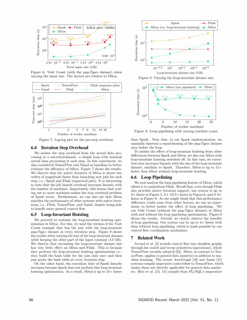
102

103

104

4.54 · 10−2 4.54 · 10−1 4.54 · 100 4.54 · 101

>100x

34.8x27.2x22.3x

4.2x

3.1x7.9x9x10.5x

Total input size (GB)

Executiontime(s)

Spark Flink

Mitoskilled after 16000s

9.08 · 101

Figure 6: Visit Count (with the pageTypes dataset) whenvarying the input size. The factors are relative to Mitos.

1 3 5 7 9 13 19 25

100

102

100

101

102

103


Tim

eper

step

(ms)

Spark TensorFlow Flink (separate jobs)

Naiad Flink Mitos

Figure 7: Log-log plot for the per-step overhead.

6.4 Iteration Step OverheadWe isolate the step overhead from the actual data pro-

cessing in a microbenchmark: a simple loop with minimalactual data processing in each step. In this experiment, wealso considered TensorFlow and Naiad as baselines to betterevaluate the efficiency of Mitos. Figure 7 shows the results.We observe that the native iteration of Mitos is about twoorders of magnitude faster than launching new jobs for eachstep, i.e., Spark and Flink (separated jobs). It is interestingto note that the job launch overhead increases linearly withthe number of machines. Importantly, this means that scal-ing out to more machines makes the step overhead problemof Spark worse. Furthermore, we can also see that Mitosmatches the performance of other systems with native itera-tions, i.e., Flink, TensorFlow, and Naiad, despite being ableto handle more general control flow.

6.5 Loop-Invariant HoistingWe proceed to evaluate the loop-invariant hoisting opti-

mization in Mitos. For this, we used the version of the VisitCount example that has the join with the loop-invariantpageTypes dataset at every iteration step. Figure 8 showsthe results when varying the size of the loop-invariant dataset,while keeping the other part of the input constant (13 GB).We observe that increasing the loop-invariant dataset sizehas very little effect on Mitos and Flink. This is becausethey perform the loop-invariant hoisting optimizations i.e.,they build the hash table for the join only once and thenjust probe the hash table at every iteration step.

On the other hand, the execution time of Spark linearlyincreases because Spark does not perform this loop-invarianthoisting optimization. As a result, Mitos is up to 45× faster

10−0.2 100 100.2 100.4 100.6

102

103

Loop-invariant dataset size (GB)

Executiontime(s)

Spark Flink

Mitos (wo. loop-invariant hoisting) Mitos

Figure 8: Varying the loop-invariant dataset size.

0 5 10 15 20 25

102

103

4.1x4.1x4.2x2.3x

1.1x


Executiontime(s)

Mitos (not pipelined) Mitos

Figure 9: Loop pipelining with varying machine count.

than Spark. Note that, in our Spark implementation, wemanually inserted a repartitioning of the pageTypes datasetonce before the loop.

To isolate the effect of loop-invariant hoisting from otherdifferences between Spark and Mitos, we also ran Mitos withloop-invariant hoisting switched off. In this case, its execu-tion time increases linearly with the size of the loop-invariantdataset, similarly to Spark. Therefore, Mitos is up to 11×faster than Mitos without loop-invariant hoisting.

6.6 Loop PipeliningWe now analyze the loop pipelining feature of Mitos, which

allows it to outperform Flink. Recall that, even though Flinkalso provides native iteration support, our system is up to3× faster in Figure 5, 3.1–10.5× faster in Figure 6, and 5–6×faster in Figure 8. As one might think that this performancedifference could come from other factors, we ran an exper-iment to better isolate the effect of loop pipelining. Weran Visit Count (without the pageTypes dataset) in Mitoswith and without the loop pipelining optimization. Figure 9shows the results. Overall, we clearly observe the benefitsof loop pipelining: Our system can be up to 4× faster withthan without loop pipelining, which is made possible by ourcontrol flow coordination mechanism.

7 Related WorkArvind et al. [3] include control flow into dataflow graphs

through the switch and merge primitives (operations), whichTensorFlow recently adopted [22]. Mitos, in contrast to Ten-sorFlow, applies to general data analytics in addition to ma-chine learning. The recent AutoGraph [16] and Janus [15]systems compile imperative control flow to TensorFlow, whichmakes them not directly applicable for general data analyt-ics. Hirn et al. [13, 14] compile from PL/SQL’s imperative


control flow to recursive SQL queries. Gevay et al. [12] sur-vey the literature on how various distributed dataflow sys-tems handle control flow. Matryoshka [11] adds control flowsupport to the flattening technique for nested parallelism.

Several systems natively support a limited number of con-trol flow constructs, such as Flink [10], and Naiad [17]. How-ever, they rely on functional-style APIs, where each con-trol flow construct is a higher-order function. For exam-ple, in TensorFlow, users call the while loop method andprovide two functions: one for building the dataflow of theloop body and another for building the dataflow of the loopexit condition. Similarly, in Flink, users call the iteratemethod and supply the loop body as a function that buildsthe dataflow job fragment representing the loop body. Asimple search for these Flink and TensorFlow methods onstackoverflow. com shows many users being confused bythis API. Mitos allows users to write imperative control flowstatements, such as regular while-loops and if statements,which makes it more accessible.

Other works have added iteration to systems that do notsupport control flow natively. HaLoop [6] and Twister [9] ex-tend MapReduce to provide support for iterations. Nonethe-less, in contrast to Mitos, the programming model of thesesystems is directly based on MapReduce rather than build-ing complex programs using a collection-based API.

Although loop-invariant hoisting is a well-known optimiza-tion in the context of distributed data analytics [10, 17, 6,9], none of these works supports programs with imperativecontrol flow constructs. SystemDS [5] does, but it cannotperform it on a binary operator having only one static in-put, e.g., the hash join that we used in Sec. 5.3.

8 ConclusionModern data analysis requires complex control flow con-

structs, yet dataflow systems either suffer from poor perfor-mance for programs with control flow or are hard to use.We presented Mitos, a system that allows users to expresscontrol flow by easy-to-use imperative constructs, and stillexecutes these programs efficiently as a single dataflow job.Mitos uses an intermediate representation based on SSA,which abstracts away from specific control flow constructs.Relying on SSA allows us to handle all imperative controlflow in a uniform way, both when building a dataflow job,and when coordinating the distributed execution of controlflow statements. Our coordination mechanism enables looppipelining and loop-invariant hoisting.

AcknowledgmentsWe thank Alexander Alexandrov for pointing our attention to

SSA, and Eleni Tzirita Zacharatou for the system name. This

work was funded by the German Ministry for Education and Re-

search as BIFOLD – Berlin Institute for the Foundations of Learn-

ing and Data (ref. 01IS18025A and ref. 01IS18037A), and German

Research Foundation – Project-ID 414984028 – SFB 1404.

9 References[1] A. Alexandrov, G. Krastev, and V. Markl. Representations

and optimizations for embedded parallel dataflowlanguages. TODS, 44(1):4, 2019.

[2] A. Alexandrov, A. Kunft, A. Katsifodimos, F. Schuler,L. Thamsen, O. Kao, T. Herb, and V. Markl. Implicitparallelism through deep language embedding. InSIGMOD. ACM, 2015.

[3] Arvind and D. E. Culler. Dataflow architectures. Annualreview of computer science, 1(1), 1986.

[4] J. Bezanson, A. Edelman, S. Karpinski, and V. B. Shah.Julia: A fresh approach to numerical computing. SIAMreview, 59(1):65–98, 2017.

[5] M. Boehm, I. Antonov, S. Baunsgaard, M. Dokter,R. Ginthor, K. Innerebner, F. Klezin, S. Lindstaedt,A. Phani, B. Rath, B. Reinwald, S. Siddiqi, and S. B.Wrede. SystemDS: A declarative machine learning systemfor the end-to-end data science lifecycle. In CIDR, 2020.

[6] Y. Bu, B. Howe, M. Balazinska, and M. D. Ernst. HaLoop:efficient iterative data processing on large clusters. VLDB,2010.

[7] E. Burmako. Scala macros: let our powers combine!: onhow rich syntax and static types work withmetaprogramming. In Proceedings of the 4th Workshop onScala. ACM, 2013.

[8] P. Carbone, A. Katsifodimos, S. Ewen, V. Markl, S. Haridi,and K. Tzoumas. Apache Flink: Stream and batchprocessing in a single engine. Bulletin of the IEEEComputer Society Technical Committee on DataEngineering, 36(4), 2015.

[9] J. Ekanayake, H. Li, B. Zhang, T. Gunarathne, S.-H. Bae,J. Qiu, and G. Fox. Twister: a runtime for iterativeMapReduce. In 19th ACM international symposium onhigh performance distributed computing. ACM, 2010.

[10] S. Ewen, K. Tzoumas, M. Kaufmann, and V. Markl.Spinning fast iterative data flows. Proceedings of the VLDBEndowment, 5, 2012.

[11] G. E. Gevay, J.-A. Quiane-Ruiz, and V. Markl. The powerof nested parallelism in big data processing–hitting threeflies with one slap–. In SIGMOD, pages 605–618, 2021.

[12] G. E. Gevay, J. Soto, and V. Markl. Handling iterations indistributed dataflow systems. ACM Computing Surveys(CSUR), 54(9):1–38, 2021.

[13] D. Hirn and T. Grust. PL/SQL without the PL. InSIGMOD, pages 2677–2680, 2020.

[14] D. Hirn and T. Grust. One with recursive is worth manyGOTOs. In SIGMOD, pages 723–735, 2021.

[15] E. Jeong, S. Cho, G.-I. Yu, J. S. Jeong, D.-J. Shin, andB.-G. Chun. JANUS: Fast and flexible deep learning viasymbolic graph execution of imperative programs. In NSDI.USENIX Association, 2019.

[16] D. Moldovan, J. Decker, F. Wang, A. Johnson, B. Lee,Z. Nado, D. Sculley, T. Rompf, and A. B. Wiltschko.AutoGraph: Imperative-style coding with graph-basedperformance. In SysML, 2019.

[17] D. G. Murray, F. McSherry, R. Isaacs, M. Isard,P. Barham, and M. Abadi. Naiad: a timely dataflowsystem. In SOSP. ACM, 2013.

[18] S. M. Orzan. On distributed verification and verifieddistribution. PhD thesis, Vrije Universiteit Amsterdam,2004.

[19] F. Rastello. SSA-based Compiler Design. Springer, 2016.

[20] C. J. Rossbach, Y. Yu, J. Currey, J.-P. Martin, andD. Fetterly. Dandelion: a compiler and runtime forheterogeneous systems. In SOSP, pages 49–68, 2013.

[21] J. Traub, Z. Kaoudi, J.-A. Quiane-Ruiz, and V. Markl.Agora: Bringing together datasets, algorithms, models andmore in a unified ecosystem [vision]. SIGMOD Record,49(4):6–11, 2020.

[22] Y. Yu, M. Abadi, P. Barham, E. Brevdo, M. Burrows,A. Davis, J. Dean, S. Ghemawat, T. Harley, P. Hawkins,et al. Dynamic control flow in large-scale machine learning.In EuroSys, page 18. ACM, 2018.

[23] M. Zaharia, M. Chowdhury, M. J. Franklin, S. Shenker, andI. Stoica. Spark: cluster computing with working sets.HotCloud, 10, 2010.


Technical Perspective: Relative Error Streaming Quantiles

Rasmus PaghBARC

University of Copenhagen, [email protected]

The paper Relative Error Streaming Quantiles, by Gra-ham Cormode, Zohar Karnin, Edo Liberty, Justin Thalerand Pavel Vesely studies a fundamental question in datastream processing, namely how to maintain informationabout the distribution of data in the form of quantiles. Moreprecisely, given a stream S of elements from some ordereduniverse U we wish to maintain a compact summary datastructure that allows us to estimate the number of elementsin the stream that are smaller than a given query elementy ∈ U , i.e., estimate the rank of y. Solutions to this problemhave numerous applications in large-scale data analysis andcan potentially be used for range query selectivity estima-tion in database engines.

The challenge is to make the size s of the summary datastructure (also known as a sketch) as small as possible whilebounding the error on rank queries. If data is available insorted order and has a known size n, an optimal solutionis to store s quantiles, that is, elements in S with specificranks. If S contains n elements we can store the elementsin S that have rank n/(s + 1), 2n/(s + 1), . . . , sn/(s + 1),which would allow us to approximate the rank of any queryelement y ∈ U up to an additive error of n/(s + 1). (Herewe ignore rounding issues for simplicity.) In other words, toachieve additive error εn it suffices to use space 1/ε.

Surprisingly, it is possible to achieve almost the samespace efficiency in the setting where elements are presentedin arbitrary order, and no bound on n is known. This wasestablished in a series of papers culminating in the work ofKarnin, Lang, and Liberty [4]. The simplest version of theirdata structure, now often referred to as the “KLL sketch”has become widely used in data processing pipelines. Thepopularity may be partly due to another property of theKLL sketch: Sketches for datasets S1 and S2 can be com-bined to form a sketch for the multiset union of the datasets. This property, referred to as mergeability means thatcomputation of KLL sketches can be efficiently carried out inparallel and distributed settings with little communication.

In Relative Error Streaming Quantiles, which appearedin PODS ’21 [2], the authors consider the situation wheremore precise information about the tails of the distribution(i.e., the largest and smallest elements) must be maintained.This setting is important because many data distributions


have few elements in the tails, and thus the KLL sketch mayhave little or no information about the distribution of thedata in the tails. A natural way of asking for more preciseinformation on elements on the lower tail is to ask for a rankerror guarantee that is multiplicative, i.e., a rank estimatethat is within some factor 1 + ε from the true rank. Incontrast, the KLL sketch offers an additive error guarantee,which is much weaker for elements with rank n. Whena multiplicative rank guarantee is possible, by symmetry,improved guarantees can also be achieved for query elementswith rank close to n.

Though multiplicative error is a desirable property, pastsolutions were significantly less efficient than the KLLsketch. A gap in performance is unavoidable for a broadclass of algorithms, as shown in a lower bound of Cormodeand Vesely [3]. Still, past solutions required larger overheadsin the dependence on the stream length n or the approxima-tion parameter ε. To improve on this, the authors go backto the KLL sketch and describe a simple but clever modifi-cation that improves past results and in fact nearly matchesthe lower bound. Though the algorithm, called ReqSketch, isrelatively simple, analyzing it is not and requires ideas thatgo significantly beyond those needed for the KLL sketch.

The new, mergeable sketch, is not only a great theoret-ical contribution — it is already available along with theKLL sketch as part of the Apache Datasketches library ofstreaming algorithms [1] and is ready to impact computingpractice!

1. REFERENCES[1] Apache datasketches.

https://datasketches.apache.org/. Accessed:2022-03-10.

[2] G. Cormode, Z. S. Karnin, E. Liberty, J. Thaler, andP. Vesely. Relative error streaming quantiles. InProceedings of the Symposium on Principles ofDatabase Systems (PODS), pages 96–108. ACM, 2021.

[3] G. Cormode and P. Vesely. A tight lower bound forcomparison-based quantile summaries. In Proceedingsof Symposium on Principles of Database Systems(PODS), pages 81–93. ACM, 2020.

[4] Z. S. Karnin, K. J. Lang, and E. Liberty. Optimalquantile approximation in streams. In Proceedings ofSymposium on Foundations of Computer Science(FOCS), pages 71–78. IEEE Computer Society, 2016.


Relative Error Streaming Quantiles

[Extended Abstract]

Graham CormodeUniversity of Warwick

Coventry, [email protected]

Zohar KarninAmazon, USA

[email protected]

Edo LibertyPinecone

San Mateo, CA, [email protected]

Justin ThalerGeorgetown UniversityWashington, D.C., USA

[email protected]

Pavel VeselýCharles University

Prague, Czech [email protected]

ABSTRACTEstimating ranks, quantiles, and distributions over stream-ing data is a central task in data analysis and monitoring.Given a stream of n items from a data universe equippedwith a total order, the task is to compute a sketch (datastructure) of size polylogarithmic in n. Given the sketch anda query item y, one should be able to approximate its rankin the stream, i.e., the number of stream elements smallerthan or equal to y.

Most works to date focused on additive εn error approx-imation, culminating in the KLL sketch that achieved op-timal asymptotic behavior. This paper investigates multi-plicative (1± ε)-error approximations to the rank. Practicalmotivation for multiplicative error stems from demands tounderstand the tails of distributions, and hence for sketchesto be more accurate near extreme values.

The most space-efficient algorithms due to prior work storeeither O(log(ε2n)/ε2) or O(log3(εn)/ε) universe items. Wepresent a randomized sketch storing O(log1.5(εn)/ε) items,

which is within an O(√

log(εn)) factor of optimal. Our algo-rithm does not require prior knowledge of the stream lengthand is fully mergeable, rendering it suitable for parallel anddistributed computing environments.

1. INTRODUCTIONUnderstanding the distribution of data is a fundamental

task in data monitoring and analysis. In many settings,we want to understand the cumulative distribution function(CDF) of a large number of observations, for instance, toidentify anomalies. In other words, we would like to trackthe median, percentiles, and more generally quantiles of amassive input in a small space, without storing all the ob-servations. Although memory constraints make an exact

This is a minor revision of the paper entitled RelativeError Streaming Quantiles, published in PODS ’21, ISBN978-1-4503-8381-3/21/06, June 20–25, 2021, Virtual Event,China. DOI: https://dl.acm.org/doi/10.1145/3452021.3458323.


computation of such order statistics impossible [22], mostapplications can be satisfied with approximating the quan-tiles, which also yields a compact function with a boundeddistance from the true CDF.

The problem of streaming quantile approximation cap-tures this task in the context of massive or distributed data-sets. Let σ = (x1, . . . , xn) be a stream of items, all drawnfrom a data universe U equipped with a total order. Forany y ∈ U , let R(y;σ) =

∣∣i ∈ 1, . . . , n | xi ≤ y∣∣ be the

rank of y in the stream. When σ is clear from context, wewrite R(y). The objective is to process the stream in onepass while storing a small number of items, and then usethose to approximate R(y) for any y ∈ U . A guarantee for

an approximation R(y) is additive if |R(y) − R(y)| ≤ εn,

and multiplicative or relative if |R(y)− R(y)| ≤ εR(y). Es-timating ranks immediately yields approximate quantiles,and vice versa, with a similar error guarantee (recall thata φ-quantile for φ ∈ [0, 1] is the bφnc’th smallest item inσ). We stress that we do not assume any particular datadistribution or that the stream is randomly-ordered.

A long line of work has focused on achieving additive errorguarantees [23, 2, 19, 24, 13, 3, 12, 1, 11, 16]. However, addi-tive error is not appropriate for many applications. Indeed,often the primary purpose of computing quantiles is to un-derstand the tails of the data distribution. When R(y) n,a multiplicative guarantee is much more accurate and thusharder to obtain. As pointed out by Cormode et al. [5], a so-lution to this problem would also yield high accuracy whenn − R(y) n, by running the same algorithm with thereversed total ordering (simply negating the comparator).

A quintessential application that demands relative error ismonitoring network latencies. In practice, one often tracksresponse time percentiles 50, 90, 99, 99.9, etc. This is be-cause latencies are heavily long-tailed. For example, Mas-son et al. [21] report that for web response times, the 98.5thpercentile can be as small as 2 seconds while the 99.5th per-centile can be as large as 20 seconds. These unusually longresponse times affect network dynamics [5] and are problem-atic for users. Furthermore, as argued by Tene in his talkabout measuring latency [27], one needs to look at extremepercentiles such as 99.995 to determine the latency such thatonly about 1% of users experience a larger latency during aweb session with several page loads. Hence, highly accuraterank approximations are required for items y whose rank is


very large (n−R(y) n); this is precisely the requirementcaptured by the multiplicative error guarantee.

Achieving multiplicative guarantees is known to be strictlyharder than additive ones. There are comparison-based ad-ditive error algorithms that store just Θ(ε−1) items for con-stant failure probability [16], which is optimal. In particular,to achieve additive error, the number of items stored maybe independent of the stream length n. In contrast, anyalgorithm achieving multiplicative error must store Ω(ε−1 ·log(εn)) items (see [5, Theorem 2]).

Remark 1. Intuitively, the reason additive-error sketchescan achieve space independent of the stream length is becausethey can take a subsample of the stream of size about Θ(ε−2)and then sketch the subsample. For any fixed item, the ad-ditive error to its rank introduced by sampling is at most εnwith high probability. When multiplicative error is required,one cannot subsample the input: for low-ranked items, themultiplicative error introduced by sampling will, with highprobability, not be bounded by any constant.

The best known algorithms achieving multiplicative errorguarantees are as follows. Zhang et al. [29] give a ran-domized algorithm storing O(ε−2 · log(ε2n)) universe items.This is essentially a ε−1 factor away from the aforemen-tioned lower bound. There is also an algorithm of Cormodeet al. [6] that stores O(ε−1 · log(εn) · log |U|) items. However,this algorithm requires prior knowledge of the data universeU (since it builds a binary tree over U), and is inapplica-ble when U is huge or even unbounded (e.g., if the data cantake arbitrary real values). Finally, Zhang and Wang [28] de-signed a deterministic algorithm requiring O(ε−1 · log3(εn))space. Recent work of Cormode and Vesely [8] proves anΩ(ε−1 · log2(εn)) lower bound for deterministic comparison-based algorithms, which is within a log(εn) factor of Zhangand Wang’s upper bound.

Despite both the practical and theoretical importance ofmultiplicative error (which is arguably an even more naturalgoal than additive error), there has been no progress onupper bounds, i.e., no new algorithms, since 2007.

In this work, we give a randomized algorithm that main-tains the optimal linear dependence on 1/ε achieved by Zhangand Wang, with a significantly improved dependence onthe stream length. Namely, we design a one-pass stream-ing algorithm that given ε > 0, computes a sketch consist-ing of O

(ε−1 · log1.5(εn)

)universe items, from which one

can derive rank or quantile estimates satisfying the relativeerror guarantee with constant probability (see Theorem 1for a more precise statement). Ours is the first algorithmto be strictly more space efficient than any deterministiccomparison-based algorithm (owing to the Ω(ε−1 log2(εn))

lower bound in [8]) and is within an O(√

log(εn)) factor ofthe known lower bound for randomized algorithms achiev-ing multiplicative error. Furthermore, it only accesses itemsthrough comparisons, i.e., is comparison-based, rendering itsuitable, e.g., for floating-point numbers or strings orderedlexicographically. Finally, our algorithm processes the inputstream efficiently, namely, its amortized update time is a log-arithm of the space bound, i.e., O

(log(ε−1) + log log(n)

).

Mergeability. The ability to merge sketches of different streamsto get an accurate sketch for the concatenation of the streamsis highly significant both in theory [1] and in practice [25].Such mergeable summaries enable trivial, automatic paral-lelization and distribution of processing massive data sets,

by splitting the data up into pieces, summarizing each pieceseparately, and then merging the results in an arbitrary way.We say that a sketch is fully mergeable if building it usingany sequence of merge operations (executed on singletonitems) leads to the same guarantees as if the entire dataset had been processed as a single stream.

The following theorem is the main result of this paper.We stress that our algorithm, which we call ReqSketch, doesnot require any advance knowledge about n, the total sizeof the input, which indeed may not be available in manyapplications.

Theorem 1. Given parameters 0 < δ ≤ 0.5 and 0 < ε ≤1, there is a randomized, comparison-based, one-pass stream-ing algorithm that, when processing a data stream consist-ing of n items from a totally-ordered universe U , produces asummary S satisfying the following property. Given S, forany y ∈ U one can get an estimate R(y) of R(y) such that

Pr

[|R(y)− R(y)| ≥ εR(y)

]< δ ,

where the probability is over the internal randomness of the

streaming algorithm. If ε ≤√

ln 1δ/ log2(εn), then the size

of S in memory words is

O

(ε−1 · log1.5(εn) ·

√log

(1

δ

));

otherwise, storing S takes O(log2(εn)

)memory words. More-

over, the summary produced is fully mergeable.

The space bound for the case ε ≤√

ln 1δ/ log2(εn) cer-

tainly applies for values of ε and n encountered in practice(e.g., for n ≤ 264 and δ ≤ 1/e, this latter requirement is im-plied by ε ≤ 1/8). A straightforward corollary of Theorem 1is a space-efficient algorithm whose estimates are simultane-ously accurate for all y ∈ U with high probability, while thespace complexity increases by a small factor only. This fol-lows from a standard use of the union bound with an epsilon-net argument (using failure probability δ′ = εδ/ log(εn)).

There is also an alternative analysis of our algorithm (build-ing on an idea from [16]), that shows a space bound ofO(ε−1 · log2(εn) · log log(1/δ)

); note the exponentially bet-

ter dependence on 1/δ, compared to Theorem 1, which,however, comes at the expense of the exponent of log(εn)increasing from 1.5 to 2. This analysis also implies a de-terministic space bound of O(ε−1 · log3(εn)), matching thestate-of-the-art result in [28].

A proof-of-concept Python implementation of ReqSketchis available at GitHub [17] and a production-quality imple-mentation is available in the DataSketches library [25].

1.1 Technical OverviewA starting point of the design of our algorithm is the KLL

sketch [16] that achieves optimal accuracy-space trade-offfor the additive error guarantee. The basic building block ofthe algorithm is a buffer, called a compactor, that receivesan input stream of n items and outputs a stream of at mostn/2 items, meant to “approximate” the input stream. Thebuffer simply stores items and once it is full, we sort thebuffer, output all items stored at either odd or even indexes(with odd vs. even selected via an unbiased coin flip), and


clear the contents of the buffer—this is called the compactionoperation. Note that a randomly chosen half of items in thebuffer is simply discarded, whereas the other half of itemsin the buffer is “output” by the compaction operation.

The overall KLL sketch is built as a sequence of at mostlog2(n) such compactors, such that the output stream of acompactor is treated as the input stream of the next com-pactor. We thus think of the compactors as arranged intolevels, with the first one at level 0. Similar compactors werealready used, e.g., in [19, 20, 1, 18], and additional ideas areneeded to get the optimal space bound for additive error, ofO(1/ε) items stored across all compactors [16].

The compactor building block is not directly applicableto our setting for the following reasons. A first observationis that to achieve the relative error guarantee, we need toalways store the 1/ε smallest items. This is because therelative error guarantee demands that estimated ranks forthe 1/ε lowest-ranked items in the data stream are exact. Ifeven a single one of these items is deleted from the summary,then these estimates will not be exact. Similarly, among thenext 2/ε smallest items, the summary must store essentiallyevery other item to achieve multiplicative error. Among thenext 4/ε smallest items in the order, the sketch must storeroughly every fourth item, and so on.

The following simple modification of the compactor fromthe KLL sketch indeed achieves the above. Each buffer ofsize B “protects”the B/2 smallest items stored inside, mean-ing that these items are not involved in any compaction(i.e., the compaction operation only removes the B/2 largestitems from the buffer). Unfortunately, it turns out thatthis simple approach requires space Θ(ε−2 · log(ε2n)), whichmerely matches the space bound achieved in [29], and inparticular has a suboptimal dependence on 1/ε.

The key technical contribution of our work is to enhancethis simple approach with a more sophisticated rule for se-lecting the number of protected items in each compaction. Inthis abstract, we describe a solution choosing this number ineach compaction at random from an appropriate geometricdistribution. In the full version [4], to get a cleaner analysis,we derandomize this distribution.

While the resulting algorithm is relatively simple, ana-lyzing the error behavior brings new challenges that do notarise in the additive error setting. Roughly speaking, whenanalyzing the accuracy of the estimate for R(y) for any fixeditem y, all error can be “attributed” to compaction opera-tions. In the additive error setting, one may suppose thatevery compaction operation contributes to the error and stillobtain a tight error analysis [16]. Unfortunately, this is notat all the case for relative error: as already indicated, toobtain our accuracy bounds it is essential to show that theestimate for any low-ranked item y is affected by very fewcompaction operations. Thus, the first step of our analysisis to carefully bound the number of compactions on eachlevel that affect the error for y, using the definition of thegeometric distribution in the compaction operation.

Organization of the abstract. We describe our sketch in Sec-tion 2; as mentioned above, the algorithm outlined in thisabstract is slightly different to the one in the full version [4].In Section 3, we sketch an analysis of this algorithm in thestreaming setting, assuming a foreknowledge of (a polyno-mial upper bound on) the stream length. Finally, in Sec-tion 4 we briefly outline how to analyze the algorithm undermerge operations and without any advance knowledge about

the stream length as well as adjustments from [7] to makeit more efficient in practice. The details can be found in thefull version [4].

1.2 Detailed Comparison to Prior WorkSome prior works on streaming quantiles consider queries

to be ranks r ∈ 1, . . . , n, and the algorithm must identifyan item y ∈ U such that R(y) is close to r; this is called thequantile query. In this work, we focus on the dual problem ofrank queries, where we consider queries to be universe itemsy ∈ U and the algorithm must yield an accurate estimatefor R(y). Unless specified otherwise, algorithms describedin this section directly solve both formulations (this holdsfor our algorithm as well). Algorithms are randomized un-less stated otherwise. For simplicity, randomized algorithmsare assumed to have constant failure probability δ. All re-ported space costs refer to the number of universe itemsstored. (Apart from storing universe items, the algorithmsmay store, for example, bounds on ranks of stored items orsome counters, but the number of such variables is propor-tional to the number of items stored or even smaller. Thus,the space bounds are in memory words, which can store anyitem or an integer with O(log(n+ |U|)) bits.)

Additive error. Manku, Rajagopalan, and Lindsay [19, 20]built on the work of Munro and Paterson [22] and gave a de-terministic solution storing at most O(ε−1 · log2(εn)) items,assuming prior knowledge of n. Greenwald and Khanna [13]created an intricate deterministic streaming algorithm thatstores O(ε−1 · log(εn)) items. This is the best known deter-ministic algorithm for this problem, with a matching lowerbound for comparison-based streaming algorithms [8]. Agar-wal et al. [1] provided a mergeable sketch of size O(ε−1 ·log1.5(1/ε)). This paper contains many ideas and observa-tions that were used in later work. Felber and Ostrovsky [11]managed to reduce the space complexity to O(ε−1 · log(1/ε))items by combining sampling with the Greenwald-Khannasketches in non-trivial ways. Finally, Karnin, Lang, and Lib-erty [16] resolved the problem by providing an O(1/ε)-spacesolution, which is optimal. For general (non-constant) fail-ure probabilities δ, the space upper bound becomes O(ε−1 ·log log(1/δ)), and they also prove a matching lower boundfor comparison-based randomized algorithms, assuming δ ≤1/n! (i.e., δ is exponentially small in n).

Multiplicative error. A large number of works sought toprovide more accurate quantile estimates for low or highranks. Only a handful offer solutions to the relative er-ror quantiles problem considered in this work (sometimesalso called the biased quantiles problem). Gupta and Zane[14] gave an algorithm for relative error quantiles that storesO(ε−3·log2(εn)) items, and used this to approximately countthe number of inversions in a list; their algorithm requiresprior knowledge of the stream length n. As previously men-tioned, Zhang et al. [29] presented an algorithm storingO(ε−2 ·log(ε2n)) universe items. Cormode et al. [6] designeda deterministic sketch storing O(ε−1 · log(εn) · log |U|) items,which requires prior knowledge of the data universe U . Theiralgorithm is inspired by the work of Shrivastava et al. [26]in the additive error setting and it is also mergeable (see[1, Section 3]). Zhang and Wang [28] gave a deterministicmerge-and-prune algorithm storing O(ε−1 · log3(εn)) items,which can handle arbitrary merges with an upper bound onn, and streaming updates for unknown n. However, it doesnot tackle the most general case of merging without a prior


bound on n. Cormode and Vesely [8] recently showed a spacelower bound of Ω(ε−1 · log2(εn)) items for any deterministiccomparison-based algorithm.

Other related works that do not fully solve the relative er-ror quantiles problem are as follows. Manku, Rajagopalan,and Lindsay [20] designed an algorithm that, for a speci-fied number φ ∈ [0, 1], stores O(ε−1 · log(1/δ)) items andcan return an item y with R(y)/n ∈ [(1 − ε)φ, (1 + ε)φ](their algorithm requires prior knowledge of n). Cormodeet al. [5] gave a deterministic algorithm that is meant toachieve error properties “in between” additive and relativeerror guarantees. That is, their algorithm aims to providemultiplicative guarantees only up to some minimum rank k;for items of rank below k, their solution only provides addi-tive guarantees. Their algorithm does not solve the relativeerror quantiles problem: [29] observed that for adversarialitem ordering, the algorithm of [5] requires linear space toachieve relative error for all ranks.

Dunning and Ertl [10, 9] describe a heuristic algorithmcalled t-digest that is intended to achieve relative error, butthey provide no formal accuracy analysis. Indeed, Cormodeet al. [7] show that the error of t-digest may be arbitrarilylarge on adversarially generated inputs. This latter paperalso compares t-digest and ReqSketch (i.e., the algorithmof Theorem 1) on randomly generated inputs and proposesimplementation improvements for ReqSketch that make itprocess an input stream faster than t-digest; see Section 4.

Most recently, Masson, Rim, and Lee [21] introduced anew notion of error for quantile sketches (they also referto their notion as “relative error”, but it is quite distinctfrom the notion considered in this work). They require thatfor a query percentile φ ∈ [0, 1], if y denotes the item inthe data stream satisfying R(y) = φn, then the algorithmshould return an item y ∈ U such that |y− y| ≤ ε · |y|. Thisdefinition only makes sense for data universes with a notionof magnitude and distance (e.g., numerical data), and thedefinition is not invariant to natural data transformations,such as incrementing every data item y by a large constant.It is also trivially achieved by maintaining a (mergeable)histogram with buckets ((1 + ε)i, (1 + ε)i+1]. In contrast,the standard notion of relative error considered in this workdoes not refer to the data items themselves, only to theirranks, and is arguably of more general applicability.

2. DESCRIPTION OF THE ALGORITHM

2.1 The Relative-Compactor ObjectThe crux of our algorithm is a building block that we call

the relative-compactor. Roughly speaking, this object pro-cesses a stream of n items and outputs a stream of at mostn/2 items (each “up-weighted” by a factor of 2), meant to“approximate” the input stream. It does so by maintaininga buffer of limited capacity.

Our complete sketch, described in Section 2.2 below, iscomposed of a sequence of relative-compactors, where theinput of the (h + 1)’th relative-compactor is the output ofthe h’th. With at most log2(εn) such relative-compactors,n being the length of the input stream, the output of thelast relative-compactor is of size O(1/ε), and hence can bestored in memory.

Compaction operations. The basic subroutine used by ourrelative-compactor is a compaction operation. The inputto a compaction operation is a list X of 2m items x1 ≤

L largest items sortedB − L smallest items in the buffer

Output every other item and discard the rest

Insert new item xt in the next open slot

xt

Figure 1: Illustration of the execution of a relative-compactorwhen inserting a new item xt into a buffer that is full at timet. See lines 5-13 of Algorithm 1.

x2 ≤ . . . ≤ x2m, and the output is a sequence Z of m items.This output is chosen to be one of the following two se-quences, uniformly at random: Either Z = x2i−1mi=1 orZ = x2imi=1. That is, the output sequence Z equals eitherthe even or odd indexed items in the sorted order of X, withboth outcomes equally probable.

Consider an item y ∈ U and recall that R(y;X) = |x ∈X |x ≤ y| is the number of items x ∈ X satisfying x ≤ y(we remark that both X and x ∈ X |x ≤ y are multisetsof universe items). The following is a trivial observationregarding the error of the rank estimate of y with respectto the input X of a compaction operation when using Z.We view the output Z of a compaction operation (with allitems up-weighted by a factor of 2) as an approximationto the input X; for any y, its weighted rank in Z should beclose to its rank in X. Observation 2.1 below states that thisapproximation incurs zero error on items that have an evenrank in X. Moreover, for items y that have an odd rankin X, the error for y ∈ U introduced by the compactionoperation is +1 or −1 with equal probability.

Observation 2.1. A universe item y ∈ U is said to beeven (odd) w.r.t a compaction operation if R(y;X) is even(odd), where X is the input sequence to the operation. If yis even w.r.t the compaction, then R(y;X)− 2 R(y;Z) = 0.Otherwise, R(y;X) − 2 R(y;Z) is a variable taking a valuefrom −1, 1 uniformly at random.

The observation that items of even rank (and in particularitems of rank zero) suffer no error from a compaction opera-tion plays an especially important role in the error analysisof our full sketch.

Full description of the relative-compactor. The complete de-scription of the relative-compactor object is given in Algo-rithm 1. The high-level idea is as follows. The relative-compactor maintains a buffer of size B = 2 · k · dlog2(n/k)ewhere k is an even integer parameter controlling the errorand n is the upper bound on the stream length. (In thisabstract, we assume that such an upper bound is available;we discuss removing this assumption in Section 4.) The in-coming items are stored in the buffer until it is full, and thenwe perform a compaction operation, as described above.

The input to the compaction operation is not all items inthe buffer, but rather the largest L items in the buffer fora parameter L ≤ B/2 such that L is even. These L largestitems are then removed from the buffer, and the output ofthe compaction operation is sent to the output stream ofthe buffer. This intuitively lets low-ranked items stay inthe buffer longer than high-ranked ones. Indeed, the lowest-


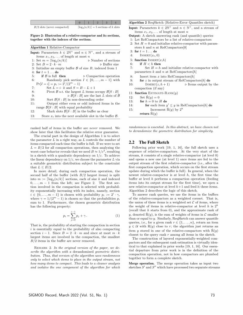
B/2 slots (never compacted) dlog2(n/k)e = 5 sections of k slots

43210

Figure 2: Illustration of a relative-compactor and its sections,together with the indexes of the sections.

Algorithm 1 Relative-Compactor

Input: Parameters k ∈ 2N+ and n ∈ N+, and a stream ofitems x1, x2, . . . of length at most n

1: Set m = dlog2(n/k)e . Number of sections2: Set B = 2 · k ·m . Buffer size3: Initialize an empty buffer B of size B, indexed from 14: for t = 1 . . . do5: if B is full then . Compaction operation6: Randomly pick section I ∈ 0, . . . ,m − 1 with

Pr[I = i] = pi := 2i/(2m − 1)7: Set L = i · k and S = B − L+ 18: Pivot B s.t. the largest L items occupy B[S : B]9: . B[S : B] are the last L slots of B

10: Sort B[S : B] in non-descending order11: Output either even or odd indexed items in the

range B[S : B] with equal probability12: Mark slots B[S : B] in the buffer as clear

13: Store xt into the next available slot in the buffer B.

ranked half of items in the buffer are never removed. Weshow later that this facilitates the relative error guarantee.

The crucial part in the design of Algorithm 1 is to selectthe parameter L in a right way, as L controls the number ofitems compacted each time the buffer is full. If we were to setL = B/2 for all compaction operations, then analyzing theworst-case behavior reveals that we need B ≈ 1/ε2, resultingin a sketch with a quadratic dependency on 1/ε. To achievethe linear dependency on 1/ε, we choose the parameter L viaa suitable geometric distribution subject to the constraintthat L ≤ B/2.

In more detail, during each compaction operation, thesecond half of the buffer (with B/2 largest items) is splitinto m := dlog2(n/k)e sections, each of size k and indexed0, . . . ,m − 1 from the left; see Figure 2. The first sec-tion involved in the compaction is selected with probabil-ity exponentially increasing with its index, namely, sectioni ∈ 0, . . . ,m − 1 is chosen with probability pi := 2i · γ,where γ = 1/(2m − 1) is chosen so that the probabilities pisum to 1. Furthermore, the chosen geometric distributionhas the following property:

pi =

i−1∑

j=0

pj + γ . (1)

That is, the probability of starting the compaction in sectioni is essentially equal to the probability of also compactingsection i − 1. Since B = 2 · k ·m and since at most m · klargest items are involved in the compaction, the smallestB/2 items in the buffer are never removed.

Remark 2. In the original version of the paper, we de-scribe the algorithm with a derandomized geometric distri-bution. Thus, that version of the algorithm uses randomnessonly to select which items to place in the output stream, nothow many items to compact. This leads to a cleaner analysisand isolates the one component of the algorithm for which

Algorithm 2 ReqSketch (Relative-Error Quantiles sketch)

Input: Parameters k ∈ 2N+ and n ∈ N+, and a stream ofitems x1, x2, . . . of length at most n

Output: A sketch answering rank (and quantile) queries1: Let RelCompactors be a list of relative-compactors2: Set H = 0 and initialize relative-compactor with param-

eters k and n at RelCompactors[0]3: for t = 1 . . . do4: Insert(xt, 0)

5: function Insert(x,h)6: if H < h then7: Set H = h and initialize relative-compactor with

parameters k and n at RelCompactors[h]

8: Insert item x into RelCompactors[h]9: for z in output stream of RelCompactors[h] do

10: Insert(z, h+ 1) . Items output by thecompaction (if any)

11: function Estimate-Rank(y)

12: Set R(y) = 013: for h = 0 to H do14: for each item y′ ≤ y in RelCompactors[h] do

15: Increment R(y) by 2h

return R(y)

randomness is essential. In this abstract, we have chosen notto derandomize the geometric distribution for simplicity.

2.2 The Full SketchFollowing prior work [19, 1, 16], the full sketch uses a

sequence of relative-compactors. At the very start of thestream, it consists of a single relative-compactor (at level 0)and opens a new one (at level 1) once items are fed to theoutput stream of the first relative-compactor (i.e., after thefirst compaction operation, which occurs on the first streamupdate during which the buffer is full). In general, when thenewest relative-compactor is at level h, the first time thebuffer at level h performs a compaction operation (feedingitems into its output stream for the first time), we open anew relative-compactor at level h+1 and feed it these items.Algorithm 2 describes the logic of this sketch.

To answer rank queries, we use the items in the buffersof the relative-compactors as a weighted coreset. That is,the union of these items is a weighted set C of items, wherethe weight of items in relative-compactor at level h is 2h

(recall that h starts from 0), and the approximate rank of

y, denoted R(y), is the sum of weights of items in C smallerthan or equal to y. Similarly, ReqSketch can answer quantilequeries, i.e., for a given rank r ∈ 1, . . . , n, return an itemy ∈ U with R(y) close to r; the algorithm just returns an

item y stored in one of the relative-compactors with R(y)closest to the query rank r among all items in the sketch.

The construction of layered exponentially-weighted com-pactors and the subsequent rank estimation is virtually iden-tical to that explained in prior works [19, 1, 16]. Our essen-tial departure from prior work is in the definition of thecompaction operation, not in how compactors are plumbedtogether to form a complete sketch.

Merge operation. The merge operation takes as input twosketches S′ and S′′ which have processed two separate streams


σ′ and σ′′ and outputs a sketch S summarizing the concate-nated stream σ = σ′ σ′′ (the order of σ′ and σ′′ does notmatter here). For the simplified sketch presented in thisabstract, merging two sketches is straightforward: At eachlevel, concatenate the buffers and if that causes the capac-ity of the compactor to be reached or exceeded, perform thecompaction operation, as in Algorithm 1. There are addi-tional complications when an upper bound n on the com-bined input size is not available in advance; for instance,the number of sections m (and the section size k) may needto be adjusted during a merge operation. These details aredescribed in the full version [4].

3. ANALYSISWe provide a sketch of the analysis in the streaming set-

ting, assuming a foreknowledge of (an upper bound on) thestream length n. To analyze the error of the full sketch, wefocus on the error in the estimated rank of an arbitrary fixeditem y ∈ U . Let R(y) be the rank of item y in the input

stream, and let Err(y) = R(y) − R(y) be the error of theestimated rank for y.

Analysis of the relatively-compactor. We first restrict ourattention to any single relative-compactor at level h (Al-gorithm 1) maintained by our sketching algorithm (Algo-rithm 2), and we use “time t” to refer to the t’th insertionoperation to this particular relative-compactor. We analyzethe error introduced by the relative-compactor for item y.Specifically, at time t, let Xt = (x1, . . . , xt) be the prefix ofthe input stream to the relative-compactor, Zt be the out-put stream, and Bt be the items in the buffer after insertingitem xt. The rank error made by the relative-compactor attime t with respect to item y is defined as

Errth(y) = R(y;Xt)− 2 R(y;Zt)− R(y;Bt). (2)

Conceptually, Errth(y) tracks the difference between y’srank in the input stream Xt at time t versus its rank asestimated by the combination of the output stream and theremaining items in the buffer at time t (output items areupweighted by a factor of 2 while items remaining in thebuffer are not). We denote the overall error of the relative-compactor by Errh(y) and the total number of items x ≤ yinserted to the level-h buffer by Rh(y). Then Errh(y) =Rh(y)− 2 Rh+1(y)−R(y;Bh), where Bh is the level-h bufferafter Algorithm 2 has processed the input stream (note thatRh+1(y) is the number of items x ≤ y in the output stream ofthe level-h relative-compactor). To bound Errh(y), we keeptrack of the error associated with y over time, and definethe increment or decrement of it as

∆th(y) = Errth(y)− Errt−1

h (y),

where Err0h(y) = 0.Clearly, if the algorithm performs no compaction opera-

tion in a time step t, then ∆th(y) = 0. (Recall that a com-

paction is an execution of lines 6-12 of Algorithm 1.) Let usconsider what happens in a step t in which a compaction op-eration occurs. Observation 2.1 shows that if y is even withrespect to the compaction, then y suffers no error, meaningthat ∆t

h(y) = 0. Otherwise, ∆th(y) is uniform in −1, 1.

It follows that E[Errh(y)] = 0, which implies that the es-

timator R(y) is unbiased. To bound the variance of Errh(y),we analyze Var[∆t

h(y)] for any step t with a compaction op-eration. We suppose that R(y;Bt) > B/2 as otherwise, no

item x ≤ y is removed from the buffer and ∆th(y) = 0.

Below, we only focus on steps t with a compaction oper-ation such that R(y;Bt) > B/2. Let it ∈ 0, . . . ,m − 1be the largest index of a section of Bt with an item x ≤ y,i.e., it is the smallest integer i ≥ 0 such that R(y;Bt) ≤B/2 + (i + 1) · k. Note that if Algorithm 1 draws I < itin line 6 during the compaction in step t, at least k itemsx ≤ y are removed from the buffer, which implies that thenumber of steps t with I < it is at most Rh(y)/k. Usingthis observation, our aim is to bound Var[Errh(y)] in termsof Rh(y)/k.

The probability of ∆th(y) 6= 0 is at most the probability

of removing an item x ≤ y, which by the definition of it andAlgorithm 1 equals

it∑

j=0

pj =

it−1∑

j=0

pj + pit = 2

it−1∑

j=0

pj + γ , (3)

where we use (1); this is where we rely on using the geometricdistribution to choose the number of sections involved in thecompaction (recall that γ = 1/(2m − 1) is small). Using (3)and that ∆t

h(y) ∈ −1, 0, 1, we get that Var[∆th(y)] =

E[(∆th(y)

)2] = Pr[∆t

h(y) 6= 0] ≤ 2∑it−1i=0 pi + γ.

Since the variables ∆th(y) are independent,

Var[Errh(y)] =∑

t

Var[∆th(y)] =

∑

t

(2

it−1∑

i=0

pi + γ

).

As observed above, the number of steps t with I < it inline 6 is at most Rh(y)/k, which implies that

∑t

∑it−1i=0 pi ≤

Rh(y)/k (we omit a formal proof of this observation).As a compaction is performed at most once in every k

steps, we have that∑t γ ≤ γ · n/k ≤ n/(n − k) ≤ 2, using

the definition of γ = 1/(2m − 1) and m = dlog2(n/k)e; thelast step uses n ≥ 2k as otherwise the whole input to therelative-compactor would be stored in the buffer which hassize at least 2k and there would be no compaction operation.

Summarizing, we have obtained the following bound onthe variance of the error at level h:

Var[Errh(y)] ≤ 2 Rh(y)

k+ 2 ≤ 4 Rh(y)

k, (4)

where the second inequality uses Rh(y) ≥ k as otherwisethere would be no level-h compaction operation affectingthe error for y, i.e., Errh(y) = 0 if Rh(y) < k

Analysis of the full sketch in the streaming setting. To makethe variance bound for a single level in (4) useful, we showthat Rh(y) roughly halves with every level. This is easy tosee in expectation, and it holds with high probability up toa certain crucial level H(y). Here, we define H(y) to be theminimal h for which 2−h+1 R(y) ≤ B/2. For h = H(y) − 1

(assuming H(y) > 0), we particularly have 22−H(y) R(y) >

B/2, or equivalently, 2H(y) < 23 · R(y)/B.

Lemma 3.1. With probability at least 1 − δ it holds thatRh(y) ≤ 2−h+1 R(y) for any h ≤ H(y).

We omit the proof by induction, using Chernoff bounds(which also requires choosing k as described below). In whatfollows, we condition on the bound on Rh(y) in Lemma 3.1for any h ≤ H(y). For h = H(y), we thus have that

RH(y)(y) ≤ 2−H(y)+1 R(y) ≤ B/2 and that Rh(y) = 0for any h > H(y). Thus, Observation 2.1 implies thatErrh(y) = 0 for any h ≥ H(y).


We are now ready to bound the overall error of the sketchfor item y, i.e., Err(y) = R(y) − R(y) where R(y) is theestimated rank of y. By the observations above, we get

Err(y) =

H(y)−1∑

h=0

2h Errh(y) .

Recall that a zero-mean random variable X with varianceσ2 is sub-Gaussian if E[exp(sX)] ≤ exp(− 1

2· s2 · σ2) for any

s ∈ R; note that a weighted sum of independent zero-meansub-Gaussian variables is a zero-mean sub-Gaussian randomvariable as well. By the analysis of level h, Errh(y) is a zero-mean sub-Gaussian variable with Var[Errh(y)] ≤ 4 Rh(y)/k.It follows that Err(y) is a zero-mean sub-Gaussian randomvariable with variance

H(y)−1∑

h=0

22h Var[Errh(y)] ≤H(y)−1∑

h=0

22h · 4 Rh(y)

k

≤H(y)−1∑

h=0

2h+3 · R(y)

k

≤ 2H(y)+3 · R(y)

k≤ 26 · R(y)2

k ·B ,

where the second inequality is due to Lemma 3.1 and thelast inequality follows from the definition of H(y).

Given the desired accuracy ε and the desired upper boundδ on failure probability, we choose k so that Var[Err(y)] ≤ε2 R(y)2/ ln(1/δ), or equivalently that k · B = k · 2 · k ·dlog2(n/k)e ≥ Θ

(ε−2 · ln(1/δ)

); this holds for k satisfy-

ing k = Θ(ε−1 ·

√ln 1

δ/ log2 (n/k)

). Then using standard

(Chernoff) tail bounds for sub-Gaussian variables concludesthe calculation of the failure probability.

Finally, for the space bound, by the choice of k above we

have that B = O(ε−1 ·

√log(εn) · log (1/δ)

), and it thus

remains to observe that the number of relative-compactorsever created by Algorithm 2 is at most O(log(εn)). Indeed,each item on level h has weight 2h, so there are at mostn/2h items inserted to the buffer at that level. For h =dlog2(n/B)e, we get that on this level, there are fewer thanBitems inserted to the buffer, which is consequently not com-pacted, so the highest level has index at most dlog2(n/B)e.(In the case ε >

√ln 1

δ/ log2(εn), we have that k = O(1)

and B = O(log(εn).)

4. ANALYSIS EXTENSIONSWe discuss how to extend the analysis presented above to

more general settings. We also outline important practicaloptimizations that are included in the ReqSketch implemen-tation in the Apache DataSketches library [25].

Handling unknown stream lengths. In previous sections, weoutlined a proof of Theorem 1 in the streaming setting as-suming that (an upper bound on) n is known, where n isthe true stream length. The space usage of the algorithmgrows polynomially with the logarithm of this upper bound,so if this upper bound is at most nc for some constant c ≥ 1,then the space usage of the algorithm will remain as statedin Theorem 1, up to a constant factor.

In the case that such a polynomial upper bound on n isnot known, we modify the algorithm slightly, and start withan initial estimate N0 of n, namely, N0 = Θ(ε−1). That is,

we begin by running Algorithm 2 with parameters k and N0.As soon as the stream length hits the current estimate Ni,the algorithm “closes out” the current data structure andcontinues to store it in “read only” mode, while initializinga new summary based on the estimated stream length ofNi+1 = N2

i (i.e., we execute Algorithm 2 with parameters kand Ni+1). This process occurs at most log2 log2(εn) manytimes, before the guess is at least the true stream lengthn. At the end of the stream, the rank of any item y isestimated by summing the estimates returned by each of theat most log2 log2(εn) summaries stored by the algorithm.A simple extension of the analysis presented above showsthat the accuracy-space tradeoff from Theorem 1 holds forthis algorithm. Nevertheless, in a practical implementation,we suggest not to close out the current summary and onlyrecompute the parameters of each buffer as described below.

Full mergeability. There are substantial additional techni-cal difficulties to analyze the algorithm under an arbitrarysequence of merge operations, especially with no foreknowl-edge of the total size of the input. Most notably, whenthe input size is not known in advance, the parameters ofk and B of each relative-compactor must change as moreinputs are processed. This makes obtaining a tight boundon the variance of the resulting estimates highly involved.In particular, as a sketch processes more and more inputs,it protects more and more items, which means that itemsappearing early in the stream may not be protected by thesketch, even though they would have been protected if theyappeared later in the stream (this is because the buffer sizeincreases as the summarized input size grows). As men-tioned above, addressing this issue is reasonably simple inthe streaming setting. However, that simple approach doesnot work for a general sequence of merge operations, andthe full version [4] contains a much more intricate analysisto give a fully mergeable summary.

Practical adjustments of ReqSketch. The description of ouralgorithm in Section 2.2 is suitable for a mathematical anal-ysis, however, there are several ways how to improve itsefficiency, which are described in [7]. First, we observe thatthe adjustments of the KLL sketch proposed by Ivkin etal. [15] are applicable to ReqSketch as well, for example, wecan allow the buffer to exceed its capacity provided that theoverall capacity of the sketch is satisfied; this can be viewedas laziness in performing compaction operations.

The main difference between the KLL sketch and ReqS-ketch is the use of the geometric distribution to choose thenumber of compacted items, and this requires the buffersize to depend on the input size n. Instead of setting thebuffer size based on an upper bound on n, it is sufficientto count the number Ch of compaction operations at eachlevel h and set the level-h buffer size to O(ε−1 · √logCh),recomputing the buffer size only when log2 Ch increases bya factor of 2; then we also decrease the section size k bya factor of

√2. With this adjustment, the buffer size will

be non-increasing in the level h. More importantly, Cor-mode et al. [7] observed that the aforementioned lazinessproposed in [15] should be restricted to level 0 only (whichhas the largest size). In other words, when we compact level0, we perform the compaction operation at any other levelin which the buffer exceeds its capacity. Somewhat sur-prisingly, this “partial laziness” significantly decreases theobserved update time (averaged over processing the wholestream), compared to the original proposal from [15].


5. CONCLUSIONSFor constant failure probability δ, we show an O(ε−1 ·

log1.5(εn)) space upper bound for relative error quantileapproximation over data streams. Our algorithm is prov-ably more space-efficient than any deterministic comparison-based algorithm, and is within an O(

√log(εn)) factor of the

known lower bound for randomized algorithms (even non-streaming algorithms). The sketch output by our algorithmis fully mergeable, with the same accuracy-space trade-off asin the streaming setting, rendering it suitable for a parallelor distributed environment. The main open question is toclose the aforementioned O(

√log(εn))-factor gap.

6. ACKNOWLEDGMENTSThe research is performed in close collaboration with Data-

Sketches [25], the Apache open source project for stream-ing data analytics. G. Cormode and P. Vesely were sup-ported by European Research Council grant ERC-2014-CoG647557. P. Vesely was also partially supported by the project19-27871X of GA CR and by Charles University projectUNCE/SCI/004. J. Thaler was supported by NSF SPXaward CCF-1918989 and NSF CAREER award CCF-1845125.

7. REFERENCES[1] P. K. Agarwal, G. Cormode, Z. Huang, J. M. Phillips,

Z. Wei, and K. Yi. Mergeable summaries. ACMTransactions on Database Systems, 38(4):26, 2013.

[2] R. Agrawal and A. Swami. A one-pass space-efficientalgorithm for finding quantiles. In COMAD-95, Pune,India, 1995.

[3] A. Arasu and G. S. Manku. Approximate counts andquantiles over sliding windows. In PODS ’04, pages286–296. ACM, 2004.

[4] G. Cormode, Z. Karnin, E. Liberty, J. Thaler, andP. Vesely. Relative error streaming quantiles. arXivpreprint arXiv:2004.01668, 2020.

[5] G. Cormode, F. Korn, S. Muthukrishnan, andD. Srivastava. Effective computation of biasedquantiles over data streams. In ICDE ’05, pages 20–31,Washington, DC, USA, 2005. IEEE Computer Society.

[6] G. Cormode, F. Korn, S. Muthukrishnan, andD. Srivastava. Space- and time-efficient deterministicalgorithms for biased quantiles over data streams. InPODS ’06, pages 263–272. ACM, 2006.

[7] G. Cormode, A. Mishra, J. Ross, and P. Vesely.Theory meets practice at the median: A worst casecomparison of relative error quantile algorithms. InKDD ’21, page 2722–2731, New York, NY, USA, 2021.ACM.

[8] G. Cormode and P. Vesely. A tight lower bound forcomparison-based quantile summaries. In PODS ’20,pages 81–93, New York, NY, USA, 2020. ACM.

[9] T. Dunning. The t-digest: Efficient estimates ofdistributions. Software Impacts, 7:100049, 2021.

[10] T. Dunning and O. Ertl. Computing extremelyaccurate quantiles using t-digests. CoRR,abs/1902.04023, 2019.

[11] D. Felber and R. Ostrovsky. A randomized onlinequantile summary in O(1/epsilon * log(1/epsilon))words. In APPROX/RANDOM ’15, volume 40 ofLIPIcs, pages 775–785, Dagstuhl, Germany, 2015.Schloss Dagstuhl–Leibniz-Zentrum fuer Informatik.

[12] S. Ganguly. A nearly optimal and deterministicsummary structure for update data streams. arXivpreprint cs/0701020, 2007.

[13] M. Greenwald and S. Khanna. Space-efficient onlinecomputation of quantile summaries. In ACM SIGMODRecord, volume 30, pages 58–66. ACM, 2001.

[14] A. Gupta and F. X. Zane. Counting inversions in lists.In SODA ’03, pages 253–254, Philadelphia, PA, USA,2003. SIAM.

[15] N. Ivkin, E. Liberty, K. Lang, Z. Karnin, andV. Braverman. Streaming quantiles algorithms withsmall space and update time. arXiv preprintarXiv:1907.00236, 2019.

[16] Z. Karnin, K. Lang, and E. Liberty. Optimal quantileapproximation in streams. In FOCS ’16, pages 71–78.IEEE, 2016.

[17] E. Liberty and P. Vesely. relativeErrorSketch.py. Inhttps:

//github.com/edoliberty/streaming-quantiles/,2021.

[18] G. Luo, L. Wang, K. Yi, and G. Cormode. Quantilesover data streams: Experimental comparisons, newanalyses, and further improvements. The VLDBJournal, 25(4):449–472, Aug. 2016.

[19] G. S. Manku, S. Rajagopalan, and B. G. Lindsay.Approximate medians and other quantiles in one passand with limited memory. In ACM SIGMOD Record,volume 27, pages 426–435. ACM, 1998.

[20] G. S. Manku, S. Rajagopalan, and B. G. Lindsay.Random sampling techniques for space efficient onlinecomputation of order statistics of large datasets. InACM SIGMOD Record, volume 28, pages 251–262.ACM, 1999.

[21] C. Masson, J. E. Rim, and H. K. Lee. Ddsketch: A fastand fully-mergeable quantile sketch with relative-errorguarantees. PVLDB, 12(12):2195–2205, 2019.

[22] J. I. Munro and M. S. Paterson. Selection and sortingwith limited storage. Theoretical computer science,12(3):315–323, 1980.

[23] I. Pohl. A minimum storage algorithm for computingthe median. IBM TJ Watson Research Center, 1969.

[24] V. Poosala, V. Ganti, and Y. E. Ioannidis.Approximate query answering using histograms. IEEEData Eng. Bull., 22(4):5–14, 1999.

[25] L. Rhodes, K. Lang, J. Malkin, A. Saydakov,E. Liberty, and J. Thaler. DataSketches: A library ofstochastic streaming algorithms. Open sourcesoftware: https://datasketches.apache.org/, 2013.

[26] N. Shrivastava, C. Buragohain, D. Agrawal, andS. Suri. Medians and beyond: new aggregationtechniques for sensor networks. In SenSys ’04, pages239–249. ACM, 2004.

[27] G. Tene. How NOT to measure latency.https://www.youtube.com/watch?v=lJ8ydIuPFeU,2015.

[28] Q. Zhang and W. Wang. An efficient algorithm forapproximate biased quantile computation in datastreams. In CIKM ’07, pages 1023–1026, 2007.

[29] Y. Zhang, X. Lin, J. Xu, F. Korn, and W. Wang.Space-efficient relative error order sketch over datastreams. In ICDE ’06, pages 51–51. IEEE, 2006.


Technical Perspective:Structure and Complexity of Bag Consistency

Mihalis YannakakisColumbia University, USA

The paper Structure and Complexity of Bag Consistencyby Albert Atserias and Phokion Kolaitis [1] studies funda-mental structural and algorithmic questions on the globalconsistency of databases in the context of bag semantics. Acollection D of relations is called globally consistent if thereis a (so-called “universal”) relation over all the attributesthat appear in all the relations of D whose projections yieldthe relations in D. The basic algorithmic problem for consis-tency is: given a database D, determine whether D is glob-ally consistent. An obvious necessary condition for globalconsistency is local (or pairwise) consistency: every pair ofrelations in D must be consistent. This condition is not suf-ficient however: It is possible that every pair is consistent,but there is no single global relation over all the attributeswhose projections yield the relations in D. A natural struc-tural question is: Which database schemas have the prop-erty that every locally consistent database over the schemais also globally consistent?

These questions were studied early on, as the theory of re-lational databases was being developed, in a model where re-lations are assumed to be sets, i.e. have no duplicate tuples.On the structural side, it was shown that the class of acyclicdatabase schemas characterizes precisely those schemas forwhich local consistency is equivalent to global consistency[2]. On the algorithmic side, the global consistency problemwas shown to be in general NP-complete [5]. If the databaseschema is acyclic however, the consistency problem can besolved in polynomial time.

The paper [1] by Atserias and Kolaitis addresses thesebasic questions in the model where the relations are bags(multisets). The relationship between the set-based and thebag-based model is by no means straightforward, and re-sults may not necessarily carry over from one model to theother. For example, the classical problem of containmentof conjunctive queries has been long well-understood in theset model (the problem is NP-complete [3]). However, theproblem appears to be much harder in the bag model, andit is still not even known to be decidable; this discrepancywas pointed out in [4], which raised the issue of revisitingfundamental problems of database theory in the bag model.

Regarding the structural question of when local consis-tency is equivalent to global consistency, [1] shows that the


same characterization holds in the bag model, i.e. the local-to-global consistency property holds precisely for the classof acyclic schemas. The proof however requires several newideas and techniques (including linear programming and net-work flows) because some basic features of the set model donot hold any more in the bag model. For example, in theset model, if the database is consistent, then the join of allthe relations can serve as the universal relation (i.e. its pro-jections yield the relations of the database). This does nothold in the bag model even for two relations.

Regarding the algorithmic question of determining whethera given database is consistent, [1] provides a sharp dichotomytheorem for all fixed database schemas in the bag model: ifthe schema is acyclic then the problem can be solved inpolynomial time, whereas if it is cyclic then the problem isNP-complete. The NP-completeness holds for example evenfor a schema with 3 relations and 3 attributes. Note, bycontrast, that in the set model, if the schema is fixed, thenthe consistency problem can be solved trivially in polyno-mial time (even if the schema is cyclic), where the degree ofthe polynomial depends on the schema.

The paper addresses fundamental consistency questionsin the bag model and resolves them exactly using nontriv-ial, elegant techniques. The relationship between local andglobal consistency arises in a variety of other settings, forexample for probability distributions, and in quantum in-formation. In the last section of their paper, Atserias andKolaitis discuss a general model of relations over semirings,which includes as special cases the set and the bag model,and provide a preview of interesting forthcoming work on thelocal-to-global consistency problem in this general setting.

1. REFERENCES[1] A. Atserias, P. Kolaitis. Structure and complexity of

bag consistency. In Proc. 40th ACM Symp. onPrinciples of Database Systems, pp. 247-259, 2021.

[2] C. Beeri, R. Fagin, D. Maier, M. Yannakakis. On thedesirability of acyclic database schemes. Journal ofACM, 30(3): 479-513, 1983.

[3] A. K. Chandra, P. Merlin. Optimal implementation ofconjunctive queries in relational databases. In Proc. 9thACM Symp. on Theory of Computing, pp. 77-90, 1977.

[4] S. Chaudhuri, M. Y. Vardi. Optimization of realconjunctive queries, In Proc. 12th ACM Symp. onPrinciples of Database Systems, pp. 59-70, 1993.

[5] P. Honeyman, R. Ladner, M. Yannakakis. Testing theuniversal instance assumption. Inf. Process. Lett.,10(1):14-19, 1979.


Structure and Complexity of Bag Consistency

Albert AtseriasUniversitat Politècnica de Catalunya

Barcelona, CataloniaSpain

[email protected]

Phokion G. KolaitisUC Santa Cruz and IBM Research

Santa Cruz, CaliforniaUSA

[email protected]

ABSTRACTSince the early days of relational databases, it was realizedthat acyclic hypergraphs give rise to database schemas withdesirable structural and algorithmic properties. In a by-now classical paper, Beeri, Fagin, Maier, and Yannakakisestablished several different equivalent characterizations ofacyclicity; in particular, they showed that the sets of at-tributes of a schema form an acyclic hypergraph if and onlyif the local-to-global consistency property for relations overthat schema holds, which means that every collection of pair-wise consistent relations over the schema is globally consis-tent. Even though real-life databases consist of bags (mul-tisets), there has not been a study of the interplay betweenlocal consistency and global consistency for bags. We em-bark on such a study here and we first show that the setsof attributes of a schema form an acyclic hypergraph if andonly if the local-to-global consistency property for bags overthat schema holds. After this, we explore algorithmic as-pects of global consistency for bags by analyzing the com-putational complexity of the global consistency problem forbags: given a collection of bags, are these bags globally con-sistent? We show that this problem is in NP, even when theschema is part of the input. We then establish the follow-ing dichotomy theorem for fixed schemas: if the schema isacyclic, then the global consistency problem for bags is solv-able in polynomial time, while if the schema is cyclic, thenthe global consistency problem for bags is NP-complete. Thelatter result contrasts sharply with the state of affairs for re-lations, where, for each fixed schema, the global consistencyproblem for relations is solvable in polynomial time.

1. INTRODUCTIONThis paper bring together two different strands of research

in database theory: the study of global consistency and thestudy of bag semantics. Before presenting an overview ofour main results, we provide some background to each ofthese two strands.

Minor revision of the paper with the same title pub-lished in the Proceedings of the 40th ACM SIGMOD-SIGACT-SIGAI Symposium on Principles of Database Sys-tems (PODS 2021), ISBN978-1-4503-8381-3/21/06, June 20-25, 2021. DOI:10.1145/3452021.3458329


The study of global consistency in relational databasesarose from the universal relation model, which is the as-sumption that all relations at hand are projections of a singlerelation, called the universal relation. Much of the work ondatabase dependencies and normalization during the 1970smade this assumption first implicitly and then explicitly, asfor instance in the paper by Beeri, Bernstein, and Good-man [8]. The universal relation model implies that occur-rences of the same attribute in different relations have thesame meaning; it also provides a framework to study depen-dencies across different relations. Furthermore, it has beenargued that the universal relation model yields logical inde-pendence and access-path independence [22], thus it can beregarded as an early model of data integration. At times,the universal relation model was surrounded by controversywith arguments both against it [18] and in favor of it [24].The controversy notwithstanding and instead of assumingthe presence of a universal relation, researchers also investi-gated when a universal relation exists.

On the algorithmic side, the universal relation problem(also known as the global consistency problem) is the follow-ing decision problem: given relations R1, . . . , Rm, is there arelation R such that, for every i ≤ m, the projection of R onthe attributes of Ri is equal to Ri? If the answer is positive,then the relations R1, . . . , Rm are said to be globally consis-tent and R is said to be a universal relation for them or awitness to their global consistency. Honeyman, Ladner, andYannakakis [15] showed that the universal relation problemis NP-complete, even for relations of arity 2.

On the structural side, the problem is to characterize whena collection of relations is globally consistent. It is easy tosee that if the relations R1, . . . , Rm are globally consistent,then they are pairwise consistent (i.e., every two of them areglobally consistent). As pointed out in [15], however, theconverse does not hold in general; in other words, pairwiseconsistency is a necessary but not sufficient condition forglobal consistency. This state of affairs raised the question:can we identify the settings in which pairwise consistencyis both a necessary and sufficient condition for global con-sistency? Let R1, . . . , Rm be a collection of relations overa schema with X1, . . . , Xm as the sets of attributes. Thesets X1, . . . , Xm can be viewed as the hyperedges of a hy-pergraph. Beeri et al. [9] showed that the sets of attributesof a schema form an acyclic hypergraph if and only if thelocal-to-global consistency property for relations over thatschema holds, which means that every collection of pairwiseconsistent relations over the schema is globally consistent.Thus, for acyclic schemas, pairwise consistency is necessary


and sufficient for global consistency. Consequently, the uni-versal relation problem is solvable in polynomial time, if thesets of attributes of the schema form an acyclic hypergraph.

Much of the research in database theory assumes that rela-tions are sets. In 1993, Chaudhuri and Vardi [12] pointed outthat there is a gap between database theory and databasepractice because“real”databases use bags (multisets). Theycalled for a re-examination of the foundations of databaseswhere the fundamental concepts and algorithmic problemsare investigated under bag semantics, instead of set seman-tics. In particular, Chaudhuri and Vardi [12] raised the ques-tion of the decidability of the conjunctive query containmentproblem under bags semantics (the same problem under setsemantics is known to be NP-complete [11]). In spite of var-ious efforts in the past and some recent progress [19, 20],this question remains unanswered at present.

It is perhaps surprising that a study of consistency notionsunder bag semantics has not been carried so far. Our maingoal here is to embark on such a study and to explore bothstructural and algorithmic aspects of pairwise consistencyand of global consistency under bag semantics. In this study,the consistency notions for bags are, of course, defined usingbag semantics in the computation of projections.

Summary of Results In general, properties of relations neednot carry over automatically to similar properties of bags.This phenomenon manifests itself in the context of consis-tency properties. Indeed, it is well known that if a collectionof relations is globally consistent, then their relational join isa witness to their global consistency (see, e.g., [15]); in otherwords, their relational join is a universal relation for themand, in fact, it is the largest universal relation. In contrast,we point out that this property fails for bags, i.e., there is acollection of bags that is globally consistent but the bag-joinof the bags in the collection is not a witness to their globalconsistency; furthermore, there may be no biggest witnessto the consistency of these bags.

Our first result asserts that two bags are consistent if andonly if they have the same projection on their common at-tributes. While the analogous fact for relations is rathertrivial, here we need to bring in tools from the theory of lin-ear programming and maximum flow problems. As a corol-lary, we obtain a polynomial-time algorithm for checkingwhether two given bags are consistent and returning a wit-ness to their consistency, if they are consistent. After this,we establish our main result concerning the structure of bagconsistency. Specifically, we show that the sets of attributesof a schema form an acyclic hypergraph if and only if thelocal-to-global consistency for bags over that schema holds.Thus, the main finding by Beeri et al. [9] about acyclicityand consistency extends to bags. The architecture of theproof, however, is different from that in [9]. In particular,if a schema is cyclic, we give an explicit construction of acollection of bags that are pairwise consistent, but not glob-ally consistent; the inspiration for our construction comesfrom an earlier construction of hard-to-prove tautologies inpropositional logic by Tseitin [23].

We then explore algorithmic aspects of global consistencyfor bags by analyzing the computational complexity of theglobal consistency problem for bags: given a collection ofbags, are these bags globally consistent? Using a sparse-model property of integer programming that is reminiscentof Caratheodory’s Theorem for conic hulls [13], we first showthat this problem is in NP, even when the schema is part of

the input. After this, we establish the following dichotomytheorem for fixed schemas: if the schema is acyclic, thenthe global consistency problem for bags is solvable in poly-nomial time, while if the schema is cyclic, then the globalconsistency problem for bags is NP-complete. The latterresult contrasts sharply with the state of affairs for rela-tions, where, for each fixed schema, the global consistencyproblem for relations is solvable in polynomial time. OurNP-hardness results build on an earlier NP-hardness resultabout three-dimensional statistical data tables by Irving andJerrum [17], which was later on refined by De Loera and Onn[21]. Translated into our context, this result asserts the NP-hardness of the global consistency problem for bags over thetriangle hypergraph, i.e., the hypergraph with hyperedges ofthe form A1, A2, A2, A3, A3, A1.

We conclude the paper with a brief overview of extensionsof the results reported here to relations over semirings.

Related Work The interplay between local consistency andglobal consistency arises naturally in several different set-tings. Already in 1962, Vorob’ev [25] studied this interplayin the setting of probability distributions and characterizedthe local-to-global consistency property for probability dis-tributions in terms of a structural property of hypergraphsthat turned out to be equivalent to hypergraph acyclicity.It appears that Beeri et al. [9] were unaware of Vorob’evwork, but later on Vorob’ev’s work was cited in a surveyof database theory by Yannakakis [27]. In recent years, theinterplay between local consistency and global consistencyhas been explored at great depth in the setting of quantuminformation by Abramsky and his collaborators (see, e.g.,[3, 4, 5]). In that setting, the interest is in contextualityphenomena, which are situations where collections of mea-surements are locally consistent but globally inconsistent -Bell’s celebrated theorem [10] is an instance of this. Thesimilarities between these different settings (probability dis-tributions, relational databases, and quantum mechanics)were pointed out explicitly by Abramsky [1, 2]. This alsoraised the question of developing a unifying framework inwhich, among other things, the results by Vorob’ev and theresults by Beeri et al. are special cases of a single result.Using a relaxed notion of consistency, we established such aresult for relations over semirings [6]. For the bag semiring,however, the relaxed notion of consistency that we studied in[6] is essentially equivalent to the consistency of probabilitydistributions with rational values (and not to the consistencyof bags). This left open the question of exploring the inter-play between (the standard notions of) local consistency andglobal consistency for bags, which is what we set to do inthe present paper.

2. RELATIONAL CONSISTENCYBasic Notions An attribute A is a symbol with an associatedset Dom(A) called its domain. If X is a finite set of at-tributes, then we write Tup(X) for the set of X-tuples; thismeans that Tup(X) is the set of functions that take eachattribute A ∈ X to an element of its domain Dom(A). Notethat Tup(∅) is non-empty as it contains the empty tuple, i.e.,the unique function with empty domain. If Y ⊆ X is a sub-set of attributes and t is an X-tuple, then the projection of ton Y , denoted by t[Y ], is the unique Y -tuple that agreeswith t on Y . In particular, t[∅] is the empty tuple.

Let X be a set of attributes. A relation over X is a func-tion R : Tup(X) → 0, 1. We write R(X) to emphasize


the fact that R is a relation over schema X. The supportSupp(R) of R is the set of X-tuples t with a non-zero value,i.e., Supp(R) := t ∈ Tup(X) : R(t) = 0. Whenever noconfusion arises, we write R′ to denote Supp(R). We saythat R is finite if its support R′ is a finite set. In what fol-lows, we will make the blanket assumption that all relationsconsidered are finite, so we will omit the term“finite”. Everyrelation R can be identified with its support R′, thus everyrelation R can be viewed as a finite set of X-tuples.

Let R be a relation over X and assume that Z ⊆ X. Theprojection R[Z] of R on Z is the relation over Z consistingof all projections t[Z], for t ∈ R. It is easy to see that forall W ⊆ Z ⊆ X, we have R[Z][W ] = R[W ]).

If X and Y are sets of attributes, then we write XY asshorthand for the union X ∪ Y . Accordingly, if x is an X-tuple and y is a Y -tuple such that that x[X∩Y ] = y[X∩Y ],then we write xy to denote the XY -tuple that agrees with xon X and on y on Y . We say that x joins with y, and that yjoins with x, to produce the tuple xy.

The join R 1 S of two relations R(X) and S(Y ) is therelation over XY consisting of all XY -tuples t such that t[X]is in R and t[Y ] is in S, i.e., all tuples of the form xy suchthat x ∈ R, y ∈ S, and x joins with y.

Consistency of Two Relations Assume that R(X) and S(X)are two relations over the schemas X and Y . We say thatR(X) and S(Y ) are consistent if there is a relation T overXY such that T [X] = R and T [Y ] = S. We also say that Twitnesses the consistency of R and S. The next proposition,whose proof is straightforward, gives a useful criterion forthe consistency of R and S.

Proposition 1. Let R(X) and S(Y ) be two relations.The following statements are equivalent:

1. R and S are consistent.

2. R[X ∩ Y ] = S[X ∩ Y ].

Global Consistency of Relations Let R1(X1), . . . , Rm(Xm)be relations over the schemas X1, . . . , Xm. We say thatthe collection R1, . . . , Rm is globally consistent if there isa relation T over X1 ∪ · · · ∪ Xm such that Ri = T [Xi] forall i ∈ [m] = 1, . . . ,m. We say that T witnesses the globalconsistency of R1, . . . , Rm, and we call it a universal relationfor R1, . . . , Rm. The next result presents well known andeasy to prove facts about global consistency (see, e.g., [15]).

Proposition 2. Assume that R1(X1), . . . , Rm(Xm) arerelations over the schemas X1, . . . , Xm.

• If T is a relation witnessing the global consistency ofthe relations R1, . . . , Rm, then T ⊆ R1 1 · · · 1 Rm.

• The collection R1, . . . , Rm is globally consistent if andonly if (R1 1 · · · 1 Rm)[Xi] = Ri for all i = 1, . . . ,m.

Consequently, if the collection R1, . . . , Rm is globally con-sistent, then the join R1 1 · · · 1 Rm is the largest universalrelation for R1, . . . , Rm.

In relational database theory, there has been an extensivestudy of both the structural and the algorithmic aspects ofglobal consistency. We begin by surveying some of the re-sults concerning the structural aspects of global consistency.The main problem is to characterize when a collection of re-lations is globally consistent.

We say that the relations R1(X1), . . . , Rm(Xm) are pair-wise consistent if for every i, j ∈ [m], the relations Ri(Xi)and Rj(Xj) are consistent. Clearly, if a relation T wit-nesses the global consistency of R1, . . . , Rm, then the re-lation T [XiXj ] witnesses the consistency of Ri and Rj , forevery i, j ∈ [m]. Thus, if the collection R1, . . . , Rm is glob-ally consistent, then the relations R1, . . . , Rm are pairwiseconsistent. The converse, however, is not true, in general.Indeed, let X1 = A1, A2, X2 = A2, A3, X3 = A3, A1and consider the relations R1(A1A2) = 00, 11, R2(A2A3) =01, 10, R3(A3A1) = 00, 11. By Proposition 1, these re-lations are pairwise consistent. By Proposition 2, however,they are not globally consistent because R1 1 R2 1 R3 = ∅.

Beeri, Fagin, Maier, and Yannakakis [9] characterized theset of schemas for which pairwise consistency is a neces-sary and sufficient condition for global consistency of rela-tions. Their characterization involves notions from hyper-graph theory that we now review.

Acyclic Hypergraphs A hypergraph is a pair H = (V,E),where V is a set of vertices and E is a set of hyperedges,each of which is a non-empty subset of V . Every collec-tion X1, . . . , Xm of sets of attributes can be identified with ahypergraph H = (V,E), where V = X1 ∪ · · · ∪Xm and E =X1, . . . , Xm. Conversely, every hypergraph H = (V,E)gives rise to a collection X1, . . . , Xm of sets of attributes,where X1, . . . , Xm are the hyperedges of H. Thus, we canmove from collections of sets of attributes to hypergraphs,and vice versa. The notion of an acyclic hypergraph gen-eralizes the notion of an acyclic graph. Since we will notwork directly with the definition of an acyclic hypergraph,we refer the reader to [9] for the precise definition. Instead,we focus on other notions that are equivalent to hypergraphacyclicity and will be of interest to us in the sequel.

Conformal and Chordal Hypergraphs The primal graph of ahypergraph H = (V,E) is the undirected graph that has Vas its set of vertices and has an edge between any two distinctvertices that appear together in at least one hyperedge of H.A hypergraph H is conformal if the set of vertices of everyclique (i.e., complete subgraph) of the primal graph of His contained in some hyperedge of H. A hypergraph H ischordal if its primal graph is chordal, that is, if every cycleof length at least four of the primal graph of H has a chord(i.e., an edge that connects two nodes on the cycle, but is notone of the edges of the cycle). To illustrate these concepts,let Vn = A1, . . . , An be a set of n vertices and considerthe hypergraphs

Pn = (Vn, A1, A2, . . . , An−1, An) (1)

Cn = (Vn, A1, A2, . . . , An−1, An, An, A1) (2)

Hn = (Vn, Vn \ Ai : 1 ≤ i ≤ n) (3)

If n ≥ 2, then the hypergraph Pn is both conformal andchordal. The hypergraph C3 = H3 is chordal, but not con-formal. For every n ≥ 4, the hypergraph Cn is conformal,but not chordal, while the hypergraph Hn is chordal, butnot conformal.

Running Intersection Property A hypergraph H has the run-ning intersection property if there is a listing X1, . . . , Xm ofall hyperedges of H such that for every i ∈ [m] with i ≥ 2,there exists a j < i such that Xi ∩ (X1 ∪ · · · ∪Xi−1) ⊆ Xj .

Join Tree A join tree for a hypergraph H is an undirectedtree T with the set E of the hyperedges of H as its vertices


and such that for every vertex v of H, the set of verticesof T containing v forms a subtree of T , i.e., if v belongs totwo vertices Xi and Xj of T , then v belongs to every vertexof T in the unique simple path from Xi to Xj in T .

Local-to-Global Consistency Property for Relations Let H bea hypergraph and let X1, . . . , Xm be a listing of all hyper-edges of H. We say that H has the local-to-global consis-tency property for relations if every pairwise consistent col-lection R1(X1), . . . , Rm(Xm) of relations over the schemasX1, . . . , Xm is globally consistent.

We are ready to state the main result in Beeri et al. [9].

Theorem 1 (Theorem 3.4 in [9]). Let H be a hyper-graph. The following statements are equivalent:

(a) H is an acyclic hypergraph.

(b) H is a conformal and chordal hypergraph.

(c) H has the running intersection property.

(d) H has a join tree.

(e) H has the local-to-global consistency property for rela-tions.

As an illustration, if n ≥ 2, the hypergraph Pn is acyclic,hence it has the local-to-global consistency property for rela-tions. In contrast, if n ≥ 3, the hypergraphs Cn and Hn arecyclic, hence they do not have the local-to-global consistencyproperty for relations.

Complexity of Global Consistency for Relations We now dis-cuss the algorithmic aspects of global consistency. The globalconsistency problem for relations (also known as the univer-sal relation problem for relations) asks: given a hypergraphH = (V, X1, . . . , Xm) and relations R1, . . . , Rm over H, isthe collection R1, . . . , Rm globally consistent? Honeyman,Ladner, and Yannakakis [15] established the following result.

Theorem 2. The global consistency problem for relationsis NP-complete.

The NP-hardness of the global consistency problem for re-lations is proved via a reduction from 3-Colorability inwhich each relation has arity 2 and consists of just six pairs.Specifically, each edge (u, v) in a given graph G gives rise to arelation of arity 2 with attributes u and v; the six pairs in therelation are the pairs of different colors chosen from the threecolors “red”, “blue”, and “green”. The membership in NPuses the observation that if a collection R1, . . . , Rm of rela-tions is globally consistent, then a witness W of this fact canbe obtained as follows: for each i ≤ m and each tuple t ∈ Ri,pick a tuple in the join R1 1 · · · 1 Rm that extends t andinsert it in W . In particular, the cardinality |W | of W isbounded by the sum

∑mi=1 |Ri| ≤ mmax|Ri| : i ∈ [m], and

thus the size of W is bounded by a polynomial in the size ofthe input hypergraph H and the input relations R1, . . . , Rm.

Several restricted cases of the global consistency problemfor relations turn out to be solvable in polynomial time.

First, Proposition 1 implies that the consistency prob-lem for two relations is solvable in polynomial time, since itamounts to checking that the two given relations R(X) andS(Y ) have the same projection on X ∩ Y .

Second, from the preceding fact and from Theorem 1, itfollows that the global consistency problem for relations issolvable in polynomial time when restricted to acyclic hy-pergraphs, since, in this case, the global consistency of a

collection of relations is equivalent to the pairwise consis-tency of the relations in the collection.

Finally, for every fixed hypergraph H = (V, X1, . . . , Xm)(be it cyclic or acyclic), the global consistency problem re-stricted to relations R1(X1), . . . , Rm(Xm) with sets of at-tributes X1, . . . , Xm is also solvable in polynomial time. Thisis so because, by Proposition 2, one can first compute thejoin J = R1 1 · · · 1 Rm in polynomial time and thencheck whether J [Xi] = Ri holds, for i = 1, . . . ,m. Whilethe cardinality |J | of this witness J can only be boundedby∏m

i=1 |Ri| ≤ max|Ri| : i ∈ [m]m, this cardinality is stillpolynomial in the size of the input because, in this case, theexponent m is fixed and not part of the input.

3. BAG CONSISTENCYBasic Notions Let X be a set of attributes. A bag over Xis a function R : Tup(X)→ 0, 1, 2, . . .. As with relations,we write R(X) to emphasize the fact that R is a bag overX; the support Supp(R) (also denoted by R′) of R is theset of X-tuples t that are assigned non-zero value. We saythat R is finite if its support R′ is a finite set. In the sequel,we will assume that all bags are finite.

If R is a bag and t is an X-tuple, then the non-negativeinteger R(t) is called the multiplicity of t in R; we write t :R(t) to denote that the multiplicity of t in R is equal to R(t).Every bag R can be viewed as a finite set of elements of theform t : R(t), where t ∈ R′ and R(t) = 0. A bag can also berepresented in tabular form. For example, the table

A B #a1 b1 : 2a2 b2 : 1a3 b3 : 5

represents the bag R = (a1, b1) : 2, (a2, b2) : 1, (a3, b3) : 5.Let R be a bag over X and assume that Z ⊆ X. If t isa Z-tuple, then the marginal of R over t is defined by

R(t) :=∑

r∈R′:r[Z]=t

R(r). (4)

Thus, every bag R over X induces a bag over Z, called themarginal of R on Z and denoted by R[Z]. It is easy to verifythat for all W ⊆ Z ⊆ X, we have R[Z][W ] = R[W ].

Let R be a bag over X and S a bag over Y . The bagjoin R 1b S of R and S is the bag over XY having sup-port R′ 1 S′ and such that every XY -tuple t ∈ R′ 1 S′ hasmultiplicity (R 1b S)(t) = R(t[X])× S(t[Y ]).

Consistency of Two Bags Two bags R(X) and S(Y ) areconsistent if there is a bag T (XY ) such that T [X] = Rand T [Y ] = S, where now the projections are computedaccording to Equation (4); we say that T witnesses the con-sistency of R and S. It is easy to see that if R(X) and S(Y )are consistent bags and T is a bag that witnesses their con-sistency, then T ′ ⊆ R′ 1 S′, that is, the support of T iscontained in the join of the supports of R and S.

By Proposition 1, if two relations R(X) and S(Y ) areconsistent, then their join R 1 S witnesses their consis-tency; moreover, R 1 S is the largest relation that hasthis property. In contrast, this is not true for bags be-cause there are consistent bags R(X) and S(Y ) such thatthe support T ′ of every bag T witnessing their consistencyis a proper subset of R′ 1 S′. For example, consider the


bags R1(AB) = (1, 2) : 1, (2, 2) : 1 and S1(BC) =(2, 1) : 1, (2, 2) : 1; their consistency (as bags) is wit-nessed by the bags T1(ABC) = (1, 2, 2) : 1, (2, 2, 1) : 1and T2(ABC) = (1, 2, 1) : 1, (2, 2, 2) : 1, but no otherbag. This example can be extended as follows. For n ≥ 2,let Rn−1(A,B) and Sn−1(B,C) be the bags

(1, 2) : 1, (2, 2) : 1, . . . , (1, n) : 1, (n, n) : 1(2, 1) : 1, (2, 2) : 1, . . . , (n, 1) : 1, (n, n) : 1,

respectively. For every n ≥ 2, the bags Rn−1 and Sn−1 areconsistent. In fact, there are exactly 2n−1 bags witnessingtheir consistency; these witnesses are pairwise incomparablein the bag-containment sense and their supports are prop-erly contained in the support (Rn−1 1b Sn−1)′ of the bagjoin Rn−1 1b Sn−1. Note that the bags Rn−1 and Sn−1 areactually relations and that their join Rn−1 1 Sn−1 witnessestheir consistency as relations, but not as bags.

By Proposition 1, two relations R(X) and S(Y ) are con-sistent if and only if R[X∩Y ] = S[X∩Y ]. It is natural to askif an analogous result holds true for bags. If two bags R(X)and S(Y ) are consistent, then clearly R[X ∩Y ] = S[X ∩Y ].The converse turns out to also be true, but its proof is farfrom obvious. We will establish the converse by bringing intothe picture concepts from linear programming and from thetheory of maximum flows.

With each pair of bags R(X) and S(Y ), we associate thefollowing linear program P (R,S). Let J = R′ 1 S′ be thejoin of the supports of R and S. For each t ∈ J , there isa variable xt. For each t ∈ J and r ∈ R′, define ar,t = 1if t[X] = r and ar,t = 0 if t[X] = r. Similarly, for each t ∈ Jand s ∈ S′, define as,t = 1 if t[Y ] = s and as,t = 0 if t[Y ] = s.The constraints of P (R,S) are:

∑t∈J ar,txt = R(r) for r ∈ R′,∑t∈J as,txt = S(s) for s ∈ S′,

xt ≥ 0 for t ∈ J .(5)

The linear program P (R,S) can be viewed as the set ofthe flow constraints of an instance of the max-flow problem.A network N = (V,E, c, s, t) is a directed graph G = (V,E)with a non-negative weight c(u, v), called the capacity, as-signed to each edge (u, v) ∈ E, and two distinguished ver-tices s, t ∈ V , called the source and the sink. A flow for thenetwork is an assignment of non-negative weights f(u, v) onthe edges (u, v) ∈ E so that both the capacity constraintsand the flow constraints are respected, that is,

f(u, v) ≤ c(u, v) for (u, v) ∈ E,∑v∈N−(u) f(v, u) =

∑w∈N+(u) f(u,w) for u ∈ V \ s, t,

where N−(u) and N+(u) denote the sets of in-neighborsand out-neighbors of u in G. The value of such a flow is thequantity

∑w∈N+(s) f(s, w) =

∑v∈N−(t) f(v, t), where the

equality follows from the flow constraints. In the max-flowproblem, the goal is to find a flow of maximum value. Aflow is saturated if f(s, w) = c(s, w) for every w ∈ N+(s)and f(v, t) = c(v, t) for every v ∈ N−(t). It is obvious thatif a saturated flow exists, then every max flow is saturated.

With each pair R(X) and S(Y ) of bags, we associate thefollowing network N(R,S). The network has 1+|R′|+|S′|+1vertices: one source vertex s∗, one vertex for each tuple rin the support R′ of R, one vertex for each tuple s in thesupport S′ of S, and one target vertex t∗. There is an arcof capacity R(r) from s∗ to r for each r ∈ R′, an arc of

capacity S(s) from s to t∗ for each s ∈ S′, and an arc ofunbounded (i.e., very large) capacity from t[X] to t[Y ] foreach t ∈ R′ 1 S′.

The next result yields several different characterizationsof the consistency of two bags.

Lemma 1. Let R(X) and S(Y ) be two bags. The follow-ing statements are equivalent:

1. R(X) and S(Y ) are consistent.

2. R[X ∩ Y ] = S[X ∩ Y ].

3. P (R,S) is feasible over the rationals.

4. P (R,S) is feasible over the integers.

5. N(R,S) admits a saturated flow.

Proof. (Sketch) The equivalence of the statements (1)and (4) is immediate from the definitions. As discussedearlier, (1) implies (2). To show that (2) implies (3), weassume that R[Z] = S[Z] and show that P (R,S) is fea-sible over the rationals. For each t ∈ J = R′ 1 S′, weset xt := R(t[X])S(t[Y ])/R(t[Z]) = R(t[X])S(t[Y ])/S(t[Z])(where the equality follows from the assumption that R[Z] =S[Z]) and verify that this is a rational solution of P (R,S).For (3) implies (5), let x∗ = (x∗

t )t∈J be a rational solutionfor P (R,S) and let f be the following assignment for N(R,S):

f(s∗, r) := c(s∗, r) = R(r) for each r ∈ R′;f(t[X], t[Y ]) := x∗

t for each t ∈ J ;f(s, t∗) := c(s, t∗) = S(s) for each s ∈ S′.

This assignment is a flow since the equations of P (R,S) saythat the flow-constraints are satisfied; furthermore, it is asaturated flow by construction. For (5) implies (1), let g bea saturated flow for N(R,S); in particular, this is a max flowfor N(R,S). Since all capacities in N(R,S) are integers, theintegrality theorem for the max-flow problem asserts thatthere is a max flow f consisting of integers (see, e.g., [26]),which, of course, is also a saturated flow. Let T (XY ) bethe bag defined by setting T (t) := f(t[X], t[Y ]) for each t ∈R′ 1 S′. Since f is saturated, we have that f(s∗, r) =c(s∗, r) = R(r) for each r ∈ R′ and f(s, t∗) = c(s, t∗) = S(s)for each s ∈ S′. This means that the flow-constraints implythat T witnesses the consistency of R and S. Thus, thestatements (1), (2), (3), and (5) are equivalent.

The equivalence of statements (1) and (2) in Lemma 1yields a simple polynomial-time test to determine the con-sistency of two bags, namely, given two bags R(X) and S(y),check whether or not R[X ∩ Y ] = S[X ∩ Y ]. Later on, wewill see that the equivalence of statements (1) and (5) impliesthat there is a polynomial-time algorithm for constructing awitness to the consistency of two consistent bags.

Global Consistency for Bags Let R1(X1), . . . , Rm(Xm) bebags over the schemas X1, . . . , Xm. We say that the col-lection R1, . . . , Rm is globally consistent if there a bag Tover X1 ∪ · · · ∪ Xm such that Ti[Xi] = Ri for all i ∈ [m].We say that the bag T witnesses the global consistency ofthe bags R1, . . . , Rm. As with relations, pairwise consis-tency of a collection of bags is a necessary, but not suf-ficient, condition for the global consistency of the collec-tion. Let H be a hypergraph and let X1, . . . , Xm be alisting of all hyperedges of H. We say that H has the


local-to-global consistency property for bags if every pairwiseconsistent collection R1(X1), . . . , Rm(Xm) of bags over theschemas X1, . . . , Xm is globally consistent. The main struc-tural result of this paper asserts that the acyclic hypergraphsare precisely the hypergraphs for which the local-to-globalconsistency property for bags holds.

Theorem 3. Let H be a hypergraph. The following state-ments are equivalent:

(a) H is an acyclic hypergraph.

(b) H is a conformal and chordal hypergraph.

(c) H has the running intersection property.

(d) H has a join tree.

(e) H has the local-to-global consistency property for bags.

Proof. (Outline) Let H be a hypergraph. By Theorem1, statements (a), (b), (c), and (d) are equivalent, becausethese statements express “structural” properties of hyper-graphs, i.e., they involve only the vertices and the hyper-edges of the hypergraph at hand. So, we only have to showthat statement (e), which involves “semantic” notions aboutbags, is equivalent to (one of) the other three statements.This will be achieved in two steps. First, we show that state-ment (c) implies statement (e), i.e., if H has the runningintersection property, then H has the local-to-global consis-tency property for bags. Second, we show that statement (e)implies statement (b) by showing the contrapositive: if His not conformal or H is not chordal, then H does not havethe local-to-global consistency property for bags.

Step 1. If the hypergraph H has the running intersectionproperty, then there is a listing X1, . . . , Xm of its hyper-edges such that for every i ∈ [m] with i ≥ 2, there isa j ∈ [i − 1] such that Xi ∩ (X1 ∪ · · · ∪ Xi−1) ⊆ Xj .Let R1(X1), . . . , Rm(Xm) be a collection of pairwise consis-tent bags over the schemas X1, . . . , Xm. By induction on i =1, . . . ,m, we show that there is a bag Ti over X1∪· · ·∪Xi thatwitnesses the global consistency of the bags R1, . . . , Ri. Theclaim is obvious for the base case i = 1. Assume that i ≥ 2and that the claim is true for all smaller indices. Let X :=X1 ∪ · · · ∪ Xi−1 and, by the running intersection property,let j ∈ [i− 1] be such that Xi ∩X ⊆ Xj . By induction hy-pothesis, there is a bag Ti−1 over X that witnesses the globalconsistency of R1, . . . , Ri−1. We show that Ti−1 and Ri areconsistent by showing that Ti−1[X∩Xi] = Ri[X∩Xi] and in-voking Lemma 1. After this, we show that if Ti is a bag thatwitnesses the consistency of the bags Ti−1 and Ri, then Ti

witnesses the global consistency of R1, . . . , Ri.

Step 2. We have to show that if if H is not conformal or H isnot chordal, then H does not have the local-to-global consis-tency property for bags. We first establish that it is enoughto show that certain “minimal” hypergraphs do not have thelocal-to-global consistency property for bags. Specifically, itis enough to show the following two statements:

1. No hypergraph Hn = (Vn, Vn \ Ai : 1 ≤ i ≤ n)with Vn = A1, . . . , An and n ≥ 3 has the local-to-global consistency property for bags. Recall that Hn

is not conformal.

2. No hypergraph Cn = (Vn, Ai, Ai+1 : i ∈ [n]) withVn = A1, . . . , An, An+1 := A1, and n ≥ 4 has thelocal-to-global consistency property for bags. Recallthat Cn is not chordal.

The preceding “minimal” non-conformal and non-chordalhypergraphs share the following properties: all their hyper-edges have the same number of vertices and all their ver-tices appear in the same number of hyperedges. Let H∗ =(V ∗, E∗) be a hypergraph and let d and k be positive in-tegers. The hypergraph H∗ is called k-uniform if everyhyperedge of H∗ has exactly k vertices. It is called d-regular if every vertex of H∗ appears in exactly d hyperedgesof H. Thus, the “minimal” non-conformal hypergraph Hn is(n−1)-uniform and (n−1)-regular. Likewise, the “minimal”non-chordal hypergraph Cn is 2-uniform and 2-regular.

Assume that H∗ is a k-uniform and d-regular hypergraphwith d ≥ 2 and with hyperedges E∗ = X1, . . . , Xm. Weconstruct a collection C(H∗) := R1(X1), . . . , Rm(Xm) ofbags and show that the bags in this collection are pairwiseconsistent but are not globally consistent. This will implythat the local-to-global consistency property for bags failsfor the hypergraphs Hn and Cn above.

For each i ∈ [m] with i = m, let Ri be the bag over Xi

defined as follows: (a) the support R′i of Ri consists of all

tuples t : Xi → 0, . . . , d−1 whose total sum∑

C∈Xit(C) is

congruent to 0 mod d; (b) Ri(t) := 1 for each such Xi-tuple,and Ri(t) := 0 for every other Xi-tuple.

For i = m, let Rm be the bag over Xm defined as follows:(a) the support R′

m of Rm consists of all tuples t : Xm →0, . . . , d−1 whose total sum

∑C∈Xm

t(C) is congruent to 1

mod d; (b) Rm(t) := 1 for each such Xm-tuple, and Rm(t) :=0 for every other Xm-tuple.

To show that the bags R1, . . . , Rm are pairwise consistent,it suffices (by Lemma 1) to show that for distinct i, j ∈ [m],we have Ri[Z] ≡ Rj [Z], where Z := Xi ∩Xj . In turn, thisfollows from the claim that for every i ∈ [m] and every Z-

tuple t : Z → 0, . . . , d − 1, we have Ri(t) = dk−|Z|−1.Indeed, since by k-uniformity every hyperedge of H has ex-actly k vertices, for every u ∈ 0, . . . , d − 1, there are ex-

actly dk−|Z|−1 many Xi-tuples ti,u,1, . . . , ti,u,dk−|Z|−1 thatextend t and have total sum congruent to u mod d. It followsthen that Ri[Z] = Rj [Z] for every two distinct i, j ∈ [m],regardless of whether m ∈ i, j or m ∈ i, j.

To show that the relations R1, . . . , Rm are not globallyconsistent, we proceed by contradiction. If T were a bagthat witnesses their consistency, then T would be non-emptyand its support would contain a tuple t such that the projec-tions t[Xi] belong to the supports R′

i of the Ri, for each i ∈[m]. In turn this means that

∑C∈Xi

t(C) ≡ 0 mod d, for i = m (6)∑

C∈Xit(C) ≡ 1 mod d, for i = m. (7)

Since by d-regularity each C ∈ V belongs to exactly d manysets Xi, adding up all the equations in (6) and (7) gives

∑C∈V dt(C) ≡ 1 mod d, (8)

which is absurd since the left-hand side is congruent to 0mod d and the right-hand side is congruent to 1 mod d.

It should be pointed out that the proof of Theorem 1 in [9]has a different architecture than the proof of our Theorem 3.In particular, to prove the equivalence between the local-to-global consistency property for relations and acyclicity,Beeri et al. make use of Graham’s algorithm, which is analgorithm for testing if a given hypergraph is acyclic. Moreimportantly, for every cyclic hypergraph H, the proof of


Theorem 1 in [9] yields a collection of relations over H thatare pairwise consistent but not globally consistent; these re-lations, however, are not pairwise consistent as bags, there-fore they cannot be used to prove Theorem 3.

As an immediate consequence of Theorems 1 and 3, weobtain the following result.

Corollary 1. Let H be a hypergraph. The followingstatements are equivalent:

(a) H has the local-to-global consistency property for rela-tions.

(b) H has the local-to-global consistency property for bags.

Complexity of Global Consistency for Bags The global con-sistency problem for bags asks: given a hypergraph H =(V, X1, . . . , Xm) and bags R1, . . . , Rm over H, is the col-lection R1, . . . , Rm globally consistent? Using an integralversion of Caratheodory’s Theorem due to Eisenbrand andShmonin [13], we can show that this problem is in NP.

At the end of Section 2, we saw that for every fixed hyper-graph H, the global consistency problem for relations overthe hyperedges of H is solvable in polynomial time. As weshall see next, the state of affairs is by far more nuancedfor bags. Every fixed hypergraph H gives rise to the deci-sion problem GCPB(H), which asks: given bags R1, . . . , Rm

over H, is the collection R1, . . . , Rm globally consistent?The next result is a dichotomy theorem that classifies thecomplexity of all decision problems GCPB(H), where H isa hypergraph.

Theorem 4. Let H = (V, X1, . . . , Xm) be a hypergraph.Then the following statements are true.

1. If H is acyclic, then GCPB(H) is in P.

2. If H is cyclic, then GCPB(H) is NP-complete.

Proof. (Hint) The first part of the theorem follows fromLemma 1 and Theorem 3. For the second part of the theo-rem, NP-hardness is proved via a series of reductions.

We first show the NP-hardness of each of the problemsGCPB(Cn) and GCPB(Hn), where n ≥ 3, as follows.

The problem GCPB(C3) generalizes the consistency prob-lem for 3-dimensional contingency tables (3DCT): given apositive integer n and, for each i, j, k ∈ [n], non-negative in-tegers R(i, k), C(j, k), F (i, j), is there an n× n× n table ofnon-negative integers X(i, j, k) such that

∑nq=1 X(i, q, k) =

R(i, k),∑n

q=1 X(q, j, k) = C(j, k),∑n

q=1 X(i, j, q) = F (i, j)

for all indices i, j, k ∈ [n]? This problem was shown to beNP-complete in [17]. To see that GCPB(C3) generalizesthe consistency problem for 3DCT, let X,Y, Z be three at-tributes with domain [n], and let R(XZ), C(Y Z), F (XY )be the bags given by the three tables R(i, k), C(j, k), F (i, j).Therefore, GCPB(C3) is NP-hard. For n ≥ 4, we show thatthere is a polynomial time reduction from GCPB(Cn−1) toGCPB(Cn). As for the problems GCPB(Hn), the prob-lem GCPB(H3) is NP-hard because H3 = C3; after this,we show that for every n ≥ 4, there is a polynomial-timereduction from GCPB(Hn−1) to GCPB(Hn).

Finally, if H is a cyclic hypergraph, then we show thatthere exists some n ≥ 4 such that GCPB(Cn) or GCPB(Hn)reduces in polynomial time to GCPB(H).

Table 1 compares the structural and algorithmic aspectsof global consistency for relations vs. those for bags.

4. RELATIONS OVER SEMIRINGSWhat do relations and bags have in common? For quite

some time, it has been realized that relations and bags canbe viewed as different instances of a single generalized con-cept of a relation in which tuples have “labels” that comefrom the domain of some algebraic structure.

Ioannidis and Ramakrishnan [16] considered relations overlabeled systems and studied the query containment prob-lem for relations over such systems. Later on Green, Kar-vounarakis, and Tannen [14] considered relations over semir-ings and studied the provenance of query answers. A semir-ing is an algebraic structure of the form K = (A,+,×, 0, 1)such that (A,+, 0) is a commutative monoid, (A,×, 1) is amonoid, × distributes over +, and a × 0 = 0 × a = 0, forevery a ∈ A. A semiring K is positive if the following twoproperties hold: (i) if a + b = 0, then a = 0 and b = 0;(ii) if a × b = 0, then a = 0 or b = 0 (i.e., K has no zerodivisors). If K is a semiring and X is a set of attributes,then a K-relation over X is a function R : Tup(X) → A.Thus, relations are B-relations where B = (0, 1,∨,∧, 0, 1)is the Boolean semiring, while bags are N-relations, whereN = (0, 1, 2, . . .,+,×, 0, 1) is the semiring of non-negativeintegers with the standard arithmetic operations.

In the PODS 2021 proceedings version of the present pa-per [7], we raised the question of whether or not the resultsabout the global consistency for bags extend to K-relations,where K is a positive semiring. In particular, does the ana-log of Theorem 3 for K-relations hold, where K is an arbi-trary positive semiring? If not, are there broad classes ofsemirings for which the analog of Theorem 3 for K-relationsholds? Since that time, we have obtained fairly completeanswers to these questions that we summarize next; theseresults will appear in a forthcoming paper.

Our first finding asserts that if K is an arbitrary positivesemiring and H is a hypergraph such that the local-to-globalconsistency property for K-relations holds, then H must beacyclic. Thus, one of the two directions in Theorem 3 holdsfor arbitrary positive semirings. Our second finding, how-ever, reveals that the reverse direction does not hold for ar-bitrary positive semirings. For this, we consider the semiringR1 = (0∪ [1,∞],+,×, 0, 1) of real numbers that are either0 or at least 1 and the acyclic hypergraph

H = (A,B,C,D), A,D, B,D, C,D).We show that there are three R1-relations T1, T2, T3 over Hthat are pairwise consistent but not globally consistent.

According to Proposition 1 and to Lemma 1, both rela-tions and bags have the following property: two relationsR(X), S(Y ) (or two bags R(X), S(Y )) are consistent if andonly if R[X ∩ Y ] = S[X ∩ Y ]. We say that a semiring Khas the inner consistency property if the preceding prop-erty holds for all pairs of K-relations. Our third findingtells that if K is a positive semiring with the inner consis-tency property and if H is an acyclic hypergraph, then thelocal-to-global consistency property holds for H. Thus, forpositive semirings with the inner consistency property, theacyclicity of a hypergraph H is equivalent to the local-to-global consistency property for H. This result provides acommon generalization of Theorem 1 for relations and ofTheorem 3 for bags.

Finally, we identify several different sufficient conditionsfor a semiring to have the inner consistency property. Asa result, we establish that the equivalence between acyclic-


Table 1: Relational Consistency vs. Bag ConsistencyRelations Bags

Witness of global consistency Join is a witnesses Join need not be a witnessLocal-to-global consistency property for H H is acyclic H is acyclicGlobal Consistency Problem for acyclic H in P in PGlobal Consistency Problem for cyclic H in P NP-complete

ity and the local-to-global consistency property holds for aplethora of semirings, including the tropical semirings, thelog semirings, Lukasiewicsz’ semiring, and every semiringthat is a bounded distributive lattice.

AcknowledgmentsThe research of Albert Atserias was partially supported byMICIN project PID2019-109137GB-C22 (PROOFS). Theresearch of Phokion Kolaitis was partially supported by NSFAward No. 1814152.

5. REFERENCES[1] S. Abramsky. Relational databases and Bell’s theorem.

In In Search of Elegance in the Theory and Practice ofComputation - Essays Dedicated to Peter Buneman,volume 8000 of Lecture Notes in Computer Science,pages 13–35. Springer, 2013.

[2] S. Abramsky. Contextual semantics: From quantummechanics to logic, databases, constraints, andcomplexity. Bull. EATCS, 113, 2014.

[3] S. Abramsky, R. S. Barbosa, K. Kishida, R. Lal, andS. Mansfield. Contextuality, cohomology and paradox.In 24th EACSL Annual Conference on ComputerScience Logic, CSL 2015, pages 211–228, 2015.

[4] S. Abramsky and A. Brandenburger. A unifiedsheaf-theoretic account of non-locality andcontextuality. CoRR, abs/1102.0264, 2011.

[5] S. Abramsky, S. Mansfield, and R. S. Barbosa. Thecohomology of non-locality and contextuality. In Proc.8th Intern. Workshop on Quantum Physics and Logic,QPL 2011, volume 95 of EPTCS, pages 1–14, 2011.

[6] A. Atserias and P. G. Kolaitis. Consistency, acyclicity,and positive semirings. CoRR, abs/2009.09488, 2020.To appear in a volume dedicated to Samson Abramskyin the series Outstanding Contributions to Logic.

[7] A. Atserias and P. G. Kolaitis. Structure andcomplexity of bag consistency. In PODS’21: Proc. ofthe 40th ACM Symposium on Principles of DatabaseSystems, pages 247–259. ACM, 2021.

[8] C. Beeri, P. A. Bernstein, and N. Goodman. Asophisticate’s introduction to database normalizationtheory. In Fourth Intern. Conf. on Very Large DataBases, pages 113–124. IEEE Computer Society, 1978.

[9] C. Beeri, R. Fagin, D. Maier, and M. Yannakakis. Onthe desirability of acyclic database schemes. J. ACM,30(3):479–513, July 1983.

[10] J. S. Bell. On the Einstein-Podolsky-Rosen paradox.Physics Physique Fizika, 1(3):195, 1964.

[11] A. K. Chandra and P. M. Merlin. Optimalimplementation of conjunctive queries in relationaldata bases. In Proc. of the 9th Annual ACM Symp. onTheory of Computing, pages 77–90, 1977.

[12] S. Chaudhuri and M. Y. Vardi. Optimization of Realconjunctive queries. In Proc. of the Twelfth ACMSymposium on Principles of Database Systems, pages59–70, 1993.

[13] F. Eisenbrand and G. Shmonin. Caratheodory boundsfor integer cones. Operations Research Letters,34(5):564 – 568, 2006.

[14] T. J. Green, G. Karvounarakis, and V. Tannen.Provenance semirings. In Proc. of the Twenty-SixthACM Symposium on Principles of Database Systems,pages 31–40, 2007.

[15] P. Honeyman, R. E. Ladner, and M. Yannakakis.Testing the universal instance assumption. Inf.Process. Lett., 10(1):14–19, 1980.

[16] Y. E. Ioannidis and R. Ramakrishnan. Containment ofconjunctive queries: Beyond relations as sets. ACMTrans. Database Syst., 20(3):288–324, 1995.

[17] R. W. Irving and M. Jerrum. Three-dimensionalstatistical data security problems. SIAM J. Comput.,23(1):170–184, 1994.

[18] W. Kent. Consequences of assuming a universalrelation. ACM Trans. Database Syst., 6(4):539–556,1981.

[19] M. A. Khamis, P. G. Kolaitis, H. Q. Ngo, andD. Suciu. Bag query containment and informationtheory. In Proc. of the 39th ACM Symposium onPrinciples of Database Systems, PODS 2020, pages95–112, 2020.

[20] G. Konstantinidis and F. Mogavero. AttackingDiophantus: Solving a special case of bag containment.In Proc. of the 38th ACM Symposium on Principles ofDatabase Systems, PODS, pages 399–413, 2019.

[21] J. A. D. Loera and S. Onn. The complexity ofthree-way statistical tables. SIAM J. Comput.,33(4):819–836, 2004.

[22] D. Maier, J. D. Ullman, and M. Y. Vardi. On thefoundations of the universal relation model. ACMTrans. Database Syst., 9(2):283–308, 1984.

[23] G. S. Tseitin. On the complexity of derivation inpropositional calculus. Structures in ConstructiveMathematics and Mathematical Logic, pages 115–125,1968.

[24] J. D. Ullman. The U.R. strikes back. In Proc. of theACM Symposium on Principles of Database Systems,pages 10–22, 1982.

[25] N. N. Vorob’ev. Consistent families of measures andtheir extensions. Theory of Probability & ItsApplications, 7(2):147–163, 1962.

[26] H. S. Wilf. Algorithms and complexity (2. ed.). A KPeters, 2002.

[27] M. Yannakakis. Perspectives on database theory.SIGACT News, 27(3):25–49, 1996.


Technical Perspective: Model Counting Meets DistinctElements in a Data Stream

David P. WoodruffCarnegie Mellon [email protected]

Model counting is the problem of approximately count-ing the number |Sol(φ)| of satisfying assignments to a givenmodel φ, which could, for example, be a formula in conjunc-tive normal form (CNF) or a formula in disjunctive normalform (DNF). One is interested in an (ε, δ)-approximationscheme, which is a randomized algorithm which outputs anumber X for which (1 − ε)|Sol(φ)| ≤ X ≤ (1 + ε)|Sol(φ)|with probability at least 1− δ. There are fully polynomial-time (ε, δ)-approximation schemes for DNFs, while for CNFsit is NP-hard to devise such a scheme. Nevertheless,such a scheme is possible for CNFs with a small number(poly(|φ|, 1/ε, 1/δ)) of calls to an NP-oracle. This often suf-fices in practice using efficient SAT solvers to replace theoracle calls.

Seemingly unrelated to model counting is the problem ofcomputing over data streams. Here an algorithm is givena stream a1, a2, . . . , am of m elements, each drawn from auniverse 0, 1n of N = 2n items, and the goal is to estimatestatistics of the stream using low memory with a single passover the data stream. A statistic of particular importance isthe number F0 of distinct elements. Computing F0 exactlyrequires Ω(min(m, 2n)) memory. However, there are verylow memory (ε, δ)-approximation schemes for F0.

The notion of efficiency for model counting is very differ-ent than that for estimating the number of distinct elementsin a data stream. In model counting one wants to minimizethe time complexity, or if the problem is NP-hard, one seeksto minimize the number of NP-oracle calls. In contrast, inthe data stream model often the main goal is to minimizethe space complexity, i.e., the memory required, to estimateF0. It is not at all clear that these two models are related.

The paper “Model Counting Meets F0 Estimation” [4] byA. Pavan, N. V. Vinodchandran, A. Bhattacharyya, andK.S. Meel is a beautiful work which gives a generic trans-formation of data stream algorithms for F0-estimation toalgorithms for model counting. The authors also show aconverse to their generic transformation. Namely, by, fram-ing F0-estimation as a special case of DNF model counting,the authors obtain a generic algorithm for tasks such as F0-estimation over affine spaces and DNF sets.

The starting point of the above paper is the observationthat a hashing-based technique of Stockmeyer for model


counting for CNFs [5], extended by Chakraborty, Meel, andVardi to DNFs [2], actually uses the same techniques as anF0-estimation data stream algorithm of Gibbons and Tirtha-pura [3].

The idea for model counting for CNFs is to hash all pos-sible solutions (assignments to variables) using a hash func-tion h to the range 0, 1m. Invoking an NP oracle multi-ple times, one can find the smallest value of m for whichh−1(0m) contains a number t between cε−2 solutions and2cε−2 solutions, for a constant c > 0, at which point one canestimate the total number of solutions as t · 2m, which canbe shown to give an (ε, δ)-approximation scheme.

The idea for F0-estimation in a data stream is to use ahash function h to map the universe 0, 1n to 0, 1n butto first restrict the range to 0, 1m for an m ≤ n. Thenone stores the set h−1(0m) of preimages, and if this set sizeexceeds 2cε−2, one increases m by 1 and only retains thoseitems in the current set that are also in the set h−1(0m+1) ofpreimages. In this way, one eventually finds an m for whichthe set h−1(0m) of preimages contains a number t betweencε−2 distinct items and 2cε−2 distinct items, and can esti-mate F0 as t · 2m, which like the algorithm for model count-ing, can be shown to given an (ε, δ)-approximation scheme.

Inspired by this striking similarity, Pavan et al. [4] givea generic transformation which captures all three distinctelement algorithms in [1]. One can show that implement-ing the various distinct element algorithms efficiently in thecontext of model counting boils down to finding the mini-mum value that a hash function takes over a structured setof values, such as the solutions to a CNF or DNF formula.This can be done efficiently by choosing certain linear alge-braic hash functions (affine maps with a Toeplitz structurefor efficiency) and performing Gaussian elimination.

1. REFERENCES[1] Ziv Bar-Yossef, T. S. Jayram, Ravi Kumar,

D. Sivakumar, and Luca Trevisan. Counting distinctelements in a data stream. In RANDOM, 2002.

[2] Supratik Chakraborty, Kuldeep S. Meel, and Moshe Y.Vardi. Algorithmic improvements in approximatecounting for probabilistic inference: From linear tologarithmic SAT calls. In IJCAI/AAAI, 2016.

[3] Phillip B. Gibbons and Srikanta Tirthapura.Estimating simple functions on the union of datastreams. In SPAA, 2001.

[4] Aduri Pavan, N. V. Vinodchandran, ArnabBhattacharya, and Kuldeep S. Meel. Model countingmeets f0 estimation. In PODS, 2021.

[5] Larry J. Stockmeyer. The complexity of approximatecounting. In STOC, 1983.


Model Counting MeetsDistinct Elements in a Data Stream

[Extended Abstract]

A. Pavan r©Iowa State University

N. V. Vinodchandran r©University of Nebraska,

Lincoln

Arnab Bhattacharyya r©National University of

Singapore

Kuldeep S. MeelNational University of

Singapore

ABSTRACTConstraint satisfaction problems (CSPs) and data streammodels are two powerful abstractions to capture a wide va-riety of problems arising in different domains of computerscience. Developments in the two communities have mostlyoccurred independently and with little interaction betweenthem. In this work, we seek to investigate whether bridgingthe seeming communication gap between the two communi-ties may pave the way to richer fundamental insights. To thisend, we focus on two foundational problems: model count-ing for CSPs and computation of zeroth frequency moments(F0) for data streams.

Our investigations lead us to observe striking similarityin the core techniques employed in the algorithmic frame-works that have evolved separately for model counting andF0 computation. We design a recipe for translation of algo-rithms developed for F0 estimation to that of model count-ing, resulting in new algorithms for model counting. We thenobserve that algorithms in the context of distributed stream-ing can be transformed to distributed algorithms for modelcounting. We next turn our attention to viewing streamingfrom the lens of counting and show that framing F0 estima-tion as a special case of #DNF counting allows us to obtaina general recipe for a rich class of streaming problems, whichhad been subjected to case-specific analysis in prior works.

1. INTRODUCTIONConstraint Satisfaction Problems (CSP’s) and the data

stream model are two core themes in computer science witha diverse set of applications in topics including probabilis-

This is a minor revision of the paper entitled “ModelCounting Meets F0 Estimation”, Proceedings of the 40thACM SIGMOD-SIGACT-SIGAI Symposium on Princi-ples of Database Systems, Virtual Event, China, June20-25, 2021. ACM 2021, ISBN 978-1-4503-8381-3.https://dl.acm.org/doi/10.1145/3452021.3458311


tic reasoning, networks, databases, and verification. Modelcounting and computation of zeroth frequency moment (F0)are fundamental problems for CSPs and the data streammodel respectively. This paper is motivated by our observa-tion that despite the usage of similar algorithmic techniquesfor the two problems, the developments in the two commu-nities have, surprisingly, evolved separately, and rarely hasa paper from one community been cited by the other.

Given a set of constraints ϕ over a set of variables in afinite domain D, the problem of model counting is to esti-mate the number of solutions of ϕ. We are often interestedwhen ϕ is restricted to a special class of representations suchas Conjunctive Normal Form (CNF) and Disjunctive Nor-mal Form (DNF). A data stream over a domain [N ] is rep-resented by a = 〈a1, a2, · · · , am〉 where each item ai is asubset of [N ]. The zeroth frequency moment, denoted as F0,of a is the number of distinct domain elements appearingin a, i.e., | ∪i ai| (traditionally, ais are singletons; we willalso be interested in the case when ais are sets). The funda-mental nature of model counting and F0 computation overdata streams has led to intense interest from theoreticiansand practitioners alike in the respective communities for thepast few decades.

The starting point of this work is the confluence of twoviewpoints. The first viewpoint contends that some of thealgorithms for model counting can conceptually be thoughtof as operating on the stream of the solutions of the con-straints. The second viewpoint contends that a stream canbe viewed as a DNF formula, and the problem of F0 es-timation is similar to model counting. These viewpointsmake it natural to believe that algorithms developed in thestreaming setting can be directly applied to model count-ing, and vice versa. We explore this connection and indeeddesign new algorithms for model counting inspired by al-gorithms for estimating F0 in data streams. By exploringthis connection further, we design new algorithms to esti-mate F0 for streaming sets that are succinctly representedby constraints. It is worth noting that the two communitiesfocus on seemingly different efficiency objectives: in stream-ing algorithms, space complexity is of major concern whilein the context of model counting, time (especially NP querycomplexity in the context of CNF formulas) is of primaryconcern. Therefore, it is striking to observe that our trans-


formation recipe leads to the design of efficient algorithmsfor F0 estimation as well as model counting wherein effi-cient is measured by the concern of the corresponding com-munity. We further investigate this observation and demon-strate that the space complexity of streaming algorithmsprovides an upper bound on the query complexity of modelcounting algorithms.

To put our contributions in context, we briefly survey thehistorical development of algorithmic frameworks in bothmodel counting and F0 estimation and point out the simi-larities.

Model CountingThe complexity-theoretic study of model counting was ini-tiated by Valiant who showed that this problem, in gen-eral, is #P-complete [32]. This motivated researchers toinvestigate approximate model counting and in particularto design (ε, δ)-approximation schemes. The complexity ofapproximate model counting depends on its representation.When the model ϕ is represented as a CNF formula ϕ, de-signing an efficient (ε, δ)-approximation is NP-hard [30]. Incontrast, when it is represented as a DNF formula, modelcounting admits an FPRAS (fully polynomial-time approx-imation scheme) [21, 22]. We will use #CNF to refer to thecase when ϕ is a CNF formula and #DNF to refer to thecase when ϕ is a DNF formula.

For #CNF, Stockmeyer [30] provided a hashing-based ran-domized procedure that can compute an (ε, δ)-approximationwith running time poly(|ϕ|, 1/ε, 1/δ), given access to an NPoracle. Building on Stockmeyer’s approach and motivatedby the unprecedented breakthroughs in the design of SATsolvers, researchers have proposed a series of algorithmic im-provements that have allowed the hashing-based techniquesfor approximate model counting to scale to formulas involv-ing hundreds of thousands of variables. The practical imple-mentations substitute the NP oracle with a SAT solver. Inthe context of model counting, we are primarily interested intime complexity and therefore, the number of NP queries isof key importance. The emphasis on the number of NP callsalso stems from practice as the practical implementation ofmodel counting algorithms have shown to spend over 99%of their time in the underlying SAT calls [29].

Karp and Luby [21] proposed the first FPRAS schemefor #DNF, which was improved in subsequent works [22,9]. Chakraborty, Meel, and Vardi [5] demonstrated thatthe hashing-based framework can be extended to #DNF,thereby providing a unified framework for both #CNF and#DNF. Meel, Shrotri, and Vardi [24, 25] subsequently im-proved the complexity of the hashing-based approach for#DNF and observed that hashing-based techniques achievebetter scalability than Monte Carlo techniques.

Zeroth Frequency Moment EstimationEstimating (ε, δ)-approximation of the kth frequency mo-ments (Fk) of a stream is a central problem in the datastreaming model [1]. In particular, considerable work hasbeen done in designing algorithms for estimating the 0th

frequency moment (F0), the number of distinct elements inthe stream. For streaming algorithms, the primary resourceconcerns are space complexity and processing time per ele-ment. In general, for a streaming algorithm to be consideredefficient, these should be poly(logN, 1/ε) where N is the sizeof the universe (we assume δ to be a small constant and ig-

nore O(log( 1δ)) factors in this discussion).

The first algorithm for computing F0 with a constantfactor approximation was proposed by Flajolet and Mar-tin, who assumed the existence of hash functions with idealproperties resulting in an algorithm with undesirable spacecomplexity [15]. In their seminal work, Alon, Matias, andSzegedy designed an O(logN) space algorithm for F0 with aconstant approximation ratio that employs 2-universal hashfunctions [1]. Subsequent investigations into hashing-basedschemes by Gibbons and Tirthapura [16] and Bar-Yossef,Kumar, and Sivakumar [3] provided (ε, δ)-approximation al-gorithms with space and time complexity logN · poly( 1

ε).

Later, Bar-Yossef et al. proposed three algorithms with im-proved space and time complexity [2]. While the three al-gorithms employ hash functions, they differ conceptually inthe usage of relevant random variables for the estimation ofF0. This line of work resulted in the development of an al-gorithm with optimal space complexity O(logN + 1

ε2) and

O(logN) update time to estimate the F0 of a stream [20].The above-mentioned works are in the setting where each

data item ai is an element of the universe. Subsequently,there has been a series of results of estimating F0 in richscenarios with a particular focus to handle the cases ai ⊆1, 2, · · · , N such as a list or a multidimensional range [3,26, 31].

The Road to a Unifying FrameworkAs mentioned above, the algorithmic developments for modelcounting and F0 estimation have largely relied on the us-age of hashing-based techniques and yet these developmentshave, surprisingly, been separate, and rarely has a work fromone community been cited by the other. In this context, wewonder whether it is possible to bridge this gap and if suchan exercise would contribute to new algorithms for modelcounting as well as for F0 estimation? The main concep-tual contribution of this work is an affirmative answer tothe above question. First, we point out that the two well-known algorithms; Stockmeyer’s #CNF algorithm [30] thatis further refined by Chakraborty et al. [5] and Gibbons andTirthapura’s F0 estimation algorithm [16], are essentiallythe same.

The core idea of the hashing-based technique of Stock-meyer’s and Chakraborty et al’s scheme is to use pairwiseindependent hash functions to partition the solution space(satisfying assignments of a CNF formula) into roughly equaland small cells, wherein a cell is small if the number of so-lutions is less than a pre-computed threshold, denoted byThresh. Then a good estimate for the number of solutionsis the number of solutions in an arbitrary cell × number ofcells. To determine the appropriate number of cells, the so-lution space is iteratively partitioned as follows. At the mth

iteration, a hash function with range 0, 1m is consideredresulting in cells h−1(y) for each y ∈ 0, 1m. An NP ora-cle can be employed to check whether a particular cell (forexample h−1(0m)) is small by enumerating solutions one byone until we have either obtained Thresh+1 number of solu-tions or we have exhaustively enumerated all the solutions.If the cell h−1(0m) is small, then the algorithm outputs t×2m

as an estimate where t is the number of solutions in the cellh−1(0m). If the cell h−1(0m) is not small, then the algo-rithm moves on to the next iteration where a hash functionwith range 0, 1m+1 is considered.

We now describe Gibbons and Tirthapura’s algorithm for


F0 estimation which we call the Bucketing algorithm. With-out loss of generality, we assume that N is a power of twothus identify [N ] with 0, 1n. The algorithm maintains abucket of size Thresh and starts by picking a hash functionh : 0, 1n → 0, 1n. It iterates over sampling levels. Atlevel m, when a data item x comes, if h(x) starts with 0m,then x is added to the bucket. If the bucket overflows, thenthe sampling level is increased to m + 1 and all elementsx in the bucket other than the ones with h(x) = 0m+1 aredeleted. At the end of the stream, the value t×2m is outputas the estimate where t is the number of elements in thebucket and m is the sampling level.

These two algorithms are conceptually the same. In theBucketing algorithm, at the sampling level m, it looks atonly the first m bits of the hashed value; this is equivalentto considering a hash function with range 0, 1m. Thus thebucket is nothing but all the elements in the stream thatbelong to the cell h−1(0m). The final estimate is the numberof elements in the bucket times the number of cells, identicalto Chakraborty et al.’s algorithm. In both algorithms, toobtain an (ε, δ) approximation, the Thresh value is chosenas O( 1

ε2). To reduce the error probability to 1/δ,the median

of O(log 1δ) independent estimations is output.

Our ContributionsMotivated by the conceptual identity between the two al-gorithms, we further explore the connections between algo-rithms for model counting and F0 estimation.

First, we formalize a recipe to transform streaming algo-rithms for F0 estimation to those for model counting. Such atransformation yields new (ε, δ)-approximate algorithms formodel counting, which are different from currently knownalgorithms. Our transformation recipe from F0 estimationto model counting allows us to view the problem of the de-sign of distributed #DNF algorithms through the lens ofdistributed functional monitoring that is well studied in thedata streaming literature.

Building on the connection between model counting andF0 estimation algorithms, we design new algorithms to es-timate F0 over structured set streams where each elementof the stream is a (succinct representation of a) subset ofthe universe. Thus, the stream is S1, S2, · · · where eachSi ⊆ [N ] and the goal is to estimate the F0 of the stream,i.e. the size of ∪iSi. In this scenario, the goal is to designalgorithms whose per-item time (time to process each Si)is poly-logarithmic in the size of the universe. Structuredset streams that are considered in the literature include 1-dimensional and multidimensional ranges [26, 31]. Severalinteresting problems, including max-dominance norm [6] andcounting triangles in graphs [3], can be reduced to comput-ing F0 over such ranges.

We observe that several structured sets can be representedas small DNF formulae and thus F0 counting over thesestructured set data streams can be viewed as a special caseof #DNF. Using the hashing-based techniques for #DNF,we obtain a general recipe for a rich class of structured setsthat include DNF sets, affine spaces, and multidimensionalranges. Prior work on structured sets had to rely on in-volved analysis for each of the specific instances, while ourwork provides a general recipe for both analysis and imple-mentation.

A natural question that arises from the transformation isthe relationship between the space complexity of the stream-

ing algorithms and the query complexity of the obtainedmodel counting algorithms. We establish a relationship be-tween these two quantities by showing that the space com-plexity is an upper bound on the query complexity.

2. NOTATIONWe will assume the universe [N ] = 0, 1n. F0 Estima-

tion: A data stream a over domain [N ] can be representedas a = a1, a2, . . . , am wherein each item ai ∈ [N ]. Letau = ∪iai. F0 of the stream a is |au|. We are interestedin a probably approximately correct scheme that returns an(ε, δ)-estimate c of F0, i.e.,

Pr[|au|1+ε≤ c ≤ (1 + ε)|au|

]≥ 1− δ.

Model Couting: Let X = x1, x2, . . . , xn be a set of Booleanvariables. For a Boolean formula ϕ over variables X, letSol(ϕ) denote the set of all satisfying assignments of ϕ. Thepropositional model counting problem is to compute |Sol(ϕ)|for a given formula ϕ. As in the case of F0, we are interestedin a probably approximately correct algorithm that takes asinputs a formula ϕ, a tolerance ε > 0, and a confidenceδ ∈ (0, 1], and returns a (ε, δ)-estimate c of |Sol(ϕ)| i.e.,

Pr[|Sol(ϕ)|

1+ε≤ c ≤ (1 + ε)|Sol(ϕ)|

]≥ 1− δ.

k-wise Independent hash functions: Let n,m ∈ N andH(n,m) ,h : 0, 1n → 0, 1m be a family of hash functions map-ping 0, 1n to 0, 1m.

Definition 1. A family of hash functions H(n,m) is k-wise independent, denoted Hk-wise(n,m), if ∀α1, α2, . . . , αk ∈0, 1m, for all distinct x1, x2, . . . xk ∈ 0, 1n,

Prh∈H(n,m)

[(h(x1) = α1)∧(h(x2) = α2) . . . (h(xk) = αk)] =1

2km

Explicit families. An explicit hash family that we use isHToeplitz(n,m), which is known to be 2-wise independent [4].

The family is defined as follows: HToeplitz(n,m) , h : 0, 1n →0, 1m is the family of functions of the form h(x) = Ax+bwith A ∈ Fm×n2 and b ∈ Fm×1

2 , and F2 is the finite field of size2. For a hash function h : 0, 1n → 0, 1m, h` : 0, 1n →0, 1`, ` ∈ 1, . . . ,m, is the function where h`(y) is thefirst ` bits of h(y).

3. FROM STREAMING TO COUNTINGAs a first step, we present a unified view of the three

hashing-based algorithms proposed in Bar-Yossef et al [2].Their first algorithm, the Bucketing algorithm discussed above,is a modification of an F0 estimation algorithm due to Gib-bons and Tirthapura [16]. The second algorithm, which wecall Minimum, is based on the idea that if we hash all theitems of the stream, then O(1/ε2)-th minimum of the hashvalues can be used to compute a good estimate of F0. Thethird algorithm, which we call Estimation, chooses a set of kfunctions, h1, h2, . . . , hk, such that each hj is picked ran-domly from an O(log(1/ε))-independent hash family. Foreach hash function hj , we say that hj is not lonely if thereexists ai ∈ a such that hj(ai) = 0. One can then estimateF0 of a by estimating the number of hash functions that arenot lonely.

Algorithm 1, called ComputeF0, presents the overarchingarchitecture of the three proposed algorithms. The architec-ture of ComputeF0 is fairly simple: it chooses a collection of


hash functions using ChooseHashFunctions, calls the subrou-tine ProcessUpdate for every incoming element of the streamand invokes ComputeEst at the end of the stream to returnthe F0 approximation.

ChooseHashFunctions. As shown in Algorithm 2, the hashfunctions depend on the strategy being implemented. Thesubroutine PickHashFunctions(H, t) returns a collection of tindependently chosen hash functions from the family H. Weuse H to denote the collection of hash functions returned,this collection is viewed as either a 1-dimensional array oras a 2-dimensional array. When H is a 1-dimensional ar-ray, H[i] denotes the ith hash function of the collection andwhen H is a 2-dimensional array H[i][j] is the [i, j]th hashfunction.

ProcessUpdate. For a new item x, the update of S, as shownin Algorithm 3 is as follows:

Bucketing For a new item x, if H[i]mi(x) = 0mi , then weadd it to S[i] if x is not already present in S[i]. If thesize of S[i] is greater than Thresh (which is set to beO(1/ε2)), then we increment the mi as in line 8.

Minimum For a new item x, ifH[i](x) is smaller than maxS[i],then we replace maxS[i] with H[i](x).

Estimation For a new item x, compute z = TrailZero(H[i, j](x)),i.e, the number of trailing zeros in H[i, j](x), and re-place S[i, j] with z if z is larger than S[i, j].

ComputeEst. Finally, for each of the algorithms, we esti-mate F0 based on the sketch S as described in the sub-routine ComputeEst presented as Algorithm 4. It is crucialto note that the estimation of F0 is performed solely usingthe sketch S for the Bucketing and Minimum algorithms.The Estimation algorithm requires an additional parameterr that depends on a loose estimate of F0.

Algorithm 1 ComputeF0(n, ε, δ)

1: Thresh← 96/ε2

2: t← 35 log(1/δ)3: H ← ChooseHashFunctions(n,Thresh, t)4: S ← 5: while true do6: if EndStream then exit;

7: x← input()8: ProcessUpdate(S, H, x,Thresh)

9: Est← ComputeEst(S,Thresh)10: return Est

Sketch Properties. For each of the three algorithms, theircorresponding sketches can be viewed as arrays of size 35 log(1/δ).The parameter Thresh is set to 96/ε2.

Bucketing The element S[i] is a tuple 〈ì,mi〉 where ì isa list of size at most Thresh, where ì = x ∈ a |H[i]mi(x) = 0mi. We use S[i](0) to denote ì andS[i](1) to denote mi.

Minimum Each S[i] holds the lexicographically Thresh manysmallest elements of H[i](x) | x ∈ a.

Estimation Each S[i] holds a tuple of size Thresh. The j’thentry of this tuple is the largest number of trailingzeros in any element of H[i, j](a).

Algorithm 2 ChooseHashFunctions(n,Thresh, t)

1: switch AlgorithmType do2: case AlgorithmType==Bucketing3: H ← PickHashFunctions(HToeplitz(n, n), t)

4: case AlgorithmType==Minimum5: H ← PickHashFunctions(HToeplitz(n, 3n), t)

6: case AlgorithmType==Estimation7: s← 10 log(1/ε)8: H ← PickHashFunctions(Hs−wise(n, n), t ×

Thresh)return H

Algorithm 3 ProcessUpdate(S, H, x,Thresh)

1: for i ∈ [1, |H|] do2: switch AlgorithmType do3: case Bucketing4: mi = S[i](0)5: if H[i]mi(x) == 0mi then6: S[i](0)← S[i](0) ∪ x7: if size(S[i](0)) > Thresh then8: S[i](1)← S[i](1) + 19: for y ∈ S do

10: if H[i]mi+1(y) 6= 0mi+1 then11: Remove(S[i](0), y)

12: case Minimum13: if size(S[i]) < Thresh then14: S[i].Append(H[i](x))15: else16: j ← arg max(S[i])17: if S[i](j) > H[i](x) then18: S[i](j)← H[i](x)

19: case Estimation20: for j ∈ [1,Thresh] do21: S[i, j]← max(S[i, j],TrailZero(H[i, j](x)))

22: return S

3.1 A Recipe For TransformationObserve that for each of the algorithms, the final compu-

tation of F0 estimation depends on the sketch S. Therefore,as long as for two streams a and a, if their correspondingsketches (and the hash functions chosen) match, then thethree schemes presented above would return the same esti-mates.

The recipe for a transformation of streaming algorithms tomodel counting algorithms is based on the following insight:

1. Capture the relationship P(S, H,au) between the sketchS, set of hash functions H, and set au at the end ofstream.

2. View the formula ϕ as symbolic representation of theunique set au represented by the stream a such thatSol(ϕ) = au.

3. Given a formula ϕ and set of hash functions H, de-sign an algorithm to construct sketch S such that theproperty P(S, H,Sol(ϕ)) holds. Using the sketch S,|Sol(ϕ)| can be estimated.

By applying the above recipe to the three F0 estima-tion algorithms, we can derive corresponding model count-ing algorithms. In particular, applying the above recipe to


Algorithm 4 ComputeEst(S,Thresh)

1: switch AlgorithmType do2: case Bucketing

3: return Median(

size(S[i](0))× 2S[i](1)i

)

4: case Minimum5: return Median

(Thresh×2m

maxS[i]

i

)

6: case Estimation(r)

7: return Median

(ln(1− 1

Thresh

∑Threshj=1 1S[i,j]≥r)

ln(1−2−r)

i

)

the Bucketing algorithm leads us to the state of the arthashing-based model counting algorithm, ApproxMC, pro-posed by Chakraborty et al. [5]. Applying the above recipeto Minimum and Estimation allows us to obtain differentmodel counting schemes. In this extended abstract we illus-trate this transformation for the Minimum-based algorithm.

3.2 Example Application of Recipe: Minimum-based Algorithm

We showcase the application of the recipe in the contextof minimum-based algorithm. For a given multiset a (e.g.:a data stream or solutions to a model), we now specify theproperty P(S, H,au) as follows:

The sketch S is an array of sets indexed by members of Hthat holds lexicographically p minimum elements of H[i](au)where p is min( 96

ε2, |au|). P is the property that specifies this

relationship.The following lemma due to Bar-Yossef et al. [2] estab-

lishes the relationship between the property P and the num-ber of distinct elements of a multiset. Let max(Si) denotethe largest element of the set Si.

Lemma 1. [2] Let a ⊆ 0, 1n be a multiset. Let H ⊆HToeplitz(n, 3n) where each H[i] is independently drawn fromHToeplitz(n, 3n), and |H| = O(log 1/δ). Let S be such that

P(S, H, au) holds. Let c = Median p·2m

max(S[i])i. Then

Pr

[ |au|(1 + ε)

≤ c ≤ (1 + ε)|au|]≥ 1− δ.

Therefore, we can transform the Minimum algorithm forF0 estimation to that of model counting given access to asubroutine that can compute S such that P(S, H,Sol(ϕ))holds. The following proposition establishes the existenceand complexity of such a subroutine, called FindMin.

Proposition 1. There is an algorithm FindMin that, givenϕ over n variables, h ∈ HToeplitz(n,m), and p as input, re-turns a set, B ⊆ h(Sol(ϕ)) so that if |h(Sol(ϕ))| ≤ p, thenB = h(Sol(ϕ)), otherwise B is the p lexicographically mini-mum elements of h(Sol(ϕ)). Moreover, if ϕ is a CNF for-mula, then FindMin makes O(p ·m) calls to an NP oracle,and if ϕ is a DNF formula with k terms, then FindMin takesO(m3 · n · k · p) time.

Equipped with Proposition 1, we are now ready to presentthe algorithm, called ApproxModelCountMin, for model count-ing. Since the complexity of FindMin is PTIME when ϕ is inDNF, we have ApproxModelCountMin as a FPRAS for DNFformulas.

Algorithm 5 ApproxModelCountMin(ϕ, ε, δ)

1: t← 35 log(1/δ)2: H ← PickHashFunctions(HToeplitz(n, 3n), t)3: S ← 4: Thresh← 96

ε2

5: for i ∈ [1, t] do6: S[i]← FindMin(ϕ,H[i],Thresh)

7: Est← Median(

Thresh×23n

maxS[i]

i

)

8: return Est

Theorem 1. Given ϕ, ε,δ, ApproxModelCountMin returnsEst such that

Pr

( |Sol(ϕ)|1 + ε

≤ Est ≤ (1 + ε)|Sol(ϕ)|)≥ 1− δ.

If ϕ is a CNF formula, then ApproxModelCountMin is apolynomial-time algorithm that makes O( 1

ε2n log( 1

δ)) calls to

an NP oracle. If ϕ is a DNF formula, then ApproxModelCountMinis an FPRAS.

We now give a proof of Proposition 1 by describing thesubroutine FindMin.

Proof. We first present the algorithm when the formulaϕ is a DNF formula. Adapting the algorithm for the caseof CNF can be done by using similar ideas. Let φ = T1 ∨T2 ∨ · · · ∨Tk be a DNF formula over n variables where Ti isa term. Let h : 0, 1n → 0, 1m be a linear hash functionin HToeplitz(n,m) defined by a m × n binary matrix A. LetC be the set of hashed values of the satisfying assignmentsfor ϕ: C = h(x) | x |= ϕ ⊆ 0, 1m. Let Cp be the firstp elements of C in the lexicographic order. Our goal is tocompute Cp.

We illustrate an algorithm with running time O(m3np)to compute Cp when the formula is just a term T . Thisalgorithm can easily be generalized to formulas with k-terms.Let T be a term with width w (number of literals) and C =Ax | x |= T. By fixing the variables in T we get a vectorbT and an N × (n−w) matrix AT so that C = ATx+ bT |x ∈ 0, 1(n−w). Both AT and bT can be computed fromA and T in linear time. Let hT (x) be the transformationATx+ bT .

We will compute Cp iteratively as follows: assuming wehave computed the (q−1)th minimum of C, we will computethe qth minimum using a prefix-search strategy. We will usea subroutine to solve the following basic prefix-search primi-tive: Given any l bit string y1 . . . yl, is there an x ∈ 0, 1n−wso that y1 . . . yl is a prefix for some string in hT (x)? Thistask can be performed using Gaussian elimination over an(l + 1)× (n− w) binary matrix and can be implemented intime O(l2(n− w)).

Let y = y1 . . . ym be the (q−1)th minimum in C. Let r1 bethe rightmost 0 of y. Then using the above-mentioned pro-cedure we can find the lexicographically smallest string inthe range of hT that extends y1 . . . y(r−1)1 if it exists. If nosuch string exists in C, find the index of the next 0 in y andrepeat the procedure. In this manner the qth minimum canbe computed using O(m) calls to the prefix-searching prim-itive resulting in an O(m3n) time algorithm. Invoking theabove procedure p times results in an algorithm to computeCp in O(m3np) time.


3.3 Distributed DNF CountingConsider the problem of distributed DNF counting. In this

setting, there are k sites that can each communicate with acentral coordinator. The input DNF formula ϕ is parti-tioned into k DNF subformulas ϕ1, . . . , ϕk, where each ϕi isa subset of the terms of the original ϕ, with the j’th site re-ceiving only ϕj . The goal is for the coordinator to obtain an(ε, δ)-approximation of the number of solutions to ϕ, whileminimizing the total number of bits communicated betweenthe sites and the coordinator. Distributed algorithms forsampling and counting solutions to CSP’s have been stud-ied recently in other models of distributed computation [12,11, 13, 14]. From a practical perspective, given the central-ity of #DNF in the context of probabilistic databases [28,27], a distributed DNF counting algorithm would entail ap-plications in distributed probabilistic databases.

From our perspective, distributed DNF counting falls withinthe distributed functional monitoring framework formalizedby Cormode et al. [7]. Here, the input is a stream a which ispartitioned arbitrarily into sub-streams a1, . . . ,ak that ar-rive at each of k sites. Each site can communicate with thecentral coordinator, and the goal is for the coordinator tocompute a function of the joint stream a while minimizingthe total communication. This general framework has sev-eral direct applications and has been studied extensively (see[8, 18, 33] and the references therein).

In distributed DNF counting problem, each sub-streamai corresponds to the set of satisfying assignments to eachsubformula ϕi, while the function to be computed is F0.

The algorithms discussed in Section 3 can be extended tothe distributed setting. We briefly describe the distributedimplementation of the minimum based algorithm.

Distributed implementation of the minimum-based algorithm.The coordinator chooses hash functions H[1], . . . , H[t] fromHToeplitz(n, 3n) and sends them to the k sites. Each site runsthe FindMin algorithm for each hash function and sends theoutputs to the coordinator. So, the coordinator receivessets S[i, j], consisting of the Thresh lexicographically small-est hash values of the solutions to ϕj . The coordinator thenextracts S[i], the Thresh lexicographically smallest elementsof S[i, 1] ∪ · · · ∪ S[i, k] and proceeds with the rest of algo-rithm ApproxModelCountMin. The communication cost isO(kn/ε2 · log(1/δ)) to account for the k sites sending theoutputs of their FindMin invocations. The time complexityfor each site is polynomial in n, ε−1, and log(δ−1).

A straightforward implementation of the Bucketing algo-rithm leads to a distributed DNF counting algorithm whosecommunication cost is O(k(n + 1/ε2) · log(1/δ)) and timecomplexity per site is polynomial in n, ε−1, and log(δ−1).Similarly, the estimation based algorithm leads to a dis-tributed algorithm with O(k(n + 1/ε2) log(1/δ)) communi-cation cost. However, we do not know a polynomial timealgorithm to implement the last algorithm on DNF terms.

Lower BoundThe communication cost for the Bucketing and Estimation-based algorithms is nearly optimal in their dependence onk and ε. Woodruff and Zhang [33] showed that the ran-domized communication complexity of estimating F0 up toa 1 + ε factor in the distributed functional monitoring set-ting is Ω(k/ε2). We can reduce the F0 estimation problem to

distributed DNF counting. Namely, if for the F0 estimationproblem, the j’th site receives items a1, . . . , am ∈ [N ], thenfor the distributed DNF counting problem, ϕj is a DNFformula on dlog2 Ne variables whose solutions are exactlya1, . . . , am in their binary encoding. Thus, we immediatelyget an Ω(k/ε2) lower bound for the distributed DNF count-ing problem. Finding the optimal dependence on N fork > 1 remains an interesting open question.

4. FROM COUNTING TO STREAMINGIn this section we consider the structured set streaming

model where each item Si of the stream is a succinct rep-resentation of a set over the universe U = 0, 1n. Ourgoal is to design efficient algorithms (both in terms of mem-ory and processing time per item) for computing | ∪i Si| -the number of distinct elements in the union of all the setsin the stream. We call this problem F0 computation overstructured set streams. We discuss two types of structuredsets DNF Sets and Affine Spaces. As we mentioned in theintroduction, other structured sets studied in the literatureare single and multi-dimensional ranges. Our techniquesalso give algorithms for estimating F0 of such structured setstreams, which we omit in this extended abstract.

DNF SetsA particular representation we are interested in is whereeach set is presented as the set of satisfying assignments toa DNF formula. Let ϕ be a DNF formula over n variables.Then the DNF set corresponding to ϕ be the set of satisfy-ing assignments of ϕ. The size of this representation is thenumber of terms in the formula ϕ. A stream over DNF setsis a stream of DNF formulas ϕ1, ϕ2, . . .. Given such a DNFstream, the goal is to estimate |⋃i Si| where Si the DNF setrepresented by ϕi. This quantity is the same as the numberof satisfying assignments of the formula ∨iϕi. We show thatthe algorithms described in the previous section carry overto obtain (ε, δ) estimation algorithms for this problem withspace and per-item time poly(1/ε, n, k, log(1/δ)) where k isthe size of the formula.

Theorem 2. There is a streaming algorithm to computean (ε, δ) approximation of F0 over DNF sets. This algorithmtakes space O( n

ε2· log 1

δ) and processing time O(n4 · k · 1

ε2·

log 1δ) per item where k is the size (number of terms) of the

corresponding DNF formula.

Proof. We show how to adapt the Minimum-value basedalgorithm from Section 3.2 to this setting. The algorithmpicks a hash function h ∈ HToeplitz(n, 3n) and maintains theset B consisting of t lexicographically minimum elements ofthe set h(Sol(ϕ1∨ . . .∨ϕi−1)) after processing i−1 items.When ϕi arrives, it computes the set B′ consisting of thet lexicographically minimum values of the set h(Sol(ϕi))and subsequently updates B by computing the t lexicograph-ically smallest elements from B ∪ B′. By Proposition 1, thecomputation of B′ can be done in time O(n4 · k · t) wherek is the number of terms in ϕi. Updating B can be donein O(t · n) time. Thus, the update time for the item ϕiis O(n4 · k · t). For obtaining an (ε, δ)-approximation, weset t = O( 1

ε2) and repeat the procedure O(log 1

δ) times and

take the median value. Thus the update time for item ϕ isO(n4 ·k · 1

ε2· log 1

δ). For analyzing space, each hash function

uses O(n) bits and and the algorithm stores O( 1ε2

) mini-


mums, resulting in overall space usage of O( nε2· log 1

δ). The

proof of correctness follows from Lemma 1.

Instead of the Minimum-value based algorithm, we couldalso adapt the Bucketing-based algorithm to obtain an al-gorithm with similar space and time complexities.

Affine SpacesAnother example of a structured stream is where each itemof the stream is an affine space represented by Ax = B whereA is a Boolean matrix and B is a zero-one vector. Withoutloss of generality, we may assume that A is a n× n matrix.Thus an affine stream consists of 〈A1, B1〉, 〈A2, B2〉, · · · , whereeach 〈Ai, Bi〉 succinctly represents a set x ∈ 0, 1n | Aix =Bi. Here operations are over the finite field of size 2. Fora n × n Boolean matrix A and a zero-one vector B, letSol(〈A,B〉) denote the set of all x that satisfy Ax = B.

Proposition 2. Given (A,B), h ∈ HToeplitz(n, 3n), and tas input, there is an algorithm, AffineFindMin, that returns aset, B ⊆ h(Sol(〈A,B〉)) so that if |h(Sol(〈A,B〉))| ≤ t, thenB = h(Sol(〈A,B〉)), otherwise B is the t lexicographicallyminimum elements of h(Sol(〈A,B〉)). The time taken by thisalgorithm is O(n4t) and the space taken by the algorithm isO(tn).

The above proposition together with the minimum-basedalgorithm gives the following theorem.

Theorem 3. There is a streaming algorithm that com-putes a (ε, δ)-approximation of F0 over affine spaces. Thisalgorithm takes space O( n

ε2· log(1/δ)) and processing time

of O(n4 1ε2

log(1/δ)) per item.

5. RELATING SKETCH SPACE COMPLEX-ITY AND NP QUERY COMPLEXITY

Our investigations reveal surprising connections betweenalgorithms for F0 estimation and model counting that are ofinterest to two different communities.

It is noteworthy that the two communities often have dif-ferent concerns: in the context of model counting, one isfocused on the NP-query complexity while in the context ofstreaming, the focus is on the space complexity. This begsthe question of whether the connections are a matter of hap-penstance or there is an inherent relationship between thespace complexity in the context of streaming and the querycomplexity for model counting. We detail our investigationson the existence of such a relationship.

In the following, we will fold the hash function h also inthe sketch S. With this simplification, instead of writingP (S, h, Sol(ϕ)) we write P (S,Sol(ϕ)).

We first introduce some complexity-theoretic notation. Fora complexity class C, a language L belongs to the complexityclass ∃ ·C if there is a polynomial q(·) and a language L′ ∈ Csuch that for every x, x ∈ L⇔ ∃y, |y| ≤ q(|x|), 〈x, y〉 ∈ L′.

Consider a streaming algorithm for F0 that constructs asketch such that P (S, au) holds for some property P usingwhich we can estimate |au|, where the size of S is poly-logarithmic in the size of the universe and polynomial in1/ε. Now consider the following Sketch-Language

Lsketch = 〈ϕ, S〉 | P (S,Sol(ϕ)) holds.

Theorem 4. If Lsketch belongs to the complexity class C,then there exists a FP∃·C model counting algorithm that es-timates the number of satisfying assignments of a given for-mula ϕ. The number of queries made by the algorithm isbounded by the sketch size.

Let us apply the above theorem to the minimum-basedalgorithm. The sketch language consists of tuples of theform 〈ϕ, 〈h, v1, · · · , vt〉〉 where v1, · · · vt is the set of t lex-icographically smallest elements of the set h(Sol(ϕ)). It canbe see that this language is in coNP. Since ∃ · coNP is

same as the class ΣP2 , we obtain a FPΣP

2 algorithm. Sincet = O(1/ε2) and h maps from n-bit strings to 3n-bit strings,it follows that the size of the sketch is O(n/ε2). Thus thenumber of queries made by the algorithm is O(n/ε2).

Interestingly, all the model counting algorithms that wereobtained following our recipe are probabilistic polynomial-time algorithms that make queries to languages in NP. Theabove generic transformation gives a deterministic polynomial-time algorithm that makes queries to a ΣP

2 language. Pre-cisely characterizing the properties of the sketch that leadto probabilistic algorithms making only NP queries is aninteresting direction to explore.

6. CONCLUSION AND FUTURE OUTLOOKOur investigation led to a diverse set of results that unify

over two decades of work in model counting and F0 estima-tion. The viewpoint presented in this work has the potentialto spur several new interesting research directions.

Higher Moments. There has been a long line of work onestimation of higher moments, i.e. Fk over data streams. Anatural direction of future research is to adapt the notionof Fk in the context of model of counting and explore itsapplications. We expect extensions of the framework andrecipe presented in this work to derive algorithms for higherfrequency moments in the context of model counting.

Sparse XORs. In the context of model counting, the perfor-mance of underlying SAT solvers strongly depends on thesize of XORs. The standard constructions lead to XORs ofsize Θ(n) and an interesting line of research has focused onthe design of sparse XOR-based hash functions [17, 19, 10]culminating in showing that one can use hash functions ofthe form h(x) = Ax+ b wherein each entry of the m-th rowof A is 1 with probability O( logm

m) [23]. Such XORs were

shown to improve the runtime efficiency. In this context,a natural direction would be to explore the usage of sparseXORs in the context of F0 estimation.

AcknowledgementsWe thank the anonymous reviewers of PODS 21 for valuablecomments. We are grateful to Phokion Kolaitis for suggest-ing exploration beyond the transformation recipe that led toresults in Section 5. Bhattacharyya was supported in partby the NRF Fellowship Programme [NRF-NRFFAI1-2019-0002] and an Amazon Research Award. Meel was supportedin part by the NRF Fellowship Programme[NRF-NRFFAI1-2019-0004] and the AI Singapore Programme [AISG-RP-2018-005], and NUS ODPRT Grant [R-252-000-685-13]. Vinodwas supported in part by NSF CCF-2130608, NSF CCF-184908 and NSF HDR:TRIPODS-1934884 awards. Pavanwas supported in part by NSF CCF-2130536, NSF CCF-1849053 and NSF HDR:TRIPODS-1934884 awards.


7. REFERENCES[1] N. Alon, Y. Matias, and M. Szegedy. The space

complexity of approximating the frequency moments.J. Comput. Syst. Sci., 58(1):137–147, 1999.

[2] Z. Bar-Yossef, T. S. Jayram, R. Kumar,D. Sivakumar, and L. Trevisan. Counting distinctelements in a data stream. In Proc. of RANDOM,volume 2483, pages 1–10, 2002.

[3] Z. Bar-Yossef, R. Kumar, and D. Sivakumar.Reductions in streaming algorithms, with anapplication to counting triangles in graphs. In Proc. ofSODA, pages 623–632. ACM/SIAM, 2002.

[4] J. L. Carter and M. N. Wegman. Universal classes ofhash functions. In Proceedings of the ninth annualACM symposium on Theory of computing, pages106–112. ACM, 1977.

[5] S. Chakraborty, K. S. Meel, and M. Y. Vardi.Algorithmic improvements in approximate countingfor probabilistic inference: From linear to logarithmicSAT calls. In Proc. of IJCAI, 2016.

[6] G. Cormode and S. Muthukrishnan. Estimatingdominance norms of multiple data streams. In G. D.Battista and U. Zwick, editors, Proc. of ESA, volume2832 of Lecture Notes in Computer Science, pages148–160. Springer, 2003.

[7] G. Cormode, S. Muthukrishnan, and K. Yi.Algorithms for distributed functional monitoring.ACM Transactions on Algorithms (TALG), 7(2):1–20,2011.

[8] G. Cormode, S. Muthukrishnan, K. Yi, and Q. Zhang.Continuous sampling from distributed streams.Journal of the ACM (JACM), 59(2):1–25, 2012.

[9] P. Dagum, R. Karp, M. Luby, and S. Ross. Anoptimal algorithm for monte carlo estimation. SIAMJournal on computing, 29(5):1484–1496, 2000.

[10] S. Ermon, C. P. Gomes, A. Sabharwal, and B. Selman.Low-density parity constraints for hashing-baseddiscrete integration. In Proc. of ICML, pages 271–279,2014.

[11] W. Feng, T. P. Hayes, and Y. Yin. Distributedsymmetry breaking in sampling (optimal distributedrandomly coloring with fewer colors). arXiv preprintarXiv:1802.06953, 2018.

[12] W. Feng, Y. Sun, and Y. Yin. What can be sampledlocally? Distributed Computing, pages 1–27, 2018.

[13] W. Feng and Y. Yin. On local distributed samplingand counting. In Proceedings of the 2018 ACMSymposium on Principles of Distributed Computing,pages 189–198, 2018.

[14] M. Fischer and M. Ghaffari. A simple parallel anddistributed sampling technique: Local glauberdynamics. In 32nd International Symposium onDistributed Computing, 2018.

[15] P. Flajolet and G. N. Martin. Probabilistic countingalgorithms for data base applications. J. Comput.Syst. Sci., 31(2):182–209, 1985.

[16] P. B. Gibbons and S. Tirthapura. Estimating simplefunctions on the union of data streams. In A. L.Rosenberg, editor, Proc. of SPAA, pages 281–291.ACM, 2001.

[17] C. P. Gomes, J. Hoffmann, A. Sabharwal, andB. Selman. From sampling to model counting. In Proc.

of IJCAI, pages 2293–2299, 2007.

[18] Z. Huang, K. Yi, and Q. Zhang. Randomizedalgorithms for tracking distributed count, frequencies,and ranks. In Proc. of PODS, pages 295–306, 2012.

[19] A. Ivrii, S. Malik, K. S. Meel, and M. Y. Vardi. Oncomputing minimal independent support and itsapplications to sampling and counting. Constraints,pages 1–18, 2015.

[20] D. M. Kane, J. Nelson, and D. P. Woodruff. Anoptimal algorithm for the distinct elements problem.In Proc. of PODS, pages 41–52. ACM, 2010.

[21] R. Karp and M. Luby. Monte-carlo algorithms forenumeration and reliability problems. Proc. of FOCS,1983.

[22] R. M. Karp, M. Luby, and N. Madras. Monte-carloapproximation algorithms for enumeration problems.Journal of Algorithms, 10(3):429 – 448, 1989.

[23] K. S. Meel and S. Akshay. Sparse hashing for scalableapproximate model counting: Theory and practice. InProc. of LICS, 2020.

[24] K. S. Meel, A. A. Shrotri, and M. Y. Vardi. Onhashing-based approaches to approximatednf-counting. In In Proc. of FSTTCS, 2017.

[25] K. S. Meel, A. A. Shrotri, and M. Y. Vardi. Not allfprass are equal: Demystifying fprass for dnf-counting(extended abstract). In Proc. of IJCAI, 8 2019.

[26] A. Pavan and S. Tirthapura. Range-efficient countingof distinct elements in a massive data stream. SIAMJ. Comput., 37(2):359–379, 2007.

[27] C. Re and D. Suciu. Approximate lineage forprobabilistic databases. Proceedings of the VLDBEndowment, 1(1):797–808, 2008.

[28] P. Senellart. Provenance and probabilities in relationaldatabases. ACM SIGMOD Record, 46(4):5–15, 2018.

[29] M. Soos and K. S. Meel. Bird: Engineering an efficientcnf-xor sat solver and its applications to approximatemodel counting. In Proceedings of AAAI Conferenceon Artificial Intelligence (AAAI)(1 2019), 2019.

[30] L. Stockmeyer. The complexity of approximatecounting. In Proc. of STOC, pages 118–126, 1983.

[31] S. Tirthapura and D. P. Woodruff. Rectangle-efficientaggregation in spatial data streams. In Proc. ofPODS, pages 283–294. ACM, 2012.

[32] L. Valiant. The complexity of enumeration andreliability problems. SIAM Journal on Computing,8(3):410–421, 1979.

[33] D. P. Woodruff and Q. Zhang. Tight bounds fordistributed functional monitoring. In Proceedings ofthe forty-fourth annual ACM symposium on Theory ofcomputing, pages 941–960, 2012.


SIGMOD Officers, Committees, and Awardees

Documents

Transcript of SIGMOD Officers, Committees, and Awardees