Seyedolhosseini, Atefesadat and Masoumi, Nasser and Modarressi, Mehdiand Karimian, Noushin (2019) Daylight adaptive smart indoor lighting controlmethod using artificial neural networks. Journal of Building Engineering, 29.p. 101141. ISSN 2352-7102

Downloaded from: https://e-space.mmu.ac.uk/626754/

Version: Accepted Version

Publisher: Elsevier BV

DOI: https://doi.org/10.1016/j.jobe.2019.101141

Usage rights: Creative Commons: Attribution-Noncommercial-No Deriva-tive Works 4.0

Please cite the published version

https://e-space.mmu.ac.uk

Available online 24 December 20192352-7102/© 2019 Elsevier Ltd. All rights reserved.

Daylight adaptive smart indoor lighting control method using artificial neural networks☆

Atefesadat Seyedolhosseini a, Nasser Masoumi a,b,*, Mehdi Modarressi c,e, Noushin Karimian d

a CST-LAB, Department of Electronics, School of Electrical and Computer Engineering, College of Eng., University of Tehran, Tehran, 1439957131, Iran b CIARS (Center for Intelligent Antenna and Radio Systems), Dept. of ECE, Faculty of Eng., University of Waterloo, Waterloo, ON, N2L3G1, Canada c Department of Computer, School of Electrical and Computer Engineering, College of Eng., University of Tehran, Tehran, 14395-515, Iran d School of Engineering Science, College of Eng., University of Tehran, Tehran, 14155-6619, Iran e School of Computer Science, Institute for Research in Fundamental Sciences (IPM), Tehran, Iran

A R T I C L E I N F O

Index terms: Smart indoor lighting system Maintained illuminance Illuminance uniformity Multiple reflections Artificial neural networks (ANNs) Nonlinear lighting Linear optimization

A B S T R A C T

Accurate and efficient adjustment of maintained illuminance and illuminance uniformity in indoor environments with daylight variations is a tremendous challenge, mainly due to the nonlinear and time-variant nature of lighting control systems. In this paper, we propose a smart lighting control method for indoor environments with both dimmable (controllable) and uncontrollable external light sources. Targeting an indoor environment with multiple zones, each requiring a different lighting condition and equipped with an unequal number of photo-detectors and dimmable light sources, this paper presents a novel control mechanism that determines the output flux of each luminary in such a way that each zone (1) receives the required maintained illuminance, (2) illu-minance uniformity conditions are met inside each zone, and (3) the power consumption is optimized. This method uses a neural network to learn the impact of each luminary on the maintained illuminance of each zone and adjust the dimming level of the luminaries to establish the required illuminance in the zones. We also rely on photodetectors to measure the daylight illuminance continuously and use it as the bias value for the neural network. The new priority value allows losing some illuminance accuracy (by allowing lager difference between the actual and required maintained illuminance values) for low-priority zones to reduce power consumption. The method has been evaluated in different test cases by chaining the widely-used DIALux tool and some MATLAB toolboxes. The evaluation results show that the method can achieve considerable accuracy by yielding an average Mean Square Error of 1.2 between the demanded and sensed illuminance values. Furthermore, when all sensors except one reference sensor are removed from each zone (to increase user comfort or reduce cost), the mean square error is less than 25.4 across all considered test cases.

1. Introduction

Smart lighting system is an integral part of any modern building thathas a direct impact on energy cost, user’s comfort, health, and safety. This great importance such systems on the improvement of human life has resulted in rapid adoption of smart indoor lighting in recent years [1–5]. The main components of a smart lighting system include dim-mable light-emitting diodes (LEDs), photodetectors, occupancy sensors, and controller units; which have been the leading research topics over the recent years [6–10]. A communication protocol, which can be either

wired or wireless, is employed for interconnecting the smart indoor lighting components [11–13]. The heart of a typical smart lighting system is a controller unit that adjusts the luminaires dimming level according to the photodetectors’ output, occupancy condition, and type of visual tasks running in each zone. Design of efficient control algo-rithms and mechanisms for smart indoor lighting systems is complex task and have attracted considerable attention over recent years [14–16]. The complexity of such designs stems from the fact that lighting systems are by nature nonlinear and time-variant (NLTV). Firstly, there may be ambient light coming from uncontrollable sources

☆ The authors would like to thank the CST-LAB (ECE-UT) researchers and technicians who provided insight, comments and measurement experiences that greatlyassisted this paper.

* Corresponding author. CST-LAB, Department of Electronics, School of ECE, College of Eng. University of Tehran, Tehran, Iran, 14395-515.E-mail addresses: aseidolhosseini@ut.ac.ir (A. Seyedolhosseini), nmasoumi@ut.ac.ir, nmasoumi@uwaterloo.ca (N. Masoumi), modarressi@ut.ac.ir

(M. Modarressi), NKarimian@ut.ac.ir (N. Karimian).

https://doi.org/10.1016/j.jobe.2019.101141 Received 8 July 2019; Received in revised form 15 December 2019; Accepted 21 December 2019

Journal of Building Engineering 29 (2020) 101141

2

that are hard to model [17]. Secondly, the luminance emitted from a source may be reflected several times by the environment objects. The main focus of this paper is to design an energy efficient control method based on neural networks to accurately determine the luminaires dimming level in order to establish the required maintained illuminance on the zones.

In order to determine luminaires dimming level, most existing research works employ two different approaches namely, linear and non-linear. The former, assumes that there is a linear relation between the photodetectors’ outputs and luminaire’s dimming level (or daylight variation). Thus, the photodetectors output is modeled as the supper position of the daylight intensity at sensor’s location, the provided illuminance by luminaires, and sensor’s noise through a linear approx-imation [18–20]. In such methods, each luminaire’s effect on photode-tectors is modeled based on the radiation pattern, sensor spatial location, and the reflection by environment objects [21]. These pa-rameters, however, can hardly be modeled and calculated directly in real world due to the complexity of the dependent parameters and multiple reflections of the light by the objects of the environment. As such, the photodetectors output is extracted using linear approximation and a control loop is required to adjust the luminaire’s dimming level in multiple steps in such a way that the photodetector’s sensed value ap-proaches to the required value. In the work carried out in Ref. [18] which is based on linear approximation, a region is extracted for T ar-guments by which a stable control loop is presented by Gershgorin’s circle theorem. The error is minimized in a desired area in response to variations in the lighting condition. In Refs. [19,20], luminaires dimming level is determined using a gradient-based optimization that minimizes a cost function. In Ref. [20], luminaires are adjusted to their maximum dimming level and the sensor’s output are, therefore, recor-ded as elements of the matrix (T). Then, a control loop according to a defined cost function has been formed to have the lighting conditions converge to the desired values. Major drawbacks of these methods, as outlined in some previous researches [22,23], are the computational load, power consumption, and latency required for the loop to converge every time to the user demand or daylight condition changes. Our neural network-based approach, however, involves in a single neural network execution in this case. Besides, the number of photodetectors in such methods are limited to the number of luminaires due to the theoretical limitations.

Regarding the second approach, some prior works have concentrated on the non-linear and time variant (NLTV) nature of lighting systems to control the luminous flux output of luminaries by various dimming patterns [24,25]. Such control schemes can be designed by open-loop or closed-loop methods [26]. Open-loop control methods estimate the daylight illuminance in the environment and there is no photodetector in the system, where the absence of feedback may result in limited performance of such systems [27]. As daylight variation is irregular, dynamic control methods with feedback could be more efficient. For example, a control loop was proposed in Ref. [25], where both zoning effect and daylight variation is taken into account to limit error between measured illuminance and desired illuminance at the photodetector location. In a separate study, learning methods are applied in order to develop a smart control system [28]. Although learning methods are mostly considered as an option to model nonlinear systems [29–32], the method in Ref. [28] is applicable to static conditions whereby daylight does not vary and objects are kept constant [28]. Besides, in Ref. [28] the inverse neural network should be considered to adjust luminaires dimming level. The method of neural network calibration and a suitable hidden layer size has not been introduced, since each indoor environ-ment based on the number of photodetectors and luminaires required different network size. Moreover, neural network in some researches requires long time training due to the wide input parameters which also results in a large amount of data for training [23]. In this paper, we present a closed-loop control method for smart lighting system that uses a neural network to model the complex relation between the luminaire’s

output flux and the maintained illuminance in the environment regions. Relying on the sensors to keep track of the daylight effect to be used as offset for the calculations, the neural network determines the appro-priate dimming level for luminaires in a single step, effectively enabling very fast response with low computational load.

In this research, according to a user-defined zone priority, occupancy condition, desired maintained illuminance and illuminance uniformity at each zone, and the measured illuminations of photodetectors, the appropriate dimming level of all luminaires are calculated. The considered indoor environment consists of multiple zones and each zone contains a different number of photodetectors. The use of a user-defined zone priority is one of the contributions of this paper. It shows the importance of the zone (which can be determined based on many pa-rameters such as presence state, duration of stay, zone type, and so forth). A power-aware linear optimization is applied in order to optimize power consumption by re-adjusting the required illuminance of the zones proportional to the zone priority. The priority level allows some illuminance accuracy loss (variations around the desirable illumina-tions) to optimize power consumption. Afterwards, the computed target illuminance values are used to determine the luminaries’ dimming levels by employing the neural network. The neural network models the controllable light sources, which are pre-trained with data obtained from the environment. In our design, the effect of time-variant uncon-trollable ambient light sources (e.g., daylight) is taken into account as a bias in the calculations. The bias values are continuously measured by photodetectors, as the difference between the desired and sensed illu-minance at each zone, and the control unit invokes the neural network to compensate for the difference.

The main contributions of this paper include: presenting a novel priority level for the power optimization and using a combination of neural network with the linear optimization to control the controllable light sources and sensors to monitor the uncontrollable light sources for fast and accurate reaction to lighting condition or user demand changes. Additionally, compared to the previous methods that use control loops, the fast response time and lower computational load can be listed as the main benefits of our proposed method. Also, unlike many prior re-searches which typically require the number of photodetectors to be equal to the number of luminaires [18–20], the present method can work with any number of photodetectors and luminaries, effectively making this method a more practical one. Moreover, in comparison to the previous neural network-based methods presented in the literature, the current research presents a novel daylight-responsive and power-efficient control method which is accurate, whereas the data for training the neural network is only obtained from the dimming the lu-minaires. Besides, the number of photodetectors in the system is not limited to the number of luminaires. The rest of the paper is organized as follows. The proposed smart indoor lighting system is introduced in Section II. Section III presents case studies and their corresponding simulation results. Finally, Section IV provides the conclusion of this paper.

2. Daylight-integrated and energy efficient smart indoorlighting control system with learning capability

A smart indoor lighting control (SILC) method suitable for NLTV indoor daylight-integrated artificial lighting systems containing multi-ple work zones is described in this section. The method is energy effi-cient using linear optimization and is based on the neural network. The SILC is closed-loop which makes it capable of monitoring irregular daylight variation. The combination of linear optimization method using the user-defined value and the neural network, to determine the dimming level of luminaires, is the main originality of this paper. As shown in Fig. 1, in an indoor environment containing m zones, q pho-todetectors, and r luminaires, the SILC inputs are:

A. Seyedolhosseini et al.

Journal of Building Engineering 29 (2020) 101141

3

- Desired maintained illuminance and illuminance uniformity D ¼[ds1, ds2, …,dsm]

- User-defined priority P of zones ¼ [Pr1, Pr2, …, Prm] - Zone occupancy condition O ¼ [o1,o2, …, om] - Measured illuminance MLI ¼ [Ml1, Ml2, …, Mlq].

SILC then determines the dimming levels of each luminaire (dl1:r) according to the inputs. The accuracy and daylight variations are monitored through measurements obtained from photodetectors (MLI) which are transferred to the SILC. This monitoring scheme increases the accuracy; it is also essential to keep track of the irregular and unpre-dictable daylight variations [27]. The control procedure of SILC com-prises of three sequential steps, as illustrated in separate blocks in Fig. 1. The initiator block extracts the system elements and delivers them to the preprocessor unit. The preprocessor unit, uses a linear optimization method to calculate the target illuminance (TLI) of photodetectors. This step aims to optimize a cost function consisting of both target values (TLI) and luminaire’s power consumption (PLED). A novel approach, by the user-defined priorities, compared to the custom methods provided in literature, is employed for this optimization problem. Finally, the deci-sion maker unit models the NLTV nature of a daylight-responsive indoor lighting system. The luminaires dimming level is determined at the decision-maker block, which deals with both controllable artificial and uncontrollable ambient light sources. This block utilizes ANNs to model the effect of luminaire’s dimming level on each photodetector’s output, in order to provide the desired maintained illuminance and illuminance uniformity for each zone. The decision-maker unit works in two main modes; learning and operational. In the operational mode, daylight as a potential input for optimizing power consumption is taken into account. The output for this process is achieved through calculation of the bias for photodetectors. As the photodetectors cannot be maintained on the zone surfaces in most areas, all photodetectors except one reference at each zone will be removed. One photodetector is kept to measure daylight variation on the zone surface and provide a feedback to the system to keep track of the irregular ambient light variation.

2.1. Initiator

The SILC shown in Fig. 1, is implemented as part of a larger system known as Central Coordinator (CC) that communicates with devices within the system, through a token-based wired/wireless network. The

details of communication methodology are not focus of this paper. The number of zones (m), the number of photodetectors (q) and the located zone of each photodetector, desired maintained illuminance and illu-minance uniformity of each zone, measured value of photodetectors (Ml1-q), and priority of each zone (pr1-m) are inputs to the initiator. Ac-cording to the inputs, the outputs shown in Fig. 1 are delivered to the next block.

To perform efficient and accurate visual tasks, adequate and suitable lighting should be provided. The degree of visibility and desired comfort in work zones are determined by the type and duration of activity. Ac-curacy in zones are determined by maintained illuminance and illumi-nance uniformity. In addition to the maintained illuminance and illuminance uniformity of a zone, which is set based on a standard or user demand, each zone has an associated priority value that indicates the maximum allowable variation in the requested maintained illumi-nance constraints of regions proportionally. This way, the priority of a zone is a user-defined metric that reflects the importance of the zone in the lighting system. Currently, we set a predefined priority values for the simulations to show its impact on power saving. However, the priority values can be set by a smart online procedure that takes some parame-ters, such as the presence of people, the number of people in the zone, the duration of stay in the zone, zone type (for instance: a corridor where people just pass through is less important than a studying desk) and so forth to set the priority. We believe this new aspect opens new oppor-tunities for further research in smart lighting systems by developing smart (maybe neural network-based) mechanisms and algorithm to set region priority levels. Thus, optimization could be achieved in zones where accuracy is less important. Priority value which defines the importance of each zone, is determined by the user. Moreover, the highest and lowest priority values are defined to be 1 and m (i.e. the number of zones), respectively. If the system receives no priority value from the user, then it is assumed that this value is 1.

The priority value of 1 indicates that the zone is highly important (the desired maintained illuminance and illuminance uniformity should be provided exactly). By increasing the value of priority to more than one, the importance of zone is decreased, effectively allowing opti-mizing the power consumption in such zones. The initiator unit creates and delivers the priority matrix to the preprocessor; where the size of the matrix is dependent on the number of photodetectors. The priority value of each photodetector is equal to the priority of its zone specified by the user.

Fig. 1. The block diagram of SILC which dashed lines indicate transfer of data through a communication protocol from/to sensors, solid lines data are determined by the user through the user interface.

A. Seyedolhosseini et al.

Journal of Building Engineering 29 (2020) 101141

4

priority m¼�p1 p2 ⋯ pq

�(1)

where the priority matrix (priority_m) with the size of 1 � q consists of priority for all photodetectors and pi denotes the priority of the ith photodetector. The priority values (p1-q) are used for the optimization process in the preprocessor block, as will be explained shortly. The oc-cupancy matrix with the size of 1 � q is also sent to the preprocessor block by the initiator unit, where the occupancy state (active or inactive) of each photodetector is equal to the occupancy state of its zone deter-mined by the presence sensors.

occupancy m¼ ½ o1 o2 ⋯ oq � (2)

where, the occupancy condition of ith photodetector is denoted by oi in the occupancy_m matrix. The oi is binary in nature; in other words, when the zone is occupant oi is set to 1, and to 0 otherwise. The initiator also delivers the desired values of maintained illuminance and illuminance uniformity of each zone, which is referred as E and U matrices in Fig. 1. During the operational mode of the daylight-responsive SILC method, with any variation in occupancy state of the zones, the output of pres-ence detector is re-sent to the initiator block and an updated occupancy matrix is generated.

2.2. Preprocessor

The illumination of an indoor space can be provided by combination of daylight and artificial lighting. The target illuminance (required illuminance which is required be provided) of each photodetector ac-cording to the required value of maintained illuminance and illumi-nance uniformity of the belonging zone, zone priority, and available daylight is determined. The target illuminance of each photodetector is determined in the preprocessor unit using optimization. This unit aims at reducing the energy consumption by adjusting the maintained illumi-nance of each zone to a lower value (around the desired one) with respect to the zone priority and occupancy state. According to the visual task, occupancy condition, and priority of each zone, target value for each photodetector output (ti) is calculated in this block. Standard re-quirements and user demand (priority and occupancy) is combined to calculate the optimum target illuminance values and as such, power consumption is also optimized. To this end, a cost function is defined as:

min� Xq

i¼1gað1; iÞ� ðti � EiÞþ

Xr

j¼1gb�1; j��PLED;j

�(3)

where, ti denotes the calculated target illuminance at the ith sensor in lx which is then sent to the decision-maker block. The desired maintained illuminance defined at the indoor lighting standard (En 12464-1) [1], according to the visual task is represented by Ei. The parameter PLEDj is the consumed power of the jth luminaire. The gain parameters, ‘ga and gb’ represent the importance of the accuracy of the maintained illumi-nance and the importance of the power consumption, respectively. The pseudo code described in Fig. 2 shows the procedure of extraction of the gains ga and gb in (3). The value m is the number of zones. The accuracy gain ga for the photodetector of the priority pk equal to 1 is defined to be at its maximum level. By increasing the value of pk, ga is decreased and instead gb is increased as shown in Fig. 2. In other word, the importance of power consumption gb in the optimization process is increased, when

the priority value increases. It is shown that the sensors in a zone with zero occupancy (ok ¼ 0) are removed from the defined cost function, as ga is considered as zero. The gains are determined according to the online values of occupancy and priority delivered by the initiator. The target values of photodetectors (t1:q) depends on the power consumption of LEDs in (3). Moreover, the variables used in the cost function should be independent of each other [20], thus, a method should be applied to rewrite (3). The power consumption of luminaires in (3) has previously been modeled with their dimming level [20–22]. In this paper, however, an expression for power consumption has been rewritten using a novel approximation, details of which are as follows. Depending on the spatial distance between luminaire and photodetector, luminaire can have specific effect on the photodetector when it is dimming. Luminaires ef-fect can be modeled and integrated in LED_Eff matrix (4).

LED Effr�q¼

2

4e11 ⋯ e1q⋮ ⋱er1 ⋯ erq

3

5

r�q

(4)

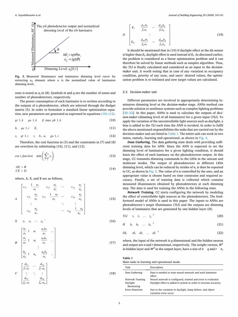
The dimension of matrix LED_Eff is r � q, where r is the number of luminaires and q is the number of sensors. Any element within this matrix (eij) is considered as an individual value of slope for the measured illuminance at the jth photodetector and the dimming level for the ith luminaire, as shown in Fig. 3.

The combination of LED_Eff, occupancy_m, and priority_m matrices are integrated within a Budget matrix. In order to rewrite (3), the Budget matrix is consisting of multiplication of the above mentioned matrices (5).

Budget¼

2

666664

e11 � O1 �1=P1

⋯e1q � Oq �1�Pq

⋮ ⋱ ⋮

er1 � O1 �1=P1

⋯erq � Oq �1�Pq

3

777775

r�q

(5)

where the photodetector’s effect is zero, when the occupancy condition is deactivated. The power consumption of each luminaire in (3) can be written as a specific photodetector’s output with maximum value at the Budget matrix (5). It worth noting that such approach is just an indica-tion for luminaire’s power consumption in (3) and it is not the accurate equivalent. However, the accuracy is high enough for the priority value of 1, as the simulation results will show in the next section. As an example, consider that in the jth row of Budget matrix the lth column has the greatest value among others. Thus, PLED,j can be written as lth photodetector target (tl), if the lth photodetector receives the maximum effect from the jth luminaire, as expressed in (6),

PLEDj¼Pj;max

maxðBudgetðj; : ÞÞtl (6)

The expression in (6) should be extracted for all r luminaires in the lighting system. The constraints in (3) can be defined by the maintained illuminance and illuminance uniformity required for each zone, as (7) and (8),

Xm

i¼1

Xq

j¼1

cij � tjfi� Ei (7)

Xm

i¼1

Xq

j¼1

dij � tjavgzonei

� ui (8)

avgzonei ¼Xq

j¼1

cij � tjfi

(9)

where in (7) and (8), the parameters cij and dij are binary in nature: if the sensor belongs to the ith zone then cij ¼ dij ¼ 1, otherwise 0. Also fi is the number of sensors in the ith zone. The desired light uniformity of the ith

Fig. 2. The procedure of calculating ga and gb in the cost function.

A. Seyedolhosseini et al.

Journal of Building Engineering 29 (2020) 101141

5

zone is noted as ui in (8). Symbols m and q are the number of zones and number of photodetectors, respectively.

The power consumption of each luminaire is re-written according to the outputs of a photodetector, which are selected through the Budget matrix (5). In order to formulate a standard linear optimization equa-tion, new parameters are generated as expressed in equations (10)–(12).

gtð1; kÞ¼ gað1; kÞ þ if maxðgbð1; kÞÞ (10)

bi¼ gað1; iÞ � Ei (11)

xi¼ gtð1; iÞ � ti � bi; ⋅ai ¼ gað1; iÞ (12)

Therefore, the cost function in (3) and the constraints in (7) and (8) are rewritten by substituting (10), (11), and (12).

cos t function¼min

Xq

i¼1xi

!

(13)

AX > BCX > D (14)

where, A, X, and B are as follows,

A¼

2

66666666664

c11 �1 � u1

a1� c12 �

u1

a2⋯ � c1q �

u1

aq

� c21 �u2

a1c21 �

1 � u2

a2⋯ � c2q �

u2

aq⋮ ⋱ ⋮

� cq1 �uqa1

⋯ cqq �1 � uqaq

3

77777777775

(15)

X ¼ ½ x1 x2 ⋯ xq �t (16)

B¼

2

66666666664

b1

a1ð1 � u1Þ �

u1b2

a2� :::

b1

a1ð1 � u2Þ �

u2b2

a2� :::

⋮bqaq

�1 � uq

��uqbqaq� :::

3

77777777775

(17)

C¼

2

666664

d11

f1⋅a1⋯

d1q

f1⋅aq⋮ ⋱ ⋮dm1

fm⋅a1

dmqfm⋅aq

3

777775

(18)

D¼

2

666664

E1 �

�d11b1

f1a1þ⋯þ

d1qbqf1aq

�

⋮

Em ��dm1b1

fma1þ⋯þ

dmqbqfmaq

�

3

777775

(19)

It should be mentioned that in (10) if daylight effect at the ith sensor is higher than Ei, daylight effect is used instead of Ei. As discussed earlier, the problem is considered as a linear optimization problem and it can therefore be solved by linear methods such as simplex algorithm. Thus, the TLI is finally calculated and considered as an input to the decision- maker unit. It worth noting that in case of any variation in occupancy condition, priority of any zone, and users’ desired values, the optimi-zation problem is re-initiated and new target values are calculated.

2.3. Decision-maker unit

Different parameters are involved in appropriately determining lu-minaires dimming level at the decision-maker stage. ANNs method can provide solution to nonlinear systems such as complex lighting problems [30–32]. In this paper, ANNs is used to calculate the outputs of deci-sion-maker (dimming level of all luminaires) for a given input (TLI). To apply the variation of the uncontrollable light sources such as daylight, a bias is added to the TLI each time the ANN is invoked. In order to fulfil the above mentioned responsibilities the tasks that are carried out by the decision-maker unit are listed in Table 1. The entire unit can work in two states, namely, learning and operational, as shown in Fig. 4.

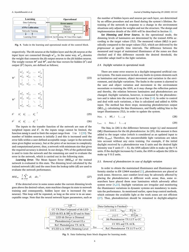
Data Gathering. The data gathering state deals with providing suffi-cient training data for ANN. Since the ANN is expected to set the dimming level of luminaires for a given lighting condition, it should learn the effect of each luminary on the photodetectors output. At this stage, CC transmits dimming commands to the LEDs in the unicast and multicast modes. The output of photodetectors at different LEDs dimming level, which can be reduced by strides of n, is then be reported to CC, as shown in Fig. 5. The value of n is controlled by the user, and an appropriate value is chosen based on time constraint and required ac-curacy. Finally, a set of training data is collected which contains measured illuminances obtained by photodetectors at each dimming step. The data is used for training the ANNs in the following state.

Network Training. CC starts configuring the network by modeling the effect of controllable light sources at the photodetectors. The feed-forward model of ANNs is used in this paper. The inputs to ANNs are photodetector’s target illuminance (TLI) and the outputs are dimming levels of luminaires that are generated by one hidden layer (H).

TLI¼ ½ t1 t2 … tq �T (20)

H¼ ½ h1 h2 … hn �T (21)

DL ¼ ½ dl1 dl2 … dlr �T (22)

where, the input of the network is q dimensional and the hidden neuron and output are n and r dimensional, respectively. The weight vectors, W1

in hidden layer and W2 in the output layer, have a size of n � q and r � n,

Table 1 Main tasks in learning and operational mode.

Task Description

Data Gathering Data is needed to train neural network and each luminaire effect

Network Training Neural network is configured, trained and error is evaluated Daylight

Monitoring Daylight effect is added to system in order to increase accuracy

Error Detection Due to the variation in daylight, lamp failure, and object variation error occur

Fig. 3. Measured illuminance and luminaires dimming level curve for extracting eij element where u is the normalized value of luminaires dimming level.

A. Seyedolhosseini et al.

Journal of Building Engineering 29 (2020) 101141

6

respectively. The ith neuron at the hidden layer and the jth neuron at the input layer are connected through w1

i,j. In the same way, w2i,j denotes

the weight that connects the jth output neuron to the jth hidden neuron. The weight vectors W1 and W2, and the bias vectors for hidden (b1) and output (b2) layers, are defined as follows;

W1¼

2

6666664

w11;1 w1

1;2 … w11;q

w12;1 w1

2;2 … w12;q

⋮ ⋮ ⋱ ⋮w1n;1 w1

n;2 … w1n;q

3

7777775

(23)

W2¼

2

6666664

w21;1 w2

1;2 … w21;q

w22;1 w2

2;2 … w22;q

⋮ ⋮ ⋱ ⋮w2n;1 w2

n;2 … w2n;q

3

7777775

(24)

b1¼�b1

1 b12 … b1

n

�T (25)

b2¼�b2

1 b22 … b2

r

�T (26)

The inputs to the transfer function of the network are sum of the weighted inputs and b1. As the inputs range cannot be limited, the function tansig is used to limit the output range from � 1 to þ1 [29]. The number of hidden neurons is initially 2 and this is increased until the error falls within a user-defined acceptable range. Larger in the network sizes gives higher accuracy, but at the price of an increase in complexity and computational power, thus, a network with minimum size that gives the required accuracy is desired. In our design, 70% of the gathered data is used to train the network and the remaining are used to evaluate the error in the network, which is carried out in the following state.

Learning Error. The Mean Square Error (MSEnn) of the trained network is evaluated in this state. The dimming level calculated by the trained network (dlc) and the ones from the lookup table (dl) are used to evaluate the network performance.

MSEnn¼1mXm

i¼1ðdli � dlciÞ2 (27)

If the detected error in some zones under the current dimming levels goes above the desired values, state machine changes its state to network training and consequently, hidden layer size is increased (by one neuron). This loop will be repeated, as long as the error is in an unac-ceptable range. Note that the neural network hyper parameters, such as

the number of hidden layers and neuron per each layer, are determined by an offline procedure and are fixed during the system’s lifetime. Re- training of the network in response to a change in the environment situations only adjusts the weights and not the structure. The design and implementation details of the ANN will be described in Section III.

Set Dimming and Error Source. In the operational mode, the dimming levels of luminaires are determined by the trained ANNs ac-cording to the target values (TLI). The measured values (MLI) is peri-odically compared to the target values (TLI), which are delivered by the preprocessor at specific time intervals. The difference between the measured and target of maintained illuminance of the zones are then checked and if this difference exceeds the desired threshold, the controller adapt itself to the light variation.

2.4. Daylight variation in operational mode

There are some error sources in a daylight-integrated artificial con-trol system. The main sources include any faults in system elements such as luminaires and sensors, object movement and variation in the envi-ronment, and daylight variations. The faults in the system is alarmed to the user and object variation and movement in the environment necessitate re-training the ANN, as it may change the reflection pattern and thereby, the relation between luminaires and photodetectors are changed. Daylight variation, however, is measured by the photodetec-tors and is taken into the account by as a bias [14]. In order to control and deal with such variations, a bias is calculated and added to ANNs input. The method has three steps; measuring photodetectors output (MLI1-q), calculating the bias illuminance, and finally adding bias to the target illuminances (TLI), in order to update the system.

biasi¼ ti � Mli; i ¼ 1; :::; q (28)

ti;new ¼ ti þ biasi; i ¼ 1; :::; q (29)

The biasi in (28) is the difference between target (ti) and measured (Mli) illuminances for the ith photodetector. In (29), this amount is then added to the target value (which is considered as an updated input to ANNs (ti,new). Therefore, the uncontrollable light variations are taken into account without any extra training. For example, if the initial daylight received by a photodetector was X units and the desired light intensity was Y units (Y > X), the ANN adjusts LEDs to make up the Y-X units. If the daylight increases by Z units, the ANN re-adjusts the LEDs to make up Y-X-Z units.

2.5. Removal of photodetectors in case of daylight variation

In order to obtain the maintained illuminance and illuminance uni-formity similar to EN-12464 standard [1], photodetectors are placed at work zones. However, user comfort level may be adversely affected by placing the photodetectors at different work areas; thus, some re-searchers have placed them near luminaires which adversely affect system error [4,23]. Daylight variations are irregular and monitoring the illuminance variations in dynamic systems are mandatory to main-tain the performance. As mentioned earlier, open-loop control methods, which estimate the available light at the work zones are not efficient [27]. Thus, photodetectors should be remained in daylight-adaptive

Fig. 4. Tasks in the learning and operational mode of the control block.

Fig. 5. Data Gathering State block diagram for learning mode.

A. Seyedolhosseini et al.

Journal of Building Engineering 29 (2020) 101141

7

control methods. In this paper, sensors are initially placed at the work zones but all

sensors except one reference sensor in each zone are eventually removed after calibration of ANNs. We have assumed that the daylight effect sensed by the reference sensor is approximately the same for all the sensors at each work zone. With any variation of measured illuminance (MLI) detected by the reference photodetector during the operational mode, the calculated bias at the reference sensor is considered for all the removed sensors. The reference sensor should be wisely selected in order to reduce the error. In this paper, we have selected a sensor with higher bias variation. Thus, the error is decreased, as the results is shown in the next section.

3. Case study and experimental results

SILC is implemented using MATLAB, and lighting conditions are evaluated in DIALux which is based on POV-Ray raytracing program [33]. DIALux is a simulation tool for lighting condition which according to many of the prior research is highly reliable [28,34–36]. Besides, DIALux as a simulation tool is validated in a previous comprehensive study against the analytical test cases of CIE171:2006 [37].

Initially, the accuracy of each unit within SILC is evaluated and then the entire system is checked for different cases studies. The desired maintained illuminance and illuminance uniformity is considered ac-cording to the standard EN-12464 considering 10 different visual tasks (laboratories, jewerelly making, watch making, Ironing, gloves making, paper sorting, type setting, reading area, technical drawing, class room). In order to monitor daylight variation and its effect on the lighting conditions of the zones, the photodetectors outputs are recorded in some certain intervals (here every 30 min).

3.1. Case studies

Different case studies are carried out, as shown in Fig. 6, and their detailed information are reported in Table 2. For all four cases a window is considered as a terminal for entering daylight. Case (a) and case (b) are both located in Tehran, Iran (longitude 51.4� and latitude 35.70�, 3h deviation from GMT and summer time). Case (c) and case (d) are located in Ludenscheid, Germany (longitude 7.63 and latitude 51.22, 1h devi-ation from GMT) and summer time. Summer is selected for simulations, since in such time daylight variations is more compared to that of other seasons. Two different locations for the case studies are considered to evaluate SILC performance. As expressed in Table 2, daylight gradient varies in different zones, and therefore, it becomes essential to employ a control method to improve the uniformity of each zone. In all cases, type of R2600/158 P8 luminaires have been employed where, each consumes 58W at 100% of illuminance. The number of photodetectors on each zone surface, related to each case study, is gathered and listed in Table 2. LEDs dimming level is increased 10% at each dimming step from 0 to 100%. The weather conditions of the test cases are also mentioned in the last column of Table 2, where for case (a) is overcast and for all others is clear.

3.2. Preprocessor

The preprocessor calculates the target illuminance of all photodetec-tors (TLI) according to the desired maintained illuminance and illumi-nance uniformity of zones and their corresponding parameters. Initially, the preprocessor forms the LED_Eff matrix to calculate the Budget matrix. As an example, in case (d) the luminaire (L1) is dimmed and the response of each three photodetectors output at each zone is recorded (using DIALux) as shown in Fig. 7. The elements of LED_Eff matrix is calculated from the approximated slope of each curve and for case (d) it is shown in (30).

LED Eff ¼

2

4378 450 457 250 299 309 47 54 54330 395 402 362 430 440 249 299 30377 86 87 346 413 420 392 470 475

3

5 (30)

In order to evaluate the preprocessor outputs, the maintained illu-minance and illuminance uniformity is calculated for all zones according to the computed TLI. The maintained illuminance and illuminance uniformity is then compared to the desired values and following to this, MSE is calculated. The preprocessor is implemented using MATLAB and the results are shown in the first row of Table 3. As it is reported, the MSE is below 1.2 for all cases when the priority is 1.

3.3. Decision-maker unit

Initially, the luminaires are dimmed from 0% to 100% one by one and also in groups in 10% steps, and the outputs of photodetectors (known by calculation points in DIALux) are stored in file, called lookup table. These data items are used for neural network training process and also to check the error which was referred to as Data Gathering state in Section II.

3.3.1. Neural network calibration In comparison to similar researches carried out which have achieved

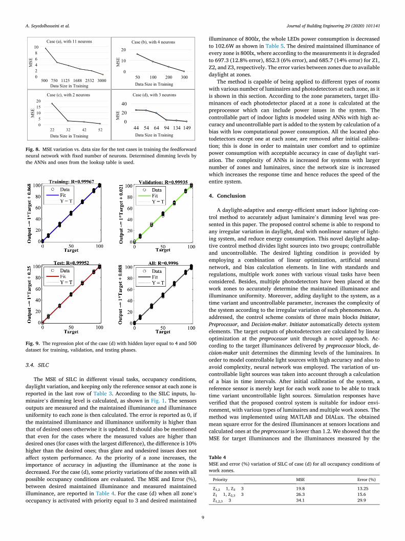
MSE of 20–30 [23], the current paper aims to reduce error. Results of the described case studies, is reported in Fig. 8 according to equation (27). The feedforward network error using sigmoid activation function for all cases converges into the desired region using the MATLAB’s neural networks toolbox, which the same function was used as fitting model in Ref. [35]. All networks initially start with 2 neuron and 20 data sets for training. The sizes of data and neurons in the hidden layer are increased while the MSE is within the desired range, as shown in Fig. 8. The regression plot (which typically used to verify the training process) of case (d) is shown in Fig. 9, as a sample, where all data converge to the Y ¼ T plot. An important consideration about the proposed design is the response time of the neural network. Neural networks generally involve a large amount of computation (in the form of multiply-and-accumulate operation on floating point numbers) to process a single input.

This imposes a considerable processing load on the underlying hardware platform, particularly, in resource-limited embedded systems. Fortunately, neural networks, and in particular the feedforward model used in this design, are shown to be very insensitive against the accuracy loss of arithmetic operations [38]. We tried different precisions for the

Fig. 6. The 3D view of four different case studies chosen for verification of SILC simulated in DIALux.

A. Seyedolhosseini et al.

Journal of Building Engineering 29 (2020) 101141

8

arithmetic operations of our target neural network in MATLAB and found the accuracy of neural network with 8-bit integer operations within less than 1% of the original neural network with 32-bit floating point operations. So, we quantize both weights and input data to 8-bit integer numbers. With 8-bit integer operations, the response time of the neural networks for the considered case studies and related sizes in Raspberry Pi II, are 0.43 ms, 0.26 ms, 0.08 ms, and 0.11 ms for case (a) to (d), respectively. This response time is quiet acceptable for our system.

3.3.2. Daylight variation The network is initially configured at a specific time of a day. As

daylight varies, bias for each photodetector is calculated and then the target values of illuminances are updated as described in (28) and (29), which is done in time intervals. The photodetector’s output is recorded

every 30 min, then the bias is calculated according to the measured values. In addition, the MSE of measured illuminances and target illu-minances when the bias is added to the ANNs input (target values) in variation of daylight is reported in the second row of Table 3. In cases where daylight only affects a specific part of the work area, the error is increased.

3.3.3. Sensor reduction The simulation response shows that the average error between the

measured values of ceiling mount photodetectors and those that are placed at work zones are beyond 60%. This result confirms the error rates reported in some prior work [23].Such error increases when daylight varies, hence increases the power consumption as the ceiling mount photodetectors senses less light. However, placing the photode-tectors at work zones can also degrade user comfort. In order to solve this problem, after an initial ANNs calibration, the current method considers keeping only the reference sensor. A photodetector with a higher bias is selected as the reference sensor, this is done in order of error reduction. To validate the idea, the outputs of photodetectors are recorded over 24 h and every 30 min, where, the bias is calculated for all sensors; if bias of reference sensor is higher than others, the error is 0, otherwise the error is updated. The outputs of reference sensor and those that will be removed from each zone are compared and the corre-sponding MSE is reported in Table 3. As it can be seen, the observed MSE is low for all cases, therefore, keeping the reference sensor for each zone is an appropriate decision. The calculated bias for each zone is then added to all target values of the zone and the dimming level of lumi-naires are determined based on the new target values. The MSE for measured illuminances and initial target values are also reported Table 3.

Table 2 Detailed information about implemented case studies.

Case Room Area (m2)

Room Height (m)

Wall reflection (%)

Number of Zones

Number of Luminaires

Work zones area (m2)

Work zones height (m)

Number of photodetectors per zone

Avg. Daylight deviationa Sky Type

a 20 2.74 20 4 12 1.52 � 0.75 0.76 4 Z1 ¼ 35%, Z2 ¼ 61% Z3 ¼ 36%, Z4 ¼ 35%

Overcast

b 9 2.74 30 2 4 Z1 ¼ 1.5 � 0.8 Z2 ¼ 2 � 1

0.76 Z1 ¼ 9, Z2 ¼ 13 Z1 ¼ 83% Z2 ¼ 49%

Clear

c 4.7 2.74 50 1 2 1.5 � .8 0.76 6 Z1 ¼ 23% Clear d 6.6 2.74 40 3 3 1.5 � 0.6 0.76 3 Z1 ¼ 57%, Z2 ¼ 64%, Z3 ¼ 62% Clear

a This is reported when all luminaires are off from 8a.m. to 8 p.m. Deviation from maximum received illuminance is stored and average deviation from the maximum is then reported. Deviation ¼ ((max-node)/max)*100.

Fig. 7. Variation of all photodetectors outputs placed at zones when L1 is dimming in the case (d), dimming value is normalized between [0, 1].

Table 3 MSE variation of different blocks of the SILC.

NO. Block MSEa Priorityb Daylight Variation

Description

CASE (a) CASE (b) CASE (c) CASE (d)

1 Preprocessor 0.9 1.2 0.8 0.9 1 – 50 different visual tasks and different occupancy conditions 2 ANNS 5.4 3.2 3.4 2.1 yes MSE of ANNs for 50 data sets for each case 3 Election of Reference

Photodetector Z1 ¼ 5.7, Z2 ¼ 0,

Z4 ¼ 0, Z3 ¼ 3.4

Z1 ¼ 0 Z2 ¼ 4.7

0 Z1,2,3 ¼ 0 – yes The MSE of the reference sensor vs. all other sensors at the same work zone over 24 h and 30 min

4 Decision-maker 20.7 10.2 5.6 5.3 – yes MSE of Decision-maker for 50 data sets for each case with considering reference sensor

5 SILC 25.4 (15.4%)

17.9 (9.1%)

15.7 (10.8%)

15.7 (7.2%)

1 yes MSE of SILC keeping the reference sensor at each zone

a MSE for all cases reported in this TABLE, the error is considered as zero, if the target and measured maintained illuminance and illuminance uniformity is higher than the desired value.

b In some simulation responses the value of priority does not affect the result, hence “-” it is used.

A. Seyedolhosseini et al.

Journal of Building Engineering 29 (2020) 101141

9

3.4. SILC

The MSE of SILC in different visual tasks, occupancy conditions, daylight variation, and keeping only the reference sensor at each zone is reported in the last row of Table 3. According to the SILC inputs, lu-minaire’s dimming level is calculated, as shown in Fig. 1. The sensors outputs are measured and the maintained illuminance and illuminance uniformity to each zone is then calculated. The error is reported as 0, if the maintained illuminance and illuminance uniformity is higher than that of desired ones otherwise it is updated. It should also be mentioned that even for the cases where the measured values are higher than desired ones (for cases with the largest difference), the difference is 10% higher than the desired ones; thus glare and undesired issues does not affect system performance. As the priority of a zone increases, the importance of accuracy in adjusting the illuminance at the zone is decreased. For the case (d), some priority variations of the zones with all possible occupancy conditions are evaluated. The MSE and Error (%), between desired maintained illuminance and measured maintained illuminance, are reported in Table 4. For the case (d) when all zone’s occupancy is activated with priority equal to 3 and desired maintained

illuminance of 800lx, the whole LEDs power consumption is decreased to 102.6W as shown in Table 5. The desired maintained illuminance of every zone is 800lx, where according to the measurements it is degraded to 697.3 (12.8% error), 852.3 (6% error), and 685.7 (14% error) for Z1, Z2, and Z3, respectively. The error varies between zones due to available daylight at zones.

The method is capable of being applied to different types of rooms with various number of luminaires and photodetectors at each zone, as it is shown in this section. According to the zone parameters, target illu-minances of each photodetector placed at a zone is calculated at the preprocessor which can include power issues in the system. The controllable part of indoor lights is modeled using ANNs with high ac-curacy and uncontrollable part is added to the system by calculation of a bias with low computational power consumption. All the located pho-todetectors except one at each zone, are removed after initial calibra-tion; this is done in order to maintain user comfort and to optimize power consumption with acceptable accuracy in case of daylight vari-ation. The complexity of ANNs is increased for systems with larger number of zones and luminaires, since the network size is increased which increases the response time and hence reduces the speed of the entire system.

4. Conclusion

A daylight-adaptive and energy-efficient smart indoor lighting con-trol method to accurately adjust luminaire’s dimming level was pre-sented in this paper. The proposed control scheme is able to respond to any irregular variation in daylight, deal with nonlinear nature of light-ing system, and reduce energy consumption. This novel daylight adap-tive control method divides light sources into two groups; controllable and uncontrollable. The desired lighting condition is provided by employing a combination of linear optimization, artificial neural network, and bias calculation elements. In line with standards and regulations, multiple work zones with various visual tasks have been considered. Besides, multiple photodetectors have been placed at the work zones to accurately determine the maintained illuminance and illuminance uniformity. Moreover, adding daylight to the system, as a time variant and uncontrollable parameter, increases the complexity of the system according to the irregular variation of such phenomenon. As addressed, the control scheme consists of three main blocks Initiator, Preprocessor, and Decision-maker. Initiator automatically detects system elements. The target outputs of photodetectors are calculated by linear optimization at the preprocessor unit through a novel approach. Ac-cording to the target illuminances delivered by preprocessor block, de-cision-maker unit determines the dimming levels of the luminaires. In order to model controllable light sources with high accuracy and also to avoid complexity, neural network was employed. The variation of un-controllable light sources was taken into account through a calculation of a bias in time intervals. After initial calibration of the system, a reference sensor is merely kept for each work zone to be able to track time variant uncontrollable light sources. Simulation responses have verified that the proposed control system is suitable for indoor envi-ronment, with various types of luminaires and multiple work zones. The method was implemented using MATLAB and DIALux. The obtained mean square error for the desired illuminances at sensors locations and calculated ones at the preprocessor is lower than 1.2. We showed that the MSE for target illuminances and the illuminances measured by the

Fig. 8. MSE variation vs. data size for the test cases in training the feedforward neural network with fixed number of neurons. Determined dimming levels by the ANNs and ones from the lookup table is used.

Fig. 9. The regression plot of the case (d) with hidden layer equal to 4 and 500 dataset for training, validation, and testing phases.

Table 4 MSE and error (%) variation of SILC of case (d) for all occupancy conditions of work zones.

Priority MSE Error (%)

Z1,2 ¼ 1, Z3 ¼ 3 19.8 13.25 Z1 ¼ 1, Z2,3 ¼ 3 26.3 15.6 Z1,2,3 ¼ 3 34.1 29.9

A. Seyedolhosseini et al.

Journal of Building Engineering 29 (2020) 101141

10

sensors, while decision-maker unit determines luminaires diming level, is 1. The response time of ANNs does not exceed 0.11 ms in experimental results using Raspberry pi II. In case of removing all sensors except one reference sensor, while considering the daylight variation, the MSE was obtained as 25.4. The current lighting system can be further extended by increasing the number of photodetectors and luminaires; requiring a larger neural network. An extended neural network system increases the computational power consumption and the response time, and hence reduces the speed of the entire system. Design of such extended system can be the challenge and focus of the future research.

Declaration of competing interest

The authors declare that they have no known competing financial interests or personal relationships that could have appeared to influence the work reported in this paper.

References

[1] Light and Lighting – Lighting of Work Places – Part I: Indoor Work Places, European Standard, EN 12464-1, 2011.

[2] L.T. Doulos, A. Kontadakis, E.N. Madias, M. Sinou, A. Tsangrassoulis, Minimizing energy consumption for artificial lighting in A typical classroom of A hellenic public School aiming for near zero energy building using LED DC luminaires and daylight harvesting systems, Elsevier J. Energy Build. 194 (2019) 201–217.

[3] A.A. Kim, Sh Wang, L.J. McCunn, Building value proposition for interactive lighting systems in the workplace: combining energy and occupant perspectives, Elsevier J. Build. Eng. 24 (July 2019) 1–14.

[4] K.H. Cheong, Y.H. Teo, J.M. Koh, U.R. Acharya, S. Ch Man Yu, A simulatiaon-aided approach in improving thermal-visual comfort and power efficiency in building, Elsevier J. Build. Eng. 24 (July 2020) 1–16.

[5] R.M. Ahmad, R.M. Reffat, A comparative study of various daylighting systems in office buildings for improving energy efficiency in Egypt, Elsevier J. Build. Eng. 18 (July 2018), 360-276.

[6] R. Razavi, et al., Occupancy detection of residential buildings using smart meter data: a large-scale study, Elsevier J. Energy Build. 183 (jan. 2019).

[7] R.E. Edwards, E. Lou, A. Bataw, S.N. Kamaruzzaman, Ch Johnson, Sustainability- LED design: feasibility of incorporating whole-life cycle energy assessment into BIM for refurbishment projects, Elsevier J. Build. Eng. 24 (July 2019).

[8] M. Karami, G.V. Mcmorrow, L. Wang, Continuous monitoring of indoor environment quality using an arduino-based data acquisition system, Elsevier J. Build. Eng. 19 (Sep. 2018) 412–419.

[9] H.N. Rafsanjani, A. Ghahramani, Extracting occupants’ energy-use patterns from wi-fi networks in office buildings, Elsevier J. Build. Eng. 26 (Nov) (2019).

[10] E.D. Dikel, G.R. Newsham, H. Xue, J.J. Valdes, Potential energy saving from high- resolution sensor controls for LED lighting, Elsevier J. Energy Build. (2018) 43–53.

[11] A. Seyedolhosseini, N. Masoumi, M. Modaressi, Performance improvement of ZigBee networks in coexitence of wi-fi signals, in: The 7th International Conference on Information Communication and Management (ICICM), Mosco, Russia, 2017.

[12] Ch H. Ke, et al., Efficiency network construction of advanced metering infrastructure using ZigBee, IEEE Trans. Mob. Comput. 18 (14) (Apr. 2019).

[13] M. Tolani, Sunny, R.K. Singh, Two-layer optimized railway monitoring system using wi-fi and ZigBee interfaced wireless sensor network, IEEE Sens. J. 17 (No. 7) (Apr. 2017) 2241–2248.

[14] A. Seyedolhosseini, et al., Zone based control methodology of smart indoor lighting systems using feedforward neural networks, in: IEEE 9th International Symposium on Telecommunications (IST), 2018.

[15] H.N. Rafsanjani, A. Ghahramani, Towards utilizing internet of things (IOT) devices for understanding individual occupants’ energy usage of personal and shared appliances in office buildings, Elsevier J. Build. Eng. 27 (Jan) (2020).

[16] I.N. Maachi, A. Mokhtari, M.E. Slimani, The natural lighting for energy saving and visual comfort in collective housing: a case study in the Algerian building context, Elsevier J. Build. Eng. 24 (July 2019).

[17] D. Caicedo, A. Pandharipande, Distributed illumination control with local sensing and actuation in networked lighting system, IEEE Sens. J. 13 (3) (March 2013).

[18] S. Afshari, S. Mishra, Decentralized feedback control of smart lighting systems, in: ASME Dynamic Systems and Control Conference, 2013.

[19] S. Afshari, S. Mishra, A. Julius, F. Lizarralde, J.D. Wason, J.T. Wen, Modeling and feedback control of color tunable LED lighting systems, Elsevier J. Energy .Build. (2014) 242–253.

[20] S. Afshari, S. Mishra, A plug-and-play realization of decentralized feedback control for smart lighting systems, IEEE Trans. Control Syst. Technol. 24 (4) (July 2016).

[21] J.F. Hughes, A.V. Dam, M. McGuire, D.F. Sklar, J.D. Foley, S.K. Feiner, K. Akeley, Computer Graphics: Principles and Practice in C, second ed., Addison-Wesley Professional, 1995.

[22] D.A. Belegundu, R. Ch Tirupathi, Optimization Concepts and Applications in Engineering, Cambridge University Press, 2019.

[23] M. Beccali, et al., Assessment of indoor illuminance and study on best photosensors position for design and commissiong of daylight linked control systems. A new method based on artificial neural network, Elsevier J. Energy 154 (2018) 466–476.

[24] Y. Gao, et al., Dynamic illuminance measurement and control used for smart lighting, Elsevier J. Meas. (March 2019).

[25] S. Li, A. Pandharipande, F.M.J. Willems, Daylighting sensing LED lighting system, IEEE Sens. J. 16 (9) (May 2016).

[26] A. Pandharipande, G.R. Newsham, Lighting controls: evolution and revolution, Light. Res. Tech. J. 50 (Aug. 2017) 115–128.

[27] P.K. Maiti, B. Roy, Evaluation of A Daylight-Responsive, iterative, closed-loop light control scheme, Light. Res. Technol. (2019) 1–17.

[28] D. Tran, Y. Kh Tan, Sensorless illumination control of A networked LED-lighting system using feedforward neural network, IEEE Trans. Ind. Electron. 61 (4) (Apr. 2014).

[29] M.H. Beale, M.T. Hagan, H.B. Demuth, Neural network toolbox user’s guide, Mathworks (2017).

[30] W. Byun, et al., Design of lighting control system considering lighting uniformity and discomfort glare for indoor space, in: International Conference on Platform Technology and Service (PlatCon), 2018.

[31] M. Bonomolo, et al., A set of indices to access the real performance of daylight- linked control systems, Elsevier J. Energy Build. (May 2017).

[32] G.W. Irwin, K. Warwick, K.J. Hunt, Neural Network Applications in Control, The Institution of Electrical Engineers, 1995, pp. 141–157.

[33] https://www.dial.de/en/dialux/. [34] L. Bellia, F. Fragliasso, Automated daylight-linked control systems performance

with illuminance sensors for side-lit offices in the mediterranean area, Elsevier J. Autom. Construct. 100 (2019) 145–162.

[35] N.K. Kandasamy, G. Karunagaran, C. Spanos, K.J. Tseng, B.H. Soong, Smart lighting system using ANN-IMC for personalized lighting control and daylight harvesting, Elsevier J. Build. Environ. 139 (2018) 170–180.

[36] E. Guerry, C.D. Galatanu, L. Canale, G. Zissis, Optimizing the luminous environment using DIALux software at “constantin and elena” eldery house-study case, Elsevier J. Procedia Manuf. 32 (2019) 466–473.

[37] R.A. Mangkuto, Validation of DIALux 4.12 and DIALux evo 4.1 against the analytical test cases of CIE 171:2006, J. Illum. Eng. Soc. 3 (2006) 139–150.

[38] Q. Zhang, et al., ApproxANN: an approximate computing framework for artificial neural network, in: Proceedings of DATE, 2015, pp. 701–706.

Table 5 Power consumption variation with different priority values of case (d) when desired maintained illuminances is 800lx and uniformity 0.7.

Priority Dimming Level LED Power (W)

Z1,2,3 ¼ 1 L1 ¼ 0.9, L2 ¼ 1, L3 ¼ 0.9 151.2 Z1,2,3 ¼ 3 L1 ¼ 0.7, L2 ¼ 0.3, L3 ¼ 0.9 102.6

A. Seyedolhosseini et al.