Setting fish quotas based on holistic ecosystem modelling including

environmental factors and foodweb interactions – a new approach

Lars Hakanson* and Andreas GyllenhammarDepartment of Earth Sciences, Uppsala University, Villav. 16, SE 752 36 Uppsala, Sweden; *Author forcorrespondence (e-mail: Lars.Hakanson@geo.uu.se)

Received 27 November 2003; accepted in revised form 8 March 2005

Key words: Aquatic systems, Baltic, Fish production, Fish quota, Foodweb modelling, Recovery,Thresholds

Abstract

We present a new approach to set fish quotas from holistic aquatic foodweb modelling (theLakeWeb-approach). This modelling includes changes in environmental conditions (nutrients, salinity,temperature, oxygen), process-based mass-balance calculations of nutrient concentrations from inflow,internal processes and outflow, calculations of how changes in nutrient concentrations affect primaryproduction, how such changes influence secondary production and how this influence fish production andbiomass. This approach gives dynamic, quantitative responses to alterations in driving variables and abi-otic/biotic feedbacks. We have applied this approach for preliminary simulations of the cod biomass in theBaltic. We also show that this approach adds a new dimension in setting fish quotas, which in the futurecould complement, rather than compete with, the more established methods used today based on fish catchstatistics and models based on other presuppositions. Our preliminary results indicate that under presentenvironmental conditions (2003), the cod is likely to be extinct if the annual catch is between 95 and 100 kt.The present fish quota is 75 kt/yr in the Baltic, but the overfishing may be 35 kt/yr. We discuss cause–effectrelationships regulating fish production, key factors influencing thresholds and points of no return con-nected to overfishing and changes in environmental conditions, factors regulating recovery and methods forsetting optimal fish quotas using this modelling approach.

Introduction and aim

There are numerous reports on declining fishstocks of several species from many parts of theworld (e.g., cod in the Baltic Sea, the North Seaand along the Atlantic coast of Canada;Hutchings 1996; FAO 2001; Anonymous 2002).The traditional method to set fish quotas usingfish catch statistics is highly uncertain (uncer-tainties up to a factor of four have been re-ported) and the quotas are also often violated

(Karagiannikos 1996; Anonymous 2002). Manypersons (about 1600 according to informalsources) are also directly and indirectly involvedin setting fish quotas in Northern Europe fordifferent species and areas. For example, thepermitted quota for cod in the Baltic Sea in 2002was 75 kt (75,000 tons) but initiated scientistsand experts affiliated with the fishing industryhave stated that the overfishing may be 50–100%of the legal quota. The fish production evidentlydepends on the survival of the roe and young

Aquatic Ecology (2005) 39:325–351 � Springer 2005

DOI 10.1007/s10452-005-3418-x

fish, the habitat conditions from ‘‘the cradle tothe grave’’ including predation and fishing byman, and how the abiotic conditions (e.g., oxy-gen, salinity, nutrient concentrations and tem-perature) vary and set the framework for the fishproduction (Busch and Sly 1992; Hakanson andBoulion 2002a). Many processes and compensa-tory effects are involved. This means that modelsare essential tools to handle these complicatedrelationships in a structured manner so that ra-tional and sustainable fish quota can be set andadjusted to prevailing and anticipated environ-mental changes. There are also many differenttypes of models addressing different target vari-ables. This paper is not meant as a literaturereview on models to predict fish production, butin a following section, we will give a briefsummary mainly to provide a background to thenew modelling approach presented in this paper.

The problems and uncertainties associated withthe methods used today to set fish quotas are wellknown to the scientists (Karagiannikos 1996;Anonymous 2002) and also to professional fish-ermen. Illegal overfishing exists since there areevident short-term economic benefits to the fish-ermen, and in many countries with poor legalcontrols, the risks of reprisals are small (see Corten1996).

It is important to emphasise that one cannotseparate the problems related to extensive fishing,eutrophication, toxic contamination and highlevels of toxins in fish and other environmentalchanges (e.g., in salinity, redox conditions, waterexchange and sediment conditions). They are allpieces of the same puzzle. For the Baltic, which isthe focus of this work, these threats have beendiscussed in many contexts (Voipio 1981; Ambio1990, 2000; Wulff et al. 2001; Hakanson et al.2002a; Hakanson 2002a).

• Eutrophication. The nutrient concentrations (Nand P) increase or stay at high levels; sedimentanoxia increases in the open water system andalso in the coastal areas (Jonsson 1992; Jonssonet al. 2003). The nutrient loading from differentsources and different Baltic countries are knownin terms of order of magnitude values (Stalnackeet al. 1999).

• Toxic contamination. Most organic toxins, butnot all, decrease in fish (the ecological half-life isabout 6 years for organic toxins like PCBs and

DDT; Hakanson 1999). There are EU recom-mendations on restrictions concerning con-sumption and sale of fat fish (e.g., salmon andherring) due to high levels of dioxins in fishmuscle. This is a key concern for the Balticfishery.

• Extensive fishing. There have been drasticreductions in catches of cod (see Figure 1) butalso of other species (like pike and perch fromBaltic coastal areas; see Soderberg and Gard-mark 2003).

These threats are certainly not unique to theBaltic but appear in many systems, e.g., Black Sea(Zaitsev and Mamaev 1997) and many othercoastal areas (Aertbjerg 2001).

A central problem in communications amongscientists, and a key reason for much misunder-standing in contexts of modelling, has to do withscale. This is evident in practically all mattersdealing with, e.g., fish modelling. Very many spe-cies, groups and size classes are involved, and dif-ferently in different systems. To sort this out ingreat detail at the scale dealing with hourly or dailychanges for individual species is a very difficult taskindeed for one system, and to try to do this in ageneral, predictive manner for many systems iseven more difficult. The LakeWeb-model discussedhere does not address the finer details of trophicinteractions or the changes from one sample site tothe next, or from one day to the next, or from onespecies to the next, in a given well-studied system.Figure 2 illustrates some important general con-cepts related to the ‘‘philosophy’’ behind the scaleof the LakeWeb-model. The curve marked CV inFigure 2 illustrates how the uncertainty in empiri-cal data generally increases if the data are collectedduring a day at a sampling site (a relatively smallCV of 0.3; CV = the coefficient of variation;CV = SD/MV; SD = standard deviation; MV =mean value), during weekly sampling (a higher CV,0.35), monthly sampling (a still higher value,CV = 0.55) and for samples collected over a year(CV = 0.95). The curve called ‘‘accessibility’’illustrates that the overall sampling effort wouldincrease, and the money and work related to theaccessibility of data needed to run and test a modelwould also increase, for models based on dailypredictions (e.g., using series of measured clima-tological data) to models for long-term predictions

326

based on fewer and more readily available datafrom standard maps and/or monitoring programs.The bolded curve is meant to illustrate one of manypossible ways to define the optimal size of a prac-tically useful model accounting for these two fac-tors, the uncertainty in the empirical data (as givenby CV) and the accessibility of the data (as given byAc = 1/d; where d is simply the number of daysused for sampling; note that it is not meaningful todetermine a mean value or a standard deviationfrom a sampling with fewer than three samples).The horizontal line illustrates that any given modeldeveloper or user would have a set of criteria todefine the practical usefulness of the model; dif-ferent users may have different criteria. Given thecurve for practical usefulness in this figure, one cannote that models striving for short-term (hourly –daily) predictions may not be very useful due to toohigh demands related to data accessibility, and thatmodels based on annual predictions would often besub-optimal due to the high uncertainties in theempirical data. The LakeWeb-model discussedhere gives weekly (or monthly) predictions and animportant reason for that is illustrated in Figure 2.

The predatory fish production is a targetvariable in the LakeWeb-model. This value rep-resents an integration over space and time in the

sense that the prey fish eaten by the predatoryfish grow, live and eat within a much wider areathan the area where the predatory fish arecaught. And the organisms eaten by the preyfish, i.e., zooplankton and zoobenthos also moveon their own accord in their search for food andsuitable habitats for reproduction. They are alsodistributed and transported by water currents.The latter aspects are important and one cannote that a typical theoretical water turnovertime for a Baltic coastal area is about 2–6 days(Hakanson 2000), that the coastal current (theCoriolis driven coastal jet) has a typical velocityof 25 cm/s or 150 km per week and that duringa week winds can blow from many directionsand with different speeds. All this creates astrong internal mixing in spite of the fact thatthe theoretical water turnover time for the Balticwater is very long (about 30 years; see Voipio1981; Wulff et al. 2001). These hydrodynamicalmixing effects also evidently influence the distri-bution of the food eaten by zooplankton, i.e.,phytoplankton and bacterioplankton. Thus, tounderstand and predict the factors regulating fishproduction one needs to look at the productionpotential of an entire system, i.e., to takean ecosystem approach and integrate many

Figure 1. Cod fishing in the Baltic Sea (FAO 2003) and the fishing quota (TAC) according to the International Baltic Sea Fisheries

Commission (IBSFC 2003).

327

processes over a wide area and a relatively longperiod of time. To illustrate this, one can firstestimate phytoplankton biomass from measure-ments of primary production given in mg C perm3 per day; multiplication with 7 gives theweekly production during the growing season;multiplication with the depth of the photic zone(D) and the size of the area (A) gives, afterdimensional adjustments, the phytoplanktonbiomass expressed in kg ww a given week as afunction of D and A – the larger the area, thelarger the phytoplankton biomass if all else isconstant. Then, a given phytoplankton biomass(BMPY) can sustain a biomass of zooplankton(BMZP) that would be a factor of 5–20 timeslower than BMPY. Then, a given zooplanktonbiomass would sustain a prey fish biomass thatwould be a factor of 5–20 lower than BMZP.Finally, a given prey fish biomass would sustaina predatory fish biomass that would be evenlower. So, to calculate a given production andbiomass of predatory fish, one needs to look atthe production potential of a larger water body,as given by A and D in this example.

The LakeWeb-model is structured to handlesuch processes and, to the best of our knowledge,no other ecosystem model does so in the same way.LakeWeb is meant to incorporate all key aspects ina general and mechanistic manner – from theenvironmental factors regulating primary produc-tion to the processes regulating secondary

production, including fish production. The focus ison the ecosystem scale also partly because societyis not interested in the contents of a samplingbottle, but in a much larger entity, the ecosystem(Odum 1986).

The LakeWeb-model has been critically testedwith positive results against very comprehensiveempirical data for lakes mainly from Eastern andWestern Europe. The model has also been testedby means of extensive sensitivity and uncertaintyanalyses (using Monte Carlo techniques) for bothuniform and characteristic coefficients of varia-tion for all model variables to quantify and rankthe uncertainties influencing the model pre-dictions (Hakanson and Boulion 2002a). Animportant feature of the model, and a pre-requi-site for its practical applicability in contexts ofaquatic management, is that it can be run by afew driving variables readily accessible fromstandard maps and monitoring programs. It alsoincludes a sub-model for toxic substances in fish,which is of special interest in the Baltic, where asstressed, fat fish have so high levels of dioxinsthat there are restrictions on consumption andsale, but the latter aspects will not be discussed inthis paper.

The aim of this paper is to:

• First, to give a few comments on modellingapproaches and a short comparison betweenthis new modelling approach (LakeWeb;

Day Week Month Year

CV

Accessibility of data (Ac =1/d)

Criteria ofusefulness

Optimal curve for predictive models (Op =10·(1-CV2)·Ac)

Val

ue (

CV

, A

c, O

p)

0

0,1

0,2

0,3

0,4

0,5

0,6

0,7

0,8

0,9

1

Figure 2. Illustration of factors regulating the optimal size of practically useful models in aquatic ecology.

328

Hakanson and Boulion 2002a) and a wellknown and much used modelling approach incontexts of marine fish production, Ecopath/Ecosim (Walters et al. 1997, 2000; Sandberg etal. 2000; Christensen et al. 2000; Harvey et al.2003). This is done to highlight the specificfeatures of the LakeWeb-approach and tostress that it actually provides a new dimensionto understand and quantitatively simulate thefactors regulating fish production and biomass.

• Secondly, to present a short description of thestructure of the LakeWeb-model. This model isbased on general principles and processes thatapply for most aquatic systems. The LakeWeb-model has been presented in a book (Hakan-son and Boulion 2002a) and the different partsof the model have been presented in severalpapers in scientific journals over the last years(see Table 1). The details of the different sub-models will not be repeated here, where theaim is to present the basic and specific princi-ples of the model.

• Thirdly, to present calibrations and changes inthe LakeWeb-model motivating the transfor-mation of the lake model into a model applicablefor the Baltic (LakeWeb to BaltWeb). We alsogive results demonstrating the potentials of themodel in contexts of settling fish quotas adjustedto changing environmental conditions.

• Finally, to use the BaltWeb-model to discussthresholds, points of no return and recoveryafter periods of overfishing.

This approach and other approaches – a brief

comparison

First, it should be stressed that different models forfish production in aquatic systems focus ondifferent targets and use different scales. Funda-mentally different approaches concern, e.g., phys-iological models, models for individual species andmodels based on functional groups, approachesusing different time scales (hours to years), differ-ent spatial scales (data from individual sites ormean values from entire ecosystems), differentdriving variables (e.g., climatological data or mapparameters) and approaches using statisticalmethods or models based on ordinary differentialequations (compartment or box models) or partialdifferential equations (two-dimensional or three-dimensional distributed models), see Peters (1991),Monte (1996), Mace (2001). To make a thoroughmodel comparison is beyond the scope of thispaper.

It should be stressed that the point we want tomake with the model comparison given in Table 2between LakeWeb and Ecopath/Ecosim is thatthese two modelling approaches are different, notcompeting, but complementary. Both these mod-elling approaches can calculate production (in kgwet weight per time unit) and biomasses (inkg ww), but LakeWeb has a separate sub-model tocalculate inflow, outflow and internal processes(sedimentation, resuspension, diffusion, etc.) ofnutrients so that the nutrient concentration can be

Table 1. The LakeWeb-model has been presented in the following papers.

Model description

The complete LakeWeb-model Hakanson and Boulion (2002a)

Uncertainty analyses of ecosystem models Hakanson (2003a)

The fish sub-model Hakanson and Boulion (2004a)

The zoobenthos sub-model Hakanson and Boulion (2003d)

The zooplankton sub-model Hakanson and Boulion (2003a)

The phytoplankton sub-model Hakanson and Boulion (2001a, 2003c)

The bacterioplankton sub-model Boulion and Hakanson (2003)

The benthic algae sub-model Hakanson and Boulion (2004b)

The macrophyte sub-model Hakanson and Boulion (2002b)

The water clarity sub-model Hakanson et al. (2003b)

The mass-balance sub-model for phosphorus Hakanson and Boulion (2003b)

The sub-model for the duration of the growing season Hakanson and Boulion (2001b)

Practical applications using the LakeWeb-model

Effects of land-use changes on aquatic foodwebs Hakanson (2002)

Effects of extensive fishing on aquatic foodwebs Hakanson et al. (2003a)

Effects of eutrophication and climate changes on aquatic foodwebs Hakanson et al. (2003c)

Effects of acid rain on aquatic foodwebs Hakanson (2003b)

329

Table 2. A brief comparison between Ecopath with Ecosim (EwE; and connected models) and LakeWeb.

1. User knowledge. To use EwE for aquatic systems requires detailed knowledge of the studied organisms. LakeWeb is an ecosystem

model which may be used without expert knowledge on ecosystem processes and without comprehensive and detailed data on food

choices, constants, production and consumption. The models have different structures, driving variables and users.

2. Basic structures. EwE is a tool kit and does not include any general well-tested foodwebs, but rather the building blocs to construct

such foodwebs. So, EwE is a platform for construction, parameterization and analyses of mass-balances of trophic interactions. It can

also be used for terrestrial ecosystems. LakeWeb is, on the other hand, an open foodweb model with a mass-balance model for

phosphorus. It can only be used for aquatic systems but it is structured in such a manner that it may be used for most lakes, rivers and

coastal areas. The processes and functional groups in the model are general.

3. Mode of operation. Ecopath can calculate biomass accumulation (as a difference between given start and end values). So, it is not

steady-state, but it is not dynamic either. When ecosystems have undergone massive changes, two or more models may be needed. To

do modeling over time, one needs Ecosim. To do spatially distributed modelling, one needs Ecospace. When seasonal changes are

important different models may have to be constructed for each month, season, or for extreme situations (‘summer‘ vs. ‘winter’).

However, Ecosim has a ‘‘forcing routine’’, which allows for manually forced changes in the conditions of the consumer groups.

LakeWeb is created to study the dynamics of foodweb interactions and therefore also to find those phenomena one needs to know in

Ecopath before one constructs the model. Instead of having to construct different models for different seasons, one gets the dynamic

response from the system with LakeWeb.

4. System demands. In Ecopath, the ecosystem should be defined so that the interactions within the system add up to a larger flow than

the interactions between the given system and the adjacent system(s). In practice, this means that the import to and export from a

system should not exceed the sum of the transfer between the sub-systems. If necessary, one or more groups originally left outside the

system may have to be included in order to achieve this. In LakeWeb, there is no restriction on the size of different flows within or

between systems. If a coastal area is to be modelled, and the export/import largely exceeds internal nutrient flows, there is nothing in

the model that hinders this from being modelled.

5. Units. Ecopath can be run with either energy-related units or nutrient related units. But if Ecosim and Ecospace are used, energy is

the only choice. In LakeWeb, the transport of phosphorus (in g per week) is modelled in the mass-balance model for phosphorus to and

from the different compartments and in the foodweb part of the model, one calculates flows of matter in kg wet weight per week to and

from the different functional groups.

6. Required input. As a rule, three of the four basic input parameters, biomass, production/biomass ratio, consumption/biomass ratio

and ecotrophic efficiency, must be at hand to run the Ecopath model. This must be done for all Ecopath groups (e.g., benthic fish, large

zooplankton, benthos, phytoplankton, detritus, etc). If some data are missing, the program might be able to estimate (via a mathe-

matical iteration process) the missing information. If not, the user will be warned by a message and the program will halt. An

alternative input is also available. Diet composition must be entered for all consumers. One also needs a lot of boundary conditions

(migration). There are also routines for providing fishery information and economical information concerning fisheries. To run

LakeWeb, one needs data on area, mean depth, maximum depth, latitude, altitude, characteristic values of water colour and pH and

characteristic concentration of total phosphorus in the tributary(ies). The BaltWeb-model also requires data on salinity.

7. Uncertainty analyses. Ecopath handles uncertainties via a resampling routine (Ecoranger). One can enter ranges and mean values for

all basic parameters (or use default values) and after selecting frequency distributions (uniform, triangular or normal), the program

runs Monte Carlo simulations. LakeWeb can be tested in the same manner, but it is not restricted to those distributions since it can also

use other transformations.

8. Sensitivity analyses. Ecopath has a simple sensitivity routine that varies all basic input parameters from �50% to +50% and checks

what this means at each step for each of the input parameters on all of the ‘missing’ basic parameters for each group in the system. In

LakeWeb, sensitivity analyses can be made via Monte Carlo simulations where all parameters are varied, one at a time, according to

their own estimated or known variance and range.

9. Foodweb outputs. Ecopath outputs the total throughput (in t per km2 per year) for many variables. It also gives all flows by trophic

levels, the trophic impacts, etc. Ecosim uses time series data for biomasses, available from single species stock assessments. EwE is thus

build more on traditional stock assessments. It has been used for exploring the effects of changes in fishing efforts. LakeWeb outputs all

flows (kg wet weight per week) and biomasses (kg ww) summed or instantaneously for any arbitrary period of the simulation period.

10. Simulation periods. Ecosim uses 10 years as default simulation period; the maximum is 100 years. One can save the end state and

continue with a new, thus enabling long-term simulations. By default, there are 100 time steps per year. This can be changed, but it is

not recommended. LakeWeb has no maximum simulation period.

11. Integration methods. Ecosim uses Adams–Basforth or 4th Runge–Kutta. LakeWeb uses Euler or Runge–Kutta.

12. Spatial distribution. With the addition of Ecospace, one can add spatial distribution. One can then assign habitats to different cells

in a user defined grid map of the modelled ecosystem. With probabilities rated for movement, one can then follow migration. LakeWeb

is a compartment model and has currently no spatially distribution, but this can be added. Those effects would have to be handled in

the same way, with probabilities of migration. This can then be governed by environmental changes, food availability, etc.

13. In summary. EwE is constructed as a tool for scientists; it requires lots of data on the system and attempts to fit the data into a

foodweb. Ecosim, like Ecopath, only describes feeding actions. No linkage is made with the surrounding environmental factors. If

detailed data are available, one can get very detailed output on foodweb interactions. LakeWeb or BaltWeb is a tool for scientists and

managers seeking knowledge of an ecosystem in relation to its physical environment and how environmental effects influence that

system.

330

related to nutrient sources (such as point sourcesand river inflow) and used to calculate chlorophyllconcentrations, which in turn regulate primaryproduction. Ecopath/Ecosim has no mass-balancemodel like this creating a quantitative link topollution sources. On the other hand, Ecopath/Ecosim is designed to handle more detailed food-web interactions than LakeWeb. The point wewould like to make is that these models, like allmodels, have benefits and limitations. To mergethese modelling approaches might open newinteresting possibilities.

In a strict sense, there is no such thing as ageneral (= generic) ecosystem model, whichworks equally well for all ecosystems and at allscales because all models need to be tested againstreliable, independent empirical data and the dataused in such validations must of necessity belongto a restricted domain. At any modelling scale, thecomplexities of natural ecosystems always exceedthe complexity and size of any model. So, simpli-fications are always needed, and this entailsproblems. The ultimate obstacle in achieving pre-dictive power and general validity for a model is tofind the most appropriate simplifications, and/oromit small and irrelevant processes related to thegiven target variables to be predicted (Monte 1995,1996; Monte et al. 1999; Peters 1991; Hakansonand Peters, 1995).

The next section describes the basic structure ofLakeWeb and in the following sections, we willshow how the model operates by giving resultsfrom the Baltic.

The LakeWeb-modelling approach

Outline of the model

The LakeWeb-model is a general dynamic modelquantifying key aquatic foodweb interactions andbiotic/abiotic feedbacks for entire systems and keyfunctional groups, which are present in most typesof aquatic systems (lakes, rivers and marine areas).The functional groups are: (1) predatory fish, (2)prey fish, (3) zoobenthos, (4) predatory zoo-plankton, (5) herbivorous zooplankton, (6) phy-toplankton, (7) bacterioplankton, (8) benthic algaeand (9) macrophytes. The functional group‘‘predatory’’ fish does the work of eating ‘‘preyfish’’, which does the job of consuming two

functional groups of zooplankton (herbivorousand predatory) and zoobenthos, etc. LakeWeb-model uses ordinary differential equations (com-partment modelling for defined lakes or marineareas) and gives weekly variations on productionand biomasses of the nine functional groups.

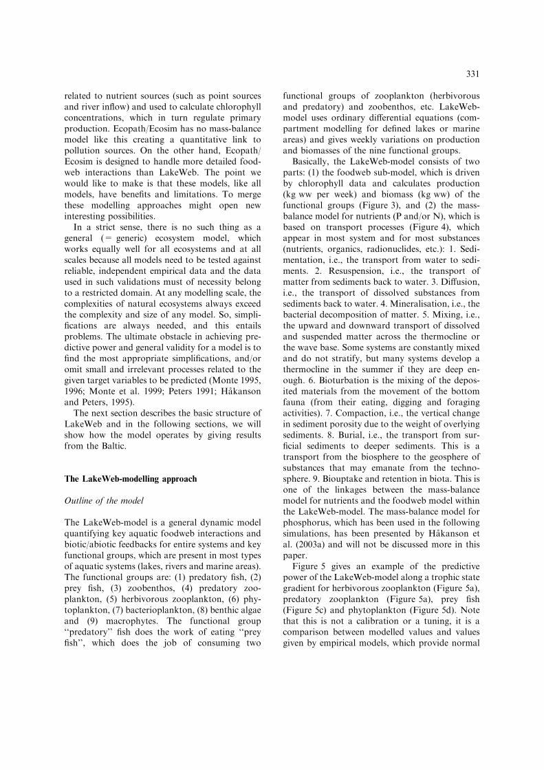
Basically, the LakeWeb-model consists of twoparts: (1) the foodweb sub-model, which is drivenby chlorophyll data and calculates production(kg ww per week) and biomass (kg ww) of thefunctional groups (Figure 3), and (2) the mass-balance model for nutrients (P and/or N), which isbased on transport processes (Figure 4), whichappear in most system and for most substances(nutrients, organics, radionuclides, etc.): 1. Sedi-mentation, i.e., the transport from water to sedi-ments. 2. Resuspension, i.e., the transport ofmatter from sediments back to water. 3. Diffusion,i.e., the transport of dissolved substances fromsediments back to water. 4. Mineralisation, i.e., thebacterial decomposition of matter. 5. Mixing, i.e.,the upward and downward transport of dissolvedand suspended matter across the thermocline orthe wave base. Some systems are constantly mixedand do not stratify, but many systems develop athermocline in the summer if they are deep en-ough. 6. Bioturbation is the mixing of the depos-ited materials from the movement of the bottomfauna (from their eating, digging and foragingactivities). 7. Compaction, i.e., the vertical changein sediment porosity due to the weight of overlyingsediments. 8. Burial, i.e., the transport from sur-ficial sediments to deeper sediments. This is atransport from the biosphere to the geosphere ofsubstances that may emanate from the techno-sphere. 9. Biouptake and retention in biota. This isone of the linkages between the mass-balancemodel for nutrients and the foodweb model withinthe LakeWeb-model. The mass-balance model forphosphorus, which has been used in the followingsimulations, has been presented by Hakanson etal. (2003a) and will not be discussed more in thispaper.

Figure 5 gives an example of the predictivepower of the LakeWeb-model along a trophic stategradient for herbivorous zooplankton (Figure 5a),predatory zooplankton (Figure 5a), prey fish(Figure 5c) and phytoplankton (Figure 5d). Notethat this is not a calibration or a tuning, it is acomparison between modelled values and valuesgiven by empirical models, which provide normal

331

reference values (often called norms) (see Table 3).To produce the results in Figure 5 there were nochanges in the model or the driving variables

except for the given five steps in TP-concentrations(10, 30, 100, 300 and 1000 lg/l). Similar tests havebeen carried out with the same positive results for

Figure 3. An outline of LakeWeb, a model to quantify all important foodweb interactions, including biotic/abiotic feedbacks in a

general manner. A preliminary version of LakeWeb for the Baltic (BaltWeb) has been used in this work.

Figure 4. Illustration of general and fundamental transport processes to, within and from aquatic systems used in the mass-balance

model for phosphorus in the LakeWeb/BaltWeb-model. The ‘‘ET-areas’’ shown in the figure are the erosion and transportation areas

where nutrients are resuspended, and the areas with ‘‘active A-sediments’’ are the biologically active sediment areas where fine

sediments are continuously being deposited (accumulation areas).

332

all nine key functional groups of organismsincluded in the LakeWeb-model. Tests like thoseshown in Figure 5 have also been carried out withgood results along humic level gradients, temper-ature gradients and lake size gradients.

Several practical scenarios describe how themodel can be applied to address important man-agement issues, like consequences of biomanipu-lations (extensive fishing; Hakanson et al. 2003a),changes in land-use (Hakanson 2002), depositionof acid rain (Hakanson 2003b), global temperaturechanges and eutrophication (Hakanson et al.2003c) and remedial measures to reduce toxins infish (Hakanson and Boulion 2002a). LakeWeb is apowerful tool to simulate remedial measures andto get realistic expectations of positive and nega-tive consequences of such measures.

Mass-balance modelling of nutrients is a centralparadigm in aquatic ecology and management(Vollenweider 1968; OECD 1982) and by including

this mass-balance model for nutrients in the food-web model, it is also possible to calculate the up-take and retention of nutrients in biota. Figure 6gives an example of how the mass-balance modelwithin the LakeWeb-model predicts TP-concen-trations in Lake Miastro, Belarus. It should benoted that in these simulations there has been notuning of the model, i.e., no changes in any of themodel algorithms of model constants, and onlychanges in the obligatory lake-specific drivingvariables (see Figure 3), which are readily accessedfrom standard monitoring programs and/or maps.

Even though Figures 5 and 6 indicate that theLakeWeb-model can predict well, there will alwaysbe situations which it will not describe well. This is,in fact, one important motive for the model. It ismeant to capture normal interactions among themost important factors influencing a given y-var-iable so that all other phenomena can be inter-preted in relation to these factors.

Figure 5. Critical model testing (sensitivity analyses) for the following four variables under default conditions (lake area = 1 km2,

mean depth = 10 m, pH = 7) along a trophic state gradient. The driving variable is the tributary TP-concentration, which has been

varied in 2-year steps from 10 to 1000 lg/l, while all else is constant. Note that the empirical models (called norms) often do not

provide any seasonal patterns, only mean values for the growing season. (a) Gives predicted biomass of herbivorous zooplankton

(curve 1) and the corresponding empirical regression line (= the norm; curve 2). (b) Gives modelled biomass of predatory zooplankton

(curve 1) and the empirical norm (curve 2). (c) Gives biomass of prey fish (curve 1) and the corresponding norm (curve 2). (d) Gives

predicted biomass of phytoplankton (curve 1) and the two empirical norms, the upper, maximum curve (2) as calculated for the entire

lake volume, and curve 3 (the mean value) as calculated for the volume of the photic zone.

333

Basic mathematical structures of the foodweb model– primary production unit

This section first gives the basic mathematicalstructure of each primary production unit in themodel. Figure 7 illustrates the principle set-up ofeach primary compartment (e.g., phytoplankton,benthic algae or macrophytes) and the obligatorydriving variables.

BMPUðtÞ ¼ BMPUðt� dtÞ þ ðIPRPU

� CONPUSU � ELPUÞdt; ð1Þ

where BMPU is the biomass (BM) of the primaryunit (PU; in kg ww).

Since this is a primary production unit, theproduction is directly related to abiotic limitingfactors, such as the concentration of nutrients,water clarity, temperature, etc. This is accountedfor in the LakeWeb-model in various ways, gen-erally by dimensionless moderator techniques.

That is:

IPRPU ¼ PRPU � YX � Ytemp; ð2Þ

where IPRPU is the initial production of the pri-mary unit (kg ww per week); PRPU the productionof the primary unit; for phytoplankton, this iscalculated from chlorophyll (kg ww per week); YX

or Ytemp the dimensionless moderators expressinghow changes in environmental conditions, likenutrient concentrations (X), water clarity or watertemperature influence primary production. YX hasthe following general definition:

YX ¼ ð1þ amp � ðXact=Xnorm � 1ÞÞ; ð3Þ

where the amplitude value (amp) quantifies howchanges in actual values (Xact) relative to a normal(= reference) value (= Xnorm) will influence theproduction; if Xact = Xnorm, then YX = 1.

The loss of biomass is given by two processes, (1)elimination (EL), which is related to the mean

Table 3. Empirical regressions illustrating the key role of total phosphorus (TP) in lake studies.

y-Value Equation Range for x r2 n Units Reference

Equations based on phosphorus used as norms in LakeWeb

Chlorophyll (summer mean) = 0.28�TP0.96 2.5–100 0.77 77 mg ww/m3 OECD82

Chlorophyll (summer max.) = 0.64�TP1.05 2.5–100 0.81 50 mg ww/m3 OECD82

Chlorophyll (weekly mean) = 0.5�TP [(0.64+0.28)/2 �0.5; (0.96 + 1.05)/2 �1)] mg ww/m3 H&B02

Max. prim. prod. (TP>10) = 20�TP-71 7–200 0.95 38 mg C/m3 d Peters (1986)

Max. prim. prod. (TP<10) = 0.85�TP1.4 mg C/m3 d Peters (1986)

Mean prim. prod. (TP>10) = 10�TP-79 7–200 0.94 38 m C/m3 d Peters (1986)

Mean prim. prod. (TP<10) = 0.85�TP1.4 mg C/m3 d Peters (1986)

Phytoplankton = 30�TP1.4 3–80 0.88 27 mg ww/m3 Peters (1986)

Phytoplankton = 30�TP(1.4–0.1�(TP/80� 1)) mg ww/m3 H&B02

Bacterioplankton (Col<50) = 0.90�TP0.66 3–100 0.83 12 mill./ml Peters (1986)

Bacterioplankton = (1+0.25�(Col/50–1)))�0.90�TP0.66 (if colour>50 mg Pt/l) H&B02

Zooplankton, herbivores = 0.77�38�TP0.64 3–80 0.86 12 mg ww/m3 Peters (1986)

Zooplankton, predators = 0.23�38�TP0.64 (the distr. coeff. is 0.77) mg ww/m3 H&B02

Zoobenthos = 810�TP0.71 3–100 0.48 38 mg ww/m2 Peters (1986)

Zoobenthos = (1–0.5�(TP/100–1))�810�TP0.71 (if TP>100) mg ww/m2 H&B02

Fish = 590�TP0.71 10–550 0.75 18 mg ww/m2 Peters (1986)

Fish yield = 7.1�TP 8–550 0.87 21 mg ww/m2 yr Peters (1986)

Other equations used as norms in LakeWeb

Fish yield = 0.0023�PrimP0.9 170–14000 0.64 66 mg ww/m2 yr H&B02

Prey fish = 0.73�fish biomass mg ww/m2 H&B02

Predatory fish = (1–0.73)�fish biomass mg ww/m2 H&B02

Macrophyte cover = 0.50�(SecMV/Dm) 229 % Vor77

Macrophytes = 1.37�log(Maccov) + 3.58 g ww/m2 yr H&B02

Zooplankton, herbivores = 0.15�(PrimP�1000)0.86 13–15000 0.61 42 g ww/m2 yr H&B02

Zooplankton, predators = 0.076�(PrimP�1000)0.84 2–3000 0.43 42 g ww/m2 yr H&B02

Many biological variables whose determinations normally require extensive and expensive field and laboratory workmay be estimated or

predicted from lake characteristic TP (in lg/l = mg/m3). Somevariablesmaybe predictedwith great precision (high r2), otherswithmuch

less.OECD82 isOECD(1982),Vor77 isVorobev (1977) andH&B02 isHakansonandBoulion (2002a). PrimP = primaryproduction (in

g ww/m2 yr), Maccov = Macrophyte cover of lake bed (in % lake area), SecMV = mean annual Secchi depth (in m), Dm = mean lake

depth (in m), Col = lake colour (mg Pt/l), n = number of lakes used in the regression, ww = wet weight and dw = dry weight.

334

characteristic turnover time of the functional group(TPU in weeks) and (2) the consumption (= CON,i.e., the predation or grazing) by a secondary pro-duction unit (SU; e.g., zooplankton, see next sec-tion). Elimination (ELPU) is generally given by

ELPU ¼ BMPU � 1:386=TPU ð4Þ

where 1.386 is the half-life constant (�ln(0.5)/0.5 = (0.693/0.5; see Hakanson and Peters 1995)andTPU is the mean, characteristic turnover time ofthe organisms in the given compartment. Table 4gives a compilation of characteristic turnover timesfor the nine functional groups of organisms in-cluded in the LakeWeb-model. Evidently, theturnover times among the single species constituting

a functional group can vary considerably. Theturnover time (T) of a given functional group oforganisms is defined in the traditional way asT = BM/PR, where BM = the biomass of theorganism in kg ww and PR = themass productionin kg ww/week. Note that the initial production(IPR; see Eq. 2) is higher than the actual produc-tion (PR = BM/T) because IPR gives produc-tion without losses from grazing and elimination.

An important feature of the LakeWeb-modelconcerns the technique to calculate predation andfeedbacks. The predation (= consumption) by asecondary unit on the biomass of a primary unit isgiven by

CONPUSU ¼ BMPU � CRSU; ð5Þ

Figure 6. Model validations giving predictions of (a) TP-concentrations in water and (b) TP-concentrations in A-sediments in Lake

Miastro, Belarus. In (a) there are three reference lines to the modelled values (curve 1), curve 2 gives TP-concentrations from the

empirical OECD-model (OECD 1982), curve 3, TP-concentrations from the Vollenweider model (1968) and curve 4, empirical data for

the lake. Note that the empirical data are based on mean monthly (not weekly) values from Lake Miastro from the given period (1980–

90). (b) gives two empirical reference lines for TP-concentrations in sediments, curve 2, the maximum TP-concentration and curve 3,

the mean value.

335

where CONPUSU is the flow of biomass out of theprimary unit (kg ww/week) from consumption bythe secondary unit. The actual consumption rateconstant, CRSU (1/week), is defined by

CRSU ¼ ðNCRSU þNCRSU

� ðBMSU=NBMSU � 1ÞÞ; ð6Þ

where NCRSU is the normal consumption rateconstant of the given secondary production unit

(1/week); NBMSU the normal (= reference)biomass of the secondary unit (kg ww); e.g., cal-culated from Table 3.

Basically, the consumption rate constant forany given functional group is related to threefactors:

1. The ratio between the actual biomass (BM) andthe normal biomass (NBM) of the predator.

Figure 7. Generalised set-up of the mathematical structure of each primary production unit in the LakeWeb-model. The figure also

gives general abbreviations.

336

The higher this ratio, the higher the predationpressure on the given prey.

2. The number of first order food choices (NR; seeFigure 8 for illustration). The structure of theLakeWeb-model involves several simplifica-tions and there are always either one or twofirst order food choices. This means that NR is1 or 2.

3. The inverse of the turnover time (TSU) of thepredator. Animals with short turnover timescreate a greater predation pressure on their preythan animals with long turnover times (and ahigher value of the actual consumption rateconstant, CRSU). So, predatory fish will eat arelatively small fraction of the total availablebiomass of its prey per time unit. Small her-bivorous zooplankton, on the other hand, arelikely to consume a larger percentage of theirprey (such as phytoplankton and bacterio-plankton) per unit of time.

That is, for animals in the secondary unit:

NCRU ¼ NRU=TU ð7Þ

A consumption rate constant of 0.2 means that20% of the biomass of the primary unit is con-sumed by the animals in the secondary unit perweek.

Basic mathematical structures of the secondaryproduction unit

Figure 9 gives an illustration of the modellingapproach and abbreviations. The basic equation is

given by

BMSUðtÞ ¼ BMSUðt� dtÞ þ ðIPRSUPU1

þ IPRSUPU2 � CONSUPU1

� CONSUPU2 � ELSUÞ � dt; ð8Þ

where BMSU is the biomass (BM) of the secondaryproduction unit (SU; in kg ww).

In the set-up shown in Figure 9, the initial sec-ondary production (IPR) is related to two flows,from primary units 1 and 2 (PU1 and PU2). Foreach flow, IPR is given by

IPRSUPU1 ¼ DC1 � CONPU1SU �MERPU1SU; ð9Þ

where DC1 is called the first order distributioncoefficient. The LakeWeb-model uses a simplegeneral system to assign weights to food choicesand adjust the consumption to the number of foodchoices. There are, for example, three food choicesfor zoobenthos (benthic algae, macrophytes and‘‘sediments’’); prey fish have a menu of three foodalternatives (predatory zooplankton, herbivorouszooplankton and zoobenthos); and predatoryzooplankton only eats herbivorous zooplankton.The secondary unit in Figure 9 has two first orderfood choices, so NR = 2. If there are more thantwo food choices, they are first differentiated by adistribution coefficient (DC1) into two first orderfood choices and then by a second distributioncoefficient (DC2) into second order food choices,etc.

CONPU1SU i s the consumption of biomass fromthe compartment PU1 from grazing by the animalsin compartment SU (kg ww/week). The actualconsumption rate constant (CRSUPU1) is calcu-lated in the same manner as already discussed forthe primary production unit.

The metabolic efficiency ratio (dimensionless),MERPU1SU, gives the fraction of the food thatactually increases the biomass of the secondaryunit (the consumer). Table 5 gives a compilationof characteristic MER-values used for all groupsof organisms in the LakeWeb-model. Note thatthe MER-value for zoobenthos eating sedimentsof low nutrition value is only 25% of the MER-value for zoobenthos feeding on benthic algae.

The initial production of the secondary unit,SU, from consumption of the second primary unit(IPRSUPU2) is handled in the same manner usingthe same consumption rate constant but (1�DC1)

Table 4. Characteristic turnover times for key functional

groups of organisms (T = BM/PR; where BM = biomass in

kg ww PR = biomass production in kg ww/day).

Group Turnover time (days)

Phytoplankton 3.2

Bacteria 2.8

Benthic algae 4.0

Herbivorous zooplankton 6.0

Predatory zooplankton 11.0

Prey fish 300

Predatory fish 450

Zoobenthos 128

Macrophytes 300

Note that the model calculates weekly and not daily changes.

Based mainly on data from Winberg (1985). From Hakanson

and Boulion (2002a).

337

instead of DC1. Then, this initial production isgiven by

IPRSUPU2 ¼ ð1�DC1Þ � CONPU2SU

�MERPU2SU: ð10Þ

So, consumption is given as a function of, (1)the normal consumption rate constants (hereNCRSUPD1 or NCRSUPD2), (2) the normal bio-masses of the two predatory units (NBMPD1 andNBMPD2), and the actual biomasses of the twopredatory units (BMPD1 and BMPD2), as these arecalculated by the LakeWeb-model in the samemanner as already discussed for the primary pro-duction unit (Eqs. 5 and 6).

Note that the model quantifies changes in theactual consumption of the prey unit related tochanges in the biomass of the consumer: moreanimals in the secondary unit (the higher BMSU)means a higher actual consumption rate constant,CRSU. If the actual biomass of the secondary unitis equal to the NBM of the secondary unit, thenBMSU/NBMSU = 1, and CRSU = NCRSU. If theactual biomass of the secondary unit, BMSU, istwice the normal biomass of the secondary unit,then CRSU = 2�NCRSU. So, the model gives alinear increase in consumption with increases inbiomass of the secondary unit.

Elimination (ELSU = the loss of biomass inkg ww/week from the secondary compartment) isgiven as

ELSU ¼ BMSU � 1:386=TSU; ð11Þ

where 1.386 is the halflife constant.Fish migrate between habitats for feeding and

spawning (Harden-Jones 1968; Northcote 1978;McDowall 1988; Wotton 1990; Brittain and Bra-brand 2001). This is accounted for in the Lake-Web-model in a simplified manner. One shouldexpect a net inflow of fish via up- and down-streamsystems or via communicating sub-basins if theactual fish biomass (BMF) is lower than the nor-mal fish biomass (NBMF), since fish are likely tomigrate to and stay in better habitats, and viceversa (Busch and Sly 1992). The migration in lakesis a function of the tributary water discharge(Qmv); if the system is large and divided intocommunicating sub-basins, the water transportbetween the basins may be used in the samemanner as tributary water discharge.

Prey fish is the most complex group of all in theLakeWeb-model. Prey fish feed on three othergroups, zoobenthos, herbivorous zooplankton andpredatory zooplankton. Neither prey fish norpredatory fish are, however, ‘‘permitted’’ to dis-play cannibalism in the LakeWeb-model, i.e.,

Figure 8. Schematic outline of a food choice panel for a secondary unit with two first order food choices, four second order and two

third order food choices.

338

feeding on their own group (like roe and/or young-of-the-year). Cannibalism exists in natural aquaticsystems among fish (see Menshutkin 1971), but to

gain simplicity, the LakeWeb-model calculates netproduction of fish. Using this set-up for prey fish,calibrations have indicated that unrealistically low

Figure 9. Set-up of each secondary unit in the LakeWeb model. The figure also gives general abbreviations.

Table 5. Metabolic efficiency ratios for key functional groups (MER = PR/CON, dimensionless).

CON PR RES FAE MER T CR Consumes Consumed by

Zooherb 100 24 36 40 0.24 6.0 0.17 Phytopl., Bacteriopl. Zoopred, Prey fish

Zoopred 100 32 48 20 0.32 11.0 0.091 Zooherb Prey fish

Zoobenthos 100 15 35 50 0.15 65 0.015 Macrophytes, Benthic algae Prey fish

Prey fish 100 16 64 20 0.16 300 0.016 Zoobenthos, Zooherb, Zoopred Pred. fish

Predatory fish 100 25 55 20 0.25 450 0.0013–0.02 Prey fish Pred. fish

The MER-value is basically calculated from the mass-balance equation, CON = PR + RES + FAE, where CON – consumption,

PR – production, RES – respiration, FAE – unassimilated food (faeces) and T – turnover time (= BM/PR, days; BM = biomass).

The actual consumption rate constant, CR, expresses reductions in biomass of prey organisms per unit of time. The values used for PR,

RES, FAE and MER are mainly based on data from Winberg (1985). From Hakanson and Boulion (2002a).

339

production values would generally be obtained forprey fish (with 3 food choices) if one sets thenormal consumption rate constant for prey fish to3/TPY. A more realistic value seems to lie betweenthe NCR-values used for predatory zooplanktonand predatory fish. The main reason for this isrelated to the structuring of the prey fish com-partment, i.e., that all types of prey fish are com-piled into one functional group.

Macrophytes can appear with relatively highbiomasses in aquatic systems and they can playseveral important roles, e.g., to bind nutrients (thisis handled in the LakeWeb-model by the mass-balance model for phosphorus), as a substrate forbenthic algae, and by providing shelter for fish andthereby increasing fish production. It is importantto note that the latter is not related to fish feedingon macrophytes (although single species, like carp,do), but indirectly, by providing more protectedliving conditions for the small fish. Also this pro-cess is included in the LakeWeb-model.

To conclude, fundamental concepts in theLakeWeb-model are: (1) Consumption rate con-stants – ‘‘how large fraction of the prey biomass isconsumed per time unit by the predator?’’ (2)Metabolic efficiency ratios for each compartment –‘‘how much of the food consumed will increase thebiomass of the consumer?’’ (3) Turnover or reten-tion rate constants for each compartment - ‘‘howlong is the mean, characteristic lifespan of thegroup?’’ (4) Food choices – ‘‘if there is a foodchoice, how much is consumed of each food type?’’(5) Migration rate constants for fish – ‘‘how largefraction of the fish will leave and enter the systemper unit of time?’’. The LakeWeb-model is basedon a general production unit that may be mecha-nistically understood and repeated for differentfunctional groups of organisms.

From LakeWeb to BaltWeb – calibrations

The main reason why we present preliminary re-sults for individual species (cod, herring and sprat)for the Baltic here is that a very high percentage ofthe predatory fish is large cod and a very highfraction of the prey fish is herring and sprat in theBaltic (Elmgren 1984; Hjerne and Hansson 2002).In the following simulations, we have set thefraction of predatory cod to 90% of predatory fishand the fraction of herring and sprat to 85% of the

prey fish. The dominance of these species in theirfunctional groups opens for a simple transforma-tion of the model to simulate these stocks.

We have also done other adjustments of theLakeWeb-model tomake the following calculationsfor the Baltic (see Table 6). Evidently, some of theseadjustments are uncertain. The main aim here it todemonstrate that adjustments of the LakeWeb-model can be made so that the model may be usedalso for brackish or marine water systems. Severalof these modifications concern primary phyto-plankton production (from chlorophyll), but thereare also modifications for water clarity and thedepth of the photic zone, sedimentation of partic-ulate matter and how this depends on salinity. Theadjustments of the LakeWeb-model for these vari-ables have been tested against mean, characteristicvalues on chlorophyll, TP-concentrations in water,TP-concentrations in sediments, concentrations ofsuspended particulatematter (SPM), sedimentationand Secchi depth from the Baltic (using data fromvarious sources, e.g., Jonsson 1992; Wallin et al.1992; Nordvarg, 2001; Wulff et al. 2001; Hakansonand Eckhell, 2005). The weakest part of theseadjustments concerns how the algorithms have beendefined for how the salinity, nutrient status and preyfish grazing influence the survival of the cod roe andthe small cod (points 3, 4 and 5 in Table 6).

Figure 10 first shows selected results from thecalibrations of the mass-balance model for phos-phorus (TP). Figure 10a illustrates how modelledTP-concentrations in water, accumulation areassediments (Figure 10b) andmean sedimentation onaccumulation areas (in cm/yr; Figure 10c) compareto empirical data available to us on these threevariables (from the given literature sources). Therehave been no other changes in the model other thanthose given in Table 6. FromFigure 10, one can seethat the mass-balance model for phosphorus inBaltWeb predicts too low mean TP-concentrationsin water (a), too low mean TP-concentrations in A-sediments (b) and too high values of mean sedi-mentation on A-areas (c). The order of magnitudevalues are not too bad, but it is evident that theconditions in the Baltic are outside the domain ofthe default empirical sub-model for sedimentationin lakes and that this approach gives too high valuesof sedimentation on A-areas in the Baltic proper.This will affect the diffusion of phosphorus fromsediments, which depends on sedimentation,which regulates the oxygen conditions and the

340

redox-potential, and hence also the internal loadingof phosphorus. So,wehave corrected sedimentationand diffusion by a factor of 0.3. This gives excellentcorrespondence to the empirical data, and is also alogical modification. We have also modified theoutput from the Baltic. The algorithm quantifyingthe transport of phosphorus out of the system formuch smaller lakes cannot be used without modi-fications for a large system like the Baltic. We havereduced the output by a factor of 0.75. This willincrease the retention of TP in the system and alsogive TP-concentrations in water corresponding tothe measured values.

From this, we will first show how the BaltWeb-model works and then we will present simulationsrelated to an ongoing debate concerning cod in theBaltic. The following simulations are meant todemonstrate the potentials of the approach.

Results

These calculations concern the Baltic proper, i.e.,the southern part of the Baltic excluding theBothnian Bay and the Bothnian Sea.

Cause and effect – simulations, examples

The results given in Figures 11, 12 and 13 dem-onstrate how the BaltWeb-model works and whatit can do. For the initial 10-year period(521 weeks), the total professional fishing ofpredatory cod has been set to 75 kilotonnes (kt)per year plus a 10% annual loss from other typesof fishing and predation. The total professionalfishing of prey fish is set to 200 kt plus a 10%annual loss from other sources. The salinity is setto 7.5&. These are the default conditions we havedefined for these simulations. The input of totalphosphorus to the Baltic proper has been in-creased by a factor of 1.33 (month 521, i.e., after a10 year simulation period). We first calculate howthis hypothetical increase in eutrophication mightaffect the system. Evidently, the idea is not tosimulate the actual eutrophication process, it is todemonstrate the probable dynamic response toincreased nutrient loading and to exemplify howthe BaltWeb-model can be used to predict a re-sponse to such a change.

Figure 11a gives the driving variable (inflow ofTP) and a comparison with the minimum and

maximum measured values for the tributary inflowof phosphorus to the system (calculated by us fromdata provided by the given literature references).Our model calculations also include direct pre-cipitation to the Baltic proper, and inflow from theBothnian Sea and the North Sea, so our values areset somewhat higher than the given empirical ref-erence values for tributary inflow. Note that thesevalues are not predicted. They are set by us toobtain the most realistic input of TP to the system– all the following results are predicted withoutany other changes in the model. The seasonalvariability given for the TP-input is calculated bythe model from tributary water discharge (which,in turn, is calculated from a sub-model driven bydata on catchment area, mean annual precipita-tion, latitude and altitude).

Figure 11b gives the predicted response in TP-concentrations in water. One can note that (afterthese calibrations), the BaltWeb-model gives TP inwater very well, and this means that the followingcalculated changes for the given ecosystem vari-ables should be realistic. One can note that afterweek 521, the TP-concentrations increase from onaverage 20 lg/l to about 25 lg/l. This is a markedchange. Figure 11c gives the corresponding chan-ges in TP-concentrations in A-sediments (0–10 cmrepresenting about 200 years of sedimentarydeposits; see Jonsson 1992). One can see a smallincrease, but this part of the system logically reactsvery slowly. The changes in sedimentation areshown in Figure 11d. Total sedimentation dependson the tributary supply of matter, the productionin the system and resuspension. Since there are nochanges in resuspension and in tributary supply inthis scenario, the calculated small changes in sed-imentation are logical. Figure 11e gives the corre-sponding changes in the concentration of SPMand the reference lines related to empirical min.and max. data. One can note that the model pre-dicts well, and that SPM is likely to increase. Thismeans that the water clarity and hence also pri-mary production will decrease. This is shown inFigure 11f for Secchi depth. Note that the changein TP-input will create two compensatory effectsinfluencing primary production, an increase in TP-concentrations in water and a decrease in Secchidepth. The net calculated effect is shown in Fig-ure 11g, which is an increase in chlorophyll-aconcentrations. This also means that phytoplank-ton production and biomass will increase, and this

341

is shown in Figure 11h. It is also interesting tonote from Figure 11h that for phytoplankton,which has a quick turnover time (T = 3.2 days,see Table 4), the production (BM/T) is muchhigher than the biomass (BM).

Figure 12 gives the corresponding results firstfor bacterioplankton (Figure 12a). The increasein bacterioplankton production and biomass ismainly related to the increase in SPM(Figure 11e). Figure 12b gives the results forbenthic algae. One can see a slight increase, whichis interesting because production of benthic algaeis highly dependent on Secchi depth, which de-creases, but also on TP-concentrations, whichincrease (Figure 11b). The calculated net effect isa small increase. Figure 12c gives the data on

macrophyte production (which is relatively low)and biomass (which is much higher). It is alsoimportant to note the scales on the y-axes. Forherbivorous zooplankton, production values areabout the same as biomass values, and thesevalues are a factor of 10 higher than the biomassvalues for the macrophytes. Figure 12e gives thecorresponding results for predatory zooplankton.These results for zooplankton reflect another typeof balance. There are increases in the foodavailable for herbivorous zooplankton since thebiomass of both phytoplankton and bacterio-plankton increases. However, prey fish eat her-bivorous zooplankton, and the biomass of preyfish increases very much (Figure 12g). This meansan increase in the predation pressure on

Table 6. The following adjustments have been made from the default conditions for the LakeWeb-model (as defined by Hakanson and Boulion (2002a))

to make the simulations for the Baltic proper.

1. Salinity vs. SPM (in mg/l) and hence also Secchi depth, water clarity and the depth of the photic zone. An increase in salinity will increase

aggregation and flocculation of suspended particles and hence increase Secchi depth and water clarity. The same approach has been used as for lakes

except that a dimensionless moderator (YSal from Hakanson, 2000) has been applied which will increase Secchi depth by a factor YSalSec defined by

YSalSec ¼ ð1þ 0:1 � ðSal=1� 1ÞÞ:This means that if the salinity is 7.5&, then YSalSec = 1.65 and the Secchi depth 1.65 times higher compared to a situation with salinity = 1&,

2. Salinity vs. cod roe; the cod roe has a certain density and it will float to a water level were the density of the water matches the density of the

roe; the roe survives if the oxygen concentration is higher than about 2 mg/l. We have used the following simple algorithm to account for this:

If GSRoe = 0 then YSalCod = 1 else YSalCod = GSRoe�(1+5�(Sal/7� 1)), where the factor for the growing season (GS) for cod roe (GSRoe) is

simply set to 1 weeks 9 to 35 and 0 for the rest of the year. This is the crucial period for survival of cod roe. This dimensional moderator (YSalSec)

operates on the factor regulating the initial production of predatory fish. If the salinity is 6&, then YSalCod = 0.29 and the initial production of

predatory fish is reduced by this factor.

3. Eutrophication vs. cod roe. We have used the following algorithm:

YTP1 ¼ ðð17� 5Þ=CTP � 5ÞÞ �GSRoe and if YTP1 ¼ 0 then YTP ¼ 1 else YTP ¼ YTP1

Also this moderator operates on the factor regulating the initial production of predatory fish. This means that if the TP-concentration

in the surface water of the Baltic proper is 20 lg/l (as it is today), then YTP = 0.6 (during the growing season) and the initial production of predatory

fish is reduced by this factor; if the TP-concentration is 15 lg/l (= the long-term environmental goal), then YTP = 1.5 (during the growing season)

and the initial production of predatory fish and cod is increased by this factor, as compared to a situation about 50 years ago when CTP was 17 lg/l.

4. Predation of cod roe; if the actual biomass, BMPY, of sprat and herring increase relative to a defined normal or norm value, NBMPY,

the predation pressure on the cod roe will increase, and this will lower the production of cod. These complicated feedbacks are handle by the

following simple approach:

If ðBMPY=NBMPYÞ > 1 then YPY1 ¼ GSRoe � ðBMPY=NBMPYÞ�2 else YPY1 ¼ 1 and if YPY1 ¼ 0 then YPY ¼ 1 else YPY ¼ YPY1

This moderator also operates on the factor regulating the initial production ofS predatory fish. This means that if BMPY/NBMPY = 2, then (for the

growing season) YPY = 1/4 and the initial production of predatory fish and cod is reduced by this factor.

5. Primary phytoplankton production (PRPH). In the LakeWeb-model, PRPH is calculated from chlorophyll-a concentration (Chl in lg/l),

which is calculated from modelled values of the TP-concentration (lg/l). Here, we calculate Chl from total-N concentration (TN in lg/l),

which is turn is calculated from modelled TP-concentrations using two empirical models based on data from the Baltic: Chl from

TN: log(Chl) = 2.87 � log(TN)�6.66; r2 = 0.91, n = 22; from Hakanson (1999)

TN from TP: log(TN) = 0.703 � log(TP) + 1.60; r2 = 0.72, n = 56; from Hakanson and Karlsson (2004)

6. Migration of fish in and out of the system. There are three main types of fish migration (refuge, feeding and spawning). In these simulations,

we have set in and out migration to the Baltic proper from Kattegat to zero because the main migration for cod would be for feeding and there is no

reason for the cod from Kattegat to migrate to the Baltic for feeding since the biomass of cod in Kattegat is reduced and there is plenty of food there

for the few remaining cod. Cod stocks are also known to be fairly stationary.

7. Predatory cod set to be 90% of predatory fish; herring and sprat set to 85% of prey fish.

8. The fishing is assumed to be evenly speed during the year, i.e., x/52 kt fish caught per week.

9. The following default value have been used for the obligatory system-specific driving variables, catchment area = 567,000 km2, area = 210,000 km2,

mean depth = 62.1 m, max. depth = 459 m, pH = 7, colour = 30 mg Pt/l, annual precipitation = 650 mm/yr, latitude = 58�N.

342

herbivorous zooplankton and the net calculatedresult is a small decrease in its biomass. Thisdecrease in biomass of herbivorous zooplanktonand the increase in prey fish biomass will reducethe biomass of predatory zooplankton, as shownin Figure 12e. The predation pressure from preyfish on zoobenthos will also cause the biomass ofzoobenthos to decrease. Maybe the most inter-esting aspects of this scenario are the predictedchanges in production and biomasses of prey andpredatory fish (Figure 12g and h). First, one cannote that production values are much lower thanthe biomasses for fish, and that this hypotheticalincrease in eutrophication will likely cause thepredatory fish biomass to go extinct under theseconditions in the Baltic proper. This will meanthat the predation pressure on the prey will godown and the biomass of prey fish go up.

The results for predatory cod and herring andsprat are given in Figure 13a and b. There is only acalculation constant separating these data fromthe data shown in Figure 12g and h. Several fac-tors influence the results. For predatory cod oneshould also add that the increases in TP-concen-trations increase the amount of SPM, and hencealso increased bacterioplankton biomass andoxygen consumption. So, the oxygen concentra-tion influencing the survival of cod roe will godown. This is expressed by the dimensionlessmoderator called YTP shown in Figure 13d. Theproduction of predatory cod is directly influencedby the value of this moderator. So, given the in-crease in eutrophication combined with a highfishing (75 kt/yr of predatory cod and 200 kt/yr of

its prey), the net result is a drastic reduction inpredatory cod biomass and a corresponding in-crease in the biomass of its prey, i.e., mainly her-ring and sprat. This will influence the entireecosystem, as these simulations show.

Threshold and points of no return

We have also carried out more extensive calcula-tions on how changes in salinity, nutrient loadingand fishing are likely to influence the predatorycod biomass (Figure 14a) and the biomass ofherring and sprat (Figure 14b) under seven dif-ferent conditions (mean salinities set to 7.5 and9.5&, mean TP-concentrations to 17.5 and 20 lg/land annual catches of predatory cod to 75, 100and 110 kt and annual catches of herring and spratto 200 and 10 kt). For simplicity, we do not showany results for the other functional groups, norresults for nutrient concentrations, chlorophyll,Secchi depth, macrophyte cover, etc. As alreadyshown, these variables are calculated in the modeland together they give comprehensive results re-lated to these changes in the driving variables.

Since there is also a considerable seasonal vari-ation in especially herring and sprat biomass (seeFigure 13b), we have calculated cumulative weeklyvalues (on an annual basis) to gain a clearer pic-ture of what is going on, and those results areshown in Figure 14.

These simulations indicate that:

• A reduced nutrient loading (causing the TP-concentrations in the surface water to change

Figure 10. Results from calibrations transforming the LakeWeb-model into a BaltiWeb-model. The three figures give (a) TP-con-

centrations in water, (b) TP-concentrations in accumulation area (A-sediments; 0–10 cm) and (c) sedimentation using the LakeWeb-

model without changes and with modifications from these calibrations. The figure also gives the corresponding maximum and

minimum values based on empirical data from the Baltic proper. The calibrations have focussed on these three parts of the mass-

balance model for phosphorus and not on the foodweb sub-model.

343

Figure 11. Simulations under default conditions. The inflow of total phosphorus to the Baltic proper has been increase by 33% week

521 (a) This is the driving variable and the subsequent figures show the predicted response. (b) The increase in mean TP-concentrations

in water and a comparison with empirical min. and max. values. (c) The increase in mean TP-concentrations in A-sediments (0–10 cm)

and empirical min. and max. values. (d) The increase in sedimentation of matter on A-sediments and empirical min. and max. values.

(e) The decrease in mean SPM-concentrations empirical min. and max. values. (f) The increase in mean Secchi depths and empirical

min. and max. values. (g) The increase in mean chlorophyll-a concentrations and empirical min. and max. values. (h) The increase in

mean weekly biomasses and production of phytoplankton.

344

Figure 12. Simulations under default conditions. The inflow of total phosphorus to the Baltic proper has been increase by 33% week

521 (Figure 11a). This is the driving variable and these results give the corresponding changes in production and biomass for: (a)

bacterioplankton, (b) benthic algae, (c) macrophytes, (d) herbivorous zooplankton, (e) predatory zooplankton, (f) zoobenthos, (g) prey

fish. and (h) predatory fish.

345

from, on average, 20 to 17.5 lg/l) would increasethe predatory cod biomass significantly and de-crease the biomass of its prey because of (i) ahigher predation pressure on the prey fish from

more predatory cod and (ii) a lower primary andsecondary production related to the lowernutrient status of the system. So, for predatorycod, these simulations indicate that a lower

Figure 14. Calculations using the BaltWeb-model to predict how biomasses of predatory cod (left) and its main prey (herring and

sprat; right) in the Baltic proper depend on environmental conditions. Abbreviations: FC = fish catch (in kt), TP = total phosphorus

concentration in surface water (in lg/l), Sal = surface water salinity (in &). Scenarios (corresponding to curve number): 1. Present

day situation (FCcod = 110, FCprey = 200, TP = 20, Sal = 7.5); 2. Cod catch lowered, but above critical limit (FCcod = 100); 3.

Lowered cod catch and lowered prey catch; cod stocks at the threshold (FCcod = 100, FCprey = 10); 4. Present cod catch quota with

no overfishing (FCcod = 75); 5. Increased cod fishing and reduced eutrophication (FCcod = 110, TP = 17.5); 7. Increased cod fishing,

reduced eutrophication and higher salinity (FC = 150, TP = 17.5, Sal = 9.5).

Figure 13. Simulations under default conditions. The inflow of total phosphorus to the Baltic proper has been increased by 33% in

week 521 (Figure 11a). This is the driving variable and these figures show the model-predicted response for: (a) Predatory cod. (b)

Herring and sprat and (c) The dimensionless moderator (YTP) quantifying how changes in TP-concentrations are likely to influence the

oxygen conditions and hence also the chances for of cod roe to survive.

346

primary production in the system is more thancompensated for by a higher survival of the codroe and the small cod when the nutrient status ofthe system reaches the levels of what they wereabout 50 years ago (17.5 lg/l).

• The results shown in Figure 14 also indicate therelative importance of how changes in nutrientconcentrations, salinity and fishing would likelyinfluence the biomasses of prey fish (herring andsprat) and predatory cod.

• One can also note that the cod quota may besignificantly increased (by a factor of two in thesimulation given by curve 7) if eutrophication isreduced to what is was 50 years ago and if naturewould allow the salinity to raise to 9.5&. Inpractice, it is evidently more or less impossiblefor man to influence the salinity since this isregulated by climatological factors. From Fig-ure 1, it is also evident that the cod biomass wasvery high in the 1980s when the salinity washigher than today (Omstedt 2004).

• An increase in salinity from 7.5 to 9.5& (corre-sponding to the conditions in the Baltic proper inthe 1980s) would likely give a much higher codbiomass even if the cod catch quota would in-crease from 75 to 150 kt (curve 7). The cod roehas a certain density and will stay floating at awater depth were the density of the water mat-ches the density of the roe. The density of thewater depends on and increases with decreasingwater temperature and increasing salinity. Forthe cod roe to survive, the oxygen concentrationmust be higher than about 2 mg/l; the salinitymust be about 10.5&. Increasing nutrient con-centrations increase primary and secondaryproduction and the amount of organic matter inthe water, and hence also the oxygen consump-tion from bacterial degradation of dead organicmatter. Increased oxygen consumption meanslower oxygen concentrations. This implies thatthe chances for the cod roe to survive are rela-tively small if the salinity is low and the nutrient

Figure 16. Simulations using different fishing rate constants (1/week) for the present environmental conditions in the Baltic proper

(TP = 20 lg/l and Sal = 7.5&) using the BaltWeb-model. (a) gives the results for fishing (kt predatory cod caught per year) and (b)

for predatory cod biomass (kt).

Figure 15. Simulations of different scenarios for recovery related to thresholds and points of no return. Initial conditions:

FCcod = 75 kt, FCprey=200, TP = 20 lg/l, Sal = 7.5&.

347

loading high. Then the cod roe will appear atgreater water depths where the oxygen concen-trations are likely lower than closer to the watersurface. This sequence of events is well docu-mented (Ambio 1999, 2000).

• If present conditions would remain constant (i.e.,themeanTP-concentration in the surfacewater ofthe Baltic proper would be about 20 lg/l and themean salinity about 7.5&), then a cod fishing stopof 15 kt (which has been discussed in Sweden),from 75 to 60 kt/yr would only achieve smallimprovements; the cod biomass would becomesomewhat higher and the biomass of herring andsprat lower.

• The question concerning the overfishing isimportant. These simulations indicate that thesystem would collapse and the predatory cod beeliminated if the annual predatory cod fishingwould stay between 95 and 100 kt (and all elsewouldbeconstant; seecurves2and3 inFigure 14).It is likely that the actual fishing today is close toorhigher than this threshold limit.This indicates thatit would be important to halt the cod fishing.

Recovery after overfishing

Figure 15 gives results from 10 simulationsaddressing the problem of recovery, thresholds andpoints of no return. It shows biomasses of predatorycod (Figure 15a) and herring and sprat (Fig-ure 15b) when 110 kt/yr of predatory cod is caughtafter week 521 (75 kt/yr before week 1) and thecorresponding curves when 75 kt/yr are caughtagain starting at different dates (weeks related todifferent years after week 1). One can note that un-der these presuppositions, the system does not re-cover within 10 years if the overfishing would allowthe total biomass of predatory cod to go belowabout 120 kt.

The latter point is stressed evenmore inFigure 16,which gives a simulation were we have changed thefishing rate constant (the fraction of predatory codremoved per time unit) in several steps.

Optimal fish quotas

The results presented in Figure 16 aim to illustratean approach to set optimal fish quota using thismodelling approach. One can note that a fishing

rate constant of 0.0055 per week or 0.29 per yearcorresponds to a cod quota of 75 kt/yr. This maynot represent the optimal fishing rate constant forthe present environmental conditions (salinity�7.5& and TP-concentration �20 lg/l). If therate constant is lower than the optimal value(0.008 per week or 0.42 per year; i.e., 42% of thefish stock caught every year; Figure 16a) less fishare caught; if the rate constant is higher there isless fish to be caught (Figure 16b).

Discussion, comments and outlook

Our results from the Baltic are preliminary, notconclusive. At present, the model is operational forlakes with an area smaller than 1000 km2, but notfor large marine systems. The basic aim of thiswork is to show that the LakeWeb-model can bemade operational also for marine systems. Thatwould mean a step forward in contexts of sus-tainable management of such systems.

It is evidently important to critically test thismodelling approach using existing environmentaldata from the Baltic, e.g., the ICES-database(ICES 2002). However, the data we need for suchtests are scattered and much information in exist-ing data-bases is not accessible to us today.

Evidently, there are benefits and drawbacks withall approaches to set fish quotas. The main benefitswith the traditional approach based on fish-catchstatistics is, as we see it, that it provides (i)empirical data on actual fish catches and gives theamount of fish, species composition, weight dis-tribution, stomach content, etc., of the fish, (ii)that many persons from professional fishermen tobiological experts are involved in the operationsand have good knowledge about the approach and(iii) that there are comprehensive data-sets andlong time-series from many areas, stocks andspecies of fish.

It has been argued (Mace 2001, and referencescited in that work) that the major drawback withthe ecosystem approach is that it cannot predictchanges in ecosystem structures. However, as wesee it, that viewpoint is not longer valid becausewith the LakeWeb-approach based on functionalgroups and fundamental abiotic/biotic interac-tions, one can quantify such changes.

For the future, the results presented here cold beimproved in many ways and it would be interesting

348

(1) to replace the mean values and assumptionsutilised in these simulations for the Balticproper with time-series of measured data,

(2) to access better data on natural (= reference)biomasses for the functional groups of organ-isms in the model,

(3) to better specify habitat conditions for indi-vidual species,

(4) to critically test and improve the preliminaryalgorithms and modifications given in Table 6,

(5) to include also a mass-balance model fornitrogen to complement the model for phos-phorus and

(6) to define the communicating sub-basins of theBaltic system and the exchange of water andnutrients and the migration of fish across suchboundaries.

The results shown in Figures 11–16 are, to thebest of our knowledge, the first of its kind incontexts of fish quota where one can see dynamicand quantitative responses in fish biomasses fromchanges in environmental factors. We have shownthat it is possible to produce these results from acomprehensive causally based foodweb model.

The point we would like to stress in presentingFigure 15 is that these very important conditionscan be simulated for the first time under differentenvironmental conditions using this modellingapproach. We argue that this could create a newscientific framework for sustainable fishery andthat it adds a new dimension to this importantsector.

The general correspondence between the presentfish quota for cod, as set by the traditional ap-proach (from ICES = International Council forthe Exploration of the Sea including an uncer-tainty margin), and the results given in Figure 16should lend some credibility to these preliminarymodelling results and illustrate why this approachin the future may provide an interesting comple-mentary method to the ones used today. Thefishing rate constant and the fish quota should beset relative to changes in environmental conditionsand this is what this type of modelling can provide.

Evidently, there are also good reasons toreconsider the entire procedure to set fish quotas,the implementation of the quota and the legalstructures to ensure that there is no overfishing.

Finally, we would like to stress that:

(1) this modelling approach is different fromexisting modelling approaches used today toset fish quota; to combine this modelling witha complementary modelling approach, forexample, Ecopath/Ecosim may improve thebasis for settling fish quota;

(2) it is essential to understand the scale problem,i.e., the fact that the cod production in theBaltic, or the fish production in any system,can be seen as an integrator over space andtime; so, foodweb modelling for entire definedecosystems over periods of weeks/monthsprovides a holistic approach to calculate theproduction potential of the system; and

(3) this modelling approach gives a possibility toquantitatively relate changes in environmentalconditions to fish production and to set fishquotas in relation to existing, anticipated orpredicted changes in such abiotic governingfactors.

Acknowledgements

This work started as a spin-off of the work withthe LakeWeb-model. There has, however, been noexternal funding for this work. It has been drivenby curiosity. We would also like to thank twoanonymous reviewers for very constructiveremarks and suggestions.

References

Aertbjerg G. (ed.) 2001. Eutrophication in Europe’s Coastal

Waters. European Environment Agency, Topic report 7/

2002, Copenhagen, 86 pp.

Ambio 1990. Special Issue: Marine Eutrophication, Vol. 19, pp.

101–176.

Ambio 2000. Eutrophication and contaminants in the aquatic

environment. Nr. 4–5, pp. 183–290.

Anonymous 2002. Report of the Workshop Course on Fish

Assessment Techniques. ICES CM 2002/D:02.

Boulion V.V. and Hakanson L. 2003. A new general model to

predict biomass and production of bacterioplankton in lakes.

Ecol. Model. 160: 91–114.

Brittain J.E. and Brabrand A. 2001. Fish Movement in Rivers,

Lakes and Estuaries in Relation to Contamination by Ra-

dionuclides. Freshwater Ecology & Inland Fisheries La-

boratory (LFI), Natural History Museums, University of

Oslo, Norway.

349

Busch W.-D.N. and Sly P.G. 1992. The Development of an

Aquatic Habitat Classification System for Lakes. CRC Press,

Boca Raton, Florida.

Christensen V., Walters C.J. and Pauly D. 2000. Ecopath with

Ecosim: A User’s Guide. Fisheries Centre, Univ. of British

Columbia, Vancouver, 130 pp.

Corten A. 1996. The widening gap between fisheries biology

and fisheries management in the European Union. Fish. Res.

27: 1–15.

Elmgren R. 1984. Trophic dynamics in the enclosed, brackish

Baltic Sea. Rapports et Proces-Verbeaux des Reunions du

Conseil International pour l’Exploration de la Mer 183: 152–

169.

FAO 2000. The State of the World Fisheries and Aquaculture

2000. Food and Agriculture Organisation, Fisheries depart-

ment, Rome. ISBN 92-5-104492-9.

FAO 2001. FAO Yearbook. Fishery Statistics, Vol. 92/1.

Capture production 2001.

Hakanson L. 1999. Water Pollution –Methods and Criteria to

Rank, Model and Remediate Chemical Threats to Aquatic

Ecosystems. Backhuys Publishers, Leiden, 299 pp.

Hakanson L. 2000. Modelling Radiocesium in Lakes and

Coastal Areas – New Approaches for Ecosystem Modellers.

A Textbook with Internet Support. Kluwer Academic Pub-

lishers, Dordrecht, 215 pp.

Hakanson L. 2002a. The Baltic – present status, what it should

be and how to get there. http://www.sedimentology.geo.uu.

se/BALTWEB_OH.pdf.

Hakanson L. 2002. Lumbering operations, lake humification

and consequences for the structure of the lake foodweb: a

case study using the LakeWeb-model for Lake Stora

Krontjarn, Sweden. Aquat. Sci. 64: 185–197.

Hakanson L. 2003a. Propagation and analysis of uncertainty in

ecosystem models. In: Canham C.D., Cole J.J. and Lauen-

roth W.K. (eds), Models in Ecosystem Science. Princeton

Univ. Press, Princeton U.S.A, pp. 139–167.

Hakanson L. 2003b. Consequences and correctives related to

acidification, liming and mercury in lake fish – a case study

for Lake Huljesjon, Sweden, using the LakeWeb-model.

Environ. Model. Assess. 8: 275–283.

Hakanson L. and Boulion V.V. 2001a. Regularities in primary

production, Secchi depth and fish yield and a new system to

define trophic and humic state indices for aquatic ecosystems.

Internat. Rev. Hydrobiol. 86: 23–62.

Hakanson L. and Boulion V.V. 2001b. A practical approach to

predict the duration of the growing season for European

lakes. Ecol. Model. 140: 235–245.

Hakanson L. and Boulion V.V. 2002a. The Lake Foodweb –

Modelling Predation and Abiotic/Biotic Interactions. Back-

huys Publishers, Leiden, 344 pp.

Hakanson L. and Boulion V.V. 2002b. Empirical and dynam-

ical models to predict the cover, biomass and production of

macrophytes in lakes. Ecol. Model. 151: 213–243.

Hakanson L. and Boulion V.V. 2003a. Modelling production

and biomasses of herbivorous and predatory zooplankton in

lakes. Ecol. Model. 161: 1–33.

Hakanson L. and Boulion V.V. 2003b. A model to predict how

individual factors influence Secchi depth variations among

and within lakes. Internat. Rev. Hydrobiol. 88: 212–232.

Hakanson L. and Boulion V.V. 2003c. A general dynamic

model to predict biomass and production of phytoplankton

in lakes. Ecol. Model. 165: 285–301.

Hakanson L. and Boulion V.V. 2003d. Modelling production

and biomasses of zoobenthos in lakes. Aqua. Ecol. 37: 277–

306.

Hakanson L. and Boulion V. 2004a. Modelling production and

biomasses of prey and predatory fish in lakes. Hydrobiologia

511: 125–150.

Hakanson L. and Boulion V. 2004b. Empirical and dynamical

models of production and biomasses of benthic algae in

lakes. Hydrobiologia 522: 75–97.

Hakanson L., Boulion V.V. and Ostapenia A. 2003a. The

influence of biomanipulations (fish removal) on the structure

of lake foodwebs, case studies using the LakeWeb-model.

Aqua. Ecol. 37: 87–99.

Hakanson L. and Eckhell J. 2005. Suspended particulate matter

(SPM) in the Baltic – empirical data and models. Ecol.

Model. (in press).

Hakanson L., Gyllenhammar A. and och Karlsson M. 2002a.

Ostersjon – hur laget ar, hur det borde vara och hur man

kommer dit! (The Baltic – present status, what it should be

and how to get there). LUVA 02-01, Geotryckeriet, Uppsala

110 sid.

Hakanson L. and Karlsson M. 2004. A dynamic model to

predict phosphorus fluxes, concentrations and eutrophication

effects in Baltic coastal areas. In: Karlsson M. (ed.), Predic-

tive Modelling – A Tool for Aquatic Environmental Man-

agement. Thesis, Dept. of Earth Sci., Uppsala Univ., 108 pp.

Hakanson L., Ostapenia A. and Boulion V.V. 2003b. A mass-

balance model for phosphorus accounting for biouptake and

retention in biota. Freshw. Biol. 48: 928–950.

Hakanson L., Ostapenia A., Parparov A., Hambright K.D. and

Boulion V.V. 2003c. Management criteria for lake ecosystems

applied to case studies of changes in nutrient loading and

climate change. Lakes Reserv. Res. Manage. 8: 141–155.

Hakanson L. and Peters R.H. 1995. Predictive Limnology

Methods for Predictive Modelling. SPB Academic Publish-

ing, Amsterdam, 464 pp.

Harden-Jones F.R. 1968. Fish Migration. Edward Arnold

Publishers, London U.K, 325 pp.

Harvey C.J., Cox S.P., Essington T.E., Hansson S. and Kitchell

J.F. 2003. An ecosystem model of food web and fisheries

interactions in the Baltic Sea. ICES J. Mar Sci. 60: 939–950.

Hjerne O. and Hansson S. 2002. The role of fish and fisheries in

Baltic Sea nutrient dynamics. Limnol. Oceanogr. 47(4): 1023–

1032.

Hutchings J. 1996. Spatial and temporal variations in the

density of northern cod and a review of hypotheses for the

stock’s collapse. Can. J. Fish. Aquat. Sci. 53: 943–962.

IBSFC 2003. Total Allowable Catches (TACs) established by

the IBSFC for the respective years in thousand tonnes

Available at: http://www.ibsfc.org.

ICES Fisheries Statistics 1973-2000. Nominal Catch Statistics,

STATLANT Programme. ICES, Copenhagen, Denmark

2002 (http://www.ices.dk/fish/statlant.asp).

Jonsson P. 1992. Large-scale changes of contaminants in Baltic

Sea sediments during the twentieth century. Thesis, Uppsala

Univ, Sweden.

350

Jonsson P., Persson J. and Holmberg P. 2003. Skargardens

bottnar (The bottom areas of the archipelago). Swedish EPA,

Report 5212, 112 pp.

Karagiannikos A. 1996. Total Allowable Catch (TAC) and

quota management system in the European Union.

Mace P.M. 2001. A new role for MSY in single-species and

ecosystem approaches to fisheries stock assessment and

management. Fish Fisheries 2: 2–32.

MARE-project see http://www.mare.su.se.

McDowall R.M. 1988. Diadromy in Fishes. Timber Press,

Portland, Oregon, USA, 308 pp.

Menshutkin V.V. 1971. Mathematical modelling of populations

and communities of aquatic animals. Leningrad (in Russian).

Monte L. 1995. A simple formula to predict approximate initial

contamination of lake water following a pulse deposition of

radionuclide. Health Phys. 68(3): 288–294.

Monte L. 1996. Collective models in environmental science. Sci.

Tot. Environ. 192: 41–47.

Monte L., Brittain J.E., Hakanson L. and Gallego E. 1999.

MOIRA Models and Methodologies for Assessing the Effec-

tiveness of Countermeasures in Complex Aquatic Systems

Contaminated by Radionuclides. ENEA, RT/AMP, 150 pp.

Nordvarg L. 2001. Predictive model and eutrophication effects

of fish farms. Dr-thesis, Uppsala Univ.

Northcote T.G. 1978. Migratory strategies and production in

freshwater fishes. In: Gerking S.D. (ed.), Ecology of Fresh-

water Fish Production. Blackwell Scientific Publications,

Oxford, UK, pp. 326–359.

Odum E. 1986. Ecology. (Moscow; in Russian).

OECD 1982. Eutrophication of Waters Monitoring, Assess-

ment and Control. OECD, Paris, 154 pp.

Omstedt A. 2004. Ostersjon idag – manga gator aterstar.

Havsutssikt 2: 6–7.

Peters R.H. 1986. The role of prediction in limnology. Limnol.

Oceanogr. 31: 1143–1159.

Peters R.H. 1991. A Critique for Ecology. Cambridge Univ.

Press, Cambridge, 366 pp.

Sandberg J., Elmgren R. and Wulff F. 2000. Carbon flows in

Baltic Sea food webs – a re-evaluation using a mass balance

approach. J. Mar. Systems 25: 249–260.

Soderberg K. and och Gardmark A. 2003. Kustfisk och fiske.

Bottniska Viken 2003: 19–21.

Stalnacke P., Grimvall A., Sundblad K. and Tonderski A. 1999.

Estimation of riverine loads of nitrogen and phosphorus to

the Baltic Sea, 1970–1993. Environ. Monit. Assess. 58: 173–

200.

Voipio A. (ed.) 1981. The Baltic Sea. Elsevier Oceanographic

Series, Amsterdam, 418 pp.

Vollenweider R.A. 1968. The scientific basis of lake eutrophi-

cation, with particular reference to phosphorus and nitrogen

as eutrophication factors. Tech. Rep. DAS/DSI/68.27,

OECD, Paris, 159 pp.

Vorobev G.A. 1977. Landscape Types of Lake Overgrowing

Natural Conditions and Resources of North European Part

of the Soviet Union. Vologda, pp. 48–60 (in Russian).

Wallin M., Hakanson L. and Persson J. 1992. Load Models for

Nutrients in Coastal Areas, Especially from Fish Farms (in

Swedish with English summary). Nordiska ministerradet

1992:502, Copenhagen, 207 pp.

Walters C.J., Christersen V. and Pauly D. 1997. Structuring

dynamic models of exploited ecosystems from trophic mass-

balance assessments. Rev. Fish Biol. Fisheries 7: 139–172.

Walters C.J., Christersen V., Pauly D. and Kitchell J.F. 2000.

Representing density dependent consequences of life history

strategies in aquatic ecosystems: Ecosim II. Ecosystems 3:

70–83.

Winberg G.G. 1985. Main Features of Production Process in

the Naroch lakes Ecological System of Naroch Lakes. Minsk,

pp. 269–284 (in Russian).

Wotton R.J. 1990. Ecology of Teleost Fishes. Chapman and

Hall, New York, USA, 404 pp.

Wulff F., Rahm L. and Larsson P. (eds) 2001. A Systems

Analysis of the Baltic Sea. Springer-Verlag, Berlin, Ecological

studies Ecological studies 148, 455 pp.

Zaitsev Yu. and Mamaev V. 1997. Marine Biological Diversity

in the Black Sea. A study of change and decline. United

Nations Publications, New York, 208 pp.

351