Self-similar growth of a compound layer in thin-film binary diffusion couples

SELF-SIMILAR GROWTH OF A COMPOUND LAYER IN

THIN-FILM BINARY DIFFUSION COUPLES

HUIFANG ZHANG and HARRIS WONG{Mechanical Engineering Department, Louisiana State University, Baton Rouge, LA 70803-6413, USA

(Received 16 June 1999; accepted 1 October 1999)

AbstractÐThe di�usion controlled growth of a compound phase AnB between two thin ®lms of material Aand B is studied with the nonlinear Kirkendall e�ect included. This growth process is important in elec-tronic materials processing and in synthesis of high-temperature materials using multilayer ®lms. Previousmodels of the growth rate do not solve the di�usion equation, and thus do not fully utilize the predictivecapability. This paper describes a self-similar transformation that reduces the nonlinear, time-dependentdi�usion equation with two free boundaries into a nonlinear ordinary di�erential equation, which is solvednumerically by a shooting method. It is found that the intrinsic di�usion coe�cients of A and B in AnBcan be determined from the positions of the interfaces without using the concentration pro®le. This pro-vides a simpler method for measuring intrinsic di�usion coe�cients. An asymptotic solution valid for smallconcentration gradients is derived and agrees with the numerical results. 7 2000 Acta Metallurgica Inc.Published by Elsevier Science Ltd. All rights reserved.

Keywords: Thin ®lms; Binary di�usion couples; Interfaces; Bulk di�usion; Phase transformations

1. INTRODUCTION

Solid-state di�usion between thin ®lms occurs in

many industrial applications. For example, during

processing of electronic materials, the assembly is

often heated to high temperatures, and atoms in a

thin ®lm will di�use into adjacent ®lms. This inter-

di�usion can destroy the function of the microelec-

tronic device and can be prevented by di�usion

barriers [1, 2]. A di�usion barrier separates ma-

terials A and B physically by interposing a barrier

layer of material X chosen so that the undesirable

intermixing of A and B is suppressed. Therefore,

predicting the transport rate of A across X and of

B across X, as well as the loss rate of X into A and

B, are important for properly choosing a di�usion

barrier.

Solid-state di�usion also plays a critical role in

the synthesis of materials from multilayer thin ®lms

of alternating components A and B. Multilayer

®lms provide a large interfacial area to facilitate

interfacial reactions. It has been observed that

atomic di�usion and reactions in thin ®lms show

features not commonly found in bulk di�usion

couples [3]. For example, typically only one product

phase (AnB) appears rather than a series ( . . . A2B,

AB, AB2 . . .) [1, 4]. (A particular phase is selected

partly because it has the largest di�usion coe�cients[5].) Furthermore, the product phase is usuallymetastable [4]. As a result, multilayer ®lms have

been used to form the amorphous phase of manycompounds [6±10]. Multilayers have also been usedin synthesizing high temperature materials by solid-

state reactions [11, 12]; atoms in multilayers di�useand react at moderate temperatures to form a com-pound that can withstand high temperatures. In

both synthesis applications, interdi�usion of atomsbetween thin ®lms determines the synthesis rate andneeds to be analyzed.This work studies the growth rate of a compound

layer AnB between a ®lm of A and a ®lm of B(Fig. 1). At time t = 0, the A and B ®lms are indirect contact. At t>0, a compound AnB is formed

by interdi�usion between A and B. The width W ofthe compound layer grows with time as atoms of Aand B di�use through the interfaces into AnB. It is

assumed that at the interfaces the concentrationsare constant and follow the equilibrium values. Thisproblem has been studied by several groups, butnone has solved the nonlinear di�usion equation.

(The nonlinearity arises owing to the Kirkendalle�ect.) Since the growth of the compound layer isgoverned by di�usion, the layer width varies with

time as

W � pt1=2: �1�

Acta mater. 48 (2000) 1371±1381

1359-6454/00/$20.00 7 2000 Acta Metallurgica Inc. Published by Elsevier Science Ltd. All rights reserved.

PII: S1359 -6454 (99 )00420 -6

www.elsevier.com/locate/actamat

{ To whom all correspondence should be addressed.

From a global mass balance, Kidson [13] derivedan equation that relates the proportionality con-

stant p to the concentrations and concentration gra-dients at the interfaces, and to the interdi�usioncoe�cients. However, without solving the nonlinear

di�usion equation, he could not proceed further.Wagner [14] developed a model that gives the para-bolic growth constant (=p 2/2) in terms of integrals

of the interdi�usion coe�cient over concentration.Shatynski et al. [15] obtained a similar relation,assuming that the concentration gradients are con-

stant in the product layer. This model is shown byWilliams et al. [16] to be mathematically equivalentto Wagner's model. Similar to Kidson's analysis,

both models do not solve the di�usion equationand thus do not yield a value for the parabolic

growth constant. In this work, by reducing the dif-fusion equation into a self-similar form, p is deter-mined for the complete range of the stoichiometric

factor n and the di�usivity ratio R=DA/DB, whereDA and DB are, respectively, the intrinsic di�usioncoe�cients of A and B in AnB [2]. It is observed

that the parabolic growth constant for each movinginterface varies linearly with DA and DB.Based on this observation, a new method is

suggested for determination of DA and DB bymeasuring the interfacial positions relative to a®xed marker point. Current techniques for calcu-lation of DA and DB require measurement of the

concentration pro®le in the compound layer [2, 13±17]. This is caused partly by a lack of a completesolution to the nonlinear di�usion equation. The

self-similar solution described in Section 5 showsthat the concentration pro®le is insensitive to DA

and DB. Hence, use of the pro®le to infer DA and

DB is bound to be inaccurate. The new method,however, does not need the concentration pro®le; itis therefore simpler and likely to be more accurate.

Calculation of the growth rate of the compoundlayer is di�cult because it requires the solution of anonlinear, free boundary problem. It is assumed inmost cases that the total concentration

CT=CA+CB is constant within the compoundlayer AnB, where CA and CB are the concentrationsof A and B in AnB [2, 18]. This leads to an interdif-

fusion coe�cient

~D � CB

CT

DA � CA

CT

DB: �2�

Since the interdi�usion coe�cient depends on con-

centration, the governing di�usion equation is non-linear. Furthermore, the locations of the interfaceswhere boundary conditions are applied are

unknown and must be determined as part of thesolution. Despite the di�usion equation beingsolved for a variety of situations [19±21], it seemsthat this particular nonlinear, free boundary pro-

blem has not been studied before.This paper is organized as follows. The governing

equation and boundary conditions are presented in

Section 2. The partial di�erential equation isreduced to an ordinary di�erential equation by aself-similar transformation (Section 3). By assuming

small composition variation in the compound layer,an analytic solution is found and summarized inSection 4. The complete governing equation is

solved by a shooting method, and the numericalmethod and results are presented in Section 5. Theresults are discussed in Section 6 and the work con-cluded in Section 7.

Fig. 1. Concentration of A vs position at time t = 0 (a)and t > 0 (b). The total concentration CT=CA+CB isassumed constant everywhere. Initially, the A ®lm at con-centration CA0 is saturated with B, and the B ®lm is satu-rated with A at concentration CA3. At t > 0, thecompound layer is bounded by two interfaces at x=ÿx1and x2, and at concentrations CA1 and CA2, respectively.

A marker point is planted at x=ÿxm.

1372 ZHANG and WONG: DIFFUSION CONTROLLED GROWTH

2. FORMULATION

Consider a ®lm of material A in contact withanother ®lm of material B at a planar interface attime t = 0 [Fig. 1(a)]. The A ®lm at concentration

CA0 is saturated with B and the B ®lm is saturatedwith A at concentration CA3. The materials canundergo interdi�usion as a result of thermally

induced atomic di�usion. At t > 0, a single com-pound AnB is formed between the ®lms of A and B,as shown in Fig. 1(b). As atoms of A and B di�use

into the compound layer AnB, the layer grows atthe expense of the two unreacted ®lms. The alloylayer does not contain exclusively the reacted atomsin stoichiometric ratio; there is an excess of

unreacted A atoms near the A ®lm, and an excessof unreacted B atoms near the B ®lm. If DA>>DB inAnB, then the Fickian ¯ux of A in the direction of

A to B is larger than that of B in the reverse direc-tion. Therefore, there is a net Fickian mass ¯ux ofA and B in the direction of A to B. However, the

condition of constant total concentrationCT=CA+CB in AnB precludes this net mass shift.To preserve a constant total concentration, a bulk(Kirkendall) mass ¯ux is generated that gives zero

net total mass ¯ux at every point in the compoundlayer [2, 18]. This leads to a nonlinear di�usionequation for the concentration CA of A in AnB:

@CA

@ t� @

@x

�~D@CA

@x

��3�

~D � CB

CT

DA � CA

CT

DB, �4�

where CB is the concentration of B in AnB.Substitution of CB � CT ÿ CA into (3) and (4)

yields an equation that contains only CA:

@CA

@ t� @

@x

��CA

CT

�DB ÿDA� �DA

�@CA

@x

�: �5�

The origin of the coordinate x is located at the A±

B interface at t = 0 (Fig. 1). If DA=DB, then theabove equation reduces to the usual linear di�usionequation.At a later time t, the compound layer is bounded

by two interfaces: one between A and AnB atx=ÿx1(t ) and one between AnB and B at x=x2(t ),as shown in Fig. 1(b). Local equilibrium is assumed

to hold at each interface so that CA is known at theinterfaces. Thus, at x=ÿx1(t ),

CA � CA1 �6a�

�CA0 ÿ CA1�@x 1

@ t

� ÿ�CA1

C0�DB ÿDA� �DA

�@CA

@x, �6b�

where CA0 is the concentration of A in the A ®lmwhich is di�erent from CT due to ®nite solubility of

B in the A ®lm. At x=x2(t ),

CA � CA2 �7a�

�CA2 ÿ CA3�@x 2

@ t

� ÿ�CA2

CT

�DB ÿDA� �DA

�@CA

@x, �7b�

where CA3 is the concentration of A in the B ®lm.

Here, CA0, CA1, CA2, and CA3 are known constants.Equations (6b) and (7b) describe local mass conser-vation at the interfaces; the left side of the equation

is the mass ¯ux generated by sweeping an interfacethrough a concentration jump, whereas the rightside is the sum of the Fickian and bulk (Kirkendall)

¯uxes.

3. SELF-SIMILAR TRANSFORMATION

Since equations (5)±(7) contain neither a lengthnor a time scale, a self-similar solution is sought. Aset of self-similar variables is de®ned:

y � x

x 1�t� , C� y� � CA�t, x�CT

: �8�

The governing equation becomes

ÿyDdC

dy� d

dy

��C�1ÿ R� � R�dC

dy

�, �9a�

R � DA

DB

, �9b�

D � x 1

DB

dx 1

dt, �9c�

where R is the di�usivity ratio, and D is the dimen-sionless parabolic rate constant for the interface

between A and AnB. This rate constant can beviewed as a nondimensionalized e�ective di�usivityfor the interface; it is an unknown constant that

needs to be determined as part of the solution.The boundary conditions (6) and (7) are also

transformed. At the interface between A and AnB,y=ÿ1,

C � C1 �10a�

D�C0 ÿ C1� � ÿ�C1�1ÿ R� � R�dCdy: �10b�

At the interface between AnB and B,

y � y2 �11a�

ZHANG and WONG: DIFFUSION CONTROLLED GROWTH 1373

C � C2 �11b�

y2D�C2 ÿ C3� � ÿ�C2�1ÿ R� � R�dCdy: �11c�

Here, Ci � CAi=CT, i= 0 . . . 3, are prescribed con-stants, and y2=x2(t )/x1(t ) is an unknown constantto be determined.

Equation (9) is an ordinary di�erential equationof second order and needs two boundary conditionsfor a solution. In addition, the locations of the

interfaces are unknown functions of time which arereduced to two unknown constants D and y2 by theself-similar transformation. Thus, in total four

boundary conditions are needed to solve (9).For many alloy couples the composition variation

is small in the compound layer so that C1 1 C2.Thus, the next section presents an asymptotic sol-

ution for equations (9)±(11) in the limit of zerocomposition variation.

4. SMALL-SLOPE ASYMPTOTIC SOLUTION

Let e � C1 ÿ C2 � 1: This small parameter isintroduced into (9)±(11) by substituting C2=C1ÿe.In the limit e 4 0, the unknowns can be expandedin series of e:

C� y� � f0� y� � ef1� y� � e2f2� y� � � � � �12�

D � D0 � eD1 � e2D2 � � � � �13�

y2 � H0 � eH1 � e2H2 � � � � : �14�When these series are substituted into (9)±(11), a

system of equations and boundary conditions areobtained. The solutions are listed below (seeAppendix A for details):

f0� y� � C1 �15a�

f1� y� � ÿ�C1 ÿ C3��C0 ÿ C3� � y� 1� �15b�

f2� y� � E3y3 � E2y

2 � E1y� E0, �15c�where E0, E1, E2, and E3 are only functions of C0,C1, C3, and R, and are given in Appendix A. The

e�ective di�usivity D for the left interface is foundto order e 2 to be a linear function of R:

D0 � 0 �16a�

D1 � �C1 ÿ C3��C1 � R�1ÿ C1��C0 ÿ C1��C0 ÿ C3� �16b�

D2 � M1R�M0

6�C0 ÿ C1�2�C0 ÿ C3��16c�

M1 � ÿ3C 21 � �5C0 � C3�C1 ÿ �3C3 � 2�C0 � 2C3

�16d�

M0 � 3C 21 ÿ �5C0 � C3�C1 � 3C0C3: �16e�

The position of the right interface is found to order

e to be independent of R:

H0 � �C0 ÿ C1��C1 ÿ C3� �17a�

H1 � �C0 ÿ C3�2�C1 ÿ C3�2

: �17b�

The above results show that to leading order theconcentration is constant within the compoundlayer. Since the concentration gradient is zero, thereis no di�usion and therefore no interfacial move-

ment. Thus, D is zero and y2 (=x2/x1) is undeter-mined. At the ®rst order, the concentration varieslinearly within the compound layer, and the inter-

faces move to conserve mass at the interfaces. Thisgives a nonzero value for D1 and a well de®nedvalue for H0, which is the leading order solution for

y2. This mismatch in order also holds for higherorder solutions for y2. As a result, only the ®rst twoterms of the expansion for y2 are presented.When the concentration is almost uniform in a

compound layer, i.e. when e 4 0, it is common toassume that the concentration varies linearlybetween the interfaces [15]. The above asymptotic

expansions give a rigorous estimation for the errorinvolved in the linear approximation.

Fig. 2. Normalized concentration vs position for di�erentdi�usivity ratios. The concentration pro®les are calculatedfor a particular case. When R = 1, the nonlinearKirkendall e�ect vanishes and an analytic solution exists

(see Discussion).


5. NUMERICAL METHOD AND RESULTS

A fourth order Runge±Kutta method is used tosolve (9)±(11). Since D and y2 are unknown, an iter-ation procedure is adopted and outlined below. A

value for D is assumed ®rst. This allows (9) to beintegrated from y=ÿ1 using the boundary con-ditions (10) for C and dC/dy. The integration pro-

ceeds until C=C2 at which point the integration isstopped and the position corresponds to y=y2. Thisvalue is substituted into (11c) to yield a new value

for D, and the procedure is repeated until D con-verges [22]. A step size of 0.01 is used in the inte-gration, and the results presented below areaccurate to at least four signi®cant ®gures.

Results of a particular case with C0=0.9,C1=0.8, C2=0.5, and C3=0.15 are presented ®rstto illustrate the general characteristics of the sol-

utions. Figure 2 shows curves of concentration vsdistance for di�usivity ratio R = 0, 1, and 1. Theconcentration pro®les all seem to cross at one

point. However, upon closer inspection, the inter-ception points are found to be very close, but notthe same.Solutions of D and y2 are plotted as a function of

R in Figs 3 and 4, respectively. It shows that D var-ies linearly with R, whereas y2 increases from oneconstant value at R= 0 to another as R41. It is

not obvious mathematically, from the governingequation and boundary conditions, that D shoulddepend linearly on R. However, since D represents

an e�ective di�usivity of the interface at x=ÿx1, itcan only be a linear combination of DA and DB.Thus, physical intuition projects D to be a linear

function of R.Following the de®nition of D in (9), a similar

nondimensionalized e�ective di�usivity for the

interface at x=x2 can be de®ned:

K � x 2

DB

dx 2

dt: �18�

This e�ective di�usivity can be expressed in termsof D and y2:

K � y22D: �19�

Values of K are plotted as a function of R in Fig. 5.

Despite the fact that y2 is a nonlinear function of

Fig. 4. Normalized position of the AnB±B interface vs dif-fusivity ratio. The analytic solution holds for R = 1 (see

Discussion).

Fig. 5. E�ective di�usivity of the AnB±B interface vs di�u-sivity ratio. The dependence is linear with positive inter-cept at R = 0. The analytic solution holds for R = 1 (see

Discussion).

Fig. 3. E�ective di�usivity of the A±AnB interface vs di�u-sivity ratio. The dependence is linear with positive inter-cept at R = 0. The analytic solution holds for R = 1 (see

Discussion).


R, y22D varies linearly with R. This again con®rmsthe physical intuition that the e�ective di�usivity

for the interfaces should depend linearly on R.The linear dependence of D and K on R simpli®es

presentation of numerical results. Let

D � d1R� d0 �20�

K � k1R� k0: �21�Thus, instead of D=D(C0, C1, C2, C3, R ) andK2=K2(C0, C1, C2, C3, R ), the R dependence isdetermined explicitly, and d0, d1, k0, and k1 are only

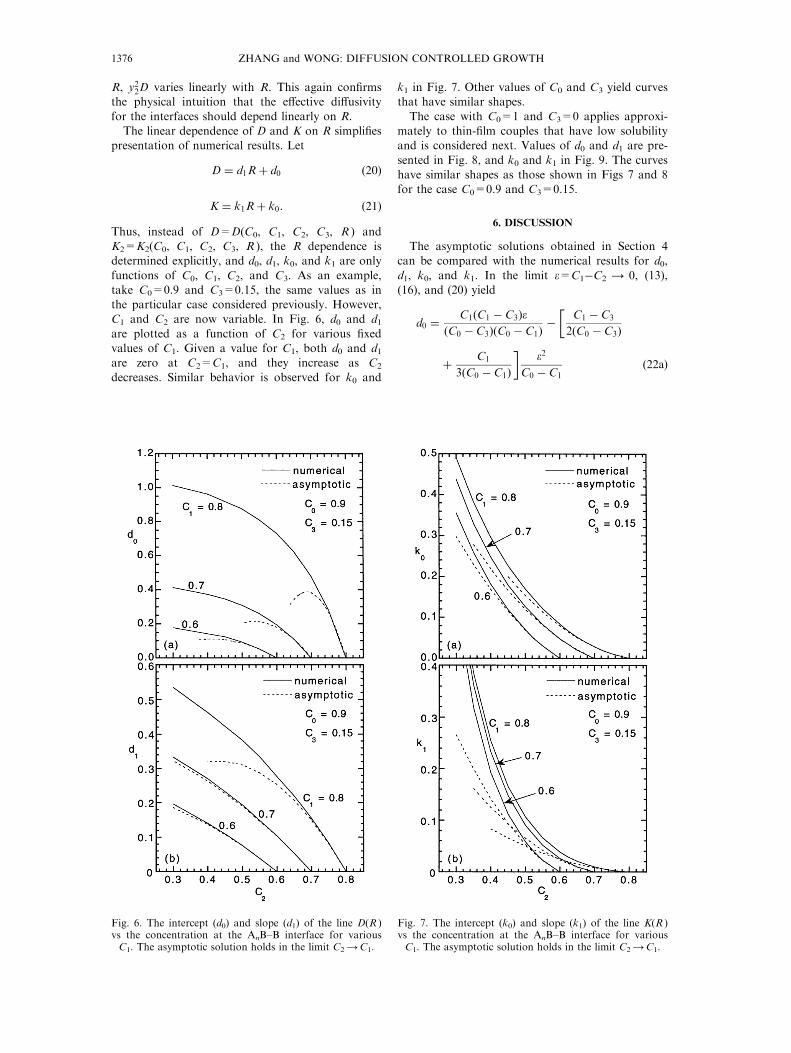
functions of C0, C1, C2, and C3. As an example,take C0=0.9 and C3=0.15, the same values as inthe particular case considered previously. However,C1 and C2 are now variable. In Fig. 6, d0 and d1are plotted as a function of C2 for various ®xedvalues of C1. Given a value for C1, both d0 and d1are zero at C2=C1, and they increase as C2

decreases. Similar behavior is observed for k0 and

k1 in Fig. 7. Other values of C0 and C3 yield curvesthat have similar shapes.

The case with C0=1 and C3=0 applies approxi-mately to thin-®lm couples that have low solubilityand is considered next. Values of d0 and d1 are pre-

sented in Fig. 8, and k0 and k1 in Fig. 9. The curveshave similar shapes as those shown in Figs 7 and 8for the case C0=0.9 and C3=0.15.

6. DISCUSSION

The asymptotic solutions obtained in Section 4can be compared with the numerical results for d0,

d1, k0, and k1. In the limit e=C1ÿC2 4 0, (13),(16), and (20) yield

d0 � C1�C1 ÿ C3�e�C0 ÿ C3��C0 ÿ C1� ÿ

�C1 ÿ C3

2�C0 ÿ C3�

� C1

3�C0 ÿ C1��

e2

C0 ÿ C1�22a�

Fig. 7. The intercept (k0) and slope (k1) of the line K(R )vs the concentration at the AnB±B interface for variousC1. The asymptotic solution holds in the limit C24C1.

Fig. 6. The intercept (d0) and slope (d1) of the line D(R )vs the concentration at the AnB±B interface for variousC1. The asymptotic solution holds in the limit C24C1.


d1 � �1ÿ C1��C1 ÿ C3�e�C0 ÿ C3��C0 ÿ C1� �

�C1 ÿ C3

2�C0 ÿ C3�

ÿ 1ÿ C1

3�C0 ÿ C1��

e2

C0 ÿ C1: �22b�

To ®nd k0 and k1, the expansions in (13) and (14)are substituted into (19) to give K � D1H

20e�

�2D1H0H1 � D2H20�e2: The solutions in (16) and

(17) together with (21) lead to

k0 � C1�C0 ÿ C1�e�C0 ÿ C3��C1 ÿ C3�

� �C1�C0 � 3C1 ÿ 7C3� � 3C0C3�e26�C0 ÿ C3��C1 ÿ C3�2

�23a�

k1 � �1ÿ C1��C0 ÿ C1�e�C0 ÿ C3��C1 ÿ C3�

ÿ �C1�C0 � 3C1 ÿ 7C3� � 3C0C3 ÿ 4�C0 ÿ C3��e26�C0 ÿ C3��C1 ÿ C3�2

:

�23b�

These asymptotic series are also plotted in Figs 6±9.In all cases, the agreement with numerical results

improves as C2 4 C1. In general, the asymptoticsolutions are su�ciently accurate if C1ÿC2 < 0.1.This accurate range of C1±C2 can be increased if C1

decreases and di�ers more from C0. The compari-son not only shows the range where the asymptoticsolutions are applicable, but also con®rms the val-

idity of both the asymptotic and the numerical sol-utions.There is yet another analytic solution that can be

compared with the numerical data. If the interdi�u-sion coe�cient DÄ is constant (i.e. R = 1), then thegoverning equation is linear and an analytic sol-ution exists [23]:

C� y� � F1 ÿ F2 erf� y��D=2

p� �24�

F1 � C1 erf� y2��D=2p � � C2 erf� ��

D=2p �

erf� y2��D=2p � � erf� ��

D=2p � �25a�

Fig. 8. The intercept (d0) and slope (d1) of the line D(R )vs the concentration at the AnB±B interface for variousC1. The asymptotic solution holds in the limit C24C1.

Fig. 9. The intercept (k0) and slope (k1) of the line K(R )vs the concentration at the AnB±B interface for variousC1. The asymptotic solution holds in the limit C24C1.


F2 � C1 ÿ C2

erf� y2��D=2p � � erf� ��

D=2p � , �25b�

where D and y2 are determined by the followingtwo equations:

C1 ÿ C2

C2 ÿ C3� y2

��pD=2

pexp� y22D=2�

herf� y2

��D=2

p� � erf�

��D=2

p�i �26a�

C1 ÿ C2

C0 ÿ C1�

��pD=2

pexp�D=2�

herf� y2

��D=2

p� � erf�

��D=2

p�i:

�26b�

The concentration pro®le, D, y2, and K �� y22D� arecompared with the numerical results for R = 1 inFigs 2±5. The agreement again validates the compu-

tational method and results.The self-similar solution can be used to measure

the intrinsic di�usion coe�cients DA and DB. From

the self-similar solution, the interfacial positionsx1(t ) and x2(t ) can be solved from (9c) and (18)with the initial conditions that x1=x2=0 at t=0:

x 1 ��2DDBt

p�27�

x 2 ��2KDBt

p: �28�

Thus, the width of the compound layer is

W � x 1 � x 2 �ÿ ��

Dp�

��Kp � ��

2DBtp

: �29�

In most experiments, the layer width W is measuredas a function of t, and plotted against t 1/2. Thedata form a straight line if the growth is controlled

by di�usion:

W � pt1=2: �30�

The slope p is found from the data, and comparisonof (29) with (30) yields

p ��2DB

p � ��d1R� d0

p�

��k1R� k0

p �, �31�

where D and K have been replaced using (20) and

(21) to show explicitly their dependence on R. In(31), d0, d1, k0, k1 are functions of only C0, C1, C2,and C3, as shown in Figs 6±9. Thus, they are deter-

mined once a thin-®lm binary di�usion couple ischosen. Hence, only two unknowns are left in (31):R and DB. If either one is given, then the other can

be found from (31), and DA follows immediatelyfrom DA=RDB.One way of completing the solution is by measur-

ing the concentration pro®le. Fitting the computedconcentration pro®le to the experimental data yieldsa value for R. Once R is known, DB (and henceDA) follows from (31). However, because the con-

centration pro®le is insensitive to R, as seen inFig. 2, this way of completing the solution is bound

to be inaccurate.If the interfacial positions can be measured rela-

tive to a ®xed laboratory frame, then DA and DB

can be found without using the concentration pro-®le. Only a point of the laboratory frame is neededas a reference. This could be a marker point in

either the A or B ®lm away from the compoundlayer. For illustrative purposes, let a marker pointbe planted in the A ®lm at x=ÿxm, as shown in

Fig. 1. If z1 is the distance between the markerpoint and the left interface, and z2 that of the rightinterface, then

z1 � ÿx 1 � xm �32�

z2 � x 2 � xm: �33�

Substitution of x1 and x2 from (27) and (28) gives

z1 � ÿ��2DB�d1R� d0�

p ��tp � xm �34�

z2 ��2DB�k1R� k0�

p ��tp � xm: �35�

Plotting z1 and z2 vs t 1/2 yields two straight lines,

the slopes of which are, respectively,

p1 � ÿ��2DB�d1R� d0�

p�36�

p2 ��2DB�k1R� k0�

p: �37�

In an experiment, these slopes are measured bycurve ®tting, and are known. Equations (36) and(37) then determine R and DB, and therefore DA.Thus, both DA and DB are found. Note that the

parabolic growth constants �p21=2 and p22=2� for theinterfaces vary linearly with R, whereas the para-bolic growth constant ( p 2/2) for the compound

layer varies nonlinearly with R, as indicated by(31).As an example, the self-similar solution is used to

calculate the intrinsic di�usion coe�cients of Agand Zn in the b-phase of Ag±Zn alloys. Williams etal. [16] conducted a detailed experimental study ofAg±Zn alloys. An Ag±Zn binary di�usion couple

can form ®ve equilibrium phases. Williams et al.fabricated alloy ingots with di�erent compositionsand used them as the terminal phases of di�usion

couples. By combining two terminal phases withproperly chosen compositions, they were able tostudy the growth rate of any one of the ®ve phases.

The data for the b-phase are the most extensive,and are selected for comparison. Williams et al.measured the thickness of the b-phase layer as a

function of time at 4008C (Table 3 in their paper).When the thickness is plotted against t 1/2, a straightline is obtained, the slope of which is calculated asp = 4.54 � 10ÿ6 m/s1/2. The equilibrium concen-


trations at the interfaces are taken from theirTable 2 for the b-phase as C0=0.46, C1=0.39,

C2=0.327, and C3=0.279, assuming that A is Znand B is Ag. For these equilibrium concentrations,the self-similar solution yields d0=0.1298,

d1=0.2256, k0=0.2097, and k1=0.3853. Thus,everything is known in (31) except R (=DZn/DAg)and DB (=DAg). However, since Williams et al. pre-

sented neither the concentration pro®le nor the lo-cation of the individual interface, there isinsu�cient information for ®nding R or DB.

Heumann and Lohmann [17] measured both thelayer thickness and the concentration pro®le for theb-phase at di�erent temperatures, from which theycalculated DAg and DZn using a method similar to

Kidson's [13]. From their Fig. 15, at 4008C, DAg=2� 10ÿ12 m2/s and DZn=1 � 10ÿ11 m2/s. This meansR=DZn/DAg=5. With this value of R, the self-simi-

lar solution can be completed; equation (31) yieldsDAg=1.54 � 10ÿ12 m2/s, which di�ers from theoriginal value by 23%. Given the large uncertainty

of the original data, this di�erence is acceptable.Hence, the self-similar solution gives at least con-sistent results.

Although this work assumes that only one com-pound phase is formed through interdi�usion, theresults may also apply to a compound layer in amulti-phase binary di�usion couple, if the concen-

trations in the neighboring layers are much moreuniform.

7. CONCLUSIONS

This work studies the di�usion-controlled growthrate of a compound layer in thin-®lm binary di�u-

sion couples. The Kirkendall e�ect is includedwhich makes the di�usion equation nonlinear. Aself-similar transformation reduces the nonlinear

partial di�erential equation with two free bound-aries to a nonlinear ordinary di�erential equation,which is solved numerically by a fourth order

Runge±Kutta method. An iteration scheme is devel-oped for calculation of the unknown boundary lo-cations. It is observed that the parabolic growthconstants for the moving interfaces depend linearly

on the intrinsic di�usion coe�cients DA and DB.Based on this observation, a new method issuggested for determination of DA and DB by

measuring the interfacial positions relative to a®xed marker point. Since the concentration pro®leis not needed in this method, it is simpler than the

methods currently in use. An asymptotic solutionvalid for small composition variation is derived andagrees with the numerical results in the appropriate

limit.

AcknowledgementsÐWe are grateful to Even Ma,Efstathios Meletis, and Aravamudhan Raman for manyhelpful discussions. In addition, we thank Ma for initiat-ing our interest in this work, and Raman and Kurt Schulz

for their comments on the manuscript. Acknowledgment ismade to the Donors of The Petroleum Research Fund,administered by the American Chemical Society(PRF]34049-G5 to HW), and to the Louisiana Board ofRegents (Research Competitiveness Subprogram,LEQSF1999-02-RD-A-21 to HW) for support of thisresearch.

REFERENCES

1. Mayer, J. W. and Lau, S. S., Electronic MaterialsScience: For Integrated Circuits in Si and GaAs.Macmillan, New York, 1990.

2. Tu, K. N., Mayer, J. W. and Feldman, L. C.,Electronic Thin Film Science. Macmillan, New York,1992.

3. Greer, A. L., Appl. Surf. Sci., 1995, 86, 329.4. Greer, A. L., Mater. Sci. Engng, 1991, A134, 1268.5. Wohlert, S. and Bormann, R., J. appl. Phys., 1999,

85, 825.6. Cheng, J. Y. and Chen, L. J., J. appl. Phys., 1991, 69,

2161.7. Michaelsen, C., Yan, Z. H. and Bormann, R., J. appl.

Phys., 1993, 73, 2249.8. Lin, J. H. and Chen, L. J., J. appl. Phys., 1995, 77,

4425.9. Shim, J. Y., Kwak, J. S., Chi, E. J., Baik, H. K. and

Lee, S. M., Thin Solid Films, 1995, 269, 102.10. Shim, J. Y., Kwak, J. S. and Baik, H. K., Thin Solid

Films, 1996, 288, 309.11. Munir, Z. A., High Temp. Sci., 1990, 27, 279.12. Munir, Z. A., Metall. Trans. A, 1992, 23A, 7.13. Kidson, G. V., J. nucl. Mater., 1961, 3, 21.14. Wagner, C., Acta metall., 1969, 17, 99.15. Shatynski, S. R., Hirth, J. P. and Rapp, R. A., Acta

metall., 1976, 24, 1071.16. Williams, D. S., Rapp, R. A. and Hirth, J. P., Metall.

Trans. A, 1981, 12A, 639.17. Heumann, T. and Lohmann, P., Z. Elektrochem.,

1955, 59, 849.18. Shewmon, P. G., Di�usion in Solids. McGraw±Hill,

New York, 1963.19. Crank, J., The Mathematics of Di�usion. Oxford

University Press, London, 1975.20. Crank, J., Free and Moving Boundary Problems.

Oxford University Press, New York, 1984.21. Carslaw, H. S. and Jaeger, J. C., Conduction of Heat

in Solids. Oxford University Press, New York, 1986.22. Zhang, H., Master thesis, Louisiana State University,

2000.23. Jost, W., Di�usion in Solids, Liquids, Gases. Academic

Press, New York, 1960.

APPENDIX A

A.1. Asymptotic solution in the limit of zerocomposition variation

The small parameter is e=C1ÿC2, which is intro-

duced into (9)±(11) by replacing C2=C1ÿe. Thegoverning equation and boundary conditions thenbecome

ÿyDdC

dy� d

dy

��C�1ÿ R� � R�dC

dy

�: �A1�

At the A±AnB interface, y=ÿ1,C � C1 �A2a�


D�C0 ÿ C1� � ÿ�C1�1ÿ R� � R�dCdy: �A2b�

At the AnB±B interface,

y � y2 �A3a�

C � C1 ÿ e �A3b�

y2D�C1 ÿ C3 ÿ e� � ÿ��C1 ÿ e��1ÿ R� � R�dCdy:

�A3c�

The unknowns are expanded in an asymptoticseries:

C� y� � f0� y� � ef1� y� � e2f2� y� � � � � �A4�

D � D0 � eD1 � e2D2 � � � � �A5�

y2 � H0 � eH1 � e2H2 � � � � : �A6�

Since y2 depends on e, the boundary conditions aty=y2 are Taylor expanded and applied at y=H0.

Thus, equation (A3) becomes

y � H0 �A7a�

C� y2� � C1 ÿ e

� C�H0� � � y2 ÿH0�dCdy�H0�

� � y2 ÿH0�22

d2C

dy2�H0� � � � � �A7b�

y2D�C1 ÿ C3 ÿ e� � ÿ ��C1 ÿ e��1ÿ R� � R�

�"

dC

dy�H0� � � y2 ÿH0�d

2C

dy2�H0�

� � y2 ÿH0�22

d3C

dy3�H0� � � � �

#:

The asymptotic expansions (A4)±(A6) are substi-

tuted into (A1), (A2), and (A7). Collection of termsof the same order of e yields a system of equations,which is solved using Maple V

1

. The system of

equations and solutions are listed below for the ®rstthree orders of e:Order e 0

:

� f0�1ÿ R� � R�d2f0

dy2�D0y

df0dy��

df0dy

�2

�1ÿ R� � 0:

�A8�

At y=ÿ1,

f0 � C1 �A9a�

�C0 ÿ C1�D0 � ÿ�C1�1ÿ R� � R�df0dy: �A9b�

At y=H0,

f0 � C1 �A10a�

�C1 ÿ C3�D0H0 � ÿ�C1�1ÿ R� � R�df0dy: �A10b�

The solutions are

f0 � C1 �A11a�

D0 � 0: �A11b�

Order e:

� f0�1ÿ R� � R�d2f1

dy2��2�1ÿ R�df0

dy� yD0

�df1dy

� f1�1ÿ R�d2f0

dy2� yD1

df0dy� 0:

At y=ÿ1,

f1 � 0 �A13a�


At y=H0,

f1 � ÿH1df0dyÿ 1 �A14a�

�C1�1ÿ R� � R�H1d2f0dy2� �Rÿ 1�df0

dy

� �C1 ÿ C3��D0H1 �D1H0� ÿD0H0

� ÿ�C1�1ÿ R� � R�df1dy:

The solutions are

f1 � ÿ�C1 ÿ C3��C0 ÿ C3� � y� 1� �A15a�

D1 � �C1 ÿ C3��C1 � R�1ÿ C1��C0 ÿ C1��C0 ÿ C3� �A15b�

H0 � �C0 ÿ C1��C1 ÿ C3� : �A15c�

Order e 2:


� f0�1ÿ R� � R�d2f2

dy2��2�1ÿ R�df0

dy�D0y

�df2dy

� �1ÿ R� f1

d2f1dy2� f2

d2f0dy2

!� �1ÿ R�

�df1dy

�2

� yD1df1dy� yD2

df0dy� 0:

At y=ÿ1,f2 � 0 �A17a�


At y=H0,

f2 � ÿH21

2

d2f0dy2ÿH1

df1dyÿH2

df0dy

, �A18a�

�C1�1ÿ R� � R� H 2

1

2

d3f0dy3�H1

d2f1dy2

!

� ��1ÿ R��C1H2 ÿH1� � RH2�d2f0

dy2

ÿ �1ÿ R�H1df1dy� �C1 ÿ C3��D0H2

�D1H1 �D2H0� ÿD0H1 ÿD1H0

� ÿ�C1�1ÿ R� � R�df2dy:

The solutions are

f2 � E3y3 � E2y

2 � E1y� E0 �A19a�

D2 � M1R�M0

6�C0 ÿ C1�2�C0 ÿ C3��A19b�

H1 � �C0 ÿ C3�2�C1 ÿ C3�2

, �A19c�

where

E3 � �C1 ÿ C3�26�C0 ÿ C1��C0 ÿ C3�2

�A19d�

E2 � ÿ�C1 ÿ C3�2�1ÿ R�2�C0 ÿ C3�2�C1�1ÿ R� � R� �A19e�

E1 � �Q1R�Q0�6�C0 ÿ C1��C0 ÿ C3�2�C1�1ÿ R� � R� �A19f�

E0 � �U1R�U0�6�C0 ÿ C3�2�C1�1ÿ R� � R� �A19g�

Q1 �ÿ 3C 31 � 3�3C0 � C3 ÿ 1�C 2

1

ÿ �2�4C0 � C3 ÿ 3�C3 � 5C 20�C1

� C 20�3C3 � 2� � C0C3�3C3 ÿ 4� ÿ C 2

3 �A19h�

Q0 � 3C 31 ÿ 3�3C0 � C3�C 2

1 � �5C 20

� 8C0C3 � 2C 23�C1 ÿ 3C0C3�C0 � C3� �A19i�

U1 � C 21 � �C3 ÿ 5C0 � 2�C1 � 3C0C3 ÿ 4C3 � 2C0

�A19j�

U0 � ÿC 21 ÿ C1C3 � 5C0C1 ÿ 3C0C3 �A19k�

M1 � ÿ3C 21 � �5C0 � C3�C1 ÿ �3C3 � 2�C0 � 2C3

�A19l�

M0 � 3C 21 ÿ �5C0 � C3�C1 � 3C0C3: �A19m�


Self-similar growth of a compound layer in thin-film binary diffusion couples

Documents

Transcript of Self-similar growth of a compound layer in thin-film binary diffusion couples