The Summer of the Beautiful White Horse (1940) - Forever ...
Upload
khangminh22Category
view
2download
0
Introduction Institutional framework and identification strategy Data Results Conclusion
School’s out for summer, school’s out forever:the long-term health consequences of leaving
school in a bad economy
Clementine Garrouste1 Mathilde Godard1,2,3
1PSL, Paris-Dauphine University, LEDa-LEGOS2CREST, 3Ecole polytechnique
Journee de la Chaire Sante – 16 mars 2015
1/31

Introduction Institutional framework and identification strategy Data Results Conclusion
Motivation
Motivation
Growing literature on the consequences of early-life conditionson health (Banerjee and al. (2009); Van Den Berg et al.(2006))
Epidemics, famines, war episodes, state of the business cycle atbirth (GDP variation, recession) etc.
More generally, it relates to the life-course approach inepidemiology :
Focus on the long-term effects on health of physical and socialexposures during gestations, childhood, adolescence, youngadulthood and later adult life.
We focus on a critical period in life : first entry on the labourmarket (after graduation).
2/31
Introduction Institutional framework and identification strategy Data Results Conclusion
Motivation
Motivation
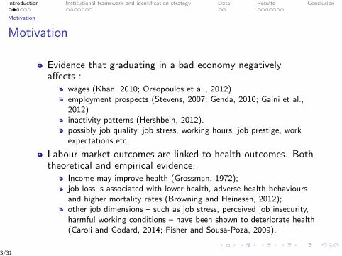
Evidence that graduating in a bad economy negativelyaffects :
wages (Khan, 2010; Oreopoulos et al., 2012)employment prospects (Stevens, 2007; Genda, 2010; Gaini et al.,2012)inactivity patterns (Hershbein, 2012).possibly job quality, job stress, working hours, job prestige, workexpectations etc.
Labour market outcomes are linked to health outcomes. Boththeoretical and empirical evidence.
Income may improve health (Grossman, 1972);job loss is associated with lower health, adverse health behavioursand higher mortality rates (Browning and Heinesen, 2012);other job dimensions – such as job stress, perceived job insecurity,harmful working conditions – have been shown to deteriorate health(Caroli and Godard, 2014; Fisher and Sousa-Poza, 2009).
3/31

Introduction Institutional framework and identification strategy Data Results Conclusion
Motivation
Research question
Does leaving school in a bad economy deteriorate health inthe long-run?
Cumulative effect or initial shock?
Relevant question in the actual context :
where the Great recession has a disproportionate impact onyouth.and young cohorts leaving school face historically highunemployment rates.
4/31

Introduction Institutional framework and identification strategy Data Results Conclusion
Literature and contribution
Literature
Recent and increasing interest in the health consequences ofleaving school in a bad economy.
Maclean (2013) on the NLSY79.Cutler et al. (2014) on Eurobarometer data.Hessel and Avendano (2013) on SHARE.
Recent papers focusing on specific outcomes : drinkingbehaviour, body weight and the probability of having anemployer-provided insurance (Maclean 2014a,b,c) .
5/31

Introduction Institutional framework and identification strategy Data Results Conclusion
Literature and contribution
Our paper
We focus on low-educated individuals who represent asubstantial share (50%) of pupils in the 1970s.
individuals born in 1958 and 1959 in England and Wales wholeft full-time education in their last year of compulsoryschooling immediately after the 1973 oil crisis – between 1974and 1976 .
Our identification strategy ⇒ comparison on very similarindividuals – born the same calendar year – whoseschool-leaving behaviour in worse economic conditions wasexogeneously induced by compulsory schooling laws.
Data ⇒ we use a repeated cross section of individuals over1983-2001 from the General Household Survey (GHS).
6/31

Introduction Institutional framework and identification strategy Data Results Conclusion
Literature and contribution
Contribution to the literature
Evidence in our data that pupils’ decisions to leave school atcompulsory age in 1974-1976 were not endogeneous to thecontemporaneous economic conditions at labour-market entry– unlike school-leavers during the 1980s and 1990s recessions.
Country/state-specific cohort effects cannot possibly bias ourresults.
Life-course perspective (1983-2001 data)
Focus on low-educated individuals
7/31

Introduction Institutional framework and identification strategy Data Results Conclusion
Strategy
Identification strategy
Within a same birth cohort pupils born at the end of thecalendar year are forced to leave school almost a yearlater than their luckier counterparts (born earlier in theyear)– and thus face higher unemployment rates at labourmarket entry.
Consider two cohorts : the 1958 and 1959 cohorts.
Not a before/after comparison. The treatment is to leaveschool in worse conditions than otherwise similar pupils (bornthe same year).
Builds on two sources :
Within-cohort variation introduced by compulsory schoolinglaws (both entry and exit rules).Sharp increase in unemployment rates after the 1973 oil crisis.
8/31

Introduction Institutional framework and identification strategy Data Results Conclusion
Institutional framework
Compulsory schooling laws in England and Wales
Figure 1: Compulsory schooling rules by month-year of birth.
Birth year Month of birth School starting date Allowed to leave school(1) (2) (3) (4)1958 January Sept. 1963 Easter 19741958 February Sept. 1963 May/June 19741958 March Sept. 1963 May/June 19741958 April Sept. 1963 May/June 19741958 May Sept. 1963 May/June 19741958 June Sept. 1963 May/June 19741958 July Sept. 1963 May/June 19741958 August Sept. 1963 May/June 19741958 September Sept. 1964 Easter 19751958 October Sept. 1964 Easter 19751958 November Sept. 1964 Easter 19751958 December Sept. 1964 Easter 1975
1959 January Sept. 1964 Easter 19751959 February to August Sept. 1964 May/June 19751959 September to December Sept. 1965 Easter 1976
9/31

Introduction Institutional framework and identification strategy Data Results Conclusion
Institutional framework
Unemployment rates over the 1973-1979 period
Figure 2: Unemployment rates for all individuals aged 16 (source: LFS)
10/31

Introduction Institutional framework and identification strategy Data Results Conclusion
Empirical approach
Model in the literature
Following Galama et al. (2010), Grossman (1972, 2000) health ismodeled as a stock that deteriorates over the lifespan. Time t ismeasured from the time an individual has completed her educationand joined the labour force (i.e. at 16).
Health is defined as :
H(t) = Im(t)α + (1− d(t))H(t − 1) (1)
where health can be improved through investment in curativemedical care Im(t) and deteriorates at d(t) which depends onhealthy consumption Ch(t) (e.g. healthy food, healthyneighborhood), unhealthy consumption Cu(t) (e.g. smoking),job-related stress z(t) (working environnement) and investment incurative care Ip(t) and on a vector of exogenous functions ξ(t).
11/31

Introduction Institutional framework and identification strategy Data Results Conclusion
Empirical approach
Figure 3: The evolution of health depending on the scenario.
NT
1
2
age
Health
0
12/31

Introduction Institutional framework and identification strategy Data Results Conclusion
Empirical approach
Our model
We use a repeated cross-section of individuals over 1983-2001 to estimatethe following equation by OLS/probit, for men and women separately:
Hi = α + γTi + BirthYeari + InterviewYeari + εi (2)
where Ti is a dummy variable taking value 1 if individual i is treated, i.eborn between the 1st of September and the 31st of December and value 0if non-treated, i.e born between the 1st of January and the 31st of August.
Hi = α + γTi + BirthYeari + f (BirthMonthi ) + InterviewYeari + εi (3)
f (BirthMonthi ) is a quadratic function of age in months within a birthyear. It is equal to (12− BirthMonthi ) + (12− BirthMonthi )
2, whereBirthMonthi denotes the month of birth of respondent i and varies from1 to 12.
13/31

Introduction Institutional framework and identification strategy Data Results Conclusion
Validity of the identification strategy
Endogeneous timing of school-leaving
Figure 4: Proportion of pupils leaving school at binding age (16); Growthin school-leaving unemployment rate
Reading: Growth in school-leaving unemployment rate faced by pupils belonging to the youngest school cohort(treated) – compared to pupils born the same year belonging to the previous school cohort (non-treated).
14/31

Introduction Institutional framework and identification strategy Data Results Conclusion
GHS, sample and variables
The General Household Survey (GHS)
GHS: repeated annual cross-sectional survey of over 13,000households in Great-Britain; ran from 1972-2011.
Includes information on:
demographics – including month-year of birth from 1983 to2001, the survey waves that we useeducation – including the age at which the individual leftfull-time education, the highest qualification obtained.earningshealth status, health care and health behaviours.
A number of the GHS respondents left school immediatelyafter the 1973 oil crisis.
15/31

Introduction Institutional framework and identification strategy Data Results Conclusion
GHS, sample and variables
Our sample
Consider individuals born in 1958 and 1959 who left full-timeeducation as soon as they reached the minimum schoolleaving age – i.e at age 16:
abstract from the 1972 increase in the school minimum leavingage.these individuals leave school between Easter 1974 and Easter1976.
Focus on England and Wales.
Outcomes of interest not collected consistently over theperiod – include all possible observations for each outcome tomaximize sample size.
16/31
Introduction Institutional framework and identification strategy Data Results Conclusion
Main results
Health outcomes (1)
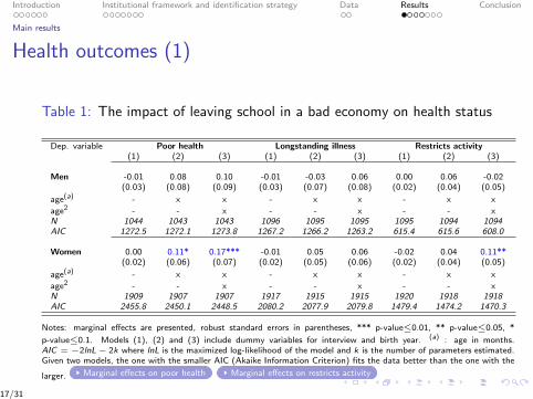
Table 1: The impact of leaving school in a bad economy on health status
Dep. variable Poor health Longstanding illness Restricts activity(1) (2) (3) (1) (2) (3) (1) (2) (3)
Men -0.01 0.08 0.10 -0.01 -0.03 0.06 0.00 0.06 -0.02(0.03) (0.08) (0.09) (0.03) (0.07) (0.08) (0.02) (0.04) (0.05)
age(a) - x x - x x - x x
age2 - - x - - x - - xN 1044 1043 1043 1096 1095 1095 1095 1094 1094AIC 1272.5 1272.1 1273.8 1267.2 1266.2 1263.2 615.4 615.6 608.0
Women 0.00 0.11* 0.17*** -0.01 0.05 0.06 -0.02 0.04 0.11**(0.02) (0.06) (0.07) (0.02) (0.05) (0.06) (0.02) (0.04) (0.05)
age(a) - x x - x x - x x
age2 - - x - - x - - xN 1909 1907 1907 1917 1915 1915 1920 1918 1918AIC 2455.8 2450.1 2448.5 2080.2 2077.9 2079.8 1479.4 1474.2 1470.3
Notes: marginal effects are presented, robust standard errors in parentheses, *** p-value≤0.01, ** p-value≤0.05, *
p-value≤0.1. Models (1), (2) and (3) include dummy variables for interview and birth year. (a) : age in months.AIC = −2lnL− 2k where lnL is the maximized log-likelihood of the model and k is the number of parameters estimated.Given two models, the one with the smaller AIC (Akaike Information Criterion) fits the data better than the one with the
larger. Marginal effects on poor health Marginal effects on restricts activity
17/31
Introduction Institutional framework and identification strategy Data Results Conclusion
Main results
Health outcomes (2)
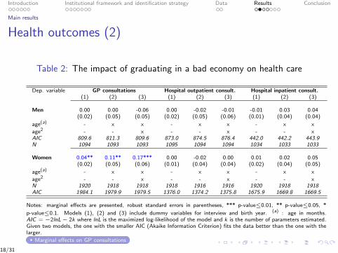
Table 2: The impact of graduating in a bad economy on health care
Dep. variable GP consultations Hospital outpatient consult. Hospital inpatient consult.(1) (2) (3) (1) (2) (3) (1) (2) (3)
Men 0.00 0.00 -0.06 0.00 -0.02 -0.01 -0.01 0.03 0.04(0.02) (0.05) (0.05) (0.02) (0.05) (0.06) (0.01) (0.04) (0.04)
age(a) - x x - x x - x x
age2 - - x - - x - - xAIC 809.6 811.3 809.6 873.0 874.5 876.4 442.0 442.2 443.9N 1094 1093 1093 1095 1094 1094 1034 1033 1033
Women 0.04** 0.11** 0.17*** 0.00 -0.02 0.00 0.01 0.02 0.05(0.02) (0.05) (0.06) (0.01) (0.04) (0.04) (0.02) (0.04) (0.05)
age(a) - x x - x x - x x
age2 - - x - - x - - xN 1920 1918 1918 1918 1916 1916 1920 1918 1918AIC 1984.1 1979.9 1979.5 1376.0 1374.2 1375.8 1675.9 1669.8 1669.5
Notes: marginal effects are presented, robust standard errors in parentheses, *** p-value≤0.01, ** p-value≤0.05, *
p-value≤0.1. Models (1), (2) and (3) include dummy variables for interview and birth year. (a) : age in months.AIC = −2lnL− 2k where lnL is the maximized log-likelihood of the model and k is the number of parameters estimated.Given two models, the one with the smaller AIC (Akaike Information Criterion) fits the data better than the one with thelarger.
Marginal effects on GP consultations
18/31

Introduction Institutional framework and identification strategy Data Results Conclusion
Main results
Health outcomes (3)
Table 3: The impact of graduating in a bad economy on health behaviour
Dep. variable Currently smokes Ever smoked Drinking(b)
(1) (2) (3) (1) (2) (3) (1) (2) (3)
Men 0.04 0.09 0.22* 0.06* 0.17** 0.27*** -0.02 -0.03 0.02(0.04) (0.11) (0.12) (0.03) (0.08) (0.09) (0.04) (0.11) (0.12)
age(a) - x x - x x - x x
age2 - - x - - x - - xN 619 618 618 619 618 618 597 596 596AIC 852.7 853.1 851.1 687.7 684.0 682.4 844.8 845.5 846.8
Women -0.01 0.04 0.02 -0.01 0.09 0.09 0.04 0.01 -0.01(0.03) (0.08) (0.09) (0.03) (0.07) (0.08) (0.03) (0.08) (0.09)
age(a) - x x - x x - x x
age2 - - x - - x - - xN 1029 1027 1027 1029 1027 1027 945 943 943AIC 1416.1 1414.6 1416.5 1280.8 1279.5 1281.5 1202.3 1201.3 1203.2
Notes: marginal effects are presented, robust standard errors in parentheses, *** p-value≤0.01, ** p-value≤0.05, * p-
value≤0.1. Models (1), (2) and (3) include dummy variables for interview and birth year. (a) : age in months. (b) :moderate to heavy drinking. AIC = −2lnL − 2k where lnL is the maximized log-likelihood of the model and k is thenumber of parameters estimated. Given two models, the one with the smaller AIC (Akaike Information Criterion) fits thedata better than the one with the larger.
Marginal effects on smoking behaviour
19/31
Introduction Institutional framework and identification strategy Data Results Conclusion
Main results
Health outcomes (4)
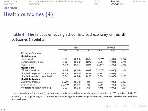
Table 4: The impact of leaving school in a bad economy on healthoutcomes (model 3)
Men Womenm.e. s.e. N m.e. s.e. N
Probit estimationsHealth statusPoor health 0.10 (0.09) 1043 0.17*** (0.07) 1907Longstanding illness 0.06 (0.08) 1095 0.06 (0.06) 1915Restricts act -0.03 (0.05) 1094 0.11** (0.05) 1918Health careGP consultations -0.06 (0.05) 1093 0.17*** (0.06) 1918Hospital outpatient consultation -0.09 (0.06) 1094 -0.00 (0.04) 1916Hospital inpatient consultation 0.04 (0.04) 1033 0.05 (0.05) 1918Health behaviourCurrently smokes 0.22* (0.12) 618 0.03 (0.09) 1027Ever smoked 0.27*** (0.09) 618 0.09 (0.08) 1027Moderate to heavy drinking 0.02 (0.13) 596 -0.01 (0.09) 943
Notes: marginal effects (m.e.) are presented, robust standard errors in parentheses (s.e.), *** p-value≤0.01, **
p-value≤0.05, * p-value≤0.1. Our models include age in month, (age in month)2, dummy variables for interviewand birth year.
20/31

Introduction Institutional framework and identification strategy Data Results Conclusion
Robustness checks
Robustness checks
Run a placebo test using the 1953 and 1954 cohorts – eachschool cohort faced same school-leaving unemployment ratesat the end of compulsory schooling. Placebo test
Differential incentives to take the GCE O-Level/CSEexaminations at the end of Year 11.
Our results are virtually unchanged when controlling by adummy indicating whether an individual holds a Year-11equivalent degree.
Results virtually unchanged when using school-leavingunemployment rates instead of dummy variable Ti .
21/31

Introduction Institutional framework and identification strategy Data Results Conclusion
Mechanisms
Labour-market outcomes
Table 5: The impact of leaving school in a bad economy onlabour-market outcomes (model 3)
Men Womenm.e. s.e. N m.e. s.e. N
Probit regressionsEconomic statusKeeping house 0.01 (0.03) 495 0.07 (0.07) 1918Unemployed 0.06 (0.06) 1095 -0.02 (0.03) 1918For those currently employedLess than 1 month 0.04 (0.05) 512 0.05 (0.04) 805Less than 3 months -0.02 (0.05) 613 0.06 (0.07) 861Less than 6 months -0.04 (0.06) 723 0.03 (0.08) 861Less than 1 year 0.01 (0.09) 723 -0.05 (0.09) 861Less than 5 years -0.00 (0.11) 723 -0.06 (0.10) 861More than 5 years 0.00 (0.11) 723 0.06 (0.10) 861
Linear regressionsEarnings (log) -0.03 (0.11) 799 -0.17 (0.17) 957
Notes: marginal effects (m.e.) are presented, robust standard errors in parentheses (s.e.), *** p-value≤0.01, **
p-value≤0.05, * p-value≤0.1. Our models include age in month, (age in month)2, dummy variables for interviewand birth year.
22/31

Introduction Institutional framework and identification strategy Data Results Conclusion
Summary results
Summary results
Leaving school in a bad economy :
seems to increase poor health, GP consultations, restrictsactivity among women.may affect smoking behaviour among men.has no effect – for both men and women – on unemployment,inactivity patterns and earnings.
23/31

Introduction Institutional framework and identification strategy Data Results Conclusion
Conclusion
Leaving school in a bad economy :
seems to increase GP consultations, poor health andprobability to declare restricts activity among low-educatedwomen in the UK.may affect smoking behaviour among men.
Additional piece of evidence in a new and increasing literature.
Cumulative effect versus initial shock?
24/31

Introduction Institutional framework and identification strategy Data Results Conclusion
Limitations
External validity :
similarity between the 1958-1959 cohorts and current cohortsof school-leavers ?similarity between the 1973 oil crisis and current Greatrecession ?
25/31

Introduction Institutional framework and identification strategy Data Results Conclusion
References
CUTLER, D., W. HUANG AND A. LLERAS-MUREY (2014) ”When Does Education Matter? TheProtective Effect of Education for Cohorts Graduating in Bad Times” National Bureau of EconomicResearch Working paper No. 20156.
GENDA, Y., A. KONDO, AND S. OHTA (2010): ”Long-term effects of a recession on labour-market entryin Japan and the United States”, Journal of Human Resources, 45(1).
HERSHBEIN, B. J (2012) ”Graduating High School in a Recession: Work, Education, and HomeProduction”, The BE journal of economic analysis & policy, 12.
HESSEL, P. AND M. AVENDANO (2013) ”Are economic recessions at the time of leaving schoolassociated with worse physical functioning in later life?” Annals of epidemiology 23, 708–715
KAHN, L. B. (2010): ”The long-term labor market consequences of graduating from college in a badeconomy”, Labour Economics, 17(2), 303–316.
MACLEAN J. C. (2013) ”The health effects of leaving school in a bad economy” Journal of healtheconomics, 32, 951–964
MACLEAN J. C. (2014a): ”Does leaving school in an economic downturn impact access toemployer-sponsored health insurance?” IZA Journal of Labor Policy, 3, 19.
MACLEAN J. C. (2014b): ”Does leaving school in an economic downturn persistently affect body weight?Evidence from panel data,” mimeo.
MACLEAN J. C. (2014c): ”The Lasting Effects of Leaving School in an Economic Downturn on AlcoholUse,” Industrial and Labor Relations Review, forthcoming.
OREOPOULOS, P., T. VON WACHTER, AND A. HEISZ (2012): ”The short and long-term career effectsof graduating in a recession”, American Economic Journal: Applied Economics, 4(1), 1–29.
STEVENS, K. (2007): ”Adverse economic conditions at labour market entry: Permanent scars or rapidcatch-up”, Department of Economics, University College London, Job market paper.
26/31
Introduction Institutional framework and identification strategy Data Results Conclusion
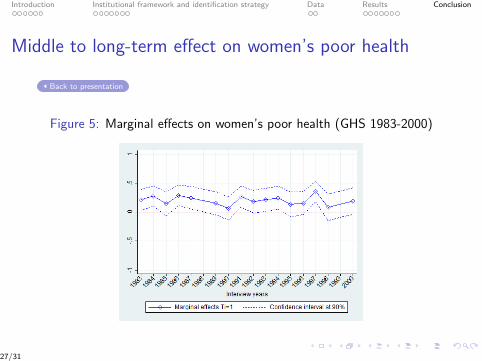
Middle to long-term effect on women’s poor health
Back to presentation
Figure 5: Marginal effects on women’s poor health (GHS 1983-2000)
27/31

Introduction Institutional framework and identification strategy Data Results Conclusion
Middle to long-term effect on women’s restricts activityillness
Back to presentation
Figure 6: Marginal effects on women’s restricts activity (GHS 1983-2000)
28/31

Introduction Institutional framework and identification strategy Data Results Conclusion
Middle to long-term effect on women’s GP consultations
Back to presentation
Figure 7: Marginal effects on consulting GP during the two weekspreceding the interview (GHS 1983-2000)
29/31
Introduction Institutional framework and identification strategy Data Results Conclusion
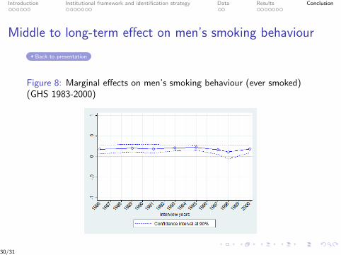
Middle to long-term effect on men’s smoking behaviour
Back to presentation
Figure 8: Marginal effects on men’s smoking behaviour (ever smoked)(GHS 1983-2000)
30/31

Introduction Institutional framework and identification strategy Data Results Conclusion
Placebo test
Back to presentation
Table 6: The impact of leaving school in a bad economy on healthoutcomes for the 1953-54 cohorts (model 3)
Men Womenm.e. s.e. N m.e. s.e. N
Probit estimationsHealth statusPoor health -0.05 (0.11) 631 -0.13 (0.08) 1204Longstanding ill 0.06 (0.11) 664 -0.02 (0.08) 1210Restricts act 0.00 (0.07) 663 -0.02 (0.06) 1213Health careGP consultations -0.04 (0.06) 664 0.04 (0.07) 1211Hospital outpatient consultation -0.10 (0.06) 664 -0.08 (0.05) 1212Hospital inpatient consultation -0.02 (0.04) 619 -0.07 (0.05) 1212Health behaviourCurrently smokes -0.09 (0.15) 390 0.18 (0.11) 653Ever smoked 0.03 (0.11) 362 0.10 (0.09) 653Moderate to heavy drinking -0.24 (0.15) 372 -0.04 (0.11) 617
Notes: marginal effects (m.e.) are presented, robust standard errors in parentheses (s.e.), *** p-value≤0.01, **
p-value≤0.05, * p-value≤0.1. Our models include age in month, (age in month)2, dummy variables for interviewand birth year.
31/31

IntroductionFrench regulation of ambulatory care
Data & Empirical strategyResults
Conclusion
Does health insurance encourage the rise in medical prices?A test on balance billing in France
Brigitte DORMONT, Mathilde PERON
PSL, Université Paris Dauphine
16 March 2015
Journée de la Chaire

IntroductionFrench regulation of ambulatory care
Data & Empirical strategyResults
Conclusion
1 Introduction
2 French regulation of ambulatory care
3 Data & Empirical strategy
4 Results
5 Conclusion
Journée de la Chaire
IntroductionFrench regulation of ambulatory care
Data & Empirical strategyResults
Conclusion
MotivationResearch QuestionLiterature
Motivation
Social health insurances are designed to favor access to care
BUT the e�ectiveness of coverage depends on their ability to controlprices
Balance billing : physicians are allowed to charge their patients
more than the regulated fee
Increase in out-of-pocket (OOP) payments
SHI coverage might favor the demand for expensive physicians whoincrease their fees in return
Increase in premiums for SHI policyholders or/and increase in OOP
Journée de la Chaire

IntroductionFrench regulation of ambulatory care
Data & Empirical strategyResults
Conclusion
MotivationResearch QuestionLiterature
Policy Questions
Should balance billing be restricted or forbidden ?
Should coverage of balance billing be restricted ?
Should the government only monitor the supply for care ?
Should the government allow balance billing to promote variouslevels of care quality ?
Journée de la Chaire

IntroductionFrench regulation of ambulatory care
Data & Empirical strategyResults
Conclusion
MotivationResearch QuestionLiterature
Purpose of this paper
Measure the causal impact of a positive shock on supplementary
health coverage on the use of physicians who charge balance billing
Scope: France, 2010-2012Ambulatory care, specialists consultations
At stake: Moral hazard induces in�ationary e�ect on medical pricesBB can increase welfare through higher quality of care
Other questions: What is the in�uence of supply organization ?Does balance billing limit access to care ?
Journée de la Chaire

IntroductionFrench regulation of ambulatory care
Data & Empirical strategyResults
Conclusion
MotivationResearch QuestionLiterature
Literature (1/2)
What is the e�ect of Balance billing on social welfare ?
Balance billing is just a transfer from patients with high WTP to physicians
Paringer (1980), Mitchell & Cromwell (1982), Zuckerman & Holahan (1989)
Balance billing allows physicians to perform higher quality of care
Glazer & McGuire (1993), Kifmann & Scheuer (2011)
Balance billing might limit access to care
Jelovac (2013)
Empirical evidences
McKnight (2007), US data : limiting BB reduces OOP without any change onhealth care use → simple rent extraction ?
Desprès and alii (2011), French data : foregone care is more frequent in regionswhere BB is higher → health care access issues ?
Journée de la Chaire

IntroductionFrench regulation of ambulatory care
Data & Empirical strategyResults
Conclusion
MotivationResearch QuestionLiterature
Literature (2/2)
What could be the e�ect of a generous coverage on BB ?
(1) On the supply side : physicians may increase their fees in response toinsurance coverage
Feldstein (1970, 1973), Sloan (1982), Feldman & Dowd (1991), Chiu(1997), Vaithianathan (2006)
(2) On the demand side :
Moral hazard : "the slope of health care spending, with respect to price"
(Einav, Finkelstein and alii, 2013)
Assuming a negative price elasticity of demand, a better coverage leads toa decrease in net health care price and an increase in health careconsumption
Pauly (1974), RAND experiments (1987), Chiappori (1998)
Journée de la Chaire
IntroductionFrench regulation of ambulatory care
Data & Empirical strategyResults
Conclusion
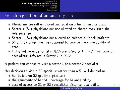
French regulation of ambulatory care
Physicians are self-employed and paid on a fee-for-service basisSector 1 (S1) physicians are not allowed to charge more than thereference feeSector 2 (S2) physicians are allowed to balance bill their patientsS1 and S2 physicians are supposed to provide the same quality ofcareBB is not an issue for GPs: 87% are is Sector 1 in 2012 → focus onspecialists: 42% are is Sector 2 in 2012
A patient can choose to visit a sector 1 or a sector 2 specialist
Her decision to visit a S2 specialist rather than a S1 will depend on
her beliefs on S2 quality : g(x1, x2)the generosity of her SHI coverage for balance billingcost of access to S1 or S2 specialists: distance, availability
Journée de la Chaire

The decision to consult a S2 specialist
bb : balance billing s : supplementary insurance coveraged1, d2 : costs relative to search, transportation and waiting time for a visit in S1 or S2
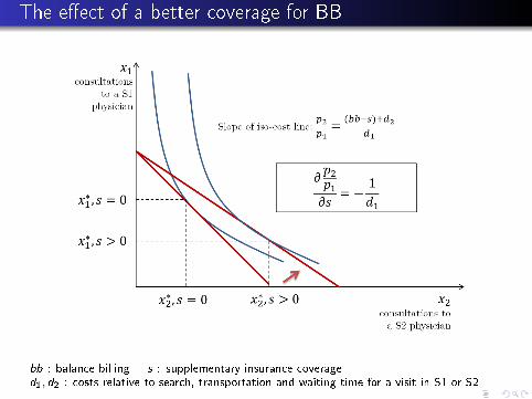
The e�ect of a better coverage for BB
bb : balance billing s : supplementary insurance coveraged1, d2 : costs relative to search, transportation and waiting time for a visit in S1 or S2

Availability of S1 and S2 specialists and BB

IntroductionFrench regulation of ambulatory care
Data & Empirical strategyResults
Conclusion
DataEmpirical strategy
1 Introduction
2 French regulation of ambulatory care
3 Data & Empirical strategyDataEmpirical strategy
4 Results
5 Conclusion
Journée de la Chaire

IntroductionFrench regulation of ambulatory care
Data & Empirical strategyResults
Conclusion
DataEmpirical strategy
Data
MGEN features :
"Mutuelle" : Non Pro�t insurance cooperative
MGEN is mandatory for teachers for basic HI
MGEN Supplemental health insurance is voluntary
There is only one SHI contract with no BB coverage
SHI premium are proportional to wage
Variables, from 2010 to 2012 :
socio-dem characteristics, income, health, specialist:population ratios (SPR)
health care consumption before and after switching
Journée de la Chaire
IntroductionFrench regulation of ambulatory care
Data & Empirical strategyResults
Conclusion
DataEmpirical strategy
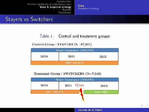
Stayers vs Switchers
Table 1 : Control and treatment groups
Journée de la Chaire

IntroductionFrench regulation of ambulatory care
Data & Empirical strategyResults
Conclusion
DataEmpirical strategy
Variables of interest
After they quit MGEN, do switchers visit specialists more often ?
Number of visits to a specialist : Q
Do they consume a higher share of sector 2 consultations ?
Share of S2 visits in the total number of visits : Q2/QAverage amount of balance billing per visit : BB/Q
Do sector 2 specialists charge them more ?
Average amount of balance billing per sector 2 visit : BB/Q2
Journée de la Chaire

IntroductionFrench regulation of ambulatory care
Data & Empirical strategyResults
Conclusion
DataEmpirical strategy
Empirical speci�cation
(1) Estimation with �xed e�ects on years 2010 and 2012 (OLS)
Yit = β0 + τQUITit + λ2012t + β1Xit + β2Sit + αi + εit , t = 2010, 2012
QUIT = 1 for Switchers in 2012, 0 else ; 2012 = 1 in 2012, 0 elseXit : demand characteristics ; Sit : supply characteristics ; αi : individual �xed e�ect
This speci�cation allows for possible correlation between individualunobserved heterogeneity and decision to quit
(2) IV estimation with �xed e�ects (2SLS)
The e�ect of a better coverage is identi�ed and consistent even ifCov(QUITit , εit) 6= 0 provided that instruments are exogenous andcorrelated with QUIT
We use retirement in 2011 before 55 and moving in 2011 as excludedinstruments
Journée de la Chaire

IntroductionFrench regulation of ambulatory care
Data & Empirical strategyResults
Conclusion
Descriptive statisticsImpact of a better coverage on balance billing
1 Introduction
2 French regulation of ambulatory care
3 Data & Empirical strategy
4 ResultsDescriptive statisticsImpact of a better coverage on balance billing
5 Conclusion
Journée de la Chaire
IntroductionFrench regulation of ambulatory care
Data & Empirical strategyResults
Conclusion
Descriptive statisticsImpact of a better coverage on balance billing
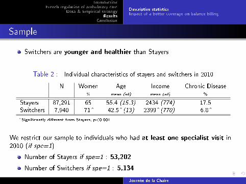
Sample
Switchers are younger and healthier than Stayers
Table 2 : Individual characteristics of stayers and switchers in 2010
N Women Age Income Chronic Disease% mean (sd) mean (sd) %
Stayers 87,291 65 55.4 (15.3) 2434 (774) 17.5Switchers 7,940 71ˆ 42.5ˆ(13) 2399ˆ(770) 6.8ˆ
ˆSigni�cantly di�erent from Stayers, p<0.001
We restrict our sample to individuals who had at least one specialist visit in2010 (if spe=1)
Number of Stayers if spe=1 : 53,202
Number of Switchers if spe=1 : 5,134
Journée de la Chaire

IntroductionFrench regulation of ambulatory care
Data & Empirical strategyResults
Conclusion
Descriptive statisticsImpact of a better coverage on balance billing
Balance billing consumption
Table 3 : Total amount of balance billing in 2010, if Spe=1
Whole sample Low SPR in S2 High SPR in S2mean (sd) mean (sd) mean (sd)
BB Stayers 30 (58.9) 11.5 (31.2) 42 (74)if Spe=1 Switchers 41ˆ(72.8) 13 (26.7) 53.6ˆ(85.5)
ˆSigni�cantly di�erent from Stayers, p<0.001
Even when they had no BB coverage, Switchers consumed morebalance billing than Stayers in 2010
When controlling for income, chronic disease, and supply side drivers,the average amount of BB per consultation is 19% higher forswitchers
Journée de la Chaire

E�ect of SHI coverage - Whole sample
A better SHI coverage increases by 9% the share of S2 consultations,with no impact on the number of visits to a specialist
Table 4 : E�ect of a more comprehensive coverage on balance billing
Estimations with individual �xed e�ects, T=2010,2012
log(Q) log(Q2/Q) log(BB/Q) log(BB/Q2)
(1) Whole sampleOLS 0.00 0.01 0.04* -0.00
2SLS \† 0.15 0.09** 0.34* -0.15
* p<0.1, ** p<0.05, *** p<0.01 (1)N=58,336
Control: 2012, income, CD, inpatient stays, GP, specialist population ratio, exp. phy.
Instruments : \ = Retired before 55; † = moved out
Tests for 2SLS regression on log(Q2/Q)
*Instruments are well correlated with QUIT (First stage Fstat = 336)*Exogeneity of QUIT rejected (Hausman test stat=4.66 (p-value=0.03))*Sargan test stat=0.048 (p-value=0.82)

E�ect of SHI coverage and supply side organization (1/3)
Table 5 : Crossed levels of S1 and S2 specialist:population ratios in 2010

E�ect of SHI coverage and supply side organization (2/3)
Positive and signi�cant impact of SHI on the share of S2consultations (+19%) for patients who lived in regions with a highsector 2 specialist:population ratio (50% of our sample)
Table 6 : E�ect of a more comprehensive coverage on balance billing
Estimation with individual �xed e�ects, T=2010,2012
log(Q) log(Q2/Q) log(BB/Q) log(BB/Q2)
(5) Low SPR2OLS -0.05 0.01 0.06 0.08
2SLS \ 0.56 0.04 -0.52 -0.91*(6) High SPR2
OLS 0.03 0.01* 0.08** 0.002SLS \ 0.14 0.19*** 0.80** 0.01
* p<0.1, ** p<0.05, *** p<0.01 (5)N=6,248 ; (6)N=28,711
Control: 2012, income, CD, inpatient stays, GP, specialist population ratio, exp. phy.
Instruments : \ = Retired before 55
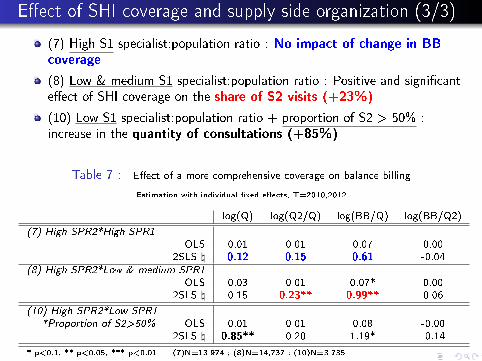
E�ect of SHI coverage and supply side organization (3/3)
(7) High S1 specialist:population ratio : No impact of change in BBcoverage
(8) Low & medium S1 specialist:population ratio : Positive and signi�cante�ect of SHI coverage on the share of S2 visits (+23%)
(10) Low S1 specialist:population ratio + proportion of S2 > 50% :increase in the quantity of consultations (+85%)
Table 7 : E�ect of a more comprehensive coverage on balance billing
Estimation with individual �xed e�ects, T=2010,2012
log(Q) log(Q2/Q) log(BB/Q) log(BB/Q2)
(7) High SPR2*High SPR1OLS 0.01 0.01 0.07 0.00
2SLS \ 0.12 0.15 0.61 -0.04(8) High SPR2*Low & medium SPR1
OLS 0.03 0.01 0.07* 0.002SLS \ 0.15 0.23** 0.99** 0.06
(10) High SPR2*Low SPR1*Proportion of S2>50% OLS 0.01 0.01 0.08 -0.00
2SLS \ 0.85** 0.20 1.19* -0.14
* p<0.1, ** p<0.05, *** p<0.01 (7)N=13,974 ; (8)N=14,737 ; (10)N=3,735
Control: 2012, income, CD, inpatient stays, GP, specialist population ratio, exp. phy.
Instruments : \ = Retired before 55

Robustness checks (1/2)
Only one instrument (retired before 55) can be used for estimationon local sub-samples
One has to check the robustness of estimates on total sample withthis instrument
Table 8 : Estimations on total sample with one or two instruments
log(Q) log(Q2/Q) log(BB/Q) log(BB/Q2)
(1) Whole sample2SLS \† 0.15 0.09** 0.34* -0.152SLS \ 0.15 0.08* 0.29 -0.05
* p<0.1, ** p<0.05, *** p<0.01 (1)N=58,336
Control: 2012, income, CD, inpatient stays, GP, specialist population ratio, exp. phy.
Instruments : \ = Retired before 55; † = moved

Robustness checks (2/2)
The instrument retired before 55 concerns mostly womenOne has to check the robustness of results when restricting thesample to women younger than 56
Table 9 : Estimation on women below 56
log(Q) log(Q2/Q) log(BB/Q) log(BB/Q2)
(5) Low SPR22SLS \ 0.56 0.04 -0.52 -0.91*
Women under 56 - 2SLS \ 1.35** 0.00 -0.60 -0.91*(6) High SPR2
2SLS \ 0.14 0.19*** 0.80** 0.01Women under 56 - 2SLS \ 0.57** 0.21** 0.99** 0.04
(7) High SPR2*High SPR12SLS \ 0.12 0.15 0.61 -0.04
Women under 56 - 2SLS \ 0.51 0.11 0.52 -0.08(8) High SPR2*Low & medium SPR1
2SLS \ 0.15 0.23** 0.99** 0.06Women under 56 - 2SLS \ 0.64 0.31** 1.44** 0.18
* p<0.1, ** p<0.05, *** p<0.01
Control: 2012, income, CD, inpatient stays, GP, specialist population ratio, exp. phy.
Instruments : \ = Retired before 55

IntroductionFrench regulation of ambulatory care
Data & Empirical strategyResults
Conclusion
1 Introduction
2 French regulation of ambulatory care
3 Data & Empirical strategy
4 Results
5 Conclusion
Journée de la Chaire

IntroductionFrench regulation of ambulatory care
Data & Empirical strategyResults
Conclusion
Main �ndings (1/2)
Evidence of moral hazard
A better coverage of balance billing by supplemental health insurance leadspatients to increase the share of S2 visits
Heterogeneity in preferences for sector 2 specialists
Switchers use more S2 specialists and pay more BB
Journée de la Chaire

IntroductionFrench regulation of ambulatory care
Data & Empirical strategyResults
Conclusion
Main �ndings (2/2)
Heterogeneity in the impact of better SHI coverage
No signi�cant impact of better coverage in areas where
there are few S2 specialists (who balance bill their patients)there are enough S1 specialists (who charge the regulated fee)
There is a positive impact of better coverage on the share of S2 visits(+23%) and the average BB (+99%) in areas where
there are many S2 specialists, and not many S1 specialists (highS2*low and medium S1)concerns about 25% of the population
Some evidence of limitation in access to care in areas with more than 50%S2 and few S1
concerns about 6% of the population (but teachers are not poorpeople)
Journée de la Chaire

IntroductionFrench regulation of ambulatory care
Data & Empirical strategyResults
Conclusion
Policy consequences
Evidence of heterogeneity in preferences for S2 specialistsWhen there is a su�cient number of S1 specialists there is no limitationin access to care nor in�ationist impact of more generous supplementalcoverage.
The issues regarding balance billing could be solved with a better
monitoring of supply for care
If there were enough Sector 1 specialists, it would be not
necessary to introduce limitation in the coverage supplied by SHI
Journée de la Chaire

merci !
Does health insurance encourage the rise in medical prices?A test on balance billing in France
Brigitte DORMONT, Mathilde PERON
PSL, Université Paris Dauphine
16 March 2015
Joint elicitation of health and income expectations:Insights from a representative survey of the French
Population.
Stéphane LuchiniAMSE/GREQAM-CNRS
March 2014 - Journée de la Chaire Santé

Team
Brigitte Dormont (Université Paris-Dauphine)Marc Fleurbaey (Princeton University)Anne-Laure Samson (Université Paris-Dauphine)Stéphane Luchini (AMSE-CNRS)Erik Schokkaert (KU Leuven)Clémence THEBAUT (HAS)Carine Vandevoorde (KU Leuven)
Part of a larger project: “Valeur de la santé” (Chaire Santé Dauphine)(that links expectations with preferences)
Joint elicitation of health and income expectations: Insights from a representative survey of the French Population.2 / 19
Introduction
Introduction
Expectations, together with preferences, are a key component ofeconomic analysisHealth and income expectations are certainly of great importancefor one’s decisions in life (as well as for public policies).
Most often, economists rely on assumptions about expectations (e.g.“rational expectations”): Individual expectations are supposed tocoincide with epidemiological and historical data
Debatable:1 individuals have private information about their future health and
income (Manski, 2004; Hurd, 2009)2 Average expectations can differ from actual observations.
Joint elicitation of health and income expectations: Insights from a representative survey of the French Population.3 / 19

Introduction
Introduction (continued)
Why eliciting health expectations and income expectations jointly?
Empirical evidence shows that there exists a positive correlationbetween health and income, and a significant gradient over the wholerange of individual situations, better health being associated withgreater income (see, e.g., Deaton, 2002)
People’s expectations may also exhibit such a gradient andeliciting health and income expectations separately would notallow one to investigate this issue.This paper proposes a method that elicits jointly health andincome expectations over the life cycle in surveys
Joint elicitation of health and income expectations: Insights from a representative survey of the French Population.4 / 19
Questionnaire Design
Eliciting Expectations
Self-reported data on expectationsAttitudinal research: respondents are asked whether they “think”or “expect” that an event will occur (Curtin, 1982)Sometimes the strength of the belief is also measured: “very,”“fairly,” “not too,” or “not at all” (Davis and Smith 1994)
Difficulties:1 Interpersonal comparability of responses2 Information difficult to use in a “structural” analysis (i.e that uses
quantitative models)
⇒ Elicitation of probabilistic expectations (see Manski 2004 for areview and Pessaran and Weale 2006)
Joint elicitation of health and income expectations: Insights from a representative survey of the French Population.5 / 19
Questionnaire Design
Eliciting Probabilistic Expectations
Probabilistic expectations: well-defined numerical scale forresponses, possible checks of internal consistency and calibration.Example:
SEE Household Income Expectations Questions: What do you think isthe percent chance (or what are the chances out of 100) that your totalhousehold income, before taxes, will be less than Y over the next 12months?
Question is asked four times, Y taking 4 values (e.g. see Dominitzand Manski 1997)Practical difficulty for life-long income and health expectations⇒A lot of questions that may not be comprehensive enough in astandard face-to-face questionnaire.
Joint elicitation of health and income expectations: Insights from a representative survey of the French Population.6 / 19

Questionnaire Design
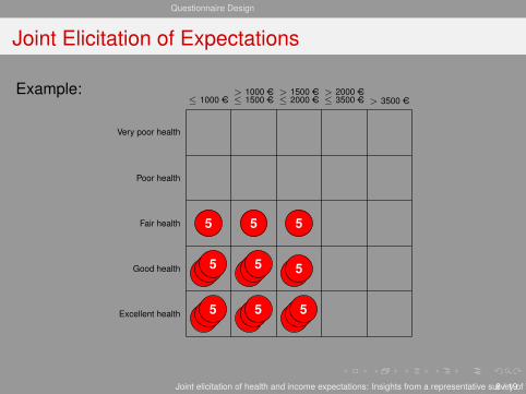
Joint Elicitation of Expectations
Subjects are given 20 tokens representing each a 5 percentchance and are asked to place them on a 5× 5 grid.Health: Typical of health-related quality of life surveys (see e.g.Ware and Sherbourne, 1992 ) and income: respondents areasked to place tokens on a 5× 5 gridMonthly income: Intervals were defined on the basis of the currentFrench equivalized monthly income.Expectations are elicited per decade 20 to 29, 30 to 49, ...(therefore up to 9 grids per topic for less than 20 years oldrespondents)Preliminary task: Each respondent first asked to indicate what cellon the grid best represents his or her health state and incomesituation during the current decade
Joint elicitation of health and income expectations: Insights from a representative survey of the French Population.7 / 19
Questionnaire Design
Joint Elicitation of Expectations
Example:≤ 1000 AC ≤ 1500 AC
> 1000 AC≤ 2000 AC> 1500 AC
≤ 3500 AC> 2000 AC
> 3500 AC
Excellent health
Good health
Fair health
Poor health
Very poor health
5 5
5 5 5
5
5 5 5
Joint elicitation of health and income expectations: Insights from a representative survey of the French Population.8 / 19

Questionnaire Design
Survey
In November and December 2009, health and incomeexpectations of a representative sample of 3,331 respondentsfrom the French population, from 18 to 97 years old, were elicited.
Survey was conducted by face-to-face interviews.
Joint elicitation of health and income expectations: Insights from a representative survey of the French Population.9 / 19

Empirical results
Mean probabilistic expectations of 40 to 50 years oldrespondents for the imagine future age 50 to 59’s
0.7
2.4
8.6
6.7
3.1
1.4
2.8
11.5
4.4
0.9
1.1
4.6
15.1
4
1.1
1.6
5.7
11.1
2.1
0.1
0.6
4.4
5.2
0.5
0.3Very poor health
Poor health
Fair health
Good health
Excellent health
[0;10
00[ AC
[1000; 1
500[AC
[1500; 2
000[AC
[2000; 3
500[AC
≥35
00AC
Joint elicitation of health and income expectations: Insights from a representative survey of the French Population.10 / 19
Empirical results
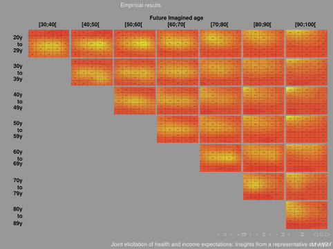
Future Imagined age[30;40[ [40;50[ [50;60[ [60;70[ [70;80[ [80;90[ [90;100[
20yto
29y
30yto
39y
40yto
49y
50yto
59y
60yto
69y
70yto
79y
80yto
89y
1.5
2.1
4.4
0.7
0.2
3.4
8.8
11.7
2.2
0.5
3.3
11.3
14.8
1.4
0.3
3.4
10.6
12.6
0.8
0.1
1.3
2.6
1.9
0
0
0.8
0.8
3
1.1
0.4
2.1
3.8
12.7
2.6
0.6
2.4
6.9
16.3
2.1
0.7
1.8
8.8
18.4
2.3
0
1.5
5.1
5.4
0.2
0
0.3
0.6
2.5
1.8
0.8
2.3
2.3
10.8
4.9
0.9
1.4
4.2
15.1
5.9
0.8
1
5.6
19.4
6.9
0.2
1.1
4
6
1.2
0
0.8
0.5
4
3.6
1.5
0.7
1.9
13.3
10.3
2.7
0.8
3.7
14.8
8
1.5
0.3
2.4
12.4
7.9
1.3
0.7
1.3
3.8
1.8
0.1
0.5
0.9
4.2
6.2
3
0.2
1.3
9.4
15.9
6
0.8
0.9
11.5
11.2
3.9
0
1.1
6.5
7.9
2.3
0.5
0.9
2.2
2.5
0.2
0.6
0.4
2.8
7.5
7.3
0.3
0.7
5.8
12.3
13.9
0.6
0.6
7.4
11.5
7.4
0
0.4
3.7
7.7
3.7
0.5
0.3
1.3
2.1
0.8
1
0.3
2.2
6
14.8
0.3
0.6
2.3
11
16.9
0.4
0.2
4.3
7.4
13.1
0
0.3
2.5
5.7
6
0.3
0.3
1.5
1.2
1.7
0.5
3.7
4.6
2
0.9
1.2
5
14
3
0.8
2
6.6
12.9
2.8
0.8
2.2
13.7
11.5
2.1
0.3
1.2
4.1
3.7
0.5
0
0.2
2
5.3
1.8
1.4
1
3.8
12.7
5.2
1.8
0.8
4.9
12.8
3.3
1.4
1.2
7.7
13.8
4.5
0.6
0.9
4.4
7.3
0.9
0.4
0.1
1.3
7
4.4
2.5
1
1.9
11.3
7.8
2.9
0.5
3.9
13.2
7.2
2.5
0.9
2.7
11.9
6.2
1.9
0.4
1
5.8
1.7
0.1
0.1
0.6
6.5
7.3
6.4
0.2
1.7
8
10.4
4.8
0.6
2
10.2
9.8
5.3
0.7
1.2
6.9
7
3.2
0
0.3
3.4
2.8
0.6
0.1
0.7
3.9
8.7
10.2
0
1.1
6.8
10.2
9.2
0.1
0.9
6
9.1
8
0.6
0.5
4.8
6.4
5.6
0
0.3
2.6
2.6
1.5
0.2
0.5
2.9
7.4
16.9
0
0.3
4
7.4
15.3
0.1
0.3
3.7
5.3
11.4
0.4
0.4
2.7
5.8
7.8
0.6
0.4
1.5
1.4
3.3
0.7
2.4
8.6
6.7
3.1
1.4
2.8
11.5
4.4
0.9
1.1
4.6
15.1
4
1.1
1.6
5.7
11.1
2.1
0.1
0.6
4.4
5.2
0.5
0.3
0.3
1.9
9.7
8.7
7.1
0.4
1.8
12.6
6.1
2.5
0.7
2.9
11.8
5
1.8
0.6
2.9
10.7
4.2
0.4
0.4
1.8
4.4
1
0.2
0.2
0.9
7.6
11
11.4
0.1
1
8.2
10.5
5.5
0.3
1.7
9.3
6.7
3.7
0.3
1.1
7
5.5
1.4
0.2
0.9
2.7
2
0.6
0.1
0.6
4.9
9.9
18.8
0
0.2
5.5
10.3
9.7
0.2
0.5
5
8.2
6
0.3
0.5
4.5
4.8
3.8
0.2
0.4
1.8
2.4
1.2
0.1
0.3
2.9
7.9
26.4
0
0.2
2.8
7.7
14.5
0.2
0.4
3
6.9
8.8
0
0.1
3.1
3.6
5.6
0.2
0.2
1.6
2.6
1.1
1
1.8
9
6.4
5.9
1.4
4
12.5
7
2.7
0.8
2.8
12.9
5
1
0.5
2.8
10.6
3.3
0.9
0.5
0.6
5
0.7
0.8
0.5
0.8
7.1
8.2
9.4
0.6
2
10.6
10.4
5.7
0.3
1.3
9.5
8.2
2.9
0
1.5
8.2
5.3
1.4
0.2
0.4
3.1
1.5
1.1
0.5
0.3
4.3
8.5
14.9
0.3
0.8
6
10.6
11.2
0.1
0.4
5.6
9.3
6.3
0.2
0.3
4.1
6.2
4.1
0.1
0.2
1.7
2.5
1.5
0.4
0
2.4
6.5
22.9
0.2
0.4
2.7
9.1
15.4
0.4
0.1
2.5
5.8
11.2
0.1
0.1
1.8
4.7
7.2
0.1
0.3
0.9
1.9
2.8
0.2
0.9
5.9
5.7
3.8
0.1
2.3
12.6
8.3
2
0.5
1.5
14.3
6.8
1.5
0.1
2
16.1
6.8
2.3
0.2
0.7
4.3
0.8
0.4
0
0.6
3.6
6.3
7.1
0
0.6
7
11.2
7.4
0.3
0.4
8
10.6
4.7
0
0.6
10.1
9.8
5.4
0.1
0.2
1.9
2.9
1.1
0
0.3
2
5.1
13.1
0
0.2
2.7
8.4
15.3
0.1
0
3.4
9
9.7
0
0.2
4.7
8.4
11.3
0.1
0.2
0.7
2.6
2.5
0.5
0.7
6.6
9.3
7.1
0.3
1.3
15.4
12.7
5.2
0.2
0.4
8.9
9.1
2.3
0.1
0.8
4.4
5.2
2.5
0.2
1.6
2.6
1.8
0.6
0.1
0.5
3.6
8.5
14.4
0.1
0.8
7.9
11.2
14.4
0
0.4
2.8
7.4
8.8
0.1
0.6
1.5
4.6
5.2
0.1
0.6
1.4
2.2
2.7
0
0.2
8
12.3
15.7
0
0.7
10.7
12.5
8.3
0
0.7
6
7.3
2.8
0.4
0.1
4.3
4
1.7
0
0.2
2
0.9
1.3
Joint elicitation of health and income expectations: Insights from a representative survey of the French Population.11 / 19

Empirical results
Marginal expectations by future age (1)
Poor healthFair healthGood healthVery good healthExcellent health
Not relevantLess than 1 KACBetween 1 KAC and 1.5KACBetween 1.5 KAC and 2.0KACBetween 2 KAC and 3.5KACMore than 3.5 KAC
Respondents less than 30 years oldFuture health states Future income
0 %
100 %
Exp
ecte
dpr
obab
ility
(in%
)
30-39 40-49 50-59 60-69 70-79 80-89 90-100
Future age
0 %
100 %
Exp
ecte
dpr
obab
ility
(in%
)
30-39 40-49 50-59 60-69 70-79 80-89 90-100
Future age
Joint elicitation of health and income expectations: Insights from a representative survey of the French Population.12 / 19
Empirical results
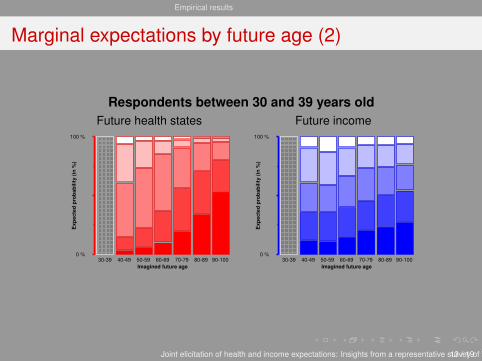
Marginal expectations by future age (2)
Respondents between 30 and 39 years oldFuture health states Future income
0 %
100 %
Exp
ecte
dpr
obab
ility
(in%
)
30-39 40-49 50-59 60-69 70-79 80-89 90-100Imagined future age
0 %
100 %
Exp
ecte
dpr
obab
ility
(in%
)30-39 40-49 50-59 60-69 70-79 80-89 90-100
Imagined future age
Joint elicitation of health and income expectations: Insights from a representative survey of the French Population.13 / 19
Empirical results
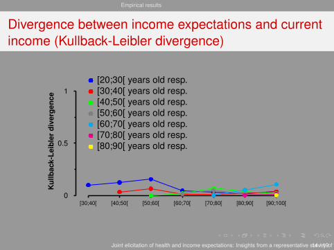
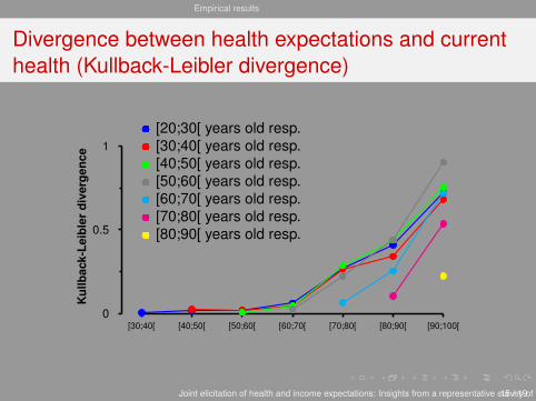
Divergence between income expectations and currentincome (Kullback-Leibler divergence)
[30;40[ [40;50[ [50;60[ [60;70[ [70;80[ [80;90[ [90;100[0
0.5
1
Kul
lbac
k-Le
ible
rdi
verg
ence
[20;30[ years old resp.[30;40[ years old resp.[40;50[ years old resp.[50;60[ years old resp.[60;70[ years old resp.[70;80[ years old resp.[80;90[ years old resp.
Joint elicitation of health and income expectations: Insights from a representative survey of the French Population.14 / 19
Empirical results
Divergence between health expectations and currenthealth (Kullback-Leibler divergence)
[30;40[ [40;50[ [50;60[ [60;70[ [70;80[ [80;90[ [90;100[0
0.5
1
Kul
lbac
k-Le
ible
rdi
verg
ence
[20;30[ years old resp.[30;40[ years old resp.[40;50[ years old resp.[50;60[ years old resp.[60;70[ years old resp.[70;80[ years old resp.[80;90[ years old resp.
Joint elicitation of health and income expectations: Insights from a representative survey of the French Population.15 / 19
Empirical results
Preliminary conclusions
Income expectations are very close to current income
Health expectations are close to current health except for futureages greater than 70:
- Driven by respondents’ pessimism regarding future health
.... one may then wonder: why not relying on current health and (inparticular) current income only instead of elicitating expectations?
Joint elicitation of health and income expectations: Insights from a representative survey of the French Population.16 / 19
Empirical results
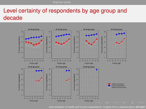
Level certainty of respondents by age group anddecade
●●
●
●●
●
●
30 40 50 60 70 80 90 100
020
4060
8010
0
20−29 age group
Future age
% o
f sur
e re
spon
dent
s
●●
● ● ● ●
●
●●
●
●●
●
●●
●
●
●
●
●
30 40 50 60 70 80 90 100
020
4060
8010
0
30−39 age group
Future age
% o
f sur
e re
spon
dent
s ●●
●●
● ●
●●
●
●
●
●●
●
●
●
●
30 40 50 60 70 80 90 100
020
4060
8010
0
40−49 age group
Future age
% o
f sur
e re
spon
dent
s
● ●● ●
●
●
●
●
●
●
●
●
●
●
30 40 50 60 70 80 90 100
020
4060
8010
0
50−59 age group
Future age
% o
f sur
e re
spon
dent
s
●● ●
●
●●
●
●
●●
●
30 40 50 60 70 80 90 100
020
4060
8010
0
60−69 age group
Future age
% o
f sur
e re
spon
dent
s
● ● ●
●●
●
●
●
30 40 50 60 70 80 90 100
020
4060
8010
0
70−79 age group
Future age
% o
f sur
e re
spon
dent
s
● ●
●
●●
30 40 50 60 70 80 90 100
020
4060
8010
0
80−89 age group
Future age
% o
f sur
e re
spon
dent
s
●
●
●
●
●
Health expectationsIncome expectationsHealth & Income expect.
Joint elicitation of health and income expectations: Insights from a representative survey of the French Population.17 / 19

Empirical results
Do expectations exhibit a gradient between health andincome?
Kendall’s rank correlation coefficient between current health andincome (bold figures on the diagonal) and expectations on healthand income by age group and decade
Future agesAge group [20; 30[ [30; 40[ [40; 50[ [50; 60[ [60; 70[ [70; 80[ [80; 90[ [90; 100][20; 30[ .045 0.087 0.138 0.127 0.116 0.111 0.137 0.123[30; 40[ .178 0.191 0.159 0.121 0.116 0.110 0.113[40; 50[ .254 0.264 0.260 0.240 0.225 0.242[50; 60[ .260 0.163 0.186 0.164 0.136[60; 70[ .168 0.151 0.134 0.133[70; 80[ .218 0.126 0.061[80; 90[ .248 0.209
⇒ Gradient between health and income, observed between currentsubjective health and income, is also present in expectations
Joint elicitation of health and income expectations: Insights from a representative survey of the French Population.18 / 19

Empirical results
Concluding remarks
At the aggregate level, marginal income expectations very muchlook like current income distribution in the population:Respondents do not expect changes in permanent income in thefuture (given that they were asked to not account for changesinduced by inflation)The same goes for marginal health expectations except for futureages greater than 70 for which respondents are more“pessimistic”.At the individual level, however, we find a substantial level ofcertainty (especially for income).Using current health and income distributions as a basis formodeling expectations (instead of eliciting expectations) wouldtherefore induce too much risk.
Joint elicitation of health and income expectations: Insights from a representative survey of the French Population.19 / 19

Karine Lamiraud1 , Robert Oxoby2 Cam Donaldson3
1 ESSEC Business School and THEMA-University of Cergy Pontoise2University of Calgary
3Glasgow Caledonian University
Incremental versus standard WTP An application to out-of-hours and emergency care
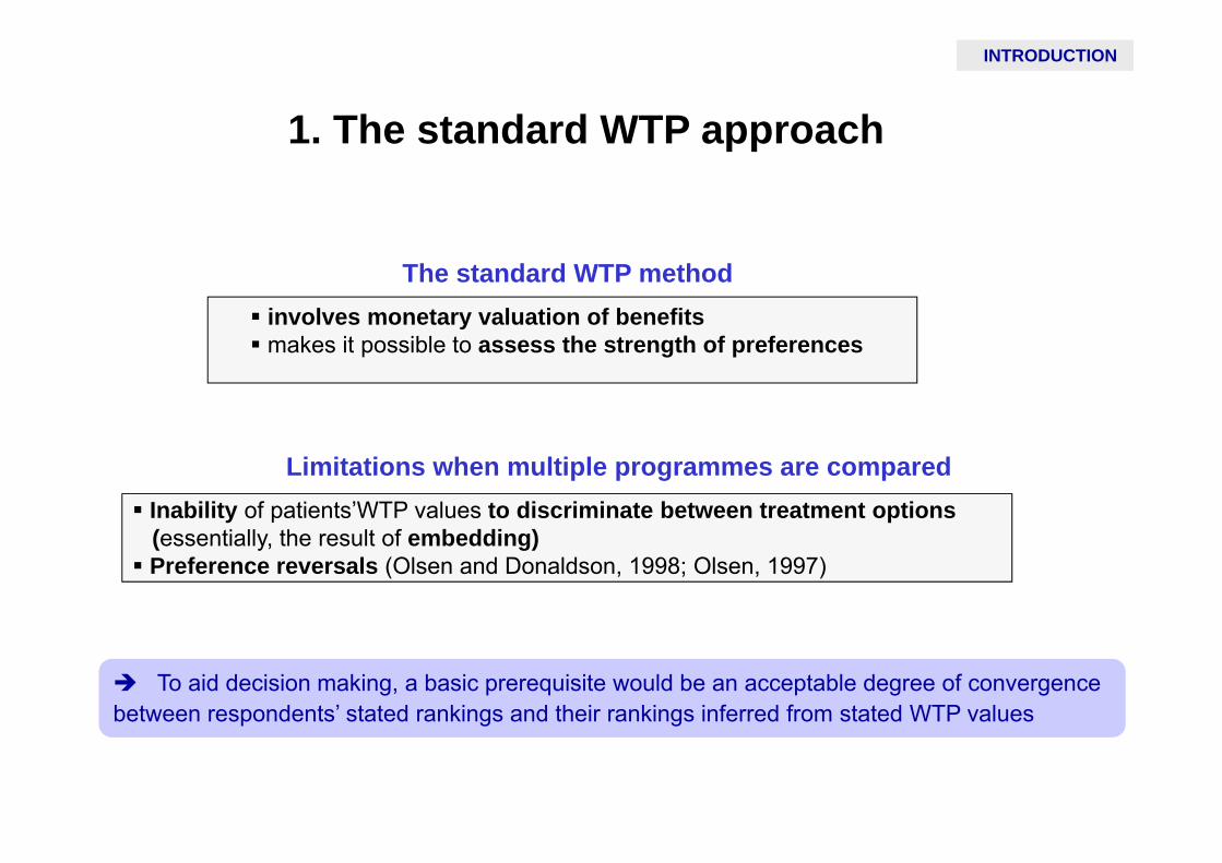
1. The standard WTP approach
INTRODUCTION
Inability of patients’WTP values to discriminate between treatment options(essentially, the result of embedding) Preference reversals (Olsen and Donaldson, 1998; Olsen, 1997)
Limitations when multiple programmes are compared
involves monetary valuation of benefits makes it possible to assess the strength of preferences
The standard WTP method
To aid decision making, a basic prerequisite would be an acceptable degree of convergence between respondents’ stated rankings and their rankings inferred from stated WTP values

2. The incremental approachINTRODUCTION
An incremental WTP approach was devised in order to encourage more differentiated answers and a higher degree of consistency among the respondents (Shackley and Donaldson, 2002)
In the incremental approach, the individual is asked
to give a value for his/her lowest ranked programme
how much more s/he would be willing to pay for his/her second ranked programme
-a theoretical basis for the incremental approach has not been elucidated
- There is little evidence showing that the incremental approach might indeed achieve greater consistency between explicit rankings and implicit rankings inferred from WTP values

3. Objectives of this study
INTRODUCTION
One purpose of this paper is to provide a theoretical basisfor the incremental approach
This study also aims to test the incremental and standard approaches
The context for the application is aiding decision making about different forms of emergency and out-of-hours service provision in France

Not equipped with medical doctors Firemen/Imbulance
Perform emergency care in addition to their usual duties
Doctors on duty
Fixed Means
4. Emergency and out-of-hours services in FranceINTRODUCTION
Emergency hospital units
“Maisons Médicales de Garde”Outpatient emergency centers
Mobile means
Dedicated to emergency care Equipped with an electrocardigram
and perfusion devices
SOS doctors
SAMU/SMURSAMU/SMUR Heavy means sent from hospitals Involved in vital emergencies
SAMU/SMUR Heavy means sent from hospitals Involved in vital emergencies
SAMU/SMUR Heavy means sent from hospitals Involved in vital emergencies
SAMU/SMUR
Mobile means

Outline
WTP study
Theoretical framework
Statistical and econometric methods
Results and Discussion
1. Assumptions
-Based on the theory of reference dependent preferences (Schoemaker, 1982) we assume that the response of any individual to a WTP question is influenced by that person’s reference point
-When a respondent is asked to value several competing policy alternatives, s/he is likely to compare each of these against the status quo (or « do nothing ») option
-The incremental approach redefines the reference point from which the response is measured (the least preferred option)
THEORETICAL FRAMEWORK
2. Implications
We show that :
in the standard approach, WTP values for each option, predominantly reflecting improvements over the status quo, fail to discriminate among the alternatives
the incremental approach, which redefines the reference point from which the response is measured, gives a more discriminating value for the intensity of preferences
THEORETICAL FRAMEWORK
1. WTP survey
Telephone survey carried out by TNS Sofres in July 2009
Representative sample of the French adult population living in urban areas (> 100 000)
Two questionnaires (standard and incremental) randomly assigned
WTP STUDY
A WTP method was implemented to assess preferences for different emergency services
Survey
2. Questionnaires
The interviewer described the characteristics of each emergency and out-of-hours actor
Respondents were asked to rank these different actors in order of preference
(from the most prefererred to the least preferred option). No equal ranking was possible
Respondents were asked to imagine that financing mechanisms for emergency services had been changed and that the resources should be provided by households through insurance premia
Respondents were then asked their WTP for such insurance premia
Part A
Part B
Part C
WTP STUDY
3. WTP questions
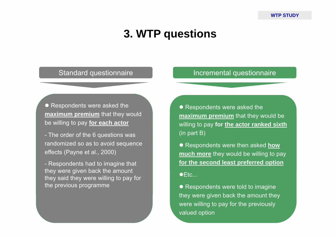
Standard questionnaire Incremental questionnaire
Respondents were asked the maximum premium that they would be willing to pay for each actor
- The order of the 6 questions was randomized so as to avoid sequence effects (Payne et al., 2000)
- Respondents had to imagine that they were given back the amount they said they were willing to pay for the previous programme
Respondents were asked the maximum premium that they would be willing to pay for the actor ranked sixth(in part B)
Respondents were then asked how much more they would be willing to pay for the second least preferred option
Etc...
WTP STUDY
Respondents were asked the maximum premium that they would be willing to pay for each actor
- The order of the 6 questions was randomized so as to avoid sequence effects (Payne et al., 2000)
- Respondents had to imagine that they were given back the amount they said they were willing to pay for the previous programme
Respondents were asked the maximum premium that they would be willing to pay for the actor ranked sixth(in part B)
Respondents were then asked how much more they would be willing to pay for the second least preferred option
Etc...
Respondents were told to imagine they were given back the amount they were willing to pay for the previously valued option
Respondents were asked the maximum premium that they would be willing to pay for each actor
- The order of the 6 questions was randomized so as to avoid sequence effects (Payne et al., 2000)
- Respondents had to imagine that they were given back the amount they said they were willing to pay for the previous programme
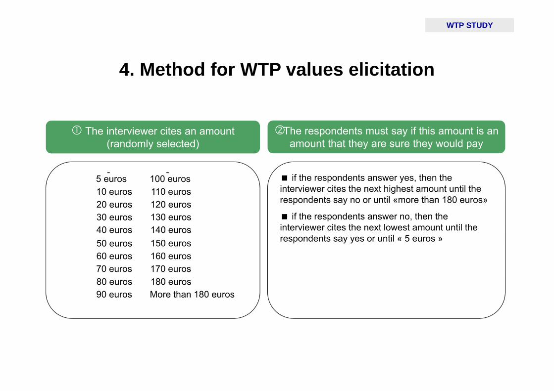
if the respondents answer yes, then the interviewer cites the next highest amount until the respondents say no or until «more than 180 euros»
if the respondents answer no, then the interviewer cites the next lowest amount until the respondents say yes or until « 5 euros »
The interviewer cites an amount (randomly selected)
The respondents must say if this amount is an amount that they are sure they would pay
5 euros10 euros20 euros30 euros40 euros50 euros60 euros70 euros80 euros90 euros
100 euros110 euros120 euros130 euros140 euros150 euros160 euros170 euros180 eurosMore than 180 euros
4. Method for WTP values elicitation
WTP STUDY

5. WTP approach
WTP STUDY
An ex ante approach (not ex post) was chosen
An insurance based ex ante approach (not tax based) was chosen

1. Aims
The empirical analysis aimed to test the validity of the incremental approach:
(i) Whether it improved consistency between respondents’ explicit ranking of the providers and the ranking implied by their WTP values
(ii) Whether it made it possible to differentiate between the various providers
STATISTICAL AND ECONOMETRIC ANALYSIS

2. Regression analyses
WTP*ij is the maximal WTP of individual i for option j
RANKij is the explicit rank for each actor (1 = most preferred .... 6 = least preferred)
Xij is a vector of individual characteristics
Zj represents a set of option dummies (SOS will be used as the reference)
* ,ij j ij ijWTP Z X
we estimated an ordered probit model on the explicit ranking
we estimated a tobit model for WTP with left-censoring and right-censoring
we used the cluster option (because each respondent assesses all six emergency options)
the regressions were run excluding the individuals with zero answers for all six options
We built a panel dataset including 6 observations per respondent (i.e.1680 observations)
ij j ij ijRANK Z X
STATISTICAL AND ECONOMETRIC ANALYSIS

1. The study population
RESULTS
280 people were interviewed:140 received the standard version, 140 received the incremental one
There were no significant differences between the 2 groups but in terms of gender distribution
All Standard Incremental p*questionnaire questionnaire
n = 280 n = 140 n = 140Age (mean) 50.1 50.9 49.4 0.46Male (%) 45.7 39.3 52.1 0.03Secondary school or short professional track (%) 31.4 32.1 30.7 0.60High school diploma (Baccalaureat) 21.4 24.3 18.6Short university studies (2 yrs) or long professional track (%) 15.7 14.3 17.1University degree higher than bachelor's (%) 31.4 29.2 33.5Individual is married or living in a couple (%) 57.1 57.9 56.4 0.81Number of children under 15 living in the household (mean) 0.4 0.4 0.4 0.95Monthly household net Income (1-10)** (mean) 5.7 5.8 5.6 0.64Excellent self assessed health (%) 30.0 30.0 30.0 0.83Good self assessed health (%) 47.9 49.3 46.4Poor self-assessed health (%) 22.1 20.7 23.6Individual has supplementary health insurance coverage (%) 90.7 90.7 90.7 1.00Used at least one of the 6 emergency services in the previous year 33.3 29.3 37.9 0.13All statistics are weighted* Test of difference between the standard and incremental versions (student t-test for continuous variables, chi2 for categorical variables)** (euros per month) 1 . < 800, 2. [800 - 1000[, 3. [1000 - 1200[, 4. [1200 - 1500[, 5. [1500 - 1800[, 6. [1800 - 2300[,7. [2300 - 3000[, 8. [3000 - 3800[, 9. [3800 - 5300[, 10. ≥ 5300 euros
2. Explicit ranking of actors
RESULTS
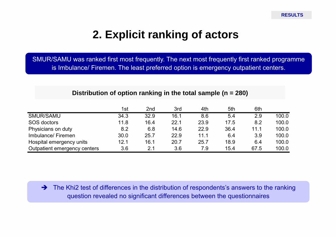
SMUR/SAMU was ranked first most frequently. The next most frequently first ranked programme is Imbulance/ Firemen. The least preferred option is emergency outpatient centers.
The Khi2 test of differences in the distribution of respondents’s answers to the ranking question revealed no significant differences between the questionnaires
Distribution of option ranking in the total sample (n = 280)
1st 2nd 3rd 4th 5th 6thSMUR/SAMU 34.3 32.9 16.1 8.6 5.4 2.9 100.0SOS doctors 11.8 16.4 22.1 23.9 17.5 8.2 100.0Physicians on duty 8.2 6.8 14.6 22.9 36.4 11.1 100.0Imbulance/ Firemen 30.0 25.7 22.9 11.1 6.4 3.9 100.0Hospital emergency units 12.1 16.1 20.7 25.7 18.9 6.4 100.0Outpatient emergency centers 3.6 2.1 3.6 7.9 15.4 67.5 100.0

3. Descriptive statistics for WTP (1)
RESULTS
The SAMU/SMUR had the highest WTP while the outpatient emergency centers had the lowest
WTP values for all types of care were significantly higher in the incremental questionnaires
WTP descriptive statistics by actor in the standard and incremental questionnaireSMUR/SAMU
SOS doctors
Doctors on duty
Ambulance/ Firemen
Hospital emergency
units
Outpatient emergency
centresStandard version mean 41.2 36.7 37.6 34.8 32.3 26.0
(n = 140) std 46.7 41.0 42.7 41.0 38.2 34.5median 30.0 25.0 20.0 20.0 20.0 10.0
% of zeros 27.9 25.0 27.9 28.6 32.1 40.0
Incremental version mean 103.2 66.1 59.5 97.9 69.2 41.9(n = 140) std 130.7 90.0 83.9 127.2 77.3 74.9
median 57.5 30.0 27.5 47.5 42.5 10.0% of zeros 19.3 25.7 26.4 19.3 19.3 35.7
4. Descriptive statistics for WTP (2)
RESULTS
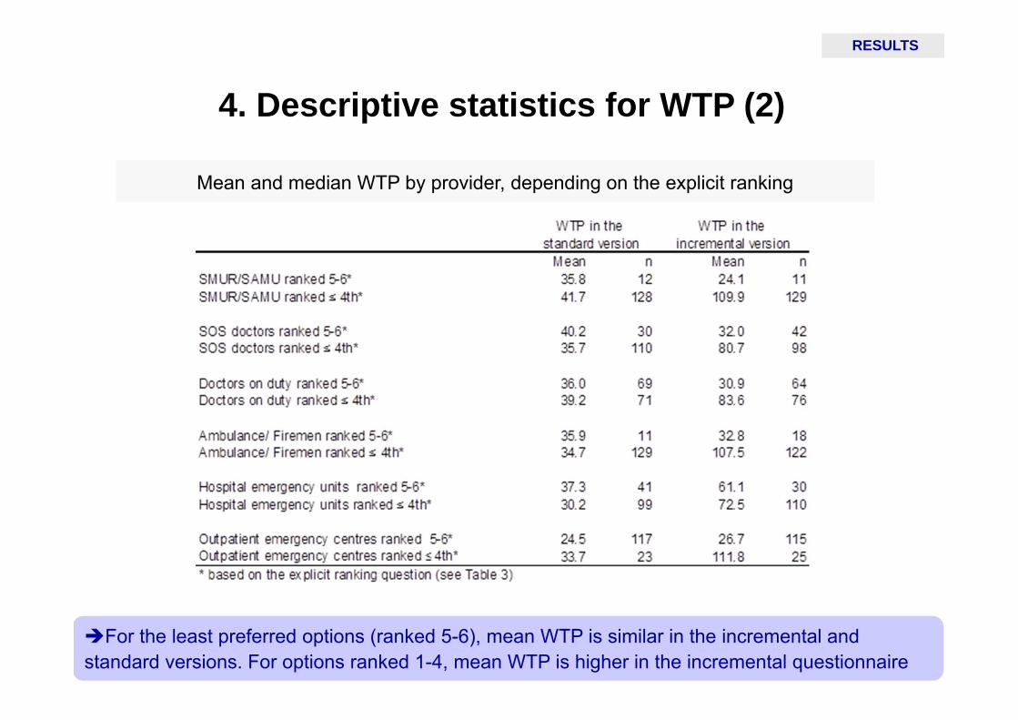
For the least preferred options (ranked 5-6), mean WTP is similar in the incremental and standard versions. For options ranked 1-4, mean WTP is higher in the incremental questionnaire
Mean and median WTP by provider, depending on the explicit ranking

5. Regression resultsRESULTS
The declared WTP based on the incremental approach provides the same ranking of providers as the explicit ranking
The standard approach is only partially consistent with explicit ranking and proves unable to differentiate between the five most preferred providers
Robustness checks (1)
DISCUSSION
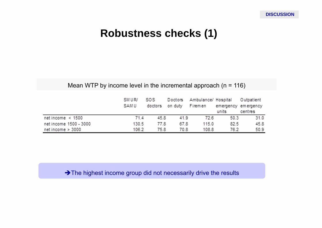
Mean WTP by income level in the incremental approach (n = 116)
The highest income group did not necessarily drive the results
Robustness checks (2)
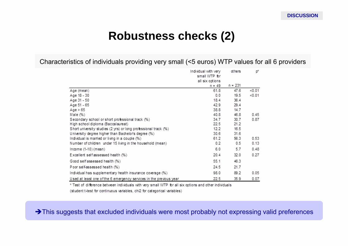
Characteristics of individuals providing very small (<5 euros) WTP values for all 6 providers
This suggests that excluded individuals were most probably not expressing valid preferences
DISCUSSION
Robustness checks (3)
We considered the possibility that, going up the scale, the maximum WTP was an
unobserved number between the last value to which the respondents said “yes” and the next
one to which they would have said no
An interval data regression model was estimated in the incremental and standard
questionnaires: the results were not qualitatively different
DISCUSSION

Conclusions
CONCLUSION
The standard approach is reasonably consistent with explicit ranking but proves
unable to differentiate between the five most preferred actors
The incremental approach provides evaluation results which are fully in line with those
of explicit ranking question
Our empirical findings are in line with our theoretical framework
Our findings suggest that the incremental approach provides results that can be used in
priority setting contexts
Improvements on earlier work
CONCLUSION
It was made explicit to respondents that their budget had not been diminished by any
WTP values they may have stated for previous programmes
Each successive programme is valued over and above that ranked immediately below it
Respondents could perceive the ranking exercise and the WTP valuations as different
processes: the wording was amended with the intention of conveying the notion of
individual value in both contexts:
“place these programmes in order of how highly you value them starting with the one you
like most. When doing this, concentrate on how much you value the proposed expansions
and how you value preventing the proposed reductions from going ahead”

Motivation Stated preference methods and health care policy
A discrete choice experiment under oath
Nicolas Jacquemet, Stephane Luchini, Jason Shogren, Verity Watson
Paris School of EconomicsUniversite de Lorraine, BETA
Jacquemet et al. (U. Lorraine – BETA & PSE) DCE under oath 1 / 12

Motivation Stated preference methods and health care policy
Economic valuation of health and health care policy
Health care is a large part of government spending
But it is not possible to fund all treatments or interventions
Decisions have to be made and should reflect society’s (unobservable) value
Stated preference methods (increasingly choice experiments - CEs) are used toquantify value
Such methods are useful for policy purpose only if they reflect true underlying preferences⇔ if they are demand revealing
Jacquemet et al. (U. Lorraine – BETA & PSE) DCE under oath 1 / 12
Motivation Stated preference methods and health care policy
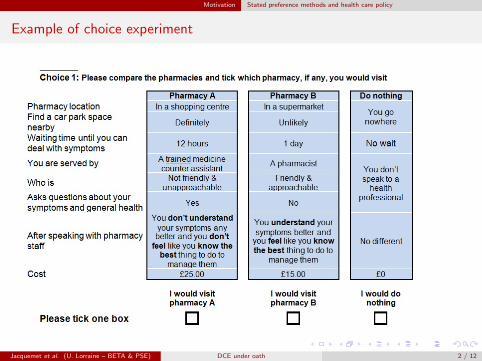
Example of choice experiment
Jacquemet et al. (U. Lorraine – BETA & PSE) DCE under oath 2 / 12

Motivation Are CEs demand revealing?
Are CEs demand revealing?
Field experiments comparing hypothetical values from CE with ’real’ values
Health - hypothetical and real values differ (Mark & Swait, 2004, HE ; Ryan et al,2009, HE)
Environment - hypothetical values higher than real, more ‘opt-in’ (Ready et al, 2010,Land Econ; Carlsson & Martinsson, 2003, JEEM; Lusk & Schroeder, 2004, AJAE)
Transportation - hypothetical values of time are lower than real (Hensher, 2010Transport Res.; Fifer et al, 2014, Transport Res.)
but such evidence comes from the comparison between two stated preferences – noreliable benchmark
To test choices are demand revealing need to know true values
Induced value experiment (Smith, 1976, AER)
Monetary rewards are used to induce values for artificial goods – preferences areknown to, and controlled by, the experimenter.
In the stated pref. literature, IV studies find no difference between hypothetical and real,but responses are not demand revealing (Collins and Vossler, 2009; Jacquemet, Joule,Luchini, and Shogren, 2009; Mitani and Flores, 2009; Taylor, McKee, Laury, andCummings, 2001; Vossler and McKee, 2006).
Jacquemet et al. (U. Lorraine – BETA & PSE) DCE under oath 3 / 12
Motivation Target behavior: an IV discrete choice experiment
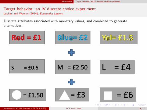
Target behavior: an IV discrete choice experimentLuchini and Watson (2014), Economics Letters.
Discrete attributes associated with monetary values, and combined to generatealternatives:
Jacquemet et al. (U. Lorraine – BETA & PSE) DCE under oath 4 / 12
Motivation Target behavior: an IV discrete choice experiment
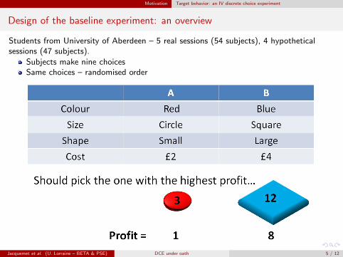
Design of the baseline experiment: an overview
Students from University of Aberdeen – 5 real sessions (54 subjects), 4 hypotheticalsessions (47 subjects).
Subjects make nine choicesSame choices – randomised order
Jacquemet et al. (U. Lorraine – BETA & PSE) DCE under oath 5 / 12
Motivation Target behavior: an IV discrete choice experiment
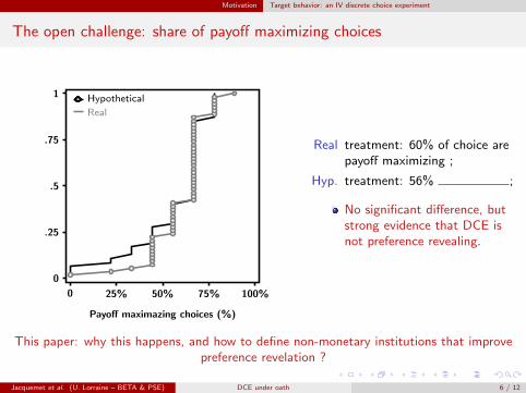
The open challenge: share of payoff maximizing choices
0
.25
.5
.75
1
Payoff maximazing choices (%)
0 25% 50% 75% 100%
Hypothetical
Real
Real treatment: 60% of choice arepayoff maximizing ;
Hyp. treatment: 56% ;
No significant difference, butstrong evidence that DCE isnot preference revealing.
This paper: why this happens, and how to define non-monetary institutions that improvepreference revelation ?
Jacquemet et al. (U. Lorraine – BETA & PSE) DCE under oath 6 / 12

Design of the experiment Treatment variables
This paper
Why this happens, and how to define non-monetary institutions that improve preferencerevelation.
1 Limited cognitive ability of subjects:Exp. 1 We provide subjects with calculators, and record their use of it.
3 sessions (47 subjects) (3 hypothetical sessions with a calculator were also run as abenchmark).
2 Lack of commitment towards the revelation exercisePrevious evidence show that a truth-telling oath enhance preference revelation inVickrey auction, Referendum, BDM and (homegrown) DCE revelation mechanisms
Grounded on the social psychology of commitment: decisions made along a sequenceof actions induce drastic changes in subsequent decision making.
Exp. 2 Truth telling oath added before the DCE experiment takes place:
“I, the undersigned ... do solemnly swear that, during the whole experiment, I will:Tell the truth and always provide honest answers”
Subjects told - signing is free, participation and earnings are not conditional on signing;3 sessions, identical in all other aspects (44 subjects) – all but 1 signed the oath.
Jacquemet et al. (U. Lorraine – BETA & PSE) DCE under oath 7 / 12
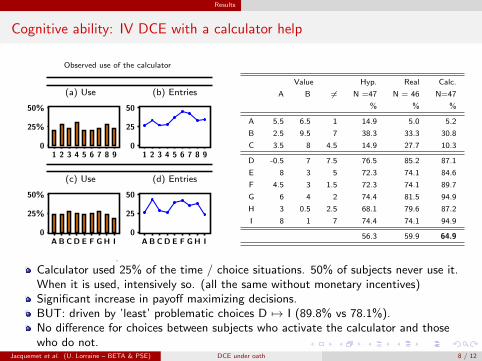
Results
Cognitive ability: IV DCE with a calculator help
Observed use of the calculator
(a) Use
0
25%
50%
1 2 3 4 5 6 7 8 9
(b) Entries
0
25
50
1 2 3 4 5 6 7 8 9
(c) Use
0
25%
50%
A B C D E F G H I
(d) Entries
0
25
50
A B C D E F G H I
.
Value Hyp. Real Calc.
A B 6= N =47 N = 46 N=47
% % %
A 5.5 6.5 1 14.9 5.0 5.2
B 2.5 9.5 7 38.3 33.3 30.8
C 3.5 8 4.5 14.9 27.7 10.3
D -0.5 7 7.5 76.5 85.2 87.1
E 8 3 5 72.3 74.1 84.6
F 4.5 3 1.5 72.3 74.1 89.7
G 6 4 2 74.4 81.5 94.9
H 3 0.5 2.5 68.1 79.6 87.2
I 8 1 7 74.4 74.1 94.9
56.3 59.9 64.9
Calculator used 25% of the time / choice situations. 50% of subjects never use it.When it is used, intensively so. (all the same without monetary incentives)Significant increase in payoff maximizing decisions.BUT: driven by ’least’ problematic choices D 7→ I (89.8% vs 78.1%).No difference for choices between subjects who activate the calculator and thosewho do not.
Jacquemet et al. (U. Lorraine – BETA & PSE) DCE under oath 8 / 12
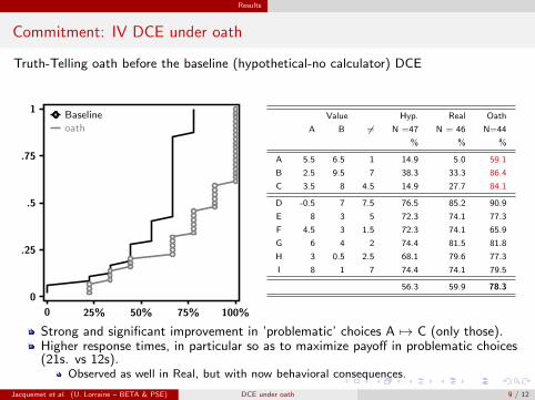
Results
Commitment: IV DCE under oath
Truth-Telling oath before the baseline (hypothetical-no calculator) DCE
0
.25
.5
.75
1
0 25% 50% 75% 100%
Baseline
oathValue Hyp. Real Oath
A B 6= N =47 N = 46 N=44
% % %
A 5.5 6.5 1 14.9 5.0 59.1
B 2.5 9.5 7 38.3 33.3 86.4
C 3.5 8 4.5 14.9 27.7 84.1
D -0.5 7 7.5 76.5 85.2 90.9
E 8 3 5 72.3 74.1 77.3
F 4.5 3 1.5 72.3 74.1 65.9
G 6 4 2 74.4 81.5 81.8
H 3 0.5 2.5 68.1 79.6 77.3
I 8 1 7 74.4 74.1 79.5
56.3 59.9 78.3
Strong and significant improvement in ’problematic’ choices A 7→ C (only those).Higher response times, in particular so as to maximize payoff in problematic choices(21s. vs 12s).
Observed as well in Real, but with now behavioral consequences.
Jacquemet et al. (U. Lorraine – BETA & PSE) DCE under oath 9 / 12

Robustness treatments
Robustness treatment I – “Task oath”
Does the oath works though fostered cognitive effort ?
Task oath, same form but reads: “I, ..., the undersigned do solemnly swear that duringthe entire experiment, I will faithfully and conscientiously fulfil the tasks that I am askedto complete to the best of my skill and knowledge”
0
.25
.5
.75
1
0 25% 50% 75% 100%
BaselineTask Oath
Value Hyp. Real Task
A B 6= N =47 N = 46 Oath
% % N=37
A 5.5 6.5 1 14.9 5.0 10.8
B 2.5 9.5 7 38.3 33.3 35.1
C 3.5 8 4.5 14.9 27.7 18.9
D -0.5 7 7.5 76.5 85.2 89.2
E 8 3 5 72.3 74.1 83.8
F 4.5 3 1.5 72.3 74.1 75.7
G 6 4 2 74.4 81.5 86.5
H 3 0.5 2.5 68.1 79.6 83.8
I 8 1 7 74.4 74.1 89.2
56.3 59.9 63.7
Slight increase, driven only by choice D. Significant increase in response times (237s.vs 157s.).
Jacquemet et al. (U. Lorraine – BETA & PSE) DCE under oath 10 / 12

Robustness treatments
Robustness treatment II – “Oath of office”
Task oath not solemn / sound enough ?
Oath of office, same form but reads: “I, ..., the undersigned do solemnly swear thatduring the entire experiment, I will faithfully and conscientiously fulfil my duties to thebest of my skill and knowledge”
0
.25
.5
.75
1
0 25% 50% 75% 100%
BaselineOath of office
Value Hyp. Real Oath of
A B 6= N =47 N = 46 office
% % N=37
A 5.5 6.5 1 14.9 5.0 0.0
B 2.5 9.5 7 38.3 33.3 24.3
C 3.5 8 4.5 14.9 27.7 8.1
D -0.5 7 7.5 76.5 85.2 91.9
E 8 3 5 72.3 74.1 94.6
F 4.5 3 1.5 72.3 74.1 75.7
G 6 4 2 74.4 81.5 91.9
H 3 0.5 2.5 68.1 79.6 75.7
I 8 1 7 74.4 74.1 91.9
56.3 59.9 61.6
Slight increase, driven only by non problematic choices. Significant increase inresponse times (213s. vs 157s.).
Jacquemet et al. (U. Lorraine – BETA & PSE) DCE under oath 11 / 12

Conclusion
Conclusion
We confirm previous evidence that a truth telling oath (drastically) improves preferencerevelation based on DCE.
As compared to previous evidence:
We contrast preference revelation according to whether stated preferences havemonetary consequences or not;
We use an IV setting, allowing to contrast revealed and true underlying preferences.
The IV setting reveals a huge discrepancy between true and DCE stated preferences –not related to cognitive limitations.
Perhaps more importantly: commitment to the truth, rather to a higher cognitive effort,is achieved by a truth telling oath.
Main open question: inference to homegrown values.
Jacquemet et al. (U. Lorraine – BETA & PSE) DCE under oath 12 / 12

Conclusion
Collins, J. P., and C. A. Vossler (2009): “Incentive compatibility tests of choice experiment valueelicitation questions,” Journal of Environmental Economics and Management, 58(2), 226–235.
Jacquemet, N., R.-V. Joule, S. Luchini, and J. Shogren (2009): “Earned Wealth, Engaged Bidders?Evidence from a second price auction,” Economics Letters, 105(1), 36–38.
Luchini, S., and V. Watson (2014): “Are choice experiments reliable? Evidence from the lab,” EconomicsLetters, 124(1), 9–13.
Mitani, Y., and N. E. Flores (2009): “Demand Revelation, Hypothetical Bias, and Threshold PublicGoods Provision,” Environmental & Resource Economics, 44(2), 231–243.
Taylor, L. O., M. McKee, S. K. Laury, and R. G. Cummings (2001): “Induced-value tests of thereferendum voting mechanism,” Economics Letters, 71(1), 61–65.
Vossler, C. A., and M. McKee (2006): “Induced-Value Tests of Contingent Valuation ElicitationMechanisms,” Environmental & Resource Economics, 35(2), 137–168.
Jacquemet et al. (U. Lorraine – BETA & PSE) DCE under oath 12 / 12

MotivationsInterpretations of SDU
What do we know?Our empirical analysis
SDU and long-term care insuranceFirst findings from an empirical analysis based on Canadian
data.
Michel Grignon 1
1McMaster University, Economics and HA&S
March 2015
Michel Grignon Chaire Sante

MotivationsInterpretations of SDU
What do we know?Our empirical analysis
Outline
1 Motivations
2 Interpretations of SDU
3 What do we know?
4 Our empirical analysis
Michel Grignon Chaire Sante

MotivationsInterpretations of SDU
What do we know?Our empirical analysis
State Dependent UtilityOutline detailed
1 Does Marginal Utility of Consumption change with health?2 How can we approach the question empirically?
Challenges.3 Implications for pensions and health insurance (mostly
public programs)
Michel Grignon Chaire Sante

MotivationsInterpretations of SDU
What do we know?Our empirical analysis
A vivid illustrationCancer Ward, Solzhenitsyn
””Read? Why should I read? We’ll all kick the bucket soon.”Bone-chewer’s scar twitched. ”That’s the point! If you don’thurry you’ll have kicked the bucket before you’ve read it. Hereyou are, quick!””
Michel Grignon Chaire Sante
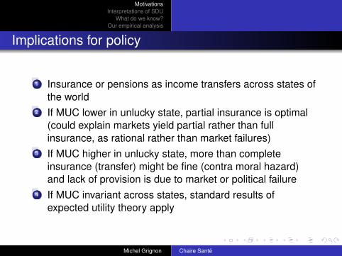
MotivationsInterpretations of SDU
What do we know?Our empirical analysis
Implications for policy
1 Insurance or pensions as income transfers across states ofthe world
2 If MUC lower in unlucky state, partial insurance is optimal(could explain markets yield partial rather than fullinsurance, as rational rather than market failures)
3 If MUC higher in unlucky state, more than completeinsurance (transfer) might be fine (contra moral hazard)and lack of provision is due to market or political failure
4 If MUC invariant across states, standard results ofexpected utility theory apply
Michel Grignon Chaire Sante
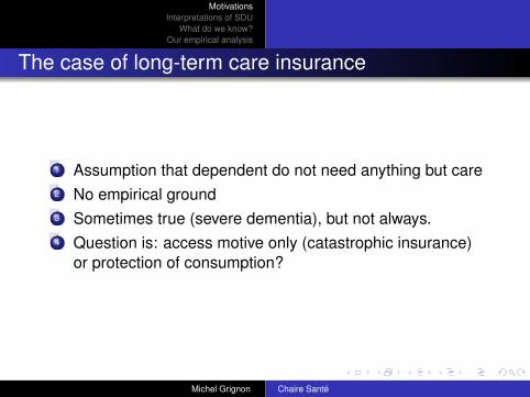
MotivationsInterpretations of SDU
What do we know?Our empirical analysis
The case of long-term care insurance
1 Assumption that dependent do not need anything but care2 No empirical ground3 Sometimes true (severe dementia), but not always.4 Question is: access motive only (catastrophic insurance)
or protection of consumption?
Michel Grignon Chaire Sante

MotivationsInterpretations of SDU
What do we know?Our empirical analysis
the utility model of SDU
U(C,S) = γ0.S + (1 + γ1.S).u(C)where C is consumption, S is sickness (e.g., a binary variabletaking the value of 1 if the individual is sick and 0 otherwise).γ0 is the effect of sickness on the level of utility (expectednegative)γ1 is the effect of sickness on the slope of the relationshipbetween consumption and utility. The latter is the parameter ofinterest: a positive γ1 indicates that the marginal utility ofconsumption is greater when sick.
Michel Grignon Chaire Sante
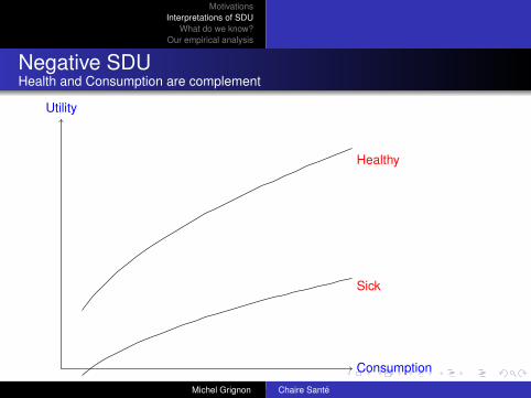
MotivationsInterpretations of SDU
What do we know?Our empirical analysis
Negative SDUHealth and Consumption are complement
Consumption
Utility
Sick
Healthy
Alternative interpretation: Tougher to be sick when rich.Michel Grignon Chaire Sante

MotivationsInterpretations of SDU
What do we know?Our empirical analysis
Positive SDUHealth and Consumption are substitutes
Consumption
Utility
Sick
Healthy
Alternative: Tougher to be sick when poor.
Michel Grignon Chaire Sante

MotivationsInterpretations of SDU
What do we know?Our empirical analysis
Implications for LTC insuranceMore formal
If u(C) =C
1α
1α
, α risk aversion, the optimal level of coverage for
an insurance with no moral hazard is: b∗ =Ch
H.((1 + γ1)
1α − 1).
If γ1 = 0 the optimal coverage rate will be 100% whatever thevalue of α (there is no moral hazard), but if γ1 = 0.1, theoptimal coverage rate will vary from 107% to 115% for values ofα comprised between 4 and 2.
Michel Grignon Chaire Sante

MotivationsInterpretations of SDU
What do we know?Our empirical analysis
Literature on health-related SDU
1 Introspection: Not conclusive but most think it is negative.2 Empirical: Revealed preferences challenging
No control in observational studiesAvenue: Critical Illness Insurance (Longo and Grignon).
3 Stated preferences (1): Viscusi. Negative for high risks(death), positive in the small.
4 Stated preferences (2): Finkelstein et al. (2008)
Michel Grignon Chaire Sante

MotivationsInterpretations of SDU
What do we know?Our empirical analysis
Empirical approach
Ui = δ0 + δ1.(Si ∗ Cδ2i ) + δ3.Si + δ4.C
δ2i + δ5.Zi
where Zi is a set of controls (taste shifters), would allow us tomeasure the effect of health on the change in utility broughtabout by a small change in consumption (marginal utility)through the sign of δ1. A positive coefficient would showpositive sickness dependent utility (S is sickness, not goodhealth), whereas a negative value would show negativesickness dependent utility and a value non-significantly differentfrom 0 would indicate sickness-independent marginal utility ofconsumption. We would also be able to infer a value for γ1 as
γ1 =δ1
δ4
Michel Grignon Chaire Sante
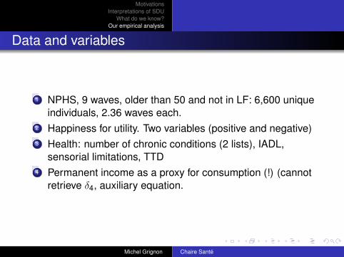
MotivationsInterpretations of SDU
What do we know?Our empirical analysis
Data and variables
1 NPHS, 9 waves, older than 50 and not in LF: 6,600 uniqueindividuals, 2.36 waves each.
2 Happiness for utility. Two variables (positive and negative)3 Health: number of chronic conditions (2 lists), IADL,
sensorial limitations, TTD4 Permanent income as a proxy for consumption (!) (cannot
retrieve δ4, auxiliary equation.
Michel Grignon Chaire Sante

MotivationsInterpretations of SDU
What do we know?Our empirical analysis
Identification assumptions
1 No error in mapping (parametric)2 No systematic differences in expressing happiness across
groups of sickness and consumption (out of labour force).
Michel Grignon Chaire Sante
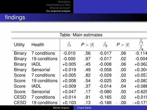
MotivationsInterpretations of SDU
What do we know?Our empirical analysis
findings
Table: Main estimates
Utility Health β1 P > |t | β3 P > |t | β1
β4Binary 7 conditions -0.010 .56 -0.017 .06 -0.114Binary 19 conditions -0.000 .97 -0.017 .02 -0.004Binary IADL +0.005 .45 -0.008 .06 +0.062Binary Sensorial +0.019 .49 -0.058 .00 +0.304Score 7 conditions +0.005 .82 -0.029 .02 +0.057Score 19 conditions +0.008 .54 -0.025 .00 +0.083Score IADL +0.009 .37 -0.014 .04 +0.086Score Sensorial +0.047 .17 -0.080 .00 +0.629CESD 7 conditions +0.014 .91 -0.165 .02 +0.019CESD 19 conditions +0.103 .13 -0.188 .00 +0.171CESD IADL -0.010 .92 -0.139 .04 -0.012CESD Sensorial -0.119 .42 -0.465 .00 -0.157
Michel Grignon Chaire Sante

MotivationsInterpretations of SDU
What do we know?Our empirical analysis
Why is Canada (perhaps) different than the US?
1 It is tough to be poor in the US anyway, healthy or not2 It is tougher to be sick when rich in the US than in Canada3 Consumption is affected, for a given level of permanent
income, more in the US than in Canada.
Michel Grignon Chaire Sante
Copyright © 2022 FDOKUMEN