arX

iv:1

001.

1490

v3 [

mat

h.G

M]

13

Aug

201

0

Scale Free Analysis and the Prime Number Theorem

Dhurjati Prasad Datta∗and Anuja Roy Choudhuri†

Department of Mathematics, University of North Bengal

Siliguri,West Bengal, Pin: 734013, India

Abstract

We present an elementary proof of the prime number theorem. The relative

error follows a golden ratio scaling law and respects the bound obtained from the

Riemann’s hypothesis. The proof is derived in the framework of a scale free nonar-

chimedean extension of the real number system exploiting the concept of relative

infinitesimals introduced recently in connection with ultrametric models of Can-

tor sets. The extended real number system is realized as a completion of the field

of rational numbers Q under a new nonarchimedean absolute value, which treats

arbitrarily small and large numbers separately from a finite real number.

Key Words: Prime number theorem, non-archimedean absolute value, relativeinfinitesimals, scale invariance

AMS Classification Numbers: 11A41, 26E30, 26E35, 28A80

∗Corresponding author, email: dp−datta@yahoo.com†Ananda Chandra College, Jalpaiguri-735101, India, email: anujaraychaudhuri@ymail.com

1

1. Introduction

We present a new proof of the Prime Number Theorem [1]. We call it elementary because

the proof does not require any advanced techniques from the analytic number theory

and complex analysis. Although the level of presentation is truly elementary even in the

standard of the elementary calculus, except for some basic properties of non-archimedean

spaces [2, 3], some of the novel analytic structures that have been uncovered here seem to

have significance not only in number theory but also in other areas of mathematics, for

instance the noncommutative geometry [4], infinite trees [5] and networks [6].

The proof of the PNT is derived on a scale invariant, nonarchimedean model R of the

real number system R, involving nontrivial infinitesimals and infinities. The model R is

realized as a completion of the field of rational numbers Q under a new nonarchimedean

absolute value ||.||, which treats arbitrarily small and large numbers separately from any

finite number. Stated more precisely, the absolute value reduces to the usual Euclidean

value for a finite rational (real) number, whereas for an arbitrarily small number, defined

in a limiting sense, it assigns a new scale invariant value. In the framework of the ordinary

real analysis, such a value would be identified simply as zero. Arbitrarily large numbers

are also assigned, by inversion, analogous finite scale invariant values. The new absolute

value is thus intrinsically scale invariant and inversion symmetric. The model constructed

here is distinct from the usual nonstandard models of R in two ways: (i) infinitesimals

arise because of our nontrivial scale invariant treatments of small and large elements and

so may be regarded members of R itself (analogous to the spirit of Nelson [7] (recall

that Robinson’s [8] infinitesimals are new elements added to R and may be considered as

extraneous to R)) and (ii) It is a completion of Q under the new absolute value. Thanks

to the Ostrowski’s theorem[2], the so called scale invariant, infinitesimals are therefore

modeled as p-adic integers τi with |τi|p < 1, |.|p being the p−adic absolute value and is

given by the adelic formula τ = τp∏

q>p

(1 + τq). By inversion, infinities are identified with

a general p−adic number τ with |τ |p > 1. The infinitesimals considered here are said

to be active as the definition involves an asymptotic limit of the form t → 0+, thereby

letting an infinitesimal directed. We show that as a consequence the value of a scale

invariant infinitesimal τ would undergo infinitely slow variations over p−adic fields Qp as

a scale free real variable t−1, called the internal (intrinsic) timelike variable, approaches

∞ through the sequence of primes p. We show how these p−adic infinitesimals leaving

in R conspire, via nontrivial absolute values, to influence the structure of the ordinary

real number set R, so that a finite real number r gets an infinitely small correction term

given by rcor = r + ǫ(t)||τ ||, where ǫ(t−1) = log t−1

t−1 is the inverse of the asymptotic PNT

2

formula of the prime counting function Π(t−1) =∑

p<t−1

1. In the ordinary analysis, there

is no room for such an ǫ thus making the value of r exact, viz., rcor = r. To recall [1],

Prime Number Theorem states that Π(t−1)ǫ(t−1) = 1 as t−1 → ∞. Moreover,

according to the Riemann’s hypothesis, the relative correction (error) should be given by

Π(t−1)ǫ(t−1) = 1 + O(t12−σ), for any σ > 0. So far no proof of the PNT could retrieve

and substantiate the RH correction term, although all the current experimental searches

on primes are known to agree with the RH value.

The proof of the PNT in the present formulation is accomplished by proving that the

value ||τ || of a scale free infinitesimal actually corresponds to the prime counting function

Π(t−1) as the internal time t−1 approaches infinity through larger and larger scales denoted

by primes p. To this end we consider an equivalent (infinite dimensional) extension ℜ of

R, in the usual metric topology, in which increments of a variable are mediated by a

combination of linear translations and inversions. We show that there exist two types of

inversions, viz., the global or growing mode leading to an asymptotic finite order variation

in the value of a dynamic variable of ℜ following the asymptotic growth formula of the

prime counting function. On the other hand, the localized inversion mode is shown to

lead to an asymptotic (golden ratio) scaling to a directed (dynamic) infinitesimal and the

relative correction to the PNT.

2. Motivation

The motivation of the work is the recently uncovered nonsmooth solutions of the scale

free equation [9, 10]

tdτ

dt= τ, τ(1) = 1 (1)

Although paradoxical (in view of the Picard’s uniqueness theorem), it is difficult to ignore

such solutions as pathological and the present work is an attempt to place them in a

rigorous footing. To recapitulate the construction of such a solution, we introduce a new

iteration in the neighbourhood of t = 1 as follows. Let t± = 1 ± η and τ± = τ(t±). The

standard solution is thus given by τs± = t±. We write a new solution as [10]

τ+ = t+, τ− = (1/t+)τ1 (2)

where the correction factor τ1 satisfies the self-similar equation

t1−dτ1−dt1−

= τ1− (3)

corresponding to the smaller scale variable t1− = 1 − η2. Continuing this iteration ad

infinitum we retrieve the standard solution as τ− =∏

i

(1/ti+) = 1 − η, where t0+ =

3

t+. We, however, get a second order discontinuous solution if we distort the small scale

variables by introducing a parity violating (residual) rescaling t1− = α1t1− = 1− η1,( but

t1+ = 1 + η1 6= α1t1+) where α1 = 1 + ǫ1 and η1 = α1(η2 − ǫ1/α1). Then one obtains a

solution as

τ+ = t+, τ− = (C

t+t1+)τ2−, t1+ = 1 + η1 (4)

where C is a constant, so that the second order correction satisfies the self similar eq(3)

in the rescaled variable t2− = 1 − η2, η2 = α2(η21 − ǫ2/α2), and so on ad infinitum.

We note that tn− → 1 as n → ∞, very fast because of two effects reducing small scale

variables ηn, viz., (i) quadratically and also (ii) due to actions of residual rescalings at

every iteration. We call the new iterated solution eq(4) a generalized (nonsmooth) solution

of eq(1) since it has a discontinuity in the second derivative at t = 1 for nonzero scaling

parameters ǫn. One can generate higher (2n order) derivative discontinuous solutions by

initiating residual rescalings at an appropriate level, viz., at (2n − 1)th order iterated

self similar equation. The smooth (standard) solution is thus retrieved in a non trivial

manner, viz., by postponing the application of residual rescalings upto an infinite order

of iterations. Another important property of nonsmooth solutions is the absence of the

reflection symmetry. Let P : Pt± = t∓ denote the reflection transformation near t = 1

(Pη = −η near η = 0). Clearly, eq(1) is parity symmetric. So is the standard solution

τ± = t± (since Pτs = τs). However, the solution (4) breaks this discrete symmetry

spontaneously: τP− = Pτ+ = t−, τP+ = Pτ− = C 1

t−1

t′1+

1t′2+

. . ., which is of course a solution

of eq(1), but clearly differs from the original solution, τP± 6= τ±. Finally, the class of

nonsmooth solutions could further be extended if one introduces nontrivial iterations

even at right hand branch τ+ of the solution (4) with a different set of residual rescalings

αn. Incidentally, the set of rescalings must be infinite. One can verify that the standard

solution is retrieved for a finite set of scaling parameters.

In view of the above (rather large) class of nonsmooth solutions one feels compelled

to consider a nonarchimedean framework of the real analysis for a rigorous justification,

which we intend to do here. We show that the said nonsmooth class of solutions actually

correspond to the smooth solutions of eq(1) in the associated nonarchimedean extension

R.

4

3. Non-archimedean model

3.1. Infinitesimals

Let R be a nonstandard extension [8] of the real number set R. Then an element of R,

denoted as t, is written as t = t + 0, t ∈ R, where 0 denotes the set of infinitesimals

(monad). The set 0 and hence R is linearly ordered that matches with the ordering of

R. The set 0 is thus of cardinality c, the continuum. The nonzero elements of 0 are new

numbers added to R which are constructed from the ring S of sequences of real numbers

via a choice of an ultrafilter to remove the zero divisors of S. A nonstandard infinitesimal is

realized as an equivalence class of sequences under the ultrafilter (for a recent illuminating

discussion of ultrafilters and nonstandard models see [13]) and as remarked already may

be considered extraneous to R. The magnitude of an element r of R is evaluated using

the usual Euclidean absolute value |r|e.

We now give a construction relating infinitesimals to arbitrarily small elements of R

in a more intrinsic manner. The words “arbitrarily small elements” are made precise in

a limiting sense in relation to a scale. The infinitesimals so defined are called relative

infinitesimals [11, 12].

Definition 1. Given an arbitrarily small positive real variable t → 0+, there exist a

rational number δ > 0 and a positive relative infinitesimal t(t) = t(t, λ), relative to

the scale δ, satisfying 0 < t(t) < δ < t and the inversion rule t(t)/δ = λ(δ/t), where

0 < λ ≪ 1, is a real constant, so that t is a (smooth) solution of

tdt

dt= −t (5)

A necessary condition for relative infinitesimals is that 0 < t1 < t2 < δ means 0 < t1+t2 <

δ (so that tis, i = 1, 2 must be sufficiently small relative to δ). A relative infinitesimal t

is negative if −t is a positive relative infinitesimal.

Now, because of the linear ordering of 0+, the set of positive infinitesimals of R, as

inherited from R and the fact that the cardinality of 0+ equals that of R, there is a one-

one correspondence between 0+ and (0, δ) ⊂ R which, we write in the present context as

τ(t) = τ0(δ/t) for an infinitesimal τ0 ∈ 0+ and a relative infinitesimal 0 < t < δ, δ → 0+,

which relates to the real variable t by the inversion rule (5). Indeed, given δ > 0 in R, there

exists a positive infinitesimal τ0 ∈ 0+ such that τ/τ0 = t/(λδ) = δ/t. We, henceforth,

identify 0+ (the set of positive infinitesimals) with the set of relative infinitesimals in

I+δ = (0, δ) ⊂ R. The qualifier relative will also be dropped. We remark that, in this

framework, a real variable t is defined relative to the scale δ by the condition t > δ.

5

Infinitesimals , so modeled, will be assigned a new absolute value. The real number set

R equipped with this absolute value (denoted henceforth by R) will be shown to support

naturally the generalized class of solutions of eq(1).

Definition 2. An (relative) infinitesimal t ∈ Iδ = (−δ, δ) ( 6= 0) is assigned with a new

absolute value, |t| = logδ−1 t−11 , t1 = |t|e/δ as δ → 0+. We also set |0| = 0.

Remark 1. We observe that there exists a nontrivial class of infinitesimals (viz., those

satisfying |t|e ≤ δ.δδ) for which the value |t| assigned to an infinitesimal t is a real number,

i.e., |t| ≥ δ. One of our aim here is to point out nontrivial influence of these infinitesimals

in real analysis. This is to be contrasted with the conventional approach. The Euclidean

value of an infinitesimal is numerically an infinitesimal. Further, the limit δ → 0+ is, of

course, considered in the Euclidean metric.

We also notice that the inversion in Definition 1 is nontrivial in the sense that in

the absence of it, the scale δ can be chosen arbitrarily close to an infinitesimal t (say),

so that letting δ → t, which, in turn, → 0+, one obtains |t| = 0. Thus, dropping the

inversion rule, we reproduce the ordinary real number system R with zero being the only

infinitesimal (c.f., Erratum of [11]).

Clearly, the above absolute value is well defined and also scale invariant. For, even as

δ → 0+ the relative ratio η = t/δ might be a constant (or approaches zero at a slower rate)

in (0,1). Further, an infinitesimal τ ∈ R has a countable number of different realizations

(representations), each for a specific choice of the scale δ, having valuations |t|δ, where

t ∈ Iδ, the image of τ under the above correspondence. Indeed, given a decreasing sequence

of (primary) scales δn so that δn → 0 as n → ∞, the limit in the above definition could

instead be evaluated over a sequence of secondary smaller scales of the form δmn , m → ∞

for each fixed n. This observation allows one to extend the Definition 2 slightly which is

now restated as

Definition 3. (i) Infinitesimals τ = tn/δn satisfying 0 < tn < δn (and tn/δ

n = (t/δ)n

) as n → ∞ are called (positive) scale free δ− infinitesimals. By inversion, elements of

|τ |e > 1 are called scale free δ− infinities. In this scale free notation, all the finite real

numbers are mapped to 1. We denote this set of δ infinitesimals and infinities by Rδ.

(ii) A relative (δ) infinitesimal τ( 6= 0) ∈ Iδ is assigned with a new (δ dependent)

absolute value, |τ |δ = logδ−n τ−11 , τ1 = |tn|e/δn, as n → ∞.

The Euclidean absolute value, however, is uniquely defined |t|e = t, t > 0.

Proposition 1. |.|δ defines a nonarchimedean semi-norm on 0.

6

Remark 2. To simplify notations, |.|δ, is written often as |.|. By a semi-norm we mean

that |.| satisfies three properties (i) |τ | > 0, τ 6= 0, (ii) | − τ | = |τ | and (iii) |τ1 + τ2| ≤

max{|τ1|, |τ2|}. Property (iii) is called the strong (ultrametric) triangle inequality [2].

Proof. The first two are obvious from the definition. For the third, let 0 < τ2 < τ1 in

0. Then there exists δ > 0 and ti > 0 so that 0 < η2 < η1 < 1 where ηi = ti/δn 6= 1 and

|τi| = logδ−n η−1i , since by definition, τi ∝ ηi. Clearly, |τ2| > |τ1|. Moreover, 0 < η2 < η1 <

η1+η2 < 1, by Definition 2. We thus have |τ1+τ2| = logδ−n(η1+η2)−1 ≤ logδ−n η−1

2 ≤ |τ2|.

One also has, |τ1 − τ2| = |τ1 + (−τ2)| ≤ max{|τ1|, |τ2|} = |τ2|.

Now, to restore the product rule, viz., |t1t2| = |t1||t2|, we note that given t and δ (

0 < t < δ ), there exist 0 < σ(δ) < 1 and v : 0 → R such that

tnδn

= (δn)σv(t)

(6)

so that, in the limit n → ∞, we have |t| = σv(t). For definiteness, we choose σ(δ) = δ

(this is justified later). The function v(t) is a (discretely valued) valuation satisfying (i)

v(t1t2) = v(t1) + v(t2) and (ii) v(t1 + t2) ≥ min{(v(t1), v(t2)}. As a result, |t1t2| = |t1||t2|

and hence

Proposition 2. |.| defines a nonarchimedean absolute value on 0.

Remark 3. The above definition of valuation (6) can be extended further to include an

extra piece, viz.,tnδn

= (δn)(σv(t)+ξ(t,δ)) (7)

where ξ > 0, vanishes with δ in such a manner that (δn)ξ = 1 in the limit. This observa-

tion offers an alternative definition of a scale free (δ) infinitesimal, viz., τ = lim tn(δn)(1+|τ |δ)

=

O(δnξ), n → ∞, which will be useful in the following. Further, the (+) sign in eq(7) tells

that τ actually is a nontrivial infinitesimal lying in (-1,1)⊂ Rδ.

We now recall the general topological structure of a nonarchimedean space [2, 3].

Definition 4. The set Br(a) = { t | ||t − a|| < r } is called an open ball in 0. The set

Br(a) = { t | ||t− a|| ≤ r } is a closed ball in 0.

Lemma 1. (i) Every open ball is closed and vice-versa (clopen ball) (ii) every point

b ∈ Br(a) is a centre of Br(a). (iii) Any two balls in 0 are either disjoint or one is

contained in another. (iv) 0 is the union of at most of a countable family of clopen balls.

(v) The set 0 equipped with the absolute value |.| is totally disconnected.

7

The proof of these assertions follow directly from the ultrametric property. Because

of the property (iv) the set 0+ can be covered by at most a countable family of clopen

balls viz., 0+ = ∪B(ti) where ti is a bounded sequence in 0, on each of which the absolute

value |.| can have a constant value. With this choice the absolute value |.| is discretely

valued. As already indicated, the discreteness of the valuation group [3] also follows from

the choice (6).

Remark 4. To emphasize, the definition of relative infinitesimals takes note of relative

position of t with respect to δ, which could then be extended as a geometric progression

to a sequence 0 < tn < δn so that tn/δn = (t/δ)n for the evaluation of |t|δ. ( To simplify

notations, we henceforth, use the same symbol τ to denote a scale free infinitesimal and

the sequence tn of arbitrarily small real numbers called the real valued realizations of the

infinitesimal τ ). δ infinitesimals carry traces of residual influence of the scale, as reflected

in the corresponding absolute values |t|δ = logδ−1 δ/|t|e, whereas a genuinely scale free one

should be independent of any scale. We notice that the above absolute value(s) seemingly

awards the real number system with a novel structure, viz., for an arbitrarily small

scale δ, numbers t and t’s satisfying t > δ and t < δ now are represented as t = δ.δ−|t0|

and t = λ.δ.δ|t0|, so that the inversion rule is satisfied. Actually, t belongs to a closed

subinterval F (say) of (0, δ), the size of which is determined by λ. Here, t0 is a special

reference point in F , for instance, t0 = t−1 ∈ F . It is often useful to rewrite the inversion

rule as an exponentiation: t/δ = (δ/t)µ, so that µ log(t/δ) = log λ−1+log(t/δ), for a given

t and δ. It also follows that although λ is a constant, the exponent µ is actually a function

both of the real variable t and the scale δ. For t → δ and δ → 0+, we have µ → ∞ and

|t0| → 0 in such a manner that |t| may have a finite value. For a δ infinitesimal, on the

other hand, µ may tend to 1+ as δ → 0+. Indeed, in that case, we have, for a given

arbitrarily small t and δ, a sequence tn such that tn = δn.δµ|t0|δ = δn.δn(µ|t0|δ) where

µ = µ/n → 1 for a sufficiently large n. Notice that such a sequence always exists. In the

limit δ → 0+, a δ infinitesimal should go over to a scale free infinitesimal. We note also that

the nontrivial factors of the form δ−|t0| and δµ|t0| in the above representation correspond

to the residual rescalings mentioned in Sec.2. In fact, letting t1 = t/δ = δ−|t0| ≈ 1 + η,

so that η = |t0| log δ−1, we get t1 = t/δ = δµ|t0| ≈ 1 − µη, µ = O(1)(> 0). Moreover, the

rate of approach of a real variable t, which equals 1 in the ordinary analysis, gets slower

in the presence of scale free infinitesimals. In fact, t approaches 0 now as t1−α, α = |t|,

rather than simply as t.

Remark 5. Further, the relativity of a real variable and an infinitesimal could be extended

over infinitesimals. Let 0 < t < δ < t. Then for a smaller scale δ, given by 0 < δ < t < δ <

8

t, δ-infinitesimal t behaves as a real variable when a smaller scale (δ) infinitesimal (relative

to the original real variable t) ˜t is given by 0 < ˜t < δ < t and so on ad infinitum.Thus

there exist a scale dependent ordering among infinitesimals. To emphasize, a real variable

undergoes changes by linear shifts whereas transition between a real variable and an

infinitesimal is accomplished by inversions relative to the scale δ as stated in Definition

1. From now on, we indicate a real variable by t when an infinitesimal is denoted either

by t or τ .

Remark 6. Another point of significance to note is that the definition of relative (δ)

infinitesimals (and infinities) of (i) is based purely in relation to the Euclidean absolute

value. The new absolute value is awarded to nontrivial infinitesimals only, viz., the

elements of (-1,1) of Rδ (where, of course, |0|δ = 0, by definition) and also to the elements

of Rδ\(−1, 1), by inversion (c.f. Definition 5).

Example 1. To give an example of Definition 2, that is, of a δ independent absolute

value, let 0 < t < δ < t such that t = δ.δ−k for a small but nonzero constant k > 0, so

that we have a class of infinitesimals t = λ.δ.δk, λ > 0. Then |t| = limδ→0

logδ−1(δ/t) = k,

since lim logδ−1 λ = 0. Thus, all the elements from a closed subinterval F of (0, δ) are

awarded the same absolute value k. This also shows that the Definition 2 is well defined

and not empty.

Example 2. To determine how λ decides the size of the closed interval F , we consider

an example as motivated by the triadic Cantor set. Let 0 < t < 1/3 < t0 < 1 < t such

that t0 = t−1 and t = λt0. Thus, for a given t, t ∈ [0, 1/3] when 0 ≤ λ ≤ t/3. The value

of µ is given by µ = log λ−1+log tlog t

where t = t−µ. For a fixed λ, µ → ∞ as t → 1+. For

an associated δ infinitesimal tn, we have, on the other hand, µ = µ/n, so that µ = O(1)

as n → ∞, when t ≈ λ−1/n. We note that although λ = 1 implies µ = 1, existence of δ

infinitesimals allow one to realise the limit µ → 1 in a nontrivial manner.

Example 3. The scale δ might correspond to the accuracy level in a computational

problem. In this context, 0 in R is identified with the interval Iδ (having cardinality of

continuum) and thus is raised to 0. A computation is therefore interpreted as an activity

over an extended field R (for an analogous, nevertheless, different approach, see [14]).

By letting δn → 0+ as n → ∞, we consider an infinite precision computation, which is

achieved progressively by increasing the accuracy level, when real numbers are represented

δ-adically, for instance, the binary or decimal representation corresponding to δ = 1/2 or

δ = 1/10 respectively. In the process, one arrives at a class of ( genuine) infinitesimals

τ = t/δn ∈ (−1, 1), n → ∞, called the scale free δ−infinitesimals here, which seem

9

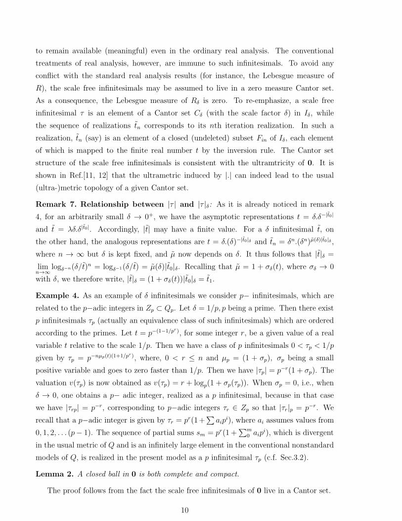
to remain available (meaningful) even in the ordinary real analysis. The conventional

treatments of real analysis, however, are immune to such infinitesimals. To avoid any

conflict with the standard real analysis results (for instance, the Lebesgue measure of

R), the scale free infinitesimals may be assumed to live in a zero measure Cantor set.

As a consequence, the Lebesgue measure of Rδ is zero. To re-emphasize, a scale free

infinitesimal τ is an element of a Cantor set Cδ (with the scale factor δ) in Iδ, while

the sequence of realizations tn corresponds to its nth iteration realization. In such a

realization, tn (say) is an element of a closed (undeleted) subset Fin of Iδ, each element

of which is mapped to the finite real number t by the inversion rule. The Cantor set

structure of the scale free infinitesimals is consistent with the ultramtricity of 0. It is

shown in Ref.[11, 12] that the ultrametric induced by |.| can indeed lead to the usual

(ultra-)metric topology of a given Cantor set.

Remark 7. Relationship between |τ | and |τ |δ: As it is already noticed in remark

4, for an arbitrarily small δ → 0+, we have the asymptotic representations t = δ.δ−|t0|

and t = λδ.δ|t0|. Accordingly, |t| may have a finite value. For a δ infinitesimal t, on

the other hand, the analogous representations are t = δ.(δ)−|t0|δ and tn = δn.(δn)µ(δ)|t0|δ ,

where n → ∞ but δ is kept fixed, and µ now depends on δ. It thus follows that |t|δ =

limn→∞

logδ−n(δ/t)n = logδ−1(δ/t) = µ(δ)|t0|δ. Recalling that µ = 1 + σδ(t), where σδ → 0

with δ, we therefore write, |t|δ = (1 + σδ(t))|t0|δ = t1.

Example 4. As an example of δ infinitesimals we consider p− infinitesimals, which are

related to the p−adic integers in Zp ⊂ Qp. Let δ = 1/p, p being a prime. Then there exist

p infinitesimals τp (actually an equivalence class of such infinitesimals) which are ordered

according to the primes. Let t = p−(1−1/pr), for some integer r, be a given value of a real

variable t relative to the scale 1/p. Then we have a class of p infinitesimals 0 < τp < 1/p

given by τp = p−nµp(t)(1+1/pr), where, 0 < r ≤ n and µp = (1 + σp), σp being a small

positive variable and goes to zero faster than 1/p. Then we have |τp| = p−r(1 + σp). The

valuation v(τp) is now obtained as v(τp) = r + logp(1 + σp(τp)). When σp = 0, i.e., when

δ → 0, one obtains a p− adic integer, realized as a p infinitesimal, because in that case

we have |τrp| = p−r, corresponding to p−adic integers τr ∈ Zp so that |τr|p = p−r. We

recall that a p−adic integer is given by τr = pr(1+∑

aipi), where ai assumes values from

0, 1, 2, . . . (p− 1). The sequence of partial sums sm = pr(1 +∑m

0 aipi), which is divergent

in the usual metric of Q and is an infinitely large element in the conventional nonstandard

models of Q, is realized in the present model as a p infinitesimal τp (c.f. Sec.3.2).

Lemma 2. A closed ball in 0 is both complete and compact.

The proof follows from the fact the scale free infinitesimals of 0 live in a Cantor set.

10

Next, we extend this nonarchimedean structure of 0 on the whole of R, which is

already realized here as an intrinsically nonstandard extension R.

Definition 5. Let Iδ(r) = r + Iδ, Iδ = (−δ, δ), δ > 0 for a real number r ∈ R. For a

finite r ∈ R, i.e., when r /∈ Iδ(0), we have ||r|| = |r|e = r. For an r ∈ Iδ(0), on the other

hand, we have ||r|| = |r| = limδ→0

logδ−1(δ/r) = σv(r), while, for an arbitrarily large r(→ ∞),

i.e., when |r|e > N, N > 0, we define ||r|| = |r−1| with a scale δ ≤ 1/N .

Proposition 3. ||.|| is a nonarchimedean absolute value on R (i.e. on R). It is discretely

valued over the set of infinitely small and large numbers. The space {R, ||.||} is denoted

as R.

Proof. For an infinitely small or large r, the proof follows from Proposition 2. For a

finite (non-zero) value of r ∈ R, we have, on the other hand, r = s+τ(t), s = r− t, τ(t) =

t, t ∈ I+δ , so that ||r|| = max{||s||, ||τ(t)||} = s = |r|e, by letting t → 0. Discreteness on

the set of infinitesimals and infinities follows from the discreteness of |.|.

Proposition 4. R is a locally compact complete (ultra-)metric space.

The proof follows from Lemma 2 and Proposition 1.

Proposition 5. The topology induced by ||.|| on R is equivalent to the usual topology.

Moreover, the imbedding i : R → R is continuous.

Proof is an obvious application of Definition 5.

Definition 6. A (δ) infinitesimal τ is an (non-archimedean) integer if |τ | < 1. It is a

unit if |τ |=1.

Lemma 3. A unit τu has the form τu = 1 + τ where |τ | < 1.

Proof. A scale free (δ) unit is defined by ||τu|| = 1. According to the valuation equation

(7), we havetunδn

= (δn)1+ξ(τu,δ) (8)

since v(τu) = 0 (tun are various realizations of τu). Thustunδ2n

= (δn)ξ → 1, as n → ∞ and

subsequently δ → 0. Thus writing τn = ξ log δn, we have the lemma, since, as n → ∞,

τu = lim tnδ2n

= lim eτn = 1 − τ0, when we have ||τ(1 + O(τ)|| = ||τ0||,( because of the

ultrametricity of ||.||) for a τ0 = τ (1 +O(τ)).

Lemma 4. Let τi be two δi infinitesimals, i = 1, 2 such that δ1 > δ2. Then there is a

canonical decomposition τ1 = τ1(1 + τ2)) where |τ1| = |τ1| < 1.

11

Proof. Recall that δ− infinitesimals live in (0,1), which is covered by clopen balls

B(τ1i), i = 1, 2, . . .. Let τ1 ∈ B(τ1i) for some i. Suppose τ1i be defined by (6) ( that

is, corresponding to λ = 1 in the inversion rule). For a general infinitesimal τ1 we have

the extended definition given by (7), viz.,

t1nδn1

= (δn1 )(|τ1i|δ1+ξ(τ1,δ2)) (9)

where ξ goes to zero faster than |τ1i| = δv(τ1i) such that (δn1 )ξ = 1 as δn1 → 0+. Now

writing ξ = (ξ) log δ2log δ1

and using Lemma 3, one obtains

t1nδn1

=t1niδn1

tunδ2n2

(10)

and so taking the limit n → ∞ the desired result follows.

Let us recall that dτ/dt = 0 means τ=constant, in R. However, in a nonarchimedean

space R, τ would be a locally constant function, which we call here a slowly varying

function. In a nonarchimedean extension of R, λ (in Definition 2) may be a slowly

varying function. Thus, the nonsmooth solutions of R (Section 2) are realized as smooth

in the nonarchimedean space R. We recall that differentiability in a nonarchimedean

space is defined in the usual sense by simply replacing the usual Euclidean metric by the

ultrametric ||x− y||, x, y ∈ R.

Definition 7. Let f : R → R be a mapping from R to itself. Then f is differentiable at

t0 ∈ R if ∃ l ∈ R such that given ε > 0, ∃ η > 0 so that

∣

∣

∣

∣

‖ f(t)− f(t0) ‖

‖ t− t0 ‖− ‖ l ‖

∣

∣

∣

∣

< ε (11)

when 0 <‖ t− t0 ‖< η, and we write f ′(t0) =df(t0)dt

= l.

Remark 8. The above definition is in conformity with the more conventional definition,

viz.,

‖f(t)− f(t0)

t− t0− l ‖< ε (12)

since∣

∣

∣

‖f(t)−f(t0)‖‖t−t0‖ − ‖ l ‖

∣

∣

∣

e<‖ f(t)−f(t0)

t−t0−l ‖< ε. As long as |t−t0|e → 0+, but t−t0 ≥ O(δ),

the above definition reduces to the ordinary differentiability. But when |t− t0|e → δ the

above gets extended to the logarithmic derivative td log f(t0)dt

= l, when we make use of the

nonarchimedean absolute value |.|.

So far in the above discussion the scale δ is unspecified. In the following, we introduce

the nonarchimedean absolute value (Definition 5) on the field of rational numbers Q,

12

construct its Cauchy completion and finally, because of the Ostrowski theorem, relate it

to the local p-adic fields. We get a minimal nonarchimedean extension of R (and which

is a subset of the above R) for each given scale δ, thus sufficing our purpose of relating

the (secondary) scales δ with the inverse primes viz., δ = 1/p. Consequently, we have a

countable number of distinct field extensions Rp of R depending on the scale at which

the origin 0 of R is probed.

3.2. Completion of the field of rational numbers

On the field of rationals Q, we now introduce a valuation ||.|| : Q → R+.

Definition 8. Let Iδ(r) = r+ Iδ, Iδ = (−δ, δ), δ > 0 for a rational number r ∈ Q. For a

finite r ∈ Q, i.e., when r /∈ Iδ(0), we have ||r|| = |r|e = r. For an r ∈ Iδ(0), on the other

hand, we have ||r|| = |r| = lim logδ−1(δ/r) = δv(r), while, for an arbitrarily large r(→ ∞),

i.e., when |r|e > N, N > 0, we define ||r|| = |r−1|u with a scale δ ≤ 1/N .

Proposition 2 is now restated for the rationals.

Corollary 1. ||.|| is a nonarchimedean absolute value over Q.

Now by the Ostrowski theorem [2], any nontrivial absolute value on Q must be equiv-

alent to any of the p−adic absolute value |.|p, p > 1 being a prime and |.|∞ = |.|e is the

usual Euclidean absolute value. From Definition 8, finite rationals of Q get the Euclidean

value, while |.|, on the arbitrarily small and large values, must be related to the p−adic

valuation. Consequently, the set of scales are represented by the primes δ = p−1.

To construct the completion of Q under ||.|| we first consider the ring S of all se-

quences of Q. The zero divisors in S are removed by the choice of an ultrafilter, as in the

usual nonstandard models of R (c.f. Sec.3.1) (see [15] for a recent work on nonstandard

extensions of Q)1. The quotient set of the Cauchy sequences C(⊂ S), under the usual ab-

solute value, modulo the maximal ideal N consisting of sequences converging to 0, gives

rise to the ordinary real number set R = C/N . The elements of diverging sequences in

Sdiv = S\C correspond to the infinitely large elements, when the inverse {a−1n } ∈ Sinv

of a divergent sequence {an} leads to an infinitesimal in the conventional approaches of

nonstandard analysis. In our approach, this realization is, however, somewhat reversed.

Notice that the set of divergent sequences Sdiv is quite a large set. Now among the all

possible divergent sequences, there exists a subset Sp of sequences which are nevertheless

1The model we consider here is a subset of Robinson’s model which deals with all possible sequences of

real numbers. The set S is a ring under the formal sum and product of sequences defined by {xn}+{yn} =

{xn + yn} and {xn}{yn} = {xnyn}, xn, yn ∈ Q.

13

p(-adically) convergent (Sp ⊂ Sdiv, since the sequence {n} is p-adically divergent for each

p). For each fixed p, let us consider the Cauchy completion of p convergent sequences {apn}

(say) (modulo the sequences p converging to zero), viz., the local field Qp. We identify,

by definition, the p-adic integers τ ∈ Zp ⊂ Qp with |τ |p ≤ 1 as the p infinitesimals (c.f.

Example 4). On the other hand, the elements τ of Qp with |τ |p > 1 are identified with

infinitely large numbers of order p. In other words, τ denotes the p limit of an inverse

sequence of the form {(apn)−1}, leading to the inversion symmetry τ = τ−1 which is valid

for a suitable p infinitesimal τ . The absolute value ||.|| when restricted to Sp thus relates

an infinitesimal τ an element of R, a nonstandard model of R, to a countable number

of p−adic realizations τp ∈ Zp with valuations ||τp|| = µp|τp|p, p = 2, 3, . . . , p 6= ∞, µp

being a constant for each p, as the neighbourhood of 0 in R is probed deeper and deeper

by letting δ = p−1 → 0 as p → ∞( c.f Example 4). In the computational model (Example

3), this might be interpreted as (inequivalent classes of ) higher precision models of a

computation. Consequently, equipped with ||.||, the set Sp decomposes into (a countably

infinite Cartesian product of) local fields Qp in a hierarchical sense as detailed in the

Lemma 5. We note that any element τ of Sp is an equivalence class of sequences of rational

numbers under the chosen ultrafilter. In each of such a class there exists a unique sequence

{apn}, say, converging to a p−adic integer or its inverse τp. A scale free infinitesimal τ

then relates to τp, and that τ indeed is an infinitesimal tells that ||τ || = µp|τp|p ≤ 1.

We say that 0 of R is probed at the depth of the (secondary) scale 1/p when a scale

free (δ) infinitesimal τ is related to a p−adic infinitesimal τp. We, henceforth, denote

infinitesimals, as usual, by 0, when p infinitesimals are denoted as 0p. Thus, 0 ≡ 0p (that

is, 0 is identified with 0p) at the (secondary) scale δ = 1/p.

Example 5. Let apn = 1 +∑n

1 αipi, where αi assumes values from 0,1, ...(p − 1). The

sequence apn is divergent in R for each prime p. In the nonstandard set R, {apn} denote a

distinct infinitely large number for each p. p−adically, however, apn converges to the unity

τpu (|τpu|p = 1). The scale free unity τu ∈ Sp now denotes the larger sequence {apn, ∀p}.

At the level of secondary scale δ = 1/p, unity τu is realized as τpu.

Remark 9. By ‘hierarchical’ we mean that as a scale free real variable t = t/δn, n →

∞ approaches 0 from the initial value 1 through the secondary scales 1/p, p → ∞,

the ordinary real variable t ∈ R would experience changes over various local fields Qp

successively by inversions.

Lemma 5. Let τp ∈ Zp and τq ∈ Zq, q being the immediate successor of the prime p.

Then an infinitesimal τ ∈ 0 when realized as a (p) infinitesimal has the representation

τ = τp(1 + τq) (13)

14

Further, a (p) unit is given as τpu = 1 + τp, |τp| < 1.

Proof. Let us fix the scale at δ = 1/pn. Then the proof follows from Lemma 3 and 4.

Corollary 2. One also has the following adelic extension

τ = τp∏

q>p

(1 + τq) (14)

where the product is over all the primes q greater than p.

Proof. This follows from the above lemma when the valuation formula (7) is extended

furtherτ

δn= (δn)

(|τi|+∑

m

ξm(τ,δm))(15)

where |τ | = |τi|, δ−1m , m > 1 primes greater than p, δ = 1/p and each of the indeterminate

functions ξm satisfies conditions analogous to that in (9). Further, ξq goes to zero faster

than ξp if q > p.

Collecting together the above results, we have

Theorem 1. The completion of Q under the absolute value ||.|| yields a countable number

of complete scale free models Rp of R, such that each element t ∈ Rp has the form

tp = t + τp∏

q>p

(1 + τq), t ∈ R, τp ∈ Qp, where τp is given by the asymptotic expression

τp = (p−n)(1+|τp|p(1+σ(η))) where η = O(δ) is a real variable. Finally, Rp locally has the

Cartesian product form Rp = R×Qp ×∏

q>p

Qq.

Proof. The only missing element is the completeness. Let us first fix a scale δ = 1/pr.

Let {an} be a Cauchy sequence in Rp. Then it is Cauchy either in p−adic metric or in the

usual metric, finishing the proof of the first part. The asymptotic representation follows

from Examples 1 and 3.

In the following section we discuss the nature of influences that the scale free nonar-

chimedean extensions of R would have on the basic structure of R itself.

4. Dynamical Properties

To recapitulate, we note that the set R, in the presence of nontrivial scales, prolifer-

ates into the above p−adically induced extensions Rp. We now investigate the converse

question, “How do these field extensions influence the standard asymptotic behaviours in

R?” Let us recall the standard asymptotic behaviour of an ordinary real variable t as it

approaches 0 is that t vanishes linearly as t → 0 (at the uniform rate 1). In the presence

of nontrivial scales the situation is altered significantly. The point 0 is now identified

15

with the set Iδ = [−δ, δ], δ = 1/pr, for some r > 0 inhabiting infinitesimals t as in

Definition 1. Corresponding to these infinitesimals there exist scale free (p) infinitesimals

τp = lim tn/δn, n → ∞ with absolute values of the form ||τp|| = |τp| = |τ |p(1 + σ(η)).

Here, η is defined by the real variable t = δ(1 + η) approaching 0+, viz., δ from the right.

In the ordinary real analysis, δ = 0 and the limiting value of t, viz., 0 is attained exactly.

For a nonzero δ, this exact value is attained by the rescaled variable t1 = t/δ, although

the value attained is now 1 instead, i.e., t1 = t/δ = 1. We are thus still in the framework

of the real analysis (and computational models based on this analysis). The presence

of infinitesimals of the form t (in the conventional sense) does not appear to induce any

new structure beyond that already existing in the system. The definition of scale free

infinitesimals and the associated absolute values now provide us with new inputs.

Definition 9. The scale free (p) infinitesimals, in association with absolute values |.|,

are called valued (scale free) infinitesimals. These infinitesimals are also said to be “ac-

tive” (directed), when infinitesimals of conventional nonstandard models are inactive (or

passive, non-directed).

Remark 10. Because of scale free infinitesimals, the exact equality of R in the ordinary

analysis is replaced by an approximate equality, for instance, the equality t = 1 is now

reinterpreted as t = O(1). In an associated nonarchimedean realization Rp the exact

equality is again realized, albeit, in the ultrametric absolute value viz., ||t|| = 1. Further,

the rescalings defined by the inversion rule in Definition 1 accommodates the residual

rescalings of Sec.2 provided the absolute value of a valued infinitesimal τp at the scale

δ = p−n is given by |τp| = p−n.

Proof and Explanations: We consider infinitesimals as defined by 0 < ˜t < ǫ <

t < δ < t (ǫ is determined shortly). We show that valued infinitesimals from (0, ǫ] would

affect the ordinary value of t nontrivially. Infinitesimals in (ǫ, δ) are (relatively) passive.

As stated above, in ordinary analysis, the limit t → 0+ in the presence of a scale is

evaluated exactly viz., t1 = 1 i.e., log t1 = 0 = O(δ). Infinitesimals, in conventional

scenario, are passive in the sense that their values remain always infinitesimally small in

any linear process (dynamical problem). In the present case, however, the numerically

small (in the ordinary Euclidean sense) infinitesimals lying closer to 0, are dominantly

valued, so as to induce an influence over a finite real variable (numbers). This is because

of the definitions of valued infinitesimals. Indeed, we reinterpret the valuation structure

(as defined in Definitions 1-3), in the context of ordinary analysis, as one admitting an

extension of the ordinary (positive) real line (δ,∞) over (ǫ, δ] ∪ (δ,∞) so that ordinary

zero is now identified as [0, ǫ], ǫ = t−11 .δ log δ−1 instead. As a consequence, we shall

16

now have log t1 = O(ǫ). In the language of a computational model, the accuracy of

the model is increased to the level denoted by ǫ. It now follows from Remark 7, that

t. logδ−1(λδ/t) = t.|τr|p(1+σp(η)) = O(δ2). This follows from the inversion law (Definition

1) and the fact that |t| ∼ O(δ) (Remark 1). Thus, fixing r = n, so that |τn|p = p−n = δ,

we get the first correction

(1 + η)(1 + σp(η)) = O(1) (16)

to the value of t1 = 1 + η from (p) infinitesimals, even for a fixed value of η. We note

that tp = 1+ σp(η) and σp > 0 must be of higher degree in the real variable η as tp ∈ Rp.

Eq(16) is interpreted as one encoding the influence of the (first order) (p) infinitesimals.

Taking into account successively the higher order (p) infinitesimals, and iterating the

above steps on each rescaled variables tp = O(1), one obtains log(1 + σp(η)) = O(ǫ),

where ǫ = t−12 .δ log δ−1, δ = q−n, q being the immediate successor to the prime p, and so

on , so that we get finally an extended version of the equality t1 = O(1) ∈ R in the set R

as

T (η) := (1 + η)∏

q≥p

(1 + σq(η))(= O(1)) (17)

The variable t ∈ R is thus replaced by the modified variable T ∈ R and hence, in this

extended framework, a solution of

tdt

dt= −t (18)

is written, for a t > 1 as 0 < t(t) = (T (η))−1 < 1, which belongs clearly to the class

of nonsmooth solutions of Sec.2. Here, σp’s take care of the residual rescalings, and

thereby introduce small scale variations in the value of η. These also relate to the size

of the undeleted closed intervals at the nth iteration of the Cantor set accommodating

(p) infinitesimals. This explains the loss of exact equality in the present extension of R.

We note that the ordinary real number set R is recovered in the limit when the said

closed intervals reduce to a singleton (Example 2). As a consequence, µ = 1, leading to

σp(η) = 0, thus retrieving the exact equality of R. For a nontrivial µ 6= 1, one, however,

verifies that σp(η) = αp(ηp − ǫp/αp)2, p being the preceding prime, when eq(18) is solved

recursively as in Sec. 2.

Remark 11. It is important to note that the above derivation is performed purely in the

ordinary analysis, except for the fact that we make use of the special representations of t

and t as induced from the valued infinitesimals. Consequently, (i) the transitions between

real and infinitesimals are interpreted as being facilitated by inversions ( for instance,

either as t− 7−→ t−1− = t+, or as t+ 7−→ t− = t−1

+ , as the case may be) as oppose to linear

17

shifts (remark 5) and (ii) the nonarchimedean p−adic absolute value |τr|p generates a

scale factor in the smaller scale logarithmic variables. In fact, this correspondence could

be made more precise.

Proposition 6. (Page 14, Ref[16]) Let τp ∈ Qp, so that τp = pr(1 +∑∞

1 aipi), where

ai assumes values from 0, 1, 2, . . . (p − 1) and r ∈ Z. Then there exists a one to one

continuous mapping φ : Qp → R+ given by φ(τp) = p−r(1 +∑

aip−2i).

Let us denote Cp = φ(Qp). It then follows that any bounded subset of Cp is a zero

(Lebesgue ) measure Cantor set in R (c.f. Example 3). Accordingly, the treatments of

ordinary analysis can be extended in a scale free manner (though remaining in the folds

of the usual topology of R) over a more general metric space ℜ accommodating the above

new structures. In view of Theorem 1, ℜ is locally (at the neighbourhood of a point

t = t0 ∈ R) a Cartesian product, viz., ℜ = R×∏

p

Cp. The product space is interpreted as

an hierarchical sense. An ordinary real variable t is extended over ℜ as T = t∏

tp where

tp = 1+ǫpτp, τp ∈ Cp being a scale free (p) infinitesimal and ǫp ≈ δp−1 log(pδ−1) denotes the

enhanced level of accuracy because of valued infinitesimals at the scale δ = δp−1, δ → 0+.

Noting that ǫq/ǫp = p/q → 0, as δ → 0+, for q > p, one may re-express T as T = t(1+ǫτ),

where ǫ ≈ δ log δ−1 when the scale is identified with δ = 2−(n−1) so that p = 2, and the

scale free infinitesimal τ now resides and varies in∏

Cp in an orderly (hierarchical) manner

as detailed below, as t → 0+ = O(δ).

Let us first recall (again) that the concept of relative infinitesimals is introduced orig-

inally in the context of a Cantor set [11, 12]. Because of these relative infinitesimals

each element of the Cantor set Cp is effectively identified with a closed interval of Rp (a

generator of a defining IFS) at every level of the scale δ → 0. In the presence of infinites-

imals a Cantor set is thus realized as Rp itself except for the fact the motion in Cp is

now visualized as a combination of linear shift (along the closed line segment) together

with an inversion in the vicinity of the Cantor point itself. As a consequence, the gener-

alized, inversion mediated metric space ℜ is represented henceforth as ℜ = R×∏

Rp. A

generalized motion in ℜ now is represented as follows.

Definition 10. The set ℜ is interpreted as having several branches R and Rp, p being a

prime. The branches Rp accommodating scale free infinitesimals and infinities are thought

to be knotted at (the scale free unity) 1. A real variable t ∈ R approaching 0=O(δ)

from 1(say) is replaced by the scale free variable t1 = t/δ. For simplicity of notation we

continue to denote t1 by t and call it a scale free variable instead (which should become

clear from the particular context). So, as the scale free t → 1+, the unique linear motion

18

is replaced by two inversion mediated modes: (i) Local or vertical mode: t+ is replaced by

t+ 7−→ t−1+ = t− which takes note of the localized effects of infinities on an infinitesimal

and (ii) global or horizontal (growing) mode: a scale free infinitesimal 0 < η ∈ Rp grows

infinitely slowly following the linear law until it shifts to a O(1) variable living possibly in

another branch Rq by inversion η− 7−→ η−1− = t+ = 1 + η where 0 . η ∈ Rq.

Remark 12. The unidirectional motion of a real variable t ∈ R approaching 0+ thus

bifurcates into two possible modes: a variable t approaching 0 = O(δ) from above will

experience, as it were, a bounce and so would get replaced by the inverted rescaled

infinitesimal variable t = δ/t living in a scale free branch Rp(say). A fraction of the

asymptotic limit t → 0+ = O(δ) of R (viz., t 7−→ t+ = t/δ = 1 + η, η → 0+) is therefore

be replaced by a growing mode of the rescaled variable t−1− = tp+ = 1 + ηp, tp+, ηp ∈ Rp

and ηp & 0 initially but subsequently growing to → 1− in the branch Rp. Besides this

growing mode, another fraction of the decreasing (decaying) mode of the flow of R, viz.,

t 7−→ t+ = t/δ = 1 + η, η → 0+, is also available as a localized mode in another branch

Rq (say) in the form t−1+ = (1+ ηq)

−1 = tq−, where, again ηq ≈ 0 grows to ηq → 1− slowly.

As a consequence, the limiting value 1 of the rescaled variable in R, now, gets a dynamic

(multiplicative) partitioning of the form tq−tp+ ≈ 1 ⇒ (1−µ(ηq)ηq)(1+ηp) = O(1), 0 .

ηp ∈ Rp, 0 . ηq ∈ Rq, which equivalently can also be written more conveniently as

(1− tηq)(1 + ηp) = O(1) (c.f. Remark 4). The local and global modes therefore appear to

induce a competition between the effects generated by infinitesimals and infinities, leading

to this dynamic partitioning of the unity. The localized factor (1− tτ ) arising from active

infinitesimals τ living in a branch of ℜ will lead to an asymptotic scaling of any scale free

(locally constant) variable T = T/t in ℜ (see Sec.4.3). Accordingly, dT/dt = 0 and hence

τ ∈∏

Rp satisfies the scale free equation

log tdτ

d log t= −τ (19)

Consequently, asymptotic limits either of the forms t → 0+ or t → ∞, in R would

ultimately behave as an unidirectional (monotonically increasing ) variable in ℜ. Moreover,

as t−1 → ∞, the ordinary linear motion of t → 0 will undergo small scale mutations,

because of zigzag motion of the inverted variables tp’s (∼ O(1)), living successively in the

rescaled branches Rp and mapping recursively the smaller and smaller neighbourhoods of

0 closer to 1. As a consequence, extended real numbers T of ℜ are directed, since each of

the (p) infinitesimals are, by definition (as it involves a limit ), directed.

Definition 11. Intrinsic (Internal) Time: A continuous monotonically increasing vari-

able t living in the product space∏

Rp, from the initial value 1, is called an internal

19

evolutionary time. The rate of variations of t is infinitely small because of the presence

of scale factors of the form δp−1, δ → 0+.

Any variable τ ∈∏

Rp is called dynamic since it undergoes spontaneous changes

(mutations) relative to the (scale free) internal time t.

With this dynamic interpretation of ℜ, it now follows that new solution constructed

in equation (17) is indeed smooth in ℜ (as it is evident from the derivation). However,

because of the presence of the irreducible O(1) correction factors this solution can not

be accommodated in the ordinary analysis (i.e., even in ℜ ) in an exact sense. In the

nonarchimedean extensions Rp, such a solution is not only admissible and smooth but

also exact, in the sense of absolute values, viz., ||τ || = 1, since ||t|| = ||ti|| = 1 for each i,

thus retrieving the ordinary equality |t1|e = 1 in the ultrametric sense.

We restate the above deductions as a

Lemma 6. The ordinary analysis on R is extended over ℜ with new structures as detailed

above (Definition 10, Remark 12). In this extended formalism accommodating dynamic

(valued) infinitesimals, 0 ∈ R+ (the set of positive reals) is identified with [0, ǫ], ǫ =

t−11 .δ log δ−1, where t1 = t/δ and t → δ+. As a consequence, a constant in R becomes a

variable over valued infinitesimals of ℜ.

Proof. We have already seen in the above that 0 ∈ R+ is actually [0, ǫ] in ℜ. We justify

it further by showing that an equation of the form

dφ

dt= 0 (20)

for finite real values of t is transformed into

d logφ

dlog t= O(1) (21)

for an infinitesimal t satisfying tδ= λ δ

t= δ−||t||, 0 < t < δ ≤ t, t → 0+, λ > 0, and

||t|| = t1(= |t|p(1+σ(η)), when one interprets 0 in relation to the scale δ as O( δ2

tlog δ−1 ).

Indeed, we first notice that (20) means dφ = 0 = O(ǫ), dt 6= 0 for an ordinary real variable.

However, as t → δ, that is, as dt = η → 0 = O(ǫ), the ordinary variable t is replaced by the

extended variable, so that d logδ−1 t = dt1 = O(ǫ). As a consequence, in the infinitesimal

neighrhood of δ, eq(20) is transformed into an equation of the form eq(21). We note that

in that neighbourhood, t and φ, are represented as t = δ.δ−t1 and φ = φ0δkt1 for a real

constant k, whence we get eq(21).

20

4.1. Directed tree

Geometrically, the ordinary real number system is represented as the (undirected) real line.

The ultrametric extension R or its equivalent inversion mediated extension (realization

) ℜ, is, on the other hand, modeled geometrically as an infinite directed, rooted tree

[4]. This is because of the one-to-one correspondence between an ultrametric space and

a wieghted, directed, rooted tree [5]. Such a wieghted, directed and rooted tree has

a natural correspondence with a polygenetic or evolutionary tree showing evolutionary

relationship among various entities having a common ancestor. It follows accordingly

that an intrinsically evolutionary sense can naturally be attached to any ultrametric

space. The concept of internal time introduced above is in consonance with the time sense

induced from the evolutionary tree model. We note that the estimation and classification

of all possible transitions among several branches of the tree model of ℜ is an interesting

combinatorial problem. This and other related issues will be explored in detail separately.

Before proving the PNT in the present dynamic extension of R, we need two more

ingredients: viz, the origin of the prime counting function and the asymptotic scaling of

active infinitesimals.

4.2. Prime Counting Function

The prime counting function arises in connection with the growing mode of a dynamic

variable in ℜ, when we assume that a scale free variable t varies over all possible primal

branches in an orderly manner following the order of the primes.

Recall that the usual ǫ− δ definition of limit (in R) does not make explicit the actual

motion of a real variable t approaching a fixed number, 0, say. In the present formalism

infinitesimals are defined by asymptotic scaling formulas (c.f. Example 1) (which would

ordinarily correspond simply to zero), and so may be considered to carry an evolutionary

arrow. A limit of the form t → 0 in ℜ would be interpreted in the context of a dynamical

problem, so that t−1 may be identified with the (physical) time. More precisely, when the

ordinary R component of ℜ = R ×∏

Rp is free of any arrow, the nontrivial components

Rp do carry an evolutionary arrow. A problem involving the asymptotic limit t → 0+

(equivalently t → ∞) in ordinary analysis is raised in the present context over ℜ as the

asymptotic limit of the extended variable T = t(1+ǫτ) where τ is an O(1) growing dynamic

variable which lives hierarchically in the sets Rp, p = 2, 3, 5, . . . as explained in Definition

10 and Remark 12 (a growing dynamic infinitesimal η is represented now as η = ǫτ). Thus,

the ordinary limit of T as t → 0+ as δ, that is, T = 0, is interpreted in the present context

as log(T/t) = log(1+ǫτ) = O(ǫΠ(t−1)) as t → 0+ hierarchically through scales δp−1. That

21

is to say, as pointed out above, as t → δ+, it changes over to various branches Rp assuming

several variables tis (all of which are different Rp valued realizations of τ) having forms

ti = 1+ηi, t0 ≡ t and i runs over the primes. Consequently, as t2 = (λ1)t−11 ∈ R2, t1 = t/δ

approaches 1/2−, we get the next level variable t3 = (2λ2)t−12 ∈ R3 and so on and so forth,

adding one unit to the prime counting function Π at every change of the primal scale.

Indeed, infinitesimal ηi grows linearly (and spontaneously) to O(1) whence it undergoes

inversion mediated transition of the form ηi− 7−→ η−1i− = 1 + ηj, where j being the next

prime. As a consequence, we have

Theorem 2. The ordinary (linear) limiting behaviour of a real variable t → 0+ in the

real number set R is raised, in the inversion mediated set ℜ, to the asymptotic limit of the

extended variable T = t(1 + ǫτ), where the O(1) dynamic variable τ is realized in relation

to every secondary (primal) scale 1/p as a variable of the form tp ≥ 1. As a consequence,

the asymptotic limit of T as τ(≡ tp) → 1/p, p → ∞ is given by log(T/t) = O(ǫΠ(t−1)),

for a locally constant infinitesimal ǫ = O(δ log δ−1) = O(t log t−1), as the real variable

t−1 → ∞.

In the next section we investigate the scaling of T (t) ∈ ℜ as t → 0 in R.

4.3. Scaling

Let us begin by recalling that the main characteristic of both the inverted motions is the

inherent directed sense. That is to say, although t1+ = 1 + η, η ↓ 0+ in R, in either of

the inverted motions, we have, however, t1+ = 1 + η, η ≈ 0, initially, but η ↑ 1−, slowly,

when t1+ ∈ Rp. As shown in the above sections, the growing mode induces the global

evolutionary sense leading to the prime counting function. Here we study the local motion

leading to the asymptotic scaling for a small scale variable T ∈ ℜ.

Because of the valued infinitesimals that contribute nontrivially to the ordinary value

of an arbitrarily small t ∈ R, the scaling behaviour of the corresponding extended variable

T ∈ ℜ is nontrivial. As explained above, an ordinary, arbitrarily small t ∈ R is extended

in ℜ as T/t = (1−O(tτ ))φ(t−1), for a class of valued infinitesimals τ(t−1). Our aim here

is to estimate lim τ as t → 0. Notice that the (-) sign in the first factor makes it a true

dynamic infinitesimal living in a Rp (c.f. Remark 12). The second factor φ corresponds

to the growing mode of a dynamic infinitesimal and is considered in Theorem 2.

We recall that the above limit may have a constant (nonzero)(ultrametric) value (c.f.

Example 1). Indeed, as t approaches 0, as δ, the ordinary variable t gets extended to the

rescaled variable T− = T−/t = 1 − O(tτ)), which now approaches 0+, via a combination

of inversions and translations. Indeed, as t → 0 in R, T− in ℜ is realized as a locally

22

constant function satisfying dT/dt = 0 so that τ ∈∏

Rp now satisfies the equation (19),

i.e.

log tdτ

d log t= −τ (22)

and changes from one copy of Rp to another near the scale 1/p by inversions via a sequence

of distinct realizations ti, i being a prime. To see in detail, let η− = tτ(t−1). As t → 0 =

O(δ) linearly and the motion should have been terminated at δ in R, now, instead is

picked up by the rescaled variable which shifts by inversion to η2− = t2t2 , t2 ≈ 0. The

limiting motion is now transmitted over to the next generation variable t2 ∈ R2, which

grows to 1/2 linearly, until the motion is again transferred to the next level by inversion

viz., 2t2 = 1/(1 + 3t3), where t3(≈ 0) ∈ R3. Recall (Definition 10) that this (and the

following) local inversions essentially inject into an infinitesimal higher order influences

from infinities. The new rescaled variable t3 now grows to 1/3, and transmits its motion

to t5 ∈ R5 near t5 → 1/5− by inversion, and so on successively over all the higher primal

scales. The exponent in η− now asymptotically assumes the form of the golden ratio

continued fraction η∞− = t1

1+ 11+... , so that the exponent has the value ν =

√5−12

. As

a consequence, the asymptotic scaling of a dynamic infinitesimal T− in ℜ is given as

T− = tT− ∼ t1+ν , t → 0+. As a consequence, the asymptotic small scale variations

(mutations) in the dynamic infinitesimal follow a generic golden ratio scaling exponent

[9].

Combining this local asymptotic scaling together with the global asymptotic of The-

orem 2, one finally arrives at the asymptotic law

Theorem 3. The generic asymptotic behaviour of a dynamic variable T ∈ ℜ, extending

the ordinary real variable t, is given by

logT

t= ǫO(Π(t−1))(1− O(tν)) (23)

as t−1 → ∞.

The above asymptotic formula is the main result of this paper. Over any finite (time)

t scale, the right hand side effectively reduces to zero, recovering the standard variable

T = t. However, in any dynamic process which persists over many (infinitely large)

time scales, the correction factor may become significant leading to a finite observable

correction to the evolving quantity T = teO(1) which may arise from the annihilation

(cancellation) of the infinitesimal (locally constant variable) ǫ by the growing mode of

the prime counting function. The proof of the prime number theorem now follows as a

corollary to Theorem 3.

23

5. Prime Number Theorem

The locally constant infinitesimal ǫ(t−1) = O(t log t−1) clearly corresponds to the inverse of

the PNT asymptotic formula for the prime counting function Π(t−1). The O(1) correction

to any dynamic variable T in ℜ is realized for a sufficiently large value of t−1 provided

(more precisely, if and only if)

ǫ(t−1)Π(t−1) = (1 +O(tν)), t−1 → ∞ (24)

with the relative correction (error) Π(t−1)ǫ(t−1) − 1 = O(tν), which clearly respects the

Riemann’s hypothesis since tν ≤ Mt(1/2−σ) for a suitable M > 0 and for any σ > 0,

t → 0+.

REFERENCES

[1] H. M. Edwards, Riemann’s Zeta Function, Dover Publications, New York, (2001).

[2] F Gouvea, p-adic Numbers: An Introduction, Springer-Verlag, berlin, (1993).

[3] P. Schneider, Nonarchimedean Functional Analysis, Springer, Berlin, (2002).

[4] J. Pearson and J. Bellissard, Noncommutative Riemannian geometry and diffusion

on ultrametric Cantor sets, arXive: math/0802.13362v2 (2008).

[5] B. Bollobas, Modern Graph Theory, Springer, Berlin, (1998).

[6] R. Albert and A. L. Barabasi, Statistical mechanics of complex networks, Rev. Mod-

ern Phys. 74, 47-101, (2002).

[7] E. Nelson, Internal Set Theory: A New Approach to Nonstandard Analysis, Bulletin

of the American Mathematical Society, Vol. 83, Number 6, 1977

[8] A. Robinson, Nonstandard Analysis, (North-Holland, Amsterdam, 1966).

[9] D P Datta, A new class of scale free solutions to linear ordinary differential equations

and the universality of the Golden Mean√5−12

= 0.618033 . . ., Chaos, Solitons &

Fractals, 17, 621-630, (2003).

[10] D. P. Datta and M. K. Bose, Higher derivative discontinuous solutions to linear ordi-

nary differential equations: a new route to complexity? Chaos, Solitons & Fractals,

22, 271-275, (2004).

24

[11] S. Raut and D.P. Datta, Analysis on a fractal set, Fractals, 17, 45-52, (2009); Erra-

tum, ibid, 17, 547, (2009).

[12] S. Raut and D.P. Datta, Nonarchimedean scale invariance and Cantor sets, Fractals,

18, 111-118, (2010).

[13] T. Tao, Ultrafilters, nonstandard analysis and epsilon management, http:// terry-

tao.wordpress.com/2007/06/25.

[14] M. Berz, Non-archimedean analysis and rigorous computation, Int. J. Applied Math.

2, 889-930, (2000).

[15] P. Laubeinheimer, T. Schick, U. Stuhler, Completion of countable nonstandard mod-

els of Q, arXive: math/0604466, (2006).

[16] V. S. Vladimirov, I. V. Volovich, E. I. Zelonov, p-adic Analysis and Mathematical

Physics, World Scientific, Singapore, (1994).

25