1

1

TOPO-GEOMETRIC SHAPE MODEL FOR 3D OBJECT

REPRESENTATION

Sajjad Baloch†, Hamid Krim†, Irina Kogan‡, and Dmitry Zenkov‡

shbaloch, ahk, iakogan, dvzenkov@ncsu.edu

North Carolina State University, Raleigh, NC 27695

Abstract

We propose a new method for representing the topology and geometry of 2D compact surfaces embedded in

a three-dimensional space. Topology is modeled through a skeletal graph, where a distance function is employed

as a Morse function. Invariance to rigid transformations follows directly from this choice of Morse function.

Geometry is captured by modeling the evolution of level curves of the distance function along topologically

homogenous parts of the surface, which in turn correspond to various graph edges. Combining topological

and geometric information leads to a weighted skeletal graph representation of a surface, which is sufficient

for reconstructing the original surface. The uniqueness and completeness of representation make the method

particularly suitable for shape recognition applications, where weighted graph isomorphism may be employed.

Index Terms

3D Object representation, Morse theory, Critical points, Elasticæ, Reeb graph, classification.

1. Introduction

Modeling of 3D objects constitutes a fundamental problem in computer vision applications. 3D objects are

usually represented by their surface boundaries, which in turn are normally parameterized by triangulated

meshes. Such a representation, however, suffers from two major drawbacks. First, it does not take into account

†Department of Electrical and Computer Engineering.

‡Department of Mathematics.

This work was supported by AFOSR F49620-98-1-0190 and NSF CCR-9984067 grants.

local correlations or similarities, thus failing to exploit underlying redundancy for a compact representation.

Second, it results in intertwined topological and geometrical information, which makes it unsuitable for shape

recognition. Various approaches have been proposed in literature for addressing these problems. One of the

foremost methods for compact representation is a variant of medial axis, known as medial axis transform

(MAT) [19], [45], [1], [12]. Incomplete shape information in medial axis descriptor limits its use for shape

reconstruction. On the other hand, an MAT complements a medial axis with additional information by

superimposing the radius information of the corresponding circles/spheres on medial axis. The resulting

model contains sufficient information for a complete yet compact shape representation, thereby allowing

their reconstruction. It, however, suffers from the drawback that for 2D surfaces, medial axis transform itself

happens to be a surface, which limits its utility for shape recognition. Pizer et al. [34], [21], on the other hand,

provide the addition information by way of spokes along the medial axis, which represents its distance from

the surface. Although the resulting shape model, known as m-reps, has been shown to reconstruct very

“simple” shapes, its utility for complex shapes of arbitrary topology is an open question. In addition, it does

not decouple topological and geometric information, and hence, is not suitable for shape recognition.

For shape recognition, the basic idea is to extract some shape features, which form a characteristic of a shape,

and subsequently employ them for recognition. A number of techniques have been proposed in literature.

Shinagawa et al. [39] use height function based Reeb graphs for shape representation. A similar approach has

been proposed by Carr, Snoeyink, and Axen [8], where they model terrain data using contour trees. Osada

et al. [31], and Ben and Krim [16] represent 3D objects by shape distributions and subsequently employ

a dissimilarity measure on distributions for shape classification. Lazarus et al. [24] propose skeletonization

based on geodesic distance from a manually chosen source point. The graphs obtained this way are called

level set diagrams. Hilaga et al. [18] extend this approach by eliminating the need of the manual selection of

a source point and propose a matching algorithm based on multiresolution Reeb graphs (MRG). Tung and

Schmitt [43] capitalized on their idea to present augmented MRGs (AMRG), thereby capturing additional

attribute features, which yield better recognition rates. In Kazhdan et al. [22], global properties of 3D objects

are captured through a reflective symmetry descriptor that is defined over a certain parametrization, which

the authors term as canonical. Kazhdan and Funkhouser [23] use rotation-invariant spherical harmonics as

Fig. 1. Weighted skeletal graph: Graph captures the topology and the weights Wi model the geometry.

a shape descriptor for recognition purposes.

A limitation of the second class of shape descriptors is that they do not represent a shape completely and,

therefore, fall short of a unique shape signature. This non-uniqueness motivates us to formulate a better

shape model, which may then be utilized for classification and recognition purposes, while simultaneously

achieving the completeness property of the first class of methods. To that end, we propose topo-geometric

shape model (TGSM), which untwines topological and geometric information, while simultaneously capturing

both completely.

2. Topo-Geometric Shape Model

TGSM is formulated in a Morse theoretic framework [29], [27], which allows topological modeling through

a skeletal graph, and geometric modeling via weight assignment. While the resulting topological graph

bears some similarities with the traditional height function based Reeb graph, it eliminates one of its major

limitations, thus achieving rotation invariance, which follows directly from its derivation from a similarity

transformation invariant Morse function — a distance function.

The graph construction algorithm involves surface sampling, and yields a set of level curves along each

graph edge, which are modeled to capture the geometry of the corresponding topologically homogenous part

of a surface. In simple words, each of these topologically homogeneous subsurfaces is represented by a weight

vector, which models the evolution of the levels curves along the subsurface. The learnt weights are finally

assigned to corresponding edges, thereby yielding a weighted graph as shown in Fig. 1, which completely

represents a surface. This completeness not only allows reconstruction of surfaces from their models, but also

leads to uniqueness of representation. Uniqueness and decoupling of topological and geometrical information

makes this representation particularly suitable for shape recognition.

The paper is organized as follows: we start with a brief overview of Morse theory given in the next section,

followed by a construction of scaling and rigid motion skeletal graph given in Section 4. Geometric model and

its implementation are presented in Sections 5 and 6, respectively. We conclude the paper with reconstruction

examples in Section 7.

3. An Overview of Morse Theory

Morse theory [29], [7], [27] allows relating the topology of a smooth manifold with the number of critical

points of a Morse function (defined below) on this manifold. A k-dimensional manifold M may be locally

parameterized as:

φ : Ω →M (1)

that is, Ω 3 u 7→ φ(u) ∈ M, where an open connected set Ω ⊂ Rk represents the parameter space. Let

f : M → R be a real-valued function on M. By definition, the function f is smooth if the composition

f φ : Ω → R is smooth for each local parametrization of M. A point x = φ(u) ∈ M, where u ∈ Ω, is called

a critical point of f if the gradient of f φ vanishes at u, i.e., 5f φ(u) = 0. The critical point x ∈ M is

called non-degenerate if the Hessian 52f φ(u) is non-singular at φ(u).1 Morse Lemma states that there exists

a parametrization of a neighborhood of a non-degenerate critical point of f : M → R in which f φ is a

quadratic form. The number of negative eigenvalues of the matrix of this form is called the index of the critical

point.

If f is a smooth function on a two-dimensional manifold M, the three possible types of non-degenerate

critical points are the local minimum (index 0), saddle point (index 1), and local maximum (index 2).

Definition 3.1: (Morse function) A smooth function f : M→ R on a smooth manifold M is called a Morse

function if all of its critical points are non-degenerate.

The basic properties of critical points of Morse functions are summarized below:

• Critical points of a Morse function are isolated.

1Both definitions are independent of the choice of the local parametrization in the neighborhood of the critical point.

Fig. 2. Manifold M and the critical points using height function.

• The number of critical points of a Morse function is stable, that is, a small perturbation of the function

neither creates nor destroys critical points.

• The number of critical points of a Morse function on a compact manifold is finite.

The level set Lc = f−1(c) ⊂ M of the Morse function f : M → R is called critical if it contains a critical

point of f . According to the Morse Deformation Lemma, if the levels Lc1 and Lc2 have different topological

types, there is a number c ∈ (c1, c2) such that Lc is a critical level.

In the rest of the paper, we will concentrate on the study of two-dimensional surfaces embedded in the

three-dimensional space R3. The points of R3 are identified with their position vectors, the latter are typed in

bold. The parameter space Ω is two-dimensional and the points in Ω are written as (u, v). Thus, if x belongs

to the surface, we write x = x(u, v).

Example 3.2: (The Height Function on a Sphere) The height function defined on a unit sphere S2 is a real

valued function h : S2 → R such that h(x, y, z) = z, ∀(x, y, z) ∈ S2. This function has two critical points,

minimum at the south pole and maximum at the north pole. Straightforward calculation confirms that both

are non-degenerate, and thus h is a Morse function.

Fig. 2 illustrates the critical points of the height function on a double torus. There are six critical points: a

minimum, a maximum, and four saddle points.

We now briefly explain how the topology of a compact orientable surface can be linked to the number

of critical points of a Morse function defined on this surface. The topological type of a compact orientable

surface M is in one-to-one correspondence with either of two numerical invariants, the genus, g, and the

Euler characteristics, χ. The former is the number of “handles” one needs to add to a sphere to obtain the

surface; the latter equals the sum of the number of vertices and the number of faces minus the number of

edges of an arbitrary triangulation of M. The two are related by:

χ = 2− 2g. (2)

It is possible to show that, for any Morse function on a compact orientable surface M, the number of

maxima plus the number of minima minus the number of saddle points equals the Euler characteristics

of M. Thus, if a Morse function on M is found, one can compute the genus of M and thus identify the

topological type of M.

4. Scaling and Rigid Motion Invariant Skeletal Graph

In this section we use the distance function to construct skeletal graphs that are invariant with respect to

scaling, translations, and rotations in the three-dimensional space.

4.1. The distance function

A distance function defined on a surface M maps each point p on a surface M to its distance from the

origin, i.e., d : p 7→ ‖p‖, ∀p ∈ M. One can show that for generic surfaces M ⊂ R3, the restriction of the

distance function d : M → R+ on M is a Morse function. We, therefore, use it for constructing skeletal

graphs.

Note that the function d given above is not invariant with respect to translation and scaling. In order to

achieve this invariance, we take the origin at the centroid µ of the surface of interest and scale the surface

accordingly to get:

dµ(p) := ‖p− µ‖,

dµ(p) =dµ(p)− dmin

dmax − dmin. (3)

Proposition 4.1: (Invariance) The distance function d given by Eq. (3) is rotation, translation and scale

invariant.

Proof: The proof follows trivially from the definition of distance function by substitution and simple

algebra.

Proposition 4.1 demonstrates the invariance of the distance function to translation, rotation and scaling under

the condition that the centroid of the manifold must be translated to the origin.

4.2. Equations for the Critical Points of the Distance Function

In order to identify the topological type of a surface, we need to locate the critical points of the distance

function. In this section, we present an analytic solution to the problem.

Assume that the surface M is locally parameterized as a patch, p = (u, v, g(u, v)), and that the centroid is

located at the origin. The distance function d(x, y, z) =√

x2 + y2 + z2 restricted to M reads

d(u, v) = d|M =√

u2 + v2 + g2(u, v).

The partial derivatives of d are

∂d

∂u=

2u + 2ggu

2√

u2 + v2 + g2(u, v),

∂d

∂v=

2v + 2ggv

2√

u2 + v2 + g2(u, v).

At a critical point the partial derivatives of d vanish. Therefore, the critical points of the distance function

on the surface M are the solutions of the system

gu(u, v) +u

g(u, v)= 0,

gv(u, v) +v

g(u, v)= 0.

The solution of these coupled partial differential equations leads to the critical points, which may

then be used to find the genus of a shape via Euler’s characteristic. Although this approach leads to a

numerical solution, complexity lies in one’s ability to find a patch to represent a surface, which may not

be straightforward for complex shapes. In addition, this approach is highly sensitive to noise, due to its

dependence on higher order derivatives. We, therefore, adopt an algorithmic approach for topological analysis,

by finding a topological structure that gives us more than simple topological information, eventually leading

(a) (b) (c)

Fig. 3. Skeletal graph of double torus: (a) Surface analyzed with an evolving sphere; (b) Intersections of the sphere and the surface;(c) Node assignment in the graph.

to a machinery for capturing complete shape information.

4.3. Algorithmic Approach to Topological Analysis

The basic idea for topological analysis of a compact surface by a distance function as a Morse function,

follows from the Morse deformation lemma, which states that a change of topology occurs only at a critical

level of the Morse function. We, therefore, need to study level sets of the distance function, and to identify

the levels where a change of their topology occurs. This requires scanning the surface with level sets of

the distance function, which happen to be concentric spheres. We, therefore, gradually increase the value of

the distance function in K steps from 0 to a sufficiently large value, say b, and find the intersections of the

surface with corresponding spheres of radii r ∈ [0, b]. The parameter K, in other words, acts as the resolution

of the skeletal graph. The larger the K, the better the precision of capturing the structural changes in the

level sets of the distance function. We, then, assign a node to each connected component in an intersection

as illustrated in Fig. 3. Hence, the skeletal graph associated with the distance function may be described as

a quotient space M/ ∼ where the equivalence relation ∼ is defined as follows:

Definition 4.2: (Equivalence) The points p and q are equivalent if they belong to the same connected component of

the level set of the function d. We write this equivalence as p ∼ q .

Recall the definition of the quotient space: M/ ∼:= [p] | p ∈ M, where the equivalence class [p] of the

point p ∈M is the set of all points q ∈M such that q ∼ p.

1) Algorithm: The definition of distance function based topological graph given above yields a construction

algorithm, which is illustrated in Fig. 4. Since the level sets of the distance function are concentric spheres,

their intersections with any shape will always be closed spherical curves. In order to generate a topological

graph, we start with a sphere of the smallest radius which is gradually increased in K steps. In the process,

we monitor its intersections with the shape. This is tantamount to intersecting the shape with K concentric

spheres with radii evenly distributed between the minimum and the maximum distance. We, therefore,

analyze the part of the surface lying between two consecutive spheres for its topological type. Each connected

component in such a region will form a topologically homogenous subsurface 2, and is subsequently specified

with a graph node at its centroid. Connectivity between the nodes is established by looking at the connectivity

of the topologically homogenous subsurfaces at two different levels.

For instance, at a particular instant, we consider three concentric spheres Sk, Sk−1, and Sk−2 as illustrated

in Fig. 4. For the given example, analyzing the shape with these spheres gives two sets of subsurfaces

Mp = M ∩ (bSk−2c ∩ dSk−1e) = M1p, . . . ,M4

p and Mc = M ∩ (bSk−1c ∩ dSke) = M1c , . . . ,M4

c, which

respectively yield two sets of nodes NMpi4i=1 and NMci

4i=1, where b.c and d.e denote exterior and interior

of the corresponding surface, and p and c denote previous and current respectively.

To establish relationships between the two sets of nodes, we look at the mutual connectivity between the

previous and current sets. Note that there is only one topological homogenous subsurface at the current level

that is connected to one at the previous level. For instance, it is only Mc1 that is connected to Mp1 . This

allows us to add an edge segment (NMp1, NMc1

) to the skeletal graph. Other edge segments in this example

are determined similarly, i.e., (NMpi, NMci

)4i=2. The complete algorithm is given in Table I.

Note that we have employed a slightly non-standard terminology while describing the graph. This is due to

the appearance of superfluous nodes (vertices in standard terminology) and edge segments (edges) in the graph,

which will be pruned to get a simplified graph composed of vertices and edges. To explain this, consider

the example of a constructed graph given in Fig. 5(a), with edge segments between various nodes. However,

not all of these nodes correspond to critical points, which demonstrates redundancy present in the learned

graph. We eventually remove this redundancy via graph simplification by merging the nodes (and the edge

segments) which lie on a topologically homogeneous path along the graph. A simplified graph is shown in

Fig. 5(b), where the mergers of redundant nodes have given rise to graph vertices and the redundant edge

segments are combined to form the graph edges. Note that the vertices of the graph in Fig. 5(b) correspond

2Topological homogeneity means no change in topology.

Fig. 4. Skeletonization of a 3D surface M.

TABLE IALGORITHM FOR CONSTRUCTING TOPOLOGICAL GRAPH

• Find the centroid of the surface M as the arithmetic mean of the vertices of the triangulated mesh and place the origin at thecentroid

• Find dmax, the maximum distance from the centroid to M• Given K, define:

rk := kdmax

K, k = 1, . . . , K

• Generate the spheres S1 and S2 with radii R = r1 and R = r2, respectively• Find Mp = M∩ (bS1c ∩ dS2e), where Mp is the part of M that lies between S1 and S2

• Assign a node NMp to each connected component Mp of Mp at the centroid of Mp

• For k = 3 to K

– Generate the “current” sphere Sk with radius R = rk

– Find Mc = M∩ (bSk−1c ∩ dSke). Hence, Mc is the portion of M that lies in between Sk−1 and Sk

– Find the connected components Mc of Mc

– For each Mc ∈ Mc do∗ Assign a node NMc at the centroid of Mc

∗ Find the connected region Mp ∈ Mp such that Mc∪Mp is a single connected region. Add an edge segment between NMc

and NMp

– end for– Mp = Mc

• end for.

to critical points of the distance function, and mark a change in the topology of level curves, while the

number of edges connecting two nodes equals the number of connected components of the level curves of

the distance function between two critical points. On the other hand, the number of cycles reflect the genus

of a given surface. In subsequent discussion, we consider only the simplified graph, and employ the standard

terminology.

(a) (b)

Fig. 5. Simplification of a skeletal graph: (a) A graph learned by the algorithm of Section 4.3.1. ; (b) Simplified graph. Note how atopologically homogeneous sequence of edge segments marked in (a) maps to an edge in (b).

5. Geometric Model

The skeletal representation given in the preceding section describes the topological structure of a surface, but

at the same time suffers from two limitations, both arising from the lack of complete geometric information.

First, it does not allow surface reconstruction. Second, any shape recognition based only on topological

information will be unable to differentiate geometric changes, resulting in low recognition rates. We, therefore,

proceed to capture geometric information, which will then be combined with the topological model for

complete shape representation.

In order to capture geometry, we note that the algorithm given in Section 4.3.1, not only constructs

topological graph but also yields level curves of the distance function. We, therefore, model the evolution

of these curves along various graph edges corresponding to topologically homogeneous parts. Since we

are working with compact surfaces, a non-singular connected component of a level set is always a simple

closed curve. The example given in Fig. 6 illustrates the idea, where a height function is employed only for

illustration purposes, and the above algorithm results in a single edge graph. Clearly, any surface may be

considered as a dense set of level curves. Given a small subset of these curves, the problem is to model

their evolution in a way so as to reconstruct the whole surface. The smaller subset in turn is generated via

a proper choice of graph resolution parameter. The constructed curve model is finally used to learn some

weights, which are assigned to respective edges. We will later demonstrate that a surface reconstructed from

the weighted graph represents the original surface arbitrarily closely.

Fig. 6. Illustration of geometric modeling: (a) A 3D object; (b) Object sampled at levels r1, . . . , rm; (c) Intersections C1, . . . , Cm

embedded in Λ bounding box to compute the distance field; (d) Vectorizing the elements of the distance field yields an n dimensionalvector ρi for each Ci.

5.1. Curve Evolution Model

An acceptable curve modeling framework is the one, which not only preserves topology of individual level

curves, but also the smoothness of a surface. The idea is to map each curve to a higher dimensional space

and to fit a smooth trajectory that passes through these points. Topological preservation is achieved through

distance fields which have been successfully used for capturing topological variations in level set methods

[25], [17], [42], [38], whereas smoothness of the trajectory is enforced through elasticæ. We combine these two

properties by formulating our curve evolution model in the space of distance fields instead of the space of

level curves.

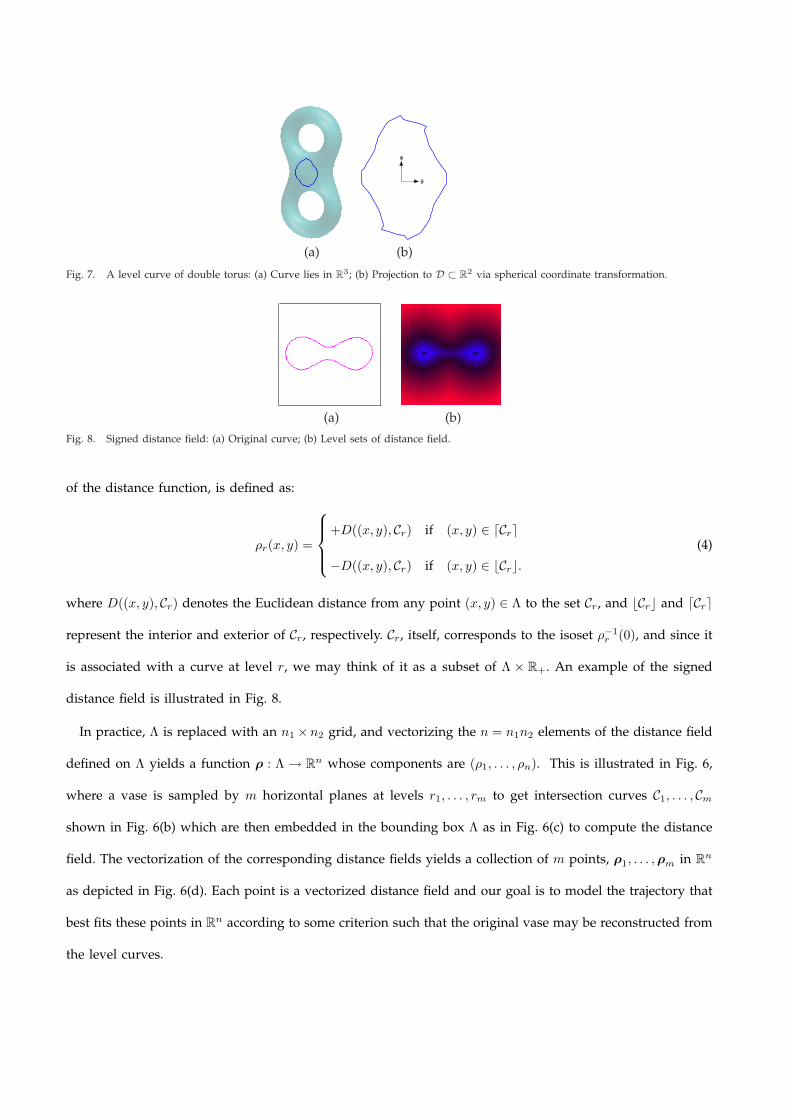
In order to explain the idea, note that level curves of the distance function are spatial curves, each curve

being a subset of a sphere. Spherical coordinates, therefore, map these level curves onto the curves in Λ =

[−π, π] × [−π2 , π

2 ], as illustrated in Fig. 7. Each curve is then view as a point in a high dimensional space,

which allows formulating geometric modeling problem as a curve fitting problem. The goal is then to fit a

trajectory in high dimensional space that passes through these points, while preserving the curve topology

and surface smoothness.

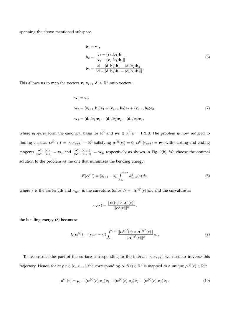
To preserve topology, we employ a signed distance field, which is always bounded, since surfaces of interest

are compact. The signed distance field ρr : Λ → R for a closed curve Cr ∈ Λ corresponding to the r-level curve

θ

φ

(a) (b)

Fig. 7. A level curve of double torus: (a) Curve lies in R3; (b) Projection to D ⊂ R2 via spherical coordinate transformation.

(a) (b)

Fig. 8. Signed distance field: (a) Original curve; (b) Level sets of distance field.

of the distance function, is defined as:

ρr(x, y) =

+D((x, y), Cr) if (x, y) ∈ dCre

−D((x, y), Cr) if (x, y) ∈ bCrc.(4)

where D((x, y), Cr) denotes the Euclidean distance from any point (x, y) ∈ Λ to the set Cr, and bCrc and dCre

represent the interior and exterior of Cr, respectively. Cr, itself, corresponds to the isoset ρ−1r (0), and since it

is associated with a curve at level r, we may think of it as a subset of Λ × R+. An example of the signed

distance field is illustrated in Fig. 8.

In practice, Λ is replaced with an n1×n2 grid, and vectorizing the n = n1n2 elements of the distance field

defined on Λ yields a function ρ : Λ → Rn whose components are (ρ1, . . . , ρn). This is illustrated in Fig. 6,

where a vase is sampled by m horizontal planes at levels r1, . . . , rm to get intersection curves C1, . . . , Cm

shown in Fig. 6(b) which are then embedded in the bounding box Λ as in Fig. 6(c) to compute the distance

field. The vectorization of the corresponding distance fields yields a collection of m points, ρ1, . . . , ρm in Rn

as depicted in Fig. 6(d). Each point is a vectorized distance field and our goal is to model the trajectory that

best fits these points in Rn according to some criterion such that the original vase may be reconstructed from

the level curves.

(a) (b)

Fig. 9. Optimal trajectory between each pair of curve vector: (a) Elasticæ fitted between ρ1 and ρ2 with constraints end point constraintsv1 and v2; (b) Problem transformed to R3, where tangential constraints become w1 and w2 and the displacement between end pointsis mapped to w3.

We adopt a piecewise interpolation approach, where for all i, we fit an arc ρ(i) between the points ρi and

ρi+1 in Rn subject to the constraints:

ρ(i)(ri) = ρi,

ρ(i)′(ri) = vi,

ρ(i)(ri+1) = ρi+1,

ρ(i)′(ri+1) = vi+1.

(5)

where the end point tangent vectors vi and vi+1 are computed from the data, and where the arc ρ(i) is

parameterized by r. The purpose of introducing tangent constraints is to ensure smoothness at joints (end

points), when later we combine arcs for all such consecutive pair of points. The optimal arc, ρ(i)(r), is the one

that minimizes a certain energy functional subject to the stated constraints. We, thus, construct a sequence

of arcs between successive points, which when put together, yields a C1 trajectory from ρ1 to ρm, passing

through ρ2, ρ3, . . . , ρm−1. Note that each arc ρ(i)(r) belongs to an affine subspace of Rn through the point ρi

and spanned by the vectors vi, vi+1, and ρi+1 − ρi.

Finding the optimal arc in Rn with n À 3 is computationally very intensive. This complexity may, however,

be greatly reduced by projecting the problem to R3 by a set of transformations, which are derived by noting

that the arc belongs to an affine subspace of Rn through the point ρi and spanned by vectors vi, vi+1, and

di := ρi+1−ρi [3] (See Fig. 9(a)). These vectors are generically independent but not necessarily orthogonal. We,

therefore, employ Gram–Schmidt orthogonalization to get an orthonormal set of basis vectors bk, k = 1, 2, 3

spanning the above mentioned subspace.

b1 = v1,

b2 =v2 − 〈v2, b1〉b1

‖v2 − 〈v2, b1〉b1‖ , (6)

b3 =d− 〈d, b1〉b1 − 〈d, b2〉b2

‖d− 〈d, b1〉b1 − 〈d, b2〉b2‖ .

This allows us to map the vectors vi, vi+1, di ∈ Rn onto vectors:

w1 = e1,

w2 = 〈vi+1, b1〉e1 + 〈vi+1, b2〉e2 + 〈vi+1, b3〉e3, (7)

w3 = 〈di, b1〉e1 + 〈di, b2〉e2 + 〈di, b3〉e3,

where e1, e2, e3 form the canonical basis for R3 and wk ∈ R3, k = 1, 2, 3. The problem is now reduced to

finding elasticæ α(i) : I = [ri, ri+1] → R3 satisfying α(i)(ri) = 0, α(i)(ri+1) = w3 with starting and ending

tangents α(i)′(ri)

‖α(i)′(ri)‖ = w1 and α(i)′(ri+1)

‖α(i)′(ri+1)‖ = w2, respectively as shown in Fig. 9(b). We choose the optimal

solution to the problem as the one that minimizes the bending energy:

E(α(i)) = (si+1 − si)∫ si+1

si

κ2α(i)(s) ds, (8)

where s is the arc length and κα(i) is the curvature. Since ds = ‖α(i)′(r)‖dr, and the curvature is:

κα(r) =‖α′(r)×α′′(r)‖

‖α′(r)‖3 ,

the bending energy (8) becomes:

E(α(i)) = (ri+1 − ri)∫ ri+1

ri

‖α(i)′(r)×α(i)′′(r)‖‖α(i)′(r)‖2 dr. (9)

To reconstruct the part of the surface corresponding to the interval [ri, ri+1], we need to traverse this

trajectory. Hence, for any r ∈ [ri, ri+1], the corresponding α(i)(r) ∈ R3 is mapped to a unique ρ(i)(r) ∈ Rn:

ρ(i)(r) = ρi + 〈α(i)(r), e1〉b1 + 〈α(i)(r), e2〉b2 + 〈α(i)(r), e3〉b3, (10)

Each ρ(i)(r), therefore, models the vectorized distance fields of the curves for r ∈ [ri, ri+1]. To recover a level

curve from ρ(i)(r), we first need to unvectorize it to get the corresponding distance field which is defined

on Λ, and then to find the zero level set of this distance field. For a complete representation of an entire

topologically homogenous part of a surface, we glue together the corresponding ρ(i)(r) to get a trajectory

ρ(r) ⊂ Rn, r ∈ [r1, rm], which is C1 smooth and is in essence a piecewise curve modeling approach:

ρ(r) = ∪m−1i=1 ρ(i)(r)1 (r ∈ [ri, ri+1]) , (11)

where 1(.) is an indicator function, which assumes a value of unity when the argument is true. The distance

field trajectory ρ, given by Eq. 11, therefore, forms the geometric model that captures the evolution of level

curves. Each graph edge is finally assigned the corresponding model of ρ(r) ⊂ Rn.

5.2. Implementation Issues

We now discuss some implementational issues.

1) Tangent computation: Given a set of m curves, ρ1, . . . , ρm, the starting and ending tangents, vi and

vi+1, i = 1, . . . , m, may be approximately computed as in [3]:

vk =ρk − ρk−1

‖ρk − ρk−1‖, k = i, i + 1. (12)

To avoid a longer vector (of larger norm) overbiasing the direction of the approximate tangent vector, we

use a weighted difference of the two curve vectors,

vk =ηk−1ρk − ηkρk−1

‖ηk−1ρk − ηkρk−1‖, (13)

where ηk = ‖ρk‖; k = i, i + 1.

2) Tangents at the Terminal Points: At the initial and terminal points, i.e., i = 1 and i = m, we find starting

and ending tangents respectively as

v1 =η0ρ1 − η1ρ0

η0‖ρ1 − η1ρ0‖, (14)

vm+1 =ηmρm+1 − ηm+1ρm

‖ηmρm+1 − ηm+1ρm‖, (15)

Fig. 10. Computing tangents.

where we assume that ρ0 and ρm+1 are well defined. This is shown in Fig. 10.

3) Graph resolution: The topo-geometric model affords reconstruction of parts of a surface using the geo-

metric model and their connection using topological information. This in turn suggests that for reconstruction

purposes, we need not to keep track of entire subparts but actually only a smaller subsets of level curves.

The number of level curves is determined by the graph resolution parameter K defined earlier. Due to the

absence of a 2D sampling theorem, we need to adopt a practical approach for selecting the “optimal” subset

of level curves. Since each curve is mapped to a point in a higher dimensional space of distance fields, we

exploit correlations among various curves to rule out the curves, which lie very close to other curves in the

optimal set of curves in high correlation sense. We, therefore, sample a surface very finely (arbitrarily large

K), to get a large number of redundant curves. To find the optimal subset, we start with just two curves, for

which we choose the outermost curves. This corresponds to curves at the maximum and minimum distance

along the corresponding subpart. The necessary inclusion of the outer most curves in the optimal set helps in

avoiding extrapolation. We, then, enlarge this subset by selecting two curves at a time, which are dissimilar to

the curves in the existing subset and adding them to the optimal set. This is repeated by moving inward from

the two outermost curves, until all curves are handled. As a measure of dissimilarity, we use the correlation

of a curve with its immediate neighbor, and regard them dissimilar if this correlation is less than some bound

εB . With an appropriate choice of εB , we can represent a surface arbitrarily closely. The entire procedure is

summarized in Table II:

6. Topo-Geometric Model

In order to combine topology and geometry in a single representation, the high dimensional geometric

trajectory ρ(r) ∈ Rn corresponding to each graph edge is parameterized by a low dimensional weight vector.

The weights, therefore, account for the geometry of the subsurface along that edge. Steps involved are

TABLE IISURFACE SAMPLING AND CURVE PRUNING

• Select a sufficiently large K that is consistent across all surfaces of interest, and sample the given surface accordingly• For each edge in the skeletal graph

– Populate CLIST with the corresponding level curves, which are indexed by the corresponding distances– Let cmin and cmax be the smallest and the largest distance level curves in CLIST– Initialize an empty V LIST– While CLIST is not empty∗ Transfer cmin from CLIST to V LIST , if the correlation between cmin and the cmin transferred to V LIST at the previous

iteration is less than εB , else remove cmin from CLIST . Do the same for cmax– End while

• End for• V LIST comprises optimal surface sampling

discussed in the next section and summarized in Table III.

TABLE IIITOPO-GEOMETRIC MODELING

• Capture topology via distance function skeletal graph• Graph edges are composed of edge segments between each pair of nodes, each of which represents a level curve• Each edge, therefore, contains multiple level curves, one for each node on its edge segments. Each of these level curves is modeled

by α(i) or ρ(i)

• The collection of ρ(i) for an edge forms a C1 smooth trajectory ρ(r), which represents the geometry of the subsurface along thatedge

• One-to-one mapping between α(i) and ρ(i) is exploited to represent the geometry by cascading α(i) to form α(r)• Parametrization coefficients of α(r) are assigned to the edge for complete representation

6.1. Edge Weights

As mentioned in Section 5, the trajectory ρ is obtained by lifting elasticæ segments (or arcs) α(i) ∈ R3

according to Eq. (10) and then gluing them together, which then represents the geometry of the corresponding

edge. In our formulation of TGSM α(i) are glued instead to construct α(r). In order to explain the idea, we

introduce some notation. Let r0 and rK be radii that correspond to two vertices of a skeletal graph, connected

by an edge. The points r1, . . . , rK−1, divide the segment [r0, rK ] into K intervals. For each interval [ri, ri+1],

we obtain an elasticæ segment α(i) in R3 as discussed in Section 5.1. Thus, for each edge, one may construct

K sets of spline coefficients, each for an edge segment along that particular edge. These coefficients carry

the geometric information with desired precision and may be assigned to the edge segments as weights. A

drawback of this approach is that the size of weight vectors grows with the number of edge segments even if

the level curves themselves do not have a significant variation among them. In addition, it leads to a highly

local descriptor falling short of a global edge representation.

Our approach for constructing weight vectors is based on wavelet decomposition [10], [26] of α. Wavelets

have successfully been employed in various signal representation [32], [33], [6] and compression applications

(a)

(b)

Fig. 11. Effect of basis rotation: (a) See how α4 and α5 map to α′4 and α′5 after projection from Rn to R3, resulting in a high curvaturecusp at the node; (b) Rotating the basis at the nodes makes the Frenet frame smoother and the resulting trajectory is first order smooth.

[36], [37], [46], [26] especially computer graphics [30], [14], [47], [40], [41], [20]. This approach exploits

vanishing moments and compact support of wavelets to compress the energy of α in few coefficients, which

eventually yields a simpler and lighter shape representation. This involves constructing a smooth trajectory

α ⊂ R3, by gluing various arcs α(i). These arcs themselves start at the origin of R3, and, therefore, require

translation in R3 to have the end points matched. This, however, introduces cusps at the end points, because

each arc α(i) was computed in its own basis, which are eliminated by rotating them to align end point

tangents, thus, yielding a C1 trajectory in R3 as shown in Fig. 11(b).

Physically, this may be viewed as rotating the arcs of the trajectory ρ(r) ⊂ Rn, so that the resulting smooth

trajectory lies in a three-dimensional affine subspace of Rn. We call this procedure piecewise projection. Recall

that the arc of ρ(i)(r) connecting the ith and (i+1)th node lies in the three-dimensional affine subspace Ei of

Rn spanned by the vectors di, vi, vi+1, and passing through the point ρi. The intersection of subspaces

Ei and Ei+1 contains the vector vi+1 as illustrated in Fig. 12(a). Each consecutive pair of arcs ρ(i)(r),

(a)

(b)

Fig. 12. Piecewise projection: (a) A trajectory in Rn; (b) Its piecewise projection onto R3.

ρ(i+1)(r), therefore, lies in a five-dimensional affine subspace spanned by the vectors vi, vi+1, vi+2, ρi+1−ρi,

ρi+2 − ρi+1, and passing through ρi+1. Applying an orthogonal transformation T that keeps the vector vi+1

intact, we can “align” the subspaces Ei and the image of Ei+1 under this transformation, TEi+1. In other

words, the three-dimensional affine subspaces Ei and TEi+1 are the same. We then perform this “alignment”

subsequently at each node, eventually obtaining a smooth trajectory in a three-dimensional affine subspace

of Rn. The procedure is illustrated in Fig. 12, where the three-dimensional affine subspaces Ei are drawn

as quadrilaterals. Two consecutive affine subspaces have a common line, and a sequence of such subspaces

appears like a folded sheet of paper with folds along common lines. The trajectory ρ is C1-smooth, however,

since it is tangent to the folds. The rotation that leaves the vectors vi intact corresponds to the process of

unfolding the sheet of paper (Fig. 12(b)). The result is a smooth trajectory β ⊂ R3. On the computational

level, this is equivalent to performing rotations of the basis in R3, as described above.

To assign a weight vector to the entire edge, we use wavelet representation of the trajectory β : [a, b] → R3,

β : t 7→ (β1(t), β2(t), β3(t)), where βi(t), i = 1, 2, 3, are the coordinate functions of the trajectory obtained

by the piecewise projection of ρ onto R3. The set of wavelet coefficients together with piecewise projection

parameters form a single weight that is assigned to each homogenous part of the graph. The resulting graph

contains sufficient amount of information needed to reconstruct the original surface with desired precision

and may be used for data storage and surface classification [4], [5].

7. Experimental Results

In this section, we present some skeletonization and geometric modeling results.

7.1. Topological model

Skeletal graphs of 3D objects of various complexity are given in Fig. 13, illustrating topology capturing

capabilities of proposed method. Fig. 14(a) shows that a high resolution graph results in dense nodes along

the edges, which in turn also contain some redundant geometric information. A simplified graph is illustrated

in Fig. 14(b), which helps in identifying topologically homogeneous parts shown color coded in Fig. 14(c).

7.2. Geometric model

Figs. 14(c) and (d) show geometric modeling of a double torus, the surface is sampled with K = 200,

resulting in various level curves along each edge. Trajectories representing geometry of each edge are given

in Fig. 15, along with their curvature profile, and their wavelet decompositions using Daubechies 20 are

given in Fig. 16. It can readily be seen that geometric differences among various subsurfaces manifest in the

form of differences in curvature and wavelet coefficients. Wavelet coefficients, in fact, uniquely define the

corresponding geometry, and therefore, are assigned to respective edges to get a weighted skeletal graph,

which completely and uniquely represents the topology and geometry of the double torus. Reconstructed

surface is given in Fig. 17(b), which closely resembles the original surface.

Further examples of reconstructed objects are given in Figs. 17 and 18, along with comparison between

original and reconstructed surfaces. Results indicate that the reconstructed surfaces lose local detail, while

retaining the global shape characteristics. This is, in fact, in accordance with the geometric formulation, where

a surface is represented by a C1 smooth trajectory. In addition, holes may be encountered in the reconstructed

surface if adequate level curves may not be sampled along an edge. These holes may, however, be filled using

techniques such as [9], [13], [11], [44], which may be easier in this case given the topological information in

the form of the skeletal graph.

Fig. 13. Topological representation via distance function based skeletal graphs.

(a) (b) (c) (d)

Fig. 14. Simplified skeletal graph: (a) Original; (b) After simplification; (c) Object color coded according to simplified graph; (d) Optimallevel curves.

−4

−2

0

2

0

1

2

3

40

0.5

1

1.5

2

2.5

3

xy

z

2

4

6

8

10

12

14

−3−2

−10

1

0

1

2

3

41

1.5

2

2.5

3

3.5

xy

z

2

4

6

8

10

12

14

16

18

20

−3−2

−10

1

0

0.5

1

1.5

23

3.5

4

4.5

5

5.5

6

xy

z

10

20

30

40

50

60

−3−2

−10

1

0

0.5

1

1.5

24.5

5

5.5

6

6.5

7

7.5

xy

z

10

20

30

40

50

60

(a) (b) (c) (d)

Fig. 15. Trajectories for various edges of graph in Fig. 14: (a) Edges a and b; (b) edges c and d; (c) edges e, f , g, and h; (d) edges hand i.

5 10 15 20 25 30 35 40−6

−4

−2

0

2

4

6

n

ψ

5 10 15 20 25 30 35 40−12

−10

−8

−6

−4

−2

0

2

4

n

ψ

5 10 15 20 25 30 35 40−10

−8

−6

−4

−2

0

2

4

n

ψ

5 10 15 20 25 30 35 40−5

−4

−3

−2

−1

0

1

2

3

4

5

n

ψ

5 10 15 20 25 30 35 40−5

0

5

10

15

20

n

ψ

5 10 15 20 25 30 35 40−2

0

2

4

6

8

10

12

14

16

n

ψ

5 10 15 20 25 30 35 40−2

0

2

4

6

8

10

n

ψ

5 10 15 20 25 30 35 40−2

0

2

4

6

8

10

n

ψ

5 10 15 20 25 30 35 40−4

−2

0

2

4

6

8

10

12

n

ψ

5 10 15 20 25 30 35 40−4

−2

0

2

4

6

8

10

12

14

16

n

ψ

5 10 15 20 25 30 35 40−5

0

5

10

15

20

25

30

35

40

n

ψ

5 10 15 20 25 30 35 40−5

0

5

10

15

20

25

30

n

ψFig. 16. Wavelet decomposition: (Top row) x-trajectory, (Middle row) y-trajectory, (Bottom row) z-trajectory; (Left column) edges a andb, (Middle left) edges c and d, (Middle right) edges e, f , g, and h, (Right column) edges h and i.

8. Conclusions

In this paper, we presented a 3D object modeling scheme that captures the topological and geometric

information of an object. Topology and rough geometric picture is captured through an extension of Reeb

graph, where we employed a distance function for object analysis, which inherently achieves rotation,

translation and scale invariance.

To enhance the geometric information, we proposed using elasticæ to model the evolution of level curves

(a) (b) (c) (d)

Fig. 17. Reconstruction: (a) Double torus; (b) Reconstructed double torus; (c) The Twins, (d) Reconstructed the Twins.

Fig. 18. Reconstruction: (Left) original objects; (Middle) reconstructed objects; (Right) comparison.

along various edges along the graph resulting in an evolution trajectory in R3. This trajectory is subsequently

represented by wavelets, whose coefficients end up as edge weights. The eventual weighted skeletal graph

may then be used as a signature of the object, with potential applications for storage and classification of 3D

objects.

Reconstruction results demonstrate the ability of the model to capture global geometric features, at the

cost of local detail. This is a direct consequence of the geometric formulation, that is based on a smooth

trajectory, which, in turn, is learnt from a small set of “dissimilar” level curves. Any small local differences

in level curves may be lost in the sampling and pruning process, the extent of which largely depends on

graph resolution parameter, similarity bound εB , and the smoothness of the trajectory. This may actually lead

to a hierarchical shape representation, where a conservative parameter selection will yield a better surface

approximation. On the other hand, if local detail is not of prime importance, parameters may be relaxed for

a light weight surface representation.

Since the elasticæ model requires at least two level curves, which may not always be the case depending

on the choice of K especially for small protrusions. In such cases, we may end up losing some data, which

may manifest in the form of holes in the reconstructed surface. Given the topological information, it may, in

that case, be readily fixed using hole filling techniques.

In addition to storage application, this model may be used for shape recognition using weighted subgraph

isomorphism, in which case weights would provide distinctive geometric features of a surface. In some cases,

one may employ curvature of the trajectory as distinguishing feature instead of the wavelet-based weights.

REFERENCES

[1] N. Amenta, S. Choi, and R. Kolluri, “Power Crust”, Proceedings of 6th ACM Symposium on Solid Modeling, pp. 249-260, 2001.

[2] S. H. Baloch, H. Krim, I. Kogan, and D. V. Zenkov, “Rotation invariant topology coding of 2D and 3D objects using Morse theory”,

Proc. ICIP 2005.

[3] S. H. Baloch, H. Krim, W. Mio, and A. Srivastav, “3D Curve Interpolation and Object Reconstruction”, Proc. ICIP, 2005.

[4] S. H. Baloch, and H. Krim, “Graph-based 3D object classification”, Proc. SPIE, Computational Imaging IV, C. A. Bouman, E. L. Miller,

I. Pollak, Editors, Vol. 6065, 2006.

[5] S. H. Baloch, and H. Krim, “3D shape recognition via topological-geometric skeletal graph editing”, In preparation.

[6] M. Barrat, and O. Lepetit, “Recursive wavelet transform for 2D signals”, GMIP, Vol. 56, No. 1, pp. 106–108, Jan. 1994.

[7] M. D. Carmo, Differential Geometry of Curves and Surfaces, Prentice-Hall, New Jersey, 1976.

[8] H. Carr, J. Snoeyink, and U. Axen, “Computing contour trees in all dimensions”, Technical Report TR-99-09, Univ. of British Columbia,

Dept. of Computer Science, August 1999.

[9] B. Curless, and M. Levoy, “A volumetric method for building complex models from range images”, Proc. SIGGRAPH96, ACM, 1996.

[10] I. Daubechies, Ten Lectures on Wavelets, SIAM, 1992.

[11] J. Davis, S. R. Marschner, M. Garr, and M. Levoy, “Filling holes in complex surfaces using volumetric diffusion”, First International

Symposium on 3D Data Processing, Visualization, and Transmission , 2002 .

[12] T. K. Dey, and W. Zhao, “Approximating the Medial Axis from the Voronoi Diagram with a Convergence Guarantee”, Algorithmica,

Vol. 38, pp. 179–200, 2003.

[13] T. Dey, and S. Goswami, “Tight cocone: A water-tight surface reconstructor”, Proc. 8th ACM Symposium on Solid Modeling and

Applications, 2003.

[14] A. Fournier, Editor. “Wavelets and their applications in computer graphics”, ACM SIGGRAPH’95, Course Notes, 1995.

[15] A. B. Hamza, and H. Krim, “Topological modeling of illuminated surfaces using Reeb graphs”, Proc. ICIP, Vol. 1, pp. 769–772,

September 2002.

[16] A. B. Hamza, and H. Krim, “Geodesic object representation and recognition”, Proc. DGCI, pp. 378–387, November 2003.

[17] X. Han, C. Xu, and J. L. Prince, “A topology preserving deformable model using level sets”, CVPR’01, pp. II:765-770, 2001.

[18] M. Hilaga, Y. Shinagawa, T. Kohmura, and T. L. Kunii, “Topology Matching for Fully Automatic Similarity Estimation of 3D

Shapes”, Proc. SIGGRAPH, pp. 203–212, August 2001.

[19] C. Hoffman, “How to construct the skeleton of CSG objects”, The Mathematics of Surfaces, IV, A. Bowyer and J. Davenport, Eds.,

Oxford University Press, 1990.

[20] I. Ihm, and S. Park, “Wavelet-based 3D compression scheme for interactive visualization of very large volume data”, Computer

Graphics Forum, Vol. 18, No. 1, 1999.

[21] S. Joshi, S., Pizer, P. T. Fletcher, A. Thall, and G. Tracton, “Multi-scale 3-D deformable model segmentation based on medial

description”, Information Processing in Medical Imaging, Lecture Notes in Computer Science, Vol. 2082, pp. 6477, Springer, 2001.

[22] M. Kazhdan, B. Chazelle, D. Dobkin, A. Finkelstein, and Thomas Funkhouser, “A Reflective Symmetry Descriptor”, European

Conference on Computer Vision, May 2002.

[23] M. Kazhdan, and T. Funkhouser, “Harmonic 3D Shape Matching”, SIGGRAPH 2002 Technical Sketches, pp. 191, July, 2002.

[24] F. Lazarus, and A. Verroust, “Level set diagrams of polyheral objects”, Proc. Fifth ACM symposium on Solid Modeling and Applications,

pp. 130–140, June 1999.

[25] R. Malladi, J. A. Sethian, and B. Vemuri, “Shape modeling with front propagation: a level set approach”, IEEE Trans. on Pattern

Analysis and Machine Intelligence, Vol. 17, No. 2, Feb. 1995.

[26] S. Mallat, A Wavelet Tour of Signal Processing, 1999.

[27] Y. Matsumoto, An Introduction to Morse Theory, American Mathematical Society, 1997.

[28] W. Mio, A. Srivastava, and E. Klassen, Interpolations with elasticæ in Euclidean spaces, To appear in Quarterly of Applied Mathematics.

[29] J. Milnor, Morse Theory, Princeton University Press, Princeton, NJ, 1963.

[30] S. Muraki, “Volume data and wavelet transforms”, IEEE Computer Graphics and Applications, Vol. 13, No. 4, pp. 50–56, 1993.

[31] R. Osada, T. Funkhouser, B. Chazelle, and D. Dobkin, “Shape Distributions”, ACM Transactions on Graphics, 21(4), pp. 807–832,

October 2002.

[32] A. P. Pentland, “Surface interpolation using wavelets”, ECCV’92 pp. 615–619, 1992.

[33] A. P. Pentland, “Interpolation using wavelet bases”, PAMI, Vol. 16, No. 4, pp. 410–414, April 1994.

[34] S. M. Pizer, D. S. Fritsch, P. Yushkevich, V. Johnson, and E. L. Chaney, “Segmentation, registration, and measurement of shape via

image object shape”. IEEE Transactions on Medical Imaging, Vol. 18, pp. 851865, 1999.

[35] G. Reeb, “Sur les points singuliers d’une forme de pfaff complement integrable ou d’une fonction numerique”, Comptes Rendus de

L’Academie ses Seances , Paris, 222, pp. 847–849, 1946.

[36] A. Said, and W. Pearlman, “An image multiresolution representation for lossless and lossy compression”, IEEE Transactions on Image

Processing, Vol. 5, pp. 1303–1310, September 1996.

[37] K. Sayood, Introduction to Data Compression, Morgan Kaufmann Publishers Inc., 1996.

[38] F. Segonne, J. P. Pons, W. E. L. Grimson, and B. Fischl, “Active Contours Under Topology Control Genus Preserving Level Sets”,

CVBIA’05, pp. 135–145, 2005.

[39] Y. Shinagawa, and T. L. Kunii, “Constructing a Reeb graph automatically from cross sections”, IEEE Computer Graphics and

Applications, 11(6), pp. 44–51, November 1991.

[40] P. Schroder, and W. Sweldens, Editors, “Wavelets in Computer Graphics”, ACM SIGGRAPH’96, Course Notes, 1996.

[41] E. Stollnitz, T. DeRose, and D. Salesin, Wavelets for Computer Graphics: Theory and Applications, Morgan Kauffmann Publishers Inc.,

1996.

[42] A. Tsai, A. J. Yezzi, W. M. Wells III, C. Tempany, D. Tucker, A. Fan, W. E. L. Grimson, and A. S. Willsky”, “A shape-based approach

to the segmentation of medical imagery using level sets”, MedImg, Vol. 22, No. 2, pp. 137–154, 2003.

[43] T. Tung, F. Schmitt, “Augmented Reeb Graphs for Content-Based Retrieval of 3D Mesh Models”, Shape Modeling International, pp.

157-166, 2004.

[44] M. Varnuska, J. Parus, and I. Kolingerova, “Simple holes triangulation in surface reconstruction”, Proceedings of Algoritmy, pp.

280–289, 2005.

[45] P. Vermeer, Medial axis transform to boundary representation conversion, Ph.D. Thesis, Purdue University, 1994.

[46] J. Wang, and K. Huang, “Medical image compression by using three-dimensional wavelet transformation”, MedImg, Vol. 15, No. 4,

pp. 547–554, August 1996.

[47] B. L. Yeo, and B. Liu, “Volume rendering of DCT-based compressed 3D scalar data”, IEEE Transactions on Visualization and Computer

Graphics, Vol. 1, No. 1, pp. 29–43, March 1995.