Rolling Horizon Approach for Dynamic Parallel Machine Scheduling Problem with Release Times

Rolling Horizon Approach for Dynamic Parallel Machine Scheduling Problemwith Release Times

Lixin Tang,*,† Shujun Jiang,† and Jiyin Liu*,†,‡

Liaoning Key Laboratory of Manufacturing System and Logistics, The Logistics Institute, NortheasternUniVersity, Shenyang, China, and Business School, Loughborough UniVersity, Leicestershire LE11 3TU, U.K.

In this paper, we study a dynamic parallel machine scheduling problem with release times, where the releasetimes and processing times of jobs may change during the production process due to uncertainties. The problemis different from classical scheduling problems in the deterministic environment where all information ofjobs is known at the beginning of the scheduling horizon and will not change during the operations throughoutthe whole horizon. In practice, there are often unpredictable events causing dynamic changes in job releasetimes and/or processing times. Traditional optimization methods cannot solve the dynamic scheduling problemdirectly even though they have been successful in solving the static version of the problem. A model predictivecontrol (MPC) strategy based rolling horizon approach is applied to tackle the dynamic parallel machinescheduling problem with the objective of minimizing the total weighted completion times of jobs, the energyconsumption due to job waiting, and the total deviation of actual job completion times from those in theoriginal schedule. When the MPC is applied to the problem, the rolling horizon approach allows applying aLagrangian relaxation (LR) algorithm to solve the model of the scheduling problem in a rolling fashion.Computational experiments are carried out comparing the proposed method with the passive adjustment methodoften adopted by human schedulers. The result shows that the proposed method yields significantly betterresults, with 11.72% improvement on average.

1. Introduction

In the classical scheduling theory, most research has focusedon deterministic machine scheduling, which was conductedunder the assumption that all the information of jobs is knownat the beginning of scheduling and will not change during theproduction process. In practical production operations, there aremany dynamic events occurring such as changes in job arrivaland processing. The arrival times and processing times of incomingjobs may be only estimates at the beginning of the schedulinghorizon. With further information, more accurate estimates maybe obtained at a later time. In other words, the originally estimatedparameters of jobs may be changed as time progresses. In thispaper, we consider the parallel machine scheduling problem withrelease times in such a dynamic environment, where the informationof later jobs may be changed during the production process due touncertainties.

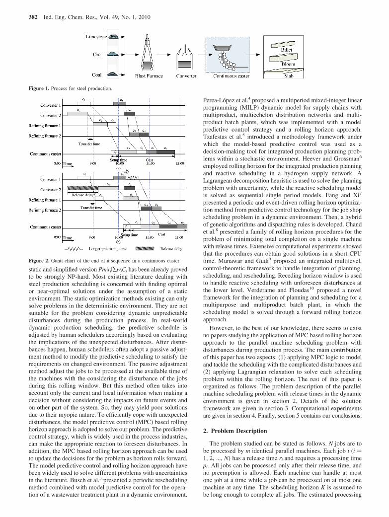
The problem under consideration is extracted from the processof steel production. Steel production is a complicated techno-logical process, which involves a serial of stages. The steelmak-ing production process is roughly illustrated in the Figure 1.Iron ore and other raw materials are melted and transformed topig iron in a blast furnace. Pig iron is then used to produceliquid steel in converters. Each batch of liquid steel producedin a converter is called a charge. After the refining process, theliquid steel is transported to continuous casters to form solidslabs. Because continuous-casting is an important stage convert-ing liquid steel to solid slabs, we take this stage as our researchbackground. The problem is to schedule the charges comingfrom the steel-making stage on the continuous-casters. Such aproblem is a single-stage parallel machine scheduling problem.In this system, there are uncertainties in upstream stages causing

changes in job release times and processing times. Theuncertainties may come from the following unpredictable events:

(1) Release-time related events(1) arrival delay of raw materials at upstream operations(2) machine breakdown at upstream operations(3) quality flaw of liquid steel at upstream operations(4) change of processing speed at upstream operations.

(2) Processing-time related events(1) change of casting speed(2) online casting width adjusting(3) caster stream breakdown(4) unsatisfactory quality of casting slabs.

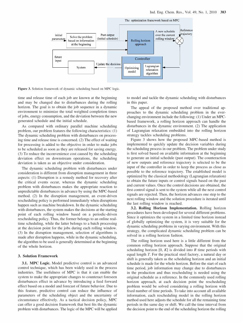
As an example, Figure 2 illustrates dynamic changes in thesteel making stage and corresponding rescheduling for acontinuous-caster. An initial schedule based on estimated jobinformation is shown in Figure 2a in which a cast consists of asequence of charges c2, c1, c3, and c4. Here, a cast means asequence of charges continuously processed on a caster. Duringthe execution of this schedule, more accurate informationbecomes available indicating that c2 will arrive late and theprocessing time of c3 will be prolonged. As a result, the currentschedule for the continuous caster becomes invalid. In such asituation, the schedule needs to be adjusted to cope with theunforeseen changes. A new schedule considering the new jobinformation is shown in Figure 2b. Since such unpredictabledisturbances often occur in real production, it is of practicalsignificance to study the dynamic scheduling problem withvarious disturbances in the production environment.

Bruno et al.1 proved that identical parallel machine schedulingto minimize the total weighted completion time problem, evenin case of two machines (P2|∑wiCi), is also non-polynomial(NP)-hard. Lenstra et al.2 proved that single machine schedulingwith release times to minimize the total weighted completiontime problem 1|ri|∑wiCi is a strongly NP-hard problem. Theparallel machine scheduling problem with release times in thedynamic environment is NP-hard in the strong sense since its

* Corresponding author. Tel.:+86-24-83680169. Fax:+86-24-83680169.E-mail: [email protected] (L.T.); [email protected] (J.L.).

† Northeastern University.‡ Loughborough University.

Ind. Eng. Chem. Res. 2010, 49, 381–389 381

10.1021/ie900206m CCC: $40.75 2010 American Chemical SocietyPublished on Web 11/10/2009

static and simplified version Pm|ri|∑wiCi has been already provedto be strongly NP-hard. Most existing literature dealing withsteel production scheduling is concerned with finding optimalor near-optimal solutions under the assumption of a staticenvironment. The static optimization methods existing can onlysolve problems in the deterministic environment. They are notsuitable for the problem considering dynamic unpredictabledisturbances during the production process. In real-worlddynamic production scheduling, the predictive schedule isadjusted by human schedulers accordingly based on evaluatingthe implications of the unexpected disturbances. After distur-bances happen, human schedulers often adopt a passive adjust-ment method to modify the predictive scheduling to satisfy therequirements on changed environment. The passive adjustmentmethod adjust the jobs to be processed at the available time ofthe machines with the considering the disturbance of the jobsduring this rolling window. But this method often takes intoaccount only the current and local information when making adecision without considering the impacts on future events andon other part of the system. So, they may yield poor solutionsdue to their myopic nature. To efficiently cope with unexpecteddisturbances, the model predictive control (MPC) based rollinghorizon approach is adopted to solve our problem. The predictivecontrol strategy, which is widely used in the process industries,can make the appropriate reaction to foreseen disturbances. Inaddition, the MPC based rolling horizon approach can be usedto update the decisions for the problem as horizon rolls forward.The model predictive control and rolling horizon approach havebeen widely used to solve different problems with uncertaintiesin the literature. Busch et al.3 presented a periodic reschedulingmethod combined with model predictive control for the opera-tion of a wastewater treatment plant in a dynamic environment.

Perea-Lopez et al.4 proposed a multiperiod mixed-integer linearprogramming (MILP) dynamic model for supply chains withmultiproduct, multiechelon distribution networks and multi-product batch plants, which was implemented with a modelpredictive control strategy and a rolling horizon approach.Tzafestas et al.5 introduced a methodology framework underwhich the model-based predictive control was used as adecision-making tool for integrated production planning prob-lems within a stochastic environment. Heever and Grossman6

employed rolling horizon for the integrated production planningand reactive scheduling in a hydrogen supply network. ALagrangean decomposition heuristic is used to solve the planningproblem with uncertainty, while the reactive scheduling modelis solved as sequential single period models. Fang and Xi7

presented a periodic and event-driven rolling horizon optimiza-tion method from predictive control technology for the job shopscheduling problem in a dynamic environment. Then, a hybridof genetic algorithms and dispatching rules is developed. Chandet al.8 presented a family of rolling horizon procedures for theproblem of minimizing total completion on a single machinewith release times. Extensive computational experiments showedthat the procedures can obtain good solutions in a short CPUtime. Munawar and Gudi9 proposed an integrated multilevel,control-theoretic framework to handle integration of planning,scheduling, and rescheduling. Receding horizon window is usedto handle reactive scheduling with unforeseen disturbances atthe lower level. Verderame and Floudas10 proposed a novelframework for the integration of planning and scheduling for amultipurpose and multiproduct batch plant, in which thescheduling model is solved through a forward rolling horizonapproach.

However, to the best of our knowledge, there seems to existno papers studying the application of MPC based rolling horizonapproach to the parallel machine scheduling problem withdisturbances during production process. The main contributionof this paper has two aspects: (1) applying MPC logic to modeland tackle the scheduling with the complicated disturbances and(2) applying Lagrangian relaxation to solve each schedulingproblem within the rolling horizon. The rest of this paper isorganized as follows. The problem description of the parallelmachine scheduling problem with release times in the dynamicenvironment is given in section 2. Details of the solutionframework are given in section 3. Computational experimentsare given in section 4. Finally, section 5 contains our conclusions.

2. Problem Description

The problem studied can be stated as follows. N jobs are tobe processed by m identical parallel machines. Each job i (i )1, 2, ..., N) has a release time ri and requires a processing timepi. All jobs can be processed only after their release time, andno preemption is allowed. Each machine can handle at mostone job at a time while a job can be processed on at most onemachine at any time. The scheduling horizon K is assumed tobe long enough to complete all jobs. The estimated processing

Figure 1. Process for steel production.

Figure 2. Gantt chart of the end of a sequence in a continuous caster.

382 Ind. Eng. Chem. Res., Vol. 49, No. 1, 2010

time and release time of each job are known at the beginningand may be changed due to disturbances during the rollinghorizon. The goal is to obtain the job sequence in a dynamicenvironment to minimize the total weighted completion timesof jobs, energy consumption, and the deviation between the newgenerated schedule and the initial schedule.

As compared with ordinary parallel machine schedulingproblem, our problem features the following characteristics: (1)The dynamic scheduling problem with disturbances on process-ing time and release time is concerned. (2) The effect of waitingfor processing is added to the objective in order to make jobsto be scheduled as soon as they are released for saving energy.(3) To reduce the inconvenience cost caused by the schedulingdeviation effect on downstream operations, the schedulingdeviation is taken as an objective under consideration.

The dynamic scheduling problem with disturbances underconsideration is different from disruption management in threeaspects: (1) Disruption is a remedy method for recovery afterthe critical events occur, whereas the dynamic schedulingproblem with disturbances makes the appropriate reaction tounpredictable disturbances in advance by using the MPC-basedmethod. (2) In the disruption management, an event-drivenrescheduling policy is performed immediately when disruptionshappen such as machine breakdown. In the dynamic schedulingwith disturbances, the system makes the decisions at the startingpoint of each rolling window based on a periodic-drivenrescheduling policy. Thus, the former belongs to an online real-time scheduling, while the latter belongs to a batch processingat the decision point for the jobs during each rolling window.(3) In the disruption management, selection of algorithms ismade after disruption happens, while in the dynamic scheduling,the algorithm to be used is generally determined at the beginningof the whole horizon.

3. Solution Framework

3.1. MPC Logic. Model predictive control is an advancedcontrol technique, which has been widely used in the processindustries. The usefulness of MPC is that it can enable thesystem to make the appropriate changes to counteract foreseendisturbances effect in advance by introducing a feed forwardeffect based on a model and forecast of future behavior. Due tothis feature, predictive control can reduce the influence ofparameters of the scheduling object and the uncertainty ofcircumstance effectively. As a tactical decision policy, MPCcan offer a good decision framework that best fits the dynamicproblem with disturbances. The logic of the MPC will be applied

to model and tackle the dynamic scheduling with disturbancesin this paper.

The appeal of the proposed method over traditional ap-proaches to the dynamic scheduling problem in the ever-changing environment include the following: (1) Under an MPC-based framework, a rolling horizon approach can handle thedisturbances in the dynamic environment. (2) The applicationof Lagrangian relaxation embedded into the rolling horizonstrategy tackles scheduling problems.

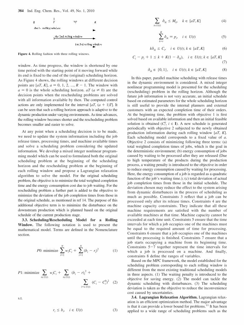
Figure 3 shows how the proposed MPC-based method isimplemented to quickly update the decision variables duringthe scheduling process in our problem. The problem under studyis first solved based on available information at the beginningto generate an initial schedule (past output). The counteractionof new outputs and reference trajectory is selected to be theinput of the controller in order to keep the process as close aspossible to the reference trajectory. The established model isoptimized by the classical methodology (Lagrangian relaxation)to obtain the future inputs or control signals based on the pastand current values. Once the control decisions are obtained, thefirst control signal is sent to the system while all the next controlsignals are rejected. Then, the horizon advances one step to thenext rolling window and the solution procedure is iterated untilthe last rolling window is reached.

3.2. Rolling Horizon Implementation. Rolling horizonprocedures have been developed for several different problems.Since it optimizes the system in a limited time horizon insteadof globally optimizing the system, it is very suitable for thedynamic scheduling problems in varying environment. With thisstrategy, the complicated dynamic scheduling problem can besolved in a rolling horizon fashion.

The rolling horizon used here is a little different from thecommon rolling horizon approach. Suppose that the originalscheduling horizon [0, K] is divided into R time periods withequal length T. For the practical steel factory, a natural day orshift is generally taken as the scheduling horizon and an initialschedule is made for the whole horizon. Before the start of eachtime period, job information may change due to disturbancesin the production and thus rescheduling is needed using theoriginal schedule as a reference. In the commonly used rollinghorizon approach, at each decision point the reschedulingproblem would be solved considering a rolling horizon withfixed number of time periods. To take into account all availableinformation, each rescheduling model in the rolling horizonmethod used here adjusts the schedule for all the remaining timeperiods in the same day or shift. We call the time interval fromthe decision point to the end of the scheduling horizon the rolling

Figure 3. Solution framework of dynamic scheduling based on MPC logic.

Ind. Eng. Chem. Res., Vol. 49, No. 1, 2010 383

window. As time progress, the window is shortened by onetime period with the starting point of it moving forward whileits end is fixed to the end of the (original) scheduling horizon.As Figure 4 shows, the rolling windows at different decisionpoints are [aT, K], a ) 0, 1, 2, ..., R - 1. The window witha ) 0 is the whole scheduling horizon. aT (a * 0) are thedecision points when the rescheduling problems are solvedwith all information available by then. The computed controlactions are only implemented for the interval [aT, (a + 1)T]. Itcan be seen that such a rolling horizon approach is adaptive to thedynamic production under varying environments. As time advances,the rolling window becomes shorter and the rescheduling problembecomes smaller and easier to solve.

At any point when a scheduling decision is to be made,we need to update the system information including the jobrelease times, processing times, and machine available timesand solve a scheduling problem considering the updatedinformation. We develop a mixed integer nonlinear program-ming model which can be used to formulated both the originalscheduling problem at the beginning of the schedulinghorizon and the rescheduling problem at the beginning ofeach rolling window and propose a Lagrangian relaxationalgorithm to solve the model. For the original schedulingproblem, the objective is to minimize the total weighted completiontime and the energy consumption cost due to job waiting. For therescheduling problem a further part is added to the objective tominimize the deviation of the job completion times from those inthe original schedule, as mentioned in ref 14. The purpose of thisadditional objective term is to minimize the disturbance on thedownstream production which is planned based on the originalschedule of the current production stage.

3.3. Scheduling/Rescheduling Model for a RollingWindow. The following notation is used to present themathematical model. Terms are defined in the Nomenclaturesection.

s.t.

In this paper, parallel machine scheduling with release timesin the dynamic environment is considered. A mixed integernonlinear programming model is presented for the scheduling(rescheduling) problem in the rolling horizon. Although thefuture job information is not very accurate, an initial schedulebased on estimated parameters for the whole scheduling horizonis still useful to provide the internal planners and externalcustomers with an expected completion time of their orders.At the beginning time, the problem with objective 1 is firstsolved based on available information and then an initial feasiblesolution is obtained (Ci

0, i ∈ I). A new schedule is generatedperiodically with objective 2 subjected to the newly obtainedproduction information during each rolling window [aT, K].Each scheduling model corresponds to a fixed value of a.Objective 2 consists of minimizing following three terms: (a)total weighted completion times of jobs, which is the goal inthe deterministic environment; (b) energy consumption of jobscaused by waiting to be processed after they are released (Dueto high temperature of the products during the productionprocess, a waiting penalty is introduced to the objective in orderto reduce energy consumption caused by waiting for processing.Here, the energy consumption of a job is regarded as a quadraticfunction of the job’s waiting time.); (c) total deviation of actualjob completion times from those in the initial schedule. Thedeviation chosen may reduce the effect to the system arisingfrom dynamic disturbances in the process of scheduling asmuch as possible. Constraints 3 reflect that a job can beprocessed only after its release times. Constraints 4 are themachine capacity constraints. They indicate that all thesemachine requirements are satisfied with the number ofavailable machines at that time. Machine capacity cannot beexceeded at each time unit. Constraints 5 ensure that the timeintervals for which a job occupies one of the machines mustbe equal to the required amount of time for processing.Constraints 6 ensure that a job occupies one of the machinesuntil the processing is finished. Constraints 7 ensure that ajob starts occupying a machine from its beginning time.Constraints 5-7 together represent the time intervals forwhich a job is processed on a machine. And finally,constraints 8 define the ranges of variables.

Based on the MPC framework, the model established for thescheduling problem correspording to each rolling window isdifferent from the most existing traditional scheduling modelsin three aspects. (1) The waiting penalty is introduced to theobjective for saving energy. (2) The model can tackle thedynamic scheduling with disturbances. (3) The schedulingdeviation is taken as the objective to reduce the inconveniencecost caused by uncertainties.

3.4. Lagrangian Relaxation Algorithm. Lagrangian relax-ation is an efficient optimization method. The major advantageis that it can provide a lower bound for problems.11 It has beenapplied to a wide range of scheduling problems such as the

Figure 4. Rolling fashion with three rolling winows.

P0: minimize ∑i)1

N

wiCi + ∑i)1

N

(bi - ri)2 (1)

P1: minimize ∑i∈U(t)

wiCi + ∑i∈U(t)

(bi - r)i2 +

∑i)∈U(t)

(Ci - Ci0)2 (2)

ri e bi, i ∈ U(t) (3)

∑i∈U(t)

δik e Mk, k ∈ [aT, K] (4)

∑k)t

K

δik ) pi, i ∈ U(t) (5)

kδik e Ci, i ∈ U(t); k ∈ [aT, K] (6)

Ci - pi + 1 e k + K(1 - δik), i ∈ U(t); k ∈ [aT, K](7)

δik ∈ {0, 1}, i ∈ U(t); k ∈ [aT, K] (8)


parallel machine scheduling problem12 or the job shop schedul-ing problem.13 Lagrangian relaxation is presented to solve themodel corresponding to each rolling window in this work. Thecoupling constraints are relaxed and embedded as a penalty termmultiplied by Lagrange multipliers in the objective function,therefore leading to a relaxed version of the primal model, whichcan be decomposed into several independent job-level subprob-lems to reduce the problem size. It is easier to solve decomposedjob-level subproblems. So it is sufficient to obtain a near-optimalschedule with quantifiable performance within a reasonablecomputation time. The feasible solutions to Lagrangian relax-ation at the beginning is an initial solution using objective 1.During the future rolling window, the scheduling problem isrescheduled again based on the updated information in thatwindow and scheduling result is adjusted.

The job-level decomposition of the model is introduced byrelaxing constraints 4 with Lagrangian multipliers {uk}. The firstsolving LR problem is denoted by L0, and the LR problemsolved at each rolling window is denoted by L1, respectively.

The job-level subproblems are solved optimally by enumera-tion. The lower bound together with the upper bound and thedeviation in the linking constraints is used to update theLagrange multipliers according to a subgradient updatingprocedure. In our algorithm, the subgradient optimizationmethod is used to update the multipliers {uk} at each iterationgiven by un+1 ) un + Rng(un), where u is a vector of multipliers{uk}, n is the iteration index, and g(u) the subgradient of L equalto (∑i

Nδik - Mk). And Rn is the step size at the nth iterationdefined as Rn ) λ(L* - Ln)/(||g(un)||2), 0 < λ < 2, where L* isestimated by the best feasible objective value found so far andLn is the dual value at the nth iteration.

4. Computational Experiments

Our approach is programmed in C++ language and run ona PC with 2.99 GHz CPU. The stopping criterion of Lagrangianrelaxation used in optimization of the subproblems during eachrolling window is set to iteration number 500. To test theperformance of the proposed method, the experimental resultsare evaluated by following the performance measures: “im-provement”, “average duality gap”, and “running time (sec-onds)”. Here improvement is used for showing the improvementamount of the proposed approach over the passive adjustmentmethod (PAM). The duality gap is defined as (J - L*)/L*. L*is the value of the dual function while the feasible objectivevalue J is the best upper bound obtained so far for each job-level subproblem. The average duality gap is equal to the totalsum of the duality gap of each problem divided by the numberof rolling windows.

Computational experiments have been carried out to comparethe proposed method with the PAM. The PAM is an often usedmethod by human schedulers for scheduling in systems withuncertainties, and it considers disturbances of the jobs duringeach rolling window. At each rolling window, the newest dataand information is first updated. The jobs after being disturbedare compulsorily moved to be processed at the available timeof the machines. And, the subsequent jobs which follow thedisturbed jobs in the initial schedule need to be adjustedrespectively. This procedure stops until all jobs are scheduledin the last rolling window. This method is inefficient but oftenused by human schedulers in real-world production for schedul-ing in the systems with uncertainties. However, it cannotgenerate ideal schedules since it just considers small partial

Figure 5. Effect of the number of rolling windows on algorithm performance(disturbance on processing time of jobs).

Figure 6. Effect of the number of rolling windows on algorithm performance(disturbance on release time of jobs).

(L0) min{Ci}

∑i)1

N

wiCi + ∑i)1

N

(bi - ri)2 + ∑

k)1

K

uk( ∑i

N

δik - Mk)

) min{Ci}

∑i)1

N

[wiCi + (bi - ri)2 + ∑

k)1

K

ukδik] - ∑k)1

K

ukMk

) min{Ci}

∑i)1

N

[wiCi + (Ci - pi + 1 - ri)2 +

∑k)1

K

ukδik] - ∑k)1

K

ukMk

(9)

(L1) min{Ci}

∑i∈U(t)

wiCi + ∑i∈U(t)

(bi - ri)2 +

∑i∈U(t)

(Ci - Ci0)2 + ∑

k)t

K

uk( ∑i∈U(t)

δik - Mk)

) min{Ci}

∑i∈U(t)

[wiCi + (bi - ri)2 + (Ci - Ci

0)2 +

∑k)t

K

ukδik] - ∑k)t

K

ukMk

) min{Ci}

∑i∈U(t)

[wiCi + (Ci - pi + 1 - ri)2 +

(Ci - Ci0)2 + ∑

k)t

K

ukδik - ∑k)t

K

ukMk]

(10)


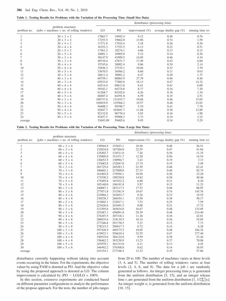
disturbance currently happening without taking into accountevents occurring in the future. For the experiments, the objectivevaluet by using PAM is denoted as PO. And the objective valueby using the proposed approach is denoted as LO. The columnimprovement is calculated by (PO - LO)/LO × 100%.

In this section, extensive experiments are conducted basedon different parameter configurations to analyze the performanceof the propose approach. For the tests, the number of jobs ranges

from 20 to 100. The number of machines varies at three levels(3, 4, and 5). The number of rolling windows varies at fourlevels (2, 4, 6, and 8). The data for a job i are randomlygenerated as follows. An integer processing time pi is generatedfrom the uniform distribution [5, 15], and an integer releasetime ri are generated from the uniform distribution [1, 1/2∑i

Npi].An integer weight wi is generated from the uniform distribution[10, 15].

Table 1. Testing Results for Problems with the Variation of the Processing Time (Small Size Data)

disturbance (processing time)

problem no.problem structures

(jobs × machines × no. of rolling windows) LO PO improvement (%) average duality gap (%) running time (s)

1 20 × 3 × 2 17863.7 19492.4 9.12 0.48 0.762 20 × 3 × 4 17253.5 19662.0 13.96 0.74 1.593 20 × 4 × 2 17371.8 17924.4 3.18 0.36 0.364 20 × 4 × 4 16352.3 17353.5 6.12 0.22 0.515 20 × 5 × 2 17561.2 18274.1 4.06 0.13 0.156 20 × 5 × 4 16081.1 16905.0 5.12 0.14 0.367 30 × 3 × 4 38147.9 43509.5 14.05 0.46 4.348 30 × 3 × 6 40710.4 47831.7 17.49 0.43 6.609 30 × 4 × 4 35745.6 38982.4 9.06 0.39 2.1410 30 × 4 × 6 33836.3 37235.1 10.04 0.32 3.7011 30 × 5 × 4 33670.5 36566.2 8.60 0.11 0.6312 30 × 5 × 6 36611.4 38981.2 6.47 0.20 1.3713 40 × 3 × 4 69759.1 88865.9 27.39 0.46 8.4614 40 × 3 × 6 65933.0 77885.8 18.13 0.47 14.3215 40 × 4 × 4 64214.4 69613.8 8.41 0.41 6.0016 40 × 4 × 6 59182.1 64374.8 8.77 0.34 7.3017 40 × 5 × 4 61268.7 65102.6 6.26 0.18 1.3418 40 × 5 × 6 60407.4 64391.0 6.59 0.15 2.5119 50 × 3 × 4 109737.6 121453.7 10.68 0.46 15.6520 50 × 3 × 6 105019.9 125568.2 19.57 0.48 23.0321 50 × 4 × 4 94488.3 99390.7 5.19 0.41 7.7822 50 × 4 × 6 92847.7 103691.7 11.68 0.38 12.8923 50 × 5 × 4 92132.0 96770.4 5.03 0.16 1.9824 50 × 5 × 6 92457.5 95908.3 3.73 0.19 3.23average 53693.89 59405.6 9.95 0.34 5.29

Table 2. Testing Results for Problems with the Variation of the Processing Time (Large Size Data)




1 60 × 3 × 4 138944.9 153623.1 10.56 0.48 26.512 60 × 3 × 6 152834.8 187304.0 22.55 0.47 41.843 60 × 4 × 4 125402.7 134511.0 7.26 0.36 11.354 60 × 4 × 6 135005.0 151471.7 12.20 0.56 14.545 60 × 5 × 4 126652.5 130994.7 3.43 0.19 3.136 60 × 5 × 6 133682.8 152047.0 13.74 0.19 3.497 70 × 3 × 6 201725.6 245283.3 21.59 0.48 63.418 70 × 3 × 8 186603.1 237600.8 27.33 0.48 92.749 70 × 4 × 6 162403.8 179594.1 10.58 0.36 23.2010 70 × 4 × 8 173520.2 199230.8 14.82 0.38 40.4611 70 × 5 × 6 175495.8 187432.2 6.80 0.21 8.2012 70 × 5 × 8 185140.0 196191.8 5.97 0.15 11.2313 80 × 3 × 6 240887.1 283117.3 17.53 0.48 88.9514 80 × 3 × 8 277071.8 331581.9 19.67 0.74 145.7615 80 × 4 × 6 223004.2 243652.7 9.26 0.33 19.5516 80 × 4 × 8 230528.3 266454.1 15.58 0.38 50.1717 80 × 5 × 6 215802.1 232017.1 7.52 0.25 7.5918 80 × 5 × 8 223626.6 241691.5 8.08 0.21 17.7219 90 × 3 × 6 313395.6 365634.0 16.67 0.48 133.0520 90 × 3 × 8 352487.1 456091.8 29.39 0.48 214.4021 90 × 4 × 6 276207.5 307318.1 11.26 0.36 42.8122 90 × 4 × 8 288835.6 318110.5 10.14 0.36 55.0523 90 × 5 × 6 277246.8 291738.5 5.23 0.15 7.7324 90 × 5 × 8 278215.5 296917.3 6.72 0.14 6.2825 100 × 3 × 6 397426.9 469175.5 18.05 0.48 184.3426 100 × 3 × 8 419922.1 556610.4 32.55 0.47 277.4027 100 × 4 × 6 350519.6 384124.0 9.59 0.38 53.4428 100 × 4 × 8 338462.2 383230.9 13.23 0.37 70.0829 100 × 5 × 6 347079.1 361333.0 4.11 0.13 4.4530 100 × 5 × 8 346492.2 376368.0 8.62 0.14 16.93average 243154.1 277348.4 13.33 0.35 57.86


Disturbances are represented in a stochastic fashion. Theentire time horizon is divided into a number of rolling windowswith dynamic events on unscheduled jobs. As done in this paper,we study two kinds of dynamic events occurring during eachrolling window based on the practical production of the steelcomplex, including variations of the process times and therelease times on jobs. The disturbance scope for the processingtime of each job is generated from the uniform distribution [0,

max(pi(ri - t)/10, 20)]. The disturbance scope for the releasetime of each job is generated from the uniform distribution [0,max(ri - t, 20)], where t is the decision point of the currentrolling window. The combination of the above parameter levelsgenerates 108 different problem scenarios, for each of which10 different problem instances have been tested.

A periodic rolling horizon scheduling strategy is adopted inthis paper where a natural day or shift is taken as the whole

Table 3. Testing Results for Problems with the Variation of the Release Time (Small Size Data)

disturbance (release time)



1 20 × 3 × 2 17180.5 18623.8 8.40 0.37 0.592 20 × 3 × 4 16553.0 20199.6 22.03 0.31 1.383 20 × 4 × 2 17261.4 17874.0 3.59 0.18 0.194 20 × 4 × 4 16668.7 17692.9 6.14 0.17 0.555 20 × 5 × 2 17185.8 17498.4 1.82 0.03 0.076 20 × 5 × 4 17357.6 18084.1 4.19 0.05 0.097 30 × 3 × 4 35577.9 41124.6 15.59 0.38 3.708 30 × 3 × 6 37559.5 46787.7 24.57 0.42 6.249 30 × 4 × 4 34988.9 39368.4 12.52 0.15 1.1710 30 × 4 × 6 33812.4 37439.4 10.73 0.23 3.1911 30 × 5 × 4 33866.7 37648.4 11.17 0.08 0.4612 30 × 5 × 6 35837.3 39216.3 9.43 0.07 0.3513 40 × 3 × 4 61116.4 73510.8 20.28 0.42 7.8114 40 × 3 × 6 62905.5 76793.1 22.08 0.38 12.2915 40 × 4 × 4 61980.1 69111.4 11.51 0.29 4.5016 40 × 4 × 6 60121.3 68946.0 14.68 0.19 4.5917 40 × 5 × 4 60823.9 63439.1 4.30 0.08 0.3618 40 × 5 × 6 59891.4 62406.1 4.20 0.06 0.2619 50 × 3 × 4 90158.9 101083.1 12.12 0.45 13.5020 50 × 3 × 6 91816.2 109196.8 18.93 0.46 20.7621 50 × 4 × 4 91953.6 96551.4 5.00 0.24 3.3822 50 × 4 × 6 93128.7 105024.1 12.77 0.20 8.5223 50 × 5 × 4 92948.4 99292.8 6.83 0.04 0.2024 50 × 5 × 6 93538.9 99394.7 6.26 0.13 2.50average 51426.4 57346.1 11.21 0.22 4.03

Table 4. Testing Results for Problems with the Variation of the Release Time (Large Size Data)

disturbance (release time)



1 60 × 3 × 4 127996.3 141793.4 10.78 0.42 21.672 60 × 3 × 6 132359.3 165750.0 25.22 0.42 35.453 60 × 4 × 4 122740.0 130733.5 6.51 0.25 6.184 60 × 4 × 6 132205.7 141971.2 7.39 0.15 3.585 60 × 5 × 4 126478.0 132701.6 4.92 0.11 1.826 60 × 5 × 6 133285.0 141714.4 6.32 0.06 1.117 70 × 3 × 6 177240.6 218449.2 23.25 0.46 55.148 70 × 3 × 8 174160.0 230579.9 32.40 0.45 77.789 70 × 4 × 6 163206.0 179426.7 9.94 0.17 12.0210 70 × 4 × 8 170198.5 179426.7 5.42 0.19 10.4011 70 × 5 × 6 175800.8 185598.5 5.57 0.06 0.8212 70 × 5 × 8 186428.2 199574.6 7.05 0.10 6.0713 80 × 3 × 6 217913.1 250359.9 14.89 0.43 73.0814 80 × 3 × 8 229638.6 298753.6 30.10 0.43 117.2515 80 × 4 × 6 220371.6 236691.5 7.41 0.14 1.8816 80 × 4 × 8 225493.9 254615.6 12.91 0.22 19.6017 80 × 5 × 6 216244.4 231591.8 7.10 0.05 1.0618 80 × 5 × 8 223533.6 247869.7 10.89 0.09 2.1119 90 × 3 × 6 277607.2 322293.0 16.10 0.44 89.6420 90 × 3 × 8 298704.2 381752.1 27.80 0.44 156.8521 90 × 4 × 6 273219.5 291333.1 6.63 0.20 15.2322 90 × 4 × 8 287705.7 320766.7 11.49 0.17 21.2323 90 × 5 × 6 275826.0 292752.0 6.14 0.08 6.8424 90 × 5 × 8 282172.9 309538.6 9.70 0.03 2.3825 100 × 3 × 6 340815.3 377570.4 10.78 0.45 135.5926 100 × 3 × 8 350476.4 437182.3 24.74 0.41 183.5127 100 × 4 × 6 345655.4 367348.2 6.28 0.14 7.7028 100 × 4 × 8 333868.5 379596.6 13.70 0.12 10.6629 100 × 5 × 6 345926.7 358354.3 3.59 0.03 1.9930 100 × 5 × 8 343882.6 367492.2 6.87 0.02 3.09average 230371.8 259119.4 12.40 0.22 36.06


time horizon. In order to illustrate the performance of theproposed method with respect to the different number of jobs,we carry out the computational experiments and the results arepresented in Tables 5 and 6. The number of rolling windows isset to different values to test its impact on solution quality.Figures 5 and 6 illustrate the solution performance againstdifferent rolling window sizes and different numbers of jobsfor disturbances on processing times of jobs and release timesof jobs, respectively. There is a clear impact of the number ofrolling windows on solution quality. As the number of rollingwindows increases, improvement becomes larger graduallywhich means that the solution quality of the proposed approachbecomes better steadily, compared to the solution of the PAM.As the number of rolling window increases, the disturbancesin the dynamic scheduling environment can be measured andhandled in a timely mannter, which results in improvement onthe quality of the solutions, although computation time increases.

The experiments are carried out based on two kinds ofsituations including the disturbances of the jobs’ processingtimes and the disturbances of the jobs’ release times. Upon the

basis of the results presented in Tables 1-4, we can make thefollowing observations about our methods.

(1) From the column improvement in the tables, we can findthat our proposed method greatly outperforms the passiveadjustment method. The average improvements of ourmethods over the passive adjustment method are 9.95%,13.33%, 11.21%, and 12.40% for four different problemsets, respectively.

(2) From the column average duality gap in the tables, wecan find that the proposed method that embeds Lagrangianrelaxation into the MPC based rolling horizon approachcan obtain near optimal schedules for the problem in arelatively short computational time, and it shows robustperformance in most cases.

(3) When the number of jobs and the number of rollingwindows are fixed, the average duality gap decreases asthe number of machine increases in most cases. This isconsistent with the intuition that for a fixed numbers ofjobs and rolling windows, when the number of machine

Table 5. Testing Results for Different Numbers of Rolling Windows with the Variation of the Processing Time




1 60 × 3 × 1 130880.1 135998.7 3.91 0.30 0.892 60 × 3 × 3 122365.2 127504.9 4.20 0.15 1.233 60 × 3 × 5 127751.9 134655.9 5.40 0.21 4.254 60 × 3 × 7 132465.1 148789.8 12.32 0.19 6.365 70 × 3 × 1 161972.2 170099.6 5.02 0.31 2.476 70 × 3 × 3 174884.9 183667.3 5.02 0.24 6.227 70 × 3 × 5 174694.7 184836.8 5.81 0.18 6.008 70 × 3 × 7 175384.7 191429.6 9.14 0.22 13.269 80 × 3 × 1 216435.4 224878.8 3.90 0.20 1.1110 80 × 3 × 3 206517.7 216486.2 4.83 0.13 1.2411 80 × 3 × 5 219832.6 235168.0 6.98 0.15 5.1612 80 × 3 × 7 221171.4 239122.3 8.12 0.17 7.7913 90 × 3 × 1 279919.7 291622.6 4.18 0.34 4.5214 90 × 3 × 3 272596.4 284639.3 4.42 0.20 6.8315 90 × 3 × 5 269844.9 285648.6 5.86 0.16 7.7616 90 × 3 × 7 278282.6 301756.0 8.44 0.13 11.6717 100 × 3 × 1 342130.1 351130.2 2.63 0.29 3.0518 100 × 3 × 3 340288.5 353764.3 3.96 0.16 4.9319 100 × 3 × 5 319812.9 342338.3 7.04 0.12 4.2920 100 × 3 × 7 361969.9 397546.1 9.83 0.16 15.71average 226460.1 240054.2 6.05 0.20 5.74

Table 6. Testing Results for Different Numbers of Rolling Windows with the Variation of the Release Time

Disturbance (release time)

Problem No.Problem structures

(Jobs × Machines × No. of rolling windows) LO PO Improvement(%) Average duality gap (%) Running time (s)

1 60 × 3 × 1 130663.0 132158.4 1.14 0.09 0.062 60 × 3 × 3 121866.2 125216.3 2.75 0.06 0.223 60 × 3 × 5 127445.6 131769.9 3.39 0.10 2.194 60 × 3 × 7 132567.1 148176.2 11.77 0.06 0.805 70 × 3 × 1 160814.0 162358.9 0.96 0.05 0.086 70 × 3 × 3 173716.7 180473.1 3.89 0.09 0.327 70 × 3 × 5 174505.2 179716.8 2.99 0.09 3.148 70 × 3 × 7 173250.9 185379.5 7.00 0.08 4.309 80 × 3 × 1 216120.7 217469.1 0.62 0.03 0.1110 80 × 3 × 3 204384.2 208882.8 2.20 0.03 0.4211 80 × 3 × 5 219085.8 231501.2 5.67 0.04 0.9212 80 × 3 × 7 221014.9 240323.5 8.74 0.04 1.5713 90 × 3 × 1 279520.5 282645.3 1.12 0.11 0.1614 90 × 3 × 3 271127.0 276714.9 2.06 0.02 0.5915 90 × 3 × 5 268268.0 276766.0 3.17 0.05 1.2416 90 × 3 × 7 279087.9 304465.2 9.09 0.05 3.0417 100 × 3 × 1 341238.7 343785.5 0.75 0.06 0.2118 100 × 3 × 3 338284.5 343266.1 1.47 0.04 0.8119 100 × 3 × 5 319791.0 327929.4 2.54 0.05 1.6120 100 × 3 × 7 358230.7 379268.1 5.87 0.06 3.51average 225549.1 233913.3 3.86 0.06 1.27


increase, there is more choice of machines for each joband the problem becomes easier to solve.

5. Conclusion

In this paper, a MPC based rolling horizon strategy ispresented for solving the parallel machine with release timesscheduling problems with disturbances, which is frequentlyhappening in the dynamic environment of practical productionsystems. A Lagrangian relaxation algorithm is presented as theoptimization tool to solve the scheduling problems based onprogressively accurate information during each rolling window.An iterative process is developed that ensures the system oftracking the initial solution as the rolling window is moving.Computational experiments results show that the rolling horizonapproach under an MPC-based framework can handle thedisturbances in the dynamic environment well. The applicationof Lagrangian relaxation embedded into the rolling horizonstrategy can tackle scheduling problems corresponding to eachrolling window effectively. And, the proposed approach obvi-ously outperforms the passive adjustment method usually usedin the practical production. The maximum average improvementis 13.33% and 12.40%. From the perspective of the averageduality gap, the proposed method can obtain satisfactorysolutions in short CPU time.

Acknowledgment

This research is partly supported by National Natural ScienceFoundation for Distinguished Young Scholars of China (GrantNo. 70425003 and 70728001), National 863 High-Tech Re-search and Development Program of China through approvedNo.2006AA04Z174, and National Natural Science Foundationof China (Grant No. 60674084).

Nomenclature

Indices

I ) set of all jobs, I ) {1, 2, ..., N}, where N is the total numberof jobs

m ) total number of identical parallel machinespi ) processing time of job ibi ) starting time of job iri ) release time of job iMk ) number of machines available at time kK ) total number of time units to be consideredR ) total number of rolling windows during the whole time horizonU(t) ) set of jobs that have not been processed until the decision

point twi ) weight of job i

Decision Variables

Ci ) completion time of job i in a rolling window, i ∈ I, it is atime point (Ci ) k means that the job completes at the end oftime unit k)

Ci0 ) completion time of job i in the initial schedule, i ∈ I

Literature Cited

(1) Bruno, J.; Coffman, E.; Sethi, R. Scheduling independent tasks toreduce mean finishing time. Commun. A.C.M. 1974, 17 (7), 382–387.

(2) Lenstra, J. K.; Rinnooy Kan, A. H. G.; Brucker, P. Complexity ofmachine scheduling problems. Ann. Discrete Math. 1977, 1, 343–362.

(3) Busch, J.; Oldenburg, J.; Santos, M.; Cruse, A.; Marquardt, W.Dynamic predictive scheduling of operational strategies for continuousprocesses using mixed-logic dynamic optimization. Comput. Chem. Eng.2007, 33, 574–587.

(4) Perea-Lopez, E.; Ydstie, B. E.; Grossmann, I. E. A model prodectivecontrol strategy for supply chain optimization. Comput. Chem. Eng. 2003,27, 1201–1218.

(5) Tzafestas, S.; Kapsiotis, G.; Kyriannakis, E. Model-based predictivecontrol for generalized production planning problems. Comput. Ind. 1997,34, 201–210.

(6) Heever, S. A.; Grossmann, I. E. A strategy for the integration ofproduction planning and reactive scheduling in the optimization of ahydrogen supply network. Comput. Chem. Eng. 2003, 27, 1813–1839.

(7) Fang, J.; Xi, Y. G. A rolling horizon job shop rescheduling strategyin the dynamic environment. Int. J. AdV. Manuf. Tech. 1997, 13, 227–232.

(8) Chand, S.; Traub, R.; Uzsoy, R. Rolling horizon procedures for thesingle machine deterministic total completion time scheduling problem withrelease dates. Ann. Oper. Res. 1997, 70, 115–125.

(9) Munawar, S. A.; Gudi, R. D. A multilevel, control-theoreticframework for integration of planning, scheduling, and rescheduling. Ind.Eng. Chem. Res. 2005, 44, 4001–4021.

(10) Verderame, P. M.; Floudas, C. A. Integrated operational planningand medium-term scheduling for large-scale industrial batch plants. Ind.Eng. Chem. Res. 2008, 47, 4845–4860.

(11) Fisher, M. The Lagrangian Relaxation Method for solving integerprogramming problems. Manag. Sci. 1981, 27 (1), 1–18.

(12) Luh, P. B.; Hoitomt, D. J.; Max, E.; Pattipati, K. P. Schedulinggeneration and reconfiguration for parallel machines. IEEE Trans. Robotic.Autom. 1990, 6 (6), 687–696.

(13) Hoitomt, D. J.; Luh, P. B.; pattipati, K. R. A practical approach tojobshop scheduling problems. IEEE Trans. Robotic. Autom. 1993, 9 (1),1–13.

(14) Pinedo, M. Scheduling: Theory, Algorithms, and Systems; New YorkUniversity: New York, 2000.

ReceiVed for reView February 5, 2009ReVised manuscript receiVed October 9, 2009

Accepted October 20, 2009

IE900206M

δik )

{1 job i is processed at time unit k, i ∈ I, k ) 1, 2, ..., K0 otherwise


Rolling Horizon Approach for Dynamic Parallel Machine Scheduling Problem with Release Times

Documents

Transcript of Rolling Horizon Approach for Dynamic Parallel Machine Scheduling Problem with Release Times