may result from straightforward geometrical constraints. Thisvariation may thus be expected in more realistic, numerical simu-lations of the geodynamo and may provide an important constrainton those models12–14. A

Received 7 November 2003; accepted 2 March 2004; doi:10.1038/nature02459.

1. Merrill, R. T. & McFadden, P. L. Geomagnetic polarity transitions. Rev. Geophys. 37, 201–226

(1999).

2. Singer, B. S. & Pringle, M. S. Age and duration of the Matuyama-Brunhes geomagnetic polarity

reversal from 40Ar/39Ar incremental heating analyses of lavas. Earth Planet. Sci. Lett. 139, 47–61

(1996).

3. McElhinny, M. W. & Lock, J. IAGA paleomagnetic databases with access. Surv. Geophys. 17, 575–591

(1996).

4. Channell, J. E. T. & Lehman, B. The last two geomagnetic polarity reversals recorded in high-

deposition-rate sediment drifts. Nature 389, 712–715 (1997).

5. Yamazaki, T. & Oda, H. Orbital influence on Earth’s magnetic field; 100,000-year periodicity in

inclination. Science 295, 2435–2438 (2002).

6. Oda, H., Shibuya, H. & Hsu, V. Palaeomagnetic records of the Brunhes/Matuyama polarity transition

from ODP Leg 124 (Celebes and Sulu seas). Geophys. J. Int. 142, 319–338 (2000).

7. Fisher, R. A. Dispersion on a sphere. Proc. R. Astron. Soc. A 217, 295–305 (1953).

8. Channell, J. E. T., Hodell, D. A. & Lehman, B. Relative geomagnetic paleointensity and d18O at

ODP Site 983 (Gardar Drift, North Atlantic) since 350 ka. Earth Planet. Sci. Lett. 153, 103–118

(1997).

9. Cande, S. C. & Kent, D. V. Revised calibration of the geomagnetic polarity time scale for the Late

Cretacous and Cenozoic. J. Geophys. Res. 100, 6093–6095 (1995).

10. Holt, J. W. & Kirschvink, J. L. The upper Olduvai geomagnetic field reversal from Death Valley,

California; a fold test of transitional directions. Earth Planet. Sci. Lett. 133, 475–491 (1995).

11. Clement, B. M. & Kent, D. V. Latitudinal dependency of geomagnetic polarity transition durations.

Nature 310, 488–491 (1984).

12. Dormy, E., Valet, J.-P. & Courtillot, V. Numerical models of the geodynamo and observational

constraints. Geochem. Geophys. Geosyst. 1, doi:2000GC000062 (2000).

13. McMillan, D. G., Constable, C. G., Parker, R. L. & Glatzmaier, G. A. A statistical analysis of magnetic

fields from some geodynamo simulations. Geochem. Geophys. Geosyst.[online] 28, doi:2000GC000130

(2001).

14. Coe, R. S., Hongre, L. & Glatzmaier, G. A. An examination of simulated geomagnetic reversals from a

palaeomagnetic perspective. Phil. Trans. R. Soc. 358, 1141–1170 (2000).

15. Clement, B. M. & Kent, D. V. A southern hemisphere record of the Matuyama-Brunhes polarity

reversal. Geophys. Res. Lett. 18, 81–84 (1991).

16. Theyer, F., Herrero-Bervera, E., Hsu, V. & Hammond, S. R. The zonal harmonic model of polarity

transitions; a test using successive reversals. J. Geophys. Res. B 90, 1963–1982 (1985).

17. Valet, J.-P., Tauxe, L. & Clement, B. Equatorial and mid-latitude records of the last geomagnetic

reversal from the Atlantic Ocean. Earth Planet. Sci. Lett. 94, 371–384 (1989).

18. Clement, B. M., Kent, D. V. & Opdyke, N. D. Brunhes-Matuyama polarity transition in three deep-sea

sediment cores. Phil. Trans. R. Soc. Lond. 306, 113–119 (1982).

19. Cisowski, S. M. et al. Detailed record of the Brunhes/Matuyama polarity reversal in high

sedimentation rate marine sediments from the Isu-Bonin Arc. Proc. ODP Sci. Res. 126, 341–352

(1992).

20. Zhu, R., Laj, C. & Mazuad, A. The Matuyama-Brunhes and upper Jaramillo transitions recorded in a

loess section at Weinan, north-central China. Earth Planet. Sci. Lett. 125, 143–158 (1994).

21. Okada, M. & Niitsuma, N. Detailed paleomagnetic records during the Brunhes-Matuyama

geomagnetic reversal, and a direct determination of depth lag for magnetization in marine sediments.

Phys. Earth Planet. Inter. 56, 133–150 (1989).

22. Valet, J.-P., Tauxe, L. & Clark, C. R. The Brunhes-Matuyama transition recorded from Lake Tecopa

sediments (California). Earth Planet. Sci. Lett. 87, 463–472 (1988).

23. Clement, B. M., Kent, D. V. Geomagnetic polarity transition records from five hydraulic piston core

sites in the North Atlantic. in Init. Rep. Deep Sea Drilling Project (ed. Ruddiman, W. F. et al.) 94,

831–852 (US Government Printing Office, Washington, 1987).

24. Athanossopolous, J. A Matuyama-Brunhes Polarity Reversal Record; Comparison Between Thermal and

Alternating Field Demagnetization of Ocean Sediments from the North Pacific Transect. PhD thesis,

Univ. California, Santa Barbara, 225 (1993).

25. Herrero-Bervera, E. & Theyer, F. Non-axisymmetric behaviour of Olduvai and Jaramillo polarity

transitions recorded in north-central Pacific deep-sea sediments. Nature 322, 159–162 (1986).

26. Clement, B. M. & Kent, D. V. A detailed record of the lower Jaramillo polarity transition from a

southern hemisphere, deep-sea sediment core. J. Geophys. Res. 89, 1049–1058 (1984).

27. Gee, J. S. et al. Lower Jaramillo polarity transition records from the equatorial Atlantic and Indian

oceans. Proc. ODP Sci. Res. 121, 377–391 (1991).

28. Clement, B. M. & Kent, D. V. A comparison of two sequential geomagnetic polarity transitions (upper

Olduvai and lower Jaramillo) from the Southern Hemisphere. Phys. Earth Planet. Inter. 39, 301–313

(1985).

29. Herrero-Bervera, E. & Khan, M. A. Olduvai termination; detailed palaeomagnetic analysis of a north

central Pacific core. Geophys. J. Int. 108, 535–545 (1992).

Acknowledgements R. Coe, D. V. Kent, J. Dauphin & B. Midson provided comments that

improved the manuscript. J. E. T. Channell and T. Yamazaki provided their data for this

work.

Competing interests statement The authors declare that they have no competing financial

interests.

Correspondence and requests for materials should be addressed to B.M.C. (clementb@fiu.edu).

..............................................................

Effectiveness of the globalprotected area network inrepresenting species diversityAna S. L. Rodrigues1, Sandy J. Andelman3, Mohamed I. Bakarr4,Luigi Boitani5, Thomas M. Brooks1, Richard M. Cowling6,Lincoln D. C. Fishpool7, Gustavo A. B. da Fonseca1,8, Kevin J. Gaston9,Michael Hoffmann1, Janice S. Long2, Pablo A. Marquet10,John D. Pilgrim1, Robert L. Pressey11, Jan Schipper12, Wes Sechrest2,Simon N. Stuart2, Les G. Underhill13, Robert W. Waller1,Matthew E. J. Watts14 & Xie Yan15

1Center for Applied Biodiversity Science, and 2IUCN-SSC/CI-CABS BiodiversityAssessment Unit, Conservation International, Washington, DC 20036, USA3National Center for Ecological Analysis and Synthesis, University of California,Santa Barbara, California 93101, USA4World Agroforestry Centre (ICRAF), Gigiri Nairobi, Kenya5Dipartimento di Biologia Animale e dell’Uomo, Universita di Roma‘La Sapienza’, 00185 Rome, Italy6Terrestrial Ecology Research Unit, Department of Botany, University of PortElizabeth, Port Elizabeth 6000, South Africa7BirdLife International, Cambridge CB3 0NA, UK8Departmento de Zoologia, Universidade Federal de Minas Gerais, Belo Horizonte31270, Brazil9Biodiversity and Macroecology Group, Department of Animal and Plant Sciences,University of Sheffield, Sheffield S10 2TN, UK10Center for Advanced Studies in Ecology and Biodiversity (CASEB) andDepartamento de Ecologıa, Facultad de Ciencias Biologicas, PontificiaUniversidad Catolica de Chile, Casilla 114-D, Santiago, Chile11New South Wales Department of Environment and Conservation, Armidale,New South Wales 2350, Australia12Department of Fish and Wildlife Resources, University of Idaho, Moscow,Idaho 83844, USA13Avian Demography Unit, Department of Statistical Sciences, University of CapeTown, Rondebosch 7701, South Africa14194W Hill Street, Walcha, New South Wales 2354, Australia15Institute of Zoology, Chinese Academy of Sciences, Beijing 100080, China.............................................................................................................................................................................

The Fifth World Parks Congress in Durban, South Africa,announced in September 2003 that the global network of pro-tected areas now covers 11.5% of the planet’s land surface1. Thissurpasses the 10% target proposed a decade earlier, at the CaracasCongress2, for 9 out of 14 major terrestrial biomes1. Suchuniform targets based on percentage of area have become deeplyembedded into national and international conservation plan-ning3. Although politically expedient, the scientific basis andconservation value of these targets have been questioned4,5. Inpractice, however, little is known of how to set appropriatetargets, or of the extent to which the current global protectedarea network fulfils its goal of protecting biodiversity. Here, wecombine five global data sets on the distribution of species andprotected areas to provide the first global gap analysis assessingthe effectiveness of protected areas in representing speciesdiversity. We show that the global network is far from complete,and demonstrate the inadequacy of uniform—that is, ‘one size fitsall’—conservation targets.

Systematic approaches to conservation planning have been devel-oped over the last two decades to guide the efficient allocation of thescarce resources available for protecting biodiversity6. Gap analysisis a planning approach based on assessment of the comprehensive-ness of existing protected area networks and identification of gaps incoverage7,8. It has also been developed into a formal methodnow applied by the US Geological Survey National Gap AnalysisProgram9 and others. Numerous gap analyses at regional scalesreveal that coverage of biodiversity by existing networks of pro-tected areas is inadequate10,11. Furthermore, many such networks are

letters to nature

NATURE | VOL 428 | 8 APRIL 2004 | www.nature.com/nature640 © 2004 Nature Publishing Group

skewed towards particular ecosystems, often those that are lesseconomically valuable, leaving others inadequately protected12. Atthe global scale, however, the degree to which biodiversity isrepresented within the existing network of protected areas isunknown.

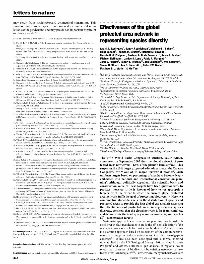
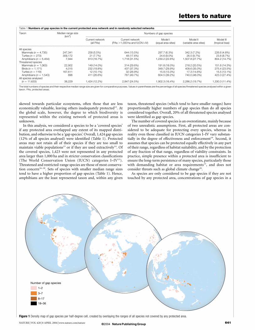
In this analysis, we considered a species to be a ‘covered species’if any protected area overlapped any extent of its mapped distri-bution, and otherwise to be a ‘gap species’. Overall, 1,424 gap species(12% of all species analysed) were identified (Table 1). Protectedareas may not retain all of their species if they are too small tomaintain viable populations13 or if they are used extractively14. Ofthe covered species, 1,423 were not represented in any protectedarea larger than 1,000 ha and in stricter conservation classifications(The World Conservation Union (IUCN) categories I–IV15).Threatened and restricted-range species are those of most conserva-tion concern16–18. Sets of species with smaller median range sizestend to have a higher proportion of gap species (Table 1). Hence,amphibians are the least represented taxon and, within any given

taxon, threatened species (which tend to have smaller ranges) haveproportionally higher numbers of gap species than do all speciesconsidered together. Overall, 20% of all threatened species analysedwere identified as gap species.

The number of covered species is an overestimate, mainly becauseof two unrealistic assumptions. First, all protected areas are con-sidered to be adequate for protecting every species, whereas inreality even those classified in IUCN categories I–IV vary substan-tially in the degree of effectiveness and enforcement19. Second, itassumes that species can be protected equally effectively in any partof their range, regardless of habitat suitability, and by the protectionof any fraction of that range, regardless of viability constraints. Inpractice, simple presence within a protected area is insufficient toensure the long-term persistence of many species, particularly thosewith demanding habitat or area requirements13, and does notconsider threats such as global climate change20.

As species are only considered to be gap species if they are nottouched by any protected area, concentrations of gap species in a

Table 1 Numbers of gap species in the current protected area network and in randomly selected networks

Taxon Median range size(km2)

Numbers of gap species

Current network(all PAs)

Current network(PAs .1,000 ha and IUCN I–IV)

Model I(equal area sites)

Model II(variable area sites)

Model III(tropical bias)

...................................................................................................................................................................................................................................................................................................................................................................

All speciesMammals (n ¼ 4,735) 247,341 258 (5.5%) 644 (13.5%) 297.7 (6.3%) 342.3 (7.2%) 226.6 (4.8%)Turtles (n ¼ 273) 309,172 21 (7.7%) 48 (17.6%) 24.6 (9.0%) 26.5 (9.7%) 23.8 (8.7%)Amphibians (n ¼ 5,454) 7,944 913 (16.7%) 1,718 (31.5%) 1,230.2 (22.6%) 1,507.8 (27.7%) 804.2 (14.7%)

Threatened speciesMammals (n ¼ 1,063) 22,902 149 (14.0%) 314 (29.6%) 191.8 (18.0%) 218.2 (20.5%) 151.6 (14.3%)Birds (n ¼ 1,171) 4,015 232 (19.8%) 437 (37.3%) 349.7 (29.9%) 409.6 (35.0%) 275.4 (23.5%)Turtles (n ¼ 119) 167,611 12 (10.1%) 32 (26.9%) 15.9 (13.3%) 17.3 (14.6%) 15.5 (13.1%)Amphibians (n ¼ 1,543) 896 411 (26.6%) 767 (49.7%) 604.5 (39.2%) 740.0 (48.0%) 423.3 (27.4%)

All species analysed(n ¼ 11,633) 38,229 1,424 (12.2%) 2,847 (24.5%) 1,902.3 (16.4%) 2,286.2 (19.7%) 1,330.3 (11.4%)

...................................................................................................................................................................................................................................................................................................................................................................

The total numbers of species and their respective median range size are given for comparative purposes. Values in parentheses are the percentage of all species/threatened species analysed within a giventaxon. PAs, protected areas.

Figure 1 Density map of gap species per half-degree cell, created by overlaying the ranges of all species not covered by any protected area.

letters to nature

NATURE | VOL 428 | 8 APRIL 2004 | www.nature.com/nature 641© 2004 Nature Publishing Group

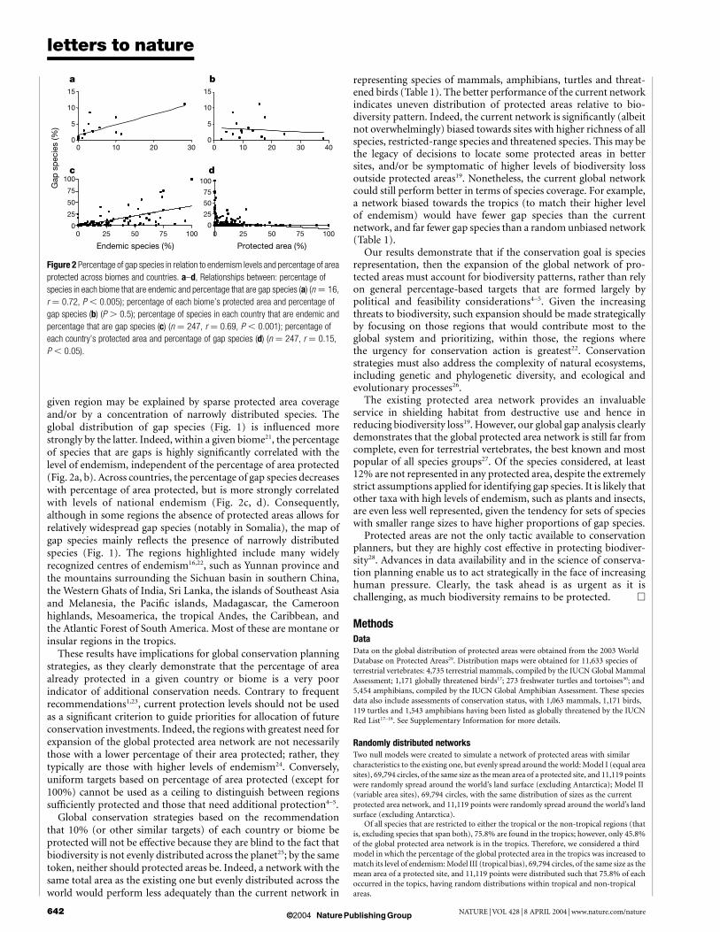
given region may be explained by sparse protected area coverageand/or by a concentration of narrowly distributed species. Theglobal distribution of gap species (Fig. 1) is influenced morestrongly by the latter. Indeed, within a given biome21, the percentageof species that are gaps is highly significantly correlated with thelevel of endemism, independent of the percentage of area protected(Fig. 2a, b). Across countries, the percentage of gap species decreaseswith percentage of area protected, but is more strongly correlatedwith levels of national endemism (Fig. 2c, d). Consequently,although in some regions the absence of protected areas allows forrelatively widespread gap species (notably in Somalia), the map ofgap species mainly reflects the presence of narrowly distributedspecies (Fig. 1). The regions highlighted include many widelyrecognized centres of endemism16,22, such as Yunnan province andthe mountains surrounding the Sichuan basin in southern China,the Western Ghats of India, Sri Lanka, the islands of Southeast Asiaand Melanesia, the Pacific islands, Madagascar, the Cameroonhighlands, Mesoamerica, the tropical Andes, the Caribbean, andthe Atlantic Forest of South America. Most of these are montane orinsular regions in the tropics.

These results have implications for global conservation planningstrategies, as they clearly demonstrate that the percentage of areaalready protected in a given country or biome is a very poorindicator of additional conservation needs. Contrary to frequentrecommendations1,23, current protection levels should not be usedas a significant criterion to guide priorities for allocation of futureconservation investments. Indeed, the regions with greatest need forexpansion of the global protected area network are not necessarilythose with a lower percentage of their area protected; rather, theytypically are those with higher levels of endemism24. Conversely,uniform targets based on percentage of area protected (except for100%) cannot be used as a ceiling to distinguish between regionssufficiently protected and those that need additional protection4–5.

Global conservation strategies based on the recommendationthat 10% (or other similar targets) of each country or biome beprotected will not be effective because they are blind to the fact thatbiodiversity is not evenly distributed across the planet25; by the sametoken, neither should protected areas be. Indeed, a network with thesame total area as the existing one but evenly distributed across theworld would perform less adequately than the current network in

representing species of mammals, amphibians, turtles and threat-ened birds (Table 1). The better performance of the current networkindicates uneven distribution of protected areas relative to bio-diversity pattern. Indeed, the current network is significantly (albeitnot overwhelmingly) biased towards sites with higher richness of allspecies, restricted-range species and threatened species. This may bethe legacy of decisions to locate some protected areas in bettersites, and/or be symptomatic of higher levels of biodiversity lossoutside protected areas19. Nonetheless, the current global networkcould still perform better in terms of species coverage. For example,a network biased towards the tropics (to match their higher levelof endemism) would have fewer gap species than the currentnetwork, and far fewer gap species than a random unbiased network(Table 1).

Our results demonstrate that if the conservation goal is speciesrepresentation, then the expansion of the global network of pro-tected areas must account for biodiversity patterns, rather than relyon general percentage-based targets that are formed largely bypolitical and feasibility considerations4–5. Given the increasingthreats to biodiversity, such expansion should be made strategicallyby focusing on those regions that would contribute most to theglobal system and prioritizing, within those, the regions wherethe urgency for conservation action is greatest22. Conservationstrategies must also address the complexity of natural ecosystems,including genetic and phylogenetic diversity, and ecological andevolutionary processes26.

The existing protected area network provides an invaluableservice in shielding habitat from destructive use and hence inreducing biodiversity loss19. However, our global gap analysis clearlydemonstrates that the global protected area network is still far fromcomplete, even for terrestrial vertebrates, the best known and mostpopular of all species groups27. Of the species considered, at least12% are not represented in any protected area, despite the extremelystrict assumptions applied for identifying gap species. It is likely thatother taxa with high levels of endemism, such as plants and insects,are even less well represented, given the tendency for sets of specieswith smaller range sizes to have higher proportions of gap species.

Protected areas are not the only tactic available to conservationplanners, but they are highly cost effective in protecting biodiver-sity28. Advances in data availability and in the science of conserva-tion planning enable us to act strategically in the face of increasinghuman pressure. Clearly, the task ahead is as urgent as it ischallenging, as much biodiversity remains to be protected. A

MethodsDataData on the global distribution of protected areas were obtained from the 2003 WorldDatabase on Protected Areas29. Distribution maps were obtained for 11,633 species ofterrestrial vertebrates: 4,735 terrestrial mammals, compiled by the IUCN Global MammalAssessment; 1,171 globally threatened birds17; 273 freshwater turtles and tortoises30; and5,454 amphibians, compiled by the IUCN Global Amphibian Assessment. These speciesdata also include assessments of conservation status, with 1,063 mammals, 1,171 birds,119 turtles and 1,543 amphibians having been listed as globally threatened by the IUCNRed List17–18. See Supplementary Information for more details.

Randomly distributed networksTwo null models were created to simulate a network of protected areas with similarcharacteristics to the existing one, but evenly spread around the world: Model I (equal areasites), 69,794 circles, of the same size as the mean area of a protected site, and 11,119 pointswere randomly spread around the world’s land surface (excluding Antarctica); Model II(variable area sites), 69,794 circles, with the same distribution of sizes as the currentprotected area network, and 11,119 points were randomly spread around the world’s landsurface (excluding Antarctica).

Of all species that are restricted to either the tropical or the non-tropical regions (thatis, excluding species that span both), 75.8% are found in the tropics; however, only 45.8%of the global protected area network is in the tropics. Therefore, we considered a thirdmodel in which the percentage of the global protected area in the tropics was increased tomatch its level of endemism: Model III (tropical bias), 69,794 circles, of the same size as themean area of a protected site, and 11,119 points were distributed such that 75.8% of eachoccurred in the topics, having random distributions within tropical and non-tropicalareas.

Figure 2 Percentage of gap species in relation to endemism levels and percentage of area

protected across biomes and countries. a–d, Relationships between: percentage of

species in each biome that are endemic and percentage that are gap species (a) (n ¼ 16,

r ¼ 0.72, P , 0.005); percentage of each biome’s protected area and percentage of

gap species (b) (P . 0.5); percentage of species in each country that are endemic and

percentage that are gap species (c) (n ¼ 247, r ¼ 0.69, P , 0.001); percentage of

each country’s protected area and percentage of gap species (d) (n ¼ 247, r ¼ 0.15,

P , 0.05).

letters to nature

NATURE | VOL 428 | 8 APRIL 2004 | www.nature.com/nature642 © 2004 Nature Publishing Group

Sixty replicates were obtained for each of these randomly distributed networks. Thesewere then overlaid with species distributional data to analyse the number of gap species ineach case. See Supplementary Information for the confidence intervals for each of themodels.

Richness of protected and unprotected cellsThe richness of each quarter-degree cell touching land (outside Antarctica) was calculatedfor all species, restricted-range species16 (occupying #50,000 km2) and threatened species.Cells touching protected areas were considered ‘protected’. Protected cells are significantly(P , 0.001) biased towards higher richness of all, restricted-range and threatened species.See Supplementary Information for a comparison of frequency distributions.

Received 21 December 2003; accepted 11 February 2004; doi:10.1038/nature02422.

1. Chape, S., Fish, L., Fox, P. & Spalding, M. United Nations List of Protected Areas (IUCN/UNEP, Gland,

Switzerland/Cambridge, UK, 2003).

2. The World Conservation Union. Parks For Life: Report of the IVth World Congress on National Parks

and Protected Areas (IUCN, Gland, Switzerland, 1993).

3. Kamden-Toham, A. et al. Forest conservation in the Congo Basin. Science 299, 346 (2003).

4. Soule, M. E. & Sanjayan, M. A. Conservation targets: do they help? Science 279, 2060–2061 (1998).

5. Pressey, R. L., Cowling, R. M. & Rouget, M. Formulating conservation targets for biodiversity pattern

and process in the Cape Floristic Region, South Africa. Biol. Conserv. 112, 99–127 (2003).

6. Margules, C. R. & Pressey, R. L. Systematic conservation planning. Nature 405, 243–253 (2000).

7. Scott, J. M. et al. Gap analysis—a geographic approach to protection of biological diversity. Wildl.

Monogr. 123, 1–41 (1993).

8. Lacher, T. E. Jr in GIS Methodologies for Developing Conservation Strategies (eds Savitsky, B. G. &

Lacher, T. E. Jr) 199–209 (Columbia Univ. Press, New York, 1998).

9. Jennings, M. D. Gap analysis: Concepts, methods, and recent results. Landscape Ecol. 15, 5–20

(2000).

10. Scott, J. M. et al. Nature reserves: Do they capture the full range of America’s biological diversity? Ecol.

Appl. 11, 999–1007 (2001).

11. Andelman, S. J. & Willig, M. R. Present patterns and future prospects for biodiversity in the Western

Hemisphere. Ecol. Lett. 6, 818–824 (2003).

12. Pressey, R. L. Ad hoc reservations—Forward or backward steps in developing representative reserve

systems? Conserv. Biol. 8, 662–668 (1994).

13. Newmark, W. D. Insularization of Tanzanian parks and the local extinction of large mammals.

Conserv. Biol. 10, 1549–1556 (1996).

14. Peres, C. A. & Lake, I. R. Extent of nontimber resource extraction in tropical forests: accessibility to

game vertebrates by hunters in the Amazon basin. Conserv. Biol. 17, 521–535 (2003).

15. The World Conservation Union, Guidelines for Protected Area Management Categories (IUCN

CNPPA/WCMC, Gland, Switzerland/Cambridge, UK, 1994).

16. Stattersfield, A. J., Crosby, M. J., Long, A. J. & Wege, D. C. Endemic Bird Areas of the World—Priorities

for Biodiversity Conservation (BirdLife International, Cambridge, UK, 1998).

17. BirdLife International. Threatened Birds of the World (Lynx Edicions/BirdLife International,

Barcelona/Cambridge, UK, 2000).

18. The World Conservation Union. IUCN Red List of Threatened Species [online] khttp://

www.redlist.orgl (2003).

19. Bruner, A. G., Gullison, R. E., Rice, R. E. & Fonseca, G. A. B. Effectiveness of parks in protecting

tropical biodiversity. Science 291, 125–128 (2001).

20. Thomas, C. D. et al. Extinction risk from climate change. Nature 427, 145–148 (2004).

21. Olson, D. M. et al. Terrestrial ecoregions of the world: A new map of life on earth. Bioscience 51,

933–938 (2001).

22. Myers, N., Mittermeier, R. A., Mittermeier, C. G., Fonseca, G. A. B. & Kent, J. Biodiversity hotspots for

conservation priorities. Nature 403, 853–858 (2000).

23. Green, M. J. B. & Paine, J. State of the World’s Protected Areas at the End of the Twentieth Century

(WCMC, Cambridge, UK, 1997).

24. Rodrigues, A. S. L. & Gaston, K. J. How large do reserve networks need to be? Ecol. Lett. 4, 602–609

(2001).

25. Gaston, K. J. Global patterns in biodiversity. Nature 405, 220–227 (2000).

26. Cowling, R. M. & Pressey, R. L. Rapid plant diversification: planning for an evolutionary future. Proc.

Natl Acad. Sci. USA 98, 5452–5457 (2001).

27. Gaston, K. J. & May, R. M. Taxonomy of taxonomists. Nature 356, 281–282 (1992).

28. Balmford, A. et al. Economic reasons for conserving wild nature. Science 297, 950–953 (2002).

29. World Database on Protected Areas. World Database on Protected Areas (IUCN-WCPA/UNEP-

WCMC, Washington DC, 2003).

30. Iverson, J. B., Kiester, A. R., Hughes, L. E. & Kimerling, A. J. The EMYSystem World Turtle Database

2003 [online] khttp://emys.geo.orst.edul (2003).

Supplementary Information accompanies the paper on www.nature.com/nature.

Acknowledgements We thank the Moore Family Foundation, the Howard Gilman Foundation

and the National Center for Ecological Analysis and Synthesis of the University of California Santa

Barbara for support. The analysis was possible thanks to the combined effort of the thousands of

individuals and hundreds of institutions who collected and compiled the data, or provided

financial support for such efforts. We are grateful to the numerous individuals who contributed to

this analysis, especially to K. Buhlmann, S. Butchart, N. Cox, P. P. van Dijk, J. Iverson, R. Kiester,

T. Lacher and B. Young. H. Possingham made valuable comments on the manuscript. Figure 1 was

generated by J. Seeber.

Competing interests statement The authors declare that they have no competing financial

interests.

Correspondence and requests for materials should be addressed to A.S.L.R.

(a.rodrigues@conservation.org).

..............................................................

Spatial structure often inhibitsthe evolution of cooperationin the snowdrift gameChristoph Hauert & Michael Doebeli

Departments of Zoology and Mathematics, University of British Columbia,6270 University Boulevard, Vancouver, British Columbia V6T 1Z4, Canada.............................................................................................................................................................................

Understanding the emergence of cooperation is a fundamentalproblem in evolutionary biology1. Evolutionary game theory2,3

has become a powerful framework with which to investigate thisproblem. Two simple games have attracted most attention intheoretical and experimental studies: the Prisoner’s Dilemma4

and the snowdrift game (also known as the hawk–dove or chickengame)5. In the Prisoner’s Dilemma, the non-cooperative state isevolutionarily stable, which has inspired numerous investi-gations of suitable extensions that enable cooperative behaviourto persist. In particular, on the basis of spatial extensions of thePrisoner’s Dilemma, it is widely accepted that spatial structurepromotes the evolution of cooperation6–8. Here we show that nosuch general predictions can be made for the effects of spatialstructure in the snowdrift game. In unstructured snowdriftgames, intermediate levels of cooperation persist. Unexpectedly,spatial structure reduces the proportion of cooperators for a widerange of parameters. In particular, spatial structure eliminatescooperation if the cost-to-benefit ratio of cooperation is high.Our results caution against the common belief that spatialstructure is necessarily beneficial for cooperative behaviour.

The Prisoner’s Dilemma illustrates that cooperating individualsare prone to exploitation, and that natural selection should favourcheaters. In this game, two players simultaneously decide whether tocooperate or defect. Cooperation results in a benefit b to therecipient but incurs a cost c to the donor (b . c . 0). Mutualcooperation thus pays a net benefit of R ¼ b 2 c, whereas mutualdefection results in payoff P ¼ 0 for both players. With unilateralcooperation, defection yields the highest payoff, T ¼ b, at theexpense of the cooperator bearing the cost S ¼ 2c. It follows thatit is best to defect regardless of the co-player’s decision. Thus,defection is the evolutionarily stable strategy, even though allindividuals would be better off if they all cooperated. This outcomeis a simple consequence of the ranking of the four payoff values:T . R . P . S. Despite this seemingly convincing argument,many natural species show altruism, with individuals bearingcosts to the benefit of others: vampire bats share blood9, alarmcalls warn from predators10, monkeys groom each other11, and fishinspect predators preferably in pairs12.

In field and experimental studies it is often difficult to assess thefitness payoffs for different behavioural patterns, and even theproper ranking of the payoffs is challenging13,14. This has led to aconsiderable gap between theory and experimental evidence, and toan increasing discomfort with the Prisoner’s Dilemma as the onlymodel to discuss cooperative behaviour15,16. The snowdrift game is aviable and biologically interesting alternative. It differs from thePrisoner’s Dilemma in that the payoffs P and S have a reverse order:T . R . S . P. This changes the situation fundamentally andleads to persistence of cooperation.

To illustrate the snowdrift game, imagine two drivers that arecaught in a blizzard and trapped on either side of a snowdrift. Theycan either get out and start shovelling (cooperate) or remain in thecar (defect). If both cooperate, they have the benefit b of gettinghome while sharing the labour c. Thus, R ¼ b 2 c/2. If both defect,they do not get anywhere and P ¼ 0. If only one shovels, however,they both get home but the defector avoids the labour cost and gets

letters to nature

NATURE | VOL 428 | 8 APRIL 2004 | www.nature.com/nature 643© 2004 Nature Publishing Group

1

Supplementary information to “Effectiveness of the global protected area network in representing species diversity”

* Notes on data and methods, and extended acknowledgements *

1 Data sources

1.1 Protected areas

Data on the global distribution of protected areas were obtained from the recently released World Database on Protected Areas1. This is a freely available database compiled by a consortium of organizations including BirdLife International, Conservation International, Fauna & Flora International, The Nature Conservancy, United Nations Environmental Programme – World Conservation Monitoring Centre, the World Resources Institute, the Wildlife Conservation Society, and the World Wildlife Fund.

Protected areas in the WDPA are recorded either as polygons (58,514 records) and/or as points (106,215 records, of which 73,863 have no corresponding polygon information). Both types of data were provided as ArcView shapefiles2, with associated tables of attributes. Data for each protected area include a unique site code, protected area name, country, geographical coordinates, designation (e.g., Nature Reserve, National Park), IUCN categories, and status (e.g., Designated, Proposed, Degazetted). Additionally, the WDPA includes data on protected areas with international status (e.g., UNESCO Man and the Biosphere Reserves, World Heritage Sites, Ramsar Wetlands), but this information was included in this analysis only when the area was also designated at a national level.

For purposes of the global gap analysis, the following records were eliminated from the WDPA: a) Point records with both Lat and Lon as zero, that is, those with no information on the exact geographical location of an area; and b) records that do not seem to correspond to established protected areas, including those with Areaname recorded as “Area Not Protected”, or Status recorded as “Degazeted”, “Proposed”, “Recommended”, “In Preparation” or “Unset”.

2

For the remaining records, we kept the maximum level of geographic data provided by the WDPA. Point records with no information on area were kept in a separate point shapefile. Point records with associated area were converted into circular shapes of the same area (centered on the coordinates provided for the point) and merged with the polygon records into a common polygon shapefile.

The resulting polygon layer contains records of areas that overlap spatially (e.g., core areas of Biosphere Reserves on top of the wider reserves). To avoid having the total protected area of the planet overestimated by these overlaps, we merged all protected areas into one single layer. For the purposes of this analysis, a single ‘protected site’ is then either an individual protected area or a set of contiguous/overlapping protected areas.

The network of protected areas as defined above is constituted of 69,794 polygons (protected sites) occupying in total about 16,002,000 km2 (11.9% of the land area outside Antarctica), and of 11,119 points for which no area was associated. Antarctica represents a highly unusual situation, as the vast region south of 60o South latitude can be considered a protected area on its own (protected though the 1959 Antarctic Treaty and its Environmental Protected Protocol), yet it holds virtually none of the species considered in the global gap analysis. We followed the WDPA 20031 and the 2003 UN List of Protected Areas3 in excluding it from the network of protected areas.

1.2 Mammals

Distribution maps for all mammal species were compiled, as part of the IUCN Global Mammal Assessment, by W. Sechrest (unpublished), L. Boitani (for large mammals of Africa4; unpublished for rodents of Africa), M. Tognelli (for rodents of South America5), and G. Ceballos (for bats of Central America5). Although all of these maps are currently undergoing formal review, draft maps were available for this global gap analysis.

The taxonomic classification of all species used in this analysis followed the second edition of Mammal Species of the World6, with modifications from draft chapters of the third edition made to incorporate the latest taxonomic information wherever possible (Reeder & Wilson, unpublished). Spatial data were compiled from primary and secondary literature (e.g., taxonomic accounts, regional atlas projects, Mammalian Species Accounts), museum records, and other scientific reports and documents. Over 1,700 sources were consulted for information on

3

species distributions. Preference was given to more recent sources, as well as sources that have comprehensive information for an entire species’ range.

Data on the extent of occurrence of mammal species were composed of polygons corresponding to different levels of certainty about species’ presence, to differences between historical and current ranges, and to native or introduced ranges. For this analysis, only polygons where the species was both reported as native and with presence coded as extant or possibly present were used, thus excluding historical and introduced ranges. Marine mammals were also excluded from the analysis (i.e., Cetacea, Sirenia, and marine species in the Order Carnivora). In total, 4,735 species were analysed corresponding to 94% of all mammals. According to the 2003 IUCN Red List7 these include 174 Critically Endangered species, 314 Endangered, and 575 Vulnerable species, although a perfect match between the IUCN assessment and the distribution maps was not possible due to minor differences in the taxonomic classification. The majority of these species were assessed in 19968 using version 2.3 of the IUCN criteria9 (now supplanted by version 3.110).

When complete, the data and results of the Global Mammal Assessment will all be freely available through the IUCN Red List web site (www.redlist.org).

1.3 Globally threatened birds

The data on the world’s globally threatened bird species were compiled by the BirdLife International partnership11, and reviewed by hundreds of experts. These data include assessments of threat for each species, following the IUCN Red List criteria (version 3.110) and range maps.

Where possible, these range maps were based on locality records that included sightings and specimen records (ideally recent sightings, although, for some species, old records are the only records). A species’ known range was derived from these records, using additional habitat and topographical information to aid range definition. For some species, a projected range was added to the known range to reflect areas between well-spaced localities of suitable habitat, and areas close to known localities that are likely to hold the species. Known and projected ranges have been combined to give an estimate of extent of occurrence for each threatened species12. For some species, possible and historical ranges were also mapped, but these were not included in this analysis. Twelve species were excluded because their ranges (if still extant) are not sufficiently known to be

4

mapped. Each polygon included within a species’ extent of occurrence has been coded according to the season of occurrence of the species: breeding, non-breeding, or resident. For marine species (those with a mainly oceanic non-breeding range) only breeding range was considered. For two species only non-breeding range is known.

The taxonomic classification used followed BirdLife International11. Of the 1,171 globally threatened birds included in this analysis (11% of all birds), 170 are Critically Endangered, 320 are Endangered, and 681 are considered Vulnerable species. The three species classified as Extinct in the Wild were excluded from the analysis. In order to match the available distribution maps, we retained for each species the threat categories as published in the 2000 assessment11, even though a more recent threat assessment is available7.

1.4 Tortoises and freshwater turtles

Data on species of tortoises and freshwater turtles were mainly obtained from the EMYSystem World Turtle Database 200313 as point data (~ 26,000 records) corresponding to museum specimens and literature citations. These points were converted into polygons and preliminarily reviewed by K. Buhlmann and T. Akre. This information will form the basis of a formal IUCN Global Turtle Assessment.

In total 273 species were analysed (a little more than 3% of all reptiles). According to the 2003 IUCN Red List7 these include 21 Critically Endangered species, 42 Endangered, and 56 Vulnerable species. However, a perfect match between the IUCN assessment and the distribution maps was not possible due to minor differences in the taxonomic classification. The majority of these species were assessed in 19968 using version 2.3 of the IUCN criteria9 but more than 80 Asian species were re-assessed in 1999 using the 3.1 version10.

When complete, the data and results of the Global Turtle Assessment will all be freely available through the IUCN Red List web site (www.redlist.org).

1.5 Amphibians

With the exception of North America (see below), amphibian maps were developed by the on-going IUCN Global Amphibian Assessment14. Distribution maps were created for all species in two stages. First, an expert on amphibians in each of 33 designated regions collected data on all species in the region. Each of

5

these experts was responsible for collating information on species taxonomy, geographic range (including a preliminary distribution map), population status, habitat preferences, trade status, and major threats and conservation measures that are currently in place or that are needed. Each regional expert also provided a preliminary assessment of threat for each species according to the IUCN Red List categories10. Second, all of the data collected in this initial stage are being reviewed (most have already been so) either through expert workshops (particularly for the more species-rich regions), or by correspondence.

The global gap analysis used the most recent data available including reviewed maps of species distributions for South America, Mesoamerica, Madagascar, South-east Asia, South Asia, New Zealand, New Guinea, Russia and the Confederation of Independent States. Distribution maps have also been reviewed for three quarters of African species, most of the species in Japan and some of the species in Australia. Data are still being reviewed for the Caribbean, West Asia, Europe, and for the remaining species of Africa, Japan and Australia. Overall, about 80% of all amphibian species have had their distribution maps formally reviewed. For many of the unreviewed species, such as those from Europe and West Asia, the data are derived from reliable published sources.

NatureServe provided the distribution maps for species in US and Canada. The main source for these maps was a database on county of occurrence developed by M. Lanoo at Ball State University15. These maps fed into the Global Amphibian Assessment as part of the process for the Red List assessment of North American species.

The taxonomic classification used follows Frost16, with modifications where deemed necessary by the experts involved in the Global Amphibian Assessment. After excluding 24 extinct species, 5,454 amphibians were included in this global gap analysis (i.e., all living amphibians). Based on the currently available assessment of threat for each species (unreviewed for the regions mentioned above), this included 341 Critically Endangered, 550 Endangered, and 652 Vulnerable species.

When complete, the data and results of the Global Amphibian Assessment will all be freely available through the IUCN Red List web site (www.redlist.org), AmphibiaWeb (www.amphibiaweb.org), and the American Museum of Natural History Amphibian Species of the World web site16 (http://research.amnh.org/herpetology/amphibia/index.html).

6

2 Data limitations

The global gap analysis is based on the comparison between maps of protected areas and maps of species distributions. Although these are the best datasets of its kind ever compiled at the global scale, they have limitations that introduce errors to the results of the analysis. Hence, two types of error are possible:

- Omission errors, which occur when a given species is considered a gap species when, in fact, it is covered, and

- Commission errors, which occur when a given species is considered covered by one or more protected areas when, in fact, it is a gap species.

For conservation purposes, it is more important to minimize commission errors than omission errors, because ignoring a species that is genuinely not represented in protected areas may have high conservation costs. Unfortunately, the current data are much more prone to commission errors.

Here, we discuss the limitations in the protected area and species data more likely to be sources of errors in the global gap analysis, to provide a better understanding of the results and implications of this study. These limitations are not exclusive to the data used in this analysis – in fact they are prevalent amongst published studies at the macroecological scale17-20.

2.1 Limitations in the protected area data

2.1.1 Missing records

Even though the WDPA is the most complete record of the world network of protected areas, it does not include all existing protected areas. The database is incomplete in part because there are gaps in information about existing protected areas, and in part because the global network is dynamic and changing. These missing records will cause omission errors.

2.1.2 Incorrect records

The results of the global gap analysis will be sensitive to records that include incorrect information about protected areas. Inaccuracies in the location of protected area boundaries or changes in status of an area (e.g. from “Proposed” to

7

“ Designated” or from “Designated” to “Degazetted”) may result in either commission or omission errors in the analysis.

2.1.3 Protected areas with point data only

Nearly half of the records used in this analysis were point data (52,694 records). For 41,575 of these, some data on area were available, and these were represented as circles centered in the respective latitude and longitude coordinates. The remaining 11,229 were represented as points. Point representations can lead to omission errors, while protected areas represented as circles can lead to both omission and commission errors. In most cases, the magnitude of errors will be much higher when using point data only. However, point records are heavily biased toward the representation of smaller protected areas, reducing the predicted magnitude of errors created by these data.

2.1.4 Uneven global coverage

The quantity and quality of data in the WPDA are unevenly distributed across countries, which will result in discrepancies in the results of the global gap analysis.

2.1.5 Lack of data on management effectiveness of protected areas

One of the major limitations of the WDPA data for the purposes of the global gap analysis is the scarcity of information regarding the management effectiveness of each protected area, i.e., the degree to which a protected area is likely to succeed in preserving the biodiversity values it contains. Without this information, any evaluation of the coverage of the global network of protected areas is necessarily an approximation in which the number of species represented is a gross overestimate of the number of species effectively protected. IUCN management categories I to VI21 provide some information on the level of management of individual protected areas, but for a large number of protected areas this information is not available. Additionally, not all countries have systematically applied IUCN categories; and among those that have, the classification has not been applied consistently. Furthermore, categories I-VI are more likely to reflect the legal status of a reserve (intended level of management) than its real management effectiveness.

8

The WDPA will change continuously as the global network itself changes and better regional data become available. Given the limitations described above, it is difficult to assess whether the published22 figure that 11.5% of the planet’s land area is protected is an underestimate or an overestimate of the true global coverage. On the one hand, there are certainly many records missing from the WDPA, particularly in relation to less traditional protected areas (e.g., private reserves) and areas classified at the sub-national level (e.g., state reserves). On the other hand, it is not possible at present to estimate the fraction of records in the WDPA which correspond to areas without any real protection.

2.2 Limitations in the biological data

2.2.1 Narrow taxonomic scope

The global gap analysis included only those taxonomic groups for which it was possible to obtain compiled maps of global coverage in digital format: mammals, amphibians, freshwater turtles and tortoises, and globally threatened birds. No attempt was made to collect species distribution maps for other taxa.

These species are analysed here as conservation targets on their own right. While other taxa would certainly benefit from the conservation of regions highlighted by the results of the global gap analysis23, no assumption is made that a network of protected areas adequate for the representation of mammals, amphibians, and threatened birds is sufficient for other taxonomic groups. Indeed, previous studies have demonstrated that vertebrate species are not likely to be adequate surrogates for other groups, particularly those with more species and high levels of endemism, such as plants and invertebrates24.

2.2.2 Missing species and incomplete species maps

Even though the taxa considered in the global gap analysis correspond to the best-known fraction of the world’s biodiversity, many vertebrate species are still being described25. Even where distribution maps are available, many are incomplete in the sense that they do not include areas where a species is actually present but has never yet been recorded. Poorly known species and poorly known regions are most likely to be affected by these kinds of limitations of biological data.

9

2.2.3 Species ranges mapped as extent of occurrence

For the majority of species, mapped ranges are gross overestimates of locations where species truly occur, as they generally correspond to extent of occurrence range maps, rather than area of occupancy12. Most of these ranges were obtained as “envelopes” including original records (point data) and through extrapolation (using, for example, habitat information) from original records. They are likely to include relatively extensive areas from which the species is absent. These overestimates of species locations are a substantial source of commission errors in this analysis, as species may be listed as present in protected areas that overlap their mapped extent of occurrence but where they do not occur (see below).

2.2.4 Uneven global coverage

As with the protected area data described above, the quality and quantity of biological data is unevenly distributed across the world. Well-known regions are less likely to have missing species, and maps of individual species from these regions will tend to show greater accuracy and levels of detail, even approaching the area of occupancy in a few cases.

2.2.5 Lack of data on species viability across the range

Even those portions of the range where the species is truly present are not all equivalent, and so it is relevant in which of those portions protected areas are located. Hence, the current presence of a species in a protected area is not a guarantee of its future persistence, even on a time scale of a few years or decades26-27. Consequently, the complete list of species reported from a given protected area is likely to be a considerable overestimate of those species whose long-term persistence can actually be effectively ensured by the protected area.

10

3 Test of data limitations: omission and commission errors in threatened amphibians of Mesoamerica

In addition to species range maps, the Global Amphibian Assessment collected, including information on conservation measures currently in place for each species, such as presence in or absence from protected areas. These data provide an opportunity to evaluate the accuracy of the results obtained by the global gap analysis, based on information provided by regional experts with ground knowledge on both the species and the protected areas.

The 280 threatened species of amphibians of the Mesoamerican region (from Mexico to Panama) were analysed as a preliminary case study. A comparison of the lists of species considered covered by the global gap analysis with those reported as covered in the Global Amphibian Assessment14 (Figure 1), found: 71% match (species reported by both assessments as either covered or gaps), 9% omission error (species reported as gaps by the global gap analysis but as covered by the Global Amphibian Assessment), and 19% commission error (species reported as covered by the global gap analysis but as gaps by the Global Amphibian Assessment).

Hence, overall, the global gap analysis underestimated the number of gap species: 38%, as compared to 48% reported by the Global Amphibian Assessment. Furthermore, for about 10% of the covered species, the experts reported that presence in protected areas is no guarantee of the species’ persistence, due to habitat degradation or because the species has not been recorded in the protected areas recently despite searches.

For the majority of the species, it was possible to determine the most likely source of the omission and commission errors (Figure 1, Table I). As predicted, most errors are due to the spatial representation of species’ ranges as extent of occurrence, which overestimate the species’ true area of occupancy and result in commission errors.

11

Figure 1. Sources of omission and commission errors obtained by comparing the lists of species considered covered by the global gap analysis with those reported as covered in the Global Amphibian Assessment.

Table I. Likely sources of omission and commission errors.

Error type Error source % Explanation

protected areas data 4% - protected area(s) not mapped

- protected area(s) mapped in the wrong place

- protected area(s) represented as points

- protected area(s) represented as circles

omission errors

species’ distribution data 5% - incomplete species’ range maps

protected areas data 3% - protected area(s) mapped in the wrong place

- protected area(s) represented as circles

commission errors

species’ distribution data 15% - species’ range maps include unoccupied areas

covered species

(42%)

gap species (29%)

PA data (4%)

species data (5%)

undetermined(1%)

PA data (3%)

species data (15%)

undetermined (1%)

omission

commission

match

covered species

(42%)

gap species (29%)

PA data (4%)

species data (5%)

undetermined(1%)

PA data (3%)

species data (15%)

undetermined (1%)

omission

commission

match

12

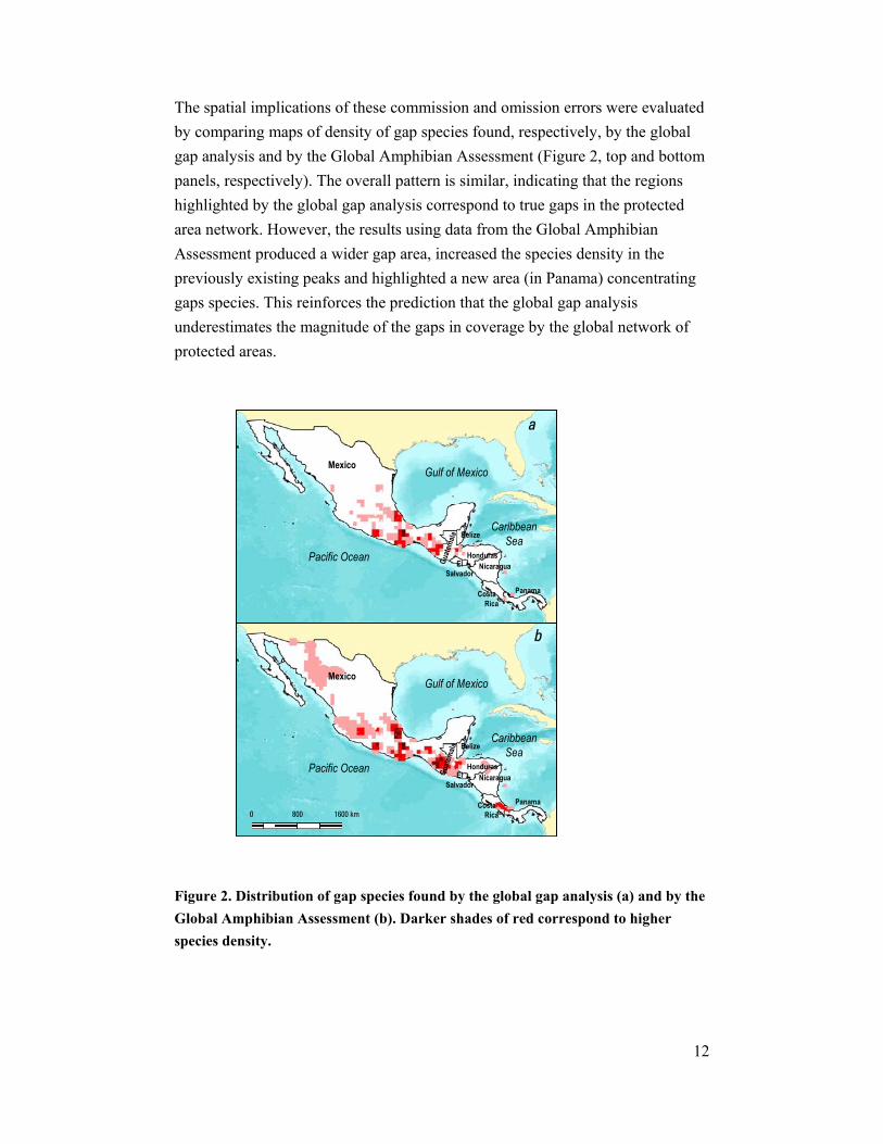
The spatial implications of these commission and omission errors were evaluated by comparing maps of density of gap species found, respectively, by the global gap analysis and by the Global Amphibian Assessment (Figure 2, top and bottom panels, respectively). The overall pattern is similar, indicating that the regions highlighted by the global gap analysis correspond to true gaps in the protected area network. However, the results using data from the Global Amphibian Assessment produced a wider gap area, increased the species density in the previously existing peaks and highlighted a new area (in Panama) concentrating gaps species. This reinforces the prediction that the global gap analysis underestimates the magnitude of the gaps in coverage by the global network of protected areas.

Figure 2. Distribution of gap species found by the global gap analysis (a) and by the Global Amphibian Assessment (b). Darker shades of red correspond to higher species density.

Mexico

Guate

mala

HondurasNicaragua

Belize

El Salvador

PanamaCostaRica

Gulf of Mexico

Pacific Ocean

Caribbean Sea

0 1600 km800

Mexico

Guate

mala

HondurasNicaragua

Belize

El Salvador

PanamaCostaRica

Gulf of Mexico

Pacific Ocean

Caribbean Sea

a

b

Mexico

Guate

mala

HondurasNicaragua

Belize

El Salvador

PanamaCostaRica

Gulf of Mexico

Pacific Ocean

Caribbean Sea

0 1600 km800

Mexico

Guate

mala

HondurasNicaragua

Belize

El Salvador

PanamaCostaRica

Gulf of Mexico

Pacific Ocean

Caribbean Sea

Mexico

Guate

mala

HondurasNicaragua

Belize

El Salvador

PanamaCostaRica

Gulf of Mexico

Pacific Ocean

Caribbean Sea

0 1600 km800

Mexico

Guate

mala

HondurasNicaragua

Belize

El Salvador

PanamaCostaRica

Gulf of Mexico

Pacific Ocean

Caribbean Sea

a

b

13

4 Note on targets based on percentage of area protected

This global gap analysis demonstrates the inadequacy of general targets based on a uniform percentage of area protected. However, percentage-based targets are useful when scaled to reflect the conservation requirements for each biodiversity component, by integrating information on aspects such as persistence, vulnerability and rarity (see reference 28 for a review).

Uniform targets are deeply ingrained in the conservation strategies of national governments and international conservation organizations. These include:

- The IUCN recommendation at the 1992 World Parks Congress (Caracas, Venezuela) that protected areas should cover a minimum of 10 per cent of each biome by 200029.

- The Forests for Life Campaign launched by WWF (www.panda.org/forests4life/), which had an initial target “to establish an ecologically representative network of protected areas, covering at least 10% of the world's forest area by the year 2000” (the target has subsequently been changed to “Protect a global network of protected areas which are well-resourced, well-managed and representative of all the world's threatened and most biologically significant forest regions by 2010”). This campaign was joined by IUCN, and gained further momentum with the creation of the WWF/World Bank Alliance. The flagship project of this Alliance is the Amazon Region Protected Areas Program (ARPA), anchored in the 1998 commitment by Brazilian President Fernando H. Cardoso to set aside at least 10 percent of Brazil's forests as conservation areas.

- The Endangered Seas Programme by WWF (www.panda.org/endangeredseas/), which is campaigning for at least 10% of marine areas to be under some form of protection by 2012.

- The Yaoundé Summit Declaration, signed on March 1999 by Cameroon, Central African Republic, Chad, the Popular Republic of Congo, Equatorial Guinea and Gabon, which commits these countries to conserving a minimum of 10% of the nation’s forests in protected areas30.

- The Protected Area Strategy released in 1993 by the Government of British Columbia, Canada, which had a goal “to designate and manage, by

14

the year 2000, a system of protected areas which protected a diversity of natural, cultural heritage and recreational values encompassing a full 12% of the province’s land base” (http://www.cd.gov.ab.ca/preserving/parks/fppc/bc_eng.pdf).

- Target 4 of the Global Strategy for Plant Conservation31, which reads “At least 10 per cent of each of the world's ecological regions effectively conserved [by 2010]”. The Strategy is supported by a wide range of organisations and institutions – governments, intergovernmental organizations, universities, research institutes, nongovernmental organizations and their networks, and the private sector. In particular, the Strategy was approved by the sixth Conference of the Parties to the Convention on Biological Diversity (COP6).

These targets have certainly played important roles in galvanising governments, the public opinion, and the private sector to conservation action. However, while they are generally intended to be a floor to conservation efforts (e.g., ‘at least 10%’) there is a danger that they become de facto ceilings32. For example, the 12% target set by the Government of British Columbia gave critical impulse to a doubling of the total protected area in the province, achieved in 2001. However, there is growing concern by the non-governmental and scientific communities that the 12% figure has become a cap inhibiting the designation of additional protected areas by the Government33.

When used to establish priorities for action amongst different regions or biomes, uniform targets may lead to the wrong conclusion that some of these are already ‘finished’, even though they may be the ones where protection is still most urgently needed. For example, the Global Strategy for Plant Conservation and corresponding COP6 decision use the 10% target to support the statement that “in general, forests and mountain areas are well represented in protected areas, while natural grasslands (such as prairies) and coastal and estuarine ecosystems, including mangroves, are poorly represented”31. Yet, this global gap analysis found that tropical montane forests are precisely the ecosystems most in need of additional protected area coverage.

15

5 Notes on methods

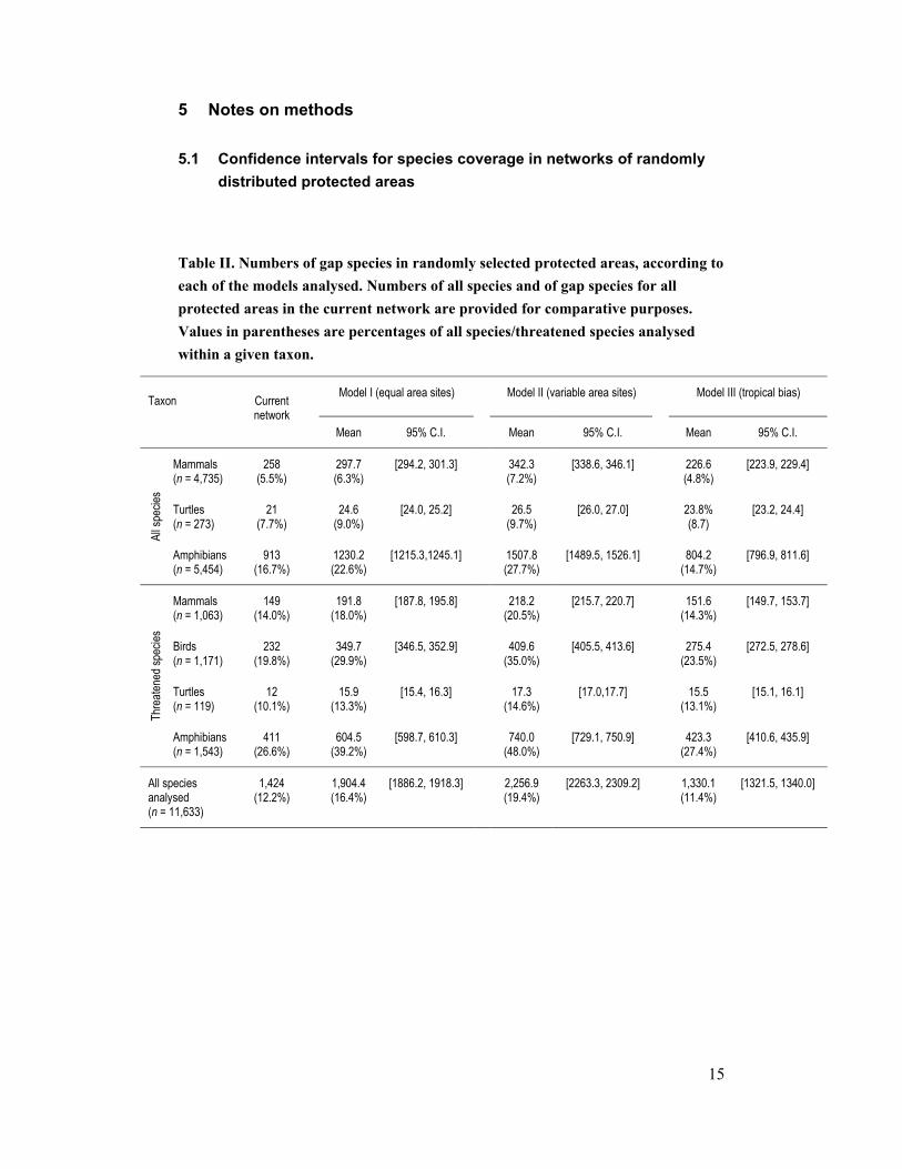
5.1 Confidence intervals for species coverage in networks of randomly distributed protected areas

Table II. Numbers of gap species in randomly selected protected areas, according to each of the models analysed. Numbers of all species and of gap species for all protected areas in the current network are provided for comparative purposes. Values in parentheses are percentages of all species/threatened species analysed within a given taxon.

Model I (equal area sites) Model II (variable area sites) Model III (tropical bias) Taxon Current network

Mean 95% C.I. Mean 95% C.I. Mean 95% C.I.

Mammals (n = 4,735)

258 (5.5%)

297.7 (6.3%)

[294.2, 301.3] 342.3 (7.2%)

[338.6, 346.1] 226.6 (4.8%)

[223.9, 229.4]

Turtles (n = 273)

21 (7.7%)

24.6 (9.0%)

[24.0, 25.2] 26.5 (9.7%)

[26.0, 27.0] 23.8% (8.7)

[23.2, 24.4]

All s

pecie

s

Amphibians (n = 5,454)

913 (16.7%)

1230.2 (22.6%)

[1215.3,1245.1] 1507.8 (27.7%)

[1489.5, 1526.1] 804.2 (14.7%)

[796.9, 811.6]

Mammals (n = 1,063)

149 (14.0%)

191.8 (18.0%)

[187.8, 195.8] 218.2 (20.5%)

[215.7, 220.7] 151.6 (14.3%)

[149.7, 153.7]

Birds (n = 1,171)

232 (19.8%)

349.7 (29.9%)

[346.5, 352.9] 409.6 (35.0%)

[405.5, 413.6] 275.4 (23.5%)

[272.5, 278.6]

Turtles (n = 119)

12 (10.1%)

15.9 (13.3%)

[15.4, 16.3] 17.3 (14.6%)

[17.0,17.7] 15.5 (13.1%)

[15.1, 16.1]

Thre

atene

d spe

cies

Amphibians (n = 1,543)

411 (26.6%)

604.5 (39.2%)

[598.7, 610.3] 740.0 (48.0%)

[729.1, 750.9] 423.3 (27.4%)

[410.6, 435.9]

All species analysed (n = 11,633)

1,424 (12.2%)

1,904.4 (16.4%)

[1886.2, 1918.3] 2,256.9 (19.4%)

[2263.3, 2309.2] 1,330.1 (11.4%)

[1321.5, 1340.0]

16

5.2 Comparison between protected and unprotected sites in terms of richness of all species, threatened species, and restricted-range species

Figure 3. Frequency distribution of the percentage of half-degree protected (green) and unprotected (grey) cells which fall in each class of species richness, for: a) all species; b) restricted range species; and c) threatened species.

a

0

5

10

15

20

25

30

35

40

0 1-2 3-6 7-14 15-30 31-62 63-126

127-254

255-248

perc

enta

ge o

f cel

lsb

0

10

20

30

40

50

60

70

80

90

number of species

c

0

5

10

15

20

25

30

35

0 1-2 3-6 7-14 15-30 31-6263

-126

0 1-2 3-6 7-14 15-30 31-62 63-126

number of species number of species

a

0

5

10

15

20

25

30

35

40

5

10

15

20

25

30

35

40

0 1-2 3-6 7-14 15-30 31-62 63-126

127-254

255-248

perc

enta

ge o

f cel

lsb

0

10

20

30

40

50

60

70

80

90

number of species

c

0

5

10

15

20

25

30

35

0 1-2 3-6 7-14 15-30 31-6263

-1260 1-2 3-6 7-14 15-30 31-6263

-126

0 1-2 3-6 7-14 15-30 31-62 63-1260 1-2 3-6 7-14 15-30 31-62 63-126

number of species number of species

17

References

1. WDPA. 2003 World Database on Protected Areas (IUCN–WCPA and UNEP–WCMC, Washington DC, USA, 2003).

2. ESRI. ArcView GIS 3.2a (Environmental Systems Research Institute, Inc., New York, USA, 2000).

3. Chape, S., Blyth, S., Fish, L., Fox, P. & Spalding, M. 2003 United Nations List of Protected Areas (IUCN and UNEP, Gland, Switzerland and Cambridge, UK, 2003).

4. Boitani, L. et al. A Databank for the Conservation and Management of the African Mammals (Istituto di Ecologia Applicata, Rome, Italy, 1999).

5. Patterson, B. D. et al. Digital Distribution Maps of the Mammals of the Western Hemisphere – Version 1.0. (NatureServe, Arlington VA, USA, 2003).

6. Wilson, D. E. & Reeder, D. M. Mammal Species of the World: A Taxonomic and Geographic Reference, 2nd ed. (Smithsonian Institution Press, Washington DC, USA) http://nmnhwww.si.edu/msw/ (2003).

7. IUCN. 2003 IUCN Red List of Threatened Species (IUCN, Gland, Switzerland and Cambridge, UK) http://www.redlist.org (2003).

8. Baillie, J. & Groombridge, B. IUCN Red List of Threatened Animals (IUCN, Gland, Switzerland, 1996).

9. IUCN. IUCN Red List Categories (IUCN Species Survival Commission, Gland, Switzerland, 1994).

10. IUCN. IUCN Red List Categories and Criteria : Version 3.1 (IUCN Species Survival Commission, Gland, Switzerland, and Cambridge, UK, 2001).

11. BirdLife International. Threatened Birds of the World (Lynx Edicions and BirdLife International, Barcelona, Spain, and Cambridge, UK, 2000).

12. Gaston, K. J. Rarity (Chapman & Hall, London, UK, 1994).

13. Iverson, J. B., Kiester, A. R., Hughes, L. E. & Kimerling, A. J. The EMYSystem World Turtle Database 2003 (Oregon State University, Oregon, USA) http://emys.geo.orst.edu (2003).

18

14. IUCN-SSC & CI-CABS. Global Amphibian Assessment (IUCN and Conservation International, Gland, Switzerland, and Washington DC, USA, 2003)

15. Blackburn, L., Nanjappa, P. & Lannoo, M. J. An Atlas of the Distribution of U.S. Amphibians (Ball State University, Muncie IN, USA, 2001).

16. Frost, D. R. Amphibian Species of the World: an Online Reference. V2.21 (15 July 2002) http://research.amnh.org/herpetology/amphibia/index.html. (2003).

17. van Jaarsveld, A. S. et al. Biodiversity assessment and conservation strategies. Science 279, 2106–2108 (1998).

18. Balmford, A., Moore, J. L., Brooks, T., Burgess, N., Hansen, L. A., Williams, P. & Rahbek, C. Conservation conflicts across Africa. Science 291, 2616–2619 (2001).

19. Burgess, N. D., Rahbek, C., Larsen, F. W., Williams, P. & Balmford, A. How much of the vertebrate diversity of sub-Saharan Africa is catered for by recent conservation proposals? Biol. Conserv. 107, 327–339 (2002).

20. Andelman, S. J. & Willig, M. R. Present patterns and future prospects for biodiversity in the Western Hemisphere. Eco. Lett. 6, 818–824 (2003).

21. IUCN. Guidelines for Protected Area Management Categories (IUCN CNPPA & WCMC, Gland, Switzerland, and Cambridge, UK, 1994).

22. Chape, S., Blyth, S., Fish, L., Fox, P. & Spalding, M. 2003 United Nations List of Protected Areas (IUCN and UNEP, Gland, Switzerland and Cambridge, UK, 2003).

23. Howard, P. C. et al. Complementarity and the use of indicator groups for reserve selection in Uganda. Nature 394, 472–475 (1998).

24. Rodrigues, A. S. L. & Gaston, K. J. How large do reserve networks need to be? Ecol. Lett. 4, 602–609 (2001).

25. Meegaskumbura, M. et al. Sri Lanka: An amphibian hot spot. Science 298, 379 (2002).

26. Newmark, W. D. Insularization of Tanzanian parks and the local extinction of large mammals. Conserv. Biol. 10, 1549–1556 (1996).

19

27. Woodroffe, R. & Ginsberg, J. R. Edge effects and the extinction of populations inside protected areas. Science 280, 2126–2128 (1998).

28. Pressey, R. L., Cowling, R. M. & Rouget, M. Formulating conservation targets for biodiversity pattern and process in the Cape Floristic Region, South Africa. Biol. Conserv. 112, 99–127 (2003).

29. IUCN. Parks For Life: Report of the IVth World Congress on National Parks and Protected Areas (IUCN, Gland, Switzerland, 1993).

30. Kamden-Toham, A. et al. Forest Conservation in the Congo Basin. Science 299, 346 (2003).

31. Secretariat of the Convention on Biological Diversity, Global Strategy for Plant Conservation (Secretariat of the Convention on Biological Diversity, Montreal, Canada) http://www.bgci.org.uk/files/7/0/global_strategy.pdf (2002).

32. Soulé, M. E. & Sanjayan, M. A. Conservation targets: do they help? Science 279, 2060–2061 (1998).

33. Sanjayan, M. A. & Soulé, M. E. Moving Beyond Brundtland: The Conservation Value of British Columbia’s 12 Percent Protected Area Strategy - A Preliminary Report. http://archive.greenpeace.org/comms/97/forest/soule.html (1996).

20

Extended acknowledgements

The global gap analysis project was funded by the Moore Family Foundation through Conservation International’s Center for Applied Biodiversity Science. The two workshops which laid the foundations for this analysis were partly funded and hosted by the Howard Gilman Foundation at White Oak Plantation and by the National Center for Ecological Analysis and Synthesis of the University of California Santa Barbara, respectively.

This work was conducted as part of the Terrestrial Vertebrate Distributions Working Group supported by the National Center for Ecological Analysis and Synthesis, a centre funded by NSF (Grant #DEB-0072909), the University of California, and the Santa Barbara campus.

The analysis was only possible thanks to the combined effort of the thousands of individuals and hundreds of institutions who collected and compiled the data, or provided financial support for such efforts, and we are indebted to all of them. In particular, we are grateful to: the BirdLife International partnership and BirdLife’s worldwide network of experts for compiling data on globally threatened birds, and to BirdLife International for making these data available to this analysis; to the IUCN Global Mammal Assessment; to the hundreds of experts worldwide who contributed data and participated in review workshops for the IUCN Global Amphibian Assessment, to the IUCN Species Survival Commission for giving us access to these data, and to NatureServe for providing the data for North American amphibians; to the World Database on Protected Areas consortium and its members, and the World Commission on Protected Areas (WCPA) for compiling and giving access to the World Database on Protected Areas.

We are thankful to the WCPA Steering Committee for its support of the partnership initiative on "Ecosystems, Protected Areas and People", which offered a framework for the global analysis as a major component of the theme on “Building a Comprehensive Global Protected Area System" of the Vth World Parks Congress.

Last but not least, we are grateful to the many individuals who contributed directly to this analysis and report, by providing technical and administrative support, data, expertise, advice, translation, photographs and/or comments on the

21

manuscript: L. Allfree, T. Allnutt, J.L. Amiet, L. Andriamaro, L. Bennun, P. Benson, S. Blyth, C. Borja, L. Bowen, K. Brandon, A. Bruner, K. Buhlmann, N. Burgess, S. Butchart, F. Castro, H. Castro, R. Cavalcanti, D. Church, N. Cox, M. Denil, E. Dinerstein, I. Dodds, R. East, J. Fanshawe, M. Foster, G. Gillquist, J. Gittleman, E. Granek, L. Hannah, F. Hawkins, C. Hilton-Taylor, D. Hubbard, D. Iskandar, K. Jones, R. Kiester, D. Knox, S. Krogh, T. Lacher, J. Lamoreux, P. Langhammer, R. Livermore, C. Loucks, G. Mace, D. Maestro, L. Manler, M. Martinez, K. Meek, R. Mittermeier, J. Morrison, P. Moyer, J. Musinsky, C. Nielsen, S. Olivieri, B. Phillips, G. Powell, J.C. Poynton, S. Quesada, C. Razafintsalama, S. Richards, , T. Ricketts, R. Ridgely, M.O. Roedel, C. Rondinini, A. Rosen, P. Ross, A. Rylands, P. Salaman, J. Seeber, C. Simmons, M. Sneary, L. Sørensen, A. Stattersfield, G. Stichler, L. Suárez, P. P. van Dijk, J. -C. Vie, C. Vynne, C. Wilson, B. Young.