Robust Stabilization Approach and H∞ Performance via Static Output Feedback for a Class of...

Hindawi Publishing CorporationMathematical Problems in EngineeringVolume 2009, Article ID 486470, 22 pagesdoi:10.1155/2009/486470

Research ArticleRobust Stabilization Approach and H∞Performance via Static Output Feedback fora Class of Nonlinear Systems

Neila Bedioui, Salah Salhi, and Mekki Ksouri

Laboratoire d’Analyse et de Commande des Systemes (LACS), Ecole Nationale des Ingenieursde Tunis (ENIT), P. B. 37, Le Belvedere, CP 1002 Tunis, Tunisia

Correspondence should be addressed to Salah Salhi, [email protected]

Received 17 November 2008; Revised 18 February 2009; Accepted 12 March 2009

Recommended by Shijun Liao

This paper deals with the stability and stabilization problems for a class of discrete-time nonlinearsystems. The systems are composed of a linear constant part perturbated by an additive nonlinearfunction which satisfies a quadratic constraint. A new approach to design a static output feedbackcontroller is proposed. A sufficient condition, formulated as an LMI optimization convex problem,is developed. In fact, the approach is based on a family of LMI parameterized by a scalar,offering an additional degree of freedom. The problem of performance taking into account an H∞criterion is also investigated. Numerical examples are provided to illustrate the effectiveness of theproposed conditions.

Copyright q 2009 Neila Bedioui et al. This is an open access article distributed under the CreativeCommons Attribution License, which permits unrestricted use, distribution, and reproduction inany medium, provided the original work is properly cited.

1. Introduction

Modeling a real process is generally a complex and difficult task. Even if in numerous cases, alinear model can capture the main dynamical characteristics of a process. In some situations,it is necessary to take into account model uncertainties in order to design an efficient controllaw.

There exists an extensive literature dealing with this problem which is in fact the mainproblem in robust control design [1–8].

Among the numerous solutions allowing taking into account model uncertainties, away which has been frequently investigated in literature consists in adding to the linear partof the model a nonlinear one which captures model uncertainties and frequently referred inliterature as nonlinear systems with separated nonlinearity.

Nonlinear systems with separated nonlinearity are a class of nonlinear systemscomposed of a linear constant part to which another nonlinear function part is added. Thisfunction depends on both time and state and satisfies a quadratic constraint [9–16]. This

2 Mathematical Problems in Engineering

class of nonlinear system can be considered as a generalized model for linear systems withparametric uncertainties where uncertainties can be norm bounded [2, 17] or polytopic[9, 10, 18, 19].

Many papers have investigated robust stability, analysis, and synthesis usingessentially Lyapunov theory which has proved to be efficient in this context. Recentproposed approaches [9–13] are based on convex optimization problems involving linearmatrix inequality (LMI) where the objective is to maximize the bounds on the nonlinearitythat systems can tolerate without unstabilities. In particular, sufficient conditions wheredeveloped in the context of static state feedback and static or dynamic output feedbackcontrollers [9–13, 15].

Even if the static output feedback stabilization (SOF) problem is considered as NP-hard [20] and still one of the most important open questions in the control theory, itconcentrates the efforts of many researchers. SOF gains, which stabilize the system, are noteasy to find due to the nonconvexity of the SOF formulation. In some papers the design ofSOF controllers for a class of discrete-time nonlinear systems is proposed [11, 15, 17]. In thispaper, we propose a new approach for robust static output feedback stabilization of a classof discrete-time nonlinear systems using LMI techniques. In fact, our approach is based onthe introduction of a relaxation scheme to the SOF problem similar to [15, 21–23]. Our majorobjective is to maximize the admissible bounds on the nonlinearity guaranteeing the stabilityof system, with a prescribed degree μ. The main contribution is the possibility of decouplingthe Lyapunov matrix to the SOF gain leading to less restrictive conditions.

The problem of performance is also treated in the context of H∞ settings. A new H∞norm characterization is proposed for this class of nonlinear discrete time systems in termsof LMI formulation.

The paper is organized as follows. Section 2 presents robust stability condition forthe class of nonlinear discrete time systems. Then, we develop our main results for robuststabilization by SOF. In Section 3, the problem of robust H∞ synthesis via SOF is presented.Section 4 presents numerical examples for robust stabilization and H∞ synthesis to illustratethe potential of the proposed conditions.

Notation 1. For conciseness the following notations are used: sym(A) = A +AT,diag(A,B) =

[A 0

0 B], [A B

• C] = [

A B

BT C], and P = PT > 0 is a symmetric and positive definite.

2. Preliminaries

In this section, we consider nonlinear discrete-time system with the following state-spacerepresentation:

x(k + 1) = Ax(k) + f(k, x), (2.1)

where x(k) ∈ Rn is the state vector of the system. A ∈ Rn×n is a constant matrix and f(k, x)a nonlinear function in both arguments k and x satisfying f(k, 0) = 0. This means that theorigin is an equilibrium point of the system.

The nonlinear function f is bounded by the following quadratic constraints:

fT (k, x)f(k, x) ≤ α2xTMTMx, (2.2)

Mathematical Problems in Engineering 3

where α > 0 is the bounding parameter of the nonlinear function f andM is a constant matrixof appropriate dimensions.

The parameter α can be defined as a degree of robustness, because its maximizationleads to an increase of robustness against uncertain perturbations. Note that constraint (2.2)is equivalent to

[x

f

]T[−α2MTM 0

0 I

][x

f

]≤ 0. (2.3)

Remark 2.1. The nonlinear function f(k, x), which satisfies the quadratic constraint (2.2), canbe considered as parameter uncertainty [17].

In the sequel, we will use the following definition to present the concept of robuststability of the system (2.1), (2.2).

Definition 2.2. System (2.1) is robustly stable with degree α > 0 if the equilibrium x = 0 isglobally asymptotically stable for all f(k, x) satisfying constraint (2.2).

In this section, we develop a method for studying robust stability of system(2.1). Before, we introduce some instrumentals tools which will be used in the proof ofcharacterization of stability of system (2.1).

Lemma 2.3 (S-procedure lemma [1]). Let Ω0(x) and Ω1(x) be two arbitrary quadratic forms overRn, then Ω0(x) < 0 for all x ∈ Rn − {0} satisfying Ω1(x) ≤ 0 if and only if there exist τ ≥ 0:

Ω0(x) − τΩ1(x) < 0, ∀x ∈ Rn − {0}. (2.4)

Proof. See [1].

Lemma 2.4 (Projection lemma [1]). Given a symmetric matrix ψ ∈ Rn×n, and two matrices P , Qof column dimensions n, there exists X such that the following LMI holds:

ψ + sym(PTXTQ

)< 0, (2.5)

if and only if the projection inequalities with respect to X are satisfied:

NPψNTp < 0, NT

QψNQ < 0, (2.6)

whereNP andNQ denote arbitrary bases of the nullspaces of P and Q, respectively.

Proof. See [1].


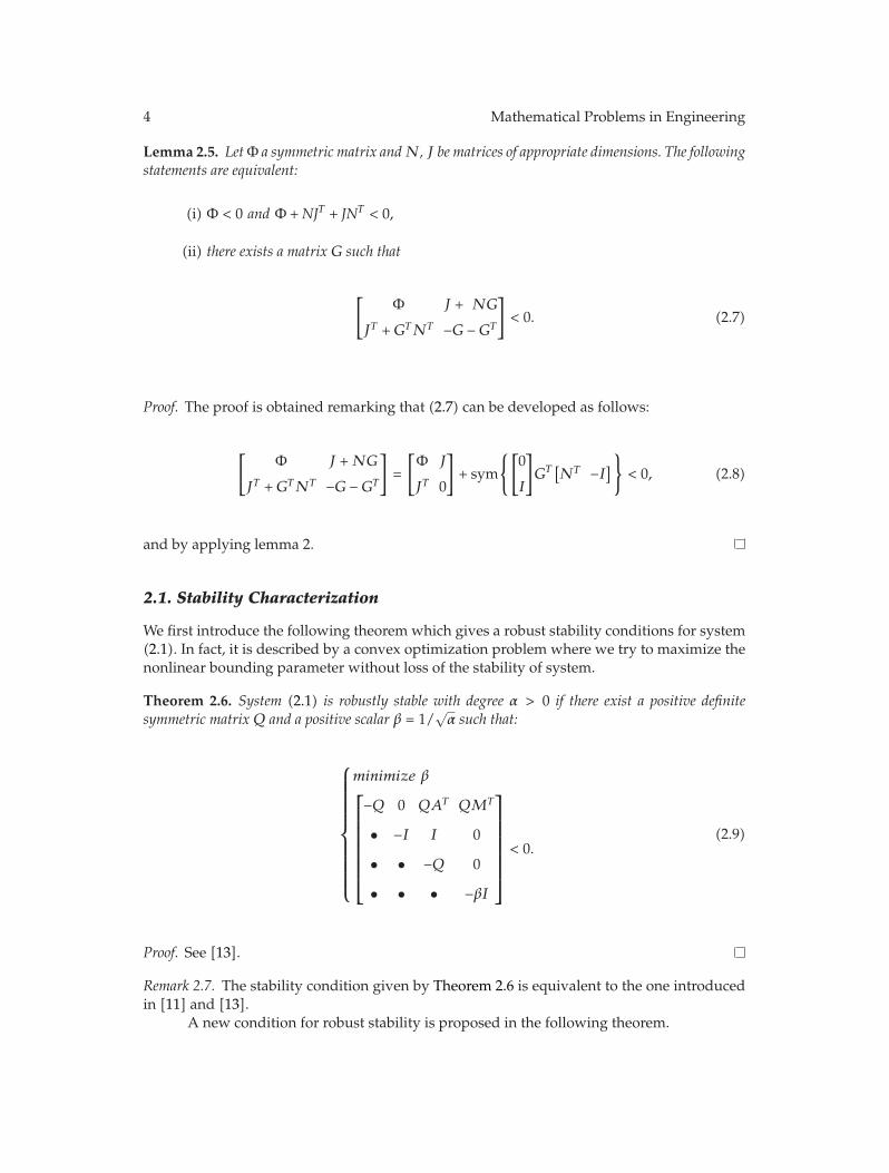
Lemma 2.5. LetΦ a symmetric matrix andN, J be matrices of appropriate dimensions. The followingstatements are equivalent:

(i) Φ < 0 and Φ +NJT + JNT < 0,

(ii) there exists a matrix G such that

[Φ J + NG

JT +GTNT −G −GT

]< 0. (2.7)

Proof. The proof is obtained remarking that (2.7) can be developed as follows:

[Φ J +NG

JT +GTNT −G −GT

]=

[Φ J

JT 0

]+ sym

{[0

I

]GT[NT −I

]}< 0, (2.8)

and by applying lemma 2.

2.1. Stability Characterization

We first introduce the following theorem which gives a robust stability conditions for system(2.1). In fact, it is described by a convex optimization problem where we try to maximize thenonlinear bounding parameter without loss of the stability of system.

Theorem 2.6. System (2.1) is robustly stable with degree α > 0 if there exist a positive definitesymmetric matrix Q and a positive scalar β = 1/

√α such that:

⎧⎪⎪⎪⎪⎪⎪⎪⎪⎪⎪⎨⎪⎪⎪⎪⎪⎪⎪⎪⎪⎪⎩

minimize β⎡⎢⎢⎢⎢⎢⎢⎢⎣

−Q 0 QAT QMT

• −I I 0

• • −Q 0

• • • −βI

⎤⎥⎥⎥⎥⎥⎥⎥⎦< 0.

(2.9)

Proof. See [13].

Remark 2.7. The stability condition given by Theorem 2.6 is equivalent to the one introducedin [11] and [13].

A new condition for robust stability is proposed in the following theorem.


Theorem 2.8. System (2.1) is stable with degree α > 0 if there exist a positive definite symmetricmatrix Q, a matrix G of appropriate dimensions, and a positive scalar β = 1/

√α, such that the

following optimization problem:

⎧⎪⎪⎪⎪⎪⎪⎪⎪⎪⎪⎪⎪⎪⎪⎨⎪⎪⎪⎪⎪⎪⎪⎪⎪⎪⎪⎪⎪⎪⎩

minimize β⎡⎢⎢⎢⎢⎢⎢⎢⎢⎢⎢⎣

−Q 0 μQ 0 Q

• −I I 0 0

• • −Q 0(A − μI

)G

• • • −βI MG

• • • • −G −GT

⎤⎥⎥⎥⎥⎥⎥⎥⎥⎥⎥⎦< 0,

(2.10)

is feasible for any prescribed scalar μ ∈] − 1 1[.

Proof. Inequality (2.9) can be expressed as follows:

⎡⎢⎢⎢⎢⎢⎣

−Q 0 QAT QMT

• −I I 0

• • −Q 0

• • • −βI

⎤⎥⎥⎥⎥⎥⎦ =

⎡⎢⎢⎢⎢⎢⎣

−Q 0 μQ 0

• −I I 0

• • −Q 0

• • • −βI

⎤⎥⎥⎥⎥⎥⎦

︸︷︷︸φ

+ sym

⎛⎜⎜⎜⎜⎜⎜⎜⎜⎝

⎡⎢⎢⎢⎢⎢⎣

0

0

A − μIM

⎤⎥⎥⎥⎥⎥⎦

︸︷︷︸N

[Q 0 0 0

]︸︷︷︸

J

⎞⎟⎟⎟⎟⎟⎟⎟⎟⎠

< 0.

(2.11)

It is not difficult to proof that φ < 0 for any μ ∈] − 1 1[. Now writing:

(i) N =

⎡⎢⎣

0

0

A−μI

M

⎤⎥⎦,

(ii) J = [Q 0 0 0]T ,

and by lemma 2, there exists a matrix G of appropriate dimensions such that inequality issatisfied.

Remark 2.9. The two optimization problems (2.9) and (2.10) are equivalent. In the case ofstability analysis or state feedback control synthesis, no improvement is obtained by problem(2.10). The main advantage of problem (2.10) will appear when dealing with static outputfeedback. In that case, we will see that it theoretically improves the obtained results.

2.2. Static Output Feedback Control

In this section, we investigate the static output feedback stabilization problem for nonlineardiscrete systems.


We consider the nonlinear discrete-time system described as follows:

x(k + 1) = Ax(k) + f(k, x, u) + Bu(k),

y(k) = Cx(k),(2.12)

where u(k) ∈ Rm is the control input, y(k) ∈ Rp is the measured output, and B ∈ Rn×m andC ∈ Rp×n are constant matrices. We assume that the pair (A,B) is stabilizable and C is fullrank matrices. Also f(k, x, u) is a nonlinear function which satisfies the following quadraticconstraints:

fT (k, x, u)f(k, x, u) ≤ α2(xTFTFx + uTHTHu

), (2.13)

where α > 0 is the bounding parameter of the function f and F and H are constant matricesof appropriate dimensions.

The objective is to find a static output feedback control law such as

u(k) = Ky(k), (2.14)

where K ∈ Rm×p.The closed loop system is given by the following state space representation:

x(k + 1) = (A + BKC)x(k) + f(k, x, u), (2.15)

and function f satisfies:

fT (k, x, u)f(k, x, u) ≤ α2xT(FTF + (HKC)THKC

)x. (2.16)

Note that in this case, the constraint (2.16) is equivalent to

[x

f

]T⎡⎣−α2(FTF + (HKC)THKC

)0

0 I

⎤⎦[x

f

]≤ 0. (2.17)

To establish a robust stabilization theory for system (2.12) with (2.13) by SOF, we givein the following theorem, an optimization problem which allows to stabilize the linear partof system (2.15) with (2.17) and at the same time to maximize the value of parameter α.


Theorem 2.10. System (2.12) is asymptotically stable by static output feedback with degree α > 0 ifthere exist a positive definite symmetric matrix Q, a matrix R∈m×p, and a positive scalar β = 1/

√α

such that the following optimization problem is solvable:

⎧⎪⎪⎪⎪⎪⎪⎪⎪⎪⎪⎪⎪⎪⎪⎨⎪⎪⎪⎪⎪⎪⎪⎪⎪⎪⎪⎪⎪⎪⎩


−Q 0 (AQ + BRC)T QFT (HRC)T

• −I I 0 0

• • −Q 0 0

• • • −βI 0

• • • • −βI

⎤⎥⎥⎥⎥⎥⎥⎥⎥⎥⎥⎦< 0,

(2.18)

where

Q = V

[Q1 0

0 Q2

]V T . (2.19)

The static output feedback gain is given by

K = RUC0Q−11 C−1

0 UT, (2.20)

with U ∈ Rp×p and V ∈ Rn×n are unitary matrices, and C0 ∈ Rp×p matrix which are obtained byusing the singular value decomposition of the matrix C:

C = U[C0 0

]V T . (2.21)

Proof. According to the Theorem 2.6, system (2.15) is robustly stable if there exist a positivedefinite symmetric matrix Q and a positive scalar β = 1/

√α such that the following

optimization problem is solvable:

⎧⎪⎪⎪⎪⎪⎪⎪⎪⎪⎪⎨⎪⎪⎪⎪⎪⎪⎪⎪⎪⎪⎩

minimize β⎡⎢⎢⎢⎢⎢⎢⎢⎣

−Q 0 QAT QMT

• −I I 0

• • −Q 0

• • • −βI

⎤⎥⎥⎥⎥⎥⎥⎥⎦< 0.

(2.22)


Now we defin

(i) A = A + BKC,

(ii) M = ( F

HKC),

(iii) Q is replaced by (2.19) with: Q1 ∈ Rp×p, Q2 ∈ R(n−p)×(n−p).

Equation (2.22) becomes:

⎧⎪⎪⎪⎪⎪⎪⎪⎪⎪⎪⎪⎪⎪⎪⎨⎪⎪⎪⎪⎪⎪⎪⎪⎪⎪⎪⎪⎪⎪⎩


−Q 0 Q(A + BKC)T QFT QCTKTHT

• −I I 0 0

• • −Q 0 0

• • • −βI 0

• • • • −βI

⎤⎥⎥⎥⎥⎥⎥⎥⎥⎥⎥⎦< 0.

(2.23)

Unfortunately, (2.23) is not convex in K and Q and cannot be solved by the LMI tools. We canintroduce some transformations to simplify the KCQ term of the inequality (2.23) by using(2.19) and (2.21) as follows:

KCQ = KU[C0 0

]V TV

[Q1 0

0 Q2

]V T

= KUC0Q1C−10 U−1︸︷︷︸

R

U[C0 0

]V T︸︷︷︸,

C

(2.24)

where R ∈ Rm×p.With this transformation we obtain the optimization problem given in Theorem 2.10.

Remark 2.11. The optimization problem given by Theorem 2.10 presents a sufficient conditionfor the robust stabilization by SOF of discrete-time nonlinear system (2.12). In fact to solvethe BMI problem, we impose a diagonal structure to Lyapunov matrix Q as in [24] and weobtain a LMI convex problem.

2.3. Main Results

In this section, we introduce a new approach for robust stabilization by SOF of nonlineardiscrete time system (2.12). The following results present solutions to static output feedbackproblem in which an improved sufficient condition is presented. In fact, this approach isderived from Theorem 2.8.

Theorem 2.12. The system (2.12) is robustly stable by static output feedback with degree α > 0, foran arbitrary prescribed number μ in ] − 1 1[ if there exist a positive definite symmetric matrix Q,


matrices R ∈ Rm×p, G ∈ Rn×n, and a positive scalar β = 1/√α such that the following optimization

problem is solvable:

⎧⎪⎪⎪⎪⎪⎪⎪⎪⎪⎪⎪⎪⎪⎪⎪⎪⎪⎨⎪⎪⎪⎪⎪⎪⎪⎪⎪⎪⎪⎪⎪⎪⎪⎪⎪⎩

minimize β⎡⎢⎢⎢⎢⎢⎢⎢⎢⎢⎢⎢⎢⎢⎢⎣

−Q 0 μQ 0 0 Q

• −I I 0 0 0

• • −Q 0 0 AG + BRC − μG

• • • −βI 0 FG

• • • • −βI HRC

• • • • • −G −GT

⎤⎥⎥⎥⎥⎥⎥⎥⎥⎥⎥⎥⎥⎥⎥⎦

< 0,(2.25)

where

G = V

[G1 0

G2 G3

]V T . (2.26)


K = RUC0G−11 C−1

0 UT, (2.27)

withU,V , and C0 are given in (2.21).

Proof. According to Theorem 2.8, the closed loop system (2.15) is robustly stable if there exista positive definite symmetric matrix Q, a matrix G of appropriate dimensions, and a positivescalar β = 1/

√α such that

⎧⎪⎪⎪⎪⎪⎪⎪⎪⎪⎪⎪⎪⎪⎪⎨⎪⎪⎪⎪⎪⎪⎪⎪⎪⎪⎪⎪⎪⎪⎩


−Q 0 μQ 0 Q

• −I I 0 0

• • −Q 0(A − μI

)G

• • • −βI MG

• • • • −G −GT

⎤⎥⎥⎥⎥⎥⎥⎥⎥⎥⎥⎦< 0,

(2.28)

where the following hold:

(i) A = A + BKC,

(ii) M = ( F

HKC),

(iii) G replaced by (2.26) where G1 ∈ Rp×p, G2 ∈ R(n−p)×p, G3 ∈ R(n−p)×(n−p),

with U,V , and C0 are given by (2.21).


Then, inequality (2.28) becomes

⎡⎢⎢⎢⎢⎢⎢⎢⎢⎢⎢⎢⎣

−Q 0 μQ 0 0 Q

• −I I 0 0 0

• • −Q 0 0 AG + BKCG − μG• • • −βI 0 FG

• • • • −βI HKCG

• • • • • −G −GT

⎤⎥⎥⎥⎥⎥⎥⎥⎥⎥⎥⎥⎦< 0. (2.29)

Unfortunately, (2.29) is not convex and cannot be solved by the LMI tools.For this reason, we introduce some transformations to simplify the KCG term of the

inequality (2.29) by using (2.26) and (2.21) as follows:

KCG = KU[C0 0

]V TV

[G1 0

G2 G3

]V T

= KUC0G1C−10 U−1︸︷︷︸

R

U[C0 0

]V T︸︷︷︸

C

, (2.30)

where R ∈ Rm×p.With this transformation, we obtain the optimization problem given by Theorem 2.12.

The following lemma gives a connection of the results of Theorem 2.10 with the one ofTheorem 2.12.

Lemma 2.13. If the SOF stabilization problem is solvable by Theorem 2.10, then it is solvable byTheorem 2.12.

Proof. If we consider the optimization problem (2.25) with G = Q and μ = 0, we obtainthe optimization problem (2.18) with Q satisfying (2.19). Therefore, if (2.25) is feasible, then(2.19) is feasible too.

3. Nonlinear Discrete-Time H∞ Norm Characterization

Stability is the minimum requirement and in practice a performance level has to beguaranteed. Performance objectives can be achieved via H∞ norm optimization. In thissection, we study the H∞ control problem for the following nonlinear discrete-time system:

x(k + 1) = Ax(k) + Bw(k) + f(k, x),

z(k) = Cx(k) +Dw(k),(3.1)


where w(k) ∈ Rq is the exogenous disturbance and z(k) ∈ Rr is the controlled output.A,B,C, and D are known constant matrices of appropriate dimensions. f(k, x) is a nonlinearfunction satisfying the following quadratic constraints:

⎡⎢⎢⎣x

w

f

⎤⎥⎥⎦

T⎡⎢⎢⎣−α2MTM 0 0

0 0 0

0 0 I

⎤⎥⎥⎦⎡⎢⎢⎣x

w

f

⎤⎥⎥⎦ ≤ 0. (3.2)

We note Twz the transfer matrix from inputw to output zwhen f(k, x) = 0 is expressedby

Twz = C(sI −A)−1B +D. (3.3)

Theorem 3.1. System (3.1) is robustly stable with ‖Twz‖∞ < γ for a prescribed constant value γ > 0,if there exist a positive definite symmetric matrix Q and positive scalars τ > 0 and β = 1/

√α such

that the following optimization problem is feasible:

⎧⎪⎪⎪⎪⎪⎪⎪⎪⎪⎪⎪⎪⎪⎪⎪⎪⎪⎨⎪⎪⎪⎪⎪⎪⎪⎪⎪⎪⎪⎪⎪⎪⎪⎪⎪⎩

min β⎡⎢⎢⎢⎢⎢⎢⎢⎢⎢⎢⎢⎢⎢⎢⎣

−Q 0 0 QAT QMT QCT

• −τγ2I 0 τBT 0 τDT

• • −I I 0 0

• • • −Q 0 0

• • • • −βI 0

• • • • • −τI

⎤⎥⎥⎥⎥⎥⎥⎥⎥⎥⎥⎥⎥⎥⎥⎦

< 0.(3.4)

Proof. Define the Lyapunov function:

V (x) = xT (k)Px(k), (3.5)

where P = PT > 0.By using the dissipative theory, we show that

V (k + 1) − V (k) + zT (k)z(k) − γ2wT (k)w(k) < 0, (3.6)

where γ > 0 is a prescribed scalar such that

‖Twz‖∞ < γ∞ < γ, (3.7)

where γ∞ is the corresponding bounding norm bound when f = 0.


Evaluating (3.6) leads to

⎡⎢⎢⎣xT

wT

fT

⎤⎥⎥⎦⎡⎢⎢⎣ATPA − P + CTC ATPB + CTD ATP

BTPA +DTC BTPB +DTD − γ2I BTP

PA PB P

⎤⎥⎥⎦⎡⎢⎢⎣xT

wT

fT

⎤⎥⎥⎦T

< 0. (3.8)

Now applying the S-procedure Lemma to (3.8) with (3.2), there exits τ > 0 such that

⎡⎢⎢⎣ATPA − P + τ−1CTC + α2MTM ATPB + τ−1CTD ATP

BT PA + τ−1DTC BTPB + τ−1DTD − τ−1γ2I BT P

PA PB P − I

⎤⎥⎥⎦ < 0, (3.9)

where P = P/τ .By Schur complement, (3.9) is equivalent to

⎡⎢⎢⎢⎢⎢⎢⎢⎢⎢⎢⎢⎣

−P 0 0 AT MT CT

• −τ−1γ2I 0 BT 0 DT

• • −I I 0 0

• • • −P−1 0 0

• • • • −βI 0

• • • • • −τI

⎤⎥⎥⎥⎥⎥⎥⎥⎥⎥⎥⎥⎦< 0, (3.10)

where β = α−2.Multiplying by diag(Q, τ, I, I, I) with Q = P−1 the both sides of (3.10), we obtain the

optimization problem (3.4).

Now, we introduce the following theorem which can be seen as an alternatecharacterization of upper bounds of the H∞ norm of.

Theorem 3.2. System (3.1) is robustly stable with ‖Twz‖∞ < γ for a prescribed constant value γ > 0,if there exist a positive definite symmetric matrixQ, a matrixG of appropriate dimensions, and positive


scalars τ > 0 and β = 1/√α such that for any prescribed scalar μ in ] −1 1 [ , the following optimization

problem is feasible:

⎧⎪⎪⎪⎪⎪⎪⎪⎪⎪⎪⎪⎪⎪⎪⎪⎪⎪⎪⎪⎪⎪⎨⎪⎪⎪⎪⎪⎪⎪⎪⎪⎪⎪⎪⎪⎪⎪⎪⎪⎪⎪⎪⎪⎩

min β⎡⎢⎢⎢⎢⎢⎢⎢⎢⎢⎢⎢⎢⎢⎢⎢⎢⎢⎣

−Q 0 0 μQ 0 0 Q

• −τγ2I 0 τBT 0 τDT 0

• • −I I 0 0 0

• • • −Q 0 0(A − μI

)G

• • • • −βI 0 MG

• • • • • −τI CG

• • • • • • −G −GT

⎤⎥⎥⎥⎥⎥⎥⎥⎥⎥⎥⎥⎥⎥⎥⎥⎥⎥⎦

< 0.(3.11)

Proof. Inequality (3.4) can be written as follows:

⎡⎢⎢⎢⎢⎢⎢⎢⎢⎢⎢⎢⎣

−Q 0 0 QAT QMT QCT


• • −I I 0 0

• • • −Q 0 0

• • • • −βI 0

• • • • • −τI

⎤⎥⎥⎥⎥⎥⎥⎥⎥⎥⎥⎥⎦

=

⎡⎢⎢⎢⎢⎢⎢⎢⎢⎢⎢⎢⎣

−Q 0 0 μQ 0 0


• • −I I 0 0

• • • −Q 0 0

• • • • −βI 0

• • • • • −τI

⎤⎥⎥⎥⎥⎥⎥⎥⎥⎥⎥⎥⎦

+ sym

⎛⎜⎜⎜⎜⎜⎜⎜⎜⎜⎜⎜⎝

⎡⎢⎢⎢⎢⎢⎢⎢⎢⎢⎢⎢⎣

0

0

0

A − μIM

C

⎤⎥⎥⎥⎥⎥⎥⎥⎥⎥⎥⎥⎦

[Q 0 0 0 0 0

]

⎞⎟⎟⎟⎟⎟⎟⎟⎟⎟⎟⎟⎠

< 0.

(3.12)

By lemma 2, denoting

φ =

⎡⎢⎢⎢⎢⎢⎢⎢⎢⎢⎢⎢⎣

−Q 0 0 μQ 0 0


• • −I I 0 0

• • • −Q 0 0

• • • • −βI 0

• • • • • −τI

⎤⎥⎥⎥⎥⎥⎥⎥⎥⎥⎥⎥⎦< 0, for any μ ∈

]−1 1

[


N =

⎡⎢⎢⎢⎢⎢⎢⎢⎢⎢⎢⎢⎣

0

0

0

A − μIM

C

⎤⎥⎥⎥⎥⎥⎥⎥⎥⎥⎥⎥⎦, J =

[Q 0 0 0 0 0

],

(3.13)

there exists a matrix G of appropriate dimensions such that (3.11) holds where γ, β, and τ arescalars previously defined.

3.1. Static Output Feedback H∞ Synthesis

In this section, we consider the static output feedback stabilization problem for the followingnonlinear discrete system (3.14):

x(k + 1) = Ax(k) + Buu(k) + Bww(k) + f(k, x, u),

z(k) = Czx(k) +Dzuu(k) +Dzww(k),

y(k) = Cyx(k),

(3.14)

where u(k) ∈ Rm is the control input, w(k) ∈ Rq is the exogenous disturbance, z(k) ∈ Rr isthe controlled output, and y(k) ∈ Rp is the measured output. Also, Bu, Bw,Cz,Dzu,Dzw andCy are known constant matrices of appropriate dimensions.

The system closed by SOF is written as

x(k + 1) = Aclx(k) + Bclw(k) + f(k, x, u),

z(k) = Cclx(k) +Dclw(k),(3.15)

where the following hold:

Acl = A + BuKCy,

Bcl = Bw,

Ccl = Cz +DzuKCy,

Dcl = Dzw.

(3.16)

The objective of this section is to design static output feedback H∞ controllers fornonlinear discrete time system (3.14).

Theorem 3.3. System (3.14) is robustly static output feedback stabilizable with ‖Twz‖∞ < γ for aprescribed constant value γ > 0 if there exist a positive definite symmetric matrix Q, a matrix R of


appropriate dimensions, and positive scalars τ > 0 and β = 1/√α such that the following optimization

problem is feasible:

⎧⎪⎪⎪⎪⎪⎪⎪⎪⎪⎪⎪⎪⎪⎪⎪⎪⎪⎪⎪⎪⎪⎨⎪⎪⎪⎪⎪⎪⎪⎪⎪⎪⎪⎪⎪⎪⎪⎪⎪⎪⎪⎪⎪⎩

min β⎡⎢⎢⎢⎢⎢⎢⎢⎢⎢⎢⎢⎢⎢⎢⎢⎢⎢⎣

−Q 0 0 QAT + (BuRCy)T QFT (HRCy)

T QCTz + (DzuRCy)

T

• −τγ2I 0 τBTw 0 0 τDTzw

• • −I I 0 0 0

• • • −Q 0 0 0

• • • • −βI 0 0

• • • • • −βI 0

• • • • • • −τI

⎤⎥⎥⎥⎥⎥⎥⎥⎥⎥⎥⎥⎥⎥⎥⎥⎥⎥⎦

< 0,(3.17)

where

Q = V

[Q1 0

0 Q2

]V T . (3.18)

The static output feedback gain is then given by

K = RUC0Q−11 C−1

0 UT, (3.19)

whereU,V , and C0 are given in (2.21).

Proof. According to Theorem 3.1, system (3.14) is robustly stable with ‖Twz‖∞ < γ for aprescribed constant value γ > 0 if there exist a positive definite symmetric matrix Q andpositive scalars τ > 0 and β = 1/

√α such that the following optimization problem is feasible:

⎧⎪⎪⎪⎪⎪⎪⎪⎪⎪⎪⎪⎪⎪⎪⎪⎪⎪⎨⎪⎪⎪⎪⎪⎪⎪⎪⎪⎪⎪⎪⎪⎪⎪⎪⎪⎩

min β⎡⎢⎢⎢⎢⎢⎢⎢⎢⎢⎢⎢⎢⎢⎢⎣

−Q 0 0 QATclQMT QCT

cl

• −τγ2I 0 τBTcl

0 τDTcl

• • −I I 0 0

• • • −Q 0 0

• • • • −βI 0

• • • • • −τI

⎤⎥⎥⎥⎥⎥⎥⎥⎥⎥⎥⎥⎥⎥⎥⎦

< 0.(3.20)


Now:

(i) Acl, Bcl, Ccl and Dcl are replaced by (3.16),

(ii) M = (F

HKCy),

(iii) Q is replaced by (3.18) where : Q1 ∈ Rp×p, Q2 ∈ R(n−p)×(n−p).

After same direct developments the result follows.

3.2. An Improved Approach of Static Output Feedback Synthesis for H∞Robust Control

In this paragraph, an H∞ robust control for nonlinear systems (3.14) improving the previousapproach is proposed.

Theorem 3.4. System (3.14) is robustly SOF stabilisable with ‖Twz‖∞ < γ for a prescribed constantvalue γ > 0 if there exist a positive definite symmetric matrix Q, matrices G and R of appropriatedimensions, and positive scalars τ > 0, and β = 1/

√α such that the following optimization problem

is feasible for any prescribed scalar μ in ] − 1 1[:

⎡⎢⎢⎢⎢⎢⎢⎢⎢⎢⎢⎢⎢⎢⎢⎢⎢⎢⎣

−Q 0 0 μQ 0 0 0 Q

• −τγ2I 0 τBTw 0 0 τDTzw 0

• • −I I 0 0 0 0

• • • −Q 0 0 0 AG − μG + BuRCy

• • • • −βI 0 0 FG

• • • • • −βI 0 HRCy

• • • • • • −τI CzG +DzuRCy

• • • • • • • −G −GT

⎤⎥⎥⎥⎥⎥⎥⎥⎥⎥⎥⎥⎥⎥⎥⎥⎥⎥⎦

< 0, (3.21)

where

G = V

[G1 0

G2 G3

]V T . (3.22)


K = RUC0G−11 C−1

0 UT, (3.23)

with R ∈ Rm×p,U,V, and C0 are given in (2.21).

Proof. According to the Theorem 3.3, the system (3.14) is robustly stable with ‖Twz‖∞ < γ fora prescribed degree γ > 0 if there exist a positive definite symmetric matrix Q, a matrix G of


appropriate dimensions, and positive scalars τ > 0 and β = 1/√α, for any prescribed scalar μ

in ] − 1 1[, such that the following optimization problem is feasible:

⎧⎪⎪⎪⎪⎪⎪⎪⎪⎪⎪⎪⎪⎪⎪⎪⎪⎪⎪⎪⎪⎪⎨⎪⎪⎪⎪⎪⎪⎪⎪⎪⎪⎪⎪⎪⎪⎪⎪⎪⎪⎪⎪⎪⎩

min β⎡⎢⎢⎢⎢⎢⎢⎢⎢⎢⎢⎢⎢⎢⎢⎢⎢⎢⎣

−Q 0 0 μQ 0 0 Q

• −τγ2I 0 τBTcl

0 τDTcl

0

• • −I I 0 0 0

• • • −Q 0 0(Acl − μI

)G

• • • • −βI 0 MG

• • • • • −τI CclG

• • • • • • −G −GT

⎤⎥⎥⎥⎥⎥⎥⎥⎥⎥⎥⎥⎥⎥⎥⎥⎥⎥⎦

< 0,(3.24)

where

(i) Acl, Bcl, Ccl, and Dcl are replaced by (3.16),

(ii) M = (F

HKCy),

(iii) G replaced by (3.22), where G1 ∈ Rp×p, G2 ∈ R(n−p)×p.

The optimization problem (3.24) is expressed as follows:

⎧⎪⎪⎪⎪⎪⎪⎪⎪⎪⎪⎪⎪⎪⎪⎪⎪⎪⎪⎪⎪⎪⎪⎪⎪⎨⎪⎪⎪⎪⎪⎪⎪⎪⎪⎪⎪⎪⎪⎪⎪⎪⎪⎪⎪⎪⎪⎪⎪⎪⎩

min β < 0⎡⎢⎢⎢⎢⎢⎢⎢⎢⎢⎢⎢⎢⎢⎢⎢⎢⎢⎢⎢⎢⎢⎣

−Q 0 0 μQ 0 0 0 Q

• −τγ2I 0 τBTw 0 0 τDTzw 0

• • −I I 0 0 0 0

• • • −Q 0 0 0 AG + BuKCyG − μG

• • • • −βI 0 0 FG

• • • • • −βI 0 HKCyG

• • • • • • −τI CzG +DzuKCy

• • • • • • • −G −GT

⎤⎥⎥⎥⎥⎥⎥⎥⎥⎥⎥⎥⎥⎥⎥⎥⎥⎥⎥⎥⎥⎥⎦

< 0.(3.25)

For this reason, we express differently the KCyG term of the inequality (3.25), by using (3.22)and (2.21), in the same way as in (2.30). Consequently, we obtain

KCyG = RCy. (3.26)

With this transformation, we obtain the optimization problem given in Theorem 3.4.


T

θ

l

m

Figure 1: Inverted pendulum scheme.

4. Numerical Examples

We present in this section two numerical examples to illustrate the proposed theory for SOFsynthesis.

Our approach Theorem 2.12 is compared to the methods presented in [11].

Example 4.1 (see [5]). We consider the nonlinear discrete-time system of inverted pendulum(see Figure 1).

The system can be described by

x(k + 1) = Ax(k) + B(u(k) + α siny(t)

),

y(k) = Cx(k),(4.1)

where x(k) = [x1(k) x2(k)]T , x1(k) and x2(k) being, respectively, the angular displacement

and velocity; u(k) represents the field current of the DC motor; the matrices A ∈ R2×2, B ∈R2×1, and C ∈ R1×2are given by:

A =

[1 0.0952

0 0.9048

]; B =

[0.048

0.952

]; C =

[1 0

]. (4.2)

The nonlinear function f is given by the following expression:

f(k, x) = αB siny (k) = αB sin x1(k). (4.3)

This function satisfies

fT (k, x)f(k, x) = α2BTB sin2x1(k)

= 0.9α2 sin2x1(k)

≤ α2xT[

0.95 0

0 0

][0.95 0

0 0

]x.

(4.4)

In this case, we take F = [ 0.95 0

0 0]; H = 0.


Table 1: Numerical Evaluation for Example 4.1.

Approach αmax K

Theorem 2.10 condition 0.8254 · 10−4 −1.9987Theorem 2.12 condition for μ = 0.7 0.06688 −0.3101

Output y

40003500300025002000150010005000

Sample

−5

−4

−3

−2

−1

0

1

2

3

4

5y=x

1

Figure 2: Output y = x1.

The nonlinear system is unstable. The matrixA is unstable which means that the linearpart of systems is unstable. Therefore, we apply the approach given by Theorems 2.10 and2.12 to stabilize system by SOF. We summarize in Table 1 the obtained results.

Figures 2 and 3 show the output trajectory obtained respectively by applyingTheorems 2.10 and 2.12 to system (3.26) with α = αmax.

We can see a drastic improvement obtained by Theorem 2.12.

Example 4.2. We consider now the nonlinear discrete-time system:

x(k + 1) =

⎡⎢⎢⎣−0.0725 0.1957 1.5931

0.0301 0.0404 0.6084

0.3764 −0.1635 0.9024

⎤⎥⎥⎦x(k) +

⎡⎢⎢⎣

1.2123 0.2895

0.6174 0.0651

0.9379 0.5110

⎤⎥⎥⎦u(k) + f(k, x(k), u(k)),

y(k) =

[0.9313 −0.7534 −0.0335

1 2 0.5

]x(k),

(4.5)

with the nonlinear function f satisfying the constraint (2.17), where F = I3 and H = I2. Theresults obtained byapproaches of Theorem 2.12 and in [11] are given in Table 2.

The new approach (Theorem 2.12) improves the results obtained by [11].


Output y

200150100500

Sample

−0.4

−0.2

0

0.2

0.4

0.6

0.8

1

1.2

y=x

1

Figure 3: Output y = x1.

Table 2: Numerical Evaluation for Example 4.2.

Approach αmax K

[11] 0.1954[ −0.1329 −0.1268

−0.4309 −0.0405

]New approach, (2.25), Theorem 2.12 for μ = 0 0.3084

[ −0.0019 −0.2766

−1.1542 0.1067

]New approach, (2.25), Theorem 2.12 for μ = −0.35 0.3329

[ 0.0357 −0.3141

−0.9812 0.0924

]

Example 4.3. We consider the nonlinear discrete-time system (3.14) with

A =

⎡⎢⎢⎢⎢⎢⎣

0.8189 0.0863 0.0900 0.0813

0.2524 1.0033 0.0313 0.2004

−0.0545 0.0102 0.7901 −0.2580

−0.1918 −0.1034 0.1602 0.8604

⎤⎥⎥⎥⎥⎥⎦, Bu=

⎡⎢⎢⎢⎢⎢⎣

0.0045 0.0044

0.1001 0.0100

0.0003 −0.0136

−0.0051 0.0926

⎤⎥⎥⎥⎥⎥⎦, Bw=

⎡⎢⎢⎢⎢⎢⎣

0.0953 0 0

0.0145 0 0

0.0862 0 0

−0.0011 0 0

⎤⎥⎥⎥⎥⎥⎦,

Cz =

⎡⎢⎢⎣

1 0 −1 0

0 0 0 0

0 0 0 0

⎤⎥⎥⎦, Dzu =

⎡⎢⎢⎣

0 0

1 0

0 1

⎤⎥⎥⎦, Cy =

[1 0 0 0

0 0 1 0

], Dyw =0,

(4.6)

with the nonlinear function f satisfying the constraint (3.2), where F = I4 and H = I4.In Table 3, we present numerical result for H∞ performance via SOF by applying

Theorem 3.3 and for different values of γ which satisfy (3.7).In Table 4, we present numerical result for H∞ performance via SOF by applying

Theorem 3.4 and for different values of γ which satisfy (3.7).


Table 3: Numerical Evaluation for Example4.3 by Theorem 3.3.

Approach αmax K

Approach, (3.17), Theorem 3.3 for γ∞ = 1.9918, γ = 2.2361 0.0032[ −2.0416 −0.1796

0.6545 −1.0362

]Approach, (3.17), Theorem 3.3 for γ∞ = 1.9918, γ = 5 0.0288

[ −2.1323 −0.0808

1.1624 −1.2381

]

Table 4: Numerical Evaluation for Example 4.3 by Theorem 3.4.

Approach αmax K

Approach, (3.21), Theorem 3.4 for γ∞ = 1.9918, γ = 2.2361, μ = 0.22 0.3643[ −0.2993 −0.1328

−0.0685 −0.0743

]Approach, (3.21), Theorem 3.4 for γ∞ = 1.9918, γ = 5, μ = 0.2400 0.4087

[ −0.3376 −0.1185

−0.0660 −0.0737

]

5. Conclusion

In this paper, the stabilization problem by static output feedback (SOF) for a particular classof nonlinear discrete time systems is investigated. A new sufficient condition is elaborated byusing Lyapunov theory and formulated by LMI constraints. We obtain a convex optimizationproblem for maximizing the bound of the nonlinearity preserving the stability of the systems.

Finally, the proposed controller design method was extended to incorporate H∞synthesis. An optimization problem, which is linear both in the admissible nonlinearitybound and the disturbance attenuation, is developed. Numerical comparisons with existingmethods in literature illustrate the improvement obtained by our approaches. All of them canalso be extended to the dynamic output feedback.

Other classes of nonlinear discrete time nonlinear systems exist and present someinteresting characteristic from a practical point of view. For example, the ones where the linearpart is affected by polytopic uncertainties. It would be interesting to extend the results of thispaper to those classes. This will be exploited in a near future.

References

[1] S. Boyd, L. El Ghaoui, E. Feron, and V. Balakrishnan, Linear Matrix Inequalities in System and ControlTheory, vol. 15 of SIAM Studies in Applied Mathematics, SIAM, Philadelphia, Pa, USA, 1994.

[2] G. Garcia, J. Bernussou, and D. Arzelier, “Robust stabilization of discrete-time linear systems withnorm-bounded time-varying uncertainty,” Systems & Control Letters, vol. 22, no. 5, pp. 327–339, 1994.

[3] W. M. Haddad and D. S. Bernstein, “Parameter-dependent Lyapunov functions and the Popovcriterion in robust analysis and synthesis,” IEEE Transactions on Automatic Control, vol. 40, no. 3, pp.536–543, 1995.

[4] E. Fridman, “Robust sampled-data control of linear singulary perturbed systems,” in Proceedings ofthe 44th IEEE Conference on decision and Control, and the European Control Conference, pp. 4324–4329,Seville, Spain, December 2005.

[5] M. S. Mahmoud and L. Xie, “Positive real analysis and synthesis of uncertain discrete time systems,”IEEE Transactions on Automatic Control, vol. 47, no. 3, pp. 403–406, 2000.

[6] A. A. Bahnasawi, A. S. Al-Fuhaid, and M. S. Mahmoud, “Linear feedback approach to the stabilisationof uncertain discrete systems,” IEE Proceedings D, vol. 136, no. 1, pp. 47–52, 1989.


[7] K. Galkowski, E. Rogers, S. Xu, J. Lam, and D. H. Owens, “LMIs-a fundamental tool in analysis andcontroller design for discrete linear repetitive processes,” IEEE Transactions on Circuits and Systems I,vol. 49, no. 6, pp. 768–778, 2002.

[8] S. Xu and J. Lam, “New positive realness conditions for uncertain discrete descriptor systems: analysisand synthesis,” IEEE Transactions on Circuits and Systems I, vol. 51, no. 9, pp. 1897–1905, 2004.

[9] D. M. Stipanovic and D. D. Siljak, “Robust stability and stabilization of discrete-time non-linearsystems: the LMI approach,” International Journal of Control, vol. 74, no. 9, pp. 873–879, 2001.

[10] D. D. Siljak and D. M. Stipanovic, “Robust stabilization of nonlinear systems: the LMI approach,”Mathematical Problems in Engineering, vol. 6, no. 5, pp. 461–493, 2000.

[11] D. W. C. Ho and G. Lu, “Robust stabilization for a class of discrete-time non-linear systems via outputfeedback: the unified LMI approach,” International Journal of Control, vol. 76, no. 2, pp. 105–115, 2003.

[12] G. Lu and D. W. C. Ho, “Generalized quadratic stability for continuous-time singular systems withnonlinear perturbation,” IEEE Transactions on Automatic Control, vol. 51, no. 5, pp. 818–823, 2006.

[13] Z. Zuo, J. Wang, and L. Huang, “Robust stabilization for non-linear discrete-time systems,”International Journal of Control, vol. 77, no. 4, pp. 384–388, 2004.

[14] S. S. Stankovic, D. M. Stipanovic, and D. D. Siljak, “Decentralized dynamic output feedback for robuststabilization of a class of nonlinear interconnected systems,” Automatica, vol. 43, no. 5, pp. 861–867,2007.

[15] N. Bedioui, S. Salhi, and M. Ksouri, “An improved LMI approach for robust static output feedbackstabilization of nonlinear systems,” in Proceedings of the 5th IEEE International Multi-Conference onSystems, Signals and Devices (SSD ’08), pp. 1–6, Amman, Jordan, July 2008.

[16] M. Abbaszadeh and H. J. Marquez, “Robust static ouput feedback dtabilization of discrete timenonlinear uncertain systems withH∞ performance,” in Proceedings of the 16thMeditteranean Conferenceon Control and Automation, Congress, pp. 226–231, Ajaccio, France, June 2008.

[17] S. Cauet, L. Rambault, and O. Bachelier, “Parameter-dependent Lyapunov stability analysis:application to an induction motor,” in Proceedings of the American Control Conference (ACC ’01), vol.1, pp. 160–165, Arlington, Va, USA, June 2001.

[18] M. Abbaszadeh and H. J. Marquez, “Robust H∞ observer design for a class of nonlinear uncertainsystems via convex optimization,” in Proceedings of the American Control Conference (ACC ’07), pp.1699–1704, New York, NY, USA, July 2007.

[19] S.-W. Kau, Y.-S. Liu, L. Hong, C.-H. Lee, C.-H. Fang, and L. Lee, “A new LMI condition for robuststability of discrete-time uncertain systems,” Systems & Control Letters, vol. 54, no. 12, pp. 1195–1203,2005.

[20] O. Toker and H. Ozbay, “On the NP-hardness of solving bilinear matrix inequalities and simultaneousstabilization with static output feedback,” in Proceedings of the American Control Conference (ACC ’95),pp. 2525–2526, Seattle, Wash, USA, June 1995.

[21] M. C. de Oliveira, J. C. Geromel, and J. Bernussou, “ExtendedH2 and H∞ norm characterizations andcontroller parametrizations for discrete-time systems,” International Journal of Control, vol. 75, no. 9,pp. 666–679, 2002.

[22] D. Mehdi, E. K. Boukas, and O. Bachelier, “Static output feedback design for uncertain linear discretetime systems,” IMA Journal of Mathematical Control and Information, vol. 21, no. 1, pp. 1–13, 2004.

[23] M. C. de Oliveira, J. C. Geromel, and J. Bernussou, “LMI optimization approach to multiobjectivecontroller design for discrete-time systems,” in Proceedings of the 38th IEEE Conference on Decision andControl (CDC ’99), vol. 4, pp. 3611–3616, Phoenix, Ariz, USA, December 1999.

[24] C. A. R. Crusius and A. Trofino, “Sufficient LMI conditions for output feedback control problems,”IEEE Transactions on Automatic Control, vol. 44, no. 5, pp. 1053–1057, 1999.

Robust Stabilization Approach and H∞ Performance via Static Output Feedback for a Class of...

Documents

Transcript of Robust Stabilization Approach and H∞ Performance via Static Output Feedback for a Class of...