REZGUI-2013 01

Open Journal of Metal, 2013, 3, 7-18 doi:10.4236/ojmetal.2013.32002 Published Online June 2013 (http://www.scirp.org/journal/ojmetal)

Predictive Models for the Ultimate Tensile and Yield Stresses Occurring in Joints of Untreated Friction Stir

Welded 2017AA (ENAW-AlCu4MgSi) Plates

Mohamed-Ali Rezgui1, Ali-Chedli Trabelsi2, Hassen Bouzaiene2, Mahfoudh Ayadi3 1Department of Mechanical Engineering, Taibah University, College of Engineering, Yanbu, Saudi Arabia

2UR-MSSDT (99-UR11-46), Tunis National Higher School of Engineering, University of Tunis, ENSIT, Tunisia 3Department of Mechanical Engineering, University of Carthage, National Engineering School of Bizerte ENIB, Bizerte, Tunisia

Email: [email protected], [email protected], [email protected], [email protected]

Received April 26, 2013; revised May 27, 2013; accepted June 3, 2013

Copyright © 2013 Mohamed-Ali Rezgui et al. This is an open access article distributed under the Creative Commons Attribution License, which permits unrestricted use, distribution, and reproduction in any medium, provided the original work is properly cited.

ABSTRACT

Friction Stir Welding (FSW) processes have been applied in numerous industrial fields and broadly embraced by the research community. In this paper, given three FSW process parameters, namely, the tool rotation speed N (rpm), the tool traverse feed F(mm/min) and the tool pin/shoulder diameters ratio (r%), we purpose to ascertain their impact on joints Ultimate Tensile Stress (UTS) and joints Yield Stress (YS). The FSW has been executed using 6 mm thick rolled plate in 2017AA. For the design of experiments strategy, we conducted a face centered central composite strategy through which 18 trials have been executed. Then, we utilized the RSM technique to formulate the predictive models which are relevant to the (UTS) and (YS) outputs. Accordingly, the study has pointed out the prevalence of the tool rotation speed and the tool diameters ratio factors; however, the tool traverse feed (F) was found trivial and statistically insignificant. Likewise, the sensitivity analysis regarding factors N, F and r% on both (UTS) and (YS) has exhibited the dominance of the tool diameters ratio (r%), indistinctively. Keywords: Friction Stir Welding; Response Surface Methodology; ANOVA; Sensitivity Analysis; Yield Stress;

Ultimate Tensile Stress; 2017AA

1. Introduction

The Friction Stir Welding (FSW) is a derivative of the conventional friction welding process that is traced back to the early 1960s. The process was patented at the TWI in 1991 [1] and has been applied heavily in many Indus- trial fields. Many research works have shown the superi- ority of the FSW on conventional fusion welding. And, the process has concerned polymers [2] and ferrous and non ferrous alloys. Furthermore, the FSW has coped with similar, dissimilar [3] and metal matrix composites [4].

In FSW, a rotating tool with a central pin is driven in the interface of two plates/sheets to be welded. The tool is then fed in the joint line prior retracting to a rest/ref- erence position. The material softens by means of the heat which is generated by the tool/part friction move- ment and the pin malaxation effect. Because the heat is mainly produced under the tool’s shoulder, a local plastic deformation zone occurred so that the welded interface is stirred and homogenously formed. Finally, the tool is

pulled away and the weldment converts into a solid state during the cooling phase [5].

During the FSW process, the material stirring power, the non-isothermal treatment and the material flow de- termine, at a large extent, the mechanical and metal properties of the joint weld zones (i.e., the weld nugget, the thermo-mechanical affected zone and the heat affected zone). The joint macrostructure, the residual stress and the fracture surface tests are important qualitative properties which are inspected in FSW joints. But also, other quantitative properties are required to control the joints quality such that the yield stress (YS) and the Ultimate Tensile Stress (UTS) [6,7]. In numerous works, both the quantitative and qualitative properties of FSW joints have been correlated with the process parameters, for in- stance, the rotation speed and welding feed rate [8,9], the tool axial load [10,11], the tool geometry [12,13] and the weld interface orientation [14]. One challenge; however, is how FSW parameters could be determined so that high

Copyright © 2013 SciRes. OJMetal

mailto:[email protected]




M.-A. REZGUI ET AL. 8

quality joints are produced cost-effectively. Statistical techniques, among other solutions, have brought substan- tial contribution in this regard. The statistical techniques may be viewed as four main classes, 1) factorial design and analysis of variance (ANOVA) [15,16], 2) response surface method RSM [17-19], 3) Taguchi method [20,21], and 4) artificial neural network & Genetic method [22, 23].

For the FSW in the 2017AA (ENAW-AlCu4MgSi), a few studies have been carried out [24,25]. This study has considered such an alloy. In a recent work [26], we have coped with the two process responses joints Tensile Elon- gation (E%) and joints Hardening Capacity (Hc), and at present, we shall report on the two quantitative properties (UTS, YS). Table 1 enlists the nominal mechanical cha- racteristics of the aluminum 2017 AA.

The remaining text is structured as follows. Section 2 lies out the study framework, the design of experiments (DoE) strategy as well as the true stress-strain curves of the tested coupons as benchmarked against the BM. Sec- tion 3 discusses and lies out the ANOVA(s) and RSM models being fit to the process responses (UTS) and (YS). Finally, Section 4 will cope with the sensitivity analysis study of the operating factors N, F and r%.

2. Experimental

2.1. Experiment Setup

The experiment FSW runs have been executed on a 7.5 kw powered universal mill (Momac model), rating up to 1700 r/min in rotation speed and up to 1080 mm/min in tool feed. A series of 6 mm thick plates in 2017AA were cut into (250 × 90) mm rectangular shapes. And, for each run, a pair of plates (set) disposed in butt configuration are welded along their length edge. The welding tool is manufactured in a high steel alloy (35 Rockwell-C Hard- ness). Figure 1 displayed the experiment setting as well as the tool geometry.

2.2. Design of Experiment Strategy

The variation assessment and response predictive models regarding (UTS) and (YS) are assessed using the RSM

Table 1. Mechanical properties of the 2017AA (BM).

Base Metal 2017AA

UTS/(MPa) YS/(MPa) E/(%)

Mechanical properties

427 276 22

Fe < 0.7427 Si. 0.2 - 0.8 Mn. 0.4 - 1.0

Cr < 0.1 Cu. 3.5 - 5.5 Mg. 0.4 - 1.0

Chemical Composition

(%)

Zn < 0.25 (Zr + Ti) < 0.25 Al. remainder

(a) (b)

Figure 1. (a) Shoulder/pin geometry; (b) Tools photography. technique. The experiment has been undertaken in a se- quential strategy. First, a 23 plan is put forward to fit first-order models for (UTS) and (YS). Then, owing to the model Lack of Fit (LoF), we augmented the design with six axial runs and four center points to fit higher order models, thereby, a face-centered composite design (FCCD) 1 was considered.

For the levels setting of N, F and r%, we performed some preliminary trials to better assign lower, intermediate and higher levels of factors. Mainly, we took into ac- count the macroscopic observation of joints texture and the surface defects (e.g., surface irregularities, excessive flash, lack of penetration, surface-open tunnels, etc.). Ac- cordingly, for the DoE coding, the actual units of the −1 and +1 levels are set at 653 rpm and 1280 rpm for the rotation speed (N), 67 mm/min and 109 mm/min for the tool traverse feed and, 33% and 44% for the tool diameters ratio (r%). The intermediate setting of N, F and r% has been maintained at 910 rpm, 86 mm/min and 39%, respectively (Table 2). Table 3 depicts the maintained constant factors throughout the experiment time.

So far, the design encoding, ANOVA tables and sensitivity analysis will be assisted by Minitab® software. Ta- ble 4 shows the study DoE layout as expressed in natural coding units.

2.3. Specimens True Stress-Strain

The tensile specimens (ASME E8M-04) have been cut longitudinally in the butt FSWed plates as shown in Fig- ure 2. Figure 3 is a photography of the tensile specimens after fracture. Insofar, these are split into 8 factorial runs, Fi = 1,8 (Figure 3(a)), 4 center point runs, Ci = 1.4 (Figure 3(b)) and 6 axial runs, Ai = 1.6 (Figure 3(c)). Each speci- men has been undergone a tensile test at room tempera- ture and at a crosshead speed of 0.1 mm/min. Among the 18 runs, nine of the tension loaded specimens have failed midway of the gauge length and six failed in the vicinity of the grip region. After specimens have been undergone tensile tests, true-stress curves generated for each, have similar pattern compared with the BM plot.



Figure 2. Tensile test specimens (ASME E8M−04).

Figure 3. Specimens and zones of fracture after tensile tests.

Table 2. Factors setting levels for the FCCD.

Levels setting Factor

(−1) (0) (+1)

N/(rpm) 653 910 1280

F/(mm/min) 67 86 109

r% 33 39 44

Table 3. Held-constant factors.

Parameters Value

Pin height/(mm) 5.3

Shoulder diameter/(mm) 18

Pin small cone diameter/(mm) 4

Tool inclination/(˚) 3

Infeed/(mm) 0.94

3. RSM for the Empirical Models of UTS and YS

3.1. Empirical Model for the Ultimate Tensile Stress (UTS)

In this section, we shall lie out the descriptive model which can convey variation in the (UTS) response, relia- bly. Allowing for a threshold of 95% C.I., the candidate/potential regression model(s) should satisfy the best trade-off among the model statistics, i.e., the LoF, R2, R2-pred, R2-adj and S (see Table 5).

According to Table 5, it is indicated that both variation in (UTS) and (YS) are satisfactorily described by means of second order models. For (UTS), the variation in factors N, F and r% explain 93.62% to 99.48% of the model variability. However, the variability in (YS) is explained

Table 4. FCCD layout for the FSW process experiment.

Factors Setting

FCCD

Process Responses

Std. run Pts. N F r UTS YS

Ord. Ord. Types /(rpm) /(mm/min) /(%) /(MPa) /(MPa)

17 1 0 910 86 39 202.5 42.5

7 2 1 653 109 44 163.0 42.0

14 3 −1 910 86 44 151.0 42.0

9 4 −1 653 86 39 232.0 51.0

2 5 1 1280 67 33 165.0 50.0

16 6 0 910 86 39 192.0 44.0

6 7 1 1280 67 44 60.0 38.0

10 8 1 1280 86 39 113.0 43.0

5 9 −1 653 67 44 223.0 46.0

11 10 1 910 67 39 202.0 48.0

3 11 −1 653 109 33 264.0 63.0

15 12 1 910 86 39 186.0 42.0

4 13 0 1280 109 33 185.0 56.0

13 14 −1 910 86 33 244.0 59.0

8 15 1 1280 109 44 62.0 36.0

1 16 1 653 67 33 280.0 68.0

12 17 −1 910 109 39 182.0 48.0

18 18 0 910 86 39 204.0 43.0

8 factorial (1) + 4 Center (0) + 6 Axial runs (−1)

by 84.48% to 95.75% of the variability in N, F and r%. When screening different models as enlisted Table 5, the LoF and R2 values advise interchangeably more than one candidate model, however, we kept on the highlighted models which exhibit better pure error standard deviation and, above all, higher model predictability (R2 (pred)).

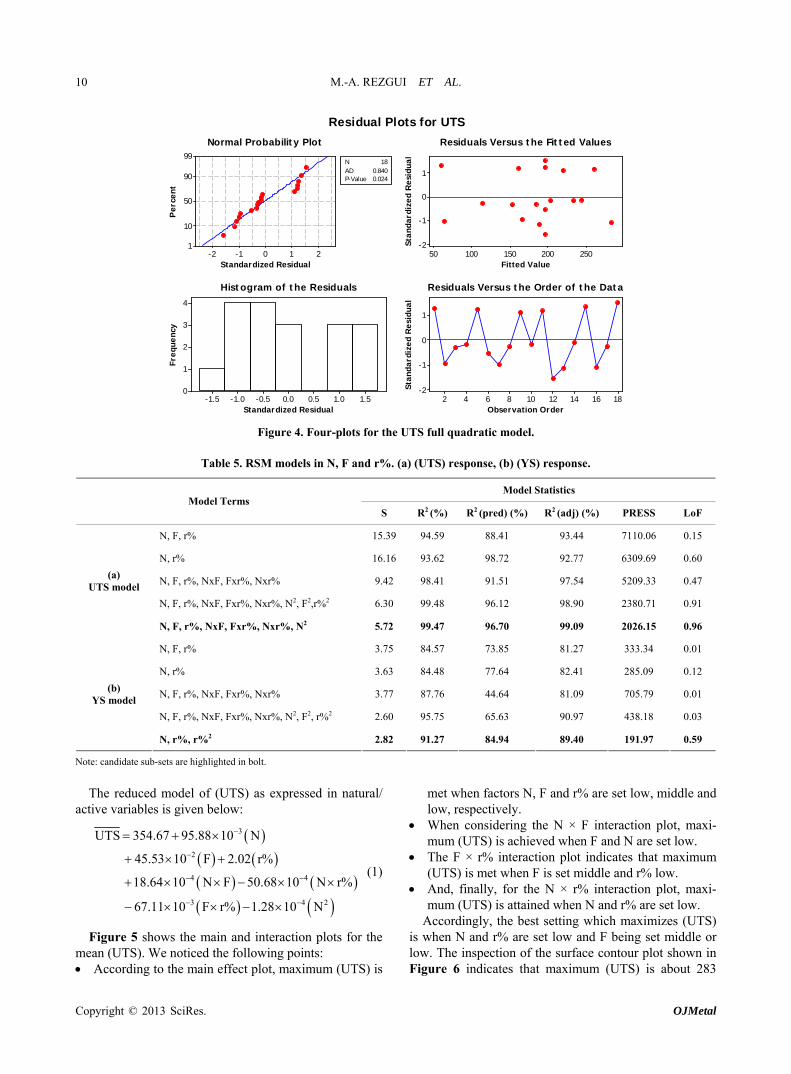
Considering the (UTS) full quadratic model shown in Table 5(a), the visual checking of the residual plots regarding the normality, independency, structureless and independence on factor setting does not question the model adequacy. Nevertheless, at 95% of C.I., the residual distribution is not normal (p-value 0.024) (Figure 4). Also, the ANOVA (see Appendix A) suggests the square terms, F2 and r%2, as fitted in the regression model are insignificant (p-value 0.750 and 0.825, resp). Interes- tingly, the regression p-values of the interactions (p = 0.000) and the squared terms (p = 0.024) are found statistically significant at 5%, suggesting presence of curvature in the (UTS) surface contour plot.


M.-A. REZGUI ET AL.


10

Standardized Residual

Per

cent

210-1-2

99

90

50

10

1

N 18AD 0.840P-Value 0.024

Fitted Value

Stan

dard

ized

Res

idua

l

25020015010050

1

0

-1

-2


Freq

uenc

y

1.51.00.50.0-0.5-1.0-1.5

4

3

2

1

0

Observation OrderSt

anda

rdiz

ed R

esid

ual

18161412108642

1

0

-1

-2

Normal Probability Plot Residuals Versus the Fitted Values

Histogram of the Residuals Residuals Versus the Order of the Data

Residual Plots for UTS

Figure 4. Four-plots for the UTS full quadratic model.

Table 5. RSM models in N, F and r%. (a) (UTS) response, (b) (YS) response.

Model Statistics Model Terms

S R2 (%) R2 (pred) (%) R2 (adj) (%) PRESS LoF

N, F, r% 15.39 94.59 88.41 93.44 7110.06 0.15

N, r% 16.16 93.62 98.72 92.77 6309.69 0.60

N, F, r%, NxF, Fxr%, Nxr% 9.42 98.41 91.51 97.54 5209.33 0.47

N, F, r%, NxF, Fxr%, Nxr%, N2, F2,r%2 6.30 99.48 96.12 98.90 2380.71 0.91

(a) UTS model

N, F, r%, NxF, Fxr%, Nxr%, N2 5.72 99.47 96.70 99.09 2026.15 0.96

N, F, r% 3.75 84.57 73.85 81.27 333.34 0.01

N, r% 3.63 84.48 77.64 82.41 285.09 0.12

N, F, r%, NxF, Fxr%, Nxr% 3.77 87.76 44.64 81.09 705.79 0.01

N, F, r%, NxF, Fxr%, Nxr%, N2, F2, r%2 2.60 95.75 65.63 90.97 438.18 0.03

(b) YS model

N, r%, r%2 2.82 91.27 84.94 89.40 191.97 0.59

Note: candidate sub-sets are highlighted in bolt.

The reduced model of (UTS) as expressed in natural/

active variables is given below:

3

2

4 4

3 4

UTS 354.67 95.88 10 N

45.53 10 F 2.02 r%

18.64 10 N F 50.68 10 N r%

67.11 10 F r% 1.28 10 N

2

(1)

Figure 5 shows the main and interaction plots for the mean (UTS). We noticed the following points: According to the main effect plot, maximum (UTS) is

met when factors N, F and r% are set low, middle and low, respectively.

When considering the N × F interaction plot, maximum (UTS) is achieved when F and N are set low.

The F × r% interaction plot indicates that maximum (UTS) is met when F is set middle and r% low.

And, finally, for the N × r% interaction plot, maximum (UTS) is attained when N and r% are set low.

Accordingly, the best setting which maximizes (UTS) is when N and r% are set low and F being set middle or low. The inspection of the surface contour plot shown in Figure 6 indicates that maximum (UTS) is about 283


300

200

100

443933

1098667

300

200

100

1280910653

300

200

100

N(rpm)

F(mm/min)

r%

653910

1280

N(rpm)

6786

109

F(mm/min)

333944

r%

Interaction Plot for UTSData Means

Figure 5. Main effects and interaction plots of response (UTS).

Figure 6. Surface contour plot of the process response (UTS). MPa for all combination of factors spaces (N versus r%, N versus F and F versus r%) given the extra factor maintained low.

3.2. Empirical Model for the Yield Stress (YS)

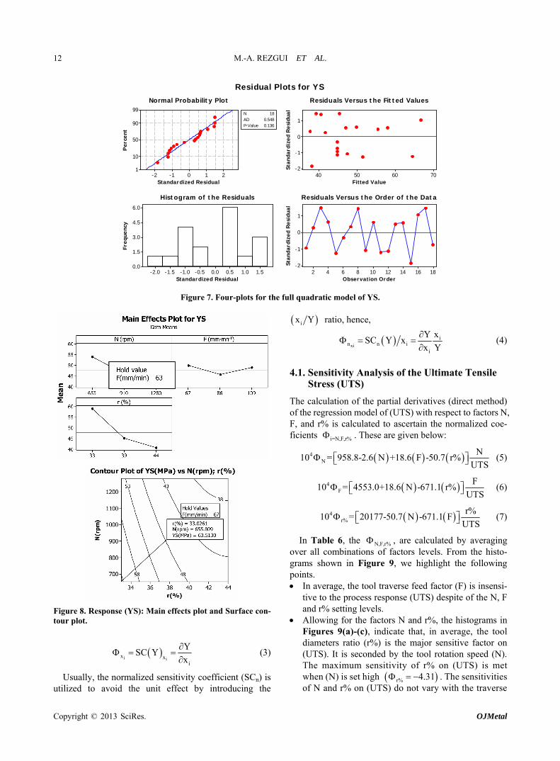
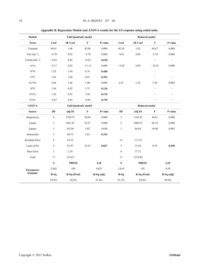
Likewise the foregoing, we seek to fit a full quadratic model to describe variation in the (YS) dataset. Allowing for a threshold of 95% C.I., the candidate/potential regression model(s) should satisfy the best trade-off among the model statistics, i.e., the LoF, R2, R2-pred, R2-adj and S. In Table 5(b), it is indicated that the full quadratic model (N, F, r%, N × F, F × r%, N × r%, N2, F2, r%2) is not considered fit (LoF 0.03 < 0.05). For the residuals, the 4-plots graph do not question the model adequacy as it is shown in Figure 7. The ANOVA given in Appendix B, pointed out the regression p-values of the interactions (p = 0.192) and the squared terms (p = 0.03 < 0.05) suggesting presence of curvature in the response surface which mainly originates from the squared terms. When considering the factors effects, the ANOVA shows that only N (p = 0.000), r% (p = 0.000) and roughly r2 (p = 0.094) are found statistically significant at 5% of Type I error.

A reduced model of (YS) is then obtained by getting rid of insignificant terms (main + interactions). Follow- ing is the regression equation as expressed in active coding.

3

2 2

YS 342.98 14.69 10 N

13.05 r% 14.77 10 r%

(2)

From Equation (2), it is shown that the (YS) response is independent of factor (F). Yet, it is advised to keep it at low level as the main effects plot suggests (Figure 8). Also, owing to the negative coefficient of terms N and r% in Equation (2), lower are N and r% higher is the process response (YS). This is further corroborated by the main effect plot shown in Figure 8. The surface contour plot which is displayed in Figure 8 shows that maximum yield stress (YS) is met when both the rotation speed (N) and tool diameters ratio (r%) are set low and the extra factor F being maintained low. Graphically, maximum yield stress is obtained at about 63.5 MPa.

4. Discussion: Sensitivity Analysis

So far, we have studied the ANOVA(s) pertaining to the (UTS) and (YS) responses. These have concerned the variability propagation through the RSM models (Equa- tions (1) and (2)) and resulting in a significant contribution to the overall output(s). The sensitivity analysis seeks, rather, to find out what process factors do produce larger variation in the responses whenever it is subjected to an infinitesimally variation. Given a dependent vari- able, iY x , the sensitivity coefficient (SC) of xi on iY x is obtained by calculating the partial derivative

f o iY x with respect to the independent factor xi [27].


M.-A. REZGUI ET AL.


12


Per

cent

210-1-2

99

90

50

10

1

N 18AD 0.548P-Value 0.136

Fitted Value

Stan

dard

ized

Res

idua

l

70605040

1

0

-1

-2


Freq

uenc

y

1.51.00.50.0-0.5-1.0-1.5-2.0

6.0

4.5

3.0

1.5

0.0

Observation Order

Stan

dard

ized

Res

idua

l

18161412108642

1

0

-1

-2

Normal Probability Plot Residuals Versus the Fitted Values

Histogram of the Residuals Residuals Versus the Order of the Data

Residual Plots for YS

Figure 7. Four-plots for the full quadratic model of YS.

Figure 8. Response (YS): Main effects plot and Surface con-tour plot.

i i

x xi

YSC Y

x

(3)

Usually, the normalized sensitivity coefficient (SCn) is utilized to avoid the unit effect by introducing the

ix Y ratio, hence,

xi

in n i

i

xYSC Y x

x Y

(4)

4.1. Sensitivity Analysis of the Ultimate Tensile Stress (UTS)

The calculation of the partial derivatives (direct method) of the regression model of (UTS) with respect to factors N, F, and r% is calculated to ascertain the normalized coe- ficients i=N,F,r% . These are given below:

4N

N10 = 958.8-2.6 N +18.6 F -50.7 r%

UTS (5)

4F

F10 = 4553.0+18.6 N -671.1 r%

UTS (6)

4r%

r%10 = 20177-50.7 N -671.1 F

UTS (7)

In Table 6, the N,F,r% , are calculated by averaging over all combinations of factors levels. From the histograms shown in Figure 9, we highlight the following points. In average, the tool traverse feed factor (F) is insensi-

tive to the process response (UTS) despite of the N, F and r% setting levels.

Allowing for the factors N and r%, the histograms in Figures 9(a)-(c), indicate that, in average, the tool diameters ratio (r%) is the major sensitive factor on (UTS). It is seconded by the tool rotation speed (N). The maximum sensitivity of r% on (UTS) is met when (N) is set high r% 4.31 . The sensitivities of N and r% on (UTS) do not vary with the traverse


Table 6. Normalized Coef. of sensitivity, Φi = N, F, r%, for the (UTS) and (YS) process (absolute maximum values are shown in bolt).

Sensitivity Coef. on (UTS) Sensitivity Coef. on (YS) N F r UTS

N F %r YS

N %r

33 283.8 −0.26 −0.13 −0.67 63.9 −0.15 −1.71

39 249.1 −0.38 −0.25 −0.91 49.6 −0.20 −1.21 67

44 220.2 −0.50 −0.39 −1.16 45.7 −0.21 −0.05

33 273.5 −0.19 −0.17 −0.85 63.9 −0.15 −1.71

39 231.2 −0.31 −0.35 −1.19 49.6 −0.20 −1.21 86

44 195.9 −0.45 −0.56 −1.59 45.7 −0.21 −0.05

33 261.1 −0.09 −0.23 −1.09 63.9 −0.15 −1.71

39 209.4 −0.21 −0.49 −1.60 49.6 −0.20 −1.21

653

109

44 166.4 −0.36 −0.84 −2.28 45.7 −0.21 −0.05

33 246.2 −0.66 −0.02 −0.95 60.2 −0.23 −1.82

39 203.6 −0.94 −0.15 −1.36 45.8 −0.30 −1.31 67

44 168.2 −1.27 −0.32 −1.85 42.0 −0.33 −0.05

33 245.0 −0.54 −0.02 −1.13 60.2 −0.23 −1.82

39 194.8 −0.82 −0.21 −1.68 45.8 −0.30 −1.31 86

44 153.0 −1.19 −0.45 −2.41 42.0 −0.33 −0.05

33 243.5 −0.38 −0.03 −1.34 60.2 −0.23 −1.82

39 184.1 −0.65 −0.28 −2.10 45.8 −0.30 −1.31

910

109

44 134.5 −1.06 −0.65 −3.24 42.0 −0.33 −0.05

33 162.3 −2.16 0.26 −1.82 54.7 −0.35 −2.00

39 108.5 −3.60 0.14 −3.22 40.3 −0.48 −1.49 67

44 63.7 −6.64 −0.12 −6.20 36.5 −0.53 −0.06

33 174.2 −1.76 0.31 −1.94 54.7 −0.35 −2.00

39 112.7 −3.06 0.17 −3.54 40.3 −0.48 −1.49 86

44 61.5 −6.13 −0.16 −7.32 36.5 −0.53 −0.06

33 188.6 −1.33 0.36 −2.06 54.7 −0.35 −2.00

39 117.9 −2.46 0.21 −3.90 40.3 −0.48 −1.49

1280

109

44 59.0 −5.47 −0.21 −8.79 36.5 −0.53 −0.06

feed (F) as it is pointed out in Figure 9(b). The histogram of Figure 9(a) shows that the maximum sensitivity of N on (UTS) occurs at the vicinity of N high . N 3.62

Table 6 indicates that local maximum sensitivity of N , F N 6.64 F 0.84 and r% r% 8.79

on (UTS) were found when N, F and r% are set (high, low, high), (low, high, high) and (high, high, high), respectively.

4.2. Sensitivity Analysis of the Yield Stress (YS)

The sensitivity analysis of factors N, F and r% on (YS) is assessed using the partial derivatives (direct method) of the regression model as formulated in Equation (2). Accordingly, i=N,F,r% are given below:

3N

N14.7 10

YS (8)

F 0 (9)



The histogram shown in Figure 10(a) points out the sensitivity of N on (YS) is almost stationary when varying N.

Allowing for the factors r%, the histograms of Figures 10(a) and 10(b) demonstrate that in average the tool diameters ratio (r%) is unique sensitive factor on (YS).

According to Table 6, the local maximum sensitivity of N N 0.53 , and r% r% 2.0 on (YS) were observed when N, F and r% are set (high, low, high), (high, middle, high) or (high, high, high) for the for- mer (i.e., factor N) and (high, low, low), (high, middle, low) or (high, high, low) for the latter.

5. Concluding Remarks (a) The paper has investigated the influence of three FSW

parameters on two process responses, namely, the joint Ultra Tensile Stress (UTS) and the joint Yield Stress (YS) produced in the aluminum 2017AA.

(b)

(a)

(c)

Figure 9. Sensitivity analysis for the process response (UTS): (a) when varying the tool rotation speed (N), (b) when varying the traverse feed (F), and (c) when varying the tool diameters ratio (r%). (b)

Figure 10. Sensitivity analysis for the process response (YS), (a) when varying the tool rotation speed (N), and (b) when varying the tool diameters ratio (r%).

r%

r%13.0 0.3 %

YSr (10)



1) The predictive models of (UTS) and (YS) are found fit using quadratic RSM models;

2) The ANOVAs and summary of fit tables (Appen- dixes A and B) have uncovered the traverse feed (F) was found irrelevant to the variation in (UTS) and (YS) because of the very small coefficient put in play in the regression Equations (1) and (2).

3) In average, the sensitivity analysis of factors N, F and r% on the responses (UTS) and (YS) has emphasized the influence of the tool diameters ratio factor (r%). The sensitivity of the tool rotation speed (N) on (UTS) came seconded in terms of prevalence. Likewise, the FSW process sensitivity was robust vis-à-vis the tool traverse feed factor (F).

The paper findings have shown that the tool geometry can be highly effective at the variation of the (UTS) and (YS) and can have significantly beneficial impacts on the quality engineering of the friction stir welded 2017AA. Besides, a shift of the factors variation space should be thought of so that a trade-off between joint macroscopic observations and the optimal parameters for FSW could be reached.

REFERENCES [1] W. M. Thomas, E. D. Nicholas, J. C. Needham, M. G.

Murch, S. P. Temple and C. J. Dawes, “Improvements Relating to Friction Welding,” GB Patent No. 9125978. 8, 1991.

[2] R. Rai, H. K. D. H. Bhadeshia and T. Debroy, “Friction Stir Welding Tools, Science and Technology of Welding and Joining,” Science and Technology of Welding & Join- ing, Vol. 16, No. 4, 2011, pp. 325-342. doi:10.1179/1362171811Y.0000000023

[3] T. P. Chen and W. B. Lin, “Optimal FSW Process Pa- rameters for Interface and Welded Zone Toughness of Dissimilar Aluminum-Steel Joint,” Science and Techno- logy of Welding & Joining, Vol. 15, No. 4, 2010, pp. 279- 285. doi:10.1179/136217109X12518083193711

[4] G. H. Payganeh, N. B. Mostafa Arab, Y. Dadgar Asl, F. A. Ghasemi and M. S. Boroujeni, “Effects of Friction Stir Welding Process Parameters on Appearance and Strength of Polypropylene Composite Welds,” International Jour- nal of Physical Sciences, Vol. 6, No. 19, 2011, pp. 4595- 4601.

[5] R. Nandan, T. Debroy and H. K. D. H. Bhadeshia, “Re- cent Advances in Friction Stir Welding—Process, Weld- ment Structure and Properties,” Progress in Materials Science, Vol. 53, No. 6, 2008, pp. 980-1023. doi:10.1016/j.pmatsci.2008.05.001

[6] M. Peel, A. Steuwer, M. Preuss and P. J. Withers, “Mi- crostructure, Mechanical Properties and Residual Stresses as a Function of Welding Speed in Aluminum AA5083 Friction Stir Welds,” Acta Materialia, Vol. 51, No. 16, 2003, pp. 4791-4801.

[7] K. Elangovan and V. Balasubramanian, “Influences of Tool Pin Profile and Tool Shoulder Diameter on the For-

mation of Friction Stir Processing Zone in AA6061 Alu- minum Alloy,” Materials & Design, Vol. 29, No. 2, 2008, pp. 362-373. doi:10.1016/j.matdes.2007.01.030

[8] A. Razal, K. Manisekar and V. Balasubramanian, “Influ- ences of Welding Speed on Tensile Properties of Friction Stir Welded AZ61A Magnesium Alloy,” Journal of Ma- terials Engineering and Performance, Vol. 21, No. 2, 2012, pp. 257-265. doi:10.1007/s11665-011-9889-0

[9] S. Lim, S. Kim, C. Lee and S. Kim, “Tensile Behavior of Friction-Stir-Welded Al6061-T651,” Metallurgical and Materials Transactions A, Vol. 35A, No. 9, 2004, pp. 2829-2835. doi:10.1007/s11661-004-0230-5

[10] H. Okuyucu, A. Kurt and E. Arcaklioglu, “Artificial Neural Network Application to the Friction Stir Welding of Aluminum Plates,” Materials & Design, Vol. 28, No. 1, 2007, 78-84. doi:10.1016/j.matdes.2005.06.003

[11] M. Jayaraman, R. Sivasubramanian and V. Balasubra- manian, “Establishing Relationship between the Base Me- tal Properties and Friction Stir Welding Process Para- meters of Cast Aluminum Alloys,” Materials & Design, Vol. 31, No. 3, 2010, pp. 4567-4576. doi:10.1016/j.matdes.2010.03.040

[12] K. Elangovan and V. Balasubramanian, “Influences of Pin Profile and Rotational Speed of the Tool on the For- mation of Friction Stir Processing Zone in AA2219 Alu- minum Alloy,” Materials Science and Engineering: A, Vol. 459, No. 1-2, 2007, pp. 7-18.

[13] S. Rajakumar, C. Muralidharan and V. Balasubramanian, “Influence of Friction Stir Welding Process and Tool Pa- rameters on Strength Properties of AA7075-T6 Alumi- num Alloy Joints,” Materials & Design, Vol. 32, No. 2, 2011, pp. 535-549. doi:10.1016/j.matdes.2010.08.025

[14] K. Kumar and S. V. Kailas, “On the Role of Axial Load and the Effect of Interface Position on the Tensile Stren- gth of a Friction Stir Welded Aluminum Alloy,” Materi- als & Design, Vol. 29, No. 4, 2008, pp. 791-797. doi:10.1016/j.matdes.2007.01.012

[15] C. Bitondo, U. Prisco, A. Squilace, P. Buonadonna and G. Dionoro, “Friction-Stir Welding of AA 2198 Butt Joints: Mechanical Characterization of the Process and of the Welds through DOE Analysis,” The International Journal of Advanced Manufacturing Technology, Vol. 53, No. 5-8, 2011, pp. 505-516. doi:10.1007/s00170-010-2879-9

[16] H. K. Mohanty, D. Venkateswarlu, M. Mahapatra and N. R. Kumar, “Modeling the Effects of Tool Probe Geome- tries and Process Parameters on Friction Stirred Alumi- nium Welds,” Journal of Mechanical Engineering and Automation, Vol. 2, No. 4, 2012, pp. 74-79. doi:10.5923/j.jmea.20120204.04

[17] S. Rajakumar, C. Muralidharan and V. Balasubramanian, “Establishing Empirical Relationships to Predict Grain Size and Tensile Strength of Friction Stir Welded AA 6061-T6 Aluminum Alloy Joints,” Transactions of Non- ferrous Metals Society of China, Vol. 20, No. 10, 2010, pp. 1863-1872. doi:10.1016/S1003-6326(09)60387-3

[18] S. Rajakumar and V. Balasubramanian, “Multi-Response Optimization of Friction-Stir-Welded AA1100 Aluminum Alloy Joints,” Journal of Materials Engineering and Per-


http://dx.doi.org/10.1179/1362171811Y.0000000023

http://dx.doi.org/10.1179/136217109X12518083193711

http://dx.doi.org/10.1016/j.pmatsci.2008.05.001

http://dx.doi.org/10.1016/j.matdes.2007.01.030

http://dx.doi.org/10.1007/s11665-011-9889-0

http://dx.doi.org/10.1007/s11661-004-0230-5





http://dx.doi.org/10.1007/s00170-010-2879-9

http://dx.doi.org/10.5923/j.jmea.20120204.04

http://dx.doi.org/10.1016/S1003-6326(09)60387-3

M.-A. REZGUI ET AL.


16

formance, Vol. 21, No. 6, 2012, pp. 809-822. doi:10.1007/s11665-011-9979-z

[19] R. Palanivel, P. K. Mathews and N. Murugan, “Deve- lopment of Mathematical Model to Predict the Mecha- nical Properties of Friction Stir Welded AA6351 Alumi- num Alloy,” Journal of Engineering Science and Techno- logy Review, Vol. 4, No. 1, 2011, pp. 25-31.

[20] A. K. Lakshminarayanan and V. Balasubranian, “Process Parameters Optimization for Friction Stir Welding of RDE-40 Aluminum Alloy Using Taguchi Technique,” Transactions of Nonferrous Metals Society of China, Vol. 18, No. 3, 2008, pp. 548-554. doi:10.1016/S1003-6326(08)60096-5

[21] A. S. Vagh and S. N. Pandya, “Influence of Process Pa- rameters on the Mechanical Properties of Friction Stir Welded AA2014-T6 Alloy Using Taguchi Orthogonal Array,” International Journal of Engineering Sciences & Emerging Technologies, Vol. 2, No. 1, 2012, pp. 51-58.

[22] K. Brahma Raju, N. Harsha and V. K. Viswanadha Raju, “Prediction of Tensile Strength of Friction Steer Welded Joints Using Artificial Neural Networks,” International Journal of Engineering Research & Technology, Vol. 1, No. 1, 2012, pp. 1-5.

[23] I. N. Tansel, M. Demetgul, H. Okuyucua and A. Yapici, “Optimizations of Friction Stir Welding of Aluminum

Alloy by Using Genetically Optimized Neural Network,” The International Journal of Advanced Manufacturing Technology, Vol. 48, No. 1-4, 2010, pp. 95-101. doi:10.1007/s00170-009-2266-6

[24] H. J. Liu, H. Fujii, M. Maedaa and K. Nogi, “Tensile Properties and Fracture Locations of Friction-Stir-Welded Joints of 2017-T351 Aluminum Alloy,” Journal of Ma- terials Processing Technology, Vol. 142, No. 3, 2003, pp. 692-699. doi:10.1016/S0924-0136(03)00806-9

[25] A. Mirjalil, H. J. Aval, S. Serajzadeh and A. H. Kokabi, “Microstructural Evolution and Mechanical Properties of FSWed 2017 AA with Different Initial Microstructures,” Proceedings of the Institution of Mechanical Engineers. Part L: Journal of Materials: Design and Applications, 2013. doi:10.1177/1464420713476400

[26] A. Trabelsi, M. A. Rezgui and S. Bezzina, “Assessment of the Tensile Elongation (e%) and Hardening Capacity (Hc) of Joints Produced in Friction Stir Welded 2017 AA (Enaw-AlCu4MgSi) Plates,” International Journal of En- gineering and Advanced Technology, Vol. 2, No. 4, 2013.

[27] D. M. Hamby, “A Review of Techniques for Parameter Sensitivity Analysis of Environmental Models,” Environ- mental Monitoring and Assessment, Vol. 32, No. 2, 1994, pp. 135-154. doi:10.1007/BF00547132

http://dx.doi.org/10.1016/S1003-6326(08)60096-5

http://dx.doi.org/10.1007/s00170-009-2266-6

http://dx.doi.org/10.1016/S0924-0136(03)00806-9

http://dx.doi.org/10.1177/1464420713476400

http://dx.doi.org/10.1007/BF00547132


Appendix A. Regression Models and ANOVA results for the UTS response using coded units.

Models Full quadratic model Reduced model

Term Coef SE Coef T P-value Coef SE Coef T P-value

Constant 188.54 2.57 73.39 0.000 188.02 2.13 88.46 0.000

N/(r·min-1) −57.31 1.99 −28.76 0.000 −57.31 1.81 −31.67 0.000

F/(mm·min−1) −6.82 1.99 −3.42 0.009 −6.86 1.81 −3.80 0.004

r/(%) −48.36 1.99 −24.26 0.000 −48.33 1.81 −26.73 0.000

N*N −11.38 3.97 −2.86 0.021 −12.59 2.83 −4.45 0.001

F*F −1.28 3.87 −0.33 0.750 − −

r%*r% −0.88 3.86 −0.23 0.825 − −

N*F 12.27 2.22 5.53 0.001 12.27 2.01 6.10 0.000

N*r% −8.74 2.22 −3.94 0.004 −8.74 2.01 −4.34 0.001

F*r% −7.75 2.22 −3.49 0.008 −7.75 2.02 −3.84 0.003

ANOVA Full Quadratic model Reduced model

Source DF Adj SS F P-value DF Adj SS F P-value

Regression 9 61054.8 171.02 0.000 7 61045.1 266.64 0.000

Linear 3 56659.2 476.12 0.000 3 56683.9 577.70 0.000

Square 3 658.2 5.53 0.024 1 648.5 19.83 0.001

Interaction 3 2324.3 19.53 0.000 3 2325.0 23.70 0.000

Residual Error 8 317.3 10 327.1

Lack-of-Fit 5 95.1 0.26 0.911 7 104.9 0.20 0.962

Pure Error 3 222.2 3 222.2

Total 17 61372.2 17 61372.2

S PRESS LoF S PRESS LoF

6.298 2381 0.911 5.719 2026 0.962

R-Sq R-Sq (Pred) R-Sq (adj) R-Sq R-Sq (Pred) R-Sq (adj)

Parameters Estimate

99.5% 96.1% 98.9% 99.5% 96.7% 99.1%


M.-A. REZGUI ET AL.


18

Appendix B. Regression Models and ANOVA results for the YS response using coded units.

Models Full Quadratic model Reduced model

Term Coef SE Coef T P-value Coef SE Coef T P-value

Constant 44.61 1.06 42.04 0.000 45.36 1.02 44.67 0.000

N/(r·min−1) −4.70 0.82 −5.70 0.000 −4.61 0.89 −5.19 0.000

F/(mm·min−1) −0.43 0.82 −0.52 0.618 − −

r/(%) −9.17 0.82 −11.13 0.000 −9.20 0.89 −10.32 0.000

N*N 1.25 1.64 0.76 0.468 − −

F*F 1.45 1.60 0.91 0.391 − −

r%*r% 3.04 1.60 1.90 0.094 4.47 1.36 3.30 0.005

N*F 1.56 0.92 1.71 0.126 − −

N*r% 1.36 0.92 1.49 0.176 − −

F*r% −0.87 0.92 −0.95 0.370 − −

ANOVA Full Quadratic model Reduced model

Source DF Adj SS F P-value DF Adj SS F P-value

Regression 9 1220.75 20.04 0.000 3 1163.65 48.81 0.000

Linear 3 1061.47 52.27 0.000 2 1060.72 66.74 0.000

Square 3 101.86 5.02 0.030 1 86.64 10.90 0.005

Interaction 3 40.75 2.01 0.192

Residual Error 8 54.16 14 111.25

Lack-of-Fit 5 51.97 14.25 0.027 5 33.54 0.78 0.590

Pure Error 3 2.19 9 77.71

Total 17 1274.9 17 1274.90

S PRESS LoF S PRESS LoF

2.602 438 0.027 2.819 192 0.59

R-Sq R-Sq (Pred) R-Sq (adj) R-Sq R-Sq (Pred) R-Sq (adj)

Parameters Estimate

95.8% 65.6% 91.0% 91.3% 85.0% 89.4%

REZGUI-2013 01

Documents

Transcript of REZGUI-2013 01