Review on fifteen Statistical Tests proposed by NIST

IJTPC, Vol. 1, November 2012.

www.IJTPC.org 18

Review on fifteen Statistical Tests proposed by NIST

J K M Sadique Uz Zaman, Ranjan Ghosh Institute of Radio Physics and Electronics, University of Calcutta 92, Acharya Prafulla Chandra Road, Kolkata – 700 009, INDIA

Accepted: 18th October, 2012

. .

ABSTRACT With a motivation to understand all the fifteen test algorithms and to write their codes independently without looking at various sites mentioned in the NIST document a review study of the NIST Statistical Test Suite is undertaken. All the codes are executed with the test data given in the NIST document and excellent agreements have been found. The codes have been put together in a software, called as CU software, executable in Linux platform. Based on the CU software, exhaustive tests are executed on a long bit sequence generated by the Blum‐Blum‐Shub generator (BBSG). The CU software executes properly giving the results almost matched with those of the NIST results.

Keywords Gaussian distribution function, error function, gamma function, Statistical test, Randomness, NIST test, P‐value

1. INTRODUCTION To look into the various aspects of randomness in a long sequence of bits the Statistical Test Suite developed by NIST [1,2,3] is an excellent and exhaustive document. The Test Suite was developed to choose today’s AES. It is a very important tool to understand randomness not only of the PRNGs but also of the crypto ciphers. The document provides many links [4,5,6]. In some cases [4,5] there are different types of useful information regarding different modules used for their programs and in some other cases [6] there are large data set of random bit sequences obtained from different PRNGs. Instead of endeavoring to study the data and information available in those links, initiatives have taken to enrich understanding of all the test algorithms with a belief that a capability would duly take shape to develop indigenous codes with scopes of future improvements, if possible. Had it been that an initiative would have been taken towards understanding the coding methodology of NIST test programs, the computing system issues would have taken the front seat for a long time keeping the scientific issues at the back. A preliminary study on BBSG [7,8], Knuth [9] and Park and Miller [10,11] algorithms is reported in a National workshop [12]. Based on this study and information available in literatures the BBSG is taken for comparison in this paper.

The NIST has documented fifteen statistical tests. In each test it adopted first a procedure to find the statistic of chi‐square (χ2) variation of a particular parameter for the given bit

sequence with that obtained from the theoretical studies of an identical sequence under the assumption of randomness. It then adopted a technique to transform the χ2 data to a randomness probability data, named as P‐value. Techniques adopted for conversion of the χ2 data to respective P‐value are described in Sec. 2. In Sec.3, the fifteen tests algorithms are narrated with better clarity of understanding. Indigenous codes of all the fifteen test algorithms have been developed in C (Linux) and have been taken together in CU software. The CU software has gives scopes to the user to select a particular test or few tests together or all tests. The CU software has been used to comparative study among the corresponding results of the NIST test suite. In Sec. 4, two points are discussed on P‐values: proportion of passing and distribution pattern. The results and discussion in connection to the CU software are presented in Sec. 5. The test results are given in Appendix A. The conclusion in brief is in Sec. 6.

2. CONVERSION OF TEST STATISTIC DATA TO PROBABILITY VALUE(S) To convert the χ2 data to probability value or P‐value the NIST has adopted broadly two approaches. In first approach the P‐value is calculated considering the χ2 data as single parameter, while in second approach the P‐value is calculated considering the number of degrees of freedom (K) data as first parameter and the χ2 data as second parameter. Six tests 1, 3, 6, 9, 13 and 15 do belong to the first approach, while the rest nine tests 2, 4, 5, 7, 8, 10, 11, 12 and 14 belong to the second one. The test names are provided in Table 5.

ashkan

Typewriter

ashkan

Typewriter

© 2012 University of Mohaghegh Ardabili.


www.IJTPC.org 19

For the first approach, a particular statistic parameter is observed for the entire bit sequence together and its χ2 variations are computed against the theoretical values obtained for the same parameter considering a corresponding bit sequence under the assumption of randomness – the χ2 data are converted to P‐value considering Standard Normal (Gaussian) distribution function Φ(x) where x is related to the χ2 data. In the second approach, the entire bit sequence is divided into N blocks and a concept of (K+1) classes with K degrees of freedom is introduced based on theoretical studies of a particular statistic parameter desired for the respective tests considering a corresponding identical bit sequence under the assumption of randomness. The said parameter is observed block‐wise across the entire bit sequence and its χ2 data are computed against the block‐wise theoretical values of the parameter – the χ2 data are then converted to P‐value considering gamma function ┌(a,z) where the parameter a is related to the K and the parameter z, to the χ2 data.

The Gaussian distribution function is given as,

Φ(z) = √

⁄∞

dx (1)

Figure 1: Plot of f1(x) = ⁄

Figure 1 shows the plot of f1(x) leading to Gaussian distribution function. It may be noted that Φ(z) = 1 when ‐∞ ≤ x ≤ +∞. Hence for ‐∞ ≤ x ≤ +∞, Φ(z) is related to χ2 data since z = χ 2⁄ ; and P‐value = 1 ‐ Φ(z). The larger is the χ2

variation, the larger is the value of Φ(z) and lesser is the value of P‐value. The bit sequence is considered as non‐random if P‐value is smaller than a significance level α = 0.01.

It may be noted that Φ(z) is used only in test 13 where the parameter z = χ 2⁄ assumes positive as well as negative values; hence Φ(z) is evaluated within limits of +ve and –ve values and the P‐value is obtained by subtracting the result of integration from unity.

If z in the Gaussian distribution assumes positive values, one resorts to error function given as,

erf(z) = √

dx where z < +∞ (2)

Figure 2 shows a plot of f2(x) leading to error function. If the limit of integration varies from 0 to +∞, the result of integration is unity. The error function erf(z) is used whenever the parameter z connected to χ2 variations assumes always positive values. It may be noted that erf(z) can be derived from Φ(z). It is readily observed that if the parameter x derived under the assumption of Gaussian distribution is to be used in error function, it is to be divided

by √2. For tests 1, 3, 6, 9 and 15, z assumes positive value and P‐value is calculated as 1 – erf(z). In test 13 the Gaussian distribution function is used to calculate P‐value.

Figure 2: Plot of f2(x) =

For the rest nine tests 2, 4, 5, 7, 8, 10, 11, 12, and 14, different approach of computation is taken to evaluate the P‐value. A concept of degrees of freedom is introduced in these tests in the form of blocks or classes. For such cases, instead of adopting the Gaussian distribution function or error function, one resorts to a distribution function based on gamma function which has two parameters. The gamma function ┌(a,z), where a is related to the degrees of freedom and z is related to χ2 variation, is given below as,

┌ , = dx (3)

Fig. 3 shows plots of ┌(a,z) for few values of a. The P‐value is computed as,

P‐value = 1 – ┌ ,┌ ,

(4)

where ┌ , is same as equation (3) and ┌ ,∞ is the integration of same function for 0 ≤ x ≤ +∞.

Figure 3: Plot of f3(a,x) =

3. DESCRIPTION OF TEST ALGORITHMS The available theoretical studies related to many statistic parameters of bit sequences under the assumption of randomness are the computational basis to estimate the χ2 variation. From broad theoretical considerations, the fifteen tests can be categorized into four categories, viz. Frequency Tests (tests 1–4), Test for Repetitive Patterns (tests 5–6), Tests for Pattern Matching (tests 7–12) and Tests based on Random Walk (tests 13–15). The algorithms of tests 1, 3, 6, 9, 13 and 15 do consider the entire bit sequence together for computation of χ2 variation and computes the P‐value based on error function, expect test 13 for which the Gaussian distribution function is used. The algorithms of tests 2 and 7 divide the entire bit sequence in N blocks and compute the P‐value based on gamma function using N as the degrees of freedom. The algorithms of tests 4, 5, 8 and 10 divide the entire bit sequence in N blocks and also consider (K+1) classes obtained from respective theoretical studies and

ashkan

Typewriter


ashkan

Typewriter


www.IJTPC.org 20

computes the P‐value based on gamma function using K as the degrees of freedom, instead of N. The algorithms of tests 11, 12 and 14, without dividing the bit sequence into blocks, introduce (K+1) classes obtained from respective theoretical studies and computes the P‐value based on gamma function with K degrees of freedom. The algorithms of all the fifteen tests are described below in sub‐sections 3.1 through 3.15.

3.1 Test 1: The Frequency Test (1 P‐value with parameter x) 3.1.1 Prelude 1. Through this test it is intended to see if the frequencies of 1 and 0 across the entire n‐bit sequence are approximately equal that is the proportion of 1s and 0s is close to ½.

2. If the number of 0s and 1s are not same, it is intended to see if their difference falls within the limit of randomness.

3.1.2 Background information in respect of randomness 1. This test is derived from central limit theorem for the random number.

2. The classic De Moivre‐Laplace theorem states that for a large number of trials the distribution of binomial sum,

normalized by √ , is closely approximate by a standard normal distribution.

3.1.3 Focus of Computation 1. Each bit 0 and 1 in the string is represented by ‐1 and 1 respectively by using the mathematical relation Xi = 2εi – 1, where Xi represents new value of the bit εi at the i

th position.

2. The sum of Xi represents Sn and Sobs = |Sn|/√

3. x = Sobs /√2

4. P‐value = 1 ‐ erf(x)

3.2 Test 2: Frequency Test within a Block (1 P‐value with parameters a, x) 3.2.1 Prelude 1. One can note that even if the first half on the n‐bit sequence is full of 1 and the second half with 0, the test 1 would have passed although the sequence is highly non‐random.

2. Through this test it is intended to ensure that frequencies of 1 and 0 are evenly distributed across the entire n‐bit sequence.

3.2.2 Background information in respect of randomness 1. The n‐bit string is divided in non‐overlapping N blocks each of M‐bit, where N= n/M . M should be taken as reasonably small. The extra bits less than M are neglected.

2. If the proportion of 1s in each block is approximately ½, the bit string can be termed as random.

3. Proportion πi of 1s in each block is given by,

πi = ∑ ε where 1 ≤ i ≤ N.

4. Chi‐square is χ2 = 4M ∑ π ½)2

3.2.3 Focus of Computation 1. For each block, πi as given above in section 3.2.2(3) is calculated for 1 ≤ i ≤ N.

2. The chi‐square (χ2) as given above is computed.

3. N is the degrees of freedom.

4. a = N/2 and x = χ2/2

5. P‐value = 1 – ┌(a,x)/┌(a,∞)

3.3 Test 3: Runs Test (1 P‐value with parameter x) 3.3.1 Prelude 1. Runs of length k means exactly k identical bits bounded by bits of opposite value.

2. In this test it is intended to see if the frequencies of runs of 1s and 0s of various lengths are in limits of randomness.

3.3.2 Background information in respect of randomness 1. εi = bit value at ith position of the n‐bit string;

π = ∑ εi

2. A checking parameter (τ ) is defined as, τ = √

3. If |π – 0.5| ≥ τ , it is not necessary to run the present test, since the Test 1 would fail for the sequence. The Runs test is executed when |π – 0.5| < τ.

3.3.3 Focus of Computation

1. Vn(obs) = ∑ r k + 1 where r(k) = 0 if εk = εk+1 and r(k)=1 otherwise.

2. x = | Vn(obs) – 2nπ(1‐ π) | / [2π(1‐ π)√2n]

3. P‐value = 1 – erf(x)

3.4 Test 4: Longest Run of Ones in a Block (1 P‐value with parameters a, x) 3.4.1 Prelude 1. In this test it is intended to see if the frequencies of longest run of 1s appearing in the tested sequence are consistent with that expected for a random sequence.

2. To execute the test the n‐bit string is divided in N non‐overlapping blocks each of M‐bit such that N= n/M as being done for Test 2. The additional bits are neglected.

3.4.2 Background information in respect of randomness 1. Considering all blocks, νi represents sum of all frequencies of longest runs of particular 1s appearing in each block.

2. For the sake computation νi is divided into (K+1) classes with 0 ≤ i ≤ K. Among n, M, N and K, an empirical relation as given below is proposed.

3. ν0 is the number of blocks where ‘1’ is the longest run of 1s or all 0s in the block, ν1 is the number of blocks where ‘11’ is the longest run of 1s, ν2 is the same for ‘111’, so on so forth. For K=3, ν3 is the number of blocks where the longest runs of 1s is ‘1111’ or more.

Minimum n Minimum M K Minimum N

128 8 3 16

6272 128 5 49

750000 104 6 75

ashkan

Typewriter



www.IJTPC.org 21

4. The number of times the longest runs of 1s are appearing in a particular block is not considered.

5. Considering randomness the theoretical studies on probabilities of occurrences of longest runs of 1s have been undertaken in detail for M=8 & K=3, M=128 & K=5, M=512 & K=5, M=1000 & K=5 and M=10000 & K=6. A representative set of one such values for M=8 & K=3 are given below,

6. The probabilities of occurrences of longest runs of 5 or more 1s are so small that these are clubbed together in ν3.

7. It may be noted for M=128 & K=5, the 6 classes are marked as ν0 ≤ 4 ones, ν1 = 5 ones, ν2 = 6 ones, ν3 = 7 ones, ν4 = 8 ones and ν5 ≥ 9 ones. Other cluster of classes, e.g. M=512 & K=5, M=1000 & K=5 and M=10000 & K=6, have their respective classes with probabilities. All related data are well compiled in the NIST document

8. It may be noted that ∑ ν = N and the sum of probabilities for a particular (M, K) group is unity.

3.4.3 Focus of Computation 1. The n‐bit string is divided in N blocks each of M‐bit long.

2. The longest runs of 1s are observed in each block and the appropriate classes (νi) are incremented. And at the end of the Nth block all the classes appropriately filled. It is to be remembered that ∑ ν = N.

3. Chi‐square statistic is given as,

χ2 = ∑

4. a = K/2 and x = χ2/2

5. P‐value = 1 – ┌(a,x)/┌(a,∞)

3.5 Test 5: Binary Matrix Rank Test (1 P‐value with parameters a, x) 3.5.1 Prelude 1. Through this test it is intended to see if the n‐bit string has repetitive patterns across its entire sequence. The n‐bit string is sequentially divided into N disjoint blocks and it is endeavored to see linear dependence among its fixed length substrings of each block.

2. Each block is represented by a matrix of M rows and Q columns such that N= n/MQ . The remaining unused bits are discarded. Usually both M and Q are taken as 32.

3. Through the test it is intended to calculate the rank of all sub‐matrices. For a sub‐matrix M1 of order M, the search is for its rank. If its determinant is non‐zero, its rank is M. If its determinant is zero, the determinants of all its sub‐matrices of order (M‐1) are calculated. If at least one determinants of order (M–1) is non‐zero, the rank of M1 is (M–1). It is the way one has to go lower order matrices to find its rank.

4. For a full rank sub‐matrix, one can conclude that it has no repetitive patterns.

3.5.2 Background information in respect of randomness 1. There are lots of theoretical studies related to rank of square binary matrix of order M ≥ 10. From the study the probabilities are given as follows,

PM = ∏ [1 – 2‐j] = 0.5×0.75×0.875×0.9375×0.9843755×0.9921875×….. = 0.2888……

PM‐1 = 2PM = 0.5776…….

PM‐2 = 4PM/9= 0.1284……. and all other probabilities are very small (≤ 0.005).

2. Considering the very small probability values of PM‐2, PM‐3 etc., it is assumed that the matrices of order M‐2 and less can be clubbed with PM‐2 and PM‐2 will then assume a value of 0.1336 instead of 0.1284. Please note that 0.2888 + 0.5776 + 0.1336 = 1.

3. From probability consideration, degrees of freedom (K) will be 2, since there are 3 classes.

4. For the sake of convenience of computation, M is taken as 32 and each sub‐matrix would contain 1024 bits (32×32).

3.5.3 Focus of Computation 1. The determinants of all the sub‐matrices of order 32 is determined and non‐zero ones are counted.

2. FM = Number of sub‐matrices having full rank M.

3. FM‐1 = Number of sub‐matrices with rank (M–1).

4. FM‐2 = N ‐ FM ‐ FM‐1 = Number of sub‐matrices with rank (M–2) and less.

5. χ2 = ∑

6. a = K/2 and x = χ2/2

7. For a = 1, ┌(a,x) = 1 – and ┌(a,∞) = 1.

8. P‐value = 1 – ┌(a,x)/┌(a,∞) =

3.6 Test 6: Discrete Fourier Transform Test (1 P‐value with parameter x) 3.6.1 Prelude 1. Through this test it is intended to see if the n‐bit string has periodic features across its entire sequence. By periodic features one understands repetitive patterns that are close to each other.

2. The focus of the test is to undertake Discrete Fourier Transform (DFT) of each bit of the sequence and to ascertain their peak heights.

3. Considering randomness one can find a peak height threshold value (T). If at most 5% of the peak heights are more than T, the sequence can be termed as random.

3.6.2 Background information in respect of randomness 1. DFT produces a sequence of complex variables to represent periodic components of different frequencies. The DFT component of the jth bit is given by fj as,

fj = ∑ ⁄

where xk is the kth bit coded in ‐1 and +1 form.

M=8 & K=3

4 classes Probabilities

ν0 ≤ ‘1’ , one 1s or no 1s 0.2148

ν1 = ‘11’ (2 ones) 0.3672

ν2 = ‘111’ (3 ones) 0.2305

ν3 ≥ ‘1111’ (4 or more ones) 0.1875

ashkan

Typewriter



www.IJTPC.org 22

2. Because of the symmetry of the real to complex‐value transform, only values of j are considered from 0 to (n/2 – 1) instead n.

3. The peak height threshold value (T) is calculated using

the relation T= log.

3.6.3 Focus of Computation 1. Each bit of 0 and 1 in an n‐bit sequence is represented by ‐1 and 1 respectively by using a relation Xi= 2εi ‐1, where Xi represents new value of the bit εi at the i

th position, 1 ≤ i ≤ n.

2. T is calculated using the relation stated above.

3. N0 = Expected theoretical (95%) number of peaks under the assumption of randomness = 0.95n/2.

4. Following the expression given above, magnitude (M) of fj is calculated for 0 ≤ j ≤ (n/2 – 1).

5. N1 = Number of peaks in M that are less than T.

6. d = . . /

7. x = | |√

8. P‐value = 1 – erf(x).

3.7 Test 7: Non‐overlapping Template Test (1 P‐value with parameters a, x) 3.7.1 Prelude 1. By this test one intends to see template matching in a non‐overlapping manner, i.e. it looks for occurrences of pre‐specified non‐periodic bit‐string and to see if the numbers of such occurrences are within the statistical limit of a sequence under the assumption of randomness.

2. An m‐bit window is considered to search for specific m‐bit pattern. If the pattern is not found, the window slides one bit position. If the pattern is found, the window is reset to the bit next to the found pattern.

3. This test detects generators producing too many occurrences of non‐periodic patterns (aperiodic).

3.7.2 Background information in respect of randomness 1. For random sequences the Central limit theorem is assumed to be applicable.

2. Mean (μ) and variance (σ2) are calculated based on approximate normal distribution. Procedures to calculate the mean and variance are given by,

μ = and σ2 = M( – )

where m is the fixed length of the non‐periodic pattern appearing M times.

3.7.3 Focus of Computation 1. n‐bit sequence is divided in N non‐overlapping blocks of M‐bit where N= n/M . Unused bits are discarded.

2. Mean μ and variance σ2 are calculated following the expression given above.

3. Wj = Number of times the specified pattern is found in the jth block. The matching search is continued for all blocks that is 1 ≤ j ≤ N.

4. χ2 = ∑µ

5. a = N/2 and x = χ2/2

6. P‐value = 1 – ┌(a,x)/┌(a,∞)

3.8 Test 8: Overlapping Template Test (1 P‐value with parameters a, x) 3.8.1 Prelude 1. Through this test one intends to detect template matching in an overlapping manner, that is, it looks for occurrences of pre‐specified bit‐string and to see if the number of such occurrences as against a sequence under the assumption of randomness.

2. An m‐bit window is considered to search for specific m‐bit pattern. The window always slides one bit position next, whether the pattern is found or not.

3. For this test the Poisson asymptotic distribution is assumed to be followed.

4. A long n‐bit string is divided in N blocks each of M‐bit such that N= n/M . Extra bits are discarded.

5. Six classes (νi) are considered, where 0 ≤ i ≤ 5. The explanation of νi follows. ν0 =329: m‐bit pattern is not found in 329 blocks; ν1 =164: m‐bit pattern is found once in 164 blocks; ν2 =150: m‐bit pattern is found twice in 150 blocks; ν3 =111: m‐bit pattern is found thrice in 111 blocks; ν4 =78: m‐bit pattern is found four times in 78 blocks; ν5 =136: m‐bit pattern is found five times or more in 136 blocks.

6. Number of degrees of freedom K for this test is 5.

7. The test detects any irregular occurrences of any periodic pattern.

8. The test rejects sequences with too many or too few occurrences of m‐runs of ones.

3.8.2 Background information in respect of randomness 1. There were many theoretical studies in respect of overlapping template matching. For computing theoretical probabilities (πi) corresponding to classes νi, values of λ and η are calculated as,

λ = and η =

where m is the fixed length of the non‐periodic pattern and M is bit size of each block.

2. The values of λ and η are necessary to calculate all values of πi. Under the assumption of randomness the theoretical probability values πi available in standard literatures are:

π0 = 0.324652, π1 = 0.182617, π2 = 0.142670, π3 = 0.106645, π4 = 0.077147, π5 = 0.166269

3.8.3 Focus of Computation 1. Few recommendations:

(i) n ≥ 106 , (ii) m = 9 or 10, (iii) N > , (iv) n ≥ MN,

(v) λ ≈ 2, (vi) K ≈ 2λ, (vii) m ≈ log M, and (viii) The πi

values given are exclusively for K=5.

2. The overlapping count of the m‐bit window is undertaken for all N blocks and the array of νi classes are correspondingly filled.

ashkan

Typewriter



www.IJTPC.org 23

3. χ2 = ∑

4. a = K/2 and x = χ2/2

5. P‐value = 1 – ┌(a,x)/┌(a,∞)

3.9 Test 9: Maurer’s “Universal Statistical” Test (1 P‐value with parameter x) 3.9.1 Prelude 1. This test focuses to measure distances in terms of L‐bit block‐numbers between L‐bit matching patterns. The distances are calculated using logarithmic function. The sum of log distances between L‐bit matching patterns is necessary for statistic distribution.

2. By this test one can conclude whether the sequence could be significantly compressed or not. A significantly compressible sequence is considered to be non‐random.

3. The Standard normal distribution function is used to obtain expected value of the test function (fn) along with its standard deviation (σ) under the assumption of randomness.

4. A long n‐bit string containing more than one million bits is divided into two blocks: one is the initialization segment with Q number of L‐bit blocks and another is the test segment with K number of L‐bit blocks. Unused bits are discarded.

3.9.2 Background information in respect of randomness 1. The test looks back through the entire sequence while walking through the test segment consisting of K number of L‐bit blocks, checking for a match with nearest previous exact L‐bit template and recording the distance in number of blocks to that previous match. The algorithm computes log of all such distances for all the L‐bit templates in the test segment (giving, effectively, the number of digits in binary expansion of each distance). Then it averages over all the expansion lengths by the number of K blocks as,

fn = ∑ log (c‐p),

where c and p are the respective indices of current and previous occurrence of same template.

Based on the Standard normal density distribution the expected value of the theoretical test statistic E(fn) is derived as,

E(fn) = 2 ∑ 1 2 log

A separate expression for variance (L) is also given. The variance is related to the theoretical standard deviation (σ) as,

σ = , where c = 0.7 – . + (4 + )

⁄

A dynamic look‐up table has been generated making use of the integer representation of the binary bits constituting the L‐bit template blocks of different sizes. The look‐up table for 6 ≤ L ≤ 16 is given in Table1.

3.9.3 Focus of Computation 1. A table with possible L‐bit value is created where last occurrence of the block number of each L‐bit is noted. In the test segment K, each block is checked and the distance between present block and the block where same L‐bit block

occurs last time is calculated. The previous block number is replaced by the current block number.

2. Test statistic function (fn) is calculated based on the following expression,

fn = ∑ log

where Tj is the table entry corresponding to the decimal representation of the contents of ith L‐bit block.

3. The previous of table entry of Tj is replaced by the current ith block number.

Table 1. The look‐up table for L varying from 6 to 16

4. The standard deviation (σ) is computed based on the expression given above and the corresponding value of variance given in the Table 1 above.

5. x = |√

|

6. P‐value = 1 – erf(x)

3.10 Test 10: Linear Complexity Test (1 P‐value with parameters a, x) 3.10.1 Prelude 1. A long bit string is usually obtained from a LFSR (Linear Feedback Shift Register).

2. The bit sequence from which a longer LFSR is obtained can be termed as random, while the shorter LFSR indicates non‐randomness.

3. The Berlekamp‐Massey Algorithm is adopted to obtain a LFSR.

4. The linear complexity test looks for length of LFSR and determines if the bit sequence from which the LFSR is obtained is random or not.

3.10.2 Background information in respect of randomness 1. A long n‐bit sequence is divided into N blocks, each of M‐bit.

2. Considering randomness the mean length of LFSR (µ) of M‐bit string is given by,

µ = +

–

3. The statistical deviation (Ti) of a LFSR of length (Li) is

Ti = (‐1)M ( Li ‐ µ) +

L Expected Value E(fn) Variance

6 5.2177052 2.954

7 6.1962507 3.125

8 7.1836656 3.238

9 8.1764248 3.311

10 9.1723243 3.356

11 10.170032 3.384

12 11.168765 3.401

13 12.168070 3.410

14 13.167693 3.416

15 14.167488 3.419

16 15.167379 3.421

ashkan

Typewriter



www.IJTPC.org 24

4. Depending on values of Ti , N blocks are divided in 7 fixed groups (νi) where 0 ≤ i ≤ 6, based on the following considerations:

ν0 (Ti ≤ ‐2.5), ν1 (‐2.5 < Ti ≤ ‐1.5), ν2 (‐1.5 < Ti ≤ ‐0.5), ν3 (‐0.5 < Ti ≤ +0.5), ν4 (+0.5 < Ti ≤ +1.5), ν5 (+1.5 < Ti ≤ +2.5), ν6 (Ti > +2.5),.

5. The theoretical probabilities (πi) of each of the 7 groups stated above are obtained from standard literature as,

π0 =0.010417, π1 =0.03125, π2 =0.125, π3 =0.5, π4 =0.25, π5 =0.0625, π6 =0.020833

3.10.3 Focus of Computation 1. The focus of the test is to find LFSR for each M‐bit sub‐stings and to find its length (Li).

2. µ is calculated for the value of M.

3. The degrees of freedom K is considered to be 6.

4. Ti is calculated for each of N blocks. Depending on the value of Ti the appropriate νi is incremented. One may note that ∑ ν = N.

5. Had it been that there was no group; T would be in one group. Creation of 7 groups provides T a choice of additional 6 groups – hence degrees of freedom are 6.

6. Chi‐square statistic is calculated as, χ2 = ∑

7. a = K/2 and x = χ2/2

8. P‐value = 1 – ┌(a,x)/┌(a,∞)

3.11 Test 11: Serial Test (2 P‐values each one with parameters a, x) 3.11.1 Prelude 1. In long n‐bit random sequence with at least one million bits, every m‐bit pattern has the same chance of appearing as every other m‐bit patterns.

2. The number of occurrences of the 2 m‐bit overlapping patterns is approximately the same as would be expected of a random sequence.

3. In n‐bit sequence, each of all m‐bit patterns is expected to occur Am times, where Am = n/2

m

4. This test counts frequency of all possible overlapping m‐bit patterns across the entire bit sequence and based on the deviations of each of all counts together one intends to see whether the sequence is random or not.

3.11.2 Background information in respect of randomness 1. Let νi represents frequency counts for 0 ≤ i ≤ (2

m ‐ 1) where i denotes the decimal value of a particular m‐bit pattern.

2. The psi‐square statistic (ψm2), similar to chi‐square (χ2),

is given by,

ψ = ∑ ν A = ∑ ν – n

3. The chi‐square statistic (χ2) in the present case is,

∆ψ = ψ ψ

∆ψ = ψ ψ

∆2ψ = ∆ψ – ∆ψ = ψ – 2ψ + ψ

4. Here the ∆ψ is the χ2 distribution with K1 = 2 degrees of freedom and ∆2 ψm

2 is another χ2 distribution with K2 = 2 degrees of freedom.

5. Two χ2 distributions coupled with two degrees of freedom gives rise two P‐values.

6. Value of m is usually small and m ≤ log – 2.

7. If m=1, the Serial Test turns out to be the frequency test (Test 1).

3.11.3 Focus of Computation 1. For m‐bit pattern νi is counted for 0 ≤ i ≤ (2

m – 1); ψ is computed with Am = n/2

m.

2. For (m‐1)‐bit pattern νi is counted for 0 ≤ i ≤ (2 – 1); ψ is computed with = 2 .

3. For (m‐2)‐bit pattern νi is counted for 0 ≤ i ≤ (2 – 1); ψ is computed with = 2 .

4. Based on ψ and ψ , ∆ψ is computed and based on ψ , ψ and ψ , ∆2ψ is computed.

5. Considering = and = ∆ψ

the P‐value1 = 1 – g(a1,x1)/g(a1,∞)

6. Considering = and = ∆2ψ

the P‐value2 = 1 – g(a2,x2)/g(a2,∞)

3.12 Test 12: Approximate Entropy Test (1 P‐value with parameters a, x) 3.12.1 Prelude 1. Entropy is a test of randomness based on repeating patterns. Larger is the entropy larger is the randomness.

2. For n‐bit string the entropy is measured by comparing the frequency of overlapping patterns of all possible m‐bit patterns with that of (m+1)‐bit patterns. The comparison between entropies of m and (m+1)‐bit patterns is termed as approximate entropy, ApEn(m), which is compared against the expected result of a random sequence.

3. For a random sequence, the ApEn(m) is a maximum value projected as 2.

4. Test of the binary sequence of e, π, √2 and √3 has shown that √3 is more irregular than π and their values show a limiting convergence towards 2.

3.12.2 Background information in respect of randomness 1. For counting m‐bit matching patterns, (m‐1) bits taken from the beginning of the sequence are appended at the end of the given n‐bit string in the form.

2. Let νi represents overlapping frequency counts of a particular m‐bit pattern for 0 ≤ i ≤ 2 , where i denotes the decimal value of a particular m‐bit pattern.

3. = ν ⁄ , π = and ∑

4. For counting (m+1)‐bit matching patterns, first m bits are appended at the end of the given n‐bit string.

5. Similarly νi represents overlapping frequency counts of a particular (m+1)‐bit pattern for 0 ≤ i ≤ 2 , here i denotes the decimal value of a particular (m+1)‐bit pattern.

ashkan

Typewriter



www.IJTPC.org 25

6. = ν ⁄ , π =

and ∑

7. ApEn(m) =

8. The number of degrees of freedom K = 2m

9. χ2 = 2n[ln 2 – ApEn(m)]

3.12.3 Focus of Computation 1. For counting m‐bit matching patterns, ν is counted in overlapping manner across the appended (n+m‐1)‐bit sequence for all possible m‐bit patterns, where 0 ≤ i ≤ 2 –1.

2. Based on 2 types of ν , values of , π and Ф are computed.

3. Again for counting (m+1)‐bit matching patterns, ν is counted in overlapping manner across the (n+m)‐bit string for all possible (m+1)‐bit patterns, where 0 ≤ i ≤ 2m+1 ‐1.

4. Based on 2 types of ν , values of , π and Ф are computed.

5. χ2 = 2n[ln 2 – ApEn(m)]

where ApEn(m =

6. a = K/2 and x = χ2/2

7. P‐value = 1 – ┌(a,x)/┌(a,∞)

3.13 Test 13: Cumulative Sums Test (2 P‐values each one with parameter x) 3.13.1 Prelude 1. This test looks whether 1s or 0s are occurring in large numbers at early stages or at later stages or 1s and 0s are intermixed evenly across the entire sequence.

3.13.2 Background information in respect of randomness 1. Since the distribution of cumulative sums is being looked into, the P‐value is calculated following the Normal distribution function (Ф) given by,

Ф(z) = √ π

⁄ du

3.13.3 Focus of Computation 1. Across the entire n‐bit sequence, the 0s are made ‐1 as it is done in Test 1. The cumulative sums of adjusted (‐1, +1) of digits of the sequence is obtained as = + with i = 1 to n and = 0. The cumulative sums may be considered as Random Walk.

2. In Test 1 the sum was of adjusted (‐1, +1) of all digits and it was seen if the summation falls within the accepted range of randomness.

3. Here the maximum magnitude (z) of the cumulative

sums is calculated as z = | |. If √

is large, the bit

sequence is considered to be non‐random.

4. The cumulative sums can undertaken in a forward manner, that is from start to end (termed as Mode 0) and also in a backward manner, that is from end to start (termed as Mode 1). For each of the two cases, two values of z are noted.

5. The P‐value is computed as follows that used Gaussian distribution function (Ф).

P‐value = 1 – ∑ Ф√

Ф√

⁄

⁄

+ ∑ Ф√

Ф√

⁄

⁄

6. Two P‐values are calculated following the Gaussian distribution function – one for the forward cumulative sums and the other, for the backward cumulative sums.

3.14 Test 14: Random Excursions Test (8 P‐values each one with parameters a, x) 3.14.1 Prelude 1. This test intends to look if the number of visits to a particular cumulative sums state within a cycle falls into a category that is expected of random sequence.

2. Eight states, e.g. ‐4, ‐3, ‐2, ‐1 and +1, +2, +3, +4 are looked into – visits to states greater than +4 are clubbed within the visits to +4 state and visits to states lesser then ‐4 are clubbed within the visits to ‐4 state.

3.14.2 Background information in respect of randomness 1. πk(s) is defined as the theoretical probability of k number of visits to a state s. For k=0 to 5 the πk(s) are being theoretically derived. Here the degrees of freedom K =5.

2. Probability of 0 number of visits to a state s: π0(s)=1– | |

3. Probability of k number of visits to a state s:

πk(s) = 1–| |

, k=1, 2, 3 and 4.

4. Probability of 5 or more number of visits to a state s:

π5(s) = | |1–

| |

5. The fourteen states, e.g. ±1, ±2, ±3, ±4, ±5, ±6, ±7 have been theoretically considered. The study indicates that, states ±5, ±6 and ±7 have very low probability occurrences and it’s the reason that first eight states are considered for practical situation. The theoretical probability values given in the NIST document are shown in Table 2.

6. It may be noted that ∑ = 1 for a visit to a particular state s.

Table 2. The theoretical probability values given in the NIST

3.14.3 Focus of Computation 1. Across the entire n‐bit sequence, all the 0s are made ‐1 as it is done in Test 1. The cumulative sums of adjusted (‐1, +1) of Xi digits of the sequence is obtained as Si = Si‐1 + Xi when 2 ≤ i ≤ n and S0 = Sn+1 = 0.

2. If the cumulative sums crosses zero J (excluding s0 = 0) times, J is termed as the number of cycles considering the zero crossing point at Sn+1.

s π0(s) π1(s) π2(s) π3(s) π4(s) π5(s)

±1 .5000 .2500 .1250 .0625 .0312 .0312

±2 .7500 .0625 .0469 .0352 .0264 .0791

±3 .8333 .0278 .0231 .0193 .0161 .0804

±4 .8750 .0156 .0137 .0120 .0105 .0733

±5 .9000 .0100 .0090 .0081 .0073 .0656

±6 .9167 .0069 .0064 .0058 .0053 .0588

±7 .9286 .0051 .0047 .0044 .0041 .0531

ashkan

Typewriter



www.IJTPC.org 26

3. If J<max(0.005√ , 500), the sequence is considered to be non‐random. One million bit sequence is considered non‐random if J is less than 500.

4. νk(s) = Frequency of k‐times of visit to the state s during J excursions. For the sake of computation one can consider

νk(s) = ∑ ν s .

If number of visits to the state s during jth excursion is exactly

equal to k, then ν s =1 otherwise ν s = 0.

5. For νk(s) with k≥5, count data is being put in ν5(s).

6. For each state, the chi‐square statistic is calculated as,

χ2 = ∑ π

π

7. a = K/2 and x = χ2/2

8. P‐value = 1 – ┌(a,x)/┌(a,∞)

9. There are eight states – hence there will be eight P‐values corresponding to each state.

3.15 Test 15: Random Excursions Variant Test (18 P‐values each one with parameter x) 3.15.1 Prelude 1. The Random Excursions Variant test looks for number of visits to a particular state in cumulative sums of random walk across the entire bit sequence and estimates deviations from expected number of visits in the random walk considering randomness.

2. 18 states, e.g. s = –9, –8, –7, –6, –5, –4, –3, –2, –1, +1, +2, +3, +4, +5, +6, +7, +8, +9 are considered.

3.15.2 Background information in respect of randomness 1. Statistic Variation σ = (4│s│ – 2) in respect of random walk for visit to different states.

3.15.3 Focus of Computation 1. Across the entire n‐bit sequence, all the 0s are made ‐1 as it is done in Test 1. The cumulative sums of adjusted (‐1, +1) of Xi digits of the sequence is obtained as Si = Si‐1 + Xi when 2 ≤ i ≤ n and S0 = Sn+1 = 0.

2. If the cumulative sums crosses zero J (excluding s0 = 0) times, J is termed as the number of cycles considering the zero crossing point at Sn+1.

3. If J<max(0.005√ , 500), the sequence is considered to be non‐random. One million bit sequence is considered non‐random if J is less than 500.

4. ξ(s) is defined as the total number of times that a state s is visited across all J cycles.

5. Here x = | – |

√

6. P‐value = 1 – erf(x).

7. There are eighteen states – hence 18 P‐values corresponding to each state are calculated.

4. PROPORTION OF PASSING AND DISTRIBUTION PATTERN In this section, two points are discussed on P‐values: one is on the proportion of passing and another is on the

distribution pattern. Based on these two points one can conclude about the randomness of bit‐sequences as well as of bit‐generators. In Table 3, number of P‐values lying in the given ranges for tests number 12, 13 and 14 are presented based on 300 bit‐sequences generated by the BBSG algorithm. Name of the fifteen tests corresponding to the test number is noted in Table 5.

Table 3. Number of P‐values lying in the given range

4.1 Proportion of passing a test based on P‐values To observe the proportion of passing of a test, it is necessary to consider large number of samples of bit‐sequences generated by a PRNG. If m samples of bit sequences obtained from a PRNG algorithm are tested by a test producing one P‐value, then a statistical threshold value (T‐value) would be,

T‐value = (1 – α) – 3 (5)

where significance level (α) = 0.01. The size of m should greater than inverse of α. If m=300, T‐value = 0.972766, it is mentioned in Table 4. This means that such a test is considered statistically successful, if at least 292 P‐values out of the 300 P‐values do pass the test.

If any test produced n number of P‐values, then to calculate T‐value in equation (5), one should consider m×n instead of m. With same values of α and m, the T‐value is 0.983907 for n=8 (tests 14). Such a test is considered statistically successful if at least 2362 P‐values out of the total 300×8 = 2400 P‐values do pass the test. From Table 4, one can see that T‐value differs for all the given three tests, because test 12 has one P‐value, test 13 has two P‐values and test 14 has eight P‐values. The status for Proportion of passing a test would be success if the value of “Observed Proportion” in Table 4 is not less than T‐value.

Table 4. Status for Proportion of passing and Distribution pattern

Range Test 12 Test 13 Test 14

0 ‐ 0.01 5 5 32

0.01 ‐ 0.1 28 49 246

0.1 ‐ 0.2 22 48 241

0.2 – 0.3 31 56 223

0.3 – 0.4 31 102 255

0.4 – 0.5 28 64 226

0.5 – 0.6 32 41 250

0.6 – 0.7 30 54 244

0.7 – 0.8 27 56 235

0.8 – 0.9 31 75 220

0.9 – 1.0 35 50 228

Test 12 Test 13 Test 14

T‐value 0.972766 0.977814 0.983907

ObservedProportion

0.983333 0.991667 0.986667

Proportion of passing status

Success Success Success

P‐value of P‐values(POP)

9.157321e‐01

8.425709e‐07

2.226391e‐01

Distribution pattern status

Uniform Non‐uniform

Uniform

ashkan

Typewriter



www.IJTPC.org 27

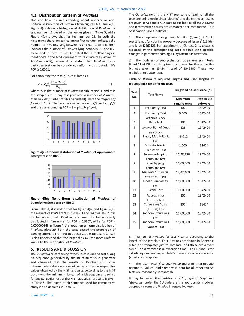
4.2 Distribution pattern of P‐values One can have an understanding about uniform or non‐uniform distribution of P‐values from figures 4(a) and 4(b). Figure 4(a) shows a histogram of distribution of P‐values for test number 12 based on the values given in Table 3, while Figure 4(b) shows that for test number 13. In both the histograms there are ten columns: first column indicates the number of P‐values lying between 0 and 0.1; second column indicates the number of P‐values lying between 0.1 and 0.2, so on and so forth. It may be noted that a methodology is mentioned in the NIST document to calculate the P‐value of P‐values (POP), where it is stated that P‐values for a particular test can be considered uniformly distributed, if it’s POP ≥ 0.0001.

For computing the POP, χ2 is calculated as

χ2 = ∑

(6)

where, Si is the number of P‐values in sub‐interval i, and m is the sample size. If any test produced n number of P‐values, then m = n×(number of files calculated). Here the degrees of freedom K = 9. The two parameters are a = K/2 and x = χ2/2 and the corresponding POP = 1 – ┌(a,x)/┌(a,∞).

Figure 4(a): Uniform distribution of P‐values of Approximate Entropy test on BBSG.

Figure 4(b): Non‐uniform distribution of P‐values of Cumulative Sums test on BBSG.

From Table 4, it is noted that for figure 4(a) and figure 4(b), the respective POPs are 9.157321e‐01 and 8.425709e‐07. It is to be noted that P‐values are seen to be uniformly distributed in figure 4(a) for POP = 0.9157, while for POP = 0.000000843 in figure 4(b) shows non‐uniform distribution of P‐values, although both the tests passed the proportion of passing criterion. From various observations on test results, it is also understood that the larger the POP, the more uniform would be the distribution of P‐values.

5. RESULTS AND DISCUSSION The CU software containing fifteen tests is used to test a long bit sequence generated by the Blum‐Blum‐Shub generator and observed that the results of P‐values and other intermediate values are almost same to the corresponding values obtained by the NIST test suite. According to the NIST document the minimum length of a bit‐sequence required for any particular test of the NIST statistical test suite is given in Table 5. The length of bit‐sequence used for comparative study is also depicted in Table 5.

The CU software and the NIST test suite of each of all the tests are being run in Linux (Ubuntu) and the test‐wise results are given in Appendix A. A meticulous look to all the P‐values and intermediate values are considered for comparison. Our observations are as follows:

1. The complementary gamma function (igamc) of CU in test 2 is not functioning properly because of large χ2 (13466) and large K (6712). For experiment of CU test 2 its igamc is replaced by the corresponding NIST module with suitable changes in parameter passing. CU igamc needs attention.

2. The modules computing the statistic parameters in tests 6 and 13 of CU are taking too much time. For these two the bit was taken as 13424 instead of 1342400. These two modules need attention.

Table 5: Minimum required lengths and used lengths of bit‐sequence for different tests

3. Number of P‐values for test 7 varies according to the length of the template. Four P‐values are shown in Appendix A for 9‐bit‐templates just to compare. And these are almost same. The difference is in execution time. The CU time is for calculating one P‐value, while NIST time is for all non‐periodic (aperiodic) templates.

4. The result‐wise (χ2 value, P‐value and other intermediate parameter values) and speed‐wise data for all other twelve tests are reasonably comparable.

It may be noted that entries of ‘erfc’, ‘igamc’, ‘exp’ and ‘stdnordis’ under the CU code are the appropriate modules adopted to compute P‐value in respective tests.

Test No.

Test Name Length of bit‐sequence (n)

Minimum requirement

Used in CU software

1 Frequency Test 100 1342400

2 Frequency Test within a Block

9,000 1342400

3 Runs Test 100 1342400

4 Longest Run of Ones in a Block

128 1342400

5 Binary Matrix Rank Test

38,912 1342400

6 Discrete Fourier Transform Test

1,000 13424

7 Non‐overlapping Template Test

10,48,576 1342400

8 Overlapping Template Test

10,00,000 1342400

9 Maurer’s “Universal Statistical” Test

13,42,400 1342400

10 Linear Complexity Test

10,00,000 1342400

11 Serial Test 10,00,000 1342400

12 Approximate Entropy Test

100 1342400

13 Cumulative Sums (Cusum) Test

100 13424

14 Random Excursions Test

10,00,000 1342400

15 Random Excursions Variant Test

10,00,000 1342400

020406080

100120

1 2 3 4 5 6 7 8 9 10

0

10

20

30

40

1 2 3 4 5 6 7 8 9 10

ashkan

Typewriter



www.IJTPC.org 28

6. CONCLUSION Modification of the igamc of CU is necessary so that it accepts large χ2 and K values. It seems the modules computing the statistic parameters for tests 6 and 13 of CU need a new model. This will be taken up in future. The model computing the statistic parameters for test 7 needs a relook since the test is taking relatively more time than that of NIST test.

7. ACKNOWLEDGMENTS We are grateful to the UGC, New Delhi for providing financial support to the first author Mr. J K M Sadique Uz Zaman. We are indeed thankful to Prof. Bimal Roy, Director, ISI‐Calcutta for providing a tacit indication towards indigenous codes.

8. REFERENCES [1] Rukhin A., Soto J., et al, 2010. A Statistical Test Suite for

Random and Pseudorandom Number Generators for Cryptographic Applications, NIST, US. http://csrc.nist.gov/publications/nistpubs/800‐22‐rev1a/SP800‐22rev1a.pdf

[2] Rukhin A., Soto J., et al, 2008. A Statistical Test Suite for Random and Pseudorandom Number Generators for Cryptographic Applications, NIST, Technology Administration, U.S. Department of Commerce.

[3] http://csrc.nist.gov/groups/ST/toolkit/rng/documentation_software.html

[4] http://gams.nist.gov/serve.cgi/Package/CEPHES/

[5] http://www.netlib.org/cephes/

[6] http://www.moshier.net/

[7] Stallings W., 2008. Cryptography and Network Security, 4th Edition, Pearson Education.

[8] Blum L., Blum M., Shub M., 1986. A Simple Unpredictable Pseudo‐Random Number Generator, SIAM Journal on Computing, 15 364‐383.

[9] Knuth D. E., 2011. The Art of Computer Programming, Vol. 2, 3rd Edition, Pearson Education.

[10] Park S. K., Miller K. W., 1988. Random number generators: good ones are hard to find, Communications of the ACM, 31 1192–1201.

[11] Teukolsky S. A., Vetterling W. T., Flannery B. P., 1988. Numerical Recipes in C: The Art of Scientific Computing, Cambridge University Press.

[12] Zaman J. K. M., Ghosh R., 2011. A Review Study of NIST Statistical Test Suite: Development of an indigenous Computer Package, National Workshop on Cryptology, contributed–talks. https://sites.google.com/a/iiitd.ac.in/nwc2011/program/contributed‐talks

ashkan

Typewriter



www.IJTPC.org 29

Appendix A: Comparative study on the results of the fifteen statistical tests coded by CU and NIST

Sl.

No.

Test name

CU Code NIST Code

Intermediate value(s) P-value(s) Exec. Time


1 Frequency (Monobit) Test

nth partial sum = -244 S_n/n =-0.000182

erfc 0.833159

0.232s nth partial sum = -244 S_n/n = -0.000182

0.833203

0.276s

2 Frequency Test within a Block

Chi^2 = 13466.320000 # of substrings = 13424 Block length = 100

Igamc from NIST 0.396631

0.216s Chi^2 = 13466.320000 # of substrings =13424 Block length=100

0.396631

0.276s

3 Runs Test Pi = 0.499909 Total # of runs= 670238 [V_n_obs - 2 n pi (1-pi)]/[ 2 sqrt(2n) pi (1-pi)] = 1.174192

erfc

0.096792

0.760s Pi = 0.499909 Total # of runs= 670238 [V_n_obs - 2 n pi (1-pi)]/[ 2 sqrt(2n) pi (1-pi)] = 1.174192

0.096802

0.300s

4 Longest Run of Ones in a

Block

N=134 M=10000 Chi^2=9.174302

igamc

0.163788

0.340s N=134 M=10000 Chi^2=9.174302

0.164010

0.288s

5 Binary Matrix Rank Test

Probability : 0.288788, 0.577576, 0.133636 Frequency: 374, 738, 198 # of matrices=1310 Chi^2= 3.512797

exp

0.172666

0.384s Probability : 0.288788, 0.577576, 0.133636 Frequency: 374, 738, 198 # of matrices=1310 Chi^2 = 3.512917

0.172655

0.496s

6 Discrete Fourier Trans. (Spectral) Test

(n=13424)

Percentile = 94.830155 N_l = 6365 N_o = 6376.400000 d = -0.902908

Erfc

0.366520

14.517s Percentile = 94.830155 N_l = 6365.000000 N_o = 6376.400000 d= -0.902915

0.366571

4.840s

7 Non-overlapping

Template Matching Test

Template: 000000001 L = 327.718750 M= 167800, N= 8 m=9, n= 1342400 Chi^2 = 4.519279 - - - - - - - - - - - - - - - -

Template: 010010011 L = 327.718750 M= 167800, N= 8 m=9, n= 1342400 Chi^2=10.393857 - - - - - - - - - - - - - - - -

Template: 110011010 L = 327.718750 M= 167800, N= 8 m=9, n= 1342400 Chi^2 = 5.554658 - - - - - - - - - - - - - - - -

Template: 111111110 L = 327.718750 M= 167800, N= 8 m=9, n= 1342400 Chi^2 = 7.204085

igamc

0.807457 -- - - - - - -

0.238192 -- - - - - - -

0.696792 -- - - - - - -

0.514383

0.944s Template: 000000001 L = 327.718750 M= 167800, N= 8 m=9, n= 1342400 Chi^2=4.519279 - - - - - - - - - - - - - - - -



Template: 111111110 L = 327.718750 M= 167800, N= 8 m=9, n= 1342400 Chi^2=7.204085

0.807501 -- - - - - - -

0.238463 -- - - - - - -

0.696977 -- - - - - - -

0.514782

5.872s

ashkan

Typewriter



www.IJTPC.org 30

Appendix A: Continued…

Sl.

No.

Test name

CU Code NIST Code



8 Overlapping Template

Matching Test

n = 1342400 m (block length of 1s) = 9 Substring length M=1032 # of substrings N =1300 Lambda [(M-m+1) / 2^m] = 2.000000 eta = 1.000000 Chi^2=4.189985 Frequencies: 454, 231, 198, 129, 96, 192 - - - - - - - - - - - - - - - - n = 1342400 m (block length of 1s) = 8 Substring length M=1032 # of substrings N =1300 Lambda [(M-m+1) / 2^m] = 4.003906 eta = 2.001953 Chi^2 = 7.600790 Frequencies: 162, 166, 175, 145, 162, 490

igamc

0.522508

-- - - - - - -

0.179454

1.016s n = 1342400 m (block length of 1s) = 9 Substring length M=1032 # of substrings N =1300 Lambda [(M-m+1) / 2^m] = 2.000000 eta = 1.000000 Chi^2=4.189985 Frequencies: 454, 231, 198, 129, 96, 192 - - - - - - - - - - - - - - - - n = 1342400 m (block length of 1s) = 8 Substring length M=1032 # of substrings N =1300 Lambda [(M-m+1) / 2^m] = 4.003906 eta = 2.001953 Chi^2= 7.600787 Frequencies: 162, 166, 175, 145, 162, 490

0.522400

-- - - - - - -

0.179653

0.444s

9 Maurer’s “Universal

Statistical” Test

L=7, Q=1280, K=190491 sum= 1180630.066662 sigma = 0.002385 variance=3.12500 exp_value=6.196251 phi = 6.197826 3 bits were discarded.

erfc

0.508936

0.244s L=7, Q=1280, K=190491 sum= 1180630.066662 sigma = 0.002385 variance=3.12500 exp_value=6.196251 phi = 6.197826 3 bits were discarded.

0.508932

0.424s

10 Linear Complexity

Test

Substring length M=1000 # of substrings N=1342 Frequencies: 24, 42, 161, 670, 325, 89, 31 Chi^2= 8.290995 Discarded bits 400.

igamc

0.217238

11.657s Substring length M=1000 # of substrings N=1342 Frequencies: 24, 42, 161, 670, 325, 89, 31 Chi^2= 8.290995 Discarded bits 400.

0.217550

17.281s

11 Serial Test n = 1342400 Block length (m) = 3 Psi_m = 8.569464 Psi_m-1 = 2.846281 Psi_m-2 = 0.044350 Del_1 = 5.723182 Del_2 = 2.921251

igamc

0.220799 0.232184

0.460s n = 1342400 Block length (m) = 3 Psi_m = 8.569464 Psi_m-1 = 2.846281 Psi_m-2 = 0.044350 Del_1 = 5.723182 Del_2 = 2.921251

0.220797 0.232091

0.408s

12

Approximate Entropy Test

n = 1342400 m (block length) = 2 Chi^2 = 5.730888 Phi(m) = -1.386293 Phi(m+1) = -2.079438 ApEn = 0.693145 Log(2)=0.693147

igamc

0.220145

3.580s n = 1342400 m (block length) = 2 Chi^2 = 5.730888 Phi(m) = -1.386293 Phi(m+1) = -2.079438 ApEn = 0.693145 Log(2)=0.693147

0.220167

0.348s

13 Cumulative Sums (Cusum)

Test (n=13424)

Forward test: Max. partial sum = 102 - - - - - - - - - - - - - - - -Backward test: Max. partial sum = 111

stdnordis 0.740842 -- - - - - - -

0.667994

43.347s Forward test: Max. partial sum = 102 - - - - - - - - - - - - - - - - Backward test: Max. partial sum = 111

0.740824 -- - - - - - -

0.667989

0.284s

ashkan

Typewriter



www.IJTPC.org 31

Appendix A: Continued…

Sl.

No.

Test name

CU Code NIST Code



14 Random Excursions

Test

n = 1342400 No. of Cycles (J)= 635 Rejection Constraint = 500.000000

x= -4, chi^2= 3.421382 x= -3, chi^2= 5.405735 x= -2, chi^2= 3.535083 x= -1, chi^2= 6.439370 x= 1, chi^2=10.159055 x= 2, chi^2=19.064742 x= 3, chi^2=13.415385 x= 4, chi^2=13.349398

igamc

0.635398 0.368361 0.618186 0.265646 0.070756 0.001867 0.019753 0.020284

1.528s n = 1342400 No. of Cycles (J)= 635 Rejection Constraint = 500.000000

x= -4, chi^2= 3.421382 x= -3, chi^2= 5.405735 x= -2, chi^2= 3.535083 x= -1, chi^2= 6.439370 x= 1, chi^2=10.159055 x= 2, chi^2=19.064742 x= 3, chi^2=13.415385 x= 4, chi^2=13.349398

0.635315 0.368393 0.618086 0.265782 0.070852 0.001869 0.019782 0.020316

0.292s

15 Random Excursions

Variant Test

n = 1342400 No. of Cycles (J) = 635

x= -9, Total visit=508 x= -8, Total visit=457 x= -7, Total visit=427 x= -6, Total visit=462 x= -5, Total visit=490 x= -4, Total visit=495 x= -3, Total visit=490 x= -2, Total visit=527 x= -1, Total visit=572 x= 1, Total visit=737 x= 2, Total visit=772 x= 3, Total visit=792 x= 4, Total visit=820 x= 5, Total visit=808 x= 6, Total visit=777 x= 7, Total visit=729 x= 8, Total visit=687 x= 9, Total visit=673

erfc

0.387350 0.197144 0.105481 0.143262 0.174991 0.137571 0.068811 0.080164 0.077083 0.004212 0.026453 0.048812 0.049748 0.105615 0.229561 0.464361 0.706314 0.795888

0.392s n = 1342400 No. of Cycles (J) = 635

x= -9, Total visit=508 x= -8, Total visit=457 x= -7, Total visit=427 x= -6, Total visit=462 x= -5, Total visit=490 x= -4, Total visit=495 x= -3, Total visit=490 x= -2, Total visit=527 x= -1, Total visit=572 x= 1, Total visit=737 x= 2, Total visit=772 x= 3, Total visit=792 x= 4, Total visit=820 x= 5, Total visit=808 x= 6, Total visit=777 x= 7, Total visit=729 x= 8, Total visit=687 x= 9, Total visit=673

0.387409 0.197172 0.105493 0.143280 0.175015 0.137588 0.068817 0.080172 0.077091 0.004207 0.026452 0.048814 0.049751 0.105627 0.229593 0.464433 0.706358 0.795931

0.388s

ashkan

Typewriter


Review on fifteen Statistical Tests proposed by NIST

Documents

Transcript of Review on fifteen Statistical Tests proposed by NIST