Berbée, Paul; Braun, Sebastian Till; Franke, Richard

Working Paper

Reversing Fortunes of German Regions, 1926-2019:Boon and Bane of Early Industrialization?

Suggested Citation: Berbée, Paul; Braun, Sebastian Till; Franke, Richard (2022) : ReversingFortunes of German Regions, 1926-2019: Boon and Bane of Early Industrialization?, ZBW -Leibniz Information Centre for Economics, Kiel, Hamburg

This Version is available at:http://hdl.handle.net/10419/250876

Standard-Nutzungsbedingungen:

Die Dokumente auf EconStor dürfen zu eigenen wissenschaftlichenZwecken und zum Privatgebrauch gespeichert und kopiert werden.

Sie dürfen die Dokumente nicht für öffentliche oder kommerzielleZwecke vervielfältigen, öffentlich ausstellen, öffentlich zugänglichmachen, vertreiben oder anderweitig nutzen.

Sofern die Verfasser die Dokumente unter Open-Content-Lizenzen(insbesondere CC-Lizenzen) zur Verfügung gestellt haben sollten,gelten abweichend von diesen Nutzungsbedingungen die in der dortgenannten Lizenz gewährten Nutzungsrechte.

Terms of use:

Documents in EconStor may be saved and copied for yourpersonal and scholarly purposes.

You are not to copy documents for public or commercialpurposes, to exhibit the documents publicly, to make thempublicly available on the internet, or to distribute or otherwiseuse the documents in public.

If the documents have been made available under an OpenContent Licence (especially Creative Commons Licences), youmay exercise further usage rights as specified in the indicatedlicence.

Reversing Fortunes of German Regions, 1926–2019:

Boon and Bane of Early Industrialization?*

Paul BerbeeZEW – Leibniz Centre for European Economic Research

Sebastian T. BraunUniversity of Bayreuth, CReAM, IZA, Kiel Institute, RWI Research Network

Richard FrankeUniversity of Bayreuth

February 28, 2022

This paper shows that 19th-century industrialization is an important determinant of

the significant changes in Germany’s economic geography observed in recent decades.

Using novel data on regional economic activity, we establish that almost half of West

Germany’s 163 labor markets experienced a reversal of fortune between 1926 and

2019, i.e., they moved from the lower to the upper median of the income distribution

or vice versa. Economic decline is concentrated in northern Germany, economic ascent

in the south. Exploiting plausibly exogenous variation in access to coal, we show

that early industrialization turned from an advantage for economic development to a

burden after World War II. The (time-varying) effect of industrialization explains

most of the decline in regional inequality observed in the 1960s and 1970s and about

half of the current North-South gap in economic development.

Keywords: Industrialization, economic development, regional inequality

JEL classification: N91, N92, O14, R12

*Acknowledgements: Elisa Poletto, Santiago Rey-Sanchez Parodi, and Sarah Stricker provided excellent research assis-tance. We thank seminar participants at IZA, LSE, the University of Bayreuth, and the ZEW for their helpful comments andsuggestions. Financial support from the Deutsche Forschungsgemeinschaft (DFG, German Research Foundation)–projectnumber 471335227 is gratefully acknowledged. All remaining errors are our own.

1 Introduction

Regional per capita income within advanced economics converged during much of the 20th

century (e.g. Barro & Sala-i Martin, 1991; Sala-i Martin, 1996; Persson, 1997). However, there

is growing evidence that convergence ended around 1980. Since then, regional disparities have

increased again (e.g. Roses & Wolf, 2018a; Gaubert, Kline, Vergara & Yagan, 2021). This “return

of regional inequality” (Roses & Wolf, 2018b) contributes to growing income inequality and might

endanger social cohesion and political stability (Iammarino, Rodriguez-Pose & Storper, 2018;

Floerkemeier, Spatafora & Venables, 2021). Of particular concern are declining regions, with

their lack of economic opportunity, growing social problems and rising political tensions (Austin,

Glaeser & Summers, 2018; Rodrıguez-Pose, 2018). What many of these declining regions have in

common is that they had a high share of industrial jobs in the past and are now suffering from

the dislocation of de-industrialization (Roses & Wolf, 2021).

Against this background, the contribution of this paper is two-fold. First, we provide a

detailed descriptive analysis of the spatial distribution of economic activity in West Germany over

the period 1926-2019. Using a novel data set for 163 labor markets, we study the rise and decline

of German regions over the past century and explore trends in regional income inequality. Second,

we quantify the effect that early industrialization, measured as the industrial employment share

in 1882, had on spatial economic development over time. We then use these results to quantify to

what degree regional differences in the early stages of industrialization can explain the changing

fortunes of West German labor markets over the past century.

West Germany witnessed a marked reversal of fortune in the 20th century: Historically,

North-western Germany was more prosperous than the South. However, the economic balance of

power reversed after the second World War, and today, the North considerably lags behind the

South.1 This reversal makes Germany a particularly interesting case for studying the historical

1Appendix Figure A-1 shows the steady relative economic decline of Northern Germany since 1950. At thattime, per capita GDP was about 15% higher in the North than in the South. This lead had vanished by 1980. Thepast four decades saw a widening gap between South and North Germany. Currently, income per capita is more

1

drivers of regional economic decline. After all, economic historians have long argued that the

decline of North-western Germany, and particularly the Ruhr region, can be traced back to

regional differences in 19th-century industrialization (Abelshauser, 1984; Nonn, 2001; Kiesewetter,

1986).

According to this argument, the reliance of the North on large-scale, capital-intensive firms—

often in heavy industries, such as coal, iron, and steel—was conducive to economic development

only until the mid-20th century. The heavy industry in the North plunged into crisis after World

War II and de-industrialization has impeded economic growth ever since. The most visible signs

of decline have been the crisis in the coal industry since 1957, in shipbuilding since the 1960s,

and the steel crisis in the 1970s. This paper tests the hypothesis that early industrialization was

first conducive and later detrimental for economic development and explores the implications for

the marked changes in Germany’s economic geography observed in recent decades.

We present three key findings. First, we show that about half of West German labor markets

experienced a reversal of fortune between 1926 and 2019, i.e., they moved from the lower to the

upper median of the income distribution or vice versa. Economic decline is concentrated in the

North: Two-thirds of northern labor markets with above-median per capita incomes in 1926 have

below-median income today. We also show that β-convergence ended in 1992. Regional income

inequality has increased moderately since 1980, after a sharp decline in the post-war era.

Second, we show that early industrialization still favored economic development in the

aftermath of World War II. However, the advantage of early industrializing regions steadily

declined and eventually became a burden in the 21st century. To establish causality, we instrument

a region’s industrial employment share in 1882 by its weighted least-cost distance to European

coalfields, while controlling for a region’s connectedness to other European markets. We exploit

the fact that heavy industries, characteristic for Germany’s early industrialization process,

were dependent on access to coal (Gutberlet, 2014; Ziegler, 2012). Coal, in turn, is found in

than 10% lower in the North than in the South.

2

Carboniferous rock strata, formed hundreds of millions of years ago. Distance to coalfields is

thus plausibly exogenous to economic development (Fernihough & O’Rourke, 2020). Our 2SLS

estimates suggest that a one standard deviation increase in the 1882 industry employment share

increases a labor market’s rank in the income distribution by 16.8 percentiles in 1957, but

decreases the rank by 14.3 percentiles in 2019.

Third, we show that regional differences in 19th-century industrialization are indeed crucial

for understanding the reversing fortunes of West German labor markets in recent decades. We

quantify the contribution of early industrialization to the North-South gap by predicting the gap

for a counterfactual scenario in which regions differ only by their 1882 industrial employment

share. Our estimates imply that regional differences in early industrialization can account for

almost half of the current North-South gap in per capita income. To quantify the contribution

of early industrialization to the evolution in region inequality, we measure the inequality of a

counterfactual income distribution in which all regions are assigned the mean 1882 industrial

employment share. We find that the declining positive impact of early industrialization explains

well over half of the decline in regional inequality from 1957-80.

Contribution to literature. Our paper contributes to several literature strands. First, we

provide new descriptive insights into the evolution of regional economic activity in Germany. Our

analysis of 163 labour markets complements previous work on regional development in Germany,

conducted at higher aggregation levels (e.g., Kaelble & Hohls, 1989; Frank, 1993; Kiesewetter,

2004). Most closely related to our work is a recent study by Wolf (2018) that describes regional

economic development in Germany over the period 1895–2010. The author constructs GDP per

capita data for 36 (East and West) German NUTS-2 regions in their 1990s boundaries. We add to

Wolf (2018) by presenting evidence for West Germany at a more disaggregated level. In addition,

we place a specific focus on transitions between quartiles of the income distribution.

Second, we contribute to an emerging literature that examines the long-term consequences of

early industrialization. Franck & Galor (2021) demonstrate that early industrialization has adverse

3

effects on regional economic development in 21st-century France, and Esposito & Abramson

(2021) show that former coal-mining regions in Europe have lower GDP per capita today than

regions where coal was not previously mined.2 Both papers attribute the negative long-term

effects to adverse consequences for human capital formation.

Our paper confirms that early industrialization has adverse long-term effects also in Germany,

where heavy industries played a crucial role in the development process. In contrast to Esposito

& Abramson (2021) and Franck & Galor (2021), we find no evidence that early industrialization

hindered human capital accumulation in the long run. This might be because the “education

expansion” of the 1960s and 1970s counteracted the de-skilling effect of early industrialization by

establishing new universities in West Germany’s industrial heartland. Instead, our results suggest

that early industrialization became a drag on economic development because of its negative

effects on local innovation.

Third, we contribute to the ongoing debate on the drivers of the fundamental changes in

regional disparities that many advanced economies have experienced in recent decades (Roses

& Wolf, 2018a; Floerkemeier et al., 2021). Our analysis relates the time-varying effects of early

industrialization to the marked changes in German economic geography. We show that the

decaying effects of early industrialization can explain much of the decline in regional income

inequality in the 1960s and 1970s. Similarly, the economic decline of northern Germany is closely

related to the legacy of early industrialization. We conclude that differences in 19th-century

industrialization are an important determinant of recent shifts in regional economic disparities.

2 Data

Unit of analysis. Our unit of analysis is the 163 West German labor markets defined in IfW

(1974) based on commuting flows.3 We aggregate our source data, collected at the level of counties

2Likewise, Matheis (2016) documents negative long-term effects of coal production on the population of UScounties.

3To the best of our knowledge, the definition in IfW (1974) is the earliest available for West Germany. Weexclude the Saarland from our sample, as it did not become part of postwar West Germany until 1957.

4

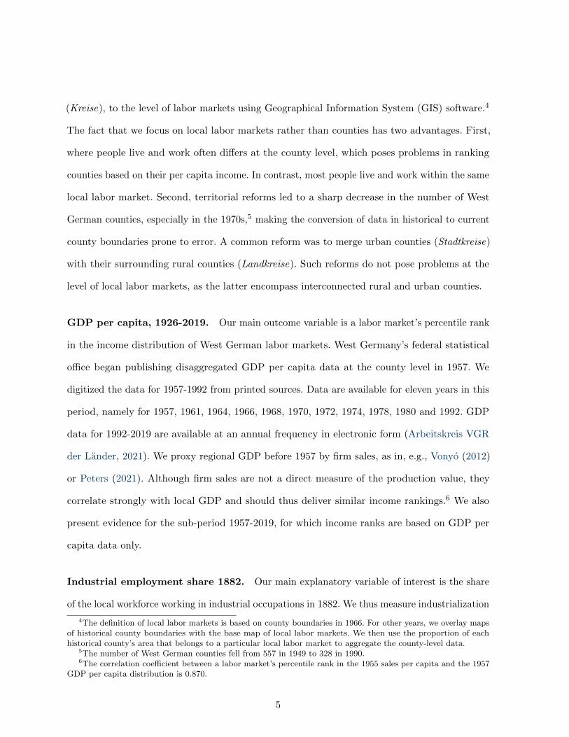
(Kreise), to the level of labor markets using Geographical Information System (GIS) software.4

The fact that we focus on local labor markets rather than counties has two advantages. First,

where people live and work often differs at the county level, which poses problems in ranking

counties based on their per capita income. In contrast, most people live and work within the same

local labor market. Second, territorial reforms led to a sharp decrease in the number of West

German counties, especially in the 1970s,5 making the conversion of data in historical to current

county boundaries prone to error. A common reform was to merge urban counties (Stadtkreise)

with their surrounding rural counties (Landkreise). Such reforms do not pose problems at the

level of local labor markets, as the latter encompass interconnected rural and urban counties.

GDP per capita, 1926-2019. Our main outcome variable is a labor market’s percentile rank

in the income distribution of West German labor markets. West Germany’s federal statistical

office began publishing disaggregated GDP per capita data at the county level in 1957. We

digitized the data for 1957-1992 from printed sources. Data are available for eleven years in this

period, namely for 1957, 1961, 1964, 1966, 1968, 1970, 1972, 1974, 1978, 1980 and 1992. GDP

data for 1992-2019 are available at an annual frequency in electronic form (Arbeitskreis VGR

der Lander, 2021). We proxy regional GDP before 1957 by firm sales, as in, e.g., Vonyo (2012)

or Peters (2021). Although firm sales are not a direct measure of the production value, they

correlate strongly with local GDP and should thus deliver similar income rankings.6 We also

present evidence for the sub-period 1957-2019, for which income ranks are based on GDP per

capita data only.

Industrial employment share 1882. Our main explanatory variable of interest is the share

of the local workforce working in industrial occupations in 1882. We thus measure industrialization

4The definition of local labor markets is based on county boundaries in 1966. For other years, we overlay mapsof historical county boundaries with the base map of local labor markets. We then use the proportion of eachhistorical county’s area that belongs to a particular local labor market to aggregate the county-level data.

5The number of West German counties fell from 557 in 1949 to 328 in 1990.6The correlation coefficient between a labor market’s percentile rank in the 1955 sales per capita and the 1957

GDP per capita distribution is 0.870.

5

after Germany’s take-off phase, typically dated to 1840-1870s, but before the rise of new industries

during Germany’s Hochindustrialisierung (Ziegler, 2012; Tilly & Kopsidis, 2020). Our measure

comes from the first German-wide occupation census that contains results at the county level

(Kaiserliches Statististisches Amt, 1884). In a robustness check, we focus only on industrial

occupations that have been identified as pivotal for Germany’s industrial take-off, namely those

in coal mining, iron and metal processing, construction of machines and instruments, and the

textile industry.

Distance to European coal fields. Our empirical analysis uses an instrumental variable

strategy to identify the causal effect of early industrialization on development. We use the

weighted least-cost distance to European coalfields as an instrument for the 1882 employment

share in industrial occupations. Access to coal is widely acknowledged as a key factor behind

the success of Germany’s early industrializing regions, which relied mainly on heavy industries

(Fremdling, 1977; Ziegler, 2012). Fernihough & O’Rourke (2020) have recently demonstrated the

importance of coal for the European Industrial Revolution in general.

Previous studies have used the proximity to the nearest coal-bearing rock strata as an

instrument for the historical use of steam engines (de Pleijt, Nuvolari & Weisdorf, 2020) and

coal mining (Esposito & Abramson, 2021). In contrast to these papers, we use the weighted least

coast distance to all European coalfields to account for the fact that the closest coalfield is not

necessarily the one that can be reached with the lowest transportation costs. This modification is

important for the German context. In particular, regions in northern and northeastern Germany

initially relied primarily on British coal, rather than coal from closer German mines, because of

the low cost of river and sea transportation (Fremdling, 1979).7

To calculate the instrumental variable, we first divide Europe in a one-by-one kilometer grid.

Based on the local geography, we assign each cell a specific transportation cost, which we take

7The relatively low price of English coal in northern Germany was also due to lower production costs in Englishmines, but this is not accounted for by our instrument.

6

from Daudin (2010). We normalize the cost to one for cells that have access to the sea. Cells with

access to a major river are assigned a cost value of 1.018, all other cells are assigned Daudin’s

value for road transport of 2.963.8 We then calculate the least-cost distance from each region to

all European coalfields, using the grid as cost surface. The algorithm finds the least-cost path

from a region to a coalfield, adding cell-specific costs along the way. The instrument for a given

region i, Ci, is the sum of the least-cost distances to all coalfields, using the area of coalfields as

weights:

Ci =

K∑k=1

areakcostik

, (1)

where costik is the least cumulative costs from region i to coalfield k and areak is the area of the

coalfield polygon in square kilometers. We take the location and extent of European coalfields

from Fernihough & O’Rourke (2020).

Figure 1 illustrates the regional variation in the instrument as well as the location of the most

important coalfields, coast lines and major rivers. Higher values indicate more favorable access

to coal. Not surprisingly, access is most favorable in the Ruhr region and in regions connected to

the Ruhr by rivers. Regions in northern Germany also have relatively favorable access to coal

because they can obtain British coal via the North Sea. To ensure that the instrument does not

just pick up the connectedness of a labor market within Europe, our empirical analysis controls

for a labor market’s sum of least-cost distances to all European grid cells on land using the same

cost vector as in equation (1) (see Section 4 for details on the empirical specification).

3 The evolution of regional per capita income, 1926-2019

Shifts in the relative position of labor markets. Table 1 documents marked changes in

the relative position of West German labor markets over the past 100 years or so. It shows the

8We take shape files of major European rivers from Fernihough & O’Rourke (2020). The value for rivers is theaverage of upstream and downstream river transport. We also probe the robustness of our results to alternativecosts vectors. In particular, we use squared transport costs and assign higher costs of 2.476 and to river and 9.75road transport, respectively, following Bairoch (1990). We also restrict the set of rivers to those that are at least20 meters wide and two meters deep in an additional robustness check.

7

Figure 1: Weighted least-cost distance to European coalfields

Major riversCoast lineMajor coal fields

Transp.-cost weighted coal access0.0634 - 0.0751 0.0751 - 0.0802 0.0802 - 0.0869 0.0869 - 0.0914 0.0914 - 0.0985 0.0985 - 0.1149 0.1149 - 0.4011

Note: See the main text for details on the construction of the weighted least-cost distance. The transport cost

vector is taken from Daudin (2010).

transitions between quartiles of the income distribution from 1926 to 2019. Change is abound:

more than half of the labor markets that were in the bottom quartile of the income distribution

in 1926 are now in the top half of the distribution. Conversely, half of the richest labor markets

in 1926 are now in the bottom half of the distribution (and 20% of them are even in the bottom

quartile). Overall, about half of West German labor markets have experienced a reversal of

fortune, i.e., they have moved from the lower to the upper median of the income distribution or

vice versa.9 The correlation between income ranks in 1926 and 2019 is only weakly positive at

0.100 and not statistically significantly different from zero.

The maps in Figure 2 illustrate how the economic weights within West Germany have shifted

over time. For each West German labor market, the maps show its quartile rank in the income

distribution in 1926, 1957, and 2019. In 1926, the economic powerhouses are scattered across the

9Appendix Table A-1 shows that reversals are only slightly less frequent in 1957-2019 (when we have GDP percapita data also for the initial year).

8

Table 1: Transitions between quartiles of the income distribution, 1926-2019 (frequencies, rowpercent)

2019Bottom Second Third Top

∑Bottom 0.244 0.195 0.439 0.122 1.000

(10) (8) (18) (5) (41)

1926

Second 0.342 0.244 0.220 0.195 1.000(14) (10) (9) (8) (41)

Third 0.220 0.268 0.122 0.390 1.000(9) (11) (5) (16) (41)

Top 0.200 0.300 0.225 0.275 1.000(8) (12) (9) (11) (40)∑

0.252 0.252 0.252 0.245 1.000(41) (41) (41) (40) (163)

Notes: The table compares positions in the income distributionof West German labor markets in 1926 and 2019. Entries arefrequencies, expressed in row percentages. The count for eachcell is in brackets. The ranking of labor markets in 1926 and2019 is based on sales and GDP per capita data, respectively.Cells shaded in green (red) indicate labor markets rising from thebottom (top) to the top (bottom) half of the income distribution.

country. They are mainly concentrated in the metropolitan areas in the west (Rhineland, Ruhr

region) and north (Bremen, Hamburg). But there are also clusters of rich labor markets in the

south, e.g. around Stuttgart or Munich. Poorer labor markets are concentrated in the southeast

of West Germany.

In 2019, the regional distribution of incomes has changed significantly. Labor markets in the

Ruhr area in particular have slipped in the income ranking. The same applies to some of the

historically rich regions in northern Germany, such as Bremerhaven or Itzehoe. By contrast, only

a few of today’s poorest labor markets are still to be found in the southeast. Instead, the poorest

regions are now concentrated in the far west and northwest of West Germany. Several large

centers of the automotive industry (Wolfsburg, Ingolstadt, Munich, Stuttgart and Sindelfingen)

top the rankings, accompanied by large cities such as Frankfurt, Dusseldorf and Cologne.

The emerging North-South divide. Figure 2 illustrates that the economic weights within

West Germany have shifted significantly over the period 1926-2019. The regions that lost ground

9

Figure 2: Regional income in West German labor markets, 1926-2019 (quartile ranks)

1 - 34

Bottom Quartile Second Quartile Third Quartile Top Quartile

(a) 1926 (b) 1957 (c) 2019

Notes: Each map shows the quartile rank in the income distribution of West German labor markets in 1926(panel (a)), 1957 (panel (b)) and 2019 (panel (c)).

in the income distribution were predominantly in the west and north, while the winning regions

were predominately in the south of Germany (see Appendix Figure A-3 for a map illustrating the

transitions between the top and bottom halves in 1926-2019). The North-South divide, subject

of current policy debates (e.g., Schrader & Laaser, 2019), has thus emerged over the past 100

years or so.

We date the emergence of the divide, and quantify its extent, by estimating the following

regression for different years:

yi,t = α+ βtNi + εi,t, (2)

where yi,t is the percentile rank of labor market i in the income distribution of year t and Ni

is a dummy for labor markets located in the north.10 Parameter βt then measures the average

10 Our baseline definition of northern labor markets adheres to federal states borders. It classifies labor markets

10

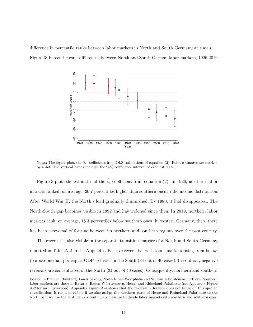
difference in percentile ranks between labor markets in North and South Germany at time t.

Figure 3: Percentile rank differences between North and South German labor markets, 1926-2019

-40

-30

-20

-10

010

2030

Perc

entil

e ra

nks

1920 1930 1940 1950 1960 1970 1980 1990 2000 2010 2020Year

Notes: The figure plots the βt coefficients from OLS estimations of equation (2). Point estimates are markedby a dot. The vertical bands indicate the 95% confidence interval of each estimate.

Figure 3 plots the estimates of the βt coefficient from equation (2). In 1926, northern labor

markets ranked, on average, 20.7 percentiles higher than southern ones in the income distribution.

After World War II, the North’s lead gradually diminished. By 1980, it had disappeared. The

North-South gap becomes visible in 1992 and has widened since then. In 2019, northern labor

markets rank, on average, 18.3 percentiles below southern ones. In western Germany, then, there

has been a reversal of fortune between its northern and southern regions over the past century.

The reversal is also visible in the separate transition matrices for North and South Germany,

reported in Table A-2 in the Appendix. Positive reversals—with labor markets rising from below-

to above-median per capita GDP—cluster in the South (34 out of 40 cases). In contrast, negative

reversals are concentrated in the North (31 out of 40 cases). Consequently, northern and southern

located in Bremen, Hamburg, Lower Saxony, North Rhine-Westphalia and Schleswig-Holstein as northern. Southernlabor markets are those in Bavaria, Baden-Wurttemberg, Hesse, and Rhineland-Palatinate (see Appendix FigureA-2 for an illustration). Appendix Figure A-4 shows that the reversal of fortune does not hinge on this specificclassification. It remains visible if we also assign the northern parts of Hesse and Rhineland-Palatinate to theNorth or if we use the latitude as a continuous measure to divide labor markets into northern and southern ones.

11

labor markets drastically changed their overall position in the national income distribution. For

example, the share of northern labor markets in the top income quartile fell from 65.0% in 1926

to just 27.5% in 2019. Conversely, the North’s share in the lowest income quartile increased from

only 14.6% to 61.0%.

The end of convergence. Underlying the marked shifts in the relative position of West

German labor markets are regional differences in growth rates. Importantly, we observe β-

convergence among West German labor markets only until 1992 but not thereafter. Let yi,t be

GDP per capita of economy i at time t. Absolute convergence implies that in a regression of

(annualized) growth between time t and time t+ s on initial GDP,

1

slog

(yi,t+syi,t

)= α+ βlog (yi,t) + εi,t+s, (3)

the parameter β is negative (see, e.g., Barro & Sala-i Martin, 1991).11

Figure 4: β-convergence from various starting dates to 2019

-1.5

-1-.5

0.5

β

1960 1970 1980 1990 2000 2010Year

Notes: The figure plots the β coefficients from OLS estimations of equation (3). Point estimates are marked by adot. The vertical bands indicate the 95% confidence interval of each estimate. Each estimate comes from a separateregression. Regressions differ in the starting point for calculating annualized GDP growth. The starting points are 1957,1961, 1970, 1980, 1992, 2000, 2009. The end point is always 2019.

11Tests of β-convergence are typically motivated by the neoclassical growth model. It predicts that poorereconomies with smaller capital stocks grow faster due to diminishing returns. Given access to the same technology,poorer countries then catch up with richer ones as they accumulate capital faster. Another driver of convergence istechnology transfers from leader to follower economies (e.g. Abramovitz, 1986).

12

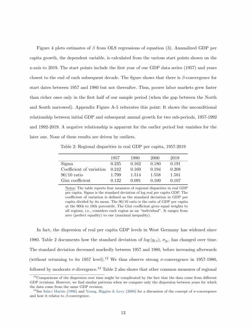
Figure 4 plots estimates of β from OLS regressions of equation (3). Annualized GDP per

capita growth, the dependent variable, is calculated from the various start points shown on the

x-axis to 2019. The start points include the first year of our GDP data series (1957) and years

closest to the end of each subsequent decade. The figure shows that there is β-convergence for

start dates between 1957 and 1980 but not thereafter. Thus, poorer labor markets grew faster

than richer ones only in the first half of our sample period (when the gap between the North

and South narrowed). Appendix Figure A-5 reiterates this point: It shows the unconditional

relationship between initial GDP and subsequent annual growth for two sub-periods, 1957-1992

and 1992-2019. A negative relationship is apparent for the earlier period but vanishes for the

later one. None of these results are driven by outliers.

Table 2: Regional disparities in real GDP per capita, 1957-2019

1957 1980 2000 2019

Sigma 0.235 0.162 0.180 0.191Coefficient of variation 0.242 0.169 0.194 0.20890/10 ratio 1.799 1.514 1.558 1.581Gini coefficient 0.132 0.091 0.100 0.107

Notes: The table reports four measures of regional disparities in real GDPper capita. Sigma is the standard deviation of log real per capita GDP. Thecoefficient of variation is defined as the standard deviation in GDP percapita divided by its mean. The 90/10 ratio is the ratio of GDP per capitaat the 90th to 10th percentile. The Gini coefficient gives equal weights toall regions, i.e., considers each region as an “individual”. It ranges fromzero (perfect equality) to one (maximal inequality).

In fact, the dispersion of real per capita GDP levels in West Germany has widened since

1980. Table 2 documents how the standard deviation of log (yi,t), σyt , has changed over time.

The standard deviation decreased markedly between 1957 and 1980, before increasing afterwards

(without returning to its 1957 level).12 We thus observe strong σ-convergence in 1957-1980,

followed by moderate σ-divergence.13 Table 2 also shows that other common measures of regional

12Comparisons of the dispersion over time might be complicated by the fact that the data come from differentGDP revisions. However, we find similar patterns when we compare only the dispersion between years for whichthe data come from the same GDP revision.

13See Sala-i Martin (1996) and Young, Higgins & Levy (2008) for a discussion of the concept of σ-convergenceand how it relates to β-convergence.

13

disparities exhibit similar trends. All measures declined markedly between 1957 and 1980 but

have increased since then. Similar trends in regional inequality have recently been documented

also for other advanced economies (Floerkemeier et al., 2021; Roses & Wolf, 2021).

4 Early industrialization and economic development, 1926-2019

This section tests the hypothesis that early industrialization was first conducive and later

detrimental for economic development, and examines possible channels through which early

industrialization might still influence development today.

The effect of industrialization on development, 1926-2019. We estimate the effect of

early industrialization on subsequent development using 2SLS. The second stage regression

quantifies the effect of the standardized industrial employment share in 1882, Ii,1882, on a labor

market’s percentile rank in the income per capita distribution:

yi,t = α+ βtIi,1882 + X′iγt + εi,t, (4)

where Xi is a set of control variables. The first stage regression uses the (log) weighted least-cost

distance to European coalfields, Ci, as an instrument for early industrialization (see Section 2 for

details on the construction of the instrument):

Ii,1882 = δ + ζlog (Ci) + X′iηt + ui, (5)

where Xi contains the same control variables as in equation (4).

The key identifying assumption for the 2SLS regression to yield a consistent estimate of

our coefficient of interest, β, is Cov(Ci, εi,t) = 0. The assumption states that (i) there is no

unobserved factor that drives economic development and is correlated with Ci and that (ii) Ci

affects economic development only through its effect on early industrialization. To rule out that

our instrument merely captures favorable location and thus better market access in general, we

include the weighted least-cost distance to all European land cells as control variable. Intuitively,

14

the control measures a region’s geographic isolation within Europe.14 We thus exploit only the

residual variation in coal access, which is not driven by a region’s favorable location in general.

Furthermore, we control for the number of towns per square kilometer in 1700, reported in

Cantoni, Mohr & Weigand (2020), to capture differences in pre-industrial development.

Table 3 reports OLS and 2SLS regression estimates of the effect of early industrialization on

economic development for 1926, 1957, and 2019. These years include the start and end point of our

sample period as well as the first year for which we have GDP per capita data. The OLS estimate

in Column (1) implies that an increase in the 1882 industrial employment share by one standard

deviation improves the rank in the 1926 income distribution by 14.42 percentiles. The 2SLS

estimate in Column (2) is only slightly smaller than the OLS estimate. Early industrialization

was thus still conducive to economic development in 1926. The same holds for 1957 (see Columns

(3) and (4)), just before the coal crisis began with a collapse in demand in the winter of 1957/58.

Table 3: Early industrialization and regional economic development

1926 1957 2019

OLS 2SLS OLS 2SLS OLS 2SLS(1) (2) (3) (4) (5) (6)

Employment share industry 1882 14.42∗∗∗ 13.19∗∗∗ 18.38∗∗∗ 16.75∗∗∗ -2.14 -14.33∗∗∗

(2.14) (3.80) (1.96) (3.12) (1.86) (5.07)

Observations 163 163 163 163 163 163R-squared 0.217 0.399 0.139F-statistic, 1st stage 23.58 23.58 23.58

Notes: The table shows results from OLS (Columns (1), (3), and (5)) and 2SLS (Columns (2), (4), and (6))

regressions of the effect of early industrialization on regional economic development. The ranking in 1926 is based

on sales per capita, the rankings in 1957 and 2019 are based on GDP per capita. The 1882 employment share in

industry, our explanatory variable of interest, is standardized with a mean of zero and a standard deviation of

one. The instrument used in the 2SLS regressions is the weighted average distance to European coalfields where

coalfield sizes serve as weights (see Section 2). All regressions include land accessibility and the number of towns

per area in 1700 as control variables. Robust standard errors are in parentheses. ∗∗∗, ∗∗, and ∗ denote statistical

significance at the 1%, 5%, and 10% level, respectively.

In 2019, in contrast, early industrialization has an adverse effect on a labor market’s ranking

14Ashraf, Galor & Omer Ozak (2010) establish that, in contrast to conventional wisdom, prehistoric geographicalisolation has positive long-run effects on cross-country differences in economic development.

15

in the income distribution. While the OLS estimate in Column (5) is relatively small, the 2SLS

estimate is sizable (Column (6)). The latter implies that an increase in the 1882 industrial

employment share by one standard deviation decreases a labor market’s rank in the income

distribution by 14.33 percentiles. The difference between OLS and 2SLS estimates suggests that

early industrialization correlates with local characteristics that still foster economic development

today.15 The first stage F-Statistic of 23.58 suggests that we do not have a weak instrument

problem (see Stock & Yogo, 2005, for critical values).

Overall, our analysis shows that early industrialization had a long-lasting positive effect on

economic development, which, however, eventually turned negative. Figure 5 plots coefficient

estimates of βt from equation (4) for the years 1926, 1935, 1950, 1957, 1961, 1970, 1980, 1992,

2000, 2010, and 2019. The positive effect of early industrialization is persistent in 1926-1957.

If anything, the effect increases from 1935 to 1957, perhaps reflecting the elevated importance

of heavy industries for both Germany’s war economy and the country’s reconstruction efforts

after the war.16 The positive effect of 19th-century industrialization begins to shrink in 1957, in

parallel with the onset of the coal crisis. The point estimate turns negative in 1992 and has been

declining ever since.

Robustness checks. We conduct several tests to assess the robustness of our 2SLS results.

Table 4 provides the results of these checks. Panel A reproduces our baseline results from Columns

(2), (4), and (6) of Table 3.

First, we add additional control variables to our baseline specification (see Panel B). These

control variables include distance to the inner-German border, which separated West from

East Germany between 1949 and 1990, location at the coast, distance to coast and rivers, and

15Esposito & Abramson (2021) also find that the adverse effects of historical coal mines on contemporary incomeare 2-3 times larger (in absolute magnitude) in their IV regressions compared to the OLS estimates. Franck &Galor (2021) show that the early adoption of steam had negative effects on GDP per capita of French departmentsin 2001-2005. Importantly, their ‘IV estimate reverses the OLS estimates [...] from a positive to a negative one’.

16The coefficient estimate of βt increases from 9.15 in 1935 to 15.68 in 1950 and 16.75 in 1957. This increase cannot reflect the change in the variable used for constructing percentile ranks, as we use sales per capita for both1935 and 1950.

16

Figure 5: The effect of early industrialization on the percentile rank in the income distribution

-20

-10

010

20

1930 1940 1950 1960 1970 1980 1990 2000 2010 2020Year

Notes: The figure plots the βt coefficients from 2SLS estimations of equation (4). Point estimates are markedby a dot. The vertical bands indicate the 95% confidence interval of each estimate. The dependent variableis the percentile rank in the income per capita distribution. The 1882 employment share in industry, ourexplanatory variable of interest, is standardized with a mean of zero and a standard deviation of one.

soil quality. Second, we vary the estimation sample (Panel C). We exclude the Ruhr region,

Germany’s industrial heartland, and the Hanseatic cities of Hamburg and Bremen, focal points of

the industrialization in northern Germany. Third, we construct the instrument using alternative

cost vectors for the least-cost paths to the coalfields (Panel D). The alternative costs vectors use

squared transportation costs, consider only rivers that are at least 20 meters wide and two meters

deep, and place higher costs on river and road transport than our baseline vector (following

Bairoch, 1990). Fourth, we estimate weighted regressions, using the 1882 population and land

area as weights (Panel E). Fifth, we use log GDP per capita as our dependent variable and only

consider the 1882 employment share in core industrial occupations as main explanatory variable

(Panel F). Core occupations, pivotal for Germany’s early industrialization process, include those

in coal mining, iron and metal processing, construction of machines, and the textile industry.

Our main result proves robust in all of these checks: Early industrialization has a beneficial effect

on economic development in the medium term, but a detrimental effect in the long term.

17

Table 4: Robustness checks of 2SLS estimates

1st stage1926 1957 2019 F-stat.(1) (2) (3) (4)

A. Baseline specificationBaseline specification 13.19∗∗∗ 16.75∗∗∗ -14.33∗∗∗ 23.58

(3.80) (3.12) (5.07)

B. Additional control variables...addding distance to inner-German border (logs) 13.62∗∗∗ 15.48∗∗∗ -15.26∗∗∗ 22.63

(4.10) (3.18) (5.40)...adding location at coast (0/1) 13.03∗∗∗ 16.81∗∗∗ -13.95∗∗∗ 23.45

(3.69) (3.14) (4.98)...adding control for soil quality 9.38∗∗ 13.72∗∗∗ -17.78∗∗∗ 22.96

(4.14) (3.26) (5.71)...adding controls for log distance to coast and rivers 9.39∗∗∗ 16.22∗∗∗ -12.96∗∗∗ 31.04

(2.70) (2.53) (4.23)...all of the controls above 7.28∗ 12.23∗∗∗ -16.38∗∗∗ 21.71

(3.91) (3.23) (5.57)

C. Different samples...excluding Ruhr valley 20.34∗∗∗ 19.60∗∗∗ -19.84∗∗ 11.25

(6.42) (5.78) (9.73)...excluding Hanseatic cities 13.00∗∗∗ 16.55∗∗∗ -14.52∗∗∗ 23.50

(3.76) (3.11) (5.10)

D. Alternative cost vectors for the instrument...using squared transportation costs 10.34∗∗∗ 14.43∗∗∗ -18.63∗∗∗ 30.30

(3.23) (2.73) (5.15)...considering only rivers at least 20 meters wide and two meters deep 7.26∗∗ 14.84∗∗∗ -14.89∗∗∗ 29.58

(3.07) (2.61) (4.31)...based on Bairoch (1990) 6.29∗∗ 13.14∗∗∗ -18.10∗∗∗ 23.75

(3.08) (2.60) (4.83)

E. Weighted regressions...weighted by 1882 population 9.01∗∗∗ 11.21∗∗∗ -11.79∗∗∗ 46.58

(3.36) (3.02) (4.32)...weighted by area 8.25 12.39∗ -22.51∗∗∗ 25.83

(7.27) (6.91) (8.71)...using Conley SEs 13.19∗∗∗ 16.75∗∗∗ -14.33∗∗∗ 29.13

(0.45) (1.47) (5.26)

F. Independent and dependent variable...1882 employment share in key industries as indep. variable 12.31∗∗∗ 15.95∗∗∗ -13.65∗∗∗ 19.88

(4.64) (3.92) (5.15)...Log turnover/GDP per capita as dep. variable 0.19∗∗∗ 0.15∗∗∗ -0.09∗∗∗ 23.58

(0.05) (0.03) (0.03)

Notes: The table reports 2SLS estimates of the βt coefficient in equation (4). The dependent variable is the percentile

rank in the income per capita distribution in 1926 (Column (1)), 1957 (Column (2)), and 2019 (Column (3)). All

regressions in Panels A to F include land accessibility and the number of towns per area in 1700 as control variables.

Regressions in Panel B add additional variables to our set of controls. Regressions in Panel C vary the estimation

sample. Regressions in Panel D vary the cost vectors for sea, river and overland transport used for constructing the

instrumental variable. Regressions in Panel E estimate weighted regressions, using population in 1882 and land area

as weights. Regressions in Panel F change the dependent and main explanatory variable. Key industries include coal

mining, machines, textile, iron and metal processing. Robust standard errors are in parentheses. ∗∗∗, ∗∗, and ∗ denote

statistical significance at the 1%, 5%, and 10% level, respectively.

18

The final robustness check in Panel F sheds additional light on the effect size by using levels

of sales (1926) and GDP (1957, 2019) per capita as dependent variables (rather than percentile

ranks). According to the estimates, a one standard deviation increase in the 1882 industrial

employment share increased 1926 sales per capita and 1957 GDP per capita by 0.19 and 0.15 log

points, respectively. However, it decreases current GDP per capita by 0.09 log points.

Channels. Previous work on the long-term effects of industrialization point to the detrimental

effects on human capital as the main channel of transmission (Franck & Galor, 2021). Indeed,

Esposito & Abramson (2021) provide evidence that former coal mining regions in Europe invested

less in tertiary education. In the German context, however, it is unlikely that a lack of investment

in higher education explains the adverse long-term effects of early industrialization. In the Ruhr

region, for example, universities were opened in Bochum (1965), Dortmund (1968), Duisburg

(1972), and Essen (1972). Appendix Table A-4 confirms that early industrialized regions do not

have a lower share of people with a university degree today. Rather, early industrialization is

positively associated with higher education (although the effect is small and not statistically

significant).17

Why does early industrialization impede regional economic development in Germany today

if it does not impair human capital formation? Descriptive evidence suggests that Germany’s

former industrial heartland has little innovation activity today (Kiese, 2019). Deindustrialization

in historically industrial regions has arguably impeded local innovation, as patent applications

are primarily filed in the industrial sector.18 Low levels of innovation, in turn, are likely to slow

regional economic growth (e.g. Akcigit, Grigsby & Nicholas, 2017). Lower innovative activity is

thus a plausible channel through which early industrialization might impede long-term prosperity.

17We use data on individuals with a university degree from the 1970, 1987, and 2011 censuses. Earlier censusesdid not ask about the educational attainment. For none of the three years considered do the 2SLS regressions showa statistically significant effect of early industrialization on the share of individuals with a university degree. Theestimated coefficient changes from negative to positive between 1970 and 2011, consistent with the establishmentof new universities in former industrial regions after World War II.

18Appendix Figure A-6 shows that early industrialization has a positive effect on industrial employment onlyuntil 1970. The effect then becomes increasingly negative, in line with previous findings for France (Franck &Galor, 2021).

19

We employ the causal mediation framework for linear IV models developed by Pinto, Dippel,

Gold & Heblich (2020)19 to test whether the adverse effect of industrialization is indeed mediated

through innovation. Results are in Table 5. Column (1) reproduces our baseline 2SLS results of

the effect of early industrialization on per capita income ranks in 2019. The total effect is −14.332

percentiles. Column (2) shows that early industrialization indeed decreases innovative activity. A

one standard-deviation increase in early industrialization reduces patents per capita in 2003-2012

by 0.355 log points.20 Column (3), in turn, suggests that patenting has a positive effect on a labor

market’s rank in the income distribution (of 30.769 percentiles per log point increase in patents).

Therefore, lower innovation activity explains −10.923 (= −0.355× 30.769) percentiles–or 76%–of

the total effect of early industrialization on economic development. Overall, then, our analysis

suggests that a lower degree of innovation is indeed the primary channel through which early

industrialization impedes contemporary development.

5 Early industrialization, reversal of fortune(s), and changinginequality

To what extent can the blessings and curses of early industrialization explain the changing

fortunes of West German labor markets, documented in Section 3? This section considers the

role of industrialization for two key empirical patterns: the emerging north-south divide and the

fall and rise of regional inequality.

Germany’s reversal of fortune(s). Consider first the north-south divide. Table 6 compares

the actual divide with the predicted divide resulting from our 2SLS estimates. The latter is

19The approach allows us to estimate the proportion of the total treatment effect in linear IV settings that canbe explained by a mediator variable without requiring an additional instrument for the mediator. Identification ispossible under the so-called partial confounding assumption. This assumption states that confounding variablesthat jointly cause the treatment and the mediator are independent of the confounding variables that jointly causethe mediator and the outcome. See Dippel, Ferrara & Heblich (2020) for details on the implementation and Dippel,Gold, Heblich & Pinto (2021) for an application.

20Data on patent applications to the European Patent Office by NUTS-3 regions come from Eurostat. Weaverage patent applications from the last ten years available. Appendix Table A-4 shows that early industrializationalready reduced patent activity in 1983-1992 and 1993-2002, but that the detrimental effect grows over time.

20

Table 5: Early industrialization, patenting activity, and development

2SLS Mediation AnalysisI1882 → y2019 I1882 → p2012 p2012 → y2019

(1) (2) (3)

Employment share industry 1882 (I1882) -14.332∗∗∗ -0.355∗∗∗ -3.409∗

(5.073) (0.101) (2.023)Log patents per 1000 persons 2003-2012 (p2012) 30.769∗∗∗

(8.723)

Direct effect: -3.409∗ (2.023)Indirect effect: -10.923∗∗ (4.391)

Notes: The table presents second stage results of the causal mediation framework for linear IV models introduced

in Pinto et al. (2020). The outcome variable is the GDP per capita rank in 2019, the mediator variable average

patents per capita in 2003-2012 (in logs). Column (1) reproduces, from Column (6) of Table (3), 2SLS regression

results of the effect of early industrialization on the outcome. Column (2) shows 2SLS results of the effect of

early industrialization on the mediator variable, and Column (3) of the effect of the mediator variable on the

outcome (controlling for early industrialization). The indirect effect is the product of the coefficients on early

industrialization in Column (2) and on the mediator variable in Column (3). The instrument is the weighted

average distance to European coalfields where coalfield sizes serve as weights (see Section 2). All regressions

include land accessibility and the number of towns per area in 1700 as control variables. Robust standard errors

are in parentheses. ∗∗∗, ∗∗, and ∗ denote statistical significance at the 1%, 5%, and 10% level, respectively.

the average difference in percentile ranks between northern and southern regions that would

have resulted if the regions had differed only in their 1882 industrial employment share.21 As

shown, the actual mean difference evolves from +20.71 percentiles in 1926 to −18.42 percentiles

in 2019. The mean difference in predicted income ranks follows a similar, though less pronounced,

trajectory.

Our estimates imply that in 1926, per capita income would have been 8.29 percentile ranks

higher in the North than in the South if the regions had differed only in the 1882 employment

share in industrial occupations. This northern advantage in predicted income ranks is due to the

fact that the average industrial employment share in 1882 was considerably larger in the North

than in the South (0.223 versus 0.156) and that early industrialization had a positive effect on

economic development in 1926. By 2019, the average differences in predicted income have become

21We first use the 2SLS estimate of βt in equation (4) to predict each labor market’s income rank, given its 1882industrial employment share. We then estimate the slope coefficient βt from a regression of the predicted incomerank on Ni. The estimate yields the mean difference in predicted GDP per capita rank between northern andsouthern labor markets.

21

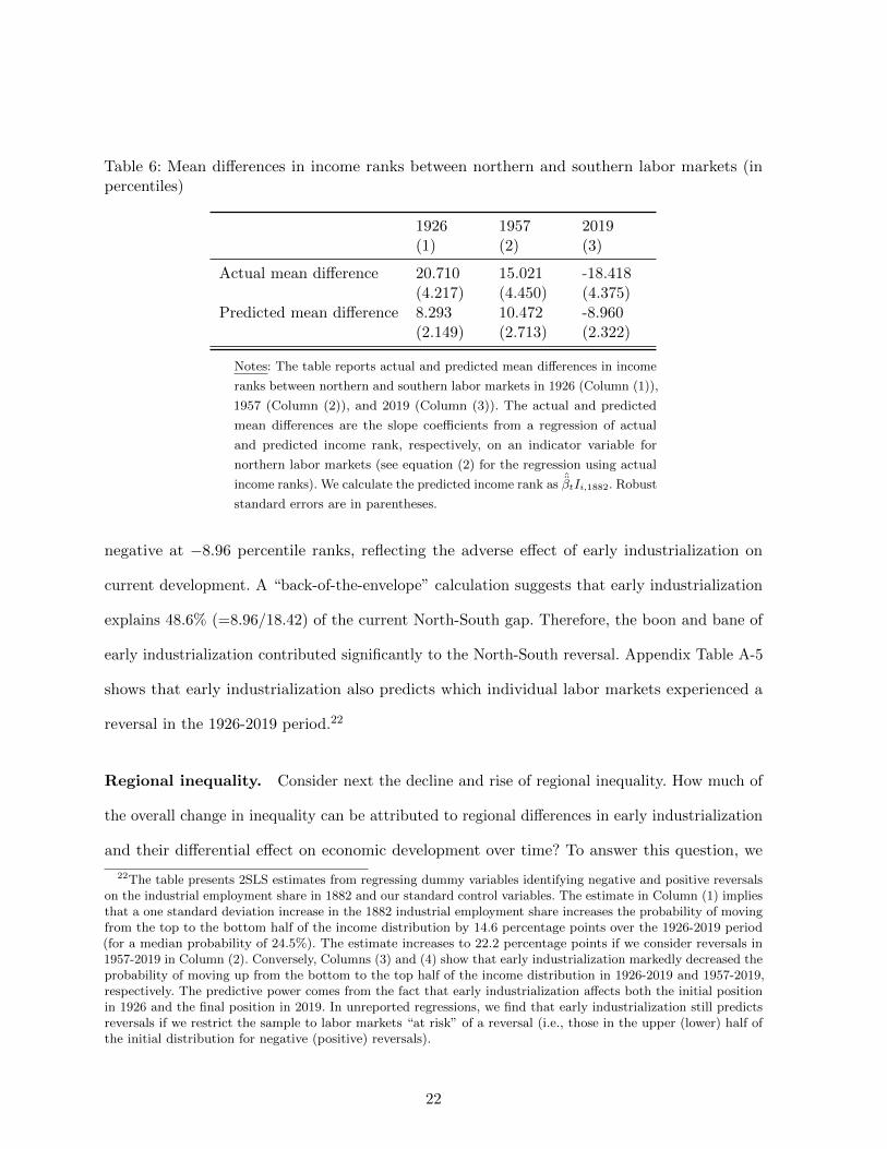
Table 6: Mean differences in income ranks between northern and southern labor markets (inpercentiles)

1926 1957 2019(1) (2) (3)

Actual mean difference 20.710 15.021 -18.418(4.217) (4.450) (4.375)

Predicted mean difference 8.293 10.472 -8.960(2.149) (2.713) (2.322)

Notes: The table reports actual and predicted mean differences in income

ranks between northern and southern labor markets in 1926 (Column (1)),

1957 (Column (2)), and 2019 (Column (3)). The actual and predicted

mean differences are the slope coefficients from a regression of actual

and predicted income rank, respectively, on an indicator variable for

northern labor markets (see equation (2) for the regression using actual

income ranks). We calculate the predicted income rank asˆβtIi,1882. Robust

standard errors are in parentheses.

negative at −8.96 percentile ranks, reflecting the adverse effect of early industrialization on

current development. A “back-of-the-envelope” calculation suggests that early industrialization

explains 48.6% (=8.96/18.42) of the current North-South gap. Therefore, the boon and bane of

early industrialization contributed significantly to the North-South reversal. Appendix Table A-5

shows that early industrialization also predicts which individual labor markets experienced a

reversal in the 1926-2019 period.22

Regional inequality. Consider next the decline and rise of regional inequality. How much of

the overall change in inequality can be attributed to regional differences in early industrialization

and their differential effect on economic development over time? To answer this question, we

22The table presents 2SLS estimates from regressing dummy variables identifying negative and positive reversalson the industrial employment share in 1882 and our standard control variables. The estimate in Column (1) impliesthat a one standard deviation increase in the 1882 industrial employment share increases the probability of movingfrom the top to the bottom half of the income distribution by 14.6 percentage points over the 1926-2019 period(for a median probability of 24.5%). The estimate increases to 22.2 percentage points if we consider reversals in1957-2019 in Column (2). Conversely, Columns (3) and (4) show that early industrialization markedly decreased theprobability of moving up from the bottom to the top half of the income distribution in 1926-2019 and 1957-2019,respectively. The predictive power comes from the fact that early industrialization affects both the initial positionin 1926 and the final position in 2019. In unreported regressions, we find that early industrialization still predictsreversals if we restrict the sample to labor markets “at risk” of a reversal (i.e., those in the upper (lower) half ofthe initial distribution for negative (positive) reversals).

22

decompose the total change in inequality into an “industrialization effect” and a residual. We

calculate the industrialization effect as the difference between observed changes in inequality and

the counterfactual change in inequality that would have occurred in the absence of differences in

early industrialization. The industrialization effect thus measures the contribution of differences

in early industrialization to the change in regional inequality.

Let ycit denote the counterfactual log income per capita of a labor market i in year t, i.e., the

income that would result if the 1882 share of industrial employment had been equal to the mean

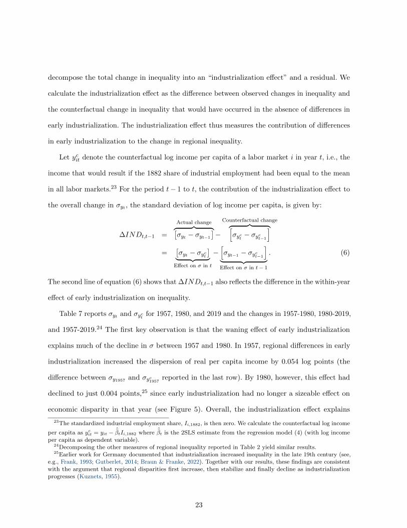
in all labor markets.23 For the period t− 1 to t, the contribution of the industrialization effect to

the overall change in σyt , the standard deviation of log income per capita, is given by:

∆INDt,t−1 =

Actual change︷ ︸︸ ︷[σyt − σyt−1

]−

Counterfactual change︷ ︸︸ ︷[σyct − σyct−1

]=

[σyt − σyct

]︸ ︷︷ ︸Effect on σ in t

−[σyt−1 − σyct−1

]︸ ︷︷ ︸Effect on σ in t− 1

. (6)

The second line of equation (6) shows that ∆INDt,t−1 also reflects the difference in the within-year

effect of early industrialization on inequality.

Table 7 reports σyt and σyct for 1957, 1980, and 2019 and the changes in 1957-1980, 1980-2019,

and 1957-2019.24 The first key observation is that the waning effect of early industrialization

explains much of the decline in σ between 1957 and 1980. In 1957, regional differences in early

industrialization increased the dispersion of real per capita income by 0.054 log points (the

difference between σy1957 and σyc1957reported in the last row). By 1980, however, this effect had

declined to just 0.004 points,25 since early industrialization had no longer a sizeable effect on

economic disparity in that year (see Figure 5). Overall, the industrialization effect explains

23The standardized industrial employment share, Ii,1882, is then zero. We calculate the counterfactual log income

per capita as ycit = yit − ˆβtIi,1882 where

ˆβt is the 2SLS estimate from the regression model (4) (with log income

per capita as dependent variable).24Decomposing the other measures of regional inequality reported in Table 2 yield similar results.25Earlier work for Germany documented that industrialization increased inequality in the late 19th century (see,

e.g., Frank, 1993; Gutberlet, 2014; Braun & Franke, 2022). Together with our results, these findings are consistentwith the argument that regional disparities first increase, then stabilize and finally decline as industrializationprogresses (Kuznets, 1955).

23

−0.050 (=0.004− 0.054) log points–or about 69%–of the actual change in σ of -0.073 over the

1957-1980 period.

Table 7: Components of changes in regional per capita income, 1957-2019

1957- 1980- 1957-1957 1980 2019 1980 2019 2019(1) (2) (3) (2)-(1) (3)-(2) (3)-(1)

σyt 0.235 0.162 0.191 -0.073 0.030 -0.043σyct 0.180 0.158 0.205 -0.023 0.047 0.024

∆ 0.054 0.004 -0.013 -0.050 -0.017 -0.068

Notes: The table reports σyt and σyct, the standard deviation of actual and

counterfactual log per capita income, for 1957 (Column (1)), 1980 (Column (2)),and 2019 (Column (3)). The last row reports σyt − σyc

t, i.e., the effect of early

industrialization on real per capita dispersion in year t. The last three columnsreport changes between 1957-1980, 1980-2019, and 1957-2019, respectively. Cellsshaded in gray report the industrialization effect, ∆INDt,t−1, as defined inequation (6).

The second key result from Table 7 is that the industrialization effect cannot explain the

increase in regional inequality since 1980. The changes in σyt and σyct move largely in parallel

over the 1980-2019 period. Therefore, the increase in regional inequality would have occurred

even if regions had not differed in their industrialization paths. If anything, regional differences

in early industrialization dampened the increase by reducing current inequality. We find that

differences in early industrialization reduced the dispersion of real per capita income by 0.013 log

points in 2019. Because labor markets with higher counterfactual income per capita tend to have

a higher 1882 industrial employment share, a moderately negative effect of early industrialization

on economic development compresses the regional income distribution in our specific context.

An alternative decomposition isolates the change in inequality that is due to changes in βt, the

effect of early industrialization on income. Appendix Table A-6 shows that this decomposition26

delivers even more pronounced results. The waning effect of industrialization—as captured by the

26The decomposition is

Actual change︷ ︸︸ ︷[σyt − σyt−1

]=

Coefficient effect︷ ︸︸ ︷[σyt − σy∗ ] +

Remainder︷ ︸︸ ︷[σy∗ − σyt−1

]where y∗ = yt − (βt − βt−1)Ii,1882. To

obtain y∗, we thus replace the coefficient βt in equation (4) by βt−1, while holding the effect of other observablesand the distribution of residuals fixed. The decomposition is similar in spirit to that proposed by Juhn, Murphy &Pierce (1993). In our context, however, observable characteristics, including Ii,1882, do not vary over time. SeeFortin, Lemieux & Firpo (2011) for an overview of the scope and limitations of different methods for decomposingdistributional statistics.

24

decline in βt—explains all of the decline in regional inequality between 1957 and 1980. What is

more, the increasingly detrimental effect of early industrialization between 1980 and 2019 slightly

reduced regional inequality over this period. These results imply that without changes in βt,

regional inequality in West Germany would have increased substantially between 1957 and 2019.

6 Conclusion

In recent decades, the spatial distribution of economic activity has changed fundamentally in

many advanced countries. Germany is no exception in this respect. Economic power within the

country shifted from the North to the South after World War II. While regional per capita

incomes converged strongly in the 1960s and 1970s, regional inequality in West Germany has

increased again in recent decades. This paper has shown that these far-reaching changes in

the economic geography of West Germany cannot be understood without accounting for the

long-lasting legacy of regional differences in 19th-century industrialization.

We show that early industrialization, measured by industrial employment in 1882, still

strongly favored regional economic development in 1957. However, the positive effect diminished

between 1957 and 1980, and industrialization became a drag on economic development at the

turn of the 21st century. For identification, we exploit variation in access to coal deposits in

Europe, while controlling for the connectedness to European markets. Whereas a one standard

deviation increase in early industrialization improved a labor market’s rank in the West German

income distribution by 16.8 percentiles in 1957, it decreases the 2019 rank by 14.3 percentiles.

The initial blessing and later curse of early industrialization strongly influenced trends in

regional inequality. We show that the waning advantage of early-industrializing regions markedly

reduced regional inequality between 1957 and 1980. Moreover, the gap between North and South

Germany, which emerged in the last forty years or so, cannot be understood without recourse

to the regions’ path to industrialization 140 years ago. Our regression estimates suggest that

differences in early industrialization can explain about half of the current gap between North

25

and South.

Our results have important implications for the policy discourse on regional economic

development. First, they illustrate that the interpretation of contemporary changes in regional

inequality, which have received much attention recently (Iammarino et al., 2018; Floerkemeier

et al., 2021), require careful consideration of the past. Development processes not only have

lasting effects, but can also bring about future changes. Second, our results show that initial

gains from industrialization can come at the expense of long-run losses (see also Matheis, 2016;

Franck & Galor, 2021). This inter-temporal trade-off raises the question of whether policy

interventions can prevent adverse effects in the long term. Indeed, Germany has managed to avoid

the shortage of university graduates in early industrialized regions, observed in other European

regions (Esposito & Abramson, 2021), presumably by establishing new universities in its former

industrial heartland. Further work is needed to clarify how policy interventions can mitigate the

negative long-term effects of industrialization identified in our study.

References

Abelshauser, W. (1984). Der Ruhrkohlenbergbau seit 1945. Wiederaufbau, Krise, Anpassung.C.H. Beck, Munchen.

Abramovitz, M. (1986). Catching up, forging ahead, and falling behind. The Journal of EconomicHistory, 46(2), 385–406.

Akcigit, U., Grigsby, J., & Nicholas, T. (2017). The rise of American ingenuity: innovation andinventors of the Golden Age. NBER Working Papers 23047, National Bureau of EconomicResearch.

Arbeitskreis VGR der Lander (2021). Bruttoinlandsprodukt, Bruttowertschopfung in denkreisfreien Stadten und Landkreisen der Bundesrepublik Deutschland 1992 und 1994 bis 2019.Stuttgart: Statistisches Landesamt Baden-Wurttemberg.

Ashraf, Q., Galor, O., & Omer Ozak (2010). Isolation and development. Journal of the EuropeanEconomic Association, 8(2-3), 401–412.

Austin, B., Glaeser, E., & Summers, L. (2018). Jobs for the heartland: place-based policies in21st-century America. Brookings Papers on Economic Activity, 2018(1), 151–255.

Bairoch, P. (1990). The impact of crop yields, agricultural productivity, and transport costson urban growth between 1800 and 1910. In A. van der Woude, A. Hayami, & J. de Vries

26

(Eds.), Urbanization in history. A process of dynamic interactions, Urbanization in History(pp. 134–151). Oxford University Press.

Barro, R. J. & Sala-i Martin, X. (1991). Convergence across states and regions. BrookingsPapers on Economic Activity, 107–182.

Braun, S. T. & Franke, R. (2022). Railsways, growth, and industrialization in a developingGerman economy, 1829-1910. The Journal of Economic History.

Cantoni, D., Mohr, C., & Weigand, M. (2020). Princes and townspeople: a collection of historicalstatistics on German territories and cities. 3: Town charters and first mentions.

Daudin, G. (2010). Domestic trade and market size in late-eighteenth-century France. TheJournal of Economic History, 70(3), 716–743.

de Pleijt, A., Nuvolari, A., & Weisdorf, J. (2020). Human capital formation during the FirstIndustrial Revolution: evidence from the use of steam engines. Journal of the EuropeanEconomic Association, 18(2), 829–889.

Dippel, C., Ferrara, A., & Heblich, S. (2020). Causal mediation analysis in instrumental-variablesregressions. The Stata Journal, 20(3), 613–626.

Dippel, C., Gold, R., Heblich, S., & Pinto, R. (2021). The effect of trade on workers and voters.The Economic Journal, 132(641), 199–217.

Esposito, E. & Abramson, S. F. (2021). The European coal curse. Journal of Economic Growth,26(1), 77–112.

Fernihough, A. & O’Rourke, K. H. (2020). Coal and the European Industrial Revolution. TheEconomic Journal, 131(635), 1135–1149.

Floerkemeier, H., Spatafora, N., & Venables, A. J. (2021). Regional disparities, growth, andinclusiveness. IMF Working Papers 2021/038, International Monetary Fund.

Fortin, N., Lemieux, T., & Firpo, S. (2011). Decomposition methods in economics. In Handbookof Labor Economics (pp. 1–102). Elsevier.

Franck, R. & Galor, O. (2021). Flowers of evil? Industrialization and long run development.Journal of Monetary Economics, 117, 108–128.

Frank, H. (1993). Regionale Entwicklungsdisparitaten im deutschen Industrialisierungsprozeß1849–1939. Eine empirisch-analytische Untersuchung. PhD thesis, Westfalische Wilhelms-Universitat Munster.

Fremdling, R. (1977). Railroads and German economic growth: a leading sector analysis with acomparison to the United States and Great Britain. The Journal of Economic History, 37(3),583–604.

Fremdling, R. (1979). Modernisierung und Wachstum der Schwerindustrie in Deutschland,1830-1860. Geschichte und Gesellschaft, 5(2), 201–227.

27

Gaubert, C., Kline, P., Vergara, D., & Yagan, D. (2021). Trends in US spatial inequality:concentrating affluence and a democratization of poverty. AEA Papers and Proceedings, 111,520–525.

Gutberlet, T. (2014). Mechanization and the spatial distribution of industries in the GermanEmpire, 1875 to 1907. The Economic History Review, 67(2), 463–491.

Iammarino, S., Rodriguez-Pose, A., & Storper, M. (2018). Regional inequality in Europe: evidence,theory and policy implications. Journal of Economic Geography, 19(2), 273–298.

IfW (1974). Infrastruktur, raumliche Verdichtung und sektorale Wirtschaftsstruktur als Bes-timmungsgrunde des regionalen Entwicklungspotentials in den Arbeitsmarktregionen derBundesrepublik Deutschland. Kiel.

Juhn, C., Murphy, K. M., & Pierce, B. (1993). Wage inequality and the rise in returns to skill.Journal of Political Economy, 101(3), 410–442.

Kaelble, H. & Hohls, R. (1989). Der Wandel der regionalen Disparitaten in der ErwerbsstrukturDeutschlands 1895–1970. In Schriften des Zentralinstituts fur sozialwissenschaftliche Forschungder Freien Universitat Berlin (pp. 288–413). VS Verlag fur Sozialwissenschaften.

Kaiserliches Statististisches Amt (1884). Berufsstatistik nach der allgemeinen Berufszahlung vom5. Juni 1882. 1. Berufsstatistik des Reichs und der kleineren Verwaltungsbezirke. Statistik desDeutschen Reichs. Neue Folge, 2.

Kiese, M. (2019). Strukturwandel 2.0: Das Ruhrgebiet auf dem Weg zur Wissensokonomie?Standort, 43(2), 69–75.

Kiesewetter, H. (1986). Das wirtschaftliche Gefalle zwischen Nord- und Suddeutschland inhistorischer Perspektive. Neues Archiv fur Niedersachsen : Zeitschrift fur Stadt-, Regional-und Landesentwicklung, 35(4), 327–347.

Kiesewetter, H. (2004). Industrielle Revolution in Deutschland. Regionen als Wachstumsmotoren.Stuttgart: Franz Steiner Verlag.

Kuznets, S. (1955). Economic growth and income inequality. The American Economic Review,45(1), 1–28.

Matheis, M. (2016). Local economic impacts of coal mining in the United States 1870 to 1970.The Journal of Economic History, 76(4), 1152–1181.

Nonn, C. (2001). Die Ruhrbergbaukrise. Entindustrialisierung und Politik 1958-1969. Gottingen:Vandenhoeck & Ruprecht.

Persson, J. (1997). Convergence across the Swedish counties, 1911–1993. European EconomicReview, 41(9), 1835–1852.

Peters, M. (2021). Market size and spatial growth – evidence from Germany’s post-war populationexpulsions. NBER Working Papers 29329, National Bureau of Economic Research.

Pinto, R., Dippel, C., Gold, R., & Heblich, S. (2020). Mediation analysis in IV settings with asingle instrument.

28

Rodrıguez-Pose, A. (2018). The revenge of the places that don’t matter (and what to do aboutit). Cambridge Journal of Regions, Economy and Society, 11(1), 189–209.

Roses, J. R. & Wolf, N. (Eds.). (2018a). The economic development of Europe’s regions. Rout-ledge.

Roses, J. R. & Wolf, N. (2018b). The return of regional inequality: Europe from 1900 to today.VOX, CEPR Policy Portal.

Roses, J. R. & Wolf, N. (2021). Regional growth and inequality in the long-run: Europe, 1900–2015.Oxford Review of Economic Policy, 37(1), 17–48.

Sala-i Martin, X. X. (1996). The classical approach to convergence analysis. The EconomicJournal, 106(437), 1019–1036.

Schrader, K. & Laaser, C.-F. (2019). Unterschiede in der Wirtschaftsentwicklung im Norden undSuden Deutschlands. Kieler Beitrage zur Wirtschaftspolitik 20, Kiel Institute for the WorldEconomy (IfW Kiel).

Stock, J. & Yogo, M. (2005). Testing for weak instruments in linear IV regression, (pp. 80–108).New York: Cambridge University Press.

Tilly, R. & Kopsidis, M. (2020). From old regime to industrial state: a history of Germanindustrialization from the eighteenth century to World War I. Chicago: The University ofChicago Press.

Vonyo, T. (2012). The bombing of Germany: the economic geography of war-induced dislocationin West German industry. European Review of Economic History, 16(1), 97–118.

Wolf, N. (2018). Regional economic growth in Germany, 1895–2010. In J. R. Roses & N. Wolf(Eds.), The economic development of Europe’s regions (pp. 149–176). Routledge.

Young, A. T., Higgins, M. J., & Levy, D. (2008). Sigma convergence versus beta convergence:Evidence from US county-level data. Journal of Money, Credit and Banking, 40(5), 1083–1093.

Ziegler, D. (2012). Die Industrielle Revolution (3rd ed.). Darmstadt: Wissenschaftliche Buchge-sellschaft.

29

A Online Appendix

A.1 Background figures and maps

Figure A-1: Normalized GDP per capita of North Germany, 1950-2020 (South Germany = 100)

70

80

90

100

110

120

130

1950 1960 1970 1980 1990 2000 2010 2020

GDP

 per capita

 of N

orthern Germany (Sou

thern Germany = 100)

Year

Notes: The figure depicts the GDP per capita of North Germany relative to that of South Germany. North

Germany includes the federal states of Bremen, Hamburg, Lower Saxony, North-Rhine Westphalia and

Schleswig-Holstein. South Germany includes the federal states of Baden-Wurttemberg, Bavaria, Hesse, and

Rhineland-Palatinate.

Source: Arbeitskreis “Volkswirtschaftliche Gesamtrechnungen der Lander”

30

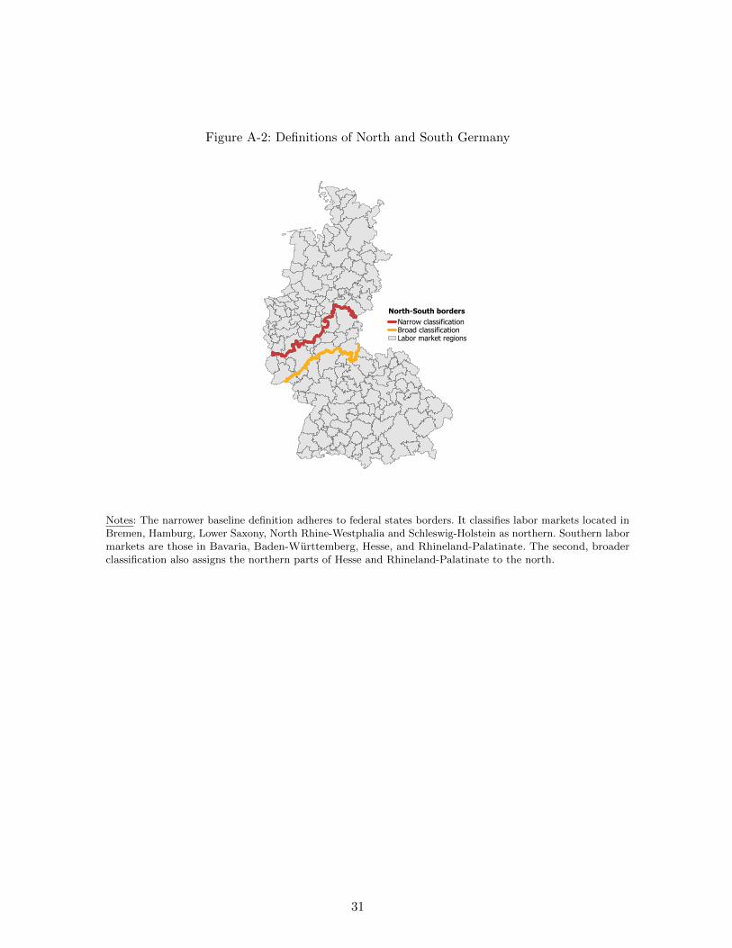
Figure A-2: Definitions of North and South Germany

Narrow classificationBroad classificationLabor market regions

North-South borders

Notes: The narrower baseline definition adheres to federal states borders. It classifies labor markets located inBremen, Hamburg, Lower Saxony, North Rhine-Westphalia and Schleswig-Holstein as northern. Southern labormarkets are those in Bavaria, Baden-Wurttemberg, Hesse, and Rhineland-Palatinate. The second, broaderclassification also assigns the northern parts of Hesse and Rhineland-Palatinate to the north.

31

A.2 The evolution of regional per capita income, 1926-2019

Table A-1: Transitions between quartiles of the income distribution, 1957-2019 (frequencies, rowpercent)

2019Bottom Second Third Top

∑Bottom 0.417 0.220 0.293 0.073 1.000

(17) (9) (12) (3) (41)

1957

Second 0.317 0.220 0.268 0.195 1.000(13) (9) (11) (8) (41)

Third 0.049 0.317 0.293 0.342 1.000(2) (13) (12) (14) (41)

Top 0.225 0.250 0.150 0.375 1.000(9) (10) (6) (15) (40)∑

0.252 0.252 0.252 0.245 1.000(41) (41) (41) (40) (163)

Notes: The table compares positions in the income distributionof West German labor markets in 1957 and 2019. Entries arefrequencies, expressed in row percentages. The count for eachcell is in brackets. The rankings of labor markets are based onGDP per capita data. Cells shaded in green (red) indicate labormarkets rising from the bottom (top) to the top (bottom) half ofthe income distribution.

32

Table A-2: Transitions between quartiles of the income distribution, 1926-2019, by region

2019Bottom Second Third Top

∑Bottom 0.028 0.000 0.042 0.014 0.085

(2) (0) (3) (1) (6)1926

Second 0.140 0.099 0.014 0.014 0.268(10) (7) (1) (1) (19)

Third 0.099 0.127 0.014 0.042 0.282(7) (9) (1) (3) (20)

Top 0.085 0.127 0.070 0.085 0.366(6) (9) (5) (6) (26)∑

0.352 0.352 0.140 0.155 1.000(25) (25) (10) (11) (71)

(a) North

2019Bottom Second Third Top

∑Bottom 0.087 0.087 0.163 0.044 0.380

(8) (8) (15) (4) (35)

1926

Second 0.044 0.033 0.087 0.076 0.239(4) (3) (8) (7) (22)

Third 0.022 0.022 0.044 0.141 0.228(2) (2) (4) (13) (21)

Top 0.022 0.033 0.044 0.054 0.152(2) (3) (4) (5) (14)∑

0.174 0.174 0.337 0.315 1.000(16) (16) (31) (29) (92)

(b) South

Notes: The table compares positions in the income distribution of West German labor markets in 1926 and2019. Panels (a) and (b) show transitions for labor markets located in North and South Germany, respectively.Entries are frequencies, expressed in row percentages. The count for each cell is in brackets. Cells shadedin green (red) indicate labor markets rising from the bottom (top) to the top (bottom) half of the incomedistribution.

33

Figure A-3: Changes in the relative income position, 1926-2019

Transi ons 1926 - 2019

Above median in both yearsBelow median in both yearsFrom below to above medianFrom above to below median

Notes: The figure shows changes in the relative income position between 1926 and 2019. Labor markets shadedin dark green (red) are those rising from the bottom (top) to the top (bottom) half of the income distribution.Labor markets shaded in light green (red) are those that are in the top (bottom) half of the income distributionin both years.

34

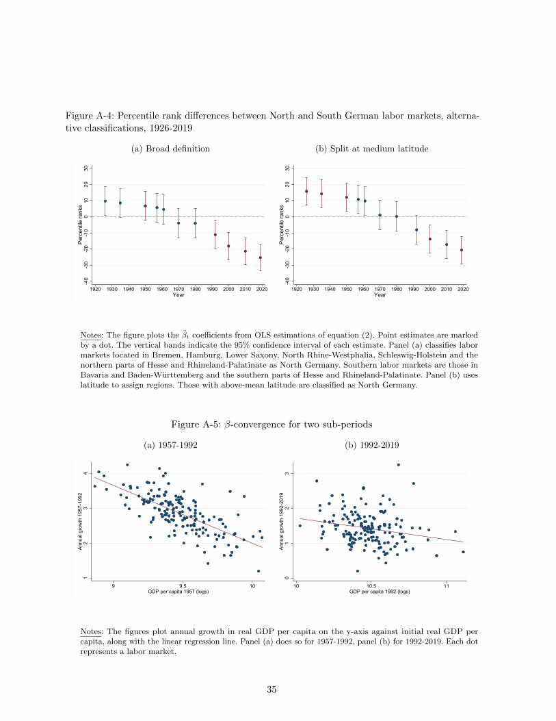
Figure A-4: Percentile rank differences between North and South German labor markets, alterna-tive classifications, 1926-2019

(a) Broad definition

-40

-30

-20

-10

010

2030

Perc

entil

e ra

nks

1920 1930 1940 1950 1960 1970 1980 1990 2000 2010 2020Year

(b) Split at medium latitude

-40

-30

-20

-10

010

2030

Perc

entil

e ra

nks

1920 1930 1940 1950 1960 1970 1980 1990 2000 2010 2020Year

Notes: The figure plots the βt coefficients from OLS estimations of equation (2). Point estimates are markedby a dot. The vertical bands indicate the 95% confidence interval of each estimate. Panel (a) classifies labormarkets located in Bremen, Hamburg, Lower Saxony, North Rhine-Westphalia, Schleswig-Holstein and thenorthern parts of Hesse and Rhineland-Palatinate as North Germany. Southern labor markets are those inBavaria and Baden-Wurttemberg and the southern parts of Hesse and Rhineland-Palatinate. Panel (b) useslatitude to assign regions. Those with above-mean latitude are classified as North Germany.

Figure A-5: β-convergence for two sub-periods

(a) 1957-1992

12

34

Annu

al g

row

th 1

957-

1992

9 9.5 10GDP per capita 1957 (logs)

(b) 1992-2019

01

23

Annu

al g

row

th 1

992-

2019

10 10.5 11GDP per capita 1992 (logs)

Notes: The figures plot annual growth in real GDP per capita on the y-axis against initial real GDP percapita, along with the linear regression line. Panel (a) does so for 1957-1992, panel (b) for 1992-2019. Each dotrepresents a labor market.

35

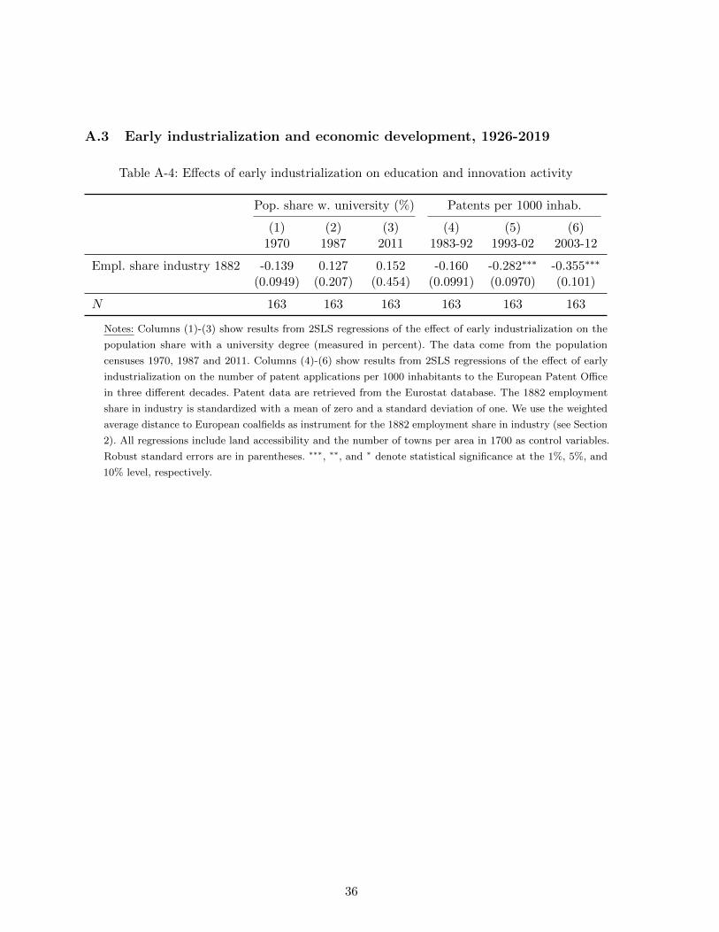
A.3 Early industrialization and economic development, 1926-2019

Table A-4: Effects of early industrialization on education and innovation activity

Pop. share w. university (%) Patents per 1000 inhab.

(1) (2) (3) (4) (5) (6)1970 1987 2011 1983-92 1993-02 2003-12

Empl. share industry 1882 -0.139 0.127 0.152 -0.160 -0.282∗∗∗ -0.355∗∗∗

(0.0949) (0.207) (0.454) (0.0991) (0.0970) (0.101)

N 163 163 163 163 163 163

Notes: Columns (1)-(3) show results from 2SLS regressions of the effect of early industrialization on the

population share with a university degree (measured in percent). The data come from the population

censuses 1970, 1987 and 2011. Columns (4)-(6) show results from 2SLS regressions of the effect of early

industrialization on the number of patent applications per 1000 inhabitants to the European Patent Office

in three different decades. Patent data are retrieved from the Eurostat database. The 1882 employment

share in industry is standardized with a mean of zero and a standard deviation of one. We use the weighted

average distance to European coalfields as instrument for the 1882 employment share in industry (see Section

2). All regressions include land accessibility and the number of towns per area in 1700 as control variables.

Robust standard errors are in parentheses. ∗∗∗, ∗∗, and ∗ denote statistical significance at the 1%, 5%, and

10% level, respectively.

36

Figure A-6: The effect of early industrialization on the employment share in industry, 1939-2019

-.1-.0

50

.05

.1.1

5

1940 1950 1960 1970 1980 1990 2000 2010 2020Year

Notes: The figure plots the coefficient estimates from separate 2SLS regressions of the employment share inindustry in different years t (1939, 1950, 1961, 1970, 1987, 1992, 2004, 2019) on the 1882 industrial employmentshare. Point estimates are marked by a dot. The vertical bands indicate the 95% confidence interval of eachestimate. The 1882 employment share in industry is standardized with a mean of zero and a standard deviationof one. We use the weighted average distance to European coalfields as instrument for the 1882 employmentshare in industry (see Section 2). All regressions include land accessibility and the number of towns per areain 1700 as control variables.

37

A.4 Early industrialization, reversal of fortune(s), and changing inequality

Table A-5: Early industrialization and reversals of fortunes

Negative reversal Positive reversal(0/1) (0/1)

1926-2019 1957-2019 1926-2019 1957-2019

(1) (2) (3) (4)

Employment share industry 1882 0.198∗∗∗ 0.267∗∗∗ -0.176∗∗∗ -0.108∗∗

(0.075) (0.077) (0.054) (0.043)

Outcome mean 0.245 0.209 0.245 0.209

Notes: The table shows results from 2SLS regressions of the effect of early industrialization on

the probability of experiencing a reversal of fortune. The dependent variable is a dummy variable

indicating a negative (Columns (1) and (2)) or positive (Columns (3) and (4)) reversal. We say that

a labor market has experienced a negative (positive) reversal if it moved from the top (bottom)

half of the income distribution to the bottom (top) half in 2019. Columns (1) and (3) take the

rank in 1926 as the starting point, columns (2) and (4) the rank in 1957. The 1882 employment

share in industry is standardized with a mean of zero and a standard deviation of one. We use the

weighted average distance to European coalfields as instrument for the 1882 employment share in

industry (see Section 2). All regressions include land accessibility and the number of towns per

area in 1700 as control variables. Robust standard errors are in parentheses. ∗∗∗, ∗∗, and ∗ denote

statistical significance at the 1%, 5%, and 10% percent level, respectively.

Table A-6: Decomposition of changes in sigmayt , 1957-2019

1957-1980 1980-2019 1957-2019(1) (2) (3)

Total change -0.073 0.030 -0.043

Of which due to:

change in βt -0.080 -0.018 -0.098remainder 0.007 0.048 0.055

Notes: The table decomposes the change in σyt into two compo-

nents, the effect of changes in βt and a remainder. See footnote(26) for details.

38