
Résumé des Travaux en Statistique et Applications des Statistiques
131
HAL Id: tel-00138299 https://tel.archives-ouvertes.fr/tel-00138299 Submitted on 29 Mar 2007 HAL is a multi-disciplinary open access archive for the deposit and dissemination of sci- entific research documents, whether they are pub- lished or not. The documents may come from teaching and research institutions in France or abroad, or from public or private research centers. L’archive ouverte pluridisciplinaire HAL, est destinée au dépôt et à la diffusion de documents scientifiques de niveau recherche, publiés ou non, émanant des établissements d’enseignement et de recherche français ou étrangers, des laboratoires publics ou privés. Résumé des Travaux en Statistique et Applications des Statistiques Stéphan Clémençon To cite this version: Stéphan Clémençon. Résumé des Travaux en Statistique et Applications des Statistiques. Mathéma- tiques [math]. Université de Nanterre - Paris X, 2006. tel-00138299
-
Upload
khangminh22 -
Category
Documents
-
view
1 -
download
0
Transcript of Résumé des Travaux en Statistique et Applications des Statistiques

HAL Id: tel-00138299https://tel.archives-ouvertes.fr/tel-00138299
Submitted on 29 Mar 2007
HAL is a multi-disciplinary open accessarchive for the deposit and dissemination of sci-entific research documents, whether they are pub-lished or not. The documents may come fromteaching and research institutions in France orabroad, or from public or private research centers.
L’archive ouverte pluridisciplinaire HAL, estdestinée au dépôt et à la diffusion de documentsscientifiques de niveau recherche, publiés ou non,émanant des établissements d’enseignement et derecherche français ou étrangers, des laboratoirespublics ou privés.
Résumé des Travaux en Statistique et Applications desStatistiques
Stéphan Clémençon
To cite this version:Stéphan Clémençon. Résumé des Travaux en Statistique et Applications des Statistiques. Mathéma-tiques [math]. Université de Nanterre - Paris X, 2006. tel-00138299

N attribué par la bibliothèque:
UNIVERSITÉ PARIS X - NANTERREEcole Doctorale Connaissance, Langage et Modélisation
Modélisation Aléatoire de Paris X - MODAL’X
Résumé des travaux en vue de l’habilitationà diriger des recherches
Discipline : Mathématiques Appliquées et Applications des Mathématiques.
Stéphan Clémençon
Le 1er Décembre 2006
M. Lucien Birgé ExaminateurM. Peter Buhlmann RapporteurM. Eric Moulines ExaminateurM. Michael Neumann ExaminateurMme Dominique Picard ExaminateurM. Yaacov Ritov RapporteurM. Philippe Soulier RapporteurM. Alexandre Tsybakov Examinateur

Remerciements

ii
Liste de publications et prépublications
• Statistical Inference for an Epidemic Model with Contact-Tracing. (2006), with P. Bertail &V.C. Tran. Submitted.
• Sharp probability inequalities for Markov chains. (2006), with P. Bertail & N. Rhomari.Submitted.
• Statistical analysis of a dynamic model for food contaminant exposure with applications todietary methyl mercury contamination. (2006), with P. Bertail & J. Tressou. Submitted
• A storage model with random release rate for modelling exposure to food contaminant.(2006), with P. Bertail & J. Tressou. Submitted.
• On Ranking the Best Instances. (2006), with N. Vayatis. Submitted.
• Nonparametric scoring and U-processes. (2006), with G. Lugosi & N. Vayatis. Submitted.
• Portfolio Selection under Extreme Risk Measure: the Heavy-Tailed ICA model. (2006), withS. Slim. To appear in International Journal of Theoretical and Applied Finance.
• Approximate Regenerative Block Bootstrap: some simulation studies. (2006), with P. Bertail.To appear in Computational Statistics and Data Analysis.
• Some comments on ’Local Rademacher Complexities and Oracle Inequalities in Risk Mini-mization’ by V. Koltchinskii. (2006), with G. Lugosi & N. Vayatis. In Annals of Statistics,vol. 34, nř6.
• Regeneration-based statistics for Harris Markov chains. (2006), with P. Bertail. In Depen-
dence in Probability and Statistics, eds P. Bertail, P. Soulier & P. Doukhan Lecture Notesin Statistics, No 187, 1-53. Springer-Verlag.
• From classification to ranking: a statistical view. (2006), with G. Lugosi & N. Vayatis. InStudies in Classification, Data Analysis, and Knowledge Organization, From Data andInformation Analysis to Knowledge Engineering, Vol. 30, eds M. Spiliopoulou, R. Kruse,A. Nürnberger, C. Borgelt & W. Gaul (eds.): Proc. 29th Annual Conference of the GfKl,Otto-von-Guericke-University of Magdeburg, March 9-11, 2005, 214-221. Springer-Verlag,Heidelberg-Berlin, 2006.
• Ranking and Scoring Using Empirical Risk Minimization. (2005), with G. Lugosi & N.Vayatis. In Lecture Notes in Computer Science, 3559, Learning Theory: 18th AnnualConference on Learning Theory, COLT 2005, Bertinoro, Italy, June 27-30, 2005. Proceedings.Editors: Peter Auer, Ron Meir, 1-15. Springer-Verlag.
• Regenerative Block Bootstrap for Markov Chains. (2005), with P. Bertail. To appear inBernoulli.

iv
• Note on the regeneration-based bootstrap for atomic Markov chains. (2005), with P. Bertail.To appear in Test.
• Edgeworth expansions for suitably normalized sample mean statistics of atomic Markovchains. (2004), with P. Bertail. Prob. Th. Rel. Fields, 130, 388–414.
• Approximate Regenerative Block-Bootstrap for Markov Chains: second-order properties.(2004), with P. Bertail. In Compstat 2004 Proc. Physica Verlag.
• Statistical Analysis of Financial Time Series under the Assumption of Local Stationarity.(2004), with S. Slim. Quantitative Finance.
• Nonparametric inference for some class of hidden Markov models. (2002). Rapport techniquede l’université Paris X, No 03-9.
• Moment and probability inequalities for sums of bounded additive functionals of regularMarkov chains via the Nummelin splitting technique. (2001), Stat. Prob. Letters, 55,227-238.
• Adaptive estimation of the transition density of a regular Markov chain. (2000), Math. Meth.
Stat., 9, No. 4, 323-357.
• Nonparametric statistics for Markov chains. (2000), PhD thesis, Université Paris 7 DenisDiderot.

Préface
Ce rapport présente brièvement l’essentiel de mon activité de recherche depuis ma thèse de doctorat[53], laquelle visait principalement à étendre l’utilisation des progrès récents de l’Analyse Har-
monique Algorithmique pour l’estimation non paramétrique adaptative dans le cadre d’observationsi.i.d. (tels que l’analyse par ondelettes) à l’estimation statistique pour des données markoviennes.Ainsi qu’il est éxpliqué dans [123], des résultats relatifs aux propriétés de concentration de la mesure(i.e. des inégalités de probabilité et de moments sur certaines classes fonctionnelles, adaptées àl’approximation non linéaire) sont indispensables pour exploiter ces outils d’analyse dans un cadreprobabiliste et obtenir des procédures d’estimation statistique dont les vitesses de convergence sur-passent celles de méthodes antérieures. Dans [53] (voir également [54], [55] et [56]), une méthoded’analyse fondée sur le renouvellement, la méthode dite ’régénérative’ (voir [185]), consistant àdiviser les trajectoires d’une chaîne de Markov Harris récurrente en segments asymptotiquementi.i.d., a été largement utilisée pour établir les résultats probabilistes requis, le comportement à longterme des processus markoviens étant régi par des processus de renouvellement (définissant de façonaléatoire les segments de la trajectoire). Une fois l’estimateur construit, il importe alors de pou-voir quantifier l’incertitude inhérente à l’estimation fournie (mesurée par des quantiles spécifiques,la variance ou certaines fonctionnelles appropriées de la distribution de la statistique considérée).A cet égard et au delà de l’extrême simplicité de sa mise en oeuvre (puisqu’il s’agit simplementd’effectuer des tirages i.i.d. dans l’échantillon de départ et recalculer la statistique sur le nouveléchantillon, l’échantillon bootstrap), le bootstrap possède des avantages théoriques majeurs surl’approximation asymptotique gaussienne (la distribution bootstrap approche automatiquement lastructure du second ordre dans le développement d’Edegworth de la distribution de la statistique).Il m’est apparu naturel de considérer le problème de l’extension de la procédure traditionnelle debootstrap aux données markoviennes. Au travers des travaux réalisés en collaboration avec PatriceBertail, la méthode régénérative s’est avérée non seulement être un outil d’analyse puissant pourétablir des théorèmes limites ou des inégalités, mais aussi pouvoir fournir des méthodes pratiquespour l’estimation statistique: la généralisation du bootstrap proposée consiste à ré-échantillonnerun nombre aléatoire de segments de données régénératifs (ou d’approximations de ces derniers) demanière à imiter la structure de renouvellement sous-jacente aux données. Cette approche s’estrévélée également pertinente pour de nombreux autres problèmes statistiques. Ainsi la premièrepartie du rapport vise essentiellement à présenter le principe des méthodes statistiques fondées surle renouvellement pour des chaînes de Markov Harris.
La seconde partie du rapport est consacrée à la construction et à l’étude de méthodes statistiquespour apprendre à ordonner des objets, et non plus seulement à les classer (i.e. leur affecterun label), dans un cadre supervisé. Ce problème difficile est d’une importance cruciale dans denombreux domaines d’ application, allant de l’élaboration d’indicateurs pour le diagnostic médicalà la recherche d’information (moteurs de recherche) et pose d’ambitieuses questions théoriqueset algorithmiques, lesquelles ne sont pas encore résolues de manière satisfaisante. Une approcheenvisageable consiste à se ramener à la classification de paires d’observations, ainsi que le suggère uncritère largement utilisé dans les applications mentionnées ci-dessus (le critère AUC) pour évaluer la

vi Préface
pertinence d’un ordre. Dans un travail mené en collaboration avec Gabor Lugosi et Nicolas Vayatis,plusieurs résultats ont été obtenus dans cette direction, requérant l’étude de U-processus: l’aspectnovateur du problème résidant dans le fait que l’estimateur naturel du risque a ici la forme d’uneU-statistique. Toutefois, dans de nombreuses applications telles que la recherche d’information,seul l’ordre relatif aux objets les plus pertinents importe véritablement et la recherche de critèrescorrespondant à de tels problèmes (dits d’ordre localisé) et d’algorithmes permettant de construiredes règles pour obtenir des ’rangements’ optimaux à l’égard de ces derniers constitue un enjeucrucial dans ce domaine. Plusieurs développements en ce sens ont été réalisés dans une série detravaux (se poursuivant encore actuellement) en collaboration avec Nicolas Vayatis.
Enfin, la troisième partie du rapport reflète mon intérêt pour les applications des concepts prob-abilistes et des méthodes statistiques. Du fait de ma formation initiale, j’ai été naturellement con-duit à considérer tout d’abord des applications en finance. Et bien que les approches historiques nesuscitent généralement pas d’engouement dans ce domaine, j’ai pu me convaincre progressivementdu rôle important que pouvaient jouer les méthodes statistiques non paramétriques pour analyserles données massives (de très grande dimension et de caractère ’haute fréquence’) disponibles enfinance afin de détecter des structures cachées et en tirer partie pour l’évaluation du risque demarché ou la gestion de portefeuille par exemple. Ce point de vue est illustré par la brève présen-tation des travaux menés en ce sens en collaboration avec Skander Slim dans cette troisième partie.Ces dernières années, j’ai eu l’opportunité de pouvoir rencontrer des mathématiciens appliqués etdes scientifiques travaillant dans d’autres domaines, pouvant également bénéficier des avancées dela modélisation probabiliste et des méthodes statistiques. J’ai pu ainsi aborder des applicationsrelatives à la toxicologie, plus précisément au problème de l’évaluation des risque de contami-nation par voie alimentaire, lors de mon année de délégation auprès de l’Institut National de laRecherche Agronomique au sein de l’unité Metarisk, unité pluridisciplinaire entièrement consacréeà l’analyse du risque alimentaire. J’ai pu par exemple utiliser mes compétences dans le domaine dela modélisation maarkovienne afin de proposer un modèle stochastique décrivant l’évolution tem-porelle de la quantité de contaminant présente dans l’organisme (de manère à prendre en compteà la fois le phénomène d’accumulation du aux ingestions successives et la pharmacocinétique pro-pre au contaminant régissant le processus d’élimination) et des méthodes d’inférence statistiqueadéquates lors de travaux en collaboration avec Patrice Bertail et Jessica Tressou. Cette directionde recherche se poursuit actuellement et l’on peut espérer qu’elle permette à terme de fonder desrecommandations dans le domaine de la santé publique. Par ailleurs, j’ai la chance de pouvoirtravailler actuellement avec Hector de Arazoza, Bertran Auvert, Patrice Bertail, Rachid Lounes etViet-Chi Tran sur la modélisation stochastique de l’épidémie du virus VIH à partir des donnéesépidémiologiques recensées sur la population de Cuba, lesquelles constituent l’une des bases dedonnées les mieux renseignées sur l’évolution d’une épidémie de ce type. Et bien que ce projetvise essentiellement à obtenir un modèle numérique (permettant d’effectuer des prévisions quant àl’incidence de l’épidémie à court terme, de manière à pouvoir planifier la fabrication de la quantitéd’anti-rétroviraux nécéssaire par exemple), il nous a conduit à aborder des questions théoriques am-bitieuses, allant de l’existence d’une mesure quasi-stationnaire décrivant l’évolution à long terme del’épidémie aux problèmes relatifs au caractère incomplet des données épidémiologiques disponibles.Il m’est malheureusement impossible d’évoquer ces questions ici sans risquer de les dénaturer, laprésentation des problèmes mathématiques rencontrés dans ce projet mériterait à elle seule unrapport entier.

Preface
The present report surveys the essentials of my research activity since my PhD thesis [53], which wasmainly devoted to extend the use of recent advances in Computational Harmonic Analysis (suchas wavelet analysis) for adaptive nonparametric estimation methods in the i.i.d. setting to statisticalestimation based on Markovian data. As explained at length in [123], certain concentration ofmeasure properties (i.e. deviation probability and moment inequalities over functional classes,specifically tailored for nonlinear approximation) are crucially required for taking advantages ofthese analytical tools in statistical settings and getting estimation procedures with convergencerates surpassing the ones of older methods. In [53] (see also [54], [55] and [56]), the regenerative
method (refer to [185]), consisting in dividing Harris Markov sample paths into asymptoticallyi.i.d. blocks, has been crucially exploited for establishing the required probabilistic results, thelong term behavior of Markov processes being governed by certain renewal processes (the blocksbeing actually determined by renewal times). But having constructed an estimator, estimation ofthe accuracy (measured by the variance, particular quantiles or any functional of the distributionfunction) of the computed statistic is next of crucial importance. In this respect and beyond itspractical simplicity (it consists in resampling data by making i.i.d. draws in the original data sampleand recompute the statistic from the bootstrap data sample), the bootstrap is known to have majortheoretical advantages over asymptotic normal approximation in the i.i.d. setting (it automaticallyapproximates the second order structure in the Edgeworth expansion of the statistic distribution).I then turned naturally to the problem of extending the popular bootstrap procedure to markoviandata. Through the works I and Patrice Bertail have jointly carried out, the regenerative methodwas revealed to be not solely a powerful analytical tool for proving probabilistic limit theoremsor inequalities, but also to be of practical use for statistical estimation: our proposed bootstrapgeneralization is based on the resampling of (a random number of) regeneration data blocks (or ofapproximation of the latter) so as to mimick the renewal structure of the data. This method hasalso been shown to be advantageous for many other statistical purposes. And the first part of thereport strives to present the principle of regeneration-based statistical methods for Harris Markovchains, as well as some of the various results obtained this way, in a comprehensive manner.
The second part of the report is devoted to the problem of learning how to order instances,instead of classifying them only, in a supervised setting. This difficult problem is of practicalimportance in many areas, ranging from medical diagnosis to information retrieval (IR) and askschallenging theoretical and algorithmic questions, with no entirely satisfactory answers yet. A pos-sible approach to this subject consists in reducing the problem to a pairwise classification problem,as suggested by a popular criterion (namely, the AUC criterion) widely used for evaluating thepertinence of an ordering. In this context some results have been obtained in a joint work withGabor Lugosi and Nicolas Vayatis, involving the study of U-processes: the major novelty consist-ing in the fact that here natural estimates of the risk are of the form of a U-statistic. However,in many applications such as IR, only top ranked instances are effectively scanned and a criterioncorresponding to such local ranking problems as well as methods for computing optimal orderingrules with respect to the latter are crucially needed. Further developments in this direction have

viii Preface
been considered in a (continuing) series of works in collaboration with Nicolas Vayatis.Finally, the last part of the report reflects my interest in practical applications of probabilistic
concepts and statistical tools. My personal background lead me to consider first applications infinance. Although historical approaches are not preferred in this domain, I have been progressivelyconvinced that nonparametric statistics could play a major role in analyzing the massive (of verylarge dimension and high-frequency) financial data for detecting hidden structure in the latterand gaining advantage of the latter in risk assesment or portfolio selection for instance. As anillustration, the works I have carried out with Skander Slim in that direction are described in aword in this third part. Recently, I also happened to meet applied mathematicians or scientistsworking in other fields, which may naturally interface with applied probability ans statistics. Hence,applications to Toxicology, and in particular to toxic chemicals dietary exposure, has also been oneof my concern this last year, which I have spent in the pluridisciplinary research unity Metariskof the National Research Agronomy Institute, entirely dedicated to dietary risk analysis. I couldthus make use of my skills in Markov modelling for proposing a stochastic model describing thetemporal evolution of the total body burden of chemical (in a way that both the toxicokinetics andthe dietary behavior may be taken into account) and adequate inference methods for the latter ina joint work with P. Bertail and J. Tressou. This line of research is still going on and will hopefullyprovide practical insight and guidance for dietary contamination control in public health practice.It is also briefly presented in this last part. Besides, I have the great opportunity to work currentlyon the modelling of the AIDS epidemic with H. de Arazoza, B. Auvert, P. Bertail, R. Lounes and C.Tran based on the cuban epidemic data available, which form one of the most informed database onany HIV epidemic. While such a research project (taking place in the framework of the ACI-NIM"Epidemic Modelling") aims at providing a numerical model (for computing incidence predictionson short horizons for instance, so as to plan the quantity of antiretrovirals required), it also posesvery challenging probabilistic and statistical problems, ranging from the proof for the existence ofa quasi-stationary distribution describing the long term behavior of the epidemic to the difficultiesencountered due to the incomplete character of the epidemic data available. Unfortunately, theyare not discussed here, presenting the wide variety of mathematical problems arising in this projectwithout denaturing it would have deserved a whole report.
Contents
I Statistical Inference for Markov Chains xi
Preliminaries 3
0.1 Markov chain analysis via renewal theory . . . . . . . . . . . . . . . . . . . . . . . . 30.2 Theoretical background . . . . . . . . . . . . . . . . . . . . . . . . . . . . . . . . . . 4
0.2.1 Regenerative Markov chains . . . . . . . . . . . . . . . . . . . . . . . . . . . . 40.2.2 General Harris recurrent chains . . . . . . . . . . . . . . . . . . . . . . . . . . 5
0.3 Dividing the trajectory into (pseudo-) regeneration cycles . . . . . . . . . . . . . . . 70.3.1 Regenerative case . . . . . . . . . . . . . . . . . . . . . . . . . . . . . . . . . . 80.3.2 General Harris case . . . . . . . . . . . . . . . . . . . . . . . . . . . . . . . . . 80.3.3 A coupling result for (Xi, Yi)1in and (Xi, Yi)1in . . . . . . . . . . . . . . 10
0.4 Practical issues . . . . . . . . . . . . . . . . . . . . . . . . . . . . . . . . . . . . . . . 110.4.1 Choosing the minorization condition parameters . . . . . . . . . . . . . . . . 110.4.2 A two-split version of the ARB construction . . . . . . . . . . . . . . . . . . . 12
Regeneration-based statistics for Harris Markov chains 15
0.5 Introduction . . . . . . . . . . . . . . . . . . . . . . . . . . . . . . . . . . . . . . . . . 150.6 Asymptotic mean and variance estimation . . . . . . . . . . . . . . . . . . . . . . . . 15
0.6.1 Regenerative case . . . . . . . . . . . . . . . . . . . . . . . . . . . . . . . . . . 150.6.2 Positive recurrent case . . . . . . . . . . . . . . . . . . . . . . . . . . . . . . . 190.6.3 Some illustrative examples . . . . . . . . . . . . . . . . . . . . . . . . . . . . 22
0.7 Robust functional parameter estimation . . . . . . . . . . . . . . . . . . . . . . . . . 230.7.1 Defining the influence function on the torus . . . . . . . . . . . . . . . . . . . 230.7.2 Some examples . . . . . . . . . . . . . . . . . . . . . . . . . . . . . . . . . . . 240.7.3 Main results . . . . . . . . . . . . . . . . . . . . . . . . . . . . . . . . . . . . . 25
0.8 Some Extreme Values Statistics . . . . . . . . . . . . . . . . . . . . . . . . . . . . . . 270.8.1 Submaxima over regeneration blocks . . . . . . . . . . . . . . . . . . . . . . . 270.8.2 Tail estimation based on submaxima over cycles . . . . . . . . . . . . . . . . 280.8.3 Heavy-tailed stationary distribution . . . . . . . . . . . . . . . . . . . . . . . 280.8.4 Regeneration-based Hill estimator . . . . . . . . . . . . . . . . . . . . . . . . 29
Regenerative-Block Bootstrap for Harris Markov chains 31
0.9 Introduction . . . . . . . . . . . . . . . . . . . . . . . . . . . . . . . . . . . . . . . . . 310.10 The (approximate) regenerative block-bootstrap algorithm . . . . . . . . . . . . . . . 320.11 Main asymptotic results . . . . . . . . . . . . . . . . . . . . . . . . . . . . . . . . . . 33
0.11.1 Second order accuracy of the RBB . . . . . . . . . . . . . . . . . . . . . . . . 330.11.2 Asymptotic validity of the ARBB for general chains . . . . . . . . . . . . . . 34
0.12 Some extensions to U-statistics . . . . . . . . . . . . . . . . . . . . . . . . . . . . . . 350.12.1 Regenerative case . . . . . . . . . . . . . . . . . . . . . . . . . . . . . . . . . . 350.12.2 General case . . . . . . . . . . . . . . . . . . . . . . . . . . . . . . . . . . . . 39

x Contents
0.13 Some simulation studies . . . . . . . . . . . . . . . . . . . . . . . . . . . . . . . . . . 400.13.1 Example 1 : content-dependent storage systems . . . . . . . . . . . . . . . . . 400.13.2 Example 2 : general autoregressive models . . . . . . . . . . . . . . . . . . . 430.13.3 Further remarks . . . . . . . . . . . . . . . . . . . . . . . . . . . . . . . . . . 49
Concluding remarks 51
II Supervised Learning Methods for Ranking Problems 53
Ranking Methods and U-processes 57
0.14 Introduction and preliminaries . . . . . . . . . . . . . . . . . . . . . . . . . . . . . . 570.14.1 The bipartite ranking problem . . . . . . . . . . . . . . . . . . . . . . . . . . 570.14.2 Outline . . . . . . . . . . . . . . . . . . . . . . . . . . . . . . . . . . . . . . . 60
0.15 The ranking problem as a pairwise classification problem . . . . . . . . . . . . . . . 600.16 Empirical ranking risk minimization . . . . . . . . . . . . . . . . . . . . . . . . . . . 630.17 Fast rates . . . . . . . . . . . . . . . . . . . . . . . . . . . . . . . . . . . . . . . . . . 650.18 Examples . . . . . . . . . . . . . . . . . . . . . . . . . . . . . . . . . . . . . . . . . . 680.19 Further remarks on convex risk minimization . . . . . . . . . . . . . . . . . . . . . . 70
Ranking the Best Instances 73
0.20 Introduction . . . . . . . . . . . . . . . . . . . . . . . . . . . . . . . . . . . . . . . . . 730.21 On Finding the Best Instances . . . . . . . . . . . . . . . . . . . . . . . . . . . . . . 73
0.21.1 A mass-constrained classification problem . . . . . . . . . . . . . . . . . . . . 730.21.2 Empirical risk minimization . . . . . . . . . . . . . . . . . . . . . . . . . . . . 740.21.3 Fast Rates . . . . . . . . . . . . . . . . . . . . . . . . . . . . . . . . . . . . . . 75
0.22 The Local Ranking Problem . . . . . . . . . . . . . . . . . . . . . . . . . . . . . . . . 760.22.1 Tailoring a criterion for the local ranking problem . . . . . . . . . . . . . . . 770.22.2 Empirical risk minimization . . . . . . . . . . . . . . . . . . . . . . . . . . . . 80
III Probabilistic Modelling and Applied Statistics 81
Applications in Finance 85
0.23 Time-Frequency Analysis of Financial Time Series . . . . . . . . . . . . . . . . . . . 850.23.1 Statistical analysis of financial returns as locally stationary series . . . . . . . 860.23.2 Empirical results . . . . . . . . . . . . . . . . . . . . . . . . . . . . . . . . . . 89
0.24 ICA Modelling for Safety-First Portfolio Selection . . . . . . . . . . . . . . . . . . . . 910.24.1 On measuring extreme risks of portfolio strategies . . . . . . . . . . . . . . . 920.24.2 The Heavy-Tailed ICA Model . . . . . . . . . . . . . . . . . . . . . . . . . . . 930.24.3 Some empirical results . . . . . . . . . . . . . . . . . . . . . . . . . . . . . . . 96
Applications in Biosciences 99
0.25 Stochastic Toxicologic Models for Dietary Risk Analysis . . . . . . . . . . . . . . . . 990.26 Modeling the exposure to a food contaminant . . . . . . . . . . . . . . . . . . . . . . 990.27 Probabilistic study in the linear rate case . . . . . . . . . . . . . . . . . . . . . . . . 1020.28 Simulation-based statistical inference . . . . . . . . . . . . . . . . . . . . . . . . . . . 104

Part I
Statistical Inference for Markov Chains


1
Abstract
Harris Markov chains make their appearance in many areas of statistical modeling, in particularin time series analysis. Recent years have seen a rapid growth of statistical techniques adapted todata exhibiting this particular pattern of dependence.
In this first part we endeavoured to present how renewal properties of Harris recurrent Markovchains or of specific extensions of the latter may be practically used for statistical inference invarious settings. When the study of probabilistic properties of general Harris Markov chains maybe classically carried out by using the regenerative method (see [185] and [182]), via the theoreticalconstruction of regenerative extensions (see [150]), statistical methodologies may also be based onregeneration for general Harris chains. In the regenerative case, such procedures are implementedfrom data blocks corresponding to consecutive observed regeneration times for the chain. And themain idea for extending the application of these statistical techniques to general Harris chains Xconsists in generating first a sequence of approximate renewal times for a regenerative extension ofX from data X1, ..., Xn and the parameters of a minorization condition satisfied by its transitionprobability kernel, and then applying the latter techniques to the data blocks determined by thesepseudo-regeneration times as if they were exact regeneration blocks.
Numerous applications of this estimation principle may be considered in both the stationaryand nonstationary (including the null recurrent case) frameworks. In Chapter 1, key concepts ofthe Markov chain theory as well as some basic notions about the regenerative method and theNummelin splitting technique are briefly recalled. This preliminary chapter also presents anddiscusses how to practically construct (approximate) regeneration data blocks, on which statisticalprocedures that will be described in the sequel are based. Then Chapters 2 and 3 deal with someimportant procedures based on (approximate) regeneration data blocks, from both practical andtheoretical viewpoints, for the following topics: mean and variance estimation, confidence intervals,Bootstrap, U-statistics, robust estimation and statistical study of extreme values. Finally, someconcluding remarks are collected in Chapter 4 and further lines of research are sketched.

2

Preliminaries
0.1 Markov chain analysis via renewal theory
Renewal theory plays a key role in the analysis of the asymptotic structure of many kinds ofstochastic processes, and especially in the development of asymptotic properties of general irre-ducible Markov chains. The underlying ground consists in the fact that limit theorems proved forsums of independent random vectors may be easily extended to regenerative random processes,that is to say random processes that may be decomposed at random times, called regeneration
times, into a sequence of mutually independent blocks of observations, namely regeneration cycles
(see [185] and [182]). The method based on this principle is traditionally called the regenerative
method. Harris chains that possess an atom, i.e. a Harris set on which the transition probabilitykernel is constant, are special cases of regenerative processes and so directly fall into the range ofapplication of the regenerative method (Markov chains with discrete state space as well as manymarkovian models widely used in operational research for modeling storage or queuing systems areremarkable examples of atomic chains). The theory developed in [150] (and in parallel the closelyrelated concepts introduced in [12]) showed that general Markov chains could all be considered asregenerative in a broader sense (i.e. in the sense of the existence of a theoretical regenerative ex-tension for the chain, see §1.2.2), as soon as the Harris recurrence property is satisfied. Hence thistheory made the regenerative method applicable to the whole class of Harris Markov chains andallowed to carry over many limit theorems to Harris chains such as LLN, CLT, LIL or Edgeworthexpansions.
In many cases, parameters of interest for a Harris Markov chain may be thus expressed in termsof regeneration cycles. While, for atomic Markov chains, statistical inference procedures may bethen based on a random number of observed regeneration data blocks, in the general Harris re-current case the regeneration times are theoretical and their occurrence cannot be determined byexamination of the data only. Although the Nummelin splitting technique for constructing re-generation times has been introduced as a theoretical tool for proving probabilistic results such aslimit theorems or probability and moment inequalities in the markovian framework, it is neverthe-less possible to make a practical use of the latter for extending regeneration-based statistical tools.Our proposal consists in an empirical method for building approximatively a realization drawnfrom a Nummelin extension of the chain with a regeneration set and then recovering approximate
regeneration data blocks. As will be shown in the next two chapters, though the implementationof the latter method requires some prior knowledge about the behaviour of the chain and cruciallyrelies on the computation of a consistent estimate of its transition kernel, this methodology allowsfor numerous statistical applications.
In section 0.2, notations are set out and key concepts of the Markov chain theory as well as somebasic notions about the regenerative method and the Nummelin splitting technique are recalled.Section 0.3 presents how to practically construct (approximate) regeneration data blocks, on whichstatistical procedures presented in the next two chapters are based. Computational issues relatedto this construction are discussed in section 0.4.

4 Preliminaries
0.2 Theoretical background
We first set out the notations and recall a few definitions concerning the communication structureand the stochastic stability of Markov chains (for further detail, refer to [167] or [148]). LetX = (Xn)n be a Markov chain on a countably generated state space (E, ), with transitionprobability Π, and initial probability distribution ν. For any B and n , we thus have
X0 ∼ ν and P(Xn+1 B | X0, ..., Xn) = Π(Xn, B) a.s. .
In what follows, Pν (respectively Px for x in E) denotes the probability measure on the under-lying probability space such that X0 ∼ ν (resp. X0 = x), ν (.) the Pν-expectation (resp. x (.)
the Px-expectation), denotes the indicator function of the event and ⇒ the convergence indistribution.
For completeness, recall the following notions. The first one formalizes the idea of communi-cating structure between specific subsets, while the second one considers the set of time points atwhich such communication may occur.
• The chain is irreducible if there exists a σ-finite measure ψ such that for all set B , whenψ(B) > 0, the chain visits B with strictly positive probability, no matter what the startingpoint.
• Assuming ψ-irreducibility, there is d and disjoints sets D1, ...., Dd (Dd+1 = D1)weighted by ψ such that ψ(E\ ❬1id Di) = 0 and x Di, Π(x,Di+1) = 1. The g.c.d. d ofsuch integers is the period of the chain, which is said aperiodic if d = 1.
A measurable set B is Harris recurrent for the chain if for any x B, Px(∑∞n=1 Xn B =
∞) = 1. The chain is said Harris recurrent if it is ψ-irreducible and every measurable set B suchthat ψ(B) > 0 is Harris recurrent. When the chain is Harris recurrent, we have the property thatPx(
∑∞n=1 Xn B = ∞) = 1 for any x E and any B such that ψ(B) > 0.
A probability measure µ on E is said invariant for the chain when µΠ = µ, where µΠ(dy) =∫xEµ(dx)Π (x, dy). An irreducible chain is said positive recurrent when it admits an invariant
probability (it is then unique).Now we recall some basics concerning the regenerative method and its application to the analysis
of the behaviour of general Harris chains via the Nummelin splitting technique (refer to [151] forfurther detail).
0.2.1 Regenerative Markov chains
Assume that the chain is ψ-irreducible and possesses an accessible atom, i.e. a measurable setA such that ψ(A) > 0 and Π(x, .) = Π(y, .) for all x, y in A. Denote by τA = τA(1) =
inf n 1, Xn A the hitting time on A, by τA(j) = inf n > τA(j− 1), Xn A for j 2 thesuccessive return times to A and by A (.) the expectation conditioned on X0 A. Assume furtherthat the chain is Harris recurrent, the probability of returning infinitely often to the atom A isthus equal to one, no matter what the starting point. Then, it follows from the strong Markov
property that, for any initial distribution ν, the sample paths of the chain may be divided intoi.i.d. blocks of random length corresponding to consecutive visits to A:
1 = (XτA(1)+1, ..., XτA(2)), ..., j = (XτA(j)+1, ..., XτA(j+1)), ...
taking their values in the torus = ❬∞n=1E
n. The sequence (τA(j))j1 defines successive timesat which the chain forgets its past, called regeneration times. We point out that the class of

0.2 Theoretical background 5
atomic Markov chains contains not only chains with a countable state space (for the latter, anyrecurrent state is an accessible atom), but also many specific Markov models arising from the fieldof operational research (see [8] for regenerative models involved in queuing theory, as well as theexamples given in §2.2.3 of Chap. 2). When an accessible atom exists, the stochastic stability
properties of the chain amount to properties concerning the speed of return time to the atom only.For instance, in this framework, the following result, known as Kac’s theorem, holds (cf Theorem10.2.2 in [148]).
Theorem 1 The chain X is positive recurrent iff A(τA) < ∞. The (unique) invariant prob-
ability distribution µ is then the Pitman’s occupation measure given by
µ(B) = A(
τA∑
i=1
Xi B)/A(τA), for all B .
For atomic chains, limit theorems can be derived from the application of the correspondingresults to the i.i.d. blocks (n)n1 (see [52] and the references therein). One may refer for exampleto [148] for the LLN, CLT, LIL, [35] for the Berry-Esseen theorem, [137], [138], [139] and [19] forother refinements of the CLT. The same technique can also be applied to establish moment andprobability inequalities, which are not asymptotic results (see [55] and [25]). As mentioned above,these results are established from hypotheses related to the distribution of the n’s. The followingassumptions shall be involved throughout the next two chapters. Let κ > 0, f : E → be ameasurable function and ν be a probability distribution on (E, ).
Regularity conditions:
0(κ) : A(τκA) < ∞ and 0(κ, ν) : ν(τκA) < ∞.
Block-moment conditions:
1(κ, f) : A((
τA∑
i=1
|f(Xi)|)κ) < ∞,
1(κ, ν, f) : ν((
τA∑
i=1
|f(Xi)|)κ) < ∞.
We point out that conditions 0(κ) and 1(κ, f) do not depend on the accessible atom chosen: if they hold for a given accessible atom A, they are also fulfilled for any other accessible atom(see Chapter 11 in [148]). Besides, the relationship between the ”block moment” conditions andthe rate of decay of mixing coefficients has been investigated in [36]: for instance, 0(κ) (as well as1(κ, f) when f is bounded) is typically fulfilled as soon as the strong mixing coefficients sequencedecreases at an arithmetic rate n−ρ, for some ρ > κ− 1.
0.2.2 General Harris recurrent chains
Regenerative extension. We now recall the splitting technique introduced in [150] for extendingthe probabilistic structure of the chain in order to construct an artificial regeneration set in thegeneral Harris case. It relies on the notion of small set. Recall that, for a Markov chain valued ina state space (E, ) with probability Π, a set S is said to be small if there exist m , δ > 0and a probability measure Γ supported by S s.t., for all x S, B ,
Πm(x, B) δΓ(B), (1)

6 Preliminaries
denoting by Πm the m-th iterate of Π. When this holds, we say that the chain satisfies the mi-
norization condition (m,S, δ, Γ). We emphasize that accessible small sets always exist for ψ-irreducible chains: any set B such that ψ(B) > 0 actually contains such a set (cf [118]). Nowlet us precise how to construct the atomic chain onto which the initial chain X is embedded, froma set on which an iterate Πm of the transition probability is uniformly bounded below. Supposethat X satisfies = (m,S, δ, Γ) for S such that ψ(S) > 0. Even if it entails replacing thechain (Xn)n by the chain
(Xnm, ..., Xn(m+1)−1
)n, we suppose m = 1. The sample space is
expanded so as to define a sequence (Yn)n of independent Bernoulli r.v.’s with parameter δ bydefining the joint distribution Pν, whose construction relies on the following randomization ofthe transition probability Π each time the chain hits S (note that it happens a.s. since the chainis Harris recurrent and ψ(S) > 0). If Xn S and
• if Yn = 1 (which happens with probability δ ]0, 1[), then Xn+1 ∼ Γ ,
• if Yn = 0, (which happens with probability 1− δ), then Xn+1 ∼ (1− δ)−1(Π(Xn+1, .) − δΓ(.)).
Set Berδ(β) = δβ + (1 − δ)(1 − β) for β 0, 1. We now have constructed the split chain, abivariate chain X = ((Xn, Yn))n, valued in E 0, 1 with transition kernel Π defined by
• for any x / S, B , β and β in 0, 1 ,
Π(x, β) , B
β
= Π (x, B)Berδ(β),
• for any x S, B , β in 0, 1 ,
Π(x, 1) , B
β
= Γ(B)Berδ(β),
Π(x, 0) , B
β
= (1− δ)−1(Π (x, B) − δΓ(B))Berδ(β).
Basic assumptions. The whole point of the construction consists in the fact that S 1
is an atom for the split chain X, which inherits all the communication and stochastic stabilityproperties from X (irreducibility, Harris recurrence,...), in particular (for the case m = 1 here)the blocks constructed for the split chain are independent. Hence the splitting method enables toextend the regenerative method, and so to establish all of the results known for atomic chains, togeneral Harris chains. It should be noticed that if the chain X satisfies (m,S, δ, Γ) for m > 1,
the resulting blocks are not independent anymore but 1-dependent, a form of dependence whichmay be also easily handled. For simplicity ’s sake, we suppose in what follows that condition is fulfilled with m = 1, we shall also omit the subscript and abusively denote by Pν theextensions of the underlying probability we consider. The following assumptions, involving thespeed of return to the small set S shall be used throughout this part of the report. Let κ > 0,f : E → be a measurable function and ν be a probability measure on (E, ).
Regularity conditions:
0(κ) : supxS
x(τκS) < ∞ and 0(κ, ν) : ν(τ
κS) < ∞.
Block-moment conditions:
1(κ, f) : supxS
x((
τS∑
i=1
|f(Xi)|)κ) < ∞,

0.3 Dividing the trajectory into (pseudo-) regeneration cycles 7
1(κ, f, ν) : ν((
τS∑
i=1
|f(Xi)|)κ) < ∞.
It is noteworthy that assumptions 0(κ) and 1(κ, f) do not depend on the choice of the smallset S (if they are checked for some accessible small set S, they are fulfilled for all accessible smallsets cf §11.1 in [148]). Note also that in the case when 0(κ) (resp., 0(κ, ν)) is satisfied, 1(κ,f) (resp., 1(κ, f, ν)) is fulfilled for any bounded f. Moreover, recall that positive recurrence,conditions 1(κ) and 1(κ, f) may be practically checked by using test functions methods (cf[121], [191]). In particular, it is well known that such block moment assumptions may be replacedby drift criteria of Lyapounov’s type (refer to Chapter 11 in [148] for further details on suchconditions and many illustrating examples).
We recall finally that such assumptions on the initial chain classically imply the desired condi-tions for the split chain: as soon as X fulfills 0(κ) (resp., 0(κ, ν), 1(κ, f), 1(κ, f, ν)), Xsatisfies 0(κ) (resp., 0(κ, ν), 1(κ, f), 1(κ, f, ν)).
The distribution of (Y1, ..., Yn) conditioned on (X1, ..., Xn+1). As will be shown in thenext section, the statistical methodology for Harris chains we propose is based on approximatingthe conditional distribution of the binary sequence (Y1, ..., Yn) given X(n+1) = (X1, ..., Xn+1). Wethus precise the latter. Let us assume further that the family of the conditional distributionsΠ(x, dy)xE and the initial distribution ν are dominated by a σ-finite measure λ of reference, sothat ν(dy) = f(y)λ(dy) and Π(x, dy) = p(x, y)λ(dy), for all x E. Notice that the minorizationcondition entails that Γ is absolutely continuous with respect to λ too, and that
p(x, y) δγ(y), λ(dy) a.s. (2)
for any x S, with Γ(dy) = γ(y)dy. The distribution of Y(n) = (Y1, ..., Yn) conditionally toX(n+1) = (x1, ..., xn+1) is then the tensor product of Bernoulli distributions given by: for allβ(n) = (β1, ..., βn) 0, 1n , x(n+1) = (x1, ..., xn+1) En+1,
Pν
Y(n) = β(n) | X(n+1) = x(n+1)
=
n∏
i=1
Pν(Yi = βi | Xi = xi, Xi+1 = xi+1),
with, for 1 i n,
Pν(Yi = 1 | Xi = xi, Xi+1 = xi+1) = δ, if xi / S,
Pν(Yi = 1 | Xi = xi, Xi+1 = xi+1) =δγ(xi+1)
p(xi, xi+1), if xi S.
Roughly speaking, conditioned on X(n+1), from i = 1 to n, Yi is drawn from the Bernoulli distri-bution with parameter δ, unless X has hit the small set S at time i: in this case Yi is drawn from theBernoulli distribution with parameter δγ(Xi+1)/p(Xi, Xi+1). We denote by (n)(p, S, δ, γ, x(n+1))
this probability distribution.
0.3 Dividing the trajectory into (pseudo-) regeneration cycles
In the preceding section, we recalled the Nummelin approach for the theoretical construction ofregeneration times in the Harris framework. Here we now consider the problem of approximatingthese random times from data sets in practice and propose a basic preprocessing technique, onwhich estimation methods we shall discuss further are based.

8 Preliminaries
0.3.1 Regenerative case
Let us suppose we observed a sample path X1, ..., Xn of length n drawn from the chain X. Inthe regenerative case, when an atom A for the chain is a priori known, regeneration blocks arenaturally obtained by simply examining the data, as follows.
Algorithm 1 (Regeneration blocks construction)
1. Count the number of visits ln =∑ni=1 Xi A to A up to time n.
2. Divide the observed trajectory X(n) = (X1, ...., Xn) into ln+ 1 blocks corresponding to the
pieces of the sample path between consecutive visits to the atom A,
0 = (X1, ..., XτA(1)), 1 = (XτA(1)+1, ..., XτA(2)), ...,
ln−1 = (XτA(ln−1)+1, ..., XτA(ln)), (n)ln
= (XτA(ln)+1, ..., Xn),
with the convention (n)ln
= when τA(ln) = n.
3. Drop the first block 0, as well as the last one (n)ln
, when non-regenerative (i.e. when
τA(ln) < n).
The regeneration blocks construction is illustrated by Fig. 1 in the case of a random walk onthe half line + with 0 as an atom.
Figure 1: Dividing the trajectory of a random walk on the half line into cycles.
0.3.2 General Harris case
The principle. Suppose now that observations X1, ..., Xn+1 are drawn from a Harris chain Xsatisfying the assumptions of §1.2.2 (refer to the latter paragraph for the notations). If we wereable to generate binary data Y1, ..., Yn, so that X (n) = ((X1, Y1), ..., (Xn, Yn)) be a realization of

0.3 Dividing the trajectory into (pseudo-) regeneration cycles 9
the split chain X described in §1.2.2, then we could apply the regeneration blocks construction
procedure to the sample path X (n). In that case the resulting blocks are still independent sincethe split chain is atomic. Unfortunately, knowledge of the transition density p(x, y) for (x, y) S2is required to draw practically the Yi’s this way. In [22] a method relying on a preliminary estima-tion of the ”nuisance parameter” p(x, y) is proposed. More precisely, it consists in approximatingthe splitting construction by computing an estimator pn(x, y) of p(x, y) using data X1, ..., Xn+1,and to generate a random vector (Y1, ..., Yn) conditionally to X(n+1) = (X1, ..., Xn+1), from dis-tribution (n)(pn, S, δ, γ, X
(n+1)), which approximates in some sense the conditional distribution(n)(p, S, δ, γ, X(n+1)) of (Y1, ..., Yn) for given X(n+1). Our method, which we call approximate re-
generation blocks construction (ARB construction in abbreviated form) amounts then to applythe regeneration blocks construction procedure to the data ((X1, Y1), ..., (Xn, Yn)) as if they weredrawn from the atomic chain X. In spite of the necessary consistent transition density estimationstep, we shall show in the sequel that many statistical procedures, that would be consistent in theideal case when they would be based on the regeneration blocks, remain asymptotically valid whenimplemented from the approximate data blocks. For given parameters (δ, S, γ) (see §1.4.1 for adata driven choice of these parameters), the approximate regeneration blocks are constructed asfollows.
Algorithm 2 (Approximate regeneration blocks construction)
1. From the data X(n+1) = (X1, ..., Xn+1), compute an estimate pn(x, y) of the transition
density such that pn(x, y) δγ(y), λ(dy) a.s., and pn(Xi, Xi+1) > 0, 1 i n.
2. Conditioned on X(n+1), draw a binary vector (Y1, ..., Yn) from the distribution estimate
(n)(pn, S, δ, γ, X(n+1)). It is sufficient in practice to draw the Yi’s at time points i when
the chain visits the set S (i.e. when Xi S), since at these times and at these times
only the split chain may regenerate. At such a time point i, draw Yi according to the
Bernoulli distribution with parameter δγ(Xi+1)/pn(Xi, Xi+1)).
3. Count the number of visits ln =∑ni=1 Xi S, Yi = 1) to the set A = S 1 up
to time n and divide the trajectory X(n+1) into ln+ 1 approximate regeneration blocks
corresponding to the successive visits of (X, Y) to A,
0 = (X1, ..., XτA(1)),
1 = (XτA(1)+1, ..., XτA
(2)), ...,ln−1= (XτA
(ln−1)+1, ..., XτA
(ln)), (n)
ln= (XτA
(ln)+1, ..., Xn+1),
where τA(1) = infn 1, Xn S, Yn = 1 and τA(j+ 1) = infn > τA(j), Xn S, Yn =
1 for j 1.
4. Drop the first block 0 and the last one (n)ln
when τA(ln) < n.Such a division of the sample path is illustrated by Fig. 2 below: from a practical viewpoint
the trajectory may only be cut when hitting the small set. At such a point, drawing a Bernoullir.v. with the estimated parameter indicates whether one should cut here the time series trajectoryor not. Of course, due to the dependence induced by the estimated transition density, the resultingblocks are not i.i.d. but, as will be shown later, are close (in some sense) to the true regenerationblocks which are i.i.d.
Next, the accuracy of this approximation in the Mallows distance’s sense (which metric is acrucial tool for proving asymptotic validity of bootstrap methods, see [30]) is shown to dependmainly on the rate of the uniform convergence of pn(x, y) to p(x, y) over S S.

10 Preliminaries
Figure 2: ARB construction for an AR(1) simulated time-series.
0.3.3 A coupling result for (Xi, Yi)1in and (Xi, Yi)1in
We now state a result claiming that the distribution of (Xi, Yi)1in gets closer and closer to thedistribution of (Xi, Yi)1in in the sense of the Mallows distance (also known as the Kantorovichor Wasserstein metric in the probability literature) as n → ∞. Hence, we express here the distancebetween the distributions PZ and PZ
of two random sequences Z = (Zn)n and Z = (Z
n)n ,
taking their values in k, by (see [160], p 76)
lpZ,Z = lp(P
Z, PZ) = min
Lp
W,W ; W ∼ PZ, W ∼ PZ
,
with (Lp (W,W))1/q
= [Dp (W,W)] , where D denotes the metric on the space χ(k) =
(k)∞ defined by D (w,w) =∑∞k=02
−kwk−wkk . For any w, w in χ(k) (.
k denotingthe usual euclidian norm of k). Thus, viewing the sequences Z(n) = (Xk, Yk)1kn and Z(n) =
(Xk, Yk)1in as the beginning segments of infinite series, we evaluate the deviation between thedistribution P(n) of Z(n) and the distribution P(n) of Z(n) using l1(P(n), P(n)).
Theorem 2 (Bertail & Clémençon, 2005b) Assume that
• S is chosen so that infxSφ(x) > 0,
• p is estimated by pn at the rate αn for the MSE when error is measured by the L∞ loss
over S2,
then
l1(P(n), P(n)) (δ inf
xSφ(x))−1α
1/2n . (3)
This theorem is established in [22] by exhibiting a specific coupling of (Xi, Yi)1in and (Xi, Yi)1in.It is a crucial tool for deriving the results stated in the next two chapters. It also clearly showsthat the closeness between the two distributions is tightly connected to the rate of convergence ofthe estimator pn(x, y) but also to the minorization condition parameters. This gives us some hintson how to choose the small set with a data driven method to obtain better finite sample results,as shall be shown in the following section.
0.4 Practical issues 11
0.4 Practical issues
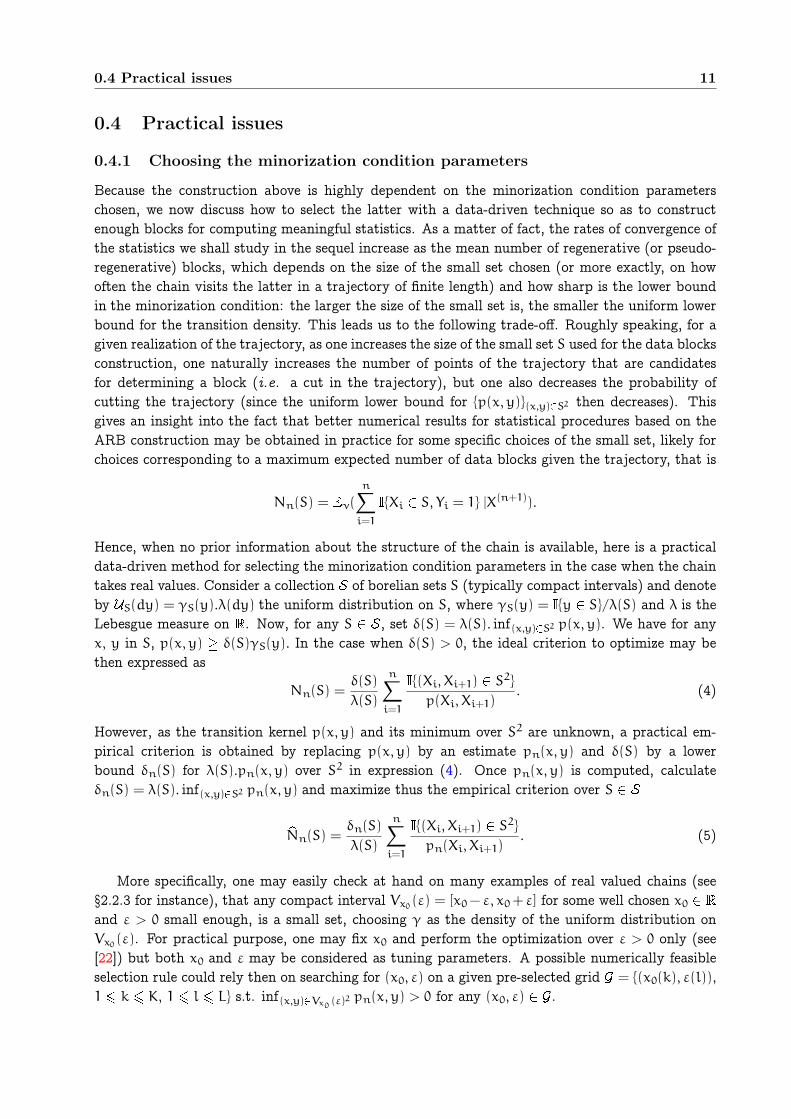
0.4.1 Choosing the minorization condition parameters
Because the construction above is highly dependent on the minorization condition parameterschosen, we now discuss how to select the latter with a data-driven technique so as to constructenough blocks for computing meaningful statistics. As a matter of fact, the rates of convergence ofthe statistics we shall study in the sequel increase as the mean number of regenerative (or pseudo-regenerative) blocks, which depends on the size of the small set chosen (or more exactly, on howoften the chain visits the latter in a trajectory of finite length) and how sharp is the lower boundin the minorization condition: the larger the size of the small set is, the smaller the uniform lowerbound for the transition density. This leads us to the following trade-off. Roughly speaking, for agiven realization of the trajectory, as one increases the size of the small set S used for the data blocksconstruction, one naturally increases the number of points of the trajectory that are candidatesfor determining a block (i.e. a cut in the trajectory), but one also decreases the probability ofcutting the trajectory (since the uniform lower bound for p(x, y)(x,y)S2 then decreases). Thisgives an insight into the fact that better numerical results for statistical procedures based on theARB construction may be obtained in practice for some specific choices of the small set, likely forchoices corresponding to a maximum expected number of data blocks given the trajectory, that is
Nn(S) = ν(
n∑
i=1
Xi S, Yi = 1 |X(n+1)).
Hence, when no prior information about the structure of the chain is available, here is a practicaldata-driven method for selecting the minorization condition parameters in the case when the chaintakes real values. Consider a collection of borelian sets S (typically compact intervals) and denoteby ❯S(dy) = γS(y).λ(dy) the uniform distribution on S, where γS(y) = y S/λ(S) and λ is theLebesgue measure on . Now, for any S , set δ(S) = λ(S). inf(x,y)S2 p(x, y). We have for anyx, y in S, p(x, y) δ(S)γS(y). In the case when δ(S) > 0, the ideal criterion to optimize may bethen expressed as
Nn(S) =δ(S)
λ(S)
n∑
i=1
(Xi, Xi+1) S2p(Xi, Xi+1)
. (4)
However, as the transition kernel p(x, y) and its minimum over S2 are unknown, a practical em-pirical criterion is obtained by replacing p(x, y) by an estimate pn(x, y) and δ(S) by a lowerbound δn(S) for λ(S).pn(x, y) over S2 in expression (4). Once pn(x, y) is computed, calculateδn(S) = λ(S). inf(x,y)S2 pn(x, y) and maximize thus the empirical criterion over S
Nn(S) =δn(S)
λ(S)
n∑
i=1
(Xi, Xi+1) S2pn(Xi, Xi+1)
. (5)
More specifically, one may easily check at hand on many examples of real valued chains (see§2.2.3 for instance), that any compact interval Vx0
(ε) = [x0− ε, x0+ ε] for some well chosen x0
and ε > 0 small enough, is a small set, choosing γ as the density of the uniform distribution onVx0
(ε). For practical purpose, one may fix x0 and perform the optimization over ε > 0 only (see[22]) but both x0 and ε may be considered as tuning parameters. A possible numerically feasibleselection rule could rely then on searching for (x0, ε) on a given pre-selected grid = (x0(k), ε(l)),
1 k K, 1 l L s.t. inf(x,y)Vx0(ε)2 pn(x, y) > 0 for any (x0, ε) .

12 Preliminaries
Algorithm 3 (ARB construction with empirical choice of the small set)
1. Compute an estimator pn(x, y) of p(x, y).
2. For any (x0, ε) , compute the estimated expected number of pseudo-regenerations:
Nn(x0, ε) =δn(x0, ε)
2ε
n∑
i=1
(Xi, Xi+1) Vx0(ε)2
pn(Xi, Xi+1),
with δn(x0, ε) = 2ε. inf(x,y)Vx0(ε)2 pn(x, y).
3. Pick (x0, ε) in maximizing Nn(x0, ε) over , corresponding to the set S = [x0 −
ε, x0+ ε] and the minorization constant δn = δn(x0, ε
).
4. Apply Algorithm 2 for ARB construction using S, δn and pn.
Remark 1 Numerous consistent estimators of the transition density of Harris chains have beenproposed in the literature. Refer to [172], [173], [174] [170], [33], [76], [158], [10] or [54] for instancein positive recurrent cases, [122] in specific null recurrent cases.
This method is illustrated by Fig. 3 in the case of an AR(1) model: Xi+1 = αXi + εi+1,
i , with εii.i.d.∼ (0, 1), α = 0.95 and X0 = 0, for a trajectory of length n = 200. Taking
x0 = 0 and letting ε grow, the expected number regeneration blocks is maximum for ε close to0.9. The true minimum value of p(x, y) over the corresponding square is actually δ = 0.118. Thefirst graphic in this panel shows the Nadaraya-Watson estimator
pn(x, y) =
∑ni=1K(h−1(x− Xi))K(h−1(y− Xi+1))∑n
i=1K(h−1(x− Xi)), (6)
computed from the gaussian kernel K(x) = (2π)−1 exp(−x2/2) with an optimal bandwidth h ∼
n−1/5. The second one plots Nn(ε) as a function of ε. The next one indicates the set S corre-sponding to our empirical rule, while the last one displays the optimal ARB construction.
Note finally that other approaches may be considered for determining practically small sets andestablishing accurate minorization conditions, which conditions do not necessarily involve uniformdistributions besides. Refer for instance to [168] for Markov diffusion processes.
0.4.2 A two-split version of the ARB construction
When carrying out the theoretical study of statistical methods based on the ARB construction, onemust deal with difficult problems arising from the dependence structure in the set of the resultingdata blocks, due to the preliminary estimation step. Such difficulties are somehow similar as theones that one traditionally faces in a semiparametric framework, even in the i.i.d. setting. The firststep of semiparametric methodologies usually consists in a preliminary estimation of some infinitedimensional nuisance parameter (typically a density function or a nonparametric curve), on whichthe remaining (parametric) steps of the procedure are based. For handling theoretical difficultiesrelated to this dependence problem, a well known method, called the splitting trick, amounts tosplit the data set into two parts, the first subset being used for estimating the nuisance parameter,while the parameter of interest is then estimated from the other subset (using the preliminaryestimate). An analogous principle may be implemented in our framework using an additional splitof the data in the ”middle of the trajectory”, for ensuring that a regeneration at least occurs inbetween with an overwhelming probability (so as to get two independent data subsets, see step 2 in

0.4 Practical issues 13
Figure 3: Illustration of Algorithm 3 - ARB construction with empirical choice of the small set.
the algorithm below). For this reason, we consider the following variant of the ARB construction.Let 1 < m < n, 1 p < n−m.
Algorithm 4 (two-split ARB construction)
1. From the data X(n+1) = (X1, ..., Xn+1), keep only the first m observations X(m) for
computing an estimate pm(x, y) of p(x, y) such that pm(x, y) δγ(y), λ(dy) a.s. and
pm(Xi, Xi+1) > 0, 1 i n− 1.
2. Drop the observations between times m + 1 and m = m + p (under standard assump-
tions, the split chain regenerates once at least in between with large probability).
3. From remaining observations X(m,n) = (Xm+1, ..., Xn) and estimate pm, apply steps 2-4
of Algorithm 2 (respectively of Algorithm 3).
This procedure is similar to the 2-split method proposed in [177], except that here the numberof deleted observations is arbitrary and easier to interpret in terms of regeneration. Of course,the more often the split chain regenerates, the smaller p may be chosen. And the main problemconsists in picking m = mn so that mn → ∞ as n → ∞ for the estimate of the transition kernelto be accurate enough, while keeping enough observation n −m for the block construction step:one typically chooses m = o(n) as n → ∞. Further assumptions are required for investigatingprecisely how to select m. In [21], a choice based on the rate of convergence αm of the estimatorpm(x, y) (for the MSE when error is measured by the sup-norm over S S) is proposed: whenconsidering smooth markovian models for instance, estimators with rate αm = m−1 log(m) may be

14 Preliminaries
exhibited and one shows that m = n2/3 is then an optimal choice (up to a log(n)). However, onemay argue, as in the semiparametric case, that this methodology is motivated by our limitationsin the analysis of asymptotic properties of the estimators only, whereas from a practical viewpointit may deteriorate the finite sample performance of the initial algorithm. To our own experience,it is actually better to construct the estimate p(x, y) from the whole trajectory and the interest ofAlgorithm 4 is mainly theoretical.
Regeneration-based statistics for Harris
Markov chains
0.5 Introduction
The present chapter mainly surveys results established at length in [19], [20] and [23]. Moreprecisely, the problem of estimating additive functionals of the stationary distribution in the Harrispositive recurrent case is considered in section 0.6. Estimators based on the (pseudo) regenerativeblocks, as well as estimates of their asymptotic variance are exhibited, and limit theorems describingthe asymptotic behaviour of their bias and their sampling distribution are also displayed. A specificnotion of robustness for statistics based on the (approximate) regenerative blocks is introduced andinvestigated in section 0.7. And asymptotic properties of some regeneration-based statistics relatedto the extremal behaviour of Markov chains are studied in section 0.8 in the regenerative case only.
0.6 Asymptotic mean and variance estimation
In this section, we suppose that the chain X is positive recurrent with unknown stationary proba-bility µ and consider the problem of estimating an additive functional of type µ(f) =
∫f(x)µ(dx) =
µ(f(X1)), where f is a µ-integrable real valued function defined on the state space (E, ). Esti-mation of additive functionals of type µ(F(X1, ..., Xk)), for fixed k 1, may be investigated in asimilar fashion. We set f(x) = f(x) − µ(f).
0.6.1 Regenerative case
Here we assume further that X admits an a priori known accessible atom A. As in the i.i.d. setting,a natural estimator of µ(f) is the sample mean statistic,
µn(f) = n−1
n∑
i=1
f(Xi). (7)
When the chain is stationary (i.e. when ν = µ), the estimator µn(f) is zero-bias. However, its
bias is significant in all other cases, mainly because of the presence of the first and last (non-
regenerative) data blocks 0 and (n)ln
(see Proposition 3 below). Besides, by virtue of Theorem 1,µ(f) may be expressed as the mean of the f(Xi)’s over a regeneration cycle (renormalized by themean length of a regeneration cycle)
µ(f) = A(τA)−1A(
τA∑
i=1
f(Xi)).
Because the bias due to the first block depends on the unknown initial distribution (see Proposition3 below) and thus can not be consistently estimated, we suggest to introduce the following esti-mators of the mean µ(f). Define the sample mean based on the observations (eventually) collected

16 Regeneration-based statistics for Harris Markov chains
after the first regeneration time only by
µn(f) = (n− τA)−1n∑
i=1+τA
f(Xi)
with the convention µn(f) = 0, when τA > n, as well as the sample mean based on the observationscollected between the first and last regeneration times before n by
µn(f) = (τA(ln) − τA)−1
τA(ln)∑
i=1+τA
f(Xi)
with ln =∑ni=1 Xi A and the convention µn(f) = 0, when ln 1 (observe that, by Markov’s
inequality, Pν(ln 1) = O(n−1) as n → ∞, as soon as 0(1, ν) and 0(2) are fulfilled).Let us introduce some additional notation for the block sums (resp. the block lengths), that
shall be used here and throughout. For j 1, n 1, set
L0 = τA, Lj = τA(j+ 1) − τA(j), L(n)ln
= n− τA(ln)
f(0) =
τA∑
i=1
f(Xi), f(j) =
τA(j+1)∑
i=1+τA(j)
f(Xi), f((n)ln
) =
n∑
i=1+τA(ln)
f(Xi).
With these notations, the estimators above may be rewritten as
µn(f) =
f(0) +∑lnj=1 f(j) + f((n)
ln)
L0+∑lnj=1Lj+ L
(n)ln
,
µn(f) =
∑lnj=1 f(j) + f((n)
ln)
∑lnj=1Lj+ L
(n)ln
, µn(f) =
∑lnj=1 f(j)
∑lnj=1Lj
.
Let µn(f) design any of the three estimators µn(f), µn(f) or µn(f). If X fulfills conditions
0(2), 0(2, ν), 1(f, 2,A), 1(f, 2, ν) then the following CLT holds under Pν (cf Theorem 17.2.2in [148])
n1/2σ−1(f)(µn(f) − µ(f)) ⇒ (0, 1) , as n → ∞,
with a normalizing constant
σ2(f) = µ (A)A((
τA∑
i=1
f(Xi) − µ(f)τA)2). (8)
From this expression, the following estimator of the asymptotic variance has been proposed in[19], adopting the usual convention regarding to empty summation,
σ2n(f) = n−1ln−1∑
j=1
(f(j) − µn(f)Lj)2. (9)
Notice that the first and last data blocks are not involved in its construction. We could haveproposed estimators involving different estimates of µ(f), but as will be seen later, it is preferableto consider an estimator based on regeneration blocks only. The following quantities shall beinvolved in the statistical analysis below. Define
α = A(τA), β = A(τA
τA∑
i=1
f(Xi)) = CovA(τA,
τA∑
i=1
f(Xi)),

0.6 Asymptotic mean and variance estimation 17
ϕν = ν(
τA∑
i=1
f(Xi)), γ = α−1A(
τA∑
i=1
(τA− i)f(Xi)).
We also introduce the following technical conditions.(C1) (Cramer condition)
limt→∞
| A(exp(it
τA∑
i=1
f(Xi))) |< 1.
(C2) (Cramer condition)
limt→∞
| A(exp(it(
τA∑
i=1
f(Xi))2)) |< 1.
(C3) There exists N 1 such that the N-fold convoluted density gN is bounded, denoting
by g the density of the (∑τA(2)
i=1+τA(1) f(Xi) − α−1β)2’s.
(C4) There exists N 1 such that the N-fold convoluted density GN is bounded, denoting
by G the density of the (∑τA(2)
i=1+τA(1) f(Xi))2’s.
These two conditions are automatically satisfied if∑τA(2)
i=1+τA(1) f(Xi) has a bounded density. Theresult below is a straightforward extension of Theorem 1 in [137] (see also Prop. 3.1 in [19]).
Proposition 3 (Bertail & Clémençon, 2004a) Suppose that 0(4), 0(2, ν), 1(4, f), 1(2,ν, f) and Cramer condition (C1) are satisfied by the chain. Then, as n → ∞, we have
ν(µn(f)) = µ(f) + (ϕν+ γ− β/α)n−1+O(n−3/2), (10)
ν(µn(f)) = µ(f) + (γ− β/α)n−1+O(n−3/2), (11)
ν(µn(f)) = µ(f) − (β/α)n−1+O(n−3/2). (12)
If the Cramer condition (C2) is also fulfilled, then
ν(σ2n(f)) = σ2(f) +O(n−1), as n → ∞, (13)
and we have the following CLT under Pν,
n1/2(σ2n(f) − σ2(f)) ⇒ (0, ξ2(f)), as n → ∞, (14)
with ξ2(f) = µ(A)VarA((∑τA
i=1 f(Xi))2− 2α−1β
∑τA
i=1 f(Xi)).
We emphasize that in a non i.i.d. setting, it is generally difficult to construct an accurate(positive) estimator of the asymptotic variance. When no structural assumption, except station-arity and square integrability, is made on the underlying process X, a possible method, currentlyused in practice, is based on so-called blocking techniques. Indeed under some appropriate mixingconditions (which ensure that the following series converge), it can be shown that the variance ofn−1/2µ
n(f) may be written
Var(n−1/2µn(f)) = Γ(0) + 2
n∑
t=1
(1− t/n)Γ(t)
and converges to
σ2(f) =
∞∑
t=∞
Γ(t) = 2πg(0),

18 Regeneration-based statistics for Harris Markov chains
where g(w) = (2π)−1∑∞t=−∞ Γ(t) cos(wt) and (Γ(t))t0 denote respectively the spectral density
and the autocovariance sequence of the discrete-time stationary process X.Most of the estimators ofσ2(f) that have been proposed in the literature (such as the Bartlett spectral density estimator, themoving-block jackknife/subsampling variance estimator, the overlapping or non-overlapping batchmeans estimator) may be seen as variants of the basic moving-block bootstrap estimator(see [129],[133])
σ2M,n =M
Q
Q∑
i=1
(µi,M,L− µn(f))2, (15)
where µi,M,L = M−1∑L(i−1)+M
t=L(i−1)+1 f(Xt) is the mean of f on the i-th data block (XL(i−1)+1, . . . ,
XL(i−1)+M). Here, the size M of the blocks and the amount L of ‘lag’ or overlap between each blockare deterministic (eventually depending on n) and Q = [n−M
L]+ 1, denoting by [] the integer part,
is the number of blocks that may be constructed from the sample X1, ..., Xn. In the case whenL = M, there is no overlap between block i and block i+ 1 (as the original solution considered by[101], [50]), whereas the case L = 1 corresponds to maximum overlap (see [154], [156] for a survey).Under suitable regularity conditions (mixing and moments conditions), it can be shown that ifM → ∞ with M/n → 0 and L/M → a [0, 1] as n → ∞, then we have
(σ2M,n) − σ2(f) = O(1/M) +O(qM/n), (16)
Var(σ2M,n) = 2cM
nσ4(f) + o(M/n), (17)
as n → ∞, where c is a constant depending on a, taking its smallest value (namely c = 2/3) fora = 0. This result shows that the bias of such estimators may be very large. Indeed, by optimizingin M we find the optimal choice M ∼ n1/3, for which we have (σ2M,n)−σ2(f) = O(n−1/3). Variousextrapolation and jackknife techniques or kernel smoothing methods have been suggested to getrid of this large bias (refer to [154] [96], [18] and [28]). The latter somehow amount to makeuse of Rosenblatt smoothing kernels of order higher than two (taking some negative values) forestimating the spectral density at 0. However, the main drawback in using these estimators isthat they take negative values for some n, and lead consequently to face problems, when dealingwith studentized statistics. In our specific Markovian framework, the estimate σ2n(f) in the atomiccase (or latter σ2n(f) in the general case) is much more natural and allows to avoid these problems.This is particularly important when the matter is to establish Edgeworth expansions at ordershigher than two in such a non i.i.d. setting. As a matter of fact, the bias of the variance maycompletely cancel the accuracy provided by higher order Edgeworth expansions (but also the oneof its Bootstrap approximation) in the studentized case, given its explicit role in such expansions(see [96]).
From Proposition 3, we immediately derive that
tn = n1/2σ−1n (f)(µn(f) − µ(f)) ⇒ (0, 1) , as n → ∞,
so that asymptotic confidence intervals for µ(f) are immediately available in the atomic case. Thisresult also shows that using estimators µn(f) or µn(f) instead of µ
n(f) allows to eliminate the onlyquantity depending on the initial distribution ν in the first order term of the bias, which maybe interesting for estimation purpose and is crucial when the matter is to deal with an estima-tor of which variance or sampling distribution may be approximated by a resampling procedurein a nonstationary setting (given the impossibility to approximate the distribution of the ”firstblock sum”
∑τA
i=1 f(Xi) from one single realization of X starting from ν). For these estimators, itis actually possible to implement specific Bootstrap methodologies, for constructing second ordercorrect confidence intervals for instance. Regarding to this, it should be noticed that Edgeworth

0.6 Asymptotic mean and variance estimation 19
expansions (E.E. in abbreviated form) may be obtained using the regenerative method by parti-tioning the state space according to all possible values for the number ln regeneration times beforen and for the sizes of the first and last block as in [138]. [19] proved the validity of an E.E. inthe studentized case, of which form is recalled below. Notice that actually (C3) corresponding totheir v) in Proposition 3.1 in [19] is not needed in the unstudentized case. Let Φ(x) denote thedistribution function of the standard normal distribution and set φ(x) = dΦ(x)/dx.
Theorem 4 (Bertail & Clémençon, 2004a) Let b(f) = limn→∞ n(µn(f) − µ(f)) be the asymp-
totic bias of µn(f). Under conditions 0(4), 0(2, ν) 1(4, f), 1(2, ν, f), (C1), we have the
following E.E.,
supx
|Pν
n1/2σ(f)−1(µn(f) − µ(f)) x
− E
(2)n (x)| = O(n−1), as n → ∞,
with
E(2)n (x) = Φ(x) − n−1/2k3(f)
6(x2− 1)φ(x) − n−1/2b(f)φ(x), (18)
k3(f) = α−1(M3,A−3β
σ(f)), M3,A =
A((∑τA
i=1 f(Xi))3)
σ(f)3. (19)
A similar limit result holds for the studentized statistic under the further hypothesis that
(C2), (C3), 0(s) and 1(s, f) are fulfilled with s = 8+ ε for some ε > 0:
supx
|Pν(n1/2σ−1
n (f)(µn(f) − µ(f)) x) − F(2)n (x)| = O(n−1 log(n)), (20)
as n → ∞, with
F(2)n (x) = Φ(x) + n−1/21
6k3(f)(2x
2+ 1)φ(x) − n−1/2b(f)φ(x).
When µn(f) = µn(f), under C4), O(n−1 log(n)) may be replaced by O(n−1).
This theorem may serve for building accurate confidence intervals for µ(f) (by E.E. inversionas in [1] or [100]). It also paves the way for studying precisely specific bootstrap methods, as in[22]. It should be noted that the skewness k3(f) is the sum of two terms: the third moment of therecentered block sums and a correlation term between the block sums and the block lengths. Thecoefficients involved in the E.E. may be directly estimated from the regenerative blocks. The nextresult follows from straightforward CLT arguments.
Proposition 5 (Bertail & Clémençon, 2006a) For s 1, under 1(f, 2s), 1(f, 2, ν), 0(2s)and 0(2, ν), then Ms,A = A((
∑τA
i=1 f(Xi))s) is well-defined and we have
µs,n = n−1ln−1∑
i=1
(f(j) − µn(f)Lj)s = α−1Ms,A+OPν (n−1/2), as n → ∞.
0.6.2 Positive recurrent case
We now turn to the general positive recurrent case. It is noteworthy that, though they may beexpressed using the parameters of the minorization condition , the constants involved in the

20 Regeneration-based statistics for Harris Markov chains
CLT are independent from the latter. In particular the mean and the asymptotic variance may bewritten as
µ(f) = A(τA)−1A(
τA∑
i=1
f(Xi)),
σ2(f) = A(τA)−1A((
τA∑
i=1
f(Xi))2),
where τA = infn 1, (Xn, Yn) S 1 and A(.) denotes the expectation conditionallyto (X0, Y0) A = S 1. However, one cannot use the estimators of µ(f) and σ2(f) definedin the atomic setting, applied to the split chain, since the times when the latter regenerates areunobserved. We thus consider the following estimators based on the approximate regeneration
times (i.e. times i when (Xi, Yi) S 1), as constructed in §1.3.2,
µn(f) = n−1A
ln−1∑
j=1
f( j) and σ2n(f) = n−1A
ln−1∑
j=1
f( j) − µn(f)Lj2,with, for j 1,
f( j) =
τA(j+1)∑
i=1+τA(j)
f(Xi), Lj = τA(j+ 1) − τA(j),
nA
= τA(ln) − τA(1) =
ln−1∑
j=1
Lj.By convention, µn(f) = 0 and σ2n(f) = 0 (resp. n
A= 0), when ln 1 (resp., when ln = 0). Since
the ARB construction involves the use of an estimate pn(x, y) of the transition kernel p(x, y), weconsider conditions on the rate of convergence of this estimator. For a sequence of nonnegativereal numbers (αn)n converging to 0 as n → ∞,
2 : p(x, y) is estimated by pn(x, y) at the rate αn for the MSE when error is measured
by the L∞ loss over S S:
ν( sup(x,y)SS
|pn(x, y) − p(x, y)|2) = O(αn), as n → ∞.
See Remark 1 for references concerning the construction and the study of transition density estima-tors for positive recurrent chains, estimation rates are usually established under various smoothnessassumptions on the density of the joint distribution µ(dx)Π(x, dy) and the one of µ(dx). For in-stance, under classical Hölder constraints of order s, the typical rate for the risk in this setup isαn ∼ (lnn/n)s/(s+1) (refer to [54]).
3 : The ”minorizing” density γ is such that infxSγ(x) > 0.
4 : The transition density p(x, y) and its estimate pn(x, y) are bounded by a constant
R < ∞ over S2.
Some asymptotic properties of these statistics based on the approximate regeneration datablocks are stated in the following theorem (their proof immediately follows from the argument ofTheorem 3.2 and Lemma 5.3 in [20]).

0.6 Asymptotic mean and variance estimation 21
Theorem 6 (Bertail & Clémençon, 2006a) If assumptions 0(2, ν),
0(8), 1(f, 2, ν),
1(f,
8), 2, 3 and 4 are satisfied by X, as well as conditions (C1) and (C2) by the split chain,
we have, as n → ∞,
ν(µn(f)) = µ(f) − β/α n−1+O(n−1α1/2n ),
ν(σ2n(f)) = σ2(f) +O(αn∨ n−1),
and if αn = o(n−1/2), then
n1/2(σ2n(f) − σ2(f)) ⇒ (0, ξ2(f)),
where α, β and ξ2(f) are the quantities related to the split chain defined in Prop. 3.
Remark 2 The condition αn = o(n−1/2) as n → ∞ may be ensured by smoothness conditionssatisfied by the transition kernel p(x, y): under Hölder constraints of order s such rates are achievedas soon as s > 1, that is a rather weak assumption.
Define also the pseudo-regeneration based standardized (resp., studentized) sample mean by
σn = n1/2σ−1(f)(µn(f) − µ(f)),tn = n1/2A
σn(f)−1(µn(f) − µ(f)).
The following theorem straightforwardly results from Theorem 6.
Theorem 7 (Bertail & Clémençon, 2006a) Under the assumptions of Theorem 6, we have
σn ⇒ (0, 1) and tn ⇒ (0, 1), as n → ∞.
This shows that from pseudo-regeneration blocks one may easily construct a consistent esti-mator of the asymptotic variance σ2(f) and asymptotic confidence intervals for µ(f) in the generalpositive recurrent case (see Chapter 3 for more accurate confidence intervals based on a regener-ative bootstrap method). In [19], an E.E. is proved for the studentized statistic tn. The mainproblem consists in handling computational difficulties induced by the dependence structure, thatresults from the preliminary estimation of the transition density. For partly solving this problem,one may use Algorithm 4, involving the 2-split trick. Under smoothness assumptions for thetransition kernel (which are often fulfilled in practice), [22] established the validity of the E.E. upto O(n−5/6 log(n)), stated in the result below.
Theorem 8 (Bertail & Clémençon, 2005b) Suppose that (C1) is satisfied by the split chain,
and that 0(κ, ν),
1(κ, f, ν), 0(κ),
1(κ, f) with κ > 6, 2, 3 and 4 are fulfilled. Let mnand pn be integer sequences tending to ∞ as n → ∞, such that n1/γ pn mn and mn =
o(n) as n → ∞. Then, the following limit result holds for the pseudo-regeneration based
standardized sample mean obtained via Algorithm 4
supx
|Pν (σn x) − E(2)n (x)| = O(n−1/2α
1/2mn ∨ n−3/2mn), as n → ∞,
and if in addition the preceding assumptions with κ > 8 and C4) are satisfied, we also have
supx
|Pν(tn x) − F(2)n (x)| = O(n−1/2α
1/2mn ∨ n−3/2mn), as n → ∞,
where E(2)n (x) and F
(2)n (x) are the expansions defined in Theorem 4 related to the split chain. In
particular, if αmn = mn log(mn), by picking mn = n2/3, these E.E. hold up to O(n−5/6 log(n)).
22 Regeneration-based statistics for Harris Markov chains
The conditions stipulated in this result are weaker than the conditions ensuring that the MovingBlock Bootstrap is second order correct. More precisely, they are satisfied for a wide range ofMarkov chains, including nonstationary cases and chains with polynomial decay of α−mixingcoefficients that do not fall into the validity framework of the MBB methodology. In particular it isworth noticing that these conditions are weaker than [95]’s conditions (in a strong mixing setting).
As stated in the following proposition, the coefficients involved in the E.E.’s above may beestimated from the approximate regeneration blocks.
Proposition 9 (Bertail & Clémençon, 2006a) Under 0(2s, ν),
1(2s, ν, f), 0(2s ∨ 8),
1(2s ∨ 8, f) with s 2, 2, 3 and 4, the expectation Ms,A = A((
∑τAi=1 f(Xi))
s) is
well-defined and we have, as n → ∞,
µs,n = n−1ln−1∑
i=1
(f( j) − µn(f)Lj)s = A(τA)−1Ms,A +OPν (α1/2mn ).
0.6.3 Some illustrative examples
Here we give some examples with the aim to illustrate the wide range of applications of the resultspreviously stated.
Example 1 : countable Markov chains. Let X be a general irreducible chain with a countablestate space E. For such a chain, any recurrent state a E is naturally an accessible atom andconditions involved in the limit results presented in §2.2.1 may be easily checked at hand. Considerfor instance Cramer condition (C1). Denote by Π the transition matrix and set A = a. Assumingthat f is µ-centered. We have, for any k :
A(eit
∑τAj=1f(Xj))
=
∞∑
l=1
A(eit∑l
j=1 f(Xj)|τA = l)PA(τA = l)
A(eit∑k
j=1 f(Xj)|τA = k)PA(τA = k) + 1− PA(τA = k).
It follows that checking (C1) boils down to showing the partial conditional Cramer condition
limt→∞
A(eit∑k
j=1 f(Xj)|τA = k) < 1,
for some k > 0 such that PA(τA = k) > 0. In particular, similarly to the i.i.d. case, this conditionthen holds, as soon as the set f(x)xE is not a point lattice (i.e. a regular grid).
Example 2 : modulated random walk on +. Consider the model
X0 = 0 and Xn+1 = (Xn+Wn)+ for n , (21)
where x+ = max(x, 0), (Xn) and (Wn) are sequences of r.v.’s such that, for all n , thedistribution of Wn conditionally to X0, ..., Xn is given by U(Xn, .) where U(x,w) is a transitionkernel from + to . Then, Xn is a Markov chain on + with transition probability kernel:
Π(x, 0) = U(x, ] − ∞, − x]),
Π(x, ]y, ∞[) = U(x, ]y− x, ∞[),
for all x 0. Observe that the chain Π is δ0-irreducible when U(x, .) has infinite left tail for allx 0 and that 0 is then an accessible atom for X. The chain is shown to be positive recurrent iff
0.7 Robust functional parameter estimation 23
there exists b > 0 and a test function V : + → [0, ∞] such that V(0) < ∞ and the drift conditionbelow holds for all x 0
∫Π(x, dy)V(y) − V(x) −1+ bx = 0,
(see [148]. The times at which X reaches the value 0 are thus regeneration times, and allow to defineregeneration blocks dividing the sample path, as shown in Fig. 1. Such a modulated random walk(for which, at each step n, the increasing Wn depends on the actual state Xn = x), provides amodel for various systems, such as the popular content-dependent storage process studied in [107](see also [44]) or the work-modulated single server queue in the context of queuing systems (cf[45]). For such atomic chains with continuous state space (refer to [148], [83], [84] and [8] for otherexamples of such chains), one may easily check conditions used in §2.2.1 in many cases. One mayshow for instance that (C1) is fulfilled as soon as there exists k 1 such that 0 < PA(τA = k) < 1
and the distribution of∑ki=1 f(Xi) conditioned on X0 A and τA = k is absolutely continuous. For
the regenerative model described above, this sufficient condition is fulfilled with k = 2, f(x) = x
and A = 0, when it is assumed for instance that U(x, dy) is absolutely continuous for all x 0and =suppU(0, dy) ❭ + = +.
Example 3: nonlinear time series. Consider the heteroskedastic autoregressive model
Xn+1 = m(Xn) + σ(Xn)εn+1, n ,
where m : → and σ : → + are measurable functions, (εn)n is a i.i.d. sequence of r.v.’sdrawn from g(x)dx such that, for all n , εn+1 is independent from the Xk’s, k n with(εn+1) = 0 and (ε2n+1) = 1. The transition kernel density of the chain is given by p(x, y) =
σ(x)−1g((y−m(x))/σ(x)), (x, y) 2. Assume further that g, m and σ are continuous functionsand there exists x0 such that p(x0, x0) > 0. Then, the transition density is uniformly boundedfrom below over some neighborhood Vx0
(ε)2 = [x0 − ε, x0 + ε]2 of (x0, x0) in 2 : there existsδ = δ(ε) ]0, 1[ such that,
inf(x,y)V2
x0
p(x, y) δ(2ε)−1. (22)
We thus showed that the chain X satisfies the minorization condition (1, Vx0(ε), δ,❯Vx0
(ε)).
0.7 Robust functional parameter estimation
Extending the notion of influence function and/or robustness to the framework of general timeseries is a difficult task (see [128] or [143]). Such concepts are important not only to detect ”outliers”
among the data or influential observations but also to generalize the important notion of efficient
estimation in semiparametric frameworks (see the recent discussion in [31] for instance). In themarkovian setting, a recent proposal based on martingale approximation has been made by [149].In [23] an alternative definition of the influence function based on the (approximate) regenerationblocks construction is proposed, which is easier to manipulate and immediately leads to centrallimit and convolution theorems.
0.7.1 Defining the influence function on the torus
The leitmotiv of this chapter is that most parameters of interest related to Harris chains arefunctionals of the distribution of the regenerative blocks (observe that is a distribution onthe torus = ❬n1En), namely the distribution of (X1, ...., XτA
) conditioned on X0 A when the

24 Regeneration-based statistics for Harris Markov chains
chain possesses an atom A, or the distribution of (X1, ...., XτA) conditioned on (X0, Y0) A in
the general case when one considers the split chain (refer to §1.2.2 for assumptions and notation,here we shall omit the subscript A and to make the notation simpler). In view of Theorem1, this is obviously true in the positive recurrent case for any functional of the stationary law µ.But, more generally, the probability distribution Pν of the Markov chain X starting from ν may bedecomposed as follows :
Pν((Xn)n1) = ν((X1, ...., XτA(1)))
∞∏
k=1
((X1+τA(k), ...., XτA(k+1))),
denoting by ν the distribution of (X1, ...., XτA) conditioned on X0 ∼ ν. Thus any functional
of the law of (Xn)n1 may be seen as a functional of (ν, ). However, pointing out that thedistribution of ν cannot be estimated in most cases encountered in practice, only functionals of are of practical interest. The object of this subsection is to propose the following definition ofthe influence function for such functionals. Let P denote the set of all probability measures onthe torus and for any b , set L(b) = k if b Ek, k 1. We then have the following naturaldefinition, that straightforwardly extends the classical notion of influence function in the i.i.d. case,with the important novelty that distributions on the torus are considered here.
Definition 10 Let T : P → be a functional on P. If for in P, t−1(T((1−t)+tδb)−T())
has a finite limit as t → 0 for any b , then the influence function T (1) of the functional T
is well defined, and by definition one has for all b in ,
T (1)(b, ) = limt→0
T((1− t)+ tδb) − T()
t. (23)
0.7.2 Some examples
The relevance of this definition is illustrated through the following examples, which aim to showhow easy it is to adapt known calculations of influence function on to this framework.
a) Suppose that X is positive recurrent with stationary distribution µ. Let f : E → beµ-integrable and consider the parameter µ0(f) = µ(f(X)). Denote by a r.v. valued in
with distribution and observe that µ0(f) = (f())/ (L()) = T() (recall the notation
f(b) =∑L(b)i=1 f(bi) for any b ). A classical calculation for the influence function of ratios yields
then
T (1)(b,) =d
dt(T((1− t)+ tb)|t=0 =
f(b) − µ(f)L(b)
(L())
Notice that (T (1)(,)) = 0.
b) Let θ be the unique solution of the equation: µ(ψ(X, θ)) = 0, where ψ : 2 → is 2.Observing that it may be rewritten as (ψ(, θ)) = 0, a similar calculation to the one used inthe i.i.d. setting (if differentiating inside the expectation is authorized) gives in this case
T(1)ψ (b,) = −
ψ(b, θ)
A(∑τA
i=1∂ψ(Xi,θ)∂θ
).
By definition of θ, we naturally have (T(1)ψ (B,)) = 0.
c) Assuming that the chain takes real values and its stationary law µ has zero mean and finitevariance, let ρ be the correlation coefficient between consecutive observations under the stationarydistribution:
ρ =µ(XnXn+1)
µ(X2n)=A(
∑τA
n=1XnXn+1)
A(∑τA
n=1X2n)
.

0.7 Robust functional parameter estimation 25
For all b in , the influence function is
T(1)ρ (b,) =
∑L(b)i=1 bi(bi+1− ρbi)
A(∑τA
t=1X2t)
,
and one may check that (T(1)ρ (,)) = 0.
d) It is now possible to reinterpret the results obtained for U-statistics in section 6. With thenotation above, the parameter of interest may be rewritten
µ(U) = (L())−2(U(1,2)),
yielding the influence function: b ,
µ(1)(b,) = 2 (L())−2( ωU(1,2)|1 = b).
0.7.3 Main results
In order to lighten the notation, the study is restricted to the case when X takes real values, i.e.
E , but straightforwardly extends to a more general framework. Given an observed trajectory oflength n, natural empirical estimates of parameters T() are of course the plug-in estimators T(n)based on the empirical distribution of the observed regeneration blocks n = (ln−1)−1
∑ln−1j=1 δj
P in the atomic case, which is defined as soon as ln 2 (notice that Pν(ln 1) = O(n−1) asn → ∞, if 0(1, ν) and 0(2) are satisfied). For measuring the closeness between n and ,consider the bounded Lipschitz type metric on P
dBL(,) = supfLip1
∫f(b)(db) −
∫f(b)(db), (24)
for any , in P, denoting by Lip1
the set of functions F : → of type F(b) =∑L(b)i=1 f(bi),
b , where f : E → is such that supxE |f(x)| 1 and is 1-Lipschitz. Other metrics (of Zolotarevtype for instance, cf [160]) may be considered. In the general Harris case, the influence functionbased on the atom of the split chain, as well as the empirical distribution of the (unobserved)regeneration blocks have to be approximated to be of practical interest. Once again, we shall usethe approximate regeneration blocks 1, ..., ln−1
(using Algorithm 2, 3 ) in the general case andconsider
n = (ln− 1)
ln−1∑
j=1
δj,
when ln 2. The next theorem gives an asymptotic bound for the error committed by replacingthe empirical distribution n of the true regeneration blocks by n, when measured by dBL.
Theorem 11 (Bertail & Clémençon, 2006a) Under
0(4),
0(4, ν),2, 3 and 4, we have
dBL(n, n) = O(α1/2n ), as n → ∞.
And if in addition dBL(n,) = O(n−1/2) as n → ∞, then
dBL(n, n) = O(α1/2n n−1/2), as n → ∞.
Given the metric on P defined by dBL, we consider now the Fréchet differentiability forfunctionals T : P → .

26 Regeneration-based statistics for Harris Markov chains
Definition 12 We say that T is Fréchet-differentiable at 0 P, if there exists a linear
operator DT(1)0
and a function ǫ(1)(.,0): → , continuous at 0 with ǫ(1)(0,0) = 0, s.t.:
P, T() − T(0) = D(1)T0(− 0) + R(1)(,0),
with R(1)(,0) = dBL(,0)ǫ(1)(dBL(,0),0). Moreover, T is said to have a canonical
gradient (or influence function) T (1)(.,0), if the following representation for DT(1)0
holds:
P, DT (1)0
(− 0) =
∫
T (1)(b,0)(db).
Now it is easy to see that from this notion of differentiability on the torus one may directlyderive CLT’s, provided the distance d(n,) may be controlled.
Theorem 13 (Bertail & Clémençon, 2006a) In the regenerative case, if T : P → is Fréchet
differentiable at and dBL(n,) = OPν (n−1/2) (or R(1)(n,) = oPν (n−1/2)) as n → ∞, and
if A(τA) < ∞ and 0 < VarA(T (1)(1,)) < ∞ then under Pν,
n1/2(T(n) − T()) ⇒ (0,A(τA)VarA(T (1)(1,)), as n → ∞.
In the general Harris case, if the split chain satisfies the assumptions above (with A replaced
by A), under the assumptions of Theorem 11, as n → ∞ we have under Pν,
n1/2(T( n) − T()) ⇒ (0,A(τA)VarA(T (1)(1,)).
Observe that if one renormalizes by l1/2n instead of renormalizing by n1/2 in the atomic case(resp., by l1/2n in the general case), one would simply get (0, VarA(T (1)(1,)) (respectively,VarA(T (1)(1,)) as asymptotic distribution, which depends on the atom chosen (resp. on theparameters of condition ).
Going back to the preceding examples, we immediately deduce the results stated below.
a) Since n1/2/l1/2n → A(τA)1/2 Pν- a.s. as n → ∞, we get that under Pν,
n1/2(µn(f) − µ(f)) ⇒ (0,A(τA)−1VarA(
τA∑
i=1
(f(Xi) − µ(f)) as n → ∞.
b) In a similar fashion, under smoothness assumptions ensuring Fréchet differentiability, theM-estimator θn being the (unique) solution of the block-estimating equation
τA(ln)∑
i=τA+1
ψ(Xi, θ) =
ln∑
j=1
τA(j+1)∑
i=τA(j)+1
ψ(Xi, θ) = 0,
we formally obtain that, if A(∑τA
i=1∂ψ(Xi,θ)∂θ
) = 0 and θ is the true value of the parameter, thenunder Pν, as n → ∞,
n1/2(θn− θ) ⇒ (0, [A(
∑τA
i=1∂ψ(Xi,θ)∂θ
)
A(τA)]−2VarA(
∑τA
i=1ψ(Xi, θ))
A(τA)).
Observe that both factors in the variance are independent from the atom A chosen. It is worthnoticing that, by writing the asymptotic variance in this way, as a function of the distributionof the blocks, a consistent estimator for the latter is readily available, from the (approximate)regeneration blocks. Examples c) and d) may be treated similarly.

0.8 Some Extreme Values Statistics 27
The concepts developed in [23] may also serve as a tool for robustness purpose, for decidingwhether a specific data block has an important influence on the value of some given estimate ornot, and/or whether it may be considered as outlier. The concept of robustness introduced hereis related to blocks of observations, instead of individual observations. Heuristically, one mayconsider that, given the regenerative dependency structure of the process, a single suspiciouslyoutlying value at some time point n may have a strong impact on the trajectory, until the (split)chain regenerates again, so that not only this particular observation but the whole ”contaminated”segment of observations should be eventually removed. Roughly stated, it turns out that examining(approximate) regeneration blocks as proposed before, allows to identify more accurately outlyingdata in the sample path, as well as their nature (in the time series context, different type of outliersmay occur, such as additive or innovative outliers). By comparing the data blocks (their length, aswell as the values of the functional of interest on these blocks) this way, one may detect the onesto remove eventually from further computations.
0.8 Some Extreme Values Statistics
We now turn to statistics related to the extremal behaviour of functionals of type f(Xn) in theatomic positive Harris recurrent case, where f : (E, ) → is a given measurable function. Moreprecisely, we shall focus on the limiting distribution of the maximum Mn(f) = max1in f(Xi) overa trajectory of length n, in the case when the chain X possesses an accessible atom A (see [9] andthe references therein for various examples of such processes X in the area of queuing systems anda theoretical study of the tail properties of Mn(f) in this setting).
0.8.1 Submaxima over regeneration blocks
For j 1, we define the submaximum over the j-th cycle of the sample path:
ζj(f) = max1+τA(j)iτA(j+1)
f(Xi).
The ζj(f)’s are i.i.d. r.v.’s with common d.f. Gf(x) = P(ζ1(f) x). The following result establishedby [171] shows that the limiting distribution of the sample maximum of f(X) is entirely determinedby the tail behaviour of the df Gf and relies on the crucial observation that the maximum valueMn(f) = max1in f(Xi) over a trajectory of length n, may be expressed in terms of submaximaover regeneration blocks as follows
Mn(f) = max(ζ0(f), max1jln−1
ζj(f), ζ(n)ln
(f)),
where ζ0(f) = max1iτAf(Xi) and ζ(n)
ln(f) = max1+τA(ln)in f(Xi) denote the maxima over the
non regenerative data blocks, and with the usual convention that the maximum over an empty setequals −∞.
Proposition 14 (Rootzén, 1988) Let α = A(τA) be the mean return time to the atom A.
Under the assumption (A1) that the first (non-regenerative) block does not affect the extremal
behaviour, i.e. Pν(ζ0(f) > max1kl ζk(f)) → 0 as l → ∞, we have
supx
| Pν(Mn(f) x) −Gf(x)n/α |→ 0, as n → ∞. (25)
Hence, as soon as condition (A1) is fulfilled, the asymptotic behaviour of the sample maximummay be deduced from the tail properties of Gf. In particular, the limiting distribution of Mn(f)

28 Regeneration-based statistics for Harris Markov chains
(for a suitable normalization) is the extreme df Hξ(x) of shape parameter ξ (with Hξ(x) =
exp(−x−1/ξ)x > 0 when ξ > 0, H0(x) = exp(− exp(−x)) and Hξ(x) = exp(−(−x)−1/ξ)x < 0
if ξ < 0) iff Gf belongs to the maximum domain of attraction MDA(Hξ) of the latter df (referto Resnick (1987) for basics in extreme value theory). Thus, when Gf MDA(Hξ), there aresequences of norming constants an and bn such that Gf(anx+ bn)
n → Hξ(x) as n → ∞, we thenhave Pν(Mn(f) a
nx+ bn) → Hξ(x) as n → ∞, with an = an/α
ξ.
0.8.2 Tail estimation based on submaxima over cycles
In the case when assumption (A1) holds, one may straightforwardly derive from (25) estimates ofHf, n(x) = Pν(Mn(f) x) as n → ∞ based on the observation of a random number of submaximaζj(f) over a sample path, as proposed in [92]:
Hf, n, l(x) = ( Gf, n(x))l,with 1 l ln and denoting by Gf, n(x) = 1
ln−1
∑ln−1i=1 ζj(f) x the empirical df of the ζj(f)’s
(with Gf, n(x) = 0 by convention when ln 1). We have the following limit result (see alsoProposition 3.6 in [92] for a different formulation, stipulating the observation of a deterministicnumber of regeneration cycles).
Proposition 15 (Bertail & Clémençon, 2006a) Let (un) be such that n(1−Gf(un))/α → η <
∞ as n → ∞. Suppose that assumptions 0(1, ν) and (A1) holds, then Hf, n(un) → exp(−η)
as η → ∞. And let Nn such that Nn/n2 → 0 as n → ∞, then we have
Hf, Nn, ln (un)/Hf, n(un) → 1 in Pν- probability, as n → ∞. (26)
Moreover if Nn/n2+ρ → ∞ as n → ∞ for some ρ > 0, this limit result also holds Pν- a.s. .
This result indicates that observation of a trajectory of length Nn, with n2 = o(Nn) as n → ∞,is required for estimating consistently the extremal behaviour of the chain over a trajectory oflength n. As shall be shown below, it is nevertheless possible to estimate the tail of the samplemaximumMn(f) from the observation of a sample path of length n only, when assuming some typeof behaviour for the latter, namely under maximum domain of attraction hypotheses. As a matterof fact, if one assume that Gf MDA(Hξ) for some ξ , of which sign is a priori known, onemay implement classical inference procedures (refer to §6.4 in [80] for instance) from the observedsubmaxima ζ1(f), ..., ζln−1(f) for estimating the shape parameter ξ of the extremal distribution,as well as the norming constants an and bn. We now illustrate this point in the Fréchet case (i.e.when ξ > 0), through the example of the Hill method.
0.8.3 Heavy-tailed stationary distribution
As shown in [171], when the chain takes real values, assumption (A1) is checked for f(x) = x
(for this specific choice, we write Mn(f) = Mn, Gf = G, and ζj(f) = ζj in what follows) in theparticular case when the chain is stationary, i.e. when ν = µ. Moreover, it is known that when thechain is positive recurrent there exists some index θ, namely the extremal index of the sequenceX = (Xn)n (see [131] for instance), such that
Pµ(Mn x) ∼n→∞
Fµ(x)nθ, (27)
denoting by Fµ(x) = µ(] − ∞, x]) = αA(∑τA
i=1 Xi x) the stationary df. In this case, asremarked in [171], if (un) is such that n(1 − G(un))/α → η < ∞, we deduce from Proposition 15

0.8 Some Extreme Values Statistics 29
and (27) that
θ = limn→∞
PA(max1iτAXi > un)
A(∑τA
i=1 Xi > un).
In [23] a natural estimate of the extremal index θ based on the observation of a trajectory of lengthN has been proposed,
θN =
∑lN−1j=1 ζj > un
∑Ni=1 Xi > un
,
which may be shown to be consistent (resp., strongly consistent) under Pµ when N = Nn is suchthat Nn/n2 → ∞ (resp. Nn/n2+ρ → ∞ for some ρ > 0) as n → ∞ and 0(2) is fulfilled. AndProposition 14 combined with (27) also entails that for all ξ in ,
G MDA(Hξ) ⇔ Fµ MDA(Hξ).
0.8.4 Regeneration-based Hill estimator
This crucial equivalence holds in particular in the Fréchet case, i.e. for ξ > 0. Recall thatassuming that a df F belongs to MDA(Hξ) classically amounts then to suppose that it satisfies thetail regularity condition
1− F(x) = L(x)x−a,
where a = ξ−1 and L is a slowly varying function, i.e. a function L such that L(tx)/L(x) → 1
as x → ∞ for any t > 0 (cf Theorem 8.13.2 in [32]). Since the seminal contribution of [110],numerous papers have been devoted to the development and the study of statistical methods inthe i.i.d. setting for estimating the tail index a > 0 of a regularly varying df. Various inferencemethods, mainly based on an increasing sequence of upper order statistics, have been proposedfor dealing with this estimation problem, among which the popular Hill estimator, relying on aconditional maximum likelihood approach. More precisely, based on i.i.d. observations X1, ...., Xndrawn from F, the Hill estimator is given by
HXk, n = (k−1k∑
i=1
lnX(i)
X(k+1)
)−1, (28)
where X(i) denotes the i-th largest order statistic of the sample X(n) = (X1, ..., Xn), 1 i n,1 k < n . Strong consistency (cf [71]) of this estimate has been established when k = kn → ∞ ata suitable rate, namely for kn = o(n) and ln lnn = o(kn) as n → ∞, as well as asymptotic normality(see [94]) under further conditions on F and kn,
♣kn(H
Xkn,n
− a) ⇒ (0, a2), as n → ∞. Now letus define the regeneration-based Hill estimator from the observation of the ln − 1 submaximaζ1, ..., ζln−1, denoting by ξ(j) the j-th largest submaximum,
an, k = Hζk, ln−1 = (k−1k∑
i=1
lnζ(i)
ζ(k+1)
)−1.
Given that ln → ∞, Pν- a.s. as n → ∞, results established in the case of i.i.d. observationsstraightforwardly extend to our setting (for comparison purpose, see [166] for properties of theclassical Hill estimate in dependent settings).
Proposition 16 (Bertail & Clémençon, 2006a) Suppose that Fµ MDA(Ha−1 ) with a > 0.
Let (kn) be an increasing sequence of integers such that kn n for all n, kn = o(n) and
ln lnn = o(kn) as n → ∞. Then the regeneration-based Hill estimator is strongly consistent
an, kln−1→ a, Pν- a.s., as n → ∞.

30 Regeneration-based statistics for Harris Markov chains
Under the further assumption that Fµ satisfies the Von Mises condition and that kn is chosen
accordingly (cf [94]), it is moreover asymptotically normal in the sense thatqkln−1(an, kln−1
− a) ⇒ (0, a2) under Pν, as n → ∞.

Regenerative-Block Bootstrap for Harris
Markov chains
0.9 Introduction
In the statistical literature there has been substantial interest in transposing the naive bootstrapmethod (ses [78]) introduced in the i.i.d. setting to dependent settings. The now well known idea ofthe moving-block bootstrap (MBB) is to resample (overlapping or disjoint) blocks of observationsto capture the dependence structure of the observations (see [130] for a recent survey and exhaustivereferences). However, as noticed by many authors, the results obtained by using this method arenot completely satisfactory for the following reasons. First, the MBB approach usually requiresstationarity for the observations and generally fails in a general nonstationary framework. Secondly,the asymptotic behaviour of the MBB distribution crucially depends on the estimation of thebias and of the asymptotic variance of the statistic of interest, which makes it difficult to applyin practice (see [96], [130]). From a theoretical viewpoint, the rate of convergence of the MBBdistribution is much slower than the one of the bootstrap in the i.i.d. case: at best it is of orderOP(n
−3/4) under restrictive conditions, stipulating the finiteness of moments at any order andan exponential rate for the decay of the strong mixing coefficients, while the bootstrap achievesOP(n
−1) in the i.i.d. setting. Finally, the choice of the size of the blocks is a key point to get anaccurate estimation: this practical problem still remains open in the general case.
Recently, various authors have been interested in bootstrapping some particular types of Markovchain (see [130], [85] and references therein). However, second order results in this frameworkare scarcely available, except in [113] for discrete Markov chains. Unfortunately, these results areweakened by the unrealistic technical assumptions (m-dependence) made on the Markovian modelsconsidered. Most bootstrap methods proposed in the literature are all asymptotically equivalentat the first order. And obtaining their exact rate of convergence is thus of prime importance forhelping pratictioners to choose a particular bootstrap technique. In [22] a specific bootstrap methodbased on the renewal properties of Markov chains has been proposed, which almost achieves thesame rate (up to log factor) as the one in the i.i.d. case in a general (eventually nonstationary)framework.
This method originates from [11] and [67], which exploits the regeneration properties of Markovchains when a (recurrent) state is infinitely often visited. The main idea underlying this methodconsists in resampling a deterministic number of data blocks corresponding to regeneration cycles.However, because of some inadequate standardization, the regeneration-based bootstrap methodproposed in [67] is not second order correct (its rate is OP(n
−1/2) only). In [21] a modification ofthe procedure introduced by [67] is proposed, which is second order correct up to OP(n
−1 log(n)) inthe unstudentized case (i.e. when the variance is known) when the chain is stationary. However,this method fails to be second order correct in the nonstationary case, as a careful look at theEdgeworth expansions (E.E.) of the statistic of interest shows (see Theorem 4, refer also to [19],[20]). The proposal in [22] consists in imitating further the renewal structure of the chain by

32 Regenerative-Block Bootstrap for Harris Markov chains
sampling regeneration data blocks, until the length of the reconstructed bootstrap series is largerthan the length n of the original data series. In this way, we approximate the distribution ofthe (random) number of regeneration blocks in a series of length n and remove significant biasterms. This resampling method, which we call the regenerative block-bootstrap (RBB), has anuniform rate of convergence of order OP(n
−1), that is the optimal rate in the i.i.d case. Unlikethe MMB, there is no need in the RBB procedure to choose the size of the blocks, which areentirely determined by the data. Besides, the second order accuracy of the RBB holds under weakconditions (stipulating a polynomial rate for the decay of the strong mixing coefficients only).These results may be extended to the much broader class of Harris Markov chains by using theempirical method to build approximatively a realization drawn from an extension of the chain witha regeneration set described in Chapter 1. This procedure is shown to be asymptotically valid,even in a nonstationary framework, that is clearly more suitable for many applications. Its secondorder validity is only established in the unstudentized stationary case, up to a rate close to theone in the i.i.d setting. The technical study of the second order properties of this method and ofthe optimal rate that may be attained in the studentized case will be carried out at length in aforthcoming article. Here we mainly focus on the case of the sample mean in the positive recurrentcase, but the ideas set out in this chapter may be straightforwardly extended to much more generalfunctionals (some extensions to V and U statistics are presented in section 0.12) and even to thenull recurrent case, when specific models are considered.
0.10 The (approximate) regenerative block-bootstrap algorithm
Although our higher order results are stated in the case of the sample mean only in this chapter,we present here a valid algorithm, applicable to general statistics Tn for which there exists anadequate standardisation Sn : this covers the case of nondegenerate U-statistics (see section 0.12),as well as the case of differentiable functionals. For the reasons mentioned in section 0.6, boththe statistic Tn and the estimate of its asymptotic variance we consider are constructed from thetrue or approximate regeneration blocks 1, ..., ln−1
, obtained by implementing Algorithm 1, 2,
3 or 4. The (approximate) regenerative block-bootstrap algorithm for estimating accurately the
corresponding sampling distribution under Pν, say H(n)Pν
(x) = Pν(S−1n (Tn−θ) x), is performed in
3 steps as follows.
Algorithm 17 (the (A)RBB algorithm, Bertail & Clémençon, 2005b)
1. Draw sequentially bootstrap data blocks 1, ..., k independently from the empirical dis-
tribution n = (ln − 1)−1∑ln−1j=1 δj
of the initial blocks 1, ..., ln−1, until the length
of the bootstrap data series l(k) =∑kj=1 l(j ) is larger than n. Let ln = infk 1,
l(k) > n.
2. From the bootstrap data blocks generated at step 1, reconstruct a pseudo-trajectory by
binding the blocks together, getting the reconstructed (A)RBB sample path
X(n) = (1, ...,ln−1).
Then compute the (A)RBB statistic and its (A)RBB standardization
Tn = T(X(n)) and Sn = S(X(n)).

0.11 Main asymptotic results 33
3. The (A)RBB distribution is then given by
H(A)RBB(x) = P(S−1n (Tn− Tn) x),
where P denotes the conditional probability given the original data.
One may naturally compute a Monte-Carlo approximation to HRBB(x) by repeating indepen-dently the procedure above B times.
We point out that the RBB differs from the regeneration-based bootstrap proposed by [67],which is not second order correct up to OP(n
−1/2), (and from its modified version in [21] too) inwhich the number of resampled blocks is held fixed to ln − 1, conditionally to the sample. Bygenerating this way a random number ln− 1 of bootstrap regenerative blocks, the bootstrap dataseries mimics the renewal properties of the chain, although it is not markovian. Consequently,the usual properties of the i.i.d. bootstrap cannot be directly used for studying the RBB method,contrary to the regeneration-based bootstrap studied in [21].
We also emphasize that the principles underlying the RBB may be applied to any (eventuallycontinuous time) regenerative process (and not necessarily markovian). In [89] for instance, anextension of the ARBB procedure to diffusion processes has been investigated.
0.11 Main asymptotic results
0.11.1 Second order accuracy of the RBB
Here we consider the asymptotic validity of the RBB for the sample mean standardized by anadequate estimator of the asymptotic variance. This is the useful version for confidence intervalsbut also for practical use of the bootstrap (see [102]). The accuracy reached by the RBB is similarto the optimal rate of the bootstrap distribution in the i.i.d. case, contrary to the MBB (see [96]).The proof relies on the E.E. stated in Theorem 4 for the studentized sample mean establishedin [19], which result mainly derives from the methods used in [138] to obtain the E.E. for theunstandardized sample mean (see also [138], [139] and [36]).
In the case of the sample mean, the bootstrap counterparts of the estimators µn(f) and σ2n(f)considered in §2.2.1 are
µn(f) = n−1A
ln−1∑
j=1
f(j ) and σ2n (f) = n−1A
ln−1∑
j=1
f(
j ) − µn(f)l(j )
2, (29)
with nA =∑ln−1j=1 l(
j ).As shall be shown below, this standardization does not deteriorate the performance of the RBB,
while the standardization of the MBB distribution in the strong mixing case is the main barrier toachieve good performance (as shown by [96]). Moreover, in opposition to the MBB, the bootstrapcounterparts in the studentized case may be defined straightforwardly in our regenerative setting.Let us consider the RBB distribution estimates of the unstandardized and studentized samplemeans
HURBB(x) = P(n1/2A σn(f)
−1µn(f) − µn(f) x),HSRBB(x) = P(n
−1/2A σ−1n (f)µn(f) − µn(f) x).
The following theorem established in [22] shows the RBB is asymptotically valid for the sam-ple mean. Moreover it ensures that the RBB attains the optimal rate of the i.i.d. Bootstrap.

34 Regenerative-Block Bootstrap for Harris Markov chains
This is noteworthy, since the RBB method applies to countable chains (for which any recurrentstate is an atom) but also to many specific Markov chains widely used in practice for modellingqueuing/storage systems (see §2.4 in [148] and [8] for a detailed account of such models).
Theorem 18 (Bertail & Clémençon, 2005b) Suppose that (C1) is satisfied. Under 0(2, ν),
1(2, f, ν),
0(κ) and 1(κ, f) with κ > 6, the RBB distribution estimate for the unstandard-
ized sample mean is second order accurate in the sense that
∆Un = supx
|HURBB(x) −HUν (x)| = OPν (n−1), as n → ∞,
with HUν (x) = Pν(n1/2A σ−1
f µn(f) − µ(f) x). And if in addition (C4), 0(κ) and 1(κ, f) are
checked with κ > 8, the RBB distribution estimate for the standardized sample mean is also
2nd order correct
∆Sn = supx
|HSRBB(x) −HSν(x)| = OPν (n−1), as n → ∞,
with HSν(x) = Pν(n1/2A σ−1
n (f)µn(f) − µ(f) x).The same results holds a.s. up to OPν (n−1 log log(n)1/2), like in the i.i.d. case under the same
moment conditions. This results from the LIL applied to the empirical moments of the blocksappearing in the E.E. of the RBB distribution. And if one is interested in getting the second ordervalidity up to oPν (n−1/2) only, then a careful examination of [138] and [19] shows that κ > 3 (resp.κ > 4) is sufficient in the standardized case (resp. the studentized case).
0.11.2 Asymptotic validity of the ARBB for general chains
The ARBB counterparts of statistics µn(f) and σ2n(f) considered in §2.2.2 may be expressed as
µn(f) = n−1A
ln−1∑
j=1
f(j )
and
σ2n (f) = n−1A
ln−1∑
j=1
f(
j ) − µn(f)l(j )
2,
denoting by nA
=∑ln−1j=1 l(
j ) the length of the ARBB data series. Define the ARBB versionsof the pseudo-regeneration based unstudentized and studentized sample means (cf §2.2.2) by
σn = n1/2A
µn(f) − µn(f)σn(f) and tn = n1/2A
µn(f) − µn(f)σn(f)
.
The unstandardized and studentized version of the ARBB distribution estimates are then given by
HUARBB(x) = P(σn x | X(n+1)) and HSARBB(x) = P(tn x | X(n+1)).
This is the same construction as in the atomic case, except that one uses the approximate regen-eration blocks instead of the exact regenerative ones (cf Theorem 3.3 in [22]).
Theorem 19 (Bertail & Clémençon, 2005b) Under the hypotheses of Theorem 4.2, we have
the following convergence results in distribution under Pν
∆Un = supx
|HUARBB(x) −HUν (x)| → 0, as n → ∞,
∆Sn = supx
|HSARBB(x) −HSν(x)| → 0, as n → ∞.
0.12 Some extensions to U-statistics 35
Second order properties of the ARBB using the 2-split trick. To bypass the technicaldifficulties related to the dependence problem induced by the preliminary step estimation, assumenow that the pseudo regenerative blocks are constructed according to Algorithm 4 (possibly in-cluding the selection rule for the small set of Algorithm 3). It is then easier (at the price of asmall loss in the 2nd order term) to get second order results both in the case of standardized andstudentized statistics, as stated below.
Theorem 20 (Bertail & Clémençon, 2004b) Suppose that (C1) and (C4) are satisfied by the
split chain. Under assumptions 0(κ, ν),
1(κ, f, ν), 0(f, κ),
1(f, κ) with κ > 6, 2, 3and 4, we have the second order validity of the ARBB distribution both in the standardized
and unstandardized case up to order
∆Un = OPν (n−1/2α1/2mn ∨ n−1/2n−1mn), as n → ∞.
And if in addition these assumptions hold with k > 8, we have
∆Sn = OPν (n−1/2α1/2mn ∨ n−1/2n−1mn), as n → ∞
In particular if αm = m log(m), by choosing mn = n2/3, the ARBB is second order correct
up to O(n−5/6 log(n)).
It is worth noticing that the rate that can be attained by the 2-split trick variant of the ARBBfor such chains is faster than the optimal rate the MBB may achieve, which is typically of orderO(n−3/4) under very strong assumptions (see [96], [130]). Other variants of the bootstrap (sievebootstrap) for time-series may also yield (at least practically) very accurate approximation (see[47], [46]). When some specific non-linear structure is assumed for the chain (see our example 3in §2.2.3), nonparametric method estimation and residual based resampling methods may also beused : see for instance [85]. However to our knowledge, no rate of convergence is explicitly availablefor these bootstrap techniques. An empirical comparison of all these recent methods may be foundin [24] (see also section 3.5 below).
0.12 Some extensions to U-statistics
We now turn to extend some of the asymptotic results stated in section 0.11 for sample meanstatistics to a wider class of functionals and shall consider statistics of the form
∑1i=jnU(Xi, Xj).
For the sake of simplicity, we confined the study to U-statistics of degree 2, in the real case only. Aswill be shown below, asymptotic validity of inference procedures based on such statistics does notstraightforwardly follow from results established in the previous sections, even for atomic chains.Furthermore, whereas asymptotic validity of the (approximate) regenerative block-bootstrap forthese functionals may be easily obtained, establishing its second order validity and give precise rateis much more difficult from a technical viewpoint and is left to a further study. Besides, argumentspresented in the sequel may be easily adapted to V-statistics
∑1i, jnU(Xi, Xj).
0.12.1 Regenerative case
Given a trajectory X(n) = (X1, ..., Xn) of a Harris positive atomic Markov chain with stationaryprobability law µ, we shall consider in the following U-statistics of the form
Tn =1
n(n− 1)
∑
1i=jn
U(Xi, Xj), (30)

36 Regenerative-Block Bootstrap for Harris Markov chains
where U : E2 → is a kernel of degree 2. Even if it entails introducing the symmetrized versionof Tn, it is assumed throughout the section that the kernel U(x, y) is symmetric. Although suchstatistics have been mainly used and studied in the case of i.i.d. observations, in dependent settingssuch as ours, these statistics are also of interest, as shown by the following examples.
In the case when the chain takes real values and is positive recurrent with stationary distribu-tion µ, the variance of the stationary distribution s2 = µ((X−µ(X))2), if well defined (note thatit differs in general from the asymptotic variance of the mean statistic studied in section 2.2), maybe consistently estimated under adequate block moment conditions by
s2n =1
n− 1
n∑
i=1
(Xi− µn)2 =
1
n(n− 1)
∑
1i=jn
(Xi− Xj)2/2,
where µn = n−1∑ni=1Xi, which is a U-statistic of degree 2 with symmetric kernel U(x, y) =
(x− y)2/2.
In the case when the chain takes its values in the multidimensional space p, endowed withsome norm ||. ||, many statistics of interest may be written as a U-statistic of the form
Un =1
n(n− 1)
∑
1i=jn
H(||Xi− Xj||),
where H : → is some measurable function. And in the particular case when p = 2, for somefixed t in 2 and some smooth function h, statistics of type
Un =1
n(n− 1)
∑
1i=jn
h(t, Xi, Xj)
arise in the study of the correlation dimension for dynamic systems (see [37]). Depth statistical
functions for spatial data are also particular examples of such statistics (cf [181]).
In what follows, the parameter of interest is
µ(U) =
∫
(x,y)E2
U(x, y)µ(dx)µ(dy), (31)
which quantity we assume to be finite. As in the case of i.i.d. observations, a natural estimator ofµ(U) in our markovian setting is Tn. Its consistency properties are now detailed and an adequatesequence of renormalizing constants for the latter is exhibited, by using the regeneration blocks
construction once again. For later use, define ωU : 2 → by
ωU(x(k), y(l)) =
k∑
i=1
l∑
j=1
U(xi, yj),
for any x(k) = (x1, ..., xk), y(l) = (y1, ..., yl) in the torus = ❬∞n=1E
n and observe that ωU issymmetric, as U.
Regeneration-based Hoeffding’s decomposition. By the representation of µ as a Pitman’soccupation measure (cf Theorem 1), we have
µ(U) = α−2A(
τA(1)∑
i=1
τA(2)∑
l=τA(1)+1
U(Xi, Xj))

0.12 Some extensions to U-statistics 37
= α−2(ωU(l,k)),for any integers k, l such that k = l. In the case of U-statistics based on dependent data, theclassical (orthogonal) Hoeffding decomposition (cf [180]) does not hold anymore. Nevertheless, wemay apply the underlying projection principle for establishing the asymptotic normality of Tn byapproximatively rewriting it as a U-statistic of degree 2 computed on the regenerative blocks only,in a fashion very similar to the Bernstein blocks technique for strongly mixing random fields (cf[75]), as follows. As a matter of fact, the estimator Tn may be decomposed as
Tn =(ln− 1)(ln− 2)
n(n− 1)Uln−1+ T
(0)n + T
(n)n + ∆n, (32)
where,
UL =2
L(L− 1)
∑
1k<lL
ωU(k,l),
T(0)n =
2
n(n− 1)
∑
1kln−1
ωU(k,0), T (n)n =
2
n(n− 1)
∑
0kln−1
ωU(k,(n)ln
),
∆n =1
n(n− 1)
ln−1∑
k=0
ωU(k,k) +ωU((n)ln,(n)ln
) −
n∑
i=1
U(Xi, Xi).
Observe that the ”block diagonal part” of Tn, namely ∆n, may be straightforwardly shown toconverge Pν- a.s. to 0 as n → ∞, as well as T (0)
n and T (1)n under obvious block moment condi-
tions (see conditions (ii)-(iii) below). And, since ln/n → α−1 Pν- a.s. as n → ∞, asymptoticproperties of Tn may be derived from the ones of Uln−1, which statistic depends on the regener-ation blocks only. The key point relies in the fact that the theory of U-statistics based on i.i.d.data may be straightforwardly adapted to functionals of the i.i.d. regeneration blocks of the form∑k<lωU(k,l). Hence, the asymptotic behaviour of the U-statistic UL as L → ∞ essentially
depends on the properties of the linear and quadratic terms appearing in the following variant ofHoeffding’s decomposition. For k, l 1, define
ωU(k,l) =
τA(k+1)∑
i=τA(k)+1
τA(l+1)∑
j=τA(l)+1
U(Xi, Xj) − µ(U).
(notice that ( ωU(k,l)) = 0 when k = l) and for L 1 write the expansion
UL− µ(U) =2
L
L∑
k=1
ω(1)U (k) +
2
L(L− 1)
∑
1k<lL
ω(2)U (k,l), (33)
where, for any b1 = (x1, ..., xl) ,
ω(1)U (b1) = ( ωU(1,2)|1 = b1) = A(
l∑
i=1
τA∑
j=1
ωU(xi, Xj))
is the linear term (see also our definition of the influence function of the parameter (ω(1,2))in section 0.7) and for all b1, b2 in ,
ω(2)U (b1, b2) = ωU(b1, b2) − ω(1)
U (b1) − ω(1)U (b2)
is the quadratic degenerate term (gradient of order 2). Notice that by using the Pitman’s occupationmeasure representation of µ, we have as well, for any b1 = (x1, ..., xl) ,
(AτA)−1ω(1)U (b1) =
l∑
i=1
µ( ωU(xi, X1)).

38 Regenerative-Block Bootstrap for Harris Markov chains
For resampling purposes, consider also the U-statistic based on the data between the firstregeneration time and the last one only:
Tn =2n(n− 1)
∑
1+τAi<jτA(ln)
U(Xi, Xj),
with n = τA(ln) − τA and Tn = 0 when ln 1 by convention.
Asymptotic normality and asymptotic validity of the RBB. Suppose that the followingconditions, which are involved in the next result, are fulfilled by the chain.
(i) (Non degeneracy of the U-statistic)
0 < σ2U = (ω(1)U (1)2) < ∞.
(ii) (Block-moment conditions: linear part) For some s 2,
(ω(1)
|U|(1)s) < ∞ and ν(ω(1)
|U|(0)2) < ∞.
(iii) (Block-moment conditions: quadratic part) For some s 2,
|ω|U|(1,2)|s < ∞ and |ω|U|(1,1)|s < ∞,
ν|ω|U|(0,1)|2 < ∞ and ν|ω|U|(0,0)|2 < ∞.
By construction, under (ii)-(iii) we have the crucial orthogonality property:
Cov(ω(1)U (1), ω(2)
U (1,2)) = 0. (34)
A slight modification of the argument given in [111] allows to prove straightforwardly that♣L(UL−
µ(U)) is asymptotically normal with zero mean and variance 4σ2U. Furthermore, by adapting theclassical CLT argument for sample means of Markov chains and using (34) and ln/n → α−1 Pν-a.s.as n → ∞, one deduces that
♣n(Tn− µ(U)) ⇒ (0, Σ2) as n → ∞ under Pν, with Σ2 = 4α−3σ2U.
Besides, estimating the normalizing constant is important (for constructing confidence intervalsor bootstrap counterparts for instance). So we define the natural estimator σ2U, ln−1 of σ2U basedon the (asymptotically i.i.d.) ln− 1 regeneration data blocks by
σ2U, L = (L− 1)(L− 2)−2L∑
k=1
[(L− 1)−1L∑
l=1,k=l
ωU(k,l) −UL]2,
for L 1. The estimate σ2U, L is a simple transposition of the jackknife estimator considered in[48] to our setting and may be easily shown to be strongly consistent (by adapting the SLLN forU-statistics to this specific functional of the i.i.d regeneration blocks). Furthermore, we derive thatΣ2n → Σ2 Pν-a.s., as n → ∞, where
Σ2n = 4(ln/n)3σ2U, ln−1.
We also consider the regenerative block-bootstrap counterparts Tn and Σ2n of Tn and Σ2n respec-tively, constructed via Algorithm 5 :
Tn =2
n(n − 1)
∑
1i<jn
U(Xi , Xj),
0.12 Some extensions to U-statistics 39
Σ2n = 4(ln/n)3σ2U, ln−1,
where n denotes the length of the RBB data series X(n) = (X1, ..., Xn) constructed from theln− 1 bootstrap data blocks, and
σ2U, ln−1 = (ln− 2)(ln− 3)−2
ln−1∑
k=1
[(ln− 2)−1
ln−1∑
l=1,k=l
ωU(k,l ) −Uln−1]
2, (35)
Uln−1 =
2
(ln− 1)(ln− 2)
∑
1k<lln−1
ωU(k,l ).
We may then state the following result.
Theorem 21 (Bertail & Clémençon, 2006a) If conditions (i)-(iii) are checked with s = 4,
we have the CLT under Pν♣n(Tn− µ(U))/Σn ⇒ (0, 1), as n → ∞.
This limit result also holds for Tn, as well as the asymptotic validity of the RBB distribution:
as n → ∞,
supx
|P(♣n(Tn− Tn))/Σn x) − Pν(
♣n(Tn− µ(U))/Σn x)| Pν→ 0.
Whereas proving the asymptotic validity of the RBB for U-statistics under these assumptionsis straightforward (its second order accuracy up to o(n−1/2) seems also quite easy to prove by
simply adapting the argument used by [109] under appropriate Cramer condition on ω(1)U (1)
and block-moment assumptions), establishing an exact rate, O(n−1) for instance as in the case ofsample mean statistics, is much more difficult. Even if one tries to reproduce the argument in [19]consisting in partitioning the underlying probability space according to every possible realization ofthe regeneration times sequence between 0 and n, the problem boils down to control the asymptoticbehaviour of the distribution P(
∑1i=jmω
(2)U (i,j)/σ2U, m y,
∑mj=1Lj = l) as m → ∞, which
is a highly difficult technical task (due to the lattice component).We point out that the approach developed here to deal with the statistic UL naturally applies
to more general functionals of the regeneration blocks∑k<lω(k,l), with ω : 2 → being
some measurable function. For instance, the estimator of the asymptotic variance σ2n(f) proposedin §2.2.1 could be derived from such a functional, that may be seen as a U-statistic based onobservation blocks with kernel ω(k,l) = (f(k) − f(l))2/2.
0.12.2 General case
Suppose now that the observed trajectory X(n+1) = (X1, ..., Xn+1) is drawn from a general Harrispositive chain with stationary probability µ. Using the split chain, we have the representation ofthe parameter µ(U) :
µ(U) = A(τA)−2A(ωU(1,2)).Using the pseudo-blocks l, 1 l ln− 1, as constructed in §1.3.2, we consider the sequence ofrenormalizing constants for Tn : Σ2n = 4(ln/n)3σ2
U,ln−1, (36)
with
σ2U,ln−1
= (ln− 2)(ln− 3)−2
ln−1∑
k=1
[(ln− 2)−1
ln−1∑
l=1,k=l
ωU( k, l) − Uln−1]2,
40 Regenerative-Block Bootstrap for Harris Markov chains
Uln−1=
2
(ln− 1)(ln− 2)
∑
1k<lln−1
ωU( k, l).We also introduce the U-statistic computed from the first approximate regeneration time and thelast one: Tn =
2n(n− 1)
∑
1+τA(1)i<jτA(ln)
U(Xi, Xj),
with n = τA(ln) − τA(1). Let us define the bootstrap counterparts Tn and Σn of Tn and Σ2nconstructed from the pseudo-blocks via Algorithm 5. Although approximate blocks are used hereinstead of the (unknown) regenerative ones l, 1 l ln − 1, asymptotic normality still holdsunder appropriate assumptions, as shown by the theorem below, which we state in the only casewhen the kernel U is bounded (with the aim to make its formulation simpler).
Theorem 22 (Bertail & Clémençon, 2006a) Suppose that the kernel U(x, y) is bounded and
that 2, 3, 4 are fulfilled, as well as (i)-(iii) for s = 4. Then we have as n → ∞,
Σ2n → Σ2 = 4A(τA)−3A(ω(1)U (1)2), in Pν-pr.
Moreover as n → ∞, under Pν we have the convergence in distribution
n1/2Σ−1n (Tn− µ(U)) ⇒ (0, 1),
as well as the asymptotic validity of the ARBB counterpart
supx
|P(♣n(Tn− Tn))/Σn x) − Pν(
♣n(Tn− µ(U))/Σn x)| Pν→
n→∞0.
0.13 Some simulation studies
We now give two examples, with a view to illustrate the scope of applications of our methodology.The first example presents a regenerative Markov chain described and studied at greater length in[107] (see also [44] and [45]) for modeling storage systems. In consideration of the recent emphasison nonlinear models in the time series literature, our second example shows to what extent theARBB method may apply to a general nonlinear AR model. Further, we point out that theprinciples exposed in this paper are by no means restricted to the markovian setting, but mayapply to any process for which a regenerative extension can be constructed and simulated from thedata available (see chapter 10 in [193]).
0.13.1 Example 1 : content-dependent storage systems
We consider a general model for storage, evolving through a sequence of input times (Tn)n (withT0 = 0 by convention), at which the storage system is replenished. Let Sn be the amount of inputinto the storage system at the nth input time Tn and Ct be the amount of contents of the storagesystem at time t. When possible, there is withdrawal from the storage system between these inputtimes at the constant rate r and the amount of stored contents that drops in a time period [T, T+∆T ]
since the latter input time is equal to CT−CT+∆T = r∆T , and when the amount of contents reacheszero, it continues to take the value zero until it is replenished at the next input time. If Xn denotesthe amount of contents immediately before the input time Tn (i.e. Xn = CTn − Sn), we have forall n ,
Xn+1 = (Xn+ Sn− r∆Tn+1)+ ,

0.13 Some simulation studies 41
with (x)+ = sup (x, 0) , X0 = 0 by convention and ∆Tn = Tn − Tn−1 for all n 1. Let K(x, ds)
be a transition probability kernel on +. Assume that, conditionally to X1, ..., Xn, the amountsof input S1, ..., Sn are independent from each other and independent from the inter-arrival times∆T1, ..., ∆Tn and that the distribution of Si is given by K(Xi, .), for 0 i n. Under the furtherassumption that (∆Tn)n1 is an i.i.d. sequence with common distribution G, independent fromX = (Xn)n, the storage process X is a Markov chain with transition probability kernel Π:
Π(Xn, 0) = Γ(Xn, [Xn, ∞[),
Π(Xn, ]x, ∞[) = Γ(Xn, ]−∞, Xn− x[)
for all x > 0, where the transition probability Γ is given by the convolution product Γ(x, ]−∞, y[)=
∫∞t=0
∫∞z=0
G(dt)K(x, dz)rt− z < y.
One may check that the chain Π is δ0-irreducible as soon as K(x, .) has infinite tail for all x 0.In this case, 0 is an accessible atom for X and it can be shown that it is positive recurrent if andonly if there exists b > 0 and a test function V : + → [0, ∞] such that V(0) < ∞ and for allx 0 : ∫
Π(x, dy)V(y) − V(x) −1+ bx = 0.
The times at which the storage process X reaches the value 0 are thus regeneration times, andallow to define regeneration blocks dividing the sample path, as shown in Figure 1. Figure 4 belowshows a reconstructed RBB data series, generated by a sequential sampling of the regenerationblocks (as described in section 0.3), on which RBB statistics may be based.
Figure 4: Reconstructed RBB data series
Simulation results We simulated two trajectories of respective length n = 100 and n = 200
drawn from this Markov chain with r = 1, K(x, dy) = Exp3(dy) and G(dy) = Exp1(dy), denotingby Expλ(dy) the exponential distribution with mean 1/λ > 0, which is a standard M/M/1 model(see [8]) for instance). In Fig. 5 below, a Monte-Carlo estimate of the true distribution of the

42 Regenerative-Block Bootstrap for Harris Markov chains
Figure 5: True and estimated mean’s distributions
sample mean standardized by its estimated standard error (as defined in (9)) computed with10000 simulated trajectories is compared to the RBB distribution (in both cases, Monte-Carloapproximations of RBB estimates are computed from B = 2000 repetitions of the RBB procedure)and to the gaussian approximation. Note also that in the ideal case where one a priori knowsthe exact form of the markovian data generating process, one may naturally construct a bootstrapdistribution in a parametric fashion by estimating first the parameters of the M/M/1 model, andthen simulating bootstrap trajectories based on these estimates. Such an ideal procedure naturallyperforms very well in practice. Of course, in most applications practicioners have generally noknowledge of the exact form of the underlying Markov model, since this is oftenly one of the majorgoals of statistical inference.
With the aim of constructing accurate confidence intervals, Table 1 compares the quantile oforder γ of the true distribution, the one of the gaussian approximation (both estimated with 10000simulated trajectories) and the mean of the quantile of order γ of the RBB distribution over 100repetitions of the RBB procedure in the tail regions.
The left tail is clearly very well estimated, whereas the right tail gives a better approximationthan the asymptotic distribution. The gain in term of coverage accuracy is quite enormous in com-parison to the asymptotic distribution. For instance at the level 95%, for n = 200, the asymptoticdistribution yields a bilateral coverage interval of level 71% only, whereas the RBB distributionyields a level of 92% in our simulation.

0.13 Some simulation studies 43
n= 100 200 ∞γ% TD RBB TD RBB ASY
1 -7.733 -7.044 -5.492 -5.588 -2.326
2 -6.179 -5.734 -4.607 -4.695 -2.054
3 -5.302 -5.014 -4.170 -4.165 -1.881
4 -4.816 -4.473 -3.708 -3.757 -1.751
5 -4.374 -4.134 -3.430 -3.477 -1.645
6 -4.086 -3.853 -3.153 -3.243 -1.555
7 -3.795 -3.607 -2.966 -3.045 -1.476
8 -3.576 -3.374 -2.771 -2.866 -1.405
9 -3.370 -3.157 -2.606 -2.709 -1.341
10 -3.184 -2.950 -2.472 -2.560 -1.282
n= 100 200 ∞γ% TD RBB TD RBB ASY
90 1.041 1.032 1.029 1.047 1.282
91 1.078 1.085 1.083 1.095 1.341
92 1.125 1.145 1.122 1.150 1.405
93 1.168 1.207 1.177 1.209 1.476
94 1.220 1.276 1.236 1.277 1.555
95 1.287 1.360 1.299 1.356 1.645
96 1.366 1.453 1.380 1.442 1.751
97 1.433 1.568 1.479 1.549 1.881
98 1.540 1.722 1.646 1.685 2.054
99 1.762 1.970 1.839 1.916 2.326
Table 1 : Comparison of the tails of the true distribution (TD), RBB and gaussian distributions.
0.13.2 Example 2 : general autoregressive models
Consider now the general heteroskedastic autoregressive model
Xn+1 = m(Xn) + σ(Xn)εn+1, n ,
where m : → and σ : → + are measurable functions, (εn)n is a i.i.d. sequence of r.v.’sdrawn from g(x)dx such that, for all n , εn+1 is independent from the Xk’s, k n withE(εn+1) = 0 and var(εn+1) = 1. The transition kernel density of the chain is given by p(x, y) =
g((y −m(x))/σ(x)), (x, y) 2. Assume further that g, m and σ are continuous functions andthere exists x0 such that p(x0, x0) > 0. Then, the transition density is uniformly boundedfrom below over some neighborhood Vx0
(ε)2 = [x0 − ε, x0 + ε]2 of (x0, x0) in 2 : there existsδ = δ(ε) ]0, 1[ such that,
inf(x,y)V2
x0
p(x, y) δ(2ε)−1. (37)
Any compact interval Vx0(ε) is thus a small set for the chain X, which satisfies the minorization
condition (1, Vx0(ε), δ,❯Vx0
(ε)), where ❯Vx0(ε) denotes the uniform distribution on Vx0
(ε) (seeexample 3 in §2.2.3). Hence, in the case when one knows x0, ε and δ such that (37) holds (thissimply amounts to know a uniform lower bound estimate for the probability to return to Vx0
(ε)
in one step), one may effectively apply the ARBB methodology to X. In the following, we usethe pratical criterion Nn(x0, ε) with x0 = 0. The choice x0 = 0 is simply motivated by observingthat our temporal simulated data fluctuate around 0. Actually, to our own practical experience,optimizing over x0 does not really improve the performance of the procedure in this case.
In what follows, we compare the performance of the ARBB to the one of some reference com-petitors for bootstrapping time series.
The sieve bootstrap is specifically tailored for linear time series (see [46], [47]). The fact that itfully exploits the underlying linear structure explains why it performs very well in this framework.When simulating linear time series, we use it as a benchmark for evaluating the pertinence of theARBB distribution. Recall also that this method requires a preliminary estimation of the orderq of the sieve : for this purpose we choose an AIC criterion of the type AIC(q) = nlog(❬MSE)+2q.As will be seen, in the linear AR(q) model below, this information criterion (almost) always enablesus to pick the right order of the model. And the resulting sieve bootstrap behaves like a parametricbootstrap method in these cases (see [38]), leading to very good numerical results, as soon as theroots of the AR(q) model are far from the unit circle. In contradistinction, we actually experienced

44 Regenerative-Block Bootstrap for Harris Markov chains
problems in our simulations, when dealing with an AR(1) model with a root close to 1: in suchcases, it may happen with high probability that one gets an estimate of the root larger than one,yielding to explosive bootstrap trajectories.
We also compared the ARBB method to the usual MBB. The difficulty for applying the lattermethod essentially relies in the choice of the block size for estimating the variance and in thechoice of the block size for the resampling procedure. As there is actually no reason for these twosizes to be equal, they should be picked separately and the estimator of the variance should becorrectly debiased (see [96]). To our knowledge, the problem of simultaneously calibrating these twoquantities has not been treated yet and leads to extremely volatile results. For comparing directlythe MBB distribution to the true standardized distribution, we have chosen here to standardize allthe distributions by the estimator (9), so as to avoid a deteriorating preliminary variance estimationstep. The MBB distribution is also correctly recentered (by the bootstrap mean). And the blocksize is chosen according to the method of [103]). It consists in estimating first the MSE of theMBB distribution corresponding to blocks of size l with a subsampling technique for various sizevalues l and then picking the size corresponding to a minimum MSE estimate. This unfortunatelyrequires to select a subsampling size and a plausible pilot size, which are in their turn also verydifficult to calibrate (see the discussion in Section 7.3 of [130]): here we have chosen n1/4 as pilotsize and bn = n10/21 as subsampling size (which is close to n1/2 in our simulations and satisfiesthe conditions needed for the MBB to be asymptotically valid). When standardized this way, theMBB has performed quite well in most simulations, except notably when data exhibit significantnonlinear features and/or nonstationarity. The reason of this misbehavior arises from the fact that,for some drawing of the fixed size blocks, the jumps between the blocks were so important, thatthe reconstructed series could not be splitted according to our randomized procedure leading to aninvalid estimator of the variance. Thus the MBB considered here can be considered as a MBB witha Markovian control ensuring that the MBB reconstructed series has some regereration properties.Such procedure clearly improved the resulting estimated distributions.
Simulation results Here are empirical evidences for three specific autoregressive models.The AR(1) model :
Xi+1 = αXi+ εi+1, i N,
with εii.i.d.∼ (0, 1), α = 0.8, X0 = 0 and for a trajectory of length n = 200.
The AR(1) model with ARCH(1) residuals called AR-ARCH model :
Xi+1 = αXi+ (1+ βX2i)1/2εi+1, i N,
with εii.i.d.∼ (0, 1), α = 0.6, β = 0.35, X0 = 0 and for a trajectory of length n = 200.
The so called ExpAR(1) model
Xi+1 = (α1+ α2e−|Xi |
2
)Xi+1+ εi+1, i N,
with εii.i.d.∼ (0, 1), α1 = 0.6, α2 = 0.1, X0 = 0 and for a trajectory of length n = 200. Such
a chain is recurrent positive under the sole assumption that |α1| < 1, (see [191]). This highlynonlinear model behaves like a threshold model: when the chain takes large values, this is almostan AR(1) model with coefficient α1, whereas for small values, it behaves as an AR(1) model witha larger autoregressive coefficient α1+ α2.
Here the true distribution of the sample mean is estimated with 10000 simulations. And for agiven trajectory, the ARBB distribution is approximated with B = 1000 resamplings of the pseudo-blocks. In a previous simulation work, we experienced that the ARBB distribution obtained may
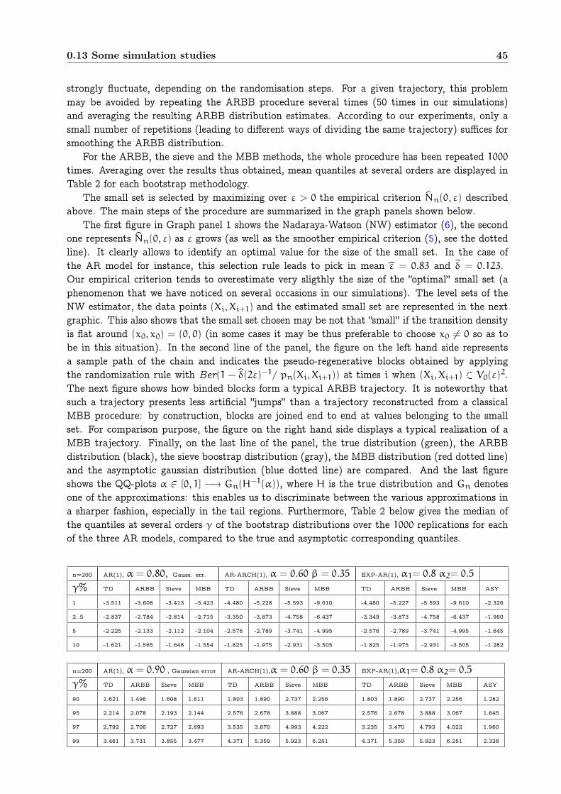
0.13 Some simulation studies 45
strongly fluctuate, depending on the randomisation steps. For a given trajectory, this problemmay be avoided by repeating the ARBB procedure several times (50 times in our simulations)and averaging the resulting ARBB distribution estimates. According to our experiments, only asmall number of repetitions (leading to different ways of dividing the same trajectory) suffices forsmoothing the ARBB distribution.
For the ARBB, the sieve and the MBB methods, the whole procedure has been repeated 1000times. Averaging over the results thus obtained, mean quantiles at several orders are displayed inTable 2 for each bootstrap methodology.
The small set is selected by maximizing over ε > 0 the empirical criterion Nn(0, ε) describedabove. The main steps of the procedure are summarized in the graph panels shown below.
The first figure in Graph panel 1 shows the Nadaraya-Watson (NW) estimator (6), the secondone represents Nn(0, ε) as ε grows (as well as the smoother empirical criterion (5), see the dottedline). It clearly allows to identify an optimal value for the size of the small set. In the case ofthe AR model for instance, this selection rule leads to pick in mean ε = 0.83 and δ = 0.123.Our empirical criterion tends to overestimate very sligthly the size of the ”optimal” small set (aphenomenon that we have noticed on several occasions in our simulations). The level sets of theNW estimator, the data points (Xi, Xi+1) and the estimated small set are represented in the nextgraphic. This also shows that the small set chosen may be not that ”small” if the transition densityis flat around (x0, x0) = (0, 0) (in some cases it may be thus preferable to choose x0 = 0 so as tobe in this situation). In the second line of the panel, the figure on the left hand side representsa sample path of the chain and indicates the pseudo-regenerative blocks obtained by applyingthe randomization rule with Ber(1 − δ(2ε)−1/ pn(Xi, Xi+1)) at times i when (Xi, Xi+1) V0(ε)2.The next figure shows how binded blocks form a typical ARBB trajectory. It is noteworthy thatsuch a trajectory presents less artificial ”jumps” than a trajectory reconstructed from a classicalMBB procedure: by construction, blocks are joined end to end at values belonging to the smallset. For comparison purpose, the figure on the right hand side displays a typical realization of aMBB trajectory. Finally, on the last line of the panel, the true distribution (green), the ARBBdistribution (black), the sieve boostrap distribution (gray), the MBB distribution (red dotted line)and the asymptotic gaussian distribution (blue dotted line) are compared. And the last figureshows the QQ-plots α [0, 1] −→ Gn(H
−1(α)), where H is the true distribution and Gn denotesone of the approximations: this enables us to discriminate between the various approximations ina sharper fashion, especially in the tail regions. Furthermore, Table 2 below gives the median ofthe quantiles at several orders γ of the bootstrap distributions over the 1000 replications for eachof the three AR models, compared to the true and asymptotic corresponding quantiles.
n=200 AR(1), α = 0.80, Gauss. err. AR-ARCH(1), α = 0.60 β = 0.35 EXP-AR(1), α1= 0.8 α2= 0.5
γ% TD ARBB Sieve MBB TD ARBB Sieve MBB TD ARBB Sieve MBB ASY
1 -3.511 -3.608 -3.413 -3.423 -4.480 -5.228 -5.593 -9.610 -4.480 -5.227 -5.593 -9.610 -2.326
2..5 -2.837 -2.784 -2.814 -2.715 -3.350 -3.873 -4.758 -6.437 -3.349 -3.873 -4.758 -6.437 -1.960
5 -2.225 -2.133 -2.112 -2.104 -2.576 -2.789 -3.741 -4.995 -2.576 -2.789 -3.741 -4.995 -1.645
10 -1.621 -1.565 -1.648 -1.554 -1.825 -1.975 -2.931 -3.505 -1.825 -1.975 -2.931 -3.505 -1.282
n=200 AR(1), α = 0.90 , Gaussian error AR-ARCH(1),α = 0.60 β = 0.35 EXP-AR(1),α1= 0.8 α2= 0.5
γ% TD ARBB Sieve MBB TD ARBB Sieve MBB TD ARBB Sieve MBB ASY
90 1.621 1.496 1.608 1.611 1.803 1.890 2.737 2.256 1.803 1.890 2.737 2.256 1.282
95 2.214 2.078 2.193 2.144 2.576 2.678 3.888 3.067 2.576 2.678 3.888 3.067 1.645
97 2,792 2.706 2.727 2.693 3.535 3.670 4.993 4.222 3.235 3.470 4.793 4.022 1.960
99 3.461 3.731 3.855 3.477 4.371 5.359 5.923 6.251 4.371 5.359 5.923 6.251 2.326

46 Regenerative-Block Bootstrap for Harris Markov chains
Figure 6: Graph panel 1: AR(1) time-series with α = 0.8

0.13 Some simulation studies 47
Figure 7: Graph panel 2: AR-ARCH(1) model with α = 0.6 and = 0.35, n = 200
Table 2: Comparing the tails of the true, ARBB and gaussian distributions for the three models
These results clearly indicate that both the sieve and MBB methods perform very well for lineartime series. In this case, the ARBB distribution tends to have larger tails. However, when consid-ering nonlinear models, the advantage of the ARBB method over its rivals plainly come into sight:for moderate sample sizes n, the sieve bootstrap tends to choose a too large value qn for the lagorder of the approximate sieve AR(qn). This problem is less serious for larger sample sizes. In thesesituations, the MBB behaves very poorly : we conjecture that it could be possibly improved byinvestigating further how to tune optimally the block size, especially for standardized distributions.
Pictures in Graph panels 2 and 3 speak volumes: for both nonlinear models, the true distributionis accurately approximated by the ARBB distribution. Note nevertheless the difference in the sizeof the ”optimal small set" and in the number of pseudo-regenerations between these models. Wepoint out that, though remarkable when compared to the gaussian approximation, the gain inaccuracy obtained by applying the ARBB methodology to the EXP-AR model is higher than theone obtained for the AR-ARCH type model. As may be confirmed by other simulations, the ARBBmethod provides less accurate results for a given (moderate) sample size, as one gets closer to aunit root model (i.e. as α tends to 1): one may get an insight into this phenomenon by simplynoticing that the rate of the number of regenerations (respectively, of the number of visits to thesmall set) then drastically decreases.

48 Regenerative-Block Bootstrap for Harris Markov chains
Figure 8: Graph panel 3: EXP-AR(1) model with α1 = 0.8 and α2 = 0.5, n = 200

0.13 Some simulation studies 49
0.13.3 Further remarks
We finally summarize our empirical findings. We first point out that, in the linear case when rootsare much less than 1 in amplitude, the sieve bootstrap clearly surpasses its competitors. But itis noteworthy that both the ARBB and the MBB also provides very good numerical results inthis case. Besides, all these methods seem to break down from a practical viewpoint for an AR(1)model with an autoregressive coefficient α tending to 1 and with a fixed (moderate) sample size:in such a case, too few pseudo-regeneration blocks may be constructed for the ARBB methodologyto be practically performant (although it is asymptotically valid). In this respect, the graph ofthe estimated number of pseudo-regenerations (see Graph panels 1-3) provides a crucial help fordiagnosing the success or the failure of the ARBB method. It is also remarkable that the sievebootstrap can lead to very bad results in this case, due to the fact that the estimated AR model mayhave a root larger than 1 (generating then explosive sieve bootstrap trajectories). This stronglyadvocates the use of preliminary tests or contrained estimation procedures (ensuring that theresulting reconstructed series is asymptotically stationary).
And as may be reported from our simulation results, the advantage of the ARBB over the sievebootstrap, the MBB and the asymptotic distributions, clearly appears when dealing with nonlinearmodels. Even if the lag is chosen very large (in mean 85 for the AR-ARCH model and 21 for theexp-AR model), the linear sieve method is unable to capture the non-linearities and performs verybadly (the distribution tends to be too much concentrated in these cases). The MBB also performspoorly in such a nonlinear setting for moderate sample sizes but nevertheless tends to surpass thesieve bootstrap for larger sample sizes, whereas the ARBB provides very accurate approximationsof the tail distributions in these examples.

50 Regenerative-Block Bootstrap for Harris Markov chains

Concluding remarks
Although we are far from having covered the unifying theme of statistics based on (pseudo) re-generation for Harris Markov chains, an exhaustive treatment of the possible applications of thismethodology being naturally beyond the scope of the present survey, we endeavoured to presenthere enough material to illustrate the power of this method. Most of the results reviewed in thispart of the report are very recent and this line of research is still in development. Now we con-clude by making a few remarks raising several open questions among the topics we focused on,and emphasizing the potential gain that the regeneration-based statistical method could providein further applications.
We point out that establishing sharper rates for the 2nd order accuracy of the ARBB whenapplied to sample mean statistics in the general Harris case presents considerable technical difficul-ties (at least to us). However, one might expect that this problem could be successfully addressedby refining some of the (rather loose) bounds put forward in the proof. Furthermore, as previouslyindicated, extending the argument to U-statistics requires to prove preliminary non-uniform limittheorems for U-statistics of random vectors with a lattice component.
In numerous applications it is relevant to consider null recurrent (eventually regenerative)chains: such chains frequently arise in queuing/network systems, related to teletraffic data forinstance (see [165]) or [93] for example), with heavy-tailed cycle lengths. Hence, exploring thetheoretical properties of the (A)RBB for these specific time series provides thus another subject offurther research: as shown by [122], consistent estimates of the transition kernel, as well as rates ofconvergence for the latter, may still be exhibited for β-recurrent null chains (i.e. chains for whichthe return time to an atom is in the domain of attraction of a stable law with β ]0, 1[ being thestable index), so that extending the asymptotic validity of the (A)RBB distribution in this caseseems conceivable.
In [89], the pseudo-regeneration approach has been successfully extended to certain continuousMarkov processes (namely, diffusion processes) for bootstrap purpose.
Turning to the statistical study of extremes now (which matters in insurance and financeapplications for instance), a thorough investigation of the asymptotic behaviour of extreme valuestatistics based on the approximate regeneration blocks remains to be carried out in the generalHarris case.
We finally mention ongoing work on empirical likelihood estimation in the markovian setting(see [105]), for which methods based on (pseudo-) regeneration blocks are expected to providesignificant results.

52 Concluding remarks

Part II
Supervised Learning Methods for
Ranking Problems


55
Abstract
Motivated by various applications, the problem of ranking/ordering instances, instead of classifyingthem solely, has recently gained much attention in machine learning. For example, a challengingtask in document retrieval applications, consists in comparing documents by degree of relevancefor a particular request, rather than simply classifying them as relevant or not. Similarly, creditestablishments collect and manage large databases containing the socio-demographic and credit-history characteristics of their clients to build a ranking rule which aims at indicating reliability.In this part of the report, the ranking problem is formulated in a rigorous statistical framework.
In Chapter 5, it is reduced to the problem of learning a ranking rule for deciding, among twoinstances, which one is "better," with minimum ranking risk (i.e. the probability of misclassifyinga pair of instances). Since the natural estimates of the risk are of the form of a U-statistic, results ofthe theory of U-processes are required for investigating the consistency of empirical risk minimizers.Results established in [59] (see also [57] and [58]) are surveyed, laying emphasis on a tail inequalityfor degenerate U-processes, and on its application for establishing that fast rates of convergencemay be achieved under specific noise assumptions, just like in classification. Results related toconvex risk minimization methods are also displayed.
Chapter 6 mainly focuses on certain aspects of the so-called bipartite ranking problem : thegoal is to learn how to order best all the instances x of a set ❳ by degree of relevance fromi.i.d. observations of a pair (X, Y), when Y is some binary r.v. indicating relevancy and X is a❳ -valued r.v. modelling some observation for predicting Y. This practically amounts to find ascoring function s : ❳ → for ranking all input values x according to the order of magnitudeof P(Y = 1 | X = x). The problem of ranking a given proportion of instances x among the "mostrelevant instances" only is considered. Such a local ranking problem is of practical importance,since in most ranking applications, in particular in the field of information retrieval, only topranked instances are effectively scanned. This chapter recapitulates the results in [62], in whichpaper criteria specifically tailored for selecting scoring functions accomplishing this task in anoptimal fashion and extending the ranking risk (pairwise classification error) studied in Chapter 5in this context have been proposed and bounds for learning rates of nonparametric scoring methodsbased on minimization of such empirical criteria over specific sets of scoring functions have alsobeen established.

56

Ranking Methods and U-processes
0.14 Introduction and preliminaries
Motivated by various applications including problems related to document retrieval or credit-riskscreening, the ranking problem has received increasing attention both in the statistical and machinelearning literature. For example, in information retrieval applications, one may be concerned withcomparing documents by degree of relevance for a particular request, rather than simply classifyingthem as relevant or not. In a similar fashion, credit establishments collect and manage largedatabases containing the socio-demographic and credit-history characteristics of their clients tobuild a ranking rule which aims at indicating reliability. Such special cases of ranking/orderingproblems may be formulated in the following framework.
0.14.1 The bipartite ranking problem
In the so-called bipartite ranking problem, the matter is to order all the elements x of a set ❳by degree of relevance, when relevancy may be observed through some binary indicator variableY: one has a system consisting of a binary random output (response) variable Y, taking its valuesin −1, 1 say, and a random input (predictor) variable X, taking its values in the space ❳ . Indocuments retrieval applications for instance, one is concerned by ordering all the documents xof a list ❳ by degree of relevance for a particular request, rather than simply classifying them asrelevant or not. Hence, this amounts to assign to each document x in ❳ a score s(x) indicatingits degree of relevance for this specific query. In this context, the challenge is to build a scoring
function s : ❳ → from sampling data, so as to rank the observations x by increasing order oftheir score s(x) as accurately as possible: the higher the score s(X) is, the more likely one shouldobserve Y = 1.
The ROC curve The accuracy of the ranking induced by s is classically measured by theso-called ROC curve (ROC standing for Receiving Operator Characteristic, refer to [98] and seealso [115]), that consists in plotting the true positive rate against the false positive rate (see Fig.9), namely the curve
z → (1− F(−)S (z), 1− F
(+)S (z)),
denoting by F(−)S (z) = P (s(X) z | Y = −1) (respectively, by F(+)
s (z) = P (s(X) z | Y = 1)) the cdfof s(X) conditioned on Y = −1 (resp., conditioned on Y = 1), or equivalently the graph of the power
function βs : α (0, 1) → 1 − F(+)s (qα), where qα = F
(−)−1s (1 − α) = infz / F(−)
s (z) 1 − α,βs(α) being the power of the test of level α for testing the null hypothesis ”Y = −1” based on thetest statistic s(X).
This measure of accuracy induces a partial order on the set = s : ❳ → measurable of allscoring functions: for any s1, s2 in , we shall say that s1 is more accurate than s2 iff its ROCcurve is above the one of s2 everywhere, that is to say iff βs2 (α) βs1 (α) for all α in (0, 1) (orequivalently, if the test defined by s1 for testing the hypothesis that Y = −1 is uniformly more

58 Ranking Methods and U-processes
powerful than the one defined by the test function s2). With respect to this criterion, the optimalranking is naturally the one induced by the regression function η(x) = P(Y = 1 | X = x), since onemay straightforwardly check that the test it defines is of Neyman-Pearson’s type. More precisely,the class of optimal scoring functions corresponds to measurable and strictly increasing transformsof the regression function η(x), as stated in the theorem below.
Theorem 23 A scoring function s in is optimal w.r.t. the ROC criterion iff there exists
Ψ : → measurable and strictly increasing on the support of η(X) s.t.: s = Ψ η.Another criterion for evaluating the accuracy of a scoring function that may be found in the
literature devoted to information retrieval is the precision-recall curve x → (P(Y = 1 | s(X) >
x), P (s(X) > x | Y = 1)).
As emphasized in [63] (see also [13]), the ranking problem is by nature very different from theclassification problem. Whereas the goal in the ranking problem consists in finding s suchthat for all α in (0, 1), the power βs(α) be as large as possible, the error rate of the classifierCs,q(X) = 2 s(X) > q − 1 obtained by thresholding a scoring function s at level q is given by:
M(Cs,q) = (1− p)(1− F(−)s (q)) + pF
(+)s (q)
= (1− p)α+ p(1− βs(α)),
with p = P(Y = 1) and α = α(q) = 1− F(−)S (q). In the case when βs is continuously differentiable,
the minimum error rate is thus obtained by tuning the threshold at level q = qα with α suchthat β
s(α) = (1 − p)/p. Hence, constructing an optimal classifier of this type consists in findinga scoring function with a ROC curve having a tangent line with slope (1− p)/p in a point with afirst coordinate as small as possible.
The Area Under the ROC curve: a standard summary ranking criterion As previouslyrecalled, the optimal ordering of ❳ is obtained for scoring functions with a ROC curve above theone of any other scoring function, which are scoring functions s such that for all α [0, 1]:
βs(α) = βη(α).
Hence, optimizing the ROC curve is a difficult problem, which amounts to recover such a transformof the regression function. In applications, this highly complex optimization problem may bereduced to optimizing a specific summary criterion, known as the AUC criterion (AUC standingfor Area Under a ROC Curve) for selecting scoring functions (see [104]). The latter is based on thesimple observation that the optimal ROC curve is also the one under which the area is maximum.The problem boils down then to searching for a scoring function s that maximizes the area underits ROC curve (see Fig. 1), namely
AUC(s) =
∫1
0
βs(α)dα.
Note that two scoring functions with the same AUC might lead to quite different rankings(different ROC curves with same integral).
This theoretical summary quantity may be easily interpreted in a probabilistic fashion, sinceby a simple change of variable it can be written as follows:
AUC(s) = P (s(X) > s(X) | Y = 1, Y = −1),
where (X, Y) denotes an input/output pair distributed as (X, Y) and independent from the latter.The AUC criterion amounts thus to choose a scoring function s such that, given two independent

0.14 Introduction and preliminaries 59
Figure 9: ROC curves.

60 Ranking Methods and U-processes
input observations X and X such that Y = 1 and Y = −1 respectively, the probability that s ranksthe instance X higher than X is minimum.
Let p = P(Y = 1). From the expression above, one may write
AUC(s) = 1−1
2p(1− p)P((s(X) − s(X))(Y − Y) < 0). (38)
Hence, maximizing AUC(s) amounts to minimize P((s(X) − s(X))(Y − Y) < 0), which maybe interpreted as a pairwise classification error: the aim being to predict (y − y)/2 from (x, x).Under this form, the ranking problem is now being reduced to a classification problem with theparticular error measure given above involving a pair of independently drawn observations.
0.14.2 Outline
In the ranking problem as formulated in this chapter, one has to compare two different observationsand decide which one is “better”. In certain settings, finding a good ranking rule amounts toconstructing a scoring function s. As previously seen, an important special case is the bipartiteranking problem in which the available instances in the data are labelled by binary labels (goodand bad): the ranking criterion is then closely related to the auc.
When viewed this way, the ranking problem is tightly connected to Stute’s conditional U-
statistics [187, 188]. Whereas Stute’s results imply that certain nonparametric estimates basedon local U-statistics give universally consistent ranking rules, the approach in [57] is different:empirical minimizers of U-statistics are considered instead of local averages, looking at things fromthe point of view of empirical risk minimization, popular in statistical learning theory (see, e.g.[198], [17], [40], [125] or [145] for instance). The crucial point is that natural estimates of the rankingrisk involve U-statistics and the methodology is thus based on the theory of U-processes, and callsin particular on maximal and concentration inequalities, symmetrization tricks, and a “contractionprinciple” for U-processes (see [70] for a comprehensive account of the theory of U-statistics andU-processes).
In [59] (see also [57] and [58]), a theoretical analysis of certain nonparametric ranking methodsinspired by boosting-, and support vector machine-type algorithms for classification and which arebased on empirical minimization of convex cost functionals over convex sets of scoring functionshas been carried out. More precisely, universal consistency of properly regularized versions of thesemethods has been established and it has been shown that fast rates of convergence may be achievedfor empirical risk minimizers under suitable noise conditions, based on a novel tail inequality fordegenerate U-processes.
The basic statistical model is introduced in section 0.15, as well as the two main special casesof the ranking problem we consider. Then basic uniform convergence and consistency results forempirical risk minimizers are stated in section 0.16. A new exponential concentration inequality forU-processes is stated in section 0.17, which serves as the main tool in establishing the performancebounds for empirical ranking risk minimization. The noise assumptions guaranteeing fast rates ofconvergence in particular cases are described in section 0.18, while section 0.19 is devoted to convexrisk minimization for ranking problems, providing this way a theoretical framework for studyingboosting and support vector machine-type ranking methods (such as the ones developped in [86]).
0.15 The ranking problem as a pairwise classification problem
Let (X, Y) be a pair of r.v.’s taking values in ❳ where ❳ is a measurable space. The randomobject X models some observation and Y its real-valued label. Let (X , Y ) denote a pair of r.v.’s
0.15 The ranking problem as a pairwise classification problem 61
identically distributed with (X, Y), and independent from the latter. Set
Z =Y − Y
2.
In the ranking problem, X and X are supposed to observed, but not their labels Y and Y . Wethink about X being “better” than X if Y > Y , that is, if Z > 0. (The normalization factor 1/2in the definition of Z above is arbitrary and plays no role in the analysis) The goal is to rank Xand X such that the probability that the better ranked of them has a smaller label is as smallas possible. We thus define a ranking rule as a function r : ❳ ❳ → −1, 1. If r(x, x ) = 1 thenthe rule r ranks x higher than x . Its performance is measured by the ranking risk
L(r) = PZ r(X,X ) < 0 ,
that is, the probability that r ranks two randomly drawn instances incorrectly. In this set-up, theranking problem boils down to a binary classification problem in which the sign of the randomvariable Z has to be guessed based upon the pair of observations (X,X ). The ranking rule withminimal risk can be now easily determined. Set
ρ+(X,X ) = PZ > 0 | X,X
ρ−(X,X ) = PZ < 0 | X,X .
Proposition 24 (Clémençon, Lugosi & Vayatis, 2005b) Define
r(x, x ) = 2[ρ+(x,x)ρ−(x,x)] − 1
and denote L = L(r) = min(ρ+(X,X ), ρ−(X,X )). Then for any ranking rule r,
L L(r) .
Let us now consider the problem of constructing ranking rules of low risk based on trainingdata. Supposed that n independent, identically distributed copies of (X, Y), have been observed:Dn = (X1, Y1), . . . , (Xn, Yn). Given a ranking rule r, these training data may be used for estimatingits risk L(r) = PZ r(X,X ) < 0, the most natural estimate being the U-statistic
Ln(r) =1
n(n− 1)
∑
i=j
[Zi,j r(Xi,Xj)<0].
The statistical challenge amounts then to study the performance of minimizers of the empiricalestimate Ln(r) over a class of ranking rules.
In the definition of r ties are broken in favor of ρ+ but obviously if ρ+(x, x ) = ρ−(x, x ), anarbitrary value can be chosen for r without altering its risk.
The actual values of the Yi’s are never used in the ranking rules discussed in this paper. It issufficient to know the values of the Zi,j, or, equivalently, the ordering of the Yi’s.
Instead of ranking two observations X,X only, one may be interested in ranking m inde-pendent observations X(1), . . . , X(m). The value of a ranking function r(X(1), . . . , X(m)) is then apermutation π of 1, . . . ,m and the goal is that π should coincide with (or at least resemble to)the permutation π for which Y(π(1)) Y(π(m)). Given a loss function ℓ that assigns a numberin [0, 1] to a pair of permutations, the ranking risk is defined as
L(r) = ℓ(r(X(1), . . . , X(m)), π) .

62 Ranking Methods and U-processes
In this general case, natural estimates of L(r) involve m-th order U-statistics. Many of the resultsstated in the sequel may be straightforwardly extended to this general setup.
Ranking and Scoring. In many interesting cases the ranking problem may be reduced tofinding an appropriate scoring function. These are the cases when the joint distribution of X andY is such that there exists a function s : ❳ → such that
r(x, x ) = 1 if and only if s(x) s(x ) .
We call such a function s an optimal scoring function (any strictly increasing transformation ofan optimal scoring function being still optimal). Here are some important special cases when theranking problem may be reduced to scoring.
Example 1 (the bipartite ranking problem.) As recalled above, in the bipartite rankingproblem the label Y is binary, taking its values in −1, 1. Writing η(x) = PY = 1|X = x, theBayes ranking risk equals
L = minη(X)(1− η(X )), η(X )(1− η(X))
= minη(X), η(X ) − (η(X))2
and also,
L = VarY + 1
2
−1
2η(X) − η(X )
.In particular, L Var
Y+12
1/4, where the equality L = Var
Y+12
holds when X and Y are
independent and the maximum is attained when η 1/2. The difficulty of the bipartite rankingproblem depends on the concentration properties of the distribution of η(X) = P(Y = 1 | X) throughthe Gini’s mean difference (|η(X) − η(X)|), which is a classical measure of concentration. Forgiven p = (η(X)), Gini’s mean difference ranges from a minimum value of zero, when η(X) p,to a maximum value of 1
2p(1 − p), when η(X) = (Y + 1) /2. The optimal ranking rule is given
by a scoring function s where s is any strictly increasing transformation of η. Then one mayrestrict the search to ranking rules defined by scoring functions s, that is, ranking rules of form
r(x, x ) = 2[s(x)s(x)] − 1. Writing L(s) def= L(r), one has
L(s) − L = η(X ) − η(X)
[(s(X)−s(X))(η(X)−η(X))<0]
.
As already mentioned in section 0.14, the ranking risk is related to the AUC criterion which is astandard performance measure in this setup (see [86]). Set p = P (Y = 1), we have
AUC(s) = 1−1
2p(1− p)L(s), (39)
so that maximizing the auc criterion boils down to minimizing the ranking error.
Example 2 (a regression model). Let Y be real-valued and the joint distribution of X and Ybe s.t. Y = m(X) + ǫ, where m(x) = (Y|X = x) is the regression function, ǫ is independent of Xand has a symmetric distribution around zero. The optimal ranking rule r may be then definedby a scoring function s, where s may be any strictly increasing transformation of m.

0.16 Empirical ranking risk minimization 63
0.16 Empirical ranking risk minimization
Based on the empirical estimate Ln(r) of the risk L(r) defined above, one may select a ranking ruleby minimizing the empirical risk over a class of ranking rules r : ❳ ❳ → −1, 1. Consider theempirical risk minimizer, over , by
rn = arg minr
Ln(r) .
In a first-order approach, the performance L(rn) = PZ rn(X,X ) < 0|Dn of the empirical riskminimizer may be investigated by using the standard bound (see [72])
L(rn) − infr
L(r) 2 supr
|Ln(r) − L(r)| . (40)
This shows that bounding the performance of an empirical minimizer of the ranking risk boilsdown to investigating the properties of U-processes, that is, suprema of U-statistics indexed by aclass of ranking rules. In a first-order approach, the next inequality (based on the standard resultsin [111]) permits to reduce the problem to the study of ordinary empirical processes.
Lemma 25 (Clémençon, Lugosi & Vayatis, 2005b) Let qτ : ❳ ❳ → be real-valued func-
tions indexed by τ T where T is some set. If X1, . . . , Xn are i.i.d. then for any convex
nondecreasing function ψ,
ψ
supτT
1
n(n− 1)
∑
i=j
qτ(Xi, Xj)
ψ
supτT
1
n/2n/2∑
i=1
qτ(Xi, Xn/2+i)
,
assuming the suprema are measurable and the expected values exist.
For each τ T , ∑n/2i=1 qτ(Xi, Xn/2+i) is a sum of n/2 i.i.d. r.v.’s, the moment generating
function of the U-process may be thus bounded by the moment generating function of an ordinaryempirical process: λ > 0,
exp
λ supτT
1
n(n− 1)
∑
i=j
qτ(Xi, Xj)
exp
λ supτT
1
n/2n/2∑
i=1
qτ(Xi, Xn/2+i)
.
Hence, basics methods for handling empirical processes can be applied directly. Using the boundeddifferences inequality (see [147]) for instance, one gets that
exp
λ supτT
1
n/2n/2∑
i=1
qτ(Xi, Xn/2+i)
exp
λ supτT
1
n/2n/2∑
i=1
qτ(Xi, Xn/2+i) +λ2
4(n− 1)
,
if each qτ takes its values in an interval of length 1. This leads to
log exp
λ supr
|Ln(r) − L(r)|
λ supr
1
n/2n/2∑
i=1
|[Zi,n/2+i r(Xi,Xn/2+i)<0] − L(r)| +λ2
4(n− 1).

64 Ranking Methods and U-processes
Standard inequalities may be applied for bounding the expected value on the right-hand side. Forexample, if the class of indicator functions has finite vc dimension V (see [134]), then
supr
1
n/2n/2∑
i=1
|[Zi,n/2+i r(Xi,Xn/2+i)<0] − L(r)| csV
n
for a universal constant c. The next result immediately derives from the Chernoff bound.
Proposition 26 (Clémençon, Lugosi & Vayatis, 2005b) Let be a class of ranking rules of
vc dimension V. Then for any t > 0,
P
supr
|Ln(r) − L(r)| > c
sV
n+ t
e−(n−1)t2 .
It is well known from the theory of empirical risk minimization for classification that the bound(40) is often quite loose, due to the fact that the variance of the estimators of the risk is ignored andbounded uniformly by a constant. Therefore, the main interest in considering U-statistics preciselyconsists in the fact that they have minimal variance among all unbiased estimators. However, thereduced-variance property of U-statistics plays no role in the previous analysis: all upper boundsobtained above remain true for an empirical risk minimizer that, instead of using estimates basedon U-statistics, estimates the risk of a ranking rule by splitting the data set into two halves asfollows
1
n/2n/2∑
i=1
[Zi,n/2+i r(Xi,Xn/2+i)<0] .
Hence, one looses the advantage of calling on U-statistics in the previous study. Let us now give amore precise insight into how one may benefit from using U-statistics.
Hoeffding’s decomposition (sharper bounds). U-statistics have been studied in depth andtheir behavior is well understood. The following classical probability inequality concerning U-statistics is due to Hoeffding [112]: t > 0,
P|Ln(r) − L(r)| > t 2 exp
−(n/2)t22σ2+ 2t/3
, (41)
with σ2 = Var([Zr(X,X)<0]) = L(r)(1 − L(r)). Therefore, the latter inequality may be improvedby replacing σ2 by a smaller term. This results from the so-called Hoeffding’s decomposition asrecalled below. Hoeffding’s decomposition (see [180] for more details) is a basic tool for studyingU-statistics. Let X,X1, ..., Xn be i.i.d. r.v.’s and denote by
Un(X1, ..., Xn) =1
n(n− 1)
∑
i=j
q(Xi, Xj)
a U-statistic of order 2 where the kernel q is a symmetric real-valued function.Assuming that q(X1, X2) is square integrable, Un − Un may be decomposed as a sum Tn of
i.i.d. r.v’s plus a degenerate U-statistic Wn. In order to write this decomposition, consider thefollowing function of one variable
h(Xi) = (q(Xi, X) | Xi) − Un ,
and the function of two variables
h(Xi, Xj) = q(Xi, Xj) − Un− h(Xi) − h(Xj).

0.17 Fast rates 65
Then we have the orthogonal expansion
Un = Un+ 2Tn+Wn ,
where
Tn(X1, ..., Xn) =1
n
n∑
i=1
h(Xi),
Wn(X1, ..., Xn) =1
n(n− 1)
∑
i=j
h(Xi, Xj) .
Wn is called a degenerate U-statistic because its kernel h satisfies
h(Xi, X) | Xi
= 0 .
The variance of Tn is
Var(Tn) =Var((q(X1, X) | X1))
n.
Therefore, Var((q(X1, X) | X1)) is less than Var(q(X1, X)) (unless q is already degenerate) andthe variance of the degenerate U-statistic Wn is O( 1
n2 ): Tn is thus leading term in this orthog-onal decomposition. Indeed, the limit distribution of
♣n(Un − Un) is the normal distribution
(0, 4Var((q(X1, X) | X1)) (see [111]). This suggests that inequality (41) may be quite loose.Indeed, exploiting further Hoeffding’s decomposition (combined with arguments related to de-
coupling, randomization and hypercontractivity of Raŋdeŋmaŋcher chaos) de la Peña and Giné [?]established a Bernstein’s type inequality of the form (41) but with σ2 replaced by the varianceof the conditional expectation (see Theorem 4.1.13 in [70]). When specialized to our setting (i.e.with q(Xi, Xj) = [Zi,j r(Xi,Xj)<0]), this yields
P|Ln(r) − L(r)| > t 4 exp
−
nt2
8s2+ ct
,
where s2 = Var(PZ r(X,X ) < 0|X) is the variance of the conditional expectation and c issome constant. This remarkable improvement is not exploited in the first-order analysis abovebut shall become crucial when establishing fast rates of convergence. As a matter of fact, it isshown in section 0.17 that under certain, quite general, conditions significantly smaller risk boundsare achievable. There it will have an essential importance to use sharp exponential bounds forU-processes, involving their reduced variance.
0.17 Fast rates
It is well known (refer to §5.2 in [40] and the references therein) that faster rate bounds forthe excess risk in the context of binary classification may be achieved when the variance of theexcess risk can be controlled by its expected value. This is guaranteed under certain “low-noise”conditions (see [192], [146] or [125]). As shown in [59], significantly sharper bounds may also beestablished in the ranking problem under some conditions that are somehow analogous to the low-noise conditions in the classification problem, which permit to benefit from the small variance ofthe U-statistic (as opposed to splitting the sample) to estimate the ranking risk. The analysisis based on the Hoeffding decomposition recalled above. Consider the following estimate of theexcess risk Λ(r) = L(r) − L = qr((X, Y), (X , Y )):
Λn(r) =1
n(n− 1)
∑
i=j
qr((Xi, Yi), (Xj, Yj)),

66 Ranking Methods and U-processes
which is a U-statistic of degree 2 with symmetric kernel:
qr((x, y), (x, y )) = [(y−y)r(x,x)<0] − [(y−y)r(x,x)<0]
The minimizer rn of the empirical ranking risk Ln(r) over also minimizes the empirical excessrisk Λn(r). The Hoeffding decomposition of Λn(r) may be written as follows:
Λn(r) −Λ(r) = 2Tn(r) +Wn(r) ,
where
Tn(r) =1
n
n∑
i=1
hr(Xi, Yi)
is a sum of i.i.d. r.v.’s with
hr(x, y) = qr((x, y), (X, Y )) −Λ(r)
and
Wn(r) =1
n(n− 1)
∑
i=j
hr((Xi, Yi), (Xj, Yj))is a degenerate U-statistic with symmetric kernel
hr((x, y), (x , y )) = qr((x, y), (x, y )) −Λ(r) − hr(x, y) − hr(x
, y ) .
The argument of the analysis relies on the fact that the contribution of the degenerate part Wn(r)is negligible compared to that of Tn(r). Minimization of Λn is thus approximately equivalent tominimizing Tn(r), which is a simple average of i.i.d. r.v.’s. Hence, known techniques used inempirical risk minimization can be invoked for studying the minimization of Tn(r).
The main tool for handling the degenerate part is a new general moment inequality for U-processes proved in [59], stated below. It is based on moment inequalities obtained for empiricalprocesses and Rademacher chaoses in [41]. However, it is noteworthy that it generalizes the in-equality established in [5], which would be actually sufficient for dealing with vc classes (see alsothe results in [3], [90] and [114]).
Theorem 27 Let X,X1, ..., Xn be i.i.d. random variables and let be a class of kernels.
Consider a degenerate U-process Z of order 2 indexed by ,
Z = supf
∑
i,j
f(Xi, Xj)
where f(X, x) = 0, x, f. Assume also f(x, x) = 0, x and supf f∞ = F. Let ǫ1, ..., ǫn be
i.i.d. Rademacher random variables and introduce the random variables
Zǫ = supf
∑
i,j
ǫiǫjf(Xi, Xj)
,Uǫ = sup
fsup
α:α21
∑
i,j
ǫiαjf(Xi, Xj) ,
M = supf,k=1...n
n∑
i=1
ǫif(Xi, Xk)
.

0.17 Fast rates 67
Then there exists a universal constant C > 0 such that for all n and q 2,
(Zq)1/q CZǫ+ q1/2Uǫ+ q(M+ Fn) + q3/2Fn1/2+ q2F
.
Also, there exists a universal constant C such that for all n and t > 0,
PZ > CZǫ+ t exp
−1
Cmin
t
Uǫ
2,
t
M+ Fn,
t
F♣n
2/3,
rt
F
.
In a fashion very similar to the conditions required for obtaining faster rates of convergencein the context of binary classification (see [192], [17], [125] and [145]), our key assumption on thejoint distribution of (X, Y) takes the following form:
Assumption 28 There exist constants c > 0 and α [0, 1] such that for all r ,
Var(hr(X, Y)) cΛ(r)α .
For α = 0 the assumption is always fulfilled and the corresponding performance bound does notyield any improvement over those of Section 0.16. However, in many natural examples Assumption28 is satisfied with values of α close to one, guaranteeing significant improvements in the rates ofconvergence.
The next theorem provides a performance bound in terms of expected values of certain Rademacherchaoses indexed by and local properties of an ordinary empirical process. These quantities havebeen thoroughly studied and are well understood. They may be easily bounded in many interestingcases (see the corollary below, where it is applied to the case when is a vc class of indicatorfunctions). In order to state the result, we introduce some quantities related to the class . Letǫ1, . . . , ǫn be i.i.d. Rademacher r.v.’s independent of the (Xi, Yi). Let
Zǫ = supr
∑
i,j
ǫiǫjhr((Xi, Yi), (Xj, Yj)) ,
Uǫ = supr
supα:α21
∑
i,j
ǫiαjhr((Xi, Yi), (Xj, Yj)) ,M = sup
r,k=1,...,n
n∑
i=1
ǫihr((Xi, Yi), (Xk, Yk)) .
Introduce the loss function
ℓ(r, (x, y)) = 2[(y−Y)r(x,X)<0] − L(r)
and define
νn(r) =1
n
n∑
i=1
ℓ(r, (Xi, Yi)) − L(r) .
And define the pseudo-distance
d(r, r ) =
[[r(X,X)=r(X,X)]|X]
21/2.
Let φ : [0,∞) → [0,∞) be a nondecreasing function such that φ(x)/x is nonincreasing and φ(1) 1such that for all r , ♣
n supr,d(r,r)σ
|νn(r) − νn(r)| φ(σ) .
68 Ranking Methods and U-processes
Theorem 29 (Clémençon, Lugosi & Vayatis, 2006) Consider a minimizer rn of the empirical
ranking risk Ln(r) over a class of ranking rules and assume Assumption 28. Then there
exists a universal constant C such that, with probability at least 1− δ, the ranking risk of rnsatisfies
L(rn) − L 2
infr
L(r) − L
+C
Zǫ
n2+
Uǫ♣
log(1/δ)
n2+
M log(1/δ)
n2+
log(1/δ)
n+ ρ2 log(1/δ)
where ρ > 0 is the unique solution of the equation♣nρ2 = φ(ρα) .
Examples in which Assumption 28 is satisfied with α > 0 are displayed in the next section. Wewill see below that the value of α in this assumption determines the magnitude of the last termwhich, in turn, dominates the right-hand side (apart from the approximation error term). Theimprovement of Theorem 29 is naturally meaningful only if infr L(r)−L does not dominate theother terms in the bound. Ideally, the class should be chosen such that the approximation errorand the other terms in the bound are balanced. The theorem would then guarantee faster rates ofconvergence. Hence, this bound enables us to design penalized empirical minimizers of the rankingrisk that select the class from a collection of classes achieving this objective, as explained in[145] or [125].
The next result illustrates Theorem 29 in the case when is a vc class.
Corollary 30 (Clémençon, Lugosi & Vayatis, 2006) Consider the minimizer rn of the em-
pirical ranking risk Ln(r) over a class of ranking rules of finite vc dimension V and assume
Assumption 28. Then there exists a universal constant C such that, with probability at least
1− δ, the ranking risk of rn satisfies
L(rn) − L 2
infr
L(r) − L
+ C
V log(n/δ)
n
1/(2−α)
.
0.18 Examples
The bipartite ranking problem. Recall that here it suffices to consider ranking rules of theform r(x, x ) = 2[s(x)s(x)] − 1 where s is a scoring function. We shall abusively write hs for hr.
Noise assumption: there exist constants c > 0 and α [0, 1] such that for all x ❳ ,
X(η(x) − η(X)
−α) c . (42)
As shown by the next result, this assumption ensures that Assumption 28 is satisfied.
Proposition 31 (Clémençon, Lugosi & Vayatis, 2005b) Under (42), we have: s
Var(hs(X, Y)) cΛ(s)α .
If α = 0 then condition (42) poses no restriction, but also no improvement is achieved. At theother extreme, when α = 1, the condition is quite restrictive as it excludes η to be differentiable,for example, if X has a uniform distribution over [0, 1]. However, interestingly, for any α < 1, itposes quite mild restrictions as highlighted in the following example:
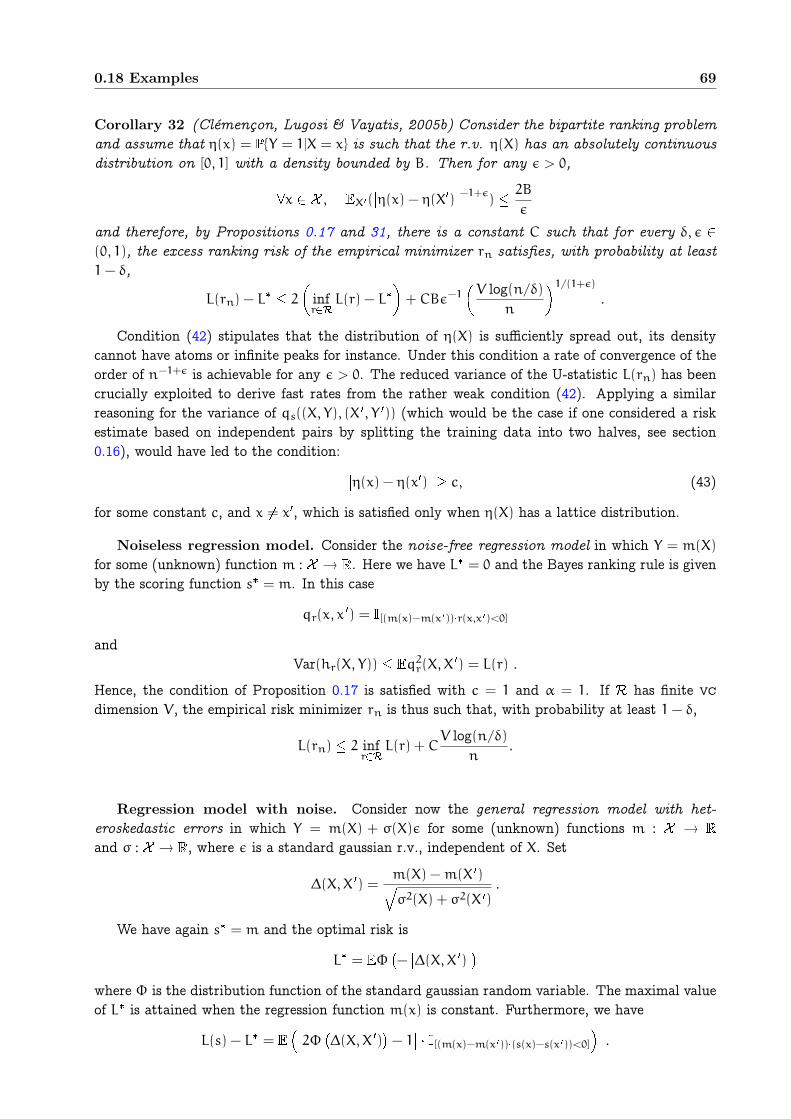
0.18 Examples 69
Corollary 32 (Clémençon, Lugosi & Vayatis, 2005b) Consider the bipartite ranking problem
and assume that η(x) = PY = 1|X = x is such that the r.v. η(X) has an absolutely continuous
distribution on [0, 1] with a density bounded by B. Then for any ǫ > 0,
x ❳ , X(η(x) − η(X)
−1+ǫ) 2B
ǫ
and therefore, by Propositions 0.17 and 31, there is a constant C such that for every δ, ǫ (0, 1), the excess ranking risk of the empirical minimizer rn satisfies, with probability at least
1− δ,
L(rn) − L 2
infr
L(r) − L
+ CBǫ−1
V log(n/δ)
n
1/(1+ǫ).
Condition (42) stipulates that the distribution of η(X) is sufficiently spread out, its densitycannot have atoms or infinite peaks for instance. Under this condition a rate of convergence of theorder of n−1+ǫ is achievable for any ǫ > 0. The reduced variance of the U-statistic L(rn) has beencrucially exploited to derive fast rates from the rather weak condition (42). Applying a similarreasoning for the variance of qs((X, Y), (X , Y )) (which would be the case if one considered a riskestimate based on independent pairs by splitting the training data into two halves, see section0.16), would have led to the condition: η(x) − η(x)
c, (43)
for some constant c, and x = x, which is satisfied only when η(X) has a lattice distribution.
Noiseless regression model. Consider the noise-free regression model in which Y = m(X)
for some (unknown) function m : ❳ → . Here we have L = 0 and the Bayes ranking rule is givenby the scoring function s = m. In this case
qr(x, x) = [(m(x)−m(x))r(x,x)<0]
andVar(hr(X, Y)) q2r(X,X
) = L(r) .
Hence, the condition of Proposition 0.17 is satisfied with c = 1 and α = 1. If has finite vc
dimension V , the empirical risk minimizer rn is thus such that, with probability at least 1− δ,
L(rn) 2 infr
L(r) + CV log(n/δ)
n.
Regression model with noise. Consider now the general regression model with het-
eroskedastic errors in which Y = m(X) + σ(X)ǫ for some (unknown) functions m : ❳ →
and σ : ❳ → , where ǫ is a standard gaussian r.v., independent of X. Set
∆(X,X ) =m(X) −m(X )qσ2(X) + σ2(X )
.
We have again s = m and the optimal risk is
L = Φ−∆(X,X )
where Φ is the distribution function of the standard gaussian random variable. The maximal valueof L is attained when the regression function m(x) is constant. Furthermore, we have
L(s) − L = 2Φ
∆(X,X )− 1
[(m(x)−m(x))(s(x)−s(x))<0]
.
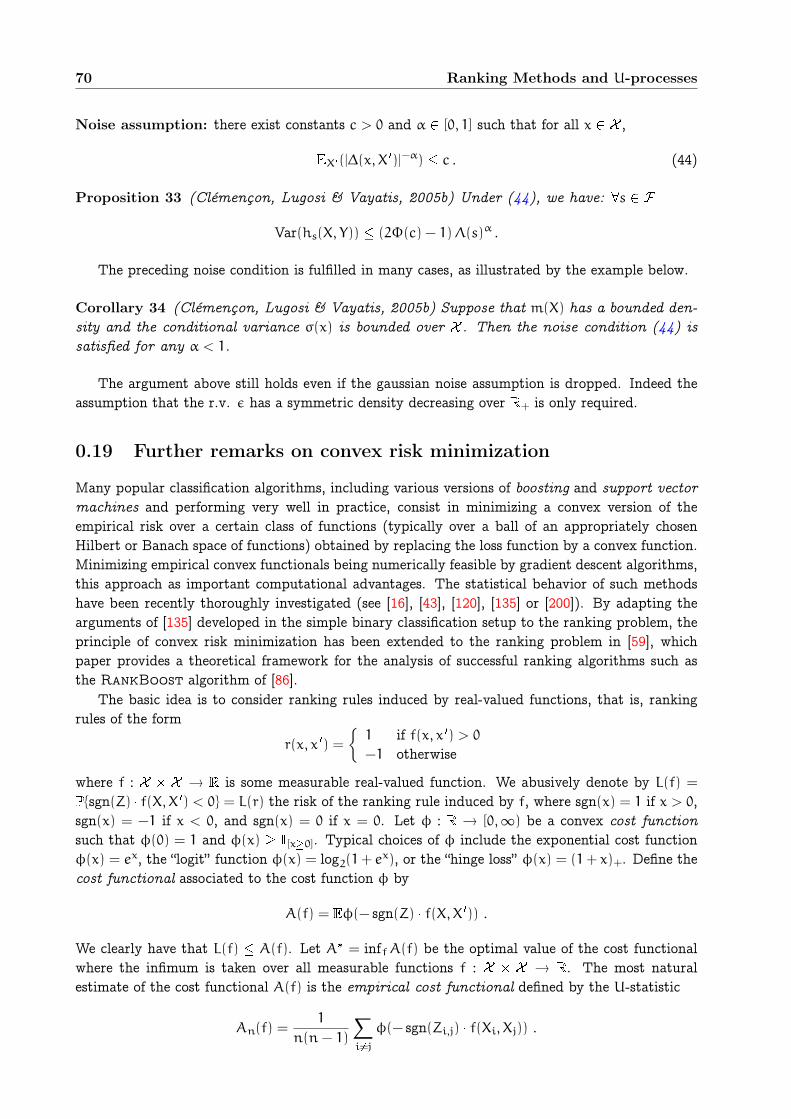
70 Ranking Methods and U-processes
Noise assumption: there exist constants c > 0 and α [0, 1] such that for all x ❳ ,
X(|∆(x, X )|−α) c . (44)
Proposition 33 (Clémençon, Lugosi & Vayatis, 2005b) Under (44), we have: s
Var(hs(X, Y)) (2Φ(c) − 1)Λ(s)α .
The preceding noise condition is fulfilled in many cases, as illustrated by the example below.
Corollary 34 (Clémençon, Lugosi & Vayatis, 2005b) Suppose that m(X) has a bounded den-
sity and the conditional variance σ(x) is bounded over ❳ . Then the noise condition (44) is
satisfied for any α < 1.
The argument above still holds even if the gaussian noise assumption is dropped. Indeed theassumption that the r.v. ǫ has a symmetric density decreasing over + is only required.
0.19 Further remarks on convex risk minimization
Many popular classification algorithms, including various versions of boosting and support vector
machines and performing very well in practice, consist in minimizing a convex version of theempirical risk over a certain class of functions (typically over a ball of an appropriately chosenHilbert or Banach space of functions) obtained by replacing the loss function by a convex function.Minimizing empirical convex functionals being numerically feasible by gradient descent algorithms,this approach as important computational advantages. The statistical behavior of such methodshave been recently thoroughly investigated (see [16], [43], [120], [135] or [200]). By adapting thearguments of [135] developed in the simple binary classification setup to the ranking problem, theprinciple of convex risk minimization has been extended to the ranking problem in [59], whichpaper provides a theoretical framework for the analysis of successful ranking algorithms such asthe RankBoost algorithm of [86].
The basic idea is to consider ranking rules induced by real-valued functions, that is, rankingrules of the form
r(x, x ) =
1 if f(x, x ) > 0−1 otherwise
where f : ❳ ❳ → is some measurable real-valued function. We abusively denote by L(f) =
Psgn(Z) f(X,X ) < 0 = L(r) the risk of the ranking rule induced by f, where sgn(x) = 1 if x > 0,sgn(x) = −1 if x < 0, and sgn(x) = 0 if x = 0. Let φ : → [0,∞) be a convex cost function
such that φ(0) = 1 and φ(x) [x0]. Typical choices of φ include the exponential cost functionφ(x) = ex, the “logit” function φ(x) = log2(1+ ex), or the “hinge loss” φ(x) = (1+ x)+. Define thecost functional associated to the cost function φ by
A(f) = φ(− sgn(Z) f(X,X )) .
We clearly have that L(f) A(f). Let A = inffA(f) be the optimal value of the cost functionalwhere the infimum is taken over all measurable functions f : ❳ ❳ → . The most naturalestimate of the cost functional A(f) is the empirical cost functional defined by the U-statistic
An(f) =1
n(n− 1)
∑
i=j
φ(− sgn(Zi,j) f(Xi, Xj)) .

0.19 Further remarks on convex risk minimization 71
Consider the ranking rule based on minimizing the empirical cost functional An over a set ofreal-valued functions f : ❳ ❳ → , i.e. fn = arg minf An(f):
rn(x, x) =
1 if fn(x, x ) > 0−1 otherwise.
As shown in Theorem 3 of [16], minimizing convex risk functionals is meaningful for rankingsince the excess convex risk may be related to the excess ranking risk L(fn) − L as follows. SetH(ρ) = infα (ρφ(−α) + (1− ρ)φ(α)) and H−(ρ) = infα:α(2ρ−1)0 (ρφ(−α) + (1− ρ)φ(α)) . And
define ψ(x) = H−1+x2
−H−
1−x2
. Then for all functions f : ❳ ❳ → ,
L(f) − L ψ−1 (A(f) −A)
where ψ−1 is the inverse of ψ. If φ is chosen convex, it is shown in [16] that limx→0ψ−1(x) = 0:if the excess convex risk converges to zero, so does the excess ranking risk. Moreover, in mostinteresting cases ψ−1(x) may be bounded, for x > 0, by a constant multiple of
♣x (such as in the
case of exponential or logit cost functions) or even by x if φ(x) = (1+ x)+ .Hence, bounding the excess ranking risk L(f) − L for convex risk minimization follows from
analyzing the excess convex risk. This may be done by decomposing it into estimation and ap-proximation errors:
A(fn) −A(f) A(fn) − inf
fA(f)
+
inff
A(f) −A.
One may naturally bound the excess convex risk over the class as follows
A(fn) − inff
A(f) 2 supf
|An(f) −A(f)| .
For simplicity’s sake, suppose that the class is uniformly bounded, say supf,x❳ |f(x)| B.Then Lemma 25 combined with the bounded differences inequality entails that for any λ > 0,
exp
λ supf
|An(f) −A(f)|
exp
λ supf
1
n/2n/2∑
i=1
φ− sgn(Zi,n/2+i) f(Xi, Xn/2+i)
−A(f)
+λ2B2
2n
.
Now standard symmetrization and contraction inequalities may provide an upper bound for theexpected supremum appearing in the exponent. In fact, by mimicking [126], we get
supf
1
n/2n/2∑
i=1
φ− sgn(Zi,n/2+i) f(Xi, Xn/2+i)
−A(f)
4Bφ (B) sup
f
1
n/2n/2∑
i=1
σi f(Xi, Xn/2+i)
where σ1, . . . , σn/2 i.i.d. Rademacher random variables independent of Dn, that is, symmetricsign variables with Pσi = 1 = Pσi = −1 = 1/2.
The Rademacher average Rn() = supf
1n/2
∑n/2i=1 σi f(Xi, Xn/2+i)
may be easily
bounded for various classes of functions. For example, consider the convex class B =f(x, x ) =
∑Nj=1wjgj(x, x
related to boosting-type classification procedures, where is a class of ranking rules. In this case,
Rn(B) BRn() const.BV♣n

72 Ranking Methods and U-processes
where V is the vc dimension of the base class .This can also be used for establishing performance bounds for kernel methods such as support
vector machines. Let k : ❳ 2❳ 2 → be a symmetric positive definite function, that is,
n∑
i,j=1
αiαjk(wi, wj) 0 ,
for all choices of n, α1, . . . , αn and w1, . . . , wn ❳ 2.A kernel-type ranking algorithm may be defined as one that performs minimization of the
empirical convex risk An(f) (typically based on the hinge loss φ(x) = (1 + x)+) over the class Bof functions defined by a ball of the associated reproducing kernel Hilbert space of the form (wherew = (x, x ))
B =
f(w) =
N∑
j=1
cjk(wj, w) : N ,N∑
i,j=1
cicjk(wi, wj) B2, w1, . . . , wN ❲
.
See [65], [179], [184] or [186] for the approximation properties of such classes. We have
Rn(B) 2B
n
tn/2∑
i=1
k((Xi, Xn/2+i), (Xi, Xn/2+i)) ,
see for example [40].In conclusion, universal consistency of such ranking rules may be derived in a straightforward
way if the approximation error inffBA(f) −A → 0 as B → ∞.

Ranking the Best Instances
0.20 Introduction
In [62], an important variant of the bipartite ranking problem has been considered, namely theproblem of ranking a given proportion of instances x among the "most relevant instances" only.Such a local ranking problem is of crucial practical importance, since in most ranking applica-tions, in particular in the field of Information Retrieval, only top ranked instances are effectivelyscanned. In a similar fashion, scoring rules for credit-risk screening elaborated by credit estab-lishment aim at indicating reliability, laying much more emphasis on most risky prospects. A novelcriterion specifically tailored for selecting scoring functions accomplishing this task in an optimalfashion is required. As a matter of fact, recall that the AUC of a scoring function s is
AUC(s) =
∫1
α=0
βs(α)dα. (45)
It is thus simply the mean power of the test function s over all possible levels α: the criterionAUC(s) weights in an uniform fashion all test errors, independently from their level. This may benot appropriate when one seeks for scoring functions s that induce an accurate ordering for themost relevant instances x only. More precisely, let u0 [0, 1] be fixed. The local ranking problemdescribed above is somehow a double issue, consisting in simultaneously determining and properlyordering the u0% the most relevant instances. Denoting by Fη the cdf of η(X), the matter is to 1.determine the set G
u0of instances that are considered relevant enough and 2. recover the order
induced by η on Gu0
.By way of preliminary, we first consider the problem of finding the best u0% instances, which we
formulate as a binary classification problem with mass constraint. Then a new theoretical criterion,wich we call the generalized AUC, is proposed for solving precisely the problem mentioned above.It boils down to the standard AUC criterion for u0 = 1. And (basic and fast) bound rates forthe local ranking risk of empirical risk minimizers established in [62] under specific conditions arebriefly recalled.
0.21 On Finding the Best Instances
We first tackle the problem of determining a given proportion u0 (0, 1) among the most relevantinstances from training data. In other words, the matter is here to find an estimate of the set
Gu0
= x ❳/η(x) > F−1η (1− u0). (46)
0.21.1 A mass-constrained classification problem
As shown by the result stated below, the set Gu0
corresponds to the classifier C : ❳ → −1,+1
with minimum misclassification probability M(C) = P(Y = C(X)) among classifiers that assignpositive label only to a proportion u0 of the instances.

74 Ranking the Best Instances
Theorem 35 (Clémençon & Vayatis, 2006) Define Cu0(X) = 2[XG
u0 ]−1 and denote M
u0=
M(Cu0). Then for any classifier C such that P(C(X) = 1) = u0,
Mu0M(C).
Furthermore, we have
M(C) −Mu0
= 2(η(X) − F−1
η (1− u0) [XG
u0∆G]), (47)
with G = x ❳/C(x) = 1 and denoting by ∆ the symmetric difference between two subsets
of ❳ .
Remark 3 Note that if a classifier C satisfies the mass constraint P(C(X) = 1) = u0, its type Ierror, i.e the probability that C leads to an incorrect prediction on a negative labeled example,α(C) = P(C(X) = +1 | Y = −1), is related to its misclassification error by
M(C) = 2(1− p)α(C) + p− u0.
Similarly, we have M(C) = 2p(1−β(C))+p−u0 with β(C) = P(C(X) = 1 | Y = +1). Hence, Cu0is
also the classifier with minimum type I error (respectively, type II error) among mass-constrainedclassifiers.
Although the point of view adopted in this chapter is very different (since we are mainlyconcerned here with building scoring functions), the problem described above may be formulatedin the framework of minimum volume set learning as considered in [178]. As a matter of fact, theset Gu0
may be viewed as the solution of the constrained optimization problem:
minGmeasurable
P(X G | Y = −1)
subject toP(X G) u0.
Although the volume set is generally computed from a known measure of reference (contrary tothe probability involved in the constraint, which must be estimated) in such problems (applicationsof the latter being mainly related to anomaly detection), learning methods for MV-set estimationmay hopefully be extended to our setting. A natural way to do it would consist in replacing X’sdistribution conditioned on Y = −1 by its empirical counterpart. This point has not been treatedin [62] but will be the subject of further investigation.
0.21.2 Empirical risk minimization
The goal is to investigate how to build estimates of the set Gu0based on training data. Suppose that
we are given n i.i.d. copies of the pair (X, Y): (X1, Y1), , (Xn, Yn). Since we are mainly motivatedhere by scoring applications, it is natural to consider candidate sets obtained by thresholding ascoring function s at level F−1
s (1 − u0), as in (46), for solving the mass-constrained classificationproblem described above, selection being ideally based on minimizing the quantity
Mn(s) =1
n
n∑
i=1
Yi = 2[s(Xi)F−1s (1−u0)] − 1.
Unfortunately, the adequate threshold level depends on X’s distribution and is generally unknown.In practice, one has to replace it by its empirical counterpart F−1
s (1 − u0), denoting by Fs(x) =
n−1∑i [s(Xi)x] the empirical cdf of the s(Xi)’s, so as to consider

0.21 On Finding the Best Instances 75
Mn(s) =1
n
n∑
i=1
Yi = 2[s(Xi)F−1s (1−u0)] − 1.
Note that Mn(s) is a biased estimate of the misclassification risk M(s) = M(Cs) of the classifierCs(X) = 2[s(X)F−1
s (1−u0)] − 1. And the interesting part of the analysis consists in showing that
the bias induced by plugging the empirical quantile estimate in the risk functional does not dete-riorate the rate bound, as stated in the next proposition which provides a standard bound for theperformance of minimizers of Mn(s) over a class 0 of scoring functions satisfying mild conditions.With no restriction, we may assume that all scoring functions s 0 take their values in (0, 1).Define the empirical risk minimizer over 0 by
sn = arg infs0
Mn(s).
The following assumptions are required in the next result.
• (i) The class of functions x → [s(x)t], indexed by (s, t) 0 (0, 1), has finite VC dimensionV .
• (ii) For all s 0, Fs,+ and Fs,− are differentiable on (0, 1) with derivatives uniformly bounded:there exist strictly positive constants b−, b+, B− and B+ s.t. (s, v) 0 (0, 1),
b+ F s,+(v) B+ and b− F s,−(v) B−. (48)
Proposition 36 (Clémençon & Vayatis, 2006) Suppose that conditions (i)-(ii) hold. Let
δ > 0. Then with probability at least 1− δ,
M(sn) − infs0
M(s) c1sV
n+ c2
sln(1/δ)
n− 1, (49)
for some constants c1 and c2.
0.21.3 Fast Rates
As in section 0.17, it is possible to improve significantly the rate (49) in some cases. Consider thefollowing conditions.
• (iii) There exist constants α ]1/2, 1[ and B > 0 s.t. for all t 0
P(η(X) − F−1
η (1− u0) t) Bt α
1−α .
• (iv) The class of df’s Fs with s 0 is a subset of (β, L), the Holder class of functionsF : (0, 1) → satisfying:
sup(x,y)(0,1)2
|F(x) − F(y)|
|x− y|β L,
with L < ∞ and β 1.
• (v) The class 0 is finite with cardinal N.
• (vi) The class 0 contains an optimal scoring function s.

76 Ranking the Best Instances
Observe first that for all t 0,
P(η(X) − F−1
η (1− u0) t) = Fη(t+ F−1
η (1− u0)) − Fη(−t+ F−1η (1− u0)).
Hence, if conditions (iv) and (vi) are both fulfilled, so is (iii) with α = β/(1+β) and B = L. Theseconditions are by no means the weakest conditions under which faster rates may be derived, butsince our main goal here is to give an insight into the problem, we use them to make the formulationof the results simpler. Hence, as shall be seen, the bound (49) may be significantly improved underthe conditions above. Define
sn = arg infs0
Mn(s).
Besides, from the relation (47), one may easily derive that
Var([Cs(X)=Y] − [Cu0(X)=Y]) (M(s) −M
u0)α
under (iii). And by slightly adapting the now standard argument in [192] based on Bernstein’sinequality (see also references in section 0.17), a sharper estimate of the convergence rate for theexcess risk of the minimizer sn of the ’ideal’ empirical criterion Mn may be established if oneassumes further that (v)-(vi) hold: with probability 1− δ,
M(sn) −Mu0 c(log(N/δ)/n)
12−α . (50)
This bound may be preserved to some extent when minimizing the biased empirical criterion,as claimed in the next theorem. The proof relies on assumption (iv), allowing us to control thedeviation between Mn(s) and Mn(s) uniformly over s 0, combined with Theorem 8.3 in [145],which permits to evaluate the performance of the Mn-minimizer in terms of Mn-risk.
Theorem 37 (Clémençon & Vayatis, 2006) Under assumptions (ii)-(vi), we have with prob-
ability 1− δ
M(sn) −Mu0 c1(log(2N/δ)/n)
12−α + c2(log(2N/δ)/n)β/2. (51)
This bound calls for some comments. As a matter of fact, taking β = α/(1 − α) the first termcorresponds to the rate bound when quantile estimation poses no problem, namely for α (1/2, 2−♣2), while the second term is governed by the dificulty of approximating (uniformly) the component
of the risk involving quantile, and is faster than the first one for α (2 −♣2, 1) only. But truth
should be said, we do not know at present whether this ’elbow’ phenomenon in the rate is simplydue to our method of proof or to a deeper aspect of the problem considered (establishing lowerbounds would be then required).
0.22 The Local Ranking Problem
The local ranking problem as considered in section 0.20 may be stated in very simple terms: thematter is to order the instances of the input space ❳ so that the best u0% be ranked as accuratelyas possible. And the class of scoring functions solving it in an optimal manner is clearly thesubset of made of functions s such that for all u (0, u0)
Gs,u = Gu,
with Gs,u = x ❳/s(x) > F−1s (1 − u)), denoting by Fs the (unconditional) cdf of s(X). In other
terms, is the collection of scoring functions s such that:
s(x) = Φ(η(x)), on Gu0

0.22 The Local Ranking Problem 77
ands(x) < inf
xGu0
s(x ), for all x / Gu0,
where Φ : [0, 1] → is any Borel function of which restriction on ]Fη(1−u0), 1] is strictly increasing.Next we propose a performance measure for evaluating the pertinence of scoring functions regardingto the local ranking problem.
0.22.1 Tailoring a criterion for the local ranking problem
By way of preliminary, we first state the following result.
Lemma 38 (Clémençon & Vayatis, 2006) For any s , we have for all u (0, 1)
Fη,+(F−1η (u)) Fs,+(F−1
s (u)),
Fs,−(F−1s (u)) Fη,−(F−1
η (u)),
and there is equality in the sole case when Gs,1−u = G1−u.
In view of this result, a wide collection of criteria with as set of optimal values could benaturally considered, depending on how one weights the type II error 1−β(s, u) = Fs,+(F−1
s (1−u))
(resp. the type I error α(s, u) = 1−Fs,−(F−1s (1−u))) according to the value of the mass u [0, u0].
However, not all criteria obtained this manner can be easily interpreted.
AUC generalization
A possible way of generalizing the standard AUC would be to consider
AUCu0(s) = P(s(X) > s(X ) ❭ s(X) F−1
s (1− u0) | Y = 1, Y = −1). (52)
It obviously boils down to the standard AUC criterion (45) for u0 = 1. And as claimed in thefollowing theorem resulting from lemma 38, corresponds to the set of generalized AUC max-imizers. Furthermore, this criterion may be expressed in a simple fashion in terms of the typeII error β(s, u0) measuring how accurate is the estimation Gs,u0
of Gu0
(see section 0.21) and aquantity measuring the performance of the ranking induced by s on the set Gs,u0
, as described inchapter 5.
Theorem 39 (Clémençon & Vayatis, 2006) Let u0 (0, 1). We have
= arg mins
AUCu0(s).
Furthermore, we have
AUCu0(s) = β(s, u0) −
1
2p(1− p)L(s,Gs,u0
), (53)
with L(s,G) = P((s(X) − s(X ))(Y − Y ) > 0 ❭ (X,X ) G2) for any measurable G ❳ .
Observe that (53) reduces to (39) when u0 = 1. Besides one may relate the generalized AUCcriterion to the truncated AUC. As a matter of fact, one may write
AUCu0(s) =
∫α(s,u0)
α=0
βs(α)dα+ β(s, u0) − α(s, u0)β(s, u0). (54)
The values α(s, u0) and β(s, u0) are the coordinates of the intersecting point between the ROCcurve α → βs(α) and the line D : β = −1−p
pα + u0
p. And the integral
∫α(s,u0)
α=0βs(α)dα represents

78 Ranking the Best Instances
β(s,u0)
β
1
D:β=-(1-p) α/p+u0/p
0
0 1α(s,u0) α
Figure 10: Truncated AUC.
the area of the surface delimited by the ROC curve, the α-axis and the line α = α(s, u0) (see Fig.??). It is worth mentioning that, contrary to what is claimed in [153], it is not necessarily pertinentto evaluate the local performance of a scoring statistic s(X) by the truncated AUC, since in generalarg mins
∫α(s,u0)
α=0βs(α)dα = .
Generalized Mann-Whitney Wilcoxon statistic
Here is another possible fashion of generalizing the AUC criterion. A natural empirical estimate ofthe AUC is the rate of concording pairs :
^AUC(s) =1
n+n−
n−∑
i=1
n+∑
j=1
[s(X−i
)<s(X+j
)],
with n+ = n − n− =∑Ni=1 [Yi=+1] and denoting by X+
i 1in+ (resp. by X−i 1in− ) the set of
instances with positive labels (resp. with negative labels) among the sample data (Xi), Yi)1in.And we have the classical relation
n+n−
n+ 1^AUC(s) +
n+(n+ + 1)
2= Wn,1(s), (55)
where W1,n(s) is the standard Wilcoxon statistic. Recall that it is the two-sample linear rank
statistic associated to the score generating function Φ1(u) = u, u (0, 1), obtained by summingthe ranks corresponding to positive labels, namely
W1,n(s) =
n+∑
i=1
rank(s(X+i ))
n+ 1,

0.22 The Local Ranking Problem 79
denoting by rank(s(X+i )) the rank of s(X+
i ) in the pooled sample s(Xj), 1 j n. Refer to [197]for basic results related to linear rank statistics. In particular, the statistic µ1(s) = W1,n(s)/n+ isan asymptotically normal estimate of
µ1(s) = X[PX(s(X ) < s(X)) | Y = 1]
= [Fs(s(X)) | Y = 1],
where X denotes an independent copy of X and PX is the probability taken with respect to thevariable X (conditional probability given (X, Y)). Note the theoretical counterpart of (55) may bewritten as
µ1(s) = (1− p)AUC(s) + p/2, (56)
and this quantity is related to the ranking risk studied in Chapter 5 by
L1(s) = −2pµ1(s) + 2p(1− p) + p2. (57)
Now, in order to take into account the highest u0% ranks only, one may consider the criterionrelated to the score generating function Φu0
(u) = u[u>1−u0]
µu0(s) = X[Φu0
(PX(s(X ) < s(X))) | Y = 1]
= [Φu0(Fs(s(X))) | Y = 1].
It has empirical counterpart µu0= Wu0,n(s)/n+, with
Wu0,n(s) =
n∑
i=1
[Yi=1]Φu0(rank(s(Xi))
n+ 1).
Define the local ranking risk at level u0 of any s by
Lu0(s) = −2pµu0
(s) + 2p(1− p) + p2,
generalizing this way (57). The next result, also based on (38), claims that coincides with theset of scoring functions with minimum local ranking risk.
Theorem 40 (Clémençon & Vayatis, 2006) Let u0 [0, 1] be fixed. We have
= arg mins
Lu0(s).
Furthermore,
2pµu0(s) − 1+ (1− u0)
2 = −L(s,Gs,u0) − 2(1− p)(1− u0)α(s, u0) − (1− p)2α(s, u0)
2.
It is worth noticing that not all combinations of α(s, u0) and L(s,Gs,u0) lead to a criterion with
as optimal set. This prevents from considering naive ’divide and conqueer’ strategies for solvingthe local ranking problem (i.e. strategies consisting in simply computing first an estimate G of theset containing the best instances and secondly solving the ranking problem over G as described inChapter 5) and stresses the importance of making use of a global criterion, synthesizing the doublegoal one would like to achieve: finding and ranking the best instances.

80 Ranking the Best Instances
0.22.2 Empirical risk minimization
Finally we collect here some remarks about the method considered in [62] for studying the perfor-mance of empirical risk minimizers, when risk is measured either by the generalized AUC or elseby the local ranking risk. As an illustration, we deal with the case when accuracy of the scoringrule is measured by the generalized AUC.
The empirical generalized AUC criterion may be naturally decomposed as follows:
^AUCn(s) = ˜AUCn(s) + ( ^AUCn(s) − ˜AUCn(s)),
denoting by ˜AUCn(s) =n(n−1)n+n−
❯n(s) the empirical AUC in the ideal case when the quantile valueis known and with
❯n(s) =1
n(n− 1)
∑
i,j
[Yi=−1,Yj=1,s(Xi)<s(Xj),s(Xj)>F−1s (1−u0)],
which is the (non symmetric) U-statistic of degree 2 with kernel
qs((x, y), (x, y )) = [y=−1,y=1,s(x)<s(x),s(x)>F−1
s (1−u0)].
Hence, even symmetrization of the U-statistic ❯n(s) is needed first, exactly the same tools of thetheory of U-processes as those used in chapter 5 permit to control sups0
˜AUCn(s) −AUC(s)
under suitable conditions. And besides, the difference sups0
^AUCn(s) − ˜AUCn(s) is controlled
using the same tricks as those invoked for the mass-constrained classification problem in the previ-ous section, but for establishing here that minimizing ^AUCn(s) is almost aquivalent to minimizing
˜AUCn(s) (the classicial results required may be found mainly in section 8 of [145] and chapter 5 in[196]). Hence, similar rate bounds as those stated for ranking risk in chapter 5 may be then easilyderived for the local ranking problem. We refer to [62] for the formulation of the latter results.

Part III
Probabilistic Modelling and Applied
Statistics


83
Abstract
In this last part, several applications of recent advances in applied probability and nonparamet-ric statistics are presented. Among the numerous disciplines with which applied mathematics maysuccessfully interface, finance is a natural field of application of probability and statistics. Beyondthe ubiquity of data in this domain, risk and uncertainty lie indeed at the core of the financialmarket activity.
In [60] a nonparametric methodology developped by [74] for estimating an autocovariance se-quence is applied to the statistical analysis of financial returns and advantages offered by thisapproach over other existing methods like fixed-window-length segmentation procedures are argu-mented. Theoretical properties of adaptivity of this method have been proved for a specific classof time series, the class of locally stationary processes, with an autocovariance structure whichvaries slowly over time in most cases but might exhibit abrupt changes of regime. It is based onan algorithm that selects empirically from the data the tiling of the time-frequency plane whichexposes best in the least squares sense the underlying second-order time-varying structure of thetime series, and so may properly describe the time-inhomogeneous variations of speculative prices.The applications considered in [60] mainly concern the analysis of structural changes occuring instock market returns, VaR estimation and the comparison between the variation structure of stockindexes returns in developed markets and in developing markets.
In [61], the Independent Component Analysis (ICA) methodology is applied to the problem ofselecting portfolio strategies, so as to provide against extremal movements in financial markets. Aspecific semi-parametric ICA model for describing the extreme fluctuations of asset prices is intro-duced, stipulating that the distributions of the IC’s are heavy tailed. An inference method basedon conditional maximum likelihood estimation has been proposed, which permits to determinepractically optimal investment strategies with respect to extreme risk.
In Biosciences, statistical analysis, embracing probabilistic modeling, estimation, hypothesistesting and design of experiments is also of crucial importance. In epidemiology, it may actuallyplay an essential role in public health practice, as illustrated by the topic treated in Chapter 8:dietary contamination in toxicology.
In [26] a specific piecewise-deterministic Markov process for describing the temporal evolutionof exposure to a given food contaminant. The quantity X of contaminant present in the bodyevolves through its accumulation after repeated dietary intakes on the one hand and the kineticsbehavior of the chemical on the other hand. The accumulation phenomenon is viewed as a markedpoint process and elimination in between intakes occurs at a random linear rate θX, randomness ofthe coefficient θ accounting for the variability of the elimination process due to metabolic factors.Ergodic properties of this process have been investigated, the latter being of crucial importance fordescribing the long-term behavior of the exposure process and assessing values of quantities suchas the proportion of time the body burden in contaminant is over a certain threshold. The processbeing not directly observable, simulation-based statistical methods for estimating steady-state ortime-dependent quantities have also been studied.

84

Applications in Finance
0.23 Time-Frequency Analysis of Financial Time Series
The modeling of the temporal variations of stock market prices has been the subject of intenseresearch for a long time now, starting with the famous Random Walk Hypothesis introduced in[14], claiming that the successive stock price variations (Xt+1− Xt)t0 are i.i.d. Gaussian r.v.’s.As numerous statistical studies showed, even if Xt is replaced by log(Xt), this classic model cannotexplain some prominent features, such as the number of large price changes observed, that is muchlarger than predicted by the Gaussian. As emphasized by many statistical works, far too numerousto mention, the following features of stock price series came into sight.
• Spells of small amplitude for the price variations alternates with spells of large amplitude.This phenomenon is traditionally called volatility persistence.
• The ”efficient markets assumption”, which claims, roughly speaking, that financial returnsare unforecastable, seems to be contradicted by the existence of very localized periods whenreturn sequences exhibit strong positive autocorrelation.
• The magnitude of the variations evolves in the long run so as to reach an ”equilibrium” level,one calls this feature mean-reversion in a stylized manner.
Although the classic Random Walk model provides explicit formula for asset pricing and theeconomic doctrine is able to interpret it, the limitations mentioned above motivated the emergenceof an abundant econometric literature, with the object to model structure in financial data. Port-folio selection/optimization, Value at Risk estimation, hedging strategies are the main stakes ofthis research activity, still developing.
Even if the seminal contribution of [82], which introduced the ARCH model, has been followedby a large number of variants, the whole complexity underlying these data has not been capturedyet by any parsimonious model and let the field of statistical analysis of financial time series opento further investigation. Selecting a statistical procedure, which allows to handle properly the time-inhomogeneous character of return series, is not an easy task, as Mandelbrot (1963) emphasized:”Price records do not ”look” stationary, and statistical expressions such as the sample variance takevery different values at different times; this nonstationarity seems to put a precise statistical modelof price change out of the question”. According to the estimation method chosen, one can eitherenhance specific patterns in the data or else make them disappear. This strongly advocates forthe application of recent adaptive nonparametric procedures to the statistical analysis of financialseries, which, by selecting adaptively from the data a ”best” representation among a large (non-parametric) class of models and including the type of structure that contributes significantly to thefit of the model only, allow to achieve more flexibility. This alternative approach has been followedby some authors for several years now (see [161], [163]). Among these attempts to deal with nonstationarities in financial data, one may mention the following works. [97] considered the use of fast
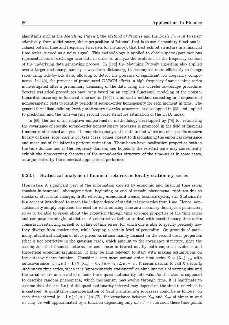
86 Applications in Finance
algorithms such as the Matching Pursuit, the Method of Frames and the Basis Pursuit to selectadaptively, from a dictionary, the superposition of ”atoms”, that is to say elementary functions lo-calized both in time and frequency (wavelets for instance), that best exhibit structure in a financialtime series, viewed as a noisy signal. This methodology is applied to obtain sparse/parsimoniousrepresentations of exchange rate data in order to analyze the evolution of the frequency contentof the underlying data generating process. In [162] the Matching Pursuit algorithm also appliedover a larger dictionary, namely a waveform dictionary, to decompose more efficiently exchangerates using tick-by-tick data, allowing to detect the presence of significant low frequency compo-nents. In [49], the presence of pronounced GARCH effects in high frequency financial time seriesis investigated after a preliminary denoising of the data using the wavelet shrinkage procedure.Several statistical procedures have been based on an explicit functional modeling of the nonsta-tionarities occuring in financial time-series. [106] introduced a method consisting in a sequence ofnonparametric tests to identify periods of second-order homogeneity for each moment in time. Thegeneral formalism defining locally stationary wavelet processes is developped in [88] and appliedto prediction and the time-varying second order structure estimation of the DJIA index.
In [60] the use of an adaptive nonparametric methodology developped by [74] for estimatingthe covariance of specific second-order nonstationary processes is promoted in the field of financialtime-series statistical analysis. It amounts to analyze the data to find which out of a specific massivelibrary of bases, local cosine packets bases, comes closest to diagonalizing the empirical covarianceand make use of the latter to perform estimation. These bases have localization properties both inthe time domain and in the frequency domain, and hopefully the selected basis may convenientlyexhibit the time-varying character of the second-order structure of the time-series in some cases,as argumented by the numerical applications performed.
0.23.1 Statistical analysis of financial returns as locally stationary series
Heuristics A significant part of the information carried by economic and financial time seriesconsists in temporal inhomogeneities: beginning or end of certain phenomena, ruptures due toshocks or structural changes, drifts reflecting economical trends, business cycles, etc. Stationarityis a concept introduced to mean the independence of statistical properties from time. Hence, non-stationarity simply expresses the need for reintroducing time as a necessary description parameter,so as to be able to speak about the evolution through time of some properties of the time seriesand compute meaningful statistics. A constructive fashion to deal with nonstationary time-seriesconsists in restricting oneself to a class of time series, for which one is able to specify precisely howthey diverge from stationarity, while keeping a certain level of generality. On grounds of parsi-mony, statistical analysis of stock prices variations mainly focused on the second order properties(that is not restrictive in the gaussian case), which amount to the covariance structure, since theassumption that financial returns are zero mean is beared out by both empirical evidence andtheoretical economic arguments. It may be thus relevant to start with making assumptions onthe autocovariance function. Consider a zero mean second order time series X = (Xn)n0 withautocovariance ΓX(n,m) = E (XnXm) = CX((n+m)/2,m−n). It seems natural to call X a locally
stationary time series, when it is ”approximately stationary” on time intervals of varying size andthe variables are uncorrelated outside these quasi-stationarity intervals. As this class is supposedto describe random phenomena, which mechanism may evolve through time, it is legitimate toassume that the size l(n) of the quasi-stationarity interval may depend on the time n on which itis centered. A qualitative characterization of locally stationary processes could be as follows: oneach time interval [n− l(n)/2, n+ l(n)/2] , the covariance between Xm and Xm at times m andm may be well approximated by a function depending only on m −m as soon these time points
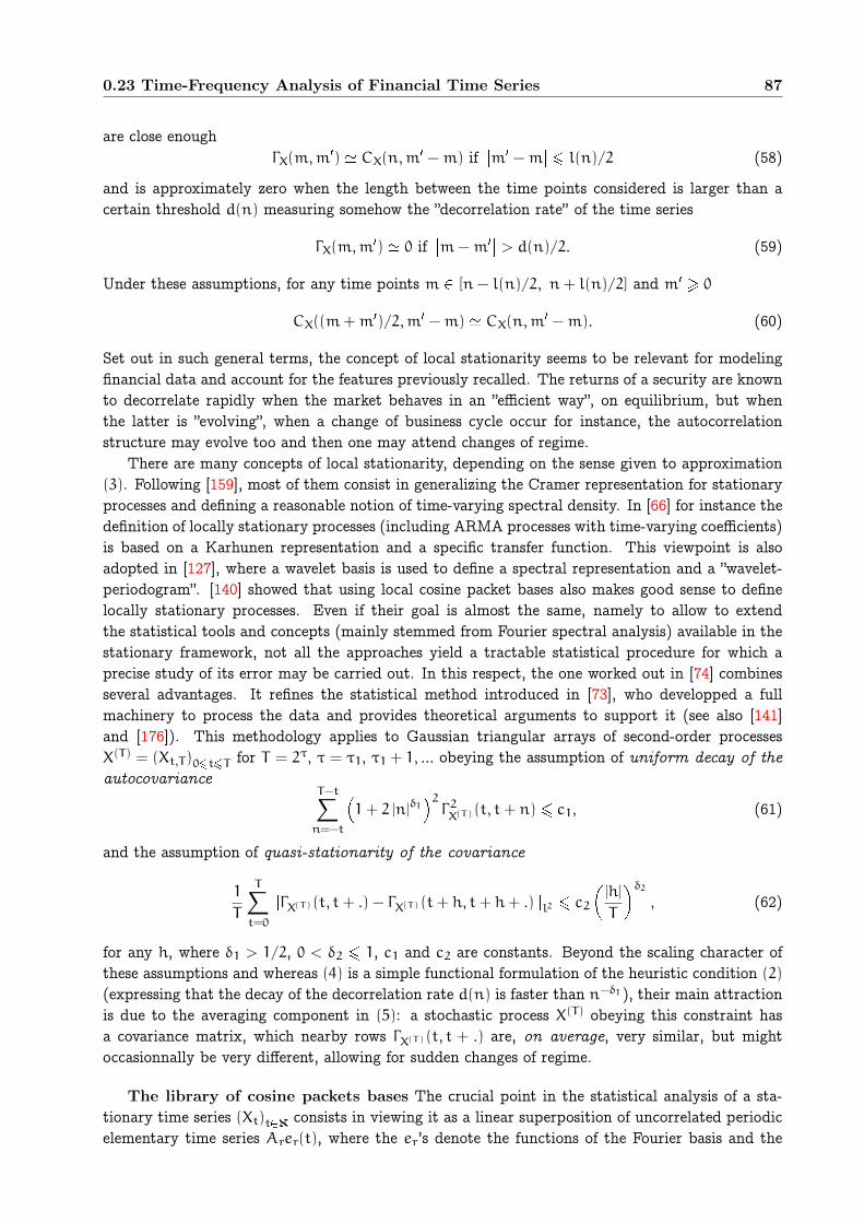
0.23 Time-Frequency Analysis of Financial Time Series 87
are close enoughΓX(m,m
) CX(n,m −m) ifm −m
l(n)/2 (58)
and is approximately zero when the length between the time points considered is larger than acertain threshold d(n) measuring somehow the ”decorrelation rate” of the time series
ΓX(m,m) 0 if
m−m > d(n)/2. (59)
Under these assumptions, for any time points m [n− l(n)/2, n+ l(n)/2] and m 0
CX((m+m)/2,m −m) CX(n,m −m). (60)
Set out in such general terms, the concept of local stationarity seems to be relevant for modelingfinancial data and account for the features previously recalled. The returns of a security are knownto decorrelate rapidly when the market behaves in an ”efficient way”, on equilibrium, but whenthe latter is ”evolving”, when a change of business cycle occur for instance, the autocorrelationstructure may evolve too and then one may attend changes of regime.
There are many concepts of local stationarity, depending on the sense given to approximation(3). Following [159], most of them consist in generalizing the Cramer representation for stationaryprocesses and defining a reasonable notion of time-varying spectral density. In [66] for instance thedefinition of locally stationary processes (including ARMA processes with time-varying coefficients)is based on a Karhunen representation and a specific transfer function. This viewpoint is alsoadopted in [127], where a wavelet basis is used to define a spectral representation and a ”wavelet-periodogram”. [140] showed that using local cosine packet bases also makes good sense to definelocally stationary processes. Even if their goal is almost the same, namely to allow to extendthe statistical tools and concepts (mainly stemmed from Fourier spectral analysis) available in thestationary framework, not all the approaches yield a tractable statistical procedure for which aprecise study of its error may be carried out. In this respect, the one worked out in [74] combinesseveral advantages. It refines the statistical method introduced in [73], who developped a fullmachinery to process the data and provides theoretical arguments to support it (see also [141]and [176]). This methodology applies to Gaussian triangular arrays of second-order processesX(T) = (Xt,T)0tT for T = 2τ, τ = τ1, τ1+ 1, ... obeying the assumption of uniform decay of the
autocovarianceT−t∑
n=−t
1+ 2 |n|
δ1
2Γ2X(T ) (t, t+ n) c1, (61)
and the assumption of quasi-stationarity of the covariance
1
T
T∑
t=0
ΓX(T ) (t, t+ .) − ΓX(T ) (t+ h, t+ h+ .)l2 c2
|h|
T
δ2
, (62)
for any h, where δ1 > 1/2, 0 < δ2 1, c1 and c2 are constants. Beyond the scaling character ofthese assumptions and whereas (4) is a simple functional formulation of the heuristic condition (2)
(expressing that the decay of the decorrelation rate d(n) is faster than n−δ1 ), their main attractionis due to the averaging component in (5): a stochastic process X(T) obeying this constraint hasa covariance matrix, which nearby rows ΓX(T ) (t, t + .) are, on average, very similar, but mightoccasionnally be very different, allowing for sudden changes of regime.
The library of cosine packets bases The crucial point in the statistical analysis of a sta-tionary time series (Xt)tℵ consists in viewing it as a linear superposition of uncorrelated periodicelementary time series Arer(t), where the er’s denote the functions of the Fourier basis and the

88 Applications in Finance
weights Ar are square integrable r.v.’s. The estimation of the variances of the Ar’s from the recordof the past observations of the time series yields both a low bias estimate of the covariance functionand a spectral tool to analyze the structure of the time series: a current ”physical” interpretationconsists in measuring the relative importance of each periodic component Arer in the mechanismruling the fluctuations of the time series by the variance of Ar. Since the 60’s, spectral analysis hasbeen in current use in econometrics for investigating the structure of economic series and comput-ing predictions for instance). The idea underlying the use of the Coifman & Wickerhaüser systemto describe locally stationary processes is to keep the notion of an expansion of the time seriesin a basis made of mutually orthogonal cosine functions, while introducing the point of view oftemporal localization. The construction of this system amounts to concatenate adequately thesequences
ξM,m(t) =
s2
Mcos (ωm(t+ 1/2)) , 0 t < M, (63)
where M = 2j is a dyadic integer, 0 m < M and ωm = π(m + 1/2)/M. For reasons of acomputational nature, the concatenations are induced by recursive dyadic partitions (RDP). ARDP of an inetravl I0,0 = 0, 1, ..., T − 1 of dyadic length T = 2τ is any partition reachable fromthe trivial partition P0 = I0,0 by successive application of the following rule: choose a dyadicsubinterval Ij,k =
kT/2j, ..., (k+ 1)T/2j− 1
in the current partition and split it into two (dyadic)
subintervals Ij+1,2k and Ij+1,2k+1 of same size, creating then a new (finer) partition. RDP maygenerate a very inhomogeneous segmentation of the time interval, with both very short subsegmentsand much longer ones for instance, permitting to describe the successive regimes of a nonstationarytime series (see Fig. 11. Given a RDP P of the time axis 0, 1, ..., T − 1, one defines a local cosine
packets basis P of ℜT by setting
ϕIj,k,m(t) = ξ2τ−j,m(t− kT/2j)
0
if t Ij,kif t / Ij,k , (64)
for all Ij,k in P, and 0 m < 2τ−j. Beyond their orthonormal character, the vectors of such a basishave the crucial property of being localized both in time and in frequency: ϕIj,k,m is supported onthe subinterval Ij,k, on which it oscillates at the frequency ωm.
Every random sequence X(T) = (X0, ..., XT−1) may be expanded in the local cosine packets basisP . Let I1, ..., InP be the subintervals forming P. Then, one may write for 0 t < T
X(T)t =
nP∑
u=1
2ju−1∑
m=0
X(T), ϕIu,m
ϕIu,m(t), (65)
where ., . denotes the usual scalar product in ℜT and 2ju the length of the subinterval Iu. Thus,on each subsegment Iu of the time interval, one has a ”Fourier type” decomposition of the timeseries into periodic time series. If, for each subinterval Iu, the components
X(T), ϕIu,m
were
almost uncorrelated, or if P almost ”diagonalizes” ΓX(T ) in an equivalent way (since PΓX(T )P is
the covariance matrix of theX(T), ϕIu,m
’s ), then one could interpret the segments I1, ..., InP as
successive regimes of quasi-stationarity for the time series X(T). In [73] it is proved that for a locally
stationary time series, there always exists such an ”almost” diagonalizing basis and a data-driven
method by complexity penalization has been introduced in [74] to select such a basis and yielda consistent covariance estimation procedure, the resulting covariance estimate being obtained byaveraging, roughly speaking, contiguous time-frequency components with small variance, gettingwhat is called macrotiles.
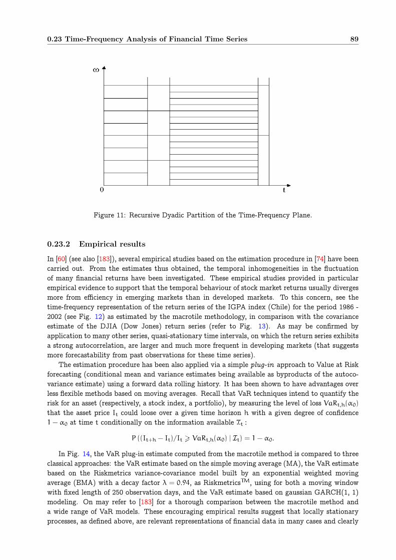
0.23 Time-Frequency Analysis of Financial Time Series 89
Figure 11: Recursive Dyadic Partition of the Time-Frequency Plane.
0.23.2 Empirical results
In [60] (see also [183]), several empirical studies based on the estimation procedure in [74] have beencarried out. From the estimates thus obtained, the temporal inhomogeneities in the fluctuationof many financial returns have been investigated. These empirical studies provided in particularempirical evidence to support that the temporal behaviour of stock market returns usually divergesmore from efficiency in emerging markets than in developed markets. To this concern, see thetime-frequency representation of the return series of the IGPA index (Chile) for the period 1986 -2002 (see Fig. 12) as estimated by the macrotile methodology, in comparison with the covarianceestimate of the DJIA (Dow Jones) return series (refer to Fig. 13). As may be confirmed byapplication to many other series, quasi-stationary time intervals, on which the return series exhibitsa strong autocorrelation, are larger and much more frequent in developing markets (that suggestsmore forecastability from past observations for these time series).
The estimation procedure has been also applied via a simple plug-in approach to Value at Riskforecasting (conditional mean and variance estimates being available as byproducts of the autoco-variance estimate) using a forward data rolling history. It has been shown to have advantages overless flexible methods based on moving averages. Recall that VaR techniques intend to quantify therisk for an asset (respectively, a stock index, a portfolio), by measuring the level of loss VaRt,h(α0)that the asset price It could loose over a given time horizon h with a given degree of confidence1− α0 at time t conditionally on the information available t :
P ((It+h− It)/It VaRt,h(α0) | t) = 1− α0.
In Fig. 14, the VaR plug-in estimate computed from the macrotile method is compared to threeclassical approaches: the VaR estimate based on the simple moving average (MA), the VaR estimatebased on the Riskmetrics variance-covariance model built by an exponential weighted movingaverage (EMA) with a decay factor λ = 0.94, as RiskmetricsTM, using for both a moving windowwith fixed length of 250 observation days, and the VaR estimate based on gaussian GARCH(1, 1)modeling. On may refer to [183] for a thorough comparison between the macrotile method anda wide range of VaR models. These encouraging empirical results suggest that locally stationaryprocesses, as defined above, are relevant representations of financial data in many cases and clearly
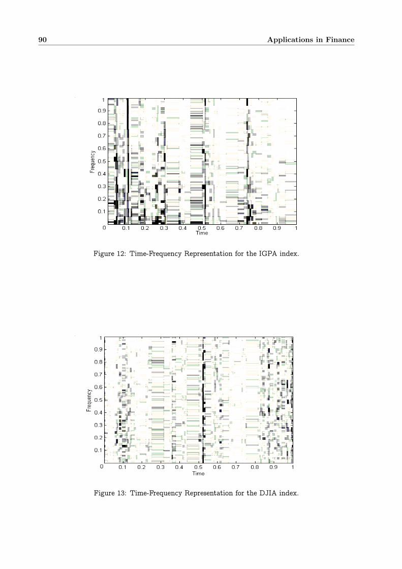
90 Applications in Finance
Figure 12: Time-Frequency Representation for the IGPA index.
Figure 13: Time-Frequency Representation for the DJIA index.
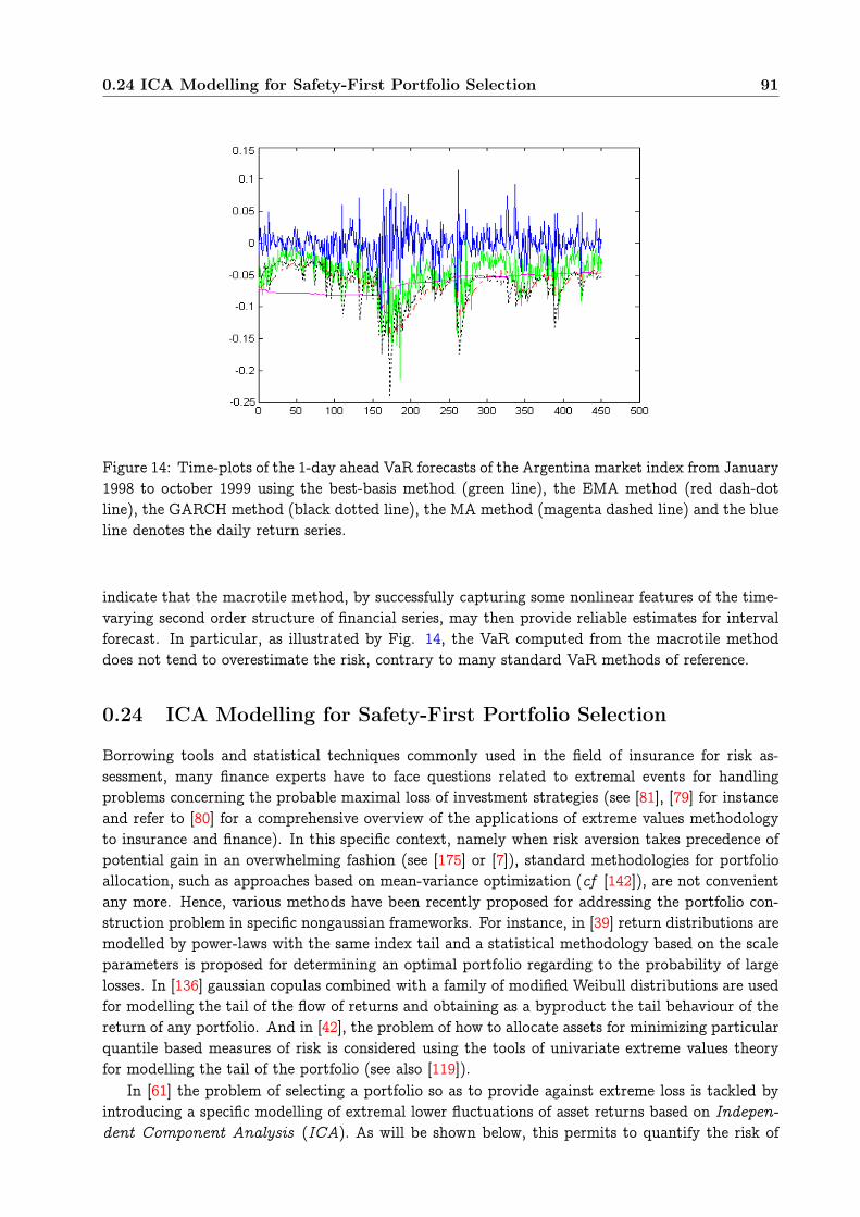
0.24 ICA Modelling for Safety-First Portfolio Selection 91
Figure 14: Time-plots of the 1-day ahead VaR forecasts of the Argentina market index from January1998 to october 1999 using the best-basis method (green line), the EMA method (red dash-dotline), the GARCH method (black dotted line), the MA method (magenta dashed line) and the blueline denotes the daily return series.
indicate that the macrotile method, by successfully capturing some nonlinear features of the time-varying second order structure of financial series, may then provide reliable estimates for intervalforecast. In particular, as illustrated by Fig. 14, the VaR computed from the macrotile methoddoes not tend to overestimate the risk, contrary to many standard VaR methods of reference.
0.24 ICA Modelling for Safety-First Portfolio Selection
Borrowing tools and statistical techniques commonly used in the field of insurance for risk as-sessment, many finance experts have to face questions related to extremal events for handlingproblems concerning the probable maximal loss of investment strategies (see [81], [79] for instanceand refer to [80] for a comprehensive overview of the applications of extreme values methodologyto insurance and finance). In this specific context, namely when risk aversion takes precedence ofpotential gain in an overwhelming fashion (see [175] or [7]), standard methodologies for portfolioallocation, such as approaches based on mean-variance optimization (cf [142]), are not convenientany more. Hence, various methods have been recently proposed for addressing the portfolio con-struction problem in specific nongaussian frameworks. For instance, in [39] return distributions aremodelled by power-laws with the same index tail and a statistical methodology based on the scaleparameters is proposed for determining an optimal portfolio regarding to the probability of largelosses. In [136] gaussian copulas combined with a family of modified Weibull distributions are usedfor modelling the tail of the flow of returns and obtaining as a byproduct the tail behaviour of thereturn of any portfolio. And in [42], the problem of how to allocate assets for minimizing particularquantile based measures of risk is considered using the tools of univariate extreme values theoryfor modelling the tail of the portfolio (see also [119]).
In [61] the problem of selecting a portfolio so as to provide against extreme loss is tackled byintroducing a specific modelling of extremal lower fluctuations of asset returns based on Indepen-
dent Component Analysis (ICA). As will be shown below, this permits to quantify the risk of

92 Applications in Finance
extreme loss of any investment strategy and to determine how diversification should be carried forminimizing this particular extreme risk measure both at the same time.
0.24.1 On measuring extreme risks of portfolio strategies
Risk quantification for financial strategies have been the object of intense research, still developping.Given the nongaussian character of financial returns distributions and in consequence the limitationof the variance as an indicator for describing the amount of uncertainty in their fluctuations, variousrisk measures have been proposed (see [189] for a recent survey on this subject), such as Value atRisk (VaR, see [77] for instance) or Expected Shortfall (ES, see [2]), which are both quantile-basedrisk measures. Risk measures may be considered in particular for guiding investment behaviour.Once a risk measure is chosen, the goal is to select an optimal portfolio with respect to this latter.Suppose that there are D (risky) assets available, indexed by i 1, ...,D. Let a certain (discrete)time scale for observing the price fluctuations be fixed and denote by Xi(t) the price of the i-thasset at time t. Let ri(t) = (Xi(t) −Xi(t− 1))/Xi(t− 1) be the return at time t 1 and denote byr(t) = (r1(t), ..., rD(t)) the flow of returns. Consider the portfolio strategy consisting in investinga fixed relative amount wi [0, 1] of the capital in the i-th asset (short sales being excluded), sothat
∑Di=1wi = 1 (the portfolio is fully invested). The return of the corresponding portfolio at
time t is then
Rw(t) =
D∑
i=1
wiri(t). (66)
Hence, if the r(t)’s are assumed to be i.i.d., so are the Rw(t)’s, with common distribution functionFw. Although in the case when one does not consider investment strategies involving short salesRw(t) is bounded below by −1 (like the ri(t)’s), here we classically use an infinite lower tailapproximation for modelling extreme lower values of portfolio returns (i.e. the left tail of the dfFw). Any risk measure is classically defined as a functional of the portfolio return distributionFw. [61] focused on the maximal relative loss of the portfolio over a large period of time T is,mT = mint=1,...,T Rw(t), of which fluctuations may be characterized by an asymptotic extremevalue distribution H in some cases, i.e. in the cases when Fw is in the domain of attraction of anextreme value distribution H with respect to its lower tail. It is a well-known result in extremevalues theory that there are only three types of possible limit distributions for the minimum ofi.i.d. r.v.’s under positive affine transformations, depending on the tail behavior of their commondensity (refer to [164] for further details on extreme values theory). It is pertinent to considerinvestment strategies w with distribution functions Fw in the maximum domain of attraction ofFréchet distribution functions Φα, α > 0 (MDA(Φα) in abbreviated form), since such dfs form theprime examples for modelling heavy-tailed phenomena (see Chap. 6 in [80] for instance). Recallthat Φα(x) = exp(−x−α)x>0 and that a df F MDA(Φα) iff F(−x) is regularly varying with index−α, that is F(−x) = x−αL(x), for some measurable function L slowly varying at ∞ (i.e. for somefunction L such that L(tx)/L(x) → 1 as x → ∞ for all t > 0). In the case when the df F behavesas a power law distribution at −∞, the tail index α characterizes the extreme lower behaviour ofan i.i.d. sequence (R(t))t0 drawn from F regarding to its minimum value:
P(c−1T ( mint=1,...,T
R(t)) −x) → 1−Φα(x),
as T → ∞ for any x > 0, where cT = supy : F(−y) n−1.As shown in several empirical studies, this class of dfs F contains left heavy-tailed distributions,
usually called power law-like dfs, that may be appropriate for modelling large lower fluctuations ofreturns. Let us observe that the smaller the tail index α is, the heavier the left tail of F is. Hence,when modelling the lower tail behaviour of the distribution of portfolio returns this way, the tail

0.24 ICA Modelling for Safety-First Portfolio Selection 93
index α may appear as a legitimate measure of extreme risk for the portfolio strategy (refer to[116] for a discussion about the relevance of this specific safety first criterion, when managing thedownside risk of portfolios is the matter). Moreover, the tail index α rules the asymptotic behaviorof the excess-of-loss df F(u)(x) = P(R < −u − x | R < −u) below the threshold −u related toF(x) = P(R x) MDA(Φα) for large u > 0, as shown by the following limit distributionalapproximation (see [99] for details on the convergence of normalized excesses over large thresholdsto Generalised Pareto Distributions): for 1+ x/α > 0,
limu→∞
F(u)(xa(u)) = (1+x
α)−α,
where a(u) is a measurable positive function such that a(u)/u → α−1 as u → ∞. The set ofstrategies w of which returns have dfs Fw in MDA(Φα) is thus naturally equipped with a completepreference relation, as follows.
Definition 41 Suppose that w1 and w2 are two portfolio strategies s.t. FwiMDA(Φαi
) with
αi > 0 for i = 1, 2. We shall say that strategy w1 is riskier (respectively, strictly riskier) than
strategy w2 regarding to extreme relative loss iff α1 α2 (resp., α1 < α2).
0.24.2 The Heavy-Tailed ICA Model
Multivariate data are often viewed as multiple indirect measurement of underlying factors or com-ponents, which cannot be directly observed. In some cases, one may hope that a few of these latentfactors are responsible for the essential structure we see in the observed data and correspond tointerpretable causes. Latent Variables Analysis aims to provide tractable theoretical frameworkand develop statistical methods for identifying these underlying components. The general settingof latent variables modelling stipulates that
X = AY, (67)
where X is an observable D-dimensional r.v. and Y is a vector of d unobserved latent variablesconverted to X by the linear transform A, classically called the mixing matrix. When d D andthe mixing matrix is of full rank d, there is no loss (but some redundancy on the contrary, whend < D) in the information carried by X. By inverting, one may write
Y = ΩX, (68)
where the de-mixing matrix Ω is any generalized pseudo-inverse of A: whereas in the case d = D,Ω is uniquely determined by (68) and is simply the inverse A−1 of the mixing matrix, additionalidentifiability constraints are necessary for guaranteeing unicity when d < D. Principal Com-
ponent Analysis (PCA) and Factor Analysis form part of a family of statistical techniques forrecovering Y and A on the basis of an observed sample drawn from X, that are typically designedfor normal distributions, which assumption clearly limited their practical application. In spite ofthe considerable evidence for non-gaussianity of financial returns or log-returns, and on the basis oftheoretical market modelling such as CAPM or APT, Factor Analysis and PCA have been neverthe-less extensively used by practicioners for gaining insight to the explanatory structure in observedreturns. In the mid-90’s, the methodology of Independent Component Analysis (refer to [117]for a comprehensive presentation of ICA), comprising highly successfull new algorithms (mainlyintroduced in the field of signal processing for Blind Source Separation (BSS)) has emerged asa serious competitor to PCA and Factor Analysis, and is based, on the contrary to these lattertechniques, on the non-normal nature of the latent components. Indeed, ICA only relies on theassumption that the underlying factors Y1, Y2, ... are statistically independent (and are naturally

94 Applications in Finance
called independent components for this reason), which hypothesis is much stronger than uncorre-lation when Y is nongaussian (heuristically, uncorrelation determines second-order cross moments,whereas statistical independence determines all of the cross-moments). Stipulating further identi-fiability conditions apart from independence and non-normality of the IC’s, many valid statisticalmethods have been proposed for estimating the ICA model, based on entropy, maximum likeli-hood, mutual information or tensorial methods. The nongaussian character of financial returnsor log-returns being now carried unanimously, several contributions to the application of ICA tofinance have been recently made. The modelling of the fluctuations of financial returns and thesearch for independent factors through ICA thus gave rise to several works, among which [15], [124]and [51].
Modelling extremal events via ICA The specific ICA model proposed in [61] for describingthe extreme lower fluctuations of asset returns, which they called the heavy-tailed ICA model.Suppose that there are D securities indexed by i 1, ...,D and let Xi(t) be the price of the i-thsecurity at time t. The returns of the i-th security are defined by
ri(t) = (Xi(t) − Xi(t− 1))/Xi(t− 1), t 1. (69)
Suppose further that the flow of daily returns of the D assets are i.i.d. realizations of a r.v.r = (r1, ..., rD) with components that are linear combinations of D independent elementary
portfolios returns R1, ..., RD, so that
r = AR, (70)
where R = (R1, ..., RD) and A = (aij) is a D by D matrix of full rank, of which inverse Ω belongsto the (compact and convex) set of parameters
= Ω = (ωij)1i,jD/ ωij 0,
D∑
k=1
ωik = 1 for 1 i, j D. (71)
We thus haveR = Ωr. (72)
The Ri’s are assumed to have heavy-tailed distributions, furthermore lower-tails are supposed tobe Pareto-like below some (unknown) thresholds:
Gi(y) = P(Ri < −y) = Ciy−αi , for y si, (73)
with strictly positive constants αi, Ci and si, 1 i D. In addition, the αi’s are supposed to bedistinct and, with no loss of generality, the IC’s are indexed so that α1 > ... > αD (the elementaryportfolios are thus sorted by increasing order of their riskiness regarding to Definition 41), so as toensure that the statistical model is identifiable.
In this framework, the next result shows that an optimal strategy with respect to extremerelative loss is straightforwardly available.
Theorem 42 (Clémençon & Slim, 2006) Under the assumptions above, the elementary port-
folio strategy ω1 = (ω11, ...,ω1D) is optimal with respect to the extreme risk measure.
Semi-parametric inference Several objects must be estimated, the tail indexes α1, ..., αD, theconstants C1, ..., CD, as well as the matrix Ω of elementary strategies. A feasible method forestimating the semi-parametric ICA model described above is based on conditional MLE, as theclassical Hill inference procedure for tail index estimation (refer to [110]). Let us first introduce

0.24 ICA Modelling for Safety-First Portfolio Selection 95
some additional notation. For i 1, ...,D, denote by Ri(1), ..., Ri(N) an i.i.d. sample drawn fromRi and by Ri(σi(1)) ... Ri(σi(N)) the corresponding order statistics. Recall that the basic Hill
estimator for the tail index αi based on this sample is:
αHi,k = (1
k
k∑
l=1
ln(Ri(σi(l))
Ri(σi(k))))−1,
with 1 k N such that Ri(σi(k)) < 0, while Ci is estimated by Ci = kN
(−Ri(σi(k)))αi . These esti-
mates are (weakly) consistent, as soon as k = k(N) is picked such that k(N) → ∞ andN/k(N) → ∞as N → ∞ (cf [144]) and are strongly consistent if furthermore k(N)/ ln lnN → ∞ as N → ∞(see [71]). They are classically interpreted as a conditional maximum likelihood estimators basedon maximization of the joint density fi,k(y1, ..., yk) of (−Ri(σi(1)), ..., −Ri(σi(k))) conditioned onthe event Ri(σi(k)) −si:
fi,k(y1, ..., yk) =N!
(N− k)!(1− Ciy
−αi
k )N−kCkiαki
k∏
l=1
y−(αi+1)l ,
for 0 < si y1 ... yk and fi,k(y1, ..., yk) = 0 otherwise. Hence the conditional likelihoodbased on R is
D∏
i=1
fi,k(−Ri(σi(1)), ...,−Ri(σi(k))).
One may now derive the conditional likelihood of the model from the observation of a sample oflength N of asset returns r(N) = (r(1), ..., r(N)) = ((ri(1))1iD, ..., (ri(N))1iD). For all 1 i D, sort the return vector observations r(l), 1 l N, so that ωir(σi(1)) ... ωir(σi(N))
(observe that the permutation σi depends on ωi: ωir(σi(l)) = R(σi(l)), 1 l N). Hence, thelikelihood function based on the observations r(σi(l)), 1 l k, 1 i D and conditioned onthe event ωir(σi(k)) −si, 1 i D is
Lk(r(N),Ω, α,C) = |detΩ|kD∏
i=1
fi,k(−ωir(σi(1)), ...,−ωir(σi(k))).
For any given r(N), the functional Lk(r(N), . , . , .) is continuous and piecewise differentiable on + +. Furthermore, as previously recalled, for any fixed Ω and for all i 1, ...,D,
fi,k(−ωir(σi(1)), ...,−ωir(σi(k)) is maximum for αi = αi and Ci = Ci with
αi = (1
k
k∑
l=1
ln(ωir(σi(l))
ωir(σi(k))))−1 and Ci =
k
N(−ωir(σi(k)))
αi .
For any Ω , L(r(N),Ω, α,C) is thus maximum for α = α = (αi)1iD and C = C = ( Ci)1iDand we denote this maximal value by Lk(Ω) = Lk(r
(N), Ω, α, C). Here, conditional MLE reducesthen to maximizing the multivariate scalar function Lk(Ω) over Ω , which may be easily shownas equivalent to maximizing over Ω :
lk(Ω) = |detΩ|k exp
−
D∑
i=1
k ln(
k∑
l=1
ln(ωir(σi(l))
ωir(σi(k)))) +
k∑
l=1
ln(−ωir(σi(l))
.In our setting, estimating the ICA model (70) thus boils down to the task of finding Ω in the
closed convex set such that lk( Ω) = maxΩ lk(Ω). In addition to the theoretical estimationprinciple described above, a numerical method for maximizing the objective function lk(Ω) (or

96 Applications in Finance
Lk(Ω)) subject to the linear matrix constraint Ω is required. Various optimization methods,among which the popular subgradient-type learning algorithms, have been introduced for prac-tically solving such a constrained optimization problem approximatively. The objective functionlk(Ω) is continuous and piecewise differentiable on D(): its gradient rlk(Ω) is well-defined ateach point Ω = (ωi,j)1i,jD such that detΩ = 0 and ωir(σi(k−1)) < ωir(σi(k)) < ωir(σi(k+1))
for all i 1, ...,D, we have
∂lk
∂ωi,j(Ω)/lk(Ω) = kγi,j(Ω)/detΩ+
k∑
l=1
rj(σi(l))/ωir(σi(l))
− k
∑kl=1rj(σi(l))/ωir(σi(l)) − rj(σi(k))/ωir(σi(k))
∑kl=1 ln(ωir(σi(l))/ωir(σi(k)))
, (74)
where γi,j(Ω) denotes the cofactor of ωi,j in Ω, 1 i, j D (the subdifferential ∂lk(Ω) is theneasily determined through equation (74) at any point Ω D()). In the applications mentionedbelow, the classical projected subgradient method is used for estimating the Heavy-tailed ICAmodel and selecting an optimal portfolio knowing the sample r(N).
0.24.3 Some empirical results
As explained above, the statistical method proposed in [61] aims at searching for independentportfolio strategies and at estimating their Pareto left tail indexes as well. It also permits torecover as a byproduct a portfolio strategy with a maximum left tail index).
As an illustration of the Heavy-tailed ICA model, here the latter is applied for analyzing thedaily return series of D = 11 international equity indexes of (developed or developing) financialmarkets over the period running from 02-January-1987 to 22-October-2002 listed in Table 0.24.3.The results indicate the allocations corresponding to the 11 independent elementary portfolios,as well as their left tail index estimate, sorted by increasing order of their extreme risk measure,obtained by implementing the statistical procedure described in §7.2.2 with the k = 200 lowestvalues (representing roughly the lowest 5% values). Descriptive statistics related to the lowertail behaviour of each elementary portfolio are also displayed in Table 0.24.3: minimum returnvalues, empirical estimates of the probability of excess (EPE in short), P(Ri < −u), that the i-thelementary portfolio looses more than u% of its value (at a one day horizon) are calculated at variousthreshold levels u over the time period considered, as well as the empirical counterpart of the meanexcess function (ME in abbreviated form), ei(u) = −(Ri + u | Ri < −u), traditionally referredto as the expected shortfall in the financial risk management context. In a general fashion, thelower tails of the single assets are globally much heavier than the ones of the least risky elementaryportfolios we obtained. For instance, the maximum relative loss suffered by the optimal elementaryportfolio (PF1) over the period of interest is 3.86% , while the minimum values of single marketindexes range from −10.29% to −40.54%. As expected, except for the FTSE100 index, zero orsmall weights in PF1 correspond to the market indexes with the most heavier left tails (namely,the Hong Kong, Malaisia and Singapore indexes, which correspond to emerging financial marketsthat are presumably very interdependent, whereas on the contrary the latter indexes have thelargest weights for PF11. These results clearly show the benefit of the diversification induced byour specific modelling of the dependence structure between the assets regarding to extreme risk.This phenomenon is also illustrated by Table 0.24.3. It shows lower tail statistics of the optimalportfolio obtained by applying our modelling as a function of the number D of market indexesinvolved in the ICA model (financial indexes being progressively added, by decreasing order oftheir tail index estimates) and plainly indicates that the lower tail becomes thinner as D grows.
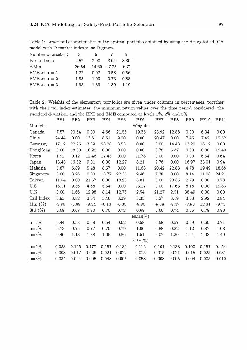
0.24 ICA Modelling for Safety-First Portfolio Selection 97
Table 1: Lower tail characteristics of the optimal portfolio obtained by using the Heavy-tailed ICAmodel with D market indexes, as D grows.
Number of assets D 3 5 7 9Pareto Index 2.57 2.90 3.04 3.30%Min -36.54 -14.60 -7.25 -6.71EME at u = 1 1.27 0.92 0.58 0.56EME at u = 2 1.53 1.09 0.73 0.88EME at u = 3 1.98 1.39 1.39 1.19
Table 2: Weights of the elementary portfolios are given under columns in percentages, togetherwith their tail index estimates, the minimum return values over the time period considered, thestandard deviation, and the EPE and EME computed at levels 1%, 2% and 3%.
PF1 PF2 PF3 PF4 PF5 PF6 PF7 PF8 PF9 PF10 PF11Markets WeightsCanada 7.57 20.64 0.00 4.66 21.58 19.35 23.92 12.88 0.00 6.34 0.00Chile 24.44 0.00 13.61 8.61 9.20 0.00 20.47 0.00 7.45 7.42 12.52Germany 17.12 22.96 3.89 28.28 3.53 0.00 0.00 14.43 13.20 16.12 0.00HongKong 0.00 18.09 16.22 0.00 0.00 0.00 3.78 6.37 0.00 0.00 19.40Korea 1.92 0.12 12.46 17.43 0.00 21.78 0.00 0.00 0.00 6.54 3.64Japan 13.43 16.82 9.01 0.00 12.27 8.21 2.76 0.00 16.97 33.01 0.94Malaisia 5.87 6.89 5.48 8.57 0.00 11.68 20.42 22.83 4.78 19.49 18.68Singapore 0.00 3.26 0.00 18.77 22.36 9.46 7.38 0.00 8.14 11.08 24.21Taiwan 11.54 0.00 21.67 0.00 18.28 3.81 0.00 23.35 2.79 0.00 0.78U.S. 18.11 9.56 4.68 5.54 0.00 23.17 0.00 17.63 8.18 0.00 19.83U.K. 0.00 1.66 12.98 8.14 12.78 2.54 21.27 2.51 38.49 0.00 0.00Tail Index 3.93 3.82 3.64 3.46 3.39 3.35 3.27 3.19 3.03 2.92 2.84Min (%) -3.86 -5.89 -8.34 -6.13 -6.35 -9.80 -9.38 -8.47 -7.93 12.31 -9.72Std (%) 0.58 0.67 0.80 0.75 0.72 0.68 0.66 0.74 0.65 0.78 0.80
EME(%)u=1% 0.44 0.58 0.58 0.54 0.62 0.58 0.58 0.57 0.59 0.60 0.71u=2% 0.73 0.75 0.77 0.70 0.79 1.06 0.88 0.82 1.12 0.87 1.08u=3% 0.46 1.13 1.38 1.05 0.86 1.51 2.07 1.30 1.91 2.03 1.49
EPE(%)u=1% 0.083 0.105 0.177 0.157 0.139 0.112 0.101 0.138 0.100 0.157 0.154u=2% 0.008 0.017 0.026 0.021 0.022 0.015 0.015 0.021 0.015 0.025 0.031u=3% 0.034 0.004 0.005 0.048 0.005 0.053 0.003 0.005 0.004 0.005 0.010

98 Applications in Finance

Applications in Biosciences
0.25 Stochastic Toxicologic Models for Dietary Risk Analysis
Certain foods may contain varying amounts of chemicals such as methyl mercury (present in seafood), dioxins (in poultry, meat) or mycotoxins (in cereals, dried fruits, etc.), which may causemajor health problems when accumulating inside the body in excessive doses. Food safety is now acrucial stake as regards public health in many countries. This topic naturally interfaces with variousdisciplines, such as biology, nutritional medicine, toxicology and of course applied mathematics withthe aim to develop rigorous methods for quantitative risk assessment. A scientific literature devotedto probabilistic and statistical methods for the study of dietary exposure to food contaminants isprogressively carving out a place in applied probability and statistics journals (see [195] or [29] forinstance).Static viewpoints for the probabilistic modeling of the quantity X of a given food contaminantingested on a short period have been considered in recent works, mainly focussing on the tailbehavior of X and allowing for computation of the probability that X exceeds a maximum tolerabledose (see [194]). However, such approaches for food risk analysis do not take into account theaccumulating and eliminating processes occurring in the body, which naturally requires to introducetime as a crucial description parameter of a comprehensive model.
0.26 Modeling the exposure to a food contaminant
Dietary behavior Suppose that an exhaustive list of P types of food, indexed by p = 1, , P,involved in the alimentation of a given population and possibly contaminated by a certain chemical,is drawn up. Each type of food p 1, , P is contaminated in random ratio K(p), with probabilitydistribution F(p) , regarding to the chemical of interest. Concerning this specific contaminantexposure, a meal may be viewed as a realization of a r.v. Q = (Q(1), , Q(P)) indicating thequantity of food of each type consumed, renormalized by the body weight. For a mealQ drawn froma distribution F on (P+,P
+), cooked from foods of which toxicity is described by a contamination
ratio vector K = (K(1), , K(P)) drawn from F = Pp=1F(p) , the global contaminant intake isU = K,Q, denoting by ., . the standard inner product on P. Its probability distribution F❯ isthe image of FF by the inner product ., ., assuming that the quantities of food consumed areindependent from the contamination levels. Here and throughout, we suppose that the contaminantintake distribution FU has a density fU with respect to λ, the Lebesgue measure on +.
The food contamination phenomenon through time for an individual of the population of inter-est may be classically modeled by a marked point process (Tn, Qn, Kn)n1 on +P+P+, theTn’s being the successive times at which the individual consumes foods among the list 1, , P(T0 = 0 being chosen as time origin) and the marks (Qn, Kn) being respectively the vector of foodquantities and the vector of contamination ratios related to the meal had at time Tn. The process(Tn, Qn)n1 describing dietary behavior is assumed independent from the sequence (Kn)n1 ofchemical contamination ratios. Although the modeling of dietary behaviors could certainly give

100 Applications in Biosciences
rise to a huge variety of models, depending on the dependence structure between (Tn, Qn) and pastvalues (Tm, Qm)m<n that one stipulates, we make here the simplifying assumption that the marksQn, n 1, form an i.i.d. sequence with common distribution F, independent from the locationtimes (Tn)n1. This assumption is acceptable for chemicals present in a few types of food, suchas methyl mercury, but certainly not for all contaminants. For chemicals present in many foods ofeveryday consumption, it would be necessary to introduce additional autoregressive structure inthe model for capturing important features of any realistic diet (the consumption of certain foodbeing typically alternated for reasons related to taste or nutritional aspects). Such a modeling taskis left for further investigation. Finally, suppose that the inter-intake times ∆Tn+1 = Tn+1 − Tn,n 1, form a sequence of i.i.d. r.v.’s with common probability distribution G(dt) = g(t)dt andfinite expectation mG =
∫∞t=0
tG(dt) < ∞, the sequence (Tn)n1 of intake times being thus a purerenewal process.
Toxicokinetics Contamination sources other than dietary are neglected in the present studyand denote by X(t) the total body burden in contaminant at time t 0. In between intakes,assume that the contamination exposure process X(t) is governed by the differential equation
x(t) = −r(x(t), θ), (75)
θ being a random parameter, taking its values in a set Θ d with d 1 say, and accounting inthe modeling for fluctuations of the (content dependent) elimination rate due to metabolic factorsat the intake times (the successive values θn, n , of θ are thus fixed at times T0, T1, ). Andthe function r(x, θ) is assumed to be strictly positive and continuous on +Θ, such that for allθ Θ, r(0, θ) = 0 (so that when X(t) eventually reaches the level 0, the process stays at this leveluntil the next intake) and for all (ǫ, θ) (0, 1)Θ:
infǫ<x<ǫ−1r(x, θ) > 0 and sup0<x<ǫ−1r(x, θ) < ∞. (76)
Under these conditions, for any initial value x(0) 0 and metabolic parameter value θ Θ, Eq.(75) has clearly a unique solution.
Remark 4 In toxicology, Eq. (75) is widely used with r(x, θ) = θx for modelling the kineticsin man of certain contaminants following intakes. As shown by many pharmacokinetics studies,there is considerable empirical evidence that it properly describes the way the elimination ratedepends on the total body burden of the chemical in numerous cases. In this context, the releaseparameter log2/θ is known as the half-life of the contaminant in the body (the time required forX to decrease by half in absence of new contaminant intake).
We assume that (θn)n is an i.i.d. sequence with common distribution H(dθ). For a given valueof the metabolic parameter θ Θ, the time necessary for the body burden (without further intake)to decrease from x0 > 0 to x (0, x0) is given by
τθ(x0, x) =
∫x0
x
1
r(y, θ)dy.
Under the assumptions stated above, we clearly have that H(τθ(x0, x) < ∞) = 1 for all 0 < x x0.The contaminant may be thus entirely eliminated from the body (the amount x reaching then thelevel 0) with probability one in the sole case when the following condition holds.
Condition (1): H(τθ(x0, 0) < ∞) = 1 for some x0 > 0.
In such a case, H(τθ(x, 0) < ∞) = 1 for all x 0. In this respect, it is noteworthy that, in thelinear case mentioned in Remark 2, τθ(x, 0) = ∞ for all θ > 0 and x > 0.

0.26 Modeling the exposure to a food contaminant 101
t
T0 T1 T2 T3
X(t)
Figure 15: Sample path of the exposure process X.
Hence, in between intake times and given the current value of the metabolic parameter θ, theprocess moves in a deterministic fashion according to (75), and has the same (upward) jumps asthe process of cumulative intakes
B(t) =
N(t)∑
n=1
Un, (77)
with Un = Kn, Qn, n , and denoting by N(t) =∑n Tn t the number of intakes until
time t. The process X is piecewise-deterministic with càd-làg trajectories (see a typical samplepath in Fig. 15) and satisfies the equation
X(t) = X(0) + B(t) −
N(t)+1∑
n=1
∫Tn∧t
Tn−1
r(X(s), θn)ds, (78)
X(0) denoting the total body burden in contaminant at initial time T0 = 0. For an account of suchpiecewise deterministic processes, one may refer to [68] (see also [69] and some ergodic results maybe found in [64]).
For the continuous-time process thus defined to be markovian, one has to record the cur-rent value θ(t) =
∑n θnt[Tn,Tn+1[ of the metabolic parameter as well as the backward re-
currence time A(t) = t − TN(t) (the time since the last intake). By construction, the process(X(t), θ(t), A(t))t0 is strongly Markovian with generator
φ(x, θ, t) = ζ(t)
∫∞
u=0
∫
θΘφ(x+ u, θ, 0) − φ(x, θ, t)FU(du)H(dθ)
− r(x, θ)∂xφ(x, θ, t) + ∂tφ(x, θ, t), (79)
denoting by ζ(t) = g(t)/∫∞s=tg(s)ds the hazard rate of the inter-intake times and provided that
φ(., θ, .) : (x, t) → φ(x, θ, t) is a bounded function with bounded continuous first derivatives in xand t for all θ Θ.
In the above setting, the time origin T0 = 0 does not necessarily correspond to an intaketime. Given the time A(0) = a since the last intake at time t = 0, we let ∆T1 have the density

102 Applications in Biosciences
ga(t) = g(a + t)/∫∞s=a
g(s)ds, making the renewal process (∆Tn)n possibly delayed, exceptnaturally in the case when the inter-intake distribution G is exponential. However, the choiceof such a memoryless distribution in the dietary context is clearly not pertinent, distributionswith increasing hazard rate being more adequate. Here and throughout we denote by Px,a theprobability measure on the underlying space such that (X(0), A(0)) = (x, a) and θ(0) ∼ H, and byx,a(.) the Px,a-expectation for all x 0 and a supp(G).
In the case when one neglects variability in the elimination process, this modeling boils down toa standard storage model with a general release rate (see [45] for instance). Basic communicationand stochastic stability properties of the stochastic process X = (X(t))t0 may be established in afashion very similar to the ones of the latter processes, although the additional assumption that therenewal times are exponentially distributed is usually required in these studies, making the processX itself Markovian (which facilitates much the study but is not relevant to the present applicationas emphasized above).
Theorem 43 (Bertail, Clémençon & Tressou, 2006a) Suppose that G(dx) = g(x)dx has in-
finite tail. Assume further that either g(x) > 0 on ]0, ǫ] for some ǫ > 0 or else that F❯ has
infinite tail. Then X reaches any state x > 0 in finite time with positive probability whatever
the starting point, i.e. for all x0 0, a supp(G), it holds
Px0,a(τx < ∞) > 0, (80)
with τx = inft 0 : Xt = x. Furthermore, if condition (1) is fulfilled, then (80) still holds
for x = 0.
Besides, either X ”heads to infinity” with probability one, i.e. is such that Px0,a(X(t) → ∞ ,
as t → ∞) = 1 for all x0 0, or else X reaches any state x > 0 in finite time with probability
one whatever the starting point, i.e. for all x0 0, a supp(G),
Px0,a(τx < ∞) = 1. (81)
If (1) is satisfied, then (81) also holds for x = 0.
An important task is to find conditions ensuring that the limiting behavior of the exposureprocess X is represented by a stationary probability measure µ describing the equilibrium state towhich the process settles as time goes to infinity. In particular, time averages over long periods,such as the mean time spent by the exposure process X over a threshold u > 0, T−1
∫T0Xtudt,
for instance, are then asymptotically described by the distribution µ. Beyond stochastic stabilityproperties, evaluating the rate at which the process converges to the stationary state is also ofcritical importance. These questions are now tackled for linear rate models.
0.27 Probabilistic study in the linear rate case
We now focus on ergodicity properties of the exposure process X(t) in the specific case when for agiven metabolic state described by a real parameter θ, the elimination rate is proportional to thetotal body burden in contaminant, i.e.
r(x, θ) = θx. (82)
Here we suppose that Θ is a subset of +, ensuring that (76) is satisfied. The linear case is ofcrucial importance in toxicology, insofar as it suitably models the pharmacokinetics behavior inman of numerous chemicals. In this case studying the long-term behavior of X can be reduced

0.27 Probabilistic study in the linear rate case 103
to investigating the properties of the embedded chain X = (Xn)n1 of which values correspond tothe ones taken by the exposure process just after intake times : Xn = X(Tn) for all n 1. Byconstruction, the chain X satisfies the following autoregressive equation with random coefficients
Xn+1 = e−θn∆Tn+1Xn+Un+1, for all n 1, (83)
and has transition probability Π(x, dy) = π(x, y)dy with transition density
π(x, y) =
∫
θΘ
∫∞
t=1θlog(1∨x
y)
fU(y− xe−θt)G(dt)H(dθ), (84)
for all (x, y) 2+ , where a∨ b = max(a, b). Ergodicity of such real-valued Markov chains Y, de-fined through stochastic recurrence equations of the form Yn+1 = αnYn+βn, where (αn, βn)n
is a sequence of i.i.d. pairs of positive r.v.’s, has been extensively studied in the literature, suchmodels being widely used in financial or insurance mathematics (see section 8.4 in [?] for instance).Specialized to our setting, well known results related to such processes enable to study the embed-ded chains X is positive recurrent under the assumption that log(1 ∨ U1) has finite expectation.Furthermore, the simple autoregressive form of Eq. (83) makes Foster-Lyapunov conditions easilyverifiable for such chains, in order to refine their stability analysis. The following assumptions arerequired in the sequel.
• (H1) [log(1∨U1)] < ∞,
• (H2) there exists some γ 1 such that (Uγ1) < ∞,
• (H3) the r.v. U1 is regularly varying with index κ > 0,
• (H4) there exists δ > 0 such that [exp(δ∆T2)] < ∞.
Theorem 44 (Bertail, Clémençon & Tressou, 2006a) Under the assumptions of Theorem
1 and supposing that (H1) is fulfilled, X(t) has an absolutely continuous limiting probability
distribution µ given by
µ([u,∞[) = m−1G
∫∞
x=u
∫∞
t=0
∫
θΘt∧
log(x/u)
θµ(dx)G(dt)H(dθ), (85)
in the sense that T−1∫T0Xtudt → µ(]0, u]), Px0,a-a.s., as t → ∞ for all x0 0 and a
supp(G). Furthermore,
• if (H3) holds and Θ is bounded, then µ is regularly varying with the same index as FU,
• and if (H2) and (H4) hold and G has finite variance σ2G, then µ has finite moment of
order γ and for all (x, a) + supp(G) there exist constants k ]0, 1[, Ka < ∞ such
that
supψ(z)1+zγ |x,a[ψ(Xt)] − µ(ψ)| Ka(1+ xγ)kt. (86)
Remark 5 When the Un’s are heavy-tailed, and under the assumption that the ∆Tn’s are expo-nentially distributed (making B(t) a time-homogeneous Lévy process), the fact that the stationarydistribution µ inherits its tail behavior from FU has been established in [9] for general determin-istic release rates. Besides, when assuming G exponential and θ fixed, one may identify the limitdistribution µ in some specific cases (see section 8 in [44] or section 2 in Chap. XIV of [8]) usingbasic level crossing arguments (X being itself markovian in this case). If FU is also exponential forinstance, µ is a Gamma distribution. And furthermore, due to the simple form of the generatorin the latter case, one may establish an exponential rate of convergence to µ by standard driftcriterion or coupling arguments (see section 5 in [169]).

104 Applications in Biosciences
In order to exhibit connections between the exposure process X = (X(t))t0 and possible nega-tive effects of the chemical on human health, it is appropriate to consider simple characteristics ofthe process X, easily interpretable from an epidemiology viewpoint. In this respect, the mean ex-position over a long time period T−1
∫Tt=0
X(t)dt is one of the most relevant features. Its asymptoticbehavior is refined in the next result.
Proposition 45 (Bertail, Clémençon & Tressou, 2006a) Under the assumptions of Theorem
1 and supposing that (H2) is fulfilled for γ = 1, we have for all (x0, a) + supp(G)
XT =1
T
∫T
t=0
X(t)dt → mµ,Px0,a-a.s. , (87)
as T → ∞ with mµ =∫∞x=0
xµ(dx). Moreover, if (H2) is fulfilled with γ 2, then there exists
a constant 0 < σ2 < ∞ s.t. for all (x0, a) + supp(G) we have the following convergence
in Px0,a-distribution ♣T(XT −mµ) ⇒ (0, σ2) as T → ∞. (88)
Remark 6 The asymptotic variance σ2 in (88) may be related to the limiting behavior of acertain additive functional of the Markov chain ((Xn, θn, ∆Tn+1))n1. In [20] (see also [19]), anestimator of the asymptotic variance of such functionals based on pseudo-renewal properties of theunderlying chain (namely, on renewal properties of a Nummelin extension of the chain) has beenproposed and a detailed study of its asymptotic properties has been carried out. Beyond the asymptotic exposure mean or the asymptotic mean time spent by X above a certainthreshold, other summary characteristics of the exposure process could be pertinently consid-ered from an epidemiology viewpoint, among which the asymptotic tail conditional expectationµ(X | X > u), denoting by µ(.) the expectation w.r.t. µ, after the fashion of risk evaluation inmathematical finance or insurance.
0.28 Simulation-based statistical inference
We now consider the statistical issues one faces when attempting to estimate certain features oflinear rate exposure models. The main difficulty lies in the fact that the exposure process X isgenerally unobservable. Food consumption data (quantities of consumed food and consumptiontimes) related to a single individual over long time periods are scarcely available in practice.And performing measurements at all consumption times so as to record the food contaminationlevels appears as not easily realizable. Instead, practitioners have at their disposal some massivedatabases, in which information related to the dietary habits of large population samples overshort periods of time is gathered. Besides, some contamination data concerning certain chemicalsand types of food are stored in data warehouses and available for statistical purposes. Finally,experiments for assessing models accounting for the pharmacokinetics behavior in man of variouschemicals have been carried out. And data permitting to fit values or probability distributionson the parameters of these models are consequently available. Estimation of steady-state or time-dependent features of the law X of the process X given the starting point (X(0), A(0)) = (x0, a) + supp(G) could thus be based on preliminary computation of consistent estimates G, FU andH of the unknown df’s G, FU and H. Hence, when the quantity of interest (X) is not analyticallyavailable from (G, FU, H), ruling out the possibility of computing plug-in estimates, a feasiblemethod could consist in simulating sample paths starting from (x0, a) of the approximate processX with law X corresponding to the estimated df’s (G, FU, H) and construct estimators based onthe trajectories thus obtained. This leads up to investigate the stability of the stochastic exposure

0.28 Simulation-based statistical inference 105
model w.r.t. G, FU and H, and consider the continuity problem consisting in evaluating a measureof closeness between X and X making the mapping X → (X) continuous for the functionalof interest (refer to [160] for an account on this topic). Hence, convergence preservation resultsmay be obtained via the continuous-mapping approach as described in [199], where it is appliedto establish stochastic-process limits for queuing systems.
Let 0 < T < ∞. Since the exposure process X has càd-làg sample paths, we use the 2
topology on the Skorohod’s space D([0, T ],) induced by the Hausdorff distance m(T) on the
space of completed graphs, allowing trajectories to be eventually close even if their jumps do notexactly match (the 2 topology would be actually sufficient for our purpose, refer to [199] for anaccount on topological concepts for sets of stochastic processes). In order to evaluate how close theapproximating and true laws are, a specific coupling has been introduced in [26] for establishingan upper bound for the L1-Wasserstein Kantorovich distance between the distributions X(T ) andX(T ) of X(T) = (X(t))t[0,T] and X(T) = (X(t))t[0,T]. This metric on the space of probability lawson D([0, T ],) is defined as follows (refer to [160]):
W(T)1 (,) = inf
Z ∼ Z ∼
[m(T)2
(Z, Z)], (89)
where the infimum is taken over all pairs (Z, Z) with marginals and and m(T)2
(Z, Z) =
m(T) (ΓZ , ΓZ), denoting by ΓZ and ΓZ the completed graphs of Z and Z. It is well-known that this
metric implies weak convergence. The law X(T ) is shown to get closer and closer to X(T ) as thedf’s G, FU and H respectively tend to G, FU and H in the Mallows sense. For p [1,∞), we denote
by Mp(F1, F2) = (∫10
F−11 (t) − F−1
2 (t)pdt)1/p the Lp-Mallows distance between two df’s F1 and F2
on the real line.The next result now establishes the asymptotic validity of simulation estimators.
Theorem 46 (Bertail, Clémençon & Tressou, 2006a) Let (G, FU, H) (resp. (G(n), F(n)U , H(n))
for n ) be a triplet of df’s on + defining a linear exposure process X (resp. X(n)) starting
from x0 0 and fulfilling the assumptions of Theorem 5. Let 0 < T ∞.
Let be a measurable function mapping D((0, T),) into some metric space (, D) with
Disc() as set of discontinuity points and such that P(X(T) Disc()) = 0. If (G(n), F(n)U , H(n)) →
(G, FU, H) in the L1-Mallows distance, then we have the convergence in distribution
Q(X(T)
(n)) ⇒ Q(X(T)) in (, D). (90)
Suppose that G (resp., G(n)) has finite variance σ2G (resp. σ2G(n)) and H (resp., H(n)) has
finite mean. If σ2G(n) remains bounded and (G(n), F
(n)U , H(n)) → (G, FU, H) in the L1-Mallows
distance, then for any Lipschitz function φ : (D((0, T),), d(T) ) → , we have
[φ(X(T)
(n))] → [φ(X(T))]. (91)
We conclude by giving several examples, illustrating how the results above apply to certain func-tionals of the exposure process in practice. Among the time-dependent and steady-state featuresof the exposure process, the following quantities are of considerable importance to practitioners inthe field of risk assessment of chemicals in food and diet.

106 Applications in Biosciences
Mean exposure value. The mapping that assigns to any trajectory X(T) D((0, T),) its
mean value T−1∫Tt=0
X(t)dt is Lipschitz w.r.t the distance m(T)2
. Hence, given consistent estimates
G(n), F(n)U and H(n) of G, FU and H, one may construct a consistent estimate of [
∫Tt=0
X(t)dt] by im-
plementing a standard Monte-Carlo procedure for approximating the expectation [∫Tt=0
X(n)(t)dt].
Maximum exposure value. In a similar fashion, the function X(T) D((0, T),) → sup0tTX(t)
is Lipschitz w.r.t the distance m(T)2
(see Theorem 13.4.1 in [199] for instance) and under the as-sumptions of Theorem 5, the expected supremum [sup0tTX(t)] is finite and may be consistentlyestimated by Monte-Carlo simulations.
First passage times. Given the starting point x0 of the exposure process X, the distributionof the first passage time beyond a certain (possibly critical) level x 0, i.e. the hitting timeτ+x = inft 0, X(t) x, is also a characteristic of crucial interest for toxicologists. The mappingX D((0,∞),) → τ+
x being continuous w.r.t. the 2-topology (refer to Theorem 13.6.4 in[199]), we have τ+
x = inft 0, X(t) x ⇒ τ+x as soon as X ⇒ X.
Steady State mean exposure. In practice, one is also concerned with steady-state character-istics, describing the long term behavior of the exposure process. The steady-state mean exposuremµ can be pertinently used as a quantitative indicator for chronic risk characterisation. By virtueof Theorem 44 and Corollary 46, in an asymptotic framework stipulating that both T → ∞ andn → ∞, it can be consistently estimated by [T−1
∫Tt=0
X(n)(t)dt since one may naturally write
[T−1
∫T
t=0
X(n)(t)dt] −mµ = [T−1
∫T
t=0
X(n)(t)dt] − [T−1
∫T
t=0
X(t)dt]
+ [T−1
∫T
t=0
X(t)dt] −mµ.
Besides, with regard to statistical applications, Theorem 46 paves the way for studying theasymptotic validity of simulation estimators and in particular of bootstrap procedures in orderto construct accurate confidence intervals (based on sample paths simulated from bootstrapped
versions of the estimates G(n), F(n)U , H(n)) as well. This is the subject of [27], in which these inference
methods have been applied to the important case of dietary methyl mercury contamination.

Bibliography
[1] Abramovitz L., Singh K.(1985). Edgeworth Corrected Pivotal Statistics and the Bootstrap,Ann. Stat., 13 ,116-132.
[2] Acerbi, C. & Tasche, D. (2001). On the coherence of expected shortfall, Journal of Banking
and Finance, 26, 1487–1503.
[3] Adamczak, R. (2005). Moment inequalities for U-statistics. Technical report, Institute ofMathematics of the Polish Academy of Sciences.
[4] Agarwal, S. Graepel, T., Herbrich, R., Har-Peled, S. & Roth, D (2005). Generalization boundsfor the area under the ROC curve. Journal of Machine Learning Research, 6:393–425.
[5] Arcones, A. & Giné, E. (1993). Limit theorems for U-processes. The Annals of Probability,21:1494–1542.
[6] Arcones, A. & Giné, E. (1994). U-processes indexed by Vapnik-Cervonenkis classes of functionswith applications to asymptotics and bootstrap of u-statistics with estimated parameters.Stochastic Processes and their Applications, 52:17–38.
[7] Arzac, E.R. & Bawa, V.S. (1977). Portfolio choice and equilibrium in capital markets withsafety-first investors, Journal of Financial Economics, 4, 277–288.
[8] Asmussen, S. (2003). Applied Probabilities and Queues. Second edition. Springer.
[9] Asmussen, S. (1998). Extremal Value Theory for Queues Via Cycle Maxima. Extremes, 1, No2, 137-168.
[10] Athreya, K.B. & Atuncar, G.S. (1998). Kernel estimation for real-valued Markov chains.Sankhya, 60, series A, No 1, 1-17.
[11] Athreya, K.B. & Fuh, C.D. (1989). Bootstrapping Markov chains: countable case. Tech. Rep.
B-89-7, Institute of Statistical Science, Academia Sinica, Taipei, Taiwan, ROC.
[12] Athreya, K.B. & Ney, P. (1978). A new approach to the limit theory of recurrent Markovchains. Trans. Amer. Math. Soc., 245, 493-501.
[13] Bach, F.R., Heckerman, D., & Horvitz, E. (2005). On the path to an ideal ROC Curve: con-sidering cost asymmetry in learning classifiers. In Tenth International Workshop on ArtificialIntelligence and Statistics (AISTATS), 2005.
[14] Bachelier, L. (1900). Théorie de la spéculation. Annales Scientifiques de l’Ecole NormaleSupérieure, 3ème série, 17, 21-88. Translation: The Random Character of Stock Market
Prices. Ed. Paul Cootner, Cambridge, MA: MIT Press.

108 Bibliography
[15] Back, A.D. & Weigend, A.S. (1997). A First Application of Independent Component Analysisto Extracting Structure from Stock Returns. Int. J. Neur. Syst., 8, 473–484.
[16] Bartlett, P.L., Jordan, M. & McAuliffe, J.D. (2005). Convexity, classification, and risk bounds.Journal of the American Statistical Association.
[17] Bartlett, P.L. & Mendelson, S. (2006). Empirical minimization. Probability Theory and
Related Fields, 135.
[18] Bertail, P. (1997). Second order properties of an extrapolated bootstrap without replacement:the i.i.d. and the strong mixing cases,Bernoulli, 3, 149-179.
[19] Bertail, P. & Clémençon, S. (2004a). Edgeworth expansions for suitably normalized samplemean statistics of atomic Markov chains. Prob. Th. Rel. Fields, 130, 388–414.
[20] Bertail, P. & Clémençon, S. (2004b). Approximate Regenerative Block-Bootstrap for MarkovChains: second-order properties. In Compstat 2004 Proc. Physica Verlag.
[21] Bertail, P. & Clémençon, S. (2005a). Note on the regeneration-based bootstrap for atomicMarkov chains. To appear in Test.
[22] Bertail, P. & Clémençon, S. (2005b). Regenerative Block Bootstrap for Markov Chains. Toappear in Bernoulli.
[23] Bertail, P. & Clémençon, S. (2006a). Regeneration-based statistics for Harris recurrent Markovchains. In Dependence in Probability and Statistics, Eds P. Bertail, P. Doukhan & P. Soulier.Springer.
[24] Bertail, P. & Clémençon, S. (2006b). Regenerative Block Bootstrap for Markov Chains: somesimulation studies. To appear in Comp. Stat. Data Analysis.
[25] Bertail, P. & Clémençon, S. & Rohmari, N. (2006a). Sharp probability inequalities for HarrisMarkov chains. Submitted.
[26] Bertail, P. & Clémençon, S. & Tressou, J. (2006b). A storage model with random release ratefor modelling exposure to food contaminants. Submitted.
[27] Bertail, P., Clémençon, S. & Tressou, J. (2006b). Statistical Analysis of a Dynamic Model forFood Contamination Exposure with Applications to Dietary Methyl Mercury Contamination.Submitted.
[28] Bertail, P. & Politis, D. (2001). Extrapolation of subsampling distribution estimators in thei.i.d. and strong-mixing cases, Can. J. Stat., 29, 667-680.
[29] Bertail, P. & Tressou, J. (2006). Incomplete generalized U-statistics for food risk assessment.Biometrics 62 (1), 66-74.
[30] Bickel, P. & Freedman, D. (1981). SOme asymptotic theory for the bootstrap. Ann. Stat., 9,1196-1217.
[31] Bickel, P.J. & Kwon, J. (2001). Inference for Semiparametric Models: Some Current Frontiers.Stat. Sin., 11, No. 4, 863-960.
[32] Bingham N.H., Goldie G.M. & Teugels J.L. (1989): Regular Variation, Cambridge UniversityPress.

Bibliography 109
[33] Birgé, L. (1983). Approximation dans les espaces métriques et théorie de l’estimation. Z.
Wahr. verw. Gebiete, 65, 181-237.
[34] Blanchard, G., Lugosi, G. & Vayatis, N. (2003). On the rates of convergence of regularizedboosting classifiers. Journal of Machine Learning Research, 4:861–894.
[35] Bolthausen, E. (1980). The Berry-Esseen Theorem for strongly mixing Harris recurrent MarkovChains. Z. Wahr. Verw. Gebiete, 54, 59-73.
[36] Bolthausen, E. (1982). The Berry-Esseen Theorem for strongly mixing Harris recurrent MarkovChains. Z. Wahr. Verw. Gebiete, 60, 283-289.
[37] Borovkova, S., Burton R. & Dehling H. (1999). Consistency of the Takens estimator for thecorrelation dimension. Ann. Appl. Prob., 9, No. 2, 376-390.
[38] Bose, A. (1988). Edgeworth correction by bootstrap in autoregressions, Ann. Statist., 16,1709-1722.
[39] Bouchaud, J.P., Sornette, D., Walter, C. & Aguilar, J.P. (1998). Taming Large Events: Opti-mal Portfolio Theory for Strongly Fluctuating Assets, International Journal of Theoretical
and Applied Finance, 1, 25–41.
[40] Boucheron, S., Bousquet, O. & Lugosi, G. (2005). Theory of classification: a survey of somerecent advances. ESAIM. Probability and Statistics, 9:323–375.
[41] Boucheron, S., Bousquet, O., Lugosi, G. & Massart, P. (2005). Moment inequalities for func-tions of independent random variables. The Annals Probability, 33:514–560.
[42] Bradley, B.O. & Taqqu, M.S. (2004). An Extreme Value Theory Approach to the Allocation ofMultiple Assets, International Journal of Theoretical and Applied Finance, 7, 1031–1068.
[43] Breiman, L. (2004). Population theory for boosting ensembles. Annals of Statistics, 32:1–11.
[44] Brockwell, P.J., Resnick, S.J. & Tweedie, R.L. (1982). Storage processes with general releaserules and additive inputs. Adv. Appl. Probab., 14, 392-433.
[45] Browne, S. & Sigman, K. (1992). Work-modulated queues with applications to storage pro-cesses. J. Appl. Probab., 29, 699-712.
[46] Bühlmann, P. (1997). Sieve Bootstrap for time series. Bernoulli, 3, 123-148.
[47] Bühlmann, P. (2002). Bootstrap for time series. Stat. Sci., 17, 52-72.
[48] Callaert, H. & Veraverbeke, N. (1981). The order of the normal approximation for a Studen-tized statistic. Ann. Stat., 9, 194-200.
[49] Capobianco, E. (2002). Multiresolution approximation for volatility processes. Quantitative
Finance, 2, No2, 91-110.
[50] Carlstein, E. (1986). The use of subseries values for estimating the variance of a general statisticfrom a stationary sequence. Ann. Statist., 14, 1171-1179.
[51] Chan, L.W. & Cha, S.M. (2001). Selection of independent factor model in finance, Proceedings
of the Third International Conference on Independent Component Analysis and Signal
Separation, (2001).

110 Bibliography
[52] Chen, X. (1999). Limit Theorems for Functionals of Ergodic Markov Chains with General
State Space. Memoirs of the AMS, 139, No 139.
[53] Clémençon, S. (2000). Méthodes d’ondelettes pour la statistique non paramétrique des
chaînes de Markov. PhD thesis, Université Paris 7 Denis Diderot.
[54] Clémençon, S. (2000). Adaptive estimation of the transition density of a regular Markov chain.Math. Meth. Stat., 9, No. 4, 323-357.
[55] Clémençon, S. (2001). Moment and probability inequalities for sums of bounded additive func-tionals of regular Markov chains via the Nummelin splitting technique. Stat. Prob. Letters,
55, 227-238.
[56] Clémençon, S. (2002). Nonparametric inference for some class of hidden Markov models. Rap-port technique de l’université Paris X, No 03-9.
[57] Clémençon, S., Lugosi, G. & Vayatis, N. (2005a). From ranking problem: a statistical view.In Studies in Classification, Data Analysis, and Knowledge Organization, From Dataand Information Analysis to Knowledge Engineering, Vol. 30, eds Myra Spiliopoulou, RudolfKruse, Andreas Nürnberger, C. Borgelt, Wolfgang Gaul (eds.): Proc. 29th Annual Conferenceof the GfKl, Otto-von-Guericke-University of Magdeburg, March 9-11, 2005, 214-221. Springer-Verlag, Heidelberg-Berlin, 2006.
[58] Clémençon, S., Lugosi, G. & Vayatis, N. (2005b). Ranking and Scoring Using Empirical RiskMinimization. In Lecture Notes in Computer Science, 3559, Learning Theory: 18th AnnualConference on Learning Theory, COLT 2005, Bertinoro, Italy, June 27-30, 2005. Proceedings.Editors: Peter Auer, Ron Meir, 1-15. Springer-Verlag.
[59] Clémençon, S., Lugosi, G. & Vayatis, N. (2006a). Nonparametric scoring and U-processes.Submitted.
[60] Clémençon, S. & Slim, S. (2003). Statistical analysis of financial time series under the assump-tion of local stationarity. Quantitative Finance.
[61] Clémençon, S. & Slim, S. (2006). On Portfolio Selection under Extreme Risk Measure: theHeavy-Tailed ICA Model. To appear in Int. J. Theoret. Appl. Finance.
[62] Clémençon, S. & Vayatis, N. (2006b). On Ranking the Best Instances. Submitted.
[63] Cortes, C. & Mohri, M. (2004). AUC Optimization vs. Error Rate Minimization. In Advances
in Neural Information Processing Systems, eds Thrun, S. Saul, L. Schölkopf, B., MIT
Press.
[64] Costa, O.L.V. (1990). Stationary Distributions for Piecewise-Deterministic Markov Processes.Journal of Applied Probability 27 (1), 60-73.
[65] Cucker, F. & Smale, S. (2002). On the mathematical foundations of learning. Bulletin of the
American Mathematical Society, 39:1–49.
[66] Dahlaus, R. (1997). Fitting time series models to nonstationary processes. Ann. Stat., 25,1-37.
[67] Datta, S. & McCormick W.P. (1993). Regeneration-based bootstrap for Markov chains. Can.
J. Statist., 21, No.2, 181-193.

Bibliography 111
[68] Davis, M.H.A. (1991). Applied Stochastic Analysis. Taylor & Francis (Stochastics Mono-graphs).
[69] Davis, M.H.A. (1984). Piecewise-Deterministic Markov Processes: A General Class of Non-Diffusion Stochastic Models. Journal of the Royal Statistical Society. Series B (Method-
ological) 46, No. 3, 353-388.
[70] de la Peña, V.H. & Giné, E. (1999). Decoupling: from Dependence to Independence.Springer, New York.
[71] Deheuvels, P. Häusler, E. & Mason, D.M. (1988). Almost sure convergence of the Hill estimator.Math. Proc. Camb. Philos. Soc., 104, 371-381.
[72] Devroye, L., Györfi, L. & Lugosi, G. (1996). A Probabilistic Theory of Pattern Recognition.Springer-Verlag, New York.
[73] Donoho, D.L., Mallat, S. & von Sachs, R. (1998). Estimating Covariances of Locally Sta-tionary Processes: Rates of Convergence of Best Basis Methods. Tech. Rep. 517, Statistics
Department. Stanford University.
[74] Donoho, D., Mallat, S., von Sachs, R. & Samuelides, Y. (2003). Locally Stationary Covarianceand Signal Estimation with Macrotiles. IEEE Transactions on Signal Processing, Vol. 51,No. 3, 614- 627.
[75] Doukhan, P. (1994). Mixing: Properties and Examples. Lecture Notes in Statist., 85.Springer, New York.
[76] Doukhan, P. & Ghindès, M. (1983). Estimation de la transition de probabilité d’une chaînede Markov Doeblin récurrente. Stochastic Process. Appl., 15, 271-293.
[77] Duffie, D. & Pan, J. (1997). An Overview of Value at Risk, The Journal of Derivatives, 4,7–49.
[78] Efron, B. (1979). Bootstrap methods: another look at the jackknife. Ann. Stat., 7, 1-26.
[79] Embrechts, P. (2000). Extremes and Integrated Risk Management, London: Risk Books,Risk Waters Group.
[80] Embrechts, P., Klüppelberg, C. & Mikosch, T. (2001). Modelling Extremal Events. Springer-Verlag.
[81] Embrechts, P., Resnick, D. & Samorodnitsky, G. (1999). Extreme Value Theory as a RiskManagement Tool, North Amer. Act. Journ. , 3, 30–41.
[82] Engle, R. (1982). Autoregressive Conditional Heteroscedasticity with Estimates of the Varianceof United Kingdom Inflation. Econometrica, Vol. 50, No. 4, 987-1008
[83] Feller, W. (1968). An Introduction to Probability Theory and its Applications: vol. I. JohnWiley & Sons, NY, 2nd edition.
[84] Feller, W. (1971). An Introduction to Probability Theory and its Applications: vol. II.
John Wiley & Sons, NY, 3rd edition
[85] Franke, J. , Kreiss, J. P. & Mammen, E. (2002). Bootstrap of kernel smoothing in nonlineartime series. Bernoulli, 8, 1–37.

112 Bibliography
[86] Freund, Y., Iyer,R., Schapire, R.E. & Singer, Y. (2004). An efficient boosting algorithm forcombining preferences. Journal of Machine Learning Research, 4(6):933–969.
[87] Friedman, J., Hastie, T. & Tibshirani, R. (2000). Additive logistic regression: a statisticalview of boosting (with discussion). Annals of Statistics, 28:307–337.
[88] Fryzlewicz, S., van Bellegem, S. & von Sachs, R. (2002). Forecasting non-stationary time seriesby wavelet process modeling. Tech. Rep., Department of Mathematics, University of Bristol.
[89] Fukasawa, M. (2005). Bootstrap and Edgeworth expansions for ergodic diffusions. Submitted.
[90] Giné, E., Latała, R. & Zinn, J. (2000). Exponential and moment inequalities for U-statistics.In High Dimensional Probability II—Progress in Probability, pages 13–38. Birkhauser.
[91] Giné, E. & Zinn, J. (1984). Some limit theorems for empirical processes. Annals of Probability,12:929–989.
[92] Glynn, W.P. & Zeevi, A. (2000). Estimating Tail Probabilities in Queues via Extremal Statis-tics. In Analysis of Communication Networks: Call Centres, Traffic, and Performance [D.R. McDonald and S.R. Turner, eds. ] AMS, Providence, Rhode Island, 135-158.
[93] Glynn, W.P. & Whitt, W. (1995). Heavy-Traffic Extreme-Value Limits for Queues. Op. Res.Lett. 18, 107-111.
[94] Goldie, C.M. (1991). Implicit renewal theory and tails of solutions of random equations. Ann.
Appl. Prob., 1, 126-166.
[95] Götze & F., Hipp, C. (1983). Asymptotic expansions for sums of weakly dependent randomvectors. Zeit. Wahrschein. verw. Geb., 64, 211-239.
[96] Götze, F. & Künsch, H.R. (1996). Second order correctness of the blockwise bootstrap forstationary observations. Ann. Statist., 24, 1914-1933.
[97] Greenblatt, S.A., (1996). Atomic Decomposition of Financial Data. Computational Eco-
nomics, 12, No 3, 275-293. Kluwer Academic Publisher.
[98] Green, D.M. & Swets, J.A. (1966). Signal detection theory and psychophysics. Wiley, NY.
[99] de Haan, L. (1984). Slow variation and the characterization of domains of attraction. In Sta-
tistical Extremes and Applications, Ed. Tiago de Oliveira, Reidel, Dordrecht (1984) 31–48.
[100] Hall P. (1983). Inverting an Edgeworth Expansion. Ann. Statist., 11, 569-576.
[101] Hall, P. (1985). Resampling a coverage pattern. Stoch. Process. Applic., 20, 231-246.
[102] Hall, P. (1992). The Bootstrap and Edgeworth Expansion. Springer.
[103] Hall, P., Horowitz, J. & Jing, B.-Y. (1995), On blocking rules for the bootstrap with depen-dent data, Biometrika, 82, 561-574.
[104] Hanley, J.A. & McNeil, J. (1982). The meaning and use of the area under a ROC curve.Radiology, 143: 29-36.
[105] Harari-Kermadec, H. (2006). Regenerative Block Empirical Likelihood. Submitted.
[106] Härdle, W., Herwartz, H. & Spokoiny, V. (2001). Time Inhomogeneous Multiple VolatilityModelling. Discussion Paper 7, Sonderforschungsbereich 373, Humboldt University, Berlin.

Bibliography 113
[107] Harrison, J.M. & Resnick, S.J. (1976). The stationary distribution and first exit probabilitiesof a storage process with general release rule. Math. Oper. Res., 1, 347-358.
[108] Haussler, D. (1995). Sphere packing numbers for subsets of the boolean n-cube with boundedVapnik-Chervonenkis dimension. Journal of Combinatorial Theory, Series A, 69:217–233.
[109] Helmers, R (1991). On the Edgeworth expansion and the bootstrap approximation for astudentized statistics. Ann. Statist. ,19, 470-484.
[110] Hill, B. (1975). A simple approach to inference about the tail of a distribution. Ann. Stat.,3, No. 5, 1163-1174.
[111] Hoeffding, W. (1948). A class of statistics with asymptotically normal distributions. Annals
of Mathematical Statistics, 10:293–325.
[112] Hoeffding, W. (1963). Probability inequalities for sums of bounded random variables. Journal
of the American Statistical Association, 58:13–30.
[113] Horowitz, J. (2003). Bootstrap Methods for Markov Processes. Econometrica, 71, No 4,10-49.
[114] Houdré, C. & Reynaud-Bouret, P. (2003). Exponential Inequalities, with constants, for U-statistics of order two. Stochastic Inequalities and Applications - Progress in Probability,Birkhauser.
[115] Hsieh, F. & Turnbull, B.W. (1996). Nonparametric and Semiparametric Estimation of theReceiver Operating Characteristic Curve. Ann. Stat., 24, No. 1, 25-40.
[116] Hyung, N. & de Vries, C. (2004). Portfolio Selection with Heavy Tails, Tinbergen Institute
Discussion Papers 05–009/2.
[117] Hyvärinen, A., Karhunen, J. & Oja, E. (2001) Independent Component Analysis , Wiley-Interscience.
[118] Jain, J. & Jamison, B. (1967). Contributions to Doeblin’s theory of Markov processes. Z.
Wahrsch. Verw. Geb., 8, 19-40.
[119] Jansen, D., Koedijk, K. & de Vries, C. (2000). Portfolio selection with limited downside risk,Journal of Empirical Finance, 7, 247–269.
[120] Jiang, W. (2004). Process consistency for Adaboost (with discussion). Annals of Statistics,32:13–29.
[121] Kalashnikov, V.V. (1978). The Qualitative Analysis of the Behavior of Complex Systems
by the Method of Test Functions. Nauka, Moscow.
[122] Karlsen, H.A. & Tjøstheim, D. (2001). Nonparametric estimation in null recurrent time series.Ann. Statist., 29 (2), 372-416.
[123] Kerkyacharian, G. & Picard, D. (2000). Thresholding algorithms, maxisets and well concen-trated bases. Test, 9, No 2, 283-344.
[124] Kiviluoto, K. & Oja, E. (1998). Independent component analysis for parallel financial timeseries. In Proc. Proc. Int. Conf. on Neural Information Processing (ICONIP’98), 2,895–989, Tokyo, Japan.

114 Bibliography
[125] Koltchinskii, V. (2006). Local Rademacher complexities and oracle inequalities in risk mini-mization. Annals of Statistics, 36.
[126] Koltchinskii, V. & Panchenko, D. (2002). Empirical margin distribution and bounding thegeneralization error of combined classifiers. Annals of Statistics, 30:1–50.
[127] Kroisandt, G., Nason, G.P. & von Sachs, R. (2000). Wavelet processes and adaptive estimationof the evolutionary wavelet spectra. J. R. Stat. Soc. Ser. B, 62, 271-292.
[128] Künsch, H.R. (1984). Infinitesimal robustness for autoregressive processes. Ann. Statist., 12,843-863.
[129] Künsch, H.R. (1989). The jackknife and the bootstrap for general stationary observations.Ann. Statist., 17, 1217-1241.
[130] Lahiri, S.N. (2003). Resampling methods for dependent Data, Springer.
[131] Leadbetter, M.R. & Rootzén, H. (1988). Extremal Theory for Stochastic Processes. Ann.
Prob., 16, No. 2, 431-478.
[132] Ledoux, M. (1996). On Talagrand’s deviation inequalities for product measures. ESAIM:
Probability and Statistics, 1:63–87, 1997.
[133] Liu R. & Singh K. (1992). Moving blocks jackknife and bootstrap capture weak dependence.In Exploring The Limits of The Bootstrap. Ed. Le Page R. and Billard L., John Wiley, NY.
[134] Lugosi, G. (2002). Pattern classification and learning theory. In L. Györfi, editor, Principles
of Nonparametric Learning, pages 5–62. Springer, Wien.
[135] Lugosi, G. & Vayatis, N. (2004). On the Bayes-risk consistency of regularized boostingmethods (with discussion). Annals of Statistics, 32:30–55.
[136] Malevergne, Y. & Sornette, D. (2001). General framework for a portfolio theory with non-Gaussian risks and non-linear correlations. In Proceedings of the 18th International Con-
ference in Finance, 26, 27 & 28 June 2001 Namur - Belgium.
[137] Malinovskii, V. K. (1985). On some asymptotic relations and identities for Harris recurrentMarkov Chains. In Statistics and Control of Stochastic Processes, 317-336.
[138] Malinovskii, V. K. (1987). Limit theorems for Harris Markov chains I. Theory Prob. Appl.,31, 269-285.
[139] Malinovskii, V. K. (1989). Limit theorems for Harris Markov chains II. Theory Prob. Appl.,34, 252-265.
[140] Mallat, S., Papanicolaou, G. & Zhang, Z. (1998). Adaptive covariance estimation of locallystationary processes. Ann. Stat., 26, No 1, 1-47.
[141] Mallat, S. & Samuelides, Y. (2001). Non-stationary covariance estimation with macrotiles.Tech. Rep., Ecole Polytechnique.
[142] Markowitz, H. (1952). Portfolio Selection. Journal of Finance, 7, 77-91.
[143] Martin, R.D. & Yohai, V.J. (1986). Influence functionals for time series. Ann. Stat., 14,781-818.

Bibliography 115
[144] Mason, D.M. (1982). Laws of large numbers for sums of extreme values, Ann. Prob., 10,756–764.
[145] Massart, P. (2006). Concentration inequalities and model selection. Ecole d’été de Prob-abilités de Saint-Flour 2003. Lecture Notes in Mathematics. Springer.
[146] Massart, P. & Nédélec, E. (2006). Risk bounds for statistical learning. Annals of Statistics,34.
[147] McDiarmid, C. (1989). On the method of bounded differences. In Surveys in Combinatorics
1989, pages 148–188. Cambridge University Press, Cambridge.
[148] Meyn, S.P. & Tweedie, R.L., (1996). Markov chains and stochastic stability. Springer.
[149] Müller, U.U., Schick, A. & Wefelmeyer, W., (2001). Improved estimators for constrainedMarkov chain models. Stat. Prob. Lett., 54, 427-435.
[150] Nummelin, E. (1978). A splitting technique for Harris recurrent chains. Z. Wahrsch. Verw.
Gebiete, 43, 309-318.
[151] Nummelin, E. (1984). General irreducible Markov chains and non negative operators.
Cambridge University Press, Cambridge.
[152] Paparoditis, E. & Politis, D.N. (2002). The local bootstrap for Markov processes. J. Statist.
Plan. Infer., 108, 301–328.
[153] Pepe, M. (2003). Statistical Evaluation of Medical Tests for Classification and Prediction.Oxford University Press.
[154] Politis, D.N. & Romano, J.P. (1992). A General Resampling Scheme for Triangular Arraysof alpha-mixing Random Variables with Application to the Problem of Spectral Density Esti-mation, Ann. Statist., 20, 1985-2007.
[155] Politis, D.N. & Romano, J.P. (1994). Large sample confidence regions based on subsamplesunder minimal assumptions. Ann. Statist., 22, 2031-2050.
[156] Politis, D.N., Romano, J.P. & Wolf, T. (2000). Subsampling. Springer Series in Statistics,Springer, NY.
[157] Politis, D.N. (2003). The impact of bootstrap methods on time series analysis. Statistical
Science , 18, No. 2, 219-230.
[158] Prakasa Rao, B.L.S. (1983). Nonparametric Functional Estimation. Academic Press, NY.
[159] Priestley, M.B. (1965). Evolutionary spectra and non-stationary processes. J. R. Statist.
Soc. B, 27, 204-237.
[160] Rachev, S. T., Rüschendorf, L. (1998). Mass Transportation Problems. Vol. I and II.Springer.
[161] Ramsey, J.B. (1999). The Contribution of Wavelets to the Analysis of Economic and FinancialData. Phil. Trans. R. Soc. Lond. A, 357, 2593-2606.
[162] Ramsey, J.B. & Zhang, Z (1996). The Application of Waveform Dictionaries to Stock MarketIndex Data. In Predictability of Complex Dynamical Systems, eds Y. Kravtsov & J. Kadtke,Springer.

116 Bibliography
[163] Ramsey, J.B. (2002). Wavelets in Economics and Finance: Past and Future. Studies in
Nonlinear Dynamics & Econometrics, 6, No 3, art. 1.
[164] Resnick, S. (1987). Extreme Values, Regular Variation and Point Processes. Springer,NY.
[165] Resnick, S. (1997). Heavy Tail Modeling And Teletraffic Data. Ann. Stat., 25, 1805-1869.
[166] Resnick, S. & Starica, C. (1995). Consistency of Hill estimator for dependent data. J. Appl.
Prob., 32, 139-167.
[167] Revuz, D (1984). Markov chains. North-Holland, 2nd edition.
[168] Roberts, G.O. & Rosenthal, J.S. (1996). Quantitative bounds for convergence rates of con-tinuous time Markov processes. Electr. Journ. Prob., 9, 1-21.
[169] Roberts, G.O. & Tweedie, R.L. (2000). Rates of Convergence of Stochastically Monotone andContinuous Time Markov Models. J. Appl. Prob., 37, (2), 359-373.
[170] Rosenblatt, M. (1970). Density estimates and Markov sequences. In Nonparametric Tech-
niques in Statistical Inference, Ed. M. Puri, 199-210.
[171] Rootzén, H. (1988). Maxima and exceedances of stationary Markov chains. Adv. Appl. Prob.,20, 371-390.
[172] Roussas, G. (1969). Nonparametric Estimation in Markov Processes. Ann. Inst. Stat. Math.,73-87.
[173] Roussas, G. (1991a). Estimation of transition distribution function and its quantiles inMarkov Processes. In Nonparametric Functional Estimation and Related Topics, Ed. G.Roussas, 443-462.
[174] Roussas, G. (1991b). Recursive estimation of the transition distribution function of a MarkovProcess. Stat. Probab. Letters, 11, 435-447.
[175] Roy, A.D. (1952). Safety first and the holding of assets, Econometrica, 20, 431–449.
[176] Samuelides, Y. (2001). Macrotile Estimation and Market Model with Jumps. PhD thesis,Ecole Polytechnique.
[177] Schick, A. (2001). Sample splitting with Markov chains. Bernoulli, 7, No 1, 33-61.
[178] Scott, C. & Nowak, R. (2006). Learning minimum volume sets. Journal of Machine Learning
Research, 7, 665–704.
[179] Scovel, S. & Steinwart, I. (2003). Fast Rates for Support Vector Machines. Technical ReportLA-UR-03-9117, Los Alamos National Laboratory.
[180] Serfling, R.J. (1980). Approximation theorems of mathematical statistics. John Wiley &Sons.
[181] Serfling, R. & Zuo, Y. (2000). General Notions of Statistical Depth Function (in Data Depth).Ann. Stat., 28, No. 2., 461-482.
[182] Sigman, K. & Wolff, R. (1993). A Review of Regenerative Processes. SIAM Review, 35, No2, 269-288.

Bibliography 117
[183] Slim, S. (2005). Nonparametric statistical methods for the analysis of stock returns and
risk modelling. PhD thesis, Université Paris X Nanterre.
[184] Smale, S. & Zhou, D.X. (2003). Estimating the approximation error in learning theory.Analysis and Applications, 1, pp. 17-41. Support Vector Machine Soft Margin Classifiers.
[185] Smith, W. L. (1955). Regenerative stochastic processes. Proc. Royal Stat. Soc., A, 232,6-31.
[186] Steinwart, I. (2001). On the influence of the kernel on the consistency of support vectormachines. Journal of Machine Learning Research, 2:67–93.
[187] Stute, W. (1991). Conditional U-statistics. Annals of Probability, 19:812–825.
[188] Stute, W. (1994). Universally consistent conditional U-statistics. The Annals of Statistics,22:460–473.
[189] Szegö, G. (2004). Risk Measures for the 21-th Century, Edited by G. Szegö Wiley (2004).
[190] Talagrand, M. (1996). New concentration inequalities in product spaces. Inventiones Math-
ematicae, 126:505–563.
[191] Tjøstheim, D. (1990). Non Linear Time series, Adv. Appl. Prob., 22, 587-611.
[192] Tsybakov, A.B. (2002). Optimal aggregation of classifiers in statistical learning. Annals of
Statistics, 32:135–166.
[193] Thorisson, H. (2000). Coupling, Stationarity and Regeneration. Springer.
[194] Tressou, J. (2005). Méthodes statistiques pour l’évaluation du risque alimentaire. Thèsede l’Université Paris X.
[195] Tressou, J. (2006). Nonparametric Modelling of the Left Censorship of Analytical Data inFood Risk Exposure Assessment. To appear in J.A.S.A.
[196] van de Geer, S. (2000). Empirical Processes in M-Estimation Cambridge Series in Statis-tical and Probabilistic Mathematics. Cambridge University Press.
[197] van der Vaart, A. (1998). Asymptotic Statistics. Cambridge University Press.
[198] Vapnik, V.N. & Chervonenkis, A.Y. (1974). Theory of Pattern Recognition. Nauka, Moscow,1974. (in Russian); German translation: Theorie der Zeichenerkennung, Akademie Verlag,Berlin, 1979.
[199] Whitt, W. (2002). Stochastic-Process Limits. An Introduction to Stochastic-Process Lim-
its and their Application to Queues. Springer.
[200] Zhang, T. (2004). Statistical behavior and consistency of classification methods based onconvex risk minimization (with discussion). Annals of Statistics, 32:56–85.