Responsibility Centers, Decision Rights, andSynergies∗

Tim Baldenius† Beatrice Michaeli ‡

April 9, 2018

∗We thank seminar participants at Washington University and the LAEF Workshopat U.C. Santa Barbara for helpful comments.†Columbia Business School, tim.baldenius@columbia.edu‡Anderson School of Management, UCLA, beatrice.michaeli@anderson.ucla.edu

Abstract

Responsibility Centers, Decision Rights, and Synergies

We consider the optimal allocation of decision rights in an incomplete contractingsetting where business unit managers choose inputs that enhance the efficiency of“joint projects” (projects that benefit their own and other divisions). With scalableproject inputs, decision rights should be bundled in the hands of one division manager.Which of the managers to designate the investment center manager—the one facing themore volatile or the more stable environment—depends on whether the project inputis a monetary investment or personally-costly effort. With discrete project-specificinputs, on the other hand, it is always optimal to split decision rights symmetricallybetween the managers provided they face comparable levels of operating volatility.This runs counter to the conventional wisdom that bundling stimulates the provision ofcomplementary inputs. The model also generates empirical predictions about the effectof contractual incompleteness on the managers’ relative incentive strength: bundlingof decision rights results in PPS divergence across divisions; splitting them results inPPS convergence.

Keywords: responsibility centers, task allocation, pay-performance sensitivity, in-vestments, risk

JEL codes: M41, D23, D86

1 Introduction

How should decision rights over investments that affect more than one divisions

(synergies) within a firm be assigned to the units? Should they be bundled in the

hands of a single division manager, making that division an investment center

and the other(s) mere profit centers, or should the decision rights be distributed

more evenly? The management literature invokes information and coordination

needs as key determinants of this design choice (e.g., Sosa and Mihm 2011): if

dispersed information is central for the investment choice, and such information

cannot easily be shared, then decision rights should be decentralized; otherwise,

they should be bundled to improve coordination. By contrast, we argue in this

paper that even in the absence of informational frictions among the business units

involved in a “joint project,” splitting decision rights between the managers can

be advantageous.

We study a setting with two business units that are engaged in stand-alone

(general) operations and collaborate on a project. The efficiency of the project

can be enhanced by upfront specific investments. For example, in a supply chain

an upstream investment (e.g., in product design) may reduce the marginal pro-

duction cost; a downstream investment (e.g., in marketing) may increase the

customers’ willingness to pay. We adopt an incomplete contracting approach

by assuming both ex-ante investments and ex-post project proceeds are non-

contractible. However, we allow for the principal to assign decision rights over in-

vestments to the business units, and we ask whether each division manager should

be in charge of one investment decision (the symmetric regime), or whether one

manager should choose both (bundling)—and if the latter, which manager.

Non-verifiability of investments has two consequences: the manager in charge

of making an investment will select it in his own best interest given his compen-

sation contract, and he will have the attendant fixed cost charged against his

divisional income measure on which his compensation is based.1 With ex-post

1There is no inconsistency in assuming nonverifiable investments and, at the same time,

1

project returns non-contractible, due to an unverifiable state realization that is

symmetrically observed by the division managers but not by the principal, we

assume the managers split the surplus equally at the margin. To avoid trivial

arguments favoring a particular allocation of decision rights, we assume these

rights can be transferred across divisions at no cost. The managers in our model

are risk averse, and they are identical except for the fact that their divisions face

differential levels of uncertainty in their operations.

We show that scalable (continuous) investments should be bundled in the

hands of the manager facing the more volatile operating environment. This

result builds on the observation in Baldenius and Michaeli (2017) that state

uncertainty translates into outcome risk and thus into compensation risk, and

that specific investments add to this risk. Therefore, an increase in a manager’s

pay-performance sensitivity (PPS) elicits greater general-purpose effort but de-

presses investment incentives by making his compensation more sensitive to the

incremental risk.2 The manager facing greater volatility has muted PPS to begin

with and thus greater induced risk tolerance, at the margin. He is more willing

to invest, which mitigates the hold-up problem associated with surplus splitting

(Williamson, 1975).

If project investments are lumpy (binary), on the other hand, decision rights

should be split symmetrically between the managers if their operating volatility

levels are not too different. The reason is that for lumpy investments an ad-

ditional strategic effect comes into play, related to the coordination motif from

the opening paragraph, but running counter to conventional wisdom. Specific

investments tend to be strategic complements: by improving the efficiency of the

project at the margin, an investment increases the optimal project scale, which in

fixed cost charges being applied to divisional P&Ls. In practice, divisions invest all the timeto support their various activities. While total divisional investments may well be verifiable,disaggregating and assigning them to particular projects is typically infeasible.

2While the PPS also scales the project-related cash flows, it does so equally for the cashproceeds and fixed costs. Therefore, the only first-order effect the PPS has on investmentincentives is through the marginal risk premium.

2

turn raises the marginal return to the other investment; and vice versa. Because

complementarities are externalities, the standard view is that they are best dealt

with by bundling decision rights—e.g., Brynjolfsson and Milgrom (2012, p.13,

emphasis added): “When many complementarities among practices exist ... the

transition will be difficult, especially when decisions are decentralized.”

On the contrary, we show that, abstracting from risk considerations, com-

plementary lumpy investments are elicited more cheaply as a (Pareto-dominant)

Nash equilibrium of a two-player non-cooperative game (the symmetric regime)

than from a single decision maker (bundling). The symmetric regime only re-

quires investing be each player’s best response to the other player investing.

Under bundling the investment center manager must prefer investing two units

(and paying the attendant fixed costs) to not investing at all. By strategic com-

plementarity, this is a more demanding condition than the Nash condition under

the symmetric regime, all else equal. Even taking into account the induced

risk tolerance argument, the symmetric regime remains optimal as long as the

respective operating environments are sufficiently similar.

We also consider project-specific inputs that are personally costly to the man-

ager who chooses them, and we label them “project efforts.” Changing the nature

of specific inputs flips the relation between PPS and equilibrium input levels:

standard moral hazard arguments apply as the PPS no longer scales the input

cost. Each manager’s project effort now is increasing in his PPS.3 There is no

longer any tradeoff between eliciting general-purpose efforts and project-specific

inputs. Decision rights over scalable investments should again be bundled, but

now in the hands of the manager with a more stable environment: facing higher-

power PPS, he will exert greater project effort. With lumpy project efforts, for

sufficiently similar volatility levels, decision rights should again be split symmet-

3The investment-risk link—or more generally, input-risk link—is present also for personally-costly project efforts. But this second-moment effect is outweighed by the first-moment effect,as in standard moral hazard models, that the PPS now scales up the manager’s internalizedshare of the project proceeds, without affecting how he internalizes the input (effort) costs.

3

rically to better leverage the strategic complementarity.

Our analysis also sheds light on the effect of contractual incompleteness on

the managers’ PPS: bundling of decision rights results in PPS divergence across

divisions; the symmetric regime results in PPS convergence. Consider monetary

investments. Under bundling, the high-volatility/low-PPS manager is given in-

vestment authority; to stimulate investment, the principal will lower his PPS

even further. Under the symmetric regime, it is the low-volatility/high-PPS

manager who is the bottleneck and whose PPS has to be lowered first to pro-

vide investment incentives. These arguments reverse in direction for personally

costly project efforts, leaving intact however the prediction of PPS divergence

(convergence) under bundling (under the symmetric regime).

Our paper contributes to the literature on task allocation. Darrough and

Melumad (1995) and Baiman et al. (1995) study how the organization structure

is affected by the relative importance of the business units to the performance of

the firm. In Bushman et al. (1995), an agent’s action affects the performance of

other agents. Holmstrom and Milgrom (1991), Feltham and Xie (1994), Zhang

(2003), and Hughes et al. (2005) consider task allocation in multi-tasking set-

tings.4 In Reichmann and Rohlfing-Bastian (2013) and Hofmann and Indjijekian

(2017), the allocation of tasks or contracting power is delegated to lower hierar-

chical levels. Liang and Nan (2014) and Friedman (2014, 2016) consider models

in which agents’ actions directly affect the variance of performance measures.

Our finding on optimal bundling of scalable personally-costly project efforts is

related to this multitasking literature, in that high-powered PPS elicits different

dimensions of efforts—some yielding only local benefits, others with externalities

across divisions—in tandem.5

Our finding that scalable monetary investments should be bundled in the

4 Autrey et al. (2010) study the determinants of agency costs due to aggregation in amulti-task setting. Heinle et al. (2012) discuss behavioral incentives in a multitask setting.

5A different but related strand of literature deals with the interaction of divisionalizedfirms’ structure and product market competition; e,g., Arya and Mittendorf (2010).

4

hands of the high-volatility manager builds on Baldenius and Michaeli (2017).

The result that decision rights over lumpy (monetary or personally-costly) inputs

should be allocated evenly among the managers contrasts with earlier calls for

bundling of authority in the presence of complementarities, e.g., Brynjolfsson and

Milgrom (2012). The reason is that in our model (i) the managers always split

the gross project returns and (ii) the manager that chooses an input also has to

“pay” for it. These assumptions seem natural in incomplete contracting settings.

Surplus splitting sets our model apart from earlier agency papers that allow for

more general contracts to divvy up the output, e.g., Zhang (2003), Hughes et

al. (2005), while the linkage of decisions rights and cost charges sets our model

apart from the literature on authority, e.g., Dessein et al. (2010).6

While our model assumes decision rights can be moved across divisions at no

direct cost, this may not always be descriptive. Instead, the firm may be “stuck”

at times with the symmetric regime for technological reasons. As noted above,

the symmetric regime calls for PPS convergence across divisions. Our model may

therefore shed new light on the puzzle of “corporate socialism.”7 In contrast, if

tasks can be freely allocated, and they are scalable, our model predicts greater

disparity in pay-performance sensitivity across business units as tasks will then

be bundled.

The paper proceeds as follows. Section 2 describes the model and the bench-

mark case. Section 3 and Section 4 consider the optimal allocation of decision

rights with scalable and lumpy monetary investments, respectively. Section 5

extends the results to personally-costly project-specific efforts. Section 6 con-

cludes.

6For a survey of the authority literature see Bolton and Dewatripont (2012). Unlike thisliterature, in our model the investment center manager has no authority over the actions of theother manager: “[a]uthority is a supervisor’s power to initiate projects and direct subordinatesto take certain actions” (Bolton and Dewatripont, 2012, p. 343).

7E.g., Levine (1991), Zenger and Hesterly (1997), Shaw et al. (2002), Siegel and Hambrick(2005).

5

2 Model

Consider two division managers i = A,B. Each exerts general (operating) efforts,

and together they implement a joint project. The setting builds on Baldenius

and Michaeli (2017). The return to general effort, ai ∈ R+, is normalized to one;

it is exerted at personal disutility v2a2i , v > 0. The joint project creates a (gross)

surplus M(q, θ,k), which depends on the project scale, q ∈ R+, a random state

of nature, θ ∈ R+, and relationship-specific investments, k ≡ (kA, kB), where ki

is chosen from some set Ki, with K = KA×KB. (We will consider both the case

of scalable investments (Ki = R+) and lumpy investments (Ki = {0, 1}).) We

assume M(q, θ,k) = (θ + kA + kB)q − q2

2, i.e., the project surplus is represented

by a quadratic function, which in turn can be derived from a standard linear-

quadratic supply chain setting.8

Before observing θ, the managers choose the investments. Investment ki

comes at a fixed cost of F (ki). Investments and the state θ are jointly observable

to the managers but cannot be communicated to the principal.9 After observing

θ, the managers implement the project under symmetric information and split

the project surplus equally. Hence, they choose the ex-post efficient project

scale, q∗(k, θ) ∈ arg maxqM(q, θ,k) = θ +∑

i ki, resulting in a value function of

M(θ,k) ≡M(q∗(θ,k), θ,k) = 12(θ+

∑i ki)

2. With equal probability, the random

state variable θ takes values (µ − √η) or (µ +√η),√η < µ, so that E(θ) ≡ µ

and V ar(θ) ≡ η. The variance of the project surplus then simplifies to:

V ar(k) ≡ V ar(M(θ,k)) = (q∗(µ,k))2 η, (1)

so that V ar(k) is increasing in each ki (as ∂∂kiV ar(k) = 2q∗(µ,k)η > 0), with

increasing differences in k. Specific investments make the joint project more

8Suppose an upstream unit makes q units of an intermediate good at variable costC(q, θA, kA) = (c − θA − kA)q. The downstream unit sells a final product at revenuesR(q, θB , kB) =

(r − q

2 + θB + kB)q. Setting

∑i θi = θ and r = c (with r sufficiently high

to ensure non-negative costs and revenues) recoups the expression for M(q, θ,k) in the text.See also Pfeiffer et al. (2011), Johnson et al. (2017).

9We ignore message games that elicit information from the managers.

6

efficient at the margin and thereby increase the project scale pointwise, for any

θ-realization. Ex ante, however, each expected unit of the project is subject to

the random shock θ. Hence, specific investment scales up the surplus variance.

Baldenius and Michaeli (2017) refer to this as the investment-risk link.

The managers split the surplus M(·) equally resulting in divisional income of

πi = ai + εi +M(θ,k)

2− FCi(k), (2)

where εi is an additively separable random shock to the general environment of

the division with mean zero and variance σ2i , and FCi(k) is division i’s fixed cost,

to be specified below. We confine attention to linear contracts and divisional per-

formance evaluation, si(πi) = αi +βiπi, where αi is Manager i’s fixed salary, and

β ≡ (βA, βB) ∈ [0, 1]2 is the vector of the managers’ pay-performance sensitiv-

ities (PPS).10,11 The managers are risk-averse with mean-variance preferences,

EUi = E[si(·)] − v2a2i −

ρ2V ar(si(·)), where ρ > 0 is the managers’ (common)

coefficient of risk aversion. Manager i’s expected utility is hence:

EUi = αi + βi

(ai +

E[M(θ,k)]

2− FCi(k)

)− v

2a2i −

ρ

2β2i

(σ2i +

V ar(k)

4

). (3)

Surplus splitting serves as a risk sharing instrument (note the scaling of V ar(k)

in the risk premium term). We label σ2i Division i’s general uncertainty, and η the

project uncertainty. Without loss of generality, we rank the general uncertainty

levels such that σ2A > σ2

B, i.e., Division A faces a more volatile environment. All

noise terms, θ and εi, i = A,B, are independent.

To ensure the managers’ participation, we impose the individual rationality

condition that, for any i = A,B,

EUi ≥ 0. (4)

10The lion share of managerial compensation in practice is based on divisional profits, seeMerchant (1989), Bushman, et al. (1995), Keating (1997), Abernethy, et al. (2004).

11The assumption βi ∈ [0, 1] ensures the principal has no incentives to destroy output andthe managers have incentives to provide general efforts.

7

-1

Contracts

signed

2

ai and ki

chosen

3

θ observed

by managers

4

Managers

implement

joint project

and split M

0

Decision

rights

assigned

Figure 1: Timeline

Moreover, the principal observes the general effort incentive constraints,

ai(βi) ∈ arg maxai

EUi[· | βi]. (5)

Given the assumed technology, each manager’s general effort choice is a function

only of his own PPS—specifically, it does not depend on any investment choices.

The fixed salary αi will be set to extract all surplus (net of compensation for the

managers’ personal disutility and risk premium), i.e., to make (4) binding—ex

ante the managers earn zero rents. The firmwide expected surplus is

W (k,β) ≡ E[M(θ,k)] +∑i=A,B

[ai(βi)−

v

2(ai(βi))

2 − FCi(k)]

−∑i=A,B

ρ

2β2i

(σ2i +

V ar(k)

4

). (6)

The timeline is given in Figure 1. At the outset the principal assigns the in-

vestment decision rights and contracts with the managers. The managers choose

their investment and general effort levels. The state of nature is realized, the

project is implemented, and the payoffs are realized.

Consider as a benchmark the case of contractible investments. The principal

instructs the managers as to the investment levels, and the managers subse-

quently implement the project and split the proceeds. Investments and the PPS

8

then are given by (superscript “∗” indicates the benchmark):

(k∗,β∗) ∈ arg maxβ∈[0,1]2,k∈K

W (k,β). (7)

To address a classic organization design issue, we now turn to non-contractible,

delegated investments: how should the principal assign decision rights over spe-

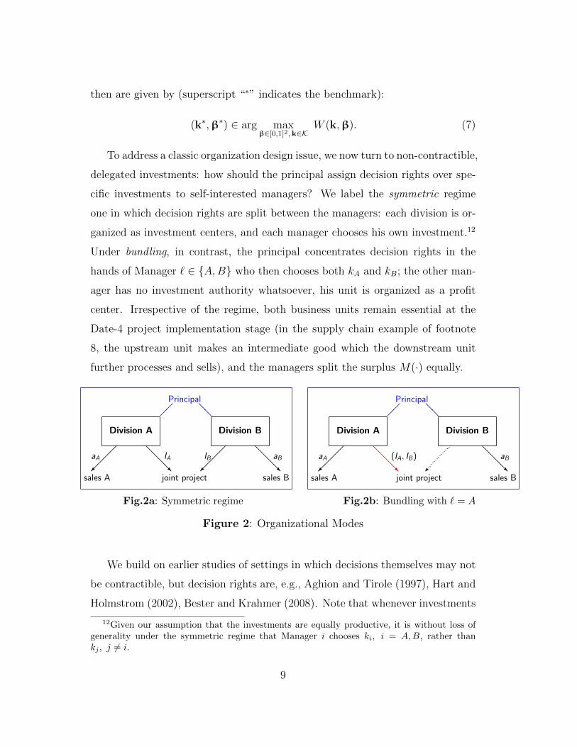
cific investments to self-interested managers? We label the symmetric regime

one in which decision rights are split between the managers: each division is or-

ganized as investment centers, and each manager chooses his own investment.12

Under bundling, in contrast, the principal concentrates decision rights in the

hands of Manager ` ∈ {A,B} who then chooses both kA and kB; the other man-

ager has no investment authority whatsoever, his unit is organized as a profit

center. Irrespective of the regime, both business units remain essential at the

Date-4 project implementation stage (in the supply chain example of footnote

8, the upstream unit makes an intermediate good which the downstream unit

further processes and sells), and the managers split the surplus M(·) equally.Intro Model Integration Investment Authority Conclusion

Setting: integration (large font)

Division A Division B

@@@@R

@@@@R

��

��

��

��

sales A

aA IA IB aB

sales Bjoint project

Principal@@

��

Vertical Integration and Investment Authority 9

Intro Model Integration Investment Authority Conclusion

Setting: bundled investment authority (large font)

Division A Division B

@@@@R

@@@@R

��

��

sales A

aA (IA, IB) aB

sales Bjoint project

Principal@@

��

Vertical Integration and Investment Authority 11

Fig.2a: Symmetric regime Fig.2b: Bundling with ` = A

Figure 2: Organizational Modes

We build on earlier studies of settings in which decisions themselves may not

be contractible, but decision rights are, e.g., Aghion and Tirole (1997), Hart and

Holmstrom (2002), Bester and Krahmer (2008). Note that whenever investments

12Given our assumption that the investments are equally productive, it is without loss ofgenerality under the symmetric regime that Manager i chooses ki, i = A,B, rather thankj , j 6= i.

9

are non-contractible, decision rights over them are inextricably tied to the asso-

ciated fixed cost charges: if Manager i has the authority to choose kj, then the

fixed cost F (kj) will reduce his own divisional income measure, πi, i.e.:13

FCi(k) =

F (ki), under the symmetric regime,

(F (kA) + F (kB))× 1i=`, under bundling with ` = i,

where 1i=` ∈ {0, 1} is the indicator function. Because the managers split the

project surplus equally irrespective of the regime choice, we can restate Manager

i’s gross expected payoff from the project (ignoring the fixed cost and omitting

project-irrelevant terms from (3)) as14

Γ(k | βi) ≡ βi

(E[M(θ,k)]

2− ρ

8βiV ar(k)

). (8)

Subtracting the manager’s internalized portion of investment fixed costs, βiFCi(·),

yields the corresponding net payoff to Manager i:

Λi(k | βi) ≡ Γ(k | βi)− βiF (Ii)

under the symmetric regime, and

Λ`i(k | βi) ≡ Γ(k | βi)− βi

∑m=A,B

F (Im)× 1i=`

under bundling.

Under the symmetric regime, at Date 2, the managers choose their respective

investments simultaneously in form of a pure-strategy Nash equilibrium: for

given β,

maxki∈Ki

Λi(ki, kj | βi), i, j = A,B, i 6= j. (9)

13We ignore here other aspects affecting the delegation of decision rights over investmentsthat, e.g., related to optionality as in Arya et al. (2002).

14There is no need to index the Γ(·)-function because the managers are identical (exceptfor their operating uncertainty). Also, in our model investments are of equal productivity andtherefore Γ(x, y | βi) ≡ Γ(y, x | βi), for any x, y, βi.

10

Denote the equilibrium investments for given β by kS(β) (superscript “S ” de-

notes the symmetric regime). At Date 1, the principal anticipates the Date-2

investment subgame outcome and solves

Program PS : maxβ∈[0,1]2

W (β) ≡ W (k,βS(β)).

We assume an interior solution and denote it by βS = (βSA, βSB). The equilibrium

investments under the symmetric regime then are kS ≡ (kSA,kSB) ≡ kS(βS).

Under bundling Manager ` is the designated investment center manager. At

Date 2 he chooses both investments (“ ` ” denotes the bundling regime):

k`(β`) ∈ arg maxk∈K

Λ``(k | β`). (10)

A key difference to the symmetric regime, as in (9), is that the profit center

manager’s PPS, βj 6=`, no longer affects any investments. The principal’s Date-1

contracting problem for given allocation of decision rights, `, reads

Program P` : maxβ∈[0,1]2

W `(β) ≡ W (β, k`(β`)).

Denote the solution to this program by β`

and the resulting investments by

k` ≡ (k`A, k`B) ≡ k`(β``).

At Date 0, the principal asks which Manager ` ∈ {A,B} delivers a higher

value of the respective programs P` under bundling, and then compares the

maximum achievable surplus with that under the symmetric regime. As we will

show now, the nature of the investments—continuous or lumpy—critically affects

the regime comparison.

3 Continuous investments

We begin by assuming investments are perfectly scalable, i.e., K = R2+. The

investment fixed costs are given by F (ki) =fk2i

2. We start with the benchmark

case and decompose the principal’s problem into two steps: First, it is easy to

11

see that the conditionally optimal PPS for given investments k is

βoi (k) =

(1 + ρv

(σ2i +

V ar(k)

4

))−1

. (11)

Let βo(k) = (βoA(k), βoB(k)). Second, the optimal investment, k∗ ∈ R2+, maxi-

mizes the value function W ∗(k) ≡ W (βo(k),k); hence, β∗i = βoi (k∗). Because

both investments come at identical fixed cost and risk premium effects, by (6) and

(1), the benchmark investments are identical: k∗A = k∗B ≡ k∗. The investment-

risk link implies that βoi (k) is decreasing in kj, for any i, j. Accounting for the

project risk reduces the PPS below βMHi = (1+ρvσ2

i )−1, the PPS in a pure moral

hazard model without joint projects. Thus, investments and PPS are substitutes

for the principal in the benchmark case. By σ2A > σ2

B, we have β∗A ≤ β∗B. We

assume f is sufficiently high to ensure all investment problems studied below are

well-behaved.15 Moreover, we assume the project uncertainty is bounded from

above:

Assumption 1 η ≤ min{ηrisk, ηpos}, where ηrisk = 4σ2B

(f−2µf

)2

and ηpos ≡ 1ρ.

Assuming η ≤ ηrisk ensures the project risk for each manager is less than his op-

erating risk; for high project risk, one would expect the divisions to be merged.16

Note that limη→ηrisk β∗i = βmini ≡ (1 + 2ρvσ2

i )−1

and, therefore, β∗i ∈ [βmini , βMHi ].

The restriction η ≤ ηpos ensures the principal chooses a positive benchmark in-

vestment level, k∗i > 0.17

15Specifically, assuming f > 6 ensures global concavity of the expected payoffs of theprincipal (in the contractible benchmark case) and of the division managers (under non-contractibility), respectively.

16To provide intuition for the bound ηrisk in Assumption 1, note that the hypothetical

investments in a risk-free world (where η → 0), krf ∈ arg maxkA,kB M(µ,k)− f∑

i k2i

2 (omitting

irrelevant terms), are given by krfi = krf = µf−2 . By (1), k∗ ≤ krf . Assuming η < ηrisk then

ensures the project-related risk would be less than the operating risk for each manager, evenif these risk-free investments were chosen. From a technical standpoint, η ≤ ηrisk is sufficientalso for the project-related risk premium for Manager i, ρ

8 (βoi (k))2 · V ar(k), to be increasingin ki for any ki ≤ krf . Under this condition, the indirect effect in form of a reduced PPS isdominated by the direct effect on the variance of the surplus.

17Taking the derivative of the principal’s expected utility, W ∗ki = E [Mki(θ,k)] −ρ8

∑i(β

oi (k))2V arki(k) − F ′(ki) = q∗(µ,k)

(1− ρη

4

∑j(β

oj (k))2

)− fki. Hence, for η ≤ ηpos,

12

In earlier incomplete contracting models that have ignored project risk, bi-

lateral investments tend to be mutually reenforcing: efficiency-enhancing invest-

ments by Manager i increase the expected project scale, which in turn raises the

marginal investment return to Manager j, and vice versa. That is, the firmwide

expected contribution margin, E[M(·)], displays increasing differences in the in-

vestments. However, by the investment-risk link as in (1), the same is true for the

managers’ project-related risk premium. Given Assumption 1, it is easy to show

though that the first-moment effect dominates, making contractible investments

complements at the margin:

Lemma 1 Given Assumption 1 and for given β, both W (k,β) and Γ(k | βi)

have strictly increasing differences in k.

Both the expected surplus in the benchmark case as well as the gross in-

vestment return functions under the two decentralized regimes (and thereby also

the managers’ net investment returns, Λi(k | βi) and Λ`i(k | βi)) display invest-

ment complementarity for given PPS. We now turn to the manager’s investment

incentives under the symmetric regime.

Lemma 2 Given Assumption 1 and k ∈ R2+, under the symmetric regime:

(a) For given β, there exists a unique equilibrium investment profile with kSi (β) =µ(2−ρηβi)

ρη(βi+βj)+4(f−1), i = A,B, j 6= i. Each investment level is decreasing in the

PPS of either manager:dkSi (β)

dβj< 0, i, j = A,B.

(b) In equilibrium, k∗i > kSA > kSB, i = A,B.

The performance measure of the investing manager scales all divisional cash

flows (including the fixed cost) equally by his PPS. Hence, the sole first-order

effect of an increase in PPS is that he will be reluctant to invest because he

the marginal investment return for small ki is positive because βj ≤ 1, j = A,B. As we show,this condition also ensures that the pressing investment distortion is underinvestment. Forcases in which overinvestment arises, see Baldenius and Michaeli (2017).

13

becomes more sensitive to the investment-risk link. Strategic complementarity

reinforces the investment-suppressing effect of PPS and implies that each man-

ager will invest less, the greater is his counterpart’s PPS.18 Comparing across

divisions, in equilibrium, Manager A will invest more than Manager B because

of the differential operating volatility, σ2A > σ2

B: greater uncertainty is associated

with relatively lower PPS for Manager A, which makes the latter more toler-

ant to the incremental investment-related project risk.19 Yet, even Manager A

underinvests relative to the benchmark level because of the holdup problem.

We now turn to the bundling regime, in which Manager `, the designated

investment center manager, chooses both kA and kB. As argued in connection

with (10), above, Manager `’s choice of k is affected only by his own PPS. In

contrast to the symmetric regime (Lemma 2), therefore, the resulting investment

profile under bundling is always symmetric: k`A = k`B, for any `. The arguments

in Lemma 2 for underinvestment and the investment-suppressing effect of the

PPS apply with only minor modifications to bundling (proof omitted):

Lemma 3 Given Assumption 1, under the bundling regime with Manager `

choosing both k ∈ R2+:

(a) For given β, Manager ` chooses k`i (β) = µ(2−ρηβ`)2ρηβ`+4(f−1)

, for any i, where

k`i (β) is decreasing in β`.

(b) In equilibrium, for any i and `, k∗i > k`i .

18As one would expect, the closed-form term for kSi (β) indicates that Manager i respondsmore sensitively to changes in βi (the direct interaction between ki and βi) than to changes inβj (the indirect effect through investment complementarity).

19Lemma 2 is silent on how the PPS under the symmetric regime, βSi , compares with thebenchmark one, β∗i . As Baldenius and Michaeli (2017) have shown in a simpler unilateralinvestment setting, this comparison can go either way because of two countervailing effects:the investment suppressing effect of effort incentives calls for lowering the PPS if investmentis noncontractible; on the other hand, equilibrium underinvestment implies that the marginalrisk premium is reduced, which calls for increasing the PPS. Baldenius and Michaeli (2017)derive conditions that predict the direction of the net effect.

14

We now ask which regime maximizes the principal’s expected payoff. A re-

maining design issue for the principal under bundling is in whose hands to concen-

trate the decision rights, i.e., which of the managers to designate the investment

center manager (whether to set ` = A or ` = B):

Proposition 1 Given Assumption 1 and k ∈ R2+, bundling with ` = A (high

volatility) dominates both bundling with ` = B as well as the symmetric regime.

Because any decentralized regime results in underinvestment relative to the

benchmark solution, the question is which regime is most effective in alleviat-

ing this distortion. With scalable investments, the answer hinges solely on the

induced risk tolerance arguments, above: Manager A faces the more volatile en-

vironment and therefore has muted PPS to begin with; hence, he is less sensitive

to the investment-induced project risk and should be assigned all investment

decision rights. Put differently, the key to stimulating delegated investment is

muted PPS, and the opportunity cost of muted PPS is minimized by designating

Manager A the investment center manager under bundling.

We now turn to non-scalable investments. Lumpiness in project investments

will amplify the role of strategic complementarity, with drastic consequences for

the ranking of the organizational modes.

4 Lumpy investments

We now consider investments of fixed size, normalized so that K = {0, 1}2, i.e.,

each investment can either be undertaken or not. Examples are the replacement

of existing equipment, M&A, or the decision to develop a new product or to

enter a new market. The assumption that both investments are of similar size is

solely for notational convenience. We continue to assume that each investment is

equally productive by normalizing the marginal gross return to one, and the fixed

cost per unit of investment to φ > 0. (None of our results hinges qualitatively

15

on this symmetry restriction.) The principal’s objective remains to maximize

W (k,β), as in (7), now with K = {0, 1}2 and fixed costs Fi(ki) = φki.

4.1 Investment incentives at Date 2 for given PPS

It is useful to begin the analysis of lumpy investments by studying the outcome

of the Date-2 investment subgame for given PPS and only then endogenizing

the PPS. The conditionally optimal investments chosen by the principal in the

contractible benchmark setting, holding fixed the PPS, are given by k∗(β) ∈

arg maxk∈{0,1}2 W (k,β). Using the investment complementarity (Lemma 1), the

benchmark investment profile will be “all or nothing:”20

k∗(β) =

(1, 1), if φ ≤ φ∗(β) ≡ 1

2{Eθ[M((1, 1), θ)−M((0, 0), θ)]

−ρ8(β2

A + β2B)[V ar(1, 1)− V ar(0, 0)]

},

(0, 0), if φ > φ∗(β).

(12)

We refer to φ∗(β) as the benchmark fixed cost threshold for given β.

Strategic complementarity affects also the set of investment profiles to arise in

equilibrium under delegation with non-contractible investments. Under bundling,

Manager `’s optimization problem remains as in (10), with investments now cho-

sen from the discrete set K = {0, 1}2 at fixed cost φ(kA + kB). Because Man-

ager `’s investment return also displays complementarity in investments (again,

Lemma 1), the equilibrium investment profile will again be “all or nothing:” the

investment center manager under bundling chooses (1, 1) for given PPS if

Γ(1, 1 | β`)− 2β`φ ≥ Γ(0, 0 | β`), (13)

20It is easy to see that the principal would be indifferent between the “mixed” investmentprofiles (1, 0) and (0, 1). However, by Lemma 1, such a mixed investment profile can never beoptimal.

16

and (0, 0) otherwise. Therefore,

k`(β`) =

(1, 1), if φ ≤ φ`11(β`) ≡ 12β`

[Γ(1, 1 | β`)− Γ(0, 0 | β`)],

(0, 0), if φ > φ`11(β`).

(14)

Below the fixed cost threshold φ`11(β`), Manager ` makes both investments; be-

yond this threshold, he foregoes any investment.

Under the symmetric regime, a Nash equilibrium in investments, kSi (β), is

determined by (9), now with ki ∈ {0, 1} at fixed cost F (ki) = φki. For the

sake of illustration, and with slight abuse of notation, for now denote the PPS

profile by the non-ordered pair β = (β, β) where β < β. Recall that, by Lemma

2 (which applies qualitatively also to lumpy investments), greater PPS lowers

a manager’s investment incentive by increasing his exposure to the marginal

investment-induced risk. All else equal, therefore, the bottleneck in terms of

eliciting investments is the manager with the greater PPS. Hence, the investment

profile kS(β) = (1, 1) constitutes an equilibrium under the symmetric regime for

φ low enough such that even the high-PPS manager has no incentive to deviate:

Γ(1, 1 | β)− βφ ≥ Γ(1, 0 | β). (15)

Denote by φ11(β) the fixed cost value at which (15) becomes binding. At the

same time, kS(β) = (0, 0) is an equilibrium for φ high enough such that even

the low-PPS manager has no incentive to deviate by investing unilaterally:

Γ(1, 0 | β)− βφ ≤ Γ(0, 0 | β). (16)

Denote by φ00(β) the fixed cost threshold at which (16) becomes binding.

Clearly, for sufficiently low fixed costs (1, 1) is the unique investment equi-

librium under the symmetric regime; for high fixed costs (0, 0) is the unique

equilibrium. For intermediate fixed costs one of two cases may arise: either both

(15) and (16) hold simultaneously, resulting in multiple symmetric equilibria; or

(15) and (16) are both violated, permitting only asymmetric equilibria in which

17

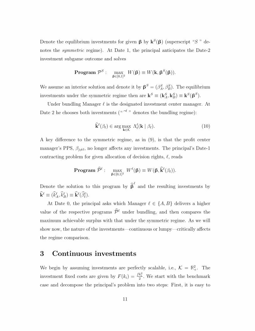
exactly one manager undertakes the investment. To characterize the set of equi-

libria, we show in the proof of Lemma 4 that the fixed cost threshold differential

for given PPS, φ11(β)− φ00(β), is proportional to some function

X(β) ≡[(2µ+ 3)

(1− βηρ

2

)− (2µ+ 1)

(1−

βηρ

2

)].

Note that X(β) is increasing in β and decreasing in β—and therefore decreasing

in the PPS differential—and it is decreasing in η. We then have:

Lemma 4 Suppose Assumption 1 holds. For k ∈ {0, 1}2 and given β = (β, β),

the (Pareto-dominant) investment equilibrium under the symmetric regime is:

(a) For X(β) ≥ 0, φ00(β) ≤ φ11(β), and kS(β) =

(1, 1), if φ ≤ φ11(β),

(0, 0), if φ > φ11(β).

A sufficient condition for X(β) ≥ 0 is that the PPS differential is small

(or the project risk η is small); specifically, β − β ≤ 1µ

(32

+ 2ρη

).

(b) For X(β) < 0, φ00(β) > φ11(β), and kS(β) =

(1, 1), if φ ≤ φ11(β),

(1, 0) or (0, 1), if φ ∈ (φ11(β), φ00(β)] ,

(0, 0), if φ > φ00(β).

Games of strategic complementarity are routinely afflicted by multiple equi-

libria. This is true also for the symmetric regime if managers face fairly similar

PPS (Lemma 4a): for intermediate values of fixed costs, both (15) and (16) hold

simultaneously, making (1, 1) and (0, 0) each a Nash equilibrium. To predict

which of these the managers will play, we note that the investment subgame sat-

isfies the conditions for a supermodular game as in Milgrom and Roberts (1990);

hence, we can invoke their Theorem 7 stating that the highest equilibrium—here,

(1, 1)—is the Pareto-dominant one. For φ ∈ (φ00(β), φ11(β)) in Lemma 4a, we

can therefore ignore the no-investment equilibrium.

18

Lemma 4b states a condition for an asymmetric equilibrium to obtain for

intermediate fixed cost values. In that equilibrium, only the manager with the

lower PPS will invest. While his investment raises the investment incentive also

for the other manager, if the PPS differential is large enough, then this strategic

complementarity effect is insufficient to compensate the high-PPS manager for

the incremental risk premium associated with investing.21

Turning now to the regime comparison for lumpy investments, we first ap-

proach this issue heuristically by asking which regime implements the investment

profile (1, 1) for a wider range of fixed cost parameters—i.e., we compare the φ-

thresholds in (14) and Lemma 4 for given β = (β, β). As a preliminary finding,

both regimes fall short of providing efficient investment incentives by this crite-

rion (holding fixed the PPS):

Lemma 5 Suppose Assumption 1 holds. For k ∈ {0, 1}2 and given β = (β, β):

(a) Under the symmetric regime, φ11(β) < φ∗(β).

(b) Under bundling, φ`11(β`) < φ∗(β), for any `.

Either regime leads the managers to underinvest for given contracts, by this

heuristic criterion. Which regime is best suited to alleviate the prevailing under-

investment problem? Conditional on bundling decision rights, to best alleviate

the underinvestment problem, the principal would designate the manager with

the lower PPS the investment center manager. For the remainder of this sub-

section, we index by `∗ the manager facing the lower of the two PPS, β. Given

Lemma 5, we say the symmetric regime investment-dominates (for given PPS)

the bundling regime whenever φ11(β) ≥ φ`∗

11(β), and vice versa.22

There are two conceptual differences between the regimes, which jointly deter-

mine the performance comparison: (a) the game forms differ—a (simultaneous-

move) non-cooperative game under the symmetric regime versus a single-agent

21In Lemma 4b, it is without loss of generality to write the investment equilibrium forintermediate fixed costs as (1, 0). This equilibrium is payoff-equivalent for all parties to (0, 1).

22On a technical level, we use here the fact that W (β,k) is concave in k for given β.

19

optimization problem under the bundling regime; (b) the risk tolerance benefit

under the bundling regime resulting from assigning the investment authority to

the agent who is more willing to invest because of his lower PPS. Our next result

identifies conditions for (a) to be the dominant force:

Lemma 6 Suppose Assumption 1 holds, k ∈ {0, 1}2, and X(β) > 1. Then, for

any given PPS of β = (β, β), φ11(β) > φ`∗

11(β), and hence the symmetric regime

investment-dominates bundling. A sufficient condition for X(β) > 1 is that the

PPS differential is small; specifically, β − β ≤ 1µ

(32

+ 1ρη

).

Lemma 6 is in stark contrast to Proposition 1, which dealt with continuous

investments. Why, with lumpy investments, does the symmetric regime generate

stronger investment incentives than the bundling regime if the PPS differential is

limited? As β−β becomes small, the risk tolerance benefit of bundling vanishes;

this leaves the different game forms. Consider the limit case where both PPS

levels converge to the same value, say x. Comparing (13) with (15), holding the

PPS for each manager fixed at x, we find that inducing (1, 1) as a Nash equilib-

rium under the symmetric regime is a less demanding condition than inducing

some Manager ` under bundling to invest two units rather than none. The reason

is that, for any given x,

Γ(1, 1 | βi = x)− Γ(1, 0 | βi = x)︸ ︷︷ ︸as in (15)

− Γ(1, 1 | β` = x)− Γ(0, 0 | β` = x)

2︸ ︷︷ ︸as in (13)

> 0,

(17)

by strategic complementarity (Lemma 2). The symmetric regime generates

strong investment incentives in aggregate by requiring that investing only be

each manager’s best response to the other manager also investing. At a fixed

cost of βiφ, Manager i reaps his share of the return from changing the investment

profile from (0, 1) to (1, 1). Investment incentives under bundling, in contrast,

are muted by the fact that the investment center manager has to pay for the

total fixed cost, 2β`φ, to change investments from (0, 0) to (1, 1).

20

(0, 0)

(1, 0)

(0, 1)

(1, 1)

(0, 0)

(1, 0) (1, 1)

(0, 1)

Γ(1, 1 | β)− Γ(0, 0 | β)− 2βφ ≥ 0

Γ(1, 1 | β)− Γ(1, 0 | β)− βφ ≥ 0

6

�����������

-

(a) Bundling: low-PPS manager

chooses kA and kB

(b) Symmetric form: Nash equilibrium (bindingconstraint is high-PPS manager)

Figure 3: Comparison of investment incentives with exogenous PPSSolid arrows indicate the binding constraints in order to elicit the investment profile (1, 1).

Loosely put, if the project proceeds are split by the managers, eliciting high

levels of inputs from two players in form of a Nash equilibrium is relatively

“cheap” if these inputs are strategic complements. We henceforth label the

game form effect the strategic complementarity effect : the symmetric regime

takes advantage of the strategic investment complementarity; bundling does not.

Figure 3 illustrates the risk tolerance and strategic complementarity effects, with

bold arrows indicating the binding investment incentive constraints.

Now consider the case of a large PPS differential, β−β; specifically, fix β while

increasing β. Investment incentives under the bundling regime are unaffected by

this change, because only the low-PPS manager matters for investments. The

bottleneck under the symmetric regime is to get the high-PPS manager to invest;

this constraint becomes tighter as β increases. Letting η vary, as a measure

of the intrinsic project uncertainty, Figure 4 plots the difference in the fixed

cost thresholds as β increases, holding β fixed. High η values (Fig. 4a) boost

the induced risk tolerance effect and dampen the strategic complementarity by

21

strengthening the increasing differences of the risk premium in k, as per (8). Both

effects work in tandem to make the symmetric regime the investment-dominant

one for a wider range of PPS differentials β − β, for small η values (Fig. 4b).

0.2 0.4 0.6 0.8 1.0

19.6

19.8

20.0

20.2

20.4

20.6

symmetricformpreferred

β

φ11(β)

φ`∗

11(β)

0.2 0.4 0.6 0.8 1.0

20.45

20.50

20.55

20.60

20.65

20.70

symmetricformpreferred

β

φ11(β)

φ`∗

11(β)

(a) High project risk: η = 0.09 (b) Low project risk: η = 0.03

Figure 4: Fixed cost thresholds comparison for µ = 40, β = 0.1, ρ = 1.Dashed line represents φ11(β). Solid line represents φ`

∗

11(β).

4.2 Regime comparison with equilibrium contracts

As before in the case of scalable investments, the optimal PPS for given k under

the contractible benchmark is βo(k) as derived in (11) but with Ki = {0, 1};

and the optimal k maximizes W ∗(k) ≡ W (k,βo(k)). As we show in the proof

of Lemma 7, the expected surplus continues to display investment complemen-

tarity even after endogenizing β, i.e., the value function W ∗(k) has increasing

differences in k. As a result, the principal’s choice of lumpy investments under

the benchmark case with endogenous contracts continues to be “all or nothing.”

Lemma 7 If Assumption 1 holds and k ∈ {0, 1}2, then the contractible bench-

mark solution is:

(k∗,β∗) =

((1, 1),βo(1, 1)), if φ ≤ φ∗ ≡ φ∗(βo(1, 1)),

((0, 0),βo(0, 0)), otherwise.

22

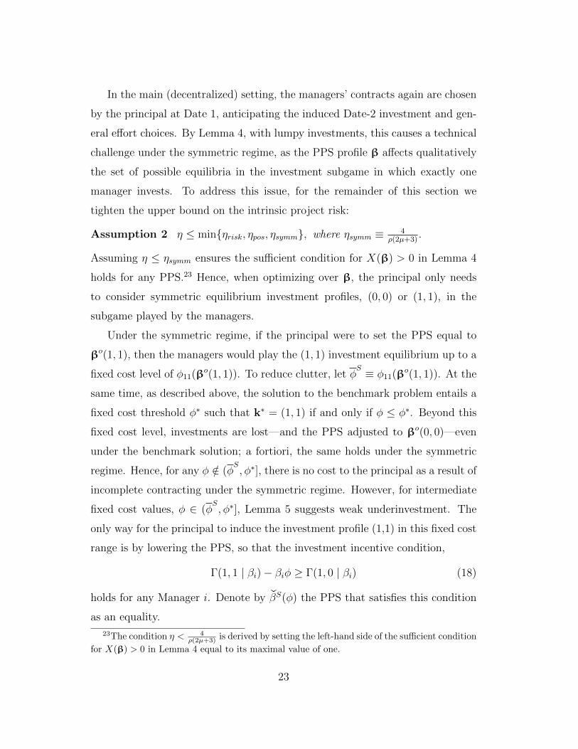
In the main (decentralized) setting, the managers’ contracts again are chosen

by the principal at Date 1, anticipating the induced Date-2 investment and gen-

eral effort choices. By Lemma 4, with lumpy investments, this causes a technical

challenge under the symmetric regime, as the PPS profile β affects qualitatively

the set of possible equilibria in the investment subgame in which exactly one

manager invests. To address this issue, for the remainder of this section we

tighten the upper bound on the intrinsic project risk:

Assumption 2 η ≤ min{ηrisk, ηpos, ηsymm}, where ηsymm ≡ 4ρ(2µ+3)

.

Assuming η ≤ ηsymm ensures the sufficient condition for X(β) > 0 in Lemma 4

holds for any PPS.23 Hence, when optimizing over β, the principal only needs

to consider symmetric equilibrium investment profiles, (0, 0) or (1, 1), in the

subgame played by the managers.

Under the symmetric regime, if the principal were to set the PPS equal to

βo(1, 1), then the managers would play the (1, 1) investment equilibrium up to a

fixed cost level of φ11(βo(1, 1)). To reduce clutter, let φS ≡ φ11(βo(1, 1)). At the

same time, as described above, the solution to the benchmark problem entails a

fixed cost threshold φ∗ such that k∗ = (1, 1) if and only if φ ≤ φ∗. Beyond this

fixed cost level, investments are lost—and the PPS adjusted to βo(0, 0)—even

under the benchmark solution; a fortiori, the same holds under the symmetric

regime. Hence, for any φ /∈ (φS, φ∗], there is no cost to the principal as a result of

incomplete contracting under the symmetric regime. However, for intermediate

fixed cost values, φ ∈ (φS, φ∗], Lemma 5 suggests weak underinvestment. The

only way for the principal to induce the investment profile (1,1) in this fixed cost

range is by lowering the PPS, so that the investment incentive condition,

Γ(1, 1 | βi)− βiφ ≥ Γ(1, 0 | βi) (18)

holds for any Manager i. Denote by qβS(φ) the PPS that satisfies this condition

as an equality.

23The condition η < 4ρ(2µ+3) is derived by setting the left-hand side of the sufficient condition

for X(β) > 0 in Lemma 4 equal to its maximal value of one.

23

Under the symmetric regime, the principal will choose the optimization pro-

gram with the greater value from among the following:

PS11 (Induce investment under symmetric regime): For any φ ∈ (φS, φ∗],

maxβ

W (β | k = (1, 1)),

subject to (5) and βi ≤ qβS(φ), for any i.

PS00 (Forestall investment under symmetric regime): For any φ ∈ (φS, φ∗],

maxβ

W (β | k = (0, 0)),

subject to (5) and βi > qβS(φ), for any i.

Evaluating these two programs yields our next result:

Proposition 2 (Symmetric regime) Suppose k ∈ {0, 1}2 and Assumption 2

holds. Under the symmetric regime, there exists a unique φS ∈ (φS, φ∗], such

that:

(i) If φ ∈ (φS, φS], then βB = qβS(φ) < βoB(1, 1) and βA = min{qβS(φ), βoA(1, 1)}.

Both managers invest, as they would under the benchmark solution.

(ii) If φ ∈ (φS, φ∗], then βi = βoi (0, 0) > βoi (1, 1), i = A,B. Neither manager

invests, whereas k∗ = (1, 1) under the benchmark solution.

Figure 5 illustrates this result graphically, with increasing fixed costs along

the x-axis. The manager with less volatile operations (Manager B) has a higher

benchmark PPS. As fixed costs increase, his PPS has to be muted first to

βB = qβS(φ) to elicit his investment. As fixed costs grow further, at some

point the investment constraint (18) may become binding even for Manager

A. Now both managers’ incentives must be muted in lockstep; hence, βA =

min{qβS(φ), βoA(1, 1)}. At fixed cost of φS, the net investment benefit falls short

of the opportunity cost of foregone general effort, so the principal gives up on

24

5 6 7 8

0.1

0.2

0.3

0.4

�

�

i

�

o

A

(0, 0)

�

o

B

(0, 0)

�

o

A

(1, 1)

�

o

B

(1, 1)

�

S

= 5.10 �

S = 6.98

k

S = (1, 1) k

S = (0, 0)

Figure 5: Optimal PPS and induced investments under the symmetric regimeNumerical example with µ = 14, ⇢ = 2, v = 0.013, �

A

= 20, �B

= 10, ⌘ = 1. In this example,under the contractible benchmark, k⇤ = (1, 1) and �⇤ = �o(1, 1) = (0.31, 0.34) if

� �

⇤ = 13.14. Otherwise, k⇤ = (0, 0) and �⇤ = �o(0, 0) = (0.36, 0.39).

allows her to expose both managers to higher-powered incentives because of the

reduced project risk.

Under bundling, incomplete contracting imposes costs on the principal also

only for intermediate fixed cost levels. Recall, to capitalize on the induced risk

tolerance e↵ect, the principal sets ` = A. For � 2 (�A,�

⇤], however, Lemma

5 suggests weak underinvestment, where �

A ⌘ �

A(1,1)(�

o(1, 1)). Manager A will

choose (1, 1) whenever

�(1, 1 | �A)� 2�A� � �(0, 0 | �A). (19)

Denote by q�(�) the PPS level that just satisfies this condition as an equality.

In analogy with the symmetric regime, under bundling the principal compares

the values of the following two optimization programs:

25

Figure 5: Optimal PPS and induced investments under the symmetric regimeNumerical example with µ = 14, ρ = 2, v = 0.013, σ2

A = 20, σ2B = 10, η = 1. In this example,

under the contractible benchmark, k∗ = (1, 1) and β∗ = βo(1, 1) = (0.31, 0.34) ifφ ≤ φ∗ = 13.14. Otherwise, k∗ = (0, 0) and β∗ = βo(0, 0) = (0.36, 0.39).

investments. This in turn allows her to expose both managers to higher-powered

incentives because of the reduced project risk.

Under bundling, incomplete contracting imposes costs on the principal also

only for intermediate fixed cost levels. Recall, to capitalize on the induced risk

tolerance effect, the principal chooses ` = A. For φ ∈ (φA, φ∗], however, Lemma

5 suggests weak underinvestment, where φA ≡ φA11(βo(1, 1)). Manager A will

choose (1, 1) whenever

Γ(1, 1 | βA)− 2βAφ ≥ Γ(0, 0 | βA). (19)

Denote by qβA(φ) the PPS level that satisfies this condition as an equality. By

strategic complementarity, it is immediate that qβA(φ) < qβS(φ) for any φ.

Under bundling the principal compares the values of the following two opti-

mization programs:

25

PA11 (Induce investment under bundling, ` = A): For any φ ∈ (φA, φ∗],

maxβ

W (β | k = (1, 1)),

subject to (5) and βA ≤ qβA(φ).

PA00 (Forestall investment under bundling, ` = A): For any φ ∈ (φA, φ∗],

maxβ

W (β | k = (0, 0)),

subject to (5) and βA > qβA(φ).

Evaluating these two programs yields:

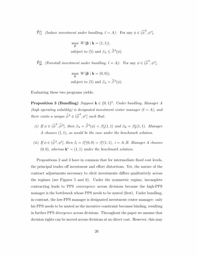
Proposition 3 (Bundling) Suppose k ∈ {0, 1}2. Under bundling, Manager A

(high operating volatility) is designated investment center manager (` = A), and

there exists a unique φA ∈ (φA, φ∗] such that:

(i) If φ ∈ (φA, φA], then βA = qβA(φ) < βoA(1, 1) and βB = βoB(1, 1). Manager

A chooses (1, 1), as would be the case under the benchmark solution.

(ii) If φ ∈ (φA, φ∗], then βi = βoi (0, 0) > βoi (1, 1), i = A,B. Manager A chooses

(0, 0), whereas k∗ = (1, 1) under the benchmark solution.

Propositions 2 and 3 have in common that for intermediate fixed cost levels,

the principal trades off investment and effort distortions. Yet, the nature of the

contract adjustments necessary to elicit investments differs qualitatively across

the regimes (see Figures 5 and 6). Under the symmetric regime, incomplete

contracting leads to PPS convergence across divisions because the high-PPS

manager is the bottleneck whose PPS needs to be muted (first). Under bundling,

in contrast, the low-PPS manager is designated investment center manager: only

his PPS needs to be muted as the incentive constraint becomes binding, resulting

in further PPS divergence across divisions. Throughout the paper we assume that

decision rights can be moved across divisions at no direct cost. However, this may

26

5 6 7 8

0.1

0.2

0.3

0.4

�

�

i

�

o

A

(0, 0)

�

o

B

(0, 0)

�

o

A

(1, 1)

�

o

B

(1, 1)

�

A

= 5.14 b�

A = 7.45

bk

A = (1, 1) bk

A = (0, 0)

Figure 6: Optimal PPS and induced investments under bundlingNumerical example with µ = 14, ⇢ = 2, v = 0.013, �

A

= 20, �B

= 10, ⌘ = 1. In this example,under the contractible benchmark, k⇤ = (1, 1) and �⇤ = �o(1, 1) = (0.31, 0.34) if

� �

⇤ = 13.14. Otherwise, k⇤ = (0, 0) and �⇤ = �o(0, 0) = (0.36, 0.39).

27

Figure 6: Optimal PPS and induced investments under bundlingNumerical example with µ = 14, ρ = 2, v = 0.013, σ2

A = 20, σ2B = 10, η = 1. In this example,

under the contractible benchmark, k∗ = (1, 1) and β∗ = βo(1, 1) = (0.31, 0.34) ifφ ≤ φ∗ = 13.14. Otherwise, k∗ = (0, 0) and β∗ = βo(0, 0) = (0.36, 0.39).

not always be the case; instead some firms may be “stuck” with the symmetric

regime for technological reasons. In this case, our model predicts harmonized

incentives and thus sheds light on the puzzle of “corporate socialism.”24

Having characterized the optimal contractual adjustments and attendant

equilibrium investments under the two regimes, we are now in a position to

generalize the result of Lemma 6 regarding the regime comparison.

Proposition 4 Suppose k ∈ {0, 1}2 and Assumption 2 holds. For given σ2B, the

principal prefers the symmetric regime to the bundling regime if σ2A ∈ (σ2

B, σ2B+δ),

for some δ > 0.

The message from our heuristic performance comparison for given PPS gener-

alizes to optimal contracts (within the class of linear schemes relying on divisional

performance measures). For lumpy capital investments, the principal trades

24Levine (1991), Zenger and Hesterly (1997), Shaw et al. (2002), Siegel and Hambrick (2005).

27

off taking advantage of strategic complementarity under the symmetric regime,

against utilizing the greater induced risk tolerance associated with low-powered

PPS under bundling. As the volatility levels converge across divisions, the risk

tolerance benefit becomes negligible and the symmetric regime is preferred. The

principal could assign all investment authority to one manager (bundling) and

mute that manager’s PPS to boost both investments. The associated oppor-

tunity cost in terms of foregone general effort exerted by Manager `, however,

makes this less advantageous than splitting decision rights between the managers

(the symmetric regime).

5 Personally costly project-specific efforts

We now consider the case where the relationship-specific inputs are not paid for

with divisional funds but instead are personally costly to the respective manager

who chooses them. Examples are foregone perquisites or private benefits from pet

projects, or simply the disutility of engaging in time-consuming market research.

To accommodate such personally-costly relationship-specific efforts (henceforth

“project efforts”), we modify the notation. At Date 2, project efforts e = (eA, eB)

are chosen at personal disutility of G(ei), respectively (replacing k chosen at

monetary divisional fixed cost of F (ki)). For simplicity, we assume the project’s

contribution margin has the same functional form as before in that q∗(θ, e) =

θ +∑

i ei and M(θ, e) = 12

(θ +∑

i ei)2.

We again compare the symmetric regime (Manager i exerts effort ei) and

bundling (Manager ` exerts both (eA, eB)) in settings where the project efforts are

either scalable or lumpy. The performance measures now read πi = ai+εi+M(θ,e)

2,

regardless of the regime, as the project effort cost is borne privately by the

managers. The manager’s expected utility is, accordingly,

EUi = αi +βi

(ai +

E[M(θ, e)]

2

)− FCi(e)− v

2a2i −

ρ

2β2i

(σ2i +

V ar(e)

4

), (20)

28

where V ar(e) ≡ V ar(M(θ, e)) = (q∗(µ, e))2 η and

FCi(e) =

G(ei), under the symmetric regime,

(G(eA) +G(eB))× 1i=`, under bundling with ` = i.

By moving from a setting of monetary to one of personally-costly project inputs,

the managers’ general effort incentive constraints in (5) are unaffected, but their

choice of the project-specific inputs is affected in that the input cost, FCi(·), is

no longer scaled by the PPS (contrast (20) with (3)).

In the benchmark case of contractible project efforts, the principal simply

maximizes (e∗,β∗) ∈ arg maxe,βW (e,β). As before, β∗ ≡ βo(e∗) where βoi (e) =(1 + ρv

[σ2i + V ar(e)

4

])−1

is the conditionally optimal PPS. For noncontractible

project efforts, Manager i’s expected gross payoff from the project is Γ(e | βi),

with Γ(·) as defined in (8) with e replacing k. The corresponding net payoff to

Manager i is denoted by Λi(e | βi) = Γ(e | βi) − G(ei) under the symmetric

regime and by Λ`i(e | βi) = Γ(e | βi) −

∑m=A,B G(em) × 1i=` under bundling.

Under the symmetric regime, at Date 2, the managers choose project efforts

simultaneously such that, for given β,

maxei

Λi(ei, ej | βi), i, j = A,B, i 6= j. (21)

As before, we focus on pure-strategy Nash equilibria. The subgame equilibrium

project efforts for given β are eS(β). At Date 1, the principal maximizes W (β) ≡

W (β, eS(β)) over β. We assume an interior solution and denote it by βS =

(βSA, βSB), resulting in equilibrium project efforts of eS ≡ (eSA, e

SB) ≡ eS(βS).

Under bundling, at Date 2, Manager ` solves, for given β,

maxe

Λ``(e | β`), (22)

which yields the solution e`(β`). At Date 1, the principal maximizes W (β, e`(β`))

over β. Assuming an interior solution, we denote it by β`

= (β`A, β`B) and

the resulting equilibrium project efforts by e` ≡ (e`A, e`B) ≡ e`(β`). Adapting

Assumption 1 to project efforts:

29

Assumption 1′ η ≤ min{ηrisk, ηpos}, where ηrisk = 4σ2B

(g−2µg

)2

and ηpos ≡ 1ρ.

5.1 Continuous project efforts

Suppose project efforts are scalable, e ∈ R2+, at personal disutility G(ei) =

ge2i2

with g sufficiently high.25 Recall that monetary investments were decreasing

in the managers’ PPS, because all cash flows were scaled by the PPS, so at the

margin greater PPS merely made the managers more sensitive to the investment-

related project risk. With project-specific personally-costly efforts, this result

flips:

Lemma 8 Given Assumption 1′ and e ∈ R2+:

(a) For given β, both W (e,β) and Γ(e | βi) have strictly increasing differences

in e.

(b) Λi(e | βi) and Λ`i=`(e | βi) have strictly increasing differences in (e, βi), for

any i, `.

(c) dΛi(e|βi)dei

≤ dW (e,β)dei

anddΛ`

i(e|β`)dei

≤ dW (e,β)dei

, for any e,β, i, `.

(d) For any β: under the symmetric regime there exists a unique Nash equilib-

rium in efforts solving (21) such thatdeSi (β)

dβj> 0 for any i, j; under bundling,

for any `, there exists a unique maximizer to (22) such thatde`i(β`)

dβ`> 0 and

de`i(β`)

dβj 6=`≡ 0 for any i.

With project efforts being personally costly, the classic moral hazard argu-

ment that stronger PPS elicits greater (project) effort is merely weakened but

not overturned by the input-risk link (the risk premium is again increasing in ei,

as ∂∂eiV ar(e) = 2q∗(µ, e)η, for any i). Put differently, the first moment-effect of

25Similar to the case of monetary investments, g > 6 ensures global concavity of the expectedpayoffs of the principal (in the contractible benchmark case) and of the division managers(under non-contractibility), respectively.

30

an increase in the PPS now dominates the second moment-effect. When design-

ing incentive contracts, the principal no longer has to trade off general effort and

project-specific inputs: ai is increasing in βi, and the project effort vector e is

increasing in β` under bundling and increasing in both β under the symmetric

regime (again, strategic complementarity).26

Accordingly, we find for the regime comparison for scalable project efforts:

Proposition 5 Given Assumption 1′ and e ∈ R2+, bundling with ` = B (low

volatility) outperforms both bundling with ` = A and the symmetric regime.

As with monetary investments, surplus splitting implies that either regime

will lead to underprovision of project efforts in equilibrium. Bundling decision

rights mitigates this problem most effectively, but now the manager facing the

more stable operating environment should be designated investment center man-

ager. A more stable environment calls for higher-powered PPS for Manager B

which, by Lemma 8, delivers greater general-purpose and project-specific effort

levels in tandem.

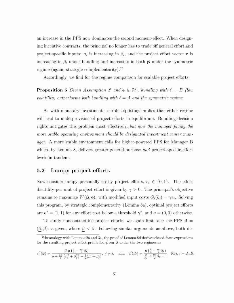
5.2 Lumpy project efforts

Now consider lumpy personally costly project efforts, ei ∈ {0, 1}. The effort

disutility per unit of project effort is given by γ > 0. The principal’s objective

remains to maximize W (β, e), with modified input costs Gi(ki) = γei. Solving

this program, by strategic complementarity (Lemma 8a), optimal project efforts

are e∗ = (1, 1) for any effort cost below a threshold γ∗, and e = (0, 0) otherwise.

To study noncontractible project efforts, we again first take the PPS β =

(β, β) as given, where β < β. Following similar arguments as above, both de-

26In analogy with Lemmas 2a and 3a, the proof of Lemma 8d derives closed-form expressionsfor the resulting project effort profile for given β under the two regimes as

eSi (β) =βiµ

(12 −

ηρ4 βi

)g + ηρ

4

(β2i + β2

j

)− 1

2 (βi + βj), j 6= i, and e`i(β`) =

µ(12 −

ηρ4 β`

)gβ`

+ ηρ2 β` − 1

fori, j = A,B.

31

centralization regimes result in underinvestment. But contrary to monetary in-

vestments, recall the PPS now stimulates, rather than depresses, project specific

inputs. Therefore, under bundling the principal designates the manager facing

higher-powered PPS the investment center manager (β` = β), while under the

symmetric regime the manager with the lower PPS now is the bottleneck in

terms of eliciting project efforts (Fig. 7).

Under bundling the investment center manager chooses (1, 1) for given PPS

if and only if

Γ(1, 1 | β = β)− 2γ ≥ Γ(0, 0 | β = β), (23)

or equivalently, if γ ≤ γ`11(β); and (0, 0) otherwise.27 Under the symmetric

regime, eS(β) = (1, 1) constitutes an equilibrium under the symmetric regime

for γ low enough such that

Γ(1, 1 | β)− γ ≥ Γ(1, 0 | β). (24)

Denote by γ11(β) the effort cost at which (24) becomes binding. At the same

time, eS(β) = (0, 0) is an equilibrium for γ ≥ γ00(β), where the latter makes

the constraint Γ(1, 0 | β) − γ ≤ Γ(0, 0 | β) binding. As in Section 4.1, one can

show (see proof of Proposition 6) that only symmetric equilibria exist provided

the managers face sufficiently similar PPS, with a sufficient condition being that

βMHB − βMH

A

βMHB

≤ 2− ηρ2µ+ 3

. (25)

This condition is met if the divisions face sufficiently similar levels of volatility,

i.e., small (σ2A − σ2

B), and η is small. It rules out asymmetric project effort

equilibria under the symmetric regime and ensures eS(β) = (1, 1) if γ ≤ γ11(β),

and eS(β) = (0, 0) otherwise, even for optimally chosen PPS, i.e., at β = βS.28

27Because we have assumed similar functional forms for all key constructs across the (mone-tary and personally costly) input scenarios, the effort cost threshold equals γ`11(β`) = β`φ

`11(β`),

with φ`11(β`) as defined in (14). (As argued above, however, the optimal assignment of deci-sion rights will differ from that for monetary inputs.) This reflects the fact that project effort

32

(0, 0)

(1, 0)

(0, 1)

(1, 1)

(0, 0)

(1, 0) (1, 1)

(0, 1)

Γ(1, 1 | β)− Γ(0, 0 | β)− 2γ ≥ 0

Γ(1, 1 | β)− Γ(1, 0 | β)− γ ≥ 0

-

����������� 6

(a) Bundling: high-PPS manager

chooses eA and eB

(b) Symmetric form: Nash equilibrium (binding

constraint is low-PPS manager)

Figure 7: Comparison of project effort incentives with exogenous PPSSolid arrows indicate the binding constraints in order to elicit the project effort profile (1, 1).

We turn now to the principal’s Date-1 contracting problem with noncon-

tractible, lumpy project efforts. Because at the benchmark PPS levels either

delegation regime would elicit suboptimal levels of project effort, any contract

adjustments will be geared toward stimulating investment. For the symmetric

regime, denote by qβS(γ) the PPS level that makes (24) binding for given effort

costs are incurred privately by the manager. In the benchmark solution, on the other hand,γ∗ = φ∗, as in Section 4.2, because ex ante the principal ultimately pays for all project inputcosts, whether monetary in nature or effort disutility.

28In the proof of Proposition 6 we show that if (β−β)/β ≤ 2−ηρ2µ+3 , only symmetric equilibria

exist under the symmetric regime. In equilibrium, βSA ≤ βSB and the relative PPS differential,(βSB − βSA)/βSB is bounded from above by (βMH

B − βMHA )/βMH

B . To see why, note that for

sufficiently low γ, both managers invest even at βS = βo(1, 1); for sufficiently high γ, eventhe principal prefers (0, 0), and so βS = βo(0, 0). Inducing (1, 1) for intermediate valuesof γ requires strengthening incentives—first to the low-PPS “bottleneck” Manager A. Thisresults in convergence of the PPS for intermediate γ. Therefore, (βSB − βSA)/βSB ≤ (βoB(0, 0)−βoA(0, 0))/βoB(0, 0) ≤ (βMH

B − βMHA )/βMH

B . Note that the sufficient condition to rule outasymmetric equilibria for monetary investments in Section 4.1 (e.g., in Lemma 4) was anupper bound on the absolute PPS differential, whereas (25) bounds the relative differential.This is again a consequence of the fact that input costs are scaled by the PPS for monetaryinvestments but not for project efforts.

33

cost, and by γS ≡ γ11(βo(1, 1)) the effort cost level up to which high project

efforts obtain without any adjustments required to the benchmark PPS. The op-

timal contract under the symmetric regime then is a straightforward adaptation

of that in Proposition 2:

Proposition 6 (Symmetric regime, project efforts) Given Assumption 1′

and e ∈ {0, 1}2, suppose (25) holds. Under the symmetric regime, there exists a

unique γS ∈ (γS, γ∗), such that:

(i) If γ ∈ (γS, γS], then βA = qβS(γ) > βoA(1, 1) and βB = max{qβS(γ), βoB(1, 1)}.

Both managers exert project effort, as would be the case under the bench-

mark solution.

(ii) If γ ∈ (γS, γ∗], then βi = βoi (0, 0) > βoi (1, 1), i = A,B. Neither manager

exerts project effort, whereas e∗ = (1, 1) under the benchmark solution.

Under bundling, designating Manager B the investment center manager most

effectively stimulates project efforts, as his stable operating environment calls for

high-powered PPS to begin with. Given ` = B, denote by qβB(γ) the PPS that

makes (23) binding for given effort cost, and by γB ≡ γB11(βo(1, 1)) the fixed

cost level up to which bundling would implement high efforts absent any PPS

adjustment, i.e., if βB = βoB(1, 1). The optimal contract under bundling then is:

Proposition 7 (Bundling, project efforts) Given Assumption 1′ and e ∈

{0, 1}2, under bundling, Manager B (low operating volatility) is designated in-

vestment center manager, and there exists a unique γB ∈ (γB, γ∗] such that:

(i) If γ ∈ (γB, γB], then βB = qβB(γ) > βoB(1, 1) and βA = βoA(1, 1). Manager

B chooses (1, 1), as would be the case under the benchmark solution.

(ii) If γ ∈ (γB, γ∗], then βi = βoi (0, 0) > βoi (1, 1), i = A,B. Manager B chooses

(0, 0), whereas e∗ = (1, 1) under the benchmark solution.

34

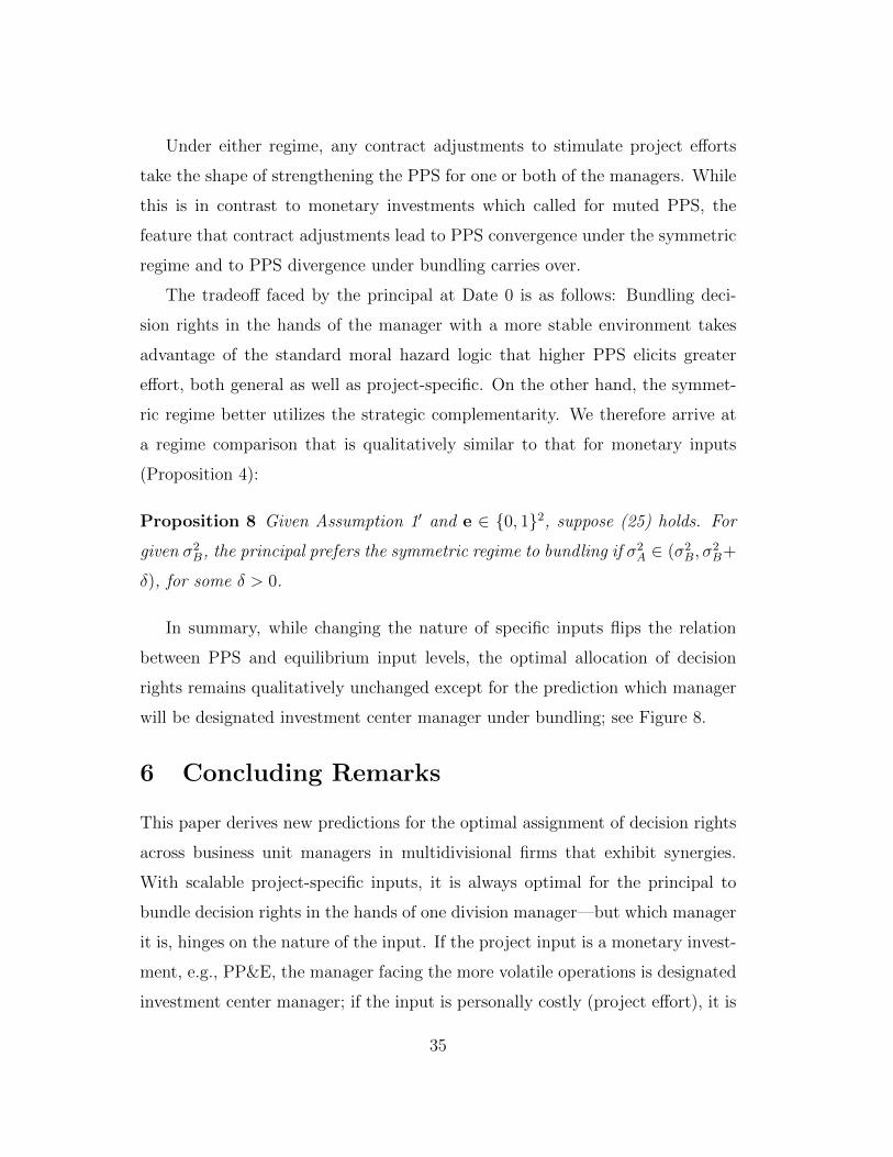
Under either regime, any contract adjustments to stimulate project efforts

take the shape of strengthening the PPS for one or both of the managers. While

this is in contrast to monetary investments which called for muted PPS, the

feature that contract adjustments lead to PPS convergence under the symmetric

regime and to PPS divergence under bundling carries over.

The tradeoff faced by the principal at Date 0 is as follows: Bundling deci-

sion rights in the hands of the manager with a more stable environment takes

advantage of the standard moral hazard logic that higher PPS elicits greater

effort, both general as well as project-specific. On the other hand, the symmet-

ric regime better utilizes the strategic complementarity. We therefore arrive at

a regime comparison that is qualitatively similar to that for monetary inputs

(Proposition 4):

Proposition 8 Given Assumption 1′ and e ∈ {0, 1}2, suppose (25) holds. For

given σ2B, the principal prefers the symmetric regime to bundling if σ2

A ∈ (σ2B, σ

2B+

δ), for some δ > 0.

In summary, while changing the nature of specific inputs flips the relation

between PPS and equilibrium input levels, the optimal allocation of decision

rights remains qualitatively unchanged except for the prediction which manager

will be designated investment center manager under bundling; see Figure 8.

6 Concluding Remarks

This paper derives new predictions for the optimal assignment of decision rights

across business unit managers in multidivisional firms that exhibit synergies.

With scalable project-specific inputs, it is always optimal for the principal to

bundle decision rights in the hands of one division manager—but which manager

it is, hinges on the nature of the input. If the project input is a monetary invest-

ment, e.g., PP&E, the manager facing the more volatile operations is designated

investment center manager; if the input is personally costly (project effort), it is

35

Project inputs Monetary investments Personally-costly efforts

Scalable Bundling the decision rights in the hands of the manager facing high general volatility

Bundling the decision rights in the hands of the manager facing low general volatility

Lumpy Symmetric allocation of decision rights across managers if they face similar general volatilities

Figure 8: Optimal allocation of decision rights

the manager facing the more stable environment. In either case the underpro-

vision of specific inputs is alleviated due to the PPS differential attributable to

the respective volatility levels. With lumpy project inputs, on the other hand,

it is always optimal to split the decision rights symmetrically between the man-

agers, provided they face comparable levels of operating volatility. This holds

for monetary investments as well as personally-costly project efforts.

Moreover, the model sheds light on the effect of contractual incompleteness

on the managers’ relative incentive strength: bundling of decision rights results

in PPS divergence across divisions; the symmetric regime results in PPS con-

vergence. To test our predictions, it would be useful to adapt earlier empirical

studies on incentives and organizational processes, e.g., Nagar (2002), by distin-

guishing between the delegation of tasks that are personally costly to managers

and those that call for managers to invest the firm’s funds in joint projects.

It is useful to clarify the driving forces behind our main findings. Our results

for scalable monetary investments are driven by the investment-risk link—or,

more generally, input-risk link—in Baldenius and Michaeli (2017): investment

incentives are depressed by high-powered PPS because of the incremental risk

exposure. Decision rights therefore should be bundled in the hands of the man-

ager whose PPS is muted to insure him against his volatile environment. The

result that scalable project efforts should be bundled in the hands of the manager

36

facing the more stable environment, on the other hand, is due to a more con-

ventional moral hazard argument: greater PPS elicits both general-purpose and

project-specific efforts in tandem. Finally, the result that a symmetric split of

decision rights elicits greater lumpy inputs is driven mainly by the model feature

that the party that chooses any action also has to bear its cost. In an incomplete

contracting setting where actions are not verifiable but decision rights are, this

seems the most plausible assumption.

37

Appendix

Proof of Lemma 1: Given Assumption 1, it is straightforward to show that∂2W (k,β)∂kA∂kB

= 1− ρη4

(β2A+β2

B) ≥ 1− ρη2> 0 and ∂2Γ(k|βi)

∂kAkB= βi

(12− ρη

4βi)∝ 1− ρη

2βi ≥

1− ρη2> 0, i = A,B.

Proof of Lemma 2:

Part (a): For given PPS, the best response for Manager i to an anticipated

investment kj by his counterpart, ki(kj | βi), is found by setting the first-order

conditions corresponding to (9) equal to zero; upon rearranging:

ki(kj | βi) =(µ+ kj)

(12− ρη

4βi)

f + ρη4βi − 1

2

, i = A,B, j 6= i.

Because ki(kj = 0 | βi) > 0, and ddkjki(kj | βi) < 1 for any kj,β, i and j 6= i, we

have a unique Nash equilibrium in investments for any PPS. (To bound the slope

of the reaction curves by one, we use the maintained assumption that f > 6.)

Solving for the equilibrium in closed form:

kSi (β) =µ (2− ρηβi)

ρη(βi + βj) + 4(f − 1), i = A,B, j 6= i.

The equilibrium investments are decreasing in either manager’s PPS:

dkSi (β)

dβi=−µρη(ρηβj + 4f − 3)

(ρη(βi + βj) + 4(f − 1))2<dkSi (β)

dβj=

−µρη(1− ρηβi)(ρη(βi + βj) + 4(f − 1))2

< 0. (26)

Part (b): We first show that kSA > kSB. Recall that βS ∈ arg maxβW (β),

where:

W (β) ≡ W (β,kS(β))

=∑i

Φi(βi) + E[M(θ,kS(β))

]− ρ

8

∑i

β2i V ar(k)−

∑i

F (kSi (β)).

38

Taking derivative,

∂W (β)

∂βi= Φ′i(βi)−

ρ

4βiV ar(k

S(β)

+∑j=A,B

[dkSj (β)

dβi

(E[Mkj(θ,k

S(β)]− ρ

8

∑l

β2l

∂V ar(kS(β))

∂kj− F ′(kSj (β))

)]= Φ′i(βi)−

ρη

4βi(q

∗(µ,kS(β)))2

+∑j=A,B

[dkSj (β)

dβi

(q∗(µ,kS(β))− ρη

4

∑l

β2l q∗(µ,kS(β))− fkSj (β)

)]≡ wSi (β) (27)

The optimal PPS vector βS satisfy the system of equations:

wSi (βS) = 0, i = A,B.

Note that wSA(β) differs from wSB(β) only in σ2i , i = A,B. Because by assumption,

σA > σB, for βSA < βSB to hold, we only need to show that βSi is decreasing in σ2i .

Applying the Implicit Function Theorem to (27):

∂βSi∂σ2

i

= −∂wS

i (β)

∂σ2i

∂wSi (β)

∂β2i

∝ ∂wSi (β)

∂σ2i

= −ρβi < 0.

Now note that kSA > kSB by (26) and the fact that kSi = kSi (βS).

Next, we show that k∗i > kSi . Recall that under the benchmark case, the

principal contracts on k∗A = k∗B = k∗. We fix kB (the investment undertaken by

the manager facing less volatile general operations) at kB = k∗ and consider the

best response of Manager A, described by

ySA(kA, k∗B) ≡ q∗(µ, kA, k

∗B)

(1

2− ρη

4βA

)− fkA = 0.

Contrast that with the conditionally optimal choice of contractible investment

on the part of the principal (benchmark case):

y∗A(kA, k∗B) ≡ q∗(µ, kA, k

∗B)

(1− ρη

4

∑i

(βoi (kA, k∗B))2

)− fkA = 0.

39

Now note that:

y∗A(kA, k∗B)− ySA(kA, k

∗B) = q∗(µ, kA, k

∗B)

(1− ρη

4

∑i

(βoi (kA, k∗B))2 − 1

2+ρη

4βA

)

∝ 1− ρη

2

(∑i

(βoi (kA, k∗B))2 − βA

)> 1− ρη

≥ 0.

It follows that, even if Manager B invests the benchmark, Manager A will un-

derinvest. Similar arguments apply to Manager B’s best response if Manager

A were to choose his benchmark investment k∗A. Combined with strategic com-

plementarity (Lemma 1), both managers thus underinvest under the symmetric

regime.

Proof of Proposition 1: In Step 1, we show the bundling regime with ` = A

outperforms the symmetric regime; in Step 2, that it outperforms the bundling

regime with ` = B.

Step 1. Fix the PPS at β = βS and consider the equilibrium under the

bundling regime with ` = A at this PPS level. Then, kAi (βS) > kSi (βS), for any

i, by βSA < βSB and strategic complementarity. For W S(β) ≡ W (kS(β),β) and

W `(β) ≡ W (k`(β),β), it follows that W S(βS) ≤ WA(βS), because: (i) W (·) is

concave in (kA, kB) for given β, and (ii) kAi ≤ k∗i , for any i, as per Lemma 3. By

revealed preference, WA(βS) ≤ WA(βA

) ≡ W (kA(βA

), βA

).

Step 2. Note that q∗(θ,k) depends solely on the sum of the investments,

henceforth denoted n ≡∑

i=A,B ki, and so does the conditionally optimal PPS

of Manager i in the benchmark solution. Therefore, slightly abusing notation,

we write q∗(θ, n) (instead of q∗(θ,k)) and βoi (n) (instead βoi (k)).

Denote the optimal PPS for Manager B under the bundling regime with ` = B

by βBB = β, resulting in total units of equilibrium investment n ≡∑

i=A,B kBi (β).

The optimal PPS vector under the bundling regime with ` = B then is βB

=

(βoA(n), β) where n ≡∑

i kBi (β). Note that β < βoB(n). Now consider the

40

bundling regime with ` = A and suppose the principal chooses a PPS vector of

β = (βA = β, βB = βoB(n)), resulting again in total investment of∑

i kAi (β) = n.

Because σ2A > σ2

B, βoB(n) > βoA(n), but there are two possible cases regarding the

ranking of βoA(n) and β.

Case 1: We claim that for βoB(n) > βoA(n) > β bundling with ` = A dominates

bundling with ` = B. Denoting Φi(βi) ≡ ai(βi) − v2(ai(βi))

2 − ρ2β2i σ

2i ; χ(βi |

n, σ2i ) ≡ Φi(βi)− ρη

8β2i (q∗(µ, n))2 and W `(β) ≡ W (k`(β`),β), we have:

WA(β, βoB(n))−WB(βoA(n), β) = χ(β | n, σ2A) + χ(βoB(n) | n, σ2

B)

−χ(βoA(n) | n, σ2A)− χ(β | n, σ2

B)

> χ(β | n, σ2A) + χ(βoA(n) | n, σ2

B)

−χ(βoA(n) | n, σ2A)− χ(β | n, σ2

B)

= −ρ2β

2 (σ2A − σ2

B

)+ρ

2(βoA(n))2

(σ2A − σ2

B

)∝ (βoA(n))2 − β2

> 0,

because βoj (n) ∈ arg maxβj χ(βj | n, σ2j ), j = A,B and βoB(n) > βoA(n) > β. By

revealed preference, WA(βA

) > WA(β, βoB(n)), i.e., the bundling regime with

` = A outperforms the bundling regime with ` = B.

Case 2: We claim that for βoB(n) > β > βoA(n) the symmetric regime domi-

nates bundling with ` = B. Again, fix β = βB

= (βoA(n), β) at the level optimal

under the bundling regime with ` = B. If the principal were to choose this PPS

vector under the symmetric regime, the managers’ investment reaction functions

would be:

kSB(kA | βB = β) ≡ kBB(kA | βB = β),

kSA(kB | βA = βoA(n)) > kBA(kB | βB = β).

By strategic complementarity, kS(βoA(n), β) > kB. Recall that W (·) is concave

in (kA, kB) for given β. Hence, W S(βB

) > WB(βB

) because kBA < kSi ≤ k∗i , i =

41

A,B (by the observation above, Lemma 2 and Lemma 3). By revealed preference,

W S(βS) > W S(βB

), which together with Step 1 above establishes the result.

Proof of Lemma 4: Using (15) and (16), if φ11(β)−φ00(β) < 0, the investment

profile (1,0) can be a Nash equilibrium for any φ ∈ (φ11(β), φ00(β)). Otherwise,

if φ11(β) − φ00(β) ≥ 0, then for any φ ∈ (φ00(β), φ11(β)), both (1, 1) and (0, 0)

can be equilibria simultaneously. We note that:

φ11(β)− φ00(β) =Γ(1, 1 | β)− Γ(1, 0 | β)

β−

Γ(1, 0 | β)− Γ(0, 0 | β)

β

=E[(q∗(θ, 1, 1))2 − (q∗(θ, 1, 0))2]

4− ρη

2β

(q∗(µ, 1, 1))2 − (q∗(µ, 1, 0))2

4

−E[(q∗(θ, 1, 0))2 − (q∗(θ, 0, 0))2]

4+ρη

2β

(q∗(µ, 1, 0))2 − (q∗(µ, 0, 0))2

4

=1

4

(E[(θ + 2)2 − (θ + 1)2]− ρη

2β((µ+ 2)2 − (µ+ 1)2)

)−1

4

(E[(θ + 1)2 − θ2] +

ρη

2β((µ+ 1)2 − µ2)

)=

1

4

[(2µ+ 3)

(1− βηρ

2

)− (2µ+ 1)

(1−

βηρ

2

)]︸ ︷︷ ︸

≡X(β)

Because β ∈ [0, 1], a sufficient condition for X(β) > 0 is that β−β < 1µ

(32

+ 2ρη

).

Note that if X(β) ≥ 0, then for any φ ∈ (φ00(β), φ11(β)), both (1, 1) and

(0, 0) can be Nash equilibria simultaneously. To predict which of these equilibria

the managers will play, we invoke Theorem 7 in Milgrom and Roberts (1990): if

multiple equilibria exist in a supermodular game (such as the managers’ Date-2

investment game) with positive spillovers (i.e., player i’s payoff is increasing in

player j’s action), then the highest equilibrium—here, (1, 1)—Pareto-dominates

the other equilibria. That is, for φ ∈ (φ00(β), φ11(β)) we can ignore the shirking

equilibrium.

Proof of Lemma 5: We need to show that φ∗(β) − φ11(β) > 0 and φ∗(β) −

42

φ`11(β`) > 0 for any given PPS profile, β = (β, β). Simplifying,

φ∗(β) =1

2

∑i=A,B

[E[M(θ, 1, 1)]

2− ρ

8β2i · V ar(1, 1)−

(E[M(θ, 0, 0)]

2− ρ

8β2i · V ar(0, 0)

)]=

E[(q∗(θ, 1, 1))2 − (q∗(θ, 0, 0))2]

4− ρη

2(β2 + β

2)(q∗(µ, 1, 1))2 − (q∗(µ, 0, 0))2

8

=E[((θ + 2)2 − θ2]

4− ρη

2(β2 + β

2)(µ+ 2)2 − µ2

8

= (µ+ 1)(

1− ρη

4(β2 + β

2)).

Similarly,

φ`11(β) =Γ(1, 1|β)− Γ(0, 0|β)

2β=

1

2(µ+ 1)

(1− ρη

2β)

;

φ`11(β) =Γ(1, 1|β)− Γ(0, 0|β)

2β=

1

2(µ+ 1)

(1− ρη

2β)

;

φ11(β) =Γ(1, 1|β)− Γ(0, 1|β)

β=

1

2

(µ+

3

2

)(1− ρη

2β).

Now note that φ`11(β) > φ`11(β) and so

φ∗(β)− φ`11(β) > φ∗(β)− φ`11(β)

= (µ+ 1)(

1− ρη

4(β2 + β

2))− (µ+ 1)

(1

2− ρη

4β

)=

1

2(µ+ 1)

(1− ρη

2(β2 + β

2 − β))

∝ 1− ρη

2(β

2 − β(1− β))

> 1− ρη

2β

2

> 0.

43

Lastly,

φ∗(β)− φ11(β) = (µ+ 1)(

1− ρη

4(β2 + β

2))−(µ+ 1 +

1

2

)(1

2− ρη

4β

)=

1

2(µ+ 1)

(1− ρη

2(β2 + β

2 − β))− 1

2

(1

2− ρη

4β

)>

1

2

(1− ρη

2β

2)− 1

2

(1

2− ρη

4β

)>

(1

2− ρη

4β

)− 1

2

(1

2− ρη

4β

)> 0.

Proof of Lemma 6: We need to show that φA11(β) ≤ φ11(β). Using the proof

of Lemma 5,

φ`∗

11(β) =1

2(µ+ 1)

(1− ρη

2β)

and φ11(β) =1

2

(µ+

3

2

)(1− ρη

2β)

so that

φ11(β)− φ`∗11(β) =1

2

(µ+

3

2

)− 1

2(µ+ 1)− ρη

2

(β

1

2

(µ+

3

2

)− β 1

2(µ+ 1)

)∝ µ+

3

2− µ− 2

2− ρη

2

(β

(µ+

3

2

)− β(µ+ 1)

)= 1− ρη

2

(2µ(β − β) + 3β − 2β)

)︸ ︷︷ ︸≡Y

Note that

X(β)− Y = 2− ρη

2

(2µ(β − β) + 3β − β)

)− 1 +

ρη

2

(2µ(β − β) + 3β − 2β)

)= 1− ρη

2β,

where Y is defined above and X(β) is defined in Lemma 5. It is straightforward

that X(β) − Y ∈ (0, 1). It follows that a sufficient condition for Y > 0 is

X(β) > 1. Lastly, note that a sufficient condition for X(β) > 1 is that β − β ≤1µ

(32

+ 1ρη

).

44

Proof of Lemma 7: Recall that the principal’s payoff under the benchmark

case can be conveniently presented as W ∗(k) ≡ W (βo(k),k), where βo(k) is

as defined in (11) (because for given k, the optimal PPS is βo(k)). Note that

∂∂φW ∗(1, 1) = −2; ∂

∂φW ∗(1, 0) = −1; and ∂

∂φW ∗(0, 0) = 0. Further, by Assump-

tion 1, limφ→0W∗(1, 1) > limφ→0W

∗(1, 0) > limφ→0W∗(0, 0). Hence, for suffi-

ciently low φ, the optimal solution is k∗ = (1, 1) and β∗ = βo(1, 1). Moreover,

limφ→∞W∗(1, 1) < limφ→∞W

∗(1, 0) < limφ→∞0W∗(0, 0). Hence, for sufficiently

high φ, the optimal solution is k∗ = (0, 0) and β∗ = βo(0, 0).

It remains to consider the solution for intermediate values of φ. To show that

it is never optimal for the principal to contract on k = (1, 0) and β = βo(1, 0)

we need to show that φ2→1 ≥ φ2→0, where

φ2→1 ≡ W ∗(1, 1)−W ∗(1, 0) and φ2→0 ≡W ∗(1, 1)−W ∗(0, 0)

2.

Note that

φ2→1 − φ2→0 ∝ 2(W ∗(1, 1)−W ∗(1, 0))− (W ∗(1, 1)−W ∗(0, 0))

= W ∗(1, 1)−W ∗(1, 0)− (W ∗(1, 0)−W ∗(0, 0))

≥ 0,

because W ∗(1, 1) − W ∗(1, 0) ≥ W ∗(1, 0) − W ∗(0, 0). To see why, treat for a

moment k as continuous variable and note that W ∗(k) has strictly increasing

differences in k. Specifically, using the Envelope Theorem,

dW ∗

dkA=∂W ∗

kA= E [MkA(θ,k)]− ρ

8

∑i

(βoi (k))2∂V ar(k)

∂kA− F ′(kA)

= q(µ,k)

(1− ρη

4

∑i

(βoi (k))2

)− fkA.

45

Taking cross-partial derivative,

d2W ∗

dkAdkB= qkB(µ,k)

(1− ρη

4

∑i

(βoi (k))2

)− q(µ,k)

ρη

2

∑i

(βoi (k)

∂βoi (k)

∂kB

).

= 1− ρη

4

∑i

(βoi (k))2 +ρη

4

∑i

(βoi (k))3ρvV ar(k)

≥ 1− ρη

2

> 0.

In summary, the contractible benchmark solution is:

(k∗,β∗) =

((1, 1),βo(1, 1)), if φ ≤ φ∗ ≡ φ∗(βo(1, 1)),

((0, 0),βo(0, 0)), otherwise.

Proof of Proposition 2: In order to elicit the investments (Program PS11),

the principal optimally sets βB = qβS(φ) and βA = min{qβS(φ), βoA(1, 1)}, where

qβS(φ) is such that the investment constraint (18) is just binding. Under the

no-investment program PS00, βi = βoi (0, 0) for each manager i = A,B.

Denote by K∗ the value of program P∗ and by KSk the value of program PSk ,

k = (0, 0), (1, 1). For any φ ∈ (φS, φ∗]:

K∗(φ) = W (βo(1, 1),k = (1, 1) | φ),

KS11(φ) = W (min{qβS(φ), βoA(1, 1)}, qβS(φ),k = (1, 1) | φ),

KS00 = W (βo(0, 0),k = (0, 0)).

Begin by considering fixed cost values φ = φS

+ν for ν → 0. Then, KS11(φ) =

K∗(φ) − δ, δ → 0, because qβS(φ) is a continuous and decreasing function of φ

and W (min{qβS(φ), βoA(1, 1)}, qβ(φ),k = (1, 1) | φ) is continuous and decreasing

in φ and increasing in βA. That is, the value of program PS11 converges to that

of the benchmark program P∗ as δ becomes small. At the same time, KS00 is

bounded away from K∗(φ) for φ close to φS. This holds because, by Lemma

5, φS < φ∗, together with the observations that at φ∗ we have KS00 = K∗(φ)

46

and that K∗(φ) is monotonically decreasing in φ. Thus, we have shown that for

φ ↓ φS, KS11(φ) > KS

00, whereas for φ ↑ φ∗, KS11(φ) < KS

00.

Lastly, since KS11(φ) is monotonically decreasing in φ whereas KS

00 is inde-

pendent of φ, it follows that there exists a unique indifference value φS at which

KS11(φS) = KS

00.

Proof of Proposition 3: The proof follows similar steps as that of Proposition

2 and is available upon request.

Proof of Proposition 4: We need to show that, given σ2A sufficiently close

to σ2B, the principal’s payoff under the symmetric regime is (weakly) larger than

under bundling with ` = A, i.e., W (kS,βS | φ) ≥ W (kA, βA| φ) for any φ.

We first show that φA ≤ φ

Sif σ2

A is sufficiently close to σ2B. Using the proof

of Lemma 6,

φS − φA =

1

2

((µ+ 1)

ρη

2(βoA(1, 1)− βoB(1, 1)) +

1

2

(1− ρη

2βoB(1, 1)

)).

Fix σ2B and note that ∂(φ

S−φA)

∂σ2A

= 12(µ+ 1)ρη

2

βoA(1,1)

∂σ2A

< 0. Further, limσ2A→σ

2B

(φS −

φA

) = 14

(1− ρη

2βoB(1, 1)

)> 0. Hence, for given σ2

B, there exists a threshold

δA > 0 such that, if σ2A−σ2

B < δA, then φS> φ

A. Depending on the parameters,

the threshold δA may be finite or infinite; in the latter case φS> φ

Afor any

σ2A > 0.

For any φ ∈ [φA, φ

S] the principal’s payoff under bundling with ` = A is lower

than under the symmetric regime, because under bundling she needs to reduce

the investing manager’s PPS to induce (1, 1), whereas under symmetric regime

the same investments are induced with the benchmark PPS.

Next, we again fix σ2B and show that φA ≤ φS for σ2

A sufficiently close to σ2B.

Suppose not. Then, at φA it must be that the payoff of the principal when she

induces investment under the symmetric regime is smaller than her payoff when

she foregoes investment, or,

W ((1, 1), (βm, qβS(φA)) | φA) < W ((0, 0),βo(0, 0)), (28)

47

where βm ≡ min{βoA(1, 1), qβS(φA)}. For the principal to induce (1, 1) at φA

under bundling she needs to contract on (qβA(φA), βoB(0, 0)), whereas under the

symmetric regime she needs to contract on (βm, qβS(φA)). As we will show below,

the principal’s expected payoff when she induces investment under the symmetric

regime is larger than her payoff when she induces investment under bundling with

` = A, i.e.,

W ((1, 1), (βm, qβS(φA)) | φA) ≥ W ((1, 1), (qβA(φA), βoB(1, 1)) | φA), (29)

if σ2A sufficiently close to σ2

B. This contradicts (28), because by definition of φA, it

has to be that W ((1, 1), (qβA(φA), βoB(1, 1)) | φA) = W ((0, 0),βo(0, 0)). It follows

that φA ≤ φS.

We now verify that (29) holds. Substituting the optimal general effort choice,

ai(βi) = βiv

, and the effort-related payoff, Φ(βi) = a(βi)− v2(a(βi))

2− ρ2β2i σ

2i , into

(29) and rearranging, gives:

[βm − qβA(φA)]

[1

v−(ρσ2

A

2+

1

2v+ρ

8V ar(1, 1)

)(βm + qβA(φA))

]+[qβS(φA)− βoB(1, 1)]

[1

v−(ρσ2

B

2+

1

2v+ρ

8V ar(1, 1)

)(qβS(φA) + βoB(1, 1))

]≥ 0.

(30)

Next, we note that:

βm ≥ qβA(φA) and qβS(φA) ≤ βoB(1, 1) (31)

because: (i) βm = min{βoA(1, 1), qβS(φA)} by definition; (ii) qβS(φA) ≥ qβA(φA) by

strategic complementarity; and (iii) βoA(1, 1) ≥ qβA(φA) because φA > φA

. Hence,

(30) holds if the following inequalities hold simultaneously:

−(

1

v−[ρσ2

A

2+

1

2v+ρ

8V ar(1, 1)

](βm + qβA(φA))

)≤ 0, (32)

1

v−[ρσ2

B

2+

1

2v+ρ

8V ar(1, 1)

](qβS(φA) + βoB(1, 1)) ≤ 0. (33)

48

We note that (33) and (32) are proportional to

− 1

v(βm + qβA(φA))+

(ρσ2

A

2+

1

2v+ρ

8V ar(1, 1)

)≤ 0, (34)

1

v(qβS(φA) + βoB(1, 1))−(ρσ2

B

2+

1

2v+ρ

8V ar(1, 1)

)≤ 0. (35)

Summing (35) and (34) yields

Q(σ2A, σ

2B) ≡ ρ

2

(σ2A − σ2

B

)− 1

v

(1

βm + qβA(φA)− 1

qβS(φA) + βoB(1, 1)

)≤ 0. (36)

A sufficient condition for (29) to hold is that (36) holds. Using (31) and the fact

that limσ2A→σ

2BβoA(1, 1) = βoB(1, 1), we have

limσ2A→σ

2B

Q(σ2A, σ

2B) ∝ −

(qβS(φA) + βoB(1, 1)

)+(βm + qβA(φA)

)≤ 2 (βm − βoB(1, 1))

= 2 (βm − βoA(1, 1))

≤ 0.

By continuity, it follows that (29) holds if σ2A ∈ (σ2

B, σ2B + δB), δB > 0.

For any φ ∈ [φA, φS] it follows by revealed preference that the principal’s

payoff under the symmetric regime is higher than her respective payoff under

bundling. For any φ > φS, under both regimes, the principal finds it too costly

to induce (1, 1) and instead acquiesces to (0, 0) by contracting on the benchmark

PPS, βo(0, 0). Hence, for φ > φS the principal’s payoff is equal under both

regimes. We cannot rank unambiguously φS and φA. If φA ≤ φS, no further

proof is required. However, if φA > φS, we need to show that W ((1, 1), β|φ) ≥

W ((1, 1), βA|φ) for any φ ∈ [φS, φA]. The proof of this inequality follows similar

steps as the derivation of (29) and is hence omitted. Lastly, let δ ≡ min{δA, δB}.

Proof of Lemma 8:

Part (a): Given Assumption 1′, it is straightforward to show that ∂2W (e,β)∂eA∂eB

=

1− ρη4

(β2A + β2

B) ≥ 1− ρη2> 0 and ∂2Γ(e|βi)

∂eAeB= βi

(12− ρη

4βi)∝ 1− ρη

2βi ≥ 1− ρη

2>

0, i = A,B.

49

Part (b): Using η ≤ 1ρ, by Assumption 1′, and taking cross-partial derivatives:

∂2Λi(e | βi)∂eA∂eB

= βi

(1

2− ρη

4βi

)∝ 1− ρη

2βi ≥ 0,

∂2Λi(e | βi)∂em∂βi

=q∗(µ, e)

2− ρη

2βiq∗(µ, e) ∝ 1− ρηβi ≥ 0,

∂2Λ`i(e | βi)

∂eA∂eB= βi

(1

2− ρη

4βi

)∝ 1− ρη

2βi ≥ 0,

∂2Λ`i(e | βi)

∂em∂βi=

q∗(µ, e)

2− ρη

2βiq∗(µ, e) ∝ 1− ρηβi ≥ 0, m = A,B, i = A,B.

Part (c): Using η ≤ 1ρ, by Assumption 1′:

∂W (e,β)

∂ei− ∂Λi(e | βi)

∂ei= q∗(µ, e)

(1− βi

2− ρη

4(β2

i + β2−i − βi)

)∝ 1− βi

2− ρη

4(β2

i + β2−i − βi) ≥

1

2− ρη

2≥ 0,

∂W (e,β)

∂ei− ∂Λ`

i(e | β`)∂ei

= q∗(µ, e)

(1− β`

2− ρη

4(β2

` + β2−` − β`)

)≥ 0, i = A,B.

Part (d): For given PPS, the best response for Manager i to an anticipated ef-

fort ej by his counterpart, ei(ej | βi), is found by setting the first-order conditions

equal to zero:

∂Γ(e | βi)∂ei

− gei = βi

(q∗(µ, e)

2− ρη

4βiq∗(µ, e)

)− gei = 0, i = A,B.

Upon rearranging:

ei(ej | βi) =(ej + µ)

(12− ρη

4βi)

gβi

+ ρη4βi − 1

2

, i = A,B, j 6= i.

Because ei(ej = 0 | βi) > 0, and ddejei(ej | βi) < 1 for any ej,β, i and j 6= i,

we have a unique Nash equilibrium in investments for any PPS. (To bound the

slope of the reaction curves by one, we use the fact that g > 6.) Solving for the

equilibrium in closed form:

eSi (β) =βiµ

(12− ηρ

4βi)

g + ηρ4

(β2i + β2

j

)− 1

2(βi + βj)

, i = A,B, j 6= i.

50

The equilibrium efforts are increasing in either manager’s PPS:

∂eSi (β)

∂βi=

2µ(1− ηρβi)(4g + ηρβ2j − 2βj)(

ηρ(β2i + β2

j

)− 2(βi + βj − 2g)

)2 ∝ g +ηρ

4β2j −

βj2≥ g − 1

2> 0.

∂eSi (β)

∂βj=

2βiµ(2− βiηρ)(1− βjηρ)(ηρ(β2i + β2

j

)− 2(βi + βj2g)

)2 ∝ (2− βiηρ)(1− βjηρ) ≥ (2− 1)(1− 1) = 0.

Under bundling, for given PPS, the first-order conditions yield:

∂Γ(e | β`)∂ei

− gei = β`

(q∗(µ, e)

2− ρη

4β`q∗(µ, e)

)− gei = 0, i = A,B.

Solving and rearranging:

e`i(β`) =µ(

12− ηρ

4β`)

gβ`

+ ηρ2β` − 1

, i = A,B, j 6= i.

It is immediate thatde`i(β`)

dβj 6=`≡ 0 and, using η ≤ 1

ρ, by Assumption 1′,

de`i(β`)

dβ`=

2gµ(1− β`ηρ)

(β`(β`ηρ− 2) + 2g)2∝ 1− β`ηρ ≥ 0.

Proof of Proposition 5: The proof follows similar steps as that of Proposition

1 and is available upon request.

Proof of Proposition 6: We begin by deriving a sufficient condition to rule

out asymmetric project effort equilibria under the symmetric regime. Recall

that eS(β) = (1, 1) is an equilibrium for γ ≤ γ11(β), whereas eS(β) = (0, 0)

is an equilibrium for γ > γ00(β). If γ11(β) − γ00(β) < 0, then eS(β) = (1, 0)

can be a Nash equilibrium for any γ ∈ (γ11(β), γ00(β)). On the other hand, if

γ11(β)− γ00(β) ≥ 0, then for any γ ∈ (γ00(β), γ11(β)), both (1, 1) and (0, 0) can

51

be equilibria simultaneously.

γ11(β)− γ00(β) = Γ(1, 1 | β)− Γ(1, 0 | β)−(Γ(1, 0 | β)− Γ(0, 0 | β)

)= β

(E[(q∗(θ, 1, 1))2 − (q∗(θ, 1, 0))2]

4− ρη

2β

(q∗(µ, 1, 1))2 − (q∗(µ, 1, 0))2

4

)−β(E[(q∗(θ, 1, 0))2 − (q∗(θ, 0, 0))2]

4− ρη

2β

(q∗(µ, 1, 0))2 − (q∗(µ, 0, 0))2

4

)=

β

4

(E[(θ + 2)2 − (θ + 1)2]− ρη

2β((µ+ 2)2 − (µ+ 1)2)

)−β

4

(E[(θ + 1)2 − θ2] +

ρη

2β((µ+ 1)2 − µ2)

)=

1

4

[β(2µ+ 3)

(1−

βηρ

2

)− β(2µ+ 1)

(1− βηρ

2

)]∝ β(2µ+ 3)

(1−

βηρ

2

)− β(2µ+ 1)

(1− βηρ

2

)> β(2µ+ 3)− β(2µ+ 3) + 2β

(1− ηρ

2

)> 0,

ifβ − ββ≤ 2− ηρ

2µ+ 3. (37)

Suppose (37) holds. For any γ ∈ (γ00(β), γ11(β)), to predict which of the sym-

metric equilibria, (1, 1) or (0, 0), the managers will play, we invoke Theorem 7 in

Milgrom and Roberts (1990): if multiple equilibria exist in a supermodular game

(such as the managers’ Date-2 effort game) with positive spillovers (i.e., player

i’s payoff is increasing in player j’s action), then the highest equilibrium—here,

(1, 1)—Pareto-dominates the other equilibria. That is, for γ ∈ (γ00(β), γ11(β))

we can ignore the shirking equilibrium. Now note that the left-hand side of (37)

in the optimal solution under the symmetric regime is bounded from above by

(βMHB −βMH

A )/βMHB ; therefore a sufficient condition for asymmetric equilibria not

to arise in equilibrium is Condition (25), which will hold for sufficiently small

volatility differential, σ2A − σ2

B, and small η.

Assuming (25) holds, under the symmetric regime the principal will choose

the optimization program with the greater value from among the following:

52

PS11 (Induce effort under symmetric regime): For any γ ∈ (γS, γ∗],

maxβ

W (β | e = (1, 1)),

subject to (5) and βi ≥ qβS(γ), for any i.

PS00 (Forestall effort under symmetric regime): For any γ ∈ (γS, γ∗],

maxβ

W (β | e = (0, 0)),

subject to (5) and βi < qβS(γ), for any i.

The remainder of the proof follows similar steps as the proof of Proposition 2

and is available upon request.

Proof of Proposition 7: The proof follows similar steps to those in the proof

of Proposition 2 and is available upon request.

Proof of Proposition 8: The proof follows similar steps as that of Proposition

4 and is available upon request.

53

References

[1] Abernethy, M., J. Bouwens and L. van Lent (2004). “Determinants of control

system design in divisionalized firms.”The Accounting Review 79, 545-570.

[2] Aghion, P., and J. Tirole (1997). “Formal and Real Authority in Organiza-

tions.” Journal of Political Economy 105, 1-29.

[3] Arya, A., J. Glover, and B. Routledge (2002). “Project Assignment Rights

and Incentives for Eliciting Ideas.” Management Science 48, 886 -899.

[4] Arya, A., and B. Mittendorf (2010). “Input Markets and the Strategic Or-

ganization of the Firm.” Foundations and Trends in Accounting 5, 1-97.

[5] Autrey, R., S. Dikolli, and D. Newman (2010). “Performance measure aggre-

gation, career incentives, and explicit incentives.” Journal of Management

Accounting Research 22, 115-131.

[6] Baiman, S., D. Larcker, and M. Rajan (1995). “Organizational Design for

Business Units.” Journal of Accounting Research 33, 205-230.

[7] Baldenius, T., and B. Michaeli (2017). “Investments and Risk Transfers.”

The Accounting Review 92, 1-24.

[8] Bester, H., and D. Krahmer (2008). “Delegation and Incentives.” The RAND

Journal of Economics 39, 664-682.

[9] Bolton, P., and M. Dewatripont (2012). “Authority in Organizations A Sur-

vey.” In The Handbook of Organizational Economics, R. Gibbons and J.

Roberts (Eds.), Princeton University Press.

[10] Bushman, R., R. Indjejikian, and A. Smith (1995). ”Aggregate Performance

Measures in Business Unit Manager Compensation: The Role of Intrafirm

Interdependencies.” Journal of Accounting Research 33, 101-128.

54

[11] Brynjolfsson, E., and P. Milgrom (2012). “Complementarity in Organiza-

tions.” The Handbook of Organizational Economics, Princeton University

Press.

[12] Darrough, M., and N. Melumad (1995). “Divisional versus Company-Wide

Performance Measures: The Tradeoff Between Screening of Talent and Allo-

cation of Managerial Attention.” Journal of Accounting Research 33, 65-93.

[13] Dessein, W., L. Garicano, and R. Gertner (2010). “Organizing for Syner-

gies.” American Economic Journal: Microeconomics 2, 77-114.

[14] Feltham, G., and D. Xie (1994). “Performance Measure Congruity and Di-

versity in Multi-Task Principal-Agent Relations.” The Accounting Review

69, 429-453.

[15] Friedman, H (2014). “Implications of power: When the CEO can pressure

the CFO to bias reports.” Journal of Accounting and Economics 58, 117-141.

[16] Friedman, H (2016). “Implications of a multi-purpose reporting system on

CEO and CFO incentives and risk preferences.” Journal of Management

Accounting Research 28, 101-132.

[17] Hart, O., and B. Holmstrom (2010). “A Theory of Firm Scope.” Quarterly

Journal of Economics 125, 483-513.

[18] Heinle, M. S., C. Hofmann, and A. H. Kunz (2012). “Identity, incentives,

and the value of information.” The Accounting Review 87, 1309 - 1334.

[19] Holmstrom, B (1999). “The Firm as a Subeconomy” Journal of Law, Eco-

nomics, and Organization 15, 74-102.

[20] Holmstrom, B., and P. Milgrom (1990). “Regulating Trade Among Agents.”

Journal of Institutional and Theoretical Economics 146, 85-105.

55

[21] Hofmann, C., and R.J. Indjejikian (2017). “Performance monitoring and

incentives in hierarchies.” Working paper.

[22] Hughes, J.S., L. Zhang, and J. Xie (2005). “Production externalities, con-

gruity of aggregate signals, and optimal task assignments.” Contemporary

Accounting Research 22, 393-408.

[23] Johnson, N., C. Loeffler, and T. Pfeiffer (2017). “An Evaluation of Alterna-

tive Market-Based Transfer Prices.” Forthcoming, Contemporary Account-

ing Research.

[24] Keating, S (1997). “Determinants of divisional performance evaluation in

practice.” Journal of Accounting and Economics 24, 243-273.

[25] Levine, D. I (1991). “Cohesiveness, productivity, and wage dispersion.”

Journal of Economic Behavior and Organization, 15, 237 - 255.

[26] Liang, P.J., and L. Nan (2014). “Endogenous precision of performance mea-

sures and limited managerial attention.” European Accounting Review 23,

693-727.

[27] Merchant, K (1989). Rewarding Results: Motivating Profit Center Man-

agers, Harvard Business School Press.

[28] Milgrom, P., and J. Roberts (1990). “Rationalizability, learning, and equi-

librium in games with strategic complementarities.” Econometrica 58, 1255-

1277.

[29] Nagar, V (2002). “Delegation and incentive compensation.” The Accounting

Review 77, 379-395.

[30] Pfeiffer, T., U. Schiller, and J. Wagner (2011). “Cost-based transfer pricing.”

Review of Accounting Studies 16 (2): 219?246.

56

[31] Reichmann, S., and A. Rohlfing-Bastian (2013). “Decentralized task assign-

ment and centralized contracting: On the optimal allocation of authority.”

Journal of Management Accounting Research 26, 33-55.

[32] Shaw, J. D., Gupta, N., and J.E. Delery (2002). “Pay dispersion and work-

force performance: Moderating effects of incentives and interdependence.”

Strategic Management Journal 23, 491-512.

[33] Siegel, P., and D. C. Hambrick (2005). “Pay Disparities within Top Man-

agement Groups: Evidence of Harmful Effects on Performance of High-

Technology Firms.” Organization Science 16, 259-274.

[34] Sosa, M., and J. Mihm (2008). “Organization design for new product devel-

opment.” In Handbook of New Product Development Management, C. Loch

and S. Kavadias (eds), Elsevier, 2008, pp. 165-197.

[35] Williamson, O. “Markets and Hierarchies: Analysis and Antitrust Implica-

tions.” Free Press, 1975.

[36] Zenger, T. and W. Hesterly (1997). “The Disaggregation of Corporations:

Selective Intervention, High-powered Incentives, and Molecular Units.” Or-

ganization Science 8, 209-222.

[37] Zhang, L (2003). “Complementarity, task assignment, and incentives.” Jour-

nal of Management Accounting Research 15, 225-246.

57