Reputation:

The Value Added by the Game Theoretic Point

of View

Mario Gilli∗

University of Milano-Bicocca - Department of Economics

Piazza Ateneo Nuovo 1 - 20126 Milano - Italy

tel: ++39 02 461916

fax: ++39 02 700439225

email: mario.gilli@unimib.it

July 1, 2010

Abstract

This paper provides a general game theoretic framework to analyze rep-

utation. The aim of this paper is to show the value added by a game

theoretic approach to informal analysis of reputation. This object is pur-

sued first through an exemplification of the contribution of game theory

to the understanding of reputation, then explaining the formal mathemat-

ical machinery used by game theory to analyze reputation. In particular

I will develop an extensive analysis of three simple cases to show how the

game theoretic approach to reputation works and its possible applications

to academic institutions. I conclude comparing the answers provided by

game theory to open question in the analysis of reputation showing how

game theory stress subtle aspects of the way reputation is built and works.

JEL: C72, D83, D82

Keywords: reputation, game theory.

∗This paper has been written following a suggestion by Emma Zavarrone, so all responsi-

bility for possible mistakes are hers.

“Until you have lost your reputation, you never realize what a burden it was or

what a freedom really is”

Margaret Mitchell, Gone with the Wind.

“ It takes 20 years to build a reputation and five minutes to ruin it. If you

think about that, you’ll do things differently”

Warren Buffet, The Essays of Warren Buffett : Lessons for Corporate America.

1 Introduction

“Reputation is the general opinion about the character, qualities, etc of some-

body or something”1 . Therefore the crucial aspects of reputation are:

1. it is an opinion;

2. it is shared by a group of agent;

3. it regards hidden characteristics

4. of a person or a group of people or an organization.

Consequently these aspects cannot be analyzed outside a context of social in-

teraction. Since the role of game theory is to provide an abstract analysis of

the implications of peopleŠs interacting behaviour when agents’ personal wel-

fare depends on everyone behaviour, game theory is the natural mathematical

language to analyze reputation. Indeed, game theory provides a formal model

for each of the defining characteristics of reputation:

1. opinion are modeled as players’ beliefs, i.e. probability measure on oppo-

nents’ characteristics and/or behaviour;

2. in game theoretic equilibria, usually players’ beliefs should be shared;

3. players’ hidden characteristics are defined as “types”, i.e. players’ private

information on the defining aspects of the game: payoffs, players and

strategies;

4. persons or organizations are modeled as “players” with their well defined

objective function.

1Hornby 1987.

1

Therefore it is not surprising that reputation is one of the most developed and

interesting field of application of game theory2 .

This paper is not a comprehensive survey of the game theoretic approach to

reputation since it would be too long and moreover there are optimal surveys3

so that it is not necessary to add a further similar work to the existing stock.

The aim of this paper instead is to show the value added by a game theoretic ap-

proach to an informal analysis of reputation. This object is pursued first through

an exemplification of the contribution of game theory to the understanding of

reputation, then explaining the formal mathematical machinery used to under-

stand the way of building reputation. In particular I will develop an extensive

analysis of three simple cases to show how the game theoretic approach to rep-

utation works and its possible applications to academic institutions. First I will

analyze these simple games informally, then after the presentation of the nec-

essary mathematical tools I will fully develop their game theoretic analysis to

enlighten the value added by game theory to informal analysis. I conclude com-

paring the answers provided by game theory to open question in the analysis of

reputation showing how game theory stress subtle aspects of the way reputation

is built and works.

The paper consequently is organized as follows: section 2 is devoted to a

quick review of the informal analysis of reputation, section 3 provides the exem-

plification of the game theoretic approach to reputation then providing notations

and results, while section 4 applies these tools to the formal analysis of previous

examples. Section 5 concludes emphasizing the importance of game theory to

understand subtle aspects of the way reputation works in specific social con-

text. Finally the appendix contains the mathematical details of the stochastic

processes involved in this analysis.

2 The Informal Analysis of Reputation

As Informal Analysis of Reputation I mean the approach elaborated by differ-

ent authors, as exemplified by Dasgupta 1988, Good 1988, Kramer 1999, Ritzer

2007, Shenkar-Yuchtman-Yaar 1997, Strathdee 2009, Zucker 1986, just to men-

tion a few, where the authors in different ways stress the social relevance of

concepts such as Reputation, Identity, Trust within the empirical analysis of

2To mention just few papers: Kreps-Wilson 1982; Kreps et al. 1982; Milgrom-Roberts

1982; Fudenberg-Levine 1989; Fudenberg-Levine 1992; Ely-Valimaki 2003, Ely et al. 2004.3See in particular Fudenberg 1992 and Mailath-Samuelson 2006.

2

specific case studies. All these notions are connected and shown to be particu-

larly relevant for the dynamic close examination of specific examples of social

interaction. Generally this approach is developed through empirical analysis,

intuition and general argumentations, but a formal mathematical model is not

presented.

According to this approach, reputation refers to an organizing principle of a

socially recognized agent by which actions are linked into a common assessment.

In particular reputation is a collective representation enacted in social relations.

As a consequence reputation is connected to forms of communication and it is

tied to a community.

Reputation operates in several different domains: personal, mass-mediated,

organizational, historical. Usually reputation begin within circles of personal

intimates, then they spread it outward.

As a consequence of this view, several aspects of reputation are stressed.

First, agents build and share reputation of those who are within their social

circle. Personal reputation has immediate consequences because of the options

opened and closed changing possible interaction outcomes: those identities that

we are given channel those identities that we can select. Therefore agents engage

in form of self-presentation and impression management to modify their images

in the eyes of others in order to change the constraints and thus the opportunities

they face.

Second, the media help to determine who people should know, how people

should care about and the social opinion people should confront with. The repu-

tation of public agents are consequently used in formal and informal transactions

among strangers.

Obviously, as social agents it is meant not only individuals, but organizations

too. In particular organizations strategically develop reputations that influence

(positively or negatively) their effectiveness: the growth of public relations and

of rating agencies are an important part of this process4 . History, constituting

narratives of personal and institutional biographies, may serve a similar role in a

more sedimented way, as an institutionally sanctioned process: in fact from this

point of view history represents settled cultural discourse about the past, de-

termined by culturally literate experts; moreover this knowledge too is acquired

through social institutions such as school and media and their reputation is

transmitted to other agents through such means.

From this point of view, since reputation restricts peopleŠs possible beliefs,

4From 1990 to 2008, major U.S. media’s usage of the term reputation has tripled, as shown

in Leslie Gaines-Ross 2008.

3

it attempts to teach how agents should think about likely behaviours and thus

likely social outcomes. People share memory and opinions because of what

they have socially learned and in this way reputational knowledge reduces the

complexity of the social world helping agents to focus on specific likely social

outcomes. Therefore, reputation is particularly valuable in an uncertain world

where it helps to focus agents’ individual expectations on focal points, working

as a potential selection device again altering opportunities and constraints. In

other words, because of this role as collector and summary of different opinions,

reputation is the most valuable the highest the social uncertainty on the hidden

characteristics of an agent. For example, this might explain why the rise of

fashionable dot.com companies in the nineties has been accompanied by the

expansion of rating agencies. In this setting clearly how to build a reputation

is as much important as knowing how to protect and salvage a lost reputation.

Indeed many surveys enlighten the fact that agents regard the loss of reputation

as the most dangerous risk for a company, exceeding all others, including market

risk, natural hazards and physical or political security. Actually, an important

aspect of reputation is that it can fallen suddenly and precipitously, but this does

not mean that reputation recovery is not possible, as many real life examples

show. To be more precise, consider the following facts:

1. only three companies from Fortune’s America’s Top 10 Most Admired

Companies in 2000 were among the Top 10 Most Admired in 2006;

2. IBM was once ranked first in Fortune’s America’s Top 10 Most Admired

Companies, fell to rank 354 in 1993 and it was again in the first Top 10

in 2003.

As this quick illustration shows, the analysis of reputation is thus closely

linked to the examination of collective memory and social mnemonic, and there-

fore it builds on cognitive sociology, on social movement research, and on so-

ciology of knowledge. What I want to show in next section, is that all these

aspects can be formally and rigorously studied within the language of math-

ematical game theory enlightening subtle aspects in the process of reputation

building, loss and recovery.

From this discussion clearly emerges that the analysis of reputation building

and maintenance, of loss and recovery of reputation, must consider the following

issues:

1. How broad is the context where the agent is trying to build a reputation

for? Are single or multitasks situations, specific or generic actions?

4

2. What have the agents at stake?

3. How informative is the observations of past outcomes in order to predict

future behaviour?

4. Is it possible to tie specific actors to observed and future outcomes?

5. Is it possible to measure reputation and, if the answer is positive, how can

it be done?

6. What algorithms can let us make accurate predictions based on these

reputation measures?

After the illustration of the game theoretic approach in sections 3 and 4, the

conclusion will listen the precise answers provided by game theory to each of

these open questions.

3 An Introduction to the game Theoretic Ap-

proach to Reputation

As the previous section argues, an agentŠs reputation helps to predict its behav-

ior, it is based on past actions and characteristics and it is found on linkability,

in the sense that reputation should allow to link past actions to a specific set of

possible identities so that future actions by the same set of possible identities are

linked to future behaviour. These links are what help to make predictions about

the agents’ future choices. Moreover, previous section has shown that reputation

involves behaviour that one might not expect in an isolated interaction exactly

because of this common expectations. Finally, previous observations show that

reputation is especially valuable in environments in which there is asymmetric

information.

These considerations imply that the branch of game theory that can help us

to build mathematical models of reputation is the theory of repeated games

with incomplete information, strategic situations where a bunch of players is

called to repeatedly act observing, may be imperfectly, players’ past behaviour

but where these players ignore some hidden characteristics of the interacting

agents.

3.1 Example 1

Consider the game shown in figure 1:

5

h l

H 2, 3 0, 2

L 3, 0 1, 1

Figure 1

A possible story behind this trivial game is the following: player raw (1) is a

university who can exert either high effort (H) or low effort (L) in the production

of its output. Player column (2) is a student who can buy either a high-priced

education (h) or a low priced one (l). Payoffs reflect likely players’ preferences.

In a simultaneous moves game as the one of figure 1, the University can not

observably choose H before student’s choice, the same holds for player 2. Player

1 would prefer to precommit to not to use L, but without an effective constraint

this promise would not be credible: any rational 1 would always choose L since it

is strictly dominant and thus any rational 2 anticipating 1’s rational behaviour

would choose l. Therefore this game has a unique (rationalizable) solution:

(L,l), which is Pareto inefficient.

3.2 A Repeated Game Approach to Reputation

To see reputation from this point of view, suppose that there is a succession of

short-lived player 2, each of whom plays the game only once, but such that each

of them can observe the players’ previous strategic choices.

Clearly short-lived players are concerned only with their payoffs in the

current period. One interpretation is that in each period, a new short-lived

player enters the game, is active for only that period and then leaves the game.

An alternative interpretation is that each short-lived player represents a contin-

uum of small anonymous long-lived agents such that each agent’s payoff depends

on its own action, the action of the large player and the average of the small

players’ actions. Moreover observable histories of play are assumed to include

the actions of the large players and only the distribution of play produced by the

small players. Since small players are negligible, change in the action of a single

6

agent does not affect the distribution of play, and so does not influence future

behavior of any small or large players, generating myopic rational behaviour5 .

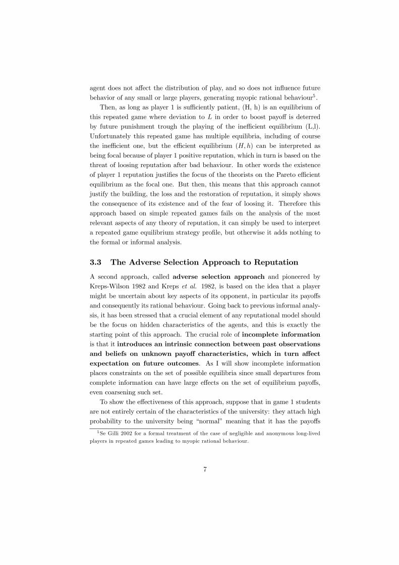
Then, as long as player 1 is sufficiently patient, (H, h) is an equilibrium of

this repeated game where deviation to L in order to boost payoff is deterred

by future punishment trough the playing of the inefficient equilibrium (L,l).

Unfortunately this repeated game has multiple equilibria, including of course

the inefficient one, but the efficient equilibrium (H,h) can be interpreted as

being focal because of player 1 positive reputation, which in turn is based on the

threat of loosing reputation after bad behaviour. In other words the existence

of player 1 reputation justifies the focus of the theorists on the Pareto efficient

equilibrium as the focal one. But then, this means that this approach cannot

justify the building, the loss and the restoration of reputation, it simply shows

the consequence of its existence and of the fear of loosing it. Therefore this

approach based on simple repeated games fails on the analysis of the most

relevant aspects of any theory of reputation, it can simply be used to interpret

a repeated game equilibrium strategy profile, but otherwise it adds nothing to

the formal or informal analysis.

3.3 The Adverse Selection Approach to Reputation

A second approach, called adverse selection approach and pioneered by

Kreps-Wilson 1982 and Kreps et al. 1982, is based on the idea that a player

might be uncertain about key aspects of its opponent, in particular its payoffs

and consequently its rational behaviour. Going back to previous informal analy-

sis, it has been stressed that a crucial element of any reputational model should

be the focus on hidden characteristics of the agents, and this is exactly the

starting point of this approach. The crucial role of incomplete information

is that it introduces an intrinsic connection between past observations

and beliefs on unknown payoff characteristics, which in turn affect

expectation on future outcomes. As I will show incomplete information

places constraints on the set of possible equilibria since small departures from

complete information can have large effects on the set of equilibrium payoffs,

even coarsening such set.

To show the effectiveness of this approach, suppose that in game 1 students

are not entirely certain of the characteristics of the university: they attach high

probability to the university being “normal” meaning that it has the payoffs

5Se Gilli 2002 for a formal treatment of the case of negligible and anonymous long-lived

players in repeated games leading to myopic rational behaviour.

7

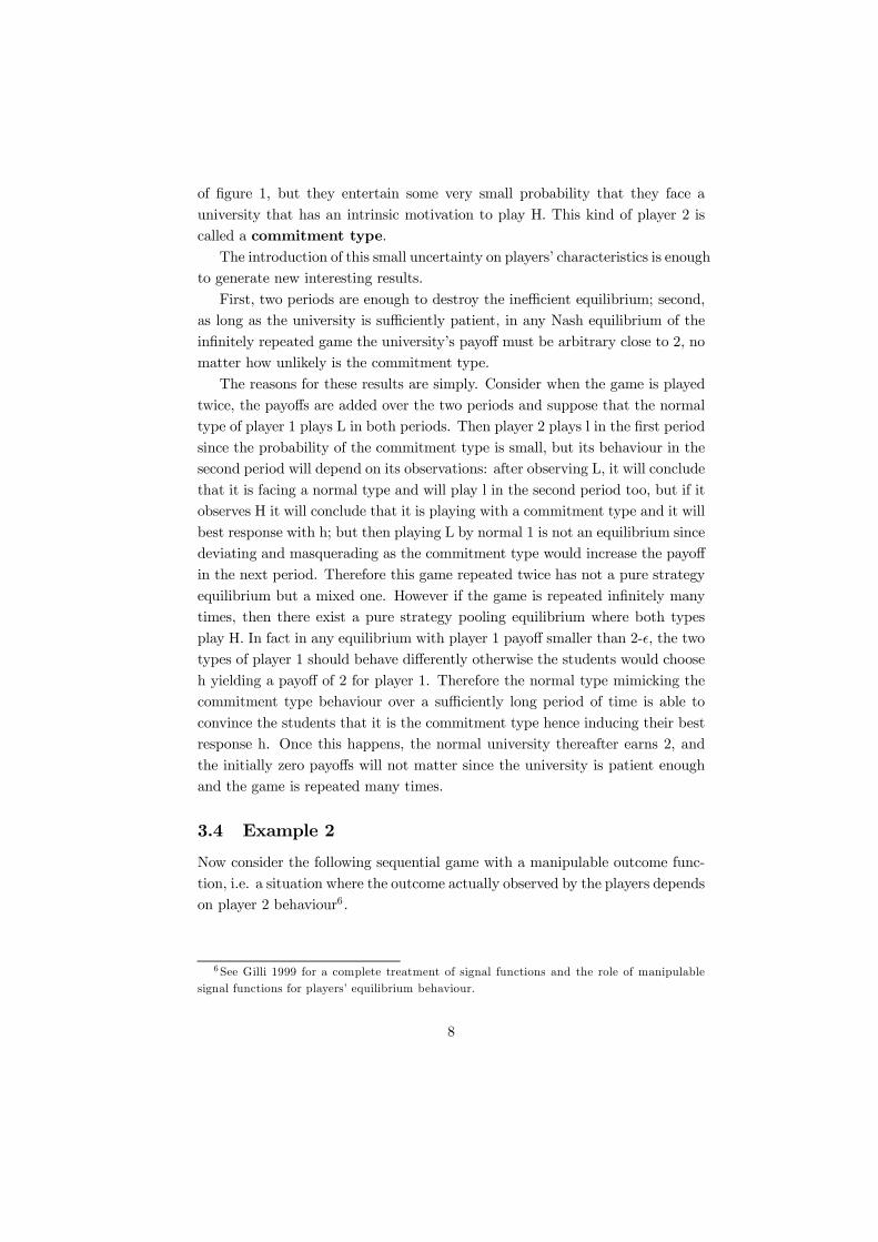
of figure 1, but they entertain some very small probability that they face a

university that has an intrinsic motivation to play H. This kind of player 2 is

called a commitment type.

The introduction of this small uncertainty on players’ characteristics is enough

to generate new interesting results.

First, two periods are enough to destroy the inefficient equilibrium; second,

as long as the university is sufficiently patient, in any Nash equilibrium of the

infinitely repeated game the university’s payoff must be arbitrary close to 2, no

matter how unlikely is the commitment type.

The reasons for these results are simply. Consider when the game is played

twice, the payoffs are added over the two periods and suppose that the normal

type of player 1 plays L in both periods. Then player 2 plays l in the first period

since the probability of the commitment type is small, but its behaviour in the

second period will depend on its observations: after observing L, it will conclude

that it is facing a normal type and will play l in the second period too, but if it

observes H it will conclude that it is playing with a commitment type and it will

best response with h; but then playing L by normal 1 is not an equilibrium since

deviating and masquerading as the commitment type would increase the payoff

in the next period. Therefore this game repeated twice has not a pure strategy

equilibrium but a mixed one. However if the game is repeated infinitely many

times, then there exist a pure strategy pooling equilibrium where both types

play H. In fact in any equilibrium with player 1 payoff smaller than 2-ǫ, the two

types of player 1 should behave differently otherwise the students would choose

h yielding a payoff of 2 for player 1. Therefore the normal type mimicking the

commitment type behaviour over a sufficiently long period of time is able to

convince the students that it is the commitment type hence inducing their best

response h. Once this happens, the normal university thereafter earns 2, and

the initially zero payoffs will not matter since the university is patient enough

and the game is repeated many times.

3.4 Example 2

Now consider the following sequential game with a manipulable outcome func-

tion, i.e. a situation where the outcome actually observed by the players depends

on player 2 behaviour6 .

6See Gilli 1999 for a complete treatment of signal functions and the role of manipulable

signal functions for players’ equilibrium behaviour.

8

2

N

A

0, 0

1

H

L

2, 3

3,−1

Figure 2

A possible story behind this simple dynamic game is a slightly change in the

previous one: player 2 is a student who should decide whether to apply (A) or

not (N) to a university (player 1), which in turn after the application can

decide whether to exert high effort (H) or low effort (L) in the production of

its output. Payoffs reflect likely players’ preferences. The main effect of the

non trivial sequential structure of this game is that the choice of N by player

2 implies that the university choice is not publicly observable but remains 1’s

private information. In other words, this is a game with imperfect public

monitoring. Does this characteristic change the way of working of reputational

effects?

Note that this game has a unique (subgame perfect) equilibrium: (L,N),

which is Pareto inefficient: if player 1 is ever called to play it would rationally

choose L, but then a rational 2 anticipating such move would choose N. This

means that in equilibrium player 1 will never be called to act and therefore its

behaviour will never be observed.

As before, to see reputation at work suppose that there is a succession of

short-lived player 2, each of whom plays the game only once, but such that each

of them can observe the players’ previous choices.

Then both the approaches seen for game 1 can be applied.

If game 2 is repeated infinitely many times and the players are enough for-

ward looking, then (H,A) is an equilibrium of this repeated game where devia-

tion to L in order to boost payoff is deterred by future punishment trough the

playing of N. Of course, as before this repeated game has multiple equilibria,

including the inefficient one.

To apply the adverse selection approach, as before suppose that the students

are not entirely certain of the characteristics of the university: they attach high

probability to the university being “normal” meaning that it has the payoffs

9

of figure 2, but they entertain some very small probability that they face a

commitment type that always plays H. In this situation, the reasoning used on

game 1 cannot show anymore that repeating the game with short-lived player

2 is enough to destroy the inefficient equilibrium, independently from players’

patience as long as the commitment type is unlikely enough. The reason for this

dramatic change in the possibility of reputation building is simply the change in

the informative structure: player 2 will observe player 1’s behaviour only playing

A, but if prior probabilities are such that the students’ myopic best responses are

always to play N then they will never have any new information on university’s

type and thus priors will not change. Moreover, the fact that students are short-

lived means that they don’t have any reason to experiment playing A since they

will not have the opportunity to exploit such new information. Of course a

mistake or a crazy type of player 1 or a long-lived player 1 would support the

efficient equilibrium (H, A): after observing L, all future students will conclude

that they are facing a normal type and will play N, but after observing H

they will conclude that they are playing with a commitment type and will best

response with A; but then if given the possibility playing L by normal 1 is not

an equilibrium since deviating and masquerading as the commitment type would

increase the payoff in the next period. Therefore everything would work as in

game 1: this means that to re-establish previous results on reputation building

and effectiveness in setting with imperfect public monitoring it is sufficient to

introduce a crazy short-lived player. In other words, the existence of “noise”

players ensures that the long-lived player can build a track record and through

it a reputation.

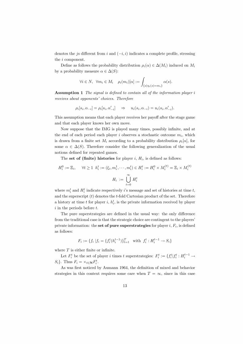
3.5 Example 3

Example 2 is particularly important because it might be applied to many general

strategic setting where there is manipulable imperfect monitoring unless the

information structure allow to avoid non informative behavior.

The previous idea of inducing public revelation of long-lived player action

as a consequence of the short-lived player choice, suggests a possible way out

from this impasse: the introduction of a new observable action for the long-lived

player that can send a signal that it is costly only for the normal type: this might

induce the application of some short-lived player whose behavior would generate

a positive informative externality allowing that kind of mimicking behavior that

generate positive reputation.

This possibility for the normal type can be represented in the following

10

picture:

1

CS NS

2

A N

−1, 0

2

N A

0, 0

1

H L

1, 3

2,−1

1

H L

2, 3

3,−1

Figure 3

Finally, it should be stressed that the realistic assumption of noisy signals

significantly complicates the analysis, as it is intuitive.

4 Building a Reputation: Notions, Results and

Applications

4.1 Notation and Tools

The previous examples have motivated the importance of modeling different

monitoring possibilities to study reputation. Therefore the building block of the

formal language to analyze reputation is the notion of Imperfect Monitoring

Game.

Consider the following generalization of the standard notion of repeated

game with discount and almost perfect information. The players play a fixed

stage game finitely or infinitely many times. The stage game is described

by a finite Imperfect Monitoring Game with Incomplete Information

(IMG)7 defined as follows:

G(η,Ξ) := (N,Si,Ξi, ui, ηi)

where:7See Gilli 1995 for a comprehensive analysis of IMGs.

11

• N = 1, · · ·N is the set of players,

• Si is the finite set of player i’s pure strategies; moreover S := ×i∈NSi,

Λi := ∆(Si) and Λ := ⊗i∈NΛi, where ∆(·) is the set of all probability

measure on a set · and ⊗i∈N∆(·i) is the set of all independent probability

measure on ×i∈N ·i;

• Ξi is the set of possible player i’s types: formally a player’s set of type is a

random variable with probability distribution µ−i ∈ ∆(Ξi)8 , its realization

ξi is a player’s type representing the player’s private information, while

µ−i is the common prior beliefs of players j = i on i’s private information.

In other words a type ξ is a full description of

— Player’s beliefs on states of nature, e.g. players’ payoffs;

— Beliefs on other players’ beliefs on states of mature and its own beliefs

— Etc.

Clearly there is a circular element in the definition of type, which is un-

avoidable in interactive situations

• ui : ∆(S) × Ξi → R is player i’s utility function, which represents pref-

erences satisfying von Neumann and Morgenstern axioms and therefore

such that: ui(α; ξi) = Eα[ui(s; ξi)], α ∈ ∆(S);

• ηi : S → Mi is player i’s signal function: ηi(s) = mi ∈ Mi is the signal

privately received by i as a consequence of the strategy profile s played.

Trivially howmi translates in information on opponents’ behavior depends

on the particular specification of ηi and on the strategy played by i herself

(active learning).

Note that imperfect public monitoring and perfect monitoring are obtained as

a specific case of the signal function:

• an IMG G(η) has imperfect public monitoring if and only if ∀i ∈

N Mi =M

• an IMG G(η) has perfect monitoring if and only if ∀i ∈ N ηi is

bijective.

As usual, omission of the index i means that I am considering a profile

belonging to the Cartesian product of the sets considered, the subscript −i

8Assume that Ξi is measurable for all i ∈ N , so that probability measures are well defined.

12

denotes the js different from i and (−i, i) indicates a complete profile, stressing

the i component.

Define as follows the probability distribution ρi(α) ∈ ∆(Mi) induced on Mi

by a probability measure α ∈ ∆(S):

∀i ∈ N, ∀mi ∈Mi ρi(mi)[α] :=

∫

s|ηi(s)=mi

α(s).

Assumption 1 The signal is defined to contain all of the information player i

receives about opponents’ choices. Therefore

ρi[si, α−i] = ρi[si, α′−i] ⇒ ui(si, α−i) = ui(si, α

′−i).

This assumption means that each player receives her payoff after the stage game

and that each player knows her own move.

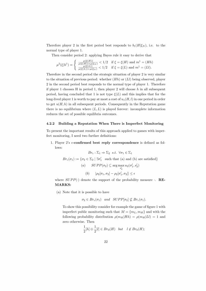
Now suppose that the IMG is played many times, possibly infinite, and at

the end of each period each player i observes a stochastic outcome mi, which

is drawn from a finite set Mi according to a probability distribution ρi[α], for

some α ∈ ∆(S). Therefore consider the following generalization of the usual

notions defined for repeated games.

The set of (finite) histories for player i, Hi, is defined as follows:

H0i := Ξi, ∀t ≥ 1 ht

i := (ξi,m1i , · · · ,m

ti) ∈ Ht

i := H0i ×M

(t)i = Ξi ×M

(t)i

Hi :=∞⋃

t=0

Hti

where mti and Ht

i indicate respectively i’s message and set of histories at time t,

and the superscript (t) denotes the t-fold Cartesian product of the set. Therefore

a history at time t for player i, hti, is the private information received by player

i in the periods before t.

The pure superstrategies are defined in the usual way: the only difference

from the traditional case is that the strategic choice are contingent to the players’

private information: the set of pure superstrategies for player i, Fi, is defined

as follows:

Fi := fi |fi = fti (h

t−1i )Tt=1 with f t

i : Ht−1i → Si

where T is either finite or infinite.

Let F ti be the set of player i times t superstrategies: F

ti := f

ti |f

ti : H

t−1i →

Si. Thus Fi = ×t∈NF ti .

As was first noticed by Aumann 1964, the definition of mixed and behavior

strategies in this context requires some care when T = ∞, since in this case

13

Fi has the cardinality of the continuum (see Kolmogorov-Fomin 1975). Hence

defining mixed superstrategies as probability distributions on pure superstrate-

gies would not be straightforward. Following Aumann 1964, a mixed strategy

should be considered as a random device for choosing a pure strategy, i.e. as a

random variable. Therefore consider an abstract probability space (Ωi,Ai, αi)

and define a mixed superstrategy for player i as a sequence φi ∈ Φi of func-

tions φti Ai- measurable with

φti : Ωi ×Ht−1

i → Si.

In general denote by x ∈ ∆(F ) a probability distribution on F constructed in

this way and by (F,F , x) a probability space where F is the Borel σ-algebra on

F . Similarly denote by (Fi,Fi, xi) and (F−i,F−i, x−i) the probability spaces

obtained through the opportune marginalizations.

The set of behavior superstrategies for a player i, Bi, is similarly defined,

asking however for an additional restriction: bi ∈ Bi if and only if bi =

(bti)∞t=1 with bti : Ω × Ht−1

i → Si where bti(·, ht−1i ) : Ω → Si is measurable

and bti(·, ht−1i ), bτi (·, h

τ−1i ) are mutually independent random variables ∀t =

τ, ∀hti, hτ

i . Therefore Bi ⊂ Φi.

To simplify denote a mixed superstrategy as φi ∈ ∆(Fi) and a behaviour

superstrategy as bi : Hi → ∆(Si).

The outcome at time t for player i, Oti(f), is defined inductively as a func-

tion of the superstrategies chosen:

O0i (f) := ξi

∀t ≥ 1 Oti(f) := ηi[f

t(O0(f), · · · , Ot−1(f))] =

= ηi[ft1(O

01(f), · · · , O

t−11 (f)), · · · , f t

N(O0N(f), · · · , O

t−1N (f))] ∈ Mi.

Then the outcome path of the imperfect monitoring game at time t for player

i, P ti (f), is defined as follows:

∀t ≥ 0 P ti (f) := O

τi (f)

tτ=0 ∈ Ξi ×M

(t)i

and the outcome path of the imperfect monitoring game for player i is

Pi(f) := Oti(f)

Tt=0 ∈ M

(T )i := Ξi ×M0

i ×M1i × · · ·

where T is either finite or infinite.

Therefore an outcome path is the sequence of outcomes induced by the play-

ers’ behavior f ∈ F .

14

As usual, when the dependence from the superstrategy profile f is omitted

this should be interpreted as a “realisation" of the mapping considered, for

example Oti is the outcome for player i realised at time t and Pi ∈ M

(∞)i is a

generic realisation of the outcome path Pi(f).

Previous definition of outcome path implicitly assumes that players have

perfect recall, therefore KuhnŠs theorem9 holds and therefore w.l.g. the analysis

is restricted to behavior superstrategies.

Player i’s intertemporal payoff function Ui : ∆(F ) × Ξi → R is so

defined:

Ui(b; ξi) := Eb

T∑

t=1

δtiui(ft(P t(f)); ξi)

where: b ∈ B, ξi ∈ Ξi, δi ∈ [0, 1) and T is either finite or infinite.

Summing up, the repeated strategic situation is modeled by means of a

Repeated Imperfect Monitoring Game with Incomplete Information

(RIMG) denoted by

GT (δ, η,Ξ) = (N,Fi,Ξi, Ui, ηi).

In the appendix I provide the formal details of the stochastic strategic en-

vironment where the players make their choices emphasizing both the objective

and the subjective aspects. In particular the discussion on players’ beliefs in

the RIMG can be summarized in the following assumption:

Assumption 2 In the RIMG every player i ∈ N updates her beliefs βi accord-

ing to the following expression:

∀fi ∈ Fi, ∀A ∈ F−i, ∀t ∈ N βti [fi](A) = E[χA(f−i)|F

t−i(fi)].

Remark: note that these beliefs on opponents’ behaviour depend on players’

beliefs about opponents’ types.

Before applying these tools to the analysis of reputation, I sum up the no-

tation introduced so far.9See for example Osborne-Rubinstein 1994.

15

NOTATION

Expression Meaning

N set of players

Si set of player i’s pure strategies

∆(·) set of probability measures on ·

Σi = ∆(Si) player i set of mixed strategies

Ξi set of types of player i

µi(·|ξi) ∈ ∆(Ξ−i) player i beliefs on opponents’ private information

ui : ∆(S)→ R player i’ utility function

ηi : S →Mi player i’ signal function

ρi[α] ∈ ∆(Mi) distribution of signals induced by a α ∈ ∆(S)

Hi = ∪∞t=0H

ti set of possible histories for player i

Fi = ×t∈NF ti set of possible superstrategies for player i

Φi, Bi set of i’s mixed, behavioral superstrategies

βi ∈ ∆(F−i) probability evaluations on opponents’ behaviour

Oti(f), P t

i (f) outcome, outcome path at time t for player i

Ui : ∆(F )→ R i’s utility function for the repeated game.

4.2 Results and Applications

To simplify the analysis, in this section I consider two players games only, where

1. player 1 is the long-lived player, and

2. player 2 is the short-lived player, representing either a succession of play-

ers living one period or a continuum of small and anonymous infinitely

living players.

Moreover assume that the type of player 2 is common knowledge, while the type

of player 1 is unknown to player 2, therefore w.l.g. Ξ1 = Ξ, which is assumed

to be finite or countable to simplify technical details. Player 1 set of types is

partitioned into

1. payoff types ΞP and

2. commitment type ΞC = Ξ \ ΞP .

Payoff types have payoffs characteristics such that the player maximizes

U1:

∀b1 ∈ B1, ξ(b1) ∈ ΞP if and only if

∃b2 ∈ B2 s.t. b1 ∈ arg maxb1∈B1

U1(b1, b2; ξ(b1)).

16

A specific payoff type is the normal type: ξN ∈ ΞP if and only if

u1(s, ξN , t) = u1(s) ∀s ∈ S, ∀t ∈ N,

i.e. the normal type has the standard payoff of the complete information stage

game and thus U1(b, ξN) = U1(b) ∀b ∈ B.

Commitment types have payoffs such that a specified superstrategy is

strictly dominant and thus is certainly played by any rational player:

∀b1 ∈ B1, ξ(b1) ∈ ΞC if and only if

∀b2 ∈ B2 b1 ∈ arg maxb1∈B1

U1(b1, b2; ξ(b1)).

AReputation Game (RG) is a Repeated Imperfect Monitoring Game with

Incomplete Information GT (δ, η,Ξ) = (N,Fi,Ξi, Ui, ηi) satisfying the following

restrictions:

1. N = 1, 2

2. Ξ1 = ΞP ∪ ΞC and Ξ2 = ∅

3. U1(b; ξ) = Eb

∑Tt=1 δ

tu1(ft(P t(f)); ξ) with ξ ∈ ΞP ∪ ΞC

4. U2(b; ξ) = Ebu2(ft(P t(f))).

The equilibrium concept used to present the results on reputation in strategic

situations is the standard Nash equilibrium.

A strategy profile (b∗1, b∗2) is a Nash equilibrium of a Reputation Game

GT (δ, η,Ξ) = (N,Fi,Ξi, Ui, ηi) if and only if

1. ∀ξ ∈ ΞP , b∗1 ∈ argmaxb1∈B1U1(b1, b∗2; ξ)

2. ∀t, ∀ht ∈ H s.t. Pb∗1,b∗2,µ(h

t) > 0

b∗2(ht2) ∈ arg max

b2(ht2)∈∆(S2)Eβ2 [u2(b

∗1(h

t1), b2(h

t2))].

Let denote the set of Nash equilibria of a Reputation Game GT (δ, η,Ξ) by

NE(GT (δ, η,Ξ)).

4.2.1 Building a Reputation When There is Perfect Monitoring

To present the main results of this approach applied to the class of games with

perfect monitoring, four further definitions are required:

17

1. Player 1’s pure strategy Stackelberg payoff is defined as follows:

v∗1 := sups1∈S1

minσ2∈Bru(s1)

u1(s1, σ2)

where Bru(s1) := argmaxσ′2∈Σ2 u2(s1, σ

′2) i.e. it the set of player 2 myopic

best reply to s1;

Remark: this is the best payoff that player 1 could get through a pre-

commitment assuming that the opponent would reply rationally.

2. Player 1’s Stackelberg pure strategy if it exists is defined as follows:

s∗1 := arg maxs1∈S1

minσ2∈Bru(s1)

u1(s1, σ2).

Remark: this is a pure strategy to which player 1 would commit, if it

had the chance to do so, given that such a commitment induces a best

reply by 2.

3. Player 1’s commitment Stackelberg type is defined as follows: ξ∗ :=

ξ(s∗1).

Remark: this is the type that if rational would always play the Stackel-

berg pure strategy.

4. Normal type of player 1’s lower bound payoff is defined as follows:

v1(ξN , µ, δ) := (1− δ) inf(b1,b2)∈NE(GT (δ,η,Ξ)) U1(b1, b2).

REMARK: it is possible to consider Stackelberg mixed strategy, which would

reinforce reputational effects, but the analysis would be significantly more com-

plex.

The main result for the case of perfect monitoring is the following.

Theorem 1 Suppose µ ∈ ∆(Ξ) assign positive probability to some sequence of

simple types ξ(sk1) such that limk→∞ v∗1(sk1) = v∗1, then

∀ǫ > 0, ∃δ′ ∈ (0, 1) s.t. ∀δ ∈ (δ′, 1) v1(ξN , µ, δ) ≥ v∗1 − ǫ.

REMARKS:

1. I will not provide a detailed proof10 , but I will show the implications of this

theorem and I will illustrate the behaviour of players beliefs in connection

with previous examples.

10A complete proof is in Mailath-Samuelson 2006.

18

2. If there a Stackelberg strategy and the associate Stackelberg type has

positive probability under µ, then the hypotheses of theorem 1 are trivially

satisfied. In this case, the normal type of player 1 builds a reputation for

playing like the Stackelberg type. Note that it builds this reputation

despite the fact that there are many other possible commitments types.

3. Theorem 1 does not tell much about equilibrium strategies, in particular

it does not imply that it is optimal for the normal type of player 1 to

choose the Stackeberg strategy in each period, which in general is not the

case.

4. The discount factor plays two roles in this results:

(a) it makes future payoffs relatively more important, as it is standard

in folk theorem arguments in repeated game theory

(b) it discounts into insignificance the initial sequence of periods during

which it may be costly for player 1 to mimic the commitment type,

which is a new aspect relevant for reputation models only.

5. The proof of theorem 1 relies on the behaviour of the posterior probability

on player 1’s type and on the probability of next period choice given today

history. The key of the proof is to show that the observation of a strategy of

player 1 increases the probability of the type committed to this choice and

consequently the probability of observing this strategy next period. This

does not mean that the posterior probability of facing this commitment

type is going to 1, since it is possible that player 1 is normal but plays like

the commitment type, as seen in the previous example.

The logic behind this result can be appreciated referring to the example of

figure 1, that is reported here to simplify reading:

h l

H 2, 3 0, 2

L 3, 0 1, 1

19

Figure 1

Clearly in this game the pure strategy Stackelberg payoff is v∗1 = 2 since

Bru(s1) =

h s1 = H

l s1 = L.

and thusminσ2∈Bru(s1) u1(s1, σ2) = 2, 1 that implies sups1∈S12, 1 = 2. Con-

sequently player 1’s Stackelberg pure strategy is s∗1 = H.

To construct a Reputation game starting from game 1, suppose that there

is perfect monitoring, i.e. η is bijective and therefore the players observe the

strategy profile played, and that there is incomplete information on the type of

player 1. In particular suppose that the set of types is Ξ1 = ξN , ξ(H), ξ(L).

Then the following strategy profile (bNE1 , bNE

2 ) is a Nash Equilibrium of the

Reputation Game:

bNE1 (ξ, ht) =

H if ξ = ξ(H) and ht ∈ H1

H if ξ = ξN and mτ = (Hh) ∀τ < t or if t = 1

L otherwise.

bNE2 (ht) =

h if mτ = (Hh) ∀τ < t or if t = 1

l otherwise.

For δ ≥ 1/2 and µ(ξ(L)) < 1/2 it is easy to show that this is a Nash equilibrium

of the Reputation Game.

First, consider player 2: at t = 1, it will choose h if and only if Eu2(s1, h) =

3(1− µ(ξ(L))) ≥ Eu2(s1, l) = 2(1− µ(ξ(L)) + 1µ(ξ(L)) which is satisfied when

µ(ξ(L)) < 1/2. Now consider its beliefs in subsequent periods; these are easily

derived by Bayes rules and satisfy the following conditions:

µt(ξ|ht) =

1 if ξ = ξ(L) and ht = h1 = (L·)

1 if ξ = ξN and mt = (L·) with t > 1µ(ξ(H))

µ(ξ(H))+µ(ξN)if ξ = ξ(H) and mt = (H·) with t ≥ 1.

Note that to show that (bNE1 , bNE

2 ) is a Nash Equilibrium it is necessary to

consider beliefs only on the equilibrium path, therefore the previous calculation

of mu(ξ|ht) is enough. To work on refinements such as Sequential equilibria it

would be necessary to specify also out-of-equilibrium beliefs where Bayes rules

does not apply.

Given these beliefs and player 1’s equilibrium strategy bNE1 , through Bayes

rule it is possible to derive player 2 beliefs on player 1’s choice of H next period:

βt2(f1(ξ, h

t) = H|ht) = µt(ξ(H)|ht)×bNE1 (H|ξ(H), ht)+µt(ξN |h

t)×bNE1 (H|ξN , ht)

20

that implies

βt2(f1(ξ, h

t) = H|ht) =

µ(ξ(H))

µ(ξ(H))+µ(ξN )× 1 + µ(ξN)

µ(ξ(H))+µ(ξN)× 1 = 1 if ht = (Hh)(t)

0 otherwise.

Therefore the Nash equilibrium condition for player 2 is satisfied since ∀t, ∀ht ∈

H2 such that PbNE

1,bNE

2,µ(h

t) > 0, if ht = (Hh)(t) then Eβ2 [u2(bNE1 (ht), h)] =

3 > Eβ2 [u2(bNE1 (ht), l)] = 2 while if ht = (Hh)(t) then Eβ2 [u2(b

NE1 (ht), l)] =

1 > Eβ2 [u2(bNE1 (ht), h)] = 0.

Finally, consider the normal type of player 1, since the behaviour of com-

mitted types ξ(H) and ξ(L) is trivial. Player 1 has complete information and it

is long-lived, therefore it easy to see that in equilibrium it gets U1(bNE1 , bNE

2 ) =

(1− δ)∑∞

τ=0 δτ × 2 = 2, while deviating at most it gets U1(b1, bNE

2 ) = (1− δ)×

3 + δ(1− delta)∑∞

τ=0 δτ × 1 = 3(1− δ) + δ. Then U1(b

NE1 , bNE

2 ) ≥ U1(b1, bNE2 )

if δ ≥ 12 . This shows that the restriction on the discount factor is needed to

ensures that the normal type of player 1 has sufficient incentives to make H

optimal mimicking ξ(H).

The two most important aspects of this example regard player 1’s beliefs on

opponent’s type and on opponent’s behaviour. The posterior probability that 2

assigns to the Stackelberg type does not converge to 1, it is actually bounded

away from 1 since it converges to µ(ξ(H))µ(ξ(H))+µ(ξN)

if h1 = (Hh) after which is

constant unless (L·) is observed. But this does not forbid the fact that the

posterior probability that 1 assigns to observing H next period is going to 1 as

long as ht = (Hh)(t): as I showed before βt2(f1(ξ, h

t) = H|ht = (Hh)(t)) = 1

and this is what drives the result.

A particularly interesting property of the Reputation Game associated to

figure 1 is that playing Ll forever is NOT a Nash equilibrium, even if it is

a(subgame perfect) equilibrium of the repeated game with complete information.

This is exactly the content of theorem 1, and I will show how it works in this

example. Formally suppose that the set of types is Ξ1 = ξN , ξ(H), ξ(L) such

that that µ(ξ(H)) < 1/3 and µ(ξ(L)) < 1/3.

Now consider the first period: clearly player 2 best reply is either l or h

depending on the values of beliefs on opponent’s behaviour:

BRu(β12(f1(ξ) = H|h0) =

h if β12(f1(ξ) = H|h0) ≥ 1/2

l if β12(f1(ξ) = H|h0) ≤ 1/2.

Player 2 beliefs can easily be derived:

β12(f1(ξ) = H|h0) = µ(ξ(H))× 1 + µ(ξN)× b1(H|ξN).

21

Therefore player 2 in the first period best responds to b1(H|ξN), i.e. to the

normal type of player 1.

Then consider period 2: applying Bayes rule it easy to derive that

µ2(ξ|h1) =

µ(ξ(H))

µ(ξ(H))+µ(ξN)< 1/2 if ξ = ξ(H) and m1 = (Hh)

µ(ξ(L))µ(ξ(L))+µ(ξN )

< 1/2 if ξ = ξ(L) and m1 = (Ll).

Therefore in the second period the strategic situation of player 2 is very similar

to the situation of previous period: whether (Hh) or (Ll) being observed, player

2 in the second period best responds to the normal type of player 1. Therefore

if player 1 chooses H in period 1, then player 2 will choose h in all subsequent

period, having concluded that 1 is not type ξ(L) and this implies that for the

long-lived player 1 is worth to pay at most a cost of u1(H, l) in one period in order

to get u(H,h) in all subsequent periods. Consequently in the Reputation game

there is no equilibrium where (L,L) is played forever: incomplete information

reduces the set of possible equilibria outcomes.

4.2.2 Building a Reputation When There is Imperfect Monitoring

To present the important results of this approach applied to games with imper-

fect monitoring, I need two further definitions:

1. Player 2’s ǫ-confirmed best reply correspondence is defined as fol-

lows:

Brǫ : Σ1 ⇒ Σ2 s.t. ∀σ1 ∈ Σ1

Brǫ(σ1) := σ2 ∈ Σ2 | ∃σ′1 such that (a) and (b) are satisfied

(a) SUPP (σ2) ⊆ argmaxs′2

u2(σ′1, s

′2)

(b) |ρ2[σ1, σ2]− ρ2[σ′1, σ2]| ≤ ǫ

where SUPP (·) denote the support of the probability measure ·. RE-

MARKS:

(a) Note that it is possible to have

σ2 ∈ Brǫ(σ1) and SUPP [σ2] ⊆ Brǫ(σ1).

To show this possibility consider for example the game of figure 1 with

imperfect public monitoring such that M = mL,mH and with the

following probability distribution ρ(mH |Hh) = ρ(mH |Ll) = 1 and

zero otherwise. Then

1

2[h]⊕

1

2[l] ∈ Br0(H) but l ∈ Br0(H);

22

(b) If there exist two different strategies σ1 and σ′1 such that ρ[σ1, σ2] =

ρ[σ′1, σ2], then it is possible that Bru(σ1) ⊂ Br0(σ1). To show this

possibility, consider the game of figure 2: from the extensive form

ρ[L,N ] = ρ[H,N ]; moreover Bru(H) = A ⊂ Br0(H) = N,A

since N ∈ argmaxu2(L, ·) and L imply the same signal distribution

of H.

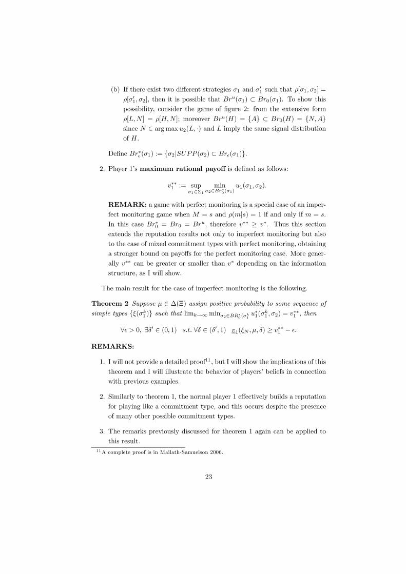
Define Br∗ǫ (σ1) := σ2|SUPP (σ2) ⊂ Brǫ(σ1).

2. Player 1’s maximum rational payoff is defined as follows:

v∗∗1 := supσ1∈Σ1

minσ2∈Br∗

0(σ1)

u1(σ1, σ2).

REMARK: a game with perfect monitoring is a special case of an imper-

fect monitoring game when M = s and ρ(m|s) = 1 if and only if m = s.

In this case Br∗0 = Br0 = Bru, therefore v∗∗ ≥ v∗. Thus this section

extends the reputation results not only to imperfect monitoring but also

to the case of mixed commitment types with perfect monitoring, obtaining

a stronger bound on payoffs for the perfect monitoring case. More gener-

ally v∗∗ can be greater or smaller than v∗ depending on the information

structure, as I will show.

The main result for the case of imperfect monitoring is the following.

Theorem 2 Suppose µ ∈ ∆(Ξ) assign positive probability to some sequence of

simple types ξ(σk1 ) such that limk→∞minσ2∈BR∗

0(σk

1

u∗1(σk1 , σ2) = v∗∗1 , then

∀ǫ > 0, ∃δ′ ∈ (0, 1) s.t. ∀δ ∈ (δ′, 1) v1(ξN , µ, δ) ≥ v∗∗1 − ǫ.

REMARKS:

1. I will not provide a detailed proof11 , but I will show the implications of this

theorem and I will illustrate the behavior of players’ beliefs in connection

with previous examples.

2. Similarly to theorem 1, the normal player 1 effectively builds a reputation

for playing like a commitment type, and this occurs despite the presence

of many other possible commitment types.

3. The remarks previously discussed for theorem 1 again can be applied to

this result.11A complete proof is in Mailath-Samuelson 2006.

23

As for theorem 1, even the proof of theorem 2 relies on the behavior of the

posterior probability on player 1’s type and on the probability of next period

choice given today history. But here there is a new crucial problem in proving the

theorem since there is imperfect monitoring with a manipulable signal functions.

The root of the problem can easily be shown to refer to the game of figure 2,

which is reported here to simplify reading:

2

N

A

0, 0

1

H

L

2, 3

3,−1

Figure 2

Clearly in this game the pure strategy Stackelberg payoff is v∗1 = 2 since

BRu(s1) =

σ2(A) = 1 s1 = H

σ2(A) = 0 s1 = L.

and thusminσ2∈Bru(s1) u1(s1, σ2) = 2, 0 that implies sups1∈S12, 0 = 2. Con-

sequently player 1’s Stackelberg pure strategy is s∗1 = H.

To construct a Reputation game starting from game 2, suppose that there

is incomplete information on the type of player 1. In particular suppose that

the set of types is Ξ1 = ξN , ξ(H).

Note that Br0(N) = Σ1 since |ρ[σ1,N ] − ρ[σ′1, N ]| = 0 for all σ1, σ′1 ∈ Σ1.

Clearly in this game the maximum rational payoff v∗∗1 = 0 since

∀σ1 ∈ Σ1 BR∗0(σ1) = Σ2

and thus minσ2∈Br∗0(σ1)=Σ2 u1(σ1, σ2) = 0 that implies supσ1∈Σ10 = 0. This

means that in this case theorem 2 is actually not relevant since v∗∗1 is equal to

the equilibrium payoff of the complete information game. Moreover differently

from the case of game 1, it is easy to construct a Nash equilibrium of the

24

reputation game corresponding to the equilibrium of the complete information

game. Consider the following strategy profile (bNE1 , bNE

2 ):

bNE1 (ξ, ht) =

H if ξ = ξ(H) and ht ∈ H

L otherwise.

bNE2 (ht) = N ∀ht ∈ H.

For any δ and µ(ξ(H)) < 1/4 it is easy to show that this is a Nash equilibrium

of the Reputation Game.

First, consider player 2: at t = 1, it will choose N if and only if Eu2(s1, N) =

0 ≥ Eu2(s1, A) = −1(1−µ(ξ(H))+3µ(ξ(H)) which is satisfied when µ(ξ(L)) <

1/4. Now consider its beliefs in subsequent periods; these are easily derived

by Bayes rules and equal to the prior since no new observation on possible

player 1’s types has been collected. Note that to show that (fNE1 , fNE

2 ) is a

Nash Equilibrium it is necessary to consider beliefs only on the equilibrium

path, therefore the previous calculation of mu(ξ|ht) is enough. To work on

refinements such as Sequential equilibria it would be necessary to specify also

out-of-equilibrium beliefs where Bayes rules does not apply.

Given these beliefs and player 1’s equilibrium strategy bNE1 , through Bayes

rule it is possible to derive player 2 beliefs on player 1’s choice of H next period:

βt2(f1(ξ, h

t) = H|ht) = µt(ξ(H)|ht)× bNE1 (H|ξ(H), ht)+

+µt(ξN |ht)× bNE

1 (H|ξN , ht) = µ(ξ(H)).

Therefore the Nash equilibrium condition for player 2 is satisfied since ∀t, ∀ht ∈

H such thatPbNE

1,bNE

2,µ(h

t) > 0Eβ2 [u2(bNE1 (ht), N)] = 0 > Eβ2 [u2(b

NE1 (ht), A)] =

3µ(H) − 1(1 − µ(H)) < 0 if µ(H) < 1/4. Finally, consider the normal type of

player 1, since the behaviour of committed type ξ(H) is trivial. Player 1 has

complete information and it is long-lived, therefore it easy to see that in equi-

librium it gets U1(bNE1 , bNE

2 ) = (1 − δ)∑∞

τ=0 δτ × 0 = 0, while deviating at

most it gets U1(b1, bNE2 ) = (1 − δ) × 0 + δ(1 − delta)

∑∞τ=0 δ

τ × 0 = 0. Then

U1(bNE1 , bNE

2 ) ≥ U1(b1, bNE2 ) ∀δ.

The most important aspects of this example is the fact that the transforma-

tion of the complete information game into a reputation game does not change

the properties of the set of Nash Equilibria. Therefore it is particularly im-

portant to understand the root of this change in the properties of the strategic

situation. Clearly the reason of this new results regard player 1’s beliefs on

opponent’s type and on opponent’s behaviour. The posterior probability that 2

assigns to the Stackelberg type does not change through time because there is

25

no collection of new information. But this forbid the possibility for the normal

type of player 1 of mimicking the commitment types, i.e. to build its reputation.

Therefore the posterior probability that 1 assigns to observing H next period is

bounded away from 1 as long as ht = (N)(t) and this is what drives the result.

This suggest that the crucial aspect is the information structure and its re-

lation with players behavior. To show that this is actually the case, consider

the strategic form game associated to game assuming that there is perfect mon-

itoring, i.e. η(s) = s:

N A

H 0, 0 2, 3

L 0, 0 3, -1

Figure 4

In this game the pure strategy Stackelberg payoff is v∗1 = 2 since

Bru(s1) =

A s1 = H

N s1 = L.

and thusminσ2∈Bru(s1) u1(s1, σ2) = 2, 0 that implies sups1∈S12, 0 = 2. Con-

sequently player 1’s Stackelberg pure strategy is s∗1 = H.

To construct a Reputation game starting from the game of figure 4, sup-

pose that there is perfect monitoring, i.e. η is bijective and therefore the play-

ers observe the strategy profile played, and that there is incomplete informa-

tion on the type of player 1. In particular suppose that the set of types is

Ξ1 = ξN , ξ(H), ξ(L).

A particularly interesting property of the Reputation Game associated to

figure 1 is that playing LN forever is NOT a Nash equilibrium, even if it is

a(subgame perfect) equilibrium of the repeated game with complete information.

This is again the content of theorem 1, and it is interesting to show that it works

or not depending on the information structure of the game. Formally suppose

that the set of types is Ξ1 = ξN , ξ(H), ξ(L) such that that µ(ξ(H)) < 1/3

and µ(ξ(L)) < 1/3.

26

Now consider the first period: clearly player 2 best reply is either N or A

depending on the values of beliefs on opponent’s behaviour:

Bru(β12(f1(ξ) = H|h0) =

N if β12(f1(ξ) = H|h0) ≤ 1/4

A if β12(f1(ξ) = H|h0) ≥ 1/4.

Player 2 beliefs can easily be derived:

β12(f1(ξ) = H|h0) = µ(ξ(H))× 1 + µ(ξN)× b1(H|ξN).

Therefore player 2 in the first period best responds to b1(H|ξN), i.e. to the

normal type of player 1.

Then consider period 2: applying Bayes rule it easy to derive that

µ2(ξ|h1) =

µ(ξ(H))

µ(ξ(H))+µ(ξN )< 1/2 if ξ = ξ(H) and m1 = (HA)

µ(ξ(L))µ(ξ(L))+µ(ξN)

< 1/2 if ξ = ξ(L) and m1 = (LN).

Therefore in the second period the strategic situation of player 2 is very similar

to the situation of previous period: whether (HA) or (LN) being observed,

player 2 in the second period best responds to the normal type of player 1.

Therefore if player 1 chooses H in period 1, then player 2 will choose A in all

subsequent period, having concluded that 1 is not type ξ(L) and this implies

that for the long-lived player 1 is worth to pay at most a cost of u1(H,N) in

one period in order to get u1(H,A) in all subsequent periods. Consequently

in the Reputation game there is no equilibrium where (L,N) is played forever:

incomplete information reduces the set of possible equilibria outcomes.

Note that this argumentation is the exact replica of the one used for game 1:

this means that it is not the payoff structure that matters but the information

structure. In particular the problem with imperfect monitoring is the fact that

there may exists strategies by player 2 such that the signal, whether public or

private, reveal no information about player 1’s choice. Therefore if such strategy

sNI2 is a best reply to anything, it belongs to Br0(σ1) for all possible σ1. To get

Bru(σ1) = Br0(σ1) it is necessary to rule out such non informative strategies,

for example introducing some noise. A possible assumption is the following:

Assumption 3 For all σ2 ∈ Σ2, the collection of probability distributions

ρ[s1, σ2]|s1 ∈ S1

is linearly independent.

Then an immediate result is the following:

27

Theorem 3 If assumption 3 holds, then

Bru(σ1) = Br∗0(σ1) = BR0(σ1)

and v∗∗1 equals the mixed-strategy Stackelberg payoff.

The proof is omitted since it is immediate.

5 Conclusion

The examples, results and calculations of this paper show the importance of the

game theoretic approach to reputation building.

Considering the question posed at the beginning of the paper, now it is

possible to consider the specific rigorous answers provided by game theory:

1. The context should be such that the choices of the agent that wish to

build a reputation are publicly observable, may be noisily: as seen this

might be a non trivial request;

2. Using reputation all agents can improve their payoffs, in particular the

agent building its reputation has at stake the possibility of reaching the

best payoff that it could get through a precommitment when facing a

rational opponent;

3. the information players can infer from the observations of past outcomes

to predict future behaviour crucially depend on two factors:

(a) the structure of strategic interaction (see example 2 and example 3)

(b) the possibility of facing "commitment" types, the possibility of ex-

istence of incomplete information on hidden characteristics of the

long-lived player.

4. to tie actors to observed and future outcomes it is necessary to have an

identity that last through time, i.e. a long lived agent;

5. reputation can be measured in term of likely future behaviour and players

beliefs are exactly this measure;

6. Bayes rule and probability rules are the well defined algorithms that con-

nect reputation measures and forecasts on future likely outcomes.

But the value added by game theory to the rigorous analysis of reputation

is shown by some other new interesting and important perspectives that are

opened by this point of view:

28

1. Reputation is possible only if in the population of possible types there

exists at least one type committed to "desirable" behaviour: it is its simple

existence that generates that informational positive externality that allow

the possibility of building reputation;

2. paradoxically enough, reputation is not based on revealing and learning

the players true characteristics, but exactly on the opposite: on the exis-

tence and persistence of pooling equilibria where the "normal" type can

publicly mimic the "good" one. Therefore there should be enough public

information to provide incentives for this mimicking and the consequent

reputation building behaviour but also enough lack of information to avoid

the possibility of perfectly learning the players’ types;

3. A player’s reputation can be modelled and measured as beliefs on its future

behaviour not on its type: these beliefs in equilibrium are shared by all

players and are correct, even if the players usually will never learn precisely

opponents types. Actually, if the players type would be perfectly learned,

then their reputation would disappear since it would be useless to behave

as a commitment type;

4. Reputation works actually as a selection device: among all possible equi-

libria of a repeated game, it selects that equilibria that give rise to the

Stackelberg payoff;

5. Reputation helps the player to reach a better payoff reducing its choice

opportunities, it works as a precommitment device: in example 1 player 1

is able to convince player 2 that it will play H since otherwise it would loose

its reputation in future plays of the game and this "promise" is credible

because of the possible loss of reputation;

6. To work as a precommitment device, the loss of reputation should depend

on observable actions: transparency and the role of media is absolutely

crucial to allow a virtuous work of this machinery, collusion and noise

should not be enough to generate confusion on player 1 behaviour;

7. To work Reputation requires that the agent is afraid of loosing it in fu-

ture interactions, therefore it regards long-lived agent: this is one further

justification for the existence of institutions such as firms or universities

besides economies of scale and scope, as a way of building and transmitting

reputation from one period to the next12

12See Kreps 1990.

29

References

[1] Aumann, R.: Mixed and Behavior Strategies in Infinite Extensive Games.

In Dresher, M., Shapley, L., Tucker, A. (eds.) Advances in Game Theory,

pp. 627-650. Princeton: Princeton University Press 1964.

[2] Billingsley, P.: Convergence of Probability Measure. New York: Wiley 1968.

[3] Billingsley, P.: Probability and Measure. New York: Wiley 1986.

[4] Dasgupta, P. 1988: Trust as a Commodity, in Gambetta, D. (ed.) Trust:

Making and Breaking Cooperative Relations. Oxford: Oxford University

Press, chapter 4, pp. 49-72.

[5] Ely J., Fudenberg D. and D. Levine 2004: When is Reputation Bad?,

mimeo.

[6] Ely, J. and J. Valimaki 2003: “Bad Reputation”, Quarterly Journal of

Economics, 3: 785-814.

[7] Fudenberg, D. and D. Levine 1989: “Reputation and Equilibrium Selection

in Games with a Patient Player”, Econometrica, 50: 443-460.

[8] Fudenberg, D. and D. Levine 1989: “Mantaining a Reputation when Strate-

gies are Imperfectly Observed”, Review of Economic Studies, 59: 561-580.

[9] Fudenberg, D. 1992: Explaining Cooperation and Commitment in Re-

peated Games, in Laffont, J. (ed.) Advances in Economic Theory. Sixth

World Congress. Cambridge, Cambridge University Press, chapter 3, pp.

89-130.

[10] Gilli, M. 1995: Modelling Strategic Interaction: a Case for Imperfect Mon-

itoring Games. Working Paper 17/95, DAE Cambridge.

[11] Gilli, M., 1999, “On Non-Nash Equilibria”, Games and Economic Behavior,

27: 184-203.

[12] Gilli, M. 2002: Rational Learning in Imperfect Monitoring Games. Working

Paper 46/2002 Department of Economics, University of Milano-Bicocca.

[13] Good, D. 1988: Individuals, Interpersonal Relations, and Trust, in Gam-

betta, D. (ed.) Trust: Making and Breaking Cooperative Relations. Oxford,

Oxford University Press, chapter 3, pp. 31-48.

30

[14] Hornby, A. S.: Oxford Advanced Learner’s Dictionary of Current English.

Oxford: Oxford University Press, 1987.

[15] Kolmogorov, A.N., and S.V. Fomin: Introductory real analysis. New York:

Dover Publications 1975.

[16] Kramer, R. 1999: “Trust and Distrust in Organizations: Emerging perspec-

tives, Enduring Questions”, Annual Review of Psychology 50: 569- 598.

[17] Kreps, D. 1990: Corporate Culture and Economic Theory, in Alt J. and K.

A. Shepsle (eds.) Perspectives on Positive Political Economy. Cambridge,

MA: Cambridge University Press, pp. 90 U 143.

[18] Kreps, D. and R. Wilson, 1982, “Reputation and Imperfect Information”,

Journal of Economic Theory, 27: 253-279.

[19] Kreps, D., P. Milgrom, J. Roberts and R. Wilson, 1982: “Rational Cooper-

ation in the Finitely Repeated Prisoners’ Dilemma”, Journal of Economic

Theory, 27: 245-252.

[20] Kuratowski, K.: Topology. New York: Academic Press 1968.

[21] Lehrer, E., 1991, “Internal Correlation in Repeated Games”, International

Journal of Game Theory 19: 431-456.

[22] Mailath G.J. and L. Samuelson: Repeated Games and Reputations. Oxford:

Oxford University Press 2006.

[23] Milgrom, P. and J. Roberts 1982: “Predation, Reputation, and Entry De-

terrence”, Journmal of Economic Theory 27: 280-312.

[24] Osborne, M.J. and A. Rubinstein: A Course in Game Theory. Cambridge

Mass.: The MIT Press 1994.

[25] Parthasarathy, K. R.: Probability Measures on Metric Spaces. New York:

Academic Press 1967.

[26] Ritzer, G. (ed): Blackwell Encyclopedia of Sociology, Oxford: Blackwell,

2007.

[27] Shenkar, O., and E. Yuchtman-Yaar. 1997: “Reputation, image, prestige,

and goodwill: An interdisciplinary approach to organizational standing”,

Human Relations 50: 1361U1381.

31

[28] Strathdee, R. 2009: “Reputation in the sociology of education”, British

Journal of Sociology of Education 30: 83 - 96 .

[29] Zucker, L. 1986: “Production of trust: Institutional sources of economic

structure, 1840-1920”, Research in Organisational Behaviour 8: 53 - 111.

32

6 The Construction of the Stochastic Process of

Beliefs and Outcomes in the Repeated Imper-

fect Monitoring Game with Incomplete Infor-

mation

Consider a Repeated Imperfect Monitoring Game with Incomplete Information

(RIMG) denoted by

GT (δ, η,Ξ) = (N,Fi,Ξi, Ui, ηi).

Starting from this strategic setting, I would construct the stochastic envi-

ronment that describes the objective and the subjective situation.

Let (F,F , x) be a probability space , where F is the set of pure superstrate-

gies, F the Borel σ-algebra of F and x ∈ ∆(F ) a generic probability measure

on F . Note that in general x will depend on µ ∈ Delta(Ξ), the probability of

players’ type, since the superstrategies actually played will depend on players’

types. Tychonov product theorem (see e.g. Kuratowski 1968) imply that F is

a compact metric space in the product topology and thus ∆(F ) is a compact

metric space if endowed with the weak topology and with the metric being the

Prohorov metric (see Billingsley 1968). Then consider the probability space

(M(∞)i ,Hi,P

ix). The construction of this probability space involves some steps.

Let Pi ∈M(∞)i be a possible outcome path for player i and define for each t ∈N

a mapping Zt : M(∞)i → Mi such that Zt(Pi) := Ot

i , that is Zt is the

projection of Pi on its t element. Consider the class HCi consisting of the cylin-

ders, that is of the sets of the form Pi ∈M(∞)i |(Zt1(Pi), · · · , Ztk(Pi)) ∈ C,

where k is an integer, (t1, · · · , tk) is a k-tuple in N and C belongs to the Borel

σ-algebra generated by M(k)i . Then it is possible to prove (see e.g. Billingsley

1986) that HCi is a field such that Hi is the σ-field generated by it. There-

fore, since the Zt are measurable functions on (M(∞)i ,Hi), if P is a probability

measure on Hi, then Ztt∈N is a stochastic process on (M(∞)i ,Hi,P).

Now consider the probability distribution inductively defined according to

the following rules: Pi,(0)x (h0i ) = P

i,(0)x (ξi) = 1 and

∀t ≥ 1 Pi,(t)x (ht−1

i ,mi) = Pi,(t−1)x (ht−1

i )× [

∫

f |P t

i(fi,f−i)=ht−1

i,mi

x(df)].

It is immediate to check that Pi,(t1)x , · · · ,P

i,(tk)x are a system of probability dis-

tributions satisfying the Kolmogorov’s consistency conditions. Therefore there

exists a probability measure Pix on Hi such that the stochastic process Ztt∈N

33

on (M(∞)i ,Hi,Pi

x) has the Pi,(t1)x , · · · ,P

i,(tk)x as its finite-dimensional distribu-

tions.

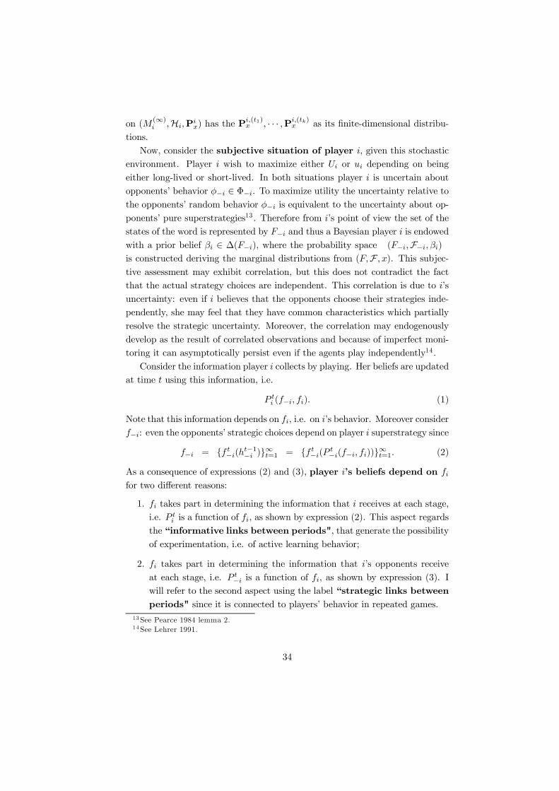
Now, consider the subjective situation of player i, given this stochastic

environment. Player i wish to maximize either Ui or ui depending on being

either long-lived or short-lived. In both situations player i is uncertain about

opponents’ behavior φ−i ∈ Φ−i. To maximize utility the uncertainty relative to

the opponents’ random behavior φ−i is equivalent to the uncertainty about op-

ponents’ pure superstrategies13 . Therefore from i’s point of view the set of the

states of the word is represented by F−i and thus a Bayesian player i is endowed

with a prior belief βi ∈ ∆(F−i), where the probability space (F−i,F−i, βi)

is constructed deriving the marginal distributions from (F,F , x). This subjec-

tive assessment may exhibit correlation, but this does not contradict the fact

that the actual strategy choices are independent. This correlation is due to i’s

uncertainty: even if i believes that the opponents choose their strategies inde-

pendently, she may feel that they have common characteristics which partially

resolve the strategic uncertainty. Moreover, the correlation may endogenously

develop as the result of correlated observations and because of imperfect moni-

toring it can asymptotically persist even if the agents play independently14 .

Consider the information player i collects by playing. Her beliefs are updated

at time t using this information, i.e.

P ti (f−i, fi). (1)

Note that this information depends on fi, i.e. on i’s behavior. Moreover consider

f−i: even the opponents’ strategic choices depend on player i superstrategy since

f−i = f t−i(h

t−1−i )

∞t=1 = f t

−i(Pt−i(f−i, fi))

∞t=1. (2)

As a consequence of expressions (2) and (3), player i’s beliefs depend on fi

for two different reasons:

1. fi takes part in determining the information that i receives at each stage,

i.e. P ti is a function of fi, as shown by expression (2). This aspect regards

the “informative links between periods", that generate the possibility

of experimentation, i.e. of active learning behavior;

2. fi takes part in determining the information that i’s opponents receive

at each stage, i.e. P t−i is a function of fi, as shown by expression (3). I

will refer to the second aspect using the label “strategic links between

periods" since it is connected to players’ behavior in repeated games.13See Pearce 1984 lemma 2.14See Lehrer 1991.

34

During the play, i is refining her information about opponents’ behavior

(passive learning), but the actual amount of information obtained depends on

the superstrategy followed (active learning). For a fixed fi construct the natural

filtration of the stochastic process given by the outcome path:

F t−i(fi) := σ(P t

i (f−i, fi)),

where σ(X(ω)) denotes the σ-algebra generated by the random variable X(ω).

Intuitively Ft−i(fi) represents all the possible information about opponents’ su-

perstrategy that i could collect at t following the dynamic superstrategy fi.

In fact σ(X(ω)) consists precisely of those events A for which, for each and

every ω, player i can decide whether or not A has occurred, i.e. whether or

not ω ∈ A, on the basis of the observed value of the random variable X. For-

mally a filtration Ft−i is an increasing sequence of sub-σ-algebras of F−i,

i.e. F1−i(fi) ⊆ F2−i(fi) ⊆ · · · ⊆ F−i, and the natural filtration of a sto-

chastic process Oti(fi)t is the filtration generated by it in the sense that

Ft−i(fi) := σ(O0

i , · · · , Oti). Finally, define F∞−i(fi) := σ(

⋃t∈NF

t−i(fi)) ⊆ F−i.

Then, for a fixed fi, Pi(f−i, fi) := Oti(f−i, fi)t∈N is a stochastic process

adapted to the natural filtration F t−i(fi), because by definition Ot

i(f−i, fi) is

F t−i(fi)-measurable. Therefore for every t and for every A ∈ F−i there exists

a version of the conditional expectation E[χA(f−i)|Ft−i(fi)], where χA is the

indicator function for the set A. Indicate such a version with βti [fi](A); then

βti [fi] ∈ ∆(F−i) is a regular conditional probability distribution (Theorem 8.1

of Parthasarathy 1967). As the notation stress, such a probability measure de-

pends on fi. This probability measure represents the updated beliefs of player i

at time t, given that she is following the superstrategy fi.

This discussion on players’ beliefs in the RIMG can be summmarized in the

following assumption:

Assumption 4 In the RIMG every player i ∈ N updates her beliefs βi accord-

ing to the following expression:

∀fi ∈ Fi, ∀A ∈ F−i, ∀t ∈ N βti [fi](A) = E[χA(f−i)|F

t−i(fi)].

Remark: this assumption is meaningful because of the existence of a regular

conditional probability.

35