Reporting of Subscores Using Multidimensional Item Response Theory

PSYCHOMETRIKA—VOL. 75, NO. 2, 209–227JUNE 2010DOI: 10.1007/S11336-010-9158-4

REPORTING OF SUBSCORES USING MULTIDIMENSIONAL ITEM RESPONSETHEORY

SHELBY J. HABERMAN AND SANDIP SINHARAY

ETS

Recently, there has been increasing interest in reporting subscores. This paper examines reporting ofsubscores using multidimensional item response theory (MIRT) models (e.g., Reckase in Appl. Psychol.Meas. 21:25–36, 1997; C.R. Rao and S. Sinharay (Eds), Handbook of Statistics, vol. 26, pp. 607–642,North-Holland, Amsterdam, 2007; Beguin & Glas in Psychometrika, 66:471–488, 2001). A MIRT modelis fitted using a stabilized Newton–Raphson algorithm (Haberman in The Analysis of Frequency Data,University of Chicago Press, Chicago, 1974; Sociol. Methodol. 18:193–211, 1988) with adaptive Gauss–Hermite quadrature (Haberman, von Davier, & Lee in ETS Research Rep. No. RR-08-45, ETS, Princeton,2008). A new statistical approach is proposed to assess when subscores using the MIRT model have anyadded value over (i) the total score or (ii) subscores based on classical test theory (Haberman in J. Educ.Behav. Stat. 33:204–229, 2008; Haberman, Sinharay, & Puhan in Br. J. Math. Stat. Psychol. 62:79–95,2008). The MIRT-based methods are applied to several operational data sets. The results show that thesubscores based on MIRT are slightly more accurate than subscore estimates derived by classical testtheory.

Key words: 2PL model, Mean squared error, augmented subscore.

There is an increasing interest in subscores because of their potential diagnostic value. Fail-ing candidates want to know their strengths and weaknesses in different content areas to planfor future remedial work. States and academic institutions such as colleges and universities oftenwant a profile of performance for their graduates to better evaluate their training and focus onareas that need instructional improvement (Haladyna and Kramer, 2004).

Multidimensional item response theory (MIRT) models (e.g., Reckase, 1997, 2007; Beguinand Glas, 2001) can be employed to report subscores. For instance, de la Torre and Patz (2005)applied a MIRT model to data from tests that measure multiple correlated abilities. This methodcan be used to estimate subscores, although the subscores, which are components of the abilityvector in the MIRT model, are in the scale of the ability parameters rather than in the scale of theraw scores. This approach provided results very similar to those based on augmentation of rawsubscores (Wainer, Vevea, Camacho, Reeve, Rosa, & Nelson, 2001). Yao and Boughton (2007)also examined subscore reporting based on a MIRT model and the Markov-chain Monte Carlo(MCMC) algorithm. However, the current approaches of reporting subscores using MIRT modelsare somewhat problematic in terms of practical application to testing programs with limited timefor analysis. For example, the MCMC algorithm employed in de la Torre and Patz (2005) or Yaoand Boughton (2007) is more computationally intensive than is currently practical given the timeconstraints of many testing programs. In addition, determination of convergence of an MCMCalgorithm is not straightforward for a typical psychometrician working for a testing company.Existing software packages that fit MIRT models (mostly using least squares estimation or max-imum likelihood estimation) have been used for subscore reporting. See, for example, Ackermanand Shu (2009). However, according to our knowledge, such applications have not consideredmore than two dimensions. Researchers have also compared different approaches, including the

Note: Any opinions expressed in this publication are those of the authors and not necessarily of Educational TestingService.

Requests for reprints should be sent to Sandip Sinharay, ETS, Princeton, NJ, USA. E-mail: [email protected]

© 2010 The Psychometric Society209

mailto:[email protected]

210 PSYCHOMETRIKA

MIRT-based methods, for reporting subscores. For example, Dwyer, Boughton, Yao, Steffen, andLewis (2006) compared four methods: raw subscores, the objective performance index (OPI)described in Yen (1987), augmentation of raw scores (Wainer et al., 2001), and MIRT-basedsubscores. On the whole, they found that the MIRT-based methods and augmentation methodsprovided the best estimates of subscores.

This paper fits the MIRT model using a stabilized Newton–Raphson algorithm (Haberman,1974, 1988) with adaptive Gauss–Hermite quadrature (Haberman, von Davier, & Lee, 2008).In typical applications, this algorithm is far faster than the MCMC algorithm, so that methodsused in this paper can be considered in operational testing. In addition, a new statistical approachis proposed to assess when subscores obtained using MIRT have any added value over (i) thetotal score and (ii) subscores based on classical test theory. This work extends to MIRT modelsthe research of Haberman (2008) and Haberman, Sinharay, and Puhan (2008), who suggestedmethods based on classical test theory (CTT) to examine whether subscores provide any addedvalue over total scores.

Section 1 provides a brief overview of the CTT-based methods of Haberman (2008) andHaberman et al. (2008). Section 2 introduces the MIRT model under study, suggests how tocompute the subscores based on MIRT, and suggests how to assess when subscores using MIRThave any added value over the total score, and over subscores based on classical test theory. Sec-tion 3 illustrates application of the methods to several data sets. Section 4 provides conclusionsbased on the empirical results observed.

Discussion in this report is confined to right-scored tests in which subscores of interest do notshare common items. Adaptation to tests with polytomous items is straightforward. Treatment ofsubscores with overlapping items is somewhat more complicated. The authors plan to report onthis case in a future publication.

1. Methods Based on Classical Test Theory

This section describes the approach of Haberman (2008) and Haberman et al. (2008) todetermine whether and how to report subscores based on CTT. Consider a test with q ≥ 2 right-scored items. A sample of n ≥ 2 examinees is used in analysis of the data. For examinee i,1 ≤ i ≤ n, and for item j , 1 ≤ j ≤ q , Xij is 1 if the response to item j is correct, and Xij is0 otherwise. The q-dimensional vectors Xi with elements Xij , 1 ≤ j ≤ q , are independent andidentically distributed for examinees i from 1 to n, and the set of possible values of Xi is denotedby �. The items test r ≥ 1 skills numbered from 1 to r . Each item j , 1 ≤ j ≤ q , intends tomeasure a single skill (in other words, the data has simple structure).1 It is assumed that eachskill corresponds to more than one item.

In a CTT-based analysis, examinee i has total raw score

Si =q∑

j=1

Xij

and raw subscores

Sik =∑

j∈J (k)

Xij , 1 ≤ k ≤ r,

where J (k) is the set of items that measure skill k. If J (k) has q(k) members, then Sik has rangefrom 0 to q(k). The true score corresponding to Si is the true total raw score Ti (which is the

1Note that this is not an overly restrictive assumption; in a recent survey of operational tests that report or intend toreport subscores, Sinharay (2010) found that each item measures only one skill for more than 20 tests.

SHELBY J. HABERMAN AND SANDIP SINHARAY 211

average of a large number of observed scores earned by the ith examinee in repeated testingson the same test or on parallel forms of the test), and the true score corresponding to Sik is thetrue raw subscore Tik . Proposed subscores are judged by how well they approximate the truesubscores Tik . The following subscores are considered for examinee i and skill k:

• The linear combination Uiks = αks + βksSik based on the raw subscore Sik which yieldsthe minimum (denoted as τ 2

ks ) of the mean squared error E([Tik − Uiks]2).• The linear combination Uikx = αkx + βkxSi based on the raw total score Si which yields

the minimum (τ 2kx ) of the mean squared error E([Tik − Uikx]2).

• The linear combination Uikc = αkc + βk1cSi + βk2cSik based on the raw subscore Sik andraw total score Si which yields the minimum (τ 2

kc) of the mean squared error E([Tik −Uikc]2).

It is also possible to consider an augmented subscore Uika = αka + ∑rk′=1 βkk′aSik′ based

on all the raw subscores (Wainer et al., 2001) which yields the minimum τ 2ka of the mean squared

error E([Tik − Uika]2). The linear combination Uikc is a special case of Uika . We will oftenrefer to the procedure by which Uikc is obtained as the Haberman augmentation. However, Uikc

typically provides results that are very similar to those of Uika and is simpler to compute thanUika . The mean squared errors of Uika and Uikc are almost always equal up to two decimal places(see, e.g., an extensive survey of operational data sets in Sinharay, 2010) and the correlationbetween Uika and Uikc is almost always larger than 0.99. Hence, we do not provide any resultsfor Uika in this paper.

To compare the possible subscores, this paper employs a measure referred to as proportionalreduction in mean squared error (PRMSE). Let τ 2

k0 be the variance of the true raw subscore Tik ,so that τ 2

k0 is the minimum of E([Tik − a]2), where a is a constant (the minimum is achievedfor a = E(Tik)). Then τ 2

ks , τ 2kx , and τ 2

kc cannot exceed τ 2k0. The proportional reductions of mean

squared error for the subscores under study are

PRMSEks = 1 − τ 2ks/τ

2k0,

PRMSEkx = 1 − τ 2kx/τ

2k0,

and

PRMSEkc = 1 − τ 2kc/τ

2k0.

The reliability coefficient of Sik is PRMSEks . Each PRMSE is between 0 and 1. Because reducedmean squared error is desired, it is clearly best to have a PRMSE close to 1. It is always the casethat PRMSEks ≤ PRMSEkc , and PRMSEkx ≤ PRMSEkc .

Consideration of the competing interests of simplicity and accuracy suggests the followingstrategy (Haberman, 2008; Haberman et al., 2008) for skill k:

• If PRMSEks is less than PRMSEkx , declare that the subscore “does not provide addedvalue over the total score,”

• Use Ukc only if PRMSEkc is substantially larger than the maximum of PRMSEks andPRMSEkx .

The first recommendation reflects the fact that the observed total score will provide moreaccurate diagnostic information than the observed subscore if PRMSEks is less than PRMSEkx .Sinharay, Haberman and Puhan (2007) discussed the strategy in terms of reasonableness andin terms of compliance with professional standards. The second recommendation involves theslight increase in computation when Ukc is employed and the challenges in explaining scoreaugmentation to clients. In practice, use of Uiks is most attractive if the raw subscore Sik has

212 PSYCHOMETRIKA

high reliability and if the correlations of the true raw subscores are not very high (Haberman etal., 2008; Haberman, 2008).

Haberman (2008) discussed the estimation from sample data of the proposed subscores, theregression coefficients, the mean squared errors and PRMSE coefficients. The straightforwardcomputations depend only on the sample moments and correlations among the subscores andtheir reliability coefficients. For large samples, the decrease in PRMSE due to estimation is neg-ligible.

2. Methods Based on Multivariate Item Response Theory

2.1. The 2PL MIRT Model

This paper employs the two-parameter logistic (2PL) MIRT model (Haberman et al., 2008;Reckase, 1997, 2007). The model assumes that an r-dimensional random ability vector θ i withelements θik , 1 ≤ k ≤ r , is associated with each examinee i. The pairs (Xi , θ i ), 1 ≤ i ≤ n, areindependent and identically distributed, and for each examinee i, the response variables Xij ,1 ≤ j ≤ q , are conditionally independent given θ i . This paper deals with dichotomous items onlyso that the response Xij can take values of 1 (for a correct answer to an item) and 0 (incorrectanswer) only.

As in customary presentations of the compensatory MIRT model (Reckase, 2007), let dj andaj be the real item intercept and r-dimensional item-discrimination vector, respectively, of itemj , 1 ≤ j ≤ q . The kth element of aj , 1 ≤ k ≤ r , denoted as ajk , corresponds to the discriminationof item j with respect to skill k. Given that an examinee has ability vector θ ,

Pj (1|θ) = exp(a′j θ + dj )

1 + exp(a′j θ + dj )

(1)

is the conditional probability that Xij = 1 and

Pj (0|θ) = 1 − P(1|θ) = 1


(2)

is the conditional probability that Xij = 0. In (1) and (2), the vector product

a′j θ =

r∑

k=1

ajkθk.

The between-item model (Adams, Wilson, & Wang, 1997) is considered here in which ajk = 0unless j is in J (k). Given examinee ability vector θ ,

p(x|θ) =q∏

j=1

Pj (xj |θ) (3)

is the conditional probability that the response vector Xi is equal to a vector x with elements xj ,1 ≤ j ≤ q , each of which is equal to either 0 or 1. The unconditional probability that Xi = x isthen

p(x) = E(p(x|θ i )

). (4)


In (4), p(x|θ i ) is the random variable defined so that p(x|θ i ) is equal to p(x|θ) when the randomability vector θ i of examinee i is equal to θ . If θ i is a continuous random vector with density f ,then

p(x) =∫

p(x|θ)f (θ) dθ . (5)

2.2. Estimation for the 2PL MIRT Model

In this paper, maximum marginal likelihood is applied under the model that θ i has a multi-variate normal distribution N(0,D). Here, 0 is the r-dimensional vector with all elements 0, andD is an r by r positive-definite symmetric matrix with elements Dkk′ , 1 ≤ k ≤ r , 1 ≤ k′ ≤ r , suchthat each diagonal element Dkk is equal to 1, and each off-diagonal element Dkk′ , k �= k′, is theunknown correlation of θik and θik′ . The assumption that the mean of θ i is 0 and the varianceDkk of each θik is 1 is imposed to permit identification under the between-item model of the itemparameters ajk and dj for each item j from 1 to q . Alternative analysis is possible in which otherdistributions of θ i are considered (Haberman et al., 2008). It appears that the practical effect ofthe multivariate normality assumption is minor. In addition, the analysis does not assume that themodel used is actually correct.

Computation of maximum marginal likelihood estimates of the model parameters aj , 1 ≤j ≤ q , dj , 1 ≤ j ≤ q , and Dkk′ , 1 ≤ k < k′ ≤ r , may be performed by a version of the stabilizedNewton–Raphson algorithm (Haberman, 1988) described in Haberman et al. (2008). Becausecalculations employ adaptive multivariate Gauss–Hermite integration (Schilling & Bock, 2005),computational time is not excessive. The software programs used in this paper are available onrequest from the authors.

If the MIRT model holds, then the model-based probability p(x) given by (5) matches theactual (and unknown) probability distribution of each observed vector Xi of responses. If themodel does not hold, then the maximum likelihood method estimates parameters that provide thebest correspondence between p(x) given by (5) and the actual probability distribution of eachvector Xi . In addition, even if the model does not hold, the procedure of Haberman (2007) can beused for each examinee i to construct random vectors θ∗

i that approximate the ability vector θ i ;in this procedure, information theory is used to construct θ∗

i with conditional distribution givenXi that is of the same form as the conditional distribution of θ i given Xi if the model holds. Forfurther details, see Haberman and Sinharay (2010).

2.3. Subscores Based on MIRT (The Expected a Posteriori Means)

Given that Xi = x, the conditional density of θ i has value

f (θ |x) = p(x|θ)f (θ)/p(x)

at the r-dimensional vector θ . The conditional expected value of θ i is

E(θ i |x) =∫

θf (θ |x) dθ .

Consider the random variable f (θ |Xi ) with value f (θ |x) if Xi = x. The unconditional densityof θ i at θ is then the expected value

g(θ) = E(f (θ |Xi )

) =∑

x∈�

f (θ |x)P (Xi = x) (6)

of f (θ |Xi ).

214 PSYCHOMETRIKA

Let θ i be the random vector E(θ i |Xi ) with value E(θ i |x) if Xi = x. Then θ i , the expecteda posteriori (EAP) mean θ i of θ i given Xi (Bock & Aitkin, 1981), is the basis for the analysisof subscores by MIRT models. Exchange of integration and summation and application of (6)shows that θ i has expectation

E(θ i ) =∑

x∈�

P (Xi = x)

∫θf (θ |x) dθ =

∫θg(θ) dθ = E(θ i ).

The covariance matrix of θ i is

Cov(θ i ) =∫ [

θ − E(θ i )][

θ − E(θ i )]′g(θ) dθ .

Here, the prime indicates a transpose, and it should be noted that E(θ i ) is a constant vector. Giventhat Xi = x, the approximation error θ i − θ i has conditional mean 0 and conditional covariancematrix

Cov(θ i |x) =∫ [

θ − E(θ i |x)][

θ − E(θ i |x)]′f (θ |x) dθ .

If Cov(θ i |Xi ) is the random matrix with value Cov(θ i |x) when Xi = x, then θ i − θ i has uncon-ditional mean 0 and unconditional covariance matrix,

Cov(θ i − θ i ) = E(Cov(θ i |Xi )

) =∑

x∈�

P (Xi = x)Cov(θ i |x). (7)

For 1 ≤ k ≤ r , let δk be the r-dimensional vector with elements

δk′k ={

1, k′ = k,

0, k′ �= k,

for 1 ≤ k′ ≤ r . The kth element θik of θ i has variance τ 2k0θ = δ′

k Cov(θ i )δk . Equation 7 implies

that the mean squared error τ 2kθ for the kth element θik of θ i is

E([θik − θik]2) = δ′

kE(Cov(θ i |Xi )

)δk.

If the model holds, then E(θ i ) = 0 and Cov(θ i ) = D, so that τ 2k0θ = 1.

2.4. PRMSEs of the Subscores Based on MIRT

For any nonzero fixed r-dimensional vector c, the reliability of c′θ i is then

ρ2(c) = 1 − c′ Cov(θ i − θ i )cc′ Cov(θ i )c

. (8)

The quantity c′ Cov(θ i − θ i )c in (8) is both the variance of c′(θ i − θ i ), where c′(θ i − θ i )

can be considered as the error in approximation of c′θ i by c′θ i , and the mean squared error fromapproximation of c′θ i by c′θ i . Similarly, c′ Cov(θ i )c in (8) is both the variance of c′θ i and theminimum possible mean squared error from approximation of c′θ i by a constant. Thus, ρ2(c)has the form

ρ2(c) = 1 − Error variance

Total variance,


which is the standard definition of reliability, and also has the form

ρ2(c) = Reduction in MSE from approximation of c′θ i by c′θ i instead of by a constant

MSE from approximation of c′θ i by a constant,

which is the usual form of a PRMSE (Haberman, 2008; Haberman et al., 2008).It follows that the PRMSE for the kth element θik of θ is

PRMSEkθM = ρ2(δk) = 1 − τ 2kθ /τ

2k0θ .

2.5. Estimation of EAP Means and PRMSEs

The EAP mean θ i depends on unknown parameters; however, parameter estimates are avail-able. Let f be the density of a random variable with a multivariate normal distribution with mean0 and covariance matrix D. Let

Pj (1|θ) = exp(a′j θ + dj )


,

Pj (0|θ) = 1 − P (1|θ),

p(x|θ) =q∏

j=1

Pj (xj |θ),

p(x) =∫

p(x|θ)f (θ) dθ ,

f (θ |x) = p(x|θ)f (θ)/p(x),

and

E(θ |x) =∫

θ f (θ |x) dθ .

Let θ i be the random vector with value E(θ |x) if Xi = x. Then θ i may be employed in placeof θ i .

To study reliability, further estimates are required. Let

Cov(θ |x) =∫ [

θ − E(θ |x)][

θ − E(θ |x)]′f (θ |x) dθ,

let Cov(θ |Xi ) be the random matrix with value Cov(θ |x) if Xi = x, and let

Cov(θ − θ) = n−1n∑

i=1

Cov(θ |Xi ).

The quantity on the right-hand side of the above equation is the average over the sample of theestimated posterior variance matrix of the examinees. Let f (θ |Xi ) be the random variable withvalue f (θ |x) if Xi = x, and let

g(θ) = n−1n∑

i=1

f (θ |Xi ).

216 PSYCHOMETRIKA

Let

θ =∫

θ g(θ) dθ = n−1n∑

i=1

θ i ,

and let

Cov(θ) =∫

(θ − θ)(θ − θ)′g(θ) dθ .

For large samples, the reliability for c′θ i is approximated by

ρ2(c) = 1 − c′Cov(θ − θ)c

c′Cov(θ)c.

The estimated variance of θik , element k of θ ik , is given by τ 2k0θ = δ′

kCov(θ)δk , and for the

kth element θik of θ i , the estimated mean squared error τ 2kθ for approximation of θik by θik is

δ′kCov(θ − θ)δk . The estimated PRMSE is PRMSEkθM = 1 − τ 2

kθ /τ2k0θ . The reliability index

for each of the dimensions described in Adams et al. (1997) is similar in spirit to this estimatedPRMSE.

For each skill k, we also fitted a unidimensional IRT (UIRT) model for items i in J (k). Forthese items, the MIRT model applies with r = 1. Equivalently, the r unidimensional IRT modelsyield the same result as the r-dimensional MIRT model in which the added restriction is imposedthat Dkk′ = 0 for k �= k′. The estimated PRMSE obtained from the univariate computations isdenoted by PRMSEkθU . The estimated marginal reliability described in, for example, Thissen,Nelson, and Swygert (2001), is similar in spirit to this estimated PRMSE.

2.6. An Alternative Approach for Reporting MIRT-based Subscores: The Use of the TestCharacteristic Curves

The reader may be concerned about comparison of PRMSE for approximation of an elementof θ i (or PRMSEkθM ) to PRMSE for approximation of a true subscore Tik (PRMSEkc) becausethe θik do not appear to be on the same scale as the true scores Tik . Several approaches to thisissue can be considered. One approach just notes that PRMSE measures are dimensionless. Theinterest should be in metrics for measurement of performance in which PRMSE is largest withoutregard to scale.

An alternative approach considers transformation of θik into the same scale as the raw sub-score. For this purpose, the test characteristic curves for the Sik (Hambleton, Swaminathan, &Rogers, 1991, p. 85) can be employed. Let the test characteristic curve for skill k be

Vk(θ) =∑

j∈J (k)

Pj (1|θ).

Under the model, the true score Tik is Vk(θ i ), and Vk(θ i ) is a function of θik . In general, Vk(θ i )

has possible values from 0 to q(k), the number of elements of J (k). Note that the raw subscoreSik also satisfies 0 ≤ Sik ≤ q(k). Consider approximation of Tik by

Uikθ = E(Vk(θ i )|Xi

).


Here, E(Vk(θ i )|Xi ) is E(Vk(θ i )|x) if Xi = x and

E(Vk(θ i )|x

) =∫

Vk(θ)f (θ |x) dθ .

In addition, E(Vk(θ i )|x) is also the conditional expected value of Vk(θ∗i ) given that X∗

i = x. ThenUikθ is the expected a posteriori mean of Vk(θ i ) given Xi . The expectation of Uikθ is

E(Uikθ ) =∑

x∈�

P (Xi = x)

∫Vk(θ)f (θ |x) dθ =

∫Vk(θ)g(θ) dθ = E

(Vk(θ i )

).

The variance of Vk(θ i ) is

σ 2(Vk(θ i )) =

∫ [Vk(θ) − E

(Vk(θ i )

)]2g(θ) dθ .

Given that Xi = x, the approximation error Uikθ −Vk(θ i ) has conditional mean 0 and conditionalvariance

σ 2(Vk(θ i )|x) =

∫ [Vk(θ) − E

(Vk(θ i )|x

)]2f (θ |x) dθ .

If σ 2(Vk(θ i )|Xi ) is the random variable with value σ 2(Vk(θ i )|x) when Xi = x, then Uikθ −Vk(θ i ) has unconditional mean 0 and unconditional variance

σ 2(Uikθ − Vk(θ i )) = E

(σ 2(Vk(θ i )|Xi

)) =∑

x∈�

P (Xi = x)σ 2(Vk(θ i )|x).

The reliability of Uikθ is then

1 − Error variance

Total variance= 1 − E(σ 2(Vk(θ i )|Xi )

σ 2(Vk(θ i )).

This reliability may be denoted by PRMSEV kθM .As in the case of θ i , parameter estimates must be employed in practice. One may let

E(Vk(θ)|x) =

∫Vk(θ)f (θ |x) dθ ,

and let Uikθ be the random variable with value E(Vk(θ)|x) if Xi = x. To estimate reliability, let

σ 2(Vk(θ)|x) =∫ [

Vk(θ) − E(Vk(θ)|x)]2

f (θ |x) dθ ,

let σ 2(Vk(θ)|Xi ) be the random variable with value σ 2(Vk(θ)|x) if Xi = x, and let

σ 2(Uikθ − Vk(θ i )) = n−1

n∑

i=1

σ 2(Vk(θ i )|Xi

).

Let

Ukθ =∫

Vk(θ)g(θ) dθ = n−1n∑

i=1

Uikθ ,

218 PSYCHOMETRIKA

and let

σ 2(Vk(θ)) =

∫ [Vk(θ) − Ukθ

]2g(θ) dθ,

where adaptive quadrature can be used to compute the integral. For large samples, the reliabilityfor Uik is approximated by

PRMSEV kθM = 1 − σ 2(Uikθ − Vk(θ i ))/

σ 2(Vk(θ)).

Similar calculations are possible when a unidimensional IRT model is fitted for each skill.The estimated reliability in this case for skill k for the EAP estimate of the test characteristiccurve Vk(θ i ) will be denoted by PRMSEV kθU .

3. Applications

We analyzed data containing examinee responses from five tests used for educational certifi-cation. All of these tests report subscores operationally and our goal here was to find out the bestpossible way to report subscores for these tests. To fit the MIRT model given by (3) and com-pute the PRMSEs, we used a Fortran 95 program written by the lead author; the program usesa variation of the stabilized Newton–Raphson algorithm (Haberman, 1988) described in Haber-man et al. (2008). Required quadratures are performed by adaptive multivariate Gauss–Hermiteintegration (Schilling & Bock, 2005).

3.1. Data Sets

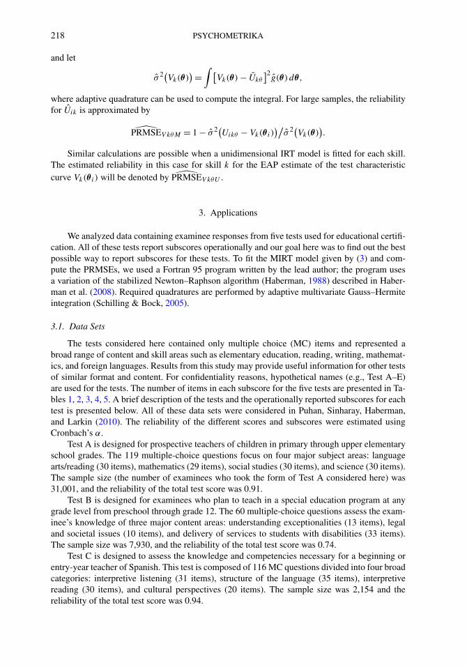
The tests considered here contained only multiple choice (MC) items and represented abroad range of content and skill areas such as elementary education, reading, writing, mathemat-ics, and foreign languages. Results from this study may provide useful information for other testsof similar format and content. For confidentiality reasons, hypothetical names (e.g., Test A–E)are used for the tests. The number of items in each subscore for the five tests are presented in Ta-bles 1, 2, 3, 4, 5. A brief description of the tests and the operationally reported subscores for eachtest is presented below. All of these data sets were considered in Puhan, Sinharay, Haberman,and Larkin (2010). The reliability of the different scores and subscores were estimated usingCronbach’s α.

Test A is designed for prospective teachers of children in primary through upper elementaryschool grades. The 119 multiple-choice questions focus on four major subject areas: languagearts/reading (30 items), mathematics (29 items), social studies (30 items), and science (30 items).The sample size (the number of examinees who took the form of Test A considered here) was31,001, and the reliability of the total test score was 0.91.

Test B is designed for examinees who plan to teach in a special education program at anygrade level from preschool through grade 12. The 60 multiple-choice questions assess the exam-inee’s knowledge of three major content areas: understanding exceptionalities (13 items), legaland societal issues (10 items), and delivery of services to students with disabilities (33 items).The sample size was 7,930, and the reliability of the total test score was 0.74.

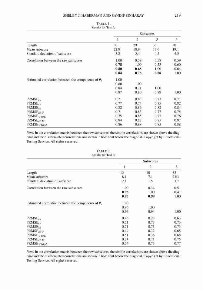
Test C is designed to assess the knowledge and competencies necessary for a beginning orentry-year teacher of Spanish. This test is composed of 116 MC questions divided into four broadcategories: interpretive listening (31 items), structure of the language (35 items), interpretivereading (30 items), and cultural perspectives (20 items). The sample size was 2,154 and thereliability of the total test score was 0.94.


TABLE 1.Results for Test A.

Subscores

1 2 3 4

Length 30 29 30 30Mean subscore 22.9 18.9 17.6 19.1Standard deviation of subscore 3.8 5.4 4.5 4.3

Correlation between the raw subscores 1.00 0.59 0.58 0.590.78 1.00 0.53 0.600.80 0.68 1.00 0.640.84 0.78 0.88 1.00

Estimated correlation between the components of θ i 1.000.80 1.000.84 0.71 1.000.87 0.80 0.89 1.00

PRMSEks 0.71 0.83 0.73 0.71PRMSEkx 0.77 0.74 0.75 0.82PRMSEkc 0.82 0.86 0.82 0.84PRMSEkθU 0.71 0.83 0.77 0.75PRMSEV kθU 0.75 0.85 0.77 0.76PRMSEkθM 0.84 0.87 0.85 0.87PRMSEV kθM 0.86 0.88 0.85 0.88

Note. In the correlation matrix between the raw subscores, the simple correlations are shown above the diag-onal and the disattenuated correlations are shown in bold font below the diagonal. Copyright by EducationalTesting Service, All rights reserved.

TABLE 2.Results for Test B.

Subscores

1 2 3

Length 13 10 33Mean subscore 8.1 7.1 23.3Standard deviation of subscore 2.1 1.5 3.7

Correlation between the raw subscores 1.00 0.34 0.510.96 1.00 0.410.95 0.99 1.00

Estimated correlation between the components of θ i 1.000.96 1.000.96 0.94 1.00

PRMSEks 0.46 0.28 0.63PRMSEkx 0.71 0.73 0.73PRMSEkc 0.71 0.73 0.73PRMSEkθU 0.49 0.32 0.65PRMSEV kθU 0.51 0.36 0.68PRMSEkθM 0.74 0.71 0.75PRMSEV kθM 0.76 0.73 0.77


220 PSYCHOMETRIKA

TABLE 3.Results for Test C.

Subscores

1 2 3 4

Length 31 35 30 20Mean subscore 23.6 22.8 24.1 14.2Standard deviation of subscore 5.1 6.0 5.1 3.2

Correlation between the raw subscores 1.00 0.70 0.79 0.530.85 1.00 0.73 0.550.93 0.87 1.00 0.580.70 0.73 0.75 1.00

Estimated correlation between the components of θ i 1.000.91 1.000.95 0.93 1.000.75 0.77 0.80 1.00

PRMSEks 0.84 0.83 0.86 0.68PRMSEkx 0.85 0.84 0.88 0.64PRMSEkc 0.89 0.88 0.91 0.77PRMSEkθU 0.82 0.85 0.82 0.68PRMSEV kθU 0.86 0.86 0.88 0.72PRMSEkθM 0.90 0.90 0.91 0.79PRMSEV kθM 0.91 0.91 0.93 0.79


TABLE 4.Results for Test D.

Subscores

1 2 3







TABLE 5.Results for Test E.

Subscores

1 2 3






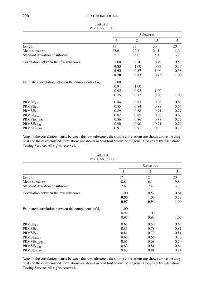
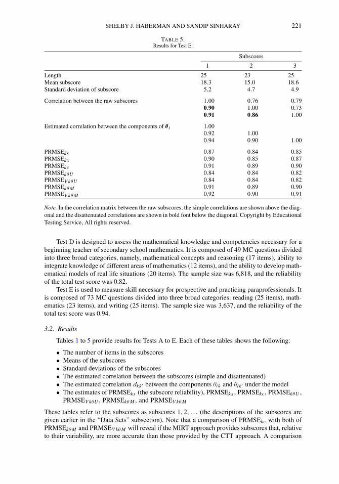
Test D is designed to assess the mathematical knowledge and competencies necessary for abeginning teacher of secondary school mathematics. It is composed of 49 MC questions dividedinto three broad categories, namely, mathematical concepts and reasoning (17 items), ability tointegrate knowledge of different areas of mathematics (12 items), and the ability to develop math-ematical models of real life situations (20 items). The sample size was 6,818, and the reliabilityof the total test score was 0.82.

Test E is used to measure skill necessary for prospective and practicing paraprofessionals. Itis composed of 73 MC questions divided into three broad categories: reading (25 items), math-ematics (23 items), and writing (25 items). The sample size was 3,637, and the reliability of thetotal test score was 0.94.

3.2. Results

Tables 1 to 5 provide results for Tests A to E. Each of these tables shows the following:

• The number of items in the subscores• Means of the subscores• Standard deviations of the subscores• The estimated correlation between the subscores (simple and disattenuated)• The estimated correlation dkk′ between the components θik and θik′ under the model• The estimates of PRMSEks (the subscore reliability), PRMSEkx , PRMSEkc, PRMSEkθU ,

PRMSEV kθU , PRMSEkθM, and PRMSEV kθM

These tables refer to the subscores as subscores 1,2, . . . (the descriptions of the subscores aregiven earlier in the “Data Sets” subsection). Note that a comparison of PRMSEkc with both ofPRMSEkθM and PRMSEV kθM will reveal if the MIRT approach provides subscores that, relativeto their variability, are more accurate than those provided by the CTT approach. A comparison

222 PSYCHOMETRIKA

of PRMSEkθM and PRMSEkθU (and also of PRMSEV kθM and PRMSEV kθU ) will reveal howmuch one gains by employing a MIRT model over a UIRT model. A comparison of PRMSEks

with both of PRMSEkθU and PRMSEV kθU will reveal how much one gains by using subscoresbased on a UIRT model rather than using the raw subscores.

The pattern of results is quite consistent. The estimated PRMSE of the MIRT subscores(both PRMSEV kθM and PRMSEkθM ) are almost always as high as, or higher than, the estimatedPRMSE of the augmented subscores. The differences are often quite small, but they are appre-ciable in a number of cases. The estimates of PRMSEV kθM are as high as, or higher than thoseof PRMSEkθM for all of our data sets.

The estimates of PRMSEs of subscores based on UIRT (both PRMSEV kθU and PRMSEkθU )are mostly slightly higher than the subscore reliability, but are substantially less than the esti-mated PRMSEs based on MIRT. The estimates of PRMSEV kθU are as high as, or higher thanthose of PRMSEkθU for all of our data sets.

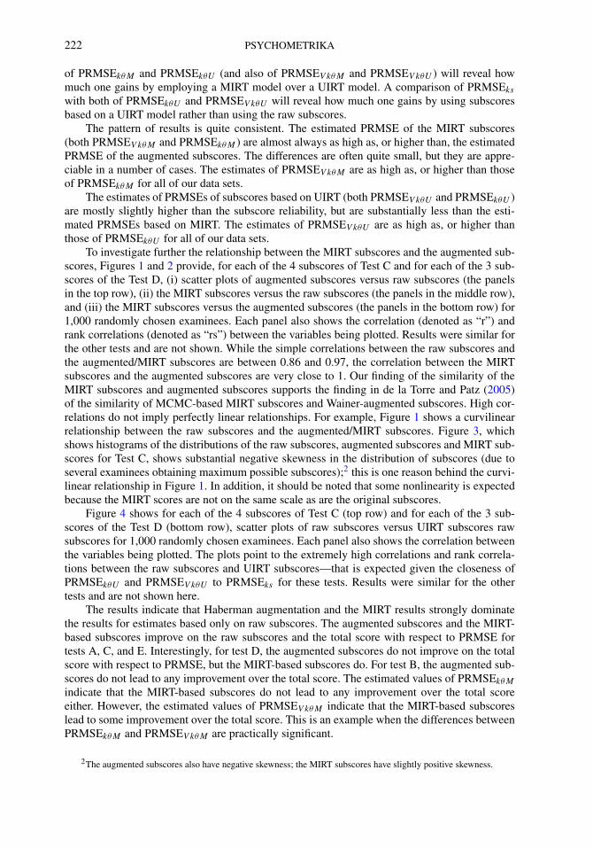
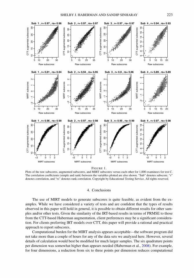
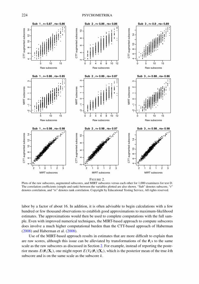
To investigate further the relationship between the MIRT subscores and the augmented sub-scores, Figures 1 and 2 provide, for each of the 4 subscores of Test C and for each of the 3 sub-scores of the Test D, (i) scatter plots of augmented subscores versus raw subscores (the panelsin the top row), (ii) the MIRT subscores versus the raw subscores (the panels in the middle row),and (iii) the MIRT subscores versus the augmented subscores (the panels in the bottom row) for1,000 randomly chosen examinees. Each panel also shows the correlation (denoted as “r”) andrank correlations (denoted as “rs”) between the variables being plotted. Results were similar forthe other tests and are not shown. While the simple correlations between the raw subscores andthe augmented/MIRT subscores are between 0.86 and 0.97, the correlation between the MIRTsubscores and the augmented subscores are very close to 1. Our finding of the similarity of theMIRT subscores and augmented subscores supports the finding in de la Torre and Patz (2005)of the similarity of MCMC-based MIRT subscores and Wainer-augmented subscores. High cor-relations do not imply perfectly linear relationships. For example, Figure 1 shows a curvilinearrelationship between the raw subscores and the augmented/MIRT subscores. Figure 3, whichshows histograms of the distributions of the raw subscores, augmented subscores and MIRT sub-scores for Test C, shows substantial negative skewness in the distribution of subscores (due toseveral examinees obtaining maximum possible subscores);2 this is one reason behind the curvi-linear relationship in Figure 1. In addition, it should be noted that some nonlinearity is expectedbecause the MIRT scores are not on the same scale as are the original subscores.

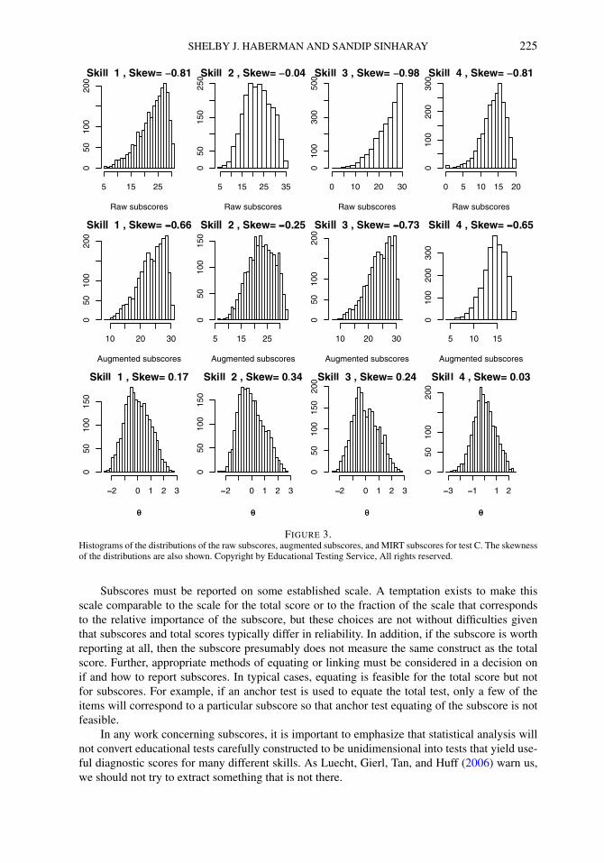
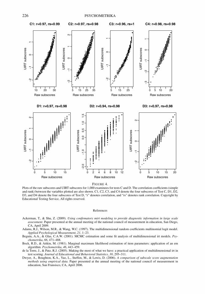
Figure 4 shows for each of the 4 subscores of Test C (top row) and for each of the 3 sub-scores of the Test D (bottom row), scatter plots of raw subscores versus UIRT subscores rawsubscores for 1,000 randomly chosen examinees. Each panel also shows the correlation betweenthe variables being plotted. The plots point to the extremely high correlations and rank correla-tions between the raw subscores and UIRT subscores—that is expected given the closeness ofPRMSEkθU and PRMSEV kθU to PRMSEks for these tests. Results were similar for the othertests and are not shown here.

The results indicate that Haberman augmentation and the MIRT results strongly dominatethe results for estimates based only on raw subscores. The augmented subscores and the MIRT-based subscores improve on the raw subscores and the total score with respect to PRMSE fortests A, C, and E. Interestingly, for test D, the augmented subscores do not improve on the totalscore with respect to PRMSE, but the MIRT-based subscores do. For test B, the augmented sub-scores do not lead to any improvement over the total score. The estimated values of PRMSEkθM

indicate that the MIRT-based subscores do not lead to any improvement over the total scoreeither. However, the estimated values of PRMSEV kθM indicate that the MIRT-based subscoreslead to some improvement over the total score. This is an example when the differences betweenPRMSEkθM and PRMSEV kθM are practically significant.

2The augmented subscores also have negative skewness; the MIRT subscores have slightly positive skewness.


FIGURE 1.Plots of the raw subscores, augmented subscores, and MIRT subscores versus each other for 1,000 examinees for test C.The correlation coefficients (simple and rank) between the variables plotted are also shown. “Sub” denotes subscore, “r”denotes correlation, and “rs” denotes rank correlation. Copyright by Educational Testing Service, All rights reserved.

4. Conclusions

The use of MIRT models to generate subscores is quite feasible, as evident from the ex-amples. While we have considered a variety of tests and are confident that the types of resultsobserved in this paper will hold in general, it is possible to obtain different results for other sam-ples and/or other tests. Given the similarity of the IRT-based results in terms of PRMSE to thosefrom the CTT-based Haberman augmentation, client preferences may be a significant considera-tion. For clients preferring IRT models over CTT, this paper will provide a rational and practicalapproach to report subscores.

Computational burden for the MIRT analysis appears acceptable—the software program didnot take more than a couple of hours for any of the data sets we analyzed here. However, severaldetails of calculation would best be modified for much larger samples. The six quadrature pointsper dimension was somewhat higher than appears needed (Haberman et al., 2008). For example,for four dimensions, a reduction from six to three points per dimension reduces computational

224 PSYCHOMETRIKA

FIGURE 2.Plots of the raw subscores, augmented subscores, and MIRT subscores versus each other for 1,000 examinees for test D.The correlation coefficients (simple and rank) between the variables plotted are also shown. “Sub” denotes subscore, “r”denotes correlation, and “rs” denotes rank correlation. Copyright by Educational Testing Service, All rights reserved.

labor by a factor of about 16. In addition, it is often advisable to begin calculations with a fewhundred or few thousand observations to establish good approximations to maximum-likelihoodestimates. The approximations would then be used to complete computations with the full sam-ple. Even with improved numerical techniques, the MIRT-based approach to compute subscoresdoes involve a much higher computational burden than the CTT-based approach of Haberman(2008) and Haberman et al. (2008).

Use of the MIRT-based approach results in estimates that are more difficult to explain thanare raw scores, although this issue can be alleviated by transformations of the θ is to the samescale as the raw subscores as discussed in Section 2. For example, instead of reporting the poste-rior means E(θ i |Xi ), one might report E(Vk(θ i )|Xi ), which is the posterior mean of the true kthsubscore and is on the same scale as the subscore k.


FIGURE 3.Histograms of the distributions of the raw subscores, augmented subscores, and MIRT subscores for test C. The skewnessof the distributions are also shown. Copyright by Educational Testing Service, All rights reserved.

Subscores must be reported on some established scale. A temptation exists to make thisscale comparable to the scale for the total score or to the fraction of the scale that correspondsto the relative importance of the subscore, but these choices are not without difficulties giventhat subscores and total scores typically differ in reliability. In addition, if the subscore is worthreporting at all, then the subscore presumably does not measure the same construct as the totalscore. Further, appropriate methods of equating or linking must be considered in a decision onif and how to report subscores. In typical cases, equating is feasible for the total score but notfor subscores. For example, if an anchor test is used to equate the total test, only a few of theitems will correspond to a particular subscore so that anchor test equating of the subscore is notfeasible.

In any work concerning subscores, it is important to emphasize that statistical analysis willnot convert educational tests carefully constructed to be unidimensional into tests that yield use-ful diagnostic scores for many different skills. As Luecht, Gierl, Tan, and Huff (2006) warn us,we should not try to extract something that is not there.

226 PSYCHOMETRIKA

FIGURE 4.Plots of the raw subscores and UIRT subscores for 1,000 examinees for tests C and D. The correlation coefficients (simpleand rank) between the variables plotted are also shown. C1, C2, C3, and C4 denote the four subscores of Test C, D1, D2,D3, and D4 denote the four subscores of Test D, “r” denotes correlation, and “rs” denotes rank correlation. Copyright byEducational Testing Service, All rights reserved.

References

Ackerman, T., & Shu, Z. (2009). Using confirmatory mirt modeling to provide diagnostic information in large scaleassessment. Paper presented at the annual meeting of the national council of measurement in education, San Diego,CA, April 2009.

Adams, R.J., Wilson, M.R., & Wang, W.C. (1997). The multidimensional random coefficients multinomial logit model.Applied Psychological Measurement, 21, 1–23.

Beguin, A.A., & Glas, C.A.W. (2001). MCMC estimation and some fit analysis of multidimensional irt models. Psy-chometrika, 66, 471–488.

Bock, R.D., & Aitkin, M. (1981). Marginal maximum likelihood estimation of item parameters: application of an emalgorithm. Psychometrika, 46, 443–459.

de la Torre, J., & Patz, R.J. (2005). Making the most of what we have: a practical application of multidimensional irt intest scoring. Journal of Educational and Behavioral Statistics, 30, 295–311.

Dwyer, A., Boughton, K.A., Yao, L., Steffen, M., & Lewis, D. (2006). A comparison of subscale score augmentationmethods using empirical data. Paper presented at the annual meeting of the national council of measurement ineducation, San Fransisco, CA, April 2006.


Haberman, S.J. (1974). The analysis of frequency data. Chicago: University of Chicago Press.Haberman, S.J. (1988). A stabilized Newton-Raphson algorithm for log-linear models for frequency tables derived by

indirect observation. Sociological Methodology, 18, 193–211.Haberman, S.J. (2007). The information a test provides on an ability parameter (ETS Research Rep. No. RR-07-18).

Princeton, NJ: ETS.Haberman, S.J. (2008). When can subscores have value? Journal of Educational and Behavioral Statistics, 33, 204–229.Haberman, S.J., & Sinharay, S. (2010, in press). Subscores based on multidimensional item response theory (ETS Re-

search Rep.). Princeton, NJ: ETS.Haberman, S.J., Sinharay, S., & Puhan, G. (2008). Reporting subscores for institutions. British Journal of Mathematical

and Statistical Psychology, 62, 79–95.Haberman, S.J., von Davier, M., & Lee, Y. (2008). Comparison of multidimensional item response models: multivari-

ate normal ability distributions versus multivariate polytomous distributions (ETS Research Rep. No. RR-08-45).Princeton, NJ: ETS.

Haladyna, S.J., & Kramer, G.A. (2004). The validity of subscores for a credentialing test. Evaluation and the HealthProfessions, 24(7), 349–368.

Hambleton, R.K., Swaminathan, H., & Rogers, H.J. (1991). Fundamentals of item response theory. Newbury Park: Sage.Luecht, R.M., Gierl, M.J., Tan, X., & Huff, K. (2006). Scalability and the development of useful diagnostic scales. Paper

presented at the annual meeting of the national council on measurement in education, San Francisco, CA, April2006.

Puhan, G., Sinharay, S., Haberman, S.J., & Larkin, K. (2010, in press). The utility of augmented subscores in a licensureexam: an evaluation of methods using empirical data. Applied Measurement in Education.

Reckase, M.D. (1997). The past and future of multidimensional item response theory. Applied Psychological Measure-ment, 21, 25–36.

Reckase, M.D. (2007). Multidimensional item response theory. In Rao, C.R., & Sinharay, S. (Eds.), Handbook of statistics(Vol. 26, pp. 607–642). Amsterdam: North-Holland.

Schilling, S., & Bock, R.D. (2005). High-dimensional maximum marginal likelihood item factor analysis by adaptivequadrature. Psychometrika, 70, 533–555.

Sinharay, S. (2010, in press). How often do subscores have added value? Results from operational and simulated data.Journal of Educational Measurement.

Sinharay, S., Haberman, S.J., & Puhan, G. (2007). Subscores based on classical test theory: to report or not to report.Educational Measurement: Issues and Practice, 21–28.

Thissen, D., Nelson, L., & Swygert, K.A. (2001). Item response theory applied to combinations of multiple-choice andconstructed-response items—approximation methods for scale scores. In Thissen, D., & Wainer, H. (Eds.), Testscoring (pp. 293–341). Hillsdale: Lawrence Erlbaum.

Wainer, H., Vevea, J.L., Camacho, F., Reeve, B.B., Rosa, K., & Nelson, L. (2001). Augmented scores—“borrowingstrength” to compute scores based on small numbers of items. In Thissen, D., & Wainer, H. (Eds.), Test scoring (pp.343–387). Hillsdale: Lawrence Erlbaum.

Yao, L.H., & Boughton, K.A. (2007). A multidimensional item response modeling approach for improving subscaleproficiency estimation and classification. Applied Psychological. Measurement, 31(2), 83–105.

Yen, W.M. (1987). A Bayesian/IRT measure of objective performance. Paper presented at the annual meeting of thepsychometric society, Montreal, Quebec, April 1987.

Manuscript Received: 13 JAN 2009Final Version Received: 5 NOV 2009Published Online Date: 27 MAR 2010

Reporting of Subscores Using Multidimensional Item Response Theory

Documents

Transcript of Reporting of Subscores Using Multidimensional Item Response Theory