Replication and Fabrication of Crafted and Natural Artifacts by ...

Replication and Fabrication of Crafted and Natural

Artifacts by Reverse Engineering using

Single Camera Photogrammetry

John Kaufman

A Thesis Submitted for the Degree of PhD

Lancaster University

July 2018

II

Disclaimer

I hereby declare that this submission is my own work and it contains no material

previously published or written by another person, to the best of my knowledge

and belief, nor material which has been accepted for the award of any other

degree or diploma of the University or other institute of higher learning except

where due acknowledgements have been made in the text.

This thesis is submitted in partial fulfilment of the requirements for the degree of

Doctor of Philosophy

Author: …………………………………………… J Kaufman

Date:

III

Acknowledgements

The author of this thesis would like to thank the following individuals and

organisations for supporting this research activity:

Dr Allan Rennie for his supervision and guidance throughout the period of time I

have been studying at Lancaster University as an off campus student. All

members of the Lancaster Product Development Unit are thanked for their

guidance and for providing many of the fabricated models. I would also like to

thank the members of the University Study Skills Unit who provided the author

with help and guidance when requested.

This research would not have been possible without the use of the computer

software supplied for the duration of the research by Agisoft’s PhotoScan Pro®,

Netfabb’s Studio Pro5® and AutoDesSys’ form-Z pro®, for which I am very grateful.

Thanks also to Mcor Technologies for the fabrication of two models, the Eureka

Cat and Eureka Man, using their Iris® Colour printer and to 3D Systems for the

fabrication on their ProJet 660® of the Clay Head, Egyptian Bowl and Sobekhotep

models.

Thanks is also given to the staff at Kendal Museum, Kendal, Cumbria for their help

and collaboration, use of their Egyptian artifacts, and workshop space during the

data collection phase.

Finally, thanks to my wife, Sandra, who supported and encouraged my project

over many years spending many hours proof reading my manuscript.

IV

Abstract

Photogrammetry has been used for recording objects for well over one hundred

and fifty years. Modern photogrammetry, or digital image capture, can be used

with the aid of a single medium range Digital Single Lens Reflex (DSLR) camera,

to transform two-dimensional (2D) images into three-dimensional (3D) Computer

Aided Design (CAD) spatial representations, and together with the use of additive

manufacturing (AM) or 3D Printing technology, geometric representations of

original cultural, historic and geological artifacts can be fabricated using a process

known as Non-invasive Reverse Engineering. Being able to replicate such objects

is of great benefit to educationalists and, for example, curators; if the original

object cannot be handled because it is fragile, then replicas can give the handler a

chance to experience the size, texture and weight of rare objects. Photogrammetry

equipment is discussed, the objective being simplicity of execution for eventual

realisation of physical products such as the artifacts discussed in this thesis. All

the digital photographic data in the research has been captured either with the use

of a mid-range DSLR camera or a compact “point and shoot” camera. As the

processing power of computers has increased and become more widely available,

and with the use of user-friendly software programs it is now possible to digitally

combine multi-view photographs, taken from 360° around the object, into 3D CAD

representational virtual images, transforming these so they are ready for AM

machines to produce replicated models of the originals.

Over 50 objects were used in this research and the results documented: from the

reproduction of small modern clay sculptures; 3,500-year-old Egyptian artifacts;

household vases, figurines and bottles; fossils, shells and rocks, although not all

successfully recreated. A variety of AM technologies have been employed, mostly

monochromatic but including colour AM machines, to fabricate the models where

good 3D models have been obtained.

A bench-mark test was performed to ascertain the justification for the additional

time and computer power required to produce ultra-high resolution digital

images for the models to be fabricated on high resolution AM technology, in

order to test the best possible limits of artifact reproduction. An in-depth case

study on four problematic artifacts was also conducted using amongst other

V

methods, RAW photographic images as opposed to camera ready Jpeg

images; the results were analysed for comparison and conclusions were drawn.

VI

Table of Contents

Disclaimer II

Acknowledgements III

Abstract IV

Table of Contents VI

List of Figures XIV

List of Tables XXV

List of Abbreviations and Acronyms XXVII

Appendices Contents see separate booklet XXX

Outputs XXXII

Contribution to Knowledge XXXIII

Chapter 1: Introduction and Background History 1

1.1 Introduction 1

1.2 Overview 1

1.3 Research Objectives 1

1.4 Digital Image Capture 3

1.5 Software programs 3

1.6 Headings and Contents for Main Body of Thesis 4

1.7 Introduction to Background History 6

1.8 Aristotle and Euclid 7

1.9 Camera Obscura 7

1.10 The Next 500 Years 9

1.11 Capturing the Photographic Image – the Early Pioneers 10

1.12 Photographic Cameras 11

1.12.1 Stereoscopic Images 11

1.12.2 Photogrammetry 15

1.12.3 Aerial Photography 15

VII

1.12.4 Le Corbusier 15

1.12.5 Spy in the Sky 17

1.13 Birth of Digital Cameras 17

1.14 The Ruby Red Beam 18

1.15 Laser Scanners 18

1.16 Personal Computers 19

1.17 Development of LS and CAD 19

1.18 Cost of Laser Scanners 22

1.19 Virtual 3D Representational Images 26

1.20 3D Reliefs 27

1.20.1 Bas-relief, Sunken and Raised Relief 27

1.20.2 Image-Based Displacement 29

1.21 Historical Conclusion 30

Chapter 2: Literature Review and Research Objectives 32

2.1 Introduction to Photogrammetry 32

2.2 Overview 33

2.3 Medical 33

2.4 Archaeology 36

2.5 Museums 38

2.6 Cultural Heritage 40

2.7 Aerial Surveillance 44

2.8 Archiving and Storage of Data 45

2.9 Heritage Lost and Gained 46

2.9.1 The Crosby Garrett Helmet 46

2.9.2 Tlingit Community of southeast Alaska, USA 50

2.10 Research Objectives - Development of Simpler Data Capture & Processing 51

2.11 Technology for Computer-literate Operatives 52

2.12 A Cost Effective, Cheaper and Safer System 53

2.13 Systems Utilisation 54

2.13.1 Local Community projects 54

2.13.2 Educational institutions 55

2.13.3 Museum and Gallery Staff 57

VIII

2.13.4 Non-invasive Replication of Unique Objects 59

2.14 Product Promotion for Business 59

2.15 Spatial/Tactile Experience by Blind and Visually Impaired 61

2.16 Conclusions 64

2.16.1 Literature Summary and Gaps in Knowledge 64

Chapter 3: Tools of the Trade – Hardware and Software 66

3.1 Photographic Hardware 66

3.2 The Camera 66

3.3 The Lens 67

3.3.1 Close-up Lens 67

3.3.2 Neutral Density Lens 69

3.4 Additional Camera Equipment 70

3.4.1 Compact Camera Support Frame 71

3.4.2 Turntable and other Props 72

3.5 Compact Camera Test – Canon IXUS 100IS® 74

3.6 Lighting 75

3.6.1 Lighting and the Kelvin Scale 76

3.6.2 Basic Lighting Equipment 78

3.7 White Balance and Grey Scale 79

3.7.1 Accuracy of the Colour requirement 80

3.7.2 Consistency in Colour printing 81

3.7.3 Uniformity of AM printers and inks 82

3.7.4 Auto White Balance camera mode 84

3.8 Light Tents 87

3.8.1 Light Tent Construction 87

3.8.2 “Studio” Lighting Conditions – Spain 89

3.9 Open Room Studio 90

3.10 Alternative “Open Studios” 92

3.11 Software 95

3.11.1 AutoDesk - 123 Catch® 95

3.11.2 Agisoft – PhotoScan Pro4® 96

3.11.3 Netfabb GmbH – Studio Pro4® 97

IX

3.11.4 DeskArts 3Data Expert® 98

3.11.5 Dassault Systèmes - SolidWorks® 99

3.12 Software Summary 100

Chapter 4: Methodology for 3D Reconstruction 101

4.1 Method 1 101

4.1.1 Open Room Studio – Setting the Scene 101

4.1.2 Data Capture – 123D Catch® 103

4.1.3 Computer Data Primary Processing 106

4.2 Case Studies 107

4.2.1 Clay Head 107

4.2.2 Unglazed Ceramic Vase 111

4.2.3 China Figurine Serenity 113

4.3 Data Chart and Image library 116

4.4 Creation of 3D Video 117

4.5 Summary 120

4.6 Method 2 120

4.6.1 “Light Tent” technique 120

4.6.2 Standard Data Capture – using PhotoScan Pro4® 122

4.7 Depth of field 123

4.8 Lens Diffraction 126

4.8.1 Histograms 130

4.9 Software control – semi automatic 132

4.10 Pre-Process Masking 134

4.10.1 Alternative uses for Pre-Process Masking 136

4.10.2 Digital Photographs, Point Cloud and 142 Polygon Images

4.11 High and Low Resolution Images 147

4.11.2 Print Problems Associated with 149 High Resolution Data

4.12 Bench Marking the Model and Adapting to the Limitations 152

of AM Technology

4.12.1 AM 3D Printing Machine Envelope Build 158 and Resolution Detail

X

4.13 AM Printer Software 164

4.13.1 AM Printer Drivers 170

4.14 Digital Photographic Information held with the Image 171

4.14.1 Focusing onto the Target 172

4.15 Data Chart and Image Library – with PhotoScan Pro4® 176

4.16 Method 3 - Adapting to Working Environments 177

4.16.1 Using a Backcloth on its Own 177

4.16.2 Hanging on the Wall 181

4.17 Coded and Non-Coded targets 182

4.18 Summary Methodology 2 & 3 185

Chapter 5: Secondary Processing 187

5.1 Using netfabbPro5® 187

5.2 Reorientation 190

5.3 Measuring the Digital Image 193

5.4 Scaling and Resizing 196

5.4.1 Scaling using PhotoScan Pro4® 197

5.4.2 Scaling using 123D Catch® 197

5.4.3 Scaling using netfabbPro5® 198

5.5 Slicing or Free Cutting 202

5.6 Hollowing 204

5.6.1 Shell creation 204

5.6.2 Volume of Material used dictated by Shell 206 Thickness or Artifact attributes

5.6.3 Observations on Material Utilisation as used 211 in the Replication of the Artifacts

5.7 Boolean Operation 212

5.8 Other useful features 213

5.9 Summary 216

Chapter 6: Repair, reconstruction and construction 218

6.1 Returned Noisy data Distorted and Incomplete Data 218

6.1.1 Returned Noisy data 218

6.1.2 Incomplete data. 219

6.1.3 Unglazed Ceramic Vase - lesson in sewing 221

XI

6.1.4 Repair using the Mesh 223

6.2 Damaged Digital Images Beyond Repair 225

6.2.1 Figure K.01 - Serenity – Items G.03 and H.32 227

6.2.2 Figure K.02 – Dolphins – Items G.04 and H.33 229

6.2.3 Figure K.03 – Glazed Vase – Item G.06 229

6.2.4 Figure K.04 – Mollusc - Item G.08 229

6.2.5 Figure K.05 – Frosted Bottle - Items G.10 and H.32 231

6.2.6 Figure K.06 – Ceramic Vase - Item G.15 232

6.2.7 Figure K.07 – China Dish - Item H.37 232

6.2.8 Figure K.08 – Batwing Sea Shell - Item H.50 232

6.2.9 Figure K.09 - Lincrusta – Acanthus - Item – G.16 233

Figure K.10 - Lincrusta – Aphrodite - Item – G.17 233

6.3 Summary of Repaired Data Images 235

6.4 Removing Flare/Glare and Reflection 236

6.4.1 Polarising filters 236

6.4.2 Testing CPL Filters – Artificial Lighting 238

6.4.2 Testing CPL Filters – Natural Lighting 240

6.5. Digital Negative Editing Software 242

6.5.1 File Format 242

6.5.2 Editing the Data, Post-processing 244

6.6 Overview of other uses and benefits 245

6.7 Repair of broken Photographic Frame 246

6.7.1 The Stair Stepping effect 251

6.8 The Egyptian Bowl 251

6.9 The lost Crown of Horus 254

6.10 Educational use 259

6.10.1 Further use of Horus’s Crown 261

6.10.2 Morphing Models 262

6.10.3 A stand for the Amphora 265

6.10.4 Flat Bottom Grain Jar 267

6.10.5 Making Technical Drawings of the Models 267

6.11 Well Protected for the Journey 268

XII

Chapter 7: Compact Camera v DSLR 271

7.1 Compact camera as an alternate option 271

7.2 Basic Trail 272

7.3 The Griffin 275

7.4 Summary 279

Chapter 8: The Finished AM Replicated Models 281

8.1 Introduction to the AM models 281

8.2 Current Diversity 281

8.3 General Observations on Replicated Artifacts 284

8.3.1 Defect or Enhancement 285

8.4 Colour Printing 288

8.4.1 Eureka Cat and Man 288

8.4.2 ‘Greyed out’ 294

8.5 Monochrome Models 295

8.5.1 Clay Head 295

8.6 The Egyptians - Ancient 297

8.6.1 Sobekhotep 297

8.6.2 The Bowl 299

8.6.3 The Vase 301

8.7 The Egyptians – Modern 304

8.7.1 Painted Fish Vase 304

8.7.2 Horus 305

8.8 The Dog 307

8.9 The Warrior 310

8.10 Ceramic Vessels 311

8.11 Handled Vessels 314

8.12 Concrete Mix 316

8.13 Items from the Natural World 317

8.13.1 Sea Shell 318

8.13.2 Fossils – Ammonite 319

8.13.3 Fossils – Trilobite 320

8.14 Varnished models 321

XIII

8.15 Summary 323

Chapter 9: RAW digital negatives 324

9.1 Historical Background 324

9.2 The Search for Solutions 325

9.3 The Digital Negative 326

9.4 Tiff and Jpeg 326

9.5 Size Matters 327

9.6 Case Studies 328

9.6.1. Warrior 330

9.6.2. Serenity 331

9.6.3. Dolphins 332

9.6.4. China Dish 333

9.7 RAW v Jpeg - For and Against 335

9.8 Conclusion 337

Chapter 10: Conclusion and Future Research 339

10.1 Introduction 339

10.2 Core Research Questions 340

10.3 Methodological Reconstructions 341

10.4 Empirical Findings 346

10.5 Theoretical Implications in RE using SC Photogrammetry 348

10.6 Limitation of the Study and Challenges 349

10.7 Recommendations for Further Research 351

10.7.2 Colour Fabrication 352

10.7.3 Questionnaires 352

10.8 Conclusion 354

References: 356

XIV

List of Figures

Chapter 1: Introduction and Background History Page

Figure 1.1 Sequential animation of goat leaping into the air to feed from plant 6

Figure 1.2 Frisius Gemma ’s illustration “ Eclipse of the Sun 24th January, 1544” 8

Figure 1.3 Johann Zahn, camera obscura portabilis, 1685. 8

Figure 1.4 Fox Talbot’s first captured photographic negative image 10

Figure 1.5 Hare’s Stereoscopic camera – c1857 12

Figure 1.6 Lenticular’s Stereoscope - c1860 12

Figure 1.7 Typical double image for binocular vision 13

Figure 1.8 Kilbourne Stereo Daguerreotype in folding stereoscope – c1860 13

Figure 1.9 Zeiss pocket stereoscopic viewer 14

Figure 1.10 Panasonic State of the art still/ video camera 14

Figure 1.11 Drone or UAV as bought in the local electronics shop with camera 16

Figure 1.12 c1975 Sasson’s Digital camera 17

Figure 1.13 Point Cloud 2D enlargement of head section – Front view 20

Figure 1.14 Enlarged head section – side view. 20

Figure 1.15 Full image – 67,063 points 21

Figure 1.16 3D scanned survey of Byland Abbey, North Yorkshire 22

Figure 1.17 Trimble MX2 Dual Head digital laser scanner 23

Figure 1.18 DAVID Structured Light Scanner SLA-2 3D-Scanner® 24

Figure 1.19 DIY 3D scanner camera Kit 24

Figure 1.20 Examples of 3D virtual textured point cloud data images 26

Figure 1.21 Roman pot shard – bas-Relief 27

Figure 1.22 Egyptian Horus raised-relief 28

Figure 1.23 Full rendered Computer Relief 29

Figure 1.24 Top and Bottom of Block showing surface displacement according to grey scale colour intensity

30

Chapter 2: Literature Review and Research Objectives

Figure 2.1 X-ray showing deformed arm bone 34

Figure 2.2 Drilling guide for fixing plate attached to model of bone 35

Figure 2.3 POIGO - Bridging the gap between Surgeon and Engineer 36

Figure 2.4 Bronze Copper helmet and mask 47

Figure 2.5 Children look eyeball to eyeball with their cultural history 48

Figure 2.6 Pre cleaned Helmet 48

Figure 2.7 After cleaning – as displayed at Christie’s 2010 49

Figure 2.8 The Kéet S’aaxw hat 50

Figure 2.9 Kaagwaantaan clan Sea Monster Hat 51

Figure 2.10 Entry Level Computer - UP!3DPP® 55

Figure 2.11 Entry Level Computer - RepRap® 56

XV

Figure 2.12 Entry Level Computer - MakerBot® 57

Figure 2.13 Children handling the Museum replicas 58

Figure 2.14 Children handling replicated models of 3500 year old Egyptian artifacts

58

Figure 2.15 Contemporary Designed Bottle 58

Figure 2.16 Goveshy 60

Figure 2.17 Morling 60

Figure 2.18 Clay Head 61

Figure 2.19 Glazed Clay Bottle 61

Figure 2.20 Mona Lisa by Leonardo De Vinci 62

Figure 2.21 AM Bas-relief of Mona Lisa – shot from above 62

Figure 2.22 AM Bas-relief of Mona Lisa – shot just above horizontal plane 63

Figure 2.23 Original relief painting showing position of X section A/B 63

Figure 2.24 Horizontal cross section of STL virtual image 64

Chapter 3: Tools of the Trade – Hardware and Software

Figure 3.1 Nikon D3100®

DSLR Camera 66

Figure 3.2 AF-S DX Zoom- Nikkor® 18-55mm f/3.5-5.6. - Zoom Lens 66

Figure 3.3 Typical set of Close up lenses 67

Figure 3.4 The Warrior – effect of - f/18 @ 35mm +0 68



Figure 3.7 Models shot at 140mm distance 69

Figure 3.8 Models shot at 140mm distance but with +10 dioptre lens 69

Figure 3.9 Selection of Neutral Density square and round Filter 70

Figure 3.10 Frame curvature as seen from above. 71

Figure 3.11 Curved pipe supporting 3 compact cameras 71

Figure 3.12 AM support arms and frame 71

Figure 3.13 Close-up of turn table showing degree markings. 72

Figure 3.14 Turn table as in use. 73

Figure 3.15 Use of cord to control radial distance. 73

Figure 3.16 Use of pole to control radial distance 74

Figure 3.17 Colour Temperature – the Kelvin Scale 77

Figure 3.18 bip® fluorescent floodlight 78

Figure 3.19 Single bulb 45W floodlight 78

Figure 3.20 A page from the Nikon Manual 79

Figure 3.21 Small part of the Pantone colour chart 81

Figure 3.22 BSi Fan Deck 475 colours 82

Figure 3.23 Original Photograph 85

Figure 3.24 Screen shot point cloud image 85

Figure 3.25 Mcor IRIS® model 85

XVI

Figure 3.26 Stratasys PolyJet J750® model v1 85

Figure 3.27 Original Sobekhotep model 86

Figure 3.28 Wrl file created in formZ 8 SE® 86

Figure 3.29 Model from PolyJet J750® 86

Figure 3.30 Re-printed colour model from the PolyJet J750® machine v2 87

Figure 3.31 Light tent set up in museum workshop – with poplin cover 88

Figure 3.32 Light tent set up without poplin cover but showing Chroma backdrop 88

Figure 3.33 Spanish walk-in-light tent 89

Figure 3.34 Under grey, dull, northern English, cloudy skies 90

Figure 3.35 Typical artifact – indicated - being photographed in Open Room setup using florescent light

91

Figure 3.36 Light Tent under the florescent lighting, including ceiling downlights 91

Figure 3.37 Photogrammetry under a Spanish Naya. Backdrop hung on wall 92

Figure 3.38 Backdrop hung from wall but with lighting - Indoors in the UK 93

Figure 3.39 Photographed whilst still hanging on wall 94

Figure 3.40 Infinite-Realities multi camera studio 94

Figure 3.41 Amphora stand 99

Figure 3.42 Arm of compact camera frame 99

Figure 3.43 Final rendering of Horus’s Crown 99

Figure 3.44 Un-rendered version of Horus’s Crown 99

Chapter 4: Methodology for 3D Reconstruction

Figure 4.1 Data Capture - Advantageous camera angles 101

Figure 4.2 Data Capture – Supporting model above horizontal plane 102

Figure 4.3 Correlation between camera position and horizontal image deviation 102

Figure 4.4 Four frames from part of the Data set of 75 photographs 103

Figure 4.5 123D Catch® Data processing Flow chart 104

Figure 4.6 Close-up screen shot of virtual image waiting to be cleaned 105

Figure 4.7 Clay head identified in blown up image amongst background “noise” 105

Figure 4.8 Original Clay head 107

Figure 4.9 Screen shot of final textured processed digital image 107

Figure 4.10 Digital model - hole under chin 108

Figure 4.11 Distortion on the back of head 109

Figure 4.12 Section of point cloud mesh 110

Figure 4.13 Final Geometric Representation FDM model 110

Figure 4.14 Original digital image of vase 111

Figure 4.15 Initial processed image – Hole in bottom & side 112

Figure 4.16 Hole removed after an extra 15 Images added 113

Figure 4.17 Clean, crisp, sharp image of China figurine 113

Figure 4.18 Textured 3D Mesh image of China figurine 114

Figure 4.19 China figurine - Point cloud 3D mesh 115

XVII

Figure 4.20 China figurine - Dark shadows and plumes 115

Figure 4.21 Vertical view of Video Map 118

Figure 4.22 Enlargement of Figure 4.21 showing camera position and projected image of the tracking path produced by the software

118

Figure 4.23 Changes that can be made to video path. 119

Figure 4.24 Turn Table and Green Chroma Key backdrop 121

Figure 4.25 The Egyptian Vase on the turn table 122

Figure 4.26 Results of out of focus images on an SLS fabricated Bowl 123

Figure 4.27 SLS fabricated Bowl using PhotoScan Pro® 124

Figure 4.28 Bowl - Double point cloud image, caused by initial out of focus data 124

Figure 4.29 Bowl - A texture point cloud “Fur” infill created by computer 125

Figure 4.30 Egyptian Bowl - Stitching of images c/o Agisoft 125

Figure 4.31 Screen shot of completed textured point cloud Egyptian bowl 126

Figure 4.32 Contrasting sharpness between f/stop images 127/128

Figure 4.33 The “Quality” results of the scanned images 129

Figure 4.34 Enlarged images to show difference in sharpness 129/130

Figure 4.35 Histogram - PhotoShop CS6® 131

Figure 4.36 Histogram - PhotoShop Elements 11® 131

Figure 4.37 Nikon User Manual explanation of RGB Histogram 132

Figure 4.38 PhotoScan Pro®

Data processing Flow Chart 133

Figure 4.39 Complex Masking line without Chroma Key backdrop 134

Figure 4.40 Simplified masking operation when backdrop is used. 134

Figure 4. 41 Non-masked images of the Egyptian Vase – pre-processing 135

Figure 4.42 Masked images of the Egyptian Vase – pre-processing 135

Figure 4.43 Original image – part of image data set of Concrete Mix 136

Figure 4.44 Original image - Sea Shell 137

Figure 4.45 Positive masked over sea shell support 137

Figure 4.46 Negitive mask of sea shell 137

Figure 4.47 Final Textured shell 137

Figure 4.48 Positive mask image of Concrete Mix 138

Figure 4.49 Final textured dense cloud image of Concrete Mix 138

Figure 4.50 Sobekhotep seen in centre of light tent 139

Figure 4.51 Screen shots of masked images and view of camera positions 140

Figure 4.52 Photograph of Sobekhotep, son of Nehesy 141

Figure 4.53 Sobekhotep - High resolution point cloud image 141

Figure 4.54 Sobekhotep – Enlarged detail of high resolution image 142

Figure 4.55 Sparse point cloud – 13,639 points 143

Figure 4.56 Medium Build Dense Cloud -1,044,192 points 144

Figure 4.57 A section of “Working Log” 145

Figure 4.58 Medium Build Polygon Mesh - 69,862 polygons 146

XVIII

Figure 4.59 Three types of mesh – depending on the number of polygons created 147

Figure 4.60 Section of polygon mesh enlarged from Medium resolution image 149

Figure 4.61 Original Ammonite fossil 150

Figure 4.62 Hand painted replica 150

Figure 4.63 Ultra-High resolution Jpeg model 153

Figure 4.64 Ultra-High resolution Tiff model 153

Figure 4.65 High resolution - Jpeg model 153

Figure 4.66 High resolution - Tiff model 153

Figure 4.67 Original photograph of Warrior 153

Figure 4.68 CR Jpeg model 153

Figure 4.69 Original model size 25mm high 153

Figure 4.70 Fabricated model size 25mm high 153

Figure 4.71 Bench mark model heads 154

Figure 4.72 Medium resolution - Jpeg and Tiff models 155

Figure 4.73 Low resolution - Jpeg and Tiff models 155

Figure 4.74 Ultra Low resolution - Jpeg and Tiff models 155

Figure 4.75 Layout of models for printing on the PolyJet J750® 156

Figure 4.76 Top view of heads showing grain or layer direction 157

Figure 4.77 Screen shot of the manual build platform layout from GrabCAD® 164

Figure 4.78 Screen shot of the Automatic layout from GrabCAD® 165

Figure 4.79 Screen shot of the Automatic layout from GrabCAD® 165

Figure 4.80 Ultimaker 250µm model 166

Figure 4.81 Without supports 166

Figure 4.82 Model showing outside supports 166

Figure 4.83 Slice level 332 - showing information about the print structure of the model in “Custom” Mode.

168

Figure 4.84 Slice level 1187 169

Figure 4.85 Enlargement of filament layers 169

Figure 4.86 Extra Fine Profile - 0.25mm nozzle 169

Figure 4.87 Fine Profile - 0.4mm nozzle 169

Figure 4.88 Fine Profile - 0.6mm nozzle 170

Figure 4.89 Normal Profile - 0.8mm nozzle 170

Figure 4.90 G code from the instructions as downloaded into a word processor 171

Figure 4.91 Digital information relating to the photographic image. Colour channel histograms shown separately

173

Figure 4.92 Digital information relating to the photographic image. Colour channel histograms seen combined

174

Figure 4.93 Photographing the Trilobite under a Naya with only natural light 178

Figure 4.94 Original Rock 179

Figure 4.95 Screen shot of textured dense cloud rock image 179

Figure 4.96 *.stl image of Rock mounted on a stand. Note holes through body 180

XIX

Figure 4.97 Original small rock 180

Figure 4.98 Textured dense cloud image of small rock with wood prop removed 181

Figure 4.99 Relief canvas - Camera positions as seen from above looking down 181

Figure 4.100 Relief canvas - Camera positions as seen from horizontal plane 182

Figure 4.101 Selection from the Photographic sequence from 68 images 182

Figure 4.102 Agisoft non coded targets 184

Figure 4.103 Coded targets 184

Figure 4.104 Quadra1 - underwater target frame 184

Figure 4.105 Selection of target shapes 185

Chapter 5: Secondary Processing

Figure 5.1 Main data processing functions of StudioPro® 188

Figure 5.2 Original imported image of Botijo 190

Figure 5.3 Reoriented image of Botijo 190

Figure 5.4 Botijo - Front facing - correct orientation 191

Figure 5.5 X,Y,Z Orientation of the three programs 192

Figure 5.6 Imported orientation into netfabbPro5®

from PhotoScanPro4® 192

Figure 5.7 Orientation of imported part and rotation table for realignment 193

Figure 5.8 Measuring tools and essential dimensions displayed 195

Figure 5.9 Removal of bulge at bottom of model 196

Figure 5.10 Botijo - Direct Imported dimensions and orientation 198

Figure 5.11 Botijo - Reoriented to correct frontal view 199

Figure 5.12 Botijo - Incorrect ratio used – therefore dimensions are incorrect 200

Figure 5.13 Botijo - Correct ratio obtained from correct alignment of artifact 201

Figure 5.14 Screen shot of new multi-dimensional Automatic Scaling chart 202

Figure 5.15 “Free cutting” tool to slice off the stepped bottom of a Botijo jug. 203

Figure 5.16 Flattening the rounded bottom of the Botijo jug 203

Figure 5.17 Half Ammonite Shell 204

Figure 5.18 Point measurements of wall thickness of Ammonite 205

Figure 5.19 Smooth Hollowed Botijo 206

Figure 5.20 Measuring points of Botijo wall thickness 206

Figure 5.21 Volume of the solid figurine is displayed on chart 209

Figure 5.22 Boolean effect – light subtracted from dark 212

Figure 5.23 Down the drain hole and into the hollowed model 213

Figure 5.24a Netfabb model information report - Part Analysis 214

Figure 5.24b Netfabb model information report - Platform Views 215

Figure 5.25 Automatic mesh lines filling in the large hole of the Trilobite. 217

Chapter 6: Repair, reconstruction and construction

Figure 6.1 Processed digital image ready to be cleaned 218

XX

Figure 6.2 Hole under chin – automatic mesh repair 219

Figure 6.3 Distortion on top of head 220

Figure 6.4 Red polygons ready to be removed 220

Figure 6.5 Hole in Vase mesh due to lack of digital data 221

Figure 6.6 Inner Vase mesh now complete 222

Figure 6.7 Identifying and Manually stitching/matching 3 points to integrate additional digital images

223

Figure 6.8 Area needing to be cleaned at mouth of Egyptian Vase 224

Figure 6.9 Working with a large scale mesh – Egyptian Vase 224

Figure 6.10 Figurine – textured point cloud image - rough, spikey surface. 227

Figure 6.11 Figurine - High resolution point cloud image 228

Figure 6.12 Mollusc - High resolution point cloud image 230

Figure 6.13 Enlarged surface texture of original Mollusc – note ridge surface 231

Figure 6.14 Smooth Shell surface of original surface to orange peel effect on image

232

Figure 6.15 Part of a roll of Lincrusta – Design “Acanthus” 234

Figure 6.16 Without CPL filter - Focal length 36mm @ f/11 @1/1.6s 237

Figure 6.17 With CPL filter - Focal length 36mm @ f/11 @ 1/1.3s 237

Figure 6.18 CPL filter not rotated - fl/48mm @ f/11 @ 2.5sec 234

Figure 6.19 CPL filter rotated - fl/48mm @ f/11 @ 3sec 238

Figure 6.20 No filter - fl/48mm @ f/11 @ 1sec 238

Figure 6.18a Enlarged image - CPL filter not rotated - fl/48mm @ f/11 @ 2.5sec - artificial lighting

239

Figure 6.19a Enlarged image - CPL filter rotated - fl/48mm @ f/11 @ 3sec – artificial lighting

239

Figure 6.20a Enlarged image - No filter - fl/48mm @ f/11 @ 1sec - artificial lighting 239

Figure 6.21 CPL filter not rotated - fl/48mm @ f/11 @ 2.5sec 240

Figure 6.22 CPL filter rotated - fl/48mm @ f/11 @ 3sec 240

Figure 6.23 No filter - fl/48mm @ f/11 @ 1sec 240

Figure 6.21a Enlarged image - CPL filter not rotated - fl/48mm @ f/11 @ 2.5sec 241

Figure 6.22a Enlarged image - CPL filter rotated - fl/48mm @ f/11 @ 3sec 241

Figure 6.23a Enlarged image - No filter - fl/48mm @ f/11 @ 1sec 241

Figure 6.24 Photo frame missing corner 246

Figure 6.25 Damaged corner removed 246

Figure 6.26 Digital image of frame 247

Figure 6.27 Frame Mask 247

Figure 6.28 Mirrored corner of frame 248

Figure 6.29 Small discrepancy on the frame to be rectified 249

Figure 6.30 Reverse of repaired frame 249

Figure 6.31 Repaired Frame 250

Figure 6.32 Copy and original bowl, combined and then off-set to facilitate repair 251

Figure 6.33 Trimming the rim of the repaired bowl 252

XXI

Figure 6.34 Underside of bowl 253

Figure 6.35 Inside of new bowl 253

Figure 6.36 Horus minus his crown 254

Figure 6.37 Point cloud image of Horus 254

Figure 6.38 Four styles of crown from large researched range 255

Figure 6.39 FDM printed model - version 1 – no support bar - unpainted 255

Figure 6.40 Crown being constructed within SolidWorks® 256

Figure 6.41 SolidWorks® screen shot - Crown version 2 257

Figure 6.42 3D printed model - Final version 2 – hand painted 257

Figure 6.43 SolidWorks® Screen shot – Horus and unattached crown 257

Figure 6.44 Finished unpainted SLS model of Horus 258

Figure 6.45 Hand painted finished model of Horus 258

Figure 6.46 The SL2 model of XYZRGB® structured light scanner 259

Figure 6.47 The first loft of the inner crown 261

Figure 6.48 Second outer crown added 261

Figure 6.49 Top Dome & fillet added to inner crown 261

Figure 6.50 Top of outer crown added and edges smoothed 261

Figure 6.51 Curled front swept extrusion added 262

Figure 6.52 Second support bar added 262

Figure 6.53 RepRap® machine as sold on e-Bay for £250.00 263

Figure 6.54 Original Roman jug 263

Figure 6.55 Screen shot of *.stl image 263

Figure 6.56 Screen shots of addition parts made for jug 264

Figure 6.57 The three stages of transformation 264

Figure 6.58 “Dressel” Wine amphora 265

Figure 6.59 Screen shot of amphora *.stl image 265

Figure 6.60 Greco Roman amphora and stand 266

Figure 6.61 SolidWorks® amphora stand 266

Figure 6.62 Unpainted white AM fabricated amphora and black stand 266

Figure 6.63 Modern flat bottom jar 267

Figure 6.64 Morphed jar together with original 267

Figure 6.65 2D Drawing of figurine Sobekhotep with information extracted from DeskArtes’ 3data Expert

®

268

Figure 6.66 Five parts of the Boxed Set Transporter 270

Chapter 7: Compact camera v DSLR

Figure 7.1 Roman Jug – Resolution 4608 x 3072 272

Figure 7.2 Spanish Botijo - Resolution 4608 x 3072 272

Figure 7.3 Dog - Resolution 4608 x 3072 272

Figure 7.4 Roman Jug – Resolution 3264 x 2448 273

Figure 7.5 Spanish Botijo - Resolution 1024 x 768 273

XXII

Figure 7.6 Dog – Resolution 640 x 480 274

Figure 7.7 The Griffin 275

Figure 7.8 Dense Cloud image of Griffin 275

Figure 7.9 Section from Shield – from 123D Catch® 276

Figure 7.10 Section from Shield – from PhotoScan® 276

Figure 7.11 Section from Shield – from original photograph 276

Figure 7.12 Original digital image and section used for comparison 276

Figure 7.13 Screen shot from netfabbPro5

®. Imported from:- Left - 123D Catch

®

Right - PhotoScan®

278

Figure 7.14 Detail from shield – 123D Catch® 279

Figure 7.15 Detail from shield – PhotoScan® 279

Chapter 8: The Finished AM Replicated Models

Figure 8.1 Gartner’s 3D Printing Hype Cycle 2015 282

Figure 8.2 Gartner’s 2017 Trends 283

Figure 8.3 Miniature FDM black dog – 50mm long x 20mm high seen alongside original clay dog

285

Figure 8.4 Enlarged detail of miniature FDM dog 286

Figure 8.5 Dog’s head further enlarged to show layer-wise effect 286

Figure 8.6 The back of Dirk Vander Kooij’s chair 287

Figure 8.7 Author tries the chair 287

Figure 8.8 Enrico Dini of Monolite UK with Radiolaria - the biggest structure ever built by the D-Shape 3D printer

287

Figure 8.9 Sand blasted enhanced tree ring wood 288

Figure 8.10 Ertel’s chair 288

Figure 8.11 Original Eureka Cat 289

Figure 8.12 Unvarnished Mcor Cat 289

Figure 8.13 Enlarged top view of Eureka cat to show vertical paper layers 290

Figure 8.14 Enlarged back hindquarters of Eureka cat show paper contours 290

Figure 8.15 Original Eureka clay man 291

Figure 8.16 Enlarged section of replicated unvarnished Eureka clay man 291

Figure 8.17 Left hand figurine with hair line printed crack visible 292

Figure 8.18 Enlarged image of faded label on back of original cat 292

Figure 8.19 Enlarged image of faded printed label visible amongst contoured paper layers on fabricated cat

292

Figure 8.20 The Eureka Man - Top row – Paper bonded, FDM and SLS. Bottom row - Original

293

Figure 8.21 The Eureka Cats – Top row – SLS and FDM Bottom row – Original and Paper bonded

294

Figure 8.22 The three items in the ProJet 660® 295

Figure 8.23 Tinted but not coloured clay head 295

Figure 8.24 The collection of heads. The Original – SLS – Hand painted FDM 296

XXIII

Figure 8.25 The FDM model head with structure supports 296

Figure 8.26 Unpainted FDM replicated model head 296

Figure 8.27 The Kendal museum replicas with the original Sobekhotep in the centre and greyed coloured models indicated

297

Figure 8.28 Clones of Sobekhotep 298

Figure 8.29 Distorted FDM models – loops and incorrect placement

of extruded filament 299

Figure 8.30

Figure 8.31 Full size replicated Egyptian bowl 299

Figure 8.32 Original 3,500 year old bowl 300

Figure 8.33 First attempt – discrepancy between sides of bowl 300

Figure 8.34 The digitally repaired and SLS fabricated Egyptian Bowl 301

Figure 8.35 Original Egyptian Vase 301

Figure 8.36 Four replicas of the Egyptian Vase 302

Figure 8.37 Repaired neck of Vase 303

Figure 8.38 Incomplete FDM model showing detached filaments 303

Figure 8.39 Minor detail of ‘chip’ in rim replicated across models 304

Figure 8.40 Egyptian Fish Vase – Original and miniature 305

Figure 8.41 Enlarged image of hand painted vase to show detail 305

Figure 8.42 Original Horus and model on left with his alternative Crown 306

Figure 8.43 Family of Dogs – Original – FDM miniature – SLS duplicate 307

Figure 8.44 Enlargement of original Dog’s face 308

Figure 8.45 Enlargement of SLS model of Dog’s face 308

Figure 8.46 Enhanced features of dog’s face due to painting 309

Figure 8.47 Warrior - Original, miniature SLS and FDM model 310

Figure 8.48 Full size SLS with residual powder 311

Figure 8.49 Miniature Urn, Vase and Vase with Silk flowers 312

Figure 8.50 Full size Urn 312

Figure 8.51 Original Vase and Silk flowers 312

Figure 8.52 Repaired FDM model of Vase 312

Figure 8.53 FDM model vase 313

Figure 8.54 Original vase with raised whirls and patterns 313

Figure 8.55 Mesh seen inside from top of vase 314

Figure 8.56 Front view of Roman vase and miniature copy 314

Figure 8.57 Side view of Roman Vase and miniature copy 314

Figure 8.58 Lopsided off set loop handle replicated 315

Figure 8.59 Surface flaws and blemishes replicated 315

Figure 8.60 Topside of concrete mix – Original left - and SLS duplicate - right 316

Figure 8.61 Hollow underside of SLS concrete mix replica 317

Figure 8.62 Sea Shells – side view - Original shell - Copy shell 318

Figure 8.63 Sea Shells – head-on view – Left-hand side – Copy. Right-hand side - Original

318

XXIV

Figure 8.64 Ammonite fossil family 319

Figure 8.65 Enlarge image of the front of the Ammonite showing the join 320

Figure 8.66 Original Trilobite next to replicated model 321

Figure 8.67 Eureka Cat - Unvarnished – top Varnished - bottom 321

Figure 8.68 Eureka Man - Unvarnished – left Varnished - right 322

Figure 8.69 Concrete Mix - Left – unvarnished – Right - Varnished showing brighter colours

322

Figure 8.70 Concrete Mix – Side view - varnished underside showing bright white base material

322

Chapter 9: RAW digital negatives

Figure 9.1 Screen shot of application window showing use of Jpeg images 324

Figure 9.2 China Dish 329

Figure 9.3 Serenity 329

Figure 9.4 Dolphins 329

Figure 9.5 Serenity - Original CR Jpeg process to an *.obj file 331

Figure 9.6 Serenity - Processed Jpeg file to an *.obj file 331

Figure 9.7 Serenity - Processed Tiff file to an *.obj file 331

Figure 9.8 Original CR Jpeg process to an *.obj file 332

Figure 9.9 Processed Jpeg file to an *.obj file 332

Figure 9.10 Processed Tiff file to an *.obj file 332

Figure 9.11 Dolphin - Head 333

Figure 9.12 Dolphin - Pupil 333

Figure 9.13 Dolphin - Iris 333

Figure 9.14 Dolphin - Quarter Iris 333

Figure 9.15 Unsuccessful results in processed *.obj files 334

Figure 9.16 UH Tiff file – the best achieved 334

Figure 9.17 Further attempts using coded targets 334

Figure 9.18 Section from Table M.1 showing building time of Point Cloud images 337

Chapter 10: Conclusions and Future Research

Figure 10.1 Flow Chart of Methodology for Monochromatic Replication 342

Figure 10.2 Schematic diagram of Concerns and Problems 345

XXV

List of Tables

Chapter 1:

Table 1.1 Details of Popular 3D Scanning Technologies priced up to $5,250 25

Chapter 4:

Table 4.1 Correlation between camera positions and horizontal image deviation 103

Table 4.2 Camera data – Clay Head 108

Table 4.3 Camera data – Clay Vase 112

Table 4.4 Camera data – China Figurine 114

Table 4.5 24 items processed using 123D Catch® 116

Table 4.6 Ammonite Fossil – wire mesh data 147

Table 4.7 Polygon Mesh count in relation to Kb file size 148

Table 4.8 Third Party Hollowed out Model Costs (August 2014) 151

Table 4.9 Numerical data comparison Hollow Heads - Stl files 158

Table 4.10 AM 3D Printing Machine Envelope Build and Resolution Detail 159 - 163

Table 4.11 Slice data for Warrior model from the Cura v2.6 software 166

Table 4.12 Layers and infill per Profile/Nozzle change 170

Table 4.13 Focusing criterion for ‘Live View’ 172

Table 4.14 Copy of ViewNX 2™ table for clarification 175

Table G.1 Data Chart for processed images using 123D Catch® Appendix G 116

Table G.2 Photographic images, size and material Appendix G 116

Table G.3 Capture data Log - 123D Catch® Appendix G 120

Table H.1 Ammonite Data Sheet – Triangles (Polygons) size in relation to Kilobytes size of File”

Appendix H 149

Table H.2 Ammonite Data Resolution Statistics “Processing 40 images with PhotoScan - Mesh Statistics”

Appendix H 149

Table J.1 Data Chart and Image Library using PhotoScan Pro4® Appendix J 176

Table J.2 Photographic images, size and material Appendix J 176

Table J.3 Capture data Log – PhotoScanPro4®

Appendix J 177

Table M.1 Warrior Head – Netfabb Data for Bench Mark Models Appendix M 154 158

Chapter 5:

Table 5.1 Dimensions of imported models into netfabbPro5® from PhotoScan

® 194

Table 5.2 ‘Scaled parts’ errors – Spanish Botijo 200

Table 5.3 Botijo wall thickness 206

Table 5.4 Appendix J reference to illustrations 207

Table 5.5 Relationship between shell depth, shape, and percentage volume of materials used

208

Table 5.6 Showing differential volume according to shell wall thickness 210

XXVI

Chapter 6:

Table 6.1 Reference table of original and failed point cloud images 226

Table 6.2 Image Quality Options 244

Table K.1 Capture data Log – Failed Artifacts Appendix K 227

Table K.2 Photographic images of Failed Artifacts Appendix K 227

Chapter 7:

Table 7.1 Basic Camera Data comparison 271

Table 7.2 Dimensional comparison between same digital image data set 278

Table L.1 Compact camera v DSLR Data comparison 272

Table M.1 Warrior Head – Netfabb Data for Bench Mark Models Appendix M 274

Chapter 8:

Table 8.1 Data comparison chart of 11 artifacts 308

Chapter 9:

Table 9.1 Image file size comparison 328

Table 9.2 Number of digital images that can be stored on a card 336

Table M.1 Warrior Head – Netfabb Data for Bench Mark Models Appendix M 327

Table N.1 Capture log – RAW & Jpeg – Photographic Image Data

Appendix N 328

Table N.2 RAW & Jpeg image Processing log – PhotoScan Data processing Information

Appendix N 328 337

Chapter 10:

Table 10.1 Results of Models Processed and Fabricated 346

XXVII

List of Abbreviations and Acronyms

2D 2 Dimensional

2.5D Two-and-a-half dimensional

3D 3 Dimensional

3DP 3D printable

ABS Acrylonitrile butadiene styrene

AF Automatic Focus

AFM Atomic Force Microscopy

AM Additive Manufacture

AP Adobe Photoshop

ASME American Society for Mechanical Engineers

ASPRS American Society for Photogrammetry and Remote Sensing

ASTM American Society for Testing and Materials

ATP Accessible Tactile Pictures

BBC British Broadcasting Corporation

BCE Before the Common Era

c about

CAA Civil Aviation Authority

CAD Computer Aided Design

CAM Computer Aided Manufacturing

CIRP College International pour la Recherche en Productique The International Academy for Production Engineering

cm centimetre

CNC Computer Numerical Control

CO Camera Obscura

CP Circular Polarising

CPD Cloud Point Data

CPL Circular Polarising Lens (filter)

CPU Central Processing Units

CR Camera Ready

CRP Close Range Photogrammetry

CT Computerised Tomography

CU Close Up

DC Dense Cloud

DIY Do It Yourself

DLP Direct Light Projection

DMP Direct Metal Printing

DSLR Digital Single Lens Reflex

DVD Digital Video Disc

DWG Drawing Database file (as used by AutoDesk)

XXVIII

ESDA Engineering Systems Design and Analysis

et al And others

EU European Union

FDM Fused Deposition Modelling

G Code A computer programming language

GB Gigabyte

gm grams

GPS Global Positioning System

H high

HD High Definition

HTML Hypertext Mark-up Language

IBD Image-Based Displacement

IBM International Business Machines

ISO International Organisation of Standardisation

IP Intellectual Property

IPU Image processing Unit

IR Infrared

JISC Joint International Systems Committee

Jpeg (jpg) Joint Photographic Experts Group

K Kelvin scale

k thousand

Kb Kilobyte

L low

LED Light-Emitting Diodes

LiDAR Light Detection and Ranging

LS Laser Scanning

LU Lancaster University

M medium

mgp Megapixels

mm millimetres

MRI Magnetic Resonance Imaging

ND Neutral Density

NEF Nikon Electronic Format

OBJ (obj) Object file (Relocatable Object Module Format)

PC Personal Computer

PCD Point Cloud Data

PET Personal Electronic Transactor

PSE Photoshop Elements

PSD Photoshop image editing file format

PDF Portable Document Format

XXIX

POIGO Bridging the gap between Surgeon and Engineer

PSG Patient-Specific Guides

RAM Random Access Memory

RAW Unprocessed digital data from camera image sensor

RE Reverse Engineering

RGB Red, Green, Blue

ROM Read only Memory

RNIB Royal National Institute for the Blind

RP Rapid Prototype

SC Single Camera

Sci-Fi Science Fiction

sec second

SL Stereolithography

SLS Selective Laser Sintering

SLR Single Lens Reflex

SMEs Small to Medium sized Enterprises

STL (stl) Standard Tessellation Language

TIFF (tiff) Tagged Image File Format

TV Television

UAV Unmanned Aerial Vehicles

UH Ultra-high

UL Ultra-low

UK United Kingdom

U3A University of the 3rd Age

US$ United States Dollars

USA United States of America

UV Ultra Violet

VR Vibration Reduction

VRML Virtual Reality Modelling Language (known as *.wri files)

w watt

WRI (wri) Windows Write Document file

WebGL Web standard to support and display 3D graphics

X-ray Electromagnetic radiation

XXX

Appendices Book - Contents

Appendix A - ASME – J. Computing & Info Science in Engineering – 2014

Appendix B - CIRP – published on line – Sciencedirect.com – 2015

CIRP – Procedia CIRP vol. 36 – 2015

Media coverage

Appendix C – Ancient Egypt - Vol. 15. No.3 - Dec. 2014

Touching History - The Egyptian collection

Appendix D - Ancient Egypt - Vol. 15. No.5 – April/May 2015

Touching History - The Lost Crown of Horus

Appendix E - American Scholar -Oct 2014 by Josie Glausiusz

Ode on a Grecian Replica

Data Charts, Photographic Images and Tables

Appendix G - Table G.1 Data Chart for processed images using 123D Catch®

Chapter 4.3 page 116

Table G.2 Photographic images, size and material Chapter 4.3 page 116

Table G.3 Capture data Log - 123D Catch®


Appendix H - Table H.1 Ammonite Data Sheet – Triangles (Polygons) Size in relation to Kilobytes size of File”


Table H.2 Ammonite Data Resolution Statistics “Processing 40 images with PhotoScan - Mesh Statistics”


Appendix J - Table J.1 Data Chart and Image Library using PhotoScan Pro4

®


Table J.2 Photographic images, size and material Chapter 4.15 page 176

Table J.3 Capture data Log – PhotoScanPro4®


Appendix K - Table K.1 Capture data Log – Failed Artifacts Chapter 6.2 page 227

Table K.2 Photographic images of Failed Artifacts Chapter 6.2 page 227 - 235

Appendix L - Table L.1 Compact v DSLR Digital Data comparison Chapter 7.1 page 272


Appendix M - Table M.1 Warrior Head – Netfabb Data for Bench Mark Models





XXXI

Appendix N - Table N.1 Capture log – RAW & Jpeg – Photographic Image Data


Table N.2 RAW & Jpeg Image log – PhotoScan Data processing Information.



Appendix P - Image Sheet 1 Warrior - Pre-processed RAW images v Camera ready Jpeg images

Chapter 9.6.1 page 330

Image Sheet 2 Serenity - Pre-processed RAW images v Camera ready Jpeg images


Image Sheet 3 Dolphins - Pre-processed RAW images v Camera ready Jpeg images



XXXII

Outputs

ASME – J. Computing & Info Science in Engineering – 2014

Reverse Engineering using Close Range Photogrammetry for Additive

Manufactured Reproduction of Egyptian Artifacts and other Objets d'art.

(ESDA1014-20304)

CIRP – published on line – Sciencedirect.com – 2015 Procedia CIRP vol. 36 – 2015

Single Camera Photogrammetry for Reverse Engineering and Fabrication of

Ancient and Modern Artifacts

CIRP 25th Design Conference - 2015

Single Camera Photogrammetry for Reverse Engineering and Fabrication of

Ancient and Modern Artifacts – PP presentation

Media coverage

Ancient Egypt - Vol. 15. No.3 - Dec. 2014

Touching History - The Egyptian collection

Ancient Egypt - Vol. 15. No.5 – April/May 2015

Touching History - The Lost Crown of Horus

American Scholar -Oct 2014 by Josie Glausiusz

Ode on a Grecian Replica

XXXIII

Contribution to Knowledge

At the inception of this research, both AM and photogrammetry were well

established in their own respective fields. As is shown in the initial chapters

covering the historical and literature review aspects of the research, 3D imaging,

Laser Scanning (including CT and MRI scanning), as well as digital image capture

using a DSLR camera were all being used to produce 3D images, and by

converting the imaging format into AM technology readable files, AM fabricated

replications were being made.

For the most part, up to this time, 3D imaging was in the domain of specialist

software experts and AM machine engineers, who, with a great deal of expertise,

could convert 2D images into 3D models. Complex software and expensive

hardware was required by those pursuing the subject, which was only available in

the commercial sector in certain large organisations with sufficient financial

resources. Both technologies were being used in universities or large companies

with R&D departments covering many disciplines and industries.

Initially this research undertook to examine the claims of a Beta version of

123D Catch® from AutoDesk, that anybody could “happy snap” with an iPhone,

iPad or compact camera, up-load to the internet and produce 3D replicated copies

of the original items. The research also undertook to determine whether these

claims were indeed achievable with some carefully planned measures using both

a mid-range DLSR camera and also a “point and shoot” compact camera. Also, by

comparison, it undertook to investigate whether there was commercial software

available which was user friendly, to process the digital images and convert the

resulting digital files to an AM printable format. It also investigated whether it was

possible, without using expensive and complex software and hardware, for a

computer literate person to achieve good 3D representations of the original

artifact, and whether the research objectives as laid out in Chapter 1 were indeed

achievable.

It is proposed that the research as described in this thesis will offer the following

contributions to knowledge:

XXXIV

With the aid of a Compact “point and shoot” camera, establish limits for

acceptable image resolution which could be used in the process of converting 2D

images into 3D replicated AM objects.

Contribute to the development of techniques and methods which can be

used by computer-literate, but not necessarily expert, computer software

operatives.

Development of a procedure which is more cost effective and cheaper than

most 3D scanning systems.

The development of a system which could potentially be utilised by a

variety of users including community projects, educational institutions, and

museums and galleries.

The development of a non-invasive procedure to replicate hand-crafted

original artifacts which may be a more economically viable method to be used by

small businesses (SME’s) for the promotion of their designs.

Comparison of the use of RAW (NEF) and Jpeg digital image format

through the use of bench mark AM models and series of 2D printed image

examples, processed within the same software, and evaluation of the benefits of

one format over the other, showing that the preconception of the use of RAW

images as superior to Jpeg was not always merited.

Examine the processing of high and ultra-high point cloud digital images

and justify their use with AM technology, demonstrating that unless the AM

technology output is of a high enough resolution, the artifacts produced will not

match the high specification of the digital images. Due to the longer time needed

to process high and ultra-high digital images, and the higher more expensive

specification of the processing computer hardware required, both time and

therefore money would be wasted.

1

Chapter 1: Introduction and Background History

1.1 Introduction

Since the dawn of man’s existence, he has left testimony of his desire to copy

and replicate those things around him that he sees and touches in both his

physical and metaphysical world. There have been many stages in the

development from the first cave drawings and hand-made figurines, to the

additive manufactured (AM) artifacts and three-dimensional (3D) images seen

today.

1.2 Overview

Over the last decade, Laser Scanning (LS) [1, 2] and Structured Light [3, 4] have

been used to digitally replicate objects of all sizes, from large historic buildings to

small statues, and have moved to dominant non-invasive method used to digitise

smaller objects [5]. In this thesis, an alternative process to the LS method of data

capture was researched using a Digital Single Lens Reflex (DSLR) camera, and it

was shown, that limited prior “expert” knowledge was required for this alternative

digitisation method. Apart from the use of the computer programs selected and

without the use of relatively expensive and complicated 3D laser equipment, this

objective was achieved. By the use of photogrammetry, high resolution digital

images could be manipulated, filtered and processed by specialist software to

produce 3D spatial images. In this research, the main primary software used was

AutoDesk’s 123D Catch®, Agisoft’s PhotoScan Pro5® and AutoDesSys’ form-Z

pro® [6-8]. The data files created where further processed by additional software,

in this case Netfabb’s StudioPro® [9]. The files where made ready for AM

machines to replicate the original photographed product into physical models. As

such, this technique could contribute to the reproduction, restoration or repair of

damaged or broken antiquities by non-invasive methods at modest cost and by

computer literate but not necessarily expert computer software operatives.

1.3 Research Objectives

To develop a simpler, more accessible method of data capture and

processing. With the use of AM (or 3D Printing technology), geometric

2

representations of original cultural, historic and geological artifacts can be

fabricated in a process known as Reverse Engineering (RE).

To investigate how well the software programs used, convert the digital 2D

images into AM models, and compare results obtained with the original

object.

That the techniques and methods employed and developed can be used by

computer-literate but not necessarily expert computer software operatives.

With the aid of one medium range DSLR camera, transform two-

dimensional images into three-dimensional CAD spatial representations,

thereby developing a system which is more cost effective and cheaper than

3D Scanning.

To experiment with a low budget compact “point and shoot” camera to

ascertain the lowest resolution for acceptable images which could be used

in the process of converting a 2D image into 3D replicated AM objects.

To develop a system that could be used by:-

1. Local Community projects

2. Educational institutions

3. Museum and Gallery staff so that the artifacts “behind glass” can be

copied and shared with the general public; if the original object cannot

be handled because it is too old or delicate, then replicas can give the

handler a chance to experience the size, texture and weight of rare

objects

4. Because of the relative low cost of the method, can be developed and

used by small businesses (SME’s) for the promotion of their products

To replicate unique objects in a non-invasive way, and by use of this

technique, contribute to restoration or repair of damaged or broken

antiquities and artifacts.

To enhance the spatial and tactile experience when “viewing” works of art

by the visually impaired.

In this thesis, the whole process was shown, from digital capture of artifacts to

their AM replication. This includes entry level AM printers, which are in use by

school age students under supervision. Whilst this thesis does not discuss

pedagogical aspects of a curriculum, by using moderately priced equipment and

3

software, as suggested in future chapters, the methods described could be

integrated into school curricula to teach both cultural history and 3D modelling

technologies [10], at many, if not all, year levels. The term Reverse Engineering

is used throughout this thesis and defined as meaning the capture, replication

and fabrication of the visible surface of the artifacts that are under discussion.

The advantage of this photographic process was that expensive 3D scanners are

not required to capture the data necessary to produce 3D CAD images, and

experienced technicians were no longer required to operate this equipment. By

using a single, relatively modest DSLR camera, good results were shown to be

obtainable.

1.4 Digital Image Capture

This thesis considers how modern photogrammetry, or digital image capture, can

be used with the aid of a single medium range DSLR camera, to transform two-

dimensional (2D) images into 3D Computer Aided Design (CAD) point cloud

images, and together with AM technology, geometric representations of original

cultural and historic artifacts can be fabricated. The research has focussed on the

use of single DSLR camera photogrammetry, an affordable and accessible

technology, as opposed to the more expensive method of 3D scanning.

The basic photogrammetry equipment required is discussed, with the main

objective being simplicity of execution for the eventual realisation of physical

products. As the processing power of computers has increased and become

widely available, at affordable prices, and software programs have improved, it is

now possible to digitally combine multi-perspective photographs, taken from 360°

around the object, into 3D CAD representational images. This has now led to the

possibility of 3D images being created without 3D scanning intervention.

1.5 Software Programs

Many software programs claim to be able to convert 2D digital photographs into

3D images. On investigation, it has been found that many are still in development

and are not necessarily available for use except experimentally. Several

commercial computer programs are available with a proven and reliable record to

“stitch” multi-view photographs together to produce a 3D image. The primary

research task investigates how well two software programs, Agisoft’s PhotoScan

4

Pro5® and Autodesk’s 123D Catch®, convert the digital 2D image into 3D point

cloud images and with the use of a third software, Netfabb’s StudioPro4®,

converted the data into files that AM machines could read and then fabricate into

physical models. Over the course of this research, both Agisoft and Netfabb have

upgraded their programs from PhotoScanPro5® to Pro7 and from StudioPro4® to

Pro7 and allowed the author access to the latest version as they became

available. For simplicity, the version numbers have been dropped in both cases.

The results obtained – the created models - were then compared with the

original photographed artifacts. The research investigates the tactile surfaces of

the replicated models and compares them to the original objects; it considers

whether those replicated models, when scaled up and down, lose surface detail

and whether the AM models created could be substituted for the original or

whether they are limited by the capability of the AM technology itself.

During the literature review, the author came across a process about which

little has been written; digitally capturing the photographic data of a painting or

drawing, into a raised 3D form which is called Image-Based Displacement (IBD).

The displacement “tool” used was a software program, AutoDesSys’ form-Z

Pro8® [8], which imprints an image onto the surface of a pre-made virtual flat

object creating a bas-relief, by manipulating a point cloud mesh. The process is

published by AutoDesSys [11], the resulting data files can then be AM replicated.

A few examples which were fabricated by the author are included in this thesis. It

was felt that this enhanced the overall research into the main theme of

simplification of the process of replicating artifacts, which can then be freely

handled by the public, enhancing the “viewing” experience by, for instance, a

visually impaired person.

1.6 Headings and Contents for Main Body of Thesis

Following on from this section, the next part of Chapter 1, will give the reader an

insight into the background and a brief history of some of the important events

leading to the developments surrounding this research. A review of existing

literature follows in Chapter 2, and the second half of Chapter 2 covers an in-

depth look at the objectives for this research, covering the development of a

simpler, more accessible method of data capture and processing; a technology

that can be used by computer-literate but not necessarily expert computer

5

software operatives; a more cost effective system than 3D scanning, which can

be used by a variety of institutions and SME’s, and which can benefit the wider

community. The use of hardware and computer software is covered in Chapter 3,

followed in Chapter 4, the different methodological techniques used in the

experimental processes employed in the thesis.

Two main types of software programs were employed in this thesis, a

primary one, which processed the digital images as described in Chapters 4, and

a secondary one, described in Chapter 5, which cleaned and finessed the virtual

3D images, and turned them into *.stl files that could be read by the AM

machines to produce the replicated models. Measurement and Scaling up of the

models so as to produce accurately sized models and some of the pitfalls that

can be encountered are covered.

In Chapter 6, the Repair of Noisy, Distorted and Incomplete Data is

examined together with several artifacts that were un-repairable within the remit

of this thesis. Several practical uses of the techniques employed are examined,

for example how Educational use and Heritage preservation can benefit, and how

to repair, renovate and replace lost parts of broken artifacts is shown in later part

of this chapter.

As described earlier, one of the prime objectives of this research was to see

how simple the process of replication and fabrication of artifacts could be made,

using both hardware and software, which could be used by operatives who were

camera and computer literate but not experts. The most critical part of the whole

operation was the initial data capture of images. Throughout this research, data

capture was carried out using a single medium range entry level DSLR Nikon

D3100® camera. As a comparison, an even simpler and a much lower cost

camera was used, an automatic Compact Canon IXUS 100IS®, “point and shot”.

These experiments, comparisons and results are documented in Chapter 7.

The physical detail and comparison of materials used in the fabrication of

AM Models is covered in Chapter 8, where the finished AM models are examined

and the different methods of manufacture are compared. The use of a more

advanced photographic format, the RAW digital image, was discussed in Chapter

9. This RAW format was compared to the simpler Jpeg format which was used

throughout this research. The results of the two types of format are examined and

evaluated. The final chapter of the thesis contains the results obtained from the

6

research, a discussion and evaluation of these results and finally conclusions

drawn from them, all found in Chapter 10.

1.7 Introduction to Background History

This historical section, traces some of the more important aspects of the

technology, and attributes the scientific discoveries made, without which this

research would not have been possible.

Figure 1.1: Sequential animation of goat leaping into the air to feed from plant.

7

From the earliest of prehistoric cave paintings, we see the animals man

hunted, the pictorial record of enemies defeated, mystical symbols as well as

everyday utensils and day to day events. Many palaeontologists and

anthropological researchers suggest that the development of the human mind

unfolds within these cave drawings, paintings and carvings. Dating from these

early periods, 20-35 thousand years ago, archaeologists have found carved

limestone, bone or ivory, as well as clay fired figurines, which are among the

oldest ceramics known.

An Italian archaeological team working in Iran, in the early 1970’s,

discovered a 5000 year old, painted ceramic bowl, depicting a goat leaping up at

a tree. It was many years later that the leaping goat figures were seen to be

sequential. Notice the position of the first goat in the first frame and how the

position and movement changed in the succeeding frames. If the bowl was spun

round the goat leapt into the air and snatched the leaves from the tree, each

animated section is seen in Figure 1.1 whilst the whole bowl can be seen in last

image [12]. This is possibly the first recorded example of an animated object.

1.8 Aristotle & Euclid

At about the same time that Aristotle was describing how light images are

projected on a wall, in Alexandria, Euclid, one of the most important and

prominent mathematicians of the ancient world, was writing the 13 volume

mathematical treatise for which he was to become famous:- The Elements. Most

of the books are a series of Mathematical Definitions and Propositions leading to

his three-dimensional geometry [13]. Optics was his first work on perspective,

which we now know as 3D imaging, based on the proposition that light travels in

straight lines [14], as yet unproven until the 10th Century by Ibn al-Haytham (see

Chapter 1.10 below).

1.9 Camera Obscura

The desire to replicate and copy to the greatest accuracy is a developing theme

through the development of Man. The ‘Camera Obscura’ (CO) or ‘darkened

room’, coming from the Latin is the first recorded principle of the modern day

camera.

http://en.wikipedia.org/wiki/Ceramic

8

Aristotle, of the Ancient Greek era, noted how light passing through a small

hole in a wall, into a darkened room, produced an inverted image of the sun on

the opposite side wall of the room, during an eclipse of the sun. A plate published

in 1544 by Frisius Gemma is thought to be the first illustration of a CO. The plate

showed exactly the image of the eclipse of the sun, as described by Aristotle,

appearing on the opposite wall of the room (Figure 1.2) [15].

Figure 1.2: Frisius Gemma’s illustration “ Eclipse of the Sun 24th January, 1544”.

There were many versions made over the following years, both in size and

materials. A popular version was a wooden box construction which was both

portable and accessible.

Figure 1.3: Johann Zahn, camera obscura portabilis (reflex box camera obscura), 1685.

9

In 1685 Johann Zahn, an optician and mathematician, was able to modify

the box CO so as to obtain an image the correct way round. He did this by adding

a mirror at 45° to reflect the image the right way round (Figure 1.3) [16]. By

adding a moveable lens at the front of the box, he was able to focus the object to

produce a very clear image, thus creating the Reflex Camera obscura - the

forbearer to our modern “through the lens” reflex camera, the Single Lens Reflex

camera (SLR) which eventually became the Digital SLR (DSLR) as in use today.

1.10 The Next 500 Years

The scientific principle behind the CO may have been used even earlier by Stone

Age man to produce their cave art, but by the 10th Century, the CO was being

used for scientific work by Ibn al-Haytham also known as Alhazen, an Arabian

scholar, proving Euclid’s proposal, that light travels in straight lines:

“Light travels in a straight line and when some of the rays reflected

from a bright subject pass through a small hole in thin material they do

not scatter but cross and reform as an upside down image on a flat

surface held parallel to the hole.” [13]

In the 13th Century, the use of the camera obscura was the established way

in which astronomers viewed the sun [17]. Three hundred years later it was being

used by artists such as the Dutchman Johannes Vermeer as a ‘tool of the trade’,

having been developed into “the pin-hole camera”. It became a device by which

the complex 3D living world of contrast light and dark, colour and texture,

foreground and horizon, could be projected onto a flat wall or table top, creating a

2D image [18]. At the speed of light, this 2D image resolved all the complexity of

perspective, which Euclid had postulated, and which the human eye and brain

struggled to translate from 3D to 2D.

The projected scene could be preserved only by the hand of an artist or

skilled draughtsman. The projected image was still transient, and still subject to

the potential error of the human hand to transpose the moving living world into an

accurate permanent replication. In the early 15th Century, the camera obscura

was being used as a “social media” event. Darkened tents or booths were set up

with the audience inside, viewing live actors performing on the outside, albeit

10

upside down and seen, at the time, by the audiences as a form of sorcery. But

such booths began appearing throughout the western world at carnivals or

country fêtes, people paying money to walk in and see on a flat table top, the live

action of the moving world outside of the tent. Today many museums around the

world still display this simple principle, and the original equipment, of a 2D

pictorial display of the outside surrounding scene, which surrounds the building in

which the camera obscura is housed.

1.11 Capturing the Photographic Image – The Early Pioneers

The Holy Grail of a fixed captured image was finally achieved in 1826 by the

French scientist, Joseph Nicéphore Niépce. He placed a bitumen coated plate in

his camera obscura, exposing it for several hours. This produced an image of his

courtyard as seen from his upstairs window [19]. In 1839 Louis Daguerre, a

printmaker and painter, presented the French Académie des Sciences with his

images he named Daguerreotype, individual images on a sheet of polished silver-

plated copper. The two French men, Nicéphore Niépce and Daguerre, had

collaborated since the mid 1820’s and by the time of Nicéphore Niépce’s death in

1833 had produced a light sensitive image which could be fixed permanently by

the use of chemistry. But it was not until 1839 that Daguerre felt confident enough

to show his invention to the French Académie [20].

Figure 1.4: Fox Talbot’s first captured photographic negative image.

11

In 1835, William Fox Talbot, an English chemist, working quite

independently of the Frenchmen, in his home at Lacock Abbey [21], discovered

light sensitive chemicals which when applied to a solid surface, such as glass.

After being subjected to daylight, formed what was to become the first

captured photographic negative image (Figure 1.4). This negative image could be

chemically stabilised and by repeating the process with the glass negative, form a

positive image. This negative glass image could be used several times to make

several copies of the original.

It was only when Daguerre proclaimed his invention in 1839 that Talbot

came forward with his invention. The race was on for whose method would be

declared the ‘inventor of photography’. Daguerre’s method was a ‘one shot’

picture and could not be replicated whereas Talbot’s method of a single negative,

which could be copied many times over to produce an infinite number of pictures,

ultimately led to the method used by photographers until the birth of digital

photography in the 1970/80s.

1.12 Photographic Cameras

Within twenty years of Talbot’s invention, such was the fast pace of development

of this new found technology, the camera as we know it was created,

transforming true to life images of 3D objects into the 2D image, the photograph,

that we are familiar with today. This was to place the camera obscura into the

realms of history. Although still used by artists, it was the automatic, light-

sensitive paper that when processed, was transformed into a true

representational picture of the captured subject, that caught the imagination. It

perhaps could be argued, that this breakthrough, by Messrs Talbot and Daguerre

can be classed amongst one of the most important scientific discoveries.

1.12.1 Stereoscopic Images

By the mid 1860’s the development of the single picture photographic camera

had advanced to produce a twin lens camera capable of taking stereoscopic

photographic images [22] (Figure 1.5). 3D imaging has been in existence since

the invention of Lenticular’s Stereoscope [23] in 1860 (Figure 1.6) and there still

12

exists many of these early stereographic picture sets [24] (Figure 1.7) and

viewing apparatus as seen in Figure 1.8.

Figure 1.5 : Hare’s Stereoscopic camera – c1857.

Figure 1.6: Lenticular’s Stereoscope - c1860.

As with historical documents and especially with photographs, they are able

to portray a very vivid picture of part of the social life and reinforcing much of the

written word, so described and explained by the New York Public Library on its

website “The Stereogranimator” [25].

“Stereoscopic photography recreates the illusion of depth by utilizing

the binocularity of human vision. Because our two eyes are set apart,

http://www.nypl.org/

13

each eye sees the world from a slightly different angle. Our brains

combine these two different eye-images into one, a phenomenon that

enables us to "see" ever so slightly, around the sides of objects,

providing spatial depth and dimension. Stereoscopic views, or

stereographs, consist of two nearly twin photographs - one for the left

eye, one for the right. Viewing the side-by-side images though a special

lens arrangement called a stereoscope helps our brains combine the

two flat images and "see" the illusion of objects in spatial depth.” [26]

Figure 1.7: Typical double image for binocular vision.

It will be noted in the examples Figures 1.7 and 1.8 of stereoscopic images, as in

all such pairs of photographs, how the right hand image has shifted across the

frame.

Figure 1.8: Kilbourne Stereo Daguerreotype in folding stereoscope.

14

This is the same effect as looking and focusing on an object and closing the

lid of each eye in turn; the object will shift in one’s vision either to the right or left.

The method of using a double image, or binocular vision, created a more solid

looking image, recreating the human experience of vision, and was a technique

that became so popular that camera manufacturers such as Zeiss® were still

producing pocket stereoscopic viewers well into the 1950s [27] (Figure 1.9).

Figure 1.9: Zeiss pocket stereoscopic viewer.

Even today, the use of stereoscopic cameras, are in demand more than

even. Modern state of the art still/video stereoscopic cameras such as the

Panasonic AG 3DA1 (Figure 1.10) are making “block buster” 3D films for the

commercial TV and cinema companies such as the 2009 James Cameron Sci-Fi

epic Avatar and more recently, Marc Webb’s 2012 film based on the Marvel

Comics character Spider-Man, and for the last few years the latest “must have”

TV supports high definition and 3D viewing.

Figure 1.10: Panasonic state of the art still/video camera.

15

1.12.2 Photogrammetry

Photogrammetry, as it is referred to, “is the practice of determining the geometric

properties of objects from photographic images and is as old as modern

photography” [5] dating, as we have seen, from the mid-19th Century.

Photography, especially aerial photography and reconnaissance was recognised

as a very important source of information/intelligence. The American Society for

Photogrammetry and Remote Sensing (ASPRS) was formed in 1934 and defined

Photogrammetry as:-

“the art, science, and technology of obtaining reliable information

about physical objects and the environment through processes of

recording, measuring and interpreting photographic images and

patterns of recorded radiant electromagnetic energy and other

phenomena” [28].

1.12.3 Aerial Photography

It was not long before the camera was taken up into a tethered hot air balloon

and in 1858 a photographer named Nader was photographing Paris from the air,

patenting his new system of aerostatic photography. Just two years later, the idea

of surveying behind the enemy lines by the use of hot air balloon and camera,

was used in Boston, during the American Civil War, producing the first

documented aerial photos to be used against an enemy. As well as the balloon,

the cameras were flown high above the houses and cities by kite, producing

photographic records of San Francisco burning in the 1906 fire which destroyed

much of the city. So aerial photography was gradually born, but it is not until the

aeroplane that the use of this new technology could find its full potential. Used in

World War 1 by both sides to survey the enemy lines, it is reported that the

airborne division of the German army was surveying 4000 images per day of the

battlefields, taken from the air [29].

1.12.4 Le Corbusier

Architects such as Le Corbusier, the Swiss-French architect, designer, painter,

urban planner, and one of the pioneers of what is now called modern

16

architecture, were able to fly over vast areas of land, charting their/his new urban

dreams as well as denigrating the industrialisation and city sprawl that had

started with the new technologies of the 19th century. Le Corbusier’s “Birds eye

view” became the new found phrase for his techniques and visions and those of

others who followed him. The view of rivers and coastlines, as seen from the air,

became the starting point for the architects and urban planners of the mid 1930s

[30]. His ideas and practices still influence many researchers who are using both

camera and LS in conjunction with unmanned aerial vehicles (UAV)s to survey

and study [31], for example forests [32], crops, valley, river [33] and coastal

movements.

Figure 1.11: Drone or UAV as available from the local electronics shop equipped with camera.

Now in the second decade of the 21st Century, UAVs are everywhere,

equipped with state of the art High Definition (HD) cameras or 3D scanners.

Drones are still on the front line in war zones surveying the battlefield, or

employed in a more genteel way of surveying crop growth, land formation,

archaeological sites or used by children playing in the park taking “selfies” from

10 - 20 meters above themselves in the air, in a UAV bought from the local toy or

electronics shops (Figure 1.11).

17

1.12.5 Spy in the Sky

In 1960, perhaps the most infamous air photographer/pilot, Francis Gary Powers,

was shot down over the Soviet Union in his U2 plane; this had been equipped

with a state-of-the-art camera designed to take high-resolution photos of the

military installations from the edge of the stratosphere, from approximately

70,000 feet above the earth’s surface, showing how far Lenticular’s Stereoscope

and Nader’s tethered balloon had progressed in less than a hundred years.

Today the “spy in the sky” has moved onto satellites, although not wholly

accepted, is now just a way of life.

1.13 Birth of the Digital Camera

Converting the 2D image, displaying it on a television screen and later on

computer monitor, was perhaps the next most important step alongside the

introduction of mass produced computers of the late 1970’s. The first digital

camera was invented in 1975 by Steve Sasson, who was an engineer working for

Eastman Kodak® (Figure 1.12).

Figure 1.12: c1975 Sasson’s Digital camera.

18

It was constructed by using a Super 8 movie camera lens, plus several

dozen digital and analogue circuits wired into circuit boards. The black and white

image that was produced took 23 seconds to process, which was then recorded

onto a cassette tape. To see the image played back, the data was read from the

tape and displayed on a black and white television [34]. This camera has

developed from the low resolution 0.01 Megapixels (mgp) early camera to 60 or

80 mgp at the top end of today’s professional range Digital Single Lens Reflex

cameras, encompassing the digital video cameras on the way.

1.14 The Ruby Red Beam

The origins of the LS can be traced back to the late 1950/60’s with the

development of the laser. The laser beam’s beginnings started in 1960 in the

Hughes Research Laboratory in California. The team was led by Theodore

Maiman, and at the time researchers referred to the ruby laser beam as “a

solution looking for a problem” [35]. The story hit the media with front page

newspaper reports of a device with “death ray” capability [36]. But the Nobel prize

was claimed four years later, after much more research and development by a

team at Columbia University in New York, led by Charles Townes [37]. In that

same year, 1964, the actor Sean Connery, in the guise of Ian Fleming’s James

Bond, the infamous secret service character 007, was strapped to a stainless

steel gurney, being sliced in two by Goldfinger, using a ruby red laser beam [38].

1.15 Laser Scanners

Within the next few years, the ruby red beam was instrumental in solving many a

problem and is today found in many everyday items, for example DVD players,

supermarket tills, and document printers, as well as scientific equipment such as

metal cutting machines and of course laser scanners. In 1968 one of the first

prototype scanning devices was built in the Physics department at Cambridge

University. A laser beam was moved around by mirrors following lines on

photographs of bubble chamber experiments, identifying particles of protons,

neutrons, etc., - the building blocks of matter. With financial backing, the

Cambridge team started a company called Laser-Scan®, producing the Sweepnik

[39]. The machine was improved and over the next few years sold as a

commercial product, around the world, to other academic institutions.

http://en.wikipedia.org/wiki/Sean_Connery

19

1.16 Personal Computer

With so much development taking place in the years between the 1950 and late

‘60’s, such technologies as previously discussed might have never got beyond

the scientific communities and the multi-national companies as ‘interesting

research products awaiting future development’, but for the event of the personal

computer; the portal to mass-communication in the 21st century. The arguments

as to who invented the first electronic or digital computer may never end but at

the end of the 1960’s they were large, heavy mainframe structures, and usually

run and owned by universities or electronics companies. The mid 1970’s saw

several companies such as IBM®, Texas Instruments®, Commodore®, Apple ll®

and Radio Shack® bringing together circuit boards, processors, numeric key pads

and monitors and looking to the business communities to market their new

“computers”. At the 1977 Consumer Electronics Show in Chicago, Commodore®

introduced the PET, and is acknowledged as the first fully functional out of the

box, desktop computer. By 1983 computers had entered into the domestic market

selling for about $200. Commodore 64 (6510, 64KB RAM, 20KB ROM with

Microsoft BASIC®, custom sound, and colour graphics), selling an estimated

17/22 million units. The personal computer (PC) had arrived and was here to stay

[40]. In a report in 2014 from the Office for National Statistics [41], the number of

computers per UK household with internet access had risen from under 10% in

1998 to just under 85% by 2014, with 18% of households owning on average

more than 3 computers.

1.17 Development of LS & CAD

The two most recent significant events were the development of computer

software that could read the point cloud data (PCD) [42] from the output of LS,

and the development of CAD.

A point cloud data set can be created by LS, in a three dimensional space,

where each point is defined by X, Y, and Z co-ordinates. These points are

reference points collected from the object that the laser is scanning. These points

could be created by computer software, which had identified hundreds, or millions

of matching points on artifacts, landscapes, or buildings etc., which had been

captured on two dimensional digital or scanned photographs.

20

Figure 1.13: Point Cloud 2D enlargement of head section – Front view.

Figure 1.14: Enlarged head section – side view.

These point clouds, however created, are reconstructed to form a 3D

surface skin of the original object. The point cloud file can then be saved,

depending on the converting software, to a variety of formats. The point cloud 3D

model can then be exported to an editing software program for further

development or enhancement. Figures 1.13 to 1.15, show the point density of the

whole image as 67,063 points The 2D screen shot of the enlarged front view of

the head of the Warrior (Figure 1.13) is somewhat confusing as it appears less

dense because of the enlargement and therefore transparent, showing the back

of the head and shoulders, through to the front. The side view seen shown in

21

Figure 1.14 is less complicated to comprehend although exactly the same size

and from the same 3D image data.

Figure 1.15: Full image – 67,063 points.

It was these developments, over the next twenty years, that brought LS to

the attention of architects, surveyors and engineers. Many technology companies

were founded or started to develop both software and scanners in this era, and

bring them to the market place [43]. By the late 1970s, market leaders emerged

such as Trimble© Navigation Limited with its’ range of 3D scanners closely

followed by academic papers on first experiences with these new machines [44].

Later, how accurate the scanners performed, information regarding data

acquisition, registration, geo-referencing and typical tasks that they were being

used for [45] and by 2010 there was plenty of detailed literature on the use and

practise of scanning of buildings and monuments as well as many other artifacts.

A typical example of this is the English Heritage’s commissioning of a survey of

Byland Abbey by a third party specialising in 3D scanning surveying [46] (Figure

1.16).

22

Figure 1.16: 3D scanned survey of Byland Abbey, North Yorkshire.

High end computers with large amounts of memory were and still are

required to handle the very large files that the scanners produce [47]. The use of

the LS became more widespread as the price of computer components, such as

the Central Processing Units (CPU) and the Random Access Memory (RAM)

dropped in proportion to their increase in speed and computing power. By the

millennium, the possibility of being able to capture true life scenes and convert

them to form a 3D image had arrived. By contrast, stereographs, the 3D

photographic imaging process which had been in existence since 1860, had been

overtaken by that ruby red beam that nobody knew what to do with forty years

earlier. As with the camera obscura, stereoscopic views, or stereographs,

consisting of two nearly identical photographs, using the camera, which had been

used for recording buildings, people, and landscapes etc., for well over one

hundred and fifty years, in most scientific and engineering fields, were obsolete.

1.18 Cost of 3D Scanners

Most professional 3D Scanners are expensive. In a comparison sheet created by

LinDarUSA® [48] in 2012 , a competitor of Trimble©, the ScanLook® was selling

from €65,400/$80K compared with the Trimble MX2® (Figure 1.17) from $90K,

then add to this the cost of software, and any extra equipment required. However,

at the other end of the scale, fully boxed and ready to go, the DAVID Structured

Light Scanner SLA-2® 3D-Scanner (Figure 1.18) 3D scanner is priced at just over

23

€3000/$3650 [49] and at the end of 2016, Apple® filed patents for a 3D scanner

[50].

Figure 1.17: Trimble MX2® Dual Head digital 3D scanner.

Comparison of LS, their efficiency and the value for money each represents

is not within the scope of this thesis and therefore is for others to determine

before such a purchase is made.

Many papers exist where either machines are compared against each other

[48], or in the case of Brecko et al. [51], cost analysis is attempted between four

types of data capture, in this case using four different machines; the DSLR

camera, X-ray based CT, structured light scanning and laser scanning. As well as

a comparison of final specimen images obtained from each piece of equipment,

this paper also contains a comparison and cost analysis including cost of

equipment, portability of equipment and processing time, as well as other

interesting data.

There is a range of other equipment, as well as laser scanners on the

market, at even lower price points than €1000/$1225 (see Table 1.1). Kinect [52]

by Microsoft was claimed to be the "fastest selling consumer electronics device",

in the Guinness Book of World Records when it was released in 2010, and had

sold over 24 million units by 2013, although not a laser scanner in the same way

as the Trimble MX2® or the David SLA-2® 3D-Scanner (Figure 1.18). It was

originally designed to be an accessory to the Xbox® computer gaming technology

but has been adapted by third parties for other uses. Although there are some

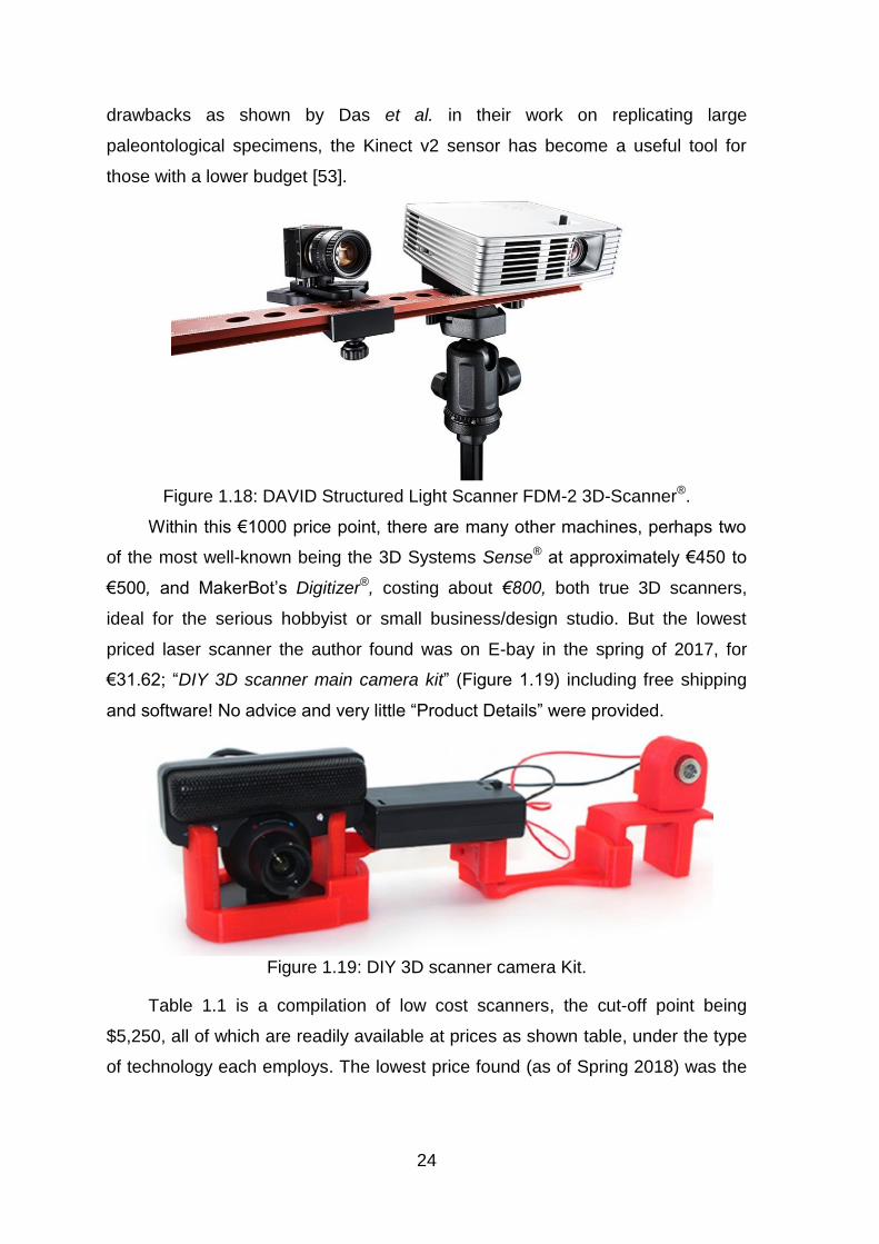
24

drawbacks as shown by Das et al. in their work on replicating large

paleontological specimens, the Kinect v2 sensor has become a useful tool for

those with a lower budget [53].

Figure 1.18: DAVID Structured Light Scanner FDM-2 3D-Scanner®.

Within this €1000 price point, there are many other machines, perhaps two

of the most well-known being the 3D Systems Sense® at approximately €450 to

€500, and MakerBot’s Digitizer®, costing about €800, both true 3D scanners,

ideal for the serious hobbyist or small business/design studio. But the lowest

priced laser scanner the author found was on E-bay in the spring of 2017, for

€31.62; “DIY 3D scanner main camera kit” (Figure 1.19) including free shipping

and software! No advice and very little “Product Details” were provided.

Figure 1.19: DIY 3D scanner camera Kit.

Table 1.1 is a compilation of low cost scanners, the cut-off point being

$5,250, all of which are readily available at prices as shown table, under the type

of technology each employs. The lowest price found (as of Spring 2018) was the

25

basic Microsoft Kinect® priced at $97, whilst the highest price found was the

Shining 3D EinScanPro+® at $ 5,199.

Table 1.1 Details of Popular 3D Scanning Technologies priced up to $5,250.

Product

Tech

no

log

y

(see b

elo

w)

Resolution Market Price* (US$)

System

Stationary 3D Scanners

Shining3D EinScan SE / SP SL 1.3 M Pixels $1,199 - $2,299

Windows

iiiDScan PrimeSense 3D Scanner SL 640×480 $1441 Windows

NextEngine 3D Scanner HD LT 0.1 mm $2,995 Windows

MakerBot Digitizer LT 500µm $788 Windows, OSX, Linux

David SLS-2 SL 60µm $3,275 Windows

Matter and Form MFS1V1 LT 250µm $499 Windows, OSX

Handheld 3D Scanner

Shining3D EinScan Pro / Pro+ WLS 0.1 mm (HD) - 0.3 mm

$3,999 - $5,199

Windows

XYZprinting Handheld SL 1500µm $170 Windows, OSX

Occipital Structure Sensor SL 500µm $379 iOS, Android, OSX, Windows, Linux,

Cubify Sense ToF 900 – 1000µm $400 Windows

Fuel 3D Scanify PhG 350µm $1,386 Windows

3D Systems iSense PhG 500 – 1000µm $73 - $409 iOS

Microsoft Kinect ToF 1280 x 960 px $97 Windows

DIY 3D Scanner Kit FabScan Pi LT 0.25mm $100 - $200 Raspberry Pi

Turntable for Mobile Phones PhG n/a Android, iOS

Murobo Atlas LT 0.25mm $209 - $244 Raspberry Pi

BQ Ciclop LT 0.3 to 0.5 mm $240 Windows, OSX, Linux

3D Printer Scanner XYZprinting Da Vinci 1.0 All in One LT 250µm $500 Window, OSX

XYZprinting Da Vinci 1.0 Pro 3-in-1 LT 250µm $700 Windows, OSX

AIO Robotics Zeus LT 150µm $2,499 Windows, OSX, Linux

*AMAZON PRICES 2018

Abbreviations

PhG Photogrammetry

LT Laser Triangulation

WLS White Light Scanning

SL Structured Light

C Contact

ToF Time of Flight

https://all3dp.com/1/best-3d-scanner-diy-handheld-app-software/#shining3d-einscan-se-sp

https://all3dp.com/1/best-3d-scanner-diy-handheld-app-software/#iiidscan-primesense-3d-scanner

https://all3dp.com/1/best-3d-scanner-diy-handheld-app-software/#nextengine-3d-scanner-hd

https://all3dp.com/1/best-3d-scanner-diy-handheld-app-software/#makerbot-digitizer

https://all3dp.com/1/best-3d-scanner-diy-handheld-app-software/#david-sls-2

https://all3dp.com/1/best-3d-scanner-diy-handheld-app-software/#matter-and-form-mfs1v1

https://all3dp.com/1/best-3d-scanner-diy-handheld-app-software/#shining3d-einscan-pro-pro

https://all3dp.com/1/best-3d-scanner-diy-handheld-app-software/#xyzprinting-handheld

https://all3dp.com/1/best-3d-scanner-diy-handheld-app-software/#occipital-structure-sensor

https://all3dp.com/1/best-3d-scanner-diy-handheld-app-software/#cubify-sense

https://all3dp.com/1/best-3d-scanner-diy-handheld-app-software/#fuel-3d-scanify

https://all3dp.com/1/best-3d-scanner-diy-handheld-app-software/#3d-systems-isense

https://all3dp.com/1/best-3d-scanner-diy-handheld-app-software/#microsoft-kinect

https://all3dp.com/1/best-3d-scanner-diy-handheld-app-software/#fabscan-pi

https://all3dp.com/1/best-3d-scanner-diy-handheld-app-software/#turntable-for-mobile-phones

https://all3dp.com/1/best-3d-scanner-diy-handheld-app-software/#murobo-atlas

https://all3dp.com/1/best-3d-scanner-diy-handheld-app-software/#bq-ciclop

https://all3dp.com/1/best-3d-scanner-diy-handheld-app-software/#xyzprinting-da-vinci-1-0-all-in-one

https://all3dp.com/1/best-3d-scanner-diy-handheld-app-software/#xyzprinting-da-vinci-1-0-pro-3-in-1

https://all3dp.com/1/best-3d-scanner-diy-handheld-app-software/#aio-robotics-zeus

26

1.19 Virtual 3D Representational image

CAD computer software such as Adobe’s Photoshop LE® and Photoshop

Elements® [54] have been able to stitch 2D digital photo images together for a

number of years, creating panoramic views of city, sea or landscapes. More

recently there were several software programs capable of stitching 150 or more,

high resolution digital images together to form a 3D image [55].

Figure 1.20: Examples of 3D virtual textured point cloud data images.

1999 saw a breakthrough in the algorithm that launched photogrammetry

software no longer requiring matched photographic scenes, but able to capture

and create large point clouds from very large photo sets (Figure 1.20). The

efficiency of the software which can convert digital images taken with a DSLR

camera is so high, that it can turn billions of point cloud data points into 3D

images within hours. This must now be a threat that the LIDAR world, with such

disadvantages as the high cost of scanning and associated equipment, collecting

data, slower speed of processing and the steep learning curve needed on the

27

research and understanding involved in utilising the entire point cloud, must now

consider [56].

1.20 3D Reliefs

1.20.1 Bas-relief, Sunken and Raised Relief

To the uninitiated or casual observer all of the above methods are the same, or

similar; reliefs being an artistic method of expression hovering between a 3D

sculpture and a 2D painting or drawing, often described as 2.5D art. Bas-relief,

from the French meaning “lower”, and sunken reliefs are those where the drawing

or pictorial image has been cut into a brick, stone, wood or metal surface.

In the main, raised relief is where the surrounding material has been cut

away to lower the original surface and leave the subject matter to stand proud. All

the aforementioned techniques are several thousand years old, with examples of

bas-relief being found from around the world (Figures. 1.21 & 1.22), in all of the

early civilisations such as Chinese, Egyptian, Persian, Greek and Indian, as well

as from the Mayan period in South America.

Figure 1.21: Roman pot shard – Bas-relief.

Today these forms of relief can be found on coins, both ancient and modern,

jewellery such as brooches and rings, and on the walls of buildings as bas or

high-reliefs, where the art work can be protruding almost 100% from the surface.

Several modern techniques exist to copy or improve on the originals, where

the different types of relief have been created using different starting criteria;

examples cited here include restoration of brick and stone relief, an art form as

practised by the Han Dynasty, (c206 BCE-220 AD). They recorded their

28

individual personal achievement, local events or national military campaigns and

victories [48].

In 2011, Wang et al. [57] proposed a method using 3D models as input data

to generate sunken reliefs, in which the incised lines form the contours below the

surface, whilst the heightened forms are on the surface level. By overlaying the

feature lines, further refinement was achieved, enhancing the final visual impact

on the viewer. The final digital 3D generated mesh was then used, via

appropriate software, for machining real geospatial parts either using AM or

computer numerical control (CNC) technologies.

Figure 1.22: Egyptian Horus raised-relief.

In a similar vein, in 2013, Yu-Wei Zhang et al. [58] looked at replication by

computer generated 3D mesh of line-based sunken relief, as found largely in the

Ancient Egyptian artwork. Their aim was to find a way of combining the contour

incised lines, which form the first outline sculpture, with the remaining sunken,

variable depth features, leading to changing shadow and thickness under strong

lighting conditions, in which replication had been problematic.

A further interesting computer based method of reconstruction of bas-relief

carving, is a system for semi-automatic creation of bas-relief sculpture as

described by Weyrich et al., in 2007.

"the unique challenge of squeezing (3D) shapes into a nearly-flat surface

while maintaining as much as possible the perception of the full 3D

29

scene. Our solution to this problem adapts methods from the tone-

mapping literature, which addresses the similar problem of squeezing a

high dynamic range image into the (low) dynamic range available on

typical display devices….. Given a 3D model, camera, and a few

parameters describing the relative attenuation of different frequencies in

the shape, our system creates a relief that gives the illusion of the 3D

shape from a given vantage point while conforming to a greatly

compressed height” [59].

Their problem was to maintain the centuries old artistic principles of bas-relief

starting with a geospatial model, a camera view of the model and a selection of

controls such as output height (relief height) and overall breadth and width, taking

into account the amount of detail to use or reject and the final material to be used

in presenting a semi-automatic computerised solution.

Working with more conventional oil paint based art works, were the paint on

canvas forms a raised relief, Peng et al. [60], in 2015 were experimenting with

UV Ink-Jet technology, whilst gaining some success they felt that many problems

were still to be overcome before high value art work would be replicated by the

use of 3D fabrication technology.

1.20.2 Image-Based Displacement

Figure 1.23: Full rendered computer relief.

30

Finally, the focus of this thesis is on image based displacement (IBD), which

is seen as a relatively new original digital method, combining both bas and raised

relief, whereby a 2D painting, drawing or relief (see Figure 1.22) is photographed

by a digital camera and the data is transformed into an AM replicated object, the

image being imprinted to appear both below and above the surface.

Figure 1.24: Top and bottom of block showing surface displacement according to grey scale colour intensity.

By converting the coloured image into a “grey scale” image (Figure 1.23),

the points of the mesh created, move relatively to the grey colour intensity of the

digital image, which displaces the surface geometrically (Figure 1.24). A coloured

textured mapping system can be applied to the whole surface so that a digital

computer file is produced which can be 3D AM fabricated as a raised or bas

surface with the original colour picture printed on top of the relief (Figure 1.24).

1.21 Historical Summary

This section intended to outline and shows how, over the millennia, scientific

knowledge has increased since the prehistoric cave paintings of early man and,

together with the development of his tools, has contributed to the development,

expansion and experience of the human mind. The desire to create, understand

and problem solve, through reason and intuition, has led us to resolve many

questions that have been asked over the centuries. And yet the solutions to many

past problems have in fact created new ones for us to ponder over. One might

argue that replication/recreation of artifacts or objets d’art by modern technology

such as AM is no further advanced than when hammer and chisel were employed

to produce the very objects we aim to replicate. But it is perhaps the by-products

of such technologies that can recreate bone or teeth for implants, or make the

availability of relief pictures for the visually impaired more accessible to a wider

White line indicates surface of block

31

population. Long slow processes were involved in reaching the digital age of

photography and the technology used in this research is part of this process,

aiming to show that with simplification and affordability, the early philosophers,

mathematicians and engineers will have been well rewarded.

32

Chapter 2: Literature Review and Research Objectives

2.1 Introduction to Photogrammetry

3D imaging has been in existence since the invention of Lenticular’s Stereoscope

in 1860. Thus, the idea of a 2D image being converted to a 3D image is not new.

In 1934 when Photogrammetry was being defined, roll film was the media that

was being used in cameras; this continued up till the late 1950’s when cassette or

cartridge format film, superseded roll films, in the small format popular snapshot

cameras of the time; but the professional photographers continued to use roll film

in expensive Rolleiflex and Hasselblad cameras. By the 1960’s Single Lens

Reflex (SLR) cameras (a development of the camera obscura), although

expensive, were being bought by the serious amateur photographers, and these

still used roll film. The big change in the recording method was to come in the

later 1970s with the event of the laser and digital imaging systems. So the

definition of photogrammetry still holds true as it was the “processes of recording,

measuring and interpreting photographic images” [28]. It is the process, the

capture of data and its use, which was of prime importance, not the system of

recording the images (by DSLR camera, 3D scanning, magnetic resonance

imaging (MRI), computed tomography (CT)) by which it was achieved. Hence,

there are many systems which now come under the overall umbrella of

photogrammetry.

Whilst not directly linked with the main theme of this research, the Medical

section (Chapter 2.3) of the literature review grew from the interest developed in

the research and work with the Egyptian artifacts in conjunction with The Kendal

Museum, Cumbria. UK., and the research that followed in finding a suitable

crown for Horus, the mythical God of Ancient Egypt. The reading of Steele et al.’s

[61] unveiling of an Egyptian mummy and the recreation of its’ skull, led by

progression to the research work being undertaken by non-invasive methods on

a variety of objects from antiquity, Egyptian mummies included, by others in the

field. From as early as 1997, when the fragile Degas figurine was scanned and

recreated [62], the beginning of the potential of the combination of these

technologies was first seen. The use of MRI and CT scanners was not intended

to be involved in any photogrammetry research for this dissertation, but these

uses were being developed at the same time in the medical field for Orthopaedic

33

reconstruction; all this background information proved useful knowledge in what

was being slowly achieved in the scientific world, including how the use of these

technologies together with AM or RP (originally called Rapid Prototyping), was

advancing and the software that was being developed alongside these advances,

so that digital photographic data could be processed as well as scanned data, to

produce virtual 3D images.

2.2 Overview

There are many methods of employing photography and 3D scanning to capture

data under the general heading of photogrammetry, as there are uses. The

differing technologies of data capture can be split into several categories: data

capture, by 3D scanners only, a combination of 3D scanners and DSLR cameras

and modern 3D stereoscopic digital cameras such as seen in Figure 1.10. Under

the heading of laser scanning there are machines which now included MRI, CT,

data capture by Close Range Photogrammetry (CRP), UAV and by single or

multiple DSLR cameras. Laser Triangulation, White Light Scanning, Structured

Light, Contact, and Time of Flight are also covered under the generic term of 3D

scanning.

Since the late 1990’s, 3D scanning has moved to the predominant non-

invasive method used to replicate both large and small 3D objects, such as large

historic buildings and small statues. The practice of using scanners in the fields of

Archaeology, Medicine, Terrestrial and Aerial Field surveying is well established,

but sometime later saw the beginning of combining photo digital capture with

laser scanners, which has more relevance to this research.

2.3 Medical

Significant results in the use of scanners were obtained in 2003, when the Rapid

Design and Manufacture Centre in Strathclyde University, Glasgow, (in

collaboration with the Royal Museum of Edinburgh and the University of

Edinburgh) undertook to reproduce a 3500-year-old Egyptian mummy. With the

use of an MRI scanner they were able to produce 3D virtual images of the artifact

without removing the age-old bandages which were preserving it [61]. As part of

the Glasgow centred research, with a software package called Shapesnatch®, a

photo projector (substituted for the LS) and digital camera were used to capture a

34

series of fine line photographic images projected onto a Greek Comedy mask.

6.2 megapixel resolutions were used to ensure the data capture produced good

results. In both instances an AM duplicated model of both the head and the mask

were produced.

With the “The development of a collaborative medical modelling service”

together with CT and MRI scanning, with what was then called rapid prototyping

(RP), full scale models of human parts such as skulls were fabricated. These

parts could be drilled, cut and reconstruction plans could be designed to aid

complex surgery units (these units consisting of CAD engineers, AM technicians

as well as medical staff) assisting the front line clinicians, Sugar et al. [63].

By 2008, Stockmans et al. [64] shows that orthopaedic surgeons were

combining the techniques of LS and AM, building patient-specific surgical guides

for patients with deformed bone structures. When presented with a case of a

deformed radius, the radius being the shorter of the two arm bones, in a boy’s

arm, a replica of the arm’s deformed bone was made, allowing the surgeons to

examine and pre-plan their operation well before the patient was anywhere near

the operating table. The pre-surgery combination of CT/MRI scanning and

CAD/CAM plus AM technology, has been used by surgeons to prepare the

surgical drilling guide used in the operation. In the X-ray image shown in Figure

2.1, the deformed bone can be seen, with the complete set of plates and drilling

guides to aid and secure the reconstruction of the repaired deformed arm shown

in Figure 2.2 [64].

Figure 2.1: X-ray showing deformed arm bone.

35

Figure 2.2: Drilling guide for fixing plate attached to model of bone1.

Only a couple of years later, surgical clinicians had become so competent in

the techniques of CT scanning and computer assisted surgical planning as to

lead discussion papers on the pros and cons of computer-assisted versus non-

computer-assisted preoperative planning, as in the work of Leong et al. [65].

By 2014, more than 60 studies had been undertaken in orthopaedic surgery,

of which 14 had focused on the manufacturing of AM osteotomy guides using

stereo-lithography (SL) or selective laser sintering (SLS) processes. The

materials used in the processing could be sterilised to the required hygienic level,

both cutting guides and replicated bones being patient-specific. Popescu et al.

[66], felt the need to create a platform (POIGO) which would bridge the

communication gap between orthopaedic surgeons and additive manufacturing

engineers. Both groups had their own very specific complex professional

language. The design and manufacturing of all components with patient-specific

guides (PSG) required collaboration between surgeons and engineers. This often

resulted in the misunderstanding of requirements either from the medical or the

engineering viewpoints. This acronym is from the original Romanian:

“Platforma online inteligenta colaborativa pentru proiectarea si

fabricarea ghidajelor personalizate in chirurgiaortopedica”.

This translated to “intelligent online platform which can support guides

designed for manufacturing process" [67].

1 Patient-specific drills@ Materialise 2015. Courtesy of Filip Stockman Torstein Husby. All rights reserved

36

POIGO (Figure 2.3), a system with protocols and knowledge support for

both surgeons and engineers, now ensures that the correct questions are asked

at the correct time, that a surgeon follows the correct procedure when requesting

a PSG and that the engineer and designer of the surgical guides understands the

implication of, for instance, where a screw or drill hole might or might not go into

a bone. This workflow procedure ensured the maximum efficiency, from all

members of a very complex team, working at the cutting edge of their field for the

ultimate benefit of the patient.

Figure 2.3: Bridging the gap between Surgeon and Engineer [66].

2.4 Archaeology

Using a similar combination of LS and DLSR, at the medieval church of

Pozzoveggiani near Padova, Italy, and with the use of several software

programs, a self-access web information portal was created in 2010 [68]. On

analysis of the final access and viewing results, it was found that of those

interviewed, only those with a “greater computer knowledge and understanding of

computer software”, were able to gain full benefit and access to the portal. But it

37

was a step towards a full interactive multi-media system with the potential of

bringing complex virtual exploration of artifacts and archaeological sites to the

interactive computer screen.

As the processing power of computers increased and become widely

available, at affordable prices, and from the early Photoshop Elements®, which

could digitally combine several 2D photographs into one, software programs have

improved so it is now possible to digitally combine multi view photographs, taken

from 360°, into 3D virtual representational images. This has now led to the

possibility of 3D images being created without LS intervention.

One such photogrammetry-based survey technology, aDoFting ZScan

Survey System® (Menci Software, Arezzo), a development of the stereoscope,

was used in 3D digital capture of medieval capitals on a church in Aosta, Italy.

This was used for the purpose of building models to assist in future conservation

of artifacts, and the building of a spatial Information System for tourist

information. The moveable camera, mounted on a horizontal bar, took three

digital images of each position from a different angle. The overall field of vision of

each position was overlapped by about 30%. As a result of the complex detail of

the capitals, from each prime camera position in the horizontal, digital capture in

a higher and lower position in the vertical was also taken, but with the maximum

rotation angle of 15° so as to minimise any photographic distortion. In all, 72 high

resolution pictures, each 10.2 megapixel, were taken of each capital. Secondary

software was used to process and clean the virtual point cloud images, which

then allowed different types of model visualization rendering to be created, to

assist in further research [69].

More recently, in 2011, Verhoeven [70] using stereoscopic photography and

processing the digital images with PhotoScan Pro®, produced a series of virtual

3D images. By virtue of the many output formats this software can produce,

including PDFs, file/image sharing is made easy. It was noted that although

PhotoScan Pro® claim to be able to process, in theory, a very large number of

photographs, in practical terms there is a maximum of approximately 1024

images. Verhoeven records that the relationship between the processing time,

speed, quantity and high resolution data, are all interlinked. The more detailed

the photogrammetric data, the greater the speed of processor needed with a

computation time penalty.

38

Waite et al. [71] commenting on a research paper presented at the 2014

Computation and Journalism Symposium, elaborated in an article written for the

American Journalism Review [72] on their use of PhotoScan Pro®. His colleague

and co-writer, Kreimer, pre-programmed a flightpath for a drone and flew two

missions over the archaeological site of Antiochia ad Cragum in Southern Turkey.

Using a Canon Powershot SX260® on the drone, 2,800 aerial images were taken

after flying over the whole site, the whole operation taking about an hour.

However, he reported that the processing of two sets of images, one with 249

and the other with 949 images, took eight hours and 30 hours respectively. But

he admits to only having 8GB of RAM, whereas AgiSoft in their manual suggest

for that quantity of photographs 15 to 45GB of RAM [55] is required, plus an i7

central processing unit (CPU).

As with any new technologies that emerge, standardisation or bench

marking is required, and to this end an investigation into the use of photographic

digital image capture, and benchmarking of datasets was recently attempted [73].

Nguyen et al. evaluated and compared four current software processing

programs, testing some 40 objects to evaluate the systems and finally choosing

one object which was then subjected to four separate datasets. Each dataset had

a constant resolution of 1600 x 1200 pixels and a varying number of input

images, from 30 to 7. In another test a constant number of 30 images were used,

but the resolution was progressively downgraded from 1600x1200 to 200x150

pixels.

Barsantia et al. [74] investigated the different techniques and characteristics

of both photogrammetry and LS, but the advantage of photogrammetry is that

expensive LS equipment is not used and experienced technicians are no longer

required to operate this equipment, since by using a relatively modest DSLR

camera, 3D virtual images are obtainable.

2.5 Museums

There has been a trend of hands on exhibits in museums over the last few years,

in order that all members of the public might more readily engage with the

collections normally housed behind glass cabinets. To fulfill this need, institutions

such as Kendal Museum, Cumbria [75], are interested in exploring potential

39

opportunities from emerging technologies so as to replicate artifacts within their

collection, in line with their mission statement:

“To safeguard and enhance all of the collections for the benefit of all

Museum users, improve the visitor experience, to increase learning

opportunities and ensure that the Museum has a sustainable future”.

The Kendal Museum collection was established in 1796, as a ‘Cabinet of

Curiosities’. While the museum’s value is in its collection of original objects,

replicas of specific objects have their place. Due to the delicate nature of most

objects, they are unable to be handled by the public. Replicas are very useful for

handling sessions, especially for school sessions and loan boxes.

Being able to replicate actual museum collection objects would be of great

benefit to teaching in local schools about the Egyptians and the material held in

the collection. In product design, Caulton [76] found that replicas or prototypes

give the handler a chance to experience the size, texture and weight of objects.

Feedback from participants in such pre-tooling and pre-manufacturing sessions,

often result in minor changes to the original design of a product, saving

companies large amounts of money by modifying designs before being sent to

the markets.

Zheng et al. [77] set out the challenge quite clearly in the title of their 2016

paper “3D Printout Models vs. 3D rendered Images: Which is Better for

Preoperative planning?”. The teams participating in the study suggested that both

methods greatly improved post-operative knowledge on planning, but on

answering a pre-set “Quality of the Surgical Plan Questionnaire”, those who were

given the 3D fabricated models (as opposed to 3D rendered images) showed a

higher score in the quality of the surgical plan.

Conversely it is obviously not possible to be physically present at all the

sites around the world to see or examine museum collections or visit ancient

monuments. Many museums are presenting on their web sites, 2D graphics of

the artifacts in their possession. Those museums with the resources and

expertise are able to create 3D virtual images on their web pages which are

accessible to all. To this end Georgiev [78] presented a set of ‘Tools’ for

exhibiting or displaying 3D graphics in web pages using the HTML5 standard.

40

This allowed complex 3D images to be added into the web browser using an

Application Programming Interface called WebGL [79]. Several applications were

presented which allowed users with limited software development skills to upload

complex graphics onto their websites so as to be viewed by the wider public. As

Georgiev points out, this can be used by e-Commerce and e-Learning sites and

once the software tools have been embedded into the author/developer’s existing

web site, the complex 3D graphics become available on all devices and web

browsers.

2.6 Cultural Heritage

In 2003, Gee [80] argued that good computer and video games enhanced the

learning experience in young children, that “games allowed players to be

producers and not just consumers”. He observed children playing mythological

and superhero video games, then looking to supplement their own knowledge by

investigating books from the library or surfing the web at home, thereby learning

outside the environment of the school.

The concept of teaching cultural heritage via the use of the computer and

the internet is nothing new and Data Games explores the possibilities in great

detail [81]. Games such as MuseumVille [82], use the databases of European

museums, libraries and galleries and create a learning game whereby the player

can create a collection or build a gallery, catalogue and hunt for lost treasures.

Millions of artifacts, books, drawings and paintings can be accessed through

Europeana [83], by means of which a virtual trip though Europe’s institutions can

be had by all, without moving from the classroom or home computer - this vast

amount of digital data can be accessed at the touch of a few keys. Long et al.

[84] surveyed the way in which the digital age, over the last 10 years, has

transformed the way Art historian scholars, librarians and teaching methods have

changed, and has transformed access to collections and resources across the

world, without the original objects themselves losing their prime importance.

Bontchev [85], in 2015 classified 14 types of modern entertainment video

games, the most popular being the “Action packed and Shootem up” type, and a

whole raft of others, but whilst the analysis and comment is not within this

dissertation, it must be noted that many contain what might be termed an

“educational or cultural” element. However, there is a classification which has

41

been termed “Serious Games” and contains among other things, documentary

games which might depict past battles, or historic events, and although these

were developed for “fun” they are used for educational purposes due to their

accuracy and realism. As Bontchev observes:

“Contemporary methods of preserving cultural heritage rely highly on

digitization and archiving as foundations for developing various virtual

heritage applications. During the last two decades, video games

proved to be an interactive visual media able to incorporate virtual

heritage in amazing and highly appealing ways. At the same time,

each video game represents a valuable artifact reflecting technological,

socioeconomic and historical issues of its creation. Therefore, video

games are an essential and integrated part of modern cultural heritage

and themselves need preservation efforts.”

The gaming technology, for example, is now used for virtual museum visits

or a virtual visit to an ancient Egyptian Temple, now with a 3D option. With the

widening availability of 3D software that can convert artifacts from 2D images into

3D virtual objects and can then be included into a video scene, plus the use of

Flash or Adobe Shockwave to ‘fly’ or ‘walk’ though a recreated (or scanned)

ancient monument set, even more realism can be added to the final 3D rendered

video game.

Digitisation of artifacts is now allowing us to resurrect and supplement large

quantities of documentation which has been amassed by historians and archivists

over centuries of knowledge gathering. As suggested by Schuhr and Lee [86],

classical fine line drawings (as well as rough archaeological sketches) of historic

buildings, scenic views, and relief works etc., have already been supplemented

by 2D photographs and Victorian 3D anaglyphs since the late 1860’s (Lenticular

3D images - see Figures 1.6 and 1.7), as well as the more modern version of 3D

images as seen through coloured lensed glasses. With the choice now of buying

a TV with “Avatar” type 3D stereoscopic capability, there is nothing to stop all of

our cultural heritage monuments and artifacts from being digitally preserved and

made widely available to the public.

42

Add a few more technologies such as reverse engineering (RE),

photogrammetry and AM, and with the modest equipment discussed, digital files

can be created, uploaded and downloaded, to be fabricated using one of a

number of AM (or 3D printing) technologies, enhancing the experience of cultural

heritage investigation and research, either in the home or classroom [87]. These

geometric models, if printed in the basic white Nylon 12 (polyamide) or white

Acrylonitrile Butadiene Styrene (ABS), depending on which machine is used, can

be painted by hand, for further enhanced realism.

“Making unauthorized copies of physical objects protected by copyright

is copyright infringement, whether those copies are made with a 3D

printer or a whittling knife” [88].

This of course opens up the greatest minefield of the digital age, in

managing the intellectual copyright of institutions who own the artifacts. But as

digital technology changes now at an ever faster pace, leaving old technology

obsolete, within twenty years software and its compatible hardware will no longer

be able to be accessed by the majority of the population. There cannot be many

households still owning a workable Sinclair ZX Spectrum® [89] or Vic20® [90] and

the tapes that held the data. Yet many would argue that the games played on

them form part of our early childhood computer heritage and should be

preserved. However, as Mailer [91] points out, the problems encountered by

those who try and preserve such digitised data not only include the technical

problems of reconstruction of these programs by building emulators. But in doing

so the copyright of those who hold the licences is infringed by the very nature of

having to hack into the original course code to save the data. Trying to obtain

permissions from licences whose companies have long since disappeared or

have been swallowed up several times in corporate buyouts is, as Mailer points

out, virtually impossible. Those who strive to save this type of digital heritage

referred to as ‘orphaned2 or abandonware3, need to be protected from complex

legal challenges from those who no longer market, distribute or sell these old

2 Orphan works are works still protected by copyright whose owner is unidentifiable or untraceable.

3 Abandonware means software (such as old video games), which is no longer commercially distributed/sold and for which

product support is no longer available. It is thus “abandoned” by its manufacturer. Many games that are abandonware are also orphan works.

43

video and computer games, and within the EU copyright reforms provision must

be made for such activities.

As seen from the last two sections of this chapter (2.5 and 2.6), the biggest

challenge for museums, which traditionally viewed their role as guardians of our

heritage and of the copyright of the artifacts and Intellectual Property (IP) that

they held, is that they were prohibited from the reproduction of items of third party

interest, to the detriment of being able to replicate artifacts which could be used

for scientific research or educational purposes. Pantalony’s [87] guide of 2013

goes some way to help those in charge of museums with this very confusing

problem and legislation, in normal peacetime circumstances. These issues not

only affect local museums around the world, but even more so in the larger

internationally renowned museums and art galleries at a time when there is much

destruction and looting from war zone areas of artifacts thousands of years old

representing irreplaceable cultural heritage [92], which had been stored and

preserved in museums, and which have now been destroyed. IP and copyright

might be a fine ideology to uphold, but digital replication and archiving perhaps

would have been the saviour of such doomed relics, as the digital files

themselves could have been moved from one place to another, and although it

might not have been possible to save the original artifact, at least copies could

have been replicated, using the technology of photogrammetry, 3D scanning and

AM fabrication techniques.

By utilising and combining some of the aforementioned techniques, it should

be possible to reconstruct some of the lost monuments with the help of Crowd

Sourcing. Access to most World Heritage sites, and many lesser sites, is now

made possible by the huge growth of international tourism, but a visit to a

monument site may be impossible whilst the destruction is occurring, which may

be by the hand of nature or of man, and when it is gone it cannot be replaced.

Stathopoulou et al. [93] when trying to reconstruct a 150 year old historic stone

bridge, which had collapsed and partially been swept away by a very heavy rain

storm, turned to the public via the web for help. Designing a crowdsourcing

platform, they were able to collect 2D data images of the bridge. These images

not only formed the basis for a virtual 3D image reconstruction, but helped its

architects and builders ensure that the small details of the bridge construction

were not lost.

44

2.7 Aerial Surveillance

The use of UAV’s increases due to the lower price points, ease of acquisition

from retail outlets, reduces weight of digital cameras as well as the improved

resolution of the digital images. Photogrammetry is the ideal technology to utilise

for UAV surveillance of large areas of land [94], whether to study crop growth

[95], tree top crowns [96], alien plant species [97] or archaeological sites [98], to

name but a few. The techniques for this type of digital image collection are

developing and the camera formats and UAVs are still under review [99]. The

small GoPro® cameras as fitted, typically, to cycle helmets and retailing under

£100 seem to be the camera of choice for these drones. Although written in 2005,

for those starting with UAV surveillance Neumann’s short paper is a good

introduction to those who wish to………

“……… purchase a new camera system or to contract aerial image

acquisition, it is important to recall some of the main camera

parameters and to understand the differences between the old

traditional analogue cameras and the new state of the art digital

cameras” [100].

In January 2015, the BBC News4 carried a feature titled “Game of

drones: As prices plummet drones are taking off ”, quoting that a DJI

Phantom Drone had been purchased with an iPhone compatible GoPro®

camera fitted to the drone, for £750. The rig was being used and flown by a

local estate agent, to fly over local properties he hoped to sell. Six months

later, two reports appeared in the media, one in early June about the

confiscation of a drone and the possible prosecution of the drones’ owner

because he flew it over the Wimbledon Tennis Courts5. The second report

was in the Times; the story was of a drone having flown within 50 feet, of an

Airbus A320 at 1,700ft, as the plane was descending in preparation to land at

Heathrow Airport. This was the second such incident reported within the

year6.

4 16

th January 2015. BBC Business News

5 29

th June 2015. London Evening Standard

6 30

th June 2015. The Times Newspspers Ltd.,

45

The police have given out warnings that the flying of drones in most

instances is illegal and both confiscation and prosecution can be expected by

the controller/owner, if caught. So although the use of drones in conjunction

with photogrammetry has proved very useful in the capture of digital images

of many scientific, cultural and archaeological projects, it seems highly

probable that without police and/or Civil Aviation authority and an appropriate

pilot’s licence, the use of drones, as a tool for aerial photogrammetry, has a

limited lifespan, for all but the professional flyers.

But for those who are determined to fly and can practise this new art of

aviation, far from the madding crowds, Ashmore, in his paper, “Drones in

Archaeology:…” [101], works through the four main techniques, which must

apply to all aerial surveying work, not just archaeology. He briefly looked at:

camera or video use; 3D Mapping; Thermal Imaging; and LINDAR, the use of

laser-based remote sensing. Finally, he looked in more detail at the best ways

for its use above archaeological sites. With the use of a DJI Phantom 2 quad

copter [102] and a software program called Ground Station, the operator was

able to control the drone using an iPad or iPhone. Having control of the

drone, there was further software, Vision [103], which controlled the camera

functions and included a safety function which would return the Drone to its

original take-off site if WiFi contact was lost with the ground controller. His

conclusion was that if one operated and flew with care, drones are a great

asset for non-invasive site recording, especially of inaccessible sites, and with

the right camera rig, for data collection for 3D visualisation modelling.

2.8 Archiving and storage of Data

In this research, it is shown that with the use of photogrammetry, virtual 3D

models can be created, without a high level of computer expertise and without

the use of relatively expensive or complicated 3D LS equipment. High resolution

point cloud image data files are created, and are then converted by additional

software programs to the files needed for AM machines to replicate the

photographed item and produce geometric representational models. The use of

this technique could contribute to the reproduction, restoration or repair of


46

lay persons, who are computer literate but not necessarily expert in the use of

specialised software or complex laser based scanning technologies.

The amount of data that needs to be stored when undertaking projects as

described, can be considerable. There are the images of the original artifacts, the

sets of photographic data that has been acquired to the many different stages of

possessed file format that accumulate. All needed to be organised and stored for

future research or archiving. In a 2015 presentation in Los Angeles [104],

Bennett, a Digital Production Librarian and Archivist, sets out a clear and logical

method in how to handle such data, at the same time giving a useful overview of

the many types of file format and the computer software that read these different

formats. Having asked the question “How do you organise all of this data”, the

final part of his presentation goes some way to answer the questions posed.

2.9 Heritage Lost and Gained

2.9.1 The Crosby Garrett Helmet

The Crosby Garrett Helmet is an example where Photogrammetry and AM

technology could have combined and would have played an important part in

preserving part of the historic local heritage, in this example in Cumbria. It could

very well apply to any community anywhere in the World, it was in the replication,

even if not full size, of objects that have been found in the local area by residents

of the local community. Due to the unique, historical and in many cases monetary

value of the objects, the local museum or gallery may not necessarily be able to

afford to compete with the World price paid at such an institution as Christie’s

when the objects are placed under the auction hammer. Alternatively the object

may be deemed too important a find to be housed in the local museum and is

moved to a major City museum such as the Victoria & Albert or the British

Museum in London. In the worst case scenario, the item, having been sold on the

World Market, moves out of the country altogether, depriving not only the local

people of their historical cultural heritage but also the Nation.

Such was the case with the Roman Helmet and face mask found in the

North West of England, so rare that only two other such helmets have been

discovered in the UK. It was found in a field by a treasure hunter with a metal

47

detector and became known as ‘The Crosby Garrett Helmet’ (Figures 2.4 and

Figure 2.5) [105].

Figure 2.4: Bronze Copper helmet and mask [106].

Named after the village near where it was found, it was discovered in May

2010 in pastureland in the small hamlet near Kirkby Stephen, Cumbria, UK.

Before it went to auction, a full study and conservation was conducted so at least

some form of provenance was established as to its historical and cultural

importance [107].

Although well over £1 million was raised through private, public and National

Heritage donations, it was sold at a London auction and fetched £2.2 million from

an anonymous private phone bidder. After much protest from the public, the

anonymous buyer allowed the helmet/mask to be displayed at the Royal

Academy exhibition ‘Bronze’7 – a prestigious international exhibition, before

moving for a few months to Carlisle’s Tullie House Museum, Cumbria.

7 In the Main Galleries, Burlington House - 15 September - 9 December 2012

http://www.tulliehouse.co.uk/

48

Figure 2.5: Children look eyeball to eyeball with their cultural history [106].

Finally moving to the British Museum for a further period of display, and it

may well have now been taken in to a private collection or out of the country by

its owner, forever.

Figure 2.6: Pre cleaned Helmet.

However, the technology was available, and still is, for an attempt to be

made for a good geometric replica of the original Roman Helmet, part of our

49

cultural heritage, to be fabricated, although not as good as having the original but

better than simply a 2D digital image.

Figure 2.7: Helmet after cleaning – as displayed at Christie’s 2010.

The helmet, when found and being made of copper alloy [108], would have

had a covering of a dull platina or oxidation from having been in the ground for

many centuries (Figure 2.6).

This would have been the ideal time to use the photogrammetric

techniques as described in this thesis. The helmet, which now, if it were

photographed or 3D scanned, having been cleaned, would present problems

from the light reflection or scatter off the cleaned metal surface, as per the

cleaned reflective face when it was displayed at Christie’s for the auction (Figure

2.7). As discussed in Chapter 6, if there were any glare, flair or reflective light,

then this would cause distortion to the processed photographed digital image.

This glare can cause “spikes” to appear on the artifact, as in Geoffrey Mann’s

Victorian Candelabra “Shine” [109]. The camera or laser beam cannot distinguish

what is surface and what is reflection. These and similar problems are common

and have been discussed by the author previously [110].

50

2.9.2 Tlingit Community of southeast Alaska, USA

On a larger scale, replication of tribal artifacts for educational purposes using a

Konica Vivid 9i laser scanner and a CT scanner, has taken place in America. The

Smithsonian Institute has collaborated with the National Museum of Natural

History in New York, USA, to replicate sacred objects, with examples shown in

Figures 2.8 and 2.98, from the Tlingit Community of southeast Alaska, USA [111].

After one hundred years of petitioning by the Tlingit people, these sacred and

ceremonial artifacts were repatriated to their rightful home with the elders of the

community.

Through the use of 3D digital technology, and close co-operation between

The Tlingit people and Smithsonian Institution, the near perfect physical replicas

were made, so that the reproduced artifacts can still be studied and seen by the

wider population for both pleasure and education. These artifacts were and still

are religious and sacred items still in use by the Tlingit people. By creating the

reproductions with minor imperfections, the reproduction artifacts are no longer

considered holy by the community and can be used or stored in a museum.

Figure 2.8: The Kéet S’aaxw hat.

This example, which used a much more complex and expensive method

than photogrammetry, could have been attempted using the photogrammetry

8 From the Smithsonian’s collection

51

techniques as described above, (the scanner sells for about $12K).These

examples show the feasibility of preservation, whilst providing security against

loss of artifacts and allowing study and educational access to items not normally

available to the general public.

Figure 2.9: Kaagwaantaan clan Sea Monster Hat.

The two replicated objects discussed above, representing local and national

heritage, are good examples of an artifact that could have been reproduced, (the

Roman Helmet), and one that has been reversed engineered by photogrammetry

and reproduced using AM technology, (the Hats of the Tlingit people).

2.10 Research Objectives

2.10 Development of Simpler Data Capture and Processing

In 2013 the European Commission funded a project entitled “3D icons” [112] with

the aim of digitising between 3000 and 4000 artifacts as high resolution 3D

images that could be viewed on personal computers and on the internet. This

project brought together 16 institutions from 11 European countries with a time

imposed deadline to finish at the beginning of 2015. Several methods of data

capture were employed using a selection of different capture and processing

software [113-115]. As a result of this project, papers from some of the

participating institutions have appeared, but all seem to have stopped short of

52

producing physical models or replications of the artifacts that were digitised as

this was not in the original project brief.

A combination of DSLR cameras and 3D scanners were used by the

institutions whom were funded by the EU, unlike many UK institutions like Kendal

Museum, where funding for such projects is limited or non-existent. However, a

simplified method, as shown in this thesis, could be employed by computer

literate museum staff to produce good quality replicated models of the museum

artifacts at minimum cost.

2.11 Technology for Computer-literate Operatives

As reported in May 2016, there were 80 software programs claiming to be able to

convert 2D digital photographs into 3D images or data models [116]. Several

commercial computer software programs are available with a proven and reliable

record to “stitch” multi-view photographs together to produce a 3D image. From

the mid 1970’s, techniques have evolved to stitch images to produce 2D photo-

mosaics [117] and by the late 1990’s commercial computer programs such as

Adobe’s Photoshop Elements®, as documented in Redwood’s “Photoshop

Elements History” [54], were widely available, being able to stitch full colour 2D

digital captured photographs together, creating panoramic views of city, sea or

landscapes [118].

So important was the goal of being able to align and stitch photographic

images together that in 2006, Szeliski, compiling a tutorial on Image Alignment

and Stitching, was able to reference over 200 relevant papers, some dating back

to the mid 1970’s [119]. However, within the last few years, software has

become available capable of stitching 100 or more high resolution digital images

together to form a virtual 3D representation.

It is shown that with the use of photogrammetry, virtual 3D models can be

created, without a high level of computer expertise and without the use of

relatively expensive or complicated 3D LS equipment. With the use of Autodesk’s

123D Catch® [6] and AgiSoft’s PhotoScan Pro® [7] as primary processing

software, high resolution point cloud image data files are created, and are then

converted by additional software programs such as Netfabb’s StudioPro® [9] to

the files needed for additive manufacturing (AM) machines to replicate the

photographed item and produce geometric representational models. The use of

53

this technique could contribute to the reproduction, restoration or repair of


lay persons, who are computer literate but not necessarily expert in the use of

specialised software or complex laser-based scanning technologies.

2.12 A Cost Effective, Cheaper and Safer System

Much has been written about the pros and cons of the use of 3D Scanning, and

such phrases from James et al. as:

“Acquiring appropriate data commonly requires expensive

instrumentation and/or significant expertise” [120]

are not uncommon in the published papers and journal articles; the quoted author

continues :

“……. camera-based approaches retain advantages over laser

scanning for applications requiring detailed data from remote, rapidly

changing or spatially limited areas, through their low cost nature and

low bulk. Furthermore, unlike laser scanners, cameras can be easily

mounted on lightweight unmanned aerial platforms such as kites and

model helicopters to obtain near-vertical coverage.”

Although aerial data collection by UAV has not been a requirement of this

research nor explored, one can imagine that the data collector would need some

training in flight planning and in how to handle an airborne light craft, but the data

processing is virtually the same, as seen from the many papers using this method

of aerial data acquisition. Remondino et al. covers all of the main requirements as

well as a list of typical uses, such as forestry and agriculture, archaeology and

cultural heritage and more. As well as examples of field work, a warning is

included that regulations in many countries are being reconsidered with regard to

the use of UAVs, the technical specifications and areas where they can and

cannot be used [121].

The Guardian newspaper reported about a “drone” that was flown over

Huddersfield by a member of staff at Maplin, who sell such vehicles. It included a

reference to the Civil Aviation Authority (CAA) who won a court case against a

UAV hobbyist in Barrow-in-Furness [122]. Perhaps the use of UAVs in remote

54

locations is a very good method of data collection but clearly in many parts of the

UK, and other parts of the world, for all intents and purposes it is not an option to

pursue without official CAA clearance.

A discussion regarding the costs of LS equipment has been included in

Chapter 1.18. It is difficult to predict how prices of the better quality equipment

will change or how the entry level LS will improve to close the differential between

the top and bottom of the market. But in the main, the data supplied has been

backed up by Straub et al in their article on small inexpensive scanners, which

require manual intervention around stationary subjects, large freestanding

(nearly) instantaneous units or very high cost scanners that capture the data

within seconds [123].

Finally, there are hazards associated with the use of lasers. This has been

thought to be acute enough at Lancaster University to have been brought to the

attention of users by Lancaster University’s managing technical staff, who have

published and widely circulated a warning document: “Lancaster University laser

policy extract – Hazard Classification for Lasers” [124]. This also comes with a

“Laser Registration Form” to be completed together with a Risk Assessment to be

undertaken and submitted to the University Safety Office.

In this warning is seen another reason for using a camera: a child, young

person or person of any age, for that matter, would be far less likely to come to

harm with a DSLR camera than with a Laser Scanner.

2.13 Systems Utilisation

2.13.1 Local Community projects

Chapter 2.6 has shown how the internet can be used as a database for building

cultural heritage projects; another extension of this idea is that of Photo Tourism,

as proposed in a system in which the internet is trawled for all the photographs of

one particular location. The example quoted returned over 15,000 photos on a

Google search for Notre Dame Cathedral [125]. Snavely et al. were able to

convert hundreds of these images into 3D point cloud geometric representation

and by way of using a state-of-the-art image based modelling system, created

Scene Visualisations. They were able to “fly” around popular world sites in 3D by

morphing between photos, also adding information and details about the

55

locations visited. Whilst some of the methods used by Snavely may seem very

advanced, it is not beyond many local community computer groups or U3A

(University of the 3rd Age), where a wealth of knowledge already exists, to

undertake similar projects but with the use of simpler and cheaper hardware.

2.13.2 Educational Institutions

Amongst the many case studies which are documented here, one

involved the reproduction of a modern clay vase, whilst two other examples dealt

with 3500 year old Egyptian clay artifacts from the Kendal Museum, Cumbria

(UK). All three objects were successfully recreated using AM technology, one on

a fused deposition modelling (FDM) machine and the other two on a selective

laser sintering (SLS) machine. These models were also printed using two AM

colour fabricators, the 3D Systems Projet 660® [126] and the Mcor IRIS®

machines. Although ownership of such colour fabricating machines is not within

the budgets of most educational institutions, except perhaps universities,

replication models could be made using such technology, by commissioning from

third party bureaux, many operating over the internet.

Figure 2.10: Entry Level Desktop AM machine - UP!3DPP® [127].

Some of the models have been printed on an entry level FDM machine, a

UP!3DPP® printer (Figure 2.10), or a RepRap® printer (Figure 2.11), showing that

such machines, which are within the budgets of many schools, are more than just

56

the latest novelty. A recent search on e-Bay produced many second generation

clones of the MakerBot® (Figure 2.12), at under £1000. At the London

3DPrintShow2014, several exhibition stands were selling these clones at

takeaway and self-assemble prices, as low as £500 (€600).

Figure 2.11: Entry Level Desktop AM machine - RepRap® [128].

In this thesis, the whole process is shown, from digital capture of artifacts to

their AM replication. This includes entry level printers as shown in the

illustrations, (Figures 2.10 to 2.12). By using moderately priced equipment and

software, as suggested and used by the author, the methods described could be

and are being integrated into school curriculums to teach modern technology at

many, if not all, year levels. The advantage of this process is that 3D scanners

are not required to capture the data necessary to produce 3D CAD images, and

experienced technicians are no longer required to operate this equipment. By

using a relatively modest DSLR camera, and understanding the simple principles

which are laid out in this thesis, good results are obtainable. A comparison

between photogrammetry and 3D scanning, their techniques and characteristics

has been shown [74].

57

Figure 2.12: Entry Level Desktop AM machine - MakerBot® [129].

2.13.3 Museum and Gallery Staff

Whilst a museum’s value is in its collection of original objects, replicas of specific

objects have their place. Due to the delicate nature of many objects, they are

unable to be handled by the general public. Replicas are very useful for handling

sessions, especially for school visits and loan boxes. Loan boxes are often used

by rural schools where it is difficult to arrange actual visits to the museum. The

school then can hire a box of material for a term and undertake practical activities

at their own site using museum resources. Loan boxes and handling collections

often consist of un-accessioned objects (not in the main museum collection), or if

the museum has large amounts of the same type of original material some can

be used. Loan boxes may have original Victorian and Roman material, but in the

case of Egyptian collections it is rare to have an original handling collection.

At present, the schools’ Egyptian loan box at Kendal Museum, Cumbria,

UK, where part of this research was conducted, is made up of general replicas

(not items in the collection), and photocopies of documents and photos. Another

area which is now in the UK school curriculum is the medieval period, but most

items held by the museum are too delicate or fragile to handle, especially by

school children.

58

Figures 2.13: Children handling the Museum replicas.

Figure 2.14: Children handling replicated models of 3,500 year old Egyptian artifacts.

Replicas, even if not exact in all detail, give the handler a chance to

experience the size, texture and weight of objects, if the original object cannot be

handled. The experience becomes far more tactile than just looking at a 2D black

and white or colour photograph. In Figures 2.13 and 2.14 the children are seen

handling replicated artifacts from the Egyptian Collection at a Kendal Museum’s

open day. The original items having been digitised previously by the author, as

described in Chapter 3.7. Part of this process was published in 2014 in the

specialist publication Ancient Egypt (see Appendix C) [130].

59

2.13.4 Non-invasive Replication of Unique Objects

Photogrammetry can be used as a non-invasive method of image data capture

for AM geometric representation of objets d'art and historic cultural artifacts,

limited only by the build envelope of the AM machines, but in some cases, if the

original model is too big for an AM machine, the CAD models can be sectioned

and joined after physical fabrication. An example where this combined technology

could have played an important part in preserving the historic local heritage is in

the replication, even if not full size, of objects that have been found in the local

area by residents of the local community. Due to the unique, historical and in

many cases monetary value of the objects, the local museum or gallery may not

necessarily be able to afford to compete with high auction prices.

Such was the case with the Roman Helmet and face mask found in the

North West of England, so rare that only two other such helmets had been

discovered in the UK. It was found in a field by a treasure hunter with a metal

detector and became known as ‘The Crosby Garrett Helmet’ (Chapter 2.9.1,

Figure 2.6).

However, the technology was available, and still is, for an attempt to have

been made, for a good geometric replica of the original Roman Helmet, part of

our cultural heritage, to be fabricated, not as good as having the original but

better than simply a 2D digital image.

Replication of tribal artifacts for educational purposes using a Konica Vivid

9i® laser scanning and a CT scanner, has taken place in America. The

Smithsonian Institute has collaborated with the National Museum of Natural

History in New York, USA, to replicate sacred objects (Chapter 2.9.2, Figures 2.8

and 2.9), from the Tlingit Community of southeast Alaska, USA [111].

2.14 Product Promotion for Business

Previous research by the author considered the diverse use of AM technology in

industry in a variety of countries by small businesses (SME’s) and how these

technologies impacted on small companies [110]. The discussion is still very

relevant to the many small traditional Craft Design businesses (who are not

necessarily using AM technology at present), but also the companies who have

encompassed the AM technology within their Design or Research and

Development departments.

60

Figure 2.15: Contemporary

Designed Bottle [131].

Figure 2.16: Goveshy [132].

Figure 2.17: Morling [133].

With the use of CAD or Photogrammetry, these companies could replicate

their designs, on a smaller scale, to include a company logo discreetly embedded

onto the surface so as to protect their design and property rights. These small

artifacts could then be sent to potential clients as examples of their work for sale.

Typically, Figures 2.15 to 2.17, taken from the Craft Councils Collection, are

some of the artifacts that have been shown at Craft Councils Fairs over the years

and are not dissimilar to some of the items and figurines that the author has

replicated in this work (see Figures 2.18 and 2.19).

61

Many of these companies, both large and small, can be seen flourishing at

such events as the Craft Councils annual International Art Fair for Contemporary

Objects “COLLECT” which ran in 2015 at the Saatchi Gallery, London. This type

of Fair, along with the many Trade Shows around the world, are where the

exhibited items on display are hand crafted, limited editions or even “one off”

creations. The designers are there to “showcase” their wares in the hope that the

designs are seen by buyers of large companies, who might want to distribute or

mass produce for the commercial markets around the world.

Figure 2.18: Clay Head. Figure 2.19: Glazed Clay Bottle.

By the use of photogrammetry, as described in this thesis, a simple and

relatively inexpensive approach is used to digitise and produce not only virtual

images, but near perfect replicated models of the original hand crafted objets

d’art. These virtual models can be used to create multiple samples of these

designs in a much quicker and more economical way than trying to replicate by

hand each time a sample is required by a potential client.

2.15 Spatial and Tactile Experience by Blind and Visually Impaired

One of the most well-known and respected organisations for the blind and

partially sighted, is the Royal National Institute for the Blind (RNIB), who amongst

62

many other things, for many years have organised Braille reading and text books

as well as audio recordings for the many people who are disabled in various

degrees due to their loss of sight. In conjunction with and independently of the

RNIB, many theatres and art galleries now have events where blind and visually

impaired people can hear descriptive accounts of plays being performed or

guided tours of sculpture in galleries. The National Gallery in London, for

example, has a running program called “Art through Words” [134]. Each session

begins with a detailed description of a painting or sculpture, ending with a visit to

the gallery.

Figure 2.20: Mona Lisa by

Leonardo De Vinci.

Figure 2.21: AM Bas-relief of Mona Lisa –

shot from above.

Many of the sculptures could be copied in the ways described in this thesis

and reproduced using AM techniques. In the case of large pieces, scaled models

would not only reduce the cost of production but make access more available. A

marble or stone bust weighing several kilos might be reduced in size and

replicated as a hollow model, easily transported in a carry case or box.

63

Figure 2.22: AM Bas-relief of Mona Lisa – shot just above horizontal plane.

Although not a detailed part of this research, looking back at the IBD

process as described in Chapter 1.20.2, this process can be and has already

been used to replicate paintings and drawings so as to replicate 2D images in a

3D format. Figure 2.20, a relief of the Mona Lisa by Leonardo De Vinci, is just

one such picture where this technique has been tried and tested. The enigmatic

smile has been distorted a little in transforming the image, under harsh side

lighting the highs and lows of the picture can be clearly seen in Figure 2.21, and

blind and partially sighted people have been able to identify the bas-relief picture-

gram. Deep shadows are cast by a lamp shining on Figures 2.21 and Figure 2.22

caused by the furrows in the 3D print replicas.

Figure 2.23: Original relief painting showing position of cross section A/A.

A A

64

In the author’s own work, a raised relief painting was successfully replicated

as seen in Figure 2.23, and in the cross section of the digitised STL file (Figure

2.24), the raised and indented pattern is clearly visible. It must be noted that the

method used to produce the relief painting (see Figure 2.21) was not the same as

in the example given for the Mona Lisa [135]. Figure 2.23 was produced using

Autodesk 123D Catch®, as will be discussed in Chapter 4.

Figure 2.24: Horizontal cross section of STL virtual image.

These techniques were by no means new, (the ancient Egyptians were

experts over 4000 years ago using their own technology), but a new application

of an existing idea. By the late 1990’s, software was available from Delcam’s

ArtCAM Insignia® and ArtCAM Pro® [136] (the software was acquired by

AutoDesk in 2014 [137]). This software was able to transform 2D images into

2.5/3D relief, using CNC technology, later to be upgraded to support 3D printing.

Stangl et al. [138] discussed, in October 2015, the importance of 3D

printable accessible tactile pictures (3DP-ATP) when supporting visually impaired

children with literacy development, and although many teachers and

organisations have shown a great interest in developing these materials the task

is far more complex than obtaining a 3D printer and learning fabrication skills.

The study suggested a way in which the community of 3DP-ATP designers can

benefit from a set of online support tools to meet the challenges of creating for

these children. For those needing a more immediate answer to the problem a

collection of tactile story books can be downloaded ready for 3D fabrication from

the internet [139].

2.16 Conclusions

2.16.1 Literature Summary and Gaps in Knowledge

In reviewing the literature during this research, an attempt has been made to

include information relevant to the research itself. Most of the research being

A A

65

conducted deals with the different methods of 3D scanning, with or without the

use of a digital camera. Others have dealt with the problems associated with

computer software or the merits of one piece of software or scanner over

another, and analysed the results. Although the use of large multi-camera

installations has become increasingly popular in the commercial world of AM

replication, very little has been investigated as a combination of photogrammetry,

small artifacts, single digital camera/compact and AM fabrication. In a variety of

situations, the benefits for the user to have or hold a replicated artifact, rather

than 2D photographic images of the object, have also been shown. This research

also looked at an example of a potential missed opportunity to preserve local

heritage, as well as the potential use of single camera photogrammetry for

promotion of business for SME’s.

In all scenarios, using non-invasive RE methods, very little attempt, if any,

was made by others to follow through the whole process; nor to simplify the

methodology and to compare the final AM results with the existing replicated

artifacts. The impact of the use of camera lens filters, or whether to shoot in RAW

or camera ready Jpeg images, and how third party photographic software could

enhance the original photographic data, had not been explored. Nor had the cost

implications of processing high and ultra-high quality point cloud digital images on

a tight budget. Nor had investigation taken place into why high quality PC images

should be processed in the first place when the AM printers that were available to

the end user could only output medium to low grade resolution objects (say

100µm or less) unless used only for 3D virtual displays.

In this research, the issues discussed above have been explored and

answers provided to these questions, thereby contributing to a gap in the

knowledge within the field of photogrammetry and AM fabrication.

66

Chapter 3: Tools of the trade - Hardware and Software

3.1 Photographic Hardware

This Chapter is broken down into three main sections, describing the equipment

used in this research. Most of it was purchased from high street stores or, in the

case of the studio lights, second hand via the internet. Two pieces were

constructed or “fabricated” from components bought from well-known DIY shops.

The first part, a corner joint (see section 3.7.1) formed part of the light tent and

proved to be very useful but rather fragile. It was decided to reconstruct the joint

in SolidWorks® and then fabricate it using an AM machine. The other, a multi

camera test support frame, was built using SolidWorks® and fabricated using an

AM printing machine. Although successful in concept, in its present form, this

proved to be very susceptible to vibration and needed to be more robust in

construction. Due to time restraints this was not pursued.

3.2 The Camera

One of the main objectives of the research was concentrating on the ease of

reproducing artifacts without complex hardware or software. A mid-range Nikon

D3100® DSLR camera was used (Figure 3.1), the digital data obtained being in

camera ready (CR) *.jpg format.

Figure 3.1: Nikon D3100®

DSLR Camera. Figure 3.2: AF-S DX Zoom- Nikkor 18-

55mm f/3.5-5.6 – Zoom Lens.

This camera came “bundled” with the choice between two lenses, either a

50mm fixed focus lens, or Nikon 18/55mm DX® auto focus lens (Figure 3.2). At

the time of purchase, in 2012, this cost £350.00

67

3.3. The Lens

A standard fixed focus prime 50mm lens, which has a wide f1.4 or f1.8 aperture

and minimum lens distortion and very good depth of field (DoF) was considered,

but the Nikkor 18/55mm DX® auto focus lens was chosen, being directly

compatible with the camera and able to automatically refocus around the subject

from the many positions and angles encountered. Minimum lens distortion was

achieved by keeping to the higher focal length end of 35/55mm on the lens.

These factors were considered more advantages than the advantage of the fixed

lens which was that a fixed lens has a greater DoF, and slower shutter speeds

which were required if the aperture was not as wide. A resolution of 3456 x 2304

pixels equates to just under 8 megapixels. An Ultraviolet (UV) filter was attached

to the lens, as is common practice, as much to protect the lens as to shield from

UV light.

3.3.1 Close-up-Lens

A set of Close-Up (CU) Lenses were purchased in case any of the as yet

unknown artifacts to be photographed proved too small for the 18/55mm lens to

cope with. These CU lenses act like other filter lenses and screw directly onto the

front of the primary lens, allowing the camera to remain at a distance without

having to move closer to the subject, providing additional magnification of the

subject.

Figure 3.3: Typical set of Close up lenses.

The problem of sharp focusing with three-dimensional subjects can be a

critical component in close up or macrophotography and the all-important depth-

of-field is significantly reduced. Closing the aperture to a smaller f/stop will

compensate for this, but an increase in lighting levels or a slower shutter speed is

then required. The CU lenses, as seen in the Figure 3.3, are generally labelled on

68

their sides with their relative “strength” or magnification using a measure of optical

strength called “dioptre”.

Figure 3.4: The Warrior – effect of - f/18 @ 35mm +0.

Figure 3.5: The Warrior – effect of - f/18 @ 35mm +4 dioptres lens.

Figure 3.6: The Warrior – effect of - f/18 @ 40mm +10 dioptres lens.

A lens labelled “No. 1” would be a relatively mild close-up attachment; those

labelled “No. 2” or “No. 4” would be relatively stronger. Close-up lenses are

69

commonly available in magnifications from +0 dioptre to +10 dioptres, notice

difference in curvature of lens. In the examples above (Figures 3.4 to 3.6), the

position and distance of camera from the subject, is the same for all three shots,

in this instance at 140mm. Only the CU lenses where changed. The first image

(Figure 3.4), has been exposed without any additional lens. In the second image,

a +4 dioptre lens has been screwed onto the primary camera lens and for the

third image (Figure 3.6), a +10 dioptre lens has been added. The effect of the

close up, or enlargement of the images is quite clearly seen.

Figure 3.7: Models shot at 140mm distance.

Figure 3.8: Models shot at 140mm distance but with +10 dioptre lens.

The two photographs (Figures 3.7 and 3.8) show the advantage of using the

close-up lens on a small object, the camera came within 140mm of the artifact.

The Peruvian chieftain, left, is only 40mm high and detail could have been lost if

the data set had been taken without the +10 dioptre lens. The two photographs

were shot using a green backdrop, producing good contrast for the larger figure

but not quite so good for the smaller one.

3.3.2 Neutral Density Lens

As with the CU lens, neutral density (ND) lenses were purchased as a precaution

for situations that might occur where the prevailing lighting conditions might be

too bright for the required focusing. An ND filter is usually plain grey, or semi/half

90

mm

40

mm

70

grey (Figure 3.9), but it is a neutral grey, so whatever light it lets through does not

affect the colour, just the brightness.

Figure 3.9: Selection of Neutral Density square and round Filters.

The ND filters also screw onto the front of the primary lens or, in some

cases, fit into a screw-on frame. The camera’s automatic exposure system works

out the filter factor. If for example, an 8x filter is used, the camera will reduce the

shutter speed from, say, 1/125sec to 1/15sec to compensate for the three stops

extra light required. Or the aperture will be opened up from f/22 to f/8. As can be

seen, the use of an ND filter allows the camera operator more flexibility in

controlling the variables encountered on the camera settings.

3.4 Additional Camera Equipment

Although different methods of data capture were employed throughout this

research, a sturdy tripod was always used with the camera, as well as a release

cable directly fitted to the camera. This additional equipment enabled the camera

positioning to be more precise if the camera was to be moved as in Chapter 4,

method 1, or as in method 2, maintain a constant position. Although the lens

used has a “Vibration Reduction (VR) function”, the use of a cable release

ensured there was minimum camera shake.

An Omega® HHLM3 Light meter (Omega Engineering Inc.) was used to

read the ambient light, ensuring that there was an even spread of light around the

71

subject. A range could be selected and read, from 20 lux, 200 lux, 2000 lux or

20,000 lux, with the facility to hold the current reading. Although this meter was

available it was in effect seldom used as the camera was able to compensate

adequately for all lighting conditions.

3.4.1 Compact Camera Support Frame

As mentioned in the introductory paragraph of this Chapter 3.1, a multi camera

test support frame was designed and built, which it was hoped would hold three

compact cameras. A serious of tests was planned, using much cheaper cameras,

all of which retailed for under £120.00 and which were all of the “point and shoot”

design. The test rig was constructed using a curved steel hollow pipe, so as to

ensure each camera had an almost identical radial distance from the subject

(seen from above Figure 3.10). Three evenly spaced camera shoe brackets were

attached to the pipe (Figure 3.11).

Figure 3.10: Frame curvature as seen from above.

Figure 3.11: Curved pipe supporting three compact cameras.

Figure 3.12: AM support arms and frame.

72

This assembly was then supported by two nylon arms attached to a frame,

which had been printed using an AM machine (Figure 3.12). This lower frame

was clipped into the camera shoe on the tripod. Unfortunately there was not

enough rigidity in the two supporting arms, whose spring or flexibility meant that

although each camera could be operated under exactly the same condition of

distance and light, the cameras vibrated, enough for the digital images obtained

to be blurred. It was realised that this was an engineering weakness in that the

materials used to construct the frame were too flexible. If time had permitted, a

new sturdier/thicker frame could have been fabricated in steel to overcome this

problem and the cameras linked to a cable release.

3.4.2 Turntable and other Props

The camera was used in two basic ways to capture the data images of the

artifacts: in the first method, the camera was moved around the artifact on a

tripod, in a 360° circle.

Figure 3.13: Close-up of turn table showing degree markings.

In the second method the camera was stationary on a tripod and the object

to be photographed was rotated on a turntable in a 360° circle (Figures 3.13 and

3.14). According to how much detail was required to be captured from the

subject, so the number of digital images required to captured and processed,

increased or decreased. The object was placed on the turn table which was

rotated either through 10° or 15° per photograph. The turntable and supporting

73

pot, on which the prime object was placed, were also painted to match the

Chrome Key covering. A rotation of 10° produced 36 images per rotation whereas

a rotation of 15° produced 24 images per rotation.

Figure 3.14: Turn table as in use.

Figure 3.15: Use of cord to control radial distance.

For another indoor photo-shoot, this time of a relief painting (Figure 3.15),

the object painting was left hanging on the wall, directly facing indirect light

74

coming from a window on the left of the photograph. In this series of image

capture, the camera was moved in a semi-circle around the hanging picture. Note

the cord (arrowed in photograph) tied to the tripod leg and the top of the central

heating radiator, thus keeping the cord tight maintained the radial distance from

lens to subject.

Figure 3.16: Use of pole to control radial distance of camera position.

In another series of photographs, the camera is kept at the same distance

from the subject by the use of a simple pole (arrowed in photograph) attached to

the tripod leg (Figure 3.16). By keeping the camera at the same distance the size

of the digital images and DoF was kept as near constant as possible.

3.5 Compact Camera Test - Canon IXUS 100 IS®

Although the Nikon D3100® was extensively used throughout, and because of the

failure of the three compact digital camera frame (see Chapter 3.4.1), a small

pocket digital compact Canon IXUS 100 IS® camera was used to take images of

a few objects. It came with 12.1 megapixels, 3.0x Optical Zoom and an optical

image stabilizer. This camera could also take high resolution images but could be

set at a lower picture resolution of 1600 x 1200 pixels, equating to just under 2

megapixels. This camera was ideal to compare a low resolution point and shoot

to the more complex D3100®. Although this camera has since been superseded

75

by a new model, it can still be purchased for under £120. These images and

results were used as comparison data in a later chapter (see Chapter 7).

Two methods of digital data capture were employed by the use of the Nikon

D3100® and these form the bulk of the discussion in future chapters, together

with the specific operating conditions in which objects were photographed. The

first part of the process was the acquisition of the digital data images using the

single DSLR camera. According to the type of processing software employed,

some 60 – 150 images were taken from different angles, for the digital data sets

needed for processing, ensuring that there was an image overlap of about 10-

20%. The images were taken using a mid-range resolution of 4608 x 3074 pixels.

The final part of the process was the conversion of the 2D digital images to 3D

CAD models, using the appropriate software as recorded in the examples cited,

and transferring this data to the AM machines which were used in the fabrication

of the artifacts to produce the geometric models.

The advantage of this single digital camera process was that 3D scanners

were not required to capture the data necessary to produce 3D CAD images, and

experienced technicians were no longer required to operate this equipment. By

using a relatively modest DSLR camera, good results were obtained. A

comparison between photogrammetry and laser scanning, their techniques and

characteristics has been shown by Barsantia et al [74].

Details and results of the three artifacts that were used for a set of trials with

different camera settings are found in Chapter 7. A processed 3D digital image

for each artifact is compared with one taken with the Nikon D3100.

3.6 Lighting

The approach employed for lighting and camera positioning for the artifacts was

different in each method used, the common factor being that shadowless, flat

lighting was required to illuminate all the artifacts, as any shadow distorted the

image captured and processed by the software. Highlights or reflections that the

lighting might have created coming off the objects could also cause distortion to

the digital image. In most cases, if the lighting level was low, the camera was

able to compensate by the combination of shutter speed or aperture opening.

Where small apertures were required, because a greater DoF was required to

76

obtain maximum sharpness, the lighting level if raised too much could cause

reflective flare. In such an instance the shutter speed would be lowered.

For future research, it might be useful to measure both the level of

brightness (lumens) emitted by the light source in relation to the reflective

spectral brightness (flare) of the light, to ascertain the point at which the digital

image is distorted by this spectral interference. As there are so many different

reflective surfaces, the outcome for such research may show that there is very

little, if any, common ground to substantiate a given set of rules, thus proving that

such an idea is unworkable and each object photographed must be tested to find

the optimum level at which the flare results in the degradation of the digital

image.

3.6.1 Light and the Kelvin Scale

The ideal lighting conditions, in which to photograph the objects, was an even,

shadowless illumination, from above and around the object. During prolonged

visits to Spain over the winter months, where the natural lighting is generally

much brighter and stronger than in Northern England where the author lives, it

was possible to take advantage of natural outdoor lighting conditions, and several

separate lighting environments were used. As will be shown, no photographic

sessions took place in direct sunlight.

The Kelvin scale is the standard method of describing the colour

temperature in a variety of situations (Figure 3.17). Although the terms

temperature and degrees are still used, degrees were deemed obsolete in 1967

by the International System of Units (SI) but still in common use in the media

industries [140]. The optimum word however is colour, and the scale ranges from

10,000K representing the cold blue light of the northern sky through to 5,000K,

the bright white noon daylight, and finishing at 1,000K, which represents the very

warm red glow of a candle flame. Even the description “temperature” can

paradoxically be counter-intuitive, because the higher the temperature, the

“colder” (cooler) the colour. The “hot” colours - the reds - are at the bottom of the

scale, whilst the cooler colours - the blues - are at the top end of the scale [141].

Through the use of compensating lens filters, the mood of the captured

photographic image can be changed, although modern DSLR cameras can be

set to automatically compensate for these colour variations.

77

Colour temperature is not so important for the data capture of artifacts that

are to be fabricated using monochromatic AM technologies, as the *.stl file

carries no colour information across to the AM machines, and the final colour of

the replicated model is the colour of the material which is utilised, although the

heating, melting and cooling process can turn a white powder or filament into a

slightly cream coloured model. If on the other hand colour printed replication of

artifacts is required, the colour temperature of the digital images is important, as

the colour bias will be carried through to the final fabricated model and could

cause the colours to be too red or too blue.

Figure 3.17: Colour Temperature – the Kelvin Scale [140].

In the UK, all photographic capture was conducted indoors with the use of

mainly fluorescent artificial lighting (Kelvin scale approximately 5,000K), with one

exception, which was an outdoor trial session at Morecambe Bay (Kelvin scale

approximately 7,000K). This also allowed for a comparison to be made between

the use of controlled artificial indoor lighting and bright outdoor sunlight (Kelvin

scale approximately 3,500-4,000K). Unless actually measured with a meter at a

specific moment in time, natural light by its very nature changes and therefore is

usually within a scale range, hence the use of “approximately” above. Artificial

light on the other hand, can be made to a particular colour temperature [141] and

when a tungsten or fluorescent light is purchased, this colour temperature can be

specified.

78

However, it was found that, as long as the correct amount of illumination

(lumens) was used, ensuring even, flat, and shadowless lighting to illuminate the

artifacts, no discernible difference was observed between indoor artificial lighting

and natural bright daylight. This was due to the camera compensating for the

difference in white light balance (see below). The indoor image data capture was

either in an “Open Room” environment (i.e. the living room of the author’s

domestic dwelling), or with the use of the Light Tent, which by virtue of its

portability, could be set up in any area. A further method was using an unusual

non-portable walk-in light tent, in Spain (see Chapter 3.7.2).

3.6.2 Basic Lighting Equipment

Two bip® fluorescent floodlight control units on telescopic stands were used, each

with 3 separate switched 100watt bulbs (Figure 3.18) and white diffusing front

covers to prevent any strong shadows being cast. Each tube was “Cool White”

equating to Kelvin scale 5000K. In addition, two smaller additional lights were

also used, these having 45W, 4000K fluorescent bulbs (Figure 3.19). These small

differences in colour temperature, known as White Balance in camera terms, are

automatically adjusted by the D3100 camera:

“as digital cameras have a far greater capacity to compensate for the

varying colours of light” [142].

Figure 3.18: bip® fluorescent floodlight. Figure 3.19: Single bulb 45W

floodlight.

79

3.7 White Balance and Grey Scale

As discussed in Chapter 3, the DSLR camera that was used had a built-in

mechanism for compensating for the varying colours of lighting conditions used

throughout this thesis and was set at Auto White Balance mode throughout. The

arguments for or against manually setting the White Balance and use of Grey

Cards, and the science behind colour is not within the scope of this thesis. Many

might perceive the use of Grey Cards as an essential part of Photography and

might question the use of automatic camera settings for White Balance. This type

of technology is standard with all modern digital cameras and can be deactivated

by the camera operator if required. Without this auto compensation, the varying

lighting colour, as can be seen from the Kelvin scale, causes the artifacts or

scene colours to change.

Figure 3.20: A page from the Nikon Manual [143].

80

Both to the human eye and the camera sensors that record the image, the

colouring can become either too blue (cold) or too red (warm). This in turn would

have an adverse effect on the final AM production if fabrication of the model

would be enabled using a colour machine. When the camera is set to Auto, the

camera sensors automatically search for the mid-grey hue within the scene and

set the white balance mode accordingly, as shown in the camera manual on

White Balance (Figure 3.20) there are eight White Balance options within the

camera settings menu. Before any condemnation of the Auto White Balance

mode on cameras the following should be considered.

3.7.1 Accuracy of the Colour requirement

If absolute colour accuracy is deemed imperative, this problem can be overcome

by the use of “Grey Cards” [144]. For example, for the studio photographer who is

shooting commercially for a shopping catalogue, this colour accuracy is very

important. The buyer, looking through a clothing catalogue, expects the colour of

the fabric of a blue shirt or red dress, as seen on the printed pages of a

catalogue, to be exactly the same colour as the goods they receive on

purchasing the item of clothing.

The grey card is a means of setting or calibrating the camera’s exposure,

manually, by providing a “colour” reference point for the prevailing lighting

conditions. This referencing works because the grey card is a neutral tone and

lacks any colour. All images captured under those lighting conditions will reflect

those settings. Under constant studio lighting, the use of grey card will be ideal,

but if a photoshoot is taken outdoors, perhaps on a sunny day with light cloud

cover, or a semi overcast sky with the sun periodically coming through, the

lighting might well change from image to image as the cloud cover rolls across

the sky or the sun hides behind a cloud. When set to manual, the white balance

will have to be reset with the grey card for every cloud shadow and lighting

change. This is not ideal if at an outdoor sporting event where fast response is

required by the camera operator, or if photographing a single object outdoors,

from perhaps 120 different angles, as would be the case in AM replication by

using a single camera for reverse engineering of the object.

The other way of compensating for such a lighting colour change would be

in pre-processing of the digital images with a program such as PhotoShop CS5,

81

Adobe Lightroom [145] or other such digital manipulation software, which all have

settings for the correction of White Balance within a set of images. Having

selected and corrected a specimen image from the batch, the setting for the

correction can be synced to the rest of the data set. This can be achieved

provided the camera operator has access to these highly specialised and

expensive programs and is skilled in the use of them.

3.7.2 Consistency in Colour printing

If colour accuracy in the printing of the artifacts is still paramount, as in the

example above for the shopping catalogue, then the next step to consider is the

graphics technology and photographic printing requirements for printing of the

colour images and the media to be used, in this case paper. There are

international colour matching standards that ensure the consistency of the colour

of ink and the print media used. British Standards [146] indicate that there are

some 25 ISO standards covering the colour and consistency of printing ink,

prepress digital data exchange, colour monitor for soft proofing etc.

Figure 3.21: Small part of the Pantone colour chart [147].

Colour standardisation exists in many countries around the World with as many

colour charts as there are colours and systems of colour classification (for

82

example, see Figures 3.21 and 3.22). There also are colour charts, tables and

wheels to convert one system to another so as to ensure consistency [148].

How any one colour may be affected by the material on which it is being

printed must also be taken into account. Certain industries evaluate the material

to be printed based on a standard of whiteness and type of surface coating;

perhaps there is a matt, a gloss or a semi-gloss finish to the surface to be printed.

The definition of absolute white must also be considered and if this surface to be

printed on is perceived as white, how far it deviates from this and appears as a

faint tint of yellow or blue [149]. These issues are covered by the ASTM E313

standard [150], and the ASTM standard for the use of colour in the workplace

(ANSI Z535.1-6. Colour Codes) [151]. Such topics must be evaluated in colour

printing so as to achieve consistency and accuracy of colour.

Figure 3.22: BSI Fan Deck 475 colours [152].

3.7.3 Uniformity of AM printers and inks.

The printing press, along with the inks used, as well as paper technology, have

evolved over many years, with time enough to confer, standardise and optimise

consistency and accuracy so as to produce, results that meet the same

international standards internationally. However, AM colour printing and the

technology of the inks, machines and media used are by comparison still in the

very early stages of development.

83

In 2014, Mcor Technologies Ltd., claimed that their IRIS machine conformed

to an international (ICC) standard based colour profile [153]. This standard was

also embedded into the driver software as well as computer screens resulting in a

what-you-see-is-what-you-get technology [154]. However, for a paper/resin

based modelling machine nothing is forthcoming from the company about the

standardisation of the paper or resin colour used and if such hues in colour are

masked by the ink or have a “sun glasses effect”, turning each colour into a hue

of its original ICC colour.

Assuming that most of the materials used to fabricate the models on AM

machines are mainly monochromatic (white), the materials used should conform

to any whiteness indices such as ASTM E313, the index used to measure the

whiteness of materials such as paper, paint and plastics. This information is

important, if for example, it is intended to colour print an object in a consistent

shade of blue, conforming to a BSI colour chart number. Having quoted such a

BSI number, this could then be converted to other colour tables such as RAL,

RGB or CMYK charts, ensuring consistent colour printing on any machine

anywhere in the World. The material used must, if white, also conform to a

specific shade of white, so as to ensure consistency from batch to batch.

Two major AM colour printing machine manufacturers were asked the

following questions about their products, as well as modified versions of the

questions being put to both BSI and ASTM:

“Do 3D printing machines comply with any 3D printing colour accuracy

standards or do the ink colours comply with BSI, CIE, ASTM or other

standards?

Assuming that most of the materials used to fabricate the models on

all your machines are mainly white, do the materials you use conform

to any whiteness indices such as ASTM E313, the index used to

measure the whiteness of materials such as paper, paint and

plastics?”

Examination of sales of AM printing machine data and materials data sheets

has not confirmed any such international standard conformity, and no response

was received from the companies that the author contacted to verify that such

84

standards exist nor that any consultation exists between AM manufactures,

printing ink or material suppliers.

3.7.4 Auto White Balance camera mode

The use of the Automatic camera setting for most situations has been

recommended by camera manufacturers. If the end result of a camera

photoshoot is to produce a landscape, portrait, or any other type of printed media

image where colour must be true to life, consistent, or totally repeatable, or where

special effects are required both in videos and other multi-media, the camera

operator must maintain control over the final appearance of images produced by

the control of the white balance via the use of grey cards. The reproduction of

such media is at a very advanced stage, and as seen in the preceding sections,

international standards have been established in every aspect of image

production and reproduction. The importance of these international colour

standards where shown in a court case in 2012 where the chocolate company

Cadbury won the right to stop its rival Nestlé from using Cadbury signature colour

Pantone 2685C purple, on the Nestlé wrappers [155].

Although ASTM and BSI have evolved a number of international standards

that cover many of the aspects of processing AM products, nothing appears to

cover colour or the colour fabrication of AM products [156] [157]. If the model is to

be made of single, solid materials, white, black etc., and the digital files are

converted to *.stl files ready for most AM printing machines, the subtleties of the

colour hues will be totally lost within the *.stl file and will not be required by the

AM machine. Whilst most AM manufacturers will point to the consistency of their

material, ink and machines, as yet there is no standardisation between these

manufacturers. In 2012, in an article about the emerging markets in 3D colour

printers, Joe Titlow stated:

“Several 3D printers are available that give you the option of seeing

your part in one or more colours. Each printer, though, handles colour

differently………….” [158].

As yet, there is still no standardisation agreed by all or any of the parties involved

in this technology.

85

Figure 3.23: Figure 3.24: Original Photograph. Screen shot point cloud image.

Figure 3.25: Mcor IRIS® model.

Figure 3.26: Stratasys PolyJet J750® model v1.

Figures 3.23 to 3.26 of the Eureka Man, which is 65mm high, illustrates the

above quote by Titlow. Although the colouration of the point cloud image (Figure

3.24) is not an ideal colour match in comparison with the original (Figure 3.23)

the IRIS colour model (Figure 3.25) however closer to the point cloud colouring

than the PolyJet J750® model v1 (Figure 3.26). Both machines used the same

colour “wrl” file which was processed using AutoDesSys software formZ 8 SE®.

Figures 3.27 to 3.29 highlighted a similar issue as above. With Figures 3.27

and 3.28, the colouring was a near matched but with the PolyJet model (Figure

3.28) the replicated model had a very distinctive red bias rendering the black and

grey colours a dark or light mauve respectively. The flesh skin tones had taken

on a reddish hue.

86

Figure 3.27: Original Sobekhotep model.

Figure 3.28: *.wrl file created in formZ 8 SE.

Figure 3.29: Model from PolyJet J750®

.

On examination of the PolyJet machine it was found that the colour

mismatch was due to a printing cartridge having been changed from clear to

yellow, prior to the printing of these models, and the yellow ink was not fully

flowing through to the printing head.

Although claiming to be able to produce more than 36,000K colour options

together with automatic colour mapping [159], the machine did not seem to have

a facility to colour check against the original software image file (*.vrml file ) and

colour compensate accordingly. This it seemed was left to the machine

technician/operator – by which time the artifact had been fabricated, wasting time

and money.

As a result of this colour printing problem, another model of the Eureka Man

was fabricated on the PolyJet J750® machine (Figure 3.30) which confirmed that

the original *.vrml file was correct. This new model was also a very good match to

the original Mcor IRIS® paper fabricated model.

87

Figure 3.30: Re-printed colour model from the PolyJet J750® machine v2.

This thesis concerns the simplicity of operation with limited prior “expert”

knowledge for an alternative method to LS, for replication of artifacts. The use of

manual setting on the camera, in the most part will not contribute to better or

more accurate fabrication of monochromatic AM models, and until there is

international standardisation within the industry, there is no justification for the

use of the Manual setting on the camera for AM colour printing and replication. A

true to life colour model will not be any more effectively produced using a Manual

rather than with using an Auto setting, but with Manual, there are all the added

complications that the manual mode entails.

3.8 Light Tents

3.8.1 Light Tents Construction

The first was a specially constructed DIY light tent made from 20mm plastic

tubing and suitably fabricated to make a 1 metre square enclosure, covered in

white poplin fabric with a front opening. It was constructed so as to make it as

portable and as versatile as possible, and the finished version could be used with

or without a Chroma Key backdrop, as seen in the Kendal Museum workshop

(Figure 3.31) without the backdrop, and if appropriate without the outer poplin

covering as in Figure 3.32.

88

Figure 3.31: Light tent set up in museum workshop – with poplin cover.

In order to obtain strong contrast between the subject matter that was being

photographed and its background, interchangeable Chroma Key [160] backdrops

were used, either white or green, depending on the colour of the subject. As seen

in Figure 3.31, the lights, (with their own muslin covers) were placed outside the

tent, allowing the fabric to soften the lighting effect and disperse any shadows.

Figure 3.32: Light tent set up without poplin cover but showing Chroma backdrop.

89

In Figure 3.32 the frame was used to support the Chroma Key backdrop, here

shown without the cotton poplin outer covering. This technique was presented at

the ESDA 2014 Biennial Conference in Denmark and later published by ASME

(see Appendix A) [161].

3.8.2 “Studio” Lighting Conditions - Spain

No supplementary lighting equipment was needed in one of the Spanish settings,

as the objects were photographed outdoors on the veranda under an off-white

canvas awning, measuring 3 metres x 4 metres, and, by pulling the side blinds

and roof canopy closed, a large walk-in light tent was formed. The very bright

sunlight was diffused through the canvas, so as to create a shadowless, evenly lit

work space, with a colour temperature of around 3750/4500K – a little warmer in

temperature than the indoor working area in the UK, (less cold blue light, more

warm yellow).

To show that data capture can be undertaken in the simplest of

circumstances, the alternative method discussed in this thesis used natural

outdoor light. In this example, the very bright sunlight had to be shaded by an

awning to ensure that there were no excessive shadows or highlights (Figure

3.32) which would distort the digital image.

Figure 3.33: Spanish walk-in-light tent.

90

This lighting set-up was under very bright sunny Spanish skies, but,

ironically the ideal natural lighting is under grey dull cloudy skies, as shown in

Figure 3.34, taken outdoors in Morecambe Bay, in the north of England. As can

be seen, although the sculpture is covered with small mosaic semi glazed tiles,

there are no highlights and minimal shadows, ideal lighting conditions! This type

of shadow would not distort the digital images when the time came to process the

photographs into 3D point cloud images.

Figure 3.34: Under grey, dull, northern English, cloudy skies.

If at all, the shallow shadows might show as differential colour tones, and

even if this did present a problem, a second camera session needed, it would

then require the use of reflector panels placed on the ground, to eliminate any

shadow. However, these reflector panels would then need to be masked out in a

pro-processing session.

3.9 Open Room Studio

As previously discussed, the method of lighting and camera positioning for the

artifacts was different in each case study, as was the surrounding environment,

but the common factor was that shadowless, flat lighting was required to

illuminate all the artifacts. All reflective surfaces were covered (television and

glass coffee table), to stop any light flare or reflection. The same was true for any

highlights or reflections coming off the artifacts that were being photographed, as

these caused distortion or “noise” to the processed digital image. In Figure 3.35

the windows were covered with translucent blinds so as to diffuse the natural

91

daylight and help create a shadowless room. The main indoor lighting consisted

of two bip® fluorescent floodlight control units on telescopic stands, with white

diffusing front covers.

Figure 3.35: Typical artifact – indicated - being photographed in an

open room setup using florescent lighting.

Although available for use as “fill in” lighting, the two small lamps with 45W

5500K bulbs were not required in this setting. One can see that the indirect

daylight was utilised if available and counterbalanced on the opposite side of the

room from the windows by the two large floodlights.

Figure 3.36: Light Tent under the florescent lighting, including ceiling downlights.

92

Apart from the room having small bright inset LED lights in the ceiling, the

room had four larger inset ceiling lights, each fitting taking 2 x 18w fluorescent

bulbs. Under normal conditions these would have been standard “warm white” at

2000/2700K but for the duration of this research, the front two were changed to

match the floodlight at 4500K. By placing the subject artifact under these ceiling

lights, any shadows created by the natural light coming in through the windows or

from the floodlight was eliminated. In Figure 3.36 the Light Tent can be seen

resting on a low table, also under the central florescent ceiling lights, whilst the

large florescent lamps are used as the primary source of lighting, supplemented

by the two smaller lamps.

3.10 Alternative “Open Studios”

In Figure 3.37, a photo-shoot had taken place with the minimum of equipment.

This was outside under a Spanish Naya, or undercover veranda. Under very

bright sunlight conditions, the enclosure provides very soft light, and only a

contrast green Chroma Key backdrop was required. This covered the pedestal

which a turntable was placed upon.

Figure 3.37: Photogrammetry under a Spanish Naya.

Backdrop hung from wall.

93

The turntable was the same colour as the backdrop and used to rotate the

artifact. In the author’s right hand can be seen the camera cable release switch.

Hanging from a picture hook on an inside wall, back in the UK, a different artifact

was being photographed but with the same backdrop. The use of two large

floodlights had to be used to compensate for the bright Spanish sun. This set of

photographic data (Figure 3.38) was to use PhotoScan Pro® and the whole front

and back of the photo frame was required for the final 3D image. The photo

frame was therefore placed on a turn table and rotated before a static camera

lens.

In another indoor photo-shoot, this time of the relief painting (Figure 3.39)

the object painting was still hanging on the wall, directly facing indirect light

coming from a window on the left of the photograph. In this series of image

capture, the camera was moved in a semi-circle around the hanging picture. A

cord was tied to the tripod leg and the top of the central heating radiator which

was just below the relief painting (Figure 3.15).

Figure 3.38: Backdrop hung from wall but with lighting - Indoors in the UK.

94

Figure 3.39: Relief painting photographed whilst still hanging on wall.

The cord was kept tight and used a central pivot line, as the tripod and

camera move in a semicircle around the painting.

Figure 3.40: Infinite-Realities multi camera studio [162].

95

By comparison, in Figure 3.40 the multi camera studio of Infinite Realities

contained over a hundred cameras poised ready to take a single synchronised

shot of a human figure to produce an AM figurine.

3.11 Software

As referred to in chapter 2.12 there are 80 software programs claiming to be able

to convert 2D digital photographs into 3D virtual images. On investigation, it has

been found that many are still in development and are not necessarily available

for use, except experimentally. Several commercial computer software programs

are available with a proven and reliable record to “stitch” multi-view photographs

together to produce a 3D image. The primary research task investigated how well

these software programs converted the original digital 2D image into 3D CAD

models and ultimately physical AM enabled models. The results obtained were

compared with the original photograph of the object or the object itself.

The research investigated the tactile surfaces of the replicated models and

compared them, where possible, to the original objects; it considered whether

those replicated models, when scaled up and down, lost surface detail and

whether the AM models created could have been substituted for the original. The

research wanted to discover if one could consistently reproduce objects using

much cheaper equipment than the standard 3D scanners, and how user-friendly

the camera generated digital image processing software was. Three main

software programs were used and will be discussed within the context of this

research.

With a little training and the simple equipment being used, staff employed at

galleries and museums could reproduce part of their collections by non-invasive

methods using reverse engineering. If good copies could be fabricated of objects,

normally held behind glass cabinets in such museums, visitors including school

children might become more engaged with ancient history, culture or modern

sculpture. Instead of just looking at the pieces behind glass, the model

reproductions could be handled by all.

3.11.1 AutoDesk – 123D Catch®

At the beginning of this research, AutoDesk had not long released 123D Catch®,

as a free Beta 8 product, which had been developed originally from Inventor.

96

AutoDesk had added a 3D printing system to a CAD modelling program, claiming

that anybody could produce 3D virtual images that could be made into model

replications. This free app was available from the App Store. These three

methods of data capture – PC, iPhone and iPad - use the AutoDesk’s Cloud

Internet service which transforms the digital data images into virtual 3D models.

Their publicity speaks of allowing ….

“…. users to capture the world around them in 3D while on the go.

Imagine the potential for photos of vacation memories, family or other

mementos brought to life in 3D. Captures made in 123D Catch can

also be used as the foundation for further 3D modelling, 3D animation,

or used to create a 3D printed object.”

Whilst the author has only used the PC version of 123D Catch®, and as will be

seen in Chapter 4.1, with quite good results, one questions the skill and

dedication of the users to obtain results “on the go”. Autodesk’s use of the words

“…. as the foundation for...” and “.. potential for…” might indicate the potential

problems that can be encountered by the novice or casual user.

123D Catch® is part of a family of products, and the user can take

advantage of a worldwide user group with a focus on 3D design and personal

fabrication of their own models as well as the usual blog pagers for support and

help. As one of the largest software companies, it has now invested in the entry

level 3D printers in line with the profile of its user group. Autodesk also introduced

cloud storage for design projects whilst connected to any of its products, allowing

free flow of data files between other users, hence allowing users to share files

between products. This also encouraged the downloading of models to be

“home” fabricated or printed by third party fabricator services, of which there are

many.

3.11.2 Agisoft – PhotoScan Professional®

Founded in 2006, this is a Russian based organisation operating out of St.

Petersburg. As an innovative research company with focus on computer vision

technology, Agisoft LLC has gained expertise in image processing algorithms,

with digital photogrammetry techniques setting the direction for the development

of applied software tools. Agisoft were very supportive of the author’s proposal to

97

use their software PhotoScan Pro®, as an alternative to 123D Catch®. Over the

years that it was in use in this research, there were several updates, and the

company has been gaining a very good reputation, as seen by the numerous

times it is now used in a variety of photogrammetric research products and

quoted in research papers from around the world. As with Autodesk, it has a very

good help line and blog, which is hosted by Alexey Pasumansky, with whom the

author has had several email dialogues and much help from his technology team.

With PhotoScan Pro®, the operator has much more control over how the

images are processed, as all the computation is done on one’s own computer.

With the use of 123D Catch®, there is less control over the processed digital data,

as this is sent via the internet to be “cloud processed” by AutoDesk. However a

much higher computer specification is required to process the data on one’s own

computer which must be at least an i5 or preferably i7 CPU with a minimum

16GB memory [55]. The author’s PC was updated to 32GB RAM before ultra-

high resolution 3D image data could be processed.

Unfortunately, unlike 123D Catch®, the software did not have the facility to

convert the captured images into a video. If required, this could be done using a

proprietary video processing program.

At the conclusion of this research over fifty objects had been processed

using photogrammetry as the core digital data collection method. With the use of

these two programs, the majority of 3D point cloud images were produced and

converted from 2D *.jpg files to 3D *.obj files.

3.11.3 Netfabb GmbH – Studio Pro®

The two primary software programs used in this research, as discussed in the

two preceding sections, processed the digital data and produced an *.obj file.

This final *.obj file had to be further processed to produce a format that AM

machines could read so as to fabricate the models; for which an *.stl file had to

be produced.

For this secondary process, the author used Netfabb GmbH StudioPro®.

This German company was founded in 2009 and, as part of FIT AG and FIT

Additive Manufacturing Group, has had access to a large machine factory of laser

sintering, electron beam melting, injection moulding, vacuum casting and 3D

98

printing technologies in metal, plastic and other materials. The author has met

several of the company directors at several trade shows in London over the last

few years.

Studio Pro® has been in use since the start of the project and was

occasionally updated over the time and was able to perform all the modifications

required by the author, resize, hollow out etc., and convert the files to the

required *.stl format.

Other software programs, which had the same processing function, such as

Mesh Lab, were trialled for a short period, but a much greater in-depth, specialist

knowledge of the structure of point cloud images and 3D virtual imaging was

required. As an ongoing free community/university project, which was being

modified at regular intervals, on balance and without exception, Studio Pro® was

much easier to use.

The success rate achieved was good but depended on controllable

factors:-

60% very good fabricated models with very good surface detail.

30% recognisable and acceptable models, but with some loss of detail.

The failure rate of the finished models was of the order of 10 to 15% and was due

to (now) known reasons. The failings of this research are fully discussed in

Chapter 6.

3.11.4 DeskArts - 3Data Expert® 10.1

DeskArts was founded in 1989 as a continuation of research projects started at

the Helsinki University of Technology. Their sponsors asked the research group

to develop industrial design software, emphasising Design, rather than the

traditional Engineering features such as seen in SolidWorks®.

Whilst looking for a company to print colour AM models, the opportunity

arose to use a ZCorp printer, (now part of the 3D Systems group), and a Mcor

Technologies® paper rapid prototyping, colour printing machine. DeskArts’ main

program 3Data Expert® relabelled under the company name as AutoDesSys Inc.,

and marketed as formZpro®, was the supporting software for both companies.

These machines read VRML files (known as *.wri) which convey the colour

information to the printing machine. DeskArts allowed the author a licence for

both programs so as to investigate the different formats and enable some models

99

to be fabricated in colour. The programs also read the standard *.stl and *.obj

files and had many of the features of PhotoScan Pro® and Studio Pro®.

3.11.5 Dassault Systèmes SolidWorks®

This software program called SolidWorks® has been a software engineering tool

for creating 3D parametric CAD models since 1993. In this research, SolidWorks®

was also used to recreate the 3-way corner joint as used in the light tent (see

Chapter 3.8.1 Light Tent Construction).

SolidWorks® Screen shots

Figure 3.41: Amphora stand. Figure 3.42: Arm of compact camera frame.

Figure 3.43: Final rendering of

Horus’s Crown.

Figure 3.44: Alternative un-rendered

version of Horus’s Crown.

100

The compact camera frame (see Chapter 3.4.1), was used to support three

compact cameras, and to create two crowns for the Egyptian god Horus (see

Chapter 6.9), as well as a stand for an Amphora type jug (Figure 3.41). In the

photographic screen shots below, part of the camera support frame is seen as a

SolidWorks®’ screen shot (Figure 3.42) and the two Crowns made for Horus

(Figures 3.43 and 3.44).

3.12 Software Summary

To conclude, with the use of photogrammetry, 3D models can be created, without

a high level of computer expertise and without the use of relatively expensive or

complicated 3D scanning equipment. The software used in this research for the

primary processing were: Autodesk’s 123D Catch® and Agisoft’s PhotoScan

Pro®. In addition, the high resolution point cloud images produced were filtered

and converted to *.stl files by StudioPro®, ready for AM machines to replicate and

produce geometric representational models.

All three programs were relatively straightforward to use with user-friendly

interfaces. The use of these techniques, as will be seen in future chapters,

contributed to the reproduction, restoration or repair of damaged or broken

antiquities by non-invasive methods at modest cost and could be used with only a

little training by laypersons who are computer literate but not necessarily expert in

the use of specialised software.

101

Chapter 4 Methodology for 3D Reconstruction

4.1 Method 1

4.1.1 Open Room Studio – Setting the Scene

As discussed and seen in Chapter 3.8, the object to be photographed was placed

on a pedestal in the room so as to allow the camera, which had been attached to

a tripod, and the camera operator, free movement around the object (Figure

3.23). Any reflective surfaces were covered so as to eliminate any glare which

stray light might cause by reflection. The furniture in the room was also moved so

that it did not impede the camera movement, but at the same time it was best

placed so as not to have to reposition them again, as both the subject and

surrounding furniture were required by the computer software, in order to stitch

each frame of the digital images together to form the final 3D virtual image.

Figure 4.1: Data Capture - Advantageous camera angles.

Any movement of background objects might cause a mismatch of the image

data stitching process The Clay Head, seen in Figure 2.18, one of many of the

objects to be photographed in this thesis, was the first object to be processed,

and is seen resting on a flat table top. On later photoshoot sessions, it was found

much more advantageous to place the artifact on a raised upturned flower pot

(Figure 4.1). This allowed for the camera angle to be well below the horizontal

plane (see arrow A) and thus to capture more detail from this obtuse angle (see

arrow B).

A

B

102

Figure 4.2: Data Capture - Supporting model above

horizontal plane.

By raising the artifact above the horizontal plane, as seen in Figures 4.1 and

4.2, more detail was obtained, for example, from the underside of the protruding

ridge (see arrow C, Figure 4.2), improving the quality of the digital data image

and therefore the finished surface detail of the replicated model.

Figure 4.3: Correlation between camera position and horizontal image deviation.

C

103

Figure 4.4: Four frames from part of the Data set of 75 photographs.

Figure 4.3 shows the camera positions seen from the horizontal plane, A1–

D1 representing the different angle plane of each photograph, as clarified in

Table 4.1. Figure 4.4 shows four frame which form part of the data set of 75

photographs that were sent for processing via the internet cloud using 123D

Catch® software.

Table 4.1: Correlation between camera positions and horizontal image deviation.

Camera position A 90° above Horizontal plane photographic capture position A1

Camera position B 35/40° above Horizontal plane photographic capture position B1

Camera position C Horizontal plane = 360° photographic capture position C1

Camera position D 35/40° below Horizontal plane photographic capture position D1

4.1.2 Data Capture – 123D Catch®

Using 123D Catch® software, as discussed in Chapter 3.8, 24 objects were

photographed both indoors and outdoors, and processed using this software.

Those data sets that were taken indoors used the basic method, as described

above (Chapter 4.1.1) the photographs taken outdoors were taken as described

in Chapter 3.7.2.

104

Using 123D Catch® as the primary digital software, the research established

a procedure as tabulated below, but it must be emphasized that this might not be

the appropriate procedure or methodology when other data processing software

is used to process the digital images (Figure 4.5).

Figure 4.5: 123D Catch® Data processing Flow chart.

To date, the research has identified a procedure in keeping with the aims

and objectives of simplicity. The software program used for the processing

showed, on several objects, digital photogrammetric problems, which have been

identified but have yet to be addressed and overcome. It has been found that

even at the lowest lighting conditions, excessive glare or flare can be present on

the digital image, and this can be the cause of distortion. The surfaces of several

of the original objects have been found to be too reflective, causing the digital

image to be distorted.

The flow chart, seen in Figure 4.5, shows seven major stages in which

digital data is captured by use of a DSLR camera (or other) to produce from sixty

to seventy-five *.jpg images which are then imported into the primary digital

software. The individual images can then be checked for quality and sent via

internet cloud technology to be processed. As Verhoeven [70] points out, the time

taken for this process is dependent on the quantity and quality of the images, (as

105

well as internet speed) but a reduction in either can result, as Nguyen et al. show

[73], in processed image data which is badly degraded.

Figure 4.6: Close-up screen shot of image waiting to be cleaned.

Having retrieved the point cloud image, filtering or cleaning of background

clutter/noise of the image was required (see Figure 4.6 and Figure 4.7). Many of

the original artifacts were placed on a patterned cloth (or even newsprint) which

covered the plinth on which the artifact was placed.

Figure 4.7: Clay head identified in blown up image amongst background “noise”.

Surface covering

to be

removed/cleaned

Surface covering to

be removed/cleaned

106

This cloth, or covering, was then removed from the returned processed

image, simply by highlighting the area and pressing the delete button within the

software indicated.

As will be seen in Chapter 6, this patterned cloth helped in the repair of

incomplete data.

The file was then ready to export as an *.obj file into secondary software

programs, in this instance StudioPro®. This created 3D textured mesh which

could be further repaired or enhanced. Figure 4.7 is a complete frame of the

returned data file before it was cleaned.

This technique was presented at the ESDA 2014 Biennial Conference in

Denmark and later published by ASME (see Appendix A) [161].

4.1.3 Computer Data Primary Processing

The first part of the process was the acquisition of the digital data images using

the DSLR camera. The images were then sent by the internet to be “cloud

processed” using an AutoDesk facility but the number of images that could be

sent was limited by the pre-requirements of AutoDesk. In the author’s view this

was a partial limitation on the quality of the final replicated models. Between

60/75 photographic images were taken from different angles, encircling by 360°

and arcing by 30° above and below the horizontal plane around the object, and if

required directly from above, ensuring that there was an image overlap of about

15-20%. To start with, the images were taken using a mid-range resolution of

3456 x 2304 pixels, but after several data sets were collected and in one or two

instances where greater detail was required, the higher resolution of 4608 x 3074

pixels was used. It was very important that the image was of a high quality, being

lit well, with no deep shadows and with the best possible focus and so it was

decided that in order to obtain the best possible data images, without any time

lost for processing, a standard format of 4608 x 3074 pixels would be used

throughout the whole photographic data image capture.

The images were used to generate a point cloud data set, and cloud

processed to turn the *.jpg images, which had been uploaded from the camera,

into either a *.3dp data file, or ready to export as *.obj or *.dwg files. After some

time, a notification by email from Autodesk came with information that the

processed files were ready to download back into the software program running

107

on the “home” computer. The returned point cloud image had now been

transformed into a 3D image which could be viewed from all angles, but it still

required to be cleaned or filtered to eliminate background noise that had been

captured along with the primary object, such as other articles or furniture that

were in the line of focus when the digital image was recorded by the DSLR.

Having been cleaned, the data file was then ready to be imported into third party

software programs, the most common file type being *.obj or *.dwg files.

4.2 Case Studies

The three examples that are cited here are taken from a serious of studies using

123D Catch® software. The first two were both eventually successful, proving that

the process worked, and the third highlighted some of the problems to be

resolved by further research. Where there was a problem in the quality of the

data capture such as noisy or distorted data, which caused problems in the final

virtual image, the detail of the remedy or repair is dealt with in Chapter 6. In some

cases there was not an answer to the problem and more tests and trials will have

to be conducted at some time in the future.

4.2.1 Clay Head

Figure 4.8: Original Clay head. Figure 4.9: Clay Head - Screen shot of textured processed digital image.

108

This artifact was a handmade, matt glazed, painted clay head, approximately

105mm high by 95mm deep. Three attempts were made to photograph this head

with alterations being made to the camera settings at each attempt (Table 4.2).

All three images were in focus, showed good detail and were well lit under indoor

florescent lighting (Figure 4.8). The final, textured digital image, in seen in Figure

4.9. But in two data sets, the processed image had a hole under the chin, see

arrowed in Figure 4.10, and in another data set, a distortion appeared on the

crown of the head (indicated in Figure 4.11). For further details, see Chapter 6.

Table 4.2 shows the results.

Table 4.2: Camera data – Clay Head.

Fig

ure

Reso

lution

Imag

es

Foca

l le

ng

th

Ap

ert

ure

Sh

utte

r spe

ed

Resu

lt

4.8 3456 x 2304 Original digital images

4.9 3456 x 2304 60 55mm A* 1/60 Final data set - Good result

4.10 2304 x 1536 52 55mm f/5.6 A* Hole under chin.

4.11 3456 x 2304 40 55mm A* 1/60 Top of head defect

A* = Automatic setting on camera

Figure 4.10: Digital model of Clay Head - hole under chin.

109

The processed photo-textured 3D mesh images (see Figures 4.10 and 4.11)

could have been repaired using StudioPro® but by increasing the number of

images, more angled shots and greater image overlap, complex repairs to the

point cloud and textured mesh were eliminated (Figure 4.12).

Figure 4.11: Distortion on the back of head.

By selecting the appropriate control in the editing section of 123D Catch®,

a wire frame (Figure 4.12) alone, wire frame and texture, or texture only model

could be obtained. This would facilitate the model repair if required.

The final data file of the head (Figure 4.13) was processed to create an *.stl

file using StudioPro®. Finally the file was sent to the Stratasys® FDM machine to

create the geometric model.

The model was instantly recognisable as a copy of the original and

although the FDM model is a little smaller than the original (Figure 4.13), being

80% of the original size, the tactile surface finish was much smoother than the

rough, prickly feel of the original. Seven artifacts were reproduced successfully

using a Stratasys® FDM machine and a further 5 remained at a stage waiting to

be fabricated. It was found that a mid-range resolution size of 3456 x 2304 pixels

produced enough definition for the production of FDM models and that increasing

the number of pixels per image resulted in either the PhotoScan Pro® software

not being able to cope or the processing time greatly increased.

110

Figure 4.12 : Clay Head - Section of point cloud mesh.

Figure 4.13: Final Geometric Representation FDM

Clay Head model.

111

This could be attributed to similar geometric errors caused by the size of the

extrusion nozzle and tool path of the Stratasys® machine as described by Brooks

et al. [163], where the surface detail on FDM models was directly related to the

size of the extrusion nozzle diameter and by increasing the software capability or

processing time, the physical capability of the nozzle was the controlling factor.

4.2.2 Unglazed Ceramic Vase

This second object was an unglazed ceramic vase that had been coated at some

time in the past with a chalky type of whitewash, much of which had come off due

to weathering, see Figure 4.14.

Figure 4.14: Original digital image of Ceramic Vase.

The difficulty in photographing this artifact was that it was hollow, so two

surfaces, not just the outside but also an inner surface, had to be digitally

captured. The vase was much bigger (200mm x 220mm) than the clay head,

and the photographs were taken outdoors in the light tent (Figure 3.24).

112

Table 4.3: Camera data – Clay Vase. F

igure

Re

solu

tion

Ima

ge

s

Foca

l

leng

th

Ap

ert

ure

Sh

utt

er

sp

ee

d

Re

sult

4.14 3456 x 2304 32mm f/11 A* Original digital images

4.15 3456 x 2304 17 32mm f/11 A* Good image but holes inside

3456 x 2304 57 32mm Auto 1/60 Took extra 17 images

4.16 3456 x 2304 72 32mm f/11 A* Extra 15 images stitch in - Good


Figure 4.15: Initial processed image – Hole in bottom & side of vase.

Table 4.3 shows the camera data from three separate data capture

sessions of the unglazed Vase. After processing the first 52 images the returned

virtual image was seen to have a hole in its base (Figure 4.15).

Another 17 images were taken with greater emphasis on the inside of the

vase. The software program allowed for manual addition of additional images,

(see Chapter 6, Figure 6.7). After this manual addition, the new set of 72

images was resent, via the internet, to be cloud processed by Autodesk. This

cloud process took from one to two hours depending on the speed of the

internet connection and the computer CPU processor. This addition of images

113

cured the problem of the hole in the base as seen in the textured image Figure

4.16.

Figure 4.16: Hole removed from vase after an extra 15 images were added.

4.2.3 China Figurine

Three attempts were made to photograph this 70mm high, 1920’s porcelain

figurine (Figure 4.17), using 123D Catch®, but unfortunately without total success.

Table 4.4 gives details of the digital image camera data of the china figurine.

Figure 4.17: Clean, crisp, sharp image of

China figurine.

114

In the first attempt, 66 digital images were recorded and as seen, typically in

Figure 4.17, all were clean crisp images, well focused. However, the internet

cloud processing returned from 123D Catch®, was unable to combine 13 of the

images from the data sets.

Table 4.4: Camera data – China Figure.

Fig

ure

Reso

lution

Imag

es

Foca

l le

ng

th

Ap

ert

ure

Sh

utte

r spe

ed

ISO

Resu

lt

4.17 3456 x 2304 Original digital image

4.18 3456 x 2304 66 55mm f/5.6 A* 100 Processed images – distortion

3456 x 2304 72 55mm A* 1/60 100 Extra 6 images

3456 x 2304 59 48mm f/14 1/10 400 Too Dark – Not processed


Typical faults were plumes and flare showing on the virtual images, as seen in

Figures 4.18 to 4.20.

Figure 4.18: Textured 3D Mesh Image of China figurine.

115

On the second attempt a similar result was found on the return of the

processed images from 123D Catch®, and so, of the 72 digital images originally

sent, 17 had to be “hand” stitched, and sent back for reprocessing (see Chapter

6.5.6, the Ceramic Vase). By examining the image closely of Figure 4.17, it can

be observed that although the main subject, the figurine, is in sharp focus, the

background is not. This technique is often used in photography to emphasise the

main subject, by decreasing the DoF, so that the background becomes blurred,

with the effect of forcing the subject forward into the viewer’s conscious vision.

But identification of matching points, as required by the processing software

on the background, has been made difficult, if not impossible. The third attempt

resulted in all 59 images being rejected as too dark to process.

Figure 4.19: China figurine - Point cloud 3D mesh.

Figure 4.20: China figurine - Dark shadows and plumes.

It can be seen from Table 4.4, that the aperture was stopped down too much for

the available light, in the hope of countering the reflective glare of the figurine,

and constant slower shutter speeds were needed. This attempt rendered the

Plumes

and flares

Areas

filled in

116

images too dark and therefore the data set was rejected by the software and not

processed.

4.3 Data Chart and Image Library – processed with 123D Catch®

For brevity, only the average or final data has been tabulated in Table G.1:

Appendix G, ‘Data Chart – Images processed using 123D Catch®’ as some

objects such as Figure G.08, ‘Mollusc’, were tried 5 times without success,

with several attempts at photo stitching being attempted, whereas two

attempts were made on Figure G.15, ‘Fat Clay’ pot, both producing good

results.

Table. 4.5: 24 items processed using 123D Catch®.

The results of the 26 items processed using 123D Catch® were as follows:-

7 - FDM models were made

5 - models waiting to be made

7 - models too distorted to proceed

2 – models with detail too fine to be made on FDM

3 - models too large to be scaled down and show detail

* FDM model made

** FDM model waiting to be made

# detail too small to be made

## Too much flare causing distortion on image

Seven models were manufactured using an FDM machine, with a further

five models with *.stl files completed see Table.4.5. For the full list of images and

image numbering (numbered with prefix G), will be found in Table G.2: Appendix

G, “Photographic images, size and material”. All these models were processed

with the minimum of computation, there was no CAD reconstruction or alteration

to the point cloud image or the photo-textured mesh; this eliminated the need for

software experts, one of the main objectives of the research.

There are obvious exceptions in which the DSLR camera cannot compete,

as in the example of the Magnetic Resonance Imaging scanning of the Egyptian

mummy by Steele and Williams [61].

117

The three case studies that are cited in this chapter were selected because

all showed similar characteristic faults which were present through most of the

data collection sessions. The remedies which were applied were also typical of

the simplicity in repairing any of the 25 items processed. Photo stitching, as in the

‘Clay Head’ and ‘the Vase’ (examples one and two, Figures 4.8 and 4.14),

contributed to the final success by the additional of eleven more images, and

there were some objects that needed even more additional images to achieve

good results.

However, there were causes which could have been subjects for elimination

in a future series of photographic images. In example 3 (the figurine Figure 4.17),

the small dark areas on the upper side of the figurine (see Figures 4.18 to 4.20),

may have been the result of highlight reflection of the shiny surface of the glazed

porcelain.

The series of images used in the set of photographs for the china figurine

were viewed close up. As the figurine was very detailed, picking out identifiable

points was also difficult – the result possibly being that the image was therefore

rejected by the software and not stitched into the main group of photographs.

This resulted in a degrading of the final photo-textured 3D mesh image,

producing a dark plume or shadow as seen on the tops of the head/hat and upper

body, in Figures 7.18 to 7.20, as the computer software compensated for what it

could not see or identify. By using ND filters and controlling, to some degree, the

amount of diffused top lighting, the problem was not resolved, nor did setting the

camera aperture to a mid-range f/8 or f/11 to help to give a greater DoF to the

images and so facilitate the stitching of images. This problem has been noted by

several other researchers who are also looking for the answer to light flare

reflecting the object being photographed [120] [164, 165].

4.4 Creation of 3D Video

It was then also possible to create and record a virtual 3D video within this

primary digital software. By using 123D Catch®, a video could be created by

selection or rejection of the 60/75 photographic images in the path the images

had taken. The software seamlessly converted the images selected into a moving

3D virtual representation. This Bi-product could be incorporated into a longer

118

company promotional video or, if short clips of several artifacts were joined

together, could be used as part of a multi-media presentation.

The image Figure 4.21 is a diagrammatic representation of the camera

positions:-

arrowed A – Camera position of the image, taken at that point;

arrowed B – expanded frame - pointing to the actual digital image;

C – the original photograph from digital sequence.

Figure 4.21: Vertical view of Video Map.

Figure 4.22: Enlargement of Figure 4.21 showing camera position and projected

image of the tracking path produced by the software.

A

C

D

D

B

119

The darker grey line shows the video tracking path. Point D, represents the

end of a series of cameras positions, and would be interpreted as a very sharp

change of direction to another lower or higher level. By eliminating these corners,

a smoother effect was obtainable as seen in the last diagrammatic screen shot

(Figure 4.23).

The time lapse between each camera angle could be controlled and the

final edited video was saved in a variety of formats ready to be imported into a

documentary type movie or as a promotional video with voice commentary and

music if required. The dark grey line linking each camera position (shown in small

white outlines) represents the camera “tracking” path. The software allowed for

the user to select and eliminate each camera position so as to smooth this

tracking path as seen in Figure 4.23.

Figure 4.23: Changes that can be made to video path.

The top photographic sequence represent the images which form the video

clip and the lower sequence are the original digital captured images which have

been processed to form the 3D virtual model. In the above diagram Figure 4.23,

points A and B represent frame positions shown in the upper line of images C,

B

A

C

Digital

Date Set

Video sequence

120

some of which might very well be eliminated so as to smooth the video path even

more than from the original track shown in Figure 4.21.

4.5 Summary

The AutoDesk software was commercially launched as freeware, aimed at the

entry level AM market. Over the last few years AutoDesk has increased the

portfolio of software programs that link into and work alongside 123D Catch® such

as 123D Make®; 123D Sculpt®; 123D Design®, to mention just a few. As well as

the free software, a fee paying licence version is now available giving additional

options and tools. Hardware options also now exist to acquire 3D printers and

other types of machines within the framework of this technology. Full descriptions

are not within the remit of this research but can be found on AutoDesk 123D

website.

123D Catch® has been used and reviewed in numerous research papers, as

well as in this research, where it was used to process 24 objects, with mixed

results, as described within this thesis. Table G.3: Appendix G, “Capture Data

Log – 123D Catch®” contains all the day to day record and evaluation as well as

photographic data of 24 artifacts. As a basic software program, it had limitations,

in that it was an internet based automatic processing program with little user

control. In this research, the other software programs in the Autodesk portfolio

were not accessed, as they were added at later dates and therefore outside this

remit, which looked only at the free, stand-a-lone software available at the start of

this research, which was 123D Catch®. Nevertheless, the video facility was found

to be useful and novel, especially if used for promotional or educational

applications.

4.6 Method 2

4.6.1 Light Tent technique

The second method of digital data capture used a collapsible Light Tent, as used

in the Kendal museum workshop and seen in Figure 3.19 or as in Figure 3.24 in

the author’s living room, its’ construction as previously discussed in Chapter

3.7.1. In Figure 4.24, the light tent was placed in an under croft, and although the

flood lights are seen in the photograph, during the daylight hours the flood lights

were not used as the natural light was shadowless but quite bright. In this setting,

121

the natural light coming from the window behind (unshaded) helped to counteract

any shadows. These examples demonstrate how versatile the light tent was, and

although it took time in putting it up and taking it down, it was a very useful tool in

the data capture process.

The light tent used to capture the Ammonite data was similar to Figure 3.20,

in that the white linen cover was not used. In an alternative scenario, the light tent

was placed in a Naya and as the natural light in this semi outdoor/indoor

environment was very soft, only a small amount of “fill in” artificial light was

needed. However a contrast green backdrop was used to enhance the contrast

with the yellow/greyish coloured Ammonite.

Figure 4.24: Turn table and green Chroma Key backdrop.

In Figure 4.24 a turntable can be seen which was used to revolve the

artifact around 360o. The camera was stationary, only being moved up or down in

the vertical plane for every complete revolution of the subject.

As highlighted in the beginning of this chapter, only a selection of the total

24 artifacts that were processed, are discussed: those that shared a common

method, both in photographic technique, or in problems that arose. The light tent

was used in the process of digitally capturing images of artifacts from antiquity to

the modern day: a 3,500 year old Egyptian figurine; an Ammonite fossil; stones

122

found in the garden; and vessels, ancient and modern. All the artifacts in this

section were processed using AgiSoft’s PhotoScan Pro® as the primary

processing software. These files were then imported into StudioPro® (Chapter 5)

to produce the *.stl file which the AM machine required in order to print the

replications. Most of the models that were made using this technique were then

processed on a 3D Systems DTM Sinterstation®, Selective Laser Sintering (SLS)

machine, in a plain white Nylon 12 (Polyamide).

4.6.2 Standard Data Capture using PhotoScan Pro®

As seen from Figure 3.23 in Chapter 3.8 in the “open room” system of data

capture, the main subject, in this case the clay head, was in a static position and

the camera was rotated at a distance of approximately 1.2 to 1.5 metres away.

With the light tent system of data capture, depending on the artifact’s size, the

camera was placed much nearer the subject. The artifact was then rotated on a

turntable between 10o and 15o, as each frame was shot, Chapter 3.4.2, Figure

3.13. This method also allowed for small objects to be photographed with the use

of close-up ring lenses which screwed onto the front of the camera’s prime or

zoom lens (Chapter 3.3.1).

Figure 4.25: The Egyptian Vase on the turn table.

123

In Figure 4.25 an original 3,500 year old Egyptian Vase can be seen on the

turntable at Kendal Museum, ready to be photographed using the standard Nikon

18/55mm DX® lens. Depending how complex in design the artifacts were, up to

144 images were captured, rotating the turntable either 10o or 15o for each frame.

4.7 Depth of Field

Being much nearer the subject increased the criticality of the focusing and the

DoF became far more important; the closer the lens to the subject, the shallower

the DoF became. Shooting at f/5.6 to f/9 in an open room became f/18 to f/22+ in

a light tent. These smaller apertures required increased illumination on the

subject or required longer timed exposures.

Figure 4.26: Results of out of focus images on an

SLS fabricated Bowl.

On examining the bowl in Figure 4.26, a small shift in the circumference of

the rim has caused the SLS model to skew. One side was thicker than the other

side; the thicker side arrowed A, the thinner side arrowed B. The correct

thickness is seen in the front of the bowl in Figure 4.27, tapering down from the

rim to a thicker section of the body, half way down.

B

A

124

Figure 4.27: SLS fabricated Bowl using PhotoScan Pro®.

It appears that the 123D Catch® processing software was able to match and

process the model even though there was a mismatch due to a slight blurring to

one side of the bowl, but the resulting model was lopsided. This was caused by

the DoF being too shallow in this set of data images.

Figure 4.28: Bowl - Double point cloud image, caused by initial out of focus data.

However, the Agisoft PhotoScan Pro® software would not tolerate this slight

blurring in the data set, and it responded by producing a double image (see

Figure 4.28). The software tried to compensate for the error and filled in the gap

(see Figure 4.29). Although lopsided, it was still possible to produce a *.stl file

and a physical SLS model, the lopsided result is seen in Figure 4.26.

125

Figure 4.29: Bowl - A texture point cloud “Fur” infill

created by computer.

It was only after the author had several failures photographing this bowl,

and decided to send the data set of 130 images to Agisoft for their examination

that they spotted this slight blurring (out of focus) in the original photographic set

and suggested a much smaller aperture, producing a deeper DoF, which

produced sharper images.

Figure 4.30: Egyptian Bowl - Stitching of images c/o Agisoft.

With their expertise, AgiSoft’s technicians were able to take the data set of

images that had been sent to them and digitally stitch the images together,

matching seven main points.

126

Figure 4.31: Screen shot of completed textured point cloud Egyptian bowl.

Fortunately this difficult repair technique was not required with any further

images processed with PhotoScan Pro® (see Figure 4.30). These new,

improved, in focus images, were then processed and the result was a perfectly

shaped reproduction of the original Egyptian Bowl. In the photograph of the

reproduced bowl, the rim is equal all around the top of the circumference (see

Figure 4.31).

4.8 Lens Diffraction

Figures 4.32, 4.34 and 4.35 show how important DoF is when processing the

dataset to create the 3D image. If the aperture is stopped down9 too far another

anomaly can occur, lens diffraction, which can distort the photographic image

recorded by the camera. There is a vast amount that has been written on the

subject both in photographic books [166] [167], magazines and on the internet

[168]. Lens diffraction is an optical effect caused by light waves spreading,

dispersing or “diffracting” as the light waves pass through the aperture in the

camera. This can have an adverse effect on the resolution of the digital image.

The dichotomy occurs as the smaller the aperture that is used, the sharper the

image becomes and depth of field increased.

9 The expression “stopped down” is a term used to indicate a reduction in the aperture setting, or increasing the f/stop

number thereby decreasing the amount of light entering the lens.

127

F/5.6 f/8

f/11 f/18

128

f/22 f/32

Figure 4.32: Contrasting sharpness between f/stop images.

However, with too small an aperture, a softening or blurring of the image

can occur. At this stage the camera has become diffraction limited. There are

Diffraction Limit charts and calculators [169] that assist the camera operator with

these problems, but if in doubt a test can be conducted to establish if diffraction

will cause a problem. Before taking the full set of images, a series of photographs

can be taken, changing the f/stop each time to find the lowest one for the

sharpest image (see Figure 4.32). Both the extreme images f/5.6 and f/32 in the

set of six images, in Figure 4.32, are softer and not as sharp as the rest of the

images. The f/5.6 aperture is too open (not enough DoF) and the f/32 aperture is

too small caused by diffraction.

In the latest versions of PhotoScan Pro7 (v1.3.2/4205 – 64 bit) that was

used, there is a “Quality” function in the “Photo” menu which will scan the dataset

that is about to be processed and grade the quality of each image in an arbitrary

scale from 0 to 1. If the score of an image falls below 0.5, it is advised by Agisoft

not to use the image (see Figure 4.33).

129

Figure 4.33: The “Quality” results of the scanned images.

In the six photographs shown in Figure 4.34, all the images except the first,

f/5.6, are above 0.5 on the scale as shown in Figure 4.33. The middle three

images, f/11, f/18, and f/22 have the highest rating. The images seen in Figure

4.34 have been enlarged to show more clearly the softening or blurring caused

by either the large aperture (f/5.6) or the aperture that is too small (f/32). As noted

by a contributors on the Agisoft-on-line Forum [170], values used in the camera

settings for photogrammetry, may not be valid for usual photography.

f/5.6 f/8

130

f/11 f/18

f/22 f/32

Figure 4.34: Enlarged images to show difference in sharpness.

The camera settings are a delicate balance between the a ISO value, the

smallest aperture value, a long shutter speed and keeping the highest luminosity

so as to produce the sharpest images for PhotoScan Pro®, or any other prim

software, to process. There can be no hard and fast rules as each operator’s

equipment may differ; the best rule perhaps is to test and compare results for any

given scenario.

4.8.1 Histograms

Histograms and their use can be useful in showing graphically the tonal range of

pixels in a photograph and can be used to edit with great precision the digital

image [171]. These histograms are shown in the right hand side of each image in

Figure 4.35 (screenshot from Adobe PhotoShop CS6®) and Figure 4.36

(screenshot from Adobe PhotoShop Elements 11®). Both programs show similar

131

information but CS6 is more spread-out. Some image editing software may show

a very basic graphic image in which only Red, Green and Blue (RGB) channels

are shown [172]. Most software also has the facility to show the dark and light

tones - the highlights, midtones and shadows - whilst the more advanced

software will have additional colour channels such as Cyan, Magenta and Yellow

[145].

Figure 4.35: Histogram - PhotoShop CS6®.

Figure 4.36: Histogram - PhotoShop Elements 11®.

Many digital cameras also have a histogram facility in the “playback” mode

and this is useful to determine and assess how an image has been exposed

[142]. Depending on the camera make, this may differ from digital editing

software histograms. Figure 4.37 has been taken from the Nikon User Manual

and explains the symbolic images and information that appear in the screen on

the back of the Nikon camera. In the histogram diagram taken from the Nikon

manual (Figure 4.37) the colour distribution in the Red, Green and Blue scale as

well as other information is shown. In Figure 4.34 the brightness of each image is

also shown (lower histogram) and at first glance all seem similar. However, on

closer examination it can be observed that each histogram is different and there

are subtle differences between the colour distribution scales as well as the white

scale. These scales give a visual guide to the change in tonal values when

editing an image.

132

Figure 4.37: Nikon User Manual explanation of RGB Histogram [143].

It has been shown despite the potential problem of diffraction caused by

stopping down the aperture too far, lens diffraction should not cause undue

problems. This is on condition that a series of tests are undertaken to determine

at what point image distortion occurs and how small the f/stop can be. This must

be determined for each camera and lens combination, before a full dataset of

digital images are taken.

As with many of the photographic processes and editing tools, it must be

understood that the objective is not to produce a beautiful coloured printed image

which is to appear in a glossy, expensive magazine, or hang in a national

photographic gallery or museum, or a family grouping to be displayed on the

domestic living room wall. Such utilisation seeks to perfect the visual image and

as such may come under greater scrutiny. In such cases, if the original image is

enlarged, many image defects may be visible to the viewer. However,

photogrammetry in relation to reverse engineering is about achieving a set of

images which satisfy the requirements of the software, software which can scan

the image and reject unsuitable images, and which transforms the digital pixels

into a point cloud image. This in turn produces a 3D model of the original artifact

that is within the fabrication limitations of the AM machines being considered.

4.9 Software control – semi automatic

In this method, the software was considered semi-automatic. It allowed far more

control, by the operator, over how the data was processed. Instead of processing

133

the data via the internet, as with the examples in the first part of this chapter, it

could be processed on the same machine, without the use of the internet, as long

as the host computer had an i5 or preferably i7 CPU with a minimum 12GB

memory.

Figure 4.38: PhotoScan Pro® Data processing Flow Chart.

The author upgraded the computer to 32GB of memory before Ultra High

scanned data could be processed. In Figure 4.38, the Flow chart is very similar to

that in Method 1 (Figure 4.5) but unfortunately the Agisoft software did not

support the creation of an independent video, although there was no requirement

for internet connectivity for data processing with PhotoScan Pro®. The software

was more demanding to use than 123D Catch®, because it was not fully

automatic, but the interface and icons employed were straightforward and easily

learned. Unlike 123D Catch® it only used the subject image and not the

background to stitch the digital images together to produce a data point cloud

image.

134

4.10 Pre-Process Masking

Editing by the user began at this early stage of the process. But first, for best

results, before processing the data, each image was masked from the

surrounding background. This masking was possible using a built in tool in the

software, as can be seen in Figures 4.39 and 4.40, the Egyptian Vase.

Figure 4.39: Complex masking line without Chroma Key backdrop.

Figure 4.40: Simplified masking operation when backdrop is used.

135

Experimentation with inter-changeable Chroma Key backdrops was

undertaken; this type of backdrop provided a very good contrast between the

main subject matter and its surroundings. Before the data set could be

processed, each individual photo frame was masked so as to outline the subject.

It was found that the time taken to mask each digital image was

considerably quicker with the use of a single plain coloured Chroma Key

background. The photographic frame in Figure 4.39 is without the Chroma Key

backdrop, and masking became a much more complex operation than in Figure

4.40 which used the backdrop. In both frames the masking line is arrowed.

Figure. 4.41: Non-masked images of the Egyptian Vase – pre-processing.

The more RAM that was available, the faster the digital data could be processed,

and the more detail that was forthcoming.

Figure 4.42: Masked images of the Egyptian Vase – pre-processing.

136

Figure 4.41 shows 10 non-masked images which formed part of a 130

digital data set that were shot for the Egyptian Vase, whilst Figure 4.42 shows

part of the masked set, which the software uses to stitch the images

together.PhotoScan Pro® was considered as being semi-automatic software, that

is, it allowed the user some freedom to manipulate the digital image as it was

being processed.

4.10.1 Alternative uses for Pre-Process Masking

In the following two examples, a Concrete Mix block (Figure 4.43) and a Sea

Shell (Figure 4.44), both items which had been placed on the turn table, needed

additional support so as to photograph them in the best possible positions, so as

to record as much data as possible. This support was provided by thin wooded

sticks as seen in Figures 4.43 and 4.44. Both were photographed in an upright

position with a supporting wooden stick pushed, as in Figure 4.44, into the shell,

or as in Figure 4.43, supporting the back of the concrete block. Both images,

Figure 4.43 and Figure 4.45, are from the data sets of images which were then

masked, as described above, before being processed by the software. Masking

frames are used by the software to build the final 3D images.

Figure 4.43: Original image – part of image data set of Concrete Mix.

137

Figure 4.44: Original image of Sea Shell.

Figure 4.45: Positive masked over sea shell support.

By examining the virtual point cloud image at each stage of processing, of

which there were four, the possibility of elimination of part of the newly created

point cloud virtual image was possible. Having removed the pixels, the software

proceeded to the completion stage.

Figure: 4.46: Negitive mask of sea shell. Figure: 4.47: Final textured shell.

138

Figures 4.45 and 4.46 show the original images having been masked, the

positive and negative of the same image are shown. In the first of these images,

the support can just be seen (indicated), in the negative/reverse image the

wooden stick has been completely eliminated and only the cutout on the base of

the shell are seen, the entry points to the shell are arrowed. The last image is of

the final textured Sea Shell without the supporting wooden stick (Figure 4.47).

The Concrete Mix block has been treated in much the same way except the

masking of the wooden sticks cuts out data from the digital image (Figure 4.48).

Figure 4.48: Positive mask image of Concrete Mix.

Figure 4.49: Final textured dense cloud image of Concrete Mix.

139

However, as can be seen from Figure 4.49, the software has compensated

for this lack of data and the stones merge in to fill the void left by the masked out

wooden sticks. Although the orientations of both of these images are not

identical, in the center of Figure 4.48, it is possible to identify and match some of

the larger stones onto the image on Figure 4.49.

The oldest and most valuable artifacts to be photographed and replicated

using the light tent method were from The Kendal museum collection which was

established in 1796, as a ‘Cabinet of Curiosities’.

Figure 4.50: Sobekhotep seen in center of light tent on turn table.

Three objects from the collection were initially chosen: a small bowl,

approximately 120mm diameter and 45mm high (Figure 4.31), a vase 120mm

high and 100mm diameter (Figure 4.42) and a statuette of Sobekhotep, son of

Nehesy10, approximately 200mm high. In Figure 4.50, is the limestone figure of

Sobekhotep (from the second Intermediate Period, Abydos, Tomb 537A’08,

which dates to around 1500BC, and was a very important and rare figurine within

the Kendal museum collection) on the turntable ready to be photographed. “This

is a very important and rare figurine which represents Sobekhotep, son of

Nehesy, an official who lived at Abydos during the Second Intermediate Period.

The figure is somewhat crude, showing Sobekhotep wearing a round wig and a

kilt, standing with the left foot forward, and has been carefully painted. The back

10

Inscribed figurine excavated by Garstang from Tomb 537 at Abydos, donated in 1923 by Ruskin to Kendal Museum

140

pillar preserves a hieroglyphic inscription, which shows that Sobekhotep's sister

Kemet gave the statuette of her brother as an offering to the god Ptah-Sokar-

Osiris:

“A boon which the king gives (on behalf of) Ptah-Sokar-Osiris, that he

may give offerings to the Ka of ... Sobekhotep the justified, begotten of

Nehesy, by his sister who causes his name to live ... Kemet” (Snape

1994: 310).

Sobekhotep may have been a soldier, and so his sister may have dedicated

the statue of her brother after he died in active service and was buried at Abydos

(Snape 1994: 312) [75].

Figure 4.51: Screen shots of masked images and view of camera positions.

The method of geometric data capture was the same for all these items. In

the case of Sobekhotep, the maximum amount of detail was required not just in

the silhouette but also of the hieroglyphics that had been written down the sides.

The camera was positioned in one of four elevations, for each data set, being

higher, lower or on the same plane as the subject being photographed at

elevations of 20° to 30° to the horizontal. This ensured that every part of the

object was recorded and that a good overlap of images was obtained, the artifact

being in the centre always at the same elevation.

141

In Figure 4.50, the camera can be seen close up to the subject, depending

on the artifact’s size, allowing for small objects to be photographed. If necessary

a close up lens could be fitted. For each object on the turn table, a rotation of 10°

would produce 144 images, but if more detail was thought to be required an extra

10 images would not increase the processing time significantly. On the other

hand a simpler artifact needing less digital information might have been rotated

only 15°, producing up to 96 images, also allowing for a few extra shots if thought

necessary.

Figure 4.52: Photograph of

Sobekhotep, son of Nehesy.

Figure 4.53: Sobekhotep –

High resolution point cloud image.

Being nearer the subject, the focusing and the DoF became far more

important, increasing criticality of the focusing. As the lens moved closer to the

subject, the shallower the DoF became but by increasing the f/stop to f/18 or

f/22+ this problem was overcome, however one must be aware that at such small

apertures there is the possibility of a loss of image sharpness due to diffraction.

At this small aperture increased illumination on the artifact or a longer time

exposure is required. Although the images seen in Figure 4.51 are the masked

142

negatives, the subject matter, Sobekhotep, filled each frame. The images in the

frames were not cropped or altered in any way as to do so would confuse the

software in the processing stage and distort the stitching process. The detail that

is shown in Figure 4.52, an original photograph, can be seen quite clearly in the

final processed screenshot of the high resolution digital images (Figures 4.53 and

4.54). The file of this image, a *.obj file, was now ready to import into StudioPro®

to produce the *.stl file required for the non-colour AM machine. If colour printing

had been available the file would have been imported into DeskArts’ 3Data

Expert® to produce the *.wri file.

Figure 4.54: Sobekhotep - Enlarged detail of high resolution image.

4.10.2 Digital Photographs, Point Cloud and Polygon Images

The mesh which forms the outer skin of the 3D model, as shown in the high

resolution image in Figure 4.54, was created from the cloud point data in the

PhotoScan Pro® process. This is a three part process based on a multiview

reconstruction of the digital photographic data taken by the camera in the original

143

shoot, as shown in Figure 4.51. In the first part (“Align Photos”) the software

identifies and estimates the camera positions and alignment, identifying common

matching positions on the image captured, forming a “sparse” point cloud data

image. This sparse point cloud, which is the first stage of the process, can be

exported into other third party software and used as a 3D reference model (see

Figure 4.55).

Figure 4.55: Sparse point cloud – 13,639 points.

In the second stage, as seen in Figure 4.56, (Build Dense Cloud) the

software builds on the sparse cloud data using the estimated camera position

data and the photographic image data, building a “dense” cloud image. Whereas

the sparse cloud point data may be thousands of points, the dense cloud data is

in the millions. As discussed in section 4.10, PhotoScan Pro® allows the user to

specify five densities of cloud points: Ultra High, High, Medium, Low or Ultra Low.

The decision on which density to use impacts on the equipment available, the

processing time taken, and the resolution of the mesh created. This in turn results

in the detail created and replicated in the final 3D model.

144

Figure 4.56: Medium Build Dense Cloud -1,044,192 points.

It is only during the “Build Dense Cloud” process that the software uses the

GPU, as can be seen from the section taken from the “Workflow Log” (Figure

4.57), where not only is the CPU used, but unless the GPU card has built in

RAM, the action will fail to proceed or become so slow that the machine will stop

working. This was experienced by the author before upgrading both CPU RAM

and the GPU card. The alternative working of the CPU and GPU has been

highlighted for clarity in Figure 4.57.

The log records the number of points in the cloud that have been

processed/created for each device (Device 1 is the CPU and Device 2 the GPU).

In this instance the image that was being processed at “High Density”. The time

taken for this section is also recorded. The Device 1 and Device 2 performance

information shows that for the calculation for the depth map stage of processing,

the Device 2 (which was the new GPU card) was processing at about 4 times the

speed of the CPU card. Due to some changes in the processing algorithms,

Agisoft have since been removed this information on the newer versions of the

program [173]. This section initializing at 10.00.25 and finishing in just over two

hours at 12:08:07

145

2017-02-04 10:00:25 Initializing... 2017-02-04 10:00:25 initializing... 2017-02-04 10:00:26 selected 138 cameras from 138 in 1.638 sec 2017-02-04 10:00:26 Loading photos... 2017-02-04 10:00:33 loaded photos in 7.083 seconds 2017-02-04 10:00:33 Reconstructing depth... 2017-02-04 10:00:34 [GPU] estimating 895x2074x160 disparity using 895x1037x8u tiles, offset -84 2017-02-04 10:00:34 [CPU] estimating 822x2113x192 disparity using 822x1057x8u tiles, offset -85 2017-02-04 10:00:35 timings: rectify: 0.234 disparity: 0.811 borders: 0.25 filter: 0.156 fill: 0 2017-02-04 10:00:35 [GPU] estimating 936x2055x128 disparity using 936x1028x8u tiles, offset -19 2017-02-04 10:00:36 timings: rectify: 0.234 disparity: 0.608 borders: 0.281 filter: 0.265 fill: 0 2017-02-04 10:00:37 [GPU] estimating 909x2054x128 disparity using 909x1027x8u tiles, offset -20 2017-02-04 10:00:38 timings: rectify: 0.265 disparity: 4.009 borders: 0.188 filter: 0.093 fill: 0 2017-02-04 10:00:38 timings: rectify: 0.234 disparity: 0.64 borders: 0.281 filter: 0.14 fill: 0 2017-02-04 10:00:38 [CPU] estimating 863x2079x192 disparity using 863x1040x8u tiles, offset -109 2017-02-04 10:00:39 [GPU] estimating 839x2076x192 disparity using 839x1038x8u tiles, offset -74 2017-02-04 10:00:40 timings: rectify: 0.281 disparity: 0.889 borders: 0.281 filter: 0.156 fill: 0 2017-02-04 10:00:41 [GPU] estimating 760x2088x256 disparity using 760x1044x8u tiles, offset -56 2017-02-04 10:00:42 timings: rectify: 0.265 disparity: 1.092 borders: 0.249 filter: 0.156 fill: 0 2017-02-04 10:00:43 [GPU] estimating 739x2137x288 disparity using 739x1069x8u tiles, offset -33 2017-02-04 10:00:43 timings: rectify: 0.265 disparity: 4.306 borders: 0.14 filter: 0.172 fill: 02017-02-04 2017-02-04 12:05:51 [GPU] estimating 664x1338x192 disparity using 664x1338x8u tiles, offset -79 2017-02-04 12:05:51 timings: rectify: 0.188 disparity: 3.244 borders: 0.155 filter: 0.095 fill: 0 2017-02-04 12:05:51 [CPU] estimating 1619x937x192 disparity using 810x937x8u tiles, offset -62 2017-02-04 12:05:52 timings: rectify: 0.187 disparity: 0.312 borders: 0.187 filter: 0.109 fill: 0 2017-02-04 12:05:52 [GPU] estimating 709x1421x192 disparity using 709x1421x8u tiles, offset -51 2017-02-04 12:05:53 timings: rectify: 0.141 disparity: 0.374 borders: 0.156 filter: 0.078 fill: 0 2017-02-04 12:05:55 timings: rectify: 0.141 disparity: 3.619 borders: 0.172 filter: 0.171 fill: 0 2017-02-04 12:05:56 [CPU] estimating 1629x1211x192 disparity using 815x1211x8u tiles, offset -35 2017-02-04 12:06:01 timings: rectify: 0.25 disparity: 4.867 borders: 0.124 filter: 0.094 fill: 0 2017-02-04 12:06:01 [CPU] estimating 1367x1322x224 disparity using 1367x1322x8u tiles, offset -161 2017-02-04 12:07:57 [CPU] estimating 515x1358x256 disparity using 515x1358x8u tiles, offset -57 2017-02-04 12:07:59 timings: rectify: 0.031 disparity: 1.56 borders: 0.11 filter: 0.031 fill: 0 2017-02-04 12:07:59 [CPU] estimating 580x1168x288 disparity using 580x1168x8u tiles, offset -105 2017-02-04 12:08:01 timings: rectify: 0.031 disparity: 1.857 borders: 0.124 filter: 0.016 fill: 0 2017-02-04 12:08:01 [CPU] estimating 709x1421x192 disparity using 709x1421x8u tiles, offset -65 2017-02-04 12:08:03 timings: rectify: 0.047 disparity: 1.747 borders: 0.11 filter: 0.078 fill: 0 2017-02-04 12:08:07 finished depth reconstruction in 7653.61 seconds 2017-02-04 12:08:07 Device 1 performance: 93.9739 million samples/sec (CPU) 2017-02-04 12:08:07 Device 2 performance: 419.511 million samples/sec (Pitcairn) 2017-02-04 12:08:07 Total performance: 513.485 million samples/sec

Figure 4.57: A section of “Working Log”.

In 2015 an American computer hardware specialist [174] recommended i7

CPUs and 128Gb RAM with GPU cards with a minimum of 4Gb on each card. In

extreme cases, where very high numbers (i.e. in the hundreds) of images are to

be processed, and very high 3D resolution images are required, as in some aerial

surveillance scenarios, computers are required using a quad GPU setup each

146

with 12Gb on board, plus pairing of CPU’s with 512Gb RAM to cope with the

additional GPUs.

Figure 4.58: Medium Build Polygon Mesh – 69,862 polygons.

In the third stage of the process, “Build Mesh”, the 3D polygonal mesh is

created, and depending on the density of the point count, a number of polygons

or triangles are created, forming the surface detail of the 3D model (see Figure

4.58). This represents the original photographed object’s outer surface or skin,

and is dependent on the original “Dense Cloud” or “Density Build setting which

can be changed by the operator.

Figure 4.58 has been created from the Medium Dense Cloud computation

and the total polygons representing the whole Warrior total some 69,862,

whereas the High resolution Dense Cloud image produced a point cloud count of

4,273,135 and a polygon count of 841,356. Enlarging the image to the same size

as Figure 4.58, the polygons are too densely packed to be able to be individually

distinguishable.

At this point, within the software program PhotoScan Pro®, there exists a

simple editing section, whereby holes can be closed in the mesh, surface

smoothed, detached or floating parts/debris removed and mesh decimation

carried out. For further complex editing and manipulation, the file can be saved in

a variety of formats and exported into programs such as was used in the thesis.

147

Having created the mesh, the final action is to build the textured image covering

the surface of the model, creating a replica of the original artifact. The software

does this by using the original photographs and, selecting the sharpest images to

map the surface of the model, as shown in Figure 4.54.

4.11 High and Low Resolution Images

As explained in the above chapter, the operator has a certain amount of control

when using PhotoScan Pro®, in processing the final 3D point cloud image; but

even this control was limited to the processing capacity of the computer. Guidi, et

al. [113] discuss the control that the operator has over this software, a semi-

automatic commercial program.

However, in processing a range of artifacts in this research, on average,

the following factors played a key role in determining the time taken and quality

achieved: the difference in the “Build Dense Cloud” function within the Agisoft’s

software was determined by both the computer’s CPU and the Graphic card’s

GPU - from Ultra High to Ultra Low (Figure 4.59).

Figure 4.59: Three types of mesh – depending on the number

of polygons created.

Ultra-High mesh Medium mesh Ultra-Low mesh

Table 4.6: Ammonite Fossil - wire mesh data.

Mesh type Ultra-High Medium Ultra-Low

Polygons 4,846,416 527,150 460,304

STL file size 236,642 kb 25,740 kb 22,476 kb

Mesh types vs Number of polygons vs Size of STL file.

148

Table 4.6 gives in indication as to the extra detail that is built into the mesh

and the corresponding increase in file size, from Ultra-High to Ultra-Low

resolution. The time factor and whether the CPU stopped functioning was due to

the fact that an i7 CPU specification was being used; and whether the computer

had 16MB, 32MB or more RAM, or if the GPU had additional RAM built in to the

processor. Only the smallest of objects with a relatively simple profile, could be

processed with 16MB RAM using Ultra-High setting.

Sections of this research were presented at the CIRP 25th Design

Conference, and subsequently published in Procedia CIRP (see Appendix B)

[121].

The processing times in the Ammonite fossil seen in Figure 4.59, increased

from around 30-45 minutes for the Ultra-Low build (using16MB RAM) to up to 6

or 8 hours for Ultra-High (using 32MB RAM), as well as increasing the size of the

final STL file: which then was reflected in the quality of the AM build.

Table 4.7: Polygon Mesh count in relation to Kb file size.

Even with an i7 CPU, with only 16MB of RAM, in trying to build an Ultra

High definition image, the computer ground to a halt within a very short time of a

few minutes. The detail of the complex mesh which is formed is shown in Figure

4.60, being of Medium resolution. This ultra-high detail of the build was in itself

controlled by the capabilities of the AM machine used, whether the machine

could print in layers of say (typically) 100µm or (with recent advances) 16µm, or

UltraHigh

High Medium LowUltraLow

Polygon count 4846416 1476046 527150 495432 460304

KB size 236642 43000 25740 24192 22476

Ultra High High Medium Low Ultra Low

20000

70000

120000

170000

220000

400500

900500

1400500

1900500

2400500

2900500

3400500

3900500

4400500

4900500

KB

siz

e

Po

lygo

n C

ou

nt

149

even if the fine detail of an ultra-high resolution could even be printed on any of

the current AM technologies.

Figure 4.60: Section of polygon mesh enlarged from Medium resolution image.

Table 4.7 shows the huge increase in size of the *.stl file, which was

converted by StudioPro®, as the polygon count increased.

Table H.1: – Ammonite Data Sheet - “Triangles (Polygons) size in relation to

Kilobytes size of File” see Appendix H, for expanded details.

Table H.2: - Ammonite Data Resolution Statistics “Processing 40 images

with PhotoScan Pro® - Mesh Statistics”. See Appendix H, for comparative

images.

4.11.2 Print Problems Associated with High Resolution Data

The size, in Kb’s, of the resulting *.stl file, at the top end of the charts (Tables 4.9

and 4.10), was too large for most current AM machines to handle and therefore

the polygon count had to be degraded or reduced. Using the current software that

was at the disposal of the author at the time of the research, the data image was

degraded. This would have been done by the software on a non-selective basis,

i.e. the polygons, both on the outside and inside, would be reduced on an equal

basis. This was far from ideal, as surface detail was inevitably lost from the

original artifact to replicated model (Figures 4.61 and 4.62).

150

The replica was printed on an SLS machine in nylon and because of the

large size (112mm x 65mm x 82mm high) it was more economical to have the

hollow model cut in half, and printed in two sections rather than one whole object

see Table 4.8.

Figure 4.61: Original Ammonite fossil.

Figure 4.62: Hand painted SLS replica.

There now exists a current generation of software, which unfortunately the

author did not have access to, which will degrade the polygon count on a

selective basis. Therefore the inside of the model could be reduced to meet the

required Kb size, whilst the outside skin or shell would remain the same. This

151

preserves the detail which is so obviously important to maintain the integrity of

the replicated model.

Table 4.8: Third Party Hollowed out Model Costs – August 2014

H/L

mm

W

mm

D

mmKb size Poly count

Volu

me c

m3

Density %

Shapew

ays

i-m

ate

rialis

e

3D

Print-

UK

.co.u

k

800 280

Ceramics

White Nylon 12 € 15,415.97

Egyptian Bowl 44 112 112 9,926 203,282 66.31 12.65Ceramics € 26.16 € 41.25White Nylon 12 € 59.75 € 80.00SandStone € 47.22

Sobekotep 162 49 80 15,666 320,824 62.15 10.70Ceramics - € 66.67White Nylon 12 € 52.84 € 88.00 £72.71SandStone € 44.42

Roman Jug 134 86 90 25,001 512,000 155.89 15.88Ceramics € 54.23 € 71.86White Nylon 12 € 111.60 € 115.20SandStone € 107.38

Spanish Botijo 204 108 107 40,741 834,372 305.01 13.10Ceramics 29,288 599,808 € 100.98White Nylon 12 € 205.09 € 209.60SandStone € 207.55

Concrete Mix 158 116 44 43,184 884,390 91.46 11.73Ceramics - € 94.00White Nylon 12 € 71.70 € 104.00SandStone € 64.08

J.51 Ammonite 112 90 41 72,073 1,476,046 67.81Ceramics 25,740 527,150 € 70.89White Nylon 12 € 92.80SandStone

Half Ammonite 112 90 41 45,018 880,620 42.61Ceramics € 44.89White Nylon 12 € 68.02SandStone

Sq Ammonite 60 60 23,157 474,234 24.40 16.87Ceramics € 27.86White Nylon 12 € 29.16 € 12.01SandStone € 20.16Utra polyamide 45,439 930,582 € 30.18 € 15.82

Ammonite FrameCeramics

White Nylon 12

SandStone

Utra polyamide

Horus 181 54 72 36,598 749,524 76.60 10.90Ceramics Green 17,054 349,262 € 29.38 € 80.06White Nylon 12 € 61.87 € 97.60 £86.84SandStone € 54.11

Sq Frame 275 205 15

Ceramics

White Nylon 12

J.47

J.50

High or Medium definition

Table 4.8: Third Party Hollowed out Model Cost - August 2014

*see Appendix G (Table G.1 and G.2) and Appendix J (Table J.1 and Table J.2)

H.53

H.59

25m

m s

q

60m

m s

q

File too Large

Wh

ole

Half

Large White Pot

G.12

J.28

J.42

J.43

152

This problem also exists if replication models are requested from third party

fabrication companies, as there is usually an upper limit either on the polygon

count or on size of file that can be uploaded to their servers. To overcome the

downloading and fabrication problem, some companies now have software that

will degrade the file before it is finally submitted to be fabricated. But, it does not

overcome the problem of down grading the detail of the model, the information

about which is being held within the high polygon count.

4.12 Bench Marking the Models and

Adapting to the Limitations of AM Technology

There would be very little advantage in processing the data and obtaining a high

resolution digital image if the AM machine that was being used to fabricate the

model could not:

a) accept and process the high kb. *.stl file produced; or

b) build the fine detail required in the model.

In such an instance, the only possible justification for the time taken and the

cost of the higher specification hardware needed to process the data would be to

use the digital 3D images for display purposes on a monitor, which in an

educational environment would be a very good combined learning tool. Such

decisions are obviously for the operator/educator to make before the second

processing stage is undertaken in converting an *.obj file to an *.stl file. For

example, the very specialised, Swiss made, Cytosurge FluidFM® 3µm micro-

technology machine (FluidFM stands for fluidic force microscopy) introduced in the

summer of 2017. This machine can print metal objects with a smaller diameter

than a human hair. Also included is a list of web sites that publish yearly lists of

“Top 10” reviewed printers.

Figures 4.63 to 4.66 show the four models (all enlarged to provide more clarity)

from the data sets that were fabricated on a high resolution 14µm Stratasys

PolyJet J750® printer with a layer resolution as fine as 14µm and accuracy as

high as 0.1 mm. Figure 4.67 is the original photograph model (also enlarged) for

comparison. These are from a section of the Warrior figurine that was used

throughout this research. The first four images are from a photoshoot session

where the data set was shot in RAW format. The last image is from the original

153

Camera Ready Jpeg data set that was first taken at the beginning of this

research.

Figure 4.63:

Ultra-High resolution Jpeg model.

Figure 4.64:

Ultra-High resolution Tiff model.

Figure 4.65:

High resolution - Jpeg model.

Figure 4.66:

High resolution - Tiff model.

Figure 4.67: Original photograph of Warrior.

Figure 4.68: CR Jpeg model.

Figure 4.69:

Original model size 25mm high. Figure 4.70:

Fabricated model size 25mm high.

25mm

154

Figure .71: Bench mark model heads.

Model Number File Type

1 - High -Tiff

2 - High - Jpeg

3 - Camera Ready - Jpeg

4 - Ultra-High - Jpeg

5 - Ultra-High - Tiff

The RAW data set (which is discussed later in Chapter 9) was then

processed into Tiff and Jpeg format and processed into five separate *.stl files,

Ultra-High to Ultra-Low, plus the original CR Jpeg file. Figure 4.69 indicates the

actual size of the original model and Figure 4.70, fabricated model; both are

shown in order to indicate the relative scale of the enlarged images Figures 4.63

to 4.66. In all, eleven heads were fabricated on the Stratasys PolyJet J750® and

as a comparison one head (the CR model) was also printed on several other

machines - full details can be seen in Table M.1 in Appendix M.

It can be observed from studying the four images Figures 4.63 to 4.66 that

at such a small size, the perceived difference between the models is minimal, if

any, and as the figures are so irregular in shape it would be very difficult to

measure the slight irregularities between the Warriors’ heads. The minimal

differences are shown in the group of heads in Figure 4.71. If a more accurate

comparison were needed, then one way might be to 3D scan each fabricated

model and superimpose the results on top of a scanned image of the original

Warrior figurine.

155

Figure 4.72: Medium resolution - Jpeg and Tiff models.

Figure 4.73: Low resolution - Jpeg and Tiff models.

Figure 4.74: Ultra Low resolution - Jpeg and Tiff models.

But then other considerations would have to be factored in, such as monitor

resolution, or if hard copy were required, 2D printer resolution, paper quality, ink

quality etc.

Figures 4.72 to 4.74 show how the final 3D replicated models degrade as

the processing resolution is downgraded in the Agisoft software. Both the

medium resolution models in Figure 4.72 are just about acceptable for detail if

156

rapid prototype models are required, but as shown, the penalty is the loss of

detail, though still giving the overall dimensions and look of the original.

The Low and Ultra Low renderings (Figures 4.73 and 4.74) in both Jpeg and

Tiff models have lost all facial and hood detail, and in the Ultra-Low model the

side hood “wings” have been partially integrated within the head. But if speed is

paramount then just over 16 minutes for the Low resolution and 10 minutes for

the Ultra-Low resolution was all that was required for the time taken for

processing of the *.stl file, ready to fabricate on an AM machine.

The greatest distinction between the models is the layer direction, which can

be seen clearly comparing the UH Jpeg (Figure 4.63). UH Tiff (Figure 4.64) and

the CR Jpeg (Figure 4.68). With small models such as the Warrior, it is purely a

personal choice whether it is better to be built vertically or horizontally, but if a

series of models are to be fabricated and kept together for comparison, as seen

in Figure 4.76, then it would be aesthetically better if the grain is the same on all

models.

Figure 4.75: Layout of models for printing on the PolyJet J750®.

Depending of which type of AM technology was employed, a larger model

may be have been prone to stress, strength or stiffness limitations if it was printed

in an incorrect orientation [175], especially for FDM models, fortunately this was

not so for poly-jet fabricated models.

Although all the models were printed in the same z axis orientation, on

examination of the screen shot from the GrabCAD® Print software (see Chapter

157

4.13) the orientation of three heads, in the x and y plan are different from the rest;

hence the different layer direction indicated by the red arrows (see Figure 4.76).

Figure 4.76: Top view of heads showing layer direction.

Detail of Figure 4.76

Image Number Resolution Type

1 - Camera Ready - Jpeg

2 - Medium - Tiff

3 - High - Tiff

4 - Ultra-High - Tiff

5 - Medium - Jpeg

6 - High - Jpeg

7 - Ultra-High - Jpeg

The number by each photograph indicates the type of file that each model

derives from and its position in the photograph (see Table 4.14). The GrabCAD®

[

T

y

p

e

a

q

u

o

t

e

fr

o

m

t

h

e

d

o

c

u

m

e

n

t

o

r

t

h

e

s

u

m

m

158

software comes with the Stratasys PolyJet J750® printer and is used to facilitate

the fabrication process within the AM machine.

Table 4.9: Numerical data comparison Hollow Heads - Stl files.

Netfabb processed Jpeg, Tiff, and CR Jpeg. W: 21.2mm D: 24mm H: 25.mm

Figure 4.63 Figure 4.64 Figure 4.65 Figure 4.66 Figure 4.67

Jpeg image Tiff Image Jpeg image Tiff image Jpeg image

Resolution Ultra-High Ultra-High High High CR (high)

Volume m3 3.33 3.46 3.35 3.38 3.31

Area m2 31.15 31.94 31.14 31.13 30.97

Triangles 694,612 833,298 174,676 185,918 131,130

Stl file size kb

33,917 40,689 8,530 9,079 6,403

Time to process*

960 mins 2030 mins 150 mins 150 mins 75 mins

* The processing time taken by PhotoScanPro®, in minutes, was based on the original full size

model not the head only.

Table 4.9 shows the numerical data of the four Warrior heads in Figures

4.63 to 4.66. This table shows a clear difference between the file size and

processing time of the Ultra High models and the original CR model. The

difference in detail can be observed between the model head photographs in

Figures 4.63 to 4.66, having all been printed on a 14µm machine, as have the

models shown in Figures 4.71 to 4.73. Appendix M (Table M.1) contains details

of the Warrior Head data pertaining to volume, surface area, number of triangles,

size of files etc., of each type of Jpeg or Tiff file.

In Chapter 9, a more in-depth look at the RAW v CR images is undertaken

but for the smaller model, without obvious problems as discussed in Chapter 8,

the question must arise as to the justification of processing RAW images versus

CR Jpeg images. The extra time and resources required to process RAW images

as shown in this operation, as opposed to the Camera Ready Jpeg images which

produced equally good results, cannot be justified.

4.12.1 AM 3D Printing Machine Envelope Build and Resolution Detail

Table 4.9 has been compiled to assist those who may be apprehensive as

to which AM machine to use. This list was compiled in July 2017, and is by no

means complete. New AM machines were being introduced on a very regular

159

basis, both at an entry level and at high end specification, with fine layer

resolution, as well as new materials for these machines.

Table 4.10: AM 3D Printing Machine Envelope Build and Resolution Detail*.

Extruder

Nozzle

Diameter

Filament

Size

inch μm mm mm

0.0027”

0.0079”

0.0118”

70 μm

200 or

300 μm

0.0027” -

0.0196”

70 –

500 μm1.75mm

0.08" 80 μm 0.35mmaio, .obj,

.ply, .stl

0.0024” -

0.0158”60 - 400μm 0.50mm 2.00mm

0.0016” -

0.004” 20 - 100μm

0.0016” -

0.0158”20 - 400μm

0.0024” -

0.008”60 - 200μm

0.008” -

0.012”

200μm -

300μm

0.3mm

0.8mm1.75mm

0.004" 100μm 1.75mm stl, g3d

dm2 - 3dp

dm2XT - 3dp

0.004” -

0.016”

100 -

400μm0.4mm

0.004” -

0.016”

100 -

400μm

0.4mm

0.3mm

0.004” -

0.016”

100 -

400μm0.3 mm

0.004” -

0.016”

100 -

400μm0.3 mm

stl, 3w,

3mf

0.002" -

0.012"50 - 500μm 0.35mm 3mm

0.05"300μm to

1200μm

1.2 mm

0.35mm

0.5 mm

3mmmulti

software

Table 4.14: AM 3D Printing Machine Envelope Build and Resolution Detail *.

Maker- Bot

https://www.makerbot.com/

Replicator +

Replicator mini +

Replicator Z18

295 x 195 x 165 mm

101 x 126 x 126 mm 1.75mm stl, obj0.004" 100μm

1.1 plus200 x 200 x 200 mm

0.004" stl

Junior

Junior 1.0w

2.0A Duo Twin Nozzle

300 x 305 x 457 mm

0.4mm

Lulzbot

https://www.lulzbot.com/

Mini

TAZ 4-6

152mm x 152mm x 158mm

280mm x 280mm x 250mm

200 x 200 x 150 mm

150 x 150 x 150 mm

stl, 3w, xyz

1.75mm

dm2T - 3dp

240 x 240 x 260 mm

mm

Data file

format

Build EnvelopeLayer Thickness

/HeightMachine Name

http://www.zeus.aiorobotics.com/

Zeus 203 x 152 x 145 mm

AIO Robotics

Fused Deposition Modeling (FDM) or - FFF (Fused Filament Fabrication)

3D Systems

http://www.3dsystems.com/3d-printers

AirWolf

https://airwolf3d.com

HD2x

Axiom Dual Drive

Axiom AW3D

Axiom AW20

289 x 203 x 305 mm

305 x 203 x 241 mm

318 x 203 x 254 mm

318 x 305 x 508 mm

2.88mm

0.35mm

0.50mm

0.80mm

g3d, stl

0.35 mm

0.50mmg3d, stl

240 x 240 x 457.5 mm 1.75mm

CubePro

285 x 230 x 270 mm

242 x 230 x 270 mm

200 x 230 x 270 mm

CubeX 274 x 265 x 241 mm

CEL

www.cel-robox.com

Robox - RBX01 210 x 150 x 100 mm

Dremel

http://www.cooksongold.com/Jewellery-Tools

Idea Builder

Delt Maker

https://www.deltamaker.com/

100μm

140 x 230 x 150 mm

240 x 240 x 558.8 mm

Da Vinci

http://eu.xyzprinting.com/eu_en/Product/

160

Extruder

Nozzle

Diameter

Filament

Size

inch μm mm mm

0.004" -

0.016"

100μm -

400μm0.4mm 1.75mm stl, obj

0.004" 100μm

0.007" 178 μm

0.0010" 254 μm

0.0010" or

0.013"

254 μm

330μm

0.0010" or

0.013"

254 μm

330μm

0.010" or

0.007"

254μm

178 μm

0.013" or

0.010" or

0.007"

330μm

254μm

178μm

0.020" or

0.013" or

0.010" or

0.007"

508μm

330μm

254μm

178μm

0.002" -

0.0118"

50µm -

300µm0.4mm 1.75mm

stl, obj,

3mf

0.004” -

0.016”

100μm -

400μm

0.006” -

0.016”

150μm -

400μm

0.006"150μm -

350μm

0.008" upto 20μm 0.4 mm

0.002"600μm -

20μm

0.25mm -

0.8mm

0.008" 200μm 0.4 mm

0.008"20μm -

200μm

0.4mm

0.8 mm

0.5 mm 3 mm

0.35mm 1.75 mm

Ultimaker 2+

210 x 210 x 205 mm

* A selection of AM printers as of October 2017 - not all manufactures information was available


/Height

mm

Data file

format

Velleman N.V.

http://www.velleman.co.uk

K8200

223 x 223 x 205 mm

120 x 120 x 115 mm

215 x 215 x 200 mm

stl, obj,

X3d,3mf,

bmp, gif,

jpg, png

Ultimaker 2 Go

Ultimaker 3

Original +

http://up3dprinters.co.uk/

205 x 255 x 205 mm

135 x 140 x 140 mm stl

stl

Type A Machines

RoBo C2 127 x 127 x 153 mm

https://www.typeamachines.com

Series 1 Pro 305 x 305 x 305mm

406 x 355 x 406 mm

905 x 610 x 914 mm

0.013" or

0.010" or

0.007" or

0.005"

330μm

254μm

178μm

127μm

Fortus 250mc

Fortus 350mc

Fortus 900mc

Fortus 450mc

1.75mm

2.85 mm

Box 3d

Plus 2

Mini 2 120 x 120 x 120mm

Ultimaker

https://ultimaker.com/

1.75mm

UP!

203 x 152 x 152 mm

203 x 203 x 150mm

254 x 254 x 305 mm

203 x 203 x 305mm

254 x 254 x 305 mm

380 x 355 x 305 mm

Mojo 127 x 127 x 127 mm

uPrint SE

uPrint SE plus

Dimension 1200es

Dimension Elite

3D R1 plus 200 x 250 x 225 mm

Stratasys

http://www.stratasys.com/3d-printers

RoBo R2 203 x 203 x 254 mm 1.75mm

New Matter

https://newmatter.com/

MOD - t 125 x 150 x 100 mm

0.4mmstl, obj,

3mf,

20μm -

300μm

0.008"

0.0118"

RoBo

https://robo3d.com/

K8204 upgrade200 x 200 x 200 mm stl200μm0.008"

Machine Name

0.4 mm

Cartridge

1.75mm

or

3.00mm

161

Resolution

dpi Min. Size Resolution

inch μm dpi μm

0.006” 150μm

0.004” 100μm

0.002” 50μm

0.002” –

0.004”

60μm –

120μmstl, 3mf

0.002” –

0.011”

60μm -

300μmstl

stl

0.0006” –

0.006”

15μm -

150μm

0.0039" 100μm

400 x 400 x 450 mm 400

x 400 x 600 mm

0.0098” –

0.0059”

25μm –

150μm

L6000

L7000 - 2head

L5000D

800 x 330 x 400 mm

800 x 330 x 400 mm

400 x 330 x 200 mm

P2000HD &HT

400 x 330 x 400 mm

300 x 300 x 300 mm

1080 x 1920 dpi

1080 x 1920 dpi

1920 x 1200 pix

1920 x 1200 pix

124 x 70 x 110 mm

192 x 108 x 200 mm

0.002” –

0.004”

25µm -

100µm

0.002” –

0.004”

25µm -

100µm

Perfactory

L5000

250 x 250 x 320 mm

P4500SD, HS, HT

S50 midi

76 x 42 x 80 mm

S90L

95 x 53 x 80 mm

800 x 500 x 400 mm

M- Flex 400 x 250 x 250 mm

Innovent 160 x 65 x 65 mm

Rapid Shape

http://www.rapidshape.de

S30

Direct Light Projection (DLP)

Norge/ Prodwayshttp://www.prodways.com/en/

L600D

D35 - 2 head

V6000

605 x 605 x 1016dpi

784 x 784 x 1016 dpi

P4 DDP XL

P4 DSP XL

P4 Standard XL

192 x 120 x 180/ 230mm

192 x 120 x 180/ 230mm

192 x 120 x 180/ 230mm

160 x 100 x 180/ 230mm

0.0039" 100μm

stl0.0039" 100μm

1920 x 1200 pix

Xprep

stl

stl, cli, slc

100μm

66μm - 150μm

66μm - 150μm

1080 x 1920 dpi

Binder Jetting (BJ)

http://www.exone.com/Systems/Production-Printers

19µm -

65µm

50 x 31 x 80 mm

124 x 70 xc 80 mm

S90 153 x 86 x 200 mm

0.0007” –

0.0026”

D30 110 x 62 x 85 mm

110 x 124 x 85 mm x 2D40

S30L 83 x 46 x 80 mm

S60 mini 76 x 42 x 110 mm

S50 mini

S50 maxi

S60 midi

S60 maxi

P1000

800 x 330 x 200 mm

720 x 230 x 150 mm

120 x 500 x 150 mm

120 x 350 x 150 mm

120 x 150 x 150 mm

mm

Data file

format


/HeightMachine Name

AM 3D Printing Machine Envelope Build and Resolution Detail *

ExOne

Exerial

S-MAX + Phenolic

S-MAX

2200 x 1200 x 600mm

1800 x 1000 x 600 mm

1800 x 1000 x 700 mm

S-Print

M-Print

800 x 500 x 400 mm

0.011" to

0.020"

200μm -

500μm

63.5μm - 150μm

95 x 543 x 110 mm

P3 Mini Multi Lens

P3 DDP

44 x 33 x 230 mm

84 x 63 x 230 mm

https://envisiontec.com/3d-printers/perfactory-family/

P4 Mini XL 115 x 72 x 220 mm

P4 Mini 64 x 40 x 220 mm

P4 DSP

P3 DSP 190 x 120 x 180/ 230mm

P4 DDP M 160 x 100 x 180/ 230mm

115 x 72 x 180/230mmP4 DDP

160 x 100 x 180/ 230mm

P4 Standard

162

Resolution


inch μm dpi μm

0.0016" 40μm

0.004" 100μm

0.0035" 90μm

0.004" -

0.0012"

100μm -

500μm

0.0012" 30μm

0.0012” or

0.0024”

30μm or

60μm

0.0098" 250μm

0.0027" 70 μm

0.0002" -

0.0024"

25 - 60

μm

0.0020” 50 μm

0.0029” 75 μm

0.00145” 37 μm

0.00153” 39 μm

0.0020” 50 μm

600 x 540dpi

375 x 375 x 790dpi

800 x 900 x 790 dpi

ProJet 3510 UHD

ProJet 3510 XHD

600 x 540dpi

3D Systems


Projet CJP869Pro

4000dpi

300 x 450dpi

x,y - 100 μm

z – 20μm

ProJet 3510 HD

295 x 211 x 142 mm

298 x 185 x 203 mm

127 x 178 x 152 mm

203 x 178 x 152mm

0.0013”

0.0011”

32 μm

32μm &

29μm

32μm,

0.004"

0.0013"

100μm

32μm

ProJet 660Pro 254 x 381 x 203 mm

ProJet 4500

ProJet MJP 2500

ProJet MJP 2500 plus

ProJet 3510 SD

ProX SLS 500 381 x 330 x 460 mm

125 μm0.0049”

RDM 750H

RDM 750F

ProX 950

236 x 185 x 127 mm

254 x 381 x 203 mm

508 x 381 x 229 mm

650 x 350 x 300 mm

650 x 750 x 50 mm

650 x 750 x 275 mm

650 x 350 x 550 mm

1500 x 750 x 550 mm

iPro 9000XL RDM1500XL

ProX 800

1500 x 750 x 550 mm

650 x 750 x 550 mm

203 x 254 x 203 mm

Projet CJP 260C

Projet CJP 360C

Projet CJP 460plus

Projet CJP 660Pro

iPro 8000 RDM650M

RDM 750SH

0.004" 100μm

0.002”

0.006”

5 μm

150 μm

AM250 250 x 250 x 300 mm

Slide and Separate Technology (SAS) - UV LED

Asiga

Renishaw

www.renishaw.com/en/metal-3d-printing

250 x 250 x 350 mm

250 x 250 x 300 mm

Electron Beam Melting (EBM)

Data file

format

200 x 200 x 380 mm


/Height

mm

100 μm

400 x 400 x 400 mm

Arcam

http://www.arcam.com/technology/products/

Stereolithography (SLA) or (SL)

96 x 54 x 200 mm

144 x 81 x 200 mm

71 x 40 x 75 mm

Freeform PRO2 75

PICO2 - HD

Freeform PRO2 50

https://www.asiga.com/products/printers/

PICO2 - 39 51 x 32 x 75

PICO2 - 50 64 x 40 x 75 mm

200 x 200 x 180 mmQ10plus

Q20plus 350 x 380 x 380 mm

A2X

ProX DMP 400

M080 80 x 80 x 95 mm

3D SYSTEMS


Fibre Laser Direct Metal Printing (DMP)

0.0012”

0.0016”

0.0020”

30 μm

40 μm

50 μmProX DMP 300

Machine Name

M400

0.0055"140μm

Laser Melting System (LMS)

Direct Metal Laser Sintering (DMLS)

M290 250 x 250 x 325 mm

M280 250 x 250 x 325 mm

140 x 140 x 125 mm

250 x 250 x 330 mm

275 x 275 x 420 mm

RenAM 500M

AM400

EOS

https://www.eos.info/systems_solutions/metal/systems_equipment

M100 100 x 100 x100 mm

ProX DMP 100 100 x 100 x 100 mm

ProX DMP 200

163

Resolution


inch μm dpi μm

0.0013" 32 μm

0.0013" 32 μm

0.0011" 28 μm

0.0006" 16 μm

0.0005" 14μm

0.0006” –

0.0019”

15μm -

50μm

0.0006” –

0.0012”

15μm -

30μm

0.0008” –

0.004”

20μm -

100μm

* A selection of AM printers as of October 2017 - not all manufactures information was available

AFM - inch mm micron

BJ – 0.04 1 1000 µm

CLI P - 0.02 0.5 500 µm

CDLM - 0.016 0.4 400 µm

CDR - 0.012 0.3 300 µm

DDP - 0.008 0.2 200 µm

DDSP 0.007 0.175 175 µm

DLM 0.006 0.15 150 µm

DLP 0.005 0.125 125 µm

DMLS - 0.004 0.1 100 µm

DMP - 0.00295 0.075 75 µm

DLP - 0.00197 0.05 50 µm

DLP - 0.00098 0.025 25 µm

EMB - 0.00078 0.02 20 µm

ERM - 0.00059 0.015 15 µm

FDM - 0.00039 0.01 10 µm

MJP 0.00019 0.005 5 µm

PLS 0.00012 0.003 3 µm

PRS - 0.00004 0.001 1 µm

RDM -

SAS

SDL

SLA -

SLM -

SLS -

STL -

HD

UHD

UHDS

XHD

XHDS

STA -

AM Printer Review Websites

http://www.toptenreviews.com/computers/3d-printers/best-3d-printers/

http://www.which.co.uk/reviews/printers-and-ink/article/best-3d-printers

http://uk.pcmag.com/printer-reviews/36506/guide/the-best-3d-printers-of-2017

http://www.techradar.com/news/best-3d-printer

https://www.3dhubs.com/best-3d-printer-guide

http://www.3ders.org/pricecompare/3dprinters/

Measurements

Selective Laser Sintering

Selective Laser Melting

Stereolithography

Selective Deposition Lamination

Slide and Separate Technology

Powder Recovery System

Plastic Laser Sintering

INDEX

Enhanced Resolution Module

Electron Beam Melting

Direct Light Projection


Direct Metal Printing

Direct Metal Laser Sintering


Digital Light Manufacturing

Desktop Digital Shell Printer

Atomic Force Microscopy

Bubble Jet

Continuous Liquid Interface Production

Continuous Digital Light Manufacturing

Control Drug Release

Digital Dental Printer

Xtreme High Definition - Single

Xtreme High Definition

Ultra-High Definition - Single

Ultra-High Definition

High Definition

Stereolithography

Standard Triangle Language or

Multi material Jet Printers

Fused Deposition Modelling

Resin Delivery Modules

Selective Lamination Composite Object

Manufacturing

Standard Tessellation Language

Concept Laser

http://www.concept-laser.de/en/machines.html

Mlab cusing & cusing R

50 x 50 x 80 mm

70 x 70 x 80 mm

90 x 90 x 80 mm

Mlab cusing 200R

M1 cusing

M2 cusing

M2 cusing multilaser

X Line 2000R 800 x 400 x 500 mm

M Line Factory400 x 400 x 425 mm

x&y - 300dpi z - 1600dpi

x&y - 600dpi z - 1800dpi

0.0006" 16μm

x & y - 600dpi z - 1600dpi

J750 490 x 390 x 200 mm

0.0011" 28 μmx & y - 600dpi z - 900dpi

100 x 100 100 mm

70 x 70 x 80 mm

50 x 50 x 80 mm

250 x 250 x 250 mm

50μm0.002"

250 x 250 x 280 mm

0.0008” –

0.0031”

20μm -

80μmμm

50 μm – 500 μm

50 μm – 500 μm

Data file

format

mm

Object 500

Object 1000 plus

234 x 192 x 149 mm

1000 x 800 x 500 mm

490 x 390 x 200 mm

255 x 252 x 200 mm

294 x 192 x 149 mm

Stratasys

http://www.stratasys.com/3d-printers

Object 24

Object 30

Object 30 Pro

Object 30 Prime

Object 260

Object 350

375 x 375 x 790dpi

750 x 750 x 890dpi

750 x 750 x 1600dpi

600 x 540dpi

ProJet 3500 MAX HD

80μm -

150μm

Machine NameBuild Envelope

Layer Thickness

/Height

sPro 140

sPro 230

sPro 60HD

550 x 550 x 460 mm

550 x 550 x 750 mm

381 x 330 x 460 mm

0.003” -

0.006”

ProJet 3500 MAX HS

ProJet 3500 MAX UHD

ProJet 3500 MAX XHD

298 x 185 x 203 mm

SLCOM

164

4.13 AM Technology Software

Many AM technologies come with proprietary software, or in some cases generic

software that will support a range of machines that have been produced by a

specific manufacturer. The software used for illustration in this chapter supports

the Stratasys range of machines: GrabCAD® [159] and for use with the Ultimaker

FDM machines: Cura® [176]. Before any artifact can be fabricated, whether

created by photogrammetry or LS techniques, and before it can be further

processed to produce a finished model, the model’s data file has to undergo one

more process: it must be turned into a file that the AM machine can process. The

original file could be many different formats but most popular might be either an

*.stl, *.vrml (wrl) or *.obj file, all containing the information to re-create the original

object.

Figure 4.77:

Screen shot of a manual build platform layout from GrabCAD®.

The difference between file types, such as *.vrml, is that they contain the

information that can reproduce the item in full colour, whereas, for instance, the

*.stl file can only produce a monochromatic model. The software allows the

operator to arrange models to be printed, either manually (Figure 4.77) or in

some cases automatically (Figure 4.78) on the print tray or platform. The

software, GrabCAD®, also checks the integrity and suitability of each model to

ascertain if there are any defects within the CAD model. A defect would have

stopped or hindered the fabrication process and in this software there was a

function to correct or reject the model.

165

If a set of models is to be printed together, the automatic function may not

orientate the models in the way that is required by the operator. It may be that

each item has been placed in the most economical orientation for printing, but not

to match the grain or layer direction which is required (see Chapter 4.12).

Depending on the AM machine being used, other criteria or preferences may be

set or changed in the software, such as speed, temperature of platform or nozzle,

calibration of heads or lasers, etc., as well as details of the materials which can

be used on any given machine.

It should be noted that with the particular layout shown in Figure 4.78 and

4.79 which is for a Stratasys Inc., PolyJet J750® [159] machine, a mixture of

monochromatic and colour models were being printed at the same time.

Figure 4.78: Figure 4.79:

Screen shot of the Automatic layout from GrabCAD®.

In Figure 4.78 it can be seen that the automatic ‘Tray Arrangement’ has not

laid out the models in the best orientation, e.g. the model of Eureka Man (circled

in red, Figure 4.78) is not square with the parallel white lines of the tray and all

the model heads have been placed on their side, some with the grain and some

across the grain (layer direction), as indicated by red arrows shown in Figure

4.79. The PolyJet J750® machine, in comparison to the Ultimaker range, is far

more complex and expensive to buy. Within the J750 machine, there exists the

option to print models in full colour and multi-material, as well as the option to

print some of the part in monochrome and some of the part in colour as shown

166

Figure 4.78. Also the layer resolution is much finer being 14µm, as opposed to a

filament FDM mono-chromatic model with the finest layer being 250µm.

Some software, for example Cura®, also generates data about the model,

such as the cost of material used, in financial terms as well as the quantity of

material used, or the length of time required to build the model. Millimeters have

been used in Table 4.15 as this is the measurement used in Cura® and not

Microns.

Table 4.11: Slice data for Warrior model from the Cura v2.6® software.

No

zzle

siz

e

Prin

t P

rofile

used

Laye

r H

eig

ht

Wa

ll

Thic

kn

ess

Nu

mb

er

of

Laye

rs

Tim

e t

o B

uild

We

ight

of

mo

de

l

Tim

e t

o B

uild

wit

h s

up

po

rt

We

ight

of

mo

de

l w

ith

su

pp

ort

0.25mm Extra Fine 0.06mm 0.88mm 1520 18hr 15min. 21g. 25hr 36min 28g

0.4mm Extra Fine 0.06mm 1.05mm 1520 9hrs 40min 23g. 14hr 13min 31g

0.4mm Fine 0.10mm 1.05mm 912 5hrs 59min 23g. 8hr 44min 32g

0.4mm Normal 0.15mm 0.7mm 608 2hrs 38min. 18g. 4hr 03min 25g

0.6mm Fine 0.15mm 1.59mm 608 3hrs 16min. 26g. 4hr 50min 35g

0.8mm Normal 0.2mm 2.1mm 451 1hrs 39min. 25g. 2hrs 51min 37g.

Selected material – PLA Infill 18/22%

For example, by inputting the cost of the filament into the options setting in

the software, an automatic costing can be calculated. Table 4.15 shows some of

the data that can be obtained from the Ultimaker B.V. Cura® software about the

Warrior model.

Figure 4.80: Figure 4.81: Figure 4.82: Ultimaker 250µm

model. Without supports. Model showing external supports.

167

In this example, the time for each model and the weight of filament used can

be calculated; four nozzles were used, each with a different size orifice and using

one of three preset print profiles as well as using or not using outer support

structure. The quality of the model built is based on filament thickness and layer

height. The higher values produced faster prints in lower resolution, lower values

produced slower prints in higher resolution.

On examination of the Cura® software several interesting insights into the

model build are explored. There are several accessible functions that the user

can modify, and the result can be inspected visually by viewing on a monitor:

• The build support structure can be identified;

• The comparative thickness of layers can be assessed;

• The infill between inner shell and outer shell can be inspected;

• The G-code can be inspected.

For this exploration, the Warrior figurine has been used as shown in Figure

4.80. Both Figure 4.81 and Figure 4.82 are screen shots from the Cura® build

software. The images show how the model would build without and with external

supports, and will indicate to the machine operator the amount of post-processing

work that will have to be undertaken before the model is finished. Figure 4.83

shows the comparison between the supports if the build was laid horizontally or

vertically and the internal support structure that would support the model. Both

the horizontal and vertical model images are shown at slice level 332, which was

approximately half way down on the horizontal model, giving visual information as

to the density of the inside of the artifact. On the right-hand side of the screen

(highlighted in red) the operator has the ability to select how the model is

constructed (Print Setup) by choosing the manually mode (Custom), either

selecting from a variety of criteria or else by selecting the basic setup and

allowing the program to process the model in a semi-automatic mode

(Recommended).

Information is displayed in the right-hand section of the screen shot in

Figure 4.83, detailing the model’s construction. The section on “shell” and “infill”

and could be of importance to the machine operator, showing how a model is to

be handled or displayed. For example, if a model is to be kept in a display cabinet

and rarely handled, a thinner outer shell and only a 20% infill might be adequate,

whilst on the other hand if the model is part of a school’s “hand-on” or loan box

168

(see Chapter 2.5), it would be prudent to increase the outer shell thickness and

infill density so as to make the model more robust. This would increase the time

taken to fabricate the model and increase the amount of material used and hence

the cost.

The inner and outer wall – red: Between wall infill – yellow and green: Support structure - blue

Figure 4.83:

Slice level 332 - showing information about the print structure of the model in “Custom” Mode.

As seen in Figure 4.83, this information is also available, automatically

calculated at the bottom part of the screen (highlighted red). The operator must

also take into consideration the strength and hardness of the material that is to be

used, as even if the model was destined to be displayed in a cabinet it still must

be robust enough to be handled in the initial fabrication, post fabrication and

finishing stages of manufacturing.

By changing the nozzle size, the profile and diameter of the extruded

filament, the difference in build time can be seen in Table 4.15; this difference

can also be explained by observing the number of rows of material that are

extruded and form the model.

169

Figure 4.84: Slice level 1187.

Figure 4.85 Enlargement of filament layers.

This is shown in Figure 4.84 at slice level 1187, being the point at which

head and shoulders met.

Figure 4.86: Extra Fine Profile - 0.25mm nozzle.

Figure 4.87: Fine Profile - 0.4mm nozzle.

A B

C D

170

Figure 4.88: Fine Profile - 0.6mm nozzle

Figure 4.89: Normal Profile - 0.8mm nozzle

Table 4.12 shows the size and extra numbers of layers as seen in close up

views in Figure 4.85 - A,B,C,D - across the white line at slice level 1187.

Table 4.12: Layers and infill per Profile/Nozzle change

Profile used Nozzle size

A Extra Fine 0.25mm 8 layers - plus infill

B Fine 0.4mm 6 layers - plus infill

C Fine 0.6mm 4 layers - no infill

D Normal 0.8mm 4 layers - no infill

The larger images of Figures 4.86 to 4.89 show the internal structure which

is put into place as the filament size is increased; the more internal layers, the

longer the build time.

4.13.1 AM Printer Drivers

One of the most well-known machine-controlling simulation software programs is

CGTech’s Vericut® [177], a software program for CNC machines which simulates

the tool paths of each of its tools, enabling the operator to detect any potential

errors or collisions, and to check for the optimum efficiency of the machine. The

original code/program to drive CNC machines was known as G code (geometric

code), NC coding (numerical control) as well as other names, and was originally

developed in the 1950s to drive CNC machines from 3-axis to 6-axis machining

centres. It has been incorporated in many software programs that now run the

AM printers. Many of the instructions are the same for both AM and CNC

machines but additional commands have been added with the development of

AM printers. The code contains every instruction that the printer/CNC undertakes

171

in moving the nozzle/head/tool in order to lay down the filament or guide a laser

beam which is usually driven using galvanometers mirrors or polygonal scanners.

Slicer programs such as Cura® and Simplify3D® generate G-code

automatically from CAD models, so most users never see or program a single

line of code. It is not really necessary for an AM machine operator to know,

understand or be able to read what the G code means, except for interest.

However, if a deeper understanding of 3D printing is required by the operator, it is

essential to know about this programming language. As it is generated

automatically by the AM machine software, it may not actually be accessible to

the operator in all programs.

The Cura® software generates this G code as a text or document file and

can be accessed and read by the operator, in a word processor such as Word or

Notepad. This is written as a series of numerical command instructions, as can

be seen in Figure 4.90, which shows a section of the code, taken at random, at

slice layer 1187, and which is also the slice level of the images above in Figures

4.84 to Figure 4.89. Although outside the scope of this thesis, if required,

information such as “The NIST RS274NGC Interpreter - Version 3” [178] or

tutorials on the web such as “G-Code Tutorial: 3D Printer Commands Simply

Explained” [179] will give the information to interpret and write or amend files

created by the software.

;LAYER:1187 G0 X100.297 Y151.154 Z71.39 ;TYPE:SUPPORT G11 G1 F1200 X99.852 Y151.599 E187.3159 G1 X99.688 Y152.008 E187.32172 G1 X99.688 Y152.868 E187.33307 G1 X99.834 Y152.781 E187.33531 G1 X100.109 Y152.018 E187.34602 G1 X100.259 Y151.552 E187.35248 G1 X100.399 Y151.166 E187.3579 G1 X100.297 Y151.154 E187.35926 G10 G0 F7200 X100.133 Y151.144 G0 X99.688 Y152.008

;TYPE:FILL G11 G1 F1800 X110.36 Y163.431 E188.49825 G1 X110.322 Y163.469 G0 F7200 X110.308 Y163.2 G1 F1800 X111.197 Y164.089 E188.51485 G1 X111.235 Y164.127 G0 F7200 X111.246 Y165.656 G1 F1800 X110.438 Y166.464 E188.52993 G1 X110.4 Y166.502 G0 F7200 X110.44 Y166.443 G1 F1800 X111.027 Y167.03 E188.54089 G1 X111.065 Y167.068 G0 F7200 X109.704 Y168.818

G0 X100.173 Y151.341 G0 X100.297 Y151.154 ;TIME_ELAPSED:81827.871633 G0 F7200 X100.977 Y157.018 G0 X101.072 Y157.666 ;TIME_ELAPSED:82404.272239

Figure 4.90: G code from the instructions as downloaded into a word processor.

These two programs which have been investigated, GrabCAD® and Cura®,

are not dissimilar to many types of AM machine software, as most of the

commercial machines are driven by software in a very similar way. But the more

sophisticated the machine, the more complex the process, the more feed or laser

172

heads, colour printing heads, base tray heating or movement, the more complex

the code will be.

4.14 Digital Photographic information held with the image

With all the data sets taken and processed using PhotoScan Pro®, the camera

was set to prioritise the aperture, which had the effect of controlling the DoF but

allowed for the shutter speed to be automatic. The shutter speed was not

recorded in the above chart for this reason, i.e. all shutter speeds were

automatic. If any of this information was important for any further research, by

reference to each camera frame, the information was embedded within the digital

image as recorded by the camera.

Modern digital cameras embed this information within the data and can be

read by using software such as ViewNX 2™ (Figure 4.63); this came on the

supporting software disk when the camera was purchased. Table 4.13, shows a

screen shot of this software information for each digital image contained within

the jpg or tiff file, alongside a copy of the information for clarification.

Table 4.13: Focusing criterion for ‘Live View’ [143].

173

4.14.1 Focusing onto the Target

There is much information as can be seen in the Table 4.17 which is embedded

in the digital image as recorded by the camera’s IPU. The Nikkor AF-S DX® 18-

55mm lens is dedicated to the Nikon D3100 and for all this digital information to

be recorded by the camera onto the image, the lens not only must fit the camera

but be electronically controllable by the camera operational system.

Although the camera can be set to fully automatic mode, there are still

decisions that the camera operator has to make, such as whether to have manual

focus or auto-focus, aperture priority (AP), shutter (speed) priority (SP) or

perhaps full manual control is required.

Figure 4.91: Digital information relating to the photographic image.

Colour channel histograms shown separately.

The camera allows the operator to choose between several options when it

comes to auto focusing. The options also allow the operator to choose between

viewing the subject through the eye viewer (Viewfinder), or using the viewing

screen on the rear of the camera (Live View (LV)). Either option has different

174

settings for the focusing point and is set through the camera “shooting” menu.

Though out this research, LV was used and Table 4.17 shows the options [180],

of which there are four AF-area modes: Face-priority; Wide-area; Normal-area;

and Subject-tracking.

It was found that using LV was easier to see and focus on the larger screen

than looking through the eye viewer. For the purpose of this thesis only ‘Wide-

area’ and ‘Normal-area’ mode are used. The red square in the centre of the

image shown in Figure 4.91 indicates where the lens automatically focused on

the artifact. In this instance, it has been incorrectly set on the “Wide Area” setting

(shown circled in red) so as to show the large focus area which should be

reserved for landscapes and non-portrait subjects.

Both Wide and Normal modes work in the same way; both can be moved

around the focusing frame and in both modes the camera automatically focuses

on the selected target subject, the basic difference being that Normal mode

allows a smaller specific area to focus upon.

Figure 4.92: Digital information relating to the photographic image.

Colour channel histograms seen combined.

175

Although very similar in their function, by using the wrong setting in

photographing small objects, this Wide-area mode could automatically change

the focal point if a series of images were taken consecutively, and therefore could

potentially change the focus of the images.

In Chapter 4.8.1 histograms were discussed and this information plus the

additional image editing facility can be found within the bundled software,

ViewNX 2™ that accompanies the camera. In the second column the colour and

brightness histograms are seen, showing each channel, Red Green and Blue

(RGB setting) with the option to alter many features within the software program,

such as white balance, sharpness, brightness etc. In Figure 4.92 the same

information is provided but in this image the red square is much smaller as the

AF Area Mode has been set to ‘Normal’. Also, the histogram has been displayed

in a different format (an optional setting).

Table 4.14: ViewNX 2™ table.

File Info 1

File Number: DSC_00004.JPG

Date created: 04/06/2017 20:06:24

Date Modified: 04/06/2017 20:06:24

File Size: 2.01 MB

Image Size: M (3456 x 2304)

File Info 2

Camera Info

Device: Nikon D3100

Lens: VR 18-55mm F/3.5-5.6G

Focal Length: 55mm

Focus Mode: AF-S

AF-Area Mode: Wide Area

VR: ON

AF Fine Tune:

Exposure

Aperture: F/18

Shutter Speed: 1/3s

Exposure Mode: Aperture Priority

Exposure Comp: +0.7EV

Exp. Tuning Metering: Matrix

ISO Sensitivity: 100

The data that was shown in Figures 4.91 and 4.92 is only a small part of the

digital information which was relevant to this particular operation, and can be

accessed using software provided with the camera. The program is an all-in-one

176

enabling the operator to transfer, view, edit and read the data from the camera

[180]. For clarity, part the right-hand table in Figure 4.92 is shown as Table 4.14

where the AF-Area Mode is highlighted.

4.15 Data Chart and Image library – processed with PhotoScan Pro®

The details of the Image library are in Table J.1: - “Data Chart -Image processed

using PhotoScan Pro®” - Appendix J, and images referred to in this section are

pre-fixed J, and can also be found in Appendix J. The original 30 artifacts were

processed using PhotoScan Pro®, three constructed in SolidWorks® (Figures J.56

to J.58) and two reconstructed in Studio Pro® (Figures J.45 and J.46).

The following information should be noted with reference to Table J.2: -

“Photographic images, size and material” - Appendix J, the minutiae for each item

has been reduced for simplicity.

With most of the artifacts there was more than one attempt to obtain good

data sets. With others, experimentation took place with camera settings,

computer processing or photoshoot backdrops, with no other purpose than “just

to see” what the results would be. Also some of the data sets taken in Method 1

were tried out using PhotoScan Pro® software. All these diversities have been

logged in the appropriate Appendix G or J. Many of the objects were

photographed against white and green Chroma Key backdrops or several

attempts were made before a processable data set was achieved. With the

Egyptian Bowl (Figure J.28), for example, there were six attempts at achieving a

good data set. In fact seven attempts were made before a good clean non blurred

set of the Aged Pot was achieved (Figure J.35). The data settings on the camera

would have been altered with each photoshoot, as with the Egyptian Bowl,

achieving the optimum DoF so as to ensure the whole bowl was in sharp focus,

although difficult to achieve. Or with the ‘Fish’ Pot v2, (Figure J.44), for example,

there were four photoshoot sessions, all resulting in processable data, but each

session was different, e.g. background cloth, number of images – (10° or 15°)

rotation, using masks or not using masks, etc. Many of the later artifacts were

only photographed once and good results achieved, but this was perhaps to be

expected due to experience gained on earlier objects.

177

From the original Roman jug (Figure J.43), two modified Roman pots were

created (Figure J.45 and J.46), and were part of an experiment in the potential

use of the software in an educational environment or how the software could be

used to modify or morph the original artifacts into a sister object, that could be

used in a history lesson in school (see Chapter 6.10.2).

Having created the long Roman jug, or to give it its proper name, a wine or

grain Dressel Amphora, a stand was needed to support it (Figure J.56), as the

Amphora had a point not a flat bottom. Created in SolidWorks®, this was seen as

another potential classroom benefit.

The author, having come across the ‘Horus’ statuette at an antique fair

(Figure J.53), and looking at one of the themes in Chapter 6 of using the

technology to repair objects, felt that reinstating Horus’s dignity by creating a

couple of Crowns seemed a natural progression of the benefits that combining

and using different software gave. Two versions were created from research

photographic documentation and the 3D models were created using SolidWorks®

(Figure J.57 and J.58).

Table J.3:- “Capture Data Log – PhotoScan Pro”’ - Appendix J, contains all

the day to day record and evaluation as well as photographic data of 33 artifacts.

Sections of this research were presented at the CIRP 25th Design Conference

and subsequently published in Procedia CIRP (see Appendix B) [181].

4.16 Method 3. Adapting to Different Working Environments

4.16.1 Using a Backcloth on its Own

The most critical part of the whole process was the data capture, the setting up of

the environment in which well-focused, shadowless images could be collected by

the camera. It was not always necessary to use the light tent, nor was it essential

to use a backcloth for Agisoft processing; for large life size building projects this

would not be possible and, as seen from Figure 4.37, it just took longer to

separate background from subject without the Chroma Key background.

Working under the Naya in Spain, or in an undercroft, as long as the lighting

was bright and without shadow, the resulting images captured would be good

enough to process.

178

Figure 4.93: Photographing the Trilobite under a Naya with only natural light.

Hanging the backcloth on a hook, on the wall, with a few rods to hold the

cloth in place and a box placed on top of a couple of stools, all covered with the

backdrop, supported the turntable. This could equally have been under a tree, in

the field, collecting stones or fossils. Simplicity in execution was the key in all

areas of the research

In Figure 4.93, the author can be seen photographing a rusty red Trilobite

(good contrasting colour) against a green backcloth, which produced a good set

of images. The high resolution, point cloud image, is shown in the adjoining

photograph. This Trilobite was just one of several “natural” objects that became

the subject matter for research being photographed under natural light. Amongst

the other objects were a piece of concrete and stone mix, an Ammonite, the

Trilobite, two sea shells and two pieces of rock found in a Spanish garden. This

diversification came about because of an article on the British Geological Survey

[182] web site.

“The GB3D type fossils online project, funded by Joint Information

Systems Committee (JISC) [183], aims to develop a single database of

the type specimens held in British collections, of macrofossil species

179

and subspecies found in the UK, including links to photographs

(including 'anaglyph' stereo pairs) and a selection of 3D digital models.”

In the JISC project, many of the fossils were LS and it was decided by

the author to investigate and see how such objects could be digitally captured

by a single DSLR camera. Five of the objects are discussed in later chapters;

all were successful in the RE and fabrication, and AM models created.

The exception was the batwing shell, which had a very shiny surface on

the inside, and the reflection caused a slight orange peel effect, which would

have been very detrimental to the smooth mother-of-pearl type surface this

shell had in its inner surface - see Chapter 6.2.8 for full details. The

remaining two objects are included in Figures 4.94 to 4.96. The first of the

rocks shown was the larger of the two and had a serious of natural holes

going through the rock.

Figure 4.94: Original rock. Figure 4.95: Screen shot of textured dense cloud rock image.

It weighed 3074 grams and measured approximately 190mm x 600mm

x 600mm (Figure 4.94). A total of 138 digital images were taken and

processed using masked images as described in the earlier section of this

Chapter 4.10.1. The holes through the stone are seen in the dense cloud

image of Figure 4.95. Although not fabricated an *.stl file was created and a

small stand was added, ready for display (Figure 4.96).

180

Figure 4.96: *.stl image of a rock mounted on a stand

and with holes through body.

The smaller rock was much smaller, being 70mm x 110mm x 40mm and

weighing 219 grams (Figure 4.97). A small wooden prop (as indicated) was

required as a support whilst on the turntable, but eliminated during image

processing (Figure 4.98). More props could have been used for stability, but this

would have entailed longer time during the masking stage prior to processing the

data set (see Chapter 4.10) and also more digital image compensation by the

software.

Figure 4.97: Original small rock.

181

Figure 4.98: Textured dense cloud image of small rock with wood prop removed.

116 images were taken with this stone and the short prop was removed in the

primary processing using the same method as with the concrete and stone mix,

see Chapter 4.10

Overall this mini project with fossils, stones and shells showed that there

were no major problems in replication of such artifacts except the normal type of

restrictions that apply to any artifacts, and that a single DSLR camera with

adequate natural lighting produced very good digital images leading to successful

replicated models.

4.16.2 Hanging on the Wall

Figure 4.99: Relief canvas - Camera positions seen from above looking down.

182

Figure 4.100: Relief canvas - Camera positions as seen from horizontal plane.

In this photoshoot session (Figure 4.99), the subject was a multimedia

“Relief” canvas which was hanging on a wall. The natural light was coming from a

window directly opposite the canvas giving a bright shadowless illumination to the

subject. Setting up the camera, as seen in Chapter 3.4.2, the series of 63 images

were captured in one session.

The camera was moved through the vertical plane 180°, then back again

but moving the camera up in the horizontal plane by approximately 40°. These

two planes can be seen in the Figures 4.99 and Figure 4.100.

Figure 4.101: Selection from the Photographic sequence of 68 images.

183

As in Figure 3.15, the camera distance in relation to the subject would have

been maintained, in this instance by a pole, not a cord, tied to the tripod keeping

it an equal distance from the wall. In the nine images from the photoshoot of 63

the changing angle can be seen in Figure 4.101. This serious of images were

processed using 123D Catch® and no additional photographs were added, only

the normal cleaning when the processed file was returned by Autodesk. Here

was an example that had broken all the aforementioned “rules”, but in reality

emphasises two golden rules, good lighting and good overlap of images

produces good 3D models.

4.17 Coded and Non-Coded targets

Chapter 4.14.1 refers to the importance of correct focusing of the camera lens on

the object that was being photographed so as to ensure sharp images were

captured. The camera could be set, either automatically or manually, to focus on

an area of different sizes known as the ‘target area’. The size of this area was

dependent on the object’s size. This procedure should not be confused with

Coded or Non-Coded targets.

Due to the irregular geometric form of most of the artifacts that have

featured in this thesis, the use of coded or non-coded targets has not been

required. The other reason for not using these has been the non-invasive method

of data capture, as shown in the use of surface coverings to help reduce flare

which might be caused by the lighting conditions and the reflective nature of the

artifacts’ surface (see Chapter 6.2).

None of the artifacts were subjected to any surface markers which might

help in the alignment of images during the point cloud image processing.

Chapters 5.2, 5.3 and 5.4 demonstrate the straightforward processes for re-

orientation, resizing, measuring and where required the re-scaling of the models

without the use of any markers or coded or none-code targets which could have

been used in the original photographs to calibrate, orientate and measure the

replicated artifacts. Coded and non-coded targets are prepared markers that can

help reconstruct a 3D model of a scene. There are two types of markers, the

difference being that the non-coded target looks like an ordinary full circle or a

figure (circular /rectangular) with 4 four segments (Figure 4.102).

184

Figure 4.102: Agisoft non coded targets [7].

Figure 4.103: Coded targets [184].

Whilst the coded target has a ring sectioned into black and white segments

around the central full circle (Figure 4.103). They can be used for creating points

on curved or flat surfaces that do not have distinct feature points, and for highly

accurate measuring between any given points.

Figure 4.104: Quadra1 - underwater target frame.

The size and shape of the targets can vary, as can their use. Digitisation of

the human face by Galantucci et al. [185] used small coded targets of the type

seen in Figure 4.102, whilst for an underwater project monitoring red coral in the

Mediterranean Sea, Drap et al. [186] used two types of rectangular frames

measuring 23x27x1.5 cm, with a series of smaller targets printed on the top

frame surface as shown in Figure 4.104. If aerial photogrammetry is undertaken

using a UAV, as might be used in mining or archaeology [187], and depending on

the height reached by the UAV, much larger targets are required so as to be

identified in the digital images captured by the camera. There are many examples

185

of coded and non-coded targets and many of the software programs used have

their own specifically designed targets (see Figure 4.105) [188].

Figure 4.105: Selection of target shapes.

Agisoft, in their manual [7] give the following advice/warning about the use of

non-coded targets:

“Non-coded targets are more appropriate for aerial surveying projects

due to the simplicity of the pattern to be printed on a large scale. But,

looking alike, they do not allow for automatic identification, so manual

assignment of an identifier is required if some referencing coordinates

are to be imported from a file correctly.”

It was felt that using both coded and non-coded targets added another layer of

complexity to the process for RE of artifacts and as shown in Chapters 5.2 to 5.8,

the software used could accommodate resizing, measuring etc. If the objects to

be photographed are complex in form and shape, with lots of matching and

identifiable points, taking an extra quantity of images is worth the extra time,

rather than struggling with the additional complexities of targets.

4.18 Summary - Methodology 2 & 3

Many of the current research papers have used PhotoScan Pro® to process the

digital information that has been obtained from a variety of sources and to turn

that captured data into 3D virtual images. The resulting point cloud files still have

186

to be processed by another software program to make them readable by AM

machines. This research found that unlike Autodesk, AgiSoft’s program was best

run and produced best results on high end CPU’s with more than average RAM,

ideally computers running a minimum i5 but preferably an i7 processor and a

minimum of 32GB RAM; 132RAM was ideal (or more) with GPU cards with a

minimum of 4GbRAM on each card. This enabled the program to handle far more

photographs, at realistic speeds (time taken to process), and therefore created

more detailed meshes. Unfortunately in most cases processing artifacts at High

or Ultra High resolution produced data files too large for the current AM

technology to handle, but the virtual screen images were excellent. Unlike 123D

Catch® a video option was not available with the version of PhotoScan Pro®

used. The operator, however, had far more control in how the input data was

processed, did not need an internet connection for processing the data, and was

confronted with a relatively simple interface, a good internet blog site to consult,

as well as a very fast e-mail help desk. Overall the program produced some very

good point cloud images which went on to produce excellent reproduction

replications of the artifacts in question.

187

Chapter 5: Secondary Processing

5.1. Using StudioPro®

Netfabb’s Studio Professional® was used for all of the research, and was

upgraded in to the latest versions as the research progressed.

The photographic images from the data capture were processed as

described in Chapter 4, using either AutoDesk’s 123D Catch® or AgiSoft’s

PhotoScan Pro®. As seen in Figures 4.5 and 4.32, both these methods used the

primary processing software to convert the images into dense cloud virtual 3D

images. In the case of PhotoScan Pro®, they could exist in this state as Ultra Low

resolution through five stages to Ultra High resolution. This could be seen in the

example of the Ammonite Fossil (Chapter 4.11, Tables 4.9 and 4.10), with a

range of over 4.8 million polygons, or triangles, to the lower end of 0.45 million

polygons. This digital information could have been saved in a selection of

formats, but in this research, all files were saved at this stage, using the above

software, as *.obj files, ready to be imported into StudioPro®.

It must be remembered and as stated by Netfabb, StudioPro® is essentially

software for AM file preparation, not for constructing or reconstruction of the

original data file. Holes and other minor errors therefore are repaired in the most

simplistic way. If there was a defect with the original *.obj, file it had to be

repaired, (as will be discussed in Chapter 6), before it could be imported into

StudioPro® for final processing and conversion into an *.stl file for the AM

machines to fabricate 3D models.

The second stage of processing started when the data had been imported

into StudioPro® in the form of a 3D textured mesh. Until exported as an *.stl file,

StudioPro® stored the file as a netfabb project file with an extension *.fabbproject

or StudioPro® Data, the software forming its own unique format. In all versions of

this software, the *.psd file lost all colour references and this information could

not be restored and used on a colour AM machine. Where colour was important,

a different software package was used, e.g. DeskArts 3Data Expert®.

188

Figure 5.1: Main data processing functions of StudioPro®.

The point cloud image

(*.obj file) was imported

into StudioPro®

The image was re-orientated

so it aligned in the X, Y and

Z planes

“Repair”

number of

Shells checked

and reduced Automatic repair as required

“Repair” modification

to triangulation

“Smooth

triangles” to

smooth the

surface

“Scale

parts” size

of the

model

measured

and resized

“Free cut” used to flatten

uneven base

Boolean function allowed

“drainage” holes to be

made

Sent to “3D Model Repair” at:-

https://netfabb.azurewebsites.net

Web service used to check model

was correct and ready to print

2

3 i

ii

iii

“Create

shell”

reduced

material by

hollowing

model

7

9

6

5

4

The processed

data image saved

(exported) as an

*.stl file

8

189

Figure 5.1 shows the main data processing sequence using StudioPro® and

is explained as follows (though not necessarily in this order, nor were all

operations required on every model):

1. The point cloud image (*.obj file) was imported into StudioPro®.

2. The image was re-orientated and repositioned so it aligned in the X,

Y and Z planes, represented by a square or oblong outlined box.

3. Automatic repair and “Apply repair” were used as required for minor

repair work.

i Using the “Repair” function, the number of “Shells” was checked

and reduced as required.

ii If required, the “Smooth triangles” command was used to

smooth the surface.

iii Using the “Repair” function, modification to the triangulation of

the model could be carried out (see Chapter 6.2).

4. The size of the imported model was measured and resized using

the “Scale parts” function so as to match the original dimensions of

the artifact.

5. The base of the object was not always flat, due to the method of

data collection. The “Free cut” function was used to rectify this

problem by cutting off any irregularities. The model was then

rechecked for height measurement.

6. The amount of material used in fabrication was reduced by

hollowing the model and using the “Create shell” function. 2.5mm –

3mm was usually sufficient thickness for the shell wall.

7. If required, drainage holes were made in convenient positions using

the Boolean function. This allowed any unused powder or liquid to

be removed when using the SLS or SL processes.

8. The processed data could then be saved (exported) as an *.stl file.

9. Finally, if required, the model could be uploaded, via the internet, to

“3D Model Repair” [189]. This web service was used to check that

the model was correct and ready to print; this facility, provided free

by Netfabb, ensured that the model was 100% error free.

190

Of the many features of StudioPro®, the preceding list of functions proved to

be the most useful in the completion of the models, examples of which are shown

below in Chapters 5.2 to 5.8.

5.2 Re-orientation

Although re-orientation of the model is not essential, it helped the operator

visually when working on the video monitor to have all models orientated in the

same axis. It was also important that when measuring the virtual image against

the original artifact, all data was in the same orientation so as not to distort the

model.

Figure 5.2: Original imported image. Figure 5.3: Re-oriented image of Botijo.

When the data was imported from 123D Catch®, the image usually, but not

always, appeared on the monitor in the correct orientation but in its own arbitrary

scale. When importing an image file from PhotoScan Pro®, the orientation was

never in the desired orientation of Z (Up), X (to the Left), and Y (Forward).

By selecting one of several controls from the tool bar (i.e. front, back, top,

right side, etc.), the model was realigned to the correct orientation. The image in

Figure 5.2 shows the orientation of the Botijo.obj file just as it was imported into

the Netfabb software program. Once the image had been re-orientated as in

Z

X

Orientation

tools

191

Figure 5.3, it could be noticed that the Z and X planes had moved and the jar was

now in the correct axis. In Figure 5.4 the jar is in the correct upright position, the Z

axis pointing upwards and the X axis parallel with the bottom of the jar.

Figure 5.4: Botijo - Front facing - correct orientation.

The orientation of the XYZ plane is explained in the Agisoft manual as

follows:-

“The local camera coordinate system has origin at the camera

projection centre. The Z axis points towards the viewing direction, X

axis points to the right, and Y axis points up.”

This is different from StudioPro®, where Z axis points upwards as seen in Figure

5.5. X axis points to the left and Y axis points forwards.

123D Catch® has the option to change the upwards position of orientation

and define the world co-ordinate system, but as the default orientation was the

same as AgiSoft’s PhotoScan Pro® this was not altered (see Figure 5.5).

However, it was a simple operation to change the orientation of the object within

this program if required. If the orientation of the component was changed in

Z

X

192

PhotoScan Pro® before the image was exported and saved as an *.obj, it would

be imported into StudioPro® retaining the new orientation.

Figure 5.5: X,Y,Z Axes orientation of the three programs.

As seen in Figure 5.6, the orientation axis is the same for both images, the

screen shot image on the left is from StudioPro® whilst the right hand image is

from PhotoScan Pro®.

Figure 5.6 Imported orientation of the Warrior into StudioPro®

from PhotoScanPro®.

193

Fortunately, within StudioPro®, it was a simple task to change the

orientation of the imported image of the component, should the imported

orientation be different from what was required. The “Rotate Parts” function could

be used by the operator who could control the rotation in all directional planes to

ensure that the model was reoriented to the desired plane (see Figure 5.7), by

filling in the required figures into the rotation chart.

Figure 5.7: Orientation of imported part and rotation table for realignment.

5.3 Measuring the Digital Image

The measuring tool was upgraded in the later versions of the software and was

able to perform a variety of functions such as: depth of shell; point to point;

angles; radius; and highlighting points on an image, all of which were able to be

screen captured for later publication in documents if required. It was found that

the resulting dimensions of the 3D image obtained from the primary software

when imported into StudioPro® did not match the original dimensions of the

object photographed. This raised the question of whether the images had been

reduced by a set percentage, or whether they had been created in an arbitrary

scale.

A selection of models was chosen and the dimensional data of each item

tabulated as shown in Table 5.1. The models were measured having been re-

orientated as in Figure 5.4, where the Z axis points upwards, X axis points to the

194

left and the Y axis points forwards. The scale-up factor and percentage increase

needed to augment the model to full size was calculated for each model.

Table 5.1: Dimensions of imported models into StudioPro® from PhotoScanPro®.

Imp

ort

ed

siz

e

Actu

al

siz

e

Sca

le-u

p

facto

r

% A

% B

Eureka Cat

Height 0.44 35.00 79.55 1.26 7954.55

Width 1.01 80.00

Depth 0.20 16.00

Warrior

Height 3.43 90.00 26.24 3.81 2623.91

Width 1.31 35.00

Depth 1.48 35.00

Horus

Height 1.43 178.00 124.48 0.80 12447.55

Width 0.48 72.00

Depth 0.58 54.00

Sobekhotep

Height 3.06 200.00 65.36 1.53 6535.94

Width 0.90 20.00

Depth 1.51 40.00

Clay Dog

Height 0.95 90.00 94.74 1.06 9473.68

Width 1.30 140.00

Depth 1.92 180.00

Clay Bottle

Height 0.90 200.00 222.22 0.45 2222.22

Width 0.46 100.00

Depth 0.22 40.00

Botijo

Height 3.48 100.00 28.73 3.48 2873.56

Width 1.86 110.00

Depth

Import Size = model size as imported into StudioPro® from PhotoScan Pro®.

Actual size = Actual size of original artifact.

Scale-up factor = Actual size divided by imported size.

% A = percentage size of imported model against original model.

195

% B = percentage size of imported model against scale-up factor.

Figure 5.8: Measuring tools and essential dimensions displayed on model of head.

On examination of the data presented in Table 5.1 it must be concluded that

the scale reduction of each model is an arbitrary one and not governed by any

percentage increase or decrease within the software. The dimensions selected,

together with a selection of measuring tools, can be displayed as seen in Figure

5.8.

In the example of the Warrior (Figure 5.9), when photographed, the model

was standing on a plinth, the camera was unable to capture any data for this

lower area and in processing, the software filled the area between the edges

forming a bulge. To ensure the maximum dimensional accuracy, the slicing off of

any such bulge or distortion was performed after the model was resized up to its

original artifact dimensions. If for example, the slicing took place before re-sizing

the Warrior, one might be deceived into thinking that the bulge was insignificant

as the excess to remove might be measured in the hundredth of a millimetre.

196

Figure 5.9: Removal of bulge at bottom of model.

As indicated in the Table 5.1, the Warrior model, before resizing, was only

3.43mm high. The bulge indicated in Figure 5.9 was the result of the processing

and had to be levelled by slicing it off along the red line, otherwise the model

when fabricated would have toppled over. When calculating the ratio to rescale

the model, see Chapter 5.4.

As discussed in Chapter 5.2, to ensure accuracy, rescaling this was best

done in the same orientation as model and artifact. The camera was unable to

capture any data for this area and in processing the software filled the area

between the edges.

5.4 Scaling and Resizing

Obtaining accurate measurements for large objects such as buildings or

monuments could have been a problem, but it was not within the scope of this

thesis, which only concerned itself with smaller sized artifacts and those which

could be easily measured. Huang et al. [190] attributes this measurement

problem to the use of long focal length lenses which produce limited field of vision

when measuring such large buildings. Their solution was to use a digital camera

197

capturing images in both horizontal and vertical directions from each station

position. Using this method with either a 300mm or a 600mm lens to....

“achieve millimetre scale accuracy at distances ranging from 40m to 250m”.

The two separate features of measuring and scaling, which existed in the

StudioPro® software, were of great importance, as the final dimensional accuracy

of the finished AM replicated artifact could be fine-tuned. This was needed to

scale up the model to full size, thus ensuring that an exact dimensional copy was

obtained.

5.4.1 Scaling Using PhotoScan Pro®

As previously discussed in Chapter 4.17, sizing and scaling could be performed

in PhotoScan Pro® using “Coded targets”, which were printed markers that can

be positioned in the scene, around the target object, before photos were taken.

These would be used by the software as reference points for coordinate system

and scale definition or as valid matches between images which would help the

camera alignment procedure via “Align Selected Cameras” option [191].

5.4.2 Scaling Using 123D Catch®

Within the basic 123D Catch® software, there was a facility to resize the 3D

model, and there were two methods of achieving this. In the first method, by

using the “Creation Tools” and specifically marking reference points and

reference distances on the photographs, a scale was created, which would then

transfer to the exported *.obj file. It was not very accurate as the process relied

on identifying two points where the distance was known between them. This

meant the operator being able to identify exactly the same points, on several

photographs, with exactly the same precision. But unless there were very specific

points on the model such as a corner or identifiable point, this operation was

prone to error.

In the second method, control points known as coded or non-coded targets

(see Chapter 4.17) were established at the initial scene which was to be

photographed; using this method, a more reliable scaling would be obtained as

the distance between control-points could be measured accurately. This was a

surface measurement from point to point in a straight or curved line. Fryer et al.

http://www.123dapp.com/catch

http://www.123dapp.com/catch

198

[192] in re-assessing a project that had been established in 2004, and using the

same data consisting of the original 16 images which had been uploaded to be

processed with 123D Catch®, came to the conclusion that:

“Although not at the level of accuracies routinely achieved in normal

terrestrial photogrammetry using control, the accuracy achieved was

certainly useful for many applications.”

They stated that in their view by the addition of more data (images) to the original

data set of 16 images, the accuracy would have been greatly improved [192].

5.4.3 Scaling Using StudioPro®

It was decided that the scaling tools available in StudioPro® were easier to use

and gave a more accurate result than the scaling facilities within the primary

software, as direct action was applied to the model ensuring that it was in the

correct orientation first. For the purpose of this discussion, the Spanish Botijo was

used for illustration (Figure 5.10).

In Chapter 5.2, the discussion centred on how to re-orientate the imported

image but in this section the importance of having the correct orientation became

very apparent. In the software there was an information table on the right hand

side of the screen. In Figure 5.10, the *.obj file has been imported into

StudioPro5® and appears as though it was in the front orientation, which of

course it was not.

Figure 5.10: Botijo - Direct Imported dimensions and orientation.

199

The re-orientated image with a new set of dimensions is seen in Figure

5.10. But it will be seen that the two sets of dimensional information contradict

each other. The first set of numbers are the dimensions of the model, in the

orientation as imported into StudioPro® as seen in the screen shot, which entered

the software at approximately 45°. To find the correct ratio increase needed to

resize the model, the height was measured on the original artifact and divided by

the model height. The software measurements were calculated in the three axes,

according to the surrounding box in which the model resided.

Figure 5.11: Botijo – Reoriented to correct frontal view.

By dividing the model’s dimensions, into the full size dimensions (named

‘dims’), the ratio or scale factor increase was calculated. Only the front of this box

is seen and the corners are highlighted in green. If the first set of measurements

had been used, Table 5.2 shows the error that would have occurred.

200

Table 5.2: ‘Scaled parts’ errors – Spanish Botijo

MHZ HSβ

CH OAH OAW

Figure 5.10 dims Imported 2.95 67.80 236.21 200.00 105.00

Figure 5.11 dims Re-orientated 3.48 57.47 200.22

All dimensions corrected to 2 decimal places

MHZ = Model Height on Z Axis (mm) OAH = Original Artifact Height (mm) OAW = Original Artifact Width (mm) CH = Computed Height (mm)

HSβ =OAH

𝑀𝐻𝑍 = scale factor or ratio (this figure is NOT a percentage)

Using the height dimension (the Z axis), divided into the height of the

original artifact, gave the ratio by which to increase the size of the model in all the

axes. When the image was rotated into the correct orientation and the ratio was

used from the original Figure 5.12 (67.80) in the “Scale parts” box, the

calculations were incorrect, as seen in Figure 5.11.

length 127.47

width 125.25

height 236.65

Figure 5.12:

Botijo - Incorrect ratio used – therefore dimensions are incorrect.

jkkk8

0 67.80

201

The actual number 67.80 is a ratio and is the amount that the model has to

be scaled up or down and is neither a percentage nor has is it a dimensional

value.

Figure 5.13, in which the Botijo was re-orientated before any measurements

were taken, shows the correct scaling ratio used and the correct dimensions

produced by the software. Fortunately the interface of the “Scale parts” in the

new version of StudioPro® has been redesigned and all the relevant dimensions

have been incorporated within one table. By visually comparing the size of the 3D

CAD model with the original, and by adjusting the scale factor needed to scale up

the model within the software, an exact dimensional copy was obtained in all X,

Y, Z axes.

length 108.05

width 106.17

height 200.02

Figure 5.13: Botijo - Correct ratio obtained from correct

alignment of artifact.

To make it even easier, the desired dimensions in the three axes X, Y, Z

can be entered in the “Target size” box, as seen in Figure 5.14, and will be

automatically re-calculated and re-sized to the measurements required. In the

“Scale parts” chart in Figure 5.14 the actual size in the Z axis would have been

increased by 1.5mm (depending on how large the bulge was), allowing for the

57.47

202

model base to be trimmed flat, and the bulge removed (Figure 5.9). By removing

the tick in the “Fix scaling ratio” box, the destination size could be entered into the

“Target size” boxes of all X, Y and Z axes, which meant that an uneven scaling

ratio could be entered.

Importing the 123D Catch® *.obj files was more straightforward, although

the images were in their own arbitrary scale, which was larger than PhotoScan

Pro®. All the images were in the correct alignment in the Z axis and only had to

be re-aligned in the X or Y axes.

Figure 5.14: Screen shot of new version the multi-dimensional,

Automatic Scaling function.

5.5 Slicing or Free Cutting

In most cases, if the artifact which was photographed had a flat bottomed

surface, it would have rested on one of a number of small plinths. As the camera

could not capture the underside of the object, a hole would be formed by the

primary software in the initial processing. This hole would have been filled in on

repairing the mesh, possibly forming an uneven surface.

203

This bulge or sloped bottom can clearly be seen in Figure 5.15 as a ridge,

indicated by the arrow. The operation of levelling the bottom of the model could

have been undertaken before rescaling the model, the problem being that the

model was quite small and any cutting required a greater degree of precision

than when the model was at full scale.

Figure 5.15: “Free cutting” tool to slice off the stepped bottom of a Botijo jug.

Figure 5.16: Flattening the rounded bottom of the Botijo jug.

Using the “Free cut” option, this bulge was removed, and by using the base

grid to align the cutting plane, a perfectly flat plane being referenced to any other

204

part of the artifact was obtained by node point alignment. In some instances this

free cutting option could also be performed by eye.

In Figure 5.16, the cutting plane was used as a marker for the rounded

section to be sliced off and discarded. Careful observation had to be made of the

perpendicular angles of the original artifact and caution had of course to be

exercised when setting the base cutting plane by node point alignment; by way of

an example, the integrity of the leaning Tower of Pisa would be totally lost if the

base were cut at a perpendicular angle to the sides.

5.6 Hollowing

5.6.1 Shell Creation

The models that were created within the computer software were solid, but by

using the “Create Shell” tool available within StudioPro5®, the models were

hollowed or shelled. This shelling process was very important for the final

outcome of the models because it reduced the amount of material that was used

in the final fabrication process (see Chapter 5.6.2).

Figure 5.17: Half Ammonite Shell.

The screen shots show the hollowed out artifacts in Figures 5.17 and 5.19,

both of which have been sliced in half to show how the outside contours of the

205

Ammonite Shell and the Botijo have been closely followed. The thickness of the

models can also be checked by measuring the wall at different points scrutinising

for consistency, as indicated in Figures 5.18 and 5.20.

The Ammonite was given a wall thickness of 2.5mm when the shelling tool

was used in the StudioPro® software; however, when random selected points

were measured, as shown in Figure 5.18, small discrepancies were found: on the

side wall, point A, 2.51mm; at the centre of the whirl, point B, 2.55 mm; point C,

the side wall, 2.55mm; and lastly point D, the flat bottom surface, 2.54mm.

Figure 5.18: Point measurements of wall thickness of Ammonite.

However, although the differences are insignificant, 0.01mm or a maximum

0.03mm, this does seem to be a recurring inconsistency. In the other example the

Botijo jar (Figure 5.19), which has smooth walls, unlike the ammonite’s undulating

walls, similar differences in wall thickness also occurs. There was a default

tolerance setting of ±0.04mm (which could be altered by the user), which all

measurements were within. The original wall thickness of the clay Botijo was

6mm so the model was hollowed to this same thickness. Figure 5.20 shows that

random measurements on the half model reveal a similar scenario to the

206

Ammonite fossil model. The very smooth, inner surface followed the outside

contour of the jar. Table 5.3 shows that all the measurements are within the

±0.04mm tolerances pre-set by the software.

Figure 5.19: Smooth hollowed Botijo. Figure 5.20: Measuring points on Botijo wall.

Table 5.3: Botijo wall thickness

Point A Handle 5.92mm

Point B Right side wall

6.10mm

Point C Back wall 6.01mm

Point D Left side wall

6.02mm

Point E Bottom surface

6.09mm

5.6.2 Volume of Material used dictated by Shell thickness or Artifact attributes

The volume of material saved by the above process (Chapter 5.6.1) could be in

the region of up to 80%, and could make a great difference to the final material

207

cost for manufacture. The hollowed out models were also faster to make and

therefore the cost of machine time was reduced. As the physical weight of the

model was also reduced, this could have further implications, for example, a very

heavy bronze or stone artifact could be too heavy to be safely handled by a

museum visitor or perhaps a child, whereas the AM replica could be engineered

to be lighter in weight.

The research investigated whether the shape of the artifact had any

influence on the amount of material which was saved by shelling the finished

solid replicated artifact. The issue was whether a very simple shape with smooth

surfaces showed a better percentage saving than a rough, heavily contoured and

ridged surfaced model, taking into account that the software followed the

contours of the artifact when creating the shell wall, with a wall thickness of either

2mm or 6mm, or whether the only percentage saving on materials on a pro rata

basis was due to the size of the replicated item and nothing to do with shape or

surface finish.

The items are illustrated and numbered in Appendix J for visual reference

(see Table 5.4) and are shown to be a cross section of the artifacts that were

processed using photogrammetry.

Table 5.4: Appendix J reference to illustrations

Eureka Cat J.40 Clay Dog J.30

Warrior J.38 Clay Bottle J.37

Horus J.53 Botijo J.47

Sobekhotep J.42

The artifacts were shelled in order of their original volume, i.e. the Eureka

Cat being the smallest with a volume of 32.09cm3 and the Botijo bottle with the

largest volume at 887.61cm3.

In the illustrations given in Table 5.5 the data of the varying shell thickness

between all seven artifacts was compared to see if the shape of the artifact had

any influence on the percentage volume lost for the comparable shell wall

thickness.

209

Apart from the variation in volume between the items, characteristics were

chosen such as:

smooth sides;

o Sobekhotep, the Clay Bottle, Eureka Cat, the Botijo and Horus

shared this attribute.

rough or undulating surfaces;

o the Clay Dog and the Warrior had both.

protruding parts;

o the Clay Dog had protruding ears and a tail, both the Dog and

Horus had front protruding legs which were quite thin. The walls of

the bottom of the legs on Horus came together to form a solid, there

was also a protruding nose/beak on Horus.

Figure 5.21: Volume of the solid figurine is displayed on chart.

Each item was shelled using a relevant 3D solid data file as a control. In

Figure 5.21, the volume which displayed in the Information ‘volume box’ was

calculated by the software of the solid figurine, before the shelling operation

began. Once the shelling process was complete the volume box returned this

new data. This new volume was then calculated as a remaining percentage of the

original whole artifact and tabulated in the appropriate column.

405.72 cm3

210

Table 5.6 shows the results of these tests. Eureka Cat, the top line on the

graph, was the object with the smallest volume, whilst the Botijo bottle, the

bottom line, was the object with the largest volume. All the other items are in

order of their volumetric size.

The only deviation was the angle of each line; this represents the wall

thickness in relation to the overall volume of the object, which was most

prominent as seen in the 6mm column, in which the least saving was obtained,

and the greatest saving when the object was large and had thin walls. The 6mm

wall thickness left only a saving of 8.36% on the Eureka Cat, whilst a 6mm wall

thickness on the Botijo still saved 67.13% of the material. If the wall thickness

was 2mm, the saving was 87.81% on the bottle against 58.34% on the cat.

Table 5.6: Showing differential volume according to shell wall thickness.

The only deviation was the angle of each line; this represents the wall

thickness in relation to the overall volume of the object, which was most

prominent as seen in the 6mm column, in which the least saving was obtained,

and the greatest saving when the object was large and had thin walls. The 6mm

wall thickness left only a saving of 8.36% on the Eureka Cat, whilst a 6mm wall

0.00

10.00

20.00

30.00

40.00

50.00

60.00

70.00

80.00

90.00

100.00

% V

olu

me

of

arti

fact

no

t re

mo

ved

Shell thickness - milimetres

Chart Title

Eureka Cat

Warrior

Horus

Sobekhotep

Clay Dog

Clay Bottle

Botijo

211

thickness on the Botijo still saved 67.13% of the material. If the wall thickness

was 2mm, the saving was 87.81% on the bottle against 58.34% on the cat.

In conclusion, Table 5.6 clearly demonstrates that the shape, roughness or

any other feature that might be selected had no bearing whatsoever on the

outcome of the volume displaced within the artifact when shelled or hollowed. All

the lines for each separate item on the graph were nearly identical in their trend.

5.6.3. Observations on Material Utilisation as used in the Replication of the Artifacts

It must be stated from the start that no actual physical testing was carried out on

any of the finished replicated artifacts. However it was observed that the larger

the object, the greater volume percentage of material was removed from it, thus

the larger the object, the greater amount of material would be saved, which

would be the logical conclusion. Having established that it was only the wall

thickness in relation to the gross volume, and not any other attributes that

governed the percentage of material saving, as seen in Table 5.5 (Chapter

5.6.2), care had to be taken in selecting the shell thickness in regard to the

material’s mechanical properties.

Much research has been done in the past and is still ongoing by others into

the mechanical properties of the materials which are now in use for additive

manufacturing processes. For example, many of the AM machine suppliers, such

as Stratasys Inc. and EOS GmbH, have carried out research themselves into the

materials they supply and use in their machines [193] [194]. These companies

also supplied tabulated test data sheets giving comparative results advising

which way the replicated item should be orientated when being fabricated using a

variety of different materials [195]. Meanwhile, Sherif-El-Gizawy et al. considered

“Processed-induced Properties of FDM products”, using ULTEM 9085, a

thermoplastic used in aerospace, automotive and military applications [196]. As

well as company sponsored reports there have been many independent pieces

of research and reviews into all aspects of the materials and processes used in

AM. Frazier’s “Metal Additive Manufacturing: A Review” where the performance

of metallic materials and AM systems are compared and the important static

mechanical properties tabulated [197], is just one such report.

212

Ultimately, as well as the mechanical properties of the material, the “how

and where” the final fabricated artifact was to be used, was also taken into

consideration when deciding how thin or thick the shell was to be constructed. If

the final resting place for the replicated artifact were to be behind glass in a

display case, then a thinner wall might have been the choice, but the time and

cost of processing will be wasted as well as the material used if the replicated

artifact disintegrates in the post processing cleaning stage. If for example, the

replication were to be used for educational purposes and handled by many

persons, an extra 0.5mm or 1.00mm in wall thickness would go a long way

towards extending its life.

5.7 Boolean Operation

The Boolean function within the software was a very simple way of creating

drainage holes, discretely within a model. It might also be necessary to include

more than one hole so as to remove as much material as possible from the inside

of the model, dependent on its geometry.

Figure 5.22: Boolean effect – light subtracted from dark.

The cylinder (which was light grey in Figure 5.22) was submerged into the

body of the Warrior, seen as dark grey in Figure 5.22. The cylinder was then

subtracted by using the Boolean function and the result was a hole in the base

through which powder or liquid could drain (Figure 5.23).

With the powder-bed laser based AM machines, there were no internal

supports to the models, so the outside walls had to be made thick enough to be

213

self-supporting. However, where an SL model was being manufactured, the

internal structure still left areas which were hollow.

In both cases, as the laser beam melted, solidified or sintered the material

that the model was being made from, unprocessed material would remain

trapped inside the model, unless there was a drainage hole. As most of the

powders were reusable, this would contribute to manufacturing savings,

especially if powdered precious metals such as gold or silver were being used.

Figure 5.23: Down the drain hole and into the hollowed model.

5.8 Other useful features

The software also had a useful report-generating section which could be used.

The report collated and provided information about the model such as its Volume,

Size, Area, Number of Triangles (polygons) and even the Centre of Gravity in

XYZ co-ordinates. Another report provided the size of the platform box together

with the six 3D views: Top, Bottom, Left, Right, Back and Front of the model.

Some of this information was very useful when models were AM fabricated by

third party agencies which had limitations on physical model size (platform box)

and polygon count due the machines that they were using. Having the volume of

each model, it was possible to calculate comparative costs on a £/€ per cm3 for

material and printing.

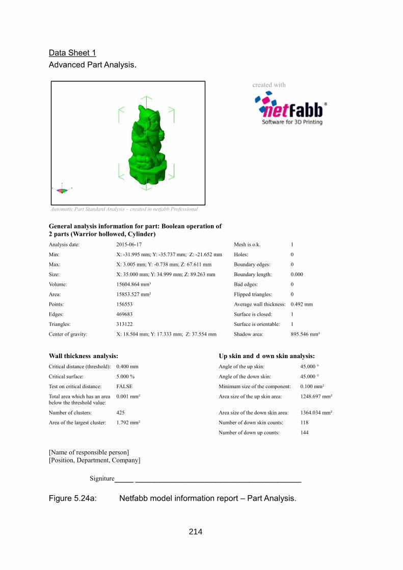
214

Data Sheet 1

Advanced Part Analysis.

Automatic Part Standard Analysis – created in netfabb Professional

created with

General analysis information for part: Boolean operation of

2 parts (Warrior hollowed, Cylinder)

Analysis date: 2015-06-17 Mesh is o.k. 1

Min: X: -31.995 mm; Y: -35.737 mm; Z: -21.652 mm Holes: 0

Max: X: 3.005 mm; Y: -0.738 mm; Z: 67.611 mm Boundary edges: 0

Size: X: 35.000 mm; Y: 34.999 mm; Z: 89.263 mm Boundary length: 0.000

Volume: 15604.864 mm³ Bad edges: 0

Area: 15853.527 mm² Flipped triangles: 0

Points: 156553 Average wall thickness: 0.492 mm

Edges: 469683 Surface is closed: 1

Triangles: 313122 Surface is orientable: 1

Center of gravity: X: 18.504 mm; Y: 17.333 mm; Z: 37.554 mm Shadow area: 895.546 mm²

Wall thickness analysis: Up skin and d own skin analysis: Critical distance (threshold): 0.400 mm Angle of the up skin: 45.000 °

Critical surface: 5.000 % Angle of the down skin: 45.000 °

Test on critical distance: FALSE Minimum size of the component: 0.100 mm²

Total area which has an area below the threshold value:

0.001 mm² Area size of the up skin area: 1248.697 mm²

Number of clusters: 425 Area size of the down skin area: 1364.034 mm²

Area of the largest cluster: 1.792 mm² Number of down skin counts: 118

Number of down up counts: 144

[Name of responsible person]

[Position, Department, Company]

Signiture____ ___________________________________

Figure 5.24a: Netfabb model information report – Part Analysis.

215

Data Sheet 2

Platform views.

Automatic Part Standard Analysis –

created in netfabb Professional

Platform Name:

Warrior hollowed and

hole. fabbproject

Report creation date:

2015-06-17 18:39

Parts on Platform:

1 parts ( 15604.864 mm³ )

Outbox Size:

35.000 mm

34.999 m m

89.263 mm

3D View

Created with netfabb Professional 5

[ Name & Signature ]

_______________________________

_______________________________

Date

Figure 5.24b: Netfabb model information report – Platform Views

216

These reports also included the possibility of adding the operator’s details

such as name, date and data file name, which were helpful in keeping

documented records of work progress. With the powder-bed laser based AM

machines, there were no internal supports to the models, so the outside walls

had to be made thick enough to be self-supporting, and these reports also

included such information about the walls. These reports, the Part Analysis report

and the Platform report of the “Warrior” model, produced by the software as Data

Sheet 1 and 2, see Figure 5.24a and Figure 5.24b, (Data Sheets 1 and 2).

5.9. Summary

As originally stated, the StudioPro® software was designed to prepare the files of

third party software into *.stl files for further AM fabrication. The software would

check for a number of common faults which occurred in the process of converting

photogrammetry images into point cloud data and reducing the number of shells

that may be created in this process. Using the automatic repair function, the

software would look for holes or badly aligned triangles/polygons, would correct

such faults, would smooth surfaces, and would prepare *.obj files. The software

would also import and convert the data from over 30 other types of data files,

leaving them ready to export into *.stl files for AM fabrication. If the repair function

was left unchecked, all holes would be filled, but any hole larger than 3mm

across, on the surface, would be flattened out in the repair process, and at that

point would be detrimental to the finished model, especially on a rough or

undulating surface. As seen in Chapters 6.2 to 6.4, repair to the mesh might not

be the answer; but retaking, adding photographic images and reprocessing the

image data set would be needed.

Conversely, if the area was on the underside which was a flat bottom

surface, this flattening effect might be beneficial. In Figure 5.25, the underside of

a trilobite fossil was repaired using the automatic feature and the large hole was

filled in by the mesh. Being the underside, this was the area on which the trilobite

stood on the turntable and no data could have been captured there. As this area

was flat, the large hole being filled in as a flat area by the mesh was beneficial to

the overall replication of the model. Resizing from either of the primary software

programs was straightforward as long as the correct orientation was first

217

established; this enabled the exact size of the original artifact to be replicated in

all axes.

Figure 5.25: Automatic mesh lines filling in the large hole of the Trilobite.

218

Chapter 6: Repair, reconstruction and construction

6.1 Repair of Noisy, Distorted and Incomplete Data

6.1.1 Returned Noisy data

When Method 1 (Chapter 4.1) was used to process the digitally captured images,

the returned processed point cloud image, as seen in Figure 6.1 (head identified)

had to be filtered, or cleaned, to eliminate background noise that had been

captured along with the original subject, such as other objects or furniture

(arrowed) that were in the line of focus when the image was recorded by the

DSLR. The software lasso tools allowed the user to highlight the area of the

section of image to be cleaned and delete it. Unlike the Agisoft process, where

the background was masked from the main subject, these background objects

were used by the AutoDesk cloud program to stitch and build the overall central

object.

Figure 6.1: Processed digital image ready to be cleaned.

The resulting processed textured 3D mesh might also show minor flaws or

distortions, which were then corrected using the methods described in Chapter

6.1.2 and 6.1.3. The processed photo-textured 3D mesh image head could have

been repaired using software, but by adding and increasing the number of

images, with more angled shots and greater image overlap, complex repairs to

the point cloud and textured mesh were eliminated. The additional photographic

digital images, once added to the original data set of images, were reprocessed

219

and sent by the internet to be cloud processed and returned ready to be

recleaned. By selecting the appropriate control in the editing section, a wire

frame, wire frame and texture, or texture only model could be obtained. This

would facilitate a limited amount of repair if required on the model.

6.1.2 Incomplete data

The main objective of the two primary software programs used in this research,

was to convert 2D images, in both cases, digital photographs, into 3D virtual point

cloud or textured images. In both instances the software programs contained

limited repair tools and were not designed to recreate parts of the image that

were missing.

(from Figure 4.10)

Figure 6.2: Hole under chin - automatic mesh repaired.

If, in the initial data collection, part of the artifact was missing and showed

up in the processed data image as a large hole, the software could fill in that hole

as a flat surface. If an object with a flat base was being photographed with the

object on a plinth, the bottom of the object could obviously not be seen by the

camera lens and that data would be missing from the data set. The software

repair commands allowed for this hole to be “filled in” but the polygons formed

would join the edges that were found into a flat plane. In the example of the flat

220

base object, this was acceptable, as a flat surface was needed to be replicated

for the base of the object.

Figure 6.3: Distortion on top of head.

However, if for example, the top part of a head was missing, this might show

up as a hole or as a bulge. In Figures 6.2 and 6.3 both problems occur, the first

hole, due to lack of data, and the second fault, a bulge (indicated), due to a small

amount of light reflection or flare. The hole under the chin (from Chapter 4.2.1:

Figure 4.10) was relatively small, (it was enlarged by the author so as to be seen

clearly in the screen shot), and the flat surface automatic repair merged with its

surroundings as seen in Figure 6.2.

Figure 6.4: Red polygons ready to be removed.

221

The bulge however, was not ideal to repair: although it was a simple matter

to remove the polygons that formed the bulge, thereby turning the image into a

mesh and deleting the rogue triangles (shown as light red in Figure 6.4 and

arrowed), this would have left too large a hole to repair without complicated

reconstruction of the mesh.

The option in this case was far more straightforward – more digital images

were taken and added to the original data set. Having “stitched” these new

images in to the data set (see Chapter 6.1.3), the whole set was then

reprocessed. As this was originally processed by 123D Catch® it was sent via the

internet back to AutoDesk.

6.1.3 Unglazed Ceramic Vase – a lesson in sewing

This example of an unglazed Ceramic Vase is very similar to the above problem,

in that after processing the original 52 images a large hole was seen to exist in

the returned data. Here was another case of not enough data having been

captured of the inner part of the vase. Another 17 images were taken with greater

emphasis on the inside of the vase.

Figure 6.5: Hole in Vase mesh due to lack of digital data.

Hole in mesh needing

additional photographic

images

222

It was found by experience that the chances for successfully matching

additional images were greatly enhanced if the “scene” was not disturbed, i.e. the

position of the vase in relation to the surrounding furniture or cloth on which it

stood. If the scene had changed then it was more difficult to match points. Of the

17 images taken, two were rejected as they were unable to identify the required

three points on the images. This meant that while the initial photoshoot data was

being processed, which could take more than an hour, the scene was not

disturbed. The data file returned was then examined for flaws, and, if all was

satisfactory, the “studio” was taken down or dismantled, unless more images

were required to be taken.

Figure 6.6: Inner Vase mesh now complete.

By turning the textured images into meshes, the fault and its repair were

clearer to identify (Figures 6.5 and 6.6). Figure 6.5 shows the result of processing

the original 52 images: a hole in the inside of the vase. Figure 6.6 clearly shows

that 15 extra digital images were needed to fill in the hole. The data image file

had now been completed, again without any complex software repairs being

necessary, and could be processed using the same procedure as with the Clay

Head. The outside and inside of the original vase was quite smooth and therefore

223

there was no loss of definition in the model made by the FDM machine. Although

this model was made to one quarter scale, a full size replication would no doubt

result in a true likeness.

Figure 6.7: Identifying and manually stitching/matching three

points to integrate additional digital images.

In Figure 6.7, three separate data images are seen with the subject, the

Vase, in sharp focus, but the large area surrounding the main subject is also in

very sharp focus. Three identifiable points were needed to match each image.

Point 1 was down on the floor by the door; point 2 was on the vase, and the third

identification, point 3, on the tablecloth on which the vase stood. This made the

identification of the reference points in each photograph easy to see and match,

either by the human eye or by the computer recognition software. It can also be

seen, that of the three identification points selected, only one is on the main

object. The other two are positioned on the surrounding background.

6.1.4 Repair using the Mesh

In the case of the Egyptian Vase, discussed in Chapter 4.9, although the images

produced a good result for the outside of the vase, there was an amount of

cleaning required in and around the neck opening (see Figure 6.8). As this was

only a small area to be cleaned, it was decided to repair the vase by cleaning the

Image 1

Image 2

New Image to be

point matched

with image 1 & 2

224

affected part using the mesh. The textured image was transformed back into a

mesh (Figure 6.9). The inside of the neck is seen in Figure 6.8 in its textured

form.

Figure 6.8: Area needing to be cleaned at mouth of Egyptian Vase.

Deleting the small triangulated polygons as seen in the enlarged screen

shot, (Figure 6.9) was a simple but tedious task well within the capabilities of

StudioPro® and an operator.

Figure 6.9: Working with a large scale mesh – Egyptian Vase.

At an enlarged scale each polygon or group of polygons was easily

identified, highlighted (indicated in Figure 6.9) and deleted. The holes in the side

225

of the neck of the vase, which were caused by deleting some of the triangles,

were so small that the repair blended in with the original sides without any

additional problems being created. Having removed the “noise” from the neck,

the next process was to hollow out or shell the vase, so as to use less material

and reduce the weight.

Finally, having made a very accurate measurement of the neck diameter of

the vase, a cylinder was created to this exact size. Using the Boolean tool, as

described in Chapter 5.7, the cylinder was placed in the neck opening and

subtracted from the whole. This took several attempts at placing the cylinder in

exactly the correct location, but when finally achieved, a clean opening through to

the hollowed body of the vase was created, ready for 3D fabrication.

6.2 Damaged Digital Images Beyond Repair

Of the many objects that were processed in the course of this research, there

were a few items which proved impossible to capture satisfactorily and simply,

using the digital methods employed, without further research into the problems

which affected these items. Koutsoudis et al. lists a selection of “friendly

materials” which are good for photogrammetric purposes and a list of “non-

friendly” materials such as water, glass, varnish, steel and many more [164]. The

main cause of these problems was light reflection off the surface of the artifacts.

These flares could not be processed by the software and caused distortion in the

digitally processed image. Even lowering the light levels as discussed in Chapter

4.2.3 did not produce the required result (i.e. this did not produce images which

could be processed).

This problem occurred on surfaces such as glass, glazed china or porcelain,

or any surface which had been polished, varnished or had a light reflective

surface. The problem could possibly be overcome, as suggested by Porter [165],

by coating the surface with fine powder chalk or talcum powder. The powder was

suspended in alcohol or acetone and sprayed on any of the artifacts which were

translucent or had a shiny surface, producing readable features, especially if then

processed using the High resolution setting in PhotoScan Pro®.

However, this method was still invasive, whilst this research used only non-

invasive methods. If invasive methods had been used, talcum powder would no

doubt have led to all types of non-reflective water soluble coatings being used,

226

but it was not how this research intended to photograph the artifacts. It could then

be argued that what was being photographed was a fine layer covering the

artifact and not the artifact itself. Although the coating was removable with water,

it was not felt that the curator of the Kendal Museum, or any other reputable

curator, would have taken kindly to giving Sobekhotep or any other c.3,500-year-

old artifact a wash under the tap.

Shown below (Figures 6.10 to 6.19) are the results of some of the failures

(fortunately there were not many), the original images having been placed

alongside the point cloud or textured digital image for comparison. Table 6.1 lists

the ten items and has identified the problems encountered, with some

explanations as to the cause. It also shows how each artifact was processed.

Table 6 .1: Reference table for original and failed artifact point cloud images.

Processed with 123D Catch® PhotoScan Pro®

Figure K.01 Serenity Item – G.03 Item – J.32

Figure K.02 Dolphins Item – G.04 Item – J.33

Figure K.03 Glazed Vase Item – G.06

Figure K.04 Mollusc Item – G.08

Figure K.05 Frosted Bottle Item – G.11 Item – J.34

Figure K.06 Ceramic Vase Item – G.17

Figure K.07 China Dish Item – J.39

Figure K.08 Batwing Sea Shell Item – J.54

Figure K.09 Lincrusta - Acanthus Item – G.18

Figure K.10 Lincrusta - Aphrodite Item – G.19

By way of explanation of Table 6.1, the Figure numbers on the left refer to

the photographic images within the table. Each named item may have one or two

Item numbers which would refer to the numerical order in which they were

processed (Item – Appendix J - J.03). The first Item number (e.g. Appendix G -

G.03) refers to the artifact being processed by 123D Catch®. If there is a second

Item number (e.g. Appendix J - J.03), the same artifact would have been

reprocessed using PhotoScan Pro®.

The full numerical Item sequence of all 58 photographic images can be

seen in Appendices G and J.

227

Table K.1:- “Capture data Log – Failed Artifacts” - Appendix K. This table

records the full numerical Item sequence of all 12 failed photographic

artifacts, day to day record and evaluation.

Table K.2:- “Photographic images of Failed Artifacts” - Appendix K.

6.2.1 Figure K.01 - Serenity – Items G.03 and J.32

Three attempts using 123D Catch® were made using Serenity and another five

attempts using PhotoScan Pro® (Appendix K - Table K.2: Figure K.01). Some of

the problems that occurred using this software have already been discussed in

Chapter 4.4.3.

Figure 6.10: Figurine - textured point cloud image - rough, spikey surface.

At a later date, the first two data sets that had been shot for 123D Catch®

processing, were processed by PhotoScan Pro®. The first attempt had been shot

at f/14, had 71 images and produced a better result than the original, whilst the

228

second attempt, shot at f/8 with a few more images added, did not give a good

result, as the shallow DoF only helped the image to merge with the background

(Appendix K - Table K.2: Figure K.01a).

Reshooting a further three digital sets, increasing from 92 images to 145

images, stopping down from f/18 to f32, and pre-process masking produced a

“good” result. However, on careful examination of the screen shot of the digital

image of the *.obj file (see Figure 6.10), the surface had a rough, spikey finish

(highlighted by the arrows), which would have needed sanding down in post-

processing to achieve a smooth finish. This High resolution digital image (Figure

6.11) could possibly have been improved by careful manipulation and cleaning of

a reprocessed Ultra High resolution point cloud image, as seen from the

PhotScanPro4® screen shot.

Figure 6.11: Figurine - High resolution point cloud image.

229

However, this would have added a couple of hours to the processing time

and would have required some very careful deleting of the highlighted point

cloud. So the result was “good” but perhaps not good enough.

6.2.2 Figure K.02 – Dolphins – Items G.04 and H.33

Four attempts were made to capture the Dolphins; two using 123D Catch® and

the other attempts with PhotoScan Pro®. Good sharp images were produced

(Appendix K - Table K.2: Figure K.02), but the reflective light from the semi

polished wood surface of the statuette produced the distortions as seen in

Appendix K - Table K.2: Figure K.02a. These two sessions were all shot at f/18,

initially with 64 images, then adding by stitching into the data set another eight, to

make it 72. Although the camera was set on automatic for the shutter timing, on

inspecting the camera log data this returned an average time of 2 seconds per

frame. The results were not greatly improved with a green Chroma Key backdrop,

although masking was not employed before the PhotoScan Pro® process began.

Reducing the f/stop even further would have increased the time per frame even

more than 2 seconds. Adding the masking frame before processing might have

been beneficial, but the time factor would certainly have been increased, both in

pre-processing and in digital capture.

6.2.3 Figure K.03 – Glazed Vase – Item G.06

This vase was semi glazed (polished) on the outside but the inner surface had

been given a high gloss white glaze (Appendix K - Table K.2: Figure K.03). Three

attempts were made, including photographic stitching, which produced 61

images. A further attempt to stitch additional images to the data set failed. It can

be seen from Appendix K - Table K.2: Figure K.03a, the final images were badly

distorted including holes in the side. No further trials were possible as this item

was not amongst the author’s permanent collection, nor was it possible to regain

access to the item.

6.2.4 Figure K.04 – Mollusc - Item G.08

This item was one of the most difficult to process, 123D Catch® was the only

software to be used and was unfortunately not at all suitable for the job in hand.

The mollusc (Appendix K - Table K.2: Figure K.04), was a very complex shape

230

which twisted and spiralled. Seven attempts were made, increasing the number

of images from 43 to 73 images at each session, including alteration to the f/stop

between f/4.8 to f/11 and adding additional photographs to the data sets by

stitching. The image, which is a mesh and textured mix, shown in Figure 6.13,

was the best result available from the series, but the arrows show the white mesh

areas which would need repairing. As this item was only in the author’s

possession for a short time, it was not possible to re-process it. If more

photographic images could have been added to the original 123D Catch® data

set, which might have helped; as might using PhotoScan Pro® with a turntable,

and photographing it from much closer positions with smaller f/stops, perhaps as

small as f/22, to give greater DoF and therefore sharper images. Also by applying

masks to the pre-processed data the background “noise” would have been

eliminated helping the overall processing.

Figure 6.12: Mollusc - High resolution textured point cloud image.

It would have been possible to repair the mesh automatically by allowing the

software to fill in the gaps, but this would have produced smooth flat areas. The

complex surface texture as seen in Figure 6.13, which is an enlargement of the

231

original surface texture, would not have been replicated in these repaired areas

and the integrity of the artifact would have been compromised. To repair the

mesh by hand would have been impractical with the software being used,

because, as stated previously, this was not the intended use of this particular

software and it did not possess the tools which would be required to be used.

Figure 6.13: Enlarged surface texture of original Mollusc –

note the ridged surface.

6.2.5 Figure K.05 – Frosted Bottle - Items G.10 and H.32

Three data sets were photographed and processed with 123D Catch® and four

sets with PhotoScan Pro®. The first attempts tried indoor and outdoor natural

lighting, using both newsprint and spotted cloth for the background in order to

help with the computer stitching of the images. Between 34 and 61 images were

shot per session but all processed data sets were equally distorted. The results

were slightly better with PhotoScan Pro®. The f/stop was lowered to f/22 and

rotated 15° on the turntable to obtain 89 images. Two masked and two unmasked

data sets were processed. The final masked set showed the best results (see

Appendix K - Table K.2: Figure K.05a), where the screw top and label on one

side of the bottle are relatively clear.

232

6.2.6 Figure K.06 – Ceramic Vase - Item G.15

The Ceramic Vase was one of the first artifacts to be processed using 123D

Catch®. This vase was photographed in a low level of natural light in the outdoor

walk-in light tent. In hindsight, the DoF was too shallow, hence the top double

image; also there was reflection off the top glazed band causing some distortion

to the images (Appendix K - Table K.2: Figure K.06a). 72 images were taken, of

which six were restitched back into the original data set. The artifact is no longer

in the author’s possession or a smaller aperture and half neutral filter might have

been tried, using the turntable and pre-processing masking.

6.2.7 Figure K.07 – China Dish - Item H.37

Apart from the black square and white elephant, there were no discernible

patterns or markings on the dish, which was white with a gold edge. Two

attempts using PhotoScan Pro® were made, but the first data set did not build at

all. The aperture was stopped down to f/29 and pre-processing masks were used.

The result is seen in Appendix K - Table K.2: Figure K.07a. The centre black

square with the elephant has emerged as a whole section. Apart from the high

gloss, which can be seen to have cause an orange peel type surface, there were

very few points on the original images which the computer software could identify

and match. Ground markers placed around the dish might have helped this

matching process. Green Chroma Key was used with 15° rotation on the

turntable and 73 images were taken.

6.2.8 Figure K.08 – Batwing Sea Shell - Item H.50

In this example, the Batwing shell, two very different surfaces existed on the

shell, the front being mother-of-pearl, smooth, silvery and quite shiny, giving off a

lot of reflected light, whilst the rear of the shell was very rough, and a matt

surface. This shell amassed 160 photographic shots using a wooden stick to

support it on the rotating turntable.

Using a fixed focus of f/22 allowed for less light to enter the camera and a

greater DoF to be obtained. The shutter speed was set to automatic but this did

not help to eliminate the light reflecting from the front of the shell. On examination

of the Metadata from the digital image, the speed of the shutter increased from

between 3 and 2.5 seconds for the darker side of the shell to between 0.25 and

233

0.5 seconds for the shiny side. In the Appendix K - Table K.2: Figure K.08a and

also Figure 6.14, the smaller photograph shows highlighted areas picked up by

the camera lens, whilst on the enlarged screen shot of the point cloud image,

indicated by the dotted line, can be seen an orange peel effect (indicated) which

the reflective surface has caused to the computer generated processed image.

Figure 6.14: Smooth shell surface of original to orange peel effect on digital image.

6.2.9 Figure K.09 - Lincrusta – Acanthus - Item – G.16

Figure K.10 - Lincrusta – Aphrodite - Item – G.17

In 2014 the Engineering Department at Lancaster University were involved in a

project with a local company in Morecambe, believed to be the only company left

that still made this original Victorian wall covering. Invented by Frederick Walton

as a development of the floor covering Linoleum, it became one of the many

Victorian success stories that is still used in the 21st century.

“Lincrusta was launched in 1877 to instant success in a host of

applications from royal homes to railway carriages. Heralded as the

first washable wallcovering, it appealed to Victorians because of its

sanitary properties as well as its durability and ornate

234

effects………Originally launched as "Linoleum Muralis", it was

subsequently re-named "Lincrusta-Walton" − Lin for Linum (flax, from

which linseed oil is made) and Crusta (Relief), with the inventor´s

name being added to prevent other firms using the same title.” [198]

Having digitised the Relief painting (Figure 2.23 and 3.27), these two

Lincrusta samples presented a challenge. The difference in surface texture was

different in that the painted relief was far more pronounced than the Lincrusta.

The ridges that had been crafted on the painted canvas surface were over 10mm

deep in places; whereas the raised relief on the Lincrusta was from 0 to 1.5mm

high off the flat surface with no negative relief at all. Both pieces of Lincrusta

were photographically processed in exactly the same way and both measured

550mm x 460mm x 3mm thick. The items were hung on the wall, suspended by

spring clips, and a string was run through the clips to form a triangular hanger.

The same method was employed to digitally capture the images in the

Relief canvas, Figure 3.27 as described in Chapter 3.9. The camera was moved

in an arc, at approximately 130mm away from the centre of the Lincrusta. On

average, good results were obtained taking between 60 and 65 images at f/14 or

f/16 on both Items. If the f/stop was opened to f/8, either blurring occurred or only

half the image was captured. Both were processed using PhotoScan Pro® at a

high resolution setting. Good *.obj resolution screen shots were obtained but

these degraded when the file was saved and converted to an *.stl file.

Figure 6.15: Part of a roll of Lincrusta – Design “Acanthus”.

235

The dark areas on the screen shot of the *.stl file image (Appendix K - Table

K.2: Figure K.09a), processed in StudioPro® show a negative layer below the

surface. The author would not recommend printing the Lincrusta as seen in

Appendix K – Table K.2: Figures K.9 or K.10 unless a fine micron printer were

used in the order of 16µm or less.

In a recent project, in October 2015, set up by the British Ceramics Biennial

[199], artists and potters were invited to create new designs using CAD. It was

hoped that by submitting the final design in the form of an *stl. file, and by using a

ceramics 3D Systems printer, modern technology in the form of AM fabrication

would lead the way, away from the tradition of water, clay and potter’s wheel. It

was hoped that whilst the exhibition was in progress several items would be

created in front of the viewing public. One of the stipulations or suggestions that

was made about any relief work on the surface of the artifacts that were created

was that a height/depth of 3mm was the minimum that was needed to be

successfully fabricated and be seen on the artifact. So, in the light of this

recommendation, 1.5mm was perhaps too fine a relief on the Lincrusta to be

printed successfully.

6.3 Summary of Repaired Data Images

In many of the artifacts that were photographed, common problems occurred, for

example, as shown in Figures 6.2, 6.3, and 6.5. Some of these problems were

identified and were resolved as examples discussed in Chapters 6.1 to 6.4, but

several recurring themes regarding very complex shapes, glazed surface objects,

and highlights caused by light reflection are still to be resolved, which are

discussed in Chapter 9. Several of the items that were used in this research were

unfortunately not in the author’s possession long enough to be re-examined and

reprocessed, for example, the ‘Mollusc’ was only processed with 123D Catch®

and not PhotoScan Pro®, which might have proved a better method of data

capture. Although the results with the item ‘Serenity’ were not perfect,

improvements were achieved and this might have also been true of the ‘Dolphins’

had longer time been spent, with more data images captured and lower lighting

levels used. The author would be most interested in investigating a method

suggested by Nicolae et al. [200] of using cold lamps and circular polaroid (CP)

236

filters on both lamps and camera, this cross polarisation reducing the amount of

(speculative) light hitting the camera sensor.

However, AutoDesk [6] in its very good and well-presented beginners’

tutorial guide to the art and tricks of producing 3D images, warns that:

“plain, reflective or transparent surfaces or objects will not work.”i

The answer remains to be found, using artifacts such as the high glazed

‘China’ dish and the glass bottle, with more advanced programs and hardware

than were the aim of this research.

6.4 Removing Flare/Glare and Reflection

It was noted in Chapters 6.2.1, 6.2.2 and 6.2.8 that excessive reflection caused

problems with the processing of the digital files of several artifacts. In this sub-

chapter, two methods are investigated which greatly help in solving the problem

of flare and light refection.

6.4.1 Polarising Filters

There are two types of polarising filters which can cut down direct reflections and

increase colour saturation of an image. The CP filter screws onto the front lens of

the digital camera in the same way as most other filters. It is different from the

linear polarising filter in that it has been designed to function with the digital

metering and autofocus system of the DSLR camera and linear filters are also

cheaper than the circular filters. Many manufacturers identify their circular

polarising filters with the CPL or PL-Cir letters on the rim of the filter. The

polarising filter works on the principle of filtering light, usually from the sun or sky,

coming from a direction perpendicular to the reflected light. Rotation of the lens

will cut the light or glare from a reflective surface such as water, glass,

vegetation, or indeed most surfaces except metal or others that are highly glazed,

which will reflect light. Usually this rotation is about 45-50º. The filtered light

allows the ‘natural’ colour to show through from the surface, intensifying the

colours.

237

Figure 6.16: Without CPL filter - Focal length 36mm @ f/11 @1/1.6s.

Figure 6.17: With CPL filter - Focal length 36mm @ f/11 @ 1/1.3s.

238

However, outdoors under very cloudy skies, as in Chapter 3.8.1, a CPL filter

may not work at reducing glare, as there may be very little light reflection, and it

may only perhaps intensify the colours by increasing the contrast. As shown in

Figures 6.16 and 6.17, the photographs were taken under partly cloudy skies with

the sun trying to break through; when turning the CPL lens until the best result

was obtained, the wet flag stones and the glass roof of the conservatory showed

the greatest changes, removing the reflection from both glass and wet stones.

Unfortunately, CPL filters do not work under artificial light conditions which

are normally used within the studio environment, except perhaps as a neutral

density filter (see Chapter 3.3.), so these would only be of limited use, unless the

artifacts were outdoors under natural light.

6.4.2 Testing CPL Filters - Artificial Lighting

A test was conducted to see if a CPL lens made any difference to glare or

reflections, on the highly polished wooden base of the figurine ‘Serenity’, under

artificial lighting conditions. In Figures 6.18 to 6.20 the focal length (fl) of 48mm

was the same in all three images, as well as the aperture setting of f/11; only the

shutter speed changed, automatically by the camera.

Figure 6.18: CPL filter not rotated

Figure 6.19: CPL filter rotated

Figure 6.20: No filter

fl/48mm @ f/11 @ 2.5sec. fl/48mm @ f/11 @ 3sec. fl/48mm @ f/11 @ 1sec.

In Figures 6.16 and 6.17, a Polaroid filter was used, whilst in Figure 6.18,

the lens was not rotated from the perpendicular. In Figure 6.19, the lens was

rotated approximately 50º from the original position and in Figure 6.20, the CPL

lens was removed. As can be seen by comparing the three photographs, Figures

6.18 to Figure 6.20, the highlights on the polished base have not significantly

changed. Figure 6.18a to 6.20a are enlarged images of the original for clarity.

239

Figure 6.18a: Enlarged image - CPL filter not rotated - fl/48mm

@ f/11 @ 2.5sec - artificial lighting.

Figure 6.19a: Enlarged image - CPL filter rotated - fl/48mm

@ f/11 @ 3sec - artificial lighting.

Figure 6.20a: Enlarged image - No filter - fl/48mm @ f/11 @ 1sec – artificial lighting.

240

6.4.2 Testing CPL Filters - Natural Lighting

In Figures 6.21 to 6.23 the same test was conducted but this time in natural

daylight, with cloudy but bright skies. The settings for both the focal length and

aperture were set and fixed, leaving the camera to automatically compensate for

the changes in light by shutter speed alteration. The reflection on the top side of

the wooden plinth and highlights on the lower front rim (as indicated by the black

arrows on Figure 6.21), can be seen in both Figures 6.21 and 6.23. As indicated

in Figure 6.21, are features being almost identical in both images, but in Figure

6.22 the reflection on the top side has disappeared and the highlight on the lower

rim greatly diminished.

Figure 6.21: CPL filter not rotated fl/48mm @ f/11 @ 2.5sec.

Figure 6.22: CPL filter rotated fl/48mm @ f/11 @ 3sec.

Figure 6.23: No filter fl/48mm @ f/11 @ 1sec.

This simple experiment demonstrates that the CPL filters are far more

effective in reducing highlights, flare and glare, in natural daylight than in artificial

light. Figure 6.21a to 6.23a are enlarged images of the original for clarity.

241

Figure 6.21a: Enlarged image - CPL filter not rotated –

fl/48mm @ f/11 @ 2.5sec - Natural Lighting.

Figure 6.22a Enlarged image - CPL filter rotated – fl/48mm @ f/11 @ 3sec - Natural Lighting

Figure 6.23a Enlarged image - No filter - fl/48mm @ f/11 @ 1sec - Natural Lighting.

242

6.5. Digital Negative Editing Software

To understand how editing software can be useful in post-processing the

dataset that has been captured by the camera, an appreciation of the differences

between the types of files, RAW, Jpeg and Tiff, is required. For a greater in-depth

understanding and explanation of file formats and the differences between them,

reference books such as by Murry et al., Encyclopaedia of Graphics File Formats,

are a valuable source of information [201].

6.5.1 File Format

The imaging sensor of the standard Nikon D3100 camera (the camera as used

for this research) captured two types of file: NEF and Jpeg. The NEF (Nikon

Electronic Format) is Nikon’s version of the RAW data file format. In addition to

capturing all the digital image data, it provides additional information about the

lens and camera identification, including the settings, time and date, and in more

advanced camera models, GPS references. Both types of file format are written

to the memory card. For hereon the RAW format acronym will be used as being a

universal format, as opposed to NEF, which is camera specific [142].

All the images which came directly from the camera as “camera ready”

images were Jpeg files. The Jpeg file can be directly read by the most basic

digital photographic software, which turns the captured data into the pixels that

are shown on computer monitors. These files can be directly processed by digital

printers straight from the memory card to produce a ‘hard’ copy photograph.

Conversely, RAW files are unprocessed data, which must be read and converted

by more specialist software, which transforms the data into files that can be read

by a host of other software, such as Gif, Eps, Pdf, Psd, Bmp, Jpeg or Tiff [202]

[203]. The two file formats most relevant to this research are Jpeg and Tiff and

unlike some of the other formats, they are not program specific, but rather

universally imported to most photo-editing software.

Apart from cropping the images (Figures 6.18 to 6.23), the contrast was

slightly enhanced so as to show the effect more clearly of the CPL filter under two

sets of lighting conditions. The prime cause of manipulation was the filtering of

light before the images were recorded by the camera’s processor. But as seen

from the images taken under artificial light, the CPL had very little, if any, effect

243

on the highlights and reflections seen in the finished images. There is, however,

another tool which can be used to pre-process the digital images before the data

set is processed by the point cloud converting software.

As discussed in Chapter 4.11.3, the imaging sensor of the digital camera

records information on many aspects of the digital image. This unprocessed data

is called “RAW data”, and is commonly referred to as ‘RAW image’ or ‘Camera

RAW’ files. The term ‘Digital Negative’ an expression arguable coined by Thomas

Knoll, the developer of Adobe Photoshop, and is often used to mean an

unprocessed RAW image similar to that of an analogue film. It goes back to the

original concept of the non-digital ‘Roll film’ camera in which a negative image

was exposed but unprocessed, prior to the chemical development stage, which

would finally produce a positive photographic print. Both type of images share in

the similarity that neither unprocessed image can be used or evaluated until

further processing.

Many standard DSLR cameras can export the data in its unprocessed

RAW form, or compress the data to another format, such as a Jpeg file. The Jpeg

format will have some of the data compressed, which cannot be manipulated,

whilst other sections of the data are accessible by post-processing editing

software programs such as Photoshop Elements 11® (PSE) [204], Photoshop

CS5/6®, Lightroom® [145] and Camera Raw®, to name but a few. The

compressed Jpeg file is processed in the camera and written to the memory card

as a file, which can be used immediately and downloaded directly to a printer

without further processing by a computer. RAW files differ in that all the data is

written to memory and none of the details are compressed but do require further

processing before an image can be obtained. Both forms can be post-processed

by the preferred editing software, but with the RAW files, there is more

information contained in the file which is accessible to be edited [171] [205].

There are five formats that the D3100 can process and the operator can

choose any one of them by selecting the “Image Quality” menu on the camera

and opting the desired format. These options are laid out in Table 6.2.

244

Table: 6.2 Image Quality Options [142].

RAW 12-bit NEF (RAW) files Best quality and creative flexibility

Fine# 8-bit files compression

ratio 1:4 Suitable for prints of Tabloid/A3

Size 4608x3072 pixels

Normal# 8-bit files compression

ratio 1:8 Suitable for prints of A4

Size 3456x2304 pixels

Basic# 8-bit files compression

ratio 1:16 Suitable for email or website use not for printing - 2304 x 1536 pixels

RAW & F Two copies of same image are recorded: one RAW one Fine# #Denotes Jpeg image

6.5.2 Editing the Data, Post-processing

If a potential problem in point cloud processing of the photographic data set of the

artifacts is envisaged, then the decision must be taken as to what post-

processing work is to be carried out on the dataset of images. The best option for

the digital set is the RAW format. Although this editing is not intended to produce

printed images, the point cloud processing still requires high quality images and

as seen in Chapter 6.2, the problems encountered of high reflection and flare can

cause serious deformity to the finished virtual 3D model. The dataset will be

checked by the point cloud processing software for quality (as already discussed

in Chapter 4.8). If the majority of photographic images fall below 0.5 when

scanned by the ‘Quality tool’, then the point cloud process is likely to produce

deformed results.

The list of options that exist within the post-processing editing software

programs depends on the complexity of the selected software and are beyond

the remit of this discussion; some of the manuals that have been written dealing

with these issues are referenced within this chapter. To dwell on a few that are

directly relevant to this chapter will give a flavour of what is possible to achieve by

an experienced operator using editing software. One of the basic

recommendations from Agisoft is not to crop or geometrically transform the

images, so although one might be tempted to crop the dataset to get a larger

magnification, such action will totally confuse the processing software when trying

to stitch the 2D photographic data together. If it is felt that better results will be

achieved with larger images, then the camera must be moved closer to the

subject, or the focus length must be adjusted.

245

The following editing software programs were used throughout this

research to enable post-processing: PhotoShop Elements 11, which is a simpler

version of Adobe Photoshop CS6® and Lightroom®`. These programs are

considered Industrial standards, in their own right; AP CS6 is Adobe’s “flagship”

and PSE is aimed at the hobbyist and domestic markets. PSE can achieve some

degree of editing and many of the features such as Contrast, Colour correction,

Image Sharpness and Light Adjustment can be achieved automatically by PSE,

as well as a certain amount of operator control. The white balance of a RAW

image (not Jpeg or Tiff) can be altered in PSE as well as Shadows, Brightness,

Contrast, Highlights together with many more tools which are relevant to editing

the digital images before post-processing to remove or lessen the effects of flare

and reflection. However, one of the main differences between the programs,

which would affect the time taken in editing, say, 130 images in a typical dataset,

is the ability in CS6 and Lightroom to synchronise and copy automatically any

edited alterations made to one image, across the whole of the dataset images. At

the same time as saving the new altered images to a new directory in a new

format, usually Tiff or Jpeg, the original RAW images are preserved in the original

unaltered format [205] [171]. If PSE was used, the settings of each editing

enhancement would have to be recorded manually, and transferred to the next

image, one by one. This would be a long and tedious operation. Each image file

would then have to be resaved with a different name and in a new format (Tiff or

Jpeg) so as to ensure the integrity of the original RAW data files.

If in photographing the artifact, none of the problems that have been

discussed seem to be present, then by shooting the dataset in Jpeg Normal or

Fine format, elimination of the additional post-processing stage will be achieved.

If on the other hand potential problems are envisaged RAW format should be

used.

6.6 Overview of other uses and benefits

In this chapter, several items were examined which required the processed data

image to be repaired for a variety of reasons where there had been a shortfall in

the original digital data that had been collected and processed. The following

examples discussed in this chapter, show how it is possible to repair artifacts

246

where the original item had been damaged, as in the photo frame (Figure 6.15) or

where part of the object had been lost, as in the missing crown on the statuette of

Horus, in Chapter 6.7, Figure 6.28. The starting point for both objects was the

same: digital collection and input of the collected data into the primary software,

PhotoScan Pro®. The secondary software, StudioPro®, was used to repair the

photo frame, whilst a third software, SolidWorks was used to recreate from

researched drawings, two versions of Horus’s crown.

6.7 Repair of broken Photographic Frame

The original Photo frame had been painted in gold, which presented two

problems, the first being that light would be reflected off the gold and would

degrade the quality of the digital images captured due to issues as discussed in

other chapters. To overcome this problem, the solution would have been to spray

the whole frame a neutral matt colour such as rust red, which itself caused the

second problem: this action might have caused the purists to strongly object as

this was a very invasive method of preparing the artifact for the photographic

digital data capture.

Figure 6.24: Photo frame missing corner. Figure 6.25:

Damaged corner of frame removed.

Uneven

holes in

frame

247

This problem has been discussed in this Chapter 6.2, and in that instance,

such a method was rejected. The overriding factor in the current situation, was

that the frame was broken as seen in Figures 6.24 and 6.25. If a renewed section

was to be grafted onto the original, in this case an AM fabricated white nylon

material, the new part would need to be painted by hand or spray gun and

blended in with the rest of the picture frame to complete the repair.

The obvious course of action was to repair the frame, attach the newly

made part in place, smoothing the joint and covering the whole repaired frame

with undercoat paint, then repainting entirely in gold. Due of the complex nature

of the frame, 112 images were digitally captured and processed to produce an

*.obj file, which in turn was imported into StudioPro® so as to repair the frame. In

addition, a thin prop was used to support the frame on the turntable. This

positioned the frame at an angle from the horizontal plane of the turntable with

the possibility of distorting the images.

Figure 6.26: Digital image of frame. Figure 6.27: Frame mask.

248

When positioning the camera for the first rotation of the turntable, this had to

be compensated for so as to maintain a 90° angle with the revolving frame. A

dark grey card was also inserted into the picture aperture, as shown in Figure

6.26, to stop the background from showing through. By using a mask (Figure

6.27), the support and centre grey card were eliminated from the digital image.

Figure 6.28: Mirrored corner of frame.

Processing the digital set with the inclusion of a wooden prop, presented

similar problems and solutions, as were used and discussed in Chapter 4.10.1,

but in this case the prop was much thicker (see Figures 4.44 and 4.45). By close

observation, it was noted that the illuminations and carvings on the frame were

not symmetrical, nor mirrored. Being hand crafted, this was not a surprise (note

the variation in hole size as indicated on Figure 6.24). In a similar slicing process

as used with the Warrior (see Figure 5.12) the damaged corner of the frame was

removed (Figure 6.24). The undamaged corner was then copied and mirrored

(Figure 6.28). In Figure 6.29 the white line also indicates the join between the

frame and corner.

249

Figure 6.29: Small discrepancy on the frame to be rectified.

Figure 6.30: Reverse of the repaired frame.

The black arrow indicates the small under-sizing of the copied mirrored

corner, which needed to be corrected, this being due to the fact that the two

corners, being hand carved, were not symmetrical. In Figure 6.30 the join as seen

from the reverse; being relatively flat and smooth, the join is hardly noticeable. To

give added strength and reinforce the joint, small strips of plastic would have

been glued across the join. However by scaling the new corner piece in one of

the three directional planes and with slight repositioning, the mirrored corner

piece was made to fit and the damaged corner was replaced. As these two

corners were not identically symmetrical, it did mean, however, that the repair

would need hand-finishing to smooth out any imperfections where the new corner

piece had been joined to the main frame, which was most prominent on the

250

carved face side. It should be noted that the two top holes in Figure 6.31 are now

identical and the top corner motifs are identical, being mirrored.

In the final stage of this repair there were two options:-

1. To fabricate the revised corner piece using AM and attaching it to

the original frame. This would have entailed cutting away the damaged corner of

the frame at exactly the correct angle, gluing on the new AM corner and as

mentioned, reinforcing the joint, then hand-finishing by filling and blending an

epoxy resin if required (this material being better than plaster of Paris as it has a

better thermal expansion, and the contraction of the plaster could lead to it falling

away from the frame) finally undercoating and respraying with gold paint.

Figure 6.31: Repaired Frame.

2. As the original frame had been digitised, it would now have been

possible to digitally join the corner piece to the frame using the Boolean option in

the software. The file would then have been converted to an *.stl file ready for the

AM machine. As the original size of the photo frame was only small,

approximately 205mm x 280mm, this was a possibility; however, for large portrait

or landscape frames whose size may go into two or three metres, option 1 might

be preferred as these large sizes may have proved too expensive to print, apart

from the difficulty of finding a machine with a platform size that could

accommodated such a large frame.

251

6.7.1 The Stair Stepping effect

A third problem that could occur, which is applicable to any repaired artifact as

well as “new” build, is the “stair stepping” effect (see Figure 8.2 – FDM dog and

Figures 8.5 and 8.6 – Mcor paper bonded cat). If an FDM or sheet lamination type

of AM machine is used, a more distinctive stepping effect will occur than with the

use of SLS or SL machines. If the surface is quite intricate, FDM or sheet

lamination may not be suitable either for a repair or new build of a model without

post-processing of the surface.

6.8 The Egyptian Bowl

In the above example, a section of the original artifact was removed, mirrored and

then grafted on to replace the missing section of the original artifact. Using the

same software as above, a repair to the Egyptian bowl was possible. As long as

the damaged artifact was reasonably symmetrical and uniform in its design, it was

possible to merge a complete copy of the original artifact and combine the original

and the copy into one item. In the case of the bowl, the copy was rotated between

90° and 135° (by trial and error), until the damage as seen around the rim were

offset from each other and when combined into one, disappeared.

Figure 6.32: Copy and original bowl, combined and

then off-set to facilitate repair.

252

In Figure 6.32, the dark and light shaded parts of the image are the two

whole 3D images merging. It was the same with the large V shaped piece that

was missing from one side (Figure 6.32).When the copy and original bowl were

combined, this missing V-piece also merged into one. The merge was performed

by using a Boolean function, in this instance to add two pieces together, as

opposed to subtracting.

Figure 6.33: Trimming the rim of the repaired bowl.

The original ancient Egyptian bowl was not perfectly symmetrical and the

copy did not superimpose 100% over the original. Therefore, very minor cleaning

was carried out by way of using the cutting function to slice off less than 1 mm

from the rim and the base. In Figure 6.33 the outer top rim was trimmed by using

the cutting plane in the software.

253

Figure 6.34: Underside of bowl.

Figure 6.35: Inside of new bowl.

On close examination this new bowl still had some imperfections and

blemishes on the inside and around the rim and these can be seen as indicated in

Figure 6.35, which under the circumstances was not such a bad thing, as the

replica bowl was supposed to appear to be 3,500 years old. The final action using

254

the software was to convert the file to an *.stl format ready to be fabricated using

additive manufacturing. When manufactured, fine grain sandpaper was used to

put a very small bevel around the top rim and to smooth off the edge of the

bottom stand.

6.9 The lost Crown of Horus

It was during the “Egyptian period” of the author’s research, and whilst

processing the three Egyptian artifacts from The Kendal Museum collection, with

Egyptology in mind and whilst rummaging in a flea market, that the modern

statuette of Horus was found. Presumably it had been produced as a memento or

souvenir for tourists on the Egyptian tourist trail, a statuette made for the tourist in

the Valley of the Kings discovering the mysteries of the Pyramids and Nile.

Figure 6.36: Horus minus his Crown. Figure 6.37: Point cloud image of Horus.

Unfortunately time had not been good to Horus, for he was crownless

(Figure 6.36). Upon examination, one could see the flattened skull where the

crown had once been attached. The question was whether RE and AM

255

techniques could be used to reinstate his majestic status. Using the same

techniques as those employed to replicate Sobekhotep, a model of Horus could

be created - that was not a problem, except that this technique could not be used

on negative space. As the crown was missing, it could not be copied. Figure 6.37

is a screen shot showing the 3D point cloud image after having processed 145

digital 2D images. A 3D graphics drawing program would have to be used to

create a crown for the statuette. The selected program to be used was by

Dassault Systems called SolidWorks®.

Figure 6.38: Four styles of crown as worn by Horus.

Bronze [206] Reproduction Resin [207] Hard stone [208] Sandstone [209]

Research found that there was no definitive crown that was worn by Horus.

Over the centuries that the Ancient Egyptian dynasties existed, several versions

of Horus wearing different crowns exist.

Figure 6.39: FDM printed model - version 1 – without support bar – unpainted.

The first crown was fabricated using a FDM machine and made in plastic;

the curled extrusion at the front of the crown, being only 2.5mm thick, soon broke

off at the base (as indicated by the dotted line on the Figure 6.39). This may have

256

been caused because it was made of a polymer, or equally the “grain”, if going

across the curled extension, may have created a weakness at this point. This is

due to the anisotropic properties inherent within layer manufacturing going across

the curled extension. If fabricated in a stronger material such as steel or bronze,

this damage might not have happened and the added bar could have been

omitted.

Figure 6.39 is the fabricated FDM printed model - version 1 (before the

curled extension broke off). The crown was redesigned and in the final version

(Figure 6.40), the curled extension was thickened to 3mm and the horizontal bar

was added for strength. It will be seen that the original AM model does not have a

support bar and is un-painted.

Figure 6.40: Crown being constructed within SolidWorks®.

This constructional stage can be seen within the CAD screen shot with the

extension bar in place (Figure 6.40). This is a typical manufacturing problem and

would have to be resolved if any type of quantity were to be envisaged, for

example fabrication using a SLS machine. Using the same method that was used

to build the first crown, a second design was created referencing the original

Egyptian research data, the result of which can be seen in Figures 6.41 and 6.42.

257

Figure 6.41: SolidWorks® screen shot Crown - version 2.

Figure 6.42: 3D printed model - Final version 2 – hand painted.

Figure 6.41 is a CAD screen shot, whilst Figure 6.42 is a photograph of the

model crown, hand-painted with a matt purple paint for the inner crown and a

semi-gloss ‘old gold’ paint for the lower outer crown.

Fig.6.43: SolidWorks® screen-shot Horus and unattached crown.

258

Fig.6.44: Finished unpainted SLS model.

Figure 6.45: Hand painted finished model.

Having already produced a 3D image of Horus, as described above, and

having converted the image to an *.stl file, all that was left to do was to assemble

259

the crown and body together (Figure 6.43). Importing both parts into StudioPro®

computer software, and joining the two parts together, was a straightforward

process, adjusting the size of the crown slightly by using the ‘scale-up’ command

so as to fit the head exactly. Once assembled and joined together, the single

artifact was hollowed out with an outer shell of 3mm.

This procedure reduced manufacturing time and used less material, thus

reducing the cost of the whole process. Finally all that was left to do was the

fabrication on a SLS machine (Figure 6.44) and then paint the white plastic

(Figure 6.45). Sections from this chapter were published in the specialist

publication Ancient Egypt (see Appendix D) [210].

6.10 Educational use

It has been shown in earlier chapters how museums and schools have

introduced, or are trying to introduce, cultural artifacts into the educational

curriculum, whether it has been the local history of the area, such as the Crosby

Garrett Helmet (Chapter 2.9.1) or a collection of less valuable artifacts from

distant lands, as found in the School Loan (Chapter 2.5). But such rare figurines

as Sobekhotep, the small Egyptian model excavated in Garstang in 1903, will by

nature of their uniqueness and fragility have to remain in glass cabinets.

Figure 6.46: The SL2 model of XYZRGB® structured light scanner.

260

As demonstrated by this dissertation, replication using photogrammetry for

the general benefit of the wider community has been possible at a modest cost.

Modest cost and simplicity is the key factor throughout this dissertation, as is

seen in contrast with Soile et al. [211], who enhanced the museum/school room

experience of visitors and school children, by drawing on the adventures of Greek

hero Odysseus, as depicted on two famous lekythos (small perfume vessels).

These lekythos were housed by the National Archaeological Museum of

Athens in Greece. By digitising and creating 3D models they hoped to inspire the

recipients with the ancient myths and stories of this famous adventurer. The

project was a great success but, unlike the procedures described in this research,

it was very complex in execution. Their equipment was impressive, see Figure

6.46; for the data collection they used the SL2 model of XYZRGB structured light

scanner which consisted of a Canon 450D HD camera, two uEye machine vision

cameras, an Infocus IN35W projector, a calibration board as well as the use of

specialist software such as 3D Studio Max and Photoshop CS5. In their

conclusion they felt that the procedures carried out were the most appropriate for

the excellent results that had been achieved:

“However the low degree of automation of the process may create

problems as the final product depends on the experience and the

knowledge of the user.”

But of great importance was…..

“… an attractive solution to the presentation of archaeological findings

in an effort to create an attractive educational tool, which may help

kids and students to participate actively during their visit to an

archaeological museum. …………. Children are encouraged to

observe, to think, to express themselves and act.”

Being the national museum, there were many more resources available to

them than to a local county museum, such as at Kendal. However, whether the

data capture is achieved with very modest means, or with more complex

equipment as cited, it is important that having obtained the digital data captured

for model replication further use can be made of this data, perhaps to widen the

261

educational horizons and interests in educational fields. The following sections of

this chapter present some suggestions for this expansion and five different

examples are presented here, all digital data having been captured using only a

single DSLR camera.

6.10.1 Further use of Horus’s Crown

Chapter 6.9, Horus has two crowns designed and created using CAD software

and referencing several books dealing with the Ancient Egyptian dynasties. Here

was seen the possibility of using the research to build the crowns in educational

environments. Although, in this instance SolidWorks® was used, there are many

other CAD software programs which could have been used to teach pupils in

schools how to design and fabricate such artifacts.

Figure 6.47:

The first loft of the inner crown. Figure 6.48:

Second outer crown added.

Figure 6.49: Top Dome & fillet added to inner crown.

Figure 6.50: Top of outer crown added and edges

smoothed.

262

Figure 6.51:

Curled front swept extrusion added. Figure 6.52:

Secondary support bar added.

Figure 6.47 to Figure 6.52 show the stages in creating the crown within this

CAD software program. Each diagram is a 2D sketch of the lofted 3D image as it

is built up using a selection of commands within the software. The CAD drawing in

Figure 6.47 was the first part of the crown model to be replicated. The other

shapes were then added in stages, Figures 6.47 to 6.52. Once the model CAD file

had been created it was converted into an *.stl file ready for AM fabrication.

6.10.2 Morphing Models

In Chapters 2.5, 2.14.2 and 2.14.3, the role of museums and educational

institutions was discussed, together with the benefits of a ‘hands-on’ experience

not only for children at school but also by the museum visitor. As the price of

entry level AM machines falls, increasing numbers of schools and even private

homes are being tempted to acquire these low cost “3D printing” machines.

These budget machines include the RepRap Prusa I3® 3D Printer Machine

(Figure 6.53) and the Aurora Z605® Replicator Machine, printing in PLA or ABS

materials. These particular machines are intended for DIY assembly by the

purchaser and in October 2015 were selling on UK E-Bay websites for between

£250.00 and £300.00. With a little imagination, these machines could fabricate far

more than the Hobgoblins and Bunny Rabbits which are so often shown in the

publicity material for their manufacturing platforms. The white fabricating material,

ABS or nylon, which could be used to replicate the artifacts discussed in this

research, could be hand painted by schoolchildren, encouraging further research

and interpretation, by participating in creating their own historic or cultural

263

artifacts. The two further examples that are discussed here, show the versatility

of the software that had been used, and how it could be further used in the

classroom or in the home.

Figure 6.53: RepRap® machine as sold on e-Bay for £250.

The main secondary software program used to convert the digital data files

captured by either Catch123D® or PhotoScan Pro® into *.obj or *.stl files, was

StudioPro®. This program had three very simple features which were employed to

manipulate or morph the original object into another shape.

Figure 6.54: Original Roman jug. Figure 6.55: Screen shot of *.stl image.

264

Figure 6.56: Screen shots of addition parts made for jug.

In the example shown, a modern copy of a Roman jug (Figure 6.54) was

digitally captured and processed using PhotoScan Pro® software, as discussed

in Chapter 4.9, and a 3D CAD *.stl file created (Figure 6.55). Importing the *.stl

file into StudioPro®, two simple shapes were created using the ‘create primitives’

function and then, using the ‘Boolean function’, these were joined together.

Figure 6.56 shows the two new shapes, a cylinder and a frustum of pyramid

ready to be joined to the main jug. This resulted in the formation of the amphora

jug as seen in Figure 6.57. The first Jug “A” is the original as digitised and

processed.

Figure 6.57: The three stages of transformation.

A

B

C

265

Figure 6.58:11 “Dressel” Wine amphora. Figure 6.59: Screen shot of amphora

*.stl image.

The second jug “B” shows the intermediate version after the additional

parts were added. Using the ‘scaling’ function, the jug was stretched in the x axis,

producing the long wine amphora “C”, a shape seen amongst the Dressel

amphora [212] (Figure 6.58). The *.stl file was now ready to fabricate on an AM

machine and be hand-painted as required by the student (Figure 6.59).

6.10.3 A stand for the Amphora

These shaped vases were designed to store or carry wine or olive oil and

would have been positioned standing up, dug into the earth of a warehouse or

pushed into sand in the hold of a ship. Stands have been made of metal [213]

such as in Figure 6.60 so that these vases could be used indoors on tiled or

mosaic floors. With the use of CAD software, such a stand can be designed and

fabricated on an AM machine (Figure 6.61), perhaps more retro than Roman.

Figure 6.62 shows the photograph of the finished AM fabricated models,

amphora supported by the three legged AM stand.

11

c100 BC wine amphora – Museo Archeological Nazionale, Florence

266

Figure 6.60: Greco Roman amphora and stand.

Figure 6.61: SolidWorks® amphora stand.

Figure 6.62: Unpainted white AM fabricated amphora and black stand.

267

6.10.4 Flat Bottom Grain Jar

A further shape was recreated using the original jug as a model, inspired by a

modern glass type of jar in which dry goods or grain might have been kept

(Figure 6.63). The circumference of the original jar was enlarged in relation to the

jar’s height. A simple operation was performed increasing the X and Y plane until

the shape was visually acceptable, then just a small amount of increase was

added in the Z direction. Turning the jar to face sideways, the cutting tool was

used to slice off part of the bottom of the jar at an angle of 25o to 30o.

Finally a stopper was created to fit the jar mouth opening; this was done

using the “create primitives” option. To make the cork for the jar opening, the

“Frustum of Pyramid” was selected and resized to fit the opening of the jar. In

Figure 6.64, the morphed jug and cork are seen together with the original jug on

the same scale.

Figure 6.63: Modern flat bottom jar [214].

Figure 6.64: Morphed jar together with original.

6.10.5 Making Technical Drawings of the Models

A further aid to the classroom was the ability to use the computer software to

create 2D drawings of the artifacts so as to record accurate information about the

objects under study. SolidWorks® CAD software has an engineering 2D technical

drawing facility as has the DeskArts’ 3data Expert® program; both facilities could

then be printed out to the standard paper sizes of A1 to A4 or to a custom

designed sheet size.

268

Figure 6.65: 2D Drawing of figurine Sobekhotep with information

extracted from DeskArts’ 3data Expert®.

Figure 6.65, a printout from this CAD software, shows four views, front,

back, left side and the right side as 2D drawing of the figurine Sobekhotep, whilst

the middle drawing is shown as an isometric view. Information could be recorded

by the students about the size, colour, materials etc., on such drawing sheets,

further engaging in the cultural learning experience.

Using these drawings as a basis, the students, if so inclined, could then

move into an art studio in order to attempt a reproduction of the artifacts

themselves by hand in materials such as clay, or to try their hand at carving in

wood or stone, adding yet another dimension to the learning process.

6.11 Well Protected for the Journey

A great amount of effort, expertise and in many cases cost has gone into the

replication of both large and small historic artifacts. Both original artifacts and

replicas need to be transported from one gallery or museum to another; yet there

is limited published material about the possibility of using RE, 3D scanning and

269

high resolution Photogrammetry to produce containers to transport original

artifacts around the world. One of the uses of the application of 3D digitisation

that Zhao and Loy reported [215], regarding a Chinese programme of Cultural

Heritage preservation, was the use of a CNC machine to cut out shapes that the

artifacts fit into perfectly. Considering the photographic illustrations in the report, it

appears materials such as foam or polystyrene sheeting were used, although this

information was not given.

This presents a further good opportunity: instead of using another form of

replication, a CNC machine, it might have been possible to use an AM machine

for the whole process. The replication model and the transportation bed could be

fabricated in one session, even perhaps an outer layer in the form of a box. Such

machines as the Stratasys Triple-jetting 3D printer [216] from the Connex3 range

are able to produce rubber-like materials [217].

“With Rubber-like PolyJet photopolymers, you can simulate rubber

with different levels of hardness, elongation and tear resistance. Grey,

black, white and translucent, Rubber-like material enables you to

simulate a very wide variety of finished products, from soft-grip

handles to footwear. With Connex3 systems, you can add colour to the

mix for exceptional final-product realism.” [217]

These materials which have soft, non-slip surfaces, together with many

other materials including Digital ABSTM [218], could be used for the replicated

model at the same time as fabricating transporting cases. Using the same

software, StudioPro®, an attempt was made to combine all of these items into one

printable file. Sobekhotep was used as the artifact to be housed in the finished

container.

Figure 6.66 is a screen shot from the software showing how the complete

five piece nested Transporter would look. The following are the listed parts:

i. Outer top lid of Transporter box.

ii. Top lid of Rubberised block

iii. Sobekhotep

iv. Lower Rubberised block

v. Lower outer casing

270

Figure 6.66: Five parts of the Boxed Set.

The practicalities of this proposal are unknown as a machine from the Connex3

range, (such as the PolyJet J750), was not available to test print the *.stl file that

had been created. This file by any standards was very large: 281,085kb, because

it combines all the components, (of which there are five) into one executionable

*.stl file.

Another way would have been to individually fabricate the parts of the

transporter; thereby reducing the overall size of the file to a more manageable

size which the AM machines could handle, but still using the capabilities of AM

technology to fabricate all parts of the packaging. Of course the cost of

manufacturing the outer box compared to using an off the shelf cardboard box

and adjusting the size of the rubberised inner blocks to fit the cardboard box

would also have to be considered.

271

Chapter 7: Compact Camera v DSLR

7.1 Compact camera as an alternative

In Chapter 3.4.1, the subject of the multi-camera test rig that was built to hold and

test the digital output of compact cameras was discussed. The point was to

establish whether there was any substantial advantage to be gained by using a

much larger and heavier DSLR camera. The outcome, unfortunately, was that the

rig that had been built and fabricated on the AM machine in nylon, was not rigid

enough to support the cameras. It was felt that further work on its design and the

materials used was needed and as this did not feature in the main plan of the

dissertation and because of a limited time schedule, further work on the rig was

abandoned. To continue with the test, as stated previously, a Canon IXUS

100IS® was used which came with a capacity for 12.1 megapixels. The resolution

was downgraded progressively for each of the tests, and as the camera was a

basic “Point and Shoot”, there were no other parameters that could be changed.

Table 7.1 shows the main data: number of images, image size in pixels, and

image of file size in kilobytes, aperture, speed and focal length, and the last three

items being totally automatic.

Table 7.1: Basic Camera Data Comparison.

Cam

era

No.

Imag

es

Ap

ert

ure

f/-

S/S

pe

ed

se

co

nd

F/L

eng

th

Imag

e

siz

e p

ix

Imag

e

File

*

siz

e -

kb

Roman Jug Nikon D3100

130 22 1/2 - 1/5 52 - 48 4608 x 3072

3477 - 3903

Roman Jug Canon IXUS

95 5 - 5.8 1/60 -1/80

14.8 - 17.9

3264 x 2448

1518 - 2003

Botijo Nikon D3100

118 18 - 22 1/2 - 1/5 26 - 40 4608 x 3072

3143 - 3955

Botijo Canon IXUS

75 2.8 - 3.5 1/60 5.4 - 9.3

1024 x 768

194 - 205

Dog Nikon D3100

88 14 1/2 - 1/4 40 - 48 4608 x 3072

3440 - 4064

Dog Canon IXUS

75 3.5 1/40 7.2 640 x 480

81 - 101

*File data is for the set of images captured

272

Table L.1 – “Compact camera v DSLR Data comparison” - Appendix L. contains

greater detail of digital data comparisons between Compact and DSLR camera

as well as mesh and image details.

7.2 Basic Trial

Three artifacts were chosen: the Dog, the Roman jug and the Spanish Botijo, and

which compared with previously collected and processed data from the Nikon

D3100®.

Figure 7.1: Roman Jug Resolution: 4608 x 3072 (Nikon).

Figure 7.2: Spanish Botijo Resolution: 4608 x 3072 (Nikon).

Figure 7.3: Dog Resolution: 4608 x 3072 (Nikon).

273

The compact camera did not come with the facility to attach a shutter

release and reference to the table shows that the speeds were much faster:

1/60th of a second as compared to the Nikon leisurely half or a quarter of a

second, with a corresponding smaller aperture, resulting in sharper images. As

the turntable method was used (see Chapter 4), a tripod for the camera was

employed to maintain a steady position throughout the data capture sessions.

Before each artifact was digitally processed, the resolution on the Canon was

reduced:

the Roman Jug - 3264 x 2448 pixels;

Spanish Botijo - 1024 x 768 pixels;

Dog - 640 x 480 pixels.

This was conducted in order to see the lowest digital camera resolution that

would produce a good 3D virtual image using PhotoScan Pro®.

Each artifact had already been photographed and processed using the

Nikon camera and PhotoScan Pro® in the normal way with the standard

resolution (as used in this dissertation) of 4608 x 3072 pixels. Figures 7.1 to 7.3

show the screen shots of the Nikon images acting as the bench mark for each

artifact, a comparison could be drawn with those screen shots from the Canon

camera, Figures 7.4 to 7.6. All Figures 7.1 to 7.6 are dense cloud images.

Figure 7.4: Roman Jug Resolution: 3264 x 2448 (Canon).

Figure 7.5: Spanish Botijo Resolution: 1024 x 768 (Canon).

274

It can be seen that all of the Canon-processed artifacts have produced

digital images, and although the printed images have been degraded, the Jug

and Botijo have still produced quite acceptable prints. However, the Dog was

very degraded and a screen shot of the ‘sparse cloud’ image was hardly visible

on the monitor screen.

Figure 7.6: Dog - Resolution: 640 x 480 (Canon).

By reference to the Table M.1 in Appendix M, it can be seen that the

‘Sparse Cloud’ count for the Dog is a mere 5,540 points and, as a ‘Dense Cloud’

(DC) image, contains only 225,501 points. In the belief that a low resolution of

640 x 480 was not going to produce a very good 3D digital image, the ‘Build

Dense Cloud’ function in PhotoScan Pro® was set to the maximum of ‘ultra-high’,

and in the case of the Dog, if there was not enough detail captured in the original

photographs, the software could not create what it could not ‘see’.

The photographs of the Botijo, taken by the Canon, were able to produce a

usable image but at the lower end of the scale producing 813,059 as a DC point

image. The Roman jug, however, produced a good result, with a resolution of

3264 x 2448, equating to just under 8 mega pixels, well within the AgiSoft’s

guide-lines; the DC count was 4,247,853 points as compared to the Nikon DC

count of 6,894,939 points.

Appendix L also shows, apart from the numerical data, the comparison of

the screen shot images such as the Mesh, Sparse point and Dense cloud

images. Also included are the “Orthophotos” which represent a digital image

produced by the software, from the original digital captured photographs. For

275

reference, the original photographic images of the artifacts can also be seen in

Appendix L.

7.3 The Griffin

At a very early stage of this research, The Griffin was photographed using the

Canon IXUS. At this point in time, no experiments had been carried out with any

software, as the actual software that was to eventually be used had not even

been decided. In the event, only 35 images were taken, without the use of a

tripod or the acquired knowledge of image overlap and what was required for

digital data capturing for the creation of 3D virtual images. It was in effect, the first

digital set taken.

Stored, but not processed on the computer, the set of Griffin images lay

dormant until the three sets of artifacts above (Chapter 7.2) had been processed.

At this stage the one set of Griffin images was processed using both AutoCad’s

123D Catch® and AgiSoft’s PhotoScan Pro®.

Figure 7.7: The Griffin. Figure 7.8: Dense Cloud image of Griffin.

This would be a good test to see how the data compared to other artifact

data sets, and how the two software programs compared to each other using the

276

minimum amount of data. It was not even certain whether a 3D image could be

obtained using a data set of 35 images.

Figure 7.9: section from Shield from 123D Catch®.

Figure 7.10: section from Shield from PhotoScan Pro®.

The original Griffin stood over one metre high, on a plinth which was raised off

the ground, standing on a stone balustrade wall, the wall being about 900mm

high (Figure 7.7). Although not known at the time, the height was the reason for

not being able to capture the top part of the Griffin’s head, as the average height

of the camera off the ground was in the region of 170cm (Figure 7.8).

Figure 7.11: section from Shield from original photograph.

Figure 7.12: original digital image and section used for comparison.

277

Apart from the missing top part of the Griffin’s head and the plinth that the Griffin

stood on, the detail obtained from both software programs was good. By using

PhotoScan Pro®, the operator had more control over the setting and therefore

was able to set the functions to the highest values.

In doing so, the detail obtained was better using the Agisoft software. In

Figures 7.9 and 7.10, a section of the shield, from the same part of each statue

has been enlarged to the same size, to show the comparative detail of that

section (Figure 7.9 being from 123D Catch® and Figure 7.10. from PhotoScan

Pro®), whilst Figure 7.11 was from the original digital photographic image and

although is enlarged from the original photograph, is reasonably sharp. Figure

7.12 shows the area selected from the original photograph.

On viewing the images, it can be seen that Figure 7.9 has begun to pixelate

(the black and white dots and jagged edges), whilst in the image in Figure 7.10

the detail is still visible. Having been processed into *.obj files they were than

imported into StudioPro® to transform into *.stl files. By referencing Table L.1 in

Appendix L, it can be seen that the imported sizes of the *.obj files are quite

different, although using the same digital data set of images. As discussed

previously in Chapter 5, as no ground markers or coded targets were used, the

resulting sizes of the 3D images are arbitrary. When entering into

correspondence with Agisoft about this arbitrary size, the following reply was

received:

“In this case PhotoScan cannot estimate the real dimensions of the

object. There's no formula for this arbitrary scale unit definition, but in

the general case it is selected as a distance between two overlapping

images with the high number of matching points, but that are not too

close with each other, to avoid small parallax effect.” [170]

Using the source data, Table L.1 and Table 7.2 show the comparison of the

two software programs and how each program converted this source data (a set

of digital images), together with the differences when exported as two distinct

*.obj data files. These in turn were imported into the secondary processing

software to produce the final *.stl file.

278

Table 7.2: Dimensional comparison between same digital image data set.

Le

ng

th

mm

Wid

th

mm

Heig

ht

mm

Trian

gle

s

*.o

bj file

siz

e k

b

*.stl file

siz

e k

b

PhotoScan Pro® 2.36 3.1 4.8 2,742,798 307,006 132,933

123D Catch® 18.34 25.90 37.74 700,618 50,289 167,143

On examining the screen shot of the two imported images side by side

(Figure 7.13), the one on the left, from 123D Catch®, has lost surface texture and

the roughness that one would have expected to see in a statue made of stone.

Figure 7.13: Screen shot from StudioPro®

Imported from: Left – 123D Catch® Right – PhotoScan Pro®.

As the mesh (the number of triangles) of the digital image was degraded,

the surface appeared to have a smooth liquid covering over the whole area,

which was the result of a loss of surface definition.

279

Figure 7.14: detail from shield

– 123D Catch®. Figure 7.15: detail from shield

– PhotoScan Pro®.

However, the figure on the right, from PhotoScan Pro® still retains the gritty

surface texture and has not lost any detail. Figures 7.14 and 7.15 show the

details from the main Figure 7.13.

7.4 Summary

The conclusion which can be drawn from the information presented is that a

small digital compact camera such as the Canon IXUS, can be used with varying

degrees of success. In this case the resolution, although lower than the Nikon,

when used at the higher resolution of 3264 x 2448, which is the standard format

for this camera, produced results in 3D image quality as good as the Nikon. Even

at the lower range of 1024 x 768 a usable amount of data was obtained so as to

produce a 3D model which could be used in a virtual presentation. It may,

however, have lost too much definition to obtain a good AM part, although this

was not tested. At the lowest level of resolution which the camera can be set to,

640 x 480, as seen from the screen shots of the dense cloud image, this was far

short of the benchmark of the Nikon camera which is required before being

processed for an *.stl file to be created. By introducing the Griffin images at a

later stage in this discussion, it was shown that even with the lack of data (i.e.

only 35 images), the resolution and data collection from the Canon was good

enough to process images and to take this through to the *.stl stage with the

intention of AM replication.

However, without the systematic planning of data capture, a less

haphazard approach would not result in an object or artifact’s complete data

280

capture, leading to loss of detail, in this case the scalp of the Griffin. To reinstate

the lost part of the 3D model would have involved complex building of the mesh,

which none of the software used was designed to do. A tripod and small step

ladder would have been very useful additions to the camera, allowing a much

higher viewpoint to be reached when photographing the statue and this would

have produced a complete data set even with the lower photograph count. A

more versatile cameraman would have jumped up and stood on the balustrade

wall, on which the Griffin was perched, and taken a few more back of head shots:

on this occasion, however, the camera shoot was unplanned as the author was

attending a wedding reception and thought the opportunity too good to miss, as

the Griffin stood watch over the guests and proceedings, in the grounds of a

minor stately home. But it does emphasise the fact, that for good results, careful

planning was required and thought needed as to what equipment should be

available.

The final conclusion must be that the compact camera was very useful (as

illustrated by the example of the Griffin), in that the camera just slipped into a

small pocket, and if used with all the rules of data capture being taken, it

produced good 3D images, when used with software which could produce good

quality, high count, point cloud images. A downside was that the Canon did not

have a controllable speed or f/ stop, and the lens was much wider focus. Small

artifacts, where the image capture was at close range, might require greater DoF

for sharp images, which this camera could not accommodate.

281

Chapter 8: The Finished AM Replicated Models

8.1 Introduction to the AM models

The main focus preceding this chapter has been the method of data capture

using only a single camera, processing this information to obtain good digital

virtual 3D images, the problems encountered on this journey, repairing bad data

and comparing the image with the real object including the photographic image.

Many artifacts have been digitally replicated, in all 54, some very successfully,

whilst others were not so successful. The model may have gone from being a

virtual 3D replication, stored in a digital file within the computer’s memory, to a

fabricated additive manufactured replica of the original artifact. Apart from the

“Bench Test” Warrior head trial (see Chapter 4.12), no mention has been made of

how its physical features compared to the original. Nor of how one AM processed

model compared to another, for example, a FDM item to the same item but

fabricated using an SLS machine. This chapter deals with these issues.

8.2 Current Diversity

Over the course of this research, the development of AM machines and materials

has continued to improve at a very fast pace, and as mentioned in previous

chapters the cost of entry level machines has continued to fall. As recently as

Summer 2015, a Kickstart company, Peachy 3D printers, through “cloud funding,”

promised a photolithographic technology replicator for $100 [219]. However, by

the spring of the following year there were reports that the company had

collapsed. (Buyer/Investor Beware! [220]). At the other end of the scale, a Dutch

company, Rohaco Industrial Handling, specialising in articulated, gantry robotic

arms, has been building a printer capable of building in concrete for Eindhoven

University of Technology [221]. Although the concept of “Contour Crafting” was

first discussed and a model built by Khoshnevis in 2004 [222], the concept and

project is now so important to the building industry, that €650,000 has been spent

on this robotic AM printer, which has a build area of 11 x 5 metres with a 4 metre

high gantry. In his original paper, Khoshnevis also suggested that his method of

construction would be ideally suited to the 3D printing of buildings for habitation

on the Moon or on Mars. With the renewed public interest in the international

282

Space Station and interplanetary exploration, this method now looks even more

likely to be achieved as a by-product of the space exploration industry.

In any developing market there are always rumours, claims and counter-

claims about new products that become available to service the core market, in

this case the production of new materials for use by the core markets of AM

machines, and by the users and manufacturers of these machines. Many of these

companies are testing the (new to them) 3D technology and buying into the entry

level 3D fabricators, originally aimed at the domestic markets. As seen in Chapter

6.11.2 with replicators being sold on e-Bay for around £250, the demand for more

and more materials that can be used by both the domestic industrial markets is

growing.

The AM market is now divided between industrial and domestic use

according to Gartner’s Hype Cycle for Emerging Technologies [223], with many

businesses looking to become digital but cautious of a large investment.

Source: The Gartner Hype Curve on 3D Printing 2017

Figure: 8.1: Gartner’s 3D Printing Hype Cycle 2017

Gartner must consider that the AM industry has expanded enough for a

dedicated 2017 Hype Cycle report just for 3D printing to be released (see Figure

8.1). Commentators [223-225] [226] seem to be mixed on their views as to what

is rising to or slipping from the “Peak of Inflated Expectation” into the “Trough of

Disillusionment”, or visa-versa, all indications of fluctuating, confusing, volatile

283

and fast moving markets. In the Hype Cycle for Emerging Technologies 2017, the

focus was on three emerging technologies (Figure 8.2), Artificial intelligence (AI),

transparently immersive experiences and digital platforms.

Figure 8.2: Gartner’s 2017 Trends [223].

In two years the focus has shifted; in 2015, Conner et al. [227] in an

assessment of the entry-level 3D printers from the perspective of small

businesses, there was interest in these entry level machines by smaller

companies and the larger 3D printer manufacturers such as Stratasys, who

acquired the entry level manufacturer of MakerBot® and 3D Systems, the

manufacturers of the Cube® family of printers. This presumably indicated that

both domestic and industrial markets were of importance to the main 3D AM

machine manufacturers so as to maintain their market dominance. But market

strategies and business plans change in this fast moving, cutting edge

technological industry. By spring 2016, 3D Systems’ web site [126] stated that

“Cube3® printers are discontinued and out of stock at 3D Systems”. The sale of

https://i0.wp.com/blogs.gartner.com/smarterwithgartner/files/2017/08/PR_296373_INFORGRAPHIC_TRENDS_R4A.jpg?ssl=1

284

these machines had now moved from the on-line manufacturers direct sales, onto

the high street and into Staples, a retailer with a national presence in the USA.

There are many companies such as Emerging Objects™ [228], which have

already developed a range of non-mainstream materials for the AM markets.

These materials include chocolate, paper, reinforced cement polymer, salt and

wood. By 2015 [229] another Dutch company, colorFabb [230] was producing not

only a wood-like filament, ‘woodFill’, but a soft flexible material with the

characteristics of cork – ‘corkFill’ - all aimed at the entry level AM hobbyist

market, using such machines as Makerbot Replicator2. If the AM machine is not

available to the hobbyist or start-up/designer business, then internet third party

fabricators give a choice of 54 [231] materials to fabricate the original or

replicated model. At the other end of the spectrum, researchers such as

Gunasekera et al [232]. have been using compounds such as 1-ethyl-3-

methylimidazolium acetate [233] in trying to manufacture materials from bio-

renewable sources, these waste materials first having to be turned into soluble

products that can be fed to the ink-jet printing heads of the AM machines [227].

These few diverse examples are a small part of what has been happening in

the continually developing AM industry within the recent period in which this

research has taken place, both in hardware machinery and the materials markets

which go together hand-in-hand with the hardware. It would have been very easy

to have been distracted by such an array of activities and to start investigating

which AM machine using which material and by which process, produced the

nearest equivalent to the original artifact that was being reverse engineered.

These objectives were better left for future investigation and research,

concentrating instead on the main criterion for now: the ability to produce an *.stl

(or equivalent) file, which resembled the original artifact, ready for the AM printer.

8.3 General Observation on Replicated Artifacts

Of the 54 artifacts which were processed, the data capture of several using both

primary methods, i.e. 123D Catch® and PhotoScan Pro®, only 15 artifacts were

finally fabricated using the limited range of fabrication printing processes which

were available to the author. These were the Stratasys Dimension 2000® FDM

machine and DTM Sinterstation SLS machine at Lancaster University, the

285

services of two AM machine manufacturers, Mcor Technologies Ltd., using a IRIS

HD 3D colour printer, and EMCO using a 3DSystems ProJet 660® colour printer,

plus two commercial internet based 3D print fabricators, ShapeWays and

Sculpteo. Later objects were fabricated on an Ultimaker 2 and a ProJet J750®

Figure 8.3: Miniature FDM black dog – 50mm long x 20mm high seen alongside original clay dog.

In all cases, the author had no input in the fabrication process, having sent

the appropriate type of digital file, which was processed and the model returned

to the author for inspection. Five artifacts were processed to yield coloured digital

files as well as non-colour digital files. These digital files were intended to be

fabricated in a monochromatic material, normally white. However, the miniature

black FDM dog (Figure 8.3) and roman amphora stand (Figure 6.52) were both

fabricated in a black ABS.

8.3.1 Defect or Enhancement

In the enlarged image of the FDM dog (Figure 8.4) the contoured layers of

the FDM process can be seen on its top back and side, where the neat layers or

contours of the black filament can be identified. This had the effect of creating

interesting patterns on the back of the dog, shown even more clearly in Figure

8.5.

286

Figure 8.4: Enlarged detail of miniature FDM dog.

Figure 8.5 Dog’s head further enlarged to show layer-wise effect.

In Chapter 6.5, the stair stepping effect can be seen as a defect, and as

such, the remedy would be to use another form of AM machine such as SLS, SL

or DLP or eliminate the effect by post-processing finishing. But this stepping

effect is not seen by all as a defect. Using a similar technique, having converted a

Fanuc robot machine, Dutch designer Dirk Vander Kooij [234], produced chairs

made of ground up recycled plastic, extruded through a heated nozzle, much like

an FDM machine. In the finished product, each layer of extruded plastic was

fused to the previous, giving the structure a layered or ribbed effect with enough

strength to seat a person (Figures 8.6 and 8.7).

20mm high

287

Figure 8.6: The back of Dirk Vander Kooij’s chair.

Figure 8.7: Author tries the chair.

In 2007, using his D-Shape 3D printer process (Figure 8.8), Enrico Dini, an

Italian designer [235], patented a method of construction using sandstone and an

inorganic binder to build a nine metre structure famously called the Radiolarian.

The machine could build sections of two metres high which were then fixed

together [236]. Although each layer of the build was 10mm thick, the final

structure was post-processed to achieve a smooth appearance instead of a

layered look.

Figure 8.8: Enrico Dini of Monolite UK with Radiolaria - the biggest structure ever built by the D-Shape 3D printer [237].

288

Ten years later this concept was in full flight. So important was this

technology, that Kidwell had already thought of the building implications and how

the construction industry might benefit from a new set of guidelines and the “Best

Practices and Applications” which were needed [238]. Additionally, one of the

foremost design, construction and engineering companies, ARUP, in

collaboration with architectural studio CLS Architetti, were constructing a 3D

concrete house for the 2018 Milan Design Week [239].

In 2014, Lisa Ertel, a German furniture designer, produced a collection of

wood furniture which had been sand-blasted. "Through the dialogue between

naturally grown wood and the input of industrial process” [240], this enhanced the

16th Century inspired collection of chunky stools and benches, with the annual

tree ring exposed. By using a larger diameter nozzle on an FDM machine so as

to increase the layer thickness, this would emphasise the stepped effect,

producing a wood grain texture. This process mimicked the creations of Ertel,

whose work was highlighted at the 2017 Milan Design Fair (Figures 8.9 and

8.10).

Figure 8.9: Sand blasted enhanced tree ring wood. Figure 8.10: Ertel’s chair.

Although a process may at first seem to have failed or be deemed a defect

to be post-processed and corrected, for some, such defects can benefit from the

serendipity effect and be utilised to enhance a design, or to create an interesting

tactile, surface texture and therefore must not be dismissed “out of hand”.

289

8.4 Colour Printing

The digital files that were produced for colour AM fabrication were not *.stl files

but *.wri files, which unlike *.stl files, retain the colour information. The overall

process was very similar but another software program was used to produce the

required colour-data-retaining files. In this case DeskArtes Oy [8] [241], a Finnish

company, allowed the author free use of their software program 3Data Export®.

Two artifacts were replicated by Mcor Technologies Ltd, the Eureka cat (Figure

8.11) and the Eureka man (Figure 8.14), which were fabricated on a IRIS HD 3D®

[242] colour AM machine. Three items printed on the ProJet 660® colour printer:

the Egyptian bowl, Egyptian figurine Sobekhotep, and the clay head,

unfortunately came out of the machine a mid-grey colour. A Eureka Cat was later

successfully fabricated in colour on the ProJet J750®.

8.4.1 Eureka Cat and Man

Both these artifacts were processed on the IRIS HD3D® printer. This machine

was different from all the other machines used in this research, in that it used

standard office A4 80gsm paper as the basic material to form the replicated

models, laser cutting each sheet of paper and then binding the sheets of paper

together with a glue-like bonding agent.

Figure 8.11: Original Eureka Cat.

Figure 8.12: Unvarnished Mcor Cat.

290

A high colour resolution was printed on all the outside edges as appropriate.

The original clay Eureka Cat, measured 180mm long by 35mm high and 16mm in

depth (Figure 8.11).

Figure 8.13: Enlarged top view of Eureka Cat to show vertical paper layers.

Figure 8.14: Enlarged back hindquarters of Eureka Cat to show paper contours.

Although the original was a darker shade of brown and glazed, the

replicated model nevertheless maintained a lot of the detail and replicated very

well as seen in Figure 8.12. In Figures 8.13 and 8.14 the paper grain, or

individual layers of paper can be seen, but the image of Figure 8.14 has been

magnified using a CU x10 dioptre lens just to show the vertical layered effect (the

horizontal lines) which were not really discernible with the naked eye.

15mm

26mm

291

Figure 8.15: Original Eureka clay man.

However, the paper layers or contours on the front are quite clear without

any enlargement (although the image Figure 8.14 has been enlarged for clarity).

The same can be said for the Eureka Man, with regard to colour and size (64mm

high x 29mm wide x 11mm deep and also made of glazed clay), but perhaps

because he was longer and narrower, the contour effect was not so noticeable

(Figure 8.16).

Figure 8.16: Enlarged section of replicated unvarnished Eureka clay man.

Two interesting little items of fine detail showed up on the backs of both

artifacts. The first was on the Eureka man (Figure 8.17): the original figure had

been repaired and a crack across the neck was visible on the right hand figurine

as seen in Figure 8.17. On close examination of the left hand replica, this crack

could just be seen as a hair line mark, as indicated.

64mm

292

Figure 8.17: Left hand figurine with hair line printed crack visible.

The second fine detail to be replicated was on the back of the Eureka cat (Figure

8.18). The original glazed cat had a partly faded label on which the detail of the

artist’s company name appeared together with information stating that the artifact

was “Handmade”, now quite faded (Figure 8.18).

Figure 8.18: Enlarged image of faded label on back of original cat.

Figure 8.19: Enlarged image of faded printed label visible amongst contoured paper layers on fabricated cat.

Although very faint and lacking colour, this label (13mm wide) was also

replicated and could just be seen on the model; also the layers were quite visible

as seen in Figure 8.19. The finished Mcor models were very true to the original

likeness both in size and in the fine detail that was captured and printed from the

13mm

lable

293

original photo shoot, although the colour was perhaps rather faded. This could

very well have been to do with the colour saturation of the original digital

photographs and any degrading during the virtual image processing stage to

obtain either the *.obj file or *.wri file. The original digital images of these Eureka

objects and the other three artifacts, which follow in Chapter 8.4.2, were taken

before any investigations into the possibility of coloured replications being made.

True colour matching and how colour would transpose across to the colour AM

machines and the ink printing process were not considered, but it is something

that users should be more aware of, if contemplating full colour replications. Both

these original models were also fabricated using FDM and SLS machines, and

although the fine detail such as the label on the cat and the hair crack on the man

were lost, the physical grooved details such as faces on both, vertical ribs on the

man in Figure 8.20, front, back legs and paws on the cat in Figure 8.21, have

been reproduced in both other forms of AM fabrication.

Figure 8.20: The Eureka Man

Top row – Paper bonded, FDM and SLS.

Bottom row – Original.

The cream coloured models in Figures 8.20 and 8.21 were both made on

the SLS machine, and then the models were coated with a “clear” satin varnish

(see Chapter 8.14).

294

Figure 8.21: The Eureka Cats Top row – SLS and FDM

Bottom row – Original and Paper bonded (unvarnished).

This was done to give additional strength and binding as they seemed on

handling to be rather fragile and possibly prone to disintegrating. In Figure 8.15,

the FDM cat is seen sitting on the raft which was formed as part of the model’s

support structure. This would normally have been removed in the cleaning

process but was left to show the raft.

8.4.2 Greyed out

Three models were selected and processed so as to be fabricated on a

3DSystems ProJet 660 colour printer. This process involved preparing the file as

with the models in Chapter 8.4.1 to produce the *.wri file. These were sent to the

fabricator for processing but unfortunately all three, which were processed

together, were returned as grey coloured models. The models had traces of

colour printed on them but in the main looked as though they had a washed-out

look (see Figure 8.22). The clay head in Figure 8.23 can be seen to have a

darker colouring to the hair and eyebrows and the face has a yellowing jaundiced

look, whilst the left ear has a faint pink tone. The SLS model was about 80% of

the original size and although the main features were good, the model had lost

the spiky rough tactile handle that the original clay head had.

However, the tactile feel of the other two models, regardless of colour or

lack of it, was more in keeping with the original Egyptian Sobekhotep sandstone

figurine and the slightly rough, reddish brown Egyptian clay bowl.

80mm long

295

Figure 8.22: The three items in the ProJet660®.

Figure 8.23: Tinted but not

coloured clay head.

Both the original Egyptian models were much smoother than that of the clay

head and the detail was also well replicated on both these models. It was

relatively easy to follow the grooves in Sobekhotep and using a light water-based

paint, to tint the body. For the rest of the highlighting, a pencil was used to follow

the grooves and copy the hieroglyphics on the sides and back. A light dusting

with a hair spray was enough to seal the paint and pencil graphite. The result can

be seen in Chapter 8.6.1 (Figure 8.28).

8.5 Monochrome Models

All of the remaining models that were fabricated were produced in a white

material with the exception of two which were printed in black.

8.5.1 Clay Head

Apart from the clay head model that was discussed in Chapter 8.4.2, another was

reproduced using an FDM machine and this can be seen on the right hand side,

in the collection of heads (Figure 8.24). Of the two replicas, this was the

smoother, possibly to be expected since the filament size and extrusion head in

the FDM machine would account for the loss of detail, as well as the reduction to

80% of its size, as discussed in Chapter 4.2.1.

296

Figure 8.24: The collection of heads.

The Original – SLS – Hand painted FDM.

The head can be seen to be still attached to the grey support material and in

Figure 8.25, some of the main structure supports are seen still in position. The

material that it was made from was quite bright, which caused the image, when

photographed, to lose its interesting features and resolution, becoming quite

lifeless (Figure 8.26). It was thus decided to hand paint the reproduction, in order

to bring back some of its character and life as seen in Figure 8.24, the model on

the right hand side.

Figure 8.25: The FDM model head with structure supports.

Figure 8.26: Unpainted FDM replicated model head.

105mm high

297

8.6 The Egyptians – Ancient

8.6.1 Sobekhotep

In Figure 8.27 all the fabricated models from the Kendal Museum collection that

were digitally copied are seen, surrounding Sobekhotep, the original coloured

3500 year old Egyptian figurine, at the centre of the display.

In this collection of models, ten were made in total:

six using a SLS machine:

1. large vase

2. miniature vase – unpainted

3. miniature vase – hand painted

4. limestone effect Sobekhotep

5. rust coloured bowl

6. miniature Sobekhotep

two using a FDM machine:

1. small Sobekhotep – not shown (as damaged in fabrication process)

2. large vase - not shown (as damaged in fabrication process)

two using a ProJet 660® machine:

1. grey coloured Sobekhotep

2. grey coloured bowl

Figure 8.27: The Kendal museum replicas with the original

Sobekhotep in the centre and the greyed coloured models indicated.

298

The grey coloured models (indicated) in Figure 8.27 are the ProJet 660®

models, and a faint colour tint can be seen trying to surface through the grey top

coat of Sobekhotep, as is the colour tint in the grey bowl though to a lesser

extent. In the family group of the Egyptian figurines (Figure 8.28), it will be seen

that the hand painted model on the right, Sobekhotep, was in fact originally the

grey colour model, whilst the other larger model (on the left) was covered with a

white emulsion paint and when dry, the surface was distressed by lightly rubbing

with a used piece of sandpaper; this process helped to produce an ageing effect,

as well as creating the effect of its having been made from limestone material.

The model at the centre back (Figure 8.28) was the height of the original artifact

(200mm) and has been left in its natural SLS state.

Figure 8.28: Clones of Sobekhotep.

The two small figurines in the front (Figure 8.28) have been fabricated

(indicated) on a FDM machine and the other on a SLS machine and then

varnished, hence its discolouration (see Chapter 8.14).

200mm high

FDM

models

299

Figure 8.29: Figure 8.30:

Distorted FDM model – loops and incorrect placement of extruded filament.

The enlarged images of the miniature FDM model (Figure 8.29 and Figure

8.30) show what can go wrong. There are several possible causes; external

influences such as a cold draught of air, the machine extrusion temperature might

have been set too high or the extrusion rate might be too fast pushing out the

filament at excessive rate. The model in Figure 8.29 is facing slightly to the right,

and apart from the missing features of the head and face, loops of extruded

filament can be seen hanging down (as indicated).

8.6.2 The Egyptian Bowl

The bowl which was discussed in Chapter 8.4.2, was in fact the second attempt

at fabrication, and is seen in greater detail in Figure 8.31.

Figure 8.31: Full size replicated Egyptian bowl.

300

The first bowl (as seen in Chapter 4.7, Figure 4.28) was fabricated at an earlier

date and reproduced at 80% of its full size (110mm diameter), using a SLS

machine. The problems that were encountered at that time related to DoF, which

caused part of the image to become out of focus; the results are documented in

Chapter 4.7. The original is seen in Figure 8.32.

Figure 8.32: Original 3,500 year old bowl.

This problem was overcome and the new digital file was sent to be fabricated.

Although the colour failed, the physical detail of the chips and grooves on the

sides of the bowl can be clearly seen in Figure 8.31.

The discrepancy between the two sides of the bowl can be seen more

clearly in the hand painted version in Figure 8.33, than in the non-painted version

(Chapter 4.7, Figure 4.26).

Figure 8.33: First attempt at bowl – discrepancy between sides of bowl.

A

B

88mm diameter

40mm high

301

Notice the distance between the arrow heads; at point A the thickness is

approximately 2mm, whilst at point B the thickness is approximately 6mm. Points

A and B are both on the rim of the bowl.

Finally, having digitally repaired this Egyptian antiquity, as shown in Chapter

6.9, it was fabricated on the SLS machine as seen in Figure 8.34.

Figure 8.34: The digitally repaired and SLS fabricated Egyptian Bowl.

8.6.3 The Vase

The third Egyptian item which was reversed engineered from Kendal Museum

can be seen in Figure 8.35. This was a 120mm high x 100mm diameter vase

made from rust coloured clay, which had been painted with contrasting brown

bands of colour.

Figure 8.35: Original Egyptian Vase.

The four replicas are seen in Figure 8.36; three were made on a SLS

machine and the fourth on a FDM machine. The largest of the models, the one on

302

the left in Figure 8.37, was very true to life, even to the lopsided stance that it

had.

The shell thickness was kept the same as the original, which was 6mm,

which also helped to make the model more realistic, in that it felt reasonably

heavy to handle, as did the original clay vase. When the first miniature was made

and the virtual model scaled down to about a third of the original size, the fact

that this scaling down would also affect the thickness of the walls was

overlooked; at its thinnest point, the vase wall was just under 2mm thick. The

model, when finished, started to disintegrate around the neck area and the pieces

had to be glued back into place.

As well as gluing, a small hole also needed to be filled using Polyfilla

(indicated in Figure 8.38), and it was at this stage that the miniature models were

also given a coat of varnish to strengthen the structures. The third model, another

miniature, was scaled down to the same size as the first miniature, but the wall

size was then increased to a thickness of 3.5mm. This also gave the model more

weight, in turn improving the physical tactile feel. After the model was fabricated

on the SLS machine it was then painted by hand (centre in Figure 8.36).

Figure 8.36: Four replicas of the Egyptian Vase.

The largest of the group and the two small models where made on the

SLS machine whilst the “pure” white model, still sitting on its’ mesh

support, was made on the FDM machine.

120mm high

60mm

303

The fourth model was made by FDM to 80% of the full scale. On this sample

model, there were two areas of concern: the first was under the rim, where the

supporting mesh framework, which normally supported the upper part of the rim

whilst the filament was extruded and solidified (indicated in Figure 8.38), failed to

peel away as it should have done, without causing any distortion or damage.

Figure 8.37: Repaired neck of Vase.

However, in this instance the supporting structure was fused to the under

surface of the rim and it was not possible to remove this part without damaging

the main body of the vase. The second problem was found at the bottom of the

vase, where again, similar to the FDM model of Sobekhotep (Figures 8:29 and

8:30), leaving loops and coils, as indicated in Figure 8.38.

Figure 8.38: Incomplete FDM model showing detached filaments.

304

Figure 8.39: Minor detail of ‘chip’ in rim replicated across models.

The replication was, however, true to the original Egyptian vase, in that all

models had the same lopsided stance and had the same ‘chip’ in the rim

(indicated in Figure 8.39).

The process employed in the digital capture and replication of these artifacts

from the Kendal Museum’s Egyptian collection was featured in the American

Scholar specialist publication [243] (see Appendix E).

8.7 The Egyptians – Modern

8.7.1 Painted Fish Vase

This vase was a modern Egyptian artifact, made in 2002 and found in a local UK

jumble sale. It had nothing to commend it, other than that it was found at the time

the ancient Egyptian artifacts from Kendal Museum were being processed. As

can be seen in Figure 8.40, it was a round painted clay vase 130mm high and

with a diameter of 120mm. However, it did have a few features which would

prove interesting to discover how they replicated. The main body of the vase had

penetrating small holes, both round and triangular, as well as a base relief of

painted pictures of fish and other ornamentation.

305

Figure 8.40: Egyptian Fish Vases – Original and SLS miniature.

Figure 8.41: Enlarged image of hand painted SLS vase to show detail.

The miniature model that was produced on the SLS machine still retained

enough detail (lower image Figure 8.41) to be able to hand paint the relief

features of the fish and other detail. Although the holes did not penetrate the

body of the miniature vase, they were clearly defined so it was possible with a

fine drill and file, to complete this detail.

8.7.2 Horus

The final Egyptian artifact that was replicated was Horus, for which two new

crowns were designed and fabricated using the SLS machine (Figure 8.42).

Without crown (as found), the original Horus is 180mm high by 54mm wide and

70mm deep.

40mm high

130mm high

306

Figure 8.42: Original Horus and SLS model on right Alternative

crowns indicated A and B.

The lost crown of Horus is discussed in Chapter 6.10 with additional information

about the CAD design in SolidWorks® in Chapter 6.11.1. The hollow model of

Horus was made using a nylon powder. The finished model was then sanded

with very fine sandpaper before being painted so as to create a very smooth

finish to the body – just like the original. The original was carved from marble or a

similar stone, and was quite heavy for its size, whereas the model of Horus was

very light to handle, which could detract from some of the attractiveness when

physically handled. The two larger crowns seen in Figure 8.42, indicated A and

B, are interchangeable, whereas the smaller version of Horus with crown, is one

single, hand painted, hollow SLS model.

180mm high

without crown

307

8.8 The Dog

The dog was made from coarse modelling clay (shown on the left in Figure 8.43)

which was quite dense and gritty. This item was one of the first to be processed

using 123D Catch® and a very small FDM replica was originally made in black.

This small version is seen sitting between the original and the SLS copy (Figure

8.43), and although maintaining the posture and pose of the original, lost all of

the fine detailed features that the artist had crafted into this coarse clay model

animal. When the full size model was manufactured on the SLS machine, the

resulting model (shown on right in Figure 8.43) still did not seem to have all the

detail, and looked as though the digital file had been degraded.

Figure 8.43: Family of Dogs

Original – FDM miniature – SLS duplicate.

Examination of the digital files revealed file sizes which were not as high as

one would have expected for such a complex subject. All the artifacts shown for

comparison in Table 8.1 were processed using the “High” setting in PhotoScan

Pro® and the *.psz files which were then produced were imported into Netfabb’s

StudioPro® for processing. Column 7 of Table 8.1 shows the number of triangles

per cm2; this gives an indication as to the amount of surface detail that had been

retained by the software and was available to be replicated by the AM machines.

Column 6 shows the percentage of available triangles (the detail) per cm2,

and although the Dog does appear at first glance in Column 4 to have a large

number of captured triangles compared with some of the other artifacts, on close

308

examination of the figures in Column 6, it is seen that percentage-wise it is the

lowest number per cm2 of all the artifacts.

Table 8.1: Data comparison chart of 11 artifacts.

Hence the loss of detail in the replica for an artifact that had so much detail

in the original. On the other hand the Spanish Botijo, which is much larger than

the Dog (305.01cm3 to 141.47cm3), had only a slightly higher percentage triangle

to surface area ratio than the Dog because it had a very smooth surface with

hardly any detail except the blemishes as seen in Chapter 8.11, Figure 8.59.

Figure 8.44: Enlargement of original Dog’s face.

Figure 8.45: Enlargement of SLS model of Dog’s face.

309

The dog was processed using PhotoScan Pro® at a time when the computer

being used could not process this software above its Build Density setting of

‘High’, as the amount of available RAM was only 12GB; had more RAM been

available at that time, an ‘Ultra High’ setting could have been used, which would

have produced a more detailed point cloud image. This in turn would have

increased the number of triangles that would have been produced by StudioPro®.

It might be possible for future work to calculate the optimum number of

digital images which might be required for the highest number of triangles, which

would equate to the greatest amount of detail by including the size or volume of

the artifact, the surface area, and the number of triangles needed per cm2 to

produce an *.stl file that would produce a high grade detailed fabricated model.

Ultimately the detail on the finished AM model will still depend on the

limitations of the AM machine used to fabricate the model.

Figure 8.46: Enhanced features of dog’s face due to painting.

The initial reaction on seeing and holding the replicated nylon fabricated dog and

the original coarse modelling clay dog (Figure 8.44), was that detail had been lost

due to the reasons stated above.

However, on reflection and after looking at the enlarged image of the dogs

(Figure 8.45), many features have been replicated and although there is some

degeneration in the copy, by virtue of the fact that the materials that the two dogs

are made from are quite different, it is almost impossible for them to be identical.

Two other factors may also play an important part in how the models are

perceived, the physical weight and the colour of the copy dog; the weight of the

replica was 136grams, representing 16.79% of the original weight.

310

By examining the hand painted version of the nylon replica (Figure 8.46),

features began to appear by virtue of the light and shade of the coloured model,

which were there in the white bright state but had been lost in the monochromatic

whiteout. So perhaps to truly say that a replica has been made of an artifact, we

must look to the weight, colour and one of ShapeWays® [231] or Sculpteo®’s

[244] many materials that can be used to fabricate a true replica.

8.9 The Warrior

This ancient Warrior (90mm x 35mm) was replicated by both FDM and SLS at the

full scale as well as a miniature by SLS.

Figure 8.47: Warrior - Original, miniature SLS and FDM models.

As with the other miniatures, a coat of varnish was applied to it (turning it yellow),

this strengthen the model as the shell was very thin. With the other miniatures,

the fine detail was lost but the overall stance and pose of the original artifact was

captured. The Dimension 1200® FDM machine, in this instance, completed the

white model on the left of the photograph without any defects in the fabricated

part. The FDM model can be seen standing on the bottom section of the raft that

supported the model during fabrication (Figure 8.47). The grey Warrior, on the

right was created on the Ultimaker 2®, but reversing the image before fabrication.

The SLS model was a good likeness but the powder which was left after

supporting the model during the fabrication process was very difficult to remove.

Perhaps this was due to an elevated machine temperature, such as the bed

311

temperature being too high. Because of this problem some damage was caused

to the detail on the model in trying to remove the powder. The model’s colour

after being fabricated, as with the other SLS models, was an ivory, as opposed to

the bright white as supplied from an internet based third party fabricator.

Figure 8.48: Full size Warrior SLS model with residual powder.

However, the bright white powder from which the model was fabricated still

clung to the surface and could not be easily removed without further damage.

Where the powder brushed away easily, for example around the face, the detail

of the eyes, nose, and mouth etc., were faint but clearly visible (Figure 8.48). The

SLS model was left in its natural state so as to show these blemishes.

8.10 Ceramic Vessels

This series of miniature models was processed using 123D Catch® and was the

first to be photographed whilst in Spain. The digital photographic capture is

described in Chapters 3.8 to 3.10 and 4.2 and the repair of artifacts in Chapter 6.

The miniature Urn seen at the back of Figure 8.49, along with the miniature

dog (Figure 8.3), as already stated, were both too small to be of real use as all

fine detail had been lost. Both miniatures were made on the FDM machine, and

both were 20mm high. When compared with the original large floor standing Urn

312

(Figure 8.50), which measured 1 metre high, or with the original Dog measuring

95mm long, the excessively small size of the replicas precluded any useful

comparison. The bas-relief on the Urn, as seen in Figure 8.49 is completely lost

on such a small model.

Figure 8.49: Miniature Urn (rear), Vase and Vase with silk flowers.

Figure 8.50: Full size Urn.

The two items in the front of the photograph (Figure 8.49) are from the same

original item, the ceramic flower vase (Chapter 4.2.2, Figure 4.14). The larger of

the two models was made 50mm high, and was fabricated on the FDM machine,

the original vase being 200mm high. The smaller model next to it, was originally

processed containing a bunch of silk flowers (Figure 8.51) and was scaled down

even more when fabricated on an SLS machine.

Figure 8.51: Original Vase and silk flowers.

Figure 8.52: Repaired FDM model of Vase.

50mm

200mm

high

313

Both items were processed completely separately and whereas the first

vase’s digital files had to be repaired (see Chapter 6.3, because of the hole on

the inside skin of the vase, seen in Figure 6.5, which had been caused through

insufficient digital data) the vase with the flowers needed no such repair.

Although the individual silk petals have not been replicated (Figure 8.49) as seen

in the original Figure 8.51, the replicated model still has the “look” of a bunch of

flowers. Figure 8.52 is the FDM repaired vase and the completed interior of the

repaired ceramic vase can now be seen.

Figure 8.53: FDM model vase. Figure 8.54: Original vase with raised whirls and patterns.

The model of the white clay vase in the photograph (Figure 8.53), was

fabricated on the FDM machine and made 75mm high, representing 20% of the

original vase height, which was 460mm high; a section of the original vase can be

seen in Figure 8.54. Although small bumps can be seen (and felt) on the model,

the raised relief of these features was lost. When compared to the original

photograph, it can be seen that they are not bumps but whirls, patterns and sharp

points oscillating in different directions around the surface of the vase (Figure

8.54).

However, an interesting insight into how the fabrication process worked

could be seen in this miniature vase. By looking down at the top, so as to see the

inside, the supporting mesh, which held the outer skin in place while the vase

was being fabricated, could be observed (Figure 8.55). This mesh structure

75mm

314

would normally be removed unless it was thought that the outer skin was too thin,

in which case the mesh could be left (as in this case).

Figure 8.55: Inside mesh as seen from top of vase.

8.11 Handled Vessels

Under this heading there are three items which were fabricated, all using a SLS

machine. The distinguishing feature on two of these items was that they both had

protrusions in the form of spouts and carrying handles. The following comments,

which at first glance may seem trivial or petty, demonstrate the visual accuracy

that the camera has captured and the digital process has been able to reproduce

blemishes and features in both model artifacts.

Figure 8.56: Front view of Roman vase and miniature copy.

Figure 8.57: Side view of Roman vase and miniature copy.

315

The first two were the Spanish and Roman vessels, whilst the third item was

the morphed amphora (being formed from the Roman Jug) and its stand. Both

the Botijo and the Roman jug were smooth, non-reflective, unglazed surfaces,

handmade in white clay. Being handmade, both were non-symmetrical, having

irregular or lopsided appendages and shapes; the interest was in how these

protrusions and irregular shapes would replicate.

Figure 8.58: Lopsided off set loop handle replicated.

Figure 8.59: Surface flaws and blemishes replicated.

It can be seen in Figures 8.56 and 8.57 how closely the contour of the

miniature Roman jug model follows the larger original, even to the small irregular

curve of the neck as indicated in Figure 8.57.

The Spanish Botijo12 (Figure 8.58), was much more regular in shape but it

can be noted how the large loop when viewed from the side view is very slightly

off centre. The replicated model shows the same irregularity (the short black dash

lines being perpendicular at 90o to the base). The minor flaw on the surface, on

the lower left side of the bottle, has a blemish on the surface (indicated), which

can be seen on the miniature in Figure 8.59. The last item in this trio was the

morphed amphora (Figure 6.49) and its stand which had been constructed using

12

A water bottle made of unglazed earthenware that cools the water it contains by evaporation

316

SolidWorks®. Full details and images can be found in Chapters 6.8.3 (see

Figures 6.52 to 6.54).

8.12 Concrete Mix

The digital capture of the Concrete Mix has been discussed in Chapter 4.10.1

and how the wooden props that supported it whist it was being photographed

were removed.

Figure 8.60: Topside of Concrete Mix.

Original - left and SLS duplicate - right

The images in Chapter 4.10.1 (Figures 4.43 and 4.44) show the underside of the

concreate mix. In Figure 8.59 several of the small stones can be identified from

the original concreate mix and seen in the SLS copy (right hand side) as

indicated. The original piece of concrete was 155mm high by 110mm wide, and

apart from the rough gritty handle, the most obvious difference between the

original concrete mix and the SLS replica is the weight. This is not really a

surprise when the underside of the replica is exposed (Figure 8.61), as being

hollow. The original weight of the solid concrete block was 567gm, whereas the

hollow replica was only 52gm having a shell wall thickness of 2mm. This concrete

replica was fabricated on the DTM Sinterstation 2000.

317

Figure 8.61: Hollow underside of SLS concrete mix replica.

8.13 Items from the Natural World

All the items that have been described up to this point have been man-

made, at some point in the last four millennia. As explained in Chapter 4.12.1, an

article by the British Geological Survey about the creation, and the use of 3D

scanners, to generate an online database of 3D virtual fossils inspired an

additional exploration of this research into processing a small selection of rocks,

fossils and shells. The challenge again was whether a single DSLR camera

performed as well as a 3D scanner. Some of the image data capture for these

highly detailed, small, irregular shaped objects was conducted in natural daylight,

in the open with only a backdrop and turntable (see Figure 4.55). If good results

were obtained, the photogrammetry process might inspire a mineralogist or fossil

hunter, both professional and amateur, to digitise their collection and display

them on a museum or school website giving access to the wider community. If

successful, the scope and applications of this research would be widened.

Apart from the concrete mix SLS replication (part natural, part man made),

shown in Figure 8.58, three other organic objects were reversed engineered and

fabricated using SLS, with some degree of success: the Trilobite, the Ammonite

and a Sea Shell.

318

8.13.1 Sea Shell

The sea shell (Figure 8.62), was perhaps the most complex to replicate as it was

quite small, being just over 80mm in length, with a large amount of fine detail.

Photographing the shell was quite a challenge, as described in Chapter 4.9.1.

Figure 8.62:

Sea Shells – side view. Original shell. Copy shell.

Figure 8.63: Sea Shells – head-on view.

Left-hand side – original. Right-hand side - copy.

Although some detail was lost, the bumps and nodules along the body

replicated well (see Figure 8.62), but as seen in Figure 8.63, some of the small

nodules from the front of the original shell (right-hand), had degraded and were

therefore not so prominent.

319

8.13.2 Fossils - Ammonite

The final two artifacts were both the fossils which were fabricated using SLS

technology. The ammonite (112mm wide x 82mm high) was used as the example

to illustrate the differences in high and low resolution (see Chapter 4.11).

Figure 8.64: Ammonite fossil family.

The effect this had on the size of the files produced, which had a consequential

effect when submitting the final *.stl file to the AM machines. In Figure 8.64, the

original fossil is seen on the right hand side of the picture. The hollow miniature

was printed in one piece, but because of the size and hence price, it was cheaper

to split the full size replica in half to be printed.

An enquiry was made to ShapeWays, the company who fabricated the two

halves, as to why it was cheaper to cut the model in half. The explanation from

them was that it was not to do with the amount of material that was used, which

was more or less the same for two halves as for a whole model. Rather it was the

fact that the two halves of the model could be nested within the fabrication

platform and would take up less room. This allowed room for other projects from

other clients to be printed, hence the cheaper price. The only drawback being

that, if the finished model is scrutinised very carefully, a faint seam can be

observed where the two halves were joined together by using adhesive glue.

320

Figure 8.65: Enlarge image of the front of the Ammonite showing the join.

This can just be seen as indicated in the enlarged segment of the replicated

fossil as seen in Figure 8.65. Interestingly, what are noticeably missing from the

copies are the very small silver grains of natural materials such as sand and the

minerals from which the fossil is formed and which sparkle, glint and reflect light.

The original weight of the solid Ammonite fossil was 729gm, whereas the hollow

replica was only 130gm having a shell wall thickness of 3mm.

8.13.3 Fossils - Trilobite

With the Trilobite, although 150 photographs were used in the data capture

process, the SLS model which was painted lacks the original gritty handle. Again,

this might have been improved if fabricated on a colour printer such as a ProJet

660®, using a more gritty sandstone material. The replica was a few millimetres

longer and wider than the original, (original 87mm x 57mm) although this did not

detract from the finished model.

The original trilobite is seen on the left hand side of Figure 8.65, next to the

hand painted replica. Apart from the weight of the original artifact (the original

fossils weighs 142gm, and the hollowed copy only 50gm) the only significant

difference between the two is that the replicated model has lost the sharp gritty

tactile surface texture, and the sharp features of the shell are not as pronounced

and more muted on the replica.

321

Figure 8.66: Original Trilobite next to replicated model.

8.14. Varnished models

When the original white models were varnished they turned cream on drying,

possibly due to the varnish used. In this instance the varnish used was from a

part-used tin of ‘clear’ satin wood vanish, itself having a yellowish hue or tinge.

Having seen this yellowing effect, it was thought that a high quality clear artists’

varnish (as used on oil or acrylic paintings) might give a clearer non-yellowing

result. Several months after the Eureka Cat and Man models had been

fabricated, it was noticed that the colours had begun to fade. It was then decided

to varnish both models as considered in the months previously with a Daler and

Rowney® gloss varnish (Figures 8.67 and 8.68). The artists’ varnish, made

specifically for acrylic paints, was crystal clear and cost £6.50 for 75ml. as

opposed to c£10.00 for a 750ml tin of varnish from the local DIY shop.

Figure: 8.67 Eureka Cat.

Unvarnished Varnished

87mm high

322

Figure: 8.68 Eureka Man.

Unvarnished Varnished

As well as the two Eureka models, part of the Concrete Mix model was

varnished to see how it affected the painted sections and whether it turned the

white base material yellow, as had happened to previously varnished models

using the ‘clear’ satin wood varnish.

Figure: 8.69 Concrete Mix. Figure: 8.70 Concrete

Mix Side view.

Left – unvarnished Right - varnished - showing brighter colours.

Varnished underside showing bright white base material.

Figures 8.69 to 8.70 show the results. The colours have been enhanced a

little but unfortunately had faded before being varnished although the white nylon

base material has not turned yellow (Figure 8.69). It was therefore concluded that

if the models were to be varnished, then it should be done soon after the models

Unvarnished

side

Vanished

side

323

have been printed or painted. Only the best crystal clear varnishes must be used

so as not to degrade the colours, or change the monochromatic base materials.

Cheaper wood or decorating varnishes should not be used.

8.15 Summary

In the collection of 15 replicated models, there was a good cross-section of the

AM processes used. There can be no doubt that all the models, with the

exception of the deformed miniature FDM model of Sobekhotep, were clearly

recognisable as replications of the originals. Two themes, however, seemed to

have run through all the models: that of the degrading of the detail from the initial

*.obj file through to the *.stl file, but more noticeably the further degradation once

the model was fabricated on the AM machines. The second was the severe

degradation of very detailed artifacts when a replica was made which was too

small, the result being of little use except perhaps to see outline, shape and form.

The limitation of an AM machine printing at 100m compared with one

printing at 60m had a negative effect on the amount of detail achieved in this

research. As AM equipment development continues and machines such as the

PolyJet J750 fabricating at a resolution of 14m become more main-stream, so

the physical detail in models will improve. In addition, techniques in the

fabrication process, such as discussed by Laput et al. [245], using an FDM soft

strand, fibres and bristle process, inspired by the ‘stringing’ effect of a hot glue

gun. Other experimental work like this by Ou et.al. [246], will result in very fine

detail, which is difficult to achieve at present but is essential for a true replicated

likeness.

324

Chapter 9: Shooting in RAW – The Digital Negative

9.1 Historical Background

When the concept of this research/thesis was first discussed, the two software

packages that were investigated and subsequently used to process the digital

images, were 123D Catch® and PhotoScan Pro®. In the documentation that was

available for the beta version of 123D Catch® that was available at the time, the

author of an online tutorial spoke about “Snaps” and photographs [247], the key

concept being “Know how to take photos using your camera to generate the best

resulting 3D model.” An online article in “Business Wire” proposed using your

iPad camera to “transform the images into a 3D model”, again only the taking of

photographs, not what digital format they took [248].

Figure 9.1: Screen shot of application window showing use of Jpeg images.

The Professional Edition, v0.9.0 of the Agisoft PhotoScan [249] user manual

noted that several image formats could be processed and would be accepted by

the software. In setting out several basic rules “for taking and selecting pictures

325

that provide the most appropriate data for 3D model generation” a “digital camera

with reasonably high resolution (5 MPix or more)” was required.

In an explanation of the graphical interface used within the software, a

screen shot was displayed showing the use of Jpeg images, enlarged on the left

of the figure for clarity, highlighted and ringed in red (Figure 9.1), clearly showing

that in the early days of the software usage, RAW or NEF images had not been

used and the quality of Jpeg images were considered sufficient for processing. In

a personal email from an Agisoft senior executive [250], the recommendation for

computer hardware configuration at that time was an i7 CPU with a minimum

8GB RAM and NVidia GeForce GTX 580® or similar GPU. Under the backdrop of

this level of technology, the project was started with the aim as previously stated -

to have simplicity of execution. Camera ready Jpeg digital images were thus used

for the research.

9.2 The Search for Solutions

By 2015, hardware and software had the capability of processing large quantities

of high quality resolution images and the minimum specification of processing

computers had risen significantly as discussed in Chapter 4.10.2.

After reviewing and analysing some of the problems encountered in Chapter

6, it was decided to test whether the use of “other means” could improve the

quality of the original images that had caused the aforementioned problems. The

main problem that recurred in photographing the artifacts was that the processing

software could not cope with light reflection or glare. This was a universal

problem and all point cloud data (PCD) processing software pointed to this as an

issue.

A circular Polaroid lens was tried as demonstrated in Chapter 6.4.2 and

found to be successful in overcoming some of the issues. Another method was of

post processing the image by manipulation of the digital negative, a method used

by 2D digital photographers for many years [172] [171]. By the 1990s, the digital

camera was beginning to take over from the roll film camera. The dark room/wet

room had given way to electronic processing and desktop publishing. The

computer, monitor and colour printer had replaced the traditional developing and

printing (D&P) process of the local photographic high-street shop; electronic

326

imaging for photographers had come of age [202]. By importing the digital image

into third party software, special effects could be created, colour editing, image

cropping, and adjusting both the brightness and contrast being a few of the tools

available.

9.3 The Digital Negative

The digital camera used a sensor which was a grid or matrix that was made up of

a series of small light receptors. These tiny sensors could not record the colour,

only the intensity of the light falling on the sensor. A small filter was attached to

each sensor site in what is called a “Bayer” pattern. For more detailed information

such reference books as RAW Workflow [205] or Graphics File Formats [251]

[252] should be consulted. It is not within the scope of this research to explain or

to examine this process in great detail, but the result was that the camera had a

processor that saved this digital information into a RAW file, containing

information with regard to brightness and colour about the scene or object that

had been photographed. This RAW file could not be edited or enhanced in this

format but had to be converted into a format that could be read by standard photo

editing software. Each camera manufacturer had a file format of their own, in the

case of the Nikon D3100® camera, as was used in this research, a NEF file,

commonly known as a Digital Negative or a camera RAW file. The camera also

had the option to download the RAW data as it was (as a NEF file) [253] or

convert the file in the camera to a Tiff or Jpeg, both these types of file being able

to be read by photo-editing software. In the case of the compact camera, also

used in this research, the Canon IXUS 100®, it converted the file to a Jpeg image

file in camera, though it did not support the downloading of the raw digital

information in any other way.

9.4 Tiff and Jpeg

Historically, with the old type of roll film, a negative would be used to produce the

final photographic image which was then developed into a positive image (the

photograph) on separate media. The negative itself would remain unaltered and if

stored correctly could be used many times without loss of quality. The concept of

the RAW data file is the same, hence it is widely known as a digital negative.

Some of the high-end “professional” cameras do not have the capability of

327

shooting in anything but RAW mode, whilst on the other hand most compact

cameras only shoot in Jpeg mode.

The RAW file could be converted to different types of files that could be read

by photo-editing software to produce a “positive” image. The RAW data could be

converted automatically by the proprietary camera-editing software or using third

party photo-editing software. The most commonly used file types were Tiff and

Jpeg but they differed in two basic ways; when a RAW data file was converted to

a Jpeg, the data was compressed and in doing so some data was permanently

lost. The data held in the Jpeg image file, after conversion from a RAW file, was

irreversibly lost and is known as lossy file. Unlike other photographic data files,

the Jpeg file was also prone to degrading every time it was opened or

manipulated, since when the file was then re-saved, even if only opened, viewed

and then closed and “saved as”, it was again compressed, with further loss of

data, resulting in further loss of quality. An on-line article by P. Taylor, describes

this process with photographic examples [254], in addition to the literature quoted

in this chapter. When converting the RAW data to a Tiff file, although

compressed, this data was not lost (hence commonly called a lossless file) and

as long as the Tiff file was not overwritten it did not degrade with constant use.

There is a lot of discussion as to whether the Jpeg file loses enough data

when processing to make any real difference when creating a 3D PCD image see

Table M.1 In Appendix M (and also from the Agisoft website) [255] [256] [257]

and the photographic reference literature contains a great deal covering the

subject but not necessarily with reference to PCD conversion. Even for 2D

photography, there are many pro’s and con’s as to whether setting the camera

mode quality to take a “fine or normal” grade Jpeg image is sufficient for all but

the best quality, large commercial photographers.

9.5 Size Matters

On a very basic and practical issue, the difference in size in digital storage terms

was quite considerable. Table 9.1 shows, for the same image, the size in

Kilobytes plus number of pixels, in RAW (NEF) format, converted to a Tiff file or a

Jpeg file, or straight from the camera as a camera ready file; fine, normal or basic

Jpeg files. The camera ready Jpeg files could also be pre-set for image size,

328

equating to the image size in pixels; large (4608 x 3072 pixels = 14.1Mpix),

medium (3456 x 2304 pixels = 7.9Mpix) or small (2304 x 1536 pixels = 3.5Mpix).

The different types of digital file (RAW, NEF, Tiff or Jpeg) of the Warrior

artifact were used for the data presented in Table 9.1.

Table 9.1: Image file size comparison.

Nikon large size image 4608 x 3072 pixels = 14.1Mpix

Image Quality (File type)

Image File size in Kb Data File size to be

processed (135 images)

1 RAW - NEF 12,350 kb

2 RAW to a Tiff 82,969kb 11,200,815kb

3 RAW to a Jpeg 8,708kb 1,175,580kb

4 CR Jpeg - Fine 6,441kb 869,535kb

5 CR Jpeg - Normal 3,603kb 486,405kb

6 CR Jpeg -Basic 1,611kb 217,485kb

The same lighting and camera settings were used on all images, except that

the image quality mode was altered each time to produce either a RAW image,

(which was then converted to a Tiff or Jpeg in photo-editing software) or a CR

image in which the mode was changed for each image from fine, normal or basic.

In Table 9.1 the large image size was selected for all image qualities. In

camera terms, this reflected the number of images that could be stored in either

the camera’s built in memory or on the removable data storage card if applicable.

As well as camera storage capacity, if say on average 135 images were

processed by the Agisoft software, the processing time taken and the power of

both CPU and GPU would have had to be taken into consideration.

Table N.1 - Appendix N, The Photographic Image data log:

“Capture log – RAW & Jpeg – Photographic Image Data”.

Table N.2 - Appendix N, PhotoScan Pro® processing data log:

“RAW & Jpeg image Processing log – PhotoScan Data

processing Information”.

9.6 Case Studies

Three of the original artifacts (Figures 9.2 to 9.4) that had been problematic,

as discussed in Chapter 6: China Dish (Chapter 6.2.7), Serenity (Chapter 6.2.1),

329

and the Dolphins (Chapter 6.2.2) as well as one artifact that had been replicated

successfully, the Warrior (Figure 3.4), were selected to be re-photographed in

RAW format. The original data-sets were all camera ready Jpegs, and processed

in PhotoScan Pro® without any editing.

Figure 9.2: China Dish.

Figure 9.3: Serenity. Figure 9.4: Dolphins.

As the former three items had shown problems with flare/glare in the original

trials, a CP lens was used (see Chapter 6.4.2). The RAW data was then pre-

processed using Adobe PhotoShop CS6® to convert the files to either Tiff or Jpeg

330

format. If required, using this photo-editing software, the digital file was altered to

enhance the images. Adobe PhotoShop Elements 11® (a cheaper version of

CS6) could have done the same editing but lacked the facility to “batch” process

the digital set of up to 140 images needed to convert the 2D image into a 3D

point cloud image.

Of the four artifacts, three were successfully converted to PCD

images and saved as *.obj files using PhotoScan Pro®, then converted to *.stl

files ready to be fabricated, but one, the China dish, was still problematic. The

details of the processing log of all four artifacts can be seen in Appendices Q and

R. It was during this RAW data processing of the newly acquired set of images,

that the original computer’s GPU was found inadequate to process the Ultra High

resolution Tiff images. Two of the artifacts’ digital data-sets were checked and

processed by Agisoft on their computers in their head office, which verified that

the data sets were not corrupted. The original GPU was then upgraded to a

NVidia GEForce® GTX 1060 6GB card, as discussed in the latter part of Chapter

4.10.2 and Chapter 4.11, and all four data sets, both in Tiff and Jpeg format, were

processed without further problems.

9.6.1. Warrior

It was decided that a benchmark model should be made from one of the

new data sets and fabricated on a PolyJet J750®, so as to have “hard-copy”

models to compare. The Warrior model was chosen and a data set of 138 images

was used. The head section of each model was isolated from the main body in

order to reduce the unnecessary amount of material used. Each resolution, UH to

UL, in both Tiff and Jpeg were processed and then AM models fabricated. The

model heads were then compared with each other and at the same time the

original CR Jpeg data set was processed and also fabricated on the same J750®

machine. These models were used as a comparison, and fully described in

Chapter 4.12 and with full details in Appendix M.

Although both the Tiff and Jpeg files were processed in the editing

software, so as to convert the NEF file, no other digital manipulation was carried

out on the RAW data. In Appendix P, Image Sheet (IS).1, “Warrior – Pre-

processing RAW images v Camera ready Jpeg images”, details can be found of

the point cloud data and screen shot images of the resulting “shaded” PCD

331

image. Also a section of the model was enlarged, as indicated in the IS.1, so as

to show the wire frame variation between the resolutions processed.

9.6.2. Serenity

As a result the glare/flare problem as described previously (Chapter 6.2.1), a CP

filter was used to try and eliminate the original problem as shown in Figure 6.10

and Figure 6.11. In this new data-set 140 digital images were used and then the

original RAW file was edited in the photo-software before saving as a Tiff or Jpeg

file. The highlights were darkened and the mid-tone contrast was slightly

increased.

Screen Shots of Cloud Point “Shaded” Serenity Images

Figure 9.5: Original CR Jpeg process

to an *.obj file.

Figure 9.6: Processed Jpeg file to

an *.obj file.

Figure 9.7: Processed Tiff file to

an *.obj file.

As can be seen from Figure 9.5, the original CR Jpeg processed model, the

“orange peel” effect (see Chapter 6.2.8) is quite noticeable on most of the surface

of the model but has been reduced considerably using the Jpeg converted image

as in Figure 9.6. However, Figure 9.7 was clearly a great improvement over both

other models and could very well be further improved by smoothing the surface in

secondary software, such as StudioPro®, which would be required to convert the

332

*.obj file into an *.stl file, ready for AM fabrication. Detailed screen shots as seen

in Figure 9.6 and Figure 9.7 as well as PCD data information are available for

inspection in Appendix P, IS.2, “Serenity – Pre-processing RAW images v

Camera ready Jpeg images”.

9.6.3. Dolphins

Similar problems to those encountered with Serenity also existed with the original

Dolphin model when the CR Jpeg data-set was processed (see Chapter 6.2.2). A

very similar pre-processing procedure took place with 141 images. The RAW

Dolphin file, as before, was saved as Tiff and Jpeg files from the original NEF file.

As with Serenity, by using the CP filter and manipulation of the RAW file, great

improvements were achieved.

Screen Shots of Cloud Point “Shaded” Dolphine Images

Figure 9.8: Original CR Jpeg process

to an *.obj file.

Figure 9.9 Processed Jpeg file to

an *.obj file.

Figure 9.10: Processed Tiff file to

an *.obj file.

The main difference between the Serenity and the Dolphin data-sets was that the

Dolphin Jpeg file was as good as the Tiff file; either could have been used to

convert to an AM ready fabrication file. The whole range of CPD images are seen

in Appendix P, IS.3 together with the processing data.

333

Selection of Screen Shots from the Dolphin Jpeg images

Figure 9.11: Head.

Figure 9.12: Eye.

Figure 9.13: Pupil.

Figure 9.14: Quarter Iris.

To further compare the Tiff resolution against the Jpeg resolution, the upper

Dolphin’s eye was used as a focal point, ringed in red on Figure 9.9. Through four

stages, the head was enlarged to the point that only a quarter of the eye’s iris

was visible and the pixels could be seen through the range of UH to UL

resolution.

However, this experiment must been seen as 2D printing/pixelation as

opposed to an AM fabrication exercise though it has shown the

increase/decrease in quality of file available to be converted into an *.stl file.

Figures 9.11 to 9.14 show examples of images that were taken from the full

photographic data set, as seen in Appendix P1.3, “Dolphin – Pre-processing

RAW images v Camera ready Jpeg images”.

9.6.4. China Dish

Of all the 59 artifacts that had been photographed, the China Dish, Figure 9.4,

was perhaps the most difficult to digitise (see Chapter 6.2.7). A further attempt

was made using the same method as with Serenity and the Dolphins but

unfortunately to no avail. The high gloss surface of the glazed porcelain together

with the featureless surface both inside and outside of the bowl, gave very few

reference points for the PhotoScanPro® to be able to identify marker points so as

to stitch the images together (Figure 9.15).

334

Figure 9.15: Unsuccessful results in processed *.obj files.

Figure 9.16: UH Tiff file – the best

achieved.

It will be noted that the elephant motif in the centres of the bowls and the

gold rim were processed and replicated. There was some success when the data

set was processed at Ultra High resolution (Figure 9.16), but not good enough to

take forward and produce an *.stl file. Another attempt was made using the

technique described in Chapter 5.2 but without placing any targets onto the

surface of the dish. A non-invasive method was the most important part of this

exercise. This was a modern dish and could easily have been washed, but had it

been a priceless museum piece, sticky-back paper or other such markers on the

surface would not have been sanctioned by any curator!

A background disk was created as seen in Figure 9.17, with coded-target

symbols printed so as to give some reference points that the processing software

could have identified and used to stitch the images together.

Figure 9.17: Further attempts using coded targets.

335

As can be seen in all the Figures 9.15 to 9.17, only the elephant and gold

rim (plus the background disk and turntable in Figure 9.17) were created into a

point cloud image.

9.7 RAW v Jpeg - For and Against

From this small experimental trial, it must be concluded that there can be no

definitive rules as to which file format to use. Two of the artifacts showed no

conclusive difference between the use of Tiff or Jpeg files. The RAW converted

Tiff and Jpeg files of the Warrior CPD screenshot show little advantage over the

original CR images. Examination of the AM fabricated heads as shown in Figure

4.71 showed very little difference between UH, H or M resolution models and the

original CR model could not be distinguished from the rest without inspection of

its side identification marking. The Dolphin images as shown in Appendix P, IS.3

are nearly identical to each other. The polarising filter definitely made a big

difference by being used with both the Dolphin and Serenity models, with some

help from pre-processing photo-editing software. Although not perfect, the RAW

converted Tiff version of the Serenity model was clearly better than the RAW

converted Jpeg and certainly both RAW versions were infinitely better than the

original CR Jpeg version.

There are three other considerations that must be taken into account:

size of the digital files that are created;

processing time to create point cloud data;

computing power and cost of processors.

As seen from Table 9.1 (Chapter 9.5), the size of the different file formats is

considerable and the immediate impact of this was on the size of the camera

memory. The approximate size of a NEF file (at say 11,500kb) was four times

larger than a normal CR Jpeg (at say 3,250kb) and in the region of 135 to 145

images were taken in one session. Although the cost of memory cards was

relatively low, not all cameras had the capacity to install removable cards and

therefore might be limited as to their storage capacity. Table 9.2 is a ready

reckoner, as supplied by SanDisk®, which helped to put this problem into

context.

336

Table 9.2: Number of digital images that can be stored on a card

337

9.8 Conclusion

Appendix N contains the data regarding the time it took to process and build

the point cloud images, and the time build can be seen by examination of the

lines of the Warrior details, as seen in Figure 9.18 and highlighted in red. All

details of time data were recorded in minutes.

Figure 9.18: Section from Appendix N Table N.2 showing building time of Point Cloud images.

As discussed in Chapter 9.6, after nearly two days and then a further 18

hours, the first two attempts failed (indicated in red in Figure 9.18). Only after a

new GPU card was installed with its own 6GB RAM were the ultra-high Tiff

resolution images successfully processed, but it still took over 33 hours to

process. This dropped down to a more manageable level when the high

resolution images were processed. If compared to the CR Jpeg images

338

(highlighted orange) the time difference is considerable. Using the old GPU, the

data-set was processed in just over four and a half hours and, the same data with

the new GPU card installed, one hour and twelve minutes.

The processing times would have been much faster if more RAM had been

available for both the i7 CPU and an even faster GPU card had been installed,

but unlike the camera memory card, this new level of technology had not reduced

in cost and therefore if images of high quality are to be regularly processed, the

cost and time implications must be considered. Within the concept of this

research, the results of the fabricated Warrior model heads (Chapter 4.12) and

Dolphin models (Chapter 9.6.3) do not seem to justify additional hardware costs

in the use of the RAW format, although if more problematic models such as

Serenity (Chapter 9.6.2) are to be undertaken, then the use of the RAW format is

perhaps justifiable.

339

Chapter 10: Conclusions and Future Research

10.1 Introduction

In an article written in February 2016, Biz Stone, co-founder of Twitter, writing for

Fast Company [258], an on line design magazine, described why designing

something easy was so exceedingly difficult.

“Keeping things simple is difficult. I like making simple things because

I’m frustrated easily by overly complicated products. When I review a

product, I think like an editor — what can we take out? Too many

options just make me confused and I’ll just delete it rather than try

unless I have to”.

This research into reverse engineering using single camera photogrammetry

has in many ways tried to emulate Stones sentiment. The following section is

used to remind the reader of the sequence of events in this thesis beginning with

the research objectives which have focussed on an ever-growing, developing and

complex technology. Chapter 1.3 not only asked the questions pertaining to the

main title, but followed through with the plans and their execution in Chapters 1.4

and 1.5, and in Chapter 3, considered the issues of hardware and software use.

The three main empirical methodologies were discussed in Chapters 4 and 5

under their own subheadings including the detailed use of the hardware and

software. Chapter 6 then considered the problems encountered as the research

progressed, identifying some that were beyond the realms of this project which

are discussed in the ’Future Research’ (Chapter 10.7). There were many benefits

found which were additional to the original objectives, and these were elaborated

upon towards the end of Chapter 6.

The research then investigated how a basic (non-DSLR) compact camera

could be used, with regard to its lowest digital pixel rating, before the 2D digital

image was degraded to such an extent that it was not usable for the overall

process to fabricate AM models. The results of this investigation into the use of a

Compact versus DSLR camera were documented in Chapter 7.

In Chapter 8, a close look was taken at the final collection of fabricated Jpeg

format AM models that were made. These consisted mainly of FDM and SLS

models, some of which were left in their natural post-fabrication state, whilst

340

others were hand painted. Both miniature and full size models were produced by

the different types of AM machines which were available at that time for this

research.

The industries of 3D animation and AM fabrication was a fast developing

environment into which this research delved, and it was decided to revisit some of

the methods of photogrammetry and use a more complex format for the image

capture. In part this was due to the upgrading of software programmes that where

available as well as some of the hardware which had also been upgraded.

For example, the GPU card was upgraded from an AMD HD7850 card with

no RAM (considered to be a medium to high end at the time of the start of the

research in late 2012) to a mid-entry level NVidia GTX 1060 card with 6GM RAM.

Agisoft, the prime processing software used, was also upgraded and new

versions became available. Their recommendation also changed for the hardware

to be used. The GPU cards, from GTX 280 to GTX 560 in 2013, to a starting

minimum card of GTX560 to the GeForce Titan X card with 12GB RAM on board

by 2016. This research used an i7’s CPU originally with 8GB of RAM this was

upgraded to 32GB of RAM (now considered the minimum requirement). Chapter

9 deals with the implementation of using the photographic RAW format and the

results this format produced. It ended with a discussion on the merits of a more

complex and expensive system over the simpler camera ready Jpeg format,

originally proposed in this research.

10.2 Core Research Questions

The initial research investigated whether it was possible by using a relatively

simple-to-operate, low-cost, mid-range DSLR camera, as opposed to, in the main,

expensive complex 3D scanners, in conjunction with other optical equipment, to

convert 2D images into 3D replications of the artifacts that were digitally captured

by the camera.

It went on to consider whether a competent computer-literate person, would

have been able to utilise user-friendly software and with the minimum of software

manipulation, produce a digital file readable by an AM machine so as to produce

fabricated models.

341

Furthermore, it considered whether the system and methodological process

could be used by local communities, educational institutes, museums, galleries

and commercial businesses both large and small. It also considered if the

methods used were within the capabilities of these communities to replicate fine

and rare objets d’art, modern sculptures and other items usually kept behind

glass. Such objects may be too fragile for ordinary members of the public, or

school children to touch and handle. Or perhaps the system could record and

replicate objects of historical heritage, which would later be shipped off to national

museums for “safe keeping”. In Chapter 2.9 two case studies are contrasted

illustrating this point of “safe keeping”, of how a missed opportunity slipped

through the hands of one community but was successfully achieved by another.

The research considered whether the complexities of the systems employed

were simple enough for the business communities, both large and small, to

capitalise on these new technologies to promote their design, research and

development projects to World-wide markets. It asked if they would be able to

produce workable facsimiles, using a single DSLR camera or even a compact

camera, by their own computer literate staff, and if necessary using third party

bureaux for the actual fabrication of the AM models.

Having obtained CR digital images of artifacts, the research further

investigated how far this technology could be employed in their repair and

renovation in a non-invasive way.

10.3 Methodological Reconstructions

This research was undertaken to explore the possibilities of how to achieve a

simpler, more accessible, less expensive means of data capture than with the use

of 3D scanners; instead an alternative method was used with a single DSLR

camera and standard software programs, each requiring a different method of

data capture, but producing a virtual model of the artifact. These two primary

programs, AutoDesk’s 123D Catch® and AgiSoft’s PhotoScan Pro®, both required

secondary software, StudioPro®, to convert the virtual files produced into an AM

readable format, so that a 3D fabricated replica of the selected artifact could then

be produced on an AM machine.

342

Figure 10.1: Flow Chart of Methodology for Monochromatic Replication.

By the end of the research, all three programs had had significant

modification to them. At the time of writing, 123D Catch® no longer exists in its

343

previous form, PhotoScan Pro® has had several upgrades and StudioPro® has

been acquired by AutoDesk and although an original updated version still is in

use, AutoDesk have rebranded and transformed this program to encompassed

many totally new functions. Figure 10.1 illustrates the processes, in the form of a

Flow Chart, which can be consulted whilst following the explanation in the

remainder of the chapter.

The two primary programs required quite different methods of data capture:

the first method used 123D Catch® to process the captured data. The camera for

stability reasons had been mounted on a tripod and was moved around the

artifact in a 360° circle. The camera was moved on the completion of each

revolution by between 30° and 40° (depending on the complexity of the artifact

and the number of images required) from the horizontal plane up and down and if

required from directly overhead, capturing between 75 and 90 digital images.

The second method required the artifact to be positioned on a turntable and

the camera was set up close to the object in a fixed position. The turntable was

rotated by 10° or 15° per frame shot and the camera moved up or down from the

horizontal on each completed circle of the turntable as per method one. In this

method, between 100 and 150 images were taken, depending on the physical

complexity of the artifact. In this method the captured data was processed using

PhotoScan Pro®.

Both sets of digital data were then processed in individual ways. The first

method was automatic, by uploading the data to a website with the operator only

being left to clean data so as to obtain the virtual image on the returned

download. This “cleaning” function removed unwanted “noise” left by this method

of data capture. This required the operator to have a “live” internet connection for

both the upload and download, which could be several hours later.

The second method was semi-automatic as the operator had more control

over the processing of the data, which was undertaken on the authors own

computer. However, the downside was that for the best results, a standard 2012

off the shelf computer with an i5 CPU and standard GPC was not powerful

enough and an i7 CPU was ideally required with 32GB of RAM. For the best

results, the subject image in each frame required masking, a somewhat tedious

but straightforward process using a built-in tool in the software.

344

Once masked, the image data was automatically processed but depending

on the processing power of the computer, this could take between one to five

hours. In this method, the artifacts were placed in a light tent, by which the

amount of light falling on the artifact was controlled, the light tent removing any

background “noise” from the subject. A third method was employed using all the

same techniques but without the light tent. In this method a backdrop was used to

eliminate background noise.

Each method produced its own type of data file, method one having the

extension *.3dp, whilst methods two and three had the extension *.obj. The data

files were then imported as virtual 3D mesh images ready to be processed in the

secondary software, StudioPro®. In this secondary software, simple repairs were

carried out to the imported mesh, if required, ready to produce the required *.stl

files. Using the tools provided in this secondary software, fine tuning of the data

file of the artifacts was possible as well as being able to carry out necessary

minor repairs on the mesh of several of the items.

Figure 10.2 indicated the concerns and problems that the user should be

aware of if successful results were to be obtained, but also mindful, as referred to

previously, that some objects such as glass and other highly reflective materials

which the artifacts might be made from, were extremely difficult, if not impossible,

to replicate by non-invasive methods. Also it should be remembered that the

higher the resolution of the point cloud image data, the greater the computing

power of both CPU and GPU required. The questions then had to be asked

whether the AM machinery that would fabricate the models was capable of

processing the very large files that would be produced and whether the AM

machine’s resolution was high enough to warrant the additional cost of the

computer processing equipment. If all was satisfactory, the finalised digital files

were then converted to *.stl files, which were readable by the AM software, now

enabling the AM machines to produce the fabricated replicas.

345

Figure 10.2: Schematic diagram of Concerns and Problems.

346

Table 10.1: Results of Models Processed and Fabricated.

Method

1 Method

2&3 CAD Total

% of Total

Total %

AM models made 6 16 4 26 44.07%

71.19% Awaiting fabrication 7 6 1 14 23.73%

Repaired - 1 1 2 3.39%

Non-manufacturable 7 6 - 13 22.04%

Detail too small 2 - - 2 6.77%

Objects too large 2 - - 2

Total processed 24 29 6 59

Table 10.1 summarises the results for all 59 objects which were processed

using a combination of the three methods described above. From the digital files

processed or created in CAD (SolidWorks®) a further six artifacts were produced.

This produced 59 artifacts of which 13 items were deemed as total failures or

required re-photographing and re-processing. The geometric detail produced in

two items was deemed too small for the AM machines to replicate. Two items

were also too large for the AM machines to handle and therefore left

uncompleted. Two damaged items were digitally captured using method 2 and

repaired using CAD, of which one item was replicated using AM.

In the latter research (Chapter 9), four of the original Camera Ready Jpeg

models were revisited and the new RAW format that was used showed a mixed

result. The question was addressed of whether the additional cost in both time

and equipment would justify the results unless very complex artifacts were to be

replicated on a regular basis.

10.4 Empirical Findings

Throughout this research, references have been made to a series of alternative,

complex, multi-equipment methods using selection of 3D scanning operated

equipment, either singly or with other optical combinations and complex software

to synchronise and unite the different methods of data capture. There are of

course, multi-camera installations with remote sensors firing simultaneously

costing many thousands of pounds (as referred to in Chapter 3.10). All these

budgets far exceeded that of the single DSLR or compact camera approach used

in this research and many of the methods quoted required hardware and software

engineers to operate the equipment and process the results.

347

Photogrammetry by reverse engineering using a single camera has shown

that none of the above complexities existed in the methods employed and

advocated in this research. Furthermore, in the initial research, the Jpeg format

models that have emerged and were recreated using AM technology, showed a

very high success rate, at just over 44% (see Table 9.1). With the use of AM

machines with greater capacity for printing finer layers than 60m and less,

greater detail has been shown to be able to be present on the fabricated models

(as shown in Chapter 4.12 using a PolyJet J750®). When the fabricated model

total was added to the *.stl files waiting to be fabricated, plus the repaired models,

this total increased to just over 71% of the artifacts processed. Also as the

operatives improve in their techniques of data capture, and with a higher level of

attention and planning in the pre-data capture stage, a better quality of data to be

processed will be ensured, in turn producing better quality fabricated models.

The various complex and precise methods used in this research have led to

the establishment of guidelines which can now be followed by computer literate

professionals employed in museums, galleries or areas involving cultural

heritage. The methods recommended for future use by others needed no

complex formulae to calculate or manipulate the software that was used. All the

software used was user friendly, although some training with the tools used in the

software might be required, but this would be expected of any user introduced to

new software.

The computer software used in this research was not Shareware, Freeware

or under development, but commercially available on a variety of licensing terms,

although Autodesk had promoted their software by not charging for the licensing

or the downloading of the program. Both Netfabb and AgiSoft licensing fees

depended on the status of the organisation using the software and whether they

were educational or commercial, but in general would have to be purchased by

organisations which would want to pursue the techniques employed in this thesis

for commercial gain. AgiSoft’s Professional commercial licence cost was

$3,499.00/£2510.00 (the basic stand-alone edition $179.00) and Netfabb

$355.00/£252.00 for a yearly licence (both quoted at 2018 prices). Although it

was commercial software, it was no more expensive than other graphic, CAD or

photographic programs. Employing a mid-range DSLR camera or even, as

348

shown, a compact camera, further reduced the budget to manageable

proportions, even when including lighting and props, to under £5,000 (at 2018

prices). When compared to some of the laser and optical equipment as used by

others, budgets of several thousand pounds would be needed per piece of

equipment. But as can be seen from the examples quoted in Chapter 1.18, the

cost and quality of 3D scanners had come down to affordable levels, and is now

within the scope of many budgets, though still not as versatile as a compact or

DSLR camera and not a piece of equipment that could be used for daily

photographic use.

It can be seen that AM fabricators at all prices existed in the market place,

but anything at entry level would not produce the quality needed for serious

replication. Whilst we all might like to own the latest colour AM printer, there are

many third party companies who are happy to invest in this machinery and

fabricate models with a few days turnaround, charging on “a pay as you go”

basis. A list of such machines and the names of the manufacturers has been

produced and included in Appendix V. This list includes such details as; model

name, the resolution, build platform and layer thickness, and should help the

reader in identification, but as stated, in a very fast moving and competitive

industry, with such a list many of the names and models soon become outdated

and obsolete.

Large artifacts presented their own set of problems in capturing all the data

but most of the artifacts in this research were under 300mm in height. One of the

bulkier items was successfully digitised and the virtual 3D textured mesh replica

cut in half and the two fabricated halves glued together, showing that apart from

the saving in cost, large objects can be sectioned and re-joined if the platform of

the AM machine is too small.

10.5 Implications in RE using SC Digital Photogrammetry

It has been shown through the examples cited in this research that there are

many organisations pursuing the preservation and restoration of National

Heritage or State Collections housed in the principal city museums or galleries

throughout the world. Teams of researchers are supported by large financial

grants that are available to many of these institutions to pursue this important

work and in one or two instances, the high cost in equipment and the manpower

349

to operate and evaluate the results has been questioned, given the limited results

obtained. The larger the team collecting the initial data, the greater the disruption

caused to the galleries where these artifacts are housed, often to the detriment of

the public who are excluded whilst the gallery may be closed for the duration of

the data collection period.

The proposed methods advocated in this research are shown to be viable

with most, but not all types of artifacts. Small sea shells and fossils, ancient and

modern statuettes, figurines, and assorted bowls and pots were reproduced using

a single camera, with a sole operator and processed using a single computer.

Even with the use of a digital compact camera it has been shown that replication

of artifacts was possible if used with the camera’s higher resolution, which means

that a compact camera can be carried in a bag or pocket ready for the

unexpected field encounter on an archaeological dig or shore line walk, away

from the studio, office or home. These facts indicate that it would be possible for

these methods to be employed by low budget, small town institutions, and country

museums to replicate their collections of artifacts with the use of the minimum

number of operators, causing minimum disruption to the public or even inviting

members of the public to participate in such projects.

What better way to entice potential art buyers to attend the sale room than

to send them, along with the catalogue, one or two miniature replicas, from the

collections which are for sale? Who would not be tempted to bid for a famous

sculpture if one was clutching a miniature sent by special courier from the auction

house? The added cost of such projects in relation to the object’s value would be

insignificant compared with the publicity or intrinsic value added. What could be

simpler than sending a digital file to a local AM fabricator, where the miniature

models could be made and delivered locally to your client, be it in New York,

Beijing, Paris or Sydney? All of this is achievable with the single camera method.

10.6 Limitations of the Study and Challenges

Although the literature review considered a number of examples of data collection

including both CT and MRI scanners, photogrammetry has its limitations and

therefore cannot compete with these types of geometry data collection. With

photogrammetry, whether using 100 synchronised digital cameras or just one

solitary camera, the sensor in the camera can only collect and record the

350

reflected surface light. It is not currently possible to delve below the layers of

bandage of an ancient mummy, nor beneath the shattered and splintered remains

of damaged bone that may lie under the skin with a DLSR or compact camera.

If this reflective light is too speculative or too reflective, ways of elimination

had to be found, otherwise the digital image was distorted and the final results did

not reflect the true image or artifact which was the subject of replication. Through

the operator’s experience that is gained in the data collection process, together

with the suggestions of others, many of the obstacles encountered were

overcome. The later use of Polaroid filters greatly helped, but there is still much

more work needed in overcoming glare produced by glass, polished metals, stone

or glazed surfaces.

Unfortunately, coloured replication of artifacts was only just touched on due

to the lack of easy access to Multi-colour printers/fabricators, but this should also

be considered for the future. The fabricated artifacts that had been hand painted

gave a good representation of the originals and brought life to the otherwise

monochromatic models, although a professional colourist or artist’s hand would

no doubt have been a greater improvement. However, the research had set out to

show that replication was possible (and to this extent it did), and not to make fake

reproductions.

With the use of the selected software, it was possible by the addition of

computer power and the number of digital data images collected to improve the

quality of the virtual 3D image to the point where a textured mesh point cloud

image was indistinguishable from an original photograph of the artifact. However,

in the final fabricated AM artifacts, where the surface was quite flat and smooth

such as the Egyptian figurine Sobekhotep (H.42), Horus (H.53), the Egyptian

bowl (H.28) or the Eureka cat (H.40) and Man (H.41), these artifacts lost very

little, if any, detail. Unlike the Clay Head (H.31), the Clay Dog (H.30), the Sea

Shell (H.55), the Ammonite (H.51) or the Concrete Mix (H.50), all instantly

recognisable as “good” representations of the originals, but on closer examination

these AM models had lost the very fine, granular, gritty complex detail of their

original counterparts.

It has also been shown that the more complex digital RAW format used to

record the original artifacts can improve and overcome certain problems that are

encountered within the photogrammetry process though at a cost both in time and

351

money. But surprisingly, using this more complex format and advanced pre-

processing software, did not always produce better results than the original,

instantly available camera-ready Jpeg format.

Hopefully with developments in AM technology in the near future, it is

anticipated that fine resolution layers will become more readily available and

affordable and the quality of fine detail on models will improve.

10.7 Recommendations for Further Research

Warning was given very early on in the research by AutoDesk [6] that:

“plain, reflective or transparent surfaces or objects will not work,”

and it has been seen in this research and that carried out by others, that this light

flare and reflection is still problematic. This is therefore a major issue that needs

to be addressed. As bright light causes the problem, lower light (or no light) might

be a solution.

As discussed, one or two alternative methods of lighting have been

suggested, but nothing about the use of an infrared camera. There is the near

infrared (IR), which is just beyond what the human eye can detect. At the other

end of this spectrum is thermal imaging technology, popularised in its use by the

military, emergency services and surveillance agencies, but it is not this end of

the spectrum that is of interest. Digital cameras can be adapted for the capture of

IR by the use of circular filters or by adaptation of the camera itself, a more

expensive alternative, but one that gives good results. There have been many

uses of IR cameras being flown in UAVs to study crops, tree crowns and

archaeological sites, to name but a few. Agisoft have stated that with the use of

PhotoScan Pro®, the IR data can be converted to produce very good point cloud

images. There does not seem to be any academic literature regarding artifacts

being processed as in this research. Whether the same techniques and methods

that have been used in this thesis, could apply, would form the basis for further

research.

The two other methods that have been used in this research, were RAW

negatives (Chapter 9) and the use of a Polaroid lens (Chapter 6.4.1) which

showed limited results. With the RAW negative and the use of specialist editing

software, it was possible to correct defects of a set of digital images; having

corrected one image, the corrections were transferred to the whole set of images

352

(batch processing). This worked well, if for instance the images had been over or

under-exposed, and with other corrections of a similar generic nature, but

correcting flare involved single manipulation of each digital negative, since the

position of the flare in each image was in a different position as the target object

was revolved around on the turn table. Equally, some of the digital images did not

have any flare coming off the artifact in that particular camera shot.

For the addition of a polaroid lens, the limitations were shown in Chapter

6.4.1; CP worked best under natural outdoor lighting, eliminating reflections from

objects such as plate glass and water and excellent results were obtained, but

metallic objects and transparent glass objects were still problematic, as was

shooting images indoors under studio lighting. These would provide the

opportunity for further research.

10.7.2 Colour Fabrication

Little was done with colour fabricated models for the reasons already

discussed and more research is therefore required into this area. Perhaps a

series of experimental trials could be set up using different sets of digital data and

processed using a selection of different coloured images, in which the colour

intensity of the images would change, to find a “best” match with the original.

Ideally, this research would need access to a range of dedicated colour

fabricating machine so as to test the consistency in the finished printed objects

comparing one manufacturer to another as well as to the original artifact. It would

also be interesting to compare the consistency of colour and permanency (as in a

BS, RAL or Pantone standard) in printing AM models, using a selection of

manufacturers’ AM machines and consistency with the same range of machine,

both at the delivery print-head and the source ink mixture used.

10.7.3 Questionnaires

At the outset of this research, there were several areas with which the author was

unfamiliar, however, was able to master a good working knowledge of each topic

under review through perseverance. The author came to the conclusion that the

research as a whole, if explained in the manner of this thesis, was not beyond the

capability of many potential users or adopters of the approach as presented in

this thesis (i.e. those who are computer literate and social or work groups of

353

people, with a collective interest in the variety of topics discussed in this thesis, to

come to grips with the techniques and procedures documented. This assumption

was based purely on the author’s experience and remained an assumption

without any firm basis to refer to except casual conversations with interested

parties.

Questionnaires are now an integral component in many areas of research,

in order to gather useful data, or for the validation of a particular development. To

validate the author’s untested assumptions, a questionnaire and demonstration

exercise, involving photogrammetry and the preparation of virtual 3D models,

could be prepared and shown to interested groups of people as suggested

previously: museums, local history groups, colleges etc. As demonstrated by

Novak and Wisdom [259], a questionnaire before and after engaging preservice

teachers, introducing them to the emerging technology of 3D printing and the

integration of its use with the elementary science curriculum which the preservice

teachers would be required to teach in schools, gave insight into the

apprehension and anxieties as well as the positive outcomes of the participants.

The paper also demonstrated the complex system of designing a questionnaire

and the ethics processes that must be satisfied in order to meet academic

standards. Kamp et al, in Applied Nursing Research [260], states :-

“Questionnaires are a standard component of quantitative research, but

seldom do researchers consider the importance of item clarity and

participant comprehension.”

Volpatto et al [261], reviews Brazilian auditory questionnaires and checklists for

medical screening as used in Brazil; both identifying the problems and possible

solutions of designing and identifying factors for specific target clients. The

method of analysis of results is obviously of great importance so as to achieve

reliable and useful data.

These papers clearly show that designing a questionnaire is not to be taken

lightly and time and consequently funding is required to achieve any meaningful

evaluation of the author’s assumptions which can be seen as a future valued

project.

354

10.8 Conclusion

The initial research undertook to investigate the claims of others, that a “happy

snap” approach and no prior knowledge of photogrammetry, was a viable

alternative to other methods of reverse engineering which employed the use of

complex photogrammetry and/or 3D scanning. The research objectives achieved

results demonstrating that artifacts could be replicated by a computer literate

person without using expensive, complex software and hardware, showing that it

was more cost effective and cheaper than most 3D scanning systems. However,

by using both a mid-range DSLR camera and a “point and shoot” compact

camera, it was found that a laissez faire “happy snaps” approach did not achieve

good results, but with careful planning, limits were established for acceptable

image resolution which could be used in the process of converting 2D images

into 3D replicated AM objects. The research further investigated with the use of

commercially available, user friendly software, the process of reverse engineering

artifacts and converting the resulting digital files into an AM printable format.

With the collaboration of the Kendal Museum, three Egyptian artifacts were

selected to be the focus of the research. This initial selection was expanded to

include some 50 other artifacts: a mixture of hand-crafted, mass produced and

naturally occurring objects. With these it was proven effectively that planned

systematic simplicity did work, within certain limitations and conditions, and that

there were also other useful applications that could be utilised from an expansion

of the basic system employed. This collaboration showed that the development of

this system could potentially be utilised by a variety of users including community

projects, educational institutions, and museums and galleries.

The research also examined the justification and consequences of

processing high and ultra-high resolution point cloud digital images, and their use

with AM technology. It was shown that longer times were required to process

high and ultra-high resolution digital images, and a greater, more expensive

specification of processing computer hardware was required. The investigation

also demonstrated that unless the AM technology output was of a high enough

resolution, the artifacts produced would not match the high specification of the

digital images, and both time and therefore money would be wasted. Within this

section of the research, comparisons were made using RAW (NEF) and Jpeg

355

digital image format. Through the use of bench-mark AM models and a series of

2D printed image examples, which were all processed within the same software,

evaluation of the benefits of one format over the other were made. It was

subsequently shown that the preconception of the use of RAW images as

superior to Jpeg was not always merited.

The popular view was that 3D scanners were the only reliable (although

mostly expensive) pieces of equipment that could reverse engineer artifacts, be

they new, old, large or small objects, with any degree of success. In this

research, acceptable results were achieved in the use of photogrammetry,

through the development of a procedure which was more cost effective and

cheaper than most 3D scanning systems. Given training in its techniques, the use

of single digital camera technology (both DSLR and compact) should be within

the achievable reach of many, if not all, computer literate operators. The

procedure was non-invasive and therefore capable of replicating hand-crafted

original artifacts, and as such might prove to be a more economically viable

method to be used by small businesses (SME’s) for the promotion of their

designs.

This system should potentially make it an ideal operating method for

organisations working with modest budgets who wish to replicate and fabricate

artifacts by non-invasive RE with the use of photogrammetry, contributing to the

development of techniques and methods which can be used by computer-literate,

but not necessarily expert, computer software operatives.

356

References

[1] Laser Design. (2017). 3D Scanning Technology — Hard Work That Looks Like “Magic”. Available: https://www.laserdesign.com/what-is-3d-scanning [Accessed January 2017].

[2] Thomas Tong. (2011). 3D Scanners: Laser Versus White Light. Available: http://go.lmi3d.com/3d-scanners-laser-versus-white-light [Accessed Jan 2013].

[3] F. Bernardini and H. Rushmeier, "The 3D model acquisition pipeline," in Computer graphics forum, 2002, pp. 149-172.

[4] H. Rubinsztein-Dunlop, A. Forbes, M. Berry, M. Dennis, D. L. Andrews, M. Mansuripur, C. Denz, C. Alpmann, P. Banzer and T. Bauer, "Roadmap on structured light," Journal of Optics, vol. 19, p. 51, 2016.

[5] V. Viswanatha, N. B. Patil and S. Pandey, "Computation of Object Parameter Values based on Reference Object Embedded in Captured Image," Research Journal of Computer Systems Engineering - RJCSE, vol. 02 pp. 183-191, 2011.

[6] AutoDesk, "123D Catch," ed. California, USA: AutoDesk Inc, 2012, p. a suite of hobbyist CAD and 3D modelling tools

[7] AgiSoft, "PhotoScan Pro," ed. St Petersburg, Russia: Agisoft LLC, 2006. [8] AutodesSys, "form-Z pro ", 8 ed. Columbus, OH. USA: AutoDesSys, Inc.,

2005, pp. a general-purpose solid and surface modeler with an extensive set of 2D/3D form manipulating and sculpting capabilities.

[9] netfabb, "Studio Professional 5 ", ed. Parsberg, Germany: netfabb GmbH, 2012, p. Provider of Additive Manufacturing software solutions.

[10] S. Foster and D. Halbstein, "Adapting curriculum to explore new 3D modeling technologies and work-flows," in ACM SIGGRAPH 2012 Posters, Los Angelies CA, USA, 2012, p. 1.

[11] M. Holewinski, "Sculpting Objects with Images in form-Z," in AutoDesSys, ed. Columbus, OH. USA, 2014.

[12] R. Ball. (2008) Oldest Animation Discovered in Iran. Animation Magazine Inc. Available: http://www.animationmagazine.net/features/oldest-animation-discovered-in-iran/ [Accessed 17/10/2012].

[13] D. Joyce, "Euclid's Elements," in Clark University, D. o. M. a. C. S. C. University, Ed., ed. Worcester, MA. USA, 1996.

[14] J. O'Connor and E. Robertson, "Euclid of Alexandria," in History of Mathematics, ed: MacTutor, 1999.

[15] F. Gemma, "Eclipse of the Sun - 24th January, 1544," in De Radio Astronomica et Geometrico', ed. London: © Science Museum / Science & Society Picture Library, 2014.

[16] J. Zahn, "The Reflex Camera Obscura, 1685 ", ed: Courtesy of the Gernsheim Collection, Harry Ransom Humanities Research Center, University of Texas at Austin., 2013.

[17] Film National Media. (2012) Camera Obscura. Available: www.nationalmediamuseum.org.uk [Accessed 07/09/2015].

[18] M. Slatoff-Burke. (2005) The Legacy of Camera Obscura. Discoveries. 29-34. Available: http://www.arts.cornell.edu/knight_institute/ publicationsprizes/discoveries/publist2005.htm [Accessed 01/12/2014].

http://www.laserdesign.com/what-is-3d-scanning

http://www.laserdesign.com/what-is-3d-scanning

http://go.lmi3d.com/3d-scanners-laser-versus-white-light

http://www.animationmagazine.net/features/oldest-animation-discovered-in-iran/

http://www.animationmagazine.net/features/oldest-animation-discovered-in-iran/

http://www.nationalmedia/

http://www.arts.cornell.edu/knight_institute/

357

[19] J. Nicéphore Niépce, "View from the Window at Le Gras," ed. Le Gras, France. : © 1996-2014 National Geographic Society, 1826, p. World's First Photograph.

[20] M. Daniel, "Daguerre (1787–1851) and the Invention of Photography," vol. Heilbrunn Timeline of Art History, ed. New York, USA: The Metropolitan Museum of Art, 2000.

[21] R. Watson, "Lacock Abbey, Fox Talbot Museum & Village," ed. Swindon SN2 2NA: Nationl Trust, 2014.

[22] R. Lenman. (2005). Stereoscopic Photography - Oxford Companion. Oxford Companion to the Photograph Photography Encyclopedia. Available:http://www.oxfordreference.com/view/10.1093/acref/ 9780198662716.001.0001/acref-9780198662716-e-1474?rskey= DihIWy&result=1 [Accessed 3/11/2012].

[23] D. Brewster, "Lenticular stereoscope," ed. National Museums Scotland: National Museums Scotland, Scottish Charity No. SC011130, 1860.

[24] Ignomini. (2012). Kaiser Panorama. Available: http://ignomini.com/ photographica/ stereophotovintage/kaiserpanorama/kaiserpanorama.html [Accessed 3/11/2012].

[25] New York Public Library. Stereogranmator. Available: www.nypl.org [Accessed January 2013].

[26] J. Heineman. (2011). Stereoscopic photography. Available: http://stereo.nypl.org/about/stereoscopy [Accessed 01/12/2014].

[27] C. Zeiss, "Pocket Stereoscope," ed. Germany, c1950. [28] ASPRS, "American Society for Photogrammetry and Remote Sensing " in

The International Society for Photogrammtery and Remote Sensing (isprs), ed. Maryland, USA.: The Imaging & Geospatial Information Society, 1934.

[29] C. Charles. (2014) Why did Germany's WWI Airforce outperform the Luftwaffe? Armchair General. Available:http://www.armchairgeneral. com/forums/showthread. php?t=98374&page=5 [Accessed 01/12/2014].

[30] E. Dainese, "Le Corbusier, Marcel Griaule, and the Modern Movement: exploring the habitat from the airplane," presented at the 11th EAEA Envisioning Architecture: Design, Evaluation, Communication Conference in 2013, Milan, Italy, 2013.

[31] M. Nagai, T. Chen, R. Shibasaki, H. Kumagai and A. Ahmed, "UAV-borne 3-D mapping system by multisensor integration," Geoscience and Remote Sensing, IEEE Transactions on, vol. 47, pp. 701-708, 2009.

[32] A. Jaakkola, J. Hyyppä, A. Kukko, X. Yu, H. Kaartinen, M. Lehtomäki and Y. Lin, "A low-cost multi-sensoral mobile mapping system and its feasibility for tree measurements," ISPRS Journal of Photogrammetry and Remote Sensing, vol. 65, pp. 514-522, 2010.

[33] U. Niethammer, M. James, S. Rothmund, J. Travelletti and M. Joswig, "UAV-based remote sensing of the Super-Sauze landslide: Evaluation and results," Engineering Geology, vol. 128, pp. 2-11, 2012.

[34] M. Zhang, "The World's first Digital Camera," vol. 2012, D. Cade, Ed., ed. Davis,San Francisco, USA.: PetaPixel, 2010.

[35] C. H. Townes, "The First Laser," in A Century of Nature: Twenty-One Discoveries that Changed Science and the World, L. Garwin and T. Lincoln, Eds., ed Chicago, USA: University of Chicago Press, 2003, pp. 107-120.

http://www.nypl.org/

http://stereo.nypl.org/

358

[36] R. Highfield, "Happy 50th birthday to the laser, the 'death ray' at every supermarket till " in The Telegraph, ed. London. UK: Copyright of Telegraph Media Group Limited 2010.

[37] C. H. Townes, N. G. Basov and A. M. Prohorov. (2006). Charles H. Townes - Biographical. Nobelprize.org. Available: http://www.nobelprize .org/nobel_prizes/physics/laureates/1964/townes-bio.html [Accessed 01/09/2016].

[38] I. Fleming, "Goldfinger," G. Hamilton, Ed., ed. UK: United Artists, 1964, p. 110 minutes.

[39] P. Hardy and P. Woodsford, "Laser-Scan History," Cambridge,UK2007. [40] I. Matthews. (2003) Commodore PET. The Amazing Commodore PET.

Commodore Business Machines,. Available: http://www.commodore.ca /products/pet/commodore _pet.htm http://www.commodore.ca/history/company/chronology_portcommodore.htm [Accessed 12/12/2014].

[41] Statista. (2014). Percentage of households with home computers in the United Kingdom (UK) from 1985 to 2014. Available: http://www.statista.com/statistics/289285/household-desktop-computers-in-the-uk-by-income-group/ [Accessed October 2014].

[42] D. Semyonov, "Algorithms used in PhotoScan - Point Cloud Data," J. Kaufman, Ed., ed. Manchester: AgiSoft LLC, 2012.

[43] T. Lemmon and P. Biddiscombe. (2005). TRIMBLE® 3D Scanning for Surveyors. Available: http://trl.trimble.com/docushare/dsweb/Get/Document-262881/022543-177_3DScanningforSurveyors_WP_1005_lr.pdf, http://www.trimble.com/corporate/about_history.aspx [Accessed 08/11/20102].

[44] K. Hanke, P. Grussenmeyer, A. Grimm-Pitzinger and T. Weinold, "First experiences with the Trimble GX scanner," Arch. of Photogrammetry and Remote Sensing and Spatial Information Sciences, vol. 36, pp. 1-6, 2006.

[45] T. Kersten, H. Sternberg, K. Mechelke and C. A. Pardo, "Terrestrial Laserscanning System Mensi GS100/GS200–Accuracy tests, Experiences and Projects at the Hamburg University of Applied Sciences," presented at the Panoramin Photogrammetry Workshop 2004, Stuttgart, Germany, 2004.

[46] D. Southam. (2010). Documenting Byland Abbey in 3D for English Heritage. Faro user Story. Available: http://www.faro.com/content. aspx?ct=uk&content=news&item=2821&tab=3 [Accessed 8/11/2012].

[47] SurvTech Solutions, "Tampa Florida 3-D Laser Scanning - History of LS," ed. Tampa, Florida. USA SurvTech Solutions 2012.

[48] LinDarUSA, "ScanLook 2.0," ed. Somervill Alabama. USA 2014. [49] DAVID Vision Systems GmbH, "DAVID Structured Light Scanner SLS-2,"

ed. Koblenz, Germany, 2009. [50] S. Holmes. (2014) Apple files patents for 3D laser scanning technology in

its handsets. DEVELOP3D. Available: http://www.develop3d.com /blog/2014/12/apple-file-patents-for-3d-laser-scanning-technology-in-its-handsets [Accessed 13/12/2014].

[51] J. Brecko, A. Mathys and P. Semal, "Cost Analyse of 3D Digitisation Techniques," Digital Presentation and Preservation of Cultural and Scientific Heritage, vol. IV, pp. 206-212, 2014.

http://www.commodore.ca/history/company/chronology_portcommodore.htm

http://www.commodore.ca/history/company/chronology_portcommodore.htm

http://www.statista.com/statistics/289285/household-desktop-computers-in-the-uk-by-income-group/

http://www.statista.com/statistics/289285/household-desktop-computers-in-the-uk-by-income-group/

http://www.trimble.com/corporate/about_history.aspx

359

[52] S. Crawford. (2013). How Microsoft Kinect Works - The Kinect Sensor. howstuffworks. Available: http://electronics.howstuffworks.com/microsoft-kinect2.htm [Accessed.

[53] A. Das, J , D. C. Murmann, K. Cohrn and R. Raskar, "A method for rapid 3D scanning and replication of large paleontological specimens," PloS one, vol. 12, p. e0179264, 2017.

[54] R. Redwood. (2005) PhotoShop Elements History. www.easyelements.com. Available: http://www.easyelements.com /photoshop-history.html [Accessed 01/01/2015].

[55] Agisoft, PhotoScan Professional Edition. St Petersberg, Russia: Agisoft LLC, 2012.

[56] S. Pfeifle. (2012). Will photogrammetry make laser scanning obsolete? Spar point Group. Available: http://www.sparpointgroup.com/Print.aspx? id=3136&lang [Accessed 11/11/2012].

[57] M. Wang, J. Chang, J. Kerber and J. J. Zhang, "A framework for digital sunken relief generation based on 3D geometric models," The Visual Computer, vol. 28, pp. 1127-1137, 2012.

[58] Y.-W. Zhang, Y.-Q. Zhou, X.-L. Li and L.-L. Zhang, "Line-based sunken relief generation from a 3D mesh," Graphical Models, vol. 75, pp. 297-304, 2013.

[59] T. Weyrich, J. Deng, C. Barnes, S. Rusinkiewicz and A. Finkelstein, "Digital bas-relief from 3D scenes," in ACM transactions on graphics (TOG), San Diego, USA, 2007, p. 32.

[60] Y. Peng, C. Chen, L. He and H. Chen, "3D Reproduction of Oil Painting Based on UV Ink-Jet Technology," ICECTT 2015, 2015.

[61] K. Steele and R. Williams, "Reverse engineering the Greek comic mask using photographic three-dimensional scanning and three dimensional printing techniques and related seepage control. ," Rapid and Virtual Prototyping and Applications : 4th National Conference, pp. 73-81, 2003.

[62] P. Failing. (2011) Unraveling the Mysteries of Degas's Sculpture. Art news. Available: http://www.thomaskinkadebirmingham.com/pdfs/ UnravelingMysteriesDegas0611.pdf [Accessed October 2015].

[63] A. Sugar, R. Bibb, C. Morris and J. Parkhouse, "The development of a collaborative medical modelling service: organisational and technical considerations," British Journal of Oral and Maxillofacial Surgery, vol. 42, pp. 323-330, 2004.

[64] F. Stockmans, K. Leuven and T. Husby. (2008). 3D deformity of the Radius. About Materialise - SurigCase Orthopaedics. Available: http://www.materialise.com/cases/striking-the-right-note-with-a-well-planned-radius-reconstruction [Accessed 14/06/2011].

[65] N. L. Leong, G. A. Buijze, E. C. Fu, F. Stockmans and J. B. Jupiter, "Computer-assisted versus non-computer-assisted preoperative planning of corrective osteotomy for extra-articular distal radius malunions: a randomized controlled trial," BMC musculoskeletal disorders, vol. 11, p. 282, 2010.

[66] D. Popescu, D. Laptoiu, A. Hadar, C. Ilie and C. Pârvu, "Workflow for Additive Manufacturing of an Individual Surgical Template," Proceedings in Manufacturing Systems, vol. 10, p. 131, 2015.

[67] D. D. Popescu, "POIGO," J. Kaufman, Ed., ed. Manchester, 2018.

http://electronics.howstuffworks.com/microsoft-kinect2.htm

http://electronics.howstuffworks.com/microsoft-kinect2.htm

http://www.easyelements.com/

http://www.materialise.com/cases/striking

360

[68] A. Guarnieri, F. Pirotti and A. Vettore, "Cultural heritage interactive 3D models on the web: An approach using open source and free software," Journal of Cultural Heritage, vol. 11, pp. 350-353, 2010.

[69] P. Salonia, S. Scolastico, A. Marcolongo and T. L. Messina, "Survey and 3D reconstruction of the St. Orso capitals in Aosta, through three-focal photogrammetry," in 15th International Conference Virtual Systems and Multimedia, VSMM'09. , Vienna, Austria, 2009, pp. 35-40.

[70] G. Verhoeven, "Taking Computer Vision aloft – Archaeological 3D Reconstructions from Aerial Photographs with PhotoScan," Archaeological Prospection, vol. 18, pp. 67-73, 20 January 2011.

[71] B. Kreimer and M. Waite, "The Feasibility of Using Small Unmanned Aerial Vehicles for Mapping News Events," presented at the Computation + Journalism Symposium, Columbia University, New York, USA, 2014.

[72] M. Waite and B. Kreimer, "Using Drones to make 3D Models on deadline," American Journalism Review, 2014.

[73] H. M. Nguyen, B. Wünsche, P. Delmas and C. Lutteroth, "3D Models from the Black Box: Investigating the Current State of Image-Based Modeling," in Proceedings of the 20th international conference on computer graphics, visualisation and computer vision (WSCG 2012), , Pilsen, Czech Republic, 2012, pp. 249-258.

[74] S. G. Barsantia, F. Remondino and D. Visintini, "3D Surveying and Modelling of Archaeological Sites - some critical issues," in ISPRS Photogrammetry,Remote Sensing and Spatial Information Sciences,, Strasbourg,France, 2013.

[75] Kendal Museum. (2012). History of Museum - From Egypt's Sands to Northan Hills. Available: http://www.kendalmuseum.org.uk/the-collections/history-of-the-museum/ [Accessed January 2013].

[76] T. Caulton, Hands-on exhibitions: managing interactive museums and science centres: Psychology Press, 1998.

[77] Y.-x. Zheng, D.-f. Yu, J.-g. Zhao, Y.-l. Wu and B. Zheng, "3D Printout Models vs. 3D-Rendered Images: Which Is Better for Preoperative Planning?," Journal of surgical education, 2016.

[78] V. Georgiev, "Tools for Presenting 3D Objects and Virtual Collections Online," Digital Presentation and Preservation of Cultural and Scientific Heritage, pp. 285-292, 2015.

[79] Khronos Group. WebGL – OpenGL ES 2.0 for the web. Available: , http://www.khronos.org/webgl/ [Accessed September 2015 ].

[80] J. P. Gee, "What video games have to teach us about learning and literacy," Computers in Entertainment (CIE), vol. 1, pp. 20-20, 2003.

[81] G. M. Friberger, J. Togelius, C. A. Borg, M. Ermacora, A. Mousten, M. Møller Jensen, V.-A. Tanase and U. Brøndsted, "Data Games," presented at the Proceedings of the Workshop on Procedural Content Generation. 2013. , Chania, Crete, Greece, 2013.

[82] GitHub. (2007). MuseumVille. Available: https://github.com/bogusjourney/ museumville/blob/master/README.mkd [Accessed September 2015].

[83] Europeana Foundation. Europeana collections. Available: http://www.europeana.eu/portal/en [Accessed September 2015].

[84] M. P. Long and R. C. Schonfeld, "Supporting the Changing Research Practices of Art Historians," Ithaka S+R's Research Support Services Program, 2014.

http://www.kendalmuseum.org.uk/the-collections/history-of-the-museum/

http://www.kendalmuseum.org.uk/the-collections/history-of-the-museum/

http://www.khronos.org/webgl/

http://www.europeana.eu/portal/en

361

[85] B. Bontchev, "Serious Games for and as Cultural Heritage," Digital Presentation and Preservation of Cultural and Scientific Heritage, pp. 43-58, 2015.

[86] W. Schuhra and J. Leeb, "Filling Gaps in cultural Heritage Documentation by 3D Photography," ISPRS-International Archives of the Photogrammetry, Remote Sensing and Spatial Information Sciences, vol. 1, pp. 365-369, 2015.

[87] M. R. E. Pantalony, "Managing Intellectual Property for Museums," WIPO. World Intellectual Property Organization, 2013.

[88] M. Weinberg, "What's the Deal with Copyright and 3D Printing?," in Public Knowledge’s Institute for Emerging Innovation, ed. Washigton DC. USA: Public Knowledge, 2013.

[89] Sinclair Research Ltd, "Zx Spectrum," ed. London, 1982 - 1992. [90] Commodore Bussiness Machines, "Vic 20," ed. USA, 1980 - 1985. [91] H. Maier, "Games as Cultural Heritage:Copyright Challenges for

Preserving (Orphan) Video Games in the EU," Humboldt Universitat zu Berlin .2015.

[92] G. Fangi, "Documentration of some Cultural Heritage Emergencies in Syria by Spherical Photogrammetry," presented at the 25th International CIPA Symposium - ISPRS Annals of the Photogrammetry, Remote Sensing and Spatial Information Sciences, Taipei, Taiwan, 2015.

[93] E. Stathopouloua, A. Georgopoulosa, G. Panagiotopoulosb and D. Kaliampakosb, "Crowdsourcing Lost Cultural Heritage," ISPRS Annals of Photogrammetry, Remote Sensing and Spatial Information Sciences, vol. 11-5/W3, pp. 295-300, 2015.

[94] G. Grenzdörffer, A. Engel and B. Teichert, "The photogrammetric potential of low-cost UAVs in forestry and agriculture," The International Archives of the Photogrammetry, Remote Sensing and Spatial Information Sciences, vol. 31, pp. 1207-1214, 2008.

[95] J. Torres-Sánchez, J. Peña, A. De Castro and F. López-Granados, "Multi-temporal mapping of the vegetation fraction in early-season wheat fields using images from UAV," Computers and Electronics in Agriculture, vol. 103, pp. 104-113, 2014.

[96] K. Stereńczak, "Factors influencing individual tree crowns detection based on airborne laser scanning data," Forest Research Papers, vol. 74, pp. 323-333, 2013.

[97] P. Dvořák, J. Müllerová, T. Bartaloš and J. Brůna, "Unmanned Aerial Vehicles for Alien Plant Species Detection and Monitoring," International Archives of the Photogrammetry, Remote Sensing & Spatial Information Sciences, vol. 40, 2015.

[98] A. Mozas-Calvache, J. Pérez-García, F. Cardenal-Escarcena, E. Mata-Castro and J. Delgado-García, "Method for photogrammetric surveying of archaeological sites with light aerial platforms," Journal of Archaeological Science, vol. 39, pp. 521-530, 2012.

[99] I. Colomina and P. Molina, "Unmanned aerial systems for photogrammetry and remote sensing: A review," ISPRS Journal of Photogrammetry and Remote Sensing, vol. 92, pp. 79-97, 2014.

[100] K. J. Neumann, "Digital Aerial Cameras," Intergraph Z/I Deutschland GMBH, pp. 1-5, 2005.

362

[101] T. Ashmore, "Drones in Archeology: professional and avocational," Concho Valley Archeological Society, San Angelo, Texas. July 2015.

[102] DJI Enterprise. (2006). DJI Phantom 2 Vision plus Manual. Available: http://www.dji.com/company [Accessed February 2015 ].

[103] DJI DroneUAV.co.uk. (2001). The Future of Possible. Available: http://droneuav.co.uk/civilian-drones/dji-phantom-2-vision-plus-manual/ [Accessed February 2015].

[104] M. J. Bennett, "Presentation on Evaluating the Creation and Preservation Challenges of Photogrammetry-based 3D Models," in DigitalCommons@UConn, ed: University of Connecticut Libraries Published Works, 2015.

[105] The Westmorland Gazette, "Youngsters Demi and Luke Mason get close up to the Crosby Garrett helmet in its new home in Carlisle ", ed. Kendal, Cumbria, 2013.

[106] M. Addison, "Rare £2m Roman helmet goes on show in Cumbria," in The Westmoreland Gazette, ed. Kendal, Cumbria: Newsquest (North West) Ltd, 2013.

[107] R. Jackson, "Roman Cavalry Sports helmet from Crosby Garrett, Cumbria," British Museum, London 2010.

[108] S. Worrell, R. Jackson, A. Mackay, R. Bland, M. Pitts and D. Bradbury, "The Crosby Garrett Roman Helmet," British Archaeology, Jan/Feb 2011 2011.

[109] G. Mann, "Shine," ed. Edinburgh: Hamilton & Inches, 2008, p. Victorian Candelabra.

[110] J. Kaufman, "Concept to Customer using Additive Manufacturing - A review of current Craft Designers' and Digital Artists' AM use and how design-led SME's could benefit by their example," MSc Engineering, Lancaster University, Lancaster, 2011.

[111] R. E. Hollinger, E. John Jr, H. Jacobs, L. Moran-Collins, C. Thome, J. Zastrow, A. Metallo, G. Waibel and V. Rossi, "Tlingit-Smithsonian Collaborations with 3D Digitization of Cultural Objects," Museum Anthropology Review, vol. 7, pp. 201-253, 2013.

[112] European Commission’s ICT Policy Support Programme, "3D-ICONS," 3D-ICONS is co-ordinated by the Università degli Studi di Napoli L'Orientale, Ed., ed, 2012.

[113] G. Guidi, P. R. Navarro, S. G. Barsantia, L. L. Micoli and M. Russo, "Quick textured mesh generation in Cultural Heritage digitization. ," presented at the Proceedings of the International Conference on Built Heritage 2013 (BH2013), , Milan, Italy, 2013.

[114] G. Barsantia, L. Micoli and G. Guidi, "Quick textured mesh generation for massive 3D digitization of museum artifacts," in Digital Heritage International Congress, Marseille, 2013, pp. 197-200.

[115] D. Akca, F. Remondino, D. Novák, T. Hanusch, G. Schrotter and A. Gruen, "Recording and modeling of cultural heritage objects with coded structured light projection systems," presented at the Institute of Geodesy and Photogrammetry,, Zurich, Switzerland, 2006.

[116] Anon. (2016). Photogrammetry - Current Suites of Software. Available: http://en.wikipedia.org/wiki/Photogrammetry [Accessed 01/01/2016].

[117] D. L. Milgram, "Computer methods for creating photomosaics," Computers, IEEE Transactions on, vol. 100, pp. 1113-1119, 1975.

http://www.dji.com/company

http://droneuav.co.uk/civilian-drones/dji-phantom-2-vision-plus-manual/

http://en.wikipedia.org/wiki/Photogrammetry

363

[118] A. West. (2010). 20 years of Adobe Photoshop. Available: http://www.webdesignerdepot.com/2010/02/20-years-of-adobe-photoshop/ [Accessed.

[119] R. Szeliski, "Image Alignment and Stitching: A Tutorial1," Microsoft Corporation, Redmond,Washington, USA2006.

[120] M. James and S. Robson, "Straightforward reconstruction of 3D surfaces and topography with a camera," Journal of Geophysical Research, vol. vol. 117, 11 Aug 2012 2012.

[121] F. Remondino, L. Barazzetti, F. Nex, M. Scaioni and D. Sarazzi, "UAV photogrammetry for mapping and 3d modeling–current status and future perspectives," International Archives of the Photogrammetry, Remote Sensing and Spatial Information Sciences, vol. 38, p. C22, 2011.

[122] R. Knowles, "UK's first drone conviction will bankrupt me, says Cumbrian man," in The Guardian, ed. London, UK: Guardian News and Media Limited 2014.

[123] J. Straub, B. Kading, A. Mohammad and S. Kerlin, "Characterization of a Large, Low-Cost 3D Scanner," Technologies, vol. 3, pp. 19-36, 2015.

[124] Hazard Classification for Lasers & Laser Registration Form E. D. Lancaster University 5.0, 2015.

[125] N. Snavely, S. M. Seitz and R. Szeliski, "Photo tourism: exploring photo collections in 3D," ACM transactions on graphics (TOG), vol. 25, pp. 835-846, 3rd July 2006.

[126] 3D Systems. (2008). Support: 3D printers. Available: http://www.3dsystems.com/shop/support/cube/videos [Accessed.

[127] L. Tiertime Technology Co., "UP!3DPP," ed. Beijing, China, 2003. [128] RepRap Ltd and eMAKER Ltd., "RepRap," ed. Bristol, UK, 2011. [129] MakerBot® Industries LLC. Stratasys, "Makerbot Replicator," ed.

Brooklyn, NY. USA. [130] J. Kaufman. (2014) Touching History: 3D Replica Artifacts. Ancient

Egypt. 32-33. Available: www.ancientegyptmagazine.com [Accessed Dec/Jan 2014].

[131] L. Rie, "Bottle," in Craft Council Collections Online vol. 13.5 x 17 x 23cm, ed. London: courtesy of the Craft Council 1967.

[132] K. Thompson, "Goveshy," in Craft Council Collections Online, ed. London: courtessy of the Craft Council, 2013, p. ceramic Bust.

[133] Katharine Morling, "Morling and the Hoard," in Crafts Council Collections Online vol. 37 x 57 x 59.9 cm, ed. London: courtesy of the Craft Council - Photo: Todd-White Art Photography, 2012, p. Ceramic figureine.

[134] The National Gallery. (2015). Art through Words. Available: http://www.nationalgallery.org.uk/whats-on/art-through-words/ [Accessed.

[135] L. da Vinci, "The Mona Lisa," ed. Florence, Italy.: The Louvre, Paris, c1503.

[136] software.informer. (2016). ArtCAM Insignia. Available: http://artcam-insignia.software.informer.com/ [Accessed.

[137] AutoDesk Inc., "Autodesk ArtCAM®," ed, 2018. [138] A. Stangl, C.-L. Hsu and T. Yeh, "Transcribing Across the Senses:

Community Efforts to Create 3D Printable Accessible Tactile Pictures for Young Children with Visual Impairments," in Proceedings of the 17th International ACM SIGACCESS Conference on Computers & Accessibility, 2015, pp. 127-137.

http://www.web/

http://www.3dsystems.com/shop/support/cube/videos

http://www.ancientegyptmagazine.com/

http://www.nationalgallery.org.uk/whats-on/art-through-words/

http://artcam-insignia.software.informer.com/

http://artcam-insignia.software.informer.com/

364

[139] Budds Dian. (2016). Anyone can 3D print these beautiful storybooks for VI kids. Available: www.fastcodedesign.com/3056557/wanted/anyone-can-3-d-print-these-beautiful-storybooks-for-vi-kids/ [Accessed Feburary 2016].

[140] mediacollege.com. (2010). Colour Temperatures in the Kelvin Scale. Available: http://www.mediacollege.com/lighting/colour/colour-temperature.html [Accessed October 2015].

[141] Narsuitus. (2004). Kelvin Scale. Available: http://forums.popphoto.com/showthread.php?284625-Kelvin-Scale [Accessed January 2016].

[142] J. Sparks, Nikon D3100, The Expanded Guide. Lewes, UK: Ammonite Press, 2011.

[143] Nikon Corporation, "Nikon - Digital Camera D3100. User's Manual," vol. SB0H02(11) - 6MB09311-02, ed. Japan: ©2010 Nikon Corporation - 2010.

[144] Pixelz. (2014). Need Accurate Colour? Let Grey Cards and White Balancing Come to Your Rescue! Pixelz Blog.

Available: https://www.pixelz.com/ [Accessed April 2017]. [145] Adobe Systems Inc., "PhotoShop CS5, Adobe Lightroom, ," ed. San

Jose, California USA: Adobe Creative Cloud, c 2012. [146] BSi, "Consistent colour, consistently happy clients," in BSi Customer

Services, B. S. I. Group, Ed., ed. London UK, 2016. [147] Pantone Colours. (2014). The Pantone Colour Matching System.

Available: http://www.pantone-colours.com/ [Accessed 01.01.2017]. [148] Rapid Tables, "Online Scientific and Engineering Resource," in <a

href="http://www.rapidtables.com" title="RapidTables.com">RapidTables.com - Engineering Resources</a>, Color Wheel Chart and Color Conversion, Eds., ed: © 2017 RapidTables.com, 2017.

[149] ASTM International, "Standard Practice for Calculating Yellowness and Whiteness Indices from Instrumentally Measured Color Coordinates," in ASTM E313-15e1, ed. West Conshohocken, PA, USA: ASTM International, 2015.

[150] x-rite, "A Guide to Understanding Color Communication," X-rite, Ed., ed. Michigan USA, 2007, p. 27.

[151] Visual Workplace Inc., "Workplace Color Coding Standards," vol. 616-583-9400, Visual Workplace Inc., Ed., ed. Michigan USA, 2017.

[152] BSi, "British Standard 2660 Colour Chart - Fan Deck ", B. S. Institute, Ed., ed. London UK: Color Harzen Europe - BritishStandardColour.com, 2017.

[153] International Commission on Illumination, "Advancing knowledge and providing standardization to improve the lighted environment," ed. Vienna, Austria, 2000 - 2017.

[154] J. Reece, "Mcor IRIS becomes first 3D printer to embrace International Colour Standard for Unprecedented 3D Printing Colour Accuracy," Mcor Technologies Ltd.,, Dunleer, Ireland2014.

[155] E. Chalcraft. (2012). Cadbury wins court battle over trademark Pantone 2658C purple wrappers. Dezeen Magazine (October 2012). Available: https://www.dezeen.com/2012/10/03/cadbury-wins-court-battle-over-trademark-purple-wrapper/#disqus_thread [Accessed May 2017].

http://www.fastcodedesign.com/3056557/wanted/anyone-can-3-d-print-these-beautiful-storybooks-for-vi-kids/

http://www.fastcodedesign.com/3056557/wanted/anyone-can-3-d-print-these-beautiful-storybooks-for-vi-kids/

http://www.mediacollege.com/lighting/colour/colour-temperature.html

http://www.mediacollege.com/lighting/colour/colour-temperature.html

http://forums.popphoto.com/showthread.php?

http://www.pixelz.com/

http://www.pantone-colours.com/

http://www.rapidtables.com/

http://www.dezeen.com/2012/10/03/cadbury-wins-court-battle-over-trademark-purple-wrapper/#disqus_thread

http://www.dezeen.com/2012/10/03/cadbury-wins-court-battle-over-trademark-purple-wrapper/#disqus_thread

365

[156] ASTM International. (2017). Additive Manufacturing Technology Standards. Available: https://www.astm.org/Standards/additive-manufacturing-technology-standards.html [Accessed 01/05/2017].

[157] Alex Price. (2013). BSi - Additive Manufacturing – Standards. Available: https://www.nottingham.ac.uk/research/groups/advanced-manufacturing-technology-research-group/documents/manufacturing-metrology-team/qcam-17/bsi.pdf [Accessed 2017].

[158] J. Titlow. (2012) What you need to know about colour 3D printing. Make Parts Fast. Available: http://www.Makepartsfast.com/what-you-need-to-know-about-colour-3D-printing/ [Accessed May 2017].

[159] Stratasys Inc, "PolyJet J750 & GrabCAD," ed. Rehovot, Israel, 1992. [160] B. Wilde. (2013). Green Screen, a Guide to Chroma Key Photography.

Available: https://www.udemy.com/blog/how-to-use-a-green-screen/ [Accessed September 2014].

[161] J. Kaufman, M. Clement and A. E. Rennie, "Reverse Engineering Using Close Range Photogrammetry for Additive Manufactured Reproduction of Egyptian Artifacts and Other Objets d'art," Journal of Computing and Information Science in Engineering, vol. 15, p. 011006, 2015.

[162] IR-Entertainments Ltd, "Infinite-Realities multi camera studio," ed. Suffolk, UK, 2014.

[163] H. Brooks, A. Rennie, T. Abram, J. McGovern and F. Caron, "Variable fused deposition modelling: analysis of benefits, concept design and tool path generation," in 5th International Conference on Advanced Research in Virtual and Rapid Prototyping., Leiria,Portugal, 2011, pp. 511-517.

[164] A. Koutsoudis, F. Arnaoutoglou and G. Pavlidis, " Structure from Motion–Multiple View Stereovision (SFM/MVS) An Introduction on how to perform SFM/MVS," University of the Aegean Summer Schools, Delphi, Greece2015.

[165] S. T. Porter. (2014). A Portable Photogrammetry Rig for the Reliable Creation of High-Quality 3D Artifact Models in the Field. University of Minnesota: Dept. of Anthropology. [Accessed June 2015].

[166] T Luhmann, S Robson, S Kyle and J. Boehm, Close-Range Photogrametry and 3D Imaging, 2nd ed. Berlin/Boston: De Gruyter, 2014.

[167] J. Schewe, The Digital Negative,, 2nd ed. San Francisco, CA: Pearson/Peachpit Press, 2016.

[168] S. Cox. (2017). What is Lens Diffraction. Available: https://photographylife.com/what-is-diffraction-in-photography/ [Accessed 01/10/2017].

[169] S. McHugh. (2005-2017). Lens Diffraction & Photography. Available: http://www.cambridgeincolour.com/tutorials/diffraction-photography.htm [Accessed 01/01/2017].

[170] Agisoft Technical Team, "Arbitrary Size of Image," J. Kaufman, Ed., Email correspondence. ed. Manchester, 2015.

[171] J. Schewe, The Digital Negative, Raw Image Processing in Lightroom, Camera Raw and Photoshop, 2nd ed.: Peachpit Press, 2016.

[172] Nick Vandome, Photoshop Elements 11. Leamington Spa: Easy Steps Ltd., 2013.

[173] Agisoft Technical Team, "Log File," J. Kaufman, Ed., ed. St Perserberg: G-mail, 2017.

[174] M. Bach, "Agisoft PhotoScan GPU Acceleration,

http://www.astm.org/Standards/additive-manufacturing-technology-standards.html

http://www.astm.org/Standards/additive-manufacturing-technology-standards.html

http://www.nottingham.ac.uk/research/groups/advanced-manufacturing-technology-research-group/documents/manufacturing-metrology-team/qcam-17/bsi.pdf



http://www.makepartsfast.com/what-you-need-to-know-about-colour-3D-printing/

http://www.makepartsfast.com/what-you-need-to-know-about-colour-3D-printing/

http://www.udemy.com/blog/how-to-use-a-green-screen/

http://www.cambridgeincolour.com/tutorials/diffraction-photography.htm

366

Agisoft PhotoScan Multi Core Performance," Puget Systems, Auburn, Washington State, USASeptember 11, 2015 2015.

[175] W. C. Smith and R. W. Dean, "Structural characteristics of fused deposition modeling polycarbonate material," Polymer testing, vol. 32, pp. 1306-1312, 2013.

[176] UltiMaker B.V., "UltiMaker & Cura," ed. 4191 PN Geldermalsen, The Netherlands, 2011.

[177] CGTech., "Vericut," ed. California, USA, 1988. [178] T. R. Kramer, F. M. Proctor and E. Messina, The NIST RS274NGC

Interpreter - v3 vol. 5416. Gaithersburg, Maryland 20899. USA: National Institute of Standards and Technology, 2000.

[179] D. Chakravorty. (2017). G-Code Tutorial: 3D Printer Commands Simply Explained. Available: https://all3dp.com/g-code-tutorial-3d-printer-gcode-commands/ [Accessed 14/08/2017].

[180] Nikon Corporation, "ViewNX 2," Ver 2.0.1 ed. Japan: Nikon Corporation, 2010.

[181] J. Kaufman, A. E. W. Rennie and M. Clement, "Single Camera Photogrammetry for Reverse Engineering and Fabrication of Ancient and Modern Artifacts," Procedia CIRP, vol. 36, pp. 223-229, 2015.

[182] British Geological Survey. Available: http://www.bgs.ac.uk/about/ home.htm [Accessed March 2015].

[183] Joint Information Systems Committee (Jisc), "JISC:GB/3D type fossils online," M. Howe, Ed., ed, 2014.

[184] Scanning Cars LLC. (2017). Coded Targets PDFs (#1001-1186. Available: http://scanningcars.com/free-coded-target-pdfs-1001-1186/ [Accessed 01/05/2017].

[185] L. Galantucci, G. Percoco and U. Dal Maso, "Coded targets and hybrid grids for photogrammetric 3D digitisation of human faces," Virtual and Physical Prototyping, vol. 3, pp. 167-176, 2008.

[186] P. Drap, J. Royera, M. Nawaf, M. Saccone, D. Merad, Lo´pez-Sanz, J. Ledoux and J. Garrabou, "Underwater Photogrammetry, Coded Targets and Plenoptic Technology:," The International Archives of the Photogrammetry, Remote Sensing and Spatial Information Sciences, vol. Volume XLII-2/W3, 2017.

[187] A. Tscharf, M. Rumpler, F. Fraundorfer, G. Mayer and H. Bischof, "On the use of uavs in mining and archaeology-geo-accurate 3d reconstructions using various platforms and terrestrial views," ISPRS Annals of the Photogrammetry, Remote Sensing and Spatial Information Sciences, vol. 2, p. 15, 2015.

[188] M. R. Shortis and J. W. Seager, "A practical target recognition system for close range photogrammetry," The Photogrammetric Record, vol. 29, pp. 337-355, 2014.

[189] Netfabb. (2015). 3DModel Repair, . Available: https://service. netfabb. com/login.php [Accessed September 2015].

[190] S. Huang, Z. Zhang, T. Ke, M. Tang and X. Xu, "Scanning Photogrammetry for Measuring Large Targets in Close Range," Remote Sensing, vol. 7, pp. 10042-10077, 2015.

[191] Agisoft.com. (2015). On line Tutorial. Available: http://www.agisoft.com /forum [Accessed January 2015].

http://scanningcars.com/free-coded-target-pdfs-1001-1186/

367

[192] J. G. Fryer and J. Chandler, "Accuracy of Autodesk 123D Catch," Geomatics World, 2013.

[193] P. Brindley, R. Goodridge, M. East and R. Hague, "Preliminary Investigation into the Mechanical Properties of Stratasys Polycarbonate & M30 ABS materials," Rapid Manufacturing Research Group, Loughborough, UK. 2008.

[194] R. Striling, "EOS - Material Data Sheet - PA 2200," EOS GmbH, Munchen .2013.

[195] 'NIAR' Test Results Pending, 2009 NIAR Testing and S. I. Testing, "Preliminary ASTM Test Data Results," ed: Stratasys Mechanical Test Reports, 2009.

[196] A. Sherif El-Gizawy, S. Corl and B. Graybill, "Process-induced Properties of FDM Products," Mechanical and Aerospace Engineering Department, University of Missouri., Columbia, MO, USA .2010.

[197] W. E. Frazier, "Metal additive manufacturing: A review," Journal of Materials Engineering and Performance, vol. 23, pp. 1917-1928, 2014.

[198] Lincruster. (1877). Available: http://lincrusta.com/AboutUs.Asp [Accessed Feburary 2016].

[199] British Ceramics Biennial. (2009). Available: http://www.britishceramicsbiennial.com/ [Accessed October 2015].

[200] C. Nicolae, E. Nocerino, F. Menna and F. Remondino, "Photogrammetry applied to Problematic artefacts," presented at the ISPRS-International Archives of the Photogrammetry, Remote Sensing and Spatial Information Sciences, Riva del Garda, Italy, 2014.

[201] J. Murry and W. Van Ryper, Encyclopedia of Graphics File Formats, Second ed.: O'Reilly & Associates, 1996.

[202] A. Davies and P. Fennessy, Electronic Imaging for Photographers, Second ed. Oxford: Focal Press/Reed Educational and Professional Publishing Ltd., 1996.

[203] D. Harman and D. Jones, The Digital Photography Handbook. London: Smith-Davies Publishing Ltd,, 2005.

[204] N. Vandome, Photoshop Elements Warwickshire, UK: Easy Steps Ltd, 2013.

[205] P. Andrews, Y. Butler and J. Farace, RAW Workflow from Capture to Archives. Oxford: Elsevier/Focal Press, 2006.

[206] Williams College of Art. (1793). Horus - bronze. Available: http://web.williams.edu/wcma/modules/ancient/60_36_4.shtml [Accessed May 2014].

[207] ArtQuid. (2006). Horus - Reproduction Resin. Available: http://www.artquid.com/artwork/5868/2826/horus-as-a-falcon.html [Accessed May 2014].

[208] Metropolitain Museum. Horus - Hard stone. Available: http://www.ancient-egypt.co.uk/metropolitan/pages/horus.htm [Accessed May 2014].

[209] The Global Egyptian Museum. (2006). Horus - sandstone. Available: http://www.globalegyptianmuseum.org/glossary.aspx?id=192 [Accessed May 2014].

[210] J. Kaufman. (2015) Touching History: The Lost Crown of Horus. Ancient Egypt. 22 - 23. Available: www.ancientegyptmagazine.com [Accessed Apl/May 2015].

http://lincrusta.com/AboutUs.Asp

http://www.britishceramicsbiennial.com/

http://web.williams.edu/wcma/modules/ancient/60_36_4.shtml

http://www.artquid.com/artwork/5868/2826/horus-as-a-falcon.html

http://www.ancient-egypt.co.uk/metropolitan/pages/horus.htm

http://www.ancient-egypt.co.uk/metropolitan/pages/horus.htm

http://www.globalegyptianmuseum.org/glossary.aspx?id=192

http://www.ancientegyptmagazine.com/

368

[211] S. Soile, K. Adam, C. Ioannidis and A. Georgopoulos, "Accurate 3d Textured Models of Vessels for the Improvement of the Educational Tools of a Museum," ISPRS-International Archives of the Photogrammetry, Remote Sensing and Spatial Information Sciences, vol. 1, pp. 211-217, 2013.

[212] P. Akesson, "Amphora Types According to Dressel," in Corpus Inscriptionum Latinarum, band XV,, H. Dressel, Ed., ed. Berlin 1899, 1999.

[213] Ancient Artifax Galleries. (2003). Custom metal stand. Available: http://www.ancientartifax.com/classic.htm [Accessed June 2015].

[214] Etsy/Globalfindings. (2015). Spanish Handmade Storage Jars. Available: https://www.etsy.com/listing/214732517/glass-storage-jars-with-cork-lid-made-in [Accessed September 2015].

[215] S. C. Loy and F. Zhao, "Application of 3D Digitization in Cultural Heritage Preservation," Digital Presentation and Preservation of Cultural and Scientific Heritage, pp. 227-241, 2015.

[216] Stratasys Ltd, "Triple-Jetting Object 500 Connex3," ed. Maine. USA: Rehovot. Israel, 2014.

[217] Stratasys Ltd, "Tango family," ed. Rehovot, Israel, 2014. [218] Stratasys Ltd - PolyJet Systems & Materials, "Digital ABS & Digital ABS2

", ed. Maine. USA: Rehovot. Israel, 2014. [219] S. Cosimo. (2015) $100 Peachy 3D printers available for pre-order.

(www.peachyprinter.com). Available: http://www.3ders.org/articles/ 20150529-peachy-printer-3d-printers-now-shipping-and-available-to-purchase.html [Accessed 15/12/2015].

[220] S. J. Grunewald. (2016). Peachy Printer Collapes After Embezzlement of $320K. 3DPrint.com. Available: https://3dprint.com/133842/peachy-printer-embezzlement/ [Accessed 06/04/2018].

[221] A. Buren. (2015) Technical University Eindhoven takes massive 11x5x4m concrete 3D printer into production. Available: http://www.3ders.org /articles /20151023-technical-university-eindhoven-takes-massive-concrete-3d-printer-into-pr [Accessed 17/12/2015].

[222] B. Khoshnevis, "Automated construction by contour crafting—related robotics and information technologies," Automation in construction, vol. 13, pp. 5-19, 2004.

[223] Gartner. (2017). Hype Cycle for Emerging Technologies. Gertner Hype Cycle. Available: www.gartner.com/newsroom/id/ [Accessed.

[224] F. Robinson. (2015) 3D Printing Trends 2015: Gartner’s Hype Cycle. Disruptive. Available: http://www.disruptivemagazine.com/opinion/3d-printing-trends-2015-gartner%E2%80%99s-hype-cycle [Accessed April 2016].

[225] L. Barber. (2017). Gartner Hype Cycle 2017: Artificial intelligence at peak hype, blockchain heads for disillusionment, but say hello to 5G. CityA.M. Available: http://www.cityam.com/270451/gartner-hype-cycle-2017-artificial-intelligence-peak-hype [Accessed July 2018].

[226] L. Columbus. (2017). Gartner's Hype Cycle for Emerging Technologies, 2017 Adds 5G And Deep Learning For First Time. Forbes. Available: https://www.forbes.com/sites/louiscolumbus/2017/08/15/gartners-hype-cycle-for-emerging-technologies-2017-adds-5g-and-deep-learning-for-first-time/#6c008f255043 [Accessed July 2018].

http://www.ancientartifax.com/classic.htm

http://www.etsy.com/listing/214732517/glass-storage-jars-with-cork-lid-made-in

http://www.etsy.com/listing/214732517/glass-storage-jars-with-cork-lid-made-in

http://www.peachyprinter.com)/

http://www.gartner.com/newsroom/id/

http://www.disruptivemagazine.com/

http://www.cityam.com/270451/gartner-hype-cycle-2017-artificial-intelligence-peak-hype

http://www.cityam.com/270451/gartner-hype-cycle-2017-artificial-intelligence-peak-hype

http://www.forbes.com/sites/louiscolumbus/2017/08/15/gartners-hype-cycle-for-emerging-technologies-2017-adds-5g-and-deep-learning-for-first-time/#6c008f255043



369

[227] B. P. Conner, G. P. Manogharan and K. L. Meyers, "An assessment of implementation of entry-level 3D printers from the perspective of small businesses," Rapid Prototyping Journal, vol. 21, pp. 582-597, 2015.

[228] Emerging Objects. (2015). Available: http://www.emergingobjects.com/ [Accessed Jan 2016].

[229] A. Buren, "ColorFabb unveils sturdy cork Fill wood-like 3D printer filament," in www.3ders.org, ed. Katwijk, Holland, 2015.

[230] colorFabb. (2013). Learn colorfabb. Available: http://learn.colorfabb.com/ [Accessed Jan 2016].

[231] Shapeways. (2007). Material Available: http://www.shapeways.com /materials/. http://www.shapeways.com/materials/material-status [Accessed 01/01/2014].

[232] D. H. Gunasekera, S. Kuek, D. Hasanaj, Y. He, C. Tuck, A. K. Croft and R. D. Wildman, "Three dimensional ink-jet printing of biomaterials using ionic liquids and co-solvents," Faraday discussions, vol. 190, pp. 509-523, 2016.

[233] a. A. H. Volker Lesch, a Christian Holmb, Jens Smiatek,, "Solvent effects of 1-ethyl-3-methylimidazolium acetate: solvation and dynamic behavior of polar and apolar solutes†," Physical Chemistry Chemical Physics PCCP, pp. 8480--8490, 14/07/2016 2015.

[234] N. Schmidt. (2010). Automated but flexible processing: ‘Endless’ by Dirk van der Kooij (NL). Daily Tonic (FRI 12.11.). Available: http://www.dailytonic.com/automated-but-flexible-processing-endless-by-dirk-van-der-kooij-nl/ [Accessed 10/02/2014].

[235] E. Dini. (2017). D-Shape. Available: https://d-shape.com/ [Accessed May 2017].

[236] T. Abrahams, "The World’s First Printed Building," Blueprint Magazine, 2010.

[237] Jan Belezina. (2012). D-Shape 3D printer can print full-sized houses. New Atlas/ Sourse:Monolite UK via The Verge. Available: http://newatlas.com/d-shape-3d-printer/21594/#gallery [Accessed 20/05/2017].

[238] J. Kidwell, "Best Practices and Applications of 3D Printing in the Construction Industry," 2017.

[239] T. Ravenscroft. (2018). "Europe's first 3D-printed house" at Milan design week. Dezeen Magazine. Available: https://www.dezeen.com/2018/03/29/ arup-cls-architetti-3d-printed-house-milan-design-week/ [Accessed 29/03/2018].

[240] E. Tucker. (2017). Lisa Ertel - Sandblasted Dune Furniture. Dezeen Magazine. Available: https://www.dezeen.com/2017/04/23/lisa-ertel-sandblasts-dune-furniture-highlight-underlying-patterns-wood-growth-milan-design-week-2017/ [Accessed May 2017].

[241] DeskArtes Oy, "3Data Expert," 10.1.0.17 ed. Olarinluoma 7,Finland, 1998-2015.

[242] Mcor Technologies Ltd, "IRIS HD," ed. Dunleer, Ireland, 2005. [243] J. Glausiusz. (2014) Ode on a Grecian Replica. The American Scholar.

Available: www.theamericanscholar.org/ode-to-be-a-grecian-replica/ [Accessed October 2014].

[244] Sculpteo, "Sculpteo 3D Printing," ed. Villejuif Paris, France, 2009.

http://www.emergingobjects.com/

http://www.3ders.org/

http://learn.colorfabb.com/

http://www.shapeways.com/materials/material-status

http://www.dailytonic.com/automated-but-flexible-processing-endless-by-dirk-van-der-kooij-nl/

http://www.dailytonic.com/automated-but-flexible-processing-endless-by-dirk-van-der-kooij-nl/

http://newatlas.com/d-shape-3d-printer/21594/#gallery

http://www.dezeen.com/2017/04/23/lisa-ertel-sandblasts-dune-furniture-highlight-underlying-patterns-wood-growth-milan-design-week-2017/



http://www.theamericanscholar.org/ode-to-be-a-grecian-replica/

370

[245] G. Laput, X. A. Chen and C. Harrison, "3D Printed Hair: Fused Deposition Modeling of Soft Strands, Fibers, and Bristles," in Proceedings of the 28th Annual ACM Symposium on User Interface Software & Technology, 2015, pp. 593-597.

[246] J. Ou, C.-Y. Cheng, L. Zhou, G. Dublon and H. Ishii, "Methods of 3D Printing Micro-pillar Structures on Surfaces," in Proceedings of the 28th Annual ACM Symposium on User Interface Software & Technology, 2015, pp. 59-60.

[247] Pouliquen D, "It’s a Snap! Take a photograph and create a 3D Model," in Autodesk University 2011 LEARN.CONNECT.EXPLORE vol. 2012, ed. California, USA: AutoDesk Inc.,, 2011.

[248] J. Gentrup. (2012) Autodesk 123D Catch for iPad Turns Your Photos Into 3D Models. Converting Physical to Digital on Mobile, Making 3D More Accessible to Everyone Business Wire. Available: http://search.proquest.com/docview/1011648878?accountid=11979 [Accessed 19.10.2012].

[249] AgiSoft LLC, Agisoft PhotoScan User Manual: Professional Edition, Version 0.9.0. St. Petersberg, Russia.: AgiSoft LLC, 2012.

[250] Alexey Pasumansky, "Hardware Configuration," J. Kaufman, Ed., e-mail ed. St Petersberg, Russia: Agisoft, 2012.

[251] D. C. Kay and J. R. Levine, Graphics file formats:2nd edition: McGraw-Hill, Inc., 1994.

[252] J. D. Murray and W. VanRyper, Encyclopedia of graphics file formats: 2nd edition. Sebastopol,CA, USA: O'Reilly & Assoc.,Inc., 1996.

[253] Nikon Inc. (2017). Nikon Electronic Format (NEF). Available: http://www.nikonusa.com/en/learn-and-explore/a/products-and-innovation /nikon-electronic-format-nef.html [Accessed 26/02/2017].

[254] Taylor P. (2010). JPEG Image Compression Degradation. Available: www.patricktaylor.com/ © Patrick Taylor 2005-2017 [Accessed September 2010].

[255] C. Stamatopoulos, C. Fraser and S. Cronk, "Accuracy aspects of utilizing RAW imagery in phtogrammetric measurement," in International Archives of the Photogrammetry, Remote Sensing and Spatial Information Sciences. XXII ISPRS Congress, Melbourne Australia, 2012, pp. 387-392.

[256] Ö. Akçay, R. Erenoglu and E. Avsar, "The Effects of JPEG Compression in Close Range Photogrammetry," International Journal of Engineering and Geosciences (IJEG), vol. Vol;2, pp. 35 - 40, 2017.

[257] K. W. Lam, Z. Li and X. Yuan, "Effects of JPEG compression on the accuracy of digital terrain models automatically derived from digital aerial images," The Photogrammetric Record, vol. 17, pp. 331-342, 2001.

[258] Biz Stone, "On How To Design Simple Solutions For Complex Problems," in Fast Company vol. 02.03.2016, ed. World Trade Center, NY USA: fastcompany dot.com, 2016.

[259] E. Novak and S. Wisdom, "Effects of 3D Printing Project-based Learning on Preservice Elementary Teachers’ Science Attitudes, Science Content Knowledge, and Anxiety About Teaching Science," Journal of Science Education and Technology, pp. 1-21, 2018.

[260] K. Kampa, G. Wyatta, S. Dudley-Brown, K. Brittaina and B. Givena, "Using cognitive interviewing to improve questionnaires: An exemplar

http://search.proquest.com/docview/1011648878?accountid=11979

http://www.nikonusa.com/

http://www.patricktaylor.com/

371

study focusing on individual and condition-specific factors," Applied Nursing Research, 2015.

[261] F. L. Volpatto, I. C. Rechia, A. H. Lessa, C. L. C. Soldera, M. I. D. da Costa Ferreira and M. S. Machado, "Questionnaires and checklists for central auditory processing screening used in Brazil: a systematic review," Brazilian Journal of Otorhinolaryngology, 2018.

Replication and Fabrication of Crafted and Natural Artifacts by ...

Documents

Transcript of Replication and Fabrication of Crafted and Natural Artifacts by ...