Religiosity and Government Corruption in the American States∗

Patrick Flavin Ph.D. Student

Department of Political Science University of Notre Dame

pflavin@nd.edu

Richard Ledet Ph.D. Student

Department of Political Science University of Notre Dame

rledet@nd.edu

∗ A previous version of this paper was presented at the 2008 annual meeting of the Midwest Political

Science Association (Chicago, IL) and at the Fourth Biennial Symposium on Religion and Politics

(Calvin College; Grand Rapids, MI). We thank Graeme Boushey, Jim Guth, Chris McHorney, and

Gregory Rathje for helpful comments.

Religiosity and Government Corruption in the American States

Abstract

There is increasing scholarly attention devoted to evaluating performance in the public sector as

a function of observable characteristics in the private sector. We are interested in the

relationship between government corruption in the public sector and citizens’ religiosity in the

private sector. If religion leads individual citizens to adopt certain attitudes and behaviors, do

aggregate levels of religiosity act similarly and lead to governments with fewer corrupt public

officials? Using data from the American states, we test this proposition and find that, despite

theoretical reasons to believe that more religious populations will tend to have lower levels of

government corruption, there is little relationship between the two. This result is robust to

multiple measures of both corruption and religiosity. We do, however, uncover evidence that the

denominational makeup of a state is related to government corruption.

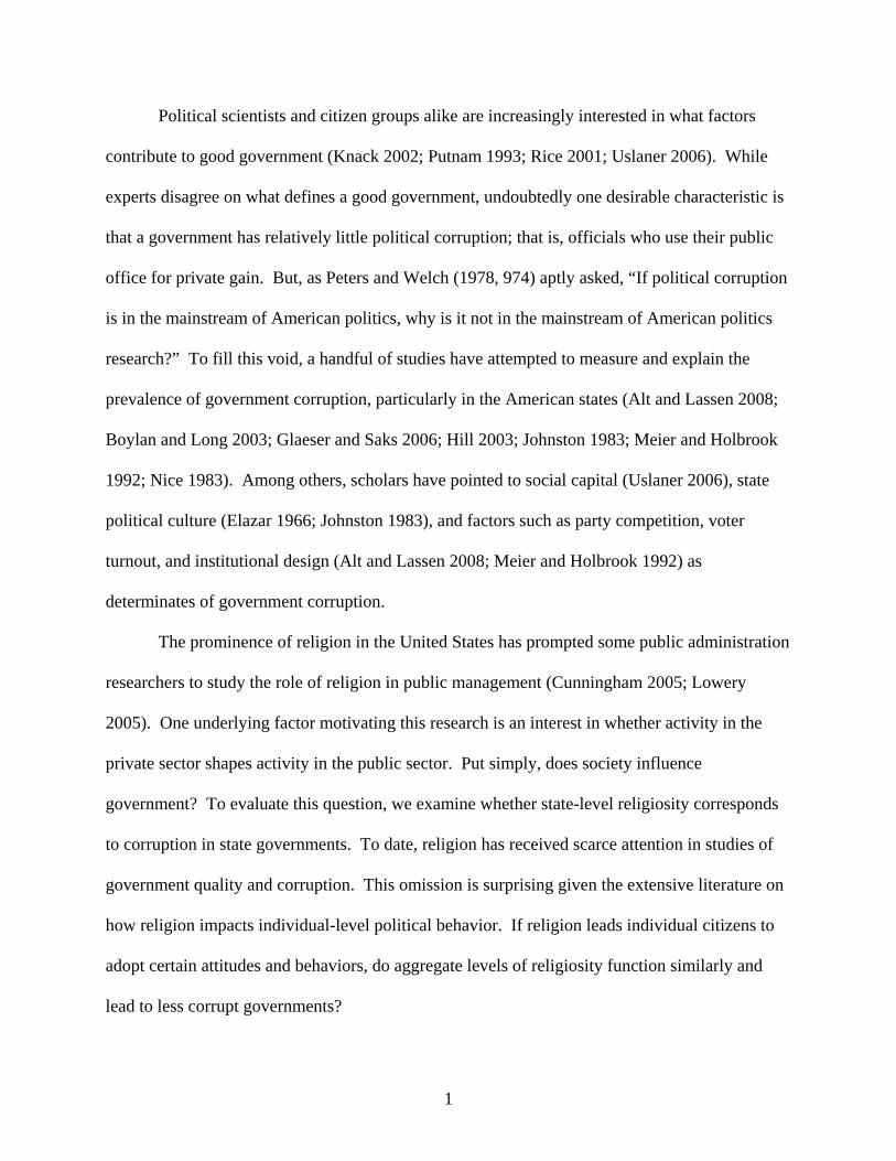
Political scientists and citizen groups alike are increasingly interested in what factors

contribute to good government (Knack 2002; Putnam 1993; Rice 2001; Uslaner 2006). While

experts disagree on what defines a good government, undoubtedly one desirable characteristic is

that a government has relatively little political corruption; that is, officials who use their public

office for private gain. But, as Peters and Welch (1978, 974) aptly asked, “If political corruption

is in the mainstream of American politics, why is it not in the mainstream of American politics

research?” To fill this void, a handful of studies have attempted to measure and explain the

prevalence of government corruption, particularly in the American states (Alt and Lassen 2008;

Boylan and Long 2003; Glaeser and Saks 2006; Hill 2003; Johnston 1983; Meier and Holbrook

1992; Nice 1983). Among others, scholars have pointed to social capital (Uslaner 2006), state

political culture (Elazar 1966; Johnston 1983), and factors such as party competition, voter

turnout, and institutional design (Alt and Lassen 2008; Meier and Holbrook 1992) as

determinates of government corruption.

The prominence of religion in the United States has prompted some public administration

researchers to study the role of religion in public management (Cunningham 2005; Lowery

2005). One underlying factor motivating this research is an interest in whether activity in the

private sector shapes activity in the public sector. Put simply, does society influence

government? To evaluate this question, we examine whether state-level religiosity corresponds

to corruption in state governments. To date, religion has received scarce attention in studies of

government quality and corruption. This omission is surprising given the extensive literature on

how religion impacts individual-level political behavior. If religion leads individual citizens to

adopt certain attitudes and behaviors, do aggregate levels of religiosity function similarly and

lead to less corrupt governments?

1

In this paper, we first develop a set of theoretical expectations that predict states with

more religious populations will have lower levels of corruption. We then empirically test this

prediction and find little relationship between religiosity and corruption in the American states.

Because there is disagreement among scholars over the measurement of both religiosity and

government corruption, we show that this result is robust to multiple measures of both. We then

uncover evidence that the denominational makeup of a state is related to corruption, with heavily

Catholic states having higher levels of corruption. Together, our findings contribute to the

understanding of corruption, an important measure of government quality.

Corruption and the Quality of State Governments

There is increased interest in evaluating the quality of governments and investigating

factors that contribute to their overall functioning. Recent work has documented a relationship

between certain values within a community (most importantly interpersonal trust) and higher

government quality. Whether measured as citizens’ perceptions of the effectiveness and

responsiveness of local governments (Rice 2001) or a “technocratic” measure of government

performance (Knack 2002), areas with higher levels of trust and generalized reciprocity tend to

have higher quality governments.

Uslaner (2006) explicitly considers corruption as a means by which government

performance can be gauged and finds that (similar to the studies citied above) reciprocal trust

and similar values associated with higher stocks of social capital promote better government by

decreasing political corruption. Earlier studies also found that larger states and those with more

traditionalistic political cultures have higher levels of corruption (Johnston 1983) while states

with divided government, elected judges, more educated citizens, a “moralistic” political culture,

2

and less urban areas tend to have lower levels of corruption (Alt and Lassen 2008; Johnston

1983; Meier and Holbrook 1992). Previous studies have also documented that corruption

“matters” insofar as it leads to observable negative consequences. Specifically, corrupt

governments are shown to be less efficient in their day-to-day operations and in serving

constituents (Knack and Keefer 1997; LaPorta et al. 1999; Mauro 1997; Woods 2008; but see

Nice 1986).

To date, however, we know little about the relationship between religion and government

corruption, so our understanding of the dynamic relationship between the private sector and the

public sector remains limited. To address this shortcoming, we explore the intersection between

the voluminous literature on religion and political behavior and the growing literature on quality

of government.

Theoretical Linkages between Religiosity and Government Corruption

Considering the United States is thought to have a generally “secular” government, what

reasons do we have for expecting a relationship between religion and government? To begin,

religious belief influences a wide range of individual behaviors.1 Most religious traditions

advocate abiding by civil law and avoiding illegal activity that benefits one privately at the

expense of the community or common good. If government officials are drawn from the

population at large, we expect more religious officials to hold public office in states with higher

levels of religiosity and that these officials will be less likely to engage in illegal (corrupt)

1 There is a large literature in political science that examines the connection between religious values and

individual behaviors (e.g., Leege and Kellstedt 1993). We ask whether these individual behaviors, when

aggregated to the state level, lead to lower levels of government corruption.

3

behavior while in office. Moreover, we expect that a more religious state population will be less

likely to tolerate illegal activity by their government, which increases the perceived costs of

government officials who may be looking to personally benefit from public office. For these

reasons, we expect that individual-level religiosity, when aggregated to the state level, will lead

to lower levels of government corruption.

The relationship we expect between religion and corruption is grounded in the idea that

characteristics of the public sector are to a great extent reflective of characteristics of the private

sector. For example, Nice (1983) concluded that political corruption is mainly a cultural by-

product. By his rationale, corruption in politics is an extension of private behavior in the public

sphere because “[i]f crime abounds in the private sector…the public sector is unlikely to remain

pure and undefiled” (509). So, states with less religious populations might be less “virtuous”

than states with more religious populations, and this difference likely extends to the public sector

and to government performance.2

Just as important as individual-level processes, the social nature of religious belonging

and worship may also promote less corruption in government. Religion promotes civil society, a

prominent theme in state-level studies of social capital (Putnam 2000) which has been shown to

increase government quality (Knack 2002; Rice 2001; Uslaner 2006). Treisman’s (2000) cross-

national research comes to a similar conclusion: religion reduces corruption because it assists in

organizing a civil society where citizens are more likely to monitor elites. Church attendance is

similar to membership in other clubs where citizens interact and participate in a rather closely

tied social network (Wald, Owen, and Hill 1988). Going to church is a form of socializing that

2 In a related literature, cross-national studies of corruption have suggested that religion may temper

illicit behavior in the public sector (e.g., Lipset and Lenz 2000).

4

fosters social capital and likely spills over into the public sector. So, church attendance likely

helps citizens build the generalized trust that has been linked to higher quality government and

less corruption.

In sum, we have two theoretical reasons to expect that states with more religious

populations will have lower levels of government corruption. First, religious values influence

individual human behavior and instill beliefs that promote abiding by the law and not using a

public office for private gain. Second, religious belonging and worship is a kind of social

activity that helps bind adherents into close social networks that have been associated with less

corruption in previous studies.

Data and Method

Is aggregate religiosity related to government corruption when controlling for other

relevant factors? We test this proposition using cross-sectional data that takes advantage of

varying levels of corruption across the American states. Before describing the data, however, we

call attention to the fact that any relationship between religiosity and government corruption is

likely exogenous or “one way” as compared to other studies that examine the impact of law

enforcement or political institutions on corruption rates. While these factors likely influence the

amount of corruption that occurs in a state, they are also, in part, a response to existing

corruption and illegal behavior. Thus, the relationship between these factors and corruption is

likely endogenous. In contrast, it is unlikely that citizens’ religious devotion is substantively

5

affected by the amount of government corruption in his or her state.3 So, we have initial

confidence that any relationship we may find runs from religiosity to corruption and not the other

way around.

Measuring Government Corruption

Because there is no uniform way to measure government corruption, we use data from

two different sources. To begin, it is important to point out that the two measures are positively

but not strongly correlated (r = .17), which provides further evidence of the difficulty of

accurately measuring government corruption.4

The first measure of government corruption comes from Boylan and Long (2003) who

surveyed reporters covering the state legislature in 1999 about their perceptions of corruption in

their respective state governments. Reporters were mailed a survey that asked a series of eight

questions pertaining to a variety of political corruption issues. The overall response rate was

36.7 percent and no responses were received from Massachusetts, New Hampshire, and New

Jersey reporters, with only one response each from Hawaii and Oregon reporters. They create a

corruption scale by normalizing, and then averaging, the responses to six questions from the

survey.5 In these data, South Dakota is the least corrupt state with a value of -1.897, while New

Mexico is the most corrupt state at 1.611. Expert surveys similar to this one are widely used by

3 Other scholars of state politics have also identified religiosity or religious affiliation as exogenous

measures and have used them as an instrument to address problems of endogeneity (e.g., Erikson, Wright,

and McIver 1993).

4 Descriptions and summary statistics for all variables used in our analysis are provided in the Appendix.

5 The value of Cronbach’s alpha (.82) for this scale indicates that it is reliable and robust.

6

scholars in studies of cross-national variation in levels of corruption (Ades and Di Tella 1999;

Fisman and Gatti 2002; Mauro 1995; Treisman 2000). In the United States, because of their

deep knowledge of the activities of state governments, these reporters are uniquely positioned to

offer accurate appraisals of the level of corruption in the state government they cover.

The second measure of government corruption comes from Glaeser and Saks (2004,

2006) and provides a conviction rate for of local, state, and federal public officials in a state per

100,000 state residents from 1990 to 2002. This corruption rate ranges from a low of .079 in

Nebraska to a high of 9.19 in Mississippi. The information pertaining to crimes committed by

public officials was obtained from the Department of Justice’s (DOJ) “Report to Congress on the

Activities and Operations of the Public Integrity Section.” The DOJ investigates and reports a

number of criminal acts by public officials that includes an “array of topics such as conflict of

interest, fraud, campaign-finance violations, and obstruction of justice.”

There are benefits to using each of the two measures. The state reporters’ perceptions of

corruption measure addresses the problem that federal prosecution is determined not only by the

amount of government corruption in a state but also the availability of prosecutorial resources

and effort, varying greatly from state to state and not fully captured by using conviction data. In

addition, federal prosecutors may be more reluctant to investigate and prosecute wrongdoing by

public officials in some states compared to others. On the other hand, the conviction rate

measure allows for a more objective and standardized measure of corruption than surveys, which

also suffer from non-response bias. In addition, the data cover a twelve year time period, which

provides a general level of corruption for each state that is less influenced by year to year

fluctuations and idiosyncrasies.

7

Measuring State-Level Religiosity

There is even greater scholarly debate over the proper measurement of religiosity. This is

due, in part, to disagreements among scholars about how best to quantify religion and an

individual’s underlying “level” of religious belief and devotion. Because religion itself is a

concept with multiple analytical dimensions that must be considered (Roof 1979), we use

multiple measures, each described below.

The first four measures we use come from data assembled by Robert Putnam for his

seminal book, Bowling Alone (2000). The data were derived from several sources including the

United States Census’ Current Population Survey, the DDB Needham’s “Life Styles” surveys,

and the Roper Social and Political Trends study. All data have been aggregated to the state level,

with the District of Columbia omitted from the analysis. For each measure of religiosity, states

with higher levels of religiosity are coded higher.

Our first measure comes from Respondents’ answer to the statement “Religion is an

important part of my life” with six response categories (i.e. no middling category) ranging from

“definitely disagree” to “definitely agree.” Second, we use a measure of religious organizations

per 1,000 state residents. Third, a measure of church attendance that simply asks respondents

whether they have attended a church service in the last week. Finally, we use a composite

measure of state religiosity developed by Putnam that combines responses to questions on church

membership, attendance, and religious belief.

As our fifth measure of religiosity, we turn to an alternative data source as a robustness

check for our findings. Specifically, we use data from the 2000 National Annenberg Election

Survey (NAES), a random-digit dialing rolling cross section survey conducted in the months

leading up to the 2000 presidential election. The major advantage of this survey is its sheer

8

sample size, over 60,000.6 To measure religiosity, we use an item that asks Respondents “How

often do you attend religious services, apart from special events like weddings and funerals?”

with five response categories: never, a few times a year, once or twice a month, once a week,

more than once a week. These responses are then aggregated to the state level to produce a mean

for each state.

Other Variables Influencing Government Corruption (Controls)

We also control for other factors that may influence levels of government corruption in

the states. To begin, we expect that states with more urban areas will have higher levels of

corruption (Johnston 1983; Meier and Holbrook 1992), so we include a measure of the percent of

a state’s population living in urban areas.7 We also expect that citizens with higher levels of

education will be more likely to closely monitor government and increase the probability that

public officials who engage in corrupt behavior will be brought to light (Glaeser and Saks 2006;

Knack 2002; Meier and Holbrook 1992). So, we control for average level of education using the

percentage of a state’s residents who have obtained a high school diploma. We also include a

measure of electoral competiveness from each state (Holbrook and Van Dunk 1993) with the

expectation that states dominated by a single political party will have higher levels of corruption

(Meier and Holbrook 1992). Finally, given the attention paid to social connectedness and

generalized reciprocity in other studies of corruption and government performance (Knack 2002;

6 The average state sample size is 1,340 respondents. The NAES did not survey respondents in Alaska or

Hawaii so these states are not included in analyses using this measure of religiosity.

7 The percent of a state’s population living in urban areas is closely related to the size of a state’s

population, which has also been show to relate to government performance (Knack 2002; Rice 2001).

9

Putnam 1993; Rice 2001; Uslaner 2006), we control for a state’s stock of social capital (Putnam

2000).8

Because our two measures of government corruption are continuous, the data lend

themselves to analysis with the old work horse of OLS. To control for the possible

heteroskedasticity that cross-sectional data of this sort are especially subject to, we report

coefficients with robust standard errors in all analyses.

Results

We succinctly present our results using the two different measures of government

corruption we detail above. In Table 1, we regress the Boylan and Long state reporters’

perceptions of corruption measure on our five different measures of religiosity and our set of

controls. Glancing across the five columns, three of the coefficients for religiosity are negatively

signed but all fail to reach conventional levels of significance. Put bluntly, these data show no

relationship between aggregate religiosity and levels of government corruption in the states. In

line with our expectations, we find that states with a larger urban population have higher levels

of corruption. Specifically, moving from the mean to one standard deviation above in urban

population is associated with a little less than half a standard deviation increase in perceived

government corruption. In all five models, the coefficient for social capital is negative but it is

8 We also experiment controlling for a state’s political culture using Sharkansky’s (1969) formulation of

Elazar’s (1966) political culture scheme. This variable ranges from 1 (Moralistic) to 9 (Traditionalistic),

with the middle value indicating an Individualistic political culture. Doing so does not substantively alter

our results. We choose to omit the measure from our model because, in some cases, it is highly collinear

with our measures of state-level religiosity.

10

bounded above zero only for one measure of religiosity (Attended Church Last Week, Column

3).

[TABLE 1: RELIGIOSITY AND STATE REPORTERS’ PERCEPTIONS OF GOVERNMENT CORRUPTION]

Next, we turn to analysis using the Glaeser and Saks conviction rate measure of

corruption. We again find that religiosity bears no statistical association with government

corruption regardless of the measure of religiosity used. We also find that, as expected, states

with a greater proportion of citizens with high school diplomas have lower levels of corruption.

Specifically, moving from the mean to one standard deviation above in high school graduation

rate is associated with a little more than half a standard deviation decrease in government

corruption using the conviction rate data.9 In sum, despite the theoretical reasons developed

above, we find little evidence that state-level religiosity is linked to lower instances of

government corruption regardless of the measure of corruption or religiosity used.

[TABLE 2: RELIGIOSITY AND CRIMINAL CONVICTIONS OF GOVERNMENT CORRUPTION] 9 To test if multicollinearity is significantly weakening the preciseness of the coefficient estimates, we

check the variance inflation factor (VIF) for each coefficient in each model. Essentially, a VIF reports

how much the variance (or uncertainty) of a coefficient is increased because of collinearity among the

independent variables. We find that none of the coefficients have a VIF greater than six and none of the

models have an average VIF greater than three, which indicates that multicollinearity is not a serious

problem. We also tested for the influence of outliers by using robust regression and re-running the

models after dropping states with high DF-beta values (a measure of the potential influence on the

parameter estimate that each observation has). Doing so does not alter our findings.

11

Finally, in addition to religiosity, we are also interested in the relationship between the

denominational composition of a state and its level of political corruption. Previous research has

hypothesized that heavily Protestant areas will tend to have more efficient and higher quality

governments (Geering and Thacker 2004; Gerring, Thacker, and Moreno 2005). In contrast,

heavily Catholic areas are sometimes associated with corrupt machine-like politics, especially in

large cities (e.g., Erie 1990). Using state measures of the percentage of residents who identify as

Catholic or a denomination placed under the Protestant designation, we test whether a state’s

denominational composition is related to its level of government corruption.10

[TABLE 3: STATE DENOMINATIONAL COMPOSITION AND GOVERNMENT CORRUPTION]

In Table 3, both measures of corruption are regressed on % Catholic and % Protestant

along with the same battery of controls as before. We find some evidence that states with larger

Catholic populations have higher levels of corruption (see Column 1). Substantively, moving

from one standard deviation below the mean to one standard deviation above for % Catholic

(moving from a state with a Catholic population of 7.2% to one with 32%) increases government

corruption by over half a standard deviation on the Boyan and Long (2003) state reporters’

perceptions of corruption measure.

Conclusion

The growing literature on government performance should be concerned about the way

that the dependent variable is conceptualized and measured. Simply put, government 10 The % Catholic and % Protestant measures correlate at .008.

12

performance is not just efficiency or responsiveness. It also depends on the amount of corruption

being perpetuated by public officials, which most previous studies have failed to take into

account as a key feature of government performance. Governments may receive high marks on

standard measures of efficiency and responsiveness (Knack 2002; Rice 2001), but if the officials

who conduct the day to day business of politics are dishonest and sleazy, then we should think

twice before passing positive judgments about government quality. Perhaps Uslaner (2006, 18)

said it best, “[c]orruption is the scourge of good government.”

To summarize our empirical findings, we find little evidence of a relationship between

the multiple measures of religiosity we have considered and government corruption but find

some evidence that the denominational makeup of states matters. This does not imply that we

should abandon efforts to understand the relationship between religion and government

performance and, in fact, points to the need for continued research on the relationship between

the two. For example, previous studies have shown that the values associated with social capital

(primarily interpersonal trust) lead to higher quality state governments (Knack 2002; Rice 2001;

Uslaner 2006). Future studies should attempt to determine the extent to which churchgoing and

religious belief are the primary source of these important values. However, given our findings

here, we conclude that religion does not seem to directly “purify” government corruption in the

American states.

13

References

Ades, Alberto and Rafael Di Tella. 1999. “Rents, Competition, and Corruption.” American

Economic Review 89(4): 982-93.

Alt, James E. and David D. Lassen. 2008. “Political and Judicial Checks on Corruption:

Evidence from American State Governments.” Economics and Politics 20(1): 33-61.

Boylan, Richard T., and Cheryl X. Long. 2003. “Measuring Public Corruption in the

American States: A Survey of State House Reporters.” State Politics and Policy

Quarterly 3(4): 420-38.

Cunningham, Robert. 2005. “Religion and Public Administration: The Unacknowledged

Common (and Competitive) Ground.” International Journal of Public Administration

28(11-12): 943-56.

Eire, Steven P. 1990. Rainbow's End: Irish-Americans and the Dilemmas of Urban Machine

Politics, 1840-1985. Berkeley: University of California Press.

Elazar, Daniel J. 1966. American Federalism: A View from the States. New York:

Crowell.

Erikson, Robert S., Gerald C. Wright and John P. McIver. 1993. Statehouse Democracy: Public

Opinion and Policy in the American States. New York: Cambridge University Press.

Fisman, Raymond and Roberta Gatti. 2002. “Decentralization and Corruption: Evidence Across

Countries.” Journal of Public Economics 83(3): 325-45.

Glaeser, Edward L., and Raven E. Saks. 2004. “Corruption in America.” Harvard Institute of

Economic Research. Discussion Paper #2043.

Glaeser, Edward L., and Raven E. Saks. 2006. “Corruption in America.” Journal of

Public Economics 90(6-7): 1053-72.

14

Gerring, John, and Strom C. Thacker. 2004. “Political Institutions and Corruption: The Role of

Unitarism and Parliamentarism.” British Journal of Political Science 34(2): 295-330.

Gerring, John, Strom C. Thacker, and Carola Moreno. 2005. “Centripetal Democratic

Governance: A Theory and Global Inquiry.” American Political Science Review 99(4):

567-81.

Hill, Kim Q. 2003. “Democratization and Corruption.” American Politics Research

31(6): 613-31.

Holbrook, Thomas M. and Emily Van Dunk. 1993. “Electoral Competition in the American

States.” American Political Science Review 87(4): 955-62.

Johnston, Michael. 1983. “Corruption and Political Culture in America: An Empirical

Perspective.” Publius 13(1): 19-39.

Knack, Stephen. 2002. “Social Capital and the Quality of Government: Evidence From

the States.” American Journal of Political Science 46(4): 772-85.

Knack, Stephen, and Philip Keefer. 1997. “Does Social Capital Have An Economic

Payoff? A Cross-Country Investigation.” Quarterly Journal of Economics 112(4): 1251-

88.

LaPorta, Rafael, Florencio Lopez-Silanes, Andrei Schleifer, and Robert W. Vishney. 1999. “The

Quality of Government.” Journal of Law, Economics, and Organization 15(1): 222-79.

Leege, David C. and Lyman A. Kellstedt. 1993. Rediscovering the Religious Factor in American

Politics. New York: M. E. Sharpe.

Lipset, Seymour Martin and Gabriel S. Lenz. 2000. “Corruption, Culture, and Markets.” In

Culture Matters: How Values Shape Human Progress, eds. Lawrence E. Harrison and

Samuel Huntington. New York: Basic

15

Lowery, Daniel. 2005. “Self-Reflexivity: A Place for Religion and Spirituality in Public

Administration.” Public Administration Review 65(3): 324-34.

Mauro, Paolo. 1995. “Corruption and Growth.” Quarterly Journal of Economics 110(3): 681-

712.

Mauro, Paolo. 1997. Why Worry About Corruption? Washington, D.C.: International Monetary

Fund.

Meier, Kenneth, and Thomas M. Holbrook. 1992. “I Seen My Opportunities and I Took

‘Em: Political Corruption in the American States.” Journal of Politics 54(1): 135-55.

Nice, David. 1983. “Political Corruption in the American States.” American Politics

Quarterly 11(4): 507-17.

Nice, David. 1986. “The Policy Consequences of Political Corruption.” Political Behavior 8(3):

287-95

Peters, John G. and Susan Welch. 1978. “Political Corruption in America: A Search for

Definitions and a Theory, or If Political Corruption Is in the Mainstream of American

Politics Why Is it Not in the Mainstream of American Politics Research?” American

Political Science Review 72(3): 974-84

Putnam, Robert. 1993. Making Democracy Work. Princeton: Princeton University

Press.

Putnam, Robert. 2000. Bowling Along: Collapse and Revival of American Community.

New York: Simon & Schuster.

Rice, Tom W. 2001. “Social Capital and Government Performance in Iowa

Communities.” Journal of Urban Affairs 23(3-4): 375-89.

16

Roof, Wade. 1979. “Concepts and Indicators of Religious Commitment: A Critical Review.” In

Robert Wuthnow ed., The Religious Dimension: New Directions in Quantitative

Research. New York: Academic Press.

Sharkansky, Ira. 1969. “The Utility of Elazar’s Political Culture: A Research Note.”

Polity 2(1): 66-83.

Treisman, Daniel. 2000. “The Causes of Corruption: A Cross-national Study.” Journal of

Public Economics 76(3): 399-457.

Uslaner, Eric M. 2006. “The Civil State: Trust, Polarization, and the Quality of State

Government.” In Public Opinion in State Politics, ed. Jeffrey Cohen. Palo Alto: Stanford

University Press.

Wald, Kenneth D., Dennis Owen, and Samuel Hill. 1988. “Churches as Political

Communities.” American Political Science Review 82(2): 531-548.

Woods, Neal D. 2008. “The Policy Consequences of Political Corruption: Evidence from State

Environmental Programs.” Social Science Quarterly 89(1): 258-71.

17

Tables

TABLE 1: RELIGIOSITY AND STATE REPORTERS’ PERCEPTIONS OF GOVERNMENT CORRUPTION

(1) (2) (3) (4) (5) Measure of Religiosity

Religion is Important

Religious Orgs.

Attended Church

Last Week

Religiosity Index

Annenberg Church

Attendance Religiosity -0.188 -0.041 0.025 0.056 -0.193

[0.266] [0.102] [0.081] [0.078] [0.428] % Population Urban Area 0.023*** 0.022*** 0.019* 0.022*** 0.023***

[0.007] [0.007] [0.009] [0.008] [0.008] % High School Diploma -0.038 -0.035 -0.005 -0.025 -0.037

[0.035] [0.035] [0.041] [0.034] [0.036] Electoral Competition -0.003 -0.002 0.008 -0.000 -0.003

[0.009] [0.009] [0.008] [0.009] [0.010] Social Capital -0.252 -0.248 -0.575* -0.325 -0.256

[0.280] [0.289] [0.284] [0.290] [0.285] Constant 2.355 1.372 -1.152 0.487 2.106

[3.048] [2.535] [2.734] [2.410] [3.358]

R² 0.42 0.42 0.42 0.42 0.42 N 44 44 38 44 44

Dependent variable: Boylan and Long state legislature reporters measure of corruption. OLS regression coefficients, robust standard errors in brackets. * denotes p<.10, ** p<.05, *** p<.01

18

TABLE 2: RELIGIOSITY AND CRIMINAL CONVICTIONS OF GOVERNMENT CORRUPTION

(1) (2) (3) (4) (5) Measure of Religiosity

Religion is Important

Religious Orgs.

Attended Church

Last Week

Religiosity Index

Annenberg Church

Attendance Religiosity 0.091 -0.181 -0.213 -0.168 0.141

[1.027] [0.324] [0.345] [0.374] [1.389] % Population Urban Area 0.009 0.006 0.005 0.011 0.009

[0.023] [0.025] [0.028] [0.024] [0.023] % High School Diploma -0.177** -0.199** -0.154 -0.202** -0.176**

[0.080] [0.082] [0.114] [0.083] [0.078] Electoral Competition -0.001 -0.002 -0.006 -0.004 -0.000

[0.034] [0.033] [0.035] [0.034] [0.034] Social Capital 0.513 0.660 0.068 0.659 0.510

[0.712] [0.758] [1.168] [0.774] [0.711] Constant 16.660** 19.051*** 15.683* 18.951*** 16.498**

[7.665] [6.031] [8.525] [5.749] [7.661]

R² 0.14 0.15 0.18 0.15 0.14 N 47 47 41 47 47

Dependent variable: Glaeser and Saks conviction rate measure of corruption. OLS regression coefficients, robust standard errors in brackets. * denotes p<.10, ** p<.05, *** p<.01

19

TABLE 3: STATE DENOMINATIONAL COMPOSITION AND GOVERNMENT CORRUPTION

(1) (2) Measure of Corruption State Reporters’ Perceptions

of Corruption State Corruption Conviction Data

% Catholic 0.020* 0.025 [0.010] [0.020]

% Protestant -0.010 0.060 [0.015] [0.061]

% Population Urban Area 0.012 0.000 [0.009] [0.027]

% High School Diploma -0.017 -0.117 [0.036] [0.073]

Electoral Competition -0.007 -0.013 [0.010] [0.030]

Social Capital -0.387 -0.117 [0.323] [0.714]

Constant 0.560 12.276** [2.649] [5.164]

R² 0.48 0.18 N 44 47

OLS regression coefficients, robust standard errors in brackets. * denotes p<.10, ** p<.05, *** p<.01

20

Appendix: Description and Summary of Measures of Data

Variable Name Description Mean, SD, Range Source

Corruption #1

State reporters’ perceptions of

government corruption (1999)

.001

.731 -1.897 to 1.611

Boylan and Long (2003)

Corruption #2 Average corruption-

related convictions per capita (1990-2002)

3.983 .101

.79 to 9.19 Glaeser and Saks (2004)

Religion is Important

Degree to which religion is important in a

respondent’s life (1-6)

4.269 .319

3.513 to 4.878 DDB Life Style Survey

Religious Organizations

Number of religious organizations per 1,000

state residents (standardized)

0 1

-2.310 to 1.984 U.S. Department of Labor

Attended Church Last

Week

Attend a church service in the last week (0-1)

(standardized)

0 1

1.831 to 2.089

Roper Social and Political Trends Survey

Religiosity Index

Composite measure of state religiosity that

combines responses to questions on church

membership, attendance, and religious belief.

-.0438 .872

-1.985 to 1.728

DDB Life Style Survey/Roper Social and Political Trends

Survey

Annenberg Church

Attendance

Frequency of church attendance (1-5)

2.951 .271

2.407 to 3.489

2000 National Annenberg Election Study

% Catholic Percentage of a state’s

residents that identify as Catholic

19.6 12.4

3.2 to 51.7 Glenmary Research Center

% Protestant Percentage of a state’s

residents that identify as “mainline” Protestant

11.1 6.6

1.6 to 34.6 Glenmary Research Center

% Population Urban Area

Percentage of state residents living in an

urban area (1990)

68.1 14.6

32.2 to 92.6 U.S. Census

% High School Diploma

Percentage of state residents with at least four

years of high school (1990)

78.5 5.7

65.9 to 87.6 U.S. Census

21

Electoral Competition

Competitiveness of state elections measured using district-level legislative election results (higher

value indicates a state is more competitive)

39.03 11.40

9.26 to 56.58

Holbrook and Van Dunk (1993)

Social Capital

Fourteen item state-level “Comprehensive Social Capital Index” (factor

score)

0 0.78

-1.42 to 1.70

Putnam (2000) http://www.bowlingalone.com/

data.php3

All data are for the state level.

22