Regional Watershed Spreadsheet Model User Manual Prepared by SAN FRANCISCO ESTUARY INSTITUTE 4911 Central Avenue, Richmond, CA 94804 Phone: 510-746-7334 (SFEI) Fax: 510-746-7300 www.sfei.org

Page 1 of 30

Table of Contents 1. RWSM OVERVIEW 3

1.1 Purpose 3 1.2 Development History 4 1.3 Overall structure of components 5

2. HYDROLOGY MODEL 5 2.1 Structure of Model 5 2.2 Required Input Files and Formatting 6 2.3 Minimum System Requirements 10 2.4 Running the Hydrology Model Tool 10

2.4.1 Launch ArcMap 10 2.4.2 Open the Catalog 10 2.4.3 Launch the RWSM Hydrology Analysis Toolbox 11 2.4.4 Populate RWSM Toolbox GUI, run analysis 12

2.4.4.1 Toolbox GUI Fields 12 2.4.4.2 View Analysis Status 14

2.4.5 Review analysis output 15 2.5 Outputs 15 2.6 Troubleshooting 16 2.7. Reasonable hydrology calibrations and outputs (QA check) 16

3. POLLUTANT SPREADSHEET MODEL 17 3.1 Structure of Model 17 3.2 Required Inputs 17 3.3 Using the Pollutant Spreadsheet Model 17 3.4 Optional Manual Calibration 18 3.5 Optional Automated Calibration 19

3.5.1 Calibration Approach 19 3.5.2 Required Inputs 20 3.5.3 Calibration Results 20

3.6 Reasonable pollutant calibrations and outputs (QA check) 20

4. REFERENCES 21

Page 2 of 30

1. RWSM OVERVIEW

1.1 Purpose The Regional Watershed Spreadsheet Model (RWSM) was developed to estimate average annual regional and sub-regional scale loads for the San Francisco Bay Area. It is part of a class of deterministic empirical models based on the volume-concentration method. The assumption within these types of models is that an estimate of mean annual volume for each land use type within a watershed can be combined with an estimate of mean annual concentration for that same land use type to derive a load which can be aggregated for a watershed or many watersheds in a region of interest. The strengths of volume-concentration models include relatively fewer data input requirements than more complex dynamic simulation models such as SWMM or HSPF, explicit selection of land uses, suitability for hypothesis testing, and manual and automated calibration or verification procedures that enable estimates of error and bias as a component of the outputs. These strengths make it a useful tool for providing regional (Bay wide) and sub-regional (e.g. individual county, Bay segment, or priority margin unit) estimates of pollutant loads. It can also be used to provide hypotheses about which watersheds may be exporting relatively higher or lower loads to the Bay relative to watershed area and for estimating regionally averaged land use specific event mean concentrations (e.g. ng/L) and exports (e.g. g/km2). It also presents an appropriate baseline and a flexible platform for analyzing the potential for flow and load changes in response to management measures at a gross scale (e.g. large scale land use changes associated with redevelopment and new development), and runoff changes in relation to climate change and changes in impoundment (again at gross scales). Although they have the great benefit of being easy to understand and use, volume-concentration models like the RWSM when developed using a regional calibration and annual average time step, are less reliable for predicting real loadings for individual watersheds, subwatersheds or industrial patches and less reliable for estimating load changes in relation to implementation of treatment BMPs. Although volume concentrations models can be developed and calibrated to simulate individual storms in individual watersheds (Ha and Stenstrom, 2008), dynamic simulation models are better at producing reliable results at these management scales because they are able to simulate rainfall and runoff processes at the scales of individual storms and differing BMP performance in relation to differing climate and landscape context. Should there be interest in the future, an RWSM could be developed and calibrated at a single watershed scale using storm scale rainfall and runoff processes, but the current version was not developed in that manner.

Page 3 of 30

1.2 Development History Development of the model began in 2010 in response to a recommendation by advisors to the Small Tributaries Loading Strategy (STLS) Team who proposed the use of a simple regional model as a tool for estimating regional loads and organizing data and information for hypothesis testing. They envisioned that once the model was developed it could be used to estimate regional scale loads but also to help guide monitoring design to address data gaps in relation to management needs. Since that time, annual funding for model development has been low ($20-35k) but reasonably consistent each year. An annual review and oversight from the STLS, the Sources Pathways and Loading Workgroup (SPLWG) of the Regional Monitoring Program for Water Quality in San Francisco Bay (RMP), and oversight from select advisors (Mike Stenstrom and Peter Mangarella), resulted in small and incremental annual developments and adjustments to the model structure as “band-aids” to the original code rather than any complete rewrites. Additionally, code development was undertaken by multiple staff and through different platforms as technology has improved over seven years. The model also went through a wholesale switch from sediment based to water based (requiring workarounds in the code), and adding on additional components for the calibration procedures, all necessary modifications based in STLS review and oversight from Mike Stenstrom and Peter Mangarella. The first years the model development (2010, 2011, and 2012) were spent developing the hydrological model and the conceptual basis for the pollutant models (Lent and McKee, 2011; Lent et al., 2012). Then in 2013 and 2014, development of the suspended sediment model and sediment-based PCB and Hg models was attempted (McKee et al., 2014) but the results were unreliable and lead to a recommendation to switch the model structure of the PCBs and Hg models to a water based structure. This lead to the first reasonable calibration of the model for PCBs but there remained lower confidence for the Hg model. The other advancement in 2015 and 2016 was the development of an error estimation component to the modeling tool (Wu et al., 2016). Further improvements were made in 2016 including updating the hydrological basis of the model to a more recent regional rainfall and runoff data set that better represents current climatic conditions and spatial microclimates, separation of the hydrology model into three subregions, and improvements in the manual and automated calibration procedures for the PCB and Hg models that resulted in satisfactory model outputs (Wu et al., 2017). Given this long history and piecemeal development, funding for 2017 has been used to compile a cohesive, flexible, and well-documented model toolkit ready for an external user community. This user manual aims to provide sufficient documentation to guide model calibration and applications.

Page 4 of 30

1.3 Overall structure of components The RWSM Tool-Kit includes four separate components that can be used to estimate pollutant loads: Table 1. The components, their platform, and the main purpose of each.

Tool-Kit Component Platform Primary Purpose

Hydrology Model ArcGIS Spatial model calculates total average annual volume for individual landscape units and aggregates them to a watershed scales.

Pollutant Calculation Spreadsheet

Microsoft Excel A spreadsheet formatted to link the results from the hydrology model and the pollutant coefficients (either user supplied or resulting from the optional calibration component(s)) to estimate total pollutant loads and average concentrations for each watershed.

Manual Calibration Microsoft Excel An optional step for the user to manually calibrate the pollutant coefficients, and/or to inform the upper and lower bounds assigned to the pollutant coefficients for the automated calibration.

Automated Calibration R An optional step for the user to perform an automated calibration procedure using an approach that is based on a constrained optimization method (“Complex Method”, Box 1965).

Further detail about each component is provided in the sections below.

2. HYDROLOGY MODEL

2.1 Structure of Model The Hydrology Model is a simple runoff model structured similarly to the model presented by Ha and Stenstrom (2008), using GIS-derived data for land use, soil type, slope and annual precipitation. The model intersects land use and soil type within each target watershed, and calculates a mean slope and precipitation for each of those intersected polygons. The user must identify a runoff coefficient for each attribute combination of land use, soil type and slope (binned, e.g. 0-5% slope, 5-10% slope and 10%+ slope). The model calculates a volume for each polygon based on the runoff coefficient and the average weighted precipitation for each polygon, and then sums those volumes for each watershed.

Page 5 of 30

2.2 Required Input Files and Formatting The RWSM tool requires three GIS vector layers, two rasters, and two csv files. Each of these can be set in the toolbox GUI and have different field requirements, listed below:

● Vector Layers ○ Watersheds

■ Polygons representing watershed regions ■ Required Field:

● Watershed Name (Text) ○ Land use

■ Polygons representing land usage for watershed areas ■ Required field:

● Land use classification code (Numeric, Real) - mapped to csv file ○ Soil Types (Text)

■ Soil types are limited to: A , B, C, D, ROCK, UNCLASS, WATER, and null 1

● Rasters NOTE: Raster cell size must be smaller than the smallest polygon in the land use layer or errors may occur.

○ Slope

■ Contains slope data for watershed areas ■ Unit = %

○ Precipitation ■ Contains precipitation data for watershed areas ■ Unit = mm

● CSV Files ○ Land Use

■ Contains further information about land use classes included in the land use vector layer. Allows the user to aggregate land uses into larger land use categories relevant to creating a link to the runoff coefficients.

■ Required fields: ● Land use classification (Text) ● Land use classification code (Numeric, Real)

○ Land use codes must be real numbers between 0 and 9.9. ● Land use code (mapped to land use vector layer ) (Numeric,

Integer) ● Land use description (Text)

○ Runoff Coefficients

1 A, B, C and D refer to the Hydrologic Soil Group

Page 6 of 30

■ Contains runoff coefficients for slope, soil, and land use combinations. ■ Required fields:

● Slope bin (Text) ○ Bins with defined limits should follow the format:

■ [lower bound]-[upper bound]% ○ The maximum bin should have no upper limit, this will be

calculated using values found in the Slope raster file and should conform to the format:

■ [lower bound]%+ ○ For example, to specify the three bins [0-5],[5-10] and

[10,max(slope raster)], use the following formats: ■ [0,5] → 0-5% ■ [5,10] → 5-10% ■ [10,max(slope raster)] → 10%+

● Soil type (Text) ○ Soil types are limited to: A, B, C, D, ROCK, UNCLASS,

WATER, and null ● Land use classification (Text) ● Land use classification code (Numeric, Real)

○ Land use codes must be real numbers between 0 and 9.9. ● Runoff coefficient (Numeric, Real)

NOTE: Field names must not contain spaces, for example use “Slope_bin” instead of slope bin. Default soil feature data and default slope and precipitation rasters are included with the tool, although the user is also free to supply their own spatial data layers. The default layers provided include:

Data Type Data Set Reference

Soil STATSGO 30-m grid USDA 1994

Precipitation 2 PRISM 1981-2010 average precipitation 800-m grid

PRISM Climate Group, Oregon State University, http://prism.oregonstate.edu, created July 2012.

Slope USGS National Elevation Dataset (NED) 10-m grid

Gesch et al. 2002. Available for download at: https://lta.cr.usgs.gov/products_overview

2 Note: Two precipitation raster files are included as defaults. One raster (prismppt_1980to2010) is the unmodified PRISM rainfall dataset. The second raster file (prismppt_19080to2010minus5) has an initial abstraction of 5 inches imposed, which is what SFEI uses and for which the SFEI runoff coefficients for the 3 subregions apply.

Page 7 of 30

Land Use 3 ABAG 2006 Association of Bay Area Government, 2006. Existing Land Use in 2005: Data for Bay Area Counties. 44 pg report and CD with GIS data layers. Available for purchase at: https://store.abag.ca.gov/projections.asp#elu

The two CSV files require/allow the model user to impart best professional judgement in aggregating land uses into classes and applying runoff coefficients to different combinations of land use class, soil type and slope. The CSV files include required fields which create links to the spatial datasets. Examples of the 2 required CSV files are included with the input data. Note: we recommend using these files as templates and maintaining the same field names because these field names will exactly match the required fields in the GUI. The Land Use CSV is the mechanism for taking a detailed land use spatial data layer (e.g. ABAG land use has over 100 specific land uses) and aggregating those land uses into simpler categories (e.g. “commercial”) for the purposes of applying runoff coefficients. The required fields for the Land Use CSV include: Land use description: The land use description field is a unique, short description of the land use (e.g. “Orchards, Groves, Vineyards, And Nurseries”). Land use code (mapped to land use vector layer): The land use code field is a unique numeric code for each specific land use. Land use classification: The land use classification field is the simpler land use category to which multiple specific land uses may be assigned (e.g. the more specific “Orchards, Groves, Vineyards, And Nurseries” land use may be attributed to the simpler land use category “Agriculture”). Multiple specific land uses may have the same land use classification (e.g. “Cropland” may also be may be attributed to the simpler land use category “Agriculture”). The model user should aggregate the specific

3 Note: Three land use layers are included in the default set. One (ABAG2005_orig.gdb) is the unmodified version from ABAG, a second layer (ABAG2005_OldUrban.gdb) is a modified version of the ABAG05 layer and includes “old” land uses. For a given aggregated land use category, old vs new is determined by the intersection of the ABAG 2005 land uses and the sfurb_1974 polygons noting urban areas at that time. A third layer (ABAG2005_OldUrbanSAs.gdb) includes the old urban areas and adds in source areas imposed on the land use layer. All source areas were lumped together and burned into the general LU layer such that Source Area became a new general LU and each Source Area was identified only as Source Area and maintained no other general LU category. Appendix A details the source areas used, how the source areas were identified, and how buffers were created around the source areas. SFEI uses the latter file.

Page 8 of 30

land uses into simpler, larger land use classifications as long as those specific land uses should be assigned the same runoff coefficients. Land use classification code: The land use classification code is a unique numeric code for each land use classification. All specific land uses assigned to the same land use classification should also receive the same land use classification code. [Note: In future iterations of this model, the land use classification code may be deleted from the list of required fields]. SFEI uses numbers 0-8 with some decimal numbers.

Included within the Hydrology Model folder is a land use CSV file. The user is free to use this CSV, modify it based on your own professional judgement or datasets, or replace it with your own version. The CSV provided is the version used in SFEI’s calibration of the Hydrology Model as of May 2017.

Page 9 of 30

The Runoff Coefficient CSV is the mechanism for applying runoff coefficients to different combinations of land use, soil type and slope. Every combination of soil type, slope bin, and land use classification must have a runoff coefficient. The required fields for the Runoff Coefficient CSV include: Slope bin The model user must define slope bins. The bins may be defined such that the user can apply different runoff coefficients to the same land use-soil type combination but with different slope characteristics. The slope unit is in percent and the bin field must be formatted as X-X% (e.g. 0-5%). For the final upper bin, the formatting must be X%+ (e.g. 10%+). The user may define as many slope bins as desired, or may include only one slope bin defined as 0%+. Soil type Each soil type name must exactly match the formatting of the soil type name in the soil polygon layer. Soil types are limited to: A, B, C, D, ROCK, UNCLASS, WATER, and null. Note: Soil types A, B, C and D are hydrologic soil groups classified by the Natural Resource Conservation Service. Details of this classification can be found in ‘Urban Hydrology for Small Watersheds’ published by the Engineering Division of the Natural Resource Conservation Service, United States Department of Agriculture, Technical Release–55. Land use classification (same as in the Land Use CSV) The land use classification field is the simpler land use category to which multiple specific land uses may be assigned (e.g. the more specific “Orchards, Groves, Vineyards, And Nurseries” land use may be attributed to the simpler land use category “Agriculture”). Multiple specific land uses may have the same land use classification (e.g. “Cropland” may also be may be attributed to the simpler land use category “Agriculture”). The model user should aggregate the specific land uses into simpler, larger land use classifications as long as those specific land uses should be assigned the same runoff coefficients. Land use classification code (same as in the Land Use CSV) The land use classification code is a unique numeric code for each land use classification. All specific land uses assigned to the same land use classification should also receive the same land use classification code. Runoff coefficient The runoff coefficient applied to each combination of land use, soil and slope. Runoff coefficients indicate the proportion of rainfall onto the landscape that runs off into the particular drainage. It should be a number between 0 and 1.

Included within the Hydrology Model folder is a runoff coefficient CSV file. The user is free to use this CSV, modify it based on your own professional judgement or datasets, or replace it with your own version. The CSV provided is the version used in SFEI’s calibration of the

Page 10 of 30

Hydrology Model as of May 2017. For the hydrology model calibration, SFEI divided the region into 3 subregions - North Bay, East Bay, and South Bay/Peninsula. For this reason, there are 3 sets of runoff coefficients in the runoff coefficient CSV. In practice, when SFEI uses the hydrology model to estimate volumes from a given watershed, we direct the model to use the runoff coefficients that correspond with the watershed’s region by selecting the appropriate column for the “Runoff Coefficient Field” (described further below).

2.3 Minimum System Requirements The RWSM tool has been tested against ArcMap 10.2.2 32-bit (it does not work with ArcMap 10.2.2 64-bit) and no other versions have been tested at this time. It requires an x86 or x64 bit processor, running at 2.2 GHz minimum but Hyper-threading (HHT) or Multi-core functionality recommended. It also requires a minimum of 4 GB of RAM but 8 GB is recommended. Disk space requirements are contingent upon watershed size and number of runs conducted on a single computer. You will also need access to ArcGIS Spatial analyst extension.

2.4 Running the Hydrology Model Tool To ensure a smooth experience we recommend running the RWSM Toolbox via ArcMap.

2.4.1 Launch ArcMap Start by launching ArcMap either from a shortcut on your desktop, the Windows start menu, or Windows search bar.

2.4.2 Open the Catalog Next, open the Catalog by navigating to Windows → Catalog:

Page 11 of 30

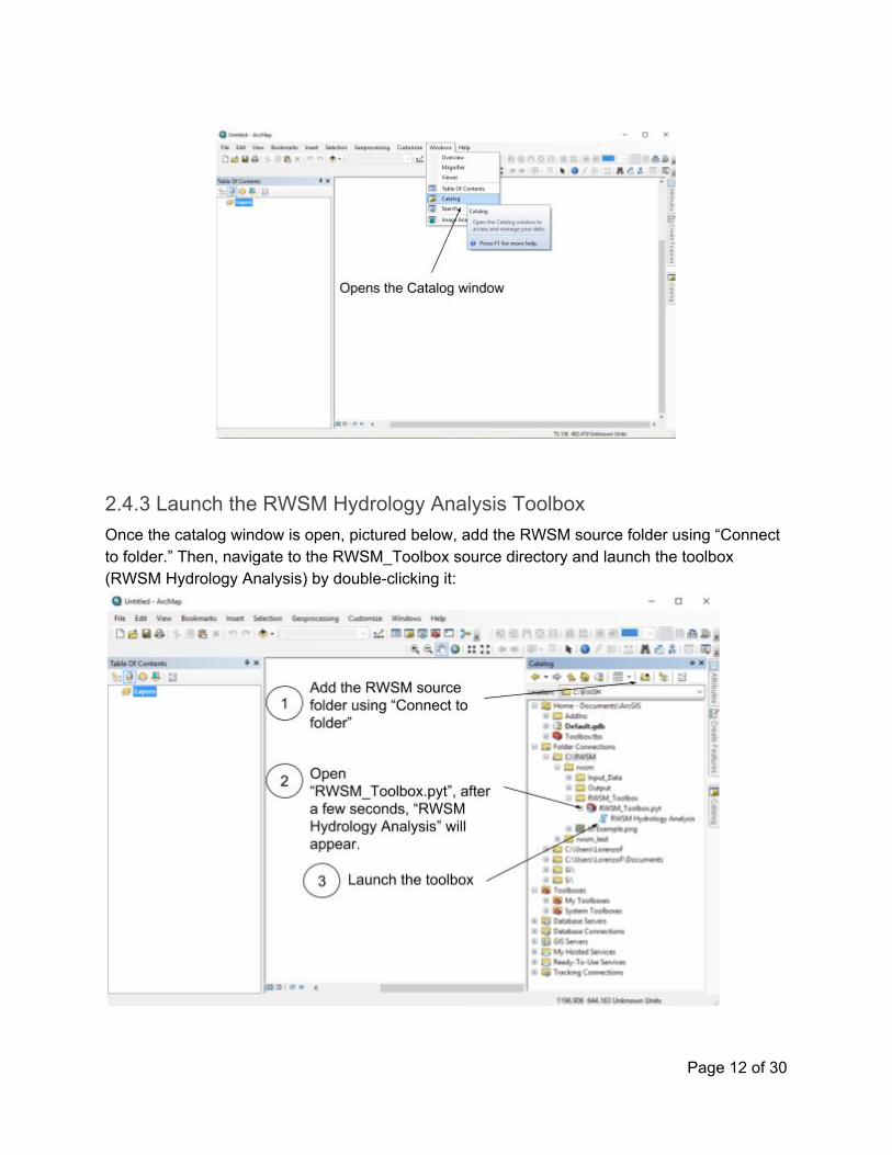
2.4.3 Launch the RWSM Hydrology Analysis Toolbox Once the catalog window is open, pictured below, add the RWSM source folder using “Connect to folder.” Then, navigate to the RWSM_Toolbox source directory and launch the toolbox (RWSM Hydrology Analysis) by double-clicking it:

Page 12 of 30

2.4.4 Populate RWSM Toolbox GUI, run analysis The RWSM Hydrology Analysis toolbox GUI should appear. If this is the first time the tool has run or no rwsm.ini file is present in the RWSM source directory, GUI fields should be blank. Add the appropriate input files and specify the appropriate fields (see Required Input Files).

If this is your first time running the model, we recommend using the Test watershed shapefile and the default files provided before using your own modified files. This will ensure that you can correctly identify the fields and run the model before introducing any confounding factors.

As the analysis runs, you’ll see a dialog box containing a progress bar and console output. These will provide status information so you can track analysis steps.

2.4.4.1 Toolbox GUI Fields The table below lists fields required to run the analysis toolbox. If running the tool for the first time, these fields will be blank. After initiating the analysis, the toolbox will create a file in the RWSM Toolbox source directory (i.e. rwsm.ini) which will be used to auto-populate these fields on succeeding runs.

Field Descriptions

Page 13 of 30

Workspace Directory to store analysis output

Watersheds - feature class Vector layer containing watershed boundaries. Used to clip other input files.

Watershed name field Field in watersheds feature class containing watershed names

Land use - feature class Vector layer containing land use regions.

Land use code field Numeric field corresponding to numeric land use codes.

Land use - CSV CSV File containing classification names, classification codes, and descriptions for land use codes used in the Land Use Vector Layer.

Land use code field (in CSV) Numeric CSV field for codes corresponding to those used in the Land Use vector layer.

Land use classification code field Numeric CSV field corresponding to land use classifications. See Required Input Files and Formatting for formatting information.

Land use description field Text CSV field describing land use classification.

Land use classification field Text CSV field for classifying land use codes.

Runoff coefficient - CSV CSV File containing runoff coefficient data.

Runoff coefficient field Numeric CSV field containing runoff coefficient values corresponding to unique combinations of slope bin, soil type, landuse class and land use class codes.

Slope bin field Text CSV field representing slope bins. See Required Input Files and Formatting for formatting information.

Soil type field Text CSV field for soil type. See Required Input Files and Formatting for formatting information.

Land use classification field Text CSV field specifying land use classification.

Land use classification code field Numeric CSV Field containing codes for land use classifications. See Required Input Files and Formatting for formatting information.

Slope - raster Raster input containing slope information.

Soils - feature class Vector layer containing soil types for regions covered by watersheds file.

Soils group field Vector layer field containing soil types.

Precipitation - raster Raster containing precipitation values for regions covered by watershed vector layer.

Page 14 of 30

Output file name Folder name used for writing analysis output, created within system folder specified in workspace. User to define output file name. File name will have a timestamp appended to folder name.

2.4.4.2 View Analysis Status After clicking “OK” in the toolbox GUI the analysis will begin. As the analysis runs, you can keep track of the analysis by viewing the console messages to the progress tracking dialog box:

Console output will show analysis steps for each watershed. At the end you will see a message noting the analysis completed and a listing of watersheds that encountered errors and could not complete the analysis. If the model encounters errors for a particular watershed, the tool will continue to run for the remaining watersheds in the dataset. Output data will still be created for watersheds that were successful, but will be absent for any watersheds that errored.

There is an example watershed geodatabase included in the Input Data folder. This geodatabase includes a test set of watersheds. One of the watersheds in this dataset will result in an error when using the PRISM dataset that has not been resampled. This is so that you can see how the model handles such errors.

Page 15 of 30

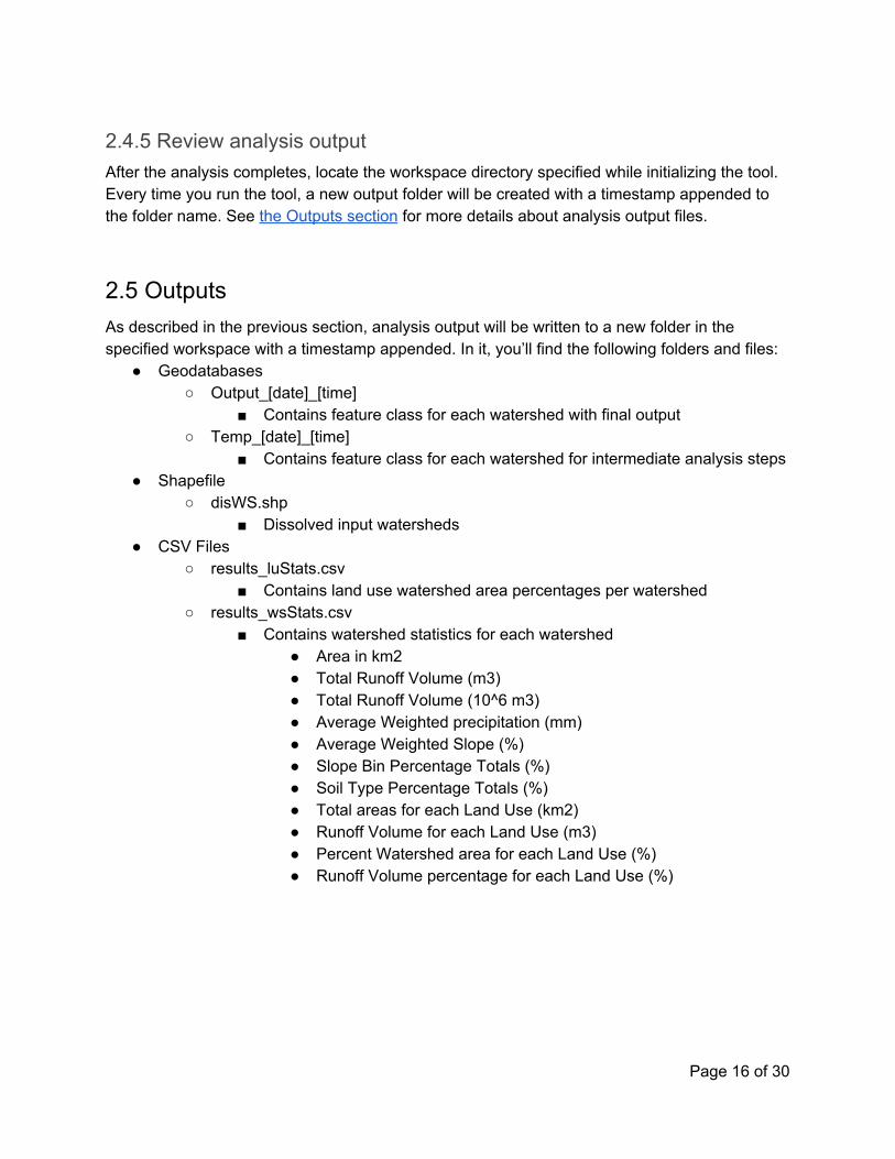
2.4.5 Review analysis output After the analysis completes, locate the workspace directory specified while initializing the tool. Every time you run the tool, a new output folder will be created with a timestamp appended to the folder name. See the Outputs section for more details about analysis output files.

2.5 Outputs As described in the previous section, analysis output will be written to a new folder in the specified workspace with a timestamp appended. In it, you’ll find the following folders and files:

● Geodatabases ○ Output_[date]_[time]

■ Contains feature class for each watershed with final output ○ Temp_[date]_[time]

■ Contains feature class for each watershed for intermediate analysis steps ● Shapefile

○ disWS.shp ■ Dissolved input watersheds

● CSV Files ○ results_luStats.csv

■ Contains land use watershed area percentages per watershed ○ results_wsStats.csv

■ Contains watershed statistics for each watershed ● Area in km2 ● Total Runoff Volume (m3) ● Total Runoff Volume (10^6 m3) ● Average Weighted precipitation (mm) ● Average Weighted Slope (%) ● Slope Bin Percentage Totals (%) ● Soil Type Percentage Totals (%) ● Total areas for each Land Use (km2) ● Runoff Volume for each Land Use (m3) ● Percent Watershed area for each Land Use (%) ● Runoff Volume percentage for each Land Use (%)

Page 16 of 30

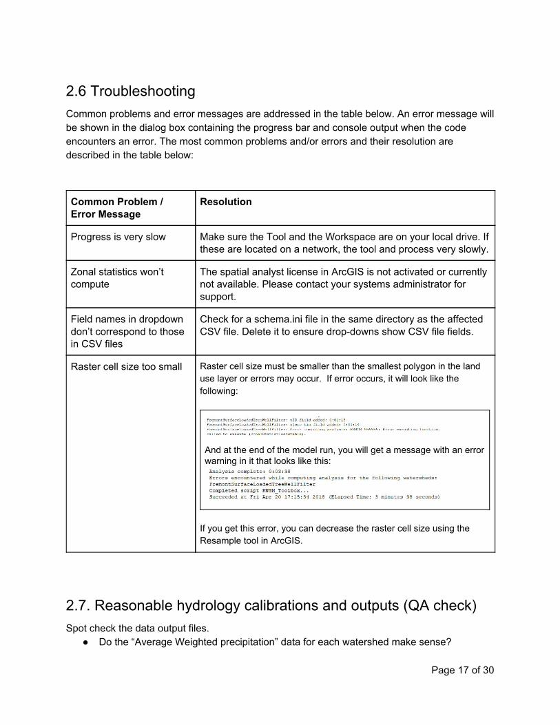
2.6 Troubleshooting Common problems and error messages are addressed in the table below. An error message will be shown in the dialog box containing the progress bar and console output when the code encounters an error. The most common problems and/or errors and their resolution are described in the table below:

Common Problem / Error Message

Resolution

Progress is very slow Make sure the Tool and the Workspace are on your local drive. If these are located on a network, the tool and process very slowly.

Zonal statistics won’t compute

The spatial analyst license in ArcGIS is not activated or currently not available. Please contact your systems administrator for support.

Field names in dropdown don’t correspond to those in CSV files

Check for a schema.ini file in the same directory as the affected CSV file. Delete it to ensure drop-downs show CSV file fields.

Raster cell size too small Raster cell size must be smaller than the smallest polygon in the land use layer or errors may occur. If error occurs, it will look like the following:

And at the end of the model run, you will get a message with an error warning in it that looks like this:

If you get this error, you can decrease the raster cell size using the Resample tool in ArcGIS.

2.7. Reasonable hydrology calibrations and outputs (QA check) Spot check the data output files.

● Do the “Average Weighted precipitation” data for each watershed make sense?

Page 17 of 30

● Do the average annual runoff depths for each watershed (volume per unit area) make sense?

● Do the watershed averaged runoff coefficients (volume per unit area per unit Average Weighted precipitation make sense? Note, these should be >10% and <90% in most if not all cases for the Bay Area and cannot be <0% and >100%. Only very small watersheds with 100% impervious cover would be expected to yield a runoff coefficient >90% and only larger flatter watersheds in the arid east Bay would be expected to yield a runoff coefficient of <10%.

3. POLLUTANT SPREADSHEET MODEL

3.1 Structure of Model The Pollutant Spreadsheet Model is based on the assumption that unit area runoff for each homogenous area can be combined with a mean concentration (called an event mean concentration or EMC) assigned to that area to generate a load for that area which can then be aggregated to subwatersheds, watersheds, sub-regions and/or the Bay Area as a whole. EMCs can be derived from a calibration process provided as part of the model or can be derived from land use specific field monitoring data if it is available. The Pollutant Spreadsheet Model consists of an Excel workbook containing three worksheets linking Hydrology Model outputs to pollutant land use coefficients for calculating watershed pollutant loads.

3.2 Required Inputs Required inputs for the Pollutant Spreadsheet Model are highlighted in light green in the spreadsheet. There are two required inputs to calculate loads using the Pollutant Spreadsheet Model:

1) The output CSV file named “[your output filename]_wsStats.csv” from the Hydrology Model. This CSV contains watershed statistics for each watershed. This data in the CSV worksheet should be copied and pasted into the first worksheet of the Pollutant Spreadsheet Model. That worksheet tab is named “Hydrology Model Output” and is highlighted in green. Do not make any changes to the CSV output from the Hydrology Model because there are numerous embedded calculations in the Pollutant Spreadsheet Model.

2) The pollutant coefficients for each land use group. These should be put into the green highlighted cells in the “Loads Calculations” worksheet for the corresponding land use group. Note: If you use alternative groupings, you will need to adjust the embedded

Page 18 of 30

equations to reflect your chosen groupings. In the Pollutant Model Spreadsheet we have computed loads for two pollutants, PCBs and Hg, for the SF Bay Region.

Caution: Equations are embedded in the worksheets - if copying and pasting results elsewhere, remember to paste as values. If you move columns at all or change your land use groupings for your pollutant, be sure to double check all of the equations.

3.3 Using the Pollutant Spreadsheet Model Once you have input your watershed statistics info into the Hydrology Model Output tab and your pollutant concentration coefficients, the loads estimates for each watershed will be displayed in the Loads Calculations worksheet and summary statistics for all of the watersheds will be displayed in the Loads Summary worksheet.

3.4 Optional Manual Calibration An Excel workbook is provided as an optional tool for manually calibrating your pollutant coefficients assuming you have a calibration dataset to work with. Required inputs for the Pollutant Manual Calibration workbook are highlighted in light green.

1) The user should first run the calibration watersheds through the Hydrology Model. The output CSV file named “[your output filename]_wsStats.csv” from the Hydrology Model contains watershed statistics for each watershed. This data in the CSV worksheet should be copied and pasted into the first worksheet of the Pollutant Manual Calibration worksheet (tab named “Hydrology Model Output” and is highlighted in green). Do not make any changes to the CSV output from the Hydrology Model because there are numerous embedded calculations in the Pollutant Manual Calibration workbook.

2) Next, the user should turn to a manual calibration worksheet. We have provided two manual calibration worksheets in the workbook (PCBs and Hg). These are identical in structure but have different land use groupings.

3) The user must fill in the measured concentrations in the calibration watersheds in column F.

4) If measured loads for the calibration watersheds are also available, that data may be input into column Z.

5) Beginning from a predefined set of coefficients based on a prior calibration or the user’s best professional judgement of pollutant concentrations prevalent in different land use groups, the user must input a set of coefficients into the green highlighted cells B3:E3 for the corresponding land use groups.

6) The user can then adjust those coefficients to improve the calibration. A few metrics to judge the strength of your calibration are provided in the table in cells G2:J4. There are also graphs in the “Calibration Graphs” worksheet which illustrate the Measured versus Simulated results.

7) Once the user is satisfied with the manual calibration, the resulting coefficients may either be used as direct input into the Pollutant Spreadsheet Model, or to define

Page 19 of 30

minimum and maximum boundary conditions for the automated manual calibration. This latter option is recommended. The user must determine the boundary conditions based on best professional judgement and the outcome of the manual calibration. It is advised to set a range that is wide enough that the auto calibration will be able to identify the best coefficients even if your manual calibration is somewhat off, but also narrow enough to minimize overlap between the land use groups. Record your recommended boundary conditions in cells B4:E5 (highlighted in green in each manual calibration worksheet).

3.5 Optional Automated Calibration

3.5.1 Calibration Approach An automatic calibration approach was developed to calibrate the pollutant models and provide an estimate of uncertainty around the calibrated EMCs. The approach was based on a constrained optimization method (“Complex Method”, Box 1965) that has been successfully used for more conventional analytes (Silverman et al., 1988; Ha and Stenstrom, 2008). Functionally, this was done by 1) randomly sampling concentrations for each land use group within their lower and upper bounds as provided by manual calibration for each calibration watershed and multiplying this with the water volumes generated from the hydrology model to get the total loads; 2) deriving simulated EMCs from the estimated loads normalized by the total volume; and 3) running the Complex Method procedure to mathematically search for the optimal combination of EMCs that minimize the difference between observed and the simulated EMCs for all calibration watersheds simultaneously. To quantify the uncertainty associated with the data and the calibration process, the model was calibrated to a randomly selected calibration point drawn from the distribution of observed data at each calibration site, instead of a single average or median concentration. The goal of this approach was to provide confidence intervals for the calibrated concentrations and resulting loads estimates. The detailed calibration procedure was as follows:

1) Construct a distribution of the observed data for each calibration watershed. The log-normal distribution was deemed appropriate based on data analysis and the typical pattern of stormwater data

2) Randomly generate observed data points based on the distribution, one for each calibration watershed.

3) Calibrate the Model for each watershed simultaneously in the same manner previously applied using the Box method (optimization process), and save the Model parameters when the calibration is deemed completed.

4) Repeat the process (steps 2-3) for a number of iterations (currently set as 100) and save the Model parameters for each iteration.

Page 20 of 30

5) Establish the distribution of model parameters from the 100 points that were produced by all iterations.

Based on the recommendation from our advisors (M. Stenstrom and P. Mangarella, personal communication, October, 2015), the 25th percentile, median, and 75th percentile of calibrated concentrations were then used to estimate a range of PCB and Hg loads for the whole region. The auto-calibration approach was implemented using R code. Separate codes were written for PCB and Hg.

3.5.2 Required Inputs The input files required by the calibration procedure are provided for users to rerun the model calibration as-is or use as a template for modification to perform their own calibration, all in CSV format. Since the names and paths of input files are currently hardcoded, users will need to change them in the code in order to run the calibration procedure. The required input files for PCB calibration are listed below. Similar files are needed for Hg.

● PCB_area_weights.csv (weighting factor for each observed data point, currently set up as 1 for each point)

● Runoff_at_PCB_watersheds.csv (simulated runoff from each land use within each watershed)

● Total_runoff_at_PCB_watersheds.csv (simulated total runoff from each watershed) ● PCB_concentration_boundary.csv (lower and upper bounds of concentrations) ● Observed_PCB_concentration.csv (observed data range for each watershed)

3.5.3 Calibration Results The auto-calibration results are summarized in four output files in CSV format:

● Calibrated_PCB_conc_by_landuse.csv ● Calibrated_PCB_conc_by_watershed.csv ● Mean_median_by_watershed.csv (median and mean concentrations and loads by

watersheds) ● Quantile_conc_by_landuse.csv

3.6 Reasonable pollutant calibrations and outputs (QA check) So now that you have some outputs, do they make sense? Here are a series of questions that you might consider asking yourself and your colleagues as you check through the outputs of your modeling efforts:

Page 21 of 30

● Do your EMCs make sense? Are the EMCs for the less polluted land use types within the range of data observed locally or published results from other regions?

● Are the EMCs in a sensible relative order to one another and does the variation from the least to the greatest make sense?

● Do the yields make sense relative to locally observed data and one another? ● During the auto-calibration process, did the coefficients tend to push against either the

upper or lower boundary as indicated by the median, the 25%ile and/or the 75%ile? If so, is that reasonable?

4. REFERENCES Box, M. J. 1965. A new method of constraint optimization and a comparison with other methods.

Computer Journal, 8(1965):42-52. Gesch, D., Oimoen, M., Greenlee, S., Nelson, C., Steuck, M., and Tyler, D., 2002, The National

Elevation Dataset: Photogrammetric Engineering and Remote Sensing, Vol. 68, (1), pp. 5-11. Ha, S. J. and Stenstrom, M. K. 2008. Predictive Modeling of Storm-Water Runoff Quantity

and Quality for a Large Urban Watershed. Journal of Environmental Engineering, 134 (9), 703-711.

Lent, M.A. and McKee, L.J., 2011. Development of regional suspended sediment and pollutant

load estimates for San Francisco Bay Area tributaries using the regional watershed spreadsheet model (RWSM): Year 1 progress report. A technical report for the Regional Monitoring Program for Water Quality, Small Tributaries Loading Strategy (STLS). Contribution No. 666. San Francisco Estuary Institute, Richmond, CA. http://www.sfei.org/sites/default/files/RWSM_EMC_Year1_report_FINAL.pdf

Lent, M.A., Gilbreath, A.N., and McKee, L.J., 2012. Development of regional suspended sediment and pollutant load estimates for San Francisco Bay Area tributaries using the regional watershed spreadsheet model (RWSM): Year 2 progress report. A technical progress report prepared for the Regional Monitoring Program for Water Quality in San Francisco Bay (RMP), Small Tributaries Loading Strategy (STLS). Contribution No. 667. San Francisco Estuary Institute, Richmond, California. http://www.sfei.org/sites/default/files/RWSM_EMC_Year2_report_FINAL.pdf

McKee, L.J., Gilbreath, A.N., Wu, J., Kunze, M.S., Hunt, J.A., 2014. Estimating Regional Pollutant Loads for San Francisco Bay Area Tributaries using the Regional Watershed Spreadsheet Model (RWSM): Year’s 3 and 4 Progress Report. A technical report prepared for the Regional Monitoring Program for Water Quality in San Francisco Bay (RMP), Sources, Pathways and Loadings Workgroup (SPLWG), Small Tributaries Loading Strategy (STLS).

Page 22 of 30

Contribution No. 737. San Francisco Estuary Institute, Richmond, California. http://www.sfei.org/documents/estimating-regional-pollutant-loads-san-francisco-bay-area-tributaries-using-regional-wate

Silverman, G.S., Stenstrom, M.K. and Fam, S., 1988. Land use considerations in reducing oil and grease in urban stormwater runoff. Journal of Environmental Systems, 18(1), pp.31-47.

Soil Survey Staff. 1994. State Soil Geographic (STATSGO) Data Base : Data Users Guide. U.S.

Department of Agriculture, Natural Resources Conservation Service (Misc. pub. no. 1492). Wu, J., Gilbreath, A.N., McKee, L.J., 2016. Regional Watershed Spreadsheet Model (RWSM):

Year 5 Progress Report. A technical report prepared for the Regional Monitoring Program for Water Quality in San Francisco Bay (RMP), Sources, Pathways and Loadings Workgroup (SPLWG), Small Tributaries Loading Strategy (STLS). Contribution No. 788. San Francisco Estuary Institute, Richmond, California. http://www.sfei.org/sites/default/files/biblio_files/RWSM%202015%20FINAL.pdf

Wu, J., Gilbreath, A.N., McKee, L.J., 2017. Regional Watershed Spreadsheet Model (RWSM): Year 6 Progress Report. A technical report prepared for the Regional Monitoring Program for Water Quality in San Francisco Bay (RMP), Sources, Pathways and Loadings Workgroup (SPLWG), Small Tributaries Loading Strategy (STLS). Contribution No. 811. San Francisco Estuary Institute, Richmond, California. http://www.sfei.org/documents/regional-watershed-spreadsheet-model-rwsm-year-6-final-report

5. Appendix A Table 1 lists all the data sources used to produce the source area points. The second column

refers to the specific attributes used to query out records. The “Field Mappings” column refers to the native fields incorporated into the source area points concatenated “ID” field. The “Source” column the methodology used to produce the dataset if it was incorporated as is.

Dataset Query Used Field Mappin

gs

Source

Industrial Storm Water

General Permit

Notice of Intent Permit

See Appendix A ID = WDID

TYPE = SIC

description

http://www.waterboards.ca.gov/water_issues/programs/stormwater/industrial.shtml

Page 23 of 30

Data for San Francisco

Bay Region1

Envirostor Cleanup

Sites database

NAME or PAST_USES = 'AUTO', 'DRUM', 'METAL',’SHIP’

ID = ENVIROSTAR

ID TYPE =

PAST_USE

http://www.envirostor.dtsc.ca.gov/public/data_download.asp

EPA Superfund Sites

site_name = 'AUTO', 'DRUM', 'METAL',’SHIP’

rhs_name ~ ‘MERCURY’,’PCB’

ID = EPA_I

D

http://cumulis.epa.gov/supercpad/cursites/srchsites.cfm

Toxic Release Inventory,

20112

contaminant = ‘MERCURY COMPOUNDS’,’MERCURY’, ’PCB’

ID = TRI FACILITY ID

http://dtsc.ca.gov/database/index.cfm

California EPA Air

Resources Board, 2008

CASid = 7439976 (mercury), 1336363 (PCB)

ID = FACID

TYPE = SIC

description

http://www.arb.ca.gov/app/emsinv/facinfo/facinfo.php

RMP Prop 13 Auto

Disassembly

kept non-redundant records

SFEI - derived from SF Regional Water Quality Control Board records for active auto / truck dismantling facilities

RMP Prop 13 Hg/PCB Hotspots

kept non-redundant records that were not spills

SFEI - derived from multiple sources: Bay Spill Reports, DTSC CalSites, Superfund, PADS, PG&E, TRI

RMP Prop 13 Hg

Emissions 2000-2007

derived from Air Resources Board

ID = FACID

TYPE = SIC

description

SFEI

Page 24 of 30

EOA Metal Recyclers Locations

Google search EOA

Table 1. Data sources for PCB/Hg Source Areas point layer. 1. Listed as “waterboard permits” in “Source” field, and broken into two subcategories. All records with XY values are

labeled “lat/long”, and all others were geocoded using ArcGIS 10 and are labeled “geocode”. 2. all applicable records from TRI were redundant with others, and therefore no records in product were attributed

“TRI” in “Source” field Table 2 details the attribution schema used to place points in different category / subcategory

assignments. As multiple disparate datasets were combined, the schema used may be less than ideal for some categories, but best judgement was used to minimize uncertainty.

Category Subcategory

Assignment Criteria

Recycling

Auto

-SIC 5015,7532 -SIC 5093 and ‘auto’ in name -superfund or envirostor and ‘auto’ in name -in Prop13 autodism database

Drums -SIC 2655 -if no SIC, ‘drum’ in past uses or name, or confirmed by Google

search

Waste -SIC 4953,5093

Metals

-SIC 5093 and ‘metal’ in name -if no SIC, must have “METAL RECLAMATION” or “RECYCLING –

SCRAP METAL” in past uses -all nonredundant metal recycleries from EOA dataset were also

included

Manufacturing

-SIC 3312,3315,3316,3317,3321,3324,3325,3341,3353,3356,3357,3363,3364,

3365,3369,3399,3411,3412,3423,3441,3442,3443,3444,3451,3462,3469,3471,3479,

3491,3494,3496,3498,3499

Page 25 of 30

-if no SIC, must have “MANUFACTURING – METALS” in past uses, or if from RMP dataset, based on expert opinion

Cement -SIC 3241

Cremation -SIC 7261

Transport Ship -SIC 3731,3732,3812,4412,4449,4481,4482,4489,4491,4492,4493,4499

-if not in any other category, if “SHIP” in past uses

SIC table for Industrial Storm Water General Permit Notice of Intent Permit Data for San

Francisco Bay Region

SIC Description

2655 Fiber Cans, Tubes, Drums, and Similar Products

3241 Cement, Hydraulic

3271 Concrete Block and Brick

3272 Concrete Products, Except Block and Brick

3273 Ready-Mixed Concrete

3312 Steel Works, Blast Furnaces (Including Coke Ovens), and Rolling Mills

3313 Electrometallurgical Products, Except Steel

3315 Steel Wiredrawing and Steel Nails and Spikes

3316 Cold-Rolled Steel Sheet, Strip, and Bars

3317 Steel Pipe and Tubes

3321 Gray and Ductile Iron Foundries

3322 Malleable Iron Foundries

3324 Steel Investment Foundries

3325 Steel Foundries, NEC

3331 Primary Smelting and Refining of Copper

3334 Primary Production of Aluminum

Page 26 of 30

3339 Primary Smelting and Refining of Nonferrous Metals, Except Copper and Aluminum

3341 Secondary Smelting and Refining of Nonferrous Metals

3351 Rolling, Drawing, and Extruding of Copper

3353 Aluminum Sheet, Plate, and Foil

3354 Aluminum Extruded Products

3355 Aluminum Rolling and Drawing, NEC

3356 Rolling, Drawing, and Extruding of Nonferrous Metals, Except Copper and Aluminum

3357 Drawing and Insulating of Nonferrous Wire

3363 Aluminum Die-Castings

3364 Nonferrous Die-Castings, Except Aluminum

3365 Aluminum Foundries

3366 Copper Foundries

3369 Nonferrous Foundries, Except Aluminum and Copper

3398 Metal Heat Treating

3399 Primary Metal Products, NEC

3411 Metal Cans

3412 Metal Shipping Barrels, Drums, Kegs, and Pails

3421 Cutlery

3423 Hand and Edge Tools, Except Machine Tools and Handsaws

3425 Saw Blades and Handsaws

3429 Hardware, NEC

3431 Enameled Iron and Metal Sanitary Ware

3432 Plumbing Fixture Fittings and Trim

3433 Heating Equipment, Except Electric and Warm Air Furnaces

3441 Fabricated Structural Metal

3442 Metal Doors, Sash, Frames, Molding, and Trim Manufacturing

Page 27 of 30

3443 Fabricated Plate Work (Boiler Shops)

3444 Sheet Metal Work

3446 Architectural and Ornamental Metal Work

3448 Prefabricated Metal Buildings and Components

3449 Miscellaneous Structural Metal Work

3451 Screw Machine Products

3452 Bolts, Nuts, Screws, Rivets, and Washers

3462 Iron and Steel Forgings

3463 Nonferrous Forgings

3465 Automotive Stamping

3466 Crowns and Closures

3469 Metal Stamping, NEC

3470 Metal Services, nec

3471 Electroplating, Plating, Polishing, Anodizing, and Coloring

3479 Coating, Engraving, and Allied Services, NEC

3482 Small Arms Ammunition

3483 Ammunition, Except for Small Arms

3484 Small Arms

3489 Ordnance and Accessories, NEC

3491 Industrial Valves

3492 Fluid Power Valves and Hose Fittings

3493 Steel Springs, Except Wire

3494 Valves and Pipe Fittings, NEC

3495 Wire Springs

3496 Miscellaneous Fabricated Wire Products

3497 Metal Foil and Leaf

Page 28 of 30

3498 Fabricated Pipe and Pipe Fittings

3499 Fabricated Metal Products, NEC

3731 Ship Building and Repairing

3732 Boat Building and Repairing

3743 Railroad Equipment

3911 Jewelry, Precious Metal

3914 Silverware, Plated Ware, and Stainless Steel Ware

3915 Jewelers' Findings and Materials, and Lapidary Work

4412 Deep Sea Foreign Transportation of Freight

4424 Deep Sea Domestic Transportation of Freight

4432 Freight Transportation on the Great Lakes - St. Lawrence Seaway

4449 Water Transportation of Freight, NEC

4481 Deep Sea Transportation of Passengers, Except by Ferry

4482 Ferries

4489 Water Transportation of Passengers, NEC

4491 Marine Cargo Handling

4492 Towing and Tugboat Services

4493 Marinas

4499 Water Transportation Services, NEC

4953 Refuse Systems

5012 Automobiles and Other Motor Vehicles

5013 Motor Vehicle Supplies and New Parts

5015 Motor Vehicle Parts, Used

5093 Scrap and Waste Materials

7261 Funeral Services and Crematories

Page 29 of 30

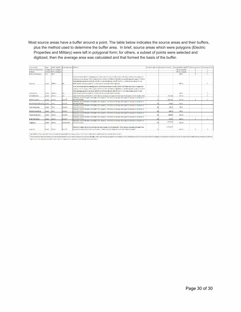
Most source areas have a buffer around a point. The table below indicates the source areas and their buffers,

plus the method used to determine the buffer area. In brief, source areas which were polygons (Electric Properties and Military) were left in polygonal form; for others, a subset of points were selected and digitized, then the average area was calculated and that formed the basis of the buffer.

Page 30 of 30