University of Catania - Department of Economics

Working Paper SeriesWorking Paper Series

n° 2010/10 – November 201o

The regional public spending for tourism in

Italy: an empirical analysis

by

Roberto Cellini

Gianpiero Torrisi

Corso Italia 55, Catania – Italy | www.demq.unict.it | e-mail: demqseg@unict.it

1

File: cellini-torrisi_(turismo-regio-ENGLISH)(1-nov-10).doc

THE REGIONAL PUBLIC SPENDING FOR TOURISM IN ITALY:

AN EMPIRICAL ANALYSIS ^

by Roberto Cellini and Gianpiero Torrisi

Roberto Cellini - Università di Catania, Facoltà di Economia. Corso Italia 55 - 95129 Catania - Italy; tel.: +39-095-7537728, e-mail cellini@unict.it; Gianpiero Torrisi - University of Newcastle upon Tyne, Center for Urban and Regional Development Studies (CURDS), Claremont Bridge – Newcastle Upon Tyne NE1 7RU, UK; tel. :+44 (0) 191 222 7728 e-mail gianpiero.torrisi@ncl.ac.uk. Abstract - In this paper, we analyse the effects of public spending for tourism in the twenty

Italian regions. The evaluation is made possible by the availability of the databank under the

project ‘Conti Pubblici Territoriali’ (‘Regional Public Account’) of the Ministry of Economic

Development, wherein the spending of all public institutions is aggregated for each region, and

it is also classified according to different criteria, including the sectoral criterion. We take a

cross-sectional regression analysis approach, and the effects of public spending for tourism on

tourism attraction are investigated. Generally speaking, the effectiveness of public spending

appears to be weak.

Keywords: Tourism; Regions; Public Spending; Regional Public Accounts

JEL Classification: R53, R58, L83, C21, M49.

SHORT BIOGRAPHY :

Roberto Cellini is Full Professor of Economics at the University of Catania; his research

interests include industrial organization and game theory, along with tourism economics.

Gianpiero Torrisi is Associate Researcher at the University of Newcastle upon Thyne –

CURDS. His research interests include public finance and local development.

^ We thank Guido Candela, John Goddard, Roberto Golinelli, and Calogero Guccio, along with two anonymous referees for helpful comments. The responsibility for any errors is, of course, ours.

2

THE REGIONAL PUBLIC SPENDING FOR TOURISM IN ITALY:

AN EMPIRICAL ANALYSIS

Abstract - In this paper, we analyse the effects of public spending for

tourism in the twenty Italian regions. The evaluation is made possible by the

availability of the databank under the project ‘Conti Pubblici Territoriali’

(‘Regional Public Account’) of the Ministry of Economic Development,

wherein the spending of all public institutions is aggregated for each region,

and it is also classified according to different criteria, including the sectoral

criterion. We take a cross-sectional regression analysis approach, and the

effects of public spending for tourism on tourism attraction are investigated.

Generally speaking, the effectiveness of public spending appears to be weak.

Keywords: Tourism; Regions; Public Spending; Regional Public Accounts

JEL Classification: R53, R58, L83, C21, M49.

3

INTRODUCTION

Starting from the mid-Nineties, in Italy, under the Project ‘CPT - Conti Pubblici Territoriali’

(i.e., RPA – Regional Public Account), data on public spending at the regional level have been

collected by aggregating, on a regional basis, all spending centres, namely, the National

Government, Regional and Local administrations, public enterprises and other public

institutions. Public expenditures were also re-classified according to different perspectives, in

particular, according to both the economic sectors to which they are devoted and according to

the functional categories. The novelty of the RPA project is relevant for empirical studies

because data on the total amount of public spending for each region, independent of the level of

government that spent the money, and information on the specific sector to which the money is

directed are made easily available through it.

In this paper, we aim to analyse the effects of public spending in a specific sector,

namely, the tourism sector. A comprehensive body of applied research is available concerning

the effect of tourism development on regional growth and the precondition for having effective

spending in tourism (Adams and Parmenter, 1995; Soukiazis and Proença 2008, just to

mention two different contributions, referring to different countries). However, no contribution

is available, as far as we know, that focuses on the effectiveness of public spending on tourism,

at the regional level. We take Italy as a case study. Tourism is of primary importance in Italy.

Nevertheless, the financial efforts of the public sector have been rather limited, as the data at

hand will clearly show. In any case, the evaluation of its effectiveness is worth analysing.

Over the period of 1996 to 2007, we can count on the data of public spending in capital

accounts and in current accounts. If we cumulate over time the spending in capital accounts,

then –based on the permanent inventory principle– we can obtain a ‘financial’ measure of the

stock of public capital accumulated over the considered period of time. If this computation is

made for the specific sector of tourism, we obtain a measure of public capital specific to this

sector. In the present paper, this piece of information is studied in comparison with other

measures of tangible and intangible forms of capital, and it is used to evaluate the effects of

public spending for tourism on the dynamics of specific inputs, as well as on the final output

(tourists’ presence, in the case at hand).

Our analysis provides information on the relationship among different inputs in the

tourism industries, and the relative importance of different types of infrastructure in attracting

tourists. A debate dating back to Hansen (1965) is still alive, for instance, on the relative

importance of general economic infrastructures vs. sector-specific structures, or on the relative

4

importance of ‘core’ economic infrastructure vs. ‘non-core infrastructure’ like social

organisations (see the review of Torrisi, 2009, or La Rosa, 2008, specific on tourism). A clear-

cut conclusion emerges from our present analysis: we find that the ties of the measures of public

capital for tourism accumulated at the regional level over the time period under consideration

(that is, the cumulative expenditure in capital accounts for tourism) is very weakly correlated

with any specific infrastructure; moreover, its links with the size and dynamics of tourists’

presence are weak as well.

The outline of the paper is as follows: Section 2 presents the data, with a particular

focus on the features of the RPA data, Section 3 describes the data related to tourists’ presence

at the regional level in Italy, and Sections 4 and 5 provide the multivariate analysis, based on

cross-sectional (or cross-regional) regression exercises. Section 6 concludes.

DATA

THE REGIONAL PUBLIC ACCOUNT

The regional public account (RPA) database1 provides financial data on revenues and

expenditures in current and capital accounts of the public sector at the regional level. Data are

available from 1996 to 2007.

The collected data are divided both according to a sector-based classification broken

down into 30 items (including tourism) that can be mapped both with respect to the

Classification of the Functions of Government (COFOG) and according to economic functional

categories (seven are in current accounts , like general administration, wages, and so on, and the

other seven are in capital accounts).

The RPA information system was developed to create a structured, centralised database

that would ensure the full accessibility and exploratory flexibility of the data, both for the

network of data producers (the Regional Teams and the Central Team) and for external users.

The primary aim of the Project was to evaluate the real adoption of the principles of

additionality in the decision of how to allocate European funds. However, the information can

easily be used to evaluate (ex-ante and ex-post) the regional policies, their bases and their

effects. The data ‘have contributed to fill an historical hole in information sources concerning

the territorial distribution of public expenses.’ (Ministero dello sviluppo economico, 2007, p. 7,

our translation).

5

The reference universes of the RPA consist of two parts: General Government and the

Public Sector. Essentially, General Government is formed of entities that primarily deliver

nonmarket services, while the definition of ‘Public Sector’ supplements and expands on that

required by the European Union for the verification of the principle of additionality. Hence, the

latter comprises, in addition to General Government, a ‘non-general-government’ sector

consisting of central and local entities that operate in the public services sector and are subject

to direct or indirect control. The numbers of entities that make up these two different universes

and the precise boundary between general government and non-general-government can vary

over time, and they are directly connected with the legal nature of the entities themselves and

the laws that govern the various sectors of public action. In the RPA database, the EU criteria

were expanded to achieve a broader coverage, thereby including, at the central level, a

significant number of public enterprises held by the state and, at the local level, several

thousand entities that had not previously been covered in a comprehensive manner by any other

statistical source. The entities within the various aggregates of the public sector are subject to

periodic monitoring as part of the RPA project.

In this paper, we always consider the tourism spending of the Public Sector, in its broad

definition used by the RPA. The benefits of considering such a vast universe of public

institutions can be expressed primarily in terms of knowledge and information acquired.

PUBLIC EXPENDITURE FOR TOURISM

Expenditures for tourism include, in particular, spending for general administration in

tourism, such as the promotion of tourism attraction and related contributions; the organisation

of and information for tourism flows (in current accounts); and the building and restoring (or

renewing) of tourism accommodation structures, which represents the major part of spending in

capital accounts.

During the period of 1996 to 2006, public expenditures for tourism registered a nominal

increase of about 33%. In relative terms, the tourism sector accounts for a very small part (about

0.20%) of public expenditures, ranging in the interval 0.18–0.25% over the years under

consideration. Expenses in capital accounts represented about 50% of the public spending for

tourism, a datum much larger than the percentage referred to the whole of public spending;

however, this ratio differs greatly across different regions: after limiting our attention to the

sector of tourism, public expenses in current accounts varied between around 14% in Basilicata

to around 85% in Lazio. Figure 1 shows the pattern of the percentage of the part of public

6

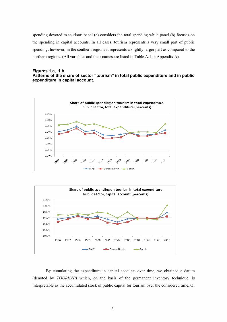
spending devoted to tourism: panel (a) considers the total spending while panel (b) focuses on

the spending in capital accounts. In all cases, tourism represents a very small part of public

spending; however, in the southern regions it represents a slightly larger part as compared to the

northern regions. (All variables and their names are listed in Table A.1 in Appendix A).

Figures 1.a, 1.b. Patterns of the share of sector “tourism” in total public expenditure and in public expenditure in capital account.

By cumulating the expenditure in capital accounts over time, we obtained a datum

(denoted by TOURKAP) which, on the basis of the permanent inventory technique, is

interpretable as the accumulated stock of public capital for tourism over the considered time. Of

7

course, we are aware that such a datum could simply be interpreted as the accumulated value of

public expenditure, and its interpretation as a measure for a capital stock could be questionable

under certain perspectives. First, sometimes public expenditure does not translate into physical

structures, even if it is in a capital account. Second, the depreciation rate is assumed to be zero

in our computation. Third, we do not consider the stock at the initial period (for this reason, the

cumulated spending is more correctly interpretable as the increase in the stock of public capital,

rather than the stock capital in itself). Fourth, we do not consider the autocorrelation of

expenditure in subsequent periods. However, the tradition of considering the cumulated

expenses in capital accounts as a measure for capital is rather widespread in economics

literature (see Romp and De Haan, 2007, for a discussion, along with Picci, 1997, 1999 on the

Italian case).

Of course, the TOURKAP data depend on the dimension of the region, and they have to

be normalised (according to the size of the region, as measured by its surface or population) if

the dimension is not explicitly accounted for in the analysis.2 Expenses for tourism, in

particular, can be related to space-serving structures or population-serving structures, so that it

is not clear ex-ante whether the normalisation according to the territorial surface is more

appropriate than the normalisation based on population.3 Nevertheless, the simple correlation

between the cross-sectional series of the cumulated public expenditure, normalised alternatively

according to the surface area and according to the population, is 0.885, so that the different

choices have no effect on the final results. Table A.2 in Appendix A (Columns 1 and 2) reports

the series. It is worth noticing that data on per-capita public expenditures for tourism at the

regional level, in capital accounts, show a great deal of variability ranging (e.g., in the per capita

case) from 0.31 (Lazio) to 24.49 (Valdaosta).

From a different perspective, cumulated expenses can be normalised according to the

tourists’ presence. Tourists’ presence is measured in this paper by the tourist overnight stays.

Indeed, such a normalisation, provides values that can be interpreted as the reciprocals of the

average productivities of public expenditures in capital accounts (See Table A.2, Col. 3):

Veneto, Lazio and Emilia R. are the regions with the lowest public capital for tourism per

tourists’ presence (i.e., the regions in which public spending is the most productive), while at

the opposite side we find Molise, Basilicata and Valdaosta.4

However, it is clear that several general infrastructures are relevant for tourism. To this

end, we take into account the indices computed by Marrocu, Paci e Pigliaru (in Barca et al.,

2006) with respect to the whole public capital. Marroccu et al. (2006) built such indices starting

from the data regarding public expenditure in capital accounts at the regional level (for all

sectors) available from the RPA, and they combined the computation with data from SISTAN

8

related to the situation in 1995. They also computed the ratio between public and private capital

so that the computation of the index for the total capital (i.e., the private capital plus the public

capital) at the regional level is possible. It is worth stressing that the data computed by Marrocu

et al. are original, since SISTAN does not provide series for the capital stock at the regional

level. The meaning of ‘capital’ adopted by Marroccu et al. is very broad, since it includes both

tangible and intangible forms of capitals (see Marroccu et al., 2006, Figures 1 and 2, page 212;

the data cover the period 1996-2002). We denote the indices for public capital and total capital

(per capita) computed by Marroccu et al. by XKPUBPOP and XKTOTPOP, respectively. The

data are reported in Table A.3 in Appendix A.

As is well known (and discussed by Marroccu et al., 2006), the public capital (in per capita

terms) appears to be larger in the southern regions of Italy as compared to the northern ones,

precisely because of the larger dimension of public spending in capital accounts. This does not

hold for the total (public and private) capital. The simple cross-sectional correlation between

total capital and public capital is equal to 0.275 (quite a low value).

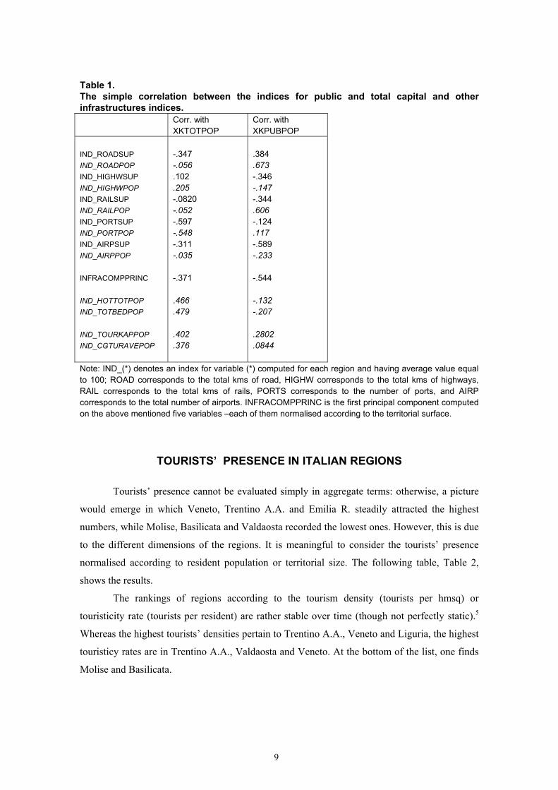
Table 1 provides the simple correlation between the two above-mentioned capital variables

(XKPUBPOP and XKTOTPOP) on the one side, and some selected indices of public

infrastructures, which we computed based on the ISTAT (2006) databank, on the other side. The

selected public infrastructures are normalised according to the territorial surface and according

to the population, but the substantial conclusions remain unchanged. Some points are worth

stressing. First, the correlation between our index for public capital specific to tourism and the

index of the general capital are 0.280 and 0.403 (total capital and public capital, respectively),

of which the latter is not low. Second, the endowment of beds and structures of accommodation

(appropriately normalised) show a good correlation with our index of public capital for tourism,

while the correlation is weak with respect to total capital. Third, the indices for transport

infrastructures show low correlation with total capital and public capital—in several cases, they

are even negative; this supports the point that public spending has weak ties with the concrete

realisation of infrastructures.

9

Table 1. The simple correlation between the indices for public and total capital and other infrastructures indices. Corr. with

XKTOTPOP Corr. with XKPUBPOP

IND_ROADSUP IND_ROADPOP IND_HIGHWSUP IND_HIGHWPOP IND_RAILSUP IND_RAILPOP IND_PORTSUP IND_PORTPOP IND_AIRPSUP IND_AIRPPOP INFRACOMPPRINC

IND_HOTTOTPOP IND_TOTBEDPOP

IND_TOURKAPPOP IND_CGTURAVEPOP

-.347 -.056 .102 .205 -.0820 -.052 -.597 -.548 -.311 -.035 -.371

.466 .479

.402 .376

.384 .673 -.346 -.147 -.344 .606 -.124 .117 -.589 -.233 -.544

-.132 -.207

.2802 .0844

Note: IND_(*) denotes an index for variable (*) computed for each region and having average value equal to 100; ROAD corresponds to the total kms of road, HIGHW corresponds to the total kms of highways, RAIL corresponds to the total kms of rails, PORTS corresponds to the number of ports, and AIRP corresponds to the total number of airports. INFRACOMPPRINC is the first principal component computed on the above mentioned five variables –each of them normalised according to the territorial surface.

TOURISTS’ PRESENCE IN ITALIAN REGIONS

Tourists’ presence cannot be evaluated simply in aggregate terms: otherwise, a picture

would emerge in which Veneto, Trentino A.A. and Emilia R. steadily attracted the highest

numbers, while Molise, Basilicata and Valdaosta recorded the lowest ones. However, this is due

to the different dimensions of the regions. It is meaningful to consider the tourists’ presence

normalised according to resident population or territorial size. The following table, Table 2,

shows the results.

The rankings of regions according to the tourism density (tourists per hmsq) or

touristicity rate (tourists per resident) are rather stable over time (though not perfectly static).5

Whereas the highest tourists’ densities pertain to Trentino A.A., Veneto and Liguria, the highest

touristicy rates are in Trentino A.A., Valdaosta and Veneto. At the bottom of the list, one finds

Molise and Basilicata.

10

Table 2. Tourists’ presence normalised according to territorial surface or resident population: Rankings of Italian regions Presence 1996 per hmsq

Presence 2007 per hmsq

Presence 1996 per resident

Presence 2007 per resident

Molise 1.043 Basilicata 1.0675 Sardegna 3.1338 Piemonte 3.1904 Calabria 3.2447 Puglia 3.8407 Sicilia 3.9167 Abruzzo 5.1459 Umbria 5.3674 Lombardia 9.584 FriuliVG 10.2583 Valdaosta 10.792 Marche 11.5526 Lazio 11.7559 Campania 13.308 Toscana 13.749 Emilia R 15.234 Veneto 23.1916 TrentinoAA 25.253 Liguria 28.3779

Molise 1.469 Basilicata 1.858 Piemonte 4.062 Sardegna 4.918 Sicilia 5.679 Calabria 5.789 Puglia 5.929 Abruzzo 6.829 Umbria 7.393 Valdaosta 9.519 Friuli VG 11.119 Lombardia 12.006 Marche 14.014 Campania 14.545 Emilia R 17.254 Toscana 18.130 Lazio 18.659 Liguria 26.139 TrentinoA.A.30.864 Veneto 33.454

Molise 1.4155 Basilicata 1.7567 Puglia 1.8345 Piemonte 1.9088 Sicilia 2.0099 Calabria 2.3794 Lombardia 2.5692 Campania 3.1660 Lazio 3.9337 Abruzzo 4.4189 Sardegna 4.5787 Umbria 5.5614 FriuliVG 6.8407 Marche 7.7632 Emilia R 8.6288 Toscana 9.0481 Liguria 9.5031 Veneto 9.6362 Valdaosta 9.9506 TrentinoAA 37.6913

Molise 2.037 Piemonte 2.370 Basilicata 2.821 Sicilia 2.910 Lombardia 3.001 Puglia 3.139 Campania 3.415 Calabria 4.369 Abruzzo 5.630 Lazio 5.844 Sardegna 7.141 Marche 7.161 Friuli VG 7.202 Liguria 8.813 Marche 8.843 Emilia R 9.039 Toscana 11.460 Veneto 12.889 Valdaosta 24.890 TrentinoA.A.42.220

Table 3 provides data on the ratio between tourists’ presence and beds (in all

accommodation structures); also, in this case, the ratio can easily be interpreted as a productivity

measure, which ranges between the minimum values in Calabria and Molise to the highest

scores of Trentino A.A. and Lazio. However, in this case, an opposite interpretation could be

appropriate as well: Calabria and Molise appear to be overendowed, while Trentino A.A. and

Lazio appear at the opposite end of the list.

11

Table 3. Tourists’ presence per bed Tourist overnight stays per bed (1996) Tourist overnight stays per bed (2007) Calabria 26.744 Molise 37.508 Basilicata 43.876 Sardegna 56.840 Abruzzo 56.865 Piemonte 60.468 Marche 60.707 Puglia 64.298 Valdaosta 66.670 Friuli VG 77.924 Sicilia 86.647 Toscana 89.787 EmiliaR 91.945 Lombardia 93.941 Trentino A.A. 94.312 Umbria 96.670 Liguria 98.809 Lazio 102.49 Veneto 103.53 Campania 110.13

Calabria 44.785 Molise 47.523 Basilicata 48.766 Puglia 54.752 Friuli VG 57.018 Piemonte 57.392 Marche 59.854 Valdaosta 60.721 Sardegna 62.625 Abruzzo 70.993 Umbria 75.665 Sicilia 80.492 Toscana 86.244 Emilia R 88.395 Friuli VG 89.754 Lombardia 90.023 Veneto 97.230 Campania 104.701 Trentino AA 111.824 Lazio 117.945

A PARAMETRIC ANALYSIS OF CROSS-REGIONAL PUBLIC SPENDING

In this Section, we aim to evaluate the effectiveness of public spending in capital accounts: (i)

first, on the accumulation of tourism structures; (ii) second, directly on the number (and growth

rate) of tourists’ presence. To this end, we took a cross-sectional (or, more precisely, a cross-

regional) regression approach. All of the analysis was carried out in per-capita terms, if not

otherwise stated.

Let us start with the evidence concerning the tourists’ presence. Cross-sectional

regressions were run in which the dependent variable was the percentage variation of tourists

per resident, regressed against the constant term, the value of tourists per resident at the initial

level, and one additional regressor. Table 4 shows the coefficients (and the significant statistics)

of the additional regressor. The standard errors are robust à la White. In formal terms, Table 4

considers each of the following regressions:

(1) iiioi exyy +++=•

201 ααα

12

where y denotes the tourists’ presence per resident (y-dot is its percentage variation over 1996-

2007; y0 is its value at the initial period), x is an additional regressor (in several cases, it is the

growth rate of a variable) and e is the residual. Results –and, in particular, the estimates of the

coefficient 2α – are provided in Table 4, whose interpretation is quite easy. For example, the

percentage variation of the hotel (per resident) is significant in explaining the percentage

variation of tourists per resident (once the initial level of tourists per resident is considered,

along with the constant term), while the percentage variation of extra-hotel structures is not

significant. In general, one can observe that the percentage variation of the density of hotels

gives a (marginal) positive and significant contribution to the growth rate of tourists (per

resident); a similar conclusion holds for the percentage variation of beds, the percentage

variation of workers in the tourism sector and the percentage variation of the share of luxury

hotels.

Quite surprisingly, the physical transportation infrastructure does not exert any positive

effect on the growth rate of tourists. This holds true for both specific infrastructures, such as

roads, railways, and ports (not reported for the sake of brevity), and the first principal

components of such structures. A similar insignificant effect emerges also for ‘cultural

endowments’, as measured by a dummy variable capturing the presence of site(s) with the

UNESCO recognition. The aggregate public capital (in all sectors, not only tourism) has a

positive effect, while the private capital has a negative effect; the total (public plus private)

capital has an insignificant effect. This outcome can be explained by observing that private

capital is higher in the regions with low specialisation in tourism.

The last three rows report results relative to two important general factors that are able

to influence tourism visits in Italian regions, namely, EU financial support and economic

growth.

As for European subsidies, it is reasonable that EU funds contribute to improve the

infrastructure endowment, and hence they may exert beneficial effects on tourism attraction. At

this point, we ran two additional regressions using the average current EU transfers received by

each region during the period from 1996 to 2007 in per capita terms (EUCUPOP) and the

accumulated value of EU transfers in capital accounts, at the regional level, during the period

from 1996 to 2007 in per capita terms (EUKAPOP). Although (as expected) both variables

showed a positive sign, they are not significant at the 5% level. Nonetheless, it is worth noticing

that, as opposed to the EU transfers in capital accounts, which were definitely not significant,

our measure of EU transfers in current accounts is significant at the 10% level and of quite a

high magnitude. Therefore, our results suggest that the EU’s direct financial role in promoting

tourism in Italian regions is quite weak and limited to transfers in current accounts.

13

As for economic performance, one could argue that the change in tourist visits across

regions could be explained by national economic growth in the sense that higher economic

growth will result in higher income available to individuals (or households) to be spent for

tourism activities. Hence, the expected sign is positive. However, using the 1996–2007 average

growth rate of GDP at regional level (GROWTH) as a proxy for economic performance, our

estimate reports a negative sign. Moreover, the coefficient is not statistically significant,

suggesting that the change in the number of tourists has not been driven by internal economic

performance.

Let us now focus on the variable of main interest in this study, which is the

accumulation of public spending for tourism in capital accounts. It has not exerted any

significant effect, both if considered per resident and if it has first been normalised to the size of

the territory under consideration. Public spending in current accounts for tourism exerted a

negative effect on the percentage growth of tourists per resident; such a negative effect is

significant if the normalisation is made according to the territorial size. However, the fact that

public spending for tourism had no positive effect on the tourists’ presence does not necessarily

mean that it was not effective at all: it simply means that it had no direct effect.

Table 4. The marginal effect of a list of factors on the growth rate of tourists per resident in Italian regions X Constant Coeff. R2

PV_HOTPOP PV_EXHOTPOP PV_HOTTOTPOP PV_HOTBEDPOP PV_EXHBEDPOP PV_TOTBEDPOP PV_WORKTOURPOP …

0.290 (0.001*) 0.419 (0.000*) 0.412 (0.000*) 0.208 (0.003*) 0.394 (0.003*) 0.277 (0.021*) 0.255 (0.005*)

0.830 (0.002*) -0.002 (0.720) -0.003 (0.870) 0.466 (0.002*) 0.032 (0.876) 0.326 (0.032*) 0.369 (0.001*)

0.503 0.273 0.270 0.684 0.272 0.398 0.431

14

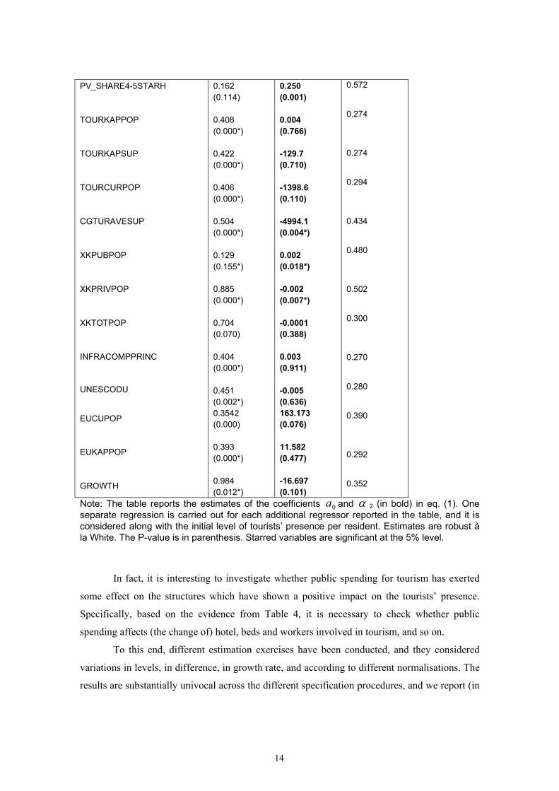
PV_SHARE4-5STARH TOURKAPPOP TOURKAPSUP TOURCURPOP CGTURAVESUP XKPUBPOP XKPRIVPOP XKTOTPOP INFRACOMPPRINC UNESCODU EUCUPOP EUKAPPOP GROWTH

0.162 (0.114) 0.408 (0.000*) 0.422 (0.000*) 0.406 (0.000*) 0.504 (0.000*) 0.129 (0.155*) 0.885 (0.000*) 0.704 (0.070) 0.404 (0.000*) 0.451 (0.002*) 0.3542 (0.000) 0.393 (0.000*) 0.984 (0.012*)

0.250 (0.001) 0.004 (0.766) -129.7 (0.710) -1398.6 (0.110) -4994.1 (0.004*) 0.002 (0.018*) -0.002 (0.007*) -0.0001 (0.388) 0.003 (0.911) -0.005 (0.636) 163.173 (0.076) 11.582 (0.477) -16.697 (0.101)

0.572 0.274 0.274 0.294 0.434 0.480 0.502 0.300 0.270 0.280 0.390 0.292 0.352

Note: The table reports the estimates of the coefficients 0a and α 2 (in bold) in eq. (1). One separate regression is carried out for each additional regressor reported in the table, and it is considered along with the initial level of tourists’ presence per resident. Estimates are robust à la White. The P-value is in parenthesis. Starred variables are significant at the 5% level.

In fact, it is interesting to investigate whether public spending for tourism has exerted

some effect on the structures which have shown a positive impact on the tourists’ presence.

Specifically, based on the evidence from Table 4, it is necessary to check whether public

spending affects (the change of) hotel, beds and workers involved in tourism, and so on.

To this end, different estimation exercises have been conducted, and they considered

variations in levels, in difference, in growth rate, and according to different normalisations. The

results are substantially univocal across the different specification procedures, and we report (in

15

Table 5) only the specification referred to percentage variation. We considered the (cross-

regional) regression

(2) iiioi uTOURKAPPOPxx +++=•

201 βββ

in which the percentage growth rate of variable x (over the period from 1996 to 2007) is

regressed against: (i) a constant term, (ii) the value of x at the initial time (i.e., x in 1996 is

denoted by x0 in eq. (2) and by X0 in Table 5), and (iii) the cumulative public spending in

capital accounts. For instance, the first row of Table 5 shows that the cumulative spending in

capital accounts was not significant in explaining the percentage growth rate of hotels (per

resident), once the initial hotels per resident (and a constant term) were taken into consideration.

The value of hotels per resident in 1996, on the other hand, has exerted a (negative) effect on its

growth rate, which, at the 6% level, is significant. That is, the density of hotels grew at a higher

rate where it was lower at the initial period (so a sort of beta-convergence has taken place). In

reference to the factor at hand, namely, the density of hotels per resident, we can thus conclude

that whereas the variation of hotels per resident has given a significant positive contribution to

the growth of tourists’ presence (as documented by Table 4), it has not been affected by public

spending in capital accounts.

Similarly, the effect of the growth of the numbers of beds on the growth of the numbers

of tourists is significant, but the growth of beds is affected significantly by public spending in

capital accounts (contrary to what one would expect). Again, the extra-hotel accommodations

were not affected in a significantly positive way by public spending in capital accounts, nor was

public spending (in capital accounts) effective in improving the quality of hotel structures (as

measured by the variation of the share of 4–5 star hotels).

So far, we have focussed on the public spending in capital accounts, because this type of

spending should have affected the variations of infrastructure. It would be interesting, however,

to analyse the effects of public spending for tourism in current accounts. To this end, we have

repeated the regression analysis reported in Table 5, adding the regressor of current public

spending for tourism (per resident; we used the average value over the period from 1996 to

2007) in each regression. The consideration of this additional regressor does not modify the

conclusions: in most cases, it is not significant; in some cases, it is significant (with a negative

sign) and precisely in such cases, public spending in capital accounts became significantly

positive. However, our interpretation does not change: public spending was in general not

significant; in some cases, the results are not robust and their signs and significance change if

different types of public spending are considered together. When public spending in capital

16

accounts for tourism appears to have had a significant positive (marginal) effect on the

accumulation of structures, the public spending in current accounts exerted a marginally

significant negative impact.

Table 5. The marginal effect of TOURKAPPOP on a list of factors potentially affecting the growth rate of tourists per resident in Italian regions

X Constant X0 TOURKAPPOP R2 PV_HOTPOP PV_EXHOTPOP PV_HOTTOTPOP PV_HOTBEDPOP PV_EXHGEDPOP PV_TOTBEDPOP PV_WORKTOURPOP PV_SHARE4-5STARH

0.047 (0.395) 5.218 (0.013*) 1.806 (0.019*) 0.296 (0.004*) 0.397 (0.002*) 0.341 (0.000*) 0.325 (0.000*) 0.715 (0.031*)

-77.71 (0.060+) -595.2 (0.002*) -150.8 (0.033*) -4.386 (0.118) -2.975 (0.355) -2.642 (0.098+) -109.1 (0.089+) 0.001 (0.382)

0.011 (0.212) -0.126 (0.119) -0.012 (0.735) 0.028 (0.288) 0.006 (0.841) 0.032 (0.263) 0.012 (0.601) -0.019 (0.122)

0.319 0.096 0.094 0.258 0.172 0.294 0.399 0.178

Note: This table reports the estimates of beta coefficients in eq. (2). One separate regression is carried out for each additional regressor reported in the table. Estimates are robust à la White. Variables denoted by * or + are significant at the 5% or 10% level, respectively.

MULTIVARIATE ANALYSIS OF THE TOURISM SUCCESS OF ITALIAN REGIONS

In this section, we present some cross-sectional regression exercises, which are aimed at

estimating the determinants of tourists’ presence (per resident) and the value generated in the

tourism sector, at the regional level, considering the twenty Italian regions. This analysis

complements the evidence presented above, and maintains the ultimate goal of evaluating the

effectiveness of public spending for tourism.

Table 6 provides the results of regressions in which the percentage variation of tourists’

presence per resident (in 2007 w.r.t. 1996) is considered as the dependent variable. This Table

17

can be considered, of course, as the extension to the multivariate context of Table 4. The

variables which appear to have a strong effect on the dynamics of tourists’ presences –and

whose coefficients are robust– are the percentage variation of hotels and the percentage

variation of workers in the tourism sector. Such variables have to be inserted as explanatory

factors in any regression considered in Table 6. It is interesting to note that the initial level of

tourist presence is always not significant. As to the public spending variables, the spending in

capital accounts is marginally insignificant (Column (2)), while the public spending in current

accounts appears to be negative and statistically significant (Column (3)). If inserted jointly

(Column (4)), the public spending in current accounts continues to have a significantly negative

coefficient, while the public spending in capital accounts becomes positive, and significant at

the 5% level. However, the joint inclusion of public spending for tourism in capital and current

accounts does not improve the explanatory power of the regression (as compared to the case in

which no variables of public spending are inserted), and the information criteria suggest one

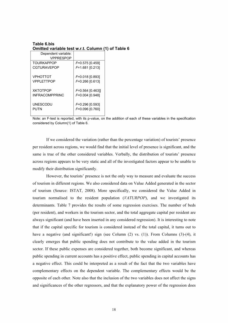
should prefer the specification without public spending variables. Tests on omitted variables,

made with reference to the specification of Column (1) of Table 6, and reported in Table 6.bis,

support the choice of that specification as the preferable one. In particular, transportation

infrastructures were not significant. Neither the presence of sites under the UNESCO

recognition nor the Putnam index of social capital exerted a significant marginal effect.

Table 6. The variation of tourists’ presence per resident (1996-2007): multivariate analysis

Dependent variable: VPPRESPOP

(1) (2) (3) (4)

COSTANT VPH VPWORKTOURPOP TOURKAPPOP CGTURAVEPOP N R2 Akaike Schwarz

0.165 (4.47) [0.000]* 0.770 (3.48) [0.003]* 0.324 (3.43) [0.003]* === === 20 0.61 -0.52 -0.36

0.192 (4.37) [0.001]* 0.780 (3.23) [0.005]* 0.284 (2.30) [0.034] -0.006 (-1.15) [0.264] 20 0.63

0.214 (5.30) [0.000]* 0.769 (3.42) [0.004]* 0.251 (1.89) [0.076]+ === -1.35Ee-4 (-3.09) [0.007] 20 0.65

0.223 (6.09) [0.000]* 0.707 (4.05) [0.001]* 0.242 (2.72) [0.015]* 0.039 (2.46) [0.026]* -0.051 (-3.46) [0.003]* 20 0.69 -0.56 -0.32

Note: Student-t is in brackets; the p-value is in squared brackets. Variables denoted by * or + are significant at the 5% or 10% level, respectively.

18

Table 6.bis Omitted variable test w.r.t. Column (1) of Table 6

Dependent variable: VPPRESPOP

TOURKAPPOP CGTURAVEPOP VPHOTTOT VPPLETTPOP XKTOTPOP INFRACOMPPRINC UNESCODU PUTN

F=0.575 [0.459] F=1.681 [0.213] F=0.018 [0.893] F=0.266 [0.613] F=0.564 [0.463]] F=0.004 [0.948] F=0.296 [0.593] F=0.096 [0.760]

Note: an F-test is reported, with its p-value, on the addition of each of these variables in the specification considered by Column(1) of Table 6.

If we considered the variation (rather than the percentage variation) of tourists’ presence

per resident across regions, we would find that the initial level of presence is significant, and the

same is true of the other considered variables. Verbally, the distribution of tourists’ presence

across regions appears to be very static and all of the investigated factors appear to be unable to

modify their distribution significantly.

However, the tourists’ presence is not the only way to measure and evaluate the success

of tourism in different regions. We also considered data on Value Added generated in the sector

of tourism (Source: ISTAT, 2008). More specifically, we considered the Value Added in

tourism normalised to the resident population (VATURPOP), and we investigated its

determinants. Table 7 provides the results of some regression exercises. The number of beds

(per resident), and workers in the tourism sector, and the total aggregate capital per resident are

always significant (and have been inserted in any considered regression). It is interesting to note

that if the capital specific for tourism is considered instead of the total capital, it turns out to

have a negative (and significant!) sign (see Column (2) vs. (1)). From Columns (3)-(4), it

clearly emerges that public spending does not contribute to the value added in the tourism

sector. If these public expenses are considered together, both become significant, and whereas

public spending in current accounts has a positive effect, public spending in capital accounts has

a negative effect. This could be interpreted as a result of the fact that the two variables have

complementary effects on the dependent variable. The complementary effects would be the

opposite of each other. Note also that the inclusion of the two variables does not affect the signs

and significances of the other regressors, and that the explanatory power of the regression does

19

not improve significantly once the two public spending variables have been inserted. Moreover,

the Akaike and the Schwarz criteria lead one to consider the specification of Column (1) to be

preferable to the specification of Column (5). Thus, the inclusion of both variables of public

spending is, in any case, questionable. Even if it is included, however, the conclusion remains

that public spending in capital accounts does not exert any positive effect on value added in the

tourism sector.

Table 7. Value-Added per capita in the tourism sector (2007)

Dependent variable: VATURPOP

(1) (2) (3) (4) (5)

COSTANT PLETT07POP WORKTOURPOP XKTOTPOP TOURKAPPOP CGTURAVEPOP N R2 F Akaike Schwarz

-3.88e-4 (-2.47) [0.024]* 1.81e-3 (3.72) [0.002]* 0.159 (3.62) [0.002]* 2.08e-6 (4.70) [0.000]* === === 20 0.95 106.6* -14.86 -14.67

2.9e-4 (5.28) [0.000]* 2.51e-3 (2.35) [0.031]* 0.255 (4.53) [0.003] === -2.46e-5 (-2.24) [0.039]* === 20 0.92 70.09*

3.41e-4 (-2.10) [0.053]+ 2.61e-3 (3.25) [0.005]* 0.161 (3.28) [0.005]* 1.86e-6 (4.05) [0.001]* -1.55e-5 (-1.44) [0.168] === 20 0.95 86.05*

-3.81e-4 (-2.17) [0.046]* 1.91e-3 (2.27) [0.038]* 0.159 (3.41) [0.004]* 2.05e-6 (4.03) [0.001]* === -0.218 (-0.19) [0.849] 20 0.95 75.09*

-4.05e-4 (-2.36) [0.033]* 2.23e-3 (2.88) [0.012]* 0.183 (4.89) [0.001]* 1.98e-6 (4.17) [0.001]* -5.363-5 (-3.36) [0.005]* 5.51 (3.09) [0.008] 20 0.97 95.84 -15.18 -14.88

Note: Student t is in parenthesis and the p-value is in squared brackets; significant variables at the 5% level are starred.

CONCLUSIONS

In this paper, we have taken a cross-sectional regression approach to analysing the effectiveness

of public spending for tourism in the Italian regions. The exercise has been made possible by the

availability of the data-bank built under the project ‘Conti Pubblici Territoriali’, in which the

20

spending of all public centres are aggregated and re-classified according to different criteria. In

particular, it is possible to know both the spending for each region (made by different public

entities) and its type and category.

The total public spending for tourism, in capital accounts, has appeared to have weak

ties with the size and dynamics of the specific physical infrastructure (of both a public and a

private nature); moreover, the effects are far from being significant as concerns the tourists’

presence, and the value-added (per capita) in the tourism sector.

In fact, our results have an exploratory nature, at the present stage. Nevertheless, they

are consistent with the results obtained by different studies. Generally speaking, the public

spending, in Italian regions, appears to have a questionable impact on the dynamics of income

and productivity in different territorial areas (see Barca et al., 2006; Ashauer, 1989, and Picci,

1997 e 1999; see also the review of La Rosa, 2008, on the effects of infrastructures).

On the point of the contribution of specific public capital—that is, the contribution of

specific investment in tourism, i.e., for the tourism sector—we limited our observations here in

noting that in other sectors, specific investments have a significant impact, unlike what we have

found for the tourism sector. Perhaps, in this case, it is also worth mentioning that tourism is a

very large and composite basket of goods and services, and the focus on a subset of factors

could be misleading.

21

REFERENCES Adams P. D. & Parmenter, B. R. (1995), “An applied general equilibrium analysis of the

economic effects of tourism in a quite small, quite open economy” Applied Economics, Vol. 27, pp. 985 – 994

Anselin, L. (1999). "Spatial Econometrics." Mimeo available at www.csiss.org/learning_resources/content/papers/baltchap.pdf.

Ashauer, D. (1989). “Is Public Expenditure Productive?”. Journal of Monetary Economics, Vol. 23, pp. 177-200.

Barca, F., Cappiello, F., Ravoni, L. & Volpe, M. (Eds.) (2006). Federalismo, Equità, Sviluppo: I risultati delle politiche pubbliche analizzati e misurati dei Conti Pubblici Territoriali. Bologna, il Mulino.

Brau, R., Lanza, A. & Pigliaru, F. (2003). How Fast Are the Tourism Countries Growing? The Cross-Country Evidence. Paper presented at CRENoS-FEEM Conference “Torusim and Sustainable Development”, Cagliari-Italy, 19-20 September.

Bull, Adrian (Eds.) (1991). The Economics of Travel and Tourism. Melbourne, Longman Cheshire Pty. Ltd..

Candela, G., & Cellini, R. (1997). Countries' Size, Consumers' Preferences and Specialization in Tourism: A Note. Rivista Internazionale di Scienze Economiche e Commerciali, Vol. 44, pp. 217-44.

Candela, G. & Cellini, R. (2006). Investment in Tourism Market: A Dynamic Model of Differentiated Oligopoly. Environmental and Resource Economics, Vol. 35, pp. 41-58.

Charnes, A., Cooper, W.W. & Rhodes, E. (1978). Measuring the Efficiency of Decision.Making Units. European Journal of Operational Research, Vol. 2, pp. 429-44

Costa, P., Manente, M. & Furlan, M. C. (Eds.) (2002). Politica economica del turismo. Roma, Nettuno - TCI.

Durbin, J. (1954). "Errors in Variables." Review of the International Statistical Institute, Vol. 22, pp. 23-32.Golden, M., & Picci, L. (2005). Proposal for a new Measure of Corruption Illustrated with Italian Data. Economics and Politics, Vol. 17, pp. 37-75.

Dwyer, L. & Forsyth, P. (eds) (2006). International Handbook of Tourism Economics. London, Edward Elgar Publishing Inc..

Hansen, L. (1982). "Large sample properties of generalized method of moments estimators." Econometrica, Vol. 50, pp. 1029-1054.

Hansen, N. M. (1965). The structure and determinants of local public investment expenditures. Review of economics and statistics, Vol.2, pp. 150-162.

Hausman, J. (1978). "Specication tests in econometrics." Econometrica, Vol. 46, pp. 1251-1271 ISTAT (2006). Le Infrastrutture in Italia. Un'analisi della dotazione e della funzionalità. Roma,

Istat. ISTAT (2008). Conti economici regionali. Roma, Istat. Lanza, A. & Pigliaru, F. (1994). The Tourism Sector in the Open Economy. Rivista

internazionale di Scienze Economiche e Commerciali, Vol. 41, pp. 15-28. Lanza, A., & Pigliaru, F. (1999). Why are Tourism Countries Small and Fast-Growing?. Crenos

Working paper 99/6. La Rosa, R. (2008). Infrastrutture e sviluppo. Università Cattolica del Sacro Cuore, Working

Paper. Mercury - Turistica (2003). Rapporto sul turismo italiano 2003. Firenze, Mercury. Ministero dello sviluppo economico (2007). Guida ai Conti Pubblici Territoriali. Roma, Moran, P. A. P. (1948). "The interpretation of statistical maps." Biometrika, Vol. 35, pp. 255-

260. Moran, P. A. P. (1950a). "Notes on continuous stochastic phenomena." Biometrika Vol. 37, pp.

17-23. Moran, P. A. P. (1950b). "A test for the serial dependence of residuals." Biometrika, Vol, 37,

pp. 178-181.

22

Picci, L. (1995). Lo stock di capitale nelle regioni italiane. DSE Working Paper No. 229, Dipartimento di Scienze Economiche Università di Bologna.

Picci, L. (1997). Infrastrutture e produttività: il caso italiano. Rivista d Politica Economica, Vol. 87, pp. 67-88.

Picci, L. (1999). Productivity and Infrastrucuture in Italian Regions. Giornale degli Economisti e Annali di Economia, Vol. 58, pp.329-53.

Putnam, R. (1996). La tradizione civica nelle regioni italiane. Milano, Mondadori. Romp, W. &. De Haan, J. (2007). Public Capital and Economic Growth: A Critical Survey.

Perspektiven der Wirtschaftspolitik, Vol. 8, pp. 6-52. Sargan, J. (1958). "The estimation of economic relationships using instrumental variables."

Econometrica, Vol. 26, pp. 393-415 Smeral, E. (2003). A Structural View of Tourism Growth. Tourism Economics, Vol. 9, pp. 77-

93. Smeral, E. & Weber, A. (2000). Forecasting International Tourism: Trends to 2010. Annals of

Tourism Research, Vol. 27, pp. 982-1006. Soukiazis, E. & S. Proença (2008),” Tourism as an alternative source of regional growth in

Portugal: a panel data analysis at NUTS II and III levels”, Portuguese Economic Journal, Vol. 7, pp. 43-61.

Torrisi, G. (2009). Public infrastructure: definition, classification and measurement issues. Economics, Management, and Financial Markets, Vol. 4, pp. 100-124..

Verbeke, J. (1995). Reports. Tourism development in Vietnam. Tourism Management, Vol. 16, pp. 315-325.

Wu, D. (1973). "Alternative Tests of Independence Between Stochastic Regressors and

Disturbances." Econometrica, Vol. 41, pp. 733-750.

23

APPENDIX A: VARIABLES Table A.1 – List of variables AIRP: number of airports TOURCUR: average annual public spending (1996 to 2007) for tourism in current account EXHOT: number of tourist accommodation structures different from hotels EXHOTBED: number of beds in EXHOT HIGHW: km of higheways HOT: number of hotel HOTBED number of beds in HOT HOTTOT: number of tourist accommodation structures (HOT+EXH) INFRACOMPPRINC: first principal component computed on specific transport infrastructures

(roads, higheways, rail, ports, airports) TOURKAP: Cumulated public spending for tourism in capital account (1996 to 2007) PORTS: number of ports PRES##: tourist presences in year ## PUTN: Putnam index for social capital RAIL: km of railways ROAD: km of roads SHARE4-5STARH: share of 4 and 5 star hotel on the number of hotel TOTBED: number of beds in HOTTOT VATUR: value added in the sector of tourism UNESCODU: dummy variable for the presence of sites under the UNESCO recognition WORKTOUR: workers employed in the tourism sector XKPUB: Index for total public capital stock per capita XKTOT: Index for total capital stock per capita D* : Variation over time (2006 or 2007 w.r.t. 1996) of variable * IND_*: Index for variable * PV_*: Percentage variation of variable * (2006 or 2007 w.r.t. 1996) *POP : * per resident *SUP : * normalised according to the territorial surface

24

Table A.2 – Cumulated public expenditure in capital account for tourism (TOURKAP), normalised according to different criteria TOURKAP/pop07

TOURKAP/sup

TOURKAP/pres07

Lazio 0.31

Campania 0.39

Puglia 0.42

Lombardia 0.45

Emilia R 0.54

Friuli VG 0.68

Marche 0.76

Umbria 0.86

Toscana 1.05

Calabria 1.30

Sicilia 1.58

Liguria 1.62

Abruzzo 1.69

Veneto 1.78

Piemonte 2.19

Molise 2.97

Basilicata 3.25

Sardegna 5.00

Trentino AA 10.92

Valdaosta 24.49

Umbria 89.4

Puglia 89.7

Lazio 99.6

Emilia R 104

Marche 121

Toscana 167

Campania 170

Calabria 173

Friuli VG 178

Lombardia 182

Basilicata 193

Abruzzo 205

Molise 214

Veneto 276

Sicilia 309

Sardegna 344

Piemonte 376

Liguria 481

Trentino AA 799

Valdaosta 937

Veneto 5.31

Lazio 5.34

Emilia R 6.02

Marche 8.60

Toscana 9.23

Campania 1.17

Umbria 1.21

Puglia 1.51

Lombardia 1.52

Liguria 1.84

Friuli 2.48

Trentino AA 2.59

Calabria 2.99

Abruzzo 3.00

Sicilia 5.44

Sardegna 7.00

Piemonte 9.26

Valdaosta 9.84

Basilicata 10.4

Molise 14.6

Note: The cumulated spending is divided as follows: (a) per 100 residents; (b) per 100 hmsq of territorial size; (c) per 10,000 tourists’ presence (all data referred to are for the year 2007).

25

Table A.3 - Indices of public capital and total capital (per capita) in Italian regions

Region

XKPUBPOP

XKTOTPOP

Piemonte 88.00 440.00Valdaosta 88.00 440.00Lombardia 67.00 478.57Trentino A A 231.00 624.32Veneto 66.00 440.00Friuli V G 134.00 496.29Liguria 146.00 442.42Emilia R 73.00 456.25Toscana 83.00 395.23Umbra 115.00 383.33Marche 94.00 391.66Lazio 116.00 446.15Abruzzo 119.00 383.87Molise 198.00 421.27Campania 107.00 314.70Puglia 83.00 286.20Basilicata 236.00 393.33Calabria 137.00 318.60Sicilia 104.00 315.15Sardegna 180.00 382.97 Simple Average 123.25 412.52Italy 100.00 313.12

Note: The normalisation is such that Italy has XKPUBPOP equal to 100.

26

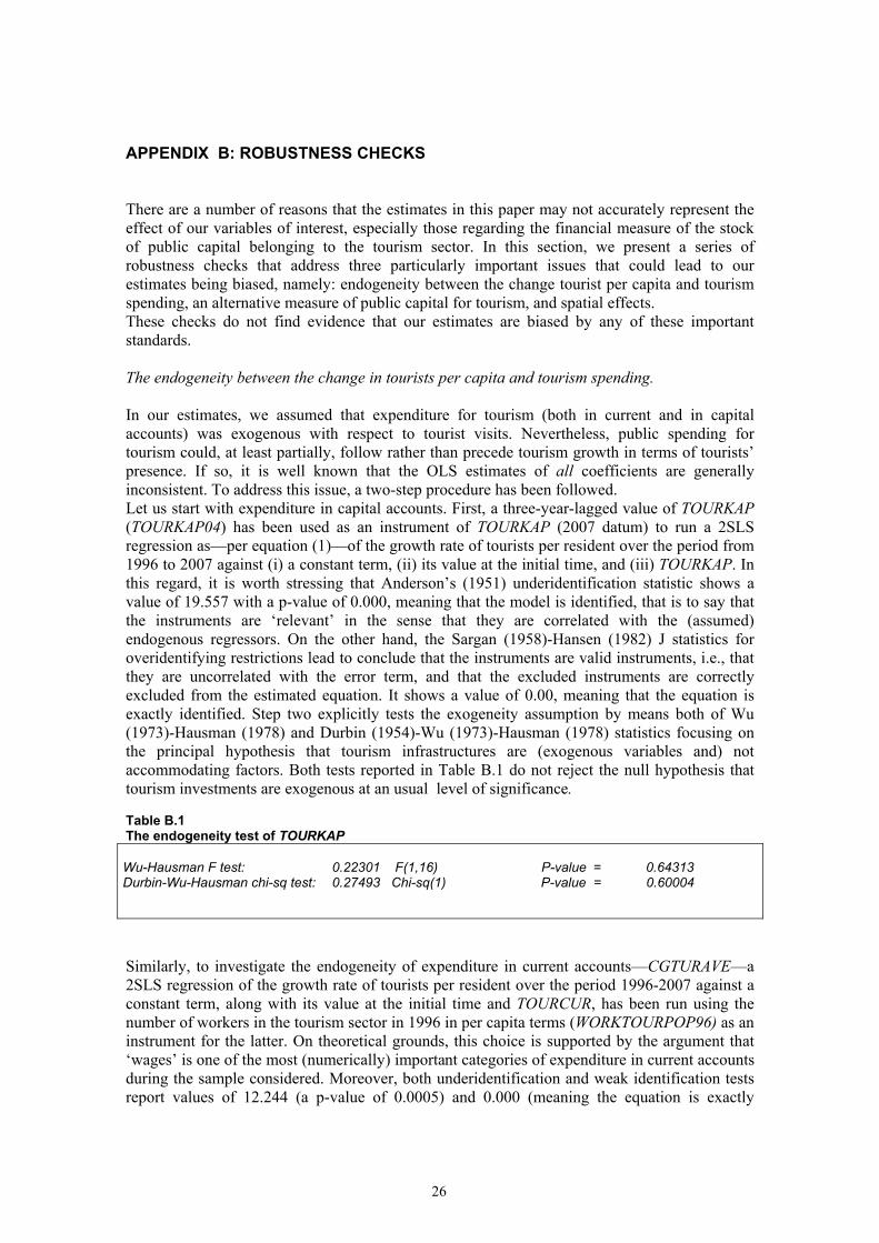
APPENDIX B: ROBUSTNESS CHECKS There are a number of reasons that the estimates in this paper may not accurately represent the effect of our variables of interest, especially those regarding the financial measure of the stock of public capital belonging to the tourism sector. In this section, we present a series of robustness checks that address three particularly important issues that could lead to our estimates being biased, namely: endogeneity between the change tourist per capita and tourism spending, an alternative measure of public capital for tourism, and spatial effects. These checks do not find evidence that our estimates are biased by any of these important standards. The endogeneity between the change in tourists per capita and tourism spending. In our estimates, we assumed that expenditure for tourism (both in current and in capital accounts) was exogenous with respect to tourist visits. Nevertheless, public spending for tourism could, at least partially, follow rather than precede tourism growth in terms of tourists’ presence. If so, it is well known that the OLS estimates of all coefficients are generally inconsistent. To address this issue, a two-step procedure has been followed. Let us start with expenditure in capital accounts. First, a three-year-lagged value of TOURKAP (TOURKAP04) has been used as an instrument of TOURKAP (2007 datum) to run a 2SLS regression as—per equation (1)—of the growth rate of tourists per resident over the period from 1996 to 2007 against (i) a constant term, (ii) its value at the initial time, and (iii) TOURKAP. In this regard, it is worth stressing that Anderson’s (1951) underidentification statistic shows a value of 19.557 with a p-value of 0.000, meaning that the model is identified, that is to say that the instruments are ‘relevant’ in the sense that they are correlated with the (assumed) endogenous regressors. On the other hand, the Sargan (1958)-Hansen (1982) J statistics for overidentifying restrictions lead to conclude that the instruments are valid instruments, i.e., that they are uncorrelated with the error term, and that the excluded instruments are correctly excluded from the estimated equation. It shows a value of 0.00, meaning that the equation is exactly identified. Step two explicitly tests the exogeneity assumption by means both of Wu (1973)-Hausman (1978) and Durbin (1954)-Wu (1973)-Hausman (1978) statistics focusing on the principal hypothesis that tourism infrastructures are (exogenous variables and) not accommodating factors. Both tests reported in Table B.1 do not reject the null hypothesis that tourism investments are exogenous at an usual level of significance. Table B.1 The endogeneity test of TOURKAP Wu-Hausman F test: 0.22301 F(1,16) P-value = 0.64313 Durbin-Wu-Hausman chi-sq test: 0.27493 Chi-sq(1) P-value = 0.60004

Similarly, to investigate the endogeneity of expenditure in current accounts—CGTURAVE—a 2SLS regression of the growth rate of tourists per resident over the period 1996-2007 against a constant term, along with its value at the initial time and TOURCUR, has been run using the number of workers in the tourism sector in 1996 in per capita terms (WORKTOURPOP96) as an instrument for the latter. On theoretical grounds, this choice is supported by the argument that ‘wages’ is one of the most (numerically) important categories of expenditure in current accounts during the sample considered. Moreover, both underidentification and weak identification tests report values of 12.244 (a p-value of 0.0005) and 0.000 (meaning the equation is exactly

27

identified), respectively. The tests reported in Table B.2 do not reject the null hypothesis that spending in current accounts for tourism is exogenous. Table B.2 The endogeneity test of TOURCUR Wu-Hausman F test: 0.33581 F(1,16) P-value = 0.57033 Durbin-Wu-Hausman chi-sq test: 0.41114 Chi-sq(1) P-value = 0.52139

Therefore, the results from Table B.1 and Table B.2 suggest that our estimates are not affected by endogeneity.

An alternative measure of tourism capital. Results concerning tourism spending, regardless of its endogeneity (which has already been analysed), could be biased because of the intrinsic weakness of the variables utilised as proxies for tourism facilities. A major concern is about the appropriateness of public spending for tourism in capital accounts—as a whole—representing public capital for tourism. Indeed, one could doubt that certain categories of public spending, such as (long-term) marketing spending or transfers, might be treated as public capital. To address this issue, different regressions have been run considering an alternative (restrictive) measure of the stock of public capital accumulated over the period from 1996 to 2007. This measure consists in the cumulated value of only ‘building and real estate’ spending (TOURKAPB) excluding, for example, the whole set of loans, public holdings, and transfers in capital accounts. Nevertheless, regressions using the aforementioned alternative proxy do not show any substantial change in the statistical significance of the coefficients. Table B.3 reports estimates relative to this alternative measure in absolute terms and normalised both according to the size of the population and the size of the surface area.

28

Table B.3 The marginal effect of building and real estate spending for tourism on the growth rate of tourists per resident in Italian regions

Regression Variables (a1) (a2) (a3) CONSTANT PRE96POP TOURKAPB TOURKAPBPOP TOURKAPBSUP N R2 F

0.108* (0.003) 0.006* (0.037) 0002 (0.593) == == 20 0.279 3.27

0.402* (0.000) -0.015* (0.029) == 61.08527 (0.627) == 20 0.275 2.54

0.400* (0.000) -0.015* (0.038) == == 30.490 (0.853) 20 0.270 2.85

Notes: estimates are robust à la White. The P-value is in parenthesis. Starred variables are significant at the 5% level. Therefore, we are confident that our main results reported in the paper do not heavily depend, in terms of statistical significance, on the particular proxy for tourism capital that we adopted. Spatial effects. As a final robustness check, we address the issue of spatial effects in our regressions. Indeed, given the explicit spatial nature of our data, it would be plausible that our regressions showed a systematic bias in capturing the effects of variables considered based on geographical grounds. In that case, spatially specific regression techniques would be required. To investigate this possibility, we test for spatial autocorrelation of residuals relative to each regression. More precisely, building on Anselin (1999), we performed the test on residuals based on the Moran’s I statistic that, in matrix notation, can be expressed as follows:

( A.1) εεεε

''

0

WSNI =

where N is the number of geographical units considered, ∑∑=

i jijwS0 is a standardisation

factor that corresponds to the sum of the weights for the nonzero cross-products, ε indexed the vector of residuals, and W is a spatial weights matrix. Moran’s I tests have been computed for all regressions reported in the paper both in the cumulative and in the consecutive distance bands case for four different distance bands. For example, the results reported in Table B.4 below refer to regressions reported in Table 4.

29

Table B.4 Moran’s I on the residual of regressions (1) reported in Table 4 Moran’s I

Distance bands Residuals of regression having the following variables as explanatory (0-1] (0-2] (0-3] (0-4] PV_HOTPOP PV_EXHOTPOP PV_HOTTOTPOP PV_HOTBEDPOP PV_EXHBEDPOP PV_TOTBEDPOP PV_WORKTOURPOP PV_SHARE4-5STARH TOURKAPPOP TOURKAPSUP CGTURAVEPOP CGTURAVESUP XKPUBPOP XKPRIVPOP XKTOTPOP INFRACOMPPRINC UNESCODU EUCUPOP EUCAPPOP GROWTH

-0.435 (0.480) -0.098 (0.935) -0.120 (0.904) 0.097 (0.789) -0.145 (0.868) -0.176 (0.818) 0.077 (0.813) 0.010 (0.912) -0.127 (0.895) -0.170 (0.833) -0.064 (0.984) 0.186 (0.670) 0.571 (0.256) -0.288 (0.671) -0.301 (0.658) -0.136 (0.881) -0.029 (0.967) -0.076 (0.967) 0.194 (0.658) 0.194 (0.658)

-0.042 (0.954) 0.056 (0.569) 0.035 (0.647) -0.217 (0.389) -0.008 (0.815) -0.136 (0.649) -0.033 (0.915) 0 (0.786) 0.027 (0.676) -0.002 (0.791) -0.038 (0.940) -0.015 (0.844) 0.098 (0.419) -0.012 (0.829) 0.002 (0.775) 0.009 (0.748) 0.086 (0.470) 0.035 (0.645) 0.078 (0.492) 0.078 (0.492)

-0.203 (0.215) -0.176 (0.324) -0.182 (0.302) -0.172 (0.341) -0.196 (0.251) -0.209 (0.194) -0.142 (0.467) -0.108 ((0.662) -0.187 (0.285) -0.197 (0.248) -0.197 (0.245) -0.176 (0.323) -0.151 (0.426) -0.264 (0.088) -0.218 (0.187) -0.192 (0.265) -0-131 (0.533) -0.167 (0.364) -0.179 (0.311) -0.179 (0.311)

0.009 (0.461) 0.033 (0.319) 0.026 (0.364) -0.076 (0.782) 0.005 (0.503) -0.073 (0.808) 0.034 (0.305) -0.057 (0.958) 0.032 (0.327) -0.001 (0.545) -0.013 (0.644) -0.016 (0.670) 0.041 (0.269) 0.083 (0.111) 0.041 (0.278) 0.014 (0.440) 0.063 (0.180) 0.039 (0.288) 0.043 (0.263) 0.043 (0.263)

30

Note: Note: Moran’s Is have been computed using linear geographic coordinates of capoluoghi (regional capital) relative to the Italian waypoint available at http://xoomer.alice.it/ntpal/GPS/ISTAT/links.html (retrieved on 18/09/2010). P-values of 2 tails distribution are in parenthesis. The results reported in Table B.4 confirm that the hypothesis of spatial independence cannot be rejected for all estimates reported in Table 4. Furthermore, Moran’s test performed in a generalised way to all estimates (Stata® do-file available upon request to the authors), confirms that, overall, the error structure of our estimates is not spatially biased. Therefore, as mentioned, we are confident that our estimates are robust with respect to all of the critical aspects here investigated.

31

ENDNOTES 1 The RPA project officially started in 1994, with the ‘Delibera’ (Decision) N. 8/1994 of the

‘Osservatorio per le Politiche Regionali’ (Regional Policy Committee); in 2004, starting with

the 2005-2007 National Statistics Programme (NSP), the RPA became a product of the National

Statistical System (SISTAN). Currently, the project and the databank are run by the Italian

Ministry of Economic Development.

2 The twenty Italian regions have very different dimensions: the populations range from 120,000

inhabitants in Valdaosta to over 9 million in Lombardia, and the surface area ranges from 326 to

2,570 thousand kmsq (Valdaosta and Sicily, respectively).

3 On the difference between space-serving and population-serving public capital, see Golden

and Picci (2005) and their references.

4 This situation is rather stable over time: an identical situation emerged with reference to the

data of 2004, and it was very similar at the beginning of the time period considered.

5 Reports on tourism in Italy are provided, e.g., by Mercury – Turistica (2003 or more recent

editions). According to the data, the regions in which tourists’ presence showed the highest

percentage growth rate (in 2007 w.r.t. 1996) are Calabria, Basilicata and Lazio, while the lowest

rates pertained to Friuli V.G., Liguria and Valdaosta.

University of Catania - Department of Economics

Corso Italia 55, Catania – Italy.

www.demq.unict.it

E-mail: demqseg@unict.it

Working Paper SeriesWorking Paper Series

Previous 10 papers of the series:

• 2010/09 – A. Pike, A. Rodríguez-Pose, J. Tomaney, G. Torrisi and V. Tselios, “In search of the ‘Economic Dividend’ of devolution: spatial disparities, spatial economic policy and decentralisation in the UK”

• 2010/08 – D. Lisi, “The impact of EPL on labour productivity in a general equilibrium

matching model”

• 2010/07 – G. Cafiso, “Trade costs and the agglomeration of production”

• 2010/06 – M. Martorana and I. Mazza, “Satisfaction and adaptation in voting behavior: an empirical exploration”

• 2010/05 – G. Coco and G. Pignataro, “Inequality of Opportunity in the Credit Market”

• 2010/04 – P. Platania, “Generalization of the financial systems of management in actuarial techniques affecting insurance of individuals”

• 2010/03 – L. Gitto, “Multiple sclerosis patients’ preferences: a preliminary study on disease awareness and perception”disease awareness and perception”

• 2010/02 – A. Cristaldi, “Convergenza e costanza del sentiero di consumo ottimo intertemporale in presenza di incertezza e lasciti”

• 2010/01 – A. E. Biondo and S. Monteleone, “Return Migration in Italy: What do weKnow?”

• 2009/04 – S. Angilella, A. Giarlotta and F. Lamantia “A linear implementation ofPACMAN”